CONTRIBUTIONS TO ADAPTIVE WEB SAMPLING DESIGNS

THE PENNSYLVANIA STATE UNIVERSITY

The Graduate School

Department of Statistics

CONTRIBUTIONS TO ADAPTIVE WEB SAMPLING DESIGNS

A Thesis in

Statistics

by

Hong Xu

c© 2007 Hong Xu

Submitted in Partial Fulfillmentof the Requirements

for the Degree of

Doctor of Philosophy

May 2007

The thesis of Hong Xu was reviewed and approved∗ by the following:

Steve K. ThompsonProfessor of StatisticsThesis Coadvisor

James L. RosenbergerProfessor of StatisticsThesis Coadvisor, Chair of Committee

Vernon M. ChinchilliDistinguished Professor of Health Evaluation Sciences

Runze LiAssociate Professor of Statistics

Mosuk ChowAssociate Professor of Statistics

BRUCE LINDSAYProfessor of Statistics, Department Head

∗Signatures are on file in the Graduate School.

Abstract

CONTRIBUTIONS TO ADAPTIVE WEB SAMPLING DESIGNS

Investigation of the characteristics and estimation of quantities of hidden and

hard-to-access population are of interest to scientists. Such populations are difficult to

target because of their elusive nature or other prohibitive characteristics. So crafting

designs of a representative sample and creating estimation methods to obtain efficient

information from the sampled data are core challenges for people who investigate

sampling theories and applications. Thompson (2006a) proposed an adaptive web

sampling ( AWS ) scheme which takes into account the social networks between sub-

jects to get a more efficient sample, and the procedures are more flexible than adaptive

sampling. Three papers which contribute to AWS are included in this thesis. They

focus on new resampling mythologies to improve the inferential estimation, produce

designs with practical restrictions to minimize the cost and maximize the sampling

simultaneously and model based estimation for non-responses. Simulated and real

data sets are used to demonstrate implementation.

iii

Contents

LIST OF TABLES vii

LIST OF FIGURES viii

Acknowledgments x

Chapter 1. Introduction 11.1 Background . . . . . . . . . . . . . . . . . . . . . . . . . . . . . . . . . . 11.2 Structure of the thesis . . . . . . . . . . . . . . . . . . . . . . . . . . . . . 2

Chapter 2. Literature Review 42.1 Sampling . . . . . . . . . . . . . . . . . . . . . . . . . . . . . . . . . . . . 42.2 Sampling designs for targeting rare populations . . . . . . . . . . . . . 52.3 Adaptive Web Sampling(AWS) . . . . . . . . . . . . . . . . . . . . . . . 92.4 Graph Model . . . . . . . . . . . . . . . . . . . . . . . . . . . . . . . . . 142.5 Sampling Inference . . . . . . . . . . . . . . . . . . . . . . . . . . . . . . 162.6 The issues on sampling rare populations . . . . . . . . . . . . . . . . . . 18

Chapter 3. Resampling designs for improved design-based inference 193.1 Introduction . . . . . . . . . . . . . . . . . . . . . . . . . . . . . . . . . . 193.2 Sampling Settings . . . . . . . . . . . . . . . . . . . . . . . . . . . . . . . 21

3.2.1 Sampling Designs . . . . . . . . . . . . . . . . . . . . . . . . . . 213.3 Design-Based Estimators . . . . . . . . . . . . . . . . . . . . . . . . . . . 23

3.3.1 Est1 . . . . . . . . . . . . . . . . . . . . . . . . . . . . . . . . . . . 233.3.2 EST2 . . . . . . . . . . . . . . . . . . . . . . . . . . . . . . . . . . 233.3.3 EST3 . . . . . . . . . . . . . . . . . . . . . . . . . . . . . . . . . . 243.3.4 EST4 . . . . . . . . . . . . . . . . . . . . . . . . . . . . . . . . . . 243.3.5 Example . . . . . . . . . . . . . . . . . . . . . . . . . . . . . . . . 24

iv

CONTENTS v

3.4 Resampling Approaches . . . . . . . . . . . . . . . . . . . . . . . . . . . 273.4.1 Rao-Blackwell Estimation . . . . . . . . . . . . . . . . . . . . . . 273.4.2 Independent Resampling (RS1) Procedure . . . . . . . . . . . . 303.4.3 Dependent Resampling Procedure I (RS2) . . . . . . . . . . . . 313.4.4 Dependent Resampling Procedure II (RS3) . . . . . . . . . . . . 323.4.5 Importance Sampling . . . . . . . . . . . . . . . . . . . . . . . . 33

3.5 Simulated Data . . . . . . . . . . . . . . . . . . . . . . . . . . . . . . . . 343.5.1 Population mean node value estimation . . . . . . . . . . . . . . 35

3.6 Discussion . . . . . . . . . . . . . . . . . . . . . . . . . . . . . . . . . . . 46

Chapter 4. Cost Optimization in Adaptive Web Sampling 494.1 Abstract . . . . . . . . . . . . . . . . . . . . . . . . . . . . . . . . . . . . 494.2 Introduction . . . . . . . . . . . . . . . . . . . . . . . . . . . . . . . . . . 49

4.2.1 AWS designs . . . . . . . . . . . . . . . . . . . . . . . . . . . . . 514.2.2 Estimation . . . . . . . . . . . . . . . . . . . . . . . . . . . . . . . 54

4.3 Cost Model . . . . . . . . . . . . . . . . . . . . . . . . . . . . . . . . . . . 554.4 Simulation . . . . . . . . . . . . . . . . . . . . . . . . . . . . . . . . . . . 57

4.4.1 Simulation Setting . . . . . . . . . . . . . . . . . . . . . . . . . . 574.4.2 Simulation Result . . . . . . . . . . . . . . . . . . . . . . . . . . . 58

4.5 Colorado Spring Data . . . . . . . . . . . . . . . . . . . . . . . . . . . . . 634.6 Discussion . . . . . . . . . . . . . . . . . . . . . . . . . . . . . . . . . . . 67

Chapter 5. Model Based Estimationfor link-tracing designs with non-responses 75

5.1 Introduction . . . . . . . . . . . . . . . . . . . . . . . . . . . . . . . . . . 755.1.1 The Model . . . . . . . . . . . . . . . . . . . . . . . . . . . . . . . 755.1.2 Applicability of the Model . . . . . . . . . . . . . . . . . . . . . . 77

5.2 Notation . . . . . . . . . . . . . . . . . . . . . . . . . . . . . . . . . . . . 785.3 Likelihood function with non-responses . . . . . . . . . . . . . . . . . . 79

5.3.1 Predictive distribution of the unobserved quantities given thedata . . . . . . . . . . . . . . . . . . . . . . . . . . . . . . . . . . . 81

5.4 Estimation . . . . . . . . . . . . . . . . . . . . . . . . . . . . . . . . . . . 845.4.1 Maximum Likelihood Estimates . . . . . . . . . . . . . . . . . . 84

5.5 Testing for randomness . . . . . . . . . . . . . . . . . . . . . . . . . . . . 885.6 Discussion . . . . . . . . . . . . . . . . . . . . . . . . . . . . . . . . . . . 89

CONTENTS vi

Chapter 6. Conclusion and Future Work 91

Bibliography 92

List of Tables

3.1 Estimates of E(var(µrs|S)) based on M-H algorithm of RS1, RS2 and RS3 413.2 Estimates of E(var(µrs|S)) based on importance sampling algorithm

for IS1, IS2 and IS3 methods . . . . . . . . . . . . . . . . . . . . . . . . . 433.3 Estimated expectation and variance and mean squares error. Based on

2,000 samples and each with 1,000 re-samples. True population valueos 0.31. µo is preliminary estimator, µRB is exact Rao-Blackwell esti-mator, µRSi, i = 1, 2, 3 are resampling estimators. The sample size is 10with initial sample size 4. . . . . . . . . . . . . . . . . . . . . . . . . . . 44

3.4 Estimated expectation and variance and mean squares error. Based on2,000 samples and each with 1,000 re-samples, importance resamplingmethod. The sample size is 10 and initial sample size is 4. . . . . . . . . 46

3.5 The acceptance rate for RS1, RS2 and RS3 . . . . . . . . . . . . . . . . . 463.6 Estimated expectation and variance and mean squares error. Based on

2,000 samples and each with 1,0000 re-samples. True population valueos 0.025. µ0i, i = 1, 2, 3, 4 are preliminary estimators. µRB is exact Rao-Blackwell estimators. µRSi, i = 1, 2, 3, 4 are estimators based on threedifferent resampling procedures. The total sample size is 10 and initialsample size is 4. . . . . . . . . . . . . . . . . . . . . . . . . . . . . . . . . 48

4.1 Transition probabilities from nodes 1 and 2 in Figure 4.1 . . . . . . . . . 534.2 Pre-specified parameter values for population proportion estimation

for the example shown in Figure 4.2 . . . . . . . . . . . . . . . . . . . . 574.3 Simulated Link Matrix for population in Figure 4.2 . . . . . . . . . . . . 624.4 msemin, the minimum value of MSE for population proportion estima-

tion and corresponding selection probabilities d. . . . . . . . . . . . . . 664.5 Pre-specified parameters value for population proportion estimation

in Figure 4.2 . . . . . . . . . . . . . . . . . . . . . . . . . . . . . . . . . . 66

vii

List of Figures

2.1 population size is 20; red dot: HIV positive people; yellow dot: HIVnegative people; black line indicates link between two people. . . . . . 11

2.2 Spatial and population graph: blue dot: population in spatial environ-ment . . . . . . . . . . . . . . . . . . . . . . . . . . . . . . . . . . . . . . 12

2.3 Top left: Population of size 20. Red circles represent units which havecharacters of interest. Other wise, units are shown in yellow circles.Other three plots are illustration of three samples based on AWS design. 13

2.4 Top left: Population of size 5. Red circles represent units which havecharacters of interest. Other wise, units are shown in yellow circles.The other three plots are illustrations of how AWS could proceed atthree steps. . . . . . . . . . . . . . . . . . . . . . . . . . . . . . . . . . . . 14

3.1 Realization of population of size 5. Red circles represent the unitswhich have characteristics we are interested in. Yellow circles repre-sent units which do not have the values we are interested in. . . . . . . 25

3.2 Four steps example of RS1 procedure. Light purple box indicates theaccepted permutation at current step. . . . . . . . . . . . . . . . . . . . 31

3.3 Population 200 with Stochastic Block structure and 3 AWS samples ofsize 10. . . . . . . . . . . . . . . . . . . . . . . . . . . . . . . . . . . . . . 36

3.4 Expected variance given conditional selection probability calculationprocedure. . . . . . . . . . . . . . . . . . . . . . . . . . . . . . . . . . . . 38

3.5 Average Cumulative Mean Standard deviation based on MCMC algo-rithm . . . . . . . . . . . . . . . . . . . . . . . . . . . . . . . . . . . . . . 40

3.6 Average Cumulative Mean Standard deviation based on importancesampling method . . . . . . . . . . . . . . . . . . . . . . . . . . . . . . . 42

3.7 Samples based on AWS designs from population of size 20 . . . . . . . 45

viii

LIST OF FIGURES ix

4.1 An illustration of adaptive web sampling. Nodes 1 and 2 are initiallychosen at random. Weighted links are used to calculate transition prob-abilities from current active set to next selected units. . . . . . . . . . . 52

4.2 Simulated wire transaction record in Bank of America. Six suspiciousTotal number of accounts is 100. . . . . . . . . . . . . . . . . . . . . . . 60

4.3 Relative efficiency between initial sample size 5 and 10, based on sim-ulated population in Figure 4.2. . . . . . . . . . . . . . . . . . . . . . . 61

4.4 Relative efficiency between initial sample size 10 and 20, based on sim-ulated population in Figure 4.2. . . . . . . . . . . . . . . . . . . . . . . 63

4.5 MSE of population proportion estimator, based on initial sample size5. The true population proportion is 0.06 in Figure 4.2. . . . . . . . . . . 64

4.6 MSE of population proportion estimator, based on initial sample size10. The true population proportion is 0.06 in Figure 4.2. . . . . . . . . . 65

4.7 MSE of population proportion estimator, based on initial sample size20. The true population proportion is 0.06 in Figure 4.2. . . . . . . . . . 67

4.8 Population proportion distribution based selection probability with ini-tial sample size 5, 10 and 20. The true population proportion is 0.06 inFigure 4.2 . . . . . . . . . . . . . . . . . . . . . . . . . . . . . . . . . . . . 68

4.9 Distribution of estimated total sample size based on different initialsample size of 5, 10 and 20. Population is in Figure 4.2. . . . . . . . . . 69

4.10 Distribution of estimated sampling waves/depth based on differentinitial sample size of 5, 10 and 20. Population is in Figure 4.2. . . . . . 70

4.11 HIV/AIDS at-risk population. Dark node indicates injection drug use.Links indicate drug-using relationships. Largest component contains300 of the 595 individuals. . . . . . . . . . . . . . . . . . . . . . . . . . . 71

4.12 Relative efficiency between initial sample size 12 and 20, based on Col-orado Spring data analysis. . . . . . . . . . . . . . . . . . . . . . . . . . 72

4.13 Population proportion distribution based on H-T estimation with ini-tial sample size 12 and 20. The true population proportion is 0.5748. . 73

4.14 Distribution of estimated total sample size based on different initialsample size of 12 and 20. Population is in 4.2. . . . . . . . . . . . . . . 74

Acknowledgements

I am most grateful and indebted to my thesis advisor, Professor Steven K.

Thompson, for the large doses of guidance, patience, and encouragement he has

given me during my time here at Penn State. I am also grateful and indebted to my

Co-advisor Professor James L. Rosenberger, for inspiration and enlightening discus-

sions on a new topic of the cost issue. I am also thankful to my committee members

Runze Li, Mosuk Chow, and Vernon M. Chinchilli. I thank my fellow students, Mike

Kwanisai for insightful commen- tary and kind cooperation. My husband Zhe Zhang,

daughter Emily Zhang, my family and relatives showed a great deal of patience and

understanding during my studies that seemed to last forever. They always picked

me up when the going was tough.

Hong Xu

The Pennsylvania State University

May, 2007

x

Chapter 1

Introduction

1.1 Background

The design of a representative sample from a rare, hidden and hard-to-access

population and estimation methods to obtain efficient information from the sampled

data are core challenges for people who investigate sampling theories and applica-

tions. The goal of this thesis is to develop more efficient resampling strategies to make

more reliable population estimates, and to propose new practical sampling methods

in the face of cost and nonresponses during the sampling procedures.

A rare population is defined as a small subset of the whole population, which

could be one hundredth percentage, one thousandth percentage or even less ( Kalton

& Anderson (1986) ). Such populations include very high/low income households;

racial, ethnic, or religious groups; persons with specific illnesses; homeless persons;

illegal drug users; individuals interested in continuing education; homosexual men

in a metropolitan area; female smokers with high school education or less and HIV/AIDS

risk people e.c.. Because of the relative rarity and elusive nature of these populations,

conventional sampling designs such as simple random sampling are inefficient for

producing data on the individuals of interest.

Methods of sampling rare populations have been reviewed by Sudman &

Kalton (1986), Kish (1991), Kalton (1991), Kalton (1993). After that, adaptive sampling

was introduced by Thompson & Seber (1996), and followed by adaptive clustered

1

2

sampling ( Thompson (1990a) ), stratified adaptive clustered sampling ( Thompson

(1990b) ). Most of this work is applied to spatial science. Link-tracing sampling can

also be called one type of adaptive sampling, which can be implemented both to spa-

tial and social science. Potterat et al. (1993) used link tracing to study data from an

HIV high risk population in Corolado Springs. Thompson (2006a) and Thompson

(2006b) used the same data for his new adaptive web sampling designs, target and

random walk designs. This thesis extends and advances the work done by Steven K.

Thompson.

1.2 Structure of the thesis

This thesis is organized as follows. Chapter 2 gives a brief overview of so-

cial networks and their characteristics. Commonly used sampling methods, adap-

tive sampling ( Thompson & Seber (1996) ) and adaptive web sampling ( Thompson

(2006a) ). Sampling inference are also discussed. The next three chapters are po-

tentially papers which contribute to adaptive sampling and adaptive web sampling.

Chapter 3 presents new resampling strategies for inference based on adaptive web

sampling designs. A Markov Chain Monte Carlo ( MCMC ) procedure is the driving

tool for the procedure in this chapter. Chapter 4 presents a class of adaptive web sam-

pling designs under the cost constraints in terms of time, money and risk etc. One

type of adaptive web sampling and cost model were described and implemented in

this chapter. A simulated data set of banking wire transactions is used to illustrate the

procedures discussed here. A data set from a high-risk population from a Colorado

Springs study is also used as an application of the methods in this chapter. In chapter

5, a new model-based approach was proposed that is an extension of the model by

Chow & Thompson (1998). This model accommodates non-random non-responses

and shows how maximum likelihood estimates could be obtained. Chapter 6 sum-

3

marizes the results of this thesis and presents conclusions for the study. A discussion

of the limitations of this study and suggestions for further research concludes Chap-

ter 6.

Chapter 2

Literature Review

2.1 Sampling

Sampling is the process of selecting units ( e.g., people, organizations, plants,

animals ) from a population of interest so that by only studying the sample we may

estimate some characteristics of a population. For example, to estimate the propor-

tion and characteristics of HIV/AIDS positive people in the USA, it would be too

expensive to interview all Americans and ask who is infected or not. We could get

just as valid information with a smaller sample and the estimates from it. So long a

sample is as representative as possible of the whole population we are investigating.

Even with the perfect questionnaire ( if such a thing exists ), our sampled data will

only be useful if the respondents are typical of the population as a whole. For this

reason, implementation of different sampling methods according to the properties or

characteristics of the population is very important. Thus, to estimate the prevalence

of a rare disease, the sample might consist of a number of medical institutions, each of

which has records of patients treated. Or in a study of transmission of disease, a sam-

pling of injection drug users is obtained by following social links from one member

of the population to another ( Thompson (2002) ).

4

5

2.2 Sampling designs for targeting rare populations

In the sampling literature, there are many conventional sampling methods in

which the selection procedure does not depend in any way on observations made

during the survey. These designs include simple random sampling, stratified sam-

pling, cluster and systematic sampling, and multistage sampling etc. In conventional

sampling, the design is based entirely on a prior information, and is fixed before the

study begins. Under such designs, researchers make decisions about the sample size

before the sampling procedure begins. The sampling frame is usually available or can

be easily obtained for such designs. And it is not difficult to obtain data on the units

of interest when conventional sampling designs are used. However, conventional

sampling methods are not appropriate for sampling the hidden and hard-to-access

population such as HIV/AIDS persons, rare and endangered species. Because of the

relative rarity and elusive nature of these populations, samples obtained by conven-

tional methods tend to contain a very few number of elements from the population

of interest. For example, the original impetus for the National Health and Social Life

Survey (Laumann et al.1994), a US national probability sample survey of sexual be-

havior was in large part concern regarding the AIDS epidemic. The survey broke

new ground in using a probability based sampling design and estimation methods

for the study of human sexual behaviors. Funding constraints due to political con-

troversies limited the sample size to 3432 people, which was considerably less than

the originally proposed sample size. When the data were collected it was found that

the people in the sample who reported having tested positive for the HIV virus num-

bered only six. For such a rare group, even a very large conventional sample would

be unlikely to be adequate. Another weakness of conventional sampling for a hidden

population is that, the selection probability is equal in conventional sampling, but

for some populations, the individual selection probability may not be equal because

6

some individuals may have a higher inclusion probability than others. For example,

in a survey to estimate rare diseases such as HIV or hepatitis C infections, a simple

random sample of medical centers is selected and the records for the patients treated

in the medical centers are obtained. However, some patients may be treated at more

than one medical center, so these patients have a higher possibility of being included

in the study than others.

There have also been a number of approaches to estimating the size of hid-

den populations. Adaptive clustered sampling ( Thompson (1990a) ) and adaptive

stratified clustered sampling ( Thompson (1990b) )are used for geographic clustered

distributed rare populations. Other adaptive sampling methods such as network

sampling ( multiplicity sampling, Birnaum & Sirken (1965) ), link tracing sampling (

Potterat et al. (1993) ), respondent driven sampling ( Heckathorn (1997), Heckathorn

(2002) ) and so on can be used for sampling populations with social network struc-

ture.

Link Tracing Sampling

The idea was first introduced by Coleman (1958). Every subject is interviewed

during the study and asked questions on their sociometric relations and more sub-

jects are included by following links. Potterat et al. (1993) and McCoy & Inciardi

(1993) used such designs in their study of heterosexual transmission and cocaine use

and associated sexual behaviors respectively. In link-tracing designs, investigators

use links between people to find other people to include in the sample. Any socio-

metric relation of interest can define a link between two individuals in the popula-

tion. The sampling design adapts based on observations made during the survey;

for example, drug users may be asked to refer other drug users to the researcher.

This is necessary because they could not know what social connections to follow or

whom to include in the sample before the investigation. The key difference between

7

the conventional sampling and adaptive sampling is that in adaptive sampling, we

take into account the information obtained during the sampling procedure. Despite

having the advantage of conveniently increasing the sample size, it is frequently nec-

essary to use link-tracing designs because it is sometimes the easiest practical way

to identify members of rare and hard-to-reach populations ( Spreen (1992); Steven

K. Thompson (1 November,2002) ).

In the social sciences, link-tracing designs provide the only practical way to

observe and study social networks. The statistical literature on design and estimation

with link-tracing designs includes procedures variously termed snowball sampling,

random walks, and network sampling.

Snowball Sampling

Snowball sampling has considerable theoretical appeal. Goodman (1961) coined

the term snowball sampling. Initial respondents are asked to identify the other people

which are related to them to include in the sample and so on for a desired number

of waves. The process stops after a certain number of waves or when there are no

more newly mentioned subjects. Snowball sampling may be defined to include all

or only a fixed number of subjects with whom they share a relationship. Snowball

designs were also developed in the graph setting with a variety of initial probability

sampling designs and any number of links and waves by Frank (1977), Frank (1978),

and Frank (1979). Frank & Snijders (1994) discussed methods for estimating the size

of a hidden population using snowball sampling.

Network Sampling

Much of the early work on network sampling was undertaken by Birnaum

& Sirken (1965) and their associates at the National Center for Health Statistics. The

links generally are symmetric, and new links added do not depend on the observed

8

information. One advantage of network sampling is that the inclusion probability for

each unit in the sample data is known and easy to calculated. On the other hand,

since it is necessary to ask additional screening questions and to spend resources

locating identified members of the rare population, network sampling costs slightly

more than standard procedures. In most of cases, network sampling costs more than

is compensated by the reduction in sampling variance. Another shortcoming of such

sampling designs is the requirement for accurate reporting about all persons in the

network. Network sampling can be used for both networks in social science (Spreen.

& Zwaagstra (1994)) or spatial science (Birnbaum & Sirken (1998)).

Random Walk Sampling

Klovdahl (1989) used the term ”random walk” design to describe the situation

where each subject is asked to name people with whom they have a social relation-

ship. After that, one subject is randomly picked from the names at each stage of

sampling. This sampling method is a modification of snowball sampling. Thompson

(2006b) contributed uniform and target walk designs, which could be implemented

more efficiently to network populations with isolated components. A random walk

procedure applied at each step produced a design with the desired stationary proba-

bilities. (Henzingera et al. (2000); Lawrence & Giles (1998)) used random walk proce-

dures to investigating internet searching.

Respondent-Driven Sampling

Heckathorn (1997) first described ”respondent-driven sampling”. The respondent-

driven sampling is based on an adaptive sampling design where the selection proce-

dure is affected by the realized network in the population (Thompson & Seber (1996);

Thompson & Frank (2000)). Salganik & Heckathorn (2004) discussed a population

proportion estimation method based on such sampling designs.

9

2.3 Adaptive Web Sampling(AWS)

All the sampling designs described above are based on following links com-

pletely. At any stage of the procedure, new units selected depend on the values of

the variables of interest associated with the units previously included, so the samples

may contain a fair number of subjects of interest. But if the population is composed of

more than one subset of linked components ( Figure 2.1 and 2.2 ), link tracing may not

be efficient to obtain sufficient subjects of interest. For example, in Figure 2.1, we will

never reach cluster 2 if the sampling started from one unit in cluster 1. A new type

of design introduced by Thompson (2006a) gains over link tracing type of sampling

designs named Adaptive Web Sampling (AWS). AWS is more flexible in controlling

how far/deep the sampling procedure could go, how the sample could be spread out,

how large the sample size could be etc. It can be applied to any graph model with

network structure. A network of spatially-based application of the designs, hidden

human populations at risk for HIV/AIDS in Colorado Springs data, and a wintering

waterfowl survey are evaluated in this paper. The work in Chapter 3 and Chapter

4 are based on the basic idea of such designs. Chapter 3 focuses on improvement of

population proportion estimation under such designs; In chapter 4, we implement a

cost model through such designs and evaluated it for different parameter values.

AWS is defined as follows: At any point in the sampling, the next unit or

next set of units is with high probability selected from a distribution that depends

on the values of variables of interest in an active set of units already selected. With

low probability the next unit is selected from a distribution that does not depend on

those values of variables of interest. The active set may consist of all the units selected

so far, or the most recently selected units, or other possibilities such as the last two

steps units or sequences of units (Thompson (2006a)). For example, in the study of

injection drug users in relation to the spread of the HIV/AIDS prevalence, we first

10

picked one person, asked if he/she is HIV positive, but we do not include a new

person by totally following the link from person one. Instead, with high probability

say 90%, we selected a new person by following link, and with low probability the

new person is randomly selected from the population. If person one did not report

anyone with whom he share the injection, then person two will be randomly selected

from the population. There are lots of variations on the general idea of AWS such as

Random and Targeted Walk Sampling Designs also described by Thompson (2006b).

Figure 2.3 is a simple example of AWS design. The top left is a population

of size 20. Red circle represent subjects which have characteristics we are interested

in. Otherwise subjects are shown in yellow circles. The other plots illustrate three

samples based on AWS. More subjects of interest are likely to be included in each

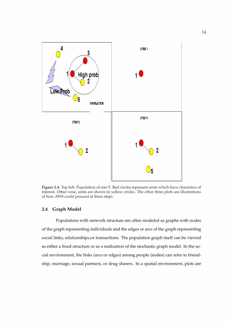
sample. Figure 2.4 is an illustration of how AWS proceeds. The top left one is a small

population of size 5. Units which are linked with each other are more likely to be

selected than isolated units. An initial sample is shown in the top right plot, which is

composed of node 1. At the second step, node 2 and node 3 could be included with

high probability; node 4 and node 5 could be selected with lower probabilities. The

bottom left showed node 2 is selected at the second step. Though node 3 has a higher

potential selection probability than then others, it is possible that node 4 and node 5

could be selected in next wave. As shown in bottom right plot, node 5 is selected.

11

poppulation graph

Figure 2.1. population size is 20; red dot: HIV positive people; yellow dot: HIV negativepeople; black line indicates link between two people.

12

Figure 2.2. Spatial and population graph: blue dot: population in spatial environment

13

poppulation graph active set adaptive sample

active set adaptive sample active set adaptive sample

Figure 2.3. Top left: Population of size 20. Red circles represent units which have charactersof interest. Other wise, units are shown in yellow circles. Other three plots are illustration ofthree samples based on AWS design.

14

Figure 2.4. Top left: Population of size 5. Red circles represent units which have characters ofinterest. Other wise, units are shown in yellow circles. The other three plots are illustrationsof how AWS could proceed at three steps.

2.4 Graph Model

Populations with network structure are often modeled as graphs with nodes

of the graph representing individuals and the edges or arcs of the graph representing

social links, relationships,or transactions. The population graph itself can be viewed

as either a fixed structure or as a realization of the stochastic graph model. In the so-

cial environment, the links (arcs or edges) among people (nodes) can refer to friend-

ship, marriage, sexual partners, or drug sharers. In a spatial environment, plots are

15

defined according to their geographic distribution. Two plots link to each other if

they are in the same neighborhood. In the graph model, U is a population with N

nodes:

U = {1, 2, · · · , N}

and

y = (y1, y2, · · · , yN )

Where yi indicates the variable we are interested, for example HIV positive

or not, or dollar amount spent on heroin per month. In the spatial situation, yi can

refer to the number of species in plot i. The N × N matrix A indicating relationship

between nodes. Aij = 1 means there is a link from node i to node j, which means

node i reported that he shared the drug-injection or needle with node j. The diagonal

elements Aii are set to zero.

Aij =

1 link exists from i to j

0 otherwise

In a social environment, the relationship between people can be directional. For ex-

ample, unit i reported to share the same injection with unit j, but unit j did not report

such a relationship with i, so Aij = 1 but Aji = 0. If both of them reported sharing

the same needle with each other, then Aij = Aji = 1, and if that is true for all i and j,

then the matrix A is symmetric. The graph model is unidirectional. For example, the

Y values for the population in Figure 2.4 is :

y1 = 1, y2 = 0, y3 = 1, y4 = 0, y5 = 0

16

and link matrix A is:

1 2 3 4 5

1 0 1 1 0 0

2 1 0 0 0 0

3 1 0 0 0 0

4 0 0 0 0 0

5 0 0 0 0 0

2.5 Sampling Inference

The objective of the sampling design is to infer the population characteristics

based on the obtained sample data. These inferential outcomes include estimation,

prediction, confidence interval, and test of hypothese. There are three categories of

sampling inference methods: design-based, model-based and mixture of design and

model based approaches.

An advantage of the design-based method is that little or no assumptions

need to be made about the population characteristics. Both population and the pop-

ulation linkage-structure are viewed as fixed unknown values. Units included in the

sample only depend on the sampling procedure, and the selection probability based

on the designs are central to the inference. Another advantage is that regardless of

whether it is a conventional or adaptive sampling procedure, the design-unbiased

strategy will be unbiased no matter what the population itself is like. But the main

disadvantage of design-based inference is that it is hard to compute the selection

probability when the design becomes complicated. Most design-based estimators re-

quire knowledge of the inclusion probability (πi) of each subject in the sample. The

inclusion probability is the probability that subject i is included in the sample. It

is hard to compute, especially without knowledge of the entire population network

17

structure. Sometimes approximations are used to estimate πi. Heckathorn (2002)

used the argument that in one-wave designs the inclusion probability for a node i

is proportional to its degree di, i.e. πi ∝ di, to derive an estimator in a respondent-

driven sampling study. Some estimators require knowledge of the population size,

which in some practical cases, especially in hidden populations, is unknown.

Thompson (2006a) proposed three new methods for estimating the popula-

tion proportion. Except for the first one which is only based on the initial sample, the

other two not only consider the information in the initial sample, but also selection

probabilities at each wave. Details are shown in Chapter 3, where three resampling

strategies are proposed to improved those estimators.

Mathematical models for modeling graphs model have also been proposed

and can be applied to a wide range of selection procedures. Under this method, the

population is not fixed, but is a realization in the stochastic graph model. Based on the

population characteristics, a joint distribution is assumed. Model-based methods also

assume that the population model depends on parameters with a prior distribution.

These models tend to be complex and solving them is not easy (Thompson & Frank

(2000)). Newman et al. (2001) noted the difficulty of providing a realistic model for a

social network.

There is, therefore, a need to develop sampling methods to make use of the

advantages of design and model based methods. Researchers tend to find a way to

balance the advantage of each by imposing design unbiasedness while seeking low

mean square error under an assumed model. Partial knowledge is assumed about the

probability distribution of the population parameters. For example, the distribution

may be assumed to be of known parametric form but with unknown parameters. Or

there is no parametric form, but the covariance matrix is proportional to a known

matrix (Thompson & Seber (1996)).

18

2.6 The issues on sampling rare populations

The sampling design methods presented above are all implemented in the

graph model. Sampling in graphs and inference from graph samples to the larger

graph of interest is one of the core challenges in graph theory. To date, the graph the-

ory has been insufficiently addressed in relation to its importance. The basic problem

is that in the various literatures, inference about graphs is made as if the data repre-

sent a realization of the entire graph. Instead, the data are usually a sample, which

in many cases is selected in such a way that it is not representative of the graph as a

whole. An example is studies of the Internet, in which values for the average degree

or the degree distribution are published. Typically, the data consist of a sample of

around fifty thousand web pages (or, in the case of the physical Internet, a large num-

ber of routers) obtained by doing a ’web crawl’, ’random walk’, or other procedure

in which links are followed from sites in the sample to add additional sites. Because

such a selection procedure gives higher probability to sites with higher degree, the

published estimates are substantially biased. The same bias is prevalent in studies of

social networks, such as studies of hidden subpopulations at risk for HIV/AIDS in

which social links are (necessarily) used in selecting the sample.

Designs for sampling in graphs, and inference methods based on design- and

model-based approaches, is a dynamic new area of graph theory. The topic has fun-

damental theoretical importance, practical importance to almost every application in-

volving networks, and challenging computational issues. It has been largely missed

in the way graph theoretic issues have been conceptualized, and has come to the

notice of researchers mainly when they discover something is wrong with their esti-

mates. Also cost is always a issue for sampling in graphs in terms of time, money and

risk, as in other situations where the researcher strives to obtain the most information

about the population for the tests cost.

Chapter 3

Resampling designs for improved design-based inference

3.1 Introduction

Sampling in graphs is one of the core challenges of graph theory that has been

insufficiently addressed so far in relation to its importance. The basic problem is that

in the various literatures inference about graphs is made as if the data represent a

realization of the entire graph. Instead, the data are usually a sample, which in many

cases is selected in such a way that it is not in fact representative of the graph as a

whole. So designs and associated inference for sampling in graphs are fundamentally

and theoretically important.

The work in this chapter is based on Active Web Sampling (AWS) designs

and associated estimators( Thompson (2006a) ). The aim is to try new methods of

resampling from the conditional distribution and estimating the Rao-Blackwell esti-

mator from that. Rao-Blackwell estimators are improved estimators for population

proportions based on conditional selection probabilities, and they are difficult to cal-

culate when the sample size is large. In this chapter, three resampling methods are

proposed and implemented in order to seek a more efficient way to approximate the

exact Rao-Blackwell estimators.

Many sampling strategies can be used to sample hidden and hard-to-access

populations, such as HIV/AIDs peoples, rare and endangered species. One such

design is Adaptive Sampling ( Thompson & Seber (1996) ) design. In such designs,

19

20

additional neighboring units or individuals are introduced into a sample when a pre-

defined condition is satisfied. This term is mainly used for designs that are based on

geographic information. The units in a neighborhood are defined to link with each

other, see Figure 2.2. In the social environment, link-tracing designs are used to in-

clude people by following links between them. Any social relation of interest can

define a link between individuals in the population. Both adaptive sampling and

link-tracing sampling designs are accomplished entirely by following links and work

well in some situations. But those sampling designs are lack of flexibilities to control

sample size, sample coverage. Since for such sampling design, snowball sampling

for instance, new units are included by following link completely, the sample and

statistic inference based on it are very sensitive to the starting points.

AWS designs gain more efficiency over the adaptive and link-tracing designs

in some situation regarding to control the depth and breadth of sample coverage.

Sample size could be predefined before the sampling procedure, and the designs are

also easily implemented. The additional units which are included in the sample are

not necessary by following links totally. Instead, at any point in the sampling, the

next unit or next set of units is with high probability selected from a distribution that

depends on the values of variables of interest in an active set of units already selected.

With low probability the next unit is selected from a distribution not depending on

those values of variables of interest. The active set may consist of all the units selected

so far, or the most recently selected units, or other possibilities include the last two

steps units or sequences of units (Thompson (2006a)). A simple example in the spatial

setting is a population with two components ( Figure 2.2 ). If the sampling started

from units only in one component, we will never reach the other component by only

following links and end up with only units in component one. AWS designs allow a

jump from cluster one to cluster two, thus we could have a better chance of inclusion

21

of the units at each step. The sampling procedure stops when sample size satisfied a

predefined number.

The preliminary estimators for population proportion can depend on initial

sample, or conditional selection probability at each step. Such estimators can be im-

proved by using Rao-Blackwell method. Thompson(Thompson (2006b)) introduced

an idea of restamping method, which is to construct a Marked chain in order to get

enough samples from the permutation sample space. Three restamping methods

based on this idea are described in this paper. And their efficiencies are also com-

pared.

3.2 Sampling Settings

3.2.1 Sampling Designs

AWS designs are used in studying population with network structure, which

are often modeled as graphs with nodes of the graph representing individuals and

the edges or arcs of the graph representing social links, relationships, or transactions.

In the social environment, the links (arcs or edges) among people (nodes) can refer to

friendship, marriage, sexual partners, or drug sharer. In a spatial environment, plots

are defined according to the geographic distribution. Two plots link to each other if

they are in a neighborhood.

For the design based method, the population is considered as a finite one

with size N units and relations between the units. The population graph itself can

be viewed as a fixed structure. Each unit is represented as a node and relations are

represented as links. Population units are labeled as U1, U2, · · · , UN . Assume each of

the N units has a value of interest yi, which is a unknown constant associated with

each population unit Ui. Randomness is introduced only through design itself. AN×N

is the link matrix among population units. Aij = 1 if there is a link from unit i to unit

22

j, otherwise Aij = 0. S0 is an initial sample of n0 elements with selection probability

PS0 . S1, S2, · · · are the new units selected at first step, second step and so on. Si may

include one unit or more units. If one new unit is added at each step, then at step

k, selection probability for this new unit Sk+1 is qSk+1|Akunder AWS design until the

sample size increases to n, which is predefined. Ak is the active set at step k, it could

be recently selected units or the whole/part of units selected so far. And the next

unit is included in the sample by following links from the Ak with probability d, and

randomly selected from the unselected units with probability 1 − d. So the next unit

inclusion probability qSk+1|Akin the sample depending on the current active set Ak.

If Ak is the units selected so far, and the units are selected without replacement, then

the selection probability for next unit j can be written as:

q(j|Ak) =

d× WAkj

WAk++ (1− d)× 1

N−nAk

link exists out from Ak

1N−nAk

no link exists out from Ak

(3.1)

Where, WAk+ could be associated with some variables which describe inter-

ested character outside from Ak.

is number of links from current active set Ak to unit j, wAk+ is the total number

of links outside from Ak, nAkis the number of units selected so far. The final sample is

S = {S0, S1, · · · , SK}, where K = n−n0 is the total number of steps. The probability

of sample in the selection order is:

P (S) = P0(S0)q(S1|A0)q(S2|A1) · · · q(SK |AK−1) (3.2)

23

3.3 Design-Based Estimators

The design-based estimation(Thompson (2006a)) are described here. Those

estimators are improved by using the Rao-Blackwell method. The design-based un-

biased estimations of population mean and variance are based on the initial sample

and conditional selection probability.

3.3.1 Est1

Based on Initial Sample values Suppose the initial sample only consists of one unit

of selection probability π0 with associated value y0, then the unbiased estimator of

population mean is:µ01 = (1/N)y0/π0. If the initial sample has more than one unit,

µ01 could be the unbiased estimator based on the initial sample design, such as H-T

estimator and µ01 = (1/N)∑

i∈S0yi/πi. For an initial random sample,

µ01 = y0 (3.3)

3.3.2 EST2

Based on Conditional selection Probability: This estimator can be thought as a

composite estimator of initial sample and nodes value with the selection probabil-

ity step by step. The first part is the unbiased estimator of population total∑

yi:

ˆτS0 = (N/n)∑

i∈S0yi/πi. If the initial sample is random sample without replacement

ˆτS0 = (N/n)∑

S0 yi = Ny0. The second part is the conditional selection probabil-

ity after initial sample. Suppose at k-step with current active set Ak−1, the term is:

zk =∑

j∈Ak−1yj + yk/qAk−1k. qAk−1k is the selection probability of next unit at step k

with yk value. An unbiased estimator for the population mean:

µ02 =1

Nn{n0 ˆτS0 +

∑zi} (3.4)

24

3.3.3 EST3

Based on Generalized estimators: This estimator is the ratio of Nµ02 and N . N is

the estimator of population size N, which is also a composite estimator of two parts:

estimator N0 of the population size N based on the initial sample and the estimator

of population size at each step Nk. N0 = Ny1, Ni = #Sk +1/P (Ski). The ratio of two

conditional probability-based estimators:

µ03 =Nµ02

N(3.5)

Where,

N = 1/n{n0N0 +∑

Ni}

3.3.4 EST4

Based on mean of ratio estimator

µ04 = 1/n∑ zi

Ni

(3.6)

3.3.5 Example

An illustration will be given to show how the design works. Suppose Figure

3.1 is the population of size N = 5. Node 1 is linked with node 2 and node 3. Node 1

and node 3 are the ones with characteristics which we are interested in (red circles),

and the associated value are y1 = 1 and y3 = 1. Node 2, node 4 and node 5 (yellow

circles) have associated value y2 = y4 = y5 = 0. The active set is the units selected,

and new units are included by following link with probability d = 0.9. Unit selection

probability is calculated by following(3.1). The total sample size is predefined to be

3. In other word, the sampling procedure stops once the sample size increases to 3.

25

Figure 3.1. Realization of population of size 5. Red circles represent the units which havecharacteristics we are interested in. Yellow circles represent units which do not have thevalues we are interested in.

The sampling procedure:

Step-0: All the nodes in the population have equal selection probabilities.

P (S0 = {1}) = P (S0 = {2}) = P (S0 = {3}) = P (S0 = {4}) = P (S0 = {5}) =15

Suppose one node is randomly selected to be the element in the initial sample S0. In

this example, we assume node 1 is selected at this step, so S0 = {1}.

Step-1: The active set consists of all the nodes selected in the initial sample at step-0.

Ai is used to denote the active set at step i. At step-1, A1 = {1} and the probability of

selecting next unit j is:

26

if j = 2, then

P (S1 = {2}|A1 = {1}) = 0.9 ∗ 12

+ (1− 0.9)14

= 0.475

if j = 3, then

P (S1 = {3}|A1 = {1}) = 0.9 ∗ 12

+ (1− 0.9)14

= 0.475

if j = 4, then

P (S1 = {4}|A1 = {1}) = 0.9 ∗ 02

+ (1− 0.9)14

= 0.025

if j = 5, then

P (S1 = {5}|A1 = {1}) = 0.9 ∗ 02

+ (1− 0.9)14

= 0.025

Note that node 2 and node 3 have higher selection probability than node 4 and node

5. This is because node 2 and node 3 are related with node 1, and new nodes are

included by following links with higher probability. So the nodes which are con-

nected with the current active set must have higher selection probability than those

which have no links to the current active set. Now suppose node 2 is selected, then

S2 = {2} and our current sample with the nodes selection order described in sub-

script is: Sc = {1(1), 2(2)}.

Step-2: We still use all the nodes selected so far to be the elements in the active set

at this step. That is, A2 = {1(1), 2(2)} with the order labeled in the subscript. The

probability of selecting next node j is:

if j = 3, then

P (S2 = {3}|A2 = {1(1), 2(2)}) = 0.9 ∗ 11

+ (1− 0.9)13

= 0.933

27

if j = 4, then

P (S2 = {4}|A2 = {1(1), 2(2)}) = 0.9 ∗ 01

+ (1− 0.9)13

= 0.0333

if j = 5, then

P (S2 = {5}|A2 = {1(1), 2(2)}) = 0.9 ∗ 01

+ (1− 0.9)13

= 0.0333

Node 3 has higher selection probability than node 4 and node 5 since it is linked with

node 1. Node 4 and node 5 have the same selection probability since they do not have

links with any other nodes in the population. Now suppose node 3 is included at this

step, then S3 = {3} our current sample is Sc = {1(1), 2(2), 3(3)}.

The sampling procedure stops at step-2 since the current sample have already

included 3 nodes. Our final sample is S = {1(1), 2(2), 3(3)} with its selection order.

According to (3.2), the sample selection probability is:

P (S = {1(1), 2(2), 3(3)}) = P (S0) ∗ P (S1 = {2}|A1) ∗ P (S2 = {3}|A2)

= 0.2 ∗ 0.475 ∗ 0.933

= 0.0886 (3.7)

3.4 Resampling Approaches

3.4.1 Rao-Blackwell Estimation

In sampling from the graph model, the original sampled data S consists of the

sequence of labels of the units, in the order selected, together with the corresponded y

value and the sample of paired units with associated relationship values which we are

interested. The minimal sufficient statistics only consists of the labels of distinct units,

together with the y value and relationship among paired units in sample ((Thompson

28

& Seber (1996))). Let Sr be the minimal sufficient statistics based on sampled data S,

then

Sr = {(i, yi), (j, k), Ajk, i ∈ S1, (j, k) ∈ S2}

Where (i, yi) is node label and associated interested value. (j, k) is the label of paired

nodes. Ajk is the network information of paired nodes j and k. S1 is the sampled

data with sequence of labels of units, but without selection Order. S2 = S1 × S1 is the

sampling space for paired nodes.

Based on the Rao-Blackwell theorem, preliminary estimators can be improved

by finding the conditional expectation of this estimator given the minimal sufficient

statistics Sr (Rao 1945, Blackwell 1949). let µ0 be the preliminary estimator, then the

improved exact Rao-Blackwell estimator is:

µrb = E(µ0|Sr) =∑

S:r(S)=Sr

µ0(S)P (S|Sr) (3.8)

Where, the conditional distribution is:

P (S|S) = P (S)/∑

S:r(S)=S

P (S) (3.9)

Note that S is an element in the permutation sampling space with reduced in-

formation Sr. For example, if Sr includes units {1, 2, 3, 4} and the relationship infor-

mation among them. The permutation sampling space should have 4! = 16 elements,

which are

{{1, 2, 3, 4}, {1, 2, 4, 3}, {1, 4, 3, 2}, {1, 3, 2, 4}, · · · }

29

Suppose n is the number of units in Sr, the expectation of preliminary estima-

tor given Sr is the expected of initial value over all n! reordering of the sample data.

When the sample size increase the calculation of this improved estimator is highly

prohibited. The variance of this estimator also involves all reordering. Enumerating

all the permutations and combinations of all the sequences given the sample space is

really hard for large sample size. So new resampling approaches are really needed to

avoid this high computation. The idea is to construct a Markov Chain in order to get

enough sample from the permutation sample space. The resampling space covers all

the reordering(permutation) of n units in the sampled data. To be different from the

sampling procedure, we use

X0, X1, X2, · · · ,

to denote the states of Markov Chain in the resampling procedure. The Markov Chain

starts at X0, which is the original sampled data S in the same order of the sample as

it is actually selected. Each state represents one reordering of all the n units. The

limiting probability distribution is the distribution of selecting the ordered sample,

given the set of distinct sample units. So the mean of the preliminary estimates based

on the ordered samples is the Rao-Blackwell estimate, and the average of the prelim-

inary estimates over the chain approaches that.

Three resampling methods RS1, RS2 and RS3 are described in this chapter.

Each of these methods is based on Markov Chains of accepted permutations. RS1 is

proposed by Steven K Thompson(Thompson (2006b)) and the other two are proposed

in this chapter. For RS1, the sample is used as the first permutation, and resampling

is processed by using the designs to give a candidate permutation, comparing the

candidate with the current one using Metropolis Hastings(Hastings (1970)), and so

on. In that way, the candidate tends to have high probability, so a good chance of

30

acceptance, but is selected independently of previous selections. Permutation also

start from the sampled data S in RS2 and RS3, but new candidate is selected depend

on previous selections.

3.4.2 Independent Resampling (RS1) Procedure

IRS was described by Thompson (Thompson (2006a)). The approach is to in-

dependently generate a tentative permutation Xk at each step K. In fact, Xk is gener-

ated by applying the same sampling procedure, but with sample size n, to the data as

if sample included the whole population, N = n. That is, to generate Yk, we used the

same design procedure, but instead of using the true population, the original sampled

data in S0 is used as our whole population. In this procedure, the proposal distribu-

tion is a conditional distribution given the minimal statistics based on S0, which is

also used as the first state X0 in the Markov chain resampling procedure. Let Pt(.|Sr)

be the conditional selection distribution, Sr is the minimal statistics. The selection

probability for the new permutation should be calculated the same way as (3.2) ex-

cept the sampled data under the actual design is used as our whole population. At

step k, the accepted permutation is:

Xk =

Xk−1 wp 1− αk

Yk ∼ Pt(.|Sr) wp αk

(3.10)

where

αk = min{1,p(Yk)pt(xk−1|Sr)p(xk−1)pt(Yk|Sr))

}

Since Pt(.|Sr) ∝ Pt(.), the accept rate at step k can be calculated:

α = min{1,p(Yk)pt(xk−1)p(xk−1)pt(Yk))

}

31

3.4.3 Dependent Resampling Procedure I (RS2)

There are many other ways to do the resampling. In this paper, Two other

methods were used. The first one is instead of independent sampling, Yk is gen-

erated by randomly switching the order of two elements in the previous accepted

permutation. Say, if Xk−1 = {3, 1, 4, 5, 2} is the accepted permutation at step (k − 1).

{1, 2} are the two randomly selected elements, then Yk = {3, 2, 4, 5, 1}. Figure 3.2 is

an illustration of RS1 procedure with four steps.

Figure 3.2. Four steps example of RS1 procedure. Light purple box indicates the acceptedpermutation at current step.

By doing this, the proposal distribution, given the present permutation, is

uniform over all the permutations that can be obtained from that one by switching

32

two elements, and has zero probability for all other permutations.

Prs1(Y = y) =

1/(n2

)permutations based on switching the order of two units

0 other permutations(3.11)

Let Y1, Y2, · · · , Yn be the sequence which is generated from Prs1. Based on the

accept-reject rate algorithm, the accepted sequence Xk is :

Xk =

Xk−1 wp 1− αk

Yk ∼ Prs1 wp αk

(3.12)

Since new candidate permutation is generated from a uniform distribution,

the probability of moving in that direction and the probability of moving back would

be the same, which would cancel out one part of the M-H ratio. The other part of

the M-H ratio should have the selection probability under the actual design for the

present and the candidate. Thus,

αk = min{1,p(Yk)

p(Xk−1)} (3.13)

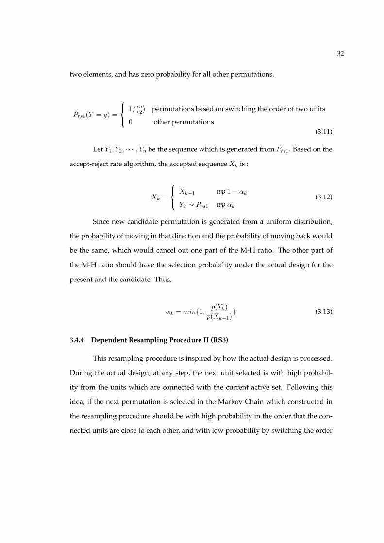
3.4.4 Dependent Resampling Procedure II (RS3)

This resampling procedure is inspired by how the actual design is processed.

During the actual design, at any step, the next unit selected is with high probabil-

ity from the units which are connected with the current active set. Following this

idea, if the next permutation is selected in the Markov Chain which constructed in

the resampling procedure should be with high probability in the order that the con-

nected units are close to each other, and with low probability by switching the order

33

of those unconnected units, then the acceptance rate may be higher than the permuta-

tions generated by switching the order of two randomly selected units. For example,

{U1, U2, ....U10} is the original sample. Links exist only between U1 and U2, U4 and U5.

In the resampling procedure, with high probability (say 0.9) the connected pair is se-

lected from {(U1, U2), (U4, U5)}. With low probability (say 0.1) non-connected paired

units are selected. The next permutation is generated by switching the order of this

two units in the current state. If at the first step {(U1, U2)} is chosen and the new se-

quence is accepted in M-H algorithm, we have {U2, U1, U3, U4, U5, ..., U10}. At the sec-

ond step, (U4, U5) is chosen and switched order, the new sequence is {U2, U1, U3, U5, U4, ..., U10}.

The proposal distribution is still uniformly distributed, denoted as Prs2 in (3.14). One

part of M-H ratio still could be canceled out, the other part of it should has the calcu-

lation as in (3.13).

Prs2(Y = y) =

0.9/(n2

)permutations generated by switching order of two connected units

0.1/(n2

)permutations generated by switching order of two unconnected units

0 other permutations(3.14)

The accepted sequence Xk is :

Xk =

Xk−1 wp 1− αk

Yk ∼ Prs2 wp αk

(3.15)

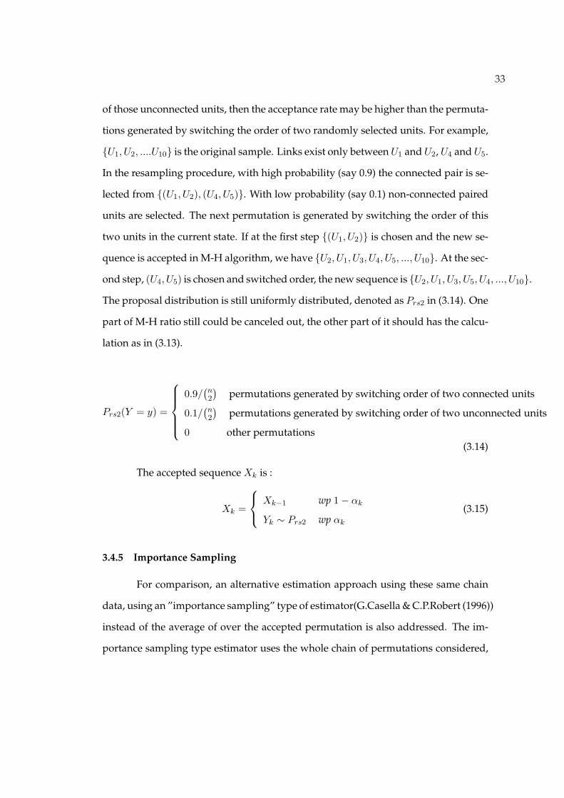
3.4.5 Importance Sampling

For comparison, an alternative estimation approach using these same chain

data, using an ”importance sampling” type of estimator(G.Casella & C.P.Robert (1996))

instead of the average of over the accepted permutation is also addressed. The im-

portance sampling type estimator uses the whole chain of permutations considered,

34

but accepted and unaccepted candidates. In other words, all the estimations during

the resampling procedures are included and weighted. Let P (Xk) be the probability

of choosing sample Xk at step k under true population, and PtXk is probability of

choosing sample Xk under the stationary distribution Pt(.). The estimations based

on importance sampling are calculated as:

E(µi) =∑

i=1,2,···nr

Pt(Xk)P (Xk)

µ(Xk)/∑

i=1,2,···nr

Pt(Xk)P (Xk)

(3.16)

So there are two approaches are used to approximating the Rao Blackwell

estimator for the three resampling procedures. One approach averages the values

of the preliminary estimator over the accepted permutations of the sample in the

Markov chain. The other approach uses a weighted average of the values of the

preliminary estimator over the whole chain including also the permutations of the

sample that were not accepted by the Metropolis Hastings step, namely IS1, IS2 and

IS3 for each resampling procedure. The relative weights are based on the ratios of

the actual selection probability of the permutation under the design divided by the

conditional probability of the permutation under the resampling design given the

previous permutation. The importance sampling estimator also is divided by the

sum of these relative weights.

3.5 Simulated Data

In this part, the AWS sampling designs and resampling approaches described

above are implemented to sample from of population of size 200 ( Figure 3.3 ). The il-

lustration of three samples each of size 10 drawn from the population are also shown.

The initial sample size is 4. Our goal is to employ different resampling approaches

in order to estimate the population mean node value, namely population proportion

estimation. We want to compare the efficiency and find the better MCMC procedure.

35

The efficiency of different resampling methods are compared based on K = 2, 000

samples. The acceptance rate are also tracked. The true population proportion is

0.31.

3.5.1 Population mean node value estimation

The population mean are valued through preliminary estimators µ0, the ex-

act Rao-Blackwell estimators µrb, and three different MCMC resampling procedures

which are used to approximate exact Rao-Blackwell estimators µrsi, i = 1, 2, 3. The

main concern is the statistical efficiency in estimating the expectation of interest among

these MCMC resampling procedures.

Most works used to investigate the MCMC efficiency are implemented by the

assessment of burn in time, convergence and variance estimation (Gilks et al. (1996)).

Methods are employed so far include between-within chains variation (Gelman &

Rubin (1992)), Raftery & Lewis (1992a), Raftery & Lewis (1992b)) algorithm, Geweke

algorithm(Geweke (1992)) etc. In physics literature, Goodman & Sokal (1989) defined

theintegrated autocorrelation time and system relaxation time. The concepts of them are

also closely related to the convergence rate of the algorithm. Since at least some

of our MCMC methods actually start in its stationary distribution, thus continues

there, there is not a question of how long to reach the stationary resampling estimator.

The question is how long it needs to run before the resampling estimator, which is

a cumulative mean of preliminary estimators, has a small enough variance. So to

compare the MCMC efficiency in our case, we consider the standard error of the

cumulative means for chains at different length, and see which one has a smaller

standard error among a set of fixed length chains. The standard error was based on

the variance between chains, not the variance within chains.

36

Figure 3.3. Population 200 with Stochastic Block structure and 3 AWS samples of size 10.

poppulation graph active set adaptive sample

active set adaptive sample active set adaptive sample

37

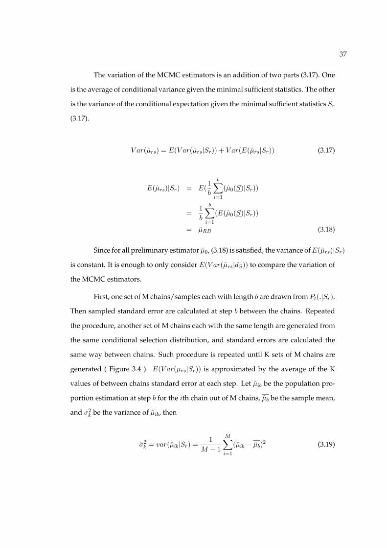
The variation of the MCMC estimators is an addition of two parts (3.17). One

is the average of conditional variance given the minimal sufficient statistics. The other

is the variance of the conditional expectation given the minimal sufficient statistics Sr

(3.17).

V ar(µrs) = E(V ar(µrs|Sr)) + V ar(E(µrs|Sr)) (3.17)

E(µrs)|Sr) = E(1b

b∑

i=1

(µ0(S)|Sr))

=1b

b∑

i=1

(E(µ0(S)|Sr))

= µRB (3.18)

Since for all preliminary estimator µ0, (3.18) is satisfied, the variance of E(µrs)|Sr)

is constant. It is enough to only consider E(V ar(µrs|dS)) to compare the variation of

the MCMC estimators.

First, one set of M chains/samples each with length b are drawn from Pt(.|Sr).

Then sampled standard error are calculated at step b between the chains. Repeated

the procedure, another set of M chains each with the same length are generated from

the same conditional selection distribution, and standard errors are calculated the

same way between chains. Such procedure is repeated until K sets of M chains are

generated ( Figure 3.4 ). E(V ar(µrs|Sr)) is approximated by the average of the K

values of between chains standard error at each step. Let µib be the population pro-

portion estimation at step b for the ith chain out of M chains, µb be the sample mean,

and σ2k be the variance of µib, then

σ2k = var(µib|Sr) =

1M − 1

M∑

i=1

(µib − µb)2 (3.19)

38

Figure 3.4. Expected variance given conditional selection probability calculation procedure.

The estimated value are presented in Table 3.1 which is based on M-H algo-

rithm and Table (3.2) which is based on importance sampling algorithm. The stan-

dard error are calculated at iterations b equals to b = 500, 1, 000, 2, 000, 4, 000, 6, 000, 8, 000, 10, 000.

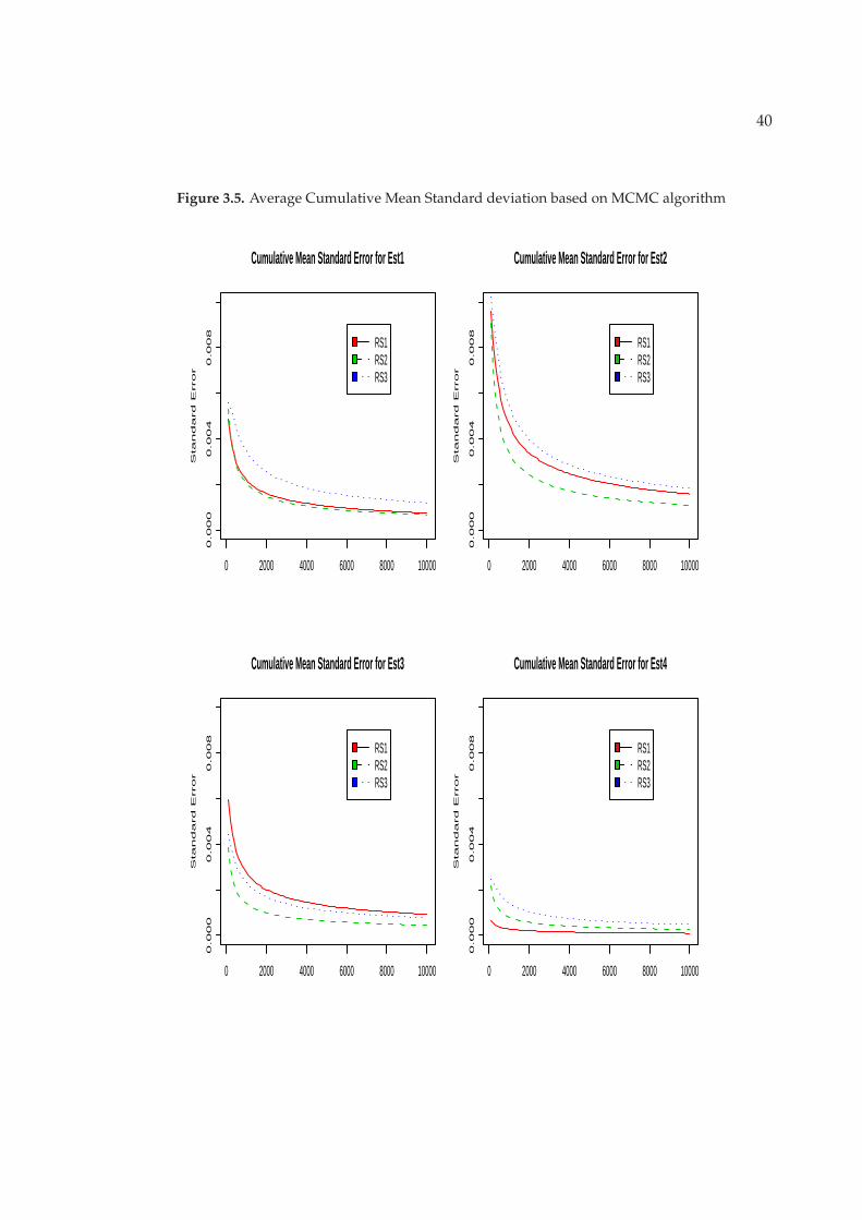
Figure 3.5 and Figure 3.6 describe the changes of estimator variation with the in-

creases of the number of interaction. RS1, RS2 and RS3 are three MCMC estimators.

IS1, IS2 and IS3 are importance resampling estimators based on three resampling

procedures. The decreases of E(V ar(µmc|S)) for independent resampling procedure

decreases faster than both the depended resampling procedures based on importance

sampling algorithm. For the MCMC algorithms, Standard error estimates based on

the third resampling method (RS3) have larger values than estimates based on the

39

other two resampling methods. And the three resampling procedures to estimate

population mean perform differently. For example, to estimate the mean based on

initial sample, RS1 and RS2 have very close standard error which are smaller than

the values based on RS3. For the estimators based on conditional selection probabil-

ity(EST2), estimators based on RS2 has the smallest values than the others. The ar-

gument is that Independent resampling procedure performs best under importance

sampling algorithm. And the procedure of randomly switching the order of two

units is the least efficient methods since it has the highest variation. For accept-reject

algorithm, the results are not consistent with the results under importance sampling

algorithm.

Another way to evaluate how the resampling methods work is to compare the

estimated expectation and variance of the estimators, and how the values are differ-

ent from true population value which equals to 0.31 for the stochastic block structure

population. Table 3.3 shows the results. All estimators are based on K = 2, 000 sam-

ples. µrb are the exact Rao-Blackwell estimators based on sample size 10. µRS and

µIS are based on average of b = 10, 000 resampling values for MCMC and impor-

tance sampling methods. It is obvious that the µRB is the best estimator since we

select every one from permutation space with distribution P (S|Sr). It shows that

the argument between the three resampling estimates thus requires more than 1,000

iterations. Figure 3.7 describes the distribution of empirical estimated values. The

vertical line is true population mean node value. There is no distinguishable dif-

ference among estimates under three resampling methods since the density plot are

almost identical. The Est2 may under estimate the population true value.

40

Figure 3.5. Average Cumulative Mean Standard deviation based on MCMC algorithm

0 2000 4000 6000 8000 10000

0.0

00

0.0

04

0.0

08

Cumulative Mean Standard Error for Est1

Sta

nd

ard

E

rror

RS1RS2RS3

0 2000 4000 6000 8000 10000

0.0

00

0.0

04

0.0

08


Sta

nd

ard

E

rror

RS1RS2RS3

0 2000 4000 6000 8000 10000

0.0

00

0.0

04

0.0

08


Sta

nd

ard

E

rro

r

RS1RS2RS3

0 2000 4000 6000 8000 10000

0.0

00

0.0

04

0.0

08


Sta

nd

ard

E

rro

r

RS1RS2RS3

41

Table 3.1. Estimates of E(var(µrs|S)) based on M-H algorithm of RS1, RS2 and RS3

b iterations

Estimators b = 500 b = 1000 b = 2000 b = 4000 b = 6000 b = 8000 b = 10, 000

EST1

µRS1 0.0153 0.0131 0.0111 0.0093 0.0084 0.0078 0.0074

µRS2 0.0140 0.0118 0.0099 0.0083 0.0075 0.0070 0.0066

µRS3 0.0243 0.0208 0.0176 0.0148 0.0134 0.0124 0.0118

EST2

µRS1 0.0323 0.0278 0.0235 0.0199 0.0179 0.0166 0.0158

µRS2 0.0229 0.0194 0.0163 0.0136 0.0123 0.0114 0.0108

µRS3 0.0379 0.0323 0.0272 0.0228 0.0207 0.0192 0.0182

EST3

µRS3 0.0192 0.0165 0.0139 0.0116 0.0105 0.0098 0.0093

µRS2 0.0094 0.0080 0.0067 0.0056 0.0051 0.0047 0.0045

µRS3 0.0161 0.0137 0.0115 0.0097 0.0088 0.0081 0.0077

EST4

µRS1 0.0019 0.0016 0.0014 0.0012 0.0010 0.0010 0.0000

µRS2 0.0055 0.0046 0.0039 0.0033 0.0030 0.0027 0.0026

µRS3 0.0098 0.0084 0.0071 0.0060 0.0054 0.0050 0.0047

42

Figure 3.6. Average Cumulative Mean Standard deviation based on importance samplingmethod

0 2000 4000 6000 8000 10000

0.0

00

0.0

04

0.0

08

IMPS:Cumulative Mean Standard Error for Est1

Sta

nd

ard

E

rror

IS1IS2IS3

0 2000 4000 6000 8000 10000

0.0

00

0.0

04

0.0

08


Sta

nd

ard

E

rror

IS1IS2IS3

0 2000 4000 6000 8000 10000

0.0

00

0.0

04

0.0

08


Sta

nd

ard

E

rro

r

IS1IS2IS3

0 2000 4000 6000 8000 10000

0.0

00

0.0

04

0.0

08


Sta

nd

ard

E

rro

r

IS1IS2IS3

43

Table 3.2. Estimates of E(var(µrs|S)) based on importance sampling algorithm for IS1, IS2and IS3 methods

b iterations

estimator b = 500 b = 1000 b = 2000 b = 4000 b = 6000 b = 8000 b = 10, 000

EST1

µIS1 0.0120 0.0104 0.0089 0.0076 0.0069 0.0065 0.0062

µIS2 0.0211 0.0187 0.0163 0.0141 0.0130 0.0122 0.0116

µIS3 0.0264 0.0236 0.0208 0.0182 0.0168 0.0158 0.0151

EST2

µIS1 0.0125 0.0107 0.0092 0.0078 0.0071 0.0066 0.0062

µIS2 0.0311 0.0271 0.0235 0.0202 0.0185 0.0172 0.0164

µIS3 0.0408 0.0361 0.0316 0.0274 0.0252 0.0236 0.0225

EST3

µIS1 0.0149 0.0129 0.0111 0.0095 0.0087 0.0081 0.0077

µIS2 0.0215 0.0188 0.0162 0.0139 0.0127 0.0119 0.0113

µIS3 0.0276 0.0244 0.0213 0.0184 0.0170 0.0159 0.0152

EST4

µIS1 0.0015 0.0013 0.0011 0.0010 9e-04 8e-04 8e-04

µIS2 0.0049 0.0040 0.0032 0.0026 0.0023 0.0022 0.002

µIS3 0.0060 0.0049 0.0040 0.0033 0.0030 0.0027 0.0026

44

Table 3.3. Estimated expectation and variance and mean squares error. Based on 2,000 sam-ples and each with 1,000 re-samples. True population value os 0.31. µo is preliminary esti-mator, µRB is exact Rao-Blackwell estimator, µRSi, i = 1, 2, 3 are resampling estimators. Thesample size is 10 with initial sample size 4.

estimators E(µ) V ar(µ) E(µ− 0.31)2

EST1 µ0 0.3479 0.0215 0.0229

µRB 0.3079 0.0224 0.0224

µRS1 0.3375 0.0304 0.0311

µRS2 0.3206 0.0310 0.0311

µRS3 0.3278 0.0298 0.0301

EST2 µO 0.2934 0.0325 0.0327

µRB 0.3124 0.0308 0.0308

µRS1 0.3176 0.0347 0.0347

µRS2 0.3130 0.0320 0.0320

µRS3 0.3093 0.0312 0.0312

EST3 µO 0.3122 0.0326 0.0326

µRB 0.3058 0.0314 0.0314

µRS1 0.3103 0.0301 0.0301

µRS2 0.3214 0.0293 0.0294

µRS3 0.3097 0.0305 0.0305

EST4 µO 0.3016 0.0335 0.0335

µRB 0.3158 0.0307 0.0307

µRS1 0.3178 0.0368 0.0368

µRS2 0.3269 0.0382 0.0384

µRS3 0.3104 0.0403 0.0403

45

Figure 3.7. Samples based on AWS designs from population of size 20

0.0 0.2 0.4 0.6 0.8 1.0

01

23

4

Distribution of Est1

De

nsity Orig

DRSIDRSIIIRS

0.0 0.5 1.0 1.5 2.0

01

23

4


De

nsity

OrigDRSIDRSIIIRS

0.0 0.2 0.4 0.6 0.8 1.0

0.0

0.5

1.0

1.5


De

nsity

OrigDRSIDRSIIIRS

−0.2 0.0 0.2 0.4 0.6 0.8 1.0 1.2

0.0

0.5

1.0

1.5


De

nsity Orig

DRSIDRSIIIRS

46

Table 3.4. Estimated expectation and variance and mean squares error. Based on 2,000 sam-ples and each with 1,000 re-samples, importance resampling method. The sample size is 10and initial sample size is 4.


EST1 µIS1 0.3089 0.0097 0.0097

µIS2 0.2967 0.0373 0.0375

µIS3 0.3049 0.0536 0.0536

EST2 µIS1 0.3901 0.0179 0.0243

µIS2 0.3078 0.0782 0.0782

µIS3 0.3190 0.1469 0.1469

EST3 µIS1 0.4429 0.0129 0.0306

µIS2 0.3085 0.0408 0.0408

µIS3 0.3940 0.0506 0.0576

EST4 µIS1 0.8783 0.0160 0.3390

µIS2 0.3205 0.0673 0.0674

µIS3 0.3305 0.0686 0.0689

3.6 Discussion

We have seen that the output of the simulation schemes such as prelimi-

nary estimators can be improved by Rao-Blackwell estimators to reduce the vari-

ation. Although the computational implementation may seem involved, the exact

Rao-Blackwell estimators can be easily programmed via recursive iterations when

the sample size is no larger than 12. But the computation duty increases while the

increases of the sample size, resampling procedures can be implemented instead of

Table 3.5. The acceptance rate for RS1, RS2 and RS3

rate(%) RS1 RS2 RS3

9.7 42.29 45.18

47

exact Rao-Blackwell calculation, either through M-H MCMC or importance sampling

algorithms. The fact that our MCMC estimators starts from its stationary distribution,

so continues from that, it is no problem for the estimators converge to the station-

ary distribution. The question is that how fast the variation change among a set of

chains with fixed length. The result is the independent resampling procedure is the

most efficient one under importance sampling algorithm. But for MCMC algorithm,

the three resampling procedures perform differently. The acceptance rate for RS1 is

lower than RS2 and RS3, since new permutations are generated independently.

Note that the above simulations are based on 200 population and the true

population proportion is around 0.31. This proportion is relatively large compared

to the definition of rare population, which is less than 0.05. In order to investigate

the effect of the large population proportion, another simulation based on 0.025 true

population proportion is implemented (3.6). The population size is also 200. The ex-

act Rao-Blackwell estimators still have good computational accuracy. They performs

best in terms of lowest mean square error. The estimators based on RS1 are more

efficient than estimators based on RS2 and RS3 since they have lower bias and mean

square error. There is not significant difference between the estimators based on RS2

and RS3.

Note that the results in this paper are based on simulations and no new meth-

ods have been developed to test which resampling procedure is better than RS1 which

is proposed by Thompson(2006). Some improved methods for testing MCMC accu-

racy and variance comparison may exist, which should be pursuit in the future.

48

Table 3.6. Estimated expectation and variance and mean squares error. Based on 2,000 sam-ples and each with 1,0000 re-samples. True population value os 0.025. µ0i, i = 1, 2, 3, 4 arepreliminary estimators. µRB is exact Rao-Blackwell estimators. µRSi, i = 1, 2, 3, 4 are estima-tors based on three different resampling procedures. The total sample size is 10 and initialsample size is 4.


EST1

µ01 0.0260 0.0062 0.0062

µRB 0.0251 0.0030 0.0030

µRS1 0.0252 0.0034 0.0034

µRS2 0.0253 0.0034 0.0034

µRS3 0.0253 0.0034 0.0034

EST2

µ02 0.0260 0.0084 0.0084

µRB 0.0251 0.0052 0.0052

µRS1 0.0253 0.0054 0.0054

µRS2 0.0254 0.0055 0.0055

µRS3 0.0254 0.0055 0.0055

EST3

µ03 0.0240 0.0063 0.0063

µRB 0.0249 0.0029 0.0029

µRS1 0.0249 0.0030 0.0030

µRS2 0.0247 0.0035 0.0035

µRS3 0.0247 0.0031 0.0031

EST4

µ04 0.0241 0.0074 0.0074

µRB 0.0247 0.0023 0.0023

µRS1 0.0247 0.0024 0.0024

µRS2 0.0246 0.0027 0.0027

µRS3 0.0247 0.0027 0.0027

Chapter 4

Cost Optimization in Adaptive Web Sampling

4.1 Abstract

The main advantage of Adaptive Web Sampling (AWS) designs is that the

sample size could be predefined and fixed prior to implementing the sampling strat-

egy ( Thompson (2006a) ). However the randomness of the sample units still exists,

and the probability of selection provides the basis for unbiased estimation. However

the variation of the selected sample units has not been fully investigated to date. In

this paper, we incorporate some practical restrictions, such as budget or time that

determine which unit or set of units should be selected at each step and when the

sampling process should stop. The objective is to minimize the cost and maximize

the sampling procedure information by efficient design of the sampling options.

4.2 Introduction

Thompson & Seber (1996) introduced adaptive sampling designs mainly im-

plemented for spatial environments. For spatially clustered populations such as ani-

mal or plant species and mineral or oil resources, adaptive cluster sampling and strat-

ified adaptive cluster sampling are also introduced (Thompson (1990a),Thompson

(1990b)) to improve the efficiency. Such designs can also be used to sample hidden

human populations, the internet, and other populations with network structures. A

weak point of such designs is the lack of control in how the initial sample is obtained

49

50

and sample coverage. Thompson (2006a) introduced a new and more flexible sam-

pling design Adaptive Web Sampling(AWS) to overcome this shortcoming and the

sample selection probability becomes step by step less dependent on the initial sam-

ple selection. These sampling designs have more flexibility and allow the possibility

for designs under different active sets, different initial sample designs or different

calculations for the selection probability at each step. However none of them are in-

vestigated under the constraints of budget, time or risk. In this chapter, we consider

a type of AWS design which is implemented based on different design factors such

as selection probabilities, initial sample size, and the number of units selected at each

step. We are seeking to find an optimal sampling procedure based on the perfor-

mance of population estimations, which depend on the different parameter values

under the same cost model. The relative efficiency and mean squared error are mea-

sured by the comparison the variation of the estimation for population proportion.

We illustrate the application of one AWS methodology to the problem of es-

timation of the population proportion in two cases. One sample is a simulated wire

transaction data set in Banking setting. The purpose is to identity the high risk fraud

sub population of participants in the money transaction. The population of subjects

for such a study are plentiful, but determination of the high risk subjects simply by

observing money transaction everyday is very time consuming. Thus, it is impor-

tant to obtain a set of representative subjects in the population in limited time. We

will demonstrate how a AWS design with cost constraint in terms of time can assist

achieving this goal. Another illustration is based on the Colorado Springs data, which

is a study of the heterosexual transmission of HIV/AIDS in a ”high-risk” population

in Colorado Springs ( Potterat et al. (1993), Rothenberg et al. (1995) ). This empirical

population was also used by Chow & Thompson (1998) as an example in a snowball

sampling design in which all links were traced, with the exception of the last wave.

51

4.2.1 AWS designs

The AWS desing proceeds as follows (Thompson (2006a)): At any point dur-

ing the sampling, the selection of the next unit or wave of units to include in the

sample is with high probability d selected with a distribution that depend on the

values of variables of interest in an “active set” of units already selected. With low

probability 1 − d, the next unit is selected from a distribution not depending on val-

ues of variables of interest. The active set could be the units selected so far, the most

recently selected units or subset of the units selected.

Figure 4.1 is an illustration of how a sample is obtained through the applica-

tion of AWS design. The population link matrix Wij is a matrix of 1 and 0s. Where a

1 indicates a link between the units labeled in the rows and columns.

1 2 3 4 5 6 7

1 0 0 1 1 1 0 0

2 0 0 0 1 1 0 0

3 1 0 0 1 0 1 0

4 1 1 1 0 1 0 1

5 1 1 0 1 0 1 0

6 0 0 1 0 1 0 0

7 0 0 0 1 0 0 0

The Nodes 1 and 2 are initially selected using any sampling designs from the entire

population of nodes. Using the information obtained from interviewing node 1 and

node 2, all the links connecting nodes 1 and 2 are observed. A red circle represents the

nodes with characteristics we are interested in such as HIV positive, suspicious bank

account etc.; blue circles represent HIV negative people. Node 6 represents one of the

52

Figure 4.1. An illustration of adaptive web sampling. Nodes 1 and 2 are initially chosen atrandom. Weighted links are used to calculate transition probabilities from current active setto next selected units.

nodes that are not connected with nodes 1 and 2. Such nodes could not be observed

so that their characteristics are unknown. We put a weighted link from active set A1

to node 3 equals to 1, WA13 = 1, since there is only one link out from A1 to node 3; A

weighted link from A1 to node 4 equals to 2 since two links are out from A1 to node

4. WA16 = 0 since node 6 is isolated from A1. New nodes are selected based on the

observed weighted links. For the snowball type adaptive sampling, new units can

only be selected from the nodes 3, 4, 5, and 7 since they are connected with the initial

sample, thus we could not control the depth and width of such sampling procedures.

The AWS design is more flexible in that new nodes can be selected not only from

the connected ones but also can be selected from those isolated nodes. Suppose the

nodes from the connected units have distribution fc, and the nodes which are isolated

from the current active set is distributed as fu. At any point during the sampling

procedure, new nodes are selected from a mixture distribution

53

Table 4.1. Transition probabilities from nodes 1 and 2 in Figure 4.1

qA13 = 16 ∗ d + (1− d)/5

qA14 = 26 ∗ d + (1− d)/5

qA15 = 26 ∗ d + (1− d)/5

qA16 = 26 ∗ d + (1− d)/5

qA17 = 16 ∗ d + (1− d)/5

fm = dfc + (1− d)fu (4.1)

where, d, fc, fu could be chosen according to different sampling purpose. In

this paper, we carried out a AWS design where d depends on a cost ratio. The cost

ratio is defined as the cost of including connected units over the cost of including

isolated units, denoted as rc. fc and fu only depend on the observed links out from

current active set. The transition probabilities for such designs are given by

q(j|Ak) =

d× WAkj

WAk++ (1− d)× 1

N−nAklink exists from Ak to j

1N−nAk

no link exists from Ak to j(4.2)

Where, WAkj is the number of links from the current active set Ak to unit j,

WAk+ is the total number of links from outside Ak, nAkis the number of units selected

so far. In Figure 4.1, the transition probabilities from initial sample nodes 1 and nodes

2 to other nodes are:

54

4.2.2 Estimation

Based on Conditional selection Probability: Thompson (2006a) derived a population

proportion estimator based on conditional selection probability. Such estimator can

be thought as a composite estimator of the initial sample and the additional samples

selected using the nodes value to determine the selection probability step by step.

The first part is the unbiased estimator of the population total∑

yi based on the

initial sample. And the second part is the estimators of∑

yi based on conditional

selection probability at any step of the sampling procedure after initial sample. In

his paper, the estimator is based on sampling with only ONE new unit included at

each step. In this paper, EST2 is enlightened by the idea proposed by Thompson, but

based on the sampling procedure which is taken by waves.

The population total∑

yi estimator based on the initial sample is:

τS0 = (N/n)∑

i∈S0

yi/πi

when units are selected with probability π. For a simple random initial sample

without replacement which is implemented in this paper,

τS0 = (N/n)∑

S0

yi = Ny0

At step K after the initial sample with active set Ak, Zk is used to estimate the

population total

Zk =∑

j∈Sck

yj +∑

l∈Sk

yl/qAkl

Here qAkl is the selection probability of unit l in wave k with yk value, Sck =

55

{S0, S1, S2, · · · , §K} is the units selected so far. An unbiased estimator for the popu-

lation mean:

µ1 =1

Nn{n0τS0 +

∑Zi} (4.3)

4.3 Cost Model

So far, there is a very sparse literature on costs for sampling hidden popula-

tion due to less attention for cost efficiency modeling, less quantified decision mak-

ing versus professional expertise or other reasons. For sampling rare populations,

the costs due to uncertain difficulties of contacting sampling units, gaining coopera-

tion of the sample units and the interviewer variation in efficiency are big issues. In

some sampling situations, the cost of sampling, measured in terms of time, money or

risk etc, may differ from wave to wave, and may also differ among units within each

wave.

Dell & Clutter (1972) model cost in Ranked Set Sampling (RSS) and the sam-

pling efficiency was evaluated through the ratio of population mean estimator be-

tween RSS and simple randomly sampling (SRS). In their cost model, cs and cq are

the cost of stratification which involved sampling and ranking and the cost of quali-

fication for one unit, respectively. RSS and SRS are compared in estimating the pop-

ulation mean through

RE(µRSS , µSRS) =cq

cq + csRPRSS (4.4)

where RPRSS = var(µSRS)var(µRSS) . Kaur et al. (1996) devised a more detailed cost

model (KPST) that incorporates more cost categories such as set up costs, cost of

ranking the units in a set, etc. W.Nahhas et al. (2002) extended their model by con-

56

sidering the cost of ranking which is assumed to be negligible in the KPST model.

The motivation behind their work is that, in certain situations, sampling and ranking

of units from the population are inexpensive while actual measurement of a unit is

costly.

In this paper, our effort is motivated by the fact that sampling the rare popula-

tion is expensive in terms of time and money under the convenience designs includ-

ing SRS. At each step, new units are selected depending on the weighted links. For

example in Figure 4.1, the weight matrix is the same as link matrix since we count

the total number of connections out from Ak. In the wire transaction case, it could

be number of total transactions, the total amount, the number of keyword hits, or

other social connections between two accounts. For simplicity, we only consider the

number of transaction records between business partners. Though we do not rank

the units, the links with larger weights should have higher probability of being se-

lected than the links with smaller weights. A cost model based on such sampling

procedures could be derived as follows: Let C1 be the cost for obtaining each unit

which is connected with the current active set, and C2 be the cost for jumping to an

isolated one, respectively. Suppose n is the total AWS sample size, n1 is the number

of units included by following links, n2 is the number of units selected randomly and

n1 + n2 = n C0 is an overhead costs for AWS, then the total cost is:

CAWS = C0 + n1 ∗ C1 + n2 ∗ C2 (4.5)

The following example will be used to illustrate the determination of parame-

ter values in the AWS based on a pre-specified total cost value. The relative efficiency

is compared to investigate the optimal parameter combination values. The parame-

ters are listed in Table 4.2.

57

Table 4.2. Pre-specified parameter values for population proportion estimation for the exam-ple shown in Figure 4.2

n0 Initial sample size {5,10,20}ns Number of units selected at each step {2,4,8}rc Cost ratio,rc = C2/C1 {1,2,4,8}d Link tracing probability 20 values evenly across (0, 1)

4.4 Simulation

4.4.1 Simulation Setting

The population shown in Figure 4.2 is a simulated data set based on wire

transaction in a banking center. Red circles represent suspicious accounts, and yellow

circles represent normal accounts. Variable Y is used to describe the accounts status:

Yi =

1 i is suspicious account

0 i is normal account(4.6)

The black lines represent a wire transaction between two accounts. The accounts

could be personal or company accounts. There are 6 suspicious accounts out of the

set of 100 accounts. For simplicity, we assume that wire transactions always exits

between paired accounts. In other words, there is a transaction from B to A once a

wire transaction from A to B. Thus, the links matrix which describe the transaction

among 100 accounts is symmetric, which is shown in Table 4.3.

There are millions of wire transaction records every week. How to capture

the rare suspicious accounts from this huge data base efficiently is always an Anti

Fraud issue for banks because of the time consuming nature of checking each account

record. Here we assume C1 units of time spent on checking an account which has a

wire transaction with already checked accounts; C2 units of time spent on checking an

58

account which is randomly picked from the unchecked account records. The AWS de-

signs was implemented as follows. An initial sample of size n0 was simply randomly

sampled from the whole population. A fixed overhead cost C0 for it is assumed. Af-

ter that, ns accounts were sampled with weight from those accounts which have wire

transaction with any accounts in the initial sample. We call this is the first wave of the

sampling procedure. And accounts obtained after the first wave are sample S1. We

add the cost for sampling and checking every account in the first wave. If the current

cumulative cost Cw is less than a pre-specified total cost Ct, we use the accounts in S1

to be the active set for next sampling wave untill Cw >= Ct. This means that when

we do not have more time for investigating accounts, the sampling procedure should

end. Suppose S is the set all the accounts we obtained by the time Ct is used up, we

obtain the information of account status, transaction behavior among them, accounts

selection order and all account selection probabilities. Based on this information, we

can estimate the proportion of suspicious accounts in the whole population. To re-

duce the sampling bias, we repeated such procedure 2,000 times, and the sampling

proportion and variance are averaged over the 2,000 samples. Combinations of the

parameters specified in Table 4.2 are used in the simulation.

4.4.2 Simulation Result

Relative efficiency(RE) and mean square error(MSE) are used to compare how

different link tracing probabilities effect the results in (4.7). Let REn0,n∗0 be the RE

between estimator based on initial sample n0 and n∗0, and which also depend on d

and ns,

REn0,n∗0 =var(µn0)var(µn∗0)

(4.7)

Figure 4.3 describes the RE for initial sample size of 10 and 5. Figure 4.4

59

describes the RE for initial sample size of 10 and 20. Both Figures show that RE

decreases when link tracing probabilities increase. Thus we may have larger esti-

mated variation when initial sample size increase. The number of units do not have a

strong effect to the RE performance, as we can see since the three lines have similar

behavior. This result can also be shown by the RE values. RE5,10 is between 1.25

and 2.5 for different selection probability as seen in Figure4.4; RE10,20 is larger than

1.5, as seen in Figure4.3. These results are reasonable since initial sample is randomly

by disregarding their relationship. This leads to more dissimilarity and randomness

which may produce larger variation. Higher cost ratio seems to lead to higher RE,

but the performance is not significant. Figure 4.5, Figure 4.6 and Figure 4.7 depict

the MSE at different values of the parameters. The value of MSE increases with the

increase in selection probability. And the sharpest increases start at selection prob-

ability around 0.8. This result is most obvious for initial sample size 5. The same

conclusion could be obtained from the RE figures. Note that MSE based on a cost

ratio of 2 is right between MSE based on cost ratio of 1 and 4. Table 4.4.2 shows the

the value of minimum mean square error and corresponding selection probabilities.

Figure 4.9 shows the estimated total sample size distribution. Figure 4.10

shows estimated sampling waves/depth distribution. Total estimated sample size

is between 15 and 55 for initial sample size 5; Total estimated sample size is between

20 and 55 for initial sample size 10, and total estimated sample size is between 30

and 65 for initial sample size 20. The larger the initial sample size, the more a large

sample size is obtained. The initial sample size seems to have no strong effect to how

many units are sampled from population. But there are more sampling waves with

larger initial sample size. This shows that, for larger initial sample sizes, more links

are followed during the whole sampling procedure. But for different initial sample

size, the sampling procedure stops around waves 8 and 9 for most of cases.

60

1

2 3

456 78

9

10

11

12131415

16

17

18

19

20

2122 23

24

25

2627

28

29

30

31

32

33

3435

36

3738 39

40

41

42

43

44

45

46

47

48

49

50

51

52

53

54

55

56

57

58

59

60

61

62 6364

6566

67

68 6970

71

72

73

74

75

76

77

7879

80

81

82

83

84

85

86

87

88

8990

91

92

93

94

95

96

97

98

99

100

Figure 4.2. Simulated wire transaction record in Bank of America. Six suspicious Total num-ber of accounts is 100.

61

0.0 0.2 0.4 0.6 0.8

1.2

1.4

1.6

1.8

2.0

2.2

d, cost ratio=1

rela

tive

effic

ienc

y

plot of relative efficiency var(est|n0=5) and var(est|n0=10)

0.0 0.2 0.4 0.6 0.8

1.2

1.6

2.0

2.4

d, cost ratio=2

rela

tive

effic

ienc

y

0.0 0.2 0.4 0.6 0.8

1.0

1.5

2.0

2.5

d, cost ratio=4

rela

tive

effic

ienc

y

Figure 4.3. Relative efficiency between initial sample size 5 and 10, based on simulated pop-ulation in Figure 4.2.

62

Table 4.3. Simulated Link Matrix for population in Figure 4.2

x[1, 2] = x[2, 1] = 1, x[2, 6] = x[6, 2] = 1, x[1, 5] = x[5, 1] = 1

x[1, 3] = x[3, 1] = 1, x[2, 5] = x[5, 2] = 1, x[5, 7] = x[7, 5] = 1

x[3, 8] = x[8, 3] = 1, x[1, 4] = x[4, 1] = 1, x[4, 9] = x[9, 4] = 1

x[13, 14] = x[14, 13] = 1, x[11, 15] = x[15, 11] = 1, x[11, 10] = x[10, 11] = 1

x[10, 12] = x[12, 10] = 1, x[12, 16] = x[16, 12] = 1, x[12, 17] = x[17, 12] = 1

x[12, 18] = x[18, 12] = 1, x[12, 19] = x[19, 12] = 1, x[12, 20] = x[20, 12] = 1

x[16, 20] = x[20, 16] = 1, x[21, 22] = x[22, 21] = 1, x[23, 36] = x[36, 23] = 1

x[24, 35] = x[35, 24] = 1, x[25, 37] = x[37, 25] = 1, x[25, 38] = x[38, 25] = 1

x[25, 26] = x[26, 25] = 1, x[26, 27] = x[27, 26] = 1, x[27, 39] = x[39, 27] = 1

x[27, 40] = x[40, 27] = 1, x[28, 39] = x[39, 28] = 1, x[29, 42] = x[42, 29] = 1

x[29, 43] = x[43, 29] = 1, x[30, 41] = x[41, 30] = 1, x[30, 32] = x[32, 30] = 1

x[31, 43] = x[43, 31] = 1, x[31, 44] = x[44, 31] = 1, x[32, 45] = x[45, 32] = 1

x[33, 46] = x[46, 33] = 1, x[26, 34] = x[34, 26] = 1, x[39, 52] = x[52, 39] = 1

x[47, 74] = x[74, 47] = 1, x[48, 61] = x[61, 48] = 1, x[49, 63] = x[63, 49] = 1

x[50, 62] = x[62, 50] = 1, x[51, 64] = x[64, 51] = 1, x[52, 66] = x[66, 52] = 1

x[53, 67] = x[67, 53] = 1, x[54, 55] = x[55, 54] = 1, x[55, 68] = x[68, 55] = 1

x[56, 57] = x[58, 59] = 1, x[59, 71] = x[60, 73] = 1, x[75, 76] = x[65, 78] = 1

x[65, 79] = x[69, 70] = 1, x[71, 85] = x[72, 85] = 1, x[98, 85] = x[83, 84] = 1

x[82, 81] = x[82, 80] = 1, x[86, 73] = x[99, 86] = 1, x[87, 88] = x[89, 91] = 1

x[95, 92] = x[93, 96] = 1, x[94, 97] = x[99, 100] = 1

63

0.0 0.2 0.4 0.6 0.8

1.5

2.0

2.5

3.0

d, cost ratio=1

rela

tive

effic

ienc

y ns=2ns=4ns=8


0.0 0.2 0.4 0.6 0.8

1.5

2.0

2.5

3.0

d,cost ratio=2

rela

tive

effic

ienc

y ns=2ns=4ns=8

0.0 0.2 0.4 0.6 0.8

1.5

2.0

2.5

3.0

d, cost ratio=4

rela

tive

effic

ienc

y ns=2ns=4ns=8

Figure 4.4. Relative efficiency between initial sample size 10 and 20, based on simulatedpopulation in Figure 4.2.

4.5 Colorado Spring Data

Colorado Spring data is from a study on the heterosexual transmission of

HIV/AIDS in a ”high-risk” population in Colorado Springs (Potterat et al. (1993);

Rothenberg et al. (1995)). 8762 people are involved, out of which 595 were directly

interviewed and 8538 refereed to as contacts by those interviewed. This study record

people’s relationship of sex, needle share, and drugs share. And also record every-

one’s HIV status, positive or negative. The population quantities interested in is pop-

64

0.0 0.2 0.4 0.6 0.8

−0.0

005

0.00

050.

0015

MSE for population proportion estimation at n0=5,ns=2

d:unit select prob.

MS

E

r=1r=2r=4

0.0 0.2 0.4 0.6 0.8

−0.0

005

0.00

050.

0015


d:unit select prob.

MS

E

r=1r=2r=4

0.0 0.2 0.4 0.6 0.8

−0.0

005

0.00

050.

0015


d:unit select prob.

MS

E

r=1r=2r=4

Figure 4.5. MSE of population proportion estimator, based on initial sample size 5. The truepopulation proportion is 0.06 in Figure 4.2.

ulation proportion which is 0.5748.

Figure 4.11 describes the population structure. Red nodes represent injection

drug users. Lines between paired nodes indicate drug-using relationships. Largest

component contains 300 of the 595 individuals. Figure 4.12 describes the relative

efficiency of RE12,20. RE is larger than 1 means better performance and less variation

for population proportion when initial sample is large. We got the similar results

as from the simulated wire transaction data. The number of nodes selected at each

wave do not have strong effect to the RE performance when link tracing probabilities

less than 0.7. And the RE values become significantly different when link tracing

probabilities larger than 0.7. The variation for initial sample size of 12 and the number

of nodes included at each wave of 20 is significantly larger than the variation for

65

0.0 0.2 0.4 0.6 0.8

−0.0

005

0.00

050.

0015


d:unit select prob.

MS

E

r=1r=2r=4

0.0 0.2 0.4 0.6 0.8

−0.0

005

0.00

050.

0015


d:unit select prob.

MS

E

r=1r=2r=4

0.0 0.2 0.4 0.6 0.8

−0.0

005

0.00

050.

0015


d:unit select prob.

MS

E

r=1r=2r=4


initial sample size 20 and the number of nodes included are 5 and 10. In Figure 4.12,

the blue curve is significantly over the green and red curves when d is larger than

0.70. We got the similar results for estimated total sample size and sampling waves

as results from simulated bank money transaction data.

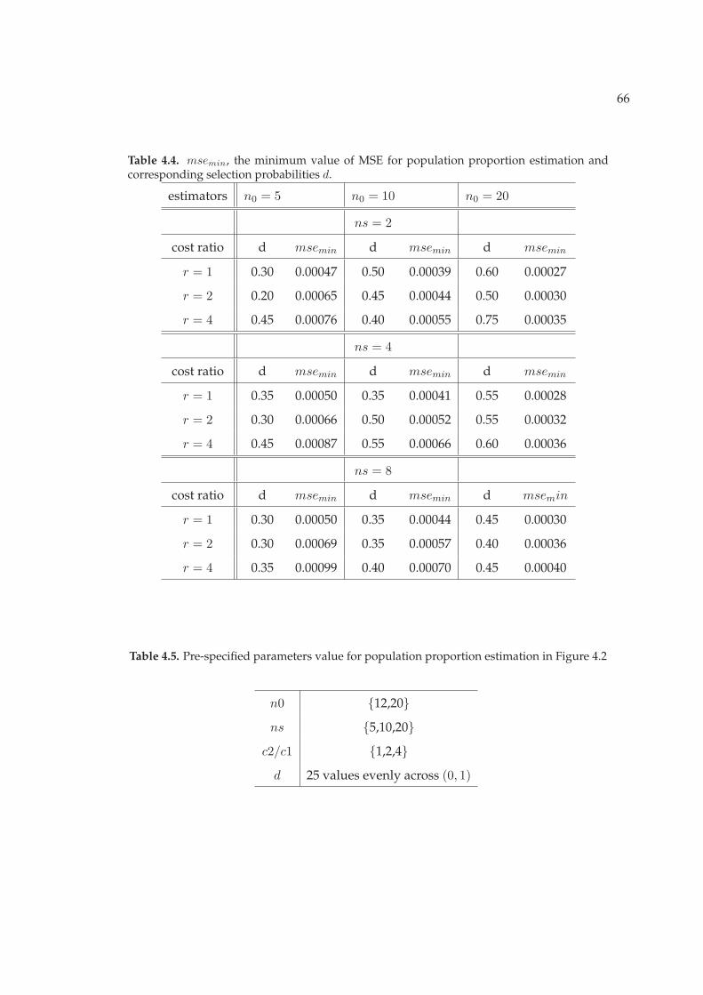
66

Table 4.4. msemin, the minimum value of MSE for population proportion estimation andcorresponding selection probabilities d.

estimators n0 = 5 n0 = 10 n0 = 20

ns = 2

cost ratio d msemin d msemin d msemin

r = 1 0.30 0.00047 0.50 0.00039 0.60 0.00027

r = 2 0.20 0.00065 0.45 0.00044 0.50 0.00030

r = 4 0.45 0.00076 0.40 0.00055 0.75 0.00035

ns = 4


r = 1 0.35 0.00050 0.35 0.00041 0.55 0.00028

r = 2 0.30 0.00066 0.50 0.00052 0.55 0.00032

r = 4 0.45 0.00087 0.55 0.00066 0.60 0.00036

ns = 8


r = 1 0.30 0.00050 0.35 0.00044 0.45 0.00030

r = 2 0.30 0.00069 0.35 0.00057 0.40 0.00036

r = 4 0.35 0.00099 0.40 0.00070 0.45 0.00040

Table 4.5. Pre-specified parameters value for population proportion estimation in Figure 4.2

n0 {12,20}ns {5,10,20}

c2/c1 {1,2,4}d 25 values evenly across (0, 1)

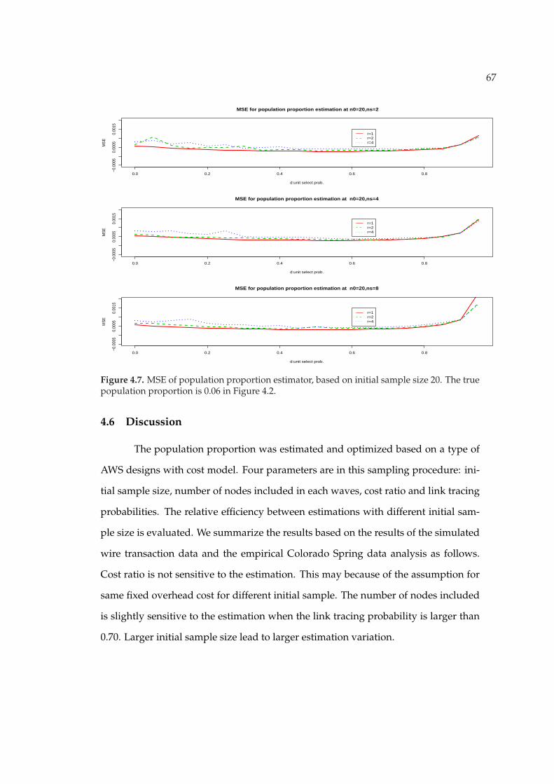
67

0.0 0.2 0.4 0.6 0.8

−0.0

005

0.00

050.

0015


d:unit select prob.

MS

E

r=1r=2r=4

0.0 0.2 0.4 0.6 0.8

−0.0

005

0.00

050.

0015


d:unit select prob.

MS

E

r=1r=2r=4

0.0 0.2 0.4 0.6 0.8

−0.0

005

0.00

050.

0015


d:unit select prob.

MS

E

r=1r=2r=4


4.6 Discussion

The population proportion was estimated and optimized based on a type of

AWS designs with cost model. Four parameters are in this sampling procedure: ini-

tial sample size, number of nodes included in each waves, cost ratio and link tracing

probabilities. The relative efficiency between estimations with different initial sam-

ple size is evaluated. We summarize the results based on the results of the simulated

wire transaction data and the empirical Colorado Spring data analysis as follows.

Cost ratio is not sensitive to the estimation. This may because of the assumption for

same fixed overhead cost for different initial sample. The number of nodes included

is slightly sensitive to the estimation when the link tracing probability is larger than

0.70. Larger initial sample size lead to larger estimation variation.

68

0.02 0.03 0.04 0.05 0.06 0.07

010

2030

4050

Distribution of Population Proportion estimation based on T−H method

population proportion estimation

Den

sity

n0=5n0=10ns=20true mean

Figure 4.8. Population proportion distribution based selection probability with initial samplesize 5, 10 and 20. The true population proportion is 0.06 in Figure 4.2

69

sample size distribution,n0=5

Freq

uenc

y

15 20 25 30 35 40 45 50

010

2030

4050

60


Freq

uenc

y

20 25 30 35 40 45 50 55

010

2030

4050

60


Freq

uenc

y

30 35 40 45 50 55 60 65

010

3050

Figure 4.9. Distribution of estimated total sample size based on different initial sample sizeof 5, 10 and 20. Population is in Figure 4.2.

70

sampling depth/waves distribution,n0=5

Freq

uenc

y

5 10 15 20 25 30 35

05

1015

2025

30


Freq

uenc

y

5 10 15 20 25 30 35

05

1015

2025


Freq

uenc

y

0 10 20 30 40

010

2030

4050

60

Figure 4.10. Distribution of estimated sampling waves/depth based on different initial sam-ple size of 5, 10 and 20. Population is in Figure 4.2.

71

Figure 4.11. HIV/AIDS at-risk population. Dark node indicates injection drug use. Linksindicate drug-using relationships. Largest component contains 300 of the 595 individuals.

72

0.0 0.2 0.4 0.6 0.8 1.0

0.0

0.5

1.0

1.5

2.0

d, cost ratio=1

rela

tive

effic

ienc

y

ns=5ns=10ns=20


0.0 0.2 0.4 0.6 0.8 1.0

0.0

0.5

1.0

1.5

2.0

d,cost ratio=2

rela

tive

effic

ienc

y

ns=5ns=10ns=20

0.0 0.2 0.4 0.6 0.8 1.0

0.0

0.5

1.0

1.5

2.0

d, cost ratio=4

rela

tive

effic

ienc

y

ns=5ns=10ns=20

Figure 4.12. Relative efficiency between initial sample size 12 and 20, based on ColoradoSpring data analysis.

73

0.54 0.56 0.58 0.60

010

2030

4050

Distribution of Population Proportion estimation based on T−H method

population proportion estimation

Den

sity

n0=12n0=20true mean

Figure 4.13. Population proportion distribution based on H-T estimation with initial samplesize 12 and 20. The true population proportion is 0.5748.

74

sample size,n0=12

Freq

uenc

y

40 60 80 100

020

4060

80


Freq

uenc

y

40 50 60 70 80 90 100 110

020

4060

80

Figure 4.14. Distribution of estimated total sample size based on different initial sample sizeof 12 and 20. Population is in 4.2.

Chapter 5

Model Based Estimationfor link-tracing designs with non-responses

5.1 Introduction

Link-tracing designs are mostly used for studying populations mostly on ”sen-

sitive” issues like in the study on illegal drug use, HIV/AIDS prevalence, prosti-

tution activities and so forth. These studies mostly suffer from high non-response

rates. In this paper we propose a model that is an extension of the model by Mosuk

and Thompson (2002). We propose a model that accommodates non-random non-

responses. We discuss how maximum likelihood estimates could be obtained. Both

real and simulated data are used to for illustration. We assume that the population of

interest has N subjects and there are different types of relations among the subjects.

Each subject, u, has a value of interest Yu. We assume that Yu is a random variable

that takes value 1 if subject u has a certain characteristic and 0 otherwise.

5.1.1 The Model

We assume a population of a known number of nodes N with each node tak-

ing two possible values 0 or 1. The proportion of 1’s in the population is

z =∑N

i=1 Yi

N(5.1)

where Yi is the y-value of node i. If we define Xuv as the indicator variable that value

1 when there is a link between nodes u and v. Given the node u has a y-value i and

75

76

node v has a y-value j, we define the link probabilities

λi+j = P (Xuv = 1|Yu = i, Yv = j) (5.2)

where i = 0, 1 and j = 0, 1. So the population graph has link probabilities λ =

{λ0, λ1, λ2}. Where λ0 is the probability of a link between any pair of nodes with

y-value 0, λ1 is the probability of a link between a node with y-value 0 and a node

with y-value 1. Similarly λ2 is the probability of a link between a pair of nodes with

y-value 1. Note that λi+j = λj+i.

In practice we don’t know the λ’s. The ratio in (5.1) is an estimator for θu =

P (a node has y-value =1). Assuming a binary probit model implies that

θu = Pr(Yu = 1|zu, β) = Φ(Z ′uβ)

Where β is a p × 1 vector of unknown parameters and Φ is the standardized

normal distribution function. Z ′u = (zu1, zu2, · · · , zup) are vector of known covariate

values.

In most link-tracing designs the value of interest Yu is obtained from the sam-

pled subject. Sensitive studies like the study of drug usage, HIV/AIDS and other

Sexually Transmitted Diseases (STDs) and so forth suffer from high non-response

rates. Which means parts of Yu value in the sample are missing. Let ru be the bi-

nary variable indicating whether yu is observed (ru = 1) or not (ru = 0). If ru is

independent of the value of interest Y the analysis can be done by just excluding the

non-responses in the estimation of parameters. This is missing completely at random

(MAR).

The model we consider here assumes that ru may depend on yu even condi-

tional on covariates Zu.

77

The aim of the work in this chapter is to develop a method for estimating the

distribution of yu

Let ru be an indicator that takes value 1 when node u accepts to be inter-

viewed and 0 otherwise. We define

βi = P (ru = 1|Yu = i) (5.3)

where i = 0, 1. The odds of a response from nodes u such that yu = i is βi

1−βi. We

define odds ratio γ as

γ =(

β1

1− β1

)/

(β0

1− β0

)(5.4)

When γ = 1 both nodes with y-value 1’s and 0’s have the same non-response rates. If

γ < 1 nodes with y-value 1 tend to give more non-responses than nodes with y-value

0. The opposite is true when γ > 1. We note that γ take values in the range (0,∞).

The goal of this paper is to estimate θ when samples are drawn from popu-

lations with unknown γ. We also note that is certain studies it is of interest to study

the pattern of non-responses. As a by-product, estimation and inference of γ helps to

answer questions about the non-response behavior. In this paper we’ll discuss how

to obtain estimators for θ and γ using a snowball sample.

5.1.2 Applicability of the Model

In most link-tracing designs the value of interest Y is obtained from the sam-

pled subject. Sensitive studies like the study of drug usage, HIV/AIDS and other

Sexually Transmitted Diseases (STDs) and so forth suffer from high non-response

rates. When non-responses are independent of the value of interest Y the analysis

can be done by just excluding the non-responses in the estimation of parameters.

This is missing completely at random.

78

The model we consider here assumes that the non-responses are related to

the value of interest Y . We assume that each subject knows, or at least has an idea of

his/her y-value. This information which the subject has affects his/her willingness

to participate in the study. So βi is the probability that a subject with y-value i will

accept to be in the study. When a subjects rejects to be in the study, the investigator is

not able to know the non-response’s y-value, nor information about the existence of

other links from the subject.

This model is more practical in dealing with non-responses which more often

are believed to be related to the y-values.

5.2 Notation

Let Sc0 be the set of all nodes that are contacted and with and their links are

followed. We define Sm0 as the set of nodes that have been contacted but refused to

participate in the study. So nodes in Sm0 are contacted after following links from some

nodes in Sc0 or if they have been selected in the initial sample. S1 is the set of nodes

in the last wave. All the nodes in S1 have known y-values otherwise the nodes with

belong to Sm0 .

The number of non-responses in the sample is denoted r(s) and ni(s) =

ni(Sc0) + ni(S1) is the number of nodes with y-value i that are in the sample. mk(s) is

the number of links of type k in the sample. We define mk(s) as

m0(s) = n0(Sc0)(n0(Sc

0)− 1)/2 + n0(Sc0)n0(S1)−m0(s) (5.5)

m1(s) = n0(Sc0)n1(Sc

0) + n0(Sc0)n1(S1) + n1(Sc

0)n0(S1)−m1(s) (5.6)

m2(s) = n1(Sc0)(n1(Sc

0)− 1)/2 + n1(Sc0)n1(S1)−m2(s) (5.7)

Let zi is the number of links from nodes u ∈ Sc0 such that yu = i to the non-

responses. Let zi be the number of unobserved links from nodes u ∈ Sc0 such that

79

yu = i to the non-responses. Since there are ni(Sc0) nodes with yu = i in Sc

0 and r(s)

non-responses in Sm0 then

zi = ni(Sc0)r(s)− zi (5.8)

Let n(s) = N − (n0(s) + n1(s) + r(s)) denote the number of nodes not in

the sample. Also let Ri denote the number of responses, not observed, that could be

obtained from the nodes not sampled i.e. nodes in S.

5.3 Likelihood function with non-responses

For the complete data in which all node types and number of links of each

type are known, the complete data likelihood is

Lc(θ, λ;d) =1∏

i=0

θNii

1∏

i=0

βR∗ii

2∏

k=0

λMkk λCk−Mk

k,0 (5.9)

where Ni is the number of nodes with y-value i, R∗i is the number of responses from

nodes with y-value i, Mk is the number of links of type k and Ck is the total possible

number of links of type k where i, j = 0, 1 and k = 0, 1, 2. Therefore C0 = N0(N0 −1)/2, C1 = N0N1 and C2 = N1(N1 − 1)/2. Thompson and Frank (2000) showed that

the observed data likelihood for snowball sampling in which all links are followed,

except for the last wave, and there are no non-responses, i.e. β0 = β1 = 1 can be

expressed as

L(θ, λ;d) = p(s|ys,x)1∏

i=0

θni(s)i

2∏

k=0

λmk(s)k λ

mk(s)k,0

1∑

j=0

θj

1∏

i=0

λni(s0)i+j,0

n(s)

(5.10)

where ni(s) is the number of nodes u ∈ S such that yu = i, ni(s0) is the number of

nodes u ∈ S0 such that yu = i, n(s) is the number of nodes not sampled, λk,0 = 1−λk,

mk(s) is the number of observed links of type k in the sample, k = i + j for {i, j} =

{0, 1} and mk(s) is the number of unobserved links of type k from the sample.

80

For a population that has non-responses the observed data likelihood is ex-

pressed as

where ni(sc0) is the number of nodes u ∈ Sc

0 such that yu = i and zi is the number of

links from node u ∈ Su0 such that yu = i to Sm

0 .

The summand term with index n(s) is the probability that there is no link

between a node u ∈ Sc0 such that yu = i and any of the n(s) nodes in S. The summand

term with index zi is the probability of a link from a node u ∈ Sc0 such that yu = i to a

node v ∈ Sm0 that is a non-respondent i.e. rv = 0. This probability can be derived as

P (link to v ∈ Sm0 ,rv = 0|Yu = i)

= P (Xuv = 1, rv = 0|Yu = i)

=∑

j

P (Xuv = 1, rv = 0, Yv = j|Yu = i)

=∑

j

P (Xuv = 1, rv = 0|Yu = i, Yv = j)P (Yv = j)

=∑

j

λi+j(1− βj)θj

=∑

j

θj(1− βj)λi+j (5.11)

Similarly the summand term with index zi is the probability that there is no

link from a node u ∈ Sc0 such that yu = i to a node v ∈ Sm

0 . Noting that θ0 + θ1 = 1

we can write

P (no link to v ∈ Sm0 ,rv = 0|Yu = i)

= P (Xuv = 0, rv = 0|Yu = i)

=∑

j

P (Xuv = 0, rv = 0|Yu = i, Yv = j)P (Yv = j)

=∑

j

(1− λi+j)(1− βj)θj

=∑

j

θj(1− βj)λi+j,0 (5.12)

81

In this sampling design, the sample data is obtained in two stages. Firstly

the investigator make contacts with the subjects by following relations. At this stage

the investigator uniquely identifies the subject. In the second stage:- After being con-

tacted the subject agrees or rejects to be in the study. When the subject agrees to be

in the study, the subject’s y-value is obtained and information on further links is ob-

tained. When the subject rejects to be in the study, the investigator does not obtain

the subject’s y-value nor information on further links. The resultant sample hence

comprises of missing values.

5.3.1 Predictive distribution of the unobserved quantities given the data

Let n1(s) denote the unknown number of nodes in S with y-value 1 and Ri as

the unknown number of responses that could be obtained from S. From the sample

data we know r(s), the number of non-respondents. We let ri(s) be the unknown

number of non-respondents in the sample with y-value i. Also zi is the known num-

ber of links from nodes in the sample with y-value i to non-respondents. We define

zij as the unknown number of links from respondents u ∈ Sc0 such that yu = i to

non-respondents v ∈ Sm0 such that yv = j where j = 0, 1. We note that zi =

∑j zij .

Let Mk be the unobserved number of links of type k and Ck the total possible links of

type k from the nodes not sampled for k = 0, 1, 2. In fact k = i + j so in the following

sections we may write i + j in place of k. So Mk are type k links in sets (Sm0 , Sm

0 ),

(Sm0 , S1), (Sm

0 , S), (S1, S1), (S1, S) and (S, S).

When ni(s) and ri(s) are known, the Ck values are

C0(ni(s), ri(s)) =(

r0(s)2

)+ r0(s)(n0(S1) + n0(s)) +

(n0(S1)

2

)+ n0(S1)n0(s) +

(n0(s)

2

)(5.13)

82

C1(ni(s), ri(s)) = r0(s)r1(s) + r0(s)[n1(S1) + n1(s)] +

r1(s)[n0(S1) + n0(s)] + n0(S1)n1(S1) +

n0(S1)n1(s) + n1(S1)n0(s) + n0(s)n1(s) (5.14)

C2(ni(s), ri(s)) =(

r1(s)2

)+ r1(s)(n1(S1) + n1(s)) +

(n1(S1)

2

)+ n1(S1)n1(s) +

(n1(s)

2

)(5.15)

The sufficient statistics are the unobserved quantities n1(s), Ri, ri(s) and zij

for i, j = 0, 1. The terms Mi+j and Ci+j can be obtained from the sufficient statistics.

Using the observed data, the joint predictive distribution for n1(s), Ri, ri(s) and zij is

Lp(.;d, n1(s), R1, ri(s), z00, z11) ∝(

ns

n1(s)

)(n1(s)R1

)(n0(s)R0

)(r(s)r1(s)

)(z∗0z00

)(z∗1z11

)

θn0(s)+r0(s)+n0(s)0 θ

n1(s)+r1(s)+n1(s)1

βn0(s)+R0

0 (1− β0)r0(s)+n0(s)−R0

βn1(s)+R1

1 (1− β1)r1(s)+n1(s)−R1

λm0(s)+z00

0 λm0(s)+n0(Sc

0)n0(s)−z00

0,0

λm1(s)+z10+z01

1 λm1(s)+n1(Sc

0)n0(s)+n0(Sc0)n1(s)−z10−z01

1,0

λm2(s)+z11

2 λm2(s)+n1(Sc

0)n1(s)−z11

2,0 (5.16)

where z∗i = min{zi, ni(Sc0)ri(s)} and zij = zi − zii for i 6= j. Considering (5.16) and

factoring out a function of the unobserved number of 1’s in S,i.e. n1(s) we get

p(ni(s)|θ, λ, β, zij , r1(s), R1) ∼(

ns

n1(s)

) 1∏

i=0

θni(s)i

1∏

i=0

1∏

j=0

λni(S

c0)nj(s)

i+j,0

∼(

ns

n1(s)

) ∏

i

θi

∏

j

λnj(S

c0)

i+j,0

ni(s)

(5.17)

We know that n0(s) + n1(s) = n(s) so (5.17) suggests that

ni(s) ∼ B(n(s), Θi) (5.18)

83

where

Θi =Λi∑i Λi

(5.19)

and

Λi = θi

∏

j

λnj(S

c0)

i+j,0 (5.20)

Similarly using (5.16)

p(Ri|θ, λ, β, zij , r1(s), n1(s)) ∼ B(ni(s), βi) (5.21)

p(ri(s)|θ, λ, β, zij , n1(s), R1) ∼(

rs

r1(s)

) 1∏

i=0

{θi(1− βi)}ri(s) (5.22)

Since r0(s) + r1(s) = r(s) so

ri(s)|θ, λ, β, zij , n1(s), R1 ∼ B(r(s),Φi) (5.23)

where

Φi = P (Yu = i|ru = 0)

=P (yu = i, ru = 0)

P (ru = 0)

=θi(1− βi)∑i θi(1− βi)

(5.24)

z00|θ, λ, β, n1(s), r1(s), R1 ∼ B(z∗0 , λ0) (5.25)

z11|θ, λ, β, n1(s), r1(s), R1 ∼ B(z∗1 , λ2) (5.26)

z01|θ, λ, β, n1(s), r1(s), R1 ∼ B(min{(n0(Sc0)r1(s), z0}, λ1) (5.27)

z10|θ, λ, β, n1(s), r1(s), R1 ∼ B(min{(n1(Sc0)r0(s), z1}, λ1) (5.28)

Given ri(s) and ni(s) we have Mi+j as the unobserved number of links of type k =

i + j in sets (Sm0 , Sm

0 ), (Sm0 , S1), (Sm

0 , S), (S1, S1), (S1, S) and (S, S). Also

Mi+j ∼ B(Ci+j , λi+j) (5.29)

where Ci+j are as given in (5.13), (5.14) and (5.15).

84

5.4 Estimation

In this section we discuss how estimation can be done using data obtained

from a link tracing design with non-responses. We discuss how to get MLEs using

the conditional predictive distributions derived in the previous section.

5.4.1 Maximum Likelihood Estimates

Getting maximum likelihood estimates involves taking the logarithm of equa-

tion (??) and then differentiating it w.r.t. the different parameters. Equating these

derivatives to zero and simultaneously solving for the parameters would yield the

maximum likelihood estimates. The maximum likelihood estimates are the values

that maximize the likelihood function. Thompson and Frank (2000) this for their

model and obtained a system of non-linear equations that can only be solved numer-

ically. For our model, its even harder to obtain the system of non-linear equations so

we suggest using recursive methods to find the maximum likelihood estimates.

MLE using EM Algorithm

The Expectation-Maximization (EM) algorithm is a method used to obtain

MLEs mostly when the complete-data likelihood is much easier to work with than

the observed-data likelihood. The EM algorithm by Dempster, et.al. (1977) maximizes

the observed-data likelihood in two main steps - the E-step and the M-step. Let us

suppose we want to find the MLE of a parameter (or vector of parameters) θ. In the

E-step or expectation step we compute, for a fixed yobs and parameter θ(t) a function

Q(θ|θ(t)) = E[lc(θ; Y )|yobs, θ(t)] where lc is the natural logarithm of the complete data

likelihood given the observed data. In the M-step or maximization step, we optimize

Q(θ|θ(t)). Hence at the (t + 1)st step the M-step finds θ(t+1) that maximizes Q(θ|θ(t))

to give Q(θ(t+1)|θ(t)) ≥ Q(θ|θ(t)). The function Q does is non-decreasing and the

85

observed-data likelihood Lo is optimized at each iteration.

If the complete-data likelihood Lc is an exponential family then lc(θ|Y ) is a lin-

ear function of the sufficient statistics T (Y ). Where T (Y ) = (T1(Y ), T2(Y ), . . . , Ts(Y ))

is an s-dimensional vector of complete-data sufficient statistics. For an exponential

family the E-step of the EM algorithm involves replacing Tj(Y ) by E[Tj(Y )|Yobs, θ(t)]

for j = 1, 2, . . . , s.

For our model, the sufficient statistics are given Ni, R∗i , Mi+j and Ci+j . From

(??) the maximum likelihood estimates for θi, βi and λi+j would be

θi =ni(s) + ri(s) + ni(s)

N(5.30)

βi =ni(s) + Ri

ni(s) + ri(s) + ni(s)(5.31)

λi+j=k =mi+j(s) +

∑k=i+j zI + Mi+j

ci+j(s) +∑

i+j=k ni(Sc0)nj(s) +

∑k=i+j zi + Ci+j

(5.32)

At iteration t of the E-step, we therefore need to compute the expected value of the

unobserved quantity given a fixed θ(t) and the observed data yobs. Using the predic-

tive distributions in section 3 and the relation E[X] = E[E(X|Y )] we obtain

E[ni(s)|yobs, θ(t), β(t), λ(t)] = n(s)Θ(t)

i (5.33)

E[ri(s)|yobs, θ(t), β(t), λ(t)] = r(s)Φ(t)

i (5.34)

E[Ri(s)|yobs, θ(t), β(t), λ(t)] = n(s)β(t)

i Θ(t)i (5.35)

E[zij |yobs, θ(t), β(t), λ(t)] = E[z∗i Υ(t)

ij |yobs, θ(t), β(t), λ(t)]

= min{zi, ni(Sc0)r(s)Φ

(t)j }Υ(t)

ij (5.36)

86

E[ni(Sc0)nj)|yobs, θ

(t), β(t), λ(t)] = ni(Sc0)n(s)Θ(t)

j (5.37)

E[Mi+j |yobs, θ(t), β(t), λ(t)] = E[Ci+jλ

(t)i+j |yobs, θ

(t), β(t), λ(t)]

= λ(t)i+jD

(t)i+j (5.38)

where D(t)i+j = E[Ci+j |yobs, θ

(t), β(t), λ(t)] and Ci+j values are as given in (5.13), (5.14)

and (5.15). After some calculations we get

D(t)0 = E[C0|yobs, θ

(t), β(t), λ(t)]

=(

r(s)2

)(Φ(t)

0 )2 + n0(S1)r(s)Φ(t)0 + n(s)r(s)Φ(t)

0 Θ(t)0

+(

n0(S1)2

)+ n0(S1)n(s)Θ(t)

0 +(

n(s)2

)(Θ(t)

0 )2 (5.39)


(t), β(t), λ(t)]

= 2(

r(s)2

)Φ(t)

0 Φ(t)1 + n1(S1)r(s)Φ

(t)0 + n(s)r(s)Φ(t)

0 Θ(t)1

+ n0(S1)r(s)Φ(t)1 + n(s)r(s)Φ(t)

1 Θ(t)0 + n0(s1)n1(S1)

+ n0(S1)n(s)Θ(t)1 + n1(S1)n(s)Θ(t)

0 + 2(

n(s)2

)Θ(t)

0 Θ(t)1 (5.40)


(t), β(t), λ(t)]

=(

r(s)2

)(Φ(t)

1 )2 + n1(S1)r(s)Φ(t)1 + n(s)r(s)Φ(t)

1 Θ(t)1

+(

n1(S1)2

)+ n1(S1)n(s)Θ(t)

1 +(

n(s)2

)(Θ(t)

1 )2 (5.41)

For our model, the M-step of the EM algorithm involves just substituting the

unknown quantities in equations (5.30), (5.31) and (5.32) by their expected values

given the observed data and the current parameter estimates. If θ(t), β(t)i and λ

(t)i+j are

the parameter estimates at the tth step, then the (t + 1)st step of the M-step computes

θ(t+1)i =

ni(s) + r(s)Φ(t)i + n(s)Θ(t)

i

N(5.42)

87

β(t+1)i =

ni(s) + n(s)β(t)i Θ(t)

i

ni(s) + r(s)Φ(t)i + n(s)Θ(t)

i

(5.43)

λ(t+1)i+j=k =

mi+j(s) +∑

min{zi, ni(Sc0)r(s)Φ

(t)j }Υ(t)

ij + λ(t)i+jD

(t)i+j

ci+j(s) +∑

i,j ni(Sc0)n(s)Θ(t)

j +∑

i,j zi + D(t)i+j

(5.44)

where summation is over {i, j} = {0, 1} such that i + j = k.

Illustrative steps for obtaining MLEs using the EM algorithm

0: Initialize θ(t)i , β

(t)i , λ

(t)i+j

1: Compute Λ(t)j , Θ(t)

i , Φ(t)i and Υ(t)

ij , using (5.19), (5.19), (5.24) and (??) respectively

2: Compute θ(t+1)i , β

(t+1)i and λ

(t+1)i+j using (5.42), (5.43) and (5.44)

4: Repeat steps 1 and 2 until either

(a) (i) |θ(t+1)i − θ

(t)i | < ε|θ(t)

i |

(ii) |β(t+1)i − β

(t)i | < ε|β(t)

i |

(iii) |λ(t+1)i − λ

(t)i | < ε|λ(t)

i |

OR

(b) |lo(θ(t+1)i , β

(t+1)i , λ

(t+1)i+j )− lo(θ

(t)i , β

(t)i , λ

(t)i+j)| < ε|lo(θ(t)

i , β(t)i , λ

(t)i+j)|

where ε is very small e.g. 10−5 and lo() is the natural log of the observed likelihood

at the current parameter estimates.

At every iteration the EM algorithm maximize the observed-data likelihood.

One of the drawbacks of the EM algorithm, just like any other optimization method,

is that it not guaranteed to converge to the global maximum but to a local maximum.

This happens especially when the function is not unimodal. Another drawback is

that the EM may sometimes converge to the MLE at a painfully slow rate. Despite

88

these limitations, the EM algorithm has proved to be handy especially when analysis

incomplete data.

Another method for finding MLE which is almost similar to the EM algorithm

is Data Augmentation (DA). In DA method we first draw a value of the missing data

from the conditional predictive distribution of Ymis, Y(t+1)mis ∼ P (Ymis|Yobs, θ

(t)). This

is called the imputation (I-) step. The next step is the prediction (P-) step in which,

conditioning on Ymis we draw the new value of θ from its complete-data posterior,

θ(t+1) ∼ P (θ|Ymis, Yobs). Repeating the I- and P-steps many times yields a stochastic

sequence {(θ(t), Y(t)mis}whose stationary distribution is P (θ, Ymis|Yobs). When t is large

then θ(t) is regarded as a random draw from P (θ|Yobs) and similarly Ymis a random

draw from P (Ymis|Yobs).

5.5 Testing for randomness

The model we have discussed assumes that the subjects’ non-response are

related to their y-values. When the non-responses are not a function of the y-values

we have β0 = β1 = β - a constant. When this is the case we say the y-values not

observed due to non-responses are missing at random. In short, the missing pattern

is not related to the y-value. In terms of the odds ratio γ defined in (5.4), when the

missing pattern is at random then γ = 1.

Under missing at random β0 = β1 = β and Θ in (5.19) does not depend on

β. Thus from (5.18) ni(s) is independent of β. Also from (5.24) we get Φi = θi. Thus

ri(s) ∼ B(r(s), θi), independent of β. We note therefore that when missing-ness is at

random then we do not need to know β for us to obtain MLEs for θ and λi+j expressed

by (5.30) and (5.32) respectively. This implies that under randomness, knowledge of

β does not affect the estimation of θ and λi+j . When β = 1 our model reduces to the

model by Chow and Thompson (2002).

89

To test for the null hypothesis Hnull : β0 = β1 = β we will use a likelihood

ratio test. Under the alternative hypothesis Halt : β0 6= β1 we can obtain the l0(βalt)

where βalt = (β0, β1) are the MLEs for the full model. Similarly under Hnull we obtain

βnull as the MLE for β. The test statistic

T = 2lo(βalt)− 2lo(βnull) ∼ χ2d (5.45)

where d is the difference in the dimension of the parameters under Halt and under

Hnull. In our case d = 1. Taking the logarithm of the observed data likelihood in (??)

under Halt and Hnull and we obtain

lo(β0, β1) =∑

i

ni(s) ln[βi] +∑

i

zi ln[∑

j

θj(1− βj)λi+j ]

+∑

i

zi ln[∑

j

θj(1− βj)λi+j,0] + C (5.46)

lo(β) =∑

i

ni(s) ln[β] +∑

i

zi ln[(1− β)∑

j

θj λi+j ]

+∑

i

zi ln[(1− β)∑

j

θj λi+j,0] + C (5.47)

By (5.45) the test statistics is

T ∗ = 2∑

i

ni(s) lnβi

β+ 2

∑

i

zi ln

∑j θj(1− βj)λi+j

(1− β)∑

j θj λi+j

+

2∑

i

zi ln

∑j θj(1− βj)λi+j,0

(1− β)∑

j θj λi+j,0

∼ χ21 (5.48)

where the ratios of ln() in (5.48) are defined and positive. For a 5% significance level,

we reject the null hypothesis and say non-responses are not due to randomness if

T ∗ > χ21,0.05 = 3.84

5.6 Discussion

This paper presents an opening to doing estimation and hypothesis testing

for network samples with non-responses but falls short in providing quantitative in-

90

ference on the estimates. Inference on the MLEs is hard to do using direct methods.

This is because of the complex nature of the observed-data likelihood and hence the

information matrix cannot be obtained analytically. One direction is using MCMC

methods or Bayesian analysis. For the similar model by Chow and Thompson (2002)

Bayesian estimation was used and HPD were obtained. The same approach, although

harder here, can be used for this model.

Chapter 6

Conclusion and Future Work

Three papers with each concentrates on different applications or challenges

of adaptive web sampling are described in this thesis. For the new resampling proce-

dures, since the Markov chain we constructed starts from its stationary distribution,

and from there convergency to its stationary distribution is not a problem, the prob-

lem is how fast each resampling procedure before it goes to a predefined smaller vari-

ance. In chapter 3, only between chains variation and mean square errors are used for

comparison. Our results are based on carefully checked works and no new methods

are developed to test the MCMC accuracy and which method is better. Also, some

other technique for MCMC comparison and other better resampling procedures may

exist, and those are valuable to be pursued. In chapter 4, one cost model based on a

type of AWS is proposed with the implementation of simulated and real study data

sets. More complected cost function would be justified from the practical aspects of

the Bank data example. Regarding Chapter 5, simulation and real data study need to

be shown. Bayesian approach may be more productive and easier to compute.

91

Bibliography

Birnaum, Z. & Sirken, M. (1965) Design of sample survey to estimate the prevvalence

of rare disease: Three unbiased estimates. Vital and Health Statistics, Government

Printing Office, Washington, DC .

Birnbaum, Z. & Sirken, M. (1998) Adaptive sampling in graphs. ASA Pro Srvy .

Chow, M. & Thompson, S. (1998) Estimation with link-tracing sampling designs -

a bayesian approach. Proceedings of the Survey Research Section. Alexandria:

American Statistical Association .

Coleman, J. (1958) Snowball sampling: Problems and techniques of chain referral

sampling. Human Organization .

Dell, T. & Clutter, J. (1972) Ranked set sampling theory with order statistics back-

ground. Biometircs 28(545-553).

Dryver, A. (1999) . adaptive sampling designs and associated estimators. Phd Thesis,

The Pennsylvania State University.

Erickson, B. (1978) Some problems of inference from chain data.

Erickson, B. (1979) Some problems of inference from chain data. Sociological Method-

ology .

Frank, O. (1977) Survey sampling in graphs. Journal of Statistical Planning and Infer-

ence pp. 235–264.

92

93

Frank, O. (1978) Estimation of the number of connected components in a graph by

using a sampled subgraph. The Scandinavian Journal of Statistics 5:177–188.

Frank, O. (1979) Estimation of population totals by use of snowball samples. In Per-

spectives on Social Network Research, Ed. P. Holland and S. Leinhardt, New York:

Academic press pp. 379–347.

Frank, O. & Snijders, T. (1994) Estimating the size of hidden populations using snow-

ball sampling. Journal of Official Statistics 10:53–67.

Frank Ove, S. T. (1994) Estimating the size of hidden populations using snowball

sampling. Journal of Official Statistics 10:53–67.

G.Casella & C.P.Robert (1996) Rao-blackwellization of sampling schemes. Biometrika

83(81-94).

Gelman, A. & Rubin, D. B. (1992) Inference from iterative simulation using multiple

sequences. Statistical Science 7(457-511).

Geweke, J. (1992) Evaluating the accuracy of sampling-based approaches to calculat-

ing posterior moments. Bayesian Statistics 4(169-194).

Gilks, W., S.Richardson & D.J.Spiegelhalter (1996) Markov Chain Monte Corlo in

Practic(Interdisciplinary Statistics). Chapman & Hall., 175 Fifth Avenue, New York,

NY, 10010,USA.

Goodman, J. & Sokal, A. D. (1989) Multigrid monte carlo method. conceptual foun-

dations. Phy. Rev. D., 40(2035-2071).

Goodman, L. A. (1961) Snowball sampling. The Annals of Mathematical Statistics .

Hastings, W. K. (1970) Monte carlo sampling methods using markov chains and their

applications. Biometrika 57, Issue 1:97–109.

94

Heckathorn, D. D. (1997) Respondent-driven sampling: A new approach to the study

of hidden populations. Social Problems .

Heckathorn, D. D. (2002) Respondent-driven samplingii: Derivingvalid population

estimates from chain-referral samples of hidden populations. Social Problems .

Henzingera, M. R., Heydonb, A., Mitzenmacherc, M. & Najork, M. (2000) On near-

uniform url sampling. Computer Networks .

Hoff, P. D., Raftery, A. E. & Handcock, M. S. (2002) Latent space approaches to social

network analysis. Journal of American Statistical Association 97(No.460, Theory

and Method).

Kalton, G. (1991) Sampling considerations in research on hiv risk and illness. In

Methodology Issues in AIDS Behavioral Research, D.G. Ostrow and R.C. kessler

eds (53-74).

Kalton, G. (1993) Sampling rare and elusive populations. New York: Department of

Economic and Social Information and Policy Analysis Statistics Division, United

Nations .

Kalton, G. & Anderson, D. W. (1986) Sampling rare population. Journal of the Royal

Statistical Society A 149.

Kaur, A., Patil, G., Shirk, S. & Taillie, C. (1996) Enviromental sampling with a con-

comitant variable: A comparison between ranked se sampling and stratified simple

random sampling. Journal of Applied Statistics 23(231-255).

Kish, L. (1991) Toxonomy of elusivee populations. Journal of Official Statistics 7(339-

347).

95

Klovdahl, A. (1989) Urban social networks: some methodological problems and pos-

sibilities. In: M. Kochen, Editor, The Small World, Ablex Publishing, Norwood,

NJ.

Klovdahl, A., Potterat, J., Woodhouse, D., Muth, J., Muth, S. & Darrow, W. (1994)

Social networks and infectious disease: the colorado springs study. Socical Science

Medical .

Lawrence, S. & Giles, C. L. (1998) Searching the world wide web. Science .

Liu, J. S. (2001) Monte Carlo Strategies in Science Computing. Springer Verlag New

York, Inc., 175 Fifth Avenue, New York, NY, 10010,USA.

McCoy, V. & Inciardi, J. A. (1993) Links women and aids: social determinants of sex-

related activities. Women Health .

Newman, M. E. J., Strogatz, S. H. & Watts, D. J. (2001) Random graphs with arbitrary

degree distributions and their applications. Phys. Rev. E .

Potterat, J., Woodhouse, D., Rothenberg, R., Muth, S., Darrow, W., Muth, J. &

Reynolds, J. (1993) Aids in colorado springs: Is there an epidemic? AIDS 7(1517-

1521).

Raftery, A. E. & Lewis, S. M. (1992a) Comment: One long run with diagnostics: Imple-

mentation strategies for markov chain monte carlo. Statistical Science 7(493-497.).

Raftery, A. E. & Lewis, S. M. (1992b) How many iterations in the gibbs sampler?.

Bayesian Statistics 4,(ed. J. M. Bernardo, J. O. Berger, A. P. Dawid, and A. F. M.

Smith)(763-774,Oxford University Press.).

Rothenberg, R., Woodhouse, D. E., Potterat, J., S.Q., M., Darrow, W. & Klovdahl,

A. (1995) Social networks in disease transmission: The colorado spring study. in

96

(eds)., r.h. needle, s.g. genser, and r.t. trotter ii, social networks, drug abuse, and

hiv transmission. NIDA Research Monograph 151(3-19).

Salganik, M. & Heckathorn, D. (2002) Making unbiased estimates from hidden pop-

ulations using respondent-driven sampling. Working Paper,No. 128 Center for the

Study of Ecoomy and Society, Department of Sociology, Cornell University(128).

Salganik, M. J. & Heckathorn, D. D. (2004) Sampling and estimation in hidden pop-

ulations using respondent-driven sampling. SOCIOLOGICAL METHODOLOGY

.

Spreen, M., C. M. (2000) Network sampling hard drug users. a structural analysis of

the clients of aid agencies heerlen. Kwantitatieve Methoden .

Spreen, M. (1992) Rare populations, hidden populations, and link tracing designs;

what and why? Bulletin de Methodologie Sociologique 36:34–58.

Spreen., M. & Zwaagstra, R. (1994) Personal network sampling, outdegree analysis

and multilevel analysis: introduction the network concept in studies of hodden

population. International Sociology .

Steven K. Thompson, L. M. C. (1 November,2002) Adaptive sampling in research on

risk related behaviors. Drug and Alcohol Dependence 68(Supplement 1):57–67.

Sudman, S. & Kalton, G. (1986) New developments in the sampling of special popu-

lations. Annual Review of Sociology 12(401-429).

Thompson, S. (1990a) Adaptive cluster sampling. Journal of the American Statistical

Association 85:1050–1059.

Thompson, S. (1990b) Stratified adaptive cluster sampling. Biometrika 78:389–397.

97

Thompson, S. (1997) Thompson, s.k. (1997). adaptive sampling in behavioral surveys.

in (eds., harrison, l. and hughes, a.), the validity of self-reported drug use: Improv-

ing the accuracy of survey estimates. NIDA Research Monograph 167, Rockville,

MD: National Institute on Drug Abuse pp. 31–43.

Thompson, S. & Frank, O. (2000) Model-based estimation with link tracing sampling

designs. Survey Methodology 26:87–98.

Thompson, S. K. (1994) Factors influencing the efficiency of adaptive cluster sam-

pling. Tech. rep., Department of Statisticse, Pennsylvania State University.

Thompson, S. K. (2002) Sampling. John Wiley and Sons, Inc., New York, 605 Third

Avenue, New York, NY 10158-0012.

Thompson, S. K. (2006a) Adaptive web sampling. To appear,Biometrica .

Thompson, S. K. (2006b) Targeted random walk designs. Tech. rep.

Thompson, S. K. & Seber, G. A. F. (1996) Adaptive Sampling. John Wiley and Sons,

Inc., New York, 605 Third Avenue, New York, NY 10158-0012.

W.Nahhas, R., Wolfe, D. A. & Chen., H. (2002) Ranked set sampling: Cost and optimal

set size. Biometircs 58(964-971).

Yang, J. & Gupta., A. (2001) Incabs: A computer program for evaluating incabinet

spectra. Proceedings of 16th International Conference on Structural Mechanics in

Reactor Technology,Washington D.C.

Vita

Education

• Ph.D.,Statistics, The Pennsylvania State University ,2007.

• M.S., Statistics, The Pennsylvania State University, 2003

• M.S.,Mathematic Education, The Tianjin Normal University, P.R.China, 1997.

• B.A.,Mathematics, The Tianjin Normal University, P.R.China, 1994.

Professional Experience

• Quantitative Financial Analysis (08/06-present), Global Risk Team, Bank ofAmerica.

• Research Fellow (01/05-07/06), Statistics Department, The Pennsylvania StateUniversity.

• Statistician intern (06/04-01/05), Research and Development Department, WyethPharmaceutical Company.

• Teaching Assistant(08/01-06/04), Statistics Department, The Pennsylvania StateUniversity

Documents

CONTRIBUTIONS TO ADAPTIVE WEB SAMPLING DESIGNS