CONTRIBUTIONS TO JOINT MONITORING OF

LOCATION AND SCALE PARAMETERS:

SOME THEORY AND APPLICATIONS

by

AMANDA KAYE MCCRACKEN

SUBHABRATA CHAKRABORTI, COMMITTEE CHAIR B. MICHAEL ADAMS

BRUCE BARRETT BURCU KESKIN ROBERT MOORE MARCUS PERRY

A DISSERTATION

Submitted in partial fulfillment of the requirements for the degree of Doctor of Philosophy in the Department of

Information Systems, Statistics, and Management Science in the Graduate School of

The University of Alabama

TUSCALOOSA, ALABAMA

2012

Copyright Amanda Kaye McCracken 2012 ALL RIGHTS RESERVED

ii

ABSTRACT

Since their invention in the 1920s, control charts have been popular tools for use in

monitoring processes in fields as varied as manufacturing and healthcare. Most of these charts

are designed to monitor a single process parameter, but recently, a number of charts and schemes

for jointly monitoring the location and scale of processes which follow two-parameter

distributions have been developed. These joint monitoring charts are particularly relevant for

processes in which special causes may result in a simultaneous shift in the location parameter

and the scale parameter.

Among the available schemes for jointly monitoring location and scale parameters, the

vast majority are designed for normally distributed processes for which the in-control mean and

variance are known rather than estimated from data. When the process data are non-normally

distributed or the process parameters are unknown, alternative control charts are needed. This

dissertation presents and compares several control schemes for jointly monitoring data from

Laplace and shifted exponential distributions with known parameters as well as a pair of charts

for monitoring data from normal distributions with unknown mean and variance. The normal

theory charts are adaptations of two existing procedures for the known parameter case, Razmy’s

(2005) Distance chart and Chen and Cheng’s (1998) Max chart, while the Laplace and shifted

exponential charts are designed using an appropriate statistic for each parameter, such as the

maximum likelihood estimators.

iii

DEDICATION

This dissertation is dedicated to my closest family members who encouraged me

throughout many years of formal education: my parents, Bob and Barbara McMillan; my

brother, Robert McMillan; my husband, Will McCracken; and my daughter, Anna McCracken.

iv

ACKNOWLEDGEMENTS

I am pleased to have the opportunity to thank those who helped me during the

dissertation development process. I would first like to thank the chairman of my doctoral

committee, Dr. Subhabrata Chakraborti, for his continuing guidance. I learned a tremendous

amount from him, both during the courses he taught and during the many hours I spent in his

office discussing details of this dissertation and my various papers and conference presentations.

I would also like to thank the other faculty members who served on my committee: Dr.

Robert Moore, Dr. Michael Adams, Dr. Marcus Perry, Dr. Burcu Keskin, and Dr. Bruce Barrett.

Their insightful comments led to significant improvements in this dissertation. Additionally,

several of my committee members were instrumental in my success during my undergraduate

and graduate coursework. I would particularly like to thank Dr. Moore for his encouragement

during my time studying undergraduate mathematics, which helped give me the confidence to

major in that subject.

Finally, I would like to thank Dr. Lorne Kuffel and the staff of the Office of Institutional

Research and Assessment (OIRA). Throughout my time as a graduate student, I was employed as

a research assistant by OIRA. My work there included the opportunity to learn about institutional

research, get to know many wonderful people, and complete a number of challenging projects. I

am truly grateful for this opportunity and the many learning experiences it provided.

v

CONTENTS

ABSTRACT .................................................................................................................................... ii DEDICATION ............................................................................................................................... iii ACKNOWLEDGEMENTS ........................................................................................................... iv LIST OF TABLES .......................................................................................................................... x LIST OF FIGURES ...................................................................................................................... xii 1 INTRODUCTION ....................................................................................................................... 1

1.1 Brief Overview of Joint Monitoring ................................................................................. 1 1.2 Parametric Charts ............................................................................................................. 2 1.3 Nonparametric Charts ...................................................................................................... 4 1.4 Focus of Dissertation ........................................................................................................ 4

1.4.1 Shewhart-Type Control Charts for Simultaneous Monitoring of Unknown Means and Variances of Normally Distributed Processes .................................................... 4

1.4.2 Control Charts for Simultaneous Monitoring of Location and Scale of Processes Following a Shifted (Two-Parameter) Exponential Distribution .............................. 5 1.4.3 Control Charts for Simultaneous Monitoring of Location and Scale of Processes Following a Laplace Distribution ............................................................................. 6

1.5 Organization of the Dissertation ...................................................................................... 7

2 LITERATURE REVIEW ............................................................................................................ 8

2.1 Parametric Joint Monitoring Schemes for Monitoring Location and Scale ..................... 8

2.1.1 Normal Distribution Joint Monitoring Schemes ....................................................... 8

2.1.1.1 One-Chart Joint Monitoring Schemes ................................................................... 8

vi

2.1.1.1.1 Standards Known, Parametric One-Chart Schemes ........................................ 9 2.1.1.1.1.1 Simultaneous Charts ............................................................................... 11 2.1.1.1.1.2 Single Charts with Traditional Control Limits ....................................... 11 2.1.1.1.1.3 Single Charts with Control Regions ....................................................... 16

2.1.1.1.2 Standards Unknown, Parametric One-Chart Schemes ................................. 17 2.1.1.1.3 Disadvantages of One-Chart Monitoring Schemes ...................................... 21

2.1.1.2 Two-Chart Joint Monitoring Schemes ............................................................... 22

2.1.1.2.1 Standards Known, Parametric Two-Chart Schemes ..................................... 24 2.1.1.2.2 Standards Unknown, Parametric Two-Chart Schemes ................................. 24 2.1.1.2.3 Disadvantages of Two-Chart Monitoring Schemes ...................................... 25

2.1.2 Shifted Exponential Distribution Monitoring Schemes .......................................... 26 2.1.3 Laplace Distribution Monitoring Schemes ............................................................. 28

2.2 Nonparametric Joint Monitoring Schemes ..................................................................... 30 2.3 Summary ........................................................................................................................ 31

3 SHEWHART-TYPE CONTROL CHARTS FOR SIMULTANEOUS MONITORING OF UNKNOWN MEANS AND VARIANCES OF NORMALLY DISTRIBUTED PROCESSES................................................................................................................................. 32

3.1 Introduction .................................................................................................................... 32 3.2 Background .................................................................................................................... 34 3.3 Statistical Framework and Preliminaries ........................................................................ 41 3.4 Distribution of Plotting Statistics ................................................................................... 43 3.5 Proposed Charting Procedures ....................................................................................... 47 3.6 Implementation............................................................................................................... 49 3.7 Illustrative Example ....................................................................................................... 51

vii

3.8 Performance Comparisons ............................................................................................. 52 3.9 Robustness to Departures from Normality ..................................................................... 54 3.10 Effects of Estimation of Parameters ............................................................................... 57 3.11 Summary and Conclusions ............................................................................................. 60

4 CONTROL CHARTS FOR SIMULTANEOUS MONITORING OF KNOWN LOCATION AND SCALE PARAMETERS OF PROCESSES FOLLOWING A SHIFTED (TWO-PARAMETER) EXPONENTIAL DISTRIBUTION ................................................................... 62

4.1 Introduction .................................................................................................................... 62 4.2 Statistical Framework and Preliminaries ........................................................................ 66 4.3 The SEMLE-Max Chart ................................................................................................. 66

4.3.1 Proposed Charting Procedure for the SEMLE-Max Chart ..................................... 67 4.3.2 Distribution of the Plotting Statistic for the SEMLE-Max Chart ........................... 68

4.4 The SEMLE-ChiMax Chart ........................................................................................... 68

4.4.1 Proposed Charting Procedure for the SEMLE-ChiMax Chart ............................... 69 4.4.2 Distribution of the Plotting Statistic for the SEMLE-ChiMax Chart ..................... 70

4.5 The SEMVUE-Max Chart .............................................................................................. 71

4.5.1 Proposed Charting Procedure for the SEMVUE-Max Chart .................................. 72 4.5.2 Distribution of the Plotting Statistic for the SEMVUE-Max Chart ........................ 73

4.6 The SE-LR Chart ............................................................................................................ 73

4.6.1 Proposed Charting Procedure for the SE-LR Chart ................................................ 74 4.6.2 Distribution of the Plotting Statistic for the SE-LR Chart ...................................... 75

4.7 The SEMLE-2 Scheme ................................................................................................... 75

4.7.1 Proposed Charting Procedure for the SEMLE-2 Scheme ....................................... 76 4.7.2 Distribution of the Plotting Statistics for the SEMLE-2 Scheme ........................... 77

viii

4.8 Implementation............................................................................................................... 78 4.9 Performance Comparisons ............................................................................................. 78 4.10 Performance Comparisons versus Normal Theory Charts ............................................. 84 4.11 Summary and Conclusions ............................................................................................. 87

5 CONTROL CHARTS FOR SIMULTANEOUS MONITORING OF KNOWN LOCATION AND SCALE PARAMETERS OF PROCESSES FOLLOWING A LAPLACE DISTRIBUTION........................................................................................................................... 88

5.1 Introduction .................................................................................................................... 88 5.2 Statistical Framework and Preliminaries ........................................................................ 89 5.3 The LapMLE-Max Chart ............................................................................................... 90

5.3.1 Proposed Charting Procedure for the LapMLE-Max Chart .................................... 91 5.3.2 Distribution of the Plotting Statistic for the LapMLE-Max Chart .......................... 92

5.4 The LapChi Chart ........................................................................................................... 93

5.4.1 Proposed Charting Procedure for the Lap-Chi Chart .............................................. 93 5.4.2 Distribution of the Plotting Statistic for the LapChi Chart ..................................... 94

5.5 The SEMLE-ChiMax Chart for Laplace Data ............................................................... 95

5.5.1 Proposed Charting Procedure for the SEMLE-ChiMax Chart for Laplace Data .... 95 5.5.2 Distribution of the Plotting Statistic for the SEMLE-ChiMax Chart for Laplace Data ......................................................................................................................... 96

5.6 The Lap-LR Chart .......................................................................................................... 96

5.6.1 Proposed Charting Procedure for the Lap-LR Chart .............................................. 97 5.6.2 Distribution of the Plotting Statistic for the Lap-LR Chart .................................... 97

5.7 The LapMLE-2 Scheme ................................................................................................. 98

5.7.1 Proposed Charting Procedure for the LapMLE-2 Scheme ..................................... 98 5.7.2 Distribution of the Plotting Statistics for the LapMLE-2 Scheme .......................... 99

ix

5.8 Implementation............................................................................................................. 100 5.9 Performance Comparisons ........................................................................................... 101 5.10 Performance Comparisons versus Normal Theory Charts ........................................... 105 5.11 Summary and Conclusions ........................................................................................... 107

6 CONCLUSIONS AND FUTURE RESEARCH ..................................................................... 108

6.1 Summary ...................................................................................................................... 108 6.2 Future Research ............................................................................................................ 109

REFERENCES ........................................................................................................................... 111 APPENDIX ................................................................................................................................. 118

x

LIST OF TABLES

Table 3.1: Observed IC ARL for the Max and the Distance Charts when the Mean and the Standard Deviation of a Phase I Sample Are Used to Estimate μ and σ................................... 38

Table 3.2: Conditional IC ARL for the Max and Distance Charts when Specified Quantiles of xands Are Used as Estimates for μ and σ, m = 30, and n = 5 ............................................. 40 Table 3.3: The H Values for the Modified Max and Distance Charts for a Nominal IC ARL of

500 ............................................................................................................................................. 50 Table 3.4: The IC Run Length Characteristics for the Normal Theory Modified Distance Chart

where m = 50, n = 5, IC ARL = 500, and H = 3.371 .......................................................... 55 Table 3.5: The IC Run Length Characteristics for the Normal Theory Modified Max Chart where m = 50, n = 5, IC ARL = 500, and H = 3.152 ..................................................................... 55 Table 3.6: Conditional IC ARL for the Modified Max and Distance Charts when Specified

Quantiles Are Used as Estimates for μ and σ, m = 30, and n = 5 .......................................... 57 Table 4.1: Appropriate Control Limits for the Shifted Exponential Charts when θ and λ Are

Known and n = 5, for Various IC ARLs ................................................................................... 78 Table 4.2: Run Length Characteristics for the SEMLE-Max and SEMVUE-Max Charts for

Various Values of θ and λ when θ = 0, λ = 1, and n = 5 ................................................ 79 Table 4.3: Run Length Characteristics for the SE-LR and SEMLE-ChiMax Charts for Various

Values of θ and λ when θ = 0, λ = 1, and n = 5 .............................................................. 80 Table 4.4: Run Length Characteristics for the SEMLE-2 Scheme for Various Values of θ and λ when θ = 0, λ = 1, and n = 5 .......................................................................................... 81 Table 4.5: Run Length Characteristics for the SEMLE-Max Chart for Small Location Shifts Not

Accompanied by Scale Shifts for Various Values of n ............................................................. 83 Table 4.6: Run Length Characteristics for Normal Theory Charts Applied to Shifted Exponential

Data for Various Values of θ and λ when θ = 0, λ = 1, and n = 5 .................................. 86 Table 5.1: Appropriate Control Limits for the Laplace Charts when a and b Are Known and n = 5, for Various IC ARLs .................................................................................................... 100

xi

Table 5.2: Run Length Characteristics for the SEMLE-ChiMax Chart for Laplace Data and the Lap-LR Chart for Various Values of a and b when a = 0, b = 1,and n = 5 ................. 102

Table 5.3: Run Length Characteristics for the LapMLE-Max and Lap-Chi Charts for Various

Values of a and b when a = 0, b = 1,and n = 5 ............................................................ 103 Table 5.4: Run Length Characteristics for the LapMLE-2 Scheme for Various Values of a and b when a = 0, b = 1,and n = 5 ........................................................................................ 104 Table 5.5: Run Length Characteristics for for Normal Theory Charts Applied to Laplace Data for

Various Values of a and b when a = 0, b = 1,and n = 5 ............................................... 106 Table A.1: IC ARL for the (X/S) Scheme and its Component Charts when the Mean and the

Standard Deviation are Known ............................................................................................... 122 Table A.2: Observed IC ARL for the (X/S) Scheme and its Component Charts when the Mean

and the Standard Deviation of a Phase I Sample Are Used to Estimate μ and σ .................... 123 Table B.1: Run Length Characteristics for the Modified Normal Theory Schemes for Various

Values of μ and σ when μ = 0, σ = 1,m = 100, and n = 5 ........................................... 126 Table B.2: Run Length Characteristics for the Modified Normal Theory Schemes for Various

Values of μ and σ when μ = 0, σ = 1,m = 75, and n = 5 ............................................. 127 Table B.3: Run Length Characteristics for the Modified Normal Theory Schemes for Various

Values of μ and σ when μ = 0, σ = 1,m = 50, and n = 5 ............................................. 128 Table B.4: Run Length Characteristics for the Modified Normal Theory Schemes for Various

Values of μ and σ when μ = 0, σ = 1,m = 30, and n = 5 ............................................. 129

xii

LIST OF FIGURES

Figure 2.1: A Simultaneous Monitoring Scheme ......................................................................... 10

Figure 2.2: A Single Chart Monitoring Scheme with a Traditional Upper Control Limit ........... 10

Figure 2.3: A Single Chart Monitoring Scheme with a Control Region ...................................... 10

Figure 2.4: A Two-chart Monitoring Scheme Consisting of Two EWMA Charts ....................... 23

Figure 3.1: Modified Max Chart ................................................................................................... 52

Figure 3.2: Modified Distance Chart ............................................................................................ 52

Figure B.1: Region of Values of μ and σ for which the Modified Distance Chart Outperforms the Modified Max Chart for Various Values of mwhen μ = 0, σ = 1, and n = 5 ............. 130

1

CHAPTER 1

INTRODUCTION

1.1 Brief Overview of Joint Monitoring

Control charts are widely used for surveillance or monitoring of processes in a variety of

industries. These graphical displays are designed to allow a practitioner to determine whether a

process is in-control (IC) or out-of-control (OOC) by taking samples at specified sampling

intervals and plotting values of some statistics on a graphical interface which includes decision

lines called control limits. The vast majority of control charts are designed to monitor a single

process parameter, such as the mean or the variance, but it is often desirable to monitor the mean

and the variance simultaneously, since both may shift at the same time and since a change in the

variance can affect the control limits of the mean chart. For some processes, special causes can

result in a simultaneous change in both the mean and the variance. For example, in circuit

manufacturing, an improperly fixed stencil can result in a shift in both the mean and variance of

the thickness of the solder paste printed onto circuit boards (Gan et al., 2004). In such cases,

simultaneous monitoring of both parameters is a logical approach to process control. As

expressed by Gan et al. (2004), “when special causes exist and cause both the mean and variance

to shift simultaneously, then it is more reasonable to combine the mean and variance information

on one scheme and look at their behavior jointly.”

In many cases, practitioners are interested in the general question of whether the process

continues to produce results which have the same, specified distribution. The distribution is most

2

commonly assumed to be the normal distribution, which is completely characterized by its mean

and variance. Thus, monitoring both mean and variance allows one to determine whether each

sample collected appears to be from the specified normal distribution or come from a normal

distribution which is different from the IC normal distribution in some way. Gan (1995) noted

that “the mean and variance charts are virtually always used together.” The common practice of

using a mean chart together with a variance (or range or standard deviation) chart is one type of

joint monitoring scheme. However, as noted by Gan (1997), doing so is “basically looking at a

bivariate problem using two univariate procedures.” Furthermore, schemes consisting of two

independent charts can be affected by the classical ‘multiple testing’ problem, and if adjustments

are not made to these charts’ control limits to account for this fact, the false alarm rate (FAR) is

inflated, since the process is deemed to be OOC whenever a signal occurs on either chart. For

example, if each chart is set at a nominal FAR of 0.0027 and the charts operate independently,

the overall FAR (the probability of a false alarm on at least one chart) is 1 − (1 − 0.0027) =0.0054,a 100% increase from the nominal 0.0027. This FAR inflation can ruin the efficacy of

the resulting monitoring procedure. Therefore, practitioners using a two-chart scheme should

select control limits for each chart such that the overall FAR is a specified value. In the earlier

example, if an overall FAR of 0.01 is desired, each chart should be calibrated at an FAR of 0.005.

1.2 Parametric Charts

As noted earlier, the most typical assumption in statistical process control (SPC) has been

that the process output follows a normal distribution. Under this model assumption, joint

monitoring of processes involves two parameters, the mean (location) and the variance (scale),

3

and typically uses an efficient statistic for monitoring each parameter. A joint monitoring scheme

links these statistics or the corresponding control charts in some way. These schemes can be

broadly classified as one- or two-chart control schemes, respectively. Ideally, a monitoring

scheme should be “simple to use, easy to understand, and quick to implement” in order to

maximize its usefulness (Chao and Cheng, 1996). A joint monitoring scheme should also clearly

indicate the parameter or parameters which are OOC. We discuss these various schemes and the

associated details below.

Though many processes do produce outputs which follow a normal distribution, there are

also many which do not. As noted by Yang et al. (2011), many service processes produce non-

normally distributed outputs. For example, a variable of interest such as the time to a certain

event that is being monitored may follow a righted-skewed exponential distribution; another

variable may have an underlying distribution that is symmetric but heavier tailed, such as the

logistic distribution. A number of authors have recommended that practitioners avoid using

charts based on the normal distribution for processes which are non-normal, since these charts

may be quite ineffective or perform rather erratically for other distributions, including highly

skewed or heavier tailed processes. Additionally, these existing charting procedures assume the

existence and independence of the mean and the variance. It is not clear how these normal theory

charts would perform for distributions which lack these traits, such as the skewed gamma

distribution, in which the mean and the variance both depend on the scale and the shape

parameters, or the Cauchy distribution, which is symmetric and has a finite median but has no

finite mean or variance. So far, however, research in the area of parametric joint monitoring has

largely overlooked cases in which processes are known to be non-normal. This is an important

4

area for further research, since few non-normal parametric joint monitoring schemes are

currently available in the literature.

1.3 Nonparametric Charts

There is not always enough knowledge or information to support the assumption that the

process distribution is of a specific shape or form (such as normal). In such cases, nonparametric

or distribution-free charts can be useful. These charts also provide a useful approach for

monitoring processes which are known to be non-normal. However, this is a relatively new area

of research, and only a handful of nonparametric joint monitoring charts are currently available

in the literature.

1.4 Focus of Dissertation

1.4.1 Shewhart-Type Control Charts for Simultaneous Monitoring of Unknown Means and Variances of Normally Distributed Processes

A number of joint monitoring schemes have been developed for process data which

follow a normal distribution with a known mean and variance. Among these are Chen and

Cheng’s (1998) Max chart and Razmy’s (2005) Distance chart. The performance of these charts,

however, is degraded in situations where the mean and/ or variance must be estimated from

process data. This can be remedied by adapting the charts to account for the variability in the

estimated parameters, a task which can be accomplished by conditioning. The resulting charts

are appropriate for use with normally distributed process data with unknown mean and variance,

though a different charting procedure should be used if the data are not normally distributed.

5

1.4.2 Control Charts for Simultaneous Monitoring of Location and Scale of Processes Following a Shifted (Two-Parameter) Exponential Distribution

The shifted, or two-parameter, exponential, is a right-skewed distribution which is often

used to model the time to some event which cannot occur prior to a specified point in time, . Its

two parameters are this location parameter, , and a scale parameter, .

Like the normal distribution, the shifted exponential distribution is completely described

by specifying these two parameters. However, this is essentially the only similarity between the

two distributions. Notably, the mean and the variance of the shifted exponential distribution both

depend on . As a result, it is not appropriate to jointly monitor the mean and variance of data

which follow a shifted exponential distribution, as these quantities are correlated. As noted by

Ramalhoto and Morais (1999), the mean and standard deviation of process samples are often

inefficient summary statistics, and in such cases, using them for process monitoring is both

wasteful and unreliable. When process data follow the shifted exponential distribution, this

situation occurs, and, as a result, an alternative to monitoring the mean and standard deviation is

necessary.

A few control charts for the shifted exponential distribution appear in the literature.

Ramalhoto and Morais (1999) studied control charts for the scale parameter of the three-

parameter Weibull distribution, which can also be used for the parameter of the shifted

exponential distribution, since, as mentioned above, the latter is merely a special case of the

former. However, using these charts requires the assumption that the location parameter is

known and fixed. Sürücü and Sazak (2009) presented a control scheme for this same distribution

based on the idea of using moments to approximate the distribution. We propose more exact

methods in which and are monitored jointly, using a well-known estimator for each

6

parameter, in order to determine whether each sample collected appears to be from the specified

IC shifted exponential distribution or to come from a different shifted exponential distribution.

1.4.3 Control Charts for Simultaneous Monitoring of Location and Scale of Processes Following a Laplace Distribution

The Laplace, or double exponential, distribution is symmetric but heavier-tailed than the

normal distribution and is commonly used to model the difference between two exponential

distributions with a common scale, for example, differences in flood levels at two different

points along a river (Puig and Stephens, 2000; Bain and Engelhardt, 1973). This distribution can

be completely described by specifying two parameters, a location parameter, , and a scale

parameter, . Despite its commonalities with the normal distribution, however, the Laplace

distribution is different enough to necessitate its own monitoring schemes. Simulation studies

indicate that using normal theory charts for Laplace-distributed process data results in a

significantly inflated false alarm rate.

As with the normal distribution, monitoring both location and scale parameters allows

one to determine whether each sample collected appears to be from the specified Laplace

distribution or come from a normal distribution which is different from the IC Laplace

distribution in some way. One way to do this is to build control charts based on appropriate

statistics, such as the maximum likelihood estimators for these parameters. We propose and

compare several monitoring schemes for this distribution.

7

1.5 Organization of the Dissertation

The dissertation is organized as follows. We present a brief review of parametric and

nonparametric joint monitoring schemes in chapter 2. In chapter 3, we study two Shewhart-type

control charts for simultaneous monitoring of unknown mean and variances of normally

distributed processes. Control charts for simultaneous monitoring of location and scale of

processes following a shifted exponential distribution will be considered and studied in chapter

4, and corresponding control charts for simultaneous monitoring of location and scale of

processes following a Laplace distribution will be considered and studied in chapter 5. Finally,

conclusions and directions for future research will be presented in Chapter 6.

8

CHAPTER 2

LITERATURE REVIEW

2.1 Parametric Joint Monitoring Schemes for Monitoring Location and Scale

2.1.1 Normal Distribution Joint Monitoring Schemes

Within the control charting literature, the vast majority of joint monitoring schemes are

parametric charts designed for monitoring the mean and variance of normally distributed

processes. A number of one- and two-chart schemes have been developed for this purpose.

2.1.1.1 One-Chart Joint Monitoring Schemes

Of the two major types of joint monitoring schemes for data from a normal distribution,

one-chart schemes have received the most attention in the recent literature. These schemes are

appealing for several reasons. First of all, they are simpler than two-chart schemes, in the sense

that they allow the practitioner to focus on a sole chart (and, in most cases, a single charting

statistic) which makes the operation easier, particularly when the process is IC (which it is far

more often than not). It is also relatively easy to set the control limits for these charts based on

the distribution of the charting statistic, which is often a combination of two statistics, one for the

mean and one for the variance. Many of these schemes also have diagnostic capability; that is,

they can indicate which of the two parameters may have shifted in case the chart signals. We first

discuss some one-chart schemes under the normal distribution when the IC mean and variance

are specified or known (the so-called standards known case).

9

2.1.1.1.1 Standards Known, Parametric One-Chart Schemes

There are situations in practice where the IC mean and variance of a normally distributed

process are known, for example, from external specifications or long-term experience. The term

“standards known” or “case K” is often used in the SPC literature for these situations in which

all relevant process parameters are known. The development, implementation, and interpretation

of control charts are simpler and more straightforward in case K. Thus, although a wide variety

of one-chart joint monitoring schemes have been developed over the years, the vast majority of

these charts have been proposed for case K.

Among the one-chart joint monitoring schemes in case K, there are two major classes:

simultaneous control charts, which use two statistics (one each for mean and variance) plotted on

the same chart, and single control charts, which use a single statistic that may actually be a

combination of two separate statistics, one each for the mean and the variance (Cheng and

Thaga, 2006). Single control charts can further be broken down into those with a two-

dimensional control region, wherein the charting statistics are plotted on a two-dimensional

plane, and those that have “traditional” control limits (i.e. horizontal line boundaries), wherein

the charting statistics are plotted against time. The following three figures use simulated data to

illustrate the various categories of one-chart joint monitoring schemes. Figure 2.1 shows an

example of a simultaneous control chart developed by Yeh, Lin, and Venkataramani (2004),

while Figures 2.2 and 2.3 show examples of single control charts with traditional control limits

(Chen and Cheng’s (1998) Max chart) and a control region (Chao and Cheng’s (1996) semi-

circle chart), respectively. These charts will be discussed in more detail in the sections that

follow.

10

Figure 2.1: A simultaneous monitoring scheme

Figure 2.2: A single chart monitoring scheme with a traditional upper control limit

Figure 2.3: A single chart monitoring scheme with a control region

-4

-2

0

2

4

0 10 20 30 40 50 60 70 80

Ch

arti

ng

stat

isti

c va

lue

Sample number

Combined CUSUM M-/V- Control Chart

Mean Variance UCL LCL

00.5

11.5

22.5

33.5

4

0 10 20 30 40 50 60 70

Max

sta

tist

ic

Sample number

Max chart

UCL

0

0.4

0.8

1.2

1.6

-1.6 -1.2 -0.8 -0.4 0 0.4 0.8 1.2 1.6

S*

X bar

Semi-Circle Chart

11

Cheng and Thaga (2006) presented a nice overview of the simultaneous and single

control charts available before 2006 and concluded that single charts are typically preferable to

simultaneous charts due to their simplicity and clarity. Their article outlined five Shewhart-type

charts, six EWMA-type charts, and two CUSUM-type charts (as well as additional charts for

multivariate and autocorrelated processes). However, major contributions have been made to the

area of joint monitoring in recent years.

2.1.1.1.1.1 Simultaneous charts

A few monitoring schemes exist in the literature in which a mean statistic and a variance

statistic are plotted within the same chart. These “simultaneous” charts can be thought of as a

compromise between single charts and two-chart schemes, since they maintain separate statistics

but only a single graphical interface. A brief discussion of these charts is provided by Cheng and

Thaga (2006), who concluded that single charts are more appealing.

2.1.1.1.1.2 Single charts with traditional control limits

Single charts with traditional control limits comprise the area of research in joint

monitoring that has seen the most development over the years. These schemes are based on a

single charting statistic which is usually some combination (function) of the minimal sufficient

statistics and . However, a few charts have been considered that consist of a single charting

statistic which is not a direct combination of a mean statistic and a variance statistic. Instead,

these schemes incorporate the target process mean and variance ( and ) directly into the

charting statistic. For example, Domangue and Patch (1991) considered an EWMA chart based

on the charting statistic = √ ( ) + (1 − ) ,where is a weighting constant such

12

that 0 ≤ ≤ 1and = 1,2,…denotes the sample number. Later, Costa and Rahim (2004)

considered an EWMA non-central chi-square (NCS) chart based on the statistic

= − + where is the sample size, = 1,2,… , denotes the observation number within each sample, isapositiveconstant, = if( − ) ≥ 0,and = − if( − ) < 0. Costa and

Rahim (2006) demonstrated that this NCS chart detects changes in the mean and increases in the

variance quicker than the − joint monitoring scheme. However, they did not consider

decreases in the variance. Also, it is not clear why the distribution of is a non-central chi-

square as claimed by these authors, as the random variable − + does not appear to

follow a normal distribution.

Among the functions to combine the mean and variance statistics, the maximum has been

quite popular. Chen and Cheng (1998) presented the Max chart which combines two normalized

statistics, one for the mean and one for the variance, by taking the maximum of the absolute

values of the two statistics. The resulting charting statistic is = max(| |, | |) where

= / , = Φ ( ) ; − 1 , ( ; ) is the cumulative distribution function

(cdf) of the chi-square distribution with degrees of freedom, is the size of the th sample,

and Φ(. ) is the cdf of the standard normal distribution. Huang and Chen (2010) provided insight

on the economically optimal choice of sample size, sampling interval, and control limits for Max

charts. They also compared the economically-designed versions of the Max chart and joint and

charts and determined that they performed similarly. Chen, Cheng, and Xie (2001) proposed a

MaxEWMA chart which similarly combines two EWMA statistics for mean and variance, = (1 − ) + and = (1 − ) + , 0 < ≤ 1, by taking the maximum of the

13

absolute values of the two, where and are the same statistics used in the original Max chart

and is a specified smoothing constant. However, Costa and Rahim (2004) showed using

simulation studies that their NCS chart is preferable to the MaxEWMA chart for detecting

increases in process variability, whether or not they are accompanied by a shift in the mean.

The MaxEWMA chart has been a popular chart in the literature. Khoo et al. (2010a)

presented a slightly different MaxEWMA chart which utilizes the range rather than as the

basis for the variance statistic. They stated that this EWMA − chart is not intended to

replace the standard MaxEWMA chart and is simply an attempt to construct a single chart using

instead of . As noted by Chao and Cheng (2008), any approach using “is bound to be less

effective” than the approaches which combine the minimal sufficient statistics. Mahmoud et al.

(2010) compared the relative efficiency of and and concluded that is strongly preferable

for normally distributed data. Thus, it seems unlikely that a practitioner would choose this chart

for process monitoring. As a further modification of the MaxEWMA chart, Khoo et al. (2010b)

proposed the Max-DEWMA chart, which combines two double EWMA statistics, =(1 − ) + and = (1 − ) + ,where and are the EWMA statistics used

in the MaxEWMA chart. While this chart has an additional layer of complexity, it outperforms

the MaxEWMA chart for small and moderate shifts in mean and/or variance, at least when the

same smoothing constant is used for both the construction of the EWMA statistics and

and the construction of the DEWMA statistics and . As is typically the case for EWMA-

type charts, choosing a small value for increases the sensitivity of both the Max-DEWMA and

MaxEWMA charts to small shifts.

Another variation on the MaxEWMA chart is Memar and Niaki’s (2011) Max

EWMAMS chart, which combines normalized versions of the EWMA statistic, =

14

(1 − ) + , and the EWMA mean-squared deviations statistic, = (1 − ) +∑ . The resulting charting statistic is

= max ( ) ( ) , Φ ; . This chart is effective for most changes

in mean and variance but is outperformed by other schemes for decreases in variance.

Other ways of combining a mean statistic and a variance statistic for joint monitoring

include using the sum of squares or a weighted loss function or adapting existing tests for

comparing the distributions of two samples, such as the likelihood ratio approach. A loss

function is an equation which indicates the severity of the difference between a point estimate

and the true value it is estimating. Some researchers have proposed charts based on the loss

function = ∑ ( ) = ( ) + ( − ) , but recently, charts based on a

general weighted loss function, = + (1 − )( − ) where is a appropriate

weighing factor between 0 and 1, have been shown to be more effective (Wu and Tian, 2005).

Wu and Tian (2005) suggested a CUSUM chart, known as the WLC chart, which is based on this

weighted loss function and is useful for jointly monitoring changes in mean and increases (but

not decreases) in variance. The statistic used for this chart is = max(0, + − ), where is a reference parameter which is determined using a design algorithm, along with the

weighting factor and the control limit.

While these approaches been rather ad-hoc, the likelihood ratio-based approach appears

to be a promising idea, rooted in solid statistical theory, for constructing a single chart, since the

joint monitoring problem under an assumed parametric distribution (such as the normal) is

analogous to testing the null hypothesis that the most recently taken sample comes from a

15

completely specified population (a simple null hypothesis) versus all alternatives (a composite

alternative hypothesis), repeatedly over time as more test samples become available. The exact

(finite sample) distribution of the likelihood ratio (LR) (also known as the generalized likelihood

ratio (GLR) statistic in this case of composite alternatives) statistic is often difficult to obtain, so

in hypothesis testing, the asymptotic properties of this statistic are generally used instead.

However, as noted by Hawkins and Deng (2009), in the control charting setting, practitioners

rarely use sample sizes large enough to make the asymptotic distribution useful, so the efficacy

of this approach could be a concern.

Hawkins and Deng (2009) proposed a pair of new charts: a generalized likelihood ratio

(GLR) chart which has the charting statistic = √ ( ) + ( ) − ln ( ) +ln − and a Fisher chart based on the statistic = −2 log where is the p-value

given by the chart for a specified mean and is the p-value given by the chart for a

specified standard deviation. They then compared the performance of these two charts to that of

the Max chart and found that the GLR chart has superior performance for detecting decreases in

variance, though another chart performs better for any mean increase not accompanied by a

variance decrease. Additionally, they noted that the Max chart and the Fisher chart both exhibit

bias, that is, the OOC average run length (ARL) is larger than the IC ARL, while the GLR chart

does not share this problem.

A few other authors have also utilized the likelihood ratio approach to control charting.

Zhou, Luo, and Wang (2010) proposed a GLR-based chart for detecting non-sustained shifts in

mean and/or variance, which may occur, for example, in healthcare settings. Zhang, Zou, and

Wang (2010) developed a likelihood ratio-based EWMA (ELR) chart which likewise is able to

detect decreases in variance. Conveniently, setting up the GLR and ELR charts does not require

16

specification of an additional parameter such as in Domangue and Patch’s chart or in Costa

and Rahim’s NCS chart. However, the limits for the ELR chart are obtained using a complicated

Markov chain approximation, making it difficult to implement in general, though the authors did

provide a table of control limits for certain sample sizes, IC ARLs, and EWMA weight

smoothing parameters.

Another method which is sometimes used for detecting an impending change is the

Shiryaev–Roberts test. This test “has been proved to be optimal for detecting a change that

occurs at distant time horizon when the observations are i.i.d. and the pre- and post-change

distributions are known” and is based upon the likelihood ratio between the two specified

distributions (Zhang, Zou, and Wang, 2011). A Shiryaev–Roberts chart based upon this test was

proposed by these authors and was shown to perform comparably to the ELR and WLC charts.

2.1.1.1.1.3 Single charts with control regions

Some researchers have developed joint monitoring schemes in which the process data are

plotted on a two-dimensional plane and are considered IC if they fall within some defined

control region. Otherwise, the process is declared OOC. A variety of these single control charts

have been developed, with semi-circular, circular, and elliptical control regions. As noted by

Chao and Cheng (2008), “the combined visual effect of points that fall in/out of a certain closed

region is more striking than points just crossing the lines.” While visually appealing, a

disadvantage of such control schemes is that the time-ordered nature of the data is lost, removing

the opportunity for the practitioner to spot time-related trends.

Charts with semi-circular control regions have been popular in the literature. Takahashi

(1989) studied several possible control regions (rectangular, sectorial, and elliptic) and noted that

17

each has advantages in detecting a particular type of change: rectangular for changes in mean

only, sectorial for changes in variance only, and elliptic for changes in both. He developed a very

complex chart for which the control region is the common area of a rectangle and a sectorial.

Chao and Cheng (1996) developed a control chart in which the points ( , ∗) are plotted

on the ( , ∗)plane, where ∗ = ∑ ( − ) . The control region for the chart is based on

the statistic = ( − ) + ∗ . If the sample data are normally distributed, has a chi-

square distribution with degrees of freedom. Furthermore, the equation for the statistic neatly

defines a circular region. However, since ∗ must be non-negative, only half of the region is

needed, and this scheme is known as a semicircle (SC) chart. Chao and Cheng (2008) expanded

upon this concept to construct an SC chart with minimum coverage area. Chen, Cheng, and Xie

(2004) utilized this statistic as the basis for an EWMA-SC chart. However, despite the chart’s

name, the control region for this chart is the area under a line, not a semi-circle. The statistic is

decomposed into mean and variance components, ( ) − 1 and ( − 1) − 1 ,

respectively, which are used to form the EWMA statistics, and . The sample points are then

plotted in the , -plane (rather than sequentially), and all points falling below a specified line

are taken to be IC.

2.1.1.1.2 Standards Unknown, Parametric One-Chart Schemes

Nearly all of the joint mean/ variance control charts available in the literature are

designed under the assumption of normality of the process distribution with specified parameters

(case K). However, in practice, more often than not, one or more of these parameters are

unknown and unspecified. This is referred to as the “standards unknown” case or “case U.”

18

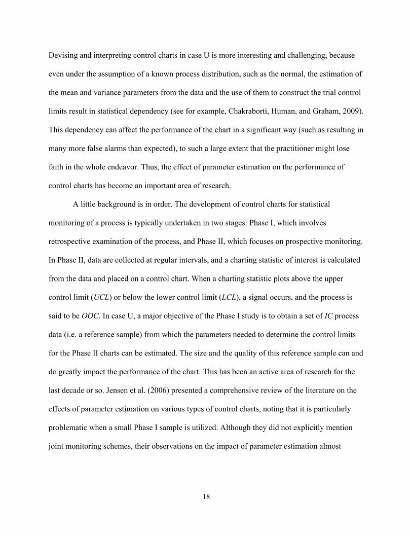
Devising and interpreting control charts in case U is more interesting and challenging, because

even under the assumption of a known process distribution, such as the normal, the estimation of

the mean and variance parameters from the data and the use of them to construct the trial control

limits result in statistical dependency (see for example, Chakraborti, Human, and Graham, 2009).

This dependency can affect the performance of the chart in a significant way (such as resulting in

many more false alarms than expected), to such a large extent that the practitioner might lose

faith in the whole endeavor. Thus, the effect of parameter estimation on the performance of

control charts has become an important area of research.

A little background is in order. The development of control charts for statistical

monitoring of a process is typically undertaken in two stages: Phase I, which involves

retrospective examination of the process, and Phase II, which focuses on prospective monitoring.

In Phase II, data are collected at regular intervals, and a charting statistic of interest is calculated

from the data and placed on a control chart. When a charting statistic plots above the upper

control limit (UCL) or below the lower control limit (LCL), a signal occurs, and the process is

said to be OOC. In case U, a major objective of the Phase I study is to obtain a set of IC process

data (i.e. a reference sample) from which the parameters needed to determine the control limits

for the Phase II charts can be estimated. The size and the quality of this reference sample can and

do greatly impact the performance of the chart. This has been an active area of research for the

last decade or so. Jensen et al. (2006) presented a comprehensive review of the literature on the

effects of parameter estimation on various types of control charts, noting that it is particularly

problematic when a small Phase I sample is utilized. Although they did not explicitly mention

joint monitoring schemes, their observations on the impact of parameter estimation almost

19

certainly extend to these charts. Further work is necessary to better understand the precise impact

of parameter estimation on joint monitoring schemes.

Traditionally, obtaining the reference sample is accomplished using an iterative

procedure in Phase I in which trial limits are first constructed from the data (several subgroups or

a number of observations), and then some charting statistics are placed on a control chart. It may

be noted that the construction of Phase I control charts has different objectives (see for example

the 2009 review article by Chakraborti et al.) from those in Phase II. Phase II control charts are

designed to have a specific IC ARL, while Phase I control charts should be constructed based on

a specified IC false alarm probability (FAP), which requires consideration of the joint

distribution of the charting statistics. In any case, subgroups corresponding to the charting

statistics which are located outside the control limits are generally considered OOC and removed

from the analysis, and new limits are estimated from the remaining data.1 This step is repeated

until no more charting statistics appear OOC so that the remaining data is taken to be IC, at

which point the final control limits may be constructed for Phase II monitoring.

However, control charts for joint monitoring in Phase I, case U, have been largely absent

from the literature so far. This is an important problem since if the Phase I chart used to identify

this IC data is incorrect or ineffective at identifying the OOC samples for removal, the resulting

parameter estimates may not be very accurate, which will affect the performance of the Phase II

chart. In fact, several researchers have demonstrated the pitfalls of estimating the parameters

using data which contains OOC samples. The resulting control limits may be too tight or too

1 There are two competing schools of thought concerning the handling of subgroups which plot OOC. Some practitioners automatically discard these subgroups, while others remove them only if they can be attributed to “assignable causes.” In our discussion, we focus primarily on the former approach; however, problems can arise with either method. In the case of the latter approach, the practitioner may fail to identify the cause of a particular subgroup which plots OOC and therefore not discard it. If, however, the subgroup was, in fact, OOC, failure to remove it could likewise result IC limits which are too tight or too loose.

20

loose, causing an inflated FAR or a higher-than-nominal IC ARL, respectively. On this point, for

example, Mabouduo-Tchao and Hawkins (2011) noted, “Plugging in parameter estimates…

fundamentally changes the run length distribution from those assumed in the known-parameter

theory and diminishes chart performance, even for large calibration samples.” Jensen et al.

(2006) pointed out that “the impact of parameter estimation…depends on the direction of the

estimation error.” Clearly, then, in case U situations, it is important to have very good Phase I

charts; otherwise, the resulting Phase II charts will suffer.

A few case U charts for joint monitoring are present in the literature. A recent example is

the simultaneous chart proposed by Yeh, Lin, and Venkataramani (2004) which involves a pair

of CUSUM mean and variance statistics which have the same scale and then plots them on one

control chart with a single set of control limits.2 The CUSUM mean and variance statistics are

computed by taking appropriate functions of and and applying the probability integral

transformation (PIT) to each, producing statistics which have the uniform distribution. Because

the PIT is used, this chart can be extended for processes with known, non-normal distributions as

well.

A substantial amount of recent research has demonstrated that in case U, a large quantity

of reference data is needed before the Phase II charts actually display their expected (nominal)

behavior. Jensen et al. (2006) noted that depending on the type of control chart being utilized,

hundreds or even thousands of reference data points may be necessary. However, it is not always

possible to have such a large “clean” dataset. In these situations an alternative class of control

charts may be useful. Among these are the self–starting charts (Hawkins, 1987) and the Q-charts

(Quesenberry, 1991). For the joint monitoring problem, Li, Zhang, and Wang (2010) recently

2 The statistics can also be placed on separate charts, resulting in a two-chart scheme.

21

proposed a self-starting EWMA likelihood-ratio (SSELR) chart which has this advantage.

However, this chart is only appropriate for univariate data.

Hawkins and Zamba (2005) presented a single chart based on a “changepoint” model

which also avoids the problem of needing a large reference dataset. In this model, the

“changepoint” is the unknown instant at which a special cause brings about a shift in one or both

of the parameters; as a result, the observations taken prior to the changepoint have a different

mean and/ or variance than the observations taken after it. A GLR test can be used to determine

whether the samples before and after a suspected changepoint seem to have the same parameters.

However, the time of the true changepoint is unknown, and it could occur between any two

samples. Thus, the chart proposed by Hawkins and Zamba (2005) uses the maximum of the GLR

statistics resulting from considering all possible changepoints. They demonstrated that this chart

is effective when as few as three Phase I data points are available. However, they acknowledge

that their procedure is inadequate for non-normal distributions.

2.1.1.1.3 Disadvantages of One-Chart Monitoring Schemes

In general, one-chart schemes are not without some weaknesses. As noted by Chao and

Cheng (2008), one-chart schemes lack a desirable feature present in two-chart schemes, that is,

they lose either the time-sequential presentation of the data, in the case of single charts with

control regions, or the separate treatment of the mean and variance statistics, in the case of single

charts with traditional control limits. In the former case, the charts do not indicate the order in

which the data are collected, making it difficult to spot time-related trends. In the latter case,

there is a reduction in the information to be gleaned by looking at the charting scheme. A signal

on a single mean-variance chart with traditional control limits cannot be attributed to variance or

22

mean without diagnostic follow-up.3 Single charts with control regions, however, do not share

this limitation.

Another disadvantage of one-chart joint monitoring schemes is that they often utilize very

complex charting statistics. Additionally, many single charts have some chart-specific “tuning”

parameters, such as in Domangue and Patch’s (1991) chart or in Costa and Rahim’s (2004)

non-central chi-square chart, which must be specified and which greatly affect the chart’s

performance (Zhang, Zou, and Wang, 2010). Choosing appropriate values for these parameters

can be quite complex. Some one-chart schemes also have the disadvantage of being insensitive

to large or small shifts in the parameters or to decreases in variance. While individual one-chart

schemes have been shown to have performance advantages over two-chart schemes, it is

inaccurate to claim that one-chart schemes always have superior performance.

2.1.1.2 Two-Chart Joint Monitoring Schemes

Since the early days of SPC, there have been joint monitoring schemes, used either

implicitly or explicitly, consisting of two charts. For normally distributed data, these two-chart

monitoring schemes are made up of a mean chart (such as the chart) and a variance chart (such

as the chart or the chart). They can consist of a pair of Shewhart, CUSUM, or EWMA

charts, one for the mean and one for the variance, or even a combination of one CUSUM and one

EWMA chart. The mean charts utilized in these schemes are typically two-sided, while the

variance charts may be either one-sided or two-sided. Figure 2.4 shows an example of a two-

3 In contrast, a signal on the variance chart of a two-chart scheme is immediately attributable to a shift in variance, although the same cannot be said of a signal on the mean chart. This fact will be discussed in greater detail later in this dissertation, but the main point here is that neither two-chart nor one-chart schemes with traditional control limits can immediately indicate whether a chart signal is caused by the mean, the variance, or both, though two-chart schemes do provide slightly more information.

23

chart monitoring scheme, constructed using simulated data. The mean of the process appears to

go OOC around subgroup 70.

Figure 2.4: A two-chart monitoring scheme consisting of two EWMA charts

A major advantage of two-chart monitoring schemes is their familiarity and the apparent

ease of visual interpretation. Such schemes have been used for many years. Furthermore, it

seems natural to some practitioners to monitor the mean and the variance separately and

simultaneously, since the statistics and are independent.

-0.5-0.3-0.10.10.30.5

0 10 20 30 40 50 60 70 80

EWM

A Va

lue

Sample number

Two-Sided EWMA Mean Control Chart

UCL=0.345

LCL=-0.345

-0.1

-0.05

0

0.05

0.1

0.15

0 10 20 30 40 50 60 70 80

EWM

A Va

lue

Sample number

High Side EWMA Variance Control Chart

UCL=0.144

24

2.1.1.2.1 Standards Known, Parametric Two-Chart Schemes

As with one-chart monitoring, the vast majority of two-chart monitoring schemes

presented in the literature are for data from a specified distribution, such as the normal, for which

the true parameters are specified. Several authors have considered the construction and

improvement of these schemes. Gan (1995) discussed scheme CC, consisting of a two-sided

CUSUM mean chart and a two-sided CUSUM variance chart; scheme EEu, consisting of a two-

sided EWMA mean chart and a high-sided EWMA variance chart; and scheme EE, consisting of

a two-sided EWMA mean chart and a two-sided EWMA variance chart, comparing these to

Domangue and Patch’s (1991) omnibus chart. He demonstrated that EE performs similarly to

scheme CC and is slightly more sensitive than CC when there is a small shift in the mean

concurrent to a slight decrease in the variance. The other schemes performed poorly in

comparison. Reynolds and Stoumbos (2004) also investigated and compared popular Shewhart,

EWMA, and CUSUM schemes, likewise recommending a pair of EWMA (or CUSUM) charts,

though with a different variance statistic than the one discussed by Gan (1995). Reynolds and

Stoumbos (2005) expanded upon this work, comparing a variety of other two- (and three-) chart

combinations, including some Shewhart-EWMA schemes. They, too, ultimately recommended a

pair of EWMA (or CUSUM) charts).

2.1.1.2.2 Standards Unknown, Parametric Two-Chart Schemes

The standards unknown situation presents even more complex problems for two-chart

monitoring schemes than it does for one-chart schemes. Perhaps for this reason, such charts (for

both Phases I and II) have not yet been studied in the literature. In the Phase I setting, a major

problem which needs to be addressed is how to conduct the iterative, parameter estimation

25

procedure for a two-chart scheme.4 Should trial limits be constructed for the two charts

simultaneously and a subgroup discarded if it plots OOC on either chart? Alternatively, should

the iterative procedure be conducted first for the variance chart (since it is independent of the

mean parameter) and then for the mean chart using only the data not already discarded? If this

second method is utilized, should the final control limits be recomputed for the variance chart

using only those samples not discarded during the estimation of the process mean? Another

difficulty is designing the scheme so that it has a specified FAP. Further research is needed to

address all of these issues and make two-chart joint monitoring schemes a viable option for case

U. For the Phase II problems, there is also a current shortage of charts that account for parameter

estimation from a Phase I reference data set. Since the impact of parameter estimation on Phase

II charts can be serious and parameters are estimated based on reference data obtained by the use

of appropriate Phase I charts, two-chart schemes for both settings should be an area of further

research.

2.1.1.2.3 Disadvantages of Two-Chart Monitoring Schemes

Two-chart schemes also have some disadvantages. Cheng and Thaga (2006) noted that

these schemes utilize more personnel, time, and other resources than do one-chart schemes.

Typical two-chart schemes give the illusion of clearly showing whether a process is OOC with

respect to mean, variance, or both, since a signal on the mean chart appears to indicate that mean

is OOC, a signal on the variance chart appears to indicate that variance is OOC, and signals on

both charts seem to indicate that both are OOC. Contrary to popular perception, this can actually

be quite misleading. As noted by Hawkins and Deng (2009), since the control limits for an

4 The appropriate approach may depend, in part, on whether practitioner chooses the discard all subgroups which plot OOC or only those for which “assignable causes” can be identified.

26

chart are functions of the IC standard deviation, an increase in the variability may lead to a false

signal on the chart, and likewise, a decrease in variability may cause the to fail to signal

even though a shift in the mean has also occurred. Furthermore, in many two-chart monitoring

schemes, the mean and variance charts are constructed completely independently, so that each

has a specified ARL. Appropriate two-chart joint monitoring schemes, however, should have

control limits which have been adjusted so that the overall ARL of the scheme is a specified

value.

2.1.2 Shifted Exponential Distribution Monitoring Schemes

The shifted exponential distribution has a prominent place in reliability and life testing

research, particularly in the context of guarantee times. As noted by Basu (2006), this

distribution can be useful for predicting the life expectancy of a cancer patient or the life span of

light bulbs. Many research problems arising from the shifted exponential distribution have been

addressed in the literature, particularly those that relate to reliability, which, in a statistical

context, is the probability that a random variable exceeds some value. Parameter estimation from

censored and uncensored data, hypothesis testing, reliability sampling plans, and prediction of

future data points are among the topics for which research on this distribution has been

conducted. A few control charts for shifted exponential data also appear in the literature, but

much more work in this area is needed.

Parameter estimation is one of the relevant areas of research regarding this distribution.

Varde (1969) derived Bayesian point estimates for both parameters. Kececioglu and Li (1985)

presented a method for calculating an optimum confidence interval for the location parameter of

a shifted exponential distribution. Lam et al. (1994) presented a method for estimating both

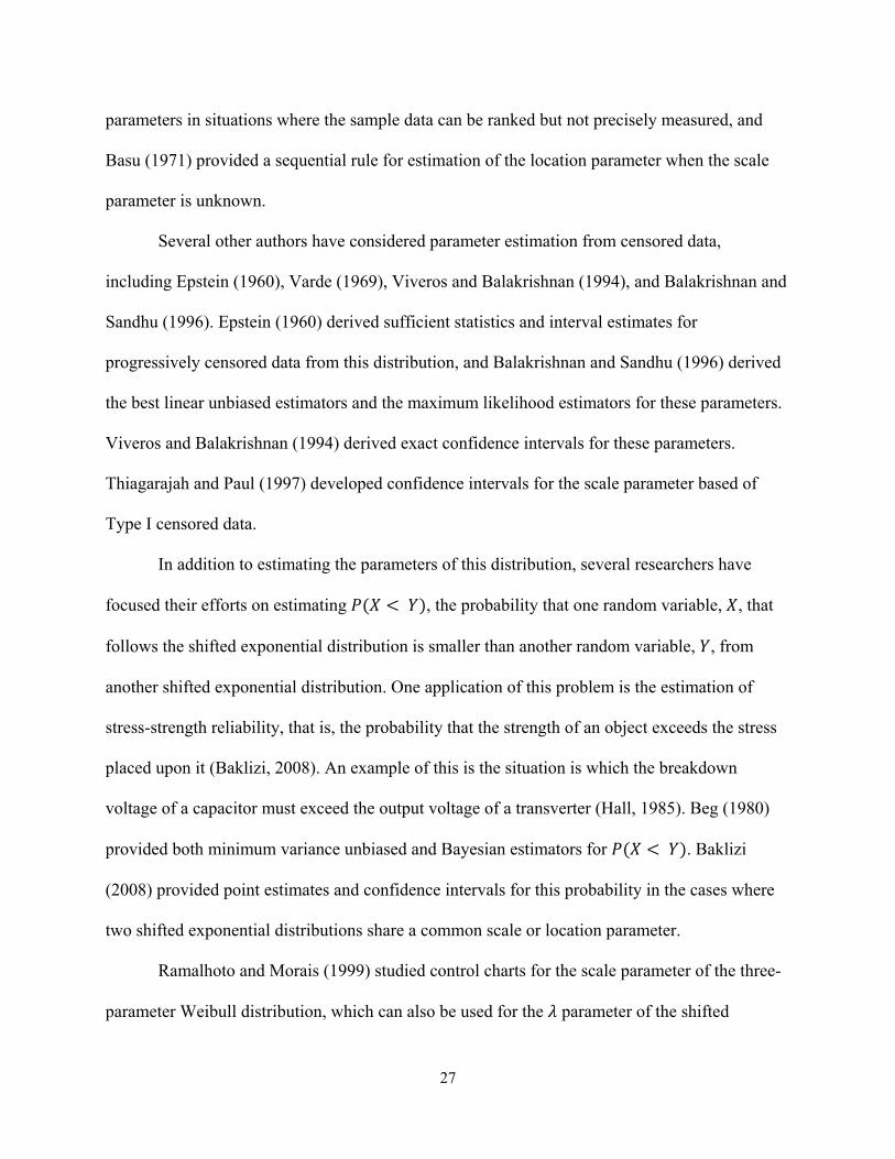
27

parameters in situations where the sample data can be ranked but not precisely measured, and

Basu (1971) provided a sequential rule for estimation of the location parameter when the scale

parameter is unknown.

Several other authors have considered parameter estimation from censored data,

including Epstein (1960), Varde (1969), Viveros and Balakrishnan (1994), and Balakrishnan and

Sandhu (1996). Epstein (1960) derived sufficient statistics and interval estimates for

progressively censored data from this distribution, and Balakrishnan and Sandhu (1996) derived

the best linear unbiased estimators and the maximum likelihood estimators for these parameters.

Viveros and Balakrishnan (1994) derived exact confidence intervals for these parameters.

Thiagarajah and Paul (1997) developed confidence intervals for the scale parameter based of

Type I censored data.

In addition to estimating the parameters of this distribution, several researchers have

focused their efforts on estimating ( < ), the probability that one random variable, , that

follows the shifted exponential distribution is smaller than another random variable, , from

another shifted exponential distribution. One application of this problem is the estimation of

stress-strength reliability, that is, the probability that the strength of an object exceeds the stress

placed upon it (Baklizi, 2008). An example of this is the situation is which the breakdown

voltage of a capacitor must exceed the output voltage of a transverter (Hall, 1985). Beg (1980)

provided both minimum variance unbiased and Bayesian estimators for ( < ). Baklizi

(2008) provided point estimates and confidence intervals for this probability in the cases where

two shifted exponential distributions share a common scale or location parameter.

Ramalhoto and Morais (1999) studied control charts for the scale parameter of the three-

parameter Weibull distribution, which can also be used for the parameter of the shifted

28

exponential distribution, since, as mentioned above, the latter is merely a special case of the

former. However, using these charts requires the assumption that the location parameter is

known and fixed. Sürücü and Sazak (2009) presented a control scheme for this same distribution

based on the idea of using moments to approximate the distribution.

There has also been research in a number of other areas. Wright et al. (1978) developed

hypothesis tests for these parameters for Type I censored data. A few authors have considered

the problem of predicting future data points from a shifted exponential distribution, including

Ahsanullan (1980) and Ahmadi and MirMostafaee (2009). Reliability sampling plans have also

been a popular research area. Balasooriya and Saw (1998) considered reliability sampling plans

for progressively censored shifted exponential data.

While the shifted exponential distribution is most commonly identified with guarantee

times, a number of other types of processes follow this distribution. Some examples in

manufacturing and healthcare settings are given by Kao (2010). Furthermore, any process which

follows the one-parameter exponential distribution also follows the shifted exponential with

location parameter zero. If there is any possibility that an assignable cause could effect a change

in that location parameter, then a chart for the shifted exponential distribution is needed to

monitor it.

2.1.3 Laplace Distribution Monitoring Schemes

The symmetric Laplace, or double exponential, distribution occurs whenever the random

variable of interest is the difference between a pair of exponentially distributed random variables

with a common scale parameter (Piug and Stephens, 2000). As noted by Kotz et al. (2001), the

Laplace distribution typically appears in the literature as a counterexample in discussions of the

29

normal distribution. However, it has numerous practical applications and is therefore deserving

of careful study in its own right. Examples include differences in flood levels at two different

points along a river (Puig and Stephens, 2000; Bain and Engelhardt, 1973), daily and weekly

observations of individual stocks in the Finnish stock market (Linden, 2001), and sunspot cycles

(Sabarinath and Anilkumar, 2008). Kotz et al. (2001) provided an in-depth overview of the

distribution, outlining its distribution, characteristics, and properties, as well as providing

examples of applications in finance, engineering, operations management, and the natural

sciences. Their extensive work provides the reader a handy reference which synthesizes the

extensive literature on the Laplace distribution into a convenient, usable form. Many research

problems arising from the Laplace distribution have been addressed in the literature, including

parameter estimation, reliability estimation, construction of tolerance limits, and hypothesis

testing. However, extensive contributions are needed in the area of process monitoring.

Most recent work has been undertaken for Type II censored samples. Balakrishnan and

Chandramouleeswaran (1996a) developed BLUEs for each of the distribution’s parameters for

samples with this type of censoring. Balakrishnan and Chandramouleeswaran (1996b) extended

these results to produce a reliability function estimator. They also presented tolerance limits for

the Laplace distribution. Childs and Balakrishnan (1996) constructed confidence intervals for

each of the distribution’s parameters by conditioning on values of some statistics used in the

calculation. Ioliopoulos and Balakrishnan (2011) constructed maximum likelihood-based exact

confidence intervals and hypothesis tests for the distribution’s parameters, likewise for Type II

censored samples.

Tests of fit for the Laplace distribution have been an area of recent research interest. Puig

and Stephens (2000) developed goodness-of-fit tests for this distribution based on the empirical

30

distribution function. Choi and Kim (2006) developed goodness-of-fit tests which are instead

based on maximum entropy.

2.2 Nonparametric Joint Monitoring Schemes

All of the methodologies discussed above, and indeed, the vast majority of available

work in the area of joint monitoring, have focused on data with a known or assumed parametric

distribution. Given the existing literature on the performance of individual normal theory charts

for the mean and the variance, it is reasonable to believe that departures from these parametric

assumptions can have a dramatic impact on the effectiveness of at least some such charts. This

can be remedied by applying a nonparametric or a distribution-free control chart that does not

require the assumption of a specific form of the underlying distribution. A recent review of

nonparametric control charts can be found in Chakraborti et al. (2011); however, the literature in

the area of nonparametric joint monitoring, both one- and two- chart schemes, is currently very

limited and thus presents a great opportunity for research and development.

The few nonparametric joint monitoring schemes available in the literature are all one-

chart schemes. Zou and Tsung (2010) proposed an EWMA control chart based on a goodness-of-

fit test. They showed that this chart is effective for detecting changes in location, scale, and

shape. Mukherjee and Chakraborti (2011) adapted a well-known nonparametric test for location-

scale which combines the Wilcoxon rank-sum location statistic with the Ansari-Bradley scale

statistic and constructed a chart based on it. Their Shewhart-type chart is called the Shewhart-

Lepage (SL) chart, and it has post-signal diagnostic capability for determining the nature of the

shift. Within the nonparametric joint monitoring literature, their paper appears to be the first

major foray into the standards unknown case, though more work is currently in progress.

31

While there is no doubt that nonparametric two-chart monitoring schemes could be

developed, as far as we know, there are none in the current SPC literature. However, Reynolds

and Stoumbos (2010) presented some schemes consisting of a pair of CUSUM charts which are

robust to the normality assumption.

2.3 Summary

A variety of control charting schemes are currently available for jointly monitoring the

mean and the variance of a normal distribution. Both one- and two-chart schemes exist in the

literature and can be useful to the practitioners. Though all available schemes have advantages

and disadvantages, one-chart schemes appear to be the more promising option, particularly since

there are many unanswered questions regarding the practical implementation of two-chart

schemes when parameters are estimated in a Phase I study.

Joint monitoring schemes for other parametric distributions, including the shifted

exponential and Laplace distributions, are largely absent from the literature.

32

CHAPTER 3

SHEWHART-TYPE CONTROL CHARTS FOR SIMULTANEOUS MONITORING OF UNKNOWN MEANS AND VARIANCES OF NORMALLY DISTRIBUTED PROCESSES

3.1 Introduction

Since their invention in the 1920s by W.A. Shewhart, Shewhart-type control charts have

been popular tools for use in statistical process control (Montgomery, 2005). These charts are

well-known to be able to detect moderate to large and transient shifts. Most of these charts are

designed to monitor a single process parameter, typically the mean ( ) or the variance ( ), but

more recently, a number of charts have been developed for jointly monitoring the mean and

variance of normally distributed processes. The issue of joint monitoring is particularly relevant

for processes in which special causes may result in a simultaneous shift in the mean and the

variance. An example given by Gan et al. (2004) is an improperly fixed stencil in circuit

manufacturing which can cause such a shift in the mean and the variance of the thickness of the

solder paste printed onto circuit boards.

Two major classes of joint monitoring schemes have been developed in the literature:

those which monitor the mean and the variance simultaneously on a single chart, and those

which use two separate charts, one each for monitoring the mean and the variance. Costa and

Rahim’s (2004) NCS chart is an example of the former, while Gan’s (1995) scheme EE is an

example of the latter. Though both types of joint monitoring schemes have advantages and

disadvantages, one-chart schemes seem to be preferable for both practical and statistical reasons.

33

In particular, the one-chart schemes typically require fewer process control resources and are

more straightforward to implement. Moreover, they seem to be more useful in situations when

the process is mostly in-control and fewer out-of-control events are anticipated. Cheng and

Thaga (2006) provided a review of the joint monitoring literature until about 2005; McCracken

and Chakraborti (2011) gave a more recent overview.

Among the available one-chart schemes for jointly monitoring the mean and the variance,

the vast majority are designed for situations in which the true parameters are known rather than

estimated from data. The term “standards known” or “case K” is typically used for situations in

which all relevant process parameters are known, while the term “standards unknown” or “case

U” is used for situations in which one or more process parameters are unknown. When one or

both of the parameters are unknown and must be estimated, it is well known that the estimation

has a big impact on the performance of the case K charts, particularly in terms of the ARL and

the FAR, in that many more false alarms are observed. Thus, when parameters are estimated, the

case K control charts must be modified (both in terms of the plotting statistic and the control

limits) to correctly account for parameter estimation, so that the charts perform at a specified

nominal IC ARL.

In this chapter, we consider the modification of a pair of existing joint monitoring

procedures for case K to case U. These are both Shewhart-type one-chart joint monitoring

schemes, useful for detecting large shifts in process parameters: Chen and Cheng’s (1998) Max

chart and Razmy’s (2005) Distance chart. These charts are similar in that both are based on the

idea of combining the estimators and (minimal sufficient statistics) of the mean ( ) and the

variance ( ) to construct a single charting statistic capable of monitoring the mean and the

variance simultaneously. Additionally, once there is a signal, these charts allow the practitioner

34

to easily determine both the direction of the shift and which of the two parameters has shifted.

Furthermore, charts of this type have played a pivotal role in the joint monitoring literature. For

example, many currently available joint monitoring charts are based on the Max chart, including

Chen, Cheng, and Xie’s (2001) MaxEWMA chart; Cheng and Thaga’s (2010) Max-CUSUM

chart; Khoo et al’s (2010a) EWMA − chart; Khoo et al’s (2010b) Max-DEWMA chart; and

Memar and Niaki’s (2011) Max-EWMAMS chart. The Max chart is a Shewhart-type chart, and

as noted by Cheng and Thaga (2006), this chart is more effective for detecting large shifts.

For purposes of comparison, we also consider a similarly-modified two-chart ( / ) scheme in various parts of this chapter.

3.2 Background

It has long been recognized that using estimated parameters in control charts designed for

situations in which the true parameters are known introduces additional variability into a

monitoring scheme. In their well-written review, Jensen et al. (2006) summarized the effects of

parameter estimation on the performance of a variety of control charts. In particular, they noted

that problems abound when a small Phase I sample is utilized. Although they did not explicitly

mention joint monitoring schemes, their observations on the impact of parameter estimation can

be shown to extend to these charts.

To understand the degree of potential impact of parameter estimation on case K joint

monitoring charts, first consider the Max chart. This chart has a plotting statistic =/√ , ( ) ( ) , where is the cdf of the standard normal distribution,

( ) is the cdf of the chi-square distribution with ( − 1) degrees of freedom, and and

are the mean and the variance of the th sample of size . When the desired IC ARL for this chart

35

is 500, the appropriate UCL, 3.29, can easily be calculated using Mathcad or estimated using

Monte Carlo simulations; the corresponding type I error probability (false alarm rate) is 0.002.5

Next, consider the Shewhart distance chart studied in Razmy (2005). The plotting statistic

of this chart is = /√ + ( ) ( ). When the desired IC ARL for this

chart is 500, the appropriate UCL, 3.52, can be obtained using Monte Carlo simulations, and the

corresponding FAR is 0.002.

Finally, consider the two-chart joint monitoring scheme which consists of an chart and

an chart.6 The plotting statistic of the chart is , and the plotting statistic of the chart is .

When the desired IC ARL for this scheme is 500, each of these charts should have an IC ARL of

999.5. When = 5,the appropriate control limits for the chart are

− /√ = −1.47 and + /√ = 1.47, while the appropriate

control limits for the chart are ( ) / = 0.13and

( ) / = 2.24. As with the Max and Distance charts, the FAR for the ( , ) scheme is 0.002.

Now, suppose that the true IC mean and variance are unknown. In practice, one would

typically estimate these parameters from an IC reference sample of size prior to implementing

a monitoring scheme. Then, one might “plug in” these estimates for the parameters when

5 Note that in the known parameter case, the FAR is the reciprocal of the IC ARL. 6 The and charts discussed in this paper are based on probability limits rather than the 3-sigma control limits given by Montgomery (2005). The differences between the 3-sigma method and the probability limits method of constructing these charts is discussed in greater detail in A.4 in the Appendix.

36

calculating and , resulting in estimated plotting statistics and , respectively. However, if

one then uses the same control limits that were used with and , the chart performance will be

degraded. In fact, it is expected that the IC ARL for the charts using the parameter estimates

would decrease from the nominal value so that more false alarms would occur.

Likewise, for the ( , ) monitoring scheme, if the true IC mean and variance are

unknown, one might “plug in” parameter estimates to compute the control limits for the and

charts. However, doing so without accounting for the additionally variability caused by the

parameter estimation will likewise cause the charts’ performances to be degraded. As for the

Max and Distance charts, it is expected that the IC ARL for the for the ( , ) scheme using the

parameter estimates would decrease from the nominal value so that more false alarms would

occur.

To examine the extent of the effect of parameter estimation on the Max and the Distance

charts and the ( , ) scheme, a simulation study was undertaken. The nominal IC ARL was set at

500, and 25,000 simulations were done.7 Table 3.1 shows values of the observed ARL for various

combinations of m and n, where m is the total size of the Phase I reference sample and n is the

size of each Phase II monitoring sample.

It is well known that in the standards known case, increasing decreases the probability

of type II error for control charts, just as is the case for hypothesis tests (see, for example,

Montgomery, 2005). This is true because larger values of improve the chart’s ability to

recognize differences between the given parameters and the mean and standard deviation of a

particular process sample. When the true mean and standard deviation are unknown and are

instead estimated from a Phase I sample, increasing likewise improves the charts’ ability to

7 Throughout this dissertation, the number of simulations is selected to ensure a low standard error of estimation.

37

recognize differences between the mean and standard deviation of the Phase I sample and the

mean and standard deviation of a given Phase II sample. However, since the Phase I mean and

standard deviation are estimates rather than the true process parameters, identifying differences

between these values and the mean and standard deviation of the Phase II sample can result in

false alarms. Thus, for a fixed , increasing results in a decrease in the nominal ARL. On the

other hand, when is fixed, increasing causes the Phase I mean and standard deviation

estimates to converge toward the true mean and standard deviation. Thus, for a fixed , larger

’s result in ARLs which are closer to the nominal ARL.

From Table 3.1, it is seen that the Max and Distance charts and the ( / ) scheme are all

affected by parameter estimation. When parameters are estimated, the observed ARL values can

be considerably lower than 500, even when a fairly large reference sample (m = 100) is used.

The departure from the nominal IC ARL is greater when smaller, more typically recommended,

reference samples ( ≈ 30) are used. Thus, it is clear that for typical situations in practice

( < 100), modifications and adjustments to the “standards known” charts must be made before

they can be used correctly in the “standards unknown” case. This is so that the IC ARL will be

close to the nominal value; otherwise, there can be a large number of false alarms that will

diminish the utility of these charts in practical situations.

38

Table 3.1: Observed IC ARL for the Max and the Distance charts when the mean and the standard deviation of a Phase I sample are used to estimate and

Max Chart Observed ARL

Distance Chart Observed ARL

( , ) Scheme Observed ARL

500 5 493.68 506.62 490.52

400 5 483.07 495.16 486.84

300 5 482.16 491.82 486.03

200 5 476.21 490.90 476.98

150 5 474.02 488.10 468.57

100 5 457.58 471.17 453.99

75 5 444.51 461.56 441.31

50 5 424.94 447.26 419.76

30 5 383.86 408.51 382.09

100 15 324.51 332.96 328.96

75 15 301.91 307.06 299.15

50 15 259.84 260.63 254.84

30 15 206.17 205.47 204.52

100 25 266.95 263.15 263.10

75 25 233.84 233.17 233.39

50 25 177.73 188.90 188.54

30 25 151.22 153.19 140.82

Although from Table 3.1 one can see the effect of the size of the Phase I sample on the IC

ARL, note that these figures are unconditional; that is, they are obtained by averaging over all

possible values of the mean and the standard deviation estimates. Since the sample mean and

39

standard deviation are random variables with their own probability distributions, the values of

these estimates would vary in practice even though the Phase I sample is obtained from an IC

process. The magnitudes of these estimates can affect the performance of the chart, and hence it

is fair to examine, in addition to the unconditional performance, the “conditional” performance

of the charts, i.e. what happens when specific values of the estimators are used in setting up the

chart. In order to study this phenomenon, a second simulation uses specific quantiles of the

distributions of ̅ and to simulate their values, to show the effects that high, low, and medium

estimates can have on the resulting IC ARL. These ARL values, obtained for some specific values

of the estimators, are called conditional ARL values. Table 3.2 shows the conditional ARL values

which shed interesting light on the effect of parameter estimation on these joint monitoring

charts.

Based on the results in Table 3.2, it is clear that the particular estimates, obtained from

different samples from an IC process, can have a dramatic impact on the observed IC ARL of the

charts. Depending on the values (quantiles) of ̅ and used, the IC ARL may be either greatly

higher or lower than what is nominally expected, and in some cases, the results of particular

combinations are not intuitive. For certain quantiles, the impact is greatest on the ( / ) scheme,

while for other quantiles, the impact is greatest on the Distance chart. “Plugging in” estimates for and in the traditional Max chart, Distance chart, or ( / ) scheme would therefore lead to

unpredictable chart performance. It is thus desirable to modify each chart so that the

unconditional IC ARL is correctly maintained at a specified nominal value.

40

Table 3.2: Conditional IC ARL for the Max and Distance charts when specified quantiles of and are used as estimates for and , = , and = 8

Mean Quantile

Variance Quantile

Max Chart Observed ARL

Distance Chart Observed ARL

( , ) Scheme Observed ARL

5th 5th 22.23 20.20 5.06

5th 25th 34.56 31.35 6.23

5th 50th 38.34 34.81 6.55

5th 75th 34.52 31.25 6.27

5th 95th 22.28 20.18 5.08

25th 5th 71.39 67.06 29.80

25th 25th 139.07 128.84 49.27

25th 50th 165.41 154.35 55.69

25th 75th 138.98 130.40 49.49

25th 95th 70.87 66.68 30.07

50th 5th 164.85 162.13 148.86

50th 25th 362.47 350.77 324.26

50th 50th 445.20 435.53 396.66

50th 75th 360.37 352.05 322.87

50th 95th 164.62 160.77 148.42

75th 5th 357.70 343.11 578.11

75th 25th 718.09 728.67 880.58

75th 50th 855.02 886.17 944.86

75th 75th 723.74 726.47 872.09

75th 95th 352.78 345.27 576.97

8 The nominal IC ARL is 500.

41

95th 5th 651.80 615.69 440.06

95th 25th 834.43 991.63 437.48

95th 50th 877.19 1098.48 441.65

95th 75th 845.33 988.03 442.50

95th 95th 648.65 621.72 439.01

3.3 Statistical Framework and Preliminaries

Let , , … , be a random sample of size from normal distribution with mean

and variance ,respectively. Further, let , , … , be a random sample of size , likewise

from the normal distribution, with mean and variance , respectively, and let the ′sand the

’s be mutually independent. The parameters , , ,and are all assumed unknown with −∞ < , < ∞ and 0 < , < ∞ . When the process is IC, = = and = = so that the two populations have the same normal distribution, with unknown mean

and unknown variance . When the process is OOC, the normality assumption is still assumed

to hold, but one or both of these equalities among the parameters is violated; in other words, in

the OOC case, either the means, the variances, or both would differ for the two normal

distributions.

Now, let = ( + +⋯+ ) and = ( + +⋯+ ) be the respective

sample means, and also let = ∑ ( − ) and = ∑ ( − ) be the

respective sample variances. It is well known that is normally distributed with mean and

variance and , while ( )

is distributed as a chi-square with ( − 1) degrees of freedom.

Furthermore, it is well known that and are mutually independent. Similarly, is normally

42

distributed with mean and variance , and ( )

is distributed as a chi-square with ( − 1) degrees of freedom, independently of . Additionally, ( , ) and ( , ) are mutually

independent. Letting = + , denote = ( )and = . Next, consider modifying the Max and the Distance charts using the estimators from a

reference sample. The proposed plotting statistics and the resulting control charts are constructed

in the same spirit as in the original case K charts, in that they use the probability integral

transformation, but suitable modifications are made to account for estimation of parameters and

the correct application of the resulting statistical distribution theory. Suppose the sample

corresponds to an IC or reference sample. Much of what follows is based on correctly accounting

for the impact of the reference sample on the plotting statistics and the chart performance. To

this end, we first consider the distribution of various statistics given (or conditionally on) , , … , , or, equivalently, on the minimal sufficient statistics, and . First, it can be seen

that conditionally, follows a normal distribution with mean ( )and variance

, and ( ) follows a chi-square distribution with ( − 1) degrees of freedom.

Moreover, and are mutually independent. Next, it can be shown that unconditionally,

when the process is IC, follows a t distribution with ( − 1)degrees of freedom, and

follows an F distribution with ( − 1)and( − 1)degrees of freedom. However, and

are not mutually independent. As a result, the two statistics ∗ = Φ { ( )}, and

∗ = Φ , ( ) , where ζ (. ) and , (. ) denote, respectively, the cdf of a t

distribution with υ degrees of freedom and an F distribution with υ andυ degrees of freedom,

43

are also dependent. As we see next, our plotting statistics are functions of ∗ and ∗, and their

dependence plays a crucial role in the correct implementation of the proposed charts. They are: i. The Modified Max chart plotting statistic: Ψ = max{|W∗ |, |W∗ |}. The corresponding

Shewhart-type chart is called the Modified Max chart. The process is declared OOC

when > where the upper control limit is obtained so that the IC ARL is some

given nominal value. ii. The Modified Distance chart plotting statistic: Δ = ∗ + ∗ . The corresponding

chart is called the Modified Distance chart, which is also a Shewhart-type chart. The

process is declared OOC when Δ > ,where the upper control limit is obtained so

that the IC ARL is equal to some given nominal value.In order to implement the charts we need to find the control limits, so we next study the

distributions of the plotting statistics.

3.4 Distribution of Plotting Statistics

Distribution of

With the Modified Max chart, the process is declared OOC when for the th test sample, Ψ > where the upper control limit is obtained so that the IC ARL is some given nominal

value. Since when parameters are estimated, the statistics ∗ and ∗that are components of the

Max chart plotting statistic are dependent, a derivation of the run length distribution is more

complicated. However, this problem can be conveniently solved by conditioning on the reference

sample as demonstrated by Chakraborti (2000). The details of the derivation are given in the

Appendix. It is shown that the (unconditional) cdf of the plotting statistic Ψ is given by

44

Ψ ≤ = ( , ) ( ) ( )( ) , > 0

where

( , ) = Φ + + ∆ − Φ ℎ + + ∆

× ( ) ( − 1)( − 1) − ( ) ( − 1)( − 1) , ℎ = {Φ(− )}, = {Φ( )}, = , {Φ(− )}, = , {Φ( )}, = / , ∆= √ ( − )/ , = √ ( − )/ , and = ( − 1) / .

The run length distribution and the associated characteristics, such as the moments and

percentiles, can all be obtained similarly by conditioning. For example, conditionally on and

, the run length random variable, , follows a geometric distribution with probability of

success (signal) 1 − ( , ), where = . Thus,

( = | , ) = [1 − ( , )][ ( , )] , = 1,2,3, …

As a result, the unconditional run length distribution can be obtained by calculating the

expectation of the conditional run length distribution over the distributions of and :

( = ) = [1 − ( , )][ ( , )] ( ) ( )( )

Similarly, the conditional ARL of the Modified Max chart equals [1 − ( , )] and the

unconditional ARL is given by

= [1 − ( , )] ( ) ( )( ) . Other moments and percentiles of the run length distribution can be calculated in a similar

manner, that is, first conditionally and then unconditionally, over the joint distribution of and

.

Note that when the process is IC, we have ∆= 0 and = 1, so that

45

( , | ) = Φ − 1 + −Φ ℎ − 1 +

× ( ) ( )( ) − ( ) ( )( ) .

Hence, the IC unconditional ARL is given by

1 − [ ( , | )] ( ) ( )( )

where = , the UCL of the Max chart. The same expression can be used to find the UCL for

a given nominal value of the IC unconditional ARL, such as 500. Note that since ( , | ) is

free of ∆and , both the conditional and the unconditional IC run length distributions (and hence

all the unconditional and conditional run length distribution characteristics such as the ARL and

the percentiles) are free of the nuisance parameters when the process is IC. This is an important

practical feature of the Modified Max chart.

Distribution of

For the Shewhart Modified Distance chart, the process is declared OOC when for the th

test sample Δ > where the UCL is obtained so that the IC ARL is equal to some given

nominal value. As in the case of the Modified Max chart, the plotting statistic Δ is a function of ∗ and ∗, and since the joint distribution (cdf) of ∗ and ∗can be obtained by conditioning

(as shown in the Appendix), the conditional and the unconditional distribution of Δ can be

obtained from it. For example, it is shown that the (unconditional) cdf of Δ is given by

Δ ≤ = ∗, ∗( , | , ) ( ) ( )( )

where ∗, ∗( , | , )denotes the conditional joint pdf of ( ∗, ∗).

46

Again, as in the case of the Modified Max chart, the run length distribution of the

Modified Distance chart can be conveniently obtained, along with the moments and percentiles,

by conditioning on the reference sample. For example, writing

∗( , ) = ∗, ∗( , | , ) where =

and following the same lines of argument as with the Modified Max chart, the run length

distribution and the associated characteristics, such as moments and percentiles, for the Modified

Distance chart can be obtained. Hence, conditionally on and , the run length, ∗, follows a

geometric distribution, with probability of success (signal) 1 − ∗( , ). Therefore ( ∗ = | , ) = [1 − ∗( , )][ ∗( , )] , = 1,2,3…

and the unconditional run length distribution can be obtained by calculating expectation over the

distribution of and :

( ∗ = ) = [1 − ∗( , )][ ∗( , )] ( ) ( )( ) . As in the case of the Modified Max chart, the unconditional ARL of the Modified Distance chart

can be calculated by finding the expectation of [1 − ∗( , )] over the distribution of

and : = [1 − ∗( , )] ( ) ( )( ) . Other moments and percentiles can be calculated in a similar manner. Again, note that when the

process is IC, we have ∆= 0 and = 1 so that the unconditional run length distribution is free

of “nuisance” parameters.

Note further that the conditional joint pdf ∗, ∗( , | , )needed in the calculation

of ∗( , ) can be obtained by differentiating the conditional joint cdf ∗, ∗( , | , ) given in (*) in Appendix A. Hence

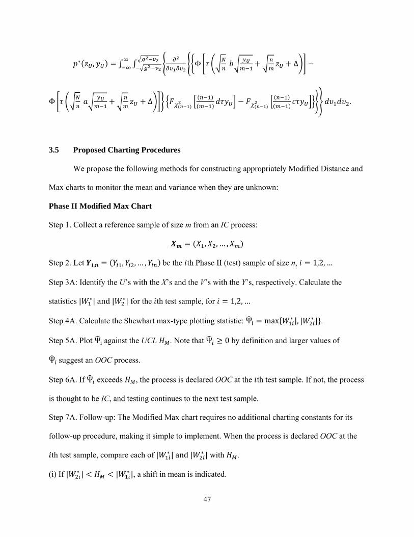
47

∗( , ) = Φ + + ∆ −

Φ + + ∆ ( ) ( )( ) − ( ) ( )( ) .

3.5 Proposed Charting Procedures

We propose the following methods for constructing appropriately Modified Distance and

Max charts to monitor the mean and variance when they are unknown:

Phase II Modified Max Chart

Step 1. Collect a reference sample of size m from an IC process: = ( , , … , ) Step 2. Let , = ( , , … , )be the th Phase II (test) sample of size n, = 1,2,…

Step 3A: Identify the U’s with the X’s and the V’s with the Y’s, respectively. Calculate the

statistics | ∗|and| ∗| for the th test sample, for = 1,2,…

Step 4A. Calculate the Shewhart max-type plotting statistic: Ψ = max{ ∗ |, | ∗ |}. Step 5A. Plot Ψ against the UCL . Note that Ψ ≥ 0 by definition and larger values of Ψ suggest an OOC process.

Step 6A. If Ψ exceeds , the process is declared OOC at the th test sample. If not, the process

is thought to be IC, and testing continues to the next test sample.

Step 7A. Follow-up: The Modified Max chart requires no additional charting constants for its

follow-up procedure, making it simple to implement. When the process is declared OOC at the

th test sample, compare each of | ∗ |and| ∗ | with .

(i) If | ∗ | < < | ∗ |, a shift in mean is indicated.

48

(ii) If | ∗ | < < | ∗ |, a shift in variance is indicated.

(iii) If | ∗ |and| ∗ |both exceed , a shift in both mean and variance is indicated.

Phase II Modified Distance Chart

Steps 1-2 Same as before.

Step 3B. Identify the U’s with the X’s and the V’s with the Y’s, respectively. Calculate the

statistics ∗ and ∗ for the th test sample, for = 1,2,…

Step 4B. Calculate the Shewhart distance-type plotting statistic: = ∗ + ∗

Step 5B. Plot against a UCL . Note that ≥ 0 by definition and larger values of suggest an OOC process.

Step 6B. If exceeds , the process is declared OOC at the th test sample. If not, the process

is considered to be IC, and testing continues to the next test sample.

Step 7B. Follow-up: The following procedure is recommended. When the process is declared

OOC at the th test sample, calculate = [ ∗ > ∗ | ] and = [ ∗ > ∗ | ]. Note that since ∗ and ∗ each follow a chi-square distribution with 1 degree of freedom,

both of these probabilities can be obtained directly from a chi-square table.

(i) If both , < 0.01, a shift in both mean and variance is indicated.

(ii) If both , > 0.05, a false alarm is indicated.

(iii) If < 0.01and > 0.05,a shift in mean is indicated.

(iv) If < 0.01and > 0.05,a shift in variance is indicated.

(v) If < 0.01 and 0.01 ≤ ≤ 0.05,a major shift in mean with possible associated

shift is variance is indicated.

49

(vi) If < 0.01 and 0.01 ≤ ≤ 0.05,a major shift in variance with possible associated

shift is mean is indicated.

3.6 Implementation

The proposed Modified Max and Distance charts are designed such that the appropriate

UCL is found based on the sample sizes and the desired nominal IC ARL. Although one can use

the analytical expressions for the IC ARL given in the earlier sections to find (solve for) the

control limits, this is bound to be tedious as the formulas involve evaluations of multi-

dimensional integrals. Instead we use simulations in R to calculate the control limits. Note that

we also use the software Mathcad to evaluate the integrals and thus spot check the simulation

results in a number of cases. In Table 2, we provide the appropriate UCL values for both of these

charts for various combinations of and , for a nominal IC ARL of 500.

From Table 3.3 it can be seen that the standard unknown values for and approach

the corresponding standards known values 3.29 and 3.52, respectively. Additionally, H does not

change much once the reference sample size is sufficiently high. It increases only slightly

when is fixed and increases from 150. However, when is fixed and increases, H

actually decreases slightly. For other values of m and n within the range of the table,

approximations to the control limit can be obtained. For example, for the Modified Max chart, a

simple polynomial fit for n = 5 yields, = 6E-09 - 6E-06 + 0.0019 + 3.0626, where = and = . This fit has a remarkably high ² = 0.9802.

50

Table 3.3: The H values for the Modified Max and Distance charts for a nominal IC ARL of 500

500 5 3.27 3.50

400 5 3.26 3.49

300 5 3.25 3.49

200 5 3.24 3.47

150 5 3.23 3.45

100 5 3.20 3.43

75 5 3.18 3.41

50 5 3.15 3.37

30 5 3.10 3.31

100 15 3.17 3.39

75 15 3.13 3.35

50 15 3.06 3.28

30 15 2.93 3.14

100 25 3.11 3.33

75 25 3.05 3.26

50 25 2.94 3.14

30 25 2.73 2.93

51

3.7 Illustrative Example

Montgomery (2005) presents a data set for an automotive manufacturing process which

involves a Phase I data set consisting of twenty-five samples of five piston ring diameters and a

Phase II data set consisting of an additional fifteen samples of five piston ring diameters. We use

this example to illustrate the effectiveness of the Modified Max and Modified Distance charts for

jointly monitoring the mean and the variance of the process. Here, = 125, and = 5.

Suppose we wish to use an IC ARL of 500. Then, using simulations, the control limits are found

to be = 3.216 for the Modified Max chart and = 3.450 for the Modified Distance chart.

The resulting control charts with the plotted statistics are shown in Figures 3.1 and 3.2,

respectively.

Though the two charts look very similar, the signal occurs at the 12th sample for the Max

chart and at the 13th sample for the Distance chart, indicating that the Max chart is somewhat

superior in this particular instance. Since the charts both signal, we use the proposed follow-up

post-signal diagnostic procedures and see that both charts indicate a shift in mean only. This is

because for the Max chart, ,∗ = 3.239exceeds = 3.216, while ,∗ = 0.624 does

not. Likewise, for the Distance chart, we calculate the two p-values = 0.0001 and =0.7391 using R and reach the same conclusion. It is interesting to note that for the same data set,

Mukherjee and Chakraborti’s (2011) Shewhart-Lepage nonparametric control chart also

signalled at the 12th sample, but their post-signal diagnostic procedure concluded that there was

evidence of both a location and a scale shift. On the parametric side, based on a two-chart

scheme made up of a traditional 3-sigma and a 3-sigma R chart as in Montgomery (2005), one

would conclude that there was evidence of a mean shift at sample 12 but no variance shift. Our

52

normal theory one-chart procedures reach the same conclusion and are correctly designed for a

specified IC ARL of 500 in the presence of estimated parameters.

Montgomery’s (2005) piston ring data

Figure 3.1: Modified Max Chart

Figure 3.2: Modified Distance Chart

Next we examine the performance of the proposed charts through a study of their run

length properties.

3.8 Performance Comparisons

The performance of the Modified Max and Distance charts is evaluated in a simulation

study. The tables and plots in Appendix B compare the performance of the two charts for various

mean and variance shifts and sample sizes, providing the ARL, the run length standard deviation,

and specified quantiles of the run length distribution. Note that the underlying distribution is

normal and that = 0 and = 1 represents the IC case. For purposes of comparison, the

modified ( / ) scheme discussed in Appendix A.4 is also included in the simulation. It is

important to realize that the control limits for this ( / ) scheme are determined by taking the

53

parameter estimation into account. The Montgomery (2005) ( / ) scheme is not directly

comparable to the Modified Max and Distance charts.

Since joint monitoring of the mean and variance of a normal distribution is analogous to

testing the null hypothesis that the sample at hand comes from a completely specified normal

distribution (a simple null hypothesis) versus all alternatives (a composite alternative

hypothesis), a likelihood ratio-based joint monitoring scheme appears to be a promising

alternative. Several researchers have considered control charts based on the likelihood ratio,

including Hawkins and Deng (2009); Zhou, Luo, and Wang (2010); Zou and Tsung (2010); and

Zhang, Zou, and Wang (2010). Following this line of argument, we considered a chart based on

the two-sample likelihood ratio statistic (the LR chart) and compared its performance to that of

the Modified Max and Distance charts in the simulations. However, the LR chart was found to

have the uniformly worst performance, often taking more than twice as long as the Max and

Distance charts to detect a shift. This relatively poor performance may result from the fact that

the many small changes in mean and variance which are detected by the ∗ and ∗ statistics

(and therefore produce a signal in that Max and Distance charts) are not large enough to produce

a significant change in the likelihood ratio statistic. As a result, the LR chart for joint monitoring

was deemed to be too conservative to be useful in practice and will not be discussed any further

in this chapter.

From the tables and the figures, it is seen that the Modified Max and Distance charts

perform rather similarly, though the Distance chart slightly outperforms the Max chart in most

cases. The Max chart has slightly superior performance in detecting moderate to large shifts in

the mean (0.75 to 3.0) accompanied by smaller or absent shifts in the variance. For example,

when = 100, = 5, and the mean shifts from 0 to 1 and there is no shift in the variance, the

54

ARL of the Modified Max chart is 9.55, while that of the Modified Distance chart is about 6%

larger. However, the Modified Distance chart has a shorter ARL in the majority of the cases,

including small shifts in the mean (less than .05) with no shift in the variance and moderate-to-

large shifts in the mean accompanied by any shift in the variance. Note that the Max chart is

easier to apply since it has a simpler follow-up post-signal diagnostic procedure. The similarity

in performance of the two charts is not surprising, given that both of these charts are based upon

functions of the same basic statistics ∗and ∗. Both charts quickly detect moderate to large

changes in the mean and/or variance.

The ( / ) scheme exhibits very promising performance, though its performance is

greatly influenced by the size of the reference sample . The scheme outperforms the Max chart

for all of the shifts studied. When = 30, this two-chart scheme also outperforms the Distance

chart for all of the shifts studied. However, when a larger set of reference data is used, we see

that the Distance chart outperforms the ( / ) scheme when a medium-to-large shift in the

variance occurs.

Next, an important question about all normal theory control charts is their robustness to

normality, that is, how their performance is affected or degraded by a departure from the

normality assumption upon which the methodology is based. We now examine this issue for the

proposed charts.

3.9 Robustness to Departures from Normality

It is of interest to examine the performance of the Modified Max and Distance charts

when the underlying process distribution is non-normal. This is particularly important in the IC

case so that one can understand the effect of non-normality on the IC ARL. To study this, we

55

performed simulations in which both the Phase I and Phase II data come from the same non-

normal distribution. We considered both skewed and symmetric distributions, as well as the

“normal-like” Laplace and t distributions. The results appear in Tables 3.4 and 3.5.

Table 3.4. The IC run length characteristics for the normal theory Modified Distance chart where = , = , IC ARL = , and = . .

Distribution (Scaled to mean 0 and variance 1)

ARL

VAR

5th Percentile

1st Quartile

Median

3rd Quartile

95th Percentile

Laplace 72.88 9471.88 4 15 38 91 258 Gamma (1,1) 27.77 966.47 3 7 17 36 89 Gamma (3,1) 82.36 11800.07 4 17 44 104 297

t(5) 69.93 8239.04 4 16 39 88 245 t(4) 48.71 3732.66 3 11 27 61 168

1H is calculated on the basis of normal distribution.

Table 3.5. The IC run length characteristics for the normal theory Modified Max chart where = , = , IC ARL = , and = . .

Distribution (Scaled to mean 0 and

variance 1)

ARL

VAR

5th Percentile

1st Quartile

Median

3rd Quartile

95th Percentile

Laplace 76.31 8370.85 4 17 44 100 263 Gamma (1,1) 37.21 1661.33 3 10 23 50 119 Gamma (3,1) 129.54 27521.56 6 26 70 166 463

t(5) 81.56 9810.29 4 19 48 105 276 t(4) 56.15 4514.14 4 13 33 73 187

2H is calculated on the basis of normal distribution.

From Tables 3.4 and 3.5, it is clearly seen that non-normality presents a major problem

for both of these charts, in that the IC run length distribution is heavily impacted. For example,

the ARL is seen to be far lower than the nominal IC ARL, which indicates the presence of a high

FAR. Other run length distribution characteristics such as the median and the percentiles are

56

impacted similarly. Though the Max chart fares somewhat better than the Distance chart, both

fall far short of the nominal IC ARL. This means that when the data arise from such distributions

a large number of false alarms will be generated, which can ruin the utility and the purpose of

control charts. It has long been known that single-parameter charts based on the normal

distribution, such as the and charts, are non-robust for some distributions including the

skewed and the heavier tailed, so it is no surprise that this problem extends to mean-variance

charts, such as the ones considered in this paper. From the tables, it can be seen that that the

charts have especially poor performance for the skewed Gamma (1,1) distribution. In fact, the

95th percentile of the IC run length distribution in this case was only 119. The (IC) non-

robustness of normal (parametric) theory based charts should be a matter of considerable concern

to practitioners.

An alternative class of control charts, known as nonparametric or distribution-free control

charts are IC robust by definition, and they can be useful in situations where the underlying

distribution is unknown or is expected to be non-normal. These charts have the same IC

distribution for all continuous distributions, which means, for example, they have the same

known false alarm rate. A number of researchers have contributed to the literature of

nonparametric control charts; for a recent overview, see Chakraborti et al. (2011). However, only

a few nonparametric joint monitoring charts are currently available; these include Mukherjee and

Chakraborti’s (2011) Shewhart-Lepage (SL) chart and Zou and Tsung’s (2010) goodness-of-fit

test-based EWMA control chart. Clearly, more research in this area is necessary.

Finally, we study the effects of parameter estimation on the performance of the proposed

charts.

57

3.10 Effects of Estimation of Parameters

In order to examine the impact of the Phase I estimation of and on the IC

performance of the Modified Max and Distance charts, we perform a simulation study to

investigate the actual or the observed ARL resulting from using particular estimates (in a similar

fashion to the simulation study we presented earlier for the original Max and Distance charts).

We find and use the appropriate control limits such that the nominal IC ARL of each chart is 500

when = 30and = 5. For the Distance chart, the UCL is 3.31; for the Max chart, the UCL is 3.10. For purposes of comparison, the ( , ) scheme was also included in this simulation. When

conditioning is used to find the proper control limits for these charts, the control limits for the

chart are ± √ , and the control limits for the chart are ( ) and

( ) . When = 30and = 5,this = .000763.

Table 3.6: Conditional IC ARL for the Modified Max and Distance charts when specified quantiles are used as estimates for and , = , and = 9

Mean Quantile

Variance Quantile

Modified Max Chart

Observed ARL

Modified Distance Chart

Observed ARL

Modified ( , ) Scheme

Observed ARL 5th 5th 54.56 41.78 5.49

5th 25th 99.06 74.46 6.83

5th 50th 116.10 86.89 7.12

5th 75th 99.28 74.19 6.81

5th 95th 53.96 41.73 5.49

9 The nominal IC ARL is 500.

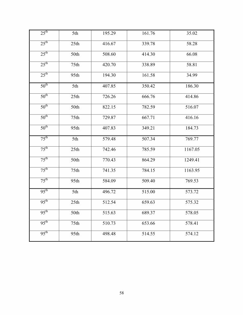
58

25th 5th 195.29 161.76 35.02

25th 25th 416.67 339.78 58.28

25th 50th 508.60 414.30 66.08

25th 75th 420.70 338.89 58.81

25th 95th 194.30 161.58 34.99

50th 5th 407.85 350.42 186.30

50th 25th 726.26 666.76 414.86

50th 50th 822.15 782.59 516.07

50th 75th 729.87 667.71 416.16

50th 95th 407.83 349.21 184.73

75th 5th 579.48 507.34 769.77

75th 25th 742.46 785.59 1167.05

75th 50th 770.43 864.29 1249.41

75th 75th 741.35 784.15 1163.95

75th 95th 584.09 509.40 769.53

95th 5th 496.72 515.00 573.72

95th 25th 512.54 659.63 575.32

95th 50th 515.63 689.37 578.05

95th 75th 510.73 653.66 578.41

95th 95th 498.48 514.55 574.12

59

It is seen that the values in Table 3.6 still vary greatly from the nominal IC ARL of 500,

indicating that the particular estimates (quantiles) of ̅ and obtained from the Phase I sample

at hand and used in the chart will greatly affect the charts’ performance.

In many cases, the conditional IC ARLs for the modified ( / ) scheme are further from

the nominal value than those of the Max and Distance charts. The modified ( / ) scheme has

particularly poor performance in this respect when low quantiles of ̅ are used. On the other

hand, when a very high quantile of ̅ is used, the modified ( / ) scheme has a closer-to-nominal

IC ARL than the other two charts.

The conditional IC ARL values in Table 3.6 are typically somewhat closer to the nominal

value than those shown in Table 3.2, indicating that the modifications have improved the charts’

robustness to error in the estimation of the parameters. In particular, note that when the 25th

percentile estimate is used for both ̅ and , the conditional IC ARL for the Modified Max chart

(416.67) is nearly three times as large as the corresponding IC ARL for the original Max chart

(139.07), and, similarly, the conditional IC ARL for the Modified Distance chart (339.78) is more

than two-and-a-half times as large as the corresponding IC ARL for the original Distance chart

(128.84). Furthermore, between the two one-chart schemes, the Max chart appears to exhibit

superior performance when a lower estimate (quantile) of the variance is used, while the

Distance chart seems preferable when a higher estimate is used. Nevertheless, the results are not

entirely satisfactory, as it is clear that the Phase I estimate of the mean and variance can greatly

impact the IC performance of the Phase II chart, particularly when m is small to moderate as is

currently recommended in the literature. This is an important problem which would benefit from

further research.

60

3.11 Summary and Conclusions

Monitoring the mean and variance is an important problem in statistical process control.

Chen and Cheng’s (1998) Max chart and Razmy’s (2005) Distance chart are applicable when the

IC mean and variance of the underlying normal distribution are known or specified. However,

when these parameters are unknown, it is necessary to estimate them from an IC reference (or a

Phase I) sample. This estimation introduces additional variability which needs to be properly

taken into account in order to apply the charts correctly. Otherwise, the IC ARL can vary greatly

and is usually much lower than what is nominally expected, which means excessive false alarms

which can vastly diminish the utility of the charts in practice. We consider modifications of the

Max chart and the Distance chart for the unknown parameter case and study their

implementation and run length properties. It is shown that the two modified charts perform

similarly, with the Distance chart having a slight advantage in most cases. The modified charts

can be used in practice whenever a Shewhart-type chart for jointly monitoring unknown mean

and variance is desirable. Further refinements, such as using averages-type charts including the

CUSUM and the EWMA charts that can be useful for detecting small and sustained changes will

be considered elsewhere in the future.

Finally, Hawkins and Zamba (2005) proposed an alternative methodology for jointly

monitoring the mean and variance of a normal distribution when the parameters are unknown

based on what is called a changepoint formulation. The “changepoint” is the unknown instant at

which a shift occurs in one or both of the parameters, such that the observations taken before the

changepoint have a different mean and/ or variance than those taken after it. The changepoint

approach to joint monitoring can be attractive in situations where practitioners do not have

access to or prefer not to collect a reference sample prior to starting prospective process

61

monitoring. Our approach, on the other hand, is a more traditional one based on current practice

which allows practitioners to use control charts with which they are familiar while making the

necessary adjustments to correct the control limits that account for estimation of parameters.

Moreover, there are situations in practice where it is common to conduct a Phase I study as a part

of routine process analysis before starting prospective monitoring.

62

CHAPTER 4

CONTROL CHARTS FOR SIMULTANEOUS MONITORING OF KNOWN LOCATION AND SCALE PARAMETERS OF PROCESSES FOLLOWING A SHIFTED (TWO-

PARAMETER) EXPONENTIAL DISTRIBUTION

4.1 Introduction

Often manufacturers of consumer products offer a guarantee that some product, if used

properly, will work for a particular amount of time. For example, an automobile may come with

a three-year/30,000 mile guarantee, under which the manufacturer agrees to fix any defects

which occur during that specified period. In order to determine an appropriate guarantee period,

a manufacturer would typically utilize a relevant statistical distribution to model the lifetime of

the product. The two-parameter exponential distribution is often an appropriate statistical model

for such circumstances. Under this model, the assumed distribution of the lifetime, , of the

product is ( ; , ) = ( )/ where < is a period during which no failure can occur,

i.e. the guarantee period, and > 0 is the scale parameter (Epstein, 1960). Thus, the

determination of a guarantee period can be accomplished by estimating the parameter . A manufacturer may also want to engage in prospective monitoring to determine whether

the distribution of the product’s lifetime has remained unchanged or whether some shift has

occurred in one or both of the distribution’s parameters. He needs a control scheme capable of

accurately determining whether each sample taken comes from the specified shifted exponential

distribution or one that differs from the specified one in some way. External factors, such as

pollution or changes in the materials used to pave roads, could alter the distribution of the

63

product’s lifetime by changing one or both of the distribution’s parameters. Control charts are a

useful tool for engaging in such process monitoring. However, the majority of control charts are

designed for situations in which the data are known or assumed to be normally distributed. When

the data are actually non-normal, however, the use of such charts is inappropriate and can be

quite misleading. Instead of using normal theory charts, practitioners should use charts designed

for the correct distribution, in this case, the shifted exponential distribution.

The monitoring of guarantee times is far from the only situation in which one might need

a control chart for the shifted exponential distribution. Kao (2010) provides examples of

processes which follow this distribution in both manufacturing and healthcare settings. Notably,

he demonstrates that time between MSRA infections in patients at a particular hospital, which

might reasonably be expected to follow a one-parameter exponential distribution, actually has a

location parameter and follows a shifted exponential distribution.

Furthermore, in practice many processes are assumed to follow the one-parameter

exponential distribution, which is simply a special case of the shifted exponential distribution. It

is often plausible that a process whose IC distribution is exponential could experience a location

shift, in which case a control chart for the shifted exponential distribution is needed to monitor it.

For example, suppose that Steve, a preschool student, occasionally bites his classmates. Also

assume that every time Steve bites another child, he is scolded by his teacher and that the time

between Steve’s biting episodes follows a one-parameter exponential distribution. Now, suppose

that following complaints from other’s children’s parents, Steve’s exasperated teacher begins

placing him in seclusion for five minutes immediately following each biting episode. This

intervention by the teacher is an assignable cause which will undoubtedly result in a location

64

shift, since Steve cannot bite another student for at least five minutes, but it may or may not

result in a shift in the scale parameter.

A large body of research on testing and estimation for the shifted exponential distribution

has been developed over the years. Researchers including Epstein (1960), Varde (1969),

Kececioglu and Li (1985), and Lam et al. (1994) have developed point and interval estimates for

the location and scale parameters of this distribution. Ahsanullah (1980) and Ahmadi and

MirMostafaee (2009) made contributions to predicting future data points from the shifted

exponential distribution.

Unfortunately, however, while parameter estimation, hypothesis testing, reliability

sampling plans, and prediction of future data points are addressed in the literature, the research

on control charts for data from this distribution is much sparser. Ramalhoto and Morais (1999)

developed a control chart for monitoring only the scale parameter, and Sürücü and Sazak (2009)

presented a control scheme for this distribution in which moments are used to approximate the

distribution. Neither method is entirely satisfactory for the purposes described above. Instead, the

product manufacturer needs a control scheme capable of jointly monitoring the location and

scale parameters.

At first, it might seem tempting to construct a chart which jointly monitors the process

mean and standard deviation, using the mean and standard deviation of process samples to

monitor the distribution, as is typically done in normal theory situations. However, these

summary statistics can be inefficient and unreliable in this case, as noted by Ramalhoto and

Morais (1999). They point out that “a more reliable alternative is to identify or fit a distributional

model for the output that is more appropriate than the normal model, and then to construct

control charts based on that model.”

65

Here, we discuss and compare several possibilities for one-chart schemes for jointly

monitoring the parameters of the shifted exponential distribution. First, we propose a pair of joint

monitoring schemes similar to Chen and Cheng’s (1998) Max chart for normally distributed data.

These schemes transform the estimators for each parameter so that they each have the standard

normal distribution and then combine them together using a max function. The Shifted

Exponential MLE Max (SEMLE-Max) chart utilizes the maximum likelihood estimators (MLEs)

of the location and scale parameters, while the Shifted Exponential MVUE Max (SEMVUE-

Max) chart utilizes the minimum variance unbiased estimators (MVUEs). As mentioned

previously, there are other ways of constructing joint monitoring schemes, but max-type charts

have been popular in the literature and with practitioners, due to their straightforwardness and

relative simplicity. Next, we suggest a max-type joint monitoring scheme similar to the SEMLE-

Max chart except that it transforms the estimators so that both have the chi-square distribution

with two degrees of freedom. Here, we transform the estimators to the chi-square distribution

rather than the normal distribution in effort to address a problem with ARL bias that occurs in

the SEMLE-Max and SEMVUE-Max charts. We call this the Shifted Exponential MLE Chi-

square Max (SEMLE-ChiMax) chart. Finally, we consider a likelihood ratio-type chart, which

we will refer to as the Shifted Exponential Likelihood Ratio (SE-LR) chart.

Additionally, we consider a two-chart joint monitoring scheme made up of a control chart

for monitoring the location and a separate control chart for monitoring the scale. Each of these

component charts utilizes the MLE of the parameter that it monitors, and the control limits for

the two charts are selected individually so that the overall IC ARL of the scheme is a specified

value. We refer to this as the SEMLE-2 joint monitoring scheme.

66

4.2 Statistical Framework and Preliminaries

Let us first consider the case where the IC parameters, and , are known or specified.

Let , , … , be a random sample of size from the shifted exponential distribution, with

location parameter and scale parameter .10 The parameters and are unknown;

however, when the process is IC, = and = . When the process is out-of-control

(OOC), one or both of these equalities is violated; in other words, either the location parameter,

the scale parameter, or both differ from the specified IC parameters, and , respectively.

However, at the outset, it is unclear whether or not the distributions are the same.

4.3 The SEMLE-Max Chart

Let = ( ) be the first order statistic of the sample. This is known to be the MLE for

the location parameter (Johnson and Kotz, 1970). Also, let = ∑ = ∑ − =− . This is the MLE of the scale parameter (Johnson and Kotz, 1970). Furthermore, and

are independent (see Johnson and Kotz, 1970; Govindarajulu, 1966; Tanis, 1964). However,

they are not unbiased, since = + and = (1 − ). Since is simply the first order statistic of the , , … , sample, its distribution is

well known to be the shifted exponential distribution with location parameter and scale

parameter / . As a result, has a chi-square distribution with 2 degrees of freedom.

The distribution of is less straightforward but still obtainable. First, observe that ∑ − = ∑ − ( ) = ∑ ( − + 1) ( ) − ( ) . Now, ∑ ( − + 10 For consistency across chapters of this dissertation, we use and for known IC parameters and and forPhase2parameters. and are reserved for use in discussion of Phase I parameters.

67

1) ( ) − ( ) has a chi-square distribution with 2 − 2 degrees of freedom (Tanis, 1964).

Thus, = ∑ ( − + 1) ( ) − ( ) has a chi-square distribution with 2 − 2 degrees

of freedom.

Now, let = Φ , 2 where (. , ) denotes the cdf of a chi-square

distribution with degrees of freedom, and let = Φ , 2 − 2 . Note that both

and have a standard normal distribution when the process is IC. We will use these two

statistics to construct the SEMLE-Max chart.

4.3.1 Proposed Charting Procedure for the SEMLE-Max chart

We propose the following method for constructing SEMLE-Max charts when the location

and scale parameters, and , are known or specified:

Step 1. Let , = ( , , … , ) be the ith Phase II sample of size , = 1,2,…

Step 2. Identify the ’ with the ’ . Calculate the statistics and for the th test sample,

for = 1,2,…

Step 3: Calculate the plotting statistic ℳ = max{| |, | |}. Step 4. Plot ℳ against a UCL ℳ. Note that ℳ ≥ 0 by definition so that the LCL is 0 and that

larger values of ℳ suggest an OOC process.

Step 5. If ℳ exceeds ℳ, the process is declared OOC at the ith test sample. If not, the process

is considered to be IC, and testing continues to the next sample.

Step 6. Follow up: When the process is declared OOC at the ith test sample, compare each of | | and | | with ℳ.

(i) If | | < ℳ < | |, a shift in the location parameter is indicated.

68

(ii) If | | < ℳ < | |, a shift in the scale parameter is indicated.

(iii) If | | and | | both exceed ℳ, a shift in both the location and scale parameters is

indicated.

4.3.2 Distribution of the Plotting Statistic for the SEMLE-Max chart

For the SEMLE-Max chart, the process is declared OOC when ℳ > ℳ where the UCL ℳ is obtained so that the IC ARL is some given nominal value. and are independent

because and − are, and as mentioned previously, both have the standard normal

distribution when the process is IC. The cdf of the plotting statistic ℳ is given by (ℳ ≤ ) =(max{| |, | |} ≤ ) = {(| | ≤ )&(| | ≤ )} = ( ( ), 2) + −, 2 − ( (− ), 2) + − , 2 × (Φ( ), 2 − 2), 2 − 2 −

(Φ(− ), 2 − 2), 2 − 2 . 11 When the process is IC, the cdf of the plotting statistic ℳ simplifies to (ℳ ≤ | ) ={ ( ) − (− )} . The IC ARL is (ℳ ) = { ( ) ( )} = { ( ) } . Thus, the UCL

ℳ = Φ .

4.4 The SEMLE-ChiMax Chart

Next, let = and = G G , 2 − 2 , 2 where and are the

maximum likelihood estimators given above. Note that both and have a chi-square

11 Further details are given in section C.3 of the Appendix.

69

distribution with two degrees of freedom when the process is IC. These are the two statistics that

we will use to construct the SEMLE-ChiMax chart.

4.4.1 Proposed Charting Procedure for the SEMLE-ChiMax chart

We propose the following method for constructing SEMLE-ChiMax charts when the

location and scale parameters, and , are known or specified:

Step 1. Let , = ( , , … , ) be the ith Phase II sample of size , = 1,2,…

Step 2. Identify the ’ with the ’ . Calculate the statistics and for the th test sample,

for = 1,2,…. Note that if the process is IC, both of these quantities should be positive. If ≤ 0, the process is declared OOC at the ith test sample. If > 0,continue to step 3.

Step 3: Calculate the plotting statistic Τ = max{ , }. Step 4. Plot Τ against a UCL . Note that Τ ≥ 0 so that the LCL is 0 and large values of

suggest an OOC process.12

Step 5. If is greater than or less than 0, the process is declared OOC at the ith test sample.

If not, the process is considered to be IC, and testing continues to the next sample.

Step 6. Follow up: When the process is declared OOC at the ith test sample, compare each of

and with .

(i) If < < , a shift in the location parameter is indicated.

(ii) If < and < 0, a shift in the location parameter is indicated.

(iii) If < < and ≥ 0, a shift in the scale parameter is indicated.

12 By its design, the SEMLE-ChiMax chart is able to detect both increases and decreases in the location parameter, though only increases in the scale parameter. In this sense, it is not particularly different from numerous normal theory schemes which detect increases and decreases in the mean but only increases in the variance.

70

(iv) If and both exceed , a shift in both the location and scale parameters is

indicated.

(v) If > and < 0, a shift in both the location and scale parameters is indicated.

4.4.2 Distribution of the Plotting Statistic for the SEMLE-ChiMax chart

For the SEMLE-ChiMax chart, the process is declared OOC when Τ ≤ 0or Τ >

where the UCL is obtained so that the IC ARL is some given nominal value. and are

independent because and − are, and as mentioned previously, both have the chi-square

distribution with two degrees of freedom when the process is IC. The cdf of the plotting statistic Τ is given by ( ≤ & > 0) = (max{ , } ≤ & > 0)= 2 2 + − , 2 − 2 ( − ), 2× [ ( , 2), 2 − 2], 2 − 2 . 13

When the process is IC, the cdf of the plotting statistic Τ simplifies to (Τ ≤ & > 0| ) ={ ( , 2)}{ ( , 2)} = { ( , 2)} . The IC ARL is ( ) = { ( , )} . Thus, the UCL

= 1 − , 2 .

13 Further details are given in section C.4 of the Appendix.

71

4.5 The SEMVUE-Max Chart

Next, let = ( ) and = ( ) . These are the minimum variance unbiased

estimators for and , respectively, though unlike and λ , they are not independent (Cohen

and Helm, 1973). In fact, they have covariance ( ). The distribution of is clearly

proportional to the distribution of , so that ( ) has a chi-square distribution with 2 −

2degrees of freedom. The distribution of is much more complicated to obtain, and we could

find no references to it in the literature. However, using the Jacobian method (see Appendix

C.1), we find that the joint distribution of and is

, ( , ) = ( − 1)Γ( − 1) ( ), > − , > 0. It can easily be shown that , ( , ) = 1.The marginal distributions can

be obtained by integrating this pdf. Doing so, we confirm that ( ) has the distribution

specified above. The pdf of is

( ) = ( − 1)Γ( − 1) ( ) ( , )( )+ ( − 1)Γ( − 1) ( )

( ) ( , ]( ).The details of the derivations can be found in Appendix C.2. When = 5, one can easily obtain

the cdf,

( ) = . 59 − 256625 ( )/ − 1 ≤ < ∞−∞ < <

72

where = ( )/ [−100,000 + 27,000 + 300,000 −300,000 − 54,000 − 3,660 + 100,000 + 27,000 + 3,660 +221.4 ],by integrating ( ). It is easy to see that this distribution has two parameters,

and .

Now, let = Φ G ( ) ,2 − 2 , and let = Φ , , where

(. , a, b) denotes the cdf of , ( ), with parameters a and b. Note that both and have a

standard normal distribution when the process is IC. We will use these two statistics to construct

the SEMVUE-Max chart.

4.5.1 Proposed Charting Procedure for the SEMVUE-Max chart

We propose the following method for constructing SEMVUE-Max charts when the

location and scale parameters, and , are known or specified:

Step 1. Let , = ( , , … , ) be the ith Phase II sample of size , = 1,2,…

Step 2. Identify the ’ with the ’ . Calculate the statistics and for the th test sample,

for = 1,2,…

Step 3: Calculate the plotting statistic ℵ = max{| |, | |} . 14 Step 3. Plot ℵ against a UCL ℵ. Note that ℵ ≥ 0 by definition so that the LCL is 0 and that

larger values of ℵ suggest an OOC process.

Step 4. If ℵ exceeds ℵ, the process is declared OOC at the ith test sample. If not, the process is

considered to be IC, and testing continues to the next sample.

14 Although C1 and C2 are correlated, the distribution of the plotting statistic can be obtain be using their joint distribution.

73

Step 5. Follow up: When the process is declared OOC at the ith test sample, compare each of | | and | | with ℵ.

(i) If | | < ℵ < | |, a shift in the location parameter is indicated.

(ii) If | | < ℵ < | |, a shift in the scale parameter is indicated.

(iii) If | | and | | both exceed ℵ, a shift in both the location and scale parameters is

indicated.

4.5.2 Distribution of the Plotting Statistic for the SEMVUE-Max chart

For the SEMVUE-Max chart, the process is declared OOC when ℵ > ℵ where the UCL ℵ is obtained so that the IC ARL is some given nominal value. Note that and are not

independent; however, both have the standard normal distribution when the process is in-control.

The cumulative distribution function of the plotting statistic ℵ is given by (ℵ ≤ ) = (max{| |, | |} ≤ ) = {(| | ≤ )&(| | ≤ )}= , ( , )( ( ), , )( ) ( ( ), )

( ) ( ( ), )+ , ( , ) .( ) ( ( ), )

( )[ ( ( ), , )]

4.6 The SE-LR Chart

Since joint monitoring of the location and scale is analogous to repeatedly testing the null

hypothesis that the sample at hand comes from a completely specified shifted exponential

population (a simple null hypothesis) versus all alternatives (a composite alternative hypothesis),

we also wish to consider a chart based upon the perspective of a likelihood ratio statistic. It can

74

be shown (see the appendix) that the likelihood ratio statistic for the shifted exponential

distribution is given by Λ = ( ) exp{− ( − )/ }. This will be a plotting statistic

used to define the SE-LR chart.

4.6.1 Proposed Charting Procedure for the SE-LR chart

We propose the following method for constructing SE-LR charts when the location and

scale parameters, and , are known or specified:

Step 1. Let , = ( , , … , ) be the ith Phase II sample of size , = 1,2,…

Step 2. Identify the ’ with the ’ . Calculate the statistics Λ for the th test sample, for = 1,2, …

Step 3: Step 3. Plot Λ against a LCL . Note that Λ ≤ 1 by definition so that the UCL is 1 and

that smaller values of Λ suggest an OOC process.

Step 4. If Λ is lower than , the process is declared OOC at the ith test sample. If not, the

process is considered to be IC, and testing continues to the next sample.

Step 5. Follow up: When the process is declared OOC at the ith test sample, calculate

and .When the process is IC, each has a chi-square distribution (with 2 and 2 − 2 degrees

of freedom, respectively). Let = [ > ] and = [ > ] . Both can be

obtained directly from a chi-square table.

(i) If both , < 0.01, a shift in both the location and scale parameters is indicated.

(ii) If both , > 0.05, a false alarm is indicated.

(iii) If < 0.01and > 0.05,a shift in the location parameter is indicated.

75

(iv) If < 0.01and > 0.05,a shift in the scale parameter is indicated.

(v) If < 0.01 and 0.01 ≤ ≤ 0.05,a major shift in the location parameter with

possible associated shift in the scale parameter is indicated.

(vi) If < 0.01 and 0.01 ≤ ≤ 0.05,a major shift in the scale parameter with possible

associated shift in the location parameter is indicated.

4.6.2 Distribution of the Plotting Statistic for the SE-LR chart

For the SE-LR chart, the process is declared OOC when Λ < ,where the LCL is

obtained so that the IC ARL is equal to some given nominal value. However, the distribution of Λ

is rather intractable.

When and are large, it is useful to consider the asymptotic properties of Λ. Consider

a function of Λ,−2ln Λ = −2 ln ( ) exp{− ( − )/ } . It can be shown (see for

example Hogg, McKean and Craig (2005)) that −2lnΛconverges in distribution to a chi-square

random variable with 2 degree of freedom. Using this property, it is simple to obtain as long

as and are appropriately large. However, when and are small or moderate as is typically

the case in control charting, can easily be obtained through Monte Carlo simulation.

4.7 The SEMLE-2 Scheme

Let = and = . Note that when the process is IC, both and have

a chi-square distribution (with 2 and 2 − 2 degrees of freedom, respectively). These are the two

statistics that we will use to construct the charts which make up the SEMLE-2 scheme.

76

4.7.1 Proposed Charting Procedure for the SEMLE-2 scheme

We propose the following method for constructing SEMLE-2 schemes when the location

and scale parameters, and , are known or specified:

Step 1. Let , = ( , , … , ) be the ith Phase II sample of size , = 1,2,…

Step 2. Identify the ’ with the ’ . Calculate the plotting statistics and for the th test

sample, for = 1,2,…. Note that if the process is IC, both of these quantities should be positive.

If ≤ 0, the process is declared OOC at the ith test sample. If > 0,continue to step 3.

Step 3. Plot E against a UCL . Note that the LCL is 0, and large values of suggest an

OOC process.

Step 4. On a separate chart, plot E against an UCL and LCL . Step 5. If E is greater than and/or E is greater than or less than , the process is

declared OOC at the ith test sample. If not, the process is considered to be IC, and testing

continues to the next sample.

Step 6. Follow up: When the process is declared OOC at the ith test sample, compare E with and E with and .

(i) If E > and < E < ,a shift in the location parameter is indicated.

(ii) If < E < and E < 0, a shift in the location parameter is indicated.

(iii) If E > and 0 < E < , a shift in the scale parameter is indicated.

(iv) If E < and 0 < E < , a shift in the scale parameter is indicated

(v) If E > and E > , a shift in both the location and scale parameters is

indicated.

77

(vi) If E < 0 and E > , a shift in both the location and scale parameters is

indicated.

(vii) If E > and E < , a shift in both the location and scale parameters is

indicated.

(viii) If E < 0 and E < , a shift in both the location and scale parameters is

indicated.

4.7.2 Distribution of the Plotting Statistics for the SEMLE-2 scheme

The SEMLE-2 control scheme consists of two charts. The process is declared OOC

whenever a signal occurs on either chart, that is, any time E < 0, E > , E > ,or E < where the control limits , , and are obtained so that the IC ARL is some

given nominal value. and are independent because and − are, and as mentioned

previously, both have the chi-square distribution (with 2 and 2 − 2 degrees of freedom,

respectively) when the process is IC. The joint cumulative distribution function of the two

plotting statistics and is given by [(0 < E ≤ )&( ≤ E ≤ )] = (0 < E ≤ ) ( ≤ E ≤ )= ( ) + 2 ( − ) , 2 − 2 ( − ) , 2× ( ), 2 − 2 − ( ), 2 − 2 .

When the process is IC, the joint cumulative distribution function of the plotting statistics and

simplifies to [(0 < E ≤ )&( ≤ E ≤ )] = { ( , 2)}{ ( , 2 − 2) −( , 2 − 2)}.

78

4.8 Implementation

In order to use the proposed charts, one must select the appropriate control limits for each

corresponding to the desired nominal IC ARL. For several of the charts, this can be accomplished

using the analytical expressions for the IC ARLgiven in the earlier sections. For the remaining

charts, we use can obtain the control limits through simulation. Here, we used simulations in R to

compute all of the control limits, and where possible we used the analytical expressions to verify

the results. As expected, we find that higher nominal ARLs require higher UCLs and lower LCLs.

Table 4.1: Appropriate control limits for the shifted exponential charts when and are known and = , for various IC ARLs

IC ARL SEMLE-Max Chart UCL

SEMVUE-Max Chart UCL

SEMLE-ChiMax Chart UCL

SE-LR Chart LCL

SEMLE-2 Scheme (Location Chart UCL/ Scale Chart UCL/ Scale Chart LCL )

125 2.88 2.82 11.04 0.000899 11.04/ 24.35/1.04 250 3.09 3.02 12.43 0.000365 12.43/ 26.12/0.86 500 3.29 3.20 13.82 0.000154 13.82/ 27.87/0.71 750 3.40 3.29 14.63 0.0000929 14.63/ 28.88/0.64 1000 3.48 3.35 15.20 0.0000659 15.20/ 29.59/0.59

4.9 Performance Comparisons

The performance of the four one-chart schemes and the two-chart SEMLE-2 scheme for

various location and scale shifts is evaluated in a simulation study so that they can easily be

compared. Tables 4.2, 4.3, and 4.4 provide the ARL, run length standard deviation, and specified

quantiles of the run length distribution when = 5. We use = 0 and = 1 for our IC shifted

exponential distribution.

79

Table 4.2: Run length characteristics for the SEMLE-Max and SEMVUE-Max charts for various values of and when = , = , and =

SEMLE-Max Chart SEMVUE-Max Chart

θ2 λ2 ARL SDRL 5%, 25%, 50%, 75%, 95% ARL SDRL 5%, 25%, 50%, 75%, 95% 0 1 498.67 498.85 26, 142, 346, 696, 1492 500.81 502.66 27, 144, 347, 692, 1514

0.1 1 539.96 539.34 26, 155, 374, 748, 1603 546.42 536.07 28, 163, 387, 758, 1627

0.25 1 359.83 355.74 20, 106, 251, 501, 1062 420.43 421.85 23, 122, 288, 582,1274

0.5 1 141.72 140.99 8, 41, 98, 198, 420 205.33 204.97 10, 59, 143, 285, 614

0.75 1 44.50 43.45 3, 13, 31, 61, 132 73.96 73.65 4, 22, 52, 102, 223

1 1 13.23 12.53 1, 4, 9, 18, 38 22.74 22.08 2, 7, 16, 31, 66

1.25 1 3.77 3.28 1, 1, 3, 5, 10 6.68 6.27 1, 2, 5, 9, 19

1.5 1 1.10 0.33 1, 1, 1, 1, 2 1.93 1.34 1, 1, 1, 2, 5

0 1.25 136.85 135.79 8, 40, 96, 191, 398 115.85 117.50 6, 33, 79, 158, 357

0.1 1.25 126.36 125.17 7, 37, 88, 176, 373 132.52 131.14 8, 39, 92, 183, 390

0.25 1.25 91.62 91.17 5, 27, 64, 125, 274 109.23 108.99 6, 32, 76, 150, 327

0.5 1.25 46.44 45.49 3, 14, 32, 65, 138 67.51 66.81 4, 18, 47, 94, 200

0.75 1.25 19.91 19.79 1, 6, 14, 27, 58 32.10 31.60 2, 10, 23, 44, 95

1 1.25 7.78 7.26 1, 3, 6, 11, 22 13.58 13.11 1, 4, 10, 19, 39

1.25 1.25 2.91 2.38 1, 1, 2, 4, 8 5.29 4.73 1, 2, 4, 7, 15

1.5 1.25 1.09 0.30 1, 1, 1, 1, 2 2.00 1.42 1, 1, 1, 3, 5

0 1.5 41.88 41.04 3, 12, 29, 58, 122 36.63 36.16 2, 11, 25, 51, 107

0.1 1.5 39.08 37.44 3, 12, 28, 55, 115 39.03 39.10 3, 11, 27, 54. 116

0.25 1.5 31.76 31.54 2, 9, 22, 44, 94 35.10 34.74 2, 10, 24, 49, 105

0.5 1.5 19.78 19.22 1, 6, 14, 28, 59 26.26 25.65 2, 8, 19, 36, 76

0.75 1.5 10.91 10.33 1, 4, 8, 15, 32 16.69 16.19 1, 5, 11, 23, 49

1 1.5 5.26 4.67 1, 2, 4, 7, 14 8.88 8.38 1, 3, 6, 12, 26

1.25 1.5 2.37 1.79 1, 1, 2, 3, 6 4.37 3.86 1, 2, 3, 6, 12

1.5 1.5 1.06 0.26 1, 1, 1, 1, 2 2.01 1.43 1, 1, 2, 3, 5

0 1.75 17.83 17.43 1, 5, 12, 24, 53 16.15 15.58 1, 5, 11, 22, 47

0.1 1.75 16.58 16.00 1, 5, 12, 23, 48 16.87 16.37 1, 5, 12, 23, 49

0.25 1.75 14.44 13.92 1, 5, 10, 20, 42 15.57 14.90 1, 5, 11 , 22, 46

0.5 1.75 10.31 9.73 1, 3, 7, 14, 30 12.89 12.31 1, 4, 9, 18, 37

0.75 1.75 6.76 6.30 1, 2, 5, 9, 19 9.57 9.08 1, 3, 7, 13, 27

1 1.75 3.85 3.28 1, 1, 3, 5, 10 6.27 5.74 1, 2, 4, 9, 18

1.25 1.75 2.10 1.52 1, 1, 2, 3, 5 3.60 3.04 1, 1, 3, 5, 10

1.5 1.75 1.05 0.24 1, 1, 1, 1, 2 1.95 1.37 1 , 1, 1, 2, 5

0 2 9.75 9.26 1, 3, 7, 13, 28 8.92 8.34 1, 3, 6, 12, 25

0.1 2 9.16 8.60 1, 3, 7, 12, 27 9.28 8.76 1, 3, 7, 13, 27

0.25 2 8.15 7.71 1, 3, 6, 11, 24 8.73 8.14 1, 3, 6, 12, 25

0.5 2 6.47 5.97 1, 2, 5, 9, 18 7.66 7.08 1, 3, 5, 10, 22

0.75 2 4.62 4.04 1, 2, 3, 6, 13 6.13 5.55 1, 2, 4, 8, 17

1 2 3.00 2.44 1, 1, 2, 4, 8 4.50 3.96 1, 2, 3, 6, 12

1.25 2 1.81 1.20 1, 1, 1, 2, 4 2.97 2.46 1, 1, 2, 4, 8

1.5 2 1.05 0.22 1, 1, 1, 1, 1 1.85 1.25 1, 1, 1, 2, 4

80

Table 4.3: Run length characteristics for the SE-LR and SEMLE-ChiMax charts for various values of and when = , = , and =

SE-LR Chart SEMLE-ChiMax Chart

θ2 λ2 ARL SDRL 5%, 25%, 50%, 75%, 95% ARL SDRL 5%, 25%, 50%, 75%, 95% 0 1 506.65 512.37 27, 143, 350, 697, 1519 499.21 500.19 26, 141, 346, 696, 1505

0.1 1 339.11 332.76 19, 101, 235 , 473, 1009 380.14 381.13 20, 110, 263, 528, 1144

0.25 1 193.34 192.78 10, 57, 134, 267, 579 223.61 222.46 12, 66, 156, 310, 668

0.5 1 71.55 71.35 4, 21, 49, 99, 213 75.61 74.73 4, 22, 53, 105, 223

0.75 1 27.25 26.18 2, 8, 19, 38, 80 22.83 22.45 2, 7, 16, 31, 68

1 1 10.70 10.15 1, 3, 8, 15, 31 6.79 6.23 1, 2, 5, 9, 19

1.25 1 4.35 3.74 1, 2, 3, 6, 12 1.93 1.34 1, 1, 1, 2, 5

1.5 1 1.84 1.26 1, 1, 1, 2, 4 1 0 1, 1, 1, 1, 1

0 1.25 323.75 322.02 18, 94, 224, 451, 974 87.35 86.78 5, 26, 61, 121, 260

0.1 1.25 222.41 219.80 11, 65, 156, 311, 666 74.33 74.41 4, 21, 52, 102, 225

0.25 1.25 127.88 126.77 7, 37, 90, 177, 380 55.23 55.15 3, 16 , 38, 77, 165

0.5 1.25 51.51 50.91 3, 15, 36, 71, 153 27.10 26.63 2, 8, 19, 37, 81

0.75 1.25 20.79 20.07 2, 6, 15, 29, 61 11.60 11.07 1, 4, 8, 16, 34

1 1.25 8.76 8.18 1, 3, 6, 12, 25 4.49 3.96 1, 2, 3, 6, 12

1.25 1.25 3.81 3.27 1, 1, 3, 5, 10 1.68 1.07 1, ,1, 1, 2, 4

1.5 1.25 1.74 1.16 1, 1, 1, 2, 4 1 0 1, 1, 1, 1, 1

0 1.5 120.79 119.82 7, 36, 84, 168, 362 27.76 27.20 2, 8, 19, 38, 82

0.1 1.5 88.77 87.67 5, 25, 62, 124, 264 25.54 24.97 2, 8, 18, 35, 75

0.25 1.5 54.74 54.61 3, 16, 37, 76, 166 20.78 20.35 2, 6, 14, 29, 62

0.5 1.5 26.50 26.16 2, 8, 18, 36, 78 12.90 12.44 1, 4, 9, 18, 37

0.75 1.5 12.63 12.20 1, 4, 9, 17, 37 6.89 6.33 1, 2, 5, 9, 20

1 1.5 6.01 5.50 1, 2, 4, 8, 17 3.34 2.75 1, 1, 2, 4, 9

1.25 1.5 2.96 2.44 1, 1, 2, 4, 8 1.53 0.91 1, 1, 1, 2, 3

1.5 1.5 1.56 0.93 1, 1, 1, 2, 3 1 0 1, 1, 1, 1, 1

0 1.75 47.55 46.74 3, 14, 34, 65, 139 12.65 12.09 1, 4, 9, 17, 37

0.1 1.75 36.34 35.58 2, 11, 26, 50, 106 11.79 11.23 1, 4, 8, 16, 34

0.25 1.75 25.08 25.28 2, 7, 17, 34, 76 10.19 9.67 1, 3, 7, 14, 29

0.5 1.75 13.28 12.54 1, 4, 9, 18, 39 7.36 6.87 1, 2, 5, 10, 21

0.75 1.75 7.29 6.85 1, 2, 5, 10, 21 4.70 4.15 1, 2, 3, 6, 13

1 1.75 4.14 3.62 1, 2, 3, 5, 11 2.68 2.15 1, 1, 2, 3, 7

1.25 1.75 2.36 1.78 1, 1, 2, 3, 6 1.43 0.78 1, 1, 1, 2, 3

1.5 1.75 1.42 0.78 1, 1, 1, 2, 3 1 0 1, 1, 1, 1, 1

0 2 22.57 21.97 2, 7, 16, 31, 66 7.24 6.78 1, 2, 5, 10, 21

0.1 2 17.85 17.24 1, 6, 12, 25, 52 6.85 6.38 1, 2, 5, 9, 19

0.25 2 13.14 12.64 1, 4, 9, 18, 38 6.16 5.60 1, 2, 4, 8, 17

0.5 2 7.94 7.51 1, 3, 6, 11, 23 4.81 4.27 1, 2, 3, 6, 13

0.75 2 4.86 4.31 1, 2, 4, 7, 13 3.45 2.90 1, 1, 3, 5, 9

1 2 3.01 2.47 1, 1, 2, 4, 8 2.22 1.64 1, 1, 2, 3, 6

1.25 2 1.93 1.34 1, 1, 1, 2, 5 1.33 0.67 1, 1, 1, 1, 3

1.5 2 1.31 0.64 1, 1, 1, 1, 3 1 0 1, 1, 1, 1, 1

81

Table 4.4: Run length characteristics for the SEMLE-2 scheme for various values of and when = , = , and =

SEMLE-2 Scheme

θ2 λ2 ARL SDRL 5%, 25%, 50%, 75%, 95% 0 1 503.12 503.82 26, 145, 350, 696, 1510

0.1 1 380.19 380.06 20, 109, 264, 526, 1135

0.25 1 222.28 221.88 12, 64, 154, 308, 667

0.5 1 76.28 75.72 4, 22, 53, 105, 228

0.75 1 23.09 22.62 2, 7, 16, 32, 68

1 1 6.71 6.21 1, 2, 5, 9, 19

1.25 1 1.93 1.33 1, 1, 1, 2, 5

1.5 1 1 0 1, 1, 1, 1, 1

0 1.25 116.35 115.47 7, 34, 81, 161, 347

0.1 1.25 95.83 95.58 6, 28, 66, 132, 286

0.25 1.25 65.14 64.95 4, 19, 45, 90, 194

0.5 1.25 29.49 29.02 2, 9, 21, 41, 87

0.75 1.25 11.88 11.37 1, 4, 8, 16, 35

1 1.25 4.54 4.03 1, 2, 3, 6, 13

1.25 1.25 1.69 1.08 1, 1, 1, 2, 4

1.5 1.25 1 0 1, 1, 1, 1, 1

0 1.5 36.70 36.26 2, 11, 25, 51, 109

0.1 1.5 32.23 31.69 2, 10, 23, 44, 96

0.25 1.5 24.99 24.49 2, 8, 17, 34, 74

0.5 1.5 14.44 13.92 1, 5, 10, 20, 42

0.75 1.5 7.31 6.79 1, 2, 5, 10, 21

1 1.5 3.41 2.85 1, 1, 3, 5, 9

1.25 1.5 1.54 0.91 1, 1, 1, 2, 3

1.5 1.5 1 0 1, 1, 1, 1, 1

0 1.75 16.12 15.60 1, 5, 11, 22, 47

0.1 1.75 14.65 14.07 1, 5, 10, 20, 43

0.25 1.75 12.27 11.70 1, 4, 9, 17, 36

0.5 1.75 8.29 7.76 1, 3, 6, 11, 24

0.75 1.75 4.99 4.46 1, 2, 4, 7, 14

1 1.75 2.74 2.19 1, 1, 2, 4, 7

1.25 1.75 1.43 0.78 1, 1, 1, 2, 3

1.5 1.75 1 0 1, 1, 1, 1, 1

0 2 8.90 8.42 1, 3, 6, 12, 26

0.1 2 8.25 7.71 1, 3, 6, 11, 24

0.25 2 7.32 6.77 1, 2, 5, 10, 21

0.5 2 5.40 4.89 1, 2, 4, 7, 15

0.75 2 3.68 3.12 1, 1, 3, 5, 10

1 2 2.29 1.71 1, 1, 2, 3, 6

1.25 2 1.35 0.68 1, 1, 1, 2, 3

1.5 2 1 0 1, 1, 1, 1, 1

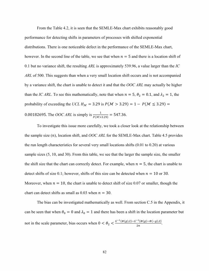
82

From the Table 4.2, it is seen that the SEMLE-Max chart exhibits reasonably good

performance for detecting shifts in parameters of processes with shifted exponential

distributions. There is one noticeable defect in the performance of the SEMLE-Max chart,

however. In the second line of the table, we see that when = 5 and there is a location shift of

0.1 but no variance shift, the resulting ARL is approximately 539.96, a value larger than the IC

ARL of 500. This suggests than when a very small location shift occurs and is not accompanied

by a variance shift, the chart is unable to detect it and that the OOC ARL may actually be higher

than the IC ARL. To see this mathematically, note that when = 5, = 0.1, and = 1, the

probability of exceeding the UCL ℳ = 3.29 is (ℳ > 3.29) = 1 − (ℳ ≤ 3.29) =0.00182695. The OOC ARL is simply is (ℳ . ) = 547.36.

To investigate this issue more carefully, we took a closer look at the relationship between

the sample size ( ), location shift, and OOC ARL for the SEMLE-Max chart. Table 4.5 provides

the run length characteristics for several very small locations shifts (0.01 to 0.20) at various

sample sizes (5, 10, and 30). From this table, we see that the larger the sample size, the smaller

the shift size that the chart can correctly detect. For example, when = 5, the chart is unable to

detect shifts of size 0.1; however, shifts of this size can be detected when = 10 or 30.

Moreover, when = 10, the chart is unable to detect shift of size 0.07 or smaller, though the

chart can detect shifts as small as 0.03 when = 30.

The bias can be investigated mathematically as well. From section C.5 in the Appendix, it

can be seen that when = 0 and = 1 and there has been a shift in the location parameter but

not in the scale parameter, bias occurs when 0 < < ( ( ), ) { ( ) ( ), }.

83

Table 4.5: Run length characteristics for the SEMLE-Max chart for small location shifts not accompanied by scale shifts for various values

= = =

μ2 σ2 ARL SDRL 5%, 25%, 50%, 75%, 95% ARL SDRL 5%, 25%, 50%, 75%, 95% ARL SDRL 5%, 25%, 50%, 75%, 95% 0 1 501.37 494.70 27, 144, 350, 697, 1470 500.53 498.97 26, 141, 350, 696, 1507 500.36 511.14 26, 140, 338, 683, 1522

0.01 1 648.37 644.33 33, 188, 452, 890, 1960 636.76 627.98 32, 183, 445, 879, 1907 590.84 588.61 30, 173, 410, 821, 1745

0.02 1 644.45 636.15 33, 191, 454, 895, 1925 618.29 619.69 31, 180, 421, 861, 1890 513.70 507.97 28, 154, 355, 711, 1543

0.03 1 632.52 633.83 32, 181, 436, 879, 1923 604.33 600.88 31, 177, 417, 836, 1838 448.09 453.89 23, 126, 310, 624, 1342

0.04 1 621.79 613.15 32, 177, 433, 865, 1853 581.69 585.36 31, 168, 400, 806, 1745 376.58 371.10 20, 110, 267, 523, 1113

0.05 1 600.82 597.19 33, 174, 422, 824, 1794 544.19 541.55 32, 159, 379, 762, 1612 309.70 307.00 17, 89, 215, 428, 926

0.06 1 598.68 593.15 31, 173, 425, 823, 1765 518.57 519.68 28, 148, 364, 721, 1538 249.18 246.86 12, 71, 173, 347, 741

0.07 1 585.90 579.16 32, 175, 409, 814, 1742 501.03 496.67 26, 145, 352, 697, 1498 198.89 192.90 11, 60, 141, 275, 582

0.08 1 580.14 584.88 31, 165, 401, 812, 1688 477.05 482.54 23, 133, 325, 668, 1450 151.56 152.43 9, 45, 104, 207, 463

0.09 1 564.78 560.18 29, 167, 399, 781, 1688 447.53 446.84 22, 127, 308, 620, 1367 120.69 119.44 6, 36, 84, 167, 362

0.10 1 562.28 558.75 30, 165, 396, 772, 1679 426.39 426.90 21, 118, 295, 596, 1273 90.15 90.19 5, 26, 62, 125, 266

0.11 1 540.47 545.22 27, 155, 367, 750, 1619 399.56 398.30 21, 117, 275, 561, 1184 69.26 68.69 4, 20, 48, 97, 206

0.12 1 520.79 522.69 27, 151, 361, 722, 1556 374.68 369.67 20, 111, 261, 517, 1105 52.25 51.72 3, 15, 36, 72, 155

0.13 1 504.78 497.85 26, 147, 348, 705, 1511 349.48 353.88 19, 97, 240, 480, 1052 38.64 38.37 2, 12, 27, 53, 117

0.14 1 495.53 494.49 26, 144, 346, 686, 1475 334.09 336.77 17, 95, 232, 460, 989 29.42 2903 2, 9, 21, 40, 88

0.15 1 486.74 486.70 26, 139, 339, 675, 1454 310.04 306.24 16, 91, 216, 430, 922 21.70 21.66 2, 6, 15, 30, 64

0.16 1 479.55 481.31 24, 138, 328, 668, 1455 289.49 287.69 16, 83, 200, 406, 876 16.06 15.64 1, 5, 11, 22, 47

0.17 1 464.77 464.45 23, 133, 329, 646, 1391 269.29 268.08 14, 80, 188, 373, 795 11.85 11.46 1, 4, 8, 16, 34

0.18 1 443.43 443.37 22, 127, 304, 617, 1336 247.75 247.94 14, 72, 169, 346, 749 8.97 8.50 1, 3, 6, 12, 26

0.19 1 432.65 429.44 22, 128, 302, 600, 1270 228.35 223.49 12, 67, 164, 318, 670 6.63 6.08 1, 2, 5, 9, 19

0.20 1 425.15 423.35 23, 123, 298, 597, 1270 211.88 211.27 10, 60, 145, 296, 646 4.89 4.35 1, 2, 3, 7, 14

As noted by Acosta-Meija (1998), “a desired feature is to have all of [the control chart’s]

out-of-control ARL values smaller than the in-control ARL.” Charts which have this property are

called ARL-unbiased. Charts like the SEMLE-Max Chart, in which the OOC ARL is larger than

the IC ARL for certain shift sizes, are called ARL-biased.

The presence of this undesirable quality might lead us to question whether it was caused

by the use of biased estimators for the location and scale parameters. However, Table 4.2 shows

us that the SEMVUE-Max chart, which is composed of unbiased estimators, is also ARL-biased.

Furthermore, the SEMVUE-Max chart typically performs more poorly than the SEMLE-Max

chart. Given its generally poor performance, the SEMVUE-Max will not be considered further in

this paper.

84

The SEMLE-ChiMax chart, on the other hand, is not ARL-biased for detecting changes in

the location parameter and increases in the scale parameter, and it substantially out-performs the

other charts except when there is a small location shift (≤ 0.5) which is not accompanied by a

mean shift. It seems likely, then, that the bias is a result of using the probability integral

transform to put the location and scale estimates on the normal scale.

The SE-LR chart is also ARL-unbiased, but it has worse performance for nearly every

shift size than does the SEMLE-ChiMax chart. It also performs worse than the SEMLE-Max

chart whenever a shift in variance occurs. In many cases, its performance is also worse than that

of the SEMVUE-Max chart.

The SEMLE-ChiMax chart has the best overall performance among the one-chart

schemes, in addition to its favorable quality of ARL-unbiasedness. Note, however, that unlike the

other charts discussed, this chart is not suitable for detecting decreases in the scale parameter.15

If detection of this type of change is desirable, the practitioner should use another chart. The

SEMLE-2 scheme is a promising alternative. In general, it has the second-best performance

among the charts considered and can detect both increases and decreases in both parameters. The

SEMLE-2 scheme is also ARL-unbiased for increases in the parameters; however, note that it

exhibits bias for small decreases in the scale parameter which are accompanied by small or no

changes in the location parameter.

4.10 Performance Comparisons versus Normal Theory Charts

It is of interest to determine whether the proposed charts perform better for process data

from a shifted exponential distribution than would normal theory charts. Here, we consider the

15 It is not uncommon for control charts to be ineffective for detecting decreases in scale parameters. For example, a number of normal theory charts are useful only for detecting increases in the variance.

85

performance of two normal theory charts for various location and scale shifts and sample sizes.

The UCLs for the normal theory charts must be selected so that they have a specified nominal IC

ARL. For = 5, the appropriate UCL for the normal theory max chart is 3.29. Table 4.6 provides

the ARL, run length standard deviation, and specified quantiles of the run length distribution.

Note that the underlying distribution of the process data is shifted exponential. We again use = 0 and = 1 for our IC shifted exponential distribution. The mean of the distribution is + , and its variance is (Johnson and Kotz, 1970). In other words, the mean and variance of

our IC distribution are both 1, and these are values to which the normal theory max and distance

charts will compare the sample means and variances.

At first glance, one might note that Chen and Cheng’s (1998) normal theory Max chart

and Ramzy’s (2005) Distance chart have shorter ARLs than the shifted exponential charts

explored above and conclude that they are preferable. However, note that the IC ARLs for the

normal theory charts are far lower than the nominal value of 500. This means that the charts will

have an unacceptably high number of false alarms, rendering them virtually useless for

monitoring this type of process.

86

Table 4.6: Run length characteristics for normal theory charts applied to shifted exponential data for various values of and when = , = , and =

Normal Theory Max Chart Normal Theory Distance Chart

θ2 λ2 ARL SDRL 5%, 25%, 50%, 75%, 95% ARL SDRL 5%, 25%, 50%, 75%, 95% 0 1 37.38 37.15 2, 11, 26, 51, 110 20.43 19.74 2, 7, 14, 28, 59

0.1 1 35.17 34.92 2, 10, 25, 49, 105 19.51 19.11 1, 6, 14, 27, 57

0.25 1 30.88 30.50 2, 9, 22, 43, 92 17.07 16.30 1, 5, 12, 24, 49

0.5 1 21.78 21.19 2, 7, 15, 30, 63 12.97 12.21 1, 4, 9, 18, 37

0.75 1 12.55 12.17 1, 4, 9, 17, 37 8.27 7.57 1, 3, 6, 11, 24

1 1 6.72 6.15 1, 2, 5, 9, 19 5.19 4.67 1, 2, 4, 7, 14

1.25 1 3.58 3.09 1, 1, 3, 5, 10 2.99 2.48 1, 1, 2, 4, 8

1.5 1 2.12 1.51 1, 1, 2, 3, 5 1.77 1.18 1, 1, 1, 2, 4

0 1.25 14.20 13.59 1, 5, 10, 20, 41 9.18 8.60 1, 3, 6, 13, 27

0.1 1.25 13.19 12.56 1, 4, 9, 18, 38 8.31 7.71 1, 3, 6, 11, 23

0.25 1.25 11.32 10.88 1, 4, 8, 15, 34 7.14 6.47 1, 2, 5, 10, 20

0.5 1.25 7.88 7.41 1, 3, 6, 11, 22 5.41 4.88 1, 2, 4, 7, 15

0.75 1.25 5.15 4.59 1, 2, 4, 7, 14 3.91 3.42 1, 1, 3, 5, 11

1 1.25 3.32 2.76 1, 1, 2, 4, 9 2.80 2.26 1, 1, 2, 4, 7

1.25 1.25 2.17 1.58 1, 1, 2, 3, 5 1.97 1.39 1, 1, 1, 2, 5

1.5 1.25 1.52 0.89 1, 1, 1, 2, 3 1.40 0.76 1, 1, 1, 2, 3

0 1. 5 7.00 6.50 1, 2, 5, 9, 20 4.92 4.43 1, 2, 4, 7, 14

0.1 1.5 6.43 6.02 1, 2, 5, 9, 18 4.55 4.04 1, 2, 3, 6, 13

0.25 1.5 5.52 4.97 1, 2, 4, 7, 16 3.94 3.36 1, 1, 3, 5, 11

0.5 1.5 4.18 3.64 1, 2, 3, 6, 11 3.16 2.60 1, 1, 2, 4, 8

0.75 1.5 3.02 2.50 1, 1, 2, 4, 8 2.53 1.95 1, 1, 2, 3, 6

1 1.5 2.16 1.60 1, 1, 2, 3, 5 1.92 1.34 1, 1, 1, 2, 5

1.25 1.5 1.61 1.00 1, 1, 1, 2, 4 1.54 0.91 1, 1, 1, 2, 3

1.5 1.5 1.30 0.64 1, 1, 1, 1, 3 1.22 0.51 1, 1, 1, 1, 2

0 1.75 4.23 3.63 1, 2, 3, 6, 12 3.18 2.63 1, 1, 2, 4, 8

0.1 1.75 3.96 3.48 1, 1, 3, 5, 11 3.02 2.44 1, 1, 2, 4, 8

0.25 1.75 3.52 2.94 1, 1, 3, 5, 10 2.68 2.14 1, 1, 2, 3, 7

0.5 1.75 2.80 2.23 1, 1, 2, 4, 7 2.25 1.67 1, 1, 2, 3, 6

0.75 1.75 2.17 1.58 1, 1, 2, 3, 5 1.85 1.24 1, 1, 1, 2, 4

1 1.75 1.67 1.05 1, 1, 1, 2, 4 1.55 0.93 1, 1, 1, 2, 3

1.25 1.75 1.38 0.72 1, 1, 1, 2, 3 1.32 0.65 1, 1, 1, 1, 3

1.5 1.75 1.18 0.46 1, 1, 1, 1, 2 1.14 0.39 1, 1, 1, 1, 2

0 2 2.99 2.46 1, 1, 2, 4, 8 2.36 1.79 1, 1, 2, 3, 6

0.1 2 2.76 2.19 1, 1, 2, 4, 7 2.24 1.67 1, 1, 2, 3, 6

0.25 2 2.53 1.98 1, 1, 2, 3, 7 2.07 1.49 1, 1, 2, 3, 5

0.5 2 2.11 1.52 1, 1, 2, 3, 5 1.79 1.19 1, 1, 1, 2, 4

0.75 2 1.72 1.13 1, 1, 1, 2, 3 1.56 0.92 1, 1, 1, 2, 3

1 2 1.43 0.78 1, 1, 1, 2, 3 1.35 0.69 1, 1, 1, 2, 3

1.25 2 1.25 0.57 1, 1, 1, 1, 2 1.20 0.49 1, 1, 1, 1, 2

1.5 2 1.11 0.36 1, 1, 1, 1, 2 1.09 0.31 1, 1, 1, 1, 2

87

4.11 Summary and Conclusions

Monitoring the location and scale parameters of a shifted exponential distribution is an

important problem in statistical process control. This chapter provides some possibilities for

monitoring data from a known shifted exponential distribution, of which the SEMLE-ChiMax

chart and the SEMLE-2 scheme appear to be the most promising. However, much more work in

this area is needed. In particular, these charts are only suitable for sample sizes larger than 1,

since they rely on statistics which are functions of order statistics. Additionally, these charts are

suitable only for Case K, and their performance may be degraded significantly if the parameters

are estimated from a Phase I sample. Finally, the adaptation of these charts for Case U is not

straightforward.

88

CHAPTER 5

CONTROL CHARTS FOR SIMULTANEOUS MONITORING OF KNOWN LOCATION AND SCALE PARAMETERS OF PROCESSES FOLLOWING A LAPLACE

DISTRIBUTION

5.1 Introduction

The Laplace, or double exponential, distribution is the appropriate statistical model in a

variety of circumstances. Suppose, for example, that some process arises as the difference

between two exponential distributions with a common scale, such as flood levels at different

points along a river. Then the difference follows a Laplace distribution (Puig and Stephens,

2000; Bain and Engelhardt, 1973). This distribution also has applications for modeling

measurement error and financial data (Kotz, Kozubowski, and Podgórski, 2001).

The Laplace distribution has pdf | |/ ,for −∞ < x < ∞,−∞ < a < ∞,and b > 0.It is similar to the normal distribution in the sense that it is symmetric, yet the

distributions also differ greatly. In Chapter 3, it was demonstrated that case U charts for the

normal distribution do not perform well when the underlying data actually have a Laplace

distribution. The Laplace distribution is heavier-tailed than the normal, and it has a sharp peak

rather than a gentle curve in the center. The difference in its tails, in particular, makes the

development of charts for Laplace data essential.

There are a number of possible approaches to monitoring processes which follow a

Laplace distribution, including exploiting the distribution’s relationship to the exponential and

89

chi-square distributions and monitoring the location and scale parameters directly using a max-

type chart designed specifically for the Laplace. Here, we discuss and compare several

possibilities for one-chart schemes for jointly monitoring the parameters of this distribution.

First, we propose a joint monitoring scheme similar to the max charts we have discussed for the

normal and shifted exponential distributions. This scheme, known as the Laplace MLE Max

(LapMLE-Max) chart, transforms the estimators for each parameter so that they each have the

standard normal distribution and then combines them together using a max function. Next, we

consider a chart known as the Laplace/Chi-square (LapChi) chart which utilizes the relationship

between the Laplace and chi-square distributions. Third, we consider a likelihood ratio-type

chart, which we will refer to as the Laplace Likelihood Ratio (Lap-LR) chart. Finally, we suggest

transforming data so that the Shifted Exponential ChiMax Chart discussed in the previous

chapter can be used to monitor it.

Additionally, we consider a two-chart joint monitoring scheme made up of a control chart

for monitoring the location and a separate control chart for monitoring the scale. Each of these

charts utilizes the MLE of the parameter that it monitors, and the control limits for the two charts

are selected so that the overall IC ARL of the two-chart scheme is a specified value. We refer to

this as the LapMLE-2 joint monitoring scheme.

5.2 Statistical Framework and Preliminaries

Let us consider the case where the IC parameters, and , are known or specified. Let , , … , be a random sample of size from the Laplace distribution, with location parameter and scale parameter > 0. In the interest of simplicity, let be an odd number; in other

words, = 2 + 1 where is some positive integer. The parameters and are unknown;

90

however, when the process is IC, = and = . When the process is OOC, one or both of

these equalities is violated; in other words, either the location parameter, the scale parameter, or

both differ from the IC parameters, and . However, at the outset, it is unclear whether or not

the distributions are the same.

5.3 The LapMLE-Max Chart

Now, let be the sample median. This is the MLE for the location parameter, and it is

unbiased (Johnson and Kotz, 1970). Also, let = ∑ | |. This is the maximum likelihood

estimator of the scale parameter (Johnson and Kotz, 1970). When is odd, = 2 + 1 where

is some positive integer. Then = ( ), the ( + 1) th order statistic of the sample, and

= ∑ ( ) − ∑ ( ) . It is clear that and are independent in this case, since the ’s

are mutually independent and ( ) is not used in computing . Since is the ( + 1)th order statistic of the sample, its pdf is ( ) = !( !) ( )| |/ 2 − | |/ (Kotz, Kozubowski, & Podgorski,

2001; Karst and Polowy, 1963). When = 0 and = 1, the cdf of is ( ) =∑ (2 − ) ( , )( ) + ∑ ( ) (2 − ) [ , )( ).

When = 5, this further simplifies to ( ) = {10(2 − ) + 5 (2 − ) +} ( , )( ) + ( ) {10 + 5 (2 − ) + (2 − ) } [ , )( ).

The distribution of is more complicated to obtain. However, Karst and Polowy (1963)

derived the pdf of = . They demonstrated that when = 5, its pdf is ( ) = − +

91

− + + + [ , )( ). By integrating, it is easy to show that its

cdf in this case is ( ) = − + − + − −+ 1 [ , )( ).

Now, let = Φ {ℸ( , , )} where ℸ(. , , ) is the cdf of the ( + 1) th order

statistic of a Laplace distribution with location parameter and scale parameter . Also, let = Φ M , , where M(. , , ) is the cdf of . Note that both and have a

standard normal distribution when the process is IC. We will use these two statistics to construct

the LapMLE-Max chart.

5.3.1 Proposed Charting Procedure for the LapMLE-Max chart

We propose the following method for constructing LapMLE-Max charts when the

location and scale parameters, and , are known or specified:

Step 1. Let , = ( , , … , ) be the ith Phase II sample of size , = 1,2,…

Step 2. Identify the ’ with the ’ . Calculate the statistics and for the th test sample,

for = 1,2,…

Step 3: Calculate the plotting statistic Υ = max{| |, | |}. Step 4. Plot Υ against a UCL . Note that Υ ≥ 0 by definition so that the LCL is 0 and that

larger values of Υ suggest an OOC process.

Step 5. If Υ exceeds , the process is declared OOC at the ith test sample. If not, the process is

considered to be IC, and testing continues to the next sample.

92

Step 6. Follow up: When the process is declared OOC at the ith test sample, compare each of | | and | | with .

(i) If | | < < | |, a shift in the location parameter is indicated.

(ii) If | | < < | |, a shift in the scale parameter is indicated.

(iii) If | | and | | both exceed , a shift in both the location and scale parameters is

indicated.

5.3.2 Distribution of the Plotting Statistic for the LapMLE-Max chart

For the LapMLE-Max chart, the process is declared OOC when Υ > where the UCL is obtained so that the IC ARL is some given nominal value. and are independent

because and are, and as mentioned previously, both have the standard normal distribution

when the process is IC. The cdf of the plotting statistic Υ is given by (Υ ≤ ) = (max{| |, | |} ≤ ) = {(| | ≤ )&(| | ≤ )} = {(ℸ[ℸ (Φ( ), , ), , ]) − (ℸ[ℸ (Φ(− ), , ), , ])} × (Φ( ), , ), , − (Φ(− ), , ), , .16 When the process

is IC, the cdf of the plotting statistic Υ simplifies to (Υ ≤ | ) = { ( ) − (− )} . The IC

ARL is ( ) = { ( ) ( )} = { ( ) } . Thus, the UCL is = Φ .

16 Details of the derivation are given in D.1 in the Appendix.

93

5.4 The LapChi Chart

Next, note that ∑ | |

has a chi-square distribution with 2 degrees of freedom.

Now, define a statistic = ∑ | |. When the process is IC, always has a chi-square

distribution with 2 degrees of freedom. This will be a plotting statistic used to define the

LapChi chart.

5.4.1 Proposed Charting Procedure for the Lap-Chi chart

We propose the following method for constructing LapChi charts when the location and

scale parameters, and , are known or specified:

Step 1. Let , = ( , , … , ) be the ith Phase II sample of size , = 1,2,…. Step 2. Identify the ’ with the ’ . Calculate the statistics X for the th test sample, for = 1,2,…. Step 3: Step 3. Plot X against a UCL . Note that X ≥ 0 by definition so that the LCL is 0 and

that larger values of X suggest an OOC process.

Step 4. If X is larger than , the process is declared OOC at the ith test sample. If not, the

process is considered to be IC, and testing continues to the next sample.

Step 5. Follow up: When the process is declared OOC at the ith test sample, calculate and .

Let = [ > | ] and = [ > | ]. These values can be determined via Monte

Carlo simulation.

(i) If both , < 0.005 or both , > 0.995, a shift in both the location and scale

parameters is indicated.

(ii) If both , > 0.025 or both , < 0.9975, a false alarm is indicated.

94

(iii) If < 0.005and > 0.025,a shift in the location parameter is indicated.

(iv) If > 0.995and < 0.975,a shift in the location parameter is indicated.

(v) If < 0.005and > 0.025,a shift in the scale parameter is indicated.

(vi) If > 0.995and < 0.975,a shift in the scale parameter is indicated.

(vii) If < 0.005 and 0.005 ≤ ≤ 0.025 or 0.975 ≤ ≤ 0.995,a major shift in the

location parameter with possible associated shift in the scale parameter is indicated.

(viii) If > 0.995 and 0.005 ≤ ≤ 0.025 or 0.975 ≤ ≤ 0.995,a major shift in the

location parameter with possible associated shift in the scale parameter is indicated.

(ix) If < 0.005 and 0.005 ≤ ≤ 0.025 or 0.975 ≤ ≤ 0.995,a major shift in the

scale parameter with possible associated shift in the location parameter is indicated.

(x) If > 0.995 and 0.005 ≤ ≤ 0.025 or 0.975 ≤ ≤ 0.995,a major shift in the

scale parameter with possible associated shift in the location parameter is indicated.

5.4.2 Distribution of the Plotting Statistic for the LapChi chart

For the LapChi chart, the process is declared OOC when X > where the UCL is

obtained so that the IC ARL is some given nominal value. The cdf of the plotting statistic is

given by (X ≤ ) = ∑ | | ≤ .When the process is IC, the cdf of the plotting

statistic X simplifies to (X ≤ | ) = ( , 2 ). The IC ARL is ( ) = ( , ). Thus, the

UCL is = X 1 − , 2 .

95

5.5 The SEMLE-ChiMax Chart for Laplace Data

Now, note that | − | has a shifted exponential distribution with location parameter = 0 and scale parameter = . Define a statistic ∗ = | − |. When the process is IC, ∗ has a shifted exponential distribution with location parameter = 0 and scale parameter = . Thus, = ( )∗, the first order statistics of the transformed sample, is the MLE for and

= ∑ ∗ = ∑ ∗ − = ∗ − is the MLE of the scale parameter. Let = and = G G , 2 − 2 , 2 . Note that both and have a chi-square

distribution with two degrees of freedom when the process is IC. We will use these two statistics

to construct the SEMLE-ChiMax chart for Laplace-distributed data.

5.5.1 Proposed Charting Procedure for the SEMLE-ChiMax chart for Laplace data

We propose the following method for transforming Laplace data for use with the

SEMLE-ChiMax chart when the location and scale parameters, and , are known or

specified:

Step 1. Let , = ( , , … , ) be the ith Phase II sample of size , = 1,2,…

Step 2. Identify the ’ with the ’ . Calculate , ∗ = | − | for = 1,2,… , . Calculate the

statistics and for the th test sample, for = 1,2,…. Note that if the process is IC, both of

these quantities should be positive. If ≤ 0, the process is declared OOC at the ith test sample.

If > 0,continue to step 3.

Step 3: Calculate the plotting statistic Τ = max{ , }. Step 4. Plot Τ against a UCL . Note that Τ ≥ 0 so that the LCL is 0 and that large values of

suggest an OOC process.

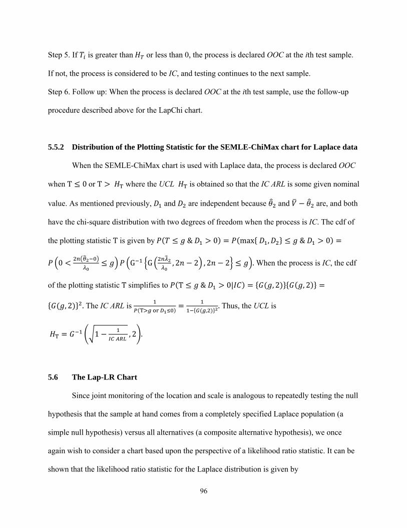
96

Step 5. If is greater than or less than 0, the process is declared OOC at the ith test sample.

If not, the process is considered to be IC, and testing continues to the next sample.

Step 6. Follow up: When the process is declared OOC at the ith test sample, use the follow-up

procedure described above for the LapChi chart.

5.5.2 Distribution of the Plotting Statistic for the SEMLE-ChiMax chart for Laplace data

When the SEMLE-ChiMax chart is used with Laplace data, the process is declared OOC

when Τ ≤ 0or Τ > where the UCL is obtained so that the IC ARL is some given nominal

value. As mentioned previously, and are independent because and − are, and both

have the chi-square distribution with two degrees of freedom when the process is IC. The cdf of

the plotting statistic Τ is given by ( ≤ & > 0) = (max{ , } ≤ & > 0) =0 < ≤ G G , 2 − 2 , 2 − 2 ≤ . When the process is IC, the cdf

of the plotting statistic Τ simplifies to (Τ ≤ & > 0| ) = { ( , 2)}{ ( , 2)} ={ ( , 2)} . The IC ARL is ( ) = { ( , )} . Thus, the UCL is

= 1 − , 2 .

5.6 The Lap-LR Chart

Since joint monitoring of the location and scale is analogous to repeatedly testing the null

hypothesis that the sample at hand comes from a completely specified Laplace population (a

simple null hypothesis) versus all alternatives (a composite alternative hypothesis), we once

again wish to consider a chart based upon the perspective of a likelihood ratio statistic. It can be

shown that the likelihood ratio statistic for the Laplace distribution is given by

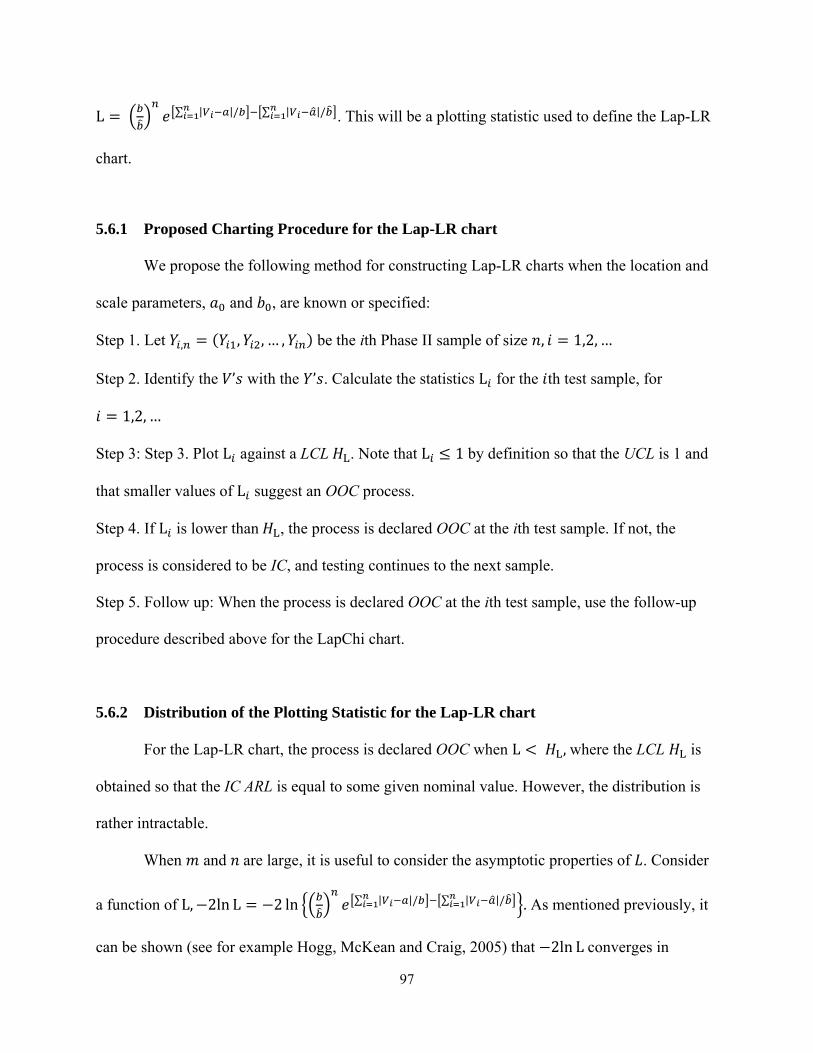
97

L = ∑ | |/ ∑ | |/ . This will be a plotting statistic used to define the Lap-LR

chart.

5.6.1 Proposed Charting Procedure for the Lap-LR chart

We propose the following method for constructing Lap-LR charts when the location and

scale parameters, and , are known or specified:

Step 1. Let , = ( , , … , ) be the ith Phase II sample of size , = 1,2,…

Step 2. Identify the ’ with the ’ . Calculate the statistics L for the th test sample, for = 1,2, …

Step 3: Step 3. Plot L against a LCL . Note that L ≤ 1 by definition so that the UCL is 1 and

that smaller values of L suggest an OOC process.

Step 4. If L is lower than , the process is declared OOC at the ith test sample. If not, the

process is considered to be IC, and testing continues to the next sample.

Step 5. Follow up: When the process is declared OOC at the ith test sample, use the follow-up

procedure described above for the LapChi chart.

5.6.2 Distribution of the Plotting Statistic for the Lap-LR chart

For the Lap-LR chart, the process is declared OOC when L < ,where the LCL is

obtained so that the IC ARL is equal to some given nominal value. However, the distribution is

rather intractable.

When and are large, it is useful to consider the asymptotic properties of . Consider

a function of L, −2ln L = −2 ln ∑ | |/ ∑ | |/ . As mentioned previously, it

can be shown (see for example Hogg, McKean and Craig, 2005) that −2ln Lconverges in

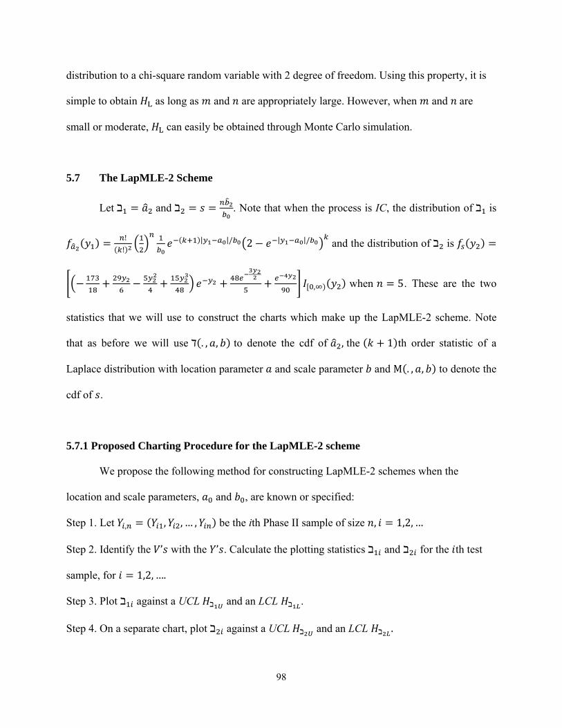
98

distribution to a chi-square random variable with 2 degree of freedom. Using this property, it is

simple to obtain as long as and are appropriately large. However, when and are

small or moderate, can easily be obtained through Monte Carlo simulation.

5.7 The LapMLE-2 Scheme

Let ℶ = and ℶ = = . Note that when the process is IC, the distribution of ℶ is

( ) = !( !) ( )| |/ 2 − | |/ and the distribution of ℶ is ( ) =− + − + + + [ , )( ) when = 5. These are the two

statistics that we will use to construct the charts which make up the LapMLE-2 scheme. Note

that as before we will use ℸ(. , , ) to denote the cdf of ,the ( + 1)th order statistic of a

Laplace distribution with location parameter and scale parameter and M(. , , ) to denote the

cdf of .

5.7.1 Proposed Charting Procedure for the LapMLE-2 scheme

We propose the following method for constructing LapMLE-2 schemes when the

location and scale parameters, and , are known or specified:

Step 1. Let , = ( , , … , ) be the ith Phase II sample of size , = 1,2,…

Step 2. Identify the ’ with the ’ . Calculate the plotting statistics ℶ and ℶ for the th test

sample, for = 1,2,…. Step 3. Plot ℶ against a UCL ℶ and an LCL ℶ .

Step 4. On a separate chart, plot ℶ against a UCL ℶ and an LCL ℶ .

99

Step 5. If ℶ is greater than ℶ or less than ℶ and/or ℶ is greater than ℶ or less than ℶ , the process is declared OOC at the ith test sample. If not, the process is considered to be

IC, and testing continues to the next sample.

Step 6. Follow up: When the process is declared OOC at the ith test sample, compare ℶ with ℶ and ℶ and ℶ with ℶ and LCL ℶ .

(i) If ℶ > ℶ and ℶ < ℶ < ℶ ,a shift in the location parameter is indicated.

(ii) If ℶ < ℶ and ℶ < ℶ < ℶ , a shift in the location parameter is indicated.

(iii) If ℶ > ℶ and ℶ < ℶ < ℶ , a shift in the scale parameter is indicated.

(iv) If ℶ < ℶ and ℶ < ℶ < ℶ , a shift in the scale parameter is indicated

(v) If ℶ > ℶ and ℶ > ℶ , a shift in both the location and scale parameters is

indicated.

(vi) If ℶ < ℶ and ℶ > ℶ , a shift in both the location and scale parameters is

indicated.

(vii) If ℶ > ℶ and ℶ < ℶ , a shift in both the location and scale parameters is

indicated.

(viii) If ℶ < ℶ and ℶ < ℶ , a shift in both the location and scale parameters is

indicated.

5.7.2 Distribution of the Plotting Statistics for the LapMLE-2 scheme

The LapMLE-2 control scheme consists of two charts. The process is declared OOC

whenever a signal occurs on either chart, that is, any time ℶ < ℶ , ℶ > ℶ ,ℶ < ℶ , or ℶ > ℶ ,where the control limits ℶ , ℶ , ℶ , and ℶ are obtained so that the IC ARL

100

is some given nominal value. ℶ and ℶ are independent and have the distributions specified

above. The joint cdf of the two plotting statistics ℶ and ℶ is given by [( < ℶ ≤ )&( ≤ ℶ ≤ )] = [ℸ( , , ) − ℸ( , , )] × M , , −M , , . When the process is IC, the joint cdf of the plotting statistics ℶ and ℶ simplifies to [( < ℶ ≤ )&( ≤ ℶ ≤ )| ] = [ℸ( , , ) − ℸ( , , )] ×[M( , , ) − M( , , )].

5.8 Implementation

In order to use the proposed charts, one must select the appropriate control limits for each

corresponding to the desired nominal IC ARL. This can be accomplished using the analytical

expressions for the IC ARL given in the earlier sections, though doing so is rather tedious.

Instead we use 100,000 simulations in R to calculate the control limits. As expected, we find that

higher nominal ARLs require higher UCLs and lower LCLs.

Table 5.1: Appropriate control limits for the Laplace charts when and are known and = , for various IC ARLs

IC ARL

LapMLE-Max Chart UCL

SEMLE-ChiMax Chart UCL

Lap-LR Chart LCL

Lap-Chi Chart UCL

LapMLE-2 Scheme (Location Chart UCL & LCL/ Scale Chart UCL/ Scale Chart LCL)17

125 2.88 11.04 .00263 23.85 ±2.83/15.26/0.36 250 3.09 12.43 .00113 25.81 ±2.72/14.92/0.39 500 3.29 13.82 .000475 27.72 ±2.58/14.45/0.43 750 3.40 14.63 .000285 28.82 ±2.35/13.54/0.52 1000 3.48 15.20 .000195 29.59 ±2.11/12.65/0.62 17 We selected the control limits for the LapMLE-2 Scheme so that both of the underlying charts have the same ARL.

101

5.9 Performance Comparisons

The performance of the three charts for various location and scale shifts is evaluated in a

simulation study so that they can easily be compared. Tables 5.2, 5.3, and 5.4 provide the ARL,

run length standard deviation, and specified quantiles of the run length distribution when = 5.

We use = 0 and = 1 for our IC Laplace distribution.

From the tables, it is seen that the Lap-LR chart performs best among the four charts

when there is a shift in only the location parameter. However, when there is a scale shift, it is

always outperformed by the LapChi chart and usually outperformed by one of the other charts as

well.

The SEMLE-ChiMax chart performs surprisingly well for this data. For most of the shifts

considered, its performance was second-best among the charts. However, this chart is not ideal,

since it is unable to detect decreases in the scale parameter.

102

Table 5.2: Run length characteristics for the SEMLE-ChiMax chart for Laplace data and the Lap-LR chart for various values of and when = , = ,and =

SEMLE-ChiMax Chart Lap-LR Chart

a2 b2 ARL SDRL 5%, 25%, 50%, 75%, 95% ARL SDRL 5%, 25%, 50%, 75%, 95% 0 1 502.44 507.55 25, 142, 348, 689, 1511 499.11 496.82 26, 146, 350, 691, 1471

0.1 1 490.58 478.23 26, 145, 345, 689, 1459 455.95 451.69 25, 138, 319, 634, 1341

0.25 1 452.25 451.87 24, 127, 317, 626, 1349 324.25 330.47 16, 89, 221, 449, 991

0.5 1 326.16 325.96 18, 93, 225, 449, 988 137.50 135.27 8, 41, 98, 191, 404

0.75 1 195.97 193.84 11, 57, 136, 272, 583 56.99 56.48 3, 17, 40, 78, 168

1 1 93.95 93.85 5, 26, 65, 132, 281 24.17 23.75 2, 7, 17, 33, 72

1.25 1 37.16 36.82 2, 11, 26, 51, 109 11.48 10.86 1, 4, 8, 16, 33

1.5 1 13.79 13.39 1, 4, 10, 19, 41 6.05 5.50 1, 2, 4, 8, 17

0 1.25 88.82 87.50 5, 26, 63, 125, 260 298.27 296.01 15, 87, 208, 416, 889

0.1 1.25 88.08 87.93 5, 26, 60, 123, 263 280.16 276.99 16, 82, 194, 391, 823

0.25 1.25 85.02 85.68 5, 24, 58, 116, 258 221.89 221.53 12, 65, 156, 308, 653

0.5 1.25 71.97 71.16 4, 21, 50, 100, 213 115.03 115.10 7, 34, 80 159 347

0.75 1.25 53.68 53.84 3, 15, 37, 74, 165 53.99 53.16 3, 16, 38, 74, 157

1 1.25 35.69 35.18 2, 11, 25, 49, 105 25.62 25.29 2, 8, 18, 36, 75

1.25 1.25 20.44 19.79 2, 6, 14, 28, 59 12.76 12.48 1, 4, 9, 17, 37

1.5 1.25 10.84 10.20 1, 3, 8, 15, 31 7.05 6.48 1, 2, 5, 10, 20

0 1. 5 28.19 27.80 2, 8, 20, 39, 83 99.63 98.50 6, 29, 69, 138, 297

0.1 1.5 27.93 27.40 2, 8, 20, 38, 82 96.69 95.56 6, 28, 67, 135, 285

0.25 1.5 27.35 26.92 2, 8, 19, 38, 81 86.15 87.54 5, 25, 59, 119, 260

0.5 1.5 24.72 24.05 2, 7, 17, 34, 73 58.22 58.10 3, 17, 40, 80, 177

0.75 1.5 20.68 20.45 1, 6, 14, 28, 62 34.66 34.46 2, 11, 24, 48, 103

1 1.5 16.39 16.13 1, 5, 11, 22, 49 20.11 19.58 2, 6, 14, 27, 60

1.25 1.5 11.67 11.16 1, 4, 8, 16, 34 11.45 10.91 1, 4, 8, 16, 33

1.5 1.5 7.69 7.19 1, 3, 5, 10, 22 6.87 6.44 1, 2, 5, 9, 20

0 1.75 12.77 12.18 1, 4, 9, 17, 37 37.73 37.55 2, 11, 26, 52, 112

0.1 1.75 12.44 11.72 1, 4, 9, 17, 36 37.18 35.90 2, 11, 26, 52, 110

0.25 1.75 12.28 11.87 1, 4, 9, 17, 36 35.42 35.08 2, 10, 24, 49, 106

0.5 1.75 11.63 11.15 1, 4, 8, 16, 34 27.77 27.37 2, 8, 19, 38, 83

0.75 1.75 10.91 10.35 1, 4, 8, 15, 31 19.94 19.34 1, 6, 14, 27, 58

1 1.75 9.01 8.54 1, 3, 6, 12, 26 13.69 13.17 1, 4, 10, 19, 40

1.25 1.75 7.16 6.54 1, 2, 5, 10, 20 8.95 8.44 1, 3, 6, 12, 26

1.5 1.75 5.41 4.93 1, 2, 4, 7, 15 6.02 5.54 1, 2, 4, 8, 17

0 2 7.23 6.71 1, 2, 5, 10, 21 18.13 17.70 1, 6, 13, 25, 53

0.1 2 7.25 6.72 1, 2, 5, 10, 21 17.72 17.21 1, 5, 12, 24, 52

0.25 2 7.14 6.56 1, 2, 5, 10, 20 17.18 16.76 1, 5, 12, 24, 50

0.5 2 6.91 6.43 1, 2, 5, 9, 20 14.96 14.45 1, 5, 10, 21, 44

0.75 2 6.40 5.79 1, 2, 5, 9, 18 11.72 11.20 1, 4, 8, 16, 34

1 2 5.69 5.18 1, 2, 4, 8, 16 9.04 8.55 1, 3, 6, 12, 26

1.25 2 4.96 4.39 1, 2, 4, 7, 14 6.66 6.14 1, 2, 5, 9, 19

1.5 2 4.01 3.46 1, 2, 3, 5, 11 4.92 4.37 1, 2, 4, 7, 14

103

Table 5.3: Run length characteristics for the LapMLE-Max and LapChi charts for various values of and when = , = ,and =

LapMLE-Max Chart LapChi Chart

a2 b2 ARL SDRL 5%, 25%, 50%, 75%, 95% ARL SDRL 5%, 25%, 50%, 75%, 95% 0 1 499.87 497.96 26, 143, 347, 694, 1495 502.11 507.23 26, 143, 345, 695, 1508

0.1 1 489.67 488.18 26, 142, 340, 680, 1465 491.78 487.77 26, 140, 338, 689, 1466

0.25 1 438.49 436.48 23, 128, 305, 607, 1307 448.78 449.14 23, 129, 310, 621, 1345

0.5 1 306.82 306.56 16, 89, 212, 425, 924 324.26 318.22 17, 95, 225, 453, 964

0.75 1 180.41 180.24 10, 52, 125, 249, 539 205.05 204.70 11, 59, 142, 284, 609

1 1 99.90 99.32 5, 29, 69, 139, 297 116.84 116.24 6, 34, 81, 162, 349

1.25 1 51.50 51.27 3, 15, 36, 71, 155 59.41 59.02 4, 17, 41, 83, 176

1.5 1 26.66 26.07 2, 8, 19, 37, 79 30.61 30.25 2, 9, 21, 42, 91

0 1.25 108.35 107.94 6, 31, 75, 150, 324 69.98 70.00 4, 21, 48, 97, 211

0.1 1.25 106.09 105.43 6, 31, 74, 146, 318 69.42 67.77 4, 20, 48, 97, 207

0.25 1.25 100.47 100.72 6, 29, 70, 139, 300 65.25 64.89 4, 19, 46, 90, 193

0.5 1.25 79.74 79.07 5, 23, 56, 111, 238 54.69 54.16 3, 16, 38, 75, 162

0.75 1.25 56.70 56.14 3, 17, 40, 79, 169 41.09 40.93 2, 12, 29, 57, 124

1 1.25 37.19 36.79 2, 11, 26, 51, 110 28.78 28.39 2, 8, 20, 40, 85

1.25 1.25 23.34 22.82 2, 7, 16, 32, 69 18.85 18.14 1, 6, 14, 26, 55

1.5 1.25 14.37 13.95 1, 4, 10, 20, 42 12.23 11.90 1, 4, 9, 17, 36

0 1. 5 33.26 32.67 2, 10, 23, 46, 98 21.19 20.92 2, 6, 15, 29, 62

0.1 1.5 33.04 32.81 2, 10, 23, 46, 98 20.81 20.52 2, 6, 14, 29, 61

0.25 1.5 32.09 31.56 2, 10, 22, 44, 95 20.26 19.79 2, 6, 14, 28, 59

0.5 1.5 28.13 27.70 2, 8, 20, 39, 83 17.92 16.86 1, 6, 13, 25, 51

0.75 1.5 22.91 22.47 2, 7, 16, 32, 68 14.77 14.10 1, 5, 11, 20, 43

1 1.5 17.41 16.84 1, 5, 12, 24, 51 11.85 11.29 1, 4, 8, 16, 34

1.25 1.5 12.76 12.25 1, 4, 9, 18, 37 9.04 8.63 1, 3, 6, 12, 26

1.5 1.5 8.95 8.43 1, 3, 6, 12, 26 6.60 6.12 1, 2, 5, 9, 19

0 1.75 14.56 14.05 1, 4, 10, 20, 43 9.59 9.12 1, 3, 7, 13, 28

0.1 1.75 14.43 13.97 1, 5, 10, 20, 42 9.50 8.98 1, 3, 7, 13, 28

0.25 1.75 14.14 13.54 1, 4, 10, 20, 41 9.29 8.80 1, 3, 7, 13, 27

0.5 1.75 13.11 12.54 1, 4, 9, 18, 38 8.56 7.96 1, 3, 6, 12, 25

0.75 1.75 11.52 11.00 1, 4, 8, 16, 34 7.58 7.05 1, 3, 5, 10, 22

1 1.75 9.70 9.20 1, 3, 7, 13, 28 6.47 5.91 1, 2, 5, 9, 19

1.25 1.75 7.83 7.30 1, 3, 6, 11, 22 5.31 4.83 1, 2, 4, 7, 15

1.5 1.75 6.14 5.63 1, 2, 4, 8, 17 4.27 3.75 1, 2, 3, 6, 12

0 2 8.09 7.58 1, 3, 6, 11, 23 5.55 5.01 1, 2, 4, 7, 16

0.1 2 8.06 7.52 1, 3, 6, 11, 23 5.52 4.99 1, 2, 4, 7, 15

0.25 2 7.89 7.33 1, 3, 6, 11, 23 5.42 4.94 1, 2, 4, 7, 15

0.5 2 7.51 6.98 1, 3, 5, 10, 22 5.20 4.71 1, 2, 4, 7, 15

0.75 2 6.92 6.40 1, 2, 5, 9, 20 4.65 4.07 1, 2, 3, 6, 13

1 2 6.13 5.62 1, 2, 4, 8, 17 4.16 3.55 1, 2, 3, 6, 11

1.25 2 5.31 4.78 1, 2, 4, 7, 15 3.66 3.10 1, 1, 3, 5, 10

1.5 2 4.45 3.91 1, 2, 3, 6, 12 3.18 2.59 1, 1, 2, 4, 8

104

Table 5.4: Run length characteristics for the LapMLE-2 scheme for various values of and when = , = ,and =

LapMLE-2 Scheme

a2 b2 ARL SDRL 5%, 25%, 50%, 75%, 95% 0 1 503.17 504.90 26, 145, 348, 697, 1509

0.1 1 490.78 489.29 26, 142, 341, 679, 1458

0.25 1 437.65 435.72 23, 126, 304, 607, 1312

0.5 1 302.64 303.01 16, 87, 210, 419, 904

0.75 1 178.53 177.32 10, 52, 124, 247, 534

1 1 97.29 96.59 6, 28, 68, 134, 291

1.25 1 50.80 50.14 3, 15, 35, 70, 152

1.5 1 26.13 25.71 2, 8, 18, 36, 77

0 1.25 107.83 107.28 6, 31, 75, 149, 321

0.1 1.25 107.28 107.24 6, 31, 74, 148, 322

0.25 1.25 99.81 98.77 6, 29, 69, 139, 298

0.5 1.25 79.43 79.03 5, 23, 55, 110, 238

0.75 1.25 55.93 55.43 3, 17, 39, 77, 166

1 1.25 36.69 36.25 2, 11, 26, 51, 109

1.25 1.25 22.98 22.44 2, 7, 16, 32, 68

1.5 1.25 14.08 13.59 1, 4, 10, 19, 41

0 1. 5 33.30 32.76 2, 10, 23, 46, 99

0.1 1.5 33.19 32.89 2, 10, 23, 46, 99

0.25 1.5 31.90 31.45 2, 9, 22, 44, 95

0.5 1.5 27.97 27.39 2, 8, 20, 39, 83

0.75 1.5 22.80 22.30 2, 7, 16, 32, 67

1 1.5 17.35 16.82 1, 5, 12, 24, 51

1.25 1.5 12.57 12.04 1, 4, 9, 17, 37

1.5 1.5 8.89 8.39 1, 3, 6, 12, 26

0 1.75 14.70 14.21 1, 5, 10, 20, 43

0.1 1.75 14.57 14.03 1, 5, 10, 20, 43

0.25 1.75 14.20 13.68 1, 4, 10, 19, 42

0.5 1.75 13.05 12.57 1, 4, 9, 18, 38

0.75 1.75 11.44 10.96 1, 4, 8, 16, 33

1 1.75 9.66 9.10 1, 3, 7, 13, 28

1.25 1.75 7.80 7.30 1, 3, 6, 11, 22

1.5 1.75 6.05 5.49 1, 2, 4, 8, 17

0 2 8.06 7.55 1, 3, 6, 11, 23

0.1 2 8.01 7.54 1, 3, 6, 11, 23

0.25 2 7.93 7.40 1, 3, 6, 11, 23

0.5 2 7.50 7.00 1, 3, 5, 10, 21

0.75 2 6.90 6.36 1, 2, 5, 9, 20

1 2 6.09 5.59 1, 2, 4, 8, 17

1.25 2 5.28 4.78 1, 2, 4, 7, 15

1.5 2 4.43 3.89 1, 2, 3, 6, 12

The LapMLE-Max chart performs fairly poorly in comparison to the other charts, nearly

always performing worse than the SEMLE-ChiMax and LapChi charts. Its best performance is

105

seen where there is a small shift in location and no scale shift; however, the Lap-LR chart

outperforms it in this case. The LapMLE-2 scheme performs analogously to the LapMLE-Max

chart, because the two charts are equivalent.

The LapChi chart has the best performance among the charts studied, except when there

is a location shift but no scale shift. As a result, this is the best joint monitoring scheme to use

with processes that follow a Laplace distribution, unless it is expected that the most commonly

occurring assignable causes will produce shifts only in the location.

5.10 Performance Comparisons versus Normal Theory Charts

It is again of interest to determine whether the proposed charts perform better for process

data from a Laplace distribution than would normal theory charts. Here, we consider the

performance of two normal theory charts for various location and scale shifts and sample sizes.

The UCLs for the normal theory charts must be selected so that they have a specified nominal IC

ARL. For = 5, the appropriate UCL for the normal theory max chart is 3.29. Table 5.5 provides

the ARL, run length standard deviation, and specified quantiles of the run length distribution.

Note that the underlying distribution of the process data is Laplace. We again use = 0 and = 1 for our IC Laplace distribution. The mean of the distribution is , and its variance is 2

(Johnson and Kotz, 1970). In other words, the mean of our IC distribution is 0, its variance is 2,

and these are values to which the normal theory max and distance charts will compare the sample

means and variances.

106

Table 5.5: Run length characteristics for normal theory charts applied to Laplace data for various values of and when = , = ,and =

Normal Theory Max Chart Normal Theory Distance Chart

a2 b2 ARL SDRL 5%, 25%, 50%, 75%, 95% ARL SDRL 5%, 25%, 50%, 75%, 95% 0 1 66.97 66.72 4, 20, 46, 93, 201 39.13 38.66 2, 12, 27, 54, 116

0.1 1 66.41 65.93 4, 19, 46, 92, 199 38.65 38.16 2, 12, 27, 53, 115

0.25 1 62.22 61.72 4, 18, 43, 86, 186 36.00 35.41 2, 11, 25, 50, 106

0.5 1 48.65 48.42 3, 14, 34, 67, 145 27.92 27.54 2, 8, 19, 38, 83

0.75 1 32.04 31.47 2, 10, 22, 44, 95 18.67 18.09 1, 6, 13, 26, 55

1 1 18.42 17.79 1, 6, 13, 25, 54 11.30 10.80 1, 4, 8, 15, 33

1.25 1 10.19 9.73 1, 3, 7, 14, 30 6.45 5.94 1, 2, 5, 9, 18

1.5 1 5.70 5.18 1, 2, 4, 8, 16 3.86 3.34 1, 1, 3, 5, 11

0 1.25 19.46 18.82 1, 6, 14, 27, 57 12.68 12.21 1, 4, 9, 17, 37

0.1 1.25 19.25 18.62 1, 6, 14, 27, 56 12.56 12.12 1, 4, 9, 17, 37

0.25 1.25 18.51 17.98 1, 6, 13, 25, 54 12.06 11.59 1, 4, 8, 17, 35

0.5 1.25 15.78 15.25 1, 5, 11, 22, 46 10.39 9.92 1, 3, 7, 14, 30

0.75 1.25 12.28 11.74 1, 4, 9, 17, 36 8.21 7.71 1, 3, 6, 11, 24

1 1.25 8.79 8.26 1, 3, 6, 12, 25 6.11 5.54 1, 2, 4, 8, 17

1.25 1.25 5.99 5.46 1, 2, 4, 8, 17 4.36 3.82 1, 2, 3, 6, 12

1.5 1.25 4.08 3.55 1, 2, 3, 5, 11 3.10 2.55 1, 1, 2, 4, 8

0 1. 5 8.43 7.91 1, 3, 6, 11, 24 6.07 5.56 1, 2, 4, 8, 17

0.1 1.5 8.37 7.88 1, 3, 6, 11, 24 6.05 5.52 1, 2, 4, 8, 17

0.25 1.5 8.18 7.66 1, 3, 6, 11, 23 5.87 5.33 1, 2, 4, 8, 17

0.5 1.5 7.42 6.88 1, 2, 5, 10, 21 5.38 4.86 1, 2, 4, 7, 15

0.75 1.5 6.36 5.84 1, 2, 5, 9, 18 4.67 4.16 1, 2, 3, 6, 13

1 1.5 5.15 4.65 1, 2, 4, 7, 14 3.86 3.32 1, 1, 3, 5, 10

1.25 1.5 4.03 3.51 1, 2, 3, 5, 11 3.11 2.57 1, 1, 2, 4, 8

1.5 1.5 3.11 2.57 1, 1, 2, 4, 8 2.48 1.92 1, 1, 2, 3, 6

0 1.75 4.84 4.31 1, 2, 3, 6, 13 3.74 3.22 1, 1, 3, 5, 10

0.1 1.75 4.83 4.31 1, 2, 3, 6, 13 3.71 3.17 1, 1, 3, 5, 10

0.25 1.75 4.72 4.20 1, 2, 3, 6, 13 3.65 3.11 1, 1, 3, 5, 10

0.5 1.75 4.44 3.92 1, 2, 3, 6, 12 3.44 2.89 1, 1, 3, 5, 9

0.75 1.75 4.03 3.49 1, 2, 3, 5, 11 3.13 2.59 1, 1, 2, 4, 8

1 1.75 3.50 2.95 1, 1, 3, 5, 9 2.78 2.22 1, 1, 2, 4, 7

1.25 1.75 2.99 2.44 1, 1, 2, 4, 8 2.40 1.83 1, 1, 2, 3, 6

1.5 1.75 2.50 1.93 1, 1, 2, 3, 6 2.06 1.48 1, 1, 2, 3, 5

0 2 3.28 2.72 1, 1, 2, 4, 9 2.66 2.11 1, 1, 2, 3, 7

0.1 2 3.27 2.73 1, 1, 2, 4, 9 2.65 2.09 1, 1, 2, 3, 7

0.25 2 3.23 2.70 1, 1, 2, 4, 9 2.64 2.07 1, 1, 2, 3, 7

0.5 2 3.11 2.57 1, 1, 2 , 4, 8 2.54 1.98 1, 1, 2, 3, 6

0.75 2 2.88 2.32 1, 1, 2, 4, 8 2.37 1.80 1, 1, 2, 3, 6

1 2 2.64 2.07 1, 1, 2, 3, 7 2.19 1.61 1, 1, 2, 3, 5

1.25 2 2.38 1.81 1, 1, 2, 3, 6 1.98 1.39 1, 1, 1, 2, 5

1.5 2 2.10 1.51 1, 1, 2, 3, 5 1.79 1.18 1, 1, 1, 2, 4

107

The results here are similar to those found for in the previous chapter. At first glance, one

might note that Chen and Cheng’s (1998) normal theory max chart and Ramzy’s (2005) distance

chart have shorter ARLs than the Laplace charts explored above and conclude that they are

preferable. However, the IC ARLs for the normal theory charts are far lower than the nominal

value of 500, indicating that the normal theory charts will have an unacceptably high number of

false alarms and rendering them virtually useless for monitoring this type of process.

5.11 Summary and Conclusions

Monitoring the location and scale parameters of a Laplace distribution is an important

problem in statistical process control. It is necessary, for example, for processes which arise as

the difference between two exponential distributions with a common scale. This chapter provides

some possibilities for monitoring data from a known Laplace distribution, among which the

LapChi chart appears to be the most promising. However, much more work in this area is

needed. In particular, these charts are only suitable for sample sizes larger than 1, since they rely

on statistics which are functions of order statistics. Additionally, these charts are suitable only for

case K, and their performance will be degraded significantly if the parameters are estimated from

a Phase I sample. Finally, the adaptation of these charts for case U is not straightforward.

108

CHAPTER 6

CONCLUSIONS AND FUTURE RESEARCH

6.1 Summary

Two-parameter distributions constitute important problems for process monitoring. In

general, it is desirable to utilize control schemes capable of identifying shifts in either or both of

the parameters. This dissertation examined control schemes for jointly monitoring the two

parameters of a shifted exponential or Laplace distribution with known IC parameters, as well as

those for a normal distribution with unknown IC parameters. For the shifted exponential and

Laplace distributions, a variety of new one- and two-chart schemes were introduced, studied, and

compared. For the normal distribution, a pair of charts designed for the known parameter case

were adapted to account for the additional variability introduced by parameter estimation.

In Chapter 3, Chen and Cheng’s (1998) Max chart and Razmy’s (2005) Distance chart

were modified for monitoring normally distributed processes with unknown means and

variances. The modified charts were shown to perform similarly, with the Modified Distance

chart being slightly superior in most cases. Additionally, both charts were shown to have good

performance for normally distributed data but far poorer performance for data from other

distributions, whether they are skewed or symmetric.

In Chapter 4, we introduced and compared five schemes for jointly monitoring the

location and scale parameters of a shifted exponential distribution with known parameters: the

SEMLE-Max, SEMVUE-Max, SEMLE-ChiMax, and SE-LR charts, and the two-chart SEMLE-

109

2 scheme. The two max-type charts were shown to be ARL-biased for small mean shifts

unaccompanied by variance shifts. The SEMLE-2 scheme was shown to have the best overall

performance, followed closely by the SEMLE-ChiMax chart.

In Chapter 5, we introduced and compared the LapMLE-Max, LapChi, and Lap-LR

charts and the two-chart LapMLE-2 scheme. We also considered transforming the data so that it

could be monitored using the SEMLE-ChiMax chart introduced in the previous chapter.

Overall, the LapChi chart was shown to be the best joint monitoring scheme to use with

processes that follow a Laplace distribution, unless the most commonly occurring assignable

causes are expected to produce shifts only in the location parameter. The Lap-LR chart was

shown to perform best among the four charts when there is a shift in only the location parameter.

6.2 Future Research

In chapter 3, we considered the unconditional and conditional IC ARL of the normal

theory charts when parameter estimates were used for the mean and standard deviation. The

“unconditional” IC ARL was obtained by averaging over the distributions of the mean and the

standard deviation, while the “conditional” IC ARLs were obtained by considering particular

values of the estimators. It was seen that the conditional IC ARLs vary widely depending on

whether low, medium, or high estimates of each parameter are used, and in most cases, the

conditional IC ARLs deviate substantially from the nominal IC ARL. However, in practice, one

would have no way of determining whether the parameter estimates being utilized were low or

high since the true parameters are unknown. Therefore, it is desirable to create monitoring

procedures which are less dependent on the quality of the parameter estimates. More research is

needed to create charts for which both the unconditional IC ARL and the conditional IC ARLs

110

resulting from particular parameter estimates are correctly maintained at a specified nominal

value.

For the Laplace and shifted exponential distributions, only charts for monitoring known

parameters are presented. Modifications are needed to produce one- and two-chart schemes

suitable for monitoring unknown parameters. Doing so is not particularly straightforward, and

much more work is needed to produce the charts.

Each of the charts presented in this dissertation is suitable for data from a particular

parametric distribution: the normal, the Laplace, or the shifted exponential. However, in practice,

it is not uncommon for a practitioner to be unsure of his data’s underlying distribution. For this

reason, it is imperative that more work be done in the area of nonparametric joint monitoring of

location and scale parameters.

Finally, all of the charts considered in this dissertation are univariate. In practice, many

monitoring problems are multivariate in nature, so these charts should be adapted for use with

multivariate data.

111

REFERENCES

Acosta-Meija, C.A. (1998). “Monitoring Reduction in Variability with the Range,” IIE Transactions, 30(6), 515-513.

Ahmadi, J. & MirMostafaee, S.M.T.K. (2009). “Prediction Intervals for Future Records and Order Statistics Coming From Two Parameter Exponential Distribution,” Statistics and Probability Letters, 79(7), 977-983.

Ahsanullah, M. (1980). “Linear Prediction of Record Values for the Two Parameter Exponential Distribution,” Annals of the Institute of Statistical Mathematics, 32(1), 363-368.

Basu, A.P. (1971). “On a Sequential Rule for Estimating the Location Parameter of an Exponential Distribution,” Naval Research Logistics Quarterly, 18(3), 329-337.

Bain, L.J. & Engelhardt, M. (1973). “Interval Estimation for the Two-Parameter Double Exponential Distribution,” Technometrics, 15(4), 875-887.

Baklizi, A. (2008). “Estimation of Pr(X < Y) Using Record Values in the One and Two Parameter Exponential Distributions,” Communications in Statistics - Theory and Methods, 37(5), 692-698.

Balakrishnan, N. & Sandhu, R.A. (1996). “Best Linear Unbiased and Maximum Likelihood Estimation for Exponential Distributions under General Progressive Type-II Censored Samples,” Sankhyā: The Indian Journal of Statistics, Series B (1960-2002), 58(1), 1-9.

Beg, M.A. (1980). “On the Estimation of Pr{Y<X} for the Two-Parameter Exponential Distribution,” Metrika, 27(1), 29-34.

Chakraborti, S., Human, S. W., & Graham, M. A. (2011). “Nonparametric (Distribution-free) Control Charts,” Chapter 26 in Methods and Applications of Statistics in Engineering, Quality and the Physical Sciences, N. Balakrishnan ed., John Wiley, New York.

Chakraborti, S., Human, S.W., & Graham, M.A. (2009). “Phase I Statistical Process Control Charts: An Overview and Some Results,” Quality Engineering, 21(1), 52-62.

Chao, M.T. & Cheng, S.W. (1996). “Semicircle Control Chart for Variables Data,” Quality Engineering, 8(3), 441-446.

112

Chao, M.T. & Cheng, S.W. (2008). “On 2-D Control Charts,” Quality Technology & Quantitative Management, 5(3), 243-261.

Chen, G. & Cheng S.W. (1998). “Max Chart: Combining X-bar Chart and S Chart,” Statistica Sinica, 8(1998), 263-271.

Chen, G., Cheng, S.W., & Xie H. (2001). “Monitoring Process Mean and Variability with One EWMA Chart,” Journal of Quality Technology, 33(2), 223-233.

Chen, G. Cheng, S.W., & Xie H. (2004). “A New EWMA Control Chart for Monitoring Both Location and Dispersion,” Quality Technology & Quantitative Management, 1(2), 217-231.

Cheng, S.W. & Thaga, K. (2006). “Single Variables Control Charts: An Overview,” Quality and Reliability Engineering International, 22(7), 811-820.

Chengalur, I.N., Arnold, J.C., & Reynolds, M.R., Jr. (1989). Variable Sampling Intervals for Multiparameter Shewhart Charts, Communications in Statistics - Theory and Methods, 18(5), 1769-1792.

Cohen, A.C., & Helm, F.R. (1973). “Estimators in the Exponential Distribution,” Technometrics, 15(2), 415-418.

Costa, A.B.F. & De Magalhães, M.S. (2007), “An Adaptive Chart for Monitoring the Process Mean and Variance,” Quality and Reliability Engineering International, 23, 821-831.

Costa, A.B.F. & Rahim, M.A. (2004). “Monitoring Process Mean and Variability with One Non-central Chisquare Chart.” Journal of Applied Statistics, 31(10), 1171-1183.

Costa, A.B.F. & Rahim, M.A. (2006). “A Single EWMA Chart for Monitoring Process Mean and Process Variance,” Quality Technology & Quantitative Management, 3(3), 295-305.

Domangue, R. & Patch, S.C. (1991) Some Omnibus Exponentially Weighted Moving Average Statistical Process Monitoring Schemes, Technometrics, 33(3), 299-313.

Epstein, B. (1960). “Estimation of the Parameters of Two Parameter Exponential Distributions from Censored Samples,” Technometrics, 2(3), 403-406.

Gan, F.F. (1995). “Joint Monitoring of Process Mean and Variance using Exponentially Weighted Moving Average Control Charts,” Technometrics, 37(4), 446-453.

Gan, F.F. (1997). “Joint Monitoring of Process Mean and Variance,” Nonlinear Analysis, Proceedings of the 2nd World Congress of Nonlinear Analysis, USA. 30, 4017-4024.

Gan, F.F., Ting, K.W., & Chang, T.C. (2004). “Interval Charting Schemes for Joint Monitoring of Process Mean and Variance,” Quality and Reliability Engineering International, 20(4), 291-303.

113

Govindarajulu, Z. (1966). “Characterization of the Exponential and Power Distributions,” Scandinavian Actuarial Journal, 1966(3-4), 132-136.

Hawkins, D.M. (1987). “Self-starting CUSUM charts for Location and Scale,” The Statistician, 36(4), 299-315.

Hawkins, D.M. & Deng, Q. (2009). “Combined Charts for Mean and Variance Information,” Journal of Quality Technology, 41(4), 415-425.

Hawkins, D. M. & Zamba, K.D. (2005). “Statistical Process Control for Shifts in Mean or Variance Using a Changepoint Formulation,” Technometrics, 47, 164-173.

Hogg, R.V., McKean, J.W., and Craig, A.T. (2005). Introduction to Mathematical Statistics, 6th Edition. Englewood Cliffs, NJ: Prentice Hall.

Huang, C.C. & Chen F.L. (2010). “Economic Design of Max Charts,” Communications in Statistics - Theory and Methods, 39(16), 2961-2976.

Jensen, W., Jones-Farmer, L.A., Champ, C.W., & Woodall, W.H. (2006). “Effects of Parameter Estimation on Control Chart Properties,” Journal of Quality Technology, 38(4), 349-364.

Johnson, N.L., & Kotz, S. (1970). Distributions in Statistics, Volume 1: Continuous Univariate Distributions, Boston: Houghton Mifflin.

Johnson, N.L., Kotz, S., & Balakrishnan, N. (1994). Distributions in Statistics, Volume 1: Continuous Univariate Distributions, 2nd Edition. Boston: Houghton Mifflin.

Kao, S.C. (2010). “Normalization of the Origin-shifted Exponential Distribution for Control Chart Construction,” Journal of Applied Statistics, 37(7), 1067-1087.

Karst, O.J. & Polowy, H. (1963). “Sampling Properties of the Median of a Laplace Distribution,” The American Mathematical Monthly, 70(6), 628-636.

Kececioglu, D. & Li, D. (1985). “Optimum Two-Sided Confidence Interval for the Location Parameter of the Exponential Distribution,” Relibility Engineering, 13(1), 1-10.

Khoo, M. B. C. (2004). “A New Bivariate Control Chart to Monitor the Multivariate Process Mean and Variance Simultaneously,” Quality Engineering, 17(1), 109-118.

Khoo, M.B.C., Wu, Z., Chen, C.-H., & Yeong, K.W. (2010a). “Using One EWMA Chart to Jointly Monitor the Process Mean and Variance,” Computational Statistics, 25(2), 299–316.

114

Khoo, M.B.C., Teh, S.Y., & Wu, Y. (2010b). “Monitoring Process Mean and Variability with One Double EWMA Chart,” Communications in Statistics - Theory and Methods, 39(20), 3678 -3694.

Kotz, S., Kozubowski, T.J., & Podgórski, K. (2001). The Laplace Distribution and Generalizations: A Revisit with Applications to Communications, Economics, Engineering, and Finance. Boston: Birkhauser.

Lam, K., Sinha, B.K., & Wu, Z. (1994). “Estimation of Parameters in a Two-Parameter Exponential Distribution Using Ranked Set Sample,” Annals of the Institute of Statistical Mathematics, 46(4), 723-736.

Li, Z., Zhang, J., & Wang, Z. (2010). “Self-starting Control Chart for Simultaneously Monitoring Process Mean and Variance,” International Journal of Production Research, 48(15), 4537-4553.

Lu, C.-W. & Reynolds, M.R., Jr (1999). “Control Charts for Monitoring the Mean and Variance of Autocorrelated Processes,” Journal of Quality Technology, 31(3), 259-274.

Maboudou-Tchao, E. & Hawkins, D. (2011). “Self-Starting Multivariate Control Charts for

Location and Scale,” Journal of Quality Technology, 43(2), 113-126.

Mahmoud, M.A., Henderson, G.R., Epprecht, E.K., & Woodall, W.H. (2010). “Estimating the Standard Deviation in Quality Control Applications,” Journal of Quality Technology, 42(4), 348-357.

Memar, A.O.M. & Niaki, S.T.A. (2011). “The Max EWMAMS Control Chart for Joint

Monitoring of Process Mean and Variance with Individual Observations,” Quality and Reliability Engineering International, 27(4), 499-514.

Mukherjee, A. & Chakraborti, S. (2012). “A Distribution-Free Control Chart for Joint

Monitoring of Location and Scale,” Quality and Reliability Engineering International, 28(3), 335-352.

Puig, P. & Stephens, M.A. (2000). “Tests of Fit for the Laplace Distribution, with Applications,” Technometrics, 42(4), 417-424.

Quesenberry, C.P. (1991). “SPC Q Charts for Start-Up Processes and Short or Long Runs,” Journal of Quality Technology, 23(3), 213-224.

Rahim, M.A. & Costa, A.B.F. (2000). “Joint Economic Design of Xbar and R Charts under Weibull Shock Models,” International Journal of Production Research, 38(13), 2871–2889.

115

Ramalhoto, M.F. & Morais, M. (1999). “Shewhart Control Charts for the Scale Parameter of a Weibull Control Variable with Fixed and Variable Sampling Intervals,” Journal of Applied Statistics, 26(1), 129-160.

Razmy, A. M. (2005), “Schemes for Joint Monitoring of Process Mean and Process Variance,”

Masters Thesis, Department of Statistics and Applied Probability, NUS. Singapore. Reynolds, M.R., Jr. & Cho, G. Y. (2006). “Multivariate Control Charts for Monitoring the Mean

Vector and Covariance Matrix,” Journal of Quality Technology, 38(3), 230-253. Reynolds, M.R., Jr. & Cho, G.Y. (2011). “Multivariate Monitoring of the Process Mean and

Variability With Variable Sampling Intervals,” Sequential Analysis, 30(1), 1-40.

Reynolds, M.R., Jr. & Kim, K. (2007). “Multivariate Control Charts for Monitoring the Process

Mean and Variability Using Sequential Sampling,” Sequential Analysis, 26(3), 283-315. Reynolds, M.R., Jr. & Stoumbos, Z.G. (2001a). “Individuals Control Schemes for Monitoring

the Mean and Variance of Processes Subject to Drifts,” Stochastic Analysis and Applications, 19(5), 863-892.

Reynolds, M.R., Jr. & Stoumbos, Z.G. (2001b). “Monitoring the Process Mean and Variance

Using Individual Observations and Variable Sampling Intervals,” Journal of Quality Technology, 33(2), 181-205.

Reynolds, M.R., Jr. & Stoumbos, Z.G. (2004). “Control Charts and the Optimal Allocation of

Sampling Resources,” Technometrics, 46(2), 200-214. Reynolds, M.R., Jr. & Stoumbos, Z.G. (2005). “Should Exponentially Weighted Moving

Average and Cumulative Sum Charts be used with Shewhart Limits?” Technometrics, 47(4), 409-424.

Reynolds, M.R., Jr. & Stoumbos, Z.G. (2006). “Comparisons of Some Exponentially Weighted

Moving Average Control Charts for Monitoring the Process Mean and Variance,” Technometrics, 48(4), 550-567.

Reynolds, M.R., Jr. & Stoumbos, Z.G. (2008). “Combinations of Multivariate Shewhart and

MEMWA Control Charts for Monitoring the Mean Vector and Covariance Matrix,” Journal of Quality Technology, 40(4), 381-393.

Reynolds, M.R., Jr. & Stoumbos, Z.G. (2010). “Robustness to Non-Normality of CUSUM

Control Charts for Monitoring the Process Mean and Variance,” Quality and Reliability Engineering International, 26(5), 453-473.

Serel, D. & Moskowitz, H. (2008). “Joint Economic Design of EWMA Control Charts for Mean

and Variance,” European Journal of Operational Research, 184(1), 157-168.

116

Stoumbos, Z.G. & Reynolds, M.R., Jr. (2005). “Economic Statistical Design of Adaptive Control Schemes for Monitoring the Process Mean and Variance: An Application to Analyzers,” Nonlinear Analysis: Real World Applications, 6(5), 817-844.

Sürücü, B. & Sazak, H. S. (2009). “Monitoring Reliability for a Three-Parameter Weibull

Distribution,” Reliability Engineering and System Safety, 94(2), 503-508. Takahashi, T. (1989). “Simultaneous Control Charts Based on ( ̅, ) and ( ̅ , ) for Multiple

Decision on Process Change,” Reports of Statistical Application Research, Union of Japanese Scientists and Engineers, 36(2), 1-20.

Tanis, E.A. (1964). “Linear Forms in the Order Statistics from an Exponential Distribution,” The

Annals of Mathematical Statistics, 35(1), 270-276. Thiagarajah, K. & Paul, S.R. (1997). “Interval Estimation for the Scale Parameterof the Two-

Parameter Exponential Dsitribution Based on Time-Censored Data,” Journal of Statistical Planning and Inference, 59(2), 279-289.

Varde, S.D. (1969). “Life Testing and Reliability Estimation for the Two Parameter Exponential

Distribution,” Journal of the American Statistical Association, 64(326), 621-631. Viveros, R., & Balakrishnan, N. (1994). “Interval Estimation of Parameters of Life from

Progressively Censored Data,” Technometrics, 36(1), 84-91. Wright, F.T., Engelhardt, M., & Bain, L.J. (1978). “Inferences for the Two-Parameter

Exponential Distribution Under Type I Censored Sampling,” Journal of the American Statistical Association, 73(363), 650-655.

Wu, Z. & Tian, Y. (2005). “Weighted-loss-function CUSUM Chart for Monitoring Mean and

Variance of a Production Process,” International Journal of Production Research, 43(14), 3027-3044.

Wu, Z. & Wang, Q. (2007). “A Single CUSUM Chart Using a Single Observation to Monitor a

Variable,” International Journal of Production Research, 45(3), 719-741. Wu, Z., Zhang, S., & Wang , P. (2007). “A CUSUM Scheme with Variable Sample Sizes and

Sampling Intervals for Monitoring the Process Mean and Variance,” Quality and Reliability Engineering International, 23(2), 157-170.

Yeh, A.B., Lin, D.K.J., & Venkataramani, C. (2004). “Unified CUSUM Charts for Monitoring Process Mean and Variability,” Quality Technology & Quantitative Management, 1(1), 65-86.

Zhang J., Li Z., & Wang Z. (2010). “A Multivariate Control Chart for Simultaneously Monitoring Process Mean and Variability,” Computational Statistics & Data Analysis, 54(10), 2244-2252.

117

Zhang, J., Zou, C., & Wang, Z. (2010). “A Control Chart Based on Likelihood Ratio Test for Monitoring Process Mean and Variability,” Quality and Reliability Engineering International, 26(1), 63-73.

Zhang, J., Zou, C., & Wang, Z. (2011). “A New Chart for Detecting the Process Mean and Variability,” Communications in Statistics - Simulation and Computation, 40(5), 728 -743.

Zhou, Q., Luo, Y., & Wang, Z. (2010). “A Control Chart Based on Likelihood Ratio Test for

Detecting Patterned Mean and Variance Shifts,” Computational Statistics & Data Analysis, 54(6), 1634-1645.

Zou, C. & Tsung, F. (2010). “Likelihood Ratio-based Distribution-free EWMA Control Charts,”

Journal of Quality Technology, 42(2), 174-196.

118

APPENDIX

A: SUPPLEMENTARY DERIVATIONS FOR CHAPTER 3

A.1 Distribution of ∗ and ∗

Recall that ∗ = Φ {ζ (W )} and ∗ = Φ { , (W )} , where =( )and = . First, consider the joint cdf of ∗ and ∗:

∗, ∗( , ) = [ ∗ ≤ , ∗ ≤ ] = ≤ Φ(√ , − 1) , ≤ , Φ(√ , − 1, − 1) = [ ≤ , ≤ ], where = {Φ(√ )}, = , {Φ(√ )}. Note that since and are not independent, the calculation of the joint probability is not straightforward.

However, this can be conveniently obtained by conditioning on and or, equivalently, on = √ ( ), = ( )

. To this end, first, conditionally on and we can write

∗, ∗( , | , ) = ≤ + + ∆, ≤ ( )( )

where = √ ( ), = ( )

, = and∆= √ ( ).

Now since and , have a standard normal and a chi-square distribution with ( − 1) degrees of freedom, respectively, and are mutually independent, we have,

∗, ∗( , | , ) = Φ + + ∆ ( ) ( )( ) (*)

119

Finally, the unconditional cdf of ∗ and ∗ can be obtained by calculating the

expectation of the conditional cdf in (*) over the distributions of and , which are mutually

independent and follow the standard normal distribution and the chi-square distribution with ( − 1) degrees of freedom, respectively. Thus the unconditional joint cdf of ∗ and ∗ is

given by: ∗, ∗( , )

= Φ + + ∆ ( ) ( )( ) ( ) ( )( ) .

RESULT 1.1

Note that in the IC case, ∆= 0 and = 1, so that from (*) and Result 1.1 it is clear that neither

the conditional nor the unconditional joint cdf depends on any nuisance parameters; in other

words, the IC joint distributions do not depend on any unknown parameters. This result implies

that the IC run length distributions of all control charts based on ∗and ∗ are free from any

nuisance parameters. Hence, for example, the false alarm rates and all IC run length distribution

characteristics, such as the standard deviation and the percentiles, are all free from any unknown

parameters.

A.2 Distribution of

The cdf of the Max chart plotting statisticΨ can be obtained directly from the above

results. For example, for the unconditional cdf, using Result 1.1, we get for any > 0, Ψ ≤ = (max{| ∗|, | ∗|} ≤ ) = (ℎ ≤ ∗ ≤ , ≤ ∗ ≤ ) where ℎ = {Φ(− )}, = {Φ( )} = , {Φ(− )}and = , {Φ( )}.

120

This probability can then be easily found by first noting that (ℎ ≤ ∗ ≤ , ≤ ∗ ≤) = ( , ) − (ℎ, ) − ( , ) + (ℎ, ) where (. , . )denotes the cdf of ∗and ∗ given

in Result 1.1. Alternatively, a direct calculation can be used to show that the unconditional cdf is

given by Ψ ≤

= Φ + + ∆ −Φ − ℎ + + ∆

× ( ) ( − 1)( − 1) − ( ) ( − 1)( − 1) ( ) ( )( ) . RESULT 1.2

A.3 Distribution of ∆

Next consider the distribution of Δ. This can also be obtained in a similar manner using

the joint cdf of ∗and ∗. For example, for the unconditional cdf, for some > 0, Δ ≤ = ( ∗ + ∗ ≤ ) = ∗, ∗( , )

where ∗, ∗( , ) is the unconditional joint pdf of ( ∗, ∗)which can be obtained by

differentiating the unconditional joint cdf ∗, ∗( , ) given in Result 1.1.

Alternatively, we can write Δ ≤ = ( ∗ + ∗ ≤ | , ) .

Now since ( ∗ + ∗ ≤ | , ) = ∗, ∗( , | , ) ,an

equivalent expression for the unconditional cdf can be then obtained in terms of the conditional

joint pdf of ∗and ∗

121

Δ ≤ = ∗, ∗( , | , ) ( ) ( )( )

RESULT 1.3

A.4 The ( / ) scheme

Consider a two-chart control scheme consisting of an chart and an chart, in which a

signal on either chart is taken as an indication that the process is OOC.

The and charts recommended by Montgomery (2005) are based on 3-sigma control

limits, rather than probability limits. Because and have different statistical distributions, the

standards known and charts with 3-sigma control limits have different IC ARLs. The chart

has an IC ARL of 370.40 regardless of the sample size , while the IC ARL of the chart

depends on . For Montgomery’s chart, the IC ARL is ( ) = ( ) =( ) = ( ) ( )( ) ( ) ( )( ) where is the standard deviation

of the ith sample, is the sample size, = − 3 1 − and = + 3 1 − are the

sample size-dependent charting constants, and = . For = 5, Montgomery’s

chart has an IC ARL of 257.13. The FAR for the combined ( / ) scheme is

1 − 1 − ( ) 1 − ( ) , and the corresponding IC ARL is . The table

below shows the IC ARL of the charts and the resulting two-chart scheme for various values of .

These values were calculated using Mathcad and confirmed using simulations in R. From the

table, it is clear that the FAR of the combined( , ) scheme depends upon .

122

Table A.1: IC ARL for the ( / ) scheme and its component charts when the mean and the standard deviation are known

Chart IC ARL Chart IC ARL ( , ) Scheme IC ARL

5 370.40 257.13 151.77

15 370.40 350.99 180.22

25 370.40 359.28 182.38

Montgomery’s standards unknown and charts also have 3-sigma control limits.

However, because these control limits incorporate parameter estimates obtained from a Phase I

data set, their IC ARLs depend upon the number of samples r in the Phase I data set.18

For the chart, the control limits are ̿ ± ̅ where ̿ is the grand mean of the Phase I

data set, ̅ is the mean of the standard deviations of the r Phase I samples, and = 3/ √ is

the sample size-dependent charting constant. For this chart, a signal occurs anytime a Phase II

sample has a sample mean greater than ̿ + ̅ or less than ̿ − ̅. Likewise, for the chart, the control limits are ̅ and ̅, where = 1 − 1 −

and = 1 + 1 − are sample size-dependent charting constants. For this chart, a signal

occurs anytime a Phase II sample has a sample standard deviation greater than ̅ or less than ̅. It is worth noting that the standards unknown and charts and the two-chart scheme

they comprise do not necessarily have the same IC ARL as their standards known counterparts,

since the parameter estimation introduces addition variability. Through simulation in R, it is easy

to see that a large number of Phase I samples must be used for the parameter estimation in order

18 Each of the samples has sample size , resulting in a total Phase I data set of size = .

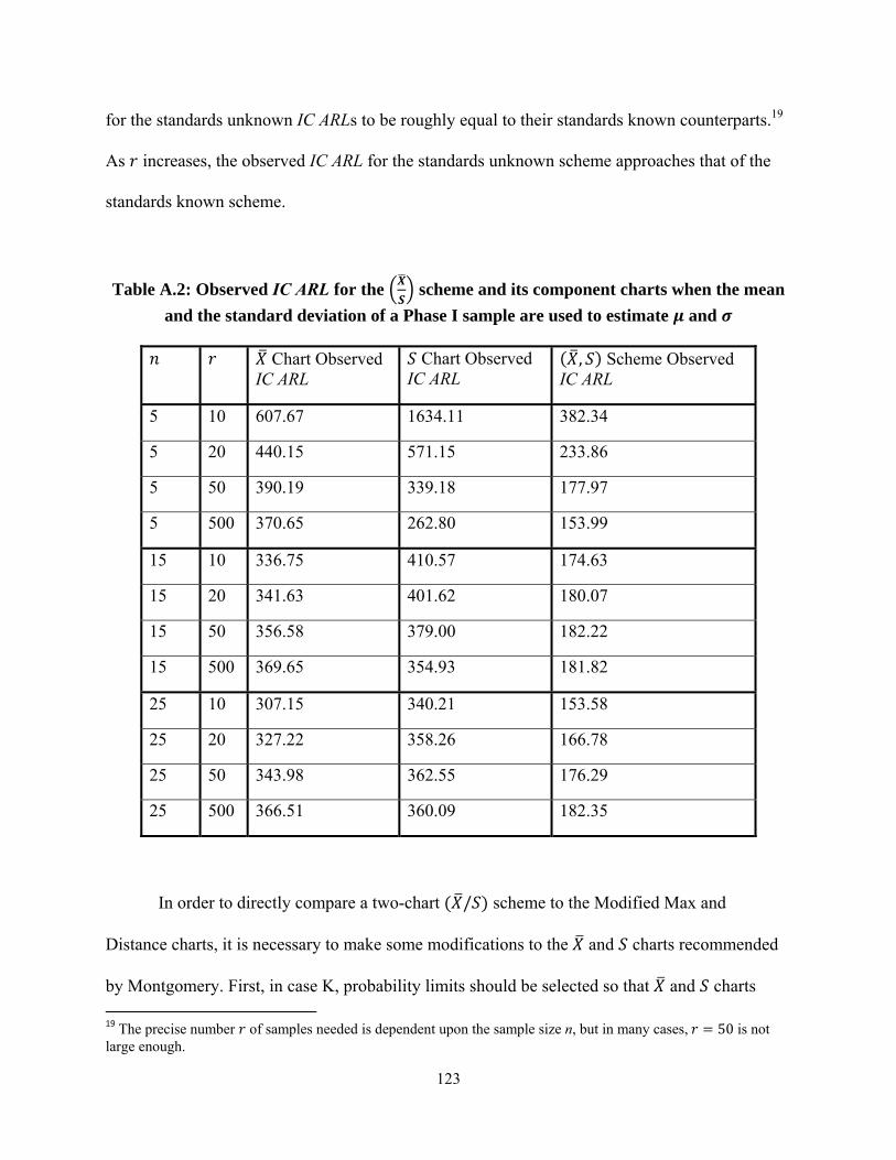
123

for the standards unknown IC ARLs to be roughly equal to their standards known counterparts.19

As increases, the observed IC ARL for the standards unknown scheme approaches that of the

standards known scheme.

Table A.2: Observed IC ARL for the scheme and its component charts when the mean

and the standard deviation of a Phase I sample are used to estimate and

Chart Observed IC ARL

Chart Observed IC ARL

( , ) Scheme Observed IC ARL

5 10 607.67 1634.11 382.34

5 20 440.15 571.15 233.86

5 50 390.19 339.18 177.97

5 500 370.65 262.80 153.99

15 10 336.75 410.57 174.63

15 20 341.63 401.62 180.07

15 50 356.58 379.00 182.22

15 500 369.65 354.93 181.82

25 10 307.15 340.21 153.58

25 20 327.22 358.26 166.78

25 50 343.98 362.55 176.29

25 500 366.51 360.09 182.35

In order to directly compare a two-chart ( / ) scheme to the Modified Max and

Distance charts, it is necessary to make some modifications to the and charts recommended

by Montgomery. First, in case K, probability limits should be selected so that and charts 19 The precise number of samples needed is dependent upon the sample size n, but in many cases, = 50 is not large enough.

124

have the same IC ARL and the overall IC ARL for the scheme is 500. The appropriate control

limits for the chart are ± ( / )√ while the appropriate control limits for the chart

are ( )( / )and ( )( / ) where = 1 − 1 − .

Next, in case U, we need to select the control limits in a way which accounts for the

additional variability caused by the parameter estimation. As for the Max and Distance charts,

we accomplish this using the conditioning technique described in section 3.4.

Recall that , , … , is a random sample of size from normal distribution with

unknown mean and variance ,that , , … , is a random sample of size , likewise from

the normal distribution, with unknown mean and variance and , and that the ′sand the

’s are mutually independent. Next, recall that the sample means and are normally

distributed with mean and variance and and and , respectively, that ( )

is

distributed as a chi-square with ( − 1) degrees of freedom, that ( )

is distributed as a chi-

square with ( − 1) degrees of freedom, and that , , , and are mutually independent.

Recall that for the case K chart, plotting statistic is and the control limits are ± ( / )√ . In case U, the plotting statistic is still , but since and are unknown, the

new control limits ± √ are obtained by plugging in and for and . Likewise,

for the case U chart, is the plotting statistic, and the control limits are ( ) and

( ) .

125

Now, in order for the scheme to have a particular IC ARL, the appropriate percentile

must be obtained by considering the joint distribution of the two plotting statistics. For each

sample, ( ) = ( ≤ ≤ , ≤ ≤ ) =− √ ≤ ≤ + √ , ( ) ≤ ≤ ( ) =

( , ) ( ) ( ) where ( , ) = Φ √√ + √ Φ 1 −+ √ ( ) − Φ √√ − √ Φ 1 − + √ ( ) ×

( ) ( ) − ( ) ( ) . The conditional IC ARL of the ( , ) scheme equals [1 − ( , )] and the unconditional IC ARL is given by

[1 − ( , )] ( ) ( )( ) . Using Mathcad, one can evaluate this

equation and obtain the value of which results in the specified IC ARL.

126

B: ADDITIONAL TABLES AND FIGURES FOR CHAPTER 3

Table B.1: Run length characteristics for the modified normal theory schemes for various values of and when = , = , = , and =

MODIFIED MAX CHART (H=3.20) MODIFIED DISTANCE CHART (H=3.43) MODIFIED ( , ) SCHEME (p0=0.000912)

μ2 σ2 ARL SDRL 5%, 25%, 50%, 75%, 95% ARL SDRL 5%, 25%, 50%, 75%, 95% ARL SDRL 5%, 25%, 50%, 75%, 95% 0 1 499.48 585.21 20, 117, 299, 662, 1660 497.03 602.45 19, 110, 294, 650, 1677 501.06 629.24 17, 104, 282, 650, 1731

0.1 1 461.62 547.08 18, 104, 272, 608, 1558 454.98 563.96 17, 97, 259, 594, 1564 456.46 585.99 16, 92, 252, 586, 1599

0.25 1 310.58 408.36 10, 62, 168, 393, 1093 299.50 404.29 10, 59, 157, 376, 1087 298.27 422.03 9, 54, 149, 366, 1098

0.5 1 101.59 152.50 4, 19, 51, 120, 368 99.06 150.93 3, 18, 49, 118, 363 91.27 150.44 3, 16, 43, 104, 333

0.75 1 28.84 45.52 1, 6, 15, 34, 102 28.96 42.33 1, 6, 15, 35, 100 25.20 38.88 1, 5, 13, 30, 89

1 1 9.55 12.99 1, 2, 5, 12, 31 10.16 13.45 1, 3, 6, 13, 33 8.51 11.29 1, 2, 5, 10, 28

1.25 1 3.96 4.29 1, 1, 3, 5, 12 4.44 5.11 1, 1, 3, 5, 14 3.69 3.97 1, 1, 2, 5, 11

1.5 1 2.17 1.86 1, 1, 2, 3, 6 2.38 2.14 1, 1, 2, 3, 6 2.06 1.72 1, 1, 1, 2, 5

2 1 1.17 0.44 1, 1, 1, 1, 2 1.22 0.55 1, 1, 1, 1, 2 1.16 0.46 1, 1, 1, 1, 2

3 1 1.00 0.02 1, 1, 1, 1, 1 1.00 0.04 1, 1, 1, 1, 1 1.00 0.03 1, 1, 1, 1, 1

0 1.25 73.87 110.32 3, 15, 38, 88, 260 65.12 101.1 2, 12, 33, 77, 233 59.86 89.34 2, 12, 31, 72, 210

0.1 1.25 70.92 106.82 3, 14, 37, 85, 253 61.48 94.86 2, 12, 31, 73, 221 58.05 86.24 2, 12, 30, 70, 204

0.25 1.25 53.97 79.65 2, 11, 29, 66, 185 46.46 69.77 2, 9, 24, 56, 163 45.25 67.06 2, 10, 24, 54, 158

0.5 1.25 26.59 36.88 1, 6, 15, 33, 91 23.19 33.51 1, 5, 13, 28, 80 22.86 31.00 1, 5, 13, 28, 77

0.75 1.25 11.96 14.80 1, 3, 7, 15, 38 10.98 13.97 1, 3, 6, 14, 36 10.70 13.19 1, 3, 6, 13, 34

1 1.25 5.79 6.35 1, 2, 4, 7, 18 5.53 6.27 1, 2, 4, 7, 17 5.34 5.84 1, 2, 3, 7, 16

1.25 1.25 3.26 3.10 1, 1, 2, 4, 9 3.19 3.06 1, 1, 2, 4, 9 3.04 2.84 1, 1, 2, 4, 8

1.5 1.25 2.11 1.69 1, 1, 2, 3, 5 2.09 1.70 1, 1, 1, 3, 5 2.00 1.56 1, 1, 1, 2, 5

2 1.25 1.24 0.55 1, 1, 1, 1, 2 1.26 0.61 1, 1, 1, 1, 2 1.23 0.56 1, 1, 1, 1, 2

3 1.25 1.00 0.07 1, 1, 1, 1, 1 1.01 0.07 1, 1, 1, 1, 1 1.00 0.06 1, 1, 1, 1, 1

0 1. 5 14.94 19.05 1, 4, 9, 19, 48 12.53 15.70 1, 3, 7, 16, 41 12.63 15.58 1, 3, 8, 16, 41

0.1 1.5 14.56 18.20 1, 4, 9, 19, 47 12.26 15.39 1, 3, 7, 15, 39 12.45 15.27 1, 3, 8, 16, 40

0.25 1.5 13.1 16.06 1, 4, 8, 17, 42 10.89 13.17 1, 3, 7, 14, 35 11.30 13.62 1, 3, 7, 14, 36

0.5 1.5 9.40 11.03 1, 3, 6, 12, 29 7.92 9.17 1, 2, 5, 10, 25 8.33 9.44 1, 2, 4, 7, 17

0.75 1.5 6.14 6.74 1, 2, 4, 8, 19 5.17 5.60 1, 2, 3, 7, 15 5.53 5.85 1, 2, 4, 7, 17

1 1.5 3.97 3.98 1, 1, 3, 5, 11 3.45 3.30 1, 1, 2, 4, 10 3.69 3.57 1, 1, 3, 5, 10

1.25 1.5 2.71 2.37 1, 1, 2, 3, 7 2.46 2.10 1, 1, 2, 3, 7 2.56 2.19 1, 1, 2, 3, 7

1.5 1.5 1.97 1.48 1, 1, 1, 2, 5 1.82 1.29 1, 1, 1, 2, 4 1.89 1.39 1, 1, 1, 2, 5

2 1.5 1.29 0.61 1, 1, 1, 1, 3 1.26 0.60 1, 1, 1, 1, 2 1.28 0.62 1, 1, 1, 1, 2

3 1.5 1.01 0.12 1, 1, 1, 1, 1 1.01 0.12 1, 1, 1, 1, 1 1.01 0.12 1, 1, 1, 1, 1

0 1.75 5.63 5.85 1, 2, 4, 7, 17 4.92 5.07 1, 2, 3, 6, 15 5.09 5.26 1, 2, 3, 7, 15

0.1 1.75 5.65 5.97 1, 2, 4, 7, 17 4.85 5.08 1, 2, 3, 6, 15 5.01 5.16 1, 2, 3, 6, 15

0.25 1.75 5.36 5.59 1, 2, 4, 7, 16 4.60 4.78 1, 2, 3, 6, 13 4.81 4.88 1, 2, 3, 6, 14

0.5 1.75 4.60 4.65 1, 2, 3, 6, 13 3.84 3.71 1, 1, 3, 5, 11 4.14 4.09 1, 1, 3, 5, 12

0.75 1.75 3.65 3.43 1, 1, 3, 5, 10 3.13 2.89 1, 1, 2, 4, 9 3.36 3.13 1, 1, 2, 4, 9

1 1.75 2.86 2.51 1, 1, 2, 4, 8 2.46 2.07 1, 1, 2, 3, 6 2.67 2.30 1, 1, 2, 3, 7

1.25 1.75 2.23 1.76 1, 1, 2, 3, 6 1.97 1.46 1, 1, 1, 2, 5 2.13 1.66 1, 1, 2, 3, 5

1.5 1.75 1.80 1.28 1, 1, 1, 2, 4 1.64 1.08 1, 1, 1, 2, 4 1.73 1.18 1, 1, 1, 2, 4

2 1.75 1.30 0.62 1, 1, 1, 1, 3 1.25 0.58 1, 1, 1, 1, 2 1.28 0.62 1, 1, 1, 1, 2

3 1.75 1.03 0.16 1, 1, 1, 1, 1 1.02 0.15 1, 1, 1, 1, 1 1.02 0.16 1, 1, 1, 1, 1

0 2 3.15 2.91 1, 1, 2, 4, 9 2.81 2.47 1, 1, 2, 4, 8 2.94 2.59 1, 1, 2, 4, 8

0.1 2 3.16 2.88 1, 1, 2, 4, 9 2.81 2.47 1, 1, 2, 4, 8 2.92 2.58 1, 1, 2, 4, 8

0.25 2 3.08 2.79 1, 1, 2, 4, 8 2.75 2.36 1, 1, 2, 3, 7 2.85 2.48 1, 1, 2, 4, 8

0.5 2 2.84 2.48 1, 1, 2, 4, 8 2.50 2.12 1, 1, 2, 3, 7 2.63 2.22 1, 1, 2, 3, 7

0.75 2 2.50 2.08 1, 1, 2, 3, 7 2.22 1.77 1, 1, 2, 3, 6 2.34 1.91 1, 1, 2, 3, 6

1 2 2.16 1.68 1, 1, 2, 3, 5 1.91 1.39 1, 1, 1, 2, 5 2.06 1.56 1, 1, 1, 3, 5

1.25 2 1.86 1.33 1, 1, 1, 2, 4 1.68 1.12 1, 1, 1, 2, 4 1.78 1.24 1, 1, 1, 2, 4

1.5 2 1.61 1.04 1, 1, 1, 2, 4 1.48 0.88 1, 1, 1, 2, 3 1.56 0.97 1, 1, 1, 2, 3

2 2 1.27 0.59 1, 1, 1, 1, 2 1.22 0.53 1, 1, 1, 1, 1 1.26 0.58 1, 1, 1, 1, 2

3 2 1.04 0.20 1, 1, 1, 1, 1 1.03 0.18 1, 1, 1, 1, 1 1.04 0.20 1, 1, 1, 1, 1

127

Table B.2: Run length characteristics for the modified normal theory schemes for various values of and when = , = , = , and =

MAX CHART (H=3.18) DISTANCE CHART (3.41) ( , ) SCHEME (p0=0.000886)

μ2 σ2 ARL SDRL 5%, 25%, 50%, 75%, 95% ARL SDRL 5%, 25%, 50%, 75%, 95% ARL SDRL 5%, 25%, 50%, 75%, 95%

0 1 503.99 603.43 19, 111, 296, 665, 1681 491.25 594.13 17, 104, 282, 658, 1685 499.58 655.94 16, 95, 267, 640, 1784

0.1 1 461.88 551.51 16, 100, 271, 612, 1575 462.46 574.37 15, 94, 258, 605, 1626 464.04 621.32 14, 85, 242, 588, 1675

0.25 1 324.88 430.83 10, 61, 170, 413, 1176 316.19 438.47 9, 56, 158, 392, 1166 312.01 465.18 8, 51, 146, 373, 1185

0.5 1 118.29 195.28 3, 18, 52, 134, 458 109.16 174.43 3, 18, 50, 126, 407 101.89 181.25 3, 15, 43, 110, 393

0.75 1 33.61 56.24 1, 6, 16, 38, 124 33.07 52.84 1, 6, 16, 38, 121 27.99 48.26 1, 5, 13, 31, 101

1 1 10.83 16.62 1, 3, 6, 13, 37 11.41 16.67 1, 3, 6, 14, 39 9.16 13.47 1, 2, 5, 11, 31

1.25 1 4.44 5.37 1, 1, 3, 5, 14 4.79 5.86 1, 1, 3, 6, 15 3.90 4.60 1, 1, 2, 5, 12

1.5 1 2.31 2.25 1, 1, 2, 3, 6 2.49 2.38 1, 1, 2, 3, 7 2.12 1.88 1, 1, 1, 3, 6

2 1 1.19 0.49 1, 1, 1, 1, 2 1.26 0.63 1, 1, 1, 1, 2 1.17 0.49 1, 1, 1, 1, 2

3 1 1.00 0.03 1, 1, 1, 1, 1 1.00 0.04 1, 1, 1, 1, 1 1.00 0.03 1, 1, 1, 1, 1

0 1.25 85.13 135.49 3, 15, 41, 99, 310 75.80 129.69 3, 13, 35, 85, 278 65.14 109.56 2, 12, 31, 75, 237

0.1 1.25 80.80 131.16 3, 14, 38, 93, 302 70.48 117.14 2, 12, 32, 81, 260 62.36 103.26 2, 11, 30, 71, 228

0.25 1.25 62.65 103.21 2, 11, 30, 72, 229 54.93 95.41 2, 10, 25, 62, 201 48.79 81.12 2, 9, 24, 56, 177

0.5 1.25 30.58 47.03 1, 6, 16, 36, 110 26.33 42.58 1, 5, 13, 31, 92 24.63 37.75 1, 5, 13, 29, 85

0.75 1.25 13.22 18.38 1, 3, 7, 16, 44 11.99 16.94 1, 3, 7, 15, 40 11.27 15.17 1, 3, 6, 14, 37

1 1.25 6.39 7.68 1, 2, 4, 8, 20 6.07 7.43 1, 2, 4, 8, 19 5.55 6.53 1, 2, 3, 7, 17

1.25 1.25 3.47 3.66 1, 1, 2, 4, 10 3.43 3.69 1, 1, 2, 4, 10 3.14 3.12 1, 1, 2, 4, 9

1.5 1.25 2.16 1.83 1, 1, 2, 3, 6 2.21 1.90 1, 1, 2, 3, 6 2.04 1.65 1, 1, 1, 2, 5

2 1.25 1.26 0.56 1, 1, 1, 1, 2 1.29 0.67 1, 1, 1, 1, 3 1.24 0.58 1, 1, 1, 1, 2

3 1.25 1.01 0.07 1, 1, 1, 1, 1 1.01 0.09 1, 1, 1, 1, 1 1.00 0.07 1, 1, 1, 1, 1

0 1. 5 16.73 23.26 1, 4, 9, 20, 56 13.74 18.60 1, 3, 8, 17, 46 13.41 18.23 1, 3, 8, 16, 44

0.1 1.5 16.33 21.98 1, 4, 9, 20, 55 13.62 19.43 1, 3, 7, 17, 45 13.12 17.65 1, 3, 7, 16, 44

0.25 1.5 14.46 19.93 1, 4, 8, 18, 48 12.11 16.26 1, 3, 7, 15, 40 11.83 15.76 1, 3, 7, 15, 39

0.5 1.5 10.36 13.38 1, 3, 6, 13, 34 8.59 10.97 1, 2, 5, 11, 28 8.70 10.66 1, 2, 5, 11, 28

0.75 1.5 6.65 7.68 1, 2, 4, 8, 21 5.57 6.49 1, 2, 3, 7, 17 5.77 6.47 1, 2, 4, 7, 18

1 1.5 4.25 4.55 1, 1, 3, 5, 13 3.64 3.77 1, 1, 2, 5, 11 3.79 3.83 1, 1, 3, 5, 11

1.25 1.5 2.83 2.58 1, 1, 2, 4, 8 2.54 2.30 1, 1, 2, 3, 7 2.60 2.32 1, 1, 2, 3 , 7

1.5 1.5 2.04 1.59 1, 1, 1, 2, 5 1.90 1.45 1, 1, 1, 2, 5 1.92 1.47 1, 1, 1, 2, 5

2 1.5 1.29 0.62 1, 1, 1, 1, 3 1.29 0.65 1, 1, 1, 1, 3 1.28 0.64 1, 1, 1, 1, 3

3 1.5 1.02 0.13 1, 1, 1, 1, 1 1.01 0.12 1, 1, 1, 1, 1 1.01 0.12 1, 1, 1, 1, 1

0 1.75 6.13 6.91 1, 2, 4, 8, 19 5.21 5.83 1, 2, 3, 7, 16 5.23 5.65 1, 2, 3, 7, 16

0.1 1.75 6.08 6.86 1, 2, 4, 8, 19 5.15 5.66 1, 2, 3, 7, 16 5.17 5.64 1, 2, 3, 7, 16

0.25 1.75 5.76 6.48 1, 2, 4, 7, 18 4.85 5.18 1, 2, 3, 6, 14 4.94 5.29 1, 2, 3, 6, 15

0.5 1.75 4.87 5.22 1, 2, 3, 6, 14 4.09 4.23 1, 1, 3, 5, 12 4.28 4.45 1, 1, 3, 5, 13

0.75 1.75 3.86 3.96 1, 1, 3, 5, 11 3.25 3.13 1, 1, 2, 4, 9 3.45 3.38 1, 1, 2, 4, 10

1 1.75 2.99 2.80 1, 1, 2, 4, 8 2.54 2.22 1, 1, 2, 3, 7 2.71 2.41 1, 1, 2, 3, 7

1.25 1.75 2.31 1.95 1, 1, 2, 3, 6 2.04 1.60 1, 1, 1, 2, 5 2.16 1.73 1, 1, 2, 3, 5

1.5 1.75 1.84 1.35 1, 1, 1, 2, 4 1.66 1.12 1, 1, 1, 2, 4 1.75 1.23 1, 1, 1, 2, 4

2 1.75 1.31 0.64 1, 1, 1, 1, 3 1.27 0.61 1, 1, 1, 1, 2 1.29 0.63 1, 1, 1, 1, 3

3 1.75 1.03 0.17 1, 1, 1, 1, 1 1.02 0.16 1, 1, 1, 1, 1 1.03 0.16 1, 1, 1, 1, 1

0 2 3.33 3.20 1, 1, 2, 4, 9 2.94 2.75 1, 1, 2, 4, 8 2.97 2.74 1, 1, 2, 4, 8

0.1 2 3.28 3.11 1, 1, 2, 4, 9 2.90 2.62 1, 1, 2, 4, 8 2.97 2.72 1, 1, 2, 4, 8

0.25 2 3.19 2.96 1, 1, 2, 4, 9 2.83 2.53 1, 1, 2, 4, 8 2.89 2.63 1, 1, 2, 4, 8

0.5 2 2.99 2.72 1, 1, 2, 4, 8 2.60 2.25 1, 1, 2, 3, 7 2.68 2.35 1, 1, 2, 3, 7

0.75 2 2.60 2.25 1, 1, 2, 3, 7 2.27 1.84 1, 1, 2, 3, 6 2.39 1.99 1, 1, 2, 3, 6

1 2 2.25 1.83 1, 1, 2, 3, 6 1.97 1.49 1, 1, 1, 2, 5 2.08 1.63 1, 1, 2, 3, 5

1.25 2 1.92 1.44 1, 1, 1, 2, 5 1.71 1.20 1, 1, 1, 2, 4 1.80 1.28 1, 1, 1, 2, 4

1.5 2 1.65 1.09 1, 1, 1, 2, 4 1.51 0.93 1, 1, 1, 2, 3 1.57 1.01 1, 1, 1, 2, 4

2 2 1.28 0.60 1, 1, 1, 1, 2 1.23 0.56 1, 1, 1, 1, 2 1.27 0.60 1, 1, 1, 1, 2

3 2 1.04 0.21 1, 1, 1, 1, 1 1.03 0.18 1, 1, 1, 1, 1 1.04 0.20 1, 1, 1, 1, 1

128

Table B.3: Run length characteristics for the modified normal theory schemes for various values of and when = , = , = , and =

MAX CHART (H=3.15) DISTANCE CHART (H=3.37) ( , ) SCHEME (p0=0.000839)

μ2 σ2 ARL SDRL 5%, 25%, 50%, 75%, 95% ARL SDRL 5%, 25%, 50%, 75%, 95% ARL SDRL 5%, 25%, 50%, 75%, 95%

0 1 500.60 591.78 17, 106, 296, 677, 1668 501.75 624.95 15, 97, 280, 668, 1736 498.96 689.19 12, 80, 243, 634, 1862

0.1 1 471.16 572.24 15, 96, 271, 633, 1607 465.47 589.63 13, 86, 255, 617, 1629 466.31 657.85 11, 72, 220, 585, 1756

0.25 1 354.26 479.14 9, 61, 181, 453, 1285 337.83 468.38 9, 56, 170, 429, 1242 337.09 538.68 7, 44, 141, 394, 1345

0.5 1 151.59 252.00 3, 20, 60, 170, 613 135.11 221.33 3, 19, 57, 155, 533 121.94 245.31 3, 14, 43, 120, 501

0.75 1 48.16 97.48 1, 6, 18, 48, 189 44.02 78.95 1, 7, 18, 48, 174 34.70 75.53 1, 5, 13, 34, 132

1 1 15.14 32.71 1, 3, 6, 15, 54 14.94 26.04 1, 3, 7, 16, 54 10.92 21.82 1, 2, 5, 12, 38

1.25 1 5.62 9.61 1, 1, 3, 6, 18 5.95 9.03 1, 1, 3, 7, 20 4.34 6.58 1, 1, 2, 5, 14

1.5 1 2.66 3.05 1, 1, 2, 3, 8 2.89 3.40 1, 1, 2, 3, 9 2.27 2.41 1, 1, 1, 3, 6

2 1 1.23 0.53 1, 1, 1, 1, 2 1.33 0.81 1, 1, 1, 1, 3 1.20 0.56 1, 1, 1, 1, 2

3 1 1.00 0.05 1, 1, 1, 1, 1 1.00 0.06 1, 1, 1, 1, 1 1.00 0.03 1, 1, 1, 1, 1

0 1.25 114.75 200.24 3, 17, 47, 125, 455 100.63 197.90 3, 14, 39, 104, 388 75.23 146.21 2, 11, 30, 78, 289

0.1 1.25 110.73 204.36 3, 15, 44, 118, 430 93.41 174.47 2, 12, 37, 99, 363 72.32 143.09 2, 10, 29, 75, 278

0.25 1.25 85.04 155.96 2, 12, 35, 91, 332 73.31 143.96 2, 10, 28, 75, 290 57.15 117.33 2, 9, 23, 59, 215

0.5 1.25 41.20 79.53 1, 7, 18, 43, 154 36.09 74.08 1, 6, 15, 37, 137 28.39 55.74 1, 5, 13, 30, 102

0.75 1.25 17.38 31.95 1, 3, 8, 19, 61 15.45 26.94 1, 3, 7, 17, 56 12.82 21.88 1, 3, 6, 14, 44

1 1.25 7.72 11.11 1, 2, 4, 9, 26 7.32 10.96 1, 2, 4, 8, 24 6.04 8.24 1, 2, 3, 7, 19

1.25 1.25 3.94 4.73 1, 1, 2, 5, 12 3.88 4.91 1, 1, 2, 5, 12 3.34 3.75 1, 1, 2, 4, 10

1.5 1.25 2.43 2.37 1, 1, 2, 3, 7 2.40 2.36 1, 1, 2, 3, 7 2.13 1.93 1, 1, 1, 3, 6

2 1.25 1.29 0.60 1, 1, 1, 1, 2 1.34 0.78 1, 1, 1, 1, 3 1.26 0.62 1, 1, 1, 1, 2

3 1.25 1.01 0.09 1, 1, 1, 1, 1 1.01 0.10 1, 1, 1, 1, 1 1.01 0.08 1, 1, 1, 1, 1

0 1. 5 21.84 37.12 1, 4, 10, 25, 78 18.11 33.54 1, 3, 9, 20, 64 14.81 23.88 1, 3, 8, 17, 52

0.1 1.5 21.70 36.46 1, 4, 11, 24, 77 17.31 29.54 1, 3, 8, 20, 62 14.56 23.74 1, 3, 7, 17, 51

0.25 1.5 18.80 31.04 1, 4, 9, 22, 67 15.16 25.66 1, 3, 8, 17, 53 12.96 19.49 1, 3, 7, 15, 44

0.5 1.5 13.08 20.65 1, 3, 7, 15, 45 10.38 16.68 1, 2, 5, 12, 35 9.44 13.99 1, 2, 5, 11, 31

0.75 1.5 7.83 10.69 1, 2, 4, 9, 26 6.58 9.21 1, 2, 4, 8, 21 6.21 8.12 1, 2, 4, 8, 20

1 1.5 4.83 5.95 1, 1, 3, 6, 15 4.11 4.89 1, 1, 3, 5, 12 3.99 4.52 1, 1, 3, 5, 12

1.25 1.5 3.15 3.17 1, 1, 2, 4, 9 2.79 2.92 1, 1, 2, 3, 8 2.72 2.64 1, 1, 2, 3, 8

1.5 1.5 2.19 1.86 1, 1, 2, 3, 6 2.02 1.71 1, 1, 1, 2, 5 1.98 1.61 1, 1, 1, 2, 5

2 1.5 1.33 0.67 1, 1, 1, 2, 3 1.33 0.72 1, 1, 1, 1, 3 1.30 0.67 1, 1, 1, 1, 3

3 1.5 1.02 0.15 1, 1, 1, 1, 1 1.02 0.14 1, 1, 1, 1, 1 1.02 0.13 1, 1, 1, 1, 1

0 1.75 7.28 10.63 1, 2, 4, 9, 23 6.05 7.77 1, 2, 4, 7, 19 5.53 6.79 1, 2, 3, 7, 17

0.1 1.75 7.29 10.03 1, 2, 4, 9, 24 5.97 7.87 1, 2, 4, 7, 19 5.48 6.66 1, 2, 3, 7, 17

0.25 1.75 6.95 9.41 1, 2, 4, 8, 22 5.57 6.94 1, 2, 3, 7, 17 5.23 6.30 1, 2, 3, 6, 16

0.5 1.75 5.63 6.74 1, 2, 3, 7, 18 4.65 5.54 1, 1, 3, 6, 14 4.49 5.17 1, 1, 3, 6, 14

0.75 1.75 4.35 4.95 1, 1, 3, 5, 13 3.63 4.19 1, 1, 2, 4, 11 3.59 3.79 1, 1, 2, 4, 11

1 1.75 3.28 3.36 1, 1, 2, 4, 9 2.75 2.66 1, 1, 2, 3, 8 2.81 2.70 1, 1, 2, 3, 8

1.25 1.75 2.50 2.27 1, 1, 2, 3, 7 2.17 1.85 1, 1, 2, 3, 6 2.20 1.86 1, 1, 2, 3, 6

1.5 1.75 1.96 1.57 1, 1, 1, 2, 5 1.76 1.33 1, 1, 1, 2, 4 1.78 1.33 1, 1, 1, 2, 4

2 1.75 1.34 0.68 1, 1, 1, 2, 3 1.30 0.66 1, 1, 1, 1, 3 1.30 0.67 1, 1, 1, 1, 3

3 1.75 1.03 0.19 1, 1, 1, 1, 1 1.03 0.18 1, 1, 1, 1, 1 1.03 0.17 1, 1, 1, 1, 1

0 2 3.72 3.96 1, 1, 2, 5, 11 3.20 3.21 1, 1, 2, 4, 9 3.09 3.05 1, 1, 2, 4, 9

0.1 2 3.66 3.79 1, 1, 2, 5, 10 3.23 3.40 1, 1, 2, 4, 9 3.05 3.00 1, 1, 2, 4, 9

0.25 2 3.62 3.93 1, 1, 2, 5, 10 3.15 3.14 1, 1, 2, 4, 9 3.00 2.94 1, 1, 2, 4, 8

0.5 2 3.29 3.38 1, 1, 2, 4, 10 2.80 2.70 1, 1, 2, 3, 8 2.76 2.59 1, 1, 2, 3, 8

0.75 2 2.87 2.73 1, 1, 2, 4, 8 2.44 2.18 1, 1, 2, 3, 7 2.45 2.18 1, 1, 2, 3, 7

1 2 2.43 2.73 1, 1, 2, 4, 8 2.10 1.72 1, 1, 1, 3, 5 2.13 1.78 1, 1, 1, 3, 5

1.25 2 2.04 1.64 1, 1, 1, 2, 5 1.79 1.31 1, 1, 1, 2, 4 1.84 1.39 1, 1, 1, 2, 4

1.5 2 1.74 1.28 1, 1, 1, 2, 4 1.56 1.01 1, 1, 1, 2, 3 1.60 1.06 1, 1, 1, 2, 4

2 2 1.32 0.65 1, 1, 1, 1, 3 1.26 0.60 1, 1, 1, 1, 2 1.28 0.63 1, 1, 1, 1, 3

3 2 1.05 0.22 1, 1, 1, 1, 1 1.03 0.19 1, 1, 1, 1, 1 1.04 0.21 1, 1, 1, 1, 1

129

Table B.4: Run length characteristics for the modified normal theory schemes for various values of and when = , = , = , and =

MAX CHART (H=3.15) DISTANCE CHART (H=3.37) ( , ) SCHEME (p0=0.000763)

μ2 σ2 ARL SDRL 5%, 25%, 50%, 75%, 95% ARL SDRL 5%, 25%, 50%, 75%, 95% ARL SDRL 5%, 25%, 50%, 75%, 95%

0 1 497.79 591.70 15, 101, 289, 671, 1681 494.29 611.70 13, 90, 273, 669, 1730 498.34 750.80 8, 59, 209, 617, 1991

0.1 1 479.93 582.64 14, 92, 273, 644, 1666 478.22 607.48 12, 84, 260, 639, 1662 477.30 732.27 7, 54, 193, 587, 1914

0.25 1 396.68 521.43 9, 64, 202, 524, 1440 381.12 525.70 8, 57, 183, 491, 1435 368.99 619.63 5, 36, 131, 422, 1558

0.5 1 204.95 320.03 4, 23, 81, 248, 839 180.86 304.65 3, 21, 70, 210, 720 159.52 353.29 2, 12, 42, 142, 724

0.75 1 83.01 167.27 2, 8, 25, 81, 362 69.98 138.31 2, 7, 24, 72, 290 51.49 142.44 1, 5, 13, 40, 216

1 1 28.62 71.56 1, 3, 8, 24, 121 23.93 49.76 1, 3, 8, 24, 95 15.81 47.81 1, 2, 5, 13, 57

1.25 1 9.68 25.67 1, 2, 4, 8, 35 9.16 18.96 1, 2, 4, 9, 34 5.57 13.32 1, 1, 2, 5, 19

1.5 1 3.92 7.30 1, 1, 2, 4, 13 4.15 7.07 1, 1, 2, 4, 14 2.65 4.45 1, 1, 1, 3, 8

2 1 1.32 0.65 1, 1, 1, 1, 3 1.51 1.31 1, 1, 1, 2, 4 1.25 0.72 1, 1, 1, 1, 2

3 1 1.01 0.07 1, 1, 1, 1, 1 1.01 0.10 1, 1, 1, 1, 1 1.00 0.05 1, 1, 1, 1, 1

0 1.25 191.30 349.41 3, 20, 65, 204, 814 156.17 305.41 3, 15, 48, 154, 690 96.71 231.80 2, 9, 28, 85, 404

0.1 1.25 179.23 328.35 3, 18, 61, 189, 757 151.26 295.24 2, 14, 48, 151, 660 92.00 228.82 2, 9, 27, 80, 380

0.25 1.25 146.92 291.88 2, 14, 46, 146, 635 123.08 256.66 2, 11, 37, 117, 540 74.30 189.15 2, 7, 22, 65, 301

0.5 1.25 76.17 173.09 2, 8, 23, 69, 316 63.74 148.55 1, 6, 18, 57, 267 38.38 98.08 1, 4, 12, 34, 150

0.75 1.25 30.41 76.48 1, 4, 10, 28, 119 26.91 66.70 1, 3, 9, 25, 108 16.51 43.26 1, 3, 6, 16, 60

1 1.25 12.54 27.96 1, 2, 5, 12, 44 11.77 25.66 1, 2, 5, 12, 43 7.38 14.41 1, 2, 3, 8, 26

1.25 1.25 5.79 12.20 1, 1, 3, 6, 19 5.65 10.15 1, 1, 3, 6, 20 3.82 6.85 1, 1, 2, 4, 12

1.5 1.25 3.15 4.39 1, 1, 2, 3, 10 3.14 4.48 1, 1, 2, 3, 10 2.30 2.54 1, 1, 1, 3, 6

2 1.25 1.39 0.73 1, 1, 1, 2, 3 1.52 1.24 1, 1, 1, 2, 4 1.30 0.76 1, 1, 1, 1, 3

3 1.25 1.02 0.12 1, 1, 1, 1, 1 1.02 0.14 1, 1, 1, 1, 1 1.01 0.09 1, 1, 1, 1, 1

0 1. 5 40.10 95.14 1, 5, 14, 38, 156 31.13 75.91 1, 4, 11, 29, 121 18.41 41.87 1, 3, 7, 18, 67

0.1 1.5 39.05 90.41 1, 5, 14, 37, 156 31.23 82.49 1, 4, 10, 28, 122 18.10 43.45 1, 3, 7, 18, 66

0.25 1.5 34.21 79.33 1, 5, 12, 33, 132 26.07 61.45 1, 4, 10, 24, 100 16.02 36.26 1, 3, 7, 16, 58

0.5 1.5 21.70 46.41 1, 3, 9, 22, 82 16.78 37.22 1, 3, 7, 16, 61 11.24 21.87 1, 2, 5, 12, 40

0.75 1.5 12.25 23.63 1, 2, 5, 13, 43 9.72 22.19 1, 2, 4, 10, 34 7.20 14.64 1, 2, 4, 8, 24

1 1.5 6.99 13.52 1, 2, 4, 8, 23 5.72 10.58 1, 1, 3, 6, 19 4.42 6.28 1, 1, 3, 5, 14

1.25 1.5 4.03 5.56 1, 1, 2, 5, 13 3.57 5.09 1, 1, 2, 4, 11 2.93 3.37 1, 1, 2, 3, 9

1.5 1.5 2.62 2.79 1, 1, 2, 3, 7 2.41 2.69 1, 1, 2, 3, 7 2.08 1.95 1, 1, 1, 2, 6

2 1.5 1.42 0.77 1, 1, 1, 2, 3 1.44 0.96 1, 1, 1, 2, 3 1.33 0.77 1, 1, 1, 1, 3

3 1.5 1.03 0.17 1, 1, 1, 1, 1 1.03 0.20 1, 1, 1, 1, 1 1.02 0.14 1, 1, 1, 1, 1

0 1.75 11.35 21.04 1, 2, 5, 12, 40 8.98 16.77 1, 2, 4, 9, 31 6.30 10.07 1, 2, 3, 7, 21

0.1 1.75 11.10 22.21 1, 2, 5, 12, 39 8.65 15.83 1, 2, 4, 9, 30 6.17 9.63 1, 2, 3, 7, 20

0.25 1.75 10.56 20.75 1, 2, 5, 11, 37 8.14 15.33 1, 2, 4, 9, 27 5.87 9.17 1, 2, 3, 7, 19

0.5 1.75 8.28 13.70 1, 2, 4, 9, 28 6.46 10.52 1, 2, 3, 7, 22 4.94 6.81 1, 1, 3, 6, 16

0.75 1.75 6.06 9.70 1, 2, 3, 7, 20 4.69 6.94 1, 1, 3, 5, 15 3.92 5.07 1, 1, 2, 5, 12

1 1.75 4.29 5.87 1, 1, 2, 5, 14 3.39 4.45 1, 1, 2, 4, 10 3.01 3.44 1, 1, 2, 4, 9

1.25 1.75 3.02 3.46 1, 1, 2, 4, 9 2.57 2.81 1, 1, 2, 3, 7 2.33 2.30 1, 1, 2, 3, 6

1.5 1.75 2.27 2.22 1, 1, 2, 3, 6 1.99 1.84 1, 1, 1, 2, 5 1.85 1.52 1, 1, 1, 2, 5

2 1.75 1.42 0.78 1, 1, 1, 2, 3 1.38 0.84 1, 1, 1, 2, 3 1.33 0.75 1, 1, 1, 1, 3

3 1.75 1.05 0.23 1, 1, 1, 1, 1 1.04 0.21 1, 1, 1, 1, 1 1.03 0.18 1, 1, 1, 1, 1

0 2 5.02 7.30 1, 1, 3, 6, 16 4.17 5.56 1, 1, 2, 5, 13 3.32 3.94 1, 1, 2, 4, 10

0.1 2 5.00 6.79 1, 1, 3, 6, 16 4.03 5.42 1, 1, 2, 5, 12 3.30 3.80 1, 1, 2, 4, 10

0.25 2 4.81 6.59 1, 1, 3, 6, 16 3.95 5.18 1, 1, 2, 5, 12 3.20 3.77 1, 1, 2, 4, 9

0.5 2 4.28 5.93 1, 1, 3, 5, 13 3.50 4.25 1, 1, 2, 4, 14 2.93 3.28 1, 1, 2, 3, 8

0.75 2 3.58 4.18 1, 1, 2, 4, 11 2.92 3.22 1, 1, 2, 3, 8 2.58 2.68 1, 1, 2, 3, 7

1 2 2.90 3.21 1, 1, 2, 3, 8 2.39 2.34 1, 1, 2, 3, 7 2.23 2.08 1, 1, 1, 3, 6

1.25 2 2.40 2.32 1, 1, 2, 3, 7 2.01 1.76 1, 1, 1, 2, 5 1.91 1.58 1, 1, 1, 2, 5

1.5 2 1.98 1.72 1, 1, 1, 2, 5 1.71 1.32 1, 1, 1, 2, 4 1.64 1.20 1, 1, 1, 2, 4

2 2 1.40 0.74 1, 1, 1, 2, 3 1.33 0.76 1, 1, 1, 1, 3 1.30 0.68 1, 1, 1, 1, 3

3 2 1.07 0.27 1, 1, 1, 1, 2 1.05 0.24 1, 1, 1, 1, 1 1.04 0.22 1, 1, 1, 1, 1

130

Figure B.1: Region of Values of and (in red) for which the Modified Distance chart outperforms the Modified Max chart for various values of when = , = , and =

= =

= =

2

1.5

1

1 2 3

σ2

μ2

2

1.5

1

1 2 3σ2

μ2

2

1.5

1

1 2 3

σ2

μ2

2

1.5

1

1 2 3

σ2

μ2

µ2

σ2

µ2

σ2

µ2

σ2

µ2

σ2

131

C: SUPPLEMENTARY DERIVATIONS FOR CHAPTER 4

C.1 The joint distribution of and

Recall that has a chi-square distribution with 2 − 2 degrees of freedom and that

follows the shifted exponential distribution with location parameter and scale parameter / .

Therefore, distribution of is ( ) = ( ) , > 0 and the distribution

of is ( ) = exp ( ) , > .Since and are independent, their joint

distribution, , ( , ) = ( ) ( ) =

( ) / exp ( ) , > 0, > . Now, note that =( ) = . Also, = ( ) = ( ) ( ) ( ) = ( ) + ( ) = + . In other

words, both and can be written as one-to-one transformations of and . We can

therefore use the Jacobian method to obtain the joint distribution of and , , ( , ). To use the Jacobian method, note that = ( )

and = + . The resulting

Jacobian is ( ),a negative number. Hence, the joint pdf of of and is , ( , ) =

( ) ( ) ( ) / exp ( )

= ( )( ) ( ), > − , > 0.

Now, , ( , ) = ( )( ) ( ) =( )( ) ( ) ( ) =

132

( )( ) ( ) / = ( )( ) ( ) = 1

since ( )( ) ( )

is the pdf of a Gamma − 1, distribution.

C.2 The distribution of

The marginal distribution of can be obtained by integrating the joint distribution of and over all possible values of . Notice that the joint distribution has the conditions > − and > 0. In other words, must be larger than both 0 and ( − ). When is between -∞ and , ( − ) > 0, so ( − ) < < ∞. However, when is

between and ∞, ( − ) < 0, so 0 < < ∞. Therefore, ( ) = ( − 1)Γ( − 1) ( ) ( , )( ) + ( )( ) ( )( ) ( , ]( ). = ( ) ( ) ( , )( ) + ( )( ) ( )( ) ( , ]( ).

Now, ( )

= ( ) ( ) + ( )( ) ( )( )

= ( ) + ( )( ) ( )( )

= ( ) + ( )( ) ( )

= ( ) + ( )( ) ( ) / − /

133

= ( ) + ( )( ) ( ) − + /

= ( ) + ( )( ) − + ( )

= ( ) + ( )( ) −Γ( − 1) ( )

+Γ( − 1) ( ) ( )

= ( ) + ( )( ) −Γ( − 1) + Γ( − 1)

= ( ) + ( − 1) − + = ( ) − ( ) + 1 = 1.

C.3 The distribution of (ℳ ≤ ) = (max{| |, | |} ≤ ) = {(| | ≤ )&(| | ≤ )} = (| | ≤ ) (| | ≤ ) = (− ≤ ≤ ) (− ≤ ≤ ) = − ≤ Φ , 2 ≤ × − ≤ Φ G , 2 − 2 ≤

= ( ( ), ) + − ≤ ≤ ( ( ), ) + −

× (Φ(− ), 2 − 2) ≤ ≤ (Φ(− ), 2 − 2)

= ( ( ), ) + − ≤ ≤ ( ( ), ) + −

× (Φ(− ), 2 − 2) ≤ ( ) ≤ (Φ( ), 2 − 2)

= ( ( ), 2) + − , 2 − ( (− ), 2) + − , 2

134

× (Φ( ), 2 − 2), 2 − 2 − (Φ(− ), 2 − 2), 2 − 2 .

C.4 The distribution of ( ≤ & > 0) = (max{ , } ≤ & > 0) = ( ≤ & ≤ & > 0) =(0 < ≤ & ≤ ) = (0 < ≤ ) ( ≤ ) =0 < ≤ G G , 2 − 2 , 2 − 2 ≤

= ( ) < ≤ + − ≤ G {G( , 2), 2 − 2}

= ( ) < ≤ + − ( ) ≤ G {G( , 2), 2 − 2}

= + − , 2 − ( − ), 2 × [ ( , 2), 2 − 2], 2 − 2

C.5 ARL Bias in the SEMLE-Max Chart

Suppose that some SEMLE-Max Chart has UCL > 0. Note that ARL bias occurs when

for some shift size, (ℳ ≤ | , ) > (ℳ ≤ | , ). Recall that the cumulative

distribution function of the statistic ℳ which defines this chart is (ℳ ≤ ) = ( ( ), 2) + − , 2 − ( (− ), 2) + − , 2 ×(Φ( ), 2 − 2), 2 − 2 − (Φ(− ), 2 − 2), 2 − 2 and that it

simplifies to { ( ) − (− )} when the process is IC. Now, suppose that = 0 and = 1

and that there has been a shift in the location parameter but not in the scale parameter. Then, (ℳ ≤ ) = ( ( ), 2) − , 2 − ( (− ), 2) − , 2 × { ( (Φ( ), 2 − 2), 2 − 2) − ( (Φ(− ), 2 − 2), 2 − 2)}

135

= ( ( ( ), 2) − 2 ), 2 − ( ( (− ), 2) − 2 ), 2 × {Φ( ) − Φ(− )}. We need to determine when ( ( ( ), 2) − 2 ), 2 − ( ( (− ), 2) − 2 ), 2 × {Φ( ) − Φ(− )} > { ( ) − (− )} .

Dividing both sides by {Φ( ) − Φ(− )} gives us ( ( ( ), 2) − 2 ), 2 −( ( (− ), 2) − 2 ), 2 > { ( ) − (− )}. Let = ( ( ( ), 2) − 2 ), 2

and = ( ( (− ), 2) − 2 ), 2 . Now suppose { − } > { ( ) − (− )}. This can

be true in one of three ways:

i) = 0 and − > { ( ) − (− )}. ii) = 0 and > { ( ) − (− )}. iii) > 0, > 0, and − > { ( ) − (− )}

Case i

Let = 0. Then ( ( ( ), 2) − 2 ), 2 = 0. Now, ( , 2) = 0 whenever ≤ 0, so we have ( ( ), 2) − 2 ≤ 0,or ≥ ( ( ), ). Next, let − > { ( ) − (− )}. Then ( ( (− ), 2) − 2 ), 2 < −{ ( ) − (− )}. However, ( ( (− ), 2) −2 ), 2 cannot be less than −{ ( ) − (− )}, because (. ,2) cannot be negative, while −{ ( ) − (− )} must be negative. Therefore, case I cannot occur.

Case ii

Let = 0. Then ( ( (− ), 2) − 2 ), 2 = 0. So, ( (− ), 2) − 2 ≤ 0.

Restated, ≥ ( ( ), ). Now let > { ( ) − (− )}. Then ( ( ( ), 2) −

136

2 ), 2 > { ( ) − (− )}. Applying the inverse function to each side gives us

( ( ), 2) − 2 > { ( ) − (− ), 2},or < ( ( ), ) { ( ) ( ), }. So in Case ii,

( ( ), ) ≤ < ( ( ), ) { ( ) ( ), } .

Case iii

Let > 0. Then ( ( ( ), 2) − 2 ), 2 > 0. Applying the inverse function to

each side gives us ( ( ), 2) − 2 > 0, or < ( ( ), ). Now let > 0. Then ( ( (− ), 2) − 2 ), 2 > 0. Applying the inverse

function to each side gives us ( (− ), 2) − 2 > 0, or < ( ( ), ). Finally, let − > { ( ) − (− )}. Then ( ( ( ), 2) − 2 ), 2 −( ( (− ), 2) − 2 ), 2 > { ( ) − (− )}. Note that ( ( ( ), 2) −

2 ), 2 − ( ( (− ), 2) − 2 ), 2 = ( ( ), )( ( ), )

= ( ( ), ) 1 − ( ( ), ) ( ( ), ) . So,

( ( ), ) 1 − ( ( ), ) ( ( ), ) > { ( ) − (− )}. Dividing both sides by

1 − ( ( ), ) ( ( ), ) gives us ( ( ), ) > { ( ) ( )}( ( ), ) ( ( ), ) . Taking the

natural log of each side gives us − ( ( ), ) > ln { ( ) ( )}( ( ), ) ( ( ), ) . Finally,

137

we have

( ( ), ) { ( ) ( )}( ( ), ) ( ( ), ) < . But

( ( ), ) { ( ) ( )}( ( ), ) ( ( ), ) = 0, so > 0. Thus, for Case iii, we have >0, < ( ( ), ), and < ( ( ), )

. Since ( ( ), ) > ( ( ), )

, we see that case iii

occurs when 0 < < ( ( ), )

.

Combining the three cases, we see that bias occurs when 0 < < ( ( ), ) { ( ) ( ), }. When = 3.29 and = 5 as was the case in our simulation

study, this means that there is bias when 0 < < 0.1386.

C.6 Lack of ARL Bias in the SEMLE-ChiMax Chart

Suppose that some SEMLE-ChiMax Chart has UCL > 0. Note that ARL bias would

occur if for some shift size, (ℳ ≤ | , ) > (ℳ ≤ | , ). Recall that the cumulative

distribution function for the statistics which defines this chart is ( ≤ & > 0) =+ − , 2 − ( − ), 2 × [ ( , 2), 2 − 2], 2 − 2 and

that it simplifies to { ( , 2)}{ ( , 2)} when the process is IC. Now, suppose that = 0 and = 1 and that there has been a shift in the location parameter but not in the scale parameter.

Then, ( ≤ & > 0) = + − , 2 − ( − ), 2

× [ ( , 2), 2 − 2], 2 − 2 = { [ − 2 , 2] − [−2 , 2]} × { ( , 2)}.

138

We need to determine when { [ − 2 , 2] − [−2 , 2]} × { ( , 2)} > { ( , 2)}{ ( , 2)}. Dividing both sides by { ( , 2)} gives us { [ − 2 , 2] −[−2 , 2]} > { ( , 2)}. Let = [ − 2 , 2] and = [−2 , 2]. Now suppose { − } > { ( , 2)}. This can be true in one of three ways:

i) = 0 and − > { ( , 2)}. ii) = 0 and > { ( , 2)}. iii) > 0, > 0, and − > { ( , 2)}

Case i

Let = 0. Then [ − 2 , 2] = 0. Now, ( , 2) = 0 whenever ≤ 0, so we have − 2 ≤ 0,or ≥ . Now let − > { ( , 2)}. Then − [−2 , 2] < { ( , 2)}. This

simplifies to < [ [ ( , )], ]. However, [ [ ( , )], ]

does not exist. Therefore, case I

cannot occur.

Case ii

Let = 0. Then [−2 , 2] = 0,which gives us ≥ 0.Now let > { ( , 2)}. Then [ − 2 , 2] > { ( , 2)}. This simplifies to < 0. However, cannot

simultaneously be less than 0 and greater than or equal to 0, so case ii cannot occur.

Case iii

Let > 0. Then [ − 2 , 2] > 0. Therefore, < . Now let > 0. Then [−2 , 2] > 0.Therefore, < 0. Finally, let − > { ( , 2)}.Then [ − 2 , 2] −

139

[−2 , 2] > { ( , 2)}. . Note that [ − 2 , 2] − [−2 , 2] = [ ][ ] =[ ]/ 1 − [ ]/ = 1 − / . So 1 − / > { ( , 2)}. Solving

for results in > ln { ( , )}/ / . However, since

{ ( , )}/ = 0, resulting in > 0. cannot simultaneously be less than 0 and greater than or equal to 0, so case iii cannot occur.

140

APPENDIX D: SUPPLEMENTARY DERIVATIONS FOR CHAPTER 5

D.1 The distribution of (Υ ≤ ) = (max{| |, | |} ≤ ) = {(| | ≤ )&(| | ≤ )} = (| | ≤ ) (| | ≤ ) = (− ≤ ≤ ) (− ≤ ≤ ) = (− ≤ Φ {ℸ( , , )} ≤ ) × − ≤ Φ M ≤

= ℸ (Φ(− ), , ) ≤ ≤ ℸ (Φ( ), , )

× (Φ(− ), , ) ≤ ≤ (Φ(− ), , )

= ℸ (Φ(− ), , ) ≤ ≤ ℸ (Φ( ), , )

× (Φ(− ), , ) ≤ ≤ (Φ( ), , )

= {(ℸ[ℸ (Φ( ), , ), , ]) − (ℸ[ℸ (Φ(− ), , ), , ])} × (Φ( ), , ), , − (Φ(− ), , ), , .