CONTROL OF MSU JUMPING ROBOT

By

Emad Alsaedi

A THESIS

Submitted to

Michigan State University

in partial fulfillment of the requirements

for the degree of

Electrical Engineering – Master of Science

2014

ABSTRACT

CONTROL OF MSU JUMPING ROBOT

By

Emad Alsaedi

The idea of Miniature jumping robots is taking exactly from the animal living around us. A

gecko lizard is a perfect example for a jumping balancing Robot, in an experiment, it was seen

how gecko lizard can balance landing using the moment of the tail. Another example is a

falling cat midair self-righting. These miniature jumping robot are becoming widely used in real

life. One cannot expect how useful to use such robot at times where human presence is at

danger. Like in the case of wars or natural disaster (as in earth quakes or nuclear like disaster as

Fukushima leaks in Japan). The MSU jumper robot is unique in terms of weight and size;

however, there is some control problem in the case of landing procedure, as well as self-

righting and maneuvering in midair. Designing a controller for MSU jumping robot is

challenging, the controller has to response in half a second as the jumping period is

close to 2 second, that short period made it almost impossible for the robot to resist

uncertainties or unmolded dynamics, as well as changes in the mass of moment of inertia

of the body due to change of body shape. We managed to add mini wings to the robot to

prolong jumping period and the stabilize landing procedure, as well as to enable the robot to

estimate the mass of moment of inertia for the body , and all of that for the controller at the tail

to force the body to land on the desired edge. MSU jumper robot has swept greatly throughout

robotics media and industry due to the tininess and light weight properties. A light weight

that doesn’t exceed 28 g and a maximum size of 6.5 cm is what made the robot special in its

types of all jumping robots.

iii

TABLE OF CONTENTS

LIST OF TABLES………………………………………………………………………………...v

LIST OF FIGURES……………………………………………………………………...……….vi

KEY TO SYMBOLS OR ABBREVIATIONS.…………………………………...……………viii

Chapter 1.Introductions…………………………………...…………………...……………..…...1

1.1.Background…………………………………………………..………...………..…1

1.2.Motivations………………...........………….…………….……………...….….….2

1.3.Objective………………………………………………..……………..…..……….3

1.3.1.Estimation………………………………………….…….………………..3

1.3.2.Controller Design………………………………..…………..…………….3

Chapter 2.Jumping procedure……………………….……………………….……………………5

2.1.Step 1……………………………………………………….………………….….5

2.2.Step 2……………………………………………………...………………………5

2.3.Step 3………………………………………………………………………….…..6

Chapter 3.Wings design…….………………………………………....…….………………….…7

Chapter 4.Modeling…………………………………………………………..……………...……8

4.1.Robot Energies ……………………………………………………...……...…….9

4.1.1.Potential Energy……………………………………………..…...…………9

4.1.2.Kinetic Energy…………………………………………………………..….9

4.2.Lagrange EOM for Robot…………………………………….…………..………9

4.3.Dynamics equations…………………………………………...………..……….12

4.4.Transformation………………….……………………....……………….………12

Chapter 5.Linearization….……………..……………………………………….………………..13

Chapter 6.Estimation …………………………………………......……...………….…….……..16

6.1.Re-parameterization…………………………………………..........………….…16

6.2.Gradient Algorithm……………………………………….………………….…..17

6.2.1.Gradient without protection……………………………..….………….…..17

6.3.2.Gradient with protection ………………………………..……………...….18

Chapter 7.Designing controller……………………...............……………………………......….20

7.1.Designing controller by MRAC………………………………….….…...….…...20

7.2.Designing controller by APPC ………………………..………….…..……..…...22

7.3.Designing controller by PD .……….…………………….………….…...……...26

7.4.Designing slide mode controller …………………….……………..……………29

iv

7.5.Designing ASMC…………………………………………….……..……………34

Chapter 8.Conclusion…………..…………………………………………….…………...…..….36

8.1.Comparison of controllers………………………………….…………………….36

8.1.1.Disturbance rejection test………………………………….……………….36

8.1.2.Uncertainties rejection test…………………………….……….…………..39

8.1.3.Summary ………………………………………………….……………….40

8.2.Contribution to MSU jumper Robot. …………….….…………………....……..41

8.3.Results of new schematic design……………………..……………………....….41

8.4.Future work……………………………………….….……………………….….41

BIBLIOGRAPHY ………..........……………………………………...….……...…………...….42

v

LIST OF TABLES

Table 4.1. LIST OF PARAMETERS FOR DYNAMICS MODELING……………….…….8

vi

LIST OF FIGURES

Figure 1.1.1. Prototype of the robot with the flexible wings (for interpretation of the

references to color in this and all other figures, the reader is referred to the

electronic version of this thesis)…………………………………………..……2

Figure 1.3.1. Schematic of landing and taking off desired position for the robot…...…….…4

Figure 2.1. Tighten wings as robot getting ready for jump …………..…………...………5

Figure 2.2. Robot in midair …………………………………………...…………..…...…..5

Figure 2.3. Robot getting down to land with 30 degree angle. ………….....………..……6

Figure 4.1. The schematic of the robot in the air. Modeling of the system………........….8

Figure 5.1. Steps response of linear and nonlinear system……...……….…………..…15

Figure 6.2.1.1. Estimation without projection. ………………………..………….............…17

Figure 6.2.1.2. Tracking, without projection. ……………………..….…………………….18

Figure 6.2.2.1. Estimation with projection…………………………....…………….....……19

Figures 6.2.2.2. Tracking is not maintained……………………..……….………………...…19

Figure 7.1.1.

= 0.5236 = 30 Degree, Tracking of MRAC………………………....……21

Figure 7.1.2. Tracking error ……………………………………………....………………21

Figure 7.2.1. Schematic diagram of desired pole placement. ………...….…..……...……23

Figure 7.2.2. APPC controller using simulink blocks………..……………..….........……23

Figure 7.2.3. Control effort. Using APPC…………….……………….……..……...……24

Figure 7.2.4. Output response……………………………………..………….…….....…..24

Figure 7.2.5. Multi reference testing for the nonlinear system…………………..……......25

Figure 7.2.6. Control effort for multi references………………….……...……………….25

Figure 7.3.1. PD scheme desgin……………………………………………...…………....26

vii

Figure 7.3.2. output response, reaching 30 degree in 0.5 sec …………………….……..27

Figure 7.3.3. Control effort to reach a 30 degree reference…….……..……................…27

Figure 7.3.4. Multi intial conditions testing…………………………………...…..……..28

Figure 7.3.5. Control effort for multi initial conditions………………………….………28

Figure 7.4.1. Signum nonlinearity function, replaced by approximation function……....31

Figure 7.4.2. Scheme of SMC……………………………………………………...…….32

Figure 7.4.3. Control effort SMC…………………………………………...…..….….…32

Figure 7.4.4. output response, reaching 30 degree in 0.5 sec….……………...……...….33

Figure 7.4.5. Tracking of desired response ………………………………….…......……33

Figure 7.4.6. Tracking response for multi initial condition..………..…...……….……34

Figure 7.4.7. Error for multi intial conditions. ( ,

,

)……....…….35

Figure 7.4.8. Control effort bounded. …………………...............................................…35

Figure 8.1.1.1. APPC versus PID 0.1 noise power...……….………..………………...…...36

Figure 8.1.1.2. APPC versus PID noise power 1. …….....................................................…37

Figure 8.1.1.3. SMC versus PD, for noise power 0.0001..………….……………...…..…37

Figure 8.1.1.4. SMC versus PID noise power 0.001………………………………...…….38

Figure 8.1.1.5. SMC versus PID noise power 0.1………………………..……………..…38

Figure 8.1.2.1. SMC,PD, response …………….……....................................................…39

Figure 8.1.2.2. SMC response alone.. …………………………………...………….....….39

Figure 8.4.1. Left to right,Weigeltosaurus, Icarosaurus, and Draco...……..…………....41

viii

KEY TO SYMBOLS OR ABBREVIATIONS

MSU Michigan State University

MRAC model reference adaptive control

APPC Adaptive Pole placement control

DOF Degree of Freedom

PD Proportional Derivative

EOM equation of motions

PE persistently excited

ASMC adaptive sliding mode controller

1

Chapter 1. Introduction

1.1. Background:

The idea of Miniature jumping robots is taking exactly from the animal living around us. For

example the gecko lizard [1] is a perfect example for a jumping balancing Robot, in an

experiment done by a group of Berkeley researchers where they capture how gecko lizard can

balance landing using the moment of the tail[2]. Another example is a falling cat midair self-

righting [3]. These miniature jumping robot are becoming widely used in real life. One cannot

expect how useful to use such robot at times where human presence is at danger. Like in the case

of wars or natural diseases (as in earth quakes or nuclear like disaster). SandFlea[4] is a robot

designed and developed by Boston dynamics. The robot has a weight of 11 pounds and a

dimensions size of 13’ L, 18’ width and 6’ height. As seen, in the reference, the robot lack a light

weight property as it is going to jump, and a light weight property reduce the impact to surface,

which may prevent a wear in the body parts with time usage or with frequent usage.

The modified MSU jumping robot is a new version of the MSU jumping robot, where in the

MSU jumping robot the landing procedure was a critical matter to the body parts of the robot. as

well as the length of jump, in designing a controller for MSU jumping robot, the controller has to

response in half a second as the jumping period is close to 1 second, that short period made

almost impossible for the robot to resist changes in the mass of moment of inertia of the body

due to change of body shape by holding and releasing wings, and that’s why the MSU jumping

robot is only designed when the mass of moment of inertia is fixed, which is only designed for

ideal cases, and that isn’t the case in outside real life. There has to be lots of factors that changes

the mass of moment of inertia for the body.

2

In this research we managed to add mini wings to the robot, it stay closed tight while jumping

and it opens wide after 0.6 seconds in midair to prolong jumping period and the stabilize landing

procedure, as well as to enable the robot to estimate the mass of moment of inertia for the body

as the body shape is changing while wings start to open, and all of that for the controller at the

tail to force the body to land on the desired edge. A minimization of landing impact problem was

solved in [5] and found 30 degree landing angle for the body.

Figure 1.1.1. Prototype of the robot with the flexible wings (for interpretation of the references to

color in this and all other figures, the reader is referred to the electronic version of this thesis)

1.2. Motivation:

MSU jumper robot has swept greatly throughout robotics media and industry due to the tininess

and light weight properties. A light weight that doesn’t exceed 28 g and a maximum size of 6.5

cm is what made the robot special in its types of all jumping robots. Meanwhile, the MSU

jumper robot still faces some challenges in the field of control in midair as in none ideal

environment there are few uncertainties the robot encounter, such as rain and wind. Like for

3

example, when the wind speed is not constant, or in the case of rain drops that act as drag force.

The controller needs to respond within short period to correct the orientation of the robot.

MSU jumping robot faces another challenge, which as the landing edge. The robot parts are not

made of steel to resist impact to the ground, while the robot is made from light weight material

that allows it to jump up high for same power giving by compressing the springs, and releasing

it. Therefore, it’s desired to limit the landing on one side which will minimize the impact and

prevent wear out of robot parts.

1.3. Objective

1.3.1. Estimation

Which is carried out for the Mass of moment of inertia for the body (Ib) while the robot is in

midair, and feeding it back to the system. that’s is done By tow methods.

a) By dealing with variation of Ib online and compensating for that by a

method such as direct MRAC and ASMC, which will deal with

changes of Ib online.

b) By online estimating and feeding the estimate to a controller scheme.

1.3.2. Controller design

A controller that will respond in a part of a second. The controller job is to force the body angle

to follow a reference of 30 degree. The controller needs to stable any initial condition from 0-18

degree.

4

30 degree

Figure 1.3.1. Schematic of landing and taking off desired position for the robot.

5

Chapter 2. Jumping procedure

2.1. Step 1: The wings tighten together as much as it can (depending on the surface of landing).

Then the spring takes off to release the body to the air. Then happen step 2

Figure 2.1. Tighten wings as robot getting ready for jump

2.2. Step 2: when the robot reach maxmaim point in mid air. Wings open up alllowing

parachoputing for robot and delaying the landing, allowing maximuim jumping period which

leads to maxumim jumping length.

Figure 2.2. Robot in midair

6

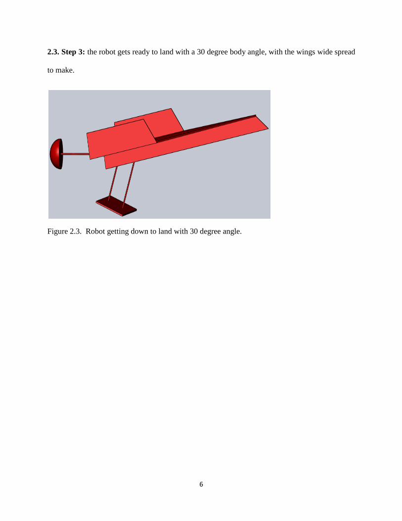
2.3. Step 3: the robot gets ready to land with a 30 degree body angle, with the wings wide spread

to make.

Figure 2.3. Robot getting down to land with 30 degree angle.

7

Chapter 3. Wings design:

The wings spreading and tightening is controlled by the spring at the bottom of the robot. The

wings are tighten by the springs during compression, and then released to flat wings after 0.8

second in mid. Wings material should be made with a light material, and firm enough to resist

wearing out during the process of spreading and tightening. A perfect material for the wings

should be of light weight and flexible, a bat wings is excellent prototype.

8

Chapter 4: Modeling [5].

B

0

Bodytail

lt

A

Y

X

C lb

θbθt

Figure 4.1 The schematic of the robot in the air. Modeling of the system

parameter

Body mass

Tail mass

Length of link BC

Length of link AC

Body angle with horizontal line.

Tale angle with horizontal line

Body moment of inertia ;

Tail moment of inertia

Table 4.1. LIST OF PARAMETERS FOR DYNAMICS MODELING

9

4.1 Robot Energies.

We use the energy to calculate the equation of motion for the robot.

4.1.1 Potential Energy

Potential energy is zero since robot is going back to same level after jump.

4.1.2 Kinetic Energy

2 2 2 2 2 21[ ( 2 cos )]

2

t bt t b b t t b b t b t b m

t b

m mI I l l l l

m m

4.2. Lagrange EOM for Robot

It’s used to calculate the equation of motions. The Potential energy of robot found to be zero as

the robot is returning to the same level after jump. For example, if we take level zero to be robot

at rest, and after robot landing to be level 2, then , that just interprets the robot is

releasing all the giving power to a kinetic energy, and that leads us to the calculation of the

kinetic energy

Since we want a one state to be controller, we can take the difference of the tail and the body as:

Defining m b t actuator’s rotation angle

Dynamics equation for the system as

2cos sint m b m bM L L

(1)

2cos sinb m t m tN L L

(2)

10

since we are concerned about the body angle b we will use only one input ,therefore our

system is under actuated , we need only a dynamic equation in terms of b , since that our

controlled angle.

First, we solve the t

and b

from Eqs.(1) and (2)

2 2cos(3)t m b

t

SL SN R

T

2 2 cos(4)t b m

b

SM SL Q

T

2

t b tt

t b

m m IM I

m m

2

t b tb

t b

m m IN I

m m

cos mR N L t b t b

t b

m m I IL

m m

,

cos mQ M L sin mS L

2 2cos mT MN L

11

From (3), (4) and m b t

,we have:

2 2

(5)t bm

SQ SR Q R

T T

Second, we utilize the conservation of angular momentum to eliminate both t

and b

in Eq. (5)

by expressing them as function of m

Angular momentum of the system:

0 ( cos ) ( cos )m t m bH M L N L

By assumption of zero angular momentum0 0H

We can solve for t and b as follows:

(6)mt

R

Q R

(7)mb

Q

Q R

Finally, plugging Eqs. (6) And (7) into (5), we can obtain:

2

( )m m

QRS Q Ru

T Q R T

(8)

12

Solving for b can result in the system output. 0

(0)

t

b m b

Qdt

Q R

(0)b

is the initial body angle.so, we can obtain the time to reach the desired angle *

b

4.3. Dynamics equations

2

( )m m

QRS Q Ru

T Q R T

0

(0)

t

b m b

Qdt

Q R

4.4. Transformation

The transformation is carried out in order to facilitate the controller scheme, and it’s transformed

to the controller form realization.

Defining parameters as:

1 mx 2 mx

3 bx 3y x

1 2x x

, 2

2 2( )

QRS Q Rx x u

T Q R T

, 3 3

Qx x

Q R

13

Chapter 5. Linearization

Linearizing the system around a desired operating points The challenge of such highly coupled

nonlinear system is by linearizing the system around a useful operating points, by forcing all the

system dynamics to zeros, we get .

So, is free to choose, and should be chosen to the constant we want the system to follow

Our desired operating point chosen arbitrary for

,

So operating point is

]

Before linearization: matrices A,B,C

[

]

[

] ]

After linearizing around desired operating points. The Jacobian would be:

[

]

,

[

]

2. Taking nothing to be unknown.

[

] , [

]

14

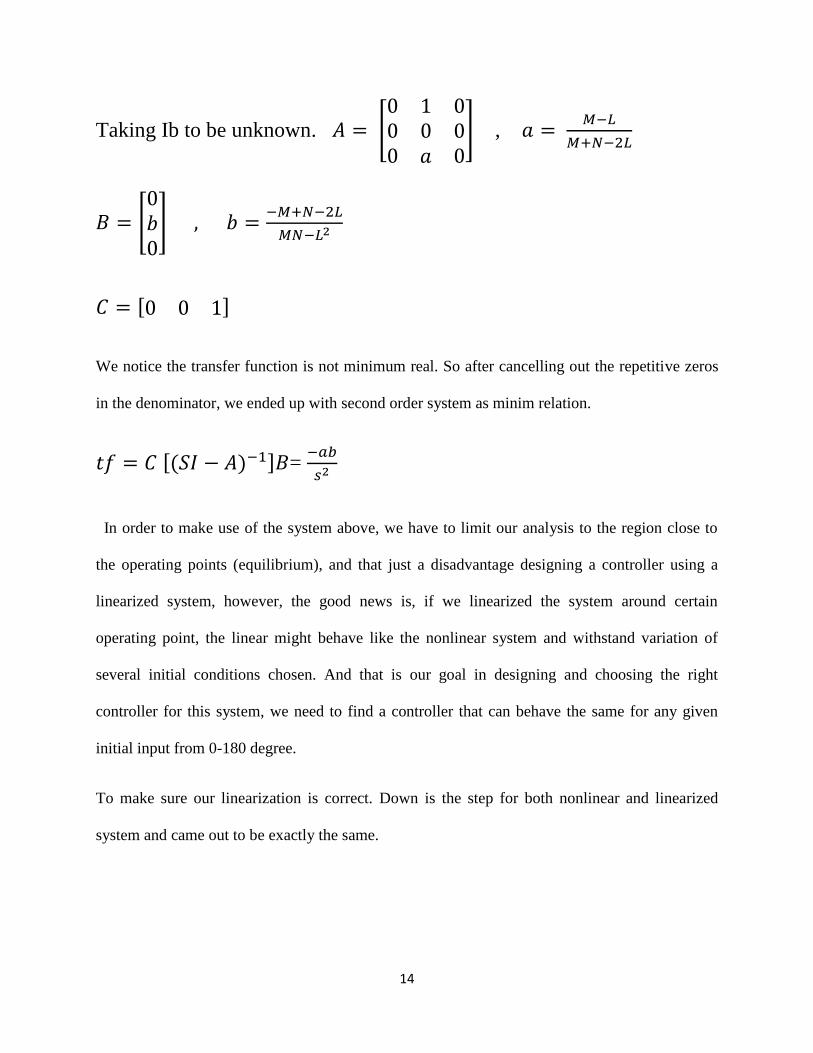
Taking Ib to be unknown. [

] ,

[ ]

]

We notice the transfer function is not minimum real. So after cancelling out the repetitive zeros

in the denominator, we ended up with second order system as minim relation.

] =

In order to make use of the system above, we have to limit our analysis to the region close to

the operating points (equilibrium), and that just a disadvantage designing a controller using a

linearized system, however, the good news is, if we linearized the system around certain

operating point, the linear might behave like the nonlinear system and withstand variation of

several initial conditions chosen. And that is our goal in designing and choosing the right

controller for this system, we need to find a controller that can behave the same for any given

initial input from 0-180 degree.

To make sure our linearization is correct. Down is the step for both nonlinear and linearized

system and came out to be exactly the same.

15

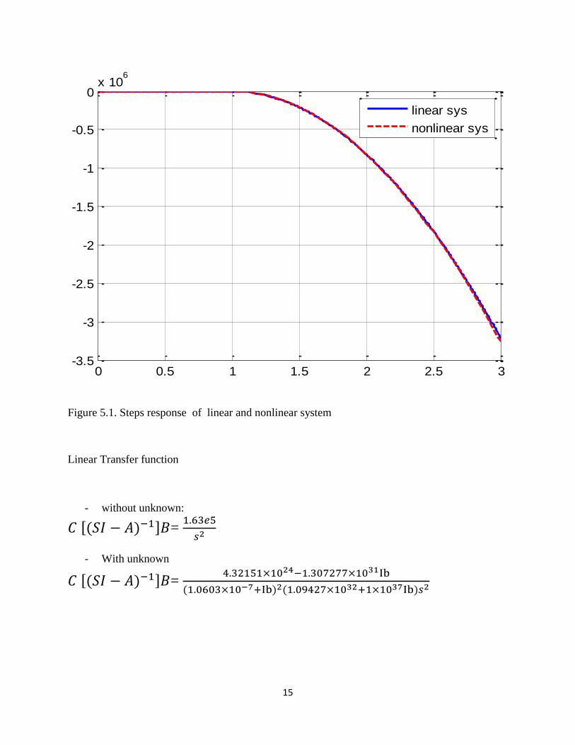
Figure 5.1. Steps response of linear and nonlinear system

Linear Transfer function

- without unknown:

] =

- With unknown

] =

0 0.5 1 1.5 2 2.5 3-3.5

-3

-2.5

-2

-1.5

-1

-0.5

0x 10

6

linear sys

nonlinear sys

16

Chapter 6 Estimation

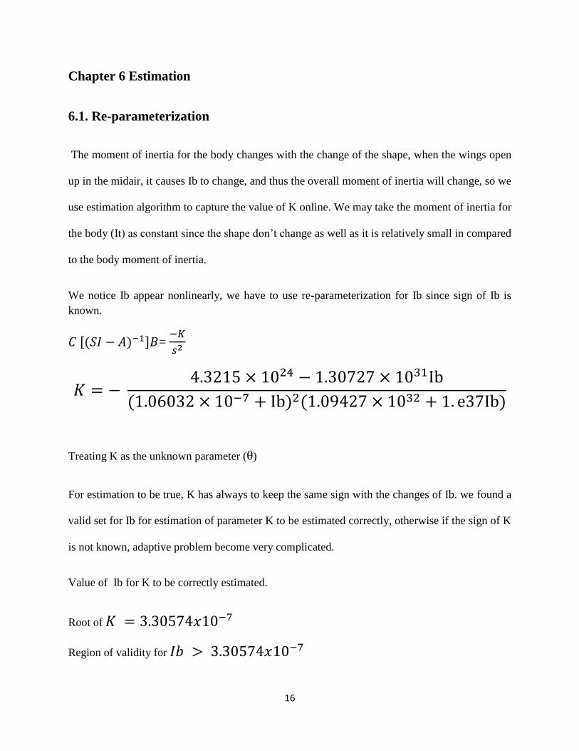
6.1. Re-parameterization

The moment of inertia for the body changes with the change of the shape, when the wings open

up in the midair, it causes Ib to change, and thus the overall moment of inertia will change, so we

use estimation algorithm to capture the value of K online. We may take the moment of inertia for

the body (It) as constant since the shape don’t change as well as it is relatively small in compared

to the body moment of inertia.

We notice Ib appear nonlinearly, we have to use re-parameterization for Ib since sign of Ib is

known.

] =

Treating K as the unknown parameter (θ)

For estimation to be true, K has always to keep the same sign with the changes of Ib. we found a

valid set for Ib for estimation of parameter K to be estimated correctly, otherwise if the sign of K

is not known, adaptive problem become very complicated.

Value of Ib for K to be correctly estimated.

Root of

Region of validity for

17

6.2. Gradient Algorithm.

Gradient algorithm is used to generate K on-line.

6.2.1.Gradient without protection.

] ,

]

, , ,

Note: We only require to be rich of at least order 2 to guarantee convergence of the unknown

parameter.

Figure 6.2.1.1. Estimation without projection.

0 0.5 1 1.5-2

0

2

4

6

8

10

12x 10

-5

Time (seconds)

Estimation without projection

Estimate of k

18

Figure 6.2.1.2. Tracking, without projection

6.2.2. Gradient with protection

In estimation of a parameters online, we use projection to ensure the estimate lay within bounded

desired values. Sometime the algorithm runs under certain conditions that make the estimate drift

away or result in an unwanted, with the prior knowledge of the unknown parameters, and knowing

the upper and lower bound, we can generate the desired estimate using those bounds and forcing

the estimate to be within the bounds. We use projection to limit within bounds

[

]

For simulation: Taking

Simulink model is included in appendix A

0 1 2 3 4 5-50

0

50

100

150

200

250Tracking

Time (seconds)

Measured

Desired

19

Figure 6.2.2.1. Estimation with projection.

Figure 6.2.2.2. Tracking is not maintained

Noting that in estimation with projection is always a tradeoff between desired tracking and

desired estimation; however in our purpose of estimation, we only wanted a true estimate of the

unknown parameter.

0 1 2 3 4 5-1.642

-1.64

-1.638

-1.636

-1.634

-1.632

-1.63

-1.628x 10

5

Time (seconds)

Estimation with Projection

Estimate of k

0 1 2 3 4 5

0

2

4

6

8

10

12

14

16

18x 10

10 Tracking

Time (seconds)

Measured

Desired

X 10^5

20

Chapter 7. Designing controller

Since we want to control only the body pitch angle, we need at least one control input to control

the motor. The body angle is moving through the angle of the tail, by maneuvering the tail in

way which result in the desired angle for the body, this procedure seen exactly in the slow

motion of a jumping gecko[ 2].

Designing controller by:

7.1.MRAC

7.2.APPC

7.3.PD

7.4.SMC

7.5.ASMC

7.1. Designing controller by MRAC:

For MRAC to work, the model reference has to be a monic of order one. And our reference

constant is of order zero, so we needed to multiply the constant of order zero with a filter of

order 1 in order to satisfy the scheme conditions.

21

Figure 7.1.1.

= 0.5236 = 30 Degree, Tracking of MRAC

Figure 7.1.2.Tracking error

0 1 2 3 4 5 6 7 8 9 10-0.1

0

0.1

0.2

0.3

0.4

0.5

0.6

0.7

Time (seconds)

data

Time Series Plot:

Yp

Ym

0 1 2 3 4 5 6 7 8 9 10-0.4

-0.3

-0.2

-0.1

0

0.1

0.2

0.3

Time (seconds)

Error

22

7.2. Designing controller by APPC

Objective: 3 bx to follow a reference of 30 degree within desired SPEC.

- Desired controller SPEC:

a) Overshoot , .

b) Settling time .

Using gradient algorithm to estimate unknown (K)

- Estimation of unknown (K)

Gradient algorithm is used to generate K on-line.

]

]

, ,

We use projection to limit within bounds

Gradient with projection :

We use projection to limit within bounds

n= order of plant=2, q= degree of Qm=1

We can choose desired dominant poles to be and the other two poles to

be atleast 10 times far to the left as shown below:

23

45=θ

-2 j

-2

-2 j

wn

-32-22

Figure 7.2.1.Schematic diagram of desired pole placement.

Overall controller is:

Figure 7.2.2. APPC controller using simulink blocks.

24

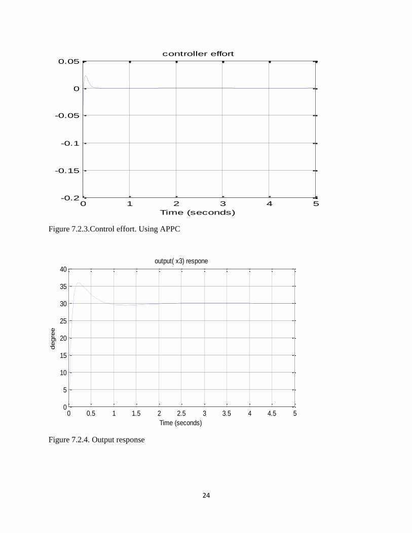
Figure 7.2.3.Control effort. Using APPC

Figure 7.2.4. Output response

0 1 2 3 4 5-0.2

-0.15

-0.1

-0.05

0

0.05controller effort

Time (seconds)

effo

rt

0 0.5 1 1.5 2 2.5 3 3.5 4 4.5 50

5

10

15

20

25

30

35

40

Time (seconds)

degre

e

output( x3) respone

25

Multi reference testing for the nonlinear system. The output response is the same

Figure 7.2.5. multi reference testing for the nonlinear system

Figure 7.2.6. Control effort for multi references.

0 0.5 1 1.5 2 2.50

0.5

1

1.5

2

2.5

3

3.5

4

4.5

5

0 0.05 0.1 0.15 0.2 0.25 0.3 0.35-0.025

-0.02

-0.015

-0.01

-0.005

0

0.005

5

2

4

3

0

1

2.5 2 1

26

7.3. Designing controller by PD

The main disadvantage of existence design procedures of PI or PID controllers are that the

desired transient performances in the closed-loop system cannot be guaranteed in the presence of

nonlinear plant parameter variations and unknown external disturbances [7].

PID don’t deal with unmolded dynamics or time delay in feedback loop, so the effect of

unmolded dynamics and time delay transient stability should be taken into account in order to

take into account of controller parameters, this put the main restriction on the practical

implementation of the controller design.

After we linearized the system into a linear form. We fed the error between the output (θb) and a

constant reference of 30 degree to a PID controller to improve the transient respond as well as to

produce zero steady state error. We found that PID is a great controller for only an ideal

environment. PID controller can’t deal with Uncertainties and variation of parameters.

PD Nonlinear plant

Sensor

r e X3 = θb+

-

yu

Figure 7.3.1. PD scheme desgin

Tuning using Simulink tuner. .

Kp= 0.9, Kd= 5

27

Figure 7.3.2. output response, reaching 30 degree in 0.5 sec

Figure 7.3.3. control effort to reach a 30 degree reference

0 0.2 0.4 0.6 0.8 10

5

10

15

20

25

30

35output response

Time (seconds)

degr

ee

theta b

0 0.05 0.1 0.15 0.2 0.25 0.3-0.015

-0.01

-0.005

0

0.005

0.01

0.015

effort

error

28

Figure 7.3.4. Multi intial conditions testing

Figure 7.3.5. Control effort for multi initial conditions.

0 0.2 0.4 0.6 0.8 15

10

15

20

25

30

35

40

0 0.002 0.004 0.006 0.008 0.01-0.04

-0.035

-0.03

-0.025

-0.02

-0.015

-0.01

-0.005

0

0.005

29

7.4. Designing slide mode controller

Sliding mode controller deal with uncertainty much better than any controller [8]. It can take all

the variation in parameters, with right high feedback gain chosen; it can result in a very good

output response. One trick here is sliding mode controller should always be designed for the

minimal realization, as it get complicated with the error differentiation. Although we represented

our system as third order, but in reality after zero pole cancelation, the system is just second

order. The complexity of feedback can always be simplified using sliding mode controller, and

that by breaking the system coupling into low reduced order components.

Two cases for Ib :

Ib is perfectly known as in the case of fixed Ib. then SMC is:

2

( )m m

QRS Q Ru

T Q R T

Defining error as

Defining sliding surface as

30

(

)

,

[

] [

] [

[

] ]

[

] [

] [

[

] ] [

]

]

[

] ([

] [

] [

] [

] )

Taking lyapunov function candidate as:

, ,

{[

] [

] [

[

] ] [

] }

Plugging in u in

31

| |

To eliminate the chattering in the controller, we choose a saturation function, that will behave as

high slop from –� to � and saturate with constant value anywhere outside the sett [-�,�] with

constant value of [8]

Sgn(y)

-1

1

0.001y

Sat ( y/ ) 1

-1

Figure 7.4.1. Signum nonlinearity function, replaced by approximation function. .

Choosing small enough can result in more precise set.

The overall control law is:

[

] ([

] [

] [

])

If we choose k1 large enough to overcome the nonlinearities in the controller. We found out the

right gain is 1081.

For simulation

=0.001,

k1=1081.7

32

Figure 7.4.2 Scheme of SMC

Figure 7.4.3 Control effort SMC

0 0.5 1 1.5 2 2.5 3-0.4

-0.3

-0.2

-0.1

0

0.1

0.2

0.3

Time (seconds)

cont

rol e

ffor

t

u

3 3 2 1

0.3

-0.3

0

0

.

3

u

33

Figure 7.4.4. output response, reaching 30 degree in 0.5 sec.

Figure 7.4.5. Ttracking of desired response

0 0.5 1 1.5 2 2.5 30

5

10

15

20

25

30

35

Time (seconds)

degr

eenonlinear system output response

0 0.1 0.2 0.3 0.4 0.5 0.60

0.1

0.2

0.3

0.4

0.5

Time (seconds)

data

measured

reference

pi/6

34

7.5. Designing ASMC

If Ib is totally not known. Then ,we use adaptive sliding mode controller.

Taking control input as

[

] ([

] [

] [

])

the adaption law is :

| |,

ASMC simulation :

,

Since we re tracking a reference

Simulation results below:

Ploting for intial conditions : top to bottom ( ,

,

)

Figure 7.4.6. Tracking response for multi initial condition

0 0.05 0.1 0.15 0.2 0.25 0.3 0.35 0.4 0.45 0.50

0.5

1

1.5

2

2.5

3

3.5

Measured

Desired

0.1 0.2 0.3 0.4 0.5

2

1

0

3

35

Figure 7.4.7. Error for multi intial conditions. ( ,

,

)

Figure 7.4.8. Control effort bounded.

0 0.05 0.1 0.15 0.2 0.25 0.3 0.35 0.4 0.45 0.5-0.07

-0.06

-0.05

-0.04

-0.03

-0.02

-0.01

0

0.01

Error

0 0.2 0.4 0.6 0.8 1 1.2 1.4 1.6 1.8 2

-0.05

-0.04

-0.03

-0.02

-0.01

0

0.01

0.02

0.03

0.04

0.05

Time Series Plot:

Time (seconds)

data

Control Effort

0.01

0

.

0

1

0.1 0.2 0.4 0.3 0.5 0

-0.04

-0.06

-0.01

0

-0.05

0.05

0 1 2

36

Chapter 8. Conclusion

8.1. Comparison of controllers.

After designing controller, one cannot really predict the behavior of the controller unless the

controller is subject to several tests such as ability to reject disturbance, or become robust to

uncertainties.

8.1.1 Disturbance rejection test

Figure 8.1.1.1. APPC versus PID 0.1 noise power

0 0.1 0.2 0.3 0.4 0.5 0.6 0.7 0.8 0.9 10

5

10

15

20

25

30

35

APPC

Ref

PID

Ref

37

Figure 8.1.1.2 APPC versus PID noise power 1

Figure 8.1.1.3. SMC versus PD, for noise power 0.0001

0 0.1 0.2 0.3 0.4 0.5 0.6 0.7 0.8 0.9 10

5

10

15

20

25

30

35

40

APPC

ref

PID

Ref

0 0.1 0.2 0.3 0.4 0.5 0.6 0.7 0.8 0.9 10

5

10

15

20

25

30

35

PID

Reference

SMC

Reference

30

0 1

30

1 0

Ref

PID

Ref

APPC

SM

C

PID

Ref

Ref

38

Figure 8.1.1.4 SMC versus PID noise power 0.001

Figure 8.1.1.5 SMC versus PID noise power 0.1

0 0.1 0.2 0.3 0.4 0.5 0.6 0.7 0.8 0.9 10

5

10

15

20

25

30

35

SMC

Ref

PID

Ref

0 0.1 0.2 0.3 0.4 0.5 0.6 0.7 0.8 0.9 10

5

10

15

20

25

30

35

PID

Ref

SMC

Ref

30

0 1

30

1

0

39

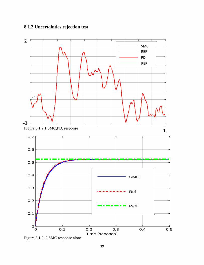
8.1.2 Uncertainties rejection test

Figure 8.1.2.1 SMC,PD, response

Figure 8.1.2..2 SMC response alone.

0 0.1 0.2 0.3 0.4 0.50

0.1

0.2

0.3

0.4

0.5

0.6

0.7Time Series Plot:

Time (seconds)

data

SMC

Ref

Pi/6

0 0.1 0.2 0.3 0.4 0.5 0.6 0.7 0.8 0.9 1-3

-2

-1

0

1

2

3

4

5

6

7

SMC

Ref

PID

Ref

2

-3

1

SMC

REF

PD

REF

40

8.1.3 Summary

Looking back at the different controllers, we found out that the PID isn’t perfect for none deal

environment, it might give great results for simulation, however in reality the case is different

where is lots of variations in parameters and uncertainties, so we excluded PD.

Looking at APPC, which is in a way suitable for nonlinear system, however we found that the

speed of adaption is much slower than the speed of the controller ( PPC), in way that delay the

settling time for the nonlinear system, another issue for APPC is that some intimal conditions can

blow up the output response and that is discovered by trying different initial conditions, as the

system has singularity at T=0, so we may take APPC, but not for a general case.

Looking at MRAC, choosing the right model reference is a great deal for a fast adaptation. But the

same problem has accrued here with APPC, since we are looking for a reasonably fast response as

the robot is in midair, we are looking for a part of a second. And using a model reference for

MRAC has to be monic of order one, which delays the speed of adaption even more than APPC,

so same case of MRAC for APPC.

Looking at sliding mode control, it’s so far the best in terms of dealing with uncertainties, and

unmolded dynamics. The speed of adaption is reasonably fast as the absolute value of the sliding

surface is chosen somewhere close to 1 and with the value of the gain gama, that will ever boost it

to a desired value, adding into account also the value of the feedback gain (k) may contribute to

the overall process by canceling out nonlinearities and fasten up the output response.

We recommend adaptive sliding mode controller as the most efficient controller in dealing with

varying system parameters and system uncertainties.

41

8.2. Contribution to MSU jumper Robot.

I have contributed to the MSU jumping robot project by designing an adaptive efficient controller

which estimate online the mass of moment of inertia for body before landing, and feeding the

estimate to a controller. Also, I have prolonged the jumping period, which lead to prolonging the

length of jump with the same power provided to MSU jumping robot.

8.3. Results of new schematic design

Spreading out wings in midair maximize drag force. Just like a parachute. The robot dose glides

and then parachute by spreading out wings.

1- Enabling wings maximizing the length of each jump for same given power.

2- Wings facilitate the landing process.

8.4. Future work

1- A three dimensional controller of a glider, as in the case of flying dragon

Figure 8.4.1. Left to right: Weigeltosaurus, Icarosaurus, and Draco.[9]

Design of the tail and the wings. More flexible to impact surface.

42

BIBLIOGRAPHY

43

BIBLIOGRAPHY

[1]. Doyoung Chang; Donghun Son; TaeWon Seo; Woochul Nam; Dongsu Jeon; Jongwon Kim,

"Kinematics-based gait planning of a quadruped gecko-like model," Robotics and Biomimetics

(ROBIO), 2009 IEEE International Conference on , vol., no., pp.233,238, 19-23 Dec. 2009

[2]. Chang-Siu, E.; Libby, T.; Tomizuka, M.; Full, R.J., "A lizard-inspired active tail enables

rapid maneuvers and dynamic stabilization in a terrestrial robot," Intelligent Robots and Systems

(IROS), 2011 IEEE/RSJ International Conference on , vol., no., pp.1887,1894, 25-30 Sept. 2011.

[3].Xin-Sheng Ge; Qi-Zhi Zhang, "Optimal Control of Nonholonomic Motion Planning for a

Free-Falling Cat," Innovative Computing, Information and Control, 2006. ICICIC '06. First

International Conference on , vol.2, no., pp.599,602, Aug. 30 2006-Sept. 1 2006

[4]. http://www.bostondynamics.com/img/SandFlea%20Datasheet%20v1_0.pdf

[5]. Jianguo Zhao, Tianyu Zhao, Ning Xi, Fernando J. Cintr´on, Matt W. Mutka, and Li Xiao

‘Controlling Aerial Maneuvering of a Miniature Jumping Robot Using Its Tail’

[7]. Valery D. Yurkevich (2011). PI/PID Control for Nonlinear Systems via Singular

Perturbation Technique,Advances in PID Control, Dr. Valery D. Yurkevich (Ed.), ISBN: 978-

953-307-267-8, InTech, Availablefrom:http://www.intechopen.com/books/advances-in-pid-

control/pi-pid-control-for-nonlinear-systems-via-singularperturbation-technique.

[8]. Khalil, H.K. (2002). Nonlinear Systems, 3rd ed., Upper Saddle River, N.J. : Prentice Hall,

ISBN0130673897.

[9]. Padian, K. 1985.The origins and aerodynamics of flight in extinct vertebrates. Palaeontology

28(3): 413-433.