electronics

Article

Control of Two Satellites Relative Motion over thePacket Erasure Communication Channel with LimitedTransmission Rate Based on Adaptive Coder

Boris Andrievsky 1,2,3,* , Alexander L. Fradkov 1,2,4 and Elena V. Kudryashova 4

1 Institute of Problems in Mechanical Engineering, Russian Academy of Sciences, 199178 Saint Petersburg, Russia;fradkov@mail.ru

2 Department of Applied Cybernetics, Saint Petersburg University, 198504 Saint Petersburg, Russia3 Scientific-Research Department, Baltic State Technical University, 190005 Saint Petersburg, Russia4 Intelligent Technologies and Robotics Research Center, ITMO University, 197101 Saint Petersburg, Russia;

e.kudryashova@spbu.ru* Correspondence: b.andrievsky@spbu.ru; Tel.: +7-812-321-4776

Received: 10 November 2020; Accepted: 23 November 2020; Published: 1 December 2020

Abstract: The paper deals with the navigation data exchange between two satellites moving in a swarm.It is focused on the reduction of the inter-satellite demanded communication channel capacity taking intoaccount the dynamics of the satellites relative motion and possible erasures in the channel navigationdata. The feedback control law is designed ensuring the regulation of the relative satellites motion.The adaptive binary coding/decoding procedure for the satellites navigation data transmission overthe limited capacity communication channel is proposed and studied for the cases of ideal and erasurechannels. Results of the numerical study of the closed-loop system performance and accuracy of thedata transmission algorithm on the communication channel bitrate and erasure probability are obtainedby extensive simulations. It is shown that both data transmission error and regulation time dependapproximately inversely proportionally on the communication rate. In addition the erasure of data inthe channel with probability up to 0.3 does not influence the regulation time for sufficiently high datatransmission rate.

Keywords: data transmission; erasure communication channel; adaptive coding; satellite formation

1. Introduction

In recent years, there has been a growing interest in using the differential force (i.e., the differencebetween the aerodynamic drag forces applied to the satellites) to eliminate the relative drift betweenthe satellites in a swarm moving in a group (without the mandatory requirement to maintain relativeposition, cf. [1–3]). Various control algorithms using differential aerodynamic drag have been proposed innumerous publications, see [4–16]. One of the fundamental publications is the work by Leonard [17] where,based on the assumption of the possibility of changing the effective cross-section of satellites, a method ofswitching control has been developed. The differential force is created by changing the attack angles ofthe plates, located on the satellites, due to the rotation of the satellites with respect to the incident airflow.Kim et al. [18] deal with a satellite constellation, consisting of a leader satellite and surrounding slave ones.The orbit of the leader is considered as a reference, whilst the relative orbits of the followers are consideredto be the Projected Circular Orbit (PCO), which is the relative orbit between the master and slave satellites,

Electronics 2020, 9, 2032; doi:10.3390/electronics9122032 www.mdpi.com/journal/electronics

Electronics 2020, 9, 2032 2 of 21

being a circular one when it is projected onto the local horizontal plane [19]. PCO predicted distances [20]between master and slave satellites are constant. The Hill–Clohessy–Witshire (HCW) equation describesthe relative motion between the satellites in the local reference frame Local Vertical Local Horizontal(LVLH), with the origin on the master satellite. Monakhova and Ivanov [21] considered the problem ofconstructing a swarm from a large number of nanosatellites immediately after their separation from thelauncher. To solve the problem of eliminating the drift between satellites, in [21] the decentralized controlbased on the force of aerodynamic drag is employed.

In the decentralized control of satellite formations, the problem of inter-satellite communicationis very important. This communication is needed for navigation data exchange between the satellites.Particularly, Sarno et al. [22] presented innovative approaches for the guidance of spacecraft formationsduring reconfiguration. The method is conceived such that each satellite autonomously determines its tasks,allowing the algorithm to run faster, but entails a higher traffic on the inter-satellite communication link.Therefore the inter-satellite communication problem is a challenging one and attracts considerable interestof many researchers.

The electron density irregularities caused by ionosphering turbulence, scatterring radio waves,and affecting satellite communication were taken into account in [23]. Delay tolerant networking(DTN) protocols, such as bundle protocol and medium access control (MAC) were considered byFreimann et al. [24] as appropriate approaches for networks with intermittent connectivity such as deepspace or low Earth orbit networks. A contact plan design approach was presented in [24] that solvedthe MAC problem by predicting additive multi-node interference and scheduling interference-free linksbased on these predictions. In [25], the algorithm called parallel data transmission for the navigationsatellite network with agility link was proposed. Based on the network characteristics, the algorithmwas designed with a polling pattern of link establishment and formulated as parallel data transmissionproblem based on deterministic scheduling the delay tolerant network. Cai et al. [26] presented a completesoftware-defined radio (SDR) model for inter-satellite communications and its implementation on afield-programmable gate array. The proposed SDR has low power consumption, which is suitable forpower-limited small satellite systems. Davarian et al. [27] presented the results of a study exploringconcepts for improving communications and tracking capabilities of deep space SmallSats. A detailedexamination of relay proximity links and networks, where both proximity hardware and networkingscenarios was addressed. A strategy for secure data correspondence between the smart city’s vehicularnodes, which uses the fundamentals of Elliptic Curve Cryptography (ECC) for key agreement andsatellite communication for the transmission of messages over vehicles is proposed by Poomagal andSathish Kumar [28]. Ujan et al. [29] presented a method to recognize received signal characteristics usinga hierarchical classification in a multi-layer perceptron neural network. The experiments were describedwhere a real-time video stream transmitted in the direct broadcast satellite was utilized with severalmodulation types of radio frequency interference. In [30], a routing algorithm to solve the link congestionproblem caused by the limited topology in a topology-inhomogeneous Low Earth Orbit (LEO) satellitenavigation augmentation network was proposed and a congestion avoidance routing model for thetopology-inhomogeneous LEO satellite navigation augmentation network was established.

Important restrictions on the control performance are imposed by communication constraints. In [21],communication constraints were taken into account in the sense of the radio signal fading with increasingthe inter-satellite distance. This leads to the space limitation within which the position of neighboringvehicles can be transmitted between them and, consequently, to reducing the number of satellites thatare available for navigation data exchange. However the limitations on the transmission rate are nottaken into account both in [21] and in the other above mentioned papers. It is worth noting that inpractice the data transmission rate over the communication channels is always limited and, moreover,its minimization is highly useful from an energy consumption viewpoint. Among other things, decreasing

Electronics 2020, 9, 2032 3 of 21

the data transmission rate for the given power consumption can make it possible to increase the power oftransmitted signals, expanding the area of inter-satellite interaction.

The present paper is focused on the reduction of the inter-satellite demanded communication channelcapacity taking into account dynamics of the satellite’s relative motion and possibility of erasing thenavigation data in the channel.

The limitations of control under constraints imposed by the limitations of the communication channelcapacity, have been deeply studied within the control theoretic literature, see [31–35] and the referencestherein. A fundamental result establishing the smallest value for which the stabilization (estimation)problem for linear time invariant (LTI) systems is obtained by Nair and Evans [31] and presented in theform of the seminal Data Rate Theorem. However, the study of the application control problems inaerospace under communication constraints is still very limited.

In the present paper, a system of two coupled satellites is considered. As in [21], the satellites areassumed to be launched at the starting time in accordance to the specified separation conditions. It isassumed that the satellites move in a low circular near-Earth orbit and are controlled using the aerodynamicdrag force, which is achieved by rotating the satellite relative to the incoming flow using a flywheel attitudecontrol system. The main focus of the paper is in the navigation data exchange between the satellites to beused to keep the satellite motion in a swarm. To this end, the adaptive coding procedure is proposed andis studied for the cases of ideal and erasure communication channel. The regulation time is taken as theperformance criterion, and its dependence on the data transmission rate is numerically studied.

The reminder of the paper is organized as follows. The existing results on control and estimationunder information constraints are briefly recalled in Section 2, where the minimum necessary data ratefor the estimation and control of Linear Time Invariant (LTI) systems in the form of the data rate theoremis specified and various coding/decoding schemes are described. Section 3 is devoted to the dynamicsof two satellites’ relative motion in a near-circular orbit. The main result is concentrated in Section 4.This section starts with designing the control law, which ensures the asymptotic regulation of the satellitesrelative motion (Section 4.1). The design is based on the linearized dynamics model without taking intoaccount the control signal saturation. The classical modal control approach based on the pole-placementtechnique is employed [36]. The behavior of the system with the saturation in control is studied inthe subsequent sections by the simulations. The next stages of the present study are dedicated to theevaluation of the proposed scheme of the inter-satellites data transmission over a digital communicationchannel, aimed for reducing the necessary channel capacity. To this end, the adaptive coding procedurefor the position transmission between the satellites in the formation, employing the kinematics processdescription, is introduced in Section 4.2. It is worth mentioning that the application of this procedure makesit possible to avoid measuring the time derivatives of the satellites relative position (these derivatives areneeded for control) due to the state observer, which is embedded into the adaptive coder/decoder pair.Then in Section 4.3, the model of the erasure communication channel, adopted in the present research,is described. Results of the numerical study of the closed-loop system performance and accuracy of thedata transmission algorithm dependence on the communication channel bitrate and erasure probabilityobtained based on the extensive simulations are presented in Section 4.4. Concluding remarks and thefuture work intentions given in Section 5 finalize the paper.

2. Control and Estimation under Information Constraints

2.1. Problem Description

Let us consider control and observation (estimation) systems containing a digital communicationchannel. For these systems, plant output measured by the sensor at discrete instants tk = kT0, whereT0 denotes the sampling interval, k = 0, 1, . . . , is converted by the coder into the characters of the coding

Electronics 2020, 9, 2032 4 of 21

alphabet S. The sequence of characters is transmitted over a digital communication channel to the decoder.The decoder transforms messages from the transmitted form in a form adequate to subsequent calculationsand transformations by the controller. In [37–39] the communication channel was considered of limitedcapacity, but was otherwise ideal. The cases of packet erasure channel and ‘blinking’ channel widely appearin various real-world systems, see, e.g., [40–49]. Therefore, for a more realistic analysis, the properties ofthe communication channel, such as distortion, erasure, and data loss, should be taken into account. In thepresent study, the effect of data erasure is considered.

Signal quantization introduces essentially non-linear properties into the system, characterized by thepresence of the dead zone, discontinuities, and saturation (associated with bit grid overflow). Additionally,the signal sampling on time involves the hybrid (continuous-discrete) system description. A rigorousexamination of the influence of time sampling and the level quantization is a complex nonlinear analysisproblem, that usually does not have an exact analytical solution. In the early studies, the level quantizationin digital control systems was usually considered a source of independent additive random noise affectingthe system. This assumption makes it possible to significantly simplify the study of level quantized systems,especially for LTI plants. However, if the quantization level is relatively high (for example, in the case ofbinary quantization), this can lead to the emergence of self-oscillations and even the system divergence,see [50–53]. Therefore, to analyze the system, its nonlinear model is required. Besides, the possibility ofthe bit grid overflow can also affect the quantizer, as a result of which the saturation is introduced to thecontrol loop [54,55].

2.2. Minimum Necessary Data Rate for Estimation and Control

The limitation of the data transmission rate over the communication channel can be expressed ininformational terms. Assume that coding alphabet S consists of µ elements. Then at each step k = 0, 1, . . .over the channel an amount of R = log2 µ bit can be transmitted per each step. Let the data transmissionbe carried out at discrete instants tk = kT0, where T0 is the sampling interval. Then the data transmissionrate in bits per second is as R = T−1

0 log2 µ bit/s. In this regard, one speaks of “information constraints” incontrol and estimation problems.

The problem of determining the minimum bandwidth of the communication channel, at which it ispossible to provide the required estimation accuracy, is posed and partially solved by Nair and Evans [56].The sufficient condition for the value obtained in Nair and Evans [56] was developed in subsequentworks in the form of the Data Rate Theorem which is a fundamental result establishing the smallestvalue for which the stabilization (estimation) problem for linear systems is solvable in principle.Nair and Evans [31] studied the exponential stabilizability of LTI plants in the sense of achieving anexponential moment stability. For a deterministic initial state case the result of [31] can be roughlypresented in the following form [57].

Let the LTI discrete-time plant be described by the difference equation:

x[k + 1] = Ax[k] + Bu[k], y[k] = Cx[k], k = 0, 1, . . . (1)

where x[k] ∈ Rn, y[k] ∈ Rl , and u[k] ∈ Rm are the state, output, and control vectors, respectively; A, B,and C are the matrices of the corresponding dimensions; and k ∈ Z+ denotes the step number (the discretetime). It is assumed that pair (A, B) is reachable and (C, A) is observable. Let the sensor be connected tothe controller over a digital communication channel, and no more than R bits of data can be transmitted ateach step k. Then the necessary and sufficient conditions for ρ-exponential (with the prespecified stabilitybound ρ > 0) stabilization are given by the inequality [31]:

Electronics 2020, 9, 2032 5 of 21

R > ∑ηj≥ρ

log2

∣∣∣∣ηj

ρ

∣∣∣∣ (bit per step), (2)

where ηj are the eigenvalues of matrix A , j = 1, . . . , n. The right-hand side of (2), denoted as

RNE = ∑ηj≥ρ

log2

∣∣∣∣ηj

ρ

∣∣∣∣ (the Nair–Evans-, or NE-number), gives a tight admissible bound when ρ-exponential

stabilization can be achieved. For real-time systems with the constant sampling interval T0, NE-numberRNE in bits per second has a form:

RNE =1T0

RNE =1T0

∑ηj≥ρ

log2

∣∣∣∣ηj

ρ

∣∣∣∣ (bit per second). (3)

Extensions of this result for stabilizing nonlinear systems in the vicinity of the origin andobserving nonlinear systems through finite capacity communication channels, including large networks,were obtained in the series of the subsequent papers, see [58–62] to mention a few.

It is worth mentioning that on practice, the data transmission rate can not be taken as small as theNE-number (3) gives due to several reasons for the data bitrate being usually much greater than RNE,but the NE-number can serve as a measure showing the maximum available possibilities of estimationand control over the existing communication channel. Furthermore, a promising approach is to employthe event-triggered control instead of the control with constant sampling time, see e.g., [63–65].

2.3. Coding/Decoding Schemes

Under the assumption that the sampling time T0 can be chosen arbitrarily, optimality of the binarycoding in the sense of the required transmission rate (in bit-per-second) has been proven in [39], see also [66].Therefore in the present study the binary quantizer is used as a core element for the coding procedure.

2.3.1. Static Binary Quantizer

Let σ[k] be a scalar information signal to be transmitted over the digital communication channelin discrete instants tk = kT0, where k = 0, 1, · · · ∈ Z+ is a sequence of natural numbers, and T0 is thesampling interval. Let us introduce the following static quantizer:

q(σ, M) = M[k]s, s = sign(σ), (4)

where sign(·) is the signum function: sign(σ) = 1, if σ ≥ 0, sign(σ) = −1, if σ < 0. Parameter M isreferred to as a quantizer range. The output signal of the quantizer is represented as one-bit informationsymbol from the coding alphabet S = −1, 1, and is transmitted to the decoder. Note that for the binarycoder, the transmission rate is as R = 1/T0 bit per second. It is assumed that the equi-memory condition isfulfilled, i.e., the coder and decoder make decisions based on the same information [67,68]. The binaryoutput codeword s ∈ S is transmitted to the decoder.

2.3.2. Zooming Strategies

In time-varying quantizers [33,39,69–72] range M is updated with time. Using such a zooming strategyimproves the steady-state accuracy of the transmission procedure and at the same time prevents theencoder saturation at the process beginning. The values of M[k] can be precomputed (the time-basedzooming) [39,73,74], or current quantized measurements can be used at each step for updating M[k]

Electronics 2020, 9, 2032 6 of 21

(the event-based zooming). For an audio channel, Moreno-Alvarado et al. [75] developed the codingschemes with the capacity to simultaneously encrypt and compress audio signals, which makes possibleincreasing necessity for transmitting sensitive audio information over insecure communication channels.

The event-based zooming can be realized in the form of the adaptive zooming [76–79], where thequantizer’s range is adjusted automatically depending on the current variations of the transmitted signal.

For the binary quantizer the following adaptive zooming algorithm was proposed and experimentallystudied in [78]:

λ[k] = (s[k] + s[k− 1] + s[k− 3])/3, s[−1] = s[−2] = 0,

M[k + 1] = mc +

ρM[k], if |λ[k]| ≤ 0.5,

M[k]/ρ, else,σ[k] = M[k]s[k],

(5)

where M[0] = M0 is an initial value of M[k] (the design parameter) and σ[k] denotes the value of σ[k]recovered at the decoder side from binary values s[k]. Unlike the case of the time-based zooming, the initialvalue M0 can be chosen arbitrarily, since M[k] is automatically adjusted and can be increased or decreasedduring the zoom-in or zoom-out stages.

2.3.3. Coders with Memory

The coding/decoding procedure can include the embedded observer, which adds a memory to thecoder. The following model of drive process is used:

x(t) = Ax(t) + Bϕ(t), y(t) = Cx(t), x(0) = x0 (6)

where x(t)∈ Rn is the process state space vector; y(t) is the scalar measured signal; A∈ Rn × n, B∈ Rn × 1

are given real matrices; and ϕ(t) is the external input signal which is assumed to be the same both on thetransmitter and the receiver sides (so that the equi-memory condition be fulfilled).

The quantized observation error σ[k] is defined as a deviation between measured signal y(t) and itsestimate y(t) quantized with given M[k] as follows:

σ[k] = q(y(tk)− y(tk), M[k]

), tk = kT0. (7)

where the estimate y(t) is generated by the following observer:

˙x(t) = Ax(t) + Bϕ(y(t)

)+ Lσ(t), y(t) = Cx(t), (8)

where x(t)∈ Rn is the state estimation vector; y(t) is the estimate of the drive process; L is (n ×1)-matrix(the column-vector) of the observer parameters; and the continuous-time observation error σ(t) is foundas an extension of σ[k] over the sampling interval. In the case of the zero-order extrapolation, σ(t) has a formσ(t) = σ[k] as tk ≤ t < tk+1.

3. Relative Motion Dynamics of Two Satellites in a Near-Circular Orbit

For describing the dynamics of the relative motion of two satellites, moving in near-circular orbits atthe Earth’s central gravitational field, equations in the Local Vertical Local Horizontal (LVLH) referencesystem in relative coordinates according to the HCW model is used, see [21,80–84].

Electronics 2020, 9, 2032 7 of 21

In the present paper, the LVLH reference system is employed, where the OZ axis is directed from thecenter of the Earth, the OY axis is directed normal to the orbital plane, and the OX axis complements thetriple to the right coordinate frame, see Figure 1.

Figure 1. Coordinate system associated with reference point O, moving in a circular orbit.

Taking into account that the motion along the normal to the orbital plane (along OY axis) is isolated,and proceeding from the universal gravitation law and Kepler’s third law under the assumption that fordistance ρ of the satellite to the center of the Earth inequalities ρ x, z are held, one obtains the followingHCW equations of satellite motion in the LVLH local coordinate system:

x = −2ωz + Fx, (9)

z = 2ωx + 3ωz + Fz, (10)

where Fx, Fz are the components of the vector of non-gravitational forces applied to the satellite, expressedin acceleration units. These forces include the aerodynamic drag force fx along the OX axis, which iscontrolled by the satellite turning through the attack angle α. Based on the physical considerations it isvalid that fx = fx(α) ≤ 0, fx(0) ≤ | fx| ≤ fx(π/2). Therefore it is natural considering angle α within0 ≤ α ≤ π/2. In (10), ω denotes the averaged angular velocity of the spacecraft in orbit and satisfies theexpression ω =

√µ/a3 where µ = GM, G is the gravitational constant, M is the mass of the central body

(for the Earth, µ = 398,603 ×109 m3s−2), and a is the semi-major axis of the satellite orbit. HCW Equations(9) and (10) are derived under the assumptions:

√x2 + z2 is small compared to ρ; the aerodynamic force

is small, the acceleration caused by it does not exceed 1.7 × 10−6 m/s2; the eccentricity of the orbit issmall, the orbit is very close to the circular one; and the orbital rate ω is approximately constant. For theresulting system (9), (10) in [17], a non-degenerate coordinate transformation is performed to the realJordan form [36], as a result of which the model (9), (10) is represented in the form of a double integratorand a harmonic oscillator, connected in parallel. For the double integrator, a speed-optimal control iscreated in the form of relay feedback with a quadratic switching function. A similar, but technically morecomplex approach is used for the harmonic oscillator. Since the control is scalar, it is not possible to applyboth control laws simultaneously and independently to both the double integrator and oscillator. To resolvethis contradiction, Leonard [17] developed and studied for different flight scenarios an algorithm forswitching from one control law to another, based on the specifics of the rendezvous problem requirements.The linearized equations of the satellites relative motion in the OXZ plane (9), (10) in the state-space formread as (cf. [5,21]):

Electronics 2020, 9, 2032 8 of 21

χ = Aχ + Bu, y = Cχ, (11)

u = −ϕ(y), (12)

where χ =[

x12 x12 z12 z12]T ∈ R4 is the system state vector, where x12 denotes the difference in

coordinates of the second and first satellites along the OX axis, x12 = x2 − x1; z12 = z2 − z1; and u denotesthe control action (difference of aerodynamic forces acting on satellites, in units of acceleration). It is limitedin modulus by the value umax. Equation (12) closes the feedback loop. In it, y is the output of the linearcontroller in the feedback, ϕ(·) is a nonlinear function describing the limitation of the control action, whichis assumed to be the saturation function, ϕ(y) = satumax(y). Since for each satellite the aerodynamic dragforce is negative (that is, it acts against the direction of motion along the longitudinal axis and lies in theinterval [−umax, 0]), then in order to provide the desired differential control−umax ≤ uij ≤ umax, the actualsteering (braking) action should only be applied to the first (along X-axis) satellite of the pair, see [21].

Matrices of dynamics model (11) have the form:

A =

0 1 0 00 0 0 −2ω

0 0 0 10 2ω 3ω2 0

, B =

0100

K =

[k1 k2 k3 k4

], (13)

Coefficients ki, i = 1, . . . , 4 are chosen at the stage of the control law synthesis.

4. Main Result

4.1. Control Law Design

Suppose that each satellite has the onboard navigation equipment, e.g., the GLONASS/GPSreceivers [85], for determining its position and is able to share this information via the digital inter-satellitecommunication channel. Therefore it is assumed that the onboard control system of each satellite issupplied by the values of all the relative coordinates x12 = x2− x1, z12 = z2− z1 and their time derivatives.Control signals for each satellite are generated so as to provide the difference u = u2 − u1, generatedin accordance with the chosen control law u = U(x12, z12, x12, z12). In the present study, for control lawdesign the pole-placement technique is employed. The design procedure is made for a LTI system modelunder the assumption that the restriction on the control signal is not “active”, i.e., u does not go beyondthe boundaries of the linear region, that is |u| ≤ umax. State-space equations of the closed-loop system(disregarding disturbances) have the form:

χ = (A− BK)χ, (14)

where matrices A, B, K are of form (13).The design problem consists of choosing the coefficients of the controller ki so as to provide the

required spectrum λABC of the matrix (A − BK) of the closed-loop system (14). The fourth orderButterworth polynomial:

D(s) = s4 + 2.6131Ω s3 + 3.4142Ω2 s2 + 2.6131Ω3 s + Ω4, (15)

Electronics 2020, 9, 2032 9 of 21

is used, where parameter Ω is the geometric mean root of the characteristic polynomial. This parameterdetermines the desired transient time of the closed-loop system.

Note, that the controller design is of a secondary meaning for this study that is focused on the dataexchange between the satellites, and the other control schemes can be used for improving the formationdynamics. For example, in the case of essential parametric uncertainty, the Implicit Reference Modeladaptive control [86,87] or the sliding mode control of [88–90] can be also employed.

4.2. Adaptive Coding for Transmission of Position Between Satellites in Formation

The application of adaptive coding for navigation data transmission between satellites in the formationis often based on the kinematic representation of the vehicle motion by the second-order model foreach channel under the assumption that the satellite speed is constant, which leads to the followingrepresentation of the data source generator (cf. [91–93]):

y[k + 1] = y[k] + T0V[k],V[k + 1] = V[k] + ξ[k],

(16)

where y[k], V[k] are the satellite position and speed with respect to the given direction, variable ξ[k]denotes the unmodeled variations of the vehicle speed and is considered as an unknown disturbance.

To estimate the change of the coded signal, the following embedded observer is introduced to theencoder and decoder ([78,93]):

y[k + 1] = y[k] + T0V[k] + l1σ[k],V[k + 1] = V[k] + l2σ[k],

(17)

where y[k], V[k] are the estimates of y[k], V[k], respectively, l1, l2 are the observer design parameters.

4.3. Erasure Channel Description

By an analogy with [47,93,94], let us assume that output measurement is encoded by an encoderand transmitted to a decoder through packet erasure channel with erasure probability p. In addition,suppose that there exists a feedback from decoder to the encoder for acknowledgment whether the packetwas erased or not. Therefore the encoder knows what information has been delivered to the decoder(i.e., the aforementioned equi-memory condition is fulfilled). Let the acknowledgment signal at time kwhich is sent by the decoder and received by the encoder be represented by ζ[k] ∈ 0, 1 as follows:

ζ[k] =

0, no erasure at instant k,

1, otherwise.(18)

Random variables ζ[k], k = 0, 1, . . . are assumed to be independent and identically distributed withcommon distribution: Pr(ζ[k] = 0) = 1− p and Pr(ζ[k] = 1) = p.

4.4. Numerical Study

4.4.1. Satellite Model Parameters

For the numerical investigations, two satellites are represented by 3U-cubesates in the form ofrectangular parallelepipeds with dimensions 10 cm ×10 cm ×30 cm. The aerodynamic drag force acting

to i-th satellite in the acceleration units is given by the relation fi = −ρV2

2Cα(∆S sin αi − S0)m−1 ms−2

Electronics 2020, 9, 2032 10 of 21

where V denotes the satellite running speed with respect to the Earth’s atmosphere; ρ = ρ(h) is theair density on the height h of the satellite orbit; αi ∈ [0, π/2] stands for the angle of attack; Cα is thedrag derivative coefficient with respect to attack angle; ∆S denotes the difference between the satellitecross-sectional areas for the cases of α = 0 and α = π/2 rad; S0 is the cross-sectional area as α = 0; and m is

the mass of the satellite. Therefore the differential drag can be found as fij = −ρV2

2Cα(∆S(sin αj − sin αi),

which divides the following maximal control action umax =ρV2

2Cα∆Sm−1 ms−2. The satellite running

speed V is related to the orbital angular velocity ω as follows: V = ωr0 =

õ

r0, where µ = MearthG,

G = 6.6743 ×10−11 m3kg−1s−2, Mearth = 5.972 ×1024 kg, so that µ = 3.986 ×1014 m3s−2 and r0 = Rearth + h,Rearth = 6.371 ×106 m.

The following values are taken for the numerical study: ∆S = 0.02 m2, Cα = 2, ρ = 6.06 ×10−11 kg/m3,h = 250 × 103 m, m = 2 kg. These parameters lead to V = 7.76 × 103 m/s, ω = 0.001172 rad/s.umax = 2.4 ×10−5 m/s2.

For controller design, parameter Ω in (15) is taken as Ω = 10−3 rad/s. The pole-placementtechnique [36] leads to K = [ −2.43 ×10−7 2.61 ×10−3 5.71 ×10−6 9.74 ×10−4 ] in (13) (in thecorresponding SI units).

4.4.2. Simulations for Ideal Communication Channel

The simulations were performed in the MATLAB/Simulink software environment. For the numericalsolution of the differential equations the MATLAB variable-step routine ode45 with the relative tolerance10−3 was used. For hybrid (continuous–discrete systems), including the coding/decoding proceduremodel, the blocks from the standard Simulink/Discrete blockset were included. The simulation time wasconfined to tfin = 54,000 s = 15 h.

Firstly, consider the “ideal” case where the position information is transferred over the channelwithout sampling and level quantization. For the performance criterion, let as pick up instant T∗ when therelative trajectory on the (X, Z) plane reaches the circle with given radius Q and does not leave it in the

future, i.e., T∗ = maxt

(√x2

12 + z212 > Q

)(T∗ is further called the regulation time). It is natural to assume

that within this circle the regulation rule switches to the rule ensuring collision avoidance, which is beyondthe scope of this paper.

The simulation results for various initial conditions are depicted in Figures 2–5. Figures 2 and 3 arerelated to the case of x12(0) = 20 m, x12(0) = 0.05 m/s, and other initial conditions are zero. Time historiesof relative positions x12(t), z12(t) and control action u(t) are plotted in Figure 2. Symbol “+” marksregulation time T∗. For the given initial conditions, T∗ = 3.27 h is obtained. Figures 4 and 5 show similarplots for the case of x12(0) = 200 m, x12(0) = 0.025 m/s, z12(0) = −50 m, and z12(0) = −0.025 m/s.In this case, T∗ = 4.61 h.

The simulation results show that, despite of the control signal saturation at the beginning of theprocess, the targeting manifold is attained for both sets of the initial conditions with regulation timeT∗ = 3.27 h (Figures 2 and 3) and T∗ = 4.61 h (Figures 4 and 5), respectively. Moreover, based on theharmonic balance method arguments [52,53] the conclusion can be made that the closed-loop system isglobally asymptotically stable.

Electronics 2020, 9, 2032 11 of 21

0 0.5 1 1.5 2 2.5 3 3.5time, h

-400

-200

0

x12, m

0 0.5 1 1.5 2 2.5 3 3.5time, h

-100

0

100

z12, m

0 0.5 1 1.5 2 2.5 3 3.5time, h

-2

0

2

u

10-5

Figure 2. Time histories of x12(t) (upper plot), z12(t) (middle plot), and u(t) (lower). The ideal channel case.x12(0) = 20 m, x12(0) = 0.05 m/s; T∗ = 3.27 h

-350 -300 -250 -200 -150 -100 -50 0 50 100

x12

, m

-100

-50

0

50

100

z12, m

trajectory initial point terminal point 10 m -vicinity

Figure 3. Satellites relative trajectories on the (XZ) plane for x12(0) = 20 m, x12(0) = 0.05 m/s. The idealchannel case. T∗ = 3.27 h.

0 5 10 15time, h

0

500

1000

x12, m

0 5 10 15time, h-200

0

200

z12, m

0 5 10 15time, h

-2

0

2

u

10-5

Figure 4. Time histories of x12(t) (upper plot), z12(t) (middle plot), and u(t) (lower plot). The idealchannel case. x12(0) = 200 m, x12(0) = 0.025 m/s, z12(0) = −50 m, z12(0) = −0.025 m/s; T∗ = 4.61 h

Electronics 2020, 9, 2032 12 of 21

-200 0 200 400 600 800 1000 1200

x12

, m

-200

-100

0

100

200

z1

2, m

trajectory initial point terminal point 10 m -vicinity

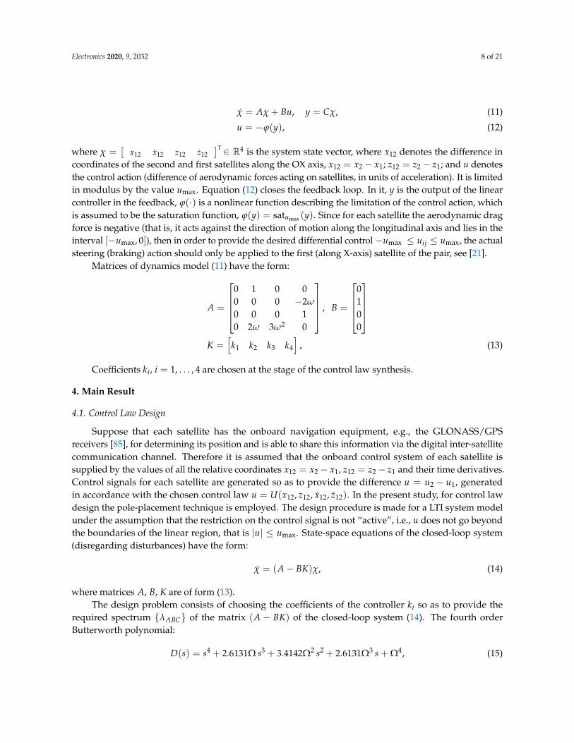
Figure 5. Satellites relative trajectories on the (XZ) plane for x12(0) = 200 m, x12(0) = 0.025 m/s,z12(0) = −50 m, z12(0) = −0.025 m/s. The ideal channel case.T∗ = 4.61 h.

4.4.3. Satellite Position Transmission Over the Digital Communication Channel with Finite Capacity

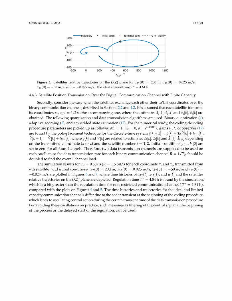
Secondly, consider the case when the satellites exchange each other their LVLH coordinates over thebinary communication channels, described in Sections 2.2 and 4.2. It is assumed that each satellite transmitsits coordinates xi, zi, i = 1, 2 to the accompanying one, where the estimates xi[k], zi[k] and ˆxi[k], ˆzi[k] areobtained. The following quantization and data transmission algorithms are used: Binary quantization (4),adaptive zooming (5), and embedded state estimation (17). For the numerical study, the coding-decodingprocedure parameters are picked up as follows: M0 = 1, mc = 0, ρ = e−0.01T0 , gains l1, l2 of observer (17)are found by the pole-placement technique for the discrete-time system y[k + 1] = y[k] + T0V[k] + l1σi[k],V[k + 1] = V[k] + l2σi[k], where y[k] and V[k] are related to estimates xi[k], zi[k] and ˆxi[k], ˆzi[k] dependingon the transmitted coordinate (x or z) and the satellite number i = 1, 2. Initial conditions y[0], V[0] areset to zero for all four channels. Therefore, two data transmission channels are supposed to be used oneach satellite, so the data transmission rate for each binary communication channel R = 1/T0 should bedoubled to find the overall channel load.

The simulation results for T0 = 0.667 s (R = 1.5 bit/s for each coordinate xi and zi, transmitted fromi-th satellite) and initial conditions x12(0) = 200 m, x12(0) = 0.025 m/s, z12(0) = −50 m, and z12(0) =−0.025 m/s are plotted in Figures 6 and 7, where time histories of x12(t), z12(t), and u(t) and the satellitesrelative trajectories on the (XZ) plane are depicted. Regulation time T∗ = 4.84 h is found by the simulation,which is a bit greater than the regulation time for non-restricted communication channel ( T∗ = 4.61 h),compared with the plots on Figures 4 and 5. The time histories and trajectories for the ideal and limitedcapacity communication channels differ due to the coder transient at the beginning of the coding procedure,which leads to oscillating control action during the certain transient time of the data transmission procedure.For avoiding these oscillations on practice, such measures as filtering of the control signal at the beginningof the process or the delayed start of the regulation, can be used.

Electronics 2020, 9, 2032 13 of 21

0 5 10 15time, h

0

500

1000

x12,

m

0 5 10 15time, h

-200

-100

0

100

200

z12,

m

0 5 10 15time, h

-2

0

2

u12

10-5

Figure 6. Time histories of x12(t) (upper plot), z12(t) (middle plot), and u(t) (lower plot). Case ofquantization, R = 1.5 bit/s, p = 0. x12(0) = 200 m, x12(0) = 0.025 m/s, z12(0) = −50 m, z12(0) =

−0.025 m/s; T∗ = 4.69 h.

-200 0 200 400 600 800 1000 1200 1400x

12, m

-200

0

200

z1

2, m

trajectory initial point terminal point 10 m -vicinity

Figure 7. Satellites relative trajectories on the (XZ) plane for x12(0) = 200 m, x12(0) = 0.025 m/s,z12(0) = −50 m, z12(0) = −0.025 m/s. Case of quantization, R = 1.5 bit/s, p = 0. T∗ = 4.69 h.

4.4.4. Case of Erasure Communication Channel

Thirdly, let us study how the erasure of data in the communication channel affects the datatransmission accuracy and the regulation time for the relative position of the satellites.

For evaluating the data transmission accuracy, the transients of the transmission procedure wereexcluded by consideration only the last 0.3tfin interval of the simulation time. For this interval, the standarddeviations σex1

and σex1of the data transmission errors ex1 [k] = x1(tk) − x1(tk), and ex1 [k] = x1(tk) −

ˆx1(tk) (respectively) were calculated. Logarithmically scaled functions σex1, σex1

versus transmissionrate R for various values of erasure probability p are plotted in Figures 8 and 9. The plots show thatthe data transmission errors decrease monotonically, looking like inversely proportional functions oncommunication rate R and are practically negligibly small as R > 1 bit/s for all considered values of p.

A summary graph of the dependence of regulation time T∗ on the data transmission rate R (for eachone channel) at various erasure probabilities p ∈ 0, 0.1, 0.2, 0.3 is shown in Figure 10. The curves inFigure 10 make an impression about the required load of the communication channel and the quality ofthe stabilization process with its use. It is seen from the plot that for significantly high data transmissionrate (exceeding 2 bit/s in our example) erasure of data in the channel with probability up to 0.3 doesnot have an effect on the regulation time. This time is defined by the system dynamics regardless of thecommunication channel capacity.

Electronics 2020, 9, 2032 14 of 21

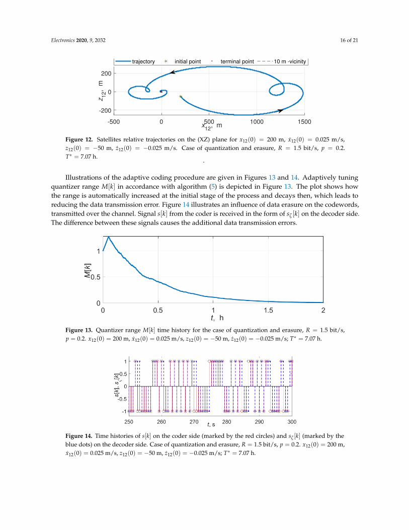
To illustrate the system performance, the particular processes for T0 = 0.667 s, x12(0) = 200 m,x12(0) = 0.025 m/s, z12(0) = −50 m, and z12(0) = −0.025 m/s and probability p = 0.2 of erasing data inthe communication channel are plotted in Figures 11 and 12. Regulation time T∗ = 7.07 h is found by thesimulation. The time histories and trajectories for the ideal and limited capacity erasure communicationchannels significantly differ from the case of the ideal channel, and from an application viewpoint, theprocess quality for these conditions is a boundary one.

0 0.5 1 1.5 2 2.5 3

R, bit/s

10-4

10-3

10-2

10-1

100

x1

, m

0

0.1

0.2

0.3

Figure 8. Data transmission error σx1 vs transmission rate R for various erasure probability p values.

0 0.5 1 1.5 2 2.5 3

R, bit/s

10-4

10-3

10-2

10-1

100

dx

1/d

t, m

/s

0

0.1

0.2

0.3

Figure 9. Data transmission error σx1 vs transmission rate R for various erasure probability p values.

Electronics 2020, 9, 2032 15 of 21

0 0.5 1 1.5 2 2.5 3

R, bit/s

4

5

6

7

8

9

10

T* ,

h

T*(R,p)

0

0.1

0.2

0.3

Figure 10. Regulation time T∗ vs transmission rate R for various erasure probability p values.

0 5 10 15time, h

0

500

1000

x12, m

0 5 10 15time, h

-200

0

200

z12, m

0 5 10 15time, h

-2

0

2

u

10-5

Figure 11. Time histories of x12(t) (upper plot), z12(t) (middle plot), and u(t) (lower plot). Case ofquantization and erasure, R = 1.5 bit/s, p = 0.2. x12(0) = 200 m, x12(0) = 0.025 m/s, z12(0) = −50 m,z12(0) = −0.025 m/s; T∗ = 7.07 h.

Electronics 2020, 9, 2032 16 of 21

-500 0 500 1000 1500x

12, m

-200

0

200

z1

2, m

trajectory initial point terminal point 10 m -vicinity

Figure 12. Satellites relative trajectories on the (XZ) plane for x12(0) = 200 m, x12(0) = 0.025 m/s,z12(0) = −50 m, z12(0) = −0.025 m/s. Case of quantization and erasure, R = 1.5 bit/s, p = 0.2.T∗ = 7.07 h. .

Illustrations of the adaptive coding procedure are given in Figures 13 and 14. Adaptively tuningquantizer range M[k] in accordance with algorithm (5) is depicted in Figure 13. The plot shows howthe range is automatically increased at the initial stage of the process and decays then, which leads toreducing the data transmission error. Figure 14 illustrates an influence of data erasure on the codewords,transmitted over the channel. Signal s[k] from the coder is received in the form of sζ [k] on the decoder side.The difference between these signals causes the additional data transmission errors.

Figure 13. Quantizer range M[k] time history for the case of quantization and erasure, R = 1.5 bit/s,p = 0.2. x12(0) = 200 m, x12(0) = 0.025 m/s, z12(0) = −50 m, z12(0) = −0.025 m/s; T∗ = 7.07 h.

Figure 14. Time histories of s[k] on the coder side (marked by the red circles) and sζ [k] (marked by theblue dots) on the decoder side. Case of quantization and erasure, R = 1.5 bit/s, p = 0.2. x12(0) = 200 m,x12(0) = 0.025 m/s, z12(0) = −50 m, z12(0) = −0.025 m/s; T∗ = 7.07 h.

Electronics 2020, 9, 2032 17 of 21

5. Conclusions

In the paper the feedback control law was designed ensuring the regulation of the relative satellitesmotion in a swarm. Unlike previous papers, the limited data transmission rate over the communicationchannels was taken into account. The adaptive coding/decoding procedure for the transmission of positionbetween the satellites in the formation, employing the kinematics process description was studied for thecases of the ideal and erasure channel. Note that an adaptive coder used in the paper was not new since itwas employed earlier for other problems in [77,78]. However such a coder was not applied to the controlof satellite swarms previously and this is an additional novelty in the paper.

The dependence of the closed-loop system performance and accuracy of the data transmissionalgorithm on the data transmission rate was numerically evaluated. It was shown that bothdata transmission error and regulation time depend approximately inversely proportionally on thecommunication rate.

In future research, disturbances and noise in the communication channel will be taken into account.

Author Contributions: Conceptualization, B.A. and A.L.F.; Data curation, B.A.; Formal analysis, E.V.K.; Fundingacquisition, A.L.F.; Investigation, B.A.; Methodology, A.L.F.; Project administration, A.L.F.; Software, B.A. and E.V.K.;Supervision, A.L.F.; Writing—original draft, B.A. Writing—review & editing, B.A. and A.L.F. All authors have readand agreed to the published version of the manuscript.

Funding: This work was supported in part by the Government of Russian Federation (Grant 08-08) and by theMinistry of Science and Higher Education of Russian Federation (Grant FZWF-2020-0015).

Conflicts of Interest: The authors declare no conflict of interest.

Abbreviations

The following abbreviations are used in this manuscript:

LTI Linear Time InvariantDTN Delay Tolerant NetworkingMAC Medium Access ControlECC Elliptic Curve CryptographyLEO Low Earth OrbitSDR Software-defined RadioIRM Implicit Reference Model

References

1. Chang, I.; Chung, S.J.; Blackmore, L. Cooperative control with adaptive graph Laplacians for spacecraftformation flying. In Proceedings of the IEEE Conference Decision and Control (CDC 2010), Atlanta, GA, USA,15–17 December 2010; pp. 4926–4933, [CrossRef]

2. Morgan, D.; Chung, S.J.; Blackmore, L.; Acikmese, B.; Bayard, D.; Hadaegh, F. Swarm-keeping strategies forspacecraft under J2 and atmospheric drag perturbations. J. Guid. Control Dyn. 2012, 35, 1492–1506. [CrossRef]

3. Monakhova, U.; Ivanov, D.; Roldugin, D. Magnetorquers attitude control for differential aerodynamic forceapplication to nanosatellite formation flying construction and maintenance. Adv. Astronaut. Sci. 2020, 170, 385–397.

4. Kumar, B.; Ng, A.; Yoshihara, K.; De Ruiter, A. Differential drag as a means of spacecraft formation control.IEEE Trans. Aerosp. Electron. Syst. 2011, 47, 1125–1135. [CrossRef]

5. Pérez, D.; Bevilacqua, R. Lyapunov-based Spacecraft Rendezvous Maneuvers using Differential Drag. In Proceedingsof the AIAA Guidance, Navigation, and Control Conference, Portland, OR, USA, 8–11 August 2011; pp. 2011–6630.

6. Varma, S.; Kumar, K. Multiple satellite formation flying using differential aerodynamic drag. J. Spacecr. Rocket.2012, 49, 325–336. [CrossRef]

Electronics 2020, 9, 2032 18 of 21

7. Horsley, M.; Nikolaev, S.; Pertica, A. Small satellite rendezvous using differential lift and drag. J. Guid.Control Dyn. 2013, 36, 445–453. [CrossRef]

8. Kumar, K.; Misra, A.; Varma, S.; Reid, T.; Bellefeuille, F. Maintenance of satellite formations using environmentalforces. Acta Astronaut. 2014, 102, 341–354. [CrossRef]

9. Dellelce, L.; Kerschen, G. Optimal propellantless rendez-vous using differential drag. Acta Astronaut. 2015,109, 112–123. [CrossRef]

10. Ivanov, D.; Monakhova, U.; Ovchinnikov, M. Nanosatellites swarm deployment using decentralized differentialdrag-based control with communicational constraints. Acta Astronaut. 2019, 159, 646–657. [CrossRef]

11. Ivanov, D.; Biktimirov, S.; Chernov, K.; Kharlan, A.; Monakhova, U.; Pritykin, D. Writing with Sunlight: Cubesatformation control using aerodynamic forces. In Proceedings of the 70th International Astronautical Congress,Washington, DC, USA, 21–25 October 2019.

12. Tang, A.; Wu, X. LEO satellite formation flying via differential atmospheric drag. Int. J. Space Sci. Eng. 2019,5, 289–320. [CrossRef]

13. Shouman, M.; Bando, M.; Hokamoto, S. Output regulation control for satellite formation flying using differentialdrag. J. Guid. Control Dyn. 2019, 42, 2220–2232. [CrossRef]

14. Smith, B.; Capon, C.; Brown, M. Ionospheric drag for satellite formation control. J. Guid. Control Dyn. 2019,42, 2590–2599. [CrossRef]

15. Traub, C.; Herdrich, G.; Fasoulas, S. Influence of energy accommodation on a robust spacecraft rendezvousmaneuver using differential aerodynamic forces. CEAS Space J. 2020, 12, 43–63. [CrossRef]

16. Traub, C.; Romano, F.; Binder, T.; Boxberger, A.; Herdrich, G.; Fasoulas, S.; Roberts, P.; Smith, K.; Edmondson,S.; Haigh, S.; et al. On the exploitation of differential aerodynamic lift and drag as a means to control satelliteformation flight. CEAS Space J. 2020, 12, 15–32. [CrossRef]

17. Leonard, C. Formationkeeping of Spacecraft via Differential Drag. Master’s Thesis, Massachusetts Institute ofTechnology, Cambridge, MA, USA, 1986.

18. Kim, D.Y.; Woo, B.; Park, S.Y.; Choi, K.H. Hybrid optimization for multiple-impulse reconfiguration trajectoriesof satellite formation flying. Adv. Space Res. 2009, 44, 1257–1269. [CrossRef]

19. Vaddi, S.; Alfriend, K.; Vadali, S.; Sengupta, P. Formation establishment and reconfiguration using impulsivecontrol. J. Guid. Control Dyn. 2005, 28, 262–268. [CrossRef]

20. Vaddi, S. Modeling and Control of Satellite Formations. Ph.D. Thesis, Department of Aerospace Engineering,Texas A&M University, College Station, TX, USA, 2003.

21. Monakhova, U.; Ivanov, D. Formation of a Swarm of Nanosatellites Using Decentralized Aerodynamic Control, Takinginto Account Communication Constraints; M.V. Keldysh Institute Preprints; Keldysh Institute: Moscow, Russia,2018. (In Russian) [CrossRef]

22. Sarno, S.; D’Errico, M.; Guo, J.; Gill, E. Path planning and guidance algorithms for SAR formation reconfiguration:Comparison between centralized and decentralized approaches. Acta Astronaut. 2020, 167, 404–417. [CrossRef]

23. Basu, S.; Groves, K.; Basu, S.; Sultan, P. Specification and forecasting of scintillations in communication/navigationlinks: Current status and future plans. J. Atmos. Sol. Terr. Phys. 2002, 64, 1745–1754. [CrossRef]

24. Freimann, A.; Petermann, T.; Schilling, K. Interference-Free Contact Plan Design for Wireless Communicationin Space-Terrestrial Networks. In Proceedings of the 2019 IEEE International Conference on Space MissionChallenges for Information Technology (SMC-IT), Pasadena, CA, USA, 30 July–1 August 2019; pp. 55–61.[CrossRef]

25. Zhao, Y.; Yi, X.; Hou, Z.; Zhang, Y.; Li, C. Parallel data transmission for navigation satellite network with agilitylink. Int. J. Satell. Commun. Netw. 2019, 37, 536–550. [CrossRef]

26. Cai, X.; Zhou, M.; Xia, T.; Fong, W.; Lee, W.T.; Huang, X. Low-Power SDR Design on an FPGA for IntersatelliteCommunications. IEEE Trans. Large Scale Integr. Syst. 2018, 26, 2419–2430. [CrossRef]

27. Davarian, F.; Asmar, S.; Angert, M.; Baker, J.; Gao, J.; Hodges, R.; Israel, D.; Landau, D.; Lay, N.;Torgerson, L.; et al. Improving Small Satellite Communications and Tracking in Deep Space—A Review of theExisting Systems and Technologies with Recommendations for Improvement. Part II: Small Satellite Navigation,Proximity Links, and Communications Link Science. IEEE Aerosp. Electron. Syst. Mag. 2020, 35, 26–40. [CrossRef]

Electronics 2020, 9, 2032 19 of 21

28. Poomagal, C.; Sathish Kumar, G. ECC Based Lightweight Secure Message Conveyance Protocol for SatelliteCommunication in Internet of Vehicles (IoV). Wirel. Pers. Commun. 2020, 113, 1359–1377. [CrossRef]

29. Ujan, S.; Navidi, N.; Landry, R.J. Hierarchical classification method for radio frequency interference recognitionand characterization in satcom. Appl. Sci. 2020, 10, 4608. [CrossRef]

30. Kuang, Y.; Yi, X.; Hou, Z. Congestion avoidance routing algorithm for topology-inhomogeneous low earth orbitsatellite navigation augmentation network. Int. J. Satell. Commun. Netw. 2020. [CrossRef]

31. Nair, G.; Evans, R. Exponential stabilisability of finite-dimensional linear systems with limited data rates.Automatica 2003, 39, 585–593. [CrossRef]

32. Bazzi, L.; Mitter, S. Endcoding complexity versus minimum distance. IEEE Trans. Inform. Theory 2005,51, 2103–2112. [CrossRef]

33. Nair, G.; Fagnani, F.; Zampieri, S.; Evans, R. Feedback control under data rate constraints: An overview.Proc. IEEE 2007, 95, 108–137. [CrossRef]

34. Matveev, A.; Savkin, A. Estimation and Control over Communication Networks; Birkhäuser: Boston, MA, USA, 2009.35. Andrievsky, B.; Matveev, A.; Fradkov, A. Control and estimation under information constraints: Toward a

unified theory of control, computation and communications. Autom. Remote Control 2010, 71, 572–633. [CrossRef]36. Kwakernaak, H.; Sivan, R. Linear Optimal Control Systems; Wiley-Interscience: New York, NY, USA, 1972.37. Nair, G.; Evans, R. Stabilizability of stochastic linear systems with finite feedback data rates. SIAM J. Control Optim.

2004, 43, 413–436. [CrossRef]38. Nair, G.; Evans, R.; Mareels, I.; Moran, W. Topological feedback entropy and nonlinear stabilization. IEEE Trans.

Automat. Control 2004, 49, 1585–1597. [CrossRef]39. Fradkov, A.; Andrievsky, B.; Evans, R. Chaotic observer-based synchronization under information constraints.

Phys. Rev. E 2006, 73, 066209. [CrossRef]40. Cover, T.; Thomas, J. Elements of Information Theory; John Wiley & Sons, Inc.: New York, NY, USA; Chichester, UK;

Brisbane, Australia; Toronto, ON, Canada; Singapore, 1991.41. Rizzo, L. Effective Erasure Codes for Reliable Computer Communication Protocols. Comput. Commun. Rev. 1997,

27, 24–36. [CrossRef]42. Tatikonda, S.; Mitter, S. Control Over Noisy Channels. IEEE Trans. Automat. Control 2004, 49, 1196–1201. [CrossRef]43. Shokrollahi, A. Raptor codes. IEEE Trans. Inform. Theory 2006, 52, 2551–2567. [CrossRef]44. Köetter, R.; Kschischang, F. Coding for Errors and Erasures in Random Network Coding. IEEE Trans. Inform. Theory

2008, 54, 3579–3591. [CrossRef]45. Patterson, S.; Bamieh, B.; El Abbadi, A. Convergence Rates of Distributed Average Consensus With Stochastic

Link Failures. IEEE Trans. Automat. Control 2010, 55, 880–892. [CrossRef]46. Diwadkar, A.; Vaidya, U. Robust synchronization in nonlinear network with link failure uncertainty.

In Proceedings of the 50th IEEE Conference Decision and Control and European Control Conference (CDC-ECC2011), Orlando, FL, USA, 12–15 December 2011; IEEE: Orlando, FL, USA, 2011; pp. 6325–6330.

47. Wang, J.; Yan, Z. Coding scheme based on spherical polar coordinate for control over packet erasure channel.Int. J. Robust Nonlinear Control 2014, 24, 1159–1176. [CrossRef]

48. Zhang, H.; Lee, S.; Li, X.; He, J. EEG self-adjusting data analysis based on optimized sampling for robot control.Electronics 2020, 9, 925. [CrossRef]

49. Jeon, S.; Park, C.; Seo, D. The multi-station based variable speed limit model for realization on urban highway.Electronics 2020, 9, 801. [CrossRef]

50. Tsypkin, Y. Stability and sensitivity of nonlinear sampled data systems. In Sensitivity Methods in Control Theory;Radanovic, L., Ed.; Pergamon: Oxford, UK, 1966; pp. 46–66. [CrossRef]

51. Pogromsky, A.; Matveev, A. A non-quadratic criterion for stability of forced oscillation. Syst. Control Lett. 2013,62, 408–412. [CrossRef]

52. Dudkowski, D.; Jafari, S.; Kapitaniak, T.; Kuznetsov, N.V.; Leonov, G.A.; Prasad, A. Hidden attractors indynamical systems. Phys. Rep. 2016, 637, 1–50. [CrossRef]

53. Kuznetsov, N. Theory of hidden oscillations and stability of control systems. J. Comput. Syst. Sci. Int. 2020,59, 647–668. [CrossRef]

Electronics 2020, 9, 2032 20 of 21

54. Hespanha, J.P.; Naghshtabrizi, P.; Xu, Y. A Survey of Recent Results in Networked Control Systems. Proc. IEEE2007, 95, 138–162. [CrossRef]

55. Xia, Y.Q.; Gao, Y.L.; Yan, L.P.; Fu, M.Y. Recent progress in networked control systems—A survey. Intern. J.Autom. Comput. 2015, 12, 343–367. [CrossRef]

56. Nair, G.; Evans, R. State estimation via a capacity-limited communication channel. In Proceedings of the 36thIEEE Conference on Decision and Control (CDC’97), San Diego, CA, USA, 10–12 December 1997; pp. 866–871.

57. Andrievsky, B.; Fradkov, A.L. Control and observation via communication channels with limited bandwidth.Gyroscopy Navig. 2010, 1, 126–133. [CrossRef]

58. De Persis, C. n-Bit stabilization of n-dimensional nonlinear systems in feedforward form. IEEE Trans.Automat. Control 2005, 50, 299–311. [CrossRef]

59. Liberzon, D.; Hespanha, J. Stabilization of nonlinear systems with limited information feedback. IEEE Trans.Automat. Control 2005, 50, 910–915. [CrossRef]

60. Matveev, A.; Proskurnikov, A.; Pogromsky, A.; Fridman, E. Comprehending complexity: Data-rate constraints inlarge-scale networks. IEEE Trans. Automat. Control 2019, 64, 4252–4259. [CrossRef]

61. Voortman, Q.; Pogromsky, A.; Matveev, A.; Nijmeijer, H. Data-rate constrained observers of nonlinear systems.Entropy 2019, 21, 282. [CrossRef]

62. Matveev, A.; Pogromsky, A. Observation of nonlinear systems via finite capacity channels, Part II: Restorationentropy and its estimates. Automatica 2019, 103, 189–199. [CrossRef]

63. Åström, K.J.; Bernhardsson, B.M. Comparison of Riemann and Lebesgue sampling for first order stochasticsystems. In Proceedings of the 41st IEEE Conference on Decision & Control (CDC 2002), Las Vegas, NV, USA,10–13 December 2002; pp. 2011–2016.

64. Yu, H.; Antsaklis, P.J. Output Synchronization of Networked Passive Systems With Event-Driven Communication.IEEE Trans. Automat. Control 2014, 59, 750–756. [CrossRef]

65. Margun, A.; Furtat, I.; Zimenko, K.; Kremlev, A. Event-triggered output robust controller. In Proceedings ofthe 25th Mediterranean Conf. Control Automation (MED 2017), Valletta, Malta, 3–6 July 2017; pp. 625–630.[CrossRef]

66. Li, K.; Baillieu, J. Robust quantization for digital finite communication bandwidth (DFCB) control. IEEE Trans.Automat. Control 2004, 49, 1573–1584. [CrossRef]

67. Gabor, G.; Gyorfi, Z. Recursive Source Coding; Springer: New York, NY, USA, 1986.68. Tatikonda, S.; Sahai, A.; Mitter, S. Control of LQG Systems Under Communication Constraints. In Proceedings

of the 37th IEEE Conference Decision and Control, Tampa, FL, USA, 18 December 1998; IEEE: Tampa, FL, USA,1998; Volume WP04, pp. 1165–1170.

69. Brockett, R.; Liberzon, D. Quantized feedback stabilization of linear systems. IEEE Trans. Automat. Control 2000,45, 1279–1289. [CrossRef]

70. Liberzon, D. Hybrid feedback stabilization of systems with quantized signals. Automatica 2003, 39, 1543–1554.[CrossRef]

71. Tatikonda, S.; Mitter, S. Control under communication constraints. IEEE Trans. Automat. Control 2004,49, 1056–1068. [CrossRef]

72. Fradkov, A.; Andrievsky, B.; Ananyevskiy, M. State estimation and synchronization of pendula systems overdigital communication channels. Eur. Phys. J. Spec. Top. 2014, 223, 773–793. [CrossRef]

73. Fradkov, A.L.; Andrievsky, B.; Evans, R.J. Adaptive Observer-Based Synchronization of Chaotic Systems withFirst-Order Coder in Presence of Information Constraints. IEEE Trans. Circuits Syst. I 2008, 55, 1685–1694.[CrossRef]

74. Fradkov, A.; Andrievsky, B.; Evans, R. Synchronization of passifiable Lurie systems via limited-capacitycommunication channel. IEEE Trans. Circuits Syst. I 2009, 56, 430–439. [CrossRef]

75. Moreno-Alvarado, R.; Rivera-Jaramillo, E.; Nakano, M.; Perez-Meana, H. Simultaneous Audio Encryption andCompression Using Compressive Sensing Techniques. Electronics 2020, 9, 863. [CrossRef]

76. Goodman, D.; Gersho, A. Theory of an adaptive quantizer. IEEE Trans. Commun. 1974, COM-22, 1037–1045.[CrossRef]

Electronics 2020, 9, 2032 21 of 21

77. Andrievsky, B.; Fradkov, A. Adaptive coding for position estimation in formation flight control. IFAC Proc. Vol.2010, 1, 72–76. [CrossRef]

78. Fradkov, A.; Andrievsky, B.; Peaucelle, D. Estimation and control under information constraints for LAAShelicopter benchmark. IEEE Trans. Control Syst. Technol. 2010, 18, 1180–1187. [CrossRef]

79. Gomez-Estern, F.; Canudas de Wit, C.; Rubio, F. Adaptive delta modulation in networked controlled systemswith bounded disturbances. IEEE Trans. Automat. Control 2011, 56, 129–134. [CrossRef]

80. Hill, G.W. Researches in the Lunar Theory. Am. J. Math. 1878, 1, 5–26. [CrossRef]81. Clohessy, W.; Wiltshire, R. Terminal guidance system for satellite rendezvous. J. Aerosp. Sci. 1960, 653–658.

[CrossRef]82. Sedwick, R.; Miller, D.; Kong, E. Mitigation of Differential Perturbations. J. Astronaut. Sci. 1999, 47, 309–331.

[CrossRef]83. Schweighart, S.; Sedwick, R. High-Fidelity Linearized J2 Model for Satellite Formation Flight. J. Guid. Control Dyn.

2002, 25, 1073–1080. [CrossRef]84. Schlanbusch, R.; Kristiansen, R.; Nicklasson, P. Spacecraft formation reconfiguration with collision avoidance.

Automatica 2011, 47, 1443–1449. [CrossRef]85. Renga, A.; Grassi, M.; Tancredi, U. Relative navigation in LEO by carrier-phase differential GPS with intersatellite

ranging augmentation. Int. J. Aerosp. Eng. 2013, 2013, 627509. [CrossRef]86. Fradkov, A.L.; Miroshnik, I.V.; Nikiforov, V.O. Nonlinear and Adaptive Control of Complex Systems; Kluwer:

Dordrecht, The Netherlands, 1999.87. Andrievsky, B.; Kudryashova, E.; Kuznetsov, N.; Kuznetsova, O. Aircraft wing rock oscillations suppression by

simple adaptive control. Aerosp. Sci. Technol. 2020, 105, 1–10. [CrossRef]88. Massey, T.; Shtessel, Y. Continuous Traditional and High-Order Sliding Modes for Satellite Formation Control.

J. Guid. Control Dyn. 2005, 28, 826–831. [CrossRef]89. Wu, S.; Sun, X.; Sun, Z.; Wu, X. Sliding-mode control for staring-mode spacecraft using a disturbance observer.

Inst. Mech. Eng. Part G J. Aerosp. Eng. 2010, 224, 215–224. [CrossRef]90. Cong, B.L.; Liu, X.D.; Chen, Z. Distributed attitude synchronization of formation flying via consensus-based

virtual structure. Acta Astronaut. 2011, 68, 1973–1986. [CrossRef]91. La Scala, B.; Evans, R. Minimum necessary data rates for accurate track fusion. In Proceedings of the 44th IEEE

Conference on Decision and Control, and the European Control Conference, Seville, Spain, 12–15 December 2005;IEEE: Seville, Spain, 2005; pp. 6966–6971.

92. Evans, R.; Krishnamurthy, V.; Nair, G.; Sciacca, L. Networked sensor management and data rate control fortracking maneuvering targets. IEEE Trans. Signal Process. 2005, 53, 1979–1991. [CrossRef]

93. Tomashevich, S.; Andrievsky, B.; Fradkov, A.L. Formation control of a group of unmanned aerial vehicleswith data exchange over a packet erasure channel. In Proceedings of the 1st IEEE Intern. Conf. IndustrialCyber-Physical Systems (ICPS 2018), Saint Petersburg, Russia, 15–18 May 2018; pp. 38–43. [CrossRef]

94. Andrievsky, B. Numerical evaluation of controlled synchronization for chaotic Chua systems over thelimited-band data erasure channel. Cybern. Phys. 2016, 5, 3–51.

Publisher’s Note: MDPI stays neutral with regard to jurisdictional claims in published maps and institutionalaffiliations.

c© 2020 by the authors. Licensee MDPI, Basel, Switzerland. This article is an open accessarticle distributed under the terms and conditions of the Creative Commons Attribution(CC BY) license (http://creativecommons.org/licenses/by/4.0/).