Embed Size (px)
Citation preview

Control System Design - LQG Part 2
Bo Bernhardsson, K. J. Åström
Department of Automatic Control LTH,
Lund University
Bo Bernhardsson, K. J. Åström Control System Design - LQG Part 2

Lecture - LQG Design
What do the “technical conditions” mean?
Introducing integral action, etc
Loop Transfer Recovery (LTR)
Examples
For theory and more information, see PhD course on LQG
Reading tip: Ch 5 in Maciejowski, Multivariable Feedback Design
see home page for more links
Bo Bernhardsson, K. J. Åström Control System Design - LQG Part 2
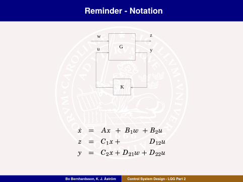
Reminder - Notation
K
w
yG
z
u
x = Ax + B1w + B2u
z = C1 x+ D12u
y = C2 x+ D21w+ D22u
Bo Bernhardsson, K. J. Åström Control System Design - LQG Part 2

Reminder - Technical Conditions
1) [A, B2] stabilizable
2) [C2, A] detectable
3) “No zeros on imaginary axis” u → z
rank
jω I − A −B2
C1 D12
= n+m ∀ω
and D12 has full column rank (no free control)
4) “No zeros on imaginary axis” w → y
rank
jω I − A −B1
C2 D21
= n+ p ∀ω
and D21 has full row rank (no noise-free measurements)
Discrete time: change imag. axis jω to unit circle e jω .
Bo Bernhardsson, K. J. Åström Control System Design - LQG Part 2
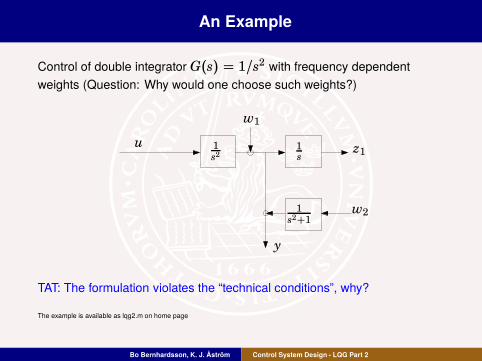
An Example
Control of double integrator G(s) = 1/s2 with frequency dependent
weights (Question: Why would one choose such weights?)eplacements
1
s2
1
s
1
s2+1
w1
w2
z1
y
u
TAT: The formulation violates the “technical conditions”, why?
The example is available as lqg2.m on home page
Bo Bernhardsson, K. J. Åström Control System Design - LQG Part 2

Answer
D12 not full rank
>Solution: New punished signal, z2 = ρu
Non-stabilizable, non-detectable modes
>Solution: Perturb 1/s and 1/(s2 + 1) weights
The matrix
jω I − A −B1
C2 D21
looses rank in ω = 0.
No input noise will lead to Kalman filter with Lopt = 0, which gives
marginally unstable Kalman filter.
>Solution: Add input noise w3 to process.
Bo Bernhardsson, K. J. Åström Control System Design - LQG Part 2

New System
1
s2
1
s+ε2
1
s2+2ε1s+1
w1
w2
w3
z1
z2
y
u
ρ σ
ρ = 0.1, σ = 0.01, ε1 = ε2 = 10−4 gives
C(s) = 12.85(s2 + 0.1248s+ 0.00778)(s2 + 0.0002s+ 1)
(s+ 0.0001)(s2 + 0.315s+ 1.768)(s2 + 5.135s+ 11.96)
Bo Bernhardsson, K. J. Åström Control System Design - LQG Part 2

The Code
rho=0.1;ep1=0.0001;ep2=0.0001;sigma=0.01;
A=[0 1 0 0 0; 0 0 0 0 0 ; 0 0 -ep1 1 0;0 0 -1 -ep1 0 ; 1 0 0 0 -ep2];
B1=[0 0 0 ; 0 0 sigma ; 0 0 0 ; 0 1 0 ; 1 0 0];
B2=[0 ; 1 ; 0 ; 0 ; 0];
C1=[0 0 0 0 1; 0 0 0 0 0 ];
C2=[1 0 0 1 0];
D11=[0 0 0; 0 0 0 ];
D12=[0; rho];
D21=[1 0 0];
D22=0;
Q=C1’*C1;
R=D12’*D12;
N=C1’*D12;
[k,s,e] = lqr(A,B2,Q,R,N);
G=eye(length(A));
H=zeros(1,length(A));
syse = ss(A,[B2 G],C2,[D22 H])
R11 = B1*B1’;
R22 = D21*D21’;
R12 = B1*D21’;
[kest,l,p]=kalman(syse,R11,R22,R12)
reg = zpk(lqgreg(kest,k));
frv=logspace(-3,3,1000);
fr1 = squeeze(freqresp(reg,frv));
loglog(frv,abs(fr1),’r’,’Linewidth’,2)
Bo Bernhardsson, K. J. Åström Control System Design - LQG Part 2
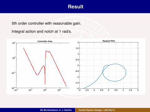
Result
5th order controller with reasonable gain.
Integral action and notch at 1 rad/s.
10-4 10-2 100 102 10410-2
10-1
100
101 Controller Gain
-2 -1.5 -1 -0.5 0 0.5 1 1.5 2-2
-1.5
-1
-0.5
0
0.5
1
1.5
2Nyquist Plot
Bo Bernhardsson, K. J. Åström Control System Design - LQG Part 2
Technical conditions - D21 not full rank
If D21 does not have full rank (i.e. R2 = D21 DT21 not pos def), some
measurements are error free.
Can use y directly for calculation of some combination of states
Kalman filter gains will become very large, trying to make use of these
error free directions. Resulting Kalman filter will be of lower order.
Luenberger observer - reduced observer of order n-rank(C)
See linear systems course
Bo Bernhardsson, K. J. Åström Control System Design - LQG Part 2
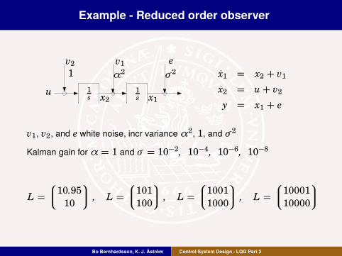
Example - Reduced order observer
1
s1
su
1 α2 σ 2
x1x2
v1v2 e
x1 = x2 + v1
x2 = u+ v2
y = x1 + e
v1, v2, and e white noise, incr variance α2, 1, and σ 2
Kalman gain for α = 1 and σ = 10−2, 10
−4, 10−6, 10
−8
L =
10.95
10
, L =
101
100
, L =
1001
1000
, L =
10001
10000
Bo Bernhardsson, K. J. Åström Control System Design - LQG Part 2
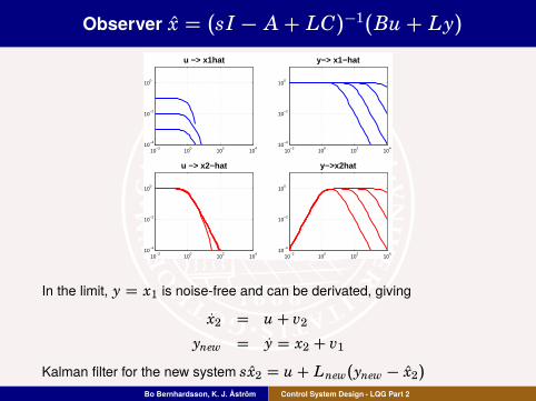
Observer x = (sI − A+ LC)−1(Bu+ Ly)
10−2
100
102
104
10−4
10−2
100
u −> x1hat
10−2
100
102
104
10−4
10−2
100
u −> x2−hat
10−2
100
102
104
10−4
10−2
100
y−> x1−hat
10−2
100
102
104
10−4
10−2
100
y−>x2hat
In the limit, y = x1 is noise-free and can be derivated, giving
x2 = u+ v2
ynew = y = x2 + v1
Kalman filter for the new system sx2 = u+ Lnew(ynew − x2)
Bo Bernhardsson, K. J. Åström Control System Design - LQG Part 2

Example - Reduced order observer
1
s1
su
1 α2 σ 2
x1x2
v1v2 e
x1 = x2 + v1
x2 = u+ v2
y = x1 + e
v1, v2, and e white noise, incr variance α2, 1, and σ 2
Optimal filter as σ → 0 is first order:
x1 = y
x2 =α
αs+ 1u+
s
αs+ 1y
x2 (1
s u if α large
x2 ( sy if α small
Bo Bernhardsson, K. J. Åström Control System Design - LQG Part 2
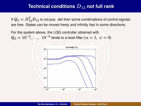
Technical conditions D12 not full rank
If Q2 = DT12 D12 is not pos. def then some combinations of control signals
are free. States can be moved freely and infinitly fast in some directions.
For the system above, the LQG controller obtained with
Q2 = 10−2, . . . , 10
−8 tends to a lead-filter (α = 1, σ = 0)
10−2
100
102
104
10−2
10−1
100
101
102
Q1=diag([1 1])
Bo Bernhardsson, K. J. Åström Control System Design - LQG Part 2

Technical Conditions - More Intuition
The following system
x = 0
y = x+ e
fails condition 4:
sI − A −B1
C2 D21
=
s 0
1 1
looses rank for s = 0
what happens with the observer in stationarity?
Bo Bernhardsson, K. J. Åström Control System Design - LQG Part 2
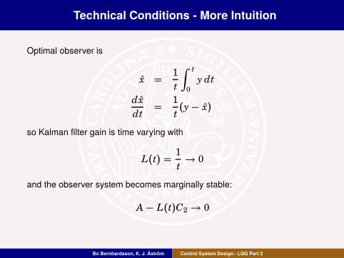
Technical Conditions - More Intuition
Optimal observer is
x =1
t
∫ t
0
y dt
dx
dt=
1
t(y− x)
so Kalman filter gain is time varying with
L(t) =1
t→ 0
and the observer system becomes marginally stable:
A− L(t)C2 → 0
Bo Bernhardsson, K. J. Åström Control System Design - LQG Part 2

Lecture - LQG Design
What do the “technical conditions” mean?
Introducing integral action, etc
Loop Transfer Recovery (LTR)
Examples
Bo Bernhardsson, K. J. Åström Control System Design - LQG Part 2

Disturbance Modeling
Integral action and generalized integral control can be generated by
disturbance modeling.
1 Recall integral action and generalized integral action
2 Choose controller that gives integral action
3 Models disturbances and incorporate the models in the controller
4 Disturbances can be load disturbances, measurement noise,
reference values.
Bo Bernhardsson, K. J. Åström Control System Design - LQG Part 2
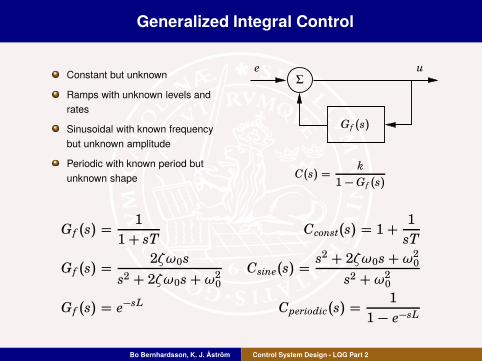
Generalized Integral Control
Constant but unknown
Ramps with unknown levels and
rates
Sinusoidal with known frequency
but unknown amplitude
Periodic with known period but
unknown shape
u
G f (s)
eΣ
C(s) =k
1−G f (s)
G f (s) =1
1+ sTCconst(s) = 1+
1
sT
G f (s) =2ζω0s
s2 + 2ζω0s+ω20
Csine(s) =s2 + 2ζω0s+ω2
0
s2 +ω20
G f (s) = e−sL Cperiodic(s) =1
1− e−sL
Bo Bernhardsson, K. J. Åström Control System Design - LQG Part 2

A General 2DOF System
Feedforward
Signal
Generator
r
u
-x
xm
ProcessΣ ΣState
Feedback
Kalman
Filter
uf b
uf f
y
The signals xm and ym = Cxm give the desired responses of states and
output, the signal u f f drives the system in the desired way
Many ways to generate command signals
Tables, dynamic models
Constraints can be accounted for
Feedforward design requires inversion of process dynamics, see
BottomUp lecture
Bo Bernhardsson, K. J. Åström Control System Design - LQG Part 2

Model Following
Desired behavior
dxm
dt= Axm + Bu, ym = Cxm.
Desired feedforward signal u = u f f can be generated in many ways. See
lecture on Bottom Up.
Bo Bernhardsson, K. J. Åström Control System Design - LQG Part 2

Integral Action by Disturbance Observer
Process and unknown but constant load disturbance v
dx
dt= Ax+ B(u + v), y = Cx,
dv
dt= 0.
Augment process state x by disturbance state v gives the following model
for the the process and its disturbances
d
dt
x
v
=
A B
0 0
x
v
+
B
0
u, y =
C 0
x
v
Is the state v stabilizable? Does it matter? Observer
d
dt
x
v
=
A B
0 0
x
v
+
B
0
u+
L x
Lv
(y− Cx),
Controller
u = u f f + K x(xm − x) − v
where u f f is the feedforward signal and xm is the desired state from the
feedforward signal generator.
Bo Bernhardsson, K. J. Åström Control System Design - LQG Part 2
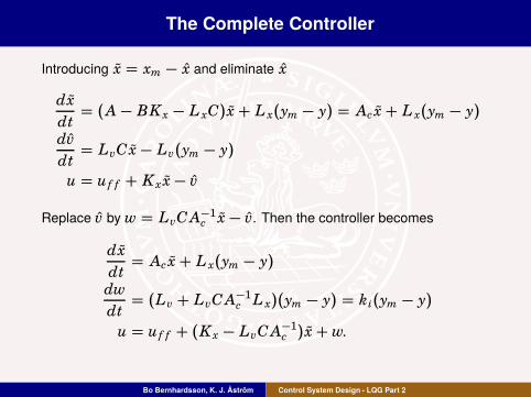
The Complete Controller
Introducing x = xm − x and eliminate x
dx
dt= (A− BK x − L xC)x+ L x(ym − y) = Ac x+ L x(ym − y)
dv
dt= LvCx− Lv(ym − y)
u = u f f + K x x− v
Replace v by w = LvC A−1c x− v. Then the controller becomes
dx
dt= Ac x+ L x(ym − y)
dw
dt= (Lv + LvC A−1
c L x)(ym − y) = ki(ym − y)
u = u f f + (K x − LvC A−1
c )x+ w.
Bo Bernhardsson, K. J. Åström Control System Design - LQG Part 2
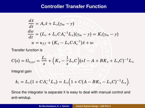
Controller Transfer Function
dx
dt= Ac x+ L x(ym − y)
dw
dt= (Lv + LvC A−1
c L x)(ym − y) = Ki(ym − y)
u = u f f + (K x − LvC A−1
c )x+ w.
Transfer function is
C(s) = Gu f be =Lv
s+(
K x −1
sLvC
)
(sI − A+ BK x + L xC)−1 L x
Integral gain
ki = Lv(1+ C A−1
c L x) = Lv
(
1+ C(A− BK x − L xC)−1 L x
)
.
Since the integrator is separate it is easy to deal with manual control and
anti-windup.
Bo Bernhardsson, K. J. Åström Control System Design - LQG Part 2
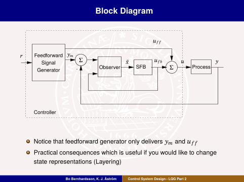
Block Diagram
-
Feedforward
Signal
Generator
ru
Controller
x
ym
Process
Σ
ΣObserver SFB
uf b
uf f
y
Notice that feedforward generator only delivers ym and u f f
Practical consequences which is useful if you would like to change
state representations (Layering)
Bo Bernhardsson, K. J. Åström Control System Design - LQG Part 2

Other Disturbances
Sinusoidal disturbances with frequency ω d can be captured by the model
dv
dt=
0 ω d
−ω d 0
v
We can deal with any disturbance that can be generated by
dw
dt= Avw, v = Cvw
The matrix Av often has eigenvalues on the imaginary axis. Why?
Bo Bernhardsson, K. J. Åström Control System Design - LQG Part 2
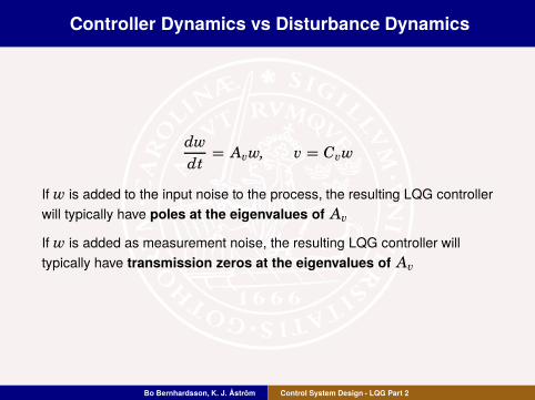
Controller Dynamics vs Disturbance Dynamics
dw
dt= Avw, v = Cvw
If w is added to the input noise to the process, the resulting LQG controller
will typically have poles at the eigenvalues of Av
If w is added as measurement noise, the resulting LQG controller will
typically have transmission zeros at the eigenvalues of Av
Bo Bernhardsson, K. J. Åström Control System Design - LQG Part 2
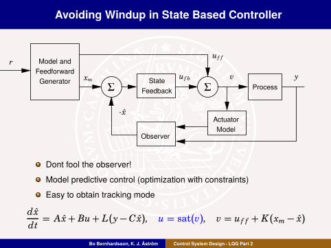
Avoiding Windup in State Based Controller
Model and
Feedforward
Generator
r
v
-x
xm
ProcessΣ ΣState
Feedback
Observer
uf b
uf f
y
Actuator
Model
Dont fool the observer!
Model predictive control (optimization with constraints)
Easy to obtain tracking mode
dx
dt= Ax+ Bu+ L(y−Cx), u = sat(v), v = u f f + K(xm− x)
Bo Bernhardsson, K. J. Åström Control System Design - LQG Part 2

Reference Values
Process model and controller
dx
dt= Ax+ Bu, y = Cx, u = −K x+ Krr.
Closed loop system
dx
dt= (A − BK)x+ BKrr, y = Cx.
Steady state output
x0 = (A− BK)−1 BKrr.
Inverse exist because A− BK is stable. Choosing
Kr =(
C(A− BK)−1B)−1
gives the output y = r. This choice gives a calibrated system. The correct
steady state is maintained by carefully matching the feedforward gain Kr
to the system parameters.
Bo Bernhardsson, K. J. Åström Control System Design - LQG Part 2

Explicit Integral Action
Process modeldx
dt= Ax+ Bu, y = Cx.
Controller (forced integral action)
u = −K(x− xm) − kiz,dz
dt= Cx− r
Augment process state by the integrator state z
d
dt
x
z
=
A 0
C 0
x
z
+
B 0
0 −1
u
r
, y =
C 0
Many design methods, pole-placemet, LQG, etc
Condition for reachability and observability?
When will it work
Bo Bernhardsson, K. J. Åström Control System Design - LQG Part 2
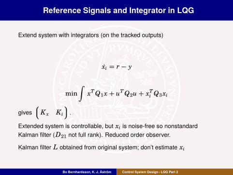
Reference Signals and Integrator in LQG
Extend system with integrators (on the tracked outputs)
xi = r− y
min
∫
xT Q1x+ uT Q2u+ xTi Q3xi
gives
K x Ki
.
Extended system is controllable, but xi is noise-free so nonstandard
Kalman filter (D21 not full rank). Reduced order observer.
Kalman filter L obtained from original system; don’t estimate xi
Bo Bernhardsson, K. J. Åström Control System Design - LQG Part 2

Reference Signals and Integrator in LQG
Use controller
u = −K x x− Kixi
or if feedforward signal u f f is available
u = −K x x− Kixi + u f f
Increased model order
Observer order not increased
Bo Bernhardsson, K. J. Åström Control System Design - LQG Part 2

Reference Signals in LQG
If r and y available separatly (2-DOF) one can do as follows (assuming
dimensions of r and y are equal)
˙xxi
=
A − BKx − LC + LDKx −BKi + LDKi
0 0
xxi
+
−L L
I −I
ry
Bo Bernhardsson, K. J. Åström Control System Design - LQG Part 2

Reference Signals in LQG
If only tracking error e = r− y is available (1-DOF)
˙xxi
=
A − BKx − LC + LDKx −BKi + LDKi
0 0
x
xi
+
−L
I
(r− y)
Bo Bernhardsson, K. J. Åström Control System Design - LQG Part 2
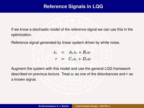
Reference Signals in LQG
If we know a stochastic model of the reference signal we can use this in the
optimization.
Reference signal generated by linear system driven by white noise.
xr = Arxr + Brw
r = Crxr + Drw
Augment the system with this model and use the general LQG framework
described on previous lecture. Treat w as one of the disturbances and r as
a known signal.
Bo Bernhardsson, K. J. Åström Control System Design - LQG Part 2

Reference Signals in LQG
If we have knowledge of future reference signals, r, this can be used to
improve tracking performance further.
Introduce a Model and Feedforward Generator as above
u = K(xm − x) + u f f
where u f f is an open loop control signal that ideally produces the desired
time variation xm in process states.
Here u f f and xm can be non-causal functions of the reference signal r if
this is known in advance
Bo Bernhardsson, K. J. Åström Control System Design - LQG Part 2
Lecture - LQG Design
What do the “technical conditions” mean?
Introducing integral action, etc
Loop Transfer Recovery (LTR)
Examples
Bo Bernhardsson, K. J. Åström Control System Design - LQG Part 2

Spectral factorisation - revisited
Assume R12 = 0
x = Ax+ v, E(vtvTt−τ ) = R1δτ
y = C2x+ e, E(e teTt−τ ) = R2δτ
0 = AP + P AT + R1 − PCT2 R−1
2 C2 P, L = PCT2 R−1
2
"Equivalent" representation of y
˙x = Ax+ Lε
y = C2 x+ ε
where ε is the “innovation” process. Can show E(εtεTt−τ ) = R2δτ
We can now write the spectrum of y in two different ways
Bo Bernhardsson, K. J. Åström Control System Design - LQG Part 2

Spectral factorisation - revisited
Φy = Φe + C2(sI − A)−1Φv(−sI − AT)−1CT
2
Φy = [Ip + C2(sI − A)−1L]Φε[. . .]∗
Hence
R2 + C2(sI − A)−1 R1(−sI − AT)−1CT2
= [Ip + C2(sI − A)−1 L]R2[Ip + C2(sI − A)−1 L]T
Kalman filter identity.
Compare previous lecture for the dual result (RDF)
If R12 = 0 then Kalman loop gain C2(sI − A)−1 L has same nice
robustness as K(sI − A)−1B2 has when Q12 = 0
Bo Bernhardsson, K. J. Åström Control System Design - LQG Part 2
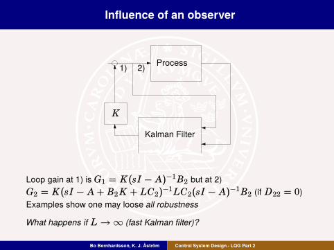
Influence of an observer
Process
Kalman Filter
K
1) 2)
Loop gain at 1) is G1 = K(sI − A)−1B2 but at 2)
G2 = K(sI − A+ B2 K + LC2)−1 LC2(sI − A)−1B2 (if D22 = 0)
Examples show one may loose all robustness
What happens if L →∞ (fast Kalman filter)?
Bo Bernhardsson, K. J. Åström Control System Design - LQG Part 2

LQG/LTR 1
Loop Transfer Recovery
Want to make G2 as robust as G1
References:
Doyle and Stein, AC79, p. 607-611
Doyle and Stein, AC81, p. 4-16
First LTR-method: Use fast (in a special way) observer
Sacrifice “noise optimality”
Almost like using an inverse for reconstruction
Not applicable if RHPL Zeros
Bo Bernhardsson, K. J. Åström Control System Design - LQG Part 2
LQG/LTR 1
First LTR-method: Add fictious input noise :
R1 := R1 + qB2 BT2
For square, minimum phase systems this gives L →∞ and
limq→∞
GLQG(s)G(s) = K(sI − A)−1B2
Easy to try this idea, doesn’t always lead to good designs.
Usually improves the robustness margins.
Dont let q go all the way to∞.
Same problem as with all designs with fast observers
Bo Bernhardsson, K. J. Åström Control System Design - LQG Part 2
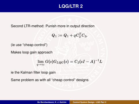
LQG/LTR 2
Second LTR-method: Punish more in output direction
Q1 := Q1 + qCT2 C2,
(ie use “cheap control”)
Makes loop gain approach
limq→∞
G(s)GLQG(s) = C2(sI − A)−1 L
ie the Kalman filter loop gain
Same problem as with all “cheap control” designs
Bo Bernhardsson, K. J. Åström Control System Design - LQG Part 2
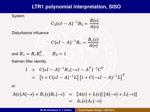
LTR1 polynomial interpretation, SISO
System
C2(sI − A)−1B2 =B(s)
A(s)
Disturbance influence
C(sI − A)−1Bv =Bv(s)
A(s)
and R1 = BvBTv , R2 = 1
Kalman filter identity
1 + C(sI − A)−1 R1(−sI − AT)−1CT
=[
1+ C(sI − A)−1 L] [
1+ C(−sI − A)−1L]T
or
A(s)A(−s) + Bv(s)Bv(−s) = [A(s) + L(s)] [A(−s) + L(−s)]
= Ao(s)Ao(−s)
Bo Bernhardsson, K. J. Åström Control System Design - LQG Part 2

LTR1 polynomial interpration, SISO
LTR-modification: Rmod1 = R1 + q2 BBT gives
C(sI − A)−1 Rmod1 (−sI − AT)−1CT
=Bv(s)Bv(−s) + B(s)q2 B(−s)
A(s)A(−s)
so
A(s)A(−s) + Bv(s)Bv(−s) + B(s)q2 B(−s)
=[
A(s) + Lmod(s)] [
A(−s) + Lmod(−s)]
= Amodo (s)Amod
o (−s)
Bo Bernhardsson, K. J. Åström Control System Design - LQG Part 2

LTR1 polynomial interpration, SISO
Now for very large q
Amodo (s)Amod
o (−s) ( (−s2)n + B(s)q2 B(−s)
gives (according to root-locus discussion) if B(s) stable
Amodo (s) ( B(s)Ak(s), Ak(s)Ak(−s) = b−2
0 ((−s2)k + q2)
where k = deg A(s) − degB(s).
Bo Bernhardsson, K. J. Åström Control System Design - LQG Part 2

LTR1 polynomial interpration, SISO
If we write the LQG controller as U = − S(s)R(s)Y we want to show that
looptransfer in LQG
C(sI − A)−1BK(sI − A+ BK + LC)−1 L =:B(s)
A(s)
S(s)
R(s).
approaches the loop transfer in LQ
K(sI − A)−1B =:K(s)
A(s)
Bo Bernhardsson, K. J. Åström Control System Design - LQG Part 2

LTR1 polynomial interpration, SISO
Closed loop polynomial is
Ac(s)Amodo (s) = A(s)R(s) + B(s)S(s)
and after some thought (for fixed s as q →∞)
R(s) ( B(s)Ak(s), S(s) (q
b0
[Ac(s) − A(s)] =q
b0
K(s)
so the loop transfer is now
B(s)
A(s)
S(s)
R(s)(
B(s)
A(s)
q
b0 Ak(s)︸ ︷︷ ︸
(1
K(s)
B(s)(
K(s)
A(s)
and we have the nice LQR-robustness over most frequencies
Bo Bernhardsson, K. J. Åström Control System Design - LQG Part 2

Lecture - LQG Design
What do the “technical conditions” mean?
Introducing integral action, etc
Loop Transfer Recovery (LTR)
Examples
Bo Bernhardsson, K. J. Åström Control System Design - LQG Part 2
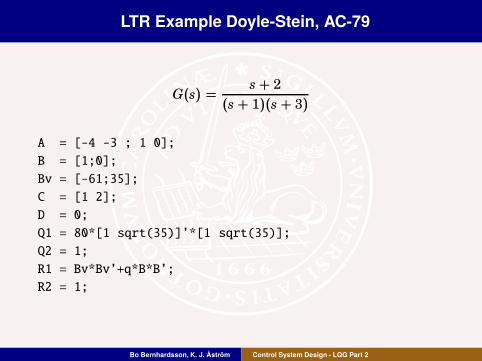
LTR Example Doyle-Stein, AC-79
G(s) =s+ 2
(s+ 1)(s+ 3)
A = [-4 -3 ; 1 0];
B = [1;0];
Bv = [-61;35];
C = [1 2];
D = 0;
Q1 = 80*[1 sqrt(35)]’*[1 sqrt(35)];
Q2 = 1;
R1 = Bv*Bv’+q*B*B’;
R2 = 1;
Bo Bernhardsson, K. J. Åström Control System Design - LQG Part 2

Doyle-Stein, AC-79 Results
10-2 10-1 100 101 102 10310-3
10-2
10-1
100
101
102 Controller Gain q=0(blue),1000(red),10000(green)
-3 -2 -1 0 1 2 3-3
-2
-1
0
1
2
3Nyquist plot
Better robustness obtained, with low extra cost (red)
Code available at home page: lqg3.m
Bo Bernhardsson, K. J. Åström Control System Design - LQG Part 2

Aircraft Design Example
Vertical-plane aircraft dynamics, from Maciejowski Ch 5.8
Inputs
Spoiler angle (tenths of degree)
Forward acceleration (m/s2)
Elevator angle (tenths of degree)
States
Altitude (m)
Forward speed (m/s)
Pitch angle (degrees)
Pitch rate (deg/s)
Vertical speed (m/s)
Bo Bernhardsson, K. J. Åström Control System Design - LQG Part 2
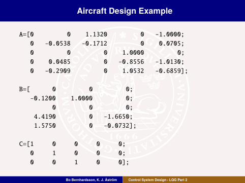
Aircraft Design Example
A=[0 0 1.1320 0 -1.0000;
0 -0.0538 -0.1712 0 0.0705;
0 0 0 1.0000 0;
0 0.0485 0 -0.8556 -1.0130;
0 -0.2909 0 1.0532 -0.6859];
B=[ 0 0 0;
-0.1200 1.0000 0;
0 0 0;
4.4190 0 -1.6650;
1.5750 0 -0.0732];
C=[1 0 0 0 0;
0 1 0 0 0;
0 0 1 0 0];
Bo Bernhardsson, K. J. Åström Control System Design - LQG Part 2

Aircraft LTR Design
Wanted:
bandwidth of 10 rad/s: σ (T(i10)) = −3dB
integral action and reference tracking
well-damped responses
Will use LTR2, gives loop gain approaching C2(sI − A)−1L
Bo Bernhardsson, K. J. Åström Control System Design - LQG Part 2

Aircraft LTR Design
Design performed in the following steps
1 Start to design Kalman filter, Guess: R1 = B2BT2 , R2 = 1
2 Introduce integrators w = 1
s+εν
3 ν colored noise: R1 = B2(I + 9xxT)B2 with clever x
4 Increase bandwidth, R1 := 100R1
5 Trim S(iω) at 5.5 rad/s
6 LTR2, cheap control, ρ = 10−6
Code available at home page: mac58.m
Bo Bernhardsson, K. J. Åström Control System Design - LQG Part 2

Gain of C2(sI − A)−1 L, R1 = B2BT2 , R2 = 1
Singular values of C(sI−A)^(−1)L, R1=BB T,R2=1
Frequency (rad/sec)
Sin
gula
r V
alue
s (d
B)
10−3
10−2
10−1
100
101
102
−40
−20
0
20
40
60
80
Need to introduce integral action
Extend system with integrators at input
Bo Bernhardsson, K. J. Åström Control System Design - LQG Part 2
Extended system
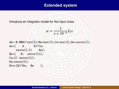
Introduce an integrator model for the input noise
w =1
s+ 10−4I3ν
Aw=-0.0001*eye(3);Bw=eye(3);Cw=eye(3);Dw=zeros(3);
Aa=[ A B1*Cw;
zeros(3,5) Aw];
Ba=[ B; zeros(3)];
Ca=[C zeros(3)];
Da=zeros(3);
B1a=[B1*Dw; Bw ];
Bo Bernhardsson, K. J. Åström Control System Design - LQG Part 2
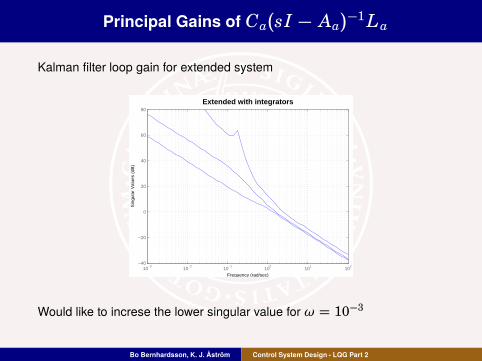
Principal Gains of Ca(sI − Aa)−1 La
Kalman filter loop gain for extended system
Extended with integrators
Frequency (rad/sec)
Sin
gula
r V
alue
s (d
B)
10−3
10−2
10−1
100
101
102
−40
−20
0
20
40
60
80
Would like to increse the lower singular value for ω = 10−3
Bo Bernhardsson, K. J. Åström Control System Design - LQG Part 2
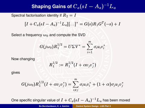
Shaping Gains of Ca(sI − Aa)−1 La
Spectral factorisation identity if R2 = I
[I + Ca(sI − Aa)−1 La][. . .]∗ = G(s)R1GT(−s) + I
Select a frequency ω0 and compute the SVD
G( jω0)R1/21 = UΣV∗ =
m∑
i=1
σiuiv∗
i
Now changing
R1/21 := R
1/21 (I +αv jv
∗
j )
gives
G( jω0)R1/21 (I +αv jv
∗
j ) =
m∑
i,= j
σiuiv∗
i + (1+α)σ ju jv∗
j
One specific singular value of I + Ca(sI − Aa)−1 La has been moved
Bo Bernhardsson, K. J. Åström Control System Design - LQG Part 2
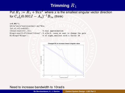
Trimming R1
Put R1 := R1 + 9xxT where x is the smallest singular vector direction
for Ca( j0.001I − Aa)−1B1a (think)
s=0.001*i;
Gf=Ca*inv(s*eye(size(Aa))-Aa)*B1a;
[u3,s3,v3]=svd(Gf);
v3real=real(v3(:,3)); % real approximation
R1sqrt=eye(3)+9*v3real*v3real’; % alfa=9, cause we want to change the gain
R1=R1sqrt*R1sqrt’; % of sigma_smallest with a factor 10
Changed R1 to increase lowest singular value
Frequency (rad/sec)
Sin
gula
r V
alue
s (d
B)
10−3
10−2
10−1
100
101
102
−40
−20
0
20
40
60
80
Need to increase bandwidth to 10rad/sBo Bernhardsson, K. J. Åström Control System Design - LQG Part 2
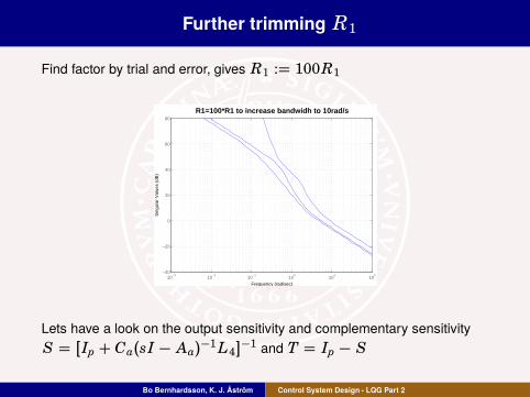
Further trimming R1
Find factor by trial and error, gives R1 := 100R1
R1=100*R1 to increase bandwidh to 10rad/s
Frequency (rad/sec)
Sin
gula
r V
alue
s (d
B)
10−3
10−2
10−1
100
101
102
−40
−20
0
20
40
60
80
Lets have a look on the output sensitivity and complementary sensitivity
S = [Ip + Ca(sI − Aa)−1 L4]
−1 and T = Ip − S
Bo Bernhardsson, K. J. Åström Control System Design - LQG Part 2
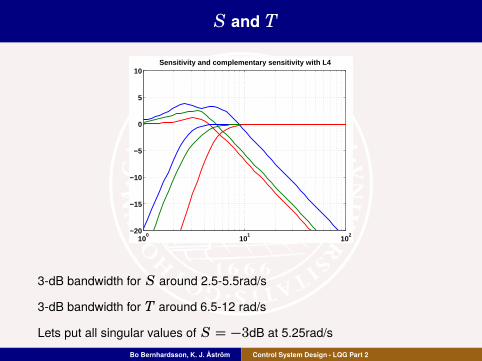
S and T
100
101
102
−20
−15
−10
−5
0
5
10Sensitivity and complementary sensitivity with L4
3-dB bandwidth for S around 2.5-5.5rad/s
3-dB bandwidth for T around 6.5-12 rad/s
Lets put all singular values of S = −3dB at 5.25rad/s
Bo Bernhardsson, K. J. Åström Control System Design - LQG Part 2
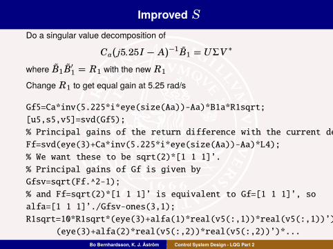
Improved S
Do a singular value decomposition of
Ca( j5.25I − A)−1 B1 = UΣV∗
where B1 B′1 = R1 with the new R1
Change R1 to get equal gain at 5.25 rad/s
Gf5=Ca*inv(5.225*i*eye(size(Aa))-Aa)*B1a*R1sqrt;
[u5,s5,v5]=svd(Gf5);
% Principal gains of the return difference with the current design
Ff=svd(eye(3)+Ca*inv(5.225*i*eye(size(Aa))-Aa)*L4);
% We want these to be sqrt(2)*[1 1 1]’.
% Principal gains of Gf is given by
Gfsv=sqrt(Ff.^2-1);
% and Ff=sqrt(2)*[1 1 1]’ is equivalent to Gf=[1 1 1]’, so
alfa=[1 1 1]’./Gfsv-ones(3,1);
R1sqrt=10*R1sqrt*(eye(3)+alfa(1)*real(v5(:,1))*real(v5(:,1))’)*
(eye(3)+alfa(2)*real(v5(:,2))*real(v5(:,2))’)*...
(eye(3)+alfa(3)*real(v5(:,3))*real(v5(:,3))’);Bo Bernhardsson, K. J. Åström Control System Design - LQG Part 2

Result
100
101
102
−20
−15
−10
−5
0
5
10Sensitivity and complementary sensitivity with L5
S(5.25) ∼ -3dB in all three directions, σ (T(10)) ∼ −3dB.
Let’s use this Kalman filter gain L5 !
Bo Bernhardsson, K. J. Åström Control System Design - LQG Part 2
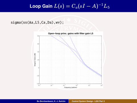
Loop Gain L(s) = Ca(sI − A)−1 L5
sigma(ss(Aa,L5,Ca,Da),wv);
Open−loop princ. gains with filter gain L5
Frequency (rad/sec)
Sin
gula
r V
alue
s (d
B)
10−3
10−2
10−1
100
101
102
−40
−20
0
20
40
60
80
Bo Bernhardsson, K. J. Åström Control System Design - LQG Part 2
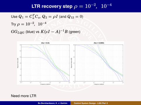
LTR recovery step ρ = 10−2, 10
−4
Use Q1 = CTa Ca, Q2 = ρ I (and Q12 = 0)
Try ρ = 10−2, 10
−4
GGLQG (blue) vs K(sI − A)−1B (green)
rho = 0.01
Frequency (rad/sec)
Sin
gula
r V
alue
s (d
B)
10−3
10−2
10−1
100
101
102
−40
−20
0
20
40
60
80
rho = 0.0001
Frequency (rad/sec)
Sin
gula
r V
alue
s (d
B)
10−3
10−2
10−1
100
101
102
−40
−20
0
20
40
60
80
Need more LTR
Bo Bernhardsson, K. J. Åström Control System Design - LQG Part 2
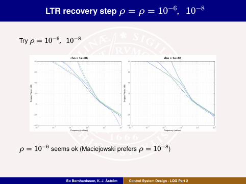
LTR recovery step ρ = ρ = 10−6, 10
−8
Try ρ = 10−6, 10
−8
rho = 1e−06
Frequency (rad/sec)
Sin
gula
r V
alue
s (d
B)
10−3
10−2
10−1
100
101
102
−40
−20
0
20
40
60
80
rho = 1e−08
Frequency (rad/sec)
Sin
gula
r V
alue
s (d
B)
10−3
10−2
10−1
100
101
102
−40
−20
0
20
40
60
80
ρ = 10−6 seems ok (Maciejowski prefers ρ = 10
−8)
Bo Bernhardsson, K. J. Åström Control System Design - LQG Part 2
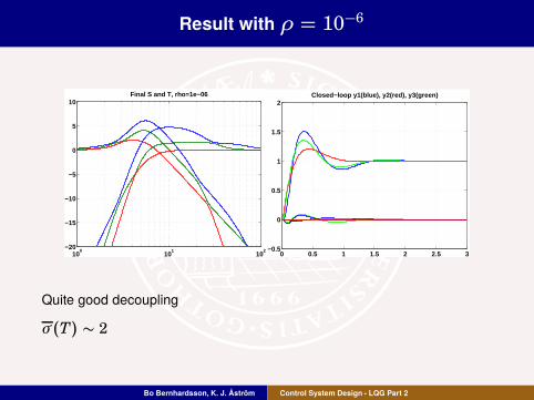
Result with ρ = 10−6
100
101
102
−20
−15
−10
−5
0
5
10Final S and T, rho=1e−06
0 0.5 1 1.5 2 2.5 3−0.5
0
0.5
1
1.5
2Closed−loop y1(blue), y2(red), y3(green)
Quite good decoupling
σ (T) ∼ 2
Bo Bernhardsson, K. J. Åström Control System Design - LQG Part 2
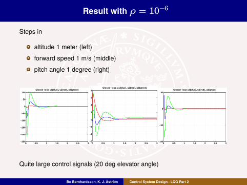
Result with ρ = 10−6
Steps in
altitude 1 meter (left)
forward speed 1 m/s (middle)
pitch angle 1 degree (right)
0 0.5 1 1.5 2 2.5 3−250
−200
−150
−100
−50
0
50
100Closed−loop u1(blue), u2(red), u3(green)
0 0.5 1 1.5 2 2.5 3−6
−4
−2
0
2
4
6
8Closed−loop u1(blue), u2(red), u3(green)
0 0.5 1 1.5 2 2.5 3−100
−50
0
50Closed−loop u1(blue), u2(red), u3(green)
Quite large control signals (20 deg elevator angle)
Bo Bernhardsson, K. J. Åström Control System Design - LQG Part 2

Controller Gain, with ρ = 10−6
Controller Gain
Frequency (rad/sec)
Sin
gula
r V
alue
s (d
B)
10−3
10−2
10−1
100
101
102
103
104
105
−40
−20
0
20
40
60
80
100
120
Quite high controller gains
K=[-598.04 -108.80 764.46 11.40 25.68 1 0 0;
-66.75 994.00 82.07 1.286 3.04 0 1 0;
-798.67 -2.364 -666.35 -24.90 56.43 0 0 1]
Bo Bernhardsson, K. J. Åström Control System Design - LQG Part 2

Gang of Four, (I + C P)−1C and P(I + C P)−1
(I+CP)^(−1)C
Frequency (rad/sec)
Sin
gula
r V
alue
s (d
B)
10−3
10−2
10−1
100
101
102
103
104
105
−80
−60
−40
−20
0
20
40
60
80P(I+CP)^(−1)
Frequency (rad/sec)
Sin
gula
r V
alue
s (d
B)
10−3
10−2
10−1
100
101
102
103
104
105
−100
−90
−80
−70
−60
−50
−40
−30
−20
−10
0
To really evaluate if this is a satisfactory design requires more domain
knowledge
Hopefully a good initial design
Bo Bernhardsson, K. J. Åström Control System Design - LQG Part 2

Summary
LQG is a useful design method that extends well to MIMO
Can handle joint minimization of several criteria, e.g. the GangOfFour, and
use model knowledge of disturbances
It can be hard to find weighting matrices achieving what you want
Extending the system, e.g. with integrators or other dynamic weights might
be needed
Loop Transfer Recovery can be helpful to improve robustness, but dont
overdo it
Bo Bernhardsson, K. J. Åström Control System Design - LQG Part 2


![Lqg Cambridge Bernd [Read Only]](https://img.pdfslide.net/doc/110x75/577d2fbf1a28ab4e1eb28dee/lqg-cambridge-bernd-read-only.jpg)