Embed Size (px)
Citation preview

The University of Newcastle
ELEC4410
Control Systems Design
Lecture 21: Design Considerations
Julio H. Braslavsky
School of Electrical Engineering and Computer Science
The University of Newcastle
Lecture 21: Design Considerations – p. 1

The University of Newcastle
Outline
Introduction
Revision of Factors Limiting Closed Loop Bandwidth
Dealing with Input Constraints in the Context of State
Feedback and Observers.
Trade-offs in State Feedback and Observers
General Feedback Design Tips
Lecture 21: Design Considerations – p. 2

The University of Newcastle
Introduction
Previous lectures have shown that, under reasonable
conditions, the closed loop poles/eigenvalues of a system
can be assigned arbitrarily to achieve stability and tracking.
Lecture 21: Design Considerations – p. 3

The University of Newcastle
Introduction
Previous lectures have shown that, under reasonable
conditions, the closed loop poles/eigenvalues of a system
can be assigned arbitrarily to achieve stability and tracking.
However, in feedback control system design there are a
number of limitations that govern what is, and, what is not
achievable: nonminimum phase zeros, unstable poles,
time-delays, saturation, etc.
These design limitations will impose constraints and tradeoffs
in our choice of the desired closed-loop poles of the system.
Lecture 21: Design Considerations – p. 3

The University of Newcastle
Synthesis vs. Design
The methodologies used to assign the location of the closed
loop poles are, rather than design, synthesis techniques:
Lecture 21: Design Considerations – p. 4

The University of Newcastle
Synthesis vs. Design
The methodologies used to assign the location of the closed
loop poles are, rather than design, synthesis techniques:
once we know where do we want the closed loop poles, they
give us a way of obtaining a controller that will realise them.
Thus, the true control system design question is:
Where should I assign the closed loop poles?
Lecture 21: Design Considerations – p. 4

The University of Newcastle
Factors Limiting Closed Loop Bandwidth
An understanding of limitations is central to understanding
control system design.
Limitations arise due to:
Noise
Disturbances
Structural Limitations (nonminimum phase zeros, unstable
poles and time delays)
Modelling Errors (uncertainty)
Actuator Limits (saturation)
There will always exist trade-offs in closed loop performance
subject to these limitations.
Lecture 21: Design Considerations – p. 5

The University of Newcastle
Factors Limiting Closed Loop Bandwidth:System Description
Consider the SISO system in the figure below
-
+ Y(s)R(s)C(s) Go(s)
Do(s)Di(s)
Dm(s)
+
+
++
+
+U(s)
Ignoring the effect of initial conditions, the plant input and
output can be expressed by the following equations:
U =C
1 + G0C︸ ︷︷ ︸Su0
R −C
1 + G0C︸ ︷︷ ︸Su0
Dm −C
1 + G0C︸ ︷︷ ︸Su0
D0 −G0C
1 + G0C︸ ︷︷ ︸T0
Di
Y =G0C
1 + G0C︸ ︷︷ ︸T0
R −G0C
1 + G0C︸ ︷︷ ︸T0
Dm +1
1 + G0C︸ ︷︷ ︸S0
D0 +G0
1 + G0C︸ ︷︷ ︸Si0
Di
Lecture 21: Design Considerations – p. 6

The University of Newcastle
Factors Limiting Closed Loop Bandwidth:Noise
Consider the effect of measurement noise on the plant
output
Y(s) = T0(s)Dm(s)
It can be easily seen that the effect of measurement noise
can be attenuated if |T0(jω)| is small in the region where
|Dm(jω)| is significant.
Given measurement noise is typically dominated by
high frequencies, measurement noise will set an upper
limit on the closed loop B.W.
Lecture 21: Design Considerations – p. 7

The University of Newcastle
Factors Limiting Closed Loop Bandwidth:Disturbances
Consider the effect of disturbances on the plant output
Y(s) = S0(s)D0(s) + Si0(s)Di(s)
Assume that the input and output disturbances have
significant energy only in the frequency bands, Bwo & Bwi
respectively, thus it is clearly desirable to have small values of
|S0(jω)| & |Si0(jω)| in the respective bands.
Because G(s) is fixed this can only be achieved provided
S0(jω) ≈ 0 in the frequency band encompassing the union
of Bwo and Bwi.
To achieve acceptable performance in the presence
of disturbances will, in general, require a lower bound
on the closed loop B.W.
Lecture 21: Design Considerations – p. 8

The University of Newcastle
Factors Limiting Closed Loop Bandwidth
Whenever we make T0(s) small to satisfy measurement noise
rejection, we necessarily increase S0(s) hence increasing
sensitivity to output disturbances at that frequency.
Whenever we make S0(s) small to satisfy disturbance
rejection, we necessarily increase T0(s) hence increasing
sensitivity to measurement noise at that frequency.
The following closed loop properties cannot be addressed
independently:
Sensitivity to measurement noise
Speed of disturbance rejection
Tuning for one of these automatically affects the other.
Lecture 21: Design Considerations – p. 9

The University of Newcastle
Factors Limiting Closed Loop Bandwidth
These trade-offs are made more precise by the following
fundamental laws.
Y(s) = −T0(s)Dm(s)
i.e. measurement noise, dm(t), is rejected only at fre-
quencies where |T0(jω)| ≈ 0.
S0(s) = 1 − T0(s)
i.e. an output disturbance is rejected only at frequen-
cies where |T0(jω)| ≈ 1.
Lecture 21: Design Considerations – p. 10

The University of Newcastle
Factors Limiting Closed Loop Bandwidth:Modelling Errors
Another source of performance limitation is due to
inadequate fidelity in the nominal model used as the basis of
control system design.
Modelling is normally good at low frequencies and
deteriorates as the frequency increases, since then dynamic
features neglected in the nominal model become
significant.
Modelling error usually sets an upper bound on closed
loop B.W.
Lecture 21: Design Considerations – p. 11

The University of Newcastle
Factors Limiting Closed Loop Bandwidth:Structural Limitations
Structural limitations were discussed in depth in Lecture 8.
If the magnitude of the real part of the dominant closed
loop poles is greater than the smallest R.H.P. zero, then large
undershoot is inevitable.
The closed loop B.W. should in practise be set less than
the smallest N.M.P zero.
If the magnitude of the real part of the dominant closed
loop poles is less than the magnitude of the largest unstable
open-loop pole, then significant overshoot will occur.
The closed loop B.W. should be set greater than the real
part of any unstable pole.
Lecture 21: Design Considerations – p. 12

The University of Newcastle
Factors Limiting Closed Loop Bandwidth:Structural Limitations
If the magnitude of the real part of the dominant closed
loop poles is greater than the magnitude of the smallest
stable open loop zero then significant overshoot will occur.
One idea is to cancel the zero in the closed loop by
placing them in the denominator of the controller.
However, they will then appear in the numerator of the
input sensitivity, which may be okay as input disturbances
can be significantly attenuated by passage through the
plant.
Alternatively, use a 2 D.O.F. controller and cancel them in
the set point response only.
Lecture 21: Design Considerations – p. 13
The University of Newcastle
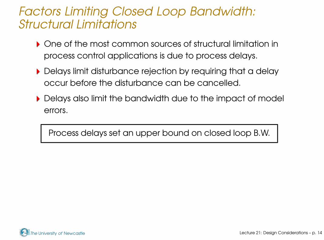
Factors Limiting Closed Loop Bandwidth:Structural Limitations
One of the most common sources of structural limitation in
process control applications is due to process delays.
Delays limit disturbance rejection by requiring that a delay
occur before the disturbance can be cancelled.
Delays also limit the bandwidth due to the impact of model
errors.
Process delays set an upper bound on closed loop B.W.
Lecture 21: Design Considerations – p. 14

The University of Newcastle
Actuator Saturation
Actuators are a source of performance limitations in control
systems. They impose
Amplitude limits by constraining the amplitude of the control
signal,
Slew rate limits by limiting the rate of change of the control
signal.
Lecture 21: Design Considerations – p. 15
The University of Newcastle
Actuator Saturation: Amplitude Limits
In a 1 DOF control loop the controller output is given by
U(s) = Su0(s) (R(s) − D0(s))
Peaks in the control action usually occur as a result of large
fast changes in either the reference r(t) or the output
disturbance d0(t). Input disturbances, di(t), are usually
attenuated by the plant and hence are neglected here.
Lecture 21: Design Considerations – p. 16

The University of Newcastle
Actuator Saturation: Amplitude Limits
In a 1 DOF control loop the controller output is given by
U(s) = Su0(s) (R(s) − D0(s))
Peaks in the control action usually occur as a result of large
fast changes in either the reference r(t) or the output
disturbance d0(t). Input disturbances, di(t), are usually
attenuated by the plant and hence are neglected here.
If the closed loop B.W. is greater than the open loop
dynamics of G0(s) then the controller sensitivity, Su0(s) will
significantly enhance the high frequency components in
R(s) and D(s). This is easily seen as the control sensitivity is
defined as,
Su0(s) ,T0(s)
G0(s)
Lecture 21: Design Considerations – p. 16

The University of Newcastle
Actuator Saturation: Slew Rate Limits
On the other hand, actuator saturation limits the maximum
speed at which the actuator can change position.
The rate of change of the input can be expressed as:
sU(s) = Su0(s) (sR(s) − sD0(s))
=T0(s)
G0(s)(sR(s) − sD0(s))
If the closed loop B.W. is much larger than that of the plant
dynamics then the rate of change of the input signal will be
large for fast changes in r(t) and d0(t).
Lecture 21: Design Considerations – p. 17

The University of Newcastle
Actuator Saturation
In conclusion:
To avoid amplitude and slew rate limit problems, it will
be necessary to place an upper limit on the closed loop
B.W.
Lecture 21: Design Considerations – p. 18

The University of Newcastle
Outline
Introduction
Revision of Factors Limiting Closed Loop Bandwidth
Dealing with Input Constraints in the Context of State
Feedback and Observers.
Trade-offs in State Feedback and Observers
General Feedback Design Tips
Lecture 21: Design Considerations – p. 19

The University of Newcastle
Actuator Saturation: Integrator Windup
Amplitude limits in conjunction with a controller with integral
action induces integrator windup, which deteriorates
closed-loop performance.
G(s)mf f- - - -
6
-¡¡C(s)
saturationsActuator
−
v(t)e(t)r(t) y(t)u(t)Note that
when the
actuator hits
its limits, the
loop is virtually open!
Lecture 21: Design Considerations – p. 20

The University of Newcastle
Actuator Saturation: Integrator Windup
Amplitude limits in conjunction with a controller with integral
action induces integrator windup, which deteriorates
closed-loop performance.
G(s)mf f- - - -
6¡¡C(s)
saturationsActuator
−
v(t)e(t)r(t) y(t)u(t)Note that
when the
actuator hits
its limits, the
loop is virtually open!
Indeed, when the error e(t) is so large that a command v(t)
to the actuator exceeds the saturation levels, the command
cannot be realised and the control loop is broken.
If the controller contains an integrator, the broken loop becomes
unstable, so that v(t) will continue to grow until v(t) À usat.
Lecture 21: Design Considerations – p. 20
The University of Newcastle
Actuator Saturation: Integrator Windup
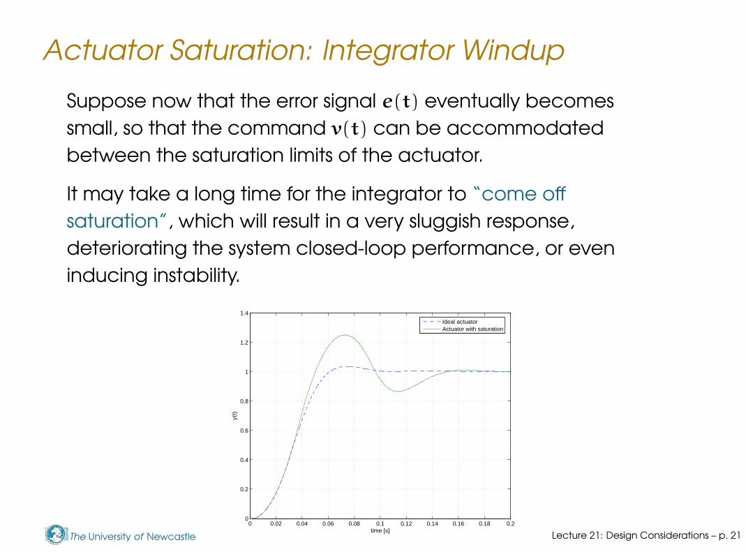
Suppose now that the error signal e(t) eventually becomes
small, so that the command v(t) can be accommodated
between the saturation limits of the actuator.
It may take a long time for the integrator to “come off
saturation”, which will result in a very sluggish response,
deteriorating the system closed-loop performance, or even
inducing instability.
0 0.02 0.04 0.06 0.08 0.1 0.12 0.14 0.16 0.18 0.20
0.2
0.4
0.6
0.8
1
1.2
1.4
time [s]
y(t)
Ideal actuatorActuator with saturation
Lecture 21: Design Considerations – p. 21
The University of Newcastle
Antiwindup Schemes
We have seen in IMC design some structures to implement in the
controller so that we can compensate the effects of integrator
windup.
Recall the principles of antiwindup compensation:
The states of the controller should be driven by the actual
input to the plant.
The states of the controller should have a stable realisation
when the actuator saturates.
Lecture 21: Design Considerations – p. 22

The University of Newcastle
Antiwindup Schemes
A general antiwindup compensation scheme is the following:
C(s)
v(t)
¡¡µ´
¶³hµ´¶³
h
h
µ´¶³
- - -- -
?
6
¾ ¾
6−
e(t)r(t)
−
u(t)
y(t)τaw
The parameter τaw can be used to tune the response.
Lecture 21: Design Considerations – p. 23

The University of Newcastle
Antiwindup Schemes
A general antiwindup compensation scheme is the following:
C(s)
v(t)
¡¡µ´
¶³hµ´¶³
h
h
µ´¶³
- - -- -
?
6
¾ ¾
6−
e(t)r(t)
−
u(t)
y(t)τaw
The parameter τaw can be used to tune the response.
The saturation block is a model of the actuator. If C(s) contains
an integration (as in PIDs), this scheme prevents instability of the
controller when the actuator saturates.
Lecture 21: Design Considerations – p. 23

The University of Newcastle
Antiwindup Schemes
A general antiwindup compensation scheme is the following:
¡¡C(s)
v(t)
µ´¶³h
µ´¶³
µ´¶³
h
h- - -- -
6
?¾
6−
e(t)r(t)
τaw
−
u(t)
y(t)
The parameter τaw can be used to tune the response.
The saturation block is a model of the actuator. If C(s) contains
an integration (as in PIDs), this scheme prevents instability of the
controller when the actuator saturates.
On the other hand, when there is no saturation, the τaw
compensation loop does not act.
Lecture 21: Design Considerations – p. 23

The University of Newcastle
Antiwindup in State Feedback
Returning to state space controllers:
We have seen how to implement a state controller with
feedback from estimated states and integral action for
robust tracking.
We show how we can modify the implementation of this
controller to incorporate antiwindup.
To do so, we will make some block diagram transformations
to bring the integrator next to the actuator in order to
implement the general antiwindup compensation.
C(s)
v(t)
¡¡µ´
¶³h µ´¶³
h
h
µ´¶³
- - -- -
?
6
¾ ¾
6−
e(t)r(t)
−
u(t)
y(t)τaw
Lecture 21: Design Considerations – p. 24

The University of Newcastle
Antiwindup in State Feedback
Start from the original closed loop configuration:
Estmated States Feedbackwith Integral Action Design
y(t)
u(t)
x’ = Ax+Bu y = Cx+Du
State−Space
K* u
State Feedback
Reference
1s
1s
Kz* u
IntegralActionGain
[B,L]* u
Gain4A−L*C* u
Gain3
C* u
Gain
Disturbance
Actuator
Lecture 21: Design Considerations – p. 25

The University of Newcastle
Antiwindup in State Feedback
Interchange state feedback loop and integrator
Estimated States Feedbackwith Integral Action Design
and Antiwindup
y(t)
u(t)
x’ = Ax+Bu y = Cx+Du
State−Space
K* u
State Feedback
Reference
1s
1s
Kz* u
IntegralActionGain
[B,L]* u
Gain4A−L*C* u
Gain3
C* u
Gain
Disturbance
du/dt
Derivative
Actuator
Lecture 21: Design Considerations – p. 26

The University of Newcastle
Antiwindup in State Feedback
Reimplement state feedback loop to eliminate d/dt:
Estimated States Feedbackwith Integral Action Design
and Antiwindup
y(t)
u(t)
x’ = Ax+Bu y = Cx+Du
State−Space
K* u
State Feedback
Reference
1s
1s
Kz* u
IntegralActionGain
[B,L]* u
Gain4A−L*C* u
Gain3
C* u
Gain
Disturbance
Actuator
Lecture 21: Design Considerations – p. 27

The University of Newcastle
Antiwindup in State Feedback
Incorporate antiwindup compensation to the integrator:
Estimated States Feedbackwith Integral Action Design
and Antiwindup
Antiwindup Scheme
y(t)
u(t)
x’ = Ax+Bu y = Cx+Du
State−Space
K* u
State Feedback
Reference
1s
1s
Kz* u
IntegralActionGain
[B,L]* u
Gain4A−L*C* u
Gain3
C* u
Gain
Disturbance
Actuatormodel
Actuator
Taw* u
AW Gain
This scheme will compensate integrator windup only when
needed.
Lecture 21: Design Considerations – p. 28

The University of Newcastle
Antiwindup in State Feedback
Estimated States Feedbackwith Integral Action Design
and Antiwindup
Antiwindup Scheme
y(t)
u(t)
x’ = Ax+Bu y = Cx+Du
State−Space
K* u
State Feedback
Reference
1s
1s
Kz* u
IntegralActionGain
[B,L]* u
Gain4A−L*C* u
Gain3
C* u
Gain
Disturbance
Actuatormodel
Actuator
Taw* u
AW Gain
Note that the principles of antiwindup compensation are
satisfied:
The states of the controller are driven by the actual input to
the plant (observer and integral action).
The states of the controller have a stable realisation when
the actuator saturates (observer and integral action).
Lecture 21: Design Considerations – p. 29

The University of Newcastle
Antiwindup in State Feedback
Example (HDD output feedback controller).
Consider the position control
of a Hard Disk Drive given by the model
G(s) =K0ω2
r
s2(s2 + 2ξωrs + ω2r)
Ignoring any input saturation, we designed an observer-based
state feedback controller with integral action to achieve
max overshoot < 3%, settling time < 0.1s.
We compare the closed loop performance of this system without
and with antiwindup compensation for an actuator saturation
level of usat = 0.065, which corresponds approximately to 100%
saturation for the maximum peak command required.
Lecture 21: Design Considerations – p. 30

The University of Newcastle
Antiwindup in State Feedback
Example (HDD output feedback controller). We can see how
performance deteriorates with actuator saturation — overshoot
jumps from 3% to 20%, and settling time from 0.1 to 0.15 s.
0 0.05 0.1 0.15 0.2−0.2
0
0.2
0.4
0.6
0.8
1
1.2
1.4
time [s]
Without AW
y(t)u(t)
0 0.05 0.1 0.15 0.2−0.2
0
0.2
0.4
0.6
0.8
1
1.2
1.4
time [s]
With AW
y(t)u(t)
On the other
hand, the ideal
performance
is almost
completely
recovered with
the antiwindup
compensation.
Lecture 21: Design Considerations – p. 31

The University of Newcastle
Antiwindup in State Feedback
Example (HDD output feedback controller). This plot shows the
effect of the parameter τaw on the compensated closed-loop
response (τaw = 0 ⇒ no compensation).
0 0.02 0.04 0.06 0.08 0.1 0.12 0.14 0.16 0.18 0.20
0.2
0.4
0.6
0.8
1
1.2
1.4
time [s]
AW with different Taw
y(t)
τaw
=100
τaw
=50
τaw
=0
C(s)
v(t)
¡¡µ´
¶³hµ´¶³
h
h
µ´¶³
- - -- -
?
6
¾ ¾
6−
e(t)r(t)
−
u(t)
y(t)τaw
Lecture 21: Design Considerations – p. 32
The University of Newcastle
Outline
Introduction
Revision of Factors Limiting Closed Loop Bandwidth
Dealing with Input Constraints in the Context of State
Feedback and Observers.
Trade-offs in State Feedback and Observers
General Feedback Design Tips
Lecture 21: Design Considerations – p. 33

The University of Newcastle
Trade-offs in State Feedback & Observers
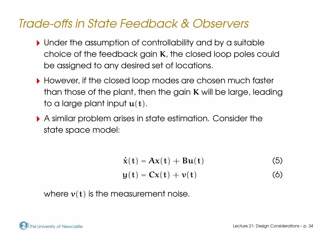
Under the assumption of controllability and by a suitable
choice of the feedback gain K, the closed loop poles could
be assigned to any desired set of locations.
Lecture 21: Design Considerations – p. 34

The University of Newcastle
Trade-offs in State Feedback & Observers
Under the assumption of controllability and by a suitable
choice of the feedback gain K, the closed loop poles could
be assigned to any desired set of locations.
However, if the closed loop modes are chosen much faster
than those of the plant, then the gain K will be large, leading
to a large plant input u(t).
Lecture 21: Design Considerations – p. 34
The University of Newcastle
Trade-offs in State Feedback & Observers
Under the assumption of controllability and by a suitable
choice of the feedback gain K, the closed loop poles could
be assigned to any desired set of locations.
However, if the closed loop modes are chosen much faster
than those of the plant, then the gain K will be large, leading
to a large plant input u(t).
A similar problem arises in state estimation. Consider the
state space model:
x(t) = Ax(t) + Bu(t) (5)
y(t) = Cx(t) + v(t) (6)
where v(t) is the measurement noise.
Lecture 21: Design Considerations – p. 34

The University of Newcastle
Trade-offs in State Feedback & Observers
Then the state estimate and the estimation error are:
˙x(t) = Ax(t) + Bu(t) + LC(x(t) − x(t)) + Lv(t) (7)
˙x(t) = (A − LC)x(t) − Lv(t) (8)
Applying the Laplace transform to (4),
X(s) = [sI − A + LC]−1x(0) − [sI − A + LC]−1LV(s) (9)
Here we see that if L is chosen to place the eigenvalues of
A − LC well into the left half plane, we will quickly eliminate
the effect of the initial error x(0).
Lecture 21: Design Considerations – p. 35

The University of Newcastle
Trade-offs in State Feedback & Observers
However, this will almost certainly require a large value for L.
We then see that the second term on the right hand side of
equation (5) will enhance the effect of the measurement
noise, since this is usually a high frequency signal.
Lecture 21: Design Considerations – p. 36

The University of Newcastle
Trade-offs in State Feedback & Observers
However, this will almost certainly require a large value for L.
We then see that the second term on the right hand side of
equation (5) will enhance the effect of the measurement
noise, since this is usually a high frequency signal.
We then need to compromise between speed of response
and noise immunity.
How to select a desired set of eigenvalues? Of course this
depends on many performance criteria (rise time, settling
time, overshoot, etc..)
We must remember that the response of a system not only
depends on the position of the poles but also on the zeros
and, of course, the limits placed on the control signal by the
actuator.
Lecture 21: Design Considerations – p. 36

The University of Newcastle
Trade-offs in State Feedback & Observers
As a guide we may place all the eigenvalues inside the region
denoted by C in the figure below.
θ
Im(s)
Re(s)
σC
r
Figure 1:
Lecture 21: Design Considerations – p. 37
The University of Newcastle
Trade-offs in State Feedback & Observers
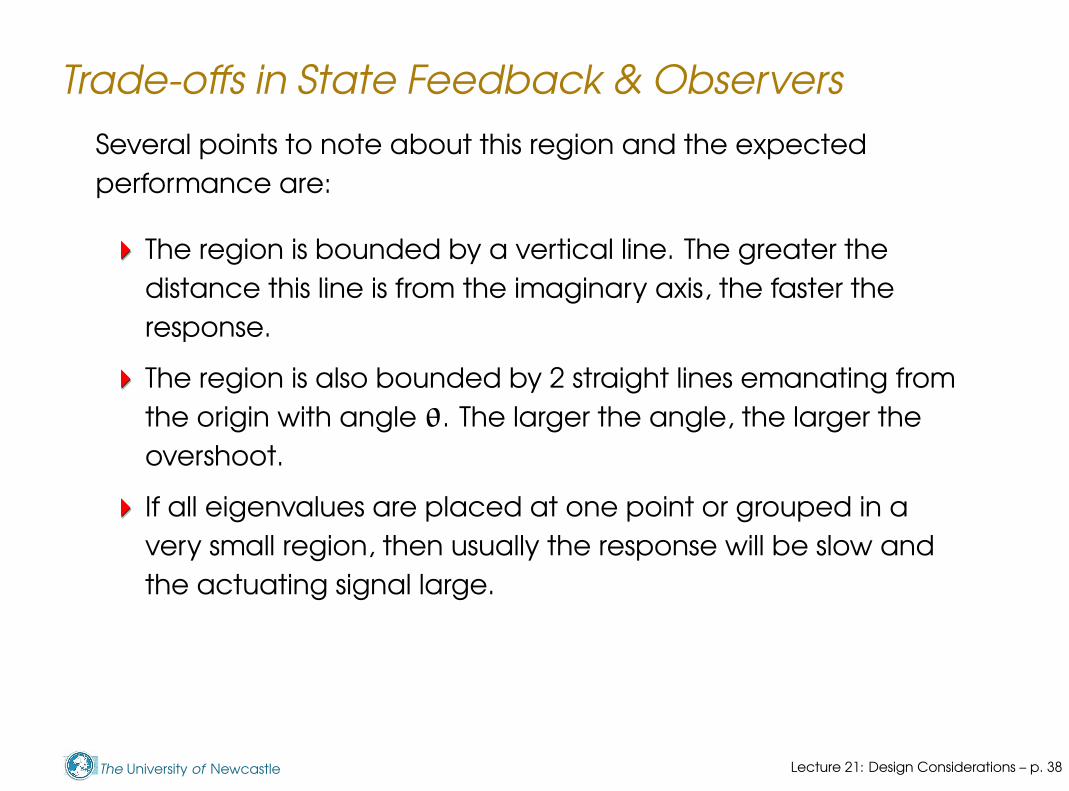
Several points to note about this region and the expected
performance are:
The region is bounded by a vertical line. The greater the
distance this line is from the imaginary axis, the faster the
response.
The region is also bounded by 2 straight lines emanating from
the origin with angle θ. The larger the angle, the larger the
overshoot.
If all eigenvalues are placed at one point or grouped in a
very small region, then usually the response will be slow and
the actuating signal large.
Lecture 21: Design Considerations – p. 38

The University of Newcastle
Trade-offs in State Feedback & Observers
It is better to place eigenvalues around a circle with radius r
inside the sector as shown. The larger the radius,
the faster the response and of course the larger the
control signal.
the larger the closed loop B.W. resulting in a system more
susceptible to noise.
Lecture 21: Design Considerations – p. 39

The University of Newcastle
Outline
Introduction
Revision of Factors Limiting Closed Loop Bandwidth
Dealing with Input Constraints in the Context of State
Feedback and Observers.
Trade-offs in State Feedback and Observers
General Feedback Design Tips
Lecture 21: Design Considerations – p. 40

The University of Newcastle
General Feedback Design Tips
How to choose an appropriate Closed Loop Bandwidth? A
general recipe you may wish to consider is:
The B.W. must be large relative to the location of unstable
poles. In particular, a suggestion is:
ωb ≥ 5∑
i∈U
pi (10)
where U denotes the set of unstable poles pi.
The B.W. must be small relative to the location of R.H.P. zeros
ξi and to time delay τ. In particular, a suggestion is:
ωb ≤
(
τ
2+
∑
i∈U ′
1
ξi
)
−1
(11)
where U ′ denotes the set of R.H.P. zeros ξi.
Lecture 21: Design Considerations – p. 41

The University of Newcastle
General Feedback Design Tips
The B.W. must be small relative to the frequency where the
relative modelling error∣
∣
∣
G∆
G0
∣
∣
∣approaches 1.
The B.W. is constrained by the input amplitude and slew rate
limits.
Having chosen the B.W. the following are additional guidelines.
Any stable, well damped zeros within the B.W. should be
cancelled in the controller.
Any stable, well damped poles within the B.W. may be
cancelled provided they are not close to the origin
compared to the B.W.
Lecture 21: Design Considerations – p. 42

The University of Newcastle
General Feedback Design Tips
Let k denote the number of open loop poles in the plant and
controller that are close to the origin relative to the B.W. (in
this sense, the distance to the origin be < 1
5ωb); then there
should be k − 1 closed loop poles at stable well damped
locations whose distance to the origin is about 1
5ωb.
The poles not constrained by the last 3 guidelines should be
placed at stable well damped locations as follows:
Not more than 2 at ωb.
The remainder at greater than 3ωb
If any of the controller poles or zeros are unstable then
alternative measurements should be used.
Lecture 21: Design Considerations – p. 43

The University of Newcastle
General Feedback Design: Further Ideas
Dominant 2nd Order Poles
For a second order system, rise time, settling time and overshoot
can be directly deduced from the pole locations. A simple
technique to utilise this knowledge to give performance
measures in a higher order system is:
Choose the closed loop poles for a higher order system as a
desired pair of dominant 2nd order poles.
Select the rest of the poles to have real parts corresponding
to sufficiently damped modes so that the system will mimic a
2nd order response with reasonable control effort.
Ensure that the zeros are far enough into the L.H.P to avoid
having any appreciable effect on the 2nd order behaviour.
Lecture 21: Design Considerations – p. 44
The University of Newcastle
General Feedback Design: Further Ideas
Observer Pole Selection
Can use the same ideas as for the feedback design.
As a rule of thumb observer poles should be chosen to be a
factor of (2 to 6)× faster than the controller poles. This
ensures the observer errors decay faster than the desired
closed loop dynamics allowing the controller poles to
dominate the total response.
If sensor noise is a problem then the observer poles may be
chosen slower than 2× the controller poles. This would yield a
system with lower bandwidth and more noise smoothing.
Unlike the controller, the observer output is a number in a
computer. Depending on the computer numerical precision,
there are no real limits on the size of this number. However,
measurement noise will limit the speed of the observer.
Lecture 21: Design Considerations – p. 45

The University of Newcastle
Summary
Revision of Factors that Limit Closed Loop Bandwidth
Noise
Disturbances
Modelling Errors
Structural Limitations
Actuator Limits
Input Constraints in State Feedback and Observers
Trade-offs in State Feedback and Observers
General Control System Design Tips
Lecture 21: Design Considerations – p. 46