Embed Size (px)
Citation preview
Controllability and Motion Algorithms for Underactuated
Lagrangian Systems on Lie Groups∗
Francesco Bullo
Coordinated Science Laboratory and
Department of General Engineering
University of Illinois at
Urbana-Champaign
1308 West Main Street
Urbana, IL 61801, USA
Naomi Ehrich Leonard
Department of Mechanical and
Aerospace Engineering
Princeton University
Princeton, NJ 08544, USA
Andrew D. Lewis
Department of Mathematics & Statistics
Queen’s University
Kingston, ON K7L 3N6, Canada
Final Submitted Version. This version: March 10, 2005
Abstract
In this paper, we provide controllability tests and motion control algorithms for under-
actuated mechanical control systems on Lie groups with Lagrangian equal to kinetic energy.
Examples include satellite and underwater vehicle control systems with the number of control
inputs less than the dimension of the configuration space. Local controllability properties of
these systems are characterized, and two algebraic tests are derived in terms of the symmet-
ric product and the Lie bracket of the input vector fields. Perturbation theory is applied to
compute approximate solutions for the system under small-amplitude forcing; in-phase signals
play a crucial role in achieving motion along symmetric product directions. Motion control
algorithms are then designed to solve problems of point-to-point reconfiguration, static inter-
polation and exponential stabilization. We illustrate the theoretical results and the algorithms
with applications to models of planar rigid bodies, satellites and underwater vehicles.
Keywords : nonlinear control, mechanical systems, nonlinear controllability, underactuatedsystems
∗Short versions of this paper appeared in the European Control Conference, Brussels, July 1997, see [3], and theNonlinear Control Systems Design Symposium, The Netherlands, July 1998, see [4].
1
Contents
1 Introduction 3
2 Preliminaries and Models 42.1 Lie groups tools . . . . . . . . . . . . . . . . . . . . . . . . . . . . . . . . . . . . . . 42.2 Mechanical control systems on Lie groups . . . . . . . . . . . . . . . . . . . . . . . 52.3 Examples: planar bodies, satellites and underwater vehicles . . . . . . . . . . . . . 6
3 Local Controllability Properties 83.1 Definitions and tests . . . . . . . . . . . . . . . . . . . . . . . . . . . . . . . . . . . 9
3.1.1 Accessibility and configuration accessibility . . . . . . . . . . . . . . . . . . 103.1.2 Controllability and configuration controllability . . . . . . . . . . . . . . . . 10
3.2 Applications to the examples . . . . . . . . . . . . . . . . . . . . . . . . . . . . . . 11
4 Approximate Solutions under Small-amplitude Forcing 134.1 Notation and results . . . . . . . . . . . . . . . . . . . . . . . . . . . . . . . . . . . 134.2 Application to the examples . . . . . . . . . . . . . . . . . . . . . . . . . . . . . . . 144.3 Inversion algorithm for systems controllable with second-order symmetric products 17
5 Control Algorithms from Motion Primitives 185.1 Primitives of motion . . . . . . . . . . . . . . . . . . . . . . . . . . . . . . . . . . . 185.2 Control algorithms . . . . . . . . . . . . . . . . . . . . . . . . . . . . . . . . . . . . 195.3 Numerical simulations . . . . . . . . . . . . . . . . . . . . . . . . . . . . . . . . . . 22
6 Conclusions 23
A Proofs 26A.1 Proposition 4.1 . . . . . . . . . . . . . . . . . . . . . . . . . . . . . . . . . . . . . . 26A.2 Lemma 4.2 . . . . . . . . . . . . . . . . . . . . . . . . . . . . . . . . . . . . . . . . 28A.3 Primitives of Motion . . . . . . . . . . . . . . . . . . . . . . . . . . . . . . . . . . . 28A.4 Lemma 5.2 . . . . . . . . . . . . . . . . . . . . . . . . . . . . . . . . . . . . . . . . 29A.5 Lemma 5.3 . . . . . . . . . . . . . . . . . . . . . . . . . . . . . . . . . . . . . . . . 30
List of Tables
1 Constant Velocity Algorithm for point-to-point reconfiguration. . . . . . . . . . . 202 Local Exponential Stabilization Algorithm. . . . . . . . . . . . . . . . . . . . . . . 203 Static Interpolation Algorithm. . . . . . . . . . . . . . . . . . . . . . . . . . . . . . 21
2
1 Introduction
Underactuated mechanical control systems provide a challenging research area of increasing interestin both application and theory. In this paper, we examine an important class of underactuatedmechanical control systems and address problems in both nonlinear controllability and nonlinearcontrol design. It is precisely because we specialize to a structured class of mechanical systemsthat we can solve relevant controllability and control design problems; we derive controllabilitytests and motion control algorithms by making use of the mechanical system structure.
Underwater vehicles, satellites, surface vessels, airships and hovercrafts are all examples ofsimple mechanical control systems on Lie groups. For these systems, relevant Lagrangian modelsare available and lift/drag type effects are sometimes negligible. Key features are the following:(1) the configuration space is a Lie group, as, for example, the group of rotations SO(3) in thecase of a satellite, (2) the Lagrangian is equal to the kinetic energy, and (3) external forces arefixed with respect to the body. From a theoretical perspective, these systems when underactuatedoffer a control challenge as they have non-zero drift (e.g., their dynamics include Coriolis effects),their linearization at zero velocity is not controllable, they are not stabilizable by continuous statefeedback and exponential stabilization cannot be achieved by smooth time-varying feedback [24].Further, they are generically not nilpotent, not feedback linearizable, not “configuration flat,” asdefined in [29], and no test is available to establish whether they are differentially flat. In otherwords, the motion planning and the stabilization problem for this class of systems cannot be solvedwith any established method.
We focus on this class of systems with fewer actuators than degrees of freedom, and we studyseveral motion control problems in the small-velocity range. From a practical point of view, we aremotivated by vehicles that are underactuated either because of an actuator failure or because of adesign choice. In the former case, our results will improve robustness to actuator failure and thuswill provide autonomous vehicles with greater reliability. In the latter case, our results may allowfor vehicle designs that include fewer actuators than typical leading to lighter, less costly designs.See [32] for a extensive discussion on autonomous underwater vehicle design.
Relevant past contributions include work on both the nonlinear controllability problem andthe constructive controllability problem (including both motion planning and stabilization). Forour work, the most important references for controllability are the works of Sussmann on small-time local controllability [34] and of Lewis and Murray on configuration controllability for simplemechanical systems [19] and [20]. Other contributions include local controllability results for otherclasses of mechanical systems, see [10] and [27], and work on global controllability issues, see [1], [7]and [22]. Regarding the constructive controllability problem, we employ the same approach asLeonard and Krishnaprasad in [16] and [14], where motion algorithms for a class of kinematicsystems on Lie groups were designed with small-amplitude periodic inputs. In later work [30]similar techniques were applied to a different class of mechanical system. Other contributions onmotion planning via oscillatory controls include [9, 36, 35]. A somewhat different approach, basedon homogeneous time-varying strategies, was employed in [25] and [28] to design exponentiallystabilizing control laws for underactuated satellites and surface vessels.
The main contributions of this work are approximate local motion primitives and control algo-rithms. Provided that certain controllability conditions are satisfied, we show how underactuatedvehicles can still perform important tasks such as stabilization (station keeping) and short rangereconfigurations (parking, tracking). In what follows we illustrate the three aspects of this work.
To derive controllability tests for our class of systems, we apply the controllability analysisdescribed in [34] and [19] to simple mechanical control systems on Lie groups (see also [5]). Keyfeatures of the analysis are a focus on the evolution of the system’s configuration when the initialvelocity is zero. The local controllability properties are characterized by the algebraic operationsof symmetric product and Lie bracket. The symmetric product, which is defined more formally inSection 2, depends upon the metric that defines the kinetic energy and, as we shall see, explicitlydescribes motions that involve both input vector fields and the drift dynamics. Our results are both
3
an application of the results in [19]: the computation of Lie brackets and symmetric products aresimplified to algebraic operations on the Lie algebra of the Lie group, the tests, which characterizereachable velocities and configurations, are independent of the initial configuration.
Guided by our interpretation of the controllability tests, we apply perturbation theory to in-vestigate the response of the mechanical system to small-amplitude forcing. The initial velocityis also assumed to have small amplitude. The approximations we obtain give further insight intothe controllability tests and are instrumental in the subsequent control design. Numerous exam-ples illustrate the meaning of good and bad symmetric products and the effects of in-phase andout-of-phase sinusoidal inputs.
On the basis of a controllability assumption, we design two motion primitives that perform thebasic tasks of changing and maintaining velocity. These motion primitives use in-phase inputs andcompensate for contributions along bad symmetric product directions. The two motion primitivessynthesize the controllability analysis and are the building blocks for designing high-level motionprocedures. Using discrete-time feedback and multiple calls to the motion primitives, we designmotion algorithms to solve the point-to-point reconfiguration problem (i.e., how to steer the systemto a desired configuration) and the static interpolation problem (i.e., how to steer the systemthrough a set of desired configurations). We solve point-to-point reconfiguration using a constantvelocity algorithm. A second approach to point-to-point reconfiguration consists of interpolatinga sequence of segments connecting initial to final configuration. We show the advantage of thelatter solution in the case the segments are steady motions of the unforced mechanical system.Next, iterating an approximate stabilization step we design an algorithm that locally exponentiallystabilizes the system to a desired configuration. Recall that exponential stabilization cannot beachieved by smooth time-varying feedback, and indeed our motion primitives are continuous, butnot smooth, functions of the state. Accordingly, our approach relies on discrete-time continuousfeedback, see [33], and on the iteration of a motion planning step, see [12] and [21]. Finally,the three algorithms are implemented numerically to verify the approximations and illustrate thecontrol design.
The paper is organized as follows. In Section 2 we present some mathematical preliminaries andprovide many examples of mechanical systems on Lie groups. In Section 3 a complete controllabilityanalysis is presented with definitions, tests and examples. Section 4 and Section 5 contain our mainresults. First, we obtain formulas for approximate solutions and we use them to gain insight into thecontrollability tests. Second, we design and simulate motion control algorithms. Our conclusionsare given in Section 6 and Appendix A contains various proofs.
2 Preliminaries and Models
In this section we review useful notions from geometric mechanics and Lie group theory andintroduce several examples of mechanical control systems on Lie groups. For a more detailedtreatment of the mathematical background, we refer the reader to [26] and [23]. An overview in arelated investigation is presented in [16].
2.1 Lie groups tools
A Lie group is a smooth manifold endowed with a smooth binary operation called group multipli-cation (satisfying associativity and existence of identity and inverse elements). A Lie algebra is avector space endowed with a skew symmetric, bilinear operation called the Lie bracket (satisfyingthe Jacobi identity). An example of a Lie group is the rotation group SO(3) (the set of orthogo-nal matrices with positive determinant under matrix multiplication). Its associated Lie algebra isthe space of skew symmetric matrices so(3) (under matrix commutation). Other examples of Liegroups are the sets SE(n) of rigid motions on the n–dimensional Euclidean space Rn.
Let G denote a matrix Lie group and g its Lie algebra. The letters g and h denote elements inG, and Id is the identity. The Greek letters ξ and η denote elements in g and adξ η = [ξ, η] denotes
4
the Lie bracket operation on g. Although most of the results in this paper hold more generally, forease of presentation we make the assumption that:
(A1) The set G is the direct product of an arbitrary number of copies of SE(3) and its propersubgroups.
G, with the assumption (A1), can be represented as a matrix Lie group with group multiplicationdefined by matrix multiplication and the Lie bracket on the associated Lie algebra given by matrixcommutation, i.e., [ξ, η] = ξη − ηξ. Let × denote the cross product on R3 and define the operator· : R3 → so(3) by xy , x× y for all x, y ∈ R3. On SE(3) and se(3) we represent a group element
g = (R, p) ∈ SO(3) × R3 and a velocity ξ = (Ω, V ) ∈ so(3) × R3 using homogeneous coordinates
g =
[R p0 1
], and ξ =
[Ω V0 0
].
Writing ξ as column vector (Ω, V ), simple algebra shows
adξ =
[Ω 0
V Ω
]. (1)
Under (A1), we can define a surjective map and local diffeomorphism called the exponentialmap exp : g → G; we refer to [23] for the general definition. For example, given x ∈ so(3),Rodrigues’ formula gives
exp(x) = Id + sin ‖x‖ x
‖x‖ + (1 − cos ‖x‖) x2
‖x‖2,
where ‖ · ‖ is the standard Euclidean norm. In an open neighborhood of the origin Id ∈ G, wedefine x = log(g) ∈ g to be the exponential coordinates of the group element g and we regardthe logarithmic map as a local chart on the manifold G. For example, if R ∈ SO(3) is such thattr(R) 6= −1, then
log(R) =φ
2 sinφ(R−RT ) ∈ so(3),
where φ satisfies 2 cosφ = tr(R)− 1 and |φ| < π. In other words, log(R) is the product of the axisand angle of rotation of R. Corresponding definitions for the group SE(3) are presented in [26].
On the Lie algebra g an inner product is defined by a self–adjoint positive definite tensor
I : g → g∗, so that, for example, the norm of ξ is computed as ‖ξ‖g = (Iξ · ξ)1/2
. This induces ametric on the group G using the logarithm map as d(g, h) = ‖ log(gh−1)‖g.
Remark 2.1 (Notions of Lie bracket). The operation of Lie bracket defined above is an operationbetween vectors on the linear space g. This should be contrasted with the usual definition of Liebracket between vector fields. The two notions are related and can be described within a unifiedframework by introducing the notion of left-invariant vector field. We refer to [23, 26] for this andrelated facts.
2.2 Mechanical control systems on Lie groups
A simple mechanical control system on a Lie group is described by the following objects: an n-dimensional Lie group G (defining the configuration space), an inertia tensor I : g → g
∗ (definingthe kinetic energy) and a set of input co-vectors1 f1, . . . , fm ⊂ g
∗ (defining the body-fixed forces).The system is said to be underactuated if the number of available input forces m is less than thenumber of degrees of freedom n.
1To simplify notation, we denote the co-vectors fi with subscripts instead of superscripts.
5
Let g ∈ G denote the configuration of the system and ξ ∈ g the body-fixed velocity, so that thekinetic energy is KE = 1
2ξT Iξ. The kinematic and dynamic equations of motion for the system
with Lagrangian equal to the kinetic energy are given by
g = g · ξ (2)
Iξ = ad∗ξ Iξ +
m∑
i=1
fiui(t), (3)
where ad∗ξ is the dual operator of adξ, the scalar input functions ui, i = 1, . . . ,m belong to the
space of bounded measurable functions Um, and∑fiui(t) is the resultant force acting on the
mechanical system. In geometric mechanics, the dynamic equation (3) is called the Euler-Poincareequation; in robotics, the kinematic equation (2) is usually expressed in some choice of coordinatesystem, as, for example, Euler angles for SO(3).
For any vector η with the property that ad∗η Iη = 0, the curve t ∈ R 7→ (exp(tη), η) is a solution
to the system (2)–(3) with no inputs. These curves are studied in mechanics [23] under the nameof relative equilibria and describe motion that corresponds to constant body-fixed velocity for theuncontrolled system.
Next, we introduce the notion of the symmetric product on the Lie algebra g. This operation isuseful for characterizing controllability and approximate solutions for mechanical control systems.It has an elegant generalization using Riemannian geometry as discussed in [19], [18] and in [6].Define the symmetric product 〈ξ : η〉 of two vectors ξ, η on g, as the vector
〈ξ : η〉 , −I−1
(ad∗
ξ Iη + ad∗η Iξ
).
For example, on so(3) ≈ R3 with the inertia tensor J and with the equality ad∗ξ = −ξ, we compute
〈ξ : η〉 = J−1(ξ×Jη+η×Jξ
). For later reference it is also useful to rewrite the dynamic equation (3)
as
ξ = −1
2〈ξ : ξ〉 +
m∑
i=1
biui(t), (4)
where we define bi , I−1fi for simplicity. Additional insight into the meaning of the symmetricproduct is provided in [19], where the operation is shown to be equivalent to a Lie bracket betweencertain vector fields on the full space TG.
Remark 2.2 (Time scaling). For λ > 0 define τ = λt. Mechanical control systems verify thefollowing property: if (g(t), ξ(t)) is a solution for t ∈ [0, 1] to the forced system (2)–(3) withexternal forcing ui(t), then (g(τ/λ), ξ(τ/λ)/λ) is a solution for τ ∈ [0, λ] with external forcingui(τ/λ)/λ2. In other words, if we find an input u(t) that achieves a desired motion in time 1, thenu(t/λ)/λ2 achieves the same motion in time λ. This time/magnitude scaling property should betaken into account when applying the control laws described later in the paper.
2.3 Examples: planar bodies, satellites and underwater vehicles
The following examples of mechanical control systems on Lie groups illustrate the richness of theclass of systems of interest. They will be often referred to later, as we study controllability anddesign control laws. To simplify notation, we let e1, . . . , en denote the standard basis on Rn; forexample, for n = 3 we set e1 = (1, 0, 0), e2 = (0, 1, 0) and e3 = (0, 0, 1).
Planar rigid body
Let g = (θ, x, y) ∈ SE(2) denote the configuration of the planar body and ξ = (ω, v1, v2) its body-fixed velocity. The kinetic energy is KE = 1
2Jω2 + 1
2m(v21 + v2
2) where J is the moment of inertia
6
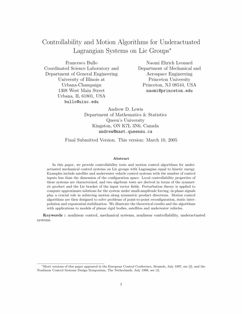
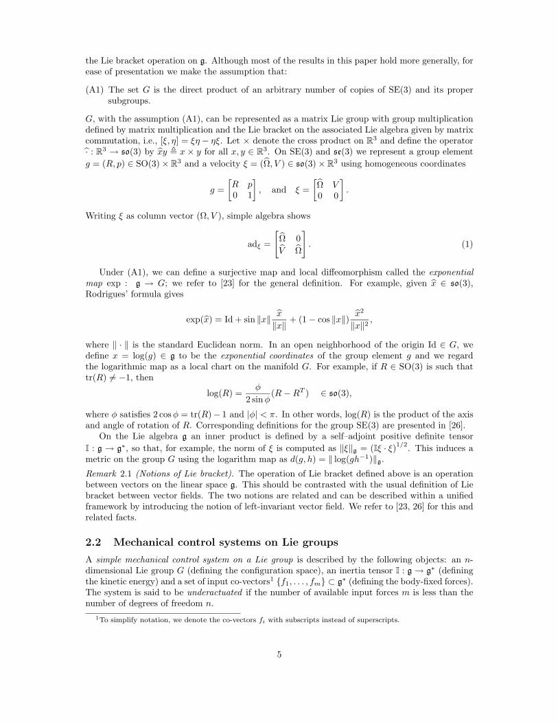
Figure 1: Rigid body in SE(2) with two forces applied at a point a distance h from the center ofmass CM. Σs denotes an inertial reference system. g = (θ, x, y) denotes the position of the body.The body reference frame (not depicted) is aligned with the direction of application of f1 and f2.
and m the mass of the body. On se(2) the adjoint operator is computed as
ad(ω,v1,v2) =
0 0 0v2 0 −ω−v1 ω 0
.
The two control inputs consist of forces applied at a distance h from the center of mass, see Figure 1.After inverting I = diag J,m,m, we have b1 = 1
me2 and b2 = −hJ e1 + 1
me3. In coordinates theequations of motion (2)–(3) read
θ = ω Jω = −hu2(t)
x = cos(θ)v1 − sin(θ)v2 , mv1 = mωv2 + u1(t)
y = sin(θ)v1 + cos(θ)v2 mv2 = −mωv1 + u2(t).
These equations provide a model for planar vehicles, for example, a hovercraft that glides on thesurface of a body of water with negligible friction.
Satellite with thrusters
Let R ∈ SO(3) be the rotation matrix describing the attitude of the satellite and let Ω =(Ω1,Ω2,Ω3) ∈ so(3) ≈ R3 be the body angular velocity. The kinetic energy is then KE = 1
2ΩT JΩ,
where J = diag J1, J2, J3 is the inertia matrix. The adjoint operator is adΩ = Ω. Assuming wehave two thrusters aligned with the first two principal axes, the equations of motion are
R = RΩ
JΩ = JΩ × Ω + e1u1(t) + e2u2(t). (5)
Accordingly, b1 = 1J1
e1 and b2 = 1J2
e2.
Satellite with rotors
Satellites can alternatively be equipped with internal rotors (momentum wheels). Consider the casein which there are two rotors aligned with two principal axes of the satellite. The configuration ofthe satellite plus rotor system is described by R ∈ SO(3) and (θ1, θ2) ∈ R2 (describing the angular
7
position of the wheels). Let Ωrot = (θ1, θ2, 0) denote the angular velocities of the rotors and Ω theangular velocities of the carrier. The kinetic energy is
KE =1
2ΩT (Jlock − Jrot)Ω +
1
2(Ω + Ωrot)
TJrot(Ω + Ωrot),
where Jlock = diag J1, J2, J3 is the inertia of the satellite-rotors system with the rotors locked,while Jrot = diag(Jrot1, Jrot2, 0) is the inertia of the rotors about their spin axes. From the kineticenergy we compute the inertia matrix as
Jsat–rot =
[Jlock Jrot
Jrot Jrot
].
Also, the adjoint operator satisfies ad(Ω,Ωrot)(v, w) = (Ω × v, 0). The dynamic equations are
[Jlock Jrot
Jrot Jrot
] [Ω
Ωrot
]=
[(JlockΩ + JrotΩrot) × Ω
0
]+
[0
e1u1(t) + e2u2(t)
],
and, by inverting the inertia matrix, the input vectors are
b1 =1
Jrot1−J1
e1 +J1
Jrot1(Jrot1−J1)e4
b2 =1
Jrot2−J2
e2 +J2
Jrot2(Jrot2−J2)e5.
Underwater vehicle in ideal fluid
The motion of a rigid body in incompressible, irrotational and inviscid fluid is Hamiltonian with aninertia tensor which includes added masses and inertias, see [13] or the original work of Kirchhoff.Let (R, p) ∈ SE(3) and (Ω, V ) ∈ se(3) denote the configuration and body velocity of the vehicle.The kinematic equations are
R = RΩ
p = RV.
For a neutrally buoyant ellipsoidal body with uniformly distributed mass, the kinetic energy isKE = 1
2ΩT JΩ + 12V
T MV , where the mass and inertia matrices of the body-fluid system areM = diag m1,m2,m3 and J = diag J1, J2, J3. The adjoint operator is given by equation (1).The unforced dynamic equations are therefore
JΩ = JΩ × Ω + MV × V
MV = MV × Ω.
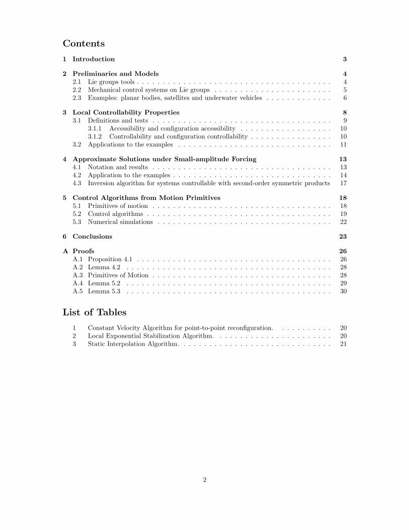
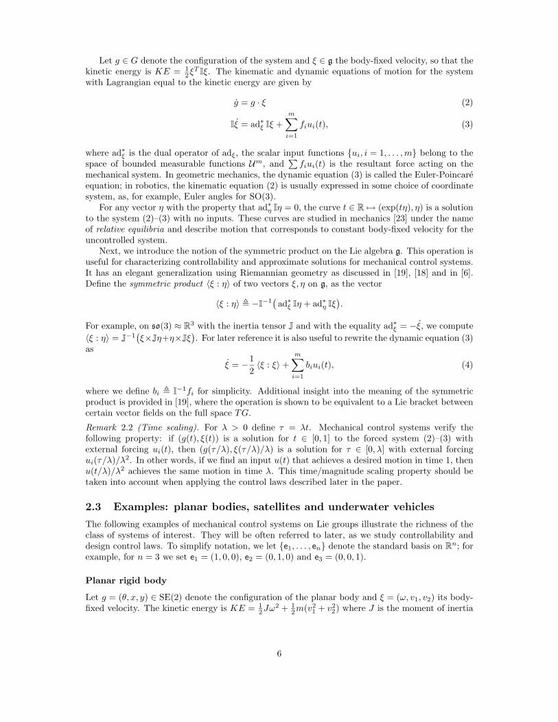
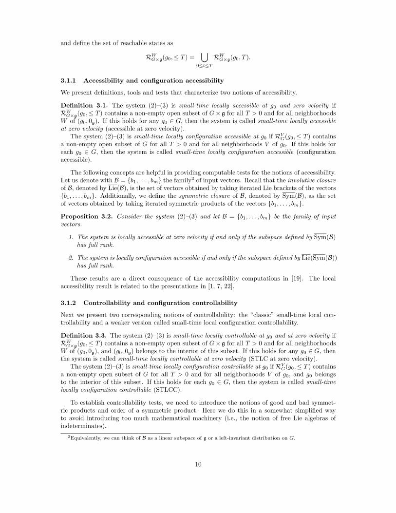
Finally, we assume there are three body-fixed forces applied at a point a distance h from the centerof mass, as depicted in Figure 2. The corresponding input vectors are
b1 =1
m1
e4, b2 = − h
J3
e3 +1
m2
e5, and b3 =h
J2
e2 +1
m3
e6.
3 Local Controllability Properties
This section deals with the nonlinear controllability properties of the systems described above.Our treatment was originally presented in [5]; it is based on the conditions for small-time localcontrollability (STLC) in [34] and for configuration controllability in [19]. While our accessibility
8
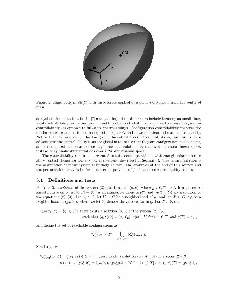
Figure 2: Rigid body in SE(3) with three forces applied at a point a distance h from the center ofmass.
analysis is similar to that in [1], [7] and [22], important differences include focusing on small-time,local controllability properties (as opposed to global controllability) and investigating configurationcontrollability (as opposed to full-state controllability). Configuration controllability concerns thereachable set restricted to the configuration space G and is weaker than full-state controllability.Notice that, by employing the Lie group theoretical tools introduced above, our results haveadvantages: the controllability tests are global in the sense that they are configuration independent,and the required computations are algebraic manipulations over an n–dimensional linear space,instead of symbolic differentiations over a 2n–dimensional space.
The controllability conditions presented in this section provide us with enough information toallow control design for low-velocity maneuvers (described in Section 5). The main limitation isthe assumption that the system is initially at rest. The examples at the end of this section andthe perturbation analysis in the next section provide insight into these controllability results.
3.1 Definitions and tests
For T > 0, a solution of the system (2)–(3), is a pair (g, u), where g : [0, T ] → G is a piecewisesmooth curve on G, u : [0, T ] → Rm is an admissible input in Um and (g(t), u(t)) are a solution tothe equations (2)–(3). Let g0 ∈ G, let V ⊂ G be a neighborhood of g0 and let W ⊂ G × g be aneighborhood of (g0, 0g), where we let 0g denote the zero vector in g. For T > 0, set
RVG(g0, T ) = g1 ∈ G | there exists a solution (g, u) of the system (2)–(3)
such that (g, ξ)(0) = (g0, 0g), g(t) ∈ V for t ∈ [0, T ] and g(T ) = g1,
and define the set of reachable configurations as
RVG(g0,≤ T ) =
⋃
0≤t≤T
RVG(g0, T ).
Similarly, set
RWG×g
(g0, T ) = (g1, ξ1) ∈ G× g | there exists a solution (g, u)(t) of the system (2)–(3)
such that (g, ξ)(0) = (g0, 0g), (g, ξ)(t) ∈W for t ∈ [0, T ] and (g, ξ)(T ) = (g1, ξ1),
9
and define the set of reachable states as
RWG×g
(g0,≤ T ) =⋃
0≤t≤T
RWG×g
(g0, T ).
3.1.1 Accessibility and configuration accessibility
We present definitions, tools and tests that characterize two notions of accessibility.
Definition 3.1. The system (2)–(3) is small-time locally accessible at g0 and zero velocity ifRW
G×g(g0,≤ T ) contains a non-empty open subset of G× g for all T > 0 and for all neighborhoods
W of (g0, 0g). If this holds for any g0 ∈ G, then the system is called small-time locally accessibleat zero velocity (accessible at zero velocity).
The system (2)–(3) is small-time locally configuration accessible at g0 if RVG(g0,≤ T ) contains
a non-empty open subset of G for all T > 0 and for all neighborhoods V of g0. If this holds foreach g0 ∈ G, then the system is called small-time locally configuration accessible (configurationaccessible).
The following concepts are helpful in providing computable tests for the notions of accessibility.Let us denote with B = b1, . . . , bm the family2 of input vectors. Recall that the involutive closureof B, denoted by Lie(B), is the set of vectors obtained by taking iterated Lie brackets of the vectorsb1, . . . , bm. Additionally, we define the symmetric closure of B, denoted by Sym(B), as the setof vectors obtained by taking iterated symmetric products of the vectors b1, . . . , bm.
Proposition 3.2. Consider the system (2)–(3) and let B = b1, . . . , bm be the family of inputvectors.
1. The system is locally accessible at zero velocity if and only if the subspace defined by Sym(B)has full rank.
2. The system is locally configuration accessible if and only if the subspace defined by Lie(Sym(B))has full rank.
These results are a direct consequence of the accessibility computations in [19]. The localaccessibility result is related to the presentations in [1, 7, 22].
3.1.2 Controllability and configuration controllability
Next we present two corresponding notions of controllability: the “classic” small-time local con-trollability and a weaker version called small-time local configuration controllability.
Definition 3.3. The system (2)–(3) is small-time locally controllable at g0 and at zero velocity ifRW
G×g(g0,≤ T ) contains a non-empty open subset of G× g for all T > 0 and for all neighborhoods
W of (g0, 0g), and (g0, 0g) belongs to the interior of this subset. If this holds for any g0 ∈ G, thenthe system is called small-time locally controllable at zero velocity (STLC at zero velocity).
The system (2)–(3) is small-time locally configuration controllable at g0 if RVG(g0,≤ T ) contains
a non-empty open subset of G for all T > 0 and for all neighborhoods V of g0, and g0 belongsto the interior of this subset. If this holds for each g0 ∈ G, then the system is called small-timelocally configuration controllable (STLCC).
To establish controllability tests, we need to introduce the notions of good and bad symmet-ric products and order of a symmetric product. Here we do this in a somewhat simplified wayto avoid introducing too much mathematical machinery (i.e., the notion of free Lie algebras ofindeterminates).
2Equivalently, we can think of B as a linear subspace of g or a left-invariant distribution on G.
10
The order of an iterated symmetric product of factors from Sym(B) is the total number of fac-tors. We say that a symmetric product from Sym(B) is bad if it contains an even number of each ofthe vectors in B. Otherwise, we say that the symmetric product is good. For example, the symmet-ric product 〈〈b1 : b2〉 : b1〉 has order three and it is good, the symmetric product 〈〈〈b1 : b2〉 : b2〉 : b1〉has order four and it is bad. More instances of good and bad symmetric products can be found inthe next section.
Proposition 3.4. Consider the system (2)–(3) and let B = b1, . . . , bm be the family of inputvectors.
1. The system is STLC at zero velocity if the subspace defined by Sym(B) has full rank andevery bad symmetric product is a linear combination of lower-order good symmetric products.
2. The system is STLCC if the subspace defined by Lie(Sym(B)) has full rank and every badsymmetric product is a linear combination of lower-order good symmetric products.
These results are a direct consequence of the results in [34] and [19]. We note that symmetricand involutive closures are simple algebraic operations that characterize controllability for the(strongly) nonlinear system (2)–(3), independent of the base point g0 ∈ G. These tests have asimple interpretation; symmetric products of input vectors identify which velocities are reachable,whereas Lie brackets of reachable velocities identify which configurations are reachable. The onlyrestriction we impose is the requirement that the system be initially at rest.
Note that the distinction between good and bad symmetric products is analogous to, andindeed derived from, the notion of good and bad Lie brackets in [34]. Similar characterizations areusually introduced when dealing with controllability properties for systems with drift. In the nextsection we present some approximate solutions that give some insight into the requirement that“bad products are spanned by lower-order good products.”
Single-input systems (n > m = 1) always fail the sufficient condition for both controllabilitynotions; if only one input vector is available, the only possible nontrivial second-order symmetricproduct is bad. It can further be proven that single-input systems are neither STLC at zerovelocity nor STLCC, see [17].
3.2 Applications to the examples
We investigate the controllability properties of the systems introduced in Section 2.3. Our examplesare selected to be instructive.
Planar rigid body
Consider the planar rigid body described in Section 2.3 with input vectors b1 = 1me2 and b2 =
−hJ e1 + 1
me3. The relevant symmetric products are computed as follows:
〈b1 : b1〉 = 0, 〈b1 : b2〉 =−h
Jme3, 〈b2 : b2〉 =
2h
Jme2, and 〈b2 : 〈b2 : b2〉〉 =
−2h
J2me3.
We distinguish the following cases which depend on the availability of the two input vectors:
[PRB1] B = b1: the system is neither accessible at zero velocity nor configuration accessible,as all symmetric products and Lie brackets vanish. An interpretation of this result is that,for all possible inputs, the body is only allowed to translate parallel to the body fixed x-axis.
[PRB2] B = b2: the system is (small-time locally) accessible at zero velocity since the subspacegenerated by the vectors b2, 〈b2 : b2〉 , 〈b2 : 〈b2 : b2〉〉 has full rank. However, the sufficientcondition for controllability fails to hold, as 〈b2 : b2〉 is a bad symmetric product and it isnot a multiple of any lower-order symmetric product (b2 is the only one). Additionally, asmentioned above, the results in [17] show that the system is neither STLC at zero velocitynor STLCC.
11
[PRB3] B = b1, b2: the system is STLC at zero velocity since the subspace generated by thevectors b1, b2, 〈b1 : b2〉 has full rank and the bad symmetric product 〈b2 : b2〉 is a linearcombination of lower-order good symmetric products: 〈b2 : b2〉 = 2h
J b1.
Satellite with thrusters
Consider the satellite with thrusters described in Section 2.3. Input vectors are b1 = 1J1
e1 and
b2 = 1J2
e2. The relevant symmetric products and Lie brackets are computed as
〈b1 : b1〉 = 〈b2 : b2〉 = 0, 〈b1 : b2〉 =J2−J1
J1J2J3
e3, and [b1, b2] =1
J1J2
e3.
The controllability properties are as follows:
[ST] B = b1, b2 and J1 6= J2: if the satellite is not axisymmetric3, then the rank of b1, b2, 〈b1 : b2〉is full and there are no bad symmetric products. Therefore, the system is STLC at zero ve-locity.
Satellite with rotors
Consider the satellite with rotors introduced in Section 2.3. For b1 and b2 defined in Section 2.3,we compute symmetric products and Lie brackets as
〈b1 : b1〉 = 〈b2 : b2〉 = 〈b1 : b2〉 = 0,
and
[b1, b2] =1
(Jrot1−J1)(Jrot2−J2)e3,
[[b1, b2] , b1] =1
(Jrot1−J1)2(J2−Jrot2)
e2,
[[b1, b2] , b2] =1
(Jrot1−J1)(Jrot2−J2)2e1.
[SR] B = b1, b2: the system is not accessible at zero velocity (every symmetric product vanishes)and hence not STLC, but it is STLCC since the involutive closure has full rank.
This result was partly expected but not trivial. Since the satellite–rotors system is not subject toany external force, its total angular momentum is conserved. Therefore, it is intuitively clear thatthe system cannot be accessible in both configurations and velocities. However, the less trivial factis that the system is STLCC. In other words, despite the conservation law, any configuration ina neighborhood of the initial can be reached, that is, any orientation R together with any rotorangles (θ1, θ2).
Underwater vehicle in ideal fluid
Consider the underwater vehicle introduced in Section 2.3, with the input forces depicted in Fig-ure 2. We compute some good symmetric products as
〈b1 : b2〉 =m2−m1
J3m1m2
e3 −h
J3m2
e5,
〈b1 : b3〉 =m1−m3
J2m1m3
e2 −h
J2m3
e6,
〈b2 : b3〉 =1
J1
(h2
J3
− h2
J2
− 1
m3
+1
m2
)e1
3If the satellite is axisymmetric, i.e., J1 = J2, then a simple analysis shows that the system is STLCC.
12
and some bad ones as
〈b1 : b1〉 = 0, 〈b2 : b2〉 =2h
I3m1
e4, 〈b3 : b3〉 =2h
I2m1
e4.
[UV] B = b1, b2, b3: Consider the 6 × 6 matrix defined by the good symmetric products oforder one and two, that is b1, b2, b3, 〈b1 : b2〉 , 〈b1 : b3〉 , 〈b2 : b3〉. This matrix is genericallynonsingular.4 Hence, the system is small-time locally accessible at zero velocity. Additionally,since the bad second-order symmetric products are proportional to b1, they are spanned bygood lower-order symmetric products (b1 is a good symmetric product of order 1). Therefore,the system is generically STLC at zero velocity.
4 Approximate Solutions under Small-amplitude Forcing
In this section we investigate the behavior of system (2)–(3) under small-amplitude forcing. Thekey analysis tool is the standard perturbation method as described in [11]. Assuming a small-amplitude input (say of order ε, for 0 < ε 1), this method provides us with a solution tosystem (2)–(3) in the form of a Taylor series in ε. Since the computation of only a few terms in theseries is tractable, we obtain an approximate expansion. However, this estimate illustrates the roleof symmetric products and Lie brackets in determining the solution of the forced system (2)–(3).Therefore, this estimate provides insight into the controllability tests introduced above and, as weshall see, it is instrumental in designing the motion algorithms of the next section.
4.1 Notation and results
We introduce the following notation. Given a possibly vector-valued function h(t) with t ∈ R+,define its first integral function h(t) with t ∈ R+, as the finite integral from 0 to t
h(t) ,
∫ t
0
h(τ)dτ.
Higher-order integrals, as for example h(t), are defined recursively. In the following, we considerinputs of the form
ui(t, ε) = εu1i (t) + ε2u2
i (t)
where 0 < ε 1 and where u1i , u
2i are O(1). Accordingly, we write the resultant forcing
∑i biui(t, ε)
as the sum of two terms of different order in ε
m∑
i=1
biui(t, ε) =
m∑
i=1
bi(εu1
i (t) + ε2u2i (t)
)
= ε b1(t) + ε2 b2(t), (6)
where we define b1(t) =∑m
i=1 biu1i (t) and b2(t) =
∑mi=1 biu
2i (t). In the following, given any quantity
y(ε), we let yk denote the kth term in the Taylor expansion of y(ε) about ε = 0; for example, we willwrite ξ(t, ε) = εξ1(t) + ε2ξ2(t) +O(ε3). The following proposition describes the system’s behaviorwhen forced by small (order ε and order ε2) amplitude inputs as defined in equation (6).
Proposition 4.1 (Approximate evolution). For 0 < ε 1 and for inputs of the form in equa-tion (6), let (g(t), ξ(t)) be the solutions of system (2)–(3). Let x(t) be the exponential coordinatesof g(t) about the initial condition g(0) = Id. Also, assume that the initial velocity is O(ε), andwrite it as ξ(0) = εξ10 + ε2ξ20 where ξ10 and ξ20 are O(1).
4The matrix is singular when h2m1m2 + J3(m1 − m2) = 0 or when h2m1m3 + J2(m1 − m3) = 0 orwhen h2(1/J3 − 1/J2) = 1/m3 − 1/m2.
13
Then for t ∈ [0, 2π] it holds that ξ(t, ε) = εξ1(t) + ε2ξ2(t) + ε3ξ3(t) +O(ε4), with
ξ1(t) = ξ10 + b1(t),
ξ2(t) = ξ20 −⟨ξ10 : ξ10
⟩ t2−
⟨ξ10 : b1(t)
⟩+
(b2 − 1
2
⟨b1 : b1
⟩)(t),
ξ3(t) = −⟨ξ10 : ξ20
⟩t+
⟨ξ10 :
⟨ξ10 : ξ10
⟩⟩ t2
4+
⟨ξ10 :
⟨ξ10 : b1(t)
⟩⟩−
⟨ξ10 :
(b2 − 1
2
⟨b1 : b1
⟩)(t)
⟩
−⟨b1(t) : ξ20
⟩+ 1
2
⟨〈ξ10 : ξ10〉 t : b1(t)
⟩+
⟨b1 :
⟨ξ10 : b1
⟩⟩(t) −
⟨b1 :
(b2 − 1
2
⟨b1 : b1
⟩)⟩(t),
and x(t, ε) = εx1(t) + ε2x2(t) +O(ε3), with
x1(t) = ξ10t+ b1(t),
x2(t) = ξ20t−⟨ξ10 : ξ10
⟩ t2
4+
(b2 − 1
2
⟨b1 : b1
⟩)(t) −
⟨ξ10 : b1(t)
⟩− 1
2
[ξ10 + b1, ξ10t+ b1
](t).
The proof is based on the standard perturbation method as described in [11] and on theapproximate solutions for the kinematic system obtained in [8]; see Appendix A.1 for a detailedaccount. Note that both symmetric products and Lie brackets show up in the Taylor expansionsand this agrees with the controllability tests presented above. Also, note that the approximationsin Proposition 4.1 hold only over a finite period of time and particular care is needed in order tocompute approximations valid over a time interval of order 1/ε.
4.2 Application to the examples
We now relate the approximations above to the controllability tests of the previous section. Tosimplify the expansions above and to investigate the nonlinear second-order effects of the inputs, we
let the initial velocity vanish, ξ(0) = 0g, and the first order input b1(t) verify b1(2π) = b1(2π) = 0g.It holds that
ξ(2π) ≈ ε2(b2 − 1
2
⟨b1 : b1
⟩)(2π), and x(2π) ≈ ε2
(b2 − 1
2
⟨b1 : b1
⟩− 1
2
[b1, b1
])(2π), (7)
where, for the remainder of this section, the symbol ≈ denotes an equality up to a third ordererror in ε. Also, if we set b2(t) = 0g, it holds that
ξ(2π) ≈ − 1
2ε2
⟨b1 : b1
⟩(2π), and x(2π) ≈ − 1
2ε2
(⟨b1 : b1
⟩+
[b1, b1
])(2π). (8)
Up to a higher-order error in ε, the final velocity ξ(2π) is determined by certain symmetric productsand the final configuration variable x(2π) is determined by certain symmetric products and Liebrackets. Next, we study in more detail these remaining terms to gain some insight into whatterms are “good,” what are “bad” and which ones we can exploit to design motion algorithms.
Single-input systems: relative equilibria and bad symmetric products
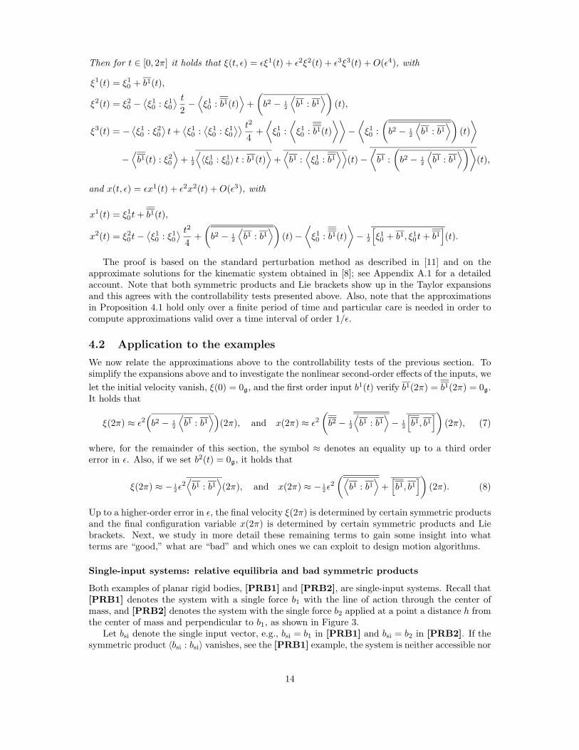
Both examples of planar rigid bodies, [PRB1] and [PRB2], are single-input systems. Recall that[PRB1] denotes the system with a single force b1 with the line of action through the center ofmass, and [PRB2] denotes the system with the single force b2 applied at a point a distance h fromthe center of mass and perpendicular to b1, as shown in Figure 3.
Let bsi denote the single input vector, e.g., bsi = b1 in [PRB1] and bsi = b2 in [PRB2]. If thesymmetric product 〈bsi : bsi〉 vanishes, see the [PRB1] example, the system is neither accessible nor
14
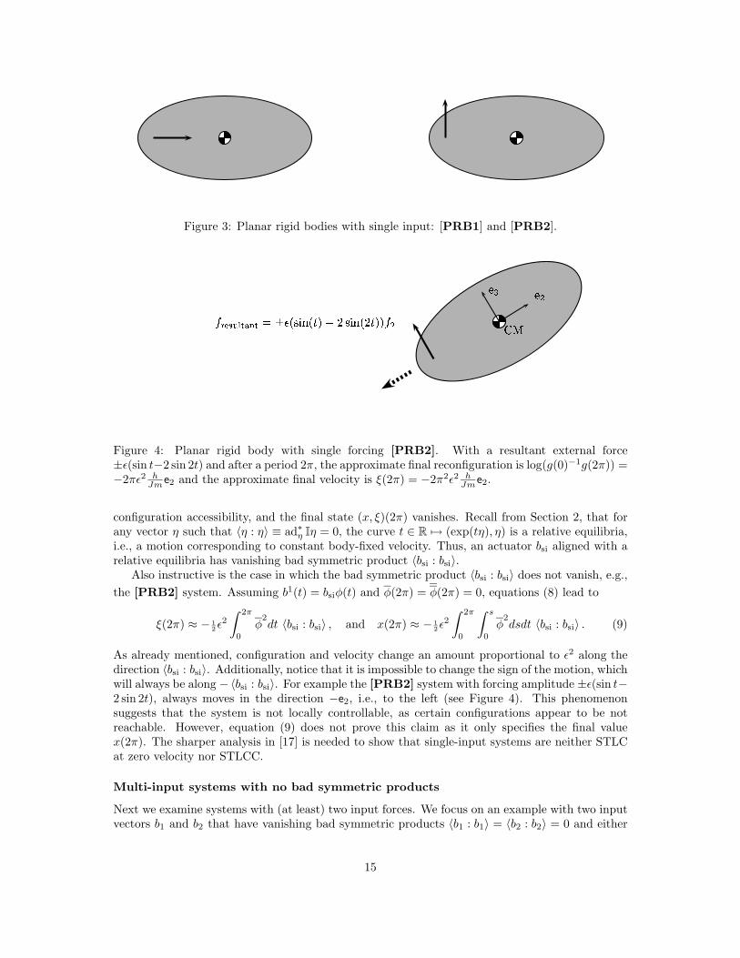
Figure 3: Planar rigid bodies with single input: [PRB1] and [PRB2].
Figure 4: Planar rigid body with single forcing [PRB2]. With a resultant external force±ε(sin t−2 sin 2t) and after a period 2π, the approximate final reconfiguration is log(g(0)−1g(2π)) =−2πε2 h
Jme2 and the approximate final velocity is ξ(2π) = −2π2ε2 hJme2.
configuration accessibility, and the final state (x, ξ)(2π) vanishes. Recall from Section 2, that forany vector η such that 〈η : η〉 ≡ ad∗
η Iη = 0, the curve t ∈ R 7→ (exp(tη), η) is a relative equilibria,i.e., a motion corresponding to constant body-fixed velocity. Thus, an actuator bsi aligned with arelative equilibria has vanishing bad symmetric product 〈bsi : bsi〉.
Also instructive is the case in which the bad symmetric product 〈bsi : bsi〉 does not vanish, e.g.,
the [PRB2] system. Assuming b1(t) = bsiφ(t) and φ(2π) = φ(2π) = 0, equations (8) lead to
ξ(2π) ≈ − 1
2ε2
∫ 2π
0
φ2dt 〈bsi : bsi〉 , and x(2π) ≈ − 1
2ε2
∫ 2π
0
∫ s
0
φ2dsdt 〈bsi : bsi〉 . (9)
As already mentioned, configuration and velocity change an amount proportional to ε2 along thedirection 〈bsi : bsi〉. Additionally, notice that it is impossible to change the sign of the motion, whichwill always be along −〈bsi : bsi〉. For example the [PRB2] system with forcing amplitude ±ε(sin t−2 sin 2t), always moves in the direction −e2, i.e., to the left (see Figure 4). This phenomenonsuggests that the system is not locally controllable, as certain configurations appear to be notreachable. However, equation (9) does not prove this claim as it only specifies the final valuex(2π). The sharper analysis in [17] is needed to show that single-input systems are neither STLCat zero velocity nor STLCC.
Multi-input systems with no bad symmetric products
Next we examine systems with (at least) two input forces. We focus on an example with two inputvectors b1 and b2 that have vanishing bad symmetric products 〈b1 : b1〉 = 〈b2 : b2〉 = 0 and either
15
non-zero good symmetric product 〈b1 : b2〉 6= 0 or non-zero Lie bracket [b1, b2] 6= 0. The satellitewith two thrusters [ST] and the satellite with two rotors [SR] are such examples. Pluggingb1(t) = b1u1(t) + b2u2(t) into equations (8), we have
ξ(2π) ≈ − 1
2ε2
⟨u1b1 + u2b2 : u1b1 + u2b2
⟩(2π)
= −ε2 〈b1 : b2〉u1 u2(2π)
and
x(2π) ≈ − 1
2ε2
(⟨b1 : b1
⟩+
[b1, b1
])(2π)
= −ε2 〈b1 : b2〉u1 u2(2π) − ε2 [b1, b2]u1 u2 − u1 u2(2π).
We interpret the operations performed on the input signals u1(t) and u2(t) as follows: u1 u2(2π) is
the inner product in the L2[0, 2π] function space between u1(t) and u2(t), whereas u1 u2 − u1 u2(2π)is the area enclosed by the plot of signals u1(t) versus u2(t). We distinguish two cases:
• Out-of-phase sinusoidal inputs generate motion along Lie brackets: First, consider the satel-lite with rotors [SR] example that is STLCC but not STLC at zero velocity. The symmetricproduct 〈b1 : b2〉 vanishes, so that we have from equation (8)
ξ(2π) ≈ 0 and x(2π) ≈ −ε2 [b1, b2]u1 u2 − u1 u2(2π).
If we want to steer the configuration x(2π) in the direction [b1, b2], sinusoidal signals at thesame frequency and out-of-phase are a simple standard choice. This is one of the basic ideasbehind the algorithms presented in [16] and other literature on motion planning for driftlesscontrol systems.
• In-phase sinusoidal inputs generate motion along good symmetric products: Second, considerthe satellite with thrusters example [ST] that is STLC at zero velocity since the symmetricproduct 〈b1 : b2〉 6= 0. If we pick sinusoidal inputs at the same frequency and in-phase, e.g.,u1(t) = u2(t) = cos(t), the contribution proportional to the Lie bracket [b1, b2] vanishes, sincethe area included by two identical signals is zero. Further, it holds that
ξ(2π) ≈ −ε2 〈b1 : b2〉 (u1)2(2π) and x(2π) ≈ −ε2 〈b1 : b2〉 (u1)2(2π),
and both velocity and configuration variables vary along −〈b1 : b2〉.5 Motion in the symmet-ric product direction is generated with sinusoidal inputs at the same frequency and in-phase.This is in contrast with the previous case and it is reminiscent of some results on gait selectionfor locomotion systems with drift, see the 1:1 gait in [27].
Multi-input systems with bad symmetric products
Finally, we examine systems with non-vanishing bad symmetric products. We focus on the planarrigid body with two forces applied at a point distant from the center of mass [PRB3]. Recallthat this system is STLC at zero velocity since the subspace b1, b2, 〈b1 : b2〉 has full rank andsince the good/bad products condition is verified by the equality 〈b2 : b2〉 = 2h
J b1. Setting b1 =b1u1(t) + b2u2(t) as above, the existence of a non-vanishing bad symmetric product causes
− 1
2ε2
⟨b1 : b1
⟩(2π) = −ε2 〈b1 : b2〉u1 u2(2π) − 1
2ε2 〈b2 : b2〉u2
2(2π),
5Also, the velocity change is maximal in the sense that on the L2[0, 2π] function space the Cauchy-Schwartzinequality on the inner product of u1(t) and u2(t) holds with equality if u1(t) = u2(t).
16
where the sign of the second term is independent of u2(t). However, motion in the 〈b2 : b2〉 directioncan be affected by a second-order input along b1. In particular by setting
b2(t) =h
2πJu2
2(2π)b1,
we obtain from equation (7)ξ(2π) ≈ −ε2 〈b1 : b2〉u1 u2(2π),
recovering this way the result for the case without bad symmetric products. In other words, the“bad” contribution due to 〈b2 : b2〉 is “annihilated” by means of the second-order input b2(t), andthis is possible only because the good/bad products condition is verified.
4.3 Inversion algorithm for systems controllable with second-order sym-
metric products
Motivated by the heuristic analysis in the last two examples, we introduce an additional definition.A system is STLC at zero velocity with second-order symmetric products if it satisfies the followingproperty:
(A2) The subspace spanbi, 〈bj : bk〉 , 1 ≤ i ≤ m, 1 ≤ j < k ≤ m has full rank and each bad sym-metric product 〈bi : bi〉 is a linear combination of the vectors b1, . . . , bm.
The planar rigid body with two forces [PRB3], the satellite with two thrusters [ST] and theunderwater vehicle [UV] satisfy this controllability condition. On the basis of this assumption,we design inputs
(b1(t), b2(t)
), that allow us to simplify the approximations in Proposition 4.1 and
steer the velocity of the system to an arbitrary value.
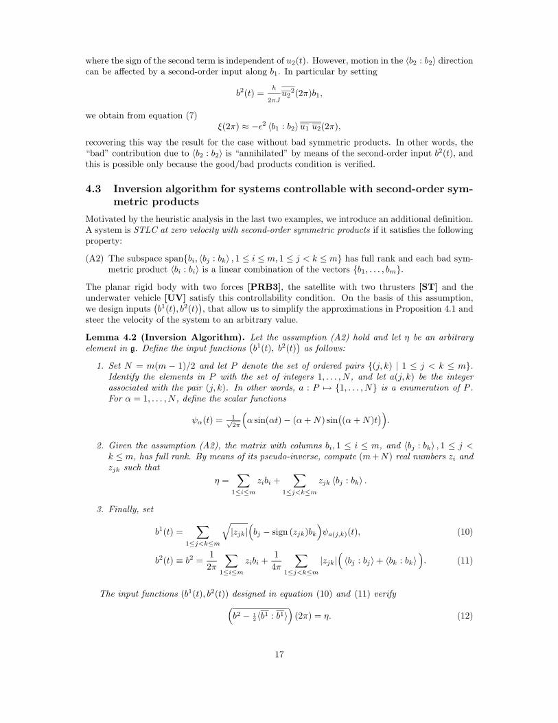
Lemma 4.2 (Inversion Algorithm). Let the assumption (A2) hold and let η be an arbitraryelement in g. Define the input functions
(b1(t), b2(t)
)as follows:
1. Set N = m(m − 1)/2 and let P denote the set of ordered pairs (j, k) | 1 ≤ j < k ≤ m.Identify the elements in P with the set of integers 1, . . . , N , and let a(j, k) be the integerassociated with the pair (j, k). In other words, a : P 7→ 1, . . . , N is a enumeration of P .For α = 1, . . . , N , define the scalar functions
ψα(t) = 1√2π
(α sin(αt) − (α+N) sin
((α+N)t
)).
2. Given the assumption (A2), the matrix with columns bi, 1 ≤ i ≤ m, and 〈bj : bk〉 , 1 ≤ j <k ≤ m, has full rank. By means of its pseudo-inverse, compute (m+N) real numbers zi andzjk such that
η =∑
1≤i≤m
zibi +∑
1≤j<k≤m
zjk 〈bj : bk〉 .
3. Finally, set
b1(t) =∑
1≤j<k≤m
√|zjk|
(bj − sign (zjk)bk
)ψa(j,k)(t), (10)
b2(t) ≡ b2 =1
2π
∑
1≤i≤m
zibi +1
4π
∑
1≤j<k≤m
|zjk|(〈bj : bj〉 + 〈bk : bk〉
). (11)
The input functions (b1(t), b2(t)) designed in equation (10) and (11) verify
(b2 − 1
2〈b1 : b1〉
)(2π) = η. (12)
17
Appendix A.2 contains the lemma’s proof. In what follows, we denote the procedure describedin the inversion algorithm with the notation:
(b1(t), b2(t)
)= Inverse(η) .
A direct manipulation of equation (10) and of b1(t) =∑m
i=1 biu1i (t) leads to the equivalent
statement
u1i (t) = −
i−1∑
j=1
√|zji| sign(zji)ψa(j,i)(t) +
m∑
j=i+1
√|zij |ψa(i,j)(t).
Note that motion along the good symmetric product direction 〈bi : bj〉 (for i < j) is generated
by the term√|zij |ψa(i,j)(t) in u1
i (t) and the term −√|zij | sign(zij)ψa(i,j)(t) in u1
j (t). Hence the
inputs u1i (t) and u1
j (t) have the common factor ψa(i,j). The other terms in the definition of u1k(t)
for all k, are at different frequencies. Therefore, they are orthogonal to ψa(i,j) in the inner productspace L2[0, 2π], and so do not generate motion in any other symmetric product direction. Thesecond term in the second order input b2 compensates for the motion excited along bad symmetricproduct directions. Its presence is a key difference with respect to the algorithms in [16] for driftlesssystems.
One of the drawbacks of the previous algorithm is that the input functions contain relativelyhigh frequencies, e.g., in an m = 3 input system, the input functions contain sinusoids withfrequency from 1 to m(m − 1) = 6. This can be mitigated by optimizing the design of thecoefficients zi, zjk and the numbering of the set P . For example, the design of the coefficientscan be optimized by employing a weighted pseudo-inverse.
5 Control Algorithms from Motion Primitives
In this section we design motion control algorithms based on the approximations in Proposition 4.1and the inversion algorithm in Lemma 4.2. Condition (A1) on the group G, and condition (A2)on the controllability of the system are assumed. We start by designing two primitive motionpatterns, Maintain-Velocity and Change-Velocity, that provide the system with some basicmotion capabilities. We then focus on more complex control algorithms to solve the point-to-pointreconfiguration problem, the local exponential stabilization problem and the static interpolationproblem.
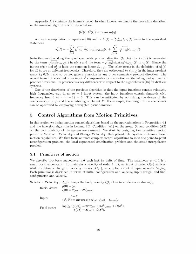
5.1 Primitives of motion
We describe two basic maneuvers that each last 2π units of time. The parameter σ 1 is asmall positive constant. To maintain a velocity of order O(σ), an input of order O(σ) suffices,while to obtain a change in velocity of order O(σ), we employ a control input of order O(
√σ).
Each primitive is described in terms of initial configuration and velocity, input design, and finalconfiguration and velocity.
Maintain-Velocity(σ, ξref): keeps the body velocity ξ(t) close to a reference value σξref.
Initial state:g(0) = g0,ξ(0) = σξref + σ2ξerror,
Input:ε= σ,
(b1, b2) = Inverse(π 〈ξref : ξref〉 − ξerror),
Final state:log(g−1
0 g(2π)) = 2πσξref + πσ2ξerror +O(σ3),ξ(2π) = σξref +O(σ3).
18
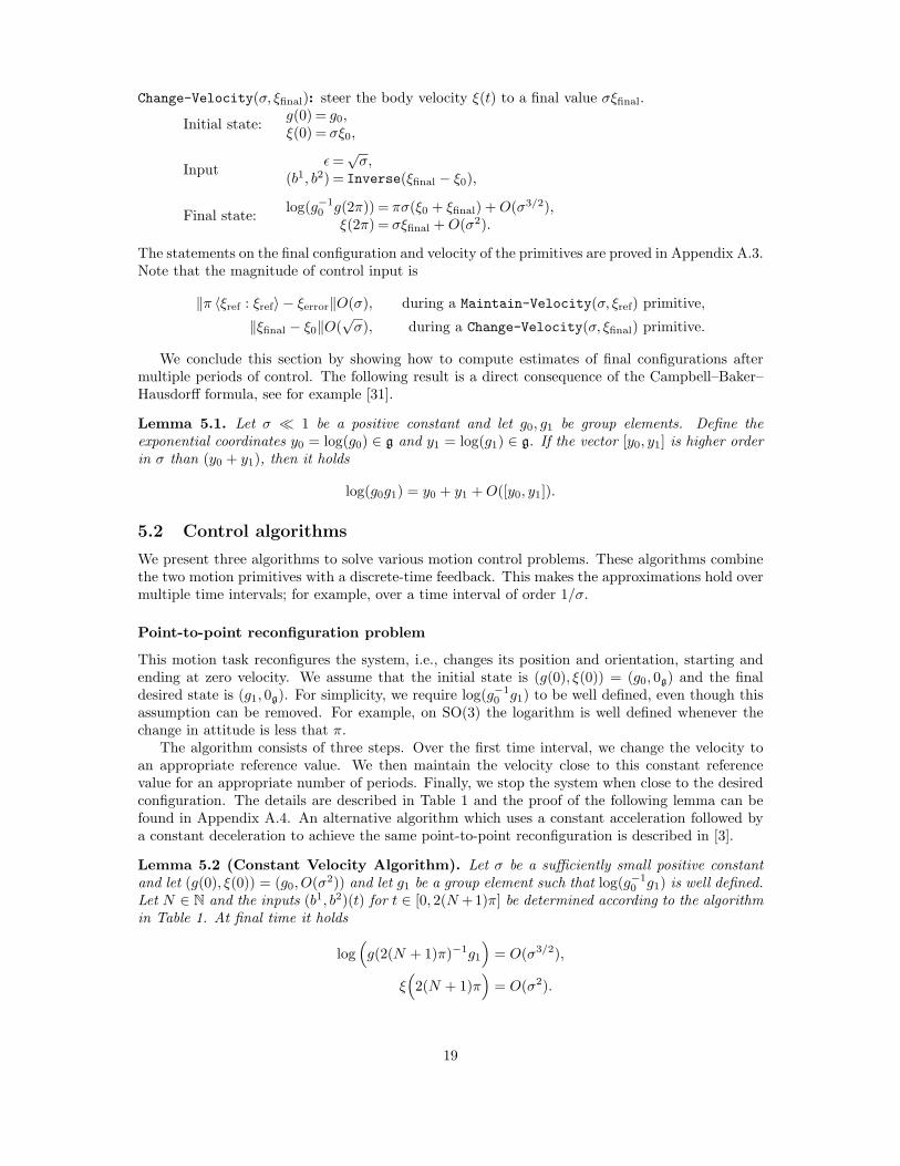
Change-Velocity(σ, ξfinal): steer the body velocity ξ(t) to a final value σξfinal.
Initial state:g(0) = g0,ξ(0) = σξ0,
Inputε=
√σ,
(b1, b2) = Inverse(ξfinal − ξ0),
Final state:log(g−1
0 g(2π)) = πσ(ξ0 + ξfinal) +O(σ3/2),ξ(2π) = σξfinal +O(σ2).
The statements on the final configuration and velocity of the primitives are proved in Appendix A.3.Note that the magnitude of control input is
‖π 〈ξref : ξref〉 − ξerror‖O(σ), during a Maintain-Velocity(σ, ξref) primitive,
‖ξfinal − ξ0‖O(√σ), during a Change-Velocity(σ, ξfinal) primitive.
We conclude this section by showing how to compute estimates of final configurations aftermultiple periods of control. The following result is a direct consequence of the Campbell–Baker–Hausdorff formula, see for example [31].
Lemma 5.1. Let σ 1 be a positive constant and let g0, g1 be group elements. Define theexponential coordinates y0 = log(g0) ∈ g and y1 = log(g1) ∈ g. If the vector [y0, y1] is higher orderin σ than (y0 + y1), then it holds
log(g0g1) = y0 + y1 +O([y0, y1]).
5.2 Control algorithms
We present three algorithms to solve various motion control problems. These algorithms combinethe two motion primitives with a discrete-time feedback. This makes the approximations hold overmultiple time intervals; for example, over a time interval of order 1/σ.
Point-to-point reconfiguration problem
This motion task reconfigures the system, i.e., changes its position and orientation, starting andending at zero velocity. We assume that the initial state is (g(0), ξ(0)) = (g0, 0g) and the finaldesired state is (g1, 0g). For simplicity, we require log(g−1
0 g1) to be well defined, even though thisassumption can be removed. For example, on SO(3) the logarithm is well defined whenever thechange in attitude is less that π.
The algorithm consists of three steps. Over the first time interval, we change the velocity toan appropriate reference value. We then maintain the velocity close to this constant referencevalue for an appropriate number of periods. Finally, we stop the system when close to the desiredconfiguration. The details are described in Table 1 and the proof of the following lemma can befound in Appendix A.4. An alternative algorithm which uses a constant acceleration followed bya constant deceleration to achieve the same point-to-point reconfiguration is described in [3].
Lemma 5.2 (Constant Velocity Algorithm). Let σ be a sufficiently small positive constantand let (g(0), ξ(0)) = (g0, O(σ2)) and let g1 be a group element such that log(g−1
0 g1) is well defined.Let N ∈ N and the inputs (b1, b2)(t) for t ∈ [0, 2(N +1)π] be determined according to the algorithmin Table 1. At final time it holds
log(g(2(N + 1)π)−1g1
)= O(σ3/2),
ξ(2(N + 1)π
)= O(σ2).
19
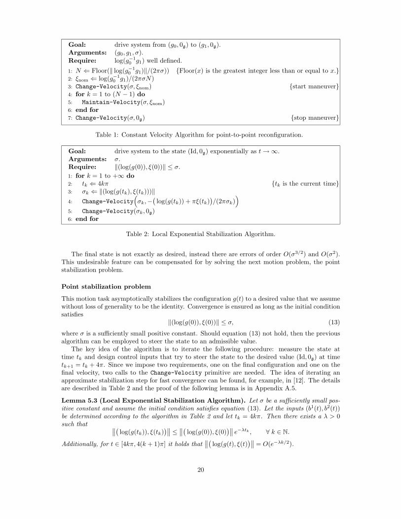
Goal: drive system from (g0, 0g) to (g1, 0g).Arguments: (g0, g1, σ).Require: log(g−1
0 g1) well defined.
1: N ⇐ Floor(‖ log(g−10 g1)‖/(2πσ)) Floor(x) is the greatest integer less than or equal to x.
2: ξnom ⇐ log(g−10 g1)/(2πσN)
3: Change-Velocity(σ, ξnom) start maneuver4: for k = 1 to (N − 1) do5: Maintain-Velocity(σ, ξnom)6: end for7: Change-Velocity(σ, 0g) stop maneuver
Table 1: Constant Velocity Algorithm for point-to-point reconfiguration.
Goal: drive system to the state (Id, 0g) exponentially as t→ ∞.Arguments: σ.Require: ‖(log(g(0)), ξ(0))‖ ≤ σ.
1: for k = 1 to +∞ do2: tk ⇐ 4kπ tk is the current time3: σk ⇐ ‖(log(g(tk), ξ(tk)))‖4: Change-Velocity
(σk,−
(log(g(tk)) + πξ(tk)
)/(2πσk)
)
5: Change-Velocity(σk, 0g)6: end for
Table 2: Local Exponential Stabilization Algorithm.
The final state is not exactly as desired, instead there are errors of order O(σ3/2) and O(σ2).This undesirable feature can be compensated for by solving the next motion problem, the pointstabilization problem.
Point stabilization problem
This motion task asymptotically stabilizes the configuration g(t) to a desired value that we assumewithout loss of generality to be the identity. Convergence is ensured as long as the initial conditionsatisfies
‖(log(g(0)), ξ(0))‖ ≤ σ, (13)
where σ is a sufficiently small positive constant. Should equation (13) not hold, then the previousalgorithm can be employed to steer the state to an admissible value.
The key idea of the algorithm is to iterate the following procedure: measure the state attime tk and design control inputs that try to steer the state to the desired value (Id, 0g) at timetk+1 = tk + 4π. Since we impose two requirements, one on the final configuration and one on thefinal velocity, two calls to the Change-Velocity primitive are needed. The idea of iterating anapproximate stabilization step for fast convergence can be found, for example, in [12]. The detailsare described in Table 2 and the proof of the following lemma is in Appendix A.5.
Lemma 5.3 (Local Exponential Stabilization Algorithm). Let σ be a sufficiently small pos-itive constant and assume the initial condition satisfies equation (13). Let the inputs (b1(t), b2(t))be determined according to the algorithm in Table 2 and let tk = 4kπ. Then there exists a λ > 0such that ∥∥(
log(g(tk)), ξ(tk))∥∥ ≤
∥∥(log(g(0)), ξ(0)
)∥∥ e−λtk , ∀ k ∈ N.
Additionally, for t ∈ [4kπ, 4(k + 1)π] it holds that∥∥(
log(g(t), ξ(t))∥∥ = O(e−λk/2).
20
Goal: drive system through points g0, g1, . . . , gM.Arguments: (g0, g1, . . . , gM , σ).Require: (g(0), ξ(0)) = (g0, 0g) and log(g−1
i gi) well defined for all 0 ≤ i ≤M .
1: for j = 1 to M do2: gtmp,j ⇐ g(t) exp(πξ(t)) t is the current time3: Nj ⇐ Floor(‖ log(g−1
tmp,jgj)‖/(2πσ))
4: ξnom,j ⇐ log(g−1tmp,jgj)/(2πσNj)
5: Change-Velocity(σ, ξnom,j)6: for k = 1 to (Nj − 1) do7: Maintain-Velocity(σ, ξnom,j)8: end for9: end for
10: Change-Velocity(σ, 0g)
Table 3: Static Interpolation Algorithm.
Static interpolation problem
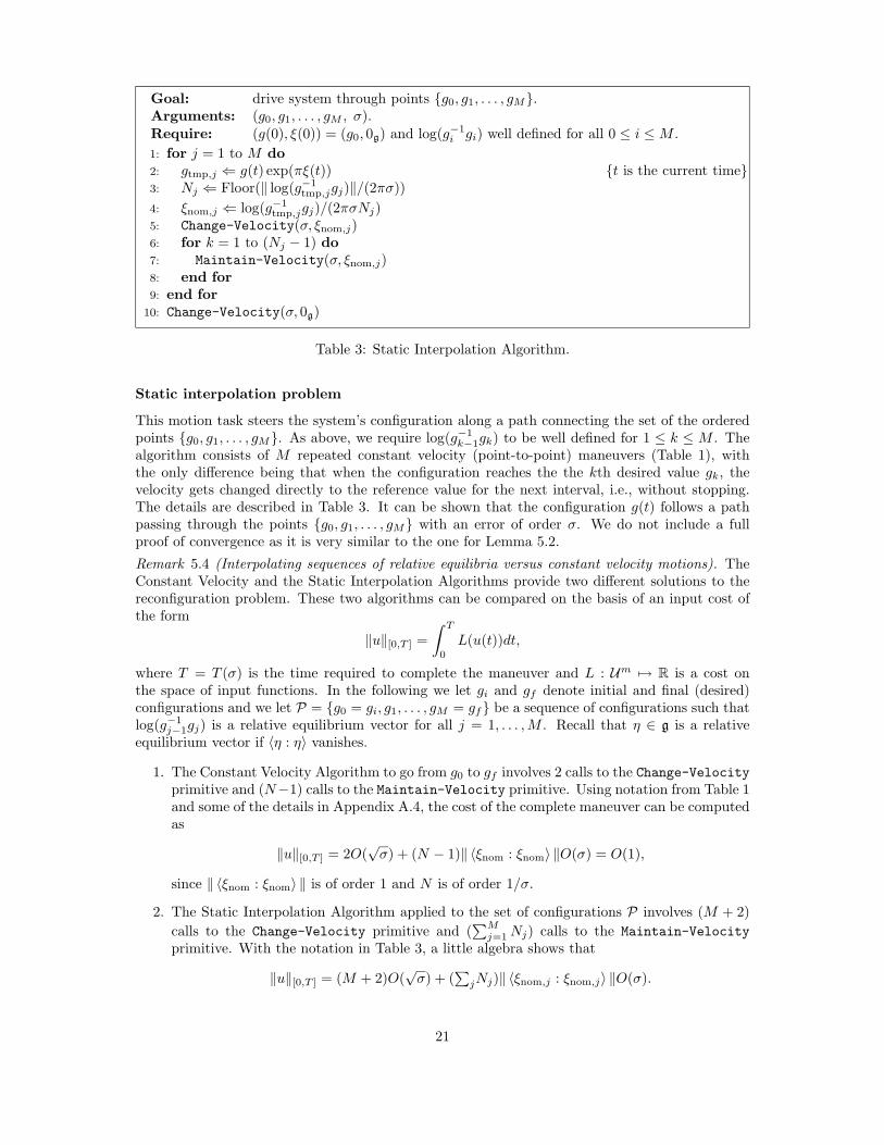
This motion task steers the system’s configuration along a path connecting the set of the orderedpoints g0, g1, . . . , gM. As above, we require log(g−1
k−1gk) to be well defined for 1 ≤ k ≤ M . Thealgorithm consists of M repeated constant velocity (point-to-point) maneuvers (Table 1), withthe only difference being that when the configuration reaches the the kth desired value gk, thevelocity gets changed directly to the reference value for the next interval, i.e., without stopping.The details are described in Table 3. It can be shown that the configuration g(t) follows a pathpassing through the points g0, g1, . . . , gM with an error of order σ. We do not include a fullproof of convergence as it is very similar to the one for Lemma 5.2.
Remark 5.4 (Interpolating sequences of relative equilibria versus constant velocity motions). TheConstant Velocity and the Static Interpolation Algorithms provide two different solutions to thereconfiguration problem. These two algorithms can be compared on the basis of an input cost ofthe form
‖u‖[0,T ] =
∫ T
0
L(u(t))dt,
where T = T (σ) is the time required to complete the maneuver and L : Um 7→ R is a cost onthe space of input functions. In the following we let gi and gf denote initial and final (desired)configurations and we let P = g0 = gi, g1, . . . , gM = gf be a sequence of configurations such thatlog(g−1
j−1gj) is a relative equilibrium vector for all j = 1, . . . ,M . Recall that η ∈ g is a relativeequilibrium vector if 〈η : η〉 vanishes.
1. The Constant Velocity Algorithm to go from g0 to gf involves 2 calls to the Change-Velocityprimitive and (N−1) calls to the Maintain-Velocity primitive. Using notation from Table 1and some of the details in Appendix A.4, the cost of the complete maneuver can be computedas
‖u‖[0,T ] = 2O(√σ) + (N − 1)‖ 〈ξnom : ξnom〉 ‖O(σ) = O(1),
since ‖ 〈ξnom : ξnom〉 ‖ is of order 1 and N is of order 1/σ.
2. The Static Interpolation Algorithm applied to the set of configurations P involves (M + 2)
calls to the Change-Velocity primitive and (∑M
j=1Nj) calls to the Maintain-Velocity
primitive. With the notation in Table 3, a little algebra shows that
‖u‖[0,T ] = (M + 2)O(√σ) + (
∑jNj)‖ 〈ξnom,j : ξnom,j〉 ‖O(σ).
21
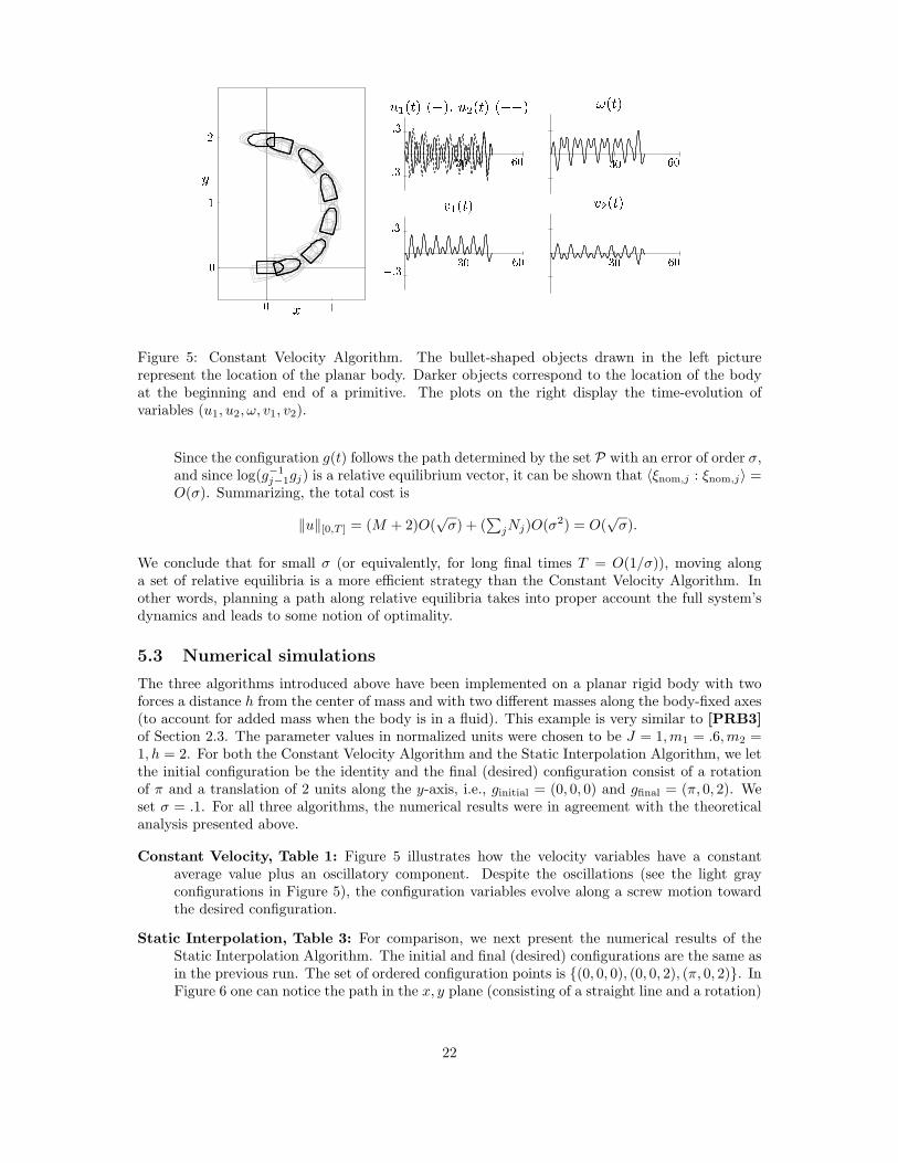
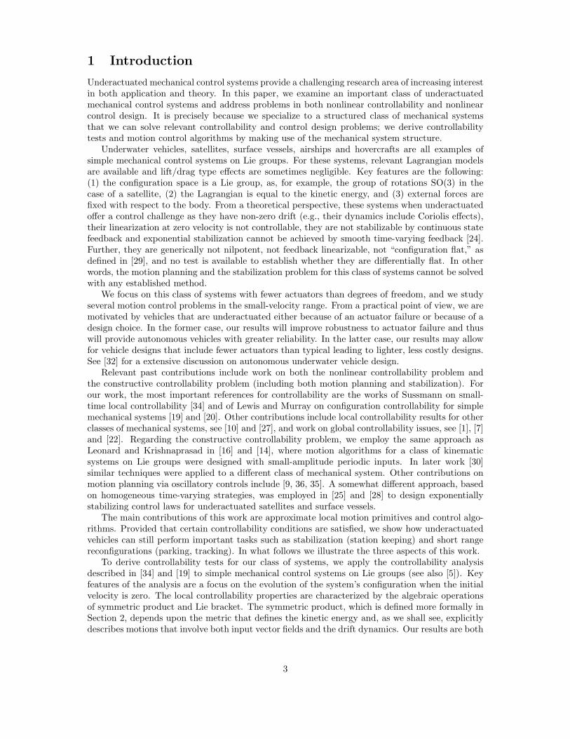
Figure 5: Constant Velocity Algorithm. The bullet-shaped objects drawn in the left picturerepresent the location of the planar body. Darker objects correspond to the location of the bodyat the beginning and end of a primitive. The plots on the right display the time-evolution ofvariables (u1, u2, ω, v1, v2).
Since the configuration g(t) follows the path determined by the set P with an error of order σ,and since log(g−1
j−1gj) is a relative equilibrium vector, it can be shown that 〈ξnom,j : ξnom,j〉 =O(σ). Summarizing, the total cost is
‖u‖[0,T ] = (M + 2)O(√σ) + (
∑jNj)O(σ2) = O(
√σ).
We conclude that for small σ (or equivalently, for long final times T = O(1/σ)), moving alonga set of relative equilibria is a more efficient strategy than the Constant Velocity Algorithm. Inother words, planning a path along relative equilibria takes into proper account the full system’sdynamics and leads to some notion of optimality.
5.3 Numerical simulations
The three algorithms introduced above have been implemented on a planar rigid body with twoforces a distance h from the center of mass and with two different masses along the body-fixed axes(to account for added mass when the body is in a fluid). This example is very similar to [PRB3]of Section 2.3. The parameter values in normalized units were chosen to be J = 1,m1 = .6,m2 =1, h = 2. For both the Constant Velocity Algorithm and the Static Interpolation Algorithm, we letthe initial configuration be the identity and the final (desired) configuration consist of a rotationof π and a translation of 2 units along the y-axis, i.e., ginitial = (0, 0, 0) and gfinal = (π, 0, 2). Weset σ = .1. For all three algorithms, the numerical results were in agreement with the theoreticalanalysis presented above.
Constant Velocity, Table 1: Figure 5 illustrates how the velocity variables have a constantaverage value plus an oscillatory component. Despite the oscillations (see the light grayconfigurations in Figure 5), the configuration variables evolve along a screw motion towardthe desired configuration.
Static Interpolation, Table 3: For comparison, we next present the numerical results of theStatic Interpolation Algorithm. The initial and final (desired) configurations are the same asin the previous run. The set of ordered configuration points is (0, 0, 0), (0, 0, 2), (π, 0, 2). InFigure 6 one can notice the path in the x, y plane (consisting of a straight line and a rotation)
22
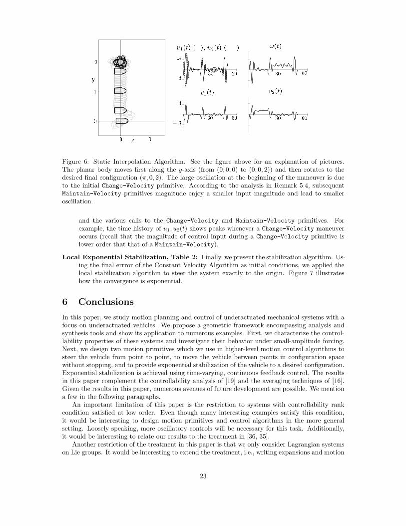
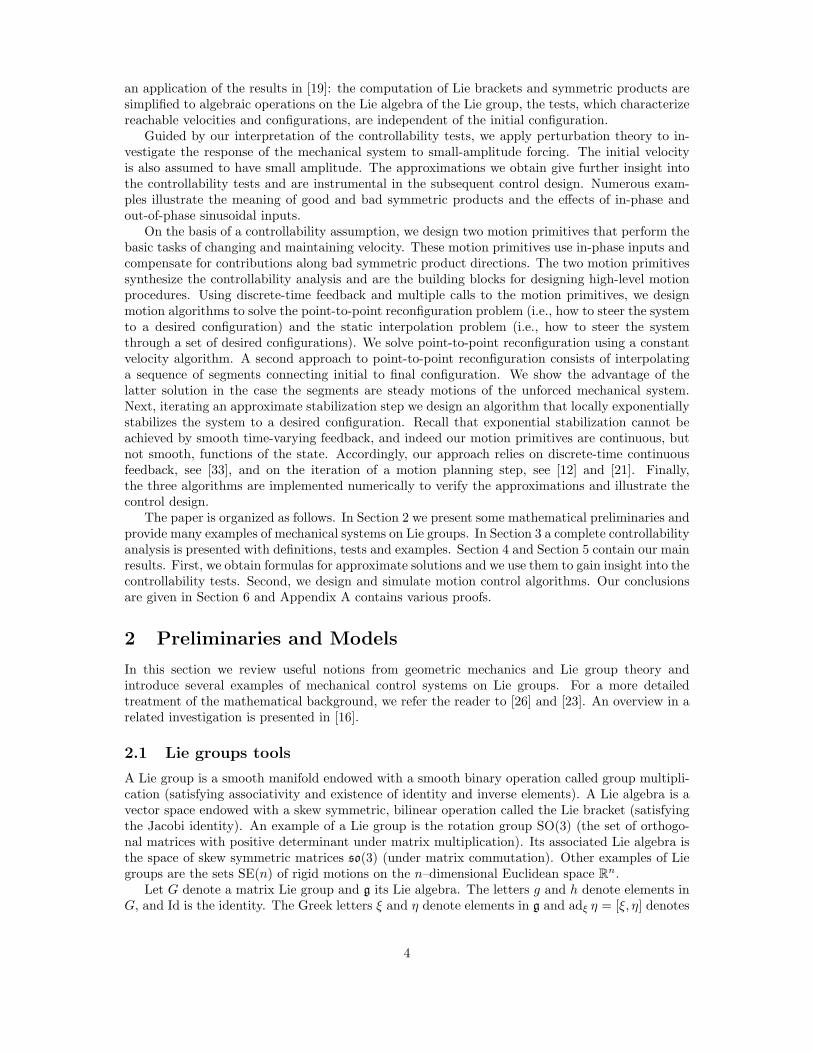
Figure 6: Static Interpolation Algorithm. See the figure above for an explanation of pictures.The planar body moves first along the y-axis (from (0, 0, 0) to (0, 0, 2)) and then rotates to thedesired final configuration (π, 0, 2). The large oscillation at the beginning of the maneuver is dueto the initial Change-Velocity primitive. According to the analysis in Remark 5.4, subsequentMaintain-Velocity primitives magnitude enjoy a smaller input magnitude and lead to smalleroscillation.
and the various calls to the Change-Velocity and Maintain-Velocity primitives. Forexample, the time history of u1, u2(t) shows peaks whenever a Change-Velocity maneuveroccurs (recall that the magnitude of control input during a Change-Velocity primitive islower order that that of a Maintain-Velocity).
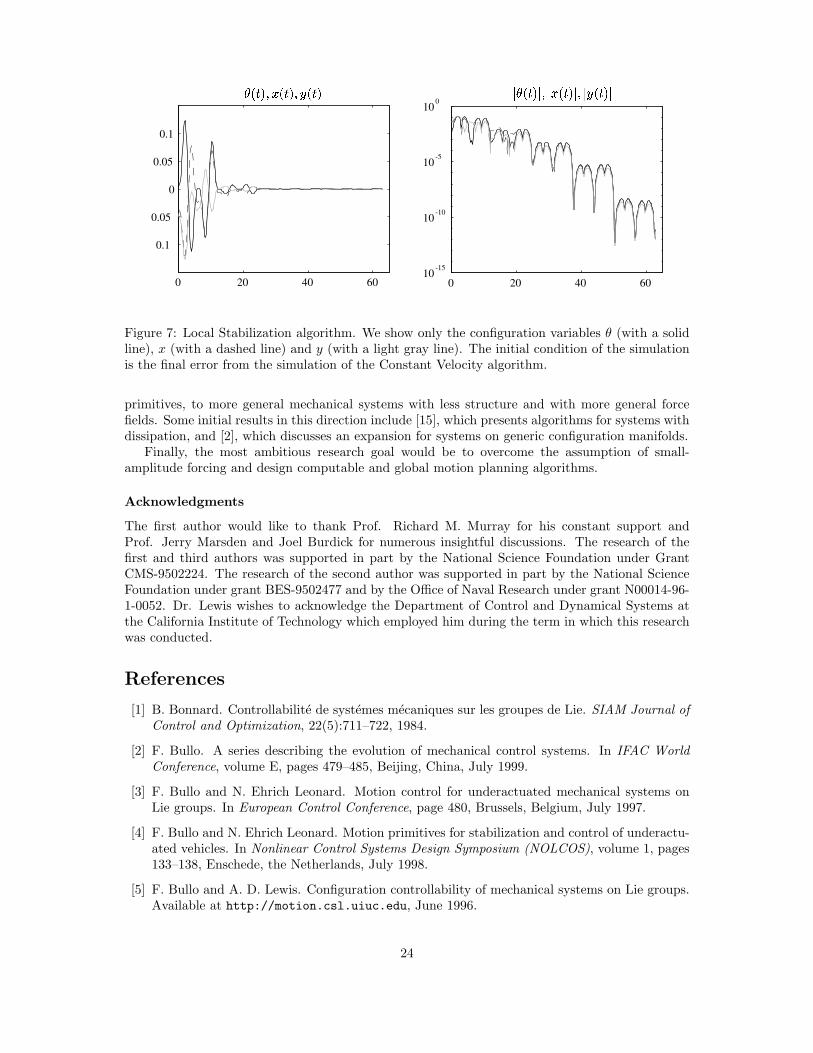
Local Exponential Stabilization, Table 2: Finally, we present the stabilization algorithm. Us-ing the final errror of the Constant Velocity Algorithm as initial conditions, we applied thelocal stabilization algorithm to steer the system exactly to the origin. Figure 7 illustrateshow the convergence is exponential.
6 Conclusions
In this paper, we study motion planning and control of underactuated mechanical systems with afocus on underactuated vehicles. We propose a geometric framework encompassing analysis andsynthesis tools and show its application to numerous examples. First, we characterize the control-lability properties of these systems and investigate their behavior under small-amplitude forcing.Next, we design two motion primitives which we use in higher-level motion control algorithms tosteer the vehicle from point to point, to move the vehicle between points in configuration spacewithout stopping, and to provide exponential stabilization of the vehicle to a desired configuration.Exponential stabilization is achieved using time-varying, continuous feedback control. The resultsin this paper complement the controllability analysis of [19] and the averaging techniques of [16].Given the results in this paper, numerous avenues of future development are possible. We mentiona few in the following paragraphs.
An important limitation of this paper is the restriction to systems with controllability rankcondition satisfied at low order. Even though many interesting examples satisfy this condition,it would be interesting to design motion primitives and control algorithms in the more generalsetting. Loosely speaking, more oscillatory controls will be necessary for this task. Additionally,it would be interesting to relate our results to the treatment in [36, 35].
Another restriction of the treatment in this paper is that we only consider Lagrangian systemson Lie groups. It would be interesting to extend the treatment, i.e., writing expansions and motion
23
0 20 40 60
0.1
0.05
0
0.05
0.1
0 20 40 6010
-15
10-10
10-5
100
Figure 7: Local Stabilization algorithm. We show only the configuration variables θ (with a solidline), x (with a dashed line) and y (with a light gray line). The initial condition of the simulationis the final error from the simulation of the Constant Velocity algorithm.
primitives, to more general mechanical systems with less structure and with more general forcefields. Some initial results in this direction include [15], which presents algorithms for systems withdissipation, and [2], which discusses an expansion for systems on generic configuration manifolds.
Finally, the most ambitious research goal would be to overcome the assumption of small-amplitude forcing and design computable and global motion planning algorithms.
Acknowledgments
The first author would like to thank Prof. Richard M. Murray for his constant support andProf. Jerry Marsden and Joel Burdick for numerous insightful discussions. The research of thefirst and third authors was supported in part by the National Science Foundation under GrantCMS-9502224. The research of the second author was supported in part by the National ScienceFoundation under grant BES-9502477 and by the Office of Naval Research under grant N00014-96-1-0052. Dr. Lewis wishes to acknowledge the Department of Control and Dynamical Systems atthe California Institute of Technology which employed him during the term in which this researchwas conducted.
References
[1] B. Bonnard. Controllabilite de systemes mecaniques sur les groupes de Lie. SIAM Journal ofControl and Optimization, 22(5):711–722, 1984.
[2] F. Bullo. A series describing the evolution of mechanical control systems. In IFAC WorldConference, volume E, pages 479–485, Beijing, China, July 1999.
[3] F. Bullo and N. Ehrich Leonard. Motion control for underactuated mechanical systems onLie groups. In European Control Conference, page 480, Brussels, Belgium, July 1997.
[4] F. Bullo and N. Ehrich Leonard. Motion primitives for stabilization and control of underactu-ated vehicles. In Nonlinear Control Systems Design Symposium (NOLCOS), volume 1, pages133–138, Enschede, the Netherlands, July 1998.
[5] F. Bullo and A. D. Lewis. Configuration controllability of mechanical systems on Lie groups.Available at http://motion.csl.uiuc.edu, June 1996.
24
[6] P. E. Crouch. Geometric structures in systems theory. IEE Proceedings, 128(5):242–252, 1981.
[7] P. E. Crouch. Spacecraft attitude control and stabilization: Application of geometric controltheory to rigid body models. IEEE Transactions on Automatic Control, 29(4):321–331, 1984.
[8] A. T. Fomenko and R. V. Chakon. Recursion relations for homogeneous terms of a convergentseries of the logarithm of a multiplicative integral on Lie groups. Functional Analysis and itsApplications, 24(1):48–58, 1990. Translated from Russian.
[9] L. Gurvits. Averaging approach to nonholonomic motion planning. In IEEE Conf. on Roboticsand Automation, pages 2541–2546, Nice, France, 1992.
[10] S. D. Kelly and R. M. Murray. Geometric phases and robotic locomotion. Journal of RoboticSystems, 12(6):417–431, 1995.
[11] H. K. Khalil. Nonlinear Systems. Prentice Hall, second edition, 1995.
[12] G. Lafferriere and H. J. Sussmann. A differential geometric approach to motion planning. InZ. Li and J. F. Canny, editors, Nonholonomic Motion Planning, pages 235–270. Kluwer, 1993.
[13] H. Lamb. Hydrodynamics. Dover Publications, New York, NY, sixth edition, 1932.
[14] N. Ehrich Leonard. Control synthesis and adaptation for an underactuated autonomous un-derwater vehicle. IEEE Journal of Oceanic Engineering, 20(9):211–220, 1995.
[15] N. Ehrich Leonard. Periodic forcing, dynamics and control of underactuated spacecraft andunderwater vehicles. In IEEE Conf. on Decision and Control, pages 1131–1136, New Orleans,LA, December 1995.
[16] N. Ehrich Leonard and P. S. Krishnaprasad. Motion control of drift-free, left-invariant systemson Lie groups. IEEE Transactions on Automatic Control, 40(9):1539–1554, 1995.
[17] A. D. Lewis. Local configuration controllability for a class of mechanical systems with a singleinput. In European Control Conference, Brussels, Belgium, July 1997.
[18] A. D. Lewis. Affine connections and distributions with applications to nonholonomic mechan-ics. Reports on Mathematical Physics, 42(1/2):135–164, 1998.
[19] A. D. Lewis and R. M. Murray. Configuration controllability of simple mechanical controlsystems. SIAM Journal of Control and Optimization, 35(3):766–790, 1997.
[20] A. D. Lewis and R. M. Murray. Decompositions of control systems on manifolds with an affineconnection. Systems & Control Letters, 31(4):199–205, 1997.
[21] P. Lucibello and G. Oriolo. Robust stabilization by iterative state steering. Automatica, 1998.Submitted.
[22] V. Manikonda and P. S. Krishnaprasad. Controllability of Lie-Poisson reduced dynamics. InAmerican Control Conference, Albuquerque, NM, June 1997.
[23] J. E. Marsden and T. S. Ratiu. Introduction to Mechanics and Symmetry. Springer Verlag,New York, NY, second edition, 1999.
[24] R. T. M’Closkey and R. M. Murray. Exponential stabilization of driftless nonlinear controlsystems using homogeneous feedback. IEEE Transactions on Automatic Control, 42(5):614–628, 1997.
[25] P. Morin and C. Samson. Time-varying exponential stabilization of a rigid spacecraft withtwo control torques. IEEE Transactions on Automatic Control, 42(4):528–534, 1997.
25
[26] R. M. Murray, Z. X. Li, and S. S. Sastry. A Mathematical Introduction to Robotic Manipula-tion. CRC Press, Boca Raton, FL, 1994.
[27] J. P. Ostrowski and J. W. Burdick. Controllability tests for mechanical systems with sym-metries and constraints. Journal Applied Mathematics and Computer Science, 7(2):101–127,1997.
[28] K. Y. Pettersen and O. Egeland. Robust attitude stabilization of an underactuated AUV. InEuropean Control Conference, Brussels, Belgium, July 1997.
[29] M. Rathinam and R. M. Murray. Configuration flatness of Lagrangian systems underactuatedby one control. SIAM Journal of Control and Optimization, 36(1):164–179, 1998.
[30] C. Rui, I. V. Kolmanovsky, P. J. McNally, and N. H. McClamroch. Attitude control ofunderactuated multibody spacecraft. In IFAC World Conference, San Francisco, CA, July1996.
[31] D. H. Sattinger and O. L. Weaver. Lie Groups and Algebras, with Applications to Physics,Geometry and Mechanics, volume 61 of AMS. Springer Verlag, New York, NY, 1986.
[32] H. Singh, D. Yoerger, and A. Bradley. Issues in AUV design and deployment for oceanographicresearch. In IEEE Conf. on Robotics and Automation, pages 1857–1862, Albuquerque, NewMexico, April 1997.
[33] O. J. Sordalen and O. Egeland. Exponential stabilization of nonholonomic chained systems.IEEE Transactions on Automatic Control, 40(1):35–49, 1995.
[34] H. J. Sussmann. A general theorem on local controllability. SIAM Journal of Control andOptimization, 25(1):158–194, 1987.
[35] H. J. Sussmann and W. Liu. Limits of highly oscillatory controls and the approximationof general paths by admissible trajectories. In IEEE Conf. on Decision and Control, pages437–442, Brighton, UK, December 1991.
[36] H. J. Sussmann and W. Liu. Lie bracket extensions and averaging: the single bracket case.In Z. Li and J. F. Canny, editors, Nonholonomic Motion Planning, pages 109–148. Kluwer,1993.
A Proofs
A.1 Proposition 4.1
Proof. We start by proving the validity of the expansion in ξ(t, ε) by means of the standardperturbation method, as presented, for example, in [11]. Consider the ordinary differential equation
x = f(x) + g(t, ε)
and let x(t, ε) denote the solution from initial condition x0(ε). At ε = 0, suppose that f(x0(0)) =g(t, 0) = 0, so that x(t, 0) = x0(0) is a constant solution. We now expand x(t, ε) and g(t, ε) in aTaylor series about the value ε = 0 and write
x(t, ε) =
∞∑
i=0
εixi(t) and g(t, ε) =
∞∑
i=0
εigi(t).
As shown in [11], the components in the expansion of x satisfy the following differential equations
xn(t) =1
n!
∂n
∂εn
∣∣∣ε=0
f(x(t, ε)) + gn(t),
26
with initial condition xn(0) = 1n!
∂n
∂εn
∣∣∣ε=0
x0(ε).
The differential equation of interest in our case is equation (4):
ξ = −1
2〈ξ : ξ〉 + εb1(t) + ε2b2(t),
and the initial condition is ξ(0, ε) = εξ10 + ε2ξ20 . The constant solution we expand about is ξ(t, 0) =ξ0(t) = 0.
Differentiating the function f(ξ(ε)) = − 12 〈ξ : ξ〉, we have
∂f
∂ε= −
⟨ξ :
∂ξ
∂ε
⟩
∂2f
∂ε2= −
⟨∂ξ
∂ε:∂ξ
∂ε
⟩−
⟨ξ :
∂2ξ
∂ε2
⟩
∂3f
∂ε3= −3
⟨∂ξ
∂ε:∂2ξ
∂ε2
⟩−
⟨ξ :
∂3ξ
∂ε3
⟩,
and noting that ∂n
∂εn
∣∣∣ε=0
ξ = n!ξn, we have
∂f
∂ε
∣∣∣ε=0
= −⟨ξ0 : ξ1
⟩
∂2f
∂ε2
∣∣∣ε=0
= −⟨ξ1 : ξ1
⟩− 2
⟨ξ0 : ξ2
⟩
∂3f
∂ε3
∣∣∣ε=0
= −6⟨ξ1 : ξ2
⟩− 6
⟨ξ0 : ξ3
⟩.
Next, we write the differential equations as described above. Recalling that ξ0(t) = 0 we have
ξ1 = b1
ξ2 = −1
2
⟨ξ1 : ξ1
⟩+ b2
ξ3 = −⟨ξ1 : ξ2
⟩.
Initial conditions are ξ1(0) = ξ10 , ξ2(0) = ξ20 , ξ3(0) = 0. Finally, we employ the notation introducedin Section 5 to integrate the three ordinary differential equations,
ξ1(t) = ξ10 + b1(t)
ξ2(t) = ξ20 − 1
2
⟨ξ10 + b1(t) : ξ10 + b1(t)
⟩+ b2(t)
ξ3(t) = −⟨ξ10 + b1(t) : ξ20 − 1
2
⟨ξ10 + b1(t) : ξ10 + b1(t)
⟩+ b2(t)
⟩.
Expanding the terms on the right hand side, one recovers all of the terms in the expansions ofξ(t, ε) in Proposition 4.1.
In the second part of the proof we prove the validity of the expansion of x(t, ε) by means of theapproximate solutions for kinematic systems obtained in [8] and used in [16]. From these referenceswe know that, if ξ(t, ε) = O(ε), then
x(t, ε) = ξ(t) − 1
2
[ξ, ξ
](t) +O(ε3).
Substituting ξ(t, ε) = εξ1(t) + ε2ξ2(t) +O(ε3), we have:
x(t, ε) = εξ1(t) + ε2ξ2(t) − 1
2ε2
[ξ1, ξ1
](t) +O(ε3).
27
And substituting the values for ξ1(t) and ξ2(t), and writing x(t, ε) = εx1(t) + ε2x2(t) +O(ε3), wehave
x1(t) = ξ10 + b1(t)
x2(t) =
(ξ20t−
⟨ξ10 : ξ10
⟩ t2
4−
⟨ξ10 : b1
⟩(t) +
(b2 − 1
2
⟨b1 : b1
⟩)(t)
)− 1
2
[ξ10 + b1, ξ10 + b1
](t).
Expanding the terms on the right hand side, one recovers all of the terms in the expansions ofx(t, ε) in Proposition 4.1.
A.2 Lemma 4.2
Here, we prove the claim (12) in Lemma 4.2.
Proof. We start by studying the properties of the functions ψa(t). A direct computation showsthat for all a, b, c
ψa(2π) = ψa(2π) = ψa(2π) = 0 (14)
ψa ψb(t) =δab
2πt+ rab(t), where rab(2π) = rab(2π) = 0, (15)
ψa t (2π) = ψa ψb(2π) = ψa rbc(2π) = 0, (16)
where δab is the Kronecker delta function. The proof of these properties are straightforward andtedious.
Next, we prove the claim (12) in Lemma 4.2. Given the definition in equation (10) and the
property(15) of the functions ψa(t), we compute the quantity⟨b1 : b1
⟩(2π) as
⟨b1 : b1
⟩(2π) =
∑
1≤j<k≤m
∑
1≤p<q≤m
√|zjkzpq|
⟨(bj − sign(zjk)bk
):(bp − sign(zpq)bq
)⟩ψa(j,k) ψa(p,q)(2π)
=∑
1≤j<k≤m
|zjk|⟨(bj − sign(zjk)bk
):(bj − sign(zjk)bk
)⟩
=∑
1≤j<k≤m
|zjk|(〈bj : bj〉 − 2 sign(zjk) 〈bj : bk〉 + 〈bk : bk〉
)
= −2∑
1≤j<k≤m
zjk 〈bj : bk〉 +∑
1≤j<k≤m
|zjk|(〈bj : bj〉 + 〈bk : bk〉
).
Summing up with b2(2π) = 2πb2, we have(b2 − 1
2〈b1 : b1〉
)(2π) =
∑
1≤i≤m
zibi +∑
1≤j<k≤m
zjk 〈bj : bk〉 ,
which proves equation (12).
A.3 Primitives of Motion
The statements in the description of both primitives are direct consequences of the following result.
Proposition A.1. Let the assumptions of Proposition 4.1 hold and let(b1(t), b2(t)
)= Inverse(η).
If ξ(0) = εξ10 + ε2ξ20 , we have
ξ(2π) = εξ10 + ε2(ξ20 − π
⟨ξ10 : ξ10
⟩+ η
)+ ε3π
(π
⟨ξ10 :
⟨ξ10 : ξ10
⟩⟩− 2
⟨ξ10 : ξ20
⟩−
⟨ξ10 : η
⟩ )+O(ε4)
(17)
x(2π) = ε2πξ10 + ε2π(2ξ20 − π
⟨ξ10 : ξ10
⟩+ η
)+O(ε3). (18)
28
Proof. Note that property (14) implies directly that b1(2π) = b1(2π) = b1(2π) = 0, so that theterms in the Taylor expansion in Proposition 4.1 simplify to
ξ1(2π) = ξ10
ξ2(2π) = ξ20 − π⟨ξ10 : ξ10
⟩+
(b2 − 1
2
⟨b1 : b1
⟩)(2π),
ξ3(2π) = −2π⟨ξ10 : ξ20
⟩+ π2
⟨ξ10 :
⟨ξ10 : ξ10
⟩⟩−
⟨ξ10 :
(b2 − 1
2
⟨b1 : b1
⟩)(2π)
⟩
+⟨〈ξ10 : ξ10〉 : b1
⟩ t
2(2π) +
⟨b1 :
⟨ξ10 : b1
⟩⟩(2π) −
⟨b1 :
(b2 − 1
2
⟨b1 : b1
⟩)⟩(2π),
x1(2π) = 2πξ10 ,
x2(2π) = 2πξ20 − π2⟨ξ10 : ξ10
⟩+
(b2 − 1
2
⟨b1 : b1
⟩)(2π) − 1
2
[ξ10 + b1, ξ10t+ b1
](2π).
Hence, ξ1(2π) and x1(2π) are as computed above. We employ Lemma 4.2 and property (15) tosimplify the remaining terms into
ξ2(2π) = ξ20 − π⟨ξ10 : ξ10
⟩+ η,
ξ3(2π) = −2π⟨ξ10 : ξ20
⟩+ π2
⟨ξ10 :
⟨ξ10 : ξ10
⟩⟩− π
⟨ξ10 : η
⟩
+⟨〈ξ10 : ξ10〉 : b1
⟩ t
2(2π) +
⟨b1 :
⟨ξ10 : b1
⟩⟩(2π) −
⟨b1 :
(b2 − 1
2
⟨b1 : b1
⟩)⟩(2π),
x2(2π) = 2πξ20 − π2⟨ξ10 : ξ10
⟩+ πη − 1
2
[ξ10 + b1, ξ10t+ b1
](2π).
Regarding the term ξ3(t), the claim is proven if
⟨〈ξ10 : ξ10〉 : b1
⟩ t
2(2π) =
⟨b1 :
⟨ξ10 : b1
⟩⟩(2π) =
⟨b1 :
(b2 − 1
2
⟨b1 : b1
⟩)⟩(2π) = 0.
However, since b1(t) is linear combination of the functions ψa(t), the latter relations correspondequality sign by equality sign to the properties in equation (16). Regarding the term x2(t), it holdsthat
[ξ10 + b1, ξ10t+ b1
](2π) = 2π2
[ξ10 , ξ
10
]+
[ξ10 , b
1(2π)
]+
[b1, ξ10t
](2π) +
[b1, b1
](2π) = 0,
as all terms in the middle expression vanish.
A.4 Lemma 5.2
Proof. Given the descriptions of the primitives Change-Velocity and Maintain-Velocity, wecompute the evolution of ξ(t) as follows. Starting from ξ(0) = O(σ2), we have:after first Change-Velocity(σ, ξnom) : ξ(2π) = σξnom +O(σ2),after first Maintain-Velocity(σ, ξnom) : ξ(4π) = σξnom +O(σ3),after kth step in the for loop : ξ(2(k + 1)π) = σξnom +O(σ3),after the final Change-Velocity(σ, 0) : ξ(2(N + 1)π) = O(σ2).
The final value of ξ is therefore as in the claim. Similarly, we can compute the change in configu-ration during each interval:after first Change-Velocity(σ, ξnom) : log
(g(0)−1g(2π)
)= πσξnom +O(σ3/2),
after first Maintain-Velocity(σ, ξnom) : log(g(2π)−1g(4π)
)= 2πσξnom +O(σ2),
after kth step in the for loop : log(g(2kπ)−1g(2(k + 1)π)
)= 2πσξnom +O(σ3),
after final Change-Velocity(σ, 0) : log(g(2Nπ)−1g(2(N + 1)π)
)= πσξnom +O(σ3/2).
29
We now need to sum the changes in configuration due to each interval by means of the approx-imation in Lemma 5.1. Combining the contributions during the first two intervals, and recallingthat [ξnom, ξnom] vanishes, we have
log(g−10 g(4π)
)= 3πσξnom +O(σ3/2) =: 3πσξnom + σ3/2η1, (19)
where η1 = O(1) is an appropriate vector in g. Next, we claim that for all k = 1, . . . , N − 1, itholds
log(g−10 g(2(k + 1)π)
)= akξnom + σ3/2ηk,
where the scalar ak and the vector ηk are of order at most 1. We prove the claim by induction.At k = 1, we recover equation (19), with a1 = 3πσ. Next, we assume that the claim holds at k,and we prove it for k+1. As dictated by Lemma 5.1, we compute the bracket between the currentvalue akξnom +σ3/2ηk and the contribution 2πσξnom +O(σ3) =: 2πσξnom +σ3ζk, where ζk = O(1)is an appropriate vector in g. We have:
[akξnom + σ3/2ηk , 2πσξnom + σ3ζk] = O(σ5/2),
so that
log(g−10 g(2(k + 2)π)
)=
(akξnom + σ3/2ηk
)+
(2πσξnom + σ3ζk
)+O(σ5/2)
=(ak + 2πσ
)ξnom + σ3/2
(ηk + σ3/2ζk + σνk
),
where νk = O(1) is an appropriate vector in g. Hence, the claim holds at k+1, with ak+1 = ak+2πσand ηk+1 = ηk + σ3/2ζk + σνk. At the end of the for loop, as k = N − 1, we have
log(g−10 g(2Nπ)
)= aN−1ξnom + σ3/2ηN−1,
where we can compute the coefficients as
aN−1 = a1 +
N−1∑
k=2
2πσ = (2N − 1)πσ and ηN−1 = η1 +
N−1∑
k=2
(σ3/2ζk + σνk
)= O(1).
The contribution of the last interval is σπξnom plus some higher-order terms, so that
log(g−10 g(2(N + 1)π)
)= 2Nπσξnom +O(σ3/2).
Finally, we apply the approximation in Lemma 5.1 for a last time to obtain
log(g(2(N + 1)π)−1g1) = log((g−10 g(2(N + 1)π)
)−1(g−10 g1
))= O(σ3/2),
where we recall that log(g−10 g1) = 2Nπσξnom and log(h−1) = − log(h).
A.5 Lemma 5.3
Proof. We start by investigating the two Change-Velocity primitives described inside the whilestatement in Algorithm 2. Assuming that at time tk it holds
∥∥(log(g(tk)), ξ(tk)
)∥∥ = σk 1,
we claim that ∥∥(log(g(tk+1)), ξ(tk+1)
)∥∥ = O(σ3/2k ). (20)
This can be seen as follows. By assumption there exist two vectors xerr and ξerr of order O(1) suchthat
log(g(tk)) = σkxerr
ξ(tk) = σkξerr.
30
With this notation, we have −(log(g(tk))+πξ(tk)
)/(2πσk) = −
(xerr +πξerr
)/(2π). Next we apply
the approximation in Lemma 5.1. After the primitive Change-Velocity(σk,−(xerr +πξerr
)/(2π)),
we compute
log(g(tk + 2π)) = 1
2σk(xerr + πξerr) +O(σ
3/2k )
ξ(tk + 2π) = −σk
(xerr + πξerr
)/(2π) +O(σ2
k),
and after the final Change-Velocity(σk, 0), we have
log(g(tk + 4π)) = O(σ3/2k ),
ξ(tk + 4π) = O(σ2k).
As tk+1 = tk + 4π, this proves equation (20). The latter equations are equivalent to
∥∥(log(g(tk+1)), ξ(tk+1)
)∥∥ ≤Mkσ3/2k , (21)
where the positive scalar Mk depends continuously on initial state and parameters of the system ofordinary differential equations (2) and (3). The parameters are σk and the coefficients in the designof (b1(t), b2(t)), for tk < t < tk+1. By looking at the details of the inversion algorithm in Lemma 4.2,these parameters are seen to be continuous function of the initial conditions
(log(g(tk), ξ(tk))
).
Hence, we know that Mk(g(tk), ξ(tk)) is a continuous function of its arguments and it is thereforebounded in a neighborhood of the point (g(tk), ξ(tk)) = (Id, 0). In other words, there exist positiveconstants B1, B2 such that
∥∥(log(g(tk)), ξ(tk)
)∥∥ < B1 =⇒ Mk(g(tk), ξ(tk)) < B2.
Finally, for some α < 1, we set σ = αmin(B1, 1/B
22
)and we prove by induction that σk < σ
and Mkσ1/2k ≤ α. At k = 0, we have by assumption
σ0 = ‖(log(g(0)), ξ(0))‖ ≤ σ < B1,
so that M0 < B2 andM0σ
1/20 < B2σ
1/2 < α < 1.
Therefore, the claim holds at k = 0. Next, we assume it at k, and prove it for k + 1. We rewriteequation (21) as
σk+1 =∥∥(
log(g(tk+1), ξ(tk+1))∥∥ ≤
(Mkσ
1/2k
)σk ≤ ασ < B1.
Hence, Mk+1 is also bounded by B2 and we have
σ1/2k+1Mk+1 ≤ σ1/2B2 < α.
This proves that Mkσ1/2k ≤ α for all k. In other words, we have that the sequence σk, k ≥ 0
satisfies σk+1 ≤ ασk with α < 1, or equivalently σk ≤ αkσ0. Therefore, for λ = − lnα > 0,∥∥(
log(g(tk)), ξ(tk))∥∥ ≤
∥∥(log(g(0)), ξ(0)
)∥∥ e−λk.
Finally we prove the last statement in Lemma 5.3. From time tk to tk+1, the system undergoestwo Change-Velocity primitives and evolves starting from a state of order O(σk) = O(e−λk)to a final state of higher order. During the two Change-Velocity primitives, the input is oforder
√σk = e−λk/2 (with the notation in Section 5.1 and in Proposition 4.1, it holds ε =
√σ).
Therefore, the expansions in Proposition 4.1 show that the state is of order√σk = e−λk/2 from
time tk to tk+1.
31