Controllability and reachability criteria for switched linear systems

Controllability and Reachability Criteria for Switched LinearSystems

Z. Sun, S. S. Ge∗ and T. H. Lee

Department of Electrical and Computer Engineering

National University of Singapore

Singapore 117576

Abstract: This paper investigates the controllability and reachability of switched

linear control systems. It is proven that both the controllable and reachable sets are

subspaces of the total space. Complete geometric characterization for both sets is

presented. The switching control design problem is also addressed.

Keywords: Switched linear systems; Controllability; Reachability; Switching control

1 Introduction

During the last decade, hybrid and switched systems have attracted considerable at-

tention (Chase, Serrano & Ramadge 1993, Branicky 1998, Wicks, Peleties & DeCarlo

1998, Ye, Michel & Hou 1998, Liberzon & Morse 1999). Basically, a switched system

consists of continuous-time/discrete-time dynamical subsystems and a rule (supervisor)

that determines the switching among them.

Switched systems deserve investigation for theoretical reasons as well as for practical

reasons. Switching among different system structures is an essential feature of many en-

gineering control applications including power systems and power electronics (Williams

& Hoft 1991, Sira-Ramirez 1991), and switched systems have numerous applications

in control of mechanical systems, air traffic control, aircrafts and satellites and many

other fields (Li, Wen & Soh 2001). Control techniques by switching among different

controllers have been applied extensively in recent years. Indeed, a switched controller

can provide a performance improvement over a fixed controller (Morse 1996, Naren-

dra & Balakrishnan 1997, Savkin, Skafidas & Evans 1999). The switched controller

architecture is proven to be a rigorous design framework for general nonlinear sys-

tems (Kolmanovsky & McClamroch 1996, Caines & Wei 1998, Leonessa, Haddad &

Chellaboina 2001). A switched controller can also achieve certain control objects which

∗To whom all correspondence should be addressed. Tel. (+65) 8746821; Fax. (+65) 7791103;E-mail: [email protected]

1

cannot be accomplished by conventional methods, such as pure feedback stabilization

of nonholonomic systems (Brockett 1983, Kolmanovsky & McClamroch 1995).

A fundamental pre-requisite for the design of feedback control systems is full knowledge

about the structural properties of the switched systems under consideration. These

properties are closely related to the concepts of controllability, observability and sta-

bility which are of fundamental importance in the literature of control. There have

been a lot of studies for switched systems, primarily on stability analysis and design

(Branicky 1998, Dayawansa & Martin 1999, Liberzon & Morse 1999). As for con-

trollability and reachability, studies for low-order switched linear systems have been

presented in Loparo, Aslanis & IIajek (1987) and Xu & Antsaklis (1999). Some suffi-

cient conditions and necessary conditions for controllability were presented in Ezzine

& Haddad (1989) and Szigeti (1992) for switched linear control systems under the as-

sumption that the switching sequence is fixed a priori. The complexity of stability and

controllability of hybrid systems was addressed in Blondel & Tsitsiklis (1999).

For controllability analysis of switched linear control systems, a much more difficult

situation arises since both the control input and the switching rule are design variables

to be determined, and thus the interaction between them must be fully understood.

For a switched linear discrete-time control system, the controllable set is not a subspace

but a countable union of subspaces in general case (Stanford & Conner 1980, Conner &

Stanford 1987). For a switched linear continuous-time control system, the controllable

set is an uncountable union of subspaces (Sun & Zheng 2001).

In this paper, we investigate the controllability and reachability issues for switched

linear control systems in detail. We prove that, both the controllable set and the

reachable set are subspaces of the total space, and the two sets always coincide with each

other. Verifiable geometric characterization is presented for the controllable subspace.

Dualistic criteria for observability and determinability are also presented.

The paper is organized as follows. In Section 2, we present the definitions of control-

lable and reachable notions. Preliminary results are given in Section 3. A complete

characterization for the controllability and reachability sets is presented in Section 4.

In Section 5, we briefly address the observability and determinability issues. An illus-

trative example is presented in Section 6. Finally, some concluding remarks are made

in Section 7.

2

2 Definitions

Consider a switched linear control system given by

x(t) = Aσx(t) + Bσuσ(t) (1)

where x ∈ <n are the states, uk : <+ ∈ <rk , k = 1, · · · ,m are piecewise continuous

input functions, σ : [t0,∞) → M = 1, 2, · · · ,m is the switching path to be designed,

and matrix pairs (Ak, Bk) for k ∈ M are referred to as the subsystems of (1).

Given a switching path σ : [t0, tf ] → M , suppose its discontinuous (jump) time instants

are t1 < t2 < · · · < ts, we refer to the sequence t0, t1, t2, · · · , ts as switching time

sequence, and the sequence σ(t0), σ(t1), · · · , σ(ts) as switching index sequence. It is

clear that these two sequences can uniquely determine the switching path, and vice-

versa.

For clarity, let x(t; t0, x0, u, σ) denote the state trajectory at time t of switched system

(1) starting from x(t0) = x0 with u(t) = [u1(t), · · · , um(t)]T .

A state x is said to be controllable at time t0, if it can be transferred to the origin in

a finite time starting from t0 by appropriate choices of input u and switching path σ.

Definition 1. State x ∈ <n is controllable at time t0, if there exist a time instant

tf > t0, a switching path σ : [t0, tf ] → M , and inputs uk : [t0, tf ] → <rk , k ∈ M , such

that x(tf ; t0, x, u, σ) = 0.

Definition 2. The controllable set of system (1) at t0 is the set of states which are

controllable at t0.

Definition 3. System (1) is said to be (completely) controllable at time t0, if its con-

trollable set at t0 is <n.

The reachability counterparts can be defined in the same fashion as follows.

Definition 4. State x ∈ <n is reachable at t0, if there exist a time instant tf > t0,

a switching path σ : [t0, tf ] → M , and inputs uk : [t0, tf ] → <rk , k ∈ M , such that

x(tf ; t0, 0, u, σ) = x.

Definition 5. The reachable set of system (1) at t0 is the set of states which are

reachable at t0.

Definition 6. System (1) is said to be (completely) reachable at t0, if its reachable set

at t0 is <n.

3

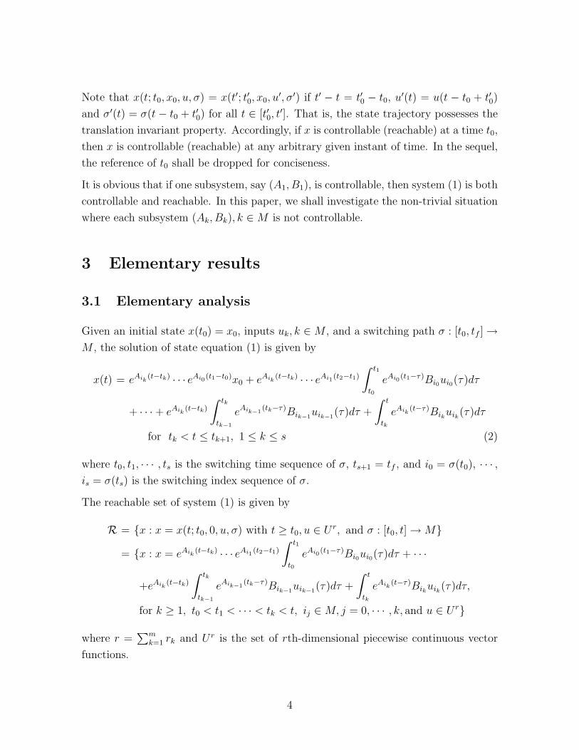
Note that x(t; t0, x0, u, σ) = x(t′; t′0, x0, u′, σ′) if t′ − t = t′0 − t0, u′(t) = u(t − t0 + t′0)

and σ′(t) = σ(t− t0 + t′0) for all t ∈ [t′0, t′]. That is, the state trajectory possesses the

translation invariant property. Accordingly, if x is controllable (reachable) at a time t0,

then x is controllable (reachable) at any arbitrary given instant of time. In the sequel,

the reference of t0 shall be dropped for conciseness.

It is obvious that if one subsystem, say (A1, B1), is controllable, then system (1) is both

controllable and reachable. In this paper, we shall investigate the non-trivial situation

where each subsystem (Ak, Bk), k ∈ M is not controllable.

3 Elementary results

3.1 Elementary analysis

Given an initial state x(t0) = x0, inputs uk, k ∈ M , and a switching path σ : [t0, tf ] →M , the solution of state equation (1) is given by

x(t) = eAik(t−tk) · · · eAi0

(t1−t0)x0 + eAik(t−tk) · · · eAi1

(t2−t1)

∫ t1

t0

eAi0(t1−τ)Bi0ui0(τ)dτ

+ · · ·+ eAik(t−tk)

∫ tk

tk−1

eAik−1(tk−τ)Bik−1

uik−1(τ)dτ +

∫ t

tk

eAik(t−τ)Bikuik(τ)dτ

for tk < t ≤ tk+1, 1 ≤ k ≤ s (2)

where t0, t1, · · · , ts is the switching time sequence of σ, ts+1 = tf , and i0 = σ(t0), · · · ,is = σ(ts) is the switching index sequence of σ.

The reachable set of system (1) is given by

R = x : x = x(t; t0, 0, u, σ) with t ≥ t0, u ∈ U r, and σ : [t0, t] → M= x : x = eAik

(t−tk) · · · eAi1(t2−t1)

∫ t1

t0

eAi0(t1−τ)Bi0ui0(τ)dτ + · · ·

+eAik(t−tk)

∫ tk

tk−1

eAik−1(tk−τ)Bik−1

uik−1(τ)dτ +

∫ t

tk

eAik(t−τ)Bikuik(τ)dτ,

for k ≥ 1, t0 < t1 < · · · < tk < t, ij ∈ M, j = 0, · · · , k, and u ∈ U r

where r =∑m

k=1 rk and U r is the set of rth-dimensional piecewise continuous vector

functions.

4

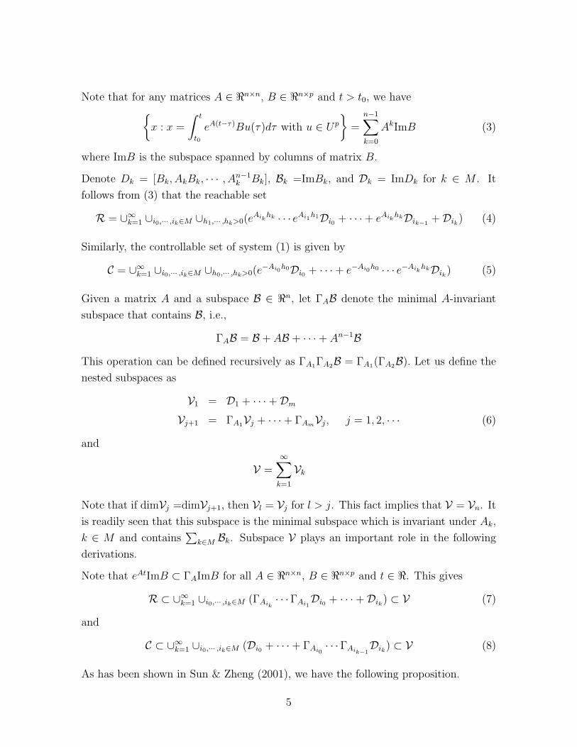
Note that for any matrices A ∈ <n×n, B ∈ <n×p and t > t0, we have

x : x =

∫ t

t0

eA(t−τ)Bu(τ)dτ with u ∈ Up

=

n−1∑

k=0

AkImB (3)

where ImB is the subspace spanned by columns of matrix B.

Denote Dk = [Bk, AkBk, · · · , An−1k Bk], Bk =ImBk, and Dk = ImDk for k ∈ M . It

follows from (3) that the reachable set

R = ∪∞k=1 ∪i0,··· ,ik∈M ∪h1,··· ,hk>0(eAik

hk · · · eAi1h1Di0 + · · ·+ eAik

hkDik−1+Dik) (4)

Similarly, the controllable set of system (1) is given by

C = ∪∞k=1 ∪i0,··· ,ik∈M ∪h0,··· ,hk>0(e−Ai0

h0Di0 + · · ·+ e−Ai0h0 · · · e−Aik

hkDik) (5)

Given a matrix A and a subspace B ∈ <n, let ΓAB denote the minimal A-invariant

subspace that contains B, i.e.,

ΓAB = B + AB + · · ·+ An−1BThis operation can be defined recursively as ΓA1ΓA2B = ΓA1(ΓA2B). Let us define the

nested subspaces as

V1 = D1 + · · ·+Dm

Vj+1 = ΓA1Vj + · · ·+ ΓAmVj, j = 1, 2, · · · (6)

and

V =∞∑

k=1

Vk

Note that if dimVj =dimVj+1, then Vl = Vj for l > j. This fact implies that V = Vn. It

is readily seen that this subspace is the minimal subspace which is invariant under Ak,

k ∈ M and contains∑

k∈M Bk. Subspace V plays an important role in the following

derivations.

Note that eAtImB ⊂ ΓAImB for all A ∈ <n×n, B ∈ <n×p and t ∈ <. This gives

R ⊂ ∪∞k=1 ∪i0,··· ,ik∈M (ΓAik· · ·ΓAi1

Di0 + · · ·+Dik) ⊂ V (7)

and

C ⊂ ∪∞k=1 ∪i0,··· ,ik∈M (Di0 + · · ·+ ΓAi0· · ·ΓAik−1

Dik) ⊂ V (8)

As has been shown in Sun & Zheng (2001), we have the following proposition.

5

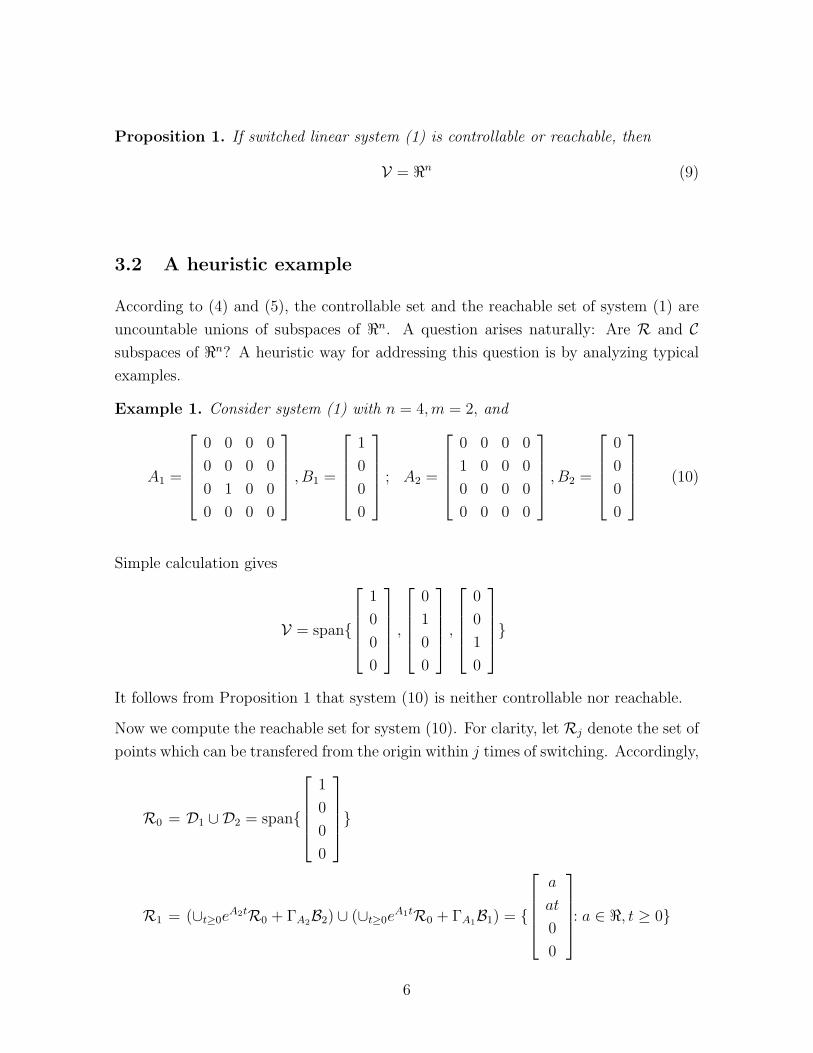
Proposition 1. If switched linear system (1) is controllable or reachable, then

V = <n (9)

3.2 A heuristic example

According to (4) and (5), the controllable set and the reachable set of system (1) are

uncountable unions of subspaces of <n. A question arises naturally: Are R and Csubspaces of <n? A heuristic way for addressing this question is by analyzing typical

examples.

Example 1. Consider system (1) with n = 4,m = 2, and

A1 =

0 0 0 0

0 0 0 0

0 1 0 0

0 0 0 0

, B1 =

1

0

0

0

; A2 =

0 0 0 0

1 0 0 0

0 0 0 0

0 0 0 0

, B2 =

0

0

0

0

(10)

Simple calculation gives

V = span

1

0

0

0

,

0

1

0

0

,

0

0

1

0

It follows from Proposition 1 that system (10) is neither controllable nor reachable.

Now we compute the reachable set for system (10). For clarity, let Rj denote the set of

points which can be transfered from the origin within j times of switching. Accordingly,

R0 = D1 ∪ D2 = span

1

0

0

0

R1 = (∪t≥0eA2tR0 + ΓA2B2) ∪ (∪t≥0e

A1tR0 + ΓA1B1) =

a

at

0

0

: a ∈ <, t ≥ 0

6

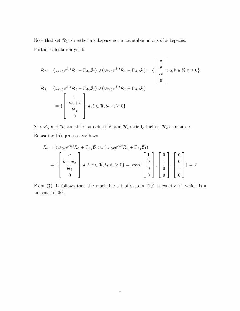
Note that set R1 is neither a subspace nor a countable unions of subspaces.

Further calculation yields

R2 = (∪t≥0eA2tR1 + ΓA2B2) ∪ (∪t≥0e

A1tR1 + ΓA1B1) =

a

b

bt

0

: a, b ∈ <, t ≥ 0

R3 = (∪t≥0eA2tR2 + ΓA2B2) ∪ (∪t≥0e

A1tR2 + ΓA1B1)

=

a

at3 + b

bt2

0

: a, b ∈ <, t2, t3 ≥ 0

Sets R2 and R3 are strict subsets of V , and R3 strictly include R2 as a subset.

Repeating this process, we have

R4 = (∪t≥0eA2tR3 + ΓA2B2) ∪ (∪t≥0e

A1tR3 + ΓA1B1)

=

a

b + ct3

bt2

0

: a, b, c ∈ <, t2, t3 ≥ 0 = span

1

0

0

0

,

0

1

0

0

,

0

0

1

0

= V

From (7), it follows that the reachable set of system (10) is exactly V , which is a

subspace of <4.

7

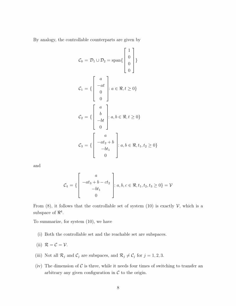
By analogy, the controllable counterparts are given by

C0 = D1 ∪ D2 = span

1

0

0

0

C1 =

a

−at

0

0

: a ∈ <, t ≥ 0

C2 =

a

b

−bt

0

: a, b ∈ <, t ≥ 0

C3 =

a

−at2 + b

−bt1

0

: a, b ∈ <, t1, t2 ≥ 0

and

C4 =

a

−at3 + b− ct2

−bt1

0

: a, b, c ∈ <, t1, t2, t3 ≥ 0 = V

From (8), it follows that the controllable set of system (10) is exactly V , which is a

subspace of <4.

To summarize, for system (10), we have

(i) Both the controllable set and the reachable set are subspaces.

(ii) R = C = V .

(iii) Not all Rj and Cj are subspaces, and Rj 6= Cj for j = 1, 2, 3.

(iv) The dimension of C is three, while it needs four times of switching to transfer an

arbitrary any given configuration in C to the origin.

8

Properties (i) and (ii) are parallel to the non-switching case while properties (iii) and

(iv) indicate complex phenomena arising when switching between different subsystems

occurs.

3.3 Rank divergent properties of eAt

As expressed in (2), the state transition matrix for switched system (1) is multiple

multiplication of matrix function of the form eAt. Accordingly, properties of exponen-

tial matrix functions play an important role in structural analysis for switched linear

systems. In this subsection, several good properties for eAt (called rank divergent

properties for convenience) shall be presented. These properties are crucial to the

derivations of the main results.

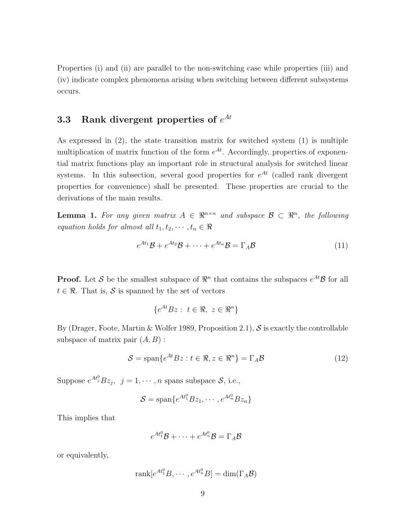
Lemma 1. For any given matrix A ∈ <n×n and subspace B ⊂ <n, the following

equation holds for almost all t1, t2, · · · , tn ∈ <

eAt1B + eAt2B + · · ·+ eAtnB = ΓAB (11)

Proof. Let S be the smallest subspace of <n that contains the subspaces eAtB for all

t ∈ <. That is, S is spanned by the set of vectors

eAtBz : t ∈ <, z ∈ <n

By (Drager, Foote, Martin & Wolfer 1989, Proposition 2.1), S is exactly the controllable

subspace of matrix pair (A,B) :

S = spaneAtBz : t ∈ <, z ∈ <n = ΓAB (12)

Suppose eAt0j Bzj, j = 1, · · · , n spans subspace S, i.e.,

S = spaneAt01Bz1, · · · , eAt0nBzn

This implies that

eAt01B + · · ·+ eAt0nB = ΓAB

or equivalently,

rank[eAt01B, · · · , eAt0nB] = dim(ΓAB)

9

Denote integer r = dim(ΓAB), and matrix function L(t1, · · · , tn) = [eAt1B, · · · , eAtnB].

Choose a nonsingular sub-matrix M0 with maximal rank in L(t01, · · · , t0n). Therefore,

M0 is nonsingular and rankM0 =rankL(t01, · · · , t0n). Denote the corresponding sub-

matrix of L(t1, · · · , tn) as M(t1, · · · , tn), and its determinant as d(t1, · · · , tn).

Since each entry in matrix M(t1, · · · , tn) is an analytic function of variables t1, · · · , tn,

d(t1, · · · , tn) is also an analytic function of its variables. As d(t01, · · · , t0n) 6= 0, function

d(t1, · · · , tn) is not identically zero. By Weierstrass Preparation Theorem (Kaplan 1966,

Theorem 62), its zeros forms a zero-measure set of <n. Therefore, for almost all

t1, · · · , tn, matrix M(t1, · · · , tn) is nonsingular. This implies that

rankL(t1, · · · , tn) ≥ rank M(t1, · · · , tn) = r = dim(ΓAB)

for almost all t1, · · · , tn. Together with the fact that S ⊆ ΓAB, we can conclude that

eAt1B + · · ·+ eAtnB = ΓAB

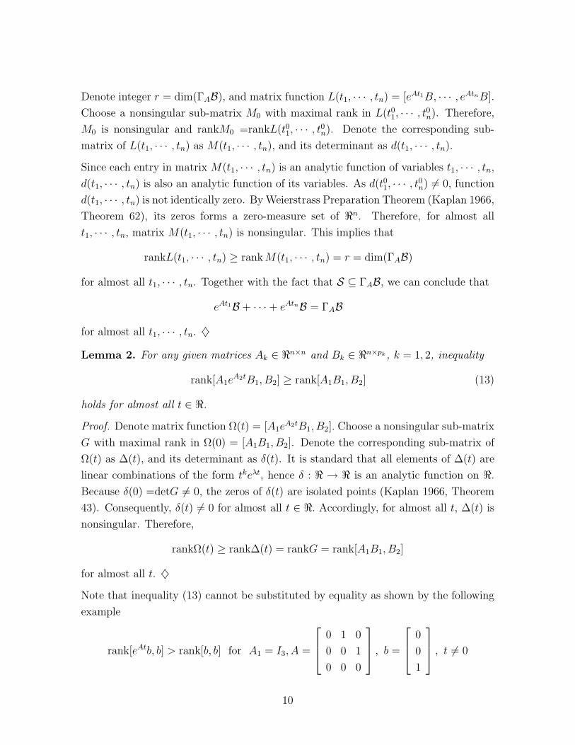
for almost all t1, · · · , tn. ♦Lemma 2. For any given matrices Ak ∈ <n×n and Bk ∈ <n×pk , k = 1, 2, inequality

rank[A1eA2tB1, B2] ≥ rank[A1B1, B2] (13)

holds for almost all t ∈ <.

Proof. Denote matrix function Ω(t) = [A1eA2tB1, B2]. Choose a nonsingular sub-matrix

G with maximal rank in Ω(0) = [A1B1, B2]. Denote the corresponding sub-matrix of

Ω(t) as ∆(t), and its determinant as δ(t). It is standard that all elements of ∆(t) are

linear combinations of the form tkeλt, hence δ : < → < is an analytic function on <.

Because δ(0) =detG 6= 0, the zeros of δ(t) are isolated points (Kaplan 1966, Theorem

43). Consequently, δ(t) 6= 0 for almost all t ∈ <. Accordingly, for almost all t, ∆(t) is

nonsingular. Therefore,

rankΩ(t) ≥ rank∆(t) = rankG = rank[A1B1, B2]

for almost all t. ♦Note that inequality (13) cannot be substituted by equality as shown by the following

example

rank[eAtb, b] > rank[b, b] for A1 = I3, A =

0 1 0

0 0 1

0 0 0

, b =

0

0

1

, t 6= 0

10

4 Main results

4.1 Geometric criteria

In this subsection, we shall identify the controllable set and the reachable set for

switched linear systems.

Theorem 1. For switched linear system (1), the reachable set is

R = V (14)

Proof. We are to design a switching path σ such that each point in V can be reached

from the origin via this switching path.

Assume that the switching index sequence of σ is periodic. i.e.,

i0 = 1, i1 = 2, · · · , im−1 = m,

im = 1, im+1 = 2, · · · , i2m−1 = m, · · · (15)

The switching time sequence t0, · · · , tl and the number l are to be designed later.

Let tf > tl. From (4), the reachable set at tf is

R(tf ) = eAilhl · · · eA2h1D1 + · · ·+ eAil

hlDil−1+Dil (16)

where hj = tj+1 − tj, j = 0, 1, · · · , l − 1 and hl = tf − tl.

Since

eAilhl · · · eA2h1D1 + · · ·+ eAil

hlDil−1+Dil

= eAilhl(eAil−1

hl−1 · · · eA2h1D1 + · · ·+ eAil−1hl−1Dil−2

+Dil−1) +Dil

it follows from Lemma 2 that

dim(eAilhl · · · eA2h1D1 + · · ·+ eAil

hlDil−1+Dil)

≥ dim(eAil−1hl−1 · · · eA2h1D1 + · · ·+ eAil−1

hl−1Dil−2+Dil−1

+Dil) (17)

for almost all hl.

11

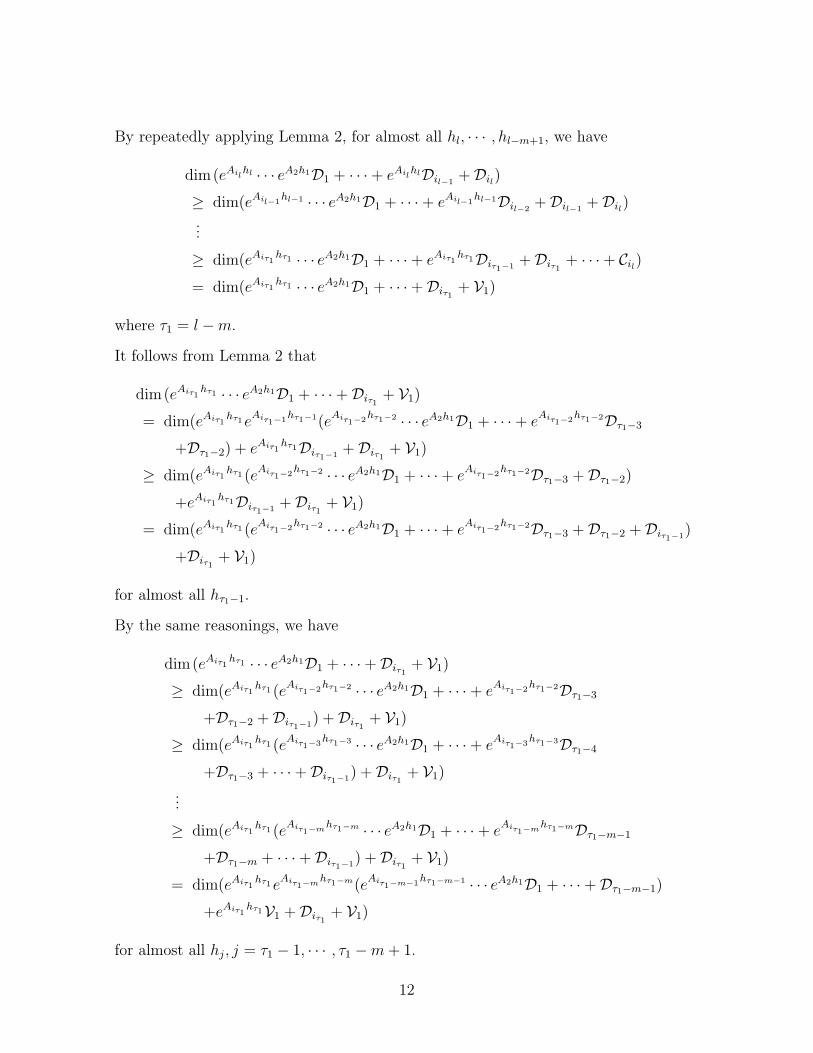
By repeatedly applying Lemma 2, for almost all hl, · · · , hl−m+1, we have


hlDil−1+Dil)

≥ dim(eAil−1hl−1 · · · eA2h1D1 + · · ·+ eAil−1

hl−1Dil−2+Dil−1

+Dil)

...

≥ dim(eAiτ1hτ1 · · · eA2h1D1 + · · ·+ eAiτ1

hτ1Diτ1−1 +Diτ1+ · · ·+ Cil)

= dim(eAiτ1hτ1 · · · eA2h1D1 + · · ·+Diτ1

+ V1)

where τ1 = l −m.

It follows from Lemma 2 that

dim(eAiτ1hτ1 · · · eA2h1D1 + · · ·+Diτ1

+ V1)

= dim(eAiτ1hτ1e

Aiτ1−1hτ1−1(e

Aiτ1−2hτ1−2 · · · eA2h1D1 + · · ·+ e

Aiτ1−2hτ1−2Dτ1−3

+Dτ1−2) + eAiτ1hτ1Diτ1−1 +Diτ1

+ V1)

≥ dim(eAiτ1hτ1 (e

Aiτ1−2hτ1−2 · · · eA2h1D1 + · · ·+ e

Aiτ1−2hτ1−2Dτ1−3 +Dτ1−2)

+eAiτ1hτ1Diτ1−1 +Diτ1

+ V1)

= dim(eAiτ1hτ1 (e

Aiτ1−2hτ1−2 · · · eA2h1D1 + · · ·+ e

Aiτ1−2hτ1−2Dτ1−3 +Dτ1−2 +Diτ1−1)

+Diτ1+ V1)

for almost all hτ1−1.

By the same reasonings, we have


+ V1)


Aiτ1−2hτ1−2 · · · eA2h1D1 + · · ·+ e


+Dτ1−2 +Diτ1−1) +Diτ1+ V1)


Aiτ1−3hτ1−3 · · · eA2h1D1 + · · ·+ e


+Dτ1−3 + · · ·+Diτ1−1) +Diτ1+ V1)

...


Aiτ1−mhτ1−m · · · eA2h1D1 + · · ·+ eAiτ1−mhτ1−mDτ1−m−1

+Dτ1−m + · · ·+Diτ1−1) +Diτ1+ V1)

= dim(eAiτ1hτ1e

Aiτ1−mhτ1−m(eAiτ1−m−1

hτ1−m−1 · · · eA2h1D1 + · · ·+Dτ1−m−1)

+eAiτ1hτ1V1 +Diτ1

+ V1)

for almost all hj, j = τ1 − 1, · · · , τ1 −m + 1.

12

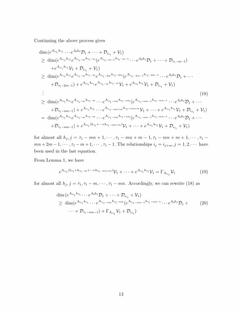
Continuing the above process gives


+ V1)

≥ dim(eAiτ1hτ1e

Aiτ1−mhτ1−m(eAiτ1−m−1

hτ1−m−1 · · · eA2h1D1 + · · ·+Dτ1−m−1)

+eAiτ1hτ1V1 +Diτ1

+ V1)

≥ dim(eAiτ1hτ1e

Aiτ1−mhτ1−meAiτ1−2m

hτ1−2m(eAiτ1−2m−1

hτ1−2m−1 · · · eA2h1D1 + · · ·+Dτ1−2m−1) + eAiτ1

hτ1eAiτ1−mhτ1−mV1 + eAiτ1

hτ1V1 +Diτ1+ V1)

... (18)

≥ dim(eAiτ1hτ1e

Aiτ1−mhτ1−m · · · eAiτ1−nmhτ1−nm(eAiτ1−nm−1

hτ1−nm−1 · · · eA2h1D1 + · · ·+Dτ1−nm−1) + eAiτ1

hτ1 · · · eAiτ1−nm+mhτ1−nm+mV1 + · · ·+ eAiτ1hτ1V1 +Diτ1

+ V1)

= dim(eAiτ1hτ1e

Aiτ1−mhτ1−m · · · eAiτ1−nmhτ1−nm(eAiτ1−nm−1

hτ1−nm−1 · · · eA2h1D1 + · · ·+Dτ1−nm−1) + eAiτ1

(hτ1+···+hτ1−nm+m)V1 + · · ·+ eAiτ1hτ1V1 +Diτ1

+ V1)

for almost all hj, j = τ1 −mn + 1, · · · , τ1 −mn + m − 1, τ1 −mn + m + 1, · · · , τ1 −mn+2m− 1, · · · , τ1−m+1, · · · , τ1− 1. The relationships ij = ij+m, j = 1, 2, · · · have

been used in the last equation.

From Lemma 1, we have

eAiτ1(hτ1+hτ1−m+···+hτ1−mn+m)V1 + · · ·+ eAiτ1

hτ1V1 = ΓAiτ1V1 (19)

for almost all hj, j = τ1, τ1 −m, · · · , τ1 −mn. Accordingly, we can rewrite (18) as


+ V1)

≥ dim(eAiτ1hτ1 · · · eAiτ1−nmhτ1−nm(e

Aiτ1−nm−1hτ1−nm−1 · · · eA2h1D1 + (20)

· · ·+Dτ1−nm−1) + ΓAiτ1V1 +Diτ1

)

13

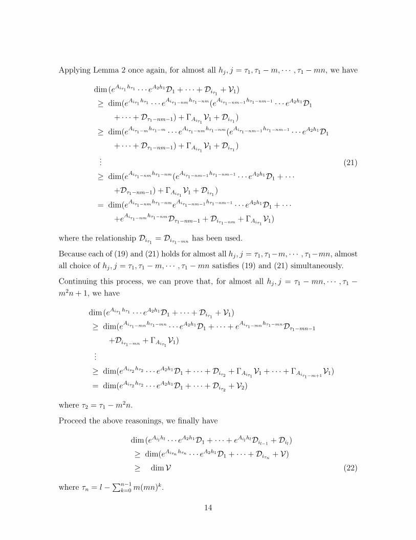
Applying Lemma 2 once again, for almost all hj, j = τ1, τ1 −m, · · · , τ1 −mn, we have


+ V1)

≥ dim(eAiτ1hτ1 · · · eAiτ1−nmhτ1−nm(e

Aiτ1−nm−1hτ1−nm−1 · · · eA2h1D1

+ · · ·+Dτ1−nm−1) + ΓAiτ1V1 +Diτ1

)

≥ dim(eAiτ1−mhτ1−m · · · eAiτ1−nmhτ1−nm(e

Aiτ1−nm−1hτ1−nm−1 · · · eA2h1D1

+ · · ·+Dτ1−nm−1) + ΓAiτ1V1 +Diτ1

)

... (21)

≥ dim(eAiτ1−nmhτ1−nm(e

Aiτ1−nm−1hτ1−nm−1 · · · eA2h1D1 + · · ·

+Dτ1−nm−1) + ΓAiτ1V1 +Diτ1

)

= dim(eAiτ1−nmhτ1−nme

Aiτ1−nm−1hτ1−nm−1 · · · eA2h1D1 + · · ·

+eAiτ1−nmhτ1−nmDτ1−nm−1 +Diτ1−nm + ΓAiτ1

V1)

where the relationship Diτ1= Diτ1−mn has been used.

Because each of (19) and (21) holds for almost all hj, j = τ1, τ1−m, · · · , τ1−mn, almost

all choice of hj, j = τ1, τ1 −m, · · · , τ1 −mn satisfies (19) and (21) simultaneously.

Continuing this process, we can prove that, for almost all hj, j = τ1 − mn, · · · , τ1 −m2n + 1, we have


+ V1)

≥ dim(eAiτ1−mnhτ1−mn · · · eA2h1D1 + · · ·+ e

Aiτ1−mnhτ1−mnDτ1−mn−1

+Diτ1−mn + ΓAiτ1V1)

...

≥ dim(eAiτ2hτ2 · · · eA2h1D1 + · · ·+Diτ2

+ ΓAiτ1V1 + · · ·+ ΓAiτ1−m+1

V1)

= dim(eAiτ2hτ2 · · · eA2h1D1 + · · ·+Diτ2

+ V2)

where τ2 = τ1 −m2n.

Proceed the above reasonings, we finally have


hlDil−1+Dil)

≥ dim(eAiτnhτn · · · eA2h1D1 + · · ·+Diτn

+ V)

≥ dimV (22)

where τn = l −∑n−1k=0 m(mn)k.

14

Let l ≥ ∑n−1k=0 m(mn)k − 1, then from (7) and (22) it follows that

Rs(tf ) = V (23)

which implies (14). ♦By Theorem 1, the controllable set is subspace V . We thus refer to V as controllable

subspace of system (1).

Theorem 2. For switched linear system (1), the controllable set is

C = V (24)

The proof is completely parallel to that of Theorem 1 and hence is omitted.

Corollary 1. Both the controllable set and the reachable set are subspaces of the total

space, and the two subspaces are always identical.

Corollary 2. For switched linear system (1), the following statements are equivalent

(i) The system is completely controllable;

(ii) The system is completely reachable; and

(iii) V = <n.

Due to Corollary 2, we can give an equivalent definition of controllability as follows.

Definition 7. System (1) is said to be (completely) controllable, if for any states x0

and xf , there exist a time instant tf > 0, a switching path σ : [0, tf ] → M , and inputs

uk : [0, tf ] → <rk , k ∈ M , such that x(tf ; 0, x0, u, σ) = xf .

Remark 1. The controllable and reachable sets are invariant under re-arrangement of

Ak and Bk for k ∈ M . That is, suppose both j1, · · · , jm and l1, · · · , lm are permutations

of 1, · · · ,m, then the controllable (reachable) set of system (1) coincide with that of the

system given by

x(t) = Aσx(t) + Bσuσ(t) (25)

where Ak = Ajkand Bk = Blk for k = 1, · · · ,m.

Remark 2. As noted in Example 1, although R and C coincide, Rj and Cj may differ

from each other for certain js. This difference is due to incomplete switching which is

a unique phenomenon of switched systems.

15

Remark 3. For a non-switched linear system (A,B), Corollary 2 degenerate to the

well known geometric characterization for controllable subspace (Wonham 1979)

C = B + AB + · · ·+ An−1B

4.2 Switching control design

By Theorems 1 and 2, any states in subspace V can transfer to each other in finite

time. In this subsection, we study the following switching control design problem for

switched system (1).

Switching Control Design Problem Given any two states x0 and xf in the con-

trollable subspace V, find a switching path σ and control input u to steer the system

from x0 to xf in finite time.

Combining the proof of Theorem 1 and the geometric approach of linear systems

(Wonham 1979), we can formulate a procedure to address this problem.

From the proof of Theorem 1, we can find a natural number l, positive real num-

bers h1, · · · , hl, and an index sequence i0, · · · , il, such that equation (22) holds. This,

together with (7), implies that

eAilhl · · · eA2h1D1 + · · ·+ eAil

hlDil−1+Dil = V (26)

Fix a positive real number h0. Define the switching time sequence as

t0 = 0, tk = tk−1 + hk−1, k = 1, · · · , l + 1 (27)

From the proof of Theorem 1.1 in Wonham (1979), for any k ∈ M and t > 0, we have

Dk = Im W kt (28)

where

W kt =

∫ t

0

eAk(t−τ)BkBTk eAT

k (t−τ)dτ

Combining (26) with (28) leads to

eAilhl · · · eA2h1ImW 1

h0+ · · ·+ eAil

hlImWil−1

hl−1+ ImW il

hl= V (29)

16

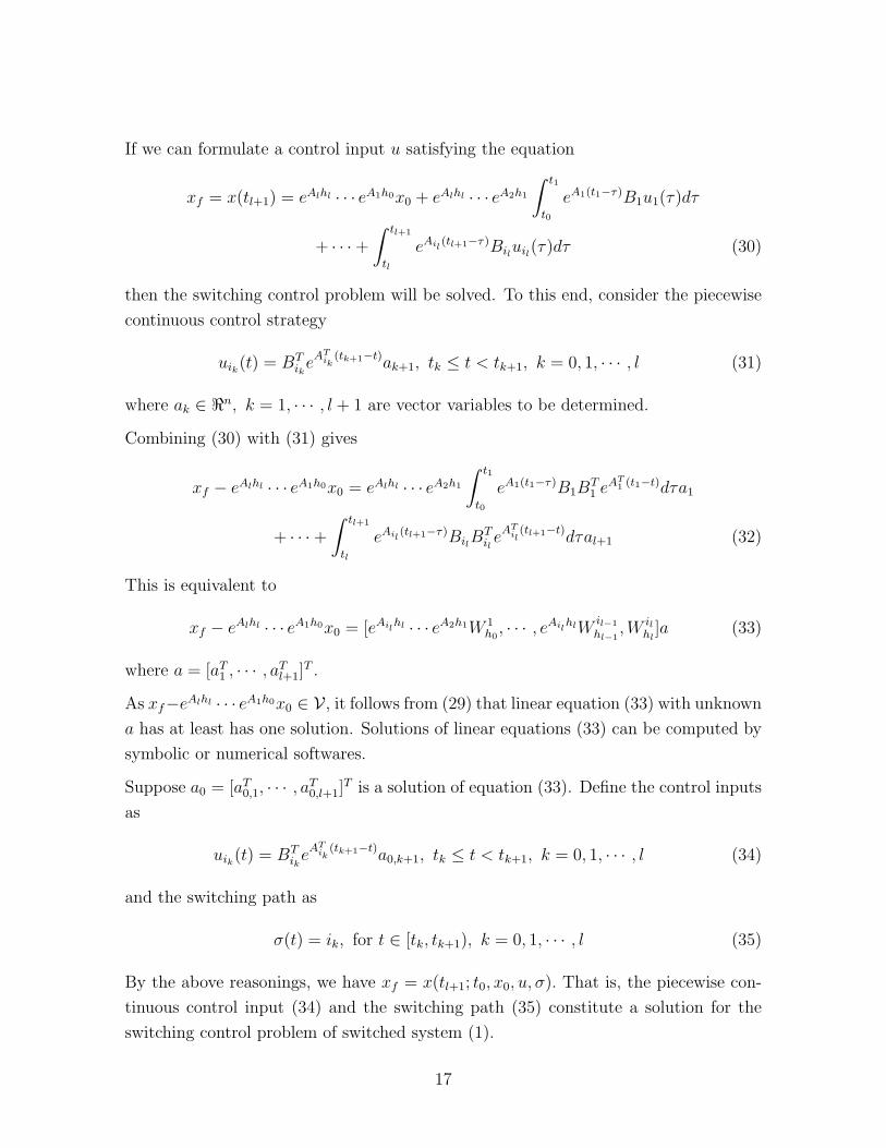
If we can formulate a control input u satisfying the equation

xf = x(tl+1) = eAlhl · · · eA1h0x0 + eAlhl · · · eA2h1

∫ t1

t0

eA1(t1−τ)B1u1(τ)dτ

+ · · ·+∫ tl+1

tl

eAil(tl+1−τ)Biluil(τ)dτ (30)

then the switching control problem will be solved. To this end, consider the piecewise

continuous control strategy

uik(t) = BTikeAT

ik(tk+1−t)ak+1, tk ≤ t < tk+1, k = 0, 1, · · · , l (31)

where ak ∈ <n, k = 1, · · · , l + 1 are vector variables to be determined.

Combining (30) with (31) gives

xf − eAlhl · · · eA1h0x0 = eAlhl · · · eA2h1

∫ t1

t0

eA1(t1−τ)B1BT1 eAT

1 (t1−t)dτa1

+ · · ·+∫ tl+1

tl

eAil(tl+1−τ)BilB

TileAT

il(tl+1−t)dτal+1 (32)

This is equivalent to

xf − eAlhl · · · eA1h0x0 = [eAilhl · · · eA2h1W 1

h0, · · · , eAil

hlWil−1

hl−1,W il

hl]a (33)

where a = [aT1 , · · · , aT

l+1]T .

As xf−eAlhl · · · eA1h0x0 ∈ V , it follows from (29) that linear equation (33) with unknown

a has at least has one solution. Solutions of linear equations (33) can be computed by

symbolic or numerical softwares.

Suppose a0 = [aT0,1, · · · , aT

0,l+1]T is a solution of equation (33). Define the control inputs

as

uik(t) = BTikeAT

ik(tk+1−t)a0,k+1, tk ≤ t < tk+1, k = 0, 1, · · · , l (34)

and the switching path as

σ(t) = ik, for t ∈ [tk, tk+1), k = 0, 1, · · · , l (35)

By the above reasonings, we have xf = x(tl+1; t0, x0, u, σ). That is, the piecewise con-

tinuous control input (34) and the switching path (35) constitute a solution for the

switching control problem of switched system (1).

17

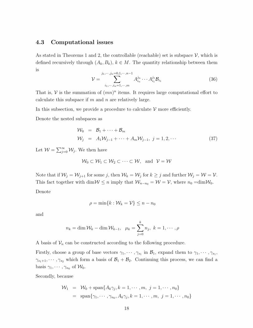
4.3 Computational issues

As stated in Theorems 1 and 2, the controllable (reachable) set is subspace V , which is

defined recursively through (Ak, Bk), k ∈ M . The quantity relationship between them

is

V =

j1,··· ,jn=0,1,··· ,n−1∑i1,··· ,in=1,··· ,m

Ajn

in· · ·Aj1

i1Bi1 (36)

That is, V is the summation of (mn)n items. It requires large computational effort to

calculate this subspace if m and n are relatively large.

In this subsection, we provide a procedure to calculate V more efficiently.

Denote the nested subspaces as

W0 = B1 + · · ·+ Bm

Wj = A1Wj−1 + · · ·+ AmWj−1, j = 1, 2, · · · (37)

Let W =∑∞

j=0Wj. We then have

W0 ⊂ W1 ⊂ W2 ⊂ · · · ⊂ W , and V = W

Note that ifWj = Wj+1 for some j, thenWk = Wj for k ≥ j and furtherWj = W = V .

This fact together with dimW ≤ n imply that Wn−n0 = W = V , where n0 =dimW0.

Denote

ρ = mink : Wk = V ≤ n− n0

and

nk = dimWk − dimWk−1, µk =k∑

j=0

nj, k = 1, · · · , ρ

A basis of Vn can be constructed according to the following procedure.

Firstly, choose a group of base vectors γ1, · · · , γs1 in B1, expand them to γ1, · · · , γs1 ,

γs1+1, · · · , γs2 which form a basis of B1 + B2. Continuing this process, we can find a

basis γ1, · · · , γn0 of W0.

Secondly, because

W1 = W0 + spanAkγj, k = 1, · · · ,m, j = 1, · · · , n0= spanγ1, · · · , γn0 , Akγj, k = 1, · · · ,m, j = 1, · · · , n0

18

we can find a basis γ1, · · · , γn0 , γn0+1, · · · , γµ1 of W1 by searching the set

γ1, · · · , γn0 , Akγj, k = 1, · · · ,m, j = 1, · · · , n0from left to right.

Continuing the process, we can find a basis γ1, · · · , γn0 , · · · γµl−1+1, · · · , γµlfor Wl.

Because

Wl+1 = Wl + spanAjγk, j = 1, · · · ,m, k = µl−1 + 1, · · · , µl= spanγ1, · · · , γµk

, Ajγk, j = 1, · · · ,m, k = µl−1 + 1, · · · , µland by searching the set

γ1, · · · , · · · , γµl, Ajγk, j = 1, · · · , m, k = µl−1 + 1, · · · , µl

from left to right for linearly independent column vectors, we can find a basis γ1, · · · , γn0 ,

· · · γµl−1+1, · · · , γµl, γµl+1, · · · , γµl+1

for Wl+1.

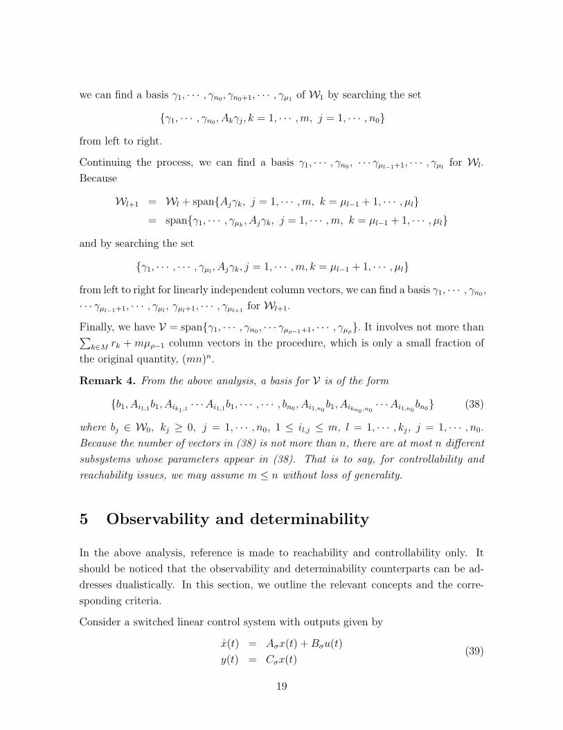
Finally, we have V = spanγ1, · · · , γn0 , · · · γµρ−1+1, · · · , γµρ. It involves not more than∑k∈M rk + mµρ−1 column vectors in the procedure, which is only a small fraction of

the original quantity, (mn)n.

Remark 4. From the above analysis, a basis for V is of the form

b1, Ai1,1b1, Aik1,1· · ·Ai1,1b1, · · · , · · · , bn0 , Ai1,n0

b1, Aikn0 ,n0· · ·Ai1,n0

bn0 (38)

where bj ∈ W0, kj ≥ 0, j = 1, · · · , n0, 1 ≤ il,j ≤ m, l = 1, · · · , kj, j = 1, · · · , n0.

Because the number of vectors in (38) is not more than n, there are at most n different

subsystems whose parameters appear in (38). That is to say, for controllability and

reachability issues, we may assume m ≤ n without loss of generality.

5 Observability and determinability

In the above analysis, reference is made to reachability and controllability only. It

should be noticed that the observability and determinability counterparts can be ad-

dresses dualistically. In this section, we outline the relevant concepts and the corre-

sponding criteria.

Consider a switched linear control system with outputs given by

x(t) = Aσx(t) + Bσu(t)

y(t) = Cσx(t)(39)

19

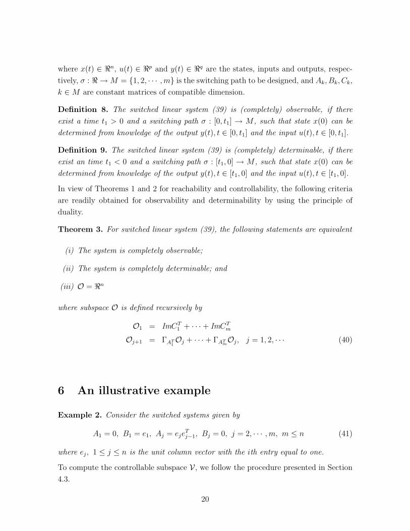
where x(t) ∈ <n, u(t) ∈ <p and y(t) ∈ <q are the states, inputs and outputs, respec-

tively, σ : < → M = 1, 2, · · · ,m is the switching path to be designed, and Ak, Bk, Ck,

k ∈ M are constant matrices of compatible dimension.

Definition 8. The switched linear system (39) is (completely) observable, if there

exist a time t1 > 0 and a switching path σ : [0, t1] → M , such that state x(0) can be

determined from knowledge of the output y(t), t ∈ [0, t1] and the input u(t), t ∈ [0, t1].

Definition 9. The switched linear system (39) is (completely) determinable, if there

exist an time t1 < 0 and a switching path σ : [t1, 0] → M , such that state x(0) can be

determined from knowledge of the output y(t), t ∈ [t1, 0] and the input u(t), t ∈ [t1, 0].

In view of Theorems 1 and 2 for reachability and controllability, the following criteria

are readily obtained for observability and determinability by using the principle of

duality.

Theorem 3. For switched linear system (39), the following statements are equivalent

(i) The system is completely observable;

(ii) The system is completely determinable; and

(iii) O = <n

where subspace O is defined recursively by

O1 = ImCT1 + · · ·+ ImCT

m

Oj+1 = ΓAT1Oj + · · ·+ ΓAT

mOj, j = 1, 2, · · · (40)

6 An illustrative example

Example 2. Consider the switched systems given by

A1 = 0, B1 = e1, Aj = ejeTj−1, Bj = 0, j = 2, · · · , m, m ≤ n (41)

where ej, 1 ≤ j ≤ n is the unit column vector with the ith entry equal to one.

To compute the controllable subspace V , we follow the procedure presented in Section

4.3.

20

It can be readily seen that

W0 = spane1By searching the independent vectors in

W1 = spane1, Aje1, j = 1, · · · ,m

we obtain that

W1 = spane1, A2e1 = spane1, e2Continue this process, we have

Wk = spane1, · · · , ek, Ajek, j = 1, · · · ,m = spane1, · · · , ek+1

for k = 2, · · · ,m− 1, and

Wm = spane1, · · · , em, Ajem, j = 1, · · · ,m = spane1, · · · , em = Wm−1

Thus V = W = Wm−1. According to Theorems 1 and 2, the controllable (reachable)

set is

R = C = spane1, · · · , emwhich is an m-dimensional subspace. If m = n, then the switched system is controllable

and reachable.

Now let us address the switching control problem for system (41). Following the pro-

cedure outlined in Section 4.2, we consider the periodic switching index sequence and

piecewise continuous inputs.

Let us choose the switching time sequence to be

t0 = 0, t1 = 1, t2 = 2, · · · (42)

Accordingly, hk = h = 1 for k = 0, 1, · · · . Simple calculation gives

eA1h = In, eAjh = In + Aj, j = 2, · · · ,m

where In is the nth order identity matrix.

Let l = ml0 with l0 to be determined. Under the periodic switching index sequence

(15), we can compute that

dim(eAilh · · · eA2hD1 + · · ·+ eAil

hDil−1+Dil)

= dim(eAilh · · · eA2hD1 + eAil

h · · · eAil−m+1h · · · eAil−m

hD1 + · · ·+D1)

= dim(Ql0B1 + Ql0−1B1 + · · ·+ B1) (43)

21

where

Q = eAmheAm−1h · · · eA2h = In + A2 + · · ·+ Am

It can be verified that vectors B1, QB1, · · · , Qm−1B1 are linearly independent, and

V = spanB1, QB1, · · · , Qm−1B1

Accordingly, we choose that l0 = m− 1.

Simple calculation gives

W 1h = e1e

T1 , W k

t = 0, k = 2, · · · ,m

For any given states x0 and xf in V , consider the equation

xf −Qm−1x0 = [Qm−1W 1h , · · · , QW 1

h ,W 1h ]a (44)

Let P denote the sub-matrix of [Qm−1B1, · · · , QB1, B1] consisting the first m rows. It

is clear that P is nonsingular. Denote

a0 = [P−1, 0](xf −Qm−1x0)

The solutions of equation (44) are given by

a = [a0(1), ∗, · · · , ∗, a0(2), ∗, · · · , ∗, · · · , a0(m), ∗, · · · , ∗]T

where a0(j) denotes the jth entry of vector a0, and the symbol ‘∗’ stands for any real

numbers.

The corresponding piecewise continuous input is

u1(t) = a0(j + 1), tmj ≤ t < tmj+1, j = 0, · · · ,m− 1 (45)

The switching index sequence (15) and control strategy (45) will steer the system from

original x0 at t = 0 to the target xf at t = m(m− 1) + 1.

The above switching control scheme involves m(m − 1) times of switching to transfer

between two arbitrarily given states in the controllable subspace. This number can be

reduced, if we use aperiodic switching index sequence instead of the periodic one. For

example, let us consider the switching index sequence

i0 = 1, i1 = 2, i2 = 1, i3 = 3, i4 = 2, i5 = 1, · · · , ik−m+1 = m, · · · , ik = 1

22

where k = (m−1)(m+2)2

. Under the switching time sequence (42), we have

dim(eAikh · · · eAi1

hDi0 + · · ·+ eAikhDik−1

+Dik)

= dim(eAikh · · · eAi1

hD1 + eAikh · · · eAik−m

hD1 + · · ·+D1)

= dim(Qm−1B1 + Qm−2B1 + · · ·+ Q1B1 + B1) (46)

where matrices Qj, j = 1, · · · ,m are defined recursively as

Q1 = eA2 · · · eAm , Qj = eA2 · · · eAm+1−jQj−1, j = 2, · · · , m− 1

It can be verified that vectors B1, Q1B1, · · · , Qm−1B1 are linearly independent, and

V = spanB1, Q1B1, · · · , Qm−1B1Accordingly, a piecewise control input can be obtained by solving the following equation

xf −Qm−1x0 = [Qm−1W1h , · · · , Q1W

1h , W 1

h ]a (47)

for any given initial state x0 and target state xf .

An interesting question arise naturally: Is (m−1)(m+2)2

the minimal switching number for

system (41)? Or equivalently, is this number can be further reduced by other switching

index sequences? We could not provide a definite answer yet, though we incline the

positive answer.

7 Conclusion

In this paper, detailed controllability and reachability analyse have been carried out

for switched linear control systems. It has been proven that, both the controllable

and reachable sets are subspaces of the total space, and the two sets always coincide

with each other. The controllable (reachable) set is exactly the minimal Ak- invariant

subspace for k ∈ M which contains∑

k∈M Bk. Criteria for observability and deter-

minability have also been obtained by duality. These results generalize Wonham’s

geometric characterizations to switched systems.

A closely related interesting problem is controlling the switched linear systems with

minimum number of switching. It seems that more rigorous rank estimation for expo-

nential matrix should be developed to address this problem.

ACKNOWLEDGEMENT

The authors would like to thank the anonymous reviewers for their constructive and

insightful comments for further improving the quality of this work.

23

References

Blondel, V. D., & Tsitsiklis, J. N. (1999). Complexity of stability and controllability

of elementary hybrid systems. Automatica, 35(3), 479–489.

Branicky, M. S. (1998). Multiple Lyapunov functions and other analysis tools for

switched and hybrid systems. IEEE Transactions on Automatic Control, 43(4),

475–482.

Brockett, R. W. (1983). Asymptotic stability and feedback stabilization. In R. W.

Brockett et al, Differential Geometric Control Theory (pp. 181–191). Boston:

Birkhauser.

Caines, P. E., & Wei, Y.-J. (1998). Hierarchical hybrid control systems: a lattice

theoretic formulation. IEEE Transactions on Automatic Control, 43(4), 501-508.

Chase, C., Serrano, J., & Ramadge, P. J. (1993). Periodicity and chaos from switched

flow systems: contrasting examples of discretely controlled continuous systems.

IEEE Transactions on Automatic Control, 38(1), 70–83.

Conner, L. T. Jr., & Stanford, D. P. (1987). The structure of controllable set for

multimodal systems. Linear Algebra and its Applications, 95(2), 171–180.

Dayawansa, W. P., & Martin, C. F. (1999). A converse Lyapunov theorem for a class

of dynamical systems which undergo switching. IEEE Transactions on Automatic

Control 44(4), 751–760.

Drager, L.D., Foote, R.L., Martin, C.F., & Wolfer, J. (1989). Controllability of linear

systems, differential geometry curves in Grassmannians and generalized Grassman-

nians, and Riccati equations. Acta Applicandae Mathematicae, 16(3), 281–317.

Ezzine, J., & Haddad, A. H. (1989). Controllability and observability of hybrid systems.

International Journal of Control, 49(6), 2045–2055.

Kaplan, W. (1966). Introduction to Analytic Functions. Reading: Addison-Wesley.

Kolmanovsky, I., & McClamroch, N. H. (1995). Developments in nonholonomic control

problems. IEEE Control Systems, 15(6), 20–36.

Kolmanovsky, I., & McClamroch, N. H. (1996). Hybrid feedback laws for a class of cas-

cade nonlinear control systems. IEEE Transactions on Automatic Control, 41(9),

1271–1282.

24

Leonessa, A., Haddad, W. M., & Chellaboina, V. (2001). Nonlinear system stabiliza-

tion via hierarchical switching control. IEEE Transactions on Automatic Control,

46(1), 17-28.

Li, Z. G., Wen, C. Y., & Soh, Y. C. (2001). Switched controllers and their applications

in bilinear systems. Automatica, 37(3), 477-481.

Liberzon, D., & Morse, A. S. (1999). Basic problems in stability and design of switched

systems. IEEE Control Systems, 19(5), 59–70.

Loparo, K. A., Aslanis, J. T., & IIajek, O. (1987). Analysis of switching linear systems

in the plain, part 2, global behavior of trajectories, controllability and attainability.

Journal of Optimization Theory and Applications, 52(3), 395–427.

Morse, A. S.(1996). Supervisory control of families of linear set-point controllers- Part

1:, exact matching. IEEE Transactions on Automatic Control, 41(10), 1413–1431.

Narendra, K. S., & Balakrishnan, J. (1997). Adaptive control using multiple models.


Savkin, A. V., Skafidas, E., & Evans, R. J. (1999). Robust output feedback stabiliz-

ability via controller switching. Automatica, 35(1), 69-74.

Sira-Ramirez, H. (1991). Nonlinear P-I controller design for switch mode dc-to-dc power

converters. IEEE Transactions and Circuits and Systems, 38(4), 410–417.

Stanford, D. P., & Conner, L. T. Jr. (1980). Controllability and stabilizability in multi-

pair systems. SIAM Journal on Control and Optimization, 18(5), 488–497.

Sun, Z., & Zheng, D. Z. (2001). On reachability and stabilization of switched linear

control systems. IEEE Transactions on Automatic Control, 46(2), 291–295.

Szigeti, F. (1992). A differential-algebraic condition for controllability and observability

of time varying linear systems. In Proceedings of 31st Conference on Decision and

Control (pp. 3088-3090).

Wicks, M. A., Peleties, P., & DeCarlo, R. A. (1998). Switched controller synthesis for

the quadratic stabilization of a pair of unstable linear systems. European Journal

of Control, 4(2), 140–147.

25

Williams, S. M., & Hoft, R. G. (1991). Adaptive frequency domain control of PPM

switched power line conditioner. IEEE Transactions on Power Electronics, 6(4),

665–670.

Wonham, W. M. (1979). Linear Multivariable Control — A Geometric Approach.

Berlin: Spinger-Verlag.

Xu, X., & Antsaklis, P. J. (1999). On the reachability of a class of second-order switched

systems. Technical report, ISIS-99-003, University of Notre Dame.

Ye, H., Michel, A. N., & Hou, L. (1998). Stability theory for hybrid dynamical systems.


26

Documents

Controllability and reachability criteria for switched linear systems