Controlling Light Through Optical Disordered Media

HAL Id: hal-00611018https://hal.archives-ouvertes.fr/hal-00611018

Preprint submitted on 25 Jul 2011

HAL is a multi-disciplinary open accessarchive for the deposit and dissemination of sci-entific research documents, whether they are pub-lished or not. The documents may come fromteaching and research institutions in France orabroad, or from public or private research centers.

L’archive ouverte pluridisciplinaire HAL, estdestinée au dépôt et à la diffusion de documentsscientifiques de niveau recherche, publiés ou non,émanant des établissements d’enseignement et derecherche français ou étrangers, des laboratoirespublics ou privés.

Controlling Light Through Optical Disordered Media :Transmission Matrix Approach

Sébastien Popoff, Geoffroy Lerosey, Mathias Fink, Albert Boccara, SylvainGigan

To cite this version:Sébastien Popoff, Geoffroy Lerosey, Mathias Fink, Albert Boccara, Sylvain Gigan. Controlling LightThrough Optical Disordered Media : Transmission Matrix Approach. 2011. �hal-00611018�

https://hal.archives-ouvertes.fr/hal-00611018

https://hal.archives-ouvertes.fr

Controlling Light Through Optical Disordered Media :

Transmission Matrix Approach

S. M. Popoff, G. Lerosey, M. Fink, A. C. Boccara, S. Gigan

Institut Langevin, ESPCI ParisTech, CNRS UMR 7587, 10 rue Vauquelin, 75231 Paris,

France.

E-mail: [email protected]

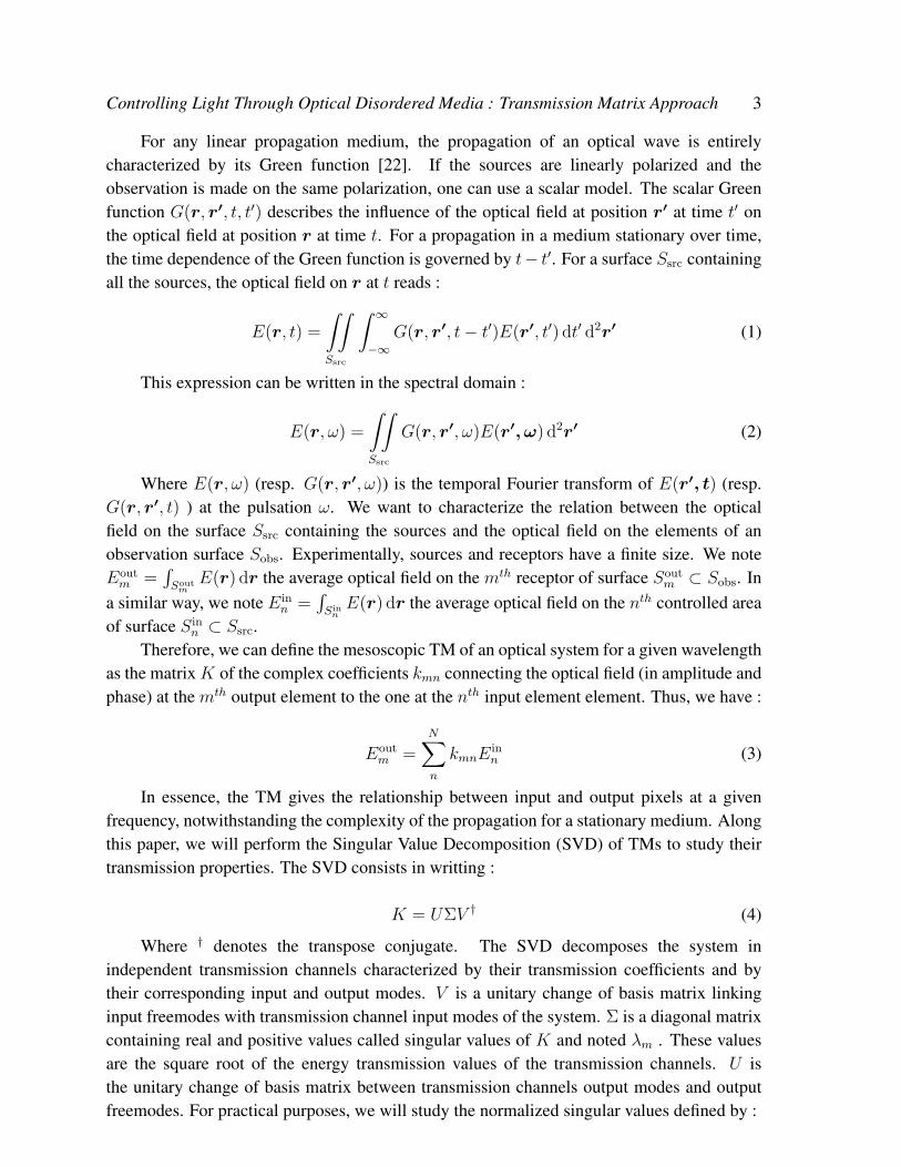
Abstract. We experimentally measure the monochromatic transmission matrix (TM) of an

optical multiple scattering medium using a spatial light modulator together with a phase-

shifting interferometry measurement method. The TM contains all information needed to

shape the scattered output field at will or to detect an image through the medium. We

confront theory and experiment for these applications and we study the effect of noise on

the reconstruction method. We also extracted from the TM informations about the statistical

properties of the medium and the light transport whitin it. In particular, we are able to isolate

the contributions of the Memory Effect (ME) and measure its attenuation length.

PACS numbers: 05.60.Cd, 71.23.-k, 78.67.-n

Submitted to: New J. Phys.

Controlling Light Through Optical Disordered Media : Transmission Matrix Approach 2

Introduction

For a long time, wave propagation was only studied in the simple cases of homogeneous

media or simple scattering were the trajectories of waves can be exactly determined [1].

Nevertheless, the effect of the multiple elastic scattering on propagation of waves is complex

but deterministic, and information conveyed inside such media is shuffled but conserved [2].

Within the last decades, the study of complex and random media has been an interdisciplinary

subject of interest, ranging from solid state physics to optics via acoustics, electromagnetism,

telecommunication and seismology [3, 4, 5, 6, 7].

Recent works in optics have shown that it is possible to achieve wavefront shaping beyond

a complex media despite multiple scattering [8, 9] and even to take advantage of the

randomness of such media to increase resolution [10] by reducing the size of the focal

spots. These works amount to performing phase conjugation. Nevertheless, in acoustics [11],

seismic [12], electromagnetics or telecommunication [13], other operations are done to

transmit information through a random propagation systems. These techniques assume that

the propagation between input and output is characterized in amplitude and phase, which is

not trivial in optics.

We recently introduced a method to experimentally measure the monochromatic transmission

matrix (TM) of a complex media [14] and presented an application to image transmission

through such media [15]. In the present paper, we will develop the TM model for optical

systems, in particular for multiple scattering media and detail the experimental acquisition

method. We will show that the TM can be exploited for different applications. The most

straightforward ones are focusing and image detection using well-established operators used

for inverse problems in various domains (telecommunication [13], seismology [12], optical

tomography [16, 17], acoustics [18, 19] and electromagnetics [20]). We will confront theory

and experiment for applications and study the statistical properties of the TM. We will in

particular study the effect of the ballistic contributions on the statistics of the TM and its

consequences on image transmission. We will finally study how the short range correlation of

the Memory Effect [21] (ME) affects the TM and how to quantify its correlation length with

the knowledge of the TM.

1. Matrix Model and Acquisition

1.1. Modeling Transmission Through a Linear Optical System

In free space, a plane wave propagates without beeing modified and its k-vector is conserved

since plane waves are the eigenmodes of the free space propagation. In contrast, a plane wave

illuminating a multiple scattering sample gives rise to a seemingly random output field. This

output field is different for a different input k-vector. In order to use a scattering medium as

an optical tool, one has to characterize the relation between input and output free modes. At a

given wavelength, we will model such a system with a matrix linking the k-vector components

of the output field to those of the input field. We will justify the validity and the interest of

such a model.


For any linear propagation medium, the propagation of an optical wave is entirely

characterized by its Green function [22]. If the sources are linearly polarized and the

observation is made on the same polarization, one can use a scalar model. The scalar Green

function G(r, r′, t, t′) describes the influence of the optical field at position r′ at time t′ on

the optical field at position r at time t. For a propagation in a medium stationary over time,

the time dependence of the Green function is governed by t− t′. For a surface Ssrc containing

all the sources, the optical field on r at t reads :

E(r, t) =

∫∫

Ssrc

∫ ∞

−∞

G(r, r′, t− t′)E(r′, t′) dt′ d2r′ (1)

This expression can be written in the spectral domain :

E(r, ω) =

∫∫

Ssrc

G(r, r′, ω)E(r′, ω) d2r′ (2)

Where E(r, ω) (resp. G(r, r′, ω)) is the temporal Fourier transform of E(r′, t) (resp.

G(r, r′, t) ) at the pulsation ω. We want to characterize the relation between the optical

field on the surface Ssrc containing the sources and the optical field on the elements of an

observation surface Sobs. Experimentally, sources and receptors have a finite size. We note

Eoutm =

∫Soutm

E(r) dr the average optical field on the mth receptor of surface Soutm ⊂ Sobs. In

a similar way, we note E inn =

∫Sinn

E(r) dr the average optical field on the nth controlled area

of surface Sinn ⊂ Ssrc.

Therefore, we can define the mesoscopic TM of an optical system for a given wavelength

as the matrix K of the complex coefficients kmn connecting the optical field (in amplitude and

phase) at the mth output element to the one at the nth input element element. Thus, we have :

Eoutm =

N∑

n

kmnEinn (3)

In essence, the TM gives the relationship between input and output pixels at a given

frequency, notwithstanding the complexity of the propagation for a stationary medium. Along

this paper, we will perform the Singular Value Decomposition (SVD) of TMs to study their

transmission properties. The SVD consists in writting :

K = UΣV † (4)

Where † denotes the transpose conjugate. The SVD decomposes the system in

independent transmission channels characterized by their transmission coefficients and by

their corresponding input and output modes. V is a unitary change of basis matrix linking

input freemodes with transmission channel input modes of the system. Σ is a diagonal matrix

containing real and positive values called singular values of K and noted λm . These values

are the square root of the energy transmission values of the transmission channels. U is

the unitary change of basis matrix between transmission channels output modes and output

freemodes. For practical purposes, we will study the normalized singular values defined by :


λm =λm√∑

k λ2k

(5)

The SVD is a powerful tool that gives access to the statistical distribution of the incident

energy injected thought the multiple transmission channels of the system. Within this matrix

model, the number of channels of the observed system is min(N,M). Nevertheless, this

number does not quantify the information that could simultaneously be conveyed in the

medium.

Quantifying information is of high interest and this work has been done in acoustics [23,

24] for Time Reversal focusing through a multiple scattering medium. In those theories,

the number of spatial and temporal Degrees of Freedom (NDOF) also called Number of

Information Grains is introduced. These degrees of freedom represent as many independent

information grains can be conveyed through the system. For a monochromatic experiment

there are only spatial degrees of freedom and NDOF is given by the number of uncorrelated

element used to recover information [2]. This number will be different on the type of

experiment considered, focusing or image detection. A focusing experiment consists in

finding the optimal input wavefront to send to maximize energy at a desired position (or

a combination of positions) on the output of the sample. An image detection experiment

consists in retrieving an image sent at the input of the system by measuring the output

complex field. For focusing experiments NDOF is given by the number of independent input

segments, which corresponds to the number of degrees of freedom the experimentalist can

control. Conversely, for detection experiments, the experimentalist cannot access more than

the number of independent output elements recorded. In the general case, we have NDOF ≤ N

for focusing and NDOF ≤ M . We choose to fix the input (resp. output) pixel size at the input

(resp. output) coherence length of the system. For this ideal sampling, NDOF is given by the

input or output dimension of the TM according to the type of experiment : NDOF = N for

focusing and NDOF = M for detection.

1.2. Experimental Setup

To measure the TM of an optical system, one needs a way to control the incident light and

to record the complex optical field. The control is now possible thanks to the emergence

of spatial light modulators (SLM) and the output complex field can be measured using an

interferometric method detailed in section 1.3. We want to study an optical system governed

by multiple scattering in which the propagation function can not be a priori calculated. The

material chosen is Zinc-Oxyde, a white pigment commonly used for industrial paints. The

sample is an opaque 80 ± 25 µm thick deposit of a ZnO powder (Sigma-Aldrich 96479) with

a measured mean free path of 6 ± 2 µm on a standard microscope glass slide. The thickness

of the sample being one order of magnitude higher than the mean free path, light transport

inside the sample is in the multiple scattering regime. To generate the incident wavefront,

the beam from a diode-pumped solid-state single longitudinal mode laser source at 532 nm

(Laser Quantum Torus) is expanded and spatially modulated by a liquid crystal SLM (Holoeye


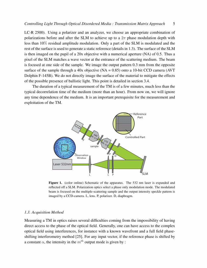
LC-R 2500). Using a polarizer and an analyzer, we choose an appropriate combination of

polarizations before and after the SLM to achieve up to a 2π phase modulation depth with

less than 10% residual amplitude modulation. Only a part of the SLM is modulated and the

rest of the surface is used to generate a static reference (details in 1.3). The surface of the SLM

is then imaged on the pupil of a 20x objective with a numerical aperture (NA) of 0.5. Thus a

pixel of the SLM matches a wave vector at the entrance of the scattering medium. The beam

is focused at one side of the sample. We image the output pattern 0.3 mm from the opposite

surface of the sample through a 40x objective (NA = 0.85) onto a 10-bit CCD camera (AVT

Dolphin F-145B). We do not directly image the surface of the material to mitigate the effects

of the possible presence of ballistic light. This point is detailed in section 3.4.

The duration of a typical measurement of the TM is of a few minutes, much less than the

typical decorrelation time of the medium (more than an hour). From now on, we will ignore

any time dependence of the medium. It is an important prerequisite for the measurement and

exploitation of the TM.

Observation

Window

x40AN : 0.75P

D

sample

P

PLL

x10AN : 0.3

CCD

Laser 532nm

SLM

Controlled Part

Reference

Part

Figure 1. (color online) Schematic of the apparatus. The 532 nm laser is expanded and

reflected off a SLM. Polarization optics select a phase only modulation mode. The modulated

beam is focused on the multiple-scattering sample and the output intensity speckle pattern is

imaged by a CCD-camera. L, lens. P, polarizer. D, diaphragm.

1.3. Acquisition Method

Measuring a TM in optics raises several difficulties coming from the impossibility of having

direct access to the phase of the optical field. Generally, one can have access to the complex

optical field using interferences, for instance with a known wavefront and a full field phase-

shifting interferometry method [25]. For any input vector, if the reference phase is shifted by

a constant α, the intensity in the mth output mode is given by :


Iαm = |Eoutm |2 = |sm +

N∑

n

eiαkmnEinn |2 (6)

= |sm|2 + |N∑

n

eiαkmnEinn |2 + 2ℜ

(eiαsm

N∑

n

kmnEinn

)

where sm is the complex amplitude of the optical field used as reference in the mth output

mode.

Thus, if we inject the nth input mode and measure I0m,Iπ

2m ,Iπm and I

3π2

m , respectively the

intensities in the mth outgoing mode for α = 0, π/2, π and 3π/2 gives :

(I0m − Iπm)

4+ i

(I

3π2

m − Iπ

2m

)

4= smkmn (7)

Commercial SLMs cannot control independently phase and amplitude of an incident

optical field. Our setup uses a phase-only modulator since the phase is the most important

parameter to control in wavefront shaping [26]. A recent method [27] allows phase and

amplitude modulation with similar commercial modulators, nevertheless, we use in this work

a phase-only configuration to keep the setup as simple as possible.

Controlling only the phase forbids us to switch off or modulate in amplitude an incident

mode. Thus we can not directly acquire the TM in the canonical basis. We want to use

a basis that utilizes every pixel with identical modulus. The Hadamard basis in which all

elements are either +1 or -1 in amplitude perfectly satisfies our constraints. Another advantage

is that it maximizes the intensity of the received wavefront and consequently decreases

the experimental sensibility to noise [28]. For all Hadamard basis vectors, the intensity is

measured on the basis of the pixels on the CCD camera. We obtain the TM in the input

canonical basis by a unitary transformation. The observed transmission matrix Kobs is directly

related to the physical one K of formula 3 by

Kobs = K × Sref (8)

where Sref is a diagonal matrix of elements where srefmm = sm represents the static

reference wavefront in amplitude and phase.

Ideally, the reference wavefront should be a plane wave to directly have access to the K

matrix. In this case, all sm are identical and Kobs is directly proportional to K. However this

requires the addition of a reference arm to the setup, and requires an interferometric stability.

To have the simplest experimental setup and a higher stability, we modulate only 65 % of the

wavefront going into the scattering sample (this correponds to the square inside the pupil of

the microscope objective as seen in Figure 1), the speckle generated by the light coming from

the 35 % static part being our reference. Sref results from the transmission of this static part

and is now unknown and no longer constant along its diagonal. Nevertheless, since Sref is

stationary over time, we can measure the response of all input vectors on the mth output pixel

as long as the reference speckle is bright enough. We will show in the next subsection that


we can go back to the amplitude elements of Sref and that the only missing information is

the phase of the reference. We will quantify the effect of the reference speckle and show that

neither does it impair our ability to focus or image using the TM, nor does it affect our ability

to retrieve the statistical properties of the TM.

1.4. Multiple Scattering and Random Matrices

Under certain conditions, the rectangle N by M TM of a system dominated by multiple

scattering [29] amounts to a random matrix of independent identically distributed entries of

Gaussian statistics. We will study the properties of such matrices thanks to the Random

Matrix Theory (RMT) and investigate the hypothesis for which the TM of multiple-scattering

samples are well described by this formalism.

We introduced previously that the SVD of a physical matrix is a powerful tool to study

the energy repartition in the different channels. For matrices of independent elements of

Gaussian distribution, RMT predicts that the statistical distribution ρ(λ) of the normalized

singular values follows the Marcenko-Pastur Law [30]. For γ = M/N , it reads :

ρ(λ) =γ

2πλ

√(λ2 − λ2

min)(λ2max − λ2) (9)

∀λ ∈ [λmin, λmax]

With λmin = (1 −√

1/γ) the smallest singular value and λmax = (1 +√

1/γ) the

maximum singular value. In particular, for γ = 1, the Marcenko-Pastur law is known as the

"quarter circle law" [31] and reads :

ρ(λ) =1

π

√4− λ2 (10)

Those predictions are valid for a TM of independent elements i.e. without any correlation

between its elements. This hypothesis can be broken by adding short range correlation but also

non trivial correlations such as ones appearing when introducing the flux conservation [32].

Since we only experimentally record and control a small part of the field on both side of the

sample, we will not be affected by this conservation condition.

Another straightforward parameter that could have an influence on the hypothesis of

independent elements is the size of the segments uses as sources (on the SLM) and receptors

(on the CCD). If the segment size is less than the coherence length (i.e. the size of a speckle

grain) two neighboring segments will be strongly correlated. The size of input (resp. output)

segments is set to fit the input (resp. output) coherence length. This way, the TM K should

respect the hypothesis of independent elements and follow the Marcenko-Pastur law.

Nevertheless the method of the acquisition introduces correlation in the TM recorded.

For M = N , K should respect the Quarter Circle law but the methods detailed in section 1.3

gives only access to the observed TM matrix Kobs = Sref .K. whose elements read :


kobsmn =

N∑

j

smjkjn = kmnsmm (11)

To study the singular value distribution of our TM, we have to be sure that we can go

back to the precise statistics of K using the observed matrix Kobs.

The effect of the reference Sref is static at the output. This means that its influence is the

same for each input vectors. Calculating the standard deviation of an output elements over the

input basis vectors we have :

√〈|kobs

mn|2〉n =√

| 〈kmn|2〉n|smm| (12)

=√

〈|kmn|2〉mn|smm| ∀m ∈ [1,M ]

We made the hypothesis that each input k-vector gives an output speckle of the same

mean intensity, it reads 〈|kmn|2〉n = 〈|kmn|2〉mn. This is valid in the diffusive regime as

long as the illumination is homogeneous. We select for the illumination only the center part

of an expanded gaussian beam. We also neglected the correlation effects that are expected

to be small regarding our system, such as Memory Effect [21] (see section 4) and long

range correlations [33]. We can now define a normalized TM Kfil whose elements kfilmn are

normalized by√

〈|kobsmn|2〉m.

kfilmn =

kobsmn√

〈|k|2〉mn |smm|2(13)

=kmn√〈|k|2〉mn

smm

|smm|(14)

This matrix is not influenced by the amplitude of the reference and reads :

Kfil =K√

〈|k|2〉mn

× Sφ (15)

Where Sφ is a diagonal matrix of complex elements of norm 1 representing the phase

contributions of the output reference speckle. In contrast with Sref , Sφ is a unitary matrix

since SφS†φ = I where I is the identity matrix. Thus if K = UΣV † then Kfil = U ′ΣV † where

U ′ = Sφ × U is a unitary matrix. Therefore, Kfil and K have singular value decompositions

with the same singular values.

We show in figure 2 that the statistics of the observed TM Kobs do not follow the quarter

circle (formula 10) law whereas the singular value distribution of the filtered matrix Kfil is

close to it. Remaining correlation effects are due to inter-element correlations between nearby

pixels. Taking a sub-matrix of the TM with only one element out of two, its statistics finally

follows correctly the expected quarter-circle law. Those results are comparable to the ones

obtained for transmission matrices in acoustics [29].

This clearly demonstrates that we can directly study the properties of K even if we

only have access to the observed matrix Kobs. We also want to point out that one has


0 1 2 30

0.2

0.4

0.6

0.8

1

Figure 2. Singular values distributions of the experimental transmission matrices obtained by

averaging over 16 realizations of disorder. The solid line is the quarter-circle law predicted

by RMT. With + the observed matrix, with � the matrix filtered to remove the reference

amplitude contribution and with ◦ the matrix obtained by filtering and removing neighboring

elements to eliminate inter-element correlations.

to be careful when interpreting deviation from a given prediction on SVD results. Once

the matrix is measured and its singular values analyzed, one has to investigate the causes

of the deviation from the Marcenko-Pastur law. Those causes could come from physical

phenomenons involved in light propagation in the medium that break the hypothesis of the

absence of correlation in the TM (like the apparition of ballistic contributions, see section 3.4)

but could also be inherent to the experimental method. However, Kobs brings all informations

on singular values that describe the physics of the propagation in a given setup.

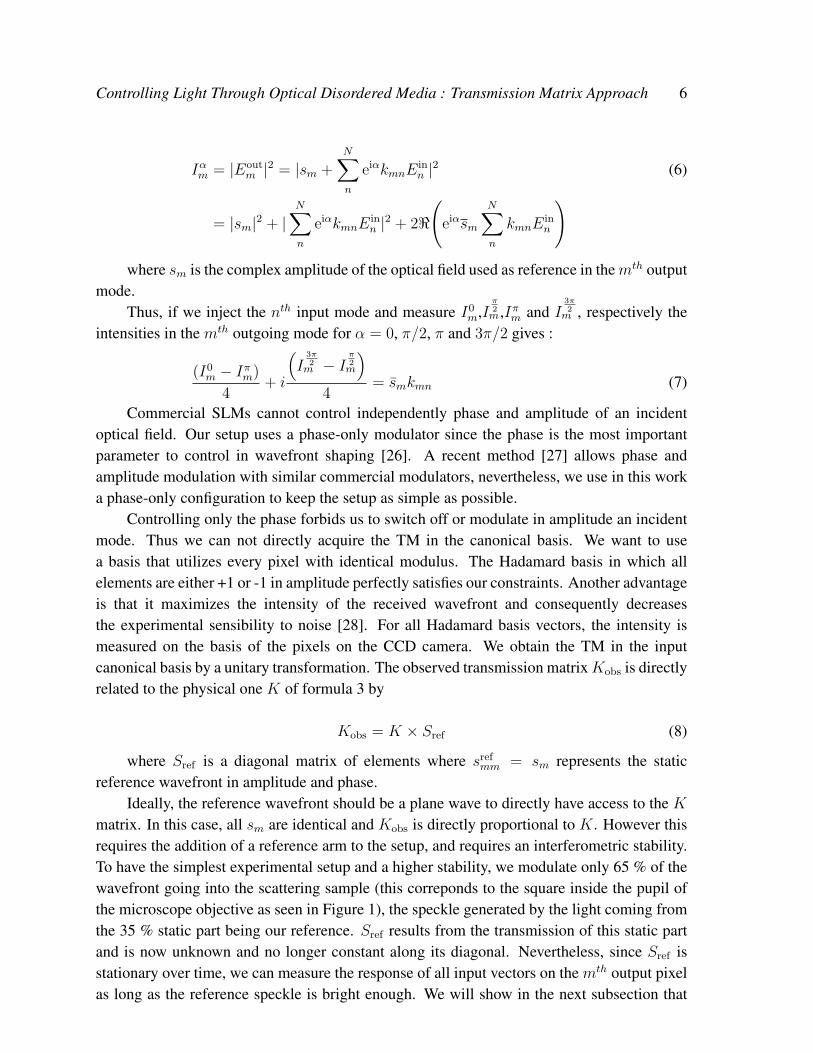
So far, we compared the experimental singular value distributions for a symmetric case

(M = N ). But what would be the effect of breaking the input / output asymmetric raio M/N

? In the same setup, we experimentally acquired TMs with a fixed number of controlled pixels

on the SLM (N = 1024) and changed the number of independent output pixels recorded by

the CCD (M = γN ) to achieve various ratio values (γ ∈ {1; 1.5; 2; 3; 4; 5}). Normalized

singular value distributions of experimental TM filtered are shown in figure 3 and follows

qualitatively the RMT prediction of equation 10.

We see that with increasing γ, the range of λ narrows. This effect has been measured in

experiment in the acoustic field [34]. Physically this means that when γ increases, all recorded

channels tend to converge toward the mean global transmission value λ = 1. When M > N ,

we record more independant informations than the rank of the TM and averaging effects lead

to a distribution that is peaked around a unique transmission value when M ≫ N . We notice

that the experimental distributions deviate from the theoretical ones as γ increases. To have

TMs with different values of γ, we record a large TM with γ = 11 and then create submatrices

by taking lines selected randomly among the lines of the original TM. By increasing γ we

increase the probability of having neighboring pixels in the TM and then are more sensitive to

correlations between nearby pixels. This modifies the statistics and decreases the number of

independent output segments. This explains the deviation from the theory. Other effects that

could bring correlations in certain experimental conditions are discussed is section 3.4.


0 1 2 3 40

0.2

0.4

0.6

0.8 γ=4γ=30 1 2 3 4

0.2

0.4

0.6

0.8 γ=1

0

γ=1,25

γ=1,5 γ=2

γ=5

0.2

0.4

0.6

0.8

0

0.2

0.4

0.6

0.8

0

0.2

0.4

0.6

0.8

0

0.2

0.4

0.6

0.8

0

0 1 2 3 4 0 1 2 3 4

0 1 2 3 40 1 2 3 4

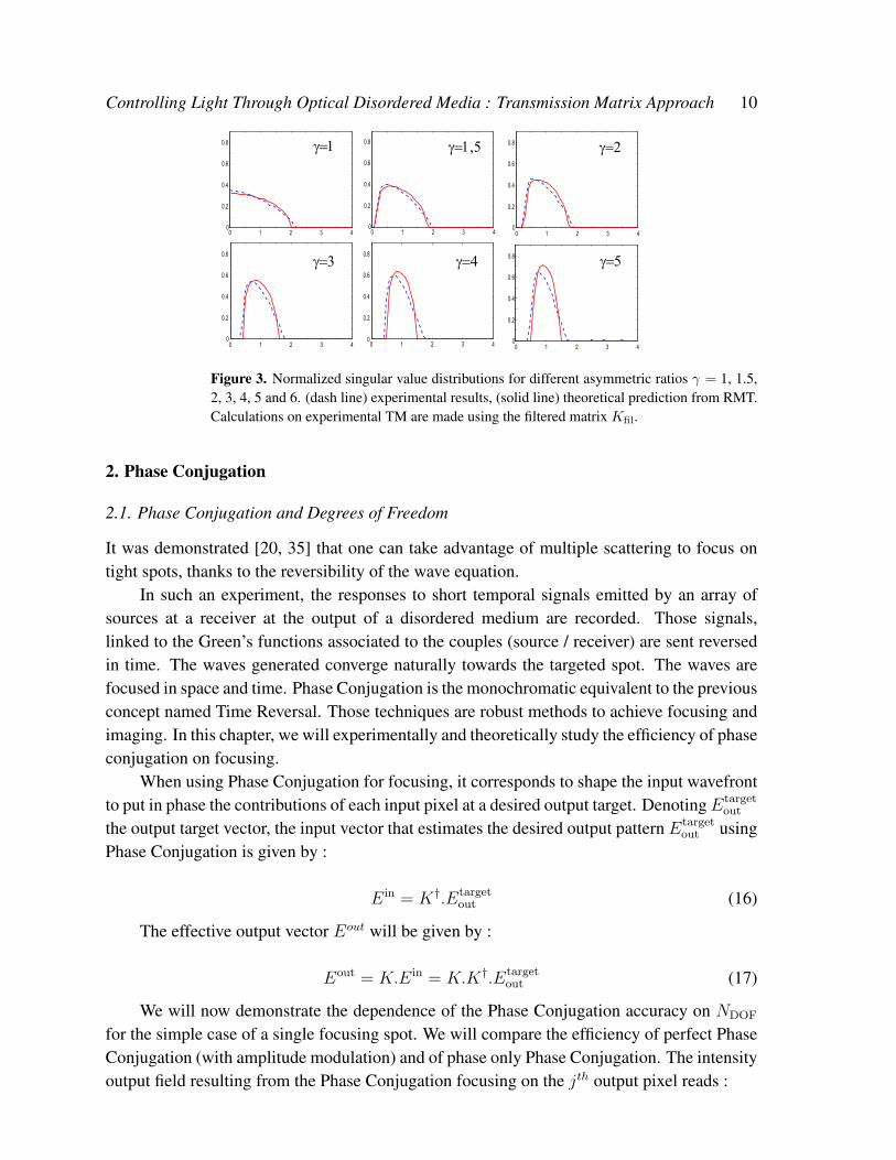
Figure 3. Normalized singular value distributions for different asymmetric ratios γ = 1, 1.5,

2, 3, 4, 5 and 6. (dash line) experimental results, (solid line) theoretical prediction from RMT.

Calculations on experimental TM are made using the filtered matrix Kfil.

2. Phase Conjugation

2.1. Phase Conjugation and Degrees of Freedom

It was demonstrated [20, 35] that one can take advantage of multiple scattering to focus on

tight spots, thanks to the reversibility of the wave equation.

In such an experiment, the responses to short temporal signals emitted by an array of

sources at a receiver at the output of a disordered medium are recorded. Those signals,

linked to the Green’s functions associated to the couples (source / receiver) are sent reversed

in time. The waves generated converge naturally towards the targeted spot. The waves are

focused in space and time. Phase Conjugation is the monochromatic equivalent to the previous

concept named Time Reversal. Those techniques are robust methods to achieve focusing and

imaging. In this chapter, we will experimentally and theoretically study the efficiency of phase

conjugation on focusing.

When using Phase Conjugation for focusing, it corresponds to shape the input wavefront

to put in phase the contributions of each input pixel at a desired output target. Denoting Etargetout

the output target vector, the input vector that estimates the desired output pattern Etargetout using

Phase Conjugation is given by :

E in = K†.Etargetout (16)

The effective output vector Eout will be given by :

Eout = K.E in = K.K†.Etargetout (17)

We will now demonstrate the dependence of the Phase Conjugation accuracy on NDOF

for the simple case of a single focusing spot. We will compare the efficiency of perfect Phase

Conjugation (with amplitude modulation) and of phase only Phase Conjugation. The intensity

output field resulting from the Phase Conjugation focusing on the jth output pixel reads :


|soutm |2 = |N∑

l

kmlk∗jl|2 (18)

For m 6= j, the average intensity of sum of the the incoherent terms reads :

⟨|soutm 6=j|2

⟩=

⟨N,N∑

l,l′

kmlk∗ml′k

∗jlkjl′

⟩(19)

=

⟨N∑

l

|kml|2|kjl|2⟩

+

⟨N,N∑

l 6=l′

kmlk∗ml′k

∗jlkjl′

⟩

= N⟨|k|2⟩2

+ 0

For m = j, the average intensity of the sum of the coherent terms reads :

⟨|soutm=j|2

⟩=

⟨(N∑

l

|kjl|2)2⟩

(20)

=

⟨N∑

l

|kjl|4⟩

+

⟨N,N∑

l 6=l′

|kjl|2|kjl′ |2⟩

= N(N − 1)⟨|k|2⟩2

+N⟨|k|4⟩

≈ N2⟨|k|2⟩2 ∀N ≫ 1

We define the energy signal to noise ratio SNR for a single spot focusing as the intensity

at the target point over the mean intensity elsewhere after phase conjugation. We directly have

SNR ≈ N = NDOF ∀N ≫ 1 (21)

Similar results are obtained considering detection instead of focusing. If Eout is the

output pattern corresponding to an unknown input target mask Etargetin to be detected, similarly

to equation 17, the reconstruction Eimage of the target is given by :

Eimage = K†.Eout = K†.K.Etargetin (22)

The reconstructed pattern for detecting a single target on the jth input pixel reads :

∣∣simgm

∣∣2 =∣∣∣∣∣

M∑

l

k∗lmklj

∣∣∣∣∣

2

(23)

And the signal to noise ratio for the reconstruction of a single pixel reads :

SNR ≈ M = NDOF ∀M ≫ 1 (24)


2.2. Experimental Phase Conjugation

To perform such an ideal Phase Conjugation focusing, one has to control the amplitude and

phase of the incident light. Our experimental setup uses a phase-only SLM to modulate the

light. Thus the input lth component of the input field to display in order to focus on the jth

output pixel reads k∗jl/|k∗

jl|. The resulting output intensity pattern for a phase only experiment

reads :

⟨|soutm |

⟩=

1..N∑

l

kml

k∗jl

|k∗jl|

=1..N∑

l

|kml| (25)

Calculating the intensity of incoherent and coherent sums in the same way as

equations 19 and 20 we have :

⟨|soutm 6=j|2

⟩= N

⟨|k|2⟩

(26)⟨|soutm=j|2

⟩≈ N2 〈|k|〉2 ∀N ≫ 1 (27)

We define SNRexp the expected signal to noise ratio that reads :

SNRexp ≈ NDOF〈|k|〉2〈|k|2〉 (28)

Experimentally, for a setup and a random medium satisfying the hypothesis introduced

in 1.4 (elements of the TM independent with a Gaussian statistic), we have〈|k|〉2

〈|k|2〉= π

4≈

0.78 [36]. Finally :

SNRexp ≈ π

4NDOF ≈ 0.78NDOF (29)

To achieve such a SNRexp using the experimental setup presented in section 1.2 one

has to remove, after measuring the TM, the reference pattern. If the reference part is still

present, the intensity coming from the segments not controlled of the SLM will increase the

background level. This effect (detailed in Appendix) modifies SNRexp. In our experimental

conditions :

SNRexp ≈ 0.5NDOF (30)

We will now use equations 16 and 22 to experimentally achieve focusing and detection.

We tested Phase Conjugation for simple targets focusing and for point objects detection

through the medium. The results are shown in figure 4.

To experimentally study the effect of NDOF over the quality of focusing, we measure

the energy signal to noise ratio for a single spot focusing. We represent in figure 5 this

experimental ratio as a function of the number of controlled segments N on the SLM and

compare it to the theoretical prediction SNR ≈ 0.5NDOF. Those experimental results

correctly fit the theoretical predictions.


0

0.1

0.2

0.3

0.4

0.5

0.6

0.7

0.8

0.9

1

0

0.1

0.2

0.3

0.4

0.5

0.6

0.7

0.8

0.9

1

0

0.1

0.2

0.3

0.4

0.5

0.6

0.7

0.8

0.9

1

0

0.1

0.2

0.3

0.4

0.5

0.6

0.7

0.8

0.9

1

Focusing

b.a.

Detection

d.c.

Figure 4. Experimental results of focusing and detection using Phase Conjugation. Results

are obtained for N = M = 256. We show typical output intensity pattern for a one spot target

focusing a. and multiple target focusing b.. We present similar results for the detection of one

point c. and two points d. before the medium. The point objects are synthesized using the

SLM.

Number of independant input pixels

Sig

na

l to

No

ise

ra

tio 10

3

102

101

101

102

103

Figure 5. Focusing Signal to Noise Ratio as function of the number of SLM controlled

segments N . We show in solid line the theoretical prediction SNR ≈ 0.5NDOF and with

× the experimental results.

2.3. Comparison with Sequential Optimization

The first breakthrough using phase-only Spatial Light Modulator for focusing through a

disordered medium were reported in [8]. The technique was a feedback optimization that

leads to substantial enhancement of the output intensity at a desired target. We will present

the principle of this approach and compare it to techniques requiring the measurement of the

TM.

The experimental setup is roughly the same than the one presented in figure 1. The

wavefront phase is controlled onto the SLM on N groups of pixels, and the full output pattern

is recorded by the CCD camera. One point target is chosen and the optical field Eoutm on this

pixel is the linear combination of the effects of the N segments on the modulator :


Eoutm =

N∑

n

kmnE0eiφn (31)

where kmn are the elements of the TM as defined in equation 3 and φn the phase imposed

on the nth pixel of the SLM.

The input amplitude term E0 is constant for a phase-only spatial light modulator with an

homogeneous illumination. The idea is, for each pixel, to test a set of phase values and keep

the one that gives the higher intensity on the target output point. The goal of this sequential

algorithm is to converge toward a phase conjugation with an efficiency depending on the finite

number of phase tested [8]. Different phase shifting algorithms were studied and their relative

efficiencies in presence of time decorrelation are analyzed in [37], we will not discuss this

problem in this paper.

In a single spot focusing experiment for a sufficient number of phase shifts tested, the

sequential algorithm and the phase conjugation computed by the knowledge of the TM are

equivalent. Nevertheless, both techniques have different advantages and drawbacks. To be

able to change the position or the shape of focal pattern, sequential optimization needs a

new optimization for each new pattern. This forbids real time applications. On the contrary,

once the TM recorded, all information is known and permits to calculate the input wavefront

for any output desired pattern, allowing for instance to change the focus location at a video

rate. Nevertheless, sequential optimization presents two strong advantages. With a setup

comparable to the one shown on figure 1, sequential algorithm is more robust to calibration

errors than the TM measurement since, even if the exact values of the phase shifts tested

are unknown, the algorithm automatically selects the best phase mask. Another asset of

this technique is that no interferometry measurement is needed. Since only the intensity

is recorded, it allows experiments using incoherent phenomenon such as focusing optical

intensity on a fluorescence probe inside a disordered material [36].

3. Noise and Reconstruction Operator

Experimentally, one cannot perform a measurement without noise. In our setup, the main

noise sources are the laser fluctuation, the CCD readout noise and the residual amplitude

modulation. Because of the error made on the TM measurement, one has to find, for

focusing or image detection, reconstructions operators very resilient to experimental noise.

These operators only give an estimation of the solution. From now on, we will make

the distinction between the two sources of perturbation on the reconstructed signal : the

experimental noise inherent to the measurement errors, and the reconstruction noise, inherent

to the reconstruction operator. We will discuss the influences of those two noises on the

performance of the technique used. Due to spatial reciprocity, focusing and image detection

are equivalent. We will thus concentrate in this section on the case of image detection.

Inverse problems are widely commons in various fields of physics. Optical image

transmission through a random system is the exact analog of Multiple-Input Multiple-Output

(MIMO) information transmission through an unknown complex environment. This has been


broadly studied in the last decades since the emergence of wireless communications [13].

Similar problems have also been studied in optical tomography in incoherent [16] and

coherent regime [17]. In a more general way, inverse problems has been widely study

theoretically for more than fifty years. A. Tikhonov [38] proposed a solution for ill-posed

system. Tikhonov regularization method was then broadly used in various domains to

approximate the solutions of inverse problems in the presence of noise.

3.1. Experimental Noise

Prospecting an optimal operator for image reconstruction, the first straightforward option is

the use of inverse matrix K−1obs for a symmetric problem (N = M ) since K−1

obsKobs = I

where I is the identity matrix. Inversion can be extended when N 6= M with the pseudo-

inverse matrix[K†

obs.Kobs

]−1

K†obs, noted K−1

obs. This operator provides a perfect focusing but

is unfortunately very unstable in presence of noise. Indeed, the singular values of K−1obs are the

inverse ones of Kobs. In other words, inverse operators tend to increase the energy sent through

otherwise low throughput channels. This way, it normalizes the energy coming out from all

channels. Singular values of Kobs below noise level have the strongest contributions in K−1obs

but are aberrant. The reconstructed image is hence dominated by noise and bears no similarity

with the input one. Another standard operator for image reconstruction or communication

is Time Reversal. This technique has been studied in acoustics [18] and electromagnetic

waves [39]. Being a matched filter [40], Time Reversal is known to be stable regarding

noise level. Unlike inversion, it takes advantage of the strong singular values by forcing

energy in the channels of maximum transmission. This way, singular values below noise

level carry few energy and do not degrade reconstruction. Its monochromatic counterpart the

Phase Conjugation uses the operator K†obs (the operator used in 2.2 for focusing and target

detection). K†obsKobs has a strong diagonal but the rest of it is not null. We will see later that

this implies that the fidelity of the reconstruction is not perfect and depends on the complexity

of the image to transmit.

An intermediate approach is to use a Mean Square Optimized operator. This operator,

that we will call MSO an denotes W is the Tikhonov regularization [38] for linear perturbated

systems mentioned earlier. It takes the experimental noise into account minimizing

transmission errors, estimated by the expected value E{[

W.Eout − E in] [

W.Eout − E in]†}

.

For an experimental noise of variance Noσ on the output pixels, W reads :

W =[K†

obs.Kobs +Noσ.I]−1

K†obs. (32)

This operator stabilizes inversion through the addition of a constraint depending on the

noise level. This operator is intermediate between the two previous one. If Noσ = 0, W

reduces to the inverse matrix K−1obs, which is optimal in this configuration, while for a very

high noise level it becomes proportional to the transpose conjugate matrix K†obs, the phase

conjugation operator. For an intermediate noise level, the channels of transmission much

greater than the noise level are used ’like in inversion’ operator and channels much below


noise level are used ’like in phase conjugation’.

3.2. Reconstruction Noise

The reconstruction noise is the perturbation brought by the reconstruction operator, even

without measurement noise. This noise is intrinsic to the techniques used. The only operator

to provide a perfect reconstruction, i.e. without any reconstruction noise, is pseudo-inversion

(or inversion for M = N ). Nevertheless, this operator is not usable in a general case since it is

very sensitive to experimental noise. Phase conjugation is stable in presence of experimental

noise but creates perturbations of the reconstructed signal. As seen in section 2.1, the signal

to noise ratio for a single focal is proportional NDOF. The same goes for imaging a single

spot, the target to detect generates a noise proportional to 1/NDOF on the rest of the image.

For multiple targets, each target detection adds a perturbation for the reconstruction of the

others, thus the intensity signal to noise ratio is approximately given by Nf/NDOF where

Nf is the number of targets to detect. In other words, the fidelity of the reconstruction with

Phase Conjugation is not perfect and depends on the complexity of the image to transmit. This

limitation forbids the reconstruction of a complex image (with Nf ≈ N ) by Phase Conjugation

through a symmetric system (with N = M ) since the reconstruction noise is of the same order

of magnitude as the useful signal.

For any reconstruction operator Op, if K is known exactly (not affected by the

experimental noise), the mean normalized reconstruction noise Nrec for a single target

detection can be estimated by :

Nrec =〈|Op×K|2mn〉m 6=n

〈|Op×K|2mn〉m=n

(33)

Nrec is define here by the ratio between the mean intensity 〈|Op×K|2mn〉m 6=n brought by

the reconstruction of a target outside its position and the mean intensity 〈|Op×K|2mn〉m=n at

the target position. The average is made over all input target positions. Graphically, Nrec is

the inverse of the signal to noise ratio defined by the mean of the intensity of the diagonal of

Op×K over the mean intensity elsewhere.

To study the reconstruction noise brought by MSO operator for different values of Noσ we

show in figure 6 the simulation results for the reconstruction noise as a function of the Noσ. It

is important to understand that, for a given Noσ, W is the ideal operator for an experimental

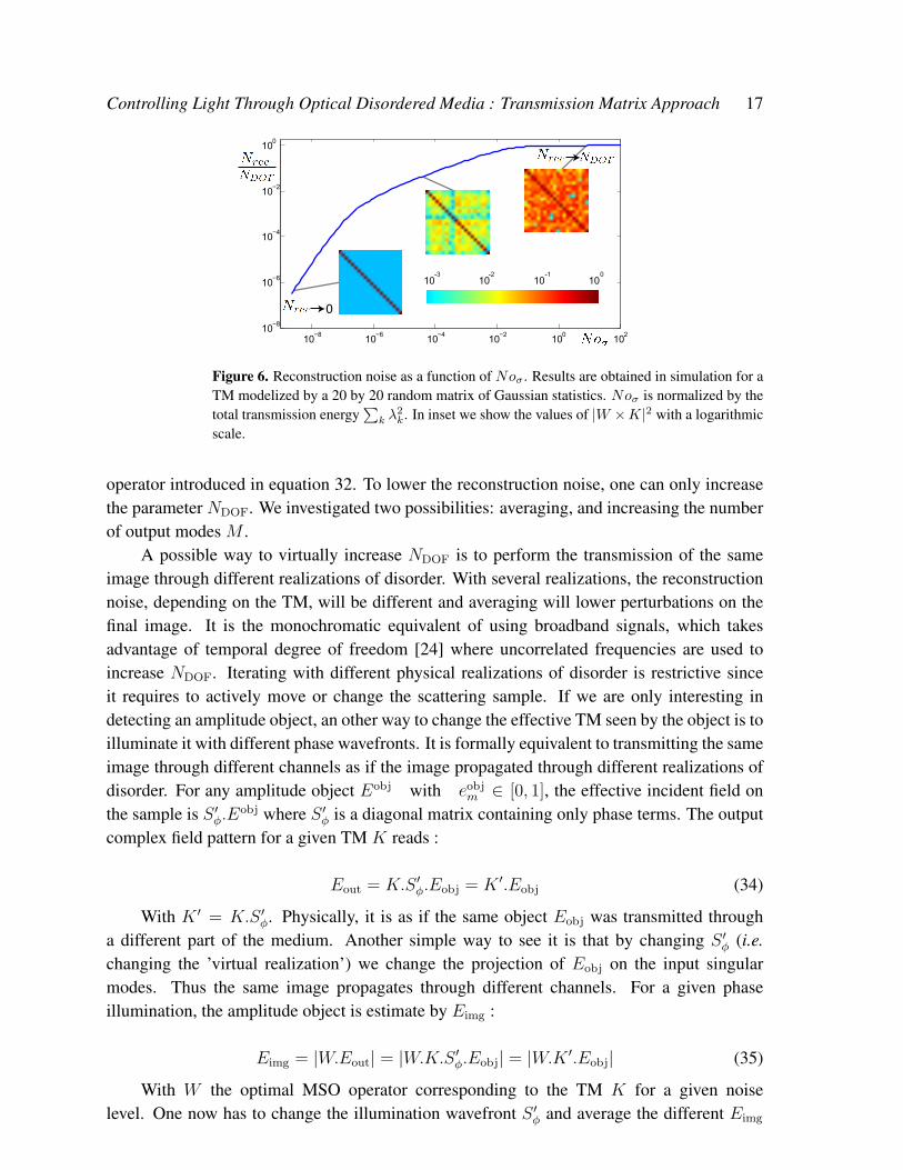
energy noise level of Noσ. In that study, the simulated TM K is noise free. We see that for

Noσ = 0 (i.e. for inversion operator), the reconstruction noise Norec is null and for Noσ → ∞(i.e. for Phase Conjugation operator) Norec tends to NDOF (here NDOF = M = N ). This

behavior is obvious when looking at the diagonal of |W ×K|2 compared to the others values.

3.3. Toward Optimal Reconstruction

In order to detect an input image with the best accuracy, one has to find the good balance

between the sensitivity to experimental noise and the influence of the reconstruction noise on

the recovered image. The mathematical optimum operator for those constrains is the MSO


10−8

10−6

10−4

10−2

100

102

10−8

10−6

10−4

10−2

100

0

01010 10 10

-1-2-3

Figure 6. Reconstruction noise as a function of Noσ . Results are obtained in simulation for a

TM modelized by a 20 by 20 random matrix of Gaussian statistics. Noσ is normalized by the

total transmission energy∑

k λ2k. In inset we show the values of |W ×K|2 with a logarithmic

scale.

operator introduced in equation 32. To lower the reconstruction noise, one can only increase

the parameter NDOF. We investigated two possibilities: averaging, and increasing the number

of output modes M .

A possible way to virtually increase NDOF is to perform the transmission of the same

image through different realizations of disorder. With several realizations, the reconstruction

noise, depending on the TM, will be different and averaging will lower perturbations on the

final image. It is the monochromatic equivalent of using broadband signals, which takes

advantage of temporal degree of freedom [24] where uncorrelated frequencies are used to

increase NDOF. Iterating with different physical realizations of disorder is restrictive since

it requires to actively move or change the scattering sample. If we are only interesting in

detecting an amplitude object, an other way to change the effective TM seen by the object is to

illuminate it with different phase wavefronts. It is formally equivalent to transmitting the same

image through different channels as if the image propagated through different realizations of

disorder. For any amplitude object Eobj with eobjm ∈ [0, 1], the effective incident field on

the sample is S ′φ.E

obj where S ′φ is a diagonal matrix containing only phase terms. The output

complex field pattern for a given TM K reads :

Eout = K.S ′φ.Eobj = K ′.Eobj (34)

With K ′ = K.S ′φ. Physically, it is as if the same object Eobj was transmitted through

a different part of the medium. Another simple way to see it is that by changing S ′φ (i.e.

changing the ’virtual realization’) we change the projection of Eobj on the input singular

modes. Thus the same image propagates through different channels. For a given phase

illumination, the amplitude object is estimate by Eimg :

Eimg = |W.Eout| = |W.K.S ′φ.Eobj| = |W.K ′.Eobj| (35)

With W the optimal MSO operator corresponding to the TM K for a given noise

level. One now has to change the illumination wavefront S ′φ and average the different Eimg


obtained to lower the reconstruction noise. To illustrate this effect we show in figure 7

simulation results for the reconstruction of a simple amplitude object using two different

phase illuminations and averaging over 10 different illuminations. The matrix is know exactly

in the simulation so all perturbations come from reconstruction noise. We see that the two first

realizations reproduce the amplitude object with different noises with amplitude of the same

order of magnitude. Averaging over multiple illuminations significantly reduces the noise

background.

0

5

10

0

5

10

0

0.1

0.2

0.3

0.4

0

5

10

0

5

10

0

0.1

0.2

0.3

0.4

x position

x positiony position

y position

Inte

nsi

ty

Inte

nsi

ty

0

5

10

0

5

10

0

0.1

0.2

0.3

0.4

x positiony positio

n

Inte

nsi

ty

a. c.b.

Figure 7. Comparisons of reconstruction simulations of a simple object for two different

’virtual realizations’ (a. and b.) and the reconstruction averaged over over 10 ’virtual

realizations’ (c.). Simulations are made for a 100 by 100 random matrix of independent

elements of Gaussian statistics. The amplitude object consists of three points of amplitude

one and the rest of the image to zero.

Since our SLM is a phase only modulator, in order to simulate amplitude objects, we

generate what we call ’virtual objects’. We use different combinations of random phase masks

to generate the same virtual amplitude object Eobj by subtracting two phase objects. From

any phase mask E(1)phase one could generate a second mask E

(2)phase where the phase of the mth

pixel is shifted by sobjm .π. The optical complex amplitude of elements of the second mask are

linked to those of the first mask by :

e(2)m = e(1)m .eisobjm π (36)

with e(j)m the mth element of E

(j)phase. We have the relation between the two masks and the

amplitude of the ’virtual object’ :

|E(2)phase − E

(1)phase| = 2. sin (Eobjπ/2) (37)

it is important to note that the norm of E(2)phase − E

(1)phase is fixed and controlled whereas

its phase is random, uncontrolled and differs from a ’virtual realization’ to another. The term

Eamp = |E(2)phase − E

(1)phase| can be estimated by :

Eimg = |W.(E(2)out − E

(1)out)| (38)

where E(1)out (resp. E

(2)out) is the complex amplitude of the output speckle resulting from

the display of the mask E(1)phase (resp. E

(2)phase). From a given set of random phase masks, we

can define in the same way as in equation 34 a diagonal matrix S ′φ containing only phase


terms. This term differs from a ’virtual realization’ to another. This way, the reconstruct

image reads :

Eimg = |W.S ′φ.Eamp| (39)

This expression is formally equivalent to equation 35, thus generating ’virtual objects’

using random phase masks is mathematically equivalent to illuminating a real object by

random phase-only wavefront.

3.4. Optimal Reconstruction in Presence of Ballistic Light

We experimentally used this technique to virtually increase NDOF, and we average the results

to lower the reconstruction noise. The complex amplitude image to detect is a grayscale 32

by 32 pixels flower image. The system is symmetric with N = M = 1024. The first step to

reconstruct the input image with the best accuracy is to find the variance of the experimental

noise Noσ in order to obtain the optimal MSO operator. To that end, we numerically

iterate the reconstruction operation for different values of the constrain in the MSO operator

(equation 32) and keep the one maximizing correlation between the reconstructed image and

the image sent, hence obtaining an estimation of the experimental noise level. This step is

made a priori knowing the image sent but could be performed by any technique leading to

an accurate estimation of the noise level. We detailed in [15] the results in a purely diffuse

system where ballistic contributions have no measurable effect. We study here the results in

presence of quantitative ballistic contributions.

In previous experiments, the focal planes of the two objectives are not the same. If

the two focal planes coincide, if we remove the sample, an incident k-vector matches an

output k-vector. Thus a pixel of the SLM corresponds to a pixel of the CCD. In the same

configuration with a scattering medium, if the part of the energy ballistically transmitted is

important enough, this ballistic part can be isolated in the TM.

To observe those contributions and study the accuracy of the reconstruction methods

in that particular case, we experimentally use a thinner and less homogeneous area of

the medium with a symmetric setup (M = N ) where input and output segments are

approximately the same size. We test the different reconstruction methods presented in 3.3

with one realization and averaging over 40 ’virtual realizations’ with random phase masks.

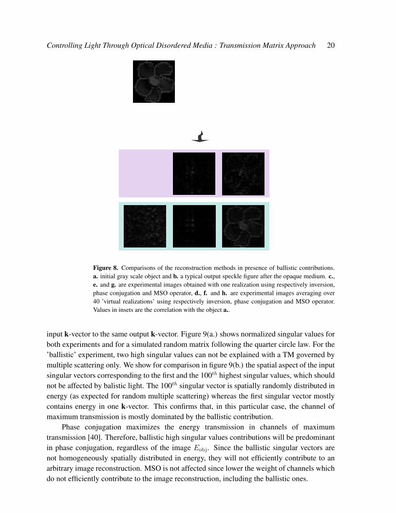
Results are shown in figure 8. As expected, we see that the inversion operation does not allow

image reconstruction, even with averaging, whereas optimal MSO allows a 93% correlation

for 40 averaging (and a 60% correlation for one realization). Phase conjugation which is

supposed to be stable in presence of noise gives a weak correlation of 31% with averaging.

Those results are similar to the ones obtained when we measure the TM of a system

governed by multiple scattering [15] for inversion (11% correlation with averaging) and for

MSO operator (94% correlation with averaging) but are very different for phase conjugation

(76% correlation with averaging). We see in figure 8(e.) and (f.) that most of the energy of

the reconstructed field is localized on very few points. In presence of strong enough ballistic

components, the direct paths associated give rise to channels of high transmission linking one


a.

Output Speckle

Emitted Image

b.

d.

e.

f.

g.

h.

Passing Through

Scattering

Medium

Inversion MSOPhase Conjugation

1 R

ea

liza

tio

n4

0 A

ve

rag

es

93.1%31.1%

23.2% 60.2%

11.0%

c.

9.5%

Figure 8. Comparisons of the reconstruction methods in presence of ballistic contributions.

a. initial gray scale object and b. a typical output speckle figure after the opaque medium. c.,

e. and g. are experimental images obtained with one realization using respectively inversion,

phase conjugation and MSO operator, d., f. and h. are experimental images averaging over

40 ’virtual realizations’ using respectively inversion, phase conjugation and MSO operator.

Values in insets are the correlation with the object a..

input k-vector to the same output k-vector. Figure 9(a.) shows normalized singular values for

both experiments and for a simulated random matrix following the quarter circle law. For the

’ballistic’ experiment, two high singular values can not be explained with a TM governed by

multiple scattering only. We show for comparison in figure 9(b.) the spatial aspect of the input

singular vectors corresponding to the first and the 100th highest singular values, which should

not be affected by balistic light. The 100th singular vector is spatially randomly distributed in

energy (as expected for random multiple scattering) whereas the first singular vector mostly

contains energy in one k-vector. This confirms that, in this particular case, the channel of

maximum transmission is mostly dominated by the ballistic contribution.

Phase conjugation maximizes the energy transmission in channels of maximum

transmission [40]. Therefore, ballistic high singular values contributions will be predominant

in phase conjugation, regardless of the image Eobj. Since the ballistic singular vectors are

not homogeneously spatially distributed in energy, they will not efficiently contribute to an

arbitrary image reconstruction. MSO is not affected since lower the weight of channels which

do not efficiently contribute to the image reconstruction, including the ballistic ones.


5 10 15 20 25 30

5

10

15

20

25

30

5

10

15

20

25

30

5 10 15 20 25 30

1st Singular Vector 100th Singular Vector

0

0.1

0.2

0.3

0.4

0.5

0.6

0.7

0.8

0.9

1

0

0.1

0.2

0.3

0.4

0.5

0.6

0.7

0.8

1 102101

Singular values by decreasing orderN

orm

aliz

ed S

ingula

r V

alu

es a.

b.

Figure 9. (a.) normalized singular values λ sorted by decreasing order for a thin non

homogeneous region of the sample with experimental conditions sensitive to ballistic waves

(dash line) and for a thicker region of the medium with the two focal planes objectives

separated by 0.3 mm (solid line). With • we show the normalized singular values of a simulated

matrix of independent Gaussian elements following the ’quarter circle law’.(b.) amplitude

of the singular vector corresponding to the maximum singular value (left) and to the 100th

singular value (right). Both share the same amplitude scale.

3.5. Pseudo-Inversion

We showed in section 1.1 that when we set the output pixel size to fit the output coherence

length, the number of degrees of freedom for detection is equal to the number M of segments

read on the CCD. This way a second approach to increase NDOF and thus the quality of the

reconstructed image is to enlarge the output observation window. An important advantage is

that the limiting time in our experiment is proportional to the number of input basis vectors

N , thus, in contrast with a focusing experiment where NDOF is equal [8] to N , increasing

the degrees of freedom for image reconstruction does not increase the measurement time.

Another consequence of increasing the size of the image recorded, that is, of increasing the

asymmetric ratio γ = M/N ≥ 1, is that the statistical properties of the matrix are deeply

modified. We saw in section 1.4 that increasing γ the range of the normalized singular values

decreases [30, 34]. A direct consequence is that the smallest non-zero singular value increases

and reads λ0γ = (1−

√1/γ). Controlling less information on the input than measured on the

output results in an averaging effect. An interesting consequence is that for a reasonable

experimental noise level, one can find a value of γ for which all singular values (and thus all

channels energy transmission) are above this noise level. In such a situation, the TM recorded

is barely sensitive to the experimental noise and since no singular values are drowned in the

noise, pseudo-inverse operator can be efficiently used.


To highlight this effect, we experimentally measure the TM of our sample for different

values of γ ≥ 1. For each TM we tested a single realization of the reconstruction of a complex

image using optimal MSO operator and pseudo-inverse operator. The results are shown in

figure 10(a.). For γ = 1 we are in agreement with previous results since optimal MSO gives a

partially accurate image when results of inversion are totally drown in noise. Increasing γ and

thus NDOF strongly improves the quality of the reconstructed image for both techniques and

reaches a > 85% fidelity for the largest value of γ = 11, without any averaging. As expected,

the curves of fidelity reconstruction as function of γ for both techniques become identical

when the value of λ0γ reaches noise level (figure 10(b.)). Above this value, pseudo-inversion

and optimal MSO are totally equivalent. One notice that experimental λ0γ are always smaller

than their theoretical predictions. We explain this deviation by the correlation induced in the

matrix by the reference pattern |Sref | (see section 1.4).

1 2 3 4 5 6 7 8 9 10 110

0.1

0.2

0.3

0.4

0.5

0.6

0.7

0.8

0.9

Corr

ela

tion C

oeffic

ient

γ ratio

γ ratio

a.

b.

0

0.1

0.2

0.3

0.4

0.5

0.6

0.7

1 2 3 4 5 6 7 8 9 10 11

Figure 10. Influence of the number of output detection modes. a. correlation coefficient

between Eimg and Eobj as a function of the asymmetric ratio γ = M/N for MSO (dashed

line) and for pseudo-inversion (solid line), without any averaging. Error bars correspond to

the dispersion of the results over 10 realizations. b. Experimental (solid line) and Marcenko-

Pastur [30] predictions (dashed line) for the minimum normalized singular value as a function

of γ. The horizontal line shows the experimental noise level Nooptσ .

We saw in this part that increasing the degrees of freedom and using an appropriate

operator that takes noise into account permits to drastically enhance the reconstruction

accuracy of an image detection. Similar results can be obtain for focusing or for output

wavefront shaping with the same techniques. Such experiments are more difficult to carry


out since they require amplitude and phase modulation. Increasing γ = N/M and thus N in

that case also presents the drawback to significantly increase the measurement time.

4. Memory Effect

To define the statistical properties of the TM of multiple scattering media in part 1.4 we did

not take into account weak correlation effects that could break the hypothesis of independent

elements of the TM. The strongest (first order) of those effects that can be recorded for system

dominated by multiple-scattering (no ballistic contribution) in the diffusive regime is the

so-called Memory Effect (ME). It brings correlation with characteristic length Lme which

depends, in transmission, on the geometry of the observation system [21]. If the speckle grain

size Lspeckle is of the same order of magnitude or smaller than the ME range Lme, ME brings

additional correlations in the TM.

We define Lspeckle as the full width at half maximum of the autocorrelation function of a

speckle intensity pattern and Lme as the attenuation length of the ME. Both length are defined

for a given observation plane.

The speckle size Lspeckle depends on the distance between the back of the sample and the

observation plane D, the width of the illumination area W and the wavenumber k. It reads :

Lspeckle =2πD

kW(40)

In contrast, Lme depends on k, D and the thickness e of the sample and reads :

Lme =D

ke(41)

Therefore, for W ≫ e we have Lme ≫ Lspeckle. This kind of geometry can be convenient

since it allows to move a focal spot along a distance greater that Lspeckle by just tilting the

SLM [41].

We experimentally fixed D = 1.5 ± 0.2 mm, W = 0.5 ± 0.1 mm and the sample has a

thickness e = 80 ± 25 µm. For those conditions, we expect Lspeckle ≈ Lme ≈ 1.5 µm. The

TM is measured. Each column of the TM is the complex amplitude response of a plane wave

with a given incident angle. One can easily reconstruct the intensity patterns for different

incident angles and calculate the correlation function between two patterns :

f(n−n′),j =

⟨(|kmn|2 ⊗m

∣∣k(M−m)n

∣∣2)j∑

m |kmn|2 ×∑

m |kmn′ |2

⟩

(n−n′)

(42)

Where ⊗m denotes the spatial convolution over the variable m and j is the variable of the

correlation fonction corresponding to a displacement in pixel in the focal plane. We average

results over all combinations of n, n′ with n− n′ = constant. Results are shown in figure 11.

It is clear that the output speckle is coherently translated for distances greater than Lspeckle.

Lspeckle is deduced from the mean autocorrelation function of the speckle pattern

f(n−n′)=0,j as response to an incident wave plane. We found Lspeckle = 1.3 ± 0.48 µm. We


−2 0 2 4 6 8 10 120

0.2

0.4

0.6

0.8

1

No

rma

lize

d C

orr

ela

tio

n

Speckle Displacement (μm)

n-n’ = 0

n-n’ = 1

n-n’ = 2

n-n’ = 3n-n’ = 4 n-n’ = 5

e-x/Lme

Figure 11. Spatial correlation functions of output speckle for a variation of the input incident

angle. The correlations functions are drawn as function of the spatial coordinate corresponding

to the displacement of the speckle pattern in the observation plane. Arrows show the maximum

of correlation functions for the highest displacements. Those peaks are barely observable due

to an exponential decay of the maximum correlation value.

define C(x) the correlation coefficient (maximum of the correlation function) between two

output speckles shifted by x in the observation plane. Exponential decay of the correlation

C(x) ∝ e−x/Lme is generally observed for an open geometry [21]. The measured C(x)

(figure 11 and 12) fit an exponential decay with Lme = 1.72± 0.13 µm.

Output Speckle Displacement (μm)

Co

rre

lati

on

Co

e�

cie

nt

0 1 2 3 4 5 6 7 810

−3

10−2

10−1

100

Figure 12. Spatial correlation decay of the memory effect. (solid line) experimental curve

of correlation coefficient as function of the spatial displacement. (dash line) exponential fit

C(x) = e−x/Lme with Lme = 1.72 µm.

We found the expected correlation lengths with a good order of magnitude for

autocorrelation (speckle grain size) and memory effect and we were able to qualitatively

separate both effects.

Conclusion

We reinterpreted in this article previous works on optical phase conjugation in term of linear

system defined by a monochromatic transmission matrix. Within this formalism, we show


how to take advantage of multiple scattering to achieve image transmission and wavefront

shaping. We also pointed out how to improve the quality of measurements in the presence of

noise, taking benefit of Random Matrix Theory and information theory. We finally showed

how to take benefit of the statistical properties of the TM to go back to physical phenomenons.

Acknowledgments

This work was made possible by financial support from "Direction Générale de l’Armement"

(DGA), Agence Nationale de la Recherche via grant ANR 2010 JCJC ROCOCO, Programme

Emergence 2010 from the City of Paris and BQR from Université Pierre et Marie Curie and

ESPCI.

Appendix

To take into account the effect of the reference beam in the effective SNR, we define Γ < 1 the

ratio of the intensity coming from the controlled part over the total intensity. This way, Γ is

also the ratio of the area of the controlled part of the SLM over the total illuminate area. One

way to understand this situation is that Ntot independent segments of the SLM are illuminated

and we control only N = Γ.Ntot of them. We injected the ratio Γ in equation 19 and 20. SNR

now reads :

SNR ≈ π/4N2 + (Ntot −N)

Ntot

(A.1)

=π/4N2 +N(1− Γ)

N/Γ≈ Γ

π

4N2 ∀N ≫ 1

For the setup shown in figure 1, the illuminated area on the SLM represents the

circumcircle of the square part that we control. The segments illuminated but not controlled

are used to produce the reference pattern. For this geometry, with an illumination disk of

radius R we have Γ =(√

(2).R)2

πR2 = 2π

. The effective SNR corrected to take into account the

reference beam is therefore :

SNR ≈(π4

) 2

πNDOF = 0.5NDOF (A.2)

References

[1] Goodman J W 1968 Introduction to Fourier optics (New York: McGraw-Hill)

[2] Skipetrov S E 2003 Phys. Rev. E 67 036621

[3] Ishimaru A 1978 Wave Propagation and Scattering in Random Media Academic (New York: Academic

Press)

[4] Sheng P 1995 Introduction to Wave Scattering, Localization and Mesoscopic Phenomena (San Diego:

Academic Press)

[5] Tourin A, Fink M and Derode A 2000 Waves in Random and Complex Media 10 31


[6] Lee P A and Ramakrishnan T V 1985 Rev. of Mod. Phys. 57 287

[7] Margerin L, Campillo M and Van Tiggelen B 1998 Geophysical journal international 134 596

[8] Vellekoop I M and Mosk A P 2007 Opt. Lett. 32 2309

[9] Yaqoob Z, Psaltis D, Feld M S and Yang C 2008 Nature Photonics 2 110

[10] Vellekoop I M, Lagendijk A and Mosk A P 2010 Nature Photonics 4 320

[11] Prada C and Fink M 1994 Wave Motion 20 151

[12] Goupillaud P L 1961 Geophysics 26 754

[13] Gore D, Paulraj A and Nabar R 2004 Introduction to Space-Time Wireless Communication (Cambridge:

Cambridge University Press)

[14] Popoff S M, Lerosey G, Carminati R, Fonk M, Boccara A C and Gigan S 2010 Phys. Rev. Lett. 104 100601

[15] Popoff S M, Lerosey G, Fink M, Boccara A C and Gigan S 2010 Nature Communications 1 1

[16] Arridge S R 1999 Inverse problems 15 R41

[17] Maire G, Drsek F, Girard J, Giovannini H, Talneau A, Konan D ,Belkebir K, Chaumet P C and Sentenac A

2009 Phys. Rev. Lett. 102 213905

[18] Fink M 1997 Physics Today 50 34

[19] Montaldo G, Tanter M and Fink M 2004 J. Acoust. Soc. Am. 115 768

[20] Lerosey G, de Rosny J, Tourin A, Derode A, Montaldo G and Fink M 2004 Phys. Rev. Lett. 92 193904

[21] Freund I, Rosenbluh M, and Feng S 1988 Phys. Rev. Lett. 61 2328

[22] Papas C H 1965 Theory of electromagnetic wave propagation (New York: McGraw-Hill)

[23] Derode A, Tourin A and Fink M 2001 Phys. Rev. E 64 036606

[24] Lemoult F, Lerosey G, de Rosny J and Fink M 2009 Phys. Rev. Lett. 103 173902

[25] Zhang T and Yamaguchi I. 1998 Opt. Lett. 23 1221

[26] Love G D 1997 Appl. Opt. 36 1517

[27] van Putten E G, Vellekoop I M and Mosk A P 2008 Appl. Opt. 47 2076

[28] Larrat B, Pernot M, Montaldo G, Fink M and Tanter M Ultrasonics, Ferroelectrics and Frequency Control,

IEEE Transactions on 57 1734

[29] Aubry A and Derode A 2010 Waves in Random and Complex Media 20 333

[30] Marcenko V A and Pastur L A Sbornik: Mathematics 1 457

[31] Wigner E P Siam Review 9 381

[32] Dorokhov O N 1984 Solid State Communications 51 381

[33] Scheffold F and Maret G 1998 Phys. Rev. Lett. 81 58000

[34] Sprik R, Tourin A, de Rosny J and Fink M 2008 Phys. Rev. B 78 12202

[35] Derode A, Roux P and Fink M 1995 Phys. Rev. Lett. 75 4206

[36] Vellekoop I M, van Putten E G, Lagendijk A and Mosk A P 2007 Opt. Lett. 16 67

[37] Vellekoop I M and Mosk A P 2008 Optics Communications 281 3071

[38] Tikhonov A N 1963 Soviet Math. Dokl 4 1035

[39] Lerosey G, de Rosny J, Tourin A and Fink M 2007 Science 315 1120

[40] Tanter M, Thomas J L and Fink M 2000 J. Acoust. Soc. Am. 108 223

[41] van Putten E G, Akbulut D, Bertolotti J, Vos W L, Lagendijk A and Mosk A P 2011 Phys. Rev. Lett. 106

193905

Documents

Controlling Light Through Optical Disordered Media