University of Nebraska - LincolnDigitalCommons@University of Nebraska - Lincoln

USGS Staff -- Published Research US Geological Survey

2013

Controls on recent Alaskan lake changes identifiedfrom water isotopes and remote sensingLesleigh AndersonUSGS, land@usgs.gov

Jennifer RoverEarth Resource Observation and Science, U.S. Geological Survey

Nikki GaulagerYukon Flats National Wildlife Refuge

Jean BirksAlberta Innovates Technology Futures

Follow this and additional works at: http://digitalcommons.unl.edu/usgsstaffpub

Part of the Geology Commons, Oceanography and Atmospheric Sciences and MeteorologyCommons, Other Earth Sciences Commons, and the Other Environmental Sciences Commons

This Article is brought to you for free and open access by the US Geological Survey at DigitalCommons@University of Nebraska - Lincoln. It has beenaccepted for inclusion in USGS Staff -- Published Research by an authorized administrator of DigitalCommons@University of Nebraska - Lincoln.

Anderson, Lesleigh; Rover, Jennifer; Gaulager, Nikki; and Birks, Jean, "Controls on recent Alaskan lake changes identified from waterisotopes and remote sensing" (2013). USGS Staff -- Published Research. 801.http://digitalcommons.unl.edu/usgsstaffpub/801

Controls on recent Alaskan lake changes identified from water isotopesand remote sensing

Lesleigh Anderson,1 Jean Birks,2 Jennifer Rover,3 and Nikki Guldager4

Received 13 May 2013; revised 13 June 2013; accepted 16 June 2013; published 12 July 2013.

[1] High-latitude lakes are important for terrestrial carbondynamics and waterfowl habitat driving a need to betterunderstand controls on lake area changes. To identify theexistence and cause of recent lake area changes in theYukon Flats, a region of discontinuous permafrost in northcentral Alaska, we evaluate remotely sensed imagery withlake water isotope compositions and hydroclimaticparameters. Isotope compositions indicate that mixtures ofprecipitation, river water, and groundwater source ~95% ofthe studied lakes. The remaining minority are moredominantly sourced by snowmelt and/or permafrost thaw.Isotope-based water balance estimates indicate 58% oflakes lose more than half of inflow by evaporation. For26% of the lakes studied, evaporative losses exceededsupply. Surface area trend analysis indicates that most lakeswere near their maximum extent in the early 1980s during arelatively cool and wet period. Subsequent reductions canbe explained by moisture deficits and greater evaporation.Citation: Anderson, L., J. Birks, J. Rover, and N. Guldager(2013), Controls on recent Alaskan lake changes identified fromwater isotopes and remote sensing, Geophys. Res. Lett., 40,3413–3418, doi:10.1002/grl.50672.

1. Introduction

[2] The likelihood of future warming trends in Alaska hasmotivated efforts to observe and evaluate recent hydrologicchange [Hinzman et al., 2005; Walvoord et al., 2012].Theory and climate models suggest greater Arctic precipita-tion with a warming atmosphere that is supported to someextent by Eurasian river discharge since the 1940s[Peterson et al., 2002]. However, a significant degree ofinterannual discharge variability is also linked with regionalatmospheric dynamics such as those characterized by theNorthern Annual Mode and Pacific Decadal Oscillationand/or El Niño–Southern Oscillation in the North Pacific sec-tor [Brabets and Walvoord, 2009; Cassano and Cassano,2010]. Other surface water trends, such as lake volume andarea, are currently ambiguous, with a diversity of variationobserved in continuous and discontinuous permafrost

regions [Riordan et al., 2006; Smith et al., 2005]. Lake sur-face observations are available in Alaska from early aerialphotographic surveys beginning in the late 1950s and bysatellite data since the late 1970s.[3] Lake surface areas, and corresponding volume, reflect

the balance between rates of surface inflow, groundwater dis-charge, and precipitation falling directly onto a lake, with ratesof water loss from surface outflow, groundwater recharge, andevaporation/evapotranspiration from the lake surface and sur-rounding wetlands. At high latitudes, permafrost distributionmay be the most important factor in determining lake densityin addition to surface flow [Williams, 1970]. In areas of contin-uous permafrost, subpermafrost groundwater is often isolatedfrom the surface, and there are unique mechanisms forthermokarst lake dynamics such as lateral expansion andbreaching [Jones et al., 2011; Labrecque et al., 2009; Pluget al., 2008]. Groundwater-surface water interactions in the in-terior regions of Alaska are more commonly found in areas ofdiscontinuous permafrost [e.g.,Minsley et al., 2012;Walvoordet al., 2012].[4] Here the focus is on a region of discontinuous perma-

frost in northeast Alaska known as the Yukon Flats (YF) thatencompasses the ~118,340 km2 low-lying area surroundingthe confluence of the Yukon and Porcupine rivers(Figure 1). YF lakes occupy depressions formed by fluvial,eolian, and thermokarst processes, have a wide diversity ofsizes and shapes, and remain frozen for 7 to 8months of eachyear. In general, shallower basins with more gradual slopesundergo larger changes in surface extent for incrementalchanges in volume than deeper counterparts with steep sides.This is likely one reason why YF lakes exhibit complexspatial patterns of change for different temporal scales[Roach et al., 2011; Rover et al., 2012].[5] Lake water isotope ratios provide a useful measure for

characterizing lake hydrology. Isotopes of oxygen andhydrogen in lake water are sensitive to hydrologic processes,and in particular, the preferential loss of light isotopes byevaporation. Here we also derive estimates of the ratio ofwater lost by evaporation to that gained by inflow (E/I) byusing an isotope-based water balance model. The isotopelabels are also used to identify the dominant sources for lakessuch as mixtures of rainfall and snowfall, groundwater,rivers, or thawed permafrost [e.g., Wolfe et al., 2007].These parameters are then used in conjunction with climaticdata and remotely sensed imagery to identify the patternsand causes of recent lake area changes.

2. Study Area and Methods

[6] The YF is a region of extreme seasonal temperature dif-ference and low precipitation (<250mm/yr) [Shulski andWendler, 2007]. Potential evapotranspiration (PET) estimates,

Additional supporting information may be found in the online version ofthis article.

1Geosciences and Environmental Change, U.S. Geological Survey,Denver, Colorado, USA.

2Alberta Innovates Technology Futures, Calgary, Alberta, Canada.3Earth Resource Observation and Science, U.S. Geological Survey,

Sioux Falls, South Dakota, USA.4Yukon Flats National Wildlife Refuge, Fairbanks, Alaska, USA.

Corresponding author: L. Anderson, Geosciences and EnvironmentalChange, U.S. Geological Survey, Denver, CO 80225, USA. (land@usgs.gov)

©2013. American Geophysical Union. All Rights Reserved.0094-8276/13/10.1002/grl.50672

3413

GEOPHYSICAL RESEARCH LETTERS, VOL. 40, 3413–3418, doi:10.1002/grl.50672, 2013

following Hogg [1997], indicate annual moisture deficits near15 cm/yr. Lakes are generally fresh to moderately brackish(<1600μS) and predominantly eutrophic or hypereutrophic[Hawkins, 1995; Heglund and Jones, 2003]. Evaporite saltfilms occur on lake margins and dry lakebeds (Figure 1) andconsist of trona, calcite, dolomite, gypsum, and halite[Clautice and Mowatt, 1981]. Vegetation is a mosaic of grassymeadows, muskeg, marsh, and forests of spruce and birch thatare highly prone to fire [Drury and Grissom, 2008].[7] Lake water isotope samples from 83 lakes were acquired

in July, August, or September between 2007 and 2010 by fixedwing aircraft (Figure 1; supporting information text). An addi-tional set of smaller lakes (n=33) was sampled by helicopterin September 2009. In July 2011, 59 lakes were sampled on footwithin five distinct 11.2 km2 areas that were previously definedand investigated for baseline limnology [Heglund and Jones,2003]. River water data used here are from Schuster et al.[2010] collected during the months of June through Octoberbetween 2006 and 2008 from the Yukon River at Circle andFort Yukon, the Porcupine River above Fort Yukon, and theChandalar River above Venetie. Water for isotope analysiswas collected in 30mL Nalgene high density polyethyleneor glass bottles that were filled to minimize headspace, sealedto prevent evaporation and analyzed within 2months of collec-tion. Water samples were prepared for oxygen and hydrogenisotope ratio analyses by automated constant temperatureequilibration with CO2, and automated D/H preparationby chromium reduction, coupled to an isotope ratio massspectrometer and are reported in δ-notation relative to Viennastandard mean ocean water (VSMOW). Analytical precisionis ± 0.08‰ and±0.9‰ for oxygen and hydrogen, respectively.

[8] Lake evaporation-to-inflow ratios (E/I) were calculatedusing the isotope mass balance method developed by Gibsonand Edwards [2002] which assumes a well-mixed lakeundergoing evaporation while maintaining a long-termconstant volume and lake water residence time (seesupporting information text for additional information). Themethod requires isotope values for inflow, lake water, andevaporated vapor and utilizes the assumption that the oxygenisotope ratios of outflow are equivalent to lake water values.The isotopic composition of evaporated vapor is difficult tomeasure but has been shown to be dependent on temperature,boundary layer state, relative humidity, and the isotopiccomposition of atmospheric moisture.[9] Of the 175 lakes sampled for water isotopes, 54 of them

were analyzed for surface area changes and trends followingthe approach described in Rover et al. [2012] with additionalanalysis for 2010 and 2011. There was classification of22 Landsat Multispectral Scanner, Thematic Mapper, andEnhanced Thematic Mapper Plus scenes during the ice-freeseason since 1979. Following a decision tree approach, waterand nonwater classes were identified, and a total of 16,371water bodies in the study area had detectable water at morethan one date and were not connected to perennial streamsand rivers. The water images were converted to vector poly-gons for calculating area at each image date [Rover et al.,2011]. When clouds, cloud shadows, or snow obstructed un-derlying water bodies, the observation was assigned a “nodata” value. Trend analyses are based on a linear regressionmethod with date and water area as the predictor andresponse, respectively, and the slope representing change inwater area per time. A two-tailed t test of the slope was used

Tertiary or early Quat Alluvium

Quat Alluvial Silt

Quat Alluvial Terrace

Quat Loess

Quat Eolian Sand

Evaporite DepositsLake - snow/permafrost source

Lake - precipitation/river/gw source

11.2 km2 areas

Escarpments and depressions

Figure 1. The surficial geology of the Yukon Flats National Wildlife Refuge from Williams [1962] is shown on a digitalelevation model (30m) with lake locations for this study, the location of evaporite deposits from Clautice and Mowatt[1981], and the 11.2 km2 areas delineated by Heglund and Jones [2003] within which 59 lakes were sampled in 2011 (indi-vidual lake locations not shown). The rectangular box encloses the area of the surface area trend analysis. Open circle symbolsindicate lakes sourced by snow and/or permafrost.

ANDERSON ET AL.: ALASKAN LAKE CHANGE FROM WATER ISOTOPES

3414

to evaluate results for p-values ≥0.01. Notably, some lakeswith insignificant linear regressions are found to have highlyvariable surface area extents.[10] Meteorological data since 1948 was obtained from the

National Centers for Environmental Prediction-NationalCenter for Atmospheric Research (NCEP-NCAR) reanalysis[Kalnay et al., 1996] for an average of grid cells that encom-pass the YF area (Figure 2). They are compared with the gridcell for Fairbanks, the location of the nearest first-orderclimate station 230 km to the south. The records show thatfollowing an arid period during the 1950s, higher relativehumidity, greater snowfall, and lower potential evaporationcharacterize the period between ~1970 and 1995, a changethat has been attributed to natural variability of the positionand strength of the Aleutian Low [Hartmann and Wendler,2005]. From the mid-1990s to the present day, temperatureshave been relatively high, humidity levels low, snowfalllow, and potential evaporation high.

3. Results

[11] The oxygen and hydrogen isotope ratios of lakesrange from �20‰ to �5‰ and �85‰ to �160‰, respec-tively (Figure 3 and Tables S1 and S2). Lakes are generallyenriched in heavy isotopes with respect to meteoric watersas represented by the Global Meteoric Water Line(GMWL), which is an indication of kinetic fractionation

effects during evaporation. Lakes are also enriched relativeto the average value for Yukon River waters (�21‰ foroxygen and �167‰ for hydrogen), which as an integrationof all regional waters is typically similar to the average isoto-pic values of precipitation and approximates the values forgroundwater. The majority of lakes plot on an evaporationline with a slope of 5 that intersects the GMWL near theaverage Yukon River value. This intersection indicates thatthe source water for most lakes is a mixture of precipitationand groundwater in addition to river water for lakes withsurface connections or within floodplains.[12] For a small group of lakes (26 of 175), plotting a line

through their position to the average river water value wasfound to produce unreasonably low slopes (m ≈ 3) that areinconsistent with regionally established slopes of 4.5 to 5.5[Gibson et al., 2002] and suggest alternative source waters.Therefore, we regressed an evaporation line with a slope of5 from each of these lakes (see supporting information text

-4

-3

-2

-1

0

1

2

3

4

1945 1955 1965 1975 1985 1995 2005 2015

Sno

w W

ater

Equ

ival

ent

-4

-3

-2

-1

0

1

2

3

4T

empe

ratu

reFairbanks

Yukon Flats

-10-8-6-4-20246810

Rel

ativ

e H

umid

ity

Fairbanks

Yukon Flats

-30

-20

-10

0

10

20

30

Pot

entia

l Eva

pora

tion

Fairbanks

Yukon Flats

Fairbanks

Yukon Flats

Trend Analysis

Year

Figure 2. Hydroclimatic parameters for an average of YFgrid cells since 1948 to 2012 derived from NCEP-NCARreanalysis shown with the data for the Fairbanks grid cell.Temperature (°C), relative humidity (%), potential evapora-tion rate (W/m2), and snow water equivalent (kg/m2) areshown as anomalies from the 1948–2012 mean.

(a)

(b)

Figure 3. Oxygen and hydrogen isotopes and calculatedevaporation-to-inflow (E/I) ratios of water in the YukonFlats: (a) Lake isotope ratios shown with the GlobalMeteoric Water Line (GMWL), and estimated monthlyprecipitation values (black) [Bowen and Revenaugh, 2003],and Yukon, Porcupine, and Chandalar River values (gray)[Schuster et al., 2010]. Dashed arcs indicate the approximateranges of isotope values for rain, snow, rivers, groundwater,and permafrost. Blue circles indicate lakes sourced bycombinations of precipitation, rivers, and groundwater, andred circles indicate those sourced by snowmelt and/orpermafrost thaw. Stars indicate approximate source valuesfor each group. (b) Colors similar to Figure 2a show thepopulations of lakes with E/I> 0.5 and 1, above whichevaporation losses are greater than 50% and 100% of inflow,respectively.

ANDERSON ET AL.: ALASKAN LAKE CHANGE FROM WATER ISOTOPES

3415

for additional discussion) and found that they intersect theGMWL near �27‰ for oxygen and �200‰ for hydrogen,values that are within the range of observed values for snow-melt and permafrost thaw [Lachniet et al., 2012;Meyer et al.,2010]. This suggests that this group of lakes is sourced bysnowmelt and permafrost thaw, most likely as talik growth.Reliance on snowmelt and/or permafrost thaw for annualrecharge would be more likely for basins that are isolated fromdeep, subpermafrost groundwater and surface flow. E/Iestimates range from 0.08 to 4.93 for the data set (Figure 3b)and are affected by the isotope composition of source waters.[13] The oxygen and hydrogen isotope compositions, and

E/I ratios of the 54 lakes analyzed for area changes span asimilar range as the larger data set. Fifteen are dominantlysourced by snowmelt and/or thawed permafrost. Time seriesof surface areas indicate that more lakes were nearer theirmaximum extent and generally varied coherently between1980 and 1990 (Figure 4a). Subsequently, particularly after

the mid-1990s, more lakes decreased or varied more signifi-cantly. Lakes that underwent less evaporation (E/I< 0.5)tended to have varied less in area, with no overall tendencyto increase or decrease (Figure 4b). In contrast, lakes thatunderwent more evaporation (E/I> 1) tended to have variedmore and often in opposing directions; some lakescompletely disappeared while others reached their maximumareas (Figure 4c). The lakes identified as sourced bysnowmelt/permafrost tended to have varied more, occupiedsmaller depressions, and had higher evaporation losses(Figure S1). A decreasing trend is evident for several of themsince the early 2000s (Figure 4d). A summary of area trendsfor the different ranges of E/I is shown in Table 1.

4. Discussion

[14] The isotope results indicate that an integration ofrainfall, snowfall, river inflow and/or flooding, and ground-water, is the water source for most YF lakes. Therefore, wepropose that lake water budgets and area/volume variationsare dominantly controlled by hydroclimate, includingamounts of precipitation gain, evaporation loss, water tableheights, and groundwater flow rates. Comparison with theclimate data support this notion as the lakes that have dimin-ished have done so concurrently with lower snowfall, relativehumidity, and higher temperatures since ~1995 (Figures 2and 4). Less moisture on multiannual to decadal time scaleslikely leads to lower water table heights and reduced subsur-face and surface inflows. This may explain the greater diversityof responses as lake levels lower because correspondingsurface area depends on basin shape, and there is a great diver-sity of basin shapes. Regional water table heights and ground-water flow rates are not known within the YF, but airborneelectromagnetic imaging has revealed surface-groundwaterconnections [Minsley et al., 2012]. Taliks beneath larger waterbodies were found to extend below the maximum depthof permafrost, allowing surface-groundwater connections,whereas smaller, shallower lakes with smaller taliks weretypically isolated.[15] The lake water isotope results also indicate that snow-

melt and/or permafrost thaw is a dominant water source forsmaller, shallower lakes that have dramatically varied in ex-tent, by either total water loss and subsequent gain, or steadydiminishment (Figure 4d). These lakes were generally moreevaporated (Figure 3b), indicating limited groundwater inter-action that is consistent with a location within permafrost orother aquatards. Subsurface drainage of lakes due to thawingpermafrost and talik growth has been proposed as a mecha-nism for lake area reductions in other regions of Alaska[Yoshikawa and Hinzman, 2003]. Here, however, the isotopedata suggest that lakes that could be within permafrostundergo significant water losses by evaporation. The

(b)

(c)

(d)

(a)

Figure 4. Change in lake extent as a % of maximum from1979 to 2011 for (a) all 54 lakes sampled within the trendanalysis area, (b) lakes with E/I< 0.5 (n= 12), (c) lakes withE/I> 1 (n = 22), and (d) lakes sourced by snowmelt and/orthawed permafrost (n = 15). Image acquisition years are indi-cated as black triangles on the horizontal time scale. Graylines indicate lakes with no surface area trends, red lines indi-cate lakes with decreasing trends, and a blue line for the onelake with an increasing trend.

Table 1. Lake Area Linear Regression Analyses (p< 0.01) for E/Iand Source

Number Increasing No Change Decreasing

E/I< 0.5 12 0 12 00.5<E/I< 1.0 20 0 15 5E/I>1.0 22 1 12 9Precip/river/groundwater 39 1 32 6Snowmelt/permafrost thaw 15 0 7 8Total 54 1 39 14

ANDERSON ET AL.: ALASKAN LAKE CHANGE FROM WATER ISOTOPES

3416

geophysical evidence within the YF suggests complexgroundwater flow paths and surface water connections suchthat subsurface conduits developed by permafrost thaw seemas likely to provide groundwater to a lake basin as drain it.[16] There is no known evidence for thermokarst drainage

in the YF similar to that which occurs in continuous perma-frost regions [Jones et al., 2011]. However, snowmelt canrecharge small, isolated basins by flowing over a frozen,and/or through a thawed, active layer (i.e., suprapermafrostflow), but isotope labeling cannot distinguish snowmelt ver-sus thawed permafrost in this region because their ranges ofvalues overlap. Nevertheless, the isotope data are consistentwith the idea of recent reductions in snowfall as a mechanismfor net water loss in some YF lakes [Jepsen et al., 2012].[17] The E/I estimates of the entire 175 lake data set indi-

cate that ~58% of lakes have evaporation losses that exceed50% of inflow, which is strong evidence for the importanceof evaporation in regional YF lake water budgets. Weacknowledge that E/I estimates are derived from waterisotope data that integrates hydrologic processes for anunknown, and possibly varying, time period that precedesthe sample date. This, and the fact that the calculations utilizemean climate state variables from reanalysis data, all intro-duce sources of uncertainty that we take into considerationfor our conclusions here. However, the assumption ofconstant volume and residence time relative to the time incor-porated by the isotope data appears to be generally valid forisolated lakes that were highly evaporated. Indeed, our obser-vations indicate minimal isotopic variation within seasons orfrom year to year (Figures S2 and S3).[18] These results lead to the conclusion that the majority

of recent lake area reductions in the Yukon Flats can beexplained as a response to a multidecadal climate trendtoward greater moisture deficit since the mid-1990s. Thiswas characterized by increasing temperatures but also by re-duced snowfall and summer humidity. Such a hydroclimaticmechanism may also be a dominant driver for other interiorregions of Alaska and high-latitude regions. We cannotdefinitively rule out individual lake reductions related topermafrost thaw, but the isotope survey indicates that thismechanism is a potential influence on a relatively small num-ber of YF lakes (26 of 175). An important implication ofthese results is that future surface water variations are likelyto remain a function of decadal-scale regional atmospherecirculation variations that control storm tracks and the mois-ture balance in the Alaskan interior even as warmer globaltemperatures become more likely. Decadal-scale climatevariation in Alaska is documented for the past 1000 yearsand the Holocene from paleohydroclimatic data [Andersonet al., 2007; Barber et al., 2004]. Such atmospheric dynamicsare currently beyond the simulation ability of climate models,but the data in this study highlight their primary importance.[19] The data also reveal remarkable hydrologic diversity

at the watershed scale. It is notable that the range of isotopeand E/I values within very small <10 km2 areas is nearlyequivalent to the range of values observed for the entire~118,340 km2 area (Figure S5). Similar hydrologic diversityat smaller spatial scales has been observed in other lake-richlandscapes [Euliss et al., 2004; Turner et al., 2010] and posessignificant challenges for accurately “scaling-up” sparselysampled areas to draw conclusions that span beyond localto regional controls. These findings indicate that attempts toproject future high-latitude lake change will benefit from

considering the effects of decadal-scale hydroclimatic varia-tions. Furthermore, isotope ratios of lake water strengthen thebasis upon which the vulnerability of individual water bodiesand lake regions can be assessed.

[20] Acknowledgments. The USGS Climate and Land Use ChangeR&D Program and the USFWS Yukon Flats National Wildlife Refugesupported this research. We thank Tyler Lewis for providing 2011 watersamples. Chris Eastoe, University of Arizona Environmental IsotopeLaboratory, provided isotope data; Paco VanSistine provided GIS support.We thank John Gibson for early insights into the data and Ted Hogg forCMI and P-PET estimates. We appreciate manuscript reviews by TylerLewis, Brent Wolfe, and anonymous reviewers that helped to improve themanuscript. Any use of trade, firm, or product names is for descriptivepurposes only and does not imply endorsement by the U.S. Government.[21] The Editor thanks BrentWolfe and an anonymous reviewer for their

assistance in evaluating this paper.

ReferencesAnderson, L., et al. (2007), Late Holocene moisture balance variability in thesouthwest Yukon Territory, Canada, Quat. Sci. Rev., 26, 130–141.

Barber, V. A., et al. (2004), Reconstruction of summer temperatures ininterior Alaska from tree-ring proxies: Evidence for changing synopticclimate regimes, Clim. Change, 63, 91–120.

Bowen, G. J., and J. Revenaugh (2003), Interpolating the isotopic composi-tion of modern meteoric precipitation, Water Resour. Res., 39(10), 1299,doi:10.1029/2003WR002086.

Brabets, T. P., andM.A.Walvoord (2009), Trends in streamflow in the YukonRiver Basin from 1944 to 2005 and the influence of the Pacific DecadalOscillation, J. Hydrol., 371, 108–119, doi:10.1016/j.jydrol.2009.03.018.

Cassano, E. N., and J. J. Cassano (2010), Synoptic forcing of precipitation inthe Mackenzie and Yukon River basins, Int. J. Climatol., 30, 658–674,doi:10.1002/joc.1926.

Clautice, K. H., and T. C. Mowatt (1981), Trona occurrences withinthe Yukon Flats Basin, Alaska, U.S. Bureau of Mines Open File Rep.,69-81, 34 pp., Washington, D.C.

Drury, S. A., and P. J. Grissom (2008), Fire history and fire managementimplications in the Yukon Flats National Wildlife Refuge, interiorAlaska, For. Ecol. Manage., 256, 304–312.

Euliss, N. H., et al. (2004), The wetland continuum: A conceptual frameworkfor interpreting biological studies, Wetlands, 24, 448–458.

Gibson, J. J., and T. W. D. Edwards (2002), Regional water balance trendsand evaporation-transpiration partitioning from a stable isotope surveyof lakes in northern Canada, Global Biogeochem. Cycles, 16(2), 1026,doi:10.1029/2001GB001839.

Gibson, J. J., E. E. Prepas, and P. McEachern (2002), Quantitative compar-ison of lake throughflow, residency, and catchment runoff using stableisotopes: Modeling and results from a regional survey of boreal lakes,J. Hydrol., 262, 128–144.

Hartmann, B., and G. Wendler (2005), The significance of the 1976 Pacificclimate shift in the climatology of Alaska, J. Clim., 18, 4824–4839.

Hawkins, D. B. (1995), Geochemistry of saline lakes of the northeasternYukon Flats, east central Alaska, Alaska Div. Geol. Geophys. Surv.Prof. Rep., 117, pp. 11–18, Anchorage, AK.

Heglund, P. J., and J. R. Jones (2003), Limnology of shallow lakes in theYukon Flats National Wildlife Refuge, interior Alaska, Lake Reserv.Manage., 19(2), 133–140.

Hinzman, L. D., et al. (2005), Evidence and implications of recent climatechange in Northern Alaska and other Arctic regions, Clim. Change, 72,251–298.

Hogg, E. H. (1997), Temporal scaling of moisture and the forest-grasslandboundary in western Canada, Agric. For. Meteorol., 84, 115–122.

Jepsen, S. M., et al. (2012), Sensitivity analysis of lake mass balance indiscontinuous permafrost: The example of disappearing Twelvemile Lake,Yukon Flats, Alaska (USA), Hydrogeol. J., 21, 185–200, doi:10.1007/s10040-10012-10896-10045.

Jones, B. M., G. Grosse, C. D. Arp, M. C. Jones, K. M. Walter Anthony, andV. E. Romanovsky (2011), Modern thermokarst lake dynamics in thecontinuous permafrost zone, northern Seward Peninsula, Alaska,J. Geophys. Res., 116, G00M03, doi:10.1029/2011JG001666.

Kalnay, E., et al. (1996), The NCEP/NCAR 40-yr reanalysis project, Bull.Am. Meteorol. Soc., 77, 437–470.

Labrecque, S., et al. (2009), Contemporary (1951–2001) evolution of lakesin Old Crow Basin, northern Yukon Canada: Remote sensing, numericalmodeling, and stable isotope analysis, Arctic, 62, 225–238.

Lachniet, M. S., et al. (2012), Revised 14C dating of ice wedge growth ininterior Alaska to MIS2 reveals cold paleoclimate and carbon recyclingin ancient permafrost terrain, Quat. Res., 78, 217–225.

ANDERSON ET AL.: ALASKAN LAKE CHANGE FROM WATER ISOTOPES

3417

Meyer, H., L. Schirrmeister, K. Yoshikawa, T. Opel, S. Wetterich,H.-W. Hubberten, and J. Brown (2010), Permafrost evidence for severewinter cooling during the Younger Dryas in North America, Geophys.Res. Lett., 37, L03501, doi:10.1029/2009GL041013.

Minsley, B. J., et al. (2012), Airborne electromagnetic imaging of discontinuouspermafrost, Geophys. Res. Lett., 39, L02503, doi:10.1029/2011GL050079.

Peterson, B. J., et al. (2002), Increasing river discharge to the Arctic Ocean,Science, 298, 2171–2173.

Plug, L. J., C. Walls, and B. M. Scott (2008), Tundra lake changes from 1978to 2001 on the Tuktoyaktuk Peninsula, western Canadian Arctic,Geophys. Res. Lett., 35, L03502, doi:10.1029/2007GL032303.

Riordan, B., D. Verbyla, and A. D. McGuire (2006), Shrinking ponds insubarctic Alaska based on 1950–2002 remotely sensed images,J. Geophys. Res., 111, G04002, doi:10.1029/2005JG000150.

Roach, J., B. Griffith, D. Verbyla, and J. Jones (2011), Mechanisms influenc-ing changes in lake area in Alaskan boreal forest, Global Change Biol.,17(8), 2567–2583, doi:10.1111/j.1365-2486.2011.02446.x.

Rover, J., C. K. Wright, N. H. Euliss Jr., D. M. Mushet, and B. K. Wylie(2011), Classifying the hydrologic function of Prairie Potholes with remotesensing and GIS,Wetlands, 31, 319–327, doi:10.1007/s13157-011-0146-y.

Rover, J., L. Ji, B. K.Wylie, and L. L. Tieszen (2012), Establishingwater bodyareal extent trends in interior Alaska from multi-temporal Landsat data,Remote Sens. Lett., 3(7), 595–604, doi:10.1080/01431161.2011.643507.

Schuster, P. F., et al. (2010), Water quality in the Yukon River Basin, Alaska,water years 2006–2008, U.S. Geol. Surv. Open File Rep., 2010-1241.

Shulski, M., and G. Wendler (2007), The Climate of Alaska, Univ. of AlaskaFairbanks, Fairbanks.

Smith, L. C., et al. (2005), Disappearing Arctic lakes, Science, 308, 1429.Turner, K. W., K. W. Turner, B. B. Wolfe, and T. W. D. Edwards (2010),Characterizing the role of hydrological processes on lake water balancesin the Old Crow Flats, Yukon Territory, Canada, using water isotopetracers, J. Hydrol., 386, 103–107, doi:10.1016/j.jhydrol.2010.03.012.

Walvoord, M. A., C. I. Voss, and T. P. Wellman (2012), Influence of perma-frost distribution on groundwater flow in the context of climate-drivenpermafrost thaw: Example from the Yukon Flats Basin, Alaska, UnitedStates, Water Resour. Res., 48, W07524, doi:10.1029/2011WR011595.

Williams, J. R. (1962), Geologic reconnaissance of the Yukon Flats district,Alaska, U.S. Geol. Surv. Bull., 1111-H.

Williams, J. R. (1970), Ground water in the permafrost regions of Alaska,U.S. Geol. Surv. Prof. Pap., 696.

Wolfe, B. B., et al. (2007), Classification of hydrological regimes of northernfloodplain basins (Peace-Athabasca Delta, Canada) from analysis of stableisotopes (δ18O, δ2H) and water chemistry, Hydrol. Processes, 21, 151–168.

Yoshikawa, K., and L. D. Hinzman (2003), Shrinking thermokarst ponds andgroundwater dynamics in discontinuous permafrost near Council, Alaska,Permafrost Periglacial Processes, 14, 151–160.

ANDERSON ET AL.: ALASKAN LAKE CHANGE FROM WATER ISOTOPES

3418

Auxiliary Material for

Controls on recent Alaskan lake changes identified from water isotopes

Lesleigh Anderson*1, Jean Birks

2, Jennifer Rover

3, Nikki Guldager

4

(1U.S. Geological Survey, Geosciences and Environmental Change, Denver Colorado,

USA

2Alberta Innovates Technology Futures, Calgary Alberta, Canada

3U.S. Geological Survey, Earth Resource Observation and Science (EROS), Sioux Falls

South Dakota, USA

4Yukon Flats National Wildlife Refuge, Fairbanks Alaska, USA)

Geophysical Research Letters

Introduction:

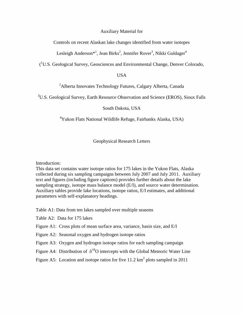
This data set contains water isotope ratios for 175 lakes in the Yukon Flats, Alaska

collected during six sampling campaigns between July 2007 and July 2011. Auxiliary

text and figures (including figure captions) provides further details about the lake

sampling strategy, isotope mass balance model (E/I), and source water determination.

Auxiliary tables provide lake locations, isotope ratios, E/I estimates, and additional

parameters with self-explanatory headings.

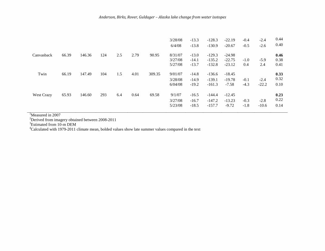
Table A1: Data from ten lakes sampled over multiple seasons

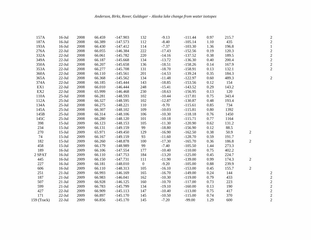
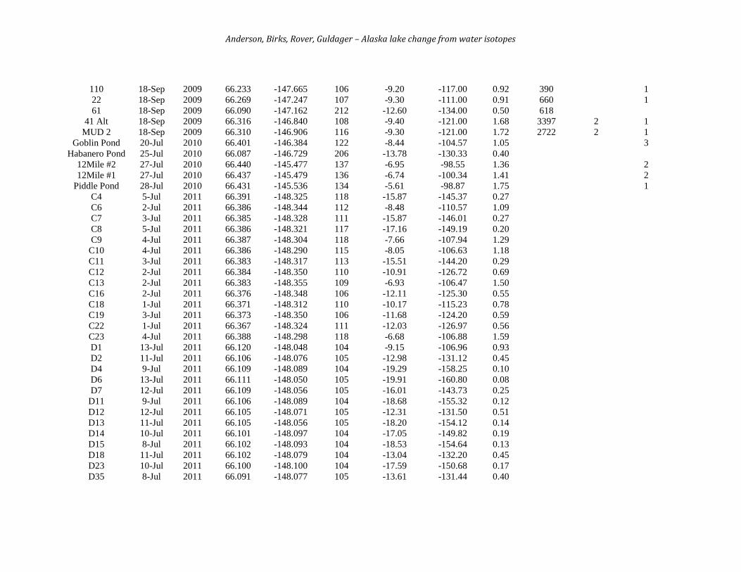
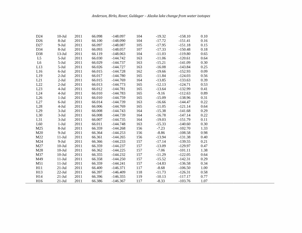
Table A2: Data for 175 lakes

Figure A1: Cross plots of mean surface area, variance, basin size, and E/I

Figure A2: Seasonal oxygen and hydrogen isotope ratios

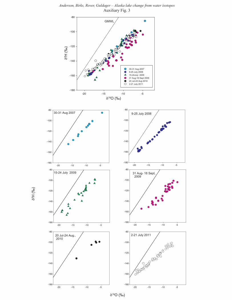
Figure A3: Oxygen and hydrogen isotope ratios for each sampling campaign

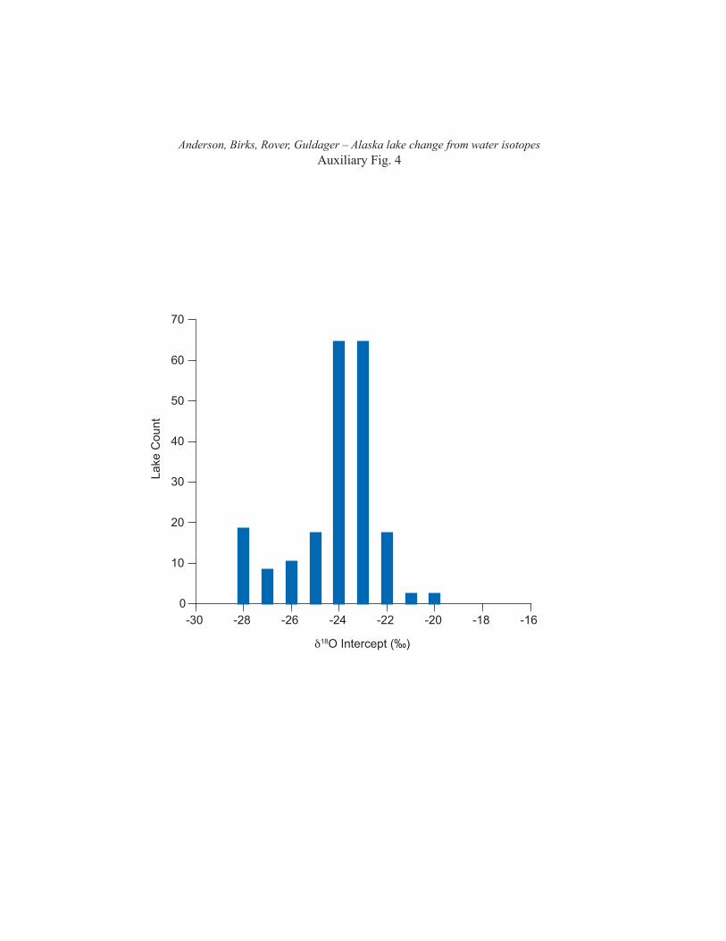
Figure A4: Distribution of 18

O intercepts with the Global Meteoric Water Line

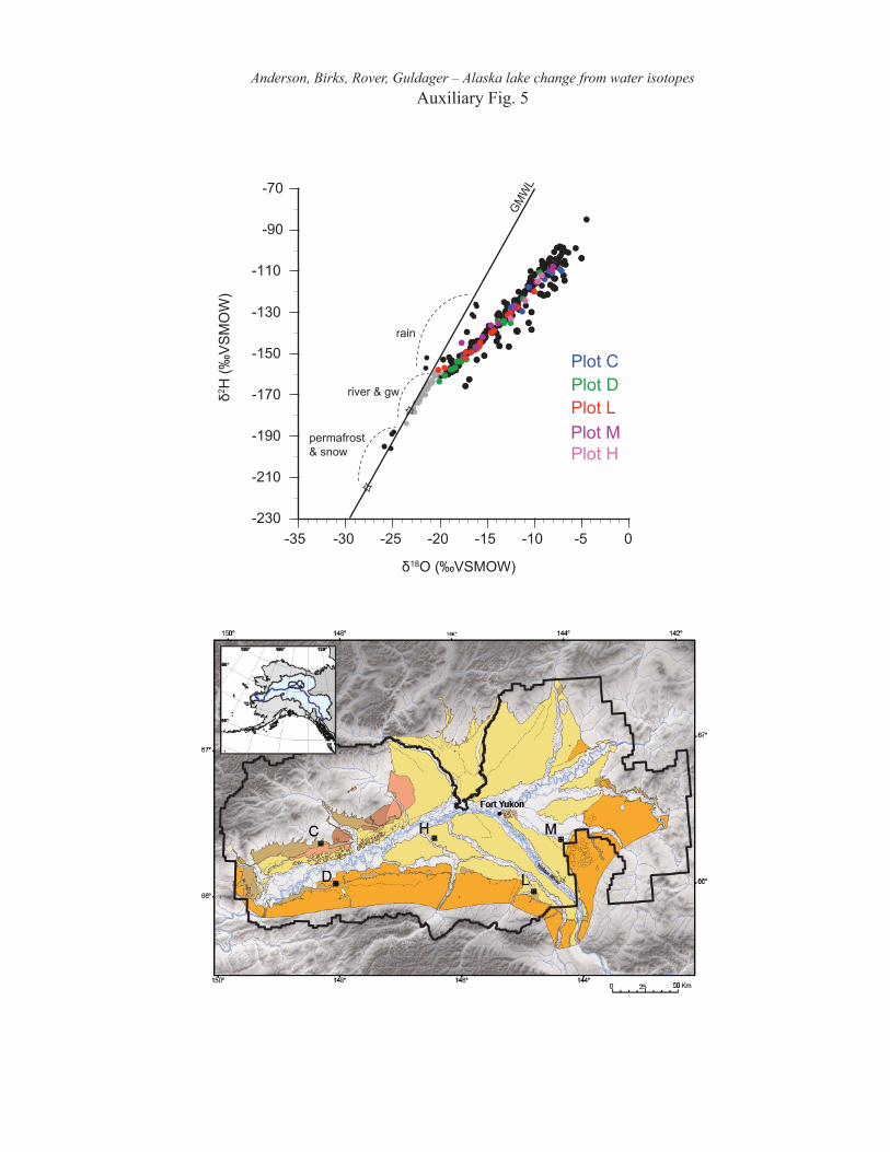
Figure A5: Location and isotope ratios for five 11.2 km2 plots sampled in 2011

Anderson, Birks, Rover, Guldager – Alaska lake change from water isotopes

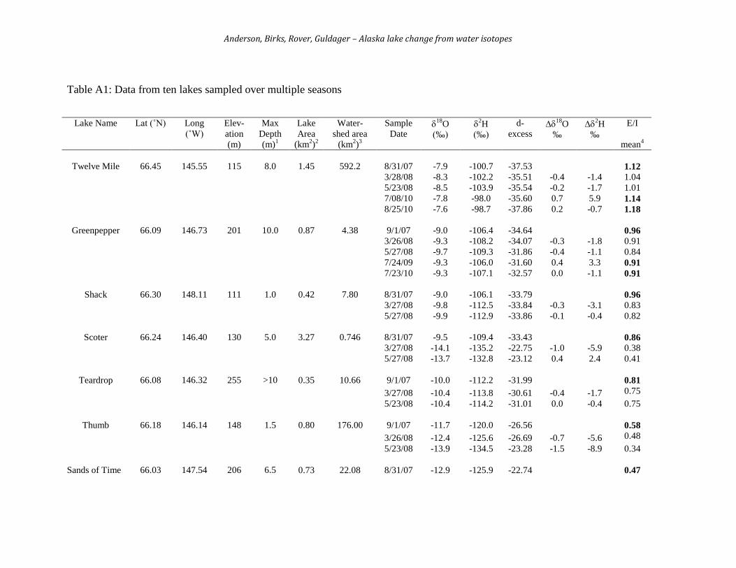
Table A1: Data from ten lakes sampled over multiple seasons

Lake Name Lat (˚N) Long

(˚W)

Elev-

ation

(m)

Max

Depth

(m)1

Lake

Area

(km2)

2

Water-

shed area

(km2)

3

Sample

Date

18O

(‰)

2H

(‰)

d-

excess

18O

‰

2H

‰

E/I

mean4

Twelve Mile 66.45 145.55 115 8.0 1.45 592.2 8/31/07 -7.9 -100.7 -37.53 1.12

3/28/08 -8.3 -102.2 -35.51 -0.4 -1.4 1.04

5/23/08 -8.5 -103.9 -35.54 -0.2 -1.7 1.01

7/08/10 -7.8 -98.0 -35.60 0.7 5.9 1.14

8/25/10 -7.6 -98.7 -37.86 0.2 -0.7 1.18

Greenpepper 66.09 146.73 201 10.0 0.87 4.38 9/1/07 -9.0 -106.4 -34.64 0.96

3/26/08 -9.3 -108.2 -34.07 -0.3 -1.8 0.91

5/27/08 -9.7 -109.3 -31.86 -0.4 -1.1 0.84

7/24/09 -9.3 -106.0 -31.60 0.4 3.3 0.91

7/23/10 -9.3 -107.1 -32.57 0.0 -1.1 0.91

Shack 66.30 148.11 111 1.0 0.42 7.80 8/31/07 -9.0 -106.1 -33.79 0.96

3/27/08 -9.8 -112.5 -33.84 -0.3 -3.1 0.83

5/27/08 -9.9 -112.9 -33.86 -0.1 -0.4 0.82

Scoter 66.24 146.40 130 5.0 3.27 0.746 8/31/07 -9.5 -109.4 -33.43 0.86

3/27/08 -14.1 -135.2 -22.75 -1.0 -5.9 0.38

5/27/08 -13.7 -132.8 -23.12 0.4 2.4 0.41

Teardrop 66.08 146.32 255 >10 0.35 10.66 9/1/07 -10.0 -112.2 -31.99 0.81

3/27/08 -10.4 -113.8 -30.61 -0.4 -1.7 0.75

5/23/08 -10.4 -114.2 -31.01 0.0 -0.4 0.75

Thumb 66.18 146.14 148 1.5 0.80 176.00 9/1/07 -11.7 -120.0 -26.56 0.58

3/26/08 -12.4 -125.6 -26.69 -0.7 -5.6 0.48

5/23/08 -13.9 -134.5 -23.28 -1.5 -8.9 0.34

Sands of Time 66.03 147.54 206 6.5 0.73 22.08 8/31/07 -12.9 -125.9 -22.74 0.47

Anderson, Birks, Rover, Guldager – Alaska lake change from water isotopes

3/28/08 -13.3 -128.3 -22.19 -0.4 -2.4 0.44

6/4/08 -13.8 -130.9 -20.67 -0.5 -2.6 0.40

Canvasback 66.39 146.36 124 2.5 2.79 90.95 8/31/07 -13.0 -129.3 -24.98 0.46

3/27/08 -14.1 -135.2 -22.75 -1.0 -5.9 0.38

5/27/08 -13.7 -132.8 -23.12 0.4 2.4 0.41

Twin 66.19 147.49 104 1.5 4.01 309.35 9/01/07 -14.8 -136.6 -18.45 0.33

3/28/08 -14.9 -139.1 -19.78 -0.1 -2.4 0.32

6/04/08 -19.2 -161.3 -7.58 -4.3 -22.2 0.10

West Crazy 65.93 146.60 293 6.4 0.64 69.58 9/1/07 -16.5 -144.4 -12.45 0.23

3/27/08 -16.7 -147.2 -13.23 -0.3 -2.8 0.22

5/23/08 -18.5 -157.7 -9.72 -1.8 -10.6 0.14

1Measured in 2007

2Derived from imagery obtained between 2008-2011

3Estimated from 10-m DEM

4Calculated with 1979-2011 climate mean, bolded values show late summer values compared in the text

Anderson, Birks, Rover, Guldager – Alaska lake change from water isotopes

Table A2: Data for 175 lakes

Lake ID Day-

Month

Year Lat (˚N) Long (˚W) Elevation

(m)

18O

(VSMOW)

2H

(VSMOW)

E/I Specific

Conduct-

ance

(µS/cm)

Source

(2=snow/

perma-

frost)

Trend

(1=dec,

2=nc,

3=inc)

12 Mile Lake 30-Aug 2007 66.450 -145.546 115 -7.90 -100.73 1.12 552 1

12 Mile Pond 30-Aug 2007 66.450 -145.563 115 -4.46 -84.94 2.24 1425

Canvasback 30-Aug 2007 66.385 -146.360 124 -13.04 -129.30 0.46 609 2

Sands of Time 30-Aug 2007 66.034 -147.544 207 -12.89 -125.86 0.47 143

Shack 30-Aug 2007 66.294 -148.114 111 -9.04 -106.11 0.96 1423

Greenpepper 31-Aug 2007 66.088 -146.733 202 -8.97 -106.40 0.96 831 1

Scoter 31-Aug 2007 66.240 -146.394 130 -9.49 -109.35 0.86 320 2

Teardrops 31-Aug 2007 66.083 -146.316 255 -10.02 -112.15 0.81 232 2

Thumb 31-Aug 2007 66.175 -146.144 148 -11.68 -120.00 0.58 126 2

Twin 31-Aug 2007 66.186 -147.493 104 -14.77 -136.61 0.33 145 2

West Crazy 31-Aug 2007 65.929 -146.596 293 -16.49 -144.37 0.23 119

252A 9-Jul 2008 66.129 -146.660 198 -10.50 -116.86 0.73 206.6 1

51A 10-Jul 2008 66.282 -149.321 110 -18.00 -155.82 0.15 127.6

83A 10-Jul 2008 66.259 -148.935 103 -9.98 -111.39 0.83 169.3

86A 10-Jul 2008 66.337 -148.984 115 -15.14 -141.79 0.30 184.3

91A 10-Jul 2008 66.240 -148.825 100 -15.22 -142.46 0.30 167.3

231A 15-Jul 2008 66.229 -146.943 117 -17.59 -150.50 0.17 72.6 2

255A 15-Jul 2008 66.223 -146.688 119 -9.91 -116.08 0.80 199.6 1

281A 15-Jul 2008 66.217 -146.417 126 -13.58 -135.62 0.41 204.2 2

281B 15-Jul 2008 66.217 -146.385 128 -10.54 -118.78 0.71 318.6 2

292A 15-Jul 2008 66.258 -146.331 118 -8.77 -112.11 0.97 700 2

295A 15-Jul 2008 66.320 -146.320 128 -10.52 -116.84 0.72 521.6 2

306A 15-Jul 2008 66.299 -146.187 130 -12.00 -127.86 0.55 405.9

129A 16-Jul 2008 66.106 -148.220 106 -18.29 -158.00 0.14 159.9

151A 16-Jul 2008 66.171 -147.975 107 -9.17 -109.27 0.93 273

174A 16-Jul 2008 66.208 -147.669 108 -18.21 -156.04 0.14 193

43A 16-Jul 2008 66.067 -149.327 92 -11.20 -121.94 0.64 169.5

69A 16-Jul 2008 66.117 -149.069 105 -14.50 -139.92 0.34 78.5

97A 16-Jul 2008 66.200 -148.682 97 -7.76 -104.12 1.26 236.9

Anderson, Birks, Rover, Guldager – Alaska lake change from water isotopes

157A 16-Jul 2008 66.459 -147.903 132 -9.13 -111.44 0.97 215.7 2

187A 16-Jul 2008 66.389 -147.573 112 -8.40 -105.14 1.10 435 2

193A 16-Jul 2008 66.430 -147.412 114 -7.37 -103.30 1.36 196.8 1

276A 22-Jul 2008 66.055 -146.384 222 -17.43 -152.56 0.19 120.3 2

332A 22-Jul 2008 66.061 -145.782 220 -14.16 -137.52 0.38 189.5 2

349A 22-Jul 2008 66.187 -145.668 134 -13.72 -136.30 0.40 200.4 2

350A 22-Jul 2008 66.207 -145.658 136 -18.51 -158.26 0.14 167.9 2

353A 22-Jul 2008 66.277 -145.708 131 -18.70 -158.91 0.13 132.1 2

360A 22-Jul 2008 66.110 -145.561 201 -14.53 -139.24 0.35 184.3

365A 22-Jul 2008 66.368 -145.562 134 -11.48 -122.97 0.60 489.3 2

374A 22-Jul 2008 66.185 -145.444 143 -18.85 -153.56 0.12 154

EX1 22-Jul 2008 66.010 -146.444 248 -15.41 -143.52 0.29 143.2

EX2 22-Jul 2008 65.999 -146.468 230 -18.63 -156.95 0.13 120

110A 25-Jul 2008 66.281 -148.593 102 -10.44 -117.81 0.75 343.4

112A 25-Jul 2008 66.327 -148.595 102 -12.87 -130.87 0.48 193.4

134A 25-Jul 2008 66.275 -148.221 110 -9.70 -115.61 0.85 734

145A 25-Jul 2008 66.307 -148.102 109 -10.03 -115.81 0.80 1392

145B 25-Jul 2008 66.314 -148.106 106 -10.30 -118.18 0.76 1450

145C 25-Jul 2008 66.280 -148.120 101 -10.18 -115.71 0.77 1164

398 15-Jul 2009 66.123 -148.153 105 -11.30 -120.90 0.62 131.2

234 15-Jul 2009 66.131 -149.159 99 -18.80 -156.90 0.12 88.5

270 15-Jul 2009 65.971 -149.450 129 -16.90 -162.50 0.38 50.9 2

74 15-Jul 2009 66.167 -149.159 93 -11.60 -128.70 0.59 191.7

182 15-Jul 2009 66.260 -148.878 100 -17.30 -165.70 0.36 186.8 2

458 15-Jul 2009 66.179 -148.989 99 -7.40 -105.50 1.44 273.3

189 16-Jul 2009 66.106 -147.554 177 -10.40 -110.00 0.75 402.2

2 SPAT 16-Jul 2009 66.110 -147.753 184 -13.20 -125.00 0.45 224.7

445 16-Jul 2009 66.150 -147.731 111 -11.90 -139.00 0.99 174.3 2

227 16-Jul 2009 66.181 -148.010 0 -9.20 -105.00 0.88 239.9

606 16-Jul 2009 66.110 -148.313 105 -16.10 -153.00 0.45 155.7 2

251 21-Jul 2009 66.993 -146.169 165 -16.70 -149.00 0.24 144 2

187 21-Jul 2009 66.983 -146.041 162 -10.30 -119.00 0.79 433 2

507 21-Jul 2009 66.928 -146.125 160 -10.70 -117.00 0.73 223 2

599 21-Jul 2009 66.783 -145.799 134 -19.10 -160.00 0.13 190 2

427 22-Jul 2009 66.909 -145.113 147 -10.40 -113.00 0.75 417 2

171 22-Jul 2009 66.897 -145.170 145 -10.50 -115.00 0.74 370 2

159 (Track) 22-Jul 2009 66.856 -145.170 145 -7.20 -99.00 1.29 600 2

Anderson, Birks, Rover, Guldager – Alaska lake change from water isotopes

287 22-Jul 2009 66.775 -145.258 140 -7.30 -98.00 1.29 881 2

331 22-Jul 2009 66.751 -145.458 142 -12.90 -127.00 0.49 534 2

395 22-Jul 2009 66.707 -145.530 134 -12.10 -124.00 0.56 224 2

456 24-Jul 2009 66.154 -144.118 177 -16.70 -145.00 0.23 153

127 24-Jul 2009 66.752 -143.502 174 -14.50 -137.00 0.37 189

84 24-Jul 2009 66.716 -143.673 162 -10.50 -116.00 0.74 216

136 24-Jul 2009 66.444 -144.384 144 -18.90 -157.00 0.13 124

332 24-Jul 2009 66.418 -145.368 138 -10.80 -119.00 0.68 374 2

112 SPAT 31-Aug 2009 66.101 -146.007 239 -7.80 -113.60 2.27 166 2 1

33 31-Aug 2009 66.625 -146.234 127 -7.90 -113.60 2.24 467 2 2

44 31-Aug 2009 66.269 -145.902 132 -7.80 -118.40 2.13 413 2 2

4 31-Aug 2009 66.867 -143.837 158 -6.80 -114.60 2.85 745 2

4 SPAT 31-Aug 2009 66.871 -143.829 159 -8.00 -117.60 2.15 985 2

68 31-Aug 2009 66.995 -143.749 185 -10.30 -129.90 1.36 3995 2

63 Alt 31-Aug 2009 66.977 -143.327 173 -13.70 -146.30 0.74 528 2

148 31-Aug 2009 66.796 -143.538 169 -8.30 -116.70 1.95 1847 2

8 31-Aug 2009 66.657 -143.839 161 -8.60 -121.30 1.80 196 2

47 1-Sep 2009 66.640 -145.301 135 -10.30 -138.40 1.28 623 2 2

55 1-Sep 2009 66.850 -145.552 152 -5.00 -103.70 4.93 357 2 2

1 SPAT 1-Sep 2009 66.754 -146.679 155 -11.80 -139.30 1.04 340 2 2

87 1-Sep 2009 66.834 -145.880 135 -7.90 -118.30 2.28 272 2 2

17 1-Sep 2009 66.612 -146.668 129 -9.00 -121.90 1.78 825 2 1

81 1-Sep 2009 66.547 -146.636 117 -12.70 -146.60 0.85 417 2 2

73 1-Sep 2009 66.440 -146.545 117 -11.80 -138.90 1.02 533 2 2

41 1-Sep 2009 66.335 -146.842 116 -10.60 -135.10 1.30 562 2 1

29 1-Sep 2009 66.244 -146.610 123 -6.90 -112.20 3.18 370 2 2

31 15-Sep 2009 66.592 -144.865 143 -6.80 -105.00 1.39 257

399 15-Sep 2009 66.654 -144.481 146 -15.30 -151.00 0.54 181 2

116 Alt 15-Sep 2009 66.633 -144.320 144 -7.60 -107.00 1.20 688

164 15-Sep 2009 66.705 -144.009 156 -8.20 -108.00 1.09 222

356 15-Sep 2009 66.782 -144.001 159 -17.80 -154.00 0.18 160

50 15-Sep 2009 66.802 -144.395 154 -8.40 -112.00 1.06 198

292 15-Sep 2009 66.043 -149.557 132 -6.40 -101.00 1.99 290

14 SPAT 18-Sep 2009 66.045 -149.569 137 -14.00 -144.00 0.69 93 2

14 18-Sep 2009 66.185 -149.420 104 -14.00 -140.00 0.38 256

26 18-Sep 2009 66.216 -149.130 102 -13.80 -142.00 0.39 55

10 18-Sep 2009 66.301 -148.459 107 -12.60 -133.00 0.50 247

Anderson, Birks, Rover, Guldager – Alaska lake change from water isotopes

110 18-Sep 2009 66.233 -147.665 106 -9.20 -117.00 0.92 390 1

22 18-Sep 2009 66.269 -147.247 107 -9.30 -111.00 0.91 660 1

61 18-Sep 2009 66.090 -147.162 212 -12.60 -134.00 0.50 618

41 Alt 18-Sep 2009 66.316 -146.840 108 -9.40 -121.00 1.68 3397 2 1

MUD 2 18-Sep 2009 66.310 -146.906 116 -9.30 -121.00 1.72 2722 2 1

Goblin Pond 20-Jul 2010 66.401 -146.384 122 -8.44 -104.57 1.05 3

Habanero Pond 25-Jul 2010 66.087 -146.729 206 -13.78 -130.33 0.40

12Mile #2 27-Jul 2010 66.440 -145.477 137 -6.95 -98.55 1.36 2

12Mile #1 27-Jul 2010 66.437 -145.479 136 -6.74 -100.34 1.41 2

Piddle Pond 28-Jul 2010 66.431 -145.536 134 -5.61 -98.87 1.75 1

C4 5-Jul 2011 66.391 -148.325 118 -15.87 -145.37 0.27

C6 2-Jul 2011 66.386 -148.344 112 -8.48 -110.57 1.09

C7 3-Jul 2011 66.385 -148.328 111 -15.87 -146.01 0.27

C8 5-Jul 2011 66.386 -148.321 117 -17.16 -149.19 0.20

C9 4-Jul 2011 66.387 -148.304 118 -7.66 -107.94 1.29

C10 4-Jul 2011 66.386 -148.290 115 -8.05 -106.63 1.18

C11 3-Jul 2011 66.383 -148.317 113 -15.51 -144.20 0.29

C12 2-Jul 2011 66.384 -148.350 110 -10.91 -126.72 0.69

C13 2-Jul 2011 66.383 -148.355 109 -6.93 -106.47 1.50

C16 2-Jul 2011 66.376 -148.348 106 -12.11 -125.30 0.55

C18 1-Jul 2011 66.371 -148.312 110 -10.17 -115.23 0.78

C19 3-Jul 2011 66.373 -148.350 106 -11.68 -124.20 0.59

C22 1-Jul 2011 66.367 -148.324 111 -12.03 -126.97 0.56

C23 4-Jul 2011 66.388 -148.298 118 -6.68 -106.88 1.59

D1 13-Jul 2011 66.120 -148.048 104 -9.15 -106.96 0.93

D2 11-Jul 2011 66.106 -148.076 105 -12.98 -131.12 0.45

D4 9-Jul 2011 66.109 -148.089 104 -19.29 -158.25 0.10

D6 13-Jul 2011 66.111 -148.050 105 -19.91 -160.80 0.08

D7 12-Jul 2011 66.109 -148.056 105 -16.01 -143.73 0.25

D11 9-Jul 2011 66.106 -148.089 104 -18.68 -155.32 0.12

D12 12-Jul 2011 66.105 -148.071 105 -12.31 -131.50 0.51

D13 11-Jul 2011 66.105 -148.056 105 -18.20 -154.12 0.14

D14 10-Jul 2011 66.101 -148.097 104 -17.05 -149.82 0.19

D15 8-Jul 2011 66.102 -148.093 104 -18.53 -154.64 0.13

D18 11-Jul 2011 66.102 -148.079 104 -13.04 -132.20 0.45

D23 10-Jul 2011 66.100 -148.100 104 -17.59 -150.68 0.17

D35 8-Jul 2011 66.091 -148.077 105 -13.61 -131.44 0.40

Anderson, Birks, Rover, Guldager – Alaska lake change from water isotopes

D24 10-Jul 2011 66.098 -148.097 104 -19.32 -158.10 0.10

D26 8-Jul 2011 66.100 -148.090 104 -17.72 -151.41 0.16

D27 9-Jul 2011 66.097 -148.087 105 -17.95 -151.18 0.15

D34 8-Jul 2011 66.093 -148.057 107 -17.33 -150.48 0.18

D38 13-Jul 2011 66.119 -148.063 104 -11.03 -119.80 0.65

L5 5-Jul 2011 66.030 -144.742 163 -11.06 -120.61 0.64

L6 5-Jul 2011 66.029 -144.737 163 -15.21 -141.09 0.30

L13 5-Jul 2011 66.026 -144.727 163 -16.08 -143.84 0.25

L16 6-Jul 2011 66.015 -144.728 162 -19.66 -152.93 0.09

L19 2-Jul 2011 66.017 -144.780 165 -11.84 -124.03 0.56

L21 2-Jul 2011 66.015 -144.769 164 -13.85 -133.63 0.39

L22 2-Jul 2011 66.013 -144.773 165 -12.13 -124.71 0.53

L23 4-Jul 2011 66.012 -144.781 165 -13.64 -132.99 0.41

L24 4-Jul 2011 66.010 -144.783 165 -9.16 -112.63 0.89

L26 1-Jul 2011 66.010 -144.759 165 -15.09 -138.96 0.31

L27 6-Jul 2011 66.014 -144.739 163 -16.66 -144.47 0.22

L28 4-Jul 2011 66.006 -144.769 165 -11.05 -121.14 0.64

L29 3-Jul 2011 66.008 -144.743 164 -15.38 -141.68 0.29

L30 3-Jul 2011 66.008 -144.739 164 -16.78 -147.14 0.22

L31 3-Jul 2011 66.007 -144.735 164 -19.03 -151.79 0.11

L60 1-Jul 2011 66.011 -144.748 163 -15.33 -140.60 0.30

M25 8-Jul 2011 66.359 -144.268 156 -7.23 -102.70 1.33

M20 9-Jul 2011 66.364 -144.253 156 -8.86 -108.58 0.98

M22 11-Jul 2011 66.361 -144.265 156 -13.94 -131.38 0.40

M24 9-Jul 2011 66.366 -144.233 157 -17.14 -139.55 0.21

M27 10-Jul 2011 66.359 -144.237 157 -13.09 -129.97 0.47

M28 10-Jul 2011 66.362 -144.225 157 -7.06 -101.11 1.38

M37 10-Jul 2011 66.355 -144.232 157 -11.29 -122.05 0.64

M49 11-Jul 2011 66.358 -144.250 157 -15.52 -142.31 0.29

M51 11-Jul 2011 66.359 -144.241 157 -14.83 -136.58 0.34

H11 21-Jul 2011 66.400 -146.371 117 -8.68 -106.50 1.00

H13 22-Jul 2011 66.397 -146.409 118 -11.73 -126.31 0.58

H14 21-Jul 2011 66.396 -146.355 119 -10.13 -117.17 0.77

H16 21-Jul 2011 66.386 -146.367 117 -8.33 -103.76 1.07

XXXX

X

XXX

XXX

X

XXXX XX

XX X

X

XX

X

X

X

X

X

X

X

XX

X

X

X X

X

X

XX

X X

X

XX

X

XX

X

X

X

X

X

1

10

100

0 10 20 30 40 50 60 70 80 90

Siz

e (k

m2 )

Mean Surface Area (%)

B.

X

X

XX

XXXXXXX

X

X

XXX

X

XX

XX

X

X

XX

X

XX

X

X

X

X

X

XXXX

X

X

X

X

X

X

X

XX

X

X

X

X

XX

X

X

0

1

2

3

4

5

0 5 10 15 20 25 30 35 40

E/I

Standard Deviation

C.

XXXXXXXXXXX XX

XXX XXXX X

XXXXXXX

X XXX

XX XXXXX

XX

X X XXX

XX

XXXX

X

0

5

10

15

20

25

30

35

40

0 10 20 30 40 50 60 70 80 90

Sta

ndar

d D

evia

tion

Mean Surface Area (%)

A.

X

Anderson, Birks, Rover, Guldager – Alaska lake change from water isotopesAuxiliary Figure 1

δ2 H (‰

)

δ18O (‰)

-180

-160

-140

-120

-100

-80

-20 -15 -10 -5

GMWL

Twelve MileCanvasbackScoterShackTwinThumbWest Crazy

Anderson, Birks, Rover, Guldager – Alaska lake change from water isotopesAuxiliary Fig. 2

δ18O (‰)-20 -15 -10 -5

δ2 H (‰

)

-180

-160

-140

-120

-100

-80

30-31 Aug 20079-25 July 200815-24July 200931 Aug-18 Sept 200920 Jul-24 Aug 20102-21 July 2011

-20 -15 -10 -5-180

-160

-140

-120

-100

-8030-31 Aug 2007

-20 -15 -10 -5-180

-160

-140

-120

-100

-80

9-25 July 2008

-20 -15 -10 -5-180

-160

-140

-120

-100

-8015-24 July 2009

-20 -15 -10 -5-180

-160

-140

-120

-100

-80

31 Aug- 18 Sept, 2009

-20 -15 -10 -5-180

-160

-140

-120

-100

-8020 Jul-24 Aug., 2010

-20 -15 -10 -5-180

-160

-140

-120

-100

-802-21 July 2011

δ2 H (‰

)

δ18O (‰)

GMWL

Anderson, Birks, Rover, Guldager – Alaska lake change from water isotopesAuxiliary Fig. 3

0

10

20

30

40

50

60

70

-30 -28 -26 -24 -22 -20 -18 -16

δ18O Intercept (‰)

Lake

Cou

ntAnderson, Birks, Rover, Guldager – Alaska lake change from water isotopes

Auxiliary Fig. 4

X

X

XX

XXXXX

XX

X

X

X

XXX

X

X

XXX

X

X

X

X

X

X

XXXX

X

XX

XX

X

X

X

X

X

X

X

XXXXX

XX

X

X

XX

X

X

X

XX

XX

X

XX

XX

XX

XX

X

X

XXXXXX

X

X

XX

X

X

X

XX

XXX

XX

X

XX

X

X

X

XXXX

XX

X

XX

X

X

XXXX

X

X

XX

XX

X

X

X

X

XXX

XX

X

XX

X

X

X

XXX

X

X

X

XXXX

XX

XXX

X

XXX

X

XX

X

XX

X

X

XX

XX

X

X

X

XX

X

XX

X

XX

X

X

XXXXX

X

X

XX

X

X

X

XX

XXX

X

XX

XX

XXXXXXXXXX

XXXXXXXXXXXX

XXXXX

XXXXXXXXXX

XXXXXXXXXXXXX

X

X

XXX

XXX

X

X

XX

X

XXXX

X

XX

-230

-210

-190

-170

-150

-130

-110

-90

-70

-35 -30 -25 -20 -15 -10 -5 0

GM

WL

rain

river & gw

permafrost& snow

δ18O (‰VSMOW)

δ2H

(‰V

SM

OW

)

Plot CX

X

XX

XX

X

X

X

X

XXX

XX

X

XX

X

X

X

XXX

X

X

X

XXXX

X

Plot D

X

XXX

X

XXX

X

XX

X

XX

X

X

Plot L

XX

XX

X

X

X

XX

Plot M

X

XX

X

Plot H

Anderson, Birks, Rover, Guldager – Alaska lake change from water isotopesAuxiliary Fig. 5

1

Auxiliary Text:

Lake sampling strategy

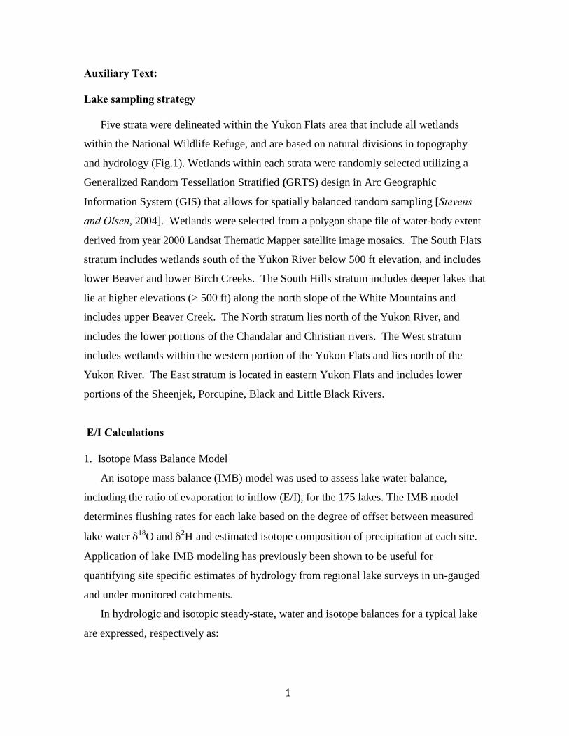
Five strata were delineated within the Yukon Flats area that include all wetlands

within the National Wildlife Refuge, and are based on natural divisions in topography

and hydrology (Fig.1). Wetlands within each strata were randomly selected utilizing a

Generalized Random Tessellation Stratified (GRTS) design in Arc Geographic

Information System (GIS) that allows for spatially balanced random sampling [Stevens

and Olsen, 2004]. Wetlands were selected from a polygon shape file of water-body extent

derived from year 2000 Landsat Thematic Mapper satellite image mosaics. The South Flats

stratum includes wetlands south of the Yukon River below 500 ft elevation, and includes

lower Beaver and lower Birch Creeks. The South Hills stratum includes deeper lakes that

lie at higher elevations (> 500 ft) along the north slope of the White Mountains and

includes upper Beaver Creek. The North stratum lies north of the Yukon River, and

includes the lower portions of the Chandalar and Christian rivers. The West stratum

includes wetlands within the western portion of the Yukon Flats and lies north of the

Yukon River. The East stratum is located in eastern Yukon Flats and includes lower

portions of the Sheenjek, Porcupine, Black and Little Black Rivers.

E/I Calculations

1. Isotope Mass Balance Model

An isotope mass balance (IMB) model was used to assess lake water balance,

including the ratio of evaporation to inflow (E/I), for the 175 lakes. The IMB model

determines flushing rates for each lake based on the degree of offset between measured

lake water 18

O and 2H and estimated isotope composition of precipitation at each site.

Application of lake IMB modeling has previously been shown to be useful for

quantifying site specific estimates of hydrology from regional lake surveys in un-gauged

and under monitored catchments.

In hydrologic and isotopic steady-state, water and isotope balances for a typical lake

are expressed, respectively as:

2

[1] I = Q + E

[2] I I = QQ + EE

Here, I is the inflow rate (m3s

-1), Q is the outflow rate (m

3s

-1) and E is the evaporation

rate (m3s

-1). I, Q and E each represent the isotopic composition of each corresponding

hydrological component. These equations can be simplified using the general

assumptions that outflow from the lake is equivalent to lake water (Q = L) and that

inflows can be approximated by the weighted annual average of precipitation (I = P).

The Craig-Gordon Model for open water evaporation [Craig and Gordon, 1965] is used

to estimate E :

[3] E = * L –h A - * - h + K

Here, * is the equilibrium fractionation between liquid and vapor (*=*-1), and

is the total enrichment factor including both equilibrium (*) and kinetic (K)

components. Combining and rearranging these equations yields an expression for the

fraction of water loss by evaporation, E/I, expressed as:

[4] E/I ≈ (L - P) / m (* - L)

Here, m is the enrichment slope derived from (h - ) / (1 - h + K) where h is

humidity (relative humidity/100), and * = (h A + ) / (h - ) is the limiting isotopic

enrichment. Values for * were estimated using temperature data and the equations from

Horita and Wesolowski [1994]. Estimates of K were determined using relative humidity

using K =CK (1-h) where CK was set to 14.2 ‰ for oxygen and 12.5 ‰ for hydrogen

[Gibson et al., 2002]. The isotopic composition of atmospheric moisture, A, was

determined using a similar method as Bennett et al., [2008]; Gibson et al., [2008] and

Gibson et al., [2010a], and [2010b], starting with the equilibrium assumption (A = p – k

*, k=1) and then iteratively adjusting k to obtain a best-fit match for 18

O and 2H

results by best fitting k to the observed local evaporation line.

3

In this study, equation [4] was used to determine E/I values from measured lake 18

O

and 2H compositions from the surveys conducted between 2007 and 2011 using

climatological averages from gridded climate datasets. The results of the E/I calculations

from 18

O are presented in this report but they are highly correlated with the E/I results

from 2H (r2

=0.9486), and similar trends were found for those calculations.

2. Climate Parameters

In the absence of a network of long-term, reliable meteorological stations within the

~118,340 km2 Yukon Flats region, climatological parameters required to run the IMB

were obtained from the North American Regional Reanalysis (NARR) dataset [Mesinger

et al., 2006]. The NARR dataset is a long-term, dynamically consistent, high-resolution,

high frequency, atmospheric and land surface hydrology dataset for the North American

domain based on meteorological station data between 1979 and 2003. Average monthly

climate fields (i.e., climate norms) were extracted for the grid cells corresponding to the

location of each of the 175 lakes in the survey. The parameters extracted were:

APCPsfc: surface total precipitation [kg/m2]

RH2m: 2 m relative humidity [%]

EVPsfc: surface evaporation [kg/m2]

TMP2m: 2 m temp. [K]

Climate data from the time period corresponding to the residence time of the lake

would give the best representation of climate conditions during lake evaporation, but

climate norms are often used in regional lake surveys where a wide variety of residence

times might be expected [e.g. Bennett et al., 2008, Gibson and Edwards, 2002, Gibson et

al., 2010a, 2010b, Pham et al., 2008, and Scott et al., 2010]. The interannual variations

observed between 2007 and 2010 are indicated by the following ranges of deviation from

long-term climate norms: T=-0.2°C to +1.5°C; RH, -2.4 % to -4.7%; P= -4.6 to 2.0

mm/mo.

The evaporation flux-weighting approach developed by Gibson et al. [2002] was

used to flux-weight (FW) estimates of relative humidity and temperature so that the water

balance calculations are representative of the open water season. For example the

evaporation flux-weighted estimates for 2m temperature over a year (TFW) is given below

4

as the sum of the temperature (T) multiplied by the evaporation (E) for each month

divided by the sum of the total evaporation over 12 months (TFW = ∑ Emonthly Tmonthly / ∑

Eannual)

Monthly precipitation 18

O estimates were obtained for each lake location based on

empirically derived relationships between latitude and elevation presented by Bowen and

Wilkinson [2002] and tuned/corrected using available Canadian Network for Isotopes in

Precipitation (CNIP) data. The 2H was calculated assuming that precipitation would

follow the relationship defined by the Global Meteoric Water Line (GMWL) [Craig,

1961]. However, rather than flux weighting, amount weighting precipitation (PAW) best

represents monthly precipitation isotope fields (P). Using precipitation from the NARR

data set, the average precipitation total for each month (P) is multiplied by the estimated

p for that month, divided by the precipitation total over 12 months (PAW = ∑ p-monthly

Pmonthly / ∑ Pannual ).

3. Isotope Mass Balance Model Assumptions

The major assumptions inherent in the IMB approach include that:

(i) The isotopic composition of atmospheric moisture is a function of the isotopic

composition of precipitation, as is expected due to near-equilibrium exchange

between vapor and liquid water in condensing air masses,

(ii) The isotopic composition of discharge is adequately characterized by the

isotopic signature of lake water (L) expected for a well-mixed lake,

(iii) The isotopic composition of inflow to the lake is equal to that of precipitation

(i.e. I = P), as would be valid where runoff is locally derived from recent

meteoric water that has not undergone substantial isotopic enrichment, and

(iv) Lake samples collected during summer/early fall are sufficiently

representative of the annual long-term isotopic composition of the lake to

evaluate the proposed hypothesis.

The first three assumptions are clearly valid for the Yukon Flats lake dataset. First,

there are no isotopically distinct vapor sources (e.g. large lakes or near ocean) or strong

evidence for mixing with transpired vapor. Second, the sampled sites did not include

very large, deep lakes with permanent stratification that would differentiate outflow from

5

lake water isotope values. Third, the similarity between precipitation and surface run-off

isotope values is evident by the similarity between Yukon River water data and integrated

precipitation.

To address the fourth assumption, temporal trends in the isotopic composition of a

subset of lakes that were sampled multiple times during the study period are more closely

examined (Table A1 and Fig. A2). The available data show the most negative 18

O and

2H values occur after spring melt, followed by evaporative enrichment over the open

water period. The greatest change in lake water isotopes, and corresponding E/I,

occurred during the period between spring melt and early summer and significantly less

change occurred during the July to September period. It is possible that E/I estimates

based on early to mid July samples may slightly underestimate evaporation, but this

effect would have limited impact on the overall range of E/I (Table A2). Therefore, we

have combined all isotope data obtained between mid-July through early September for

our analyses.

Furthermore, because our purpose here is to evaluate the overall range of hydrologic

states in the study area, we also combined the mid to late summer data for all of the five

years during which sampling campaigns were conducted (2007-2011). This approach is

validated by comparing the data for each sampling campaign (Fig. A3) which shows that

the range of all the isotope values (max – min = ~15‰) is similar from one year to the

next, and far greater than the largest observed seasonal change at an individual site.

These results are similar to the spatial and temporal variations observed by other regional

lake surveys including the Old Crow Flats, northern Yukon Territory [Turner et al.,

2010] that is the nearest available data set to the Yukon Flats. There also, the greatest

difference in isotopes and E/I estimates occurs between ice-out and early summer. The

overall range of the entire data set is also similar from year to year and exceeds individual

lake seasonal variations.

5. Source water evaluation

Visibly evident within the 18

O and 2H scatter plot are two groups of lakes

(Fig. 3) that appear to be defined by regressions (local evaporation lines, LEL) with

similar slopes but different intercepts on the GMWL. More specifically, when inflow

6

(i) was estimated using precipitation (p) based on the geographical position of the

lake, the LEL regression between some of the lakes (L) and the p value produced

unrealistically low slopes (m = 1 to 3) compared with slopes that are either theoretically

predicted or observed in similar areas (m ≈ 4.5 to 5.5). This suggested that assumption

(iii), where I approximates p, should be re-evaluated for this group of lakes.

Here we use the constant local evaporation line (LEL) approach, with a slope of 5,

to derive the intercepts with the GMWL for all lakes [e.g., Wolfe et al., 2007]. A slope of

5 is slightly higher than the empirically derived slope of 4.6 from the dataset, yet it is

similar to slopes derived from other high latitude lake surveys [Gibson et al., 2005].

Fitting an LEL with a slope of 5 to each of the lake data points identified a range of

intercept values on the GMWL between -30 and -20‰ for 18

O and a bi-modal

distribution (Fig. A4). The majority of lakes (n= 124) plot on the LEL that intercepts the

GMWL at -24‰ ± 1‰. A small group (n=26) plots on the LEL that intercepts the

GMWL at -28‰ ± 1‰. Therefore, the source water, I, used to estimate E/I for these 26

lakes was ~4‰ more negative than the expected p, allowing some variance related to

elevation and latitude. Although further refinement of I may be possible by coupling

the E/I estimates with both 18

O and 2H following the method of Yi et al., [2008], this

approach is not necessary in order to determine the existence of two groups, one sourced

by water relatively enriched in O18

, and the other relatively depleted.

References:

Bennett, K.E. et al., (2008). Water Yield estimates for critical loadings assessment:

comparisons of gauging methods versus and isotopic approach. Can. J. Fish. Aquat.

Sci. 65: 83-99.

Bowen, G.J., & B. Wilkinson. (2002). Spatial distribution of d18

O in meteoric

precipitation. Geology, 30:315-318.

Craig, H. (1961). Isotopic variations in meteoric waters. Science, 133:1702-1703.

Craig, H., and L. I. Gordon (1965), Deuterium and oxygen-18 variation in the ocean and

the marine atmosphere, Proc. Conf. on Stable Isotopes in Oceanographic Studies and

Paleotemperatures, ed: E. Tongiorgi, pp. 9-130, Spoleto, Italy.

7

Gibson, J.J., et al., (2005). Progress in isotope hydrology in Canada. Hydrol. Proc. 19,

303-327.

Gibson, J.J., et al., (2002). Quantitative comparison of lake throughflow, residency, and

catchment runoff using stable isotopes: modeling and results from a regional survey of

Boreal lakes. J. Hydrol. 262: 128-144.

Gibson, J.J. et al., (2010a) Interannual variations in water yield to lakes in northeastern

Alberta: Implications for estimating critical loads of acidity. J. Limnol., 69(Suppl. 1):

126-134.

Gibson, J.J. et al., (2010b) Site-specific estimates of water yield applied in regional acid

sensitivity. J. Limnol., 69 (Suppl. 1): 67-76

Scott, K.A. et al., (2010) Limnological characteristics and acid sensitivity of boreal

headwater lakes in northwest Saskatchewan, Canada. J. Limnol., 69 (Suppl. 1): 33-44.

Horita, J., and D. Wesolowski (1994), Liquid-vapour fractionation of oxygen and

hydrogen isotopes of water from the freezing to the critical temperature, Geochim.

Cosmochim. Acta., 58, 3425-3437.

Stevens, D. L. and Olsen, A. R. 2004. Spatially balanced sampling of natural resources. J.

Amer. Stat. Assoc. 99, 262 – 278.

Turner, K.W. et al., (2010). Characterizing the role of hydrologic processes on lake

water balances in the Old Crow Flats, Yukon Territory, Canada, using water isotope

tracers. J. Hydrol., 386, 103-117.

Mesinger F. et al., (2006). North American Regional Reanalysis: A long-term, consistent,

high-resolution climate dataset for the North American domain, as a major

improvement upon the earlier global reanalysis datasets in both resolution and

accuracy. Bull. Amer .Meteorol. Soc., 87: 343-360.

Pham, S. V. et al., (2008). Spatial variability of climate and land-use effects on lakes of

the northern Great Plains, Limnology and Oceanography, 53(2), 728-742, doi:

10.4319/lo.2008.53.2.0728.

Wolfe, B.B. et al., (2007). Classification of hydrological regimes of northern floodplain

basins (Peace-Athabasca Delta, Canada) from analysis of stable isotopes (18

O, 2H)

and water chemistry. Hydrol. Proc. 21, 151-168.

Yi, Y. et al., (2008). A coupled isotope tracer method to characterize input water to

lakes. J. Hydrol. 35, 1-13.

8

Auxiliary Figure Captions

Figure A1. Data from 54 lakes that were analyzed for surface area changes: a.) Standard

deviation of area variation versus mean surface area as a % of maximum, b.) Maximum

lake size versus mean area as a % of maximum, and c.) Lake E/I versus area standard

deviation of area variation. Red symbols indicate lakes sourced by snow and/or

permafrost thaw.

Figure A2. Isotope data from the sub-set of lakes sampled during different seasons from

Table A1. The arrow colors correspond to lake symbols and indicate the direction and

magnitude of isotopic change for each lake.

Figure A3. Isotope data for the 175 lakes from Table A2, including the 54 lakes used for

comparisons with lake area trends, shown by individual sampling campaigns carried out

between Aug-Sept 2007 and July 2011. Top panel shows all data and lower panels show

data for each campaign.

Figure A4. The distribution of 18

O-intercept values on the GMWL from individual lake

water 18

O and 2H values regressed by an LEL with a slope of 5.

Figure A5: Lake isotope ratios shown with the Global Meteoric Water Line (GMWL),

and estimated monthly precipitation values (black) [Bowen and Wilkinson, 2003], and

Yukon, Porcupine and Chandalar River values (gray) [Schuster et al., 2010]. Dashed

arcs indicate the approximate ranges of isotope values for rain, snow, rivers,

groundwater, and permafrost. Colors show the isotope ratios of lakes sampled within the

five 11.2 km2 plot areas (C, D, L, M, H) during July 2011 from Heglund and Jones

[2003]. Plot locations are shown with the Yukon Flats National Wildlife boundary.