Embed Size (px)
Citation preview
1
Convective heat transfer coefficients for exterior building surfaces:
Existing correlations and CFD modelling Thijs Defraeye
a, *, Bert Blocken
b and Jan Carmeliet
c,d
a Laboratory of Building Physics, Department of Civil Engineering, Katholieke Universiteit Leuven, Kasteelpark Arenberg 40, 3001 Heverlee, Belgium b Building Physics and Systems, Eindhoven University of Technology, P.O. Box 513, 5600 Eindhoven, The Netherlands c Chair of Building Physics, Swiss Federal Institute of Technology Zurich (ETHZ), Wolfgang-Pauli-Strasse 15, 8093 Zürich, Switzerland d Laboratory for Building Science and Technology, Swiss Federal Laboratories for Materials Testing and Research (Empa), Überlandstrasse 129, 8600 Dübendorf, Switzerland
Abstract
Convective heat transfer at exterior building surfaces has an impact on the design and performance of
building components such as double-skin facades, solar collectors, solar chimneys, ventilated
photovoltaic arrays, etc. and also affects the thermal climate and cooling load in urban areas. In this study,
an overview is given of existing correlations of the exterior convective heat transfer coefficient (CHTC)
with the wind speed, indicating significant differences between these correlations. As an alternative to
using existing correlations, the applicability of CFD to obtain forced CHTC correlations is evaluated, by
considering a cubic building in an atmospheric boundary layer. Steady Reynolds-Averaged Navier-Stokes
simulations are performed and, instead of the commonly used wall functions, low-Reynolds number
modelling (LRNM) is used to model the boundary-layer region for reasons of improved accuracy. The
flow field is found to become quasi independent of the Reynolds number at Reynolds numbers of about
105. This allows limiting the wind speed at which the CHTC is evaluated and thus the grid resolution in
the near-wall region, which significantly reduces the computational expense. The distribution of the
power-law CHTC-U10 correlation over the windward and leeward surfaces is presented (U10 = reference
wind speed at 10 m height). It is shown that these correlations can be accurately determined by
simulations with relatively low wind speed values, which avoids the use of excessively fine grids for
LRNM, and by using only two or three discrete wind speed values, which limits the required number of
CFD simulations.
Keywords: surface transfer coefficient, Computational Fluid Dynamics, wind speed, building, cube,
correlation
* Corresponding author. Tel.: +32 (0)16321348; fax: +32 (0)16321980.
E-mail address: [email protected]
Accepted for publication in Energy Conversion and Management, July 14, 2010
2
1. Introduction
The convective heat exchange at an exterior building surface, due to air flow along the surface, is usually
modelled by convective heat transfer coefficients (CHTCs) which relate the convective heat flux normal
to the wall qc,w (W/m²) to the difference between the surface temperature at the wall Tw (°C) and a
reference temperature Tref (°C), which is generally taken as the outside air temperature. The convective
heat flux is assumed positive away from the wall. The CHTC (hc,e - W/m²K) is defined as:
c,wc,e
w ref
qh
(T T )=
− (1)
Convective heat transfer predictions at exterior building surfaces, by means of CHTCs, are required
for several building and urban engineering applications. CHTCs are of interest for the energy
performance analysis of buildings or building components, especially if they are composed of materials
which have a relatively low thermal resistance (e.g. glass), resulting in a relatively high sensitivity to the
CHTC. Examples are glazed buildings, double-skin facades, greenhouses, textile buildings, solar
collectors, solar chimneys and ventilated photovoltaic arrays. Often, information on CHTCs is used to
determine convective moisture transfer coefficients (CMTCs), by using the Chilton-Colburn analogy.
Both CHTCs and CMTCs have an impact on the heat and moisture transport in the building envelope, and
they are required for example to assess drying of facades, wetted by wind-driven rain [1,2] or by surface
condensation by undercooling during clear cold nights [3,4]. This hygrothermal behaviour within the
envelope and at the exterior surface is important for several physical, chemical and biological weathering
processes such as microbiological vegetation (algae) and mould growth, reaction of deposited pollutants
on the wetted surface, freeze-thaw degradation, salt transport, crystallisation and related deterioration, etc.
CHTCs and CMTCs are required to predict the turbulent heat and moisture fluxes from building surfaces
and streets for the analysis of the climate in urban areas with so-called mesoscale Urban Canopy Models
[5-7], for example to evaluate the influence of urban heat islands on the cooling load for buildings.
CHTC correlations have been determined in the past using wind-tunnel experiments on flat plates and
bluff bodies, full-scale experiments on buildings and numerical (CFD) simulations. CHTCs for buildings
are often correlated to the wind speed at a reference location, for example the mean wind speed at a
height of 10 m above the ground U10 (m/s). Linear or power-law CHTC-U correlations are mostly
reported. Linear correlations account for buoyancy effects at low wind speeds, using an intercept, while
power-law correlations are generally used for forced convective heat transfer.
The aim of this paper is twofold. First, an overview of the relevant research on CHTCs for exterior
building surfaces is presented (section 2), from the viewpoint of building aerodynamics, i.e. the specific
wind-flow pattern around a building. To the knowledge of the authors, this type of overview, including
flat-plate correlations, wind-tunnel experiments on reduced-scale models, full-scale experiments and CFD
simulations has not yet been performed. A recent and extensive review on CHTC correlations for
applications towards solar collectors was provided by Palyvos [8]. Hagishima et al. [9] and Roy et al. [10]
included a more concise overview of CHTC correlations in their work, from the viewpoint of urban
canopy modelling and the greenhouse climate, respectively. In the overview in this paper, primarily
additional information to existing reviews will be presented, while for other information, reference will be
made to these earlier reviews.
In this overview, significant differences between the existing correlations are found, as a result from
the specific conditions under which they have been derived. Thereby these correlations are only
applicable under certain conditions but this is not always acknowledged by their users. As an alternative
to using existing correlations, researchers or designers may also choose to determine such correlations for
their specific building configuration of interest (e.g. street canyon), by means of CFD for example.
Therefore, as a second part of this study (section 3), the use of CFD for the analysis of forced convective
heat transfer at exterior building surfaces is evaluated by considering the case of an isolated cubic
building in a neutral atmospheric boundary layer (ABL). The main focus of this part is on establishing a
computationally economical approach to determine CHTC-U10 correlations for a specific building
configuration by CFD simulations, i.e. with a minimum number of CFD simulations and without the use
of excessively fine grids in the boundary-layer region. In addition, the distribution of the CHTC over the
windward and leeward surfaces is presented. In section 4, the conclusions are given.
2. Existing correlations
3
2.1. Flat-plate experiments
Estimations of CHTCs for exterior building surfaces have often been based on CHTC-U∞ correlations for
flat plates, where U∞ is the free-stream air speed (m/s). Some of these flat-plate correlations were based
on the heat and momentum transfer analogy, using only empirical information about the flow field, and
they can be represented by Eq.(2) for forced convection [11,12]:
b c
x xNu a Re Pr= (2)
where a, b and c are empirical parameters, Nux is the Nusselt number, based on the distance along the
plate (x - m), Pr is the Prandtl number of air and Rex is the Reynolds number, based on x and U∞. The
exponent b is about 0.8 for turbulent flow. Other flat-plate correlations were based on convective heat
transfer experiments on flat plates in wind tunnels which allowed a direct determination of empirical
CHTC-U∞ correlations (e.g. [13,14]). Especially the correlations derived by Jürges [14] have been used
extensively for building applications:
c,e
0.78c,e
h 4.0U 5.6 U 5 m / s
h 7.1U U 5 m / s
∞ ∞
∞ ∞
= + <
= > (3)
Jürges found a linear correlation at low speeds, also accounting for buoyancy effects, and a power-law
correlation for forced convection, with an exponent approximately equal to 0.8, as in Eq.(2). Many other
CHTC predictions by wind-tunnel experiments on flat plates are mentioned in a recent and extensive
review by Palyvos [8], for applications towards solar collectors.
All these empirical correlations somehow lack physical similarity regarding the flow pattern, as flow
along a building surface and its turbulence content can be considerably different from that along a flat
plate. Thereby it is also difficult to obtain a reliable estimate of U∞, being “some” undefined wind speed
near the building surface, and usually the exact location where U∞ is evaluated, is chosen in a rather
arbitrary way. Nevertheless, a lot of valuable information about CHTCs was obtained from flat-plate
experiments, for example the influence of surface roughness on the CHTC, and the obtained correlations
were for a long time considered sufficient for practical purposes.
2.2. Full-scale experiments The need for more accurate and truthful estimates of CHTCs for buildings led to an extensive amount of
field measurements for building facades [15-26], for roofs [24,27,28] and to study the effect of glazing
framework on the CHTC [29-31]. A clear overview of the different experimental techniques to determine
these CHTCs and their limitations was given by Hagishima et al. [9]. CHTCs were also determined for
greenhouses of which a concise review can be found in Roy et al. [10]. For solar collectors, the CHTC
has been investigated by Shakerin [32] and Sharples and Charlesworth [33], to mention a few. An
extensive review, specifically for this application, can be found in Palyvos [8].
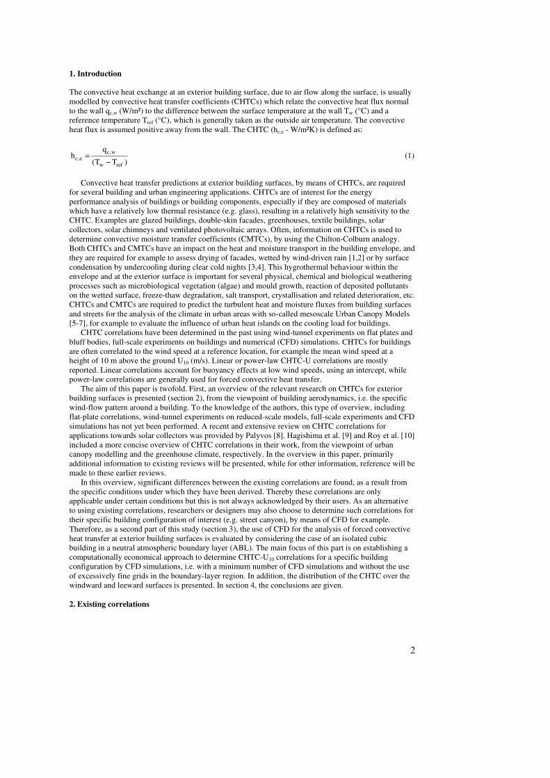
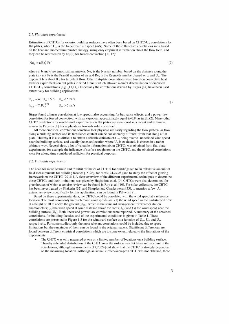
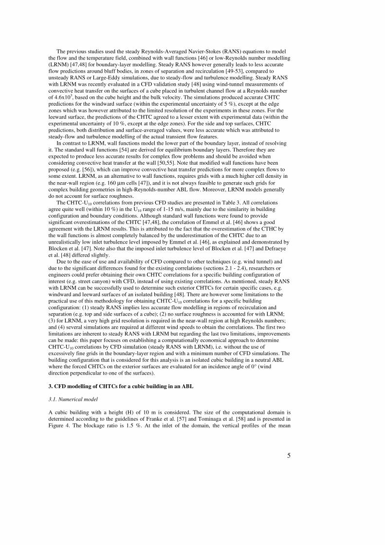
Based on these experimental data, the CHTC could be correlated with the wind speed at a reference
location. The most commonly used reference wind speeds are: (1) the wind speed in the undisturbed flow
at a height of 10 m above the ground (U10), which is the standard arrangement for weather station
anemometers; (2) the wind speed at some distance above the roof (UR); and (3) the wind speed near the
building surface (US). Both linear and power-law correlations were reported. A summary of the obtained
correlations, for building facades, and of the experimental conditions is given in Table 1. These
correlations are presented in Figure 1-3 for the windward surface as a function of U10, UR and US,
respectively. For some studies, only the most relevant correlations could be included due to space
limitations but the remainder of them can be found in the original papers. Significant differences are
found between different empirical correlations which are to some extent related to the limitations of the
experiments:
• The CHTC was only measured at one or a limited number of locations on a building surface.
Thereby a detailed distribution of the CHTC over the surface was not taken into account in the
correlations, although measurements [17,20,24] did show that the CHTC is strongly dependent
on the measuring location. Although an actual surface-averaged CHTC was not obtained, these

4
point-wise CHTC data are often used as if they are valid for an entire surface. Such limited
spatial resolution, however, is characteristic for full-scale experiments.
• The CHTC at a certain location on the surface, and also US or UR, are in reality related to the
specific flow field near the building surface. The measurements of all these parameters are
therefore case-specific: their values are influenced by the specific building geometry, building
surroundings and location of the measurement positions. These influences are embedded in the
CHTC-U correlations, which are therefore also case-specific.
• Apart from the work of Hagishima and Tanimoto [24], the influence of turbulent fluctuations on
the CHTC has not been taken into account in the correlations.
• The influence of the wind direction was generally taken into account by classifying a surface as
windward or leeward, where windward covers the whole range of wind directions with incidence
angles from -90° to 90°. The incidence angle is defined as the angle between the approach flow
wind direction and the normal to the windward surface. Lui and Harris [26] however showed
that a more detailed dependency on the wind direction is required.
• Mostly smooth surfaces were considered in the analyses and the influence of different surface
roughness on the CHTC was not addressed.
• Due to the difference in thermal stratification of the atmospheric boundary layer (ABL) during
daytime or nighttime, the flow field around the building and thus the obtained correlation
depended to some extent on the measuring period, especially for low wind speeds.
Although full-scale experiments can provide realistic CHTC data for exterior building surfaces, the large
variety in building configurations, boundary conditions and experimental setups usually resulted in quite
case-specific correlations which are not always applicable for other types of buildings and other boundary
conditions.
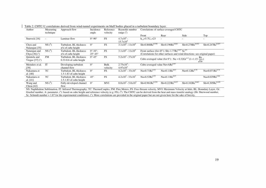
2.3. Wind-tunnel experiments
A significant amount of research has been performed by wind-tunnel experiments of convective heat
transfer of isolated bluff bodies, mostly cubes, placed in a turbulent boundary layer [16,34-42]. In contrast
to full-scale experiments, detailed information of the distribution of the CHTC over each surface, its
relation with the flow field and the dependency on flow direction was provided. Surface-averaged values
of the CHTC and their correlation with the air speed were mostly reported, providing a better estimate of
the overall heat loss from a surface than the single-point measurements in full-scale experiments. The
obtained correlations and the experimental conditions are presented in Table 2. Note that some
correlations (obtained with the naphthalene sublimation technique) rely on the analogy between heat and
mass transfer to estimate the CHTC [35,36,42]. A remarkable correspondence is found for the exponent b
(Eq.(2)), especially for windward (b ≈ 0.53) and leeward (b ≈ 0.66) surfaces.
Since most of these experiments were not performed in the context of building engineering/building
aerodynamics, they were usually carried out for rather thin turbulent boundary layers, with respect to the
body height, and at relatively low Reynolds numbers, compared to those typically encountered for
buildings. These boundary conditions limit the applicability of these CHTC correlations for exterior
building surfaces, although this type of (wind-tunnel) experiments itself is very valuable to determine
CHTCs.
Note that, apart from wind-tunnel experiments on isolated bluff bodies, a significant amount of
research has been done (not mentioned in Table 2) on the determination of CHTCs/CMTCs for urban
surfaces, such as street canyons (e.g. [43-45]), for which corresponding references can be found in
Hagishima et al. [9].
2.4. Numerical methods
Recently, Computational Fluid Dynamics was used to predict convective heat transfer at exterior building
surfaces [46-48]. The main advantages of CFD for this application are that: (1) a specific and complex
building or building configuration can be analysed; (2) very high spatial resolution data are obtained; (3)
high Reynolds number flows for atmospheric conditions (105-107) can be considered and (4) detailed
information on the flow field as well as the thermal field is available. In these previous studies, this
allowed for a detailed analysis of: the CHTC distribution over building surfaces; the influence of
turbulence and wind direction; the correlation with different reference wind speeds (U10, US); the thermal
boundary layer etc. However, some important limitations of the applied numerical models have to be
emphasised.
5
The previous studies used the steady Reynolds-Averaged Navier-Stokes (RANS) equations to model
the flow and the temperature field, combined with wall functions [46] or low-Reynolds number modelling
(LRNM) [47,48] for boundary-layer modelling. Steady RANS however generally leads to less accurate
flow predictions around bluff bodies, in zones of separation and recirculation [49-53], compared to
unsteady RANS or Large-Eddy simulations, due to steady-flow and turbulence modelling. Steady RANS
with LRNM was recently evaluated in a CFD validation study [48] using wind-tunnel measurements of
convective heat transfer on the surfaces of a cube placed in turbulent channel flow at a Reynolds number
of 4.6x10³, based on the cube height and the bulk velocity. The simulations produced accurate CHTC
predictions for the windward surface (within the experimental uncertainty of 5 %), except at the edge
zones which was however attributed to the limited resolution of the experiments in these zones. For the
leeward surface, the predictions of the CHTC agreed to a lesser extent with experimental data (within the
experimental uncertainty of 10 %, except at the edge zones). For the side and top surfaces, CHTC
predictions, both distribution and surface-averaged values, were less accurate which was attributed to
steady-flow and turbulence modelling of the actual transient flow features.
In contrast to LRNM, wall functions model the lower part of the boundary layer, instead of resolving
it. The standard wall functions [54] are derived for equilibrium boundary layers. Therefore they are
expected to produce less accurate results for complex flow problems and should be avoided when
considering convective heat transfer at the wall [50,55]. Note that modified wall functions have been
proposed (e.g. [56]), which can improve convective heat transfer predictions for more complex flows to
some extent. LRNM, as an alternative to wall functions, requires grids with a much higher cell density in
the near-wall region (e.g. 160 µm cells [47]), and it is not always feasible to generate such grids for
complex building geometries in high-Reynolds-number ABL flow. Moreover, LRNM models generally
do not account for surface roughness.
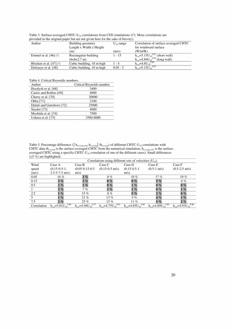
The CHTC-U10 correlations from previous CFD studies are presented in Table 3. All correlations
agree quite well (within 10 %) in the U10 range of 1-15 m/s, mainly due to the similarity in building
configuration and boundary conditions. Although standard wall functions were found to provide
significant overestimations of the CHTC [47,48], the correlation of Emmel et al. [46] shows a good
agreement with the LRNM results. This is attributed to the fact that the overestimation of the CTHC by
the wall functions is almost completely balanced by the underestimation of the CHTC due to an
unrealistically low inlet turbulence level imposed by Emmel et al. [46], as explained and demonstrated by
Blocken et al. [47]. Note also that the imposed inlet turbulence level of Blocken et al. [47] and Defraeye
et al. [48] differed slightly.
Due to the ease of use and availability of CFD compared to other techniques (e.g. wind tunnel) and
due to the significant differences found for the existing correlations (sections 2.1 - 2.4), researchers or
engineers could prefer obtaining their own CHTC correlations for a specific building configuration of
interest (e.g. street canyon) with CFD, instead of using existing correlations. As mentioned, steady RANS
with LRNM can be successfully used to determine such exterior CHTCs for certain specific cases, e.g.
windward and leeward surfaces of an isolated building [48]. There are however some limitations to the
practical use of this methodology for obtaining CHTC-U10 correlations for a specific building
configuration: (1) steady RANS implies less accurate flow modelling in regions of recirculation and
separation (e.g. top and side surfaces of a cube); (2) no surface roughness is accounted for with LRNM;
(3) for LRNM, a very high grid resolution is required in the near-wall region at high Reynolds numbers;
and (4) several simulations are required at different wind speeds to obtain the correlations. The first two
limitations are inherent to steady RANS with LRNM but regarding the last two limitations, improvements
can be made: this paper focuses on establishing a computationally economical approach to determine
CHTC-U10 correlations by CFD simulation (steady RANS with LRNM), i.e. without the use of
excessively fine grids in the boundary-layer region and with a minimum number of CFD simulations. The
building configuration that is considered for this analysis is an isolated cubic building in a neutral ABL
where the forced CHTCs on the exterior surfaces are evaluated for an incidence angle of 0° (wind
direction perpendicular to one of the surfaces).
3. CFD modelling of CHTCs for a cubic building in an ABL
3.1. Numerical model
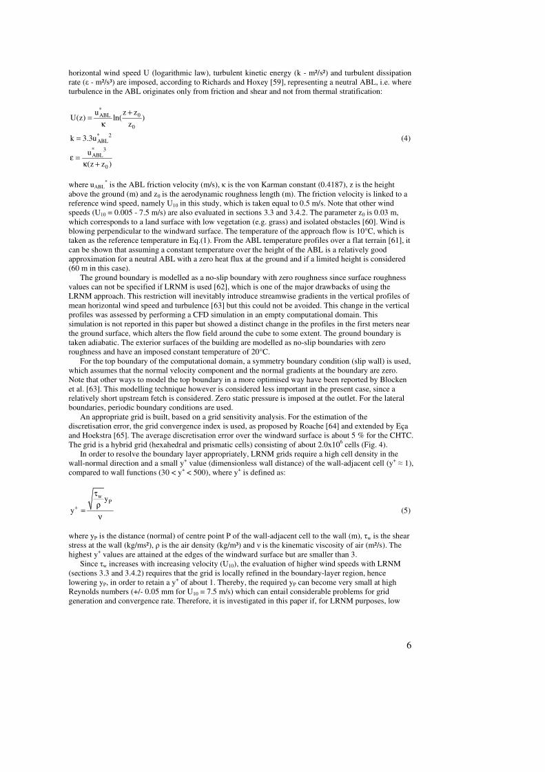
A cubic building with a height (H) of 10 m is considered. The size of the computational domain is
determined according to the guidelines of Franke et al. [57] and Tominaga et al. [58] and is presented in
Figure 4. The blockage ratio is 1.5 %. At the inlet of the domain, the vertical profiles of the mean
6
horizontal wind speed U (logarithmic law), turbulent kinetic energy (k - m²/s²) and turbulent dissipation
rate (ε - m²/s³) are imposed, according to Richards and Hoxey [59], representing a neutral ABL, i.e. where
turbulence in the ABL originates only from friction and shear and not from thermal stratification:
*
0ABL
0
* 2ABL
* 3ABL
0
z zuU(z) ln( )
z
k 3.3u
u
(z z )
+=
κ
=
ε =κ +
(4)
where uABL* is the ABL friction velocity (m/s), κ is the von Karman constant (0.4187), z is the height
above the ground (m) and z0 is the aerodynamic roughness length (m). The friction velocity is linked to a
reference wind speed, namely U10 in this study, which is taken equal to 0.5 m/s. Note that other wind
speeds (U10 = 0.005 - 7.5 m/s) are also evaluated in sections 3.3 and 3.4.2. The parameter z0 is 0.03 m,
which corresponds to a land surface with low vegetation (e.g. grass) and isolated obstacles [60]. Wind is
blowing perpendicular to the windward surface. The temperature of the approach flow is 10°C, which is
taken as the reference temperature in Eq.(1). From the ABL temperature profiles over a flat terrain [61], it
can be shown that assuming a constant temperature over the height of the ABL is a relatively good
approximation for a neutral ABL with a zero heat flux at the ground and if a limited height is considered
(60 m in this case).
The ground boundary is modelled as a no-slip boundary with zero roughness since surface roughness
values can not be specified if LRNM is used [62], which is one of the major drawbacks of using the
LRNM approach. This restriction will inevitably introduce streamwise gradients in the vertical profiles of
mean horizontal wind speed and turbulence [63] but this could not be avoided. This change in the vertical
profiles was assessed by performing a CFD simulation in an empty computational domain. This
simulation is not reported in this paper but showed a distinct change in the profiles in the first meters near
the ground surface, which alters the flow field around the cube to some extent. The ground boundary is
taken adiabatic. The exterior surfaces of the building are modelled as no-slip boundaries with zero
roughness and have an imposed constant temperature of 20°C.
For the top boundary of the computational domain, a symmetry boundary condition (slip wall) is used,
which assumes that the normal velocity component and the normal gradients at the boundary are zero.
Note that other ways to model the top boundary in a more optimised way have been reported by Blocken
et al. [63]. This modelling technique however is considered less important in the present case, since a
relatively short upstream fetch is considered. Zero static pressure is imposed at the outlet. For the lateral
boundaries, periodic boundary conditions are used.
An appropriate grid is built, based on a grid sensitivity analysis. For the estimation of the
discretisation error, the grid convergence index is used, as proposed by Roache [64] and extended by Eça
and Hoekstra [65]. The average discretisation error over the windward surface is about 5 % for the CHTC.
The grid is a hybrid grid (hexahedral and prismatic cells) consisting of about 2.0x10⁶ cells (Fig. 4).
In order to resolve the boundary layer appropriately, LRNM grids require a high cell density in the
wall-normal direction and a small y+ value (dimensionless wall distance) of the wall-adjacent cell (y+ ≈ 1),
compared to wall functions (30 < y+ < 500), where y+ is defined as:
wPy
y+
τ
ρ=
ν (5)
where yP is the distance (normal) of centre point P of the wall-adjacent cell to the wall (m), τw is the shear
stress at the wall (kg/ms²), ρ is the air density (kg/m³) and ν is the kinematic viscosity of air (m²/s). The
highest y+ values are attained at the edges of the windward surface but are smaller than 3.
Since τw increases with increasing velocity (U10), the evaluation of higher wind speeds with LRNM
(sections 3.3 and 3.4.2) requires that the grid is locally refined in the boundary-layer region, hence
lowering yP, in order to retain a y+ of about 1. Thereby, the required yP can become very small at high
Reynolds numbers (+/- 0.05 mm for U10 = 7.5 m/s) which can entail considerable problems for grid
generation and convergence rate. Therefore, it is investigated in this paper if, for LRNM purposes, low
7
wind speeds, and hence a relatively large yP, can be used to determine CHTC-U10 correlations (see
sections 3.3 and 3.4.2).
3.2. Numerical simulation
The simulations are performed with the CFD package Fluent 6.3, which uses the control volume method.
Steady RANS is used in combination with a turbulence model. The realizable k-ε model [66] is used
together with LRNM to take care of the viscosity-affected region, for which the one-equation Wolfshtein
model [67] is used. Note that this realizable k-ε turbulence model with LRNM was evaluated in the
previously mentioned CFD validation study (section 2.4, [48]) where a good agreement with experimental
data was obtained for both windward and leeward surfaces. Based on the results of this validation study,
the focus will be only on these two surfaces.
The focus of this paper is on forced convection where the possibility of using low speeds to determine
CHTC-U10 correlations, for LRNM purposes, is investigated. Therefore, buoyancy effects are not taken
into account in the simulations, since they will otherwise affect the air flow field at such low Reynolds
numbers. Radiation is also not considered in the simulations since the focus was only on forced
convection, and fixed temperature boundary conditions are used for the building surfaces.
Second-order discretisation schemes are used throughout. The SIMPLE algorithm is used for
pressure-velocity coupling. Pressure interpolation is second order. Convergence was assessed by
monitoring the velocity, turbulent kinetic energy and temperature on specific locations in the flow field
and heat fluxes on the surface of the cube.
3.3. Reynolds number dependence of the flow field
The intention is to determine the forced CHTC-U10 correlations at relatively low U10 (Reynolds numbers),
without compromising their accuracy for use at higher U10. The motivation for using low U10 is
computational economy when using the fine LRNM grids. To allow extrapolation to higher U10, Reynolds
number independence should be achieved. This implies that the overall flow field around the building at
low U10 is similar to that found at higher Reynolds numbers (U10 = 5 - 15 m/s), typical for forced
convective ABL flow. Otherwise, the CHTC distribution over the different surfaces will differ. For sharp-
edged bluff bodies, which have fixed separation points, namely the edges, and which are immersed in
deep turbulent boundary layers, such as the ABL, it is generally assumed in wind-tunnel testing that the
flow field becomes independent of the Reynolds number once a certain Reynolds number is exceeded.
This threshold value is called the critical Reynolds number, Recr. Reynolds number independence was
confirmed by wind-tunnel experiments [68-75] and the corresponding Recr values, based on the building
height (H) and the wind speed at that height (UH), are reported in Table 4. Note however that most of
these experiments were not always extensive studies on this Reynolds number effect or were performed
for a restricted Reynolds number range. Some studies [75-77] showed that Reynolds number dependency
is influenced by wind direction, building geometry and the location on the surface and that it can differ
for mean and fluctuating flow quantities, which could partially explain the differences found in Table 4.
Since this study specifically aims at determining the CHTC at low wind speeds, for LRNM purposes,
the Reynolds number dependency in the numerical simulations is investigated by analysing the flow field
at different wind speeds, namely for U10 = 0.005, 0.05, 0.15, 0.5 and 5 m/s, resulting in Reynolds numbers
of 3.5x10³ to 3.5x10
6, based on the building height H and U10. Note that the focus is on the overall flow
field, not on the flow in the boundary layer near the building surface. Since the simulations are steady,
any Reynolds number dependency by unsteady behaviour (e.g. vortex shedding) is not captured.
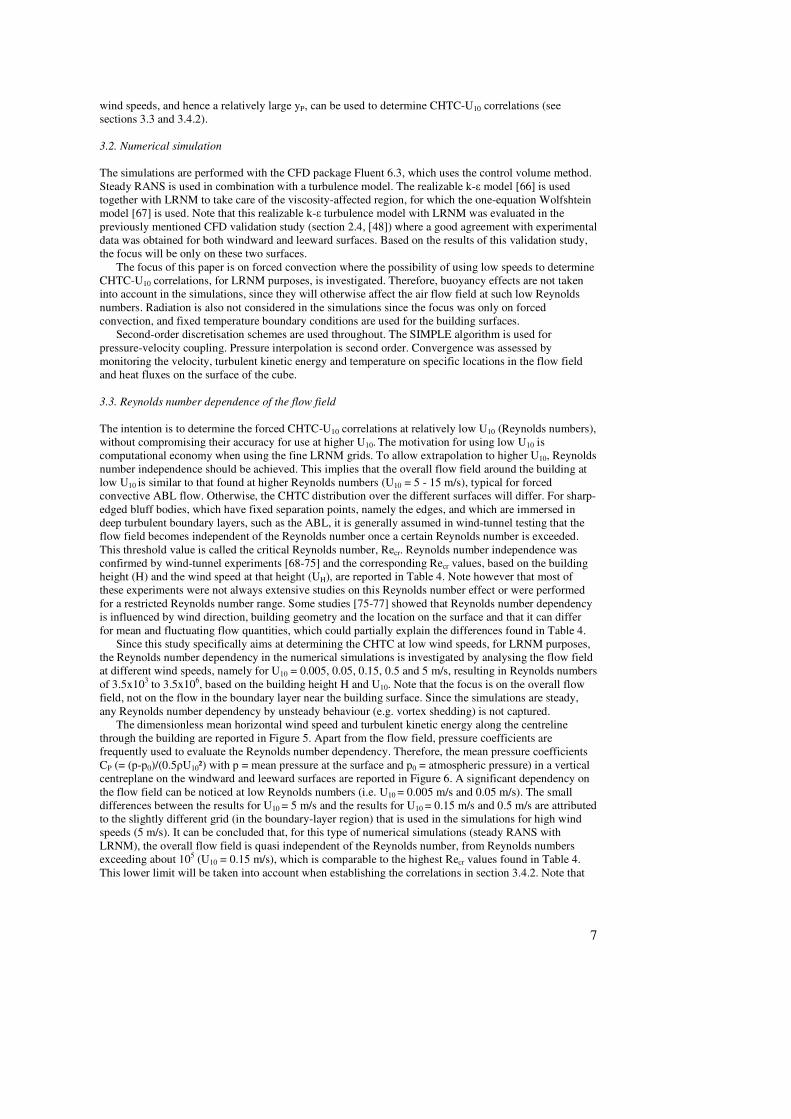
The dimensionless mean horizontal wind speed and turbulent kinetic energy along the centreline
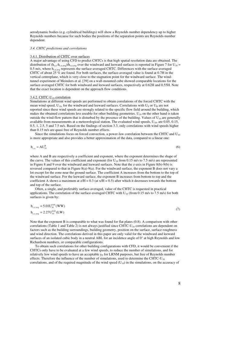
through the building are reported in Figure 5. Apart from the flow field, pressure coefficients are
frequently used to evaluate the Reynolds number dependency. Therefore, the mean pressure coefficients
CP (= (p-p0)/(0.5ρU10²) with p = mean pressure at the surface and p0 = atmospheric pressure) in a vertical
centreplane on the windward and leeward surfaces are reported in Figure 6. A significant dependency on
the flow field can be noticed at low Reynolds numbers (i.e. U10 = 0.005 m/s and 0.05 m/s). The small
differences between the results for U10 = 5 m/s and the results for U10 = 0.15 m/s and 0.5 m/s are attributed
to the slightly different grid (in the boundary-layer region) that is used in the simulations for high wind
speeds (5 m/s). It can be concluded that, for this type of numerical simulations (steady RANS with
LRNM), the overall flow field is quasi independent of the Reynolds number, from Reynolds numbers
exceeding about 105 (U10 = 0.15 m/s), which is comparable to the highest Recr values found in Table 4.
This lower limit will be taken into account when establishing the correlations in section 3.4.2. Note that
8
aerodynamic bodies (e.g. cylindrical buildings) will show a Reynolds number dependency up to higher
Reynolds numbers because for such bodies the positions of the separation points are Reynolds-number
dependent.
3.4. CHTC predictions and correlations
3.4.1. Distribution of CHTC over surfaces
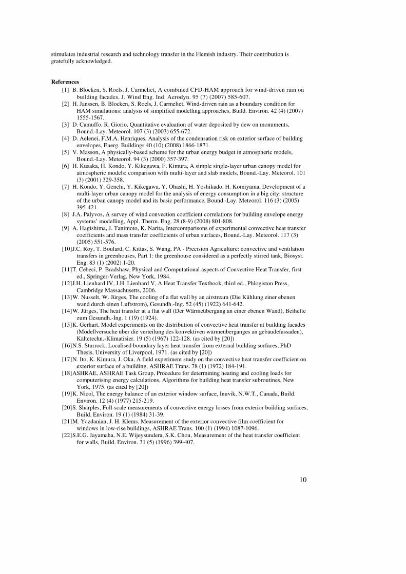
A major advantage of using CFD to predict CHTCs is that high spatial resolution data are obtained. The
distribution of (hc,e-hc,e,avg)/hc,e,avg over the windward and leeward surfaces is reported in Figure 7 for U10 =
0.5 m/s, where hc,e,avg represents the surface-averaged CHTC. Differences with the surface-averaged
CHTC of about 25 % are found. For both surfaces, the surface-averaged value is found at 0.7H in the
vertical centreplane, which is very close to the stagnation point for the windward surface. The wind-
tunnel experiment of Meinders et al. [39] on a wall-mounted cube showed comparable locations for the
surface-averaged CHTC for both windward and leeward surfaces, respectively at 0.62H and 0.55H. Note
that the exact location is dependent on the approach flow conditions.
3.4.2. CHTC-U10 correlation
Simulations at different wind speeds are performed to obtain correlations of the forced CHTC with the
mean wind speed, U10, for the windward and leeward surfaces. Correlations with US or UR are not
reported since these wind speeds are strongly related to the specific flow field around the building, which
makes the obtained correlations less useable for other building geometries. U10 on the other hand is taken
outside the wind-flow pattern that is disturbed by the presence of the building. Values of U10 are generally
available from measurements at a meteorological station. The evaluated wind speeds, U10, are 0.05, 0.15,
0.5, 1, 2.5, 5 and 7.5 m/s. Based on the findings of section 3.3, only correlations with wind speeds higher
than 0.15 m/s are quasi free of Reynolds number effects.
Since the simulations focus on forced convection, a power-law correlation between the CHTC and U10
is more appropriate and also provides a better approximation of the data, compared to a linear one:
B
c,e 10h AU= (6)
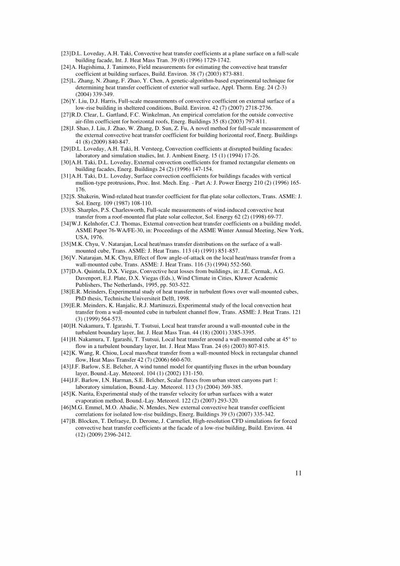
where A and B are respectively a coefficient and exponent, where the exponent determines the shape of
the curve. The values of this coefficient and exponent (for U10 from 0.15 m/s to 7.5 m/s) are represented
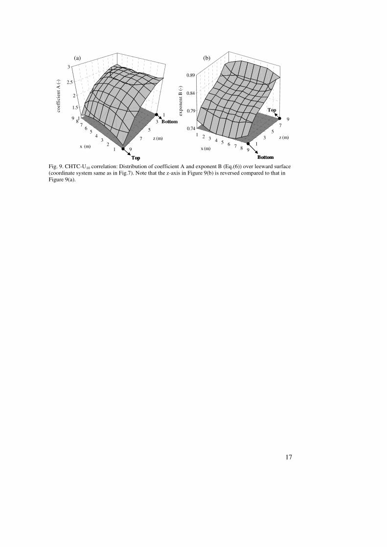
in Figure 8 and 9 over the windward and leeward surfaces. Note that the z-axis in Figure 8(b)-9(b) is
reversed compared to that in Figure 8(a)-9(a). For the windward surface, the exponent B does not vary a
lot except for the zone near the ground surface. The coefficient A increases from the bottom to the top of
the windward surface. For the leeward surface, the exponent B increases from bottom to top and the
coefficient A shows a maximum at z/H = 0.3 (at x/H = 0.5) after which it decreases towards the bottom
and top of the surface.
Often, a single, and preferably surface-averaged, value of the CHTC is requested in practical
applications. The correlation of the surface-averaged CHTC with U10 (from 0.15 m/s to 7.5 m/s) for both
surfaces is given by:
0.85
c,e,avg 10
0.83
c,e,avg 10
h 5.01U (WW)
h 2.27U (LW)
=
= (7)
Note that the exponent B is comparable to what was found for flat plates (0.8). A comparison with other
correlations (Table 1 and Table 2) is not always justified since CHTC-U10 correlations are dependent on
factors such as the building surroundings, building geometry, position on the surface, surface roughness
and wind direction. The correlations derived in this paper are only valid for the windward and leeward
surfaces of an isolated cubic body in a neutral ABL for an incidence angle of 0° at high Reynolds and low
Richardson numbers, or comparable configurations.
To obtain such correlations for other building configurations with CFD, it would be convenient if the
CHTCs only have to be evaluated at a few wind speeds, to reduce the number of simulations, and for
relatively low wind speeds to have an acceptable yP for LRNM purposes, but free of Reynolds number
effects. Therefore the influence of the number of simulations, used to determine the CHTC-U10
correlations, and of the required magnitude of the wind speed (U10) in the simulations, on the accuracy of

9
the obtained correlations is investigated. For this, surface-averaged CHTC data from CFD (hc,e,avg) for the
windward surface are used to compose several CHTC-U10 correlations (cases) by approximation, by only
using CHTC data at a limited number of wind speeds U10 (predominantly low wind speeds and a low
number of wind speeds). The accuracy of such a specific CHTC-U10 correlation is evaluated by
comparing the surface-averaged CHTC, predicted by the correlation (hc,e,avg,corr), to the actual CHTC data
(hc,e,avg) at several wind speeds. The difference │hc,e,avg,corr-hc,e,avg│/hc,e,avg is presented in Table 5 for these
different cases. Note that accurate CHTC-U10 correlations by using CFD data at low wind speeds should
also provide accurate predictions for higher wind speeds (Reynolds numbers).
Case A, in Table 5, is composed using all evaluated wind speeds which are quasi free of Reynolds
number effects and therefore obviously gives a good approximation over the whole range of wind speeds.
At U10 = 0.05 m/s, a large difference is found, which is attributed to Reynolds number effects. If this wind
speed is used in a correlation (case B), large errors are therefore found when extrapolating to high U10.
For case C and D, still observable extrapolation errors are found at high wind speeds. Since case E (0.5 -
1 m/s) provides a much more accurate extrapolation, the errors for case C and case D could be attributed
to a remaining, but small, Reynolds dependency for U10 = 0.15 m/s. It is shown that correlations with two
wind speeds (case E and case F) and with relatively low wind speeds can provide accurate estimates of
the CHTC and do not necessarily have to cover a large Reynolds number range. Note that these wind
speeds are about a factor 10 lower that those found for a typical forced convective ABL. This implies that
the grid resolution in the boundary layer can roughly be taken a factor 10 coarser. Based on this study, it
is advised that, if CHTC-U10 correlations for sharp-edged buildings in turbulent boundary layers are
obtained with CFD, simulations are made with at least two wind speeds corresponding to a minimum
Reynolds number of about 3x10⁵ and where the lowest and highest wind speed differ with at least a factor
2.
4. Conclusions
In a first part, an overview of the research on CHTC correlations for exterior building surfaces was given
and some limitations of each methodology were identified. A large variation in the CHTC-U correlations
was found, which was related to the specific conditions under which each correlation was derived,
limiting to some extent their applicability for other building configurations.
In a second part, an alternative to using existing CHTC-U correlations was explored, namely the use
of CFD for the prediction of forced CHTCs for a specific building configuration. The focus was on an
isolated cubic building in a neutral ABL at an incidence angle of 0°. Only the windward and leeward
surfaces were considered since an earlier validation study showed that accurate CHTC predictions could
be obtained here with steady RANS if combined with LRNM, instead of the commonly used wall
functions.
The aim of this study was to improve the practical use of steady RANS with LRNM to obtain CHTC-
U10 correlations. For steady RANS and for a sharp-edged building, the overall flow field was found to
become quasi independent of the Reynolds number at Reynolds numbers of about 105, based on H and
U10. Thereby the CHTC-U10 correlations could be determined by using relatively low wind speeds (U10 ≈
1 m/s), which avoids the use of excessively fine grids for LRNM, and still provide a good approximation
for higher wind speeds by extrapolation. Moreover, evaluating only two or three wind speeds was found
to be sufficient to provide accurate correlations, which reduces the required number of CFD simulations.
Furthermore the CHTC was found to vary significantly across windward and leeward surfaces and the
CHTC was found to be equal to the surface-averaged CHTC at a height of approximately 0.7H for both
surfaces. The local CHTC-U10 (power-law) correlation (Eq.(6)) was characterised by an exponent B
which was quasi-constant for the windward surface, but which varied significantly over the leeward
surface.
Conflict of interest statement
The authors of the manuscript entitled: “Convective heat transfer coefficients for exterior building
surfaces: Existing correlations and CFD modelling” do not have any conflict of interest.
Acknowledgements
This research is funded by the Government of Flanders. As a Flemish government institution, IWT-
Flanders (Institute for the Promotion of Innovation by Science and Technology in Flanders) supports and
10
stimulates industrial research and technology transfer in the Flemish industry. Their contribution is
gratefully acknowledged.
References
[1] B. Blocken, S. Roels, J. Carmeliet, A combined CFD-HAM approach for wind-driven rain on
building facades, J. Wind Eng. Ind. Aerodyn. 95 (7) (2007) 585-607.
[2] H. Janssen, B. Blocken, S. Roels, J. Carmeliet, Wind-driven rain as a boundary condition for
HAM simulations: analysis of simplified modelling approaches, Build. Environ. 42 (4) (2007)
1555-1567.
[3] D. Camuffo, R. Giorio, Quantitative evaluation of water deposited by dew on monuments,
Bound.-Lay. Meteorol. 107 (3) (2003) 655-672.
[4] D. Aelenei, F.M.A. Henriques, Analysis of the condensation risk on exterior surface of building
envelopes, Energ. Buildings 40 (10) (2008) 1866-1871.
[5] V. Masson, A physically-based scheme for the urban energy budget in atmospheric models,
Bound.-Lay. Meteorol. 94 (3) (2000) 357-397.
[6] H. Kusaka, H. Kondo, Y. Kikegawa, F. Kimura, A simple single-layer urban canopy model for
atmospheric models: comparison with multi-layer and slab models, Bound.-Lay. Meteorol. 101
(3) (2001) 329-358.
[7] H. Kondo, Y. Genchi, Y. Kikegawa, Y. Ohashi, H. Yoshikado, H. Komiyama, Development of a
multi-layer urban canopy model for the analysis of energy consumption in a big city: structure
of the urban canopy model and its basic performance, Bound.-Lay. Meteorol. 116 (3) (2005)
395-421.
[8] J.A. Palyvos, A survey of wind convection coefficient correlations for building envelope energy
systems’ modelling, Appl. Therm. Eng. 28 (8-9) (2008) 801-808.
[9] A. Hagishima, J. Tanimoto, K. Narita, Intercomparisons of experimental convective heat transfer
coefficients and mass transfer coefficients of urban surfaces, Bound.-Lay. Meteorol. 117 (3)
(2005) 551-576.
[10] J.C. Roy, T. Boulard, C. Kittas, S. Wang, PA - Precision Agriculture: convective and ventilation
transfers in greenhouses, Part 1: the greenhouse considered as a perfectly stirred tank, Biosyst.
Eng. 83 (1) (2002) 1-20.
[11] T. Cebeci, P. Bradshaw, Physical and Computational aspects of Convective Heat Transfer, first
ed., Springer-Verlag, New York, 1984.
[12] J.H. Lienhard IV, J.H. Lienhard V, A Heat Transfer Textbook, third ed., Phlogiston Press,
Cambridge Massachusetts, 2006.
[13] W. Nusselt, W. Jürges, The cooling of a flat wall by an airstream (Die Kühlung einer ebenen
wand durch einen Luftstrom), Gesundh.-Ing. 52 (45) (1922) 641-642.
[14] W. Jürges, The heat transfer at a flat wall (Der Wärmeübergang an einer ebenen Wand), Beihefte
zum Gesundh.-Ing. 1 (19) (1924).
[15] K. Gerhart, Model experiments on the distribution of convective heat transfer at building facades
(Modellversuche über die verteilung des konvektiven wärmeüberganges an gebäudefassaden),
Kältetechn.-Klimatisier. 19 (5) (1967) 122-128. (as cited by [20])
[16] N.S. Sturrock, Localised boundary layer heat transfer from external building surfaces, PhD
Thesis, University of Liverpool, 1971. (as cited by [20])
[17] N. Ito, K. Kimura, J. Oka, A field experiment study on the convective heat transfer coefficient on
exterior surface of a building, ASHRAE Trans. 78 (1) (1972) 184-191.
[18] ASHRAE, ASHRAE Task Group, Procedure for determining heating and cooling loads for
computerising energy calculations, Algorithms for building heat transfer subroutines, New
York, 1975. (as cited by [20])
[19] K. Nicol, The energy balance of an exterior window surface, Inuvik, N.W.T., Canada, Build.
Environ. 12 (4) (1977) 215-219.
[20] S. Sharples, Full-scale measurements of convective energy losses from exterior building surfaces,
Build. Environ. 19 (1) (1984) 31-39.
[21] M. Yazdanian, J. H. Klems, Measurement of the exterior convective film coefficient for
windows in low-rise buildings, ASHRAE Trans. 100 (1) (1994) 1087-1096.
[22] S.E.G. Jayamaha, N.E. Wijeysundera, S.K. Chou, Measurement of the heat transfer coefficient
for walls, Build. Environ. 31 (5) (1996) 399-407.
11
[23] D.L. Loveday, A.H. Taki, Convective heat transfer coefficients at a plane surface on a full-scale
building facade, Int. J. Heat Mass Tran. 39 (8) (1996) 1729-1742.
[24] A. Hagishima, J. Tanimoto, Field measurements for estimating the convective heat transfer
coefficient at building surfaces, Build. Environ. 38 (7) (2003) 873-881.
[25] L. Zhang, N. Zhang, F. Zhao, Y. Chen, A genetic-algorithm-based experimental technique for
determining heat transfer coefficient of exterior wall surface, Appl. Therm. Eng. 24 (2-3)
(2004) 339-349.
[26] Y. Liu, D.J. Harris, Full-scale measurements of convective coefficient on external surface of a
low-rise building in sheltered conditions, Build. Environ. 42 (7) (2007) 2718-2736.
[27] R.D. Clear, L. Gartland, F.C. Winkelman, An empirical correlation for the outside convective
air-film coefficient for horizontal roofs, Energ. Buildings 35 (8) (2003) 797-811.
[28] J. Shao, J. Liu, J. Zhao, W. Zhang, D. Sun, Z. Fu, A novel method for full-scale measurement of
the external convective heat transfer coefficient for building horizontal roof, Energ. Buildings
41 (8) (2009) 840-847.
[29] D.L. Loveday, A.H. Taki, H. Versteeg, Convection coefficients at disrupted building facades:
laboratory and simulation studies, Int. J. Ambient Energ. 15 (1) (1994) 17-26.
[30] A.H. Taki, D.L. Loveday, External convection coefficients for framed rectangular elements on
building facades, Energ. Buildings 24 (2) (1996) 147-154.
[31] A.H. Taki, D.L. Loveday, Surface convection coefficients for buildings facades with vertical
mullion-type protrusions, Proc. Inst. Mech. Eng. - Part A: J. Power Energy 210 (2) (1996) 165-
176.
[32] S. Shakerin, Wind-related heat transfer coefficient for flat-plate solar collectors, Trans. ASME: J.
Sol. Energ. 109 (1987) 108-110.
[33] S. Sharples, P.S. Charlesworth, Full-scale measurements of wind-induced convective heat
transfer from a roof-mounted flat plate solar collector, Sol. Energy 62 (2) (1998) 69-77.
[34] W.J. Kelnhofer, C.J. Thomas, External convection heat transfer coefficients on a building model,
ASME Paper 76-WA/FE-30, in: Proceedings of the ASME Winter Annual Meeting, New York,
USA, 1976.
[35] M.K. Chyu, V. Natarajan, Local heat/mass transfer distributions on the surface of a wall-
mounted cube, Trans. ASME: J. Heat Trans. 113 (4) (1991) 851-857.
[36] V. Natarajan, M.K. Chyu, Effect of flow angle-of-attack on the local heat/mass transfer from a
wall-mounted cube, Trans. ASME: J. Heat Trans. 116 (3) (1994) 552-560.
[37] D.A. Quintela, D.X. Viegas, Convective heat losses from buildings, in: J.E. Cermak, A.G.
Davenport, E.J. Plate, D.X. Viegas (Eds.), Wind Climate in Cities, Kluwer Academic
Publishers, The Netherlands, 1995, pp. 503-522.
[38] E.R. Meinders, Experimental study of heat transfer in turbulent flows over wall-mounted cubes,
PhD thesis, Technische Universiteit Delft, 1998.
[39] E.R. Meinders, K. Hanjalic, R.J. Martinuzzi, Experimental study of the local convection heat
transfer from a wall-mounted cube in turbulent channel flow, Trans. ASME: J. Heat Trans. 121
(3) (1999) 564-573.
[40] H. Nakamura, T. Igarashi, T. Tsutsui, Local heat transfer around a wall-mounted cube in the
turbulent boundary layer, Int. J. Heat Mass Tran. 44 (18) (2001) 3385-3395.
[41] H. Nakamura, T. Igarashi, T. Tsutsui, Local heat transfer around a wall-mounted cube at 45° to
flow in a turbulent boundary layer, Int. J. Heat Mass Tran. 24 (6) (2003) 807-815.
[42] K. Wang, R. Chiou, Local mass/heat transfer from a wall-mounted block in rectangular channel
flow, Heat Mass Transfer 42 (7) (2006) 660-670.
[43] J.F. Barlow, S.E. Belcher, A wind tunnel model for quantifying fluxes in the urban boundary
layer, Bound.-Lay. Meteorol. 104 (1) (2002) 131-150.
[44] J.F. Barlow, I.N. Harman, S.E. Belcher, Scalar fluxes from urban street canyons part 1:
laboratory simulation, Bound.-Lay. Meteorol. 113 (3) (2004) 369-385.
[45] K. Narita, Experimental study of the transfer velocity for urban surfaces with a water
evaporation method, Bound.-Lay. Meteorol. 122 (2) (2007) 293-320.
[46] M.G. Emmel, M.O. Abadie, N. Mendes, New external convective heat transfer coefficient
correlations for isolated low-rise buildings, Energ. Buildings 39 (3) (2007) 335-342.
[47] B. Blocken, T. Defraeye, D. Derome, J. Carmeliet, High-resolution CFD simulations for forced
convective heat transfer coefficients at the facade of a low-rise building, Build. Environ. 44
(12) (2009) 2396-2412.
12
[48] T. Defraeye, B. Blocken, J. Carmeliet, CFD analysis of convective heat transfer at the surfaces of
a cube immersed in a turbulent boundary layer, Int. J. Heat Mass Tran. 53 (1-3) (2010) 297-
308.
[49] M. Murakami, A. Mochida, Y. Hayashi, Examining the k-ε model by means of a wind tunnel test
and Large-Eddy simulation of the turbulence structure around a cube, J. Wind Eng. Ind.
Aerodyn. 35 (1990) 87-100.
[50] S. Murakami, Comparison of various turbulence models applied to a bluff body, J. Wind Eng.
Ind. Aerodyn. 46-47 (1993) 21-36.
[51] S. Murakami, A. Mochida, R. Ooka, S. Kato, S. Iizuka, Numerical prediction of flow around a
building with various turbulence models: comparison of k-ε EVM, ASM, DSM and LES with
wind tunnel tests, ASHRAE Trans. 102 (1) (1996) 741-753.
[52] G. Iaccarino, A. Ooi, P.A. Durbin, M. Behnia, Reynolds averaged simulation of unsteady
separated flow, Int. J. Heat Fluid Fl. 24 (2) (2003) 147-156.
[53] Y. Tominaga, A. Mochida, S. Murakami, S. Sawaki, Comparison of various revised k-ε models
and LES applied to flow around a high-rise building model with 1:1:2 shape placed within the
surface boundary layer, J. Wind Eng. Ind. Aerodyn. 96 (4) (2008) 389-411.
[54] B.E. Launder, D.B. Spalding, The numerical computation of turbulent flows, Comput. Method.
Appl. M. 3 (2) (1974) 269-289.
[55] B.E. Launder, On the computation of convective heat transfer in complex turbulent flows, Trans.
ASME: J. Heat Trans. 110 (1988) 1112-1128
[56] M. Popovac, K. Hanjalic, Compound wall treatment for RANS computation of complex
turbulent flows and heat transfer, Flow Turbul. Combust. 78 (2) (2007) 177-202.
[57] J. Franke, A. Hellsten, H. Schlünzen, B. Carissimo, Best practice guideline for the CFD
simulation of flows in the urban environment, COST Action 732: Quality assurance and
improvement of microscale meteorological models, Hamburg, 2007.
[58] Y. Tominaga, A. Mochida, R. Yoshie, H. Kataoka, T. Nozu, M. Yoshikawa, T. Shirasawa, AIJ
guidelines for practical applications of CFD to pedestrian wind environment around buildings,
J. Wind Eng. Ind. Aerodyn. 96 (10-11) (2008) 1749-1761.
[59] P.J. Richards, R.P. Hoxey, Appropriate boundary conditions for computational wind engineering
models using the k-ε turbulence model, J. Wind Eng. Ind. Aerodyn. 46-47 (1993) 145-153.
[60] J. Wieringa, Updating the Davenport roughness classification, J. Wind Eng. Ind. Aerodyn. 41-44
(1992) 357-368.
[61] H. Panofsky, J. Dutton, Atmospheric Turbulence, Wiley, New York, 1984.
[62] Fluent Inc., Fluent 6.3 User’s Guide, Lebanon - New Hampshire, 2006.
[63] B. Blocken, T. Stathopoulos, J. Carmeliet, CFD simulation of the atmospheric boundary layer:
wall function problems, Atmos. Environ. 41 (2) (2007) 238-252.
[64] P.J. Roache, Perspective: a method for uniform reporting of grid refinement studies, Trans.
ASME: J. Fluid. Eng. 116 (3) (1994) 405-413.
[65] L. Eça, M. Hoekstra, A verification exercise for two 2-D steady incompressible turbulent flows,
in: P. Neittaanmäki, T. Rossi, M. Majava, O. Pironneau (Eds.), Proceedings of the ECCOMAS
2004, Jyväskylä, Finland, 2004.
[66] T.H. Shih, W.W. Liou, A. Shabbir, Z. Yang, J. Zhu, A new k-ε eddy viscosity model for high
Reynolds number turbulent flows, Comput. Fluids 24 (3) (1995) 227-238.
[67] M. Wolfshtein, The velocity and temperature distribution in one-dimensional flow with
turbulence augmentation and pressure gradient, Int. J. Heat Mass Tran. 12 (3) (1969) 301-318.
[68] W.G. Hoydysh, R.A. Griffiths, Y. Ogawa, A scale model study of the dispersion of pollution in
street canyons, APCA paper 74-157, in: Proceedings of the 67th Annual Meeting of the Air
Pollution Control Association, Denver, USA, 1974.
[69] I.P. Castro, A.G. Robins, The flow around a surface-mounted cube in uniform and turbulent
streams, J. Fluid Mech. 79 (2) (1977) 307-335.
[70] N. J. Cherry, R. Hillier, M. E. M. P. Latour, Unsteady measurements in a separated and
reattaching flow, J. Fluid Mech. 144 (1984) 13-46.
[71] M. Ohba, Experimental studies for effects of separated flow on gaseous diffusion around two
model buildings, Trans. AIJ: J. Arch. Plan. Environ. Eng. 406 (1989) 21-30.
[72] N. Djilali, I.S. Gartshore, Turbulent flow around a bluff rectangular plate, Part 1: experimental
investigation, Trans. ASME: J. Fluid. Eng. 113 (1991) 51-59.
[73] W.H. Snyder, Some observations of the influence of stratification on diffusion in building wakes,
in: I.P. Castro, N.J. Rockliff (Eds.), Stably Stratified Flows: Flow and Dispersion over

13
Topography. Fourth Conference on Stably Stratified Flows: Institute of Mathematics and its
Application, Clarendon Press, Oxford, U.K., 1994, pp. 301-324.
[74] A. Mochida, S. Murakami, S. Kato, The similarity requirements for wind tunnel model studies of
gas diffusion, J. Wind Eng. Japan 59 (1994) 23-28.
[75] K. Uehera, S. Wakamatsu, R. Ooka, Studies on the critical Reynolds number indices for wind-
tunnel experiments on flow within urban areas, Bound.-Lay. Meteorol. 107 (2) (2003) 353-370.
[76] H.C. Lim, I.P. Castro, R.P. Hoxey, Bluff bodies in deep turbulent boundary layers: Reynolds
number issues, J. Fluid Mech. 571 (2007) 97-118.
[77] S. Song, J.K. Eaton, Reynolds number effects on a turbulent boundary layer with separation,
reattachment, and recovery, Exp. Fluids 36 (2) (2004) 246-258.
14
Figures
0
10
20
30
40
50
0 5 10 15U10 (m/s)
hc
,e (
W/m
²K)
ASHRAE Task Group [18]Sharples [20] - edge siteSharples [20] - centre siteYazdanian and Klems [21]Liu and Harris [26]
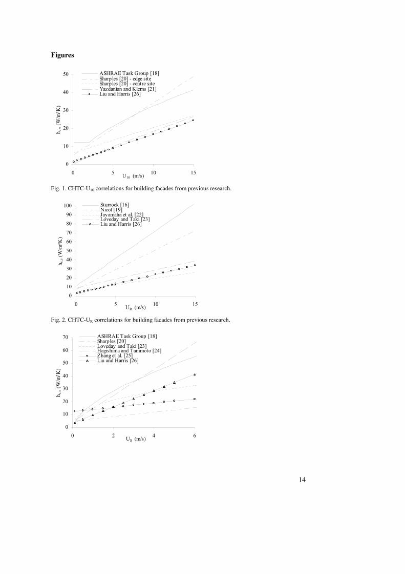
Fig. 1. CHTC-U10 correlations for building facades from previous research.
0
10
20
30
40
50
60
70
80
90
100
0 5 10 15UR (m/s)
hc
,e (
W/m
²K)
Sturrock [16]Nicol [19]Jayamaha et al. [22]Loveday and Taki [23]Liu and Harris [26]
Fig. 2. CHTC-UR correlations for building facades from previous research.
0
10
20
30
40
50
60
70
0 2 4US (m/s)
hc
,e (
W/m
²K)
6
ASHRAE Task Group [18]Sharples [20]Loveday and Taki [23]Hagishima and Tanimoto [24]Zhang et al. [25]Liu and Harris [26]
15
Fig. 3. CHTC-US correlations for building facades from previous research.
15 H
6 H
H
5 H
11 H
Flow
direction
H
15 H
6 H
H
5 H
11 H
Flow
direction
H
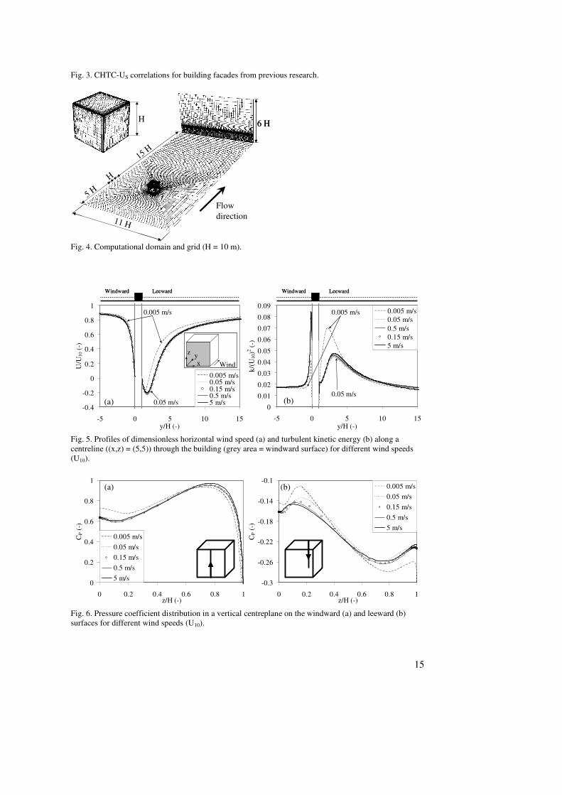
Fig. 4. Computational domain and grid (H = 10 m).
0
0.01
0.02
0.03
0.04
0.05
0.06
0.07
0.08
0.09
-5 0 5 10 15y/H (-)
k/(
U10)2
(-)
0.005 m/s
0.05 m/s
0.5 m/s
0.15 m/s
5 m/s
-0.4
-0.2
0
0.2
0.4
0.6
0.8
1
-5 0 5 10 15y/H (-)
U/U
10 (
-)
0.005 m/s0.05 m/s0.15 m/s0.5 m/s5 m/s
0.005 m/s
0.05 m/s
0.005 m/s
0.05 m/s(a) (b)
Wind
z
xy
Windward Leeward Windward Leeward
0
0.01
0.02
0.03
0.04
0.05
0.06
0.07
0.08
0.09
-5 0 5 10 15y/H (-)
k/(
U10)2
(-)
0.005 m/s
0.05 m/s
0.5 m/s
0.15 m/s
5 m/s
-0.4
-0.2
0
0.2
0.4
0.6
0.8
1
-5 0 5 10 15y/H (-)
U/U
10 (
-)
0.005 m/s0.05 m/s0.15 m/s0.5 m/s5 m/s
0.005 m/s
0.05 m/s
0.005 m/s
0.05 m/s(a) (b)
Wind
z
xy
0
0.01
0.02
0.03
0.04
0.05
0.06
0.07
0.08
0.09
-5 0 5 10 15y/H (-)
k/(
U10)2
(-)
0.005 m/s
0.05 m/s
0.5 m/s
0.15 m/s
5 m/s
-0.4
-0.2
0
0.2
0.4
0.6
0.8
1
-5 0 5 10 15y/H (-)
U/U
10 (
-)
0.005 m/s0.05 m/s0.15 m/s0.5 m/s5 m/s
0.005 m/s
0.05 m/s
0.005 m/s
0.05 m/s(a) (b)
Wind
z
xy
Wind
z
xy
Windward Leeward Windward Leeward
Fig. 5. Profiles of dimensionless horizontal wind speed (a) and turbulent kinetic energy (b) along a
centreline ((x,z) = (5,5)) through the building (grey area = windward surface) for different wind speeds
(U10).
0
0.2
0.4
0.6
0.8
1
0 0.2 0.4 0.6 0.8 1z/H (-)
CP (
-)
0.005 m/s
0.05 m/s
0.15 m/s
0.5 m/s
5 m/s-0.3
-0.26
-0.22
-0.18
-0.14
-0.1
0 0.2 0.4 0.6 0.8 1z/H (-)
CP (
-)
0.005 m/s
0.05 m/s
0.15 m/s
0.5 m/s
5 m/s
(a) (b)
0
0.2
0.4
0.6
0.8
1
0 0.2 0.4 0.6 0.8 1z/H (-)
CP (
-)
0.005 m/s
0.05 m/s
0.15 m/s
0.5 m/s
5 m/s-0.3
-0.26
-0.22
-0.18
-0.14
-0.1
0 0.2 0.4 0.6 0.8 1z/H (-)
CP (
-)
0.005 m/s
0.05 m/s
0.15 m/s
0.5 m/s
5 m/s
(a) (b)
Fig. 6. Pressure coefficient distribution in a vertical centreplane on the windward (a) and leeward (b)
surfaces for different wind speeds (U10).
16
12
34
56
78
9
1
3
5
7
9
-25%-20%-15%-10%-5%0%
5%
10%
15%
20%
25%
(hc,e-h
c,e
,av
g)/
hc,e
,av
g (%
)
x (m)
z (
m)
12
34
56
78
9
1
3
5
7
9
-25%-20%-15%-10%-5%0%5%
10%
15%
20%
25%
(hc,e-h
c,e
,av
g)/
hc,e
,av
g (%
)
x (m)
z (
m)
(a) (b)
Wind
z
x
y
12
34
56
78
9
1
3
5
7
9
-25%-20%-15%-10%-5%0%
5%
10%
15%
20%
25%
(hc,e-h
c,e
,av
g)/
hc,e
,av
g (%
)
x (m)
z (
m)
12
34
56
78
9
1
3
5
7
9
-25%-20%-15%-10%-5%0%5%
10%
15%
20%
25%
(hc,e-h
c,e
,av
g)/
hc,e
,av
g (%
)
x (m)
z (
m)
(a) (b)
Wind
z
x
y
Wind
z
x
y
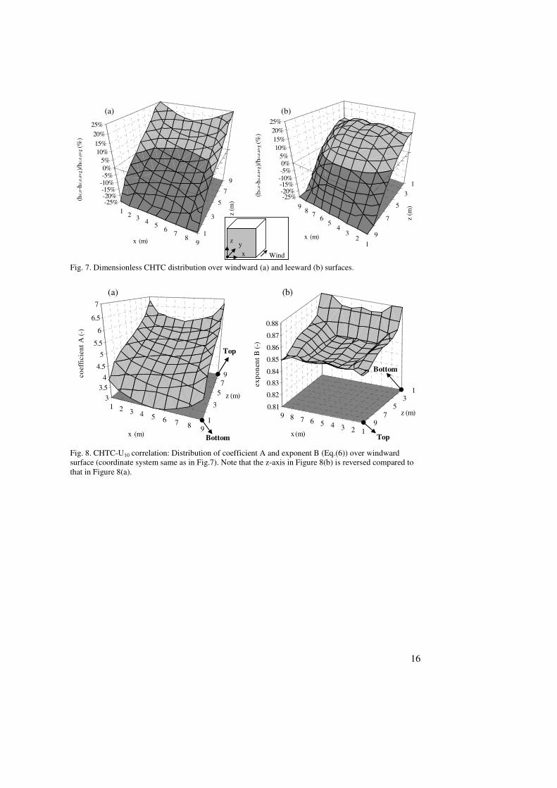
Fig. 7. Dimensionless CHTC distribution over windward (a) and leeward (b) surfaces.
1 2 3 4 5 6 7 89
1
3
5
7
9
3
3.5
4
4.5
5
5.5
6
6.5
7
co
eff
icie
nt
A (
-)
x (m)
z (m)
123456789
13
5
79
0.81
0.82
0.83
0.84
0.85
0.86
0.87
0.88
ex
po
nen
t B
(-)
x (m)
z (m)
(a) (b)
Bottom
Top
Bottom
Top
1 2 3 4 5 6 7 89
1
3
5
7
9
3
3.5
4
4.5
5
5.5
6
6.5
7
co
eff
icie
nt
A (
-)
x (m)
z (m)
123456789
13
5
79
0.81
0.82
0.83
0.84
0.85
0.86
0.87
0.88
ex
po
nen
t B
(-)
x (m)
z (m)
(a) (b)
Bottom
Top
Bottom
Top
Fig. 8. CHTC-U10 correlation: Distribution of coefficient A and exponent B (Eq.(6)) over windward
surface (coordinate system same as in Fig.7). Note that the z-axis in Figure 8(b) is reversed compared to
that in Figure 8(a).
17
12
34
56
78
91
3
5
7
9
1
1.5
2
2.5
3
co
eff
icie
nt
A (
-)
x (m)
z (m)1 2 3 4 5 6 7 8 9
1
3
5
7
9
0.74
0.79
0.84
0.89
ex
po
nen
t B
(-)
x (m)
z (m)
(a) (b)
Bottom
Top
Bottom
Top
12
34
56
78
91
3
5
7
9
1
1.5
2
2.5
3
co
eff
icie
nt
A (
-)
x (m)
z (m)1 2 3 4 5 6 7 8 9
1
3
5
7
9
0.74
0.79
0.84
0.89
ex
po
nen
t B
(-)
x (m)
z (m)
(a) (b)
Bottom
Top
Bottom
Top
Fig. 9. CHTC-U10 correlation: Distribution of coefficient A and exponent B (Eq.(6)) over leeward surface
(coordinate system same as in Fig.7). Note that the z-axis in Figure 9(b) is reversed compared to that in
Figure 9(a).

18
Table 1. CHTC-U correlations derived from full-scale measurements on building facades. Author Building geometry Wind speed Surface Correlations of CHTC
Length x Width x Height (m) Value Location Range (m/s)
Gerhart [15] Building, 30 m high UR 6 m above roof - - (c)
Sturrock [16] Tower, 26 m high UR - - WW 6.1 UR+11.4
US 0.3 m from facade 0.5-3.5 WW+LW - Ito et al. [17] Open L-shaped building, 18 m high
UR 8 m above roof 0.5-13 WW+LW -
ASHRAE Task Group [18]
(derived from Ito et al. [17])
- US 0.3 m from facade - WW+LW
WW
LW
18.6US0.605
US=0.25 U10 (U10 > 2 m/s)
US=0.5 (U10 < 2 m/s)
US=0.05 U10+0.3
Nicol [19] Rectangular building UR - 0-5 WW+LW 4.35 UR+7.55
US 1 m from facade 0.5-20 WW+LW 1.7 US+5.1 (a) Sharples [20] (b) Tower (20x36x78 m)
U10 0-12 WW
LW
2.9 U10+5.3 (a)
1.5 U10+4.1 (a)
Yazdanian and Klems [21] Small, single storey, rectangular
building
U10 0-12 WW
LW
1/3 2 0.89 2
10(0.84∆T ) +(2.38U )
1/3 2 0.617 2
10(0.84∆T ) +(2.86U )
Jayamaha et al. [22] Vertical wall (1.2x1.8 m) UR above vertical wall 0-4 WW+LW 1.444 UR+4.955
US 1 m from facade 0.5-9 WW
LW
16.15US0.397
16.25US0.503
Loveday and Taki [23] Rectangular building with L-shaped
ground floor (21x9x28 m)
UR 11 m above roof 0.5-16 WW
LW
2.00 UR+8.91
1.77 UR+4.93
Hagishima and Tanimoto [24] Two adjacent rectangular buildings
(16.6x26.8x16.5 m + 22.2x15.3x9.9
m)
US 0.13 m from facade/roof 0.5-3 RF
WW+LW
2 2 2
3.96 u +v +w +2k +6.42
2 2 2
10.21 u +v +w +2k +4.47
Zhang et al. [25] Small building (3x3x3 m) US 0.2 m from facade 1-7 WW+LW -0.0203 US2 + 1.766 US + 12.263
US 0.5 m from facade 0-3.5 WW
LW
6.31 US+3.32
5.03 US+3.19
UR 1 m above roof 0-9 WW
LW
2.08 UR+2.97
1.57 UR+2.66
Liu and Harris [26] (b) Rectangular building (8.5x8.5x5.6
m)
U10 0-16 WW
LW
1.53 U10+1.43
0.90 U10 +3.28
WW: Windward (incidence angles (angle between approach flow wind direction and the normal to the windward surface) from -90° to 90°), LW: Leeward (remainder of incidence
angles), RF: Roof, ∆T: Temperature difference between exterior surface and environment, u, v, w : x, y, z components of mean wind speed, k: turbulent kinetic energy, (a): edge site on
18th floor of the tower, (b): More correlations are provided in the original paper but are not given here for the sake of brevity, (c): No consistent correlation could be obtained.
Formatted: Space Before: 0pt, After: 0 pt, Line spacing: single
19
Table 2. CHTC-U correlations derived from wind-tunnel experiments on bluff bodies placed in a turbulent boundary layer. Author Measuring
technique
Approach flow Incidence
angle
Reference
velocity
Reynolds number
range (a)
Correlations of surface-averaged CHTC
Front Rear Side Top
Sturrock [16] - Laminar flow 0°-90° FS 4.7x10⁴ -
15.7x10⁴
hc,e=5.7U∞+23
- - -
Chyu and
Natarajan [35]
NS (b) Turbulent, BL thickness
±¼ of cube height
0° FS 3.1x10⁴ - 11x104 Sh=0.868Re0.538
Sh=0.196Re0.661
Sh=0.278Re0.652 Sh=0.247Re0.657
Natarajan and
Chyu [36] (c)
NS (b) Turbulent, BL thickness
±¼ of cube height
0°-10°-
25°-45°
FS 3.1x10⁴ - 11x104 Front surface (for 45°): Sh= 1.77Re0.637 Sc1/3
(Correlations for other surfaces and wind directions: see original paper)
Quintela and
Viegas [37] (c)
FM Turbulent, BL thickness
0.33-0.6 of cube height
0°-45° FS 5.2x10³ - 37x103 Cube-averaged value (for 0°): 0.27 Re
Nu 0.32Gr (1 1.15 )Gr
= +
Meinders et al.
[39]
IT Developing turbulent
channel flow
0° Bulk
velocity
2.75x10³ -
4.97x10³
Cube-averaged value Nu=ARe0.65
Nakamura et
al. [40]
TC Turbulent, BL thickness
1.5-1.83 of cube height
0° FS 4.2x10³ - 33x103 Nu=0.71Re0.52
Nu=0.11Re0.67
Nu=0.12Re0.70
Nu=0.071Re0.74
Nakamura et
al. [41]
TC Turbulent, BL thickness
1.5-1.83 of cube height
45° FS 4.2x10³ - 33x103 Nu=0.52Re0.55
Nu=0.11Re0.67
Nu=0.029Re0.84
Wang and
Chiou [42]
NS (b) Fully-developed channel
flow
0° MVI 8.0x10² - 5.0x10³ Sh=0.961Re0.529
Sh=0.223Re0.637
Sh=0.102Re0.663
Sh=0.305Re0.639
NS: Naphthalene Sublimation, IT: Infrared Thermography, TC: ThermoCouples, FM: Flux Meters, FS: Free-Stream velocity, MVI: Maximum Velocity at Inlet, BL: Boundary Layer, Gr:
Grashof number, A: parameter, (a): based on cube height and reference velocity (e.g. FS), (b): The CHTC can be derived from the heat and mass transfer analogy (Sh: Sherwood number,
Sc: Schmidt number = 1.87 for the experimental conditions), (c): More correlations are provided in the original paper but are not given here for the sake of brevity.
20
Table 3. Surface-averaged CHTC-U10 correlations from CFD simulations ((a): More correlations are
provided in the original paper but are not given here for the sake of brevity).
Table 4. Critical Reynolds numbers.
Author Critical Reynolds number
Hoydysh et al. [68] 3400
Castro and Robins [69] 4000
Cherry et al. [70] 30000
Ohba [71] 2100
Djilali and Gartshore [72] 25000
Snyder [73] 4000
Mochida et al. [74] 7500
Uehera et al. [75] 3500-8000
Table 5. Percentage difference (│hc,e,avg,corr-hc,e,avg│/hc,e,avg) of different CHTC-U10 correlations with
CHTC data (hc,e,avg is the surface-averaged CHTC from the numerical simulation, hc,e,avg,corr is the surface-
averaged CHTC using a specific CHTC-U10 correlation of one of the different cases). Small differences
(≤5 %) are highlighted.
Correlations using different sets of velocities (U10)
Wind
speed
(m/s)
Case A
(0.15-0.5-1-
2.5-5-7.5 m/s)
Case B
(0.05-0.15-0.5
m/s)
Case C
(0.15-0.5 m/s)
Case D
(0.15-0.5-1
m/s)
Case E
(0.5-1 m/s)
Case F
(0.5-2.5 m/s)
0.05 16 % 2 % 8 % 10 % 17 % 19 %
0.15 3 % 3 % 0 % 0 % 5 % 6 %
0.5 2 % 1 % 0 % 1 % 0 % 0 %
1 3 % 7 % 3 % 1 % 0 % 1 %
2.5 1 % 15 % 8 % 5 % 2 % 0 %
5 1 % 21 % 13 % 9 % 4 % 1 %
7.5 2 % 25 % 15 % 11 % 5 % 2 %
Correlation hc,e=5.01U100.85 hc,e=4.56U10
0.77 hc,e=4.75U100.81 hc,e=4.85U10
0.82 hc,e=4.89U100.85 hc,e=4.93U10
0.86
Author Building geometry
Length x Width x Height
(m)
U10 range
(m/s)
Correlation of surface-averaged CHTC
for windward surface
(W/m²K)
Emmel et al. [46] (a) Rectangular building
(6x8x2.7 m)
1 - 15 hc,e=5.15U100.81 (short wall)
hc,e=4.84U100.82
(long wall)
Blocken et al. [47] (a) Cubic building, 10 m high 1 - 4 hc,e=4.6U100.89
Defraeye et al. [48] Cubic building, 10 m high 0.05 - 5 hc,e=5.15U100.82