Embed Size (px)
Citation preview
Article
Convergence, Divergence
, and Reconvergence in aFeedforward Network Improves Neural Speed andAccuracyHighlights
d Feedforward signals in this network converge, diverge, and
reconverge
d Individual spike trains become progressively more
informative at each layer
d Whereas second-order neurons average out noise, third-
order neurons detect coincidences
d At each layer, postsynaptic neurons are well tuned to their
presynaptic inputs
Jeanne & Wilson, 2015, Neuron 88, 1014–1026December 2, 2015 ª2015 Elsevier Inc.http://dx.doi.org/10.1016/j.neuron.2015.10.018
Authors
James M. Jeanne, Rachel I. Wilson
In Brief
Convergence and reconvergence are
thought to be canonical circuit motifs.
Jeanne and Wilson identify a three-layer
feedforward network in Drosophila
olfaction that computes progressively
more informative single-neuron sensory
representations by matching
postsynaptic properties to the statistics
of presynaptic inputs.
Neuron
Article
Convergence, Divergence, and Reconvergencein a Feedforward NetworkImproves Neural Speed and AccuracyJames M. Jeanne1 and Rachel I. Wilson1,*1Department of Neurobiology, Harvard Medical School, 220 Longwood Ave, Boston, MA 02115, USA
*Correspondence: [email protected]
http://dx.doi.org/10.1016/j.neuron.2015.10.018
SUMMARY
One of the proposed canonical circuit motifs em-ployed by the brain is a feedforward network whereparallel signals converge, diverge, and reconverge.Here we investigate a network with this architecturein the Drosophila olfactory system. We focus on aglomerulus whose receptor neurons converge in anall-to-all manner onto six projection neurons thatthen reconverge onto higher-order neurons. Wefind that both convergence and reconvergenceimprove the ability of a decoder to detect a stimulusbased on a single neuron’s spike train. The first trans-formation implements averaging, and it improvespeak detection accuracy but not speed; the secondtransformation implements coincidence detection,and it improves speed but not peak accuracy. Ineach case, the integration time and threshold of thepostsynaptic cell are matched to the statistics ofconvergent spike trains.
INTRODUCTION
The maximum rate of information flow grows with the number of
parallel channels in a transmission line (Stein, 1967). This allows
for the transmission of more information over a fixed time win-
dow or, equivalently, the need for less time to transmit a fixed
amount of information. Accordingly, sensation typically begins
with a large array of peripheral sensors. For example, vision be-
gins with a large array of photoreceptors, and hearing begins
with a large array of hair cells (Sterling and Laughlin, 2015).
The olfactory system represents another example of this strat-
egy. The detailed architecture of the olfactory system has been
most fully characterized in Drosophila (Figure 1A), but the verte-
brate olfactory system has a similar architecture (Bargmann,
2006). Each Drosophila odorant receptor is expressed by �40
olfactory receptor neurons (ORNs) in each antenna, on average.
All the ORNs that express the same receptor have similar odor
response properties (de Bruyne et al., 1999, 2001), and they proj-
ect their axons to the same glomerulus in the brain (Vosshall
et al., 2000). There, they converge onto postsynaptic projection
neurons (PNs). Each PN pools input from every single ORN in its
cognate glomerulus (Kazama andWilson, 2009). Given the theo-
1014 Neuron 88, 1014–1026, December 2, 2015 ª2015 Elsevier Inc.
retical benefits of pooling from parallel channels, we would
expect to detect a near-threshold odor stimulus more quickly
and accurately based on a single PN spike train, as compared
to a single ORN spike train.
The benefits of pooling from parallel channels are not neces-
sarily limited to the periphery: pooling could also be useful in
central circuits. Specifically, a signal might diverge onto many
neurons, whose activity then converges at a later stage. This
could allow the brain to reduce noise accumulated indepen-
dently in transmission along the parallel channels (Alonso
et al., 1996; Faisal et al., 2008). Divergent neural architecture is
widespread in central sensory circuits. For example, in the retina,
each photoreceptor signal diverges onto many postsynaptic bi-
polar cells (Cohen and Sterling, 1990). In the cochlea, each hair
cell signal diverges onto many postsynaptic ganglion cells (Lib-
erman, 1980). In the Drosophila olfactory system, each ORN
axon diverges to synapse onto all the identical ‘‘sister’’ PNs in
the same glomerulus (Kazama and Wilson, 2009). However, it
is difficult to show that the neurons that receive divergent signals
actually reconverge onto a common postsynaptic neuron. Even
if they do, the effect of pooling will not be straightforward,
because these convergent inputs may be correlated as a conse-
quence of having diverged upstream.
Here we use a single olfactory coding channel inDrosophila as
a setting to investigate these questions.We study a population of
�40 ORNs that diverge and converge, in an all-to-all manner,
onto six postsynaptic PNs.We show that these sister PNs recon-
verge onto a specific class of lateral horn neurons (LHNs). We
investigate how the representation of a near-threshold stimulus
is transformed at the ORN-to-PN step and again at the PN-to-
LHN step. We find that the function of convergence is different
in the two cases: the first step implements averaging, and the
second step implements coincidence detection. In each case,
the integrative properties of the postsynaptic cell match the sta-
tistics of their convergent presynaptic spike trains.
RESULTS
Sensory Processing across Three Layers of OlfactoryCircuitryOur approach in this study was to inject a brief packet of spikes
into the ORNs presynaptic to one glomerulus and to trace this
signal through three synaptically connected layers: from ORNs
to PNs, and then from PNs to LHNs (Figure 1A). We selected
glomerulus DA1 for these experiments because we have good
0 20 40 60 800
20
40
60
80
ORN firing rate (spikes/sec)
PN
firin
g ra
te (s
pike
s/se
c)
−50 0 50 100 1500
50
100
time after light onset (msec)
firin
g ra
te (s
pike
s/se
c)
−50 0 50 100 1500
50
100
firin
g ra
te (s
pike
s/se
c)
time after light onset (msec)
A 100 msec stimulus
PN
ORN
LHN
B
D
E
0 20 40 60 800
20
40
60
80
PN firing rate (spikes/sec)LHN
firin
g ra
te (s
pike
s/se
c)
F
C
ORNPN
PNLHN
G
ORNs PNs LHNs
antennallobe
lateralhorn
light
−50 0 50 100 1500
0.5
1
time after light onset (msec)
firin
g ra
te (n
orm
aliz
ed) ORN
PNLHN
H
0
10
20
30
spon
tane
ous
rate
(spi
kes/
sec)
ORN PN LHN ORN PN LHN
mean SD
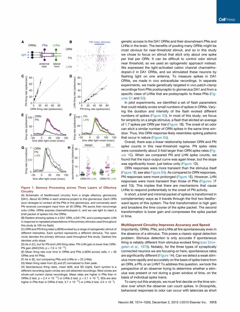
Figure 1. Sensory Processing across Three Layers of Olfactory
Circuitry
(A) Schematic of feedforward circuitry from a single olfactory glomerulus
(DA1). About 40 ORNs in each antenna project to this glomerulus. Each ORN
axon diverges to contact all the PNs in this glomerulus, and conversely each
PN receives convergent input from all 40 ORNs. PN axons then reconverge
onto LHNs. ORNs express channelrhodopsin-2, and we use light to inject a
brief packet of spikes into the ORNs.
(B) Rasters showing spikes in a DA1 ORN, a DA1 PN, and a postsynaptic LHN
in response to repeated presentations of the primary stimulus used throughout
this study (a 100 ms flash).
(C) ORN and PN firing rates (±SEM) evoked by a range of optogenetic stimuli of
different intensities. Each symbol represents a different stimulus. The open
circle denotes the primary stimulus used throughout this study. Dashed line
denotes unity slope.
(D) As in (C), but for PN and LHN firing rates. PN-LHN gain is lower than ORN-
PN gain (ANCOVA, p = 7.6 3 10�13).
(E) Mean firing rate over time in ORNs and PNs (±SEM across cells; n = 58
ORNs and 44 PNs).
(F) As in (E), but comparing PNs and LHNs (n = 25 LHNs).
(G) Mean firing rates from (E) and (F) normalized to their peak.
(H) Spontaneous firing rates, mean (left), and SD (right). Each symbol is a
different recording (open circles are cell-attached recordings; filled circles are
whole-cell current clamp recordings). Mean rates are higher in PNs than in
ORNs (t test, p = 2.4 3 10�13) or LHNs (t test, p = 5.1 3 10�5). SDs are also
higher in PNs than in ORNs (t test, 3.7 3 10�13) or LHNs (t test, 3.0 3 10�4).
N
genetic access to the DA1 ORNs and their downstream PNs and
LHNs in the brain. The benefits of pooling many ORNs might be
most obvious for near-threshold stimuli, and so in this study
we chose to focus on stimuli that elicit only about one spike
per trial per ORN. It can be difficult to control odor stimuli
near threshold, so we used an optogenetic approach instead.
We expressed the light-activated cation channel channelrho-
dopsin-2 in DA1 ORNs, and we stimulated these neurons by
flashing light on one antenna. To measure spikes in DA1
ORNs, we made in vivo extracellular recordings. In separate
experiments, we made genetically targeted in vivo patch-clamp
recordings from PNs postsynaptic to glomerulus DA1 and from a
specific class of LHNs that are postsynaptic to these PNs (Fig-
ures S1 and S2).
In pilot experiments, we identified a set of flash parameters
that could reliably evoke small numbers of spikes in ORNs. Vary-
ing the duration and intensity of the flash evoked different
numbers of spikes (Figure S3). In most of this study, we focus
for simplicity on a single stimulus, a flash that elicited an average
of 1.7 spikes per ORN per trial (Figure 1B). The onset of an odor
can elicit a similar number of ORN spikes in the same time win-
dow. Thus, this ORN response likely resembles spiking patterns
that occur in nature (Figure S4).
Overall, there was a linear relationship between ORN and PN
spike counts in this near-threshold regime. PN spike rates
were consistently about 3-fold larger than ORN spike rates (Fig-
ure 1C). When we compared PN and LHN spike counts, we
found that the input-output curve was again linear, but the slope
was significantly lower, just below unity (Figure 1D).
ORN responses were more transient than the stimulus itself
(Figure 1E; see also Figure S4). As compared to ORN responses,
PN responses were more prolonged (Figure 1E). However, LHN
responses were more transient than those of PNs (Figures 1F
and 1G). This implies that there are mechanisms that cause
LHNs to respond preferentially to the onset of PN activity.
In short, a brief and minimal packet of spikes is transformed in
complementary ways as it travels through the first two feedfor-
ward layers of this system. The first transformation is high gain
and broadens the time course of the spike packet. The second
transformation is lower gain and compresses the spike packet
in time.
Multilayered Circuitry Improves Accuracy and SpeedImportantly, ORNs, PNs, and LHNs all fire spontaneously even in
the absence of a stimulus. This poses a classic signal detection
problem. Stimulus detection is only accurate if spontaneous
firing is reliably different from stimulus-evoked firing (van Dron-
gelen et al., 1978). Notably, for the three types of synaptically
connected neurons we are focusing on here, spontaneous rates
are significantly different (Figure 1H). Canwe detect a weak stim-
ulusmore rapidly and accurately on the basis of spike trains from
an ORN, a PN, or an LHN? To address this question, we took the
perspective of an observer trying to determine whether a stim-
ulus was present or not during a given window of time, on the
basis of individual spike trains.
To carry out this analysis, wemust first decide on the timewin-
dow over which the observer can count spikes. In Drosophila,
behavioral responses to odor can occur with latencies as short
euron 88, 1014–1026, December 2, 2015 ª2015 Elsevier Inc. 1015
0 20 40 60 80 1000
1
2
3
time after light onset (msec)
accu
racy
(dʹ )
B
C
A
D
0 3 60
1
prob
abili
ty
0 3 60
1
prob
abili
ty
0 3 60
1
spike count
prob
abili
ty
ORN
PN
LHN
0
5
10
15
peak
acc
urac
y
OR
N
PN
LHN
20
40
60
80
>120la
tenc
y to
dʹ
= 1
(mse
c)
n.s. ** n.s.
OR
N
PN
LHN
ORNPNLHN
first spike decoderE F G
hitrate
falsealarmrate0
50
100
% o
f tria
ls
OR
NP
NLH
N
60
70
80
90
net a
ccur
acy
(%)
OR
NP
NLH
N
* *
28
30
32
34
36
38
first
spi
ke la
tenc
y (m
sec) *
OR
NP
NLH
N
spontaneous
evoked
spike count decoder
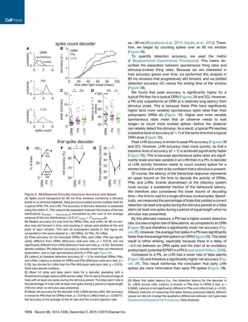
Figure 2. Multilayered Circuitry Improves Accuracy and Speed
(A) Spike count histograms for 80 ms time windows containing a stimulus
(solid) or no stimulus (dashed). Data are accumulated across multiple trials for
a typical ORN, PN, and LHN. The accuracy of stimulus detection is assessed
using the metric d0. This value is the separation between the means of the two
distributions (mevoked � mspontaneous) normalized by the root of the average
variance of the two distributions (O(1/2 (s2evoked + s2
spontaneous))).
(B) Median accuracy (d0) over time for ORNs, PNs, and LHNs. An 80 ms win-
dow was slid forward in time, and resulting d0 values were plotted at the end
point of each window. This and all subsequent panels in this figure are
computed on the same dataset (n = 58 ORNs, 44 PNs, 25 LHNs).
(C) Peak accuracy (d0) for individual ORNs, PNs, and LHNs. PNs are signifi-
cantly different from ORNs (Wilcoxon rank-sum test, p = 0.013), but not
significantly different from LHNs (Wilcoxon rank-sum test, p = 0.25). Solid bars
denote medians. PN detection accuracy is actually lower than our theoretical
expectation, due to high spontaneous activity in PNs; see Figure S8.
(D) Latency to baseline detection accuracy (d0 = 1) for individual ORNs, PNs,
and LHNs. Latency is similar for ORNs and PNs (Wilcoxon rank-sum test, p =
0.33), but shorter for LHNs than for PNs (Wilcoxon rank-sum test, p = 0.015).
Solid bars denote medians.
(E) Mean hit rates and false alarm rates for a decoder operating with a
threshold of a single spike (±SEMacross cells). The hit rate is the percentage of
trials with at least one spike during the stimulus period. The false alarm rate is
the percentage of trials with at least one spike during a period of equal length
(100 ms) when no stimulus was presented.
(F) Mean net accuracy for the decoder in (E) (±SEM across cells). Net accuracy
is worse for PNs than for ORNs (t test, p = 0.018) or LHNs (t test, p = 0.00077).
Net accuracy is the average of the hit rate and the correct rejection rate.
1016 Neuron 88, 1014–1026, December 2, 2015 ª2015 Elsevier Inc.
as �80 ms (Bhandawat et al., 2010; Gaudry et al., 2013). There-
fore, we began by counting spikes over an 80 ms window
(Figure 2A).
To quantify detection accuracy, we used the metric
d0 (Supplemental Experimental Procedures). This metric de-
scribes the separation between spontaneous firing rates and
stimulus-evoked firing rates. Because we are interested in
how accuracy grows over time, we performed this analysis in
80 ms windows that progressively slid forward, and we plotted
detection accuracy (d0) versus the ending time of the window
(Figure 2B).
We found that peak accuracy is significantly higher for a
typical PN than for a typical ORN (Figures 2B and 2C). However,
a PN only outperforms an ORN at a relatively long latency from
stimulus onset. This is because these PNs have significantly
higher (and more variable) spontaneous spike rates than their
presynaptic ORNs do (Figure 1H). Higher and more variable
spontaneous rates mean that an observer needs to wait
longer—to count more evoked spikes—before the observer
can reliably detect the stimulus. As a result, a typical PN reaches
a baseline level of accuracy (d0 = 1) at the same time that a typical
ORN does (Figure 2D).
Peak LHN accuracy is similar to peak PN accuracy (Figures 2B
and 2C). However, LHN accuracy rises more quickly, so that a
baseline level of accuracy (d0 = 1) is achieved significantly faster
(Figure 2D). This is because spontaneous spike rates are signif-
icantly lower and less variable in an LHN than in a PN. A decoder
of LHN activity therefore needs to count evoked spikes for a
shorter interval in order to be confident that a stimulus is present.
Of course, the latency of the behavioral response represents
an upper bound on the time to decode the activity of ORNs,
PNs, and LHNs. Events downstream of the olfactory system
must occupy a substantial fraction of the behavioral latency.
We therefore also considered the lower bound of decoding
time—the time towait for a single stimulus-evoked spike. Specif-
ically, wemeasured the percentage of trials that yielded a correct
detection (at least one spike during the stimulus period) or a false
alarm (at least one spike during a period of equal length when no
stimulus was presented).
By this alternate measure, a PN had a higher correct detection
rate, but also a higher rate of false alarms, as compared to anORN
(Figure 2E) and therefore a significantly lower net accuracy (Fig-
ure 2F). However, the average first spike in a PN was significantly
faster than theaverage first spike in anORN (Figure 2G). This latter
result is rather striking, especially because there is a delay of
�4.5 ms between an ORN spike and the start of an excitatory
postsynaptic potential (EPSP) in aPN (KazamaandWilson, 2008).
Compared to a PN, an LHN had a lower rate of false alarms
(Figure 2E) and therefore a significantly higher net accuracy (Fig-
ure 2F). This result reinforces the conclusion that early LHN
spikes are more informative than early PN spikes (Figure 2B).
(G) Mean first spike latency (i.e., the detection latency for the decoder in
E), ±SEM across cells. Latency is shorter in PNs than in ORNs (t test, p =
0.0092). Latency is not significantly different in PNs and LHNs (t test, p = 0.32).
Different methods of measuring first spike latency produced slightly different
values but did not change the qualitative differences between cell types (see
Supplemental Experimental Procedures, Data Analysis).
C D
BA
E
0 40 800
5
10
time after light onset (msec)
accu
racy
(dʹ )
4 msec15 msec
30 msec
60 msecsimulated pool of 40 ORNs
0 10 200
50
100
% o
f tria
ls
0 10 200
20
40
dete
ctio
nla
tenc
y (m
sec)
spike count threshold (# of ORN spikes) spike count threshold (# of ORN spikes)
F
OR
N n
umbe
r
60 msec15 msec
4 msec
0
10
20
30
40
100 msec stimulus
hitrate
falsealarmrate
4 msec
0
0.80
0.50
0.2 60 msec
0 10 20 30spike count
prob
abili
ty
30 msec
0 30 600
20
40
integration time (msec)
late
ncy
to d
ʹ =
1(m
sec)
1 ORN
40 ORNs
0 30 600
5
10
integration time (msec)
peak
acc
urac
y
1 ORN
40 ORNs
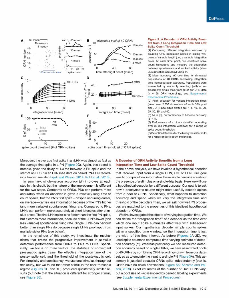
Figure 3. A Decoder of ORN Activity Bene-
fits from a Long Integration Time and Low
Spike Count Threshold
(A) Comparing different integration windows by
counting ORN population spikes in sliding win-
dows of variable length (i.e., a variable integration
time). At each time point, we construct spike
count histograms and measure the separation
between spontaneous and evoked activity (stim-
ulus detection accuracy) using d0.(B) Mean accuracy (d0) over time for simulated
populations of 40 ORNs. Increasing integration
time increased peak accuracy. Populations were
assembled by randomly selecting (without re-
placement) single trials from all of our ORN data
(n = 58 ORN recordings, see Supplemental
Experimental Procedures).
(C) Peak accuracy for various integration times
(mean over 2,000 simulations of each ORN pool
size). ORN pool sizes plotted are: 1, 5, 10, 15, 20,
25, 30, 35, and 40.
(D) As in (C), but for latency to baseline accuracy
(d0 = 1).
(E) Performance of a binary classifier (operating
over 30 ms integration windows) for a range of
spike count thresholds.
(F) Detection latencies for the binary classifier in (E)
for a range of spike count thresholds.
Moreover, the average first spike in an LHNwas almost as fast as
the average first spike in a PN (Figure 2G). Again, this speed is
notable, given the delay of 1.3 ms between a PN spike and the
start of an EPSP in an LHN (see data on paired PN-LHN record-
ings below; see also Fisxek and Wilson, 2014; Kohl et al., 2013).
In summary, single-neuron accuracy (d0) improves at each
step in this circuit, but the nature of the improvement is different
for the two steps. Compared to ORNs, PNs can perform more
accurately when an observer is given a relatively long time to
count spikes, but the PN’s first spike—despite occurring earlier,
on average—carries less information because of the PN’s higher
(and more variable) spontaneous firing rate. Compared to PNs,
LHNs can perform more accurately at short latencies after stim-
ulus onset. The first LHN spike is no faster than the first PN spike,
but it carries more information, because of the LHN’s lower (and
less variable) spontaneous firing rate. Single LHNs can perform
better than single PNs do because single LHNs pool input from
multiple sister PNs (see below).
In the remainder of this study, we investigate the mecha-
nisms that create the progressive improvement in stimulus
detection performance from ORNs to PNs to LHNs. Specif-
ically, we focus on three factors: the statistics of convergent
presynaptic spike trains, the effective integration time of the
postsynaptic cell, and the threshold of the postsynaptic cell.
For simplicity and consistency, we use one stimulus throughout
this study, but we found that other stimuli in the near-threshold
regime (Figures 1C and 1D) produced qualitatively similar re-
sults (but note that the situation is different for stronger stimuli,
see Figure S3).
N
A Decoder of ORN Activity Benefits from a LongIntegration Time and Low Spike Count ThresholdIn the above analysis, we have invoked a hypothetical decoder
that receives input from a single ORN, PN, or LHN. Our goal
was to compare how informative these single neurons are about
the presence of a stimulus on a single-trial basis. Here wewill use
a hypothetical decoder for a different purpose. Our goal is to ask
how a postsynaptic neuron might most usefully decode spikes
from a pool of ORNs. Specifically, what happens to detection
accuracy and speed when we vary the integration time and
threshold of the decoder? Then, we will ask how well PN proper-
ties are matched to the properties of this idealized hypothetical
decoder of ORNs.
We first investigated the effects of varying integration time.We
can define the ‘‘integration time’’ of a decoder as the time over
which one input spike summates effectively with subsequent
input spikes. Our hypothetical decoder simply counts spikes
within a specified time window, so the integration time is just
the width of this time interval. As before (Figures 2A–2D), we
used spike counts to compute a time-varying estimate of detec-
tion accuracy (d0). Whereas previously we had measured detec-
tion accuracy based on single ORNs, we here assembled pools
of 40 ORNs by combining ORN recordings drawn from our data-
set, so as to emulate the input to a single PN (Figure 3A). This as-
sembly is justified because ORNs spike independently (that is,
ORNs have no noise correlations; Figure S5; Kazama and Wil-
son, 2009). Exact estimates of the number of DA1 ORNs vary,
but a pool size of�40 is implied by genetic labeling experiments
(see Supplemental Experimental Procedures).
euron 88, 1014–1026, December 2, 2015 ª2015 Elsevier Inc. 1017
C
B
A
0
10
20
dist
ance
to P
N s
pike
thre
shol
d (m
V)
0
10
20
norm
aliz
ed s
pike
coun
t thr
esho
ld(%
of t
otal
OR
N in
puts
)−100 0 100 2000
0.5
1
time after light onset (msec)
firin
g ra
te(n
orm
aliz
ed)
ORNsPNsfiltered ORNs (23 msec filter)
0 20 40 600
0.5
1
time after light onset (msec)
cum
ulat
ive
OR
N s
pike
cou
nt
4.5 msecdelay
PNspiketime
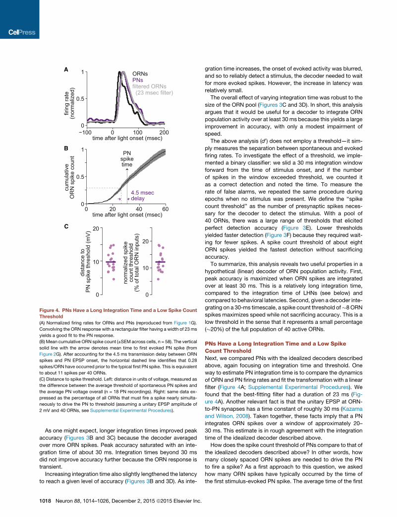
Figure 4. PNs Have a Long Integration Time and a Low Spike Count
Threshold
(A) Normalized firing rates for ORNs and PNs (reproduced from Figure 1G).
Convolving the ORN response with a rectangular filter having a width of 23 ms
yields a good fit to the PN response.
(B) Mean cumulative ORN spike count (±SEM across cells, n = 58). The vertical
solid line with the arrow denotes mean time to first evoked PN spike (from
Figure 2G). After accounting for the 4.5 ms transmission delay between ORN
spikes and PN EPSP onset, the horizontal dashed line identifies that 0.28
spikes/ORN have occurred prior to the typical first PN spike. This is equivalent
to about 11 spikes per 40 ORNs.
(C) Distance to spike threshold. Left: distance in units of voltage, measured as
the difference between the average threshold of spontaneous PN spikes and
the average PN voltage overall (n = 18 PN recordings). Right: same data ex-
pressed as the percentage of all ORNs that must fire a spike nearly simulta-
neously to drive the PN to threshold (assuming a unitary EPSP amplitude of
2 mV and 40 ORNs, see Supplemental Experimental Procedures).
As one might expect, longer integration times improved peak
accuracy (Figures 3B and 3C) because the decoder averaged
over more ORN spikes. Peak accuracy saturated with an inte-
gration time of about 30 ms. Integration times beyond 30 ms
did not improve accuracy further because the ORN response is
transient.
Increasing integration time also slightly lengthened the latency
to reach a given level of accuracy (Figures 3B and 3D). As inte-
1018 Neuron 88, 1014–1026, December 2, 2015 ª2015 Elsevier Inc.
gration time increases, the onset of evoked activity was blurred,
and so to reliably detect a stimulus, the decoder needed to wait
for more evoked spikes. However, the increase in latency was
relatively small.
The overall effect of varying integration time was robust to the
size of the ORN pool (Figures 3C and 3D). In short, this analysis
argues that it would be useful for a decoder to integrate ORN
population activity over at least 30 ms because this yields a large
improvement in accuracy, with only a modest impairment of
speed.
The above analysis (d0) does not employ a threshold—it sim-
ply measures the separation between spontaneous and evoked
firing rates. To investigate the effect of a threshold, we imple-
mented a binary classifier: we slid a 30 ms integration window
forward from the time of stimulus onset, and if the number
of spikes in the window exceeded threshold, we counted it
as a correct detection and noted the time. To measure the
rate of false alarms, we repeated the same procedure during
epochs when no stimulus was present. We define the ‘‘spike
count threshold’’ as the number of presynaptic spikes neces-
sary for the decoder to detect the stimulus. With a pool of
40 ORNs, there was a large range of thresholds that elicited
perfect detection accuracy (Figure 3E). Lower thresholds
yielded faster detection (Figure 3F) because they required wait-
ing for fewer spikes. A spike count threshold of about eight
ORN spikes yielded the fastest detection without sacrificing
accuracy.
To summarize, this analysis reveals two useful properties in a
hypothetical (linear) decoder of ORN population activity. First,
peak accuracy is maximized when ORN spikes are integrated
over at least 30 ms. This is a relatively long integration time,
compared to the integration time of LHNs (see below) and
compared to behavioral latencies. Second, given a decoder inte-
grating on a 30-ms timescale, a spike count threshold of�8ORN
spikes maximizes speed while not sacrificing accuracy. This is a
low threshold in the sense that it represents a small percentage
(�20%) of the full population of 40 active ORNs.
PNs Have a Long Integration Time and a Low SpikeCount ThresholdNext, we compared PNs with the idealized decoders described
above, again focusing on integration time and threshold. One
way to estimate PN integration time is to compare the dynamics
of ORN and PN firing rates and fit the transformation with a linear
filter (Figure 4A; Supplemental Experimental Procedures). We
found that the best-fitting filter had a duration of 23 ms (Fig-
ure 4A). Another relevant fact is that the unitary EPSP at ORN-
to-PN synapses has a time constant of roughly 30 ms (Kazama
and Wilson, 2008). Taken together, these facts imply that a PN
integrates ORN spikes over a window of approximately 20–
30 ms. This estimate is in rough agreement with the integration
time of the idealized decoder described above.
How does the spike count threshold of PNs compare to that of
the idealized decoders described above? In other words, how
many closely spaced ORN spikes are needed to drive the PN
to fire a spike? As a first approach to this question, we asked
how many ORN spikes have typically occurred by the time of
the first stimulus-evoked PN spike. The average time of the first
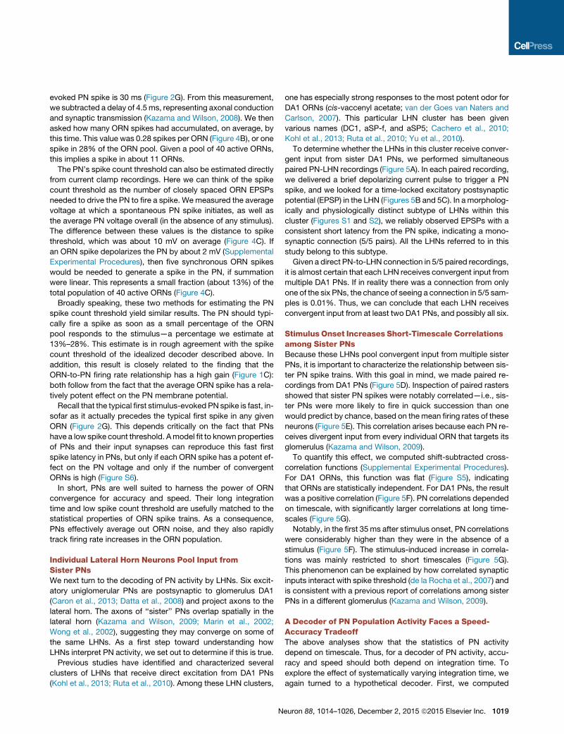
evoked PN spike is 30 ms (Figure 2G). From this measurement,
we subtracted a delay of 4.5ms, representing axonal conduction
and synaptic transmission (Kazama and Wilson, 2008). We then
asked how many ORN spikes had accumulated, on average, by
this time. This value was 0.28 spikes per ORN (Figure 4B), or one
spike in 28% of the ORN pool. Given a pool of 40 active ORNs,
this implies a spike in about 11 ORNs.
The PN’s spike count threshold can also be estimated directly
from current clamp recordings. Here we can think of the spike
count threshold as the number of closely spaced ORN EPSPs
needed to drive the PN to fire a spike. We measured the average
voltage at which a spontaneous PN spike initiates, as well as
the average PN voltage overall (in the absence of any stimulus).
The difference between these values is the distance to spike
threshold, which was about 10 mV on average (Figure 4C). If
an ORN spike depolarizes the PN by about 2 mV (Supplemental
Experimental Procedures), then five synchronous ORN spikes
would be needed to generate a spike in the PN, if summation
were linear. This represents a small fraction (about 13%) of the
total population of 40 active ORNs (Figure 4C).
Broadly speaking, these two methods for estimating the PN
spike count threshold yield similar results. The PN should typi-
cally fire a spike as soon as a small percentage of the ORN
pool responds to the stimulus—a percentage we estimate at
13%–28%. This estimate is in rough agreement with the spike
count threshold of the idealized decoder described above. In
addition, this result is closely related to the finding that the
ORN-to-PN firing rate relationship has a high gain (Figure 1C):
both follow from the fact that the average ORN spike has a rela-
tively potent effect on the PN membrane potential.
Recall that the typical first stimulus-evoked PN spike is fast, in-
sofar as it actually precedes the typical first spike in any given
ORN (Figure 2G). This depends critically on the fact that PNs
have a low spike count threshold. Amodel fit to known properties
of PNs and their input synapses can reproduce this fast first
spike latency in PNs, but only if each ORN spike has a potent ef-
fect on the PN voltage and only if the number of convergent
ORNs is high (Figure S6).
In short, PNs are well suited to harness the power of ORN
convergence for accuracy and speed. Their long integration
time and low spike count threshold are usefully matched to the
statistical properties of ORN spike trains. As a consequence,
PNs effectively average out ORN noise, and they also rapidly
track firing rate increases in the ORN population.
Individual Lateral Horn Neurons Pool Input fromSister PNsWe next turn to the decoding of PN activity by LHNs. Six excit-
atory uniglomerular PNs are postsynaptic to glomerulus DA1
(Caron et al., 2013; Datta et al., 2008) and project axons to the
lateral horn. The axons of ‘‘sister’’ PNs overlap spatially in the
lateral horn (Kazama and Wilson, 2009; Marin et al., 2002;
Wong et al., 2002), suggesting they may converge on some of
the same LHNs. As a first step toward understanding how
LHNs interpret PN activity, we set out to determine if this is true.
Previous studies have identified and characterized several
clusters of LHNs that receive direct excitation from DA1 PNs
(Kohl et al., 2013; Ruta et al., 2010). Among these LHN clusters,
N
one has especially strong responses to the most potent odor for
DA1 ORNs (cis-vaccenyl acetate; van der Goes van Naters and
Carlson, 2007). This particular LHN cluster has been given
various names (DC1, aSP-f, and aSP5; Cachero et al., 2010;
Kohl et al., 2013; Ruta et al., 2010; Yu et al., 2010).
To determine whether the LHNs in this cluster receive conver-
gent input from sister DA1 PNs, we performed simultaneous
paired PN-LHN recordings (Figure 5A). In each paired recording,
we delivered a brief depolarizing current pulse to trigger a PN
spike, and we looked for a time-locked excitatory postsynaptic
potential (EPSP) in the LHN (Figures 5B and 5C). In a morpholog-
ically and physiologically distinct subtype of LHNs within this
cluster (Figures S1 and S2), we reliably observed EPSPs with a
consistent short latency from the PN spike, indicating a mono-
synaptic connection (5/5 pairs). All the LHNs referred to in this
study belong to this subtype.
Given a direct PN-to-LHN connection in 5/5 paired recordings,
it is almost certain that each LHN receives convergent input from
multiple DA1 PNs. If in reality there was a connection from only
one of the six PNs, the chance of seeing a connection in 5/5 sam-
ples is 0.01%. Thus, we can conclude that each LHN receives
convergent input from at least two DA1 PNs, and possibly all six.
Stimulus Onset Increases Short-Timescale Correlationsamong Sister PNsBecause these LHNs pool convergent input from multiple sister
PNs, it is important to characterize the relationship between sis-
ter PN spike trains. With this goal in mind, we made paired re-
cordings from DA1 PNs (Figure 5D). Inspection of paired rasters
showed that sister PN spikes were notably correlated—i.e., sis-
ter PNs were more likely to fire in quick succession than one
would predict by chance, based on themean firing rates of these
neurons (Figure 5E). This correlation arises because each PN re-
ceives divergent input from every individual ORN that targets its
glomerulus (Kazama and Wilson, 2009).
To quantify this effect, we computed shift-subtracted cross-
correlation functions (Supplemental Experimental Procedures).
For DA1 ORNs, this function was flat (Figure S5), indicating
that ORNs are statistically independent. For DA1 PNs, the result
was a positive correlation (Figure 5F). PN correlations depended
on timescale, with significantly larger correlations at long time-
scales (Figure 5G).
Notably, in the first 35 ms after stimulus onset, PN correlations
were considerably higher than they were in the absence of a
stimulus (Figure 5F). The stimulus-induced increase in correla-
tions was mainly restricted to short timescales (Figure 5G).
This phenomenon can be explained by how correlated synaptic
inputs interact with spike threshold (de la Rocha et al., 2007) and
is consistent with a previous report of correlations among sister
PNs in a different glomerulus (Kazama and Wilson, 2009).
A Decoder of PN Population Activity Faces a Speed-Accuracy TradeoffThe above analyses show that the statistics of PN activity
depend on timescale. Thus, for a decoder of PN activity, accu-
racy and speed should both depend on integration time. To
explore the effect of systematically varying integration time, we
again turned to a hypothetical decoder. First, we computed
euron 88, 1014–1026, December 2, 2015 ª2015 Elsevier Inc. 1019
A B
C
0 20 40 60 800
0.5
1
1.5
time after PN spike (msec)
LHN
vol
tage
(mV
)
ORNs PNs LHNs
antennallobe
lateralhorn
light
PN spike time
2 mV30 msec
−200−300 −100 0 100time after light onset (msec)
D F
E100 msec stimulus
0 10 20 30 400
0.2
0.4
0.6
0.8
integration window (msec)
corr
elat
ion
G
***
* evoked (first 35 msec)spontaneous
ORNs PNs LHNs
light
corr
elat
ion
0
0.1
0.2
−10 0 10 −10 0 10−10 0 10time lag (msec)
spontaneous evokedfull
responsefirst
35 msec
PN-PN recording
PN-PN recordings
PN-PN recordings
PN-LHN recordings
PN-LHN recording
Figure 5. Individual Lateral Horn Neurons Pool Input from Sister
PNs, and Stimulus Onset Increases Short-Timescale Correlationsamong Sisters
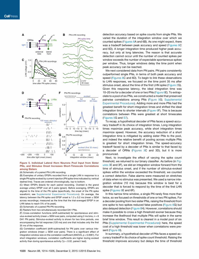
(A) Schematic of a paired PN-LHN recording.
(B) Examples of unitary EPSPs recorded from a single LHN in response to a
single PN spike evoked by current injection (PN spike time indicated by vertical
dashed line). Traces are ordered chronologically, top to bottom.
(C) Mean EPSPs (black) for each paired recording. Overlaid is the grand
average unitary EPSP over all 5 pairs (green). Before averaging, EPSPs are
aligned to the time of the PN spike (specifically, the onset of the PN spike
waveform; see Supplemental Experimental Procedures). On average, the
latency between the PN spike and EPSP onset is 1.3 ± 0.2 ms (mean ± SEM
across recordings; measured as the time that the trial-averaged EPSP in an
LHN takes to reach 5% of its peak).
(D) Schematic of a paired PN-PN recording.
(E) Rasters from two simultaneously recorded DA1 PNs.
(F) Cross-correlation functions (shift-subtracted) for spontaneous and stim-
ulus-evoked activity (mean ± SEM over pairs, computed using 2 ms bins, n = 8
DA1 PN pairs). Stimulus-evoked activity is shown for two time periods, one
encompassing the full response (120 ms) and one that includes only the first
35 ms of the response.
(G) Correlation coefficient (shift-subtracted) for PN pairs over various inte-
gration windows (mean ± SEM over pairs). There is a significant effect of
integration window size on the correlation coefficient (ANOVA, p = 0.0061). For
short integration windows, correlation coefficients are higher during evoked
activity than during spontaneous activity (*p < 0.02, paired t test).
1020 Neuron 88, 1014–1026, December 2, 2015 ª2015 Elsevier Inc.
detection accuracy based on spike counts from single PNs. We
varied the duration of the integration window over which we
counted spikes (Figures 6A and 6B). As one might expect, there
was a tradeoff between peak accuracy and speed (Figures 6C
and 6D). A longer integration time produced higher peak accu-
racy, but only at long latencies. The reason is that accurate
detection cannot occur until the number of counted spikes per
window exceeds the number of expectable spontaneous spikes
per window. Thus, longer windows delay the time point when
peak accuracy can be reached.
We next considered data from PN pairs. PN pairs consistently
outperformed single PNs, in terms of both peak accuracy and
speed (Figures 6C and 6D). To begin to link these observations
to LHN responses, we focused on the time point 35 ms after
stimulus onset, about the time of the first LHN spike (Figure 2G).
Given this response latency, the ideal integration time was
10–20ms for a decoder of one or two PNs (Figure 6E). To extrap-
olate to a pool of six PNs, we constructed amodel that preserved
pairwise correlations among PNs (Figure 5G; Supplemental
Experimental Procedures). Adding more and more PNs had the
greatest benefit for short integration times and shifted the ideal
integration time to shorter intervals (Figure 6F). This is because
correlations between PNs were greatest at short timescales
(Figures 5G and S7).
To recap, a hypothetical decoder of PNs faces a speed-accu-
racy tradeoff in its choice of integration times. Long integration
times maximize peak accuracy, while short integration times
maximize speed. However, the accuracy reduction of a short
integration time is mitigated by adding sister PNs to the pool,
and indeed the relative benefit of pooling across multiple PNs
is greatest for short integration times. The speed-accuracy
tradeoff faced by a decoder of PNs is similar to that faced by
a decoder of ORNs (Figures 3C and 3D), but it is more
pronounced.
Next, to investigate the effect of varying the spike count
threshold, we returned to our binary classifier. As before (in Fig-
ures 3E and 3F), we slid an integration window forward from the
time of stimulus onset, and if the number of stimulus-evoked
spikes within the window exceeded the threshold, we counted
a correct detection. False alarms were measured on stretches
of data when no stimulus was presented. We used a narrow inte-
gration window (10 ms) because this window is best for a
decoder that is forced to respond by the time of the first LHN
spike (Figures 6E and 6F).
In this narrow time window, a single PN rarely fires more than
twice, so we focused on thresholds of one or two PN spikes. For
a decoder pooling from two sister PNs, raising the threshold from
one spike to two spikes reduced false positives (Figure 6G) but
also delayed detection (Figure 6H). However, correlations should
make it possible to cross a high threshold sooner because they
increase the likelihood that multiple PNs will spike in the same
brief time window. This result is clearest in a model pool of six
PNs (Supplemental Experimental Procedures): here, the speed
cost of a high threshold was lower when correlations were pre-
sent (Figure 6I).
In summary, a hypothetical decoder of PNs faces a speed-ac-
curacy tradeoff in its choice of spike count threshold. Raising the
threshold improves accuracy but delays the time of threshold
0 30 6026
30
34
late
ncy
to d
ʹ = 1
(mse
c)
integration time (msec)
1 PN2 PNs
A
C
B
10 20 30 40 50 600
1
2
time after light onset (msec)ac
cura
cy (d
ʹ )
10 msec
60 msecsingle PNs
D
E
spike count threshold (# of PN spikes)
F
0 30 600
2
4
peak
acc
urac
y
integration time (msec)
1 PN2 PNs
G
data: 1-2 PNs model: 1-6 PNs
1 2 3 4 5 610
20
30
40
50
late
ncy
(mse
c)
# of PNs firing a first spike
6 PNs6 PNs
(trials shifted)
data: 2 PNs data: 2 PNs model: 6 PNsH I
hitrate
falsealarmrate
1 20
50
100
% o
f tria
ls
1 225
30
35
dete
ctio
n la
tenc
y (m
sec)
0 30 600.5
1
1.5
accu
racy
at 3
5 m
sec
integration time (msec)
3-6 PNs2 PNs1 PN
0 30 600.5
1
1.5
accu
racy
at 3
5 m
sec
integration time (msec)
2 PNs1 PN
60 msec
10 msec
0
1
0 5 10
0
0.860 msec
10 msec
100 msec stimulus spike count
prob
abili
ty
Figure 6. A Decoder of PN Population Activity Faces a Speed-Accu-
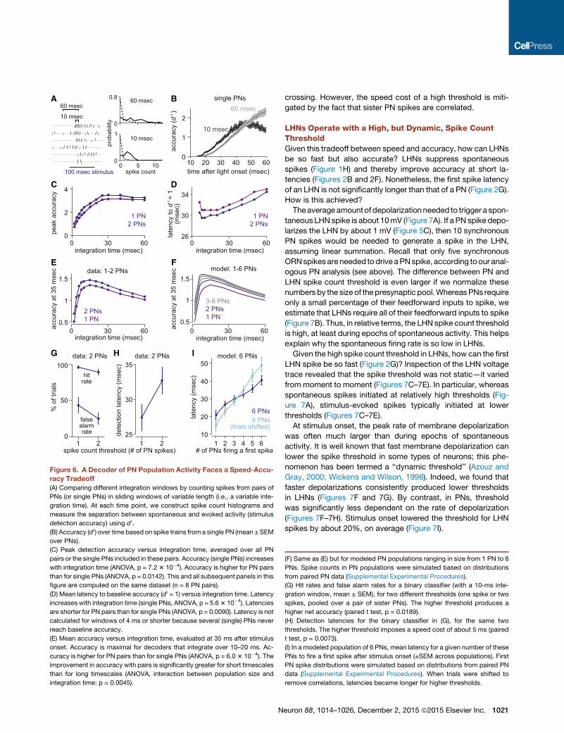
racy Tradeoff
(A) Comparing different integration windows by counting spikes from pairs of
PNs (or single PNs) in sliding windows of variable length (i.e., a variable inte-
gration time). At each time point, we construct spike count histograms and
measure the separation between spontaneous and evoked activity (stimulus
detection accuracy) using d0.(B) Accuracy (d0) over time based on spike trains from a single PN (mean ± SEM
over PNs).
(C) Peak detection accuracy versus integration time, averaged over all PN
pairs or the single PNs included in these pairs. Accuracy (single PNs) increases
with integration time (ANOVA, p = 7.23 10�4). Accuracy is higher for PN pairs
than for single PNs (ANOVA, p = 0.0142). This and all subsequent panels in this
figure are computed on the same dataset (n = 8 PN pairs).
(D) Mean latency to baseline accuracy (d0 = 1) versus integration time. Latency
increases with integration time (single PNs, ANOVA, p = 5.63 10�4). Latencies
are shorter for PN pairs than for single PNs (ANOVA, p = 0.0090). Latency is not
calculated for windows of 4 ms or shorter because several (single) PNs never
reach baseline accuracy.
(E) Mean accuracy versus integration time, evaluated at 35 ms after stimulus
onset. Accuracy is maximal for decoders that integrate over 10–20 ms. Ac-
curacy is higher for PN pairs than for single PNs (ANOVA, p = 6.03 10�4). The
improvement in accuracy with pairs is significantly greater for short timescales
than for long timescales (ANOVA, interaction between population size and
integration time: p = 0.0045).
N
crossing. However, the speed cost of a high threshold is miti-
gated by the fact that sister PN spikes are correlated.
LHNs Operate with a High, but Dynamic, Spike CountThresholdGiven this tradeoff between speed and accuracy, how can LHNs
be so fast but also accurate? LHNs suppress spontaneous
spikes (Figure 1H) and thereby improve accuracy at short la-
tencies (Figures 2B and 2F). Nonetheless, the first spike latency
of an LHN is not significantly longer than that of a PN (Figure 2G).
How is this achieved?
Theaverageamountof depolarization needed to trigger a spon-
taneous LHNspike is about 10mV (Figure 7A). If a PN spike depo-
larizes the LHN by about 1 mV (Figure 5C), then 10 synchronous
PN spikes would be needed to generate a spike in the LHN,
assuming linear summation. Recall that only five synchronous
ORNspikesareneeded todrive aPNspike, according to our anal-
ogous PN analysis (see above). The difference between PN and
LHN spike count threshold is even larger if we normalize these
numbers by the size of the presynapticpool.WhereasPNs require
only a small percentage of their feedforward inputs to spike, we
estimate that LHNs require all of their feedforward inputs to spike
(Figure 7B). Thus, in relative terms, the LHN spike count threshold
is high, at least during epochs of spontaneous activity. This helps
explain why the spontaneous firing rate is so low in LHNs.
Given the high spike count threshold in LHNs, how can the first
LHN spike be so fast (Figure 2G)? Inspection of the LHN voltage
trace revealed that the spike threshold was not static—it varied
from moment to moment (Figures 7C–7E). In particular, whereas
spontaneous spikes initiated at relatively high thresholds (Fig-
ure 7A), stimulus-evoked spikes typically initiated at lower
thresholds (Figures 7C–7E).
At stimulus onset, the peak rate of membrane depolarization
was often much larger than during epochs of spontaneous
activity. It is well known that fast membrane depolarization can
lower the spike threshold in some types of neurons; this phe-
nomenon has been termed a ‘‘dynamic threshold’’ (Azouz and
Gray, 2000; Wickens and Wilson, 1998). Indeed, we found that
faster depolarizations consistently produced lower thresholds
in LHNs (Figures 7F and 7G). By contrast, in PNs, threshold
was significantly less dependent on the rate of depolarization
(Figures 7F–7H). Stimulus onset lowered the threshold for LHN
spikes by about 20%, on average (Figure 7I).
(F) Same as (E) but for modeled PN populations ranging in size from 1 PN to 6
PNs. Spike counts in PN populations were simulated based on distributions
from paired PN data (Supplemental Experimental Procedures).
(G) Hit rates and false alarm rates for a binary classifier (with a 10-ms inte-
gration window, mean ± SEM), for two different thresholds (one spike or two
spikes, pooled over a pair of sister PNs). The higher threshold produces a
higher net accuracy (paired t test, p = 0.0189).
(H) Detection latencies for the binary classifier in (G), for the same two
thresholds. The higher threshold imposes a speed cost of about 5 ms (paired
t test, p = 0.0073).
(I) In a modeled population of 6 PNs, mean latency for a given number of these
PNs to fire a first spike after stimulus onset (±SEM across populations). First
PN spike distributions were simulated based on distributions from paired PN
data (Supplemental Experimental Procedures). When trials were shifted to
remove correlations, latencies became longer for higher thresholds.
euron 88, 1014–1026, December 2, 2015 ª2015 Elsevier Inc. 1021
B DC
F
0 2 40
5
10
15
20
dist
ance
to s
pike
thre
shol
d (m
V)
dV/dt at spike threshold (mV/msec)0 1 2
0
5
10
15
20example PN example LHN
A
E
G H
dist
ance
toth
resh
old
(mV
)
0 2 40
5
10
15
20
0 2 40
5
10
15
20
dyna
mic
thre
shol
dsl
ope
(mV
/(mV
/mse
c))
dV/dt at spike threshold (mV/msec)
PNs LHNs
PN LHN−6
−4
−2
0I
0
5
10
15
20
dist
ance
toth
resh
old
(mV
)
0
100
200
300
norm
aliz
ed s
pike
coun
t thr
esho
ld(%
of t
otal
inpu
ts)
PN LHN PN LHN
0.8 1 1.27
8
9
10
11di
stan
ce to
thre
shol
d (m
V)
dV/dt at threshold (mV/msec)
spontaneousspikes
firstevokedspike
−60
−50
−40
−30
−20 spontaneousspike spontaneous
depolarization
stimulus-evokedspike
500 msec
volta
ge (m
V)
−55
−45
−35
−25
20 msec
volta
ge (m
V)
−60 −50 −40 −30−5
0
5
dV/d
t (m
V/m
sec)
voltage (mV)
phase portrait
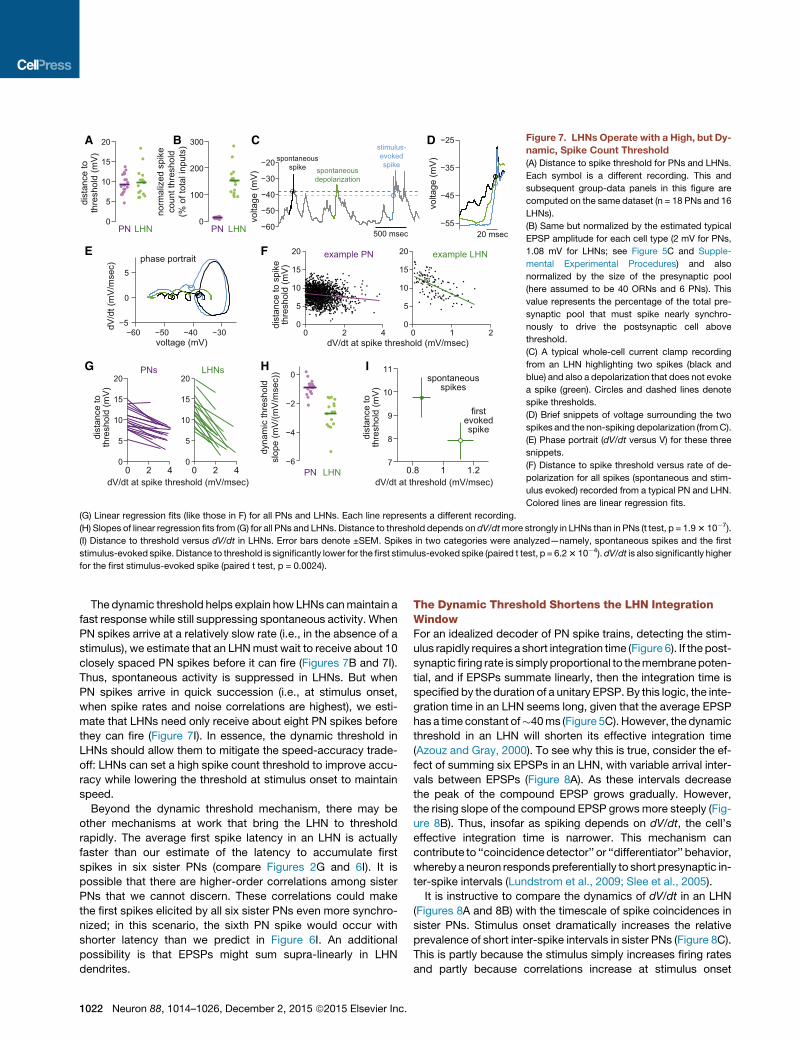
Figure 7. LHNs Operate with a High, but Dy-
namic, Spike Count Threshold
(A) Distance to spike threshold for PNs and LHNs.
Each symbol is a different recording. This and
subsequent group-data panels in this figure are
computed on the same dataset (n = 18 PNs and 16
LHNs).
(B) Same but normalized by the estimated typical
EPSP amplitude for each cell type (2 mV for PNs,
1.08 mV for LHNs; see Figure 5C and Supple-
mental Experimental Procedures) and also
normalized by the size of the presynaptic pool
(here assumed to be 40 ORNs and 6 PNs). This
value represents the percentage of the total pre-
synaptic pool that must spike nearly synchro-
nously to drive the postsynaptic cell above
threshold.
(C) A typical whole-cell current clamp recording
from an LHN highlighting two spikes (black and
blue) and also a depolarization that does not evoke
a spike (green). Circles and dashed lines denote
spike thresholds.
(D) Brief snippets of voltage surrounding the two
spikes and the non-spiking depolarization (fromC).
(E) Phase portrait (dV/dt versus V) for these three
snippets.
(F) Distance to spike threshold versus rate of de-
polarization for all spikes (spontaneous and stim-
ulus evoked) recorded from a typical PN and LHN.
Colored lines are linear regression fits.
(G) Linear regression fits (like those in F) for all PNs and LHNs. Each line represents a different recording.
(H) Slopes of linear regression fits from (G) for all PNs and LHNs. Distance to threshold depends on dV/dtmore strongly in LHNs than in PNs (t test, p = 1.93 10�7).
(I) Distance to threshold versus dV/dt in LHNs. Error bars denote ±SEM. Spikes in two categories were analyzed—namely, spontaneous spikes and the first
stimulus-evoked spike. Distance to threshold is significantly lower for the first stimulus-evoked spike (paired t test, p = 6.23 10�4).dV/dt is also significantly higher
for the first stimulus-evoked spike (paired t test, p = 0.0024).
The dynamic threshold helps explain how LHNs canmaintain a
fast response while still suppressing spontaneous activity. When
PN spikes arrive at a relatively slow rate (i.e., in the absence of a
stimulus), we estimate that an LHNmust wait to receive about 10
closely spaced PN spikes before it can fire (Figures 7B and 7I).
Thus, spontaneous activity is suppressed in LHNs. But when
PN spikes arrive in quick succession (i.e., at stimulus onset,
when spike rates and noise correlations are highest), we esti-
mate that LHNs need only receive about eight PN spikes before
they can fire (Figure 7I). In essence, the dynamic threshold in
LHNs should allow them to mitigate the speed-accuracy trade-
off: LHNs can set a high spike count threshold to improve accu-
racy while lowering the threshold at stimulus onset to maintain
speed.
Beyond the dynamic threshold mechanism, there may be
other mechanisms at work that bring the LHN to threshold
rapidly. The average first spike latency in an LHN is actually
faster than our estimate of the latency to accumulate first
spikes in six sister PNs (compare Figures 2G and 6I). It is
possible that there are higher-order correlations among sister
PNs that we cannot discern. These correlations could make
the first spikes elicited by all six sister PNs even more synchro-
nized; in this scenario, the sixth PN spike would occur with
shorter latency than we predict in Figure 6I. An additional
possibility is that EPSPs might sum supra-linearly in LHN
dendrites.
1022 Neuron 88, 1014–1026, December 2, 2015 ª2015 Elsevier Inc.
The Dynamic Threshold Shortens the LHN IntegrationWindowFor an idealized decoder of PN spike trains, detecting the stim-
ulus rapidly requires a short integration time (Figure 6). If the post-
synaptic firing rate is simply proportional to themembranepoten-
tial, and if EPSPs summate linearly, then the integration time is
specified by the duration of a unitary EPSP. By this logic, the inte-
gration time in an LHN seems long, given that the average EPSP
has a time constant of�40ms (Figure 5C). However, the dynamic
threshold in an LHN will shorten its effective integration time
(Azouz and Gray, 2000). To see why this is true, consider the ef-
fect of summing six EPSPs in an LHN, with variable arrival inter-
vals between EPSPs (Figure 8A). As these intervals decrease
the peak of the compound EPSP grows gradually. However,
the rising slope of the compound EPSP growsmore steeply (Fig-
ure 8B). Thus, insofar as spiking depends on dV/dt, the cell’s
effective integration time is narrower. This mechanism can
contribute to ‘‘coincidencedetector’’ or ‘‘differentiator’’ behavior,
whereby aneuron respondspreferentially to short presynaptic in-
ter-spike intervals (Lundstrom et al., 2009; Slee et al., 2005).
It is instructive to compare the dynamics of dV/dt in an LHN
(Figures 8A and 8B) with the timescale of spike coincidences in
sister PNs. Stimulus onset dramatically increases the relative
prevalence of short inter-spike intervals in sister PNs (Figure 8C).
This is partly because the stimulus simply increases firing rates
and partly because correlations increase at stimulus onset
0 10 20 30 40 500
2
4
6
8simulated compound EPSPs
LHN
vol
tage
(mV
)
time after first PN spike (msec)
0
0.4
0.8
1.2
1.6
standard deviation of spike time distribution (msec)
peak
rate
of
depo
lariz
atio
n (m
V/m
sec)
0 5 10 15 200
2
4
6
peak
dep
olar
izat
ion
(mV
)
unitary EPSP
0 5 10 15 200
0.2
0.4
prob
abili
ty
inter-spike interval (msec)
paired trials
0 5 10 15 200
0.2
0.4
prob
abili
ty
inter-spike interval (msec)
shifted trials
A
B
C
D
first two evoked spikesspontaneous spikes
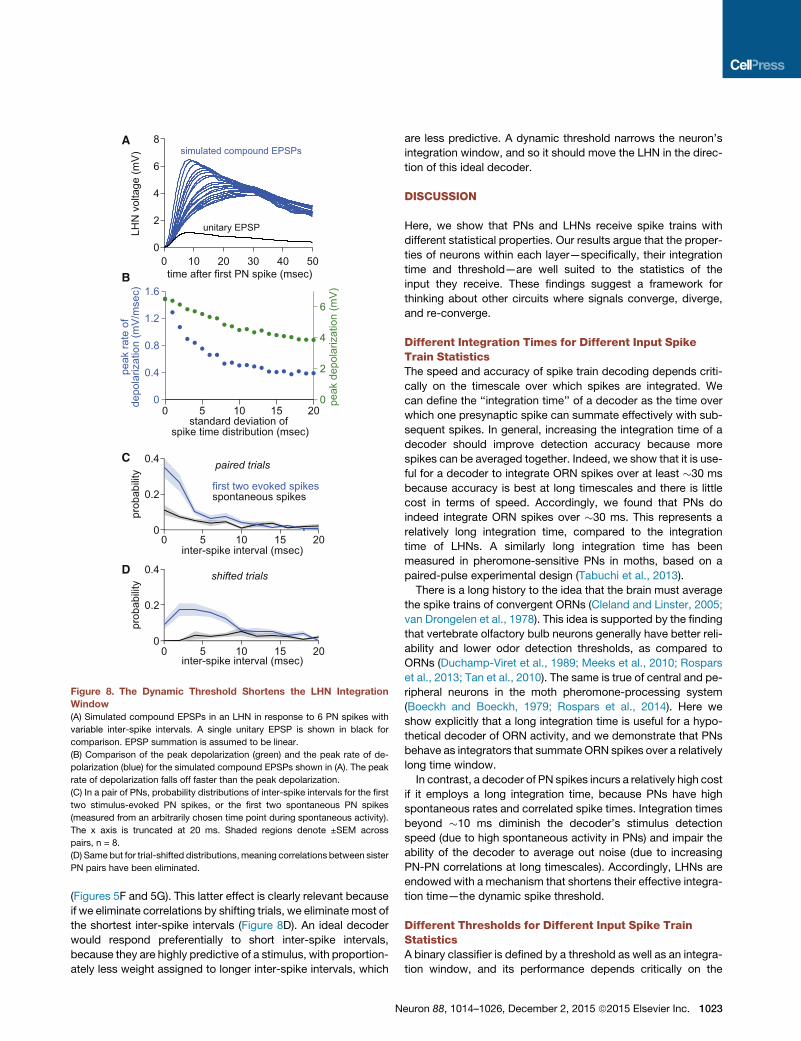
Figure 8. The Dynamic Threshold Shortens the LHN Integration
Window
(A) Simulated compound EPSPs in an LHN in response to 6 PN spikes with
variable inter-spike intervals. A single unitary EPSP is shown in black for
comparison. EPSP summation is assumed to be linear.
(B) Comparison of the peak depolarization (green) and the peak rate of de-
polarization (blue) for the simulated compound EPSPs shown in (A). The peak
rate of depolarization falls off faster than the peak depolarization.
(C) In a pair of PNs, probability distributions of inter-spike intervals for the first
two stimulus-evoked PN spikes, or the first two spontaneous PN spikes
(measured from an arbitrarily chosen time point during spontaneous activity).
The x axis is truncated at 20 ms. Shaded regions denote ±SEM across
pairs, n = 8.
(D) Same but for trial-shifted distributions,meaning correlations between sister
PN pairs have been eliminated.
(Figures 5F and 5G). This latter effect is clearly relevant because
if we eliminate correlations by shifting trials, we eliminate most of
the shortest inter-spike intervals (Figure 8D). An ideal decoder
would respond preferentially to short inter-spike intervals,
because they are highly predictive of a stimulus, with proportion-
ately less weight assigned to longer inter-spike intervals, which
N
are less predictive. A dynamic threshold narrows the neuron’s
integration window, and so it should move the LHN in the direc-
tion of this ideal decoder.
DISCUSSION
Here, we show that PNs and LHNs receive spike trains with
different statistical properties. Our results argue that the proper-
ties of neurons within each layer—specifically, their integration
time and threshold—are well suited to the statistics of the
input they receive. These findings suggest a framework for
thinking about other circuits where signals converge, diverge,
and re-converge.
Different Integration Times for Different Input SpikeTrain StatisticsThe speed and accuracy of spike train decoding depends criti-
cally on the timescale over which spikes are integrated. We
can define the ‘‘integration time’’ of a decoder as the time over
which one presynaptic spike can summate effectively with sub-
sequent spikes. In general, increasing the integration time of a
decoder should improve detection accuracy because more
spikes can be averaged together. Indeed, we show that it is use-
ful for a decoder to integrate ORN spikes over at least �30 ms
because accuracy is best at long timescales and there is little
cost in terms of speed. Accordingly, we found that PNs do
indeed integrate ORN spikes over �30 ms. This represents a
relatively long integration time, compared to the integration
time of LHNs. A similarly long integration time has been
measured in pheromone-sensitive PNs in moths, based on a
paired-pulse experimental design (Tabuchi et al., 2013).
There is a long history to the idea that the brain must average
the spike trains of convergent ORNs (Cleland and Linster, 2005;
van Drongelen et al., 1978). This idea is supported by the finding
that vertebrate olfactory bulb neurons generally have better reli-
ability and lower odor detection thresholds, as compared to
ORNs (Duchamp-Viret et al., 1989; Meeks et al., 2010; Rospars
et al., 2013; Tan et al., 2010). The same is true of central and pe-
ripheral neurons in the moth pheromone-processing system
(Boeckh and Boeckh, 1979; Rospars et al., 2014). Here we
show explicitly that a long integration time is useful for a hypo-
thetical decoder of ORN activity, and we demonstrate that PNs
behave as integrators that summate ORN spikes over a relatively
long time window.
In contrast, a decoder of PN spikes incurs a relatively high cost
if it employs a long integration time, because PNs have high
spontaneous rates and correlated spike times. Integration times
beyond �10 ms diminish the decoder’s stimulus detection
speed (due to high spontaneous activity in PNs) and impair the
ability of the decoder to average out noise (due to increasing
PN-PN correlations at long timescales). Accordingly, LHNs are
endowed with a mechanism that shortens their effective integra-
tion time—the dynamic spike threshold.
Different Thresholds for Different Input Spike TrainStatisticsA binary classifier is defined by a threshold as well as an integra-
tion window, and its performance depends critically on the
euron 88, 1014–1026, December 2, 2015 ª2015 Elsevier Inc. 1023
choice of threshold. We have formulated this problem in terms of
the ‘‘spike count threshold’’ of a postsynaptic neuron, which we
define as the number of closely spaced presynaptic spikes
needed to drive a postsynaptic spike. In general, a binary classi-
fier faces a speed-accuracy tradeoff in its choice of threshold:
lower thresholds yield faster first spike latencies, but also poorer
accuracy, due to high false alarm rates.
Our results draw attention to two factors that can affect this
tradeoff: spontaneous activity and correlations between neu-
rons. First, if spontaneous activity and correlations are both
low, then the accuracy cost of a low threshold is diminished.
Second, if presynaptic spike trains are correlated, speed can
be achieved with a high threshold (Middleton et al., 2009). These
two factors are most relevant to a decoder of ORNs and a
decoder of PNs, respectively.
ORNs are uncorrelated; the DA1 ORNs also have low sponta-
neous firing rates. Thus, a hypothetical decoder that integrates
over time (and over many ORNs) can achieve a relatively low
and constant level of baseline activity. This enables the de-
coder’s threshold to be set at a low value without sacrificing ac-
curacy. Accordingly, we found that the spike count threshold in a
PN is relatively low. This enables PNs to respond rapidly, re-
sponding preferentially to those ORNs that happened to spike
earliest. A similar inference has been reached for pheromone-
sensitive ORNs and PNs in the moth (Rospars et al., 2014). (As
an aside, we note that PN noise is considerably higher than we
would predict for a hypothetical decoder that simply pools
ORN spike trains; this additional noise is likely due to noisy input
from local interneurons; see Figure S8.)
As compared to their presynaptic ORNs, the DA1 PNs
have relatively high spontaneous firing rates, and their sponta-
neous spikes are correlated. As a consequence, an accurate
decoder of PN spikes must have a high threshold. Accord-
ingly, we found that LHNs do indeed have a high spike count
threshold. In principle, a high threshold will delay detection.
However, in this case, the speed-accuracy tradeoff is miti-
gated by the correlations among sister PNs. These correla-
tions allow a decoder to set a high threshold without sacri-
ficing too much speed. PN correlations also increase at
stimulus onset, which further improves both accuracy and
speed. Indeed, we find that LHNs respond to a stimulus
remarkably rapidly.
LHNs also have a dynamic threshold, meaning that they are
not linear decoders. Because the spike threshold in LHNs de-
pends on the rate of change of its membrane potential, not all
incoming spikes are treated equally. This allows LHNs tomitigate
the speed-accuracy tradeoff that faces a linear decoder. In the
absence of a stimulus, the spike count threshold is high, which
suppresses spontaneous activity. At stimulus onset, the
threshold drops, which should yield both a speed benefit and
an accuracy benefit.
A high and dynamic threshold makes this type of LHN a ‘‘coin-
cidence detector.’’ Similar coincidence detector properties are
found in layer IV visual cortical neurons. Interestingly, like
LHNs, these neurons receive correlated convergent feedforward
signals—in this case, from thalamic neurons, whose correlations
derive from divergent retinal projections (Alonso et al., 1996). In
both LHNs and layer IV cortical neurons, therefore, presynaptic
1024 Neuron 88, 1014–1026, December 2, 2015 ª2015 Elsevier Inc.
spike train statistics and postsynaptic properties are seemingly
well matched.
Integrators and DifferentiatorsIt is useful to think of PNs as integrators and LHNs as differentia-
tors. PNs average presynaptic spikes over a relatively long time
window, and their spike threshold is fairly static. By contrast, the
LHN spike threshold depends more steeply on dV/dt, and as a
consequence, effective integration time is shortened in LHNs.
In general, an integrator is a neuron whose firing rate depends
mainly on themean input current. Conversely, a differentiator is a
neuron whose firing rate depends mainly on the variance of the
input current. There is a continuous spectrum of behaviors
from differentiation to integration (Ratte et al., 2013, 2014). Our
results extend this literature by showing how the intrinsic proper-
ties of a neuron—whether integrator or differentiator—may be
usefully matched to population spiking statistics of its inputs.
The mechanisms that distinguish integrators from differentia-
tors can be recapitulated in Hodgkin-Huxley models of spiking
neurons (Azouz and Gray, 2000; Lundstrom et al., 2008). In
particular, lowering the level of the voltage-gated Na+ conduc-
tance promotes differentiation. If the Na+ conductance is low
enough, the level of Na+ channel inactivation can become a
limiting factor in spike initiation. In this regime, the spike
threshold becomes sensitive to the speed of subthreshold depo-
larization, because channel activation is faster than inactivation.
Fast depolarization allows activation to win out over inactivation,
and spike threshold falls. Conversely, slow depolarization allows
inactivation to keep pace with activation, and spike threshold
rises.
Spike Timing Correlation and SynchronyNeurons that are tuned to the same sensory features often
exhibit ‘‘noise correlations’’—i.e., correlated spontaneous activ-
ity and correlated trial-to-trial fluctuations in stimulus-evoked ac-
tivity. From the perspective of an idealized decoder, correlations
can be either harmful or helpful. When two neurons are function-
ally identical, positive correlations will generally be harmful (Aver-
beck et al., 2006). Many studies have measured correlations in
population codes and developed a theory of their origin and
function (Averbeck et al., 2006; Cohen and Kohn, 2011). How-
ever, comparatively few studies have investigated how corre-
lated activity influences downstream circuitry, mainly because
of the difficulty in identifying downstream targets of correlated
populations. Here, we have the rare opportunity to directly inves-
tigate both a pool of correlated neurons (sister PNs) and some of
the postsynaptic recipients of their convergent axons (LHNs).
We found that correlations between PNs exhibited two prop-
erties that ameliorate their adverse effects. First, correlations
are smaller for shorter timescales of analysis. This widely
observed phenomenon (Bair et al., 2001; Cohen and Kohn,
2011; Giridhar et al., 2011) indicates that millisecond-timescale
spike precision is largely independent fromPN to PN. The conse-
quence of this finding is that short-timescale decoders will
benefit more from pooling PNs than long-timescale decoders
do (Figures 6F and S7).
Second, correlations increase at the onset of a stimulus,
although only at short timescales. This phenomenon likely arises
from a feedforward mechanism—namely, the interaction be-
tween correlated excitatory synaptic currents and the spike
threshold in the postsynaptic neuron (de la Rocha et al., 2007).
These short timescale correlations carry information about the
presence of a stimulus but require a decoder tuned to short inte-
gration windows.
LHNs, the true biological decoders of PN activity, are indeed
tuned to short integration windows by virtue of their dynamic
threshold. This means that PN correlations, as viewed by an
LHN, are relatively small and stimulus dependent. LHNs thus
minimize the deleterious (stimulus-independent) and maximize
the advantageous (stimulus-dependent) effects of correlated
inputs.
Convergence, divergence, and reconvergence may represent
a general mechanism for distilling information from a large pop-
ulation of neurons into an individual cell, while remaining rela-
tively immune to accumulated noise and preserving speed. At
successive layers of a feedforward network, convergence can
allow a single cell to explicitly represent information that was
only implicit in earlier layers. Under the correct conditions, a
signal injected into the front end of the network will propagate
securely, while spurious noise injected into any individual neuron
will tend to die out. Finally, as the signal propagates, temporal
compression of the spike packet can counteract the delays
necessarily involved with transmission between layers. In this
manner, some fundamental constraints on neural computations
(noise, delays) can be counteracted.
EXPERIMENTAL PROCEDURES
Fly Stocks
In virtually all experiments, the genotype used was Mz19-Gal4,UAS-CD8:
GFP;JK1029-VP16-AD,ChaDBD/UAS-ChR2. A handful of recordings were
conducted in different, but related, genotypes (see Supplemental Experi-
mental Procedures). All experiments were performed in males. Mz19-
Gal4 drives expression in DA1 PNs (Tanaka et al., 2004). JK1029-VP16-
AD,ChaDBD drives strong expression in several clusters of LHNs receiving
DA1 PN input (Kohl et al., 2013), as well as strong expression in DA1 ORNs.
See Supplemental Experimental Procedures for details.
Electrophysiology
In vivo extracellular ORN recordings were performed using saline-filled sharp
quartz electrodes. In vivo PN and LHN patch-clamp recordings were per-
formed fromGFP-labeled somata under visual control as described previously
(Fisxek and Wilson, 2014). See Supplemental Experimental Procedures for
details.
Optogenetic Stimulation
ORNswere stimulated with blue light (470 nm) produced by an LED coupled to
an optical fiber. The end of the fiber was precisely aligned to the antenna ipsi-
lateral to the recorded neuron. The contralateral antenna was not stimulated.
See Supplemental Experimental Procedures for details.
Spike Detection
Spikes were detected using custom-written MATLAB routines. See Supple-
mental Experimental Procedures for details.
Data Inclusion
Five whole-cell PN recordings were omitted because their activity fell far
outside the distribution expected on the basis of cell-attached PN recordings,
which constitute a useful benchmark because they are non-invasive. See Sup-
plemental Experimental Procedures for details.
N
Data Analysis, Simulating Populations of >2 PNs, PN Integrate-and-
Fire Model, and Statistics
See Supplemental Experimental Procedures for details.
SUPPLEMENTAL INFORMATION
Supplemental Information includes Supplemental Experimental Procedures
and eight figures and can be found with this article online at http://dx.doi.
org/10.1016/j.neuron.2015.10.018.
ACKNOWLEDGMENTS
We thank Johnanes Kohl and Greg Jefferis for providing JK1029-VP16-
AD,ChaDBD flies and for kindly sharing information about the morphologies
of LHNs labeled by this line. Members of the Wilson lab provided feedback
on the manuscript. This work was funded by NIH grant R01 DC008174.
J.M.J. was supported by an NRSA postdoctoral fellowship (F32 NS083262).
R.I.W. is an HHMI Investigator.
Received: July 17, 2015
Revised: September 24, 2015
Accepted: October 8, 2015
Published: November 12, 2015
REFERENCES
Alonso, J.M., Usrey, W.M., and Reid, R.C. (1996). Precisely correlated firing in
cells of the lateral geniculate nucleus. Nature 383, 815–819.
Averbeck, B.B., Latham, P.E., and Pouget, A. (2006). Neural correlations, pop-
ulation coding and computation. Nat. Rev. Neurosci. 7, 358–366.
Azouz, R., and Gray, C.M. (2000). Dynamic spike threshold reveals a mecha-
nism for synaptic coincidence detection in cortical neurons in vivo. Proc.
Natl. Acad. Sci. USA 97, 8110–8115.
Bair, W., Zohary, E., and Newsome, W.T. (2001). Correlated firing in macaque
visual areaMT: time scales and relationship to behavior. J. Neurosci. 21, 1676–
1697.
Bargmann, C.I. (2006). Comparative chemosensation from receptors to ecol-
ogy. Nature 444, 295–301.
Bhandawat, V., Maimon, G., Dickinson,M.H., andWilson, R.I. (2010). Olfactory
modulation of flight in Drosophila is sensitive, selective and rapid. J. Exp. Biol.
213, 3625–3635.
Boeckh, J., and Boeckh, V. (1979). Threshold and odor specificity of phero-
mone-sensitive neurons in the deutocerebrum of Antheraea pernyi and A.
polyphemus (Saturnidae). J. Comp. Physiol. A Neuroethol. Sens. Neural
Behav. Physiol. 132, 235–242.
Cachero, S., Ostrovsky, A.D., Yu, J.Y., Dickson, B.J., and Jefferis, G.S. (2010).
Sexual dimorphism in the fly brain. Curr. Biol. 20, 1589–1601.
Caron, S.J., Ruta, V., Abbott, L.F., and Axel, R. (2013). Random convergence
of olfactory inputs in the Drosophila mushroom body. Nature 497, 113–117.
Cleland, T.A., and Linster, C. (2005). Computation in the olfactory system.
Chem. Senses 30, 801–813.
Cohen, M.R., and Kohn, A. (2011). Measuring and interpreting neuronal corre-
lations. Nat. Neurosci. 14, 811–819.
Cohen, E., and Sterling, P. (1990). Convergence and divergence of cones onto
bipolar cells in the central area of cat retina. Philos. Trans. R. Soc. Lond. B Biol.
Sci. 330, 323–328.
Datta, S.R., Vasconcelos, M.L., Ruta, V., Luo, S., Wong, A., Demir, E., Flores,
J., Balonze, K., Dickson, B.J., and Axel, R. (2008). The Drosophila pheromone
cVA activates a sexually dimorphic neural circuit. Nature 452, 473–477.
de Bruyne, M., Clyne, P.J., and Carlson, J.R. (1999). Odor coding in a model
olfactory organ: the Drosophila maxillary palp. J. Neurosci. 19, 4520–4532.
de Bruyne, M., Foster, K., and Carlson, J.R. (2001). Odor coding in the
Drosophila antenna. Neuron 30, 537–552.
euron 88, 1014–1026, December 2, 2015 ª2015 Elsevier Inc. 1025
de la Rocha, J., Doiron, B., Shea-Brown, E., Josi�c, K., and Reyes, A. (2007).
Correlation between neural spike trains increases with firing rate. Nature
448, 802–806.
Duchamp-Viret, P., Duchamp, A., and Vigouroux, M. (1989). Amplifying role of
convergence in olfactory system a comparative study of receptor cell and sec-
ond-order neuron sensitivities. J. Neurophysiol. 61, 1085–1094.
Faisal, A.A., Selen, L.P., and Wolpert, D.M. (2008). Noise in the nervous sys-
tem. Nat. Rev. Neurosci. 9, 292–303.
Fisxek, M., and Wilson, R.I. (2014). Stereotyped connectivity and computations
in higher-order olfactory neurons. Nat. Neurosci. 17, 280–288.
Gaudry, Q., Hong, E.J., Kain, J., de Bivort, B.L., and Wilson, R.I. (2013).
Asymmetric neurotransmitter release enables rapid odour lateralization in
Drosophila. Nature 493, 424–428.
Giridhar, S., Doiron, B., and Urban, N.N. (2011). Timescale-dependent shaping
of correlation by olfactory bulb lateral inhibition. Proc. Natl. Acad. Sci. USA
108, 5843–5848.
Kazama, H., and Wilson, R.I. (2008). Homeostatic matching and nonlinear
amplification at identified central synapses. Neuron 58, 401–413.
Kazama, H., and Wilson, R.I. (2009). Origins of correlated activity in an olfac-
tory circuit. Nat. Neurosci. 12, 1136–1144.
Kohl, J., Ostrovsky, A.D., Frechter, S., and Jefferis, G.S. (2013). A bidirectional
circuit switch reroutes pheromone signals in male and female brains. Cell 155,
1610–1623.
Liberman, M.C. (1980). Morphological differences among radial afferent fibers
in the cat cochlea: an electron-microscopic study of serial sections. Hear. Res.
3, 45–63.
Lundstrom, B.N., Hong, S., Higgs, M.H., and Fairhall, A.L. (2008). Two compu-
tational regimes of a single-compartment neuron separated by a planar
boundary in conductance space. Neural Comput. 20, 1239–1260.
Lundstrom, B.N., Famulare, M., Sorensen, L.B., Spain, W.J., and Fairhall, A.L.
(2009). Sensitivity of firing rate to input fluctuations depends on time scale sep-
aration between fast and slow variables in single neurons. J. Comput.
Neurosci. 27, 277–290.
Marin, E.C., Jefferis, G.S., Komiyama, T., Zhu, H., and Luo, L. (2002).
Representation of the glomerular olfactory map in the Drosophila brain. Cell
109, 243–255.
Meeks, J.P., Arnson, H.A., and Holy, T.E. (2010). Representation and transfor-
mation of sensory information in the mouse accessory olfactory system. Nat.
Neurosci. 13, 723–730.
Middleton, J.W., Longtin, A., Benda, J., and Maler, L. (2009). Postsynaptic
receptive field size and spike threshold determine encoding of high-frequency
information via sensitivity to synchronous presynaptic activity. J. Neurophysiol.
101, 1160–1170.
Ratte, S., Hong, S., De Schutter, E., and Prescott, S.A. (2013). Impact of
neuronal properties on network coding: roles of spike initiation dynamics
and robust synchrony transfer. Neuron 78, 758–772.
1026 Neuron 88, 1014–1026, December 2, 2015 ª2015 Elsevier Inc.
Ratte, S., Lankarany, M., Rho, Y.A., Patterson, A., and Prescott, S.A. (2014).
Subthreshold membrane currents confer distinct tuning properties that enable
neurons to encode the integral or derivative of their input. Front. Cell. Neurosci.
8, 452.
Rospars, J.P., Sanda, P., Lansky, P., andDuchamp-Viret, P. (2013). Responses
of single neurons and neuronal ensembles in frog first- and second-order olfac-
tory neurons. Brain Res. 1536, 144–158.
Rospars, J.P., Gremiaux, A., Jarriault, D., Chaffiol, A., Monsempes, C., Deisig,
N., Anton, S., Lucas, P., and Martinez, D. (2014). Heterogeneity and conver-
gence of olfactory first-order neurons account for the high speed and sensi-
tivity of second-order neurons. PLoS Comput. Biol. 10, e1003975.
Ruta, V., Datta, S.R., Vasconcelos, M.L., Freeland, J., Looger, L.L., and Axel,
R. (2010). A dimorphic pheromone circuit in Drosophila from sensory input to
descending output. Nature 468, 686–690.
Slee, S.J., Higgs, M.H., Fairhall, A.L., and Spain, W.J. (2005). Two-dimensional
time coding in the auditory brainstem. J. Neurosci. 25, 9978–9988.
Stein, R.B. (1967). The information capacity of nerve cells using a frequency
code. Biophys. J. 7, 797–826.
Sterling, P., and Laughlin, S. (2015). Principles of Neural Design (Cambridge,
Massachusetts: MIT Press).
Tabuchi, M., Sakurai, T., Mitsuno, H., Namiki, S., Minegishi, R., Shiotsuki, T.,
Uchino, K., Sezutsu, H., Tamura, T., Haupt, S.S., et al. (2013). Pheromone
responsiveness threshold depends on temporal integration by antennal lobe
projection neurons. Proc. Natl. Acad. Sci. USA 110, 15455–15460.
Tan, J., Savigner, A., Ma, M., and Luo, M. (2010). Odor information processing
by the olfactory bulb analyzed in gene-targeted mice. Neuron 65, 912–926.
Tanaka, N.K., Awasaki, T., Shimada, T., and Ito, K. (2004). Integration of che-
mosensory pathways in the Drosophila second-order olfactory centers. Curr.
Biol. 14, 449–457.
van der Goes van Naters, W., and Carlson, J.R. (2007). Receptors and neurons
for fly odors in Drosophila. Curr. Biol. 17, 606–612.
van Drongelen, W., Holley, A., and Døving, K.B. (1978). Convergence in the
olfactory system: quantitative aspects of odour sensitivity. J. Theor. Biol. 71,
39–48.
Vosshall, L.B., Wong, A.M., and Axel, R. (2000). An olfactory sensory map in
the fly brain. Cell 102, 147–159.
Wickens, J.R., and Wilson, C.J. (1998). Regulation of action-potential firing in
spiny neurons of the rat neostriatum in vivo. J. Neurophysiol. 79, 2358–2364.
Wong, A.M., Wang, J.W., and Axel, R. (2002). Spatial representation of the
glomerular map in the Drosophila protocerebrum. Cell 109, 229–241.
Yu, J.Y., Kanai, M.I., Demir, E., Jefferis, G.S., and Dickson, B.J. (2010). Cellular
organization of the neural circuit that drives Drosophila courtship behavior.
Curr. Biol. 20, 1602–1614.