CONVERGENCE ESTIMATES FOR MULTIGRID ALGORITHMS …...CONVERGENCE ESTIMATES FOR MULTIGRID ALGORITHMS 25 results most naturally apply to finite element multigrid algorithms but can also

mathematics of computationvolume 57, number 195iuly 1991, pages 23-45

CONVERGENCE ESTIMATES FOR MULTIGRID ALGORITHMSWITHOUT REGULARITY ASSUMPTIONS

JAMES H. BRAMBLE, JOSEPH E. PASCIAK, JUNPING WANG, AND JINCHAO XU

Abstract. A new technique for proving rate of convergence estimates of multi-

grid algorithms for symmetric positive definite problems will be given in this

paper. The standard multigrid theory requires a "regularity and approxima-

tion" assumption. In contrast, the new theory requires only an easily verified

approximation assumption. This leads to convergence results for multigrid re-

finement applications, problems with irregular coefficients, and problems whose

coefficients have large jumps. In addition, the new theory shows why it suffices

to smooth only in the regions where new nodes are being added in multigrid

refinement applications.

1. Introduction

In recent years, multigrid methods have been used extensively as tools for

obtaining approximations to solutions of partial differential equations (see the

references in [13], [14], [20]). In conjunction, there has been intensive research

into the theoretical understanding of the convergence properties of the methods

(cf. [3]—[10], [14], [17], [19]). This paper will present some new results on the

convergence of multigrid algorithms. In particular, we shall prove multigrid

convergence results under regularity-free assumptions.

The standard multigrid analysis uses a "regularity and approximation" as-

sumption [6], [20]. This hypothesis is proved using elliptic regularity for the

solution of the underlying partial differential equation as well as approximation

and inverse properties of the discrete multilevel spaces. In contrast, two-level

schemes have been proved to converge under apparently weaker assumptions

[12], [14], [16], [18], [22], [23]. These arguments often only require approxi-

mation properties of the subspace. In this paper, we shall prove convergence

Received April 17, 1990; revised July 24, 1990.1980 Mathematics Subject Classification (1985 Revision). Primary 65N30; Secondary 65F10.This manuscript has been authored under contract number DE-AC02-76CH00016 with the U.S.

Department of Energy. Accordingly, the U.S. Government retains a nonexclusive, royalty-free

license to publish or reproduce the published form of this contribution, or allow others to do so,

for U.S. Government purposes. This work was also supported in part under the National Science

Foundation Grant No. DMS84-05352, DMS88-05311-04 and by the U.S. Army Research Officethrough the Mathematical Sciences Institute, Cornell University. The third author's research was

supported by Office of Naval Research Contract No. 0014-88-K-0370 and by the Institute forScientific Computation of the University of Wyoming through National Science Foundation Grant

No. RII-8610680.

© 1991 American Mathematical Society0025-5718/91 $1.00+ $.25 per page

23

License or copyright restrictions may apply to redistribution; see https://www.ams.org/journal-terms-of-use

24 J. H. BRAMBLE, J. E. PASCIAK, JUNPING WANG, AND JINCHAO XU

estimates for general multilevel procedures under these weaker approximation

assumptions. Somewhat weaker results of this form are proved in [7].

In the case of mesh refinement, the regularity and approximation constants

may grow with some power of the ratio of the finest to coarsest mesh size. Our

theory will show that the rate of convergence for these examples is no worse

than 1 - c/j, where j is the number of levels in the multigrid scheme. In

addition, our analysis explains why it is only necessary to smooth in the region

where refined triangles (or nodes) are being added.

Other applications of the theory to be provided include general //0' equiv-

alent forms and operators whose coefficients have large jumps. Both of the

above-mentioned multigrid applications satisfy the approximation assumption,

and hence the theory of this paper provides a fundamental analysis. In con-

trast, an analysis proving regularity and approximation estimates for these cases

is either unavailable or leads to inequalities with large constants.

We should note that there has been some attempt to generalize the two-level

analysis to the multilevel case [1], [21]. For example, [21] provides an analysis

for an algorithm which requires applying a Chebyshev iterative scheme for the

coarse grid correction, the number of terms depending on the convergence rate

of the two-level scheme. The work estimates for this scheme are the same as

those for the general multigrid algorithm with the number of correction steps

( p in Algorithm S or N) equal to the number of terms in the Chebyshev series

and hence is unacceptable for large p. The analysis presented here provides

an estimate for the multilevel algorithm (including the V-cycle) without placing

any restrictions on the convergence rate of the two-level algorithm. This is

important since, as far as we know, there is no computationally effective way of

improving the theoretical convergence rate of the two-level algorithm without

assuming the regularity and approximation property.

The outline of the remainder of the paper is as follows. In §2, following [6],

we define the multigrid algorithms and derive some fundamental recurrence re-

lations. In §3, we give the regularity-free multigrid convergence analysis. In

§4, we consider the application of the earlier theory to the case of general /70'

equivalent forms. Finite element and finite difference applications are consid-

ered there. An example in which the grid is locally refined and smoothing is

only on the refined subregion is given in §5. In §6, we consider the applications

to problems which have large jumps in coefficients. In §7, we give the results of

numerically computed convergence factors which illustrate the theory developed

in this paper. Finally, we include an appendix in which some issues concerning

the implementation of the schemes are considered.

2. The multigrid algorithms

In this section, following [6], we describe the multigrid algorithms in both the

symmetric and nonsymmetric cases. Along the way, we derive basic recurrence

relations which play major roles in the analysis of the methods. For conve-

nience, the algorithms are developed in an abstract Hubert space setting. The


CONVERGENCE ESTIMATES FOR MULTIGRID ALGORITHMS 25

results most naturally apply to finite element multigrid algorithms but can also

be applied to certain formulations of finite difference multigrid algorithms.

Let us assume that we are given a nested sequence of finite-dimensional vector

spaces

M0 C Mx c • • • C Mj.

In addition, let A(-, •) and (•, -)k be symmetric positive definite bilinear forms

on Mk for k = 0, ... , j . We shall develop multigrid algorithms for the solu-

tion of the problem: Given / e M., find v e M. satisfying

(2.1) A(v,<f>) = (f,<p)j for all 0 € Jl/;..

To define the multigrid algorithms, we shall define auxiliary operators. For

k = 0, ... , j, define the operator Ak: Mk<-> Mk by

(2.2) (Akw,(j))k=A(w,<p) for all <t> e Mk.

The operator Ak is clearly symmetric (in both the A(-, •)- and (•, -)fc-inner

products) and positive definite. Also define the projectors Pk : M. i-> Mk and

operators Pk: Mk+X •-► Mk by

A(Pkw, <j>) = A(w , (j>) for all <j> e Mk,

and

(Plw,(j))k = (w,(p)k+X for all </> e Mfc.

Note that Pk is symmetric in the ,4-inner product.

To define the smoothing process, we require a linear operator Rk: Mk>-+ Mk

for k = X, ... , j. We assume that Rk is a symmetric and positive semi-

definite operator in the (•, -)k-inner product and set Kk = I - RkAk on Mk .

Clearly, Kk is symmetric in the inner product A(-, •), and we further assume

that Kk is nonnegative in the sense that A(Kku, u) > 0 for all u e Mk. These

assumptions imply that the spectrum of Kk is in [0, 1 ].

We first define the symmetric multigrid operator Bsk: Mk i-» Mk by induc-

tion.

Algorithm S. Set Bs0 = A^1. Assume that Bsk_x has been defined and define

Bkg for g € Mk as follows:

(1) Set *° = 0 and q° = 0.

(2) Define x for I — X, ... , m(k) by

(2.3) x =x~X +Rk(g-Akx~X).

(3) Define xm(k)+l = xm(k) + q" where ql for i=X,...,p is defined by

i i-l , ns rn0 , , m(k), . i-U

q=q + Bk_x[Pk_x(g - Akx ') - Ak_xq }.

(4) Set B[g = x2m{k)+{ where x' is defined for l = m(k)+2,... ,2m(k)+ X

by (2.3).



In this algorithm, m(k) is a positive integer which may vary from level to

level and determines the number of smoothing iterations on that level. Because

of this variable smoothing, the above algorithm is more general than that usually

described [3], [4], [13], [14]. If all of the m(k) are the same, then this algorithm

is the usual symmetric multigrid algorithm described in a notation which is

convenient for our analysis. Note that Bk is clearly a linear operator for each

k. In this algorithm, p is a positive integer. The cases p = X and p = 2

correspond respectively to the symmetric "V and W cycles of multigrid.

The definition of the nonsymmetric multigrid operator Bk is similar except

that the smoothings of Step 4 are excluded. More precisely, we define Bk: Mk >-+

Mk by induction.

Algorithm N. Set B^ = A^ . Assume that Bk_x has been defined and define

Bkg for g e Mk as follows:

(1) Set x° = 0 and q° = 0.

(2) Define xl for I = X, ... , m(k) by (2.3).

(3) Define Bkg = xm( ' + qp where q' for i = X, ... , p is defined by

(2.4) ,' = «'-' + Bl_x [P¡_x(g - AkxmW) - Ak_xq'~\

The above algorithm defines a linear operator Bk which is equivalent to the

standard nonsymmetric multigrid algorithms described in [4], [14] when m(k)

is constant.

Let g = Akx . It is straightforward to check that qp defined by (2.4) satisfies

(2.5) qP = (!-(!- Bl_xAk_xf)A-¿yPlxAk(x - xm(k\

A trivial computation gives that

(2.6) x-xm(k)=K^k)x.

Noting that on Mk , Pk_xAk = Ak_xPk_x , and combining (2.5) and (2.6) gives

(2.7) I-BnkAk=[(I-Pk_x) + (I-Bnk_xAk_x)pPk_x]Kkn(k) on Mk.

Equation (2.7) gives a fundamental recurrence relation for the nonsymmetric

multigrid algorithms. The analogous recurrence in the symmetric case is

(2.8) /- B[Ak = K?k) \(I-Pk_x) + (I-Bsk_xAk_l)pPk_x}K?k] onMk,

which follows from similar reasoning.

We now restrict our attention to the case of p = X. Note that Kk = K*k ,

where K*k is the adjoint with respect to the inner product A(-, ■). Conse-

quently,

(/- BnkAkr = K?k\(I -Pk_x) + (I-Bnk_xAk_x)*Pk_x}.

Multiplying this with (2.7), we find by a straightforward induction argument

(2.9) / - B)A] = (I- B]A/(I - BnA).



Let HI • HI denote the norm corresponding to the inner product A(-, ■) on M-.

Clearly, the convergence rate of Algorithm S is bounded by the operator norm

of / - BSjA- with respect to ||| • ||| , which is the square of the operator norm

of / - B)Ai .

For our analysis, we will write / - Bn-A- as a product of operators. By (2.7),

for k = X, ... , j, we clearly have that, on M.,

I - B"kAkPk = (I- Pk) + (I- B¡_xAk_xPk_x)K^k)Pk

(2.10) =(/-C,4-,A-,)(í-Vrt)

= (I-BlxAk_xPk_x)(I-Tk),

where Tk = (I-Kk(k))Pk . Note that we have used the fact that Pk_x(I-Pk) = 0

in the derivation of the above equality. For convenience, we define T0 = P0

and hence

I-B]Aj = (I-T0)(I-Tx)-.-(I-Tj),

from which it follows that

(2.11) (I-B]Aj)* = (I-Tj)---(I-Tx)(I-TQ),

since Tk = Tk. We note that each factor of (2.11) is defined on all of M,. To

develop bounds for the convergence of either Algorithm S or N, it suffices to

estimate the operator norm of (/ - B"A.)*.

The more general case p > X is quite similar. We first consider the nonsym-

metric algorithm. Set

ek = (I - B"kAkPk)* fork = 0,...,j.

A manipulation similar to that used above yields ek = (I - Tk)spk_x for k =

X, ... , j . Thus,

(2.12)ej = (I-TJ)(I-Tj.x)epj_2ep-ix

= (I-TJ)---(I-Tl)(I-T0)ep-ieP2-1..-eP:lx.

Clearly, |||e^-1e^_ ••• e^~,||| < 1. Consequently, estimates for Algorithm N

with p > X follow from the estimates for Algorithm N with p = X . Similar

arguments applied to the symmetric algorithm imply that

(213) I-B]A] = (I-T)).-.(I-Tx)(I-TQ)Dj.(I-TQ)(I-TX)...(I-T¡),

where the 111 • 111 norm of the operator D is also bounded by one. Consequently,

the convergence rate for p > X is always bounded by the convergence rate for the

case of p = X. Our analysis will not guarantee an improved rate of convergence

for p > X under the regularity-free assumption (3.3). In contrast, the proofs



assuming the regularity and approximation assumption [6], [14], [20] do suggest

such improvements.

3. Multigrid analysis

In this section, we give an analysis of the multigrid algorithms described in

the previous section. Our goal is to prove inequalities of the form:

(3.1) A((I - BSjAj)u , u) < SjA(u, u) for all u e Mj,

or

(3.2) A((I - B"Aj)u, (I - BjAj)u) < ô}A(u, u) for all u G My

From the previous discussion, it suffices to prove (3.2) when p = X.

In contrast to the usual multigrid analysis [6], [20], we will relate «J in

(3.2) to somewhat different a priori assumptions. Let kk denote the largest

eigenvalue of Ak. Our main assumption is the existence of linear operators

Qk: Mj t-> Mk for k = 0, X, ... , j, with Q. = I, satisfying the following

properties. We assume that there are constants Cx and C2 not depending on

k for which

(3 3) ll(ß*-ßjt-i)"lljfc <CxX~kxA(u,u) fork=X,...,j,

A(Qku, Qku) < C2A(u, u) for k = 0.j - 1.

The inequalities in (3.3) hold for all u e M.. As will be demonstrated in §§4-6,

in various applications the derivation of inequalities of the form (3.3) only uses

the approximation properties of the subspaces.

We will also make a second assumption concerning the symmetric smoothing

operator Rk . Assume that Mk = "the range of Rk " contains the range of

Qk - Qk-i ■ We further assume that there exists a constant CR independent of

k which satisfies

II II2(3.4) Ä < CR(Rku, u)k for all u e Mk.

Ak

Let ?k denote the orthogonal projection of Mk onto Mk with respect to

(•, -)k . We note that for v e Mk and <j> e Mk ,

(RkPlv,<f>)k = (v,Rk<p)k = (Rkv,4>)k,

i.e., RkP°k = Rk .

Remark 3.1. The above assumption on Rk represents a minimal requirement

for a symmetric operator to be considered a smoother and is a natural condition

to be satisfied. The fact that Rk need not be definite on Mk plays an important

role in certain applications. In effect, the above assumption only requires that

Rk smooth on the range of Qk - Qk_x ■ In a refinement application described

in §5, Mk will only contain degrees of freedom in a refinement subdomain and

hence smoothing need only be done in that subdomain. Algorithms which only



smooth in the refinement regions have been suggested in [2]. An example of an

Rk satisfying (3.4) is Rk = kkl?k , where kk is any upper bound for kk (we

need Kk nonnegative) and ?k is the orthogonal projection of Mk onto Mk

with respect to (•, •)k.

We can now state and prove the theorem for estimating <5 in (3.1) and (3.2).

Theorem 1. Assume that (3.3) and (3.4) hold, and define B* and B" by Algo-

rithm S andN, respectively. Then (3.1) and (3.2) hold with

(3-5) âJ = l-èj'

where C = [X + C\'2 + (CRCx)l/2]2.

Proof. From the earlier discussion, we may assume, without loss of generality,

that p = X. In this case, (3.1) and (3.2) are equivalent. Let Ek = (I-BkAkPk)*.

By (2.10), we have for k = X, ... , j

(3.6) Ek = (I-Tk)Ek_x.

Equality (3.6) also holds for k = 0 provided that we define E_x = I.

We note that to prove (3.2) for ó given by (3.5), it suffices to show that

(3.7) A(u, u) < Cj[A(u, u) - A(EjU, E¿u)].

We start from (3.6) and compute

A(Ek_xii, Ek_xu) = A(Eku, Eku) + 2A(Tk(I - Tk)Ek_xu, Ek_xu)

+ A(TkEk_xu,TkEk_xu)

= A(Eku, Eku) + A(Tk(I - Tk)Ek_xu, Ek_xu)

+ A(TkEk_xu,Ek_xu).

From the definition of Tk , the operator Tk(I - Tk) is symmetric with respect

to A(-, ■) and positive semidefinite, and hence

(3.8) A(TkEk_xu, Ek_xu) <A(Ek_xu, Ek_xu) - A(Eku, Eku).

Summing from 0 to j gives

(3.9) ^2A(TkEk-iu' Ek-iu) - A(u> u) ~ A(Eju> Eju)-fc=0

By (3.7) and (3.9), (3.5) is reduced to proving that

j

(3.10) A(u, u) < CjYA(TkEk-iu> Ek-iu)-k=0

To this end, we use the fact that ß = / to write

j

" = E(ß*-ß*-i)"+ßow-¡fc=i



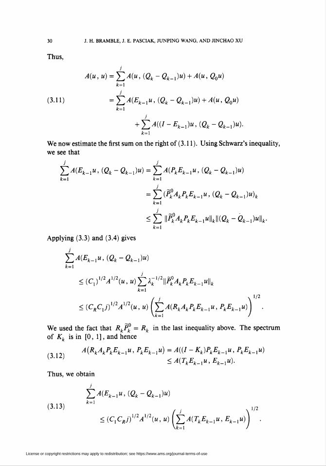
Thus,

A(u, u) = YA(u> (Qk-Qk-i)u) + A(u> ßo")fc=i

(3.11) = Y,A(Ek_xu, (Qk - Qk_x)u)+A(u, Q0u)k=l

+ YA((I-Ek_x)u,(Qk-Qk_x)u).k=l

We now estimate the first sum on the right of (3.11 ). Using Schwarz's inequality,

we see that

Y,A(Ek_xu, (Qk - Qk_x)u) = JTA(PkEk_xu, (Qk - Qk_x)u)k=l k=l

= £l(P°kAkBkEk-i«>(Qk-Qk-i)»)kk=l

j

k=i

Applying (3.3) and (3.4) gives

<Eii^X^-i"U(ß*-ß*->i

!>(£*_,«, (ß*-ß*-i)«)k=i

< (Cx)1/2Al/2(u, u)Y*k~1,2\\P°kAkPkEk_xu\\k

k=l

(J \1/2

< (CRCxj)l/2Al/2(u, u) \TA(RkAkPkEk_xu,PkEk_xu)\ .

We used the fact that Rk?k = B.k in the last inequality above. The spectrum

of Kk is in [0, 1], and hence

f312x A(RkAkPkEk-i^pkEk-i^)=A((i-Kk)PkEk-i^^kEk-i^

<A(TkEk_xu,Ek_xu).

Thus, we obtain

j

(3.13) *-1

YA(Ek_xu,(Qk-Qk_x)u)

¡i v/2< (CxCRj)1/2Al/2(u, u) YA(TkEk-i»> Ek-i«) ■

Kk=l



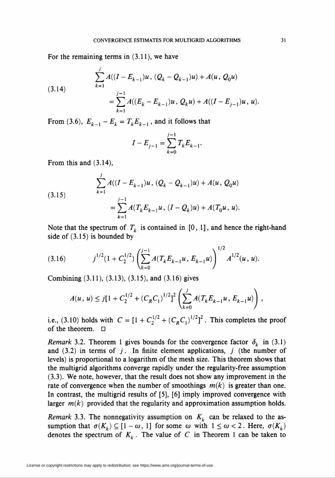
For the remaining terms in (3.11), we have

J

YA((I-Ek_x)u,(Qk-Qk_x)u) + A(u,Q0u)(3.14) k=l ._]

= YA((Ek-Ek_l)u,Qku) + A((I-Ej_x)u,u).k=\

From (3.6), Ek_x - Ek = TkEk_x, and it follows that

l-Ej-i-EVt-vk=0

From this and (3.14),

£>((/ ~Ek_x)u, (Qk - Qk_x)u) +A(u, Q0u)(3.15) k=l ._]

= YA(TkEk_xu,(I-Qk)u) + A(T0u,u).k=l

Note that the spectrum of Tk is contained in [0, 1], and hence the right-hand

side of (3.15) is bounded by

n-x s 1/2

(3.16) jXI2(X + C\'2)[YáA(TkEk_xu,Ek_xu)\ Al/2(u,u).\k=o J

Combining (3.11), (3.13), (3.15), and (3.16) gives

,1/2 , ln n ^1/2,2

U=0

A(u, u) < j[X + C\'2 + (CRCx)ll2f YA(TkEk-iu> Ek-i") .

i.e., (3.10) holds with C = [1 + C2' + (CRCxy/zf . This completes the proof

of the theorem. D

Remark 3.2. Theorem 1 gives bounds for the convergence factor ôk in (3.1)

and (3.2) in terms of j. In finite element applications, j (the number of

levels) is proportional to a logarithm of the mesh size. This theorem shows that

the multigrid algorithms converge rapidly under the regularity-free assumption

(3.3). We note, however, that the result does not show any improvement in the

rate of convergence when the number of smoothings m(k) is greater than one.

In contrast, the multigrid results of [5], [6] imply improved convergence with

larger m(k) provided that the regularity and approximation assumption holds.

Remark 3.3. The nonnegativity assumption on Kk can be relaxed to the as-

sumption that o(Kk) ç [1 - co, 1] for some co with 1 < co < 2. Here, o(Kk)

denotes the spectrum of Kk . The value of C in Theorem 1 can be taken to



be C = [1 + C21/2 + (CRCxco/(2 - co))l,2]2/(2 - co). The assumption on a(Kk)

implies that o(Tk) ç [0, co]. In this case, (3.8) is replaced by

(2-co)A(TkEk_xu, Ek_xu) <A(Ek_xu, Ek_xu) - A(Eku, Eku)

and (3.12) is replaced by

A(RkAkPkEk-lU>PkEk-lU) ^ YTÂ(TkEk-iu> £*-i")-

The remainder of the proof is similar.

4. Application to an Hr\ equivalent form

In this section, we consider applying the multilevel results of the previous

section to forms A(-, •) defined on a subspace M. ç //¿(fl). We will only

assume that the quadratic form is equivalent to the square of the Hl(Q) norm

on M., i.e.,

(4.1) c0\\v\\2x<A(v,v)<cx\\v\\2x forallve-M,.

1 1holds for positive constants c0, cx. Here, ||-||, denotes the norm in H (Q).

As far as we know, it is not possible to prove the regularity and approxima-

tion assumption ((3.3) of [6]) under such a weak assumption on the form. In

contrast, we shall see that it is possible to apply the theory of the preceding

section to natural multigrid algorithms and guarantee rapid convergence. Ex-

amples for which (4.1) is known, yet regularity and approximation results are

not available, include elliptic problems with bounded measurable coefficients

and various finite difference applications.

We start with a nested sequence of multigrid spaces

M0 C Mx C ■•• C Mj.

The most natural examples result from finite element subspaces defined on a

sequence of nested triangulations. For example, in the two-dimensional case,

when Q is a polygonal domain, we can define spaces of piecewise linear func-

tions as follows. Since fl is polygonal, start with a coarse triangulation t0 =

(J/ t0 of quasi-uniform size h0, where t0 represents an individual triangle

and t0 denotes the triangulation. Successively finer triangulations {t^ , A: =

X, ... , j} of size hk = 2~ h0 are defined by breaking each triangle of a coarser

triangulation into four triangles by connecting the midpoints of the edges. The

subspace Mk is defined to be the continuous functions defined on Q which are

piecewise linear with respect to xk and vanish on 9Q.

Let Qk denote the L (ß) projection onto Mk . It is known that, since the

triangulations are quasi-uniform,

(4.2) ||v/-fl*)«||<cAfcH,

and

(4.3) HßHIi^CIK.



for ail v e Hq(Çï) (see, e.g., [11], [23]). Here, ||-|| denotes the norm in L2(Q).

Let (•, •)k be a discrete inner product on Mk x Mk which satisfies

(4.4) c\\vf <(v,v)k<C\\v\\2 for all v e Mk.

The constants c and C in (4.4) are assumed to be independent of k =

0, ... , j . For example, we can take

(4.5) (u,v)k = h2kYu(xi)v(Xi)>

where {jc.} is the collection of nodes for Mk and the sum in (4.5) is taken over

this set. Combining (4.1)-(4.4) shows that (3.3) holds. Since, in this case, we

use discrete inner products, we can take Rk to be kk I, where kk = 0(hk ) is

a bound for the largest eigenvalue of Ak . Consequently, we can apply Theorem

1 to provide the following proposition.

Proposition 4.1. Assume that (4.1)—(4.4) hold. Then the convergence rates of

Algorithms S and N are bounded by

As the first application of this result, we will consider the following elliptic

>undary va

the problem

boundary value problem. Let fi be a polygonal domain in R and consider

Ed du /••/-»

u = 0 ondCi.

We assume that the matrix {a. } is symmetric for each x e Q. The corre-

sponding form A(-, •) is defined by

(4.7) A(u,v)=YjaaiiWjWidX + LamdX-

For this application, the only additional requirement is that the coefficients are

such that (4.1) holds. This means that the coefficients can have rather com-

plex jumps provided that they remain between fixed upper and lower bounds.

Proposition 4.1 applies and gives a convergence bound for the corresponding

multigrid algorithms. As far as we know, appropriate elliptic regularity esti-

mates (cf. [4], [6]) for the weak solutions of problem (4.6) are not known.

Without such estimates, neither the theory of [4] nor [6] would yield useful

convergence bounds.

For our second application of Proposition 4.1, we consider a finite difference

operator applied to the problem

-V-aVu = f inQ,(4-8) 'K J u = 0 ondCi.



For this application, we assume that the domain is the union of squares in a

coarse square mesh of size h0 and that the coefficient a in (4.8) is continuous

on Q and bounded from below by a positive constant c. The coarse finite

difference mesh is formed by the above-mentioned squares. Successively finer

grids are defined by breaking each square into four subsquares in the obvious

way. We seek the solution of the finite difference equations on the 7th grid.

The finite difference stencil at the grid point i, k of the y'th grid is given by

(EhX>i,k = ai,k+lß\Xi,k ~ Xi,k+V + ai,k-1/2(^1,k ~ Xi,k-¡)

+ ai+l/2,k(Xi,k ~*/+l,Jfc) + ai-lß,k\Xi,k ~Xi-\,k)'

We also consider finite element spaces of piecewise linear functions as defined

above. The coarse triangulation of Q is formed by dividing each of the coarse

squares mentioned above into two triangles by one of the diagonals. Nodal

interpolation x -> x provides a natural correspondence between the nodal

vectors in the finite difference approximation and functions in Af., i.e., x is

the function in Af ■ which takes on the values of X on the nodes of the grid.

It is easy to show that the norm induced by the form

(4-9) ¿(*.J0 = DL**W*.*

is equivalent to the H norm on Af.. The sum in (4.9) is over all nodes of

the jth mesh. Consequently, Proposition 4.1 guarantees rates of convergence

for the corresponding multigrid algorithms (with discrete inner products given

by, for example, (4.5)).

This algorithm corresponds to a natural finite difference multigrid algorithm.

In fact, the finite element spaces can be used to provide interpolation and re-

striction operators connecting the original sequence of finite difference spaces

M0, ... ,Mj. Define the kth grid operator Lkh by ([20])

(4.10) Lkh=l[LhIk,

where Ik is the interpolation matrix (corresponding to the imbedding of Mk

in Mj ) and Ik is its transpose. Then the multigrid algorithm using the form

of (4.9) is exactly the same as the finite difference multigrid algorithms using

(4.10). Proposition 4.1 provides an estimate for its rate of convergence.

The discussion given in this section extends without difficulty to problems

in more than two dimensions and other boundary conditions as well as more

general finite element spaces.

5. A REFINEMENT APPLICATION

In this section, we shall apply the results of §3 to the case of finite element

approximation with locally refined grids. Such mesh refinements are conve-

nient for accurate modeling of problems with various types of singular behav-

ior. Here, we shall make use of the fact that the operator Rk need not satisfy



smoothing conditions on the whole space but rather only on a subspace con-

taining the range of Qk-Qk_x ■ This will allow an analysis of algorithms which

only smooth on the nodes which are interior to the subdomain of refinement.

We consider the boundary value problem (4.6), but for convenience, we take

a = 0. As in §4, we assume that the coefficient matrix is symmetric and that the

resulting form (4.7) satisfies (4.1). It is well known that jumps in coefficients,

nonconvex domains, or singular data results in solutions with various types of

singular behavior [15]. To accurately solve such problems, it is convenient to

use an appropriate mesh refinement. We shall present a flexible mesh refinement

scheme in this section which leads to multigrid algorithms whose convergence

rate can be bounded by applying Theorem 1.

For convenience, we will only consider the case of piecewise linear finite

elements. Applications with other finite element spaces are possible. Also the

case of more than two dimensions presents no inherent difficulty.

The first step in the definition of the algorithms involves the development of

sequences of nested refined grids. These grids are defined in terms of a given

sequence of nested subdomains

ßj £ß;_l Ç •■• CßQ = ß.

We assume that we are given a coarse triangulation of ß = \J¡ x0 . This coarse

triangulation provides the first grid {t0} . Given that a grid {tk_x} has been

defined, the grid {xk} is defined by refining those triangles of {tk_x} which are

in Qk . This refinement is done by breaking each triangle of the mesh {rfc_,}

in ßj. into four triangles by connecting the midpoints of the edges. We assume

dÇlk aligns with the mesh {rk_x} .

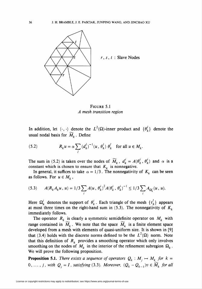
The space Mk is defined to be the set of continuous functions on ß which

are piecewise linear with respect to the grid {xk} and vanish on dQ. We note

that the continuity constraint implies that there are no new degrees of freedom

corresponding to nodes on d£lk (see Figure 5.1). These new nodes on dClk

will be called slave nodes since, by continuity, their values are determined by

the values of their neighboring nodes (which were already in the previous grids).

It is easy to see that the space Affc has a nodal basis consisting of the vertices

of {t^} excluding the slave nodes.

To fit this application into the abstract framework of §2 and §3, we need

to define discrete inner products and smoothing operators Rk . We shall use

the L (ß)-inner product for the discrete inner product on each level. The use

of L (ß)-inner products in the multigrid algorithms often leads to algorithms

which require the solution of Gram matrix problems in the implementation.

We shall avoid this (see the Appendix) by a judicious choice of the smoothing

operator Rk. Let

(5.1) ATJt = {êA/it|supp0cnJfc}.



r,s,t : Slave Nodes

Figure 5.1

A mesh transition region

In addition, let (•, •) denote the L (ß)-inner product and {9k} denote the

usual nodal basis for Mk . Define

(5.2) Rku = aY(d'k)~\u,e'k)elk for all u e Mk.i

The sum in (5.2) is taken over the nodes of Mk, dk = A(6'k, 6lk) and a is a

constant which is chosen to ensure that Kk is nonnegative.

In general, it suffices to take a = 1/3 . The nonnegativity of Kk can be seen

as follows. For u e Mk,

(5.3) A(RkAku, u) = X/3j2A(u, dik)2A(d[, dkfl < l/3£^(«, u).i i

Here ß[ denotes the support of 6[ . Each triangle of the mesh {xk} appears

at most three times on the right-hand sum in (5.3). The nonnegativity of Kk

immediately follows.

The operator Rk is clearly a symmetric semidefinite operator on Mk with

range contained in Mk . We note that the space Mk is a finite element space

developed from a mesh with elements of quasi-uniform size. It is shown in [9]

that (3.4) holds with the discrete norms defined to be the L (ß) norm. Note

that this definition of Rk provides a smoothing operator which only involves

smoothing on the nodes of Mk in the interior of the refinement subregion ß^..

We will prove the following proposition.

Proposition 5.1. There exists a sequence of operators Qk : Mj i-> Mk for k =

0, ... , j, with Qj = I, satisfying (3.3). Moreover, (Qk - Qk_,)v e Mk for all



v e Mj. Consequently, Algorithms S andïS using A(-, •), L2(Çl)-inner products,

and Rk by (5.2), converge with rates bounded by

Proof. We need only construct a sequence of operators Qk , k = 0,... , j - X,

satisfying (3.3) with (Qk - Qk_x)v Ç. Mk for all v e Mk . To do this, we use

a technique given in [9]. Let h0 denote the mesh size of the original coarse

mesh and define hk = 2~ h0. We clearly have that kk < chk . Let Mk be

the space defined from the full mesh of size hk , i.e., ~Mk is the space obtained

above when taking £lk = £lk_x = ■ ■■ = ß0 = ß. Clearly, Mk satisfies the usual

approximation and inverse properties, which imply that the L (ß) projection

operator Qk onto Mk satisfies

(5.4) \\(I-Qk)v\\<ck-kl/2Al/2(v,v)

and

(5.5) A(Qkv,Qkv)<CA(v,v),

for all v e HQ (ß). Moreover, both Affc and Mk have the same mesh restricted

to ßfc and Mk ç Mk . Let v e M. For k = 0,... , j - X, define Qkv = w,where w is the unique function in Mk satisfying

wI v

Qkv at the nodes of Mk in the interior of ß^+1

at the remaining nodes of Mk.

Note that from the construction, (Qk-Qk_x)v is a function in Mk with support

in Çlk , i.e., it is in Affc . We are left to verify (3.3).

We first prove that

(5.6) \\(I-Qk)v\\2<crklA(v,v),

from which the first inequality of (3.3) follows. By the definition of Qk and

the triangle inequality,

||(7 - Qk)v\\ = \\v - w\\ = \\v - w\\a(5-7) „ - „- "+1

<||(/-ß*)«|| + ||ß*«-«'|lot+1,

where ||-||n denotes the L2 norm on Qk+l. By (5.4), it suffices to estimate

the second term on the right-hand side of (5.7) by the first. But by the definition

of w,

\\Qkv - w\\lM < Ch\ Y (Qkv(x'k) - v(xlk))2,i

where the sum is taken over the nodes x'k of Mk on dClk+x. Clearly,

h¡EíQkV(4)-v(4))2<c\\(i-Qk)v\\.i

This proves (5.6) and completes the proof of the first inequality of (3.3).



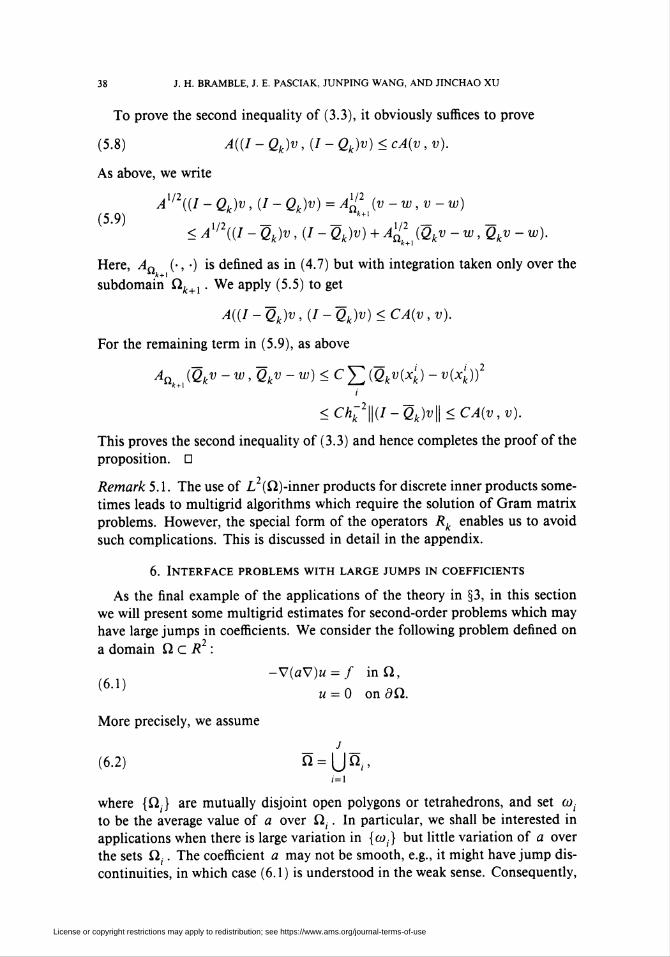
To prove the second inequality of (3.3), it obviously suffices to prove

(5.8) A((I - Qk)v, (I - Qk)v) < cA(v , v).

As above, we write

A1/2((I - Qk)v , (I - Qk)v) = Axi] (v-w,v-w)(5 9) k+i

< Al/2((I - Qk)v , (I - Qk)v) + Al¿2+¡ (Qkv -w,Qkv- w).

Here, An (•, •) is defined as in (4.7) but with integration taken only over the

subdomain ßA:+1. We apply (5.5) to get

A((I-Qk)v,(I-Qk)v)<CA(v,v).

For the remaining term in (5.9), as above

AakJQkv ~w,Qkv-w)< CY,(Qkv(4) -^(¿k))2i

<Ch;2\\(I-Qk)v\\<CA(v,v).

This proves the second inequality of (3.3) and hence completes the proof of the

proposition. D

Remark 5. X. The use of L2(ß)-inner products for discrete inner products some-

times leads to multigrid algorithms which require the solution of Gram matrix

problems. However, the special form of the operators Rk enables us to avoid

such complications. This is discussed in detail in the appendix.

6. Interface problems with large jumps in coefficients

As the final example of the applications of the theory in §3, in this section

we will present some multigrid estimates for second-order problems which may

have large jumps in coefficients. We consider the following problem defined on

a domain fie/? :

-V(flV)« = / inß,(6.1) 1y u = 0 ondß.

More precisely, we assume

j

(6.2) ß = Un/'í=i

where {ß,} are mutually disjoint open polygons or tetrahedrons, and set coi

to be the average value of a over ß(. In particular, we shall be interested in

applications when there is large variation in {&>(} but little variation of a over

the sets ß;. The coefficient a may not be smooth, e.g., it might have jump dis-

continuities, in which case (6.1) is understood in the weak sense. Consequently,



we assume that co¡ > 0 for each i, and that there are constants c0 and cx not

depending on i = X, ... , J satisfying

(6.3) c0a>p¡(v, v) < At(v , v) < c^p^v , v) for all v € Hl(a.).

Here, A¡(-, •) is defined by

Ai(u,v)=l aVu-Vvdx.Ja,

Similarly, Z>;(-, •) denotes the Dirichlet form on ß( and

(6.4) A(u,v) = Y,Ai(u,v).i

The purpose of this section is to apply the results of §3 to provide estimates

for appropriately defined multigrid algorithms for (6.1) which depend only on

the constants c0, cx of (6.3) but not on the values of co¡. This means that

max; co ¡I min; coi can be very large without significantly reducing the rate of

convergence for these multigrid algorithms. To achieve this rate of convergence,

we use a discrete inner product which is weighted by the coefficients {gjJ and

a coarse triangulation which aligns with the boundaries of {ß(}. By this we

mean that IJ, öß, is a subset of \J¡ dx0 , where {t0} is the coarse triangulation

of ß (see §4).

As far as we know, the dependence of the elliptic regularity estimates (in

the weighted norms) is not known for this type of problem. Consequently, the

regularity and approximation assumptions necessary for the standard theory

are not available. Some analysis for a fixed number of levels has been given in

[23] although the estimates given there tend rapidly to one as the number of

levels is increased. In contrast, the bounds we shall derive here only deteriorate

quadratically with the number of levels (see Proposition 6.1).

To begin our analysis, we introduce the following weighted inner products:

j

(6.5) (»>v)lI(c1) = Y03í(u>v)l\c1¡)>i=i

and

j

(6.6) (u,v)H^Q) = Y,°>iDi(u>v)>í=i

with the induced norms denoted by IHIl2(Q) and || • Hj/w™ > respectively. No-

tice that by (6.3), A[/2(-, •) is equivalent to || • Hî,^. As is done in §4, we

assume that ß is triangulated by a nested sequence of quasi-uniform meshes

{xk: k = 0, ... , j} with {9ß(} being a subgrid of {t0} . Corresponding to

these triangulations, as in §4, we have the multilevel spaces

Af0 C Afj C • • • C Af..


l"ll//'(£2)


The operators Qk needed in the analysis of §3 can be taken to be the weighted

L2 projections Qk: L2(ß) >-> Mk defined by

(6.7) (Qku, «)L2(0) = (u, v)L2jQ) for all u 6 L2(ß), v € Mk.

The following result is taken from [23] for the verification of (3.3).

Lemma 6.1. Assume the decomposition (6.2) has no cross points, namely there

is no point on the interface that belongs to more than two ß, 's. Then, for all

ueHr](ri),

\\(I-Qt)u\\Ll{a)<Chk\\u\\„L(Q)

and

WQk^Him - cIMk(£ir

More generally, in the presence of cross points, we have, for all u € Mjt

( h V/2ll('-ß>lk(n)<C^log^J

and

( h V/2\\Q>\\hi(çi)<c^Yj) l|M|k(nr

Remark 6.1. The first part of the above result holds in three dimensions but, in

general, the second does not [23].To completely define the multigrid algorithms, we need only define the dis-

crete inner products and the smoothing operators {Rk} . The discrete inner

products are defined by the weighted inner product (6.5). We define the opera-

tor Rk by

(6.8) **«=«£(<)" V0í)l>{ÍI)0;,

Here, d'k = A(6'k, d'k) and a is a constant chosen so that Kk is nonnegative.

From the discussion in §5, it suffices to take a = 1/3.

By the inverse inequality, we have that the largest eigenvalue of Ak (defined_2

by (2.2)) is bounded by Chk . As a consequence, Lemma 6.1 implies that the

assumption (3.3) holds with Cx and C2 satisfying

Cx<Cxj\ C2<C2f,

where C, and C2 are constants independent of k and j. The constant y is

equal to zero if the interface has no cross points and otherwise y equals one.

Applying Theorem 1 gives the following proposition.



Proposition 6.1. For the operators and inner products defined above, the conver-

gence rate of Algorithm S and N are bounded by

where y = 0 or 1 as explained above.

Remark 6.2. The above proposition holds for three-dimensional applications

provided that, for example, there are no internal cross points.

Remark 6.3. The special form of the smoothing operators Rk defined in (6.8)

enables us to avoid the solution of Gram matrix problems associated with the

inner products appearing in the multigrid algorithms. This is discussed in detail

in the appendix.

7. Numerical results

In this section, we provide the results of numerical examples illustrating the

theory developed in the earlier sections. Specifically, the actual reduction factor

ôj satisfying (3.1) is numerically computed in several examples. Note that á

is the largest eigenvalue of the operator I - BjAj and can be computed numer-

ically. We shall provide results in the case of local refinement (see §5) as well

as quasi-uniform meshes applied to problems where the coefficients defining the

differential operator have jumps (see §§4 and 6). The results of the refinement

calculations appear to be independent of the number of levels. In contrast,

the examples in which the coefficients have jumps show a slow deterioration

in the rate of convergence as the number of levels increases. Both cases show

asymptotic convergence behavior which is somewhat better than the worst-case

analysis provided by the earlier theory. In all of the reported results, we use a

symmetric V-cycle algorithm with m(k) = X for all k .

We report the numerically computed value of Sj as a function of the mesh

parameters. We note however that, since the operator S. is symmetric, it can

be used as a preconditioner and the overall convergence of the algorithm can

be accelerated by preconditioned conjugate gradient iteration. In this case, the

condition number of the preconditioned system is bounded by (1 - <$.)" .

For the first example, we consider the application of the multigrid algorithm

to the finite element equations corresponding to a problem with mesh refine-

ment. For this example, the domain ß will be the unit square, and we shall

approximate the solution to

-Au = / in ß,7.1

«-O onôfi.

The corresponding form A(-, •) is the Dirichlet form on ß.

The sequence of grids which we shall consider will be progressively more

refined as we approach the corner ( 1, 1 ). We will use the scheme described in

§5 for generating the mesh. We start by breaking the square into sixteen smaller



squares of side length 1/4. The coarse triangulation is defined by splitting

each of these smaller squares into two triangles, for example, along the diagonal

between the bottom left to the upper right corner. For integers 0 < / < j, we

define ß^ = ß for k = 0, ... , / and ük = [1 - 2J~k, 1] x [1 - 2J~k, 1] for

k > J. This generates a sequence of meshes with geometrically decreasing mesh

size, with local refinement (for k > J ) on domains of geometrically decreasing

size. Such a mesh would be effective if, for example, the function / in (7.1)

behaved like a ô function distribution at the point (1,1). The finite element

spaces Af0 c • •• c Af are defined as in §5.

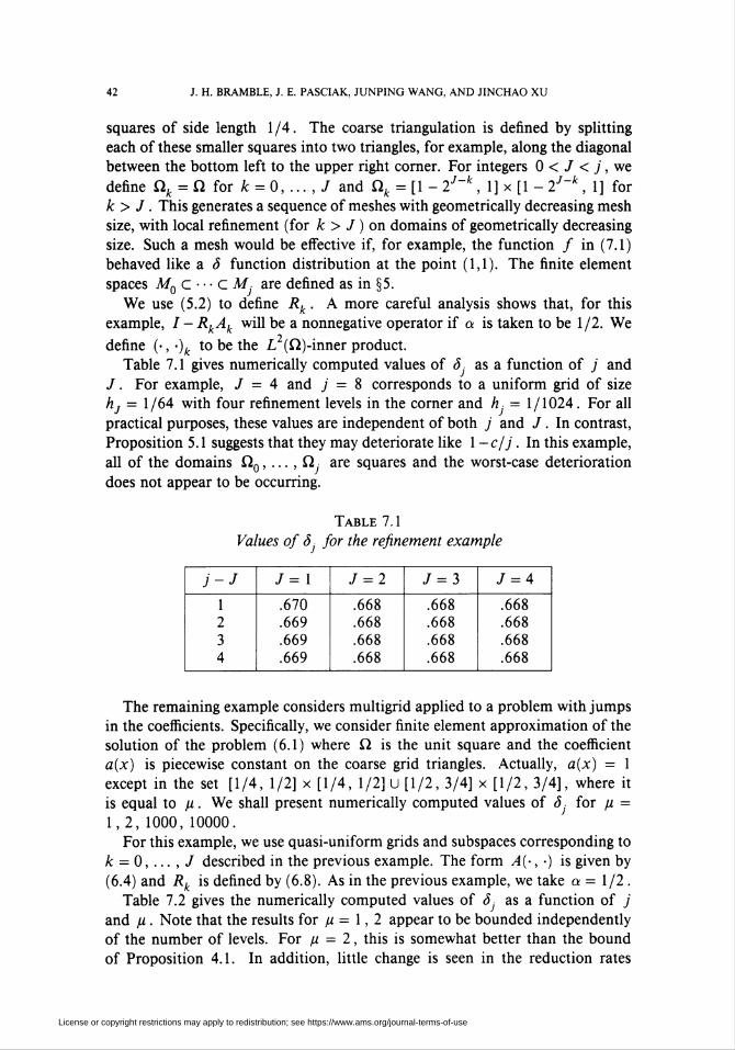
We use (5.2) to define Rk. A more careful analysis shows that, for this

example, I - RkAk will be a nonnegative operator if a is taken to be 1/2. We

define (-,-)k to be the L2(ß)-inner product.

Table 7.1 gives numerically computed values of ¿ as a function of j and

J. For example, J = 4 and j: = 8 corresponds to a uniform grid of size

hj = 1/64 with four refinement levels in the corner and h = 1/1024. For all

practical purposes, these values are independent of both j and J . In contrast,

Proposition 5.1 suggests that they may deteriorate like 1 -c/j . In this example,

all of the domains ß0, ... , ß are squares and the worst-case deterioration

does not appear to be occurring.

Table 7.1

Values of á for the refinement example

J-J J = X J = 2 J = 3 7 = 4

1234

.670

.669

.669

.669

.668

.668

.668

.668

.668

.668

.668

.668

.668

.668

.668

.668

The remaining example considers multigrid applied to a problem with jumps

in the coefficients. Specifically, we consider finite element approximation of the

solution of the problem (6.1) where ß is the unit square and the coefficient

a(x) is piecewise constant on the coarse grid triangles. Actually, a(x) = X

except in the set [1/4, 1/2] x [1/4, 1/2] u [1/2, 3/4] x [1/2, 3/4], where itis equal to ft. We shall present numerically computed values of á for ß =

1,2, 1000, 10000.For this example, we use quasi-uniform grids and subspaces corresponding to

k = 0, ... , J described in the previous example. The form A(-, ■) is given by

(6.4) and Rk is defined by (6.8). As in the previous example, we take a = 1/2 .

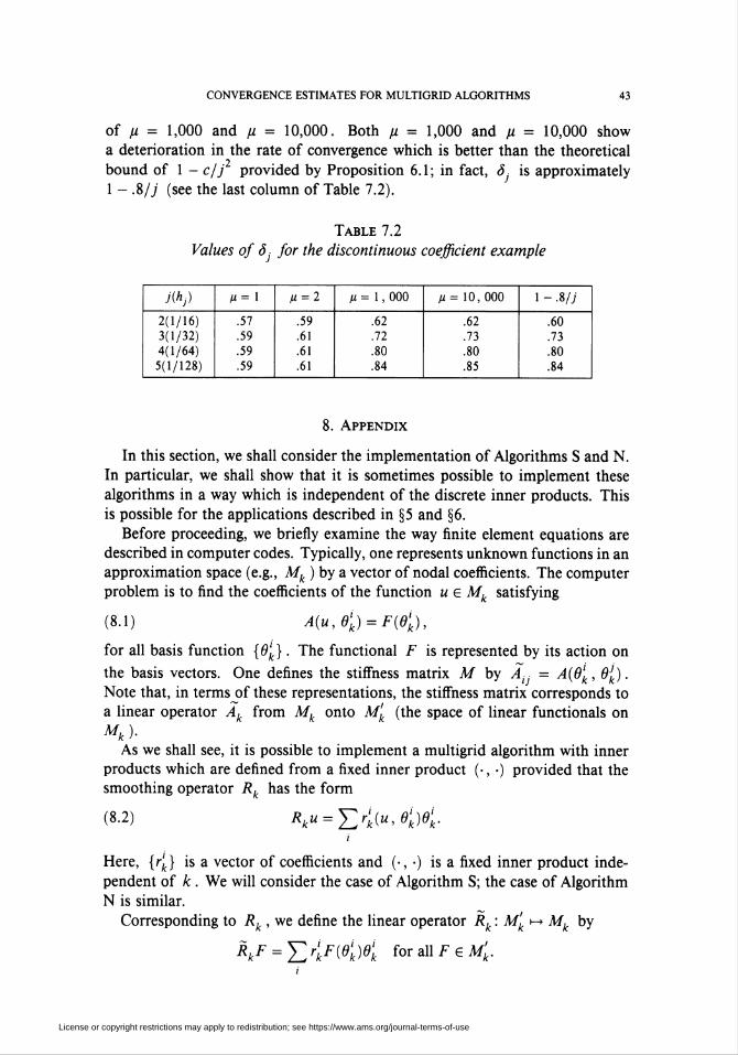
Table 7.2 gives the numerically computed values of <J. as a function of j

and p.. Note that the results for ft = X, 2 appear to be bounded independently

of the number of levels. For p. = 2, this is somewhat better than the bound

of Proposition 4.1. In addition, little change is seen in the reduction rates



of p = 1,000 and p = 10,000. Both p = 1,000 and p = 10,000 showa deterioration in the rate of convergence which is better than the theoretical

bound of 1 - c/j provided by Proposition 6.1; in fact, á is approximately

1 - .8/7 (see the last column of Table 7.2).

Table 7.2

Values of S for the discontinuous coefficient example

j(hj) H=\ lt = 2 n = 1, 000 fi= 10,000 1 - .8/7

2(1/16)3(1/32)4(1/64)5(1/128)

.57

.59

.59

.59

.59

.61

.61

.61

.62

.72

.80

.84

.62

.73

.80

.85

.60

.73

.80

.84

8. Appendix

In this section, we shall consider the implementation of Algorithms S and N.

In particular, we shall show that it is sometimes possible to implement these

algorithms in a way which is independent of the discrete inner products. This

is possible for the applications described in §5 and §6.

Before proceeding, we briefly examine the way finite element equations are

described in computer codes. Typically, one represents unknown functions in an

approximation space (e.g., Af^ ) by a vector of nodal coefficients. The computer

problem is to find the coefficients of the function u e Mk satisfying

(8.1) A(u,d'k) = F(6'k),

for all basis function {d'k}. The functional F is represented by its action on

the basis vectors. One defines the stiffness matrix Af by A¡, = A(d'k, 6k).

Note that, in terms of these representations, the stiffness matrix corresponds to

a linear operator Ak from Mk onto Mk (the space of linear functionals on

Mk).As we shall see, it is possible to implement a multigrid algorithm with inner

products which are defined from a fixed inner product (•, ■) provided that the

smoothing operator Rk has the form

(8.2) Rku = Yr'k(u,e'k)d'k.i

Here, {r'k} is a vector of coefficients and (•, •) is a fixed inner product inde-

pendent of k . We will consider the case of Algorithm S; the case of Algorithm

N is similar.

Corresponding to Rk , we define the linear operator Rk: M'k^ Mk by

V = £'^(« forallT-eAT,fc-


44 J. H. BRAMBLE, J. E. PASCIAK JUNPING WANG, AND JINCHAO XU

Instead of defining a sequence of operators Bk : Mk >-> Mk , k = 0, ... , j, we

define, by induction, a sequence of operators Bk: Mk>-> Mk , k = 0, ... , j, as

follows:Set Bq = Âq1 . Assume that Bsk_x has been defined and define Bkg for

g e Mk as follows:

(1) Set jc° = 0 and q° = 0.

(2) Define xl for / = 1, ..., m(k) by

(8.3) xl = x~l + Rk(g - Äkx'~l).

(3) Define xm{k)+i = xm(k) + q" , where ql for i=X,...,p is defined by

i i—I , ni r, 7 "l(fc), 7 I—Ilq = <? +Bk_x[(g-Akx ')-Ak_xq ].

(4) Set 77^ = x2m(fc)+1, where jc7 is defined for 1= m(k)+2,...,2m(k)+X

by (8.3).

It is not difficult to check that 77'^. = BsiÄi. In addition, B'F = B*f asj j j j j ¡J

long as

(f,9) = F(6) for all 0 e Af,..

This means that the multigrid algorithm using BSj as a preconditioner for (8.1)

leads to the same set of iterates as the multigrid algorithm using BSj as a precon-

ditioner for (2.1 ). Thus, the above algorithm is an implementation of Algorithm

S provided that we use a fixed inner product (•, •) and Rk has the form of

(8.2). Note that the use of Pk_x in Step 3 of Algorithm S has been avoided in

the above implementation. This is because the natural imbedding of Af¿ into

Af^ is used. In addition, the inner products do not appear in the implemen-

tation.

Remark 8.1. The above implementation is somewhat simpler than a direct im-

plementation of Algorithm S. This is because the prolongation and restriction

parts of the above implementation only involve the relations between finite el-

ement spaces. The coefficients of the operator only affect the computation of

Rk (see (5.2) and (6.8)) and Äk .

Bibliography

1. O. Axelsson and P. S. Vassilevski, Algebraic multilevel preconditioning methods, II, (pre-

print).

2. D. Bai and A. Brandt, Local mesh refinement multilevel techniques, SIAM J. Sei. Statist.

Comput. 8(1987), 109-134.

3. R. E. Bank, and C. C. Douglas, Sharp estimates for multigrid rates of convergence with

general smoothing and acceleration, SIAM J. Numer. Anal. 22 (1985), 617-633.

4. R. E. Bank and T. Dupont, An optimal order process for solving finite element equations,

Math. Comp. 36 (1981), 35-51.

5. D. Braess and W. Hackbusch, A new convergence proof for the multigrid method including

the V-cycle, SIAM J. Numer. Anal. 20 (1983), 967-975.



6. J. H. Bramble and J. E. Pasciak, New convergence estimates for multigrid algorithms, Math.

Comp. 49(1987), 311-329.

7. J. H. Bramble, J. E. Pasciak, J. Wang, and J. Xu, Convergence estimates for product iterativemethods with applications to domain decomposition and multigrid, (preprint).

8. J. H. Bramble, J. E. Pasciak, and J. Xu, The analysis of multigrid algorithms for nonsym-

metric and indefinite elliptic problems, Math. Comp. 51 (1988), 389-414.

9. J. H. Bramble, J. E. Pasciak, and J. Xu, Parallel multilevel preconditioners, Math. Comp.

55(1990), 1-22.

10. J. H. Bramble, J. E. Pasciak, and J. Xu, The analysis of multigrid algorithms with nonnested

spaces or noninherited quadratic forms, Math. Comp. 56 (1991), 1-34.

11. J. H. Bramble and J. Xu, Some estimates for a weighted L projection, Math. Comp. 56

(1991), 463-476.

12. A. Brandt, Algebraic multigrid theory: the symmetric case, Appl. Math. Comput. 19(1986),23-56.

13. A. Brandt, Multi-level adaptive solutions to boundary-value problems, Math. Comp. 31

(1977), 333-390.

14. W. Hackbusch, Multi-grid methods and applications, Springer-Verlag, New York, 1985.

15. R. B. Kellogg, Interpolation between subspaces of a Hubert space, Tech. Note BN-719, Univ.

of Maryland, Inst. Fluid Dynamics and Appl. Math., 1971.

16. M. Kocvara and J. Mandel, A multigrid method for three-dimensional elasticity and algebraic

convergence estimates, Appl. Math. Comput. 23 (1987), 121-135.

17. J. F. Maitre and F. Musy, Algebraic formalization of the multigrid method in the symmetric

and positive definite case—a convergence estimation for the V-cycle, Multigrid Methods for

Integral and Differential Equations (D. J. Paddon and H. Holstein, eds.), Clarendon Press,

Oxford, 1985.

18. J. Mandel, Étude algébrique d'une méthode multigrille pour quelques problèmes de frontière

libre, C.R. Acad. Sei. Paris Sér. I. Math. 298 (1984), 469-472.

19. J. Mandel, Multigrid convergence for nonsymmetric, indefinite variational problems and one

smoothing step, (Proa Copper Mtn. Conf. Multigrid Methods), Applied Math. Comput. 19

(1986), 201-216.

20. J. Mandel, S. F. McCormick, and R. Bank, Variational multigrid theory, Multigrid Methods(S. McCormick, ed.), SIAM, Philadelphia, PA, 1987, pp. 131-178.

21. P. Vassilevski, Iterative methods for solving finite element equations based on multilevelsplitting of the matrix, Bulgarian Academy of Sciences, Sofia, Bulgaria, (preprint).

22. J. Xu, Convergence estimates for some multigrid algorithms, Proc. 1989 Houston Domain

Decomp. Methods Conf. Third Internat. Sympos. Domain Decomposition Methods for

Partial Differential Equations (T. Chan, R. Glowinski, J. Periaux, and O. Widlund, eds.),

SIAM, Philadelphia, PA, 1990, pp. 174-187.

23. J. Xu, Theory of multilevel methods, Ph.D. Thesis, Cornell University and Penn State Uni-

versity, Dept. Math. Rep AM-48, 1989.

Department of Mathematics, Cornell University, Ithaca, New York 14853

E-mail address: [email protected]

Department of Applied Science, Brookhaven National Laboratory, Upton, New York

11973E-mail address: [email protected]

Mathematics Department, The University of Wyoming, Laramie, Wyoming 82071

Department of Mathematics, Pennsylvania State University, University Park, Penn-

sylvania 16802


Documents

CONVERGENCE ESTIMATES FOR MULTIGRID ALGORITHMS …...CONVERGENCE ESTIMATES FOR MULTIGRID ALGORITHMS 25 results most naturally apply to finite element multigrid algorithms but can also