Convex computation of the maximumcontrolled invariant set for polynomial

control systems?

Milan Korda1, Didier Henrion2,3,4, Colin N. Jones1

March 27, 2013

Abstract

We characterize the maximum controlled invariant (MCI) set for discrete- aswell as continuous-time nonlinear dynamical systems as the solution of an infinite-dimensional linear programming problem. For systems with polynomial dynamicsand compact semialgebraic state and control constraints, we describe a hierarchy offinite-dimensional linear matrix inequality (LMI) relaxations whose optimal valuesconverge to the volume of the MCI set; dual to these LMI relaxations are sum-of-squares (SOS) problems providing a converging sequence of outer approximationsto the MCI set. The approach is simple and readily applicable in the sense thatthe approximations are the outcome of a single semidefinite program with no addi-tional input apart from the problem description. A number of numerical examplesillustrate the approach.

1 Introduction

Given a controlled dynamical system described by a differential (continuous-time) ordifference (discrete-time) equation, its maximum controlled invariant (MCI) set is theset of all initial states that can be kept within a given constraint set ad infinitum usingadmissible control inputs. This set goes by many other names in the literature, e.g.,viability kernel in viability theory [5], or (A,B)-invariant set in the linear case [14].

Set invariance is an ubiquitous and essential concept in dynamical systems theory, as faras both analysis and control synthesis is concerned. In particular, by its very definition,

?A preliminary version of this work, dealing with discrete-time systems only, has been submitted forpossible presentation at the IEEE Conf. on Decision and Control, 2013.

1Laboratoire d’Automatique, Ecole Polytechnique Federale de Lausanne, Station 9, CH-1015, Lau-sanne, Switzerland. milan.korda,colin.jones@epfl.ch

2CNRS, LAAS, 7 avenue du colonel Roche, F-31400 Toulouse; France. henrion@laas.fr3Universite de Toulouse, LAAS, F-31400 Toulouse; France4Faculty of Electrical Engineering, Czech Technical University in Prague, Technicka 2, CZ-16626

Prague, Czech Republic

1

arX

iv:1

303.

6469

v1 [

mat

h.O

C]

26

Mar

201

3

the MCI set determines fundamental limitations of a given control system with respectto constraint satisfaction. In addition, there is a very tight link between invariant setsand (control) Lyapunov functions. Indeed, sub-level sets of a Lyapunov function giverise to invariant sets. Conversely, at least in the linear case, any controlled invariant setgives rise to a control Lyapunov function, and therefore these sets can be readily used todesign stabilizing control laws; see, e.g., [9] for a general treatment and, e.g., [18, 27] forapplications in model predictive control design.

The problem of (maximum) controlled invariant set computation for discrete-time systemshas been a topic of active research for more than four decades. The central tool in thiseffort has been the contractive algorithm of [7] and its expansive counterpart [19]. For anexhaustive survey and historical remarks see the survey [9] and the book [13].

Both algorithms, although conceptually applicable to any nonlinear system, have beenpredominantly applied in a linear setting where they boil down to a sequence of linearprograms and polyhedral projections. Finite termination of this sequence is a subtle prob-lem and sharp results are available only in the uncontrolled setting where no projectionsare required [17]; for discussion of finite-termination in the controlled case see [44]. Thecontractive and expansive algorithms were combined in [18] to design an algorithm termi-nating in a finite number of iterations and outputting an ε-accurate inner approximationof the MCI set (with the accuracy measured by the Hausdorff distance). Another lineof research, culminating in [41], exploits the linearity of the system dynamics in a moresystematic way and approximates the maximum (or minimum) robust controlled invariantset by the Minkowski sum of a parametrized family of sets. Very recently, in continu-ous time, [31] developed a parallel algorithm for ellipsoidal approximations of the robustMCI set scalable to very high dimensions. Computation of low-complexity polyhedralcontrolled invariant sets was investigated in [11] and [12].

In the nonlinear case, a common practice is to exploit the tight connection between in-variance and Lyapunov functions and seek invariant sets as sub-level sets of a (control)Lyapunov function; see, e.g., [15, 50] and references therein for recent theoretical devel-opments on the related problem of region of attraction computation and, e.g., [35] forpractical applications of these techniques. This, however, typically leads to non-convexbilinear optimization problems which are notoriously hard to solve. Therefore, one of-ten has to resort to ad-hoc analysis of the specific system at hand, which is typicallytractable only in small dimensions; see [45, 46] for concrete examples. Related in spiritis the localization technique of [26] for discrete-time uncontrolled systems, also requiringconsiderable effort in analysing the system.

Recently, a general approach using a hierarchy of finite-dimensional linear programs (LPs)was used in [6] to design a controller ensuring invariance of a given candidate polyhedralset. In our opinion, although being the current state of the art, this work still suffersfrom the following drawbacks: 1) the sets obtained are convex polytopes (not generalsemi-algebraic sets, a fact particularly limiting in the nonlinear case where nonconvexMCI sets are common); 2) the geometry of the candidate polytopic set must be given apriori; 3) there are no convergence guarantees to the MCI set. In this paper, we explicitlyaddress all these points.

Building upon our previous work [20] on the computation of the region of attraction (ROA)

2

for polynomial control systems, in this paper we characterize the maximum controlledinvariant (MCI) set for discrete- as well as continuous-time polynomial systems as thesolution to an infinite-dimensional LP problem in the cone of nonnegative measures. Thedual of this problem is an infinite-dimensional LP in the space of continuous functions.Finite-dimensional relaxations of the primal LP and finite-dimensional approximations ofthe dual LP turn out to be semidefinite programs (SDPs) also related by duality. Theprimal relaxations lead to a truncated moment problem while the dual approximations toa sum-of-squares (SOS) problem. Super-level sets of one of the polynomials appearing inthe dual SOS problem then provide outer approximations to the MCI set with guaranteedconvergence as the degree of the polynomial tends to infinity.

The main mathematical tool we use are the so-called occupation measures which allowus to study the time evolution of the whole ensemble of initial conditions (described by ameasure) rather than studying trajectories associated to each initial condition separately.The use of measures to study dynamical systems has a very long tradition: see [43] forprobably the first systematic treatment1; for purely discrete-time treatment see [23, Chap-ter 6]. To the best of the authors’ knowledge our paper is the first one to use occupationmeasures for MCI set (approximate) computation. The MCI set was previously charac-terized using occupation measures in [16], but there the characterization is rather indirectand not straightforwardly amenable to computation. Apart from the authors’ work [20],the related problem of region of attraction computation was tackled using measures in [51].There, however, a very different approach was taken, not using occupation measures butrather analyzing convergence via discretization of the state-space and propagating theinitial distribution by means of a discretized transfer operator. Here, instead, we employthe (discounted) occupation measure which captures the behaviour of the trajectoriesemanating from the initial distribution over the infinite time horizon. As a result, ourapproach requires no discretization and, contrary to [51], provides true guarantees (notin an “almost-everywhere” or “coarse” sense) and, more importantly, is applicable in acontrolled setting. Closely related to the occupation measures used here is the Rantzer’sdensity [42] which was used in [40] to assess the stability of attractor sets of uncontrollednonlinear systems. The approach, however, does not immediately yield approximationsof the MCI set (or the region of attraction) and applies to uncontrolled systems only.

Similar in spirit to our approach, from the dual viewpoint of optimization over functions,are the Hamilton-Jacobi approaches (e.g., [36, 37]). However, contrary to these methods,our approach does not require state-space discretization and comes with convergenceguarantees.

The contribution of our paper with respect to previous work on the topic can be summa-rized as follows:

• we deal with fully general continuous-time and discrete-time polynomial dynamicsunder semi-algebraic state and control constraints;

• our approximated MCI set is described by (the intersections of) polynomial super-level sets, including more restrictive classes (e.g. polytopes, ellipsoids, etc.);

1In [43], J. E. Rubio used Young measures [49] rather than occupation measures, but the basic ideaof “linearizing” a nonlinear problem by going into an infinite-dimensional space of measures is the same.

3

• we provide a convex infinite-dimensional LP characterization of the MCI set;

• we describe a hierarchy of convex finite-dimensional SDPs to solve the LP withconvergence guarantees;

• our approach is simple and readily applicable in the sense that the approximationsare the result of a single SDP with no additional data required apart from theproblem description.

The contribution with respect to our previous work [20] can be summarised as follows:

• in [20] we compute the ROA, which is a related although different object: it is theset of all of initial conditions that can be steered to a given target set while satisfyingstate and control constraints. In particular, the MCI set differs from the ROA inthe sense that we do not try to hit any target set at a given time but rather try tokeep the state within a given set forever. Therefore we had to adapt our techniqueto deal explicitly with invariance;

• in [20] we dealt with continuous-time systems only, whereas we can cope, withminor modifications, with discrete-time systems as well; we choose to describe boththe continuous-time and discrete-time setups in parallel precisely to underline thesecommon features;

• in [20] we considered only a finite time-horizon, whereas here we show how to cope,with the help of discounting, with an infinite horizon. This brought additionaltechnical issues not encountered in finite time.

What can be considered a drawback of our approach is the fact that the approximationsto the MCI set we obtain are from the outside and therefore not invariant. However,accurate outer approximations provide important information as to the performance lim-itations of the control system and are of practical interest, e.g., in collision avoidance.Therefore we believe that our work bears both theoretical and practical value, and natu-rally complements existing inner-approximation techniques.

The paper is organised as follows. The problem to be solved is described in Section 2.Occupation measures are introduced in Section 3. The infinite-dimensional primal anddual LPs are described in Sections 4 and 5, respectively. The finite-dimensional relaxationswith convergence results are presented in Section 6. Numerical examples are in Section 7.A reader interested only in the semialgebraic outer approximations of the MCI set canconsult directly the infinite-dimensional dual LPs (8) and (9) and their finite-dimensionalapproximations (11) and (13) in discrete and continuous time, respectively.

1.1 Notation

Measures are understood as signed Borel measures on a Euclidean space, i.e., as countablyadditive maps from the Borel sets to the real numbers. From now on all subsets of aEuclidean space we refer to are automatically understood as Borel. The vector space ofall signed Borel measures with its support contained in a set X is denoted by M(X).

4

The support (i.e., the smallest closed set whose complement has a zero measure) of ameasure µ is denoted by sptµ. The space of continuous functions on X is denoted byC(X) and likewise the space of once continuously differentiable functions is C1(X). Theindicator function of a set X (i.e., a function equal to one on X and zero otherwise) isdenoted by IX(·). The symbol λ denotes the n-dimensional Lebesgue measure (i.e., thestandard n-dimensional volume). The integral of a function v with respect to a measureµ over a set X is denoted by

∫Xv(x) dµ(x). Sometimes for conciseness we use the shorter

notation∫v dµ omitting the integration variable and also the set over which we integrate

if they are obvious from the context. The ring of polynomials in (possibly vector) variablesx1,. . . ,xn is denoted by R[x1, . . . , xn].

2 Problem statement

The approach is developed in parallel for discrete and continuous time.

2.1 Discrete time

Consider the discrete-time control system

xt+1 = f(xt, ut), xt ∈ X, ut ∈ U, t ∈ 0, 1, . . . (1)

with a given polynomial vector field f with entries fi ∈ R[x, u], i = 1, . . . , n, and givencompact basic semialgebraic state and input constraints

xt ∈ X := x ∈ Rn : gXi(x) ≥ 0, i = 1, 2, . . . , nX,ut ∈ U := u ∈ Rm : gU i(u) ≥ 0, i = 1, 2, . . . , nU

with gXi ∈ R[x], gU i ∈ R[u].

The maximum controlled invariant (MCI) set is defined as

XI :=x0 ∈ X : ∃

(xt∞t=1, ut∞t=1

)s.t. xt+1 = f(xt, ut),

ut ∈ U, xt ∈ X, ∀t ∈ 0, 1, . . ..

A control sequence ut∞t=0 is called admissible if ut ∈ U for all t ∈ 0, 1, . . . .In words, the MCI set is the set of all initial states which can be kept inside the constraintset X ad infinitum using admissible control inputs.

2.2 Continuous time

Consider the relaxed continuous-time control system

x(t) ∈ conv f(x(t), U), x(t) ∈ X, t ∈ [0,∞), (2)

5

where conv denotes the convex hull, f is a polynomial vector field with entries fi ∈R[x, u], i = 1, . . . , n, and compact basic semialgebraic state and input constraint sets aredefined by

X := x ∈ Rn : gXi(x) ≥ 0, i = 1, 2, . . . , nX,U := u ∈ Rm : gU i(u) ≥ 0, i = 1, 2, . . . , nU

with gXi ∈ R[x], gU i ∈ R[u]. The meaning of the convex differential inclusion (2) is asfollows: for all time t, the state velocity x(t) is constrained to the convex hull of theset f(x(t), U) := f(x(t), u) : u ∈ U ⊂ Rn. The connection of this convexified (orrelaxed) control problem (2) and the classical control problem x = f(x, u) is the Filippov-Wazewski Theorem [5], which shows that the trajectories of x = f(x, u) are dense (in thesupremum norm) in the set of trajectories of the convexified inclusion2 (2). Therefore,from a practical point of view, there is little difference between the two formulations forthe purposes of MCI set computation; see Section 3.2 and Appendices B and C of [20] fora detailed discussion on this subtle issue. The simplest assumption under which the MCIsets for both systems coincide is f(x, U) being convex for all x, which is in particular truefor input-affine systems of the form x = f(x) + g(x)u with U convex.

The maximum controlled invariant (MCI) set is defined as

XI :=x0 ∈ X : ∃ x(·) s.t. x(t) ∈ conv f(x(t), U) a.e., x(t) ∈ X ∀ t ∈ [0,∞)

,

where x(·) is required to be absolutely continuous and a.e. stands for “almost everywhere”with respect to the Lebesgue measure on [0,∞).

In words, the MCI set is the set of all initial states for which there exists a trajectory ofthe convexified inclusion (2) which remains in X ad infinitum.

3 Occupation measures

In this section we introduce the concept of occupation measures which is the centrepieceof our approach.

3.1 Discrete time

Given a discount factor α ∈ (0, 1), an initial condition x0 and an admissible controlsequence ut|x0∞t=0 such that the associated state sequence xt|x0∞t=0 remains in X for alltime, we define the discounted occupation measure µ(· | x0) ∈M(X × U) as

µ(A×B | x0) :=∞∑t=0

αtIA×B(xt|x0 , ut|x0) (3)

for all sets A ⊂ X and B ⊂ U .

2Note that the set conv f(x(t), U) is closed for every t since f is continuous and U compact; thereforethere is no need to take closure of the convex hull in order to apply the Filippov-Wazewski theorem.

6

In words, the discounted occupation measure measures the (discounted) number of visitsof the state-control pair trajectory (x(· |x0), ν(· |x0)) to subsets of X×U . The discountingin the definition of the occupation measure ensures that µ(A×B | x0) is always finite; infact we have µ(X × U | x0) = (1− α)−1.

Now suppose that the initial condition is not a single point but an initial measure3 µ0 ∈M(X) and an admissible control sequence is associated to each initial condition from thesupport of µ0 in such a way that the corresponding state sequence remains in X. Thenwe define the average discounted occupation measure µ ∈M(X × U) as

µ(A×B) :=

∫X

µ(A×B |x0) dµ0(x0).

The average discounted occupation measure measures the discounted average number ofvisits in subsets of X × U of trajectories starting from the initial distribution µ0.

Now we derive an equation linking the measures µ0 and µ. This equation will play a keyrole in subsequent development and in a sense replaces the dynamics equation (1). Toderive this equation fix an initial condition x0 ∈ X and a control sequence ut|x0∞t=0 suchthat the associated state sequence xt|x0∞t=0 stays in X. Then for any v ∈ C(X) we have∫

X×Uv(x) dµ(x, u |x0) =

∞∑t=0

αtv(xt|x0) = v(x0|x0) + α∞∑t=0

αtv(xt+1|x0)

= v(x0|x0) + α∞∑t=0

αtv(f(xt|x0 , ut|x0))

= v(x0|x0) + α

∫X×Uv(f(x, u)) dµ(x, u |x0).

Integrating w.r.t. µ0 we arrive at the sought equation∫X×U

v(x) dµ(x, u) =

∫X

v(x) dµ0(x) + α

∫X×U

v(f(x, u)) dµ(x, u) ∀v ∈ C(X). (4)

Note that this is an infinite-dimensional linear equation in variables (µ0, µ).

The following crucial Lemma establishes the connection between the support of any initialmeasure µ0 solving (4) and the MCI set XI .

Lemma 1 For any pair of measures (µ0, µ) satisfying equation (4) with sptµ0 ⊂ X andsptµ ⊂ U ×X we have sptµ0 ⊂ XI .

Proof: A detailed proof is in Appendix A.

3The initial measure µ0 can be thought of as the probability distribution of the initial state, althoughwe do not require the mass of µ0 to be normalized to one.

7

3.2 Continuous time

Given an initial condition x0 and a trajectory x(· | x0) of the inclusion (2) that remainsin X for all t ≥ 0, there exists an admissible time-varying measure-valued relaxed controlνt(· |x0) ∈M(U), νt(U |x0) = 1, such that

x(t) =

∫U

f(x(t), u) dνt(u |x0)

almost everywhere with respect to the Lebesgue measure on [0,∞). This follows fromthe definition of the convex hull (in fact, for each t, νt(· |x0) can be taken to be a convexcombination of finitely many Dirac measures).

Then, given a discount factor β > 0, we define the discounted occupation measure µ(· | x0) ∈M(X × U) as

µ(A×B | x0) :=

∫ ∞0

∫U

e−βtIA×B(x(t |x0), u) dνt(u |x0) dt

for all sets A ⊂ X and B ⊂ U .

In words, the discounted occupation measure measures the (discounted) time spent bythe state-control pair trajectory (x(· |x0), ν(· |x0)) in subsets of X × U . The discountingin the definition of the occupation measure ensures that µ(A×B | x0) is always finite; infact we have µ(X × U | x0) = β−1.

Now suppose that the initial condition is not a single point but an initial measure4 µ0 ∈M(X) and a state trajectory that remains in X along with an admissible relaxed controlis associated to each initial condition from the support of µ0. Then we define the averagediscounted occupation measure µ ∈M(X × U) as

µ(A×B) :=

∫X

µ(A×B | x0) dµ0(x0).

Now we derive an equation linking the measures µ0 and µ. This equation will play a keyrole in subsequent development and in a sense replaces the dynamics equation (2). Toderive the equation, fix an initial condition x0 ∈ X, a trajectory x(· | x0) that remainsin X with an associated admissible relaxed control νt(· | x0). Then for any v ∈ C1(X)integration by parts yields∫

X×Ugrad v · f(x, u) dµ(x, u |x0) =

∫ ∞0

∫U

e−βtgrad v ·f(x(t | x0), u) dνt(u |x0) dt

=

∫ ∞0

e−βtd

dtv(x(t |x0)) dt

= β

∫ ∞0

e−βtv(x(t |x0)) dt− v(x(0 |x0))

= β

∫X×U

v(x) dµ(x, u |x0)− v(x(0 |x0)),

4The initial measure µ0 can be thought of as the probability distribution of the initial state, althoughwe do not require the mass of µ0 to be normalized to one.

8

where the boundary term at infinity vanishes due to discounting and the fact that X isbounded. Integrating with respect to µ0 then gives the sought equation

β

∫X×U

v(x) dµ(x, u) =

∫X

v(x) dµ0(x)+

∫X×U

grad v ·f(x, u) dµ(x, u) ∀v ∈ C1(X). (5)

Note that this is an infinite-dimensional linear equation in variables (µ0, µ).

The following crucial Lemma establishes the connection between the support of any initialmeasure satisfying (5) and the MCI set XI .

Lemma 2 For any pair of measures (µ0, µ) satisfying equation (5) with sptµ0 ⊂ X andsptµ ⊂ U ×X we have λ(sptµ0) ≤ λ(XI).

Proof: A detailed proof is in Appendix B.

4 Primal LP

In this section we show how the MCI set computation problem can be cast as an infinite-dimensional LP problem in the cone of nonnegative measures. As in [20], the basic ideais to maximize the mass of the initial measure µ0 subject to the constraint that it bedominated by the Lebesgue measure, that is, µ0 ≤ λ. System dynamics is captured bythe equations (4) and (5) for discrete and continuous times, respectively; state and inputconstraints are expressed through constraints on the supports of the initial and occupationmeasure. The constraint that µ0 ≤ λ can be equivalently rewritten as µ0 + µ0 = λ forsome nonnegative slack measure µ0 ∈ M(X). This constraint is in turn equivalent to∫Xw(x) dµ0(x) +

∫Xw(x) dµ0(x) =

∫Xw(x) dλ(x) for all w ∈ C(X). These considerations

lead to the following primal LPs.

4.1 Discrete time

The primal LP in discrete time reads

p∗ = sup µ0(X)s.t.

∫v(x) dµ(x, u) =

∫v(x) dµ0(x) + α

∫v(f(x, u)) dµ(x, u) ∀ v ∈ C(X)∫

w(x) dµ0(x) +∫w(x) dµ0(x) =

∫w(x) dλ(x) ∀w ∈ C(X)

µ ≥ 0, µ0 ≥ 0, µ0 ≥ 0spt µ ⊂ X × U, spt µ0 ⊂ X, spt µ0 ⊂ X,

(6)where the supremum is over the vector of measures (µ, µ0, µ0) ∈ M(X × U) ×M(X) ×M(X).

This is an infinite-dimensional LP in the cone of nonnegative Borel measures. The fol-lowing Lemma, which is our main theoretical result, relates an optimal solution of thisLP to the MCI set XI .

9

Theorem 1 The optimal value of LP problem (6) is equal to the volume of the MCI setXI , that is, p∗ = λ(XI). Moreover, the supremum is attained by the restriction of theLebesgue measure to the MCI set XI .

Proof: The proof follows from Lemma 1 by the same arguments as Theorem 1 in [20]. Bydefinition of the MCI set XI , for any initial condition x0 ∈ XI there exists an admissiblecontrol sequence such that the associated state sequence remains in X. Therefore for anyinitial measure µ0 ≤ λ with sptµ0 ⊂ XI there exist a discounted occupation measure µwith sptµ ⊂ X × U and a slack measure µ0 with spt µ0 ⊂ X such that the constraints ofproblem (6) are satisfied. One such measure µ0 is the restriction of the Lebesgue measureto XI , and therefore p∗ ≥ λ(XI). The fact p∗ ≤ λ(XI) follows from Lemma 1.

4.2 Continuous time

The primal LP in continuous time reads

p∗ = sup µ0(X)s.t. β

∫v(x) dµ(x, u) =

∫v(x) dµ0(x) +

∫grad v · f(x, u) dµ(x, u) ∀v ∈ C1(X)∫

w(x) dµ0(x) +∫w(x) dµ0(x) =

∫w(x) dλ(x) ∀w ∈ C(X)

µ ≥ 0, µ0 ≥ 0, µ0 ≥ 0spt µ ⊂ X × U, spt µ0 ⊂ X, spt µ0 ⊂ X,

(7)where the infimum is over the vector of measures (µ, µ0, µ0) ∈M(X×U)×M(X)×M(X).

This is an infinite-dimensional LP in the cone of nonnegative Borel measures. The fol-lowing Lemma, which is our main theoretical result, relates an optimal solution of thisLP to the MCI set XI .

Theorem 2 The optimal value of LP problem (7) is equal to the volume of the MCI setXI , that is, p∗ = λ(XI). Moreover, the supremum is attained by the restriction of theLebesgue measure to the MCI set XI .

Proof: The fact that µ0 equal to the restriction of the Lebesgue measure to XI is feasiblein (7) (and therefore p∗ ≥ λ(XI)) follows by the same arguments as in discrete time. Thefact that p∗ ≤ λ(XI) follows from Lemma 2.

5 Dual LP

In this section we derive LPs dual to the primal LPs (6) and (7). Since the primal LPsare in the space of measures, the dual LPs will be on the space of continuous functions.Super-level sets of feasible solutions to these LPs then provide outer approximations to theMCI sets, both in discrete and in continuous time. Both duals can be derived by standardinfinite-dimensional LP duality theory; see [20] for a derivation in a similar setting or [3]for a general theory of infinite-dimensional linear programming.

10

5.1 Discrete time

The dual LP in discrete time reads

d∗ = inf

∫X

w(x) dλ(x)

s.t. αv(f(x, u)) ≤ v(x), ∀ (x, u) ∈ X × Uw(x) ≥ v(x) + 1, ∀x ∈ Xw(x) ≥ 0, ∀x ∈ X,

(8)

where the infimum is over the pair of functions (v, w) ∈ C(X)× C(X).

The following key observation shows that the unit super-level set of any function w feasiblein (8) provides an outer-approximation to XI .

Lemma 3 Any feasible solution to problem (8) satisfies v ≥ 0 and w ≥ 1 on XI .

Proof: Given any x0 ∈ XI there exists a sequence ut∞t=0, ut ∈ U , such that xt ∈ X forall t. The first constraint of problem (8) is equivalent to αv(xt+1) ≤ v(xt), t ∈ 0, 1, . . ..By iterating this inequality we get

v(x0) ≥ αtv(xt)→ 0 as t→∞

since xt ∈ X and X is bounded. Therefore v(x0) ≥ 0 and w(x0) ≥ 1 for all x0 ∈ XI .

The following theorem is instrumental in proving the convergence results of Section 6.

Theorem 3 There is no duality gap between primal LP problems (6) on measures anddual LP problem (8) on functions in the sense that p∗ = d∗.

Proof: Follows by the same arguments as Theorem 2 in [20] using standard infinite-dimensional LP duality theory (see, e.g., [3]) and the fact that the feasible set of theprimal LP is nonempty and bounded in the metric inducing the weak-* topology onM(X) ×M(X × U) ×M(X). To see non-emptiness, notice that the vector of measures(µ0, µ, µ0) = (0, 0, λ) is trivially feasible. To see the boundedness, it suffices to evaluate theequality constraints of (6) for v(x) = w(x) = 1. This gives µ0(X) + µ0(X) = λ(X) < ∞and µ(X) = µ0(X)/(1 − α), which, since α ∈ (0, 1) and all measures are nonnegative,proves the assertion.

5.2 Continuous time

The dual LP in continuous time reads

d∗ = inf

∫X

w(x) dλ(x)

s.t. grad v · f(x, u) ≤ βv(x), ∀ (x, u) ∈ X × Uw(x) ≥ v(x) + 1, ∀x ∈ Xw(x) ≥ 0, ∀x ∈ X,

(9)

11

where the infimum is over the pair of functions (v, w) ∈ C1(X)× C(X).

The following key observation shows that the unit super-level set of any function w feasiblein (9) provides an outer-approximation to XI .

Lemma 4 Any feasible solution to problem (9) satisfies v ≥ 0 and w ≥ 1 on XI .

Proof: Given any x0 ∈ XI there exists an admissible relaxed control function νt(·),νt(U) = 1, such that x(t) ∈ X for all t. For that x(t) we have d

dtv(x(t)) =

∫U

grad v ·f(x(t), u) dνt(u) ≤

∫Uβv(x(t)) dνt(u) = νt(U)βv(x(t)) = βv(x(t)). Then by Gronwall’s

inequality v(x(t)) ≤ eβtv(x0), and consequently

v(x0) ≥ e−βtv(x(t))→ 0 as t→∞

since x(t) ∈ X and X is bounded. Therefore v(x0) ≥ 0 and w(x0) ≥ 1 for all x0 ∈ XI .

The following theorem is instrumental in proving the convergence results of Section 6.

Theorem 4 There is no duality gap between primal LP problems (7) on measures anddual LP problem (9) on functions in the sense that p∗ = d∗.

Proof: Follows by the same arguments as Theorem 2 in [20] using standard infinite-dimensional LP duality theory (see, e.g., [3]) and the fact that the feasible set of theprimal LP is nonempty and bounded in the metric inducing the weak-* topology onM(X) ×M(X × U) ×M(X). To see non-emptiness, notice that the vector of measures(µ0, µ, µ0) = (0, 0, λ) is trivially feasible. To see the boundedness, it suffices to evaluate theequality constraints of (7) for v(x) = w(x) = 1. This gives µ0(X) + µ0(X) = λ(X) < ∞and µ(X) = µ0(X)/β, which, since β > 0 and all measures are nonnegative, proves theassertion.

6 LMI relaxations

In this section we present finite dimensional relaxations of the infinite-dimensional LPs.Both in continuous and discrete time, the relaxations of the primal LPs lead to a truncatedmoment problem which translates to a semidefinite program (SDP) that can be solvedby freely available software, e.g., SeDuMi [38] or SDPA [47]. Dual to the primal SDPrelaxation is a sum-of-squares (SOS) problem that again translates to an SDP problem.The following discussion closely follows the one in [28].

We only highlight the main ideas behind the derivation of the finite-dimensional relax-ations. The reader is referred to [20, Section 5] or to the comprehensive reference [32]for details. First, since the supports of all measures feasible in (6) and (7) are compact,these measures are uniquely determined by their moments, i.e., by integrals of all mono-mials (which is a sequence of real numbers when indexed in, e.g., the canonical monomialbasis). Therefore, it suffices to restrict the test functions w(x) and v(x) in (6) and (7) toall monomials, reducing the linear equality constraints on measures µ0, µ and µ0 of (6)

12

and (7) to linear equality constraints on their moments. Next, by the Putinar Positivstel-lensatz (see [32, 39]), the constraint that the support of a measure is included in a givencompact basic semialgebraic set is equivalent to the feasibility of an infinite sequence ofLMIs involving the so-called moment and localizing matrices, which are linear in the co-efficients of the moment sequence. By truncating the moment sequence and taking onlythe moments corresponding to monomials of total degree less than or equal to 2k, wherek ∈ 1, 2, . . . is the relaxation order, we obtain a necessary condition for this truncatedmoment sequence to be the first part of a moment sequence corresponding to a measurewith the desired support.

In what follows, Rk[·] denotes the vector space of real multivariate polynomials of totaldegree less than or equal to k. Furthermore, throughout the rest of this section we makethe following standard standing assumption:

Assumption 1 One of the polynomials modeling the sets X resp. U is equal to gXi(x) =R2X − ‖x‖2

2 resp. gU i(u) = R2U − ‖u‖2

2 with RX , RU sufficiently large constants.

This assumption is completely without loss of generality since redundant ball constraintscan be always added to the description of the compact sets X and U .

6.1 Discrete time

The primal relaxation of order k in discrete time reads

p∗k = max (y0)0

s.t. Ak(y, y0, y0) = bkMk(y) 0, Mk−dXi

(gXi, y) 0, i = 1, 2, . . . , nXMk−dUi

(gU i, y) 0, i = 1, 2, . . . , nUMk(y0) 0, Mk−dXi

(gXi, y0) 0, i = 1, 2, . . . , nXMk(y0) 0, Mk−dXi

(gXi, y0) 0, i = 1, 2, . . . , nX ,

(10)

where the notation 0 stands for positive semidefinite and the minimum is over momentsequences (y, y0, y0) truncated to degree 2k corresponding to measures µ, µ0 and µ0 in (6).The linear equality constraint captures the two linear equality constraints of (6) withv(t, x) ∈ R2k[t, x] and w(x) ∈ R2k[x] being monomials of total degree less than or equal to2k. The matrices Mk(·) are the moment and localizing matrices, following the notationsof [32] or [20]. In problem (10), a linear objective is minimized subject to linear equalityconstraints and LMI constraints; therefore problem (10) is a semidefinite program (SDP).

The dual relaxation of order k in discrete time reads

d∗k = inf w′ls.t. v(x)− αv(f(x, u)) = q0(x, u) +

∑nX

i=1 qi(x, u)gXi(x) +∑nU

i=1 ri(x, u)gU i(u)

w(x)− v(x)− 1 = p0(x) +∑nX

i=1 pi(x)gXi(x)

w(x) = s0(x) +∑nX

i=1 si(x)gXi(x),(11)

where l is the vector of Lebesgue moments over X indexed in the same basis in whichthe polynomial w(x) with coefficients w is expressed. The minimum is over polynomials

13

v(x) ∈ R2k[x] and w ∈ R2k[x], and polynomial sum-of-squares qi, pi, si, i = 1, . . . , nX andri, i = 1, . . . , nU , of appropriate degrees. In problem (11), a linear objective function isminimized subject to sum-of-squares (SOS) constraints; therefore problem (11) is an SOSproblem which can be readily cast as an SDP (see, e.g., [32]).

6.2 Continuous time

The primal relaxation of order k in continuous time reads

p∗k = max (y0)0

s.t. Ak(y, y0, y0) = bkMk(y) 0, Mk−dXi

(gXi, y) 0, i = 1, 2, . . . , nXMk−dUi

(gU i, y) 0, i = 1, 2, . . . , nUMk(y0) 0, Mk−dXi

(gXi, y0) 0, i = 1, 2, . . . , nXMk(y0) 0, Mk−dXi

(gXi, y0) 0, i = 1, 2, . . . , nX ,

(12)

where the notation 0 stands for positive semidefinite and the minimum is over momentsequences (y, y0, y0) truncated to degree 2k corresponding to measures µ, µ0 and µ0 in (7).The linear equality constraint captures the two linear equality constraints of (7) withv(t, x) ∈ R2k[t, x] and w(x) ∈ R2k[x] being monomials of total degree less than or equal to2k. The matrices Mk(·) are the moment and localizing matrices, following the notationsof [32] or [20]. In problem (12), a linear objective is minimized subject to linear equalityconstraints and LMI constraints; therefore problem (12) is a semidefinite program (SDP).

The dual relaxation of order k in continuous time reads

d∗k = inf w′ls.t. βv(x)− grad v ·f(x, u) = q0(x, u)+

∑nX

i=1 qi(x, u)gXi(x)+∑nU

i=1 ri(x, u)gU i(u)

w(x)− v(x)− 1 = p0(x) +∑nX

i=1 pi(x)gXi(x)

w(x) = s0(x) +∑nX

i=1 si(x)gXi(x),(13)

where l is the vector of Lebesgue moments over X indexed in the same basis in whichthe polynomial w(x) with coefficients w is expressed. The minimum is over polynomialsv(x) ∈ R2k[x] and w ∈ R2k[x], and polynomial sum-of-squares qi, pi, si, i = 1, . . . , nX andri, i = 1, . . . , nU , of appropriate degrees. In problem (13), a linear objective function isminimized subject to sum-of-squares (SOS) constraints; therefore problem (13) is an SOSproblem which can be readily cast as an SDP (see, e.g., [32]).

6.3 Convergence results

In this section we state several convergence results for the finite dimensional relaxationsresp. approximations (10), (12) resp. (11), (13). Let wk and vk denote an optimal solutionto the kth dual SDP approximation (11) or (13), and define

XIk := x ∈ X : vk(x) ≥ 0.

14

Then, in view of Lemmata 3 and 4, we know that wk over-approximates the indicatorfunction of the MCI set XI on X, i.e., wk ≥ IXI

on X, and that the sets XIk approximatefrom the outside the MCI set XI , i.e., XIk ⊃ XI . In the sequel we prove the following:

• The optimal values of the finite-dimensional primal and dual problems p∗k and d∗kcoincide and converge to the optimal values of the infinite dimensional primal anddual LPs p∗ and d∗ which also coincide (in view of Theorems 3 and 4) and are equalto the volume of the MCI set.

• The sequence of functions wk converges on X from above to the indicator functionof the MCI set in L1 norm. In addition, the running minimum mini≤k wi convergeson X from above to the indicator function of the MCI set set in L1 norm and almostuniformly.

• The sequence of sets XIk converges to the MCI set XI in the sense that the volumediscrepancy tends to zero, i.e., limk→∞ λ(XIk \XI) = 0.

The proofs of the results follow very similar reasoning as analogous results on region ofattraction approximations in [20, Section 6].

Lemma 5 There is no duality gap between primal LMI problems (10 and 12) and dualLMI problems (11 and 13), i.e. p∗k = d∗k.

Proof: The argument closely follows the one in [20, Theorem 4] and therefore we onlyoutline the key points of the proof. To prove the absence of duality gap, it is sufficientto show that the feasible sets of the primal SDPs (10) and (12) are non-empty andcompact. The result then follows by standard SDP duality theory (see [20, Theorem 4]for a detailed argument). The non-emptiness follows trivially since the vector of measures(µ0, µ, µ) = (0, 0, λ) is feasible in the primal infinite-dimensional LPs (6) and (7) andtherefore the truncated moment sequences corresponding to these measures are feasiblein the primal SDP relaxations (10) and (12). To see the compactness observe that the firstcomponents (i.e., masses) of the truncated moment vectors y0, y and y are bounded. Thisfollows by evaluating the equality constraints of (6) and (7) for w(x) = v(x) = 1. Indeed,in discrete-time we get (y)0 = (y0)0/(1−α) and in continuous-time we get (y)0 = (y0)0/β;in addition, in both cases we have (y0)0 + (y0)0 = λ(X) < ∞ and therefore the firstcomponents are indeed bounded (since they are trivially bounded from below, in factnonnegative, due to the constraints on moment matrices). Boundedness of the evencomponents of each truncated moment vector then follows from the structure of thelocalizing matrices corresponding to the functions from Assumption 1. Boundedness ofthe entire truncated moment vectors then follows since the even moments appear on thediagonal of the positive semidefinite moment matrices.

The following result shows the convergence of the optimal values of the relaxations to theoptimal values of the infinite-dimensional LPs.

Theorem 5 The sequence of infima of LMI problems (11) and (13) converges monoton-ically from above to the supremum of the LP problems (8) and (9), i.e., d∗ ≤ d∗k+1 ≤ d∗k

15

and limk→∞ d∗k = d∗. Similarly, the sequence of maxima of LMI problems (10) and (12)

converges monotonically from above to the maximum of the LP problems (6) and (7), i.e.,p∗ ≤ p∗k+1 ≤ p∗k and limk→∞ p

∗k = p∗.

Proof: The monotonicity of the optimal values of the relaxations p∗k resp. approximationsd∗k is evident form the structure of the feasible sets of the corresponding SDPs. Theconvergence of the primal relaxations pk to p∗ follows from the compactness of the feasiblesets of the primal SDPs (10) and (12) (shown in the proof of Lemma 5) by standardarguments on the convergence of Lasserre’s LMI hierarchy (see, e.g., [32]). The convergeof the optimal value of the dual approximations d∗k to d∗ then follows from Lemma 5.

The next theorem shows functional convergence from above to the indicator function ofthe MCI set.

Theorem 6 Let wk ∈ R2k[x] denote the w-component of a solution to the dual LMIproblems (11) or (13) and let wk(x) = mini≤k wi(x). Then wk converges from above toIXI

in L1 norm and wk converges from above to IXIin L1 norm and almost uniformly.

Proof: The convergence in L1 norm follows immediately from Theorem 5 and from thefact that wk ≥ IXI

by Lemmata 3 and 4. The convergence of the running minima followsfrom the fact that there exists a subsequence of wk∞k=0 which converges almost uniformly(by, e.g., [4, Theorems 2.5.2 and 2.5.3]).

Our last theorem shows a set-wise convergence of the outer-approximations to the MCIset.

Theorem 7 Let (vk, wk) ∈ R2k[x] × R2k[x] denote an optimal solution to the dual LMIproblem (11) or (13) and let XIk := x ∈ Rn : vk(x) ≥ 0. Then XI ⊂ XIk,

limk→∞

λ(XIk \XI) = 0 and λ(∩∞k=1XIk \XI) = 0.

Proof: From Lemmata 3 or 4 we have XIk ⊃ XI and wk ≥ IXI; therefore, since w ≥ v+1

and w ≥ 0 on X, we have wk ≥ IXIk≥ IXI

and x : wk(x) ≥ 1 ⊃ XIk ⊃ X0. FromTheorem 6, we have wk → IXI

in L1 norm on X. Consequently,

λ(XI) =

∫X

IXIdλ = lim

k→∞

∫X

wk dλ ≥ limk→∞

∫X

IXIkdλ

= limk→∞

λ(XIk) ≥ limk→∞

λ(∩ki=1XI i) = λ(∩∞k=1XIk).

But since XI ⊂ XIk for all k, we must have

limk→∞

λ(XIk) = λ(XI) and λ(∩∞k=1XIk) = λ(XI),

and the theorem follows.

16

7 Numerical examples

In this section we present numerical examples that illustrate our results. The primalSDP relaxations were modeled using Gloptipoly 3 [21] and the dual SOS problems usingYalmip [34]. The resulting SDP problems were solved using SeDuMi [38] (which, in thecase of primal relaxations, also returns the dual solution providing the outer approxima-tions). For numerical computation (especially for higher relaxation orders), the problemdata should be scaled such that the constraint sets are (within) unit boxes or unit balls;for ease of reproduction, most of the numerical problems shown are already scaled. Onour problem class we observed only marginal sensitivity to the values of the discrete- andcontinuous-time discount factors α and β and report results with α = 0.9 and β = 1 forall examples presented.

For a discussion on the scalability of our approach and the performance of alternativeSDP solvers see the Conclusion and the acrobot-on-a-cart example below.

7.1 Discrete time

7.1.1 Double integrator

Consider the discrete-time double integrator:

x+1 = x1 + 0.1x2

x+2 = x2 + 0.05u

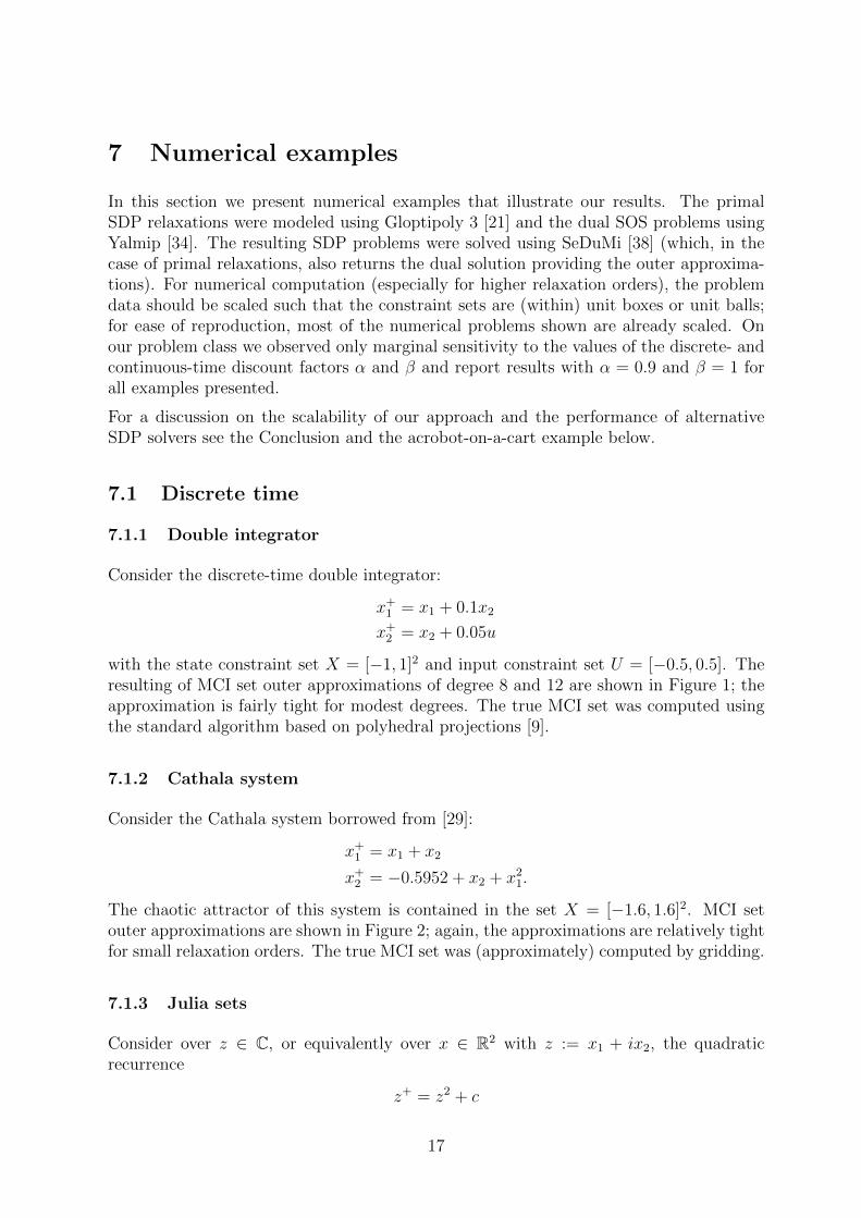
with the state constraint set X = [−1, 1]2 and input constraint set U = [−0.5, 0.5]. Theresulting of MCI set outer approximations of degree 8 and 12 are shown in Figure 1; theapproximation is fairly tight for modest degrees. The true MCI set was computed usingthe standard algorithm based on polyhedral projections [9].

7.1.2 Cathala system

Consider the Cathala system borrowed from [29]:

x+1 = x1 + x2

x+2 = −0.5952 + x2 + x2

1.

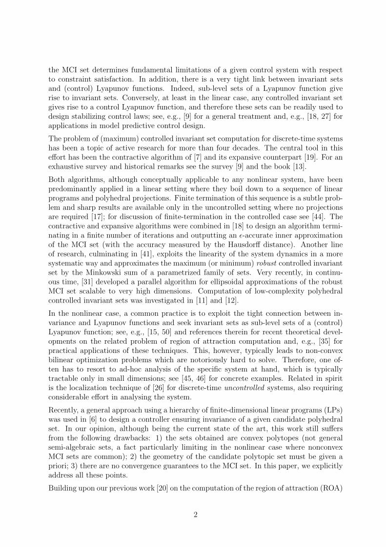
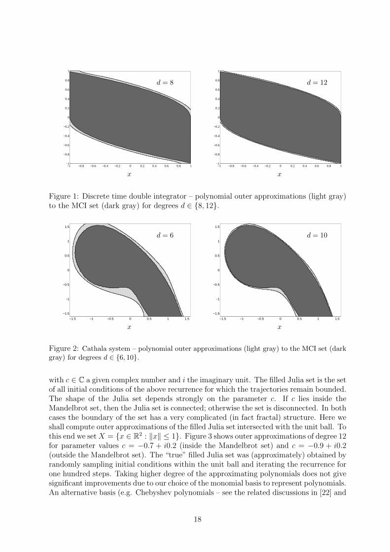
The chaotic attractor of this system is contained in the set X = [−1.6, 1.6]2. MCI setouter approximations are shown in Figure 2; again, the approximations are relatively tightfor small relaxation orders. The true MCI set was (approximately) computed by gridding.

7.1.3 Julia sets

Consider over z ∈ C, or equivalently over x ∈ R2 with z := x1 + ix2, the quadraticrecurrence

z+ = z2 + c

17

−1 −0.8 −0.6 −0.4 −0.2 0 0.2 0.4 0.6 0.8 1−1

−0.8

−0.6

−0.4

−0.2

0

0.2

0.4

0.6

0.8

1

−1 −0.8 −0.6 −0.4 −0.2 0 0.2 0.4 0.6 0.8 1−1

−0.8

−0.6

−0.4

−0.2

0

0.2

0.4

0.6

0.8

1

x x

d = 8 d = 12

Figure 1: Discrete time double integrator – polynomial outer approximations (light gray)to the MCI set (dark gray) for degrees d ∈ 8, 12.

−1.5 −1 −0.5 0 0.5 1 1.5

−1.5

−1

−0.5

0

0.5

1

1.5

−1.5 −1 −0.5 0 0.5 1 1.5

−1.5

−1

−0.5

0

0.5

1

1.5

x x

d = 6 d = 10

Figure 2: Cathala system – polynomial outer approximations (light gray) to the MCI set (darkgray) for degrees d ∈ 6, 10.

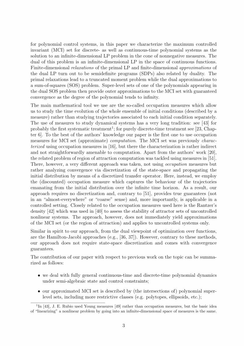
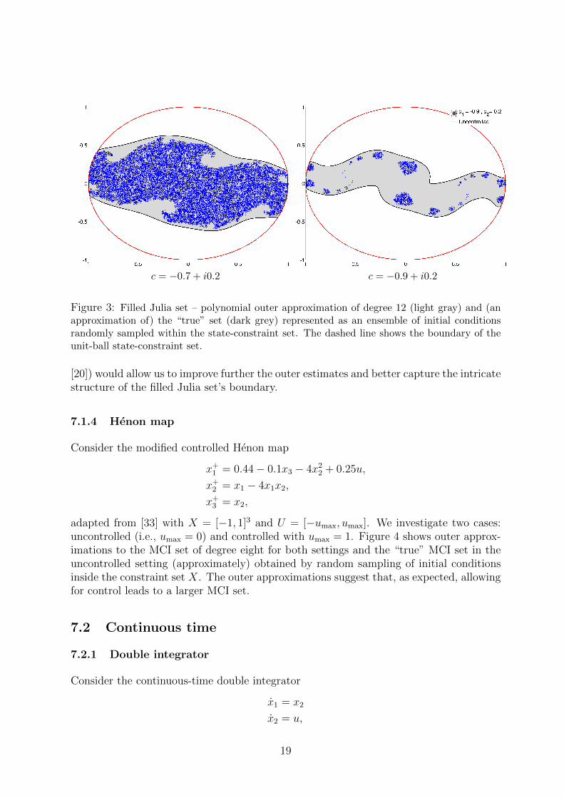
with c ∈ C a given complex number and i the imaginary unit. The filled Julia set is the setof all initial conditions of the above recurrence for which the trajectories remain bounded.The shape of the Julia set depends strongly on the parameter c. If c lies inside theMandelbrot set, then the Julia set is connected; otherwise the set is disconnected. In bothcases the boundary of the set has a very complicated (in fact fractal) structure. Here weshall compute outer approximations of the filled Julia set intersected with the unit ball. Tothis end we setX = x ∈ R2 : ‖x‖ ≤ 1. Figure 3 shows outer approximations of degree 12for parameter values c = −0.7 + i0.2 (inside the Mandelbrot set) and c = −0.9 + i0.2(outside the Mandelbrot set). The “true” filled Julia set was (approximately) obtained byrandomly sampling initial conditions within the unit ball and iterating the recurrence forone hundred steps. Taking higher degree of the approximating polynomials does not givesignificant improvements due to our choice of the monomial basis to represent polynomials.An alternative basis (e.g. Chebyshev polynomials – see the related discussions in [22] and

18

c = −0.7 + i0.2 c = −0.9 + i0.2

Figure 3: Filled Julia set – polynomial outer approximation of degree 12 (light gray) and (anapproximation of) the “true” set (dark grey) represented as an ensemble of initial conditionsrandomly sampled within the state-constraint set. The dashed line shows the boundary of theunit-ball state-constraint set.

[20]) would allow us to improve further the outer estimates and better capture the intricatestructure of the filled Julia set’s boundary.

7.1.4 Henon map

Consider the modified controlled Henon map

x+1 = 0.44− 0.1x3 − 4x2

2 + 0.25u,

x+2 = x1 − 4x1x2,

x+3 = x2,

adapted from [33] with X = [−1, 1]3 and U = [−umax, umax]. We investigate two cases:uncontrolled (i.e., umax = 0) and controlled with umax = 1. Figure 4 shows outer approx-imations to the MCI set of degree eight for both settings and the “true” MCI set in theuncontrolled setting (approximately) obtained by random sampling of initial conditionsinside the constraint set X. The outer approximations suggest that, as expected, allowingfor control leads to a larger MCI set.

7.2 Continuous time

7.2.1 Double integrator

Consider the continuous-time double integrator

x1 = x2

x2 = u,

19

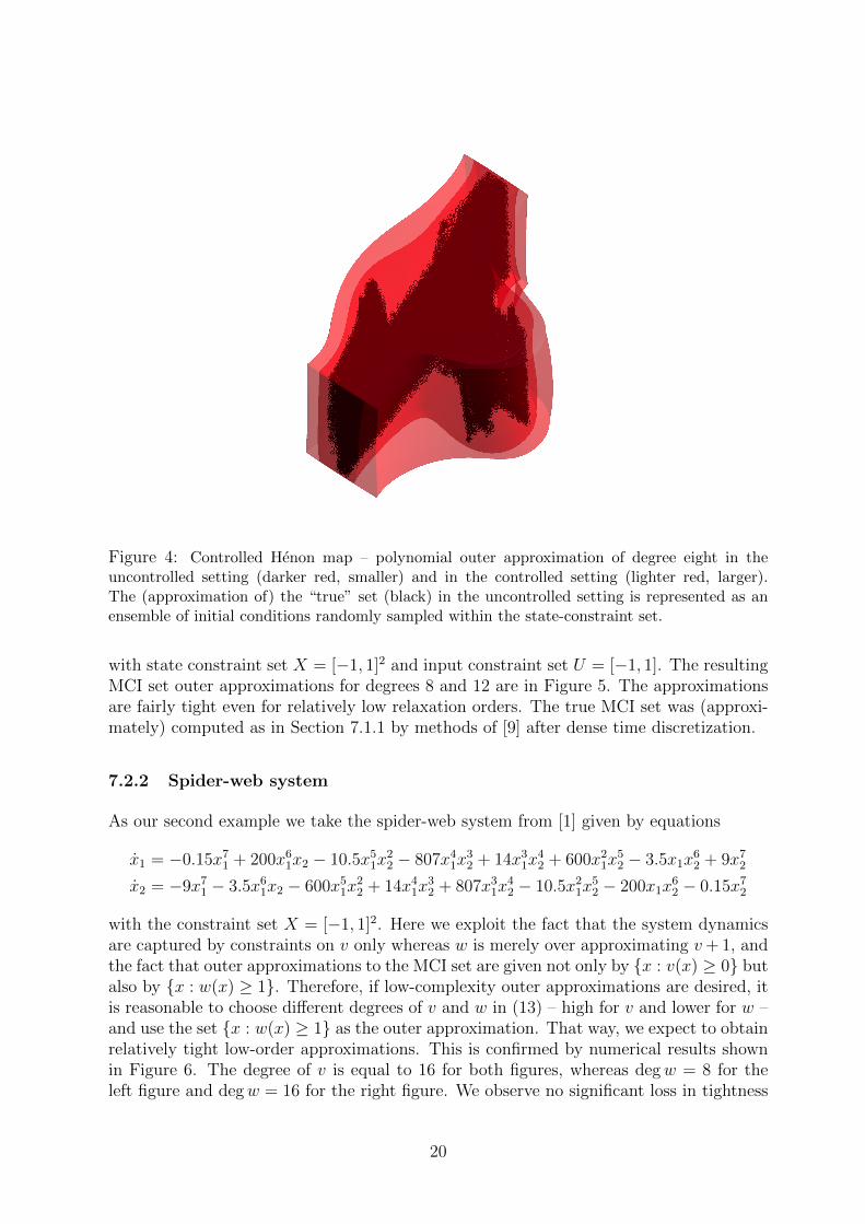
Figure 4: Controlled Henon map – polynomial outer approximation of degree eight in theuncontrolled setting (darker red, smaller) and in the controlled setting (lighter red, larger).The (approximation of) the “true” set (black) in the uncontrolled setting is represented as anensemble of initial conditions randomly sampled within the state-constraint set.

with state constraint set X = [−1, 1]2 and input constraint set U = [−1, 1]. The resultingMCI set outer approximations for degrees 8 and 12 are in Figure 5. The approximationsare fairly tight even for relatively low relaxation orders. The true MCI set was (approxi-mately) computed as in Section 7.1.1 by methods of [9] after dense time discretization.

7.2.2 Spider-web system

As our second example we take the spider-web system from [1] given by equations

x1 = −0.15x71 + 200x6

1x2 − 10.5x51x

22 − 807x4

1x32 + 14x3

1x42 + 600x2

1x52 − 3.5x1x

62 + 9x7

2

x2 = −9x71 − 3.5x6

1x2 − 600x51x

22 + 14x4

1x32 + 807x3

1x42 − 10.5x2

1x52 − 200x1x

62 − 0.15x7

2

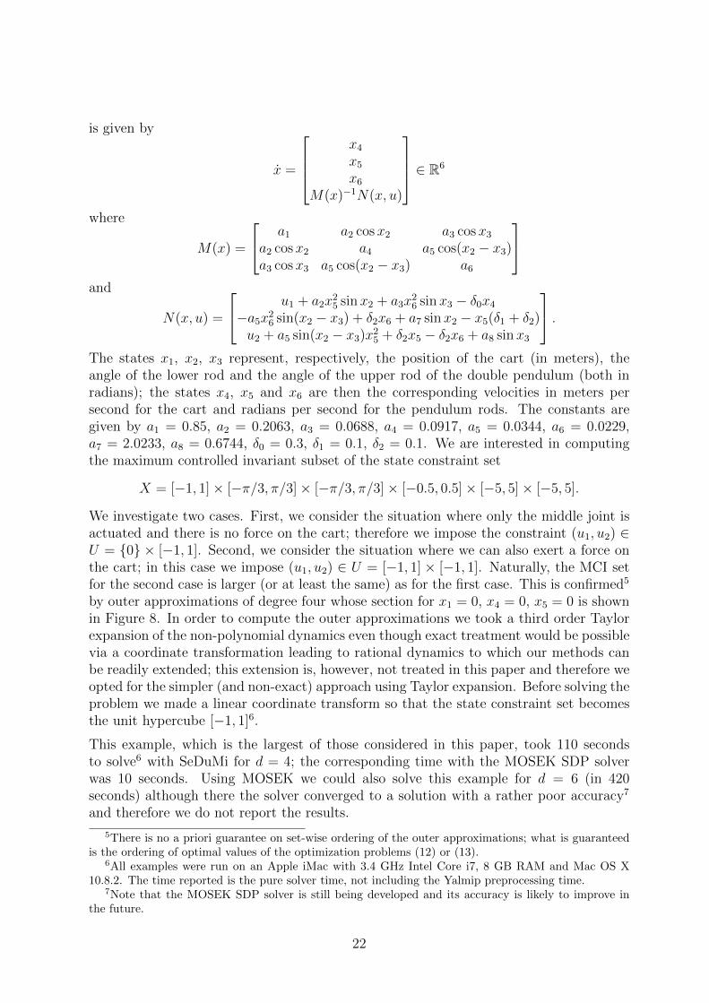
with the constraint set X = [−1, 1]2. Here we exploit the fact that the system dynamicsare captured by constraints on v only whereas w is merely over approximating v+ 1, andthe fact that outer approximations to the MCI set are given not only by x : v(x) ≥ 0 butalso by x : w(x) ≥ 1. Therefore, if low-complexity outer approximations are desired, itis reasonable to choose different degrees of v and w in (13) – high for v and lower for w –and use the set x : w(x) ≥ 1 as the outer approximation. That way, we expect to obtainrelatively tight low-order approximations. This is confirmed by numerical results shownin Figure 6. The degree of v is equal to 16 for both figures, whereas degw = 8 for theleft figure and degw = 16 for the right figure. We observe no significant loss in tightness

20

−1 −0.8 −0.6 −0.4 −0.2 0 0.2 0.4 0.6 0.8 1−1

−0.8

−0.6

−0.4

−0.2

0

0.2

0.4

0.6

0.8

1

−1 −0.8 −0.6 −0.4 −0.2 0 0.2 0.4 0.6 0.8 1−1

−0.8

−0.6

−0.4

−0.2

0

0.2

0.4

0.6

0.8

1

x x

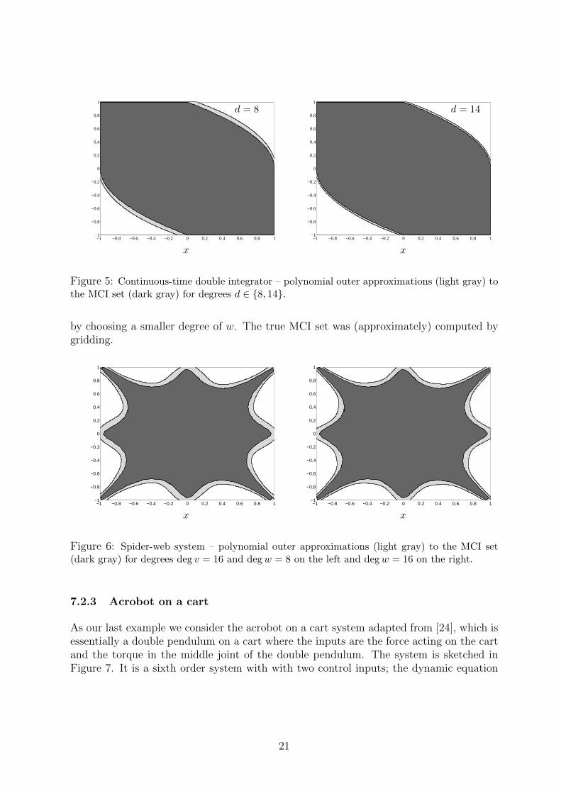
d = 8 d = 14

Figure 5: Continuous-time double integrator – polynomial outer approximations (light gray) tothe MCI set (dark gray) for degrees d ∈ 8, 14.

by choosing a smaller degree of w. The true MCI set was (approximately) computed bygridding.

−1 −0.8 −0.6 −0.4 −0.2 0 0.2 0.4 0.6 0.8 1−1

−0.8

−0.6

−0.4

−0.2

0

0.2

0.4

0.6

0.8

1

−1 −0.8 −0.6 −0.4 −0.2 0 0.2 0.4 0.6 0.8 1−1

−0.8

−0.6

−0.4

−0.2

0

0.2

0.4

0.6

0.8

1

x x

Figure 6: Spider-web system – polynomial outer approximations (light gray) to the MCI set(dark gray) for degrees deg v = 16 and degw = 8 on the left and degw = 16 on the right.

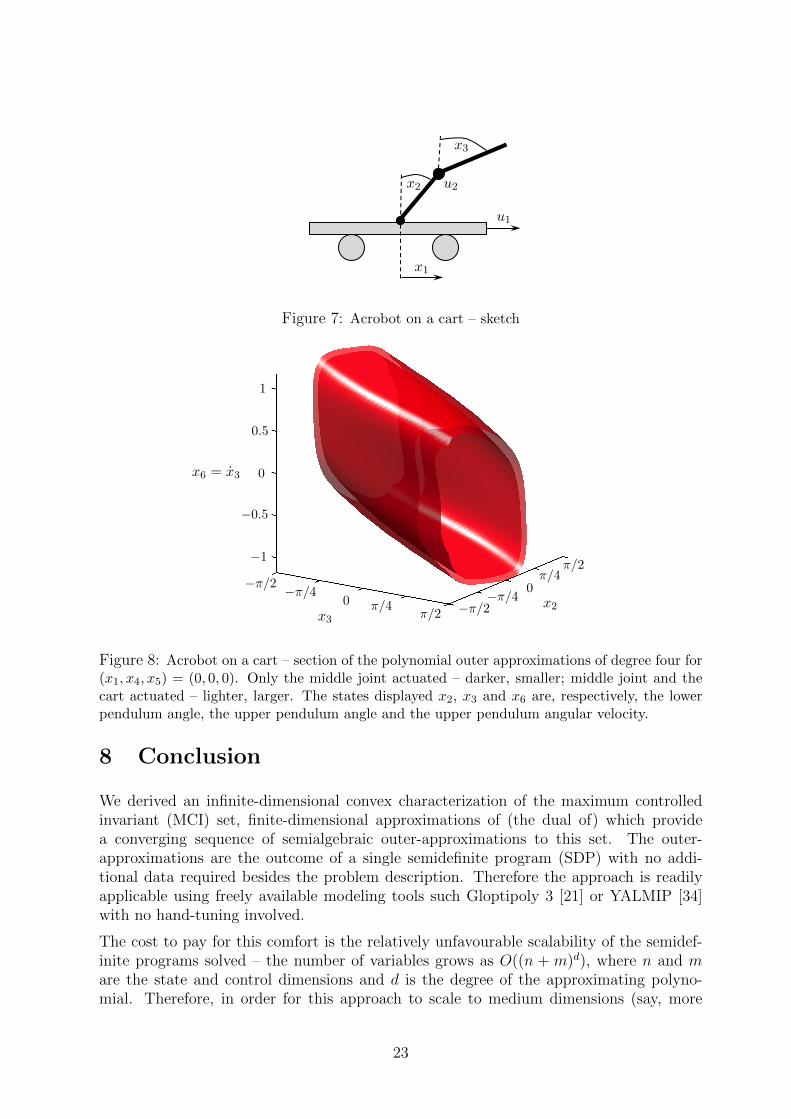
7.2.3 Acrobot on a cart

As our last example we consider the acrobot on a cart system adapted from [24], which isessentially a double pendulum on a cart where the inputs are the force acting on the cartand the torque in the middle joint of the double pendulum. The system is sketched inFigure 7. It is a sixth order system with with two control inputs; the dynamic equation

21

is given by

x =

x4

x5

x6

M(x)−1N(x, u)

∈ R6

where

M(x) =

a1 a2 cosx2 a3 cosx3

a2 cosx2 a4 a5 cos(x2 − x3)a3 cosx3 a5 cos(x2 − x3) a6

and

N(x, u) =

u1 + a2x25 sinx2 + a3x

26 sinx3 − δ0x4

−a5x26 sin(x2 − x3) + δ2x6 + a7 sinx2 − x5(δ1 + δ2)

u2 + a5 sin(x2 − x3)x25 + δ2x5 − δ2x6 + a8 sinx3

.The states x1, x2, x3 represent, respectively, the position of the cart (in meters), theangle of the lower rod and the angle of the upper rod of the double pendulum (both inradians); the states x4, x5 and x6 are then the corresponding velocities in meters persecond for the cart and radians per second for the pendulum rods. The constants aregiven by a1 = 0.85, a2 = 0.2063, a3 = 0.0688, a4 = 0.0917, a5 = 0.0344, a6 = 0.0229,a7 = 2.0233, a8 = 0.6744, δ0 = 0.3, δ1 = 0.1, δ2 = 0.1. We are interested in computingthe maximum controlled invariant subset of the state constraint set

X = [−1, 1]× [−π/3, π/3]× [−π/3, π/3]× [−0.5, 0.5]× [−5, 5]× [−5, 5].

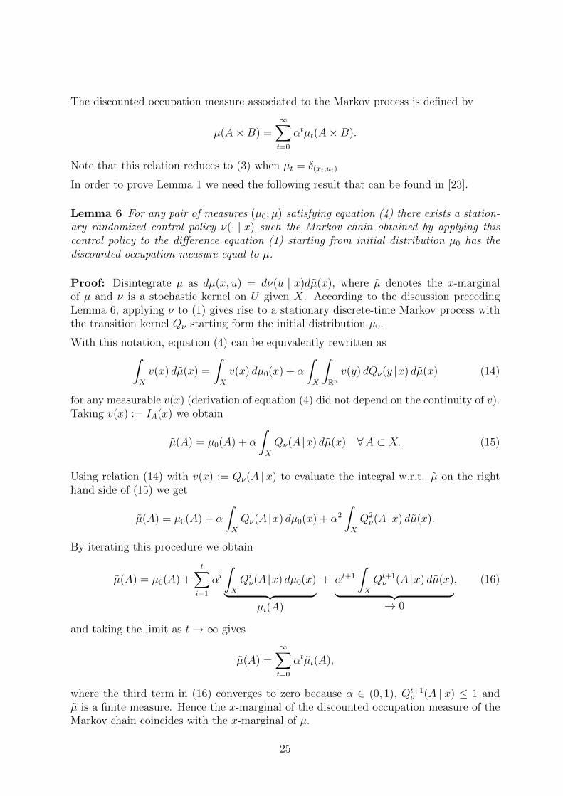
We investigate two cases. First, we consider the situation where only the middle joint isactuated and there is no force on the cart; therefore we impose the constraint (u1, u2) ∈U = 0 × [−1, 1]. Second, we consider the situation where we can also exert a force onthe cart; in this case we impose (u1, u2) ∈ U = [−1, 1] × [−1, 1]. Naturally, the MCI setfor the second case is larger (or at least the same) as for the first case. This is confirmed5

by outer approximations of degree four whose section for x1 = 0, x4 = 0, x5 = 0 is shownin Figure 8. In order to compute the outer approximations we took a third order Taylorexpansion of the non-polynomial dynamics even though exact treatment would be possiblevia a coordinate transformation leading to rational dynamics to which our methods canbe readily extended; this extension is, however, not treated in this paper and therefore weopted for the simpler (and non-exact) approach using Taylor expansion. Before solving theproblem we made a linear coordinate transform so that the state constraint set becomesthe unit hypercube [−1, 1]6.

This example, which is the largest of those considered in this paper, took 110 secondsto solve6 with SeDuMi for d = 4; the corresponding time with the MOSEK SDP solverwas 10 seconds. Using MOSEK we could also solve this example for d = 6 (in 420seconds) although there the solver converged to a solution with a rather poor accuracy7

and therefore we do not report the results.

5There is no a priori guarantee on set-wise ordering of the outer approximations; what is guaranteedis the ordering of optimal values of the optimization problems (12) or (13).

6All examples were run on an Apple iMac with 3.4 GHz Intel Core i7, 8 GB RAM and Mac OS X10.8.2. The time reported is the pure solver time, not including the Yalmip preprocessing time.

7Note that the MOSEK SDP solver is still being developed and its accuracy is likely to improve inthe future.

22

x1

u1

u2x2

x3

Figure 7: Acrobot on a cart – sketch

x3

x2

x6 = x3

−π/2 −π/40 π/4

π/2 −π/2−π/4 0

π/4π/2

−1

−0.5

0

0.5

1

Figure 8: Acrobot on a cart – section of the polynomial outer approximations of degree four for(x1, x4, x5) = (0, 0, 0). Only the middle joint actuated – darker, smaller; middle joint and thecart actuated – lighter, larger. The states displayed x2, x3 and x6 are, respectively, the lowerpendulum angle, the upper pendulum angle and the upper pendulum angular velocity.

8 Conclusion

We derived an infinite-dimensional convex characterization of the maximum controlledinvariant (MCI) set, finite-dimensional approximations of (the dual of) which providea converging sequence of semialgebraic outer-approximations to this set. The outer-approximations are the outcome of a single semidefinite program (SDP) with no addi-tional data required besides the problem description. Therefore the approach is readilyapplicable using freely available modeling tools such Gloptipoly 3 [21] or YALMIP [34]with no hand-tuning involved.

The cost to pay for this comfort is the relatively unfavourable scalability of the semidef-inite programs solved – the number of variables grows as O((n + m)d), where n and mare the state and control dimensions and d is the degree of the approximating polyno-mial. Therefore, in order for this approach to scale to medium dimensions (say, more

23

than m + n = 6) one either has to tradeoff accuracy by taking small d or go beyondthe standard freely available solvers such as SeDuMi or SDPA. One possibility is par-allelization; for instance, the free parallel solver SDPARA [48] allows for the approachto scale to larger dimensions. Alternatively, one can utilize one of the (few) commercialSDP solvers; in particular, the recently released MOSEK SDP solver seems to show farsuperior performance on our problem class, and therefore this may allow the approach toscale to larger dimensions (see also the discussion following the acrobot-on-a-cart examplein Section 7.2.3). Finally, one can resort to customized structure-exploiting solutions; thisis a promising direction of future research currently investigated by the authors. At thispoint it should be emphasized that, to the best of the authors’ knowledge, all of the ex-isting approaches providing approximations of similar quality experience similar or worsescalability properties.

Other directions of future research include the extension of the presented approach toinner approximations of MCI sets, to stochastic systems and to uncertain systems. Par-tial results on the inner approximations for the related problem of region of attractioncomputation already exist [28], albeit in uncontrolled setting only.

Appendix A

We start by embedding our problem in the setting of discrete-time Markov control pro-cesses; terminology and notation is borrowed from the classical reference [23]. Let usdefine a stochastic kernel on U given X as a map ν(· | ·) such that ν(· | x) is a prob-ability measure on U for all x ∈ X and ν(B | ·) is a measurable function on X for allB ⊂ U . Any such stochastic kernel gives rise to a discrete-time Markov process whenapplied to system (1) as a stationary randomized control policy (a policy which, givenx, chooses the control action randomly based on the probability distribution ν(· |x), i.e.,Prob(u ∈ B |x) = ν(B |x) for all B ⊂ U). The transition kernel Qν(· | ·) of this stationaryMarkov process is then given by

Qν(A |x) =

∫U

IA(f(x, u)) dν(u |x) = Prob(x+ ∈ A |x) ∀A ⊂ Rn,

where x is the current state and x+ the successor state. The t-step transition kernel isthen defined by induction as

Qtν(A |x) :=

∫Rn

Q(A |y) dQt−1ν (y |x), t ∈ 2, 3, . . .

with Q1ν := Qν . Given an initial distribution µ0, the distribution of the Markov chain at

time t, µt, is given by

µt(A) =

∫X

Qtν(A |x) dµ0(x) = Prob(xt ∈ A).

The joint distribution of state and control is then

µt(A×B) =

∫A

ν(B |x) dµt(x).

24

The discounted occupation measure associated to the Markov process is defined by

µ(A×B) =∞∑t=0

αtµt(A×B).

Note that this relation reduces to (3) when µt = δ(xt,ut)

In order to prove Lemma 1 we need the following result that can be found in [23].

Lemma 6 For any pair of measures (µ0, µ) satisfying equation (4) there exists a station-ary randomized control policy ν(· | x) such the Markov chain obtained by applying thiscontrol policy to the difference equation (1) starting from initial distribution µ0 has thediscounted occupation measure equal to µ.

Proof: Disintegrate µ as dµ(x, u) = dν(u | x)dµ(x), where µ denotes the x-marginalof µ and ν is a stochastic kernel on U given X. According to the discussion precedingLemma 6, applying ν to (1) gives rise to a stationary discrete-time Markov process withthe transition kernel Qν starting form the initial distribution µ0.

With this notation, equation (4) can be equivalently rewritten as∫X

v(x) dµ(x) =

∫X

v(x) dµ0(x) + α

∫X

∫Rn

v(y) dQν(y |x) dµ(x) (14)

for any measurable v(x) (derivation of equation (4) did not depend on the continuity of v).Taking v(x) := IA(x) we obtain

µ(A) = µ0(A) + α

∫X

Qν(A |x) dµ(x) ∀A ⊂ X. (15)

Using relation (14) with v(x) := Qν(A | x) to evaluate the integral w.r.t. µ on the righthand side of (15) we get

µ(A) = µ0(A) + α

∫X

Qν(A |x) dµ0(x) + α2

∫X

Q2ν(A |x) dµ(x).

By iterating this procedure we obtain

µ(A) = µ0(A) +t∑i=1

αi∫X

Qiν(A |x) dµ0(x)︸ ︷︷ ︸µi(A)

+ αt+1

∫X

Qt+1ν (A |x) dµ(x)︸ ︷︷ ︸→ 0

, (16)

and taking the limit as t→∞ gives

µ(A) =∞∑t=0

αtµt(A),

where the third term in (16) converges to zero because α ∈ (0, 1), Qt+1ν (A | x) ≤ 1 and

µ is a finite measure. Hence the x-marginal of the discounted occupation measure of theMarkov chain coincides with the x-marginal of µ.

25

Finally, to establish equality of the whole measures observe that

∞∑t=0

αtµt(A×B) =∞∑t=0

αt∫A

ν(B |x) dµt(x) =

∫A

ν(B |x) dµ(x) = µ(A×B).

Proof of Lemma 1: Disintegrate µ to dµ(x, u) = dν(u | x)dµ(x) as in the proof ofLemma 6. Then for any x ∈ S := spt µ we have∫

U

IS(f(x, u)) ν(u |x) = 1.

This relation says that the support of µ is invariant under ν and follows from Lemma 6,from the definition of the occupation measure µ, from the definition of the support andfrom the fact that ν(· |x) is a probability measure for all x.

Define an admissible stationary deterministic control policy by taking any measurableselection u(x) ∈ spt ν(· |x) ⊂ U . Define further the sequence of probability measures

νn(A |x) =ν(B1/n(u(x)) ∩ A |x)

ν(B1/n(u(x)) ∩ U |x)∀n ∈ 1, 2, . . ., A ⊂ U,

where B1/n(u(x)) is a closed ball of radius 1/n centered at u(x). Then νn(· |x) convergesweakly-* (or weakly or narrowly) to δu(x) and∫

U

IS(f(x, u)) νn(u |x) = 1 ∀n ∈ 1, 2, . . ..

Therefore,

1 = lim supn→∞

∫U

IS(f(x, u)) νn(u |x) ≤∫U

IS(f(x, u)) δu(x)(u) = IS(f(x, u(x))),

where the inequality follows by the Portmanteau lemma since the set u | f(x, u) ∈S ∩B1/n(u(x)) is closed for all x by continuity of f . Therefore in fact IS(f(x, u(x))) = 1and so f(x, u(x)) ∈ spt µ for all x ∈ spt µ. Therefore spt µ ⊂ X is invariant for the closedloop system xt+1 = f(xt, u(xt)), where u(x) is an admissible deterministic control policy.Therefore necessarily spt µ ⊂ XI . Finally, from equation (4) clearly sptµ0 ⊂ spt µ and sosptµ0 ⊂ XI .

9 Appendix B

Lemma 7 For any pair of measures (µ0, µ) solving (5), there exists a family of trajec-tories of the convexified inclusion (2) starting from µ0 such that the x-marginal of itsdiscounted occupation measure is equal to the x-marginal of µ.

Proof: The proof is based on fundamental results of [2] and [8] and on the compactifica-tion procedure discussed in [30].

26

We begin by embedding the problem in a stochastic setting. To this end, define theextended state space E as the one-point compactification of Rn, i.e., E = Rn∪∆, where∆ is the point compactifying Rn. Define also the linear operator A : D(A) → C(E × U)by

w 7→ Aw := gradw · f,where the domain of A, D(A), is defined as

D(A) := w : E → R | w ∈ C1(Rn), w(∆) = 0, limx→∆

w(x) = 0,

limx→∆

gradw · f(x, u) = 0 ∀ u ∈ U.

In words, D(A) is the space all continuously differentiable functions vanishing at infinitysuch that gradw · f also vanishes at infinity for all u ∈ U . Now consider the relaxedmartingale problem [8]: find a stochastic process Y : [0,∞] × Ω → E defined on somefiltered probability space (Ω,F , (Ft)t≥0, P ) and a stochastic kernel ν(· | ·) (stationaryrelaxed Markov control) on U given E such that

• P (Y (0) ∈ A) = µ0(A) ∀A ⊂ E

• for all w ∈ D(A) the stochastic process

w(Y (t))−∫ t

0

∫U

Aw(Y (τ), u) ν(du |Y (τ)) dτ (17)

is an Ft-martingale (see, e.g., [25] for a definition).

Observe that there exists a countable subset of D(A) (e.g., all polynomials with rationalcoefficients attenuated near infinity) dense in D(A) in the supremum norm. Next, D(A)is clearly an algebra that separates points of E and A1 = 0. Finally, since f(x, u) ispolynomial and hence locally Lipschitz, the ODE x = f(x, u) has a solution on [0,∞)for any x0 ∈ E and any fixed u ∈ U in the sense that if there is a finite escape timete, then we define x(t) = ∆ for all t ≥ te. Each such solution satisfies the martingalerelation (17) (with a trivial probability space). Therefore, A satisfies Conditions 1-3 of [8]and it follows from Theorem 2.2 and Corollary 2.2 therein that for any pair of measuressatisfying the discounted Liouville’s equation (5), there exists a solution to the abovemartingale problem whose discounted occupation measure is equal to µ, that is,

µ(A×B) = E∫ ∞

0

e−βtIA×B(Y (t), u) ν(du |Y (t)) dt, P (Y (0) ∈ A) = µ0(A),

where E denotes the expectation w.r.t. the probability measure P . From the martingaleproperty of (17) and the definition of A we get

Ew(Y (t)) − E∫ t

0

∫U

gradw · f(Y (τ), u) ν(du |Y (τ)) dτ

= EY (0).

Now let µt denote the marginal distribution of Y (t) at time t; that is,

µt(A) := P (Y (t) ∈ A) = EIA(Y (t)) ∀ A ⊂ X.

27

Then the above relation becomes∫X

w(x) dµt(x)−∫ t

0

∫X

∫U

gradw(x) · f(x, u) ν(du |x) dµτ (x) dτ =

∫w(x) dµ0(x),

where we have used Fubini’s thorem to interchange the expectation operator and integra-tion w.r.t. time. Defining the relaxed vector field

f(x) =

∫U

f(x, u) ν(du |x) ∈ conv f(x, U)

and rearranging we obtain∫X

w(x) dµt(x) =

∫w(x) dµ0(x) +

∫ t

0

∫X

gradw(x) · f(x) dµτ (x) dτ, (18)

where the equation holds for all w ∈ C1(X) almost everywhere with respect to theLebesgue measure on [0,∞). The Lemma then follows from Ambrosio’s superpositionprinciple [2, Theorem 3.2] using the same arguments as in the proof of Lemma 4 in [20].

Proof of Lemma 2: Suppose that a pair of measures (µ0, µ) satisfies (5) and thatλ(sptµ0 \XI) > 0. From Lemma 7 there is a family of trajectories of (2) starting from µ0

with discounted occupation measure whose x-marginal coincides with the x-marginal ofµ. However, this is a contradiction since no trajectory starting from sptµ0 \XI remainsin X for all times and sptµ ⊂ X. Thus, λ(sptµ0 \XI) = 0 and so λ(sptµ0) ≤ λ(XI).

10 Acknowledgements

The authors are grateful to Slavka Jadlovska for providing the acrobot-on-a-cart systemand Andrea Alessandretti for providing the spider-web system.

References

[1] A. A. Ahmadi. Non-monotonic Lyapunov functions for stability of nonlinear andswitched systems: theory and computation. Master’s Thesis, MIT, Boston, 2008.

[2] L. Ambrosio. Transport equation and Cauchy problem for non-smooth vector fields.In L. Ambrosio et al. (eds.), Calculus of variations and nonlinear partial differentialequations. Lecture Notes in Mathematics, Vol. 1927, Springer-Verlag, Berlin, 2008.

[3] E. J. Anderson, P. Nash. Linear programming in infinite-dimensional spaces: theoryand applications. Wiley, New York, 1987.

[4] R. B. Ash. Real analysis and probability. Academic Press, San Diego, CA, 1972.

[5] J. P. Aubin, H. Frankowska. Set-valued analysis. Springer-Verlag, Berlin, 1990.

28

[6] M. A. Ben Sassi, A. Girard. Controller synthesis for robust invariance of polynomialdynamical systems using linear programming. System Control Letters 61(4):506-512,2012.

[7] D. Bertsekas. Infinite time reachability of state-space regions by using feedbackcontrol. IEEE Trans. Autom. Control 17(5):604-613, 1972.

[8] A. G. Bhatt, V. S. Borkar. Occupation Measures for Controlled Markov Process:Characterization and Optimality. Annals of Probability, 24:1531-1562, 1996.

[9] F. Blanchini. Set invariance in control. Automatica, 35(11):1747-1767, 1999.

[10] F. Blanchini. Ultimate boundedness control for uncertain discrete time systems viaset-induced Lyapunov functions. IEEE Trans. Autom. Control 39(2):428-433, 1994.

[11] F. Blanchini, S. Miani, C. Savorgnan. Dynamic augmentation and complexity re-duction of set-based constrained control. Proc. IFAC World Congress on AutomaticControl, Seoul, South Korea, 2008.

[12] T. B. Blanco, M. Cannon, B. De Moor. On efficient computation of low-complexitycontrolled invariant sets for uncertain linear systems. Int. J. Control 83(7):1339-1346, 2010.

[13] F. Blanchini, S. Miani. Set-theoretic methods in control. Birkhauser, Boston, 2007.

[14] C. E. T. Dorea, J. C. Hennet. (A, B)-invariant polyhedral sets of linear discrete-timesystems. J. Optim. Theory Appl., 103(3):521-542, 1999.

[15] G. Chesi. Domain of attraction; analysis and control via SOS programming. LectureNotes in Control and Information Sciences, Vol. 415, Springer-Verlag, Berlin, 2011.

[16] V. Gaitsgory, M. Quincampoix. Linear programming approach to deterministic in-finite horizon optimal control problems with discounting. SIAM J. on Control andOptimization, 48:2480-2512, 2009.

[17] E. G. Gilbert, K. T. Tan. Linear systems with state and control constraints: thetheory and application of maximal output admissible sets. IEEE Trans. Autom.Control 36(9):1008-1020, 1991.

[18] R. Gondhalekar, J. Imura, K. Kashima. Controlled invariant feasibility – A generalapproach to enforcing strong feasibility in MPC applied to move-blocking. Auto-matica 45(12):2869-2875, 2009.

[19] P. O. Gutman, M. Cwikel. An algorithm to find maximal state constraint sets fordiscrete-time linear dynamical systems with bounded controls and states. IEEETrans. Autom. Control 32(3):251-254, 1987.

[20] D. Henrion, M. Korda. Convex computation of the region of attraction of polynomialcontrol systems. arXiv:1208.1751, August 2012.

[21] D. Henrion, J. B. Lasserre, J. Lofberg. Gloptipoly 3: moments, optimization andsemidefinite programming. Optim. Methods and Software 24:761–779, 2009.

29

[22] D. Henrion, J. B. Lasserre, C. Savorgnan. Approximate volume and integration forbasic semialgebraic sets. SIAM Review 51:722-743, 2009.

[23] O. Hernandez-Lerma, J. B. Lasserre. Discrete-time Markov control processes: basicoptimality criteria. Springer-Verlag, Berlin, 1996.

[24] S. Jadlovska, A. Jadlovska. Inverted pendula simulation and modeling – a gener-alized approach. International Conference on Process Control, Kouty nad Desnou,Czech Republic, 2010.

[25] O. Kallenberg. Foundations of modern probability. Springer-Verlag, Berlin, 2010.

[26] A. N. Kanatnikov, A. P. Krishchenko. Localization of compact invariant sets ofdiscrete-time nonlinear systems. Int. J. Bifurcation and Chaos 21(7):2057-2065,2011.

[27] E. C. Kerrigan. Robust constraint satisfaction: Invariant sets and predictive control.Ph.D. Thesis. Univ. Cambridge, UK, 2000.

[28] M. Korda, D. Henrion, C. N. Jones. Inner approximations of the region of attractionfor polynomial dynamical systems. arxiv.org/pdf/1210.3184, October 2012.

[29] A. P. Krishchenko. A. N. Kanatnikov. Maximal compact positively invariant sets ofdiscrete-time nonlinear systems. Proc. IFAC World Congress on Automatic Control,Milano, Italy, 2011.

[30] T. G. Kurtz. Equivalence of stochastic equations and martingale problems. Stochas-tic Analysis 2010, 113-130, Springer-Verlag, Berlin, 2011.

[31] A. N. Daryin, A. B. Kurzhanski. Parallel algorithm for calculating the invariant setsof high-dimensional linear systems under uncertainty. Computational Mathematicsand Mathematical Physics 53(1):34-43, 2013.

[32] J. B. Lasserre. Moments, positive polynomials and their applications. Imperial Col-lege Press, London, UK, 2009.

[33] M. Liu, S. Zhang, Z. Fan, M. Qiu. H∞ State Estimation for Discrete-Time ChaoticSystems Based on a Unified Model. IEEE Trans. on Systems, Man, and Cybernetics– Part B, Cybernetics, 42(4):1053-1063, 2012.

[34] J. Lofberg. YALMIP : A toolbox for modeling and optimization in MATLAB. InProc. IEEE CCA/ISIC/CACSD Conference, Taipei, Taiwan, 2004.

[35] A. Majumdar, A. A. Ahmadi, R. Tedrake. Control Design Along Trajectories withSums of Squares Programming. IEEE International Conference on Robotics andAutomation (ICRA), 2013 (to appear).

[36] K. Margellos, J. Lygeros. Hamilton-Jacobi formulation for reach-avoid differentialgames. IEEE Transactions on Automatic Control, 56:1849-1861, 2011.

[37] I. Mitchell, C. Tomlin. Overapproximating reachable sets by Hamilton-Jacobi pro-jections. Journal of Scientific Computing, 19:323-346, 2003.

30

[38] I. Polik, T. Terlaky, Y. Zinchenko. SeDuMi: a package for conic optimization. IMAworkshop on Optimization and Control, Univ. Minnesota, Minneapolis, 2007.

[39] M. Putinar. Positive polynomials on compact semi-algebraic sets. Indiana Univ.Mathematics Journal, 42:969-984, 1993.

[40] R. Rajarama, U. Vaidya, M. Fardadc, B. Ganapathysubramanian. Stability in thealmost everywhere sense: A linear transfer operator approach. Journal of Mathe-matical Analysis and Applications, 368:144-156, 2010.

[41] S. V. Rakovic. Parameterized robust control invariant sets for linear systems:theoretical advances and computational remarks. IEEE Trans. Autom. Control,55(7):1599-1614, 2010.

[42] A. Rantzer. A dual to Lyapunov’s stability theorem. Systems & Control Letters,42:161-168, 2001.

[43] J. E. Rubio. Control and Optimization: The Linear Treatment of Nonlinear Prob-lems. Manchester University Press, Manchester, UK, 1985.

[44] R. Vidal, S. Schaert, J. Lygeros, S. Sastry. Controlled invariance of discrete timesystems. HSCC, Lecture Notes on Computer Science, 1790, Springer-Verlag, Berlin,2000.

[45] K. Starkov. Bounds for compact invariant sets of the system describing dynamicsof the nuclear spin generator. Communications in Nonlinear Science and NumericalSimulation 14(6):2565-2570, 2009.

[46] K. Starkov. Estimation of the domain containing all compact invariant sets of theoptically injected laser system. Int. J. Bifurcation and Chaos 17(11):4213-4217, 2007.

[47] M. Yamashita, K. Fujisawa, M. Fukuda, K. Kobayashi, K. Nakta, M. Nakata. Latestdevelopments in the SDPA Family for solving large-scale SDPs. In M. Anjos, J.B. Lasserre (Eds.). Handbook on Semidefinite, Cone and Polynomial Optimization:Theory, Algorithms, Software and Applications. Springer, NY, USA, Chap. 24, 687-714, 2011.

[48] M. Yamashita, K. Fujisawa, M. Kojima. SDPARA: SemiDefinite Programming Al-gorithm paRAllel version. Parallel Computing 29:1053-1067, 2003.

[49] L. C. Young. Calculus of variations and optimal control theory. Sunders, Philadel-phia, 1969.

[50] U. Topcu, A. K. Packard, P. Seiler, G. J. Balas. Robust region-of-attraction esti-mation. IEEE Transactions on Automatic Control, 55:137-142, 2010.

[51] K. Wang, U. Vaidya. Transfer operator approach for computing domain of attrac-tion. IEEE Conference on Decision and Control (CDC), Atlanta, GA, 2010.

31