Convolution, Correlation, �& �

Fourier Transforms James R. Graham

10/25/2005

Introduction

•  A large class of signal processing techniques fall under the category of Fourier transform methods – These methods fall into two broad categories

•  Efficient method for accomplishing common data manipulations

•  Problems related to the Fourier transform or the power spectrum

Time & Frequency Domains

•  A physical process can be described in two ways –  In the time domain, by the values of some some

quantity h as a function of time t, that is h(t), -∞ < t < ∞ –  In the frequency domain, by the complex number, H,

that gives its amplitude and phase as a function of frequency f, that is H(f), with -∞ < f < ∞

•  It is useful to think of h(t) and H(f) as two different representations of the same function –  One goes back and forth between these two

representations by Fourier transforms

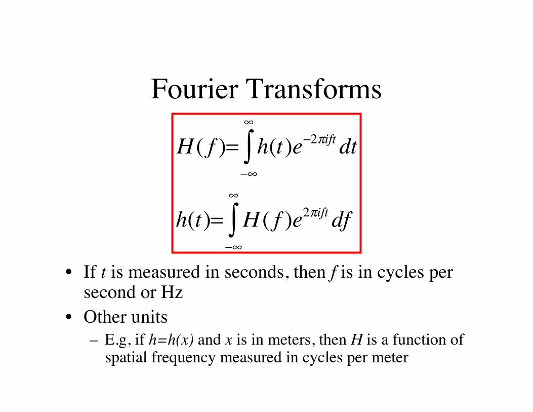
Fourier Transforms

•  If t is measured in seconds, then f is in cycles per second or Hz

•  Other units –  E.g, if h=h(x) and x is in meters, then H is a function of

spatial frequency measured in cycles per meter �

H ( f )= h(t)e−2πift dt−∞

∞

∫

h(t)= H ( f )e2πift df−∞

∞

∫

Fourier Transforms

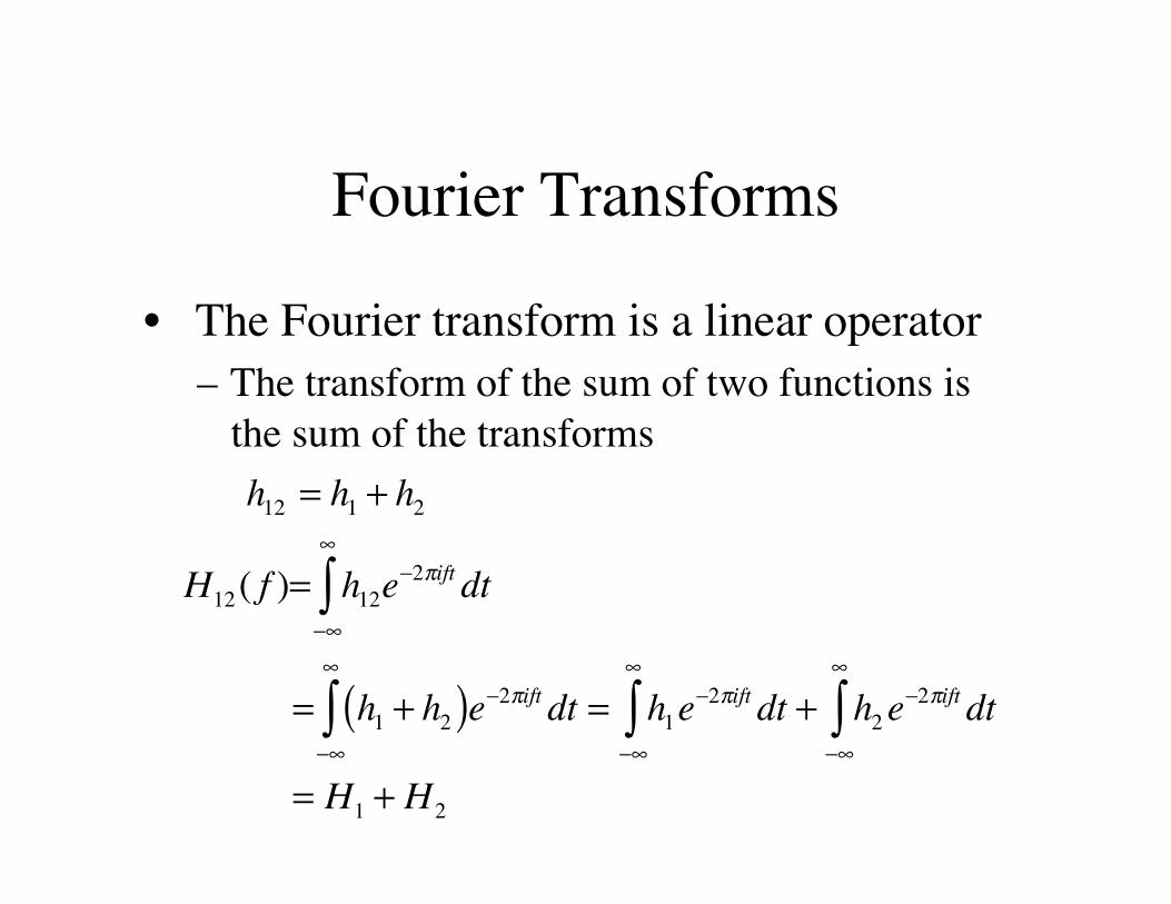
•  The Fourier transform is a linear operator – The transform of the sum of two functions is

the sum of the transforms

�

h12 = h1 + h2

H12 ( f )= h12e−2πift dt

−∞

∞

∫

= h1 + h2( )e−2πift dt−∞

∞

∫ = h1e−2πift dt

−∞

∞

∫ + h2e−2πift dt

−∞

∞

∫= H1 + H2

Fourier Transforms

•  h(t) may have some special properties – Real, imaginary – Even: h(t) = h(-t) – Odd: h(t) = -h(-t)

•  In the frequency domain these symmetries lead to relations between H(f) and H(-f)

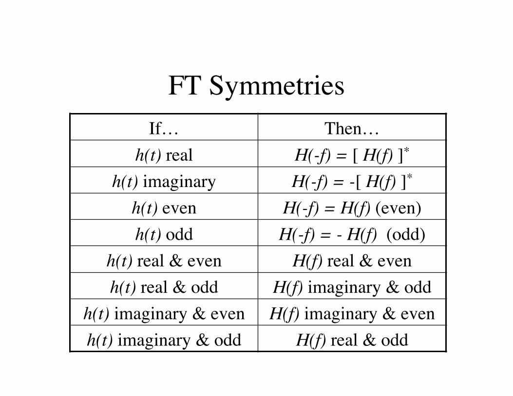
FT Symmetries If… Then…

h(t) real H(-f) = [ H(f) ]* h(t) imaginary H(-f) = -[ H(f) ]*

h(t) even H(-f) = H(f) (even) h(t) odd H(-f) = - H(f) (odd)

h(t) real & even H(f) real & even h(t) real & odd H(f) imaginary & odd

h(t) imaginary & even H(f) imaginary & even h(t) imaginary & odd H(f) real & odd

Elementary Properties of FT

�

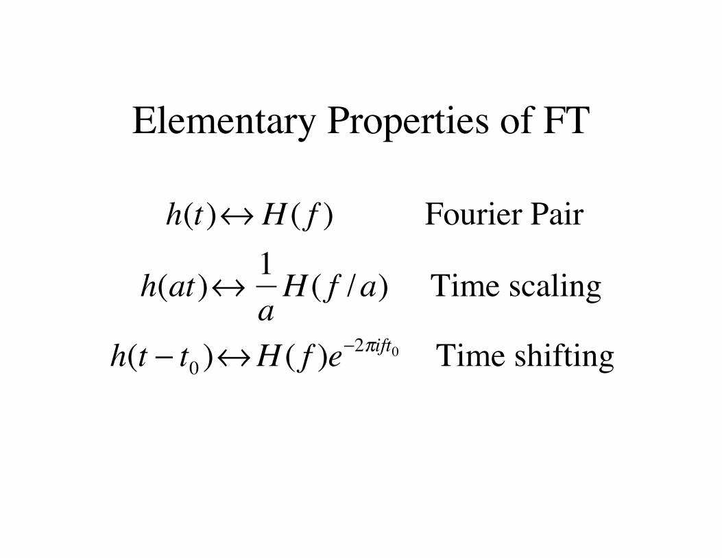
h(t)↔ H ( f ) Fourier Pair

h(at)↔ 1aH ( f /a) Time scaling

h(t − t0 )↔H ( f )e−2πift0 Time shifting

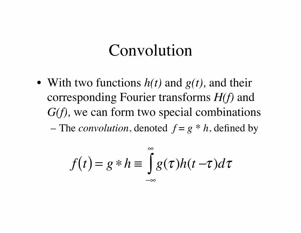
Convolution

•  With two functions h(t) and g(t), and their corresponding Fourier transforms H(f) and G(f), we can form two special combinations – The convolution, denoted f = g * h, defined by

�

f t( ) = g∗h ≡ g(τ )h(t −−∞

∞

∫ τ )dτ

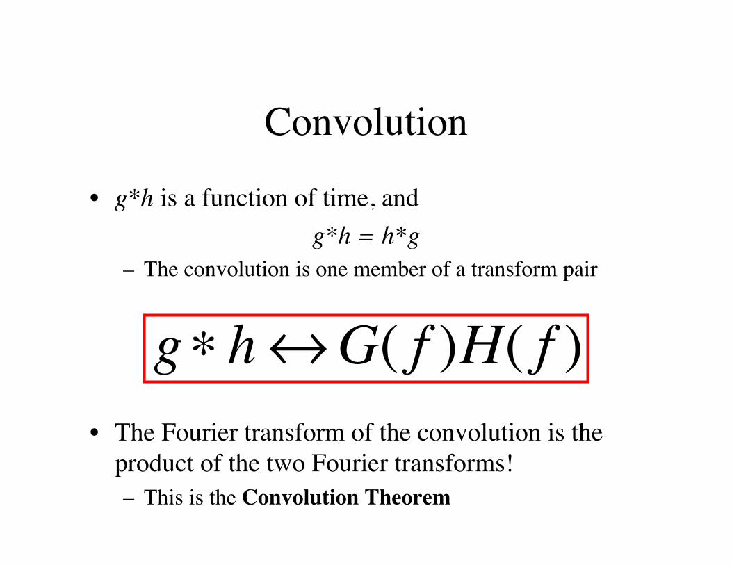
Convolution

•  g*h is a function of time, and g*h = h*g

–  The convolution is one member of a transform pair

•  The Fourier transform of the convolution is the product of the two Fourier transforms! –  This is the Convolution Theorem

�

g∗ h↔G( f )H( f )

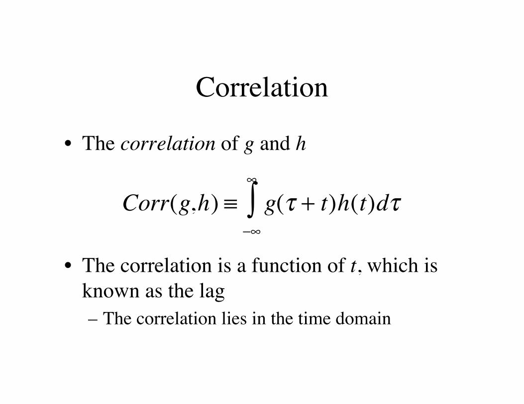
Correlation

•  The correlation of g and h

•  The correlation is a function of t, which is known as the lag – The correlation lies in the time domain �

Corr(g,h) ≡ g(τ + t)h(t−∞

∞

∫ )dτ

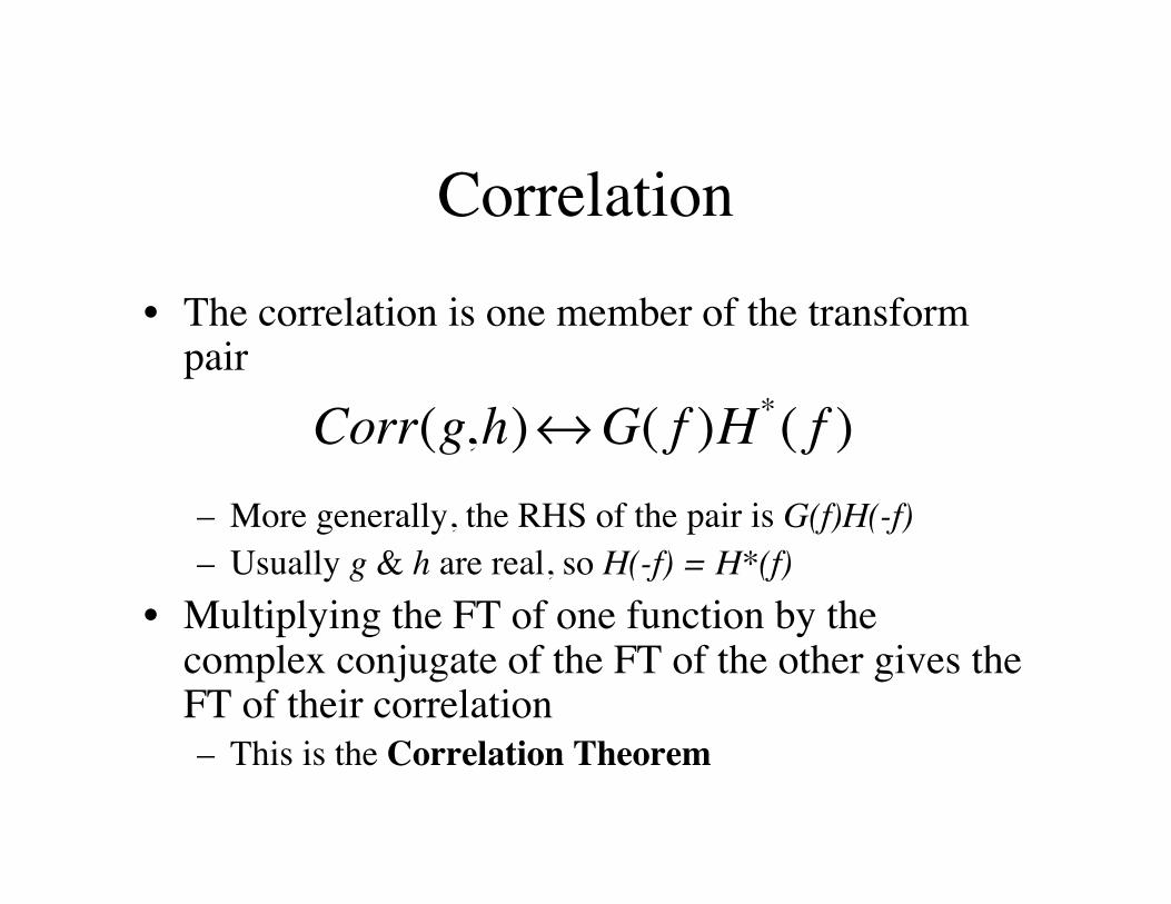
Correlation

•  The correlation is one member of the transform pair

–  More generally, the RHS of the pair is G(f)H(-f) –  Usually g & h are real, so H(-f) = H*(f)

•  Multiplying the FT of one function by the complex conjugate of the FT of the other gives the FT of their correlation –  This is the Correlation Theorem

�

Corr(g,h)↔G( f )H*( f )

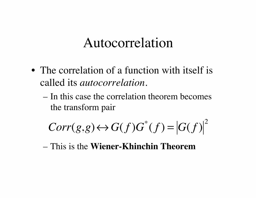
Autocorrelation

•  The correlation of a function with itself is called its autocorrelation. –  In this case the correlation theorem becomes

the transform pair

– This is the Wiener-Khinchin Theorem

�

Corr(g,g)↔G( f )G*( f ) = G( f ) 2

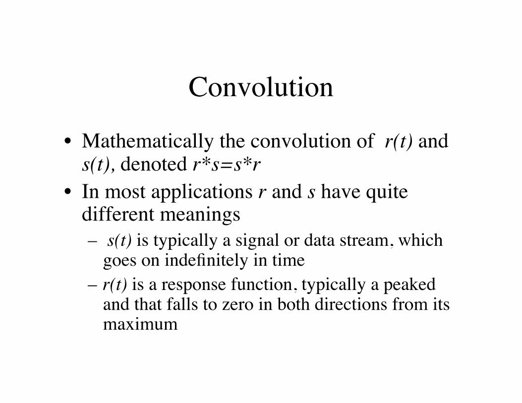
Convolution

•  Mathematically the convolution of r(t) and s(t), denoted r*s=s*r

•  In most applications r and s have quite different meanings –  s(t) is typically a signal or data stream, which

goes on indefinitely in time –  r(t) is a response function, typically a peaked

and that falls to zero in both directions from its maximum

The Response Function

•  The effect of convolution is to smear the signal s(t) in time according to the recipe provided by the response function r(t)

•  A spike or delta-function of unit area in s which occurs at some time t0 is – Smeared into the shape of the response function – Translated from time 0 to time t0 as r(t - t0)

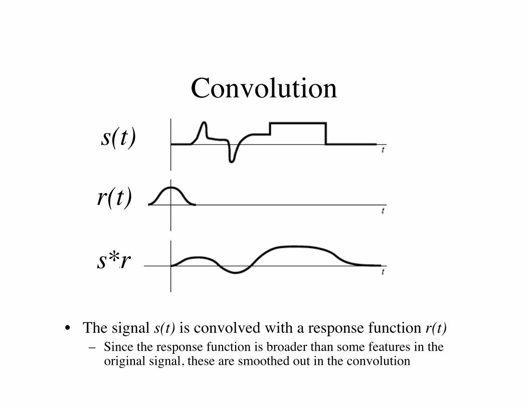
Convolution

•  The signal s(t) is convolved with a response function r(t) –  Since the response function is broader than some features in the

original signal, these are smoothed out in the convolution

s(t)

r(t)

s*r

Fourier Transforms & FFT

•  Fourier methods have revolutionized many fields of science & engineering –  Radio astronomy, medical imaging, & seismology

•  The wide application of Fourier methods is due to the existence of the fast Fourier transform (FFT)

•  The FFT permits rapid computation of the discrete Fourier transform

•  Among the most direct applications of the FFT are to the convolution, correlation & autocorrelation of data

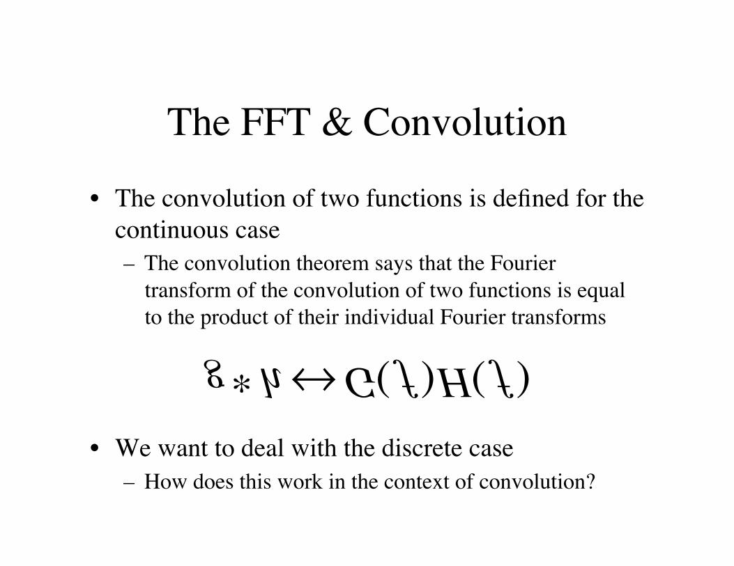
The FFT & Convolution

•  The convolution of two functions is defined for the continuous case –  The convolution theorem says that the Fourier

transform of the convolution of two functions is equal to the product of their individual Fourier transforms

•  We want to deal with the discrete case –  How does this work in the context of convolution?

�

g∗ h↔G( f )H( f )

Discrete Convolution

•  In the discrete case s(t) is represented by its sampled values at equal time intervals sj

•  The response function is also a discrete set rk –  r0 tells what multiple of the input signal in channel j is

copied into the output channel j –  r1 tells what multiple of input signal j is copied into the

output channel j+1 –  r-1 tells the multiple of input signal j is copied into the

output channel j-1 –  Repeat for all values of k

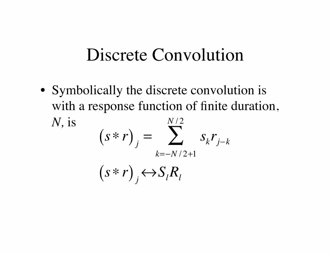
Discrete Convolution

•  Symbolically the discrete convolution is with a response function of finite duration, N, is

�

s∗ r( ) j= skrj−k

k=−N / 2+1

N / 2

∑s∗ r( ) j

↔SlRl

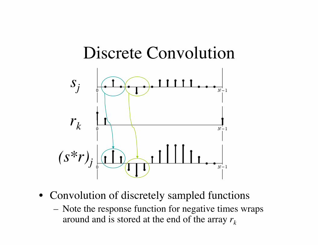
Discrete Convolution

•  Convolution of discretely sampled functions –  Note the response function for negative times wraps

around and is stored at the end of the array rk

sj

rk

(s*r)j

Examples

•  Java applet demonstrations – Continuous convolution

•  http://www.jhu.edu/~signals/convolve/ – Discrete convolution

•  http://www.jhu.edu/~signals/discreteconv/