Cooperative Navigation for

Autonomous Underwater Vehicles

Alexander Bahr

Navigare 2011, 4 May 2011, Bern

Distributed Intelligent Systems and Algorithms Laboratory

disal.epfl.ch

• Land, atmosphere and sea surface maps:

• Many parameters obtainable through remote sensing

• High-resolution

• (Almost) complete coverage

• Up to date

• Cheap to obtain

• Subsurface maps:

• In situ measurements required !

• Low resolution

• Sparse

• Out-of-date (often by decades)

• Expensive to obtain

Alexander Bahr

Why go under water ?

38°12’ N 155° 03’ W (700 km * 1500 km)

46°31’ N 6°34’ E (60 m * 150 m)

Seaglider (University of Washington, USA)

Outline

• What is an AUV?

• Types of AUVs

• Payloads (sensing/scientific and navigation)

• Challenges in underwater robotics (Communication, Navigation)

• Cooperative Navigation

• Applications

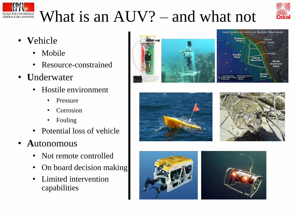
• Vehicle

• Mobile

• Resource-constrained

• Underwater

• Hostile environment

• Pressure

• Corrosion

• Fouling

• Potential loss of vehicle

• Autonomous

• Not remote controlled

• On board decision making

• Limited intervention capabilities

Alexander Bahr

What is an AUV? – and what not

Alexander Bahr - Navigare 2011,

5.4.2011 Bern

Types of AUVs – active propulsion

Low end AUV Top end AUV

Dimensions 0.7 m length * 0.1 m diameter 5 m length * 0.7 m diameter

Price $15’000 $2’000’000

Top speed 1 m/s 3 m/s (15 m/s ?)

Max depth 100 m 11’000m

Endurance 2h 24h (72h)

Pictures courtesy of University of Hydroid, Ocean Server

Cetus (Lockheed Martin, USA)

Gavia (Hafmynd, Iceland)

Hovering AUV (MIT/Bluefin)

Nereus, hybrid AUV/ROV (WHOI)

Flapping foil AUV (MIT)

SeaBed (WHOI, USA)Solar AUV (AUVSI, USA)

SAPPHIRES (Saab, Sweden)

Types of AUVs – active propulsion

http://auvac.org/resources/browse/configuration/

Seaglider (University of Washington, USA)

Types of AUVs – buoyancy driven

• Vehicle changes buoyancy from positive to negative and back

• Attached wings cause forward motion

• Maximum depth (2000 m)

• Forward speed (0.3 m/s)

• Range: 5000 km (and more)

• Very long endurance vehicle (6 months – many years)

• Very low power consumption

• Limited sensing capabilities

• Limited navigation sensors

• Limited controllability

• Bio fouling becomes relevant

• Price: $100’000

Pictures courtesy of University of Washington/APL, Webb Research

Alexander Bahr - Navigare 2011,

5.4.2011 Bern

Seaglider (University of Washington, USA)

XRAY glider (University of Washington, USA)

Types of AUVs – buoyancy driven

Pictures courtesy of University of Washington/APL, Webb Research

External sensing payloads

• Conductivity, Temperature, Depth

• Fluorescence

• Backscatter

• Passive acoustics

• Camera (still)

• Simple sonar (side-scan, pencil beam)

• Magnetometer

• Small chemical sensors (O2, chlorophyll)

• Video Camera

• Sophisticated sonar (multi-beam, SAS)

• Active acoustics (sub-bottom profiler)

• Sampler

• Manipulator

• Large chemical sensors (CO2)

• Computationally expensive sensors

External sensing payloads• Side-scan sonar

• Photos

• Imaging sonar

• Multi-beam sonar:

Pictures courtesy of Dana Yoerger, Hanu Singh, Hafmynd,

Bluefin, IMOS Australia

Navigation payloads

• GPS

• Depth

• Simple accelerometer (orientation)

• 3 axis magnetic compass

• Doppler Velocity Logger (DVL)

• Simple Inertial Navigation System (INS)

• Long / Ultra-short Base Line

• Fiber-optic north seeking gyro

• Sophisticated INS

Pictures courtesy of University of Hydroid, Ocean Server, Webb Research

• What does not work

• Very High Frequency, Ultra High Frequency radio (MHz)(Wifi, Bluetooth, etc.)

• Extremly High Frequency radio (GHz)(GSM, Satellite)

• Infrared

• What “sort-of” works (short range)

• Very Low Frequency radio (kHz)

• Green/blue LEDs

• Directed laser

• Return current

• What works

• Extremly Low Frequency (Hz)

• Acoustic

Challenges - communication

Pictures courtesy of WHOI, MIT, Grumman, ANU, US Navy

• Acoustic modem (WHOI, Benthos, MIT, …)

• Range: O(100 m) – O(1-10 km)

• Data rate: O(bytes/s) – O(kbytes/s)

• Energy expensive O(1 Joule/byte)

• Small channel capacity (one modem at a time)

• Strong temporal and local variations of channel

• Interference with navigation equipment (LBL, DVL)

• Strong acoustic signature

• Multipath

• Direct (1)

• Surface bounce (2)

• Thermocline Bounce (3)

• Bottom bounce (4)

Acoustic communication

4

2

3

1T1

T2

32 bytes every 10s !

Underwater navigation

• Absolute positioning

• GPS (only when surfacing)

• LBL:

1. AUV send query ping to all beacons

2. Beacon 1 responds

3. Beacon 2 responds

4. Vehicle computes position

• Beacon field needs to be predeployed

• Operating area is limited by to a few km2

• Vision-aided navigation

1-5 km

Picture courtesy of Ryan Eustice

Underwater navigation

• Relative positioning:

• Depth sensor underwater navigation is a 2D problem

• Magnetic compass ($1k; accuracy: 1-3 degrees)

• Fiber Optical Gyro (FOG) ($40k; accuracy: 0.1 degree)

• Inertial Navigation System

• Doppler Velocity Logger (DVL)

– Provides 2D speed over ground

– Maximum distance to seafloor: 30 m – 200 m

Best case AUV navigation accuracies

– Surface: GPS

– Near seafloor: 0.1% distance traveled

– Mid-water column: 1.5 km/h drift

Pictures courtesy of RDI, IXSEA

Surface vehicle

(GPS)0%

0.1%

1%

10%

Nav

igat

ion

err

or

[%/d

ista

nce

tra

vel

led]

AUV deluxe

(INS with fiber- optic gyro)

AUV

(DVL/compass based navigation)

Glider

(compass + speed estimate)

Different vehicles have different navigation sensors with different accuracies

Cooperative navigation

Pictures courtesy of University of Washington/APL, Hydroid, Kongsberg

Cooperative navigation

• Each vehicle is outfitted with an acoustic modem

• Vehicle broadcast

– Position estimate (x,y, depth, course, speed)

– Certainty estimate

– (additional information)

• Inter-vehicle measurement (range is available)

In heterogeneous teams:

“Use other vehicles’ position estimate to update my own”

x

P

x,P ,r

r

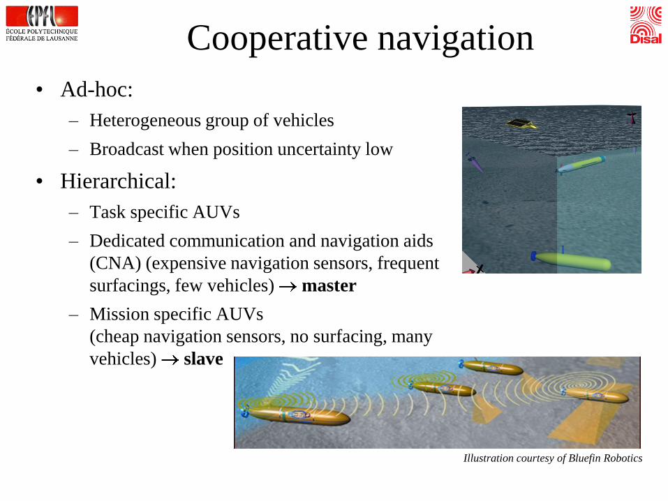
Cooperative navigation

• Ad-hoc:

– Heterogeneous group of vehicles

– Broadcast when position uncertainty low

• Hierarchical:

– Task specific AUVs

– Dedicated communication and navigation aids

(CNA) (expensive navigation sensors, frequent

surfacings, few vehicles) master

– Mission specific AUVs

(cheap navigation sensors, no surfacing, many

vehicles) slave

Illustration courtesy of Bluefin Robotics

Cooperative Navigation experiment

• Panama City, FL, December 2006

• Mine Counter Measure (MCM)

• 2 Autonomous Surface Crafts

• 1 AUV:

– Bluefin 12’’

– Navigation: depth gauge, DVL, INS, compass

– Acoustic modem

• ASCs followed AUV

• ASCs broadcast GPS position, AUV got range to ASC

30 m !

Cooperative Navigation experiment

Applications

• Static missions

• Pre-programmed

• List of waypoints

• Non-adaptive

• Adaptive missions

• Partially pre-programmed

• List of behaviors

• Vehicle adapts depending on

sensor reading

• Multi-vehicle missions

• Pre-programmed or adaptive

warm

cold

Pictures courtesy of Ocean Server

Conclusions

• AUVs face difficulties not encountered in other environments

• Expensive hardware, but cheaper alternatives are underway

• Experiments require careful planning and execution

• Most difficult terrain to navigate in

• Drift will always get you

• Absolute position update requires extensive infrastructure OR

• Cooperative navigation

Thank you !