Embed Size (px)
Citation preview
COOPERATIVE QUERY ANSWERING FOR APPROXIMATE ANSWERS WITH
NEARNESS MEASURE IN HIERARCHICAL STRUCTURE INFORMATION SYSTEMS
by
Thanit Puthpongsiriporn
B.Engr in I.E., Chulalongkorn University, Bangkok, Thailand
M.S. in I.E., University of Pittsburgh
Submitted to the Graduate Faculty of
the School of Engineering in partial fulfillment
of the requirements for the degree of
Doctor of Philosophy
University of Pittsburgh
2002
UNIVERSITY OF PITTSBURGH
SCHOOL OF ENGINEERING
This dissertation was presented
by
Thanit Puthpongsiriporn
It was defended on
August 7th, 2002
and approved by
Dr. Harvey Wolfe, Professor, Department of Industrial Engineering
Dr. Michael Spring, Associate Professor, Department of Industrial Engineering
Dr. Jayant Rajgopal, Associate Professor, Department of Industrial Engineering
Dr. Mary Besterfield-Sacre, Assistant Professor, Department of Industrial
EngineeringCommittee Chairperson: Dr. Bopaya Bidanda, Professor, Department of
Industrial Engineering
Committee Chairperson: Dr. Ming-En Wang, Assistant Professor, Department of
Industrial Engineering
ii
ABSTRACT
COOPERATIVE QUERY ANSWERING FOR APPROXIMATE ANSWERS WITH NEARNESS MEASURE IN HIERARCHICAL STRUCTURE INFORMATION SYSTEMS
Thanit Puthpongsiriporn, Ph.D.
University of Pittsburgh
Cooperative query answering for approximate answers has been utilized in
various problem domains. Many challenges in manufacturing information retrieval, such
as: classifying parts into families in group technology implementation, choosing the
closest alternatives or substitutions for an out-of-stock part, or finding similar existing
parts for rapid prototyping, could be alleviated using the concept of cooperative query
answering.
Most cooperative query answering techniques proposed by researchers so far
concentrate on simple queries or single table information retrieval. Query relaxations in
searching for approximate answers are mostly limited to attribute value substitutions.
Many hierarchical structure information systems, such as manufacturing information
systems, store their data in multiple tables that are connected to each other using
hierarchical relationships – “aggregation”, “generalization/specialization”,
“classification”, and “category”. Due to the nature of hierarchical structure information
systems, information retrieval in such domains usually involves nested or jointed queries.
In addition, searching for approximate answers in hierarchical structure databases not
only considers attribute value substitutions, but also must take into account attribute or
iii

relation substitutions (i.e., WIDTH to DIAMETER, HOLE to GROOVE). For example,
shape transformations of parts or features are possible and commonly practiced. A bar
could be transformed to a rod. Such characteristics of hierarchical information systems,
simple query or single-relation query relaxation techniques used in most cooperative
query answering systems are not adequate.
In this research, we proposed techniques for neighbor knowledge constructions,
and complex query relaxations. We enhanced the original Pattern-based Knowledge
Induction (PKI) and Distribution Sensitive Clustering (DISC) so that they can be used in
neighbor hierarchy constructions at both tuple and attribute levels. We developed a
cooperative query answering model to facilitate the approximate answer searching for
complex queries. Our cooperative query answering model is comprised of algorithms for
determining the causes of null answer, expanding qualified tuple set, expanding
intersected tuple set, and relaxing multiple condition simultaneously. To calculate the
semantic nearness between exact-match answers and approximate answers, we also
proposed a nearness measuring function, called “Block Nearness”, that is appropriate for
the query relaxation methods proposed in this research.
iv
Descriptors
Cooperative query answering Approximate answers
Query relaxation Multiple condition relaxation
Attribute value substitution Attribute substitution
Relation substitution Query subsumption
Nearness measuring Neighbor Hierarchies
Part substitution Part Classification
Group technology
v

ACKNOWLEDGEMENTS
I am very thankful to my advisors Dr. Bopaya Bidanda, Dr. Ming-En Wang and
Dr. John Manley for their invaluable suggestions and assistance. I am greatly indebted
with your tremendous support and continual guidance during the course of this research
and my doctoral program. This dissertation could not have been completed without you.
I am also grateful to my committee members Dr. Harvey Wolfe, Dr. Jayant
Rajgopal, Dr. Mary Besterfield-Sacre, and Dr. Michael Spring for their helpful comments
and contributions.
I wish to express my deep appreciation to Dr. Richard Billo who gave me
tremendous support, valuable ideas, and opportunities that changed my life forever.
Special thanks go to the faculty, staffs – especially Lisa Bopp and Jim Segneff –
and fellow students in the Department of Industrial Engineering, University of Pittsburgh
for their support and encouragement.
My appreciation extends to my special friends, Owat Sunan, Ravipim Chaveesuk,
Marty Adickes, and David Porter. You made Pittsburgh my hometown. Our friendships
will never faint.
I would like to express my utmost gratitude to my wife Tichila and our beloved
children, Kittipoj, Nicholas, and Natalie for being there for me and giving me love,
support, and inspiration.
Finally, I would like to dedicate this work to my parents for their support,
understanding, and endless love. I will try harder to always follow yours footprints. I am
eternally indebted to you.
vi

TABLE OF CONTENTS
Page
ABSTRACT....................................................................................................................... iii
ACKNOWLEDGEMENTS............................................................................................... vi
LIST OF TABLES............................................................................................................. xi
LIST OF FIGURES .......................................................................................................... xii
1.0 INTRODUCTION ......................................................................................................1
1.1 Research Motivation ..........................................................................................10
1.1.1 Part Classification in Group Technology Implementation ........................11
1.1.2 Part Substitution in Rapid Prototyping ......................................................11
1.2 Research Objectives...........................................................................................20
1.3 Research Deliverables........................................................................................21
2.0 BACKGROUND ......................................................................................................22
2.1 Relational Database ...........................................................................................22
2.1.1 Association.................................................................................................26
2.1.2 Aggregation................................................................................................26
2.1.3 Generalization/Specialization ....................................................................29
2.1.4 Category.....................................................................................................30
2.2 Queries ...............................................................................................................30
2.3 Cooperative Query Answering ..........................................................................35
2.3.1 Different Types of Cooperative Query Answering Systems .....................36
2.3.2 Application Domains of Cooperative Query Answering...........................37
vii
2.3.3 Supporting Database Platforms..................................................................37
2.3.4 Types of Cooperative Query Answers.......................................................39
2.4 Part Family Classification Data Structures ........................................................41
3.0 LITERATURE REVIEW .........................................................................................45
3.1 Approaches in Finding Approximate Answers..................................................45
3.2 Query Relaxation ...............................................................................................49
3.3 Creating and Maintaining the Knowledge Base for Query Relaxation .............52
3.4 Semantic Nearness Measures for Approximate Answers..................................54
3.4.1 When should the semantic nearness be established? .................................55
3.4.2 Which objects (query answers or the queries themselves) should the system compare to determine the semantic proximity?.............................55
3.4.3 How should the nearness values be stored or represented? .......................57
4.0 THE DESIRED COOPERATIVE QUERY ANSWERING SYSTEM....................59
4.1 Query Relaxation by Attribute Value Substitutions ..........................................60
4.2 Query Relaxation by Attribute, and Relation Substitutions...............................64
4.3 Complex Query and Simultaneous Multiple Query Condition Relaxations......68
4.3.1 Approach for Joint (or Nested) Query Relaxations ...................................69
4.4 Approach for Simultaneous Multiple Query Condition Relaxation ..................70
4.5 Approximate Answer Nearness Calculation......................................................71
5.0 NEIGHBORHOOD HIERARCHY DEVELOPMENT TOOLS..............................74
5.1 Distribution Sensitive Clustering (DISC) ..........................................................76
5.2 Pattern-based Knowledge Induction (PKI)........................................................82
6.0 QUERY RELAXATION........................................................................................105
viii
6.1 Rearranging Query Conditions ........................................................................106
6.1.1 Selection Conditions and Joint Conditions ..............................................107
6.1.2 Rearranging Query Condition Algorithm ................................................108
6.2 Determining the causes of null answers...........................................................109
6.3 Query Relaxation through Attribute Value Substitutions................................112
6.4 Query Relaxation through Attribute Substitutions ..........................................115
6.5 Query Relaxation through Relation Substitutions ...........................................118
6.6 Simultaneous Multiple Query Selection Condition Relaxation.......................120
6.7 Query Relaxation Algorithms ..........................................................................127
6.7.1 Expanding Qualified Tuple Set................................................................127
6.7.2 Expanding Intersected Tuple Set .............................................................128
6.7.3 Query Relaxation .....................................................................................129
7.0 NEARNESS CALCULATION ..............................................................................130
7.1.1 Attribute Value Nearness.........................................................................130
7.1.2 Attribute Nearness ...................................................................................131
7.1.3 Relation Nearness ....................................................................................132
7.1.4 Query Nearness........................................................................................134
8.0 CASE STUDY........................................................................................................137
8.1 Course Scheduling Background.......................................................................138
8.1.1 Study Course Scheduling vs. Rapid Prototyping.....................................139
8.1.2 The Complexities of Course Scheduling .................................................140
8.1.2.1 Graduation Requirements..............................................................140
ix

8.1.2.2 Constraints.....................................................................................141
8.2 Cooperative Query Answering for Study Course Scheduling .........................141
8.2.1 The Student Database ..............................................................................142
8.2.2 Building the course schedule knowledge base.........................................145
8.2.3 Searching for approximate answers .........................................................147
8.3 Reliability Test.................................................................................................149
8.4 Summary of Results.........................................................................................150
9.0 CONCLUSIONS AND FUTURE WORK .............................................................157
9.1 Conclusions......................................................................................................157
9.2 Future Work .....................................................................................................159
APPENDIX A STUDENT DATABASE TABLE DESCRIPTIONS .............................164
APPENDIX B COURSE PLANNER PROGRAM .........................................................180
APPENDIX C SAMPLES OF NEIGHBOR HIERARCHIES........................................189
APPENDIX D TEST PROBLEM CONDITIONS..........................................................205
BIBLIOGRAPHY............................................................................................................207
x

LIST OF TABLES
Page
Table 1 Data Retrieval and Information Retrieval Differences .........................................31
Table 2 Relation ALUM_PLATE......................................................................................85
Table 3 Approximate Answers of Q: WIDTH = 3 AND LENGTH = 144 AND THICKNESS = 0.5...............................................................................................96
Table 4 Abstract Value Ranges of Attribute WIDTH in Relation ALUM_PLATE........102
Table 5 Abstract Value Ranges of Attribute AREA in Relation ALUM_PLATE..........103
Table 6 Test problems’ approximate answers generated by Course Planner .................152
Table 7 Expert A’s best course schedules comparing with the approximate answers from the Course Planner program ......................................................................152
Table 8 Expert B’s best course schedules comparing with approximate answers from the Course Planner program ......................................................................153
Table 9 Expert C’s best course schedules comparing with approximate answers from the Course Planner program ......................................................................153
Table 10 Assessment results of the approximate answers generated by the Course Planner program based on all experts.................................................................155
xi
LIST OF FIGURES
Page
Figure 1 The Simplified Part Feature Classification Scheme............................................15
Figure 2 Diagram Representing the Database Model of the Simplified Part Feature Classification Scheme ..........................................................................................16
Figure 3 Enhanced Part Feature Classification Scheme ....................................................27
Figure 4 Relational Conceptual Model of the Enhanced Modified Part Classification Scheme .................................................................................................................28
Figure 5 Attribute Value Conversions from DIAMETER to WIDTH ..............................67
Figure 6 Inferential Relationship Measured by Inclusion Between Patterns’ Cardinalities(92) .....................................................................................................86
Figure 7 Neighbor Hierarchy after the First Iteration........................................................93
Figure 8 Neighbor Hierarchy after the Second Iteration ...................................................93
Figure 9 Neighbor Hierarchy of Members of Attribute STOCK_NO in Relation ALUM_PLATE....................................................................................................95
Figure 10 A Neighbor Hierarchy of WIDTH in ALUM_PLATE through the Modified PKI......................................................................................................100
Figure 11 An Attribute Abstract Value Neighbor Hierarchy of WIDTH in ALUM_PLATE through the Modified PKI .......................................................103
Figure 12 An Attribute Abstract Value Neighbor Hierarchy of AREA in ALUM_PLATE through the Modified PKI .......................................................104
Figure 13 The Conceptual Enhanced Entity-Relationship diagram of the student database ..............................................................................................................144
xii
1.0 INTRODUCTION
The three common problems of retrieving data from a traditional database system
are: 1) not knowing how to compose queries (or the database query language), 2) getting
information overload, and 3) not getting any data items at all. The first problem
generally occurs when a user is first introduced to the database. The second problem
results from under-specified queries, and the last problem is caused by over-specified
queries. As databases expand, it is difficult for users to stay current with the changes of
the stored information or database schemas. Naïve users who do not have adequate
knowledge regarding the stored information or database schemas tend to compose either
over- or under-specified queries.
Many studies have been done to assist users in overcoming these problems.
Cooperative querying has been one of the chosen solutions. It is a type of information
retrieval (IR). The common objective of cooperative querying systems is to improve
system-user interactions. Cooperative querying gives database retrieval systems a human
intelligence by mimicking their ability to produce informative answers. Such is achieved
by utilizing some artificial intelligence mechanisms, and rules or facts, from the existing
and/or supplemental knowledge developed by application domain experts.
Some cooperative querying systems allow users to ask questions with little or no
knowledge of the query language.(1,2) Harada and others(3,4,5) proposed a natural language
system. Their cooperative dialog system incorporated an utterance interpreter module
that facilitated natural language interactions between users and the system. Wu and
Ichikawa(6) developed a knowledge-based database assistant (KDA) for their natural
1
language query system that guided users in performing database retrieval tasks. Zhang (7)
proposed techniques that assisted users in formulating queries without having to use the
database query language.
Another group of cooperative querying systems is capable of generating
alternative intelligent answers that are more meaningful or helpful when users encounter
such overabundant or null answer situations. There are many types of cooperative query
answers. Types of cooperative answers vary depending on their developers’ intentions,
the system configurations, and the user settings. Answers generated by these cooperative
database systems can be: 1) some type of feedback that aids users in composing better
queries, 2) additional sets of records whose topic is relevant to the submitted query, or 3)
sets of data items from the databases that have similar characteristic with the ones
specified by query conditions. Different methodologies have been developed for many
specific problem domains. Intentional answer is a summary of the answer set generated
from cooperative query answering techniques to provide the general idea of the records
being retrieved. For example, when users submit under-specified queries, a cooperative
query answering system can replace or attach to the traditional answers with the summary
information of the answer set. Intentional answers are commonly drawn by comparing
the submitted queries and the database’ integrity constraints or the application knowledge
of the database. For instance, when a user requests a list of automobiles that have
wheels, instead of returning a long list containing all data items (cars) stored in the
database, the system could present a database integrity constraint such as “every
automobile must have wheels”. Minker and Gal(8) used semantic query optimization to
2
identify interactions between integrity constraints and queries to achieve such cooperative
answers. Another method of deriving intentional and extensional answers from known
integrity constraints in a relational database was proposed by Motro.(9) One feature of
Zhang’s(7) interactive database query system was the generation of associative answers
that provided additional relevant information relating to the answers of a query. The
author used case-based and probabilistic reasoning techniques to obtain such cooperative
answers.
The third types of cooperative answers are sets of data items that satisfy parts of
the selection conditions of the queries that are over-specified or bound to null. Those
cooperative query answers can be, for instance, in case of electronic library catalog
systems, related articles or, in case of Internet searching, sites with similar interests and
number of hits. Some cooperative query answering systems offer approximate (or
partial) answers when the conditions of the submitted queries cannot be matched exactly
(over-specified queries). Instead of returning null answers to users, using some
intelligent agents, the cooperative query answering systems will search for the neighbors
of the unavailable exact-match answers.(10,11) Pirotte and Roelants,(12) and Andreasen(13)
utilized sets of rules represented by predicates in order to derive cooperative answers for
null-bound queries. Also, Corella,(14) and Shum and Muntz(15,16) presented in their papers
the uses of taxonomy of concepts for approximate answering. Lately, many researchers
focus on issues of approximate answer ranking or the evaluation of the nearness of the
approximate answers and the exact-match answers. A methodology for automatic
3
generation of nearness matrix using Pattern-based Knowledge Induction (PKI) and
Dynamic Nearness were developed by Merzbacher.(17)
In general, cooperative answers for null-bound queries can be classified into three
major types: 1) suggestive responses, 2) corrective responses, or 3) partial answers.(18)
Suggestive responses are the kinds of information presented to users when cooperative
answering mechanisms anticipate the follow-up queries for the posted queries.
Corrective responses are provided to users when cooperative systems detect erroneous
presuppositions. Approximate or partial answers are alternative data items available in
the database that satisfy parts of the selection conditions stated in the queries. For
example, in a student-teacher database schema, a user tries to retrieve a list of
undergraduate students taking a course with a particular instructor, in the current
semester, who received higher than 95% on the midterm exam. If the database system
can’t find any data items – students in this case – that satisfy the selection conditions, and
consequently responds with a null answer, the user will have to guess which query
condition(s) caused the query to return null (whether no student scores more than 95%,
the instructor does not actually teach the course, no undergraduate student takes the
course in the semester, etc.). On the other hand, with a cooperative query answering
mechanism, the system may propose a query for retrieving the student roster, sorted by
midterm exam score, for that class as a suggestive response. If the class is actually
restricted to graduate students, the system may present the user with this fact, or indicate
that only graduate students are allowed to take that course as a corrective response. In
case of partial answer, the system may return a list of students whose properties satisfy at
4
least one selection condition (i.e. undergraduate students with scores of more than 95%
for that course in that particular semester but with different instructor).
To find cooperative answers for a null-bound query, a cooperative system must
first determine what caused the query to fail. Second, the system has to modify the query
by altering or dropping the query conditions that cause the query to return an empty
answer set. Then, it can present the approximate answers, obtained from the adjusted
queries, to the user.
In order to find the cause(s) of null answer, the system can compare the submitted
query with the database integrity constraints to see if there is any constraint violation by
any parts of the query selection conditions that causes the query to return a null answer.
Database integrity constraints provide a quick check for identifying the query selection
conditions that make the query “over-specified”. However, not all over-specified
conditions violate the database integrity constraints. The user may compose a query
having selection conditions that follow the integrity constraints of the database, but none
of the existing data items can satisfy all query conditions, which will result in a null
answer as well. Alternatively, the system can determine the cause of null answers by
continually altering the selection conditions of the submitted query and testing the new
queries, which result from the modification of the original query, whether they result in
retrieval of any data items. Once a set of data items is obtained, the system can compare
the original over-specified query with the successful relaxed queries and is able to
conclude the causes of failure or to obtain partial answers. This process of modifying a
null-bound query into a set of more general queries is called “query relaxation”. Through
5
this query relaxation process, the query’s selection conditions are relaxed or dropped
systematically. The original query is transformed into a set of broader specified queries,
which have fewer or more general selection conditions and are more likely to return some
set of data items. After the first iteration, if none of the relaxed queries still yield null
answers, the constraints of these queries will get further relaxed. In general, the query
relaxation process continues until one or more relaxation stopping criteria are met, or the
process is interrupted by the user. Through this query relaxation process, the system is
able to compile the causes of null information and returns the approximate answers.
The idea of providing users cooperative answers is well adapted today.
Cooperative query answering for approximate answers has become an important part of
our life. It is an indispensable component of all large-scale databases as more users get
involved with larger and larger databases in this information age. Different cooperative
query answering techniques have been incorporated, at various degrees of
implementation, in almost every electronic library catalog system, and in all Internet
search engines. In a library catalog system, a user may search for articles by providing
the system with authors’ names, titles, publishers or key words of interest. The system
returns a list of articles with key words that exactly match, are closely related, or are
broadly similar to the one requested by the user. This intelligent retrieving system allows
researchers to discover more articles within a shorter period of time than they would do
using a conventional catalog system. Another example of cooperative query answering is
Internet browsing. When searching for web sites by topics of interest on the Internet
using any search engine, what users usually get are pages of a web site directory that
6

contain some aspects, such as titles or contexts, in common with the desired topic. In
addition, numbers of hits are also provided to help us get the idea of how accurate or how
general the keywords are. Then users can use this information in modifying the search
criteria.
The capability to provide approximate (or partial) answers, when users submit
over-specified queries that are bound to null answers of cooperative query answering is
very useful and is the focus of this research study. This is because over-specified queries
are more problematic than under-specified queries and the ability to find similar or the
closest match answers can be applied to many information retrieval problems in
hierarchical structure databases.
Under-specified queries generally result in an unmanageable set of answers.
However, users can always further refine those under-specified queries to reduce the size
of the answer sets or conclude more meaningful information from the results themselves,
given that sets of answers are returned from the system. On the other hand, without a
cooperative query answering mechanism, null answers resulted from over-specified
queries will leave users frustrated about what causes their queries to fail. Inexperienced
users especially will have to perform trial-and-error corrections of the queries to obtain
the desired information. Equipped with a cooperative query answering mechanism, a
database system will be able to intelligently respond with more meaningful answers when
encountered with null answer queries. As a result, these cooperative answers will assist
users in improving their queries and achieving what they are seeking more effectively
and efficiently.
7
Most cooperative query answering techniques proposed by researchers so far
concentrate on simple queries or single table information retrieval. Furthermore, query
relaxations in searching for approximate answers are mostly limited to attribute value
substitutions. A great deal of research on this topic has concentrated on the mechanisms
by which alternate queries are generated in order to address the issues of query
relaxation, relaxation controlling methods, and representation of cooperative answers.
Most of the research results search for approximate answers by attribute value alterations
in selection conditions of the query. For example, a query selection condition “Attribute
= c” that causes the query to return a null answer is modified to “Attribute > c” or
“Attribute = c”, where c and c′ are any attribute values in the domain of the attribute and
c′ ≠ c. Only a small amount of research has been done to study query relaxation that truly
performs attribute and relation substitutions on query selection conditions. Some query
relaxations that allow such substitutions require that the original and the replacing
relations possess the same set of attributes. Examples of research studies that utilize this
type of relaxation are those cooperative query answering techniques that are based on
Type Abstraction Hierarchy.(19) A popular example used in this group of work is a flight
schedule with a list of specific locations and times of departure and arrival may be
replaced with a set of train schedules that have similar values to those departure and
arrival attributes. These substitutions are made possible by projecting data items from
relevant relations into predetermined views. Therefore, those kinds of substitutions are
limited to the predefined sets of relations and data items. Also, such predefined views
require frequent maintenance as new data items are added to the relations. Furthermore,
8

these types of relation substitutions imply that the replacing and the original relations
have the same set of attributes. Substitutions of attributes and/or relations without such
requirements are essential for manufacturing information retrieval.
As stated thus far, cooperative query answering for null-bound queries has been a
popular research topic for decades and has many uses in countless applications.
However, most proposed cooperative answering techniques still have some restrictions
that are unsuitable for many problem sets especially in hierarchical structure information
systems. Many hierarchical structure information systems – such as medical, academic
(which will be further mentioned in the Case Study chapter), and manufacturing
information systems – store their data in multiple tables that are connected to each other
using hierarchical relationships – “aggregation”, “generalization/specialization”,
“classification”, and “category”. Information retrieval in such domains usually involves
nested or jointed queries. In addition, searching for approximate answers in hierarchical
structure databases not only considers attribute value substitutions, but also must take
into account attribute or relation substitutions.
New query relaxation techniques that allow the system to perform simultaneous
relaxation on multiple attribute values, attributes and/or relations in the query selection
conditions must be developed. Furthermore, dependencies among selection conditions
must also be incorporated into the relaxation operation in order to comprehend real world
problems. With the improved mechanism, the system would be able to search for
approximate answers in a broader search space, which would result in a better chance of
9
user satisfaction. The results from query relaxation process would be more reliable, and
more accurate, as well.
1.1 Research Motivation
Cooperative query answering for approximate answers has been utilized in many
problem domains. However, its use in hierarchical structure information systems has
received very little attention. Currently available cooperative query answering
techniques have many limitations and are not totally capable of handling the hierarchical
structure querying. New cooperative query answering techniques that allow complex
query relaxations must be developed. Since relaxation by a cooperative answering
system often results in a large set of alternate answers, nearness measures for the
approximate answers for this type of cooperative query answering system are essential
and must be developed as well. Without appropriate nearness measures, the inquirer
would still have to manually search for the right substitution that has the closest features
to the exact-match one. Equipped with suitable nearness measuring functions, the
process of selecting the most appropriate substitute part or part family would be more
reliable and require less time.
Two applications that have been the inspiration of this research are the use of
cooperative query answering concepts in part classifications for group technology
implementation and part substitution for rapid prototyping.
10

1.1.1 Part Classification in Group Technology Implementation
Group technology plays a significant role in manufacturing information systems.
As the name implies, the technique has been used to group together parts with similar
features, or parts that require the similar production processes into classes. Group
technology provides manufacturers, distributors, and retailers effective plans for their
shop floor layouts, inventory systems, production scheduling, etc.. One common
problem in implementing group technology concepts is that no matter how well the
grouping criteria are designed, there are always gray areas where parts do not fit perfectly
with any families. If decisions are made without a well-defined algorithm, the result
could be classifying parts into inappropriate groups. As a consequence, altering a plant
layout because of a poor part family grouping to rectify the wrong partitioning decisions
always associated with a considerably higher expense.
1.1.2 Part Substitution in Rapid Prototyping
Another problem with manufacturing information systems arises when one
attempts to search for an alternative that has similar properties with a particular part.
Such a situation could occur when a needed part is out of stock. For rapid prototyping
implementations, being able to find similar parts can significantly improve the time
needed to develop a prototype.
To illustrate the usefulness of part substitution in manufacturing information
systems, consider a company that is operated under a make-to-order type of business. Its
products require a high number of parts and subassemblies; and countless numbers of
11
components need to be stocked. In addition, most of the company’s components are not
produced in-house; they have to be ordered from vendors in advance. If a single part of
the entire assembly were missing, the company would not be able to complete and deliver
the product until the missing part is acquired from its vendor. The company suffers from
a high inventory cost and a long inventory turnover problem. A part substitution system
that allows users to query the company’s inventory database for parts with similar
features, when the needed parts are not available, would tremendously improve the
company’s productivity.
In an analogous manner, both part classification and part substitution problems in
manufacturing information systems and cooperative query answering for approximate
answers try to achieve the same objective – that is, finding a similar or closest match.
Group technology concept searches for the closest match or the most suitable part family
for a part that falls into the gray area of the part classification scheme. Cooperative query
answering for partial answer searches for the closest approximate answer for a query
when the exact-match does not exist.
Due to the nature of information in manufacturing databases, entity types are
frequently connected to each other by hierarchical relationships such as aggregation,
generalization/specialization, and category. Information retrieval in such domains
usually involves nested or jointed queries. In addition, searching for approximate
answers in manufacturing information systems not only considers attribute value
substitutions, but also must take into account attribute or relation substitutions (i.e.,
WIDTH to DIAMETER, HOLE to GROOVE). For example, shape transformations of
12

parts or features are possible and commonly practiced. A bar could be transformed to a
rod.
To perform relaxations on complex query, including attribute and/or relation
substitutions, the system must also take into account the query condition dependencies
between attributes and attributes, relations and relations, and attributes and relations. The
condition dependency consideration is essential to sustain the logic of the query. Simple
single query relaxation techniques used in most cooperative query answering systems are
not appropriate for manufacturing information retrieval. Also, many restrictions and
limitations of the currently available query relaxation techniques are not applicable for
such a domain.
To demonstrate the needs of attribute and relation substitutions and the
consideration of condition dependency in a query relaxation for approximate answers,
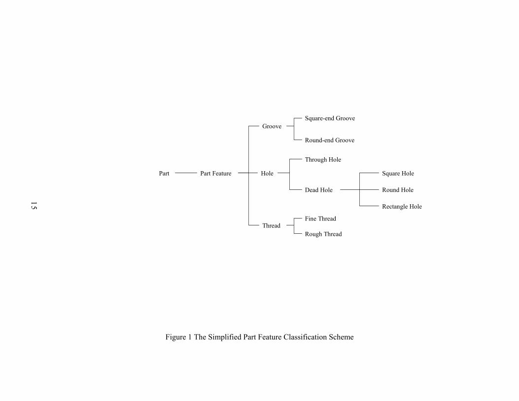
consider the simplified part feature classification scheme as depicted in Figure 1, and its
database model illustrated in Figure 2.
In this particular part feature classification scheme, a part feature can be either or
both a groove and/or a hole. A groove can be classified into either a square-end or a
round-end groove; and, a hole is further categorized into a through hole and a dead hole.
Both types of holes can take the shape of a square hole, a round hole, or a rectangular
hole.
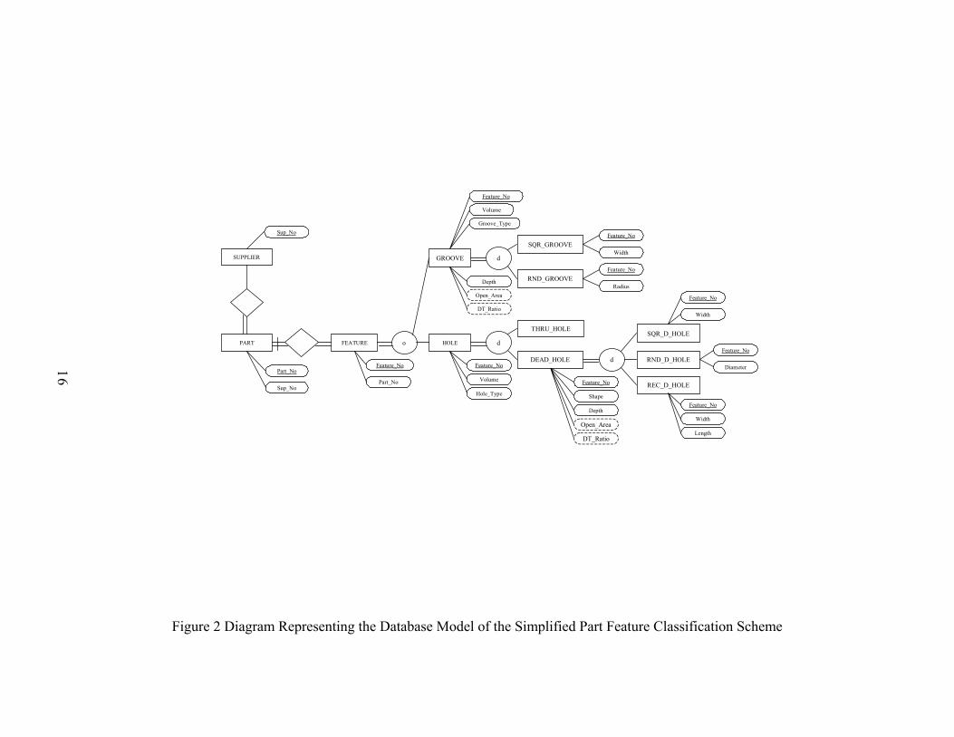
Figure 2 shows the translation of the part feature classification tree into an entity-
relation diagram representation. Relation PART has an aggregation relationship with
relation FEATURE. The relationship links from relation FEATURE to GROOVE and
13

HOLE is an overlap generalization. So are the relationships between GROOVE and
SQR_GROOVE, and GROOVE and RND_GROOVE. The rest relations are connected
together with disjointed generalization relationships.
14
Part Feature
Groove
Hole
Square-end Groove
Round-end Groove
Square Hole
Round Hole
Through Hole
Dead Hole
Rectangle Hole
Part
ThreadFine Thread
Rough Thread
15
Figure 1 The Simplified Part Feature Classification Scheme
PART FEATURE o
SUPPLIER
HOLE
THRU_HOLE
d
DEAD_HOLE
SQR_D_HOLE
RND_D_HOLE
REC_D_HOLE
dFeature_No
Diameter
Feature_No
Width
Feature_No
Length
Width
Feature_No
Depth
Shape
DT_Ratio
Open_Area
Feature_No
Volume
Hole_Type
GROOVE
Groove_Type
Feature_No
Volume
Depth
Open_Area
DT_Ratio
SQR_GROOVE
RND_GROOVE
d
Feature_No
Width
Feature_No
Radius
Feature_No
Part_No
Part_No
Sup_No
Sup_No
16
Figure 2 Diagram Representing the Database Model of the Simplified Part Feature Classification Scheme

To illustrate query relaxation for approximate answers, suppose that one needs to
retrieve a part having a 1×2×1 inch square-end groove from the stock room. To the
database system, the user poses a query in order to locate the needed part as follows:
Q: SELECT PART.PART_NO, PART.LOCATION
FROM PART, FEATURE, GROOVE, SQR_GROOVE
WHERE PART.PART_NO = FEATURE.PART_NO (1)
AND FEATURE.FEATURE_TYPE = “GROOVE” (2)
AND FEATURE.FEATURE_NO = GROOVE.FEATURE_NO (3)
AND GROOVE.GROOVE _TYPE = “SQUARE” (4)
AND GROOVE.FEATURE_NO = SQR_GROOVE.FEATURE_NO (5)
AND SQR_GROOVE.WIDTH = 1 (6)
AND SQR_GROOVE.LENGTH = 2 (7)
AND GROOVE.DEPTH = 1; (8)
If the part with such features does not exist in the database at the time of inquiry,
the system activates its query relaxation mechanism to search for any available
approximate answers. The system will look into the SQR_GROOVE relation to see if
there is any part having a square-end groove feature with the similar dimension by
replacing the constant value in selection condition 6, 7, and/or 8. If there exists at least
one square-end groove in the SQR_GROOVE relation, eventually, after some iterations
of query relaxation, the system will be able to present some partial answers to the user.
However, in the event the available closest neighbors of the intended feature in the
SQR_GROOVE relation cannot satisfy the need of the user, the system may offer the
17

user a similar feature available from the RND_GROOVE relation. This is because a
round-end groove feature is logically the next closest neighbor of the square-end groove
feature in this part feature classification scheme. Also, a round-end groove feature can be
practically transformed into a square-end groove with some machining processes.
Therefore, approximate answers to this query could be obtained from the
RND_GROOVE relation as well.
To query any similar feature in the RND_GROOVE relation, the original query
needs to be transformed through a query relaxation process. The result from such a
process could be a query with a new set of selection conditions, such as the following:
Q′: SELECT PART.NUMBER, PART.LOCATION
FROM PART, FEATURE, GROOVE, SQR_GROOVE
WHERE PART.PART_NO = FEATURE.PART_NO (1)
AND FEATURE.FEATURE_TYPE = “GROOVE” (2)
AND FEATURE.FEATURE_NO = GROOVE.FEATURE_NO (3)
AND GROOVE.GROOVE _TYPE = “ROUND” (4′)
AND GROOVE.FEATURE_NO = RND_GROOVE.FEATURE_NO (5′)
AND RND_GROOVE.WIDTH = 1 (6′)
AND RND_GROOVE.LENGTH = 2 (7′)
AND GROOVE.DEPTH = 1; (8′)
In Q′, the constant value of the fourth selection condition is modified from “SQUARE” to
“ROUND”. Also, SQR_GROOVE is replaced with RND_GROOVE in selection
18
condition 5 to 8. SQR_GROOVE relation is substituted by RND_GROOVE relation in
this case.
Searching for approximate answers to query Q can be extended even further by
altering the constant value of the second selection condition from “GROOVE” to
“HOLE” for the same reason as substituting a round-end groove with square-end groove.
A version of the modified queries from relation relaxation by substituting GROOVE with
HOLE, can be:
Q′′: SELECT PART.NUMBER, PART.LOCATION
FROM PART, FEATURE, GROOVE, SQR_GROOVE
WHERE PART.PART_NO = FEATURE.PART_NO (1)
AND FEATURE.FEATURE_TYPE = “HOLE” (2′′)
AND FEATURE.FEATURE_NO = HOLE.FEATURE_NO (3′′)
AND HOLE.HOLE_TYPE = “DEAD” (4′′)
AND HOLE.FEATURE_NO = D_HOLE.FEATURE_NO (5.1′′)
AND D_HOLE.SHAPE = “ROUND” (5.2′′)
AND D_HOLE.FEATURE_NO = RND_D_HOLE.FEATURE_NO (5.3′′)
AND RND_D_HOLE.DIAMETER = 1 (6′′)
AND D_HOLE.DEPTH = 1; (8′′)
The GROOVE relation is replaced by HOLE relation in Q′′ through the query
relaxation process. Consequently, the SQR_GROOVE relation must be substituted by
RND_D_HOLE relation since SQR_GROOVE relation is dependent on the GROOVE
19

relation. Selection conditions 5, 6, and 8 are switched to 5.3′, 6′, and 8′. The attribute in
the 6th condition is transformed to another attribute, which is more appropriate for the
new relation. The seventh selection condition of Q is dropped because it is no longer
applicable; and selection condition 5.1′ and 5.2′ are added to make the Q′′ complete.
1.2 Research Objectives
The objectives of the proposed research are:
1. To improve the capability of the current query relaxation techniques,
most of which cover only simple single relation queries, such that
complex (nested or jointed) queries can be relaxed as well.
2. To extend the current research on query relaxation to cooperative query
answering by allowing attribute and/or relation substitution, and
simultaneous multiple query condition relaxation. Also, to demonstrate
how dependencies of the query conditions can be taken into
consideration in the query relaxation process.
3. To develop appropriate semantic nearness measures for calculations of
the semantic distances between exact-match answers and approximate
answers resulted from the proposed cooperative query answering
techniques.
4. To form a framework for developing a higher level cooperative query
answering system that includes: 1) query relaxation techniques, 2)
approaches for development and maintenance of the knowledge base
20

needed to support the proposed relaxation techniques, and 3) functions
for semantic nearness measuring between approximate and exact-match
answers.
1.3 Research Deliverables
1. Neighbor knowledge discovering techniques that can be used to
construct neighbor hierarchies of attribute values, attributes, and
relations.
2. Algorithms for determining the causes of null answer, expanding
qualified tuple set, expanding intersected tuple set, and relaxing
multiple conditions simultaneously, substituting attribute value,
substituting attribute, and substituting relation.
3. A query relaxation model for approximate answering searching of
multi-relation (nested) queries.
4. A nearness measuring function that can be used to calculate the
semantic nearness between exact-match answers and approximate
answers, and is suitable for the proposed query relaxation methods.
21
2.0 BACKGROUND
This chapter provides the background of the research topic. Section 2.1 offers
the explanations, terminologies of databases, and their representations. Descriptions of
different types of relationships used in part classification schemes are also presented in
this section. Section 2.2 provides the detail regarding queries, database query languages,
and an example of query represented by structured query language (SQL). Types,
application domains, supporting database platforms, and various forms of cooperative
answers of cooperative query answering systems are stages in Section 2.3 .
2.1 Relational Database
Currently, many types of databases are utilized in information systems. Some
commonly used database models are relational, object-oriented, deductive, network, and
hierarchical databases. Among all types of databases, relational databases are the most
popular ones. They have been used as the backbone of many commercial database
software applications, such as Microsoft Access and Oracle, due to their simplicity and
capability of storing all sorts of conventional data. Object-oriented and deductive
databases have also been widely accepted, and implemented in many current information
systems. Object-oriented databases have gained more and more popularity since they
were introduced. That is because they use flexible object structures and have object
operations that allow more data manipulations than the other database models. Their
structures provide seamless or less-effort integration with the current object-oriented
22
programming languages such as C++ or JAVA. Their flexible object structures also
make them suitable for modeling or storing new types of data such as complex
engineering design, geographic information, multimedia data, etc.. Deductive databases,
as implied by the name, allow deductions or inferences of additional information (rules)
from the existing data (facts). Deductive databases are often used in the systems
equipped with artificial intelligence, logic, or knowledge base capabilities.
In this paper, relational databases are used as the platform for the methodology
development due to their popularity, simplicity and formality. Also, techniques
developed for relational databases are generally easy to adapt to object-oriented
databases.
In order to discuss the proposed cooperative query answering methodology, it is
necessary to describe a formal database representation and some of its common
terminologies. Databases are data repositories that store collections of related data and
are modeled after the interested portion of the real world, often called “mini-world”. In
this regard, the Entity-Relationship (ER) model is a popular high-level conceptual data
model used to represent database designs . In an ER model, an entity is the basic object
(or concept) existing in the mini-world. For example in an academic setting, a student, a
class, and an instructor, for example, are entities in a school database scheme. The
objects’ properties of interest are the attributes of the entity in an ER model. Name,
address, student ID number, and GPA are the interesting attributes of each student entity.
Each entity has values for its attributes, called attribute values. Entities having the same
set of attributes are grouped together, and are referred to as an “aggregation” of an entity
23
type. For instance, the STUDENT entity type is a collective name of all students. The
member set of an entity type at any particular point in time is called the entity set of that
entity type. The attribute used to identify an entity from its entity set is the key attribute
of the entity. Each entity in an entity type must have a unique value for its key attribute.
Domains of attributes are the sets of values that may be assigned to attributes.
They are generally declared in the data model or the design document of the database.
Every attribute must associate with a data type such as string, number, or date that are
used to define the attribute at the time in which the table was created. In some cases,
domains of attributes are explicitly defined by the database developer. They can be
stated as sets or ranges of attribute values. The set of the values that a WIDTH attribute
can possibly take, for instance, is the set of real numbers from zero to infinity. For a
START TIME or STOP TIME attribute of an entity type, the domain of the attribute
contains all values between 00:00:01 AM to 12:00:00 PM. The domain of the
WORKING DAY attribute is a set whose members are {“Monday”, “Tuesday”,
“Wednesday”, “Thursday”, “Friday”, “Saturday”, “Sunday”}.
When two (or more) entities associate or interact with each other, there exists a
relationship between the two entities. Each connection between entities is called a
“relationship instance.” Relationship type and set of relationship are defined on
relationship instance the same way entity type and entity set are defined. An enhanced
Entity-Relationship (EER) model is a extended version of the ER model. The EER
model is capable of modeling complex relationships such as aggregation, generalization/
24
specialization, and category; and, therefore, permits users to model databases containing
complex structures.
Relational databases are generally represented by “relational models.”(20)
Through a relational model, a relational database is expressed as a collection of relations.
Generally speaking, a relation is a table in the database. When mapping an EER
conceptual model to a relational model, entity types in the EER model are replaced by
relations. Each row or record in a table (or an entity in the EER model) is referred to as a
“tuple” in the relational model. Each column or field in a table is represented by an
attribute of the relation. Associations between relations in relational database models can
assume either one of the four relationship structures: 1) association, 2) aggregation, 3)
generalization/ specialization or 4) category. (21)
Distinguishing each type of relationship helps identify the dependencies between
selection conditions, especially when relation substitution is performed. In order to
demonstrate the meaning and the differences of each type of the relationship structures,
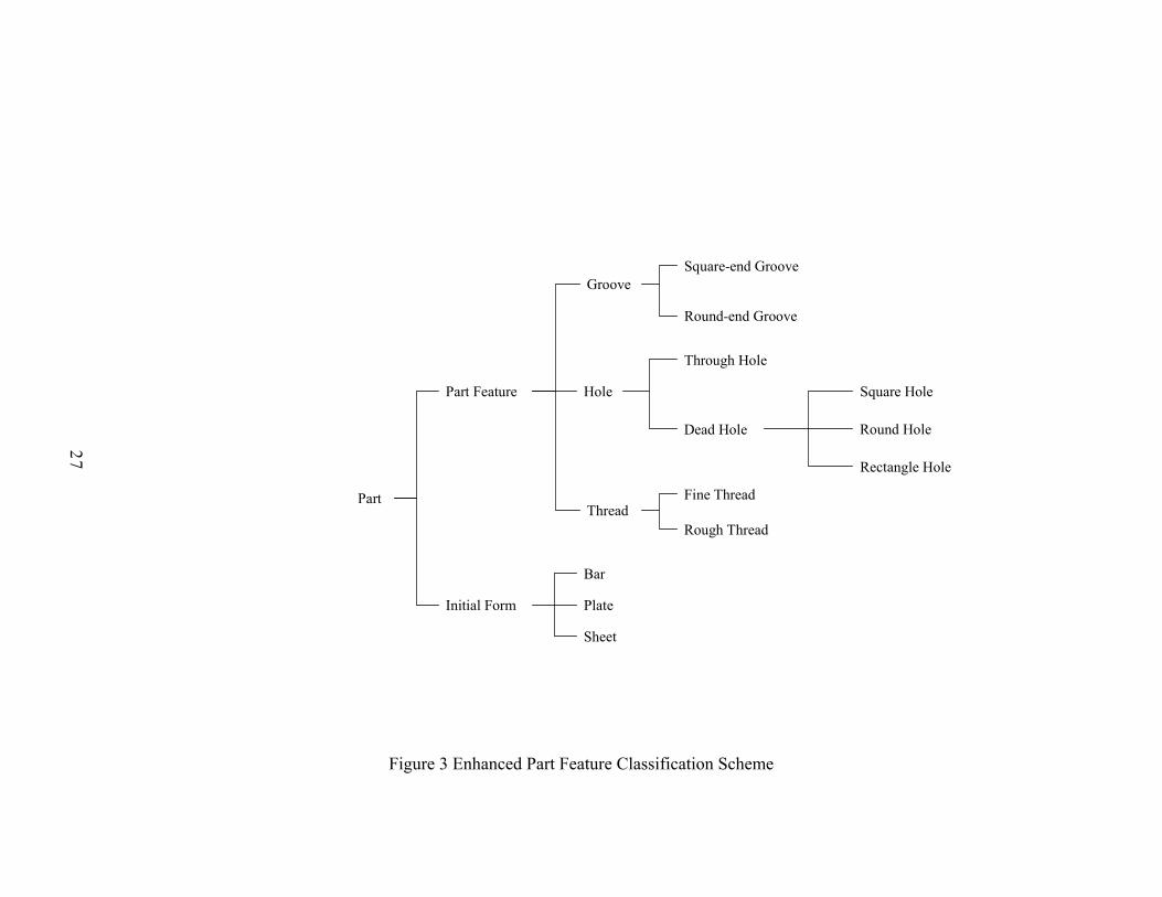
consider the part feature classification scheme and database model shown in Figure 3 on
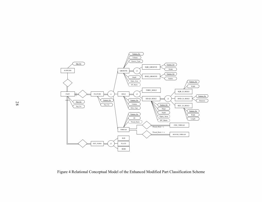
page 27 and Figure 4 on page 28, which are enhanced versions of the example in the
previous chapter. In this version of the part feature classification scheme, we added to
the previous example the information related to suppliers, initial forms, and another type
of part feature, “threat”. Figure 3 depicts the classification and coding scheme of this
modified version of part feature classification scheme. Suppliers supply parts. The
initial form of a part can be specialized into three groups which are bar, plate, and rod.
25

Threads are the combination of fine thread and rough thread. The EER representation of
this product scheme is illustrated in Figure 4.
2.1.1 Association
The most common relationship type utilized in relational databases is
“association.” Association represents the basic relationship between any two entity
types. As a matter of fact, whenever two relations are linked together, by default, the
relationship is of type association. Aggregation, generalization/specialization, and
category relationships, which will be mentioned next, are special cases of association. In
this part scheme example, relation SUPPLIER and PART are connected together with an
association relationship.
2.1.2 Aggregation
“Aggregation” is used instead of association when one wants to define “IS-
PART-OF” relationships between whole and component relations. The relationships
between PART and FEATURE and PART and INIT_FORM in the classification scheme
are modeled using an aggregation relationship in order to convey the design idea that
FEATURE and INIT_FORM relations should by viewed as components of PART
relation.
26
Part Feature
Groove
Hole
Square-end Groove
Round-end Groove
Square Hole
Round Hole
Through Hole
Dead Hole
Rectangle Hole
Part
Initial Form
Bar
Plate
Sheet
ThreadFine Thread
Rough Thread
27
Figure 3 Enhanced Part Feature Classification Scheme
PART FEATURE o
SUPPLIER
HOLE
THRU_HOLE
d
DEAD_HOLE
SQR_D_HOLE
RND_D_HOLE
REC_D_HOLE
dFeature_No
Diameter
Feature_No
Width
Feature_No
Length
Width
Feature_No
Depth
Shape
DT_Ratio
Open_Area
Feature_No
Volume
Hole_Type
GROOVE
Groove_Type
Feature_No
Volume
Depth
Open_Area
DT_Ratio
SQR_GROOVE
RND_GROOVE
d
Feature_No
Width
Feature_No
Radius
Feature_No
Part_No
Part_No
Sup_No
Sup_No
INIT_FORM
BAR
PLATE
ROD
d
Feature_No
LR
Thread_Ratio
FINE_THREAD
ROUGH_THREAD
THREAD
Thread_Ratio < x
Thread_Ratio >= x
28
Figure 4 Relational Conceptual Model of the Enhanced Modified Part Classification Scheme

2.1.3 Generalization/Specialization
Generalization/specialization relationships are used to model the relationships
between super-classes and their sub-classes. “Generalization” is the process of defining
sub-classes of an relation, whereas, “Specialization” is the reverse process of
generalization. Generalization and specialization are normally interchangeable. In the
rest of the paper we will use the term generalization for both generalization and
specialization relationships. Examples of such relationship types are the relationships
between relation HOLE and DEAD_HOLE, and HOLE and THRU_HOLE in Figure 4.
Through generalization, we define HOLE relation as the super-class and DEAD_HOLE
and THRU_HOLE as its sub-classes. (Specialization is simply the opposite.)
A unique characteristic of generalization is that it allows sub-classes to inherit the
properties (attributes) of their super-classes. Thus, not only does DEAD_HOLE possess
its own attributes such as Shape, Depth, Open Area, Depth-Thickness Ratio, but also it
inherits the attributes from its super-class, HOLE, which are Feature Number, Volume,
and Hole Type.
One important constraint of generalization is the “disjointedness constraint.”
There are two types of disjointedness: disjointed and overlapping. A disjoint
generalization is used when a super-class instance can be classified into only one sub-
class type. An overlapping generalization indicates that a super-class instance can be
mapped into several sub-class instances of multiple sub-class types. In our part scheme
example, the relation DEAD_HOLE and THRU_HOLE have a disjoint generalization
29

relationship with HOLE relation. This means a hole can be either a dead hole or a
through hole. The relation GROOVE, HOLE, and THREAD have an overlapping
generalization relationship with FEATURE, which implies that a feature can be classified
into more than one feature groups. For example, a thread hole feature is both a hole and
thread. The other generalization relationships in our example are the relationships
between relation DEAD_HOLE and SQR_D_HOLE, DEAD_HOLE and
RND_D_HOLE, DEAD_HOLE and REC_D_HOLE, INIT_FORM and BAR,
INIT_FORM and PLATE, and INIT_FORM and ROD.
2.1.4 Category
The last type of relationship commonly used in relational databases is “Category.”
Category relationship is used for the modeling of the relationship in which a sub-class has
more than one super-class. Therefore, with a category relationship, the sub-class inherits
the attributes from all of its super-classes. Examples of this type of relationship are the
relationships between relation ROUGH_THREAD, FINE_THREAD and THREAD.
2.2 Queries
There are two types of database retrievals; “data retrieval (DR)” and “information
retrieval (IR).”(22) The differences between DR and IR are shown in Table 1.
30

Table 1 Data Retrieval and Information Retrieval Differences
Data Retrieval Information Retrieval Matching Exact match Partial match, best match Inference Deductive Inductive Model Deterministic Probabilistic Classification Monothetic Polythetic Query Language Artificial Natural Query Specification Complete Incomplete Item wanted Matching Relevant Error response Sensitive Insensitive
The major difference between DR and IR is getting exact match answers versus
partial or approximate answers. In DR, database retrievals are done mainly through
standard query language such as Structured Query Language. If there is no exact match
data instance, the query will return a null answer. On the other hand, in the IR concept, if
no exact match data instance is found, the system will try to find any close match data
instances, and present these to the user as the alternative answers. The proposed
cooperative query answering methodology is considered a type of information retrieval.
It is developed, however, from a data retrieval query language, Structured Query
Language (SQL).
Different types of data can be retrieved from databases through the use of queries.
These include numerical data, text, multimedia data, etc..(23),(24) The three major parts of
a query are: 1) the attributes of interest, 2) the relations that contain the entities whose
attributes are being retrieved, and 3) the conditions on the properties that the entities in
the answer set must possess. Query conditions stated in a query can be classified into
two types: the selection conditions, and the joint conditions. The query selection
31
conditions are the criteria used for separating the qualified entities from its entire
population. The joint conditions specify how entities from different relations are linked
together when the query involves more than one relation. (In the case of a recursive
relationship, joint conditions indicate how entities from the same relation are associated
to each other.) Both selection condition and joint condition are evaluated as either true
when at least one entity from the entire population meets the criteria, or false when none
of the entities in the specific entity type satisfies the condition.
Queries can be expressed in many forms using different query languages.
According to Demolombe(25) relational database management system query language can
be divided into three main categories: those derived from Relational Calculus(26), those
derived from Algebraic language(27,26), and those derived from Predicate Calculus
language.(28,29,30) Structured Query Language (SQL) is the standard query language for
relational databases and is based on relational algebraic language. In terms of query
representation, SQL language has more expressive power than most of the other query
languages because it is not only able to represent almost any queries, but also is capable
of incorporating aggregate functions, grouping, and ordering operations. In SQL, a query
is denoted in the form of the SQL SELECT statement. The SQL SELECT statement is
comprised of three main blocks; the SELECT block, the FROM block, and the WHERE
block.
The SELECT block in SQL SELECT statement is used to list the attributes of
interest that the user wants as the answer to the query. The FROM block tells the system
from which relation(s) the attributes of interest are supposed to be pulled. The WHERE
32
block allows the user to specify the properties that the entities in the answer set must
possess and how entities from multiple relations are joined together. The WHERE clause
is expressed through a series of query conditions connected together with operators and,
or, and not. A selection condition of a query is in the form of A op C where A is a
relation attribute, op is =, <>, <, <=, >, or >= and C is a constant. A joint condition is
expressed in the form of Ai op Aj where Ai and Aj are relation attributes and op is =, <>, <,
<=, >, or >=. Each individual query condition is evaluated as either TRUE or FALSE. A
query condition is assessed as TRUE only if at least one member from the stated
relation(s) meets all query conditions. Otherwise, it is evaluated as FALSE.
Let’s consider Q1: “Give me a list of part numbers and part locations of parts that
have a groove feature having two square ends and the groove dimension of 1×2×1”. Q1
is expressed using SQL SELECT statement as follow:
Q1: SELECT PART.NUMBER, PART.LOCATION
FROM PART, FEATURE, GROOVE, SQR_GROOVE
WHERE PART.PART_NO = FEATURE.PART_NO (1)
AND FEATURE.FEATURE_TYPE = “GROOVE” (2)
AND FEATURE.FEATURE_NO = GROOVE.FEATURE_NO (3)
AND GROOVE.GROOVE _TYPE = “SQUARE” (4)
AND GROOVE.FEATURE_NO = SQR_GROOVE.FEATURE_NO (5)
AND SQR_GROOVE.WIDTH = 1 (6)
AND SQR_GROOVE.LENGTH = 2 (7)
AND GROOVE.DEPTH = 1; (8)
Query condition (2), (4), and (6)-(8) are selection conditions of Q1. Query
condition (2) is the selection condition on relation FEATURE indicating that only groove
33

features are wanted. Query condition (1), (3), and (5) are joint conditions that join
relation PART with FEATURE, FEATURE with GROOVE, and GROOVE with
SQR_GROOVE, respectively. The system acquires the answer set by first evaluating the
selection conditions of each relation. Since there is no selection condition on relation
PART, the entire entity set of relation PART is qualified for the answer. Second, it
assesses all members in relation FEATURE against its selection condition (condition
number 2). Only those members that cause condition (2) to be TRUE are separated from
the entity set of relation FEATURE and are put into a set of “qualified” entities of
FEATURE. This process of selection condition evaluation is repeated for relation
GROOVE and SQR_GROOVE. Notice that only entities from relation SQR_GROOVE
that satisfy ALL of SQR_GROOVE’s selection conditions (condition number 6 to 8) are
considered qualified. Next, the system uses joint conditions (1), (3), and (5) to link the
qualified entity set of PART, FEATURE, GROOVE, and SQR_GROOVE and performs
an intersection operation to get the answer set of the query. As stated before,
conventional queries search for exact match answers. If exact match answers do not
exist, the system returns null answers. Q1 could result in a null answer in the following
situations:
1) At least one of the qualified entity sets of the four relations is an empty
set meaning that none of the members in the entity set meet the
relation’s selection condition(s).
2) All qualified entity sets of the four relations are not empty, but the result
from the intersection operation of them is an empty set.
34
Again, this exact match searching is the main drawback of the conventional data
retrieval system. To alleviate the problems, many cooperative query answering
techniques have been developed and incorporated in many of today information systems.
2.3 Cooperative Query Answering
Cooperative query answering concepts are based on “human intelligent
responses”.(31) A human tends to reply to questions with informative responses rather
than rejection answers in the situation where the answers to the questions are not known,
or negative. People are likely to include their experiences or knowledge pertaining to the
topics of the questions in such kinds of circumstances. For example, when someone
standing at a bus stop is asked: “Have you seen the 28X bus scheduled to stop at
10:00AM going to the airport pass by?”, the person might reply with the following
answers:
“I’m not sure, but I saw a 28X pass by 15 minutes ago.”
“No, but 28X scheduled at 9:00AM just passed by.”
“Yes, but the next one should be arriving in half an hour or so.”
“Yes, but you can catch the airport shuttle leaving from the Holiday Inn hotel
in 10 minutes.”
To provide such useful information in this situation, the person must first have
some knowledge about the schedule of 28X buses. Then the individual has to process the
question by combining it with the known knowledge and facts to get such cooperative
answers. The facts and knowledge required in this situation are: 1) an observation
35
regarding the 28X bus, 2) the current time, 3) the schedule of the bus, and 4) different
means to the airport, etc..
A typical database system, on the other hand, does not have this essential
cooperative answering capacity. When a user submits a question in the form of a query, a
standard database system usually replies with only “yes” or “no” in the situation
mentioned in the bus stop example. This is because the conventional query answering
system requires “exact matching” between the query conditions and the answer
properties. This exact match property of a typical query answering mechanism sometime
causes user frustration, especially when a negative answer is not expected. Many
cooperative query answering techniques have been developed to improve information
retrieval by incorporating human-like intelligent question answering into the standard
database systems. The objective of cooperative query answering is to give traditional
database systems human intelligence responses, so the system can answer with more
useful information, such as providing indirect answers, intentional answers, and/or partial
answers.
2.3.1 Different Types of Cooperative Query Answering Systems
Many types of cooperative query answering systems have been developed, and
proposed. Each cooperative query answering system is different from the other systems
in three aspects: 1) the intended application domain, 2) the supporting database model or
platform, and 3) the type of cooperative answers.
36

2.3.2 Application Domains of Cooperative Query Answering
Different application domains deal with different data types – traditional,
geometric, multimedia, temporal – and, therefore, require different approaches. Various
cooperative query answering techniques have been implemented in many application
domains such as biological, agricultural, and the health industry. Lately, the concept has
been utilized extensively in querying for multimedia data, especially image retrieval.
Petrakis and Faloutsos(32) proposed a method for “similarity searching” in medical image
databases. Other examples of cooperative query answering techniques for medical
multimedia databases are stated in (33), (34), (35), (36), and (37). Che, Chen, Aberer,
and Eisner developed smart query relaxation for a biological database.(38,39,40) GPCRDB,
an advanced data management system for the pharmacology and biology areas, were
presented by Che, Chen, Aberer, and Eisner.(41,42,43) However, so far only single table
query relaxation has been the main focus of most research groups. Cooperative query
answering for hierarchical structure information systems have not yet received enough
attention.
2.3.3 Supporting Database Platforms
The supporting database platform is the most important design aspect of any
cooperative query answering system. Some cooperative answering techniques might be
applicable for many database platforms, but, most of the time, each technique can support
only the predetermined type of databases. Different groups of databases that have been
37
the focus of many research studies are deductive database, object-oriented database, and
relational database.
“Deductive databases” are mainly used in conjunction with artificial intelligence
or an expert system, since their data and database structures are stored in terms of
predicates, predicate clauses, and rules. The cooperative query answering techniques for
this type of database evolves around the relationships between predicate clauses and their
reciprocal clauses. Some examples of the approaches for incorporating cooperative query
answering in deductive databases were proposed by Cholvy and Demolombe(44), and also
by Mielinski(45), and Gaasterland.(46)
The second group of databases implementing cooperative query answering is in
the “object-oriented” or “semantically rich” framework. These types of databases make
extensive use of the generalization or aggregation hierarchy of classes, which are also
called taxonomy of concepts. Cooperative query answers for this database platform are
typically acquired by searching the generalization hierarchy or the “taxonomy tree” for a
higher or a maximum concept that subsumes the set of answers resulted from the query.
Some research studies on cooperative query answering in object-oriented database are
Shum and Muntz (15,16) and Alashqur, Su, and Lam.(47,48)
Another database model that has been the focus of cooperative query answering
studies is the relational database. Cooperative query answering techniques have been
developed for relational databases more than for all the other database types. Motro(18)
used integrity constraints in derivation of intentional answers. Chu, Lee, and Chen(49)
used “type inference” and “induced rules” to provide intentional answers.
38
2.3.4 Types of Cooperative Query Answers
Generally speaking, “cooperative answers” are any kind of extra information that
a database system offers its users in addition to the set of data items resulting from an
evaluation of queries. Again, each cooperative answering method is, in most cases,
tailored for a type of specific cooperative answer type; consequently, the design of a
cooperative query answering system is also governed by the type of cooperative answers.
The three major types of cooperative answers are intentional answers, associative
answers, and partial or approximate answers.
An “intentional answer” is the brief and more meaningful interpretation of the
traditional results from the query that the cooperative system provides to the user as the
substitute or supplemental information. It gives the user the description of the query
answers. Intentional answers are very useful for novice users that do not have an
adequate knowledge about the stored data. They convey the information that could help
users compose better subsequent queries. Intentional answers, in the form of brief
summary information, are also very helpful when the posted queries result in very large
answer sets. For example, the result of a query: “List Ph.D. candidate students who have
taken the qualifying exam”, which is actually a list of the entire population of Ph.D.
candidate students, can be substituted with “All Ph.D. candidate students must pass the
qualifying exam.” Intentional answers are usually derived from the meta data of the
database or the knowledge base such as database integrity constraints. Some work that
has been done in the field of intentional answers are presented in (12) and (50).
39
The second type of cooperative query answers, which is similar to the intentional
answer, is the “associative answer.” Intentional answers and associative answers share
the same concept of providing the supplemental information in addition to the traditional
query answer set. While intentional answers give the users the common characteristics of
the answers, or the brief summary of the answer set, associative answers offer additional
information that is not explicitly asked but is relevant to the answer set or topic of the
query, which might be of interest to the user. An example of an associative answer is:“30
undergrad students and 10 graduate students are currently registered for the Database
Design course” or “30 undergrad students (15 female and 15 male) registered for the
Database Design course” when the user posts the query: “How many undergraduate
students registered for the Database Design course”. Notice that the system not only
gave the number of graduate students in the first response, but also broke down the
number into female and male students in the second response. This is because, according
to the knowledge base, numbers of undergraduate students are usually associated with
numbers of graduate students, or gender is always retrieved along with number of
students. Associative answers are usually obtained from the knowledge base derived by
applying some knowledge discovery or data mining techniques onto the database.(51,52,53)
The last major type of cooperative query answer, which is the focus of this
research, is the “partial or approximate answer.” Unlike the other cooperative answer
types, which are some forms of useful additional information attached to the original
query answers, approximate answers are presented to the users when an exact matched
answer is not available or does not exist in the database.
40

Besides intentional, associative, and approximate answers, there are also other
unique minor types of cooperative query answers. One of them is called “explanations.”
This type of cooperative answer, which is provided to the users along with the
conventional or cooperative answers, helps the user understand why the system returns
such answers and, in turn, makes better decisions on whether or not he should accept the
answers, or how to compose the next query to achieve better results. A framework that
generates the explanations of how the system acquires the cooperative query answers and
the intentional meanings of the answer sets was proposed by Minock.(54)
2.4 Part Family Classification Data Structures
Manufacturing requires a wide scope of detailed information. Some examples of
different sets of information stored in a manufacturing information system are: resource
schedules (including the utilization plan for men and machines), shop floor control,
production data, bill of materials, inventory management, and product information. One
commonly shared property of these data sets is that the relationship between the objects
or relations are frequently represented by aggregation, generalization, and category.
Srirangapatna(55) stated in his work that the structural abstraction hierarchies –
aggregation, generalization, and category –were essential for databases integrated in the
specialized applications such as engineering computer automated design (CAD). This is
because most of the information in the manufacturing domain possesses some forms of
hierarchies of super-classes and sub-classes such as assembly-subassembly, product-
feature, product family-product, etc..
41

The use of hierarchical structures in product classification principles under the
group technology paradigm was emphasized in research noted in (56) and (57). Billo(58) ,
and Billo and Bidanda(59),(60) stated in their papers that several rules of classification and
coding scheme correspond to the object-oriented data abstraction principles of
“Generalization with Disjoint Subclasses”, “Generalization with Overlapping
Subclasses”, “Classification”, and “Aggregation”. In their papers, these structural
hierarchies can be used for modeling the classification and coding principles of E-tree, N-
tree, X-tree, or C-tree.
An “E-tree”, in a classification and coding scheme, is used when the member in
an object class (super-class) can be classified into groups of mutually exclusive sub-
classes. In other words, a member of the super-class object can be further categorized
into one and only one sub-class. An “E-tree” can be represented in the object-oriented or
relational database model through the use of “Generalization with Disjoint Subclasses”.
An example of an E-tree classification in the part scheme is where a hole feature can be
either a hole with a bottom or a bottomless hole. (Shown in Figure 3) It cannot be both a
through hole and dead hole at the same time.
An “N-tree” in classification and coding principles is similar to the E-tree
mentioned earlier. The main difference between them is that, for an N-tree, a member of
the super-class object can be traversed to more than one subclass, while an E-tree
prohibits such linkages. N-tree in classification and coding principles can be modeled by
Generalization with Overlapping Subclasses. In our part scheme, a feature can be both or
either a hole and a thread at the same time (i.e. a threaded hole). Therefore, the
42

relationships connecting FEATURE with GROOVE, HOLE, and THREAD are defined
using an N-tree (Figure 3) and are represented in the relational model (Figure 4) as
Generalization with Overlapping Subclasses.
An “X-tree” in classification and coding schemes is used when a class of objects
possesses properties found in multiple other classes. An X-tree is represented in the
object-oriented model by Category, which allows a sub-class to inherit the attributes from
all of its super-classes. Examples of an X-tree in the part scheme example are the
relationship between ROUGH_THREAD, FINE_THREAD and THREAD.
A “C-tree” of the classification and coding scheme is used to symbolize the
combination of E-tree, N-tree and X-tree. The C-tree is represented by Aggregation in
the object-oriented model. Relation PART, FEATURE, and INIT_FORM are associated
through a C-tree in the classification and coding scheme in the part scheme example.
In general, the queries involved with such types of data structures are joint
queries, since the complete information of an object or a concept (a product in this
example) must be retrieved from many relations linked together with hierarchical
structures. Incorporating the cooperative query answering concept with such hierarchy-
rich manufacturing information databases requires query relaxation techniques capable of
dealing with joint queries and relaxation of multiple query constraints simultaneously.
Furthermore, relaxation of query conditions for these hierarchical structures requires the
consideration of dependencies among query conditions. As stated previously, without the
condition dependency consideration, query relaxation will result in unreliable answers.
43

Therefore, cooperative query answering techniques that are restricted solely to query
relaxation of attribute values are not practical for manufacturing information databases.
44

3.0 LITERATURE REVIEW
As stated earlier, our objective is to develop a cooperative query answering
system that can handle nested or joint queries, and allows multiple query conditions to be
relaxed simultaneously with the consideration of dependencies among query conditions.
Also, the system must have a suitable and reliable measure for nearness between the
approximate answers and the exact-match ones. To accomplish such goals, methods for
finding approximate answers, query relaxation, construction and maintenance of neighbor
knowledge, and nearness calculation issues need to be addressed. This section
summarizes the research efforts completed thus far in the field of cooperative query
answering. In Section 3.1 , concepts, different principles, and tools used for cooperative
query answering, and the research works related to the topic are presented. Section 3.2
describes the three major means to relax a query: dropping query conditions, attribute
value substitutions, and attribute and/or relation substitutions. Techniques for both
manual and automated construction (and maintenance) of the neighbor knowledge are
presented in Section 3.3 . Section 3.4 presents various approaches for semantic nearness
measuring and examples of research studies using different approaches.
3.1 Approaches in Finding Approximate Answers
Early cooperative query answering techniques found approximate answers by
calculating the semantic distance for every tuple in the relation using some form of
nearness function. A certain number of tuples that have the closest distance to the
45
unavailable exact-match answer were presented to the user. These techniques are
practical only for relations with small numbers of records. Later, many researchers have
developed cooperative query answering methodologies using more sophisticated
approaches in finding cooperative query answers. Diverse principles such as fuzzy set,
knowledge discovery, and probabilistic theory have been exploited as the tools to
generate cooperative answers. Ribeiro (61) proposed a fuzzy set model for cooperative
databases. The model was designed to obtain cooperative query answers for
bibliographic databases or information retrieval (IR) systems. Antonio(62) used a
“Generalized Quantifier” in query language to produce cooperative question answering.
Keen(63) employed inductive dependencies in additional to functional dependencies at the
tuple level to provide approximate answers to queries. Gassterland (64) combined
integrity constraints, user constraints, and user interfacing(which allowed users to
interactively work with the system) to obtain cooperative query answers.
The main thrust in cooperative query answering studies in the last two decades
has been the use of abstraction hierarchy in acquiring approximate answers. Abstraction
hierarchies allow developers to represent the knowledge related to application domains
and their collected data in the forms of generalization/specialization relationships. This
information representation format of abstraction hierarchy makes it the most popular tool
for cooperative query answering. This is because the structure resembles the neighbor
knowledge structure required for deriving of approximate answers. Abstraction
hierarchies have been used in the domain of modeling human knowledge for cooperative
responses for many years. An early use of abstraction hierarchy representation in
46
modeling human cognition in the Oriental game of Go was presented by Friedenbach.(65)
In his work, a hierarchy of related concepts was used to explain how the game was
played. Fu (66) introduced the concept of the hierarchical organization of the data in the
databases produced from data mining or knowledge discovery. He demonstrated that
cooperative query answering could be acquired through multiple-layered database, which
has resulted from data mining. Han(67,68,69) developed cooperative query answering
techniques that used some knowledge discovery tools, in particular attribute-oriented
induction, and discovered knowledge stored in abstraction hierarchies to produce
intentional and associative answers. Chu and Chen(70,71) proposed a use of abstraction
hierarchy structure in a framework for integrating data and knowledge to support
cooperative query answering. The framework utilized three layers of generalization: the
object layer that contained an abstraction hierarchy of the extensional data, the subject
layer that stored another abstraction hierarchy of the knowledge base, and the object-
subject layer that held another hierarchy for patterns or concepts used to couple the other
two layers.
The concept of Type Abstraction Hierarchy (TAH) used to represent the
knowledge base for neighbor object information was developed by Chen, Chu, and
Lee.(49,72,73) Under the concept of TAH, a “type” can be defined recursively as:(48)
a) A primitive type (e.g., integer, real, etc).
b) If t1, …, tn are types and a1, …, an are attributes, then t:(a1:t1,
…, an:tn) is a type called a tuple-type which can be abbreviated as t.
c) If t1, …, tn are types, then t:(a1:t1, …, an:tn) is a type called a set-type which can be abbreviated as t.
47
TAH is a multi-level object (or concept) representation that allows a super-class
and a sub-class to have different representations, and can be viewed at different instance
layers. To use TAH for query relaxation, three groups of knowledge, which are
represented in the form of tables, are needed:
1) Type-Hierarchy tables – define subtype relationships among types,
2) Attribute-Type tables – provide relationships between attribute names and type
names, and
3) Abstract-mapping tables – lists pairs of matched super-type and sub-type instances.
Later, the CoBase(74,75) cooperative database system was developed by this team of
researchers at the University of California at Los Angeles (UCLA) as the prototype of a
cooperative query answering system that made use of TAH. It provided cooperative
query answers by utilizing their internally developed cooperative query language CoSQL,
which is a modification of SQL. CoSQL allowed users to compose queries and to control
query relaxation through the use of cooperative operators such as “SIMILAR-TO”. An
example of the use of CoBase system was demonstrated in a framework for cooperative
query answer generation proposed by Minock(54). The TAH concept and the CoBase
database system have been used as the fundamental tools to find cooperative query
answers in many of this group of researchers’ later works. Lee (76) utilized type
abstraction hierarchy to provide cooperative answers. He generated intentional answers
as the cooperative query answers via TAH. Other examples of work in this group are
Associative Query Answering,(52,53) CoBase – a cooperative information system,(74)
Image Retrieval,(33,34,35,36,37) and Query Formulation from High-level Concepts.(77)
48
Despite its adaptability property, TAH still had some shortcomings. First, it was
quite static. Any updating for the TAH, which is necessary after instantiations of new
data into the database, required manual manipulation. Frequently, very few adjustments
were made to TAH after the initial development of the hierarchy. More often, updating
of TAH is ignored. Second, TAH does not have any quantitative nearness measuring.
Consequently, there is no ranking of the approximate answers. Third, TAH does not
permit user control over the query modification process. Most importantly, TAH only
allows one query condition to be relaxed at a time.
To overcome the inadequacies of TAH, Merabacher(78) proposed Attribute
Abstraction Hierarchy with nearness (AAH). It utilizes Pattern-based Knowledge
Inference (PKI) to construct the initial attribute abstraction hierarchy based upon patterns
found in database instances. Then, Dynamic Nearness (DN) is used to improve or
automatically update the attribute abstraction hierarchy based upon the historic
information of query access patterns. Merabacher’s method allowed multiple query
conditions to be relaxed simultaneously. It also permitted control of query relaxation by
the user, the knowledge gathered from the application domain and the context of the
query. These techniques still did not support relaxation of multiple-relation queries.
Relation substitutions still require predefined views.
3.2 Query Relaxation
Query relaxation is one of the most important design aspects of cooperative query
answering for null-bound queries. It controls how the system will modify queries to
49

acquire approximate answers when exact answers do not exist, or are unavailable. It also
dictates how narrow or wide the search space of the approximate answers is. Typically,
once the causes of null are identified, query relaxations can be done by:
1) dropping off the null-bound query conditions,
2) substituting attribute values (the right-hand-sides or the constants of the query
conditions) with their neighbors, and
3) replacing attributes and/or relations (the left-hand-sides of the query
conditions) with their neighbors.
The first option is the easiest approach since no additional database knowledge is
required. The system needs to determine only which of the conditions in the query
caused the null answer. Dropping a query condition could result in a significant loss of
information, especially if the query has only one selection condition. Most researchers
prefer attribute value substitutions as opposed to dropping problematic conditions for
their query relaxation operations. The most popular methods for attribute value
substitutions are to replace the condition constants with abstract ranges, or substitute
them with other values that make the conditions more general. For example, a query
condition: “Time = 8:00AM” may be modified to “Time >= 7:00AM AND Time <=
10:00AM”, or a query condition “Salary < 50000” may be relaxed to “Salary < 100000”.
If the query still returns an empty set, the values are then relaxed further. Substitution of
attribute values with their neighbors is a lot more complicated than the first query
relaxation method because the system needs the neighbor information of attribute values.
If the system uses any values that are too far away from the original values, it could result
50
in a large set of answers, or answers that are too distant from the searched ones.
Alternatively, if the system replaces the attribute values with new values that are too
close to the original ones, it may not find any approximate answer. The system likely
will require unacceptable computational time to search for the approximate answers. The
last query relaxation method is the most difficult because the system not only needs
knowledge about the neighbors of the attribute values, but must also realize any inter-
relation relationships between attributes and any side effects that could result from
altering those attributes or relations.
Rule-based query relaxation for cooperative query answering was presented by
Cuppens and Demolombe.(79,80) In their proposal, queries were represented in object
level and meta level, and the query relaxations were achieved through query
transformation rules similar to the first and the second approach stated earlier. Che,
Aberer and Chen(39,40) presented in their papers the utilization of domain knowledge to
relax queries in three aspects: keyword or concept generalization, residue pattern
relaxation, and secondary structure expansion. In order to perform generalization of
“keyword”, they created a hierarchy that represented three levels of relationships among
terms, which are strong similarities (between synonyms), weak similarities (between
sibling nodes), and generalizations (between a child-parent node pair). Then, keyword
generalizations were achieved by replacement of the original terms with its synonyms,
siblings, and parents until the answer was acquired or the terms could not be relaxed
further. Due to some special characteristics of biological information, which is the
intended application of the techniques, residue pattern relaxation, and secondary structure
51
expansion were important factors of the development of their query relaxation
methodology. Residue pattern relaxation was achieved by breaking the entire query
condition clause into multiple sub-clauses (residues). Then, one or more atomic
conditions (characters in this case) in each residue were substituted with their fuzzy
equivalent atomic conditions. For secondary structure expansion, the last atomic
condition (character) from the preceding secondary structure and the first atomic
condition (character) from the following secondary structure were added to the secondary
structure in focus to form a new structure (segment of the keyword).
Most current cooperative answering techniques perform query relaxations through
either or both query condition dropping and attribute value substitution. Some of them
that perform attribute value substitution only allow one query condition to be relaxed at a
time. The abilities to relax a query using the attribute and/or relation substitution and
carry out simultaneous multiple condition relaxation will make the cooperative query
answering system more robust and increase the chance that the approximate answers will
satisfy users’ needs.
3.3 Creating and Maintaining the Knowledge Base for Query Relaxation
As mentioned earlier, relaxing queries through attribute value, attribute, and
relation substitutions require that the system possess the neighbor information. These
sets of neighbor knowledge are generally stored in the database in the form of abstraction
hierarchies. The main challenges of using abstraction hierarchies are the development
and maintenance of the hierarchies. In the early stage of cooperative query answering
52
research, creating and updating of abstraction hierarchies were mostly performed
manually by the application experts. However, as the databases grew faster and faster, it
was impossible to keep up with the changes of their structures and stored data. Many
researchers proposed different techniques that could be used to automate these
activities.(81 ,82 ,83) Various knowledge discovery tools, including generalization, data
summarization, concept clustering, rule discovery, query rewriting, lazy evaluation,
semantic query optimization, etc., were used to develop the knowledge base for an
intelligent query answering system in Huang’s work.(84) Ozawa and Yamada(85) used
fuzzy logic techniques in conjunction with a category utility to construct concept
hierarchies of data tuples to generate intentional answers. Their methods required that
the predefined linguistic labels of the background knowledge for the data attributes,
which were used in classification of data, must be provided.
A more popular method that is used to construct neighbor abstraction hierarchies
for numeric values is the information entropy.(86) This method involves evaluation of
clustering results using entropy measure. The objectives of the information entropy
method were to maximize the entropy of data partitions.(87,88) Since the entropy is
maximized when the data are partitioned evenly, this approach considers only the
frequency of each attribute value. The value distribution of the data is excluded from this
method. Another method for developing neighbor hierarchies of numerical values was
proposed by Gennari, Langley, and Fisher.(89) The proposed method, called CLASSIT,
used mean and standard deviation to classify numerical values in to classes. The
goodness measure used in their works was 1/σ. Then, it was further revised to σ to
53

resolve the goodness value problem for single member clusters. These two numerical
value clustering methods consider only the frequencies of values.
Chu and Chiang(90,91)presented a method to automatically generate abstraction
hierarchies for numerical attribute values by considering both frequency and value
distribution of the data. In their efforts, they developed a clustering measure called
Relaxation Error that allowed them to optimize their clustering results. Merzbacher and
Chu(92) also proposed a method to generate abstraction hierarchy for non-numerical
attribute values using the Pattern Based Knowledge Induction (PKI) technique. They
also developed another technique, called Dynamic Nearness, that can be used to update
the neighbor knowledge resulted from PKI.
3.4 Semantic Nearness Measures for Approximate Answers
Generally, query relaxations result in large sets of approximate answers. Without
any kind of ranking mechanism, selecting the best or the closest answers still requires
some manual searching by the user. Semantic nearness measures allow the system to
take the guesswork from the user. Also, by removing the human interaction, errors from
different users are minimized. Three questions must be addressed to incorporate
semantic nearness measuring with a cooperative query answering system. These
questions are:
1) When should the semantic nearness be established?
2) Which objects (query answers or the queries themselves) should the system
compare to determine the semantic proximity?
54
3) How should the nearness values be stored or represented?

3.4.1 When Should the Semantic Nearness be Established?
Nearness values can be assigned in advance and then used later for any query
relaxations that are applicable. They can be calculated after the relaxation process is
completed, and partial answers are acquired. To determine nearness values in advance,
the system clusters all existing tuples in the relation of interest and calculates nearness
values for each neighbor set. Since the system needs to perform the calculation only
once, this approach is faster than the other method. However, computing nearness values
in advance only works with predetermined sets of queries. If users try to retrieve any
non-existent tuples, the system will fail to produce nearness values. This approach does
not work if there is more than one expected exact match answer. In such cases, an
algorithm for combining the nearness values between a partial answer and all exact match
answers must be defined. The second approach, which is calculating the nearness values
each time the system obtains a partial answer set, overcomes these problems by trading
computational time with flexibility.
3.4.2 Which Objects (Query Answers or the Queries Themselves) Should the System Compare to Determine the Semantic Proximity?
Nearness calculation can be divided into two groups based on the objects used in
the measurement. The first group of nearness measuring techniques calculates the
semantic proximity by comparing the approximate answers and the exact match answers
directly. The second group of nearness measurement compares the original queries and
55
the relaxed queries instead of the answers. The rationale behind the approach of the first
group is that the same set of answers can be retrieved by an infinite number of different
queries. Instead of calculating the closeness between the queries, nearness value
assignments are performed on the answer set that has determinable number of members.
This approach assumes that there is only one exact match answer.
The second group of nearness calculation techniques acquire nearness values by
comparing the original query with the relaxed queries that produce the answers. Since
the answers from a query are strictly related to the query conditions, the semantic
closeness between the intended answer and a partial answer should be proportional to the
nearness between the original query and the relaxed queries that generate those
approximate answers. This observation is true if the relaxed queries are not resultant
from substituting attribute values, attribute, or relations randomly or with their extreme
values. For example, a user is searching for a part with a hole feature having a diameter
of less than one half inch, but the exact match part does not exist. Let’s also assume that
there are two parts with hole features having diameters of 0.6 inch and 99 inches in the
relation. If the original query condition “DIAMETER < 0.5” is relaxed by replacing the
constant of the condition with any extreme values from its value spectrum such as
“DIAMETER <100”, both hole features will return as the approximate answers by the
modified query (and will have the same nearness value according to this approach). This
situation would not happen if query conditions were relaxed systematically by first
replacing attribute values with their closest neighbors. If the modified query still yields a
null answer, then the system will shift to the next closest neighbors. The usefulness of
56
this concept is obvious when there is more than one exact match answer. In such a case,
there is no need to adjust the nearness values between a partial answer and multiple exact
match answers.
3.4.3 How Should the Nearness Values be Stored or Represented?
The most accepted method for storing or representing semantic nearness between
the acquired approximate answers and the exact matched answers is the use of nearness
matrixes, and nearness functions. It is known that nearness matrices require much shorter
calculation times than do the nearness functions. However, the shortcoming of using
nearness matrixes is that they require a large amount of memory space and must be
updated periodically.
Yoon and Kim(93,94) developed neighbor matrix-based query relaxation techniques
for document-rich digital libraries. Chu and Zhang(95) developed a query similarity
measuring method based on query features which include: query topic, output attribute
list, and constraints. According to their method, the similarity of any two queries was the
weighted sum of the similarity function of each feature of the two queries. Chu, Yoon,
and Hsu(96) used time wrapping techniques to measure the similarity of different length
subsequences in sequence databases. They assumed there was some relationship between
any two consecutive numbers such as a trend or a pattern. Due to this assumption their
techniques are not appropriate for our purposes. Chiang (97) developed a quality measure
for approximate answers called relaxation error and algorithms for Type Abstraction
Hierarchy (TAH) based upon the minimization of relaxation error. Nearness functions
57

are used to calculate and update the distance between each neighbor node. The nearness
values are stored in nearness matrixes for better computational time.
58
4.0 THE DESIRED COOPERATIVE QUERY ANSWERING SYSTEM
Previous cooperative query answering techniques proposed by many research
groups have limitations that are not appropriate for hierarchy-structure databases, such as
those used for manufacturing information systems. The main objective of this research
study is to develop an ideal cooperative query system that has fewer restrictions, and is
suitable for such hierarchy-rich databases. The desired cooperative query answering
system in this research must possess the following features:
1. The ability to search for approximate answers through query relaxations
that allow substitutions of attribute values, attributes, and relations with
their appropriate neighbors as indicated in the application domain
knowledge.
2. Competence of handling not only simple single-relation queries, but also
complex queries such as: joint or nested queries.
3. The capability to carry out simultaneous multiple query condition
relaxations by taking into consideration the dependencies among query
conditions, such that query relaxations for approximate answers can be
optimized and are more reliable.
4. Incorporate with a nearness ranking mechanism that provides the means to
measure the semantic proximity between exact match answers and the
partial answers, and is suitable for the query relaxation techniques used to
support the desired features mentioned above.
59

The rest of this chapter provides an overview of the approaches used to
accomplish each aspect of the desired cooperative query answering system. Also stated
in this chapter are different sets of knowledge or additional information needed to support
those desired features, such as: neighbor hierarchies, attribute mapping knowledge, and
attribute value conversion functions. The detailed explanations of the techniques used to
acquire and maintain those sets of additional knowledge are provided in next chapter.
4.1 Query Relaxation by Attribute Value Substitutions
As the name implies, query relaxations through attribute value substitutions are
carried out by replacing the attribute values of the query selection conditions (the
constants of query conditions) that are evaluated as FALSE with other attribute values
until approximate answers are returned. The value used in an attribute substitution can be
any value that is included in the domain of the attribute of the selection condition. This
attribute domain, as mentioned in Section 2.1 , refers to the set of all values that can be
possibly assigned to the attribute. In other words, it provides the universal set of all
eligible values that can be used in query relaxations. Domains of attributes are defined at
the design stage of the relations. Such information is generally stored in the meta-model
of the database.
Obviously, in order to acquire the best set of approximate answers (the alternative
answers that are close to the unavailable exact match ones), attribute values must be
substituted with their close neighbors as opposed to any values in the domain. Distant
neighbors of an attribute value should be used in attribute value substitutions only when
60
all of the closer neighbors fail to produce any partial answer. Thus, the knowledge
pertaining to neighboring relationships among the attribute values is essential for efficient
attribute alterations in partial answer searching.
Generally, neighbors of an attribute value could vary from one application to the
others as opposed to the domain of an attribute value that stays the same within the
database. This is because different applications can have different abstract meanings for
the same attribute value. Different applications may require different resolutions or
precisions for their attribute value neighbor knowledge. For example, the neighbors of
1:00 hour as a “traveling time” could be;
• the values between 0:45 hour to 1:20 hours for a BUS_SCHEDULE
attribute,
• the values between 0:55 hour to 1:03 hours for an
AIRPLANE_SCHEDULE attribute, or
• the values between 0:59:30 hour to 1:00:45 hours for an
RACE_TRACK_RECORD attribute.
The neighbors of “Thursday” could be {“ Wednesday”, “Friday”} based on the day order
for a particular application, or they can be {“Sunday”, “Tuesday”} based on the
alphabetical order in another application.
In some cases, it is not practical to define neighbors for every value in the
domain, especially when the domain is a set of continuous numbers. Sometimes, several
different unique values in a domain provide the same abstract meaning for a certain
application. Therefore, for a domain with a large number of attribute values such as the
61

domain of continuous numbers, it is more efficient to develop neighbor knowledge based
upon the abstract values that are defined on groups or ranges of actual values. For
example, the START TIME values from 5:01:00 AM to 7:00 AM could be referred as
“early morning”; 7:01 AM to 10:30 AM could be referred as “morning”; 10:31 AM to
12:00 AM could be referred as “mid morning”; 12:01 AM to 4:00 PM could be referred
as “afternoon”; 4:01 PM to 6:00 PM could be referred as “late afternoon”; 6:01 PM to
9:00 PM could be referred as “evening”; and 9:01 PM to 5:00 AM could be referred as
“night”. By constructing the neighbor knowledge based on those abstract values (“early
morning”, “morning”, etc.), the resultant neighbor knowledge is more manageable and
can be acquired faster. Again, different applications will have distinct sets of abstract
meanings defined on different ranges or sets of attribute values. The definitions of
abstract meanings are very sensitive to the application for which that they are developed.
To be able to systematically search for approximate answers by attribute value
substitutions, values in attribute domains must be organized so that different levels of
neighboring relationships among the attribute values – for example, close neighbors,
related neighbors, and remote neighbors – can be accessed easily when the are needed.
The entire set of attribute values of an attribute domain must be transformed into a
hierarchy that indicates how close each attribute value is to the other values. The most
accepted way of representing this type of neighbor information of attribute values is
through attribute value neighbor hierarchies.
In the past, these attribute value neighbor hierarchies were constructed manually
by the application domain experts. As the database grows, developing the hierarchies
62
and keeping them current consumes an enormous amount of time. Most cooperative
query answering systems need algorithms for automated construction and updating of
attribute value hierarchies. So far, many clustering techniques that allow the database
system to automatically create attribute value hierarchies, such as those stated in Section
3.2 , have been proposed and claimed for their successes and effectiveness. In this study,
the clustering techniques for construction of attribute value neighbor hierarchies are
adapted from the Pattern-based Knowledge Induction (PKI)(17,92) technique developed by
Merzbacher and Chu, and the Distribution Sensitive Clustering (DISC) Method(90,91)
proposed by Chu and Chiang. These two clustering algorithms have already been proven
for their effectiveness and efficiency. Those algorithms not only generate hierarchies of
clusters, but also calculate nearness values between neighbors, which are essential for
our query relaxations. Since PKI was developed for clustering data instances at the tuple
level, some modifications were performed so that it is suitable for clustering at the
attribute level. The proposed Modified PKI can be used for neighbor hierarchy
construction of both numeric and non-numeric attributes that have some inferential
relationships with another attributes of the relation. The DISC clustering algorithm was
designed for constructing neighbor hierarchies of numerical values based on occurrence
frequencies and value distributions. Since the results of the DISC clustering algorithm
are hierarchies of sequential numerical value clusters, we used the algorithm to cluster the
actual attribute values into sets or ranges. Then, abstract values developed based on those
sets or ranges are used as the input for the Modified PKI clustering algorithm.
63
To perform an attribute value substitution, the system first determines whether
abstract values are defined for the attribute. If abstract values of the attribute exist, the
system replaces the constant of the condition with a set or range of the abstract value to
which it belongs. Second, if abstract values are not defined (or the condition is still
evaluated as FALSE after the constant is replaced with its equivalent abstract set or
range), the system relaxes the condition by substituting the value (or the abstract range)
with its closest neighbor as indicated in the neighbor hierarchy. Then, the system
continues relaxing the condition by replacing the condition constant with its further
distant neighbors until the condition is TRUE or every neighbor is tested.
4.2 Query Relaxation by Attribute, and Relation Substitutions
In the bus schedule example mentioned previously, one of the answers that the
person could reply is: “Yes, but you can catch the airport shuttle leaving at the Holiday
Inn hotel in 10 minutes”. That person answers the question with such a response because
both bus 28X and airport shuttle schedules are related under the same topic, which is
“how to get to the airport”. Bus 28X schedule and the airport shuttle schedule could be
viewed as two different entity types. That person actually provides an alternative answer
by a relation substitution. Substituting attribute values of the null-bound conditions only
does not guarantee that partial answers found by the system are the best (the closest)
alternatives to the exact-match answers in all cases. After several iterations, partial
answers may be those remote neighbors that are no longer useful to the user. Actually,
the user might be more willing to take approximate answers from a different relation
64
instead of accepting those distant neighbor answers. To improve the quality of
approximate answers and chances to satisfy user needs, the system must be able to search
for the close-match answers in a wider search space. One way to increase the answer
search space is to replace the attributes or the relations of the selection conditions that are
bound to null with other related (under the specific query topic) attributes or relations.
In this paper, the scope of query relaxation for partial answers is extended out to
allow attribute and relation substations. This type of query relaxation is also useful when
attributes are related or can be derived from another attributes (of the same or different
relation). Attribute and relation substitution helps the system to expand the search space
for partial answers, which results in improving cooperative answering.
Similar to attribute value substitutions, alteration of attributes and relations
requires that the attribute and relation neighbor knowledge must be incorporated within
the database in addition to the traditional data. The attribute and relation neighbor
knowledge can be classified into two sets, attribute mapping and attribute value
conversion functions.
Attribute mapping knowledge tells the system what attribute(s) can be substituted
with what attribute(s). For example, for the part feature example, the application experts
may want to permit substitutions of ‘BAR.WIDTH’ with ‘ROD.DIAMETER’. Besides a
fact indicating that relation ROD and BAR are neighbors to each other, the application
domain knowledge must also include another fact specifying how the attributes of those
two relations are mapped (the attribute DIAMETER of ROD is mapped to the attribute
WIDTH and HEIGHT of BAR).
65
When a query is relaxed by attribute substitutions or relation alterations (which
also result in substituting attributes with their corresponding attributes of the replacing
relations), the attribute values of the original selection conditions might need to be
modified as well in order to accommodate the changes. The knowledge used for
adjusting the constants of query conditions when attribute substitution is performed on
the conditions are attribute value conversion functions. For instance, substituting a
selection condition “BAR.WIDTH = 5” with “ROD.DIAMETER = 5” may not be
appropriate in some cases. If the bar being searched for is meant to be inserted into a
square hole and requires a complete surface contact, a rod with a diameter of five inches
won’t meet the specification. Instead, the system can try to locate any rod with a
diameter larger than the bar’s diagonal width (which is 22 )5()5( + or 7.07 in this case).
With some machining processes, a 7.07-diameter rod can be transformed into a bar with
the appropriate size. Therefore, in this case, the selection condition “BAR.WIDTH = 5”
should be replaced with “ROD.DIAMETER = 7.07”.
Figure 5.a shows how a rod can be fitted in to a square hole. However, the
selection condition “ROD.DIAMETER = 5” can be replaced with “BAR.WIDTH = 5”
without any attribute value conversion under the opposite situation of the similar
requirement, shown in Figure 5.b.
66
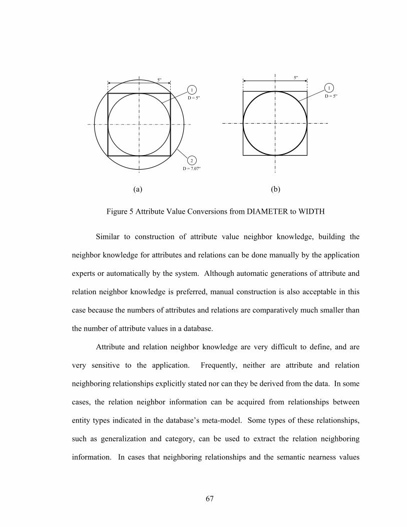
5′′
1
2
D = 5′′
D = 7.07′′
5′′
1
D = 5′′
(a) (b)
Figure 5 Attribute Value Conversions from DIAMETER to WIDTH
Similar to construction of attribute value neighbor knowledge, building the
neighbor knowledge for attributes and relations can be done manually by the application
experts or automatically by the system. Although automatic generations of attribute and
relation neighbor knowledge is preferred, manual construction is also acceptable in this
case because the numbers of attributes and relations are comparatively much smaller than
the number of attribute values in a database.
Attribute and relation neighbor knowledge are very difficult to define, and are
very sensitive to the application. Frequently, neither are attribute and relation
neighboring relationships explicitly stated nor can they be derived from the data. In some
cases, the relation neighbor information can be acquired from relationships between
entity types indicated in the database’s meta-model. Some types of these relationships,
such as generalization and category, can be used to extract the relation neighboring
information. In cases that neighboring relationships and the semantic nearness values
67
among attributes cannot be drawn directly from either the database’s extensional or
intentional data, developing of such knowledge must rely mainly on the application
domain experts.
4.3 Complex Query and Simultaneous Multiple Query Condition Relaxations
To facilitate query relaxation processes, many cooperative query answering
systems, such as CoBASE, develop neighbor hierarchies by applying their clustering
algorithms at the tuple level of each relation. If the information of an object (or concept)
is stored in several relations, the attributes of interest of the object are projected into a
view. Then, the neighbor hierarchy of the object is developed based upon the view. For
example, different airplane types are clustered to form a neighbor hierarchy of airplanes
based on an airplane view containing a set of attributes from several related relations.
Through those methods, only the specific combinations of relations, attributes, and
attribute values that exist when the neighbor hierarchy was developed can be relaxed. In
another words, query relaxations through the neighbor knowledge developed by those
techniques cannot be performed on the queries having their conditions defined on any
relations, attributes, or attribute values that do not exist in the view used to generate the
neighbor hierarchy (i.e. new data instances). Such types of neighbor knowledge work
well for sets of predetermined query structures. The system will fail to generate
approximate answers for any ad hoc queries that include relation, attributes, or attribute
values outside the scope of the predefined views.
68

In addition, most cooperative query answering systems are designed to handle
only single relation query relaxations. To overcome those limitations of the previous
query relaxation techniques, constructing neighbor hierarchies at the attribute level, and
relaxing each query condition separately are proposed in this paper. Developing
neighbor hierarchies for each attribute independently also enable query relaxations of
complex queries such as joint or nested queries.
To construct an attribute value neighbor hierarchy for every attribute, algorithms
used for value clustering must be effective and require low computational time. The
neighbor hierarchy construction techniques used in this paper, Modified DISC and
Modified PKI clustering algorithms, on average, only spend minutes to complete an
attribute value neighbor hierarchy (comparing to days or even months if it is done
manually). Therefore, it is feasible to create neighbor hierarchies for all attributes (that
are meant to be relaxed) in the database. In the following subsections, approaches for
relaxing complex queries are explained in detail.
4.3.1 Approach for Joint (or Nested) Query Relaxations
The differences between joint queries and single-relation queries are: the
conditions of joint queries are either selection conditions or joint conditions, whereas,
single-relation queries only use selection conditions, and joint queries can have selection
conditions for several relations. Because of those different characteristics of joint
queries, null answers could result from: 1) at least one of its relations has an empty
qualified tuple set, or 2) the intersection of the qualified tuple sets of the joined relations
69
is an empty set. Based on these facts, our approach used to find approximate answers for
a joint query is divided into six steps. First, the system needs to separate joint conditions
from selection conditions. Second, selection conditions are grouped by relation and
ordered alphabetically. Third, the system tests if the qualified tuple set of any relation is
empty. This is done by evaluating each selection condition individually, and together all
selection conditions of each relation as a group. If either a single condition or a group of
conditions of a relation is assessed as FALSE, the cause of null is “empty qualified tuple
set”. Fourth, the system performs attribute value, attribute and/or relation substitutions,
as stated in Section 4.1 , until the qualified tuple sets of all relations are not empty. Fifth,
the system uses the joint conditions to test whether the intersected qualified tuple sets are
empty. Sixth, if the intersected qualified tuple sets are empty, the system iteratively
performs, again, attribute value, attribute, and/or relation substitutions to expand the
qualified tuple set from each relation until approximate answers are returned.
4.4 Approach for Simultaneous Multiple Query Condition Relaxation
The main problem of simultaneous multiple query condition relaxation is the
number of combinations of relaxing selection conditions needed to consider at each query
relaxation iteration. By limiting query relaxations to a single condition only, the number
of relaxation possibilities is limited to the number of selection conditions in the query.
For example, relaxation of a query with four selection conditions, Q:A AND B AND C
AND D, can be done in four ways (altering either one of the four selection conditions).
However, if multiple selection condition relaxation is permitted, to relax the query Q, the
70

system has a total of 24 – 1 relaxation possibilities. The number of relaxation possibilities
becomes worse as the iteration number increases.
To solve this problem, a simultaneous multiple query condition relaxation
algorithm, called “Next Maximum Nearness Relaxation”, is proposed. The algorithm
utilizes a greedy searching method and the subsumption properties among relaxation
possibilities as the tool to reduce number of relaxation possibilities. Based on the greed
search approach, our query transformation techniques only allow substitutions of values
with their next closest neighbors, which is their higher adjacent neighbor nodes in the
hierarchies because the results from the modified PKI and DISC always are neighbor
hierarchies with monotonic nearness values. Using subsumption properties, relaxation
possibility A ∧ B ∧ C′ ∧ D subsumes all other relaxation possibilities that have C′ as a
component (relaxing the constants of condition C and one or more another condition with
their closest neighbor node). Since the other relaxation possibilities that have C′ as a
component always have the total nearness less than relaxing condition C only, those
relaxation possibilities can be disregarded from the consideration as long as C has not
been relaxed.
4.5 Approximate Answer Nearness Calculation
Without a means to calculate the semantic nearness between approximate answers
and the exact match answers, cooperative query answering for null answer will not be
complete. Many researchers have proposed various functions for nearness measures.
Each approach was developed for a specific application, and has some advantages and
71
shortcomings. As stated in Section 3.4 , semantic nearness can be determined either
before or after the query relaxation process. Also, mentioned in that section, semantic
proximity can be calculated by comparing either the exact-match answers with the
approximate answers or the original queries with the relaxed queries. Since increasing
the flexibility of query relaxation is one of the main themes of this research, computing
the nearness for partial answers by comparing the relaxed queries and the original query
after the query relaxation operation is adopted. To relax a query, the system first
rearranges the selection conditions of a query by their relations. Next, it groups the
selection conditions of the same relation together. Finally, the system uses the
relationships between the relations to determine if there are any dependencies among
those selection condition groups. After the query is relaxed and approximate answers are
obtained, the nearness between the original selection conditions and the transformed
conditions of each dependent group is computed. Finally, the nearness between the
relaxed query and the initial query is calculated by combining together the nearness
values of each dependent selection condition group.
In this paper, query relaxations can be accomplished through attribute value,
attribute, and/or relation substations. Each substitution may involve one or more query
condition. Therefore, to measure the semantic nearness between the original query and a
relaxed query, we defined “blocks” of query conditions. Before the query relaxation
operation, each block represents each condition of the original query. If a query
relaxation that involves several conditions is performed, those condition blocks are
merged together and form a new block that contains multiple query conditions. For an
72

m-condition query, when the relaxation operation is completed (the system obtains
approximate answers), there will be a certain number of condition blocks, k where k is
less than m. Then, the semantic nearness of the relaxed query is a function of the
summation of the nearness of those condition blocks. Nearness measuring functions that
take into account all query relaxation aspects presented in this research study are
provided in Chapter 7.0 .
73

5.0 NEIGHBORHOOD HIERARCHY DEVELOPMENT TOOLS
In order to provide cooperative answers, one needs to have some knowledge
relevant to the question topic. Similarly, a cooperative query answering system requires
additional information related to the query and the data in the database in order to derive
partial answers. Various types of knowledge must be added to the database to facilitate
different desired features of a cooperative query answering system. The scope of
cooperative query answering capabilities set by the system designers and developers
dictate what types of knowledge are required. For example, query relaxations for
approximate answers are achievable mainly by utilizing neighbor relationships of
attribute values, attributes, and relations. In addition, semantic distances among attribute
values, attributes, and relations are also essential if one wants to address the issues of
query relaxation optimization and/or semantic nearness calculation. These sets of
knowledge are the crucial parts for most cooperative query answering systems.
Various sets of knowledge are essential for the proposing cooperative query
answering techniques and partial answer nearness calculation algorithm. As mentioned
in Chapter4.0 , the neighbor hierarchies needed for our desired cooperative query
answering system can be developed both manually by the application domain experts and
automatically by some clustering techniques. Although neighbor hierarchies can be
created manually by application domain experts, automatic construction of neighbor
hierarchies by the system are preferred due to their complexities and time consuming
74
nature. Using automated neighbor hierarchy techniques, constructing and updating
hierarchies can be performed as often as necessary. This chapter provides the detailed
explanation of the automatic neighbor hierarchy development techniques used in this
paper. Two techniques adapted from previous clustering algorithms, Distribution
Sensitive Clustering (DISC)(90,91), and Pattern-based Knowledge Induction (PKI)(92), are
used in neighbor hierarchy constructions for attribute values. The PKI clustering
algorithm can be used to cluster both numeric and non-numeric attribute values, whereas
DISC algorithm can be used for numerical attribute values only. A PKI clustering
technique assumes that some inferential relationships among the clustered attribute values
and the values of the other attributes in the relation exist. Value information (unique
values and their occurrence frequencies) of at least two attributes is required to use the
PKI clustering algorithm. The DISC clustering technique does not require such an
assumption, and can be used to cluster attribute values of any single attribute with or
without the attribute value information from another attributes.
These attribute value (attribute and relation) neighbor knowledge are, by their
nature, very sensitive and can vary from one application to another application. With
such characteristics, it is very likely that a set of rules or neighboring relationships
developed for a particular application will need some modifications before it can be used
for another application. Since many users can utilize the same database (in many
different applications), different sets of knowledge may need to be developed
individually for each application. Application experts will be the ones who decide what
is applicable and what needs adjustments. The knowledge used in the query relaxation
75
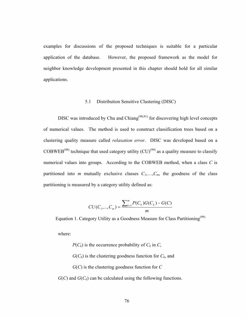
examples for discussions of the proposed techniques is suitable for a particular
application of the database. However, the proposed framework as the model for
neighbor knowledge development presented in this chapter should hold for all similar
applications.
5.1 Distribution Sensitive Clustering (DISC)
DISC was introduced by Chu and Chiang(90,91) for discovering high level concepts
of numerical values. The method is used to construct classification trees based on a
clustering quality measure called relaxation error. DISC was developed based on a
COBWEB(98) technique that used category utility (CU)(99) as a quality measure to classify
numerical values into groups. According to the COBWEB method, when a class C is
partitioned into m mutually exclusive classes C1,…,Cm, the goodness of the class
partitioning is measured by a category utility defined as:
mCGCGCP
CCCUm
k kkm
∑ =−
= 11
)()()(),...,(
Equation 1. Category Utility as a Goodness Measure for Class Partitioning(99)
where:
P(Ck) is the occurrence probability of Ck in C,
G(Ck) is the clustering goodness function for Ck, and
G(C) is the clustering goodness function for C
G(C) and G(Ck) can be calculated using the following functions.
76
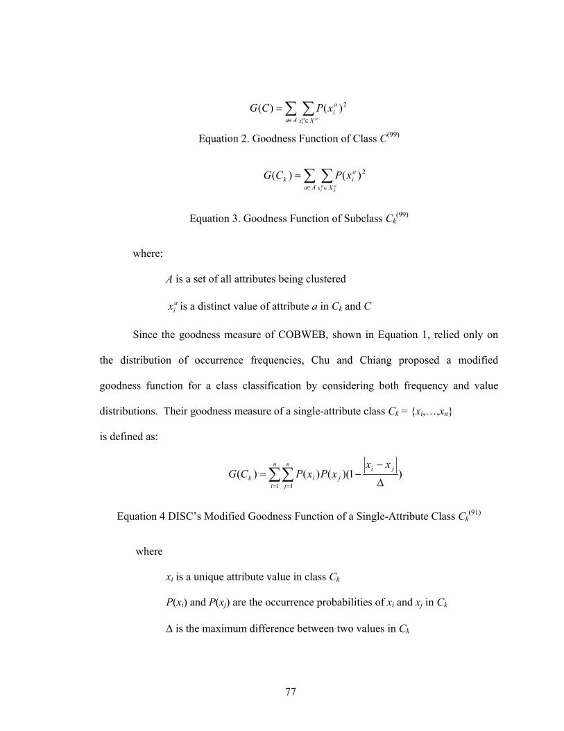
∑ ∑∈ ∈
=Aa Xx
ai
aai
xPCG 2)()(
Equation 2. Goodness Function of Class C(99)
∑ ∑∈ ∈
=Aa Xx
aik
ak
ai
xPCG 2)()(
Equation 3. Goodness Function of Subclass Ck(99)
where:
A is a set of all attributes being clustered
is a distinct value of attribute a in Caix k and C
Since the goodness measure of COBWEB, shown in Equation 1, relied only on
the distribution of occurrence frequencies, Chu and Chiang proposed a modified
goodness function for a class classification by considering both frequency and value
distributions. Their goodness measure of a single-attribute class Ck = {xi,…,xn}
is defined as:
)1)(()()(1 1 ∆
−−= ∑∑
= =
jin
i
n
jjik
xxxPxPCG
Equation 4 DISC’s Modified Goodness Function of a Single-Attribute Class Ck(91)
where
xi is a unique attribute value in class Ck
P(xi) and P(xj) are the occurrence probabilities of xi and xj in Ck
∆ is the maximum difference between two values in Ck
77
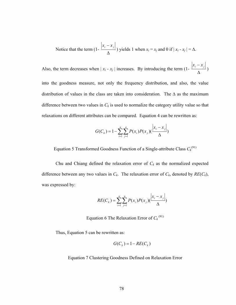
Notice that the term (1- ∆
− ji xx) yields 1 when xi = xj and 0 if | xi - xj | = ∆.
Also, the term decreases when | xi - xj | increases. By introducing the term (1- ∆
− ji xx)
into the goodness measure, not only the frequency distribution, and also, the value
distribution of values in the class are taken into consideration. The ∆ as the maximum
difference between two values in Ck is used to normalize the category utility value so that
relaxations on different attributes can be compared. Equation 4 can be rewritten as:
))(()(1)(1 1 ∆
−−= ∑∑
= =
jin
i
n
jjik
xxxPxPCG
Equation 5 Transformed Goodness Function of a Single-attribute Class Ck(91)
Chu and Chiang defined the relaxation error of Ck as the normalized expected
difference between any two values in Ck. The relaxation error of Ck, denoted by RE(Ck),
was expressed by:
∑∑= = ∆
−=
n
i
n
j
jijik
xxxPxPCRE
1 1))(()()(
Equation 6 The Relaxation Error of Ck (91)
Thus, Equation 5 can be rewritten as:
)(1)( kk CRECG −=
Equation 7 Clustering Goodness Defined on Relaxation Error
78
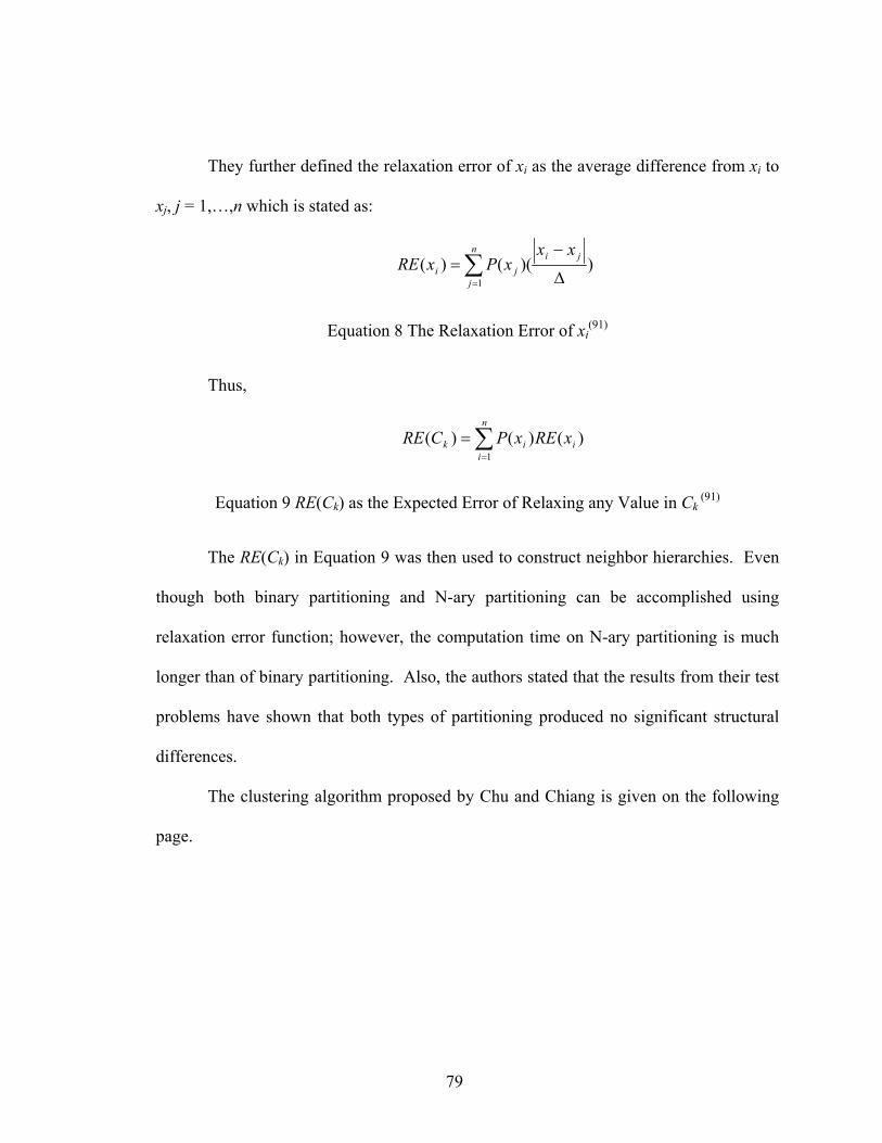
They further defined the relaxation error of xi as the average difference from xi to
xj, j = 1,…,n which is stated as:
∑= ∆
−=
n
j
jiji
xxxPxRE
1))(()(
Equation 8 The Relaxation Error of xi(91)
Thus,
∑=
=n
iiik xRExPCRE
1)()()(
Equation 9 RE(Ck) as the Expected Error of Relaxing any Value in Ck (91)
The RE(Ck) in Equation 9 was then used to construct neighbor hierarchies. Even
though both binary partitioning and N-ary partitioning can be accomplished using
relaxation error function; however, the computation time on N-ary partitioning is much
longer than of binary partitioning. Also, the authors stated that the results from their test
problems have shown that both types of partitioning produced no significant structural
differences.
The clustering algorithm proposed by Chu and Chiang is given on the following
page.
79
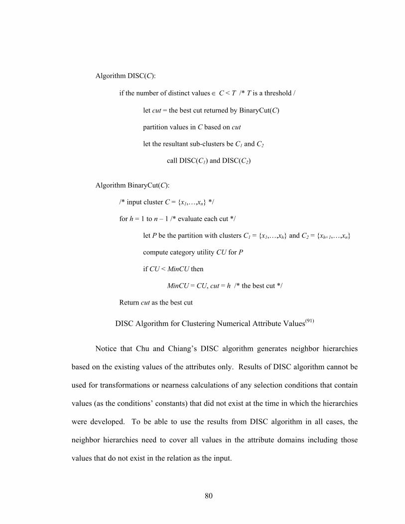
Algorithm DISC(C):
if the number of distinct values ∈ C < T /* T is a threshold /
let cut = the best cut returned by BinaryCut(C)
partition values in C based on cut
let the resultant sub-clusters be C1 and C2
call DISC(C1) and DISC(C2)
Algorithm BinaryCut(C):
/* input cluster C = {x1,…,xn} */
for h = 1 to n – 1 /* evaluate each cut */
let P be the partition with clusters C1 = {x1,…,xh} and C2 = {xh+1,…,xn}
compute category utility CU for P
if CU < MinCU then
MinCU = CU, cut = h /* the best cut */
Return cut as the best cut
DISC Algorithm for Clustering Numerical Attribute Values(91)
Notice that Chu and Chiang’s DISC algorithm generates neighbor hierarchies
based on the existing values of the attributes only. Results of DISC algorithm cannot be
used for transformations or nearness calculations of any selection conditions that contain
values (as the conditions’ constants) that did not exist at the time in which the hierarchies
were developed. To be able to use the results from DISC algorithm in all cases, the
neighbor hierarchies need to cover all values in the attribute domains including those
values that do not exist in the relation as the input.
80

To resolve the problem of neighbor hierarchies generated by DISC, a
modification to the algorithm is proposed in this paper. Since a neighbor cluster
produced by DISC is comprised of sequential numerical values, a range of values is used
to define a cluster instead of a set of values. To cover every value in the attribute
domain, the value range of each cluster starts at the mid-point between the cluster’s
lowest value and its preceding cluster’ highest value, and ends at the mid point between
the cluster’s highest value and its following cluster’ lowest value. For the first cluster,
which has the lowest existing value, the range starts from the lowest value covered by the
attribute domain. For the last cluster, the range ends at the highest value indicated by the
domain of the attribute.
Since the occurrence probabilities of non-existing values are zero based upon
DISC’s definition, adding those attribute values to the neighbor clusters produced by
DISC algorithm does not affect the overall goodness of the neighbor hierarchy.
However, it allows the hierarchy to cover the entire domain of the attribute. As a result,
relaxing query conditions having attribute values that did not exist at the time the
hierarchy was developed as their constants is possible.
An algorithm for modifying neighbor hierarchies generated by DISC is provided
on the following page.
81
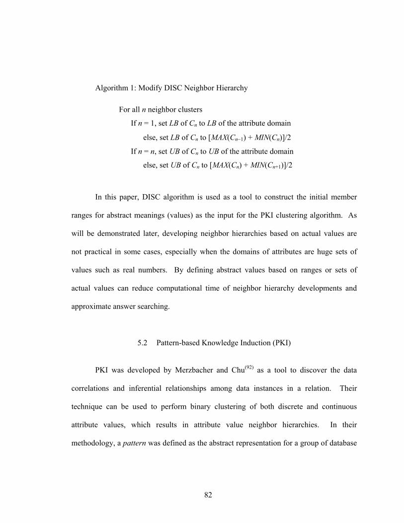
Algorithm 1: Modify DISC Neighbor Hierarchy
For all n neighbor clusters
If n = 1, set LB of Cn to LB of the attribute domain
else, set LB of Cn to [MAX(Cn−1) + MIN(Cn)]/2
If n = n, set UB of Cn to UB of the attribute domain
else, set UB of Cn to [MAX(Cn) + MIN(Cn+1)]/2
In this paper, DISC algorithm is used as a tool to construct the initial member
ranges for abstract meanings (values) as the input for the PKI clustering algorithm. As
will be demonstrated later, developing neighbor hierarchies based on actual values are
not practical in some cases, especially when the domains of attributes are huge sets of
values such as real numbers. By defining abstract values based on ranges or sets of
actual values can reduce computational time of neighbor hierarchy developments and
approximate answer searching.
5.2 Pattern-based Knowledge Induction (PKI)
PKI was developed by Merzbacher and Chu(92) as a tool to discover the data
correlations and inferential relationships among data instances in a relation. Their
technique can be used to perform binary clustering of both discrete and continuous
attribute values, which results in attribute value neighbor hierarchies. In their
methodology, a pattern was defined as the abstract representation for a group of database
82
instances with a specified property. A pattern is expressed by an atomic query condition.
The formal representation of a pattern P is:
PC = P : D → T (92)
where:
C is an atomic query condition that expresses P
D is the domain of a relation
T is a set of tuples that satisfies the condition C
For example, in relation ALUM_PLATE shown in Figure 6 on page 86, PWIDTH = 3
refers to 3 tuples, and PLENGTH = 144 refers to 7 tuples. From the fact that a data instance
can be a member of more than one abstract pattern class (i.e. parts with stock number of
308-0013 and 308-0019 are members of both PWIDTH = 3 and PLENGTH = 144), an inferential
relationship between patterns can be defined based on the subsumption property of one
pattern to another as in the following:
An inferential relationship between two patterns A and B, represented by
A → B, indicating that when A is true, B also holds. A is the premise and
B is the consequence of the relationship.(92)
Rule: Subsumption Property between Two Patterns
For example, from the ALUM_PLATE table as shown in Table 2, the data
indicates that all of the aluminum plates having WIDTH = 3 have length = 144.
Therefore, we can conclude that:
PWIDTH = 3 → PLENGTH = 144.
83
The usefulness of an inferential relationship is measured by the “confidence” and
“popularity” of the relationship. The inferential confidence is defined based on the
cardinalities of the patterns. The cardinalities of patterns A and B are denoted by |PA| and
|PB|, and are defined as the numbers of distinct data instances matching the conditions of
patterns A and B, respectively.
The cardinality of pattern PWIDTH = 3 and PLENGTH = 114 from Equation 10 are:
|PWIDTH = 3| = 3
|PLENGTH = 144| = 7
The inferential confidence of the inferential relationship A→ B is defined as:
A
BA
PPP
BAI
=→ )(ξ
Equation 10 Inferential Confidence of an Inferential Relationship(92)
84
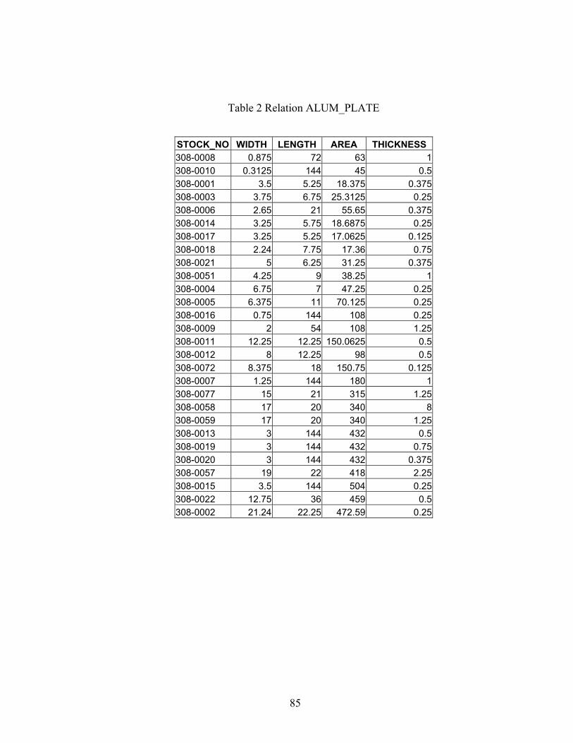
Table 2 Relation ALUM_PLATE
STOCK_NO WIDTH LENGTH AREA THICKNESS 308-0008 0.875 72 63 1 308-0010 0.3125 144 45 0.5 308-0001 3.5 5.25 18.375 0.375 308-0003 3.75 6.75 25.3125 0.25 308-0006 2.65 21 55.65 0.375 308-0014 3.25 5.75 18.6875 0.25 308-0017 3.25 5.25 17.0625 0.125 308-0018 2.24 7.75 17.36 0.75 308-0021 5 6.25 31.25 0.375 308-0051 4.25 9 38.25 1 308-0004 6.75 7 47.25 0.25 308-0005 6.375 11 70.125 0.25 308-0016 0.75 144 108 0.25 308-0009 2 54 108 1.25 308-0011 12.25 12.25 150.0625 0.5 308-0012 8 12.25 98 0.5 308-0072 8.375 18 150.75 0.125 308-0007 1.25 144 180 1 308-0077 15 21 315 1.25 308-0058 17 20 340 8 308-0059 17 20 340 1.25 308-0013 3 144 432 0.5 308-0019 3 144 432 0.75 308-0020 3 144 432 0.375 308-0057 19 22 418 2.25 308-0015 3.5 144 504 0.25 308-0022 12.75 36 459 0.5 308-0002 21.24 22.25 472.59 0.25
85
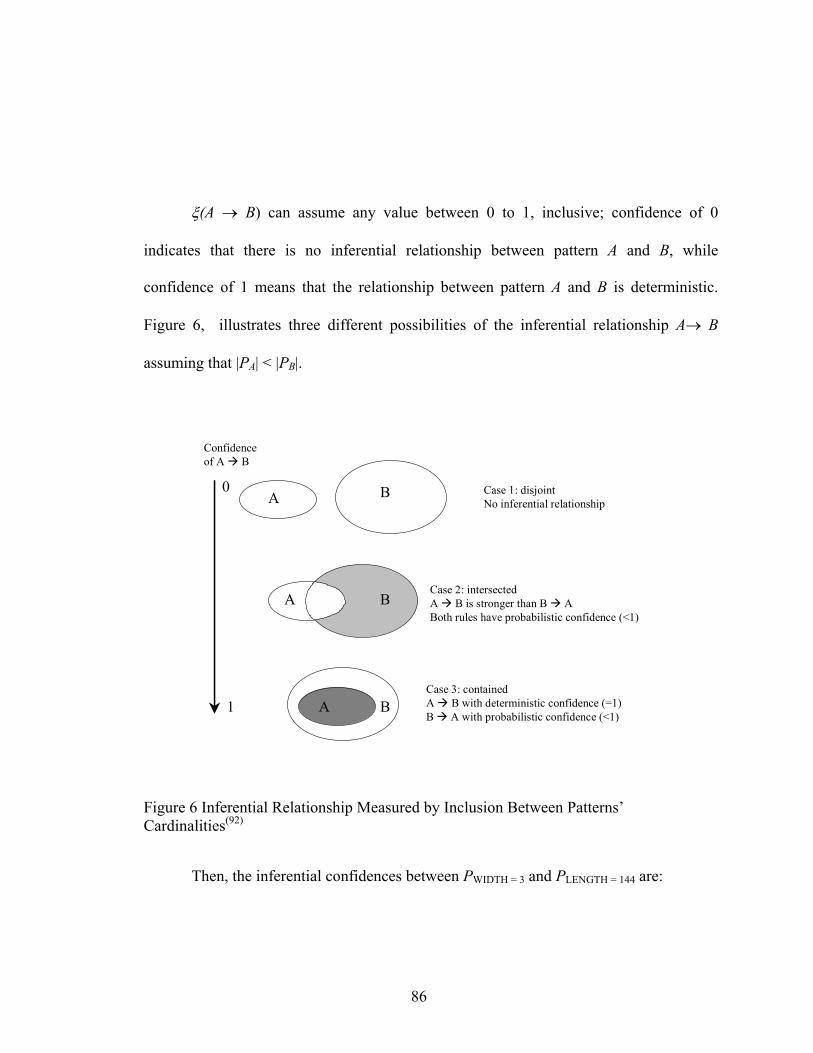
ξ(A → B) can assume any value between 0 to 1, inclusive; confidence of 0
indicates that there is no inferential relationship between pattern A and B, while
confidence of 1 means that the relationship between pattern A and B is deterministic.
Figure 6, illustrates three different possibilities of the inferential relationship A→ B
assuming that |PA| < |PB|.
A B
A B
A B
Case 1: disjointNo inferential relationship
Case 2: intersectedA B is stronger than B ABoth rules have probabilistic confidence (<1)
Case 3: containedA B with deterministic confidence (=1)B A with probabilistic confidence (<1)
Confidenceof A B
0
1
Figure 6 Inferential Relationship Measured by Inclusion Between Patterns’ Cardinalities(92)
Then, the inferential confidences between PWIDTH = 3 and PLENGTH = 144 are:
86
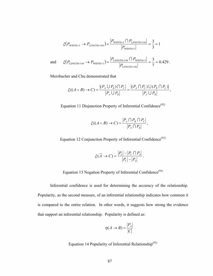
( ) 133
3WIDTH
144LENGTH3WIDTH144LENGTH3WIDTH ===→
=
==== P
PPPP
Iξ
and ( ) 429.073
144LENGTH
3WIDTH144LENGTH3WIDTH144LENGTH ===→
=
==== P
PPPP
Iξ .
Merzbacher and Chu demonstrated that
BA
CBCA
BA
CBA
PPPPPP
PPPPP
CBAU
IUI
U
IU )()()())(( ==→∨ξ ,
Equation 11 Disjunction Property of Inferential Confidence(92)
BA
CBA
PPPPP
CBAI
II=→∧ ))((ξ ,
Equation 12 Conjunction Property of Inferential Confidence(92)
AC
ACC
PPPPP
CA−
−=→
I)(ξ .
Equation 13 Negation Property of Inferential Confidence(92)
Inferential confidence is used for determining the accuracy of the relationship.
Popularity, as the second measure, of an inferential relationship indicates how common it
is compared to the entire relation. In other words, it suggests how strong the evidence
that support an inferential relationship. Popularity is defined as:
CP
BA A=→ )(η
Equation 14 Popularity of Inferential Relationship(92)
87
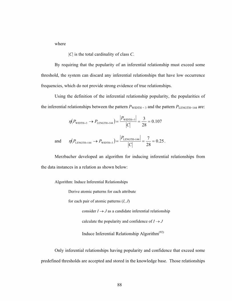
where
|C| is the total cardinality of class C.
By requiring that the popularity of an inferential relationship must exceed some
threshold, the system can discard any inferential relationships that have low occurrence
frequencies, which do not provide strong evidence of true relationships.
Using the definition of the inferential relationship popularity, the popularities of
the inferential relationships between the pattern PWIDTH = 3 and the pattern PLENGTH=144 are:
( ) 107.02833WIDTH
144LENGTH3WIDTH ===→ === C
PPPη
and ( ) 25.0287144LENGTH
3WIDTH144LENGTH ===→ === C
PPPη .
Merzbacher developed an algorithm for inducing inferential relationships from
the data instances in a relation as shown below:
Algorithm: Induce Inferential Relationships
Derive atomic patterns for each attribute
for each pair of atomic patterns (I, J)
consider I → J as a candidate inferential relationship
calculate the popularity and confidence of I → J
Induce Inferential Relationship Algorithm(92)
Only inferential relationships having popularity and confidence that exceed some
predefined thresholds are accepted and stored in the knowledge base. Those relationships
88
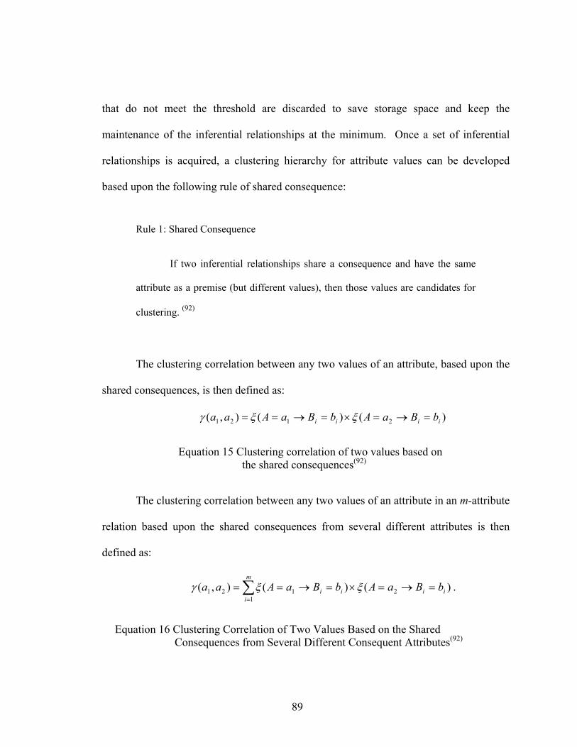
that do not meet the threshold are discarded to save storage space and keep the
maintenance of the inferential relationships at the minimum. Once a set of inferential
relationships is acquired, a clustering hierarchy for attribute values can be developed
based upon the following rule of shared consequence:
Rule 1: Shared Consequence
If two inferential relationships share a consequence and have the same
attribute as a premise (but different values), then those values are candidates for
clustering. (92)
The clustering correlation between any two values of an attribute, based upon the
shared consequences, is then defined as:
)()(),( 2121 iiii bBaAbBaAaa =→=×=→== ξξγ
Equation 15 Clustering correlation of two values based on the shared consequences(92)
The clustering correlation between any two values of an attribute in an m-attribute
relation based upon the shared consequences from several different attributes is then
defined as:
∑=
=→=×=→==m
iiiii bBaAbBaAaa
12121 )()(),( ξξγ .
Equation 16 Clustering Correlation of Two Values Based on the Shared Consequences from Several Different Consequent Attributes(92)
89

From the fact that the maximum value of the clustering correlation formula is
m – 1, the normalized clustering correlation is:
),(1
1),( 2121 aam
aa γγ−
=
Equation 17 Normalized Clustering Correlation of Two Values(92)
Using the developed normalized clustering correlation values, Merzbacher
proposed a clustering algorithm based upon a greedy algorithm as follows:
Algorithm 2: Binary Cluster(92)
repeat
induce inferential relationships and determine γ
sort γ in descending order
for each ), ji aa(γ over a threshold T
if a and are not yet clustered i ja
cluster a and ja i
replace a and ja in DB with Ji i,j having a nearness of ),( ji aaγ until fully
clustered
The following example demonstrates how the Binary Cluster algorithm works.
Figure 9 on page 95 illustrates a neighbor hierarchy of data instances in the
ALUM_PLATE relation resulted from the Binary Cluster algorithm.
Example 1 Neighbor hierarchy of aluminum plates
In this example, a Binary Cluster algorithm is executed in order to construct a
neighbor hierarchy of the aluminum plates based on attribute STOCK_NO.
90
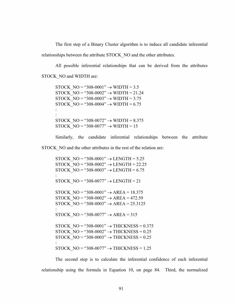
The first step of a Binary Cluster algorithm is to induce all candidate inferential
relationships between the attribute STOCK_NO and the other attributes.
All possible inferential relationships that can be derived from the attributes
STOCK_NO and WIDTH are:
STOCK_NO = “308-0001” → WIDTH = 3.5 STOCK_NO = “308-0002” → WIDTH = 21.24 STOCK_NO = “308-0003” → WIDTH = 3.75 STOCK_NO = “308-0004” → WIDTH = 6.75 : : STOCK_NO = “308-0072” → WIDTH = 8.375 STOCK_NO = “308-0077” → WIDTH = 15
Similarly, the candidate inferential relationships between the attribute
STOCK_NO and the other attributes in the rest of the relation are:
STOCK_NO = “308-0001” → LENGTH = 5.25 STOCK_NO = “308-0002” → LENGTH = 22.25 STOCK_NO = “308-0003” → LENGTH = 6.75 : STOCK_NO = “308-0077” → LENGTH = 21
STOCK_NO = “308-0001” → AREA = 18.375 STOCK_NO = “308-0002” → AREA = 472.59 STOCK_NO = “308-0003” → AREA = 25.3125 : STOCK_NO = “308-0077” → AREA = 315
STOCK_NO = “308-0001” → THICKNESS = 0.375 STOCK_NO = “308-0002” → THICKNESS = 0.25 STOCK_NO = “308-0003” → THICKNESS = 0.25 : STOCK_NO = “308-0077” → THICKNESS = 1.25
The second step is to calculate the inferential confidence of each inferential
relationship using the formula in Equation 10, on page 84. Third, the normalized
91
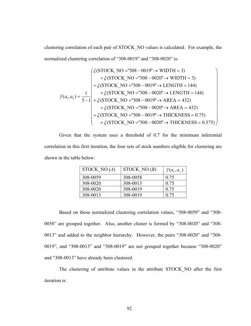
clustering correlation of each pair of STOCK_NO values is calculated. For example, the
normalized clustering correlation of “308-0019” and “308-0020” is:
=→−=×=→−=+
=→−=×=→−=+
=→−=×=→−=+
=→−=×=→−=
−=
)375.0THICKNESS"0020308"STOCK_NO( )75.0THICKNESS"0019308"STOCK_NO(
)432AREA"0020308"STOCK_NO( )432AREA"0019308"STOCK_NO(
)144LENGTH"0020308"STOCK_NO( )144LENGTH"0019308"STOCK_NO()3WIDTH"0020308"STOCK_NO(
)3WIDTH"0019308"STOCK_NO(
151),( 21
ξξ
ξξ
ξξ
ξξ
γ aa
Given that the system uses a threshold of 0.7 for the minimum inferential
correlation in this first iteration, the four sets of stock numbers eligible for clustering are
shown in the table below:
STOCK_NO (A) STOCK_NO (B) ),( ji aaγ 308-0059 308-0058 0.75 308-0020 308-0013 0.75 308-0020 308-0019 0.75 308-0013 308-0019 0.75
Based on those normalized clustering correlation values, “308-0059” and “308-
0058” are grouped together. Also, another cluster is formed by “308-0020” and “308-
0013” and added to the neighbor hierarchy. However, the pairs “308-0020” and “308-
0019”, and “308-0013” and “308-0019” are not grouped together because “308-0020”
and “308-0013” have already been clustered.
The clustering of attribute values in the attribute STOCK_NO after the first
iteration is:
92
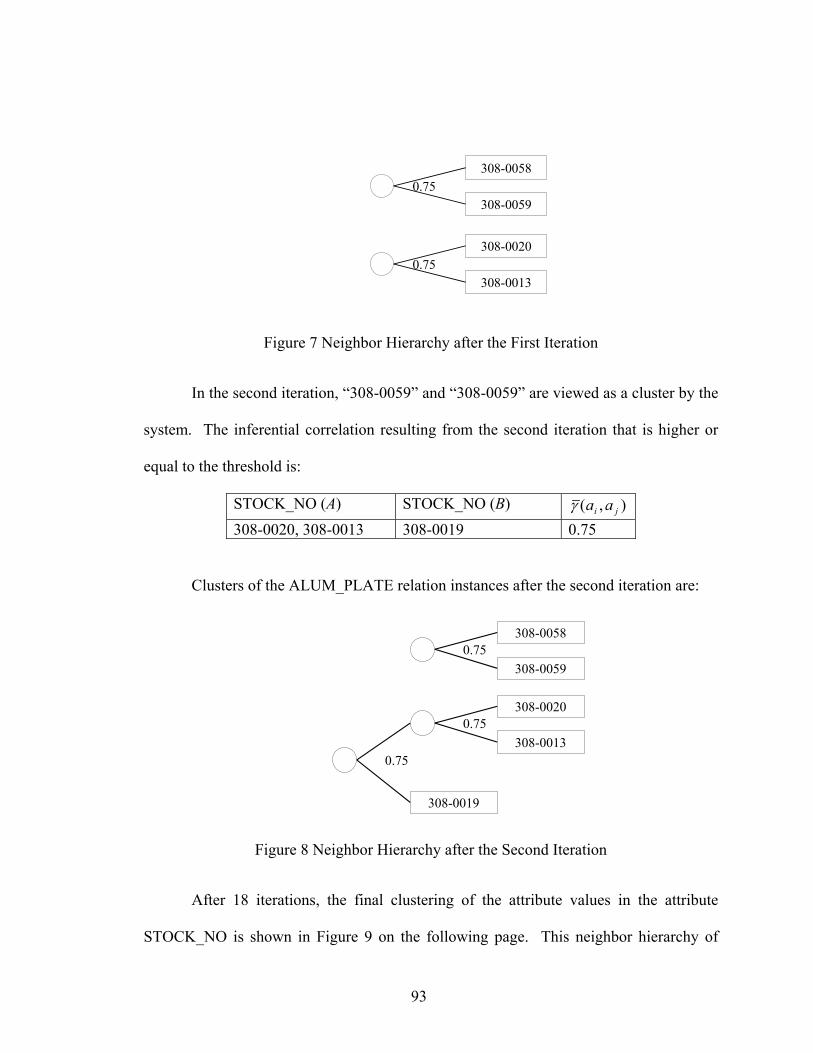
308-0058
308-00590.75
308-0020
308-00130.75
Figure 7 Neighbor Hierarchy after the First Iteration
In the second iteration, “308-0059” and “308-0059” are viewed as a cluster by the
system. The inferential correlation resulting from the second iteration that is higher or
equal to the threshold is:
STOCK_NO (A) STOCK_NO (B) ),( ji aaγ 308-0020, 308-0013 308-0019 0.75
Clusters of the ALUM_PLATE relation instances after the second iteration are:
308-0058
308-00590.75
308-0020
308-00130.75
308-0019
0.75
Figure 8 Neighbor Hierarchy after the Second Iteration
After 18 iterations, the final clustering of the attribute values in the attribute
STOCK_NO is shown in Figure 9 on the following page. This neighbor hierarchy of
93

tuples in the relation ALUM_PLATE can be used to determine the semantic nearness
between tuples. For any two attribute values in the neighbor hierarchy, the nearness
between the two values is the maximum nearness value of the neighbor nodes that cover
both of them. For example, the nearness between the aluminum plate with the stock
number of 308-0022 and 308-0020 is 0.071.
94
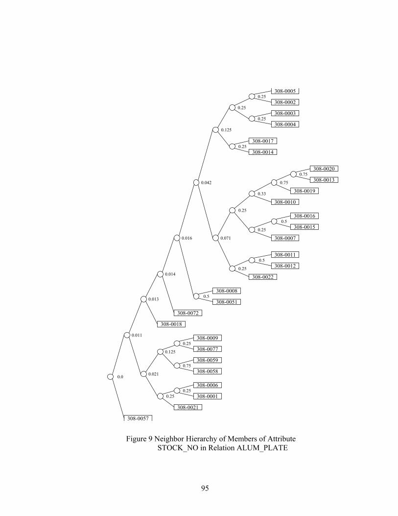
308-0072
308-0057
308-0020
308-0019
308-0018
308-0013
308-0010
308-0005
308-00020.25
0.75
0.071
0.25
0.33
0.75
308-0016
308-0007
308-00150.5
0.25
308-0011
308-0022
308-00120.5
0.25
308-0003
308-00040.25
0.042
0.25
308-0017
308-00140.25
0.125
308-0006
308-0021
308-00010.25
0.25
308-0008
308-00510.5
308-0009
308-00770.25
308-0059
308-00580.75
0.125
0.021
0.016
0.014
0.013
0.011
0.0
Figure 9 Neighbor Hierarchy of Members of Attribute STOCK_NO in Relation ALUM_PLATE
95
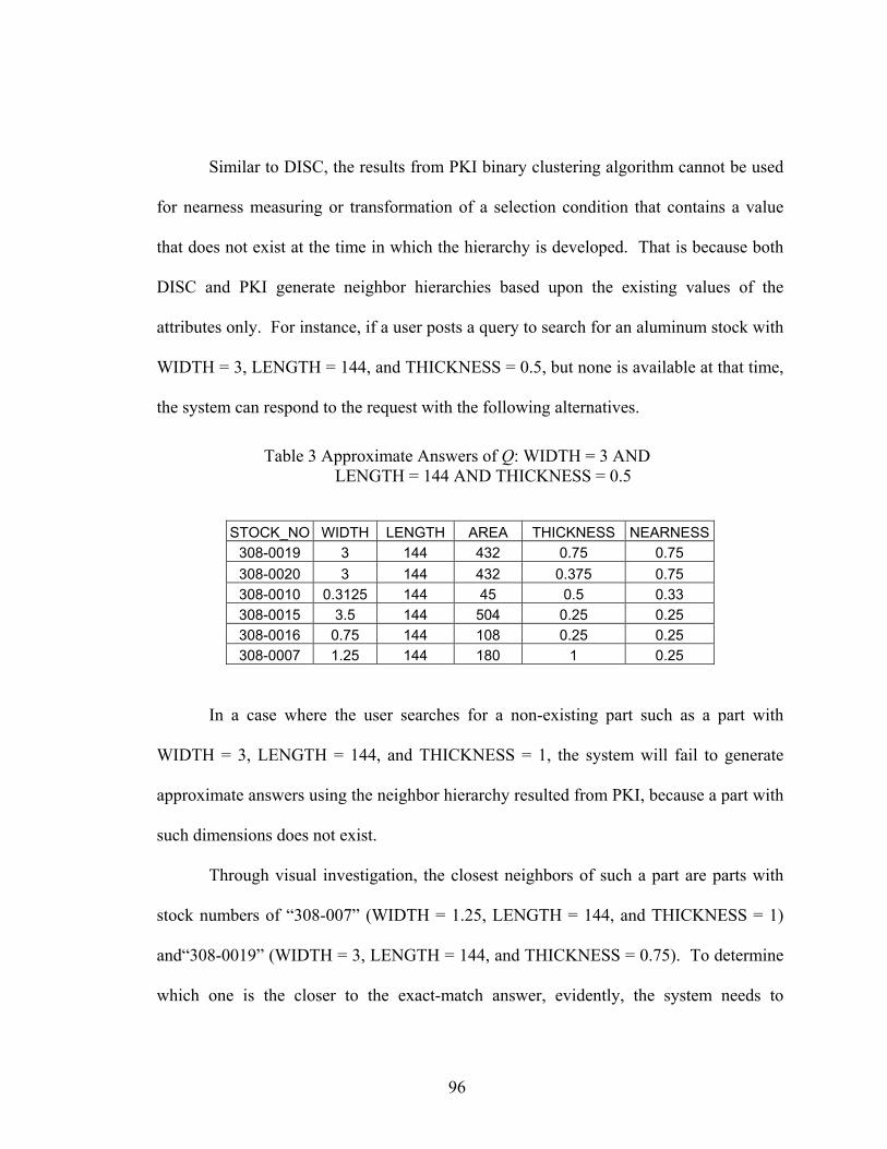
Similar to DISC, the results from PKI binary clustering algorithm cannot be used
for nearness measuring or transformation of a selection condition that contains a value
that does not exist at the time in which the hierarchy is developed. That is because both
DISC and PKI generate neighbor hierarchies based upon the existing values of the
attributes only. For instance, if a user posts a query to search for an aluminum stock with
WIDTH = 3, LENGTH = 144, and THICKNESS = 0.5, but none is available at that time,
the system can respond to the request with the following alternatives.
Table 3 Approximate Answers of Q: WIDTH = 3 AND LENGTH = 144 AND THICKNESS = 0.5
STOCK_NO WIDTH LENGTH AREA THICKNESS NEARNESS 308-0019 3 144 432 0.75 0.75 308-0020 3 144 432 0.375 0.75 308-0010 0.3125 144 45 0.5 0.33 308-0015 3.5 144 504 0.25 0.25 308-0016 0.75 144 108 0.25 0.25 308-0007 1.25 144 180 1 0.25
In a case where the user searches for a non-existing part such as a part with
WIDTH = 3, LENGTH = 144, and THICKNESS = 1, the system will fail to generate
approximate answers using the neighbor hierarchy resulted from PKI, because a part with
such dimensions does not exist.
Through visual investigation, the closest neighbors of such a part are parts with
stock numbers of “308-007” (WIDTH = 1.25, LENGTH = 144, and THICKNESS = 1)
and“308-0019” (WIDTH = 3, LENGTH = 144, and THICKNESS = 0.75). To determine
which one is the closer to the exact-match answer, evidently, the system needs to
96

compare the semantic nearness between WIDTH = 3 and WIDTH = 1.25, and
THICKNESS = 1 and THICKNESS = 0.75.
From this example, to relax a query, constructing neighbor hierarchies at the
“attribute level” is adopted in this paper instead of at the tuple level as suggested by
Merzbacher and Chu. Query relaxation algorithms and nearness calculation based on the
nearness value of each attribute in the query are explained in greater detail in Chapter 6.0
and 7.0 , respectively.
To develop neighbor hierarchies at the attribute level, the pattern correlation
functions used in PKI clustering algorithm need to be modified. PKI was developed for
clustering relation instances at the tuple level using the induced inferential relationships
between the values of the key attribute, and the values in the other attributes of the
relation. Because of the uniqueness property of the key attribute, each clustering attribute
value matches up with one and only one value from another attribute in the relation.
However, mapping between values from a non-unique attribute to another non-unique
attribute could result in one-to-many relationships. For example, an attribute value 144 of
the attribute LENGTH is mapped to 5 values (0.25, 0.375, 0.5, 0.75,1) of the attribute
THICKNESS. To develop a neighbor hierarchy of a non-unique attribute, we proposed
to generalize the rule of shared consequence proposed by Merzbacher and Chu must be
generalized so that it can be applied on any attribute in the relation. The Modified Shared
Consequence Rule is given below.
97
Rule 2: Modified Shared Consequence
If two inferential relationships share the same “set of
consequences” (same set of values from an attribute) and have the
same attribute as a premise (but different values), then those values
are candidates for clustering.
The clustering correlation function proposed by Merzbacher and Chu, as shown in
Equation 15 on page 89, is only applicable if the attribute A as the premise of the
inferential relationship is a unique attribute. The clustering correlation between two
attribute values for the modified rule of shared consequence is:
∑=
=→=×=→==′n
jjj bBaAbBaAaa
12121 )()(),( ξξγ
Equation 18 Clustering Correlation of Two Values Based on the Modified Shared Consequences
Where:
bj is a unique value in attribute B.
The clustering correlation function for any two values based on the shared
consequences from several different consequent attributes, shown in Equation 16, is also
modified to:
∑∑= =
=→=×=→==′m
i
n
jjiji bBaAbBaAaa
1 12121 )()(),( ξξγ
Equation 19 Clustering Correlation of Two Values Based on the Modified Shared Consequences from Several Different Consequent Attributes
98
Notice that:
0)()( 21 ==→=×=→= jiji bBaAbBaA ξξ
when Bi is a unique attribute because A = a1 and A = a2 can never have the same
consequence Bi = bj. Therefore, the maximum value of γ (a1, a2) is m – 2 (instead of m –
1) when A is not the key attribute. The normalized clustering correlation for a non-
unique attribute in an m-attribute relation, modified from Equation 17, on page 90, is:
),(2
1),( 2121 aam
aa γγ ′−
=′
Equation 20 Normalized Clustering Correlation Of Two Values of a Non-key Attribute
These modified clustering correlation and modified normalized clustering
correlation functions are then combined with the binary clustering algorithm to generate
attribute value neighbor hierarchies. A neighbor hierarchy of the attribute WIDTH in the
relation ALUM_PLATE acquired through the modified PKI is shown in Figure 10 on
page 100.
99
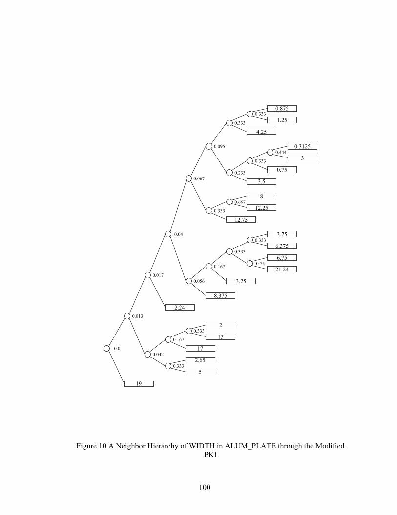
0.875
4.25
1.250.333
0.333
0.3125
0.75
3
3.5
0.444
0.233
0.333
8
12.75
12.250.667
0.333
3.75
6.3750.333
6.75
21.240.75
0.333
3.25
8.375
0.167
0.056
2
17
150.333
0.167
2.65
50.333
0.013
0.04
0.067
0.095
0.00.042
0.017
2.24
19
Figure 10 A Neighbor Hierarchy of WIDTH in ALUM_PLATE through the Modified PKI
100

To resolve the non-existing value problem, a neighbor hierarchy must cover the
entire domain of the attribute. Therefore, a set of attribute abstract values defined on the
exclusive ranges of attribute values must be developed. Each defined attribute abstract
value should represent a unique application meaning of all actual values contained in its
range. Once the set of attribute abstract values is developed they can be used to refer to a
set, or a range, of the actual values. These attribute abstract values are then used as the
input for the modified PKI clustering algorithm instead of the actual attribute values.
Using attribute abstract values are better than the actual values when the differences
between the actual values do not really represent any true differences for the application.
For example, final exam scores of 95.00 to 100.00 could indicate that the student will
receive an A as the final grade, while the scores of 85.00 to 94.99 imply that the student
will receive a B. In a case where the letter grades are the only meaningful information
that the database users are interested in, a set of attribute abstract values can be described
as {“A”, “B”, “C”, “D”, “F”}. Defining attribute abstract values not only allow the
developer to cover the entire attribute domain, but can also help reduce computational
time for neighbor hierarchy construction when the domain set is very large, or is defined
on continuous numeric values. Clearly, the attribute abstract values are sensitive to the
application domain. Defining ranges of the actual values for attribute abstract values
relies mainly on the application domain expert. As stated earlier, the approach for
developing the initial set of abstract values taken in this paper is to use the results from
DISC clustering algorithm. Once abstract ranges (or sets) are developed, the frequency of
the actual values can be projected onto their abstract ranges. Then, the abstract values
101

and their projected occurrence frequencies are used as the input for the PKI clustering
algorithm.
For example, based upon the experience of application domain experts, the width
of aluminum plates can be classified into six major groups: “bar”, “strip”, “narrow”,
“standard”, “wide”, and “special cut”. The ranges of actual widths defined for these
width groups are delineated in Table 4 below:
Table 4 Abstract Value Ranges of Attribute WIDTH in Relation ALUM_PLATE
Abstract Value Abstract Meaning Lower Bound Upper Bound w1 Bar 0.000 1.999 w2 Strip 2.000 3.999 w3 Narrow 4.000 5.999 w4 Standard 6.000 7.999 w5 Wide 8.000 19.999 w6 Special Cut 20.000 24.000
Once the attribute abstract values and their ranges or member sets are defined,
each actual value’s frequency can be projected into its abstract value. A neighbor
hierarchy of attribute WIDTH generated by the proposing PKI using the attribute abstract
values is given in Figure 11. The abstract ranges for the attribute AREA are shown in
Table 5, and a neighbor hierarchy for the attribute AREA is shown in Figure 12.
102
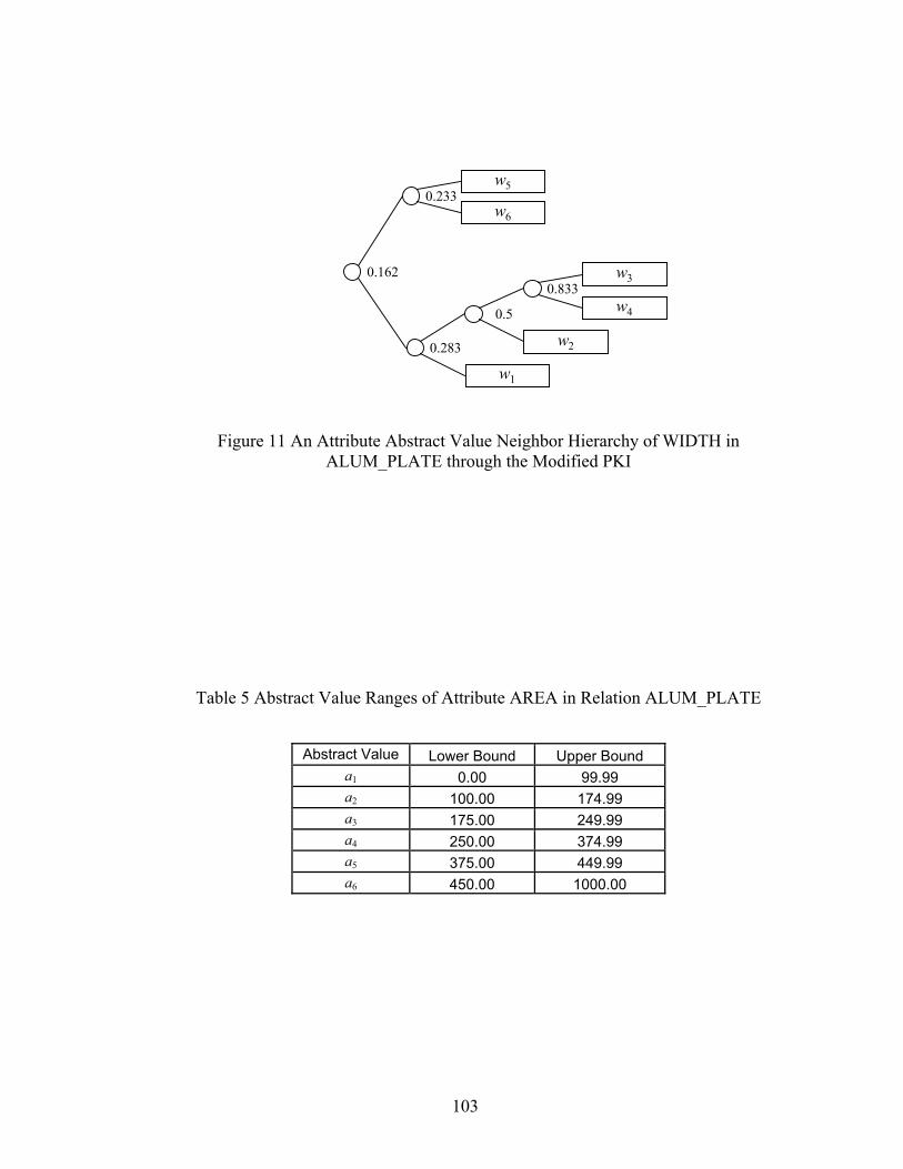
w3
w2
w4
w1
0.833
0.283
0.5
w5
w6
0.233
0.162
Figure 11 An Attribute Abstract Value Neighbor Hierarchy of WIDTH in ALUM_PLATE through the Modified PKI
Table 5 Abstract Value Ranges of Attribute AREA in Relation ALUM_PLATE
Abstract Value Lower Bound Upper Bound a1 0.00 99.99 a2 100.00 174.99 a3 175.00 249.99 a4 250.00 374.99 a5 375.00 449.99 a6 450.00 1000.00
103
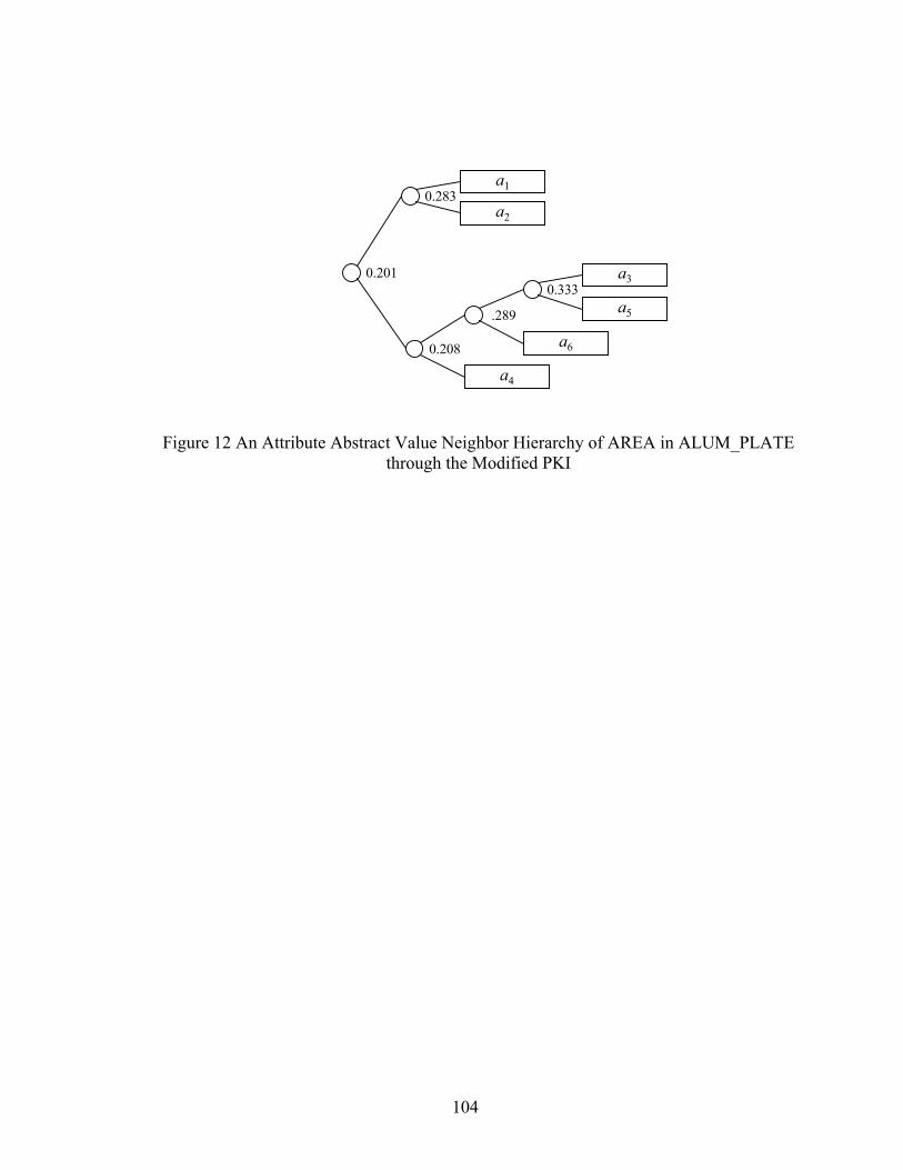
a3
a6
a5
a4
0.333
0.208
.289
a1
a2
0.283
0.201
Figure 12 An Attribute Abstract Value Neighbor Hierarchy of AREA in ALUM_PLATE through the Modified PKI
104
6.0 QUERY RELAXATION
To find approximate answers for over-specified queries, a corporative query
answering system needs to expand the answer space of the query. This can be achieved
by transforming the query into a set of less constrained queries through a process called
query relaxation. Query relaxations can be done accomplished by either or both 1)
dropping the null-bound query conditions and 2) replacing the over-specified conditions
with more relaxing ones. Although dropping the null-bound conditions of a query is
easier to do, the system could lose much of the information conveyed in the query. The
latter approach preserves more information that the user implies in the query.
Relaxing a query can be done at three levels: attribute value, attribute, and
relation level. To obtain a set of relaxed queries, the system utilizes the application
domain knowledge and applies appropriate query transformation algorithms . Various
sets of application domain knowledge can be developed using the techniques described in
Chapter 5.0 .
In this research, query relaxations are done in three major steps. First, the system
rearranges the conditions of the query to prepare the query for relaxation operations.
Rearranging query conditions help improve system computational time. In this step,
selection conditions and joint conditions are separated. Next, the system determines the
causes of null answers. Finally, the system performs the appropriate query condition
relaxation for each cause of null.
This chapter describes the proposed query relaxation techniques for acquiring
approximate answers. Also, this chapter provides a detailed explanation of how to apply
105
the application domain knowledge in query relaxation. An assumption presumed
throughout this chapter is: in searching for partial answers, only the selection conditions
whose attributes’ domains are numeric values or sets of structured text are used in
queries. Free text attributes that are used to store comments or notes about the tuples are
outside the scope of this research. This is because assigning the nearness values between
free text entries requires totally different clustering and relaxation techniques such as
document searching or word thesaurus, which have already been addressed by many
other researchers.
6.1 Rearranging Query Conditions
Typically, all queries expressed through SQL are in the SELECT-FROM-
WHERE structure, with the WHERE block being optional. The WHERE block consists
of query conditions connected with the operators AND. Users have the flexibility of
constructing the WHERE blocks by putting the desired query conditions in any order.
However, to be able to relax a query more systematically and effectively, the query
conditions must be rearranged before query relaxations are performed. Also, as will be
explained in a later section of this chapter and in the next chapter, the proposed query
relaxations through attribute value, attribute, and/or relation substitutions (and also how
semantic proximity calculations are performed and determining causes of null answer)
rely mainly on the relationships between query selection conditions and their relations.
The proposed cooperative query answering system performs relaxations of
selections and joint conditions at different times and require different relaxation methods.
106
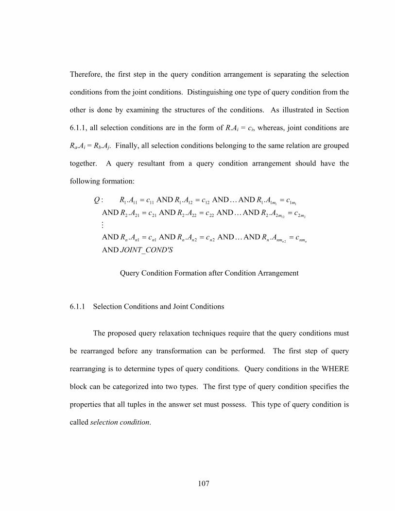
Therefore, the first step in the query condition arrangement is separating the selection
conditions from the joint conditions. Distinguishing one type of query condition from the
other is done by examining the structures of the conditions. As illustrated in Section
6.1.1, all selection conditions are in the form of R.Ai = ci, whereas, joint conditions are
Ra.Ai = Rb.Aj. Finally, all selection conditions belonging to the same relation are grouped
together. A query resultant from a query condition arrangement should have the
following formation:
D'S JOINT_CON
cARcARcAR
cARcARcAR
cARcARcARQ
nn nmnmnnnnnnn
mm
mm
AND
. AND AND . AND . AND
. AND AND . AND . AND
. AND AND . AND . :
2
212
11
2211
2222222221212
1111212111111
===
===
===
K
M
K
K
Query Condition Formation after Condition Arrangement
6.1.1 Selection Conditions and Joint Conditions
The proposed query relaxation techniques require that the query conditions must
be rearranged before any transformation can be performed. The first step of query
rearranging is to determine types of query conditions. Query conditions in the WHERE
block can be categorized into two types. The first type of query condition specifies the
properties that all tuples in the answer set must possess. This type of query condition is
called selection condition.
107
A selection condition can be expressed as
Ra.Ai = ci
Where:
Ra is a relation
Ai is an attribute of Ra
Ci is a constant.
When a query involves with only one relation, a shortened expression of a
selection condition can also be denoted as
Ai = ci .
The second type of query condition is called joint condition. Joint conditions
serve as the linkages between pairs of relations in multi-relation, joint or nested queries.
A joint condition is denoted as:
Ra.Ai = Rb.Aj
where:
Ra and Rb are relations and Ra ≠ Rb
Ai is an attribute of Ra
Aj is an attribute of Rb.
6.1.2 Rearranging Query Condition Algorithm
An algorithm that serves as the query condition rearranging procedure used for
the cooperative query answering system is provided in on the following page.
108
Algorithm 3: Rearranging Query Condition
Step 1: Separate joint conditions from selection conditions
Step 2: For each sub-query
Put selection conditions that belong to the same relation together until all
selection conditions are grouped
6.2 Determining the causes of null answers
Optimizing computational time of the query relaxation process is a major issue
that developers of a cooperative query answering system cannot overlook. If the system
cannot acquire approximate answers in a timely manner, users may turn to a manual
search. Determining the causes of a null answer helps the system improve its
computational time. Instead of randomly relaxing any selection condition of the
submitted query, knowing the causes of null answer allows the system to relax the query
at the root causes of the problems.
To demonstrate the causes of null answers, let’s consider query Q that is a joint
query based on two relations, R1 and R2 and is expressed as follow:
:Q 1S AND AND 2S 212111 .. ARAR =
where
Si is a set of selection conditions defined on attributes of relation Ri,
:iS 11 ii aA = AND AND …AND , ∀i = 1 and 2, 22 ii aA =ii imim aA =
109

and is the joint condition used to link together tuples in R212111 .. ARAR = 1
and R2.
Let T1 and T2 be the sets of tuples from R1 and R2 that satisfied all of the selection
conditions stated in S1 and S2, respectively. Q is bound to null if at least one of the
following conditions is true:
1) S1 is over-specified or T1 = {∅}.
2) S2 is over-specified or T2 = {∅}.
3) The intersection of T1 and T2 through the joint condition
is an empty set or T = {∅} 212111 .. ARAR = 212111 .. ATA I
Condition 1 is true when at least one of the selection conditions in S1 is evaluated
as FALSE for all tuples in R1 or none of the tuples in R1 can satisfy all selection
conditions in S1. Alternatively, condition 1 is true if
∃i (∀t ) is FALSE ii aAt 11. =
or ∀t (∃i ) is FALSE ii aAt 11. =
where t ∈ R1and i = 1,2,…,mi
From this example, we can conclude that a query will return a null answer if at
least one of the relations has an empty set for its qualified tuple set (condition 1 and 2), or
if the intersection between the not-empty qualified tuple sets is an empty set (condition
3). Checking the query for these conditions enables the system to determine the causes of
null answer. The procedure for determining the causes of null answer is formalized in an
110
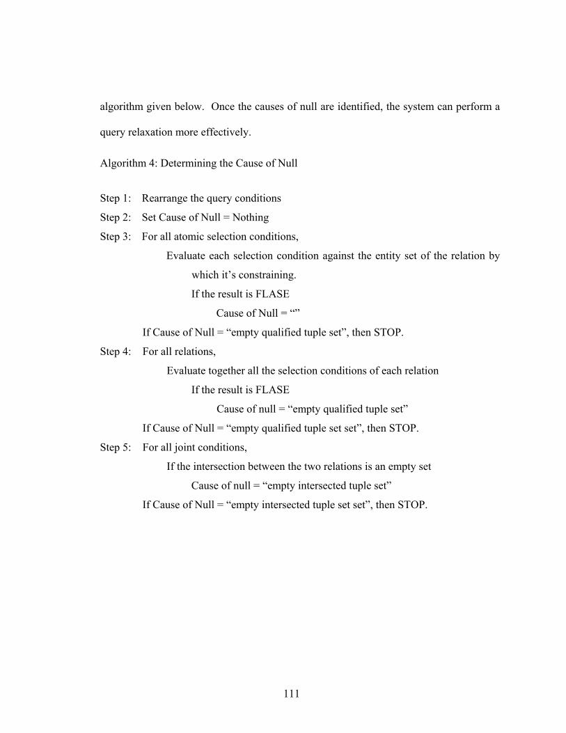
algorithm given below. Once the causes of null are identified, the system can perform a
query relaxation more effectively.
Algorithm 4: Determining the Cause of Null
Step 1: Rearrange the query conditions
Step 2: Set Cause of Null = Nothing
Step 3: For all atomic selection conditions,
Evaluate each selection condition against the entity set of the relation by
which it’s constraining.
If the result is FLASE
Cause of Null = “”
If Cause of Null = “empty qualified tuple set”, then STOP.
Step 4: For all relations,
Evaluate together all the selection conditions of each relation
If the result is FLASE
Cause of null = “empty qualified tuple set”
If Cause of Null = “empty qualified tuple set set”, then STOP. Step 5: For all joint conditions,
If the intersection between the two relations is an empty set
Cause of null = “empty intersected tuple set”
If Cause of Null = “empty intersected tuple set set”, then STOP.
111

6.3 Query Relaxation through Attribute Value Substitutions
The fundamental method of relaxing an over-specified query is to replace the
constants (or attribute values) of its null-bound selection conditions with other values.
For our cooperative query answering system, a query can be relaxed through attribute
value substations using the following rule:
Rule: Query Relaxation through Attribute Value Substitution
Attribute value substitution is performed by replacing the constant
of an atomic selection condition with its closest neighbors that do not
already exist in the query’s other selection conditions having the same
attribute.
If a set of attribute abstract values is defined for the attribute and the constant
appearing in the selection condition is an actual value (not an abstract value), the
selection condition is first relaxed by replacing the actual value with the range (or set) of
values representing the abstract value of the constant. In cases where the attribute
abstract values are not defined, or the constant of the selection condition is already an
abstract value, the constant of the condition is substituted with its closest neighbor node.
To relax a selection condition having a neighbor node as its constant, the neighbor node
is replaced by its closest parent node (another node with the highest nearness that
contains the current node).
112

When the system evaluates a selection condition having an abstract value or a
neighbor node as its constant, it replaces the selection condition with a series of selection
conditions that cover the entire set or range of values under the abstract meaning or the
neighbor node. If the domain of the attribute consists of discrete values such as random
integer numbers or text, a selection condition A = vi or will be replaced by: AinA =
A = a1 OR A = a2 OR … OR A = ai-1 OR A = ai+1 OR … OR A = an
or A IN (a1, a2,…, ai-1, ai+1,…, an)
where
{a1, a2,…, ai-1, ai, ai+1,…, an} is the set of attribute values that are
members of the abstract value set or of neighbor node . Ain
On the other hand, if the domain of the attribute is comprised of continuous
values, a selection condition A = vi or will be replaced by: AinA =
A >= a1 AND A <= an
or A BETWEEN (a1, an)
where
[a1, an] is the set of attribute values covered by the abstract value vi or the
neighbor node n . Ai
The algorithm for query relaxation through attribute value substitution is shown
on the following page.
113
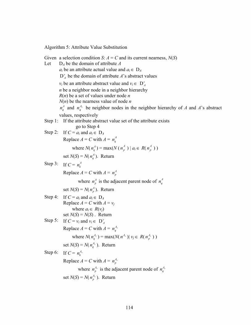
Algorithm 5: Attribute Value Substitution
Given a selection condition S: A = C and its current nearness, N(S) Let DA be the domain of attribute A ai be an attribute actual value and ai ∈ DA be the domain of attribute A’s abstract values v
AD vi be an attribute abstract value and vi ∈ v
AD n be a neighbor node in a neighbor hierarchy R(n) be a set of values under node n N(n) be the nearness value of node n and be neighbor nodes in the neighbor hierarchy of A and A’s abstract
values, respectively
Aqn vA
qn
Step 1: If the attribute abstract value set of the attribute exists go to Step 4
Step 2: If C = ai and ai ∈ DA
Replace A = C with A = n Aq
where N( n ) = max(N ( ) | aAq
Apn i ∈ R( ) ) A
pn
set N(S) = N( n ). Return Aq
Step 3: If C = Akn
Replace A = C with A = n Ap
where n is the adjacent parent node of Ap
A
Aqn
set N(S) = N( n ). Return p
Step 4: If C = ai and ai ∈ DA Replace A = C with A = vj
where ai ∈ R(vj) set N(S) = N(S) . Return
Step 5: If C = vi and vi ∈ vAD
Replace A = C with A = n vAq
where N( n ) = max(N( )| vvAq
vA
vAn j ∈ R( ) ) vApn
set N(S) = N( n ). Return q
Step 6: If C = vAkn
Replace A = C with A = n vAp
where vn is the adjacent parent node of Ap
vA
vAqn
set N(S) = N( n ). Return p
114
6.4 Query Relaxation through Attribute Substitutions
The second level of query relaxation is to replace the attribute of a selection
condition with its neighbor. To allow this type of relaxation, the system needs to have
the attribute mapping knowledge and the appropriate attribute value conversion
functions. The rule for query relaxation through attribute substitution is defined as
follows:
Rule: Query Relaxation through Attribute Substitution
If neighbors of S selection condition’s attribute and attribute value
conversion functions of the condition’s constant are available, attribute
substitution is performed by replacing the attribute and the constant of the
selection condition with their closest neighbors, and their correspondent
values providing that the replacing attributes do not already exist in the
query’s other selection conditions.
A set of selection conditions S is replaced with S′, where S and S′ are denote as
:S 11 aA = AND AND …AND 22 aA = mm aA =
and AND AND …AND , :S ′ 11 aA ′=′ 22 aA =′ nn aA ′=′
when
1) a neighboring link exists between the attribute set of S, A, and the
attribute set of S′, A′ in the attribute neighbor matrix
2) N(A, A′) ≥ a threshold
115

3) the inferential confidence, ξ(C′ → C), of the inferential relationship
between the attribute value set of S, C, and the attribute value set of S′,
C′, is greater than or equal to a threshold
A and A′ are sets containing all attributes of S and S′ , respectively. A and A′ are
expressed as:
{ }mAAAA ,...,, 21=
and { }nAAAA ′′′=′ ,...,, 21 .
C and C′ are sets containing the selection condition constants of S and S′ denoted
as:
{ }maaaC ,...,, 21=
and { }naaaC ′′′=′ ,...,, 21 .
Notice that numbers of selection conditions of C and C′ does not need to be the
same.
116
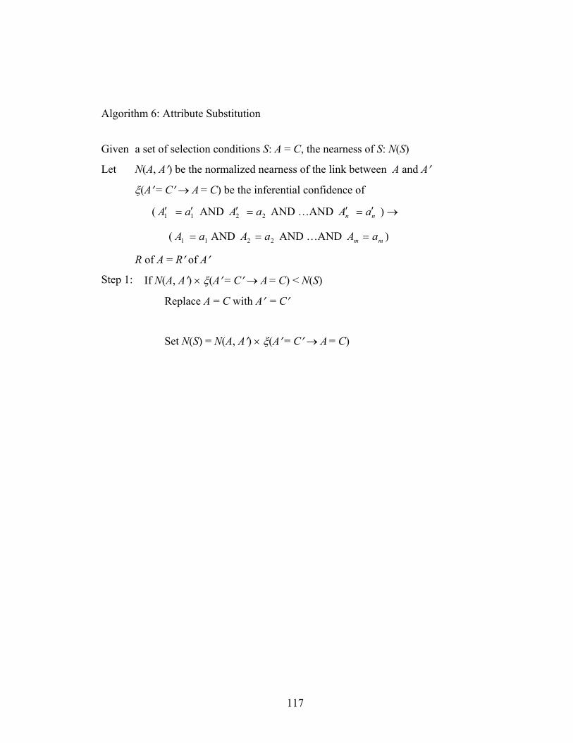
Algorithm 6: Attribute Substitution
Given a set of selection conditions S: A = C, the nearness of S: N(S)
Let N(A, A′) be the normalized nearness of the link between A and A′
ξ(A′ = C′ → A = C) be the inferential confidence of
( aA = AND AND …AND ) → 11 ′′ 22 aA =′ nn aA ′=′
( aA = AND AND …AND ) 11 22 aA = mm aA =
R of A = R′ of A′
Step 1: If N(A, A′) × ξ(A′ = C′ → A = C) < N(S)
Replace A = C with A′ = C′
Set N(S) = N(A, A′) × ξ(A′ = C′ → A = C)
117

6.5 Query Relaxation through Relation Substitutions
Query relaxation through relation substitution is similar to query relaxation
through attribute substitution. It requires that the system have the attribute mapping
knowledge and appropriate attribute value conversion functions. The difference is, if the
selection conditions being replaced are not the all selection conditions of the query, the
system needs to check whether or not the rest of the query’s selection conditions have
any dependencies on the replaced conditions (relation). If that is true, relation
substitution is executed on both groups of selection conditions given that the dependant’s
attribute mapping and attribute value conversion functions are also available. We define
the rule for query relaxation through relation substitution as:
Rule: Query Relaxation through Relation Substitution
If neighbors of s selection condition’s attribute and attribute value
conversion functions of the condition’s constant are available, relation
substitution is performed by replacing the attributes and the constants of
the super-class’ and its sub-classes’ selection conditions with their
correspondent neighbors and mapped values, providing that the replacing
attributes do not already exist in the query’s other selection conditions.
118
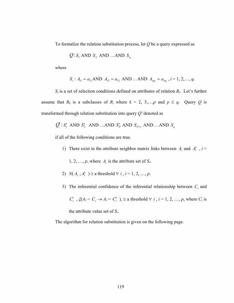
To formalize the relation substitution process, let Q be a query expressed as
:Q 1S AND AND …AND 2S qS
where
:iS 11 ii aA = AND AND …AND , i = 1, 2,…, q. 22 ii aA =ii imim aA =
Si is a set of selection conditions defined on attributes of relation Ri. Let’s further
assume that Rk is a subclasses of Ri where k = 2, 3,…,p and p ≤ q. Query Q is
transformed through relation substitution into query Q′ denoted as
:Q′ 1S ′ AND AND …AND AND AND …AND 2S ′ PS ′ 1+PS qS
if all of the following conditions are true.
1) There exist in the attribute neighbor matrix links between and , i =
1, 2, …, p, where is the attribute set of S
iA iA′
iA i.
2) N( , ) ≥ a threshold ∀ i , i = 1, 2, …, p. iA iA′
3) The inferential confidence of the inferential relationship between and
, ξ(A
iC
iC ′ i = C → Ai i = ), ≥ a threshold ∀ i , i = 1, 2, …, p, where CiC ′ i is
the attribute value set of Si.
The algorithm for relation substitution is given on the following page.
119
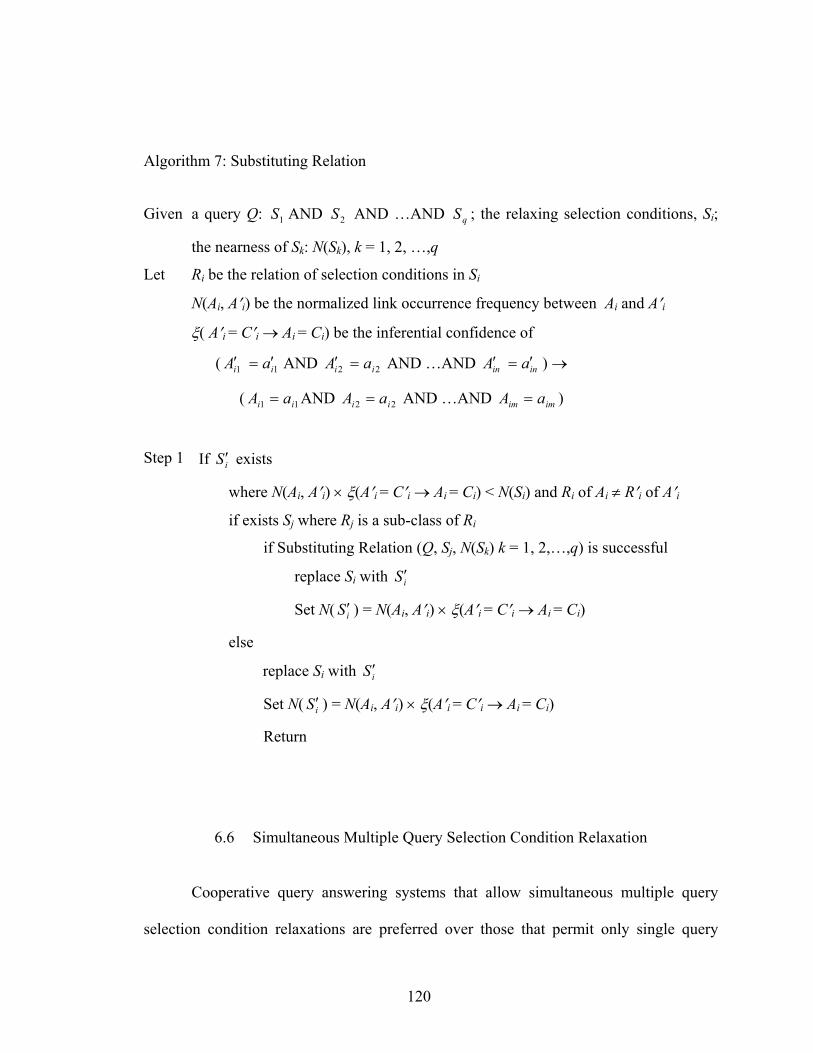
Algorithm 7: Substituting Relation
Given a query Q: AND AND …AND ; the relaxing selection conditions, S1S 2S qS i;
the nearness of Sk: N(Sk), k = 1, 2, …,q
Let Ri be the relation of selection conditions in Si
N(Ai, A′i) be the normalized link occurrence frequency between Ai and A′i
ξ( A′i = C′i → Ai = Ci) be the inferential confidence of
( aA = AND AND …AND ) → 11 ii ′′ 22 ii aA =′ inin aA ′=′
( aA = AND AND …AND ) 11 ii 22 ii aA = imim aA =
Step 1 If exists iS ′
where N(Ai, A′i) × ξ(A′i = C′i → Ai = Ci) < N(Si) and Ri of Ai ≠ R′i of A′i
if exists Sj where Rj is a sub-class of Ri
if Substituting Relation (Q, Sj, N(Sk) k = 1, 2,…,q) is successful
replace Si with iS ′
Set N( Si′ ) = N(Ai, A′i) × ξ(A′i = C′i → Ai = Ci)
else
replace Si with iS ′
Set N( S ) = N(Ai′ i, A′i) × ξ(A′i = C′i → Ai = Ci)
Return
6.6 Simultaneous Multiple Query Selection Condition Relaxation
Cooperative query answering systems that allow simultaneous multiple query
selection condition relaxations are preferred over those that permit only single query
120
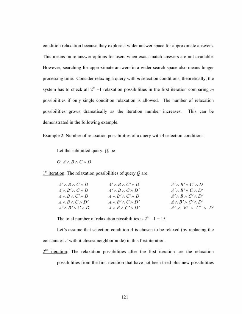
condition relaxation because they explore a wider answer space for approximate answers.
This means more answer options for users when exact match answers are not available.
However, searching for approximate answers in a wider search space also means longer
processing time. Consider relaxing a query with m selection conditions, theoretically, the
system has to check all 2m –1 relaxation possibilities in the first iteration comparing m
possibilities if only single condition relaxation is allowed. The number of relaxation
possibilities grows dramatically as the iteration number increases. This can be
demonstrated in the following example.
Example 2: Number of relaxation possibilities of a query with 4 selection conditions.
Let the submitted query, Q, be
Q: A ∧ B ∧ C ∧ D
1st iteration: The relaxation possibilities of query Q are:
A′ ∧ B ∧ C ∧ D A ∧ B′ ∧ C ∧ D A ∧ B ∧ C′ ∧ D A ∧ B ∧ C ∧ D′ A′ ∧ B′ ∧ C ∧ D
A′ ∧ B ∧ C′ ∧ D A′ ∧ B ∧ C ∧ D′ A ∧ B′ ∧ C′ ∧ D A ∧ B′ ∧ C ∧ D′ A ∧ B ∧ C′ ∧ D′
A′ ∧ B′ ∧ C′ ∧ D A′ ∧ B′ ∧ C ∧ D′ A′ ∧ B ∧ C′ ∧ D′ A ∧ B′ ∧ C′ ∧ D′ A′ ∧ B′ ∧ C′ ∧ D′
The total number of relaxation possibilities is 24 – 1 = 15
Let’s assume that selection condition A is chosen to be relaxed (by replacing the
constant of A with it closest neighbor node) in this first iteration.
2nd iteration: The relaxation possibilities after the first iteration are the relaxation
possibilities from the first iteration that have not been tried plus new possibilities
121
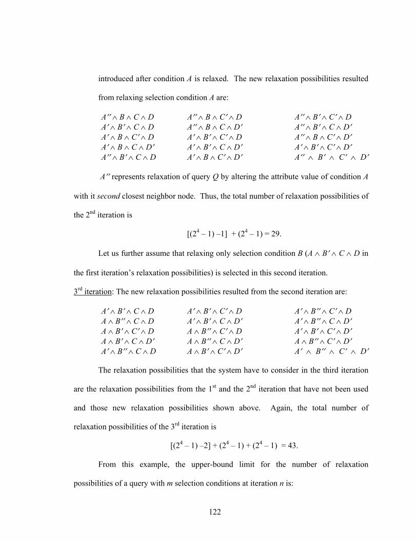
introduced after condition A is relaxed. The new relaxation possibilities resulted
from relaxing selection condition A are:
A′′ ∧ B ∧ C ∧ D A′ ∧ B′ ∧ C ∧ D A′ ∧ B ∧ C′ ∧ D A′ ∧ B ∧ C ∧ D′ A′′ ∧ B′ ∧ C ∧ D
A′′ ∧ B ∧ C′ ∧ D A′′ ∧ B ∧ C ∧ D′ A′ ∧ B′ ∧ C′ ∧ D A′ ∧ B′ ∧ C ∧ D′ A′ ∧ B ∧ C′ ∧ D′
A′′ ∧ B′ ∧ C′ ∧ D A′′ ∧ B′ ∧ C ∧ D′ A′′ ∧ B ∧ C′ ∧ D′ A′ ∧ B′ ∧ C′ ∧ D′ A′′ ∧ B′ ∧ C′ ∧ D′
A′′ represents relaxation of query Q by altering the attribute value of condition A
with it second closest neighbor node. Thus, the total number of relaxation possibilities of
the 2nd iteration is
[(24 – 1) –1] + (24 – 1) = 29.
Let us further assume that relaxing only selection condition B (A ∧ B′ ∧ C ∧ D in
the first iteration’s relaxation possibilities) is selected in this second iteration.
3rd iteration: The new relaxation possibilities resulted from the second iteration are:
A′ ∧ B′ ∧ C ∧ D A ∧ B′′ ∧ C ∧ D A ∧ B′ ∧ C′ ∧ D A ∧ B′ ∧ C ∧ D′ A′ ∧ B′′ ∧ C ∧ D
A′ ∧ B′ ∧ C′ ∧ D A′ ∧ B′ ∧ C ∧ D′ A ∧ B′′ ∧ C′ ∧ D A ∧ B′′ ∧ C ∧ D′ A ∧ B′ ∧ C′ ∧ D′
A′ ∧ B′′ ∧ C′ ∧ D A′ ∧ B′′ ∧ C ∧ D′ A′ ∧ B′ ∧ C′ ∧ D′ A ∧ B′′ ∧ C′ ∧ D′ A′ ∧ B′′ ∧ C′ ∧ D′
The relaxation possibilities that the system have to consider in the third iteration
are the relaxation possibilities from the 1st and the 2nd iteration that have not been used
and those new relaxation possibilities shown above. Again, the total number of
relaxation possibilities of the 3rd iteration is
[(24 – 1) –2] + (24 – 1) + (24 – 1) = 43.
From this example, the upper-bound limit for the number of relaxation
possibilities of a query with m selection conditions at iteration n is:
122
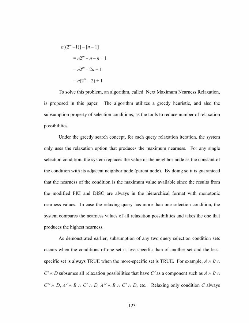
n[(2m –1)] – [n – 1]
= n2m – n – n + 1
= n2m – 2n + 1
= n(2m – 2) + 1
To solve this problem, an algorithm, called: Next Maximum Nearness Relaxation,
is proposed in this paper. The algorithm utilizes a greedy heuristic, and also the
subsumption property of selection conditions, as the tools to reduce number of relaxation
possibilities.
Under the greedy search concept, for each query relaxation iteration, the system
only uses the relaxation option that produces the maximum nearness. For any single
selection condition, the system replaces the value or the neighbor node as the constant of
the condition with its adjacent neighbor node (parent node). By doing so it is guaranteed
that the nearness of the condition is the maximum value available since the results from
the modified PKI and DISC are always in the hierarchical format with monotonic
nearness values. In case the relaxing query has more than one selection condition, the
system compares the nearness values of all relaxation possibilities and takes the one that
produces the highest nearness.
As demonstrated earlier, subsumption of any two query selection condition sets
occurs when the conditions of one set is less specific than of another set and the less-
specific set is always TRUE when the more-specific set is TRUE. For example, A ∧ B ∧
C′ ∧ D subsumes all relaxation possibilities that have C′ as a component such as A ∧ B ∧
C′′ ∧ D, A′ ∧ B ∧ C′ ∧ D, A′′ ∧ B ∧ C′ ∧ D, etc.. Relaxing only condition C always
123

produces a relaxed query that is semantically closer to the original query than relaxing the
condition C and one or more another selection conditions. Since the other relaxation
possibilities that have C′ as a component always have a total nearness less than or equal
to the option that has only C′, the other relaxation possibilities can be disregarded as long
as C has not been relaxed yet. Using the subsumption properties and the greedy
searching when query relaxation is performed helps reduce the number of relaxation
options the system needs to investigate in each iteration.
To allow multiple conditions to get relaxed simultaneously, the query answering
system also needs to track the changes it has performed to the original query to prevent
infinite loop searching. This is accomplished with the Next Maximum Nearness
Relaxation algorithm, which is given the following pages.
124
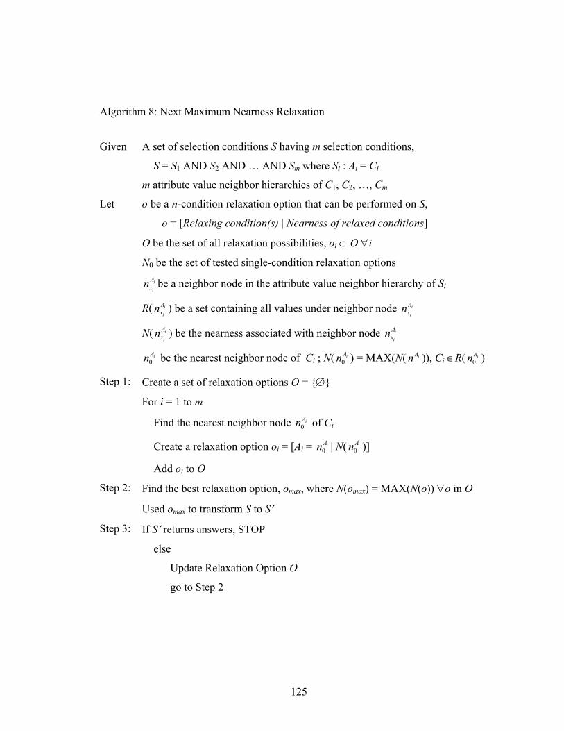
Algorithm 8: Next Maximum Nearness Relaxation
Given A set of selection conditions S having m selection conditions,
S = S1 AND S2 AND … AND Sm where Si : Ai = Ci
m attribute value neighbor hierarchies of C1, C2, …, Cm
Let o be a n-condition relaxation option that can be performed on S,
o = [Relaxing condition(s) | Nearness of relaxed conditions]
O be the set of all relaxation possibilities, oi ∈ O ∀i
N0 be the set of tested single-condition relaxation options i
i
Axn be a neighbor node in the attribute value neighbor hierarchy of Si
R( ) be a set containing all values under neighbor node i
i
Axn i
i
Axn
N( ) be the nearness associated with neighbor node i
i
Axn i
i
Axn
iAn0 be the nearest neighbor node of Ci ; N( ) = MAX(N( )), Ci ∈R( ) iAn0
iAn iAn0
Step 1: Create a set of relaxation options O = {∅}
For i = 1 to m
Find the nearest neighbor node of CiAn0 i
Create a relaxation option oi = [Ai = | N( )] iAn0iAn0
Add oi to O
Step 2: Find the best relaxation option, omax, where N(omax) = MAX(N(o)) ∀o in O
Used omax to transform S to S′
Step 3: If S′ returns answers, STOP
else
Update Relaxation Option O
go to Step 2
125
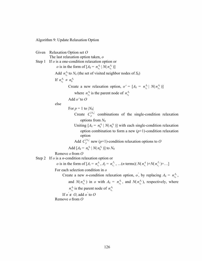
Algorithm 9: Update Relaxation Option
Given Relaxation Option set O The last relaxation option taken, o
Step 1 If o is a one-condition relaxation option or o is in the form of [Ak = | N( )] k
k
Axn k
k
Axn
Add to Nk
k
Axn k (the set of visited neighbor nodes of Sk)
If n ≠ k
k
Ax
kAn0
Create a new relaxation option, o′ = [Ak = n | N( n )]
where is the parent node of
k
k
Ay
k
k
Ay
k
k
Ayn k
k
Axn
Add o′ to O else
For p = 1 to |N0| Create 0N
pC combinations of the single-condition relaxation options from N0
Uniting [Ak = | N( )] with each single-condition relaxation option combination to form a new (p+1)-condition relaxation option
kAn0kAn0
Add 0NpC new (p+1)-condition relaxation options to O
Add [Ak = | N( )] to NkAn0kAn0 0
Remove o from O Step 2 If o is a n-condition relaxation option or
o is in the form of [Ai = , Ai
i
Axn j = , …(n terms)| N( )+N( )+…]j
j
Axn i
i
Axn j
j
Axn
For each selection condition in o Create a new n-condition relaxation option, o′, by replacing Ak = n ,
and N( ) in o with A
k
k
Ax
k
k
Axn k = , and N( ), respectively, where
is the parent node of n
k
k
Ayn k
k
Ayn
k
k
Ayn k
k
Ax
If o′ ∉ O, add o′ to O Remove o from O
126
6.7 Query Relaxation Algorithms
The algorithms for relaxing a null-bound query caused by an empty qualified
tuple set and an empty intersected tuple set are presented in this subsection. Section 6.7.3
provides an aggregate query relaxation algorithm that combines all query relaxation
techniques presented here in one algorithm.
6.7.1 Expanding Qualified Tuple Set
Query relaxation by expanding the qualified tuple set is performed when the
qualified tuple set of a relation is empty. Based upon the cause of null as stated in
Section 0, expanding the qualified tuple set is done on two levels. The first level is
performed when at least one of the selection conditions in the condition group is assessed
as FALSE. In the first level, each selection condition is relaxed until the condition is
evaluated as TRUE. If the qualified tuple set of the selection condition group is still an
empty set after all selection conditions are assessed as TRUE, the condition group is
relaxed further using simultaneous multiple selection condition relaxation algorithm.
127
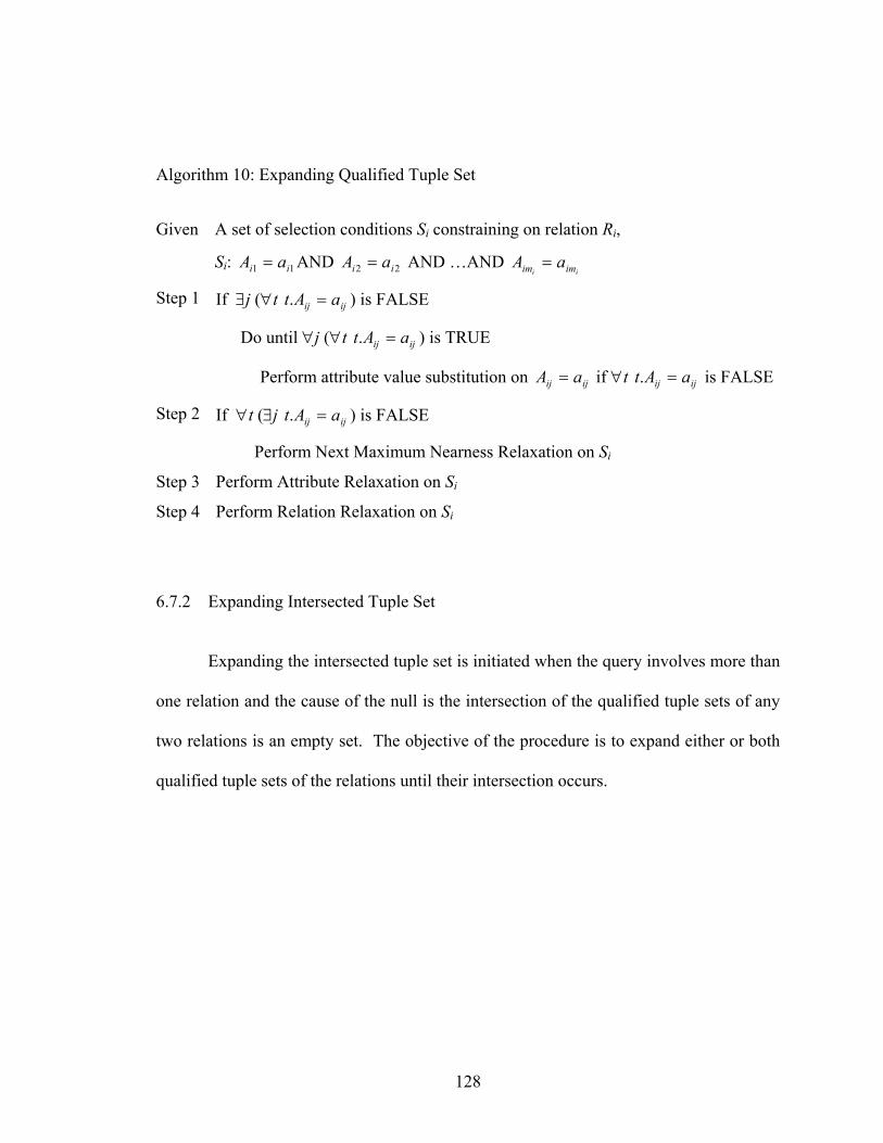
Algorithm 10: Expanding Qualified Tuple Set
Given A set of selection conditions Si constraining on relation Ri,
Si: AND AND …AND 11 ii aA = 22 ii aA =ii imim aA =
Step 1 If ∃j (∀t t ) is FALSE ijij aA =.
Do until ∀j (∀t t ijij aA =. ) is TRUE
Perform attribute value substitution on if ∀t is FALSE ijij aA = ijij aAt =.
Step 2 If ∀t (∃j t ) is FALSE ijij aA =.
Perform Next Maximum Nearness Relaxation on Si
Step 3 Perform Attribute Relaxation on Si
Step 4 Perform Relation Relaxation on Si
6.7.2 Expanding Intersected Tuple Set
Expanding the intersected tuple set is initiated when the query involves more than
one relation and the cause of the null is the intersection of the qualified tuple sets of any
two relations is an empty set. The objective of the procedure is to expand either or both
qualified tuple sets of the relations until their intersection occurs.
128
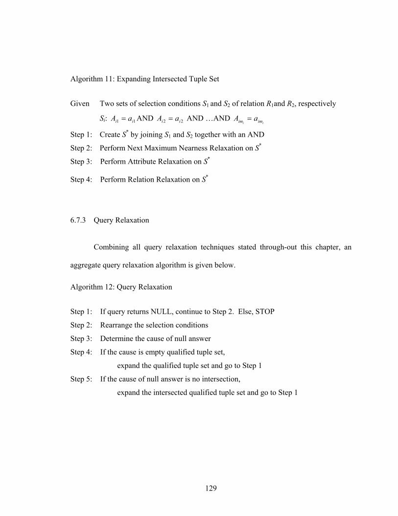
Algorithm 11: Expanding Intersected Tuple Set
Given Two sets of selection conditions S1 and S2 of relation R1and R2, respectively
Si: AND AND …AND 11 ii aA = 22 ii aA =ii imim aA =
Step 1: Create S* by joining S1 and S2 together with an AND
Step 2: Perform Next Maximum Nearness Relaxation on S*
Step 3: Perform Attribute Relaxation on S*
Step 4: Perform Relation Relaxation on S*
6.7.3 Query Relaxation
Combining all query relaxation techniques stated through-out this chapter, an
aggregate query relaxation algorithm is given below.
Algorithm 12: Query Relaxation
Step 1: If query returns NULL, continue to Step 2. Else, STOP
Step 2: Rearrange the selection conditions
Step 3: Determine the cause of null answer
Step 4: If the cause is empty qualified tuple set,
expand the qualified tuple set and go to Step 1
Step 5: If the cause of null answer is no intersection,
expand the intersected qualified tuple set and go to Step 1
129
7.0 NEARNESS CALCULATION
Measuring the semantic nearness between exact match answers and approximate
answers is one important aspect of cooperative query answering, secondary to the
techniques used to ascertain the cooperative answers. It helps to add confidence to the
alternative answers. With no way to measure the semantic nearness between the target
answers and the approximate answers produced by the system, accepting the answer is
doubtful to the users. Also, in cases where the results of a query relaxation is a large set
of close match answers, the system can use semantic nearness to sort the approximate
answers before presenting them to the user. As stated previously, semantic nearness can
be obtained by comparing the exact match answers with the approximate answers or the
original queries with the relaxed queries. The approach taken in this research was to
compare the queries for nearness calculation because the theme of this research is to
increase the flexibility of cooperative query answering operation. It has been shown so
far that relaxations of queries are performed in three levels: attribute value, attribute, and
relation level. Methods for measuring the semantic nearness at different levels are
described in Section 7.1.1 to 7.1.3. Section 7.1.4 provides the proposed query nearness
measuring function that combines together the nearness measuring of all three levels.
7.1.1 Attribute Value Nearness
When attribute value substitution is performed on a selection condition, the
semantic proximity of the original selection condition and the relaxed one is the nearness
between the original attribute value (query constant) before the condition relaxation is
130
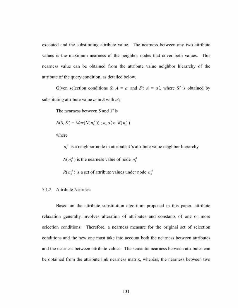
executed and the substituting attribute value. The nearness between any two attribute
values is the maximum nearness of the neighbor nodes that cover both values. This
nearness value can be obtained from the attribute value neighbor hierarchy of the
attribute of the query condition, as detailed below.
Given selection conditions S: A = ai and S′: A = a′i, where S′ is obtained by
substituting attribute value ai in S with a′i.
The nearness between S and S′ is
N(S, S′) = Max(N( n )) ; aAk i, a′i ∈ R( ) A
kn
where
Akn is a neighbor node in attribute A’s attribute value neighbor hierarchy
N( ) is the nearness value of node Akn A
kn
R( ) is a set of attribute values under node Akn A
kn
7.1.2 Attribute Nearness
Based on the attribute substitution algorithm proposed in this paper, attribute
relaxation generally involves alteration of attributes and constants of one or more
selection conditions. Therefore, a nearness measure for the original set of selection
conditions and the new one must take into account both the nearness between attributes
and the nearness between attribute values. The semantic nearness between attributes can
be obtained from the attribute link nearness matrix, whereas, the nearness between two
131
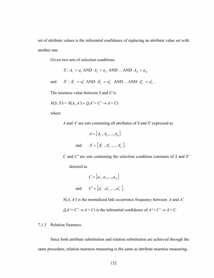
set of attribute values is the inferential confidence of replacing an attribute value set with
another one.
Given two sets of selection conditions
:S 11 aA = AND AND …AND 22 aA = mm aA =
and AND AND …AND . :S ′ 11 aA ′=′ 22 aA ′=′ nn aA ′=′
The nearness value between S and S′ is
N(S, S′) = N(A, A′) × ξ(A′ = C′ → A = C)
where
A and A′ are sets containing all attributes of S and S′ expressed as
{ }mAAAA ,...,, 21=
and { }nAAAA ′′′=′ ,...,, 21 .
C and C′ are sets containing the selection condition constants of S and S′
denoted as
{ }maaaC ,...,, 21=
and { }naaaC ′′′=′ ,...,, 21 .
N(A, A′) is the normalized link occurrence frequency between A and A′.
ξ(A′ = C′ → A = C) is the inferential confidence of A′ = C′ → A = C
7.1.3 Relation Nearness
Since both attribute substitution and relation substitution are achieved through the
same procedure, relation nearness measuring is the same as attribute nearness measuring.
132
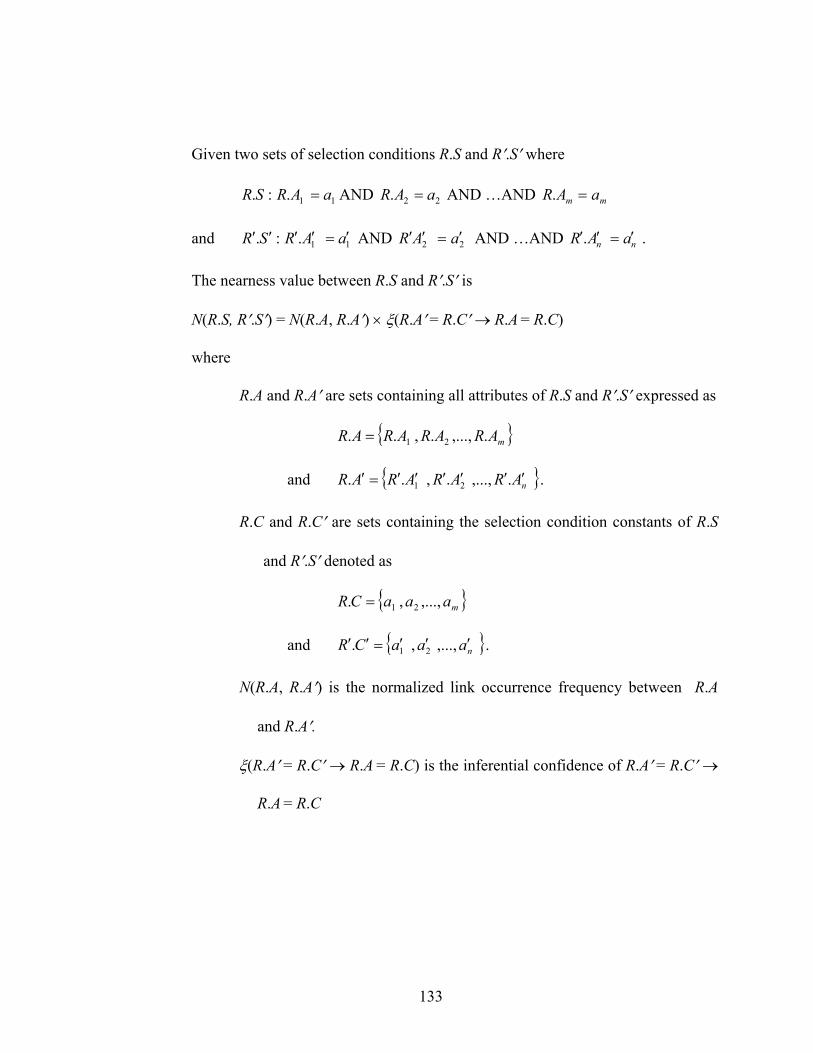
Given two sets of selection conditions R.S and R′.S′ where
:.SR 11. aAR = AND AND …AND 22. aAR = mm aAR =.
and AND AND …AND :.SR ′′ 11. aAR ′=′′ 22 aAR ′=′′ nn aAR ′=′′. .
The nearness value between R.S and R′.S′ is
N(R.S, R′.S′) = N(R.A, R.A′) × ξ(R.A′ = R.C′ → R.A = R.C)
where
R.A and R.A′ are sets containing all attributes of R.S and R′.S′ expressed as
{ }mARARARAR .,...,.,.. 21=
and { }nARARARAR ′′′′′′=′ .,...,.,.. 21 .
R.C and R.C′ are sets containing the selection condition constants of R.S
and R′.S′ denoted as
{ }maaaCR ,...,,. 21=
and { }naaaCR ′′′=′′ ,...,,. 21 .
N(R.A, R.A′) is the normalized link occurrence frequency between R.A
and R.A′.
ξ(R.A′ = R.C′ → R.A = R.C) is the inferential confidence of R.A′ = R.C′ →
R.A = R.C
133
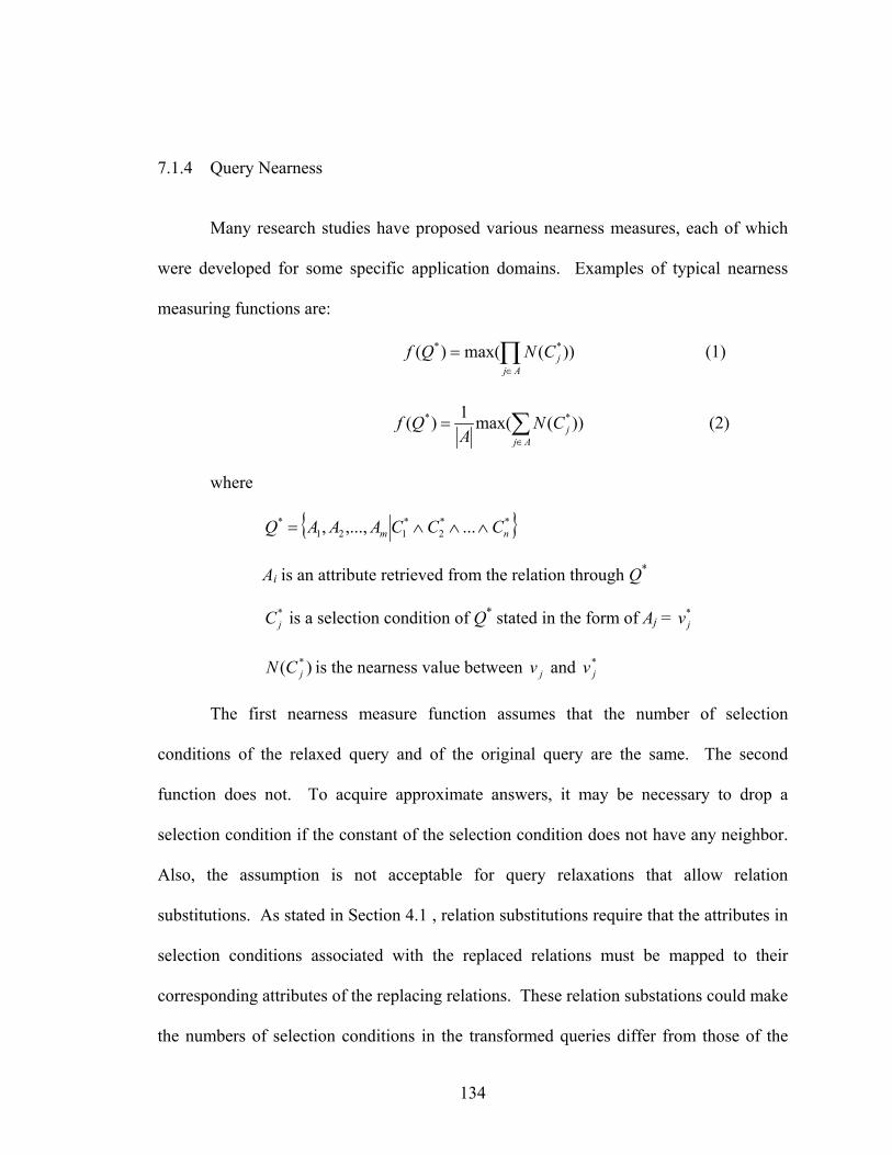
7.1.4 Query Nearness
Many research studies have proposed various nearness measures, each of which
were developed for some specific application domains. Examples of typical nearness
measuring functions are:
))(max()( ** ∏∈
=Aj
jCNQf (1)
))(max(1)( ** ∑∈
=Aj
jCNA
Qf (2)
where
{ }**2
*121
* ...,...,, nm CCCAAAQ ∧∧∧=
Ai is an attribute retrieved from the relation through Q*
is a selection condition of Q*jC * stated in the form of Aj = *
jv
is the nearness value between v and )( *jCN j
*jv
The first nearness measure function assumes that the number of selection
conditions of the relaxed query and of the original query are the same. The second
function does not. To acquire approximate answers, it may be necessary to drop a
selection condition if the constant of the selection condition does not have any neighbor.
Also, the assumption is not acceptable for query relaxations that allow relation
substitutions. As stated in Section 4.1 , relation substitutions require that the attributes in
selection conditions associated with the replaced relations must be mapped to their
corresponding attributes of the replacing relations. These relation substations could make
the numbers of selection conditions in the transformed queries differ from those of the
134
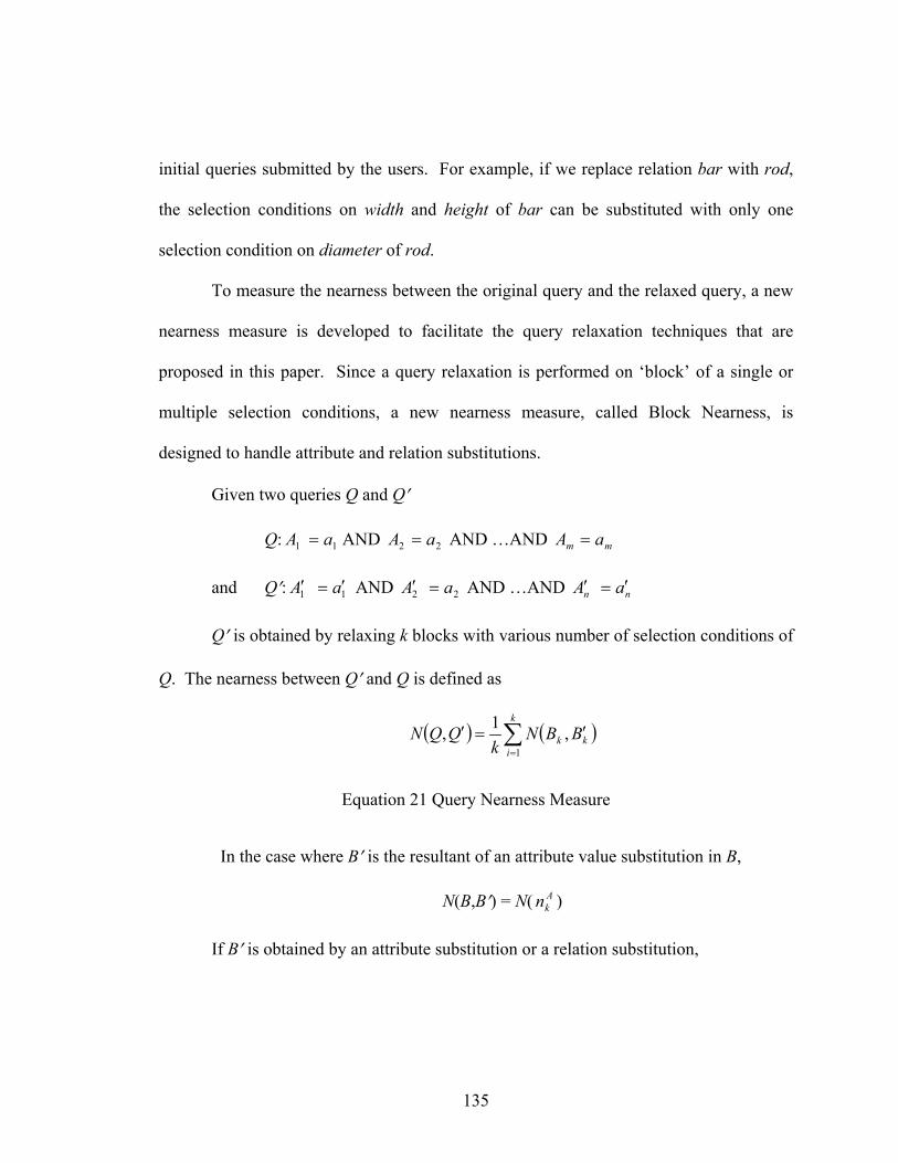
initial queries submitted by the users. For example, if we replace relation bar with rod,
the selection conditions on width and height of bar can be substituted with only one
selection condition on diameter of rod.
To measure the nearness between the original query and the relaxed query, a new
nearness measure is developed to facilitate the query relaxation techniques that are
proposed in this paper. Since a query relaxation is performed on ‘block’ of a single or
multiple selection conditions, a new nearness measure, called Block Nearness, is
designed to handle attribute and relation substitutions.
Given two queries Q and Q′
Q: AND AND …AND 11 aA = 22 aA = mm aA =
and Q′: AND AND …AND 11 aA ′=′ 22 aA =′ nn aA ′=′
Q′ is obtained by relaxing k blocks with various number of selection conditions of
Q. The nearness between Q′ and Q is defined as
( ) ( )∑=
′=′k
ikk BBN
kQQN
1,1,
Equation 21 Query Nearness Measure
In the case where B′ is the resultant of an attribute value substitution in B,
N(B,B′) = N( ) Akn
If B′ is obtained by an attribute substitution or a relation substitution,
135

N(B,B′) = N(A, A′) × ξ(A′ = C′ → A = C)
In addition to the two relaxation types mentioned above, a block can also be
relaxed by both attribute value substitution and attribute substitution. In this case, the
nearness between B and B′ is
N(B,B′) = N( ) × N(A, A′) × ξ(A′Akn = C′ → A = C).
136
8.0 CASE STUDY
So far, we have demonstrated through examples how the proposed cooperative
query answering model works and its applications in a manufacturing information
system. However, the proposed neighbor hierarchy construction and query relaxation
technique is applicable to other types of hierarchical structure information systems as
well. In this chapter, we first demonstrate how the proposed cooperative query
answering model can be used to solve a course scheduling problem. We developed a
cooperative query answering system called the “Course Planner” program. The program
allows searching for similar study plans using the neighbor hierarchy construction and
query relaxation techniques presented in this paper. Course Planner provides advisors
and students in the Department of Industrial Engineering at the University of Pittsburgh
another tool for course scheduling. Later in this chapter, we demonstrated the reliability
of the proposed cooperative query answering model using the Course Planner program.
Cooperative query answering is useful only when the database or the knowledge
base is not complete – the knowledge base does not contain exact match answer(s) for all
possible query conditions, therefore, it is not appropriate to validate the approximate
answers by comparing them against the optimal solutions (i.e. the course schedules that
satisfy all user conditions). We chose to measure the “reliability” of the proposed
cooperative query answering model. In other words, we demonstrated whether the
proposed concept could perform query relaxations and produce results as intended. The
assessment was carried out by comparing expert opinions with computer generated
137
approximate answers. A detailed explanation on the reliability test of the proposed
cooperative query answering model is presented in Section 8.3.
8.1 Course Scheduling Background
The department of Industrial Engineering at the University of Pittsburgh requires
that students meet all program requirements in order to graduate. Some important
requirements are 1) obtaining QPA of at least 2.0, 2) maintaining an active student status
in the graduating semester, and 3) completing all mandatory courses as stated in the
department curriculum. Although the department already provides a guideline on which
courses should be taken in each semesters, many students cannot or choose not to follow
the guideline due to many reasons. In addition, usually, the standard course schedule is
not suitable for students who 1) transfer from other programs, schools or universities, 2)
are granted with options to take higher level courses, and/or 3) are registered for
cooperative engineering (Co-op) programs. For those students with such special
conditions, course scheduling becomes a riddle that can greatly affect how soon students
can graduate.
Typically, study course planning is done manually using published school course
information such as offering terms, class dates and times. Although many courses are
offered in many semesters, course scheduling has been a challenge to both students and
advisors. Manual course scheduling usually requires substantial amount of time and
experience.
138
8.1.1 Study Course Scheduling vs. Rapid Prototyping
Study course scheduling is similar to rapid prototyping. Both domains usually
involve databases that frequently utilize hierarchical-type relationships. In a
manufacturing information system, part features are classified into categories and stored
in multiple tables, which relate to each other through association, generalization, and
aggregation relationships. Similarly, in an academic information system, courses can
also be specialized into groups such as required general courses, required program
courses, humanity and social science elective courses, and technical elective courses.
Querying in both the academic and manufacturing information domains typically involve
multiple tables and, therefore, requires joint queries to retrieve data across those tables.
Both study course scheduling and rapid prototyping can greatly benefit historical
study plans or existing designs, respectively. In rapid prototyping domain, the
manufacturer can capitalize on the existing product designs, specifications, and/or
manufacturing processes by recycling the available information and applying it to the
new designs that contain similar features. Course scheduling usually requires
considerations of which semesters the courses are offered, and what days and times the
classes are held. Students could avoid such time-consuming course scheduling by
comparing their graduation requirements with graduated students’ course schedules. If
similar course schedules are available, students could either directly follow those study
plans or use them as guidelines or starting points for their class planning.
139
8.1.2 The Complexities of Course Scheduling
The goal of course scheduling is trying to meet all graduation requirements (by
taking all mandatory courses) within a reasonable amount of time. Although such a task
is very simple, achieving it requires a clear understanding and thorough planning. Course
scheduling has many requirements and constraints, which are summarized in the
following subsections. Such complexities of course scheduling make the problem
difficult and inspired us to develop an intelligent information retrieval system using the
proposed cooperative query answering concept.
8.1.2.1 Graduation Requirements
Some common graduation requirements are that a student 1) must undertake a
number of courses to obtain a specific numbers of credits, 2) acquire a cumulative quality
point average (QPA) of 2.0, and 3) complete all logistic related tasks (i.e. apply for
graduation). In this research, we assume that students have completed or will satisfy all
graduation requirements except taking the mandatory courses. Basically, we focus only
whether a student takes all the courses as stated in the program curriculum. For the
Department of Industrial Engineering at the University of Pittsburgh, a student has to
complete all 48 mandatory courses, which can be classified into one of the following
categories, 1) school of engineering required courses, 2) humanities electives, 3) social
science electives, 4) department required courses, 5) technical electives, and 6) school
and departmental seminars.
140
8.1.2.2 Constraints
The three most important constraints in study course scheduling are 1) course
availability 2) course prerequisites, and 3) class times (days and times). Course
availability indicates when (or in what semester) the courses will be offered for students
to take. Most courses especially the core courses are offered regularly every fall, spring,
or summer semester. Some courses are available for students in almost every semester,
particularly those popular humanities and social science electives. A few courses are
offered only every other year.
Although classes may be offered only in a certain semester, some students are not
eligible to register for those classes due to the prerequisite requirements. Thus, course
prerequisites also dictate whether students can take the courses. The last constraint of
study course scheduling is the class times. Courses offered by different schools or
departments have a high tendency to have time conflicts. Students cannot take any two
courses with the same or overlapping class times.
8.2 Cooperative Query Answering for Study Course Scheduling
We developed an intelligent information retrieval system, called the “Course
Planner” program, using Visual Basic programming language. The application is a user
interface program that takes user queries, passes the queries to the traditional student
database, perform query relaxations if necessary using the proposed neighbor hierarchy
construction and query relaxation algorithms, and presents results back to the users.
141

Course Planner takes user current academic status and plans for the coming
semesters as the input. When all information is entered, the program transforms user
conditions into an SQL SELECT statement and uses it to fetch exact-match answers or
any close-match course schedules along with their nearness values. Based on the
nearness values of the alternative answers, user can compare and select the most desired
course schedules or modify the inputs and execute the query relaxation again.
The detailed explanation regarding the student database and steps in acquiring
similar course schedules (or approximate answers) are shown in the following
subsections.
8.2.1 The Student Database
A traditional student database consists of tables with relationships as depicted in
Figure 13 on page 144. The STUDENT table stores student demographic and program
information. Course identification, subject, title, offering semester, class times and all
other course related information are kept in the HUMAN, SOCIAL, IE_REQ,
ENGR_REQ, and IE_ELECT tables accordingly with their course types. The
STU_PRGSS table holds students’ completed courses and their grades.
All tables mentioned so far store the typical student information. Three additional
tables were added to the database to facilitate the neighbor knowledge construction,
which is essential for our approximate answer search and nearness calculations. These
tables store information related to graduated students (completed course schedules). The
PLAN table stores information detailing how graduated students spent each semester
142
such as taking classes, participating in the Co-op program, and what courses these
students took to satisfy each curriculum course. The table was built based upon data pull
from the STUDENT and STU_PRGSS table. The 01ER, 01IG, and 01LL fields represent
student activities in the summer, spring, and fall semesters of the graduating year.
Similarly, field nER, nIG, and nLL contain the student activities in the summer, spring,
and fall semesters of the nth year before the graduation. Values in those fields, which can
be either “C”, “W”, or “-”, indicate whether students take courses, work as part of the Co-
op program, or drop in that particular semester. The PMATH0220, PPHYS0104, …,
PH/S-6, PIE1085 fields provide the information regarding what courses students chose to
register to obtain credits for the specific curriculum courses.
The PLAN_TERM table provides student status snapshots based on the program
requirements (curriculum). Each entry in the PLAN_TERM table represents a snapshot
of a student’s academic status at the end of a particular semester, which is indicated in the
PTERMINV field. For example, PTERMINV = “2LL” means the student is in a fall term
and this year is the second last year according to the student’s plan for graduation. As the
names imply, field FL_LEFT, SP_LEFT, and SR_LEFT tell the numbers of fall, spring,
and summer semesters left before graduation when a particular semester is completed
based on each study plan. The TMATH0220, TPHYS0104, …, TH/S-6, TIE1085 fields
indicate whether the curriculum courses have or have not been completed. Values in
these fields can be either “-” for completed and “NOT YET” for the opposite.
143
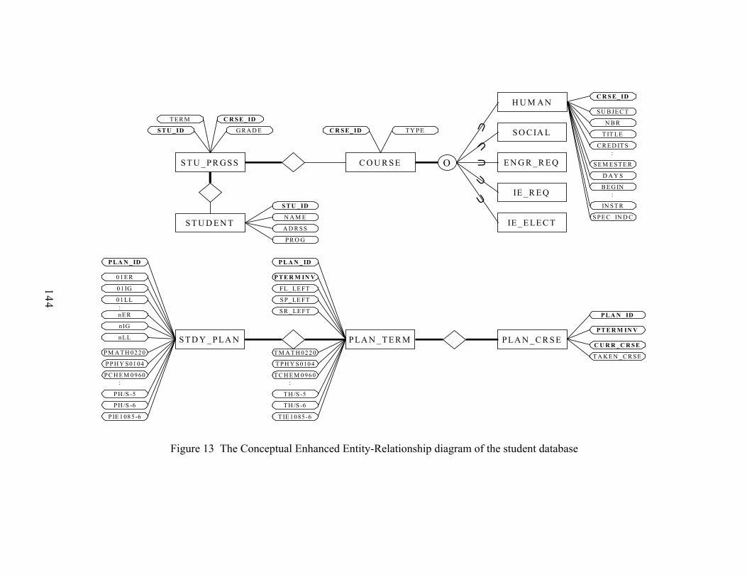
144
E N G R _ R E Q
IE _ R E Q
IE _E LE C T
S O C IA L
:
S T D Y _ P LA N
0 1 E R
0 1 IG
0 1 LL
P M A T H 02 2 0
nE R
nIG
n LL
P P H Y S01 04
P C H E M 09 60
P H /S -5
:
P H /S -6
P IE 1 08 5 -6
P L A N _ID
P LA N _T E R M
P T E R M IN V
F L_ LE FT
S P_ LE FT
T M A T H 0 2 2 0
S R _LE FT
T P H Y S 010 4
T C H E M 0 96 0
T H /S -5
:
T H /S -6
T IE 10 85 -6
P L A N _ ID
P LA N _C R S EP T E R M IN V
C U R R _C R S E
T A KE N _ C R S E
P L A N _ID
H U M A NS U B JE C T
N B R
T IT LE
S E M E S T E R
C R E D IT S
D A Y S
B E G IN
IN S T R
:
S P E C_IN D C
C R S E_ ID
:
C O U R S E
T Y P EC R S E_ID
S T U _P R G S S
G R A D ES T U _ID
C R S E_ IDT E R M
S T U D E N TN A M E
S T U _ID
P R O G
A D R S S
O U
UU
U
U
Figure 13 The Conceptual Enhanced Entity-Relationship diagram of the student database
Table PLAN_CRSE provides the information indicating what courses students
have already completed in what semester. The PLAN_CRSE table is similar to table
STU_PRGSS except that the PLAN_CRSE table consists of less number of fields and
data have been transformed such that they are suitable for our neighbor hierarchy
construction algorithms. See Appendix A for descriptions of tables in the student
database.
8.2.2 Building the Course Schedule Knowledge Base
To develop a knowledge base for the cooperative query answering system, we
first collected samples of completed course schedules. Such course schedules are
basically graduated students’ course registrations by term. We adopted some
assumptions regarding those course schedules so that it is possible and reasonable to use
those study plans as our approximate answers. The assumptions are:
1. Our department’s program curriculum has been updated periodically
corresponding to the advancement in the engineering field. In fact, our
curriculum has been changed three times in the past seven years and a
new curriculum has just been implemented two years ago. Therefore,
obtaining completed course schedules for the knowledge construction
for the current curriculum is impossible. We assumed that the
differences between the old and the new curriculums are minor and it is
acceptable for the system to recommend infeasible solutions – course
schedules that include classes that are no longer required or available in
145

certain semesters – given that some manual schedule adjustments are
expected.
2. Since the completed course schedules belong to graduated students, we
assumed that each completed course schedule covers all courses as
stated in the program curriculum or are adequate to allow students to
graduate.
3. As a consequent of the first assumption, we assumed all courses with
prerequisites and their required predecessor courses are taken in
appropriate orders or such anomalies are acceptable and already
approved by student advisors and the department.
4. Courses taken in the same semester by a student did not have
overlapping class time among each other.
We let the system process and put the completed course schedule information into
three auxiliary tables (PLAN, PLAN_TERM, and PLAN_CRSE) as mentioned in
Subsection 8.2.1. These tables provide the system three levels of study plan information
needed for our query relaxations and nearness calculations.
The second step in creating our study course schedule knowledge base is to
construct neighbor hierarchies of attribute values in those three tables. This step is
carried out by the neighbor hierarchy construction procedures included in our Course
Planner program. The procedures create neighbor hierarchies by utilizing the proposed
Modified Pattern-based Knowledge Induction technique. (See program screen shots and
samples of neighbor hierarchy result files in Appendix B.)
146

8.2.3 Searching for Approximate Answers
The Course Planner program has a screen that allows users (students or advisors)
to enter their current academic information. (See a picture of the data input screen in
Appendix B.) Users check all the courses that have been completed so far. Also, users
provide the system their plans for the coming semesters, whether to take classes, to work
for the co-op programs, or to skip in any certain semesters. Once all data is entered in the
data inputting screen, users activate the query relaxation and approximate answer
searching procedures. All major steps in acquiring approximate answers are summarized
as follow:
1. The system creates an SQL Select statement (the original query) based on the
inputs the user provides in the data-entering screen.
2. The system tests the original query whether it returns any exact-match
answers. If the original query returns any answers, the system presents the
answers and stops. Otherwise, the system continues to the next step.
3. If the system cannot find any the exact-match answer for the original query,
the system iteratively relaxes one or more query selection condition using the
developed neighbor hierarchies and the Next Maximum Nearness algorithm
proposed in this paper until approximate answers are obtained. The steps
Course Planner takes to acquire approximate answers are:
• The system first determines which query condition relaxation or
combination of multiple condition relaxations yields the highest
nearness value.
147

• The system modified the original query using the relaxation option
with the highest nearness value and test the relaxed query.
• If the relaxed query still produces no approximate answer, the system
then determine the condition relaxation option (which may require
relaxing any single or multiple query condition) that produces the next
highest nearness values and has not been explored yet.
• The system continues relaxing the original query with the next best
relaxation option until approximate answer(s) is acquired.
• Typically, we can stop the query relaxation process as soon as at least
one approximate answer is found. However, we let the system
continue relaxing the original query until all course schedules in the
knowledge base are returned as the approximate answers since our
answer set is small and we want to be able to rank all possible answers
and present them in appropriate order to our experts.
4. Once approximate answers are available, the system calculates the nearness
values by comparing the selection conditions of the original query and those
of the relaxed queries that return approximate answers.
5. The system ranks all answers using their nearness values, and presents the
answers along with their nearness values to the user.
6. The user examines each approximate answer and selects the most satisfied
answer. If none of the approximate answers satisfies the user needs, the user
148
may continue modifying the desired course schedule conditions and executing
the query relaxation and approximate answer searching again.
8.3 Reliability Test
Since comparing the computer generated approximate answers with the optimal
solution was not appropriate, the reliability test of the proposed model was carried out
using expert opinions – whether computer generated approximate answers were
acceptable.
To demonstrate the reliability of the proposed cooperative query answering
model, randomly selected students were used as test problems. For each test student,
experts were asked to pick the best solution from the set of completed course schedules
that were available in the knowledge base. We limited our experts’ choices because the
approximate answers generated by the Course Planner program could only be any ones of
those existed in the knowledge base.
For each test problem, computer generated course schedules were evaluated as
either "acceptable" or "not acceptable" comparing to the expert best solution.
Approximate answers of a test problem were “acceptable” if the expert’s best solution
was actually one of the three approximate answers with the highest nearness values for
the test problem. Otherwise, computer generated study plans were considered not
acceptable.
The outcomes of the approximate answer assessments (X) then could be either
acceptable (or 1) or not acceptable (or 0). So we tested the null hypothesis that the
149
proposed cooperative query answering model was NOT reliable ( 0~:0 =µH versus
0~: >µaH where µ~ represented the median of the distribution of X) using a
nonparametric test (the sign test 0~:0 =µH ). A significance level of .1 was used in the
test.
8.4 Summary of Results
We used available published class information for spring 2002, summer 2002, and
fall 2003 semesters, and course schedules of students who graduated in year 1998 to 2001
to represent the diversity of study plans in developing of the knowledge base. Neighbor
hierarchies necessary for similar course searching were built based on class information
including offering terms, days, and times.
We used eighteen graduated students’ course schedules as the basis for all
possible answers of the Course Planner program. Included in these eighteen schedules
were six study plans with the Engineering Cooperative programs. These eighteen
completed course schedules suggested study plans that allowed students to meet all
program requirements and graduate within eight to fourteen semesters.
Ninety six neighbor hierarchies for attributes in the three auxiliary tables were
constructed by the Course Planner program (see examples of neighbor hierarchy result
file and the auxiliary tables in Appendix C). Computational times spent in creating these
neighbor hierarchies range from less than a minute for a small table (20 columns by 18
150

rows) to approximate six hours for a large table (6 columns by 2481 rows) on a Pentium
900 MHz CPU.
We tested the Course Planner program and the proposed cooperative query
answering model with fifteen test problems (students). Of which, six test students were
sophomores, other six were juniors, and the other three were seniors (see Appendix D for
the conditions of the test problems). Approximate answers for each test problem (course
schedules and their nearness values) were obtained in less than a minute. We found that
all suggested study plans generated by the Course Planner program needed additional
manual scheduling of five to eleven courses.
Approximate answers generated by the Course Planner program for the fifteen
test problems are shown in Table 6. The closest approximate answers for student S02
was plan 0090. Plan 1000, 0010, 0020, and 0110 the course schedules with the second,
the third, the fourth, and the fifth highest nearness values, respectively.
We asked three experts to choose the best course schedule for each test student.
Experts’ best course schedules are shown in Table 7, Table 8, and Table 9. For each test
problem, the plan that are bolded are the experts’ best choice. If the expert best schedule
is either the first, the second, or the third choice generated by the Course Planner
program, we consider the approximate answers is acceptable, see the individual result
column (Ind. Result) in each table.
151
Table 6 Test problems’ approximate answers generated by Course Planner
1st 2nd 3rd 4th 5th 1 S02 0090 1000 0010 0020 0110 2 S03 0090 0010 0020 1000 6177 3 S04 0040 0050 0080 0030 0060 4 S05 0040 0080 0030 0050 0060 5 S06 0090 0010 0020 1000 0110 6 S07 6177 0090 0010 0020 7 J02 0040 0080 0050 0030 0060 8 J03 0080 0040 0050 0030 0060 9 J04 0100 1000 0110 0120 0090
10 J05 0060 0030 0050 0040 0070 11 J06 0030 3032 0020 0090 0010 12 J08 0130 6177 2646 0020 0090 13 401 0110 1000 0010 0020 14 404 0100 2646 0110 6177 0020 15 405 2646 0010 0090 6177 0020
Table 7 Expert A’s best course schedules comparing with the approximate answers from the Course Planner program
1st 2nd 3rd 5th Ind.
Result 1 S02 0090 1000 0010 0020 0110 Y 2 S03 0090 0010 0020 1000 6177 Y 3 S04 0040 0050 0080 0030 N 4 S05 0040 0080 0030 0050 0060
1000
0090
4th
0060 Y
5 S06 0090 0010 0020 1000 0110 Y 6 S07 6177 1000 0090 0010 0020 Y 7 J02 0040 0080 0050 0030 0060 Y 8 0080 0040 0050 0030 0060 Y 9 J04 0100 1000 0110 0120 0090 N
10 J05 0060 0030 0050 0040 0070 Y 11 J06 0030 3032 0020 0090 0010 Y 12 J08 0130 6177 2646 0020 0090 Y 13 401 0110 0090 1000 0010 0020 Y 14 404 0100 2646 0110 6177 0020 N 15 405 2646 0010 0090 6177 0020 Y
J03
152
Table 8 Expert B’s best course schedules comparing with approximate answers from the Course Planner program
1st 2nd 3rd 4th 5th Ind.
Result 1 S02 0090 1000 0010 0020 0110 Y 2 S03 0090 0010 0020 1000 6177 Y 3 S04 0040 0050 0080 0030 0060 Y 4 S05 0040 0080 0030 0050 0060 Y 5 S06 0090 0010 0020 1000 0110 Y 6 S07 6177 1000 0090 0010 0020 Y 7 J02 0040 0080 0050 0030 0060 Y 8 J03 0080 0040 0050 0030 0060 Y 9 J04 0100 1000 0110 0120 0090 N
10 J05 0060 0030 0050 0040 0070 Y 11 J06 0030 3032 0020 0090 0010 Y 12 J08 0130 6177 2646 0020 0090 N 13 401 0110 0090 1000 0010 0020 Y 14 404 0100 2646 0110 6177 0020 Y 15 405 2646 0010 0090 6177 0020 Y
Table 9 Expert C’s best course schedules comparing with approximate answers from the Course Planner program
1st 2nd 3rd 4th 5th Ind.
Result 1 S02 0090 1000 0010 0020 0110 Y 2 S03 0090 0010 0020 1000 6177 Y 3 S04 0040 0050 0080 0030 0060 N 4 S05 0040 0080 0030 0050 0060 N 5 S06 0090 0010 0020 1000 0110 Y 6 S07 6177 1000 0090 0010 0020 N 7 J02 0040 0080 0050 0030 0060 N 8 J03 0080 0040 0050 0030 0060 N 9 J04 0100 1000 0110 0120 0090 N 10 J05 0060 0030 0050 0040 0070 N 11 J06 0030 3032 0020 0090 0010 Y 12 J08 0130 6177 2646 0020 0090 N 13 401 0110 0090 1000 0010 0020 N 14 404 0100 2646 0110 6177 0020 N 15 405 2646 0010 0090 6177 0020 Y
153

Again, for each test problem, only if the expert’s best study plan actually ranked
in the first, the second, or the third place, we considered the solution generated by the
Course Planner program for that test problem acceptable to that particular expert. Based
on the facts that 1) there is no absolute best course schedule for any particular student or
set of graduation requirements and 2) different expert are likely to have different criteria
for acceptable and unacceptable course schedules, each test case assessment results from
the three experts may contradict to each other. However, a student is practically assigned
to an advisor, and a course schedule suggested by the student’s advisor is generally
accepted by other faculty, despite the fact that that study plan may be unacceptable to
another faculty. To conclude a group decision for a test problem, if at least one expert
agreed that the solution generated by the Course Planner program for a test problem was
acceptable, the approximate answers for the test problem was considered acceptable (xi =
1). Otherwise, the approximate answers for the test problem was unacceptable (xi = 0).
The evaluation results for all test problems are shown in Table 10.
154
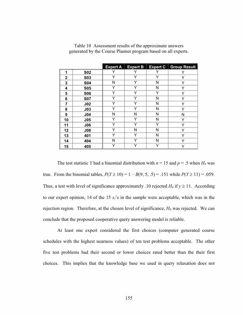
Table 10 Assessment results of the approximate answers generated by the Course Planner program based on all experts.
Expert A Expert B Expert C Group Result1 S02 Y Y Y Y 2 S03 Y Y Y Y 3 S04 N Y N Y 4 S05 Y Y N Y 5 S06 Y Y Y Y 6 S07 Y Y N Y 7 J02 Y Y N Y 8 J03 Y Y N Y 9 J04 N N N N 10 J05 Y Y N Y 11 J06 Y Y Y Y 12 J08 Y N N Y 13 401 Y Y N Y 14 404 N Y N Y 15 405 Y Y Y Y
The test statistic Y had a binomial distribution with n = 15 and p = .5 when H0 was
true. From the binomial tables, P(Y ≥ 10) = 1 – B(9; 5, .5) = .151 while P(Y ≥ 11) = .059.
Thus, a test with level of significance approximately .10 rejected H0 if y ≥ 11. According
to our expert opinion, 14 of the 15 xi’s in the sample were acceptable, which was in the
rejection region. Therefore, at the chosen level of significance, H0 was rejected. We can
conclude that the proposed cooperative query answering model is reliable.
At least one expert considered the first choices (computer generated course
schedules with the highest nearness values) of ten test problems acceptable. The other
five test problems had their second or lower choices rated better than the their first
choices. This implies that the knowledge base we used in query relaxation does not
155

match perfectly with those of the experts. The result also shows that different experts
have diverse preferences.
To close the gap between the system’s knowledge base and the experts’
experience, one can share the computer-constructed neighbor hierarchies with the experts
and modify those hierarchies based on experts’ feedback. However, if several experts are
involved, it is very likely that experts’ opinions will both conflict and concur among each
other. One needs to combine those experts’ opinions using techniques such as Delphi
method, which could raise the complexity level of knowledge base construction.
Alternatively, one can qualify experts with a set of preliminary test problems.
Disqualifying experts who have knowledge or criteria apart from others (i.e. Expert C in
our case study) can help reduce the complexity of knowledge construction.
In this research, we accept such dissimilarity because 1) it is a nature of a
knowledge base to be sensitive to its developers and/or users, and 2) the difference is
converged and acceptable based on the result of our analysis.
156

9.0 CONCLUSIONS AND FUTURE WORK
9.1 Conclusions
In this paper, we have introduced new approaches for neighbor hierarchy
construction and query relaxations that overcome the limitations of the traditional
intelligent database systems. Query relaxation techniques have been extended to allow
attribute and relation substitutions, relaxations of complex queries and simultaneous
multiple condition relaxations. Such capabilities are achieved through constructing
neighbor hierarchies at the attribute level (rather the tuple level), the ability to relax
multiple query conditions simultaneously, and an appropriate nearness calculation
function.
We have presented techniques necessary for developing neighbor hierarchies at
the attribute level. The Modified Pattern-based Knowledge Induction technique allows
construction of neighbor hierarchies for non-unique attributes based upon confidences,
popularities, and correlations of relationships among attribute values. The technique is
capable of clustering both discrete and continuous attribute values. Modified PKI is not
limited to numerical attribute values. It works effectively with both numerical and string
values. We have demonstrated how the Modified DISC can be used for defining abstract
values and their actual value ranges for the Modified PKI.
We have defined three causes of null answers that are 1) null-bound conditions, 2)
empty qualified tuple set, and 3) empty intersected tuple set. The ability to identify the
157

causes of null allows the cooperative query answering system to relax null-bound queries
at the roots of the problems and deploys the most appropriate relaxation methods. In
summary, identifying the causes of null help make searching for approximate answers
more effective.
We have shown how multiple condition relaxations can be achieved through a
query relaxation algorithm called Next Maximum Nearness. Based on a greedy search
approach and the subsumption properties among relaxation options, Next Maximum
Nearness technique helps minimize number of relaxation options needed to be considered
at each query relaxation iteration. The algorithm also helps reduce computational time in
approximate answer searching.
A new approach for nearness calculations called Block Nearness is introduced.
Block Nearness makes it possible to determine nearness of approximate answers that
result from attribute value substitutions, attribute substitutions, and relation substitutions
as proposed in this paper.
Finally, we demonstrated that the proposed neighbor hierarchy construction and
query relaxation techniques were applicable for various types of hierarchical structure
information systems in general. We developed a cooperative query answering system for
study course scheduling tasks, called “Course Planner”, for the Department of Industrial
Engineering at University of Pittsburgh. Using the course Planner program, we
demonstrated the reliability of the proposed cooperative query answering model.
158

9.2 Future Work
We have introduced a cooperative query answering system that is capable of
handling jointed queries in this paper. However, there are other types of complex queries
that are beyond the scope of this research such as queries with OR operators in the
WHERE clauses and queries with aggregation functions (i.e. SUM(), COUNT(), MIN(),
MAX()). Such complex queries are commonly used in many domains including
manufacturing information systems.
A query with an OR operator in its WHERE clause is assessed as TRUE (or the
query returns some answers) when the selection conditions on either side of the OR is
evaluated as TRUE. Based on such fact, a cooperative query answering system only
needs to relax those queries by breaking down the entire query condition statements into
multiple groups of selection conditions using OR’s as the break points. Each of these
groups of selection conditions forms a sub-query, in which the selection conditions are
connected with only AND operators. If the system can find approximate answers for any
sub-query, the approximate answers are the answers to the original query as well.
Furthermore, we can utilize the subsumption property to eliminate any sub-queries that
subsume other sub-queries to improve the computational times of query relaxations.
The values returned by many query aggregate functions tie strongly with the
number of the query’s qualified tuples. For example, the higher the number of the
qualified tuples, the higher the value returned from COUNT and MAX, and the lower the
value of MIN.
159
Consider the following query Q.
Q: “COUNT(FEATURE_NBR) = 10 AND WIDTH = 5”
Suppose that the query returns six tuples. (Thus, COUNT(FEATURE_NBR) = 6.) By
substituting the attribute value of the query condition “WIDTH = 5” with its neighbor set,
the query either returns the same set of answers or a new set of answers with a higher
number of tuples. Eventually, after some relaxation iterations, the value of
COUNT(FEATURE_NBR) will be equal or greater than ten. Using these relationships
between the number of the qualified tuples and the values returned by query aggregate
functions, the proposed query relaxation techniques may also be used to relax queries
with aggregate function in their WHERE clauses.
Query aggregate functions SUM and AVG are different from the three functions
mentioned earlier, since the values of SUM and AVG not only depend on the numbers of
tuples, but also tie to the domains of the attributes. The values of SUM and AVG are
proportional to the number of tuples only when the domain of the attribute is a set of all
positive or all negative values.
Also, we have assumed that all query selection conditions do not have any
dependency among each other. Although the assumption is generally true and helps ease
the complexities of query relaxations, considerations of query condition dependencies are
useful when relation substitutions are carried out on joint queries between super-classes
and their sub-classes. As illustrated in part scheme example in Chapter 2, when relation
GROOVE is replaced with relation HOLE, not only must the attributes in the selection
conditions of GROOVE be changed to those of HOLE, but also must the selection
160
conditions on the sub-class of relation GROOVE, relation SQR_GROOVE be substituted
by those of relation SQR_HOLE to reflect the super-class - sub-class relationships.
These types of chain effects resulted from the dependencies between query conditions are
essential for sustaining the logic of the original query and the “super-class–sub-class”
structure. Such types of relationships, which could be indicated in the meta-model of the
database, can be used as the basis for query condition dependencies checking. The
relationship type between any two relations – association, aggregation, generalization,
and category – dictates whether there should be any dependencies between the query
conditions of the query. Once the relationship type is determined and condition
dependencies are identified, relation and attribute substitution of the dependant
conditions can be performed accordingly.
Another assumption adopted in this research is that correlations between attributes
do exist. This assumption is used in our Modified Pattern-based Knowledge Induction
technique. Such assumption allows us to derive patterns that imply relationship between
any two inter-attribute values. Including or excluding any attribute(s) in the table when
one attempts to construct a neighbor hierarchy for values in an attribute does affect the
nearness value assigned to each neighbor node. Therefore, attribute correlations and the
effect of adding or removing attribute in neighbor hierarchy construction must be further
investigated and characterized.
To construct neighbor hierarchies, solely the Modified Pattern-based Knowledge
Induction technique may not produce perfect or close to perfect results as mentioned in
the Validation chapter. Incorporating expert intelligence with the computer generated
161

knowledge can improve the results generated by the cooperative query answering system.
Another means to improve approximate answers is to consider decision rules when query
relaxation is carried out. In case of the Course Planner program, for example, rules such
as 1) good course schedules must not suggest students to skip any fall or spring
semesters, 2) students should not register for less than four classes in any semesters
except summer semesters. Such rules can help filter out course schedules that would not
be recommended by any advisors. Although these considerations are beyond our
research focus, more study on the effect of incorporating human intelligence and rules on
neighbor hierarchy constructions and query relaxations must be conducted.
Evidently, cooperative query answering increases the usefulness of a typical
database system. But such usefulness is obtained at a cost. Developing and
implementing the concept on a database system requires additional resources – funding,
manpower, and time. Therefore, one must weigh the development costs against the
benefits when choosing whether to add cooperative query answering capability to a
database system.
Finally, the applications of the proposed cooperative query answering concept in
Internet searching is a wonderful research opportunity. The emerging Resource
Description Framework (RDF) provides a promising mechanism for the development of
the semantic web.(100) In summary, RDF allows developers to describe resources on the
web using metadata. For example, RDF schemas can be used to define “author” and
“writer”. Another RDF schema may be created to describe “person” and how it relates to
the author schema and the writer schema. An RDF schema can be a Generalized Schema
162

or a Specialized Schema. This concept of RDF helps create ontology that defines
relationships between various schemas and is the key component that allows us to share
common knowledge in a domain of interest in the vast space of the electronic information
world. It is considered critical for semantic interoperability on the Web. With RDF,
developers can define and relate their web pages (or the contents of their web pages) with
others in an easier and more effective fashion.
However semantic web searching not only requires a successful implementation
of RDF, but it also needs software tools or agents that are capable of inferring the
hierarchical schema of those RDF element descriptions. Since element descriptions in
RDF are connected to each other via association, generalization and specialization
relationships similar to how objects (attribute values, attributes, and relations) are related
in our cooperative query answering concept, we believe that using the proposed
approximate answer search and the RDF concept is a strong combination and a definite
possibility.
163

APPENDIX A

C:\Documents and Settings\ff418\My Wednesday, July 17, 2002 Documents\Works\Personal\ClassPlanPROD.mdb Table: COURSE_HUMAN_PROD Page: 1
Columns Name Type Size COURSE_NO Text 255 Subject Text 50 Credits Text 50 Term_Offered Text 50 TDAY Text 255 time Text 255
C:\Documents and Settings\ff418\My Wednesday, July 17, 2002 Documents\Works\Personal\ClassPlanPROD.mdb Table: COURSE_IE_REQ_PROD Page: 2
Columns Name Type Size COURSE_NO Text 255 Subject Text 50 Credits Text 50 Term_Offered Text 50 TDAY Text 255 time Text 255
C:\Documents and Settings\ff418\My Wednesday, July 17, 2002 Documents\Works\Personal\ClassPlanPROD.mdb Table: IE_PLAN Page: 3
Columns Name Type Size PLAN_ID Text 255 01ER Text 255 01IG Text 255 01LL Text 255 02ER Text 255 02IG Text 255 02LL Text 255 03ER Text 255 03IG Text 255 03LL Text 255 04ER Text 255 04IG Text 255 04LL Text 255 05ER Text 255 05IG Text 255 05LL Text 255
165

06ER Text 255 06IG Text 255 06LL Text 255 07ER Text 255 07IG Text 255 07LL Text 255 PLAN_ID0025 Text 255 PBUSERV 1925 Text 255 PCHEM 0960 Text 255 PCHEM 0970 Text 255 PENGR 0011 Text 255 PENGR 0012 Text 255 PENGR 0020 Text 255 PENGR 0022 Text 255 PENGR 0081 Text 255 PENGR 0082 Text 255 PENGR 0135 Text 255 PENGR 1010 Text 255 PENGR 1869 Text 255 PHUM&SOC SCI-1 Text 255 PHUM&SOC SCI-2 Text 255 PHUM&SOC SCI-3 Text 255 PHUM&SOC SCI-4 Text 255 PHUM&SOC SCI-5 Text 255 PHUM&SOC SCI-6 Text 255 PIE 0015 Text 255 PIE 1021 Text 255 PIE 1035 Text 255 PIE 1040 Text 255 PIE 1051 Text 255 PIE 1052 Text 255 PIE 1054 Text 255 PIE 1056 Text 255
C:\Documents and Settings\ff418\My Wednesday, July 17, 2002 Documents\Works\Personal\ClassPlanPROD.mdb Table: IE_PLAN Page: 4 PIE 1061 Text 255 PIE 1071 Text 255 PIE 1081 Text 255 PIE 1083 Text 255 PIE 1085-1 Text 255 PIE 1085-2 Text 255 PIE 1085-3 Text 255 PIE 1085-4 Text 255 PIE 1085-5 Text 255 PIE 1085-6 Text 255 PIE 1090 Text 255 PMATH 0220 Text 255 PMATH 0230 Text 255 PMATH 0240 Text 255 PMATH 0250 Text 255 PPHYS 0104 Text 255 PPHYS 0105 Text 255 PPHYS 0106 Text 255 PTECH ELECTIVE-1 Text 255 PTECH ELECTIVE-2 Text 255 PTECH ELECTIVE-3 Text 255 PTECH ELECTIVE-4 Text 255
166

C:\Documents and Settings\ff418\My Wednesday, July 17, 2002 Documents\Works\Personal\ClassPlanPROD.mdb Table: IE_PLAN_COURSE Page: 5
Columns Name Type Size PLAN_ID Text 255 PTERMINV Text 255 CURR_CNUM Text 50 TCNUM Text 20
C:\Documents and Settings\ff418\My Wednesday, July 17, 2002 Documents\Works\Personal\ClassPlanPROD.mdb Table: IE_PLAN_TERM Page: 6
Columns Name Type Size PLAN_ID Text 255 PTERMINV Text 255 PY_NO Long Integer 4 PT_NO Text 255 FL_LEFT Double 8 SP_LEFT Double 8 SR_LEFT Double 8 TBUSERV 1925 Text 255 TCHEM 0960 Text 255 TCHEM 0970 Text 255 TCO-OP-1 Text 255 TCO-OP-2 Text 255 TCO-OP-3 Text 255 TENGR 0011 Text 255 TENGR 0012 Text 255 TENGR 0020 Text 255 TENGR 0022 Text 255 TENGR 0081 Text 255 TENGR 0082 Text 255 TENGR 0135 Text 255 TENGR 1010 Text 255 TENGR 1869 Text 255 THUM&SOC SCI-1 Text 255 THUM&SOC SCI-2 Text 255 THUM&SOC SCI-3 Text 255 THUM&SOC SCI-4 Text 255 THUM&SOC SCI-5 Text 255 THUM&SOC SCI-6 Text 255 TIE 0015 Text 255 TIE 1021 Text 255 TIE 1035 Text 255 TIE 1040 Text 255 TIE 1051 Text 255 TIE 1052 Text 255 TIE 1054 Text 255
167

TIE 1056 Text 255 TIE 1061 Text 255 TIE 1071 Text 255 TIE 1081 Text 255 TIE 1083 Text 255 TIE 1085-1 Text 255 TIE 1085-2 Text 255 TIE 1085-3 Text 255 TIE 1085-4 Text 255 TIE 1085-5 Text 255 TIE 1085-6 Text 255 TIE 1090 Text 255 TMATH 0220 Text 255 TMATH 0230 Text 255
C:\Documents and Settings\ff418\My Wednesday, July 17, 2002 Documents\Works\Personal\ClassPlanPROD.mdb Table: IE_PLAN_TERM Page: 7 TMATH 0240 Text 255 TMATH 0250 Text 255 TPHYS 0104 Text 255 TPHYS 0105 Text 255 TPHYS 0106 Text 255 TTECH ELECTIVE-1 Text 255 TTECH ELECTIVE-2 Text 255 TTECH ELECTIVE-3 Text 255 TTECH ELECTIVE-4 Text 255
C:\Documents and Settings\ff418\My Wednesday, July 17, 2002 Documents\Works\Personal\ClassPlanPROD.mdb Table: PRGSS_PLAN Page: 8
Columns Name Type Size STUPROGSS_ID Long Integer 4 SSN Text 11 SNAME Text 25 PID Text 255 RNUM Integer 2 CNUM Text 20 TCNUM Text 20 GRADE Text 2 TERMNO Long Integer 4 CCREDITS Byte 1
C:\Documents and Settings\ff418\My Wednesday, July 17, 2002 Documents\Works\Personal\ClassPlanPROD.mdb Table: PRGSS_STUDENT Page: 9
Columns
168

Name Type Size STUPROGSS_ID Long Integer 4 SSN Text 11 SNAME Text 25 PID Text 255 RNUM Integer 2 CNUM Text 20 TCNUM Text 50 GRADE Text 2 TERMNO Long Integer 4 CCREDITS Byte 1
C:\Documents and Settings\ff418\My Wednesday, July 17, 2002 Documents\Works\Personal\ClassPlanPROD.mdb Query: Q_PLAN_0010 Page: 10
SQL SELECT [PRGSS_PLAN].[SSN] AS SSN0010, Min(IIf([TERMNO]=0,Null,Left([TERMNO],4))) AS FIRST_TERM FROM PRGSS_PLAN
Columns Name Type Size SSN0010 Text 11 FIRST_TERM Text 0
C:\Documents and Settings\ff418\My Wednesday, July 17, 2002 Documents\Works\Personal\ClassPlanPROD.mdb Query: Q_PLAN_0015 Page: 11
SQL SELECT [PRGSS_PLAN].[SSN] AS SSN0015, Max(IIf([TERMNO]=0,Null,Left([TERMNO],4))) AS LAST_YEAR FROM PRGSS_PLAN
Columns Name Type Size SSN0015 Text 11 LAST_YEAR Text 0
C:\Documents and Settings\ff418\My Wednesday, July 17, 2002 Documents\Works\Personal\ClassPlanPROD.mdb
169
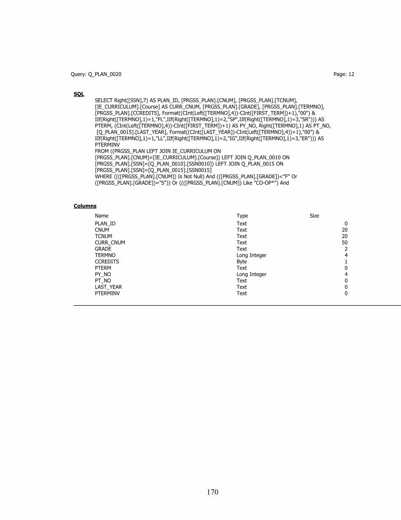
Query: Q_PLAN_0020 Page: 12
SQL SELECT Right([SSN],7) AS PLAN_ID, [PRGSS_PLAN].[CNUM], [PRGSS_PLAN].[TCNUM], [IE_CURRICULUM].[Course] AS CURR_CNUM, [PRGSS_PLAN].[GRADE], [PRGSS_PLAN].[TERMNO], [PRGSS_PLAN].[CCREDITS], Format((CInt(Left([TERMNO],4))-CInt([FIRST_TERM])+1),"00") & IIf(Right([TERMNO],1)=1,"FL",IIf(Right([TERMNO],1)=2,"SP",IIf(Right([TERMNO],1)=3,"SR"))) AS PTERM, (CInt(Left([TERMNO],4))-CInt([FIRST_TERM])+1) AS PY_NO, Right([TERMNO],1) AS PT_NO, [Q_PLAN_0015].[LAST_YEAR], Format((CInt([LAST_YEAR])-CInt(Left([TERMNO],4))+1),"00") & IIf(Right([TERMNO],1)=1,"LL",IIf(Right([TERMNO],1)=2,"IG",IIf(Right([TERMNO],1)=3,"ER"))) AS PTERMINV FROM ((PRGSS_PLAN LEFT JOIN IE_CURRICULUM ON [PRGSS_PLAN].[CNUM]=[IE_CURRICULUM].[Course]) LEFT JOIN Q_PLAN_0010 ON [PRGSS_PLAN].[SSN]=[Q_PLAN_0010].[SSN0010]) LEFT JOIN Q_PLAN_0015 ON [PRGSS_PLAN].[SSN]=[Q_PLAN_0015].[SSN0015] WHERE ((([PRGSS_PLAN].[CNUM]) Is Not Null) And (([PRGSS_PLAN].[GRADE])<"F" Or ([PRGSS_PLAN].[GRADE])="S")) Or ((([PRGSS_PLAN].[CNUM]) Like "CO-OP*") And
Columns Name Type Size PLAN_ID Text 0 CNUM Text 20 TCNUM Text 20 CURR_CNUM Text 50 GRADE Text 2 TERMNO Long Integer 4 CCREDITS Byte 1 PTERM Text 0 PY_NO Long Integer 4 PT_NO Text 0 LAST_YEAR Text 0 PTERMINV Text 0
170
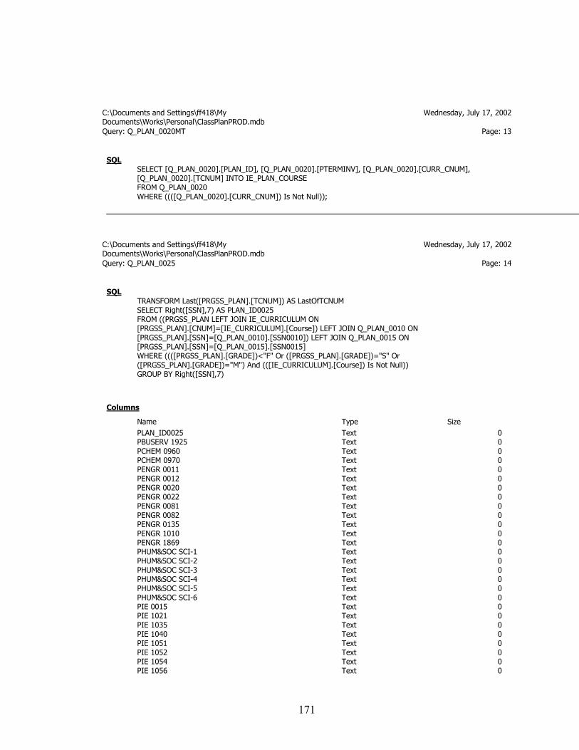
C:\Documents and Settings\ff418\My Wednesday, July 17, 2002 Documents\Works\Personal\ClassPlanPROD.mdb Query: Q_PLAN_0020MT Page: 13
SQL SELECT [Q_PLAN_0020].[PLAN_ID], [Q_PLAN_0020].[PTERMINV], [Q_PLAN_0020].[CURR_CNUM], [Q_PLAN_0020].[TCNUM] INTO IE_PLAN_COURSE FROM Q_PLAN_0020 WHERE ((([Q_PLAN_0020].[CURR_CNUM]) Is Not Null));
C:\Documents and Settings\ff418\My Wednesday, July 17, 2002 Documents\Works\Personal\ClassPlanPROD.mdb Query: Q_PLAN_0025 Page: 14
SQL TRANSFORM Last([PRGSS_PLAN].[TCNUM]) AS LastOfTCNUM SELECT Right([SSN],7) AS PLAN_ID0025 FROM ((PRGSS_PLAN LEFT JOIN IE_CURRICULUM ON [PRGSS_PLAN].[CNUM]=[IE_CURRICULUM].[Course]) LEFT JOIN Q_PLAN_0010 ON [PRGSS_PLAN].[SSN]=[Q_PLAN_0010].[SSN0010]) LEFT JOIN Q_PLAN_0015 ON [PRGSS_PLAN].[SSN]=[Q_PLAN_0015].[SSN0015] WHERE ((([PRGSS_PLAN].[GRADE])<"F" Or ([PRGSS_PLAN].[GRADE])="S" Or ([PRGSS_PLAN].[GRADE])="M") And (([IE_CURRICULUM].[Course]) Is Not Null)) GROUP BY Right([SSN],7)
Columns Name Type Size PLAN_ID0025 Text 0 PBUSERV 1925 Text 0 PCHEM 0960 Text 0 PCHEM 0970 Text 0 PENGR 0011 Text 0 PENGR 0012 Text 0 PENGR 0020 Text 0 PENGR 0022 Text 0 PENGR 0081 Text 0 PENGR 0082 Text 0 PENGR 0135 Text 0 PENGR 1010 Text 0 PENGR 1869 Text 0 PHUM&SOC SCI-1 Text 0 PHUM&SOC SCI-2 Text 0 PHUM&SOC SCI-3 Text 0 PHUM&SOC SCI-4 Text 0 PHUM&SOC SCI-5 Text 0 PHUM&SOC SCI-6 Text 0 PIE 0015 Text 0 PIE 1021 Text 0 PIE 1035 Text 0 PIE 1040 Text 0 PIE 1051 Text 0 PIE 1052 Text 0 PIE 1054 Text 0 PIE 1056 Text 0
171

PIE 1061 Text 0 PIE 1071 Text 0 PIE 1081 Text 0 PIE 1083 Text 0 PIE 1085-1 Text 0 PIE 1085-2 Text 0 PIE 1085-3 Text 0 PIE 1085-4 Text 0 PIE 1085-5 Text 0 PIE 1085-6 Text 0 PIE 1090 Text 0 PMATH 0220 Text 0
C:\Documents and Settings\ff418\My Wednesday, July 17, 2002 Documents\Works\Personal\ClassPlanPROD.mdb Query: Q_PLAN_0025 Page: 15 PMATH 0230 Text 0 PMATH 0240 Text 0 PMATH 0250 Text 0 PPHYS 0104 Text 0 PPHYS 0105 Text 0 PPHYS 0106 Text 0 PTECH ELECTIVE-1 Text 0 PTECH ELECTIVE-2 Text 0 PTECH ELECTIVE-3 Text 0 PTECH ELECTIVE-4 Text 0
C:\Documents and Settings\ff418\My Wednesday, July 17, 2002 Documents\Works\Personal\ClassPlanPROD.mdb Query: Q_PLAN_0030 Page: 16
SQL TRANSFORM Max(IIf(IsNull([PTERMINV]),"-",IIf([CNUM] Like "CO-OP*","W","C"))) AS REGIS SELECT [Q_PLAN_0020].[PLAN_ID] FROM Q_PLAN_0020 GROUP BY [Q_PLAN_0020].[PLAN_ID] PIVOT [Q_PLAN_0020].[PTERMINV];
Columns Name Type Size PLAN_ID Text 0 01ER Text 0 01IG Text 0 01LL Text 0 02ER Text 0 02IG Text 0 02LL Text 0 03ER Text 0 03IG Text 0 03LL Text 0 04ER Text 0 04IG Text 0 04LL Text 0
172
05ER Text 0 05IG Text 0 05LL Text 0 06ER Text 0 06IG Text 0 06LL Text 0 07ER Text 0 07IG Text 0 07LL Text 0
C:\Documents and Settings\ff418\My Wednesday, July 17, 2002 Documents\Works\Personal\ClassPlanPROD.mdb Query: Q_PLAN_0035 Page: 17
SQL SELECT Q_PLAN_0030.*, Q_PLAN_0025.* FROM Q_PLAN_0030 INNER JOIN Q_PLAN_0025 ON [Q_PLAN_0030].[PLAN_ID]=[Q_PLAN_0025].[PLAN_ID0025];
Columns Name Type Size PLAN_ID Text 0 01ER Text 0 01IG Text 0 01LL Text 0 02ER Text 0 02IG Text 0 02LL Text 0 03ER Text 0 03IG Text 0 03LL Text 0 04ER Text 0 04IG Text 0 04LL Text 0 05ER Text 0 05IG Text 0 05LL Text 0 06ER Text 0 06IG Text 0 06LL Text 0 07ER Text 0 07IG Text 0 07LL Text 0 PLAN_ID0025 Text 0 PBUSERV 1925 Text 0 PCHEM 0960 Text 0 PCHEM 0970 Text 0 PENGR 0011 Text 0 PENGR 0012 Text 0 PENGR 0020 Text 0 PENGR 0022 Text 0 PENGR 0081 Text 0 PENGR 0082 Text 0 PENGR 0135 Text 0 PENGR 1010 Text 0 PENGR 1869 Text 0
173

PHUM&SOC SCI-1 Text 0 PHUM&SOC SCI-2 Text 0 PHUM&SOC SCI-3 Text 0 PHUM&SOC SCI-4 Text 0 PHUM&SOC SCI-5 Text 0 PHUM&SOC SCI-6 Text 0 PIE 0015 Text 0 PIE 1021 Text 0 PIE 1035 Text 0
C:\Documents and Settings\ff418\My Wednesday, July 17, 2002 Documents\Works\Personal\ClassPlanPROD.mdb Query: Q_PLAN_0035 Page: 18 PIE 1040 Text 0 PIE 1051 Text 0 PIE 1052 Text 0 PIE 1054 Text 0 PIE 1056 Text 0 PIE 1061 Text 0 PIE 1071 Text 0 PIE 1081 Text 0 PIE 1083 Text 0 PIE 1085-1 Text 0 PIE 1085-2 Text 0 PIE 1085-3 Text 0 PIE 1085-4 Text 0 PIE 1085-5 Text 0 PIE 1085-6 Text 0 PIE 1090 Text 0 PMATH 0220 Text 0 PMATH 0230 Text 0 PMATH 0240 Text 0 PMATH 0250 Text 0 PPHYS 0104 Text 0 PPHYS 0105 Text 0 PPHYS 0106 Text 0 PTECH ELECTIVE-1 Text 0 PTECH ELECTIVE-2 Text 0 PTECH ELECTIVE-3 Text 0 PTECH ELECTIVE-4 Text 0
C:\Documents and Settings\ff418\My Wednesday, July 17, 2002 Documents\Works\Personal\ClassPlanPROD.mdb Query: Q_PLAN_0035_CQAMT Page: 19
SQL SELECT [Q_PLAN_0035].[01ER], [Q_PLAN_0035].[01IG], [Q_PLAN_0035].[01LL], [Q_PLAN_0035].[02ER], [Q_PLAN_0035].[02IG], [Q_PLAN_0035].[02LL], [Q_PLAN_0035].[03ER], [Q_PLAN_0035].[03IG], [Q_PLAN_0035].[03LL], [Q_PLAN_0035].[04IG], [Q_PLAN_0035].[04LL], [Q_PLAN_0035].[05ER], [Q_PLAN_0035].[05IG], [Q_PLAN_0035].[05LL], [Q_PLAN_0035].[06ER], [Q_PLAN_0035].[06IG], [Q_PLAN_0035].[06LL], [Q_PLAN_0035].[07ER], [Q_PLAN_0035].[07IG], [Q_PLAN_0035].[07LL] INTO IE_PLAN_CQA FROM Q_PLAN_0035;
174

C:\Documents and Settings\ff418\My Wednesday, July 17, 2002 Documents\Works\Personal\ClassPlanPROD.mdb Query: Q_PLAN_0035MT Page: 20
SQL SELECT Q_PLAN_0035.* INTO IE_PLAN FROM Q_PLAN_0035;
C:\Documents and Settings\ff418\My Wednesday, July 17, 2002 Documents\Works\Personal\ClassPlanPROD.mdb Query: Q_PLAN_0040 Page: 21
SQL SELECT [Q_PLAN_0020].[PLAN_ID], [Q_PLAN_0020].[PTERMINV], [Q_PLAN_0020].[PTERM], [Q_PLAN_0020].[PY_NO], [Q_PLAN_0020].[PT_NO] FROM Q_PLAN_0020 GROUP BY [Q_PLAN_0020].[PLAN_ID], [Q_PLAN_0020].[PTERMINV], [Q_PLAN_0020].[PTERM], [Q_PLAN_0020].[PY_NO], [Q_PLAN_0020].[PT_NO] ORDER BY [Q_PLAN_0020].[PLAN_ID], [Q_PLAN_0020].[PTERMINV], [Q_PLAN_0020].[PTERM];
Columns Name Type Size PLAN_ID Text 0 PTERMINV Text 0 PTERM Text 0 PY_NO Long Integer 4 PT_NO Text 0
C:\Documents and Settings\ff418\My Wednesday, July 17, 2002 Documents\Works\Personal\ClassPlanPROD.mdb Query: Q_PLAN_0050 Page: 22
SQL SELECT A.PLAN_ID, A.PTERMINV, A.PTERM, A.PY_NO, A.PT_NO, B.PTERM, B.PY_NO, B.PT_NO FROM Q_PLAN_0040 AS A INNER JOIN Q_PLAN_0040 AS B ON A.PLAN_ID=B.PLAN_ID
Columns Name Type Size PLAN_ID Text 0 PTERMINV Text 0 A.PTERM Text 0 A.PY_NO Long Integer 4 A.PT_NO Text 0 B.PTERM Text 0 B.PY_NO Long Integer 4
175
B.PT_NO Text 0
C:\Documents and Settings\ff418\My Wednesday, July 17, 2002 Documents\Works\Personal\ClassPlanPROD.mdb Query: Q_PLAN_0060 Page: 23
SQL SELECT Q_PLAN_0040.*, [Q_PLAN_0050].B.PTERM, [Q_PLAN_0050].B.PY_NO, [Q_PLAN_0050].B.PT_NO FROM Q_PLAN_0040 LEFT JOIN Q_PLAN_0050 ON
Columns Name Type Size PLAN_ID Text 0 PTERMINV Text 0 Q_PLAN_0040.PTERM Text 0 Q_PLAN_0040.PY_NO Long Integer 4 Q_PLAN_0040.PT_NO Text 0 B.PTERM Text 0 B.PY_NO Long Integer 4 B.PT_NO Text 0
C:\Documents and Settings\ff418\My Wednesday, July 17, 2002 Documents\Works\Personal\ClassPlanPROD.mdb Query: Q_PLAN_0070 Page: 24
SQL SELECT [Q_PLAN_0060].[PLAN_ID], [Q_PLAN_0060].[PTERMINV], [Q_PLAN_0060].Q_PLAN_0040.PTERM AS PTERM, [Q_PLAN_0060].Q_PLAN_0040.PY_NO AS PY_NO, [Q_PLAN_0060].Q_PLAN_0040.PT_NO AS PT_NO, Sum(IIf(B.PT_NO="1",1,0)) AS FL_LEFT, Sum(IIf(B.PT_NO="2",1,0)) AS SP_LEFT, Sum(IIf(B.PT_NO="3",1,0)) AS SR_LEFT FROM Q_PLAN_0060 GROUP BY [Q_PLAN_0060].[PLAN_ID], [Q_PLAN_0060].[PTERMINV], [Q_PLAN_0060].Q_PLAN_0040.PTERM, [Q_PLAN_0060].Q_PLAN_0040.PY_NO,
Columns Name Type Size PLAN_ID Text 0 PTERMINV Text 0 PTERM Text 0 PY_NO Long Integer 4 PT_NO Text 0 FL_LEFT Double 8 SP_LEFT Double 8 SR_LEFT Double 8
176
C:\Documents and Settings\ff418\My Wednesday, July 17, 2002 Documents\Works\Personal\ClassPlanPROD.mdb Query: Q_PLAN_0080 Page: 25
SQL TRANSFORM Last(IIf(IsNull([CURR_CNUM]),"-","NOT YET")) AS TOKEN SELECT [Q_PLAN_0070].[PLAN_ID], [Q_PLAN_0070].[PTERMINV], [Q_PLAN_0070].[PY_NO], [Q_PLAN_0070].[PT_NO], [Q_PLAN_0070].[FL_LEFT], [Q_PLAN_0070].[SP_LEFT], [Q_PLAN_0070].[SR_LEFT] FROM Q_PLAN_0070 INNER JOIN Q_PLAN_0020 ON [Q_PLAN_0070].[PLAN_ID]=[Q_PLAN_0020].[PLAN_ID] WHERE ((([Q_PLAN_0020].[PTERM])>[Q_PLAN_0070]![PTERM]) And (([Q_PLAN_0020].[CURR_CNUM]) Is Not Null)) GROUP BY [Q_PLAN_0070].[PLAN_ID], [Q_PLAN_0070].[PTERMINV], [Q_PLAN_0070].[PY_NO], [Q_PLAN_0070].[PT_NO], [Q_PLAN_0070].[FL_LEFT], [Q_PLAN_0070].[SP_LEFT], [Q_PLAN_0070].[SR_LEFT] ORDER BY [Q_PLAN_0070].[PLAN_ID], [Q_PLAN_0070].[PTERMINV]
Columns Name Type Size PLAN_ID Text 0 PTERMINV Text 0 PY_NO Long Integer 4 PT_NO Text 0 FL_LEFT Double 8 SP_LEFT Double 8 SR_LEFT Double 8 TBUSERV 1925 Text 0 TCHEM 0960 Text 0 TCHEM 0970 Text 0 TCO-OP-1 Text 0 TCO-OP-2 Text 0 TCO-OP-3 Text 0 TENGR 0011 Text 0 TENGR 0012 Text 0 TENGR 0020 Text 0 TENGR 0022 Text 0 TENGR 0081 Text 0 TENGR 0082 Text 0 TENGR 0135 Text 0 TENGR 1010 Text 0 TENGR 1869 Text 0 THUM&SOC SCI-1 Text 0 THUM&SOC SCI-2 Text 0 THUM&SOC SCI-3 Text 0 THUM&SOC SCI-4 Text 0 THUM&SOC SCI-5 Text 0 THUM&SOC SCI-6 Text 0 TIE 0015 Text 0 TIE 1021 Text 0 TIE 1035 Text 0 TIE 1040 Text 0 TIE 1051 Text 0 TIE 1052 Text 0 TIE 1054 Text 0 TIE 1056 Text 0
177
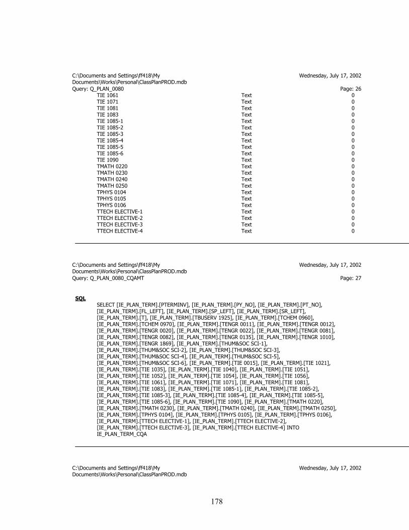
C:\Documents and Settings\ff418\My Wednesday, July 17, 2002 Documents\Works\Personal\ClassPlanPROD.mdb Query: Q_PLAN_0080 Page: 26 TIE 1061 Text 0 TIE 1071 Text 0 TIE 1081 Text 0 TIE 1083 Text 0 TIE 1085-1 Text 0 TIE 1085-2 Text 0 TIE 1085-3 Text 0 TIE 1085-4 Text 0 TIE 1085-5 Text 0 TIE 1085-6 Text 0 TIE 1090 Text 0 TMATH 0220 Text 0 TMATH 0230 Text 0 TMATH 0240 Text 0 TMATH 0250 Text 0 TPHYS 0104 Text 0 TPHYS 0105 Text 0 TPHYS 0106 Text 0 TTECH ELECTIVE-1 Text 0 TTECH ELECTIVE-2 Text 0 TTECH ELECTIVE-3 Text 0 TTECH ELECTIVE-4 Text 0
C:\Documents and Settings\ff418\My Wednesday, July 17, 2002 Documents\Works\Personal\ClassPlanPROD.mdb Query: Q_PLAN_0080_CQAMT Page: 27
SQL SELECT [IE_PLAN_TERM].[PTERMINV], [IE_PLAN_TERM].[PY_NO], [IE_PLAN_TERM].[PT_NO], [IE_PLAN_TERM].[FL_LEFT], [IE_PLAN_TERM].[SP_LEFT], [IE_PLAN_TERM].[SR_LEFT], [IE_PLAN_TERM].[T], [IE_PLAN_TERM].[TBUSERV 1925], [IE_PLAN_TERM].[TCHEM 0960], [IE_PLAN_TERM].[TCHEM 0970], [IE_PLAN_TERM].[TENGR 0011], [IE_PLAN_TERM].[TENGR 0012], [IE_PLAN_TERM].[TENGR 0020], [IE_PLAN_TERM].[TENGR 0022], [IE_PLAN_TERM].[TENGR 0081], [IE_PLAN_TERM].[TENGR 0082], [IE_PLAN_TERM].[TENGR 0135], [IE_PLAN_TERM].[TENGR 1010], [IE_PLAN_TERM].[TENGR 1869], [IE_PLAN_TERM].[THUM&SOC SCI-1], [IE_PLAN_TERM].[THUM&SOC SCI-2], [IE_PLAN_TERM].[THUM&SOC SCI-3], [IE_PLAN_TERM].[THUM&SOC SCI-4], [IE_PLAN_TERM].[THUM&SOC SCI-5], [IE_PLAN_TERM].[THUM&SOC SCI-6], [IE_PLAN_TERM].[TIE 0015], [IE_PLAN_TERM].[TIE 1021], [IE_PLAN_TERM].[TIE 1035], [IE_PLAN_TERM].[TIE 1040], [IE_PLAN_TERM].[TIE 1051], [IE_PLAN_TERM].[TIE 1052], [IE_PLAN_TERM].[TIE 1054], [IE_PLAN_TERM].[TIE 1056], [IE_PLAN_TERM].[TIE 1061], [IE_PLAN_TERM].[TIE 1071], [IE_PLAN_TERM].[TIE 1081], [IE_PLAN_TERM].[TIE 1083], [IE_PLAN_TERM].[TIE 1085-1], [IE_PLAN_TERM].[TIE 1085-2], [IE_PLAN_TERM].[TIE 1085-3], [IE_PLAN_TERM].[TIE 1085-4], [IE_PLAN_TERM].[TIE 1085-5], [IE_PLAN_TERM].[TIE 1085-6], [IE_PLAN_TERM].[TIE 1090], [IE_PLAN_TERM].[TMATH 0220], [IE_PLAN_TERM].[TMATH 0230], [IE_PLAN_TERM].[TMATH 0240], [IE_PLAN_TERM].[TMATH 0250], [IE_PLAN_TERM].[TPHYS 0104], [IE_PLAN_TERM].[TPHYS 0105], [IE_PLAN_TERM].[TPHYS 0106], [IE_PLAN_TERM].[TTECH ELECTIVE-1], [IE_PLAN_TERM].[TTECH ELECTIVE-2], [IE_PLAN_TERM].[TTECH ELECTIVE-3], [IE_PLAN_TERM].[TTECH ELECTIVE-4] INTO IE_PLAN_TERM_CQA
C:\Documents and Settings\ff418\My Wednesday, July 17, 2002 Documents\Works\Personal\ClassPlanPROD.mdb
178

Query: Q_PLAN_0080MT Page: 28
SQL SELECT Q_PLAN_0080.* INTO IE_PLAN_TERM FROM Q_PLAN_0080;
C:\Documents and Settings\ff418\My Wednesday, July 17, 2002 Documents\Works\Personal\ClassPlanPROD.mdb Query: Q_PLAN_0090 Page: 29
SQL SELECT Q_PLAN_0020.PTERM FROM Q_PLAN_0020 GROUP BY Q_PLAN_0020.PTERM ORDER BY Q_PLAN_0020.PTERM;
Columns Name Type Size PTERM Text 0
179

APPENDIX B
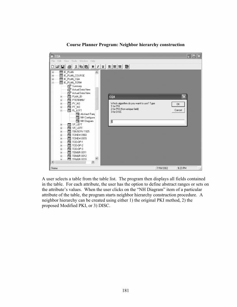
Course Planner Program: Neighbor hierarchy construction
A user selects a table from the table list. The program then displays all fields contained in the table. For each attribute, the user has the option to define abstract ranges or sets on the attribute’s values. When the user clicks on the “NH Diagram” item of a particular attribute of the table, the program starts neighbor hierarchy construction procedure. A neighbor hierarchy can be created using either 1) the original PKI method, 2) the proposed Modified PKI, or 3) DISC.
181
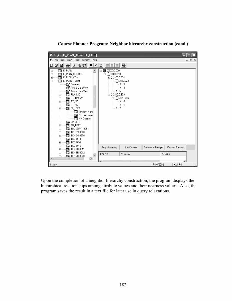
Course Planner Program: Neighbor hierarchy construction (cond.)
Upon the completion of a neighbor hierarchy construction, the program displays the hierarchical relationships among attribute values and their nearness values. Also, the program saves the result in a text file for later use in query relaxations.
182
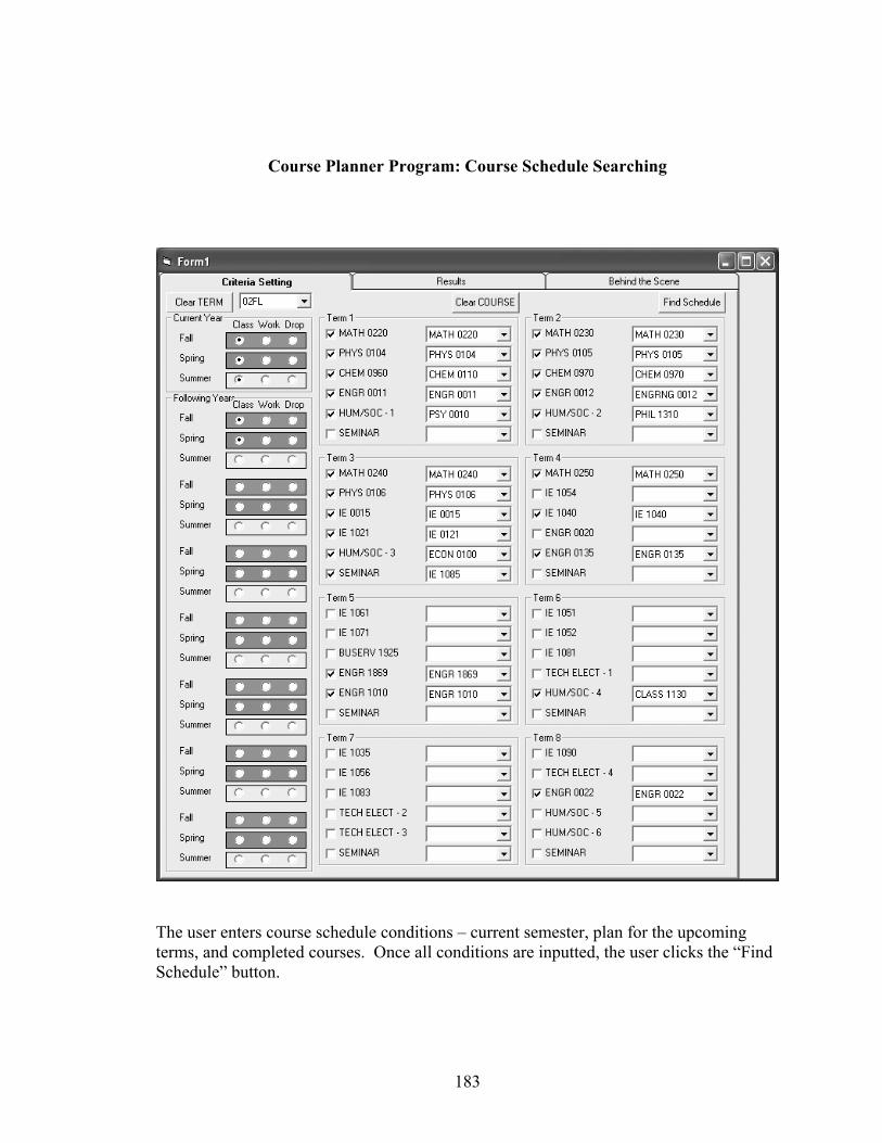
Course Planner Program: Course Schedule Searching
The user enters course schedule conditions – current semester, plan for the upcoming terms, and completed courses. Once all conditions are inputted, the user clicks the “Find Schedule” button.
183

The Course Planner Program converts the study plan conditions entered by the user into a corresponding SQL SELECT statement. SELECT IE_PLAN.PLAN_ID , [01IG], [01LL], [02ER], [02IG],[PMATH 0220],[PPHYS 0104],
[PCHEM 0960],[PENGR 0011],[PHUM&SOC SCI-1],[PMATH 0230],[PPHYS 0105], [PCHEM 0970],[PENGR 0012],[PHUM&SOC SCI-2],[PMATH 0240],[PPHYS 0106], [PIE 0015],[PIE 1021],[PHUM&SOC SCI-3],[PMATH 0250],[PIE 1040],[PENGR 0135], [PENGR 1869],[PENGR 1010],[PHUM&SOC SCI-4],[PENGR 0022], IE_PLAN_TERM.*
FROM IE_PLAN, IE_PLAN_TERM WHERE IE_PLAN.PLAN_ID=IE_PLAN_TERM.PLAN_ID AND
[01IG]='C' AND [01LL]='C' AND [02ER]='C' AND [02IG]='C' AND FL_LEFT =1 AND SP_LEFT =2 AND SR_LEFT =1 AND PTERMINV ='02LL' AND [TMATH 0220]='-' AND [PMATH 0220]='MATH 0220' AND [TPHYS 0104]='-' AND [PPHYS 0104]='PHYS 0104' AND [TCHEM 0960]='-' AND [PCHEM 0960]='CHEM 0110' AND [TENGR 0011]='-' AND [PENGR 0011]='ENGR 0011' AND [THUM&SOC SCI-1]='-' AND [PHUM&SOC SCI-1]='PSY 0010' AND [TMATH 0230]='-' AND [PMATH 0230]='MATH 0230' AND [TPHYS 0105]='-' AND [PPHYS 0105]='PHYS 0105' AND [TCHEM 0970]='-' AND [PCHEM 0970]='CHEM 0970' AND [TENGR 0012]='-' AND [PENGR 0012]='ENGRNG 0012' AND [THUM&SOC SCI-2]='-' AND [PHUM&SOC SCI-2]='PHIL 1310' AND [TMATH 0240]='-' AND [PMATH 0240]='MATH 0240' AND [TPHYS 0106]='-' AND [PPHYS 0106]='PHYS 0106' AND [TIE 0015]='-' AND [PIE 0015]='IE 0015' AND [TIE 1021]='-' AND [PIE 1021]='IE 0121' AND [THUM&SOC SCI-3]='-' AND [PHUM&SOC SCI-3]='ECON 0100' AND [TMATH 0250]='-' AND [PMATH 0250]='MATH 0250' AND [TIE 1054]='NOT YET' AND [TIE 1040]='-' AND [PIE 1040]='IE 1040' AND [TENGR 0020]='NOT YET' AND [TENGR 0135]='-' AND [PENGR 0135]='ENGR 0135' AND [TIE 1061]='NOT YET' AND [TIE 1071]='NOT YET' AND [TBUSERV 1925]='NOT YET' AND [TENGR 1869]='-' AND [PENGR 1869]='ENGR 1869' AND [TENGR 1010]='-' AND [PENGR 1010]='ENGR 1010' AND [TIE 1051]='NOT YET' AND [TIE 1052]='NOT YET' AND [TIE 1081]='NOT YET' AND [TTECH ELECTIVE-1]='NOT YET' AND [THUM&SOC SCI-4]='-' AND [PHUM&SOC SCI-4]='CLASS 1130' AND [TIE 1035]='NOT YET' AND [TIE 1056]='NOT YET' AND [TIE 1083]='NOT YET' AND [TTECH ELECTIVE-2]='NOT YET' AND [TTECH ELECTIVE-3]='NOT YET' AND [TIE 1090]='NOT YET' AND [TTECH ELECTIVE-4]='NOT YET' AND [TENGR 0022]='-' AND [PENGR 0022]='ENGR 0022' AND [THUM&SOC SCI-5]='NOT YET' AND
[THUM&SOC SCI-6]='NOT YET'
184
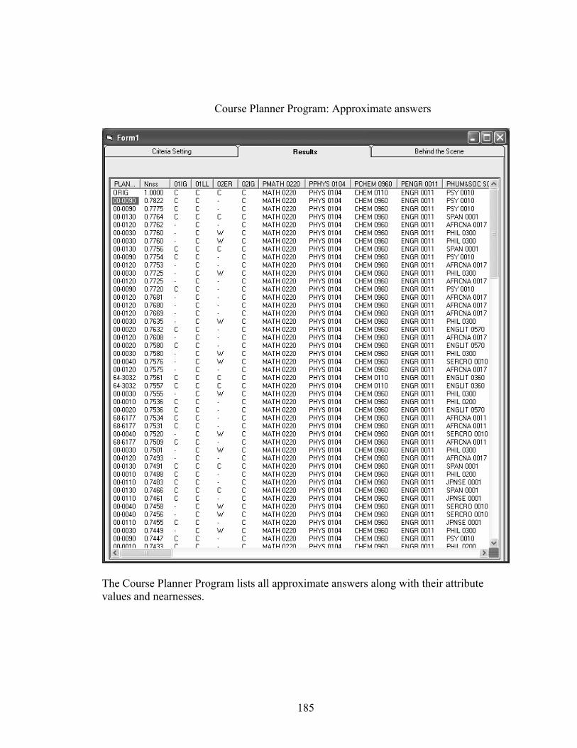
Course Planner Program: Approximate answers
The Course Planner Program lists all approximate answers along with their attribute values and nearnesses.
185
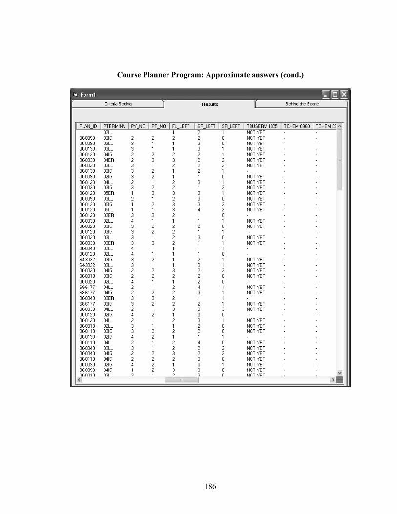
Course Planner Program: Approximate answers (cond.)
186

Course Planner Program: Approximate answers (cond.)
To help the user understand each course schedule option (approximate answer), the Course Planner Program allows the user to click on any plan ID to open up the Course
187

Detail window. The window provides a comprehensive comparison between the user’s graduate requirements (the original query conditions) and those of selected study plan.
188

APPENDIX C
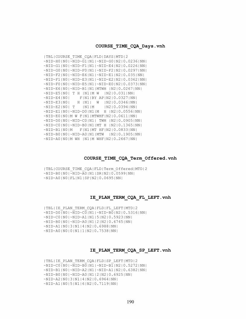
COURSE_TIME_CQA_Days.vnh
|TBL|COURSE_TIME_CQA|FLD|DAYS|MTD|2 ~NID~H0|N0|~NID~G1|N1|~NID~G0|N2|0.0236|NN| ~NID~G1|N0|~NID~F1|N1|~NID~E4|N2|0.0226|NN| ~NID~G0|N0|~NID~F0|N1|~NID~F2|N2|0.0297|NN| ~NID~F2|N0|~NID~E6|N1|~NID~E1|N2|0.035|NN| ~NID~F1|N0|~NID~E3|N1|~NID~E2|N2|0.0362|NN| ~NID~F0|N0|~NID~E5|N1|~NID~E0|N2|0.0373|NN| ~NID~E6|N0|~NID~B1|N1|MTWH |N2|0.0267|NN| ~NID~E5|N0| T H |N1|M W |N2|0.031|NN| ~NID~E4|N0| F|N1|BY AP|N2|0.0327|NN| ~NID~E3|N0| H |N1| W |N2|0.0346|NN| ~NID~E2|N0| T |N1|M |N2|0.0394|NN| ~NID~E1|N0|~NID~D0|N1|M H |N2|0.0556|NN| ~NID~E0|N0|M W F|N1|MTWHF|N2|0.0611|NN| ~NID~D0|N0|~NID~C0|N1| TWH |N2|0.0905|NN| ~NID~C0|N0|~NID~B0|N1|MT H |N2|0.1365|NN| ~NID~B1|N0|M F|N1|MT HF|N2|0.0833|NN| ~NID~B0|N0|~NID~A0|N1|MTW |N2|0.1905|NN| ~NID~A0|N0|M WH |N1|M WHF|N2|0.2667|NN|
COURSE_TIME_CQA_Term_Offered.vnh
|TBL|COURSE_TIME_CQA|FLD|Term_Offered|MTD|2 ~NID~B0|N0|~NID~A0|N1|SR|N2|0.0599|NN| ~NID~A0|N0|FL|N1|SP|N2|0.0695|NN|
IE_PLAN_TERM_CQA_FL_LEFT.vnh
|TBL|IE_PLAN_TERM_CQA|FLD|FL_LEFT|MTD|2 ~NID~D0|N0|~NID~C0|N1|~NID~B0|N2|0.5316|NN| ~NID~C0|N0|~NID~A1|N1|5|N2|0.5923|NN| ~NID~B0|N0|~NID~A0|N1|2|N2|0.6745|NN| ~NID~A1|N0|3|N1|4|N2|0.6988|NN| ~NID~A0|N0|0|N1|1|N2|0.7538|NN|
IE_PLAN_TERM_CQA_SP_LEFT.vnh
|TBL|IE_PLAN_TERM_CQA|FLD|SP_LEFT|MTD|2 ~NID~C0|N0|~NID~B0|N1|~NID~B1|N2|0.5272|NN| ~NID~B1|N0|~NID~A2|N1|~NID~A1|N2|0.6382|NN| ~NID~B0|N0|~NID~A0|N1|2|N2|0.6925|NN| ~NID~A2|N0|3|N1|4|N2|0.6964|NN| ~NID~A1|N0|5|N1|6|N2|0.7119|NN|
190
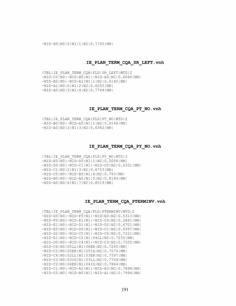
~NID~A0|N0|0|N1|1|N2|0.7765|NN|
IE_PLAN_TERM_CQA_SR_LEFT.vnh
|TBL|IE_PLAN_TERM_CQA|FLD|SR_LEFT|MTD|2 ~NID~C0|N0|~NID~B0|N1|~NID~A0|N2|0.6066|NN| ~NID~B0|N0|~NID~A1|N1|1|N2|0.6145|NN| ~NID~A1|N0|0|N1|2|N2|0.6255|NN| ~NID~A0|N0|3|N1|4|N2|0.7744|NN|
IE_PLAN_TERM_CQA_PT_NO.vnh
|TBL|IE_PLAN_TERM_CQA|FLD|PT_NO|MTD|2 ~NID~B0|N0|~NID~A0|N1|1|N2|0.6146|NN| ~NID~A0|N0|2|N1|3|N2|0.6362|NN|
IE_PLAN_TERM_CQA_PY_NO.vnh
|TBL|IE_PLAN_TERM_CQA|FLD|PY_NO|MTD|2 ~NID~E0|N0|~NID~D0|N1|1|N2|0.5058|NN| ~NID~D0|N0|~NID~C1|N1|~NID~C0|N2|0.6351|NN| ~NID~C1|N0|2|N1|3|N2|0.6753|NN| ~NID~C0|N0|~NID~B0|N1|4|N2|0.763|NN| ~NID~B0|N0|~NID~A0|N1|5|N2|0.8184|NN| ~NID~A0|N0|6|N1|7|N2|0.8519|NN|
IE_PLAN_TERM_CQA_PTERMINV.vnh
|TBL|IE_PLAN_TERM_CQA|FLD|PTERMINV|MTD|2 ~NID~G0|N0|~NID~F0|N1|~NID~E0|N2|0.5313|NN| ~NID~F0|N0|~NID~E1|N1|~NID~C0|N2|0.5881|NN| ~NID~E1|N0|~NID~D1|N1|~NID~D2|N2|0.6701|NN| ~NID~E0|N0|~NID~D0|N1|~NID~C1|N2|0.6997|NN| ~NID~D2|N0|~NID~C5|N1|~NID~C6|N2|0.7221|NN| ~NID~D1|N0|~NID~C2|N1|04LL|N2|0.7235|NN| ~NID~D0|N0|~NID~C4|N1|~NID~C3|N2|0.7505|NN| ~NID~C6|N0|05LL|N1|06ER|N2|0.7245|NN| ~NID~C5|N0|05ER|N1|05IG|N2|0.7574|NN| ~NID~C4|N0|02LL|N1|03ER|N2|0.7597|NN| ~NID~C3|N0|03IG|N1|03LL|N2|0.7704|NN| ~NID~C2|N0|04ER|N1|04IG|N2|0.7864|NN| ~NID~C1|N0|~NID~A2|N1|~NID~A3|N2|0.7898|NN| ~NID~C0|N0|~NID~B0|N1|~NID~A1|N2|0.7994|NN|
191

~NID~B0|N0|~NID~A0|N1|07LL|N2|0.8519|NN| ~NID~A3|N0|02ER|N1|02IG|N2|0.8344|NN| ~NID~A2|N0|01IG|N1|01LL|N2|0.8648|NN| ~NID~A1|N0|06IG|N1|06LL|N2|0.9074|NN| ~NID~A0|N0|07ER|N1|07IG|N2|0.9444|NN|
IE_PLAN_TERM_CQA_TBUSERV 1925.vnh
|TBL|IE_PLAN_TERM_CQA|FLD|TBUSERV 1925|MTD|2 ~NID~A0|N0|-|N1|NOT YET|N2|0.5751|NN|
192
COURSE_SOCIAL_PROD_COURSE_NO.vnh
|TBL|COURSE_SOCIAL_PROD|FLD|COURSE_NO|MTD|2 ~NID~FE0|N0|~NID~FD0|N1|~NID~FD1|N2|0.1035|NN| ~NID~FD1|N0|~NID~FC2|N1|PS 2317|N2|0.0845|NN| ~NID~FD0|N0|~NID~FC1|N1|~NID~FC0|N2|0.1798|NN| ~NID~FC2|N0|~NID~EY13|N1|~NID~EY3|N2|0.1056|NN| ~NID~FC1|N0|~NID~FB1|N1|~NID~EZ0|N2|0.1973|NN| ~NID~FC0|N0|~NID~FB0|N1|~NID~EZ2|N2|0.1988|NN| ~NID~FB1|N0|~NID~FA1|N1|~NID~EY9|N2|0.2013|NN| ~NID~FB0|N0|~NID~FA0|N1|~NID~EY0|N2|0.2471|NN| ~NID~FA1|N0|~NID~EZ4|N1|~NID~EY8|N2|0.2114|NN| ~NID~FA0|N0|~NID~EZ1|N1|~NID~EZ3|N2|0.2731|NN| ~NID~EZ4|N0|~NID~EY7|N1|~NID~EY10|N2|0.2395|NN| ~NID~EZ3|N0|~NID~EY5|N1|~NID~EY4|N2|0.3028|NN| ~NID~EZ2|N0|~NID~EY12|N1|~NID~EY2|N2|0.3048|NN| ~NID~EZ1|N0|~NID~EY6|N1|~NID~EY11|N2|0.3144|NN| ~NID~EZ0|N0|~NID~EY1|N1|~NID~ET66|N2|0.3299|NN| ~NID~EY13|N0|~NID~EU44|N1|~NID~EQ21|N2|0.2646|NN| ~NID~EY12|N0|~NID~EU24|N1|~NID~ET5|N2|0.2667|NN| ~NID~EY11|N0|~NID~EX5|N1|PS 1911|N2|0.3025|NN| ~NID~EY10|N0|~NID~EX2|N1|HIST 1005|N2|0.304|NN| ~NID~EY9|N0|~NID~EW7|N1|~NID~EU42|N2|0.3212|NN| ~NID~EY8|N0|~NID~EW8|N1|~NID~EW10|N2|0.3315|NN| ~NID~EY7|N0|~NID~EV18|N1|~NID~EU48|N2|0.3363|NN| ~NID~EY6|N0|~NID~EX3|N1|~NID~ET85|N2|0.3443|NN| ~NID~EY5|N0|~NID~EX1|N1|~NID~EW9|N2|0.3564|NN| ~NID~EY4|N0|~NID~EX0|N1|~NID~ET3|N2|0.3577|NN| ~NID~EY3|N0|~NID~EX4|N1|~NID~EU34|N2|0.3702|NN| ~NID~EY2|N0|~NID~EV21|N1|~NID~EV11|N2|0.379|NN| ~NID~EY1|N0|~NID~EV8|N1|~NID~EU14|N2|0.3892|NN| ~NID~EY0|N0|~NID~EU22|N1|~NID~ET30|N2|0.4|NN| ~NID~EX5|N0|~NID~EW2|N1|~NID~ET99|N2|0.4013|NN| ~NID~EX4|N0|~NID~EW11|N1|~NID~EW5|N2|0.4097|NN| ~NID~EX3|N0|~NID~EW4|N1|~NID~EV22|N2|0.4198|NN| ~NID~EX2|N0|~NID~EW3|N1|~NID~EU33|N2|0.4279|NN| ~NID~EX1|N0|~NID~EW6|N1|~NID~EW0|N2|0.4422|NN| ~NID~EX0|N0|~NID~EW1|N1|~NID~EU36|N2|0.4742|NN| ~NID~EW11|N0|~NID~EV9|N1|~NID~EV6|N2|0.4004|NN| ~NID~EW10|N0|~NID~EV17|N1|~NID~EU17|N2|0.4076|NN| ~NID~EW9|N0|~NID~EV16|N1|~NID~EU49|N2|0.4198|NN| ~NID~EW8|N0|~NID~EV14|N1|~NID~ET100|N2|0.4211|NN| ~NID~EW7|N0|~NID~EV15|N1|~NID~EV1|N2|0.4226|NN| ~NID~EW6|N0|~NID~EV5|N1|~NID~ET18|N2|0.425|NN| ~NID~EW5|N0|~NID~EV13|N1|~NID~EU38|N2|0.4276|NN| ~NID~EW4|N0|~NID~EV10|N1|~NID~EV19|N2|0.4308|NN| ~NID~EW3|N0|~NID~EV12|N1|~NID~EU32|N2|0.444|NN| ~NID~EW2|N0|~NID~EV4|N1|~NID~EV20|N2|0.4594|NN| ~NID~EW1|N0|~NID~EV3|N1|~NID~EV7|N2|0.4881|NN| ~NID~EW0|N0|~NID~EV0|N1|~NID~EV2|N2|0.498|NN|
193
~NID~EV22|N0|~NID~EU39|N1|~NID~AZ0|N2|0.4089|NN| ~NID~EV21|N0|~NID~EU47|N1|AFRCNA 0031|N2|0.4167|NN| ~NID~EV20|N0|~NID~EU40|N1|~NID~ET77|N2|0.425|NN| ~NID~EV19|N0|~NID~EU46|N1|~NID~EU2|N2|0.4259|NN| ~NID~EV18|N0|~NID~EU43|N1|~NID~EU27|N2|0.4272|NN| ~NID~EV17|N0|~NID~EU41|N1|~NID~EU51|N2|0.4299|NN| ~NID~EV16|N0|~NID~EU45|N1|~NID~EU23|N2|0.4323|NN| ~NID~EV15|N0|~NID~EU12|N1|~NID~EU35|N2|0.4436|NN| ~NID~EV14|N0|~NID~EU30|N1|~NID~ET87|N2|0.4457|NN| ~NID~EV13|N0|~NID~EU10|N1|~NID~EU21|N2|0.4463|NN| ~NID~EV12|N0|~NID~EU37|N1|~NID~ET95|N2|0.4529|NN| ~NID~EV11|N0|~NID~EU25|N1|~NID~ET74|N2|0.4533|NN| ~NID~EV10|N0|~NID~EU3|N1|~NID~EU7|N2|0.4593|NN| ~NID~EV9|N0|~NID~EU50|N1|~NID~EU0|N2|0.4792|NN| ~NID~EV8|N0|~NID~EU11|N1|~NID~EU31|N2|0.4826|NN| ~NID~EV7|N0|~NID~EU19|N1|~NID~EU26|N2|0.485|NN| ~NID~EV6|N0|~NID~EU1|N1|SOC 1414|N2|0.4857|NN| ~NID~EV5|N0|~NID~EU29|N1|~NID~EU13|N2|0.4921|NN| ~NID~EV4|N0|~NID~EU6|N1|~NID~EU16|N2|0.4942|NN| ~NID~EV3|N0|~NID~EU18|N1|~NID~EU15|N2|0.5058|NN| ~NID~EV2|N0|~NID~EU4|N1|~NID~EU8|N2|0.5094|NN| ~NID~EV1|N0|~NID~EU9|N1|~NID~EU28|N2|0.511|NN| ~NID~EV0|N0|~NID~EU5|N1|~NID~EU20|N2|0.5175|NN| ~NID~EU51|N0|~NID~ET98|N1|SOC 0010|N2|0.4022|NN| ~NID~EU50|N0|~NID~ET9|N1|~NID~ET44|N2|0.4039|NN| ~NID~EU49|N0|~NID~ET68|N1|~NID~ET89|N2|0.4155|NN| ~NID~EU48|N0|~NID~ET93|N1|~NID~ET7|N2|0.42|NN| ~NID~EU47|N0|~NID~ET82|N1|AFRCNA 0039|N2|0.425|NN| ~NID~EU45|N0|~NID~ET8|N1|~NID~ET47|N2|0.4275|NN| ~NID~EU46|N0|~NID~ET53|N1|~NID~ET4|N2|0.4275|NN| ~NID~EU44|N0|~NID~ET97|N1|~NID~ET94|N2|0.4331|NN| ~NID~EU43|N0|~NID~ET45|N1|ANTH 0680|N2|0.439|NN| ~NID~EU42|N0|~NID~ET91|N1|ECON 0100|N2|0.4396|NN| ~NID~EU41|N0|~NID~ET92|N1|~NID~ET80|N2|0.4411|NN| ~NID~EU40|N0|~NID~ET55|N1|~NID~ET32|N2|0.45|NN| ~NID~EU39|N0|~NID~ET14|N1|HIST 1783|N2|0.4538|NN| ~NID~EU38|N0|~NID~ET96|N1|~NID~ET81|N2|0.4568|NN| ~NID~EU37|N0|~NID~ET84|N1|~NID~ET90|N2|0.4619|NN| ~NID~EU36|N0|~NID~ET29|N1|PSY 0310|N2|0.4625|NN| ~NID~EU34|N0|~NID~ET23|N1|~NID~ET50|N2|0.4667|NN| ~NID~EU35|N0|~NID~ET24|N1|ECON 0230|N2|0.4667|NN| ~NID~EU33|N0|~NID~ET60|N1|HIST 0600|N2|0.4684|NN| ~NID~EU32|N0|~NID~ET59|N1|HIST 0089|N2|0.4695|NN| ~NID~EU31|N0|~NID~ET62|N1|HPS 0621|N2|0.4714|NN| ~NID~EU30|N0|~NID~ET64|N1|~NID~ET34|N2|0.4727|NN| ~NID~EU29|N0|~NID~ET6|N1|~NID~ET78|N2|0.48|NN| ~NID~EU28|N0|~NID~ET73|N1|~NID~ET83|N2|0.4889|NN| ~NID~EU27|N0|~NID~ET88|N1|~NID~ET52|N2|0.4966|NN| ~NID~EU26|N0|~NID~ET69|N1|~NID~ET33|N2|0.4974|NN| ~NID~EU24|N0|~NID~ET0|N1|~NID~ET16|N2|0.5|NN| ~NID~EU21|N0|~NID~ET75|N1|PSY 2970|N2|0.5|NN| ~NID~EU22|N0|~NID~ET12|N1|~NID~ET19|N2|0.5|NN| ~NID~EU25|N0|~NID~ET72|N1|AFRCNA 0087|N2|0.5|NN| ~NID~EU23|N0|~NID~ET28|N1|~NID~ES1|N2|0.5|NN|
194
~NID~EU20|N0|~NID~ET46|N1|~NID~ET70|N2|0.5071|NN| ~NID~EU19|N0|~NID~ET67|N1|~NID~ET61|N2|0.508|NN| ~NID~EU18|N0|~NID~ET10|N1|~NID~ET79|N2|0.5094|NN| ~NID~EU17|N0|~NID~ET51|N1|SOC 0446|N2|0.519|NN| ~NID~EU16|N0|~NID~ET48|N1|~NID~ET63|N2|0.52|NN| ~NID~EU15|N0|~NID~ET49|N1|~NID~ET57|N2|0.5278|NN| ~NID~EU14|N0|~NID~ET54|N1|HPS 0437|N2|0.5283|NN| ~NID~EU13|N0|~NID~ET76|N1|~NID~ET35|N2|0.5333|NN| ~NID~EU12|N0|~NID~ET20|N1|~NID~ET22|N2|0.5333|NN| ~NID~EU11|N0|~NID~ET11|N1|~NID~ET15|N2|0.5357|NN| ~NID~EU10|N0|~NID~ET39|N1|~NID~ET86|N2|0.5362|NN| ~NID~EU9|N0|~NID~ET71|N1|~NID~ET43|N2|0.54|NN| ~NID~EU4|N0|~NID~ET56|N1|~NID~ET40|N2|0.55|NN| ~NID~EU7|N0|~NID~ET1|N1|~NID~ET21|N2|0.55|NN| ~NID~EU8|N0|~NID~ET37|N1|~NID~ET36|N2|0.55|NN| ~NID~EU6|N0|~NID~ET25|N1|~NID~ET2|N2|0.55|NN| ~NID~EU5|N0|~NID~ET17|N1|~NID~ET31|N2|0.55|NN| ~NID~EU3|N0|~NID~ET13|N1|~NID~ET58|N2|0.5538|NN| ~NID~EU2|N0|~NID~ET65|N1|~NID~ET27|N2|0.5583|NN| ~NID~EU1|N0|~NID~ET41|N1|~NID~ET38|N2|0.5889|NN| ~NID~EU0|N0|~NID~ET26|N1|~NID~ET42|N2|0.6|NN| ~NID~ET100|N0|~NID~EP40|N1|SOC 1325|N2|0.42|NN| ~NID~ET99|N0|PS 0200|N1|PS 0300|N2|0.4222|NN| ~NID~ET98|N0|SOC 0465|N1|SOC 0471|N2|0.4269|NN| ~NID~ET97|N0|PSY 0035|N1|PSY 0405|N2|0.4289|NN| ~NID~ET96|N0|~NID~ER6|N1|~NID~ER11|N2|0.435|NN| ~NID~ET95|N0|HIST 0101|N1|HIST 0501|N2|0.4474|NN| ~NID~ET94|N0|PSY 0420|N1|PSY 1514|N2|0.4489|NN| ~NID~ET93|N0|ANTH 1787|N1|ANTH 2715|N2|0.45|NN| ~NID~ET92|N0|SOC 0002|N1|SOC 0438|N2|0.4513|NN| ~NID~ET91|N0|ECON 0110|N1|ECON 0800|N2|0.4523|NN| ~NID~ET90|N0|HIST 0601|N1|HIST 0670|N2|0.4579|NN| ~NID~ET89|N0|~NID~ES2|N1|PS 1603|N2|0.46|NN| ~NID~ET88|N0|ANTH 0582|N1|ANTH 0780|N2|0.4663|NN| ~NID~ET87|N0|~NID~K0|N1|SOC 2010|N2|0.4667|NN| ~NID~ET85|N0|ANTH 0768|N1|ANTH 1738|N2|0.4667|NN| ~NID~ET86|N0|PSY 1950|N1|PSY 2210|N2|0.4667|NN| ~NID~ET84|N0|HIST 0100|N1|HIST 0401|N2|0.4799|NN| ~NID~ET83|N0|ECON 1100|N1|ECON 2720|N2|0.48|NN| ~NID~ET82|N0|AFRCNA 0029|N1|AFRCNA 0030|N2|0.4833|NN| ~NID~ET81|N0|~NID~ES0|N1|~NID~ER3|N2|0.486|NN| ~NID~ET80|N0|SOC 0005|N1|SOC 0007|N2|0.4933|NN| ~NID~ET79|N0|PSY 0010|N1|PSY 0505|N2|0.4945|NN| ~NID~ET74|N0|AFRCNA 0017|N1|AFRCNA 0027|N2|0.5|NN| ~NID~ET76|N0|HIST 1131|N1|HIST 1683|N2|0.5|NN| ~NID~ET78|N0|HIST 0200|N1|HIST 1190|N2|0.5|NN| ~NID~ET72|N0|~NID~EP50|N1|AFRCNA 1006|N2|0.5|NN| ~NID~ET77|N0|PS 1000|N1|PS 1910|N2|0.5|NN| ~NID~ET73|N0|ECON 0280|N1|ECON 1110|N2|0.5|NN| ~NID~ET71|N0|~NID~EA0|N1|ECON 3100|N2|0.5|NN| ~NID~ET75|N0|PSY 2280|N1|PSY 2505|N2|0.5|NN| ~NID~ET70|N0|HIST 1000|N1|HIST 1001|N2|0.5029|NN| ~NID~ET69|N0|PSY 0160|N1|PSY 1205|N2|0.5048|NN| ~NID~ET68|N0|~NID~ER13|N1|PS 1261|N2|0.5056|NN|
195

~NID~ET67|N0|PSY 0105|N1|PSY 1050|N2|0.5083|NN| ~NID~ET66|N0|~NID~EP34|N1|HPS 0613|N2|0.5092|NN| ~NID~ET65|N0|~NID~ER1|N1|PS 2543|N2|0.51|NN| ~NID~ET64|N0|~NID~EP22|N1|SOC 0150|N2|0.52|NN| ~NID~ET60|N0|~NID~EP35|N1|HIST 0500|N2|0.5333|NN| ~NID~ET63|N0|PS 1211|N1|PS 1511|N2|0.5333|NN| ~NID~ET62|N0|HPS 0427|N1|HPS 2645|N2|0.5333|NN| ~NID~ET61|N0|PSY 0182|N1|PSY 0510|N2|0.5333|NN| ~NID~ET59|N0|HIST 0302|N1|HIST 0671|N2|0.5364|NN| ~NID~ET58|N0|~NID~EQ8|N1|~NID~EP51|N2|0.5381|NN| ~NID~ET57|N0|PSY 0012|N1|PSY 1210|N2|0.55|NN| ~NID~ET55|N0|PS 2114|N1|PS 2502|N2|0.55|NN| ~NID~ET56|N0|HIST 0124|N1|HIST 1769|N2|0.55|NN| ~NID~ET54|N0|HPS 0515|N1|HPS 0612|N2|0.5596|NN| ~NID~ET53|N0|~NID~ER4|N1|~NID~EP38|N2|0.5638|NN| ~NID~ET52|N0|~NID~EQ23|N1|ANTH 1602|N2|0.5645|NN| ~NID~ET51|N0|SOC 0362|N1|SOC 0432|N2|0.5657|NN| ~NID~ET50|N0|~NID~EQ2|N1|~NID~EB0|N2|0.5667|NN| ~NID~ET49|N0|~NID~EP32|N1|PSY 0421|N2|0.575|NN| ~NID~ET48|N0|PS 0500|N1|PS 1601|N2|0.5778|NN| ~NID~ET47|N0|~NID~ER5|N1|~NID~EP24|N2|0.5788|NN| ~NID~ET46|N0|~NID~EP42|N1|HIST 1479|N2|0.58|NN| ~NID~ET45|N0|ANTH 0536|N1|ANTH 0620|N2|0.5867|NN| ~NID~ET43|N0|~NID~EP39|N1|ECON 1700|N2|0.59|NN| ~NID~ET44|N0|~NID~EQ18|N1|AFRCNA 1903|N2|0.59|NN| ~NID~ET17|N0|~NID~BO0|N1|HIST 1776|N2|0.6|NN| ~NID~ET8|N0|~NID~EQ15|N1|ECON 3400|N2|0.6|NN| ~NID~ET11|N0|~NID~DD0|N1|HPS 0611|N2|0.6|NN| ~NID~ET0|N0|~NID~DB0|N1|AFRCNA 0024|N2|0.6|NN| ~NID~ET5|N0|AFRCNA 0023|N1|AFRCNA 0025|N2|0.6|NN| ~NID~ET29|N0|PSY 1973|N1|PSY 1975|N2|0.6|NN| ~NID~ET19|N0|~NID~AT0|N1|ECON 1630|N2|0.6|NN| ~NID~ET20|N0|~NID~DY0|N1|AFRCNA 1020|N2|0.6|NN| ~NID~ET6|N0|~NID~Z0|N1|HIST 0688|N2|0.6|NN| ~NID~ET18|N0|~NID~BG0|N1|SOC 0426|N2|0.6|NN| ~NID~ET3|N0|~NID~EP3|N1|~NID~BU0|N2|0.6|NN| ~NID~ET32|N0|PS 2903|N1|PS 2970|N2|0.6|NN| ~NID~ET33|N0|PSY 0184|N1|PSY 3340|N2|0.6|NN| ~NID~ET12|N0|~NID~Y0|N1|HIST 1154|N2|0.6|NN| ~NID~ET23|N0|~NID~EP10|N1|ECON 3902|N2|0.6|NN| ~NID~ET1|N0|~NID~DR0|N1|ANTH 1607|N2|0.6|NN| ~NID~ET21|N0|~NID~DC0|N1|PSY 3290|N2|0.6|NN| ~NID~ET24|N0|ECON 0500|N1|ECON 3110|N2|0.6|NN| ~NID~ET40|N0|HIST 1433|N1|HIST 1619|N2|0.6|NN| ~NID~ET37|N0|HIST 0187|N1|HIST 1086|N2|0.6|NN| ~NID~ET35|N0|HIST 1690|N1|HIST 1781|N2|0.6|NN| ~NID~ET26|N0|HIST 1901|N1|HIST 2990|N2|0.6|NN| ~NID~ET34|N0|~NID~H0|N1|SOC 2305|N2|0.6|NN| ~NID~ET31|N0|HIST 2005|N1|HIST 2404|N2|0.6|NN| ~NID~ET41|N0|~NID~ER10|N1|SOC 1903|N2|0.6|NN| ~NID~ET39|N0|~NID~ER2|N1|PSY 2225|N2|0.6|NN| ~NID~ET42|N0|HIST 2902|N1|HIST 3000|N2|0.6|NN| ~NID~ET38|N0|SOC 3902|N1|SOC 3903|N2|0.6|NN| ~NID~ET4|N0|~NID~ER7|N1|~NID~DQ0|N2|0.6|NN|
196
~NID~ET30|N0|HPS 0623|N1|PS 1234|N2|0.6|NN| ~NID~ET15|N0|~NID~BW0|N1|HPS 2673|N2|0.6|NN| ~NID~ET28|N0|HPS 2502|N1|HPS 2649|N2|0.6|NN| ~NID~ET27|N0|HPS 2503|N1|SOC 2315|N2|0.6|NN| ~NID~ET2|N0|~NID~EN0|N1|PS 2020|N2|0.6|NN| ~NID~ET9|N0|~NID~EP54|N1|HIST 1900|N2|0.6|NN| ~NID~ET25|N0|~NID~EK0|N1|PS 2503|N2|0.6|NN| ~NID~ET36|N0|HIST 1115|N1|HIST 1586|N2|0.6|NN| ~NID~ET22|N0|~NID~EE0|N1|ECON 3160|N2|0.6|NN| ~NID~ET14|N0|~NID~ER9|N1|SOC 0317|N2|0.6|NN| ~NID~ET10|N0|~NID~CV0|N1|PSY 2125|N2|0.6|NN| ~NID~ET7|N0|ANTH 2763|N1|ANTH 2789|N2|0.6|NN| ~NID~ET16|N0|ANTH 2490|N1|PSY 1305|N2|0.6|NN| ~NID~ET13|N0|AFRCNA 0010|N1|SOC 2340|N2|0.6|NN| ~NID~ES2|N0|~NID~ER12|N1|~NID~EQ20|N2|0.6061|NN| ~NID~ES1|N0|~NID~ER8|N1|~NID~CR0|N2|0.6143|NN| ~NID~ES0|N0|~NID~ER0|N1|ANTH 1535|N2|0.65|NN| ~NID~ER13|N0|~NID~EQ22|N1|~NID~EQ6|N2|0.6026|NN| ~NID~ER12|N0|~NID~EQ17|N1|PSY 2325|N2|0.62|NN| ~NID~ER11|N0|~NID~EQ16|N1|~NID~EQ24|N2|0.6242|NN| ~NID~ER10|N0|~NID~EQ19|N1|~NID~EP48|N2|0.625|NN| ~NID~ER9|N0|~NID~EQ11|N1|~NID~EJ0|N2|0.6296|NN| ~NID~ER8|N0|~NID~EQ12|N1|AFRCNA 0088|N2|0.6308|NN| ~NID~ER7|N0|~NID~EQ14|N1|~NID~BX0|N2|0.6333|NN| ~NID~ER6|N0|~NID~EQ7|N1|~NID~EP43|N2|0.64|NN| ~NID~ER5|N0|~NID~EQ13|N1|~NID~EP4|N2|0.6405|NN| ~NID~ER4|N0|~NID~EQ9|N1|~NID~EP36|N2|0.6423|NN| ~NID~ER3|N0|~NID~EQ3|N1|~NID~EP44|N2|0.6447|NN| ~NID~ER2|N0|~NID~EQ4|N1|~NID~EQ10|N2|0.6596|NN| ~NID~ER1|N0|~NID~EQ5|N1|~NID~AD0|N2|0.6857|NN| ~NID~ER0|N0|~NID~EQ0|N1|~NID~EQ1|N2|0.7741|NN| ~NID~EQ24|N0|~NID~EP52|N1|PS 1901|N2|0.6047|NN| ~NID~EQ23|N0|~NID~EP53|N1|ANTH 1786|N2|0.6061|NN| ~NID~EQ22|N0|~NID~EP12|N1|~NID~L0|N2|0.6111|NN| ~NID~EQ21|N0|~NID~EP19|N1|PSY 2476|N2|0.6167|NN| ~NID~EQ20|N0|~NID~EP33|N1|~NID~DO0|N2|0.62|NN| ~NID~EQ19|N0|~NID~EP47|N1|~NID~EP45|N2|0.625|NN| ~NID~EQ18|N0|~NID~EP49|N1|AFRCNA 1901|N2|0.625|NN| ~NID~EQ17|N0|~NID~EP16|N1|~NID~CO0|N2|0.6381|NN| ~NID~EQ14|N0|~NID~EP7|N1|PS 2703|N2|0.64|NN| ~NID~EQ15|N0|~NID~EP23|N1|~NID~AB0|N2|0.64|NN| ~NID~EQ16|N0|~NID~EP46|N1|~NID~EP29|N2|0.64|NN| ~NID~EQ13|N0|~NID~EP8|N1|~NID~EP41|N2|0.6429|NN| ~NID~EQ12|N0|~NID~EP18|N1|~NID~BH0|N2|0.6467|NN| ~NID~EQ11|N0|~NID~EP17|N1|~NID~EP13|N2|0.65|NN| ~NID~EQ10|N0|~NID~EP27|N1|~NID~EP37|N2|0.6509|NN| ~NID~EQ9|N0|~NID~EP14|N1|~NID~EP31|N2|0.6527|NN| ~NID~EQ8|N0|~NID~EP15|N1|ANTH 2513|N2|0.66|NN| ~NID~EQ7|N0|~NID~EP25|N1|~NID~EP30|N2|0.664|NN| ~NID~EQ6|N0|~NID~EP20|N1|HIST 0789|N2|0.6667|NN| ~NID~EQ5|N0|~NID~EP5|N1|AFRCNA 1030|N2|0.6667|NN| ~NID~EQ4|N0|~NID~EP28|N1|~NID~EP21|N2|0.6677|NN| ~NID~EQ3|N0|~NID~EP9|N1|~NID~EP26|N2|0.68|NN| ~NID~EQ2|N0|~NID~EP11|N1|HPS 3902|N2|0.7|NN|
197
~NID~EQ1|N0|~NID~EP6|N1|~NID~EP2|N2|0.7643|NN| ~NID~EQ0|N0|~NID~EP0|N1|~NID~EP1|N2|0.7833|NN| ~NID~EP54|N0|HIST 1903|N1|HIST 3902|N2|0.61|NN| ~NID~EP53|N0|ANTH 0538|N1|ANTH 0669|N2|0.6137|NN| ~NID~EP52|N0|PS 1903|N1|PS 2902|N2|0.6192|NN| ~NID~EP51|N0|~NID~EF0|N1|PS 1213|N2|0.625|NN| ~NID~EP50|N0|~NID~DZ0|N1|AFRCNA 1037|N2|0.625|NN| ~NID~EP46|N0|PS 1900|N1|PS 1902|N2|0.625|NN| ~NID~EP44|N0|ECON 1901|N1|ECON 2000|N2|0.625|NN| ~NID~EP43|N0|HPS 1901|N1|HPS 2530|N2|0.625|NN| ~NID~EP48|N0|SOC 2902|N1|SOC 2990|N2|0.625|NN| ~NID~EP49|N0|AFRCNA 1900|N1|AFRCNA 1902|N2|0.625|NN| ~NID~EP47|N0|SOC 1900|N1|SOC 3000|N2|0.625|NN| ~NID~EP45|N0|SOC 1901|N1|SOC 1902|N2|0.625|NN| ~NID~EP42|N0|~NID~EM0|N1|HIST 1670|N2|0.6333|NN| ~NID~EP40|N0|~NID~BV0|N1|~NID~BL0|N2|0.6333|NN| ~NID~EP41|N0|~NID~EI0|N1|HPS 1410|N2|0.6333|NN| ~NID~EP39|N0|~NID~DU0|N1|ECON 1150|N2|0.6375|NN| ~NID~EP38|N0|~NID~DF0|N1|ANTH 1530|N2|0.64|NN| ~NID~EP37|N0|PSY 2000|N1|PSY 3902|N2|0.64|NN| ~NID~EP36|N0|~NID~EC0|N1|~NID~E0|N2|0.6429|NN| ~NID~EP35|N0|HIST 0301|N1|HIST 0751|N2|0.6444|NN| ~NID~EP34|N0|HPS 0605|N1|HPS 1653|N2|0.648|NN| ~NID~EP32|N0|PSY 1075|N1|PSY 1215|N2|0.65|NN| ~NID~EP33|N0|~NID~BZ0|N1|~NID~I0|N2|0.65|NN| ~NID~EP31|N0|~NID~DL0|N1|HPS 1612|N2|0.66|NN| ~NID~EP25|N0|HPS 2902|N1|HPS 3000|N2|0.664|NN| ~NID~EP26|N0|ECON 2770|N1|ECON 2990|N2|0.664|NN| ~NID~EP30|N0|HPS 2904|N1|HPS 2990|N2|0.664|NN| ~NID~EP29|N0|PS 2990|N1|PS 3000|N2|0.664|NN| ~NID~EP28|N0|PSY 1900|N1|PSY 1902|N2|0.664|NN| ~NID~EP27|N0|PSY 1903|N1|PSY 2990|N2|0.664|NN| ~NID~EP23|N0|~NID~CM0|N1|~NID~A48|N2|0.6667|NN| ~NID~EP22|N0|SOC 0230|N1|SOC 1438|N2|0.6667|NN| ~NID~EP24|N0|~NID~EL0|N1|ECON 1670|N2|0.6667|NN| ~NID~EP21|N0|PSY 2220|N1|PSY 3000|N2|0.67|NN| ~NID~EP19|N0|~NID~AV0|N1|ANTH 2630|N2|0.68|NN| ~NID~EP20|N0|~NID~EG0|N1|PSY 1155|N2|0.68|NN| ~NID~EP18|N0|~NID~EO0|N1|~NID~DJ0|N2|0.6857|NN| ~NID~EP9|N0|ECON 2250|N1|ECON 3000|N2|0.7|NN| ~NID~EP16|N0|~NID~EH0|N1|~NID~DA0|N2|0.7|NN| ~NID~EP17|N0|~NID~BP0|N1|~NID~BK0|N2|0.7|NN| ~NID~EP13|N0|~NID~AA0|N1|~NID~O0|N2|0.7|NN| ~NID~EP11|N0|HPS 2680|N1|HPS 2999|N2|0.7|NN| ~NID~EP12|N0|~NID~CK0|N1|~NID~AH0|N2|0.7|NN| ~NID~EP10|N0|ECON 1902|N1|ECON 1903|N2|0.7|NN| ~NID~EP14|N0|~NID~AS0|N1|~NID~AM0|N2|0.7|NN| ~NID~EP15|N0|~NID~DK0|N1|PSY 1230|N2|0.7|NN| ~NID~EP8|N0|~NID~ED0|N1|~NID~DP0|N2|0.7111|NN| ~NID~EP7|N0|~NID~DH0|N1|~NID~CX0|N2|0.7333|NN| ~NID~EP5|N0|~NID~AP0|N1|PS 1202|N2|0.75|NN| ~NID~EP4|N0|~NID~BB0|N1|~NID~AN0|N2|0.75|NN| ~NID~EP6|N0|ANTH 1901|N1|ANTH 2902|N2|0.75|NN| ~NID~EP3|N0|~NID~CT0|N1|~NID~B11|N2|0.7714|NN|
198
~NID~EP1|N0|ANTH 1900|N1|ANTH 3000|N2|0.775|NN| ~NID~EP2|N0|ANTH 1903|N1|ANTH 2980|N2|0.775|NN| ~NID~EP0|N0|~NID~A53|N1|ANTH 2000|N2|0.79|NN| ~NID~EO0|N0|~NID~BR0|N1|HIST 2721|N2|0.8|NN| ~NID~EN0|N0|~NID~CJ0|N1|PS 2607|N2|0.8|NN| ~NID~EM0|N0|~NID~BT0|N1|HIST 2775|N2|0.8|NN| ~NID~EL0|N0|~NID~DS0|N1|ECON 2713|N2|0.8|NN| ~NID~EK0|N0|~NID~CF0|N1|PS 2567|N2|0.8|NN| ~NID~EJ0|N0|~NID~BN0|N1|AFRCNA 1031|N2|0.8|NN| ~NID~EI0|N0|~NID~CD0|N1|~NID~D0|N2|0.8|NN| ~NID~EH0|N0|~NID~DI0|N1|AFRCNA 1023|N2|0.8|NN| ~NID~EG0|N0|~NID~BE0|N1|~NID~X0|N2|0.8|NN| ~NID~EF0|N0|~NID~CC0|N1|~NID~BY0|N2|0.8|NN| ~NID~EE0|N0|~NID~DT0|N1|~NID~AU0|N2|0.8|NN| ~NID~ED0|N0|~NID~AJ0|N1|~NID~M0|N2|0.8|NN| ~NID~EC0|N0|~NID~DX0|N1|PSY 1235|N2|0.8|NN| ~NID~EB0|N0|~NID~U0|N1|HIST 1750|N2|0.8|NN| ~NID~EA0|N0|~NID~AK0|N1|ECON 2130|N2|0.8|NN| ~NID~DZ0|N0|~NID~DV0|N1|~NID~DN0|N2|0.8|NN| ~NID~DY0|N0|~NID~DW0|N1|AFRCNA 0052|N2|0.8|NN| ~NID~DX0|N0|~NID~CS0|N1|~NID~BQ0|N2|0.8|NN| ~NID~DW0|N0|AFRCNA 1004|N1|AFRCNA 1055|N2|0.8|NN| ~NID~DV0|N0|AFRCNA 1022|N1|AFRCNA 1034|N2|0.8|NN| ~NID~DU0|N0|~NID~DG0|N1|~NID~BC0|N2|0.8|NN| ~NID~DT0|N0|~NID~DM0|N1|~NID~BM0|N2|0.8|NN| ~NID~DS0|N0|~NID~DE0|N1|~NID~AL0|N2|0.8|NN| ~NID~DR0|N0|~NID~S0|N1|ANTH 2720|N2|0.8|NN| ~NID~DQ0|N0|~NID~Q0|N1|ANTH 2466|N2|0.8|NN| ~NID~DP0|N0|~NID~BI0|N1|~NID~B14|N2|0.8|NN| ~NID~DO0|N0|~NID~CW0|N1|~NID~CB0|N2|0.8|NN| ~NID~DN0|N0|AFRCNA 0020|N1|AFRCNA 1038|N2|0.8|NN| ~NID~DM0|N0|~NID~AI0|N1|~NID~AE0|N2|0.8|NN| ~NID~DL0|N0|~NID~AW0|N1|~NID~P0|N2|0.8|NN| ~NID~DK0|N0|~NID~AC0|N1|~NID~A44|N2|0.8|NN| ~NID~DJ0|N0|~NID~BJ0|N1|~NID~T0|N2|0.8|NN| ~NID~DI0|N0|AFRCNA 0016|N1|AFRCNA 1035|N2|0.8|NN| ~NID~DH0|N0|~NID~A41|N1|AFRCNA 0013|N2|0.8|NN| ~NID~DG0|N0|~NID~R0|N1|~NID~B12|N2|0.8|NN| ~NID~DF0|N0|~NID~N0|N1|~NID~A45|N2|0.8|NN| ~NID~DE0|N0|~NID~W0|N1|~NID~V0|N2|0.8|NN| ~NID~DD0|N0|~NID~CZ0|N1|~NID~BS0|N2|0.8|NN| ~NID~DC0|N0|~NID~CY0|N1|~NID~CE0|N2|0.8|NN| ~NID~DB0|N0|AFRCNA 0012|N1|AFRCNA 1053|N2|0.8|NN| ~NID~DA0|N0|~NID~BD0|N1|~NID~A43|N2|0.8|NN| ~NID~CZ0|N0|HPS 2571|N1|HPS 2700|N2|0.8|NN| ~NID~CY0|N0|PS 2201|N1|PS 2378|N2|0.8|NN| ~NID~CX0|N0|HIST 1763|N1|PS 1383|N2|0.8|NN| ~NID~CW0|N0|PS 2381|N1|PS 2501|N2|0.8|NN| ~NID~CV0|N0|~NID~CU0|N1|PSY 2100|N2|0.8|NN| ~NID~CU0|N0|PSY 1225|N1|PSY 1315|N2|0.8|NN| ~NID~CT0|N0|~NID~C3|N1|ECON 2001|N2|0.8|NN| ~NID~CS0|N0|PSY 1115|N1|PSY 1635|N2|0.8|NN| ~NID~CR0|N0|~NID~CQ0|N1|PS 2563|N2|0.8|NN| ~NID~CQ0|N0|~NID~CP0|N1|PS 2525|N2|0.8|NN|
199
~NID~CP0|N0|PS 1611|N1|PS 2301|N2|0.8|NN| ~NID~CO0|N0|~NID~CN0|N1|HPS 2692|N2|0.8|NN| ~NID~CN0|N0|HPS 0630|N1|HPS 2501|N2|0.8|NN| ~NID~CM0|N0|~NID~CL0|N1|HIST 1796|N2|0.8|NN| ~NID~CL0|N0|HIST 1325|N1|HIST 3649|N2|0.8|NN| ~NID~CK0|N0|HIST 1240|N1|PS 1346|N2|0.8|NN| ~NID~CJ0|N0|~NID~CI0|N1|PS 2562|N2|0.8|NN| ~NID~CI0|N0|~NID~CH0|N1|PS 2557|N2|0.8|NN| ~NID~CH0|N0|~NID~CG0|N1|PS 2327|N2|0.8|NN| ~NID~CG0|N0|PS 2306|N1|PS 2560|N2|0.8|NN| ~NID~CF0|N0|PS 2518|N1|PS 2541|N2|0.8|NN| ~NID~CE0|N0|PS 2040|N1|PS 2316|N2|0.8|NN| ~NID~CD0|N0|~NID~A19|N1|~NID~A18|N2|0.8|NN| ~NID~CC0|N0|PS 1381|N1|PS 2030|N2|0.8|NN| ~NID~CB0|N0|~NID~CA0|N1|PS 2310|N2|0.8|NN| ~NID~CA0|N0|PS 1581|N1|PS 2343|N2|0.8|NN| ~NID~BZ0|N0|HIST 2071|N1|HIST 2087|N2|0.8|NN| ~NID~BY0|N0|PS 1636|N1|PS 2564|N2|0.8|NN| ~NID~BX0|N0|HIST 2008|N1|HIST 2012|N2|0.8|NN| ~NID~BW0|N0|HPS 2498|N1|HPS 2625|N2|0.8|NN| ~NID~BV0|N0|HPS 2525|N1|HPS 2679|N2|0.8|NN| ~NID~BU0|N0|HIST 1904|N1|HPS 2497|N2|0.8|NN| ~NID~BT0|N0|HIST 1669|N1|HIST 2119|N2|0.8|NN| ~NID~BS0|N0|HPS 1702|N1|HPS 2526|N2|0.8|NN| ~NID~BR0|N0|HIST 1902|N1|HIST 2600|N2|0.8|NN| ~NID~BQ0|N0|~NID~A17|N1|~NID~A13|N2|0.8|NN| ~NID~BP0|N0|HIST 1044|N1|HIST 1120|N2|0.8|NN| ~NID~BO0|N0|HIST 1015|N1|HIST 2069|N2|0.8|NN| ~NID~BN0|N0|ECON 1380|N1|PS 1353|N2|0.8|NN| ~NID~BM0|N0|ECON 1230|N1|ECON 2110|N2|0.8|NN| ~NID~BL0|N0|~NID~J0|N1|SOC 2905|N2|0.8|NN| ~NID~BK0|N0|~NID~A6|N1|PS 1629|N2|0.8|NN| ~NID~BJ0|N0|ECON 1030|N1|PS 1332|N2|0.8|NN| ~NID~BI0|N0|~NID~C2|N1|~NID~C0|N2|0.8|NN| ~NID~BH0|N0|~NID~G0|N1|SOC 2442|N2|0.8|NN| ~NID~BG0|N0|~NID~BF0|N1|HIST 1767|N2|0.8|NN| ~NID~BF0|N0|HIST 0014|N1|HIST 1116|N2|0.8|NN| ~NID~BE0|N0|HIST 0123|N1|HIST 1090|N2|0.8|NN| ~NID~BD0|N0|ECON 0630|N1|HIST 1775|N2|0.8|NN| ~NID~BC0|N0|ECON 1360|N1|ECON 2150|N2|0.8|NN| ~NID~BB0|N0|~NID~BA0|N1|PS 1241|N2|0.8|NN| ~NID~BA0|N0|~NID~B7|N1|~NID~A4|N2|0.8|NN| ~NID~AZ0|N0|~NID~AY0|N1|PS 1311|N2|0.8|NN| ~NID~AY0|N0|~NID~AX0|N1|HIST 2091|N2|0.8|NN| ~NID~AX0|N0|~NID~B6|N1|SOC 2426|N2|0.8|NN| ~NID~AW0|N0|~NID~A35|N1|HIST 1169|N2|0.8|NN| ~NID~AV0|N0|~NID~B10|N1|~NID~A11|N2|0.8|NN| ~NID~AU0|N0|ECON 1200|N1|ECON 2570|N2|0.8|NN| ~NID~AT0|N0|ECON 0330|N1|PS 1602|N2|0.8|NN| ~NID~AS0|N0|~NID~AR0|N1|PS 1317|N2|0.8|NN| ~NID~AR0|N0|~NID~AQ0|N1|~NID~A5|N2|0.8|NN| ~NID~AQ0|N0|~NID~A0|N1|PS 1530|N2|0.8|NN| ~NID~AP0|N0|~NID~AO0|N1|PS 2321|N2|0.8|NN| ~NID~AO0|N0|~NID~A2|N1|PS 2200|N2|0.8|NN|
200
~NID~AN0|N0|~NID~B8|N1|SOC 1447|N2|0.8|NN| ~NID~AM0|N0|~NID~A9|N1|~NID~A12|N2|0.8|NN| ~NID~AL0|N0|ECON 0360|N1|ECON 0530|N2|0.8|NN| ~NID~AK0|N0|ECON 2270|N1|ECON 3150|N2|0.8|NN| ~NID~AJ0|N0|~NID~A50|N1|ANTH 0715|N2|0.8|NN| ~NID~AI0|N0|ECON 0400|N1|ECON 2200|N2|0.8|NN| ~NID~AH0|N0|~NID~AG0|N1|PS 1321|N2|0.8|NN| ~NID~AG0|N0|~NID~AF0|N1|PS 1231|N2|0.8|NN| ~NID~AF0|N0|~NID~A51|N1|~NID~A1|N2|0.8|NN| ~NID~AE0|N0|ECON 1540|N1|ECON 2260|N2|0.8|NN| ~NID~AD0|N0|~NID~A46|N1|SOC 1365|N2|0.8|NN| ~NID~AC0|N0|ANTH 2692|N1|ANTH 2728|N2|0.8|NN| ~NID~AB0|N0|~NID~F0|N1|SOC 1476|N2|0.8|NN| ~NID~AA0|N0|ANTH 1540|N1|PS 1235|N2|0.8|NN| ~NID~Z0|N0|~NID~A26|N1|HIST 2010|N2|0.8|NN| ~NID~Y0|N0|~NID~A47|N1|HPS 0517|N2|0.8|NN| ~NID~X0|N0|~NID~A29|N1|HIST 1123|N2|0.8|NN| ~NID~W0|N0|~NID~A24|N1|ECON 0120|N2|0.8|NN| ~NID~V0|N0|~NID~B13|N1|ECON 1410|N2|0.8|NN| ~NID~U0|N0|ANTH 2609|N1|HPS 1703|N2|0.8|NN| ~NID~T0|N0|~NID~B3|N1|~NID~A42|N2|0.8|NN| ~NID~S0|N0|ANTH 1603|N1|ANTH 2753|N2|0.8|NN| ~NID~R0|N0|~NID~A28|N1|ECON 1680|N2|0.8|NN| ~NID~Q0|N0|ANTH 1466|N1|ANTH 2784|N2|0.8|NN| ~NID~P0|N0|~NID~B2|N1|~NID~B5|N2|0.8|NN| ~NID~O0|N0|ANTH 1764|N1|ANTH 1777|N2|0.8|NN| ~NID~N0|N0|~NID~A32|N1|ANTH 1776|N2|0.8|NN| ~NID~M0|N0|~NID~C1|N1|ECON 2020|N2|0.8|NN| ~NID~L0|N0|SOC 1362|N1|SOC 1488|N2|0.8|NN| ~NID~K0|N0|SOC 0352|N1|SOC 1333|N2|0.8|NN| ~NID~J0|N0|SOC 1360|N1|SOC 2004|N2|0.8|NN| ~NID~I0|N0|SOC 2205|N1|SOC 2345|N2|0.8|NN| ~NID~H0|N0|SOC 2203|N1|SOC 2303|N2|0.8|NN| ~NID~G0|N0|SOC 1342|N1|SOC 2240|N2|0.8|NN| ~NID~F0|N0|SOC 1448|N1|SOC 2201|N2|0.8|NN| ~NID~E0|N0|SOC 0003|N1|SOC 1321|N2|0.8|NN| ~NID~D0|N0|PSY 1025|N1|PSY 2205|N2|0.8|NN| ~NID~C3|N0|~NID~B9|N1|~NID~A20|N2|1|NN| ~NID~C0|N0|~NID~B0|N1|~NID~A39|N2|1|NN| ~NID~C2|N0|~NID~B4|N1|~NID~A25|N2|1|NN| ~NID~C1|N0|~NID~B1|N1|HIST 1668|N2|1|NN| ~NID~B14|N0|~NID~A52|N1|~NID~A36|N2|0.8667|NN| ~NID~B11|N0|~NID~A14|N1|~NID~A21|N2|1|NN| ~NID~B10|N0|~NID~A10|N1|PSY 2455|N2|1|NN| ~NID~B9|N0|~NID~A16|N1|~NID~A15|N2|1|NN| ~NID~B8|N0|~NID~A7|N1|PS 1233|N2|1|NN| ~NID~B7|N0|~NID~A3|N1|~NID~A8|N2|1|NN| ~NID~B6|N0|~NID~A49|N1|HPS 2685|N2|1|NN| ~NID~B0|N0|~NID~A33|N1|HIST 1766|N2|1|NN| ~NID~B4|N0|~NID~A40|N1|HIST 0675|N2|1|NN| ~NID~B1|N0|~NID~A34|N1|~NID~A37|N2|1|NN| ~NID~B5|N0|~NID~A30|N1|~NID~A38|N2|1|NN| ~NID~B3|N0|~NID~A27|N1|HIST 1641|N2|1|NN| ~NID~B2|N0|~NID~A31|N1|HIST 1684|N2|1|NN|
201
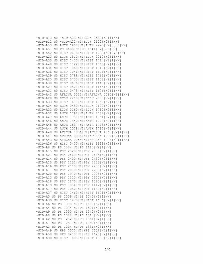
~NID~B13|N0|~NID~A23|N1|ECON 2530|N2|1|NN| ~NID~B12|N0|~NID~A22|N1|ECON 2120|N2|1|NN| ~NID~A53|N0|ANTH 1902|N1|ANTH 2990|N2|0.85|NN| ~NID~A51|N0|PS 0600|N1|PS 1341|N2|0.9|NN| ~NID~A52|N0|HIST 0678|N1|HIST 1788|N2|0.9|NN| ~NID~A23|N0|ECON 1510|N1|ECON 2010|N2|1|NN| ~NID~A35|N0|HIST 1420|N1|HIST 1764|N2|1|NN| ~NID~A40|N0|HIST 1122|N1|HIST 1768|N2|1|NN| ~NID~A34|N0|HIST 1060|N1|HIST 1313|N2|1|NN| ~NID~A36|N0|HIST 1046|N1|HIST 1626|N2|1|NN| ~NID~A29|N0|HIST 0788|N1|HIST 1765|N2|1|NN| ~NID~A25|N0|HIST 0755|N1|HIST 1108|N2|1|NN| ~NID~A30|N0|HIST 0676|N1|HIST 1447|N2|1|NN| ~NID~A27|N0|HIST 0521|N1|HIST 1145|N2|1|NN| ~NID~A31|N0|HIST 0475|N1|HIST 1676|N2|1|NN| ~NID~A42|N0|AFRCNA 0011|N1|AFRCNA 0085|N2|1|NN| ~NID~A28|N0|ECON 2210|N1|ECON 2500|N2|1|NN| ~NID~A33|N0|HIST 1677|N1|HIST 1757|N2|1|NN| ~NID~A24|N0|ECON 0450|N1|ECON 2100|N2|1|NN| ~NID~A22|N0|ECON 0160|N1|ECON 1710|N2|1|NN| ~NID~A32|N0|ANTH 1792|N1|ANTH 2782|N2|1|NN| ~NID~A47|N0|ANTH 1751|N1|ANTH 1761|N2|1|NN| ~NID~A46|N0|ANTH 1542|N1|ANTH 1773|N2|1|NN| ~NID~A45|N0|ANTH 1537|N1|ANTH 1793|N2|1|NN| ~NID~A44|N0|ANTH 1528|N1|ANTH 1782|N2|1|NN| ~NID~A48|N0|AFRCNA 1056|N1|AFRCNA 1068|N2|1|NN| ~NID~A41|N0|AFRCNA 0086|N1|AFRCNA 1002|N2|1|NN| ~NID~A43|N0|AFRCNA 0054|N1|AFRCNA 1003|N2|1|NN| ~NID~A26|N0|HIST 0400|N1|HIST 1191|N2|1|NN| ~NID~A8|N0|PS 1504|N1|PS 1610|N2|1|NN| ~NID~A15|N0|PSY 2520|N1|PSY 2535|N2|1|NN| ~NID~A21|N0|PSY 2460|N1|PSY 2465|N2|1|NN| ~NID~A14|N0|PSY 2400|N1|PSY 2450|N2|1|NN| ~NID~A10|N0|PSY 2252|N1|PSY 2253|N2|1|NN| ~NID~A16|N0|PSY 2110|N1|PSY 2235|N2|1|NN| ~NID~A11|N0|PSY 2010|N1|PSY 2200|N2|1|NN| ~NID~A20|N0|PSY 1970|N1|PSY 2005|N2|1|NN| ~NID~A13|N0|PSY 1320|N1|PSY 2320|N2|1|NN| ~NID~A18|N0|PSY 1270|N1|PSY 1325|N2|1|NN| ~NID~A19|N0|PSY 1054|N1|PSY 1112|N2|1|NN| ~NID~A17|N0|PSY 1052|N1|PSY 1130|N2|1|NN| ~NID~A37|N0|HIST 1460|N1|HIST 1621|N2|1|NN| ~NID~A5|N0|PS 1509|N1|PS 1543|N2|1|NN| ~NID~A39|N0|HIST 1470|N1|HIST 1656|N2|1|NN| ~NID~A6|N0|PS 1378|N1|PS 1607|N2|1|NN| ~NID~A4|N0|PS 1374|N1|PS 1501|N2|1|NN| ~NID~A9|N0|PS 1350|N1|PS 1542|N2|1|NN| ~NID~A0|N0|PS 1322|N1|PS 1513|N2|1|NN| ~NID~A2|N0|PS 1252|N1|PS 1361|N2|1|NN| ~NID~A1|N0|PS 1251|N1|PS 1352|N2|1|NN| ~NID~A3|N0|PS 1204|N1|PS 1331|N2|1|NN| ~NID~A49|N0|HPS 2520|N1|HPS 2536|N2|1|NN| ~NID~A50|N0|HPS 0410|N1|HPS 1620|N2|1|NN| ~NID~A38|N0|HIST 1685|N1|HIST 1758|N2|1|NN|
202

~NID~A12|N0|SOC 0444|N1|SOC 1445|N2|1|NN| ~NID~A7|N0|PS 1521|N1|PS 1710|N2|1|NN|
IE_PLAN_CQA_01ER.vnh
|TBL|IE_PLAN_CQA|FLD|01ER|MTD|2 ~NID~A0|N0|-|N1|C|N2|0.7616|NN|
IE_PLAN_CQA_01IG.vnh
|TBL|IE_PLAN_CQA|FLD|01IG|MTD|2 ~NID~A0|N0|-|N1|C|N2|0.675|NN|
IE_PLAN_CQA_01LL.vnh
|TBL|IE_PLAN_CQA|FLD|01LL|MTD|2 ~NID~A0|N0|-|N1|C|N2|0.4591|NN|
IE_PLAN_CQA_02ER.vnh
|TBL|IE_PLAN_CQA|FLD|02ER|MTD|2 ~NID~B0|N0|~NID~A0|N1|W|N2|0.6623|NN| ~NID~A0|N0|-|N1|C|N2|0.7579|NN|
IE_PLAN_CQA_02IG.vnh
|TBL|IE_PLAN_CQA|FLD|02IG|MTD|2 ~NID~A0|N0|-|N1|C|N2|0.4591|NN|
IE_PLAN_CQA_02LL.vnh
|TBL|IE_PLAN_CQA|FLD|02LL|MTD|2 ~NID~B0|N0|~NID~A0|N1|W|N2|0.6623|NN| ~NID~A0|N0|-|N1|C|N2|0.694|NN|
203

IE_PLAN_CQA_07ER.vnh
|TBL|IE_PLAN_CQA|FLD|07ER|MTD|2 ~NID~A0|N0|-|N1|C|N2|0.4892|NN|
IE_PLAN_CQA_07IG.vnh
|TBL|IE_PLAN_CQA|FLD|07IG|MTD|2 ~NID~A0|N0|-|N1|C|N2|0.4892|NN|
IE_PLAN_CQA_07LL.vnh
|TBL|IE_PLAN_CQA|FLD|07LL|MTD|2 ~NID~A0|N0|-|N1|C|N2|0.4892|NN|
204

APPENDIX D

Test Problem Conditions
Test Student Information Student Plans for Future Semesters 1st Year 2nd Year 3rd Year 4th Year 5th Year 6th Year 7th Year # StuID Current Term Coop? Terms to grad FL SP SR FL SP SR FL SP SR FL SP SR FL SP SR FL SP SR FL SP SR
1 S02 2nd Fall n 5 S S S S S S S S 2 S03 2nd Fall n 6 S S S S S S S S S 3 S04 2nd Fall y 8 (5+3 COOP) S S S S S W S W S W S 4 S05 2nd Fall y 8 (5+3 COOP) S S S S S W S W S W S 5 S06 2nd Fall n 5 S S S S S S S S 6 S07 2nd Fall n 6 S S S S S S S S S 7 J02 3rd Fall y 6 (3+3 COOP) S S S S S W S W S W S 8 J03 3rd Fall y 8 (5+3 COOP) S S S S S S S S S W S W S W S 9 J04 4th Fall n 4 S S S S S S S S S S S
10 J05 1st Fall y 7 (4+3 COOP) S W S W S W S S 11 J06 2nd Fall n 4 S S S S S S S 12 J08 3rd Fall n 4 S S S S S S S S S 13 401 5th Fall y 3 S S S S S W S W S W S S S S 14 404 4th Fall n 2 S S S S S S S S S 15 405 4th Fall n 2 S S S S S S S S S Shaded Already passed S Took or plan to take courses W Worked or plan to work to fulfill Coop program requirements
Blank Idle/drop
206

BIBLIOGRAPHY
BIBLIOGRAPHY
1. Motro, A., “FLEX: A Tolerant and Cooperative User Interface to Databases,” IEEE Transactions on Knowledge Data Engineering, Vol. 2, June 1990, pp. 231-246.
2. Motro, A., “SEAVE: A Mechanism for Verifying User Presuppositions in Query Systems,” ACM Transactions on Office Information Systems, Vol. 4, No. 4 (October, 1986), pp. 312-330.
3. Proceedings of 1995 IEEE International Conference on Fuzzy Systems (International Joint Conference of the 4th IEEE International Conference on Fuzzy Systems and the 2nd International Fuzzy Engineering Symposium), 1995, “User Model for Intelligent Cooperative Dialog System by K. Ishimaru, N. Harada, K. Yamada, A. Nukuzuma, and H. Furukawa”, Vol. 5, pp. 7-8.
4. Proceedings of 1995 IEEE International Conference on Fuzzy Systems (International Joint Conference of the 4th IEEE International Conference on Fuzzy Systems and the 2nd International Fuzzy Engineering Symposium), 1995, “Method of Topic Processing for Cooperative Dialog System by H. Furukawa, N. Harada, K. Yamada, A. Nukuzuma, and K. Ishimaru”, Vol. 5, pp. 7-8.
5. Proceedings of 1995 IEEE International Conference on Fuzzy Systems (International Joint Conference of the 4th IEEE International Conference on Fuzzy Systems and the 2nd International Fuzzy Engineering Symposium), 1995, “Cooperative Dialog System for Decision Support by N. Harada, K. Ishimaru, A. Nukuzuma, H. Furukawa, and K. Yamada”, Vol. 5, pp. 7-8.
6. Wu, Xu, Ichikawa, Tadao, “KDA: A Knowledge-Based Database Assist with a Query Guiding Facility,” IEEE Transactions on Knowledge and Data Engineering, Vol. 4, No. 5 (October 1992), pp. 443-453.
7. Zhang, G., “Interactive Query Formulation Techniques for Databases”(Ph.D. Dissertation, Computer Science, University of California, Los Angeles, 1998)
8. Minker, J., Gal, A., “Producing Cooperative Answers in Deductive Databases,” Logic and Logic Grammar for Language Processing, P. Saint-Dizier and S. Szpakowics, eds, Ellis Horwood, New York, 1990.
9. Proceeding of the 1989 15th International Conference on Very Large Data Base, 1988, “Using Integrity Constraints to Provide Intentional Responses to Relational Queries by A. Motro”, pp. 237-246.
208
10. Minker, J., Wilson, G. A., Zimmerman, B. H., “Query Expansion by The Addition of Clustered Terms for a Document Retrieval System,” Information Storage and Retrieval, Vol. 8, (1972), pp. 329-348.
11. Proceeding of the second International Conference on Expert Database Systems, Virginia, USA, 1988, “Cooperative Answering: A Methodology to Provide Intelligent Access to Database by F. Cuppens and R. Demoloube”
12. Proceeding of the 1989 5th International Conference on Data Engineering, 1989, “Constraints for Improving the Generation of Intentional answers in a Deductive Database by A. Pirotte and D. Roelants” (IEEE Computer Society, 1998), pp. 652-659.
13. Andreasen, T., “Semantic Query Answering,” Proceeding of COMAD 90 (New Delhi, India: McGraw-Hill, 1990.
14. Proceedings of the 1984 (1st) International Workshop on Expert Database System, 1984, “Semantic Retrieval and Levels of Abstraction by F. Corella”, pp. 91-114
15. Proceedings of the 1988 2nd International Conference on Expert Database System, 1988, “Implicit Representation for Extensions Answers by C. D. Shum, R. Muntz”, pp. 257-273.
16. Proceedings of the 1988 14th International Conference on Very Large Data Base, 1988, “An Information-theoretic Study on Aggregate Responses by C. D. Shum, R. Muntz”, pp. 479-490.
17. Merzbacher, Matthew Allen, “Nearness and Cooperative Query Answering” (unpublished Ph.D. Dissertation, Computer Science, University of California, Los Angeles, 1993).
18. Motro, A., "Query Generalization: A Method for Interpreting Null Answers," Expert Database Systems, vol. , 1986, pp 597-616.
19. Chu, W., Chen, Q., “A Structured Approach for Cooperative Query Answering,” IEEE Transactions on Knowledge and Data Engineering, Vol. 6, No.5 (October, 1994), pp. 738-749.
20. Codd, E. F., “A Relational model of Data for Large Shared Data Banks,” Communications of the ACM, Vol. 13, No.6 (June, 1970).
209
21. Smith, J., Smith, D. C. P., “Database Abstraction: Aggregation and Generalization,” ACM Transactions on Database System, Vol. 2, No.2 (1977).
22. Proceedings of the 1990 ACM-SIGMOD International Conference on Management of Data, Atlantic City, June, 1990, “Querying Database Knowledge by A. Motro and Q. Yuan”, pp. 173-183.
23. Chock, M., Cardenas, A. F., Klinger, A., “Database Structure and Manipulation Capabilities of a Picture Data Base Management System (PICDMS),” IEEE Transactions on Pattern Analysis and Machine Intelligence, Vol. 6, No.4 (July, 1985).
24. Joseph, T., Cardenas, A. F., “PICQUERY: A High Level Query Language for Pictorial Data Base Management,” IEEE Transactions on Software Engineering, Special Issue on Image Data Management, 1988.
25. Proceedings of the Fifth International Conference on Very Large Data Bases, Rio de Janeiro, Brazil, October 3-5, 1979, “Semantic Checking of Questions Expressed in Predicate Calculus Language by Robert Demolombe” (IEEE Computer Society, 1979), pp. 444-450.
26. Codd, E. F., “Relational Completeness of Data Base Sublanguages in Data Base Systems,” Courant Computer Science Symposium 6 (Rustin Ed., Prentice Hall, 1972), pp. 69-58.
27. Proceedings of ACM-SIGMOD, May, 1974, “SEQUAL: A Structured English Query Language by D. D. Chamberlin and R. F. Boyce”, 1974.
28. Proceedings of JCIT3, August, 1987, “The Language of SYNTEX2, an Implemented Relational Like DBMS by R. Demolombe, M. Lemaitre, and J. M. Nicolas” (Moneta Ed., North-Holland, 1987).
29. Pirotte, A., Wodon, P., “A Comprehensive Formal Query Language for a Relational Data Base: FQL,” RAIRO Informatique, Vol. 11, No.2, 1977.
30. Zloof, M., “Query-by-example,” AFIPS Conference Proceedings, Vol. 4, 1975.
31. Cole, P., Morgan, J., ed., Syntax and Semantics, “Logic and Conversation by H. Grice”, Academic Press, 1975.
32. Petrakis, Euripides G. M., Faloutsos, Christos, “Similarity Searching in Medical Image Databases,” IEEE Transactions on Knowledge and Data Engineering, Vol. 9, No.3 (May/June 1997), pp. 435-447.
210

33. Chu, Wesley W., Johnson, David B., Kangarloo, Hooshang, “A Medical Digital Library to Support Scenario and User-Tailed Information Retrieval,” IEEE Transactions on Information Technology in Biomedicine, Vol. 4, No. 2 (June 2000), pp. 97-107.
34. Chu, W. W., Cardenas, A. f., tiara, r. K., “KMeD: A Knowledge-based Multimedia Medical Distributed Database System,” Information Systems, Vol. 20, No. 2 (1995), pp. 75-96.
35. Hsu, C. C., Chu, W. W., Tiara, R. K., “A Knowledge-based Approach for Retrieving Images by Content,” IEEE Transactions on Knowledge Data Engineering, Vol. 8, August, 1996, pp. 522-532.
36. Chu, W. W., Hsu, C. C., Cardenas, A. F., Taira, R. K., “Knowledge-based Image Retrieval with Spatial and Temporal Constructs,” IEEE Transactions Knowledge Data Engineering, Vol. 10, December, 1998, pp. 872-888.
37. Sheth, A., Klas, W., ed., Managing Multimedia Data, “Content-based Image Retrieval Using Metadata and Relaxation Techniques by W. W.Chu, , C. C. Hsu, I. T. Ieong, R. K. Taira”, New York, NY, McGraw-Hill, 1998.
38. Proceedings of the User Interfaces to Data Intensive Systems, 1999, “The Design of Query Interfaces to the GPCRDB Biological Database by Dunren Che, K. Aberer, and Y. Chen”, pp. 22-31.
39. Proceedings of the 11th International Conference on Scientific and Statistical Database Management, 1999, “The Advanced Web Query System of GPCRDB by Dunren Che, Yangjun Chen, K. Aberer, and H. Eisner”, pp. 281.
40. Proceedings of the 1999 11th International Conference on Scientific and Statistical Database Management, Cleveland, 1999, “Query system in a biological database by C. Dunren, C. Yangjun, A. Karl”, pp. 158-167.
41. Proceedings of the 1999 User Interfaces to Data Intensive Systems, 1999, “The Design of Query Interfaces to the GPCRDB Biological Database by D. Che, K. Aberer, and Y. Chen”, pp. 22-31.
42. Proceedings of the 11th International Conference on Scientific and Statistic Database Management, 1999, “A Query System in Biological Database by Duren Che, Yangjun Chen, and K. Aberer”, 1999, pp. 158-167.
211
43. Proceedings of the 11th International Conference on Scientific and Statistic Database Management, 1999, “The Advanced Web Query System of GPCRDB by Duren Che, Yangjun Chen, K. Aberer and H. Eisner”, 1999, p. 281.
44. Proceedings of the first International Conference on Expert Database Systems, 1986, “Querying a Rule Base by L. Cholvy and R. Demolombe”, pp. 365-371.
45. Minker, J., ed., Foundations of Deductive Database and Logic Programming, “Intelligent Query Answering in Rule Based Systems by T. Imielinski”, Morgan Kaufman Publishers, 1988.
46. Gaasterland, T., “Cooperative Answering through Controlled Query Relaxation,” IEEE Expert, Vol. 2, No.5 (September/October 1997), pp. 48-59.
47. Proceedings of the 6th International Conference on Data Engineering, 1990, “A Rule-based Language for Deductive Object-oriented Databases by A. M. Alashqur, S. Y. W. Su, and H. Lam”, 1990, pp. 58-67.
48. Proceedings of the 15th International Conference on Very Large Data Bases, 1989, “OQL: A Query Language for Manipulating Object-oriented Databases by A. M. Alashqur, S. Y. W. Su, and H. Lam”, 1989.
49. Proceedings of the 7th IEEE Computer Society International conference on Data Engineering, Washington, DC, 1991, “Using Type Inference and Induced Rules to Provide Intentional Answers by W. W. Chu, R. C. Lee, and Q. Chen”, pp.396-403.
50. Motro, A, “Intentional Answers to Database Queries,” IEEE Transactions on Knowledge and Data Engineering, Vol. 6, No.3 (June, 1994), pp. 444-453.
51. Imielinski, T., “Intelligent Query Answering in Rule Based Systems,” Journal of Logic Programming, Vol. 4, 1987, pp. 229-257.
52. Chu, W. W., Chen, Q., “Neighbor and Associative Query Answering,” Journal of Intelligent Information Systems, Vol. 1, No. 3-4 (1992), pp. 355-382
53. Proceedings of the 8th SMIS, NC, October, 1994, “A Case-based Reasoning Approach for Associative Query Answering by G. Fouque′, W. W. Chu, and H. Yau”, 1994
54. Minock, M., “Toward Scalable and Extensible Explanation for Cooperative Information Systems”, dissertation, University of California, Los Angeles, 1997
212
55. Srirangapatna, N., “Design and Formal Specification of A Data Model and Language for a Database System for CAD Applications” (unpublished Ph.D. Dissertation, University of Alberta, Canada, 1989).
56. Billo, R. E., Rucker, R., and Shunk, D. L., “Integration of a Group Technology Classification and Coding System with an Engineering Database,” Journal of Manufacturing Systems, Vol. 6, No.1 (1987), pp. 37-45.
57. Billo, R. E., Rucker, R., and Shunk, D. L., “Enhancing Group Technology Modeling with Database Abstractions,” Journal of Manufacturing Systems, Vol. 7, No.2 (1988), pp. 95-106.
58. Billo, R., “Organizing Principles for the Design of Classification & Coding Software,” Journal of Manufacturing Systems, Vol. 17, No.6 (1998), pp. 405-417.
59. Billo, R. E., Bidanda, B., “Representing Group Technology Classification and Coding Techniques with Object Oriented Modeling Principles,” IIE Transaction, No.27 (1995), pp. 542-554.
60. Surresh, N., ed., Group Technology, “Part Family Identification: The Role of Engineering Databases by R. E. Billo and B. Bidanda”, (1997), pp. 58-76.
61. Reibeiro, B., “Approximate Answers in Intelligent System (Information Retrieval, Query)”, dissertation, University of California, Los Angeles, 1995
62. Antonio, B., “Cooperative query answering with Generalized Quantifiers”, Journal of Intelligent Information Systems, vol. 12, No. 1 (1999), pp. 75-97.
63. Keen, D., “Inductive Dependencies (Database, Rough sets)”, thesis, University of Kentucky, 1994
64. Gaasterland, T., “Generating Cooperative Answers in Deductive Databases (User Interface, Natural Language, Logic Programming)”, thesis, University of Maryland Collage Park, 1992
65. Friedenbach, K., “Abstraction Hierarchies: A Model of Perception and Cognition in the Game of Go”, dissertation, University of California, Santa Cruz, 1980
66. Fu, Y., “Discovery of Multiple-level rules from large databases”, thesis, Simon Fraser University, Canada, 1996
213
67. Han, Jiawei, Huang, Yue, Cercone, Nick, Fu, Yongjian, “Intelligent Query Answering by Knowledge Discovery Techniques,” IEEE Transaction on Knowledge and Data engineering, Vol. 8, No.3 (June, 1996), pp. 373-390.
68. Fayyad, U. M., Piatetsky-Shapiro, G., Smyth, P., and Uthurusamy, R., eds., Advances in Knowledge Discovery and Data Mining, “Exploration of the Power of Attribute-oriented Induction in Data Mining by J. Han, Y. Fu” (AAAI/MIT Press, 1996), pp. 399-421.
69. Proceeding of the 2nd International Conference on Cooperative Information Systems, Toronto, May, 1994, “Cooperative Query Answering Using Multiple-Layered Databases by J. Han, Y. Fu, and R. Ng”, pp. 47-58.
70. Proceedings of the 1st International Workshop on Interoperability in Multimedia Systems, 1991, “A Pattern-based Approach for Deriving Approximate and Intentional Answers by W. W. Chu, Qiming Chen, and Rei-Chi Lee”, 1991, pp. 262-265.
71. Proceedings of the 2nd International Conference on Systems Integration, 1992, “A Pattern Based Approach for Integrating Data and Knowledge to Support Cooperative Query Answering by W. W. Chu and Q. Chen”, 1992, pp. 615-624.
72. Ras, Z. W., Zemankova, M., Emrich, M. L., ed., Methodologies for Intelligent Systems, “Providing Cooperative Answers via Knowledge-based Type Abstraction and Refinement by Q. Chen, W. Chu and R. Lee” (North-Holland, Elsevier Science Publishing Co. Inc., 1990), Chapter 5.
73. Deen, S. M., ed., Cooperating Knowledge Based Systems, “Cooperative Query Answering via Type Abstraction Hierarchy by W. Chu, Q. Chen and R. Lee” (Elsevier Science Publishing Co. Inc., 1991).
74. Proceedings of the 1993 ACM SIGMOD, Washington, DC, May, 1993, “The Design and Implementation of CoBase by Wesley W. Chu, M. A. Merzbacher, and L. Berkovich”, 1993.
75. Chu, W. W., Yang, H., Chiang, K., Minock, M., Chow, G., Larson, C., “CoBase: A Scalable and Extensible Cooperative Information System,” Intelligent Information Systems, Vol. 6, No.3 (1996), pp. 223-259.
76. Lee, R., “Query Processing with Database Semantics (Semantic Query Optimization)”, dissertation, University of California, Los Angeles, 1990
214
77. Zhang, G., Chu, W.W, Meng, F., Kong, G., ed., User Interfaces to Data Intensive Systems, “Query Formulation from High-level Concepts for Relational Databases by Wesley W. Chu” (IEEE, 1999) pp. 64-75
78. Merabacher, Mattew Allen, “Nearness and Cooperative Query Answering” (unpublished Ph.D. dissertation, Computer Science, University of California, Los Angeles, 1993).
79. Cuppens, F., Demolombe, R., “How to Recognize Interesting Topics to Provide Cooperative Answering,” Information Systems, Vol. 14, No. 2 (1989), pp. 163-173.
80. Cuppens, F., Demolombe, R., “Extending Answers to Neighbor entities in a Cooperative Answering Context,” Decision Support Systems, Vol. 1, No. 11 (1991), pp. 1-11.
81. Yu, C. T., Sun W., “Automatic Knowledge Acquisition and Maintenance for Semantic Query Optimization,” IEEE Transactions on Knowledge and Data Engineering, Vol. 1, 1989, pp. 362-375.
82. Han, J.m Cai, Y., Cercone, N., “Data-driven discovery of Quantitative Rules in Relational Databases,” IEEE Transactions on Knowledge and Data Engineering, Vol. 5, 1993, pp. 29-40.
83. Proceedings of the 1994 AAAI Workshop on Knowledge Discovery in Databases (KDD 94), Seattle, July, 1994, “Dynamic Generation and Refinement of Concept Hierarchies for Knowledge Discovery in Database by J. Han and Y. Fu”, pp. 157-168
84. Huang, Y., “Intelligent Query Answering by Knowledge Discovery Techniques”, thesis, Simon Fraser University, Canada, 1993
85. Proceedings of 1995 Joint Conference on the 4th IEEE International Conference on Fuzzy Systems and the 2nd International Fuzzy Engineering Symposium, Piscataway, NJ, 1995, “Discovery of Global Knowledge in a Database for Cooperative Answering by Jun Ozawa and Koichi Yamada”, 1995.
86. Shannon C. E., Weaver, W., The Mathematical Theory of Communication (Urbana, Illinois, University of Illinois Press, 1964)
87. Piatetsky-Shapiro, G., Frawley, William J., ed., Knowledge Discovery in Databases, “Information Discovery through Hierarchical Maximum Entropy Discretization and Synthesis by David K. Y. Chiu, Andrew K. C. Wong, and Benny Cheung” (AAAI Press/The MIT Press, 1991)
215
88. Wong, A. K. C., Chiu, David K. Y., “Synthesizing Statistical Knowledge from Incomplete Mixed-mode Data,” IEEE Transactions on Pattern Analysis and Machine Intelligence, Vol. 9, No.6 (1987), pp. 796-803.
89. Genari, J., Langley, P. Fisher, D., “Models of Incremental Concept Formation,” Artificial Intelligence, Vol. 40, 1989, pp. 11-62.
90. Proceedings of the AAAI Workshop on Knowledge Discovery in Database, 1994, “Abstraction of High Level Concepts from Numerical Values in Databases by W. Chu and K. Chiang”, pp. 133-144.
91. Chu, W. W., Chiang, K., Hsu, C. C., Yau, H. “An Error-based Conceptual Clustering Method for Providing Approximate Query Answers,” Communications of the ACM, Vol. 39, No. 12 (December, 1996), pp. 216-230
92. Proceedings of the AAAI Workshop on Knowledge Discovery in Database, Washington D.C,1993, “Pattern-based Clustering for Database Attribute Values by M. Merzbacher and W. Chu,” 1993.
93. Proceedings of the 1996 International Conference on Digital Libraries and Information Services for the 21st Century, Seoul, Korea, 1996, “Multimedia Query Processing in Digital Libraries by Jongpil Yoon and Sung-Hyuk Kim”, 1996, pp. 88-106.
94. Proceedings of the 1st International Forum on Research and Technology Advances in Digital Libraries, 1998, “A Three-level User Interface to Multimedia Digital Libraries with Relaxation Restriction by Jongpil Yoon and Sung-Hyuk Kim”, 1998, pp. 206-215.
95. Proceedings of International Conference in Intelligent Information Systems, November, 1997, “Associative Query Answering via Query Feature Similarity by W. W. Chu and G. Zhang”, pp. 405-409.
96. Chu, Wesley W., Yoon, Jeehee, Hsu, Chicheng, “Efficient Searches for Similar Subsequences of Different Lengths in Sequence Databases,” IEEE, 2000, pp. 23-31.
97. Chiang, K., “Automatic Generation of Type Abstraction Hierarchies for Cooperative Query Answering” (unpublished Ph.D. dissertation, Computer Science University of California, Los Angeles, 1995).
98. Fisher, D. H., “Knowledge Acquisition via Incremental Conceptual Clustering,” Machine Learning, Vol. 2, No.2 (1987), pp. 139-172.
216

99. Proceedings of the 7th Annual Conference of the Cognitive Science Society, 1985, “Information, Uncertainty, and the Unity of Categories by M. A. Gluck and J. E. Corter”, pp. 283-287.
100. Spring, Michael, “Resource Description Framework (RDF) Tutorial”, http://www.sis.pitt.edu/~mbsclass/”
217