Coordinated Multi-Point Transmission for Interference ... · Coordinated Multi-Point Transmission for Interference Mitigation in ... Talha Ahmad, B.Eng. A ... Coordinated Multi-Point

Coordinated Multi-Point Transmission for

Interference Mitigation in Cellular Distributed

Antenna Systems

by

Talha Ahmad, B.Eng.

A thesis submitted to the Faculty of Graduate and Postdoctoral Affairs

in partial fulfillment of the requirements for the degree of

Master of Applied Science in Electrical and Computer Engineering

Ottawa-Carleton Institute for Electrical and Computer Engineering (OCIECE)

Department of Systems and Computer Engineering

Carleton University

Ottawa, Ontario, Canada

June 2011

Copyright c©

Talha Ahmad, 2011

The undersigned recommend to

the Faculty of Graduate and Postdoctoral Affairs

acceptance of the thesis

Coordinated Multi-Point Transmission for Interference

Mitigation in Cellular Distributed Antenna Systems

Submitted by

Talha Ahmad, B.Eng.

in partial fulfillment of the requirements for the degree of

Master of Applied Science in Electrical and Computer Engineering

Thesis Supervisor, Dr. Halim Yanıkomeroglu

Chair, Department of Systems and Computer Engineering, Dr. Howard Schwartz

Carleton University

2011

...

In the name of God ,most Gracious ,most Merciful

“Read! In the name of your Lord Who has created (all that exists) – created man

from a clot. Read! And your Lord is the Most Generous – He Who has taught (the

use of) the pen. He has taught man that which he did not know.”

The Holy Qur’an, Chapter 96, Verses 1–5

Abstract

Distributed antenna systems (DASs) have been shown to improve the coverage and

increase the capacity in cellular networks by reducing the access distance to user

terminals (UTs) and by attaining macrodiversity gains. However, the conventional

DASs do not inherently mitigate inter-cell interference. In this thesis, coordinated

multi-point transmission schemes are developed for interference mitigation in the

downlink of a cellular DAS.

The thesis is comprised of two parts. In the first part, two precoding schemes are

developed, which enable coordinated transmission from multiple distributed antenna

ports in a cellular DAS with a total power constraint. The goal is to serve multiple

UTs in a particular resource block in each cell, while mitigating intra-cell and inter-

cell interference. Simulation is used to show the performance gains attained by the

proposed DAS schemes as compared to their co-located antenna system counterparts,

and by centralized multi-cell processing as compared to single-cell processing.

In the second part, the joint selection of the ports and the corresponding beam

steering coefficients that maximize the minimum signal-to-interference-plus-noise ra-

tio of the UTs in a coordinated multi-cell DAS, in which the transmit power of each

port is fixed, is considered. This problem is NP-hard. To circumvent this difficulty, a

two-stage polynomial-complexity technique that relies on semidefinite relaxation and

Gaussian randomization is developed. The performance of the proposed technique is

shown to be comparable to that of exhaustive search. Additionally, it is demonstrated

that proper port selection yields significant power savings in the cellular network.

ii

Acknowledgements

I begin by praising God, the Creator and Sustainer of all the worlds.

I would like to sincerely thank my supervisor, Professor Halim Yanıkomeroglu,

for his support, guidance, and encouragement throughout the course of my master’s

program. I am also grateful to him for giving me the opportunity to be a part of a

knowledgeable, productive, and tightly-knit research group.

My sincere gratitude to Dr. Gary Boudreau (Ericsson Canada), whose insightful

advice greatly enhanced the quality of my research.

A very special thanks to Dr. Saad Al-Ahmadi, Dr. Ramy Gohary, and Akram

Salem Bin Sediq, whose mentorship and influence significantly accelerated my learning

and productivity.

On the personal side, I wish to thank my parents, grandparents, aunts, uncles,

and cousins for their unconditional love, incomparable upbringing, and support of my

academic aspirations.

I wish to thank my colleagues and friends, Furkan Alaca, Dr. Muhammad Aljuaid,

Imran Ansari, Tamer Beitelmal, Dr. Gurhan Bulu, Dr. Ghassan Dahman, Soumi-

tra Dixit, Dr. Petar Djukic, Heba Eid, Yaser Fouad, Arshdeep Kahlon, Kevin Luo,

Mahmudur Rahman, Rozita Rashtchi, Dr. Mohamed Rashad Salem, Alireza Shari-

fian, Dr. Daniel Calabuig Soler, Dr. Sebastian Szyszkowicz, Aizaz Chaudhry, Tariq

Shehata, Meraj Siddiqui, Nazia Ahmad, Mohammad Aslam Malik, Rajab Legnain,

Amar Farouk Merah, Rami Sabouni, Shafiqul Islam, Muhammad Ajmal Khan, Dany

David, and Dr. Laurence Smith for making my experience an enjoyable one.

iii

Contents

Abstract ii

Acknowledegements iii

Contents iv

List of Figures vi

List of Tables vii

Nomenclature viii

1 Introduction 11.1 Cellular Networks . . . . . . . . . . . . . . . . . . . . . . . . . . . . . 11.2 Distributed Antenna Systems . . . . . . . . . . . . . . . . . . . . . . 21.3 Coordinated Multi-Point Transmission and Reception . . . . . . . . . 21.4 Thesis Contributions and Organization . . . . . . . . . . . . . . . . . 31.5 Publications . . . . . . . . . . . . . . . . . . . . . . . . . . . . . . . . 5

2 Background 72.1 Related Works on Distributed Antenna Systems . . . . . . . . . . . . 72.2 Related Works on CoMP . . . . . . . . . . . . . . . . . . . . . . . . . 82.3 Information-Theoretic Background . . . . . . . . . . . . . . . . . . . 9

3 Coordinated Multi-Point Downlink Transmission Schemes 113.1 Related Literature . . . . . . . . . . . . . . . . . . . . . . . . . . . . 113.2 Background: Basic Linear Algebra . . . . . . . . . . . . . . . . . . . 12

3.2.1 Eigenvectors and Eigenvalues . . . . . . . . . . . . . . . . . . 133.2.2 Null Space of a Matrix . . . . . . . . . . . . . . . . . . . . . . 133.2.3 Rank of a Matrix . . . . . . . . . . . . . . . . . . . . . . . . . 133.2.4 Singular Value Decomposition . . . . . . . . . . . . . . . . . . 14

3.3 Single-Cell Processing . . . . . . . . . . . . . . . . . . . . . . . . . . 143.3.1 System Model . . . . . . . . . . . . . . . . . . . . . . . . . . . 143.3.2 DAS Block Diagonalization . . . . . . . . . . . . . . . . . . . 193.3.3 DAS Zero-Forcing Dirty Paper Coding . . . . . . . . . . . . . 233.3.4 An Exemplary Configuration . . . . . . . . . . . . . . . . . . . 25

3.4 Centralized Multi-Cell Processing . . . . . . . . . . . . . . . . . . . . 27

iv

v

3.4.1 System Model . . . . . . . . . . . . . . . . . . . . . . . . . . . 283.4.2 DAS Block Diagonalization . . . . . . . . . . . . . . . . . . . 293.4.3 DAS Zero-Forcing Dirty Paper Coding . . . . . . . . . . . . . 31

3.5 Performance Evaluation . . . . . . . . . . . . . . . . . . . . . . . . . 323.5.1 Single-Cell System (Interference-Free Environment) . . . . . . 333.5.2 Multi-Cell System with Single-Cell Processing . . . . . . . . . 413.5.3 Multi-Cell System with Centralized Processing . . . . . . . . . 48

4 Coordinated Max-Min Fair Multi-Cell Port Selection and BeamSteering Optimization using Semidefinite Relaxation 534.1 Related Literature . . . . . . . . . . . . . . . . . . . . . . . . . . . . 534.2 Background: Mathematical Optimization . . . . . . . . . . . . . . . . 54

4.2.1 Convex Optimization Problem . . . . . . . . . . . . . . . . . . 554.2.2 Semidefinite Programming . . . . . . . . . . . . . . . . . . . . 554.2.3 Relaxation of an Optimization Problem . . . . . . . . . . . . . 55

4.3 System Model . . . . . . . . . . . . . . . . . . . . . . . . . . . . . . . 564.4 Problem Statement and Proposed Solution . . . . . . . . . . . . . . . 584.5 Coordinated Multi-Cell Port Selection . . . . . . . . . . . . . . . . . 58

4.5.1 Positive Semidefinite Relaxation . . . . . . . . . . . . . . . . . 614.5.2 Randomization for Coordinated Port Selection . . . . . . . . . 64

4.6 Coordinated Beam Steering Optimization . . . . . . . . . . . . . . . . 664.7 A Two-Stage Approach to obtain an Approximate Solution to the Joint

Optimization Problem . . . . . . . . . . . . . . . . . . . . . . . . . . 714.8 Complexity Analysis . . . . . . . . . . . . . . . . . . . . . . . . . . . 71

4.8.1 Computational Complexity of the First Stage . . . . . . . . . 724.8.2 Computational Complexity of the Second Stage . . . . . . . . 734.8.3 Computational Complexity of the Two-Stage Approach . . . . 73

4.9 Performance Evaluation . . . . . . . . . . . . . . . . . . . . . . . . . 74

5 Conclusions and Future Work 935.1 Summary . . . . . . . . . . . . . . . . . . . . . . . . . . . . . . . . . 935.2 Contributions . . . . . . . . . . . . . . . . . . . . . . . . . . . . . . . 945.3 Future Work . . . . . . . . . . . . . . . . . . . . . . . . . . . . . . . . 94

Appendices 96

A Proofs and Derivations for Chapter 4 97A.1 Derivation of the matrix notation in (4.7) . . . . . . . . . . . . . . . . 97A.2 Proof for Lemma 4.1 . . . . . . . . . . . . . . . . . . . . . . . . . . . 98

References 99

List of Figures

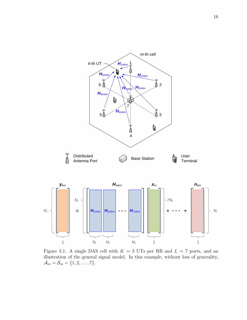
3.1 A single DAS cell with K = 3 UTs per RB and L = 7 ports, and anillustration of the general signal model. In this example, without lossof generality, Am = Sm = {1, 2, . . . , 7}. . . . . . . . . . . . . . . . . . 16

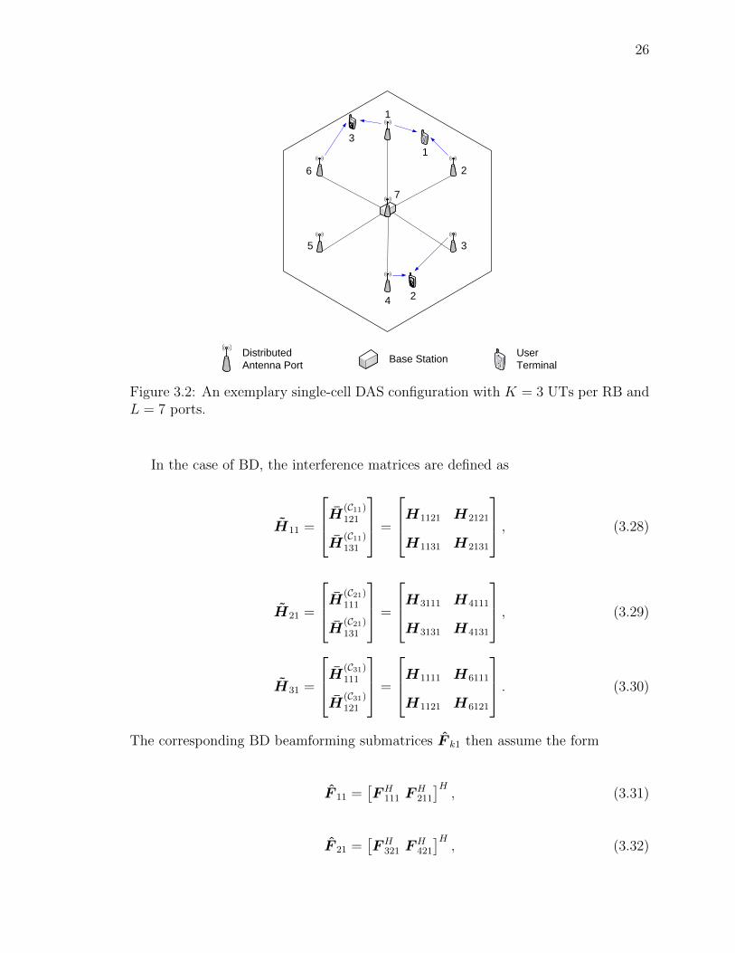
3.2 An exemplary single-cell DAS configuration with K = 3 UTs per RBand L = 7 ports. . . . . . . . . . . . . . . . . . . . . . . . . . . . . . 26

3.3 A comparison between the ergodic and outage aggregate cell spectralefficiencies per RB achieved by DAS BD and DAS ZF-DPC and thoseachieved by their CAS counterparts in a single-cell system that oper-ates in an interference-free environment. Nt = 2 and |Ckm| = 3, ∀k. . 35



3.6 A comparison between the aggregate cell spectral efficiencies per RBachieved by DAS BD and DAS ZF-DPC and those achieved by theirCAS counterparts for different values of Nt in a single-cell system thatoperates in an interference-free environment. |Ckm| = 3, ∀k. . . . . . 39

3.7 A comparison between the aggregate cell spectral efficiencies per RBachieved by DAS BD and DAS ZF-DPC for different values of |Ckm| ina single-cell system that operates in an interference-free environment.Nt = 3. . . . . . . . . . . . . . . . . . . . . . . . . . . . . . . . . . . . 40

3.8 A comparison between the aggregate cell spectral efficiencies per RBachieved by DAS BD and DAS ZF-DPC, and those achieved by theirCAS counterparts for different UT locations in a single-cell system thatoperates in an interference-free environment. Nt = 2 and |Ckm| = 3, ∀k. 41

3.9 A seven-cell DAS with single-cell processing, K = 3 UTs per RB, andL = 7 ports per cell. . . . . . . . . . . . . . . . . . . . . . . . . . . . 42

3.10 A comparison between the ergodic and outage aggregate cell spectralefficiencies per RB achieved by DAS BD and DAS ZF-DPC and thoseachieved by their CAS counterparts for a cell that operates in an inter-cell interference environment. Nt = 2 and |Ckm| = 3, ∀k. . . . . . . . 44

vi

vii



3.13 A comparison between the aggregate cell spectral efficiencies per RBachieved by DAS BD and DAS ZF-DPC for different values of |Ckm|for a cell that operates in an inter-cell interference environment. Nt = 3. 47

3.14 A seven-cell DAS with centralized multi-cell processing, K = 3 UTsper RB, and L = 7 ports per cell. . . . . . . . . . . . . . . . . . . . . 49

3.15 A comparison between the ergodic and outage average aggregate spec-tral efficiency per cell per RB achieved by DAS BD and DAS ZF-DPCwith centralized multi-cell processing and with single-cell processingfor a seven-cell cluster. Nt = 2 and |Ck| = 3, ∀k. . . . . . . . . . . . . 50

3.16 A comparison between the ergodic and outage average aggregate spec-tral efficiency per cell per RB achieved by DAS BD and DAS ZF-DPCwith centralized multi-cell processing and with single-cell processingfor a seven-cell cluster. Nt = 3 and |Ck| = 3, ∀k. . . . . . . . . . . . . 52

4.1 A seven-cell DAS cluster with seven ports per cell. . . . . . . . . . . . 764.2 A comparison between the largest minimum SINR achieved by port

selection with exhaustive search and with the technique proposed in thefirst stage, and that achieved by the one-port (without coordination)and all-port strategies for a two-cell cluster in the SMa scenario. . . . 77

4.3 A comparison between the largest minimum spectral efficiency achievedby port selection with exhaustive search and with the technique pro-posed in the first stage, and that achieved by the one-port (withoutcoordination) and all-port strategies for a two-cell cluster in the SMascenario. . . . . . . . . . . . . . . . . . . . . . . . . . . . . . . . . . . 78

4.4 A comparison between the largest minimum SINR achieved by the portselection technique proposed in the first stage, and that achieved by theone-port (without coordination) and all-port strategies for a seven-cellcluster in the SMa scenario. . . . . . . . . . . . . . . . . . . . . . . . 80

4.5 A comparison between the largest minimum spectral efficiency achievedby the port selection technique proposed in the first stage, and thatachieved by the one-port (without coordination) and all-port strategiesfor a seven-cell cluster in the SMa scenario. . . . . . . . . . . . . . . . 81

4.6 The distribution of the number of ports activated per cell by the portselection technique proposed in the first stage for a seven-cell clusterin the SMa scenario. . . . . . . . . . . . . . . . . . . . . . . . . . . . 82

viii

4.7 The average number of ports activated per cell by the port selectiontechnique proposed in the first stage for a seven-cell cluster in the SMascenario. . . . . . . . . . . . . . . . . . . . . . . . . . . . . . . . . . . 83

4.8 A comparison between the average spectral efficiency per cell achievedby the port selection technique proposed in the first stage, by the single-port (without coordination) and all-port transmission strategies, andby the CAS for a seven-cell cluster in the SMa scenario. . . . . . . . . 84

4.9 A comparison between the largest minimum SINR achieved by the portselection technique proposed in the first stage, and that achieved by theone-port (without coordination) and all-port strategies for a seven-cellcluster in the UMa scenario. . . . . . . . . . . . . . . . . . . . . . . . 86

4.10 A comparison between the largest minimum spectral efficiency achievedby the port selection technique proposed in the first stage, and thatachieved by the one-port (without coordination) and all-port strategiesfor a seven-cell cluster in the UMa scenario. . . . . . . . . . . . . . . 87

4.11 The distribution of the number of ports activated per cell by the portselection technique proposed in the first stage for a seven-cell clusterin the UMa scenario. . . . . . . . . . . . . . . . . . . . . . . . . . . . 88

4.12 The average number of ports activated per cell by the selection tech-nique proposed in the first stage for a seven-cell cluster in the UMascenario. . . . . . . . . . . . . . . . . . . . . . . . . . . . . . . . . . . 89

4.13 A comparison between the average spectral efficiency per cell achievedby the port selection technique proposed in the first stage, by the single-port (without coordination) and all-port transmission strategies, andby the CAS for a seven-cell cluster in the UMa scenario. . . . . . . . 90

4.14 A comparison between the largest minimum SINR achieved by thecomputationally-efficient two-stage approach proposed herein, an exhaustive-search based close-to-optimal solution, and the port selection techniquein the first stage for a two-cell cluster in the SMa scenario. . . . . . . 91

4.15 A comparison between the largest minimum spectral efficiency achievedby the computationally-efficient two-stage approach proposed herein,an exhaustive-search based close-to-optimal solution, and the port se-lection technique in the first stage for a two-cell cluster in the SMascenario. . . . . . . . . . . . . . . . . . . . . . . . . . . . . . . . . . . 91

List of Tables

3.1 System and simulation parameters used for the cellular DAS architecture 33

4.1 Algorithm 1 – Generating a close-to-optimal set of port states . . . . 664.2 Algorithm 2 – Generating close-to-optimal beam steering coefficients . 704.3 Complexity of the proposed techniques and the corresponding exhaus-

tive search . . . . . . . . . . . . . . . . . . . . . . . . . . . . . . . . . 744.4 System parameters used to simulate the cellular DAS architecture . . 744.5 IMT-Advanced scenario parameters used to simulate the cellular DAS 754.6 Channel gains between the ports and the UTs in each cell

(×10−4

). 92

ix

Nomenclature

Acronyms

Acronym Meaning

3GPP 3rd Generation Partnership Project

BC Broadcast channel

BD Block diagonalization

BS Base station

CAS Co-located antenna system

CDMA Code division multiple access

CoMP Coordinated multi-point

CSI Channel state information

DAS Distributed antenna system

DPC Dirty paper coding

IC Interference channel

ICI Inter-cell interference

LTE Long Term Evolution

IMT International Mobile Telecommunications

MAC Medium access control

MIMO Multiple-input multiple-output

NLoS Non-line-of-sight

NP-hard Non-deterministic polynomial-time hard

OFDM Orthogonal frequency division multiplexing

x

xi

OFDMA Orthogonal frequency division multiple access

PSD Positive semidefinite

RB Resource block

SDP Semidefinite program

SDR Semidefinite relaxation

SINR Signal-to-interference-plus-noise ratio

SMa Suburban macro-cell

SNR Signal-to-noise ratio

SVD Singular value decomposition

UMa Urban macro-cell

UT User terminal

ZFBF Zero-forcing beamforming

ZF-DPC Zero-forcing dirty paper coding

xii

Mathematical Operators and Symbols

Symbol Meaning

(·)∗ Complex conjugate

(·)T Transpose of the vector or matrix argument

(·)H Hermitian of the vector or matrix argument

IN N ×N identity matrix

0M×N M ×N all zero-matrix

Rn×m Space of n×m real matrices

Cn×m Space of n×m complex matrices

| · | Absolute value of the scalar argument, determinant of the matrix

argument, or cardinality of the set argument

‖ · ‖2 Frobenius norm of the matrix argument

E{·} Expected value

P{E} Probability of event E occurring

Tr(·) Trace of the matrix argument

rank(·) Rank of the matrix argument

diag(·) Vector comprised of the diagonal elements of the matrix argument

⊕ Direct sum of matrices

{·} Set complement

{·} \ {·} Set difference

sgn(·) Element-wise signum function

Chapter 1

Introduction

1.1 Cellular Networks

Cellular networks gained commercial momentum during the 1990s as a convenient

means of voice communication. The primary usage of these networks has since shifted

toward data communication, and it is expected that data-intensive applications, such

as mobile Internet and multimedia services, will consume most of the resources in

future cellular networks.

In a cellular network, a geographical area is tessellated into smaller regions called

cells. A base station (BS) is located in each cell and it provides wireless services

to mobile user terminals (UTs) in its coverage region. All BSs in the network are

connected to each other with a wired backbone network. When a UT moves from one

cell to another, the serving BS hands off its responsibilities to the BS in the new cell.

As is characteristic of a terrestrial wireless channel, UTs that are located far from

the BS are likely to receive highly attenuated signals. This phenomenon is called

path loss. In addition to path loss, UTs that are located close to the periphery of

the cell may suffer from inter-cell interference (ICI), i.e., the interference caused by

transmissions from the BSs in other cells. Both path loss and ICI reduce the signal-

to-interference-plus-noise ratio (SINR), and in turn, the achievable data rates, of the

UTs, especially those at the cell edge. Hence, there is a need to develop efficient

and cost-effective techniques to combat these phenomena in order for future cellular

1

2

networks to satisfy the anticipated consumer demands.

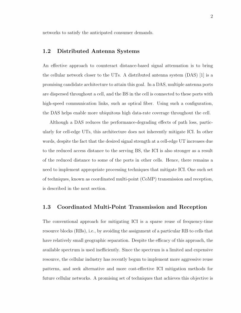
1.2 Distributed Antenna Systems

An effective approach to counteract distance-based signal attenuation is to bring

the cellular network closer to the UTs. A distributed antenna system (DAS) [1] is a

promising candidate architecture to attain this goal. In a DAS, multiple antenna ports

are dispersed throughout a cell, and the BS in the cell is connected to these ports with

high-speed communication links, such as optical fiber. Using such a configuration,

the DAS helps enable more ubiquitous high data-rate coverage throughout the cell.

Although a DAS reduces the performance-degrading effects of path loss, partic-

ularly for cell-edge UTs, this architecture does not inherently mitigate ICI. In other

words, despite the fact that the desired signal strength at a cell-edge UT increases due

to the reduced access distance to the serving BS, the ICI is also stronger as a result

of the reduced distance to some of the ports in other cells. Hence, there remains a

need to implement appropriate processing techniques that mitigate ICI. One such set

of techniques, known as coordinated multi-point (CoMP) transmission and reception,

is described in the next section.

1.3 Coordinated Multi-Point Transmission and Reception

The conventional approach for mitigating ICI is a sparse reuse of frequency-time

resource blocks (RBs), i.e., by avoiding the assignment of a particular RB to cells that

have relatively small geographic separation. Despite the efficacy of this approach, the

available spectrum is used inefficiently. Since the spectrum is a limited and expensive

resource, the cellular industry has recently begun to implement more aggressive reuse

patterns, and seek alternative and more cost-effective ICI mitigation methods for

future cellular networks. A promising set of techniques that achieves this objective is

3

CoMP, which is also known as multi-cell multiple-input multiple-output (MIMO) or

network MIMO.

Under the CoMP framework, a high-speed backbone network that connects the

BSs to each other is used to establish coordination between these BSs. By means

of this coordination, various ICI mitigation techniques can be implemented, thus

increasing the SINR of cell-edge UTs. Although the concept of BS coordination has

existed in the research community for a relatively long period of time (see, e.g., [2,

3, 4]), CoMP has recently been proposed as a candidate technology for enhancing

data rates in future cellular networks [5, 6, 7]. In particular, CoMP is envisioned to

be an integral part of the 3rd Generation Partnership Project (3GPP) Long Term

Evolution (LTE) Advanced specifications (Release 11 and beyond) [8, 9].

Although coordination among BSs is the most common type of CoMP, it can be

observed that transmission from multiple distributed antenna ports in a DAS to a

particular UT is also an intra-cell level of CoMP. Hence, the DAS architecture and

CoMP schemes (both at the intra-cell and inter-cell levels) complement each other

to collectively achieve improved performance in cellular networks. In fact, the use

of CoMP schemes in conjunction with cellular DASs is in consideration for LTE-

Advanced; see [8, Section 20.1].

1.4 Thesis Contributions and Organization

In this thesis, both intra-cell and inter-cell downlink CoMP schemes are incorporated

into a cellular DAS architecture. In doing so, not only are the performance-degrading

effects of path loss reduced, but ICI is also mitigated. Hence, significantly improved

performance is attained in the cellular network.

An approach that is common to all the chapters in the thesis is port selection,

wherein a subset of the available distributed antenna ports in a cell or a cluster of cells

are chosen for transmission to each UT. Port selection is motivated by the trade-off

4

between the benefit to a particular UT that is achieved by using a large number of

ports to transmit to this UT, and the performance loss that is suffered by other UTs

as a result of the increased levels of interference. It is shown in the thesis that an

individual (per-port or per-antenna) power constraint is desirable to fully realize the

performance gains of port selection. In particular, it is demonstrated that, when each

port transmits at a fixed power level, significant improvement in the performance can

be attained using proper port selection.

Throughout the thesis, a variety of metrics are used to assess the performance of

the schemes and algorithms that are developed for the cellular DAS. These include

the aggregate cell spectral efficiency per RB, the average aggregate spectral efficiency

per cell per RB, and the maximum minimum SINR (i.e., the maximum achievable

guarantee on the minimum SINR of the UTs). The first two metrics represent overall

performance of a particular cell or the network, while the third one can be related to

the performance of cell-edge UTs.

The thesis is organized as follows:

• In Chapter 2, a brief literature review is given for DAS and CoMP, in addition

to suitable information-theoretic models for cellular systems employing various

levels of CoMP. The existing results for these models are used to assess the

challenges involved in the design of downlink CoMP schemes for a cellular DAS.

• In Chapter 3, two closely-related precoding schemes are developed for a cellular

DAS with a priori port selection and coordinated transmission from multiple

distributed antenna ports. These schemes are extensions of existing ones for

a co-located antenna system (CAS), i.e., a conventional cellular system. The

performance gains of the DAS schemes over the corresponding CAS schemes are

demonstrated using simulation. The results in this chapter provide important

insights, which are used to develop the algorithms described in the next chapter.

5

• Chapter 4 contains the main contribution of thesis. In this chapter, a two-stage

approach is proposed for determining an approximate set of binary port states

and the corresponding beam steering coefficients that collectively maximize the

minimum SINR in a cellular DAS with inter-cell coordination and fixed transmit

power levels at each port. In each stage of this approach, the semidefinite

relaxation (SDR) technique with Gaussian randomization is used to efficiently

generate a close-to-optimal solution to an optimization problem that is non-

deterministic polynomial-time hard (NP-hard). Hence, the proposed approach

is capable of providing an approximate solution to the original NP-hard problem

in polynomial time, and simulation is used to demonstrate its efficacy.

• The thesis is concluded in Chapter 5 with a summary of the main contributions

and a discussion of potential ideas for future work in the area of downlink CoMP

transmission in a cellular DAS.

1.5 Publications

Chapter 3

• Talha Ahmad, Saad Al-Ahmadi, Halim Yanikomeroglu, and Gary Boudreau,

“Downlink linear transmission schemes in a single-cell distributed antenna sys-

tem with port selection,” in Proceedings of IEEE Vehicular Technology Confer-

ence (VTC2011-Spring), May 2011.

Chapter 4

• Talha Ahmad, Ramy Gohary, Halim Yanikomeroglu, Saad Al-Ahmadi, and

Gary Boudreau, “Coordinated port selection and beam steering optimization

in a multi-cell distributed antenna system using semidefinite relaxation,” under

review in IEEE Transactions on Wireless Communications.

6

• Talha Ahmad, Ramy Gohary, Halim Yanikomeroglu, Saad Al-Ahmadi, and

Gary Boudreau, “Coordinated max-min fair port selection in a multi-cell dis-

tributed antenna system using semidefinite relaxation,” submitted to IEEE

Global Communications Conference (Globecom 2011) Workshop on Distributed

Antenna Systems for Broadband Mobile Communications, December 2011.

Chapter 2

Background

2.1 Related Works on Distributed Antenna Systems

Distributed antenna systems were originally introduced in [1] to fill coverage gaps

in indoor wireless networks, and early research on DASs was in the context of such

networks (see, e.g., [10]).

Early works on the integration of DASs in cellular networks appeared in [11]–[14],

and these were primarily focussed on code division multiple access (CDMA) based

systems. In addition to incorporating this architecture into cellular networks, it was

shown in these works that dispersing the antennas of the BS over the geographic area

of the cell results in increased capacity as well as reduced transmit power levels.

In [15], the uplink outage signal-to-noise ratio (SNR) performance of a generalized

MIMO DAS with multi-antenna ports and multi-antenna UTs was evaluated for var-

ious diversity combining schemes using a composite fading channel model. This work

was followed by [16], wherein the uplink and downlink outage capacity achieved by

such a generalized MIMO DAS was investigated. Furthermore, in [17], it was demon-

strated that a DAS achieves significantly higher capacity as compared to a traditional

MIMO system, i.e., a CAS.

Although the performance improvements offered by a DAS as compared to a

CAS are clear, the literature regarding transmission and power allocations schemes

in a DAS was relatively limited in the past. Recently, however, novel DAS signal

7

8

processing and resource allocation schemes, particularly those involving coordination

between multiple ports and/or cells, have begun to appear; see, e.g., [18, 19] (both of

these works will be discussed in further detail in Section 3.1).

A comprehensive overview of the DAS architecture and related coordinated trans-

mission and power allocation schemes, as well as other resource allocation schemes,

can be found in [20, 21].

2.2 Related Works on CoMP

The term coordinated multi-point transmission and reception serves as an umbrella

for techniques and schemes that utilize coordination between multiple transmitters

and/or receivers to mitigate interference. In the context of cellular networks, CoMP

generally refers to coordination between BSs for both uplink and downlink. The focus

in this thesis is on the latter scenario, and hence, an overview of literature related to

the downlink case will be provided in this section.

The set of techniques that fall under the CoMP umbrella spans both the physical

and medium access control (MAC) layers. For instance, physical layer CoMP tech-

niques include coordinated multi-cell beamforming and precoding (see, e.g., [22, 23]),

while MAC layer techniques include coordinated UT scheduling and power allocation

(see, e.g., [24]). The focus herein is on the earlier set of techniques.

An assumption that is commonly made when designing CoMP schemes is that all

the BSs have perfect channel state information (CSI) for all the UTs in the coordina-

tion region. Furthermore, it is generally assumed that the coordination between the

BSs is perfect, i.e., the backbone links have negligible delay, are relatively error-free,

and have infinite capacity. Although such assumptions simplify the design, they are

not necessarily applicable in practice, especially when the number of coordinating

BSs is large. To alleviate such impractical assumptions while maintaining design

tractability, clustered coordination schemes have been proposed [25, 26]. In such

9

schemes, a large cellular network is divided into smaller clusters of cells. The BSs of

the cells in a particular cluster coordinate their transmissions, but there is limited or

no inter-cluster coordination. Additionally, in some works, such as [27] and [28], the

heavy overhead on the backbone is reduced by designing schemes that rely only on

locally available CSI.

Although CoMP techniques impose a heavier load on the backbone and also have

relatively strict delay and error threshold requirements, their potential advantages

in terms of the achievable data rates have been demonstrated both numerically [29]

and analytically [30]. They have also been shown to outperform conventional non-

coordinating cellular networks, even in the presence of moderate amounts of channel

estimation error [31]. Furthermore, in [32], a performance trade-off has been investi-

gated between BS coordination and denser BS deployment in future cellular networks.

A detailed overview of existing CoMP schemes, their performance, and the chal-

lenges involved in their implementation, can be found in [33] and [34].

2.3 Information-Theoretic Background

In this section, the underlying information-theoretic models will be presented for

cellular systems with different levels of coordination.

Consider a single-cell system in which a multi-antenna BS transmits to one or

more UTs1. If the number of UTs in the cell is exactly one, then such a system

can be modelled as a point-to-point MIMO channel, for which, the capacity can be

achieved using the singular value decomposition (SVD) based water-filling scheme

proposed in [35]. However, if there are multiple UTs in the cell, then such a system

can be modelled as a Gaussian MIMO broadcast channel (BC), for which, the dirty

paper coding (DPC) scheme [36] is known to achieve the capacity [37]. However,

DPC is difficult to implement in practice, and hence, there exist various linear and

1The antennas of the BS may be either co-located or distributed.

10

non-linear sub-optimal schemes that are more practical (see, e.g., [38]–[44]). Such

schemes will be the focus of the discussion in Chapter 3.

Now, let us consider a more general multi-cell system in which the BS in each

cell operates independently as described above. Such a system can be treated as

a MIMO interference channel (IC). Although information-theoretic results exist for

some special cases (see, e.g., [45]), the capacity region of a general MIMO IC has

not yet been characterized. It is, therefore, difficult to gauge the performance of

transmission schemes designed for such systems. A simplifying strategy is to establish

full multi-cell coordination, which results in a larger MIMO BC. This is the approach

taken to model the system in Chapter 4.

Chapter 3

Coordinated Multi-Point Downlink Transmission

Schemes

In this chapter, the focus is on the design and performance evaluation of downlink

transmission schemes in a cellular DAS, wherein a subset of the available multi-

antenna ports of a cell transmit in a coordinated manner to serve one or more multi-

antenna UTs in a particular RB.

3.1 Related Literature

As mentioned in Section 2.3, a single-cell CAS with multi-antenna UTs can be mod-

eled as a Gaussian MIMO BC, for which the optimal transmission scheme is DPC.

However, DPC is difficult to implement in practice due to its computational complex-

ity, and several sub-optimal transmission schemes have been proposed for mitigating

inter-user interference. In [38], the zero-forcing dirty paper coding (ZF-DPC) scheme

is proposed, which uses LQ decomposition on the aggregate channel matrix, which

consists of the channel matrices of all single-antenna UTs, to eliminate a part of the

inter-user interference. The remaining interference is mitigated by means of successive

dirty paper encoding. In [38], ZF-DPC is shown to be asymptotically optimal with

increasing SNR. In [40]–[43], this scheme is extended to incorporate multi-antenna

UTs. A linear scheme that mitigates inter-user interference is zero-forcing beam-

forming (ZFBF), which spatially orthogonalizes all single-antenna UTs by using the

11

12

pseudo-inverse of the aggregate channel matrix as the precoding matrix. An exten-

sion of this scheme for multi-antenna UTs is block diagonalization (BD) [39], in which

the precoding matrix of each UT is designed such that its transmitted signal is in the

null space of the channel matrices of the other UTs.

With the incorporation of port selection, the CAS-based versions of the schemes

described above cannot be directly applied to a DAS, and processing modifications

are necessary. In this chapter, the ZF-DPC and BD schemes are extended to fit the

cellular DAS architecture.

In [18], the performance of various multi-user transmission schemes, including BD,

is explored in the context of a single-cell DAS with multi-antenna ports. However,

the schemes presented in [18] do not incorporate port selection. Furthermore, single-

antenna UTs are mainly assumed and spatial multiplexing of multiple data streams

for each UT is not included. Both these features are included in the schemes described

herein. In [19], port selection is explored for a multi-user cellular DAS. However, the

UTs are orthogonalized through orthogonal frequency division multiplexing (OFDM).

In contrast, orthogonalization is achieved using spatial precoding in this chapter.

3.2 Background: Basic Linear Algebra

In this section, a brief overview will be provided for matrix analysis topics that are

relevant to the formulation in this chapter. Before proceeding, however, it is necessary

to state that throughout this chapter and the rest of the thesis, scalars are denoted

by lower-case regular-face letters, vectors are denoted by lower-case bold-face letters,

and matrices are denoted by upper-case bold-face letters.

13

3.2.1 Eigenvectors and Eigenvalues

Let A be a square matrix. A non-zero vector v is called a right eigenvector of A if

there exists a scalar, λ, such that

Av = λv, (3.1)

and it is called a left eigenvector of A if there exists a scalar, λ, such that

vHA = λvH . (3.2)

In (3.1) and (3.2), λ is called an eigenvalue of A corresponding to v and vH , respec-

tively [46, Section 6.1].

3.2.2 Null Space of a Matrix

Let B ∈ Cm×n be a rectangular matrix. The null space, which is also referred to as

the kernel, of the matrix B is the set of vectors y such that

By = 0. (3.3)

The dimension of the null space of a matrix is called the nullity of this matrix [46,

Section 4.5].

3.2.3 Rank of a Matrix

The rank of a matrix is defined as the minimum number of linearly independent

columns or rows of this matrix [46, Section 4.5]. This value is related to the nullity

of the matrix as follows. Consider the matrix B defined above, and let r denote the

rank of B. Then, the nullity of B is equal to n− r.

14

3.2.4 Singular Value Decomposition

Consider the rectangular matrix B defined in Section 3.2.2. Any such matrix can be

factorized as follows:

B = UΣV H , (3.4)

where U ∈ Cm×m and V ∈ Cn×n are unitary matrices1 and Σ ∈ Rm×n is a diagonal

matrix of the form

Σ =

σ1

. . .

σp

,where p = min(m,n), and σ1, . . . , σp are called the singular values of B [46, Section

7.1]. These singular values are generally arranged in decreasing order, and are related

to the eigenvalues as follows:

λi = σ2i , i = 1, . . . , p. (3.5)

3.3 Single-Cell Processing

In this section, the DAS BD and DAS ZF-DPC schemes will be developed under the

assumption that the BS in each cell operates independently from those in other cells.

3.3.1 System Model

Consider a cellular DAS consisting of M cells which use the same set of frequency-

time RBs each. The BS in each cell is connected to L distributed Nt-antenna ports

with high-speed communication links (e.g., optical fiber). Additionally, the BS in

each cell has reliable knowledge of the gains between the ports and each UT in this

1A matrix U is said to be unitary if UHU = UUH = I, where I is an identity matrix [46,Section 5.3.1].

15

cell. A multi-user system that uses a narrow-band multiple access scheme, such as an

orthogonal frequency division multiple access (OFDMA) based one, is considered. In

this system, there are K UTs per RB in each cell, and these UTs are equipped with

Nr antennas each.

Let Sm represent the set of indices of all ports in the m-th cell, where |Sm| = L

and | · | denotes the cardinality of the set argument. Let Am represent the set of

active ports in the m-th cell (Am ⊆ Sm). Also, let Ckm denote the set of ports in the

m-th cell that transmit to the k-th UT in this cell in a coordinated manner, and let

Ikm denote the set of ports in the m-th cell that cause interference to this UT. Hence,

Ckm⋃Ikm = Am for all k,m, and

⋃Kk=1 Ckm =

⋃Kk=1 Ikm = Am for all m.

Before proceeding with a description of the signal and channel models, it is empha-

sized that all formulation that follows is applicable to a single RB. However, explicit

reference to a particular RB index is omitted for notational brevity.

In Fig. 3.1, a single cell of the cellular DAS with L = 7 and K = 3 is shown, and

the signal model that follows in this section is illustrated.

Signal Model

The received signal, ykm ∈ CNr , of the k-th UT in the m-th cell can be expressed as

ykm = Hmkmxm +M∑

n=1,n 6=m

Hnkmxn + nkm, k = 1, . . . , K, m = 1, . . . ,M, (3.6)

where, Hnkm ∈ CNr×|An|Nt is a matrix consisting of the complex-valued channel gains

between all active ports in the n-th cell and the k-th UT in the m-th cell, nkm ∈ CNr

is a zero-mean complex Gaussian noise vector with covariance matrix E{nkmnHkm} =

σ2INr , where INr denotes an Nr×Nr identity matrix, and xm ∈ C|Am|Nt is the signal

16

Distributed

Antenna PortBase Station

User

Terminal

m-th cell

k-th UT 1

2

3

4

5

6

7

H1mkm

H6mkm

H7mkm

H2mkm

H3mkm

H4mkm

H5mkm

ykm = H1mkm H2mkm H7mkm. . . xm + . . . + nkm

Hmkm

1

Nr

Nt Nt Nt

7Nt

1

Nr

1

Nr

ykm xm nkm

Figure 3.1: A single DAS cell with K = 3 UTs per RB and L = 7 ports, and anillustration of the general signal model. In this example, without loss of generality,Am = Sm = {1, 2, . . . , 7}.

17

transmitted from the active ports in the m-th cell. This signal is of the form

xm =K∑k=1

F ′kmukm, (3.7)

where ukm ∈ CNr denotes the data vector of the k-th UT in the m-th cell, and

F ′km ∈ C|Am|Nt×Nr is its precoding matrix. For convenience, this precoding matrix

will be designed in two separate stages: beamforming and power allocation. To

facilitate this two-stage approach, it is chosen to be of the form F ′km = F kmΛ12km,

where F km ∈ C|Am|Nt×Nr is the transmit beamforming matrix and Λkm ∈ CNr×Nr is

a diagonal power allocation matrix. Using this notation, (3.6) can be re-written as

ykm = HmkmF kmΛ12kmukm +Hmkm

K∑j=1, j 6=k

F jmΛ12jmujm+

M∑n=1,n 6=m

Hnkm

K∑j=1

F jnΛ12jnujn + nkm, (3.8)

where the second and third terms on the right-hand side of (3.8) represent the intra-

cell and inter-cell interference experienced by the k-th UT in the m-th cell, respec-

tively. In Sections 3.3.2 and 3.3.3, the focus will on be the design of the precoding

matrix to mitigate intra-cell interference. The ICI will be treated as additional noise.

The ports in each cell in the cellular DAS considered herein are subject to a total

power constraint, Pt; that is, E{xmxHm} ≤ Pt for all m, where E{·} denotes the

expectation operation. Assuming that the data vectors, ukm, are zero-mean with

identity covariance matrix for all k,m, this constraint can be expressed as

K∑k=1

Tr(Skm) ≤ Pt, m = 1, . . . ,M, (3.9)

where Skm = F ′kmF′Hkm is the transmit covariance matrix of the k-th UT in the m-th

cell, and Tr(·) is the trace operator.

18

It is important to note that a per-port or per-antenna power constraint would

be more practical for a cellular DAS since the ports are geographically dispersed

throughout the cell, and each antenna is equipped with a separate power amplifier.

Furthermore, it will be shown later that the performance gains promised by port

selection are not fully realized in a system that is subject to a total power con-

straint. However, the total power constraint is considered herein due to the following

two reasons. Firstly, it enables a fair comparison between the performance of the

DAS transmission schemes presented herein and that of corresponding schemes in a

CAS, which is generally subject to a total power constraint. Secondly, the design

of transmission schemes is significantly more challenging if the system is subject to

an individual power constraint. Although there exist numerical algorithms that use

convex optimization techniques to attain this goal (see, e.g., [47]–[49]), no closed-

form analytically derivable optimal precoding scheme satisfying an individual power

constraint has yet been developed.

If a per-port power constraint was to be imposed upon the system, the inequality

in (3.9) would be revised to

K∑k=1

Tr (Sjkm) ≤ Pj, ∀j ∈ Am, (3.10)

where Pj is the power constraint of the j-th port of the m-th cell, Sjkm = F ′jkmF′Hjkm

is the transmit covariance matrix for the signal transmitted by the j-th port in the

m-th cell to the k-th UT in this cell, such that F ′km =[F ′H1km . . .F

′H|Am|km

]H[47].

Channel Model

The matrix Hnkm in the DAS signal model above represents a quasi-static frequency-

flat wireless channel with Rayleigh fading, log-normal shadowing, and path loss com-

19

ponents. This matrix can be expressed as

Hnkm =[H1nkm H2nkm . . . H |An|nkm

], k = 1, . . . , K, m, n = 1, . . . ,M, (3.11)

where

Hjnkm =√ρ(djnkm

)sjnkmH

′jnkm. (3.12)

In (3.12), djnkm is the distance between the j-th port in the n-th cell and the k-th UT

in the m-th cell, and ρ(·) is a path loss function, which depends on the propagation

environment. Shadowing is represented by sjnkm, which is log-normal distributed

with 0 dB mean and standard deviation σs in dB. Multipath fading is represented

by the matrix H ′jnkm ∈ CNr×Nt . Each element of this matrix is complex Gaussian

distributed with zero mean and unit variance.

The corresponding channel matrix for the CAS can be written as

Hnkm =√ρ(dBSn,km

)sBSn,km H

′nkm, (3.13)

where sBSn,km denotes log-normal shadowing between |An|Nt co-located antennas at

the BS of the n-th cell and the k-th UT in the m-th cell, and it has the same statistics

as sjnkm above. The distance between this BS and this UT is denoted by dBSn,km,

and H ′nkm ∈ CNr×|An|Nt is the multipath fading coefficient matrix.

3.3.2 DAS Block Diagonalization

Considering the first term on the right-hand side of (3.8), the rows of F km corre-

sponding to those columns of Hmkm that represent the transmit antennas of the

ports in Ikm, can be set to zero, since those particular ports do not transmit desired

signals to the k-th UT in the m-th cell. The remaining non-zero rows of F km can

then constitute the submatrix F km ∈ C|Ckm|Nt×Nr . This reduction is performed to

20

simplify the beamforming matrix design.

Eliminating intra-cell interference requires the following condition (which is com-

monly referred to as the zero-forcing condition in the literature) to be satisfied:

HmjmF km = 0, ∀j 6= k. Using the dimensional reduction described above, this

condition can be expressed as

HmjmF km = 0, ∀j 6= k, (3.14)

where Hmkm ∈ CNr×|Ckm|Nt is a channel matrix containing only those columns of

Hmkm that correspond to the transmit antennas of the ports in Ckm. To satisfy this

zero-forcing constraint, a matrix known as the interference matrix can be defined for

each UT. This matrix is a collection of the complex-valued channel gains between the

antennas of the ports that are selected for transmission to the a particular UT in the

m-th cell and the antennas of the other K − 1 UTs in this cell. In particular, the

interference matrix of the k-th UT in the m-th cell is defined as

Hkm ,[H

(Ckm)Hm1m . . . H

(Ckm)Hm(k−1)m H

(Ckm)Hm(k+1)m . . . H

(Ckm)HmKm

]H, k = 1, . . . , K, (3.15)

where H(Ckm)mjm ∈ CNr×|Ckm|Nt is a submatrix containing only those columns of Hmjm

that correspond to the transmit antennas of the ports in Ckm. The goal is to design

the beamforming matrix of the k-th UT such that it is orthogonal to the interference

matrix corresponding to this UT.

Let Lkm , rank(Hkm), where rank(·) denotes the rank of the matrix argument.

Assuming that Hkm is full-rank for all k,m, Lkm = min{Nr(K − 1), |Ckm|Nt} 2. To

satisfy the zero-forcing constraint in (3.14), the columns of the beamforming matrix,

F km, must span the null space of Hkm. To obtain candidate vectors for the columns

2This follows from the reasonable assumption that the UTs are located sufficiently far apart suchthat their fading coefficients are independent [50].

21

of F km, the following SVD is performed.

Hkm = U km Σkm

[V

(1)

km V(0)

km

]H, (3.16)

where V(1)

km contains in its columns the first Lkm right singular vectors of Hkm, and

V(0)

km contains the remaining |Ckm|Nt−Lkm right singular vectors. The columns of V(0)

km

form an orthogonal basis for the null space of Hkm, and hence, a linear combination

of these columns can be used to design F km. It can be noted that such a design is

only possible if there is a sufficient number of columns in V(0)

km. Hence, to satisfy

the zero-forcing constraint, it is necessary that V(0)

km is non-empty for all k,m. This

constraint can equivalently be expressed as

Nr(K − 1) < mink=1,...,K

(|Ckm|Nt), m = 1, . . . ,M. (3.17)

This is the dimensionality constraint of a cellular DAS with port selection and single-

cell processing, which limits the number of UTs that can be simultaneously served in

a particular RB such that the zero-forcing condition in (3.14) is satisfied3.

Now, assuming that V(0)

km has a sufficient number of columns, a subset of these

vectors can be chosen such that the effective channel gain is maximized. This can be

achieved by performing the following SVD [39].

HmkmV(0)

km = U km

Σkm 0

0 0

[V (1)

km V(0)

km

]H, (3.18)

where Σkm ∈ CLkm×Lkm is a diagonal matrix comprised of the non-zero singular values

of HmkmV(0)

km as its diagonal elements, Lkm = rank(HmkmV(0)

km), and V(1)

km contains

3The DAS dimensionality constraint does not, however, impose a strict limit on the overallnumber of active UTs since a different set of UTs can be selected for service in another RB usingan appropriate scheduling algorithm.

22

the first Nr right singular vectors of HmkmV(0)

km. Then, F km can be expressed as

F km = V(0)

kmV(1)

km. (3.19)

It is noted that this transmit beamforming submatrix is designed to only mitigate

inter-user interference in the m-th cell. Although completely orthogonalizing all the

data streams at the BS would reduce the processing complexity at the UTs, this ap-

proach has been shown in [39] to be sub-optimal in terms of the maximum achievable

aggregate spectral efficiency. Therefore, each UT is assigned the task of separating

its corresponding data streams. This can be done by using the decoding matrix UH

km,

where U km is obtained from (3.18).

After designing the beamforming matrix, the next step is to allocate the total

transmit power Pt to the multiple data streams, such that the aggregate cell spectral

efficiency is maximized. This can be achieved using the water-filling technique [51].

Let Σm be a diagonal matrix that contains in its main diagonal the singular values

corresponding to each UT in the m-th cell, i.e.,

Σm = ⊕Kk=1Σkm, m = 1, . . . ,M,

where ⊕ denotes the direct sum operation [52, Section 0.9.2]4. The optimal power

allocation matrix, Λm, which is of the form

Λm = ⊕Kk=1Λkm, m = 1, . . . ,M,

can then be obtained by performing water-filling on the diagonal elements of Σm.

Using the beamforming, power allocation, and decoding matrices described above,

the aggregate cell spectral efficiency of the m-th cell in a particular RB can be ex-

4The direct sum of matrices is notationally equivalent to forming a block diagonal matrix withthe argument matrices constituting its block diagonal entries.

23

pressed as

Rm,BD =K∑k=1

log2

∣∣∣Θ +(UH

kmHmkmF kmΛ12km

)2∣∣∣

|Θ|, (3.20)

where | · | denotes the determinant of the matrix argument, and

Θ = σ2INr +M∑

n=1,n 6=m

K∑j=1

(UH

kmHnkmF jnΛ12jn

)2.

It is again emphasized that the total power constraint limits the performance

improvements promised by port selection in a multi-cell DAS. Additionally, by its

very nature, the water-filling algorithm may effectively perform port selection by

limiting or eliminating the transmit power of certain ports. However, the total power

constraint is considered here for tractability reasons. If the system was subject to

an individual (per-port or per-antenna) power constraint, the power allocation stage

(involving water-filling) described above would be appropriately replaced.

3.3.3 DAS Zero-Forcing Dirty Paper Coding

In this section, the ZF-DPC scheme, and in particular, the one described in [41] for

multi-antenna UTs, is extended to the DAS with port selection.

Let π denote a permutation operator for UT ordering. In the ZF-DPC scheme,

successive dirty paper encoding is used to generate the data vector of the π(k)-th

UT, uπ(k), such that the interference caused by transmissions intended for the UTs

indexed between π(1) and π(k−1) is eliminated. The remaining intra-cell interference

is mitigated using a BD-based zero-forcing technique. In this case, the zero-forcing

condition can be written as

Hmπ(j)mF π(k)m = 0, ∀k > j. (3.21)

Similar to the DAS BD scheme in Section 3.3.2, an interference matrix corre-

24

sponding to the π(k)-th UT can be defined as

Hπ(k)m ,[H

(Cπ(k)m)H

mπ(1)m H(Cπ(k)m)H

mπ(2)m . . . H(Cπ(k)m)H

mπ(k−1)m

]H, k = 2, . . . , K. (3.22)

From this point onward, the design of the transmit beamforming and power allocation

matrices is analogous to that described for the DAS BD scheme. In particular, the

technique involving two SVD operations (see Section 3.3.2) is used to obtain the

precoding and decoding matrices, F π(k)m and UH

π(k)m, respectively, for each UT.

It can be noted that there is no interference matrix for the π(1)-th UT because the

data vectors of the other K− 1 UTs are designed to mitigate interference to this UT.

In this case, an SVD analogous to the one in (3.18) is applied directly to Hmπ(1)m,

and the resulting singular value matrix, Σπ(1)m, is used for power allocation.

Now, using the precoding and decoding matrices described above, the maximum

aggregate cell spectral efficiency per RB of the m-th cell achieved by the DAS ZF-DPC

scheme can be expressed as

Rm,ZF-DPC = maxπ

K∑k=1

log2

∣∣∣Ξ +(UH

π(k)mHmπ(k)mF π(k)mΛ12

π(k)m

)2∣∣∣

|Ξ|, (3.23)

where

Ξ = σ2INr +M∑

n=1,n 6=m

K∑j=1

(UH

π(k)mHnπ(k)mF π(j)nΛ12

π(j)n

)2,

and the maximization over π is due to the fact that the UT ordering affects the

achievable spectral efficiency. In particular, in the BD-based zero-forcing technique,

the precoding matrices of the UTs are designed to lie in the null space of other UTs’

channels, whereas successive dirty paper encoding does not incur any such limitation

on the precoder design. Therefore, the π(K)-th UT is the most restricted in terms of

the number of available spatial degrees of freedom, while the π(1)-th UT is the least

restricted. It is for this reason that ZF-DPC outperforms BD, as will be shown in

25

Section 3.5. Although some heuristic UT ordering strategies have been proposed in

the literature (see, e.g., [34]), an arbitrary ordering is considered herein for simplicity.

3.3.4 An Exemplary Configuration

In this section, the application of the DAS BD and DAS ZF-DPC schemes described

in Sections 3.3.2 and 3.3.3, respectively, will be illustrated by means of an example.

Consider the setup shown in Fig. 3.2, in which M = 1, K = 3, and S1 =

{1, 2, . . . , 7}. To evenly cover the geographic area of the cell, six of the ports are

distributed uniformly in the cell at a distance of 23rc from the BS, where rc is the

circumradius of the hexagonal cell, and the seventh port is co-located with the BS at

the center of the cell. The location of each UT is fixed as shown in Fig. 3.2. Each

UT receives desired signals from the two ports that have the shortest distance to it,

i.e., C11 = {1, 2}, C21 = {3, 4}, and C31 = {1, 6}. In this case, ports 5 and 7 are

inactive, and hence, A1 = {1, 2, 3, 4, 6}. The channel matrix for each of the UTs can

be expressed as

Hk1 =[H11k1 H21k1 H31k1 H41k1 H61k1

], k = 1, 2, 3, (3.24)

where Hjnkm is as described in (3.12). The channel submatrices H1k1 for the UTs

can be written as

H111 =[H1111 H2111

], (3.25)

H121 =[H3121 H4121

], (3.26)

H131 =[H1131 H6131

]. (3.27)

26

Distributed

Antenna PortBase Station

User

Terminal

7

1

2

3

4

5

6

1

2

3

Figure 3.2: An exemplary single-cell DAS configuration with K = 3 UTs per RB andL = 7 ports.

In the case of BD, the interference matrices are defined as

H11 =

H(C11)121

H(C11)131

=

H1121 H2121

H1131 H2131

, (3.28)

H21 =

H(C21)111

H(C21)131

=

H3111 H4111

H3131 H4131

, (3.29)

H31 =

H(C31)111

H(C31)121

=

H1111 H6111

H1121 H6121

. (3.30)

The corresponding BD beamforming submatrices F k1 then assume the form

F 11 =[FH

111 FH211

]H, (3.31)

F 21 =[FH

321 FH421

]H, (3.32)

27

F 31 =[FH

131 FH631

]H, (3.33)

and the full BD beamforming matrices can be expressed as

F 11 =[FH

111 FH211 0H3Nt×Nr

]H, (3.34)

F 21 =[0H2Nt×Nr F

H321 F

H421 0HNt×Nr

]H, (3.35)

F 31 =[FH

131 0H3Nt×Nr FH631

]H, (3.36)

where 0a×b represents a a× b all-zero matrix.

For the ZF-DPC scheme, the interference matrices for the UTs can be written as

Hπ(2)1 = H(Cπ(2)1)

π(1)1 =[H31π(1)1 H41π(1)1

], (3.37)

Hπ(3)1 =

H(Cπ(3)1)

π(1)1

H(Cπ(3)1)

π(2)1

=

H11π(1)1 H61π(1)1

H11π(2)1 H61π(2)1

, (3.38)

where Hjmπ(k)m is the channel matrix between the j-th port in the m-th cell and

the π(k)-th UT in this cell. The beamforming submatrices and full beamforming

matrices for this scheme can be obtained analogously to the ones in (3.31)–(3.33) and

(3.34)–(3.36), respectively.

3.4 Centralized Multi-Cell Processing

In this section, transmission schemes analogous to those in Section 3.3 will be devel-

oped under the assumption that the transmissions from the ports in all cells are fully

coordinated by a central controller. Such a system can be viewed as a larger cell,

which is hereby referred to as a super-cell.

28

3.4.1 System Model

The system model in this section is analogous to that in Section 3.3.1, and hence,

some repetitive details will be omitted. In the super-cell, which consists of a cluster

of M cells, the central controller is connected to LM distributed Nt-antenna ports.

In addition, there are KM Nr-antenna UTs in the super-cell, each of which can be

served using any of the LM ports5.

Let S represent the set of indices of all ports in the super-cell, where |S| = LM .

Let A represent the set of active ports in the super-cell (A ⊆ S). Also, let Ck denote

the set of ports that transmit to the k-th UT in a coordinated manner, and let Ik

denote the set of ports that cause interference to this UT, k = 1, . . . , KM .

Signal Model

The received signal, yk ∈ CNr , of the k-th UT can be expressed as

yk = Hkx+ nk, k = 1, . . . , KM, (3.39)

where, Hk ∈ CNr×|A|Nt is the complex-valued channel matrix between all active ports

in the super-cell and the k-th UT, nk ∈ CNr is a zero-mean complex Gaussian noise

vector with covariance matrix E{nknHk } = σ2INr , and x ∈ C|A|Nt is the signal

transmitted from the active ports. This transmitted signal is of the form

x =KM∑k=1

F ′kuk, (3.40)

where uk ∈ CNr denotes the data vector of the k-th UT, and F ′k ∈ C|A|Nt×Nr is its

precoding matrix. Analogous to Section 3.3.1, this precoding matrix is chosen to be

5To enable a fair comparison between the single-cell processing schemes and the correspondingcentralized multi-cell processing schemes, K UTs are randomly located in each of the M cells thatcomprise the super-cell.

29

of the form F ′k = F kΛ12k , where F k ∈ C|A|Nt×Nr is the transmit beamforming matrix

and Λk ∈ CNr×Nr is a diagonal power allocation matrix.

The ports in the super-cell are subject to a total power constraint, PtM ; that is,

E{xxH} ≤ PtM . Assuming that the data vectors, uk, are zero-mean with identity

covariance matrix for all k, this constraint can be expressed as

KM∑k=1

Tr(Sk) ≤ PtM, (3.41)

where Sk = F ′kF′Hk is the transmit covariance matrix of the k-th UT.

Channel Model

The channel matrix Hk in the signal model above can be expressed as

Hk =[H1k H2k . . . H |A|k

], k = 1, . . . , KM, (3.42)

where

H`k =√ρ(d`k)s`kH

′`k. (3.43)

In (3.43), d`k is the distance between the `-th port and the k-th UT, s`k represents

log-normal shadowing with 0 dB mean and standard deviation σs in dB, and H ′`k ∈

CNr×Nt represents Rayleigh fading.

3.4.2 DAS Block Diagonalization

In this section, the goal is to design the precoding matrices of the UTs such that inter-

user interference is mitigated. It is noted that in the case of single-cell processing in

Section 3.3.2, the number of UTs per cell in a particular RB is chosen such that the

DAS dimensionality constraint in (3.17) is satisfied. However, for a system in which

the values of Nt and Nr, as well as the number of coordinating ports per UT are

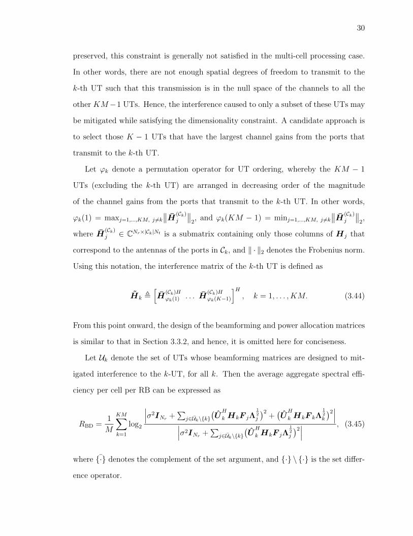
30

preserved, this constraint is generally not satisfied in the multi-cell processing case.

In other words, there are not enough spatial degrees of freedom to transmit to the

k-th UT such that this transmission is in the null space of the channels to all the

other KM−1 UTs. Hence, the interference caused to only a subset of these UTs may

be mitigated while satisfying the dimensionality constraint. A candidate approach is

to select those K − 1 UTs that have the largest channel gains from the ports that

transmit to the k-th UT.

Let ϕk denote a permutation operator for UT ordering, whereby the KM − 1

UTs (excluding the k-th UT) are arranged in decreasing order of the magnitude

of the channel gains from the ports that transmit to the k-th UT. In other words,

ϕk(1) = maxj=1,...,KM, j 6=k∥∥H(Ck)

j

∥∥2, and ϕk(KM − 1) = minj=1,...,KM, j 6=k

∥∥H(Ck)j

∥∥2,

where H(Ck)j ∈ CNr×|Ck|Nt is a submatrix containing only those columns of Hj that

correspond to the antennas of the ports in Ck, and ‖ · ‖2 denotes the Frobenius norm.

Using this notation, the interference matrix of the k-th UT is defined as

Hk ,[H

(Ck)Hϕk(1) . . . H

(Ck)Hϕk(K−1)

]H, k = 1, . . . , KM. (3.44)

From this point onward, the design of the beamforming and power allocation matrices

is similar to that in Section 3.3.2, and hence, it is omitted here for conciseness.

Let Uk denote the set of UTs whose beamforming matrices are designed to mit-

igated interference to the k-UT, for all k. Then the average aggregate spectral effi-

ciency per cell per RB can be expressed as

RBD =1

M

KM∑k=1

log2

∣∣∣σ2INr +∑

j∈Uk\{k}(UH

k HkF jΛ12j

)2+(UH

k HkF kΛ12k

)2∣∣∣∣∣∣σ2INr +

∑j∈Uk\{k}

(UH

k HkF jΛ12j

)2∣∣∣ , (3.45)

where {·} denotes the complement of the set argument, and {·} \ {·} is the set differ-

ence operator.

31

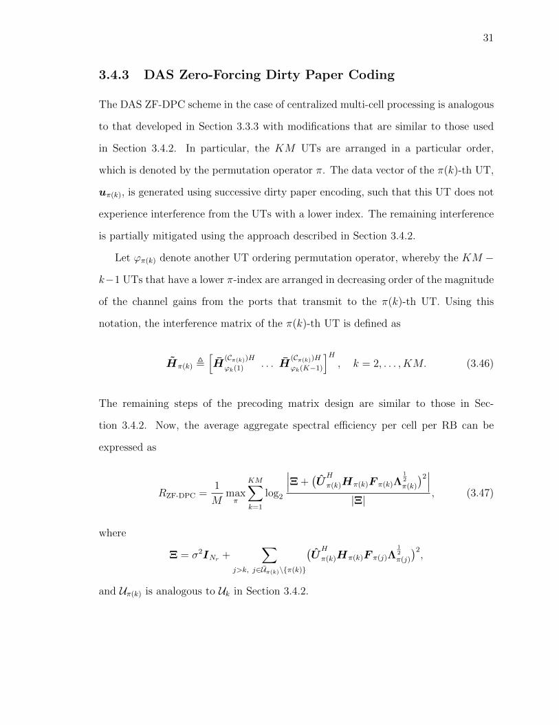
3.4.3 DAS Zero-Forcing Dirty Paper Coding

The DAS ZF-DPC scheme in the case of centralized multi-cell processing is analogous

to that developed in Section 3.3.3 with modifications that are similar to those used

in Section 3.4.2. In particular, the KM UTs are arranged in a particular order,

which is denoted by the permutation operator π. The data vector of the π(k)-th UT,

uπ(k), is generated using successive dirty paper encoding, such that this UT does not

experience interference from the UTs with a lower index. The remaining interference

is partially mitigated using the approach described in Section 3.4.2.

Let ϕπ(k) denote another UT ordering permutation operator, whereby the KM −

k−1 UTs that have a lower π-index are arranged in decreasing order of the magnitude

of the channel gains from the ports that transmit to the π(k)-th UT. Using this

notation, the interference matrix of the π(k)-th UT is defined as

Hπ(k) ,[H

(Cπ(k))Hϕk(1) . . . H

(Cπ(k))Hϕk(K−1)

]H, k = 2, . . . , KM. (3.46)

The remaining steps of the precoding matrix design are similar to those in Sec-

tion 3.4.2. Now, the average aggregate spectral efficiency per cell per RB can be

expressed as

RZF-DPC =1

Mmaxπ

KM∑k=1

log2

∣∣∣Ξ +(UH

π(k)Hπ(k)F π(k)Λ12

π(k)

)2∣∣∣

|Ξ|, (3.47)

where

Ξ = σ2INr +∑

j>k, j∈Uπ(k)\{π(k)}

(UH

π(k)Hπ(k)F π(j)Λ12

π(j)

)2,

and Uπ(k) is analogous to Uk in Section 3.4.2.

32

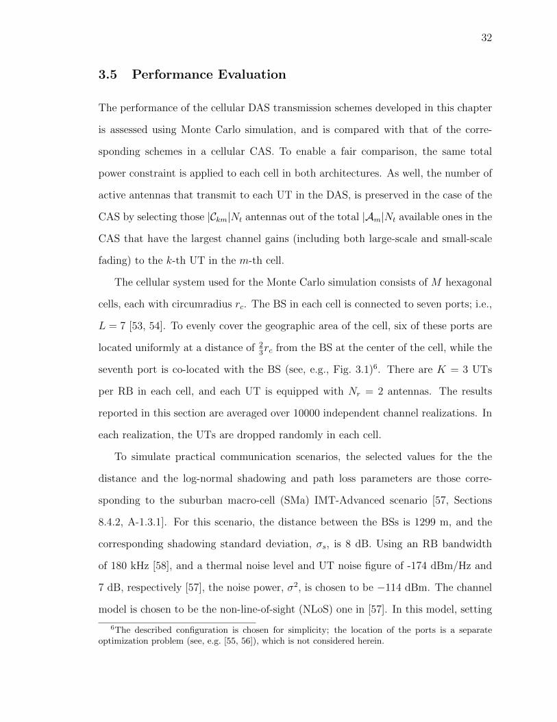
3.5 Performance Evaluation

The performance of the cellular DAS transmission schemes developed in this chapter

is assessed using Monte Carlo simulation, and is compared with that of the corre-

sponding schemes in a cellular CAS. To enable a fair comparison, the same total

power constraint is applied to each cell in both architectures. As well, the number of

active antennas that transmit to each UT in the DAS, is preserved in the case of the

CAS by selecting those |Ckm|Nt antennas out of the total |Am|Nt available ones in the

CAS that have the largest channel gains (including both large-scale and small-scale

fading) to the k-th UT in the m-th cell.

The cellular system used for the Monte Carlo simulation consists of M hexagonal

cells, each with circumradius rc. The BS in each cell is connected to seven ports; i.e.,

L = 7 [53, 54]. To evenly cover the geographic area of the cell, six of these ports are

located uniformly at a distance of 23rc from the BS at the center of the cell, while the

seventh port is co-located with the BS (see, e.g., Fig. 3.1)6. There are K = 3 UTs

per RB in each cell, and each UT is equipped with Nr = 2 antennas. The results

reported in this section are averaged over 10000 independent channel realizations. In

each realization, the UTs are dropped randomly in each cell.

To simulate practical communication scenarios, the selected values for the the

distance and the log-normal shadowing and path loss parameters are those corre-

sponding to the suburban macro-cell (SMa) IMT-Advanced scenario [57, Sections

8.4.2, A-1.3.1]. For this scenario, the distance between the BSs is 1299 m, and the

corresponding shadowing standard deviation, σs, is 8 dB. Using an RB bandwidth

of 180 kHz [58], and a thermal noise level and UT noise figure of -174 dBm/Hz and

7 dB, respectively [57], the noise power, σ2, is chosen to be −114 dBm. The channel

model is chosen to be the non-line-of-sight (NLoS) one in [57]. In this model, setting

6The described configuration is chosen for simplicity; the location of the ports is a separateoptimization problem (see, e.g. [55, 56]), which is not considered herein.

33

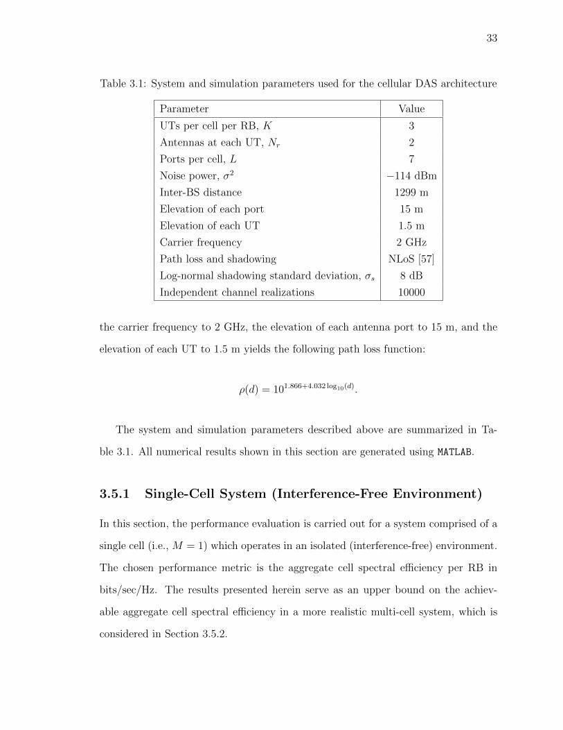
Table 3.1: System and simulation parameters used for the cellular DAS architecture

Parameter Value

UTs per cell per RB, K 3

Antennas at each UT, Nr 2

Ports per cell, L 7

Noise power, σ2 −114 dBm

Inter-BS distance 1299 m

Elevation of each port 15 m

Elevation of each UT 1.5 m

Carrier frequency 2 GHz

Path loss and shadowing NLoS [57]

Log-normal shadowing standard deviation, σs 8 dB

Independent channel realizations 10000

the carrier frequency to 2 GHz, the elevation of each antenna port to 15 m, and the

elevation of each UT to 1.5 m yields the following path loss function:

ρ(d) = 101.866+4.032 log10(d).

The system and simulation parameters described above are summarized in Ta-

ble 3.1. All numerical results shown in this section are generated using MATLAB.

3.5.1 Single-Cell System (Interference-Free Environment)

In this section, the performance evaluation is carried out for a system comprised of a

single cell (i.e., M = 1) which operates in an isolated (interference-free) environment.

The chosen performance metric is the aggregate cell spectral efficiency per RB in

bits/sec/Hz. The results presented herein serve as an upper bound on the achiev-

able aggregate cell spectral efficiency in a more realistic multi-cell system, which is

considered in Section 3.5.2.

34

Port Selection versus Transmit Antenna Selection

Port selection can be viewed as a special case of transmit antenna selection, wherein

a subset of all transmit antennas are selected to transmit to a particular UT based

on a specified metric such as the channel gain or the received SINR. However, with

port selection, the antennas at each port are selected as a group. The performance of

both approaches is compared in Examples 3.1 and 3.2 below with antenna selection

referring to the selection of |Ckm|Nt antennas with the largest channel gains (includ-

ing both large-scale and small-scale fading) to the k-th UT out of the total |Am|Nt

antennas. Unlike antenna selection, however, the criterion used for port selection in

the simulations reported herein is large-scale fading (path loss and shadowing) only.

In Figs. 3.3 and 3.4, it is shown that although port selection is less flexible, its

performance is comparable to that of antenna selection for both DAS ZF-DPC and

DAS BD. Hence, antenna selection in the DAS is not considered beyond this initial

comparison in this section.

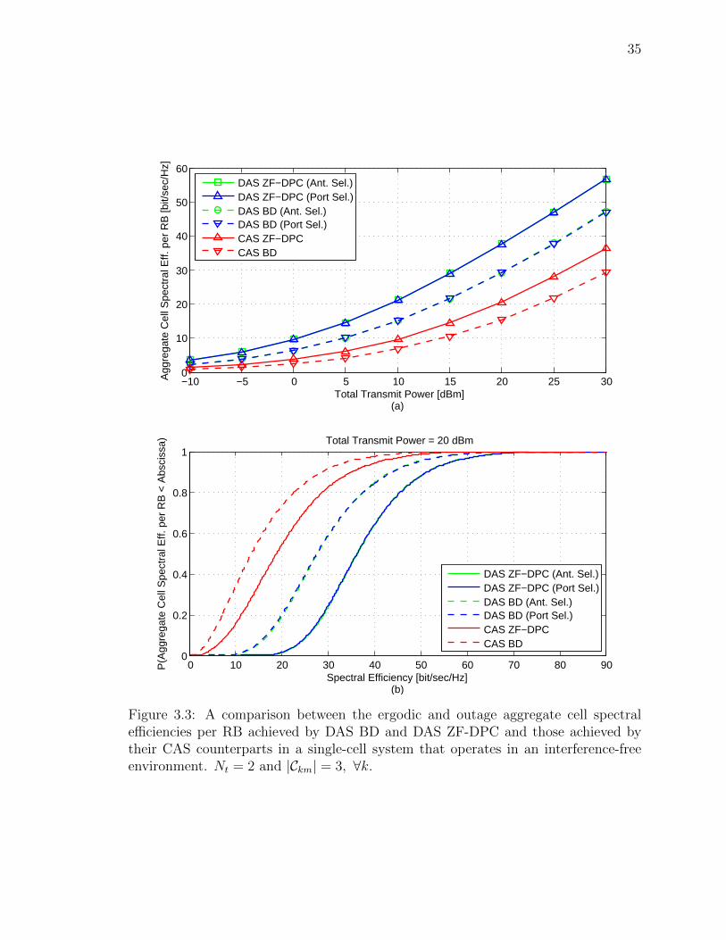
Example 3.1. In Fig. 3.3(a), the ergodic aggregate cell spectral efficiency per RB

achieved by DAS BD and DAS ZF-DPC is compared with those achieved by the CAS

counterparts of these schemes7. In Fig. 3.3(b), the outage probability of these schemes

is shown versus the aggregate cell spectral efficiency per RB when Pt = 20 dBm. In

this scenario, |Ckm| = 3 for all k and Nt = 2. The DAS dimensionality constraint is

satisfied here because Nr(K − 1) = 4 < mink∈{1,...,K} |Ckm|Nt = 6. However, no more

UTs could be simultaneously served by this system while satisfying the zero-forcing

condition unless either additional antennas were deployed at each port or a greater

number of ports coordinated their transmissions to each UT.

It can be seen from the figure that both DAS schemes achieve higher aggregate cell

spectral efficiencies than their CAS counterparts. For example, when Pt = 20 dBm in

7Each of these spectral efficiencies is obtained by evaluating the corresponding expressions (see,e.g., (3.20) and (3.23)) for each independent channel realization, and then averaging the results overall of the realizations.

35

−10 −5 0 5 10 15 20 25 300

10

20

30

40

50

60

Total Transmit Power [dBm](a)

Agg

rega

te C

ell S

pect

ral E

ff. p

er R

B [b

it/se

c/H

z]

DAS ZF−DPC (Ant. Sel.)DAS ZF−DPC (Port Sel.)DAS BD (Ant. Sel.)DAS BD (Port Sel.)CAS ZF−DPCCAS BD

0 10 20 30 40 50 60 70 80 900

0.2

0.4

0.6

0.8

1

P(A

ggre

gate

Cel

l Spe

ctra

l Eff.

per

RB

< A

bsci

ssa)

Spectral Efficiency [bit/sec/Hz](b)

Total Transmit Power = 20 dBm


Figure 3.3: A comparison between the ergodic and outage aggregate cell spectralefficiencies per RB achieved by DAS BD and DAS ZF-DPC and those achieved bytheir CAS counterparts in a single-cell system that operates in an interference-freeenvironment. Nt = 2 and |Ckm| = 3, ∀k.

36

Fig. 3.3(a), each DAS scheme achieves over 80% higher ergodic aggregate cell spectral

efficiency per RB than the corresponding CAS scheme. Moreover, DAS ZF-DPC

outperforms DAS BD by approximately 28%. This gain is due to the availability of

additional spatial degrees of freedom in the case of DAS ZF-DPC since the interference

is partially mitigated through successive DPC encoding. Hence, the zero-forcing

condition must only be satisfied for the remaining interference. �

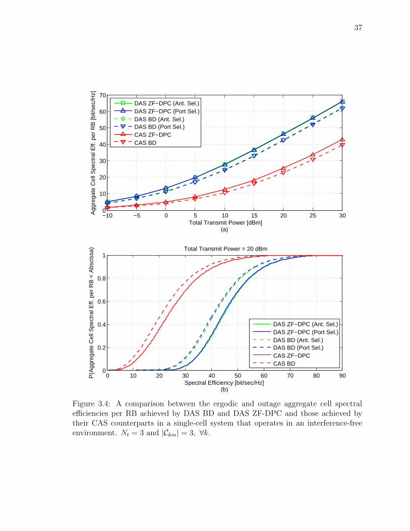
Example 3.2. In Fig. 3.4, a comparison similar to the one in Fig. 3.3 is considered,

except that now Nt = 3. It can be seen from this figure that, in comparison to

the case of Nt = 2 considered in Example 3.1, a single additional antenna at each

port results in improved performance for both DAS schemes. Furthermore, the gap

between both DAS schemes is reduced. For example, when Pt = 20 dBm, DAS ZF-

DPC only achieves approximately 9% higher ergodic aggregate spectral efficiency than

DAS BD, which is considerably less than the corresponding result in Example 3.1. �


except that now |Ckm| = 7, ∀k. The observation made from comparing the two figures

is similar to that in Example 3.2. It can be seen that by using all L = 7 ports to serve

each UT leads to improved performance for both DAS schemes, and that the gap

between DAS ZF-DPC and DAS BD is reduced. This improvement can be attributed

to the additional spatial degrees of freedom that are made available by increasing

|Ckm| from 3 to 7 for all k. �

Effect of the Number of Antennas per Port

Example 3.4. Following the lead from Examples 3.1 and 3.2, in this example, the

effect the number of antennas per port is further investigated. In Fig. 3.6, the ag-

gregate cell spectral efficiencies per RB achieved by both the DAS and CAS schemes

are compared for different values of Nt when Pt = 20 dBm and |Ckm| = 3 for all k.

It can be noted from the figure that the points at Nt = 2 and Nt = 3 are the same

37

−10 −5 0 5 10 15 20 25 300

10

20

30

40

50

60

70


Agg

rega

te C

ell S

pect

ral E

ff. p

er R

B [b

it/se

c/H

z]


0 10 20 30 40 50 60 70 80 900

0.2

0.4

0.6

0.8

1

P(A

ggre

gate

Cel

l Spe

ctra

l Eff.

per

RB

< A

bsci

ssa)





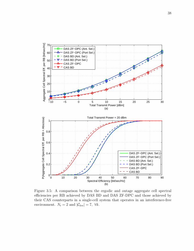
38

−10 −5 0 5 10 15 20 25 300

10

20

30

40

50

60

70


Agg

rega

te C

ell S

pect

ral E

ff. p

er R

B [b

it/se

c/H

z]


0 10 20 30 40 50 60 70 80 900

0.2

0.4

0.6

0.8

1

P(A

ggre

gate

Cel

l Spe

ctra

l Eff.

per

RB

< A

bsci

ssa)





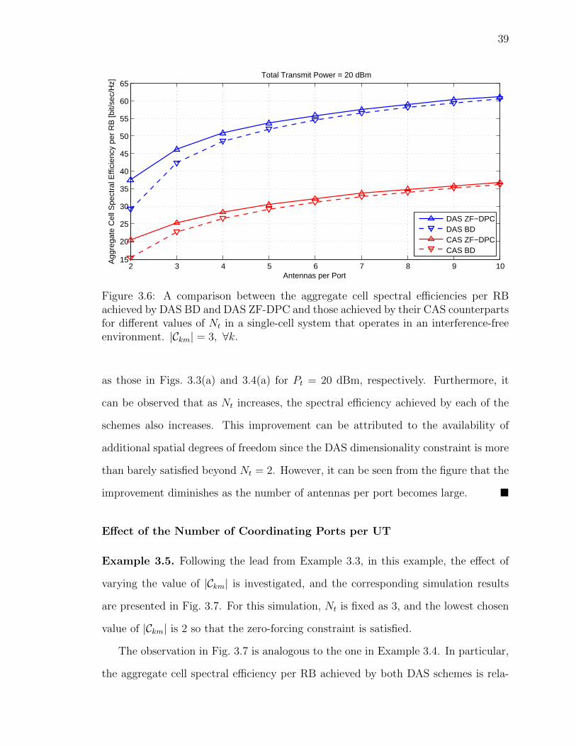
39

2 3 4 5 6 7 8 9 1015

20

25

30

35

40

45

50

55

60

65

Antennas per Port

Agg

rega

te C

ell S

pect

ral E

ffici

ency

per

RB

[bit/

sec/

Hz]


DAS ZF−DPCDAS BDCAS ZF−DPCCAS BD

Figure 3.6: A comparison between the aggregate cell spectral efficiencies per RBachieved by DAS BD and DAS ZF-DPC and those achieved by their CAS counterpartsfor different values of Nt in a single-cell system that operates in an interference-freeenvironment. |Ckm| = 3, ∀k.

as those in Figs. 3.3(a) and 3.4(a) for Pt = 20 dBm, respectively. Furthermore, it

can be observed that as Nt increases, the spectral efficiency achieved by each of the

schemes also increases. This improvement can be attributed to the availability of

additional spatial degrees of freedom since the DAS dimensionality constraint is more

than barely satisfied beyond Nt = 2. However, it can be seen from the figure that the

improvement diminishes as the number of antennas per port becomes large. �

Effect of the Number of Coordinating Ports per UT

Example 3.5. Following the lead from Example 3.3, in this example, the effect of

varying the value of |Ckm| is investigated, and the corresponding simulation results

are presented in Fig. 3.7. For this simulation, Nt is fixed as 3, and the lowest chosen

value of |Ckm| is 2 so that the zero-forcing constraint is satisfied.

The observation in Fig. 3.7 is analogous to the one in Example 3.4. In particular,

the aggregate cell spectral efficiency per RB achieved by both DAS schemes is rela-

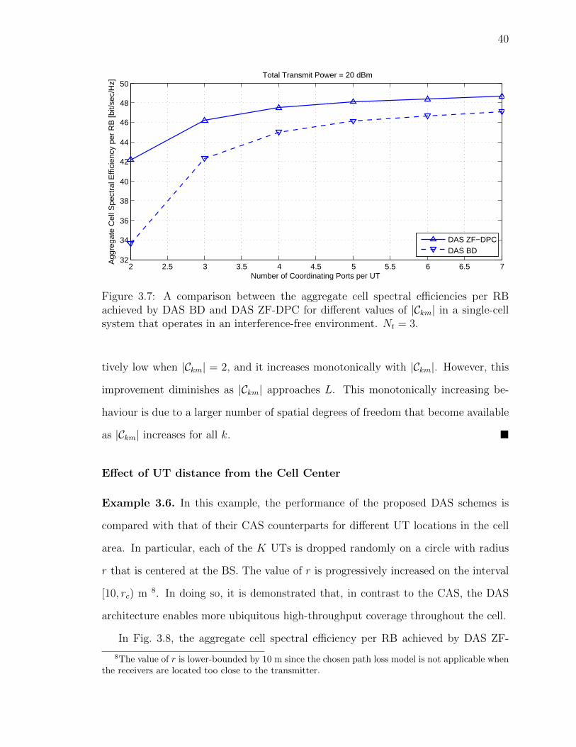
40

2 2.5 3 3.5 4 4.5 5 5.5 6 6.5 732

34

36

38

40

42

44

46

48

50

Number of Coordinating Ports per UT

Agg

rega

te C

ell S

pect

ral E

ffici

ency

per

RB

[bit/

sec/

Hz]


DAS ZF−DPCDAS BD

Figure 3.7: A comparison between the aggregate cell spectral efficiencies per RBachieved by DAS BD and DAS ZF-DPC for different values of |Ckm| in a single-cellsystem that operates in an interference-free environment. Nt = 3.

tively low when |Ckm| = 2, and it increases monotonically with |Ckm|. However, this

improvement diminishes as |Ckm| approaches L. This monotonically increasing be-

haviour is due to a larger number of spatial degrees of freedom that become available

as |Ckm| increases for all k. �

Effect of UT distance from the Cell Center

Example 3.6. In this example, the performance of the proposed DAS schemes is

compared with that of their CAS counterparts for different UT locations in the cell

area. In particular, each of the K UTs is dropped randomly on a circle with radius

r that is centered at the BS. The value of r is progressively increased on the interval

[10, rc) m 8. In doing so, it is demonstrated that, in contrast to the CAS, the DAS

architecture enables more ubiquitous high-throughput coverage throughout the cell.

In Fig. 3.8, the aggregate cell spectral efficiency per RB achieved by DAS ZF-

8The value of r is lower-bounded by 10 m since the chosen path loss model is not applicable whenthe receivers are located too close to the transmitter.

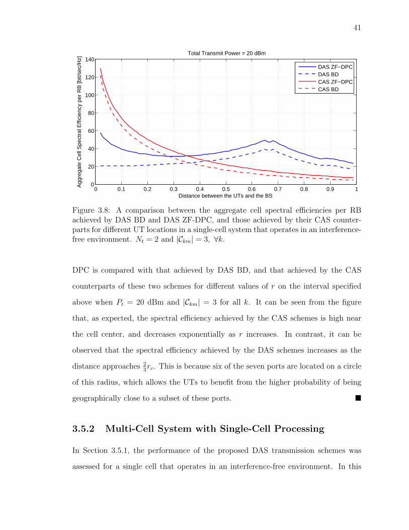
41

0 0.1 0.2 0.3 0.4 0.5 0.6 0.7 0.8 0.9 10

20

40

60

80

100

120

140

Distance between the UTs and the BS

Agg

rega

te C

ell S

pect

ral E

ffici

ency

per

RB

[bit/

sec/

Hz]


DAS ZF−DPCDAS BDCAS ZF−DPCCAS BD

Figure 3.8: A comparison between the aggregate cell spectral efficiencies per RBachieved by DAS BD and DAS ZF-DPC, and those achieved by their CAS counter-parts for different UT locations in a single-cell system that operates in an interference-free environment. Nt = 2 and |Ckm| = 3, ∀k.

DPC is compared with that achieved by DAS BD, and that achieved by the CAS

counterparts of these two schemes for different values of r on the interval specified

above when Pt = 20 dBm and |Ckm| = 3 for all k. It can be seen from the figure

that, as expected, the spectral efficiency achieved by the CAS schemes is high near

the cell center, and decreases exponentially as r increases. In contrast, it can be

observed that the spectral efficiency achieved by the DAS schemes increases as the

distance approaches 23rc. This is because six of the seven ports are located on a circle

of this radius, which allows the UTs to benefit from the higher probability of being

geographically close to a subset of these ports. �

3.5.2 Multi-Cell System with Single-Cell Processing

In Section 3.5.1, the performance of the proposed DAS transmission schemes was

assessed for a single cell that operates in an interference-free environment. In this

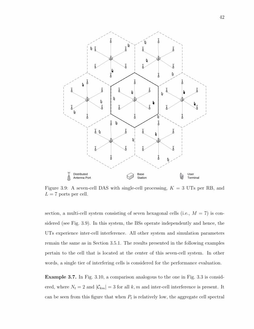
42

Distributed

Antenna Port

Base

Station

User

Terminal

Figure 3.9: A seven-cell DAS with single-cell processing, K = 3 UTs per RB, andL = 7 ports per cell.

section, a multi-cell system consisting of seven hexagonal cells (i.e., M = 7) is con-

sidered (see Fig. 3.9). In this system, the BSs operate independently and hence, the

UTs experience inter-cell interference. All other system and simulation parameters

remain the same as in Section 3.5.1. The results presented in the following examples

pertain to the cell that is located at the center of this seven-cell system. In other

words, a single tier of interfering cells is considered for the performance evaluation.

Example 3.7. In Fig. 3.10, a comparison analogous to the one in Fig. 3.3 is consid-

ered, where Nt = 2 and |Ckm| = 3 for all k,m and inter-cell interference is present. It

can be seen from this figure that when Pt is relatively low, the aggregate cell spectral

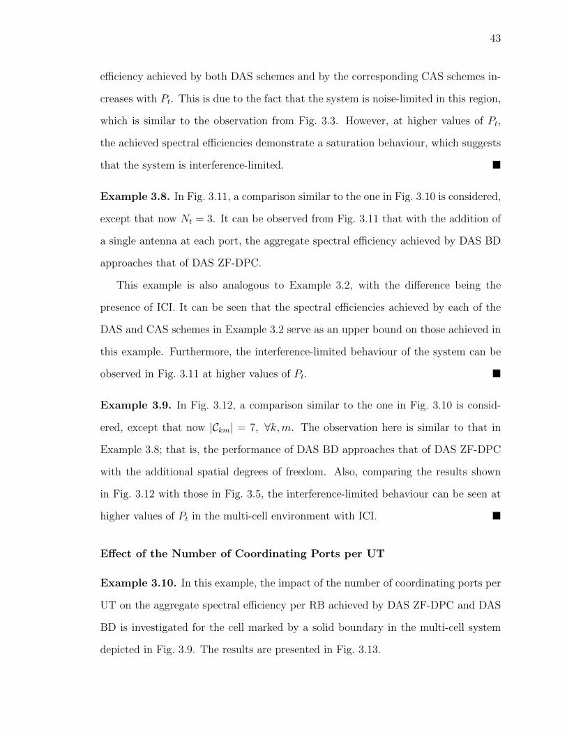
43

efficiency achieved by both DAS schemes and by the corresponding CAS schemes in-

creases with Pt. This is due to the fact that the system is noise-limited in this region,

which is similar to the observation from Fig. 3.3. However, at higher values of Pt,

the achieved spectral efficiencies demonstrate a saturation behaviour, which suggests

that the system is interference-limited. �


except that now Nt = 3. It can be observed from Fig. 3.11 that with the addition of

a single antenna at each port, the aggregate spectral efficiency achieved by DAS BD

approaches that of DAS ZF-DPC.

This example is also analogous to Example 3.2, with the difference being the

presence of ICI. It can be seen that the spectral efficiencies achieved by each of the

DAS and CAS schemes in Example 3.2 serve as an upper bound on those achieved in

this example. Furthermore, the interference-limited behaviour of the system can be

observed in Fig. 3.11 at higher values of Pt. �

Example 3.9. In Fig. 3.12, a comparison similar to the one in Fig. 3.10 is consid-

ered, except that now |Ckm| = 7, ∀k,m. The observation here is similar to that in

Example 3.8; that is, the performance of DAS BD approaches that of DAS ZF-DPC

with the additional spatial degrees of freedom. Also, comparing the results shown

in Fig. 3.12 with those in Fig. 3.5, the interference-limited behaviour can be seen at

higher values of Pt in the multi-cell environment with ICI. �

Effect of the Number of Coordinating Ports per UT

Example 3.10. In this example, the impact of the number of coordinating ports per

UT on the aggregate spectral efficiency per RB achieved by DAS ZF-DPC and DAS

BD is investigated for the cell marked by a solid boundary in the multi-cell system

depicted in Fig. 3.9. The results are presented in Fig. 3.13.

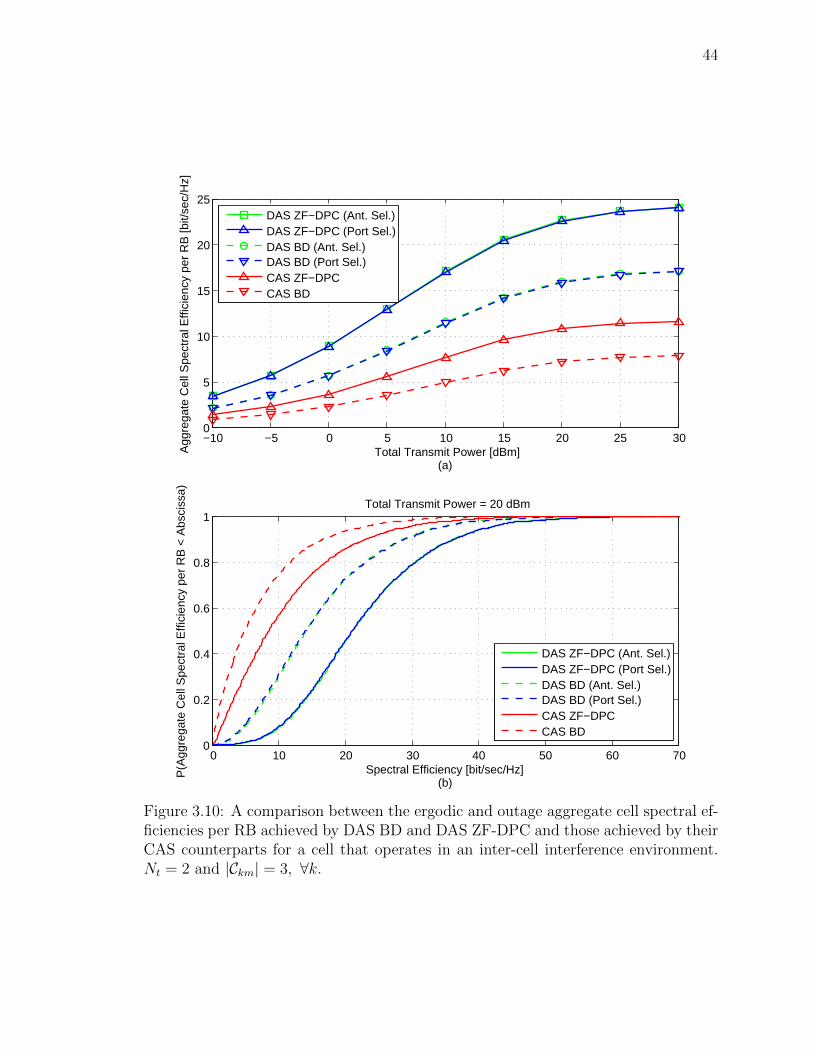
44

−10 −5 0 5 10 15 20 25 300

5

10

15

20

25


Agg

rega

te C

ell S

pect

ral E

ffici

ency

per

RB

[bit/

sec/

Hz]


0 10 20 30 40 50 60 700

0.2

0.4

0.6

0.8

1

P(A

ggre

gate

Cel

l Spe

ctra

l Effi

cien

cy p

er R

B <

Abs

ciss

a)




Figure 3.10: A comparison between the ergodic and outage aggregate cell spectral ef-ficiencies per RB achieved by DAS BD and DAS ZF-DPC and those achieved by theirCAS counterparts for a cell that operates in an inter-cell interference environment.Nt = 2 and |Ckm| = 3, ∀k.

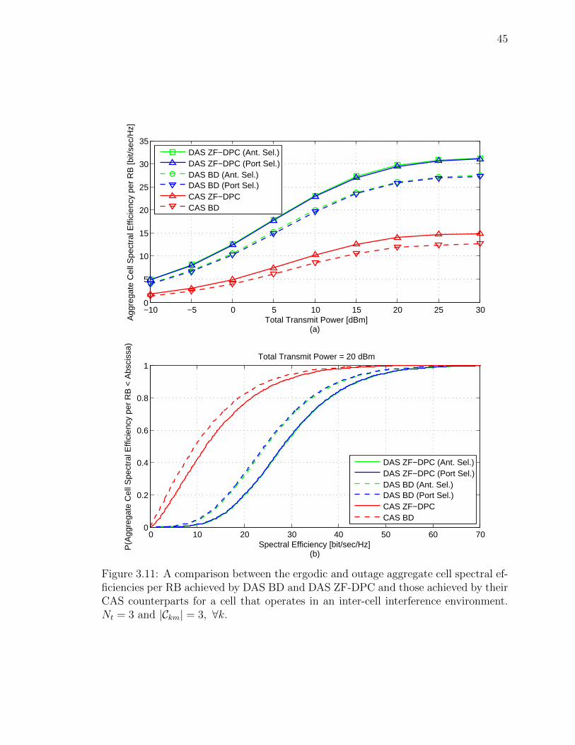
45

−10 −5 0 5 10 15 20 25 300

5

10

15

20

25

30

35


Agg

rega

te C

ell S

pect

ral E

ffici

ency

per

RB

[bit/

sec/

Hz]


0 10 20 30 40 50 60 700

0.2

0.4

0.6

0.8

1

P(A

ggre

gate

Cel

l Spe

ctra

l Effi

cien

cy p

er R

B <

Abs

ciss

a)





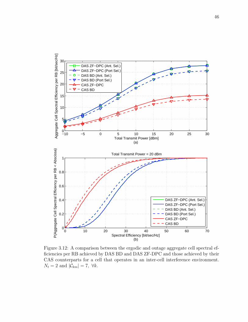
46

−10 −5 0 5 10 15 20 25 300

5

10

15

20

25

30


Agg

rega

te C

ell S

pect

ral E

ffici

ency

per

RB

[bit/

sec/

Hz]


0 10 20 30 40 50 60 700

0.2

0.4

0.6

0.8

1

P(A

ggre

gate

Cel

l Spe

ctra

l Effi

cien

cy p

er R

B <

Abs

ciss

a)





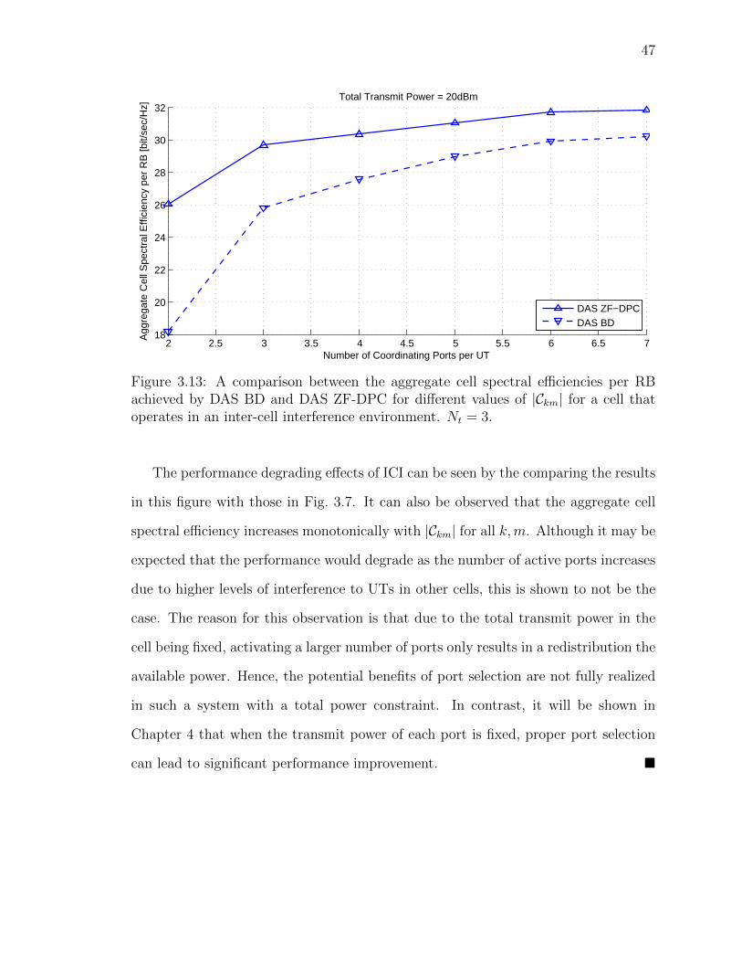
47

2 2.5 3 3.5 4 4.5 5 5.5 6 6.5 718

20

22

24

26

28

30

32

Number of Coordinating Ports per UT

Agg

rega

te C

ell S

pect

ral E

ffici

ency

per

RB

[bit/

sec/

Hz]

Total Transmit Power = 20dBm

DAS ZF−DPCDAS BD

Figure 3.13: A comparison between the aggregate cell spectral efficiencies per RBachieved by DAS BD and DAS ZF-DPC for different values of |Ckm| for a cell thatoperates in an inter-cell interference environment. Nt = 3.

The performance degrading effects of ICI can be seen by the comparing the results

in this figure with those in Fig. 3.7. It can also be observed that the aggregate cell

spectral efficiency increases monotonically with |Ckm| for all k,m. Although it may be

expected that the performance would degrade as the number of active ports increases

due to higher levels of interference to UTs in other cells, this is shown to not be the

case. The reason for this observation is that due to the total transmit power in the

cell being fixed, activating a larger number of ports only results in a redistribution the

available power. Hence, the potential benefits of port selection are not fully realized

in such a system with a total power constraint. In contrast, it will be shown in

Chapter 4 that when the transmit power of each port is fixed, proper port selection

can lead to significant performance improvement. �

48

3.5.3 Multi-Cell System with Centralized Processing

In this section, the performance of the schemes developed in Section 3.4 is assessed.

Similar to Section 3.5.2, a seven-cell system is considered; however, the BSs now

coordinate their transmissions in a centralized manner, and any of the LM = 49

ports in the cluster may be selected for transmission to a particular UT (see Fig. 3.14).

Additionally, the cluster of seven cells is subject to a total power constraint of 7Pt

as described in Section 3.4. To enable a comparison with the single-cell processing

results in Section 3.5.2, the performance metric is chosen to be the average spectral

efficiency per cell per RB. In other words, instead of considering the spectral efficiency

of the cell at the center of the cluster as was previously the case, the aggregate spectral

efficiency of the entire cluster is determined, and then scaled by a factor of 1/M .

Example 3.11. In Fig. 3.15, the average aggregate spectral efficiency per cell per

RB achieved by DAS ZF-DPC and DAS BD with centralized multi-cell processing is

compared with those achieved by these schemes with single-cell processing. In this

system, Nt = 2 and |Ck| = 3 for all k. It can be seen from this figure that DAS

BD with multi-cell processing outperforms the corresponding scheme with single-cell

processing for all values of transmit power. This gain can be attributed to

• the more flexible total power constraint for the cluster as a whole rather than

one for each cell, and

• the increased flexibility in port selection (since the ports that can be selected

to transmit to a particular UT need not be associated with the same cell).

However, in the case of DAS ZF-DPC, it is interesting that while centralized multi-

cell processing outperforms single-cell processing at higher power levels, the opposite

is true when the power is relatively low. This observation suggests that using the

available spatial degrees of freedom for diversity is preferable instead of using them

for interference mitigation through BD-based zero forcing at low power values.

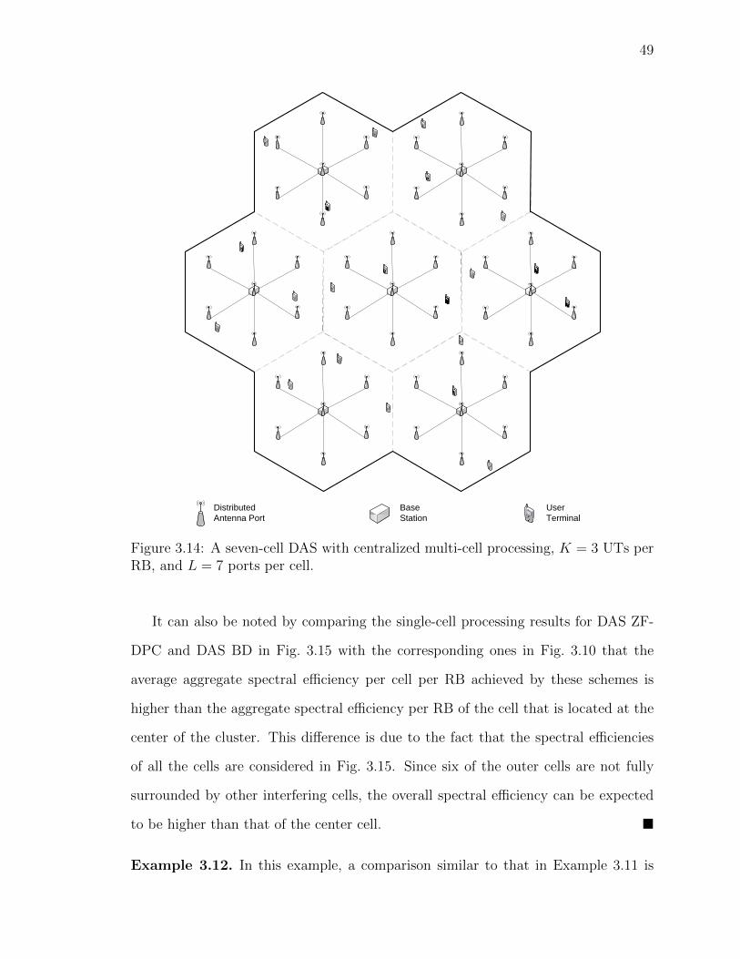
49

Distributed

Antenna Port

Base

Station

User

Terminal

Figure 3.14: A seven-cell DAS with centralized multi-cell processing, K = 3 UTs perRB, and L = 7 ports per cell.

It can also be noted by comparing the single-cell processing results for DAS ZF-

DPC and DAS BD in Fig. 3.15 with the corresponding ones in Fig. 3.10 that the

average aggregate spectral efficiency per cell per RB achieved by these schemes is

higher than the aggregate spectral efficiency per RB of the cell that is located at the

center of the cluster. This difference is due to the fact that the spectral efficiencies

of all the cells are considered in Fig. 3.15. Since six of the outer cells are not fully

surrounded by other interfering cells, the overall spectral efficiency can be expected

to be higher than that of the center cell. �

Example 3.12. In this example, a comparison similar to that in Example 3.11 is

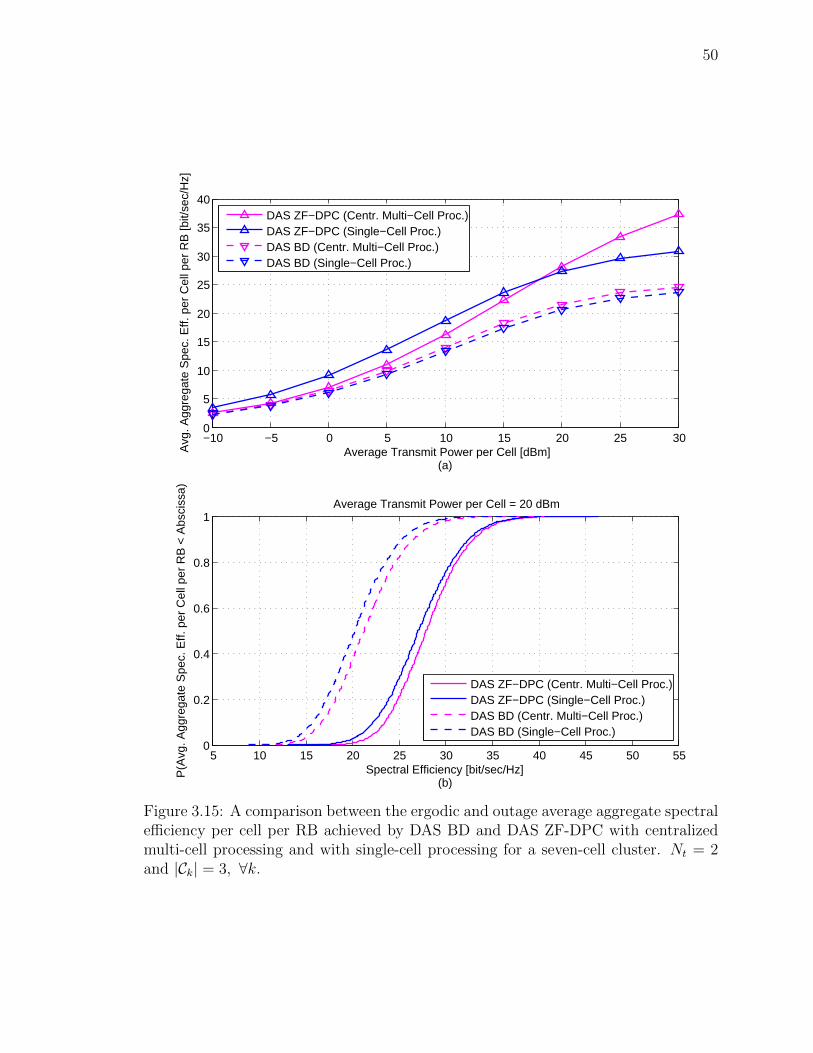
50

−10 −5 0 5 10 15 20 25 300

5

10

15

20

25

30

35

40

Average Transmit Power per Cell [dBm](a)

Avg

. Agg

rega

te S

pec.

Eff.

per

Cel

l per

RB

[bit/

sec/

Hz]

5 10 15 20 25 30 35 40 45 50 550

0.2

0.4

0.6

0.8

1

P(A

vg. A

ggre

gate

Spe

c. E

ff. p

er C

ell p

er R

B <

Abs

ciss

a)


Average Transmit Power per Cell = 20 dBm

DAS ZF−DPC (Centr. Multi−Cell Proc.)DAS ZF−DPC (Single−Cell Proc.)DAS BD (Centr. Multi−Cell Proc.)DAS BD (Single−Cell Proc.)


Figure 3.15: A comparison between the ergodic and outage average aggregate spectralefficiency per cell per RB achieved by DAS BD and DAS ZF-DPC with centralizedmulti-cell processing and with single-cell processing for a seven-cell cluster. Nt = 2and |Ck| = 3, ∀k.

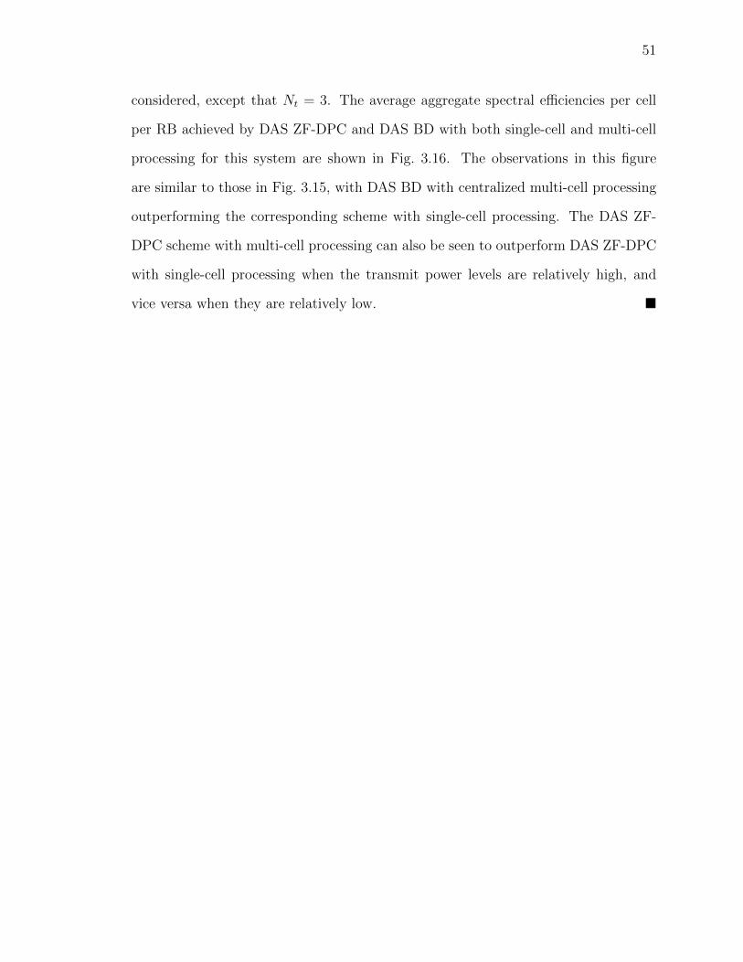
51

considered, except that Nt = 3. The average aggregate spectral efficiencies per cell

per RB achieved by DAS ZF-DPC and DAS BD with both single-cell and multi-cell

processing for this system are shown in Fig. 3.16. The observations in this figure

are similar to those in Fig. 3.15, with DAS BD with centralized multi-cell processing

outperforming the corresponding scheme with single-cell processing. The DAS ZF-

DPC scheme with multi-cell processing can also be seen to outperform DAS ZF-DPC

with single-cell processing when the transmit power levels are relatively high, and

vice versa when they are relatively low. �

52

−10 −5 0 5 10 15 20 25 300

10

20

30

40

50

Average Transmit Power per Cell [dBm](a)

Avg

. Agg

rega

te S

pec.

Eff.

per

Cel

l per

RB

[bit/

sec/

Hz]

10 20 30 40 50 60 700

0.2

0.4

0.6

0.8

1

P(A

vg. A

ggre

gate

Spe

c. E

ff. p

er C

ell p

er R

B <

Abs

ciss

a)


Average Transmit Power per Cell = 20 dBm



Figure 3.16: A comparison between the ergodic and outage average aggregate spectralefficiency per cell per RB achieved by DAS BD and DAS ZF-DPC with centralizedmulti-cell processing and with single-cell processing for a seven-cell cluster. Nt = 3and |Ck| = 3, ∀k.

Chapter 4

Coordinated Max-Min Fair Multi-Cell Port

Selection and Beam Steering Optimization using

Semidefinite Relaxation

Recall that in each of the two coordinated downlink transmission schemes developed

in Chapter 3, the subset of antennas ports that transmit to each UT is pre-selected.

Although jointly selecting ports and designing the precoding coefficients would yield

improved performance, this is a challenging optimization problem. In this chapter,

this problem is addressed for a cellular DAS in which the UTs and ports have a single

antenna each, at most a single UT is permitted to occupy a particular RB in each

cell, and each port transmits using a fixed power.

4.1 Related Literature

Despite the envisioned benefits of using multiple antenna ports (see Section 2.1), poor

selection and weighting of ports can yield low SINRs, resulting in undesirable per-

formance. This fact has been demonstrated in [53] for cellular distributed antenna

systems with no coordination among the BSs. In [54], a system with no BS coordi-

nation, similar to the one in [53], is considered. For this system the weights of the

antenna ports are chosen to match the phases of the channel coefficients and either a

single-port or an all-port transmission strategy is selected.

In contrast with both [53] and [54], in this work, a cluster of cells is considered

53

54

in which the BSs organize their transmissions in a coordinated manner. Since coor-

dination among multiple cells is a generalization of coordination within a single cell,

the CoMP system considered herein subsumes those considered in [53] and [54], and

offers a greater number of degrees of design freedom. Also, unlike [54], in which the

transmission strategies are selected and fixed prior to choosing the antenna weights,

the focus herein is on the joint optimization of the ports to be used for transmission

and their corresponding weights, which are henceforth referred to as beam steering

coefficients. The joint optimization of these parameters allows further exploitation of

the coordination among the BSs to enable the UTs to achieve higher SINRs. However,

this joint optimization problem can be shown to be NP-hard [59, 60], which implies

that finding the global optimal solution is computationally prohibitive for many prac-

tical systems. To circumvent this difficulty, a novel polynomial-complexity two-stage

technique is proposed. This technique will later be shown to yield close-to-optimal

solutions efficiently.

Before indulging into the specific problem statement and the details of the pro-

posed two-stage technique, certain topics in optimization theory that are relevant to

the formulation developed in this chapter are briefly described in the next section.

4.2 Background: Mathematical Optimization

In mathematics, an optimization problem is one in which an objective is maximized

over a set of variables, such that a given set of constraints is satisfied; that is

maxx

f0(x), (4.1a)

subject to fi(x) ≤ bi, i = 1, . . . ,m. (4.1b)

In the above problem, x is the optimization variable, f0(x) is the objective function,

and the inequalities in (4.1b) constitute the constraint set [61, Section 1.1].

55

4.2.1 Convex Optimization Problem

A certain class of optimization problems are called convex optimization problems. In

such problems, the objective function and the functions in the constraint set are all

convex. By definition, a function fi(x) is convex if the inequality

fi(αx+ βy) ≤ αfi(x) + βfi(y)

is satisfied for all α, β ∈ R [61, Section 1.1].

Convex optimization problems can be solved efficiently using numerical techniques

such as interior-point methods, and bear an extremely useful property: if an optimal

solution exists, then it is guaranteed to be globally optimal.

4.2.2 Semidefinite Programming

A specific type of a convex optimization problem, known as a semidefinite pro-

gram (SDP), is for the form

maxX

Tr(CX), (4.2a)

subject to Tr(DiX) Di bi, i = 1, . . . ,m, (4.2b)

X � 0, (4.2c)

where “Di” denotes either “≤”, “=”, or “≥” in the i-th constraint [61, Section

4.6.2], [62]. In other words, the objective function is linear and the optimization

variable, i.e., the matrix X, is positive semidefinite (PSD).

4.2.3 Relaxation of an Optimization Problem

It is often the case that a particular optimization problem is difficult to solve. One

candidate approach for circumventing this difficulty is to consider a relaxed version

56

of this problem instead. For certain types of problems, the relaxed version is often

easier to solve.

Let S denote the constraint set of the original optimization problem, and let U

denote the constraint set of the corresponding relaxed problem. Using the relaxation

technique, some of the constraints constituting S are either appropriately replaced

with looser ones, or omitted altogether. Therefore, S ⊂ U , and the optimal value of

the relaxed problem is an upper-bound on that of the original problem [63].

It is important to note that the optimal solution to the relaxed problem is not

necessarily optimal, or even feasible, for the original problem. Therefore, an additional

step is generally required to generate a candidate approximate solution to the original

problem using the optimal solution to the relaxed problem.

4.3 System Model

Consider the multi-cell DAS configuration described in Section 3.3.1. In this chapter,

the transmissions of the BSs in the M cells are coordinated by a central controller,

which is assumed to have reliable knowledge of the gains between the LM ports in the

M -cell cluster and each UT in the M cells. For tractability of the optimization prob-

lem tackled herein, the ports and UTs are assumed to be equipped with one antenna

each, i.e., Nt = Nr = 1. Additionally, a multi-user system is considered in which

no more than one UT within the cell is assigned the same RB; e.g., OFDMA-based

systems. This is a special case of the more general scenario considered in Chapter 3,

where multiple UTs can be served simultaneously in each cell in a particular RB.

Although the general case of multiple UTs per cell per RB yields a richer problem, it

is also more challenging, and is not considered herein.

Each port uses a fixed power to transmit to a particular UT within the cell, which

inherently causes interference to UTs that use the same RB in other cells. Restricting

the antenna ports to use fixed powers facilitates their hardware design and enables

57

the use of low-cost power amplifiers with relatively small dynamic ranges.

Consider a specific RB. Let α`m ∈ {0, 1} be the binary coefficient representing the

on-off state of the `-th port in the m-th cell on this RB, and let w`m and P`m denote

the corresponding complex beam steering coefficient and the power transmitted by

this port, respectively, for ` = 1, . . . , L, m = 1, . . . ,M . The term beam steering

coefficient is deliberately chosen to distinguish it from general terms such as precoding

coefficient and antenna weight. This choice is motivated by the fact that, due to the

fixed transmit power at each port, the corresponding coefficient has unit magnitude,

i.e., it lies on the unit circle. Hence, each coefficient only steers the phase of the

signals transmitted from the corresponding port.

The received signal of the UT in the m-th cell is given by

ym =L∑`=1

α`m√P`mh`mmw`mxm+

M∑n=1,n6=m

L∑`=1

α`n√P`nh`nmw`nxn+nm, m = 1, . . . ,M,

(4.3)

where h`nm is the complex-valued channel gain between the `-th port of the n-th

cell and the UT in the m-th cell, and xm is the normalized data symbol of the UT

satisfying E{xmxn} = δmn, where δmn is equal to 1 when m = n and zero otherwise.

The additive white noise of the UT in the m-th cell is denoted by nm ∼ CN (0, σ2),

where CN (·, ·) denotes a complex Gaussian distribution.

Let α be the vector containing the LM port states, {α`m}, and let w be the vector

containing the LM beam steering coefficients, {w`m}. The SINR of the UT in the

m-th cell can be expressed as

SINRm(α,w) =

(∑L`=1 α`m

√P`mh`mmw`m

)2

σ2 +∑M

n=1,n 6=m(∑L

`=1 α`n√P`nh`nmw`n

)2 , m = 1, . . . ,M. (4.4)

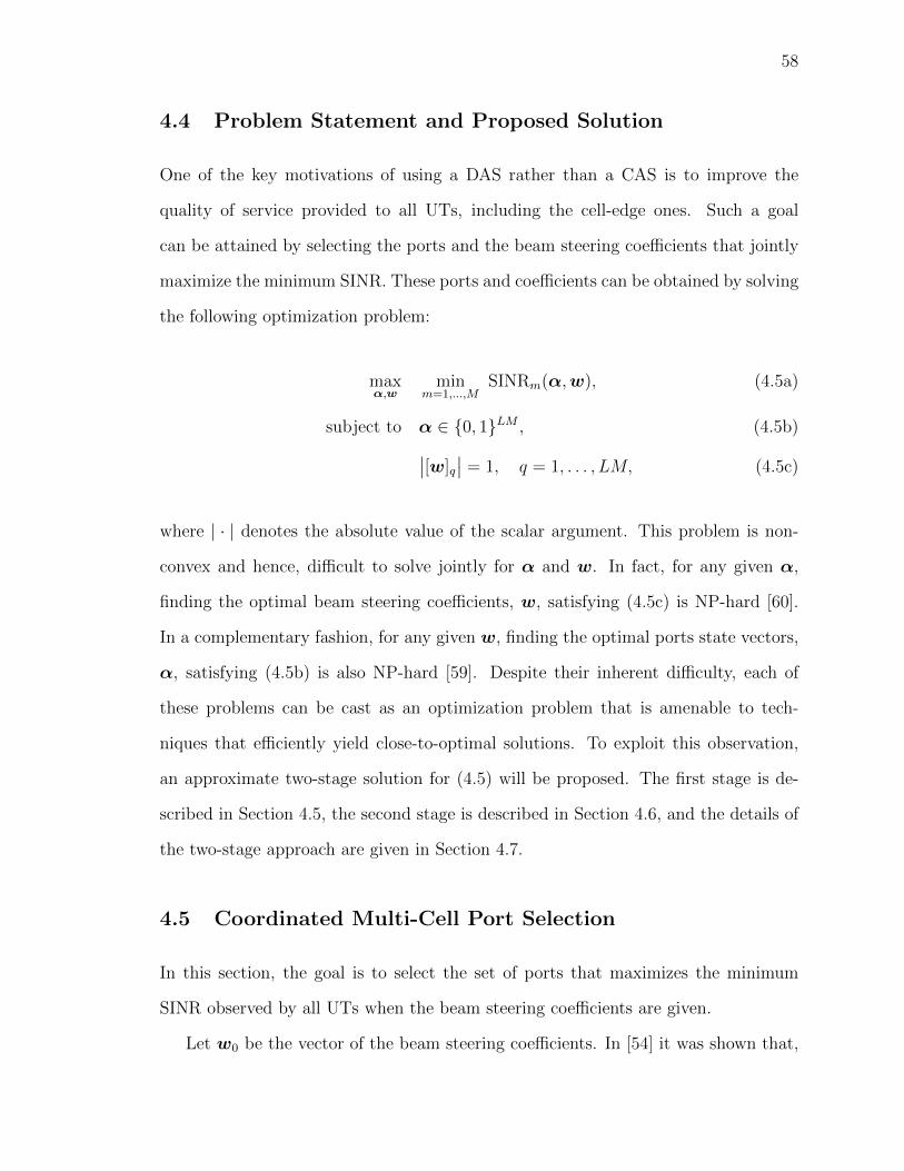
58

4.4 Problem Statement and Proposed Solution

One of the key motivations of using a DAS rather than a CAS is to improve the

quality of service provided to all UTs, including the cell-edge ones. Such a goal

can be attained by selecting the ports and the beam steering coefficients that jointly

maximize the minimum SINR. These ports and coefficients can be obtained by solving

the following optimization problem:

maxα,w

minm=1,...,M

SINRm(α,w), (4.5a)

subject to α ∈ {0, 1}LM , (4.5b)∣∣[w]q∣∣ = 1, q = 1, . . . , LM, (4.5c)

where | · | denotes the absolute value of the scalar argument. This problem is non-

convex and hence, difficult to solve jointly for α and w. In fact, for any given α,

finding the optimal beam steering coefficients, w, satisfying (4.5c) is NP-hard [60].

In a complementary fashion, for any given w, finding the optimal ports state vectors,

α, satisfying (4.5b) is also NP-hard [59]. Despite their inherent difficulty, each of

these problems can be cast as an optimization problem that is amenable to tech-

niques that efficiently yield close-to-optimal solutions. To exploit this observation,

an approximate two-stage solution for (4.5) will be proposed. The first stage is de-

scribed in Section 4.5, the second stage is described in Section 4.6, and the details of

the two-stage approach are given in Section 4.7.

4.5 Coordinated Multi-Cell Port Selection

In this section, the goal is to select the set of ports that maximizes the minimum

SINR observed by all UTs when the beam steering coefficients are given.

Let w0 be the vector of the beam steering coefficients. In [54] it was shown that,

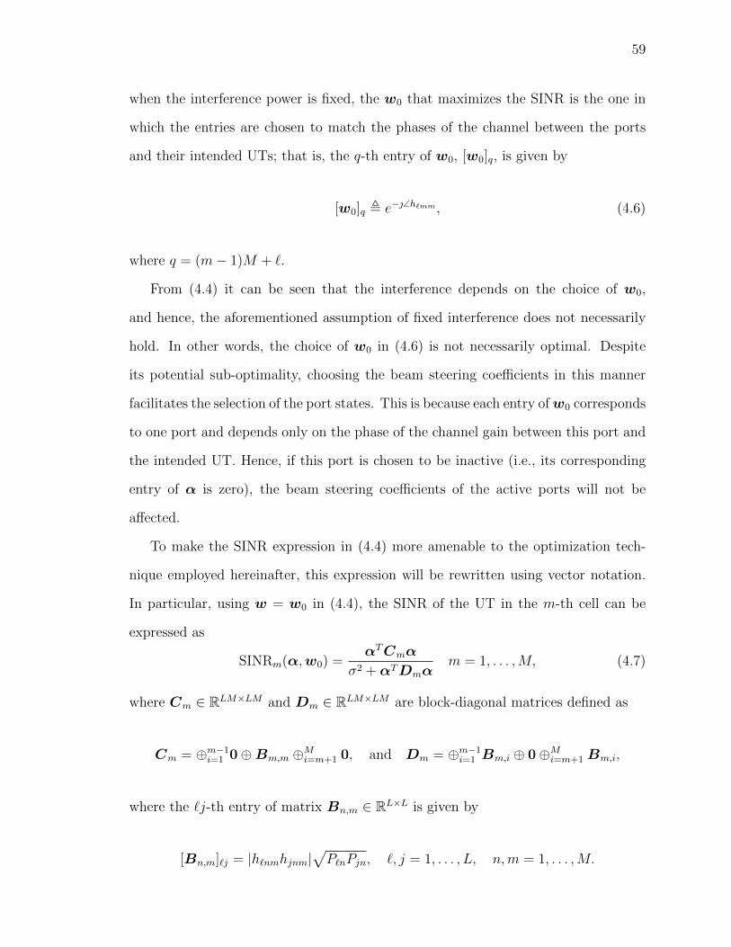
59

when the interference power is fixed, the w0 that maximizes the SINR is the one in

which the entries are chosen to match the phases of the channel between the ports

and their intended UTs; that is, the q-th entry of w0, [w0]q, is given by

[w0]q , e−∠h`mm , (4.6)

where q = (m− 1)M + `.

From (4.4) it can be seen that the interference depends on the choice of w0,

and hence, the aforementioned assumption of fixed interference does not necessarily

hold. In other words, the choice of w0 in (4.6) is not necessarily optimal. Despite

its potential sub-optimality, choosing the beam steering coefficients in this manner

facilitates the selection of the port states. This is because each entry ofw0 corresponds

to one port and depends only on the phase of the channel gain between this port and

the intended UT. Hence, if this port is chosen to be inactive (i.e., its corresponding

entry of α is zero), the beam steering coefficients of the active ports will not be

affected.

To make the SINR expression in (4.4) more amenable to the optimization tech-

nique employed hereinafter, this expression will be rewritten using vector notation.

In particular, using w = w0 in (4.4), the SINR of the UT in the m-th cell can be

expressed as

SINRm(α,w0) =αTCmα

σ2 +αTDmαm = 1, . . . ,M, (4.7)

where Cm ∈ RLM×LM and Dm ∈ RLM×LM are block-diagonal matrices defined as

Cm = ⊕m−1i=1 0⊕Bm,m ⊕Mi=m+1 0, and Dm = ⊕m−1

i=1 Bm,i ⊕ 0⊕Mi=m+1 Bm,i,

where the `j-th entry of matrix Bn,m ∈ RL×L is given by

[Bn,m]`j = |h`nmhjnm|√P`nPjn, `, j = 1, . . . , L, n,m = 1, . . . ,M.

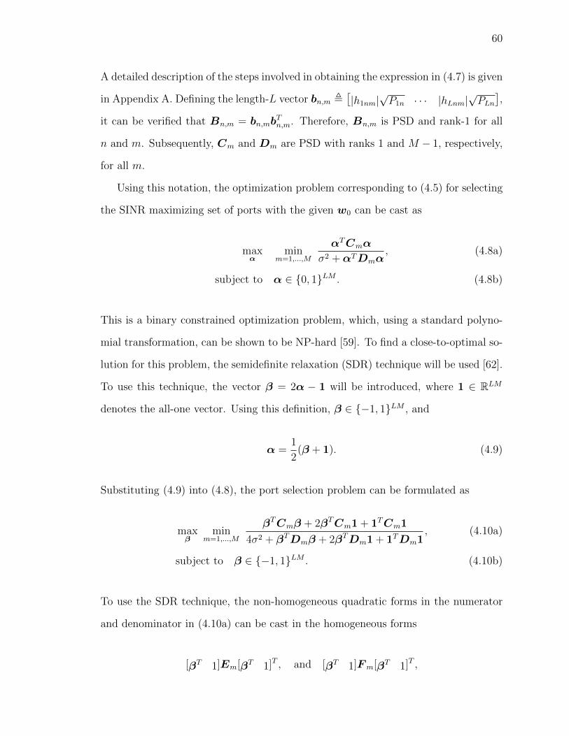
60

A detailed description of the steps involved in obtaining the expression in (4.7) is given

in Appendix A. Defining the length-L vector bn,m ,[|h1nm|

√P1n · · · |hLnm|

√PLn

],

it can be verified that Bn,m = bn,mbTn,m. Therefore, Bn,m is PSD and rank-1 for all

n and m. Subsequently, Cm and Dm are PSD with ranks 1 and M − 1, respectively,

for all m.

Using this notation, the optimization problem corresponding to (4.5) for selecting

the SINR maximizing set of ports with the given w0 can be cast as

maxα

minm=1,...,M

αTCmα

σ2 +αTDmα, (4.8a)

subject to α ∈ {0, 1}LM . (4.8b)

This is a binary constrained optimization problem, which, using a standard polyno-

mial transformation, can be shown to be NP-hard [59]. To find a close-to-optimal so-

lution for this problem, the semidefinite relaxation (SDR) technique will be used [62].

To use this technique, the vector β = 2α − 1 will be introduced, where 1 ∈ RLM

denotes the all-one vector. Using this definition, β ∈ {−1, 1}LM , and

α =1

2(β + 1). (4.9)

Substituting (4.9) into (4.8), the port selection problem can be formulated as

maxβ

minm=1,...,M

βTCmβ + 2βTCm1 + 1TCm1

4σ2 + βTDmβ + 2βTDm1 + 1TDm1, (4.10a)

subject to β ∈ {−1, 1}LM . (4.10b)

To use the SDR technique, the non-homogeneous quadratic forms in the numerator

and denominator in (4.10a) can be cast in the homogeneous forms

[βT 1]Em[βT 1]T , and [βT 1]Fm[βT 1]T ,

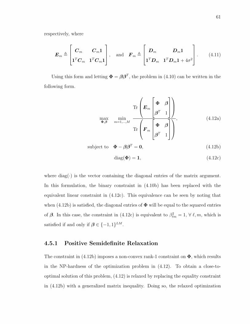
61

respectively, where

Em ,

Cm Cm1

1TCm 1TCm1

, and Fm ,

Dm Dm1

1TDm 1TDm1 + 4σ2

. (4.11)

Using this form and letting Φ = ββT , the problem in (4.10) can be written in the

following form.

maxΦ,β

minm=1,...,M

Tr

Em

Φ β

βT 1

Tr

Fm

Φ β

βT 1

, (4.12a)

subject to Φ− ββT = 0, (4.12b)

diag(Φ) = 1, (4.12c)

where diag(·) is the vector containing the diagonal entries of the matrix argument.

In this formulation, the binary constraint in (4.10b) has been replaced with the

equivalent linear constraint in (4.12c). This equivalence can be seen by noting that

when (4.12b) is satisfied, the diagonal entries of Φ will be equal to the squared entries

of β. In this case, the constraint in (4.12c) is equivalent to β2`m = 1, ∀ `,m, which is

satisfied if and only if β ∈ {−1, 1}LM .

4.5.1 Positive Semidefinite Relaxation

The constraint in (4.12b) imposes a non-convex rank-1 constraint on Φ, which results

in the NP-hardness of the optimization problem in (4.12). To obtain a close-to-

optimal solution of this problem, (4.12) is relaxed by replacing the equality constraint

in (4.12b) with a generalized matrix inequality. Doing so, the relaxed optimization

62

problem corresponding to (4.12) can be expressed as:

maxX,x

minm=1,...,M

Tr

Em

X x

xT 1

Tr

Fm

X x

xT 1

, (4.13a)

subject to X − xxT � 0, (4.13b)

diag(X) = 1, (4.13c)

where X ∈ RLM×LM and x ∈ RLM are the optimization variables corresponding

to Φ and β in the original problem, respectively. Neither the objective in (4.13a)

nor the constraint in (4.13b) is convex. To cast problem (4.13) in a more convenient

form, an auxiliary variable, t, is introduced that lower-bounds the objective function1.

Furthermore, it can be noted that the matrix X −xxT is the Schur complement [46]

of the matrix

Ψ =

X x

xT 1

, (4.14)

and is PSD if and only if Ψ is PSD. Using this observation, the constraint in (4.13b)

will be cast as a convex linear matrix inequality constraint in (4.15c) below. Now,

1The introduction of such an auxiliary variable is a relatively common practice when dealing withmax-min or min-max optimization problems (see, e.g., [59]).

63

the problem in (4.13) can be rewritten as

maxt,X,x

t, (4.15a)

subject to t ≤ Tr(EmΨ)

Tr(FmΨ), m = 1, . . . ,M, (4.15b)

Ψ =

X x

xT 1

� 0, (4.15c)

diag(X) = 1. (4.15d)

The problem in (4.15) is still non-convex in (t,x,X) because the inequality con-

straint in (4.15b) involves products of the form tx and tX. Fortunately, however,

it can be seen that these constraints are quasi-linear in (t,x,X). This is because

both the super-level and the sub-level sets corresponding to a fixed t are convex [61,

Section 3.4]. The constraint in (4.15b) can be expressed in the form

Tr((tFm −Em)Ψ

)≤ 0, m = 1, . . . ,M. (4.16)

To find the optimal value of t, it is noted that the left hand side of (4.16) is

monotonically increasing in t for any given x and X satisfying (4.13b). To show this,

it suffices to show that Tr(FmΨ

)is strictly positive. This is shown in the following

lemma.

Lemma 4.1. For the matrix Fm defined in (4.11) and the matrix Ψ defined in (4.14),

Tr(FmΨ

)> 0, m = 1, . . . ,M.

Proof. See Appendix A.

Using this lemma, the optimal t, which is denoted by t?, can be obtained by

64

solving a series of convex feasibility problems. Each of these problems is of the form

find X,x, (4.17a)

subject to Tr ((t0Fm −Em)Ψ) ≤ 0, m = 1, . . . ,M, (4.17b)

Ψ =

X x

xT 1

� 0, (4.17c)

diag(X) = 1. (4.17d)

For each instance of this problem, the value of t0 is fixed. To determine an interval

within which it lies, it is noted that at the optimal solution, t0 represents the minimum

SINR observed by the UTs. This SINR is upper-bounded by

tmax = minm=1,...,M

1TCm1

σ2, (4.18)

which corresponds to a situation in which there is no interference and all ports are

active. Hence, the optimal t0 must lie in the interval [0, tmax].

Using an argument analogous to the one in [61, Section 4.2.5], it can be seen that

if (4.17) is feasible for a particular value of t0, then t0 ≤ t?. Conversely, if (4.17) is

infeasible for this value of t0, then t0 > t?. Hence, the optimal value of t0 must lie on

the boundary of the feasible set of (4.15) and can be found using a bisection search.

4.5.2 Randomization for Coordinated Port Selection

Let X? and x? denote the optimal solution of (4.15) corresponding to t = t? obtained

by the bisection search. To obtain a candidate solution of the optimization problem

in (4.10), the Gaussian randomization technique will be used. This technique is known

to yield a close-to-optimal solution for NP-hard optimization problems with a similar

underlying structure (see e.g., [64]).

65

To apply this technique to the current problem, a set of J1 length-LM random

vectors V = {v(j)}J1j=1 is generated from the Gaussian distributionN (x?,X?−x?x?T ).

For sufficiently large J1, the vectors in V provide an approximate solution to the

following stochastic optimization problem:

maxX?=E{vvT }x?=E{v}

t, (4.19a)

subject to E{

[vT 1](tFm −Em

)[vT 1]T

}≤ 0, m = 1, . . . ,M, (4.19b)

E{[v]2r} = 1, r = 1, . . . , LM. (4.19c)

Since X?−x?x?T � 0, it can be seen that this optimization problem is equivalent to

the one in (4.15). Hence, it can be seen that the set of vectors in V solve the problem

in (4.15) on average [62].

The goal now is to use the vectors in V to extract candidate solutions to the

problem in (4.10). To do so, each realization of v(j) ∈ V is quantized and the corre-

sponding objective in (4.10) is evaluated. In particular, for each v(j) ∈ V , a candidate

binary solution β(j)

is obtained as follows:

β(j)

= sgn(v(j) − x?), j = 1, . . . , J1, (4.20)

where sgn(·) is the element-wise signum function. Using (4.9), the corresponding

candidate solutions of (4.8) are obtained and the one yielding the largest objective is

chosen; i.e.,

α? = arg maxj=1,...,J

minm=1,...,M

SINRm(α(j),w0). (4.21)

The SDR-based randomization technique proposed herein for close-to-optimal port

selection is summarized in the algorithm in Table 4.1.

In Section 4.9, it will be shown that when the beam steering coefficients are fixed,

66

Table 4.1: Algorithm 1 – Generating a close-to-optimal set of port states

• Initialize a = 0, b = tmax, ε > 0.

• While (b− a) > ε:

– Set t0 = (a+ b)/2 and solve (4.17).

– If (4.17) is feasible, set a = t0; else, set b = t0.

• For j = 1, . . . , J1,

– Generate v(j) ∼ N (x?,X? − x?x?T ).

– Use (4.20) to obtain β(j)

, and (4.9) to obtain α(j).

• Determine α? using (4.21).

the above SDR technique with Gaussian randomization provides a close-to-optimal

solution of the port selection problem with a relatively small J1.

4.6 Coordinated Beam Steering Optimization

In the previous section, the problem of selecting the antenna ports that maximize the

minimum SINR when the beam steering coefficients are fixed was considered. In this

section, the complementary problem is considered in which the port state vectors are

fixed and the beam steering coefficients are to be optimized.

Let α0 be a given port state vector. Analogous to the approach used in Section 4.5,

vector notation will be introduced to express the SINR in a convenient form that

facilitates the optimization of the beam steering coefficients.

Define the M2 matrices {Qn,m}Mn,m=1 such that the `j-th entry of the nm-th matrix

is given by

[Qn,m]`j = α`nh`nmh∗jnmαjn

√P`nPjn, `, j = 1, . . . , L, n,m = 1, . . . ,M,

where (·)∗ denotes the complex conjugate. Furthermore, define block-diagonal matri-

67

ces Sm ∈ CLM×LM and Tm ∈ CLM×LM as

Sm = ⊕m−1i=1 0⊕Qm,m ⊕Mi=m+1 0, and Tm = ⊕m−1

i=1 Qm,i ⊕ 0⊕Mi=m+1 Qm,i.

Using an argument analogous to the one used in Section 4.5, it can be shown that

the matrices {Qn,m}Mn,m=1 are PSD and rank-1, and that the matrices {Sm}Mm=1 and

{Tm}Mm=1 are PSD with ranks 1 and M − 1, respectively.

Using this notation, the SINR of the UT in the m-th cell can be expressed as

SINRm(α0,w) =wHSmw

σ2 +wHTmwm = 1, . . . ,M. (4.22)

With the port state vector being fixed as α0, the general optimization problem

in (4.5) reduces to

maxw

minm=1,...,M

wHSmw

σ2 +wHTmw, (4.23a)

subject to∣∣[w]q

∣∣ = 1, q = 1, . . . , LM, (4.23b)

where the constraint in (4.23b) ensures that the entries of w lie on the unit circle, i.e.,

the power of each port is constant. This problem is non-convex, and in fact, a variant

of it, in which the antennas have to satisfy a total power constraint but no unit circle

constraints, has been shown to be NP-hard [60]. A close-to-optimal solution to the

problem considered in [60] was obtained using the SDR-based Gaussian randomization

technique. This technique was also used for the max-min fair problems considered

in [65] and [66], wherein, in contrast to the above optimization problem, the antennas

are also subject to a total power constraint. Following the lead of [60, 65, 66], the SDR-

based Gaussian randomization technique will be utilized to find a close-to-optimal

solution for the beam steering optimization problem in (4.23) with the unit circle

constraint in (4.23b).

68

Similar to the approach used in Section 4.5, in applying the SDR technique, the

optimization problem in (4.23) is relaxed by letting Υ = wwH , and subsequently

dropping the rank-1 constraint on Υ. Let W ∈ CLM×LM be the counterpart of Υ

in the relaxed problem. Introducing an auxiliary variable s that serves as a lower-

bound on the objective function in (4.23a), the relaxed optimization problem can be

expressed as

maxs,W

s, (4.24a)

subject to sσ2 + Tr((sTm − Sm)W ) ≤ 0, m = 1, . . . ,M, (4.24b)

diag(W ) = 1, (4.24c)

W � 0. (4.24d)

Because of the product of the optimization variables in (4.24b), this constraint is not

convex. However, similar to the relaxation of the port selection problem in Section 4.5,

it can be shown that this problem is quasi-linear, and that its optimal solution lies on

the boundary of the feasible set. This point can be found by using a bisection search

over s. Let s0 denote the value of s at any iteration of the bisection search. We seek

the maximum value of s0 for which the following feasibility problem has a solution.

find W , (4.25a)

subject to s0σ2 + Tr((s0Tm − Sm)W ) ≤ 0, m = 1, . . . ,M, (4.25b)

diag(W ) = 1, (4.25c)

W � 0. (4.25d)

It is straightforward to see that this problem is convex, and hence, can be solved

efficiently for any given s0. However, to facilitate the bisection search, it is desirable

to upper-bound s0.

69

Let smax denote the upper-bound on the value of s0. A candidate smax can be

obtained by upper-bounding the SINR expression in (4.22). In particular, since, by

construction, Tm � 0, we have

SINRm(α0,w) ≤ wHSmw

σ2

≤ ‖w‖22

σ2‖Sm‖2 (4.26)

≤ LM

σ2‖Sm‖2, (4.27)

where (4.26) follows from the submultiplicative property of the 2-norm [67], and (4.27)

follows from the fact that ‖w‖22 ≤ LM . Hence, a candidate value of smax is

smax = minm=1,...,M

LM‖Sm‖2

σ2.

Let W ? denote the solution of the relaxed problem corresponding to the optimal

s0 obtained from the bisection search. The Gaussian randomization technique is then

used to generate an approximate solution of the original problem in (4.23). To apply

this technique, a set of J2 length-LM random vectors, Z = {z(j)}J2j=1, is drawn from

the Gaussian distribution CN (0,W ?). Similar to the discussion in Section 4.5.2, for

sufficiently large J2, these vectors provide an approximate solution to the following

stochastic optimization problem:

maxW ?=E{zzH}

s, (4.28a)

subject to E{sσ2 + zH(sTm − Sm)z

}≤ 0, m = 1, . . . ,M, (4.28b)

E{∣∣[z]q

∣∣} = 1, q = 1, . . . , LM. (4.28c)

In other words, the set of vectors in Z solve the problem in (4.24) on average [62].

Now, to obtain candidate beam steering coefficients, {[w(j)]q}LMq=1, that lie on the

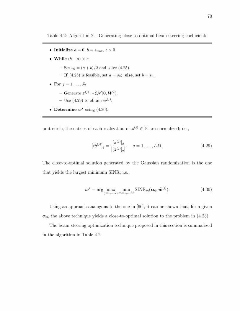
70

Table 4.2: Algorithm 2 – Generating close-to-optimal beam steering coefficients

• Initialize a = 0, b = smax, ε > 0

• While (b− a) > ε:

– Set s0 = (a+ b)/2 and solve (4.25).

– If (4.25) is feasible, set a = s0; else, set b = s0.

• For j = 1, . . . , J2

– Generate z(j) ∼ CN (0,W ?).

– Use (4.29) to obtain w(j).

• Determine w? using (4.30).

unit circle, the entries of each realization of z(j) ∈ Z are normalized; i.e.,

[w(j)]q =[z(j)]q∣∣[z(j)]q

∣∣ , q = 1, . . . , LM. (4.29)

The close-to-optimal solution generated by the Gaussian randomization is the one

that yields the largest minimum SINR; i.e.,

w? = arg maxj=1,...,J2

minm=1,...,M

SINRm(α0, w(j)). (4.30)

Using an approach analogous to the one in [66], it can be shown that, for a given

α0, the above technique yields a close-to-optimal solution to the problem in (4.23).

The beam steering optimization technique proposed in this section is summarized

in the algorithm in Table 4.2.

71

4.7 A Two-Stage Approach to obtain an Approximate Solu-

tion to the Joint Optimization Problem

In this section the techniques developed in Sections 4.5 and 4.6 are used to develop a

two-stage approach for generating an efficiently-computable approximate solution to

the joint optimization problem in (4.5).

In the first stage, the beam steering coefficients are chosen as in (4.6), the matri-

ces {Em,Fm}Mm=1 are constructed, and a set of J1 port state vectors are generated

using (4.20) and (4.9). Out of those J1 vectors, the J ≤ J1 candidates that yield

the largest minimum SINR are selected. Notice that the close-to-optimal solution

of (4.8) generated by (4.21) corresponds to setting J = 1 and does not necessarily

yield a close-to-optimal solution of the problem in (4.5), as will be shown in Sec-

tion 4.9.

In the second stage, each of the J candidate vectors obtained in the first stage is

used to construct the matrices {Sm,Tm}Mm=1 and the corresponding close-to-optimal

beam steering coefficients are generated using (4.30). Finally, the approximate solu-

tion of problem (4.5) is chosen to be the pair of port state vector and beam steering

coefficient vector that jointly yield the largest objective in (4.5a).

It will be shown in Section 4.9 that this two-stage approach, with relatively small

J1 and J , yields a significantly better performance than that achieved by port selection

with the initial beam steering coefficients, and that achieved by the close-to-optimal

port state vector chosen in the first stage with the corresponding close-to-optimal

beam steering coefficients obtained in the second stage.

4.8 Complexity Analysis

In this section, bounds will be provided on the computational complexity of the pro-

posed techniques. More specifically, it will be shown that each of the techniques that

72

yield close-to-optimal solutions in Sections 4.5 and 4.6 has a polynomial complexity.

Hence, the two-stage approach proposed in Section 4.7 for obtaining an approximate

solution to the joint optimization problem in (4.5) also has polynomial complexity.

4.8.1 Computational Complexity of the First Stage

In the first stage of the approach proposed in Section 4.7, the beam steering co-

efficients are fixed. In this case, the optimal port state vector could be found by

exhaustive search over all possible vectors. The computational complexity of this

approach is O(2LM

), and hence, it is inefficient for large L and M .

In contrast, the SDR-based Gaussian randomization technique proposed in Sec-

tion 4.5 involves solving a sequence of convex optimization problems, each with a PSD

constraint (refer to (4.17)). For general-use solvers, e.g., CVX [68], the complexity of

solving problems of this form would be O((LM)6.5 log(1/ε0)

), where ε0 > 0 is the

solution accuracy [69]. However, the problem in (4.17) has a particular structure that

can exploited to develop more efficient solving techniques. For instance, the primal-

dual path-following interior-point method developed in [70] has been particularized

in [62] to solve a PSD-constrained convex optimization problem similar to the one

in (4.17) with complexity O((LM)4.5 log(1/ε0)

).

Let ε1 > 0 be the solution accuracy of the bisection search used in Section 4.5.

Since this search is over the interval [0, tmax] and its convergence rate is exponential,

the number of bisection search iterations is given by log(tmax/ε1), where tmax is defined

in (4.18). For the Gaussian randomization procedure described in Section 4.5.2, the

computational complexity of generating and evaluating the objective corresponding

to the J1 random samples is O((LM)2J1

)[63]. Now, combining these observations,

it can be seen that the complexity of the proposed port selection technique is

O((LM)4.5 log(1/ε0) log(tmax/ε1) + (LM)2J1

). (4.31)

73

4.8.2 Computational Complexity of the Second Stage

In the second stage, close-to-optimal beam steering coefficients for a given port state

vector could be obtained by discretizing each coefficient using Nb bins. Then, the

coefficients that yield the largest minimum SINR could be determined by using an

exhaustive search over all possible bin combinations. The complexity of such as ap-

proach would be O(NLMb

), which, similar to the exhaustive search in the port selec-

tion problem, is computationally inefficient. However, in Section 4.6, close-to-optimal

beam steering coefficients are generated using a variation of the SDR-based Gaussian

randomization technique. Using a discussion analogous to the one in Section 4.8.1, it

can be shown that the complexity of this technique is

O((LM)4.5 log(1/ε0) log(smax/ε1) + (LM)2J2

). (4.32)

4.8.3 Computational Complexity of the Two-Stage Approach

Using exhaustive search to solve the joint optimization problem in (4.5) with dis-

cretized beam steering coefficients involves a complexity of O((2Nb)

LM). This com-

plexity is computationally prohibitive, even for a relatively small system. For exam-

ple, for a two-cell cluster with seven ports in each cell, and Nb = 100, the exhaustive

search involves about 20014 ≈ 1.64× 1032 combinations.

Using the two-stage approach presented in Section 4.7 and the complexity discus-

sions in Sections 4.8.1 and 4.8.2, it can be readily seen that the complexity of this

technique is bounded by

O(

(LM)4.5 log(1/ε0)(J log(smax/ε1) + log(tmax/ε1)

)+ (LM)2(J2J + J1)

). (4.33)

The results presented in this section are summarized in Table 4.3

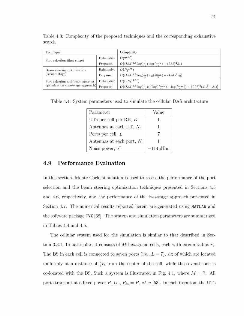
74

Table 4.3: Complexity of the proposed techniques and the corresponding exhaustivesearch

Technique Complexity

Port selection (first stage)Exhaustive O

(2LM

)Proposed O

((LM)4.5 log( 1

ε0) log( tmax

ε1) + (LM)2J1

)Beam steering optimization(second stage)

Exhaustive O(NLMb

)Proposed O

((LM)4.5 log( 1

ε0) log( smax

ε1) + (LM)2J2

)Port selection and beam steeringoptimization (two-stage approach)

Exhaustive O((2Nb)

LM)

Proposed O((LM)4.5 log( 1

ε0)(J log( smax

ε1) + log( tmax

ε1))

+ (LM)2(J2J + J1))

Table 4.4: System parameters used to simulate the cellular DAS architecture

Parameter Value

UTs per cell per RB, K 1

Antennas at each UT, Nr 1

Ports per cell, L 7

Antennas at each port, Nt 1

Noise power, σ2 −114 dBm

4.9 Performance Evaluation

In this section, Monte Carlo simulation is used to assess the performance of the port

selection and the beam steering optimization techniques presented in Sections 4.5

and 4.6, respectively, and the performance of the two-stage approach presented in

Section 4.7. The numerical results reported herein are generated using MATLAB and

the software package CVX [68]. The system and simulation parameters are summarized

in Tables 4.4 and 4.5.

The cellular system used for the simulation is similar to that described in Sec-

tion 3.3.1. In particular, it consists of M hexagonal cells, each with circumradius rc.

The BS in each cell is connected to seven ports (i.e., L = 7), six of which are located

uniformly at a distance of 23rc from the center of the cell, while the seventh one is

co-located with the BS. Such a system is illustrated in Fig. 4.1, where M = 7. All

ports transmit at a fixed power P , i.e., P`n = P , ∀`, n [53]. In each iteration, the UTs

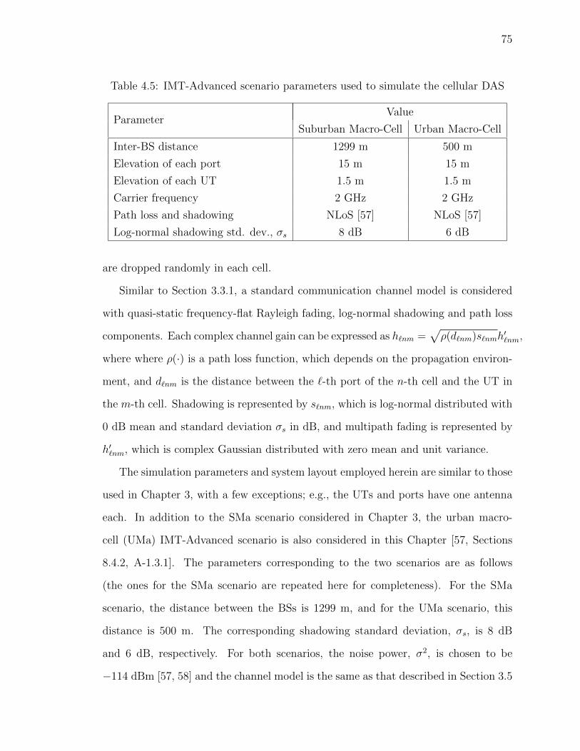
75

Table 4.5: IMT-Advanced scenario parameters used to simulate the cellular DAS

ParameterValue

Suburban Macro-Cell Urban Macro-Cell

Inter-BS distance 1299 m 500 m

Elevation of each port 15 m 15 m

Elevation of each UT 1.5 m 1.5 m

Carrier frequency 2 GHz 2 GHz

Path loss and shadowing NLoS [57] NLoS [57]

Log-normal shadowing std. dev., σs 8 dB 6 dB

are dropped randomly in each cell.

Similar to Section 3.3.1, a standard communication channel model is considered

with quasi-static frequency-flat Rayleigh fading, log-normal shadowing and path loss

components. Each complex channel gain can be expressed as h`nm =√ρ(d`nm)s`nmh

′`nm,

where where ρ(·) is a path loss function, which depends on the propagation environ-

ment, and d`nm is the distance between the `-th port of the n-th cell and the UT in

the m-th cell. Shadowing is represented by s`nm, which is log-normal distributed with

0 dB mean and standard deviation σs in dB, and multipath fading is represented by

h′`nm, which is complex Gaussian distributed with zero mean and unit variance.

The simulation parameters and system layout employed herein are similar to those

used in Chapter 3, with a few exceptions; e.g., the UTs and ports have one antenna

each. In addition to the SMa scenario considered in Chapter 3, the urban macro-

cell (UMa) IMT-Advanced scenario is also considered in this Chapter [57, Sections

8.4.2, A-1.3.1]. The parameters corresponding to the two scenarios are as follows

(the ones for the SMa scenario are repeated here for completeness). For the SMa

scenario, the distance between the BSs is 1299 m, and for the UMa scenario, this

distance is 500 m. The corresponding shadowing standard deviation, σs, is 8 dB

and 6 dB, respectively. For both scenarios, the noise power, σ2, is chosen to be

−114 dBm [57, 58] and the channel model is the same as that described in Section 3.5

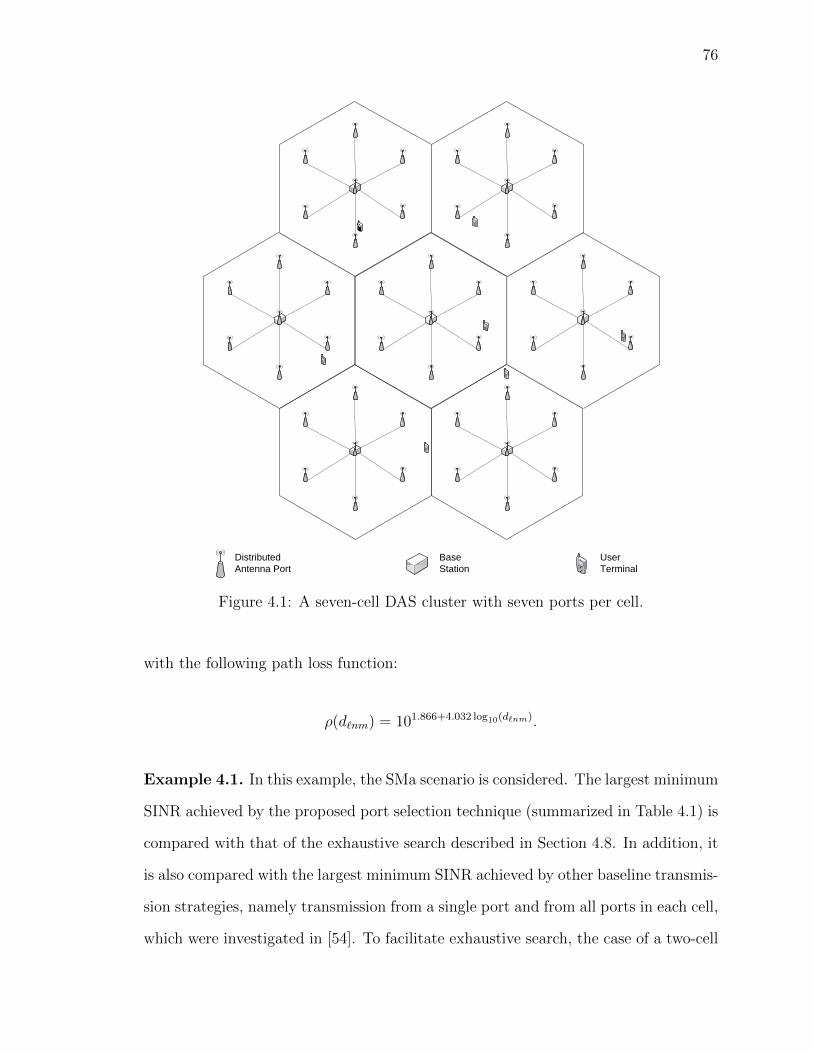
76

Distributed

Antenna Port

Base

Station

User

Terminal

Figure 4.1: A seven-cell DAS cluster with seven ports per cell.

with the following path loss function:

ρ(d`nm) = 101.866+4.032 log10(d`nm).

Example 4.1. In this example, the SMa scenario is considered. The largest minimum

SINR achieved by the proposed port selection technique (summarized in Table 4.1) is

compared with that of the exhaustive search described in Section 4.8. In addition, it

is also compared with the largest minimum SINR achieved by other baseline transmis-

sion strategies, namely transmission from a single port and from all ports in each cell,

which were investigated in [54]. To facilitate exhaustive search, the case of a two-cell

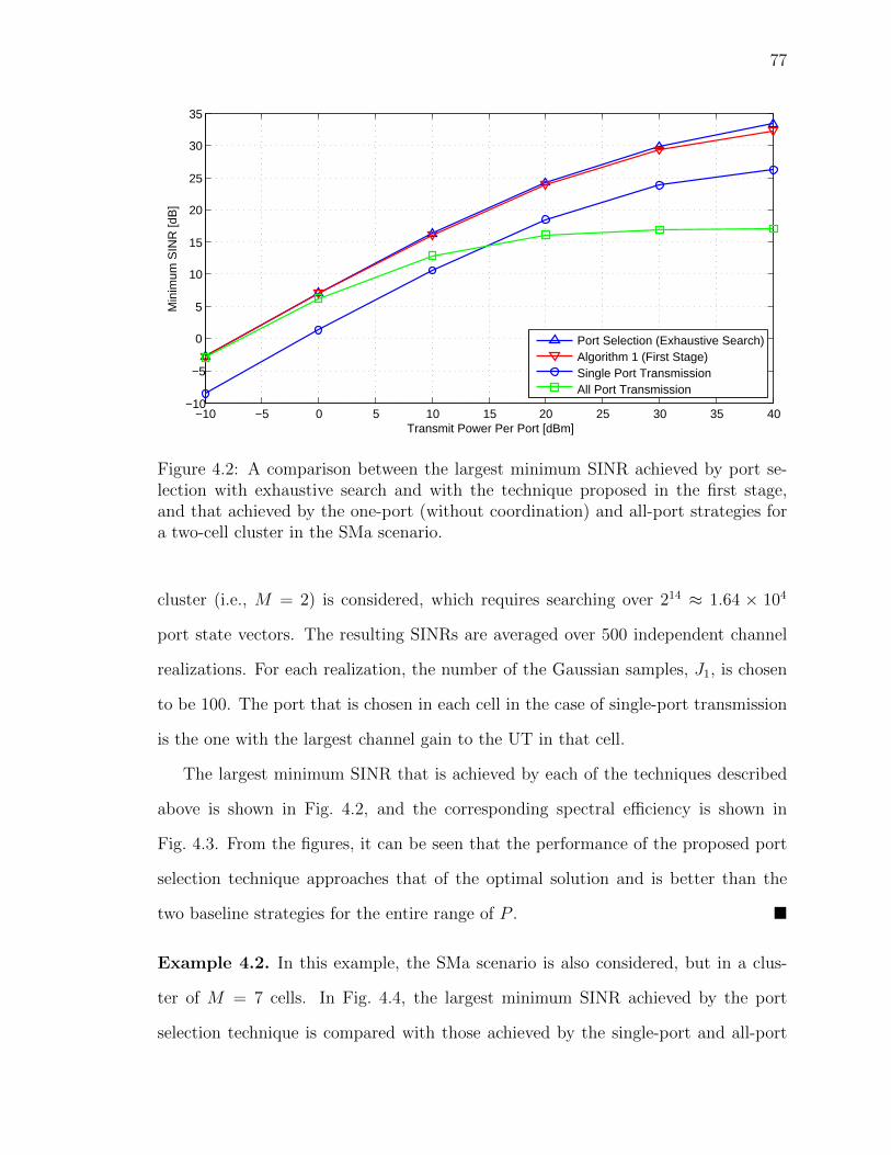
77

−10 −5 0 5 10 15 20 25 30 35 40−10

−5

0

5

10

15

20

25

30

35

Transmit Power Per Port [dBm]

Min

imum

SIN

R [d

B]

Port Selection (Exhaustive Search)Algorithm 1 (First Stage)Single Port TransmissionAll Port Transmission

Figure 4.2: A comparison between the largest minimum SINR achieved by port se-lection with exhaustive search and with the technique proposed in the first stage,and that achieved by the one-port (without coordination) and all-port strategies fora two-cell cluster in the SMa scenario.

cluster (i.e., M = 2) is considered, which requires searching over 214 ≈ 1.64 × 104

port state vectors. The resulting SINRs are averaged over 500 independent channel

realizations. For each realization, the number of the Gaussian samples, J1, is chosen

to be 100. The port that is chosen in each cell in the case of single-port transmission

is the one with the largest channel gain to the UT in that cell.

The largest minimum SINR that is achieved by each of the techniques described

above is shown in Fig. 4.2, and the corresponding spectral efficiency is shown in

Fig. 4.3. From the figures, it can be seen that the performance of the proposed port

selection technique approaches that of the optimal solution and is better than the

two baseline strategies for the entire range of P . �

Example 4.2. In this example, the SMa scenario is also considered, but in a clus-

ter of M = 7 cells. In Fig. 4.4, the largest minimum SINR achieved by the port

selection technique is compared with those achieved by the single-port and all-port

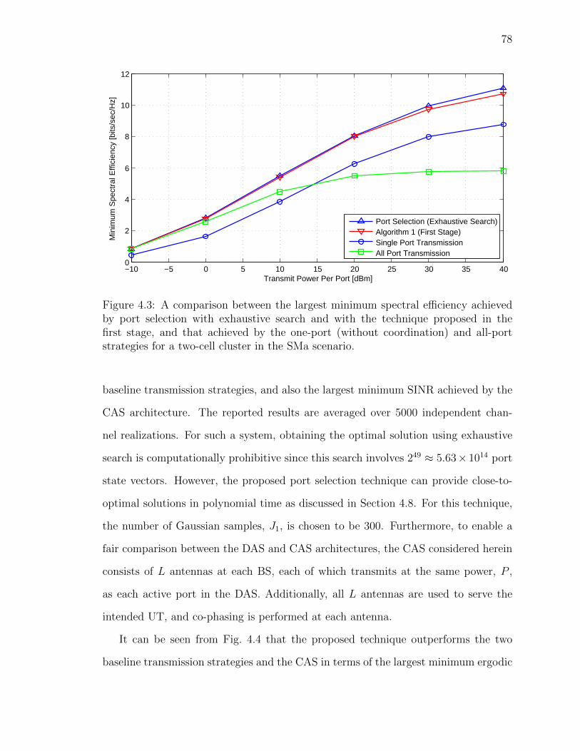
78

−10 −5 0 5 10 15 20 25 30 35 400

2

4

6

8

10

12


Min

imum

Spe

ctra

l Effi

cien

cy [b

its/s

ec/H

z]

Port Selection (Exhaustive Search)Algorithm 1 (First Stage)Single Port TransmissionAll Port Transmission

Figure 4.3: A comparison between the largest minimum spectral efficiency achievedby port selection with exhaustive search and with the technique proposed in thefirst stage, and that achieved by the one-port (without coordination) and all-portstrategies for a two-cell cluster in the SMa scenario.

baseline transmission strategies, and also the largest minimum SINR achieved by the

CAS architecture. The reported results are averaged over 5000 independent chan-

nel realizations. For such a system, obtaining the optimal solution using exhaustive

search is computationally prohibitive since this search involves 249 ≈ 5.63× 1014 port

state vectors. However, the proposed port selection technique can provide close-to-

optimal solutions in polynomial time as discussed in Section 4.8. For this technique,

the number of Gaussian samples, J1, is chosen to be 300. Furthermore, to enable a

fair comparison between the DAS and CAS architectures, the CAS considered herein

consists of L antennas at each BS, each of which transmits at the same power, P ,

as each active port in the DAS. Additionally, all L antennas are used to serve the

intended UT, and co-phasing is performed at each antenna.

It can be seen from Fig. 4.4 that the proposed technique outperforms the two

baseline transmission strategies and the CAS in terms of the largest minimum ergodic

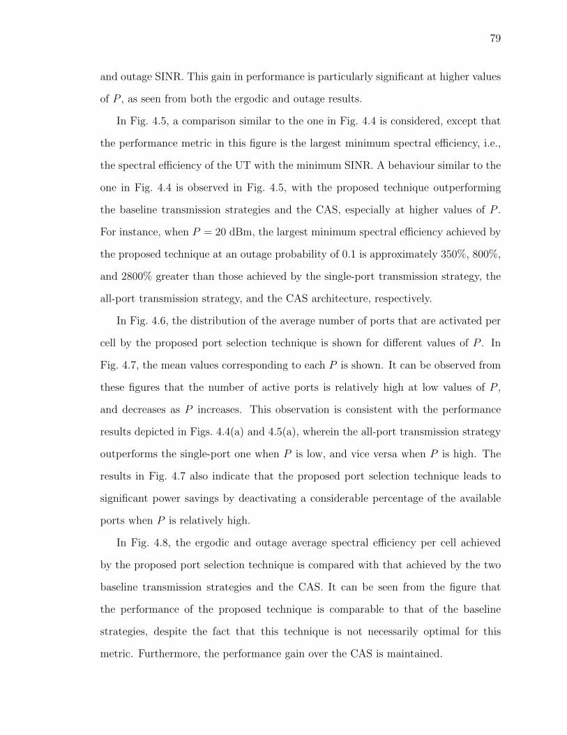
79

and outage SINR. This gain in performance is particularly significant at higher values

of P , as seen from both the ergodic and outage results.

In Fig. 4.5, a comparison similar to the one in Fig. 4.4 is considered, except that

the performance metric in this figure is the largest minimum spectral efficiency, i.e.,

the spectral efficiency of the UT with the minimum SINR. A behaviour similar to the

one in Fig. 4.4 is observed in Fig. 4.5, with the proposed technique outperforming

the baseline transmission strategies and the CAS, especially at higher values of P .

For instance, when P = 20 dBm, the largest minimum spectral efficiency achieved by

the proposed technique at an outage probability of 0.1 is approximately 350%, 800%,

and 2800% greater than those achieved by the single-port transmission strategy, the

all-port transmission strategy, and the CAS architecture, respectively.

In Fig. 4.6, the distribution of the average number of ports that are activated per

cell by the proposed port selection technique is shown for different values of P . In

Fig. 4.7, the mean values corresponding to each P is shown. It can be observed from

these figures that the number of active ports is relatively high at low values of P ,

and decreases as P increases. This observation is consistent with the performance

results depicted in Figs. 4.4(a) and 4.5(a), wherein the all-port transmission strategy

outperforms the single-port one when P is low, and vice versa when P is high. The

results in Fig. 4.7 also indicate that the proposed port selection technique leads to

significant power savings by deactivating a considerable percentage of the available

ports when P is relatively high.

In Fig. 4.8, the ergodic and outage average spectral efficiency per cell achieved

by the proposed port selection technique is compared with that achieved by the two

baseline transmission strategies and the CAS. It can be seen from the figure that

the performance of the proposed technique is comparable to that of the baseline

strategies, despite the fact that this technique is not necessarily optimal for this

metric. Furthermore, the performance gain over the CAS is maintained.

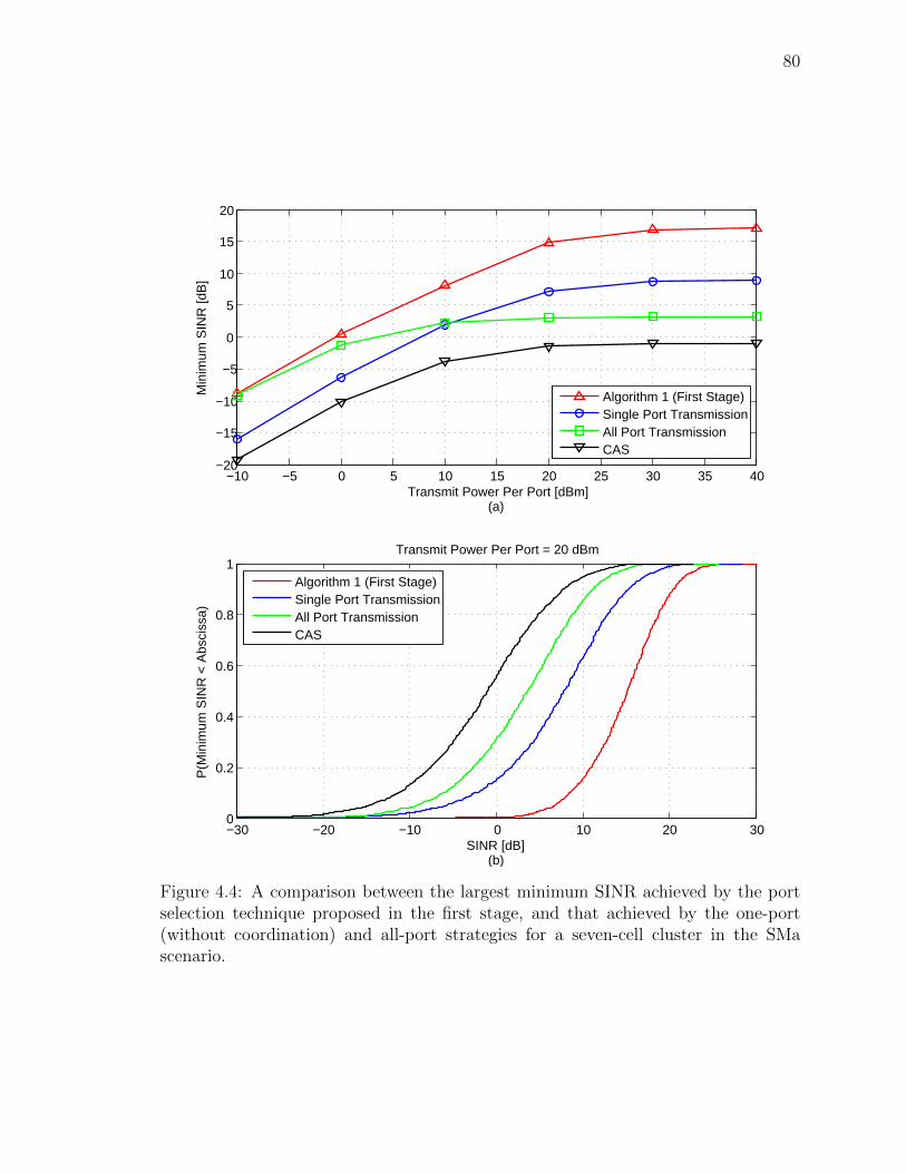
80

−10 −5 0 5 10 15 20 25 30 35 40−20

−15

−10

−5

0

5

10

15

20

Transmit Power Per Port [dBm](a)

Min

imum

SIN

R [d

B]

Algorithm 1 (First Stage)Single Port TransmissionAll Port TransmissionCAS

−30 −20 −10 0 10 20 300

0.2

0.4

0.6

0.8

1

SINR [dB](b)

P(M

inim

um S

INR

< A

bsci

ssa)

Transmit Power Per Port = 20 dBm


Figure 4.4: A comparison between the largest minimum SINR achieved by the portselection technique proposed in the first stage, and that achieved by the one-port(without coordination) and all-port strategies for a seven-cell cluster in the SMascenario.

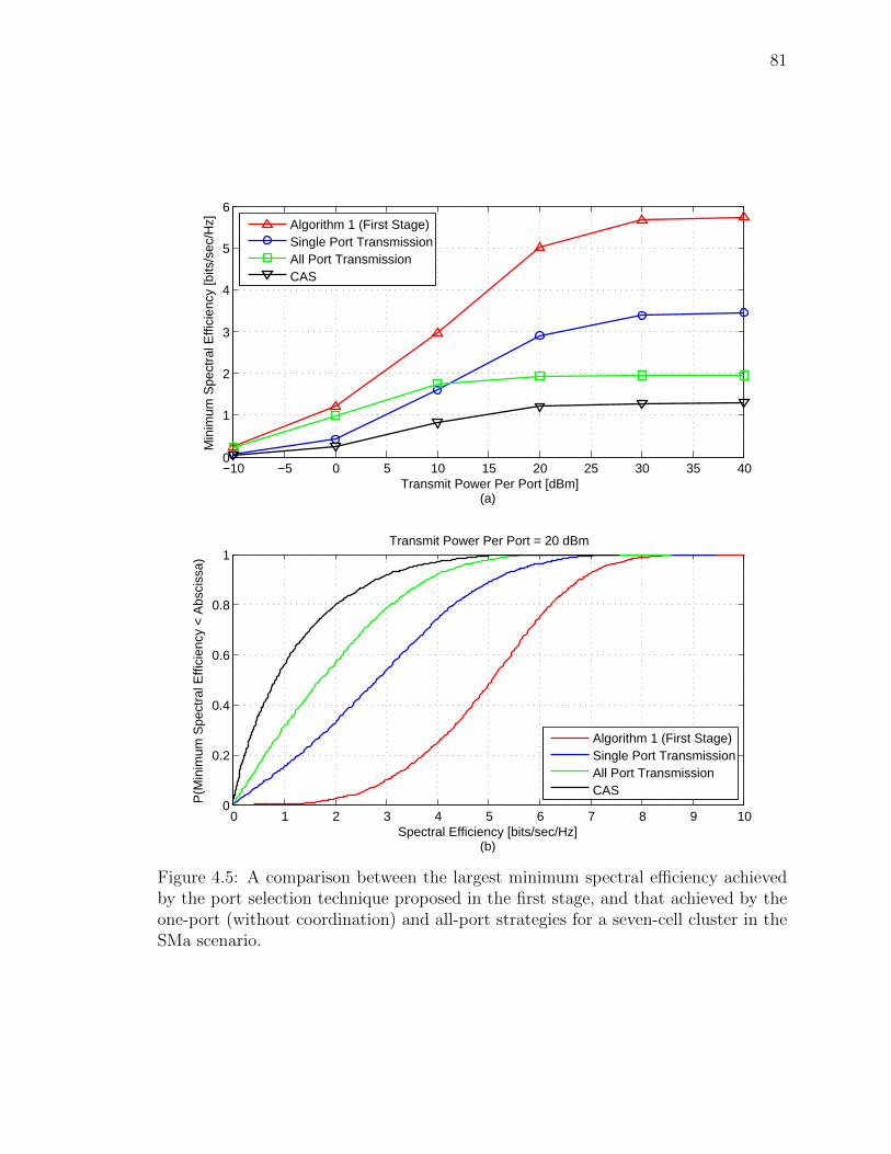
81

−10 −5 0 5 10 15 20 25 30 35 400

1

2

3

4

5

6


Min

imum

Spe

ctra

l Effi

cien

cy [b

its/s

ec/H

z]


0 1 2 3 4 5 6 7 8 9 100

0.2

0.4

0.6

0.8

1

Spectral Efficiency [bits/sec/Hz](b)

P(M

inim

um S

pect

ral E

ffici

ency

< A

bsci

ssa)



Figure 4.5: A comparison between the largest minimum spectral efficiency achievedby the port selection technique proposed in the first stage, and that achieved by theone-port (without coordination) and all-port strategies for a seven-cell cluster in theSMa scenario.

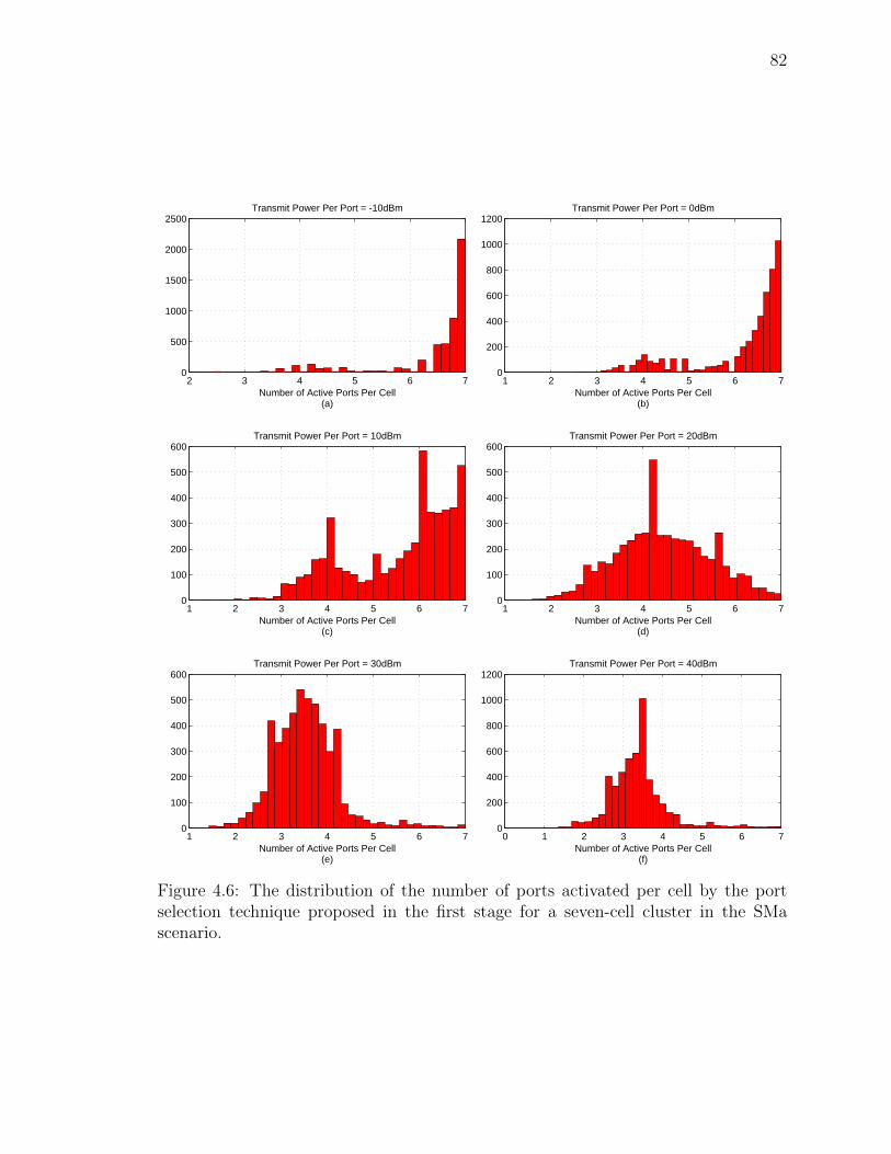
82

2 3 4 5 6 70

500

1000

1500

2000

2500

Number of Active Ports Per Cell(a)

Transmit Power Per Port = -10dBm

1 2 3 4 5 6 70

200

400

600

800

1000

1200

Number of Active Ports Per Cell(b)

Transmit Power Per Port = 0dBm

1 2 3 4 5 6 70

100

200

300

400

500

600

Number of Active Ports Per Cell(c)


1 2 3 4 5 6 70

100

200

300

400

500

600

Number of Active Ports Per Cell(d)


1 2 3 4 5 6 70

100

200

300

400

500

600

Number of Active Ports Per Cell(e)


0 1 2 3 4 5 6 70

200

400

600

800

1000

1200

Number of Active Ports Per Cell(f)


Figure 4.6: The distribution of the number of ports activated per cell by the portselection technique proposed in the first stage for a seven-cell cluster in the SMascenario.

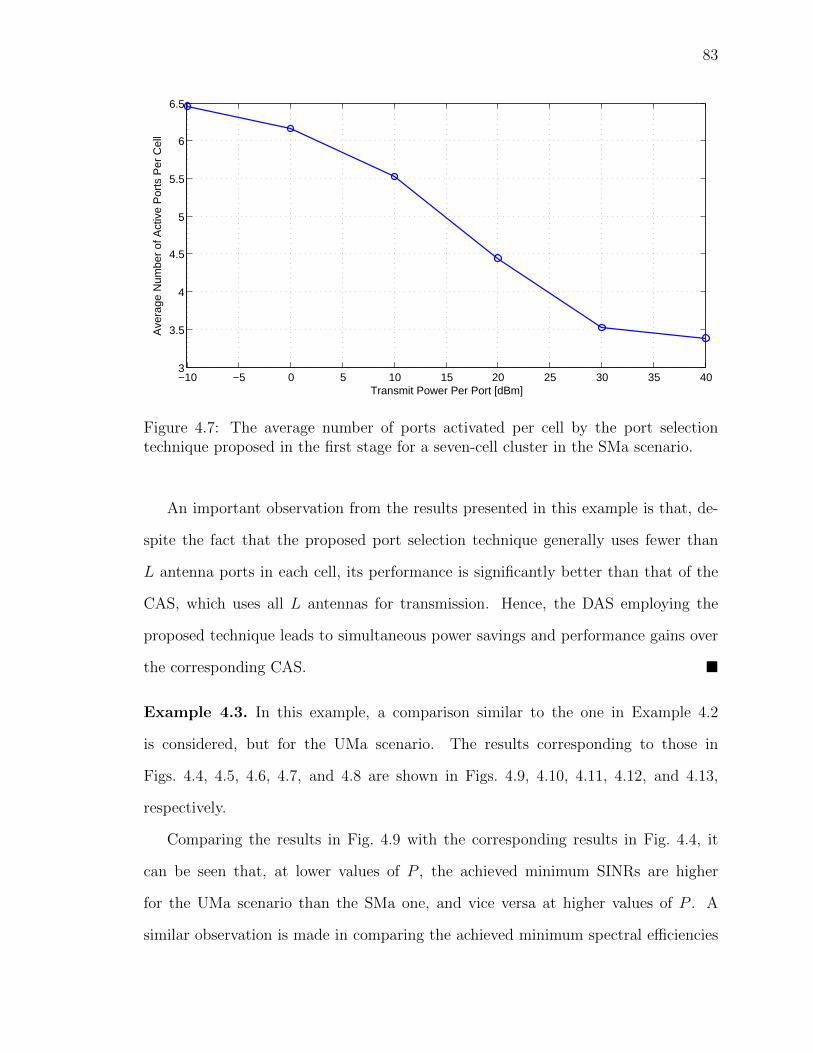
83

−10 −5 0 5 10 15 20 25 30 35 403

3.5

4

4.5

5

5.5

6

6.5


Ave

rage

Num

ber

of A

ctiv

e P

orts

Per

Cel

l

Figure 4.7: The average number of ports activated per cell by the port selectiontechnique proposed in the first stage for a seven-cell cluster in the SMa scenario.

An important observation from the results presented in this example is that, de-

spite the fact that the proposed port selection technique generally uses fewer than

L antenna ports in each cell, its performance is significantly better than that of the

CAS, which uses all L antennas for transmission. Hence, the DAS employing the

proposed technique leads to simultaneous power savings and performance gains over

the corresponding CAS. �

Example 4.3. In this example, a comparison similar to the one in Example 4.2

is considered, but for the UMa scenario. The results corresponding to those in

Figs. 4.4, 4.5, 4.6, 4.7, and 4.8 are shown in Figs. 4.9, 4.10, 4.11, 4.12, and 4.13,

respectively.

Comparing the results in Fig. 4.9 with the corresponding results in Fig. 4.4, it

can be seen that, at lower values of P , the achieved minimum SINRs are higher

for the UMa scenario than the SMa one, and vice versa at higher values of P . A

similar observation is made in comparing the achieved minimum spectral efficiencies

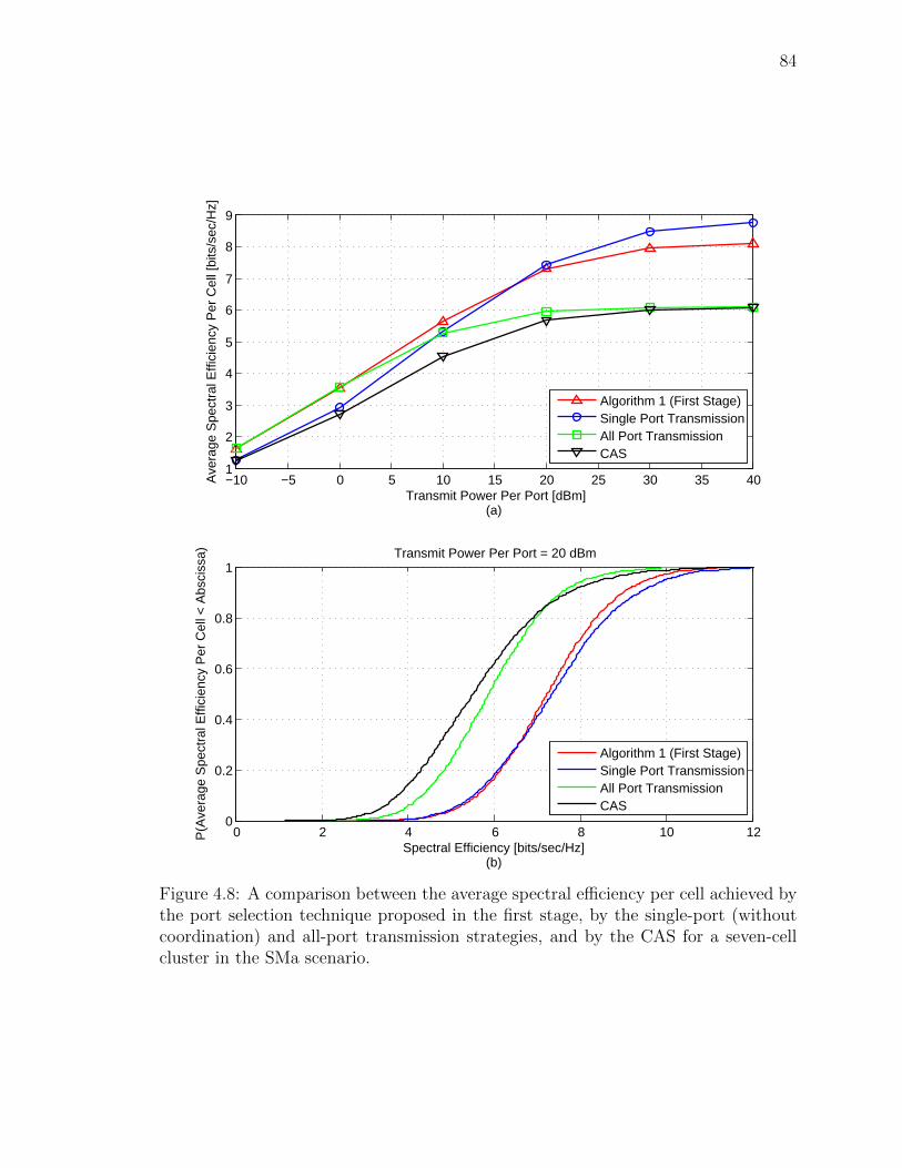
84

−10 −5 0 5 10 15 20 25 30 35 401

2

3

4

5

6

7

8

9


Ave

rage

Spe

ctra

l Effi

cien

cy P

er C

ell [

bits

/sec

/Hz]


0 2 4 6 8 10 120

0.2

0.4

0.6

0.8

1


P(A

vera

ge S

pect

ral E

ffici

ency

Per

Cel

l < A

bsci

ssa) Transmit Power Per Port = 20 dBm


Figure 4.8: A comparison between the average spectral efficiency per cell achieved bythe port selection technique proposed in the first stage, by the single-port (withoutcoordination) and all-port transmission strategies, and by the CAS for a seven-cellcluster in the SMa scenario.

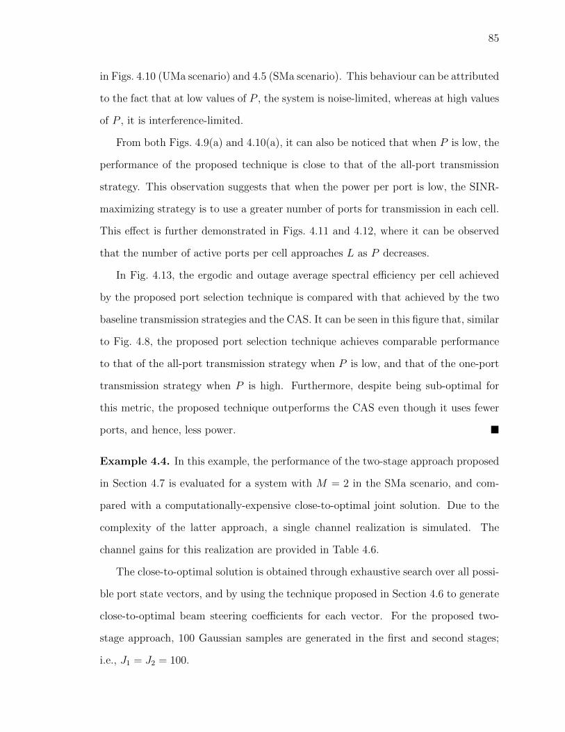
85

in Figs. 4.10 (UMa scenario) and 4.5 (SMa scenario). This behaviour can be attributed

to the fact that at low values of P , the system is noise-limited, whereas at high values

of P , it is interference-limited.

From both Figs. 4.9(a) and 4.10(a), it can also be noticed that when P is low, the

performance of the proposed technique is close to that of the all-port transmission

strategy. This observation suggests that when the power per port is low, the SINR-

maximizing strategy is to use a greater number of ports for transmission in each cell.

This effect is further demonstrated in Figs. 4.11 and 4.12, where it can be observed

that the number of active ports per cell approaches L as P decreases.

In Fig. 4.13, the ergodic and outage average spectral efficiency per cell achieved

by the proposed port selection technique is compared with that achieved by the two

baseline transmission strategies and the CAS. It can be seen in this figure that, similar

to Fig. 4.8, the proposed port selection technique achieves comparable performance

to that of the all-port transmission strategy when P is low, and that of the one-port

transmission strategy when P is high. Furthermore, despite being sub-optimal for

this metric, the proposed technique outperforms the CAS even though it uses fewer

ports, and hence, less power. �

Example 4.4. In this example, the performance of the two-stage approach proposed

in Section 4.7 is evaluated for a system with M = 2 in the SMa scenario, and com-

pared with a computationally-expensive close-to-optimal joint solution. Due to the

complexity of the latter approach, a single channel realization is simulated. The

channel gains for this realization are provided in Table 4.6.

The close-to-optimal solution is obtained through exhaustive search over all possi-

ble port state vectors, and by using the technique proposed in Section 4.6 to generate

close-to-optimal beam steering coefficients for each vector. For the proposed two-

stage approach, 100 Gaussian samples are generated in the first and second stages;

i.e., J1 = J2 = 100.

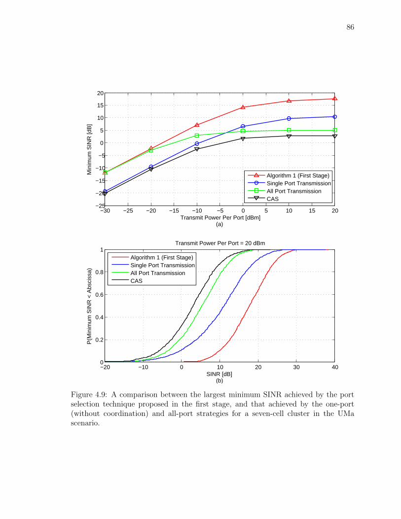
86

−30 −25 −20 −15 −10 −5 0 5 10 15 20−25

−20

−15

−10

−5

0

5

10

15

20


Min

imum

SIN

R [d

B]


−20 −10 0 10 20 30 400

0.2

0.4

0.6

0.8

1

SINR [dB](b)

P(M

inim

um S

INR

< A

bsci

ssa)



Figure 4.9: A comparison between the largest minimum SINR achieved by the portselection technique proposed in the first stage, and that achieved by the one-port(without coordination) and all-port strategies for a seven-cell cluster in the UMascenario.

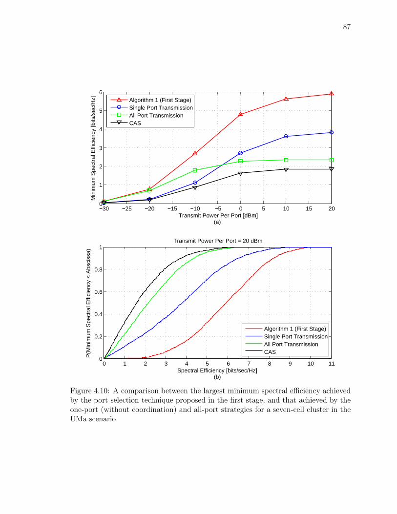
87

−30 −25 −20 −15 −10 −5 0 5 10 15 200

1

2

3

4

5

6


Min

imum

Spe

ctra

l Effi

cien

cy [b

its/s

ec/H

z]


0 1 2 3 4 5 6 7 8 9 10 110

0.2

0.4

0.6

0.8

1


P(M

inim

um S

pect

ral E

ffici

ency

< A

bsci

ssa)



Figure 4.10: A comparison between the largest minimum spectral efficiency achievedby the port selection technique proposed in the first stage, and that achieved by theone-port (without coordination) and all-port strategies for a seven-cell cluster in theUMa scenario.

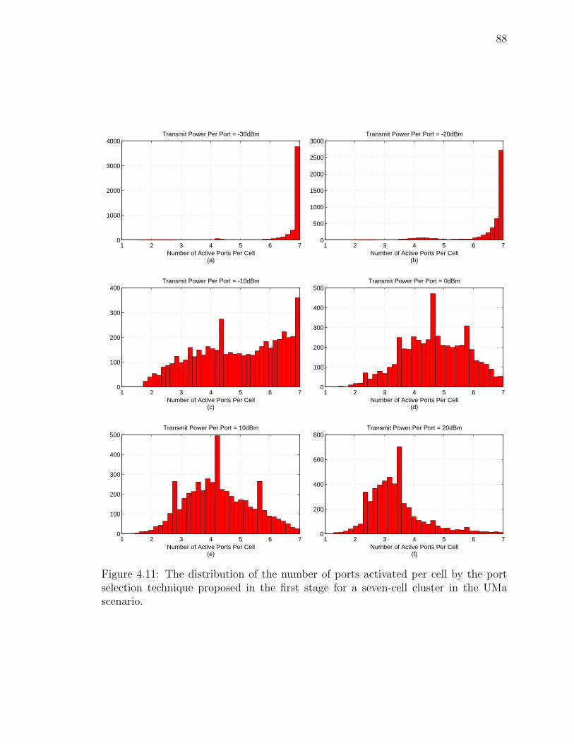
88

1 2 3 4 5 6 70

1000

2000

3000

4000

Number of Active Ports Per Cell(a)


1 2 3 4 5 6 70

500

1000

1500

2000

2500

3000

Number of Active Ports Per Cell(b)


1 2 3 4 5 6 70

100

200

300

400

Number of Active Ports Per Cell(c)


1 2 3 4 5 6 70

100

200

300

400

500

Number of Active Ports Per Cell(d)


1 2 3 4 5 6 70

100

200

300

400

500

Number of Active Ports Per Cell(e)


1 2 3 4 5 6 70

200

400

600

800

Number of Active Ports Per Cell(f)


Figure 4.11: The distribution of the number of ports activated per cell by the portselection technique proposed in the first stage for a seven-cell cluster in the UMascenario.

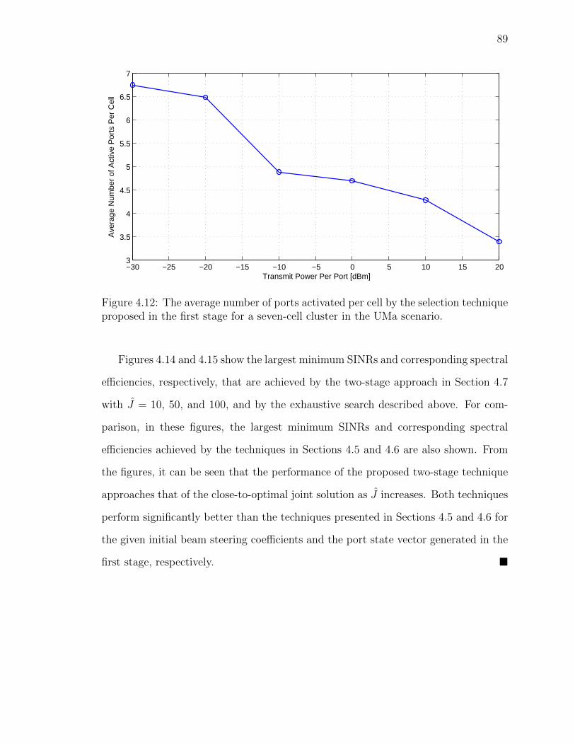
89

−30 −25 −20 −15 −10 −5 0 5 10 15 203

3.5

4

4.5

5

5.5

6

6.5

7


Ave

rage

Num

ber

of A

ctiv

e P

orts

Per

Cel

l

Figure 4.12: The average number of ports activated per cell by the selection techniqueproposed in the first stage for a seven-cell cluster in the UMa scenario.

Figures 4.14 and 4.15 show the largest minimum SINRs and corresponding spectral

efficiencies, respectively, that are achieved by the two-stage approach in Section 4.7

with J = 10, 50, and 100, and by the exhaustive search described above. For com-

parison, in these figures, the largest minimum SINRs and corresponding spectral

efficiencies achieved by the techniques in Sections 4.5 and 4.6 are also shown. From

the figures, it can be seen that the performance of the proposed two-stage technique

approaches that of the close-to-optimal joint solution as J increases. Both techniques

perform significantly better than the techniques presented in Sections 4.5 and 4.6 for

the given initial beam steering coefficients and the port state vector generated in the

first stage, respectively. �

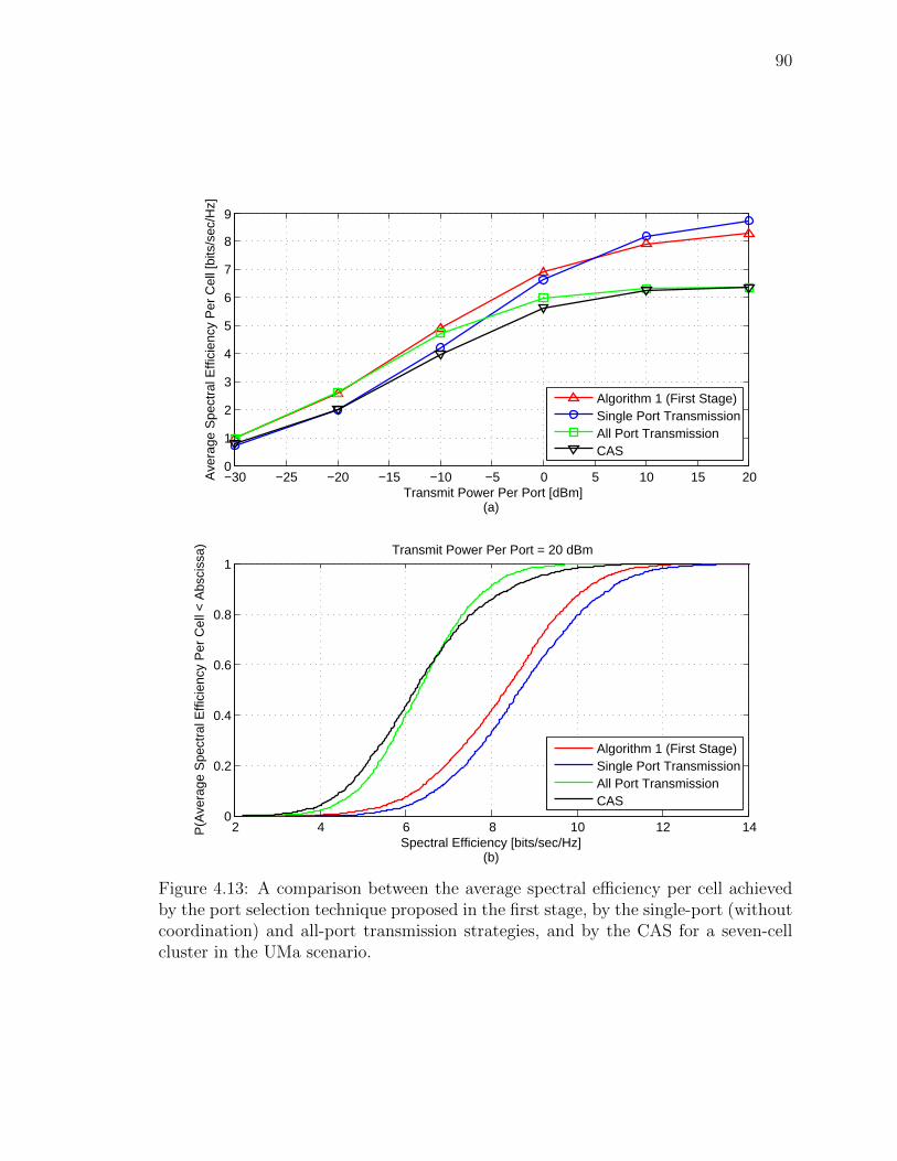
90

−30 −25 −20 −15 −10 −5 0 5 10 15 200

1

2

3

4

5

6

7

8

9


Ave

rage

Spe

ctra

l Effi

cien

cy P

er C

ell [

bits

/sec

/Hz]


2 4 6 8 10 12 140

0.2

0.4

0.6

0.8

1


P(A

vera

ge S

pect

ral E

ffici

ency

Per

Cel

l < A

bsci

ssa) Transmit Power Per Port = 20 dBm


Figure 4.13: A comparison between the average spectral efficiency per cell achievedby the port selection technique proposed in the first stage, by the single-port (withoutcoordination) and all-port transmission strategies, and by the CAS for a seven-cellcluster in the UMa scenario.

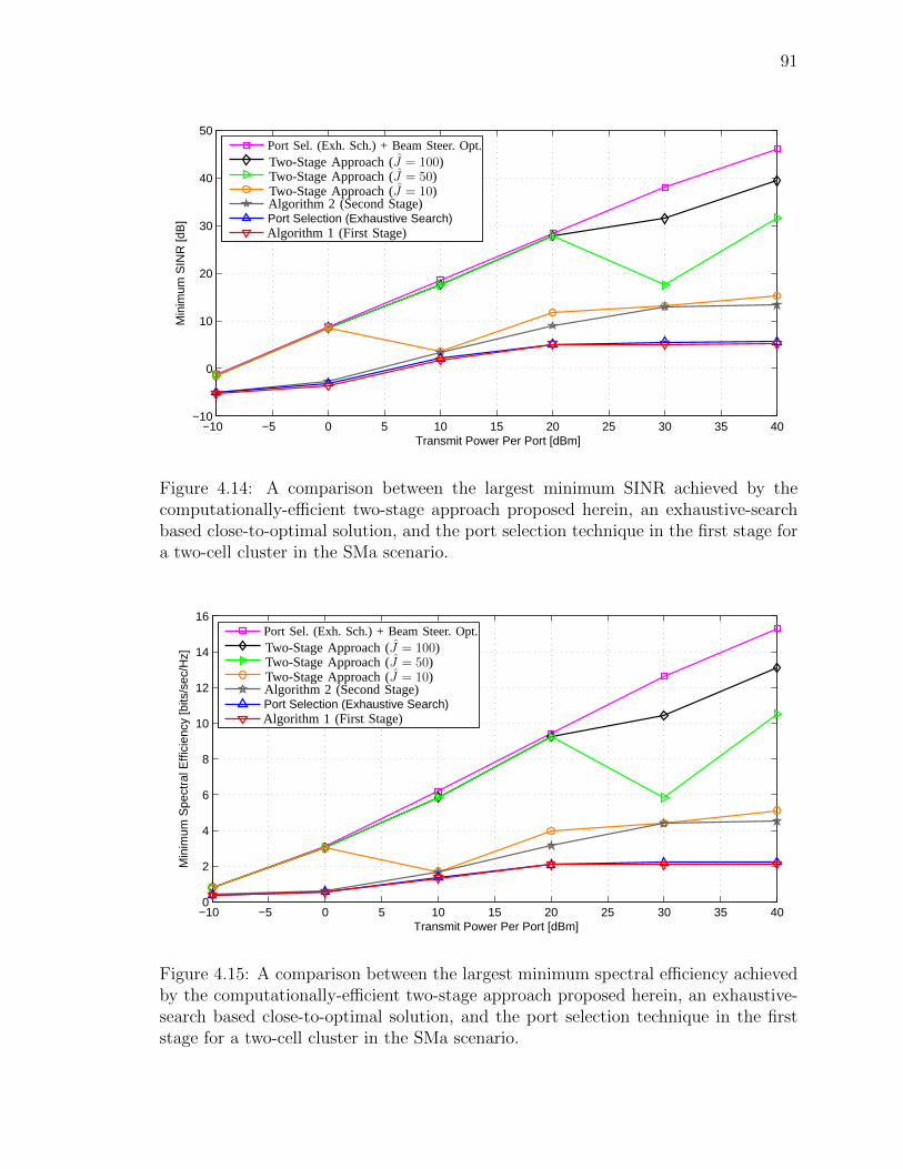
91

1

−10 −5 0 5 10 15 20 25 30 35 40−10

0

10

20

30

40

50


Min

imum

SIN

R [d

B]

Port Selection (Exhaustive Search)

Port Sel. (Exh. Sch.) + Beam Steer. Opt.

Algorithm 2 (Second Stage)Two-Stage Approach (J = 10)Two-Stage Approach (J = 50)Two-Stage Approach (J = 100)

Algorithm 1 (First Stage)

June 29, 2011 DRAFT

Figure 4.14: A comparison between the largest minimum SINR achieved by thecomputationally-efficient two-stage approach proposed herein, an exhaustive-searchbased close-to-optimal solution, and the port selection technique in the first stage fora two-cell cluster in the SMa scenario.

1

−10 −5 0 5 10 15 20 25 30 35 400

2

4

6

8

10

12

14

16


Min

imum

Spe

ctra

l Effi

cien

cy [b

its/s

ec/H

z]

Port Selection (Exhaustive Search)

Port Sel. (Exh. Sch.) + Beam Steer. Opt.

Algorithm 2 (Second Stage)Two-Stage Approach (J = 10)Two-Stage Approach (J = 50)Two-Stage Approach (J = 100)

Algorithm 1 (First Stage)

June 29, 2011 DRAFT

Figure 4.15: A comparison between the largest minimum spectral efficiency achievedby the computationally-efficient two-stage approach proposed herein, an exhaustive-search based close-to-optimal solution, and the port selection technique in the firststage for a two-cell cluster in the SMa scenario.

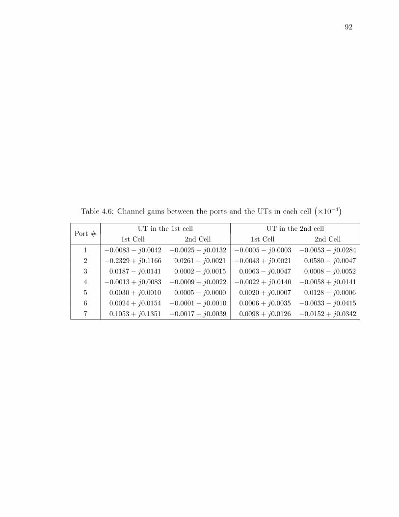
92

Table 4.6: Channel gains between the ports and the UTs in each cell(×10−4

)Port #

UT in the 1st cell UT in the 2nd cell

1st Cell 2nd Cell 1st Cell 2nd Cell

1 −0.0083− j0.0042 −0.0025− j0.0132 −0.0005− j0.0003 −0.0053− j0.0284

2 −0.2329 + j0.1166 0.0261− j0.0021 −0.0043 + j0.0021 0.0580− j0.0047

3 0.0187− j0.0141 0.0002− j0.0015 0.0063− j0.0047 0.0008− j0.0052

4 −0.0013 + j0.0083 −0.0009 + j0.0022 −0.0022 + j0.0140 −0.0058 + j0.0141

5 0.0030 + j0.0010 0.0005− j0.0000 0.0020 + j0.0007 0.0128− j0.0006

6 0.0024 + j0.0154 −0.0001− j0.0010 0.0006 + j0.0035 −0.0033− j0.0415

7 0.1053 + j0.1351 −0.0017 + j0.0039 0.0098 + j0.0126 −0.0152 + j0.0342

Chapter 5

Conclusions and Future Work

5.1 Summary

In this thesis, CoMP transmission schemes are integrated into the DAS architecture.

In the first part of the thesis, two coordinated transmission schemes, namely DAS

ZF-DPC and DAS BD, are developed to serve multiple UTs in a particular RB in

each cell with no intra-cell interference. These schemes are also extended to the

multi-cell processing case, wherein a central processing entity is used to coordinate

the transmission between ports in a cluster of cells, which is subject to a total power

constraint. Simulation is used to demonstrate the performance gains of the DAS

as compared to the CAS, and also those attained by using centralized multi-cell

processing instead of single-cell processing.

In the second part of the thesis, a coordinated multi-cell DAS is considered,

wherein the transmit power of each port is fixed. For this system, the problem

of jointly selecting ports and optimizing their beam steering coefficients to maximize

the minimum SINR of the UTs is considered. This problem is NP-hard. A two-stage

approach is proposed to circumvent this difficulty. In each stage, a sub-problem of

the original joint optimization problem is considered. This problem is also NP-hard,

and the SDR-based Gaussian randomization technique is used to generate close-to-

optimal solutions in polynomial time. Furthermore, the two-stage approach provides

an approximate solution to the joint optimization problem in polynomial time. The

93

94

efficacy of the proposed approach is demonstrated using simulation results. Further-

more, it is shown that proper port selection not only results in improved performance,

but also provides significant power saving opportunities in the cellular network.

5.2 Contributions

• The ZF-DPC and BD schemes are extended to the DAS architecture for intra-

cell and inter-cell interference mitigation.

• The joint selection of ports and their corresponding beam steering coefficients

that maximize the minimum SINR, which is an NP-hard optimization problem,

is tackled using the SDR-based Gaussian randomization technique.

• The proposed two-stage approach generates an approximate solution to the joint

optimization problem in polynomial time, and also provides significant power

savings (by deactivating selected ports) without compromising performance.

5.3 Future Work

The following is a list of potential topics for future research that are related to the

work presented in this thesis. These topics are organized based on relevance to the

two main chapters in the thesis.

• Chapter 3:

– The design of transmission schemes such as DAS ZF-DPC and DAS BD

with a per-port or per-antenna power constraint.

– The development of a distributed multi-cell processing algorithm, which,

although is likely to be sub-optimal as compared to centralized multi-cell

processing, would alleviate the load on the backbone network and loosen

the CSI requirements for each BS.

95

– An investigation of the effect of the number of ports in each cell and their

layout on the performance of the cellular system.

• Chapter 4:

– The development of an algorithm using the SDR-based Gaussian random-

ization technique for the case in which the system is subject to a per-port

power constraint, instead of the transmit power being fixed for each port.

– The development of an algorithm that would allow the BSs to determine

the port states and beam steering coefficients in a distributed manner (to

alleviate the requirement of a central processing entity and the related

signalling overhead).

– The design of a port selection and beam steering optimization technique

that maximizes the aggregate spectral efficiency. The formulation of such

an optimization problem would be fundamentally different than the one

in Chapter 4, and may not be amenable to the SDR-based Gaussian ran-

domization technique employed herein.

– The joint optimization of the port states, beam steering coefficients, and

the UT scheduling for a given frequency-time RB. This is a more general

cross-layer design problem that subsumes the optimization problem consid-

ered in this thesis, and hence, can be expected to yield better performance.

– The development of a port selection and beam steering optimization tech-

nique for serving multiple UTs in each cell in the same RB.

A more general topic of practical importance is the investigation of the perfor-

mance of CoMP schemes and algorithms such as the ones designed in this thesis in the

presence of imperfect CSI. Such imperfections generally arise due to delay resulting

from measurement and feedback to the processing entity and/or errors introduced by

the feedback medium.

Appendices

96

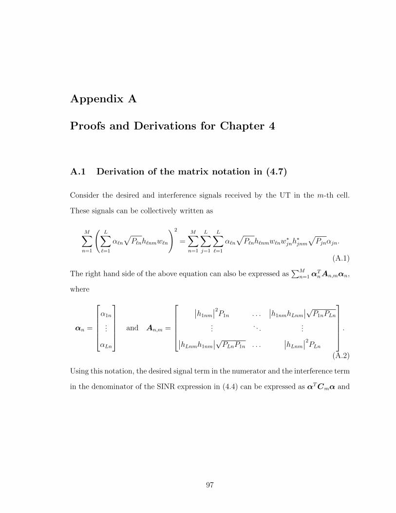
Appendix A

Proofs and Derivations for Chapter 4

A.1 Derivation of the matrix notation in (4.7)

Consider the desired and interference signals received by the UT in the m-th cell.

These signals can be collectively written as

M∑n=1

(L∑`=1

α`n√P`nh`nmw`n

)2

=M∑n=1

L∑j=1

L∑`=1

α`n√P`nh`nmw`nw

∗jnh∗jnm

√Pjnαjn.

(A.1)

The right hand side of the above equation can also be expressed as∑M

n=1αTnAn,mαn,

where

αn =

α1n

...

αLn

and An,m =

∣∣h1nm

∣∣2P1n . . .∣∣h1nmhLnm

∣∣√P1nPLn...

. . ....∣∣hLnmh1nm

∣∣√PLnP1n . . .∣∣hLnm∣∣2PLn

.(A.2)

Using this notation, the desired signal term in the numerator and the interference term

in the denominator of the SINR expression in (4.4) can be expressed as αTCmα and

97

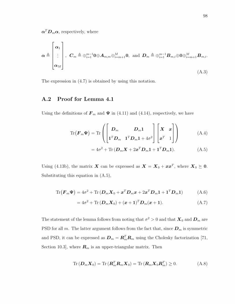
98

αTDmα, respectively, where

α ,

α1

...

αM

, Cm , ⊕m−1i=1 0⊕Am,m⊕Mi=m+10, and Dm , ⊕m−1

i=1 Bm,i⊕0⊕Mi=m+1Bm,i.

(A.3)

The expression in (4.7) is obtained by using this notation.

A.2 Proof for Lemma 4.1

Using the definitions of Fm and Ψ in (4.11) and (4.14), respectively, we have

Tr(FmΨ

)= Tr

Dm Dm1

1TDm 1TDm1 + 4σ2

X x

xT 1

(A.4)

= 4σ2 + Tr (DmX + 2xTDm1 + 1TDm1). (A.5)

Using (4.13b), the matrix X can be expressed as X = X0 + xxT , where X0 � 0.

Substituting this equation in (A.5),

Tr(FmΨ

)= 4σ2 + Tr (DmX0 + xTDmx+ 2xTDm1 + 1TDm1) (A.6)

= 4σ2 + Tr (DmX0) + (x+ 1)TDm(x+ 1). (A.7)

The statement of the lemma follows from noting that σ2 > 0 and thatX0 andDm are

PSD for all m. The latter argument follows from the fact that, since Dm is symmetric

and PSD, it can be expressed as Dm = RTmRm using the Cholesky factorization [71,

Section 10.3], where Rm is an upper-triangular matrix. Then

Tr (DmX0) = Tr (RTmRmX0) = Tr (RmX0R

Tm) ≥ 0. (A.8)

Bibliography

[1] A. Saleh, A. Rustako, and R. Roman, “Distributed antennas for indoor radiocommunications,” IEEE Trans. Commun., vol. 35, no. 12, pp. 1245–1251, Dec.1987.

[2] S. V. Hanly and P. Whiting, “Information-theoretic capacity of multi-receivernetworks,” Telecommunication Systems, vol. 1, no. 1, pp. 1–42, Dec. 1993.

[3] A. Wyner, “Shannon-theoretic approach to a gaussian cellular multiple-accesschannel,” IEEE Trans. Inf. Theory, vol. 40, no. 6, pp. 1713–1727, Nov. 1994.

[4] S. Shamai and B. Zaidel, “Enhancing the cellular downlink capacity via co-processing at the transmitting end,” in Proc. IEEE Veh. Technol. Conf., vol. 3,2001, pp. 1745–1749.

[5] G. Boudreau, J. Panicker, N. Guo, R. Chang, N. Wang, and S. Vrzic, “Inter-ference coordination and cancellation for 4G networks,” IEEE Commun. Mag.,vol. 47, no. 4, pp. 74–81, Apr. 2009.

[6] M. Sawahashi, Y. Kishiyama, A. Morimoto, D. Nishikawa, and M. Tanno, “Coor-dinated multipoint transmission/reception techniques for LTE-advanced,” IEEEWireless Commun. Mag., vol. 17, no. 3, pp. 26–34, Jun. 2010.

[7] A. Ghosh, R. Ratasuk, B. Mondal, N. Mangalvedhe, and T. Thomas, “LTE-Advanced: next-generation wireless broadband technology,” IEEE WirelessCommun. Mag., vol. 17, no. 3, pp. 10–22, Jun. 2010.

[8] 3rd Generation Partnership Project (3GPP), “Overview of 3GPP Release11 V0.0.7,” 3GPP, Tech. Rep., Jun. 2011. [Online]. Available: http://www.3gpp.org/ftp/Information/WORK PLAN/Description Releases/

[9] ——, “Technical Specification Group Radio Access Network; Evolved UniversalTerrestrial Radio Access (E-UTRA); Further advancements for E-UTRAphysical layer aspects,” 3GPP, TR 36.814, Mar. 2010. [Online]. Available:http://www.3gpp.org/ftp/Specs/archive/36 series/36.814/

[10] H. Yanikomeroglu and E. Sousa, “CDMA distributed antenna system for in-door wireless communications,” in Proc. IEEE Int. Conf. on Universal PersonalCommun., vol. 2, Oct. 1993, pp. 990–994.

99

http://www.3gpp.org/ftp/Information/WORK_PLAN/Description_Releases/

http://www.3gpp.org/ftp/Information/WORK_PLAN/Description_Releases/

http://www.3gpp.org/ftp/Specs/archive/36_series/36.814/

100

[11] ——, “CDMA sectorized distributed antenna system,” in Proc. IEEE 5th Int.Symp. Spread Spectrum Techniques and Applications, vol. 3, Sep. 1998, pp. 792–797.

[12] ——, “Power control and number of antenna elements in CDMA distributedantenna systems,” in Proc. IEEE Int. Conf. Commun., vol. 2, Jun. 1998, pp.1040–1045.

[13] A. Obaid and H. Yanikomeroglu, “Reverse-link power control in CDMA dis-tributed antenna systems,” in Proc. IEEE Wireless Commun. Networking Conf.,vol. 2, 2000, pp. 608–612.

[14] H. Yanikomeroglu and E. Sousa, “Antenna gain against interference in cdmamacrodiversity systems,” IEEE Trans. Commun., vol. 50, no. 8, pp. 1356–1371,Aug. 2002.

[15] W. Roh and A. Paulraj, “Outage performance of the distributed antenna systemsin a composite fading channel,” in Proc. IEEE 56th Veh. Technol. Conf., vol. 3,Sep. 2002, pp. 1520–1524.

[16] ——, “MIMO channel capacity for the distributed antenna systems,” in Proc.IEEE 56th Veh. Technol. Conf., vol. 2, Sep. 2002, pp. 706–709.

[17] L. Xiao, L. Dai, H. Zhuang, S. Zhou, and Y. Yao, “Information-theoretic capac-ity analysis in MIMO distributed antenna systems,” in Proc. IEEE 57th Veh.Technol. Conf., vol. 1, Apr. 2003, pp. 779–782.

[18] T. Wang, Y. Wang, K. Sun, and Z. Chen, “On the performance of downlink trans-mission for distributed antenna systems with multi-antenna arrays,” in Proc.IEEE 70th Veh. Technol. Conf., Sep. 2009.

[19] L. Ling, T. Wang, Y. Wang, and C. Shi, “Schemes of power allocation andantenna port selection in OFDM distributed antenna systems,” in Proc. IEEE72nd Veh. Technol. Conf., Sep. 2010.

[20] X.-H. You, D.-M. Wang, B. Sheng, X.-Q. Gao, X.-S. Zhao, and M. Chen, “Coop-erative distributed antenna systems for mobile communications,” IEEE WirelessCommun. Mag., vol. 17, no. 3, pp. 35–43, Jun. 2010.

[21] H. Zhu, S. Karachontzitis, and D. Toumpakaris, “Low-complexity resource al-location and its application to distributed antenna systems,” IEEE WirelessCommun. Mag., vol. 17, no. 3, pp. 44–50, Jun. 2010.

[22] W. Liu, S. Ng, and L. Hanzo, “Multicell cooperation based SVD assisted multi-user MIMO transmission,” in Proc. IEEE Veh. Technol. Conf., Apr. 2009.

[23] H. Dahrouj and W. Yu, “Coordinated beamforming for the multicell multi-antenna wireless system,” IEEE Trans. Wireless Commun., vol. 9, no. 5, pp.1748–1759, May 2010.

101

[24] L. Venturino, N. Prasad, and X. Wang, “Coordinated scheduling and powerallocation in downlink multicell OFDMA networks,” IEEE Trans. Veh. Technol.,vol. 58, no. 6, pp. 2835–2848, Jul. 2009.

[25] H. Huang and M. Trivellato, “Performance of multiuser MIMO and networkcoordination in downlink cellular networks,” in Proc. Int. Symp. on Modelingand Optimization in Mobile, Ad Hoc, and Wireless Networks and Workshops,Apr. 2008, pp. 85–90.

[26] J. Zhang, R. Chen, J. Andrews, A. Ghosh, and R. Heath, “Networked MIMOwith clustered linear precoding,” IEEE Trans. Wireless Commun., vol. 8, no. 4,pp. 1910–1921, Apr. 2009.

[27] E. Bjornson, R. Zakhour, D. Gesbert, and B. Ottersten, “Cooperative multicellprecoding: Rate region characterization and distributed strategies with instan-taneous and statistical CSI,” IEEE Trans. Signal Process., vol. 58, no. 8, pp.4298–4310, 2010.

[28] R. Zhang and L. Hanzo, “Joint and distributed linear precoding for centralisedand decentralised multicell processing,” in Proc. IEEE Veh. Technol. Conf., Sep.2010.

[29] G. Foschini, K. Karakayali, and R. Valenzuela, “Coordinating multiple antennacellular networks to achieve enormous spectral efficiency,” IEE Proc.-Commun.,vol. 153, no. 4, pp. 548–555, Aug. 2006.

[30] S. Jing, D. Tse, J. Soriaga, J. Hou, J. Smee, and R. Padovani, “Multicell downlinkcapacity with coordinated processing,” EURASIP J. Wirel. Commun. Netw., vol.2008, pp. 18:1–18:19, Jan. 2008.

[31] S. Parkvall, E. Dahlman, A. Furuskar, Y. Jading, M. Olsson, S. Wanstedt, andK. Zangi, “LTE-Advanced – evolving LTE towards IMT-Advanced,” in Proc.IEEE Veh. Technol. Conf., Sep. 2008.

[32] Y. Liang, A. Goldsmith, G. Foschini, R. Valenzuela, and D. Chizhik, “Evolutionof base stations in cellular networks: Denser deployment versus coordination,”in Proc. IEEE Int. Conf. Commun., May 2008, pp. 4128–4132.

[33] D. Gesbert, S. Hanly, H. Huang, S. Shamai Shitz, O. Simeone, and W. Yu,“Multi-cell mimo cooperative networks: A new look at interference,” IEEE J.Sel. Areas Commun., vol. 28, no. 9, pp. 1380–1408, Dec. 2010.

[34] M. Karakayali, G. Foschini, and R. Valenzuela, “Network coordination for spec-trally efficient communications in cellular systems,” IEEE Wireless Commun.Mag., vol. 13, no. 4, pp. 56–61, Aug. 2006.

[35] E. Telatar, “Capacity of multi-antenna gaussian channels,” European Transac-tions on Telecommunications, vol. 10, no. 6, pp. 585–595, Nov. 1999.

102

[36] M. Costa, “Writing on dirty paper,” IEEE Trans. Inf. Theory, vol. 29, no. 3, pp.439–441, May 1983.

[37] H. Weingarten, Y. Steinberg, and S. Shamai, “The capacity region of the gaussianmultiple-input multiple-output broadcast channel,” IEEE Trans. Inf. Theory,vol. 52, no. 9, pp. 3936–3964, Sep. 2006.

[38] G. Caire and S. Shamai, “On the achievable throughput of a multiantenna gaus-sian broadcast channel,” IEEE Trans. Inf. Theory, vol. 49, no. 7, pp. 1691–1706,Jul. 2003.

[39] Q. Spencer, A. Swindlehurst, and M. Haardt, “Zero-forcing methods for downlinkspatial multiplexing in multiuser MIMO channels,” IEEE Trans. Signal Process.,vol. 52, no. 2, pp. 461–471, Feb. 2004.

[40] M. Karakayali, G. Foschini, R. Valenzuela, and R. Yates, “On the maximumcommon rate achievable in a coordinated network,” in Proc. IEEE Int. Conf.Commun., vol. 9, Jun. 2006, pp. 4333–4338.

[41] A. Dabbagh and D. Love, “Precoding for multiple antenna gaussian broadcastchannels with successive zero-forcing,” IEEE Trans. Signal Process., vol. 55,no. 7, pp. 3837–3850, Jul. 2007.

[42] M. Maddah-Ali, M. Sadrabadi, and A. Khandani, “Broadcast in MIMO systemsbased on a generalized QR decomposition: Signaling and performance analysis,”IEEE Trans. Inf. Theory, vol. 54, no. 3, pp. 1124–1138, Mar. 2008.

[43] L. Sun and M. McKay, “Eigenmode transmission for the MIMO broadcast chan-nel with semi-orthogonal user selection,” in Proc. IEEE Globecom, Nov. 2009,pp. 2212–2217.

[44] W. Yu and J. Cioffi, “Trellis precoding for the broadcast channel,” in Proc. IEEEGlobecom, vol. 2, 2001, pp. 1344–1348.

[45] R. Etkin, D. Tse, and H. Wang, “Gaussian interference channel capacity towithin one bit,” IEEE Trans. Inf. Theory, vol. 54, no. 12, pp. 5534–5562, Dec.2008.

[46] T. Moon and W. Stirling, Mathematical Methods and Algorithms for Signal Pro-cessing. Upper Saddle River, NJ: Prentice Hall, 2000.

[47] R. Zhang, “Cooperative multi-cell block diagonalization with per-base-stationpower constraints,” IEEE J. Sel. Areas Commun., vol. 28, no. 9, pp. 1435–1445,Dec. 2010.

[48] A. Tolli, M. Codreanu, and M. Juntti, “Linear cooperative multiuser MIMOtransceiver design with per BS power constraints,” in Proc. IEEE Int. Conf.Commun., Jun. 2007, pp. 4991–4996.

103

[49] S. Shi, M. Schubert, N. Vucic, and H. Boche, “MMSE optimization with per-base-station power constraints for network MIMO systems,” in Proc. IEEE Int.Conf. Commun., May 2008, pp. 4106–4110.

[50] Y. Hadisusanto, L. Thiele, and V. Jungnickel, “Distributed base station cooper-ation via block-diagonalization and dual-decomposition,” in Proc. IEEE Globe-com, Dec. 2008.

[51] D. Tse and P. Viswanath, Fundamentals of Wireless Communications. NewYork: Cambridge University Press, 2005.

[52] R. A. Horn and C. R. Johnson, Matrix Analysis. New York, NY: CambridgeUniversity Press, 1985.

[53] J. Park, E. Song, and W. Sung, “Capacity analysis for distributed antenna sys-tems using cooperative transmission schemes in fading channels,” IEEE Trans.Wireless Commun., vol. 8, no. 2, pp. 586–592, Feb. 2009.

[54] W. Choi and J. Andrews, “Downlink performance and capacity of distributedantenna systems in a multicell environment,” IEEE Trans. Wireless Commun.,vol. 6, no. 1, pp. 69–73, Jan. 2007.

[55] X. Wang, P. Zhu, and M. Chen, “Antenna location design for generalized dis-tributed antenna systems,” IEEE Trans. Commun., vol. 13, no. 5, pp. 315–317,May 2009.

[56] T. Zhang, C. Zhang, L. Cuthbert, and Y. Chen, “Energy efficient antenna de-ployment design scheme in distributed antenna systems,” in Proc. IEEE Veh.Technol. Conf., Sep. 2010.

[57] International Telecommunication Union (ITU), “Guidelines for evaluation ofradio interface technologies for IMT-Advanced,” ITU-R, TR M.2135-1, Dec.2009. [Online]. Available: http://www.itu.int/pub/R-REP-M.2135-1-2009

[58] 3rd Generation Partnership Project (3GPP), “Evolved Universal TerrestrialRadio Access (E-UTRA); Radio Frequency (RF) system scenarios,” 3GPP,TR 36.942, Dec. 2010. [Online]. Available: http://www.3gpp.org/ftp/Specs/html-info/36942.htm

[59] L. Vandenberghe and S. Boyd, “Semidefinite programming,” SIAM Rev., vol. 38,no. 1, pp. 49–95, Mar. 1996.

[60] N. Sidiropoulos, T. Davidson, and Z.-Q. Luo, “Transmit beamforming forphysical-layer multicasting,” IEEE Trans. Signal Process., vol. 54, no. 6, pp.2239–2251, 2006.

[61] S. Boyd and L. Vandenberghe, Convex Optimization. Cambridge, U.K.: Cam-bridge Univ. Press, 2004.

http://www.itu.int/pub/R-REP-M.2135-1-2009

http://www.3gpp.org/ftp/Specs/html-info/36942.htm

http://www.3gpp.org/ftp/Specs/html-info/36942.htm

104

[62] Z.-Q. Luo, W.-K. Ma, A.-C. So, Y. Ye, and S. Zhang, “Semidefinite relaxationof quadratic optimization problems,” IEEE Signal Process. Mag., vol. 27, no. 3,pp. 20–34, May 2010.

[63] W.-K. Ma, T. Davidson, K. M. Wong, Z.-Q. Luo, and P.-C. Ching, “Quasi-maximum-likelihood multiuser detection using semi-definite relaxation with ap-plication to synchronous CDMA,” IEEE Trans. Signal Process., vol. 50, no. 4,pp. 912–922, Apr. 2002.

[64] M. Goemans and D. Williamson, “Improved approximation algorithms for max-imum cut and satisfiability problem using semi-definite programming,” J. ACM,vol. 42, no. 6, pp. 1115–1145, Nov. 1995.

[65] E. Karipidis, N. Sidiropoulos, and Z.-Q. Luo, “Quality of service and max-minfair transmit beamforming to multiple cochannel multicast groups,” IEEE Trans.Signal Process., vol. 56, no. 3, pp. 1268–1279, 2008.

[66] T.-H. Chang, Z.-Q. Luo, and C.-Y. Chi, “Approximation bounds for semidefi-nite relaxation of max-min-fair multicast transmit beamforming problem,” IEEETrans. Signal Process., vol. 56, no. 8, pp. 3932–3943, 2008.

[67] G. H. Golub and C. F. van Loan, Matrix Computations, 3rd ed. Baltimore,MD: The Johns Hopkins University Press, 1996.

[68] M. Grant and S. Boyd, “CVX: Matlab software for disciplined convex program-ming, version 1.21,” http://cvxr.com/cvx, Jan. 2011.

[69] Z.-Q. Luo, T. Davidson, G. Giannakis, and K. M. Wong, “Transceiver optimiza-tion for block-based multiple access through ISI channels,” IEEE Trans. SignalProcess., vol. 52, no. 4, pp. 1037–1052, Apr. 2004.

[70] C. Helmberg, F. Rendl, R. J. Vanderbei, and H. Wolkowicz, “An interior-pointmethod for semidefinite programming,” SIAM J. Optim., vol. 6, no. 2, pp. 342–361, 1996.

[71] N. J. Higham, Accuracy and Stability of Numerical Algorithms. Philadelphia,PA: Society for Industrial and Applied Mathematics, 2002.

http://cvxr.com/cvx

Documents

Coordinated Multi-Point Transmission for Interference ... · Coordinated Multi-Point Transmission for Interference Mitigation in ... Talha Ahmad, B.Eng. A ... Coordinated Multi-Point