COORDINATED ORBIT AND ATTITUDE CONTROL OF A … · control of both attitude and position - denoted as coordinated pointing - to ensure that the instrument can operate as expected

COORDINATED ORBIT AND ATTITUDE CONTROL OF A SATELLITE FORMATION INA SATELLITE SIMULATOR TESTBED

S. Wehrmann(1), M. Schlotterer(1)

(1)German Aerospace Center, Institute of Space Systems, Robert-Hooke-Str. 728359 Bremen, Germany, +49-421-244201118, [email protected]

ABSTRACT

This paper presents coordinated orbit and attitude control of a satellite formation on an air bearingtable. The investigated application is the use of the formation as a telescope. The coordination andexact control of the relative position and attitude of the satellites towards each other is a challengingformation flying problem. The satellite relative dynamics are investigated in a hardware-in-the-loopenvironment.

For the validation of the formation control strategy, the Test Environment for Applications of MultipleSpacecraft (TEAMS), a test facility for satellite formations and swarms based on air cushion vehicles,at the Institute of Space Systems of the DLR in Bremen, Germany, is used. Two 5-DoF vehicles arefloating on a granite table with a total experiment area of 5m x 4m. Each vehicle has a thrustersystem, a reaction wheel system and its own onboard computer running the control algorithms.

A laser, attached to the first vehicle, is pointed at a fixed target on the other vehicle to demonstrate thetelescope application. The Clohessy-Wiltshire equations are used for the guidance and feedforwardcontrol of the satellites position in orbit. A second controller is used to calculate the correct pointingangles for the laser and the target. The control law is based on the relative distance and velocityof the two satellites. To achieve the optimal control of the linear system, LQR controllers are usedtogether with feedforward for optimal tracking and to cover the nonlinearities. The characteristics ofthe facility and its devices are introduced, the control algorithms for both satellites are explained andsimulation and HIL test results are presented.

1. INTRODUCTION

In many space applications, modern approaches show a trend of moving away from the classical sin-gle satellite missions, where one satellite includes a complete set of sensors and instruments, towardsfractionated and distributed sensor missions. There multiple satellites are carrying different typesof sensors or different elements of a larger single instrument and act in a formation. Such missionspromise an increase of imaging quality, an increase of service quality and in many cases a decreaseof deployment costs for satellites that can become smaller and less complex due to mission require-ments.

GNC 2017 - S. Wehrmann 1

Satellite formation flying is an enabling technology for this kind of missions. It allows multiplesatellites to cooperate and act in some sense as a single physically larger spacecraft. A potentialapplication for the latter case is forming a telescope from at least two spacecraft. This requires a tightcontrol of both attitude and position - denoted as coordinated pointing - to ensure that the instrumentcan operate as expected. Developing and testing of this control system is a challenging task. For firststeps simulations and later on-ground physical demonstrators can be used.

This paper focuses on the realization of the coordinated attitude and position control for a formationof two satellites using the ground-based Test Environment for Applications of Multiple Spacecraft(TEAMS) within a Master thesis project. In section 2 the test set-up is introduced and special charac-teristics are provided. Section 3 describes the controller structure and general controller design whilein section 4 the guidance laws for attitude and position control are presented. Finally, section 5 showssimulation and experiment results for the coordinated attitude and position control.

2. THE TEST ENVIRONMENT FOR APPLICATIONS OF MULTIPLE SPACECRAFT(TEAMS)

The Test Environment for Applications of Multiple Spacecraft (TEAMS) at the Institute of SpaceSystems of DLR (German Aerospace Center) has the objective to emulate the force- and torque-freedynamics of in-orbit satellites. The satellites are represented by air cushion vehicles floating on agranite table with a total experiment area of 4m by 5m. Two types of air cushion vehicles representthe spacecraft. The two bigger ones called TEAMS 5D have an actuated linear stage to simulatevertical movement and a rotatable upper platform to simulate attitude dynamics (attitude platform).These vehicles can emulate five degrees of freedom. The four smaller vehicles are called TEAMS 3Dand are able to emulate three degrees of freedom. They are mainly used for swarm simulations.Furthermore, the facility is equipped with an infrared tracking system which provides position andattitude of the vehicles at an update rate of 60 Hz.

For the test described in this paper the two TEAMS 5D vehicles are used. The following sectionprovides more information about the vehicle and its properties.

2.1. TEAMS 5 DoF Vehicle

The vehicles used for experiments described in this paper have five degrees of freedom (TEAMS 5D).They consist of two different platforms: The lower platform glides over the granite table on air cush-ions, while the upper platform sits on top of a spherical air bearing, which is connected to the lowerplatform. In the following chapters the upper platform will be named as ”attitude platform” and thelower platform will be named as ”position platform”.

Due to the air cushions and the spherical air bearing, each vehicle has five degrees of freedom (twotranslational and three rotational). Both platforms have two independent storage systems for com-pressed air. The system on the position platform supplies air for the spherical air bearing and theair pads. To generate torques and forces on the vehicle, the storage system on the attitude platform


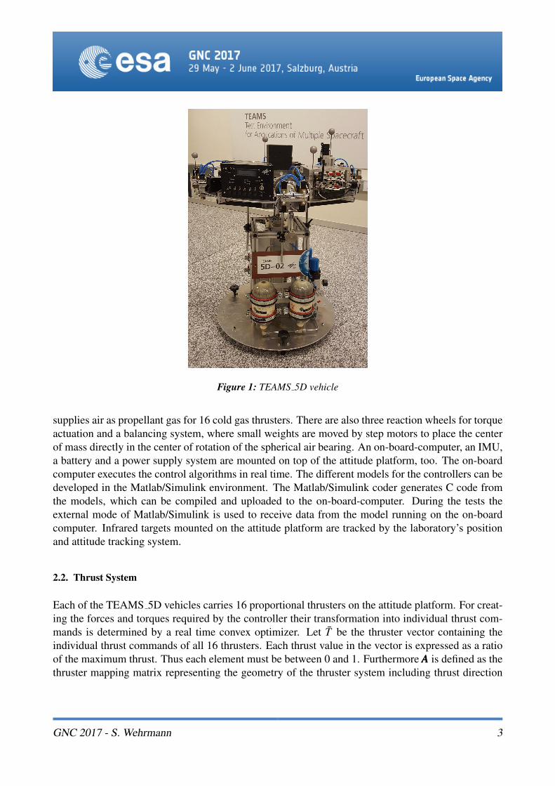
Figure 1: TEAMS 5D vehicle

supplies air as propellant gas for 16 cold gas thrusters. There are also three reaction wheels for torqueactuation and a balancing system, where small weights are moved by step motors to place the centerof mass directly in the center of rotation of the spherical air bearing. An on-board-computer, an IMU,a battery and a power supply system are mounted on top of the attitude platform, too. The on-boardcomputer executes the control algorithms in real time. The different models for the controllers can bedeveloped in the Matlab/Simulink environment. The Matlab/Simulink coder generates C code fromthe models, which can be compiled and uploaded to the on-board-computer. During the tests theexternal mode of Matlab/Simulink is used to receive data from the model running on the on-boardcomputer. Infrared targets mounted on the attitude platform are tracked by the laboratory’s positionand attitude tracking system.

2.2. Thrust System

Each of the TEAMS 5D vehicles carries 16 proportional thrusters on the attitude platform. For creat-ing the forces and torques required by the controller their transformation into individual thrust com-mands is determined by a real time convex optimizer. Let T be the thruster vector containing theindividual thrust commands of all 16 thrusters. Each thrust value in the vector is expressed as a ratioof the maximum thrust. Thus each element must be between 0 and 1. Furthermore AAA is defined as thethruster mapping matrix representing the geometry of the thruster system including thrust direction


and lever arms. The augmented force/torque vector F = [~F ,~T ] can then be computed as

F =AAAT . (1)

The calculation of the thruster vector T for a given F can be expressed as a convex optimizationproblem:

min∑ T +λ‖AAAT − F‖1 (2)

subject to

T ≥ 0 (3)T ≤ 1 (4)

CCCAAAT = 0 (5)

and

CCC =

−F2 F1 0 0 0 0−F3 0 F1 0 0 0

... 0 · · · . . . . . . . . .0 −F3 F2 0 0 00 −F4 0 F2 0 0...

... 0 · · · . . . . . .

(6)

The optimizer searches for the minimum of the sum of all elements of T and thus minimizes the airconsumption of the thruster system. The constraint (5) guarantees that AAAT ∼ F , even if the thrustersystem can not fulfill the commanded force/torque. In that case, the second term of the cost functioncauses AAAT to be as near to F as possible, if λ is large enough, while still minimizing ∑ T . If thethruster system can fullfil the commanded force/torque, the second term of the cost function can beminimized to 0 and the optimizer only minimizes the air consumption.

To solve the optimization problem on the onboard computer and in realtime the code generator forconvex optimization CVXGEN [3] has been used.

2.3. System Model

For designing the control law and for simulating the motion of the vehicles, the system dynamicshave to be modeled. The vehicle on the table can be modeled as a single rigid body in a first orderapproach. If a force (external or generated by the thrusters) affects the vehicle the displacementfollows Newton’s second law:

~F = m ·~a. (7)

The translational motion can be modeled by a double integrator:


[~s~v

]=

[000 111000 000

][~s~v

]+

[~0~a

]. (8)

The rotational movement is caused by torques which act on the vehicle. To describe the relationsbetween the acting torques and the angular velocity of the attitude platform, Euler’s equation of amomentum-biased rigid body can be used:

~T − ~Tw = III~ω +~ω× (III~ω + ~hw), (9)

where ~T is the external torque, ~Tw the commanded reaction wheels’ torque, ~hw is the stored momentumand III is the inertia tensor of the attitude platform.

The differential equation for the quaternion representing the attitude is given by [6]:

q =12

0 ωz −ωy ωx−ωz 0 ωx ωyωy −ωx 0 ωz−ωx −ωy −ωz 0

q (10)

Due to the fact, that the thrusters and the reaction wheels have special characteristics and limitations,they have to be modeled as well. These models include the saturation and the response time of bothactuators.

2.4. Parameter identification

In order to achieve an accurate control a high level of accuracy is required for the determination ofparameters such as the magnitude and direction of thruster forces and the platform’s inertia tensor.Procedures were devised to identify inaccuracies in the manufacturing processes of the platform’scomponents and assembly process. The algorithms for the identification are explained in [2].

For the inertia tensor identification an open-loop manoeuvre is executed on one axis by means ofits reaction wheel; this is followed by a closed-loop return to the initial attitude. The procedure isrepeated on each axis. Using equation (9) the inertia tensor can be calculated.

For identification, the thruster to be identified is set to the maximum thrust for a fixed time while allother thrusters are kept turned off. In this procedure the reaction wheels are used in a closed controlloop (PI velocity regulator) to keep a static attitude under thruster action. In steady state the thrustertorque is equal to the the control torque created by the wheels.


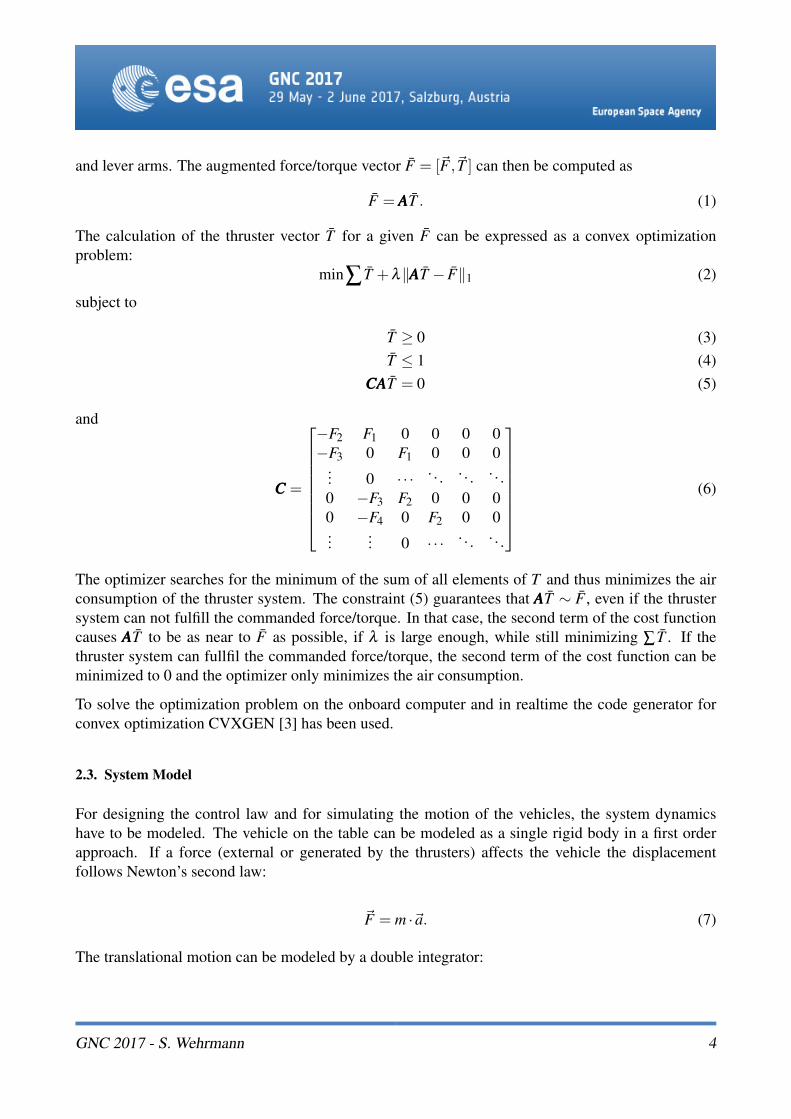
Figure 2: Feedback controller with feedforward [2]

3. CONTROL ALGORITHMS

For position and pointing a control system was designed. The overall structure for both controllers(position and attitude) is a feedback controller together with feedforward as shown in figure 3.

The feedforward control imposes the predicted forces and torques on the plant, which are needed tofollow the trajectory given by the guidance. In an undisturbed ideal case the system then followsthe trajectory provided by the guidance with a zero control error such that the feedback control loophas no effect. Nonlinearities of the system are included in the guidance such that the feedforwardcontrol brings the system in a state which has only small deviations from the required state given bythe guidance. With these small deviation it is possible to design a linear feedback controller.

3.1. Control laws

For the attitude control we use an approach, which was discussed in [6]. The attitude control law isgiven by:

~T = 2kpqe4

qe1qe2qe3

+ kd~ω. (11)

This control law uses directly unit quaternions to calculate an output torque for the system. It has thestructure of a general PD controller, where the error quaternion is used for the proportional feedbackpart, and the error of the angular velocity for the differential part. One disadvantage of this law is,that it is not globally asymptotically stable. A problematic case occurs if the rotation angle of theerror quaternion is exactly π which correlates to qe4 = 0. But due to the feedforward control, it canguaranteed, that there are only control errors much smaller than π . A big advantage is, that there is nounwinding in contrast to other quaternion control laws with better performance but with unwinding.

The structure of a PD controller can also be used to generate a force to control the position:


~f = kp~∆s+ kd ~∆v, (12)

where ~∆s is the position error and ~∆v is the velocity error. In the next step, the controller gains kpand kd for both controllers are calculated. One method to calculate these gains is the linear quadraticregulator (LQR) using the linearized model. For the attitude controller we get:

kp =

√q2

R, kd =

√2III√

q2

R+

q1

R, (13)

where III is the Moment of Inertia in the corresponding axis.

The position controller was designed analog. The only difference is, that in place of rotational inertiaIII, it is necessary to use linear inertia m (mass), albeit different weights were used:

kp =

√q2

R, kd =

√2m√

q2

R+

q1

R. (14)

q1 and q2 are the elements of the LQR matrix Q, which weights the control errors in the optimizationprocess.

Q =

[q1 00 q2

](15)

R is also an element of the LQR algorithm to weight the control inputs.

3.2. Simulation of the controllers

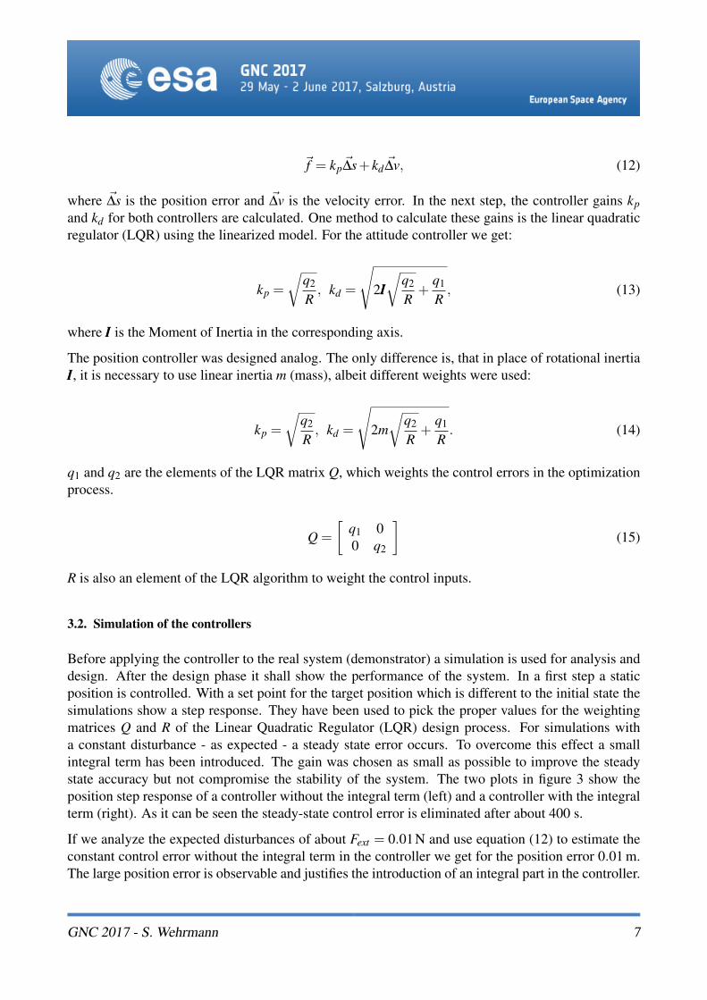
Before applying the controller to the real system (demonstrator) a simulation is used for analysis anddesign. After the design phase it shall show the performance of the system. In a first step a staticposition is controlled. With a set point for the target position which is different to the initial state thesimulations show a step response. They have been used to pick the proper values for the weightingmatrices Q and R of the Linear Quadratic Regulator (LQR) design process. For simulations witha constant disturbance - as expected - a steady state error occurs. To overcome this effect a smallintegral term has been introduced. The gain was chosen as small as possible to improve the steadystate accuracy but not compromise the stability of the system. The two plots in figure 3 show theposition step response of a controller without the integral term (left) and a controller with the integralterm (right). As it can be seen the steady-state control error is eliminated after about 400 s.

If we analyze the expected disturbances of about Fext = 0.01N and use equation (12) to estimate theconstant control error without the integral term in the controller we get for the position error 0.01 m.The large position error is observable and justifies the introduction of an integral part in the controller.


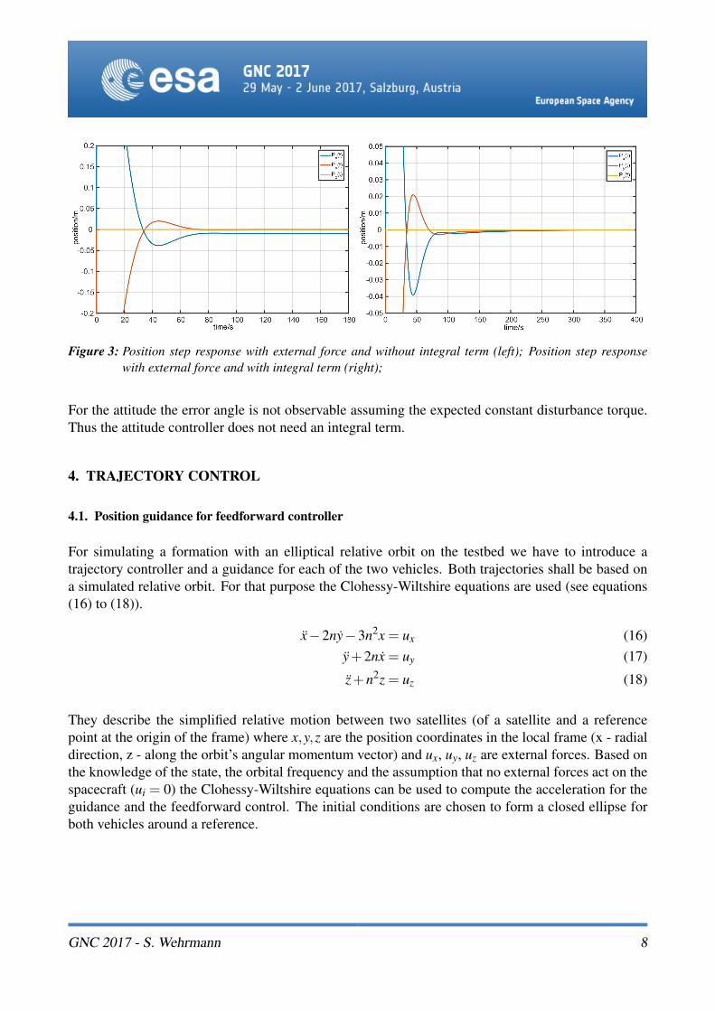
Figure 3: Position step response with external force and without integral term (left); Position step responsewith external force and with integral term (right);

For the attitude the error angle is not observable assuming the expected constant disturbance torque.Thus the attitude controller does not need an integral term.

4. TRAJECTORY CONTROL

4.1. Position guidance for feedforward controller

For simulating a formation with an elliptical relative orbit on the testbed we have to introduce atrajectory controller and a guidance for each of the two vehicles. Both trajectories shall be based ona simulated relative orbit. For that purpose the Clohessy-Wiltshire equations are used (see equations(16) to (18)).

x−2ny−3n2x = ux (16)y+2nx = uy (17)

z+n2z = uz (18)

They describe the simplified relative motion between two satellites (of a satellite and a referencepoint at the origin of the frame) where x,y,z are the position coordinates in the local frame (x - radialdirection, z - along the orbit’s angular momentum vector) and ux, uy, uz are external forces. Based onthe knowledge of the state, the orbital frequency and the assumption that no external forces act on thespacecraft (ui = 0) the Clohessy-Wiltshire equations can be used to compute the acceleration for theguidance and the feedforward control. The initial conditions are chosen to form a closed ellipse forboth vehicles around a reference.


4.2. Attitude guidance for feedforward controller

In order to enable pointing during relative motion a guidance and feedforward function is also neededfor the attitude. For each relative position of the two satellites, the attitude guidance has to calculatea quaternion for both satellites. It is assumed that the relative state of both vehicles is well known atevery time.

In [2] an algorithm to point a laser in a fixed target was presented. This algorithm was picked up andenhanced to point a laser into a moving target on another satellite.

To calculate the correct attitude the closest approach of the laser ray line to the origin ~δ b and thedirection of the laser ray ~ρb have to be determined. Both vectors are shown in figure 4. ~δ b and ~ρb

are mutually orthogonal by construction. The circle in the figure illustrates the attitude platform. ~rbp

presents the direct pointing line between the attitude platform and the target. The algorithm in [2]calculates the attitude ϕ by:

ϕ = arcsin||~δ b||||~rb

p||(19)

which lets the laser pointing directly into the target. In the illustration there is shown only one anglefor better understanding. In the real model the algorithm calculates three angles for the attitude.

Figure 4: Pointing correction of a laser ray to hit a fixed target

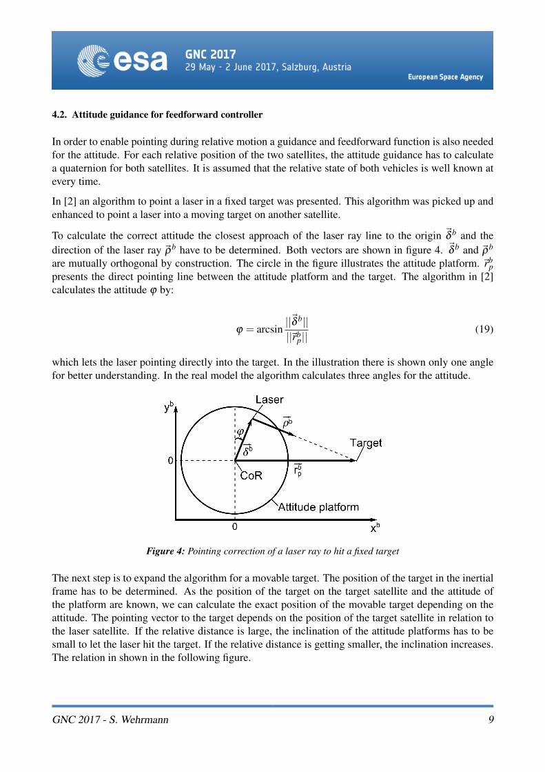
The next step is to expand the algorithm for a movable target. The position of the target in the inertialframe has to be determined. As the position of the target on the target satellite and the attitude ofthe platform are known, we can calculate the exact position of the movable target depending on theattitude. The pointing vector to the target depends on the position of the target satellite in relation tothe laser satellite. If the relative distance is large, the inclination of the attitude platforms has to besmall to let the laser hit the target. If the relative distance is getting smaller, the inclination increases.The relation in shown in the following figure.


Figure 5: Relations between the relative position and the inclination of the platforms

To obtain the angular rate and acceleration for the attitude feedforward controller the first and secondderivative of the attitude matrix R(t) is needed. For that the relative position vector rP(t) = rT (t)−rC(t) can be written as an unitary vector multiplied by a scalar length [2]:

rP(t) = R(t)

Rx(t)Ry(t)Rz(t)

. (20)

The first and second derivatives of the scalar term are:

R(t) = ‖rP(t)‖

R(t) =rPx(t) rPx(t)+ rPy(t) rPy(t)

‖rP(t)‖

R(t) =rPx(t) rPx(t)+ rPy(t) rPy(t)+ r2

Px(t)+ r2Py(t)

‖rP(t)‖−

−(rPx(t) rPx(t)+ rPy(t) rPy(t))

2

‖rP(t)‖3 . (21)

As the vehicles are moving on a horizontal plane, rPz(t) = rPz(t) = 0. The derivatives of the firstelement of the unitary vector are:

Rx(t) =rPx(t)R(t)

Rx(t) =rPx(t)−Rx(t) R(t)

R(t)

Rx(t) =rPx(t)−2Rx(t) R(t)−Rx(t) R(t)

R(t). (22)

The terms for Ry and Rz are similar to Rx. Given the matrices

ΩΩΩ =

0 ωrz −ωry−ωrz 0 ωrxωry −ωrx 0

ΩΩΩ =

0 ωrz −ωry−ωrz 0 ωrxωry −ωrx 0

(23)


the angular rate and angular acceleration can be computed from:

ΩΩΩ = R(t)R(t)T (24)

ΩΩΩ = R(t)R(t)T −(

R(t)R(t)T)2

. (25)

Using Euler’s equation (9) one can also get the torques needed to keep the satellite on the referenceattitude trajectory.

5. RESULTS

The results of the real tests of the controllers on the TEAMS 5D vehicles are compared with thesimulation of a formation flight. Both satellites have the same relative orbit in relation to the referencepoint. But the starting points are on opposite positions on that orbit.

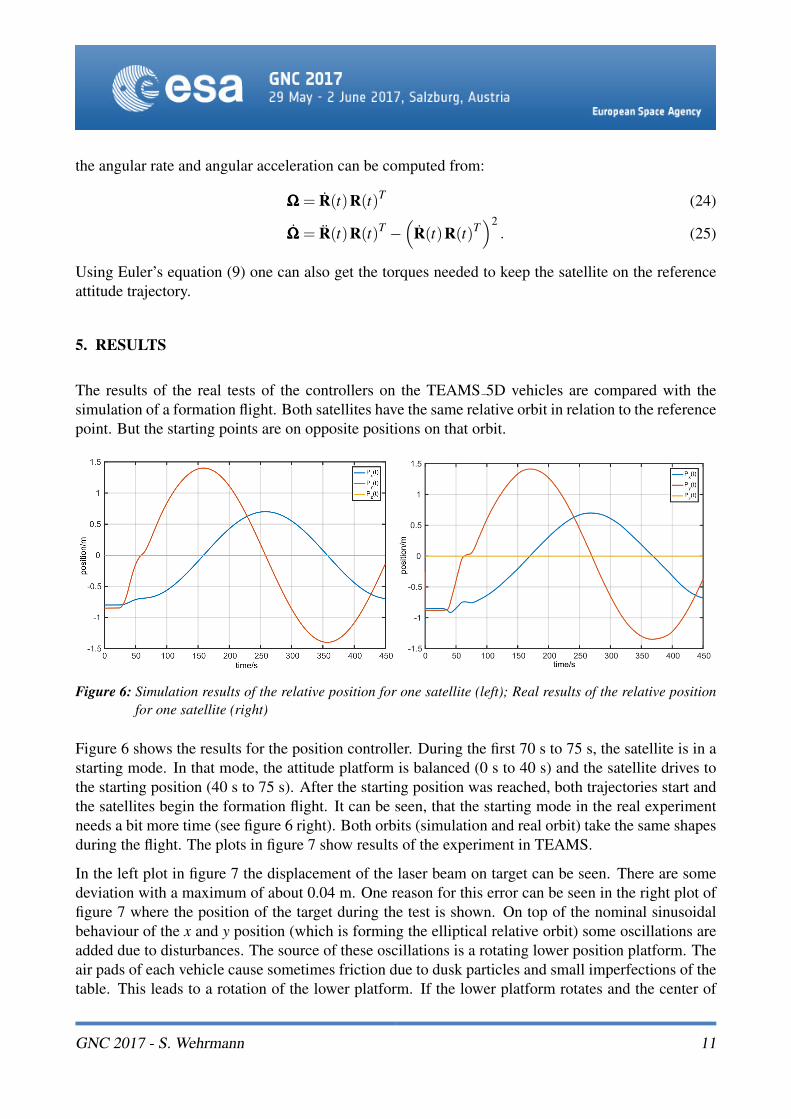
Figure 6: Simulation results of the relative position for one satellite (left); Real results of the relative positionfor one satellite (right)

Figure 6 shows the results for the position controller. During the first 70 s to 75 s, the satellite is in astarting mode. In that mode, the attitude platform is balanced (0 s to 40 s) and the satellite drives tothe starting position (40 s to 75 s). After the starting position was reached, both trajectories start andthe satellites begin the formation flight. It can be seen, that the starting mode in the real experimentneeds a bit more time (see figure 6 right). Both orbits (simulation and real orbit) take the same shapesduring the flight. The plots in figure 7 show results of the experiment in TEAMS.

In the left plot in figure 7 the displacement of the laser beam on target can be seen. There are somedeviation with a maximum of about 0.04 m. One reason for this error can be seen in the right plot offigure 7 where the position of the target during the test is shown. On top of the nominal sinusoidalbehaviour of the x and y position (which is forming the elliptical relative orbit) some oscillations areadded due to disturbances. The source of these oscillations is a rotating lower position platform. Theair pads of each vehicle cause sometimes friction due to dusk particles and small imperfections of thetable. This leads to a rotation of the lower platform. If the lower platform rotates and the center of


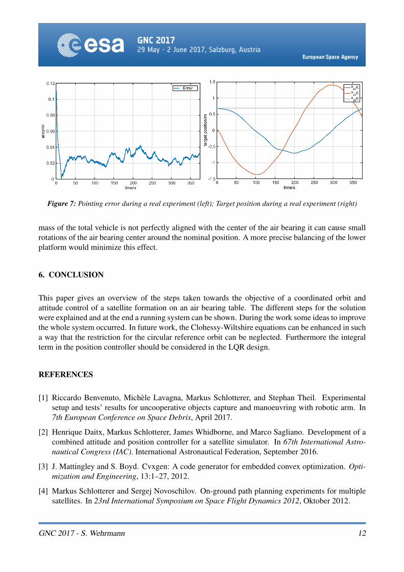
Figure 7: Pointing error during a real experiment (left); Target position during a real experiment (right)

mass of the total vehicle is not perfectly aligned with the center of the air bearing it can cause smallrotations of the air bearing center around the nominal position. A more precise balancing of the lowerplatform would minimize this effect.

6. CONCLUSION

This paper gives an overview of the steps taken towards the objective of a coordinated orbit andattitude control of a satellite formation on an air bearing table. The different steps for the solutionwere explained and at the end a running system can be shown. During the work some ideas to improvethe whole system occurred. In future work, the Clohessy-Wiltshire equations can be enhanced in sucha way that the restriction for the circular reference orbit can be neglected. Furthermore the integralterm in the position controller should be considered in the LQR design.

REFERENCES

[1] Riccardo Benvenuto, Michele Lavagna, Markus Schlotterer, and Stephan Theil. Experimentalsetup and tests’ results for uncooperative objects capture and manoeuvring with robotic arm. In7th European Conference on Space Debris, April 2017.

[2] Henrique Daitx, Markus Schlotterer, James Whidborne, and Marco Sagliano. Development of acombined attitude and position controller for a satellite simulator. In 67th International Astro-nautical Congress (IAC). International Astronautical Federation, September 2016.

[3] J. Mattingley and S. Boyd. Cvxgen: A code generator for embedded convex optimization. Opti-mization and Engineering, 13:1–27, 2012.

[4] Markus Schlotterer and Sergej Novoschilov. On-ground path planning experiments for multiplesatellites. In 23rd International Symposium on Space Flight Dynamics 2012, Oktober 2012.


[5] Markus Schlotterer and Stephan Theil. Testbed for on-orbit servicing and formation flying dy-namics emulation. In AIAA Guidance, Navigation, and Control Conference 2010, August 2010.Paper-Nr: AIAA 2010-8108.

[6] M. J. Sidi. Spacecraft Dynamics and Control. Cambridge University Press, 2006.

[7] S. Vromen, F.J. de Bruijn, and Erwin Mooij. Guidance for autonomous rendezvous and dockingwith envisat using hardware-in-the-loop simulations. In IWSCFF 2015, Juni 2015.

[8] Sebastian Wehrmann. Koordinierte Bahn- und Lageregelung einer Satellitenformation. Master’sthesis, Universitat Bremen, Februar 2017.


Documents

COORDINATED ORBIT AND ATTITUDE CONTROL OF A … · control of both attitude and position - denoted as coordinated pointing - to ensure that the instrument can operate as expected