Embed Size (px)
Citation preview

Coordination of Battery Energy Storage and Power-to-Gas in
Distribution Systems
Master Thesis
Teodor Ognyanov Trifonov
Aalborg University Fredrik Bajers Vej 5, 9220 Aalborg

Title : Coordination of Battery Energy Storage and Power-to-Gas in Distribution
Systems
Project type : Master Thesis
Project period : 01.02.2016 – 10.01.2017
Student : Teodor Ognyanov Trifonov
Student № : 20147778
Supervisor : Jiakun Fang
____________________
Teodor Trifonov
Copies : 3
Pages, total : 77
Appendix : 17
Supplements : 3 CDs
Abstract:
Concerning the rapid development and deployment of Renewable Energy Systems and the need to
store that energy, the target of this thesis is to coordinate between an Energy Storage System and a
Power-to-Gas system in a manner that fully utilizes their complementary advantages . Different
technologies concerning the Energy Storage System and Power-to-Gas systems are investigated, as
well as suitable roles for the Energy Storage System in the electrical grid. Steady-state models are
created of Renewable Energy Systems and of a Power-to-Gas system as well as the respected grids.
Charging strategies are created for the Energy Storage System and production strategies for the
Power-to-Gas system. The size of the Energy Storage System is then observed with regards to the
Renewable Energy Systems and in coordination with the Power-to-Gas system. As a result it is found
that it is possible to store surplus energy from Renewable Energy Systems and it can further on be
stored in the form of methane and that with a proper charging strategy the capacity of the Energy
Storage System can be lowered.

ii
Table of Contents
NOMENCLATURE _________________________________________________________________________________ V
CHAPTER 1 – INTRODUCTION __________________________________________________________________ 1
1.1 Background and motivation _______________________________________________________________ 1
1.2 Background and motivation _______________________________________________________________ 1
1.2 Problem Formulation ________________________________________________________________________ 3
1.3 Project Limitations __________________________________________________________________________ 3
1.4 Methodology ______________________________________________________________________________ 4
1.5 The organization of the thesis _________________________________________________________________ 4
CHAPTER 2 OVERVIEW OF ENERGY STORAGE SYSTEMS ___________________________________ 5
2.1 Role of the energy storage system in the grid ________________________________________________ 5
2.1.1 Bulk Energy Services (BES) _____________________________________________________________ 6
2.1.2 Ancillary Services _____________________________________________________________________ 6
2.1.3 Transmission Infrastructure Services ___________________________________________________ 7
2.1.4 Distribution Infrastructure Services ________________________________________________ 7
2.1.5 Customer Energy Management Services _________________________________________________ 7
2.2 Electrochemical Energy Storage ____________________________________________________________ 9
2.2.1 Lead-Acid Batteries (LA) _______________________________________________________________ 9
2.2.2 Lithium – Ion ________________________________________________________________________ 11
2.2.3 Vanadium Redox _____________________________________________________________________ 12
2.2.4 Compressed Air Energy Storage (CAES) ________________________________________________ 14
2.3 Heat storage _____________________________________________________________________________ 15
2.3.1 Aquifer Thermal Energy Storage (ATES) ________________________________________________ 16
2.3.2 Pit Thermal Energy Storage (PTES) ____________________________________________________ 16
2.4 Power-to-Gas (PtG) ______________________________________________________________________ 17
2.4.1 Alkaline Electrolysis (AE) _____________________________________________________________ 18
2.4.2 Proton Exchange Membrane (PEM) ____________________________________________________ 19
2.4.3 Chemical Methanation ________________________________________________________________ 20
2.5 Technology Comparison __________________________________________________________________ 20
2.6 Conclusions _____________________________________________________________________________ 22
CHAPTER 3 POWER SYSTEM WITH RENEWABLES _________________________________________ 24

iii
3.1 Grid Layout ______________________________________________________________________________ 24
3.2 Electrical Demand _______________________________________________________________________ 24
3.3 Wind Turbine Modelling __________________________________________________________________ 25
3.4 Modelling of Photovoltaic Modules ________________________________________________________ 26
3.5 Renewable Power Generation _____________________________________________________________ 28
3.5.1 Wind Power _________________________________________________________________________ 28
3.5.2 PV power generation _________________________________________________________________ 32
3.6 Conclusion ______________________________________________________________________________ 34
CHAPTER 4 NATURAL GAS SYSTEM SIMULATION __________________________________________ 35
4.1 Supporting Gas Grid ________________________________________________________________________ 35
4.1.1 Natural Gas Grid Parameters _____________________________________________________________ 35
4.1.2 Newton-Raphson method ________________________________________________________________ 36
4.2 Power-to-Gas Simulation ____________________________________________________________________ 38
4.3 Gas Powered Generator Regulation ___________________________________________________________ 39
4.3.1 Kalman Filter9 _________________________________________________________________________ 40
4.3.2 Least Error Squares (LES) _________________________________________________________________ 42
4.4 Gas Grid Simulation and Demand _____________________________________________________________ 42
4.4.1 Leas Error Squares ______________________________________________________________________ 42
4.4.2 Kalman Filter __________________________________________________________________________ 43
4.4.3 Power-to-Gas Gas Demand _______________________________________________________________ 45
4.5 Conclusions _______________________________________________________________________________ 45
CHAPTER 5 ENERGY STORAGE AND ITS OPTIMAL SIZING ________________________________ 46
5.1. Obtaining the Storage System Size ________________________________________________________ 46
5.1.1 Flowchart for obtaining Storage System Capacity _______________________________________ 46
5.1.2 Sizing Storage System with regards to the import/export ________________________________ 46
5.1.3 Sizing Storage System with regards to the price of electrical power _______________________ 47
5.2 Sizing of the ESS__________________________________________________________________________ 49
5.3.1 Sizing Storage System Capacity with Surplus Power Method ______________________________ 49
5.3.2 Sizing Storage System Capacity with Surplus Power and Price Method ____________________ 51
5.4 Sizing ESS with PtG via Surplus Power and Price Method _____________________________________ 53
5.5 Sizing of ESS with Electrochemical Characteristics __________________________________________ 54
5.6 Conclusions _____________________________________________________________________________ 56

iv
CHAPTER 6 CONCLUSION AND FUTURE WORK _____________________________________________ 57
6.1 Conclusions _______________________________________________________________________________ 57
6.2 Future work ______________________________________________________________________________ 57
BIBLIOGRAPHY __________________________________________________________________________________ 58
APPENDIX A ______________________________________________________________________________________ 61
APPENDIX B ______________________________________________________________________________________ 70
Appendix B.1 Wind Turbines _________________________________________________________________ 70
Appendix B.2 Solar Panels____________________________________________________________________ 75

v
Nomenclature
Symbol Description Unit
Indices
m Indices of numerical procedure (iteration step)
Input Parameters – Grid
Residual percentage %
Input Parameters – Photovoltaic
Solar irradiance W/m2 Ambient temperature OC
Input Parameters – Wind Turbine
V Velocity of the wind m/s Air Density kg/m3
Datasheet Parameters – Photovoltaic
Reference solar irradiance W/m2 Maximum power point and Short circuit current at
STC A
Nominal Operation Cell Temperature OC Ambient Nominal Operation Cell Temperature OC Reference ambient temperature OC
Maximum power point and Short circuit voltage at STC
V
Current, Voltage and Power temperature coefficients %/OC
Datasheet Parameters – Wind Turbine
A Swept Area of Blades m2 Efficiency coefficient of the wind turbine
Variables – Grid
Power consumption and generation in the grid MW
Price and price limit of electrical power in the grid Currency/MWh
Residual power in the grid MW
Variables – Energy Storage System
Energy capacity of the ESS MWh
Input/output power at the ESS MW
Power consumed and generated by ESS MW
Efficiency of the ESS %
Variables – Photovoltaic
Coefficient Output current A
Maximum power point and Short circuit current A
Short-circuit current at G A
Power generation photo voltaic MW
Power generation photovoltaic type “n” MW
Open circuit voltage and o pen circuit voltage at G V
Output voltage [V] V
Maximum and Minimum voltage [V] V
Maximum power point voltage [V] V
Number of Photovoltaics from type ”p”
Temperature variation

vi
Voltage variation Modules connected in series Modules connected in parallel
Variables – Wind Turbine
Power generation wind turbine MW
Power generation Wind turbine type “n” MW
Number of WTs from type ”n”
Variables – Power-to-Gas
PtG constant Energy demand MWh
Energy demand for creating 1 mol of CH4 MWh Gas demand from the PtG system mol Gas production PtG
Lower Heating Value Efficiency of the PtG % Energy demand for creating 1 mol of CH4 kJ
Variables & Parameters – Gas Grid
Diameter of pipe between nodes k and l mm Gas demand from the GPG at city ‘v’ m3 Diameter of pipe between nodes k and l km Nodal Gas pressure at both ends of the pipeline kPa Power demand from the GPG at city ‘v’ MW Power consumption at city ‘v’ at moment ‘m’ MW
Gas flow rate measured in section k-l
Gas supply and demand at node k
Resistance coefficient of the pipeline
Efficiency of GPG at city ‘v’ %
Variables & Parameters – Load Prediction
Kalman gain for moment m Prediction error for moment m
Prediction error for moment m-1
Prediction error estimation based on a previous
estimate
Noise of the environment Past data Contro signal
Process noise
Estimated load at moment m.
Estimation for moment m-1 Estimation based on a previous estimate Past observed data at moment m
Regression coefficients Factors affecting the load
Factor matrix
Estimated load Regression coefficient matrix

INTRODUCTION
1
Chapter 1 – Introduction With the increasing development and deployment of renewables, energy system integration draws
broad interest as a way to make energy systems work more efficiently. The purpose of this master thesis
is to propose the concepts and methodology to coordinate the Electrical Energy Storage System (ESS)
and the Power-to-Gas (PtG) system. This chapter contains basic concepts that are needed to understand
why coordination is necessary between an ESS and a PtG.
1.1 Background and motivation
1.2 Background and motivation
In the future of energy supply, Renewable Energy Sources (RES) will have more and more impact on the
power grid. In the past, humanity has mainly depended on fossil-fuel technologies to satisfy its energy
needs [1]. Figure 1 presents the
vision of where the worlds
energy should come from in the
year 2100 according to the
German Advisory Council on
Global Change .It can be seen
that the time to phase out the
fossil-fuel based energy is
closer than ever. With years
passing, humanity will increase
its energy demand and fossil
fuels alone will not be able to
meet that demand. When that
time comes, researchers and
engineers working on different
RES projects will have to make
sure that this demand can be
satisfied only with the use of green technologies. According to Figure 1, this turning point will occur
around the year 2030 and by then a lot of work needs to be done as to how different RES can be more
efficient. This can happen through new technologies ., finding specific optimal geographical locations for
placing RES, or even creating new RES [2].
Denmark has set an ambitious goal where 100% of the energy supply must come from Renewable
Energy Systems (RES). Due to this in the next years, it is expected that more and more of the energy
supply needs of the country will be covered by RES. In the future, most of the energy supply needs will
be covered by wind power parks, both onshore and offshore.
Figure 1 The World Energy Vision 2100 [2]

INTRODUCTION
2
Table 1 Energy policy for Denmark until 2050 [3]
Table 1 presents the Danish government`s energy policy milestones until 2050. Until the year 2020 half
of the electrical supply must be covered by wind power, Recent studies reveal that as of January 2015
total wind power penetration in Denmark has reached 39% [4].
By the year 2030, according to Table 1, coal and oil burners must be phased out from the electrical
system. Coal and oil burners are fundamental to the power system of any country due to their high
power output and mature technology. Due to this most coal and oil burner power plants are used for
covering the bulk of the electrical needs of citizens. One way of dealing with this issue is through an
increase in the offshore wind power parks [5]. In recent years, wind energy has been dramatically
increased.
By the year 2035, both electrical and heat supply must be covered by RES. At the moment heating for
homes comes from cogeneration, also called Combined Heat and Power (CHP), where electrical and
heat energy is produced and supplied to the consumers. For the RES to cover both these sectors, a
certain flexibility must first be achieved. Research into forecasting methods must be increased so that
operators can have better knowledge of how the RES production is going to change in the future.
Certain operational practices must be altered like faster dispatch times, which will reduce regulation
resources need and larger balance authority areas. To cover the fluctuating electrical energy demand,
flexible generation sources can be used, with natural gas combustion turbines and hydropower plants
being amongst the most flexible generators. To help with this flexibility and also fulfill the 2035
milestone, that is presented in Table 1, a PtG system which transforms the electrical energy produced by
RES into chemical energy can be used for covering the heating needs of consumers and the electrical
needs as well. Through the use of such a system surplus electric power can be converted into chemical
and then can be used immediately or stored for future use[6, 7].
The last milestone set by the policy is that by the year 2050, all of the energy supplied must come from
RES and cover the electrical, heat, industry and transport demand.
Reaching these milestones will not be easy, mainly because it is expected of RES to cover the needs of
more than one energy sector, but not impossible. In the past years, much research has been done in
developing new and better technologies than before to increase the RES efficiency. Due to this, the
number of RES installed in the power system will keep increasing. Unfortunately, these RES work thanks
to nature which is often sporadic. As a result of this, a problem is brought to attention connected with
the security of supply. That is the issue with surplus power.
Today
2017 2022 2027 2032 2037 2042 2047
Half of the traditional consumption of electricity is covered by wind power 2020
Coal and Oil burners are phased out from the Danish power plants
2030 The electricity and heat supply is covered by renewable energy 2035
All energy supply - electricity, heat, industry and transport - is covered by renewable energy
2050

INTRODUCTION
3
Power balance issue
In the electrical system, there are stability criteria regarding the power system frequency at all voltage
levels, which state that the frequency must be at 50 Hz ± 0.5 Hz. This criterion requires that the
production and consumption of electrical power must always be equal.
Figure 2 Demand and Supply balance [8]
Higher generation than the load (positive surplus power) will lead to an increase in frequency and
having a lower generation that the load (negative surplus power) will result in a decrease in the
frequency of the grid, as can be seen from Figure 2.This can lead to un-synchronism of generators and
over voltages [9].
However, this obstacle can be overcome by introducing Energy Storage Systems (ESS). An ESS can be
used to supply the power system in times of decreased RES production and can also be used to absorb
surplus power in terms of increased RES production. Also pairing such a system with a PtG system can
ensure that the gas grid, as well as the electrical system, can benefit from surplus power produced by
RES.
1.2 Problem Formulation
Taking into consideration that the creation of large ESS is still very expensive and that the efficiency of
PtG is very low, the purpose of this master project is to coordinate these two technologies in a manner
that fully utilizes their complementary advantages in a grid dominated by RES. The ESS is sized through
varying the RES that is installed in the power system. The PtG will create methane (CH4) which will be
pumped into the gas grid from where it can help gas-burner power plants or the transport sector.
The main objectives of this paper are:
Investigate different ESS technologies available on the market and what services they can
perform.
Investigate different PtG technologies.
Make an assessment of whether a coordination between an ESS and a PtG would be beneficial
1.3 Project Limitations
The following assumptions and limitations are set.
The Electrical Power System, RES, ESS and PtG will all be represented by simplified models in
order for the complexity of the simulations to be reduced.
No power flow models will be created for the LV grid to find the best location for each RES.
No real models will be conducted to back up the results of this paper.

INTRODUCTION
4
The steady-state models for power and gas systems are used. These models are used to size the
ESS for past events. They are utilized as a way of showing what would have happened if there
was an ESS installed in that period of time and will help in determining whether the system will
benefit from such a technology.
1.4 Methodology
The following process will be followed to collect all the necessary information needed for completion of
this thesis.
First, different ESS services will be presented and compared. The one that fits the problem will be
chosen further on. After that different kind of ESS and PtG systems will be presented and compared.
Afterward, a base scenario will be created. This scenario will contain the electrical load data for a set
location, over the course of a month (March 2015), in hourly intervals. The weather data will also be
collected at the same intervals for this area so that different RES like wind turbines and solar panels can
also be modeled.
After choosing the service provided by the ESS, a LV grid will be created, and the ESS will be placed.
After that through varying the number of installed RES and using different charging scenarios, the size of
the ESS will be found.
Further on, a PtG system will be modeled for covering the gas needs of consumers in the gas grid. This
system will be connected with the ESS to find whether or not the size of the ESS can be reduced.
As a final step, the size for a specific ESS technology will be found.
1.5 The organization of the thesis
This thesis is composed of six themed chapters. The first chapter is where the background and
motivation, problem statement and methodology are presented. The second chapter is an introduction
to the ESS and P2G technologies. Also, different roles for the ESS are looked through in an attempt to
find the one that suits the current needs the best. Chapter three presents how different RES systems are
modelled. Chapter four introduces the PtG system and its working process. It also explains how
production strategy for the PtG is formed. In Chapter five different sizing scenarios are formed and the
resultant ESS capacities are analyzed. Chapter six is dedicated to conclusions that are drawn out from
this paper as well as tasks for future work.

OVERVIEW OF ENERGY STORAGE SYSTEMS
5
Chapter 2 Overview of Energy Storage Systems The following chapter deals with the connection between a system with a high number of Renewable
Energy Sources (RES) and Energy Storage Systems (ESS). Different services provided by ESS that can
bring greater stability to the system have been explained. Various types of ESS have been presented and
compared. The purpose of this chapter is to find the best service or combination of services with the
appropriate ESS technology that best fits Denmark`s needs for a future with predominant RES.
2.1 Role of the energy storage system in the grid Balancing the supply and demand in a RES dominant system can be achieved through the use of ESS. The
shape of the request consumption profile can be predicted, and the ESS output can be increased or
decreased very fast depending on the needs. Having a system dominated by RES makes it harder to
maintain a balance between production and consumption due to differences in generation and
consumption profiles. Having higher generation from one RES at a certain time does not usually mean
that there are consumers in need of that power. Using energy storage systems in such cases can
increase the grid flexibility and the grid stability [10].
The applications for ESS can range from Bulk Energy Services (BES) through Ancillary Services (AS),
Transmission / Distribution Infrastructure Services (T/D IS) to Customer Energy Management Services
(CEMS). [11]
Figure 3 ESS Placement in Grid

OVERVIEW OF ENERGY STORAGE SYSTEMS
6
Table 2 shows the different services that can be performed by an ESS, while Figure 3 shows a one line
diagram of the locations where Energy Storage Systems should be installed to be able to carry out their
functions.
Table 2 ESS Services Source[11]
2.1.1 Bulk Energy Services (BES)
1. Electric Energy Time-Shift(EET-S) – The act of purchasing electrical energy in periods with low
price and the selling that energy when the price is higher, Time-Shift can also be used to store
excess power generation and then release the energy when the RES has decreased production
e.g. PV. An Energy Storage System for this size ranges between 1-500 MW a discharge duration
of less than 1 hour and 250+ cycles per minimum yearly. Such a service is used for small PV
panels and wind farms, but given the size range this service can be further expanded, [11]
2. Electric Supply Capacity(ESC) – Such a service can be used to help If there is a need for extra
energy in the grid. This type of service is location-dependent and is used as a way to avoid the
need to buy extra generation capacity from the electricity market. Such a system can be
discharged when there is a lack of RES energy with high load demand and charged when there is
excess RES energy with lowered load demand. The ESS size can be between 1 – 500 MW with a
discharge duration of 2-6 hours and 5 to 100 cycles per year.[11]
3. Forecast Hedging (FH) – A service that is mainly used for renewable systems. With RES it is
never certain that the production will match what the owner has promised. This service can
then be used to supply the difference between what was forecasted and what is produced.[12]
2.1.2 Ancillary Services
1. Regulation – A service used for maintaining the balance between production and demand,
Essentially performing frequency regulation. Having greater demand than supply leads to a
decrease in frequency and having a greater supply than demand leads to an increase in the grid
frequency.[13] Such a system needs to be between 10 and 40 MW with a discharge duration of
15 to 60 minutes and must be able to perform between 250 to 10 000 cycles per year. [11]
2. Voltage Support(VS) – Service that maintains the voltage in a certain window of operation. This
service is used to offset the reactance in the distribution grid. When there is a voltage drop, the
current must increase the power supplied to stay the same. This forces the system to consume
more reactive power which drops the voltage further. Further increase of the current brings to
shutting down of generators and lines due to self-protection purposes.
BES AS TIS DIS CEMS
Electric Energy Time-Shift
Regulation Transmission Upgrade Deferral
Distribution Upgrade Deferral
Power Quality
Electric Supply Capacity
Voltage Support Transmission Congestion Relief
Voltage Support Power Reliability
Forecast Hedging Black Start

OVERVIEW OF ENERGY STORAGE SYSTEMS
7
Such an ESS need to have a size of 1 – 10 MVAR. In this mode, the duration is of no interest
because no real power is needed from the ESS. A general estimation is made that the operation
time should be around 30 minutes.[11]
3. Black Start(BS) – A service that energizes the distribution lines, transmission lines and helps to
bring back power plants after a grid failure. After energizing the lines and contribute to start the
generator, the ESS ramps slowly down as the generator picks up the load. The size should be
between 5 and 50 MW. With work time between 15 and 60 minutes. The yearly cycles for such
a service are usually in the range of 10 – 20 cycles.[11]
2.1.3 Transmission Infrastructure Services
1. Transmission Upgrade Deferral(TUD) – When there is a line that is reaching its maximum
carrying capacity, or a substation in the same predicament, ESS are used to take some of the
load off and postpone the needed upgrade for a couple of years. Usually, such high loads are
reached on specific days for a few hours every year. Such a system is in the 10 – 100 MW range
with a discharge duration between 2-8 hours and between 10-50 cycles per year.[11]
2. Transmission Congestion Relief(TCR) – Transmission Congestion happens when the customer's
energy needs cannot be met. It is said that a system is in such a state while everything is
operating at optimum conditions, but the demand can still not be fulfilled.[14] An ESS can be
used to store energy while the system is operating normally and then discharge the same
energy on peak times. Such a system requires a size between 1-100 MW with discharge duration
of up to 4 hours and between 50 and 100 cycles per year.[11]
2.1.4 Distribution Infrastructure Services
1. Distribution Upgrade Deferral (DUD ) with VS – Serves the same purpose as Transmission
Upgrade Deferral, of postponing system upgrade by a couple of years. Such a system could be
used as voltage support at the same time, by tap changing regulators and switching of
capacitors that follow the variations of the load. Tiny amounts of real power are drawn from
the ESS in this case. A size for an ESS performing such a service is between 500 kW – 10 MW
with a discharge duration of up to 4 hours and between 50 to 100 cycles per year.[11]
2.1.5 Customer Energy Management Services
1. Power Quality(PQ) – Such a service is used to deal with voltage magnitude changes, significant
variations in the nominal frequency [50 Hz], low power factor, power outage up to a few
seconds. All of these factors affect the customer negatively. An ESS thus can be used to deal
with all of these disturbances. Size for such an ESS varies from 100 kW to 10MW. The duration
of discharge for such a system ranges from a few seconds to a quarter of an hour. Yearly cycles
that an ESS has to perform is between 10 and 200 cycles.[11]
2. Power Reliability (PR)– Essentially an Uninterruptable Power System (UPS). If there is a major
problem with the grid, e.g. blackout, such a system deals with the needs of consumers it has
access to. The size of such a system is dependent on how much power and for how long it
must operate. Increasing this so-called “islanded mode” can be done through the use of diesel
generators.[11]

OVERVIEW OF ENERGY STORAGE SYSTEMS
8
Specs Action
Size [MW] Discharge Duration [h] Cycles per year
EET-S 1-500 1 250+
ESC 1-500 2-6 5-100
Regulation 10-40 0.25-1 250-10000
VS 1-10 MVAR 0.5 -
BS 5-50 0.25-1 10-20
TUD 10-100 2-8 10-50
TCR 1-100 4 50-100
DUD 0.5-10 4 50-100
PQ 0.1-10 0.002-0.25 10-200
PR - - -
Table 3 Summary of ESS specifications
The following figure, Figure 4, presents a general classification of Electrical Energy Storage Systems.
These systems are divided into mechanical, thermodynamic, electrochemical and electromagnetic. In
the next sub-chapters, only technologies from the thermodynamic and electrochemical trees will be
revised. Main reason for that is because the other branches do not meet the intended need (help in
dealing with surplus energy ) or Denmark does not have the needed geography for accommodating
these technologies.
Figure 4 Classification of Electrical Energy Storage

OVERVIEW OF ENERGY STORAGE SYSTEMS
9
2.2 Electrochemical Energy Storage With batteries, electrical energy can be converted to chemical energy and held until that energy needs
to be discharged. Most of the battery ESS rely on cells to hold the energy. The size depends on the way
the cells are connected to each other, voltage level is increased by connecting more cells in a series and
capacity is increased by connecting cells in parallel.
There are many different battery technologies on the market. Different kinds of literature and Internet
articles separate these four technologies from the rest – Lead – Acid Batteries as the most mature
technology out there. Lithium-Ion (Li-Ion) as a widely used technology for electronic devices and with
potential for performing utility functions. Vanadium Redox Battery (VRB) as a flow battery is one of
them.
2.2.1 Lead-Acid Batteries (LA)
This technology has been around for a very long time. Since the 1870s when lead-acid batteries were
first used for ancillary services.[1]
Figure 5 Lead-Acid Battery Discharge/Charge Cycles Source[15]
Figure 5 shows how charging and discharging affects the Lead-Acid Battery. As the name suggest, there
is a lead alloy electrodes submerged in an acid electrolyte. From the figure, it can be seen that during
discharge Lead Sulfate forms on the electrodes and as more sulfate forms the lower the voltage of the
battery. Charging is done at a voltage higher than the nominal battery voltage. While discharging the
lead sulfate is reconverted to sulfuric acid and lead. It is also important to mention that some sulfation
remains on the plates, which leads to lowered capacity.[15]
Positive aspects of this technology are its maturity and price. Negative aspects include toxicity, self-
discharge, temperature sensitive and sulfation. Efficiency is at 75-85 % with a lifetime of 3-10 years
depending on the electrode type (different electrodes are used for various applications). Optimal
temperature of the surrounding environment is 25oC. [1]
Voltage Support
Frequency Support
Short Duration
PQ
Long Duration
PQ
Short Duration PQ + Load
Shift+Regulation
Capacity (MWh) 0.003 3 0.006 40 10
Initial costs( $/kW)
PCS 153 165 153 215 173
BOP 50 100 50 100 100
Storage 60 315 60 1.258 315
O&M cost($/kW-year)
Fixed 7.3 16.5 7.3 43.5 17.6
Variable 6.7 7 6.7 6.9 6.5

OVERVIEW OF ENERGY STORAGE SYSTEMS
10
NPV disposal costs($/kW) 1.3 0.8 1.3 1.8 1.4
Total Capital Cost (M$) 2.6 5.8 2.6 15.7 5.9
Table 4 Lead-Acid Cost per Application Source:[1] est.2004$
Maturity Capacity(MWh) Power (MW)
Duration (h)
Efficiency Lifetime (cycles)
Total cost ($/kW)
Cost ($/kWh)
Grid support (ancillary services) and integration of intermittent renewables
Commercial 200 50 4 85-90 2200 1700-1900 425-475
Commercial 250 20-50 5 85-90 4500 4600-4900 920-980
Demonstration 400 100 4 85-90 4500 2700 675
Grid Support and Power Quality
Demonstration 0.25-50 1-100 0.25-1 75-90 >100 000
950-1590 2770-3800
Transmission and Distribution Support
Demonstration 3.2-48 1-12 3.2-4 75-90 4500 2000-4600 625-1150
Table 5 Advanced Lead-Acid Total Costs Source:[1] est.2010$
Table presents different applications for Lead-Acid technologies and the various expenses associated
with these technologies. In the table, PCS stands for Power Conversion System and BOP is Balance of
Plant (infrastructure and facility cost). Fixed stands for labor and parts, the variable, is the cost of
consumables.
( ) (1)
Table presents examples of Advanced Lead-Acid total cost with installed size, capacity, duration
efficiency and lifetime cycles.
Figure 6 Lead-Acid Technology around the world[16]
OVERVIEW OF ENERGY STORAGE SYSTEMS
11
Figure 6 shows the world distribution of the Lead-Acid Battery technology. As it can be expected from
such a mature technology, it is spread all around the world. According to [16] this technology nowadays
is performing in a wide variety of actions where most of these actions are connected with the
integration of RESs to the grid or help regulation. Of course, many sites have been decommissioned or
are about to be changed with Lithium-Ion technology.
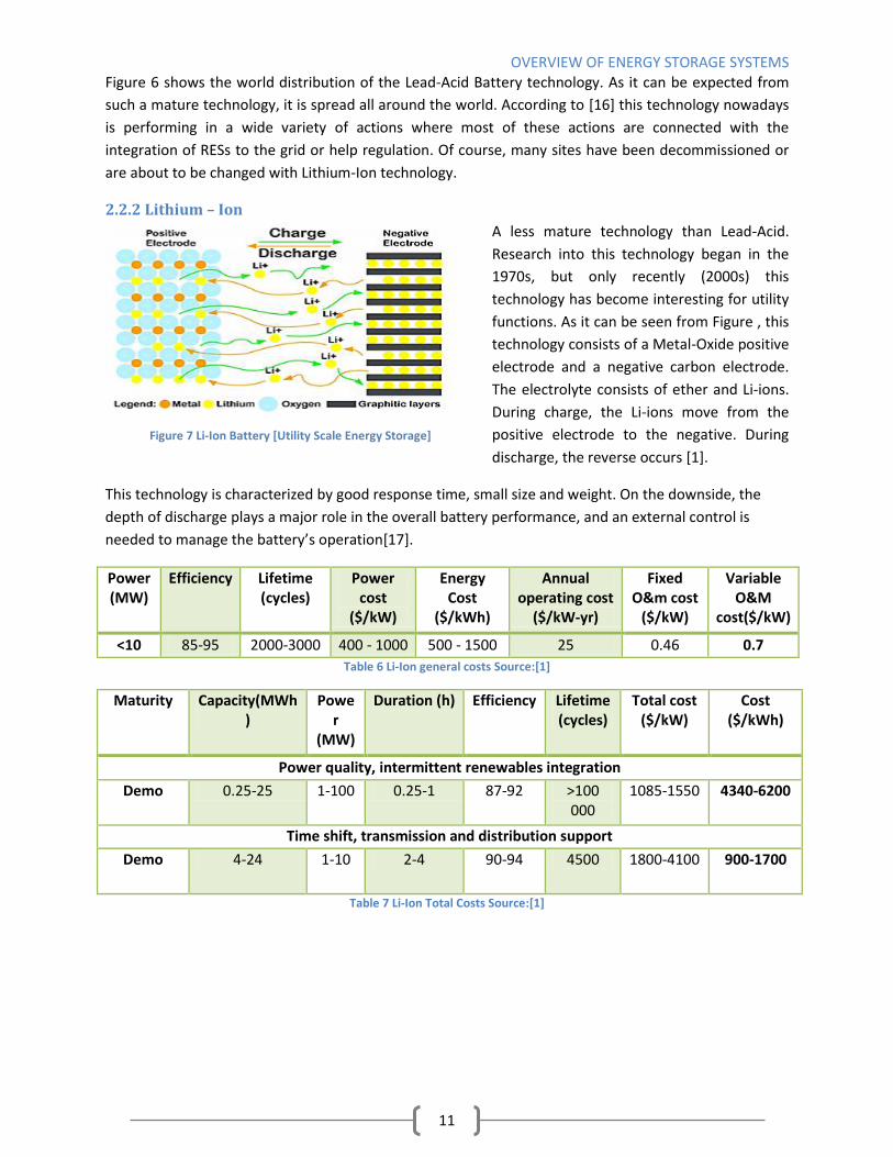
2.2.2 Lithium – Ion
A less mature technology than Lead-Acid.
Research into this technology began in the
1970s, but only recently (2000s) this
technology has become interesting for utility
functions. As it can be seen from Figure , this
technology consists of a Metal-Oxide positive
electrode and a negative carbon electrode.
The electrolyte consists of ether and Li-ions.
During charge, the Li-ions move from the
positive electrode to the negative. During
discharge, the reverse occurs [1].
This technology is characterized by good response time, small size and weight. On the downside, the
depth of discharge plays a major role in the overall battery performance, and an external control is
needed to manage the battery’s operation[17].
Power (MW)
Efficiency Lifetime (cycles)
Power cost
($/kW)
Energy Cost
($/kWh)
Annual operating cost
($/kW-yr)
Fixed O&m cost
($/kW)
Variable O&M
cost($/kW)
<10 85-95 2000-3000 400 - 1000 500 - 1500 25 0.46 0.7
Table 6 Li-Ion general costs Source:[1]
Maturity Capacity(MWh)
Power
(MW)
Duration (h) Efficiency Lifetime (cycles)
Total cost ($/kW)
Cost ($/kWh)
Power quality, intermittent renewables integration
Demo 0.25-25 1-100 0.25-1 87-92 >100 000
1085-1550 4340-6200
Time shift, transmission and distribution support
Demo 4-24 1-10 2-4 90-94 4500 1800-4100 900-1700
Table 7 Li-Ion Total Costs Source:[1]
Figure 7 Li-Ion Battery [Utility Scale Energy Storage]

OVERVIEW OF ENERGY STORAGE SYSTEMS
12
Figure 8 Lithium-Ion technology around the world [16]
Figure 8 presents a world view of the distribution of the Lithium-Ion technology. At first glance, it is
noticed that this technology is more popular than Lead-Acid technology. This can be due to the low self-
discharge rate and the high energy density that this technology presents. The uses of the Lithium-Ion
technology around the world are many. Some of the biggest projects perform frequency regulation
(South Korea,48MW,12MWh), residential energy storage (Germany,42MW,21MWh), RES integration
(Japan,40MW,20MWh)[16]
2.2.3 Vanadium Redox
This battery is a redox flow battery. The
energy and power of such a battery
depend on the volume of the electrolyte
and the area of electrodes respectively.
This technology is as old as the Li-ion
battery technology, with NASA starting
research on it in the 1970s. The working
principle of such a technology is shown in
Figure 9. The battery consists of 2
reservoirs that are filled with electrolyte.
During a discharge cycle, V2+ is oxidized,
and an electron is released. During
charging an electron is accepted by VO2+
and is reduced to VO2+. Also as it can be seen, hydrogen is exchanged in the cell, which is done to keep
the neutrality of the charge.The cross diffusion leads to losses for the cycles unless both sides contain
vanadium, then there are no losses. VRB is characterized by a long cycle life, but a lowered efficiency,
mainly due to the different systems present, like pumps and membranes.[1, 18, 19].
EET-S [10hr]
TIS/DIS+Regultaion Renewables EET-S + Regulation
Short Duration PQ + EET-S+Regulation
Capacity (MWh) 100 90 90 67
Initial costs( $/kW)
PCS 397 466 466 311
Figure 9 Vanadium Redox Battery Source: [Redox Flow Battery]
OVERVIEW OF ENERGY STORAGE SYSTEMS
13
BOP 100 100 100 100
Storage 2125 2125 2125 1417
O&M cost($/kW-year)
Fixed 54.8 56.1 56.1 38.8
Variable 7 - - 1.9
Total Capital Cost (M$) 26.2 26.9 26.9 18.3 Table 8 VRB cost per application Source: [1]
Maturity Capacity(MWh) Power (MW)
Duration (h)
Efficiency Lifetime (cycles)
Total cost
($/kW)
Cost ($/kWh)
Grid support and integration of intermittent renewables
Demo 250 50 5 65-75 >10000 3100-3700
620-740
Time shift, transmission and distribution support.
Demo 4-40 1-10 4 65-70 >10000 3000-3310
750-830
Table 9 VRB cost by Benefit Source :[1]
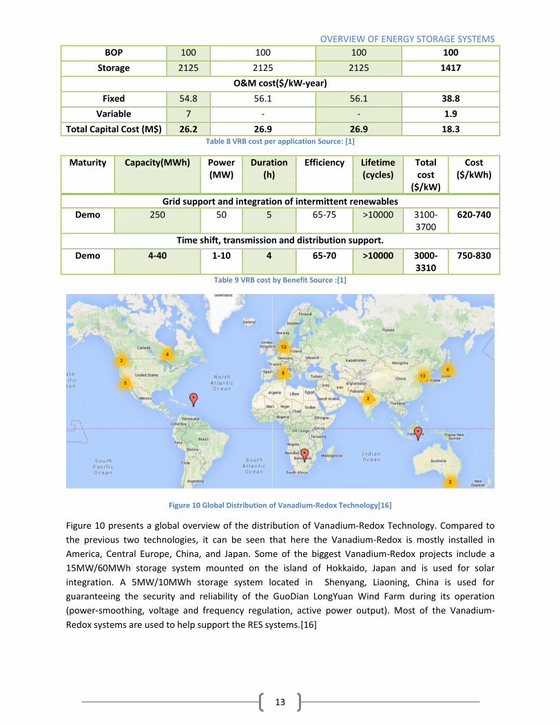
Figure 10 Global Distribution of Vanadium-Redox Technology[16]
Figure 10 presents a global overview of the distribution of Vanadium-Redox Technology. Compared to
the previous two technologies, it can be seen that here the Vanadium-Redox is mostly installed in
America, Central Europe, China, and Japan. Some of the biggest Vanadium-Redox projects include a
15MW/60MWh storage system mounted on the island of Hokkaido, Japan and is used for solar
integration. A 5MW/10MWh storage system located in Shenyang, Liaoning, China is used for
guaranteeing the security and reliability of the GuoDian LongYuan Wind Farm during its operation
(power-smoothing, voltage and frequency regulation, active power output). Most of the Vanadium-
Redox systems are used to help support the RES systems.[16]

OVERVIEW OF ENERGY STORAGE SYSTEMS
14
2.2.4 Compressed Air Energy Storage (CAES)
This storage system uses a cavern, usually salt mines. When charging, an electric motor compresses air
and pumps it into the cavern. When there is a need for the energy, the air is released through an
expansion turbine and combusted to drive a generator. This technology combines many different
devices, and that is why the overall
efficiency is around 40%. Compressing the
air increases the temperature and thus a
cooling system must be installed.To
generate power, the air must be heated,
usually with gas burners, which supply the
larger portion of energy that will be
converted into electrical energy. This
system has a few variations when it comes
to the utilization of the process heat
needed from the combustion turbine.
Diabatic CAES uses only the gas burner and
can also recover the heat from the air after the combustion turbine to heat the air that is about to enter
the combustion turbine. Adiabatic CAES does not use a gas-burner, but the heat that is produced during
the air compression stage. Regarding capacity, such a system is only limited by the size of the cavern,
and if there is not one present, an aboveground CAES can be considered (air is stored in human-made
vessels) though the capacity of such a system is smaller than when using a natural cavern.[1, 20]
Small 10MW CAES Bulk 300 MW CAES
EET-S [3/10 hrs]
Renewable EET-S
Renewable Forecast Hedging
EET-S (10 hr)
Renewable EET-S
Renewable Forecast Hedging
Capacity (MWh)
30/100 100 50 3000 3000 1500
Initial costs( $/kW)
Combustion Turbine
270/270 300 300 270 300 300
BOP 160/160 200 200 170 210 210
Storage 120/400 400 200 10 18 18
O&M cost($/kW-year)
Fixed 19/24.6 31 27 13 23.6 23.6
Variable 4.7/65 21.9 7.9 58.8 13.1 4.5
Total Capital Cost (M$)
5.5/8.3 9 7 135 158.3 158.3
Table 10 CAES Cost per application Source:[7]
Figure 11 CAES Source [1]

OVERVIEW OF ENERGY STORAGE SYSTEMS
15
Type Size Maturity Capacity (MWh)
Power (MW)
Duration (h)
Lifetime (cycles)
Total cost ($/kW)
Cost ($/kWh)
Grid support and integration of intermittent renewables
CT-CAES (underground)
Small Demonstration 1400-3600
180 8 >13 000 960 120
Large Demonstration 1400 - 3600
180 20 >13 000 1150 160
CT-CAES (underground)
Small Commercial 1080 135 8 >13 000 1000 125
Large Commercial 2700 135 20 >10 000 1250 60
Time shift, capacity credit, transmission and distribution support
CAES (aboveground)
Small Demonstration 250 50 5 >10 000 1950-2150
390-430
Table 11 CAES Total Costs Source: [7]
Figure 12 CAES world distribution
From Figure 12 it can be seen that this technology is not as popular as the electro-chemical one. All the
projects that [16] has information for are located in USA and Europe (2 UK, 2 Germany, and 1
Switzerland). This may be due to the low efficiency and geographical conditions. On the other hand
these projects have high Power: Larne, County Antrim, United Kingdom-Generation:330MW/Demand
during compression cycle:220MW, Große Hellmer 1E, Elsfleth, Germany – 321 MW, used to absorb night
power from the nearby nuclear power plant, one of the caverns is reserved for black-start if the nuclear
power plant needs it. Also, two new projects are announced in America with around 300 MW power
output each.[16]
2.3 Heat storage The heat storage technology allows for storing of heat energy for hours, days or even months. This can
be done through the use of different materials that change their phase, chemicals or even simple heat
storage by the heating material. It is also important to mention that heat storage could also mean

OVERVIEW OF ENERGY STORAGE SYSTEMS
16
changing electrical energy into cold energy (mostly used for refrigeration purposes).Around half of the
total energy demand for the entire world is heat energy. In the future, this value is likely to decrease due
to higher energy efficiency. In Demark's future, where RES will have higher influence, heat storage will
play a major role in supply and distribution of thermal energy [21].
2.3.1 Aquifer Thermal Energy Storage (ATES)
This technology uses an underground
reservoir to store hot and cold water. As
you can see from Figure 13, during the
summer, the cold water reservoir is used
to cool down the building, and in return,
the hot water reservoir is used to heat
the building in the winter. There are two
modes, a cyclic mode where the wells are
switched seasonally and a continuous
mode where the wells are not switched.
This technology falls under the sensible
heat storage category.[22]
2.3.2 Pit Thermal Energy Storage (PTES)
Relatively mature energy storage technology is
going back to the 1980s and is mainly used for
seasonal storage. This technology has been
developed by the Danish Technical University
(DTU) and since 1995 various demonstration
storages have been created with pit sizes from
(1 500 m3 to 200 000m3). The largest pit
storage in Denmark is located in Vojens and is
partnered with a 70 000 m2 solar heating plant
and is currently used to cover the heating
needs of 2000 consumers (45% of consumption
is covered). PTES is an excavated area the
inside and bottom of which is covered with a
special material called High-Density
Polyethylene (HDPE).The lid is created from the
same material, and it floats on the surface for
the pit to be always covered while the water
levels are changing. This technology falls under
the category of latent heat storage.Figure 14
is an aerial photograph of the Vojens
PTES.[21, 23, 24]
Figure 4 ATES Source: [15]
Figure 14 PTES Vojens, Denmark Source [ The world's largest solar heating plant to be established in Vojens, Denmark]
Figure 13 Aquifer Thermal Energy Storage [14]

OVERVIEW OF ENERGY STORAGE SYSTEMS
17
Figure 15 Heat Storage distribution around the world [16]
No information could be found in particular locations for PTES and ATES (besides Denmark). Figure 15
presents different kinds of Heat Storage technologies all over the world – most are Chilled Water and Ice
Thermal Storage which are not very useful in a country like Denmark. Also, not applicable to Denmark,
are technologies from the last heat storage category, phase changing materials heat storage.
Technologies that fall under this category are the Molten Salt Storage and Storage of Heat with the use
of a parabolic trough (curved mirror).
From Figure 15, it can be seen that the Heat Storage is very popular around the world, especially in
countries with higher average temperatures and stronger solar radiation throughout the year. Same as
with the CAES, the power of such projects is immense, 280 MW Solar Power Plant that uses parabolic
trough to store heat located in Gila Bend, Arizona, United States, and a 160 MW power plant that
utilizes the Molten Salt Storage technology based in Morocco are amongst the biggest currently
operational Heat Storage systems.[16]
2.4 Power-to-Gas (PtG) This storage technology presents another method of storing electricity in the form of chemical energy.
This subchapter focuses on the production and utilization of hydrogen (H2) and methane (CH4)
Compared to other technologies explained so far, the PtG technology allows for some level of freedom
when it comes to utilizing the gas product. The gas can be used for fueling transport vehicles, central
heating or it can be transformed back into electricity and help by supporting of the electrical grid.
Various PtG systems are either in operation or are still in a Research and Development (R&D )phase but
are expected to appear on the market shortly. A few examples are Alkaline Electrolysis (AE), Proton
Exchange Membrane (PEM), Chemical and Biological Methanation.[20, 25]
Figure 16 shows the role of PtG in the Danish Power Grid[25].

OVERVIEW OF ENERGY STORAGE SYSTEMS
18
Figure 16 Role of Power - to- Gas in the Danish Grid Source:[17]
2.4.1 Alkaline Electrolysis (AE)
As stated in [20], Electrolysis is a chemical decomposition that is originated from the interaction
between electric current and water. This process requires highly pure water with removed minerals and
ions. After that, an electric current is applied with the help of which the deionized water is split into
hydrogen and oxygen.
( ) ( ) ( ) (2) Seen from an electrical point of view, the applied DC is the cause of surplus electrons on the cathode
and not enough electrons on the anode. The process of a positively charged electron passing from the
cathode to the anode , in the water, results in the forming of hydrogen and oxygen. It is also important
to mention that the amount of hydrogen that can be added to the natural grid network depends on the
content of the natural gas and varies from location to location. [20]
Alkaline electrolysis is a mature technology with a low cost and high durability. The anode and cathode
are usually of nickel-plated steel and steel. Hydrogenics do R&D to improve electrolysers for use in the
power-to-gas market.[26]
Table 13 shows the evolution of this technology for years 2011, 2015 and 2020 translated from German
to English.[27]

OVERVIEW OF ENERGY STORAGE SYSTEMS
19
2011 2015 2020
Delivery Pressure (bar) <30 60 60
Power Density (kA/m3 2-4 <6 <8
Cell Voltage (V) 1.8-2.4 1.8-2.2 1.7-2.2
Load Density (W/cm2) 1 1 2
Cell Surface max. (m2) 4 4 4
Efficiency (%) 62-82 67-82 67-82
Maturity Commercial
Power Consumption per stack (kWh/Nm3H2) 4.2-5.9 4.2-5.5 4.1-5.2
Power Consumption per system (kWh/Nm3H2) 4.5-7 4.4-6 4.3-5.7
Production rate H2 per stack (Nm3/hr) 760 1000 1500
Capacity rate per system (kWe) 3800 5000 7000
Lifetimer (hrs) 90000 90000 90000
Table 13 Alkaline Electrolysis technology evolution Source:[16]
2.4.2 Proton Exchange Membrane (PEM)
Another method for performing electrolysis is
through the use of a PEM. Figure 17 shows a
general view of this technology. The liquid is
transported in the cell, which is gas and water
proof. The cell has an anode and a cathode which
are in charge of producing oxygen and hydrogen
respectively. This technology is still in R&D but
already there are plans for significant investments
in the MW scale, which are expected to cost less than alkaline
electrolysis.[20]
Table 14 shows the evolution of this technology for years 2011, 2015 and 2020 translated from German
to English.[27]
2011 2015 2020
Delivery Pressure (bar) <30 60 60
Power Density (kA/m3 6-20 10-25 15-30
Cell Voltage (V) 1.8-2.2 1.7-2 1.6-1.8
Load Density (W/cm2) 4.4 5 5.4
Cell Surface max. (cm2) 300 1300 5000
Efficiency (%) 67-82 74-87 87-93
Maturity R&D - Pre - commercial
Power Consumption per system (kWh/Nm3H2) 4.5-7.5 4.3-5.5 4.1-4.8
Production rate H2 per system (Nm3/hr) 30 120 500
Capacity rate per system (kWe) 150 500 2000
Lifetimer (hrs) 20000 50000 60000
Table 14 PEM technology evolution Source:[16]
Figure 17 PEM Source:[16]

OVERVIEW OF ENERGY STORAGE SYSTEMS
20
2.4.3 Chemical Methanation
Another way of creating Synthetic Natural Gas (SNG) is through the process of methanation. Worldwide
around 80 % of the energy produced comes from fossil fuel plants. This process increases the amount of
CO2 emissions in the air, making it dangerous for the climate of the planet and life of humans. One way
to reduce the carbon dioxide emissions is by combining the H2 gas obtained from electrolysis and the
CO2 gas, as shown in equation (3):
( ) ( ) ( ) ( ) (3) Equation (3) is called the Sabatier reaction. Using (2) and (3) gives us:
( ) ( ) ( ) ( ) (2) Using atmospheric CO2 allows for the methanation plant to be independent of sources of CO2, which
allows building such a plant at a better location. Unfortunately, this process has low efficiency, due to
the low number of particles in the air (around 390 parts per million). Thus according to [28], it is more
efficient to use CO2 from concentrated sources like biomass for example.[20, 29, 30]
Chemical methanation occurs through the utilization of a catalyst, which in most cases is Nickel (Ni) due
to cost reasons. The process works in two temperature ranges:200-550 and 550 -750 OC.[20] Table 15
shows the characteristics of this technology:
Characteristic Value
Process temperature (OC) 200-750
Delivery pressure (bar) 4-80
Max. Production capacity (MWCH4) <500
Maturity Commercial
Catalyst cost (euro/kg in 2013) 250
Lifetime catalyst (h) 24 000
Deployment time (min) <5
Cold start time hours
Methanation efficiency % 70-85
Table 15 Chemical Methanation Characteristic Source: [20, 28, 31]
2.5 Technology Comparison So far, the three types of technologies that are useful in Denmark, given its geographical situation, have
been presented. Most different types of storage are contained in the Electrochemical Energy Storage
section. After that is the Heat Storage and the Gas Energy Storage. These technologies have different
working principles, explained in 2.2, 2.3 and 2.4, and can help the power system in various ways. For
example, the Electrochemical Storage is fast-acting and can help with power regulation, energy time
shift, etc. The Heat and Gas Storage have bigger sizes and a high Technology Readiness Level (TRL),
where high TRL means technology is well-known and mature, and a low TRL implies that technology is
new and often in the phase of basic research [32] . The sensible heat storage also possesses a high TRL
level but cannot be used to help with the problem of surplus power.
In order to tackle the problem with raised in Chapter 1, regarding the security of supply and the surplus
power, a fast acting Storage System is needed. Such a system can be found by examining the population
of the Electrochemical Energy Storage family.

OVERVIEW OF ENERGY STORAGE SYSTEMS
21
0
1000
2000
3000
4000
5000
6000
0 2000 4000 6000 8000
Po
we
r C
ost
- $
/kW
Energy Cost - $/kWh Lead Acid Battery Li-Ion Vanadium Redox CAES
Table 16 Electrical Energy Storage Project Sizes
Lead-Acid Lithium-Ion Vanadium-Redox CAES
Power Energy Power Energy Power Energy Power Energy
[MW] [MWh] [MW] [MWh] [MW] [MWh] [MW] [MWh]
50 200 1-100 0.25-25 50 250 180 1400-3600
20-50 250 1-10 4-24 1-10 4-40 135 1800
100 400
135 2700
1-100 0.25-50
50 250
Table 16 is a comparative table between different storage systems and the energy capacity and power
that was achieved. Figure presents the costs of reaching the needed capacity and electricity ($/kWh and
$/kW respectively). Table is an application matrix presenting the applications. discussed at the
beginning of this chapter and have been compared to different ESS technologies. The “X” marks that
research have been done into a certain technology and “-” means that the no research has been done
into whether that technology can perform certain actions or the technology is just not suitable.
Service that is needed for the future: As it can be seen from Table 17, a lot of R&D has been done by
utilizing storage systems for different applications. Storage systems are helping with frequency
regulation, time shifting, upgrade deferral, etc. It can also be seen that there is a need for research into
the ESC (ESC differs from EET-S with longer discharge duration and fewer cycles per year) and PR. This is
the reason why this master thesis will focus on theoretical research into utilizing the market available
ESS technologies for ESC and PR applications that will help with the surplus power problem incurred
from a large number of RES.
Electrical Energy Storage Systems: From Table 16 and Figure 18 it can be seen that projects with the
“battery type” ESS can achieve a power output between 1 and 100 MW (max.50MW for VRB) and store
energy between 0.25 and 400,25,250 MWh for LA, Li-Ion and VRB respectively. It is also noticeable that
CAES achieves better power (50 – 180 MW) and energy capacity (250-3600 MWh). Using Figure 18, it is
also noticed that the CAES achieves better results in the price per kW and kWh. The projects utilizing
VRB keep their price per kW and kWh steady around 3100-3700 $ per kW and 620-830$ per kWh. The Li-
Application matrix
LA Li-Ion VRB CAES
EET-S - X X X
ESC - - - -
FH - - - X
Regulation X X X -
VS X - X X
BS - - - -
TUD X X X X
TCR X X X X
DUD X X X X
PQ X X X X
PR - - - -
Table 17 Application Matrix Figure 18 Energy-Power Costs

OVERVIEW OF ENERGY STORAGE SYSTEMS
22
Ion battery prices for power and energy capacity depend on the service that it is built for – Power
Quality and Integration of Renewables has a higher energy cost, while Time Shift, Transmission, and
Distribution Support have a higher power cost. The same can be said to be true for the Lead – Acid
batteries, prices for power and energy depend on the service provided. Many factors play a role in the
price of equipment, location country, etc. It is important to mention that these prices are guidelines and
are used to help make the best decision when choosing the ESS that will perform ESC and PR in our
hypothetical case.
Heat Storage Systems: Given the geographical location of Denmark and that by the year 2050 the
government wants 100% of energy production to come from renewable systems, some thought must be
put into how the population will keep their homes warm throughout the year. One way is to store
energy in the form of heat in the summer and use it later in the winter. Another solution is to simply use
electrical heaters in the winter, though that solution presents an increase in the electrical loads and
inevitably large portions of the Distribution network will have to be upgraded. Another solution is to
simply use the existing gas network and use the gas created from the PtG system to supply Gas Powered
Generators with fuel. From there the gas can be used for heating or, given the fast response time of
GPG, for regulation. Even more, the PtG process can be used to supply transportation fuel and can even
be stored, and if need be, it can be used to help the Electric Grid.
Figure 5 P2G distribution around the world[16]
Figure 19 presents the location of PtG projects around the world. As it can be seen, the Power2Gas is
not that popular around the world. Projects are located in Central Europe, and a 2MW project is in the
process of being created in Toronto, Canada. The biggest working project is located in Falkenhagen,
Brandenburg, Germany and is used for renewables capacity firming. This project is a demonstration of
the entire process chain in creating gas from power (wind power, electrolyzer, gas treatment
measurement and injection of hydrogen into the gas grid). The rated power is 1 MW[16].
2.6 Conclusions In this chapter, different functions for electrical energy storage technologies have been presented and
their attributes have been discussed. It was found that electrochemical technologies are used widely
around the world to help the power grid with the integration or RES. It was also found that these

OVERVIEW OF ENERGY STORAGE SYSTEMS
23
techniques, as mature as may they be, still have a quite high price range. It was also found that the
electro-mechanical storage systems are not as widely popular worldwide, but on the other hand, have
significant power outputs. A conclusion can be made that in a 100% RES future a good way to support
the population with reliable electricity and heat is a combination between RES, electrical storage
system, and a PtG system. The gas produced from the PtG can be used in a variety of ways from burning
it in GPG to help with power system regulation, storing it and when the community needs to be heated
it is burned to providing the transport sector with fuel [5, 6].

POWER SYSTEM WITH RENEWABLES
24
Chapter 3 Power System with Renewables The following chapter presents the electrical power system in which the ESS is installed. An explanation
on the simulation methods for different facilities in that power system has also been provided.
3.1 Grid Layout The following sub-chapter gives information about the data used for simulations in this thesis. Figure 20
presents the general idea about the elements in the studied system. From there it is seen that the ESS is
put between the electrical substation (or grid) and the consumers. The power grid presented below
works at 66 kV. The distances between bus bars are shown below, and information on the cable
connecting the bus bars can be found in [33].
Figure 20 Grid layout Source:[34]
The grid in Figure 20 consists of electrical consumers, ESS and RES (Wind Turbines and Photovoltaics ).
The consumption data has been obtained from [35] and is given in 15-minute intervals, which due to
computing difficulties has been averaged into hourly intervals.
To simulate the working process for the RES, weather data matching the time interval of the
consumption data and the geographical location is needed. The wind power generation is determined
by the air density and wind speed. Such data is obtained from [36] in the form of hourly intervals. The
hourly solar irradiance and the temperature has been obtained from [37] to simulation the PV power
output. As a last hourly electricity price data has been obtained from [38].
A program by the name of ESSPC (ESS and PtG Coordinator), has been developed in MATLAB. All the
results and figures that are presented further on have been obtained through it. A short manual for this
program is in Appendix A including the steps needed to calculate other cases.
3.2 Electrical Demand Figure 21 represents the electrical demand by the consumers in the grid. This is the demand profile for
which the storage system is sized, and the RES have to cover.

POWER SYSTEM WITH RENEWABLES
25
Figure 21 Electrical Demand Consumers
The data presented consists of hourly load demands for the month of March 2015. It is seen that the
demand fluctuates from as low as 8 MW to as high as almost 22 MW. The dataset starts from the 1st of
March at 00:00, which means that each upward spike represents daytime demand and every valley is
nighttime demand, which judging by the graph almost does not change in the course of the month. Each
five high spikes are followed by two smaller spikes. Thus it is safe to assume that these seven spikes
form the demand for a week. Also, because the power demand is so high in the daytime during the
week, we can be confident that the area this profile belongs to is either a city center area, or an area
dominated by office buildings and thus support of it is vital to the economy of the city.
3.3 Wind Turbine Modelling In this sub-chapter, the equations for simulating a Wind Turbine are presented. Using [39] the following
formula is used for each datapoint ‘m’:
( )
( )
( ) ( ) ( ) (5)
From the datasheet of the wind
turbine the wind speed to
coefficient of performance of
the wind turbine ( ) is
needed, a curve that shows how
the changes according to
the wind speed. After
interpolating the new the
power output can be calculated.
The wind speed to power curve
from the datasheet is also used
by the program but not in the
calculations rather than for
visualization of what the
manufacturer says the turbine Figure 21 Wind Turbine Simulation

POWER SYSTEM WITH RENEWABLES
26
should produce at different wind speeds. More information on how these curves are represented in
ESSPC can be seen in Appendix A.
3.4 Modelling of Photovoltaic Modules This sub-section presents the mathematical equations used for the PV system [40, 41]:
( )
( )
( )
( (
( ) ( )
( )
⁄ ) ) (6)
Where is the output current and is output voltage and and are coefficients obtained through
the following equations:
( )
( ( )
( )
⁄ ) ( ( )
( )
( )
⁄ ) (7)
( )
(
( ) ( )
⁄ )
( ( )
( )
⁄ )
(8)
In (7) and (8), and depend on the following parameters : Short-circuit current [ ], Open circuit
voltage ( ), Maximum power point voltage [ ] and Maximum power point current[ ].
( )
( ( ) )⁄ ( ( ) ) (9)
( ) ( ( ) ) (10)
( ) (
( ) )⁄ ( ( ) ) (11)
( ) ( ( ) ) (12)
, and are provided from the manufacturer for defined standard test conditions
(STC). is the reference solar irradiance and is the reference ambient temperature ( =1000[W/m2]
and =25OC). is the current temperature coefficient [%/OC] and is the voltage temperature
coefficient [%/OC]. Both are given by the manufacturer. G and T are the solar irradiance and the ambient
temperature respectively, and are the input values for the PV model.
According to [40], to increase the accuracy, (9) and (11) must be changed:
( )
( ( ) ) ( ) (13)
( )
( ( ) ) ( ) (3)
Where is the voltage variation accounted to the solar irradiance
( ) (4)
is the open circuit voltage at G

POWER SYSTEM WITH RENEWABLES
27
( )
( )
[ ( ( )
⁄ ) ⁄ ] (5) Where is the SC current at G
( )
( ( ) )⁄ (6)
Through the use of (6) → (17), the I-V curve for a given technology can be found for different
atmospheric conditions (G and T).
In (2), Vp is the output voltage of the module. The equations up until now are used for simulation of I-V
curves for different PV technologies. In MATLAB by simply varying or , or can be calculated
respectively. In order to obtain the power P , produced by the module ( ), an assumption
must be made regarding .
From [42] the equations for obtaining the voltage of a PV module as a function of the ambient
temperature are presented below.
Power produced from a solar module is dependent on its temperature. With an increase in the
temperature of the solar module, the current produced increases exponentially, while the voltage is
decreased. The higher the temperature of the solar module, the worse the power output is [43].
According to [42], the voltage of a solar module is:
Coldest day of the period
( ) (7)
(8) Hottest day of the period
( ) (20)
( ) (21) where, is the power temperature coefficient [%/OC] , NOCT is the Nominal Operation Cell Temperature and is the ambient temperature STC value for which NOCT is given. All values are given by the manufacturer.
To obtain , ( )
and ( )
need to be obtained as a function of ( ).
( )
( )
( )
(22)
After obtaining , can be found and after that the, power produced by the module is found:
( )
( )
( )
(23)

POWER SYSTEM WITH RENEWABLES
28
Figure 22 Model framework of PV module
Figure 22 presents the steps and accompanying equations that are performed to simulate the power
output of the PV module. First and are calculate via (9),(10),(11) and (12). After that
those values are passed over to be calculated via (7) and (8). As it was mentioned before, the accuracy
of (9) and (11) can be increased by changing them. That is done through first finding dV via (15),(16) and
(13)and afterwards calculating (13) and (14) which are the transformed (9) and (11). and are
calculated with the use of (7) and (8) again. The next step that is taken is to calculate using
(14),(15),(16) and (17). is calculated with the use of (6) and then both and are passed on to (23)
which calculates the power outputted by the module for the particular data point “m”. These actions
are repeated for every data point of Solar Irradiance and Ambient Temperature that is procured.
3.5 Renewable Power Generation As explained before, the power system uses two different RES, wind turbines, and photovoltaics. The
purpose of this sub-section is to present information on the RES used and simulation results.
3.5.1 Wind Power
Three different wind turbines have been considered for installation in the power system. The Bonus
2300/82.4, NEG Micon 2000/72 and the Nordex N90/2300. Further on in this work, these machines are
named Wind Turbines type 1, 2 and 3 respectively.
Error! Reference source not found. presents the power production profile for the first type of turbine in
he timeframe of interest, the month of March 2015. Detailed information on how the data is collected
and used can be found in Appendix A.

POWER SYSTEM WITH RENEWABLES
29
The left y-axis represents the power produced from Wind Turbine type 1 in [kW] and the right axis gives
us information on the wind speed, in [m/s]. Error! Reference source not found. presents how the power
roduction changes with regards to the wind speed. It can be noticed that the wind speed is mostly in the
4[m/s] to 9 [m/s] window. It can also be seen that the turbine power production fluctuates and
produces around 250 [kW] low to as high as 1400 [kW]. To understand the reason for this behavior,
Figure 24 and Figure 25 are needed.
Figure 24 is the efficiency curve of the Wind Turbine Type 1. It is noticed that the effectiveness of the
turbine reaches its peak when working with the wind around 10 – 11 [m/s]. With the information
Figure 25 Wind Turbine type 1 Efficiency Curve Figure 24 Wind Turbine type 1 Power Curve
Figure 23 Wind Turbine type 1 power production with wind speed

POWER SYSTEM WITH RENEWABLES
30
obtained from Figure 23, it can be judged that the turbine rarely operates in its most efficient state.
Figure , on the other hand, contains information on the power curve, provided from [44]. Here it can be
seen that the power production reaches its peak around a wind speed of 15 [m/s] and maintains that
production until it reaches its cut-off speed at 25 [m/s]. Unfortunately, due to the poor wind conditions
in the zone for the observed timeframe, the turbine can at the very best produce around 60% of its
capacity. These factors lead to the poor performance of this technology and will have an effect in sizing
the storage system.
Figure 26 shows the production profile of the turbine without the wind speed.
Figure 26 Wind Turbine type 1 power production
After simulation the first turbine technology, the other two technologies are also simulated. With the
help of Figure , the performance can be compared. Here the power production is shown in MW
and will be used in MATPOWER in that unit while performing the power flows.
POWER SYSTEM WITH RENEWABLES
31
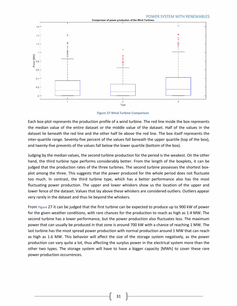
Figure 27 Wind Turbine Comparison
Each box-plot represents the production profile of a wind turbine. The red line inside the box represents
the median value of the entire dataset or the middle value of the dataset. Half of the values in the
dataset lie beneath the red line and the other half lie above the red line. The box itself represents the
inter-quartile range. Seventy-five percent of the values fall beneath the upper quartile (top of the box),
and twenty-five prevents of the values fall below the lower quartile (bottom of the box).
Judging by the median values, the second turbine production for the period is the weakest. On the other
hand, the third turbine type performs considerably better. From the length of the boxplots, it can be
judged that the production rates of the three turbines. The second turbine possesses the shortest box-
plot among the three. This suggests that the power produced for the whole period does not fluctuate
too much. In contrast, the third turbine type, which has a better performance also has the most
fluctuating power production. The upper and lower whiskers show us the location of the upper and
lower fence of the dataset. Values that lay above these whiskers are considered outliers. Outliers appear
very rarely in the dataset and thus lie beyond the whiskers.
From Figure 27 it can be judged that the first turbine can be expected to produce up to 900 kW of power
for the given weather conditions, with rare chances for the production to reach as high as 1.4 MW. The
second turbine has a lower performance, but the power production also fluctuates less. The maximum
power that can usually be produced in that zone is around 700 kW with a chance of reaching 1 MW. The
last turbine has the most spread power production with normal production around 1 MW that can reach
as high as 1.6 MW. This behavior will affect the size of the storage system negatively, as the power
production can vary quite a lot, thus affecting the surplus power in the electrical system more than the
other two types. The storage system will have to have a bigger capacity [MWh] to cover these rare
power production occurrences.

POWER SYSTEM WITH RENEWABLES
32
3.5.2 PV power generation
As with the wind turbines, three different solar module technologies are used in this work. Dymond
CS6X-320 P-FG, TSM-245 PC/PA05 and SW 285 Mono. They are again further on referred to as type 1, 2
and 3. The datasheets for this photovoltaics have been obtained from the sites of their respective
manufacturers[45-47] and can be seen in Appendix B. The power production of every photovoltaic can
be explained using an IV curve such as the one shown in Figure 28. As explained before, to simulate the
power production of a solar module, information is needed about the solar irradiance [W/m2] and
temperature[OC]. The solar irradiance affects the current of the Photovoltaic, and the temperature
affects the voltage. Figure 28 is an
example case using 826 [W/m2] and 28
[OC] as input information. The blue line
corresponds to the current of that
module at that solar irradiance, and the
red line corresponds to the power that
can be produced in [W]. The power
production is found through tracing the x-
axis voltage, found using Eq.(18-21), to
the red power curve. This process is
repeated for every hour of the period,
and thus we obtain the power production
for that hour. Unfortunately, the power
produced by a single solar module is not
that much, and the search for an optimal
number of solar modules will take a very long time to simulate using ESSPC. To decrease the
computation time, the modules are connected in solar arrays. The reason for this is that in an array, by
connecting modules in series the voltage of the system can be increased, and by connecting modules in
parallel the current of the system can increase [40, 41]. Following this rule, Eq. (11) & (12) can be
changed, so they obtain the following forms:
( )
( ( ( ) )⁄ ( ( ) ) ) (24)
( )
( ( ( ) )) (25)
where, and is the number of modules connected in parallel and in series respectively.
Using this information, a solar array can be created with far greater power production capabilities than
one module. The power production profile of such an array, consisting only of modules of type 1, can be
seen in Figure .
Figure 28 Current-Voltage Curve Solar module type 1 – 826 [W/m
2] 28 [
OC].

POWER SYSTEM WITH RENEWABLES
33
Figure 29 Solar Array power production type 1
To achieve this power production profile, 35 module must be connected in parallel and another 18 in
series. The resultant array can at the very best produce around 110 [kW]. Each spike represents
daytime, while each valley represents nighttime. It can be judged that except a few days, the arrays will
normally produce around 110 [kW] at its peak every day.
Figure 30 Solar Array comparison
After performing the same actions for the other two solar technologies, a comparison between their
production profiles can be made using Figure .
It can be noticed that the median lines lie almost at the very bottom of the boxplot for each technology.
This is because the nighttime power production is also included in the datasets. The lack of outliner
points are also noticed, which means that any high power production occurrences for this period are not
to be expected. The first type possesses the most fluctuating power generation that can reach as high as

POWER SYSTEM WITH RENEWABLES
34
0.11 [MW] followed by the second type with around 0.095 [MW] and lastly the third kind with a power
production of 0.09 [MW].
3.6 Conclusion In this chapter, the electrical power grid layout for this master thesis has been examined. After that, the
models of the the wind turbine and solar modules have been explained, and the information is given on
how to obtain the different variables needed for the models to work. After the simulation of different
models, an analysis was performed on their power production and the effect they will have on an ESS.

NATURAL GAS SYSTEM SIMULATION
35
Chapter 4 Natural Gas System Simulation The purpose of the next chapter is to give the information on the gas network studied. This includes
Information on different elements and simulation methods.
4.1 Supporting Gas Grid Here, the natural gas grid parameters and a detailed explanation the process used in obtaining
are presented.
4.1.1 Natural Gas Grid Parameters
Figure 31 Grid Layout with PtG Source:[34]
Figure 31 shows the combined electrical and gas grid layout that is being used in this thesis. The layout is
as simplified as possible. There are two GPGs that perform peak regulation for two different cities. Peak
regulation was chosen due to the fact that the PtG system cannot produce significant amounts of
synthetic natural gas. A load prediction algorithm is also used for the two cities in an attempt to further
decrease the gas demand. An explanation of how the two load prediction algorithms work and how the
peak regulation is performed can be found in 4.2. The consumption for the two cities has also been
obtained from[35]. To keep track of the gas pressure at different nodes, the amount of synthetic natural
gas that has to be produced and with a view to making sure that the normal workflow of the gas grid is
not affected, the Newton-Raphson method is used. 4.1.2 gives a detailed explanation of how the
Newton-Raphson method works for this layout.
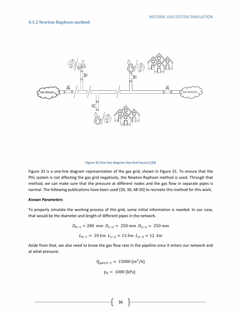
NATURAL GAS SYSTEM SIMULATION
36
4.1.2 Newton-Raphson method
Figure 32 One line diagram Gas Grid Source:[34]
Figure 32 is a one-line diagram representation of the gas grid, shown in Figure 31. To ensure that the
PtG system is not affecting the gas grid negatively, the Newton-Raphson method is used. Through that
method, we can make sure that the pressure at different nodes and the gas flow in separate pipes is
normal. The following publications have been used [20, 30, 48-50] to recreate this method for this work.
Known Parameters
To properly simulate the working process of this grid, some initial information is needed. In our case,
that would be the diameter and length of different pipes in the network.
Aside from that, we also need to know the gas flow rate in the pipeline once it enters our network and
at what pressure.
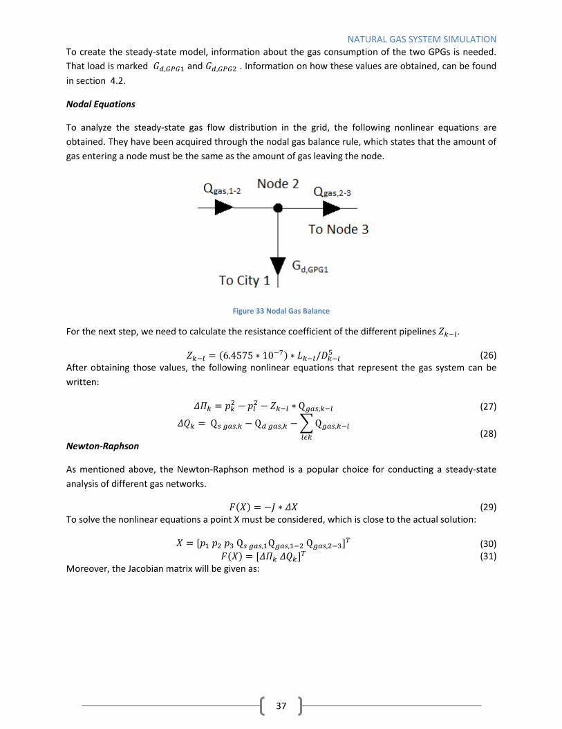
NATURAL GAS SYSTEM SIMULATION
37
To create the steady-state model, information about the gas consumption of the two GPGs is needed.
That load is marked and . Information on how these values are obtained, can be found
in section 4.2.
Nodal Equations
To analyze the steady-state gas flow distribution in the grid, the following nonlinear equations are
obtained. They have been acquired through the nodal gas balance rule, which states that the amount of
gas entering a node must be the same as the amount of gas leaving the node.
Figure 33 Nodal Gas Balance
For the next step, we need to calculate the resistance coefficient of the different pipelines .
( ) (26)
After obtaining those values, the following nonlinear equations that represent the gas system can be
written:
(27) ∑
(28)
Newton-Raphson
As mentioned above, the Newton-Raphson method is a popular choice for conducting a steady-state
analysis of different gas networks.
( ) (29) To solve the nonlinear equations a point X must be considered, which is close to the actual solution:
(30)
( ) (31)
Moreover, the Jacobian matrix will be given as:

NATURAL GAS SYSTEM SIMULATION
38
000000
0000
0000
000
000
00000
32,
3
21,
2
21,
1
1,.
1
32,
3
3
3
2
3
21,
2
2
2
1
2
1
1
gasgas
gasgass
gas
gas
Q
Q
pQ
Q
pQ
Q
pQ
Q
Qpp
pQpp
p
(32)
To verify the convergence of the Newton-Raphson method, various calculations have been conducted at
different initial pressure and gas flow conditions. One set of these values has been chosen as initial
conditions for the gas system in this chapter.
4.2 Power-to-Gas Simulation In this sub-chapter, the equations for simulating the PtG system are presented. These equations were
obtained from [30].
(33) Equation (33) gives the energy demand [MWh] needed to transform [mol] into methane. As it is
known from eq. (4 Ch.2), the energy needed for turning 1 mol is . In Eq. (33) that value is
turned into [MWh] through multiplying by .
To simplify the equations for the entire process, the constant is defined. It denotes the conversion
of energy from electrical to natural gas form.
(34) Here, the efficiency ( ) is predefined by the user in advance. The energy density of natural gas is
presented through its Lower Heating Value (LHV).
Now, [ ] can be obtained, which is the amount of methane that is produced by the PtG.
(35) However, if the amount of methane that is needed is known and we only need to know how much
energy is withdrawn from the ESS, following equation is used.
(36)

NATURAL GAS SYSTEM SIMULATION
39
Figure 34 shows the working process of the
PtG for this thesis. The model that was
created obtains information from the gas –
grid and based on that tells the PtG how
much methane must be produced. Based
on that information our model calculates
the needed electrical consumption from the
ESS to fulfill this demand. An explanation of
how is obtained can be found the
next sub-chapter.
4.3 Gas Powered Generator Regulation In an attempt to help the local consumers of two cities, with synthetic natural gas (SNG) produced from
surplus energy from RES, Peak regulation has been chosen to be performed for each city. This service
has been selected because GPGs are fast-acting and also the PtG system is not going to be able to
produce enough SNG to take care of the base load.
Peak Regulation
Peak regulation is performed through the use of a load prediction sequence in an attempt to minimize
the gas demand as much as possible. More information on the working principle of the load prediction
algorithms and the way they are used in this work can be found in 4.2.1 and 4.2.2.
Figure 35 Peak Regulation Example
Figure 34 Simulation of PtG

NATURAL GAS SYSTEM SIMULATION
40
Figure 35 contains an example of how peak regulation has been utilized in this paper. The blue line
represents the consumer demand at different intervals. The dotted line represents the limit the base
power sources are prepared to cover. Everything above the dotted line at this moment must be covered
by our GPGs.
4.3.1 Kalman Filter9
This method works as a recursive estimator. Here, past data is used to predict the next value. A
downside of this algorithm is the fact that it is not possible to predict more than one value ahead. The
equations through this subchapter have been adapted with the help of these sources [51, 52].
The general equation for the Kalman Filter is:
( ) (37) This method is composed of two processes, a prediction process, and an update process. The prediction
process output value is used as an input value for the update process. Afterward, the value that is
outputted through the update process becomes an input value for the prediction process.
Prediction process:
Estimation
(38) Here A and B are identity matrices. is a control signal, which identifies that the user has some sort of
effect on the outcome. In this work it is assumed that the user has no effect on the outcome, so the
control signal is equal to zero. Also, due to the fact that there is only one input signal, Eq.(38) can be
minimized to:
(39)
Prediction error
(40)
Update process:
Kalman Gain
(
) (41) Here, the purpose of H is the same as A and B from Eq.(38), filtering of the signals. Because there is only
one signal, H is assumed to be equal to zero.
Estimate update
( ) (42)
Error update
( )
(43)
This algorithm can be summarized by the following figure:

NATURAL GAS SYSTEM SIMULATION
41
Figure 36 Working principle of the Kalman Filter
The process is first given an estimate of zero and a prediction error of one. After that in the prediction
process, through Eq.(39,40) corrects these values and passes the outputs along to the update process
which utilizes Eq.(41,42). Then the new and are calculated based on our load data . This
whole process is looped until the moment the data runs out for . After that one last iteration is
performed and the result is presented through the last value.
As mentioned above, is the load data. In an attempt to gain more accurate predictions, the electrical
load is divided into hourly values and the load for each hour is predicted based on load data from the
previous days at that same hour and the user is presented with an estimation of the load for the next 24
hours. In order to decrease the error, the first week data is used to teach the Kalman Filter. The
estimations begin at day 8.
{[
]
⏞
Figure 37 Kalman Filter load data presentation
Then the real value of electrical load demand is compared to the predicted load.
(44)
The next step is to find with the help of . The following equation obtained from [30] is
used :
(
) (45)

NATURAL GAS SYSTEM SIMULATION
42
4.3.2 Least Error Squares (LES)
This method is a part of the multiple linear regression approaches. Here, the load is estimated based on
information about different factors. In this work, the factors used are humidity, wind speed, and
temperature[53]. Eq.(21) presents an example of the equation used in the multiple linear regression
approaches.
(46)
Where, , and stand for humidity, wind speed and temperature respectively and is an error.
The LES algorithm allows us to predict the load, based on all the available information available have on
the electrical consumption and affecting factors.
(47) In matrix form, Eq.(47) will obtain the following form:
[
]
n-m
3
n-m
2
n-m
1
3-m
3
3-m
2
3-m
1
2-m
3
2-m
2
2-m
1
1-m
3
1-m
2
1-m
1
yyy1
yyy1
yyy1
yyy1
[
]
(48) In Eq.(48), the regression coefficients are the only unknown left. It can be found via the following
equation.
( ) (49) Where S is a matrix containing all the past load data.
An example of how the Kalman Filter and the LES approach data is introduced to the program, created in
parallel with this thesis, can be seen in Appendix A.
4.4 Gas Grid Simulation and Demand As mentioned before, the gas demand from the PtG is formulated from the power regulation needs of
two other cities. The working principles of the two algorithms have been presented, and now an
algorithm must be chosen that is used to form the gas demand for each city.
4.4.1 Leas Error Squares
A condition of the LES is to have information on the environment, and more importantly, data is needed
on the humidity, temperature and wind speed. As shown in section 4.1 the distances between the
different GPG are very small, and due to that, the same weather information is used as the one for the
Wind Turbines and Solar Arrays

NATURAL GAS SYSTEM SIMULATION
43
Figure 38 Load profile and regulation profile Area 1 LES
Figure 39 Load profile and regulation profile Area 2 LES
The left part of Figure 38 shows the load of the city for the entire period. The load prediction for the
area is obtained and from there the power regulation profile, which is seen on the right. From the load
profile, it can be judged that the area is the same as the one for which the ESS is sized, a city center or
office complex with loads varying from 2 to 7 [MW]. As it can be seen from the load prediction profile,
the LES gathered information on the load and accompanying factors for the first week of operation and
started predicting in the second week. The power regulation profile possesses the same outline as the
normal load, with peak demand during the week, around 2[MW], and no demand during the weekend.
The reason for that is mostly caused by the prediction algorithm overestimating the request, and thus
no regulation power is needed.
The profiles on Figure 39 show a different picture than Figure 38. Here the load profile is filled with
spikes. Such a profile may belong to either a commercial or residential area. On the right, it can be seen
that the regulation profile is full of spikes ranging around 1 - 2 [MW], but the spikes are also in higher
number than for the previous area.
4.4.2 Kalman Filter
This time the Kalman filter algorithm is used for predicting the load of the two cities and obtaining the
regulation profiles.

NATURAL GAS SYSTEM SIMULATION
44
Figure 40 Load profile and regulation profile Area 1 Kalman Filter
Figure 41 Load profile and regulation profile Area 2 Kalman Filter
First, it is noticed that the Kalman Filter needs less information in order to start working. Figure 40
shows a regulation profile quite similar to the one in Figure 38. The only difference is that now the
spikes are more, due to the faster-learning process of the Kalman Filter, and can reach as high as
around 2.8 [MW]. The outlook is better when comparing Figure 39 and Figure 41. It can be seen that in
the beginning, the regulation profile has relatively high values, but as time goes on, the algorithm is
learning, and thus the power demand from the GPG is becoming quite low.
As it became apparent before, different algorithms predict more or less accurately depending on the
area. For this case, it is chosen that the gas demand is formed with the help of the LES, for shaping the
regulation profile for city 1 and the Kalman Filter for shaping the regulation profile for city 2.

NATURAL GAS SYSTEM SIMULATION
45
4.4.3 Power-to-Gas Gas Demand
Figure 42 Methane Production PtG
After obtaining the regulation demand for the GPG, it is turned into Gas Demand. Through the Newton-
Raphson method, the Gas Demand from the PtG system can be obtained. Figure 42 shows that demand.
It can essentially be seen that gas demand profile is a combination of the two regulation profiles for the
two zones. This is the reason why it is crucial to choose the right load prediction method for each zone.
The profile shows a very high methane demand in the first third of the month of up to 550 [m3/h].This
high rise is essentially due to the effect of the Kalman filter and its inability to be trained for that specific
load with less information. After the high rise, the demand lowers and for the rest of the period reach as
high as around 300 [m3/h], which is a significant difference compared to the first third.
4.5 Conclusions In this chapter, some insight has been cast on the combined electrical and gas grid network layout.
Afterward information was given on how the PtG simulation is performed and how the demand is
obtained through the prediction algorithms. In order to ensure the safe operation of the gas network,
the Newton – Raphson method is used.

ENERGY STORAGE AND ITS OPTIMAL SIZING
46
Chapter 5 Energy Storage and its Optimal Sizing This chapter contains the results obtained in the course of this master thesis using ESSPC.
5.1. Obtaining the Storage System Size This section explains how the size of the storage system can be found. First, a case is presented where
the storage system is sized only depending on what is imported to the grid or exported. In the second
case, the storage system is sized with regards to the price of electricity.
5.1.1 Flowchart for obtaining Storage System Capacity
Figure presents the different methodologies for obtaining the size of
the Storage System. First of all, a representation of the Wind Turbines
must be created. After inputting all the necessary information, the user
can decide to add even more different types of Wind Turbines to the
area. After this process has been finished the next step is to simulate
the Photovoltaics (PVs). Again a choice can be made regarding the
number of types of Solar Modules technologies being simulated. The
next step is to present the Load Data (Consumer Data) for the grid
where the RESs have been placed. After presenting the Grid Data to
ESSPC, the Storage System can now be sized. The only way that this
could be done is by varying the different RESs and calculating the
Storage System Size for each combination and then getting the
combination of RES that gives the smallest Storage System Size. How
this is done and what different cases are considered in this thesis can
be seen in section 5.3.
5.1.2 Sizing Storage System with regards to the import/export
To find the capacity of the ESS. First, the power input/output of the ESS
must be obtained for each data point “m.” The Residual Power ( ) in
the grid is the difference between the Generation and Consumption in
the grid. If the Residual Power value is positive, the ESS is charged and
if it is negative, it is discharged. Of course, unless the ESS is sized for “islanded mode”, the ESS cannot
charge/discharge for the whole value of the Residual Power. The Residual Percentage ( ) is
introduced here, which refers to what percentage of the charge/discharge power at that time must
come from the ESS. The power that is stored/discharged from the ESS ( ) can then be found:
( )
( )
(50) Now that the power input/output for each data point is known, the needed energy capacity can be
found for the ESS ( ) at every datapoint:
( )
( )
( )
(51) From here, the needed ESS capacity for the entire observed time frame, can be found:
( ) ) ( ) ) (52)
Figure 43 Flowchart Sizing Storage System

ENERGY STORAGE AND ITS OPTIMAL SIZING
47
5.1.3 Sizing Storage System with regards to the price of electrical power
To find the capacity of the ESS for this case, two more things need to be introduced besides what has
been done for the first instance. First the price of power that comes from the higher voltage grid.
Second is the use of MATPOWER, package of MATLAB files that can perform PF and OPF calculations.
MATPOWER provides information on the power losses in the test grid, also through making the
substation bus bar the slack bus, information is provided on the power that enters or leaves the grid
through the substation for every hour. Now ( )
is divided in three different parts depending on the
( ), ( )and ( ) of electrical power.
If is greater than
( )
( ( )
( )
) (53)
( ) (54)
If is greater than and ( )
is greater than the price limit ( )
( )
( ( )
( )
) (55)
( ) (56)
If is greater than and ( )
is smaller than
( )
(57)
( )
(58)
With (53) and (55) the charge and
discharge events that were
happening in (52) are divided into
and . is used for
what must be produced by the
Storage System in order to satisfy
the consumers, is used for
what is unneeded in the LV grid at
that data point and needs to be
stored. When the system is
producing it is taken that it cannot
be consuming and vice versa (54)
and (56). This is done with
MATPOWER, the power flow
toolbox can perform Power Flow
calculations for only one Figure 44 Charging Strategy choice tree

ENERGY STORAGE AND ITS OPTIMAL SIZING
48
data point. Also due to the fact that the storage system is both a Consumer and Generator this division
must be made because the consumption and generation data is entered in different fields of the
toolbox. From the equations above it can also be noticed that that data is given to MATPOWER through
another criterion, the price of power. Here the user sets a where if the at that time is
higher we choose to support the grid with the help of the Storage System. But if the at that time is
smaller than the the Storage System performs no action and the grid is supported entirely
with cheap power from the higher voltage grid/substation. The choice tree presented in Figure 44
explains this charging strategy.
Figure 45 shows the price of electricity for the month of March 2015. The price is given in $/MW. It can
be seen that at the beginning of the month, the prices vary a lot from as low 10 $/MW to as high as
almost 500 $/MW. After that, until the end of the month, the prices are considerably lower with the
occasional spikes. Here the value of the median and the mean value of the dataset is given. This is done
to help the user with their choice in setting a price limit, which as mentioned in Chapter 3, will be used
to signal to the ESS that the price from the grid is too high and it should cover the electrical need of the
grid.
Figure 45 Electrical Power Price
It can be seen that the mean value of the dataset is around 52 $/MW. The median value, on the other
hand, is smaller and is around 30 $/MW. This is because of a significant portion of the prices, in the
given timeframe, are tiny. In ESSPC, the user can observe this information and try different prices and
see how that affects the ESS capacity. In this work, 82 $/MW are set as the price limit. The number of
RES is then found to be 13, 9, 12 for Wind Turbines of types 1 2 and 3 and 9 10 9 for Photovoltaics of
types 1 2 and three respectively.

ENERGY STORAGE AND ITS OPTIMAL SIZING
49
5.2 Sizing of the ESS The size of the ESS depends on the number of installed RES, weather conditions throughout the
observed time frame and consumer load. To find the best combination of RES, the following equation is
used:
( )
( )
( )
(59) Where “n” is the number of different models that are available, and WT and PV refer to the power
generation from the Wind Turbine and the Photovoltaic respectively.
Obtaining the optimal number of RESs can be found by testing different combinations of RESs and then
matching them to the storage system size that they have procured. For example, if the algorithm has
access to 2 different WTs and 1 PV model, the equation above will look like this:
( )
( )
( )
( )
(60) From here, different combinations of and are tested and the data for each
combination is forwarded to help find the size of ESS. The smallest ESS size is then found and traced
back to its RES combination.
5.3.1 Sizing Storage System Capacity with Surplus Power Method
Figure 46 RES combinations Surplus Power
Figure 46 is a representation of all the different ESS capacities that can be achieved with a various
number of RES at 50% of the Surplus Power. The graphs have been zoomed-in around the area where
the smallest ESS capacity of 331.4 [MWh] is obtained. To achieve this 21 Wind Turbines of type 1 are
required , 24 of type 2, 19 of type 3 and 12 of each type of Photovoltaic. It is also noticed that having a
smaller number of RES will bring to a slightly larger ESS. Due to this, it is important to mention that this
thesis will not make a techno-economic analysis based on the number of RES installed in the grid. In the
“Results” section of ESSPC, the user can input different RES combinations and observe how they affect
the ESS. Such an observation is performed in 5.3.1 and 5.3.2.

ENERGY STORAGE AND ITS OPTIMAL SIZING
50
This whole process can be summarized with the following objective function:
( ) ( ( )
) ( ( )
)
( )
(( ( )
( )
) ( )
) (61)
subject to following constraints:
Here is the percentage of power the ESS can cover, be it provide to the system or absorb. This
value is 1 only in the time when electricity price is too high for the consumers and the ESS must provide
what is demanded.
Error! Reference source not found. 48 and 49, present a comparison between the different ESS
apacities with regards to the charging method. Here, only the surplus power charging method is used,
where the ESS is charged based
on 50% of the positive surplus
energy and discharged based on
50% of the negative surplus
power.
Figure 47 presents the hourly
power profile that must be
covered from the substation. It
can be noticed that quite often
the external power system must
help the power system in keeping
the demand covered. The areas
where nothing is imported from
outside mean that all of the
requests in the grid are covered by the RES and the actual surplus power is transmitted through the
substation elsewhere. As it can be seen, these hours are not many. Another noticeable feature is the
larger amount of power that has to be supplied from the substation, which reaches as high as 30 [MW].
This is because MATPOWER also calculates the losses from the line. Thus after supplying the power from
the substation, a portion of it will be lost in the lines, and only the needed amount will reach the
consumers.
𝐶𝑜𝑛𝑠𝑡𝑟𝑎𝑖𝑛𝑡𝑠 ≤ 𝑓(𝑦 𝑝) ≤
𝑓(𝑅𝑝𝑒𝑟)
≤ 𝑓(𝑥 𝑛) ≤
Figure 47 Effect of RES with no ESS

ENERGY STORAGE AND ITS OPTIMAL SIZING
51
Figure 48 presents the behavior of the
ESS and the effect it will have on the
grid. The first plot shows how the
energy inside the ESS changes over the
course of the month and the second
plot shows the amount of power that is
charged or discharged from the ESS
every hour. It can be seen that the ESS
capacity profile is represented by some
different in size hills. Each hilltop
represents the end of a cycle of positive
RES surplus power, and each valley
bottom represents the end of a cycle
where the RES could not meet the
demand. Also, from the second plot, it
can be noticed that due to the high
fluctuating power production, mainly
from the wind turbines, the charging
power at times is more than twice of
what is discharged for the whole period.
It is also observed that the discharge
profile mostly falls in the same window
when compared to the charging profile
for the entire period. The last plot
covers the power that has been
imported from beyond the network. On
a first glance, when compared to Figure
48 it can be noticed that the ESS has
had a positive effect on the system, the power supplied from the substation has decreased, which
means fewer losses and that the otherwise lost power can be useful somewhere else.
5.3.2 Sizing Storage System Capacity with Surplus Power and Price Method
As mentioned before, another method has been devised in sizing the ESS. This method utilizes the
electrical power price. Through it, the ESS can supply the power system when the cost of electricity is
too high to purchase from outside the system, in the case beyond the substation.
Once again, this process can be presented by the following objective function:
( ) (( ( )
( )
) ( )
( )
( ) ((
( )
( ) )
( ))
( )) ((
( )
( ( )
( )
)) ( )
( )
( ) (
( )
( ( )
( )
)) ( )
) (( ( )
( ( )
( )
)) ( )
( )
( )
( ) ) (62)
Figure 48 ESS capacity with the Surplus Power method with number of RES for Surplus Power method

ENERGY STORAGE AND ITS OPTIMAL SIZING
52
Now the next charging method that includes
the price of electricity is executed. The
number of RES stays the same as the number
of RES as before.
Here it can be seen that the ESS is constantly
charging throughout the whole month of
March. The reason for this behavior is the
significant number of RES that is present.
Because the number of RES is greater than
what this method needs, the ESS almost
constantly charges throughout the whole
period and at the end reaches a size of around
1800 MWh. It can also be seen that the
charging cycles have not increased in number,
compared to Figure 48, but some have
increased in power. However, the biggest
change, which also affects the ESS, is the lack
of discharging cycles in the middle of the
month. This is due to the change of charging
strategy, and those areas where it is noticed a
lack of discharging events correspond with the
lowest prices of electricity that were observed
in Figure 45. The amount of imported power from
outside has also worsened, mainly because the ESS is
not operational most of the time.
An overview of all the results obtained in sizing the
ESS with the surplus power method can observe in
Figure 50. The first row presents the total amount of
money that have been paid for imported power. It can Figure 50 End results for sizing ESS with optimal
number of RES for Surplus Power method
Figure 49 ESS capacity with the Surplus Power and Price method with number of RES for Surplus Power method
𝐶𝑜𝑛𝑠𝑡𝑟𝑎𝑖𝑛𝑡𝑠 ≤ 𝑓(𝑦 𝑝) ≤
𝑓( 𝑅𝑝𝑒𝑟)
𝑓( 𝑃𝑝𝑟𝑖 𝑔) 𝑢𝑠𝑒𝑟 𝑠𝑒𝑡
≤ 𝑓(𝑥 𝑛) ≤

ENERGY STORAGE AND ITS OPTIMAL SIZING
53
be seen that with no ESS, that value is around 414460 $, while with a 331 MWh ESS using the Surplus
Power method, that value is around 342670 $. Using the Surplus Power and Price method with this
configuration brought worse results in term of the price paid, 376880 $ and size of the ESS, 1830 MWh.
The last two rows showing the highest and lowest discharge rate are the same for both ESS for both
methods.
5.4 Sizing ESS with PtG via Surplus Power and Price Method In Figure 51 the capacity profile of the ESS
working with the PtG, at 85% efficiency(see
2.4.3), can be seen. It is important to
mention that 44 Wind Turbines have been
utilized (16 from type 1, 13 type 2 and 15 type
3) and 21 Solar Arrays (8, 7, 6 for types 1 2
and 3 respectively). In order to obtain this
optimal profile, 10 more Wind Turbines had
to be added than for the case in 5.3.2, but on
the other hand, the number of Solar Arrays
was decreased by 7. What can be noticed
from the capacity profile is the shape which is
similar to the one obtained in 5.3.2, and it
roughly resembles the methane production
profile from {methane production Figure}.
The charge/discharge profile is quite different
from the one before. Now the discharge
events have a slightly higher number and are
slightly larger, and there are also discharges in
places where there were no before. This is
due to the charging strategy when the price is
in the predetermined limits, in the first case
the grid did not need the ESS, but in the case
of Figure 51, the ESS is still required. This is
the reason why the size is relatively bigger for
this ESS than from the one before, because of
the effect of the ESS.
The end results can be observed in Figure 52.
The results shown before are combined with
results from a study that was similar to the
one in 5.3.2, sizing the ESS with the RES for
Surplus Power and Price Method, but utilizing
only the Surplus Power method. Figure 52 is
quite different to Figure 50, where the PtG
was not used. For starters, due to the
increased number of RES, the total price paid
for imported power has decreased, but it is
Figure 51 ESS capacity PtG and with the Surplus Power and Price method with combination of RES for Surplus Power and Price
method.
Figure 52 End results for sizing ESS with PtG and optimal number of RES for Surplus Power and Price method

ENERGY STORAGE AND ITS OPTIMAL SIZING
54
still a bit higher than the total price paid for imported power with no ESS and PtG. The total ESS capacity
has also increased from 314 MWh to roughly 579 MWh, which is a change once again brought by the
PtG.
This information is proof that for the currently chosen Grids, Consumers, and RES, the combination of
ESS and PtG will not bring better results in lowering the ESS capacity. Evidence was also found that the
PtG has the potential of lowering the ESS given slightly different starting conditions, like changing the
demand profiles, the prediction algorithms and introducing various more RESs.
5.5 Sizing of ESS with Electrochemical Characteristics Gathering the valuable information from the sections so far, it is known that through the Surplus Power
and Price method we obtained the smallest ESS capacity. Afterward coordinating that ESS with PtG did
not bring better results.
Lead-Acid Lithium-Ion Vanadium-Redox CAES
Power Energy Power Energy Power Energy Power Energy
[MW] [MWh] [MW] [MWh] [MW] [MWh] [MW] [MWh]
50 200 1-100 0.25-25 50 250 180 1400-3600
20-50 250 1-10 4-24 1-10 4-40 135 1800
100 400
135 2700
1-100 0.25-50
50 250 Table 18 Electrical Energy Storage Project Sizes
Table 18 has already been presented in 2.5, and it is brought it here for easy reference. It can be
noticed that the 314[MWh] and the 578[MWh] Storage Systems obtained in the course of this study
match the power output of all these projects, but with regards to the size, fit only the Lead-Acid and the
CAES technologies. This means that the ESS capacities fit real projects utilizing the Lead-Acid and CAES.
So far the ESS is sized without regards to the efficiency. Now, that there is a rough estimation of the
parameters are to be needed, one of the following technologies can be fitted, and a real ESS capacity
can be obtained.
The Lead-Acid is chosen to be fit, seeing as the 314 [MWh] ESS is the smallest obtained in the course of
this study.
In order to perform this task, the Lead-Acid roundtrip efficiency is needed. From 2.2.1 the value of 85%
is taken. Also with a view to include the roundtrip effectiveness in the calculations, the following change
must be made in accordance with [54].
( )
is divided into charging and discharging events. Where if ( )
( )
( )
and if
( )
( )
( )
For charging events there is
( )
( )
( )
√ (63) And for discharging events

ENERGY STORAGE AND ITS OPTIMAL SIZING
55
( )
( )
( )
√
⁄
(64) Where is the efficiency of the chosen ESS.
As explained before, the Lead-Acid battery will be sized with accordance to the Surplus Power and Price
method without coordination with the PtG system. For this case the objective function will acquire the
following form:
( ) ((
( )
( ) )
( )
( )
( )
( (( ( )
( )
) ( )
) ( )
)
( )
√ (( ( )
( ( )
( )
)) ( )
( )
( )
( ( )
( ( )
( )
)) ( )
)
( )
√
⁄ (( ( )
( ( )
( )
)) ( )
( )
( )
( ) )
(65) subject to following constraints:
Figure 53 presents the Lead-Acid capacity found through the aforementioned method. A definite size
increase is observed where the ESS now reaches 363 [MWh]. As expected, the profile maintains its
previous shape.
𝐶𝑜𝑛𝑠𝑡𝑟𝑎𝑖𝑛𝑡𝑠 ≤ 𝑓(𝑦 𝑝) ≤
𝑓(𝑅𝑝𝑒𝑟)
𝑓( 𝑃𝑝𝑟𝑖 𝑔) 𝑢𝑠𝑒𝑟 𝑠𝑒𝑡
≤ 𝑓(𝜂𝐸𝑆𝑆) ≤
≤ 𝑓(𝑥 𝑛) ≤

ENERGY STORAGE AND ITS OPTIMAL SIZING
56
Figure 53 Lead-Acid capacity Surplus Power and Price method without PtG
As for the charge/discharge characteristic, due to the effect of the now added efficiency, it can be
noticed that the spikes have slightly larger values than before.
Figure 54 Charge-Discharge characteristic Lead - Acid
5.6 Conclusions In this chapter results have been obtained on sizing the storage system with different combinations of
RES and different methods. It was found that the smallest ESS size is found through the Surplus Power
and Size method with number of RES specifically set for that method. Afterwards the effect of the PtG
system on the ESS was observed and a conclusion was reached that for this particular case a
coordination between the two systems will bring an increase in the ESS size, and thus is not wanted. As
a last result, via information obtained from simulations an ESS technology was chosen and the ESS was
sized with that particular technology. The results showed that installing a Lead-Acid technology, the ESS
will have an increase of size by about 20 [MWh] compared to the perfect case, where the technology
has not yet been chosen.

CONCLUSIONS AND FUTURE WORK
57
Chapter 6 Conclusion and Future Work
6.1 Conclusions Coordination between ESS and PtG systems will play an important role in the future power system. Due
to the large number of RES that are installed and will continue to be installed, a method for utilizing the
excess renewable energy is needed. A number of different technologies have the ability to store this
excess energy and then release it when needed. Through the use of different charging methods, an ESS
can be optimally sized for taking care of the electrical needs of nearby consumers, as well as the gas
demand.
This work introduced a few of the most well-known ESS technologies. The technologies were compared
and one that can best perform the task at hand was chosen. In this work, a few charging strategies were
developed for charging the ESS with and without connection to the PtG system, as well as a strategy for
gas demand from the PtG.
In this master thesis it was found out that it is possible to store surplus energy from RES and store it as
electrochemical energy which afterwards can be turned into methane. With the proper charging
strategy, tailored to the the given area, the size of the ESS can be optimized to be as small as possible.
Furthermore, by setting gas demand strategies with load-prediction algorithms it was found that using
the PtG system under these initial conditions will increase the ESS size even though the number of RES
is smaller.
6.2 Future work In the future, the ESSPC can be further enhanced by introducing a number of different features, like for
example:
Easy introduction of a more complicated power grid and the ability to change the position of the
ESS.
Easy introduction of a more complicated gas network with a number of different gas consumers.
Improving the computation time of the ESSPC, so that more types of RES can be introduced and
a more in-depth observation can be performed.
Introduction of a wider variety of charging strategies.
Introduction of a wider variety of load prediction algorithms if GPGs are to be used.

BIBLIOGRAPHY
58
Bibliography [1] D. G. Rachel Carnegie , David Nderitu, Paul V. Preckel, "Utility Scale Energy Storage Systems,"
State Utility Forecasting Group2013. [2] ISPRE, "Research and Development on Renewable Energies " ISPRE2011. [3] (1/9). Available: http://www.ens.dk/en/supply/renewable-energy/wind-power/offshore-wind-
power/current-offshore-wind-farm-projects [4] M. Bredsdorff. (2015, 01/10). 6/1. Available: https://ing.dk/artikel/tordnende-succes-39-
procent-af-stroemmen-kom-fra-vindmoeller-i-2014-173290 [5] B. V. Mathiesen, H. Lund, D. Connolly, H. Wenzel, P. A. Østergaard, B. Möller, et al., "Smart
Energy Systems for coherent 100% renewable energy and transport solutions," Applied Energy, vol. 145, pp. 139-154, 5/1/ 2015.
[6] B. V. L. Mathiesen, Henrik; Hansen, Kenneth; Skov, Iva Ridjan; Djørup, Søren Roth;, S. S. Nielsen, Peter; Thellufsen, Jakob Zinck; Grundahl, Lars; Lund, Rasmus, and D. W. C. Søgaard; Drysdale, David; Østergaard, Poul Alberg, "IDA's Energy Vision 2050: A Smart Energy System strategy for 100% renewable Denmark," Aalborg University2015.
[7] L. Bird, M. Milligan, and D. Lew, "Integrating Variable Renewable Energy: Challenges and Solutions," National Renewable Energy Laboratory, Technical ReportSeptember 2013 2013.
[8] TEPCO, "Tokyo Electric Power Company," N. o. electricity, Ed., ed: TEPCO. [9] A. Oudalov, D. Chartouni, and C. Ohler, "Optimizing a Battery Energy Storage System for Primary
Frequency Control," IEEE Transactions on Power Systems, vol. 22, pp. 1259-1266, 2007. [10] "The future role and challenges of Energy Storage," ed: European Commission, 2014. [11] G. H. Abbas A. Akhil, Aileen B. Currier, Benjamin C. Kaun, Dan M. Rastler, and A. L. C. Stella
Bingqing Chen, Dale T. Bradshaw, and William D. Gauntlett, "DOE/EPRI 2013 Electricity Storage Handbook in Collaboration with NRECA," Sandia National Laboratories2013.
[12] G. P. Pierre Pinson, Bernd Klocki, Jody Verboomen, "Dynamic Sizing of Energy Storage for Hedging Wind Power Forecast Uncertainty," presented at the Power & Energy Society General Meeting, 2009.
[13] D. P. Kothari and I. J. Nagrath, Modern Power System Analysis: Tata McGraw-Hill Publishing Company, 2003.
[14] H. Singh, S. Hao, and A. Papalexopoulos, "Transmission congestion management in competitive electricity markets," IEEE Transactions on Power Systems, vol. 13, pp. 672-680, 1998.
[15] (21/02). Battery Basics. Available: http://www.progressivedyn.com/battery_basics.html [16] SandiaNationalLaboratories. (10/06). DOE GLOBAL ENERGY STORAGE DATABASE. Available:
http://www.energystorageexchange.org/ [17] X. Luo, J. Wang, M. Dooner, and J. Clarke, "Overview of current development in electrical energy
storage technologies and the application potential in power system operation," Applied Energy, vol. 137, pp. 511-536, 1/1/ 2015.
[18] T. K. Toshikazu SHIBATA*, Yoshiyuki NAGAOKA, Kazunori KAWASE and a. K. YANO, "Redox Flow Batteries for the Stable Supply of Renewable Energy."
[19] "Vanadium Redox Flow Batteries: An In-Depth Analysis " EPRI, Palo Alto, CA:2007 1014836. [20] P. S. J. H. Lukas Grond, "Systems Analyses Power to Gas," KEMA Nederland B.V., Technology
Review20/06 2013. [21] B. E. Allan Schrøder Pedersen, Claus Hviid Christensen,Claus Kjøller,Frank Elefsen,John Bøgild
Hansen,Jørgen Hvid, Rambøll,Per Alex Sørensen,Søren Knudsen Kær,Thomas Vangkilde-Pedersen,Thorkild Feldthusen Jensen,, "Status and recommendations for RD&D on energy storage technologies in a Danish context," 31/01 2014.
[22] J. Kim, Y. Lee, W. S. Yoon, J. S. Jeon, M.-H. Koo, and Y. Keehm, "Numerical modeling of aquifer thermal energy storage system," Energy, vol. 35, pp. 4955-4965, 12// 2010.

BIBLIOGRAPHY
59
[23] (2014, 29/02/2016). The world's largest solar heating plant to be established in Vojens, Denmark. Available: http://solar-district-heating.eu/NewsEvents/News/tabid/68/ArticleId/367/The-worlds-largest-solar-heating-plant-to-be-established-in-Vojens-Denmark.aspx
[24] F. Ulbjerg. (2014). SOUTH-JUTLAND STORES THE SUN’S HEAT IN THE WORLD'S LARGEST PIT HEAT STORAGE. Available: http://www.ramboll.com/projects/re/south-jutland-stores-the-suns-heat-in-the-worlds-largest-pit-heat-storage
[25] Hydrogenics. (23/02). Excess Wind Power Turned into Gas in Denmark Using Hydrogenics Technology. Available: http://www.hydrogenics.com/about-the-company/news-updates/2014/02/18/excess-wind-power-turned-into-gas-in-denmark-using-hydrogenics-technology
[26] (23/02). POWER-TO-GAS TECHNOLOGY OFFER NEW MARKET OPPORTUNITIES FOR ELECTROLYSER MANUFACTURERS. Available: http://biocat-project.com/news/power-to-gas-technology-provides-new-market-opportunities-for-manufacturers-of-electrolysers/
[27] M. G. Tom Smolinka, Jürgen Garche "„Stand und Entwicklungspotenzial der Wasserelektrolyse zur Herstellung von Wasserstoff aus regenerativen Energien“," 05/07 2011.
[28] M. Sterner, "Bioenergy and renewable power methane in integrated100% renewable energy systems.Limiting global warming by transforming energy systems " 14, Erneuerbare Energien und Energieeffizienz.Renewable Energies and Energy Efficiency Kassel University, 2009.
[29] S. H. A. K. Sayah, M. Farazar, "CO2 Abatement by Methanol Production from Flue-Gas in Methanol Plant " International Journal of Chemical, Molecular, Nuclear, Materials and Metallurgical Engineering, vol. 4, 2010.
[30] Q. Zeng, J. Fang, J. Li, and Z. Chen, "Steady-state analysis of the integrated natural gas and electric power system with bi-directional energy conversion," Applied Energy.
[31] M. S. a. A. Bertucco, "Synthetic Natural Gas (SNG) from Coal and Biomass: a Survey of Existing Process Technologies, Open Issues and Perspectives," in Natural Gas, P. Potocnik, Ed., ed, 2010.
[32] EARTO, "The TRL Scale as a Research & Innovation Policy Tool,EARTO Recommendations," European Association of Research and Technology Organisations2014.
[33] "XLPE_Cu_single_core_66_kV_DS_EN," N. Cables, Ed., ed: NKT cables, 2016. [34] Dreamstime, "Dreamstime," ed. https://www.dreamstime.com: Dreamstime, 2016. [35] "Distribution Zone Substation Information," Ausgrid, Ed., ed: Ausgrid, 2016. [36] "Modern-Era Retrospective Analysis for Research and Applications (MERRA), version 2," ed.
gmao.gsfc.nasa.gov: National Aeronautics and Space Administration (NASA) / Goddard Space Flight Center, 2016.
[37] "CAMS Radiation Service v2.7 all-sky irradiation (derived from satellite data).", ed: MINES ParisTech (France), 2016.
[38] "National Electricity Market Price," AEMO, Ed., ed: AEMO, 2016. [39] (2016, 18/03). Windpower Program. Available: http://www.wind-power-program.com [40] A. Bellini, S. Bifaretti, V. Iacovone, and C. Cornaro, "Simplified model of a photovoltaic module,"
in Applied Electronics, 2009. AE 2009, 2009, pp. 47-51. [41] X. Weidong, W. G. Dunford, and A. Capel, "A novel modeling method for photovoltaic cells," in
Power Electronics Specialists Conference, 2004. PESC 04. 2004 IEEE 35th Annual, 2004, pp. 1950-1956 Vol.3.
[42] K. Provence, "Calculating PV Array Voltage," ed, 2013. [43] (2013, 20/03). Solar Panel Temperature Affects Output – Here's what you need to know.
Available: http://www.solar-facts-and-advice.com/solar-panel-temperature.html [44] (2003). Wind Turbine Power Calculator. Available: http://xn--drmstrre-64ad.dk/wp-
content/wind/miller/windpower%20web/en/tour/wres/pow/index.htm [45] CanadianSolar. (2016, 16/11). CanadianSolar. Available: http://www.canadiansolar.com/ [46] TrinaSolar. (2016, 16/11). TrinaSolar. Available: http://www.trinasolar.com/us/index.html [47] SolarWorld. (2016, 16/11). SolarWorld. Available: https://www.solarworld-usa.com/

BIBLIOGRAPHY
60
[48] S. Clegg and P. Mancarella, "Integrated Electrical and Gas Network Flexibility Assessment in Low-Carbon Multi-Energy Systems," IEEE Transactions on Sustainable Energy, vol. 7, pp. 718-731, 2016.
[49] S. Clegg and P. Mancarella, "Integrated Modeling and Assessment of the Operational Impact of Power-to-Gas (P2G) on Electrical and Gas Transmission Networks," IEEE Transactions on Sustainable Energy, vol. 6, pp. 1234-1244, 2015.
[50] M. Abeysekera, J. Wu, N. Jenkins, and M. Rees, "Steady state analysis of gas networks with distributed injection of alternative gas," Applied Energy, vol. 164, pp. 991-1002, 2/15/ 2016.
[51] G. Czerniak. (2013). Greg Czerniak`s Kalman Guide. Available: http://greg.czerniak.info/guides/kalman1/
[52] S. A.-h. Soliman and A. M. Al-Kandari, "8 - Dynamic Electric Load Forecasting," in Electrical Load Forecasting, ed Boston: Butterworth-Heinemann, 2010, pp. 291-352.
[53] S. A.-h. Soliman and A. M. Al-Kandari, "1 - Mathematical Background and State of the Art," in Electrical Load Forecasting, ed Boston: Butterworth-Heinemann, 2010, pp. 1-44.
[54] D. Lee, J. Kim, and R. Baldick, "Stochastic Optimal Control of the Storage System to Limit Ramp Rates of Wind Power Output," IEEE Transactions on Smart Grid, vol. 4, pp. 2256-2265, 2013.

APPENDIX A
61
Appendix A The following Appendix shows the sequence of actions that must be made in ESSPC so that a custom
user case can be created.
Figure 55 shows the starting screen of ESSPC. Here each button brings you to a different window where
you can insert data for models or conduct simulations. There is a sequence to creating a proper case. As
you can see all the buttons except one are colored in red, and there is only one green button. After
pressing the green button and coming back to this window, another green button will appear and so on.
Figure 55 Main Window Screenshot
Figure 55 is a screenshot of the window where the wind turbine information is inserted. As with the
main window the areas where data needs to be inserted is marked with green. After filling the green
area with the necessary information, merely clicking the left mouse button anywhere in the window will
reveal the next green area. The Efficiency Coefficient, Power Curve, and Wind Speed data are necessary
for creating a specific wind turbine model. The information is entered with “[ ]” brackets. Also, it is
important to mention that the number of values in all three fields must be equal. Pressing a yellow
button will automatically load a wind turbine that has been used in this master thesis.

APPENDIX A
62
Figure 56 Wind Turbine model creation Type 1
After taking care of the parameters, the next step is to present information on the wind speed and air
density. It is preferred that the file is a .xls and contains only values without any text, similar to Figure
57.
{
⏞
Figure 57 Weather Data form
After the data is loaded and is shown in the table ESSPC will need help determining which column
contains the needed information. This action is performed by typing the respective number of the
column in the fields below the table named Wind Speed and Air Density. The last step is to press the
“Evaluate” button, and the graphs will show all the relevant information for that specific wind turbine
model. The “Evaluate” button also clears all the fields, so that the user can insert information about the
next wind turbine. Pressing the “Back ” will bring the user back into the main window and will also show
a comparison of the power production of all inserted wind turbines in the form of a box plot.
After returning to the main window, the next button has changed its color from red to green. The solar
module window works on the same principle as the previous window. First, the datasheet parameters of
the chosen solar module are inserted in the green areas and pressing the yellow button will
automatically load information for one of the solar modules used in the thesis. The weather data is
inserted the same way as before for the wind turbine models. After that, there is an option to test the
solar module by presenting a value for Solar Irradiation and Temperature. The graph below will output
an I-V curve for that specific Solar Irradiation and Temperature so that the user can see whether a
mistake was made in the data insertion process. In order to make the simulation faster, the user is

APPENDIX A
63
presented with the option of combining the solar modules in parallel and/or in series with a view to
create a solar array. By pressing the “Evaluate” button, information will be shown on the power
production for the whole period with this technology and the fields will clear, awaiting information on
the next solar module. Pressing the “Back” button will once again display a box plot of the power
production of different technologies for the whole period.
Figure 58 Solar Module model creation Type 1
The next step is to insert the electrical load for the consumers. Again a .xls file containing no words and
only numerical values is needed, in a form similar to Figure 59.
{[
]
⏞
Figure 59 Electrical Consumption Data form
After filling the first table with information, pressing the green “Done ” button will sort the data in the
needed form for the study. In the Unit box, the user must define in what units the consumer load is and
then the user must press the last green “Done” button which will transform the data into the needed
form for the case. Pressing “Done” will also visualize the consumer load information for the whole
period in a separate graph.

APPENDIX A
64
Figure 60 Electrical Load input window
The next step in creating a custom scenario is to supply ESSPC with information on the electrical grid.
There are three windows which must be filled containing information on the busbars, branches, and
generators. When opening the Grid Information window, you will see that the information is prefilled in
all windows. There are two options from there, either you can submit prefilled information in .xls format
to fit the different tables, or you can insert the information manually right in the charts. It is important
to mention that there are fields which must not be changed and are marked with 999.

APPENDIX A
65
Figure 61 Grid parameter information
After providing all the necessary information for creating a custom case, the storage system can now be
sized. After opening the window, there are three areas which provide the user with flexibility in sizing
the ESS without a PtG system. As before the sequence In which the information is to be filled is marked
with green. The first area sizes the ESS with the surplus power method. The user can set limits regarding
the number of RES that is to be installed in the grid. The limits are shared by ALL the wind turbine
technologies and all the solar module technologies. After pressing “OPTIMUM,” ESSPC will calculate the
optimum number of RES that is to be installed in order to obtain the smallest ESS size. The optimum
number is shown in the tables below, where each value represents the number of RES that must be
placed, form each technology. The first row of wind turbine represents the first type of wind turbines
and so on.

APPENDIX A
66
Figure 62 Sizing the ESS without PtG
Next, the ESS can be sized using the surplus power and price method. The data is inserted in a similar
way to the one shown in Figure 57. The price can be in different currencies, and the user can choose
which type of currency is used and then by pressing the “Summarise Data” button a graph will show the
mean and median values of the whole dataset. This can help the user determine the highest price for
that period, where the ESS will stay inactive. Similar to before, pressing “Optimum,” ESSPC will calculate
the optimum number of RES that is to be installed using this method.
Finally, the user can get more in depth information on the ESS size with different RES combinations. For
example, if there are three wind turbines in the scenario and the user wants to see the ESS size for 2
wind turbines of type 1, 3 of type 2 and 5 of type 3, he must enter the numbers in the field in the
following form: 2 3 5. The process is similar for the for the Solar Panels. An example of this can be seen
in the figure before. After pressing “Calculate,” a separate window will open with information on the

APPENDIX A
67
capacity of the ESS, the power that goes in and out and the amount of power that is supplied from the
grid to support the city.
Now, information on the Gas Grid must be inserted. The first step is to fill the information on the gas
grid like pressure at the beginning of the pipes, the amount of methane that is entering the area,
distances between nodes and pipe diameters. Next step is to set the gas demand from the GPGs and the
respective efficiencies. The electrical demand from the GPGs can be calculated through using the
Kalman Filter or LES method.
Figure 63 Gas Grid modeling
After choosing the Kalman Filter, the user can then load the electrical load in the different cities and
obtain the power demand from the GPGs. If the user wants to use the LES method, information must be
supplied on different weather factors (only three for the moment). The factors can be referred to
various cities by the markings in the top left corner. As a final step, the demand from the PtG system can
be calculated. This is done by pressing the “Perform NR” button, which will give information in the table
below about the behavior of the gas grid for each interval.
Sizing the ESS with the PtG is done similar to before.

APPENDIX A
68
Figure 64 Sizing the ESS without PtG
As a last option, the user can supply ESSPC with roundtrip efficiency for a chosen storage technology.
This will give information on how the size changes with regards to the technology chosen and different
methods.

APPENDIX A
69
Figure 65 Sizing ESS with round-trip efficiency

APPENDIX B
70
Appendix B This Appendix contains datasheet information on the different RES technologies that were used in this
thesis.
Appendix B.1 Wind Turbines
Name Bonus 2300/82.4
Rated Power 2300 kW Swept area blade
[m^2] 5333 The wind speed and power curve information was obtained in numerical form. The efficiency data was
obtained from the figure below. As the figure at the source did not have proper y-axis markings, a
program by the name of WebPlotDigitizer was used .
Wind Speed [m/s] Output Power
[kW] Approx. Efficiency
[%]
1 0 0
2 0 0
3 0 0
4 36 0.207189192
5 124 0.353069451
6 226 0.390658229
7 368 0.399607938
8 580 0.417507356
9 811 0.417507356
10 1103 0.412137531
11 1370 0.3915532
12 1633 0.358439276
13 1855 0.321745469
14 1945 0.268942185
15 1988 0.22508861
16 2000 0.183919948
17 2000 0.153490938
18 2000 0.127536781
19 2000 0.109637363
20 2000 0.093527886
21 2000 0.080998294
22 2000 0.070258643
23 2000 0.063098876
24 2000 0.05363715
25 2000 0.050192188
26 0 0
27 0 0
28 0 0
29 0 0

APPENDIX B
71
30 0 0
Name NEG Micon
2000/72
Rated Power 2000 kW Swept area blade
[m^2] 4071
Wind Speed [m/s] Output Power
[kW] Approx. Efficiency
[%]
1 0 0
2 0 0
3 0 0
4 36 0.207189192
5 124 0.353069451
6 226 0.390658229
7 368 0.399607938
8 580 0.417507356
9 811 0.417507356
10 1103 0.412137531
11 1370 0.3915532
12 1633 0.358439276
13 1855 0.321745469
14 1945 0.268942185
15 1988 0.22508861
16 2000 0.183919948
17 2000 0.153490938
18 2000 0.127536781

APPENDIX B
72
19 2000 0.109637363
20 2000 0.093527886
21 2000 0.080998294
22 2000 0.070258643
23 2000 0.063098876
24 2000 0.05363715
25 2000 0.050192188
26 0 0
27 0 0
28 0 0
29 0 0
30 0 0

APPENDIX B
73
Name Nordex
N90/2300
Rated Power 2300 kW Swept area blade
[m^2] 6362
Wind Speed [m/s] Output Power
[kW] Approx. Efficiency
[%]
1 0 0
2 0 0
3 0 0
4 70 0.196915556
5 183 0.353660085
6 340 0.390759381
7 563 0.407454065
8 857 0.414873924
9 1225 0.418583854
10 1607 0.4055991
11 1992 0.380557075
12 2208 0.329545542
13 2300 0.273896597
14 2300 0.218247652
15 2300 0.174655978
16 2300 0.144976541
17 2300 0.119934516
18 2300 0.103239832
19 2300 0.088400114
20 2300 0.077270325
21 2300 0.067995501
22 2300 0.058720676
23 2300 0.05306327
24 2300 0.048463987
25 2300 0.043859872
26 0 0
27 0 0
28 0 0
29 0 0
30 0 0

APPENDIX B
74

APPENDIX B
75
Appendix B.2 Solar Panels
DOUBLE-GLASS MODULE
DYMOND CS6X-325P-FG

APPENDIX B
76
TSM-PC05

APPENDIX B
77
Sunmodule Plus
SW 285 MONO