Embed Size (px)
Citation preview
Dissertation
Copositivity in InfiniteDimension
zur Erlangung des akademischen Grades einesDoktors der Naturwissenschaft (Dr. rer. nat.).
Dem Fachbereich IV - Mathematikder Universität Trier vorgelegt
von
M.Sc. Claudia Adams
Trier, 2018


Eingereicht am: 17.12.2018Disputation am: 11.02.2019
Gutachter: Prof. Dr. Mirjam DürProf. Dr. Leonhard Frerick

Zusammenfassung
Viele kombinatorische Optimierungsprobleme können als konvexe Pro-bleme über einem Kegel formuliert werden, beispielsweise das stabileMengen Problem, das Cliquenproblem oder das Problem des maximalenSchnitts. Insbesondere NP-schwere Probleme können als copositive Opti-mierungsprobleme formuliert werden. Hierbei liegt die Schwierigkeit desneuen Problems vollständig in der Copositivitätsbedingung.Copositive Optimierung ist ein vergleichsweise neues Thema in der Op-timierung. Es behandelt die Optimierung über dem sogenannten copo-sitiven Kegel, welcher eine Obermenge des positiv semidefiniten Kegelsdarstellt. Sein Dualkegel ist der Kegel der vollständig positiven Matrizen,in welchem alle Matrizen enthalten sind, die als Summe von nichtnega-tiven, symmetrischen Vektor-Vektor-Produkten zerlegt werden können.Die zugehörigen Optimierungsprobleme haben eine lineare Zielfunktion,lineare Nebenbedingungen in der Matrixvariable und eine Kegelbeding-ung. Manche Optimierungsprobleme können als kombinatorische Pro-bleme über unendlich dimensionalen Graphen formuliert werden, wiezum Beispiel die Berechnung der sogennanten Kusszahl, welche als stabileMengen Problem über der Sphäre beschrieben werden kann. In der vor-liegenden Arbeit werden wir diskutieren, inwieweit das Konzept der Co-positivität in einem unendlichdimensionalen Raum verallgemeinert wer-den kann. Für Spezialfälle werden wir Anwendungen in der kombina-torischen Optimierung präsentieren.
In Kapitel 2 geben wir zunächst eine Einführung in die Thematik der copo-sitiven Optimierung im Endlichdimensionalen und präzisieren einige An-wendungen in der kombinatorischen Optimierung. Um diese Theorie ineinem unendlichendimensionalen Raum zu verallgemeinern, benötigenwir Werkzeuge aus der Funktionalanalysis, denn anstelle von beispiels-weise Matrizen wollen wir Operatoren in Hilberträumen betrachten. Diewichtigsten Aspekte hierzu werden wir in Kapitel 3 aufzeigen. Einewichtige und verbreitete Norm in der Funktionalanalysis ist die (sym-
i
ii
metrische) projektive Norm. In Kapitel 4 werden wir diese und einigeihrer Eigenschaften näher betrachten sowie ihre Bedeutung für unser Ziel,die Verallgemeinerung des Konzepts von Copositivität bzw. vollständi-ger Positivität im Unendlichdimensionalen, herausarbeiten. Mit Hilfedieser Norm werden wir zwei besondere Fälle, welche für eine Verall-gemeinerung von copositiver Optimierung in Frage kommen, betrach-ten. In Kapitel 5 analysieren wir den ersten dieser beiden Fälle. Dieserbasiert auf [24], wo die Autoren eine Verallgemeinerung des copositivenKegels als Kegel der copositiven Kerne über einem kompakten metrischenRaum vorstellten. Darüber hinaus wurden der Dualkegel, die zugehöri-gen Optimierungsprobleme sowie Aussagen zur Dualität formuliert undbewiesen. Außerdem wurden Anwendungen in der kombinatorischenOptimierung vorgestellt. Der zweite Fall, den die symmetrische projektiveNorm liefert, führt zu einer anderen Verallgemeinerung von Copositivität,hier bezüglich eines Hilbertraumes. Diese neue Theorie wird in Kapitel 6eingeführt. Im Rahmen dieser Thematik werden wir Eigenschaften disku-tieren, die analog zum endlichdimensionalen Fall gelten, und Unterschiedezu diesem aufzeigen. Wir werden Verallgemeinerungen des copositivenund des vollständig positiven Kegels im L2 sowie deren besondere Eigen-schaften betrachten. Als zentraler Punkt wird hier die Darstellung desvollständig positiven Kegels mit Hilfe seiner Extremalstrahlen bewiesen.
Danksagung
An dieser Stelle möchte ich mich bei all denjenigen bedanken, die zu derEntstehung dieser Arbeit beigetragen haben.
Mein erster Dank gilt meinen beiden Betreuern Prof. Dr. Mirjam Dür undProf. Dr. Leonhard Frerick, nicht nur für die Möglichkeit diese Arbeit zuschreiben, sondern auch für ihre umfassende und fachlichliche Betreuungin den letzten Jahren. Prof. Dr. Mirjam Dür brachte mir die copositiveOptimierung nahe und betreute sowohl meine Bachelor- als auch meineMasterarbeit. Trotz ihres Wechsels an die Universität Augsburg währendmeiner Promotionszeit war die sehr gute Betreuung und ein reger Aus-tausch weiterin gegeben. Darüber hinaus, gab sie mir die Möglichkeitmeine Forschung auf vielen Konferenzen im In- und Ausland zu präsen-tieren. Prof. Dr. Leonhard Frerick war stets offen für Fragen und Diskus-sionen jeglicher Form. Inbesondere in der zweiten Hälfte der Promotion,war er mein wichtiger Ansprechpartner vor Ort. Seine Kompetenz undIntuition für interessante Fälle und Eigenschaften in der Analysis warenausschlaggebend für den Verlauf dieser Arbeit.
Weiter möchte ich der Deutschen Forschungsgemeinschaft und den Ver-antwortlichen des Graduiertenkollegs 2126 Algorithmische Optimierung(ALOP) an der Universität Trier für die finanzielle Unterstützung und dievielfältigen Möglichkeiten zur fachlichen Weiterbildung während meinerPromotionszeit danken.
Außerdem möchte ich mich bei meinen Kollegen und dem SIAM StudentChapter für die angenehme Arbeitsatmosphäre und hilfreiche Diskussio-nen bedanken. Mein Dank gilt insbesondere Oliver Hauke, der mir fachlichwie auch privat während unseres Studiums und der Promotion zur Seitestand. Ferner danke ich ihm, für seine hilfreichen Hinweise bei der Entste-hung dieser Arbeit. Ein weiterer Dank geht an Dr. Duy Van Nguyen fürdie gemeinsame Zusammenarbeit sowie für seine Hilfe während meinesStudiums und der Promotion, aber vor allem auch für die angenehme Zeit
iii
iv
im Büro. Ich danke ihm auch für die Korrektur dieser Arbeit. Außerdemdanke ich Bernd Perscheid für gute Gespräche, hilfreiche Ratschläge undoffenen Ohren sowie für seine Korrektur.
Und natürlich gilt ein besonderer Dank meiner Familie. Meine Eltern be-gleiteten und unterstützten mich in jeglicher Form auf meinem gesamtenWeg. Ein großer Dank geht an meine Schwester Anne, nicht nur für dieKorrektur dieser Arbeit, sondern auch für ihre vielfältige und stetige Un-terstützung in jeder Lebenslage. Ich danke Jonas, für seine Ermutigungenund engagierte Unterstützung.
Contents
1 Introduction 1
2 Basic facts on copositive optimization 3
2.1 Motivation . . . . . . . . . . . . . . . . . . . . . . . . . . . . . 3
2.2 Preliminaries . . . . . . . . . . . . . . . . . . . . . . . . . . . . 4
2.3 Applications . . . . . . . . . . . . . . . . . . . . . . . . . . . . 12
2.4 Approximation hierarchies . . . . . . . . . . . . . . . . . . . . 17
3 Relevant tools from functional analysis 21
3.1 Preliminaries . . . . . . . . . . . . . . . . . . . . . . . . . . . . 21
3.2 The tensor product of two vector spaces . . . . . . . . . . . . 21
3.3 Tensor norms . . . . . . . . . . . . . . . . . . . . . . . . . . . 24
3.4 Algebraic theory of symmetric tensor products . . . . . . . . 30
3.5 Symmetric tensor norms . . . . . . . . . . . . . . . . . . . . . 32
4 Discussion of special cases 41
4.1 Properties of the symmetric projective norm . . . . . . . . . 41
4.2 Numerical experiments . . . . . . . . . . . . . . . . . . . . . . 54
4.3 Interpretation for duality . . . . . . . . . . . . . . . . . . . . . 65
5 Copositivity for continuous kernels 67
5.1 Theoretical results . . . . . . . . . . . . . . . . . . . . . . . . . 67
5.2 Duality . . . . . . . . . . . . . . . . . . . . . . . . . . . . . . . 73
v
vi CONTENTS
5.3 Application . . . . . . . . . . . . . . . . . . . . . . . . . . . . 76
5.4 Approximation hierarchies . . . . . . . . . . . . . . . . . . . . 78
6 Copositivity in Hilbert spaces 81
6.1 The copositive cone . . . . . . . . . . . . . . . . . . . . . . . . 81
6.2 The completely positive cone and its extreme rays . . . . . . 87
6.3 Duality and application? . . . . . . . . . . . . . . . . . . . . . 98
6.4 Current literature . . . . . . . . . . . . . . . . . . . . . . . . . 99
7 Conclusions and outlook 101
7.1 Summary . . . . . . . . . . . . . . . . . . . . . . . . . . . . . . 101
7.2 Further research . . . . . . . . . . . . . . . . . . . . . . . . . . 103
Appendix 105
Bibliography 107
Chapter 1
Introduction
Many combinatorial optimization problems on finite graphs can be formu-lated as conic convex programs, e.g. the stable set problem, the maximumclique problem or the maximum cut problem. Especially NP-hard prob-lems can be written as copositive programs. In this case the complexity ismoved entirely into the copositivity constraint. Copositive programmingis a quite new topic in optimization. It deals with optimization over the so-called copositive cone, a superset of the positive semidefinite cone, wherethe quadratic form x>Ax has to be nonnegative for only the nonnegativevectors x. Its dual cone is the cone of completely positive matrices, whichincludes all matrices that can be decomposed as a sum of nonnegativesymmetric vector-vector-products. The related optimization problems arelinear programs with matrix variables and cone constraints.However, some optimization problems can be formulated as combinatorialproblems on infinite graphs. For example, the kissing number problem canbe formulated as a stable set problem on a circle. In this thesis we will dis-cuss how the theory of copositive optimization can be lifted up to infinitedimension. For some special cases we will give applications in combina-torial optimization.
In Chapter 2 we give an introduction to the topic of copositive optimizationin finite dimension and some applications in combinatorial optimization.To lift this theory to infinite dimension we need tools from functional anal-ysis since we will study e.g. operators in Hilbert spaces instead of matrices.These tools will be described in Chapter 3.An essential and popular norm in functional analysis is the (symmetric)projective norm. In Chapter 4 we will have a closer look at it and explainits importance for our theory in infinite dimension. With this norm we can
1
2 CHAPTER 1. INTRODUCTION
examine two special cases for a generalization of copositive optimizationin infinite dimension.The first case will be discussed in Chapter 5. This case is based on [24],where the authors gave an approach how to generalize the copositive coneas the cone of copositive kernels over a compact metric space. They alsoformulated the dual cone, the related optimization problems and dualitystatements. Beyond that they presented some applications in combinato-rial optimization.The second case that results from the symmetric projective norm leads toa different approach to generalize copositive optimization to an infinitedimensional space, in particular to a selfdual Hilbert space. This new the-ory will be presented in Chapter 6. In this context we will discuss someproperties which are equivalent to the ones in finite dimension and wewill also point out differences to finite dimension. We will consider thegeneralization of the copositive and completely positive cone, respectively,in the setting of L2 and their special characteristics. As an important in-strument we will prove the representation of the completely positive coneby its extreme rays.
Chapter 2
Basic facts on copositiveoptimization
In this chapter we will introduce the fundamental knowledge about copos-itive optimization. At first we will give a short motivation of this specialkind of cone optimization and embed it in the theory. Furthermore we willgive an overview of the current research in copositive optimization. Lastbut not least we will consider some applications of copositive optimizationin finite dimension.
2.1 Motivation
Copositive optimization is a quite new topic in mathematical optimization.It considers linear optimization problems over the cone of the so-called co-positive matrices.Many combinatorial optimization problems on finite graphs can be formu-lated as conic convex programs (e.g. the stable set problem, the maximumclique problem, the maximum cut problem). Especially NP-hard problemscan be written as copositive programs. In this case the complexity is movedentirely into the cone constraint. Copositive programs are useful not onlyin combinatorial but also in quadratic optimization. Since checking copos-itivity is NP-hard, we have to mention that there exist different approachesto approximate the copositive cone, for example by sum-of-squares decom-position [42] or nonnegativity of the coefficients of a special polynomial[16]. These approximations lead to linear or semidefinite programs. Moreparticularly with an algorithm via inner and outer approximations [11] a
3

4 CHAPTER 2. BASIC FACTS ON COPOSITIVE OPTIMIZATION
copositive program can be approximated by a sequence of linear programs.A comprehensive overview over the topic of copositive optimization canbe found in [7, 13, 25].
2.2 Preliminaries
In this section we will introduce the copositive and the completely positivecone and some of their properties which will be relevant later in this thesis.In this context, we will also have a look at the cone of positive semidefinitematrices. Furthermore, we will consider the related optimization problemsover these cones.
But first we will discuss the notation. Although in this chapter we considerthe theory in finite dimension, the notation will already now be geared tothe infinite dimensional case. Therefore we introduce now the notationof tensors and tensor products from an algebraic viewpoint. For twovector spaces X,Y the tensor product can be constructed as a space of linearfunctionals on the vector space B(X × Y) of bilinear maps on X × Y. Forx ∈ X and y ∈ Y we denote by x ⊗ y the functional given by evaluation atthe point (x, y), i.e.
(x ⊗ y)(A) =⟨A, x ⊗ y
⟩= A(x, y),
for each bilinear form A on X × Y. The tensor product X ⊗ Y is a subspaceof the dual B(X × Y)′, which includes all linear functionals on B(X × Y),spanned by their elements. Therefore a typical tensor, i.e. an element of thetensor product X ⊗ Y, has the form
u =
k∑i=1
λi xi ⊗ yi,
where k is a positive integer, λi ∈ R, xi ∈ X and yi ∈ Y for i = 1, . . . , k. Notethat the representation of u is in general not unique. This description andmore details about it can be found in [48, Chapter 1].
Moreover for a positive integer n we will denote by Rn the n-dimensionalreal space and by Rn
+ the nonnegative orthant in Rn. An element a ∈ Rn isa map a : 1, . . . ,n → R. By a(i) we will mark the i-th entry of the vector a.For two positive integers m,n we will denote the space of m × n matrices
2.2. PRELIMINARIES 5
byRm×n, which is equal toRm⊗Rn in the tensor notation. A matrix A with
A =
a11 · · · a1n
. . .am1 · · · amn
∈ Rm×n
is a map A : 1, . . . ,m× 1, . . . ,n → R. By A(i, j) we will denote the (i, j)-thentry of A. For a, b ∈ Rn the product ab> ∈ Rn×n is in tensor notation equal toa⊗b ∈ Rn
⊗Rn. This product describes a map a⊗b : 1, . . . ,n×1, . . . ,n → Rwith (a ⊗ b) (i, j) = a(i)b( j). If it fits with the context, we will use the tensornotation already in this chapter.
In this thesis we will only consider symmetric matrices or operators. LetSn be the set of symmetric n × n matrices. Then we have the followingdefinition:
Definition 2.1. The copositive cone COPn is defined as
COPn :=A ∈ Sn : x>Ax ≥ 0 for all x ∈ Rn
+
.
In the context of tensors the condition x>Ax ≥ 0 is equivalent to the condi-tion 〈A, x ⊗ x〉 ≥ 0, where
〈A,B〉 := trace(B>A) =
n∑i, j=1
A(i, j)B(i, j)
denotes the inner product of two matrices. Since we only consider symmet-ric matrices in this thesis, the inner product is equal to 〈A,B〉 := trace(BA).
Definition 2.2. For an arbitrary given cone K ⊆ Sn the dual cone K ∗ isdefined as follows:
K∗ := A ∈ Sn : 〈A,B〉 ≥ 0 for all B ∈ K .
With this definition it can be shown, cf. [5, Theorem 2.3], that the dual coneof the copositive cone is the cone CPn of completely positive matrices:
COP∗
n = CPn := convx ⊗ x : x ∈ Rn
+
, (2.1)
where conv(M) denotes the convex hull of a set M ⊆ Rn. Furthermore, thedual cone of CPn is again COPn, i.e.
COP∗∗
n = CP∗n = COPn,
cf. [5, Theorem 2.3].
6 CHAPTER 2. BASIC FACTS ON COPOSITIVE OPTIMIZATION
Proposition 2.3. COPn and CPn are both pointed closed convex cones withnonempty interior.
For a proof of Proposition 2.3 see [5, Proposition 1.24, Theorem 2.2].
In this context we also have to mention that testing, whether a matrix iscopositive or not, is a co-NP-complete decision problem. This means thatchecking copositivity is NP-hard, but if the to be examined matrix is notcopositive then there exists a certificate for this that can be checked inpolynomial time, cf. [21, 41]. Intuitively this should also hold for testingif a matrix is completely positive, but a formal proof for this assumptiondoes not exist so far. These issues are discussed in [1], [22, Theorem 5.5]and [41, Theorem 3].
Another important cone in this context is the positive semidefinite cone:
S+n :=
A ∈ Sn : x>Ax ≥ 0 for all x ∈ Rn
= conv x ⊗ x : x ∈ Rn
=(S
+n)∗ .
Indeed the equations hold by the selfduality of S+n , cf. [32, Lemma 1.2.6].
Furthermore, the following relations hold true:
CPn ⊆ S+n and S
+n ⊆ COPn,
cf. [5, Remark 1.10, Remark 2.4].
Like the copositive and the completely positive cone, the positive semidefi-nite cone is full-dimensional, closed, convex, pointed and has a nonemptyinterior, cf. [5, Proposition 1.21]. If we consider in addition the cone ofentrywise nonnegative matricesNn, the following inclusions hold true:
CPn ⊆ S+n ∩Nn and S
+n +Nn ⊆ COPn. (2.2)
Matrices in S+n ∩Nn are called doubly nonnegative. For n ≤ 4 equality holds
in both inclusions and for n ≥ 5 the inclusions are strict, i.e. not everycopositive matrix can be written as the sum of a positive semidefinite anda symmetric nonnegative matrix, cf. [5, Remark 1.10, Remark 2.4]. A specialexample for this is the so-called 5×5 Horn-matrix, which is copositive, butneither nonnegative, nor positive semidefinite and it cannot be representedas a sum of a positive semidefinite and a symmetric nonnegative matrix.A proof of this can be found in [5, Example 1.30].
An essential tool in conic optimization is the following well-known result:
2.2. PRELIMINARIES 7
Lemma 2.4. A closed convex coneK ⊆ Rn is pointed if and only if its dual coneK∗ has a nonempty interior.
Proof. At first we show the sufficient part: Let y ∈ int(K ∗), then⟨x, y
⟩> 0
for all 0 , x ∈ K because the interior ofK ∗ can be characterized as follows:
int(K ∗) = Rn\ cl
((K ∗)c)
= Rn\ cl
(y ∈ Rn : ∃x ∈ K :
⟨x, y
⟩< 0
)= Rn
\y ∈ Rn : ∃ 0 , x ∈ K :
⟨x, y
⟩≤ 0
=
y ∈ Rn :
⟨x, y
⟩> 0 ∀0 , x ∈ K
.
Assume now that K is not pointed. Then there exists 0 , x ∈ K ∩ (−K )with x ∈ K and −x ∈ K . Together we have:⟨
x, y⟩> 0, since x ∈ K and y ∈ int(K ∗),⟨
−x, y⟩> 0, since − x ∈ K and y ∈ int(K ∗).
This is a contradiction and thereforeK is pointed.Now we prove the necessity: Let K be pointed. Since K is closed andconvex, there exists a supporting hyperplane H =
x ∈ Rn :
⟨x, y
⟩= 0
with
H ∩ K = 0 and K ⊆ H+ =x ∈ Rn :
⟨x, y
⟩≥ 0
. Therefore we have⟨
x, y⟩≥ 0 for all x ∈ K and hence y ∈ K ∗. Since H ∩K = 0, it follows that⟨
x, y⟩
= 0⇔ x = 0. Hence, we get⟨x, y
⟩> 0 for all 0 , x ∈ K . Therefore
y ∈ int(K ∗) and hence int(K ∗) , ∅.
It is well-known that the interior of the copositive cone COPn is the cone ofstrictly copositive matrices:
int (COPn) =A ∈ Sn : x>Ax > 0 for all x ≥ 0, x , 0
= A ∈ Sn : 〈A, x ⊗ x〉 > 0 for all x ≥ 0, x , 0 ,
cf. [10, Lemma 2.3].
The following characterization of the interior of CPn has been proven in[20, Theorem 7.4]:
int (CPn) =BB> : rank(B) = n,B > 0
.
The interior points of COPn and CPn are important instruments to showstrong duality for optimization problems. In these statements a strictlyfeasible point is necessary, cf. Theorem 2.8.
Other important tools in this context are the extreme rays of COPn andCPn.
8 CHAPTER 2. BASIC FACTS ON COPOSITIVE OPTIMIZATION
Definition 2.5. LetK be a convex cone and x ∈ K . Then x is called extremeinK if for every decomposition x = y+z with y, z ∈ K and y , 0 , z holds:y = αx and z = βx with α, β ≥ 0. The ray αx : α ≥ 0 generated by x iscalled extreme ray ofK . We denote the set of extreme rays ofK by Ext(K ).
For n ≤ 4 the extreme rays of COPn are the extreme rays of S+n +Nn, which
are generated by ei ⊗ e j for i, j = 1, . . . ,n and by a ⊗ a with a ∈ Rn havingpositive and negative entries, cf. [31, Theorem 3.2]. For n = 5 for examplethe Horn-matrix is extremal for COPn. Unfortunately for n > 5 a fullcharacterization of the extreme rays of the copositive cone COPn is still anopen problem. Some examples of extreme rays are listed in the followingtheorem:
Theorem 2.6. [20, Theorem 8.20] For n ≥ 2 the following results concerning theextreme rays of the copositive cone COPn hold:
1. αEi j ∈ Ext (COPn), where Ei j denotes the matrix with all entries equal to 0,except E(i, j) = E( j, i) = 1 for i, j = 1, . . . ,n and α > 0.
2. x ⊗ x ∈ Ext (COPn), where x ∈ Rn\ (Rn
+ ∪ (−Rn+)).
3. Properties, when A ∈ Ext (COPn) if A(i, j) ∈ −1, 0,+1 and A(i, i) = +1for all i, j = 1, . . . ,n can be found in [33].
4. A ∈ Ext (COPn) if and only if PDADP> ∈ Ext (COPn), where P is apermutation matrix and D is a diagonal matrix such that D(i, i) > 0 for alli = 1, . . . ,n.
5. For M ∈ COPn \ 0, B ∈ Rn×m we have(
M BB> 0
)∈ Ext (COPn+m) if and
only if B = 0 and M ∈ Ext (COPn).
For a comprehensive overview of the extreme rays ofCOPn we refer to [20,Chapter 8.3] and the references given therein.
In contrast to COPn, the sets Ext(S+n ) and Ext(CPn) are exactly known. The
extreme rays of the positive semidefinite cone S+n are generated by the
symmetric rank-one matrices:
Ext(S
+n)
= x ⊗ x : x ∈ Rn ,
cf. [5, Proposition 1.21].
2.2. PRELIMINARIES 9
The extreme rays of the completely positive cone are generated by thenonnegative symmetric rank-one matrices:
Ext (CPn) = x ⊗ x : x ≥ 0 . (2.3)
A proof of this can be found in [5, Proposition 2.1 and Remark 2.3]. Notehere that the extreme rays of CPn are not only pleasant objects in theory,they will be also very useful for the reformulation of the maximum cliqueproblem, which we will discuss in the next subsection.
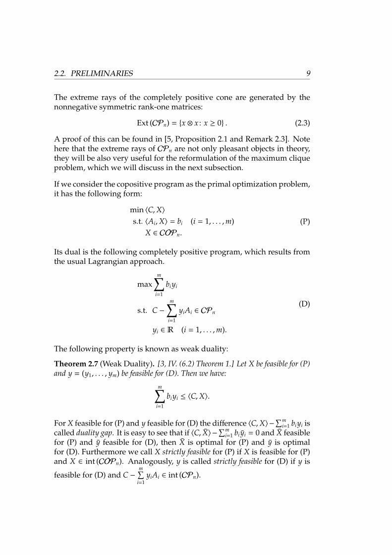
If we consider the copositive program as the primal optimization problem,it has the following form:
min 〈C,X〉s.t. 〈Ai,X〉 = bi (i = 1, . . . ,m)
X ∈ COPn.
(P)
Its dual is the following completely positive program, which results fromthe usual Lagrangian approach.
maxm∑
i=1
biyi
s.t. C −m∑
i=1
yiAi ∈ CPn
yi ∈ R (i = 1, . . . ,m).
(D)
The following property is known as weak duality:
Theorem 2.7 (Weak Duality). [3, IV. (6.2) Theorem 1.] Let X be feasible for (P)and y = (y1, . . . , ym) be feasible for (D). Then we have:
m∑i=1
biyi ≤ 〈C,X〉.
For X feasible for (P) and y feasible for (D) the difference 〈C,X〉−∑m
i=1 biyi iscalled duality gap. It is easy to see that if 〈C, X〉−
∑mi=1 bi yi = 0 and X feasible
for (P) and y feasible for (D), then X is optimal for (P) and y is optimalfor (D). Furthermore we call X strictly feasible for (P) if X is feasible for (P)and X ∈ int (COPn). Analogously, y is called strictly feasible for (D) if y is
feasible for (D) and C −m∑
i=1yiAi ∈ int (CPn).
10 CHAPTER 2. BASIC FACTS ON COPOSITIVE OPTIMIZATION
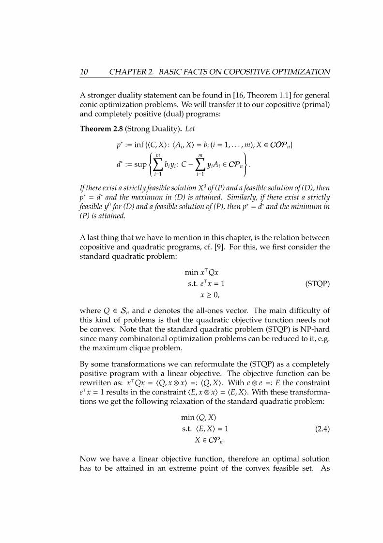
A stronger duality statement can be found in [16, Theorem 1.1] for generalconic optimization problems. We will transfer it to our copositive (primal)and completely positive (dual) programs:
Theorem 2.8 (Strong Duality). Let
p∗ := inf 〈C,X〉 : 〈Ai,X〉 = bi (i = 1, . . . ,m),X ∈ COPn
d∗ := sup
m∑i=1
biyi : C −m∑
i=1
yiAi ∈ CPn
.If there exist a strictly feasible solution X0 of (P) and a feasible solution of (D), thenp∗ = d∗ and the maximum in (D) is attained. Similarly, if there exist a strictlyfeasible y0 for (D) and a feasible solution of (P), then p∗ = d∗ and the minimum in(P) is attained.
A last thing that we have to mention in this chapter, is the relation betweencopositive and quadratic programs, cf. [9]. For this, we first consider thestandard quadratic problem:
min x>Qxs.t. e>x = 1
x ≥ 0,(STQP)
where Q ∈ Sn and e denotes the all-ones vector. The main difficulty ofthis kind of problems is that the quadratic objective function needs notbe convex. Note that the standard quadratic problem (STQP) is NP-hardsince many combinatorial optimization problems can be reduced to it, e.g.the maximum clique problem.
By some transformations we can reformulate the (STQP) as a completelypositive program with a linear objective. The objective function can berewritten as: x>Qx = 〈Q, x ⊗ x〉 =: 〈Q,X〉. With e ⊗ e =: E the constrainte>x = 1 results in the constraint 〈E, x ⊗ x〉 = 〈E,X〉. With these transforma-tions we get the following relaxation of the standard quadratic problem:
min 〈Q,X〉s.t. 〈E,X〉 = 1
X ∈ CPn.
(2.4)
Now we have a linear objective function, therefore an optimal solutionhas to be attained in an extreme point of the convex feasible set. As
2.2. PRELIMINARIES 11
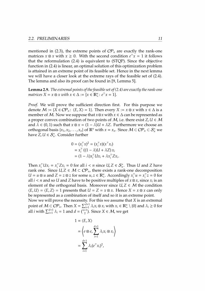
mentioned in (2.3), the extreme points of CPn are exactly the rank-onematrices x ⊗ x with x ≥ 0. With the second condition e>x = 1 it followsthat the reformulation (2.4) is equivalent to (STQP). Since the objectivefunction in (2.4) is linear, an optimal solution of this optimization problemis attained in an extreme point of its feasible set. Hence in the next lemmawe will have a closer look at the extreme rays of the feasible set of (2.4).The lemma and also its proof can be found in [9, Lemma 5].
Lemma 2.9. The extremal points of the feasible set of (2.4) are exactly the rank-onematrices X = x ⊗ x with x ∈ ∆ :=
x ∈ Rn
+ : e>x = 1.
Proof. We will prove the sufficient direction first. For this purpose wedenoteM := X ∈ CPn : 〈E,X〉 = 1. Then every X := x ⊗ x with x ∈ ∆ is amember ofM. Now we suppose that x⊗x with x ∈ ∆ can be represented asa proper convex combination of two points ofM, i.e. there exist Z,U ∈ Mand λ ∈ (0, 1) such that x ⊗ x = (1 − λ)U + λZ. Furthermore we choose anorthogonal basis x1, x2, . . . , xn of Rn with x = xn. SinceM ⊂ CPn ⊂ S
+n we
have Z,U ∈ S+n . Consider further
0 = (x>i x)2 = (x>i x)(x>xi)= x>i ((1 − λ)U + λZ) xi
= (1 − λ)x>i Uxi + λx>i Zxi.
Then x>i Uxi = x>i Zxi = 0 for all i < n since U,Z ∈ S+n . Thus U and Z have
rank one. Since U,Z ∈ M ⊂ CPn, there exists a rank-one decompositionU = u ⊗ u and Z = z ⊗ z for some u, z ∈ Rn
+. Accordingly x>i u = x>i z = 0 forall i < n and so U and Z have to be positive multiples of x⊗ x, since xi is anelement of the orthogonal basis. Moreover since U,Z ∈ M the condition〈E,U〉 = 〈E,Z〉 = 1 presents that U = Z = x ⊗ x. Hence X = x ⊗ x can onlybe represented as a combination of itself and so it is an extreme point.Now we will prove the necessity. For this we assume that X is an extremalpoint ofM ⊂ CPn. Then X =
∑d+1i=1 λixi ⊗ xi with xi ∈ Rn
+ \ 0 and λi ≥ 0 forall i with
∑d+1i=1 λi = 1 and d =
(n+12
). Since X ∈ M, we get
1 = 〈E,X〉
=
⟨e ⊗ e,
d+1∑i=1
λixi ⊗ xi
⟩
=
d+1∑i=1
λi(e>xi)2,
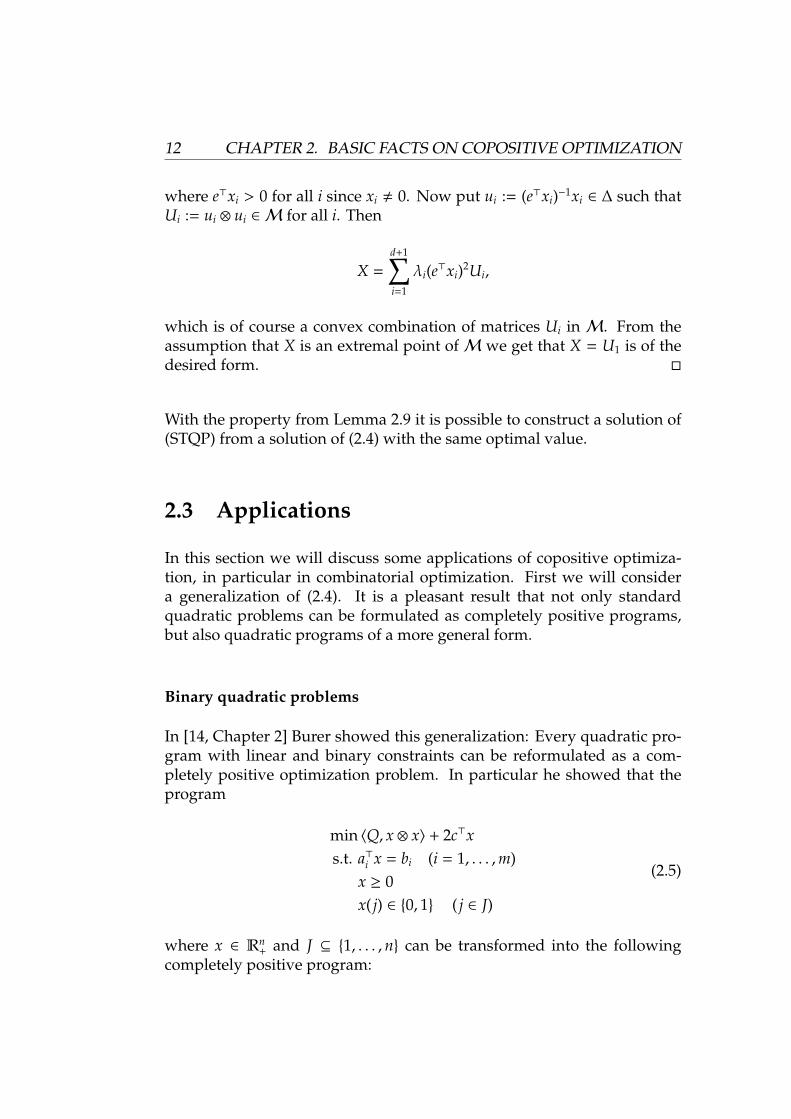
12 CHAPTER 2. BASIC FACTS ON COPOSITIVE OPTIMIZATION
where e>xi > 0 for all i since xi , 0. Now put ui := (e>xi)−1xi ∈ ∆ such thatUi := ui ⊗ ui ∈ M for all i. Then
X =
d+1∑i=1
λi(e>xi)2Ui,
which is of course a convex combination of matrices Ui in M. From theassumption that X is an extremal point ofM we get that X = U1 is of thedesired form.
With the property from Lemma 2.9 it is possible to construct a solution of(STQP) from a solution of (2.4) with the same optimal value.
2.3 Applications
In this section we will discuss some applications of copositive optimiza-tion, in particular in combinatorial optimization. First we will considera generalization of (2.4). It is a pleasant result that not only standardquadratic problems can be formulated as completely positive programs,but also quadratic programs of a more general form.
Binary quadratic problems
In [14, Chapter 2] Burer showed this generalization: Every quadratic pro-gram with linear and binary constraints can be reformulated as a com-pletely positive optimization problem. In particular he showed that theprogram
min 〈Q, x ⊗ x〉 + 2c>xs.t. a>i x = bi (i = 1, . . . ,m)
x ≥ 0x( j) ∈ 0, 1 ( j ∈ J)
(2.5)
where x ∈ Rn+ and J ⊆ 1, . . . ,n can be transformed into the following
completely positive program:
2.3. APPLICATIONS 13
min 〈Q,X〉 + 2c>xs.t. a>i x = bi (i = 1, . . . ,m)
〈ai ⊗ ai,X〉 = b2i (i = 1, . . . ,m)
x( j) = X( j, j) ( j ∈ J)(1 x>
x X
)∈ CPn+1.
This reformulation works only if system (2.5) fulfills the so-called key con-dition, i.e. a>i x = bi for i = 1, . . . ,m and x ≥ 0 implies x( j) ≤ 1 for all j ∈ J.Burer also showed that the key condition can be enforced without loss ofgenerality.
Next we will describe how a special NP-hard combinatorial optimizationproblem can be transferred into a copositive program. In this contextwe will consider in particular the maximum stable set problem and themaximum clique problem.
The maximum stable set problem
In [16] de Klerk and Pasechnik showed that the maximum stable set pro-blem can be transformed into a conic convex optimization problem over thecopositive cone. Unfortunately the copositive program remains NP-hard.
Definition 2.10. Let G = (V,E) be a finite, undirected and simple graphwith set of vertices V and set of edges E ⊆ V ×V. A set of vertices S ⊆ V iscalled a stable set if for every pair i, j ∈ S holds
i, j
< E, where
i, j
denotes
the edge between i and j.
With this definition we can formulate the maximum stable set problem:
α(G) = max |S|s.t. S is a stable set in G,
i.e. finding a stable set S in G of maximal cardinality |S|. α(G) is called thestability number of G.
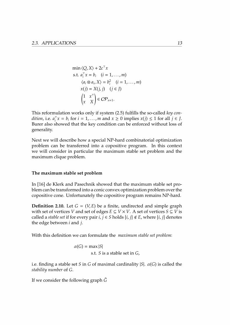
If we consider the following graph G
14 CHAPTER 2. BASIC FACTS ON COPOSITIVE OPTIMIZATION
Figure 2.1: Example graph G
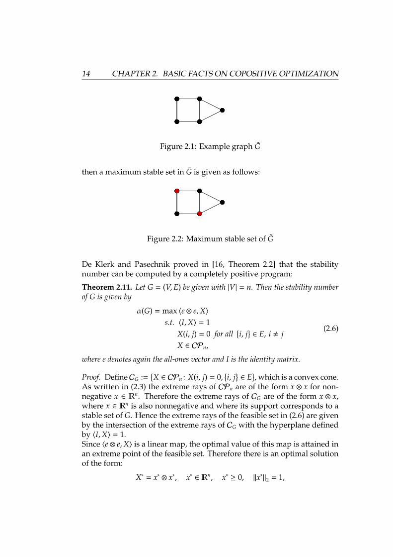
then a maximum stable set in G is given as follows:
Figure 2.2: Maximum stable set of G
De Klerk and Pasechnik proved in [16, Theorem 2.2] that the stabilitynumber can be computed by a completely positive program:
Theorem 2.11. Let G = (V,E) be given with |V| = n. Then the stability numberof G is given by
α(G) = max 〈e ⊗ e,X〉s.t. 〈I,X〉 = 1
X(i, j) = 0 for alli, j
∈ E, i , j
X ∈ CPn,
(2.6)
where e denotes again the all-ones vector and I is the identity matrix.
Proof. DefineCG :=X ∈ CPn : X(i, j) = 0,
i, j
∈ E
, which is a convex cone.
As written in (2.3) the extreme rays of CPn are of the form x ⊗ x for non-negative x ∈ Rn. Therefore the extreme rays of CG are of the form x ⊗ x,where x ∈ Rn is also nonnegative and where its support corresponds to astable set of G. Hence the extreme rays of the feasible set in (2.6) are givenby the intersection of the extreme rays of CG with the hyperplane definedby 〈I,X〉 = 1.Since 〈e ⊗ e,X〉 is a linear map, the optimal value of this map is attained inan extreme point of the feasible set. Therefore there is an optimal solutionof the form:
X∗ = x∗ ⊗ x∗, x∗ ∈ Rn, x∗ ≥ 0, ‖x∗‖2 = 1,
2.3. APPLICATIONS 15
and where the support of x∗ corresponds to a stable set of G, denoted byS∗. We denote now the optimal value of the objective function in (2.6) byλ := max 〈e ⊗ e,X∗〉. Then:
λ = max(e>x)2 : ‖x‖2 = 1, x ≥ 0, supp(x) = supp(x∗)
.
The optimality conditions of this problem imply
x∗ =1√|S∗|
xS∗ ,
where xS∗ denotes the incidence vector of the stable set S∗, i.e. (xS∗)(i) = 1 ifi ∈ S∗ and (xS∗)(i) = 0 otherwise. Therefore we have
λ = (e>x∗)2 =|S∗|2
|S∗|= |S∗|.
Hence S∗ must be a maximum stable set and hence λ = α(G).
Remark 2.12. An essential tool in the proof of Theorem 2.11 is the set ofextreme rays of CPn. Without their characterization the proof of the refor-mulation (2.6) of the maximum stable set problem as completely positiveprogram would not work.Another relevant aspect in this context is that there exists an optimal solu-tion X∗ with X∗ = x∗ ⊗ x∗ and that supp(x∗) corresponds to the vertices ofthe maximum stable set. This follows from the proof of Theorem 2.11.
The dual (copositive) program of (2.6) is the following:
min ts.t. t ∈ R, K ∈ COPn
K(i, i) = t − 1 for all i ∈ VK(i, j) = −1 for all
i, j
< E.
(2.7)
Although the copositive formulation (2.7) of the maximum stable set pro-blem remains NP-hard, this formulation has the advantage that the com-plexity is moved entirely into the copositivity constraint. The new for-mulation is a convex optimization problem with linear objective, linearconstraints and one cone constraint.
16 CHAPTER 2. BASIC FACTS ON COPOSITIVE OPTIMIZATION
The maximum clique problem
Another well-known NP-hard problem in combinatorial optimization isthe maximum clique problem. This problem is equivalent to the maximumstable set problem in the complementary graph. The complementary graphG of a graph G is defined by the same set of vertices as G and two differentvertices in G are connected by an edge if and only if they were not connectedin G. For a survey of the maximum clique problem see [8]. In this sectionwe will show that this problem can be reformulated as a copositive andcompletely positive program, respectively.
Definition 2.13. Let G = (V,E) be a finite, undirected and simple graphwith set of vertices V and set of edges E ⊆ V × V. A clique of G is a subsetC of vertices such that every pair of vertices in C is joined by an edge.
With this definition the maximum clique problem is given by:
ω(G) = max |C|s.t. C is a clique in G,
i.e. finding a clique set C in G of maximal cardinality |C|. ω(G) is called theclique number of G.
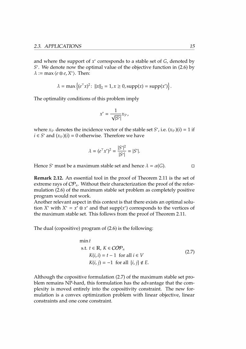
A maximum clique of the graph G in Figure 2.1 is the following:
Figure 2.3: Maximum clique of G
We denote now by AG the adjacency matrix of a graph G. Motzkin andStraus [40] showed the following equality:
1ω(G)
= minx>(e ⊗ e − AG)x : e>x = 1, x ≥ 0
, (2.8)
where e denotes the all-ones vector as before. If we combine the Motzkin-Straus formulation (2.8) with the completely positive formulation (2.4), weget:
1ω(G)
= min 〈e ⊗ e − AG,X〉 : 〈e ⊗ e,X〉 = 1,X ∈ CPn .
2.4. APPROXIMATION HIERARCHIES 17
Then its dual is:
1ω(G)
= max λ : λ(e ⊗ e − AG) − e ⊗ e ∈ COPn ,
cf. [25, Chapter 2]. In particular strong duality holds. As in the maximumstable set reformulation, the complexity of the reformulation is entirely inthe cone constraint since we have a convex program with a linear objective,linear constraints and the cone constraint. Furthermore a discrete programchanged to a continuous one.
2.4 Approximation hierarchies
In the last part of this chapter we will discuss some approximation hierar-chies of the copositive cone. Since checking whether a matrix is copositiveis NP-hard it is important to think about an easier way to check copositivityby approximating the copositive cone. The easiest way to approximatingthe copositive cone is of course to replace it by the positive semidefinitecone. Here we will present three popular approximation techniques, whichlead to approximation hierarchies.
The first approximation is based on the following idea: By definition amatrix A ∈ Rn×n is copositive if and only if the quadratic form z>Az isnonnegative for all nonnegative arguments z. Equivalently for a givensymmetric matrix A and x ∈ Rn the following polynomial can be consid-ered:
PA(x) :=n∑
i=1
n∑j=1
A(i, j)x(i)2x( j)2.
In conclusion A is copositive if and only if PA(x) ≥ 0 for all x ∈ Rn. Asufficient condition for this nonnegativity is that PA(x) has a representationas a sum of squares of polynomials, i.e.
PA(x) =
l∑i=1
fi(x)2 for all x ∈ Rn
for some polynomial functions f1(x), . . . , fl(x). Then it is easy to see thatPA(x) ≥ 0 for all x ∈ Rn. Parrilo showed in [42] that PA(x) has such arepresentation as a sum of squares if and only if A ∈ S+
n +Nn. For a given
18 CHAPTER 2. BASIC FACTS ON COPOSITIVE OPTIMIZATION
matrix A ∈ Rn×n we consider the following family of polynomials:
Pr(x) :=
n∑k=1
x(k)2
r
· PA(x).
It is clear that P0(x) = PA(x). Furthermore if for some r we have Pr(x) ≥ 0for all x, then PA(x) ≥ 0 for all x. Moreover if Pr(x) has a sum of squaresdecomposition, then Pr+1(x) also has a sum of squares decomposition. Withthis property Parrilo [42] defined the following hierarchy of cones forr ∈N0:
Krn :=
A ∈ Sn : PA(x) ·
n∑i=1
x(i)2
r
has a sum of squares decomposition
.Parrilo also showed that S+
n + Nn = K 0n ⊂ K
1n ⊂ . . . ⊂ COPn and that
int (COPn) ⊆⋃
r∈N0K
rn. Therefore the convex cone K r
n approximates thecopositive cone COPn from the interior. The condition A ∈ K r
n can bechecked by solving a semidefinite feasibility problem. So the related opti-mization problem overK r
n is equivalent to a semidefinite program.
Another approach has been introduced by de Klerk and Pasechnik [16].They approximated the copositive cone by a system of linear inequalities.For this we consider again the polynomial PA(x) =
∑ni=1
∑nj=1 A(i, j)x(i)2x( j)2
with x ∈ Rn. Another sufficient condition for its nonnegativity is that allcoefficients of PA(x) are nonnegative, i.e. A(i, j) ≥ 0 for all i, j. This propertyis equivalent to A ∈ Nn. For r ∈N0 and Pr(x) =
(∑nk=1 x(k)2)r PA(x) as before
the authors defined the convex cone
Crn :=
A ∈ Sn : PA(x) ·
n∑i=1
x(i)2
r
has nonnegative coefficients
.De Klerk and Pasechnik verified that Nn = C0
n ⊂ C1n ⊂ . . . ⊂ COPn and
int (COPn) ⊆⋃
r∈N0C
rn. Accordingly the convex cone Cr
n also approximatesthe copositive cone from the interior. Since all of these cones Cr
n are poly-hedral cones, the related optimization problem corresponds to a linearprogram.
Between the two hierarchies of cones the following relation holds true:
Crn ⊆ K
rn for all r ∈N0.
The last approximation we want to illustrate, goes back to Peña et al.[44]. The authors used the standard multiindex notation, i.e. for a given
2.4. APPROXIMATION HIERARCHIES 19
multiindex β ∈Nn we have |β| := β1 + . . .+ βn and xβ := xβ1
1 . . . xβnn . With this
notation the following set can be defined:
Ern :=
∑β∈Nn,|β|=r
xβx>(Sβ + Nβ)x : Sβ ∈ S+n ,Nβ ∈ Nn
.This approach is based on the fact that a matrix, which can be representedas the sum of a positive semidefinite matrix and an entrywise nonnegativematrix, is copositive, cf. (2.2). Furthermore Peña et al. defined the followingcone:
Qrn :=
A ∈ Sn : x>Ax
n∑i=1
x(i)2
r
∈ Ern
.They were also able to show that Cr
n ⊆ Qrn ⊆ K
rn for all r ∈N0. In particular
Qrn = K r
n for r ∈ 0, 1. Therefore also Qrn grows with r. The condition
A ∈ Qrn can be written as a system of linear matrix inequalities, hence if
COPn is replaced by the cone Qrn, the resulting optimization problem is a
positive semidefinite program.
Note that all convex cones K rn, Cr
n and Qrn have pleasant theoretical prop-
erties, but a fundamental aspect is that they approximate the copositivecone uniformly. There are other techniques to approximate the copositivecone in a certain direction more precisely, e.g. approximate COPn via par-titions of the standard simplex into smaller simplices [12]. By using theobjective function to figure out which simplices have to be splitted further,this method can approximateCOPn in the needed direction more precisely.This technique also leads to linear programs.
In this chapter we formulated and proved some basics of copositive op-timization in finite dimension. We defined the copositive as well as thecompletely positive cone and their properties and furthermore the relatedoptimization problems. These results can be used among other things toreformulate the standard quadratic problem (STQP) and also a more gen-eral form of a quadratic program (2.5) into a completely positive program.Moreover we presented some applications of copositive and completelypositive programs, respectively, especially in combinatorial optimization.Besides the stability number and the clique number, many other quantitiesin combinatorial optimization can be calculated by solving a copositiveprogram. An overview of the applications of copositive optimization can
20 CHAPTER 2. BASIC FACTS ON COPOSITIVE OPTIMIZATION
be found in [7, 13, 25]. Finally we gave some approximation hierarchies ofthe copositive cone.
Chapter 3
Relevant tools from functionalanalysis
In this chapter we will introduce some important aspects from functionalanalysis. We will also define three special norms: the (symmetric) pro-jective norm, the (symmetric) injective norm and the (symmetric) Hilbert-Schmidt norm. Especially the symmetric projective norm gives us helpfulhints for our goal to generalize the principle of copositivity and its dualityin a suitable infinite dimensional space.
3.1 Preliminaries
Our notation concerning Banach spaces is the standard one, like e.g. in [46].A Banach space is a normed space which is complete in the metric definedby its norm. Or in other words, every Cauchy sequence is required toconverge. Many of the well-known function spaces are Banach spaces. Forexample the spaces of continuous functions on compact sets, the Lp
−spaces(i.e. the space of classes of p-integrable functions), Hilbert spaces, or thespaces of continuous linear maps from one Banach space into another areBanach spaces.
3.2 The tensor product of two vector spaces
We consider in this thesis real vector spaces only, i.e. vector spaces over thefieldR of real numbers. First we will consider two fundamental examples:
21
22 CHAPTER 3. RELEVANT TOOLS FROM FUNCTIONAL ANALYSIS
Example 3.1. For m,n ∈N as well as u ∈ Rm = R1,...,m and v ∈ Rn = R1,...,n,let u ⊗ v ∈ Rm×n = R1,...,m×1,...,n be defined by
u ⊗ v (i, j) := u(i) v( j), for 1 ≤ i ≤ m, 1 ≤ j ≤ n.
We set
Rm⊗Rn := span u ⊗ v : u ∈ Rm, v ∈ Rn
and calculate
Rm⊗Rn = Rm×n,
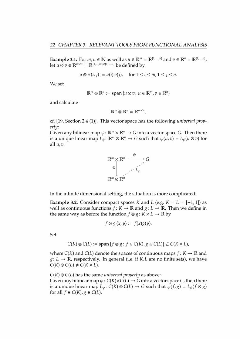
cf. [19, Section 2.4 (1)]. This vector space has the following universal prop-erty:Given any bilinear map ψ : Rm
×Rn→ G into a vector space G. Then there
is a unique linear map Lψ : Rm⊗ Rn
→ G such that ψ(u, v) = Lψ(u ⊗ v) forall u, v.
Rm×Rn
ψG
⊗
Rm⊗Rn
Lψ
In the infinite dimensional setting, the situation is more complicated:
Example 3.2. Consider compact spaces K and L (e.g. K = L = [−1, 1]) aswell as continuous functions f : K → R and g : L → R. Then we define inthe same way as before the function f ⊗ g : K × L→ R by
f ⊗ g (x, y) := f (x)g(y).
Set
C(K) ⊗ C(L) := spanf ⊗ g : f ∈ C(K), g ∈ C(L)
⊆ C(K × L),
where C(K) and C(L) denote the spaces of continuous maps f : K→ R andg : L → R, respectively. In general (i.e. if K,L are no finite sets), we haveC(K) ⊗ C(L) , C(K × L).
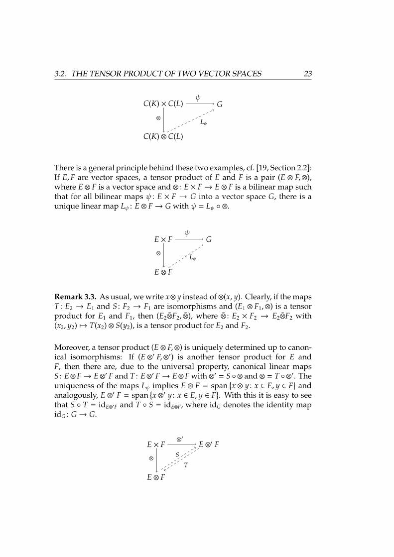
C(K) ⊗ C(L) has the same universal property as above:Given any bilinear mapψ : C(K)×C(L)→ G into a vector space G, then thereis a unique linear map Lψ : C(K) ⊗ C(L) → G such that ψ( f , g) = Lψ( f ⊗ g)for all f ∈ C(K), g ∈ C(L).
3.2. THE TENSOR PRODUCT OF TWO VECTOR SPACES 23
C(K) × C(L)ψ
G
⊗
C(K) ⊗ C(L)
Lψ
There is a general principle behind these two examples, cf. [19, Section 2.2]:If E,F are vector spaces, a tensor product of E and F is a pair (E ⊗ F,⊗),where E ⊗ F is a vector space and ⊗ : E × F→ E ⊗ F is a bilinear map suchthat for all bilinear maps ψ : E × F → G into a vector space G, there is aunique linear map Lψ : E ⊗ F→ G with ψ = Lψ ⊗.
E × Fψ
G
⊗
E ⊗ F
Lψ
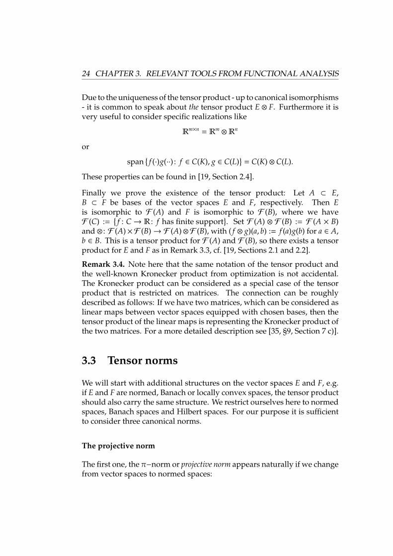
Remark 3.3. As usual, we write x⊗ y instead of ⊗(x, y). Clearly, if the mapsT : E2 → E1 and S : F2 → F1 are isomorphisms and (E1 ⊗ F1,⊗) is a tensorproduct for E1 and F1, then (E2⊗F2, ⊗), where ⊗ : E2 × F2 → E2⊗F2 with(x2, y2) 7→ T(x2) ⊗ S(y2), is a tensor product for E2 and F2.
Moreover, a tensor product (E ⊗ F,⊗) is uniquely determined up to canon-ical isomorphisms: If (E ⊗′ F,⊗′) is another tensor product for E andF, then there are, due to the universal property, canonical linear mapsS : E⊗F→ E⊗′ F and T : E⊗′ F→ E⊗F with ⊗′ = S ⊗ and ⊗ = T ⊗′. Theuniqueness of the maps Lψ implies E ⊗ F = span
x ⊗ y : x ∈ E, y ∈ F
and
analogously, E ⊗′ F = spanx ⊗′ y : x ∈ E, y ∈ F
. With this it is easy to see
that S T = idE⊗′F and T S = idE⊗F, where idG denotes the identity mapidG : G→ G.
E × F⊗′
E ⊗′ F
⊗
E ⊗ F
S
T
24 CHAPTER 3. RELEVANT TOOLS FROM FUNCTIONAL ANALYSIS
Due to the uniqueness of the tensor product - up to canonical isomorphisms- it is common to speak about the tensor product E ⊗ F. Furthermore it isvery useful to consider specific realizations like
Rm×n = Rm⊗Rn
or
spanf (·)g(··) : f ∈ C(K), g ∈ C(L)
= C(K) ⊗ C(L).
These properties can be found in [19, Section 2.4].
Finally we prove the existence of the tensor product: Let A ⊂ E,B ⊂ F be bases of the vector spaces E and F, respectively. Then Eis isomorphic to F (A) and F is isomorphic to F (B), where we haveF (C) :=
f : C→ R : f has finite support
. Set F (A) ⊗ F (B) := F (A × B)
and ⊗ : F (A)×F (B)→ F (A)⊗F (B), with ( f ⊗ g)(a, b) := f (a)g(b) for a ∈ A,b ∈ B. This is a tensor product for F (A) and F (B), so there exists a tensorproduct for E and F as in Remark 3.3, cf. [19, Sections 2.1 and 2.2].
Remark 3.4. Note here that the same notation of the tensor product andthe well-known Kronecker product from optimization is not accidental.The Kronecker product can be considered as a special case of the tensorproduct that is restricted on matrices. The connection can be roughlydescribed as follows: If we have two matrices, which can be considered aslinear maps between vector spaces equipped with chosen bases, then thetensor product of the linear maps is representing the Kronecker product ofthe two matrices. For a more detailed description see [35, §9, Section 7 c)].
3.3 Tensor norms
We will start with additional structures on the vector spaces E and F, e.g.if E and F are normed, Banach or locally convex spaces, the tensor productshould also carry the same structure. We restrict ourselves here to normedspaces, Banach spaces and Hilbert spaces. For our purpose it is sufficientto consider three canonical norms.
The projective norm
The first one, the π−norm or projective norm appears naturally if we changefrom vector spaces to normed spaces:
3.3. TENSOR NORMS 25
Definition 3.5. Let E, F be normed spaces. For z ∈ E ⊗ F set
π(z) := π(z; E,F) := inf
n∑ν=1
‖xν‖E∥∥∥yν
∥∥∥F
: n ∈N, z =
n∑ν=1
xν ⊗ yν
.Then π is a norm and has the following universal property:If ψ : E × F → G is a continuous bilinear map with values in a normedspace G, then there is a unique continuous linear map Lψ : (E ⊗ F, π) → Gsuch that ψ = Lψ ⊗. Moreover,∥∥∥ψ∥∥∥ := sup
‖x‖E≤1‖y‖F≤1
∥∥∥ψ(x, y)∥∥∥
G
= sup‖x‖E≤1‖y‖F≤1
∥∥∥Lψ(x ⊗ y)∥∥∥
G
= supπ(z)≤1
∥∥∥Lψ(z)∥∥∥
G
=:∥∥∥Lψ
∥∥∥ .With E⊗πF we will denote the tensor product E⊗F equipped withπ(·; E,F).
In the next proposition we will formulate some properties of π, cf. [19,Section 3.2]. For normed spaces E, F and G we denote by L(E,F) the setof linear maps from E to F. Moreover we denote the set of linear andcontinuous functions by L(E,F) := T : E→ F : T linear and continuousand we denote by B(E,F; G) := B : E × F→ G : B bilinear and continuousthe set of continuous and bilinear functions, where bilinear means linearin each variable. Furthermore E′ := L(E,R) denotes the (topological) dual
of E. Last we denote by E 1= F that E and F are isometric.
Proposition 3.6. Let E, F be normed spaces, then:
1.
B(E,F; G) 1= L(E ⊗π F,G)
and π is the unique seminorm on E ⊗ F which has this property for G = R.In particular,
π(z; E,F) = max | 〈S, z〉 | : S ∈ L(E,F′), ‖S‖ ≤ 1
26 CHAPTER 3. RELEVANT TOOLS FROM FUNCTIONAL ANALYSIS
and the duality bracket given by
(E ⊗π F)′ 1= B(E,F;R) 1
= L(E,F′)
can be calculated by the trace duality.
2. π(x ⊗ y; E,F) = ‖x‖E∥∥∥y
∥∥∥F
for all (x, y) ∈ E × F.
3. π is finitely generated, i.e. for all z ∈ E ⊗ F
π(z; E,F) = infπ(z; M,N) : z ∈M ⊗N,M ⊂ E,N ⊂ F,
dim(M),dim(N) < ∞.
Special situations concerning the projective norm are stated in the nextexample. These examples give a concrete setting to calculate the projectivenorm:
Example 3.7. 1. If E = Rm and F = Rn equipped with ‖·‖1, then onE ⊗ F = Rm×n we have
π(z) =
m∑i=1
n∑j=1
|z(i, j)|,
where z = (z(i, j))(i, j) ∈ Rm×n, cf. [30, Example 4.47].
2. More generally, if µ and ν are σ-finite measures on measure spaces Xand Y, we have for the spaces E = L1(µ) and F = L1(ν) as well as forf ∈ E ⊗ F = span
g(·)h(··) : g ∈ L1(µ), h ∈ L1(ν)
that
π( f ) =
∫X×Y| f (x, y)| d(µ ⊗ ν)(x, y) =
∥∥∥ f∥∥∥
L1(µ⊗ν),
cf. [19, Section 3.3 Proposition].
3. If E = Rm and F = Rn equipped with the Euclidean norm ‖·‖2, then
π(z) =
k∑ν=0
λν,
where 0 ≤ λ0 ≤ . . . ≤ λk are the singular values of z ∈ Rm⊗Rn = Rm×n,
cf. [48, Example 2.10].
Remark 3.8. Example 3.7 can be generalized to Hilbert spaces E and F, cf.[19, Ex 3.28].
3.3. TENSOR NORMS 27
The injective norm
The second tensor norm we want to consider is the ε−norm or injectivenorm, which is the dual norm of the projective norm.
Definition 3.9. If E and F are normed spaces, then for z ∈ E ⊗ F we define:
ε(z) := ε(z; E,F) : = sup|⟨x′ ⊗ y′, z
⟩| : ‖x′‖E′ ≤ 1,
∥∥∥y′∥∥∥
F′≤ 1
= sup
∣∣∣ n∑ν=1
x′(xν)y′(yν)∣∣∣ : ‖x′‖E′ ≤ 1,
∥∥∥y′∥∥∥
F′≤ 1
,if z =
∑nν=1 xν ⊗ yν. We write E ⊗ε F for E ⊗ F equipped with ε(·; E,F).
As mentioned in [19, Section 4.3] the norm ε behaves in a dual way to πconcerning subspaces and quotients, i.e. ε respects subspaces isometricallyand ε does not respect quotients.
Remark 3.10. The injective norm ε is the dual norm of the projective normπ in the sense of trace duality. But the converse property that π is thedual of ε, does not hold in this sense, cf. [19, Section 6.1]. This meansthat (E⊗εE)′ , E′⊗πE′ in general. But in the finite case this equality holds.Trace duality means as formulated in [19, Section 2.6]: Let φ ∈ (E⊗F)′ withassociated map T ∈ L(E,F′) and z ∈ E ⊗ F with associated S ∈ L(F′,E) withfinite rank. Then we have
⟨φ, z
⟩= trE(S T) = trF′(T S).
For the next proposition we need the following definition:
Definition 3.11. A subset A ⊂ BE′ is called norming if for all x ∈ E
‖x‖E = sup | 〈x′, x〉 | : x′ ∈ A .
For a normed space E we note by BE the closed unit ball x ∈ E : ‖x‖E ≤ 1.
The following proposition gives some properties of the injective norm:
Proposition 3.12. [19, Section 4.1] Let E, F be normed spaces. Then:
1. If E and F are finite dimensional, then
E ⊗ε F 1= (E′ ⊗π F′)′.
2. ε(x ⊗ y; E,F) = ‖x‖E∥∥∥y
∥∥∥F
for all x ∈ E, y ∈ F.
28 CHAPTER 3. RELEVANT TOOLS FROM FUNCTIONAL ANALYSIS
3. ε ≤ π on E ⊗ F.
4. For norming subsets A ⊂ BE′ and B ⊂ BF′ we have
ε(z; E,F) = sup|⟨x′ ⊗ y′, z
⟩| : x′ ∈ A, y′ ∈ B
.
The following examples present a way to calculate the injective norm intwo special situations.
Example 3.13. 1. If E = Rm and F = Rn are equipped with ‖·‖∞, then onE ⊗ F = Rm×n we have
ε(z) = sup1≤i≤m1≤ j≤n
|z(i, j)|,
where z = (z(i, j))(i, j) ∈ Rm×n, cf. [30, Remark 4.64].
2. More generally, if K, L are compact spaces, f ∈ C(K) ⊗ C(L), then wehave
C(K) ⊗ C(L) =
f ∈ C(K × L) : ∃n ∈N, gν ∈ C(K), hν ∈ C(L) :
f (·, ··) =
n∑ν=1
gν(·)hν(··),
cf. [19, Section 2.4. (2)] and moreover
ε( f ) = sup| f (x, y)| : (x, y) ∈ K × L
.
Duality of norms
Before we consider a third norm, we will discuss the definition of a dualnorm in infinite dimension, cf. [48, Chapter 7.1]. In finite dimension thedefinition of the dual norm is clear: If E and F are finite dimensionalnormed spaces and α is a tensor norm, then E ⊗ F is algebraically the dualspace of E′ ⊗α F′ and we set α′ to be the dual norm such that
E ⊗α′ F = (E′ ⊗α F′)′ .
I.e. if u ∈ E ⊗ F, then
α′(u) = sup | 〈u, v〉 | : v ∈ E′ ⊗ F′, α(v) ≤ 1 . (3.1)
3.3. TENSOR NORMS 29
In the sense of trace duality, this means that the duality between E⊗ F andE′ ⊗ F′ works in the following way: If we consider u as an operator fromE′ to F and v from F into E′, then 〈u, v〉 = tr(v u).
To get a definition of the dual norm in infinite dimension, Ryan [48, Chapter7.1] uses [48, Proposition 6.3] to extend the definition in finite dimension.With that, the dual norm α′ is defined as the unique tensor norm thatcorresponds with the dual norm on tensor products of finite dimensionalspaces. Let u ∈ X ⊗ Y, where X and Y have to be Banach spaces, then:
α′(u) = infα′E,F(u) : u ∈ E ⊗ F,E ⊆ X,F ⊆ Y,dim E,dim F < ∞
,
where α′E,F(u) = α′(u; E ⊗ F).
The Hilbert-Schmidt norm
Now we have a look at the third norm. If the vector spaces Gand H are equipped with scalar products 〈·, ·〉G and 〈·, ·〉H, there is auniquely determined scalar product 〈·, ·〉G⊗H on G ⊗ H with the property⟨x1 ⊗ y1, x2 ⊗ y2
⟩G⊗H = 〈x1, x2〉G
⟨y1, y2
⟩H for all x1, x2 ∈ G, y1, y2 ∈ H, cf. [19,
Section 26.7]. The norm σ := σ(·; G,H), with
σ(z) :=√〈z, z〉G⊗H
is called the Hilbert-Schmidt norm on G ⊗ H and we write G ⊗σ H for thenormed space (G ⊗ H, σ). Note that the Hilbert-Schmidt norm is onlydefined for vector spaces that are equipped with a scalar product.
Remark 3.14. Note that the dual norm of the Hilbert-Schmidt norm is againthe Hilbert-Schmidt norm, i.e. σ′ = σ, cf. [19, Section 26.7, Corollary 2].
Last we will give a special example for the Hilbert-Schmidt norm:
Example 3.15. If G = Rm, H = Rn, then on G ⊗H = Rm×n we have
〈w, z〉G⊗H =
m∑i=1
n∑j=1
w(i, j)z(i, j)
for w = (w(i, j))(i, j), z = (z(i, j))(i, j) ∈ Rm×n and σ(w) =(∑m
i=1∑n
j=1 |w(i, j)|2)1/2
,cf. [19, Section 26.7].
30 CHAPTER 3. RELEVANT TOOLS FROM FUNCTIONAL ANALYSIS
The completions in Banach spaces
If we consider the context of Banach spaces (or particularly in the context ofHilbert spaces), the „tensor products “ should be of the same form. Therewe consider the completions
E⊗πF of E ⊗π F,E⊗εF of E ⊗ε F,
and G⊗σH of G ⊗σ H.
By definition the first two spaces are Banach spaces and the third one iseven a Hilbert space. It can be proven that
L1(µ)⊗πL1(ν) 1= L1(µ ⊗ ν),
C(K)⊗εC(L) 1= C(K × L),
L2(µ)⊗σL2(ν) 1= L2(µ ⊗ ν),
cf. [19, Ex 3.27 and Section 4.2 (3)] and [34, 2.6.11 Example]. In case of twoHilbert spaces G and H we have
• G′⊗πH is canonically isomorphic to the space of nuclear operatorsfrom G to H,
• G′⊗εH is canonically isomorphic to the space of compact operatorsfrom G to H,
• G′⊗σH is canonically isomorphic to the space of Hilbert-Schmidt op-erators from G to H,
with∑nν=1 x′ν ⊗ yν 7→
∑nν=1 x′ν(·)yν.
3.4 Algebraic theory of symmetric tensor prod-ucts
In this section we are going to define a symmetric tensor product, whichhas the same universal property only for symmetric bilinear maps insteadof all bilinear maps, as it is in the case in the full tensor product E ⊗ F.
3.4. ALGEBRAIC THEORY OF SYMMETRIC TENSOR PRODUCTS 31
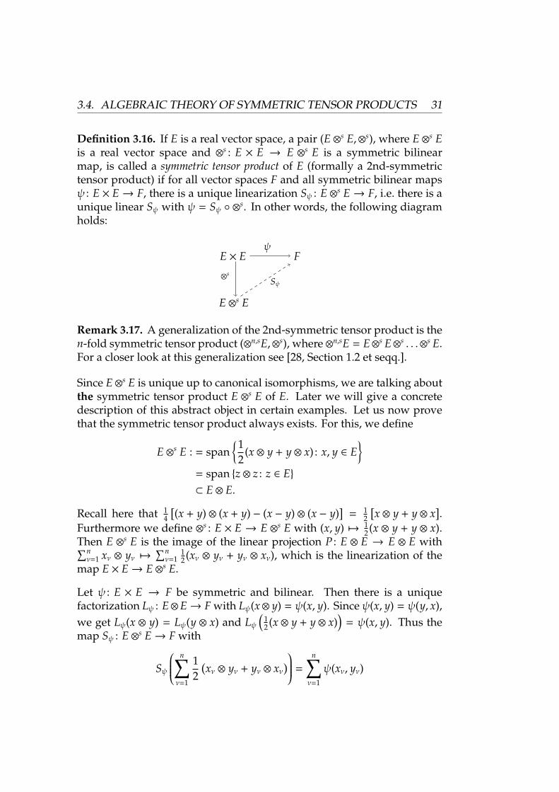
Definition 3.16. If E is a real vector space, a pair (E ⊗s E,⊗s), where E ⊗s Eis a real vector space and ⊗s : E × E → E ⊗s E is a symmetric bilinearmap, is called a symmetric tensor product of E (formally a 2nd-symmetrictensor product) if for all vector spaces F and all symmetric bilinear mapsψ : E × E→ F, there is a unique linearization Sψ : E ⊗s E→ F, i.e. there is aunique linear Sψ with ψ = Sψ ⊗s. In other words, the following diagramholds:
E × Eψ
F
⊗s
E ⊗s E
Sψ
Remark 3.17. A generalization of the 2nd-symmetric tensor product is then-fold symmetric tensor product (⊗n,sE,⊗s), where ⊗n,sE = E⊗s E⊗s . . .⊗s E.For a closer look at this generalization see [28, Section 1.2 et seqq.].
Since E ⊗s E is unique up to canonical isomorphisms, we are talking aboutthe symmetric tensor product E ⊗s E of E. Later we will give a concretedescription of this abstract object in certain examples. Let us now provethat the symmetric tensor product always exists. For this, we define
E ⊗s E : = span1
2(x ⊗ y + y ⊗ x) : x, y ∈ E
= span z ⊗ z : z ∈ E⊂ E ⊗ E.
Recall here that 14
[(x + y) ⊗ (x + y) − (x − y) ⊗ (x − y)
]= 1
2
[x ⊗ y + y ⊗ x
].
Furthermore we define ⊗s : E × E → E ⊗s E with (x, y) 7→ 12 (x ⊗ y + y ⊗ x).
Then E ⊗s E is the image of the linear projection P : E ⊗ E → E ⊗ E with∑nν=1 xν ⊗ yν 7→
∑nν=1
12 (xν ⊗ yν + yν ⊗ xν), which is the linearization of the
map E × E→ E ⊗s E.
Let ψ : E × E → F be symmetric and bilinear. Then there is a uniquefactorization Lψ : E⊗E→ F with Lψ(x⊗ y) = ψ(x, y). Since ψ(x, y) = ψ(y, x),we get Lψ(x ⊗ y) = Lψ(y ⊗ x) and Lψ
(12 (x ⊗ y + y ⊗ x)
)= ψ(x, y). Thus the
map Sψ : E ⊗s E→ F with
Sψ
n∑ν=1
12(xν ⊗ yν + yν ⊗ xν
) =
n∑ν=1
ψ(xν, yν)
32 CHAPTER 3. RELEVANT TOOLS FROM FUNCTIONAL ANALYSIS
is well-defined, linear and satisfies
ψ(x, y) = Sψ(12(x ⊗ y + y ⊗ x
)).
If S : E ⊗s E→ F is linear, we write
S(12(x ⊗ y + y ⊗ x
))= ψ(x, y) = Sψ
(12(x ⊗ y + y ⊗ x
)).
Then by linearity we have S = Sψ on E ⊗s E.
3.5 Symmetric tensor norms
As in the case of the tensor product of normed spaces (or spaces with scalarproduct) in Section 3.3, we consider here in an analogous way the sym-metric projective norm, the symmetric injective norm and the symmetricHilbert-Schmidt norm on the symmetric tensor product.
Therefore we consider from now on only symmetric tensor products of theform E ⊗s E, where E is either a normed space or a Banach space and theindex s denotes that it is symmetric.
The symmetric projective norm
We will start with the analogue of the π-norm for a symmetric tensorproduct, which is the so-called symmetric projective norm πs:
Definition 3.18. Let E be a normed space. For z ∈ E ⊗s E we set
πs(z) := πs(z; E,E) := inf
m∑ν=1
‖xν‖2E : m ∈N, z =
m∑ν=1
±xν ⊗ xν
.Note that ± is meant summandwise, i.e. it depends on the summationindex ν.
Remark 3.19. [28, Section 2.3] The following relation between the projectivenorm and the symmetric projective norm holds:
π(z) ≤ πs(z) ≤ 2π(z),
for all z ∈ E ⊗s E.
3.5. SYMMETRIC TENSOR NORMS 33
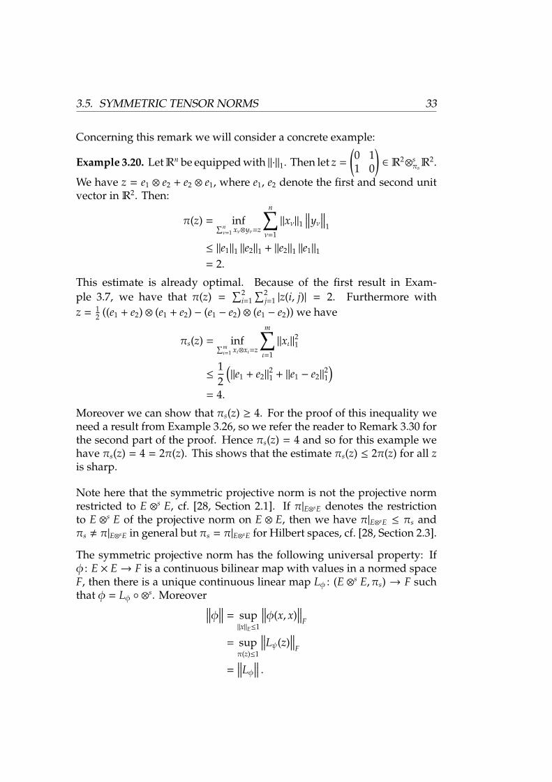
Concerning this remark we will consider a concrete example:
Example 3.20. LetRn be equipped with ‖·‖1. Then let z =
(0 11 0
)∈ R2
⊗sπsR2.
We have z = e1 ⊗ e2 + e2 ⊗ e1, where e1, e2 denote the first and second unitvector in R2. Then:
π(z) = inf∑nν=1 xν⊗yν=z
n∑ν=1
‖xν‖1∥∥∥yν
∥∥∥1
≤ ‖e1‖1 ‖e2‖1 + ‖e2‖1 ‖e1‖1
= 2.
This estimate is already optimal. Because of the first result in Exam-ple 3.7, we have that π(z) =
∑2i=1
∑2j=1 |z(i, j)| = 2. Furthermore with
z = 12 ((e1 + e2) ⊗ (e1 + e2) − (e1 − e2) ⊗ (e1 − e2)) we have
πs(z) = inf∑mι=1 xι⊗xι=z
m∑ι=1
‖xι‖21
≤12
(‖e1 + e2‖
21 + ‖e1 − e2‖
21
)= 4.
Moreover we can show that πs(z) ≥ 4. For the proof of this inequality weneed a result from Example 3.26, so we refer the reader to Remark 3.30 forthe second part of the proof. Hence πs(z) = 4 and so for this example wehave πs(z) = 4 = 2π(z). This shows that the estimate πs(z) ≤ 2π(z) for all zis sharp.
Note here that the symmetric projective norm is not the projective normrestricted to E ⊗s E, cf. [28, Section 2.1]. If π|E⊗sE denotes the restrictionto E ⊗s E of the projective norm on E ⊗ E, then we have π|E⊗sE ≤ πs andπs , π|E⊗sE in general but πs = π|E⊗sE for Hilbert spaces, cf. [28, Section 2.3].
The symmetric projective norm has the following universal property: Ifφ : E × E→ F is a continuous bilinear map with values in a normed spaceF, then there is a unique continuous linear map Lφ : (E ⊗s E, πs) → F suchthat φ = Lφ ⊗s. Moreover∥∥∥φ∥∥∥ = sup
‖x‖E≤1
∥∥∥φ(x, x)∥∥∥
F
= supπ(z)≤1
∥∥∥Lψ(z)∥∥∥
F
=∥∥∥Lφ
∥∥∥ .
34 CHAPTER 3. RELEVANT TOOLS FROM FUNCTIONAL ANALYSIS
With E ⊗sπs
E we will denote the tensor product E ⊗s E equipped withπs(·; E,E).
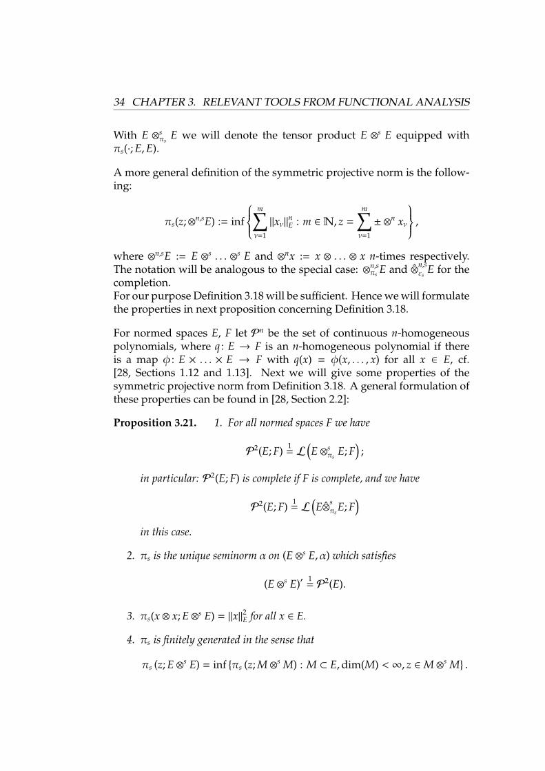
A more general definition of the symmetric projective norm is the follow-ing:
πs(z;⊗n,sE) := inf
m∑ν=1
‖xν‖nE : m ∈N, z =
m∑ν=1
± ⊗n xν
,where ⊗n,sE := E ⊗s . . . ⊗s E and ⊗nx := x ⊗ . . . ⊗ x n-times respectively.The notation will be analogous to the special case: ⊗n,s
πs E and ⊗n,sεs
E for thecompletion.For our purpose Definition 3.18 will be sufficient. Hence we will formulatethe properties in next proposition concerning Definition 3.18.
For normed spaces E, F let Pn be the set of continuous n-homogeneouspolynomials, where q : E → F is an n-homogeneous polynomial if thereis a map φ : E × . . . × E → F with q(x) = φ(x, . . . , x) for all x ∈ E, cf.[28, Sections 1.12 and 1.13]. Next we will give some properties of thesymmetric projective norm from Definition 3.18. A general formulation ofthese properties can be found in [28, Section 2.2]:
Proposition 3.21. 1. For all normed spaces F we have
P2(E; F) 1
= L(E ⊗s
πsE; F
);
in particular: P2(E; F) is complete if F is complete, and we have
P2(E; F) 1
= L(E⊗s
πsE; F
)in this case.
2. πs is the unique seminorm α on (E ⊗s E, α) which satisfies
(E ⊗s E)′ 1= P2(E).
3. πs(x ⊗ x; E ⊗s E) = ‖x‖2E for all x ∈ E.
4. πs is finitely generated in the sense that
πs (z; E ⊗s E) = inf πs (z; M ⊗s M) : M ⊂ E,dim(M) < ∞, z ∈M ⊗s M .
3.5. SYMMETRIC TENSOR NORMS 35
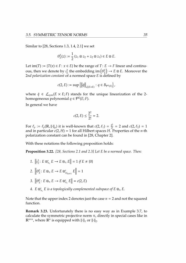
Similar to [28, Sections 1.3, 1.4, 2.1] we set
θ2E(z) :=
12
(z1 ⊗ z2 + z2 ⊗ z1) ∈ E ⊗ E.
Let im(T) := T(x) ∈ F : x ∈ E be the range of T : E→ F linear and continu-ous, then we denote by ι2E the embedding im
(θ2
E
)→ E ⊗ E. Moreover the
2nd polarization constant of a normed space E is defined by
c(2,E) := sup∥∥∥q
∥∥∥L(E×E)
: q ∈ BP2(E)
,
where q ∈ Lsym(E × E; F) stands for the unique linearization of the 2-homogeneous polynomial q ∈ P2(E; F).
In general we have
c(2,E) ≤22
2!= 2.
For `p := `p(R, ‖·‖p) it is well-known that c(2, `1) = 22
2! = 2 and c(2, `2) = 1and in particular c(2,H) = 1 for all Hilbert spaces H. Properties of the n-thpolarization constant can be found in [28, Chapter 2].
With these notations the following proposition holds:
Proposition 3.22. [28, Sections 2.1 and 2.3] Let E be a normed space. Then:
1.∥∥∥ι2E : E ⊗s
πsE→ E ⊗π E
∥∥∥ = 1 if E , 0
2.∥∥∥∥θ2
E : E ⊗π E→ E ⊗sπ|E⊗sE
E∥∥∥∥ = 1
3.∥∥∥θ2
E : E ⊗π E→ E ⊗sπs
E∥∥∥ = c(2,E)
4. E ⊗sπs
E is a topologically complemented subspace of E ⊗π E.
Note that the upper index 2 denotes just the case n = 2 and not the squaredfunction.
Remark 3.23. Unfortunately there is no easy way as in Example 3.7, tocalculate the symmetric projective norm πs directly in special cases like inRn×n, where Rn is equipped with ‖·‖1 or ‖·‖2.
36 CHAPTER 3. RELEVANT TOOLS FROM FUNCTIONAL ANALYSIS
The symmetric injective norm
The second tensor norm we want to consider, analogous to the ε-norm, isthe symmetric injective norm εs, which is the dual norm of the symmetricprojective norm.
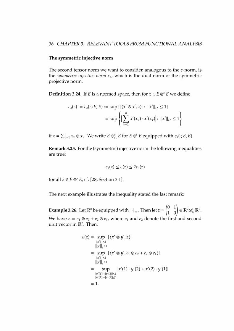
Definition 3.24. If E is a normed space, then for z ∈ E ⊗s E we define
εs(z) := εs(z; E,E) := sup | 〈x′ ⊗ x′, z〉 | : ‖x′‖E′ ≤ 1
= sup
∣∣∣ n∑ν=1
x′(xν) · x′(xν)∣∣∣ : ‖x′‖E′ ≤ 1
if z =
∑nν=1 xν ⊗ xν. We write E ⊗s
εsE for E ⊗s E equipped with εs(·; E,E).
Remark 3.25. For the (symmetric) injective norm the following inequalitiesare true:
εs(z) ≤ ε(z) ≤ 2εs(z)
for all z ∈ E ⊗s E, cf. [28, Section 3.1].
The next example illustrates the inequality stated the last remark:
Example 3.26. LetRn be equipped with ‖·‖∞. Then let z =
(0 11 0
)∈ R2
⊗sεsR2.
We have z = e1 ⊗ e2 + e2 ⊗ e1, where e1 and e2 denote the first and secondunit vector in R2. Then:
ε(z) = sup‖x′‖1≤1‖y′‖1≤1
|⟨x′ ⊗ y′, z
⟩|
= sup‖x′‖1≤1‖y′‖1≤1
|⟨x′ ⊗ y′, e1 ⊗ e2 + e2 ⊗ e1
⟩|
= sup|x′(1)|+|x′(2)|≤1|y′(1)|+|y′(2)|≤1
|x′(1) · y′(2) + x′(2) · y′(1)|
= 1.
3.5. SYMMETRIC TENSOR NORMS 37
And furthermore:
εs(z) = sup‖x′‖1≤1
| 〈x′ ⊗ x′, z〉 |
= sup‖x′‖1≤1
| 〈x′ ⊗ x′, e1 ⊗ e2 + e2 ⊗ e1〉 |
= sup|x′(1)|+|x′(2)|≤1
|x′(1) · x′(2) + x′(2) · x′(1)|
= 1/2.
Indeed the second equality in each case holds by Definition 3.9 and Defi-nition 3.24. This shows that the estimate ε(z) ≤ 2εs(z) for all z is sharp.
Note here that also the symmetric injective norm is not the injective normrestricted to E ⊗s E (see [28, Section 3.1]). If ε|E⊗sE denotes the restrictionto E ⊗s E of the injective norm, then εs ≤ ε|E⊗sE is valid and in particularεs = ε|E⊗sE for Hilbert spaces.
Definition 3.24 is just the special definition for E ⊗s E. A more general oneis the following:
εs(z; E,E) : = sup | 〈⊗nx′, z〉 | : ‖x′‖E′ ≤ 1
= sup
∣∣∣ m∑k=1
〈x′, xk〉n∣∣∣ : ‖x′‖E′ ≤ 1
if z =
∑mk=1 ⊗
nxk. The notation will be analogous to the one we used before:⊗
n,sεs E and ⊗n,s
εsE for the completion, cf. [28, Section 3.1]. For our purpose
Definition 3.24 is sufficient. For this case we will give some properties ofthe symmetric injective norm from Definition 3.24. The general statementscan be found in [28, Section 3.2].
Proposition 3.27. 1. εs(x ⊗ x; E ⊗s E) = ‖x‖2E for all x ∈ E
2. εs ≤ πs on E ⊗s E
3. εs is finitely generated, i.e.
εs(z; E ⊗s E) = inf εs(z; M ⊗s M) : M ⊂ E,dim(M) < ∞, z ∈M ⊗s M .
The general formulation of following proposition can be found in [28,Section 3.1]:
38 CHAPTER 3. RELEVANT TOOLS FROM FUNCTIONAL ANALYSIS
Proposition 3.28. Let E be a normed space. Then:
1.∥∥∥ι2E : E ⊗s
εsE→ E ⊗ε E
∥∥∥ ≤ c(2,E′)
2.∥∥∥ι2E′ : E′ ⊗s
εsE′ → E′ ⊗ε E′
∥∥∥ ≤ c(2,E)
3.∥∥∥θ2
E : E ⊗ε E→ E ⊗sεs
E∥∥∥ = 1 if E , 0
4. E ⊗sεs
E is the topologically complemented subspace of E ⊗ε E.
Again, the upper index 2, denotes the special case for our purpose and notthe squared function.
Remark 3.29. Unfortunately there is no simple formula known to calculatethe symmetric projective norm εs concerning Rn equipped with ‖·‖∞ or inC(K) ⊗ C(K), where K is a compact space, analogous to Example 3.13.
Duality
Now we will formulate the duality betweenπs and εs for the 2nd symmetrictensor product, cf. [28, Chapter 4]. If E is a normed space, then the maps
E⊗sεs
E→(E′ ⊗s
πsE′
)′ 1= P2(E′)
E′⊗sεs
E′ →(E ⊗s
πsE)′ 1
= P2(E)
are metric injections, i.e. ‖Ix‖F = ‖x‖E for I ∈ L(E,F), cf. [19, A1].
Furthermore just like in (3.1) the duality between πs and εs holds, i.e.
πs(u) = supεs(w)≤1
| 〈u,w〉 |
for u ∈ E ⊗sπs
E and w ∈ E′ ⊗sεs
E′. With this property and the results fromExample 3.26 we can now prove the inequality from Example 3.20, whichwas still to be done.
Remark 3.30. In Example 3.20 we used the fact that πs(z) ≥ 4, which wewill prove now. In the situation of Example 3.26 we know that εs(z) = 1/2.Moreover with the duality of πs and εs in the situation of Example 3.20 thefollowing holds for w ∈ R2
⊗sεsR2:
πs(z) = supεs(w)≤1
| 〈z,w〉 |
≥ 〈e1 ⊗ e2 + e2 ⊗ e1, 2 (e1 ⊗ e2 + e2 ⊗ e1)〉= 4.
Consequently πs(z) ≥ 4 and the still pending inequality is proved.
3.5. SYMMETRIC TENSOR NORMS 39
The symmetric Hilbert-Schmidt norm
Last but not least we consider a third symmetric norm, analogous tothe Hilbert-Schmidt norm. If a vector space F is equipped with a scalarproduct 〈·, ·〉F there is a uniquely determined scalar product 〈·, ·〉F⊗sF with〈x1 ⊗ x1, x2 ⊗ x2〉F⊗sF = 〈x1, x2〉F 〈x1, x2〉F for x1, x2 ∈ F, cf. [19, Section 26.7].The norm σs := σs(·; F,F) with
σs(z) :=√〈z, z〉F⊗sF
is called the symmetric Hilbert-Schmidt norm on F ⊗s F and we write F ⊗sσs
Ffor the normed space (F ⊗s F, σs).
Remark 3.31. Note here that in contrast to the symmetric projective and thesymmetric injective norms, the symmetric Hilbert-Schmidt norm is equalto the Hilbert-Schmidt norm restricted to F⊗s F, which is denoted by σ|F⊗sF,i.e. σs(z) = σ|F⊗sF(z) for all z ∈ F ⊗s F. This results from the uniqueness ofthe scalar product.
In the present chapter concerning functional analysis we gave an overviewover the most important tools for our further research. Of particular impor-tance were the algebraic theory of the symmetric tensor products. It willbe essential for our further research since we will consider only symmet-ric operators. An important instrument will be the symmetric projectivenorm, which is not only the restriction of the projective norm to symmet-ric tensor products. Rather it arises via the symmetric decompositions ofthe considered tensor. With the help of this norm we will find suitablespaces for our goal to generalize the concept of copositivity in an infinitedimensional space.

40 CHAPTER 3. RELEVANT TOOLS FROM FUNCTIONAL ANALYSIS
Chapter 4
Discussion of special cases
In this chapter we will have a closer look at the symmetric projective normand its special properties. We will analyze how the value of the symmetricprojective norm depends on the different p-norms. Furthermore we will seethat there are two special cases depending on the choice of p in which thesymmetric projective norm is easier to calculate and that in the other casesthe calculation is not so easy. Moreover we will give different examples toillustrate these special cases. In the second part of this chapter we will givesome numerical experiments for a special kind of decomposition. Lastwe will discuss the importance of the symmetric projective norm for ourgoal to generalize the topic of copositivity and completely positivity in aninfinite dimensional space.
4.1 Properties of the symmetric projective norm
First we will repeat the definition of the symmetric projective norm partic-ularly for `n
p ⊗s `n
p :
Definition 4.1. The symmetric projective norm πs,p on the symmetric tensorspace `n
p ⊗s `n
p , with `np := (Rn, ‖·‖p) depending on p is for z ∈ `n
p ⊗s `n
p definedas follows:
πs,p(z) := πs
(z; `n
p , `np
):= inf
N∑ν=1
‖xν‖2p : N ∈N, z =
N∑ν=1
± xν ⊗ xν
.For the sake of simplicity we will drop p in the index of πs,p if it is clearwhich p is used.
41
42 CHAPTER 4. DISCUSSION OF SPECIAL CASES
The symmetric projective norm is generally very impractical to calculatebecause of the many possibilities for decompositions of a tensor and be-yond that the different choices of values of p. Therefore we thought aboutspecial cases depending on the value of p, in which the symmetric projec-tive norm would be easier to calculate. Furthermore as a special issue, itwould be less complicated if the set of decompositions would be smaller.With regard to the generalization of the completely positive cone, we wereable to prove the following result that deals only with nonnegative decom-positions:
Theorem 4.2. Let z =∑Nν=1 uν ⊗ uν with uν ≥ 0. If p = 1 or p = 2, then:
πs,p(z) =
N∑ν=1
‖uν‖2p .
Proof. First we prove the case p = 1: Consider z =∑Nν=1 uν ⊗ uν ∈ `n
1 ⊗s `n
1and uν ≥ 0. With z(i, j) we denote the (i, j)-th entry of z. Then:
πs
(z; `n
1 , `n1
)≥ π
(z; `n
1 , `n1
)=
n∑i, j=1
∣∣∣z(i, j)∣∣∣
=
n∑i, j=1
z(i, j)
=
N∑ν=1
n∑i, j=1
uν(i) · uν( j)
=
N∑ν=1
n∑i=1
uν(i)
2
=
N∑ν=1
‖uν‖21
≥ πs
(z; `n
1 , `n1
).
This chain of inequalities shows that
πs
(z; `n
1 , `n1
)≥
N∑ν=1
‖uν‖21 ≥ πs
(z; `n
1 , `n1
)
4.1. PROPERTIES OF THE SYMMETRIC PROJECTIVE NORM 43
and therefore the equality is proved:
πs
(z; `n
1 , `n1
)=
N∑ν=1
‖uν‖21 .
Now we show the property for p = 2: Let z =∑Nν=1 uν ⊗ uν ∈ `n
2 ⊗s `n
2 anduν ≥ 0. With z(i, j) we denote again the (i, j)-th entry of z. Furthermore letλν(z) with ν = 1, . . . ,K be the singular values of z. Then:
πs
(z; `n
2 , `n2
)≥ π
(z; `n
2 , `n2
)=
K∑ν=1
|λν(z)|
=
K∑ν=1
λν(z)
= tr(z)
=
n∑i=1
z(i, i)
=
N∑ν=1
n∑i=1
uν(i) · uν(i)
=
N∑ν=1
n∑i=1
(uν(i))2
=
N∑ν=1
‖uν‖22
≥ πs
(z; `n
2 , `n2
).
Again this chain of inequalities shows that
πs
(z; `n
2 , `n2
)≥
N∑ν=1
‖uν‖22 ≥ πs
(z; `n
2 , `n2
)and therefore equality holds:
πs
(z; `n
2 , `n2
)=
N∑ν=1
‖uν‖22 .
44 CHAPTER 4. DISCUSSION OF SPECIAL CASES
Remark 4.3. Note that in the case p = 1 the restriction uν ≥ 0 for all ν isessential for the proof of Theorem 4.2. But in the case p = 2 this restrictionis not necessary for the proof. So this property holds for any positivesemidefinite z, and not only for completely positive z. But nonetheless itis a useful result that we need just a single - and particularly nonnegative- decomposition to determine πs,p.
In the next example we will show that in the case p ∈ (1, 2) the equalityfrom Theorem 4.2 does not hold in general:
Example 4.4. Let A =
(2 11 2
). We have one decomposition A =
∑2i=1 bi ⊗ bi
with b1 = (√
3/2, 0)> and b2 = (1/√
2,√
2)> and a second A =∑3
j=1 c j⊗c j withc1 = (0, 1)>, c2 = (1, 1)> and c3 = (1, 0)>. First for p ∈ [1, 2] we determine:
2∑i=1
‖bi‖2p =
√
32
p
+ 0p
1/p
2
+
(( 1√
2
)p
+√
2p
)1/p2
=32
+( 12p/2 + 2p/2
)2/p
=32
+12
(1 + 2p)2/p
whereas
3∑j=1
∥∥∥c j
∥∥∥2
p=
((0p + 1p)1/p
)2+
((1p + 1p)1/p
)2+
((1p + 0p)1/p
)2
= 1 + 22/p + 1
= 2 + 22/p.
Next we show that for p ∈ [1, 2] we have
3∑j=1
∥∥∥c j
∥∥∥2
p≥
2∑i=1
‖bi‖2p .
Especially for p ∈ (1, 2) the inequality holds strictly. To illustrate thisinequality, we consider the graph of the difference
∑3j=1
∥∥∥c j
∥∥∥2
p−
∑2i=1 ‖bi‖
2p:
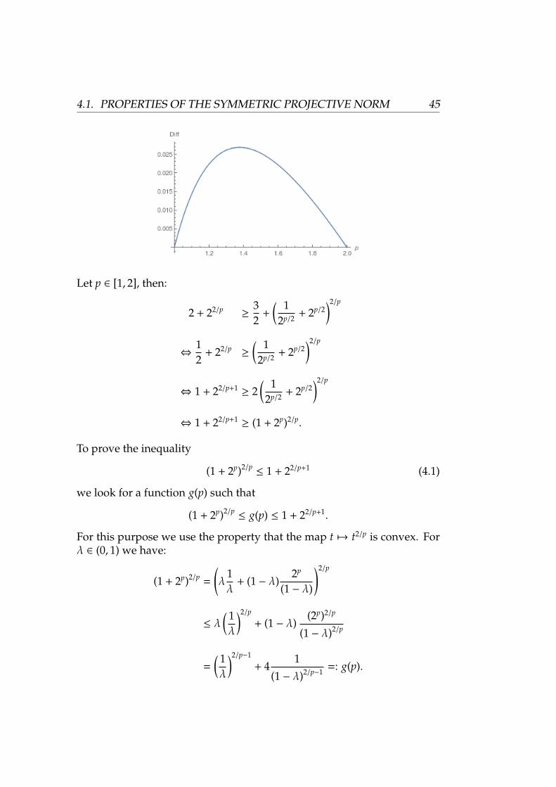
4.1. PROPERTIES OF THE SYMMETRIC PROJECTIVE NORM 45
Let p ∈ [1, 2], then:
2 + 22/p≥
32
+( 12p/2 + 2p/2
)2/p
⇔12
+ 22/p≥
( 12p/2 + 2p/2
)2/p
⇔ 1 + 22/p+1≥ 2
( 12p/2 + 2p/2
)2/p
⇔ 1 + 22/p+1≥ (1 + 2p)2/p.
To prove the inequality
(1 + 2p)2/p≤ 1 + 22/p+1 (4.1)
we look for a function g(p) such that
(1 + 2p)2/p≤ g(p) ≤ 1 + 22/p+1.
For this purpose we use the property that the map t 7→ t2/p is convex. Forλ ∈ (0, 1) we have:
(1 + 2p)2/p =
(λ
1λ
+ (1 − λ)2p
(1 − λ)
)2/p
≤ λ( 1λ
)2/p
+ (1 − λ)(2p)2/p
(1 − λ)2/p
=( 1λ
)2/p−1
+ 41
(1 − λ)2/p−1 =: g(p).
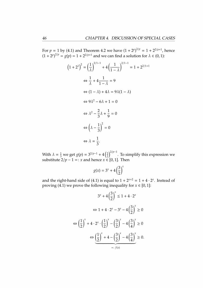
46 CHAPTER 4. DISCUSSION OF SPECIAL CASES
For p = 1 by (4.1) and Theorem 4.2 we have (1 + 2p)2/p = 1 + 22/p+1, hence(1 + 2p)2/p = g(p) = 1 + 22/p+1 and we can find a solution for λ ∈ (0, 1):(
1 + 21)2
=( 1λ
)2/1−1
+ 4( 11 − λ
)2/1−1
= 1 + 22/1+1
⇔1λ
+ 41
1 − λ= 9
⇔ (1 − λ) + 4λ = 9λ(1 − λ)
⇔ 9λ2− 6λ + 1 = 0
⇔ λ2−
23λ +
19
= 0
⇔
(λ −
13
)2
= 0
⇔ λ =13.
With λ = 13 we get g(p) = 32/p−1 + 4
(32
)2/p−1. To simplify this expression we
substitute 2/p − 1 = : x and hence x ∈ [0, 1]. Then
g(x) = 3x + 4(32
)x
and the right-hand side of (4.1) is equal to 1 + 2x+2 = 1 + 4 · 2x. Instead ofproving (4.1) we prove the following inequality for x ∈ [0, 1]:
3x + 4(32
)x
≤ 1 + 4 · 2x
⇔ 1 + 4 · 2x− 3x− 4
(32
)x
≥ 0
⇔
(12
)x
+ 4 · 2x·
(12
)x
−
(32
)x
− 4(34
)x
≥ 0
⇔
(12
)x
+ 4 −(32
)x
− 4(34
)x
︸ ︷︷ ︸= : f (x)
≥ 0.
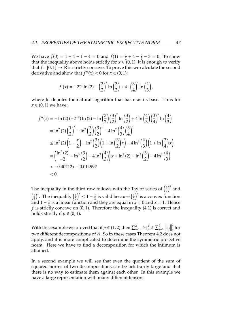
4.1. PROPERTIES OF THE SYMMETRIC PROJECTIVE NORM 47
We have f (0) = 1 + 4 − 1 − 4 = 0 and f (1) = 12 + 4 − 3
2 − 3 = 0. To showthat the inequality above holds strictly for x ∈ (0, 1), it is enough to verifythat f : [0, 1]→ R is strictly concave. To prove this we calculate the secondderivative and show that f ′′(x) < 0 for x ∈ (0, 1):
f ′(x) = −2−x ln (2) −(32
)x
ln(32
)+ 4 ·
(34
)x
ln(43
),
where ln denotes the natural logarithm that has e as its base. Thus forx ∈ (0, 1) we have:
f ′′(x) = − ln (2) (−2−x) ln (2) − ln(32
) (32
)x
ln(32
)+ 4 ln
(43
) (34
)x
ln(43
)= ln2 (2)
(12
)x
− ln2(32
) (32
)x
− 4 ln2(43
) (34
)x
≤ ln2 (2)(1 −
x2
)− ln2
(32
) (1 + ln
(32
)x)− 4 ln2
(43
) (1 + ln
(34
)x)
=
(ln2 (2)−2
− ln3(32
)− 4 ln3
(43
))x + ln2 (2) − ln2
(32
)− 4 ln2
(43
)< −0.40212x − 0.014992
< 0.
The inequality in the third row follows with the Taylor series of(
32
)xand(
34
)x. The inequality
(12
)x≤ 1 − x
2 is valid because(
12
)xis a convex function
and 1 − x2 is a linear function and they are equal in x = 0 and x = 1. Hence
f is strictly concave on (0, 1). Therefore the inequality (4.1) is correct andholds strictly if p ∈ (0, 1).
With this example we proved that if p ∈ (1, 2) then∑2
i=1 ‖bi‖2p ,
∑3j=1
∥∥∥c j
∥∥∥2
pfor
two different decompositions of A. So in these cases Theorem 4.2 does notapply, and it is more complicated to determine the symmetric projectivenorm. Here we have to find a decomposition for which the infimum isattained.
In a second example we will see that even the quotient of the sum ofsquared norms of two decompositions can be arbitrarily large and thatthere is no way to estimate them against each other. In this example wehave a large representation with many different tensors.
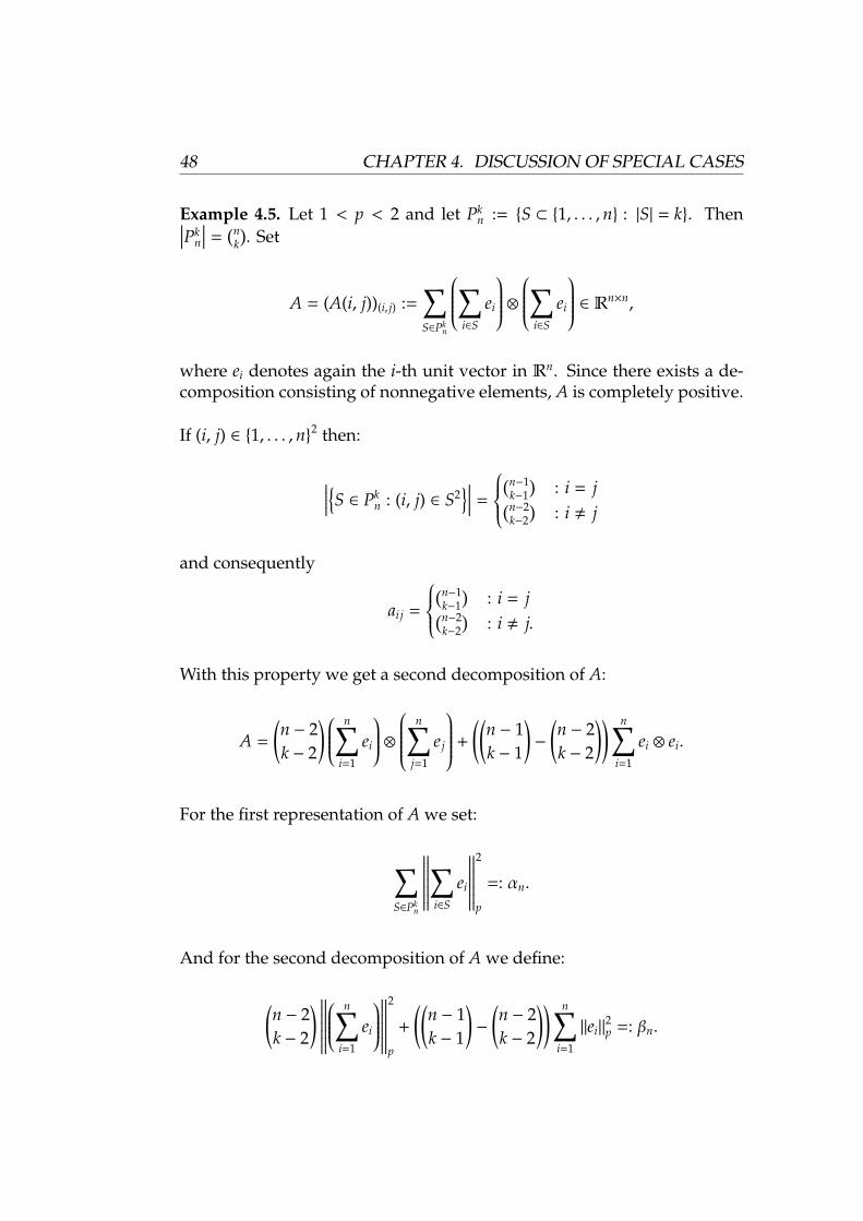
48 CHAPTER 4. DISCUSSION OF SPECIAL CASES
Example 4.5. Let 1 < p < 2 and let Pkn := S ⊂ 1, . . . ,n : |S| = k. Then∣∣∣Pk
n
∣∣∣ =(n
k
). Set
A = (A(i, j))(i, j) :=∑S∈Pk
n
∑i∈S
ei
⊗∑
i∈S
ei
∈ Rn×n,
where ei denotes again the i-th unit vector in Rn. Since there exists a de-composition consisting of nonnegative elements, A is completely positive.
If (i, j) ∈ 1, . . . ,n2 then:
∣∣∣∣S ∈ Pkn : (i, j) ∈ S2
∣∣∣∣ =
(n−1
k−1
): i = j(n−2
k−2
): i , j
and consequently
ai j =
(n−1
k−1
): i = j(n−2
k−2
): i , j.
With this property we get a second decomposition of A:
A =
(n − 2k − 2
) n∑i=1
ei
⊗ n∑
j=1
e j
+
((n − 1k − 1
)−
(n − 2k − 2
)) n∑i=1
ei ⊗ ei.
For the first representation of A we set:
∑S∈Pk
n
∥∥∥∥∥∥∥∑i∈S ei
∥∥∥∥∥∥∥2
p
=: αn.
And for the second decomposition of A we define:
(n − 2k − 2
) ∥∥∥∥∥∥∥ n∑
i=1
ei
∥∥∥∥∥∥∥
2
p
+
((n − 1k − 1
)−
(n − 2k − 2
)) n∑i=1
‖ei‖2p =: βn.
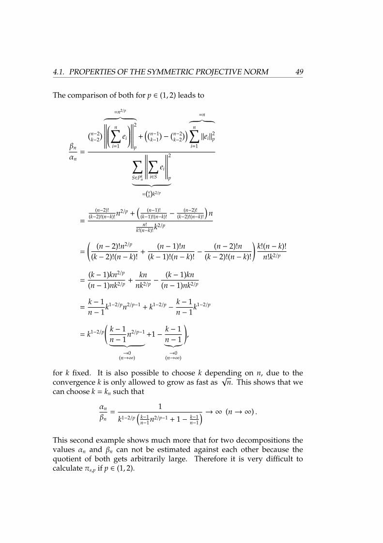
4.1. PROPERTIES OF THE SYMMETRIC PROJECTIVE NORM 49
The comparison of both for p ∈ (1, 2) leads to
βn
αn=
(n−2k−2
)=n2/p︷ ︸︸ ︷∥∥∥∥∥∥∥
n∑i=1
ei
∥∥∥∥∥∥∥
2
p
+((n−1
k−1
)−
(n−2k−2
))=n︷ ︸︸ ︷
n∑i=1
‖ei‖2p
∑S∈Pk
n
∥∥∥∥∥∥∥∑i∈S ei
∥∥∥∥∥∥∥2
p︸ ︷︷ ︸=(n
k)k2/p
=
(n−2)!(k−2)!(n−k)!n
2/p +(
(n−1)!(k−1)!(n−k)! −
(n−2)!(k−2)!(n−k)!
)n
n!k!(n−k)!k
2/p
=
((n − 2)!n2/p
(k − 2)!(n − k)!+
(n − 1)!n(k − 1)!(n − k)!
−(n − 2)!n
(k − 2)!(n − k)!
)k!(n − k)!
n!k2/p
=(k − 1)kn2/p
(n − 1)nk2/p +kn
nk2/p −(k − 1)kn
(n − 1)nk2/p
=k − 1n − 1
k1−2/pn2/p−1 + k1−2/p−
k − 1n − 1
k1−2/p
= k1−2/p
(k − 1n − 1
n2/p−1︸ ︷︷ ︸→0
(n→∞)
+1 −k − 1n − 1︸︷︷︸→0
(n→∞)
),
for k fixed. It is also possible to choose k depending on n, due to theconvergence k is only allowed to grow as fast as
√n. This shows that we
can choose k = kn such that
αn
βn=
1
k1−2/p(
k−1n−1n2/p−1 + 1 − k−1
n−1
) →∞ (n→∞) .
This second example shows much more that for two decompositions thevalues αn and βn can not be estimated against each other because thequotient of both gets arbitrarily large. Therefore it is very difficult tocalculate πs,p if p ∈ (1, 2).
50 CHAPTER 4. DISCUSSION OF SPECIAL CASES
The last case we will discuss is the case p > 2:
Proposition 4.6. Let z =∑Mι=1 uι ⊗ uι with uι ≥ 0. If p > 2 then
πs,p(z) , inf
N∑ν=1
‖xν‖2p : z =
N∑ν=1
xν ⊗ xν, xν ≥ 0,N ∈N
.Proof. To prove the result, we consider the n × n identity matrix In and aspecial decomposition of it:
In =
n∑i=1
ei ⊗ ei,
where ei denotes again the i-th unit vector in Rn. This is up to rearrange-ments or multiples the unique nonnegative and symmetric decompositionof In. Therefore we know:
n∑i=1
‖ei‖2p = n = inf
N∑ν=1
‖xν‖2p : In =
N∑ν=1
xν ⊗ xν, xν ≥ 0,N ∈N
.There is no possibility to get a symmetric and nonnegative decompositionwith a smaller sum of squared norms. However, with [19, Section 8.8,Corollary] it follows that
πs,p (In) =
n2/p if p ≥ 2n if p ≤ 2.
For p > 2 and n ≥ 2 we get:
πs,p(In) = n2/p < n = inf
N∑ν=1
‖xν‖2p : In =
N∑ν=1
xν ⊗ xν, xν ≥ 0,N ∈N
.In particular
n2/p
n→ 0 for n→∞.
Therefore if p > 2 it is not possible to calculate πs,p by considering only thenonnegative decompositions as Proposition 4.6 shows.
4.1. PROPERTIES OF THE SYMMETRIC PROJECTIVE NORM 51
Another question that arises while thinking about special properties ofthe symmetric projective norm is whether there is any relation betweenthe number of summands of a decomposition and the size of its sumof squared norms. For example whether a higher (or lower) number ofsummands leads to a higher (or lower) sum of squared norms or the otherway around.
In a first result, we want to show that a decomposition with more sum-mands may have the same norm.
Lemma 4.7. Let z =∑mν=1 uν ⊗ uν. Then for any n > m there exists a different
decomposition z =∑nι=1 wι ⊗ wι such that
∑mν=1 ‖uν‖
2p =
∑nι=1 ‖wι‖
2p.
Proof. Let k := n − m. We construct the decomposition as follows: Forι = 1, . . . ,m − 1 we set wι := uν. Furthermore for ι = m, . . . ,m + k we definewι := 1
√k+1
um. Then obviously∑mν=1 uν ⊗ uν =
∑nι=1 wι ⊗ wι = z, and we get
the following sums of squared norms for the two decompositions:
α :=m∑ν=1
‖uν‖2p =
m−1∑ν=1
‖uν‖2p + ‖um‖2p
β :=n∑ι=1
‖wι‖2p =
m−1∑ι=1
‖uι‖2p +
m+k∑ι=m
∥∥∥∥∥∥ 1√
k + 1um
∥∥∥∥∥∥2
p
.
To prove that both sums of squared norms have the same value, we calcu-late their difference:
β − α =
m−1∑ι=1
‖uι‖2p +
m+k∑ι=m
∥∥∥∥∥∥ 1√
k + 1um
∥∥∥∥∥∥2
p
−
m−1∑ν=1
‖uν‖2p − ‖um‖2p
= (k + 1)
∣∣∣∣∣∣ 1√
k + 1
∣∣∣∣∣∣2
‖um‖2p − ‖um‖
2p
= 0.
Hence it is true that∑mν=1 ‖uν‖
2p =
∑nι=1 ‖wι‖
2p.
As the above lemma shows, a larger number of summands does not neces-sarily imply a larger sum of squared norms. The principle of duplicatingsummands, which is used in the proof of Lemma 4.7, is well-known inoptimization. Although we duplicated only one summand, the resultwould stay the same if we would duplicate more than one summand. Inoptimization this principle is used for example in [26, Chapter 3].
52 CHAPTER 4. DISCUSSION OF SPECIAL CASES
The next example shows a stronger statement of Lemma 4.7. Here wewill consider two decompositions and we will see that the one with moresummands has a smaller sum of squared norms.
Example 4.8. We consider the matrix
A =
2 1 1 1 11 2 1 1 11 1 2 1 11 1 1 2 11 1 1 1 2
and two decompositions A =
∑6i=1 bi ⊗ bi =
∑5j=1 ci ⊗ c j. For the sake of
clarity we collect the vectors bi (i = 1, . . . , 6) and c j ( j = 1, . . . , 5) in matricesB = (b1, b2, b3, b4, b5, b6) and C = (c1, c2, c3, c4, c5), respectively. Then:
B =
1 1 0 0 0 01 0 1 0 0 01 0 0 1 0 01 0 0 0 1 01 0 0 0 0 1
∈ R5×6,
C =
1.1145 0.3408 0.4039 0.6885 0.006790.0009 0.0553 0.0773 1.3326 0.4639
0 0.1039 1.2388 0.6743 00 1.2046 0.3646 0.6277 0.1483
0.3129 0.3461 0.6143 0.3011 1.1464
∈ R5×5.
We calculate now the sum of squared norms of the first decomposition:
6∑i=1
‖bi‖2p = (1p + 1p + 1p + 1p + 1p)2/p + 5 · (1p)2/p
= 52/p + 5
and for the second decomposition we have:
5∑j=1
∥∥∥c j
∥∥∥2
p= (1.1145p + 0.3408p + 0.4039p + 0.6885p + 0.00679p)2/p
+ (0.0009p + 0.0553p + 0.0773p + 1.3326p + 0.4639p)2/p
+ (0p + 0.1039p + 1.2388p + 0.6743p + 0p)2/p
+ (0p + 1.2046p + 0.3646p + 0.6277p + 0.1483p)2/p
+ (0.3129p + 0.3461p + 0.6143p + 0.3011p + 1.1464p)2/p
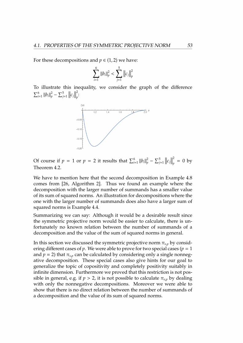
4.1. PROPERTIES OF THE SYMMETRIC PROJECTIVE NORM 53
For these decompositions and p ∈ (1, 2) we have:6∑
i=1
‖bi‖2p <
5∑j=1
∥∥∥c j
∥∥∥2
p
To illustrate this inequality, we consider the graph of the difference∑6i=1 ‖bi‖
2p −
∑5j=1
∥∥∥c j
∥∥∥2
p:
Of course if p = 1 or p = 2 it results that∑6
i=1 ‖bi‖2p −
∑5j=1
∥∥∥c j
∥∥∥2
p= 0 by
Theorem 4.2.
We have to mention here that the second decomposition in Example 4.8comes from [26, Algorithm 2]. Thus we found an example where thedecomposition with the larger number of summands has a smaller valueof its sum of squared norms. An illustration for decompositions where theone with the larger number of summands does also have a larger sum ofsquared norms is Example 4.4.
Summarizing we can say: Although it would be a desirable result sincethe symmetric projective norm would be easier to calculate, there is un-fortunately no known relation between the number of summands of adecomposition and the value of the sum of squared norms in general.
In this section we discussed the symmetric projective norm πs,p by consid-ering different cases of p. We were able to prove for two special cases (p = 1and p = 2) that πs,p can be calculated by considering only a single nonneg-ative decomposition. These special cases also give hints for our goal togeneralize the topic of copositivity and completely positivity suitably ininfinite dimension. Furthermore we proved that this restriction is not pos-sible in general, e.g. if p > 2, it is not possible to calculate πs,p by dealingwith only the nonnegative decompositions. Moreover we were able toshow that there is no direct relation between the number of summands ofa decomposition and the value of its sum of squared norms.
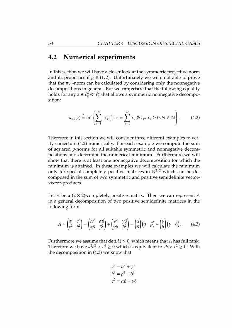
54 CHAPTER 4. DISCUSSION OF SPECIAL CASES
4.2 Numerical experiments
In this section we will have a closer look at the symmetric projective normand its properties if p ∈ (1, 2). Unfortunately we were not able to provethat the πs,p-norm can be calculated by considering only the nonnegativedecompositions in general. But we conjecture that the following equalityholds for any z ∈ `n
p ⊗s `n
p that allows a symmetric nonnegative decompo-sition:
πs,p(z) ?= inf
N∑ν=1
‖xν‖2p : z =
N∑ν=1
xν ⊗ xν, xν ≥ 0,N ∈N
. (4.2)
Therefore in this section we will consider three different examples to ver-ify conjecture (4.2) numerically. For each example we compute the sumof squared p-norms for all suitable symmetric and nonnegative decom-positions and determine the numerical minimum. Furthermore we willshow that there is at least one nonnegative decomposition for which theminimum is attained. In these examples we will calculate the minimumonly for special completely positive matrices in R2×2 which can be de-composed in the sum of two symmetric and positive semidefinite vector-vector-products.
Let A be a (2 × 2)-completely positive matrix. Then we can represent Ain a general decomposition of two positive semidefinite matrices in thefollowing form:
A =
(a2 c2
c2 b2
)=
(α2 αβαβ β2
)+
(γ2 γδγδ δ2
)=
(αβ
) (α β
)+
(γδ
) (γ δ
). (4.3)
Furthermore we assume that det(A) > 0, which means that A has full rank.Therefore we have a2b2 > c4
≥ 0 which is equivalent to ab > c2≥ 0. With
the decomposition in (4.3) we know that
a2 = α2 + γ2
b2 = β2 + δ2
c2 = αβ + γδ
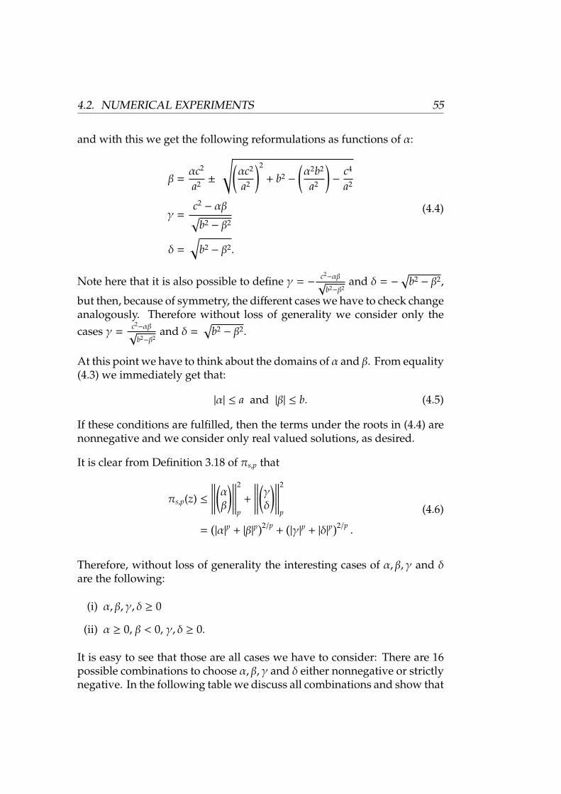
4.2. NUMERICAL EXPERIMENTS 55
and with this we get the following reformulations as functions of α:
β =αc2
a2 ±
√(αc2
a2
)2
+ b2 −
(α2b2
a2
)−
c4
a2
γ =c2− αβ√
b2 − β2
δ =√
b2 − β2.
(4.4)
Note here that it is also possible to define γ = −c2−αβ√
b2−β2and δ = −
√b2 − β2,
but then, because of symmetry, the different cases we have to check changeanalogously. Therefore without loss of generality we consider only thecases γ =
c2−αβ√
b2−β2and δ =
√b2 − β2.
At this point we have to think about the domains of α and β. From equality(4.3) we immediately get that:
|α| ≤ a and |β| ≤ b. (4.5)
If these conditions are fulfilled, then the terms under the roots in (4.4) arenonnegative and we consider only real valued solutions, as desired.
It is clear from Definition 3.18 of πs,p that
πs,p(z) ≤
∥∥∥∥∥∥(αβ
)∥∥∥∥∥∥2
p
+
∥∥∥∥∥∥(γδ
)∥∥∥∥∥∥2
p
=(|α|p + |β|p
)2/p+
(|γ|p + |δ|p
)2/p .
(4.6)
Therefore, without loss of generality the interesting cases of α, β, γ and δare the following:
(i) α, β, γ, δ ≥ 0
(ii) α ≥ 0, β < 0, γ, δ ≥ 0.
It is easy to see that those are all cases we have to consider: There are 16possible combinations to choose α, β, γ and δ either nonnegative or strictlynegative. In the following table we discuss all combinations and show that
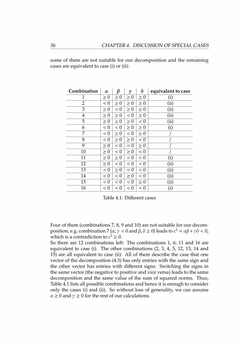
56 CHAPTER 4. DISCUSSION OF SPECIAL CASES
some of them are not suitable for our decomposition and the remainingcases are equivalent to case (i) or (ii):
Combination α β γ δ equivalent to case1 ≥ 0 ≥ 0 ≥ 0 ≥ 0 (i)2 < 0 ≥ 0 ≥ 0 ≥ 0 (ii)3 ≥ 0 < 0 ≥ 0 ≥ 0 (ii)4 ≥ 0 ≥ 0 < 0 ≥ 0 (ii)5 ≥ 0 ≥ 0 ≥ 0 < 0 (ii)6 < 0 < 0 ≥ 0 ≥ 0 (i)7 < 0 ≥ 0 < 0 ≥ 0 /8 < 0 ≥ 0 ≥ 0 < 0 /9 ≥ 0 < 0 < 0 ≥ 0 /
10 ≥ 0 < 0 ≥ 0 < 0 /11 ≥ 0 ≥ 0 < 0 < 0 (i)12 ≥ 0 < 0 < 0 < 0 (ii)13 < 0 ≥ 0 < 0 < 0 (ii)14 < 0 < 0 ≥ 0 < 0 (ii)15 < 0 < 0 < 0 ≥ 0 (ii)16 < 0 < 0 < 0 < 0 (i)
Table 4.1: Different cases
Four of them (combinations 7, 8, 9 and 10) are not suitable for our decom-position, e.g. combination 7 (α, γ < 0 and β, δ ≥ 0) leads to c2 = αβ+γδ < 0,which is a contradiction to c2
≥ 0.So there are 12 combinations left: The combinations 1, 6, 11 and 16 areequivalent to case (i). The other combinations (2, 3, 4, 5, 12, 13, 14 and15) are all equivalent to case (ii): All of them describe the case that onevector of the decomposition (4.3) has only entries with the same sign andthe other vector has entries with different signs. Switching the signs inthe same vector (the negative to positive and vice versa) leads to the samedecomposition and the same value of the sum of squared norms. Thus,Table 4.1 lists all possible combinations and hence it is enough to consideronly the cases (i) and (ii). So without loss of generality, we can assumeα ≥ 0 and γ ≥ 0 for the rest of our calculations.
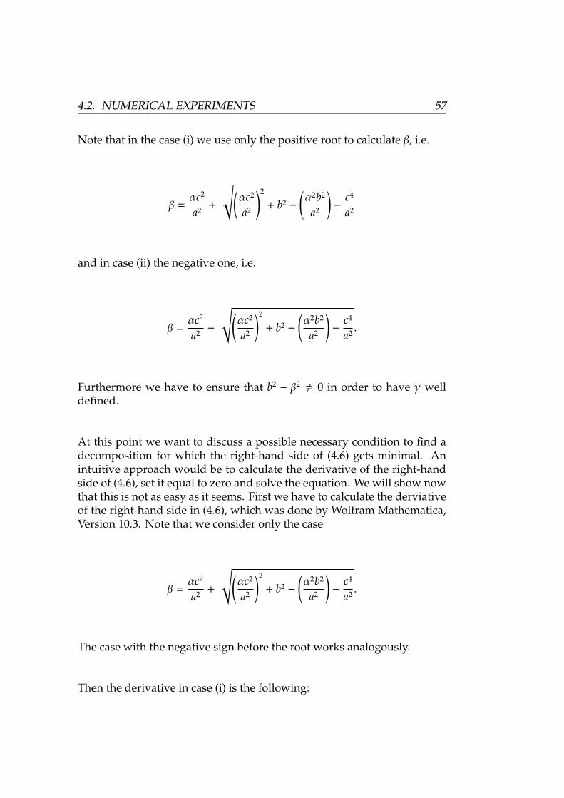
4.2. NUMERICAL EXPERIMENTS 57
Note that in the case (i) we use only the positive root to calculate β, i.e.
β =αc2
a2 +
√(αc2
a2
)2
+ b2 −
(α2b2
a2
)−
c4
a2
and in case (ii) the negative one, i.e.
β =αc2
a2 −
√(αc2
a2
)2
+ b2 −
(α2b2
a2
)−
c4
a2 .
Furthermore we have to ensure that b2− β2 , 0 in order to have γ well
defined.
At this point we want to discuss a possible necessary condition to find adecomposition for which the right-hand side of (4.6) gets minimal. Anintuitive approach would be to calculate the derivative of the right-handside of (4.6), set it equal to zero and solve the equation. We will show nowthat this is not as easy as it seems. First we have to calculate the derviativeof the right-hand side in (4.6), which was done by Wolfram Mathematica,Version 10.3. Note that we consider only the case
β =αc2
a2 +
√(αc2
a2
)2
+ b2 −
(α2b2
a2
)−
c4
a2 .
The case with the negative sign before the root works analogously.
Then the derivative in case (i) is the following:
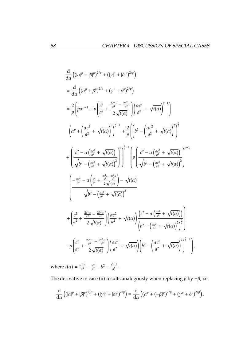
58 CHAPTER 4. DISCUSSION OF SPECIAL CASES
ddα
((|α|p + |β|p
)2/p+
(|γ|p + |δ|p
)2/p)
=d
dα
((αp + βp)2/p
+(γp + δp)2/p
)=
2p
pαp−1 + p
c2
a2 +2c4α
a4 −2b2α
a2
2√
t(α)
(αc2
a2 +√
t(α))p−1
(αp +
(αc2
a2 +√
t(α))p) 2
p−1
+2p
b2−
(αc2
a2 +√
t(α))2
p2
+
c2− α
(αc2
a2 +√
t(α))
√b2 −
(αc2
a2 +√
t(α))2
p
2p−1 p
c2− α
(αc2
a2 +√
t(α))
√b2 −
(αc2
a2 +√
t(α))2
p−1
−αc2
a2 − α
(c2
a2 +2c4α
a4 −2b2α
a2
2√
t(α)
)−
√t(α)√
b2 −(αc2
a2 +√
t(α))2
+
c2
a2 +2c4α
a4 −2b2α
a2
2√
t(α)
(αc2
a2 +√
t(α)) (
c2− α
(αc2
a2 +√
t(α)))
(b2 −
(αc2
a2 +√
t(α))2) 3
2
−p
c2
a2 +2c4α
a4 −2b2α
a2
2√
t(α)
(αc2
a2 +√
t(α)) b2
−
(αc2
a2 +√
t(α))2
p2−1 ,
where t(α) = α2c4
a4 −c4
a2 + b2−
b2α2
a2 .
The derivative in case (ii) results analogously when replacing β by −β, i.e.
ddα
((|α|p + |β|p
)2/p+
(|γ|p + |δ|p
)2/p)
=d
dα
((αp + (−β)p)2/p
+(γp + δp)2/p
).
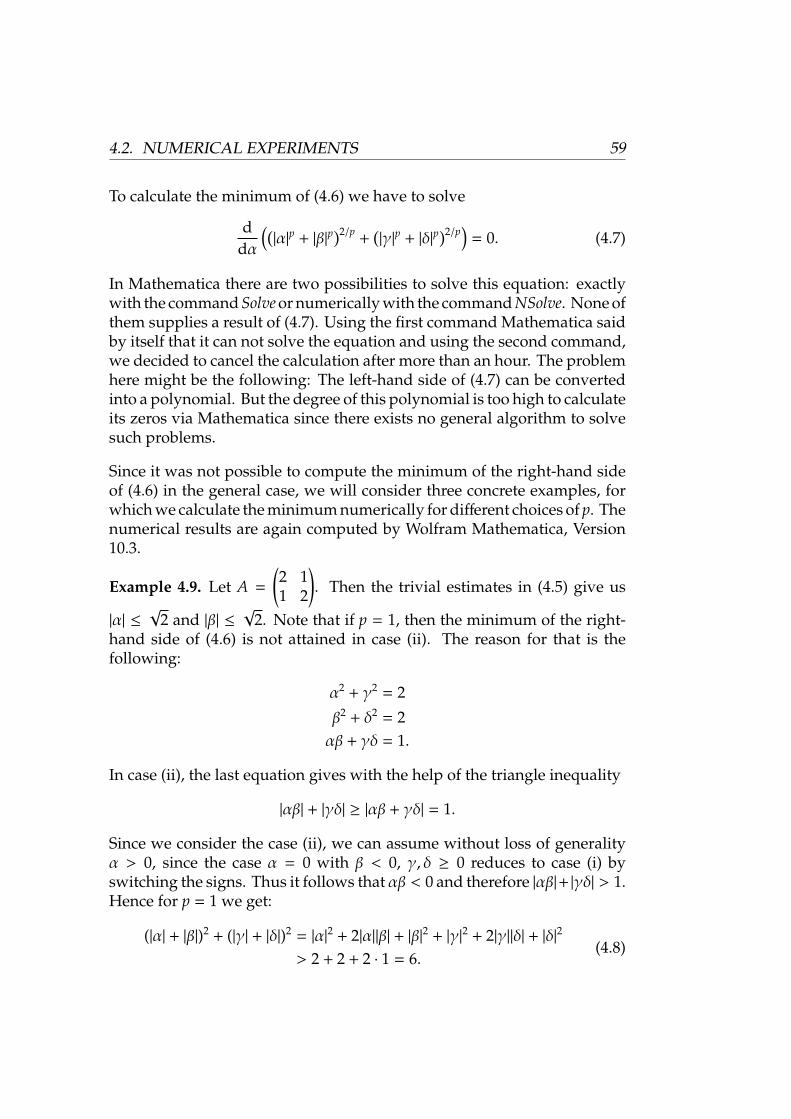
4.2. NUMERICAL EXPERIMENTS 59
To calculate the minimum of (4.6) we have to solve
ddα
((|α|p + |β|p
)2/p+
(|γ|p + |δ|p
)2/p)
= 0. (4.7)
In Mathematica there are two possibilities to solve this equation: exactlywith the command Solve or numerically with the command NSolve. None ofthem supplies a result of (4.7). Using the first command Mathematica saidby itself that it can not solve the equation and using the second command,we decided to cancel the calculation after more than an hour. The problemhere might be the following: The left-hand side of (4.7) can be convertedinto a polynomial. But the degree of this polynomial is too high to calculateits zeros via Mathematica since there exists no general algorithm to solvesuch problems.
Since it was not possible to compute the minimum of the right-hand sideof (4.6) in the general case, we will consider three concrete examples, forwhich we calculate the minimum numerically for different choices of p. Thenumerical results are again computed by Wolfram Mathematica, Version10.3.
Example 4.9. Let A =
(2 11 2
). Then the trivial estimates in (4.5) give us
|α| ≤√
2 and |β| ≤√
2. Note that if p = 1, then the minimum of the right-hand side of (4.6) is not attained in case (ii). The reason for that is thefollowing:
α2 + γ2 = 2
β2 + δ2 = 2αβ + γδ = 1.
In case (ii), the last equation gives with the help of the triangle inequality
|αβ| + |γδ| ≥ |αβ + γδ| = 1.
Since we consider the case (ii), we can assume without loss of generalityα > 0, since the case α = 0 with β < 0, γ, δ ≥ 0 reduces to case (i) byswitching the signs. Thus it follows that αβ < 0 and therefore |αβ|+ |γδ| > 1.Hence for p = 1 we get:
(|α| + |β|)2 + (|γ| + |δ|)2 = |α|2 + 2|α||β| + |β|2 + |γ|2 + 2|γ||δ| + |δ|2
> 2 + 2 + 2 · 1 = 6.(4.8)
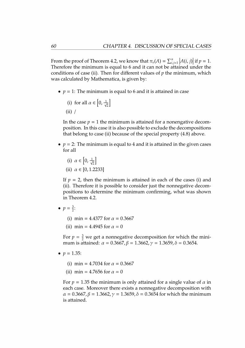
60 CHAPTER 4. DISCUSSION OF SPECIAL CASES
From the proof of Theorem 4.2, we know that πs(A) =∑n
i, j=1
∣∣∣A(i, j)∣∣∣ if p = 1.
Therefore the minimum is equal to 6 and it can not be attained under theconditions of case (ii). Then for different values of p the minimum, whichwas calculated by Mathematica, is given by:
• p = 1: The minimum is equal to 6 and it is attained in case
(i) for all α ∈[0, 1√
2
](ii) /
In the case p = 1 the minimum is attained for a nonengative decom-position. In this case it is also possible to exclude the decompositionsthat belong to case (ii) because of the special property (4.8) above.
• p = 2: The minimum is equal to 4 and it is attained in the given casesfor all
(i) α ∈[0, 1√
2
](ii) α ∈ [0, 1.2233]
If p = 2, then the minimum is attained in each of the cases (i) and(ii). Therefore it is possible to consider just the nonnegative decom-positions to determine the minimum confirming, what was shownin Theorem 4.2.
• p = 32 :
(i) min = 4.4377 for α = 0.3667
(ii) min = 4.4945 for α = 0
For p = 32 we get a nonnegative decomposition for which the mini-
mum is attained: α = 0.3667, β = 1.3662, γ = 1.3659, δ = 0.3654.
• p = 1.35:
(i) min = 4.7034 for α = 0.3667
(ii) min = 4.7656 for α = 0
For p = 1.35 the minimum is only attained for a single value of α ineach case. Moreover there exists a nonnegative decomposition withα = 0.3667, β = 1.3662, γ = 1.3659, δ = 0.3654 for which the minimumis attained.
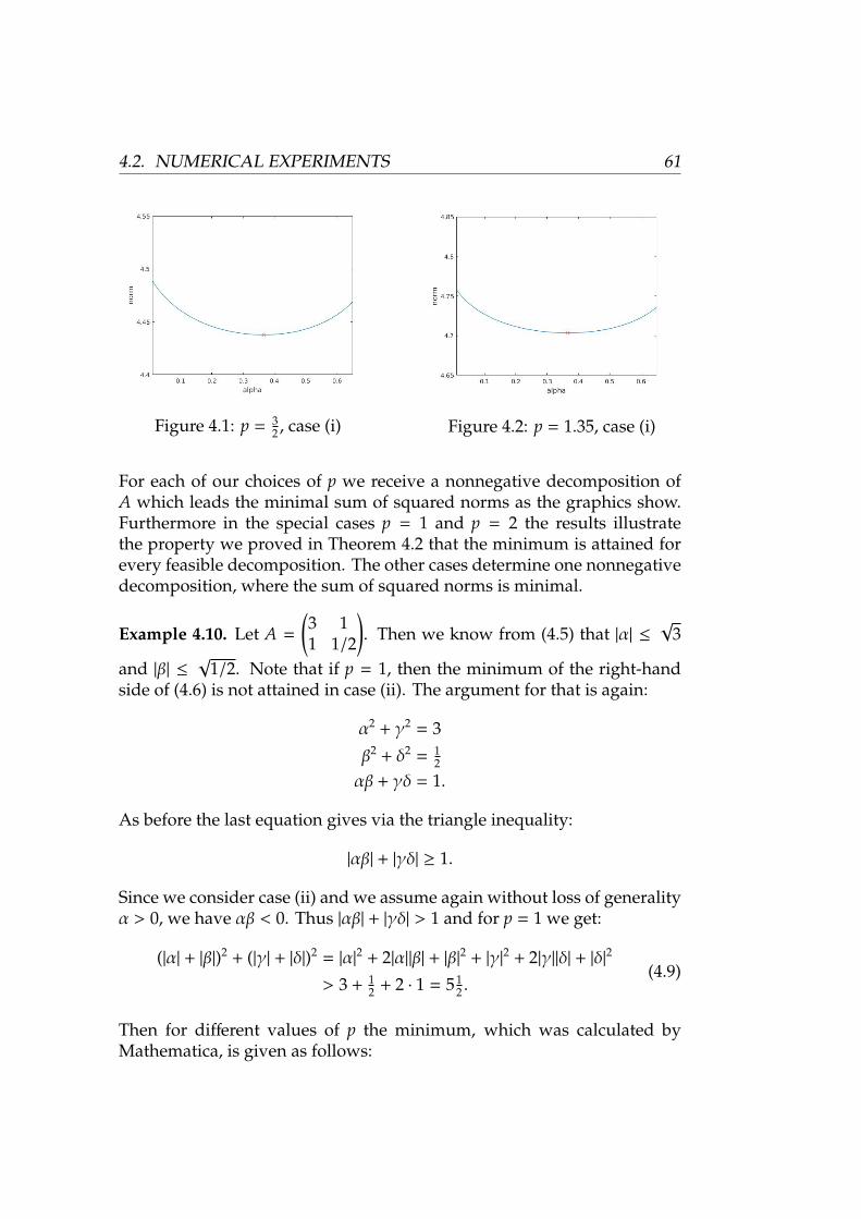
4.2. NUMERICAL EXPERIMENTS 61
Figure 4.1: p = 32 , case (i) Figure 4.2: p = 1.35, case (i)
For each of our choices of p we receive a nonnegative decomposition ofA which leads the minimal sum of squared norms as the graphics show.Furthermore in the special cases p = 1 and p = 2 the results illustratethe property we proved in Theorem 4.2 that the minimum is attained forevery feasible decomposition. The other cases determine one nonnegativedecomposition, where the sum of squared norms is minimal.
Example 4.10. Let A =
(3 11 1/2
). Then we know from (4.5) that |α| ≤
√3
and |β| ≤√
1/2. Note that if p = 1, then the minimum of the right-handside of (4.6) is not attained in case (ii). The argument for that is again:
α2 + γ2 = 3
β2 + δ2 = 12
αβ + γδ = 1.
As before the last equation gives via the triangle inequality:
|αβ| + |γδ| ≥ 1.
Since we consider case (ii) and we assume again without loss of generalityα > 0, we have αβ < 0. Thus |αβ| + |γδ| > 1 and for p = 1 we get:
(|α| + |β|)2 + (|γ| + |δ|)2 = |α|2 + 2|α||β| + |β|2 + |γ|2 + 2|γ||δ| + |δ|2
> 3 + 12 + 2 · 1 = 51
2 .(4.9)
Then for different values of p the minimum, which was calculated byMathematica, is given as follows:
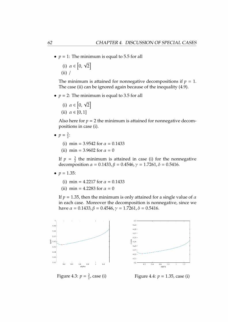
62 CHAPTER 4. DISCUSSION OF SPECIAL CASES
• p = 1: The minimum is equal to 5.5 for all
(i) α ∈[0,√
2]
(ii) /
The minimum is attained for nonnegative decompositions if p = 1.The case (ii) can be ignored again because of the inequality (4.9).
• p = 2: The minimum is equal to 3.5 for all
(i) α ∈[0,√
2]
(ii) α ∈ [0, 1]
Also here for p = 2 the minimum is attained for nonnegative decom-positions in case (i).
• p = 32 :
(i) min = 3.9542 for α = 0.1433(ii) min = 3.9602 for α = 0
If p = 32 the minimum is attained in case (i) for the nonnegative
decomposition α = 0.1433, β = 0.4546, γ = 1.7261, δ = 0.5416.
• p = 1.35:
(i) min = 4.2217 for α = 0.1433(ii) min = 4.2283 for α = 0
If p = 1.35, then the minimum is only attained for a single value of αin each case. Moreover the decomposition is nonnegative, since wehave α = 0.1433, β = 0.4546, γ = 1.7261, δ = 0.5416.
Figure 4.3: p = 32 , case (i) Figure 4.4: p = 1.35, case (i)
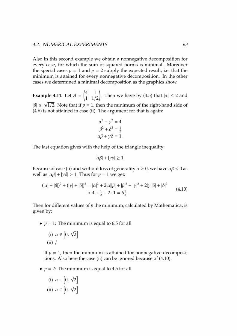
4.2. NUMERICAL EXPERIMENTS 63
Also in this second example we obtain a nonnegative decomposition forevery case, for which the sum of squared norms is minimal. Moreoverthe special cases p = 1 and p = 2 supply the expected result, i.e. that theminimum is attained for every nonnegative decomposition. In the othercases we determined a minimal decomposition as the graphics show.
Example 4.11. Let A =
(4 11 1/2
). Then we have by (4.5) that |α| ≤ 2 and
|β| ≤√
1/2. Note that if p = 1, then the minimum of the right-hand side of(4.6) is not attained in case (ii). The argument for that is again:
α2 + γ2 = 4
β2 + δ2 = 12
αβ + γδ = 1.
The last equation gives with the help of the triangle inequality:
|αβ| + |γδ| ≥ 1.
Because of case (ii) and without loss of generality α > 0, we have αβ < 0 aswell as |αβ| + |γδ| > 1. Thus for p = 1 we get:
(|α| + |β|)2 + (|γ| + |δ|)2 = |α|2 + 2|α||β| + |β|2 + |γ|2 + 2|γ||δ| + |δ|2
> 4 + 12 + 2 · 1 = 61
2 .(4.10)
Then for different values of p the minimum, calculated by Mathematica, isgiven by:
• p = 1: The minimum is equal to 6.5 for all
(i) α ∈[0,√
2]
(ii) /
If p = 1, then the minimum is attained for nonnegative decomposi-tions. Also here the case (ii) can be ignored because of (4.10).
• p = 2: The minimum is equal to 4.5 for all
(i) α ∈[0,√
2]
(ii) α ∈[0,√
2]
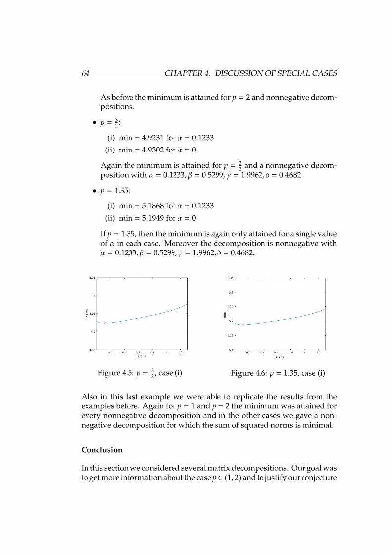
64 CHAPTER 4. DISCUSSION OF SPECIAL CASES
As before the minimum is attained for p = 2 and nonnegative decom-positions.
• p = 32 :
(i) min = 4.9231 for α = 0.1233
(ii) min = 4.9302 for α = 0
Again the minimum is attained for p = 32 and a nonnegative decom-
position with α = 0.1233, β = 0.5299, γ = 1.9962, δ = 0.4682.
• p = 1.35:
(i) min = 5.1868 for α = 0.1233
(ii) min = 5.1949 for α = 0
If p = 1.35, then the minimum is again only attained for a single valueof α in each case. Moreover the decomposition is nonnegative withα = 0.1233, β = 0.5299, γ = 1.9962, δ = 0.4682.
Figure 4.5: p = 32 , case (i) Figure 4.6: p = 1.35, case (i)
Also in this last example we were able to replicate the results from theexamples before. Again for p = 1 and p = 2 the minimum was attained forevery nonnegative decomposition and in the other cases we gave a non-negative decomposition for which the sum of squared norms is minimal.
Conclusion
In this section we considered several matrix decompositions. Our goal wasto get more information about the case p ∈ (1, 2) and to justify our conjecture
4.3. INTERPRETATION FOR DUALITY 65
(4.2). Here we discussed which of the decompositions would be suitableand restricted them to two different cases. Furthermore we calculated thederivative of the sum of squared norms of this special decomposition andequate it to zero to determine the minimum. Unfortunately Mathematicawas not able to solve this problem analytically. For some numerical resultswe discussed three different examples and for every example the two dif-ferent cases (i) and (ii). For each case we calculated the minimum of thesum of p-norms numerically.For each example and each case of p we found a nonnegative decompo-sition for which the minimum is attained. In particular for p = 3
2 andp = 1.35 there was a unique α for which the corresponding decompositionis nonnegative.These examples strengthened our conjecture
πs,p(z) ?= inf
N∑ν=1
‖xν‖2p : z =
N∑ν=1
xν ⊗ xν, xν ≥ 0,N ∈N
,i.e. that theπs,p-norm can be calculated by considering only the nonnegativedecompositions if the matrix is completely positive for p ∈ (1, 2).
4.3 Interpretation for duality
In this section we will discuss the meaning of the symmetric projectivenorm for our goal to generalize the topic of copositivity and completelypositivity in infinite dimension. In the cases p = 1 and p = 2 it is mucheasier to calculate the projective norm, since the sum of squared norms isconstant for all nonnegative decompositions and the minimum is attained.
For the sake of simplicity we will discuss the needed spaces only for vectors.
First we will consider the case p = 1, which leads to Rn equipped withthe 1-norm ‖·‖1. This space is equivalent to the space of Borel measuresM(1, . . . ,n) equipped with the total variation norm ‖·‖tv. Note that twopairs (V, φ) and (W, ψ) are called equivalent if there is an isomorphismf : V → W such that ψ = f φ, cf. [29, VI. Chapter 3]. We use the symbol to denote the equivalence of two products; thus:
(Rn, ‖·‖1) (M(1, . . . ,n), ‖·‖tv) ,
where the total variation norm is defined as follows:
66 CHAPTER 4. DISCUSSION OF SPECIAL CASES
Definition 4.12. [48, Section 5.1] Let A be a σ-algebra of subsets of a setΩ. A partition of Ω ∈ A is any finite set A1, . . . ,An of pairwise disjointsubsets ofA satisfying
⋃ni=1 Ai = Ω. If µ : A→ X is a vector measure, i.e. a
countable additive function with values in a Banach space X, then the totalvariation norm of µ is given by
∥∥∥µ∥∥∥tv
= |µ|(Ω) = sup
n∑i=1
|µ(Ai)| : A1, . . . ,An is a partition of Ω
.The dual space of (Rn, ‖·‖1) is (Rn, ‖·‖∞). This space is equivalent to(C (1, . . . ,n) , ‖·‖∞), i.e.
(Rn, ‖·‖∞) (C (1, . . . ,n) , ‖·‖∞) .
The second case p = 2 leads to the space Rn equipped with the 2-norm‖·‖2. This space is equivalent the Hilbert space L2(m), where m denotes thecounting measure, equipped with the same norm ‖·‖2, i.e.
(Rn, ‖·‖2) (L2(m), ‖·‖2
).
A very fundamental property in this context is that this Hilbert space isselfdual, which is why we can consider the same space on the primal andon the dual side.
On that basis we will discuss in the next chapter a generalization of co-positivity and completely positivity that results from the first case p = 1.After that we will discuss in Chapter 6 the generalizations of both conesthat follows from second case p = 2.
Chapter 5
Copositivity for continuouskernels
In Chapters 4.1 and 4.3 we discussed that there are two practical cases(p = 1 and p = 2), in which the symmetric projective norm can be calculatedcomparatively easily. This leads us to the conclusion that in these two casesalso a generalization of the concept of copositivity would be possible to beformulated in an appropriate way. In this chapter we will have a look atthe first case p = 1 and the resulting generalization which deals with thecopositive cone of continuous Hilbert-Schmidt kernels and the completelypositive cone of symmetric, signed Radon measures. Furthermore wewill give a representation of the completely positive cone by its extremerays and provide a copositive formulation of the stable set problem. Thetheory which is discussed in this chapter is based on [24]. The formulatedstatements and their proofs can be found there or in the references giventherein.
5.1 Theoretical results
Let V be a compact metric space with probability measure ω, which has tobe strictly positive on open sets. Such a measure ω always exists for thefollowing reason: If V is compact and metrizable, then V is also separable,see Proposition A.4. So V has a countable dense subset (see DefinitionA.2) and that is why there exists a sequence (xn)n∈N which lies dense in V.Furthermore we choose a sequence an > 0 with
∑n∈N an = 1 and also define
ω(A) :=∑
n∈N anXA(xn) for any set A ⊆ V. Here XT(x) denotes the indicator
67
68 CHAPTER 5. COPOSITIVITY FOR CONTINUOUS KERNELS
function XT : V ⊃ T → 0, 1, which is equal to 1 if x ∈ T and otherwiseequal to 0. Thus ω is a probability measure which is strictly positive onopen sets.
A natural generalization of finite n×n−matrices are real-valued continuousHilbert-Schmidt kernels on a compact Hausdorff space V. The set ofcontinuous Hilbert-Schmidt kernels is defined as follows:
C(V × V)sym =K : V × V → R : K is symmetric and continuous
.
Here symmetry means that K is symmetric concerning its arguments, i.e.for all x, y ∈ V we have K(x, y) = K(y, x).
Analogously to the finite case we give the following definition of copositi-vity:
Definition 5.1. We name a kernel K ∈ C(V × V)sym copositive if∫V
∫V
K(x, y) f (x) f (y) dω(x)dω(y) ≥ 0 for all f ∈ C(V)≥0,
where C(V)≥0 denotes the convex cone of all nonnegative continuous func-tions on V. The convex cone of copositive kernels is denoted by COPV.
Furthermore we have to think about a generalization of duality in infinitedimension because we also want to find a representation of the dual coneof the cone of copositive kernels. The dual space of C(V × V)sym equippedwith the supremum norm ‖·‖∞ consists of all continuous linear functionalsequipped with the 1−norm ‖·‖1. By the Riesz’ representation theorem A.5the space of all continuous linear functionals equipped with the 1-norm‖·‖1 can be identified with the space of symmetric, signed Radon measuresM(V × V)sym equipped with the total variation norm ‖·‖tv, see [27, 1.1Definition] and Definition 4.12.
Therefore let K be a continuous kernel and let µ be a symmetric, signedRadon measure on V × V. Then the duality is given by the pairing⟨
K, µ⟩
=
∫V×V
K(x, y) dµ(x, y). (5.1)
Moreover we have to equip the spaces C(V × V)sym and M(V × V)sym witha topology, e.g. to define closure properties. Therefore we use the weakesttopologies which are compatible with the pairing (5.1), which are the weaktopology on C(V × V)sym and the weak∗ topology on M(V × V)sym.
Moreover with (5.1) we can give the following definition:
5.1. THEORETICAL RESULTS 69
Definition 5.2. The dual cone of the cone of copositive kernels is given by
CPV =µ ∈M(V × V)sym :
⟨K, µ
⟩≥ 0 for all K ∈ COPV
,
which we call the cone of completely positive measures.
In the finite case a subset of the copositive cone is the cone of positive semi-definite matrices. In infinite dimension we have the following definition:
Definition 5.3. A kernel K ∈ C(V × V)sym is called positive (semi-)definite if∫V
∫V
K(x, y) f (x) f (y) dω(x)dω(y) ≥ 0 for all f ∈ C(V),
where C(V) denotes the space of continuous functions. We denote the setof positive semidefinite kernels by S+
V.
In [6, Lemma 1] Bochner proved that a kernel K ∈ C(V × V)sym is positivesemidefinite if and only if for any choice of x1, . . . , xN of finitely manypoints in V, the matrix (K(xi, x j))N
i, j=1 is positive semidefinite. This is ageneralization of the finite characterization, cf. [5, Theorem 1.10 (c)].
In [24, Lemma 2.1] a similar property is shown for copositive kernels:
Lemma 5.4. Let V be a compact space with probability measureωwhich is strictlypositive on open sets. A kernel K ∈ C(V × V)sym is copositive if and only if forany choice of finitely many points x1, . . . , xN ∈ V, the matrix (K(xi, x j))N
i, j=1 iscopositive.
Remark 5.5. An important aspect, which follows from Lemma 5.4, is thatthe set COPV is independent of the choice of ω.
An alternative characterization of copositive kernels is the following, see[24, Lemma 2.2]:
Lemma 5.6. A kernel K ∈ C(V×V)sym is copositive if and only if for any choice offinitely many points x1, . . . , xN in V, the sum
∑Ni=1
∑Nj=1 K(xi, x j) is nonnegative.
Next we have a look at a representation of the cone of completely positivemeasures by its extreme rays, for which the proof can be found in [24,Proposition 2.3].
70 CHAPTER 5. COPOSITIVITY FOR CONTINUOUS KERNELS
Proposition 5.7. The cone of completely positive measures is equal to
CPV = cl cone
N∑i=1
aiδxi ⊗ aiδxi : N ∈N, xi ∈ V, ai ≥ 0
,where the closure is taken with respect to the weak∗ topology Rn
⊗sπsRn and by δx
we denote the Dirac measure of x.
Next we will show that the set of extreme rays of the completely positivecone consists of all product measures of the form µ ⊗ µ, where µ is anonnegative measure on V. For this purpose we have to formulate somehelping properties first. The next two statements and their proofs can befound in [24, Lemma 2.5 and Proposition 2.6].
Lemma 5.8. Let B be a compact set in a topological space such that 0 < B. Thenthe setK defined by the unionK =
⋃λ≥0 λB is closed.
Proposition 5.9. The set
B = cl conv
N∑i=1
aiδxi ⊗ aiδxi : N ∈N, xi ∈ V, ai ≥ 0,N∑
i=1
ai = 1
is weak∗ compact and the equality
CPV =⋃λ≥0
λB
holds. Hence the extreme rays ofCPV are exactly the rays generated by the extremepoints of B.
Furthermore we need two results from Choquet theory [45, Proposition 1.5and Chapter 3, Theorem]:
Theorem 5.10 (Milman’s converse of the Krein-Milman theorem). Supposethat X is a compact convex subset of a locally convex space. Suppose further thatZ ⊆ X, and that X = cl conv Z. Then the extreme points of X are contained inthe closure of Z, i.e. Ext (X) ⊆ cl Z.
Theorem 5.11 (Choquet). Suppose that X is a metrizable compact convex subsetof a locally convex space E, an let x0 ∈ X. Then there exists a probability measureP on X which represents x0, i.e.
u(x0) =
∫X
u(x) dP(x) for every continuous linear functional u on E,
and is supported by the extreme points of X, i.e. P(X \ Ext (X)) = 0.
5.1. THEORETICAL RESULTS 71
With these properties we can now prove the following theorem concern-ing the extreme rays of the cone of completely positive measures, cf. [24,Theorem 2.4].
Theorem 5.12. A measure generates an extreme ray of the coneCPV of completelypositive measures if and only if it is a product measure of the form µ ⊗ µ, whereµ ∈M(V) is a nonnegative measure on V.
Proof. First we define the following sets
M+1 (V) :=
µ ∈M(V) : µ ≥ 0, µ(V) = 1
K1 :=
µ ⊗ µ : µ ∈ M+
1
.
We will prove that
Ext (cl convK1) = K1,
i.e. the extreme rays of the closed convex hull of K1 are equal to K1. SinceK1 is weak∗ compact we get the first inclusion from Theorem 5.10:
Ext (cl convK1) ⊆ K1.
To prove the other inclusion, we assume that µ⊗µ ∈ K1 can be representedas µ ⊗ µ = 1
2 (ν1 + ν2) for some ν1, ν2 ∈ cl convK1, i.e. that µ ⊗ µ can bewritten as a convex combination of two product measures in cl convK1.FurthermoreK1 is weak∗ compact and weak∗metrizable. Then by Theorem5.11 there exist two probability measures P1,P2 on M+
1 such that for allu ∈
(M(V × V)sym
)′the following description holds:
u(νi) =
∫M+
1
u(ρ ⊗ ρ) dPi(ρ), i = 1, 2.
Let P := 12 (P1 + P2), then it follows that for all F ∈ C(V × V)sym
(µ ⊗ µ)(F) =12
∫M+
1
(ρ ⊗ ρ)(F) dP1(ρ) +
∫M+
1
(ρ ⊗ ρ)(F) dP2(ρ)
=
∫M+
1
(ρ ⊗ ρ)(F) d(12
(P1 + P2))
(ρ)
=
∫M+
1
(ρ ⊗ ρ)(F) dP(ρ).
72 CHAPTER 5. COPOSITIVITY FOR CONTINUOUS KERNELS
According to our conditions V is a compact metrizable space and henceseparable. Therefore the space C(V) of continuous functions on V is sepa-rable too, cf. [49, p.33]. Consequently there exists a countable dense subsetH of C(V)≥0. Furthermore let f ∈ H and let 11V be the constant functionequal to 1 on V. Then we consider
F :=12
( f ⊗ 11V) +12
( f ⊗ 11V).
Therefore we have
µ( f ) = (µ ⊗ µ)(F)
=
∫M+
1
(ρ ⊗ ρ)(F) dP(ρ)
=
∫M+
1
ρ( f ) dP(ρ).
(5.2)
Analogously we set F′ = f ⊗ f and get
µ( f )2 = (µ ⊗ µ)(F′)
=
∫M+
1
(ρ ⊗ ρ)(F′) dP(ρ)
=
∫M+
1
ρ( f )2 dP(ρ).
(5.3)
If µ( f ) = 0, then by (5.2) it follows that ρ( f ) = 0 P-almost everywhere.Furthermore if µ( f ) > 0, we divide (5.2) and (5.3) by µ( f ) and µ( f )2, respec-tively, and get the following equations:∫
M+1
ρ( f )µ( f )
dP(ρ) = 1 =
∫M+
1
ρ( f )2
µ( f )2 dP(ρ).
Therefore there exists a set N f ⊂ M+1 with P(N f ) = 0 such that ρ( f ) = µ( f )
for all ρ ∈ M+1 \ N f . Furthermore we set N =
⋃f∈H N f and since H is
countable we know that P(N) = 0 and ρ( f ) = µ( f ) for all ρ ∈ M+1 \ N
and for all f ∈ H. Since H is dense in C(V)≥0 it follows that ρ = µ for allρ ∈ M+
1 \N.
Because 0 ≤ Pi(N) ≤ 2P(N) = 0 we get for i = 1, 2 and for all F ∈ C(V×V)sym
5.2. DUALITY 73
that
νi(F) =
∫M+
1 \N(ρ ⊗ ρ)(F) dPi(ρ)
=
∫M+
1 \N(µ ⊗ µ)(F) dPi(ρ)
= (µ ⊗ µ)(F)∫M+
1 \NdPi(ρ)
= (µ ⊗ µ)(F).
Hence, ν1 = ν2 = µ ⊗ µ, so µ ⊗ µ can be represented only by a convexcombination of itself, i.e. µ ⊗ µ ∈ Ext (cl convK1) and the second inclusionis proved. Consider now cl convK1 = B and with Proposition 5.9 thetheorem follows.
Remark 5.13. Theorem 5.12 also gives us another representation of thecone of completely positive measures by its extreme rays:
CPV = cl
N∑ν=1
µν ⊗ µν : µν ∈M(V), µν ≥ 0, ν = 1, . . . ,N,N ∈N
.5.2 Duality
In this section we will have a look at two special applications of copositiveoptimization in infinite dimension. The first one is the stable set problemthat determines the stability number. In [24, Chapter 3] the authors formu-lated the stable set problem of an infinite graph as a completely positiveprogram and by duality this leads to a copositive program. For both prob-lems strong duality holds. The second application we will consider in thissection is the so-called kissing number problem, which can be illustratedas the stable set problem over a sphere. In [24, Chapter 4] the authors gavea copositive formulation of this problem too.
First we have to define a generalization of a graph in infinite dimension,cf. [24, Definition 1.1]:
Definition 5.14. Consider a graph whose vertex set is a Hausdorff topolog-ical space. An open clique is an open subset of the vertex set, where everytwo vertices are adjacent. The graph is called topological packing graph ifeach finite clique is contained in an open clique.
74 CHAPTER 5. COPOSITIVITY FOR CONTINUOUS KERNELS
As a generalization of (2.6) in [24, Chapter 3] the authors gave the followingcopositive formulation of the maximum stable set problem: Let G = (V,E)be a compact topological packing graph with metrizable vertex set. Fur-thermore let E =
x, y
: x , y,
x, y
< E
and D = (x, x) : x ∈ V. Then the
copositive program which supplies the stability number is the following:
α(G) = inf ts.t. t ∈ R,K ∈ COPV
K(x, x) = t − 1 for all x ∈ VK(x, y) = −1 for all
x, y
< E.
(5.4)
To receive the dual program the authors followed the arguments in [3,Chapter IV]. The problem (5.4) can be seen as a general conic problem ofthe form
inf 〈x, c〉1s.t. x ∈ K , Ax = b
(5.5)
with the notations as follows:
x = (t,K) ∈ R × C(V × V)sym
c = (1, 0) ∈ R ×M(V × V)sym
〈·, ·〉1 :(R × C(V × V)sym
)×
(R ×M(V × V)sym
)→ R
K = R≥0 × COPV
A : R × C(V × V)sym → C(V) × C(E)A(t,K) = (x 7→ K(x, x) − t, (x, y) 7→ K(x, y))
b = (−1,−1) ∈ C(V) × C(E).
Indeed, the condition t ∈ R can be easily replaced by t ∈ R≥0 in (5.4) sincet ≥ 0 holds automatically because diagonal elements of copositive kernelsare nonnegative. The dual problem of (5.5) has the following form:
sup⟨b, y
⟩2
c − A∗y ∈ K ∗.
We use the following notation:
〈·, ·〉2 : (C(V) × C(E)) × (M(V) ×M(E))→ Ry = (µ0, µ1) ∈M(V) ×M(E)A∗ : M(V) ×M(E)→ R ×M(V × V)sym
A∗(µ0, µ1) = (−µ0(V), µ0 + µ1)K∗ = R≥0 × CPV.
5.2. DUALITY 75
Note that the map A∗ is the adjoint of A because
⟨A(t,K), (µ0, µ1)
⟩2 =
∫V
K(x, x) − t dµ0(x) +
∫E
K(x, y) dµ1(x, y)
= −tµ0(V) +
∫V×V
K(x, y) d(µ0 + µ1)(x, y)
=⟨(t, k),A∗(µ0, µ1)
⟩1 .
Thus, we receive the dual of (5.4), which is a completely positive program:
sup µ(V × V)s.t. µ ∈ CPV
µ(D) = 1suppµ ⊆ D ∪ E,
(5.6)
where µ = −µ0 − µ1 and the support of a measure µ is given by
suppµ = (V × V) \O
and
O =⋃
W open in V×Vµ(W)=0
W.
Furthermore the authors were able to prove that the optimal value of thecompletely positive program (5.6) is equal to the stability number too:
Theorem 5.15. Let G = (V,E) be a compact topological packing graph. Then theoptimal value of the completely positive program (5.6) is attained and equals α(G).
In [24, Theorem 3.2] they were also able to prove that strong duality holdsfor (5.4) and (5.6):
Theorem 5.16. There is no duality gap between the primal copositive program(5.4) and the dual completely positive program (5.6). In particular the optimalvalue of both programs equals α(G).
76 CHAPTER 5. COPOSITIVITY FOR CONTINUOUS KERNELS
5.3 Application
A special application of the maximum stable set problem is the so-calledkissing number problem. The kissing number inRn is the maximum num-ber τn of unit spheres that can be arranged simultaneously around a unitsphere in an n-dimensional space without pairwise overlapping. A exten-sive overview over the known kissing numbers so far and the developmentof this topic can be found in [2] and the references given therein. The fol-lowing facts can be found in [2, Introduction]. Up to now the values of τn
are only known for n = 1, 2, 3, 4, 8, 24. For the other values of n only lowerand upper bounds are known. It is not difficult to identify the kissing num-ber for n = 1 and n = 2, where the centers of the spheres are arranged in aline and in a plane, respectively. It becomes more difficult for larger n. Forn = 3 the kissing number is τ3 = 12. Furthermore in this case the points canbe moved around obtaining infinitely many new suitable configurationsapart from the configurations that arise by orthogonal transformation. Indimension n = 4 it is known that τ4 = 24, but a proof of the uniqueness upto orthogonal transformations of the optimal configuration of points is stillan open problem. Moreover the known kissing numbers in higher dimen-sions are τ8 = 240 and τ24 = 196560. In contrast to dimension 4, in thesecases it is known that the optimal configuration of points of the spheresis unique up to orthogonal transformations. Additionally the differencebetween the lower and upper bounds can be very big, e.g. for n = 5 thelower bound is equal to 40 and the upper bound is equal to 44, while thebounds for n = 20 are 17400 and 36764. Moreover in [2] an approach bysemidefinite programming is used to verify the known kissing numbers(n = 3, 4, 8, 24) and to calculate new upper bounds for the kissing numberin dimension n = 5, 6, 7, 9, 10, 13, 14, 15, 16, 17.
In [24, Chapter 4] the authors gave the following copositive formulation ofthe kissing number problem:
inf ts.t. t ∈ R,K ∈ COPSn−1
K(x, x) = t − 1 for all x ∈ Sn−1
K(x, y) = −1 for all x, y ∈ Sn−1 with x>y ∈ [−1, 1/2] ,
(5.7)
where Sn−1 = x ∈ Rn : x>x = 1 denotes the n-dimensional unit sphere.
In [24, Chapter 4] they also showed that the copositive program (5.7) can beapproximated by a sequence of semi-infinite linear programs, i.e. programs
5.3. APPLICATION 77
with a finite number of variables and an infinite number of constraints.Their reasoning is the following: The packing graph is invariant underthe orthogonal group. Therefore the copositive formulation is invariantunder this group too. By convexity the copositive formulation (5.7) can berestricted to copositive kernels which are invariant under the orthogonalgroup. Thus K(x, y) depends only on the inner product x>y.
With the Theorem of Stone-Weierstrass it follows that polynomials lie densein C([−1, 1]), cf. [49, Satz I.2.10 and Satz VIII.4.7]. Therefore we can ap-proximate K(x, y) by
∑dk=0 ck(x>y)k. Then, by Lemma 5.6 the copositivity
condition K ∈ COPSn−1 translates to
N∑i=1
N∑j=1
d∑k=0
ck(x>i x j)k≥ 0 for all N ∈N and x1, . . . , xN ∈ Sn−1. (5.8)
The other constraints of (5.7) change in the same way and by consideringthat x>x = 1 for x ∈ Sn−1, the following semi-infinite linear program results.Its optimal value converges to the kissing number if the degree d tends toinfinity.
inf 1 +
d∑k=0
ck
c0, . . . , cd ∈ RN∑
i=1
N∑j=1
d∑k=0
ck(x>i x j)k≥ 0 for all N ∈N and x1, . . . , xN ∈ Sn−1
d∑k=0
cksk≤ −1 for all s ∈ [−1, 1/2] .
The condition∑d
k=0 cksk = −1 is relaxed to∑d
k=0 cksk≤ −1 to make the
problem feasible for finite degree d. This relaxation does not affect theoptimal value if d goes to infinity.
Further on all the difficulty of the problem lies in constraint (5.8). In contrastto this, the other constraint
∑dk=0 cksk
≤ −1 for all s ∈ [−1, 1/2] is quite easy.Although there are infinitely many linear conditions on the coefficients ck,this can be modeled equivalently as a semidefinite constraint using thesum of squares technique for polynomial optimization, cf. [43, 37].
78 CHAPTER 5. COPOSITIVITY FOR CONTINUOUS KERNELS
5.4 Approximation hierarchies
Based on the results of [24], Kuryatnikova and Vera discussed in [36]different ways to approximate the copositive cone COPV. Therein theauthors generalized the approaches from Peña et al. [44] and de Klerkand Pasechnik [16] for an inner approximation of the copositive cone fromfinite to infinite dimension. Note that also in infinite dimension the easiestway to approximate COPV is to replace it by S+
V. Derived from Chapter2.4 we will present here the generalizations of Cr
n and Qrn. To that purpose
we repeat the definitions:
Crn =
A ∈ Sn : PA(x) ·
n∑i=1
x(i)2
r
has nonnegative coefficients
,where PA(x) =
∑ni=1
∑nj=1 A(i, j)x(i)2x( j)2 for a given symmetric matrix A.
Furthermore we had
Ern =
∑β∈Nn,|β|=r
xβx>(Sβ + Nβ)x : Sβ ∈ S+n ,Nβ ∈ Nn
Q
rn =
A ∈ S+n : x>Ax
n∑i=1
x(i)2
r
∈ Ern
.To approximate the kissing number, Kuryatnikova and Vera [36] extendedthe definitions of Cr
n and Qrn. Since they considered a special kind of
tensors which are used in numerical applications we will only present ashort summary of their generalizations and results. Of course we willadjust our notation to their theory. For F ∈ C(Vd+2) and v = (v1, . . . , vd) ∈ Vd
let Fv = F(:, :, v1, . . . , vd) be the 2-slice of F obtained by fixing all but thefirst two variables. Moreover a function F ∈ C(Vd+2) is called 2-psd if Fv ispositive definite for all v ∈ Vd.
We set Pd as the group of permutations on d elements. Then for any d ∈Nwe define θ : C(Vd)→ C(Vd) as the symmetrization (Reynolds) operator:
θ(F) :=1d!
∑η∈Pd
F(vη) ∀v ∈ Vd,
where vη = (vη(1), . . . , vη(d)) for a permutation η ∈ Pd. If d ∈ N, then for anyr ∈N, v ∈ Vd the lifting operator ·⊕r : C(Vd)→ C(Vd+r) is defined as
F(v) 7→ F⊕r(v,u1, . . . ,ur) for all u1, . . . ,ur ∈ V.
5.4. APPROXIMATION HIERARCHIES 79
Then the authors introduced the following sets:
CrV :=
K ∈ C(V × V)sym : θ(K⊕r) = θ(T), T ∈ C(Vr+2)≥0
,
QrV :=
K ∈ C(V × V)sym : θ(K⊕r) = θ(S) + θ(T),
S,T ∈ C(Vr+2), T ∈ C(Vr+2)≥0, S is 2-psd,
where C(Vd)≥0 :=F ∈ C(Vd) : F(v) ≥ 0, ∀v ∈ Vd
denotes the set of non-
negative continuous functions on Vd. In particular if V = 1, . . . ,n, thenC
rV = Cr
n and QrV = Qr
n for any r. Furthermore the authors were able toprove for V ⊆ Rn compact that
C0V ⊆ C
1V ⊆ . . . ⊆ COPV,
Q0V ⊆ Q
1V ⊆ . . . ⊆ COPV.
Define a kernel K as strictly copositive if there exists an ε > 0 such that forany choice of v1, . . . , vn ∈ V we have
minx∈∆
n∑i=1
n∑j=1
K(vi, v j) ≥ ε,
where ∆ = x ∈ Rn : e>x = 1, x ≥ 0 denotes the standard simplex inRn. Theset of strictly copositive kernels is denoted by COP+
V.
For this generalization of the interior of the copositive cone the authorswere also able to prove that
COP+V ⊆
⋃r∈N0
CrV ⊆
⋃r∈N0
QrV.
Apart from these convergence results they have also shown that the boundsobtained by replacing COPV by Cr
V or QrV converge to the stability number
α(G) of a compact topological packing graph G = (V,E). With this tech-niques and V = Sn−1 they were able verify the previously known kissingnumbers and give new lower and upper bounds for the unknown kissingnumbers.
For the sake of completeness we have to mention here that De Laat andVallentin presented in [17] the hierarchy las∗r which is based on Lasserre’shierarchy for finite graphs [38]. This hierarchy can be seen as a generaliza-tion of K r
n. A description of these concepts in this thesis would go to farand we refer to [17, Section 3].
80 CHAPTER 5. COPOSITIVITY FOR CONTINUOUS KERNELS
In this chapter we discussed copositivity for Hilbert-Schmidt kernels andcompletely positivity for symmetric, signed Radon measures. Besides thedefinition, we gave some interesting results in infinite dimension and inparticular the proof of extreme rays of the cone of completely positivemeasures as an essential aspect. Furthermore we presented as an applica-tions the generalization of the maximum stable set problem and the kissingnumber problem. All of these results were obtained from [24]. Last wecited the approximation hierarchies by Kuryatnikova and Vera [36]. Inthe next chapter we will discuss what happens in the special case p = 2and consider the copositive as well as the completely positive cone in theselfdual Hilbert space L2(µ).
Chapter 6
Copositivity in Hilbert spaces
In this chapter we will discuss a generalization of the copositive and thecompletely positive cone as well as their characteristics for the case p = 2which leads to the space L2(µ), where µ is a σ-finite measure. We willformulate and prove important properties of these cones and comparethem with the theory in finite dimension and the results from the case p = 1,respectively. Furthermore we will give impressions of the difficulties thatresult in this kind of generalization.
6.1 The copositive cone
First we will give a definition of the copositive cone concerning the spaceL2(µ). For this purpose, we will repeat the definition of the copositive coneconcerning C(V) from Definition 5.1 and show the connection to the newcone. Let E be either the space C(V) of all continuous real valued functionson a metrizable compact space V or E = Lp(µ), with 1 ≤ p < +∞, for someσ−finite measure µ on some measurable space (V,A), whereA is assumedto be countably generated. Note that E = C(V) leads to the theory whichwe discussed in Chapter 5 and E = L2(µ) leads to a new case, which wewill consider in this chapter. We remark that it is possible to give thefollowing definitions and to prove some of the results in the much moregeneral context of Riesz-spaces, but for our purpose the above spaces aremore than sufficient.
We will introduce in this chapter the copositive cone concerning L2(µ),thus we denote from now on COPV =: COPC(V) to get a more noticeabledistinction between both cones. In [24, Inequality (2)] the cone COPC(V) of
81
82 CHAPTER 6. COPOSITIVITY IN HILBERT SPACES
copositive kernels on a metrizable compact space V is defined as the coneof all symmetric continuous functionals F on V × V such that∫
V
∫V
F(x, y) f (x) f (y) dω(x)dω(y) ≥ 0
for all f ∈ C(V) and f ≥ 0. There ω is a regular measure on V such thatω(O) > 0 for all ∅ , O ⊂ V is open. We remark thatCOPC(V) is independentof such a measure ω. It is clear that COPC(V) equals to the cone of allsymmetric continuous functions F on V × V such that∫
V
∫V
F(x, y) dµ(x)dµ(y) ≥ 0
for all regular Radon measure µ ≥ 0 on V, cf. (5.1), Remark 5.13 and [24].Expressed in the language of the symmetric tensor product, COPC(V) is thecone of all F ∈ C(V)⊗s
εsC(V) such that⟨
F, µ ⊗ µ⟩≥ 0
for all µ ∈ C(V)′ = M(V) and µ ≥ 0. This is what we now take as a generaldefinition:
Definition 6.1. Let E = Lp(µ) for 1 ≤ p < +∞ or E = C(V). Then we set
COPE :=z ∈ E⊗s
εsE : 〈z, x′ ⊗ x′〉 ≥ 0 for all x′ ∈ E′, x′ ≥ 0
.
The copositive cone COPC(V) regarding the continuous functions over Vand its properties were discussed in Chapter 5. In this chapter we will nowhave a closer look at COPL2(µ):
COPL2(µ) =z ∈ L2(µ)⊗s
εsL2(µ) : 〈z, x′ ⊗ x′〉 ≥ 0 for all x′ ∈ L2(µ)′, x′ ≥ 0
.
If z ∈ L2(µ)⊗sεs
L2(µ), then there is a unique compact self-adjoint operatorT = Tz such that ⟨
T f , f⟩
L2(µ) =⟨z, f ⊗ f
⟩L2(µ)⊗s
εs L2(µ) .
With this identification the cone COPL2(µ) can be considered as the cone ofall self-adjoint compact operators T on L2(µ) such that
⟨T f , f
⟩L2(µ) ≥ 0 for
all f ∈ L2(µ) and f ≥ 0.
In contrast to the characteristics in finite dimension in Proposition 2.3, wecan prove the following theorem:
6.1. THE COPOSITIVE CONE 83
Theorem 6.2. The copositive cone COPL2(µ) is a closed convex and pointed cone.Furthermore it has no interior points if dim(L2(µ)) = +∞.
Proof. The copositive cone in L2(µ)⊗sεs
L2(µ) is the dual cone of the setspan
f ⊗ f : f ∈ L2(µ), f ≥ 0
and hence convex and closed. To prove that
COPL2(µ) is pointed we assume that there is a z ∈ COPL2(µ) such that also−z ∈ COPL2(µ). Then 〈z, x′ ⊗ x′〉 = 0 for all x′ ∈ L2(µ)′. Thus εs(z) = 0 andhence z = 0. Last we prove that COPL2(µ) has no interior point. For this,let (V,A, µ) be a σ-finite measure space with dim L2(µ) = +∞. We assumethat z is an interior point of COPL2(µ). Then there exists an ε > 0 suchthat z − w ∈ COPL2(µ) for all w ∈ L2(µ)⊗s
εsL2(µ) with εs(w) ≤ ε. Addition-
ally we denote z =∑∞
ν=0 λν fν ⊗ fν with an orthonormal basis ( fν)ν∈N0 andλν ∈ R with λν → 0 as ν → ∞. Then there exists an n ∈ N with |λν| < ε/2for all ν ≥ n. Furthermore for k ∈ N let wk ∈ L2(µ)⊗s
εsL2(µ) be given by
wk =∑∞
ν=n λν fν ⊗ fν + ε2
∑kν=n fν ⊗ fν. Thus z−wk ∈ COPL2(µ) and for f ∈ L2(µ)
it is valid that
⟨z − wk, f ⊗ f
⟩=
n−1∑ν=0
λν⟨
f , fν⟩2−ε2
k∑ν=n
⟨f , fν
⟩2
≤ max0≤k≤n−1
|λk|
n−1∑ν=0
⟨f , fν
⟩2−ε2
k∑ν=n
⟨f , fν
⟩2 .
Denote max1≤k≤n−1 |λk| =: s. To construct k ∈ N and f ∈ L2(µ) with⟨z − w, f ⊗ f
⟩< 0 it is sufficient to find an f ≥ 0 such that
sn−1∑ν=0
⟨f , fν
⟩2−ε2
∞∑ν=n
⟨f , fν
⟩2 < 0.
We assume that such an f does not exist. Then for all f ∈ L2(µ) with f ≥ 0we have
∥∥∥ f∥∥∥
L2(µ)=
∞∑ν=0
⟨f , fν
⟩2
12
≤
(1 +
2sε
) 12
n−1∑ν=0
⟨f , fν
⟩2
12
.
We pick Xk ∈ A pairwise disjoint with µ(Xk) > 0 and⋃
k Xk = V. For theexistence see [4, Chapter 7, Ex. 1.3]. Set fk := 1
µ(Xk)1/2XXk ≥ 0, where XA
84 CHAPTER 6. COPOSITIVITY IN HILBERT SPACES
denotes again the indicator function. Then∥∥∥ fk
∥∥∥L2(µ)
= 1 holds and for allg ∈ L2(µ) by the Cauchy-Schwarz inequality we have
|⟨
fk, g⟩
L2(Xk) | ≤∥∥∥ fk
∥∥∥L2(Xk)
∥∥∥g∥∥∥
L2(Xk).
Since∥∥∥g
∥∥∥2
L2(µ)=
∑k∈N
∥∥∥g∥∥∥2
L2(Xk)it follows that
∥∥∥g∥∥∥
L2(Xk)→ 0 for k → ∞.
Therefore ⟨fk, g
⟩L2(µ) =
⟨fk, g
⟩L2(Xk) → 0 for k→∞.
Indeed, the equality holds by the definition of fk. So in particular⟨fk, fν
⟩→ 0 for k→∞ and 0 ≤ ν ≤ n.
Thus we have
1 =∥∥∥ fk
∥∥∥L2(µ)
≤
(1 +
2sε
) 12
n−1∑ν=0
⟨fk, fν
⟩2
12
→ 0 for k→∞,
which is a contradiction. Therefore there exists an f ∈ L2(µ) with f ≥ 0 suchthat
⟨z − wk, f ⊗ f
⟩< 0. But this is a contradiction to z−wk ∈ COPL2(µ). Thus
z − w < COPL2(µ) for all w ∈ L2(µ)⊗sεs
L2(µ) with εs(w) ≤ ε. Consequently zcan not be an interior point of COPL2(µ) and the proof is complete.
Remark 6.3. In contrast to COPL2(µ) the cone COPC(V) has a nonemptyinterior, for example 11V×V is an interior point of COPC(V).
Analogous to Lemma 5.4 we can formulate and prove the following prop-erty:
Lemma 6.4. Let z ∈ L2(µ)⊗sεs
L2(µ). Then z ∈ COPL2(µ) if and only if for alldecompositionsE = E1, . . . ,En of V with Ei∩E j = ∅ (i , j) and 0 < µ(Ei) < +∞,1 ≤ j ≤ n holds that
(⟨z,XEν ⊗ XEι
⟩)1≤ν,ι≤n is copositive.
Proof. Let z ∈ COPL2(µ) with z =∑∞
k=0 %khk ⊗ hk and let h0, hh, . . . be an
6.1. THE COPOSITIVE CONE 85
orthonormal system in L2(µ). Then we have:⟨z,XEν ⊗ XEι
⟩=
∞∑k=0
%k⟨hk,XEν
⟩ ⟨hk,XEι
⟩=
∞∑k=0
%k
∫Eν
hk dµ∫
Eιhk dµ
=
n∑ν=1
n∑ι=1
⟨z, ανXEν ⊗ αιXEι
⟩=
⟨z,
n∑ν=1
n∑ι=1
αναιXEν ⊗ XEι
⟩=
⟨z,
n∑ν=1
ανXEν
⊗ n∑ν=1
ανXEν
⟩≥ 0, for all αν ≥ 0.
Thus(⟨
z,XEν ⊗ XEι⟩)
1≤ν,ι≤n is copositive.Conversely, let f ∈ L2(µ) and f ≥ 0. For ε > 0 choose E1, . . . ,En pair-wise disjoint with 0 < µ(E j) < +∞ for all j and α1, . . . , αn ≥ 0 such that∥∥∥ f −
∑nν=1 ανXEν
∥∥∥2< ε. Then:
π
f ⊗ f −
n∑ν=1
ανXEν ⊗
n∑ν=1
ανXEν
≤π
f ⊗
f −n∑ν=1
ανXEν
+ f ⊗
n∑ν=1
ανXEν
− n∑ν=1
ανXEν
⊗ n∑ν=1
ανXEν
≤
∥∥∥ f∥∥∥ ε + ε
(∥∥∥ f∥∥∥ + ε
).
Therefore for ε > 0 and f ∈ L2(µ) with f ≥ 0 we can choose E1, . . . ,En
measurable and α1, . . . , αn ≥ 0 such that
πs
f ⊗ f −
n∑ν=1
ανXEν
⊗ n∑ν=1
ανXEν
< ε.Recall that in L2(µ) holds: π(z) = πs(z) for all z. Hence:⟨
z, f ⊗ f⟩
=
⟨z, f ⊗ f −
n∑ν=1
ανXEν
⊗ n∑ν=1
ανXEν
⟩ +
⟨z,
n∑ν=1
ανXEν
⊗ n∑ν=1
ανXEν
⟩≥ − ε.
86 CHAPTER 6. COPOSITIVITY IN HILBERT SPACES
Consequently we have⟨z,
n∑ν=1
ανXEν
⊗ n∑ν=1
ανXEν
⟩ =
n∑ν=1
n∑ι=1
αναι⟨z,XEν ⊗ XEι
⟩≥ 0,
and hence z ∈ COPL2(µ).
By duality we have the following definition of the dual cone of COPE:
Definition 6.5. The completely positive cone CPE′ for E′, where E′ = C(V)′ orE′ = L2(µ)′ is given as
CPE′ :=z ∈
(E⊗s
εsE)′
: 〈z,w〉 ≥ 0 ∀w ∈ COPE
.
With this definition the completely positive cone regarding C(V) and Lp(µ)with 1 ≤ p < +∞ is given as follows. Since(
C(V)⊗sεs
C(V))′
=µ ∈ C(V × V)′ : µ symmetric
,
we get for the completely positive cone regarding C(V) that
CPC(V)′ =
µ ∈ C(V × V)′ : µ symmetric and
∫V
K dµ ≥ 0 ∀K ∈ COPC(V)
.
If we consider E = Lp(µ) with 1 ≤ p < +∞we have(Lp(µ)⊗s
εsLp(µ)
)′= Lq(µ)⊗s
πsLq(µ)
for 1p + 1
q = 1, cf. [19, Section 6.2]. With this property the completely positivecone regarding Lp(µ) is
CPLp(µ) =z ∈ Lq(µ)⊗s
πsLq(µ) : 〈z,w〉 ≥ 0 for all w ∈ COPLp(µ)
.
With these characteristics we will have a closer look at the completelypositive cone concerning L2(µ) and its special properties in the next section.
6.2. THE COMPLETELY POSITIVE CONE AND ITS EXTREME RAYS 87
6.2 The completely positive cone and its extremerays
In this section we will have a closer look at the completely positive coneand especially at its extreme rays. Recall here some important aspectsof functional analysis which can be found in the Appendix. They willbe useful for some results we need to prove the representation of thecompletely positive cone by its extreme rays, which is the goal of thecurrent section.
We define the following set
B :=
f ∈ L2(µ) : f ≥ 0,∥∥∥ f
∥∥∥L2(µ)≤ 1
.
By Proposition A.3 the space L2(µ) is separable since by assumption (In-troduction of Section 6.1) µ is σ-finite andA is countably generated. ThusB equipped with the σ(L2(µ),L2(µ)′) = σ(L2(µ),L2(µ))-topology (= weaktopology) is compact and metrizable, and hence by Proposition A.4 a sep-arable topological space. Therefore due to duality it is also possible toconsider the weak∗- topology σ(L2(µ)⊗πsL2(µ),L2(µ)⊗εsL2(µ)).
In contrast to the properties in the finite dimensional case in Proposition2.3 we can prove the following theorem:
Theorem 6.6. CPL2(µ) is a closed convex pointed cone in L2(µ)⊗πsL2(µ) and ithas no interior points if dim(L2(µ)) = +∞.
Proof. Since the completely positive cone CPL2(µ) is the dual cone of thecopositive cone COPL2(µ), it is closed and convex. To prove that CPL2(µ)
is pointed we assume that z ∈ CPL2(µ) and that also −z ∈ CPL2(µ). Then〈w, z〉 = 0 for all w ∈ L2(µ)⊗s
εsL2(µ). Thus πs(z) = 0 and hence z = 0. To
prove that CPL2(µ) has no interior point we show that the generalization ofS
+n in L2(µ)
S+L2(µ) :=
z ∈ L2(µ)⊗s
πsL2(µ) :
⟨z, f ⊗ f
⟩≥ 0 ∀ f ∈ L2(µ)
has no interior point. Since CPL2(µ) ⊆ S
+L2(µ)
it follows directly that alsoCPL2(µ) has no interior point. Therefore let z ∈ S+
L2(µ)be an interior point.
Then we have z =∑∞
ν=0 λν fν ⊗ fν, where f0, f1, . . . is an orthonormal systemin L2(µ), and 0 ≤ λν ↓ 0 with
∑∞
ν=0 λν < ∞. Therefore there exists an ε > 0
88 CHAPTER 6. COPOSITIVITY IN HILBERT SPACES
with z − εg ⊗ g ∈ S+L2(µ)
for all g ∈ L2(µ) with∥∥∥g
∥∥∥L2(µ)
= 1. Let λν0 < ε andg = fν0 , then
∞∑ν=0
λν fν ⊗ fν − ε fν0 ⊗ fν0 =(λν0 − ε
)fν0 ⊗ fν0 +
∞∑ν=0ν,ν0
λν fν ⊗ fν.
With λν0 − ε < 0 it follows that z − εg ⊗ g < S+L2(µ)
since it has a negativeeigenvalue. Therefore S+
L2(µ)has no interior points and hence neither has
CPL2(µ).
Remark 6.7. Just like CPL2(µ) the cone CPC(V) has no interior points. Letx0, x1 ∈ V with x1 , x0 and consider δx0 ⊗ δx0 ∈ CPC(V), where δx denotes theDirac measure of x. Then δx0 ⊗ δx0 − ε
(δx1 ⊗ δx1
)< CPC(V) for all ε > 0.
Remark 6.8. A preferable result in this context would be a generalizationof Lemma 2.4 in infinite dimension. Unfortunately this is not possible:Consider
S+(L2(µ),σ) :=
z ∈ L2(µ)⊗s
σL2(µ) :
⟨z, f ⊗ f
⟩≥ 0 ∀ f ∈ L2(µ)
.
This cone is pointed and has no interior point. MoreoverS+(L2(µ),σ)
is selfdual,thus its dual cone also has no interior points.
Remark 6.9. Another interesting question in this context is whethera z ∈ CPL2(µ) can be approximated by a sequence zn ∈ CPL2(µ) withzn ∈ span
(XEν ⊗ XEι
)such that z − zn ∈ CPL2(µ), i.e. zn =
∑∞
ι=1 hι ⊗ hι withhι ≥ 0 and further
∑∞
ι=1 ‖hι‖2L2(µ) < πs(z) + ε. However, we were not able to
prove the existence of such a sequence so far.
Next we will repeat the definition of the trace for our purpose. It can befound in [19, Section 2.5]:
Definition 6.10. Let E be a vector space. For a linear map T : E → E withT =
∑ml=1 xl⊗xl and representing matrix (〈el,Tek〉)lk , where e1, . . . , en is a basis
of E with coefficient functionals e∗k, cf. [39, p. 340, Definition], the trace is
tr(T) = tr
m∑l=1
xl ⊗ xl
=
m∑l=1
〈xl, xl〉 =
m∑l=1
⟨ n∑k=1
〈xl, ek〉 e∗k, xl
⟩=
n∑k=1
⟨e∗k,
m∑l=1
〈xl, ek〉 xl
⟩=
n∑k=1
⟨e∗k,Tek
⟩.

6.2. THE COMPLETELY POSITIVE CONE AND ITS EXTREME RAYS 89
Hence the trace of T is the sum of the diagonal elements of the representingmatrix of the mapping T. Because of the circumstance that we considerhere the case p = 2, where the symmetric projective norm of a completelypositive operator is constant for all decompositions by Theorem 4.2, we donot need the representing matrix to calculate the trace.
Analogously to Theorem 4.2 we prove the following theorem:
Theorem 6.11. Let z ∈ L2(µ)⊗sπs
L2(µ) with z =∑Nν=1 fν ⊗ fν and fν ≥ 0, then
πs(z) = tr(z) =
N∑ν=1
∥∥∥ fν∥∥∥2
L2(µ). (6.1)
Proof. The idea of the proof of (6.1) is to show both inequalities and thusthe equality holds. The trace is tr : E ⊗ E→ R with
∑ν xν ⊗ xν 7→
∑x′ν(xν).
Let z =∑nν=1 fν ⊗ fν, then:
tr(z) = tr
n∑ν=1
fν ⊗ fν
=
n∑ν=1
⟨fν, fν
⟩=
n∑ν=1
∫V
fν fν dµ
=
n∑ν=1
∥∥∥ fν∥∥∥2
L2(µ)
≥ πs(z).
Conversely let z =∑Nν=1 gν ⊗ hν, then:
tr(z) = tr
N∑ν=1
gν ⊗ hν
=
N∑ν=1
⟨gν, hν
⟩≤
N∑ν=1
∥∥∥gν∥∥∥
L2(µ)‖hν‖L2(µ) .
90 CHAPTER 6. COPOSITIVITY IN HILBERT SPACES
The last inequality holds by the Cauchy-Schwarz inequality. Using theinfimum supplies the definition of the π-norm on the right-hand side ofthe inequality:
tr(z) ≤ π(z) ≤ πs(z)
The last inequality holds by [28, Section 2.3]. Combining both inequalitiesleads to (6.1):
πs(z) = tr(z) =
N∑ν=1
∥∥∥ fν∥∥∥2
L2(µ).
Remark 6.12. Note that the restriction f ≥ 0 is not necessary for the proof.So this holds for any positive semidefinite z, and not only for completelypositive z.
Next for z ∈ CPL2(µ) with πs(z) = 1 we want to construct a probability space(V,S ,P) such that ω 7→ fω ⊗ fω is measurable with respect to the Borelσ-algebra and restricted as well as z =
∫V
fω ⊗ fω dP(ω). Note here that themeasurability poses no problem, since every continuous map f : A→ B ona metric (or topological) space A in the metric (or topological) space B isBorel-measurable, cf. [27, III, Corollary 1.4].
But first we will prove the following lemma:
Lemma 6.13. The convex set convf ⊗ f : f ∈ L2(µ), f ≥ 0
is πs-dense in
CPL2(µ).
Proof. We use: If M ⊆ L2(µ) finite and ε > 0, then there exists a measurabledecomposition E = E1, . . . ,En of V such that∥∥∥∥∥∥∥ f −
n∑ν=1
1µ(Eν)
∫Eν
f dµXEν
∥∥∥∥∥∥∥L2(µ)
< ε for all f ∈M.
6.2. THE COMPLETELY POSITIVE CONE AND ITS EXTREME RAYS 91
We set SE : L2(µ)→ L2(µ) with f 7→∑nν=1
(1
µ(Eν)
∫Eν
f dµ)XEν . Then:
∥∥∥SE( f )∥∥∥2
L2(µ)=
∫V
n∑ν=1
(1
µ(Eν)
∫Eν
f dµ)XEν
2
dµ
=
n∑ν=1
n∑ι=1
1µ(Eν)
1µ(Eι)
(∫Eν
f dµ) (∫
Eιf dµ
)µ(Eν ∩ Eι)
=
n∑ν=1
1µ(Eν)2
(∫Eν
f dµ)2
µ(Eν)
=
n∑ν=1
1µ(Eν)
(∫Eν
f dµ)2
≤
n∑ν=1
1µ(Eν)
(∫Eν| f | dµ
)2
≤
n∑ν=1
1µ(Eν)
√µ(Eν)2
(∫Eν
f 2 dµ) 1
2 ·2
=
n∑ν=1
∫Eν
f 2 dµ
=
∫V
f 2 dµ
=∥∥∥ f
∥∥∥2
L2(µ).
Furthermore we have SE( f ) ≥ 0 if f ≥ 0 and SE is self-adjoint. For ameasurable decomposition E of V we set R : L2(µ)⊗s
πsL2(µ)→ L2(µ)⊗s
πsL2(µ)
continuous and linear with∑∞
ν=0 λνgν ⊗ gν 7→∑∞
ν=0 λνSE(gν)⊗ SE(gν), whereλν ↓ 0 and g0, g1, . . . an orthonormal system of L2(µ). This map R fulfillsπs(R(z)) ≤ πs(z) and further
im(R) ⊂ span1
2(XEν ⊗ XEι +XEι ⊗ XEν
): 1 ≤ ν, ι ≤ n
⊂ L2(µ) ⊗ L2(µ).
Furthermore we have that R(CPL2(µ)) ⊂ CPL2(µ). In the following we needto show for any z ∈ CPL2(µ), i.e. 〈z,w〉 ≥ 0 for all w ∈ COPL2(µ) that R(z) isalso in CPL2(µ), i.e. 〈R(z),w〉 ≥ 0 for all w ∈ COPL2(µ). For that purpose let
92 CHAPTER 6. COPOSITIVITY IN HILBERT SPACES
z =∑∞
ν=0 λνgν ⊗ gν and w =∑∞
ι=0 %ιhι ⊗ hι. Then we have:
〈R(z),w〉 =
∞∑ν=0
∞∑ι=0
λν%ι⟨SE(gν) ⊗ SE(gν), hι ⊗ hι
⟩=
∞∑ν=0
∞∑ι=0
λν%ι⟨SE(gν), hι
⟩2
=
∞∑ν=0
∞∑ι=0
λν%ι⟨gν,SE(hι)
⟩2
=
∞∑ν=0
∞∑ι=0
λν%ι⟨gν ⊗ gν,SE(hι) ⊗ SE(hι)
⟩=
∞∑ι=0
%ι 〈z,SE(hι) ⊗ SE(hι)〉
=
⟨z,∞∑ι=0
%ιSE(hι) ⊗ SE(hι)⟩.
It remains to show that∑∞
ι=0 %ιSE(hι)⊗ SE(hι) ∈ COPL2(µ). Indeed since f ≥ 0we have:⟨ ∞∑
ι=0
%ιSE(hι) ⊗ SE(hι), f ⊗ f⟩
=
⟨ ∞∑ι=0
%ιhι ⊗ hι,SE( f ) ⊗ SE( f )⟩≥ 0.
Therefore for z ∈ CPL2(µ) we have shown that R(z) ∈ CPL2(µ) and furtherthat R(z) =
∑Kk=1 δk fk ⊗ fk with fk ≥ 0. In the last step we need to show
that for a z ∈ CPL2(µ) with z =∑∞
ν=0 gν ⊗ gν and for all ε > 0 there exists adecomposition E such that πs(z − RE(z)) < ε. Furthermore we choose n0
with∑∞
ν=n0+1 |λν| < ε/4 and select E such that
πs(SE(gν) ⊗ SE(gν) − gν ⊗ gν
)<ε2
1∑n0ν=0 |λν| + 1
.
Then:
πs (z − RE(z)) ≤n0∑ν=0
|λν|πs(SE(gν) ⊗ SE(gν) − gν ⊗ gν
)+
∞∑ν=n0+1
|λν|∥∥∥SE(gν)
∥∥∥2
L2(µ)
+
∞∑ν=n0+1
|λν|∥∥∥gν
∥∥∥2
L2(µ)
<ε2
+ 2 ·ε4
= ε.
6.2. THE COMPLETELY POSITIVE CONE AND ITS EXTREME RAYS 93
Therefore convf ⊗ f : f ∈ L2(µ), f ≥ 0
lies πs-dense in CPL2(µ) and the
proof is complete.
We will show now:
Theorem 6.14. Let (X,A , µ) be a σ-finite measure space such that A is countablygenerated. Then for all z ∈ CPL2(µ) with πs(z) = 1 there exists a probabilitymeasure P on B, equipped with the Borel σ-algebra in such a way that
z =
∫B
f ⊗ f dP( f ).
Furthermore for every representation of that kind we have
1 = πs(z) =
∫B
∥∥∥ f∥∥∥2
L2(µ)dP( f ),
which is equivalent to
P(
f ∈ B :∥∥∥ f
∥∥∥L2(µ)
< 1)
= 0.
Proof. Let f (n)ν ∈ L2(µ) with f (n)
ν ≥ 0 for n ∈N and ν = 1, . . . ,n. Furthermorelet
πs
z −n∑ν=1
f (n)ν ⊗ f (n)
ν
→ 0 for n→∞. (6.2)
Moreover without loss of generality we have
n∑ν=1
∥∥∥ f (n)ν
∥∥∥2
L2(µ)= πs
n∑ν=1
f (n)ν ⊗ f (n)
ν
= 1 (6.3)
simply by scaling. Write
n∑ν=1
f (n)ν ⊗ f (n)
ν =
∫B
f ⊗ f dPn( f ), (6.4)
where Pn =∑nν=1
∥∥∥ f (n)ν
∥∥∥2
L2(µ)δ f (n)
ν∥∥∥∥ f (n)ν
∥∥∥∥L2(µ)
. Thus every Pn is a probability measure
on B.
94 CHAPTER 6. COPOSITIVITY IN HILBERT SPACES
Since C(B) is separable (cf. [49, p. 33]), there exists a convergent subse-quence, which we denote by (Pn)n∈N. Then (Pn)n∈N converges to a proba-bility measure P on B with respect to the weak∗-topology σ(Me(B),C(B))by the compactness of probability measures.
For this we have to show that∫B
f ⊗ f dP( f ) exists. Thus we have to provethat the map f 7→ f ⊗ f is continuous. Let w ∈ L2(µ)⊗s
εsL2(µ), then we have
to show that for n→∞ holds:⟨fn ⊗ fn,w
⟩→
⟨f0 ⊗ f0,w
⟩.
For this we choose a z ∈ L2(µ)⊗L2(µ) such that εs(w−z) < ε and we consider⟨fn ⊗ fn − f0 ⊗ f0,w
⟩=
⟨fn ⊗ fn − f0 ⊗ f0,w − z
⟩+
⟨fn ⊗ fn − f0 ⊗ f0, z
⟩.
Thus we have |⟨
fn ⊗ fn − f0 ⊗ f0,w − z⟩| ≤ 2ε. Let z =
∑∞
ν=0 hν⊗hν. We knowthat for all h ∈ L2(µ) it is valid that
⟨fn, h
⟩→
⟨f0, h
⟩. With
⟨fn, h
⟩2→
⟨f0, h
⟩2
it follows that ⟨fn ⊗ fn, h ⊗ h
⟩→
⟨f0 ⊗ f0, h ⊗ h
⟩.
Hence ⟨fn ⊗ fn, z
⟩→
⟨f0 ⊗ f0, z
⟩and therefore ⟨
fn ⊗ fn − f0 ⊗ f0, z⟩→ 0 as n→∞.
Thus we have for n large enough
|⟨
fn ⊗ fn − f0 ⊗ f0,w − z⟩| ≤ 2ε.
This proves that f 7→ f ⊗ f is continuous and that the integral∫B
f ⊗ f dP( f )exists.
Then for all h ∈ L2(µ) it follows:
〈z, h ⊗ h〉 = limn→∞
n∑ν=1
〈 f (n)ν , h〉2
= limn→∞
∫B
〈 f , h〉2 dPn( f )
=
∫B
〈 f , h〉2 dP( f )
= 〈
∫B
f ⊗ f dP( f ), h ⊗ h〉.
6.2. THE COMPLETELY POSITIVE CONE AND ITS EXTREME RAYS 95
With this we get z =∫B
f ⊗ f dP( f ). The first equality uses property (6.2)and the second equality uses (6.4), i.e. that Pn converges on continuousfunctions. The third equality holds by the weak∗ convergence of Pn to Pand the last equality is valid by the Theorem of Hille [23, II Theorem 6].
Last we show the second property of the theorem:∫B
∥∥∥ f∥∥∥2
L2(µ)dP( f ) = lim
n→∞
∫B
∥∥∥ f∥∥∥2
L2(µ)dPn( f )
= limn→∞
∫B
∥∥∥ f∥∥∥2
L2(µ)
n∑ν=1
∥∥∥ fν∥∥∥2
L2(µ)dδ f (n)
ν( f )
= limn→∞
∫B
∥∥∥ f∥∥∥2
L2(µ)πs
n∑ν=1
f (n)ν ⊗ f (n)
ν
dδ f (n)ν
( f )
= limn→∞
∫B
∥∥∥ f∥∥∥2
L2(µ)dδ f (n)
ν( f )
= limn→∞
n∑ν=1
∥∥∥ f (n)ν
∥∥∥2
L2(µ)
= limn→∞
πs
n∑ν=1
f (n)ν ⊗ f (n)
ν
= πs(z)= 1.
The first equality holds by the weak convergence of Pn to P and the secondby the definition of Pn. The third, the fourth and the sixth equality are ful-filled by (6.3). The seventh is satisfied by (6.2) and the last by assumption.
The property P(
f ∈ B :∥∥∥ f
∥∥∥L2(µ)
< 1)
= 0 follows directly with the equa-
tion∫B
∥∥∥ f∥∥∥2
L2(µ)dP( f ) = 1.
In the next theorem we will prove a representation of the extreme rays ofthe completely positive cone.
Theorem 6.15. The set Ext(CPL2(µ)
)of extreme rays of the completely positive
cone CPL2(µ) is given by
Ext(CPL2(µ)
)=
[0,∞) f ⊗ f : f ∈ L2(µ), f ≥ 0
.
96 CHAPTER 6. COPOSITIVITY IN HILBERT SPACES
Proof. Let A = [0,∞) z0 be an extreme ray ofCPL2(µ) with z0 , 0 and withoutloss of generality πs(z0) = 1. Then by Theorem 6.14 we have
z0 =
∫B
f ⊗ f dP( f )
for some probability measure P. For every measurable subset S ⊂ B wehave
z0 =
∫S
f ⊗ f dP( f ) +
∫B\S
f ⊗ f dP( f )
and since z0 is an extreme direction there exists some λS ≥ 0 such that
λSz0 =
∫S
f ⊗ f dP( f ) (6.5)
for all measurable S ⊂ B. Then f 7→ f ⊗ f is P-almost surely constant.The argument for this is the following: By equation (6.5) we know that∫
Sf ⊗ f dP( f ) ∈ span(z0). We consider z0
=w ∈ L2(µ)⊗s
εsL2(µ) : w(z0) = 0
,
where z0 denotes the annihilator of z0 in L2(µ)⊗s
πsL2(µ), cf. [39, p. 48/49
Definition and Remark]. Then let A ⊂ z0 be countable and dense (this
is possible since L2(µ)⊗sεs
L2(µ) is a separable Banach space). Then for allw ∈ A it is valid that∫
Sw( f ⊗ f ) dP( f ) = 0 for all measurable S ⊂ B.
Then
f 7→ w( f ⊗ f ) ≡ 0 P−a.e.
Since A is countable there exists a measurable set N ⊆ B with P(N) = 0such that w( f ⊗ f ) = 0 for all w ∈ A and for all f ∈ B \ N. Hence for allf ∈ B \ N it holds f ⊗ f ∈ A = span(z0). Therefore we have z0 = f0 ⊗ f0
with f0 ∈ L2(µ) and f0 ≥ 0.
Conversely let f0 ∈ L2(µ) with f0 ≥ 0 and∥∥∥ f0
∥∥∥L2(µ)
= 1. Furthermore letf0 ⊗ f0 = z1 + z2 with z1, z2 ∈ CPL2(µ). Then for j = 1, 2 we have:
1πs(z j)
z j =
∫B
f ⊗ f dP j( f ), with P j
(f :
∥∥∥ f∥∥∥
L2(µ)< 1
)= 0. (6.6)
6.2. THE COMPLETELY POSITIVE CONE AND ITS EXTREME RAYS 97
And therefore:
f0 ⊗ f0 =
∫B
f ⊗ f d(πs(z1)P1 + πs(z2)P2)( f ). (6.7)
Set P( f ) := [πs(z1)P1 + πs(z2)P2]( f ). Consequently we have:
1 =(πs( f0 ⊗ f0)
)2
=
∫B
∥∥∥ f∥∥∥2
L2(µ)dP( f )
=
∫B
1 d(πs(z1)P1 + πs(z2)P2)( f )
= πs(z1) + πs(z2).
Thus P is a probability measure. Furthermore it follows:
1 =∥∥∥ f0
∥∥∥2
L2(µ)
=⟨
f0 ⊗ f0, f0 ⊗ f0⟩
=
∫B
⟨f , f0
⟩2 dP( f ).
The first equation holds by assumption. The second is true because of∥∥∥ f0
∥∥∥2
L2(µ)=
⟨f0, f0
⟩2=
⟨f0 ⊗ f0, f0 ⊗ f0
⟩and the third follows with equality
(6.7): ⟨f0 ⊗ f0, f0 ⊗ f0
⟩=
⟨∫B
f ⊗ f dP( f ), f0 ⊗ f0
⟩=
∫B
⟨f ⊗ f , f0 ⊗ f0
⟩dP( f )
=
∫B
⟨f , f0
⟩2 dP( f ).
Consequently we get⟨
f , f0⟩2
= 1 and∥∥∥ f0
∥∥∥L2(µ)
=∥∥∥ f
∥∥∥L2(µ)
= 1 for P-almostall f . Thus f = ± f0 is valid for P-almost all f and with f ∈ B it followsthat f ≥ 0. This is why we have f = f0 P-almost everywhere as wellas P1- and P2-almost everywhere too. With f = f0 P-almost everywhere,f0 ⊗ f0 = z1 + z2 and (6.6) we have:
z1 = πs(z1) · z0 and z2 = πs(z2) · z0.
Therefore z1 and z2 lie in the same extreme ray and thus f0⊗ f0 is an extremeray of CPL2(µ).
98 CHAPTER 6. COPOSITIVITY IN HILBERT SPACES
Remark 6.16. With the result from Theorem 6.15 we get a new representa-tion of the completely positive cone CPL2(µ) by its extreme rays:
CPL2(µ) = cl conv cone
f ⊗ f : f ∈ L2(µ), f ≥ 0,∥∥∥ f
∥∥∥L2(µ)≤ 1
,
where the closure is taken with respect to the weak∗- topologyσ(L2(µ)⊗πsL2(µ),L2(µ)⊗εsL2(µ)).
Remark 6.17. The proof of Theorem 6.15 also gives a characterization ofthe extreme rays of the positive semidefinite cone S+
L2(µ):
Ext(S
+L2(µ)
)=
[0,∞) f ⊗ f : f ∈ L2(µ)
.
6.3 Duality and application?
With these theoretical basics the next step would be to formulate the pri-mal and dual optimization problems over the copositive as well as thecompletely positive cone similarly to Section 5.2. Unfortunately a directreformulation is not possible. The main difficulty with an exact reformu-lation is that the trace is not defined in L2(µ)⊗s
εsL2(µ).
An interesting application of these optimization problems would be thekissing number problem, i.e. the maximum stable set problem over a cir-cle. But also for this problem a direct copositive formulation is not possiblesince we need measures that describe the feasible set correctly. In a directway this is very difficult to be realized in L2(µ), perhaps another way viaapproximations would work.
Although we considered in this chapter another generalization concerningL2(µ) instead of the set of continuous functions the results have a similarstructure like the outcome of Chapter 5. Of course both chapters differ inessential characteristics, in particular the existence of usual tools, e.g. thetrace, was difficult to realize. But nevertheless we obtained a generalizationof the principle of copositivity as well as completely positivity that fitssuitably into the previous results of copositivity in finite and even more ininfinite dimension.
6.4. CURRENT LITERATURE 99
6.4 Current literature
The topic of copositive optimization in infinite dimension is a topical sub-ject in cone optimization hence not solely we have been doing research inthis topic. Therefore we will set [18] in contrast to our work.
The paper [18] by DeCorte, de Oliveira Filho and Vallentin, which waspublished during our work, also treats a generalization of copositive andcompletely positive optimization. In this paper the copositive and thecompletely positive cones are also discussed concerning the space L2(µ).Some of their definitions and results may look similar to our work althoughthe research was done independently. But in contrast to our theory, the au-thors considered the tensor product concerning the Hilbert-Schmidt norm.In our notation this is the space L2(µ)⊗s
σsL2(µ) = L2(µ ⊗ µ), which is the
simplest way to generalize the theory. But in this space there is no traceavailable. We discussed this topic in a more general way since we candefine the theory for all kernels, not only for continuous ones as it is thecase in [18]. Furthermore our generalization provides a trace that we candefine uniquely and that gives us the possibility to work via propertiesof the diagonal or instruments like the polarization formula. In particularthe trace is an essential component in the formulation of the optimiza-tion problems. Our theory in this chapter corresponds to the choice of amaximal sized copositive and a minimal sized completely positive cone,which we control via the tensor product concerning the projective or theinjective norm, respectively. In the paper of DeCorte et al. both cones weredefined regarding the tensor product equipped with the Hilbert-Schmidtnorm, which can be seen compared to our definitions as an in-betweenconcerning their size.

100 CHAPTER 6. COPOSITIVITY IN HILBERT SPACES
Chapter 7
Conclusions and outlook
7.1 Summary
The goal of this thesis was to generalize the topic of copositivity and com-pletely positivity suitably to an infinite dimensional space. In order to doso we introduced the topic of copositivity in finite dimension in Chapter 2.After a short motivation and preliminaries we presented some basic prop-erties, the definition of the copositive and the completely positive cone aswell as their special properties, i.e. both are pointed closed convex coneswith nonempty interior. Furthermore we gave a representation of therespective interiors and considered their extreme rays. In particular therelated optimization problems and duality statements were formulated.As an application we considered binary quadratic problems and problemsfrom combinatorial optimization which can be formulated as copositiveprograms. The advantage of the reformulation is that the complexity ofthe new problem lies entirely in the cone constraint. Last we cite someapproximation hierarchies of the copositive cone.In order to generalize this theory in infinite dimension we introducedthe background from functional analysis in Chapter 3 especially for Ba-nach spaces. In this chapter we presented the tensor product of two vec-tor spaces and three different tensor norms (projective, injective, Hilbert-Schmidt norm), which can be defined over normed and especially Hilbertspaces. For these norms we formulated special properties and explainedthe duality between the projective and the injective norm. As a special topicwe presented the algebraic theory of the symmetric tensor product, whichforms the basis for the generalization of copositivity and completely posi-tivity later. Also here we gave three different symmetric tensor norms: the
101
102 CHAPTER 7. CONCLUSIONS AND OUTLOOK
symmetric projective, the symmetric injective and the symmetric Hilbert-Schmidt norm. A crucial point is that these norms are in general not simplythe restrictions of the general norms to the symmetric spaces. They are cal-culated only for the symmetric decompositions. Also for these norms wepresented some special properties and discussed the duality between thesymmetric projective and the symmetric injective norm. We illustrated thischapter with some appropriate examples.In Chapter 4 we discussed the symmetric projective norm in more detail.We were able to prove that in two spacial cases (p = 1 and p = 2) thesymmetric projective norm can be determined by considering only thenonnegative decompositions and in particular that one nonnegative de-composition is enough for its calculation. Especially for the case p ∈ (1, 2)we compute many different examples. For a special decomposition of apositive semidefinite matrix we tried to verify our conjecture that also inthis case the symmetric projective norm can be determined via the non-negative decompositions. These examples strengthen our conjecture butunfortunately we were not able to prove this equality.The symmetric projective norm leads not only to nice numerical results butalso gave us hints for our goal to generalize the topic of copositivity andcompletely positivity suitably to infinite dimension. It is intuitive that ifthe norm is quite easy to calculate, then we would also get a duality theoryin which calculations are possible.The first case p = 1 leads to the setting of copositivity in Hilbert-Schmidtkernels, which was first introduced in [24]. Analogous to the finite casewe gave in Chapter 5 the definitions of the cone of copositive kernels andthe cone of completely positive measures. Moreover we proved specialproperties, in particular the representation of the completely positive coneby its extreme rays. It is pleasant to see that the representations and prop-erties look similar to the finite case. Nonetheless the proofs here are morecomplicated. As an application we considered some problems from com-binatorial optimization. The kissing number problem, which is a specialformulation of the stable set problem, was of particular interest. Regardingthis application we cited approximation hierarchies as a generalization ofthe finite ones.In Chapter 6 we discussed the respective generalizations of the copositiveand the completely positive cone for the second special case of the projec-tive norm, i.e. p = 2. The advantage here in contrast to Chapter 5 is that thiscase leads to the selfdual Hilbert space L2(µ), i.e. both cones, the copositiveand the completely positive, are subsets of the same space. Analogous tothe previous case, we defined the copositive and the completely positivecone in L2(µ). As a pleasant result we proved that both cones are closed
7.2. FURTHER RESEARCH 103
convex and pointed. In contrast to the finite case they have no interiorpoints. Another useful result was the characterization of the set of extremerays of the completely positive cone. The proof to this representation wasquite extensive and required some auxiliary statements which we provedtoo. In this context we mentioned the difficulties relating to reformulate theoptimization problems. Last we referenced to the very topical literature.
7.2 Further research
As presented in this thesis copositive optimization in infinite dimension isa new topic in optimization. Therefore we had to discuss the basic prop-erties and generalizations of statements from finite dimension first. Butnow there is a more specific framework to refine this topic. In particularfor Hilbert spaces the theory can be further developed.There are many possibilities to expand this theory. Starting with findingmore representations, characteristics and properties of the copositive andthe completely positive cone, respectively. Like in Sections 2.4 and 5.4 anapproximation of COPL2(µ) would be a desirable extension of this topic. Anext step could be the formulation of the primal and the dual optimizationproblems such that the basic properties in functional analysis hold true.This theory around the primal-dual pair would offer many possibilitiesfor further research too. For example finding constraint qualifications ornecessary optimality conditions would be essential points in optimization.A fundamental result in this context would be the proof of strong dualitybetween the primal and the dual program.Furthermore a transfer of the known solution techniques from finite di-mension like the simplex partition via inner and outer approximations orthe interior point method would be a new field in this context. Moreoveran application of this new theory to the topic of quadratic programs, es-pecially standard quadratic programs, or to optimization problems withbinary constraints would also be worth considering. Apart from the kiss-ing number problem there are many more problems from combinatorialoptimization that can be formulated as copositive program. It would beinteresting to transfer those into our context.

104 CHAPTER 7. CONCLUSIONS AND OUTLOOK
Appendix
Here we will state some definitions and properties concerning separability,which are relevant in Chapters 5 and 6. The use of these aspects fromfunctional analysis is explained in these chapters too.
Definition A.1. [15, p. 102] Let A be a σ-algebra on the set X. Then Ais countably generated if there is a countable subfamiliy C of A such thatA = σ(C ).
Definition A.2. [15, p. 86] A metric space is called separable if it has acountable dense subset.
Proposition A.3. [15, Proposition 3.4.5] Let (X,A , µ) be a measure space and1 ≤ p < +∞. If µ is σ-finite and A is countably generated, then Lp(X,A , µ) isseparable.
Proposition A.4. [35, §4, Section 5 (2)] Let (X, d) be a compact metrizable space.Then (X, d) is separable.
Definition .1. [47, 3.16 Definition] A complex function f on a locally com-pact Hausdorff space X is said to vanish at infinity if for every ε > 0 thereexists a compact set S ⊂ X such that | f (x)| < ε for all x not in S. We denotethe class of all continuous functions on X that vanish at infinity by C0(X).
Theorem A.5. [47, 6.19 Theorem] If X is a locally compact Hausdorff space, thenevery bounded linear functional Φ on C0(X) is represented by a unique regularcomplex Borel measure µ, in the sense that
Φ f =
∫X
f dµ
for every f ∈ C0(X). Moreover, the norm of Φ is the total variation norm of µ:
‖Φ‖ =∥∥∥µ∥∥∥
tv(X).
105

106 Appendix
Bibliography
[1] K.M. Anstreicher, S. Burer, P.J.C. Dickinson, An algorithm for computingthe cp-factorization of a completely positive matrix, Working Paper.
[2] C. Bachoc, F. Vallentin, New upper bounds for kissing number from semi-definite programming, Journal of the American Mathematical Society21-3, 909–924, 2008.
[3] A. Barvinok, A course in convexity, Graduate Studies in Mathematics54, Oxford University Press, 2002.
[4] Y.M. Berezansky, Z.G. Sheftel, G.F. Us, Functional Analysis Vol. I, Op-erator Theory: Advances and Applications Vol. 85, Birkhäuser, 1996.
[5] A. Berman, N. Shaked-Monderer, Completely positive matrices, WorldScientific Publishing Co., 2003.
[6] S. Bochner, Hilbert distances and positive definite functions, Annals ofMathematics Vol. 42, No. 3, 647-656, 1941.
[7] I.M. Bomze, Copositive optimization - recent developments and applica-tions, European Journal of Operational Research 216(3), 509-520, 2012.
[8] I.M. Bomze, M. Budinich, P.M. Pardalos, M. Pelillo, The MaximumClique Problem, Handbook of Combinatorial Optimization, KluwerAcademic Publishers, 1-74, 1999.
[9] I.M. Bomze, M. Dür, E. de Klerk, C. Roos, A.J. Quist, T. Terlaky,On copositive programming and standard quadratic optimization problems,Journal of Global Optimization 18(4), 301-320, 2000.
[10] S. Bundfuss, Copositive matrices, copositive programming and applications,Ph.D. Thesis, Technical University Darmstadt, 2009.
107
108 BIBLIOGRAPHY
[11] S. Bundfuss, M. Dür, An adaptive linear approximation algorithm forcopositive programs, SIAM Journal of Optimization 20(1), 30-53, 2009.
[12] S. Bundfuss, M. Dür, Algorithmic copositivity detection by simplicial par-titions, Linear Algebra and its Applications 428(7), 1511-1523, 2008.
[13] S. Burer, Copositive Programming, In: M.F. Anjos, J.B. Lasserre (Eds.),Handbook of Semidefinite, Conic and Polynomial Optimization, In-ternational Series in Operations Research + Management Science 166,Springer Science+Business Media, 2012.
[14] S. Burer, On the copositive representation of binary and continuous non-convex quadratic programs, Mathematical Programming 120 Ser. A, 479-495, 2009.
[15] D.L. Cohn, Measure Theory, Birkhäuser Basel, 2nd Edition, 2013.
[16] E. de Klerk, D.V. Pasechnik, Approximation of the stability number of agraph via copositive programming, SIAM Journal on Optimization 12(4),875-892, 2002.
[17] D. de Laat, F. Vallentin, A semidefinite programming hierarchy for packingproblems in discrete geometry, Mathematical Programming 151(2), 529-553, 2015.
[18] E. DeCorte, F.M. de Oliveira Filho, F. Vallentin, Complete positivity anddistance avoiding sets, arXiv:1804.09099v2, 2018.
[19] A. Defant, K. Floret, Tensor Norms and Operator Ideals, North-Hollandand Mathematics Studies, Volume 176, 1993.
[20] P.J.C. Dickinson, The copositive cone, the completely positive cone and theirgeneralisations, Ph.D. Thesis, University of Groningen, 2013.
[21] P.J.C. Dickinson, A new Certificate for Copositivity, Preprint, http://www.optimization-online.org/DB_HTML/2017/07/6146.html,2018.
[22] P.J.C. Dickinson, L. Gijben On the Computational Complexity of Mem-bership Problems for the Completely Positive Cone and its Dual, Computa-tional Optimization and Applications 57(2), 403–415, 2014.
[23] J. Diestel, J.J. Uhl, Jr., Vector Measures, Mathematical Surveys andMonographs, Volume 15, American Mathematical Society, 1977.
BIBLIOGRAPHY 109
[24] C. Dobre, M. Dür, L. Frerick, F. Vallentin, A copositive formulation forthe stability number of infinite graphs, Mathematical Programming 160Ser. A, 65-83, 2016.
[25] M. Dür, Copositive Programming - a Survey, In: M. Diehl, F. Glineur,E. Jarlebring, W. Michiels (Eds.), Recent Advances in Optimizationand its Applications in Engineering, Springer Berlin Heidelberg, 3-20,2010.
[26] M. Dür, P. Groetzner, A factorization method for completely positive ma-trices, Preprint, http://www.optimization-online.org/DB_HTML/2018/03/6511.html, 2018.
[27] J. Elstrodt Maß- und Integrationstheorie, Springer, 6. Edition, 2010.
[28] K. Floret, Natural norms on symmetric tensor products of normed spaces,Note di Mathematica 17, 153–188, 1997.
[29] S.A. Gaal, Linear Analysis and Representation Theory, Springer Sci-ence+Business Media, 1973.
[30] W. Hackbusch, Tensor spaces and numerical tensor calculus, Springer,2012.
[31] M. Hall, Jr., M. Newman, Copositive and completely positive quadraticforms, Mathematical Proceedings of the Cambridge Philosophical So-ciety 59, 329-339, 1963.
[32] C. Helmberg, Semidefinite Programming for Combinatorial Optimization,Habilitation, Konrad-Zuse-Zentrum für Informationstechnik Berlin,2000.
[33] A.J. Hoffman, F. Pereira, On copositive matrices with −1, 0, 1 entries,Journal of Combinatorial Theory 14(3), 302-309, 1973.
[34] R.V. Kadison, J.R. Ringrose, Fundamentals of the Theory of OperatorAlgebras, Bd. 1: Elementary Theory, Academic Press, 1983.
[35] G. Köthe, Topological Vector Spaces I, Springer, 1983.
[36] O. Kuryatnikova, J.C. Vera Lizcano, Approximating the cone of copositivekernels to estimate the stability number of infinite graphs, Electronic Notesin Discrete Mathematics 62, 303-308, 2017.
110 BIBLIOGRAPHY
[37] J.B. Lasserre, Global optimization with polynomials and the problem ofmoments, SIAM Journal of Optimization 11(3), 769-817, 2001.
[38] J.B. Lasserre, An explicit equivalent positive semidefinite program for non-linear 0-1 programs, SIAM Journal of Optimization 12(3), 756-769, 2002.
[39] R. Meise, D. Vogt, Introduction to Functional Analysis, Oxford GraduateTexts in Mathematics 2, 1997.
[40] T.S. Motzkin, E.G. Straus, Maxima for graphs and a new proof of a theoremof Turan, Carnadian Journal of Mathematics 17, 533-540, 1965.
[41] K.G. Murty, S.N. Kabadi, Some NP-complete problems in quadratic andnonlinear programming, Mathematical Programming 39, 117-129, 1987.
[42] P. Parrilo, Structured Semidefinite Programs and Semialgebraic Geome-try Methods in Robustness and Optimization, Ph.D. Thesis, CaliforniaInstitute of Technology, Pasadena, 2000.
[43] P. Parrilo, Semidefinite programming relaxations for semialgebraic prob-lems, Mathematical Programming Ser. B 96, 293-320, 2003.
[44] J. Peña, J.C. Vera, L.F. Zuluaga, Computing the stability number of a graphvia linear and semidefinite programming, SIAM Journal of Optimization18(1), 87-105, 2007.
[45] R.R. Phelps, Lectures on Choquet’s Theorem, Springer, 2001.
[46] W. Rudin, Functional Analysis, McGraw-Hill Book Company, 1973.
[47] W. Rudin, Real and Complex Analysis, McGraw-Hill Book Company, 3.Edition, 1987.
[48] R.A. Ryan, Introduction to Tensor Products of Banach Spaces, Springer,2002.
[49] D. Werner, Funktionalanalysis, Springer, 5. Edition, 2005.


![arXiv:1401.4728v2 [math.AT] 14 Jun 2014spectral sequence, a result not yet known over fields with infinite cohomological dimension. To remedy this situation, we comparethe motivic](https://img.pdfslide.net/doc/110x75/5f3f69ca35b80c19792cc76b/arxiv14014728v2-mathat-14-jun-2014-spectral-sequence-a-result-not-yet-known.jpg)