Science of the Total Environment 408 (2010) 2714–2725

Contents lists available at ScienceDirect

Science of the Total Environment

j ourna l homepage: www.e lsev ie r.com/ locate /sc i totenv

Copper content in lake sediments as a tracer of urban emissions: Evaluation througha source–transport–storage model

Qing Cui, Nils Brandt, Rajib Sinha, Maria E. Malmström ⁎

Industrial Ecology, Royal Institute of Technology (KTH), Teknikringen 34, SE 100 44 Stockholm, Sweden

⁎ Corresponding author. Tel.: +46 8 790 8745; fax: +E-mail address: malmstro@kth.se (M.E. Malmström)

0048-9697/$ – see front matter © 2010 Elsevier B.V. Adoi:10.1016/j.scitotenv.2010.02.045

a b s t r a c t

a r t i c l e i n f o

Article history:Received 7 October 2009Received in revised form 24 February 2010Accepted 26 February 2010Available online 8 April 2010

Keywords:Diffuse sourceLake sedimentUrban drainage areaCopper

A coupled source–transport–storage model was developed to determine the origin and path of copper frommaterials/goods in use in the urban drainage area and the fate of copper in local recipient lakes. The modelwas applied and tested using five small lakes in Stockholm, Sweden. In the case of the polluted lakes RåckstaTräsk, Trekanten and Långsjön, the source strengths of copper identified by the model were found to be welllinked with independently observed copper contents in the lake sediments through the model. The modelresults also showed that traffic emissions, especially from brake linings, dominated the total load in all fivecases. Sequential sedimentation and burial proved to be the most important fate processes of copper in alllakes, except Råcksta Träsk, where outflow dominated. The model indicated that the sediment coppercontent can be used as a tracer of the urban diffuse copper source strength, but that the response to changesin source strength is fairly slow (decades). Major uncertainties in the source model were related tomanagement of stormwater in the urban area, the rate of wear of brake linings and weathering of copperroofs. The uncertainty of the coupled model is in addition affected mainly by parameters quantifying thesedimentation and bury processes, such as particulate fraction, settling velocity of particles, andsedimentation rate. As a demonstration example, we used the model to predict the response of thesediment copper level to a decrease in the copper load from the urban catchment in one of the case studylakes.

46 8 790 5034..

ll rights reserved.

© 2010 Elsevier B.V. All rights reserved.

1. Introduction

To manage diffuse sources of pollutants in the urban area, it isnecessary to quantify the sources. Generally, it is difficult to monitorthe diffuse sources themselves, but easier to monitor the environ-mental levels of pollutants (e.g. sediment metal level in the lake).Such environmental levels are also commonly used for classificationof pollution severity. In this work we focus on copper as oneimportant heavy metal, and use case studies in Stockholm, Sweden.

In order to use, for example, the sediment metal content as anindicator of the strength of the urban source, we need to understandhow it is coupled to the heavymetals emitted frommaterials/goods inuse in the urban drainage area. This coupling is governed by the fate ofthe metal in the local recipient and its drainage area. It is thusparticularly important to identify and quantify the dominantprocesses and factors affecting this fate. In order to chooseappropriate abatement methods, it is also important to understandthe response of the actual sediment metal level to a change in theurban load and the time taken to achieve this response (responsetime).

To understand the relationship between lake sediment content ofheavy metals and the urban load, information from the anthropo-sphere and the surrounding environment is needed. Such informationis usually obtained from different fields of study. Diffuse sources in anurban catchment are often quantified by the pollutant concentrationin different waters in combination with the water flows (Larm, 2000;Rule et al., 2006; Tiefenthaler et al., 2008). Most previous studies ofurban diffuse emissions focus on the quality of the urban runoff, i.e.stormwater and sewage (Rule et al., 2006; Göbel et al., 2007).Therefore, they cannot give the emission strength from each sourcedirectly. Those previous approaches were tailored to guide end-of-pipe control of pollution, but are not sufficient for source control ofurban diffuse emissions, as those are not individually resolved. InStockholm, Sörme and Lagerkvist (2002) proposed evaluating urbanemissions from substance flow analysis (SFA) and using thisapproach, they quantified urban copper emissions to a centralizedsewer treatment plant.

In the field of environmental modelling, a variety of models areavailable that quantify the fate of metals in aquatic systems, especiallylakes. These include e.g. Dynabox (van der Voet et al., 2000), QWASI(Woodfine et al., 2000) and a dynamic lake mass-balance model fromLindström and Håkanson (2001). Previously, we presented a dynamicsource–transport–storage model quantifying the diffuse sources andfate of copper in the local recipient and its drainage area, thereby

2715Q. Cui et al. / Science of the Total Environment 408 (2010) 2714–2725

providing a coupling between sediment metal content and urbandiffuse emission (Cui et al., 2009). Malmström et al. (2009) discussedhow this approach can be used for a system of coupled recipients anddrainage areas within an urban area. By coupling a source model to afate model, our model enables us to predict the dynamic response ofthe aquatic levels of copper to changes of copper use in the urban areaor pulse loads of copper, which previous models in the literature havenot been capable of.

In this paper, we deepen the studies of the model of Cui et al.(2009) with the overall aim of evaluating the use of sediment coppercontent as an indicator of urban diffuse emissions and to provide amodel which can be used to help guiding abatement of copperpollution. Obviously, the copper content in the lake sediment cannotbe related to the actual source of copper; for this for example a SFAmodel can be applied. In order for the copper concentration in theaquatic environment to function as an indirect measure of the urbansource strength, it is necessary that it is proportional to this strengthand that the time taken to reflect a change in the load is appropriate inrelation to the monitoring. To test these issues are thus key focuseshere.

Specific objectives of this work were to: (1) Present and test asource model for urban copper emissions to the aquatic environmentand a coupled source-transport-storagemodel for copper levels in thisaquatic environment. The models are tested against existing modelestimates of urban sources and monitoring data in five cases inStockholm, Sweden. Analysis of model sensitivity and uncertainty isused to indicate monitoring needs and data gaps. (2) Indicatedominant sources and fate processes for copper in the five casestudy lakes. (3) Evaluate particularly the sediment copper level as anindirect measure of urban load of copper, through investigation of the

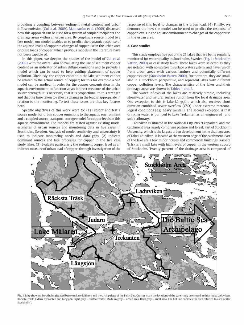
Fig. 1.Map showing Stockholm situated between Lake Mälaren and the archipelago of the BaRåcksta Träsk, Judarn, Trekanten and Långsjön. Light grey — surface water. Medium grey — uStockholm”.

response of this level to changes in the urban load. (4) Finally, wedemonstrate how the model can be used to predict the response ofcopper levels in the aquatic environment to changes of the copper usein the urban area.

2. Case studies

This study employs five out of the 21 lakes that are being regularlymonitored for water quality in Stockholm, Sweden (Fig. 1; StockholmVatten, 2000) as case study lakes. These lakes were selected as theyare isolated, with no upstream surface water system, and have run offfrom urban areas with various landuse and potentially differentcopper source (Stockholm Vatten, 2000). Furthermore, they are small,also in a Stockholm perspective, and represent lakes with differentcopper pollution levels. The characteristics of the lakes and theirdrainage areas are shown in Tables 1 and 2.

The water inflows of the lakes are relatively simple, includingstormwater and natural surface runoff from the local drainage area.One exception to this is Lake Långsjön, which also receives shortduration combined sewer overflow (CSO) under extreme meteoro-logical conditions (e.g. heavy rainfall). The second exception is thatdrinking water is pumped to Lake Trekanten as an engineered (andsole) tributary.

Laduviken is situated in the National City Park ‘Ekoparken’ and thecatchment area largely comprises pasture and forest. Part of StockholmUniversity, which is the largest urban development in the drainage areaof Lake Laduviken, is located at the western edge of the catchment. Eastof the lake are a few minor houses and commercial buildings. RåckstaTräsk is a small lake with high levels of copper in the western suburbof Stockholm. Twenty percent of the drainage area is composed of

ltic Sea. Crosses mark the locations of the case study lakes used in this study: Laduviken,rban area. Dark grey — rural area. The full line encloses the area referred to as “Greater

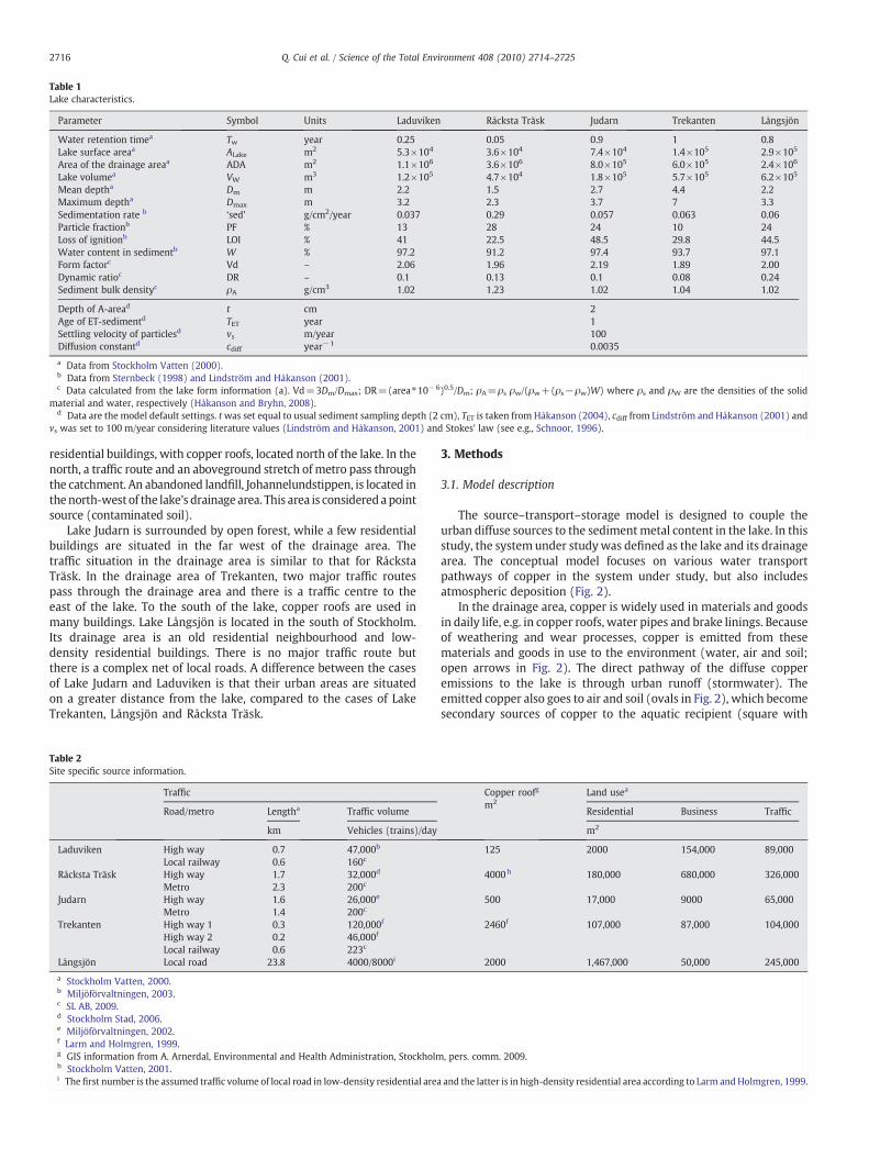
Table 1Lake characteristics.

Parameter Symbol Units Laduviken Råcksta Träsk Judarn Trekanten Långsjön

Water retention timea Tw year 0.25 0.05 0.9 1 0.8Lake surface areaa ALake m2 5.3×104 3.6×104 7.4×104 1.4×105 2.9×105

Area of the drainage areaa ADA m2 1.1×106 3.6×106 8.0×105 6.0×105 2.4×106

Lake volumea VW m3 1.2×105 4.7×104 1.8×105 5.7×105 6.2×105

Mean deptha Dm m 2.2 1.5 2.7 4.4 2.2Maximum deptha Dmax m 3.2 2.3 3.7 7 3.3Sedimentation rate b ‘sed’ g/cm2/year 0.037 0.29 0.057 0.063 0.06Particle fractionb PF % 13 28 24 10 24Loss of ignitionb LOI % 41 22.5 48.5 29.8 44.5Water content in sedimentb W % 97.2 91.2 97.4 93.7 97.1Form factorc Vd – 2.06 1.96 2.19 1.89 2.00Dynamic ratioc DR – 0.1 0.13 0.1 0.08 0.24Sediment bulk densityc ρA g/cm3 1.02 1.23 1.02 1.04 1.02

Depth of A-aread t cm 2Age of ET-sedimentd TET year 1Settling velocity of particlesd vs m/year 100Diffusion constantd cdiff year−1 0.0035

a Data from Stockholm Vatten (2000).b Data from Sternbeck (1998) and Lindström and Håkanson (2001).c Data calculated from the lake form information (a). Vd=3Dm/Dmax; DR=(area⁎10−6)0.5/Dm; ρA=ρs ρw/(ρw+(ρs−ρw)W) where ρs and ρW are the densities of the solid

material and water, respectively (Håkanson and Bryhn, 2008).d Data are the model default settings. twas set equal to usual sediment sampling depth (2 cm), TET is taken from Håkanson (2004), cdiff from Lindström and Håkanson (2001) and

vs was set to 100 m/year considering literature values (Lindström and Håkanson, 2001) and Stokes' law (see e.g., Schnoor, 1996).

2716 Q. Cui et al. / Science of the Total Environment 408 (2010) 2714–2725

residential buildings, with copper roofs, located north of the lake. In thenorth, a traffic route and an aboveground stretch of metro pass throughthe catchment. An abandoned landfill, Johannelundstippen, is located inthenorth-west of the lake's drainage area. This area is consideredapointsource (contaminated soil).

Lake Judarn is surrounded by open forest, while a few residentialbuildings are situated in the far west of the drainage area. Thetraffic situation in the drainage area is similar to that for RåckstaTräsk. In the drainage area of Trekanten, two major traffic routespass through the drainage area and there is a traffic centre to theeast of the lake. To the south of the lake, copper roofs are used inmany buildings. Lake Långsjön is located in the south of Stockholm.Its drainage area is an old residential neighbourhood and low-density residential buildings. There is no major traffic route butthere is a complex net of local roads. A difference between the casesof Lake Judarn and Laduviken is that their urban areas are situatedon a greater distance from the lake, compared to the cases of LakeTrekanten, Långsjön and Råcksta Träsk.

Table 2Site specific source information.

Traffic

Road/metro Lengtha Traffic volume

km Vehicles (trains)/day

Laduviken High way 0.7 47,000b

Local railway 0.6 160c

Råcksta Träsk High way 1.7 32,000d

Metro 2.3 200c

Judarn High way 1.6 26,000e

Metro 1.4 200c

Trekanten High way 1 0.3 120,000f

High way 2 0.2 46,000f

Local railway 0.6 223c

Långsjön Local road 23.8 4000/8000i

a Stockholm Vatten, 2000.b Miljöförvaltningen, 2003.c SL AB, 2009.d Stockholm Stad, 2006.e Miljöförvaltningen, 2002.f Larm and Holmgren, 1999.g GIS information from A. Arnerdal, Environmental and Health Administration, Stockholmh Stockholm Vatten, 2001.i The first number is the assumed traffic volume of local road in low-density residential area

3. Methods

3.1. Model description

The source–transport–storage model is designed to couple theurban diffuse sources to the sedimentmetal content in the lake. In thisstudy, the system under studywas defined as the lake and its drainagearea. The conceptual model focuses on various water transportpathways of copper in the system under study, but also includesatmospheric deposition (Fig. 2).

In the drainage area, copper is widely used in materials and goodsin daily life, e.g. in copper roofs, water pipes and brake linings. Becauseof weathering and wear processes, copper is emitted from thesematerials and goods in use to the environment (water, air and soil;open arrows in Fig. 2). The direct pathway of the diffuse copperemissions to the lake is through urban runoff (stormwater). Theemitted copper also goes to air and soil (ovals in Fig. 2), which becomesecondary sources of copper to the aquatic recipient (square with

Copper roofg

m2Land usea

Residential Business Traffic

m2

125 2000 154,000 89,000

4000h 180,000 680,000 326,000

500 17,000 9000 65,000

2460f 107,000 87,000 104,000

2000 1,467,000 50,000 245,000

, pers. comm. 2009.

and the latter is in high-density residential area according to Larm andHolmgren, 1999.

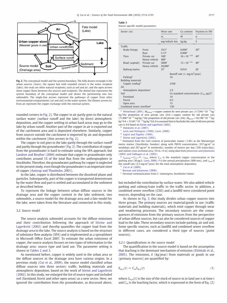
Fig. 2. The conceptual model and the system boundary. The fully drawn rectangle is theurban sources (store); the square box with rounded corners is the water recipient(lake); the ovals are other natural recipients, such as soil and air; and the open arrowsshow copper flows between the sources and recipients. The dotted line represents thesystem boundary of the conceptual model and shows the partitioning into twosubmodels. The single-line arrows represent the pathways of copper from otherenvironmental compartments (air and soil) to the water system. The thinner arrows to/from air represent the copper exchange with the external system.

Table 3Source specific model parameters.

Sector (m) Wear rate Cu content Fraction to SW

wr M α

mg/vehicle km kg/kg %

TrafficBrake linings Front 10.5a 0.090a 20b

Rear 5.13a 0.068a

Tires Private car 100c 18×10−6d 40e

Heavy vehicle 400c

Road (asphalt) Private car 5000c 13×10−6e 40e

Heavy vehicle 20,000c

Railway/metro 35f 0.014 20

Runoff rate (r, mg/m2/year)Parkingg 16

Building materialsCopper roofingh 2100

AirAtmospheric depositioni 2.5

Soil Cu standard concentration (CCu, µg/l)c

Farmland 14Forest 6.5Open area 15

Combined sewer overflowj 150

a Westerlund (2001). MB,front=copper content for new private cars (117,941⁎10−6 kg/kg)*the proportion of new private cars (0.4)+copper content for old private cars(71,990⁎10−6 mg/kg)⁎the proportion of old private cars (0.6). MB,rear=92,198⁎10−6 kg/kg⁎0.4+51241⁎10−6 kg/kg⁎0.6. It is assumed that in Stocholm the ratio of old/newprivatecars is 4:6 based on Sörme and Lagerkvist (2002).

b Hulskotte et al. (2007).c Larm and Holmgren (1999); Larm (2000).d Legret and Pagotto (1999).e Sörme and Lagerkvist (2002).f Estimated from the CuO content of particulate matter (1.8%) at the Mariatorget

metro station (Stockholm, Sweden) along with PM10 concentration (357 μg/m3 inweekdays and 267 μg/m3 in weekends), number of metros per day (556 trains/day),and station cross sectional area (10 m×6 m) using data from Johansson and Johansson(2003) and Gidhagen et al. (2003).

g rparking=CCu×P−ratm, where Ccu is the standard copper concentration in theparking area (30 μg/L; Larm, 2000), P is the annual precipitation (600 mm), and ratm isthe runoff rate (2.5 mg/m2/year) for the total atmospheric deposition.

h Cui et al (2009).i Burman and Johansson (2000).j Personal communication from C. Lännergren, Stockholm Vatten.

Runoff rate (r, mg/m2/year)

2717Q. Cui et al. / Science of the Total Environment 408 (2010) 2714–2725

rounded corners in Fig. 2). The copper in air partly goes to the naturalsurface water (surface runoff and the lake) by direct atmosphericdeposition, and the copper settling in urban hard areas may go to thelake by urban runoff. Another part of the copper in air is exported outof the catchment area and is deposited elsewhere. Similarly, copperfrom sources outside the catchment is imported by air and depositedwithin the catchment (thin arrows in Fig. 2).

The copper in soil goes to the lake partly through the surface runoffand partly through the groundwater (Fig. 2). The contribution of copperfrom the groundwater is hard to estimate using the SFA approach, butLandner and Reuther (2004) estimate that copper in groundwater onlycontributes around 1% of the total flux from the anthroposphere inStockholm. Therefore, the groundwater pathway for copper is neglectedin thepresent study, even though thegroundwater is an important storeof copper (Aastrup and Thunholm, 2001).

In the lake, copper is distributed between the dissolved phase andparticles. Subsequently, part of the copper is transported downstreamby the water flow and part is settled and accumulated in the sedimentas described below.

To represent the linkage between urban diffuse sources in thedrainage area and the copper content in the lake sediment, twosubmodels, a source model for the drainage area and a fate model forthe lake, were taken from the literature and connected in this study.

3.2. Source model

The source analysis submodel accounts for the diffuse emissionsand their contribution following the approach of Sörme andLagerkvist (2002) and thereby quantifies the copper load from thedrainage area to the lake. The source analysis is based on the structureof substance flow analysis (SFA) and is implemented as a spreadsheetin Microsoft Office Excel 2007. To estimate the urban emissions ofcopper, the source analysis focuses on two types of information in thedrainage area: source type and land use. The parameter setting isshown in Tables 2 and 3.

As mentioned before, copper is widely used in the urban area sothe diffuse sources in the drainage area have various origins. In aprevious study (Cui et al., 2009), the source model classified urbandiffuse sources into three sectors: traffic, building materials andatmospheric deposition, based on the work of Sörme and Lagerkvist(2002). In this study, we enlarged the list of source types and includedsoil (farmland, forest and other open areas) as a new sector. Here, weignored the contribution from the groundwater, as discussed above,

but included the contribution by surface water. We also added vehicleparking and railway/train traffic to the traffic sector. In addition, acombined sewer overflow (CSO) and a landfill were considered pointsources, depending on the case.

As shown in Fig. 3, this study divides urban copper sources intothree groups. The primary sources are material/goods in use (trafficmaterials and building materials), which emit copper through wearand weathering processes. The secondary sources are the conse-quences of emissions from the primary sources from the perspectiveof urban diffuse sources, but can also be considered sources of copperload to the lake. These secondary sources include parking, air and soil.Some specific sources, such as landfill and combined sewer overflowin different cases, are considered a third type of sources (pointsources).

3.2.1. Quantifications in the source modelThe quantification in the source model is based on the assumption

that leaching is the dominant mechanism of emission (Elshkaki et al.,2005). The emissions, E (kg/year) from materials or goods in use(primary sources) are quantified by:

Em;n tð Þ = CmSm;n tð Þ ð1Þ

where Sm,n(t) is the size of the stock of source m in land use n at time tand Cm is the leaching factor, which is expressed in the form of Eq. (2)

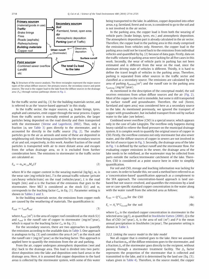
Fig. 3. Structure of the source analysis. The three rectangles represent the major sourcetypes of the urban diffuse sources: the primary source, the secondary source and pointsources. The oval is the copper load to the lake from the diffuse sources in the drainagearea (Fin) through various pathways shown in Fig. 2.

2718 Q. Cui et al. / Science of the Total Environment 408 (2010) 2714–2725

for the traffic sector and Eq. (3) for the building materials sector, andis referred to as the ‘source-based approach’ in this study.

In the traffic sector, the major sources, e.g. brake linings, tyres,asphalt and catenaries, emit copper through the wear process. Copperfrom the traffic sector is normally emitted as particles, the largerparticles being deposited on the road directly and then transportedwith the stormwater (Sörme and Lagerkvist, 2002). Thus, only afraction (α, see Table 3) goes directly to the stormwater, and isaccounted for directly in the traffic source (Fig. 2). The smallerparticles go to the air as aerosols and some of these are deposited inneighbouring soil; these being accounted for by the secondary sourcesof air and soil, respectively, in this work. Another fraction of the smallparticles is transported with air to more distant areas and escapesfrom the urban drainage area, so it is excluded from furtherconsideration here. The emissions to stormwater in the traffic sectorare calculated as:

Em = αmwr;mMmLT ð2Þ

where M is the copper content in the wearing material (kg/kg), wr isthe wear rate (mg/vehicle km), T is the annual traffic volume (privatecars/heavy vehicle/train) on the road (vehicles/year), L is the roadlength (km) and α is the fraction of the emissions that goes to thestormwater. Here MLT is considered as the stock S(t) and wr

corresponds to the leaching factor Cm in Eq. (1). Parameter setting isshown in Tables 2 and 3.

In the building materials sector, the emissions from copper roofsare caused by the weathering of materials. The quantification is:

Eroof = rroofAroof ð3Þ

where Aroof (m2) is the area of copper roof considered as the stock S(t)and rroof is the runoff rate of copper to stormwater (mg/m2/year),which is equal to the leaching factor Cm in Eq. (1).

For the secondary sources, there are two approaches to quantifythe emissions according to the available data in Table 3. One approachis analogous to Eq. (3) and considers the area A (m2) as the stock andthe runoff rate r (mg/m2/year) as the leaching factor. This approach isapplied here to quantify the emissions from the air and parking.

From the air, copper undergoes atmospheric deposition (wet anddry) back to the drainage area. This load is divided into two parts:direct deposition into the lake and deposition onto hard areas in thedrainage area. Here, it is assumed that copper deposition to the hardareas is collected by the stormwater system, with some of this water

being transported to the lake. In addition, copper deposited into otherareas, e.g. farmland, forest and so on, is considered to go to the soil andis not involved in the air sector.

In the parking area, the copper load is from both the wearing ofvehicle parts (brake linings, tyres, etc.) and atmospheric deposition.The atmospheric deposition part is already calculated in the air sector.Therefore, the copper load in the parking area in this study comprisedthe emissions from vehicles only. However, the copper load in theparking area could not be traced back to the emissions from individualvehicles and quantified by Eq. (2) because of data gaps. Firstly, data onthe traffic volume in parking areaswere lacking for all five cases in thiswork. Secondly, the wear of vehicle parts in parking has not beenestimated and is different from the wear on the road, since thedominant driving state of vehicles is different. Thirdly, it is hard todefine the travel length of vehicles in the parking areas. Therefore,parking is separated from other sources in the traffic sector andclassified as a secondary source. The emissions are calculated by thearea of parking Aparking(m2) and the runoff rate in the parking arearparking (mg/m2/year).

As mentioned in the description of the conceptual model, the soilreceives emissions from urban diffuse sources and the air (Fig. 2).Most of the copper in the soil is immobile, but some is still transportedby surface runoff and groundwater. Therefore, the soil (forest,farmland and open area) was considered here as a secondary sourceto the lake. As mentioned previously, we ignored the transport ofcopper with groundwater, but included transport from soil by surfacewater to the lake (see below).

Combined sewer overflow (CSO) is a special source, which appearsonly in the case of Lake Långsjön. The overflow only happens duringheavy rainfall to relieve the flood pressure on the municipal drainagesystem. It is complex work to quantify the original source of copper inCSO. Firstly, the overflow contains not only stormwater but also sewerwater, and the diffuse sources of copper in sewers are not involved inthe list of source types in Fig. 3. Secondly, the drainage area of the lakein Fig. 1 is defined by the surface runoff and the stormwater flow. Forevaluating copper emissions in the sewer, the drainage area of thelake needs to be redefined, as the wastewater may be collected fromparts outside the surface/stormwater catchment of the lake. There-fore, CSO is considered as a point source here in order to simplifyquantification.

For soil and CSO, storage and leaching information was lacking forour cases. In order to handle this, we used amethod here referred to asa ‘concentration-based’ quantification approach as a complement tothe SFA approach. The concentration-based approach is land use-based but not source-resolved, and quantifies the emissions by a landuse or case-specific standard copper concentration in the water alongwith the water runoff from the selected area as follows:

ECSO = Q*CCu;CSO for the CSO ð4aÞ

Es = As*P*CCu;soil for the soil ð4bÞ

where CCu is the standard copper concentration in stormwater in theselected area (µg/l), as quantified in Stockholm Vatten (2000), Q is theflux of CSO (m3/year), As is the area of soil (m2) and P is the meanannual precipitation in Stockholm (m/year). The parameter setting isshown in Table 3.

3.2.2. Linking the source model to the lake modelNot all copper that is emitted goes to the lake. Here we assumed

that a fraction αm of the diffuse emissions goes to the stormwater, anda fraction βn of the stormwater goes directly to the recipient, withoutpassing through a stormwater treatment facility. The βn factorrepresents the proportion of the stormwater that is collected andtransmitted to the lake, and it is determined by the land use (Eq. (5);values given in Table 4). Therefore, in the source model, the copper

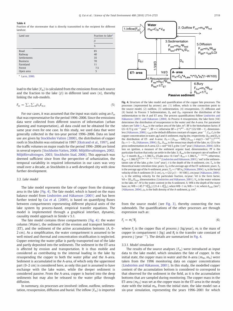
Table 4Fraction of the stormwater that is directly transmitted to the recipient for differentlanduse.

Land use Fraction to lakea

β

%

Road 85Railway 40Settlements 35Business 70Farmland 11Forest 7.5Open area 5

a Larm, 2000.

Fig. 4. Structure of the lake model and quantification of the copper fate processes. Theprocesses (represented by arrows) are: (1) inflow, which is the connection point tothe source model, (2) outflow, (3) sedimentation, (4) resuspension, (5) diffusion and(6) burial. In Process 3 Sedimentation, DA and DET represent the distribution of thesedimentation to the A and ET area. The process quantifications follow Lindström andHåkanson (2001) and Håkanson (2004). In Process 4 resuspension, the lake form (Vd)determines the distribution of resuspension to the water and the A-area. For parametervalues see Table 1. ALake is the surface area of the lake, m2; BF is the bioturbation factor, IfGSN0.73 g cm−2 year−1, BF=1; otherwise BF=2⁎ t0.5−0.2⁎(GS/100−1), dimension-less (Håkanson, 2006); cdiff is the default diffusion constant of copper, year−1; CW, CS is thecopper concentration inwater, μg/l and A-sediment,mg/kg dw, respectively;DET andDA isthe distribution of ET- and A-area; DA=((Dmax−WB)/(Dmax+exp(3−Vd1.5)))0.5/Vd,DET=1−DA (Håkanson, 2004); Dm, Dmax is the mean/max depth of the lake, m; GS is thegross sedimentation onA-area, GS=sed⁎Vd/3, gdw /(cm2 year) (Håkanson, 2004); LOI isloss on ignition, a measure of the sediment organic load, dimensionless; PF is theparticulate fraction that only can settle in the lake, %; Rout is the transport rate of outflow. IfTWb1 month; Rout=1.386/Tw; if Lake areab0.1 km2: Rout=1.386/Tw 1−0.5/Tw; otherwise,Rout=1.386/Tw(30/(Tw+30−1)+0.5)/1.5 (LindströmandHåkanson,2001); ‘sed’ is the sedimen-tation rate of the lake, g dw /(cm2 year); t is the depth of the A-sediment, cm; Tw is thetheoreticalwater retention time, years; TET is the average age of the ET-sediment, years; TAis the average age of theA-sediment, years; TA=t⁎BF/vb (Håkanson, 2004); vb is the burialvelocity of the A-sediment (0–2 cm), vb=GS/(ρ(1−W/100)), cm/year (Håkanson, 2004);vs is the settling velocity for the particulate fraction, m/year; Vd is the form factor,Vd=3Dm/Dmax, dimensionless (Lindström and Håkanson, 2001); Vw is the water volumein the lake, m3;W is the water content in the A-sediment, %; WB is the depth of the wavebase,m;WB=(45.7⁎ALake0.5 )/(21.4+ALake

0.5 ), whenWBb1 m,WB=1m;where ALake (km2)(Håkanson, 2004). ρA is the bulk density of the A-sediment, g /cm3.

2719Q. Cui et al. / Science of the Total Environment 408 (2010) 2714–2725

load to the lake (Fin) is calculated from the emissions from each sourceand the fraction to the lake (β) in different land uses (n), therebylinking the sub-models.

Fin = ∑n∑mβnEm;n ð5Þ

For our cases, it was assumed that the input was static using an Finthat was representative for the period 1996–2006. Since the emissionsdata were collected from different sources of information (urbanplanning and transportation), all data could not be obtained for thesame year even for one case. In this study, we used data that weregenerally collected in the ten-year period 1996–2006. Data on landuse are given by Stockholm Vatten (2000), the distribution of copperroofs in Stockholm was estimated in 1997 (Ekstrand et al., 1997), andthe traffic volumes onmajor roads for the period 1996–2006 are listedin several reports (Stockholm Vatten, 2000; Miljöförvaltningen, 2002;Miljöförvaltningen, 2003; Stockholm Stad, 2006). This approach wasdeemed sufficient since from the perspective of urbanization, thetemporal variability in required information in our cases was verysmall over a decade, as Stockholm is a well-developed city with slowfurther development.

3.3. Lake model

The lake model represents the fate of copper from the drainagearea in the lake (Fig. 4). The fate model, which is based on the massbalance model from Lindström and Håkanson (2001) and has beenfurther tested by Cui et al. (2009), is based on quantifying fluxesbetween compartments representing different physical units of thelake system by process-based, empirical transfer equations. Themodel is implemented through a graphical interface, dynamic,causality model approach in Simile v 5.1.

The fate model contains three compartments (Fig. 4): the watercolumn (Water), the sediment of the erosion and transport bottoms(ET), and the sediment of the active accumulation bottoms (A, 0–2 cm). As a simplification, the water compartment is assumed to bewell mixed and thermal and concentration stratification is neglected.Copper entering the water pillar is partly transported out of the lakeand partly deposited into the sediments. The sediment in the ET-areais affected by erosion and transportation. It is thus mobile andconsidered as contributing to the internal loading in the lake byresuspending the copper to both the water pillar and the A-area.Sediment is accumulated in the A-area, of which only the uppermostpart (0–2 cm) is considered here, as only this part is assumed to haveexchange with the lake water, while the deeper sediment isconsidered passive. From the A-area, copper is buried into the deepsediments but may also be released to the water pillar throughdiffusion.

In summary, six processes are involved: inflow, outflow, sedimen-tation, resuspension, diffusion and burial. The inflow (Fin) is imported

from the source model (see Fig. 3), thereby connecting the twosubmodels. The quantifications of the other processes are throughexpression such as:

Fj = mi*Rj ð6Þ

where Fj is the copper flux of process j (kg/year), mi is the mass ofcopper in compartment i (kg) and Rj is the transfer rate constant ofprocess j (year−1). The details are summarized in Fig. 4.

3.3.1. Model simulationThe results of the source analyses (Fin) were introduced as input

data to the lake model, which simulates the fate of copper. In theinitial state, the copper mass in water and the A-area (mW, mA) weretaken from the 1996 monitoring data on copper concentrations(Lindström and Håkanson, 2001). In this study, the modelled coppercontent of the accumulation bottom is considered to correspond tothat observed for the sediment in the field, as it is the accumulationbottoms that are sampled during monitoring. The copper mass in theET-area (mET) was set as the copper mass in the ET-area in the steadystate with the initial mA. From the initial state, the lake model ran asix-year simulation, representing the years 1996–2001 for which

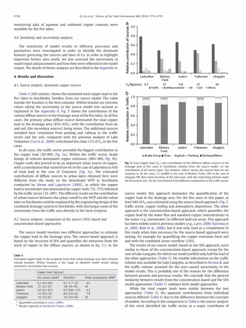
Fig. 5. Total copper load (Fin) and contribution of the different diffuse sources in thedrainage area of five cases in Stockholm, Sweden from the source model. (a) thecontribution of all source types. The notation ‘others’ means the sources that are notcommon to all the cases, i.e. landfill in the case of Råcksta Träsk, CSO in the case ofLångsjön NB: Bars show fractions of the total load, with this load being printed underthe horizontal axis; (b) the contribution from different components in the traffic sector.

2720 Q. Cui et al. / Science of the Total Environment 408 (2010) 2714–2725

monitoring data of aqueous and sediment copper contents wereavailable for the five lakes.

3.4. Sensitivity and uncertainty analyses

The sensitivity of model results to different processes andparameters were investigated in order to identify the dominantfeatures governing the sources and fates of Cu. In order to highlightimportant further data needs, we also assessed the uncertainty inmodel input and parameters and how theywere reflected in themodeloutput. The details of theses analyses are described in the Appendix A.

4. Results and discussion

4.1. Source analysis: dominant copper sources

Table 5 (left column) shows the estimated total copper load to thefive lakes in Stockholm, Sweden, from our source model. The valueoutside the brackets is the best estimate. Within bracket are extremevalues taking the uncertainty in the source model into account asexplained in the Appendix A. Fig. 5 shows the contribution of thevarious diffuse sources in the drainage areas of the five lakes. In all fivecases, the primary urban diffuse source dominated the total copperload in the drainage area (83%–93%), with the contribution from airand soil (the secondary sources) being minor. The additional sourcesincluded here (emissions from parking and railway in the trafficsector and the soil) compared with the previous analysis of LakeTrekanten (Cui et al., 2009) contributed less than 11% of Fin in the fivecases.

In all cases, the traffic sector provided the biggest contribution tothe copper load (50–80%, Fig. 5a). Within the traffic sector, brakelinings of vehicles dominated copper emissions (80%–90%, Fig. 5b).Copper roofs also proved to be an important urban source of copper,with a contribution that varied from 4% in the case of Laduviken to 43%of total load in the case of Trekanten (Fig. 5a). The estimatedcontributions of diffuse sources to urban lakes obtained here weredifferent from the study on the Henriksdal WTP in Stockholmconducted by Sörme and Lagerkvist (2002), in which the copperload in stormwaterwas dominated by copper roofs (72–77%) followedby the traffic sector (23–28%). The different results on the contributionof urban sources between the urban runoff to the WTP and the urbanlakes in Stockholm could be explained by the engineering design of thecombined drainage system in Stockholm, with discharges some of thestormwater from the traffic area directly to the local recipient.

4.2. Source analysis: comparison of the source (SFA)-based andconcentration-based approaches

The source model involves two different approaches to estimatethe copper load in the drainage area. The source-based approach isbased on the structure of SFA and quantifies the emissions from thestock of copper in the diffuse sources, as shown in Eq. (1). In the

Table 5Estimated copper loads to the recipients from their urban drainage area. Best estimateoutside brackets. Within brackets is the range of obtained model results takingparametric uncertainty into account.

Copper load (kg/year)

Our source model StormTaca Water programme 2000b

Laduviken 6.1 (4.2–8.8) 8.1 (1.7–12) 6.5Råcksta Träsk 27 (21–35) 38 (10–78) 36Judarn 5.8 (4.1–8.2) 4.5 (0.81–7.0) 4.2Trekanten 12 (9.4–16) 8.0 (2.0–22) 7.9Långsjön 16 (12–22) 25 (5.9–43) 26

a Quantified according to Larm (2000).b Results reported in Stockholm Vatten (2000).

source model, this approach dominates the quantification of thecopper load in the drainage area. For the five cases in this paper, atleast 94% of Fin was estimated using the source-based approach (Fig. 5,traffic sector, copper roofing and atmospheric deposition). The otherapproach is the concentration-based approach, which quantifies thecopper load by the water flux and standard copper concentrations inthe water (e.g. stormwater) in different land use areas. This approachhas beenwidely used in previous studies (e.g., Larm, 2000; Karvelas etal., 2003; Rule et al., 2006), but it was only used as a complement inthis study when data necessary for the source-based approach werelacking, for example for quantifying the copper emissions from soiland with the combined sewer overflow (CSO).

The results of our source model, based on the SFA approach, weresimilar to those of the concentration-based approach, except for thecase of Lake Långsjön, forwhich ourmodel yielded only half the load ofthe other approaches (Table 5). No reliable information on the trafficvolume was available for Lake Långsjön, as described in Section 2, andthe traffic volume assumed for the area caused uncertainty in themodel results. This is probably one of the reasons for the differencebetween present and previous results. We conclude that the generalsimilarity between results from the concentration-based and the SFAmodel approaches (Table 5) validates both model approaches.

While the total copper loads were similar between the twoapproaches (Table 5), the apparent contributions from individualsources differed (Table 6) due to the difference between the conceptsof models. According to the comparison in Table 6, the source analysisof this work identified the traffic sector as a major contributor of

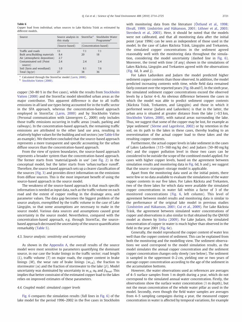
Table 6Copper load from individual, urban sources to Lake Råcksta Träsk as estimated bydifferent models.

Source Source analysis inthis study

StormTaca Stockholm WaterProgrammeb

(Source-based) (Concentration-based)

Traffic and roads 13 7.1 7.1Built area/Building materials 8.4 20 18Air (atmospheric deposition) 2.7Contaminated soil (Pointsource)

2.4 2.4 2.4

Soil (farm and woodland) 1.0 8.1 7.6Total (kg/yr) 27 38 36

a Calculated through the StormTac model (Larm, 2000).b Stockholm Vatten (2000).

2721Q. Cui et al. / Science of the Total Environment 408 (2010) 2714–2725

copper (50–80 % in the five cases), while the results from StockholmVatten (2000) and the StormTac model identified urban areas as themajor contributor. This apparent difference is due to all trafficemissions in all land use types being accounted for in the traffic sectorin the SFA approach, whereas the concentration-based approachemployed in StormTac (Larm, 2000) and by Stockholm Vatten(Personal communication with Lännergren C., 2009) only includesthose traffic emissions occurring in traffic areas (roads, parking andrailways). In the concentration-based approach, the remaining trafficemissions are attributed to the other land use area, resulting inrelatively higher values for the building and soil sectors (see Table 6 foran example). We therefore concluded that the source-based approachrepresents a more transparent and specific accounting for the urbandiffuse sources than the concentration-based approach.

From the view of system boundaries, the source-based approachrepresents a broader system than the concentration-based approach.The former starts from ‘material/goods in use’ (see Fig. 2) in theconceptual model, but the latter starts from ‘urban/surface runoff’.Therefore, the source-based approach sets up a clearer classification ofthe sources (Fig. 3) and provides direct information on the emissionsfrom diffuse sources. This is the most important benefit of using thesource-based approach in the source model.

The weakness of the source-based approach is that much specificinformation is needed as input data, such as the traffic volume on eachroad and the extent of copper roofing in the drainage area, andparameter values. The data gap becomes the biggest problem of thesource analysis, exemplified by the traffic volume in the case of LakeLångsjön, so that some assumptions are necessary to make in thesource model. Various data sources and assumptions caused greatuncertainty in the source model. Nevertheless, compared with theconcentration-based approach, e.g. through StormTac, the source-based approach decreased the uncertainty of the source quantificationremarkably (Table 5).

4.3. Source analysis: sensitivity and uncertainty

As shown in the Appendix A, the overall results of the sourcemodel were most sensitive to parameters quantifying the dominantsource, in our case the brake linings in the traffic sector; road length(L), traffic volume (T) on major roads, the copper content in brakelinings (M), the wear rate of brake linings (wr,B), the fraction tostormwater (α) and the fraction of stormwater to the lake (β). Modeluncertainty was dominated by uncertainty in wr,B, αB and βRoad. Thisimplies that better constraint of the estimated copper load to the lakesrelies on improved estimates of these parameters.

4.4. Coupled model: simulated copper levels

Fig. 6 compares the simulation results (full lines in Fig. 6) of thelake model for the period 1996–2002 in the five cases in Stockholm

with monitoring data from the literature (Östlund et al., 1998;Ekvall, 1999; Lindström and Håkanson, 2001; Lithner et al., 2003;Sternbeck et al., 2003). Here, it should be noted that the modelswere not calibrated, and that all monitoring data after the initialpoint (year 1996) can be seen as independent of those used in themodel. In the case of Lakes Råcksta Träsk, Långsjön and Trekanten,the simulated copper concentrations in the sediment agreedreasonably well with the monitoring data throughout the simula-tion, considering the model uncertainty (dashed line in Fig. 6).Moreover, the trend with time (if any) shown in the simulations ofLakes Råcksta, Långsjön and Trekanten agreed with the observations(Fig. 6d, h and j).

For Lakes Laduviken and Judarn the model predicted highersediment copper contents than those observed. In addition, the modelpredicted increasing contents with time, while field data remainedfairly constant over the reported years (Fig. 6b and f). In the sixth year,the simulated sediment copper concentrations exceed the observedlevels by a factor 4–6. An obvious difference between the cases inwhich the model was able to predict sediment copper contents(Råcksta Träsk, Trekanten, and Långsjön) and those in which itperformed worse (Judarn and Laduviken) is that in the latter, theurban area is situated at greater distance from the lake (N0.5 km,Stockholm Vatten, 2000), with natural areas surrounding the lake.Thus, we suggest that some of the copper may be lost, for example as‘pipe sediment’ (Sörme and Lagerkvist, 2002) or by retention in thesoil, on its path to the lakes in these cases, thereby leading to anoverestimation of the actual copper load to these lakes and theresulting copper contents.

Furthermore, the actual copper levels in lake sediment in the casesof Lakes Laduviken (115–160 mg/kg dw) and Judarn (50–80 mg/kgdw) and the copper pollution level in those two cases can beconsidered to be outside the scope of the combinedmodel applied. Forcases with higher copper levels, based on the agreement betweensimulation results and monitoring data in Fig. 6d, h and j, we suggestthat the source–transport–storage model is applicable.

Apart from the monitoring data used as the initial points, therewere few or no data available to evaluate the simulations of the watercopper contents in our five lakes. For Lakes Råcksta and Trekanten,two of the three lakes for which data were available the simulatedcopper concentrations in water fall within a factor of 3 of themonitored concentrations (Fig. 6, left column). This level ofagreement between model results and monitoring data is similar tothe performance of the original lake model in previous studies(Lindström and Håkanson, 2001; Cui et al., 2009). For Lake RåckstaTräsk, the agreement between simulated water concentrations ofcopper and observations is also similar to that obtained by the QWASImodel as shown by Sinha (2009). For Lake Judarn, the simulatedconcentration of copper in water is much higher than observed in thefield in the year 2001 (Fig. 6e).

Generally, the model reproduced the copper content of water lesswell than the copper content of sediment. This can be explained fromboth the monitoring and the modelling view. The sediment observa-tions we used correspond to the model simulation results, as themodel simulates the annual copper concentration and the sedimentcopper concentration changes only slowly (see below). The sedimentis sampled in the uppermost 0–2 cm, yielding one or two years ofaverage copper concentration according to the age of the sediment inthe accumulation bottoms.

However, the water observations used as references are averagesof 4–5 surface samples from 1 m depth during a year, which do notcorrespond to the simulated annual water concentration. Firstly, theobservations show the surface water concentration (1 m depth), butnot the mean concentration of the whole water pillar as used in themodel. Secondly, even though the field water samples are averagesfrom 4–5 sampling campaigns during a year, the measured copperconcentration in water is affected by temporal variations, for example

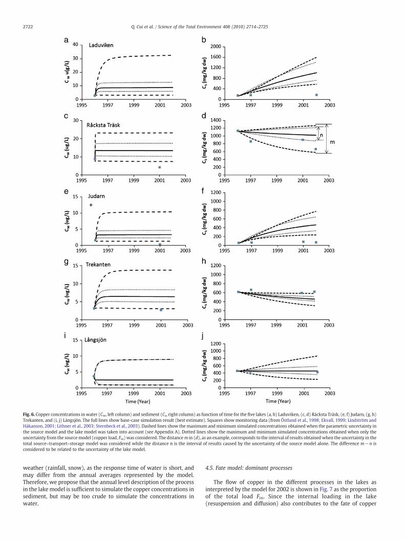
Fig. 6. Copper concentrations in water (Cw, left column) and sediment (Cs, right column) as function of time for the five lakes (a, b) Laduviken, (c, d) Råcksta Träsk, (e, f) Judarn, (g, h)Trekanten, and (i, j) Långsjön. The full lines show base-case simulation result (best estimate). Squares showmonitoring data (from Östlund et al., 1998; Ekvall, 1999; Lindström andHåkanson, 2001; Lithner et al., 2003; Sternbeck et al., 2003). Dashed lines show the maximum andminimum simulated concentrations obtained when the parametric uncertainty inthe source model and the lake model was taken into account (see Appendix A). Dotted lines show the maximum and minimum simulated concentrations obtained when only theuncertainty from the sourcemodel (copper load, Fin) was considered. The distancem in (d), as an example, corresponds to the interval of results obtainedwhen the uncertainty in thetotal source–transport–storage model was considered while the distance n is the interval of results caused by the uncertainty of the source model alone. The difference m−n isconsidered to be related to the uncertainty of the lake model.

2722 Q. Cui et al. / Science of the Total Environment 408 (2010) 2714–2725

weather (rainfall, snow), as the response time of water is short, andmay differ from the annual averages represented by the model.Therefore, we propose that the annual level description of the processin the lakemodel is sufficient to simulate the copper concentrations insediment, but may be too crude to simulate the concentrations inwater.

4.5. Fate model: dominant processes

The flow of copper in the different processes in the lakes asinterpreted by the model for 2002 is shown in Fig. 7 as the proportionof the total load Fin. Since the internal loading in the lake(resuspension and diffusion) also contributes to the fate of copper

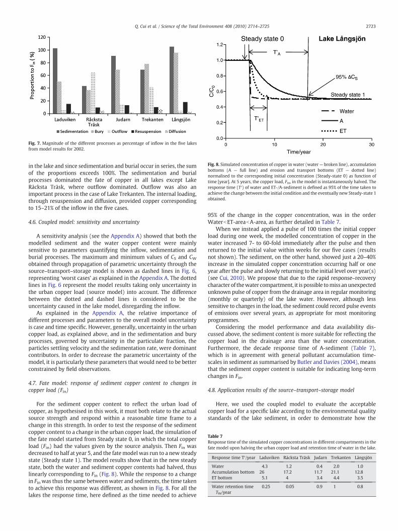
Fig. 7. Magnitude of the different processes as percentage of inflow in the five lakesfrom model results for 2002.

Fig. 8. Simulated concentration of copper in water (water— broken line), accumulationbottoms (A — full line) and erosion and transport bottoms (ET — dotted line)normalised to the corresponding initial concentration (Steady-state 0) as function oftime [year]. At 5 years, the copper load, Fin, in the model is instantaneously halved. Theresponse time (T′) of water and ET-/A-sediment is defined as 95% of the time taken toachieve the change between the initial condition and the eventually new Steady-state 1obtained.

Table 7Response time of the simulated copper concentrations in different compartments in thefate model upon halving the urban copper load and retention time of water in the lake.

Response time T′/year Laduviken Råcksta Träsk Judarn Trekanten Långsjön

Water 4.3 1.2 0.4 2.0 1.0Accumulation bottom 26 17.2 11.7 21.1 12.8ET bottom 5.1 4 3.4 4.4 3.5

Water retention timeTW/year

0.25 0.05 0.9 1 0.8

2723Q. Cui et al. / Science of the Total Environment 408 (2010) 2714–2725

in the lake and since sedimentation and burial occur in series, the sumof the proportions exceeds 100%. The sedimentation and burialprocesses dominated the fate of copper in all lakes except LakeRåcksta Träsk, where outflow dominated. Outflow was also animportant process in the case of Lake Trekanten. The internal loading,through resuspension and diffusion, provided copper correspondingto 15–21% of the inflow in the five cases.

4.6. Coupled model: sensitivity and uncertainty

A sensitivity analysis (see the Appendix A) showed that both themodelled sediment and the water copper content were mainlysensitive to parameters quantifying the inflow, sedimentation andburial processes. The maximum and minimum values of CS and CWobtained through propagation of parametric uncertainty through thesource–transport–storage model is shown as dashed lines in Fig. 6,representing ‘worst cases’ as explained in the Appendix A. The dottedlines in Fig. 6 represent the model results taking only uncertainty inthe urban copper load (source model) into account. The differencebetween the dotted and dashed lines is considered to be theuncertainty caused in the lake model, disregarding the inflow.

As explained in the Appendix A, the relative importance ofdifferent processes and parameters to the overall model uncertaintyis case and time specific. However, generally, uncertainty in the urbancopper load, as explained above, and in the sedimentation and buryprocesses, governed by uncertainty in the particulate fraction, theparticles settling velocity and the sedimentation rate, were dominantcontributors. In order to decrease the parametric uncertainty of themodel, it is particularly these parameters that would need to be betterconstrained by field observations.

4.7. Fate model: response of sediment copper content to changes incopper load (Fin)

For the sediment copper content to reflect the urban load ofcopper, as hypothesised in this work, it must both relate to the actualsource strength and respond within a reasonable time frame to achange in this strength. In order to test the response of the sedimentcopper content to a change in the urban copper load, the simulation ofthe fate model started from Steady state 0, in which the total copperload (Fin) had the values given by the source analysis. Then Fin wasdecreased to half at year 5, and the fatemodel was run to a new steadystate (Steady state 1). The model results show that in the new steadystate, both the water and sediment copper contents had halved, thuslinearly corresponding to Fin (Fig. 8). While the response to a changein Fin was thus the same betweenwater and sediments, the time takento achieve this response was different, as shown in Fig. 8. For all thelakes the response time, here defined as the time needed to achieve

95% of the change in the copper concentration, was in the orderWaterbET-areabA-area, as further detailed in Table 7.

When we instead applied a pulse of 100 times the initial copperload during one week, the modelled concentration of copper in thewater increased 7- to 60-fold immediately after the pulse and thenreturned to the initial value within weeks for our five cases (resultsnot shown). The sediment, on the other hand, showed just a 20–40%increase in the simulated copper concentration occurring half or oneyear after the pulse and slowly returning to the initial level over year(s)(see Cui, 2010). We propose that due to the rapid response–recoverycharacter of thewater compartment, it is possible tomiss an unexpectedunknown pulse of copper from the drainage area in regular monitoring(monthly or quarterly) of the lake water. However, although lesssensitive to changes in the load, the sediment could record pulse eventsof emissions over several years, as appropriate for most monitoringprogrammes.

Considering the model performance and data availability dis-cussed above, the sediment content is more suitable for reflecting thecopper load in the drainage area than the water concentration.Furthermore, the decade response time of A-sediment (Table 7),which is in agreement with general pollutant accumulation time-scales in sediment as summarised by Butler and Davies (2004), meansthat the sediment copper content is suitable for indicating long-termchanges in Fin.

4.8. Application results of the source–transport–storage model

Here, we used the coupled model to evaluate the acceptablecopper load for a specific lake according to the environmental qualitystandards of the lake sediment, in order to demonstrate how the

2724 Q. Cui et al. / Science of the Total Environment 408 (2010) 2714–2725

proposed model can be applied in a practical sense, using lakeTrekanten as a case. For Trekanten, the monitored sediment coppercontent of 475 mg/kg dw (Rauch, 2007) in year 2007 corresponded toClass 4 (100–500 mg/kg dw) according to the Swedish EPA classifi-cation (Rauch, 2007). To restore the lake sediment copper content toClass 3 (25–100 mg/kg dw), the urban load of copper needs to bedecreased. Model simulations, using arbitrarily decreased urbancopper loads (Fin), showed that Finb3.8 kg/year is required to meetClass 3 criteria. This corresponds to a reduction of the copper loadwith around 70% from the level representative of the years 1996–2002. Simulation results furthermore suggested that a decade will beneeded to restore the sediment copper content after the source hasbeen decreased (results not shown).

According to the source analysis, the dominant sources of copperin the drainage area of Trekanten are traffic (69%) and copper roofs(23%). Thus, reducing copper roofing and traffic in the catchmentwould be efficient ways to meet the requirement of decreased urbanload of copper. In reality, copper roofing in this drainage area hadgreatly decreased by 2008, but the volume of traffic on the highwayhas increased 12–19% during the last 5–6 years (S. Thörnelöf, pers.comm. 2008). According to model simulations, the overall response ofthe copper content of the sediment to these changes is not expectedbefore the end of the 2010s.

5. Conclusions

This study attempts to link the information on copper sources inthe urban area and the fate of copper in the local aquatic recipient in asource–transport–storage model. Pervious modelling has focusedeither on the sources of copper (e.g., Larm, 2000; Sörme andLagerkvist, 2002) or on the fate of copper in the aquatic environment(e.g., van der Voet et al., 2000; Woodfine et al., 2000; Lindström andHåkanson, 2001). Through coupling the sources and the fate of copperin the aquatic model, the model can be used to predict the dynamicresponse of the sediment copper level to changes of copper use in theurban catchment.

Similarity between model results from the source-based approachfor estimating the copper source strength used here and a concen-tration-based approach used previously in the literature validatedboth approaches (Table 5). The source-based approach decreased theuncertainty in the estimate of the copper load, compared to theconcentration-based approach, and provided a direct coupling to theindividual, urban sources. The major weakness of the source-basedapproach is the requirement of extensive site specific data. The sourceanalysis indicated that the traffic sector (especially brake linings) wasthe dominant diffuse source in the drainage area in all five casesassessed here (see Fig. 5). In the case of Lake Trekanten, copper roofswere also an important source.

Tests of the coupled source–transport–storage model in five casesin Stockholm indicated that the model is applicable for quantifyingthe sediment copper levels for urban lakes with high copper levels inthe sediments (Lakes Trekanten, Råcksta Träsk and Långsjön) but isnot so accurate for cases with lower levels of copper (Lakes Laduvikenand Judarn; see Fig. 6). The model was better at predicting the coppercontent in sediment than in water, which may be related to theagreement of the spatial and temporal resolution of the model, themodel input, and the field observations used to test the model. Thelake fate model suggested that sedimentation and burial processesdominated the fate of copper in all cases except Lake Råcksta Träsk,where outflow is the dominant process, due to the low waterretention time of this recipient. The model results suggested that theinternal loading of copper from the sediments to the water pillar,through resuspension and diffusion, was low in all five cases (Fig. 7).

The sensitivity analysis and uncertainty analyses showed that theuncertainty in the estimate of the copper source strength could bedecreased particularly by better constraining the wear rate of brake

linings, the fraction of copper that goes to stormwater and the fractionof the stormwater that goes from roads directly to the lake. For thefate part of the model, model uncertainty due to parametricuncertainty was dominated by the uncertainty in the source estimatealong with uncertainty in the particulate fraction, the settling velocityof particles, and the sedimentation rate.

The model response of the sediment copper content in theaccumulation bottoms to a change in the copper load from thedrainage area (Fin) showed that the simulated sediment copperconcentration (CS) linearly reflected Fin, but with a temporal delay onthe decade level. Based on this, we suggest that sediment can be usedto indicate long-term variations in the urban load. Model resultsfurthermore suggests that considerable pulse loads of copper to thelake from the urban catchment may be missed by monitoring thecopper content of the lake water, as copper levels are rapidly reducedthere. Although the reflection of the pulse is weaker in the sediment,its duration is longer, such that the same pulse could readily bedetected by monitoring of the sediment copper levels.

Finally, we demonstrated how themodel can be used in an appliedsense to guide abatement of copper pollution. Simulation resultsindicated that for lake Trekanten, as an example, a 70% decrease in thecopper load from the level representative of the years 1996–2002would be necessary for the lake sediment copper contents to meetcriteria for the next better class, as defined by the Swedish EPA. Thismagnitude of decrease of the copper load can in this particular caseonly be achieved by combined abatement of emissions from trafficand copper roofing. Model results furthermore indicate that therecovery of the copper levels in the sediment upon decrease of thesource will take around a decade.

Encouraged by the fairly good agreement between model resultsand independent survey and field monitoring data, we propose thatthe coupled source–transport–storage model may find applied use forguiding planning of monitoring and abatement of copper pollution ofurban lakes. We furthermore propose that the model concept isworthy of testing for more complex water systems and also for otherpollutants than copper, considered here.

Acknowledgements

Gratitude is expressed to Drs. Arne Jamtrot, Anja Arnerdal andStina Thörnelöf from the Environmental and Health Administration,Stockholm, Sweden, and Christer Lännergren from Stockholm Vatten,Stockholm, Sweden, for providing data and for valuable discussions.Prof. Lars Håkanson, Department of Earth Science, Uppsala University,Uppsala, Sweden is acknowledged for advice on the lake modelling.We thank Valentina Rolli, Industrial Ecology, KTH, Stockholm,Sweden, for helpful assistance with information collection. Q. Cuialso acknowledges financial support from the China ScholarshipCouncil.

Appendix A. Supplementary data

Supplementary data associated with this article can be found, inthe online version, at doi:10.1016/j.scitotenv.2010.02.045.

References

Aastrup M, Thunholm B. Heavy metals in Stockholm groundwater-concentrations andfluxes. Water Air Soil Pollut Focus 2001;1:25–41.

Burman L, Johansson C. Tungmetaller i nederbörd på Södermalm. Stockholm, Sweden:Miljöförvaltningen; 2000. Report No.: SLB. analysis 4:00. In Swedish.

Butler D, Davies JW. Urban drainage. 2nd ed. London: Spon Press; 2004. p. 46–7.Cui, Q. Tracing Copper from society to the aquatic environment: Model development

and case studies in Stockholm. [Licentiate Thesis] TRITA-IM 2009:29, Stockholm,Sweden: Department of Industrial Ecology, Royal Institute of Technology; 2010.

Cui Q, Brandt N, Malmström ME. Sediment metal contents as indicators of urban metalflows in Stockholm. In: Havránek M, editor. Urban Metabolism: Measuring theEcological City: Proceeding of the international conference ConAccount; 2008 Sep11–12. Prague, Czech: Charles University Environment Center; 2009. p. 255–82.

2725Q. Cui et al. / Science of the Total Environment 408 (2010) 2714–2725

Ekstrand S, Hansen C, Johansson D, Östlund P. Kartläggning av koppartak i Stockholm,Solna och Sundbyberg med digitala flygbilder. Stockholm, Sweden: Institutet förVatten- och Luftvårdsforskning(IVL); 1997. In Swedish.

Ekvall J. Sedimentundersökning i sjön Trekanten 1996—tungmetaller, PAH, toxicitet.Stockholm, Swden: Stockholm Vatten; 1999. Report No. 14/99. In Swedish.

Elshkaki A, Van der Voet E, Timmermans V, Van Holderbeke M. Dynamic stockmodelling: A method for the identification and estimation of future waste streamsand emissions based on past production and product stock characteristics. Energy2005;30:1353–63.

Gidhagen L, Johansson C, Ström J, Kristensson A, Swietlicki E, Pirjola L, et al. Modelsimulation of ultrafine particles inside a road tunnel. Atmos Environ 2003;37:2023–36.

Göbel P, Dierkes C, Coldewey WG. Storm water runoff concentration matrix for urbanareas. J Contam Hydrol 2007;91:26–42.

Håkanson L. Internal loading: a new solution to an old problem in aquatic sciences.Lakes Reserv Res Manage 2004;9:3-23.

Håkanson L. Suspended Particulate Matter in Lakes, Rivers, and Marine Systems.Blackburn Press; 2006.

Håkanson L, Bryhn AC. A dynamic mass-balance model for phosphorus in lakes with afocus on criteria for applicability and boundary conditions. Water Air Soil Pollut2008;187:119–47.

Hulskotte JHJ, Schaapp M, Visschedijk AJH. Brake wear from vehicles as an importantsource of diffuse copper pollution. Water Sci Technol 2007;56(1):223–31.

Johansson C, Johansson P. Particulate matter in the underground of Stockholm. AtmosEnviron 2003;37:3–9.

Karvelas M, Katsoyiannis A, Samara C. Occurrence and fate of heavy metals in thewastewater treatment process. Chemosphere 2003;53:1201–10.

Landner L, Reuther R. Metals in society and in the environment: a critical review ofcurrent knowledge on fluxes, speciation, bioavailability and risk for adverse effectsof copper, chromium, nickel and zinc. Kluwer Academic Publishers; 2004. 248 pp.

Larm, T. Watershed-based design of stormwater treatment facilities: model develop-ment and applications [Dissertation].Stockholm, Sweden: Civil and EnvironmentalEngineering, Royal Institute of Technology; 2000. TRITA-AMI PHD 1038.

Larm, T., Holmgren, A. (1999) Föroreningsbelastning till sjön Trekanten. Utvärdering avberäkningsmodell för dagvatten. Stockholm: Stockholm Vatten, Stockholm,Sweden; 1999. Report No.: nr 44/99. In Swedish.

Legret M, Pagotto C. Evaluation of pollutant loadings in the runoff waters from a majorrural highway. Sci Total Environ 1999;235:143–50.

LindströmM, Håkanson L. A model to calculate heavy metal load to lakes dominated byurban runoff and diffuse inflow. Ecol Model 2001;137:1-21.

Lithner G, Holm K, Ekström C. Metaller och organiska miljögifter i vattenlevandeorganismer och deras miljö i Stockholm 2001. Stockholm (Sweden): Institutet förtillämpad miljöforskning (ITM), Stockholms Universitet-; 2003. Report No. 108. InSwedish.

MalmströmME, Rolli V, Cui Q, Brandt N. Sources and Fates of Heavy Metals in Complex,Urban Aquatic Systems: Modelling study based on Stockholm, Sweden. In: BrebbiaCA, Tiezzi E, editors. Ecosystems and sustainable development VII; 2009. p. 83–96.

Miljöförvaltningen. Beskrivning av problembilden för halterna av kvävedioxid (NO2)och inandningsbara partiklar (PM10) i Stockholms län i förhållande till miljökva-litetsnormerna. Stockholm, Sweden; 2002. Report No.: 5:2002. In Swedish.

Miljöförvaltningen. Kartläggning av partikelhalter (PM10) i Stockholms och Uppsalalän. Stockholm, Sweden; 2003. Report No.: LVF 2003:1. In Swedish.

Östlund P, Sternback J, Brorström-Lundén E. Metaller, PAH, PCB och totalkolväten isediment runt Stockholm-flöden och halter. Stockholm, Sweden: Institutet förVatten-och Luftvårdsforskning(IVL); 1998; 1998. Report No.: B1297. In Swedish.

Rauch S. Trace elements i Stockholm sedimentsStockholm: Stockholm Stad; 2007. ISSN1653–9168.

Rule KL, Comber SDW, Ross D, Thornton A, Makropoulos CK, Rautiu R. Diffuse sources ofheavy metals entering an urban wastewater catchment. Chemosphere 2006;63:64–72.

Schnoor JL. Environmental Modeling: Fate and Transport of Pollutants in Water, Air, &Soil. New York: Wiley; 1996.

Sinha, R. Modelling copper sources and fate in Lake Råcksta Träsk, Stockholm: Sedimentcopper content as indicator of urbanmetal emissions. Master Thesis. Department ofIndustrial Ecology, Royal Institute of Technology, Stockholm, Sweden; 2009.

SL AB [Internet] Stockholm: Time table of Metro and Roslagsbanan. [cited 2009 Apr]Available from: www.sl.se.

Sörme L, Lagerkvist R. Sources of heavy metals in urban wastewater in Stockholm. SciTotal Environ 2002;298:131–45.

Sternbeck J. Datering av sjösediment från Stockholmstrakten. Stockholm: Institutet förVatten-och Luftvårdsforskning(IVL), Stockholm, Sweden; 1998. In Swedish.

Sternbeck J, Brorström-Lundén E, Remberger M, Kaj L, Palm A, Junedahl E, Cato I. WFDPriority substances in sediments from Stockholm and the Svealand coastal region.Stockholm: Institutet för tillämpad miljöforskning (IMT), Stockholms Universitet,Stockholm, Sweden; 2003. Report No.: B 1539.

Stockholm Stad. Evaluation of the effects of the Stockholm trial on road traffic.Stockholm; 2006.

Stockholm Vatten. Vattenprogram för Stockholm 2000. Stockholm, Sweden; 2000. InSwedish.

Stockholm Vatten. Klassificering av dagvatten och recipienter samt riktlinjer förreningskrav, del 3: Rening av dagvatten—exempel på åtgärder och kostnadsber-äkningar. Stockholm, Sweden; 2001. In Swedish.

Tiefenthaler LL, Stein ED, Schiff KC. Watershed and land use-based sources of tracemetals in urban storm water. Environ Toxicol Chem 2008;27:277–87.

Van der voet E, Guinee JB, Udo de Haes HA. Metals in the Netherlands: application ofFLUX, Dynabox and the indicators. Environ Policy 2000;22:113–26.

Westerlund KG. Metal emissions from Stockholm traffic-wear of brake linings.Stockholm, Sweden: The Stockholm Environment and Health Protection Admin-istration; 2001. Report No.: 3:2001.

Woodfine DG, Seth R, Mackay D, Havas M. Simulating the response of metalcontaminated lakes to reductions in atmospheric loading using a modifiedQWASI model. Chemosphere 2000;41:1377–88.