Embed Size (px)
Citation preview
Copyright 2000-2009 Networking Laboratory
Chapter 6. Chapter 6. GRAPHSGRAPHS
Horowitz, Sahni, and Anderson-FreedFundamentals of Data Structures in C, 2nd Edition
Computer Science Press, 2008
Fall 2009 Course, Sungkyunkwan University
Hyunseung [email protected]
Fall 2009 Data Structures
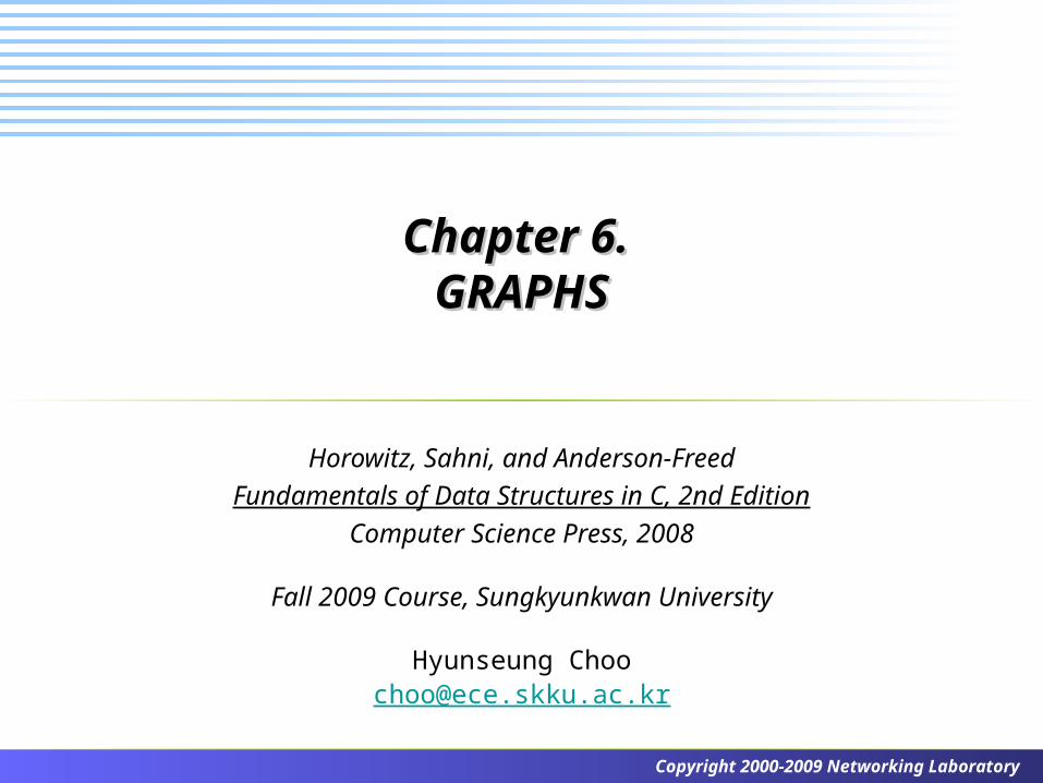
The Graph Abstract Data Type
Introduction
the bridges of Koenigsberg
c d
e
a bf
g
AKneiphof
C
B
Dc
a b
de
g
f
C
A
B
D
(a) (b)
Networking Laboratory 2/48
Fall 2009 Data Structures
The Graph Abstract Data Type
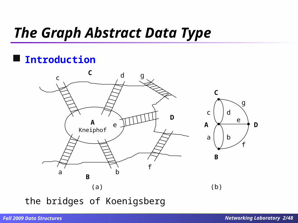
Def) A graph G = (V,E) where V(G): nonempty finite set of vertices, E(G): finite set of edges possibly empty undirected graph:
unordered (vi,vj) = (vj,vi)
directed graph ordered:<vi,vj> <vj,vi>
0
3
1 2
G1
0
21
4 5 63
G2
0
1
2
G3
Networking Laboratory 3/48
Fall 2009 Data Structures
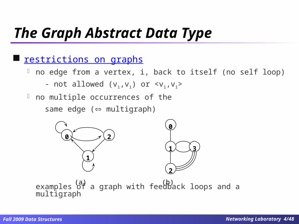
The Graph Abstract Data Type
restrictions on graphs no edge from a vertex, i, back to itself (no self loop)
- not allowed (vi,vi) or <vi,vi>
no multiple occurrences of the
same edge ( multigraph)
examples of a graph with feedback loops and a multigraph
0 2
1
1
2
3
0
(a) (b)
Networking Laboratory 4/48
Fall 2009 Data Structures
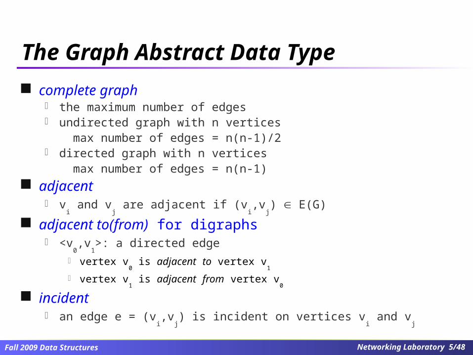
The Graph Abstract Data Type
complete graph the maximum number of edges undirected graph with n vertices
max number of edges = n(n-1)/2 directed graph with n vertices
max number of edges = n(n-1) adjacent
vi and v
j are adjacent if (v
i,v
j) E(G)
adjacent to(from) for digraphs <v
0,v
1>: a directed edge
vertex v0 is adjacent to vertex v
1
vertex v1 is adjacent from vertex v
0
incident an edge e = (v
i,v
j) is incident on vertices v
i and v
j
Networking Laboratory 5/48
Fall 2009 Data Structures
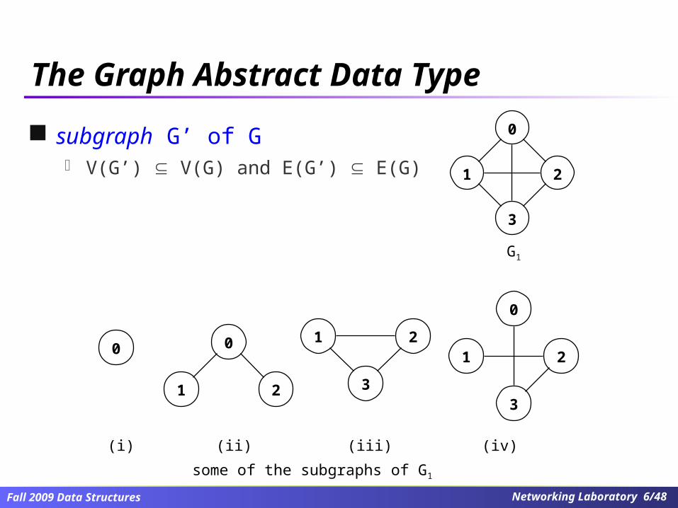
The Graph Abstract Data Type
subgraph G’ of G V(G’) V(G) and E(G’) E(G)
0 0
1 2 3
1 2
0
3
1 2
(i) (ii) (iii) (iv)
some of the subgraphs of G1
0
3
1 2
G1
Networking Laboratory 6/48
Fall 2009 Data Structures
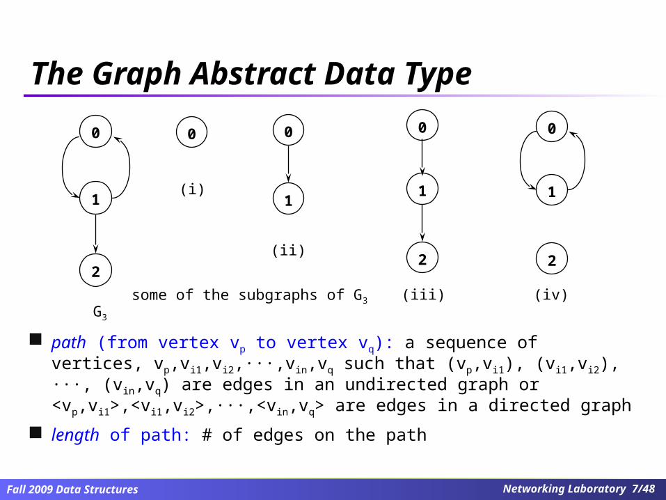
The Graph Abstract Data Type
path (from vertex vp to vertex vq): a sequence of vertices, vp,vi1,vi2,···,vin,vq such that (vp,vi1), (vi1,vi2), ···, (vin,vq) are edges in an undirected graph or <vp,vi1>,<vi1,vi2>,···,<vin,vq> are edges in a directed graph
length of path: # of edges on the path
0 0
1
0
1
2
0
1
2
(i)
(ii)
(iii) (iv)some of the subgraphs of G3
0
1
2
G3
Networking Laboratory 7/48
Fall 2009 Data Structures
The Graph Abstract Data Type
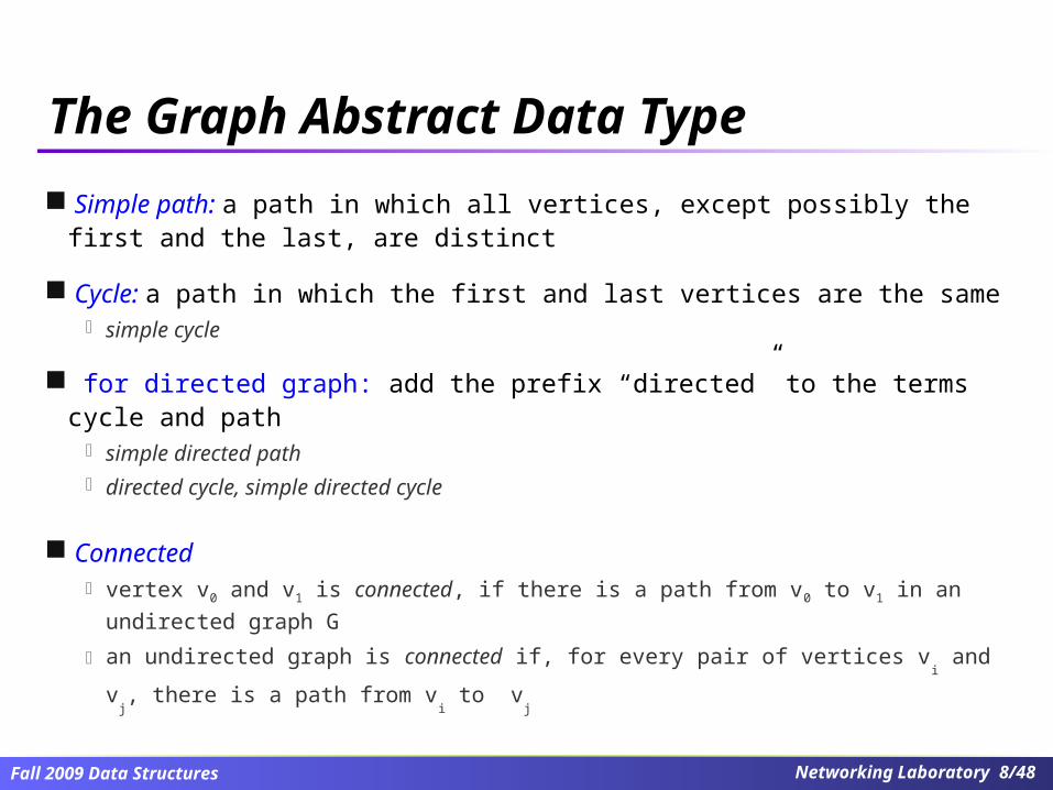
Simple path: a path in which all vertices, except possibly the first and the last, are distinct
Cycle: a path in which the first and last vertices are the same simple cycle
for directed graph: add the prefix “directed” to the terms cycle and path simple directed path directed cycle, simple directed cycle
Connected vertex v0 and v1 is connected, if there is a path from v0 to v1 in an undirected
graph G
an undirected graph is connected if, for every pair of vertices vi and v
j, there is a
path from vi to v
j
Networking Laboratory 8/48
Fall 2009 Data Structures
connected component (of an undirected graph) maximal connected subgraph
a graph with two connected components
0
3
1 2
H1
4
5
6
7
G4
H2
The Graph Abstract Data Type
Networking Laboratory 9/48
Fall 2009 Data Structures
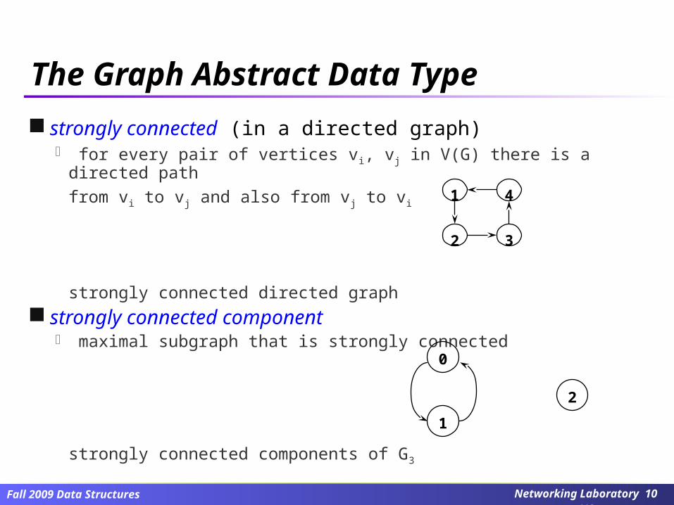
strongly connected (in a directed graph) for every pair of vertices vi, vj in V(G) there is a directed path
from vi to vj and also from vj to vi
strongly connected directed graph strongly connected component
maximal subgraph that is strongly connected
strongly connected components of G3
4
3
1
2
0
1
2
The Graph Abstract Data Type
Networking Laboratory 10/48
Fall 2009 Data Structures
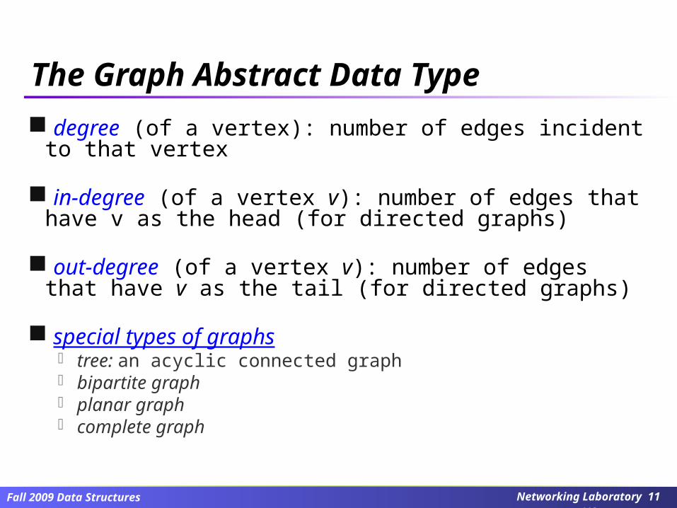
degree (of a vertex): number of edges incident to that vertex
in-degree (of a vertex v): number of edges that have v as the head (for directed graphs)
out-degree (of a vertex v): number of edges that have v as the tail (for directed graphs)
special types of graphs tree: an acyclic connected graph bipartite graph planar graph complete graph
The Graph Abstract Data Type
Networking Laboratory 11/48
Fall 2009 Data Structures
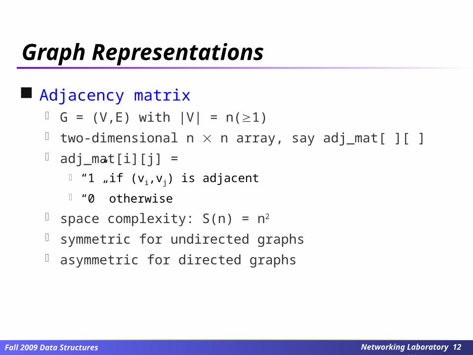
Graph Representations
Adjacency matrix G = (V,E) with |V| = n(1) two-dimensional n n array, say adj_mat[ ][ ] adj_mat[i][j] =
“1” if (vi,vj) is adjacent
“0” otherwise
space complexity: S(n) = n2
symmetric for undirected graphs asymmetric for directed graphs
Networking Laboratory 12/48
Fall 2009 Data Structures
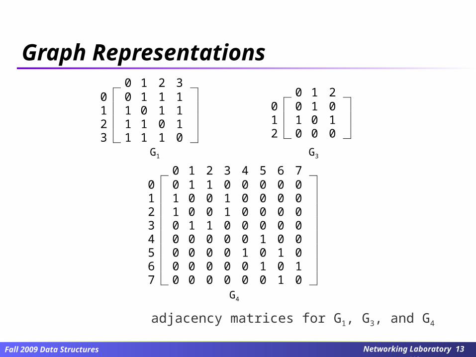
adjacency matrices for G1, G3, and G4
0 1 2 30 0 1 1 11 1 0 1 12 1 1 0 13 1 1 1 0
0 1 20 0 1 01 1 0 12 0 0 0
0 1 2 3 4 5 6 70 0 1 1 0 0 0 0 01 1 0 0 1 0 0 0 02 1 0 0 1 0 0 0 03 0 1 1 0 0 0 0 04 0 0 0 0 0 1 0 05 0 0 0 0 1 0 1 06 0 0 0 0 0 1 0 17 0 0 0 0 0 0 1 0
G1 G3
G4
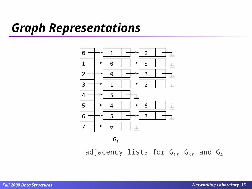
Graph Representations
Networking Laboratory 13/48
Fall 2009 Data Structures
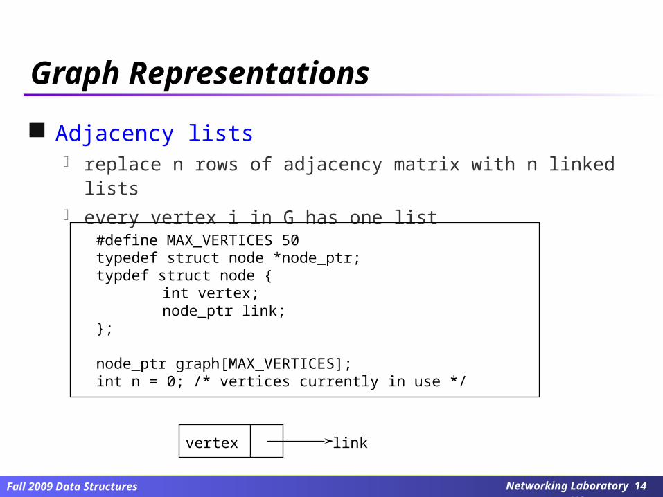
Graph Representations
Adjacency lists replace n rows of adjacency matrix with n linked lists every vertex i in G has one list
#define MAX_VERTICES 50typedef struct node *node_ptr;typdef struct node {
int vertex;node_ptr link;
};
node_ptr graph[MAX_VERTICES];int n = 0; /* vertices currently in use */
vertex link
Networking Laboratory 14/48
Fall 2009 Data Structures
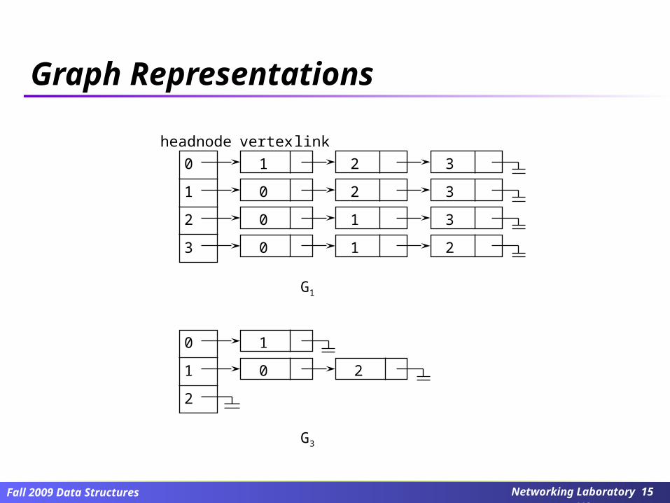
10
1
2
3
2
0 2
0 1
0 1
headnode vertex link
3
3
3
2
0
1
2
0
1
2
G1
G3
Graph Representations
Networking Laboratory 15/48
Fall 2009 Data Structures
adjacency lists for G1, G3, and G4
0
1
2
3
4
5
6
7
1 2
0 3
0 3
1 2
5
4 6
5 7
6
G4
Graph Representations
Networking Laboratory 16/48
Fall 2009 Data Structures
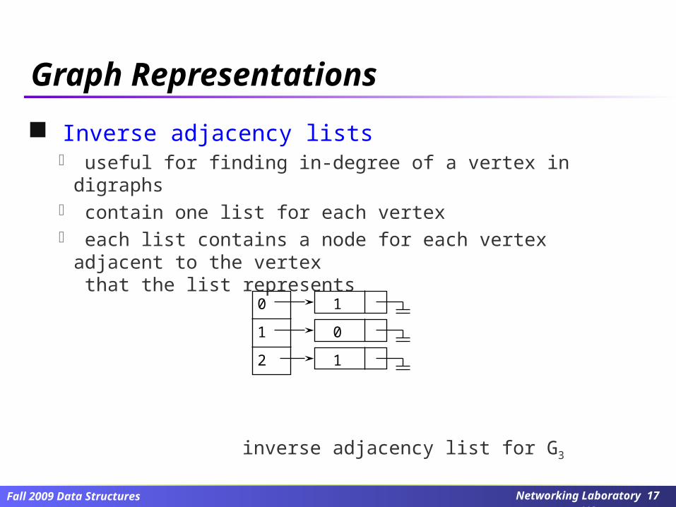
Graph Representations
Inverse adjacency lists useful for finding in-degree of a vertex in digraphs contain one list for each vertex each list contains a node for each vertex adjacent to the vertex
that the list represents
inverse adjacency list for G3
0
1
2
0
1
1
Networking Laboratory 17/48
Fall 2009 Data Structures
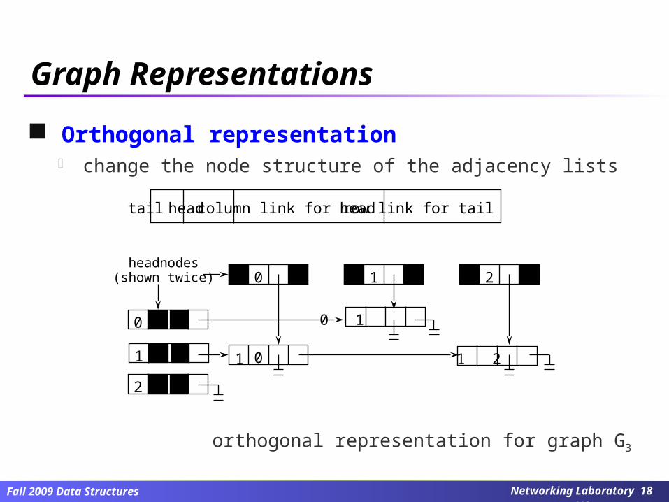
Orthogonal representation change the node structure of the adjacency lists
orthogonal representation for graph G3
tail head column link for head row link for tail
0 1 2
0
1
2
0
0 1
1 2
headnodes(shown twice)
1
Graph Representations
Networking Laboratory 18/48
Fall 2009 Data Structures
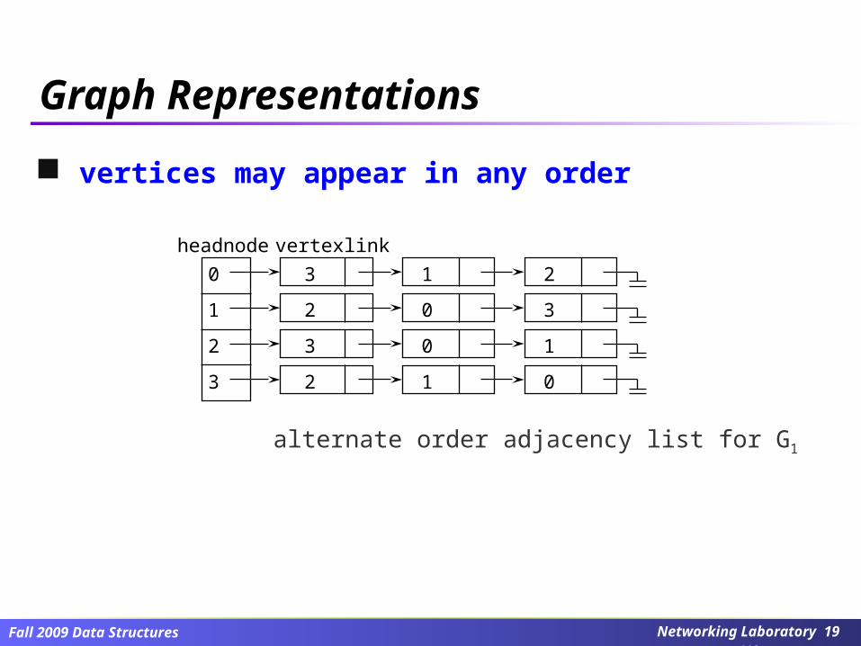
vertices may appear in any order
alternate order adjacency list for G1
30
1
2
3
1
2 0
3 0
2 1
headnode vertex link
2
3
1
0
Graph Representations
Networking Laboratory 19/48
Fall 2009 Data Structures
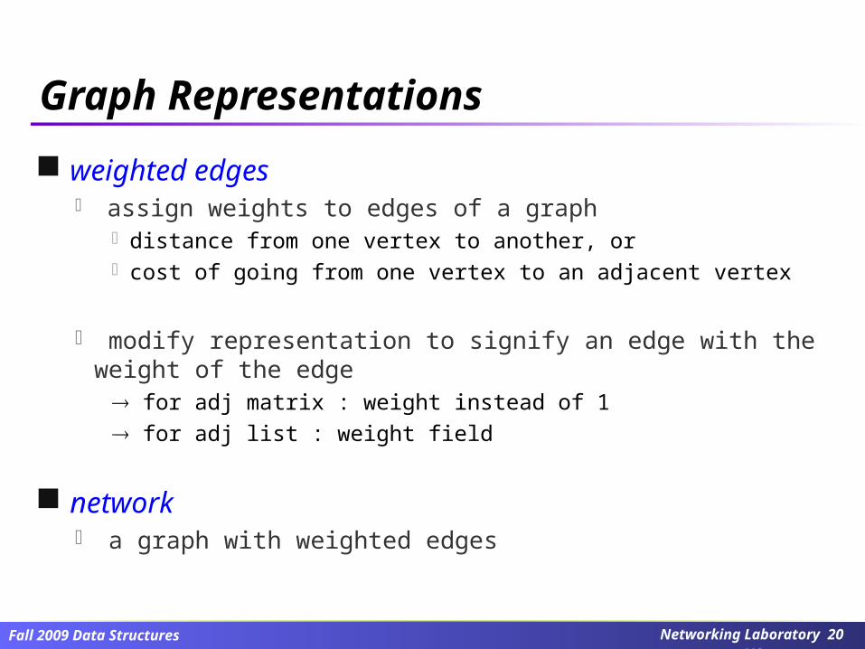
weighted edges assign weights to edges of a graph
distance from one vertex to another, or cost of going from one vertex to an adjacent vertex
modify representation to signify an edge with the weight of the edge for adj matrix : weight instead of 1
for adj list : weight field
network a graph with weighted edges
Graph Representations
Networking Laboratory 20/48
Fall 2009 Data Structures
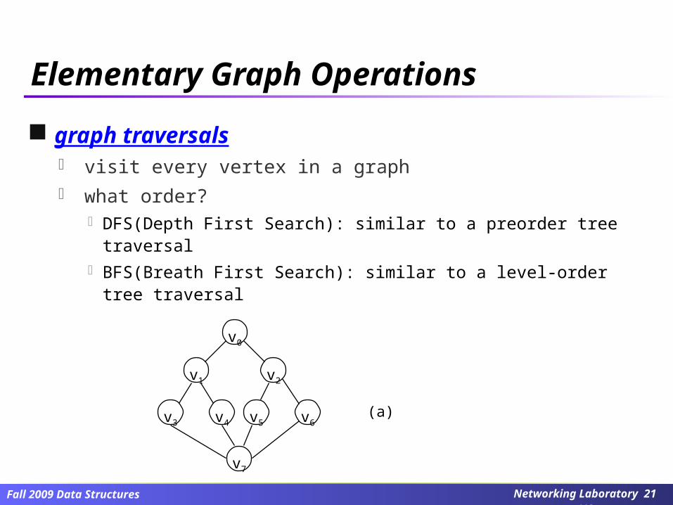
graph traversals visit every vertex in a graph what order?
DFS(Depth First Search): similar to a preorder tree traversal BFS(Breath First Search): similar to a level-order tree traversal
v0
v1 v2
v3 v4 v5 v6
v7
(a)
Elementary Graph Operations
Networking Laboratory 21/48
Fall 2009 Data Structures
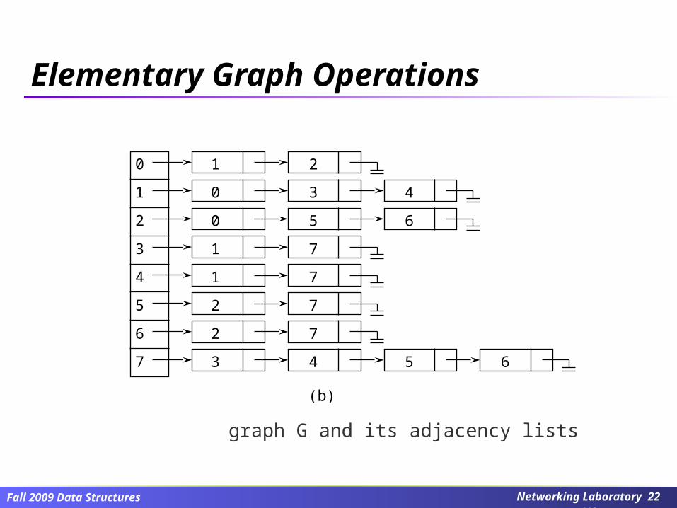
graph G and its adjacency lists
0
1
2
3
4
5
6
7
1 2
0 3
0 5
1 7
1
2 7
2 7
3
4
6
7
4 5 6
(b)
Elementary Graph Operations
Networking Laboratory 22/48
Fall 2009 Data Structures
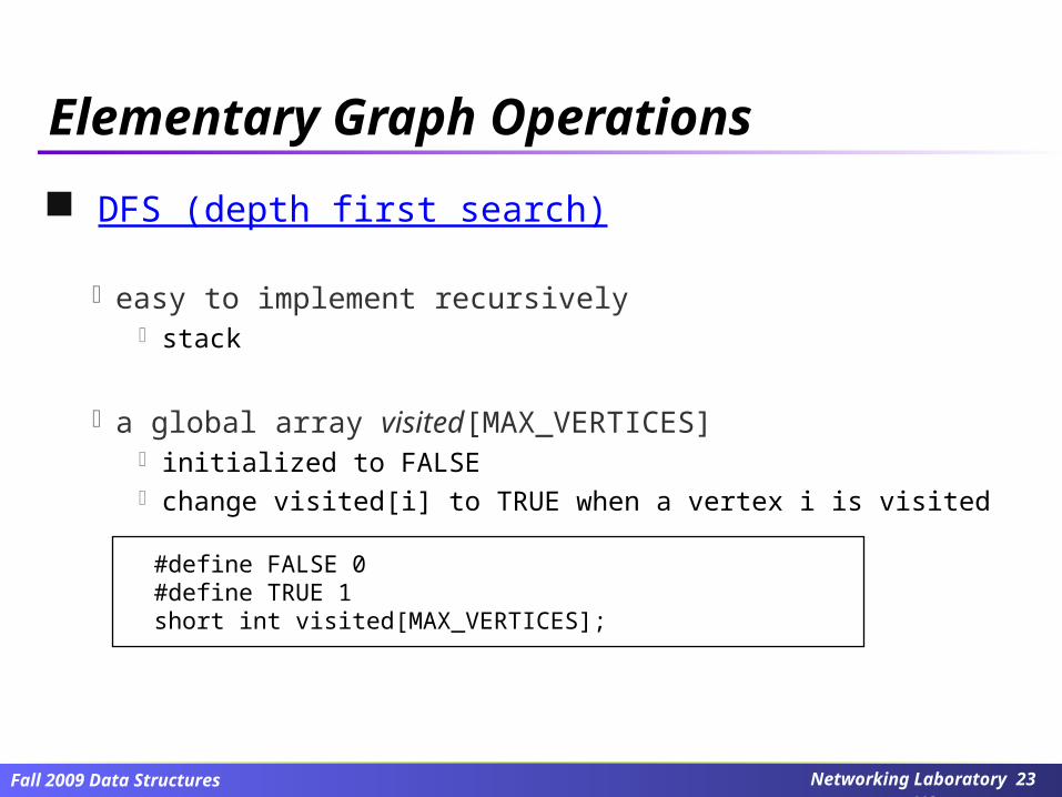
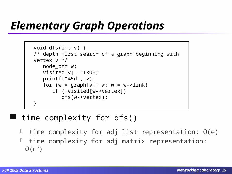
DFS (depth first search)
easy to implement recursively stack
a global array visited[MAX_VERTICES] initialized to FALSE change visited[i] to TRUE when a vertex i is visited
Elementary Graph Operations
#define FALSE 0#define TRUE 1short int visited[MAX_VERTICES];
Networking Laboratory 23/48
Fall 2009 Data Structures
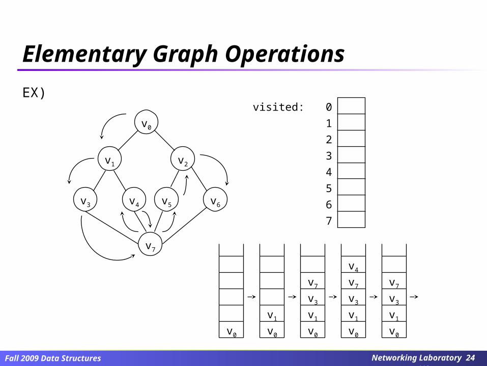
EX)
v0
v1 v2
v3 v4 v5 v6
v7
0
1
2
3
4
5
6
7
v0
v1
v0
v7
v3
v1
v0
v4
v7
v3
v1
v0
v7
v3
v1
v0
visited:
Elementary Graph Operations
Networking Laboratory 24/48
Fall 2009 Data Structures
time complexity for dfs()
time complexity for adj list representation: O(e) time complexity for adj matrix representation: O(n2)
Elementary Graph Operations
void dfs(int v) {/* depth first search of a graph beginning with vertex v */ node_ptr w; visited[v] = TRUE; printf(“%5d”, v); for (w = graph[v]; w; w = w->link) if (!visited[w->vertex]) dfs(w->vertex);}
Networking Laboratory 25/48
Fall 2009 Data Structures
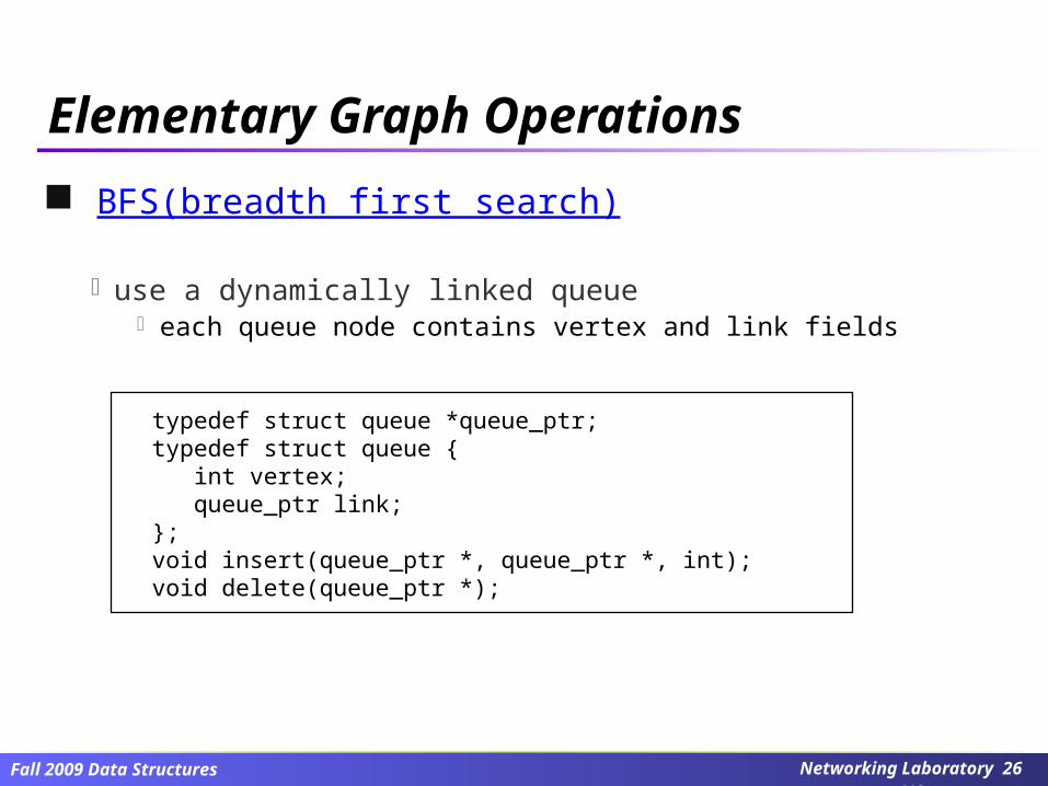
BFS(breadth first search)
use a dynamically linked queue each queue node contains vertex and link fields
Elementary Graph Operations
typedef struct queue *queue_ptr;typedef struct queue { int vertex; queue_ptr link;};void insert(queue_ptr *, queue_ptr *, int);void delete(queue_ptr *);
Networking Laboratory 26/48
Fall 2009 Data Structures
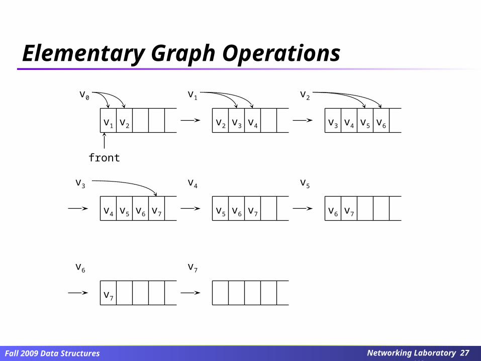
v0
v1 v2 v2 v3 v4 v3 v4 v5 v6
v4 v5 v6 v7
v1 v2
v3
front
v5 v6 v7
v4
v6 v7
v5
v7
v6 v7
Elementary Graph Operations
Networking Laboratory 27/48
Fall 2009 Data Structures
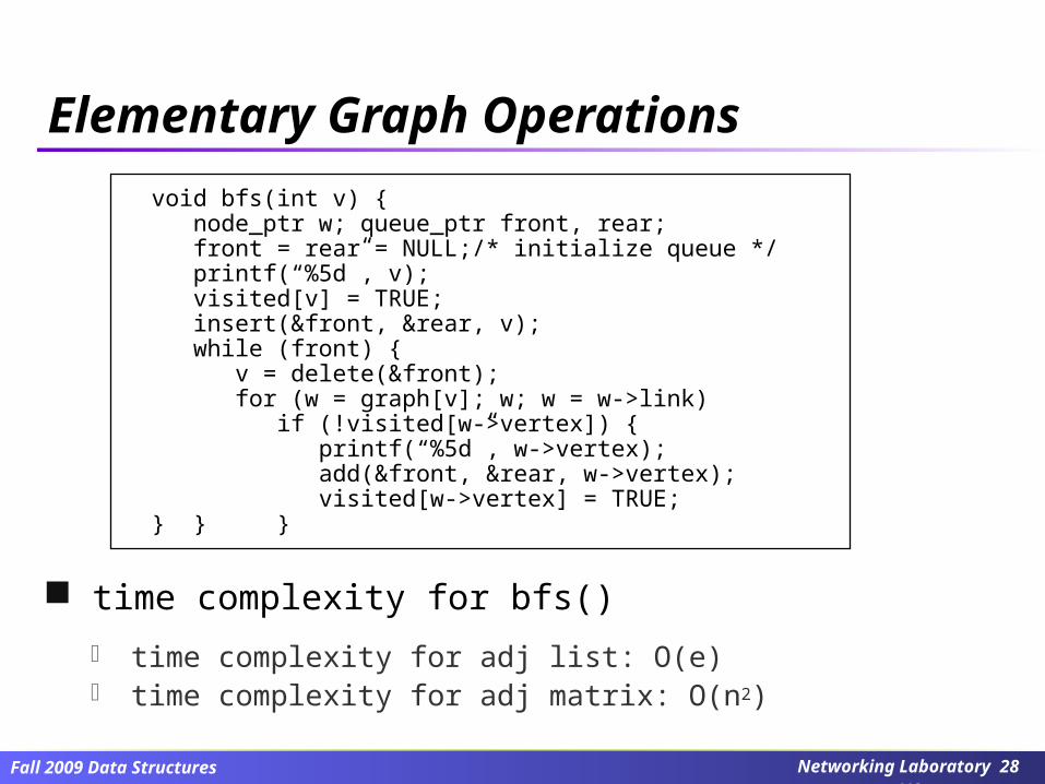
time complexity for bfs()
time complexity for adj list: O(e) time complexity for adj matrix: O(n2)
Elementary Graph Operations
void bfs(int v) { node_ptr w; queue_ptr front, rear; front = rear = NULL;/* initialize queue */ printf(“%5d”, v); visited[v] = TRUE; insert(&front, &rear, v); while (front) { v = delete(&front); for (w = graph[v]; w; w = w->link) if (!visited[w->vertex]) { printf(“%5d”, w->vertex); add(&front, &rear, w->vertex); visited[w->vertex] = TRUE;} } }
Networking Laboratory 28/48
Fall 2009 Data Structures
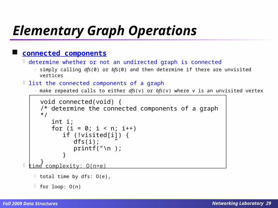
connected components determine whether or not an undirected graph is connected
- simply calling dfs(0) or bfs(0) and then determine if there are unvisited vertices list the connected components of a graph
- make repeated calls to either dfs(v) or bfs(v) where v is an unvisited vertex
time complexity: O(n+e)
total time by dfs: O(e),
for loop: O(n)
Elementary Graph Operations
void connected(void) {/* determine the connected components of a graph */ int i; for (i = 0; i < n; i++) if (!visited[i]) { dfs(i); printf(“\n”); }}
Networking Laboratory 29/48
Fall 2009 Data Structures
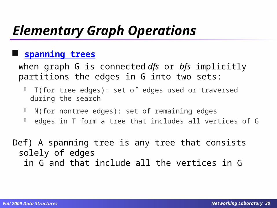
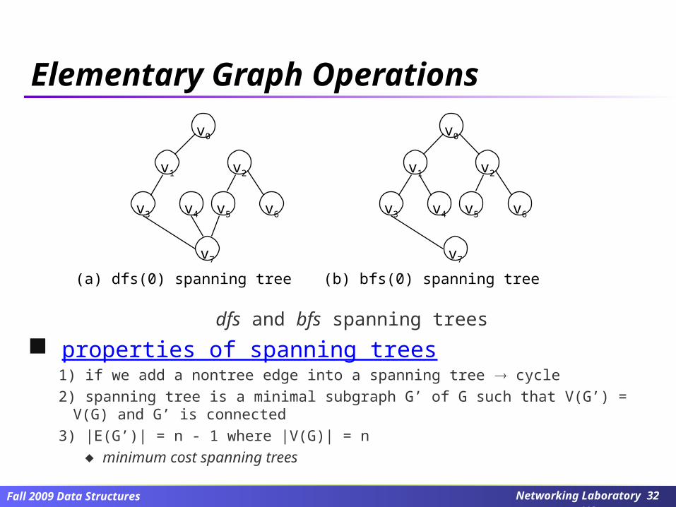
spanning trees
when graph G is connected dfs or bfs implicitly partitions the edges in G into two sets:
T(for tree edges): set of edges used or traversed during the search
N(for nontree edges): set of remaining edges edges in T form a tree that includes all vertices of G
Def) A spanning tree is any tree that consists solely of edges in G and that include all the vertices in G
Elementary Graph Operations
Networking Laboratory 30/48
Fall 2009 Data Structures
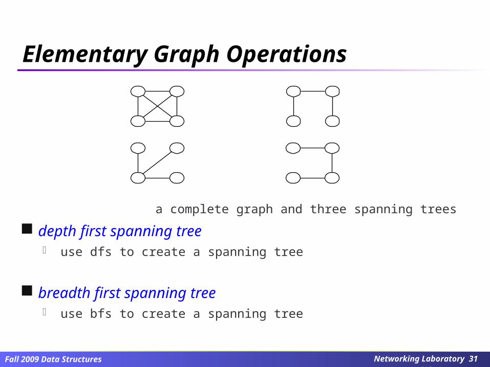
a complete graph and three spanning trees
depth first spanning tree use dfs to create a spanning tree
breadth first spanning tree use bfs to create a spanning tree
Elementary Graph Operations
Networking Laboratory 31/48
Fall 2009 Data Structures
dfs and bfs spanning trees
properties of spanning trees1) if we add a nontree edge into a spanning tree cycle
2) spanning tree is a minimal subgraph G’ of G such that V(G’) = V(G) and G’ is connected
3) |E(G’)| = n - 1 where |V(G)| = n
minimum cost spanning trees
v0
v1 v2
v3 v4 v5 v6
v7
v0
v1 v2
v3 v4 v5 v6
v7
(a) dfs(0) spanning tree (b) bfs(0) spanning tree
Elementary Graph Operations
Networking Laboratory 32/48
Fall 2009 Data Structures
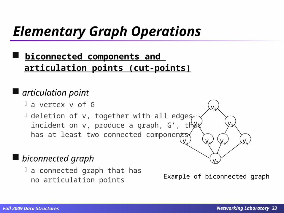
biconnected components and articulation points (cut-points)
articulation point a vertex v of G deletion of v, together with all edges
incident on v, produce a graph, G’, that has at least two connected components
biconnected graph a connected graph that has
no articulation points
v0
v1 v2
v3 v4 v5 v6
v7
Example of biconnected graph
Elementary Graph Operations
Networking Laboratory 33/48
Fall 2009 Data Structures
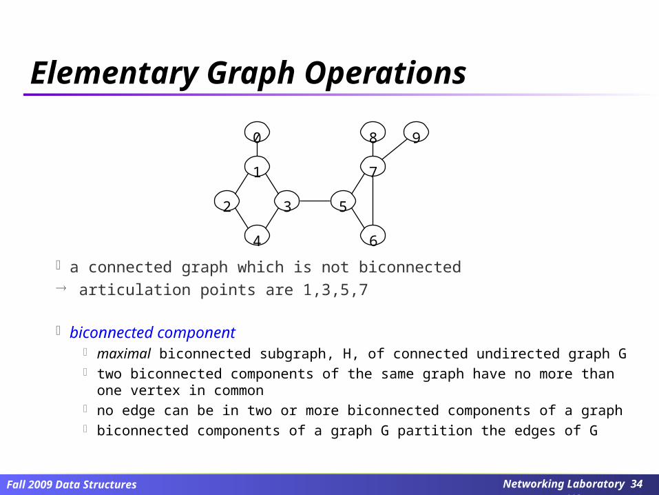
a connected graph which is not biconnected articulation points are 1,3,5,7
biconnected component maximal biconnected subgraph, H, of connected undirected graph G two biconnected components of the same graph have no more than one vertex in
common no edge can be in two or more biconnected components of a graph biconnected components of a graph G partition the edges of G
0
1
2 3
4
8
7
5
9
6
Elementary Graph Operations
Networking Laboratory 34/48
Fall 2009 Data Structures
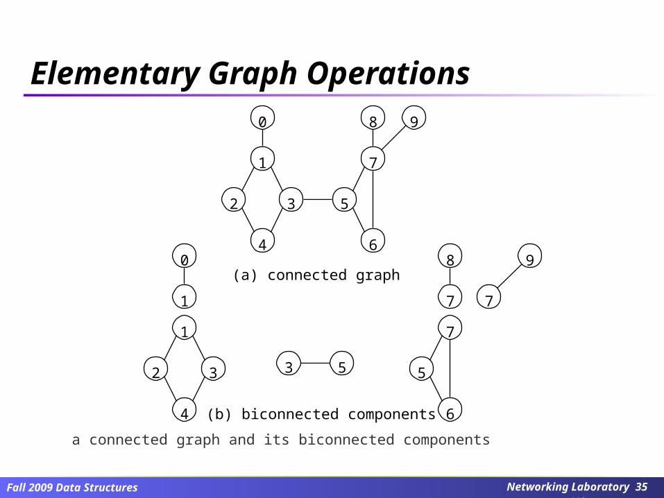
a connected graph and its biconnected components
0
1
2 3
4
8
7
5
9
60
1
1
2 3
4
7
5
6
8
7 7
9
3 5
(a) connected graph
(b) biconnected components
Elementary Graph Operations
Networking Laboratory 35/48
Fall 2009 Data Structures
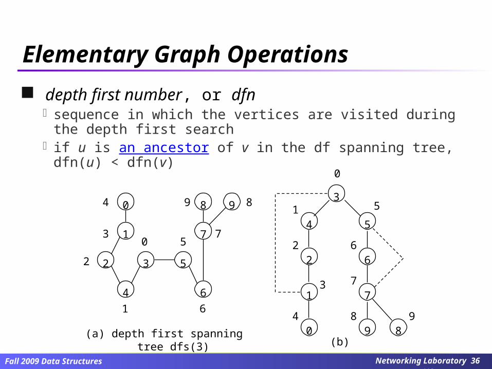
depth first number, or dfn sequence in which the vertices are visited during the depth first
search if u is an ancestor of v in the df spanning tree, dfn(u) < dfn(v)
0
1
2 3
4
8
7
5
9
6
1
0 5
6
7
9 84
3
2
0
3
4 5
2 6
1 7
0 9 8
1
2
3
4
5
6
7
8 9
(a) depth first spanning tree dfs(3)(b)
Elementary Graph Operations
Networking Laboratory 36/48
Fall 2009 Data Structures
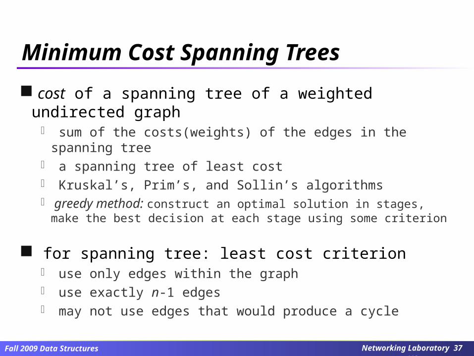
cost of a spanning tree of a weighted undirected graph sum of the costs(weights) of the edges in the spanning tree a spanning tree of least cost Kruskal’s, Prim’s, and Sollin’s algorithms greedy method: construct an optimal solution in stages, make the best
decision at each stage using some criterion
for spanning tree: least cost criterion use only edges within the graph use exactly n-1 edges may not use edges that would produce a cycle
Minimum Cost Spanning Trees
Networking Laboratory 37/48
Fall 2009 Data Structures
(1) Kruskal’s algorithm
select the edges for inclusion in T in nondecreasing order of their cost
an edge is added to T if it does not form a cycle with the edges that are already in T
exactly n-1 edges are selected
Minimum Cost Spanning Trees
Networking Laboratory 38/48
Fall 2009 Data Structures
Kruskal’s algorithm
Minimum Cost Spanning Trees
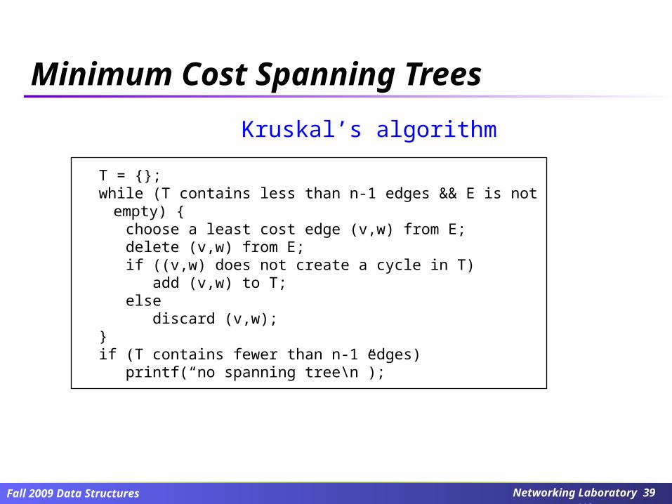
T = {};while (T contains less than n-1 edges && E is not empty) { choose a least cost edge (v,w) from E; delete (v,w) from E; if ((v,w) does not create a cycle in T) add (v,w) to T; else discard (v,w);}if (T contains fewer than n-1 edges) printf(“no spanning tree\n”);
Networking Laboratory 39/48
Fall 2009 Data Structures
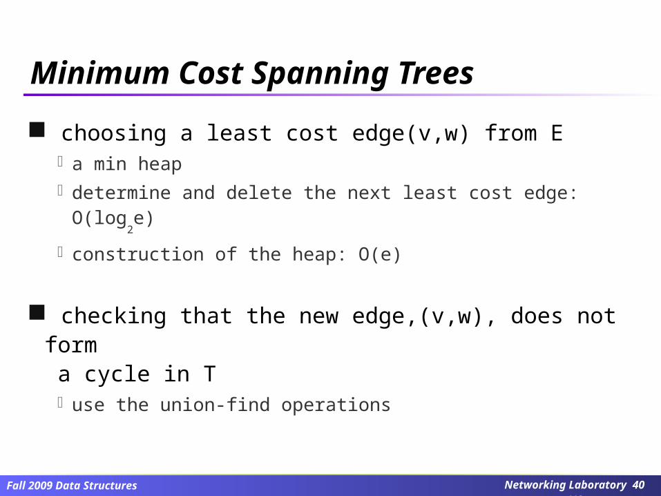
choosing a least cost edge(v,w) from E a min heap
determine and delete the next least cost edge: O(log2e)
construction of the heap: O(e)
checking that the new edge,(v,w), does not form a cycle in T
use the union-find operations
Minimum Cost Spanning Trees
Networking Laboratory 40/48
Fall 2009 Data Structures
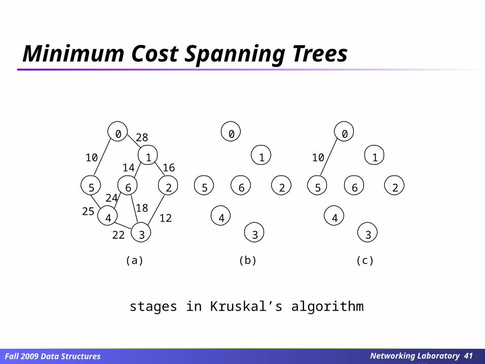
0
1
5 6 2
4
3
28
16
1218
22
2524
1410
(a)
0
1
5 6 2
4
3
(b)
0
1
5 6 2
4
3
10
(c)
stages in Kruskal’s algorithm
Minimum Cost Spanning Trees
Networking Laboratory 41/48
Fall 2009 Data Structures
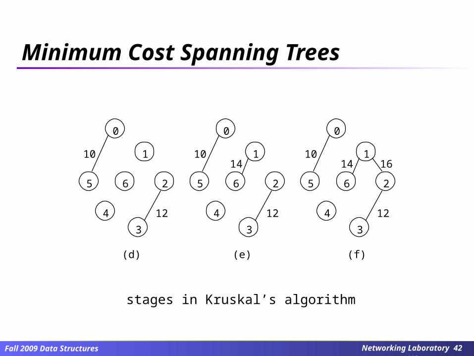
0
1
5 6 2
4
3
12
10
(d)
0
1
5 6 2
4
3
12
1410
(e)
0
1
5 6 2
4
3
16
12
1410
(f)
stages in Kruskal’s algorithm
Minimum Cost Spanning Trees
Networking Laboratory 42/48
Fall 2009 Data Structures
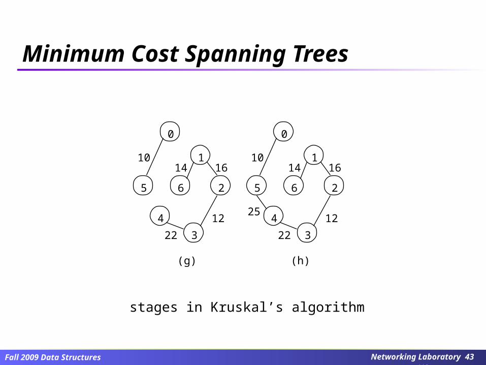
0
1
5 6 2
4
3
16
12
22
1410
(g)
0
1
5 6 2
4
3
16
12
22
25
1410
(h)
Minimum Cost Spanning Trees
stages in Kruskal’s algorithm
Networking Laboratory 43/48
Fall 2009 Data Structures
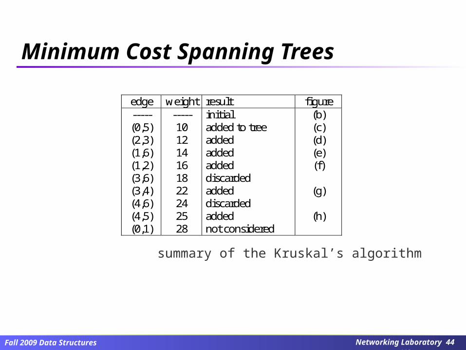
summary of the Kruskal’s algorithm
edge weight result figure ----- (0,5) (2,3) (1,6) (1,2) (3,6) (3,4) (4,6) (4,5) (0,1)
----- 10 12 14 16 18 22 24 25 28
initial added to tree added added added discarded added discarded added not considered
(b) (c) (d) (e) (f)
(g)
(h)
Minimum Cost Spanning Trees
Networking Laboratory 44/48
Fall 2009 Data Structures
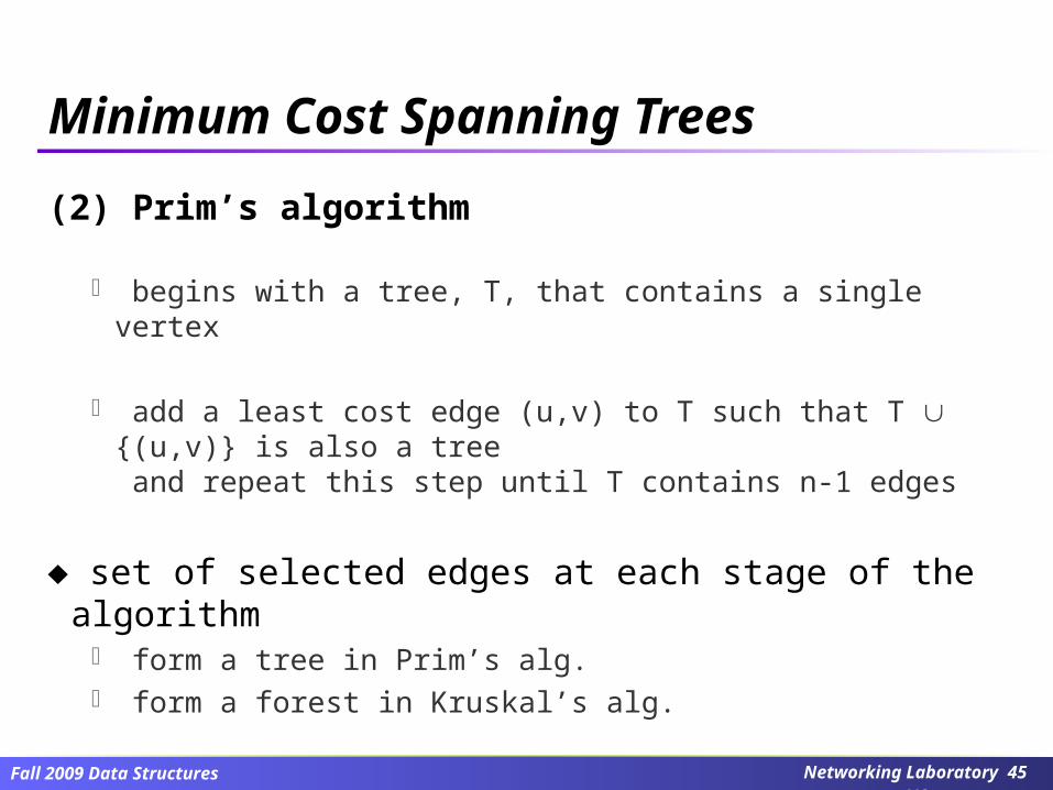
(2) Prim’s algorithm
begins with a tree, T, that contains a single vertex
add a least cost edge (u,v) to T such that T {(u,v)} is also a tree and repeat this step until T contains n-1 edges
set of selected edges at each stage of the algorithm form a tree in Prim’s alg. form a forest in Kruskal’s alg.
Minimum Cost Spanning Trees
Networking Laboratory 45/48
Fall 2009 Data Structures
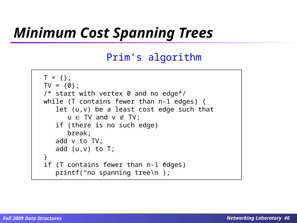
Prim’s algorithm
Minimum Cost Spanning Trees
T = {};TV = {0}; /* start with vertex 0 and no edge*/while (T contains fewer than n-1 edges) { let (u,v) be a least cost edge such that u TV and v TV; if (there is no such edge) break; add v to TV; add (u,v) to T;}if (T contains fewer than n-1 edges) printf(“no spanning tree\n”);
Networking Laboratory 46/48
Fall 2009 Data Structures
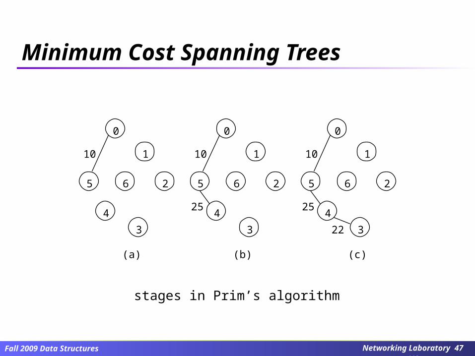
0
1
5 6 2
4
3
10
0
1
5 6 2
4
3
25
10
0
1
5 6 2
4
322
25
10
(a) (b) (c)
stages in Prim’s algorithm
Minimum Cost Spanning Trees
Networking Laboratory 47/48
Fall 2009 Data Structures
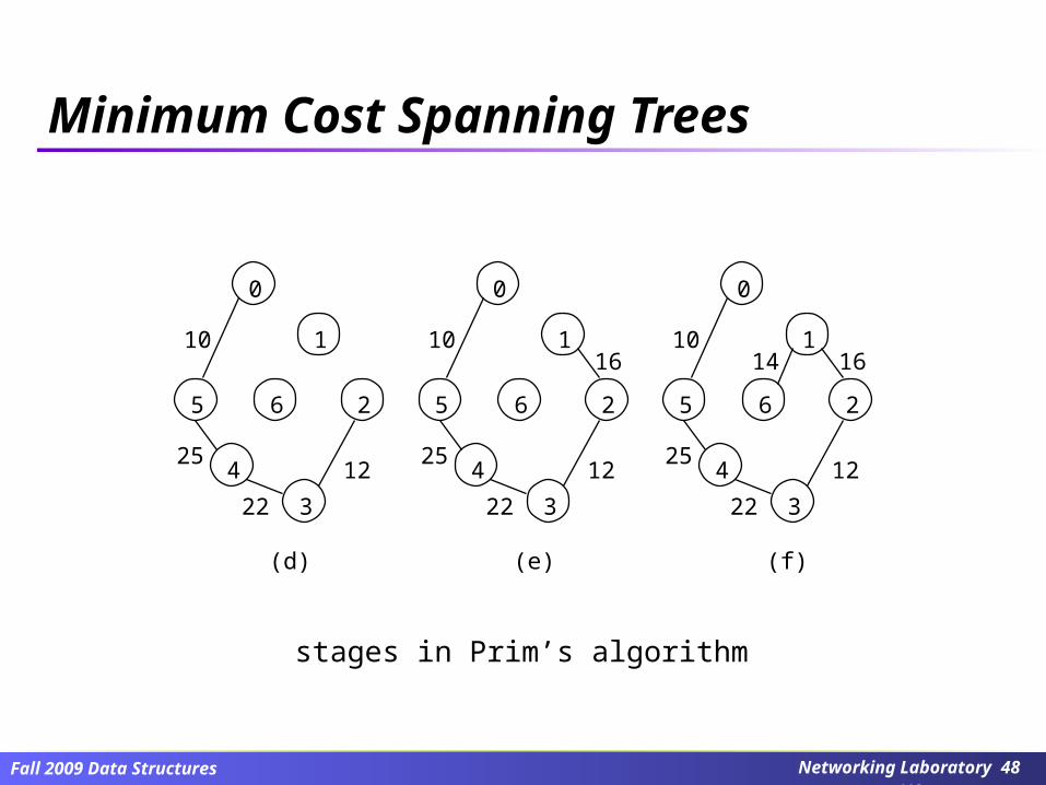
Minimum Cost Spanning Trees
0
1
5 6 2
4
3
12
22
25
10
0
1
5 6 2
4
3
16
12
22
25
10
0
1
5 6 2
4
3
16
12
22
25
1410
(d) (e) (f)
stages in Prim’s algorithm
Networking Laboratory 48/48