Embed Size (px)
Citation preview

©Copyright 2008 Erin Hoffmann Lay
Investigating Lightning-to-Ionosphere Energy Coupling Based on VLF Lightning Propagation Characterization
Erin Hoffmann Lay
A dissertation submitted in partial fulfillment of the requirements for the degree of
Doctor of Philosophy
University of Washington
2008
Program Authorized to Offer Degree: Physics

University of Washington Graduate School
This is to certify that I have examined this copy of a doctoral dissertation by
Erin Hoffmann Lay
and have found that it is complete and satisfactory in all respects, and that any and all revisions required by the final examining committee have been
made.
Chair of the Supervisory Committee:
______________________________________________________ Robert Holzworth
Reading Committee:
______________________________________________________ Robert Holzworth
______________________________________________________ Abram Jacobson
______________________________________________________ Michael McCarthy
Date: _______________________

In presenting this dissertation in partial fulfillment of the requirements for the doctoral degree at the University of Washington, I agree that the Library shall make its copies freely available for inspection. I further agree that extensive copying of the dissertation is allowable only for scholarly purposes, consistent with “fair use” as prescribed in the U.S. Copyright Law. Requests for copying or reproduction of this dissertation may be referred to Proquest Information and Learning, 300 North Zeeb Road, Ann Arbor, MI 48106-1346, to whom the author has granted “the right to reproduce and sell (a) copies of the manuscript in microform and/or (b) printed copies of the manuscript made from microform.”
Signature_________________________________
Date_____________________________________

University of Washington
Abstract
Investigating Lightning-to-Ionosphere Energy Coupling Based on VLF Lightning
Propagation Characterization
Erin Hoffmann Lay
Chair of the Supervisory Committee: Professor Robert Holzworth
Department of Earth and Space Sciences
In this dissertation, the capabilities of the World-Wide Lightning Location Network
(WWLLN) are analyzed in order to study the interactions of lightning energy with the
lower ionosphere. WWLLN is the first global ground-based lightning location network
and the first lightning detection network that continuously monitors lightning around
the world in real time. For this reason, a better characterization of the WWLLN could
allow many global atmospheric science problems to be addressed, including further
investigation into the global electric circuit and global mapping of regions of the lower
ionosphere likely to be impacted by strong lightning and transient luminous events.
This dissertation characterizes the World-Wide Location Network (WWLLN) in
terms of detection efficiency, location and timing accuracy, and lightning type. This
investigation finds excellent timing and location accuracy for WWLLN. It provides the
first experimentally-determined estimate of relative global detection efficiency that is
used to normalize lightning counts based on location. These normalized global lightning
data from the WWLLN are used to map intense storm regions around the world with
high time and spatial resolution as well as to provide information on energetic
emissions known as elves and terrestrial gamma-ray flashes (TGFs). This dissertation
also improves WWLLN by developing a procedure to provide the first estimate of
relative lightning stroke radiated energy in the 1-24 kHz frequency range by a global
lightning detection network.
These characterizations and improvements to WWLLN are motivated by the desire
to use WWLLN data to address the problem of lightning-to-ionosphere energy

coupling. Therefore, WWLLN stroke rates are used as input to a model, developed by
Professor Mengu Cho at the Kyushu Institute of Technology in Japan, that describes the
non-linear effect of lightning electromagnetic pulses (EMP) on the ionosphere by
accumulating electron density changes resulting from the interaction of the EMP of ten
successive lightning strokes with the lower ionosphere. Further studies must be
completed to narrow uncertainties in the model, but the qualitative ionospheric response
to successive EMPs is presented. Results from this study show that the non-linear effect
of lightning EMP due to successive lightning strokes must be taken into account, and
varies with altitude, such that the most significant electron density enhancement occurs
at 88 km altitude.

i
TABLE OF CONTENTS
Page
List of Figures ................................................................................................................... v
List of Tables .................................................................................................................viii
Chapter 1: Introduction ..................................................................................................... 1
1.1 Motivation for real-time global lightning detection................................................ 1
1.1.1 Practical Applications ...................................................................................... 1
1.1.2 Fundamental Geophysics ................................................................................. 2
1.2 Types of Lightning.................................................................................................. 3
1.2.1 Cloud-to-Ground.............................................................................................. 3
1.2.2 In-cloud ............................................................................................................ 5
1.3 Lightning Detection Systems.................................................................................. 6
1.3.1 Satellite Detection............................................................................................ 7
1.3.2 Regional Ground-Based Detection .................................................................. 8
1.3.3 Overview of World-Wide Lightning Location Network ................................. 9
1.4 Effects of Lightning Energy in the Earth System ................................................. 10
1.4.1 Elves/sprites ................................................................................................... 10
1.4.2 Terrestrial Gamma-ray Flashes...................................................................... 13
1.5 Global Electric Circuit .......................................................................................... 15
1.6 Ionospheric Wave Propagation ............................................................................. 17
1.7 Dissertation Outline .............................................................................................. 18
Chapter 2: World-Wide Lightning Location Network.................................................... 20
2.1 Network Introduction............................................................................................ 20
2.2 WWLLN Hardware .............................................................................................. 21
2.3 WWLLN Software................................................................................................ 23
Chapter 3: Global Detection Efficiency and Location Accuracy ................................... 26
3.1 Overview............................................................................................................... 26
3.2 Brazil Integrated Network/WWLLN Comparison................................................ 26
3.2.1 Method ........................................................................................................... 27
ii
3.2.2 Results............................................................................................................ 28
3.2.3 Summary of Brazil Study............................................................................... 30
3.2.4 Advances in WWLLN since this study.......................................................... 31
3.3 FORTE/WWLLN Comparison............................................................................. 31
3.3.1 Overview........................................................................................................ 31
3.3.2 FORTE photodiode detector .......................................................................... 32
3.3.3 WWLLN/PDD Comparison Methodology.................................................... 33
3.3.4 Results............................................................................................................ 34
3.3.5 Conclusion ..................................................................................................... 40
3.4 Detection range of WWLLN stations ................................................................... 40
3.5 Conclusion ............................................................................................................ 45
Chapter 4: Global Mapping of Strong Lightning............................................................ 46
4.1 Introduction........................................................................................................... 46
4.2 Land/ocean events in local time............................................................................ 46
4.3 Events in local time: higher resolution ................................................................. 51
4.4 Summary ............................................................................................................... 52
Chapter 5: Narrow Bipolar Events and Ionospheric Propagation................................... 54
5.1 Motivation............................................................................................................. 54
5.1.1 FORTE RF/WWLLN Comparison ................................................................ 54
5.1.2 Narrow Bipolar Events Hypothesis ............................................................... 55
5.2 Narrow Bipolar Events: WWLLN/LASA coincidence study............................... 56
5.2.1 Method ........................................................................................................... 56
5.2.2 Results............................................................................................................ 56
5.3 Conclusions........................................................................................................... 61
Chapter 6: Experimental evidence of energetic lightning effects on ionosphere and magnetosphere ......................................................................................................... 63
6.1 WWLLN/ISUAL elves comparison ..................................................................... 63
6.1.1 Motivation...................................................................................................... 63
6.1.2 Method ........................................................................................................... 63

iii
6.1.3 Results............................................................................................................ 64
6.1.4 Discussion ...................................................................................................... 70
6.2 WWLLN/RHESSI TGF comparison .................................................................... 71
6.2.1 Motivation...................................................................................................... 71
6.2.2 Method ........................................................................................................... 71
6.2.3 Results............................................................................................................ 71
6.2.4 Summary ........................................................................................................ 74
Chapter 7: Lightning stroke radiated VLF energy.......................................................... 75
7.1 Motivation to provide stroke energy..................................................................... 75
7.2 Absolute Calibration ............................................................................................. 75
7.2.1 Determining An by using narrowband VLF Transmitters.............................. 77
7.2.2 Frequency response........................................................................................ 80
7.2.3 Summary and suggestions for the future ....................................................... 83
7.3 Relative energy radiated as determined by a single station .................................. 84
7.4 Relative Calibration .............................................................................................. 86
Chapter 8: Modeling Lightning EMP/Ionospheric Interaction....................................... 92
8.1 Overview............................................................................................................... 92
8.2 Model Formulation ............................................................................................... 93
8.3 In situ validation of EM code................................................................................ 96
8.4 Relaxation of enhanced electron density. ............................................................. 98
8.5 Accumulated enhancements due to successive lightning strokes. ...................... 100
Chapter 9: Conclusion and Future Work ...................................................................... 110
9.1 World-Wide Lightning Location Network Characterization.............................. 110
9.2 Findings on energetic events correlated with lightning ...................................... 111
9.3 Modeling of lightning electromagnetic pulse ..................................................... 112
9.4 Future Work ........................................................................................................ 113
9.4.1 WWLLN Characterization........................................................................... 113
9.4.2 Lightning/Ionospheric Coupling.................................................................. 114
9.4.3 Narrow Bipolar Events ................................................................................ 114

iv
9.4.4 Global electric circuit................................................................................... 115
References..................................................................................................................... 116
Appendix A: Schematics for WWLLN Service Unit and Preamplifier........................ 124

v
LIST OF FIGURES Figure Number ............................................................................................................ Page
1.1 Examples of electric field changes due to CG lightning............................................. 4
1.2 Example of electric field change due to NBE lightning stroke .................................. 6
1.3 Averaged global flash density [Christian et al., 2003]................................................ 7
1.4 Image of a sprite and an elve .................................................................................... 11
1.5 Cartoon of current theory of TGF production [Smith et al., 2007]........................... 15
1.6: A schematic representation of the global electric circuit [Roble and Tzur 1986] ... 16
1.7 Diurnal variation of fair weather electric field and global thunderstorm activity [Roble and Tzur 1986] .................................................................................................... 16
2.1 WWLLN map of real-time lightning locations......................................................... 20
2.2 Cartoon schematic of a WWLLN VLF receiving station ......................................... 22
2.3 Example 64-sample waveform of a lightning sferic ................................................. 23
3.1 Region of Brazil/WWLLN comparison.................................................................... 28
3.2 Histogram of return stroke peak currents measured by the BIN .............................. 29
3.3 Location offsets of shared WWLLN-BIN events. .................................................... 30
3.4 Time-difference histogram of WWLLN-sferic time minus PDD-trigger time......... 34
3.5 WWLLN station locations (January 2005) w/ 6 broad region borders..................... 35
3.6 A superposed epoch of PDD waveforms with WWLLN coincidences.................... 39
3.7 Ratio of events detected by Darwin to events detected by network as a whole ....... 41
3.8 Station detection range model for noon .................................................................... 44
3.9 Station detection range for midnight......................................................................... 44
4.1 One year of WWLLN flash density data vs time...................................................... 47
4.2 Data from Figure 4.1 separated into six broad regions............................................. 48
4.3 Overlaid, normalized land data from Figure 4.2....................................................... 49
4.4 Five days of land/ocean WWLLN flash density data ............................................... 50
4.5 Percentage of total lightning in nighttime in each region ......................................... 51
4.6 Total number of nighttime counts for March 2006 – February 2007 ....................... 53
5.1 Spectrogram of an example of strong IC lightning................................................... 55
5.2 Full NBE waveform as detected by 5 LASA stations............................................... 57

vi
5.3 Range-normalized electric field of a NBE................................................................ 58
5.4 Power spectrum of a NBE......................................................................................... 59
5.5 Full FP waveform as detected by 5 LASA stations .................................................. 60
5.6 Ratio of VLF power to total power versus total VLF power.................................... 61
5.7 VLF to total power for only coincident WWLLN/LASA sferics ............................. 61
6.1 Time difference histogram of coincident WWLLN lightning/ISUAL elves ............ 64
6.2 Locations of elves and coincident WWLLN lightning ............................................. 65
6.3 Time differences (zoomed) between ISUAL elve and WWLLN stroke .................. 65
6.4 Distance separation between WWLLN location and ISUAL estimated location..... 66
6.5 Latitude and longitude differences between WWLLN and elve locations ............... 66
6.6 ISUAL-to-WWLLN distance vs elve-to-WWLLN distance .................................... 67
6.7 Spatial configuration: ISUAL location, estimated-elve, and WWLLN lightning .... 68
6.8 More relative locations of satellite, elve location estimate, WWLLN location........ 68
6.9 Elves (27 October 2005) and all WWLLN lightning within 2 hours of elves.......... 69
6.10 Six non-coincident elves and WWLLN-located lightning within 2 hours ............. 70
6.11 Time difference histogram of coincident WWLLN lightning/TGFs...................... 72
6.12 Locations of all TGFs and coincident TGFs/WWLLN lightning........................... 72
6.13 Time difference (zoomed) between TGF time and WWLLN stroke time.............. 73
6.14 Distance between WWLLN location and RHESSI sub-satellite point................... 73
7.1 Average value of amplitude of NWC and NPM transmitters ................................... 79
7.2 Values of ADunedin over time ...................................................................................... 79
7.3 Example spectrogram of frequency calibration procedure ....................................... 81
7.4 Frequency response of 3 WWLLN stations.............................................................. 81
7.5 Frequency response of preamp and sound card, alone and together......................... 82
7.6 Histogram of the 509 lightning strokes in relative-energy case study...................... 85
7.7 Map of lightning strokes in relative-energy case study ............................................ 85
7.8 Relative stroke energy estimates from one storm detected by 2 stations ................. 87
7.9 The best fit for relative energy.................................................................................. 88
7.10 Relative stroke energy estimates from two storms detected by 2 stations.............. 88

vii
7.11 LWPC-predicted spectra for a simulated stroke at 9N, 95.5W............................... 90
8.1 Lightning current pulse shape used in 2D-EMP model ............................................ 94
8.2 Comparison of rocket-measured electric field with 2-D EMP model ...................... 97
8.3 Comparison of rocket-measured E-field with 2-D EMP model (4-kHz filter)......... 98
8.4 Numerically-calculated relaxation times for different altitudes ............................. 100
8.5 Cumulative lightning probability vs. lightning peak current [Rodger et al., 2005] 101
8.6 Electron density profiles from 2D-EMP model ...................................................... 103
8.7 Percentage change in electron density from 2D-EMP model................................. 103
8.8 Electron density at 92, 90, 88, and 85 km altitude after each successive stroke .... 105
8.9 Percent change in Ne for 92, 90, 88, 85 km altitude after each successive stroke.. 105
8.10 Perturbed electron density profile......................................................................... 106
A.1 Schematic of WWLLN service unit....................................................................... 124
A.2 Schematic of WWLLN preamplifier...................................................................... 125

viii
LIST OF TABLES
Table Number ............................................................................................................. Page
3-A Active station locations during Brazil comparison study ....................................... 27
3-B Results of WWLLN/PDD regional comparison 2005 ............................................ 36
3-C Results of WWLLN/PDD land/ocean comparison ................................................. 37
3-D Results of WWLLN/PDD land/ocean coincidence comparison............................. 38
7-A Properties of narrowband VLF transmitters NPM and NWC ................................ 77

ix
ACKNOWLEDGEMENTS
I would like to acknowledge the support of the University of Washington Space
Physics Group in the Department of Earth and Space Science. In particular, I would like
to thank my advisor, Prof. Robert Holzworth, for his guidance, support, and suggestions
over the years. I would also like to thank my secondary advisors, Prof. Abram Jacobson
and Prof. Michael McCarthy for their support and guidance and their excellent
comments on many drafts of this dissertation. I would also like to thank Prof. Jacobson,
for teaching me data analysis techniques and critical thinking, and Prof. McCarthy, for
teaching me hardware building and testing as well as critical thinking. I thank Prof.
Robert Winglee for teaching me the basics of computer modeling. I very much
appreciate the many discussions I have had with Dr. Jeremy Thomas regarding my
research. I also appreciate the help and distraction provided to me by fellow graduate
students and my officemates Michael Kokorowski and Ariah Kidder. I would like to
acknowledge Dr. Mengu Cho for providing me with his lightning EMP model for use in
this dissertation, and Dr. Harald Frey and Dr. David Smith for providing ISUAL and
RHESSI data, respectively, for use in this dissertation. Finally, I am grateful for my
wife, Amy, for her unending support and presence that made my success in graduate
school possible.

x
DEDICATION
To Dad
1
Chapter 1: Introduction
In this dissertation, the capabilities of the World-Wide Lightning Location Network
(WWLLN) are analyzed in order to study the interactions of lightning energy with the
lower ionosphere. Section 1.1 describes the motivation for real-time global lightning
detection in terms of practical applications and geophysical studies. A brief introduction
to different types of lightning is provided in Section 1.2. Section 1.3 describes regional
ground-based lightning detection networks and current lightning detection satellite
capabilities, as well as an overview of the WWLLN. The effects of lightning energy in
the Earth system are described in Section 1.4. The global electric circuit is explained in
Section 1.5 and radio wave propagation in the Earth-Ionosphere waveguide is
summarized in Section 1.6. A dissertation outline is presented in Section 1.7.
1.1 Motivation for real-time global lightning detection
Developments in very-low-frequency (VLF; 3-30 kHz) electromagnetic lightning
detection and global-positioning-system (GPS) timing now allow both continental and
oceanic lightning detection with comparable efficiency. In particular, the World-Wide
Lightning Location Network (WWLLN) monitors global lightning in real-time
[Dowden et al., 2002; Lay et al., 2004; Rodger et al., 2004, 2005a]. VLF lightning
monitoring with WWLLN is intrinsically long range, because it takes advantage of,
rather than rejects, long-range propagation paths in the Earth-ionosphere waveguide.
The waveguide propagation paths available in VLF allow useful detection over 104 km.
1.1.1 Practical Applications
A real-time, global lightning detection system has a variety of applications in the
scientific, commercial, and governmental sectors. Scientifically, it could provide better
global tracking of severe storms, especially storms and hurricanes over the oceans. Its
seasonal and yearly averaged data could be used as an indicator of global climate
change [Schlegel et al., 2001]. Lightning estimates in areas with poor radar coverage

2
can be used to estimate convective rainfall as well as to predict flash flooding [Tapia et
al., 1998]. Global lightning data could be used in the commercial sector for shipping or
aviation purposes. In fact, several airlines have already begun using WWLLN data to
monitor severe convective regions over the oceans. Global lightning data could also be
used in the governmental sector for problems such as forest fire management and the
initialization of weather forecast models.
1.1.2 Fundamental Geophysics
Over the past few decades, a handful of rocket flights in the ionosphere (e.g. Kelley et
al., 1985; Li et al., 1991) have detected electric field transients due to lightning strokes at
altitudes of 70-400 km, providing the first direct in situ evidence that VLF lightning
generated waves can penetrate the ionosphere. Also, it has been shown that lightning
generates whistler wave radiation that can propagate into the outer magnetosphere
(Holzworth et al. 1999). Lightning-generated whistler waves can also interact with electrons
in the radiation belts, causing lightning-induced electron precipitation (Goldberg et al.
1986). Extremely high energy gamma-ray bursts coming from the Earth’s atmosphere, now
termed terrestrial gamma-ray flashes (TGFs), were first unexpectedly observed by the
BATSE satellite (Fishman et al. 1994). TGFs are another indication of very energetic
coupling of lightning with the magnetosphere.
In addition to lightning energy coupling with the upper ionosphere and magnetosphere,
lightning has the ability to affect conductivity and electron density in the lower ionosphere,
which could subsequently affect the ability of lightning energy to couple into the upper
ionosphere and magnetosphere. Access to real-time global lightning data could allow a
deeper investigation of these effects. It could provide a method to track lightning-driven
ionospheric perturbations globally in time and space. These results could provide a
better understanding of the daily variation of the global electric circuit [Volland, 1984].
Also, data on global variation in strong lightning would be extremely helpful in
estimating the direct impacts on the local, regional and global atmosphere of transient
luminous events (TLEs), such as sprites, elves, and halos [Rodger, 1999].
3
The focus of this dissertation is to address the following questions:
1. How significant is nighttime lightning in perturbing lower ionospheric electron
density?
2. What regions of the world have the largest lightning-induced electron density
perturbation? How do these regions vary in time?
In order to answer these questions, as well as other geophysical questions, this
dissertation focuses on obtaining a better understanding of the WWLLN by addressing
the following questions:
1. What are the characteristics of WWLLN in terms of detection efficiency, timing
and location accuracy, lightning type, and lightning strength?
2. How do these characteristics vary spatially and temporally?
3. How does one determine lightning stroke radiated VLF energy using the
WWLLN?
1.2 Types of Lightning
There are many different types of lightning, and even within one family of
lightning type, there is no “typical” lightning stroke. This makes studying and modeling
the effects of lightning difficult, since each stroke has a different current profile, and
radiates different amounts of energy. Average global flash rates have been found to be
44 ± 5 flashes/sec [Christian et al., 2003].
1.2.1 Cloud-to-Ground
The type of lightning that most concerns human safety is called cloud-to-ground
(CG) lightning. CG lightning strokes form a conductive path between the cloud and
ground, along which large amounts of current flow due to a potential difference
between the cloud and ground. Because of these large currents flowing between cloud
and ground, CG lightning is a safety concern, and humans have developed lightning

4
detection networks to monitor it. Some of these networks will be discussed in this
dissertation.
Within the CG lightning categorization, there are two main types: negative and
positive CG lightning. Negative CG lightning transfers negative charge from the cloud
to the ground and comprises about 90% of CG strokes. Because the negative charge
center of clouds are typically lower in altitude than the positive charge center, stroke
channel lengths for negative CGs are typically 5-8 km. It is the current flowing in these
kilometer-length channels that allows the generation of radiation with km-scale
wavelengths (3-30 kHz, very low frequency; VLF). Figure 1.1(i) shows an example of
an electric field waveform as detected by a lightning receiver 474 km from the lightning
stroke.
Figure 1.1: Example of electric field changes due to lightning for a i) negative CG stroke and a ii) positive CG stroke, with electric field in V/m and time in µs. The trigger for each lightning stroke is fixed to 0.0 µs on the horizontal axis. The Los Alamos Sferic Array receiver station name and detection range
are listed above each plot. Reproduced from Smith et al. [2002].
As mentioned above, there is no “typical” lightning stroke, but statistics have been
gathered for a number of CG strokes, and these indicate that negative CG lightning
events (flashes) often consist of more than one stroke. The first stroke is typically the
strongest, with a median peak current of ~30 kA [Rakov and Uman, 2003 p146]. CGs
with large peak currents (>~50 kA) are often able to generate “elves”, and optical
phenomena about thunderstorms that will be discussed in more depth in section 1.4.1 of

5
this dissertation [Barrington-Leigh and Inan, 1999]. Negative CGs have an average of
~4 subsequent strokes in a flash that are typically weaker than the first stroke with a
median peak current of ~12 kA. Current flows for ~75 µs during the first stroke of flash,
and for ~32 µs during the subsequent strokes [Rakov and Uman, 2003 p144-6].
The second main type of CG lightning is positive lightning. Positive CGs often
have longer channel lengths due to the fact that the positive charge center in the cloud is
usually higher than the negative charge center. Positive CGs are unlikely to have more
than one stroke in a flash [Rakov and Uman, 2003], and they also often transfer larger
amounts of charge to the ground (median at 80 C as opposed to 7.5 C for negative CGs)
than negative CGs because the current flows for a longer amount of time in the stroke
channel (median 230 µs) [Rakov and Uman, 2003 p215]. Figure 1.1(ii) shows an
example of the electric field change due to a positive CG, plotted versus the same time
axis as the example negative CG in Figure 1.1(i).
Often, the charge-moment of positive CGs is calculated as an estimate of strength.
The charge-moment is the product of the amount of charge moved from cloud-to-
ground (in Coulombs) times the distance moved (in km). It is thought that positive CGs
with charge-moments larger than ~350-600 C-km could be correlated with an optical
phenomena above thunderstorms called “sprites” [Cummer and Lyons, 2005]. Sprites
will be discussed in more detail in Section 1.4.1 of this dissertation.
1.2.2 In-cloud
Although CG strokes are well-studied because of the hazards they pose to humans,
the most typical type of lightning is actually in-cloud (IC) lightning. This type of
lightning occurs between different charge layers within the cloud or between two
clouds. It is typically weaker than CG lightning, meaning that it has lower peak currents
and transfers smaller amounts of charge over shorter distances. The most common type
of IC lightning has a flash duration of anywhere between 15 and 660 ms [Rakov and
Uman, 2003 p325]. Because it is about 3 times as frequent on average as CG lightning

6
[Rakov and Uman, 2003 p44], and it occurs higher in altitude than CG strokes, IC
lightning could have significant affects on the atmosphere and ionosphere.
A newly-discovered type of IC lightning, named a Narrow Bipolar Event (NBE),
transfers charge between cloud charge layers, but is unusually strong (peak currents
~30-40 kA) and very fast (~25 µs) compared to common IC events [LeVine, 1980;
Willett, 1989; Smith et al., 1999]. An example NBE electric field waveform is shown in
Figure 1.2. One must note the change in time scale when comparing the NBE duration
to CG electric field waveforms shown in Figure 1.1.
Recently, this subset of IC lightning has been a focus of lightning research because
it has also been correlated with changes in storm stages that indicate increased
convective activity [Wiens et al., 2008]. It is also the most predominant type of
lightning measured by high frequency (3-300 Mhz) radio-wave instruments on satellites
[Suszcynsky et al., 2000a]. Therefore, it is possible that NBE measurements could be a
sensitive indicator of severe storms for satellite-based instruments.
Figure 1.2: Example of electric field change due to NBE lightning stroke. Vertical axis represents electric field in V/m, horizontal axis shows time in µs. The Los Alamos Sferic Array receiver station name and
detection range are listed above the plot. Reproduced from Smith et al. [2002].
1.3 Lightning Detection Systems
In order to determine location and timing accuracy, detection efficiency, and stroke
type detected by WWLLN, we compare WWLLN data to lightning detected by regional
ground-based networks and satellite-based lightning detection instruments. This section
will describe the detection methods for satellite-based instruments and regional ground-
based networks. The section will also provide a brief overview of WWLLN.
7
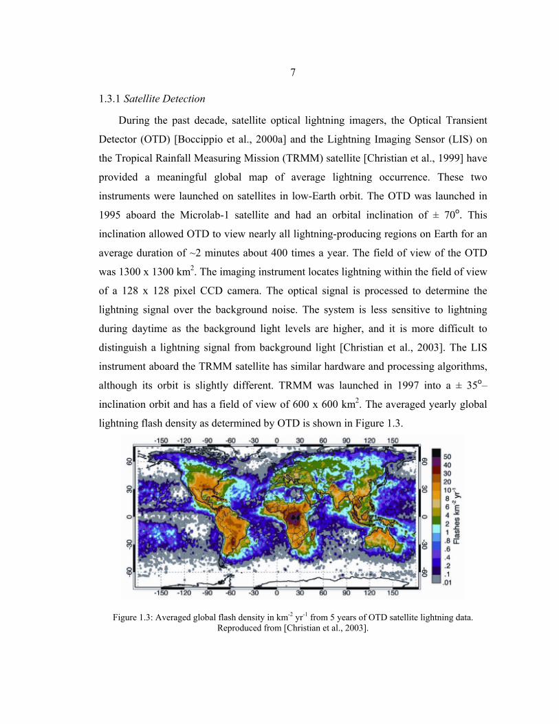
1.3.1 Satellite Detection
During the past decade, satellite optical lightning imagers, the Optical Transient
Detector (OTD) [Boccippio et al., 2000a] and the Lightning Imaging Sensor (LIS) on
the Tropical Rainfall Measuring Mission (TRMM) satellite [Christian et al., 1999] have
provided a meaningful global map of average lightning occurrence. These two
instruments were launched on satellites in low-Earth orbit. The OTD was launched in
1995 aboard the Microlab-1 satellite and had an orbital inclination of ± 70o. This
inclination allowed OTD to view nearly all lightning-producing regions on Earth for an
average duration of ~2 minutes about 400 times a year. The field of view of the OTD
was 1300 x 1300 km2. The imaging instrument locates lightning within the field of view
of a 128 x 128 pixel CCD camera. The optical signal is processed to determine the
lightning signal over the background noise. The system is less sensitive to lightning
during daytime as the background light levels are higher, and it is more difficult to
distinguish a lightning signal from background light [Christian et al., 2003]. The LIS
instrument aboard the TRMM satellite has similar hardware and processing algorithms,
although its orbit is slightly different. TRMM was launched in 1997 into a ± 35o–
inclination orbit and has a field of view of 600 x 600 km2. The averaged yearly global
lightning flash density as determined by OTD is shown in Figure 1.3.
Figure 1.3: Averaged global flash density in km-2 yr-1 from 5 years of OTD satellite lightning data. Reproduced from [Christian et al., 2003].

8
In Figure 1.3, the prevalence of lightning over land versus over ocean is apparent.
This figure also shows that central Africa is the region on Earth with the highest flash
density.
Several years of observations from these two instruments have allowed lightning
seasonal and local-time variations to be statistically separated, resulting in a
comprehensive lightning distribution versus local time, season, and geographic position
[Christian et al., 2003; Boccippio et al., 2000b; Petersen and Rutledge, 2001]. Nesbitt
and Zipser [2003] have used data from the TRMM satellite to study the diurnal cycle of
precipitation features over land and ocean. However, the infrequency of satellite
observations over a given point, and the precession of the satellite’s orbit, together,
cause years of cumulative data to be required to separate local-time variability from
other changes, such as seasonal and geographic effects. In the interest of studying
variabilities on a daily basis and in connection to certain storms, real-time global
detection by WWLLN is also important.
While the OTD and LIS instruments have provided extremely useful global
averages for the lightning community, their data has not been used in comparison to
WWLLN data. Instead, we have used data from the FORTE photodiode detector and
the radio frequency (RF) antenna lightning detection instruments on the FORTE
satellite. These instruments will be described in Sections 3.3.2 and 5.1.1, respectively.
1.3.2 Regional Ground-Based Detection
Ground-based regional detection systems, such as the National Lightning Detection
Network (NLDN) in the U.S. [Cummins et al., 1998], provide detailed information
about lightning strokes in real-time, but only for limited areas on Earth. These networks
typically measure lightning radiation in the low frequency range (30-300 kHz) and
require a density of 1 receiver every 100-300 km due to signal attenuation. About 300
sensors are deployed in the United States for the NLDN. Ground-based regional
networks usually have very high detection efficiencies (>95%) and are able to estimate
stroke peak current and lightning type based on the electric field waveform.

9
This dissertation uses lightning data from 2 regional, ground-based networks, the
Brazil Integrated Network (BIN; now called Brazil-Southeast 2 [Pinto et al., 2007]) and
the Los Alamos Sferic Array (LASA). Each of these networks is similar to NLDN, but
on a smaller scale. The BIN detects lightning in Southern Brazil, and LASA detects
lightning in the Great Plains of the U.S. LASA data have the advantage that complete
lightning waveforms are available in addition to the locations.
1.3.3 Overview of World-Wide Lightning Location Network
The WWLLN has been providing continuous accurate locations and times for
lightning strokes globally since August 2003 [Lay et al., 2004; Rodger et al., 2005a;
Jacobson et al., 2006]. A variety of comparisons have been made between WWLLN
lightning locations and regional ground-based network locations. Jacobson et al. [2006]
has shown that in 2004 WWLLN had a flat detection efficiency in the Southeastern U.S.
of ~4% for all types of strokes with peak current magnitude above 40 kA by comparison
to LASA. The value of 4% from this study may be off by 25-30% because it assumed a
LASA detection efficiency of 100% while LASA actually has a slightly lower detection
efficiency. Rodger et al., [2004, 2005a] have studied WWLLN capabilities in Australia
and New Zealand. We will take these detection efficiencies into account to normalize
WWLLN flash rates when using WWLLN to monitor the global effect of lightning
EMP on the lower ionosphere. The comparisons between WWLLN and other lightning
detection networks will be discussed in more detail in Chapter 3.
The WWLLN has two main advantages in addressing the question of interest of
this dissertation: (1) The WWLLN is the only lightning location network with the
capability to continuously monitor the location of lightning strokes around the entire
world. Thus it is the only network with the capabilities to expand the study of the
effects of lightning energy to a global level. (2) The WWLLN detects all types of
lightning strokes that have peak currents with magnitudes above ~40 kA with a constant
detection efficiency [Jacobson et al., 2006]. Since the magnitude of the lightning
electromagnetic pulse is dependent on the peak current, and not lightning type, it is

10
important to monitor all types of lightning with strong peak current. Regional networks
such as the NLDN only report cloud-to-ground lightning activity.
1.4 Effects of Lightning Energy in the Earth System
Over the past few decades, a handful of rocket flights in the ionosphere [e.g. Kelley
et al., 1985; Li et al., 1991] have detected electric field transients due to lightning
strokes at altitudes of 70-400 km, providing the first direct in situ evidence that VLF
lightning-generated waves can penetrate the ionosphere. Also, it has been shown that
lightning generates whistler wave radiation that can propagate into the outer
magnetosphere [Holzworth et al., 1999]. Lightning-generated whistler waves can
interact with electrons in the radiation belts, causing lightning-induced electron
precipitation [Goldberg et al., 1986]. Optical phenomena that occur above
thunderstorms, known as transient luminous events (TLEs), provide evidence of
lightning energy coupling to the atmosphere and lower ionosphere. We will describe
two main types of TLEs (sprites and elves) in Section 1.4.1. Extremely high energy
gamma-ray bursts, now termed terrestrial gamma-ray flashes (TGFs), have been
observed as originating from the Earth’s atmosphere [Fishman et al., 1994], and will be
described in more detail in Section 1.4.2. The research in this dissertation will focus on
energy coupling to the lower ionosphere from the lightning electromagnetic pulse
(EMP), of which elves are optical evidence, and touch briefly on energy radiated into
the magnetosphere via TGFs.
1.4.1 Elves/sprites
Lightning has the ability to affect conductivity and electron density in the lower
ionosphere, which could subsequently affect the ability of lightning energy to couple
into the upper ionosphere and magnetosphere. Transient luminous events (TLEs), such
as sprites and elves, are evidence of lightning energy coupling with the lower
ionosphere via quasi-electrostatic as well as electromagnetic fields, and can cause

11
ionization, heating and optical emissions in the lower ionosphere [Inan et al., 1991,
Tarenenko et al., 1993, Fukunishi et al., 1996].
Sprites are optical phenomena that occur above thunderstorms between 40 to 90 km
altitude and last for 10s of ms [Sentman et al., 1995; Boeck et al., 1995]. Sprites are
associated with large electrostatic fields caused by lightning strokes that transfer a large
amount of charge to the ground from a given altitude (more than ~350-600 C-km)
[Cummer and Lyons, 2005]. The majority of observed sprites have occurred in
association with positive cloud-to-ground strokes, but also have been observed rarely in
association with negative CGs [Barrington-Leigh et al., 1999, Taylor et al., 2008]. The
large altitude extent of the sprite (50-80 km) indicates that changes in conductivity and
electron density could arise over a large altitude range. This could be significant in
cloud-to-ionosphere charge movement as well as in lightning energy propagation in the
Earth-ionosphere waveguide. Figure 1.4(i) shows a sprite imaged by the Tohoku
University Sprite Group.
Figure 1.4: Image of i) a sprite and ii) an elve taken by the Tokohu University Sprite Group
(http://pat.geophys.tohoku.ac.jp/~thermo/sprites/).
Elves are another type of TLE, but are caused by the lightning electromagnetic
pulse (EMP) instead of a quasi-electrostatic field. The lightning EMP expands outward
from a high peak current (>50 kA) cloud-to-ground stroke: [Barrington-Leigh and Inan,
1999]. When it reaches an altitude of 85-95 km after ~1 ms, its electric field can interact
with the ionospheric plasma, causing optical excitation and secondary ionization. The

12
elves themselves are the optical emissions, which expand in a ring shape and last 1 to 3
ms. The first images of elves were published in the work of Fukunishi et al., [1996].
Figure 1.4(ii) shows an elve imaged by the Tohoku University Sprite Group. They are
more difficult to image than sprites due to the fact that they are produced just ~1 ms
after the lightning stroke. If the lightning stroke is visible in the field of view of the
imager, then it will overwhelm the sensor and the elve will likely not be visible. Recent
successful imaging of elves has occurred by allowing the Earth’s limb or cloud cover to
obscure the lightning stroke and leave the elve visible, or by sensitive electronics and
sophisticated processing algorithms [Frey et al., 2005].
Barrington-Leigh and Inan [1999] have shown by observing elves with a
photometric array that the EMP from lightning can interact with a region of the lower
ionosphere up to 700 km in diameter. Mende et al. [2005] have reported enhanced
electron density in the same region as a detected optical emission from an elve. These
observations indicate that the electromagnetic pulse from strong lightning strokes could
be creating enhanced electron density over a large region of the lower ionosphere. The
ISUAL instrument on the FORMOSAT-2 satellite has been operating since 2004,
detecting sprites, sprite halos and elves. In areas of the world with regional ground-
based detection networks, some of these detected TLEs have been correlated with
possible causative lightning strokes. To better understand the global dynamics of these
elves, global lightning detection is needed. Only WWLLN can provide this lightning
detection coverage. By monitoring the locations and stroke energies of lightning strokes
globally and comparing them to detected TLEs, we could learn what types of lightning
storms are connected with energetic events in different regions of the world. From this
information it may be possible to predict what conditions of strong lightning cause the
greatest effects on the lower ionosphere, and which regions of the world will be affected
at any given time.
Given that making in situ measurements of lightning-driven fields in the lower
ionosphere is very difficult, and has only been accomplished a handful of times, models

13
of the interaction between the lightning stroke and that region can be illuminating.
Various models predict the interaction between single lightning strokes and the lower
ionosphere and are consistent with optical observations of TLEs [Taranenko et al.,
1993; Fernsler and Rowland, 1996; Pasko et al., 1997; Cho and Rycroft, 1998]. These
models indicate that lightning causes electron heating and ionization of the lower
ionosphere that affects local conductivity and electron density. It has also been
proposed that in severe thunderstorms with high flash rates of strong lightning strokes,
the time between flashes could be smaller than the decay time for ionization changes of
10-100 s, allowing lightning-induced electron density increases to accumulate in the
lower ionosphere locally [Barrington-Leigh and Inan, 1999]. By using the
electromagnetic model developed in Cho and Rycroft [1998], Rodger et al. [2001]
predicted a possible ten-fold increase in nighttime lower ionospheric electron density
caused by the accumulated effects of NLDN-located lightning. We will improve on this
study by taking into account the non-linear response of electron density variations due
to lightning EMP. We will also expand this study globally using WWLLN lightning
flash rates of strokes with large amounts of radiated energy.
In summary, previous research based on observations and models of elves indicates
that thunderstorms with high flash rates of strong lightning strokes could cause an
accumulated increase of electron density and conductivity in the lower ionosphere, a
key region for the coupling of lightning energy with the upper ionosphere and
magnetosphere.
1.4.2 Terrestrial Gamma-ray Flashes
Terrestrial Gamma-ray Flashes (TGFs) are high-energy gamma-rays that have been
detected in space as originating from the Earth. These events are a relatively new area
of lightning physics, and much progress has been made in the field in the past 5 years.
TGFs were first unexpectedly observed by the BATSE satellite that was developed to
study gamma-rays from the sun and beyond [Fishman et al., 1994]. TGFs are another
indication of very energetic coupling of lightning with the magnetosphere. Since 2002,

14
the RHESSI spacecraft has detected hundreds of TGFs, which have been used to
correlate lightning strokes and TGFs [Smith et al., 2005]. Smith et al. [2005] report an
estimated ~50 TGFs per day globally. The mechanism behind TGFs as well as the
manner in which they are able to reach the upper ionosphere without severe attenuation
are still under investigation. The following are the main questions initially posed
regarding TGFs:
Are they associated with lightning strokes, or with some other part of the lightning
process? If they are associated with lightning, what type of stroke, and what strength of
stroke (either in peak current or charge moment change) are they associated with? Are
the gamma-rays beamed away from the source or isotropically radiated? What is the
cause of the few extremely energetic TGFs that were detected over regions with no
lightning?
Over the past five years, our understanding of TGFs has grown considerably. The
contributions from this dissertation research will be explained in Section 6.2, but this
introduction explains the current state of understanding. It is now understood that TGFs
are associated with the lightning stroke itself, and not some other process in the cloud.
TGFs do not seem to be associated with strokes having large charge-moment changes
[Cummer et al., 2005]. The process by which TGFs are now thought to be generated is
illustrated in Figure 1.5. Primary electrons produced by the lightning stroke are
accelerated by relativistic runaway breakdown. Those electrons emit bremsstrahlung
gamma-rays before being stopped by collisions with neutral molecules. The gamma-
rays then Compton scatter without confinement to magnetic-field lines and some are
able to reach the spacecraft altitude of 600 km. Electrons produced near top of
atmosphere can escape along magnetic-field lines [Smith et al., 2007, Dwyer and Smith,
2005] and are thought to be the cause of extremely high energy TGFs detected far from
lightning areas.

15
Figure 1.5: Cartoon of current theory of TGF production. Red cone is original electron beam, purple lines are gamma-ray paths from Compton scattering, red spirals show electrons produced near the top of the
atmosphere traveling along magnetic field lines (Reproduced from Smith et al., [2007]).
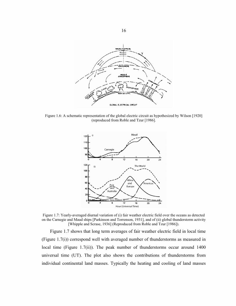
1.5 Global Electric Circuit
The global electric circuit (GEC) is the name used to describe the “spherical
capacitor” electrical system formed between the conducting Earth and conducting upper
atmosphere and ionosphere. An average 300 kV potential exists between the Earth and
ionosphere [Roble and Tzur, 1986]. The region between the two is filled with air, which
acts as a leaky resistor because of non-zero conductivity. It has long been hypothesized
that thunderstorms act as the generator in this circuit, providing current to the
ionosphere and maintaining the potential difference [Wilson, 1920]. In fair weather
regions, the evidence of this electrical circuit is in the form of the “fair weather return
current” which is a current from the ionosphere to Earth of 1 to 2 pA/m2. Integrating
over all fair weather regions gives a total ionosphere-to-Earth current of an average of
~1000 kA. If there was no mechanism to maintain the Earth/ionosphere potential
difference, a current of this magnitude would allow the capacitor to discharge within
~40 minutes [Roble and Tzur, 1986]. Therefore, it is hypothesized that ~1000
thunderstorms globally each provide about 1 kA of current up to the ionosphere. A
cartoon illustration of this hypothesis of the global circuit is shown in Figure 1.6.
16
Figure 1.6: A schematic representation of the global electric circuit as hypothesized by Wilson [1920] (reproduced from Roble and Tzur [1986].
Figure 1.7: Yearly-averaged diurnal variation of (i) fair weather electric field over the oceans as detected on the Carnegie and Maud ships [Parkinson and Torrenson, 1931], and of (ii) global thunderstorm activity
[Whipple and Scrase, 1936] (Reproduced from Roble and Tzur [1986]).
Figure 1.7 shows that long term averages of fair weather electric field in local time
(Figure 1.7(i)) correspond well with averaged number of thunderstorms as measured in
local time (Figure 1.7(ii)). The peak number of thunderstorms occur around 1400
universal time (UT). The plot also shows the contributions of thunderstorms from
individual continental land masses. Typically the heating and cooling of land masses
17
causes increased thunderstorms in the local afternoon. By converting all local times to
UT, one can add the different continental thunderstorm contributions to produce the
“world” distribution shown in Figure 1.7(ii) [Whipple and Scrase, 1936].
Although thunderstorms have been hypothesized for nearly a century as the
generator for the global electric circuit, there have not been detection capabilities
available to test this prediction thoroughly. Only in the past 35 years have lightning
detection networks been set up in certain regions [Cummins, 1998] and satellites to
monitor weather have been launched (Christian et al., 2003). However, as mentioned in
Section 1.3, regional networks are limited to small coverage regions and low-Earth
orbiting satellites can only monitor a small region at a time and must average over
months to determine global activity. To truly address the question of the generator of
the GEC and the daily variabilities in the GEC, one must have a method to detect all
thunderstorms globally all the time. In the work of Holzworth et al. [2005a], data from
the early stages of WWLLN were used in comparison to simultaneously recorded
vertical return current detected via electric field sensors on stratospheric balloons.
While the detection efficiency of WWLLN was not well characterized at that time, this
study indicated that WWLLN could provide an opportunity to more thoroughly
investigate the correlation between total global thunderstorm activity and vertical return
current.
1.6 Ionospheric Wave Propagation
The conducting Earth and conducting ionosphere form an electromagnetic
waveguide through which very low frequency (VLF; 3-30 kHz) radiation efficiently
propagates with little attenuation. It is this mechanism which makes the long-range
detection of VLF energy from lightning strokes, and, hence, the WWLLN, possible.
Because VLF radiation can travel for thousands of kilometers in the Earth-ionosphere
waveguide, it is possible to receive signals from all over the world at 5 or more
WWLLN receiver stations with only about 30 stations world wide.

18
The Earth-ionosphere waveguide also provides for one of the most useful methods
for probing the lower ionosphere. The lower ionosphere (~65-85 km altitude) is difficult
to probe by using many traditional techniques; the altitude is too high for balloons (~30
km) and too low for low-earth orbiting satellites (~400-800 km). The electron density in
the lower ionosphere is too low to reflect signals from ionosondes and incoherent
scatter radars. Rocket flights are useful for in situ measurements, but are very short
duration and only make measurements locally. Remote sensing of the lower ionosphere
by measuring phase and amplitude of VLF signals that propagate in the Earth-
ionosphere waveguide provides longer-term monitoring of the ionosphere than rocket
flights allow. Typically the signals available for study are narrowband transmitters run
by governments for submarine communication [Helliwell et al., 1973; McRae and
Thomson, 2000]. Recently, some researchers have begun to use lightning radiation as a
probe of the ionosphere as well [Cummer et al., 1998; Cheng and Cummer, 2005].
In order to better understand the data, ionospheric wave propagation theory was
developed in conjunction with these experimental measurements [Budden, 1961; Wait,
1970]. These theories were based on electromagnetic waveguide theory, using the
conducting earth and conducting ionosphere as the “walls” of the waveguide. They
originally assume a flat earth with a sharply bounded ionosphere, and then add
complexity to take into account the curvature of the Earth and the gradual change in
ionospheric conductivity. More recently, computer programs have been developed to
model the propagation of VLF waves using this waveguide mode theory of radio wave
propagation. The most widely used of these programs is the Long-Wave Propagation
Capability (LWPC) described in Ferguson and Snyder [1987]. A modified version of
this code will be used for some analyses in this dissertation.
1.7 Dissertation Outline
This introductory chapter has provided a brief introduction to the scientific
questions and previous studies that motivate this dissertation. The focus of this
dissertation is to study the coupling between lightning energy and the lower ionosphere.
19
WWLLN data are used to monitor spatial/temporal variability of strong coupling
regions and an electromagnetic model is presented to describe the expected
accumulated energy deposition from multiple lightning strokes. This dissertation also
presents the research required to validate the WWLLN as well as the application of
WWLLN data to provide information on high-density regions of nighttime lightning as
well as into elves and terrestrial gamma-ray flashes. The following is a detailed outline
of the chapter structure of this dissertation:
Chapter 2 provides a complete introduction to the World-Wide Lightning Location
Network. Detection efficiency and location accuracy validation of the WWLLN is
presented Chapter 3. Findings from Chapter 3 are used in Chapter 4 to provide time-
dependent maps of regions of strong nighttime lightning. Chapter 5 presents an
investigation into whether the WWLLN can detect narrow-bipolar pulses as is
suggested by initial research. Chapter 6 will focus on two case studies that use
WWLLN to provide information on elves and terrestrial gamma-ray flashes. Chapter 7
builds on the existing capabilities of WWLLN by developing a method to determine
lightning stroke radiated energy in the VLF band. Chapter 8 investigates the lightning
EMP/ionosphere interaction by modifying a model to propagate the lightning EMP to
the lower ionospheric plasma. Finally, a summary and conclusion are presented in
Chapter 9.
20
Chapter 2: World-Wide Lightning Location Network
2.1 Network Introduction
The WWLLN is the only lightning location network with the capability to
continuously monitor the location of lightning strokes around the entire world. The
WWLLN detects lightning strokes, regardless of lightning type, that have peak currents
with magnitudes above ~40 kA with a constant detection efficiency [Jacobson et al.,
2006]. The WWLLN originated from the “toga” network [Dowden et al., 2002].
The WWLLN has been providing continuous accurate locations and times for
lightning strokes globally since August 2003 [Lay et al., 2004; Rodger et al., 2005a;
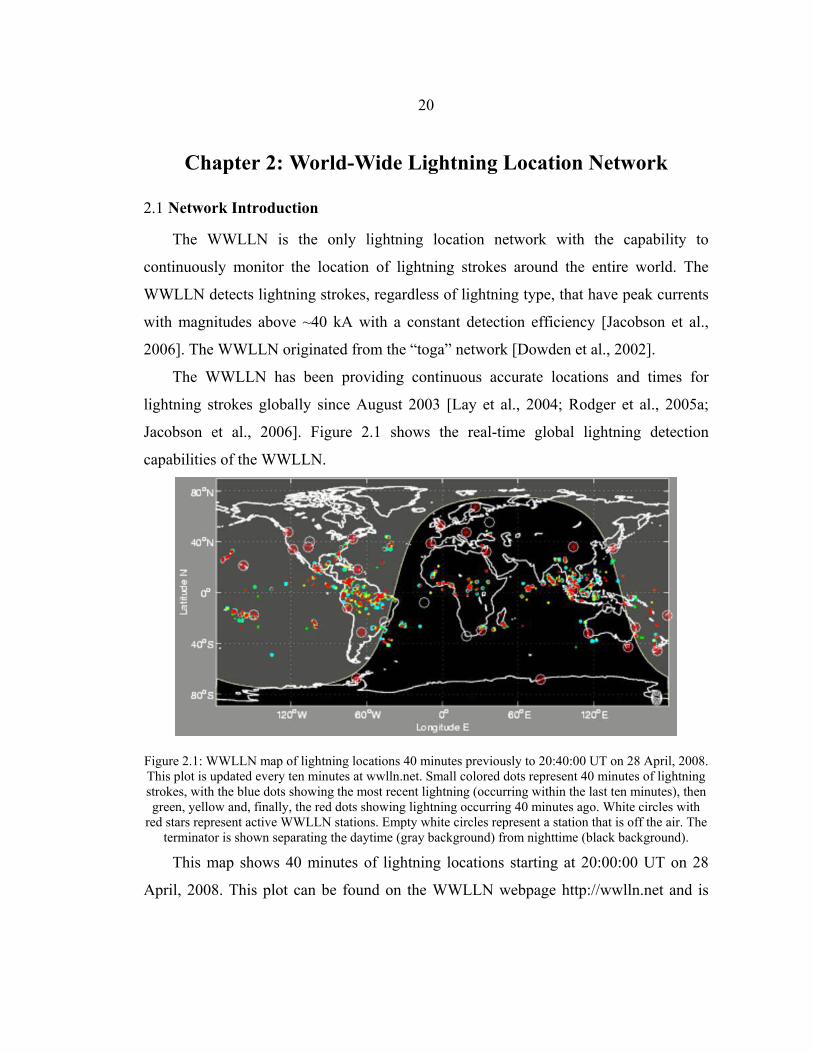
Jacobson et al., 2006]. Figure 2.1 shows the real-time global lightning detection
capabilities of the WWLLN.
Figure 2.1: WWLLN map of lightning locations 40 minutes previously to 20:40:00 UT on 28 April, 2008. This plot is updated every ten minutes at wwlln.net. Small colored dots represent 40 minutes of lightning strokes, with the blue dots showing the most recent lightning (occurring within the last ten minutes), then green, yellow and, finally, the red dots showing lightning occurring 40 minutes ago. White circles with
red stars represent active WWLLN stations. Empty white circles represent a station that is off the air. The terminator is shown separating the daytime (gray background) from nighttime (black background).
This map shows 40 minutes of lightning locations starting at 20:00:00 UT on 28
April, 2008. This plot can be found on the WWLLN webpage http://wwlln.net and is

21
updated every ten minutes. It shows 40 minutes of global lightning locations, with the
blue dots showing the most recent lightning (occurring within the last ten minutes), then
green, yellow and, finally, the red dots show lightning occurring 40 minutes ago. The
red stars with the white circles around them show the active WWLLN stations around
the world. The white line separating the black area from the gray area is the day-night
terminator. Jacobson et al. [2006] shows that the WWLLN has a flat detection
efficiency of ~4% for all types of strokes with peak current magnitude above 40 kA.
Rodger et al., [2005a] has found that the detection efficiency in Australia and New
Zealand is dramatically higher, at ~26% of CG strokes. We will take detection
efficiency into account in our studies using WWLLN flash rates by normalizing the
WWLLN flash rates based on these detection efficiencies.
2.2 WWLLN Hardware
Dowden et al. [2002] describe the instrumentation at each site and present data
from the initial six receiving sites spanning from New Zealand to Japan. The VLF
receiver stations each consist of a short (1.5m) whip antenna, a GPS receiver, a VLF
receiver, and an Internet connected processing computer. A cartoon schematic of a
WWLLN station is shown in Figure 2.2. The components inside the dotted line are
housed inside a building, while the antennas and preamp are mounted outside.
Schematics of the preamplifier and Service Unit (containing timing and VLF processing
electronics) are found in Appendix A.
The VLF antennas are typically mounted on ferro-concrete buildings. These
buildings shield the antenna from local man-made noise because they are adequate
conductors at VLF and thus remain at ground potential. In addition, the vertical electric
field from strong CG lightning dominates over power-line noise. For these reasons,
WWLLN receivers have relative freedom from the restriction of noise-free receiver
locations required for other long-range lightning location techniques [e.g., Fullekrug
and Constable, 2000]. The antennas measure radio wave pulses (sferics) in the VLF

22
band (1-24 kHz) radiated by lightning discharges. Lightning-generated waves in this
frequency range can propagate many thousands of kilometers in the Earth-ionosphere
waveguide because of low attenuation and high power spectral density [Crombie,
1964].
Figure 2.2: Cartoon schematic of a WWLLN VLF receiving station. Elements inside the dotted line are housed inside a building.
The preamp provides a gain of 10 to the electric field signal detected by the
antenna. This amplified signal is then routed via a long cable inside a building to the
Service Unit, which serves to isolate the signal via an audio transformer and then sends
the signal to the computer sound card. The Service Unit also provides power to the
preamplifier.
The GPS antenna provides one pulse per second. This pulse is input to the
computer sound card and used to adjust the time-stamp on each VLF waveform. The
GPS antenna also provides an NMEA signal giving the exact location of the station, that
is input to the computer via a serial port connection.
The requirements for the station computer are minimal: It must be able to run
RedHat Linux, and must have a sound card and serial port. A sufficient amount of RAM
is 248 or 512 MB and 20-40 GB is plenty of hard-disk space. The computer also must
be continuously connected to the internet.

23
2.3 WWLLN Software
The software for each WWLLN station was developed by Dr. James Brundell and
the TOGA (time of group arrival) methodology was developed by Dowden and his team
[Dowden et al., 2002]. This software functions as follows: The VLF electric field is
sampled at ~48kHz. When the difference between two consecutive samples exceeds a
given threshold level, a 64-sample waveform is saved to short-term memory to be
analyzed. This waveform consists of 16 pre-trigger data points and 48 post-trigger
points. Figure 2.3 shows an example of such a waveform detected at a WWLLN VLF
station.
Figure 2.3: Example 64-sample waveform of a lightning sferic. Time is in milliseconds on the x-axis and uncalibrated vertical electric field is on the y-axis.
When a sferic waveform is captured, the software determines the time of group
arrival (TOGA) of the group energy for that sferic. The reason the TOGA method was
developed was because the sferic waveform becomes dispersed during its propagation
of often thousands of kilometers in the Earth-ionosphere waveguide. Thus the trigger
time does not necessarily indicate the time of arrival of the group energy. If the wave is
extremely dispersed, the arrival of the group energy will occur later than the trigger
time.
The TOGA is calculated as follows: The group velocity in a waveguide is given by
vg(ω) = dω/dk , where k(ω) is the frequency dependent wave vector. The electric field

24
of the wave can be expressed as a sum of Fourier components of the frequency, ω: E(r,
t, ω) = ΣA(ω)cos(φ(ω)), where φ(ω) = ωt - k(ω)r + φ0. The slope of the phase φ(ω) at a
given time t and range r, is then given by )(d
ddd
ωωωϕ
gvrtkrt −=−= . This equation
shows that dφ/dω equals zero when t equals the group travel time, )(ωg
g vrt = . An
instantaneous time for which dφ/dω at a given value of ω is not sensible for a
broadband source such as a lightning sferic. Instead, an average dφ/dω is determined
over the frequency band of 6-22 kHz. This band is chosen because lightning energy is
maximum over this band, and our WWLLN stations are sensitive to this band. The
TOGA is defined as the instant when the regression line of dφ/dω has zero slope when
averaged over the frequency band of 6 to 22 kHz [Dowden et al., 2002]. The software
on each WWLLN VLF station computer determines the TOGA for each sferic by
calculating the time when the regression line of dφ/dω in this frequency band equals
zero and then reports that time to the central processing computer to be used in
lightning location.
The software also calculates an uncalibrated integrated energy flux density, Y, for
each station, which will be used later in this dissertation to determine a calibrated
energy radiated per lightning stroke. This energy flux density is the integrated energy in
the uncalibrated electric field at the antenna and is determined as follows:
( ) tcE'
0
2
∆= ∑samples
Yµ
(2.1)
where E’ is the uncalibrated electric field as shown on the y-axis of Figure 2.3, c is the
speed of light, µ0 = 4π*10-7 W/(A*m), and ∆t=1/(sampling frequency). Chapter 7 of this
dissertation describes how the uncalibrated integrated energy can be used to help
determine the magnitude of the lightning stroke in terms of total radiated energy.
The integrated energy in the electric field waveform, the TOGA, and the station
identification number are sent to the central processing station. If five or more stations

25
detect an event, the location and time of the discharge is determined by using the
downhill simplex method to minimize the difference in location and time given by the
five or more stations. While detection of an event by 4 stations would be enough to
produce a location estimate, the 5th station allows error analysis. The minimization
routine produces a location and timing “residual” that indicates an accuracy estimate of
the measurement. The global data are then posted to the internet every 10 minutes (see
http://wwlln.net), and sent in real-time to research groups and commercial customers.

26
Chapter 3: Global Detection Efficiency and Location Accuracy
3.1 Overview
In order for WWLLN to provide useful global coverage, we must understand its
global detection efficiency. During the development of the network, a number of studies
have been completed to achieve this goal. The studies presented here include (1) a case-
study comparison of WWLLN detection efficiency and location accuracy done in Brazil
in 2003 (Section 3.1), and (2) a comparison of WWLLN lightning locations to optical
lightning detector data on the FORTE satellite in order to determine a relative global
detection efficiency for the network (Section 3.2). Section 3.3 will investigate the
detection range of WWLLN stations.
These studies have been conducted in conjunction with additional detection
efficiency studies done by members of the WWLLN team: Rodger et al. [2005a]
completed a comparison of WWLLN data in Australia to the local Australian lightning
location network, Kattron, and found a detection efficiency of ~26% of CG strokes in
Australia and ~10% of IC strokes, with a location error of 4.2 ± 2.7 km. By comparison
to the Los Alamos Sferic Array (LASA) in the southeastern U.S., Jacobson et al. [2006]
found that WWLLN detects ~4% of all strokes, CG and IC, with peak current greater
than ~30 kA, and detects with a spatial accuracy of ~15 km. Of the coincident events
between WWLLN and LASA, 26% were labeled as IC lightning by LASA. Similarly,
Rodger et al. [2006a] found the result of a flat detection efficiency for strokes with peak
currents larger than ~40 kA by comparison to the New Zealand Lightning Detection
Network (NZLDN).
3.2 Brazil Integrated Network/WWLLN Comparison
The March 2003 comparison between WWLLN and the Brazilian Integrated
Network (BIN) was motivated by the desire to study the “worst-case scenario” for the

27
WWLLN system, as it covered a region of the world where the nearest WWLLN
receiver was >7000 km away during a time when WWLLN had not yet implemented
the TOGA algorithm. Instead, the trigger time at the station was used as the time of
arrival of the sferic. During data-collection period for this study (March 2003), the
WWLLN was composed of just 11 active VLF receivers. Table 3-A shows the locations
of these receivers.
Table 3-A: Station locations for stations active during Brazil comparison study
Station Latitude (deg) Longitude E (deg)
Dunedin, New Zealand -45.8639 170.514 Darwin, Australia -12.3718 130.868 Perth, Australia -32.0663 115.836 Singapore 1.2971 103.779 Brisbane, Australia -27.5534 153.052 Osaka, Japan 34.8232 135.523 Tainan, China 22.9969 120.219 Budapest, Hungary 47.4748 19.062 Seattle, USA 47.654 -122.309 Cambridge, USA 42.3604 -71.0894 Durban, South Africa -29.8711 30.9764
3.2.1 Method
We compare WWLLN lightning events with residuals (error estimates) less than 20
µs that occurred on 6, 7, 14, 20, and 21 March 2003 in the range of 40º to 55º W, 15º to
25º S to events in the same range measured by a land-based local Brazil lightning
detection network, the Brazilian Integrated Network (BIN) [Pinto and Pinto Jr., 2003;
Pinto Jr. et al., 2003]. Figure 3.1 shows the region of interest in Brazil. We study these
data because the BIN data had already been procured by our group for use in the sprite
balloon campaign in 2002-2003 in Brazil [Holzworth et al., 2005b].
BIN consists of 21 sensors in the region of interest, with an overall stated detection
efficiency of 80% of all cloud-to-ground lightning strokes. However, the efficiency is
dependent on return stroke peak current. Detection efficiency of events with peak
current greater than 50 kA is 90% with a location accuracy of less than 1 km. For events
with peak current less than 10 kA, detection efficiency could be as low as 30% with

28
approximately 5 km location accuracy. The return stroke peak current measurement also
includes uncertainty due to assumed lightning return stroke speeds, as expected for
detectors of this type [e.g., MacGorman and Rust, 1998]. BIN cites an uncertainty of
20-30% for strokes with peak current greater than 10 kA and up to 100% uncertainty for
strokes with less than 10 kA peak current [Pinto Jr., personal communication, 2003].
Figure 3.1: Region of Brazil comparison between lightning location networks used in this study. As there were no WWLLN receivers in South America, this region of Brazil is a low-coverage region of the
WWLLN.
3.2.2 Results
In the five-day time period, 671 WWLLN events and 63,893 BIN events were
reported in the region of interest. Taking into account the 80% accuracy of BIN [Pinto
Jr. et al., 2003], a rough estimate of the percentage of all CG lightning events measured
by WWLLN in this region is ~0.8%. To measure the accuracy of WWLLN, we compare
the data sets from the two networks to find “shared” events. A lightning stroke is
assumed to be shared if each network measures an event within 3 ms and 50 km of the
other. According to these criteria, 289 of the 671 WWLLN events are common to the
BIN stroke data.
The shared events have an average return stroke peak current of 86 kA, as
measured by BIN. In contrast, the average peak current of the entire BIN dataset is 33.3
kA, suggesting that the WWLLN network only detects large discharges that exceed an

29
approximate “threshold” in return stroke peak current. The histogram in Figure 3.2
represents this threshold by comparing the BIN peak current distribution of the entire
BIN data set to only the BIN events which were also observed by WWLLN. Overall, a
greater fraction of the strokes have negative polarity, as expected. However, for
discharges with an absolute value of peak current less than 50 kA the figure shows that
there is a larger proportion of such low-current lightning in the overall BIN dataset
(black) than in the subset made up of only shared events (white). For events with peak
current greater than 50 kA, the relative pattern is reversed. This pattern illustrates that
WWLLN detection is biased towards lightning strokes with large peak currents.
Figure 3.2: Histogram of return stroke peak currents measured by the BIN, shown in 50 kA bins centered on the single peak current value noted beneath them. The two outermost bins contain data for all strokes with peak current greater or less than 175 kA. Distributions are shown for shared WWLLN-BIN events
(white) and all measured BIN events (black).
Next, we estimate the spatial and temporal accuracy of WWLLN by analyzing the
shared events. Time differences between the shared strokes are on average 0.06 ±
0.2 ms. To calculate location offsets for WWLLN strokes relative to their shared BIN
events, we plot each shared BIN event at (0,0) and determine the east-west and the
north-south deviation of the WWLLN positions (Figure 3.3).
WWLLN events have a mean deviation of 3.2 km north (dashed-dotted line),
7.3 km east (dotted line) from BIN events. The plotted ellipse of one standard deviation
encompasses (0,0), indicating no statistically significant difference in the location of the

30
shared events. The elongation of the data spread is possibly a systematic error due to
differences between east-to-west and west-to-east VLF propagation in the Earth-
ionosphere waveguide [Wait, 1970]. The location errors might be improved by using an
enhanced location finding algorithm that incorporates ionospheric propagation. In
analyzing the data for random error, we find that the absolute location error is 20.25 ±
13.5 km for WWLLN network observations in this part of Brazil.
Figure 3.3: Location offsets of shared WWLLN-BIN events relative to the BIN-determined discharge position. Each shared BIN event is taken to be at (0,0) and the corresponding WWLLN event is plotted relative to (0,0). Mean location offset is 3.2 km north (dashe-dotted), 7.3 km east (dotted). One standard
deviation (ellipse) encompasses (0,0).
3.2.3 Summary of Brazil Study
This analysis has shown that WWLLN provides lightning location of about 0.8% of
lightning events in Brazil with an accuracy of 20.25 ± 13.5 km and 0.06 ± 0.2 ms. The
WWLLN detection efficiency, while low compared to the BIN, suffices to mark storm
occurrence due to the large number of total lightning strokes that occur in storm
systems. In addition, this study was the first study of WWLLN to show that WWLLN
detects high-peak-current lightning.
The greatest advantage of WWLLN is global lightning coverage in real time at low
cost. By comparison with a regional network on the outskirts of the current WWLLN
coverage zone, our analysis indicates that the WWLLN-reported lightning events have
31
spatial resolution on the order of magnitude of an isolated thunderstorm and excellent
temporal accuracy. For many applications, the benefits of a global overview in real time
may outweigh the fact that a very low percentage of the total lightning activity is
reported. The WWLLN is shown to be an important scientific and operational tool for
lightning and severe-storm researchers to characterize remote storms, and should prove
to be a highly useful tool for the atmospheric-sciences community.
3.2.4 Advances in WWLLN since this study
Two improvements have been made since this study to increase the total percentage
of lightning events measured by the WWLLN. The first is the installation of additional
stations in the low coverage region. One may refer to Figure 2.1 for a complete station
coverage map as of April 2008. The second is the implementation of the TOGA timing
algorithms, described in Section 2.3, that takes the dispersion of the sferic into account
by measuring time of group arrival (TOGA) of the sferic. This new algorithm accounts
for the long propagation distance of VLF waves from Brazil and thus increases
accuracy of the timestamp at each VLF receiving station that is used in the location of
each lightning event. Since January 2008, WWLLN has been running a new lightning
location algorithm that recycles packets (TOGAs from VLF stations) if they were not
used in locating a lightning stroke, meaning that if a particular set of packets did not
produce a valid location, only the first packet is thrown out, and the others are reused to
try to find a valid location.
3.3 FORTE/WWLLN Comparison
3.3.1 Overview
Although comparisons of the WWLLN to ground-based networks have determined
its detection efficiency over small geographic regions as discussed in sections 3.1 and
3.2, and some attempts have been made to model the global detection efficiency
[Rodger et al., 2005a, 2006], the detection efficiency of WWLLN has not yet been

32
determined on a global scale. Given that WWLLN VLF receiver stations are not spread
uniformly around the world, and that topographical features vary over the earth, the
detection efficiency around the world could vary as well. We also study the relative
detection efficiency over land and over ocean for WWLLN. One might expect a
difference in detection efficiency given that lightning-generated VLF radio waves
propagate with less attenuation over sea water than over land [Wait, 1970]. Since the
WWLLN requires that the signal from a lightning sferic be detected by five or more
WWLLN VLF stations, a larger attenuation over land could mean that a lightning stroke
over land may be less likely to trigger the required five stations.
In this section we describe a systematic check of the long-range VLF relative
detection efficiency over land and over ocean, and over diverse geographical regions,
using the FORTE satellite photodiode detector (PDD) optical measurements of
lightning as a reference.
3.3.2 FORTE photodiode detector
We use optical lightning data from the photodiode detector (PDD) on the Fast On-
Orbit Recording of Transient Events (FORTE) satellite [Suszcynsky et al., 2000b, 2001;
Kirkland et al., 2001]. The PDD is a non-imaging silicon photodiode collecting light
from within a circular field of view of diameter 1200 km at ground level. Because the
PDD is non-imaging, any event it detects can be located only to within this 1200-km
footprint. The PDD is triggered by a rising optical signal intensity. Once the intensity
exceeds the threshold level and a trigger occurs, a 128-sample register is stored in
memory, including 32 samples preceding and 96 samples following the trigger. The
sample interval is 15 µs, so the record duration is about 1.9 ms. The FORTE satellite is
in a 70º circular orbit at 800-km altitude. Thus the PDD “spotlight” sweeps out the
entire region where lightning is found on Earth.
Because the PDD instrument is satellite-based, it observes lightning from above,
meaning that it can only detect light that manages to escape from the cloud tops.
Previous studies have shown that the majority of PDD-detected events are in-cloud (IC)

33
lightning [Susczynsky et al., 1999], although the PDD is also able to detect scattered
light from the in-cloud portion of a cloud-to-ground (CG) lightning stroke [Susczynsky
et al., 2000b].
Because of high daytime background light levels, the trigger level for the PDD
instrument is set higher during daytime than nighttime to avoid contamination from
false triggers. This trigger level difference has the effect of biasing the daytime PDD
data to high peak current strokes.
It has been shown that PDD has a detection efficiency lower than, but constant
relative to, LIS detection efficiency over all areas of the world [Light et al., 2003].
Thus, we are confident that PDD data serve as an adequate proxy for LIS or OTD data,
with the proviso that the PDD locates lightning only to within the 1200-km-diameter
field of view, as opposed to within an individualized pixel of an imager. An advantage
of PDD for this study is that we can examine optical waveforms relative to the VLF
lightning trigger. For this study we assume equal PDD detection efficiencies for land
and ocean.
3.3.3 WWLLN/PDD Comparison Methodology
In this study we search for coincident lightning events between WWLLN-detected
lightning sferics and PDD-detected optical waveforms measured between 1 August
2003 and 31 December 2005. To find coincident events, we first exclude any WWLLN
events that occur outside the PDD 1200-km field of view. From this reduced WWLLN
data set, we compare the WWLLN sferic time to the optical trigger time. All PDD
events that are within 200 ms of a WWLLN-located sferic are corrected in time for the
optical signal delay to the satellite, by assuming the WWLLN sferic location as truth. A
histogram of the corrected time differences of WWLLN-measured sferic time minus
optical trigger time is shown in Figure 3.4. Figure 3.4 peaks at -0.25 ms, indicating that
the sferic time usually precedes the optical trigger by about 0.25 ms. From this
histogram, we choose a classification for coincident events as pairs having a corrected
time difference for sferic-optical trigger time between -0.80 ms to 0.30 ms. We choose
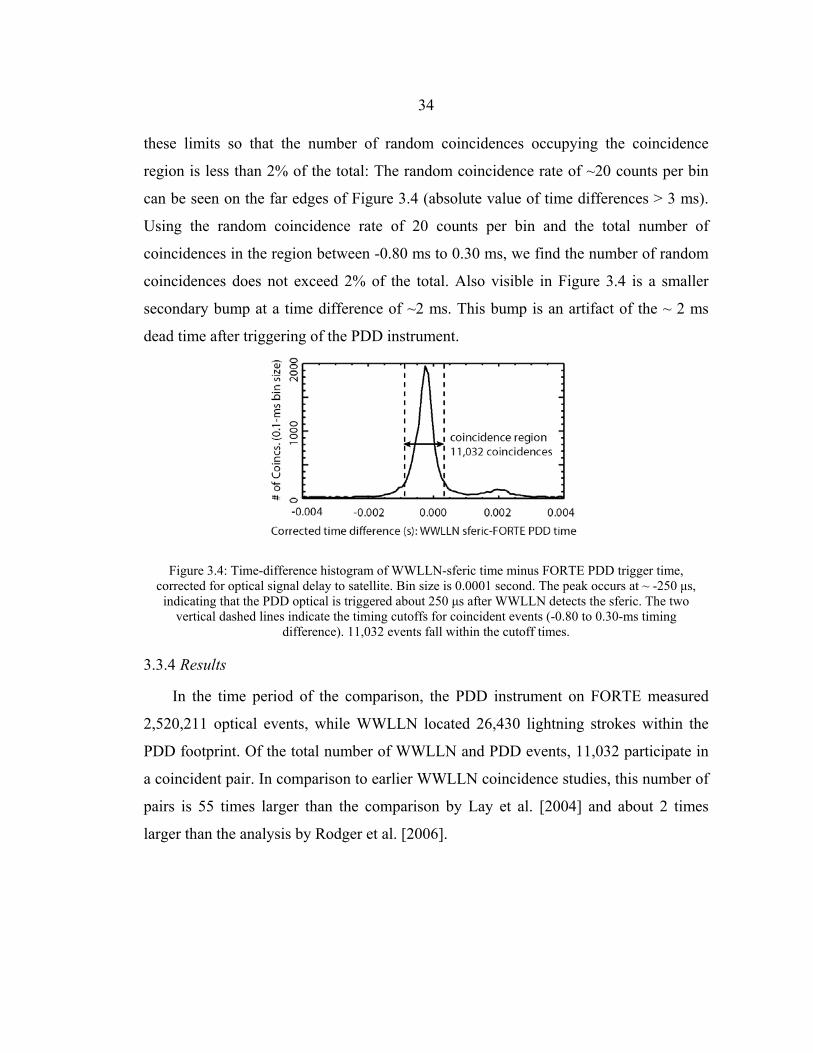
34
these limits so that the number of random coincidences occupying the coincidence
region is less than 2% of the total: The random coincidence rate of ~20 counts per bin
can be seen on the far edges of Figure 3.4 (absolute value of time differences > 3 ms).
Using the random coincidence rate of 20 counts per bin and the total number of
coincidences in the region between -0.80 ms to 0.30 ms, we find the number of random
coincidences does not exceed 2% of the total. Also visible in Figure 3.4 is a smaller
secondary bump at a time difference of ~2 ms. This bump is an artifact of the ~ 2 ms
dead time after triggering of the PDD instrument.
Figure 3.4: Time-difference histogram of WWLLN-sferic time minus FORTE PDD trigger time, corrected for optical signal delay to satellite. Bin size is 0.0001 second. The peak occurs at ~ -250 µs,
indicating that the PDD optical is triggered about 250 µs after WWLLN detects the sferic. The two vertical dashed lines indicate the timing cutoffs for coincident events (-0.80 to 0.30-ms timing
difference). 11,032 events fall within the cutoff times.
3.3.4 Results
In the time period of the comparison, the PDD instrument on FORTE measured
2,520,211 optical events, while WWLLN located 26,430 lightning strokes within the
PDD footprint. Of the total number of WWLLN and PDD events, 11,032 participate in
a coincident pair. In comparison to earlier WWLLN coincidence studies, this number of
pairs is 55 times larger than the comparison by Lay et al. [2004] and about 2 times
larger than the analysis by Rodger et al. [2006].

35
To examine regional differences in the WWLLN detection efficiency, we separate
these events into the six global regions shown in Figure 3.5. The motivation of the
division locations was to try to avoid cutting major continental landmasses apart.
Figure 3.5: WWLLN station locations (diamonds) in January 2005 and the six broad regions used in this study. The thickness of the coastlines shows the size of the coastal region used in the land/ocean study.
Table 3-B shows the results of this categorization. The data are divided into six
columns corresponding to the six global regions of interest. The first and second rows
show the number of PDD events and WWLLN events, respectively, in each regional
box. The third row shows the number of coincident events in each region. The fourth
row shows relative detection efficiencies (the total number of WWLLN events detected
divided by the total number of PDD events detected) and the fifth row shows the
fraction of WWLLN events in each region that were coincident with a PDD event.
One must note that the values shown in Table 3-B do not represent absolute
detection efficiencies, since, in general, the PDD instrument detects mainly IC lightning
while the WWLLN detects mainly CG lightning. In a comparison of PDD to NLDN,
which estimates a detection efficiency of ~90% for high peak current strokes,
Suszcynsky et al. [1999] found that the PDD only detected 5.5% of NLDN-detected
negative CG lightning and 8.3% of positive CG lightning. However, even without an
absolute detection efficiency calibration, this analysis can provide an understanding of
the relative detection efficiency of the WWLLN on a global scale.

36
The region with the highest detection efficiency is Australasia (region 6), and the
lowest detection efficiency is in Europe (region 2), followed by Africa (region 5). The
fraction of WWLLN strokes that are coincident with PDD events (row 5 in Table 3-B)
does not correspond directly to the detection efficiency. The lowest fraction is once
again in region 2 (Europe), but the highest fraction is now in region 5 (Africa). This
difference may mean that the strokes that are detected by PDD in Africa are more likely
to be the type of stroke that also is detected by the WWLLN (high-peak current CG
strokes). We have now also been able to analyze data from 2006 for these 6 regions. In
2006, WWLLN stations were added in Honolulu, Hawaii; Rothera, Antarctica;
Kingston, Australia; Cordoba, Argentina; Ascension Island; and Lanzhou, China. These
additions have increased the detection efficiency as compared to PDD, by 20% overall,
and regionally by ~100% in Region 1, ~50% in Region 4, and ~10% in Region 5.
Table 3-B: Results of WWLLN/PDD regional comparison 2005
Region # 1 2 3 4 5 6
PDD total 232,380 88,474 187,935 480,907 802,771 727,744
WWLLN total 2,204 428 1,552 4,198 4,821 13,227
# coincs 905 161 655 1,692 2,131 5,488
totalPDD totalWWLLN
0.009 0.005 0.008 0.009 0.006 0.018
totalWWLLNcoincs#
0.411 0.376 0.422 0.403 0.442 0.415
To examine land/ocean differences in the WWLLN detection efficiency, we
separate these events into land and ocean subsets in two ways. In the absence of a
coincident WWLLN-located lightning stroke, PDD events can be located only to within
the 1200-km-diameter PDD footprint, meaning that an optical event detected with the
sub-satellite point located within 600 km of the coastline could have occurred over
either the land or ocean.

37
Therefore, the first classification (shown in Table 3-C) labels events as “over land”
(1st column, Table 3-C) only if either the WWLLN location, or the FORTE sub-satellite
point, is over land and more than 600 km from the coastline, and labels events as “over
ocean” (2nd column, Table 3-C) only if either the WWLLN location, or the FORTE sub-
satellite point, are over ocean and more than 600 km from the coastline. The lightning
“within 600 km of coast” (3rd column, Table 3-C) is all the remainder and corresponds
to lightning that occurred over any surface within 600 km of coast. Most of the
lightning-prone areas of Australasia and central America are swept into the coastal
category in Table 3-C. This classification scheme provides us a basis to compare
land/ocean differences for all PDD and WWLLN events, as opposed to only coincident
events.
Table 3-C: Results of WWLLN/PDD land/ocean comparison using 600-km coastal areas
over land &
>600km
from coast
over ocean
& >600km
from coast
within
600km of
coast
total
PDD total 401,902 255,107 1,863,202 2,520,211
wwlln total 2,892 2,064 21,474 26,430
wwlln/PDD 0.007 0.008 0.012 0.010
In addition to showing lightning counts in the three categories described above,
Table 3-C also includes a “total” column to provide a quick reference to the total
number of PDD and WWLLN events that were detected within the PDD “spotlight”
during the time period of the study. We find the ratio of total number of WWLLN
events to total number of PDD events over land and ocean in the last row of Table 3-C.
WWLLN detects 0.7% of the number of events PDD detects over land and 0.8% over
ocean, indicating a difference of less than 13% in WWLLN detection efficiency over
land and over ocean. The ratio of total coastal WWLLN to total coastal PDD events is
slightly higher, at 1.2%. We believe this increased ratio can be explained thus: the
number of events within 600 km of the coastline is dominated by lightning in
Australasia, as most of the land in that region is not more than 600 km from a coastline,

38
and Australasia is the region of highest WWLLN detection efficiency as seen in Table
3-B.
Next, we focus on coincident events measured by PDD and WWLLN. For this
second grouping of data, we take advantage of the more accurate WWLLN location in
analyzing events by first assigning each PDD event coincident with a WWLLN event
with the location of that WWLLN event. Because WWLLN-measured strokes have a
location accuracy of 15-20 km, we next sort coincident events into land and ocean
subsets with only a ~50-km-semi-width “coastal” region. The land/ocean/coastal
separation map was created using high-resolution continental borders, including major
islands, on a 1440×900 pixel grid, covering –70 to 70 degrees latitude. The pixels
covering land areas were given a value of 1 and those covering ocean were given a
value of zero. A smoothing procedure over 4 pixels gives any land or ocean within 2
pixels of the coastline a value in between 0 and 1, and it is these pixels that are
classified as coastal. At the equator, this gives a coastal area of ~55 km from the coast.
Therefore, islands smaller than ~110 km will not be included in the ‘land’ category. The
continental border thickness in Figure 3.5 indicates the width of the coastal region in
this study. WWLLN events located in the coastal region are not used in the land/ocean
local time study (Chapter 4), but are included in Table 3-D as coastal events. The 50-
km-semi-width swath of rejected data additionally allows us to reduce the occurrence of
erroneously classifying an oceanic lightning event as over land (or vice versa) due to the
15-20 km location accuracy of WWLLN [Lay et al., 2004; Rodger et al., 2004;
Jacobson et al., 2006].
Table 3-D: Results of WWLLN/PDD land/ocean coincidence comparison
over land over ocean coastal total
# coincs 4,307 4,122 2,603 11,032
WWLLN total 11,074 9,290 6,066 26,430
totalWWLLNcoincs #
0.389 0.444 0.429 0.417

39
Table 3-D shows the results of this stratification. The 1st row shows the number of
coincident events, separated into “over land”, “over ocean”, and “coastal” events by
using the criteria described in the previous paragraph. In the second row of Table 3-D,
all WWLLN data are also separated into the three categories using the 50-km-semi-
width “coastal” region. The bottom row shows the total number of coincident events
divided by the total number of WWLLN events. These results show that 38.9% of
WWLLN events over land participate in a coincidence with a PDD event, while 44.4%
of oceanic WWLLN events participate in a coincidence. The small percentage
difference in land/ocean coincidence detection efficiency indicates that it is unlikely
that the WWLLN will completely miss a storm with lightning of similar magnitude over
ocean relative to over land. With these statistics, we can begin to use the WWLLN to
study relative differences in the effects of strong lightning over land versus over ocean.
Figure 3.6: A superposed epoch of PDD waveforms with WWLLN coincidences. The median (solid line), 75th percentile (dashed-dotted line), and 25th percentile (dotted line) in amplitude of all PDD waveforms
which participated in a 1.1-ms coincidence with WWLLN are separately plotted. These statistics are computed independently for each time bin. The waveforms are individually shifted in time to place the
WWLLN-calculated sferic time at 0.00 seconds.
A superposed-epoch accumulation of the optical waveform and the sferic stroke
time has been performed to further validate the comparison. Figure 3.6 shows the
median, 75th percentile, and 25th percentile in amplitude of all PDD waveforms which
participated in a coincidence with WWLLN. The amplitudes are considered separately
in each time bin. The waveforms are shifted in time to position the WWLLN-calculated
sferic time at 0.00 seconds. The 0.3- to 0.4-ms delay in the optical peak is slightly

40
longer than found by Susczynsky et al. [2000b] in a VHF/optical comparison, in which
a 243-µs average delay of the optical peak was attributed to a 105-µs average delay
between VHF and optical emission plus an average 138-µs broadening due to scattering
delay of light in its travel through the cloud. Figure 3.6 shows general agreement with
the timing data and waveform shapes of previous studies, giving cause to trust the
coincidences found by this comparison.
With confidence in the WWLLN/PDD-detected coincidences and in the relative
detection efficiency of WWLLN over land and ocean, we can use the entire, not just
PDD-coincident, WWLLN data set to look at land/ocean effects in high peak current
lightning occurrence. In Chapter 4 of this dissertation, we will look at local time
differences in lightning over land and over ocean and demonstrate the suitability of
WWLLN as a tool to study these variations on shorter time scales than can be seen from
satellite averages.
3.3.5 Conclusion
The comparison of the World-Wide Lightning Location Network with satellite
optical data has provided global verification of the capabilities of the WWLLN in
detecting lightning globally and over land versus ocean with a similar relative detection
efficiency. It has also provided relative detection efficiencies for six large geographical
regions over 2 years that will be used in this dissertation to determine global lightning
count rates.
3.4 Detection range of WWLLN stations
Figure 3.7 indicates that WWLLN stations can detect lightning at very large
distances, as expected from fundamental VLF propagation [Crombie, 1964]. By using
WWLLN observational data we can characterize the typical WWLLN station observing
range, i.e., at what distance can a particular station detect a lightning stroke. We use a
sample of WWLLN data from 1–30 April 2005 to determine the detection range of each

41
station. To calculate the detection range, we find which events of the entire WWLLN
data set each station participated in detecting.
For this example, we will discuss and calculate the detection range of the Darwin
WWLLN station, hosted by Charles Darwin University. We calculate the distance
between the Darwin station location and each lightning event that was detected at the
Darwin WWLLN station. We then determine the number of events Darwin detected
versus distance from the station, in 200-km bins, as well as the number of events the
WWLLN as a whole detected versus distance from Darwin. Because of the spherical
geometry of the Earth, the bins increase in area until 10 megameters (Mm) and then
decrease in area for the larger distances. Thus, the bins that contain data from 10 Mm
have better statistics than those at either 1 Mm or 20 Mm. Figure 3.7 shows a histogram
of the ratio of the events the Darwin WWLLN station “saw” over the total number of
events the WWLLN network detected versus the distance of the lightning stroke from
the Darwin station. A ratio of one would indicate that the Darwin station participated in
the detection of all the lightning that the WWLLN reported in that 200-km-width bin.
The black dots show the ratio for events that occurred ±2 h around local noon, and the
gray plusses show the ratio for events that occurred ±2 h around local midnight. While
lightning located very far from the Darwin WWLLN station may have propagated under
a mixture of both day and night ionospheres when considering the case of local noon at
Darwin, this situation will be dominated by the daytime ionospheric propagation
conditions around the WWLLN station.
Figure 3.7: Ratio of the number of events detected by the Darwin station to the number of events detected at the same range from Darwin by the network as a whole. The black dots show this ratio for ±2 h around
local noon, while the gray plusses are for ±2 h around local midnight.

42
Figure 3.7 shows that Darwin has a larger detection range around local midnight
than around local noon, as is expected because of ionization density changes between
day and night in the Earth-ionosphere waveguide, leading to lower attenuation for
propagation under the nighttime ionosphere than for propagation under the daytime
ionosphere [Wait, 1970]. The longer propagation distances during nighttime is typical
of the 18 WWLLN stations that were part of the network in April 2005. The plot also
shows that during the day, Darwin detects the majority of lightning within ~8 Mm, and
the detection ability drops to zero at around 14 Mm. For the other 17 stations, these
values ranged from 5 to 10 Mm for noon, and 6 to 13 Mm for midnight. Figure 3.7 also
shows that the Darwin station does not detect as large a percentage of strokes within
~0.5Mm of the receiver. Strokes that occur very near Darwin will have low
propagation-produced dispersion and may not have a very dispersed waveform at the
station. As the dispersion is tested at each station to determine if an observation is
consistent with a lightning-produced sferic [e.g., Rodger et al., 2005a], such sferics may
be rejected. This rejection may explain the lower detection ability at short ranges from
the WWLLN station. The plot shows that during nighttime, the detection ability falls off
more slowly with distance, becoming zero around 14-Mm to 15-Mm distance.
The Darwin detection-range findings are representative of all WWLLN stations.
Note that the ratio does not reach unity, particularly during local midnight conditions.
We interpret this finding as due to lightning detected by the necessary 5 stations without
Darwin participating in the detection. Due to higher attenuation in the daytime
ionosphere, it is less likely for a sferic to trigger 5 stations excluding Darwin around
noon than around midnight, making the maximum noon ratio larger than the maximum
midnight ratio. Note that if we only include lightning reported by exactly 5 stations
including Darwin, the ratio would always be 1, such that values which lie below 1 are
caused by multiple-station detection of lightning. These results could allow more
accurate modeling of global detection efficiency, and could be the starting point to
address differences in detection efficiency between nighttime and daytime.

43
By using station detection ranges found for the other stations in this 1-30 April
2005 data set, and by using an average station detection range for stations that were not
yet in operation during this time, we generate a map that shows how many stations are
within detection range of a given point on Earth. Figure 3.8 and Figure 3.9 show the
results of this global model using a 2o latitude x 2o longitude pixel resolution. Figure 3.8
shows results for noon and Figure 3.9 shows results for midnight. Since it is never noon
or midnight over the entire globe at once, this representation shows how many stations
would be in detection range of each point when that point is at local noon or midnight.
The color scale indicates how many stations could participate in locating a stroke at
each location. One can see that in the daytime, there are many regions for which the
minimum number of stations (5) is not reached. This finding does not mean that
lightning will never be located in that region during the daytime since the cutoffs in
detection ranges are not sharp as used in the model, but more gradual. For example, for
the case of Darwin studied specifically in Figure 3.7, one can see that detection ability
for daytime starts falling off around 8 Mm, but does not reach zero until ~ 14 Mm. In
Figure 3.8, the regions for which the minimum number of stations is not reached could
indicate lower detection efficiency, since it is more unlikely that 5 stations would detect
a lightning stroke. In the nighttime, the minimum number of stations covering a given
region is 11, so the detection efficiency should be higher and more uniform during the
nighttime. This type of plot could be produced on a more regular basis to determine a
time-dependent detection efficiency.

44
Figure 3.8: Station detection range model for noon. Color scale represents average number of stations that could detect a stroke at a given location. Station locations are indicated by triangles. One can see that the
required number of 5 stations is not met in certain regions.
Figure 3.9: Station detection range for midnight. Color scale represents average number of stations that could detect a stroke at a given location. Station numbers are indicated by triangles. One can see that the
required number of 5 stations is met in all regions.
45
3.5 Conclusion
These studies to determine detection efficiency, location accuracy, and timing
accuracy have provided crucial understanding about the WWLLN that will be used in
this dissertation. To summarize these findings, a study of the WWLLN in a “worst-case
scenario” in which the closest WWLLN station was > 7000 km away and in which the
TOGA algorithm had not been implemented showed a location accuracy of 20.25 ±
13.5 km and a timing accuracy of 0.06 ± 0.2 ms. The comparison between the WWLLN
and FORTE PDD optical data produced an experimentally-determined, global relative
detection efficiency. It also indicated that the WWLLN detects lightning over the land
and over the ocean with comparable efficiency. Finally, the study of detection range of
individual WWLLN stations showed that a station can detect lightning out to a range of
~8 Mm during the daytime and to a range of ~12 Mm during the nighttime. The
detection range can be used in global modeling of detection efficiency, and, if
calculated on a more frequent basis, could be useful in future global detection efficiency
models.
46
Chapter 4: Global Mapping of Strong Lightning
4.1 Introduction
After determining a best estimate of global detection efficiency, we would like to
use WWLLN to map regions most likely to have significantly-modified ionospheric
electron density from lightning EMP. Such a global map of regions with significantly-
modified electron density could be used in determining which regions are likely to
produce TLEs such as elves or sprites, or would be helpful in further study of the global
electric circuit. In mapping such regions, we consider nighttime lightning. During the
daytime, the sun is the dominant source of enhanced ionization in the ionosphere.
Therefore, EMP from nighttime lightning could have a significant effect on the
ionosphere since the solar source is gone. For that reason, we are interested in how
much of a region’s total lightning occurs under the nighttime ionosphere.
4.2 Land/ocean events in local time
Using WWLLN data from 2005, we will show that WWLLN local time variations
of flash density are consistent with previous satellite and regional ground-based studies,
and can be used as a tool to further study the land/ocean diurnal cycle of lightning in
real-time or over a short time scale. Figure 4.1 indicates that WWLLN data, taken over
one year and the entire globe, shows a peak in lightning over land in the local afternoon
around 1800 local time, and shows that the diurnal cycle of oceanic lightning, while
having a much smaller amplitude than that of land lightning, peaks in the morning
around 0800 local time. Local time for each stroke is defined as local solar time at the
location of the lightning stroke.
This global study shows that the annually averaged WWLLN diurnal variation is
consistent with previous studies using satellite optical detectors: Williams et al. [2000]
show lightning counts over land peak around 1600 local time while lightning counts
over ocean remain relatively constant throughout a local day. Nesbitt and Zipser [2003]
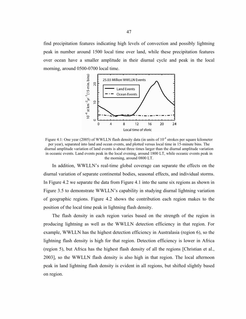
47
find precipitation features indicating high levels of convection and possibly lightning
peak in number around 1500 local time over land, while these precipitation features
over ocean have a smaller amplitude in their diurnal cycle and peak in the local
morning, around 0500-0700 local time.
Figure 4.1: One year (2005) of WWLLN flash density data (in units of 10-4 strokes per square kilometer per year), separated into land and ocean events, and plotted versus local time in 15-minute bins. The
diurnal amplitude variation of land events is about three times larger than the diurnal amplitude variation in oceanic events. Land events peak in the local evening, around 1800 LT, while oceanic events peak in
the morning, around 0800 LT.
In addition, WWLLN’s real-time global coverage can separate the effects on the
diurnal variation of separate continental bodies, seasonal effects, and individual storms.
In Figure 4.2 we separate the data from Figure 4.1 into the same six regions as shown in
Figure 3.5 to demonstrate WWLLN’s capability in studying diurnal lightning variation
of geographic regions. Figure 4.2 shows the contribution each region makes to the
position of the local time peak in lightning flash density.
The flash density in each region varies based on the strength of the region in
producing lightning as well as the WWLLN detection efficiency in that region. For
example, WWLLN has the highest detection efficiency in Australasia (region 6), so the
lightning flash density is high for that region. Detection efficiency is lower in Africa
(region 5), but Africa has the highest flash density of all the regions [Christian et al.,
2003], so the WWLLN flash density is also high in that region. The local afternoon
peak in land lightning flash density is evident in all regions, but shifted slightly based
on region.

48
Figure 4.2: The same year of WWLLN flash density data as shown in Figure 4.1, now separated into the six broad regions shown in Figure 3.5. a)-f) show data from regions 1-6, respectively. Similar diurnal
patterns are seen in each region. However, the land and ocean peak amplitudes do not occur at the same LT in each region. Poisson statistics define error bars on the order of the width of the line.
To better represent the relative positions of the peak, Figure 4.3 shows land lightning
data for all six regions on the same plot, normalized to the same peak amplitude. As the
peaks are fairly broad, the center of a full-width-half-max (FWHM) estimate is marked
at the top of Figure 4.3, with each adjusted peak labeled by region number. Land
lightning over Europe (region 2) peaks earliest, around 1500 local time, while land
lightning over North America (region 1) peaks latest, around 1900 LT. The time of peak
lightning flash density over North America is consistent with findings from 5-year and
10-year averaged NLDN data that indicate that, in areas of the U.S. with significant
diurnal variation, peak lightning flash rates occur between 1600 and 2000 LT [Zajac
and Rutledge, 2001; Orville and Huffines, 2001]. Both of these studies looked at
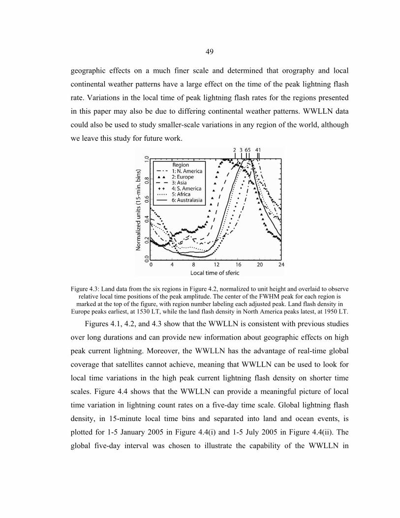
49
geographic effects on a much finer scale and determined that orography and local
continental weather patterns have a large effect on the time of the peak lightning flash
rate. Variations in the local time of peak lightning flash rates for the regions presented
in this paper may also be due to differing continental weather patterns. WWLLN data
could also be used to study smaller-scale variations in any region of the world, although
we leave this study for future work.
Figure 4.3: Land data from the six regions in Figure 4.2, normalized to unit height and overlaid to observe relative local time positions of the peak amplitude. The center of the FWHM peak for each region is
marked at the top of the figure, with region number labeling each adjusted peak. Land flash density in Europe peaks earliest, at 1530 LT, while the land flash density in North America peaks latest, at 1950 LT.
Figures 4.1, 4.2, and 4.3 show that the WWLLN is consistent with previous studies
over long durations and can provide new information about geographic effects on high
peak current lightning. Moreover, the WWLLN has the advantage of real-time global
coverage that satellites cannot achieve, meaning that WWLLN can be used to look for
local time variations in the high peak current lightning flash density on shorter time
scales. Figure 4.4 shows that the WWLLN can provide a meaningful picture of local
time variation in lightning count rates on a five-day time scale. Global lightning flash
density, in 15-minute local time bins and separated into land and ocean events, is
plotted for 1-5 January 2005 in Figure 4.4(i) and 1-5 July 2005 in Figure 4.4(ii). The
global five-day interval was chosen to illustrate the capability of the WWLLN in
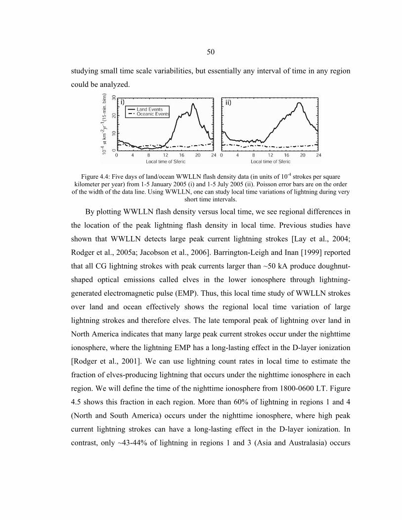
50
studying small time scale variabilities, but essentially any interval of time in any region
could be analyzed.
Figure 4.4: Five days of land/ocean WWLLN flash density data (in units of 10-4 strokes per square kilometer per year) from 1-5 January 2005 (i) and 1-5 July 2005 (ii). Poisson error bars are on the order
of the width of the data line. Using WWLLN, one can study local time variations of lightning during very short time intervals.
By plotting WWLLN flash density versus local time, we see regional differences in
the location of the peak lightning flash density in local time. Previous studies have
shown that WWLLN detects large peak current lightning strokes [Lay et al., 2004;
Rodger et al., 2005a; Jacobson et al., 2006]. Barrington-Leigh and Inan [1999] reported
that all CG lightning strokes with peak currents larger than ~50 kA produce doughnut-
shaped optical emissions called elves in the lower ionosphere through lightning-
generated electromagnetic pulse (EMP). Thus, this local time study of WWLLN strokes
over land and ocean effectively shows the regional local time variation of large
lightning strokes and therefore elves. The late temporal peak of lightning over land in
North America indicates that many large peak current strokes occur under the nighttime
ionosphere, where the lightning EMP has a long-lasting effect in the D-layer ionization
[Rodger et al., 2001]. We can use lightning count rates in local time to estimate the
fraction of elves-producing lightning that occurs under the nighttime ionosphere in each
region. We will define the time of the nighttime ionosphere from 1800-0600 LT. Figure
4.5 shows this fraction in each region. More than 60% of lightning in regions 1 and 4
(North and South America) occurs under the nighttime ionosphere, where high peak
current lightning strokes can have a long-lasting effect in the D-layer ionization. In
contrast, only ~43-44% of lightning in regions 1 and 3 (Asia and Australasia) occurs

51
under the nighttime ionosphere. This ~20% difference suggests high peak current
lightning in the Americas may input a more significant amount of energy into the
nighttime ionospheric D-region than would Asia and Australia.
Figure 4.5: Percentage of total lightning in nighttime (1800 – 0600 LT) in each region. More than 60% of lightning in regions 1 and 4 (North and South America) occurs under the nighttime ionosphere, where
strong lightning strokes can have a long-lasting effect in the D-layer ionization.
Local time studies of WWLLN lightning data show that peak flash density of
strong lightning varies for the different continents by up to five hours in local time. We
have suggested that WWLLN data can give an indication of the local time distributions
of effects from strong lightning strokes, such as elves, sprites, and electron density and
conductivity variability in the lower ionosphere. WWLLN is shown to have the ability
to address questions regarding land/ocean lightning differences in local time on any
time scale in any location on Earth. WWLLN data could be useful for researchers trying
to verify lightning count rates during short campaigns, or, as is commonly the case,
during a time when low-Earth orbiting optical lightning satellites are not viewing the
regional area of interest. In the next section, local time variations are analyzed at a
higher spatial resolution.
4.3 Events in local time: higher resolution
In addition to local time effects broken into land and ocean for the six large
geographic regions, these local time effects are analyzed with higher resolution. In this
case, the chosen resolution is 3.6º x 3.6º bins in latitude and longitude. This bin size is
useful because it covers a region about the same size as can be affected by the lightning
EMP (200-700 km diameter). The count rate has been scaled by the area of the bin to

52
reflect number of counts per square kilometer in each bin. The global detection
efficiency, as determined by using the regional networks and satellite comparisons
discussed in Chapter 3, was used to scale the WWLLN counts, in 1-hour bins. Figure
4.6 shows the total number of nighttime counts, on a log10 scale, for March 2006 -
February 2007.
In Figure 4.6, we see that the Central American region has a large amount of
nighttime lightning. Central America is also a region that has higher-than-average
numbers of detected elves and terrestrial gamma-ray flashes. This analysis shows that
possibly this region has large peak current lightning during the nighttime that could be
correlated to these increased numbers for energetic lightning effects.
4.4 Summary
This analysis has shown that WWLLN can be used to provide an idea of where and
when nighttime lightning is prevalent globally. Globally averaged, the data are
consistent with satellite measurements of diurnal variation in lightning activity. By
separating the WWLLN data into regions – an analysis that is difficult to do with
satellite data while still having enough lightning counts to make the results meaningful
– we find that more than 60% of lightning in the Americas occurs under the nighttime
ionosphere, while less than 40% of lightning in Europe occurs under the nighttime
ionosphere. Furthermore, using WWLLN data, we can map global variations of strong
nighttime lightning on a much finer spatial scale for different seasons. This information
could be useful to determine the timing of future rocket-based, balloon-based, or
ground-based campaigns to further study energetic effects of lightning above
thunderstorms and in the ionosphere.

53
Figure 4.6: Total number of nighttime counts/area for March 2006 – February 2007 on a log10 scale. Bin size is 3.6 x 3.6 degrees in latitude and longitude.

54
Chapter 5: Narrow Bipolar Events and Ionospheric Propagation
5.1 Motivation
As described in Chapter 3, many comparison studies between WWLLN and
ground-based regional networks and between WWLLN and FORTE satellite
measurements indicated that WWLLN is able to detect in-cloud (IC) lightning. In fact,
Jacobson et al. [2006] found that WWLLN detected 4% of lightning with peak current
greater than ~40 kA regardless of lightning type. The LASA data in that particular study
included more than 50% IC strokes, indicating that WWLLN could detect high-peak
current IC lightning.
5.1.1 FORTE RF/WWLLN Comparison
In a similar study to that presented in Section 3.3, we have compared WWLLN
lightning to lightning detected by the FORTE radio frequency (RF) (3 – 85 MHz)
instrument from which one can better understand the type of causative lightning stroke.
Unfortunately, the RF instrument stopped working in June of 2003, so the overlapping
data set with WWLLN occurs when WWLLN is in its test phase, with receivers only
covering Australasia (longitude 60E to 180 E, latitude 40S to 40 N). However, there
were about 35,000 FORTE RF events in this region from June 2002 – June 2003 with
1760 coincident WWLLN events. From these coincidences we were able to determine
likely lightning types for the coincident WWLLN strokes. A visual inspection of many
coincident waveforms revealed that about 10% of the coincident events were IC
lightning. Figure 5.1 shows an example of an RF waveform as detected by FORTE that
was coincident to a WWLLN event.
Given that narrow bipolar events are thought to make up this category of strong
pulse pairs [Smith et al., 1999], this would indicate that WWLLN is able to detect
NBEs. A more quantitative comparison made use of predefined criteria on waveform
timing, the SNR of the autocorrelation function, total energy and median energy in

55
order to automatically classify FORTE RF events. This quantitative comparison found
that in this region, WWLLN detected coincident events with 5% of the total FORTE RF
events, and with 6.9% of FORTE “strong pulse pairs” which are correlated with NBEs.
These results suggest that WWLLN preferentially detects NBEs compared to other
events detected by the FORTE RF instrument.
Figure 5.1: Spectrogram of an example of strong IC lightning. The first pulse represents the radio waves that travel directly from the cloud to the satellite, while the second pulse represents the radio waves that
bounce off the ground before being detected at the satellite.
5.1.2 Narrow Bipolar Events Hypothesis
Based on these findings, we hypothesize that the IC lightning detected by WWLLN
mainly consists of Narrow Bipolar Events (NBEs), which are very energetic, extremely
short (tens of µs) IC lightning strokes (described in more detail in Section 1.2).
We investigate this issue further by completing another WWLLN/LASA
comparison, similar to that of Jacobson et al. [2006]. However, this time waveforms of
the coincident IC-classified events were analyzed in addition to simply using the
automatic LASA classification to determine what types of lightning are seen by
WWLLN. This investigation will be discussed in Section 5.2.

56
5.2 Narrow Bipolar Events: WWLLN/LASA coincidence study
5.2.1 Method
This study searched for WWLLN events coincident within 2 ms and 200 km of a
LASA event with an archived NBE/Fast Pulse (FP)-classified waveform. The NBE
classification is done via an automatic procedure based on the relationship between the
signal-to-noise ratio and the rise-plus-fall time of the initial pulse. The FP classification
includes events that are very narrow temporally, but do not have such high signal-to-
noise ratios as NBEs. Both NBEs and FPs are then classified as in-cloud, since it is
assumed that cloud-to-ground processes cannot occur on this time scale [Smith et al.,
2002]. The full NBE/FP waveforms have been archived for 49 days in 2006: May 02-
08, 10, 13-18, 20-30; June 01, 07-22, 30; and July 01-07. Only at LASA events detected
by the Great Plains Network, covering the region 107.3 W to 95.3 W and 43.3 N to 31.3
N, were included in this study.
5.2.2 Results
Twenty-two WWLLN events were coincident with a LASA event using this
criteria. This small number of coincidences was surprising when compared with the
large number of FORTE RF coincidences. While this is still not well understood, this
small number of coincidences could stem from many sources. The location and time of
the two comparisons differ. It could be that WWLLN does not detect NBEs as
efficiently in the U.S. Great Plains as in Australasia, or it could be that NBEs comprise
a smaller percentage of total lightning events in the Great Plains region. Upon
examination of the waveforms of these events, we find that 3 are unambiguously NBEs.
The three coincident WWLLN/LASA NBE events all occur on the same day, 26 May
2006, and are detected by only the 5 nearest WWLLN stations: Seattle, Boston, Los
Alamos, Mexico City, and Puerto Rico. Figure 5.2 shows the full waveform as detected
by 5 LASA stations. Each panel shows a waveform detected by a different station,
along with the distance (range) between the lightning stroke and each station. The top

57
panel represents the closest station to the stroke and the bottom panel the farthest station
from the stroke. Because the stations are different distances from the lightning stroke,
the signal arrived at each with different time delays. The trigger time at each station is
represented at zero µs, and the x-axis label of each panel tells how large of a time delay
that trigger time is from the lightning stroke time. In the first three panels, one can see
the narrow-bipolar nature of the signal, with the initial rise above zero V/m, and then
fall to below zero V/m. In the first two panels, one can clearly see the two ionospheric
reflections of the signal: the first reflection reflects from the ionosphere and
Figure 5.2: Full NBE waveform as detected by 5 LASA stations. Each panel shows a waveform detected by a different station, along with the distance (range) between the lightning stroke and each station. The trigger time at each station is represented at zero µs, and the value of seconds of day (sod) below each
panel shows time delay between lightning stroke time and trigger time.

58
then reaches the detector; the second reflects off the ground, then the ionosphere and
then reaches the detector. In the bottom two panels, the ground pulse has decayed over
distance, so the detector triggers on the reflection pulses, which is why the narrow
bipolar nature is no longer evident.
In order to compare lightning strokes of different magnitudes, we normalize the
electric field of the sferic to a range of 100 km, using a radial amplitude attenuation
over distance of r -1 for LF radiation along a line of sight. For normalization, we choose
one of the waveforms of the same stroke detected at multiple stations based on the
largest signal-to-noise ratio, and with the requirement that the stroke be farther than 100
km from the receiver (to avoid electrostatic signatures). The waveform shown in the
first panel of Figure 5.2 is normalized in this manner in Figure 5.3. This waveform is
detected by the LNK station at a range of 274 km, and then normalized to 100 km.
Figure 5.3: Range-normalized electric field of a NBE sferic detected by the LNK station at a range of 274 km, and then normalized to 100 km, using 1/r amplitude attenuation.
From the range-normalized electric field, we find the power spectrum, to determine
how much power is radiated versus frequency, as WWLLN detects sferics in the 1 to 24
kHz range. Figure 5.4 shows the power spectrum of the sferic in Figure 5.3. We then
integrate power over frequency: first, we integrate over the entire frequency band to get
the total power in the waveform. Second, we integrate the power over only the VLF
band (1 to 24 kHz) to determine how much power is radiated in the WWLLN-detectable

59
range. In a typical NBE, about one third of the total power is emitted in the 1 to 24 kHz
range.
Figure 5.4: Power spectrum of the sferic in Figure 5.3.
We will next investigate the 19 coincident WWLLN/LASA events in the NBE/FP
category that have ambiguous waveforms. Figure 5.5 shows one of these waveforms, as
detected by 5 LASA stations. This waveform has a very fast rise time (~15 µs), typical
of a NBE but the lack of a clear ionospheric reflection of the pulse indicates that this
may be a cloud-to-ground stroke. Also, instead of being detected by only the 5 closest
WWLLN stations, as would be likely if the NBE had very little power in the VLF band,
these events often triggered WWLLN stations half way around the world. These two
pieces of evidence suggests that the automatic LASA classification of FPs as ICs may
be erroneously classifying strange CG events as IC lightning. Possibly many of
WWLLN events coincident with LASA “IC events” in the Jacobson et al. [2006] study
were of this type.

60
Figure 5.5: Full FP waveform as detected by 5 LASA stations. Each panel shows a waveform detected by a different station, along with the distance (range) between the lightning stroke and each station. The trigger time at each station is represented at zero µs, and the value of seconds of day (sod) below each
panel shows time delay between lightning stroke time and trigger time.
In order to better determine what about the WWLLN-detected NBEs makes them
detectable, those three NBEs are compared with the total 218 NBE/FP-classified events
that occurred on 26 May 2006. Figure 5.6 shows the ratio of VLF power to total power
along the horizontal axis versus total VLF power on the vertical axis. The coincident
NBEs are in red. One can see that many of the NBE/FPs have low VLF power, and the
coincident NBEs have a ratio of VLF power to total power around 0.3.

61
Figure 5.6: Ratio of VLF power to total power along the horizontal axis versus total VLF power on the vertical axis. The coincident NBEs are in red.
Figure 5.7: Same type of plot as Figure 5.6, but showing only the 22 coincident WWLLN/LASA sferics.
Figure 5.7 shows the same type of plot as Figure 5.6, but with only the 22
coincident WWLLN/LASA sferics. Here, we see that the VLF power ratio of the three
WWLLN-detected NBEs is on the very low end of coincident events, indicating that the
radiated VLF energy from these NBEs may be very close to the WWLLN-detection
threshold for strokes in the LASA-covered region. It is possible that only very powerful
NBEs located within a reasonable distance of 5 WWLLN stations have enough VLF
energy to trigger the required 5 WWLLN stations.
5.3 Conclusions
Based on comparisons with LASA ground-based waveforms and FORTE RF
satellite-based waveforms, the WWLLN network is able to detect NBEs if the NBE is

62
powerful enough to trigger 5 required stations. In the region covered by the LASA
Great Plains network (107.3 W to 95.3 W and 43.3 N to 31.3 N) the majority of NBEs
seem unable to trigger the required 5 stations. However, in the Austral-asia region in
2003, a large percentage of NBEs detected by the FORTE RF instrument were
coincident with WWLLN events, indicating that either NBEs radiate more energy from
Austral-asian storms, or similarly energetic NBEs are more likely to be detected by 5
WWLLN stations due to higher station density.
We also find that many of the LASA-classified FPs do not have waveforms that are
unequivocally IC lightning strokes. In fact, the majority of LASA FP/WWLLN
coincidences were detected by extremely distant WWLLN stations (up to halfway
around the world), a finding that is more consistent with CG lightning.

63
Chapter 6: Experimental evidence of energetic lightning effects on ionosphere and magnetosphere
6.1 WWLLN/ISUAL elves comparison
6.1.1 Motivation
The ISUAL instrument has been taking optical images and spectroscopy data on
elves globally since May of 2004. We were provided ISUAL elves data for October
2005 by Dr. Harald Frey of the Space Sciences Lab at UC Berkeley. In order to more
accurately determine the location and time of the elve-producing lightning, it is useful
to have ground-based measurements of lightning activity. WWLLN is particularly
useful in this case because it is the only network able to detect lightning globally, so it
could potentially enhance information of elve-producing strokes over oceans where
there is no other lightning coverage. It has been found that detected elves are more often
seen over water, so this oceanic coverage is particularly important if the majority of
elves occur over water, and if one intends to determine the difference between elve-
producing conditions and non-elve producing conditions. WWLLN data also is able to
provide better location and timing information on ISUAL-detected elves that occur in
regions without coverage from any other lightning detection network.
6.1.2 Method
We look for ISUAL elve/WWLLN lightning coincidences occurring during
October 2005 by using the following criteria: Time-difference between WWLLN
lightning stroke and elve detected by ISUAL, corrected for the time of flight from the
WWLLN location to the satellite, must be less than or equal to 200 ms and the distance
difference between WWLLN location and ISUAL-estimated elve location must be less
than 1500 km. Because the satellite observes elves from 1000 to 4000 km away, the
magnitude of the timing error introduced by considering time of flight from the
WWLLN location (on the ground) to satellite instead of from 90 km above the ground-

64
based WWLLN location (elves altitude) is a maximum of 10 µs. We plot the time
difference histogram of coincidences meeting these two criteria in Figure 6.1, and from
this plot we further reduce the coincident data set to contain the closest matches (time
differences between -5 and 15 ms). A zoomed-in version of the close coincidences is
shown in Figure 6.3.
Figure 6.1: Time difference histogram of all coincident WWLLN lightning/ISUAL elves. Positive values indicate that the elve occurred after WWLLN stroke time. The background level for negative time
differences is higher than for positive, meaning that WWLLN often detects a subsequent stroke from the elve-causative stroke, but never an earlier stroke than the elve-producing stroke.
6.1.3 Results
We find that 29 of 159 elves have one or more coincident WWLLN events within
200 ms and 1500 km (18.2%). Of those 29 elves, 13.8% of the total, or 22 elves, are in
the closely coincident subset (time differences between 5 and 20 ms). The locations of
all elves detected by ISUAL in October 2005 (blue dots) along with the WWLLN
locations (green stars) and ISUAL locations (red dots) of the closely coincident events
are plotted in Figure 6.2. Close coincidences are found in all regions, meaning that
WWLLN seems to be able to detect elve-producing strokes fairly uniformly over the
world.
Next, we study the information from the comparison in timing differences between
WWLLN lightning strokes and ISUAL-detected elves. As can be seen from Figure 6.1,
the background level of coincidences on the left side of the peak (negative time
differences) is higher than on the right side, meaning that WWLLN often detects a
subsequent stroke from the elve-causative stroke, but never an earlier stroke than the

65
elve-producing stroke. An interpretation of this result is that elves are most often caused
by the first stroke in the flash.
Figure 6.2: Locations of all ISUAL-detected elves (blue dots), locations of elves closely coincident to a
WWLLN stroke (red dots), and locations of WWLLN lightning locations (green stars) closely coincident with an ISUAL detected elve. Coincidences are found in all regions, meaning that WWLLN seems to be
able to detect elve-producing strokes fairly uniformly over the world.
Figure 6.3 shows a zoomed-in view of the histogram in Figure 6.1 to look at only
the close coincidences with time differences between -5 and +15 ms. For these close
coincidences the WWLLN stroke precedes the elve by 4.8 ± 3.4 ms, where 3.4 ms is the
standard deviation. This indicates that ISUAL timing may be late by ~3.5 ms in order
for the timing to be consistent with electromagnetic theories of elves (speed-of-light
propagation of the EMP would result in an elve 1 to 2 ms after the lightning stroke).
Figure 6.3: Time difference between ISUAL elve and WWLLN stroke. Only closely coincident events are included in this histogram. These coincidences indicate that typically the stroke precedes the elve by
4.8 ± 3.4 ms, indicating that ISUAL timing may be late by ~3.5 ms in order for the timing to be consistent with electromagnetic theories of elves.

66
ISUAL data analysis provides an estimate of the latitude and longitude of the
detected elves. Next, we analyze that location estimate by using the location of the
closely coincident WWLLN events as “ground truth”. As discussed above, previous
studies have shown WWLLN location accuracy to be ~15 km [Jacobson et al., 2006,
Rodger et al., 2005a]. To provide this error analysis of ISUAL-estimated locations, we
look at the distance separation between the WWLLN location and the ISUAL-estimated
elve location for the closely coincident events. Figure 6.4 shows that the majority of
close coincidences have a distance separation of less than 400 km even though the
imposed criteria for a coincidence allowed a distance separation of 1500 km.
Figure 6.4: Distance separation (km) between WWLLN location and ISUAL estimated location. Even with a 1500 km distance limit, the majority of coincidences have a separation of less than 400 km.
Figure 6.5: Latitude and longitude differences between WWLLN locations and ISUAL estimated locations shows a consistent skew. ISUAL typically estimates a location that is too far west and too far
south. Error is 2.1 ± 3.0 in longitude degrees and 0.45 ± 0.61 in latitude.
As shown in Figure 6.5, latitude and longitude differences between WWLLN
locations and ISUAL estimated locations shows a consistent skew to the estimated
ISUAL location. The ISUAL processing algorithm systematically estimates a location

67
that is too far west and south. The error in latitude and longitude is 0.45 with a standard
deviation of 0.61 in latitude and 2.1 with a standard deviation of 3.0 in longitude
degrees. We look at these same data in a slightly different manner in Figure 6.6, in
which we plot the distance between the ISUAL sub-satellite point and the WWLLN
location versus distance between ISUAL-estimated elve location and WWLLN location.
As shown in Figure 6.6, the error in the ISUAL estimated elve location begins
increasing rapidly at a sub-satellite distance of more than 3100 km from the WWLLN
stroke.
Figure 6.6: Distance between ISUAL sub-satellite point and WWLLN location is plotted versus distance between ISUAL-estimated elve location and WWLLN location. Error in ISUAL-estimated elve location
begins increasing rapidly at a sub-satellite distance of more than 3100 km from WWLLN stroke.
Next, we investigate possibilities for the increased error at distances of greater than
3100 km in Figure 6.6 by looking more closely at the coincident event with the greatest
location error (~1200 km). Figure 6.7 represents the spatial configuration of the ISUAL
sub-satellite point (red diamond), ISUAL-estimated elve location (blue diamond), and
WWLLN location (blue asterisk) for that particular coincident event. The estimated elve
location is between the sub-satellite point and the WWLLN location. In this case, an
elve that is estimated to have occurred over land, may have actually occurred over the
ocean.
We look further into the systematic error made evident by Figure 6.5 by studying
the spatial configurations of 4 more coincident events (plotted in Figure 6.8). The
symbols are the same as in Figure 6.7. We find that ISUAL data processing consistently
estimates the elve to be closer to the satellite than it actually is. A hypothesis as to the

68
cause of this systematic error is that the elves actually occur over the visible horizon
(~3100 from the spacecraft), and yet the processing algorithm assumes they must be
closer than the horizon. If the data is reprocessed allowing the possibility of the elve to
occur over the horizon, then a much closer estimate to the WWLLN location results.
Reprocessing the event with a 1200 km location error makes the distance error less than
400 km.
Figure 6.7: The spatial configuration of ISUAL sub-satellite point (diamond), estimated ISUAL elve location (triangle), and WWLLN location (circle) for the coincident elve event (at 4:44:34.646 UT on 1 October 2005) with distance error of ~1200 km. In this case, an elve that is estimated to have occurred
over land, may have actually occurred over the ocean
Figure 6.8: More relative locations of satellite (diamonds), elve location estimate (triangles), WWLLN location (circles). It seems that ISUAL estimates the elve to be closer to the satellite than it actually is.
The uppermost event is the same as that in Figure 6.7.
Finally, we look at a few case studies of elves with all local WWLLN lightning are
also shown (as opposed to only coincident elves/WWLLN events). Figure 6.9 shows
results from the first case study, on 27 October 2005. Elves detected in the region are
shown as asterisks. Green triangles represent elves that are coincident with a WWLLN
stroke. Red triangles are elves without a coincident WWLLN event. Blue dots represent
all WWLLN lightning occurring in this region between 2 hours before the first detected
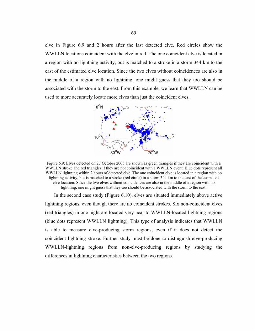
69
elve in Figure 6.9 and 2 hours after the last detected elve. Red circles show the
WWLLN locations coincident with the elve in red. The one coincident elve is located in
a region with no lightning activity, but is matched to a stroke in a storm 344 km to the
east of the estimated elve location. Since the two elves without coincidences are also in
the middle of a region with no lightning, one might guess that they too should be
associated with the storm to the east. From this example, we learn that WWLLN can be
used to more accurately locate more elves than just the coincident elves.
Figure 6.9: Elves detected on 27 October 2005 are shown as green triangles if they are coincident with a WWLLN stroke and red triangles if they are not coincident with a WWLLN event. Blue dots represent all WWLLN lightning within 2 hours of detected elve. The one coincident elve is located in a region with no
lightning activity, but is matched to a stroke (red circle) in a storm 344 km to the east of the estimated elve location. Since the two elves without coincidences are also in the middle of a region with no
lightning, one might guess that they too should be associated with the storm to the east.
In the second case study (Figure 6.10), elves are situated immediately above active
lightning regions, even though there are no coincident strokes. Six non-coincident elves
(red triangles) in one night are located very near to WWLLN-located lightning regions
(blue dots represent WWLLN lightning). This type of analysis indicates that WWLLN
is able to measure elve-producing storm regions, even if it does not detect the
coincident lightning stroke. Further study must be done to distinguish elve-producing
WWLLN-lightning regions from non-elve-producing regions by studying the
differences in lightning characteristics between the two regions.

70
Figure 6.10: Six non-coincident elves (red triangles) in one night (9 October 2005) are located very near to WWLLN-located lightning (blue dots). This type of analysis indicates that WWLLN is able to measure
elve-producing storm regions, even if it does not detect the coincident lightning stroke.
6.1.4 Discussion
From the comparison of WWLLN lightning events to ISUAL-detected elves during
October 2005, we find close coincidences globally, meaning that WWLLN seems to be
able to detect elve-producing strokes fairly uniformly over the world (Figure 6.2).
Secondly, we find that WWLLN often sees subsequent strokes from the same lightning
flash (Figure 6.1) but not previous strokes. An interpretation of this result is that elves
are most often caused by the first stroke in the flash. The comparison has also shown
that it is possible to use WWLLN data to more accurately locate ISUAL-detected elves.
This could be useful for determining the relative frequencies of elves over land versus
over water by more accurately locating the elves over land or water. Finally, we find
that WWLLN is able to measure elve-producing storm regions, even if it does not detect
the coincident lightning stroke (Figure 6.10). Further study should be done to try to
distinguish elve-producing WWLLN-lightning regions from non-elve-producing
regions. In particular, the energy-calibrated WWLLN may help in this endeavor, to
determine the strength of lightning strokes in given storms as well as how much energy
is input in the lower ionosphere from elve-producing strokes.

71
6.2 WWLLN/RHESSI TGF comparison
6.2.1 Motivation
RHESSI-detected terrestrial gamma-ray flashes are similar to ISUAL-detected
elves in that they are also energetic events associated with lightning and detected by a
satellite. Similarly, WWLLN will be useful to provide information on TGFs on a global
scale because it has global lightning coverage. In the TGF case, we use WWLLN
locations to determine possibilities for the beaming of gamma-ray energy. We also use
WWLLN data to help determine the magnitude of lightning possibly associated with
TGFs.
6.2.2 Method
The method of comparison for WWLLN lightning and RHESSI-detected
Terrestrial Gamma-Ray Flashes (TGFs) is similar to that of the WWLLN/ISUAL
comparison. We look for RHESSI TGF/WWLLN lightning coincidences occurring
between June 2002 and October 2006 by using the following criteria: Time-difference
between WWLLN lightning stroke and RHESSI-detected TGF, corrected for the time of
flight from the WWLLN location to the satellite, must be less than or equal to 200 ms
and the distance difference between WWLLN location and RHESSI-estimated TGF
location must be less than 1500 km. We plot the time difference histogram of
coincidences meeting these two criteria in Figure 6.11, and from this plot we further
reduce the coincident data set to contain the closest matches (time differences between
–3.0 and 5.0 ms). Again, the time of flight between the source and satellite was taken
into account for all time differences.
6.2.3 Results
Of the 713 TGFs detected by RHESSI during this time period, 64 have one or more
coincidences with WWLLN events within 200 ms and 1500 km (9.0%). Using the
criteria for closely coincident events, we find that 31 of those 64 TGF/ WWLLN
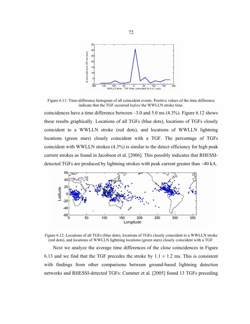
72
Figure 6.11: Time-difference histogram of all coincident events. Positive values of the time difference indicate that the TGF occurred before the WWLLN stroke time.
coincidences have a time difference between –3.0 and 5.0 ms (4.3%). Figure 6.12 shows
these results graphically. Locations of all TGFs (blue dots), locations of TGFs closely
coincident to a WWLLN stroke (red dots), and locations of WWLLN lightning
locations (green stars) closely coincident with a TGF. The percentage of TGFs
coincident with WWLLN strokes (4.3%) is similar to the detect efficiency for high peak
current strokes as found in Jacobson et al. [2006]. This possibly indicates that RHESSI-
detected TGFs are produced by lightning strokes with peak current greater than ~40 kA.
Figure 6.12: Locations of all TGFs (blue dots), locations of TGFs closely coincident to a WWLLN stroke
(red dots), and locations of WWLLN lightning locations (green stars) closely coincident with a TGF.
Next we analyze the average time differences of the close coincidences in Figure
6.13 and we find that the TGF precedes the stroke by 1.1 ± 1.2 ms. This is consistent
with findings from other comparisons between ground-based lightning detection
networks and RHESSI-detected TGFs: Cummer et al. [2005] found 13 TGFs preceding

73
strokes detected by the Duke University electric field sensor by 1.24 ± 0.97 ms, and
Stanley et al. [2006] found 5 TGFs preceding LASA-detected lightning by 1.8 to 5.1
ms.
Figure 6.13: Time difference between TGF time and WWLLN stroke time, corrected for the time of flight to the satellite. Only closely coincident TGFs are included in this histogram. These coincidences indicate
that typically the TGF precedes the stroke by 1.1 ± 1.2 ms. Next we study the distance separation between coincident lightning and the
RHESSI sub-satellite point in order to address the question of whether TGF energy is
tightly beamed or not. The majority of close coincidences have a separation between
WWLLN location and RHESSI sub-satellite point of less than 400 km (Figure 6.14).
The mean separation is 373 km, with standard deviation of 169 km. However, the
maximum distance separation is ~700 km, giving the first indication that TGF-energy
may not be tightly beamed from the source.
Figure 6.14: Distance between WWLLN location and RHESSI sub-satellite point. Even with a 1500 km
distance limit, the majority of close coincidences have a separation of less than 400 km. The mean separation is 373 km, with standard deviation of 169 km.

74
6.2.4 Summary
In this comparison, we find close coincidences in all global regions, meaning that
WWLLN seems to be able to detect TGF-producing strokes fairly uniformly over the
world (Figure 6.12). The percentage of TGFs coincident with WWLLN strokes (4.3%)
is similar to the detection efficiency for high peak current strokes as found in Jacobson
et al. [2006]. This finding indicates that RHESSI-detected TGFs are possibly produced
by lightning strokes with peak current greater than ~40 kA. In the comparison of time
differences between TGFs and WWLLN strokes, we find that WWLLN sees fewer
preceding strokes than subsequent strokes from the TGF-coincident lightning stroke
(Figure 6.11). A possible interpretation of this result is that TGFs are most often caused
by the first stroke in the flash, but not always. A study of the distances between the
RHESSI sub-satellite point and WWLLN location gives no evidence for a small
beaming angle of the TGF energy as the separation could be greater than 700 km.
Similarly to the investigation of elves, a calibrated stroke energy estimate from
WWLLN would also enhance the knowledge of how strong a stroke must be to produce
a TGF, as well as how much energy is input to the magnetosphere from TGFs globally.

75
Chapter 7: Lightning stroke radiated VLF energy
7.1 Motivation to provide stroke energy
The WWLLN has been providing accurate lightning locations and times globally
for the past five years. An important next step in its development is to implement an
algorithm that estimates stroke-radiated energy along with its location and time. No
other network or satellite has the capability to monitor the strength of lightning strokes
globally, and this additional capability would enhance the possibilities for a variety of
studies in lightning science. Most notably it would provide useful data for a study of
how lightning energy can affect lower-ionospheric electron density and conductivity on
a global scale. Using radiated energy estimates, we could determine when in local time
and where on Earth the strongest lightning occurs. Also, knowing which storms contain
the strongest lightning strokes would help in determining which storms globally are
most likely to affect conductivity in the lower ionosphere. Also, this information would
be useful in order to correlate elves detected by ISUAL and TGFs detected by RHESSI
with lightning strokes world-wide with known stroke energy. This comparison may help
determine the conditions necessary for elves and TGFs as well as predictions for
regions most likely to be affected by these phenomena. The steps taken to determine the
stroke energy are explained in this chapter.
7.2 Absolute Calibration
The radiated energy of a vertical cloud-to-ground lightning stroke propagates
outward from the lightning stroke, mainly confined in the Earth-Ionosphere waveguide
(EIWG). A given WWLLN station measures the uncalibrated, integrated energy flux at
the station location as described in Section 2.3. As a reminder, this quantity has been
defined as
( ) tcE'
0
2
∆= ∑samples
Yµ
, (7.1)

76
where E’ is the uncalibrated electric field as shown on the y-axis of Figure 2.3, c is the
speed of light, µ0 = 4π*10-7 W/(A*m), and ∆t=1/(sampling frequency). In order to
know the calibrated electric field in units of V/m, E, we must determine the conversion
factor, An, to convert computer sound card units to V/m for each station n. This
conversion factor is influenced by two variables. The first variable is the system gain
that depends on antenna configuration, preamplifier gain, service unit gain, and sound
card gain. The system gain could potentially be calculated by subjecting each station to
similar calibration procedures. The second variability results from different electrical
effects due to site geometry (i.e. location of the antenna on building roof relative to
other buildings, the quality of the ground plane to which it is connected). The electrical
environment variability may be much more difficult to determine than the system gain.
If station conversion factors are determined, we may define the absolute electric
field as detected at station n as nAE'E = . The calibrated integrated energy flux at a
given station is:
( ) 2
n0
2n
0
22 At
cE'At
cE)/( YmenergyW
samplessamples
=∆=∆= ∑∑ µµ. (7.2)
Here we have assumed that B=E/c in the far field of the radiated lightning energy,
where B is the magnetic field of the sferic. Therefore, in order to calculate W in
calibrated units, we must determine the conversion factor, An. We could then estimate
the total energy radiated at the stroke location by the following formula:
( )( )rhW απρε exp2= , (7.3)
where ρ is the radius of a small circle on the Earth with the lightning stroke at its center
and the WWLLN receiving station on the circle, r is the great-circle stroke-to-receiver
distance, h is the height of the ionosphere, W is the time-integrated energy flux at the
receiver, and α is the attenuation of the stroke. Therefore, in order to calculate the
energy radiated at the location of the stroke, we must know r, h, W, and α. The
WWLLN location algorithm determines r to within 20 km, as described in Chapter 3.
The height of the ionosphere, h, is estimated to be ~75 km in the daytime and ~85 km at
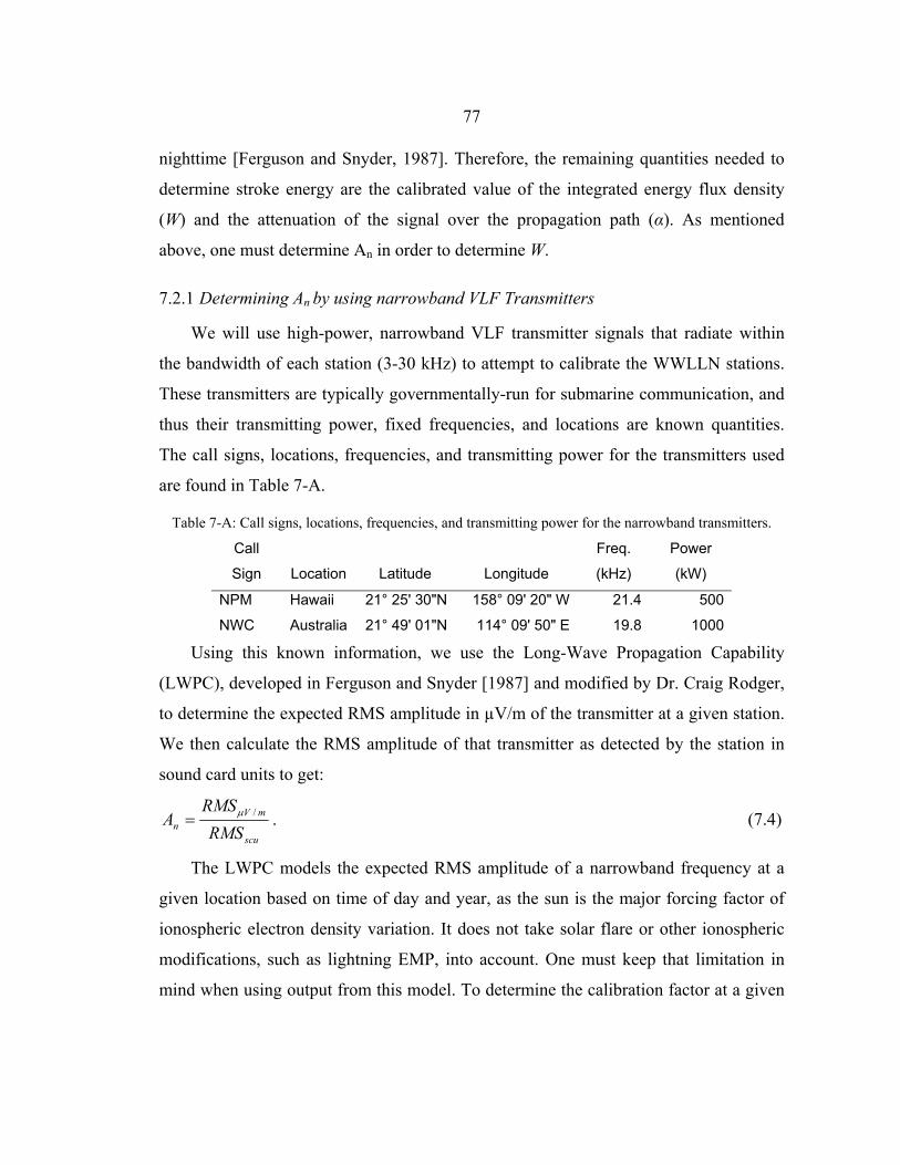
77
nighttime [Ferguson and Snyder, 1987]. Therefore, the remaining quantities needed to
determine stroke energy are the calibrated value of the integrated energy flux density
(W) and the attenuation of the signal over the propagation path (α). As mentioned
above, one must determine An in order to determine W.
7.2.1 Determining An by using narrowband VLF Transmitters
We will use high-power, narrowband VLF transmitter signals that radiate within
the bandwidth of each station (3-30 kHz) to attempt to calibrate the WWLLN stations.
These transmitters are typically governmentally-run for submarine communication, and
thus their transmitting power, fixed frequencies, and locations are known quantities.
The call signs, locations, frequencies, and transmitting power for the transmitters used
are found in Table 7-A.
Table 7-A: Call signs, locations, frequencies, and transmitting power for the narrowband transmitters.
Call
Sign Location Latitude Longitude
Freq.
(kHz)
Power
(kW)
NPM Hawaii 21° 25' 30"N 158° 09' 20" W 21.4 500
NWC Australia 21° 49' 01"N 114° 09' 50" E 19.8 1000
Using this known information, we use the Long-Wave Propagation Capability
(LWPC), developed in Ferguson and Snyder [1987] and modified by Dr. Craig Rodger,
to determine the expected RMS amplitude in µV/m of the transmitter at a given station.
We then calculate the RMS amplitude of that transmitter as detected by the station in
sound card units to get:
scu
mVn RMS
RMSA /µ= . (7.4)
The LWPC models the expected RMS amplitude of a narrowband frequency at a
given location based on time of day and year, as the sun is the major forcing factor of
ionospheric electron density variation. It does not take solar flare or other ionospheric
modifications, such as lightning EMP, into account. One must keep that limitation in
mind when using output from this model. To determine the calibration factor at a given

78
frequency, we use the estimated RMS amplitude in µV/m predicted by the LWPC for a
given WWLLN station/VLF transmitter pair, and compare that value to the actual
detected amplitude of that frequency band at the WWLLN station in computer sound
card units (scu). The LWPC-predicted signal strength of the NPM transmitter at the
Dunedin station is 422 µV/m and 1245 µV/m from the NWC transmitter.
Next, we find the measured amplitude in sound card units of these narrowband
transmitters as detected by the Dunedin WWLLN station. To determine this amplitude,
15-second waveforms recorded at local noon in Dunedin for the period of 15 January
2007 to 8 March 2007 are analyzed. From each of these waveforms, we find the average
RMS value of the signal in a ± 1 kHz band surrounding the center frequency of the
NWC and NPM VLF transmitters. A 4th order Butterworth bandpass filter with 3dB
point at the transmitter frequency ± 1 kHz is used to determine the amplitude of each
transmitter as measured in sound card units.
Figure 7.1 shows the average value of the amplitude of the NWC and NPM
transmitters as detected at the Dunedin station in sound card units over time. The
sporadic dropouts in amplitude occur when the transmitter was turned off. The error in
the 15 second measurement is on the order of the size of the data points in Figure 7.1.
Therefore, before 1 March 2007, the main source of variation in the RMSscu amplitude
is the daily variation on the order of 6% for NWC and 5% for NPM. A day-to-day
variation of this magnitude is excellent for a VLF electric field antenna in the middle of
a high noise area; McRae and Thomson [2000] reports a minimum variation of 0.5 to 1
dB in magnetic field amplitude as measured in a quiet location using a loop antenna.
This variation is most likely caused by error in the measurement techniques in addition
to ionospheric variability of 0.1 to 0.3 dB not taken into account in the LWPC model,
such as solar flares and strong lightning strokes. The variation of 5-6% in RMSscu
amplitude will limit the accuracy to which we can know An.
After 1 March 2007, the amplitude of both transmitters changes dramatically. This
change continues for months after 8 March 2007 and could have occurred due to a

79
change in the grounding of the instrument. In fact, the preamplifier in Dunedin was
recently replaced due to weathering and water damage of the electronics. This damage
could have caused the change in gain of the instrument. The possibility of a sudden gain
change such as shown in Figure 7.1 indicates that the conversion factor should be
monitored on a daily or weekly basis at each station.
Figure 7.1: Average value of amplitude of NWC (dots) and NPM (plusses) transmitters as detected at the Dunedin station in scu over time. The daily variation in RMS amplitude is less than 6% before 1 March
2007. After 1 March 2007, the amplitude of both transmitters changes dramatically. This could be a problem with the grounding of the instrument. The semi-regular drop-outs in amplitude are due to the
transmitter being turned off.
From these data, to get scu
mVn RMS
RMSA /µ= , we must divide the amplitude predicted by the
LWPC code by the RMSscu amplitude detected at the station. The values for An over this
period of time are shown in Figure 7.2.
Figure 7.2: Values of ADunedin over time. The conversion factors track each other well over time, adding reliability to the measurement.
80
The average conversion factor for 15 January to 1 March 2007, as determined by the
NWC transmitter when it is turned on, is 1.94 ± 0.13 m/Vµ /scu. As determined by
NPM, the average conversion factor is 1.81 ± 0.10 m/Vµ /scu. However, this
conversion factor holds for the narrowband frequency of the transmitter. The next
section describes the process to determine the conversion factor at 13 kHz from the
conversion factors at the narrowband transmitter frequencies. We find the conversion
factor at 13 kHz to determine the amplitude of the sferic, which covers the frequency
range of 1 to 24 kHz. Thirteen kHz is chosen as it is the middle of the band of
maximum sferic amplitude of 10-16 kHz [Dowden et al., 2002]. For that same reason, it
is also the frequency for which the approximate group velocity of the sferic is used in
the downhill-simplex lightning location algorithm, as is mentioned in Section 2.3.
7.2.2 Frequency response
Once we have determined this conversion factor at certain frequencies, we must
take into account the frequency response of the WWLLN station in order to determine
the conversion factor at 13 kHz. To determine if all antennas behave similarly, we have
taken a frequency spectrum at the WWLLN station in Dunedin, New Zealand; the
network WWLLN station in Seattle, Washington; and a test station on the roof of
another building on the University of Washington campus. The Dunedin and Seattle
network stations have the same VLF antenna design (wire wrapped tightly around a
pole of ~1 inch diameter) but different environments. The test station antenna in Seattle
has a newer design that was implemented in many of the more recently-installed
WWLLN stations (2 wires, crossed at the top of the antenna, splayed out inside of a 2 to
4 inch diameter tube, and connected at the bottom of the antenna). The frequency-
response study of all 3 stations was completed to determine whether the frequency
response from one station could be used on all stations.
To measure these frequency spectra, we cover the antenna with a metal sleeve to
shield out external electric fields. We then drive the metal sleeve with a frequency-

81
ramping signal generator from 1-30 kHz. The electric field capacitively couples to the
antenna, similar to the way a sferic couples to the antenna. An example spectrogram
from this procedure is shown in Figure 7.3, with frequency in kHz on the vertical axis,
time in seconds on the horizontal axis, and intensity of the signal in dB represented by
color.
Figure 7.3: Example spectrogram of frequency calibration procedure. Vertical axis is frequency (kHz), horizontal axis is time (seconds), and color bar shows intensity of the signal (dB).
The frequency response curves for the three stations tested are shown in Figure 7.4.
Dunedin has a fairly linear increase in sensitivity until about 22 kHz, and then a rapid
fall-off. Seattle sensitivity peaks around 13 kHz, and then falls off rapidly, most
probably due to the notch filter at 24.7 kHz.
Figure 7.4: Frequency response of 3 WWLLN stations: Dunedin (dashed), Seattle (solid), and Seattle test station (dotted).
The frequency response of the preamplifier only and the computer sound card only
from the test station, and then the response of the preamplifier and sound card together

82
are shown in Figure 7.5. The response of the Seattle test station is remarkably similar to
the convolution of the two, meaning that the frequency response of the antenna in its
surrounding environment is relatively flat.
Figure 7.5: Frequency response of preamplifier only (solid line), sound card only (plusses) and preamp and sound card together (dots).
Figure 7.4 shows that the two other stations have a differently shaped response. The
Seattle station has a narrowband filter to remove the aliased signal from the NLK
transmitter at 24.7 kHz, which transmits from less than 100 miles away. As one can see,
each station is dramatically different in frequency response, indicating that we will not
be able to generalize frequency response curves to all stations. Because each station
host puts up their own VLF antenna in the best possible location in their environment
and provides their own computer, the differences in frequency response could arise
from different antenna designs at the different stations, different electrical environments
(nearby buildings, etc.), or different sound card responses. It is possible that by
measuring the preamplifier response and sound card response of each station, along
with the frequency response of any filters included in that station, we may be able to
provide a fairly good approximation to the frequency response to each station.
However, access to many of the already-installed stations is difficult, so it will be
difficult to measure these quantities. It would also be difficult to compare the
preamplifier/sound card convolved response to actual response for more cases by
repeating the calibration procedure described above. For this reason, another method by
which to determine stroke energy is developed and analyzed. This method is explained
in the following section.

83
From the frequency response curve of the Dunedin station, we find that the
conversion factor at 19.8 kHz must be multiplied by 1.61 to get 3.13 ± 0.21 m/Vµ /scu
at 13 kHz from NWC and 2.99 ± 0.16 m/Vµ /scu from NPM, which are in agreement
with one another. For lightning strokes detected by the Dunedin station during this time
period, we could use these conversion factors to determine their energy flux density in
absolute units. The process by which we determine the amount of radiated energy
produced by these strokes will be described in Section 7.3.
7.2.3 Summary and suggestions for the future
Results from the frequency response analysis and the narrowband transmitter
analysis are as follows: The daily ionospheric variation affects the narrowband signals
as measured at WWLLN stations by as much as 6%. Stations can suddenly change in
gain based on grounding factors (i.e. Dunedin). These two findings indicate that
transmitter amplitudes and calibration factors should be monitored on a frequent basis.
Also, the frequency response of each station needs to be monitored. We cannot simply
use the frequency response curve found at one station to calibrate all the rest. It is
possible that, by determining the frequency response of each station’s preamplifier and
sound card, we could produce a useable estimate of station frequency response.
However, this may not be true if environmental factors affect the antenna frequency
response. Testing all stations by shielding out the external field with a metal sleeve and
driving the antenna with known frequencies is not feasible.
Two improvements to the network are suggested as solutions to these problems.
One is to measure transmitter amplitude at each station on a regular basis (1-2 times per
day) this will allow us to take ionospheric variability into account in the calibration
factor, and it will provide an added benefit of making WWLLN a global ionospheric
monitoring network. Another suggestion is to develop a small, calibrated transmitter
that sweeps through frequencies and that can be run at each station to get a frequency
response for each station. That transmitter could also emit a frequency wave with a

84
given amplitude at a certain time each day to provide a second calibration point in
addition to the VLF transmitters. This calibration point would be useful in determining
the system gain for each VLF station, but ultimately may not be able to decrease the
error significantly in the calibration amplitude estimate due to the electrical
environment of the antenna.
7.3 Relative energy radiated as determined by a single station
While we work on implementing the above suggestions for an absolute calibration
of the stroke energy, this dissertation has addressed the question: “how big is one stroke
relative to another?” If stations are not calibrated relative to one another, then we can
still determine the relative energy radiated by strokes in a given storm as observed by a
single station.
We look again at Equation 7.3: ( )( ) ( )( )rhYArhW n απραπρε exp2exp2 2== . We do
not know An, but all energies measured by station n will be scaled by that same factor,
as well as by all other constants. Therefore, we can find a relative energy as determined
by that station: ( )( )rYrel αρε exp= . (7.5)
Here we have assumed that h, the ionospheric height, is a constant, which
reasonably can be assumed for a storm-to-station great circle path that does not cross
the terminator. For a conservative estimate, it is required that, for the daytime
ionosphere, the solar zenith angle of the stroke and the station be 70 degrees or less (0
degrees is solar noon, 90 degrees is sunset or sunrise). For the nighttime ionosphere, it
is required that the solar zenith angle be 120 degrees or greater (180 degrees is solar
midnight).
An example case study analyzes a conglomeration of storms off the west coast of
Central America on 1 July 2007. This study was limited to strokes detected by the Sao
Paulo WWLLN station between 3:00 UT and 7:30 UT. All stroke-to-receiver paths in
this study are under the nighttime ionosphere, as defined above. For each stroke, εrel was
determined as detected by the Sao Paulo station. That value is then divided by the

85
minimum value of εrel in this case study to produce a normalized value of stroke
magnitude, εrel,norm. Figure 7.6 shows a histogram of the 509 lightning strokes that are
included in the studied range, with εrel,norm represented along the x-axis, and number of
counts in each bin along the y-axis.
Figure 7.6: Histogram of the 509 lightning strokes in relative-energy case study. εrel,norm is along the x-axis, and number of counts in each bin along the y-axis. Mean value of εrel,norm is 6.6 ± 3.6.
The mean value of is εrel,norm is 6.6 with a standard deviation of 3.6. Figure 7.7 is a map
of the lightning strokes in this case study. Strokes with a normalized energy within one
standard deviation of the mean are plotted in red, strokes more than one sigma below
the mean are in blue, strokes more than one sigma above the mean are in green, and
strokes more than 2 sigma above the mean are in black. The sizes of the dots represent
the different magnitude ranges, although they are not to scale, relatively.
Figure 7.7: Map of lightning strokes in relative-energy case study. Strokes plotted have normalized energy within one σ of mean (red), more than one σ below mean (blue), more than one σ above mean
(green), and more than 2 σ above mean (black). Sizes of the dots represent the different magnitude ranges, although they are not to scale, relatively.

86
This section has described a possible method for determining relative magnitudes
of lightning strokes in a given storm region, a capability that could greatly enhance the
utility of the network in addressing a wide range of scientific questions. As is shown in
the following section, relative magnitudes determined separately from two stations
agree, in that both stations find the same smaller magnitude strokes and larger
magnitude strokes. The next step to verify this technique would be to compare relative
magnitudes as determined by WWLLN to peak currents or charge moments of lightning
located by a regional ground-based lightning detection network.
7.4 Relative Calibration
Section 7.3 demonstrates a method to determine relative normalized magnitudes of
WWLLN lightning strokes in a given storm by using data from a single station. Next,
the relative energies of a given storm detected by two different WWLLN stations are
used to try to determine the relative conversion factor An1/An2, where An1 is the
conversion factor for station n1 and An2 is the conversion factor for station n2. The
following analysis is performed on the same case-study storm as in Section 7.3, but here
we require that each stroke be detected by the Sao Paulo station and the Cordoba,
Argentina station. Since the absolute calibration factors, An1 and An2, for these two
stations (as discussed in Section 7.2) have not yet been resolved, the absolute energy of
each stroke cannot be determined, but only the relative energy (from Section 7.3).
For example, we take the relative energy estimate from Equation (7.5) and include
the calibration factor An. The energy estimate from the same stroke, as estimated by a
second station, should be the same, since it is the same lightning stroke. We then get the
following equation:
( )( ) ( )( )222
222112
111 expexp nnnnnnnnnn rAYrAY αραρε == (7.6)
The unknown variables in this equation are An1, An2 αn1, and αn2, and we hope to
determine a relative calibration factor, An1/An2, by assuming values for αn1, and αn2. For
the storm in the case study, the storm-to-receiver distance is comparable for the Sao

87
Paulo (~6,500 km) and Cordoba (~5,600 km) stations. Therefore, we assume that sferics
propagating on each path will undergo the same attenuation of 2dB/Mm under the
nighttime ionosphere [Wait, 1970]. Relative stroke energy estimates are shown in
Figure 7.8. In this case, the energy estimate using YSaoPaulo is plotted along the x-axis
and the estimate using YCordoba is plotted along the y-axis. One can see that for large
strokes, the slope increases, possibly indicating that the Sao Paulo station is reaching a
maximum value in electric field. Because each station only records and transmits the
time-integrated energy flux, we cannot verify this limiting hypothesis with the current
information. In order to verify for certain that the Sao Paulo station was reaching a
threshold, one would need to save full waveforms as detected at the station and analyze
the shape of the waveforms. Without the full waveforms, the finding in this dissertation
indicates either that a non-linear model for ACordoba/ASauPaulo may be required for larger
amplitude strokes, or that this method of calibration may only be valid for smaller
magnitude strokes.
Figure 7.8: Relative stroke energy estimates from one storm detected by 2 stations. X-axis shows energy estimate using YSaoPaulo and y-axis shows the energy estimate using YCordoba.
Therefore, we will try to determine the best estimate for the slope for the strokes
with lower amplitudes. To make this estimate, the best linear fit to points within one
standard deviation of the mean is calculated. In this case, the best fit to these data points
gives ACordoba/ASauPaulo = 0.091 ± 0.004, with an R-squared value of 0.62. The best fit for

88
the strokes with relative energy within one standard deviation of the mean is shown in
Figure 7.9.
Figure 7.9 The best fit for the strokes with relative energy within one standard deviation of the mean.
The next question is, how accurate is the attenuation estimate along both great-
circle paths of 2dB/Mm? To answer this question, in Figure 7.10, we plot the same
lightning strokes as in Figure 7.8, overlaid with the same plot of strokes in another
storm (centered on 19.5N, 74.5W) at the same time. As shown by Figure 7.10, the slope
of the line, ACordoba/ASauPaulo = 0.066 ± 0.001, is not the same for the second storm. This
finding indicates that perhaps the attenuation coefficients cannot be assumed to be the
same for both these paths.
Figure 7.10: Relative stroke energy estimates from two storms detected by 2 stations. Storm 1 (in red) is the same as in Figure 7.8. Storm2 (in blue) is a storm centered on 19.5N, 74.5W that occurred at the same
time as Storm 1 and was detected by the same two stations.
89
Next, we determine better estimates for the attenuation coefficients by using results
from the LWPC code as described in Rodger et al. [2005a] in which a sample lightning
stroke waveform with a peak current of 28 kA is propagated to a receiver location. This
model may provide a more accurate attenuation rate of the sferic because it takes into
account the ionospheric propagation conditions along specific great-circle paths instead
of an averaged estimate for many propagation conditions. In this case, we propagate a
typical waveform from the center of the storm region (9 N, 95.5 W for storm 1, 19.5 N,
74.5 W for storm 2) to both the Cordoba and Sao Paulo WWLLN station. Figure 7.11
shows the LWPC-predicted spectra received at these two stations for a simulated stroke
at 9N, 95.5W. The vertical axis shows the magnitude of the electric field waveform at a
point 110 km away from a stroke (top panel), at the Sao Paulo receiver 6472 km from
the source (middle panel), and at the Cordoba receiver 5592 km from the source
(bottom panel). The horizontal axis represents frequency in kHz. The stronger
attenuation at the higher frequencies is evident in the bottom two panels. Each
waveform is integrated over the frequency range of 2 to 24 kHz to estimate the total
VLF energy received at that location. Then the attenuation in the VLF wave packet is
calculated from the difference in amplitude between the VLF energy at 110 km from the
source and the VLF energy at the WWLLN receiving station.
The same simulated sferic waveform is propagated from 19.5N, 74.5W to the Sao
Paulo and Cordoba stations. Based on these simulation results, we find an average
attenuation of 4.67 dB/Mm over the storm 1/Sao Paulo great circle path, an average
attenuation of 5.08 dB/Mm over the storm 1/Cordoba path, 6.12 dB/Mm for storm
2/Sao Paulo, and 6.41 dB/Mm for storm 2/Cordoba. Error in the LWPC estimate has
been determined for narrowband transmitters as between 0.5 and 1.0 dB at the receiver
location. However, it is nearly impossible to experimentally determine LWPC
uncertainties for broadband emitters (lightning strokes) since one typically does not
know the expected amplitude in V/m at a receiving station from a lightning stroke. For

90
this case, we will assume that the attenuation rates for broadband emitters to be 0.5 to
1.0 dB as well.
Figure 7.11: LWPC-predicted spectra for a simulated stroke at 9N, 95.5W. Vertical axis shows the magnitude of the electric field at a point 110 km away from a stroke (top panel), at the Sao Paulo receiver 6472 km from the source (middle panel), and at the Cordoba receiver 5592 km from the source (bottom
panel). The horizontal axis represents frequency in kHz. The stronger attenuation at the higher frequencies is evident in the bottom two panels.
An explanation of the difference in LWPC-calculated attenuation rates from the
Wait rates is that these are broadband attenuation rates as opposed to narrowband
estimates from a single frequency. Also, the estimate of 2 dB/Mm from Wait [1970] is
an average of the many paths and frequencies measured, but the attenuations in the
many cases varied from less than 2 dB/Mm to 3 or 4 dB/Mm. In any case, the
variability in these attenuation rates and the difference between these estimated rate and
the previous assumed rate of 2 dB/Mm from Wait [1970] shows the sensitivity of
attenuation of VLF sferics to ionospheric parameters, and better knowledge of
ionospheric behavior would greatly enhance the ability to estimate stroke energy via
VLF measurement of lightning sferics.
Using these new attenuation rates, code estimates An1 =0.090 ± 0.004, An2= 0.084 ±
0.002. While the values of the conversion coefficient are still not equal within the

91
bounds of error for the two storms, the values are much closer than the first estimate
that assumed an attenuation coefficient of 2 dB/Mm for each storm/station great circle
path. Again, one must keep in mind that the LWPC method does not take into account
sporadic disturbances to the waveguide, such as solar flares, solar proton events, or
strong lightning activity. The modeled attenuation rates of 4.67 to 6.41 dB/Mm for these
great circle paths may be much closer to the actual attenuation than 2 dB/Mm, but they
have an estimated error of 0.5 to 1.0 dB as mentioned above. This finding indicates that
before being able to calibrate the stations relative to one another, we need to better
understand the ionospheric attenuation coefficient and the factors that affect that
coefficient.
In summary, while we cannot determine an absolute calibration for the energy of
strokes for the network, we can determine relative energy of strokes in a single storm by
using data from a single station, and we have developed a method that could be used to
determine relative calibration factors of WWLLN stations using 2 stations and 2 storms
when a more accurate measure of ionospheric propagation effects is developed. The 2-
stations-2-storms comparison shows that relative magnitudes of strokes agree when
determined via energy estimates from 2 separate stations, in that both stations find the
same smaller magnitude strokes and larger magnitude strokes. To improve these
estimates to an absolute level, it may be a good idea to develop a well-calibrated VLF
generator that can be positioned at each station to transmit a given electric field to the
antenna and sweep through all 3-30 kHz. This would provide a frequency response
calibration and could provide an improved value for calibration amplitude. However,
there may always be a fairly high uncertainty in the absolute conversion factor due to
unknown effects from the differing electrical environments for each VLF antenna.

92
Chapter 8: Modeling Lightning EMP/Ionospheric Interaction
8.1 Overview
As mentioned above, electric fields radiated by lightning can surpass required
thresholds in the lower ionosphere to produce enhanced attachment, optical emissions,
and ionization and many models have been developed to describe this interaction.
However, the majority of EMP simulation codes only model a single lightning stroke.
Recent articles suggest the possibility of accumulated electron density enhancements if
the stroke rate exceeds the relaxation rate of the electron density enhancements
[Barrington-Leigh and Inan, 1999; Tarenenko et al., 1993]. Rodger et al. [2001] used
the model developed in Cho and Rycroft [1998] to accumulate ionization enhancements
based on the peak currents of NLDN-detected strokes in the continental US. They found
a possible 100% to 900% increase in conductivity in the 88 to 92 km altitude range for a
period of more than an hour. However, they did not include the non-linear effect of the
EMP interaction with the ionosphere. The non-linear effect refers to fact that when one
lightning stroke causes enhanced ionization in a certain region, the next lightning stroke
will interact in a medium with a different background electron density if enough time
has not passed for the electron density to return to its original conditions. This section
builds on the study of Rodger et al. [1999] by addressing non-linear effects of the
lightning EMP/ionosphere interaction. This study uses the Cho and Rycroft [1998]
model with a few modifications to describe the accumulated effect of strong lightning
strokes on the nighttime lower ionosphere.
Section 8.2 presents the model developed in Cho and Rycroft [1998] that is used in
this dissertation to describe the interaction of the ionosphere and the electromagnetic
pulse radiated by lightning. Section 8.3 compares the Cho and Rycroft [1998] model to
in situ rocket electric field measurements to provide the first in situ validation of an
EMP model in the lower ionosphere. Section 8.4 presents a numerical method used to
determine the relaxation behavior of a region of perturbed electron density. Section 8.5
93
presents results on accumulated electron density enhancements that consider the non-
linearity of the interaction of lightning EMP with the ionosphere, and the relaxation of
electron density during the inter-stroke time.
8.2 Model Formulation
This section describes the model developed in Cho and Rycroft [1998] to predict
the interaction of the ionosphere and the electromagnetic pulse radiated by lightning. It
also describes the modifications made to the nighttime background electron density
profile used in the code.
This model is an axi-symmetric model that places a vertical lightning stroke at the
origin. It uses the Finite Difference Time Domain technique to propagate the EM field
in time and 2-dimensional space. The electric field interacts with the electrons in the
ionosphere, causing attachment, recombination, optical emission, and ionization when
the reduced electric field (magnitude of the electric field divided by the neutral number
density) surpasses certain thresholds.
The initial cloud charge distribution governed by the following equations, with E as
electric field, ρt representing the thundercloud charge density, ρs representing the space
charge density, and jt representing current density in the lightning channel:
0ερρ ts +−=⋅∇ E (8.1)
( ) 0=⋅∇+∂∂
Eσρt
s (8.2)
( ) 0=⋅∇+∂∂
tjt
tρ (8.3)
One can refer to Cho and Rycroft [1998] for equations for ρt, ρs, and jt. By integrating jt
one gets a current pulse shape similar to that shown in Figure 8.1. The time constant and
total charge transferred can be varied in the input to the model. Figure 8.1 shows an
example for a transfer of 20 coulombs of charge with a time constant of 15 µs.

94
Figure 8.1: Lightning current pulse shape used in 2D-EMP model. Total charge transferred and time constant are variable inputs to the code.
The model uses the following equations to govern the propagation of the EM field in a
medium:
t∂∂
−=×∇BE (8.4)
jEB ooo tµεµ +
∂∂
=×∇ (8.5)
tjEj += σ (8.6)
ie σσσ += (8.7)
where E is the electric field and B is the magnetic field. Constants in these equations are
µ0, the magnetic permeability of a vacuum; ε0, the permittivity of free space, e, the
electric charge of an electron; and me, the mass of an electron. J is the total current
density and jt is the current density of the lightning stroke. The electrical conductivity
of the medium, σ is the sum of the electron and ion conductivities, σe and σi,
respectively. Ion conductivity is approximated by the following function of altitude
only, as the effect of the wave electric field on the ion density is insignificant: )0.7/()3.4/(-20)4.7/(-13 102.8101.7)( kmzkmzkmz
i eeez ∗⋅−⋅=σ . (8.8)
Electron conductivity is given by
mn
e
eeee vn
nmeen
Θ==
2
µσ , (8.9)
where the conditions of the medium (ionospheric plasma) are ne, electron density; nn,
neutral density; <θν>m, momentum transfer collision rate in m3/s; and σi, the ion

95
conductivity. A typical way to write electron conductivity is eneµe , where µe is the
electron mobility. In Equation (8.9),
mnee vnm
eΘ
=1µ . (8.10)
The electron mobility is a decreasing function with respect to an increasing electric field
because the collision frequency increases as electrons are heated. This effect is
represented in the momentum transfer collision rate, <θν>m, which is approximated
from experimental measurements of electron swarms in laboratory experiments [Razier,
1991]:
smvm
/102.3 315−⋅=Θ for E/nn < 10-24 Vm2 (8.11)
smnEv
nm
/1066.4 334.0
7
⋅=Θ − for E/nn ≥ 10-24 Vm2 (8.12)
The neutral density is a function of altitude only, given by
)/exp(102.5)( 25nn hzzn −⋅= , (8.13)
where hn is the scale height for neutral density, 7 km.
The electron density is governed by the following equation:
( ))/()/( naniene nERnERnnt
n−=
∂∂
, (8.14)
where, nn is the neutral number density, ne is the electron number density, and Ri and Ra
are the ionization and attachment rates, respectively.
As mentioned above, the background electron density is not well known at any
particular time, and has a significant impact on the magnitude of the electric field as it
penetrates the ionospheric medium. The original profile used in the Cho EMP model is
given by: -3)km3.4/( m08.0)( z
e ezn = for z ≤ 105 km and ne(z > 105 km) = ne(z = 105 km). (8.15)
For this comparison, the original electron density profile used by Cho and Rycroft
[1998] in their 2-D EMP model was replaced with the electron density profile proposed
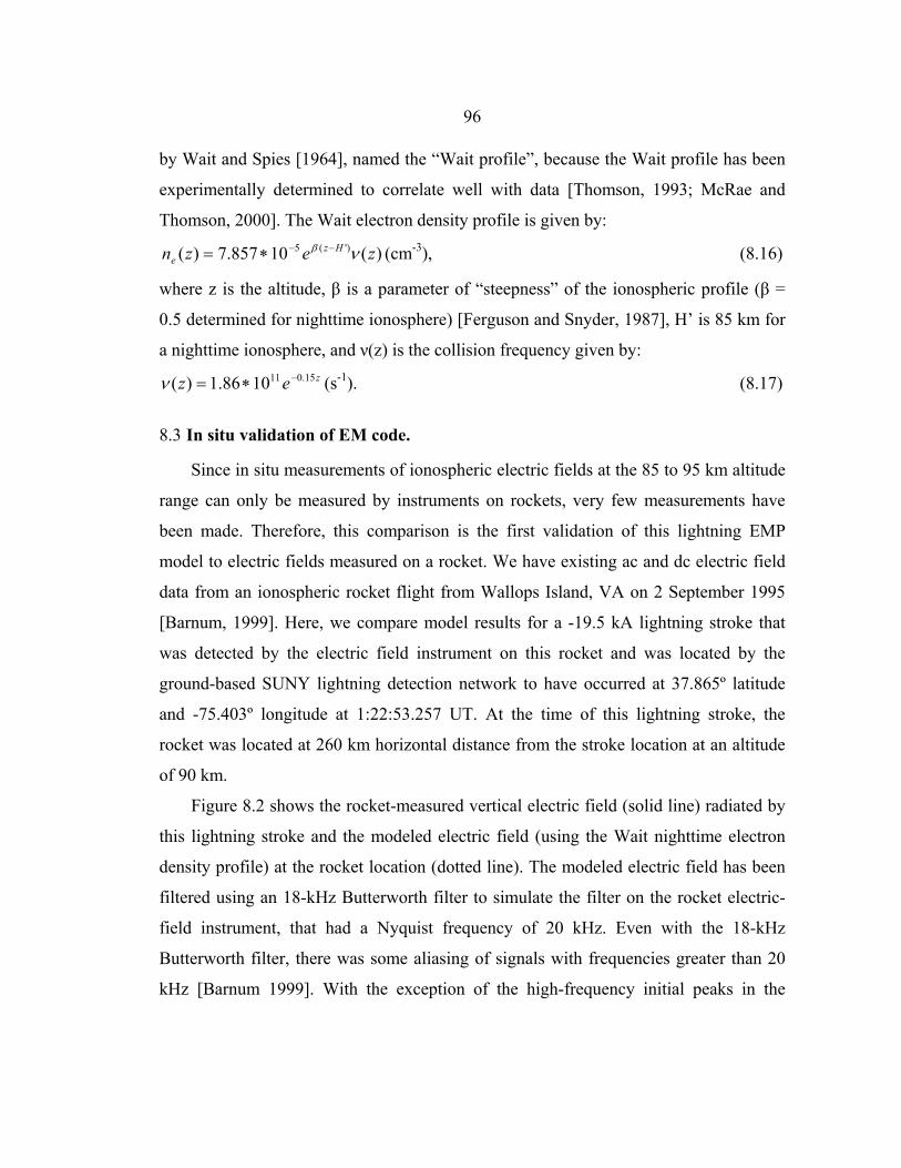
96
by Wait and Spies [1964], named the “Wait profile”, because the Wait profile has been
experimentally determined to correlate well with data [Thomson, 1993; McRae and
Thomson, 2000]. The Wait electron density profile is given by:
)(10857.7)( )'(5 zezn Hze νβ −−∗= (cm-3), (8.16)
where z is the altitude, β is a parameter of “steepness” of the ionospheric profile (β =
0.5 determined for nighttime ionosphere) [Ferguson and Snyder, 1987], H’ is 85 km for
a nighttime ionosphere, and ν(z) is the collision frequency given by: zez 15.0111086.1)( −∗=ν (s-1). (8.17)
8.3 In situ validation of EM code.
Since in situ measurements of ionospheric electric fields at the 85 to 95 km altitude
range can only be measured by instruments on rockets, very few measurements have
been made. Therefore, this comparison is the first validation of this lightning EMP
model to electric fields measured on a rocket. We have existing ac and dc electric field
data from an ionospheric rocket flight from Wallops Island, VA on 2 September 1995
[Barnum, 1999]. Here, we compare model results for a -19.5 kA lightning stroke that
was detected by the electric field instrument on this rocket and was located by the
ground-based SUNY lightning detection network to have occurred at 37.865º latitude
and -75.403º longitude at 1:22:53.257 UT. At the time of this lightning stroke, the
rocket was located at 260 km horizontal distance from the stroke location at an altitude
of 90 km.
Figure 8.2 shows the rocket-measured vertical electric field (solid line) radiated by
this lightning stroke and the modeled electric field (using the Wait nighttime electron
density profile) at the rocket location (dotted line). The modeled electric field has been
filtered using an 18-kHz Butterworth filter to simulate the filter on the rocket electric-
field instrument, that had a Nyquist frequency of 20 kHz. Even with the 18-kHz
Butterworth filter, there was some aliasing of signals with frequencies greater than 20
kHz [Barnum 1999]. With the exception of the high-frequency initial peaks in the

97
modeled data, the model using the Wait profile is consistent with the measured in situ
electric field in terms of timing of the pulses and the magnitude of the electric field.
When comparing modeled data using the original Cho and Rycroft [1998] electron
density profile, the magnitude of the model output is ~10 times larger, indicating a
much lower agreement with the data.
Figure 8.2: Comparison of rocket-measured vertical electric field (solid line) with 2-D EMP model output (dotted line) for a -19.5 kA CG stroke at 260 km range and 90 km altitude.
This comparison indicates that the model represents amplitude variations in time
very well. There is some discrepancy at high frequencies near the beginning of the
waveform, possibly due to the shape of the input current waveform or the filtering of
the rocket data. By modifying the characteristic time, τ, from 15µs to 25µs, the
magnitude of the initial downward peak decreases by 17% and the first upward peak
decreases by 50%. By filtering the model results using a 4-kHz Butterworth filter
instead of a 18-kHz filter, we get the modeled result shown in Figure 8.3. This
comparison between the model results with a 4-kHz filter and the data is a much closer
agreement than with the 18-kHz filter. This finding suggests that the rocket may
actually be filtering off lower frequencies than reported from the pre-flight calibration.

98
Figure 8.3: Comparison of same rocket-measured vertical electric field (solid line) with 2-D EMP model
output (dotted line) as in Figure 8.2, but using a 4kHz Butterworth filter.
Another source of error in the magnitude could be the background electron density
profile. While the Wait profile models the situation better than the original Cho and
Rycroft [1998] profile, it most likely does not represent the actual profile perfectly,
either. As is found below in Section 8.5, previous lightning strokes could modify the
electron density profile so that it can no longer be represented by a simple exponential.
In a test case, the 2D-EMP code was run with a background electron density of 6 times
the original profile. The results showed a decrease in magnitude of electric field at 90
km by a factor of 3. This test shows that the background electron density can have a
significant impact on the magnitude of the electric field at lower ionospheric altitudes.
Based on these variations resulting from different input model parameters in addition to
uncertainty in the validity of the 18-kHz Butterworth filter on the rocket, it is unclear
whether this is a limitation of the rocket data or an error in the 2D-EMP model.
8.4 Relaxation of enhanced electron density.
The 2-D EMP code runs for 2 ms while the lightning stroke propagates to the lower
ionosphere. After the EMP perturbation, the perturbed electron density undergoes
recombination (capture of an electron by a positive ion) and attachment (electron
capture by neutral molecule) and will eventually return to the original steady state
electron density. A numerical solution has been determined by using a 4th order Runge-
Kutta method to describe nighttime relaxation of ionospheric electron density
perturbations caused by an impulsive sferic. The differential equation used to describe
the change in electron density in this simulation is:

99
2ee
e NNqt
Nαβ −−=
∂∂
[Rodger et al. 1998], (8.18)
with q steady-state ionization rate due to cosmic rays, β as the attachment coefficient, α
as the recombination coefficient. The value of q for steady-state is determined by setting
the left-hand side of Equation (8.18) to zero. The values for α and β also are taken from
Rodger et al. [1998] in which a simplified ionospheric chemistry model is described and
found to give similar results to the much more complex Sodankyla Ion Chemistry
model [Verronen et al., 2005]. Attachment dominates below 80 km altitude due to high
concentrations of cluster ions, and recombination dominates above 85 km altitude due
to high concentrations of +2O .
The value of β is determined as the combination of attachment coefficients for the
two reactions, 0.5eVNONO 2222 ++→++ −e and 0.5eVOOOO 2222 ++→++ −e ,
by the equation ( ) 4.1/21 βββ += , with β1 for the former reaction and β2 for the latter.
β1 is given by ]][NO[101 2243
1−⋅=β , where the number density of O2 and N2 in m-3 is
represented by [O2] and [N2], respectively, and determined by the MSIS-E-90
ionospheric model developed by NASA Goddard Space Flight Center [Hedin et. al.,
1977; http://omniweb.gsfc.nasa.gov/vitmo/msis_vitmo.html]. The value for β2 is more
complicated, and determined by the following equations:
[ ]22
3
3
2
2165.02 Oexp)/1)((
−
−−=
eeeen T
aTa
Ta
TTββ (8.19)
2454239 103.2825103.4665101.1617)( nnn TTT −−− ⋅+⋅−⋅=β (8.20)
nn TTa 3.2964107.8193)( 21 −⋅= (8.21)
2322 104.5446-3.764610-1.9159)( nnn TTTa ⋅+⋅= (8.22)
3523213 101.7856 +107.6427-101.227710-7.6834)( nnnn TTTTa −−− ⋅⋅⋅+⋅= (8.23)
where Te is the electron temperature as determined by the MSIS-E-90 ionospheric
model, and we assume Tn, the neutral temperature, is equal to the electron temperature.

100
Recombination reactions are dominated by hydrated cluster ions (i.e. H+(H2O)n) for
altitudes below 80 km and dominated by +2O for altitudes above 80 km. The value of
the recombination coefficient is approximated in Rodger et al. [1998]:
eT/300105.2 11⋅=α m3s-1 for z ≤ 80 km, (8.24)
( ) 55.012 300/102 −⋅= eTα m3s-1 for z > 80 km. (8.25)
Figure 8.4 shows the results of this relaxation code for a 200% enhancement in
electron density at different ionospheric altitudes. At the altitudes of 85 and 90 km,
relaxation to within 5% of original levels is very slow. These altitudes are also the
altitudes at which the EMP has the most significant impact on electron density. From
this simulation, we see that if large strokes occur more frequently than the relaxation
time of the electron density enhancement, then the enhancement may accumulate over a
period of a number of strokes. Subsequent strokes then will interact with a modified
ionosphere, and may create non-linear behavior. This non-linear behavior will be
analyzed in Section 8.5.
Figure 8.4: Numerically-calculated relaxation times for different altitudes for an electron density enhancement of 200%. At the altitudes of 85 and 90 km, relaxation to within 5% of original levels is 1500
seconds or longer.
8.5 Accumulated enhancements due to successive lightning strokes.
In the following simulation, the above-described 2-D EMP model predicts the
change in electron density due to lightning EMP. The electron density enhancement
then is allowed to relax for a time t via the above numerical method. Next, the 2-D EMP
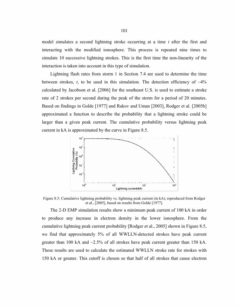
101
model simulates a second lightning stroke occurring at a time t after the first and
interacting with the modified ionosphere. This process is repeated nine times to
simulate 10 successive lightning strokes. This is the first time the non-linearity of the
interaction is taken into account in this type of simulation.
Lightning flash rates from storm 1 in Section 7.4 are used to determine the time
between strokes, t, to be used in this simulation. The detection efficiency of ~4%
calculated by Jacobson et al. [2006] for the southeast U.S. is used to estimate a stroke
rate of 2 strokes per second during the peak of the storm for a period of 20 minutes.
Based on findings in Golde [1977] and Rakov and Uman [2003], Rodger et al. [2005b]
approximated a function to describe the probability that a lightning stroke could be
larger than a given peak current. The cumulative probability versus lightning peak
current in kA is approximated by the curve in Figure 8.5.
Figure 8.5: Cumulative lightning probability vs. lightning peak current (in kA), reproduced from Rodger et al., [2005], based on results from Golde [1977].
The 2-D EMP simulation results show a minimum peak current of 100 kA in order
to produce any increase in electron density in the lower ionosphere. From the
cumulative lightning peak current probability [Rodger et al., 2005] shown in Figure 8.5,
we find that approximately 5% of all WWLLN-detected strokes have peak current
greater than 100 kA and ~2.5% of all strokes have peak current greater than 150 kA.
These results are used to calculate the estimated WWLLN stroke rate for strokes with
150 kA or greater. This cutoff is chosen so that half of all strokes that cause electron
102
density enhancements have peak currents larger than 150 kA and half have peak
currents less than 150 kA. The estimated stroke rate of 150-kA-or-greater strokes in
storm 1 is 0.2 s-1, or 1 every 5 seconds. For this simulation, a 150-kA stroke excites the
ionospheric electron density using the 2-D EMP simulation, and then the electron
density relaxes for 5 seconds via the numerical method described in the previous section
before the next 150-kA stroke occurs at the same location. For real lightning locations,
subsequent strokes would not occur in exactly the same location, but most probably
within the storm region of 30-50 km. This initial simplification is used since we are
focused on investigating the non-linear affect of successive strokes. Hopefully, this will
extend to a more realistic case in the future.
Figure 8.6 shows the steady-state electron density profile (right side), along with
the electron density profile after one 150-kA stroke (left side, top panel) and after ten
150-kA strokes (left side, bottom panel), spaced 5 seconds apart. Figure 8.7 shows the
percent change in electron density from steady-state for the same two simulation cases.
After one stroke, the maximum change in electron density is 34%, and occurs at 88.5
km altitude and 103 km range. After ten strokes, the maximum percentage change is
295% at an altitude of 87 km and a range of 103 km. It is also apparent that the space
around the region of enhanced electron density actually has a slight decrease in electron
density, and the region near the horizontal origin (in the electrostatic field of the stroke)
has a substantial decrease in electron density.

103
Figure 8.6: Initial, or steady-state, electron density profile (right side), along with the electron density profile after one 150-kA stroke (top panel) and after ten 150-kA strokes (bottom panel), spaced 5 seconds
apart.
Figure 8.7: Percentage change in electron density from steady-state after one 150 kA stroke (top panel)
and after ten 150 kA strokes (bottom panel).

104
Figure 8.8 shows the electron density at 92, 90, 88, and 85 km altitude and Figure
8.9 shows the percentage change in electron density at these altitudes after each
successive stroke. The non-linear behavior of the effect of EMP on the medium is clear
at all altitudes. At 92 km altitude, the electron density approaches a limit of ~5.45 x 10⁸
m-3, or about a 13% increase. The electron density at 90 km seems more slowly to
approach a limit of ~100% increase. The increase in electron density at 88 km appears
to be the most linear, with an increase of ~250% over 10 strokes. The change in electron
density per stroke at 85 km actually increases as the number of successive strokes
grows. Based on results from 90 and 92 km, one might expect electron densities at 85
and 88 km to reach limits eventually, but they show no sign of converging within these
10 strokes. Over 10 successive strokes, the electron density at 85 km increases 183%.
An explanation of processes underlying this behavior is the following: The amount
of ionization at a particular location due to a lightning stroke is dependent on the
magnitude of the electric field at that location, and electric fields that surpass an
ionization threshold increase electron density. However, the magnitude of the electric
field is dependent on the conductivity, which is in turn directly dependent on electron
density. Because the relaxation times for enhanced electron density are slow, as shown
in Figure 8.4, an electron density enhancement may remain when the next stroke occurs.
This enhancement leads to increased conductivity of the medium. As conductivity
increases, the electric field of the wave attenuates to a greater degree as it passes
through the medium. At some point, the medium reaches a limit where conductivity is
too high to allow the electric field to penetrate with enough amplitude to reach the
ionization threshold, and therefore, the electron density does not increase past that
point. At 92 km altitude, that limit seems to be reached at an electron density of ~5.45 x
108 m-3. At 85 km, the rate of electron density increase is actually higher for subsequent
lightning strokes. An explanation of this effect is that 85 km is near the lower boundary
of the region of electron density enhancement. Below the region of enhancement, a
region of decreased electron density develops over successive strokes as shown in

105
Figure 8.7. The lower region of decreased electron density allows the radiated electric
field to penetrate to 85 km altitude with less attenuation.
Figure 8.8: Electron density at 92, 90, 88, and 85 km altitude after each successive stroke.
Figure 8.9: Percent change in electron density for 92, 90, 88, 85 km altitude after each successive stroke.
In order to investigate the dependence of the model output on the input electron
density profile, we ran the 10 successive stroke 2D-EMP model for an initial electron
density profile with the parameters H’ = 85 km and β = 0.4 km-1, instead of the original
profile of H’ = 85 km and β = 0.5 km-1. This creates a background electron density
profile with the same characteristic height, but with a less steep increase in electron
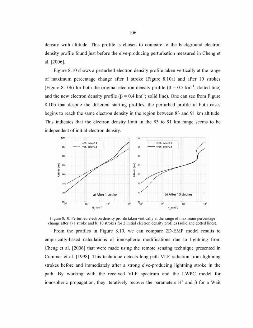
106
density with altitude. This profile is chosen to compare to the background electron
density profile found just before the elve-producing perturbation measured in Cheng et
al. [2006].
Figure 8.10 shows a perturbed electron density profile taken vertically at the range
of maximum percentage change after 1 stroke (Figure 8.10a) and after 10 strokes
(Figure 8.10b) for both the original electron density profile (β = 0.5 km-1; dotted line)
and the new electron density profile (β = 0.4 km-1; solid line). One can see from Figure
8.10b that despite the different starting profiles, the perturbed profile in both cases
begins to reach the same electron density in the region between 83 and 91 km altitude.
This indicates that the electron density limit in the 83 to 91 km range seems to be
independent of initial electron density.
Figure 8.10: Perturbed electron density profile taken vertically at the range of maximum percentage change after a) 1 stroke and b) 10 strokes for 2 initial electron density profiles (solid and dotted lines).
From the profiles in Figure 8.10, we can compare 2D-EMP model results to
empirically-based calculations of ionospheric modifications due to lightning from
Cheng et al. [2006] that were made using the remote sensing technique presented in
Cummer et al. [1998]. This technique detects long-path VLF radiation from lightning
strokes before and immediately after a strong elve-producing lightning stroke in the
path. By working with the received VLF spectrum and the LWPC model for
ionospheric propagation, they iteratively recover the parameters H’ and β for a Wait
107
electron density profile in the VLF propagation path following the technique presented
in [Cheng and Cummer, 2005]. Using this technique, Cheng et al. [2006] found a
background Wait electron density profile with values of H’=85 km and β=0.4
immediately before an elve-producing lightning stroke. The error in their method is
estimated at 0.2 km in H’ and 0.01 km-1 in β [Cummer et al., 1998]. Cheng et al. [2006]
also statistically analyzes the effects on lower ionospheric electron density of 27
lightning strokes with peak current >60 kA.
Figure 4a of Cheng et al. [2006] presents a perturbed electron density profile
associated with an elve-producing lightning stroke estimated by the NLDN to have -106
kA peak current. They find that this lightning stroke causes an enhancement in electron
density between 88 and 96 km altitude, with a 2-fold increase at ~92 km. It also creates
a decrease in electron density between 78 and 88 km, with a 5-fold decrease at ~82 km.
Figure 4b of Cheng et al. [2006] presents an averaged perturbed profile for the 27
averaged lightning strokes with mean peak current -79 kA. They find that these strokes
cause an average enhancement in electron density between 83 and 95 km altitude, with
a 2-fold increase at ~88 km. These strokes also create an average decrease in electron
density between 75 and 83 km, with a 1.5-fold decrease at ~80 km.
Although the background electron density profiles are different, with the
background profile of the solid line in Figure 8.10a being closer than that of the dotted
line to the background profile in Figure 4b of Cheng et al. [2006], the perturbed profile
in Figure 8.10a of this dissertation (modeled 1 -150 kA stroke) is similar to the profile
(in terms of regions and magnitudes of increase and decrease) for the averaged strokes
of -79 kA presented in Figure 4b of Cheng et al. [2006]. This signifies that the model
may underestimate the perturbed change in electron density for a lightning stroke of a
given peak current. In this case, a -150 kA stroke models a perturbation that represents
the experimentally determined perturbation for strokes with an average peak current of
-79 kA. The perturbed profile in Figure 8.10b (modeled 10 -150 kA strokes) is slightly
larger in magnitude than the perturbation due to one elve-producing lightning stroke

108
shown in Cheng et al. [2006] Figure 4a. Also, after 10 strokes the modeled electron
density enhancement has moved lower than that shown in Figure 4a of Cheng et al.
[2006], which is consistent with the findings presented above that successive lightning
strokes effectively move the region of enhanced electron density lower in altitude as the
electron density at higher altitudes reaches a limiting amount.
In the following paragraphs, we will discuss some of the remaining uncertainties
that could be producing these discrepancies between the empirically-based calculations
of electron density perturbations and the 2D-EMP modeled results. Peak currents
estimated by the NLDN are noted to have uncertainties of at least 20% to 30%
[Cummins et al., 1998]. This uncertainty could modify the 2D-EMP estimate of electron
density enhancement by a factor of 3 because of a larger radiated electric field from the
lightning stroke. Another source of error is the description of the lightning stroke
current pulse. By narrowing the pulse, dI/dt increases (where I is the current in the
stroke), and, therefore, the radiated electric field increases because it is dependent on
dI/dt. A change in the width of the pulse by 10 µs can increase the magnitude of the
electric field in the EMP by 30%. Uncertainty in peak current and in dI/dt could
increase or decrease the electric field of the lightning radiation that is responsible for
ionization and attachment as it passes through the lower ionosphere.
Another source of error may be the overall shape of the lightning current pulse. In a
recent study, Frey et al. [2005] found that 50% of ISUAL-detected elves were
accompanied by a lightning stroke with a β-type stepped leader. The stepped leader is
one of the original stages of a lightning stroke in which a conducting path is created
between cloud and ground in a number of discrete steps. The β-type stepped leaders are
characterized by long, bright steps with higher average speed than the more typical α-
type stepped leader. In an electric field waveform associated with a β-type stepped
leader, a series of bipolar pulses are evident about 2 to 5 ms before the return stroke
[Rakov and Uman, 2003]. It is possible that this β-type leader radiation could be a
factor in the total lightning EMP electron density modification. This leader activity has

109
not been included in the simple current pulse of the modeled return stroke, and could be
a cause of the discrepancy between the experimentally-based estimates of electron
density enhancement and the modeled electron density enhancement.
In addition to error in the magnitude of the electric field, there could be error in the
reduced electric field thresholds for ionization and attachment. The thresholds used in
the Cho and Rycroft [1998] model were determined in laboratory electron swarm
experiments. It is possible that the real world case (ionospheric plasma) behaves
differently than the controlled experiment. Therefore, the thresholds for ionization may
be different than those used in the model. This error could cause an underestimate in
ionization even if the magnitude of the electric field were correct. These uncertainties
reveal the need for more in situ measurements to better understand the many unknown
quantities in this type of ionospheric research. Bearing these uncertainties in mind, it is
possible that the 2-D EMP code underestimates the electron density enhancements in
the lower ionosphere.
The findings based on this model suggest that one must take the non-linearity into
account when modeling the effect of successive strokes on lower ionospheric nighttime
electron densities. It also shows that the non-linear behavior is different at different
altitudes. A maximum electron density limit is reached after fewer strokes for higher
altitudes than lower altitudes. The region with the most significant effect (88 km) does
not seem to reach an electron density limit for these ten strokes. The limiting modeled
electron density profile is the same in the 83 to 91 km altitude range regardless of the
initial electron density. The non-linearity suggests that a linear approach, such as that in
Rodger et al. [2001] may significantly overestimate the change in electron density at
higher altitudes and underestimate it at lower altitudes. One must also remember that in
general the Cho and Rycroft [1998] model may underestimate changes in electron
density. However, this simulation describes qualitative behavior of electron density
enhancements at different altitudes due to multiple successive lightning strokes.

110
Chapter 9: Conclusion and Future Work
9.1 World-Wide Lightning Location Network Characterization
During the course of this dissertation research, the World-Wide Lightning Location
Network has developed from a fledgling network of 13 stations world wide with little
known about its behavior and characteristics to a much better characterized network
with fairly uniform global coverage by 30 stations. This research has provided
preliminary location and timing accuracy, detection efficiency, and lightning-type
studies, finding excellent location and timing accuracy, even in a worst-case scenario.
The lightning-type studies using FORTE RF data indicated that WWLLN detects in-
cloud lightning that are most likely NBEs, but only 3 such events were found in a 49-
day case study of LASA waveforms of WWLLN-detected events in the Great Plains
region. This finding indicates that either NBEs radiate more energy from Austral-asian
storms, similarly energetic NBEs are more likely to be detected by 5 WWLLN stations
due to higher station density, or NBEs comprise a smaller percentage of total lightning
in the Great Plains. The relative detection efficiency world-wide has been characterized
in comparison to the FORTE PDD instrument. Global relative detection efficiency in
combination with localized regional detection efficiencies led to normalized WWLLN
global lightning count rates for the first time, as shown in Chapter 4.
However, we must continue work to determine the dynamic detection efficiency of
WWLLN as new stations are added. The study of station detection range, presented in
Section 3.4, shows that we must include day/night differences in lightning propagation
to VLF stations as well as the near-range detection voids in a reliable model of dynamic
detection efficiency.
In addition to these improvements in the characterization of the network, the first
attempts were made at providing an estimate of stroke energy. We found that WWLLN
could be used to provide relative stroke energies for lightning in the same storm, but
there are still some obstacles to overcome in determining an absolute lightning energy

111
calibration. The main two obstacles are determining the gain and frequency response of
each VLF station and better understanding ionospheric propagation of lightning energy
in different ionospheric conditions.
9.2 Findings on energetic events correlated with lightning
In this dissertation, WWLLN was used to investigate spacecraft-detected elves and
TGFs. We have been able to use WWLLN to help better locate ISUAL-detected elves
by exposing an error in the location-estimating algorithm for the spacecraft data. More
accurate elve locations could allow a more accurate study of differences in elves that
occur over water and over land. WWLLN is able to detect elve-causative lightning
world-wide, and now could be used to determine the relative strength of lightning stroke
as compared to non-elve-producing strokes in the same storm.
Lightning locations from WWLLN were able to help address some of the questions
regarding terrestrial gamma-ray flashes. These data were able to provide the first
evidence that TGFs are not narrowly beamed from the source. WWLLN data were also
used to determine that RHESSI-detected TGFs are most likely associated with the first
stroke in a lightning flash, and with large peak current lightning (greater than 40 kA).
The analysis presented in this dissertation provides the first global study of regional
differences in lightning count rates versus local time using continuous ground-based
data. The findings from WWLLN agree well with satellite averages over the whole
world, but also provide new information on the amount of lightning over each continent
under the nighttime ionosphere. We find that over 60% of lightning in the Americas
occur under the nighttime ionosphere while less than 40% of lightning in Europe occurs
during that time. We are also able to provide global mapping of nighttime lightning for
different seasons without the need for many years of averaging, as is required by
satellites. As mentioned in the previous section, a dynamic detection ability that
considers the diurnal and spatial variability in WWLLN sensitivity would greatly
enhance the usefulness of WWLLN data in addressing these types of studies. With such

112
capabilities, WWLLN could provide information on regions of the ionosphere most
likely to be associated with conductivity variations, and in which one would be most
likely to detect TLEs during a field campaign.
9.3 Modeling of lightning electromagnetic pulse
This dissertation has described a 2D-EMP model to predict the lightning-to-
ionosphere energy coupling. Cho and Rycroft [1998] has shown that optical emissions
as simulated by this model are consistent with observations of elves. The first in situ
comparison of modeled data with rocket-measured electric fields has been performed.
This comparison shows that the temporal extent of the modeled pulse is similar to the
rocket-measured electric field pulse, but the high frequency peak of the modeled
electric field is about 10 times larger than the rocket-measured electric field pulse. It is
unclear whether this is a limitation of the rocket data or an error in the 2D-EMP model.
A comparison of the modeled electron density enhancements to experimentally-
estimated enhancements [Cheng et al., 2006] has shown that the model underestimates
electron density enhancements in the 85 the 95 km altitude range for a -150 kA stroke.
Therefore, one must not consider modeled results as quantitative truth, but may use
them to determine qualitatively how the EMP from successive lightning strokes couples
to the lower ionosphere. In this light, we find that the EMP from successive strokes
interacts non-linearly with the ionospheric plasma. The maximum electron density is
reached earlier for higher altitudes, yet the region with the most significant affect (88
km) behaves fairly linearly for these ten strokes. The maximum modeled electron
density profile is the same in the 83 to 91 km altitude range regardless of the initial
electron density. The non-linearity suggests that the results in Rodger et al. [2001] may
significantly overestimate the change in electron density at higher altitudes and
underestimate it at lower altitudes.

113
9.4 Future Work
9.4.1 WWLLN Characterization
The work in this dissertation has provided much improvement in the
characterization of WWLLN detection efficiency, but a concrete global estimate of
WWLLN detection efficiency still must be completed. One beneficial study would be to
determine the detection efficiency by comparing WWLLN to the yearly averaged OTD
satellite-detected lightning count rate globally. This comparison requires a collaboration
with member of the OTD team, and will only provide an annual detection efficiency
estimate relative to a 5-year average, not a dynamic estimate. However, this comparison
would be highly beneficial to WWLLN. Next, one must support the findings from the
OTD/WWLLN comparison with a determination of the day/night dynamics in detection
efficiency as well as changes in detection efficiency as more stations are added and as
stations sporadically go off the air due to loss of power or internet connectivity. An
expansion of the study of station detection range presented in Section 3.4 could be used
for this project. Also, a better characterization of the threshold trigger levels at each
individual station would be useful to achieve this goal.
An improved estimate of radiated stroke energy could be provided by determining
a more accurate absolute calibration for each WWLLN VLF station, in conjunction with
a better understanding of daily ionospheric variations. This dissertation has proposed
the possibility of transmitting the amplitude of narrowband VLF transmitters as
detected by WWLLN stations to the central processing computer. This would
effectively create a global ionospheric monitoring network out of the already existing
WWLLN, which could in turn be used as input to a dynamic detection efficiency
estimate.
By using either the relative stroke energy as determined by the method proposed in
this dissertation or an improved absolute energy estimate, correlation studies between
radiated energy per stroke and elves/TGFs could provide more information about the

114
strength of lightning required to produce such events, and allow WWLLN data to be
used to more accurately predict where these lightning-produced energetic effects will
occur.
9.4.2 Lightning/Ionospheric Coupling
Given the difficulty of experimentally determining lower ionospheric electron
densities, it is nearly impossible to verify a model of the lightning EMP effect on the
lower ionosphere. However, further study using the remote sensing technique of Cheng
and Cummer [2005] in the VLF band and of Jacobson et al. [2007] in the LF (30-300
kHz) band would be valuable.
Modeling of lightning/ionospheric coupling will continue to be useful while
experimental measurements are difficult. It would be useful to improve the lightning
EMP/ionosphere model by more accurately determining uncertainties. The model
should also be modified to predict electron density variations based on WWLLN
lightning counts, locations, and stroke radiated energy. A model of this sort could
provide a real-time estimate of ionospheric regions likely to be perturbed by lightning
activity. Such a model would have to be based on improved estimates of WWLLN
stroke radiated energy as well as on results of the 2D-EMP successive-strokes model. In
order to make real-time predictions without overwhelming computer time, one could
use the results from Section 8.5 to estimate equations for the non-linear behavior of
electron density enhancements for various altitudes.
9.4.3 Narrow Bipolar Events
The findings in this dissertation regarding NBEs are somewhat contradictory, given
that a comparison with satellite RF measurements indicated a large number of
WWLLN-detected NBEs while comparisons with a ground-based regional network
indicated very few coincident NBEs. It may be useful to probe this question further by
studying coincidences with ground-based regional networks for a longer period of time,

115
as well as for different regions. Once may be able to determine if WWLLN is more
likely to detect NBEs at different times of year and in certain regions.
It may also be useful to use the LASA-detected lightning waveform, and, using the
LWPC, propagate radiation from that wave to all WWLLN stations that detected the
lightning stroke. This simulation could provide an idea of the trigger thresholds at
different stations for detecting NBEs.
9.4.4 Global electric circuit
While this dissertation has not investigated the hypothesis of the global electric
circuit, the global circuit hypothesis is a main motivation for providing a better
characterization of WWLLN. With a dynamic detection efficiency estimate of
WWLLN, one could begin a real-time study of measuring global lightning variations
simultaneously with fair weather return current.
Similarly, the improvements of WWLLN presented in this dissertation hopefully
will allow WWLLN data to be used to address many atmospheric electricity and
meteorological questions.

116
REFERENCES
Barnum, H.B. (1999), Electromagnetic and optical characteristics of lightning measured in the Earth’s ionosphere, Ph.D. thesis, Univ. of Washington, Seattle, Washington.
Barrington-Leigh, C.P. and U.S. Inan. (1999), Elves triggered by positive and negative lightning discharges. Geophys. Res. Letters, 26, 6, 683-686.
Barrington-Leigh, C.P., U.S. Inan, M. Stanley, and S.A. Cummer (1999), Sprites Triggered by Negative Lightning Discharges, Geophys. Res. Lett., 26(24), 3605–3608.
Boccippio, D.J., K. Driscoll, W. Koshak, R. Blakeslee, W. Boeck, D. Buechler, H. Christian, and S. Goodman (2000a), The Optical Transient Detector (OTD): Instrument characteristics and cross-sensor validation. J. Atmos. Oceanic Tech., 17, 441-458.
Boccippio, D.J., S.J. Goodman, and S. Heckman (2000b), Regional differences in tropical lightning distributions. J. Appl. Meteor., 39, 2231-2248.
Boeck, W.L., O.H. Vaughan Jr., R.J. Blakeslee, B. Vonnegut, M. Brook, and J. McKune (1995), Observations of lightning in the stratosphere, J. Geophys. Res., 100(D1), 1465–1475.
Budden, K.G. (1961), The Waveguide Mode Theory of Wave Propagation., Logos Press, London.
Cheng, Z., and S.A. Cummer (2005), Broadband VLF measurements of lightning-induced ionospheric perturbations, Geophys. Res. Lett., 32, L08804, doi:10.1029/2004GL022187.
Cheng, Z., S.A. Cummer, D.N. Baker, and S.G. Kanekal (2006), Nighttime D region electron density profiles and variabilities inferred from broadband measurements using VLF radio emissions from lightning, J. Geophys. Res., 111, A05302, doi:10.1029/2005JA011308.
Cho, M and M.J. Rycroft (1998), Computer simulation of the electric field structure and optical emission from cloud-top to the ionosphere, J. of Atmos. and Solar-Terr. Phys., 60, 871-888.
Christian, H.J., R.J. Blakeslee, S.J. Goodman, D.A. Mach, M.F. Stewart, D.E. Buechler, W.J. Koshak, J.M. Hall, W.L. Boeck, K.T. Driscoll, and D.J. Boccippio (1999), The Lightning Imaging Sensor. 11th International Conference on Atmospheric Electricity, Global Hydrology and Climate Center, NASA Marshall Space Flight Center, Huntsville, Alabama.

117
Christian, H.J., R.J. Blakeslee, D.J. Boccippio, W.L. Boeck, D.E. Buechler, K.T. Driscoll, S.J. Goodman, J.M. Hall, W.J. Koshak, D.M. Mach, and M.F. Stewart (2003), Global frequency and distribution of lightning as observed from space by the Optical Transient Detector, J. Geophys. Res., 108(D1), 10.1029/2002JD002347.
Crombie, D.D. (1964), Periodic fading of VLF signals received over long paths during sunrise and sunset. Journal of Research National Bureau of Standards, Radio Science, 68D, 27-34.
Cummins, K.L., M.J. Murphy, E.A. Bardo, W.L. Hiscox, R. Pyle, and A.E. Pifer (1998), Combined TOA/MDF technology upgrade of U.S. National Lightning Detection Network. J. Geophys. Res., 103, 9035-9044.
Cummer, S.A., Inan, U.S. and Bell, T.F. (1998), Ionospheric D region remote sensing using VLF radio atmospherics. Radio Science 33, pp. 1781–1792.
Cummer, S.A., and W.A. Lyons (2005), Implications of lightning charge moment changes for sprite initiation, J. Geophys. Res., 110, A04304, doi:10.1029/2004JA010812.
Cummer, S.A., Y. Zhai, W. Hu, D.M. Smith, L.I. Lopez, and M.A. Stanley (2005), Measurements and implications of the relationship between lightning and terrestrial gamma ray flashes, Geophys. Res. Lett., 32, L08811, doi:10.1029/2005GL022778.
Dowden, R.L., J.B. Brundell, and C.J. Rodger (2002), VLF lightning location by time of group arrival (TOGA) at multiple sites. J. Atmos. Solar-Terrest. Phys., 64, 817-830.
Dwyer, J.R., and D.M. Smith (2005), A comparison between Monte Carlo simulations of runaway breakdown and terrestrial gamma-ray flash observations, Geophys. Res. Lett., 32, L22804, doi:10.1029/2005GL023848.
Ferguson, J.A., and F.P. Snyder (1987), The segmented waveguide program for long wavelength propagation calculations. Technical Document No. 1071, Naval Ocean Systems Center, San Diego, California, USA.
Fernsler, R.F. and H.L. Rowland (1996), Models of lightning-produced sprites and elves, J. Geophys. Res., 101(D23), 29,653-662.
Fishman, G.J., P.N. Bhat, R. Mallozzi, J.M. Horack, T. Koshut, C. Kouveliotou, G.N. Pendleton, C.A. Meegan, R.B. Wilson, W.S. Paciesas, S.J. Goodman, H.J. Christian (1994), Discovery of intense gamma-ray flashes of atmospheric origin, Science, 264, 5163: 1313-1316.
Frey, H.U., S.B. Mende, S.A. Cummer, A.B. Chen, R.R. Hsu, H.T. Su, Y.S. Chang, T. Adachi, H. Fukunishi, and Y. Takahashi (2005), Beta-type stepped leader of elve-producing lightning, Geophys. Res. Lett., 32, L13824, doi:10.1029/2005GL023080.

118
Fukunishi, H., Y. Takahashi, M. Kubota, K. Sakanoi, U.S. Inan, W.A. Lyons (1996), Elves: Lightning-induced transient luminous events in the lower ionosphere, Geophys. Res. Lett., 23, 16, 2157-2160.
Fullekrug, M., and S. Constable (2000), Global triangulation of intense lightning discharges, Geophys. Res. Lett., 27, 333-336.
Goldberg, R.A., J.R. Barcus, L. Hale, S.A. Curtis (1986), Direct observation of magnetospheric electron-precipitation stimulated by lightning, J. of Atmos. And Terr. Phys., 48 (3), 293-299.
Golde, R.H. (1977), Lightning, Academic Press, London, UK.
Hedin, A.E et al. (1977), A Global Thermospheric Model Based on Mass Spectrometer and Incoherent Scatter Data MSIS, 1, N2 Density and Temperature, J. Geophys. Res., 82(16), 2139–2147.
Helliwell, R.A., Katsufrakis, J.P. and Trimpi, M.L. (1973), Whistler-induced amplitude perturbations in VLF propagation. J. Geophys. Res. 78, pp. 4679–4688.
Holzworth R.H, R.M. Winglee, B.H. Barnum, Y.Q. Li, and M.C. Kelley (1999), Lightning whistler waves in the high-latitude magnetosphere, J. Geophys. Res., 104, A8, 17369-17,378.
Holzworth, R.H., E.A. Bering III, M.F. Kokorowski, E.H. Lay, B. Reddell, A. Kadokura, H. Yamagishi, N. Sato, M. Ejiri, H. Hirosawa, T. Yamagami, S.Torii, F. Tohyama, M. Nakagawa, T. Okada, and R.L. Dowden (2005a), Balloon observations of temporal variation in the global circuit compared to global lightning activity, Advances in Space Res., 36,11, 2223-2228.
Holzworth, R.H., M.P. McCarthy, J.N. Thomas, J. Chin, T.M. Chinowsky, M.J. Taylor, and O. Pinto Jr. (2005b), Strong electric fields from positive lightning strokes in the stratosphere, Geophys. Res. Lett., 32, L04809, doi:10.1029/2004GL021554.
Inan, U.S., T.F. Bell, J.V. Rodriguez (1991), Heating and ionization of the lower ionosphere by lightning, Geophys. Res. Lett., 18, 705-708.
Jacobson, A.R., R. Holzworth, J. Harlin, R. Dowden, and E. Lay (2006), Performance Assessment of the World Wide Lightning Location Network (WWLLN), Using the Los Alamos Sferic Array (LASA) as Ground Truth, J. Atmos. and Oceanic Technology, 23, 1082-1092.
Jacobson, A.R., R. Holzworth, E. Lay, M. Heavner, and D.A. Smith (2007), Low-frequency ionospheric sounding with Narrow Bipolar Event lightning radio emissions: regular variabilities and solar-X-ray responses, Ann. Geophys., 25, 2175– 2184.

119
Kelley, M.C., C.L. Siefring, R.F. Pfaff, P.M. Kintner, M. Larsen, R. Green, R.H. Holzworth, L.C. Hale, J.D. Mitchell, and D. LeVine (1985), Electrical measurements in the atmosphere and the ionosphere over an active thunderstorm. 1. Campaign overview and initial ionospheric results, J. Geophys. Res., 90, A10, 9815-9823.
Kirkland, M.W., D.M. Suszcynsky, J.L.L. Guillen, and J.L. Green (2001), Optical observations of terrestrial lightning by the FORTE satellite photodiode detector. J. Geophys. Res., 106, 33,499-33,509.
Lay, E.H., R.H. Holzworth, C.J. Rodger, J.N. Thomas, O. Pinto, Jr., and R.L. Dowden (2004), WWLL Global Lightning Detection System: Regional Validation Study in Brazil, Geophys. Res. Lett., 31, L03102, doi: 10.1029/2003GL018882.
Le Vine, D.M. (1980), Sources of the Strongest RF Radiation From Lightning, J. Geophys. Res., 85(C7), 4091–4095.
Li, Y.Q., R.H. Holzworth, H. Hu, M. McCarthy, R.D. Massey, P.M. Kintner, J.V. Rodrigues, U.S. Inan, and W.C. Armstrong (1991), Anomalous optical events detected by rocket-borne sensor in the WIPP campaign, J. Geophys. Res., 96, A2 1315-1326.
Light, T.E., S.M. Davis, W. Boeck, A.R. Jacobson (2003), Global nighttime lightning flash rates and characteristics observed with the FORTE satellite, Los Alamos National Laboratory technical report, LA-UR 03-5909.
MacGorman, D.R., and R.W. Rust (1998), The Electrical Nature of Storms, Oxford University Press, Oxford.
McRae, W.M. and N.R Thomson (2000), VLF phase and amplitude: daytime ionospheric parameters. J. of Atmos. and Solar-Terr. Physics 62 7, pp. 609–618.
Mende, S.B., H.U. Frey, R.R. Hsu, H.T. Su, A.B. Chen, L.C. Lee, D.D. Sentman, Y. Takahashi, and H. Fukunishi (2005), D region ionization by lightning-induced electromagnetic pulses, J. of Geophys. Res., 110, A11312, doi:10.1029/2005JA011064.
Nesbitt, S.W. and E.J. Zipser (2003), The Diurnal Cycle of Rainfall and Convective Intensity according to Three Years of TRMM Measurements. J. of Climate, 16, 1456-1475.
Orville, R.E. and G.R. Huffines (2001), Cloud-to-Ground Lightning in the United States: NLDN Results in the First Decade, 1989–98. Monthly Weather Rev., 129, 1179-1193.
Parkinson, W.C, and O.W. Torrenson (1931), The diurnal variation of the electrical potential of the atmosphere over the oceans, Compt. Rend. De l’Assemblee de Stockholm, 1930; IUGG (sect. Terres. Magn. Electr. Bull. 8, 340-345.

120
Pasko, V.P, U.S. Inan, T.F. Bell, and Y.N. Tarenenko (1997), Sprites produced by quasi-electrostatic heating and ionization in the lower ionosphere, J. of Geophys. Res., 102, A3, 4529-4561.
Petersen, W.A. and S.A. Rutledge (2001), Regional variability in tropical convection: Observations from TRMM. J. Climate, 14, doi:10.1175/1520-0442.
Pinto, I.R.C.A., and O. Pinto Jr.(2003), Cloud-to-ground lightning distribution in Brazil, J. Atmos. Solar-Terr. Physics, 65(6): 733-737.
Pinto, Jr. O., I.R.C.A. Pinto, and K.P. Naccarato (2007), Maximum cloud-to-ground lightning flash densities observed by lightning location systems in the tropical region: A review, Atmos. Res., 84(3): 189-200.
Pinto, Jr. O., I.R.C.A. Pinto, J.H. Diniz, A.C. Filho, A.M. Carvalho, and L.C.L. Chechiglia (2003), A long-term study of the lightning flash characteristics in the southeastern Brazil, J. Atmos. Solar-Terr. Physics, 65(6): 739-748.
Rakov, V.A. and M.A. Uman (2003), Lightning: Physics and Effects. Cambridge University Press. Cambridge, United Kingdom.
Razier, Y.P. (1991), Gas Discharge Physics, Springer-Verlag, Berlin.
Roble, R.G. and I. Tzur (1986), The global atmospheric-electrical circuit. In The Earth’s Electrical Environment, Studies in Geophysics, pages 206-231. National Academy Press, Washington, DC.
Rodger, C.J., O.A. Molchanov, and N.R. Thomson (1998), Relaxation of transient ionization in the lower ionosphere, J. Geophys. Res., 103(A4), 6969–6975.
Rodger, C.J. (1999), Red sprites, upward lightning, and VLF perturbations, Rev. Geophys., 37, 317-336.
Rodger, C.J., M. Cho, M.A. Clilverd, and M.J. Rycroft (2001), Lower ionospheric modification by lightning-EMP: Simulation of the night ionosphere over the United States. Geophys. Res. Lett., 28(2), 199-202.
Rodger, C.J., J.B. Brundell, R.L. Dowden, and N.R. Thomson (2004), Location accuracy of long distance VLF lightning location network. Ann. Geophys., 22, 747-758.
Rodger, C.J., J.B. Brundell, and R.L. Dowden (2005a), Location accuracy of VLF World Wide Lightning Location (WWLL) network: Post-algorithm upgrade. Ann. Geophys., 23, 277-290.
Rodger, C.J., M.A. Clilverd, N.R. Thomson, D. Nunn, and J. Lichtenberger (2005b), Lightning driven inner radiation belt energy deposition into the atmosphere: regional and global estimates, Ann. Geophys., 23, 3419-3430.
121
Rodger, C.J., S.W. Werner, J.B. Brundell, N.R. Thomson, E.H. Lay, R.H. Holzworth, and R.L. Dowden (2006), Detection efficiency of the VLF World-Wide Lightning Location Network (WWLLN): Initial case study, Ann. Geophys., 24, 3197-3214.
Schlegel, K., G. Diendorfer, S. Thern, and M. Schmidt (2001), Thunderstorms, lightning and solar activity - Middle Europe, J. Atmos. Sol.-Terr. Phys., 63, 1705-1713.
Sentman, D.D., E.M. Wescott, D.L. Osborne, D.L. Hampton, and M.J. Heavner (1995), Preliminary Results from the Sprites94 Aircraft Campaign: 1. Red Sprites, Geophys. Res. Lett., 22(10), 1205–1208.
Smith, D.A., X.M. Shao, D.N. Holden, C.T. Rhodes, M. Brook, P.R. Krehbiel, M. Stanley, W. Rison, and R.J. Thomas (1999), A distinct class of isolated intracloud lightning discharges and their associated radio emissions, J. Geophys. Res., 104(D4), 4189–4212.
Smith, D.A., K.B. Eack, J. Harlin, M.J. Heavner, A.R. Jacobson, R.S. Massey, X.M. Shao, and K.C. Wiens (2002), The Los Alamos Sferic Array: A research tool for lightning investigations, J. Geophys. Res., 107(D13), 4183, doi:10.1029/2001JD000502.
Smith, D.M., L.I. Lopez, R.P. Lin, C.P. Barrington-Leigh (2005), Terrestrial gamma-ray flashes observed up to 20 MeV, Science, 307, 5712, 1085 – 1088, DOI: 10.1126/science.1107466.
Smith, D.M., J.R. Dwyer, B.W. Grefenstette, B.J. Hazelton, Y. Yair, J. Bor, E.H. Lay, R.H. Holzworth (2007), Eos Trans. AGU, 88(52), Fall Meet. Suppl., Abstract AE31A-0051
Stanley, M.A., X.M. Shao, D.M. Smith, L.I. Lopez, M.B. Pongratz, J.D. Harlin, M. Stock, and A. Regan (2006), A link between terrestrial gamma-ray flashes and intracloud lightning discharges, Geophys. Res. Lett., 33, L06803, doi:10.1029/2005GL025537.
Suszcynsky, D.M., M. Kirkland, P. Argo, R. Franz, A. Jacobson, S. Knox, J. Guillen, J. Green, and R. Spalding (1999), Thunderstorm and lightning studies using the FORTE optical lightning system (FORTE/OLS), Proceedings of the 11th International Conference on Atmospheric Electricity, edited by H. Christian, NASA/CP-1999-209261, 672-675.
Suszcynsky, D., A. Jacobson, J. Fitzgerald, C. Rhodes, E. Tech, and D. Roussel-Dupre (2000a), Satellite-based global lightning and severe storm monitoring using VHF receivers. EOS, Trans. Am. Geophys. Union, 81, F91.

122
Suszcynsky, D.M., M.W. Kirkland, A.R. Jacobson, R.C. Franz, S.O. Knox, J.L.L. Guillen, and J.L. Green (2000b), FORTE observations of simultaneous VHF and optical emissions from lightning: Basic Phenomenology. J. Geophys. Res., 105, 2191-2201.
Suszcynsky, D.M., T.E. Light, S. Davis, M.W. Kirkland, J.L. Green, and J. Guillen, (2001), Coordinated Observations of Optical Lightning from Space using the FORTE Photodiode Detector and CCD Imager. J. Geophys. Res., 106, 17,897-17,906.
Tapia, A., J.A. Smith, M. Dixon (1998), Estimation of convective rainfall from lightning observations, Journal of Appl. Meteor., 37, 1497-1509.
Tarenenko, Y.N., U.S. Inan, and T.F. Bell (1993), Interaction with the lower ionosphere of electromagnetic pulses from lightning: heating, attachment, and ionization, Geophys. Res. Lett., 20, 15, 1539-1542.
Taylor, M., M. Bailey, P. Pautet, S. Cummer, N. Jaugey, J. Thomas, N. Solorzano, F. Sao Sabbas, R. Holzworth, O. Pinto Jr., and N. Schuch (2008), Rare Measurements of a Sprite with Halo Event Driven by a Negative Lightning Discharge Over Argentina, Geophys. Res. Lett., doi:10.1029/2008GL033984, in press.
Thomson, N.R. (1993), Experimental daytime VLF ionospheric parameters. Journal of Atmospheric and Terrestrial Physics 55 2, pp. 173–184.
Verronen, P.T., A. Seppälä, M.A. Clilverd, C.J. Rodger, E. Kyrölä, C.F. Enell, T. Ulich, and E. Turunen (2005), Diurnal variation of ozone depletion during the October–November 2003 solar proton events, J. Geophys. Res., 110, A09S32, doi:10.1029/2004JA010932.
Volland, H. (1984), Atmospheric Electrodynamics, Springer-Verlag, New York.
Wait, J.R. (1970), Electromagnetic Waves in Stratified Media, Pergamon Press Inc., New York.
Wait, J.R. and K.P. Spies (1964), Characteristics of the Earth-Ionosphere Waveguide for VLF Radio Waves, Nat. Bureau of Standards Tech. Notes, 300, Washington, DC.
Whipple, F.J.W., and F.J. Scrase (1936), Point discharge in the electric field of the Earth, Geophys. Memoirs (London) VIII(68), 20.
Wiens, K.C., T. Hamlin, J. Harlin, and D.M. Suszcynsky (2008), Relationships among Narrow Bipolar Events, ‘‘total’’ lightning, and radar-inferred convective strength in Great Plains thunderstorms, J. Geophys. Res., 113, D05201, doi:10.1029/2007JD009400.
Willett, J.C., J.C. Bailey, and E.P. Krider (1989), A Class of Unusual Lightning Electric Field Waveforms With Very Strong High-Frequency Radiation, J. Geophys. Res., 94(D13), 16,255–16,267.

123
Williams, E., K. Rothkin, D. Stevenson, and D. Boccippio (2000), Global Lightning Variations Caused by Changes in Thunderstorm Flash Rate and by Changes in the Number of Thunderstorms. J. of Applied Meterology, 39, 2223-2230.
Wilson, C.T.R. (1920), Investigation on lightning discharges and on the electric field of thunderstorms. Phil. Trans. A 221, 73-115.
Zajac, B.A. and S.A. Rutledge (2001), Cloud-to-ground lightning activity in the contiguous United States from 1995 to 1999. Monthly Weather Rev., 129 (5), 999-1019.

124
Appendix A: Schematics for WWLLN Service Unit and Preamplifier
Figure A.1: Schematic for WWLLN Service Unit

125
Figure A.2: Schematic for WWLLN preamplifier

126
VITA
Erin Hoffmann Lay Degrees Earned: Bachelor of Arts, Physics Grinnell College, Grinnell, IA Spring 2002 Master of Sciences, Physics University of Washington, Seattle, WA Fall 2003 Doctor of Philosophy, Physics University of Washington, Seattle, WA Spring 2008