Embed Size (px)
Citation preview
Copyright © 2011 Pearson Addison-Wesley. All rights reserved.
Chapter 3
A Consumer’s Constrained Choice
If this is coffee, please bring me some tea; but if this is tea, please bring me some coffee.
Abraham Lincoln

Copyright © 2011 Pearson Addison-Wesley. All rights reserved.3-2
Chapter 3 Outline
3.1 Preferences3.2 Utility3.3 Budget Constraint3.4 Constrained Consumer Choice3.5 Behavioral Economics
Copyright © 2011 Pearson Addison-Wesley. All rights reserved.3-3
Chapter 3: Model of Consumer Behavior• Premises of the model:1.Individual tastes or preferences determine
the amount of pleasure people derive from the goods and services they consume.
2.Consumers face constraints, or limits, on their choices.
3.Consumers maximize their well-being or pleasure from consumption subject to the budget and other constraints they face.
Copyright © 2011 Pearson Addison-Wesley. All rights reserved.3-4
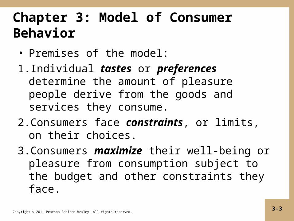
3.1 Preferences
• To explain consumer behavior, economists assume that consumers have a set of tastes or preferences that they use to guide them in choosing between goods.
• Goods are ranked according to how much pleasure a consumer gets from consuming each.• Preference relations summarize a consumer’s ranking
• is used to convey strict preference (e.g. a b)
• is used to convey weak preference (e.g. a b)
• ~ is used to convey indifference (e.g. a ~ b)
Copyright © 2011 Pearson Addison-Wesley. All rights reserved.3-5
3.1 Preferences
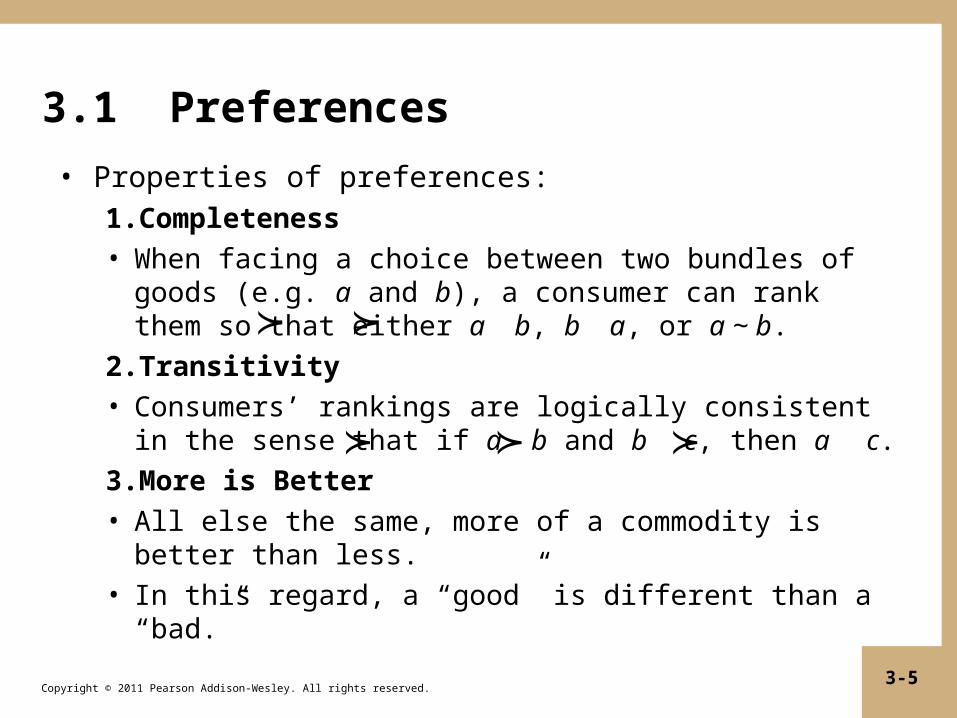
• Properties of preferences:1.Completeness• When facing a choice between two bundles of goods
(e.g. a and b), a consumer can rank them so that either a b, b a, or a ~ b.
2.Transitivity• Consumers’ rankings are logically consistent in the
sense that if a b and b c, then a c.3.More is Better• All else the same, more of a commodity is better than
less.• In this regard, a “good” is different than a “bad.”
Copyright © 2011 Pearson Addison-Wesley. All rights reserved.3-6
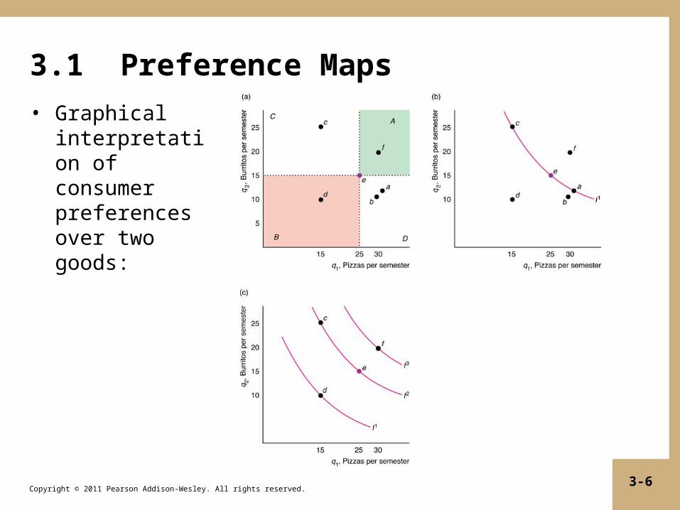
3.1 Preference Maps• Graphical
interpretation of consumer preferences over two goods:
Copyright © 2011 Pearson Addison-Wesley. All rights reserved.3-7
3.1 Indifference Curves• The set of all bundles of goods that a consumer views
as being equally desirable can be traced out as an indifference curve.
• Five important properties of indifference curves:1.Bundles of goods on indifference curves further from
the origin are preferred to those on indifference curves closer to the origin.
2.There is an indifference curve through every possible bundle.
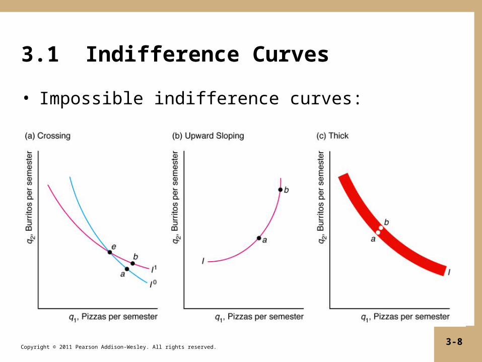
3.Indifference curves cannot cross.4.Indifference curves slope downward.5.Indifference curves cannot be thick.
Copyright © 2011 Pearson Addison-Wesley. All rights reserved.3-8
3.1 Indifference Curves
• Impossible indifference curves:
Copyright © 2011 Pearson Addison-Wesley. All rights reserved.3-9
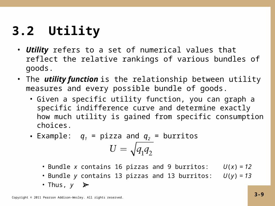
3.2 Utility• Utility refers to a set of numerical values that reflect
the relative rankings of various bundles of goods.• The utility function is the relationship between utility
measures and every possible bundle of goods.• Given a specific utility function, you can graph a
specific indifference curve and determine exactly how much utility is gained from specific consumption choices.
• Example: q1 = pizza and q2 = burritos
• Bundle x contains 16 pizzas and 9 burritos: U(x) = 12• Bundle y contains 13 pizzas and 13 burritos: U(y) = 13• Thus, y x
Copyright © 2011 Pearson Addison-Wesley. All rights reserved.3-10
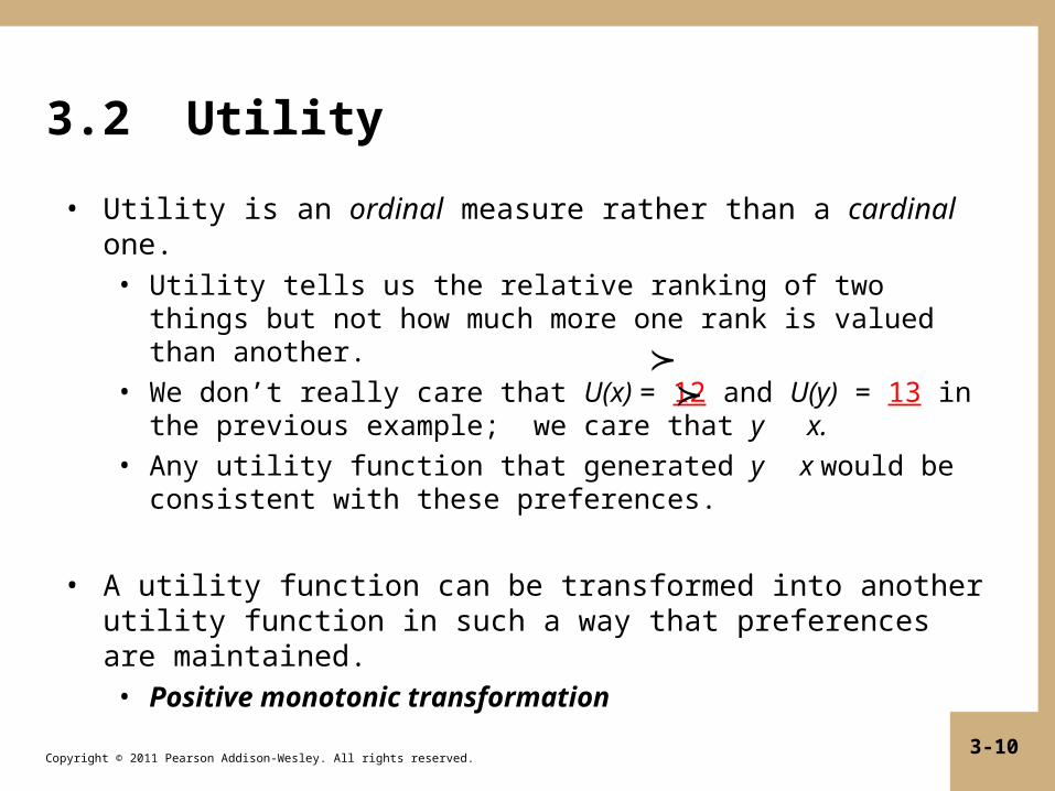
3.2 Utility
• Utility is an ordinal measure rather than a cardinal one.• Utility tells us the relative ranking of two things but not how
much more one rank is valued than another.• We don’t really care that U(x) = 12 and U(y) = 13 in the
previous example; we care that y x.• Any utility function that generated y x would be
consistent with these preferences.
• A utility function can be transformed into another utility function in such a way that preferences are maintained.• Positive monotonic transformation
Copyright © 2011 Pearson Addison-Wesley. All rights reserved.3-11
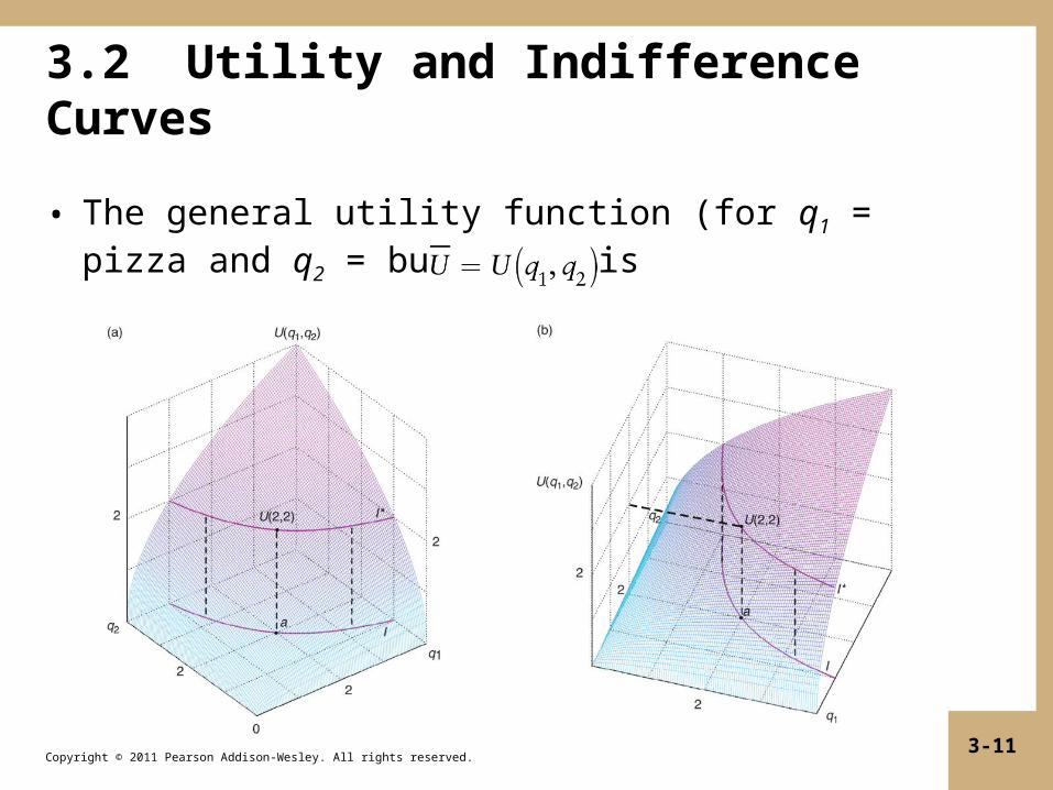
3.2 Utility and Indifference Curves
• The general utility function (for q1 = pizza and q2 = burritos) is
Copyright © 2011 Pearson Addison-Wesley. All rights reserved.3-12
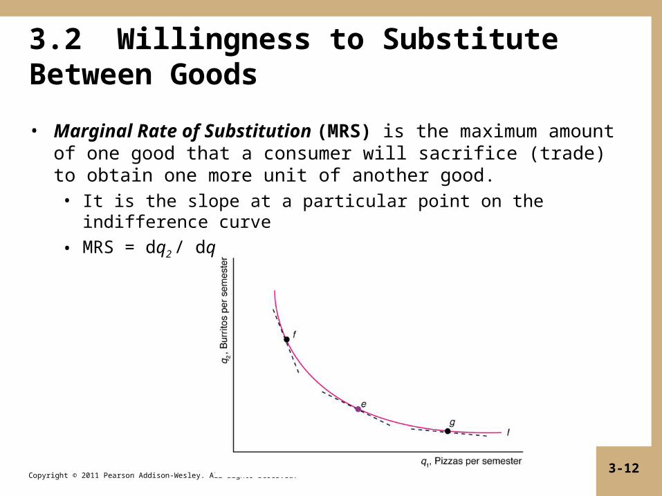
3.2 Willingness to Substitute Between Goods
• Marginal Rate of Substitution (MRS) is the maximum amount of one good that a consumer will sacrifice (trade) to obtain one more unit of another good.• It is the slope at a particular point on the indifference curve
• MRS = dq2 / dq1

Copyright © 2011 Pearson Addison-Wesley. All rights reserved.3-13
3.2 Marginal Utility and MRS
• The MRS depends on how much extra utility a consumer gets from a little more of each good.• Marginal utility is the extra utility that a consumer
gets from consuming the last unit of a good, holding the consumption of other goods constant.
• Using calculus to calculate the MRS:

Copyright © 2011 Pearson Addison-Wesley. All rights reserved.3-14
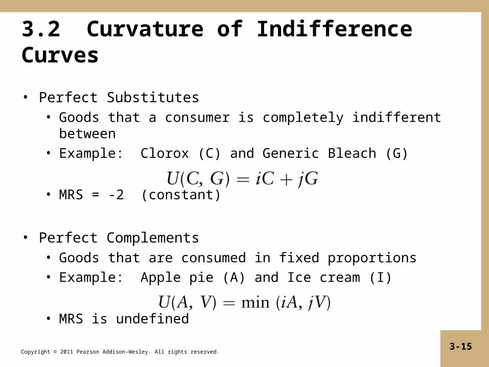
3.2 Curvature of Indifference Curves
• MRS (willingness to trade) diminishes along many typical indifference curves that are concave to the origin.
• Different utility functions generate different indifference curves:
Copyright © 2011 Pearson Addison-Wesley. All rights reserved.3-15
3.2 Curvature of Indifference Curves
• Perfect Substitutes• Goods that a consumer is completely indifferent
between• Example: Clorox (C) and Generic Bleach (G)
• MRS = -2 (constant)
• Perfect Complements• Goods that are consumed in fixed proportions• Example: Apple pie (A) and Ice cream (I)
• MRS is undefined

Copyright © 2011 Pearson Addison-Wesley. All rights reserved.3-16
3.2 Curvature of Indifference Curves• Imperfect Substitutes
• Between extreme examples of perfect substitutes and perfect complements are standard-shaped, convex indifference curves.
• Cobb-Douglas utility function (e.g. ) indifference curves never hit the axes.
• Quasilinear utility function (e.g. ) indifference curves hit one of the axes.

Copyright © 2011 Pearson Addison-Wesley. All rights reserved.3-17
3.3 Budget Constraint• Consumers maximize utility subject to constraints.• If we assume consumers can’t save and borrow, current
period income determines a consumer’s budget.
• Given prices of pizza (p1) and burritos (p2), and income Y, the budget line is
• Example:• Assume p1 = $1, p2 = $2 and Y = $50
• Rewrite the budget line equation for easier graphing (y=mx+b form):

Copyright © 2011 Pearson Addison-Wesley. All rights reserved.3-18
3.3 Budget Constraint
• Marginal Rate of Transformation (MRT) is how the market allows consumers to trade one good for another.• It is the slope of the budget line:
Copyright © 2011 Pearson Addison-Wesley. All rights reserved.3-19
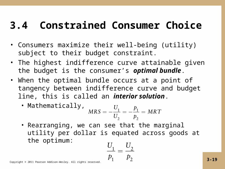
3.4 Constrained Consumer Choice
• Consumers maximize their well-being (utility) subject to their budget constraint.
• The highest indifference curve attainable given the budget is the consumer’s optimal bundle.
• When the optimal bundle occurs at a point of tangency between indifference curve and budget line, this is called an interior solution.• Mathematically,
• Rearranging, we can see that the marginal utility per dollar is equated across goods at the optimum:
Copyright © 2011 Pearson Addison-Wesley. All rights reserved.3-20
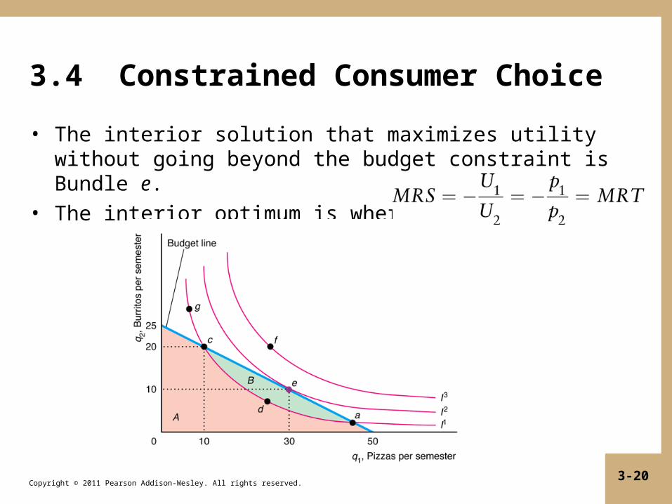
3.4 Constrained Consumer Choice
• The interior solution that maximizes utility without going beyond the budget constraint is Bundle e.
• The interior optimum is where
Copyright © 2011 Pearson Addison-Wesley. All rights reserved.3-21
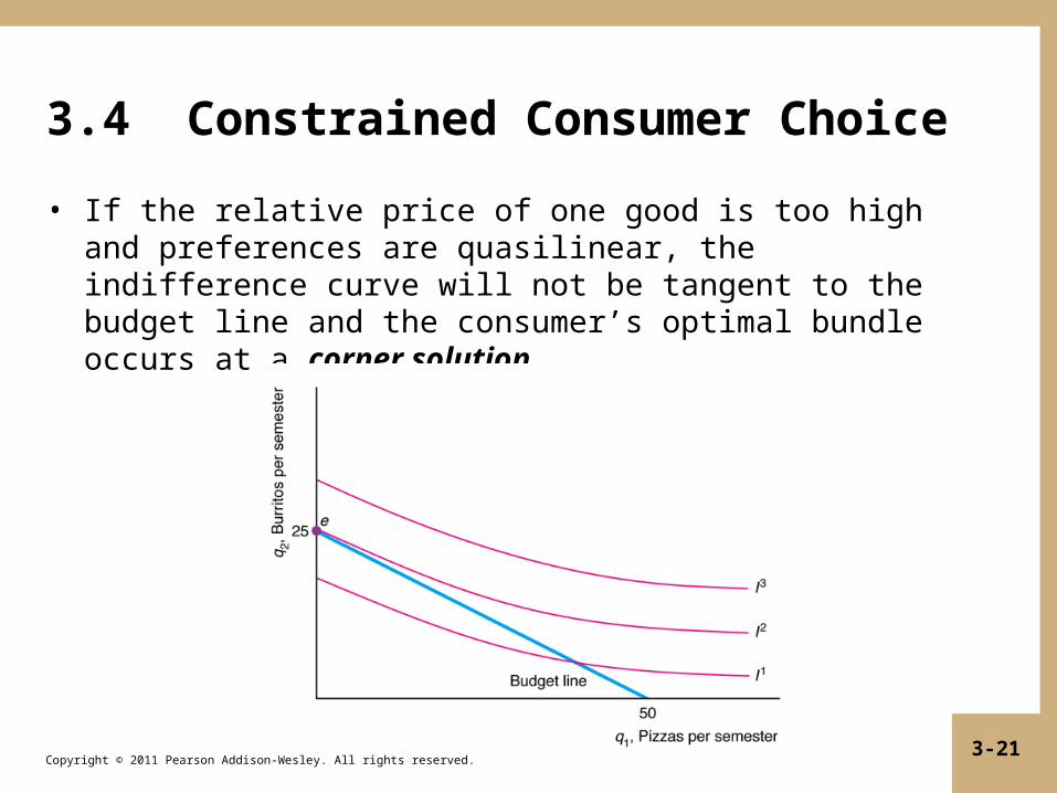
3.4 Constrained Consumer Choice
• If the relative price of one good is too high and preferences are quasilinear, the indifference curve will not be tangent to the budget line and the consumer’s optimal bundle occurs at a corner solution.

Copyright © 2011 Pearson Addison-Wesley. All rights reserved.3-22
3.4 Consumer Choice with Calculus
• Our graphical analysis of consumers’ constrained choices can be stated mathematically:
• The optimum is still expressed as in the graphical analysis:
• These conditions hold if the utility function is quasi-concave, which implies indifference curves are convex to the origin.
• Solution reveals utility-maximizing values of q1 and q2 as functions of prices, p1 and p2, and income, Y.
Copyright © 2011 Pearson Addison-Wesley. All rights reserved.3-23
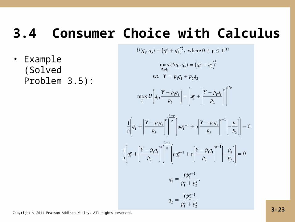
3.4 Consumer Choice with Calculus
• Example (Solved Problem 3.5):
Copyright © 2011 Pearson Addison-Wesley. All rights reserved.3-24
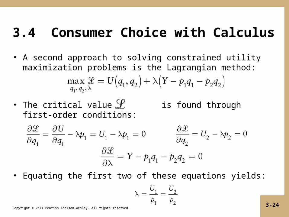
3.4 Consumer Choice with Calculus
• A second approach to solving constrained utility maximization problems is the Lagrangian method:
• The critical value of is found through first-order conditions:
• Equating the first two of these equations yields:

Copyright © 2011 Pearson Addison-Wesley. All rights reserved.3-25
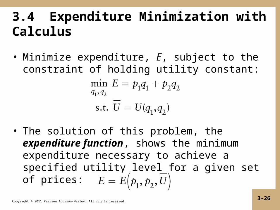
3.4 Minimizing Expenditure
• Utility maximization has a dual problem in which the consumer seeks the combination of goods that achieves a particular level of utility for the least expenditure.
Copyright © 2011 Pearson Addison-Wesley. All rights reserved.3-26
3.4 Expenditure Minimization with Calculus
• Minimize expenditure, E, subject to the constraint of holding utility constant:
• The solution of this problem, the expenditure function, shows the minimum expenditure necessary to achieve a specified utility level for a given set of prices:

Copyright © 2011 Pearson Addison-Wesley. All rights reserved.3-27
3.5 Behavioral Economics• What if consumers are not rational, maximizing
individuals?• Behavioral economics adds insights from psychology
and empirical research on cognition and emotional biases to the rational economic model.
• Tests of transitivity: evidence supports transitivity assumption for adults, but not necessarily for children.
• Endowment effect: some evidence that endowments of goods influence indifference maps, which is not the assumption of economic models.
• Salience: evidence that consumers are more sensitive to increases in pre-tax prices than post-tax price increases from higher ad valorem taxes.
• Bounded rationality suggests that calculating post-tax prices is “costly” so some people don’t bother to do it, but they would use the information if it were provided.
Copyright © 2011 Pearson Addison-Wesley. All rights reserved.3-28
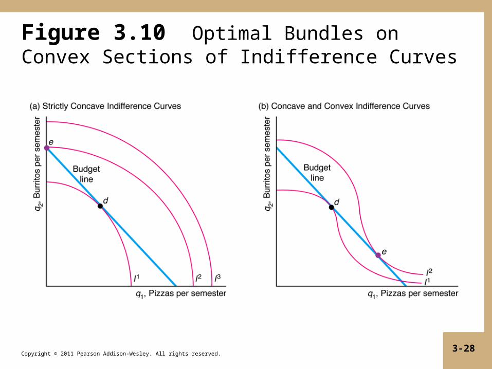
Figure 3.10 Optimal Bundles on Convex Sections of Indifference Curves