Embed Size (px)
Citation preview

Copyright
by
Ellen Elizabeth Reid
2012
The Thesis Committee for Ellen Elizabeth Reid
Certifies that this is the approved version of the following thesis:
The effect of temperature and terrace geometry on carbonate
precipitation rate in an experimental setting
APPROVED BY
SUPERVISING COMMITTEE:
Wonsuck Kim
Joel Johnson
David Mohrig
Supervisor:
The effect of temperature and terrace geometry on carbonate
precipitation rate in an experimental setting
by
Ellen Elizabeth Reid, B.S.Geo.Sci.
Thesis
Presented to the Faculty of the Graduate School of
The University of Texas at Austin
in Partial Fulfillment
of the Requirements
for the Degree of
Master of Science in Geological Sciences
The University of Texas at Austin
August 2012

Dedication
This thesis is dedicated to my parents, who have never stopped supporting me and
believing in me during my pursuit of higher education.
v
Acknowledgements
First and foremost, I would like to acknowledge my adviser Wonsuck Kim, who
aided me in every way from the initial concept of my research to writing the thesis. My
research would not have been possible without him. Wonsuck, I appreciate your gracious
patience and guidance. I’d also like to thank my committee of David Mohrig and Joel
Johnson, for visiting my flume, generating ideas for what direction to take my
experiments, and revising my thesis. I would like to thank my lab assistant Eric Swanson
for countless hours constructing and refining the flume and assisting in conducting the
experiments. I would like to thank Jake Jordan and Kiran Sathaye for their constant
encouragement and input (and MATLAB assistance). Finally, I would like to thank the
Jackson School of Geosciences for their support during my undergraduate and graduate
career, and shaping me into the geologist that I am today.
vi
Abstract
The effect of temperature and terrace geometry on carbonate
precipitation rate in an experimental setting
Ellen Elizabeth Reid, M.S.Geo.Sci.
The University of Texas at Austin, 2012
Supervisor: Wonsuck Kim
Through flume experiments we demonstrate the calcite precipitation process seen
at geothermal hot springs in the lab setting. A series of four experiments were run,
varying temperature and terrace ridge height while all other experimental parameters,
including initial substrate slope, spring water discharge, and CO2 input were kept
constant. The goal of the experiments was to measure the temperature and terrace height
control quantitatively in terms of the amount of overall travertine aggradation,
aggradation rate changes in time and downstream direction, as well as to observe the
effect of these parameters on processes occurring during precipitation. Using the final
deposit thickness measured manually at the end of each experiment and elevation data
obtained from a laser topographic profiler, I conclude that high temperature and small
terrace heights favor increased precipitation of travertine. However, the amount of
precipitation also depends on location within a terrace pond. Flow velocity increases as it
approaches a terrace lip, resulting in enhanced precipitation and greater thicknesses in the

vii
downstream direction through increased CO2 degassing, a process called downstream
coarsening.
viii
Table of Contents
List of Tables ......................................................................................................... xi
List of Figures ....................................................................................................... xii
Chapter 1: Introduction ........................................................................................1
Travertine environments and associated patterns ...........................................2
Precipitation process .......................................................................................3
Rate of precipitation ........................................................................................5
Hot springs environments and Mammoth Hot Springs, Yellowstone ............6
Travertine terrace formation and growth processes ........................................7
Biological impact on travertine precipitation .................................................8
Previous studies ..............................................................................................9
Chapter 2: Experimental Design ........................................................................11
Precipitation process in the laboratory .........................................................11
Design for experimental set ..........................................................................13
Chapter 3: Data Collection and Processing .......................................................15
Chapter 4: Results................................................................................................17
Deposit thickness ..........................................................................................17
Temperature influence on pond aggradation ................................................18
Step height influence on pond aggradation ...................................................19
Step aggradation............................................................................................19
Deposit thickness variance and slope in a single pond .................................20
Aggradation rate............................................................................................20
Chapter 5: Discussion ..........................................................................................22
Temperature influence on bed aggradation ...................................................22
Step height influence on thickness ................................................................22
Control of flow path on step thickness .........................................................23
ix
Overall downstream trend in precipitation ...................................................23
Downstream coarsening in a single pond .....................................................24
Fluctuations in aggradation rate with time ....................................................25
Future experimental goals .............................................................................26
Chapter 6: Conclusions .......................................................................................27
References ..............................................................................................................81
Tables ................................................................................................................................29
Figures ..............................................................................................................................33
x
List of Tables
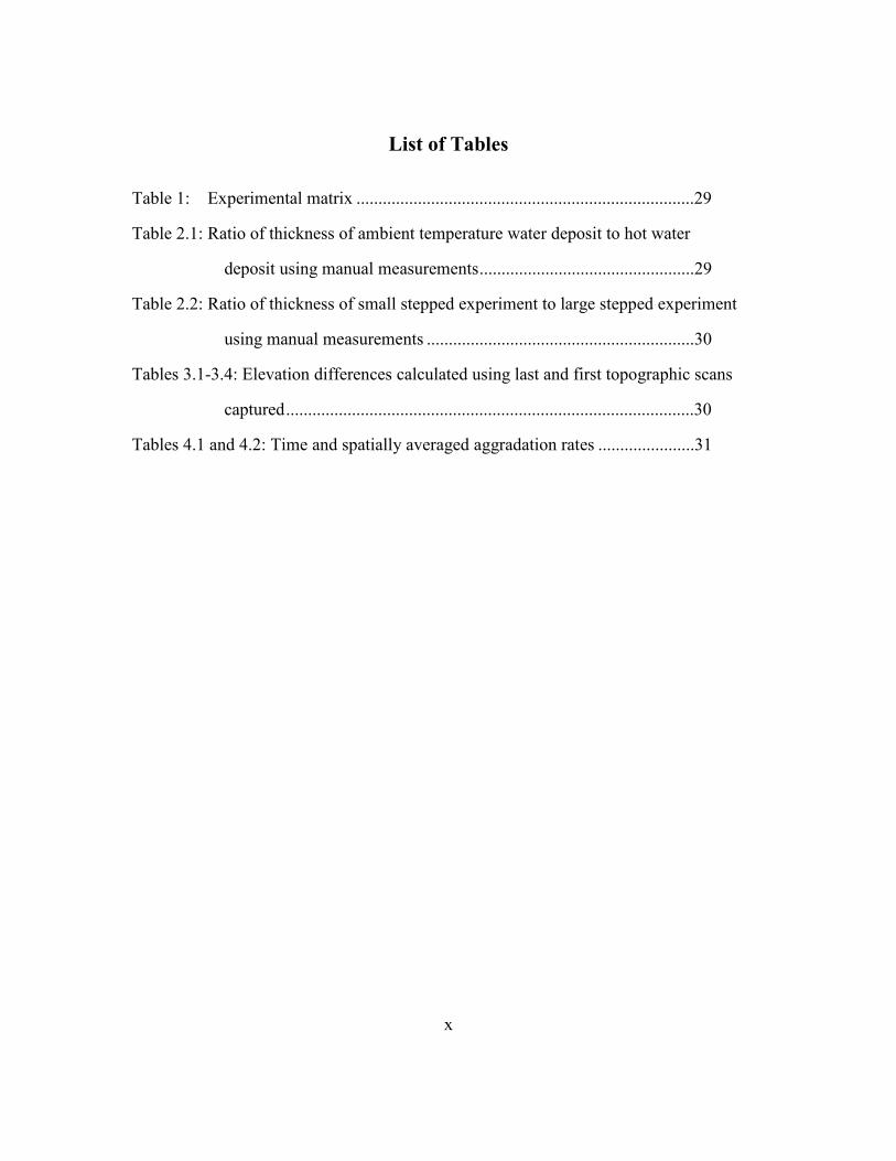
Table 1: Experimental matrix .............................................................................29
Table 2.1: Ratio of thickness of ambient temperature water deposit to hot water
deposit using manual measurements .................................................29
Table 2.2: Ratio of thickness of small stepped experiment to large stepped experiment
using manual measurements .............................................................30
Tables 3.1-3.4: Elevation differences calculated using last and first topographic scans
captured .............................................................................................30
Tables 4.1 and 4.2: Time and spatially averaged aggradation rates ......................31
xi
List of Figures
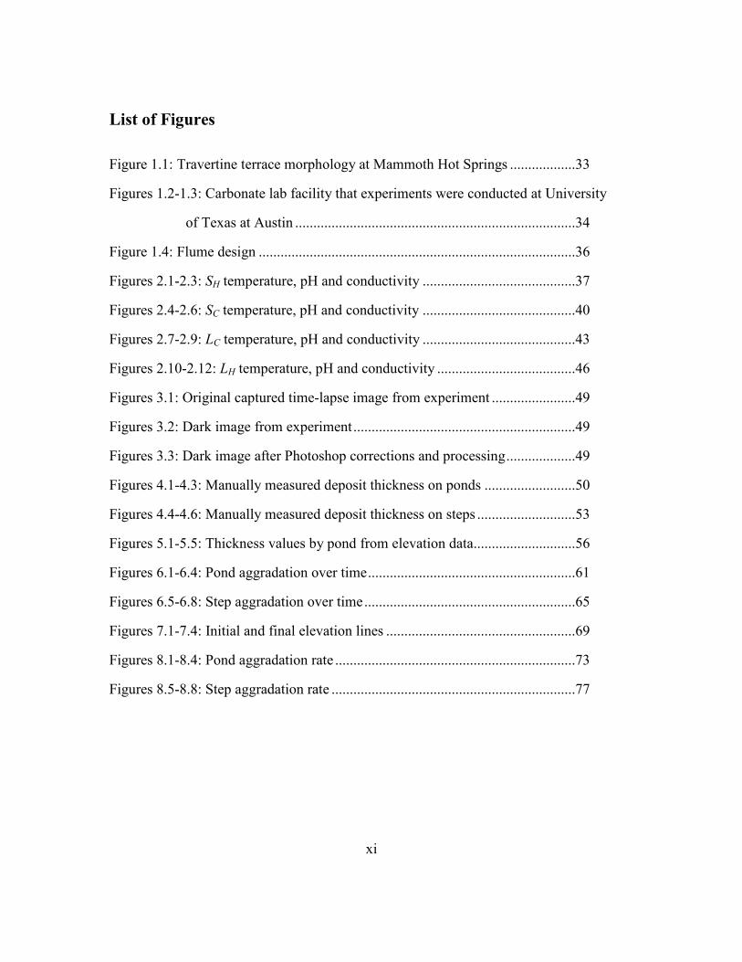
Figure 1.1: Travertine terrace morphology at Mammoth Hot Springs ..................33
Figures 1.2-1.3: Carbonate lab facility that experiments were conducted at University
of Texas at Austin .............................................................................34
Figure 1.4: Flume design .......................................................................................36
Figures 2.1-2.3: SH temperature, pH and conductivity ..........................................37
Figures 2.4-2.6: SC temperature, pH and conductivity ..........................................40
Figures 2.7-2.9: LC temperature, pH and conductivity ..........................................43
Figures 2.10-2.12: LH temperature, pH and conductivity ......................................46
Figures 3.1: Original captured time-lapse image from experiment .......................49
Figures 3.2: Dark image from experiment .............................................................49
Figures 3.3: Dark image after Photoshop corrections and processing ...................49
Figures 4.1-4.3: Manually measured deposit thickness on ponds .........................50
Figures 4.4-4.6: Manually measured deposit thickness on steps ...........................53
Figures 5.1-5.5: Thickness values by pond from elevation data............................56
Figures 6.1-6.4: Pond aggradation over time .........................................................61
Figures 6.5-6.8: Step aggradation over time ..........................................................65
Figures 7.1-7.4: Initial and final elevation lines ....................................................69
Figures 8.1-8.4: Pond aggradation rate ..................................................................73
Figures 8.5-8.8: Step aggradation rate ...................................................................77
1
Chapter 1: Introduction
I have conducted a series of experiments precipitating calcite in the laboratory setting
using a flume. Water discharge and initial substrate slope were held constant while temperature
and terrace height were varied for each experiment, and the resulting deposit was analyzed. The
field process analogue for setting parameter standards in the hot water experiments is a hot
springs environment, such as Mammoth Hot Springs, Yellowstone National Park. Travertine
here forms as terraces, which is the morphology I attempted to recreate in the experiments.
Studying the travertine precipitation process and its resulting deposits is useful in a number of
applications. Travertine deposits are very sensitive to water chemistry, transport conditions, and
climate. Therefore, travertine serves as a reliable source for reconstructing paleoenvironments
(Fouke 2000). Some hot springs are in particularly harsh, unusual environments and contain
unique microorganisms; these can be used for discern information about primordial life on Earth
as well as potential life on other planets (Fouke 2000). Travertine also has industrial application.
When urban settings sit on top of limestone/carbonate rocks or karst environments, limestone
precipitation in pipes and boilers is a major issue and source of financial loss for cities (Hammer
2008). Travertine also can serve as a reservoir for hydrocarbons, for example, the Itaborai Basin
in Southeastern Brazil was a carbonate hot spring in the Paleocene (Sant’ Anna 2004).
In this study, we focus on the temperature and terrace geometry controls on carbonate
precipitation patterns to enhance our ability to utilize carbonate sedimentary records for
reconstructing paleoenvironments.
2
Travertine environments and associated patterns
Travertine is a type of carbonate, a precipitated form of limestone with the chemical
formula CaCO3, and includes all deposits in non-marine settings in its strictest definition.
Travertine will precipitate in an array of environments, including hot springs, mountainous
streams, caves, and waterfalls (Hammer 2008; Fouke 2000). It forms in predictable yet poorly
understood morphologies based on the surrounding environment and local conditions. For
example, in hot springs such as Mammoth Hot Springs in Yellowstone, much work has been
done studying travertine terraces, also known as cascading dams (Hammer 2008), rimstone
(Goldenfeld 2006), or barrages (Pentecost 1994). Travertine terraces appear as a series of steps:
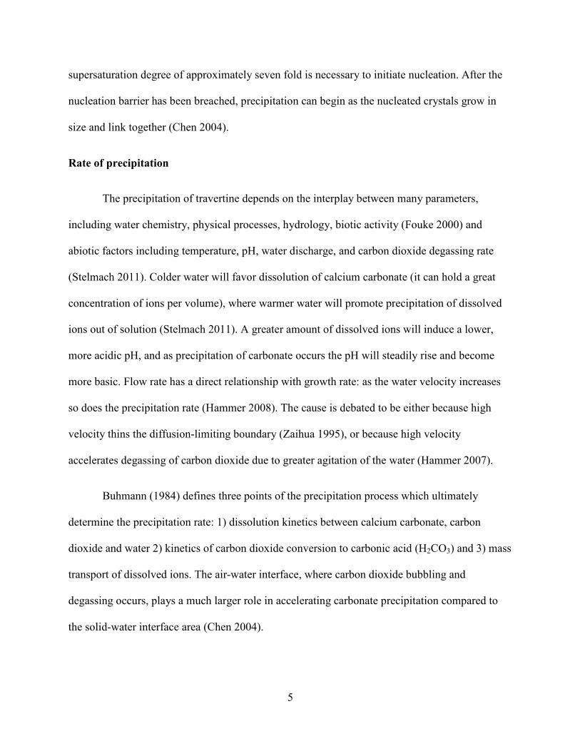
laterally extensive, vertical ridges with flat tops that cover most of the surface area (Figure 1.1).
A second dominant morphology present in hot springs is travertine domes, for which Goldenfeld
(2006) provides a growth model. Other potential morphologies of travertine include needle-like
speleothems in caves and tufa in low-temperature locations (Fouke 2000). Travertine
morphology depends on environmental conditions. Chavetz (1984) classifies five morphological
variations for all travertine deposits, including cascade, lake-fill, sloping mound, cone or fan,
terraced mound, and fissure ridge. All of these classifications are informal; there is currently no
systematic way of naming or organizing travertine deposits (Pentecost 1994). For example, in
some literature “tufa” refers to cold water carbonate precipitate (Hammer 2007). In other
literature, whether a deposit is classified as travertine or tufa depends on the degree of
cementation (Pentecost 1994).
Travertine can form in a wide range of temperatures, from 5 degrees to 95 degrees
Celsius, though most environments are within the 10-30 degree Celsius range (Chavetz 1984).
When travertine is deposited it is fragile, friable, poorly cemented, and subject to degradation
3
from external environmental forces. For this reason travertine deposits in tectonically active
areas are relatively young, Quaternary age and younger (Sant’Anna 2004). Many travertine
deposits have a high proportion of sand and mud grains in their composition, especially in
turbulent, high-energy environments (Pentecost 1994). Travertine is also more commonly found
in warm, tropical climates than in high latitude locations (Pentecost 2000). Travertine deposits
can be deposited very rapidly, up to five millimeters per day. This is a million-fold difference
compared to the rates of classic depositional environments and erosional landscapes, however
travertine precipitates on much shorter time scales (Veysey 2008). The thickness of these terrace
deposits can be over a variety of scales, from millimeters to hundreds of meters (Goldenfeld
2006).
Travertine precipitation and local topography feedback on one another (Goldenfeld 2006)
– the geomorphology of the location can influence the morphology of the travertine deposit that
forms as a result, but deposits can also have an effect on water flow and as a result the
topography of the evolving surface. Its presence can also change the slope of the land, and the
overlying pattern of erosion and accumulation, including protecting the underlying surface from
erosion (Pentecost 1994). Because of the resulting irregular topography and the rapid formation
of deposit, it is often difficult if not impossible to correlate between travertine layers in
stratigraphy (Sant’Anna 2004).
Precipitation process
The saturation of water with calcium carbonate can result in either dissolution or
precipitation, depending on the saturation degree (Hammer 2008). When dissolved carbonate and
calcium ions become supersaturated in water, they will precipitate out as travertine, according to
4
the equation Ca2+ + CO3
2- = CaCO3 . These ions are usually dissolved into water by dissolved
carbon dioxide interacting with limestone or other carbonates. The source of the carbon dioxide
can either be the soil or atmosphere (the resulting is meteogene travertine) or hot rock or CO2-
rich fluid (thermal travertine) (Pentecost 1994). At this stage the solution is usually saturated to
slightly supersaturated with respect to calcite and completely supersaturated with respect to
carbon dioxide (Chavetz 1984). When the carbon dioxide leaves by degassing the solution then
becomes supersaturated with calcite to the degree necessary to precipitate travertine. After
degassing of CO2, the degree of saturation of 5-10 times with respect to calcite is achieved,
which is necessary to initiate carbonate precipitation. (Chen 2004).
Two stages exist in this process: 1) degassing, which is marked by an increase in the pH
and 2) precipitation, where there is an increase in the conductivity of the water (Chen 2004).
Carbon dioxide degassing can be visible to the eye as gas bubbles on the surface of the water or
carbon dioxide vapor rising in hot water environments. The carbon dioxide degasses by multiple
mechanisms: first, turbulent flow and mixing of the water promotes degassing. This is believed
to be the dominant mechanism for precipitation, and can promote degassing by an order of
magnitude (Buhmann 1984). Chen (2004) found that flowing water produced four times as much
precipitation compared to stationary water in his experiments. Evaporation also will promote
degassing and precipitation, however in many environments precipitation occurs on such short
time scales that evaporation is not a major factor. Metabolic activity by microbes will uptake
CO2 and therefore also promote precipitation, but these are thought to have less of an effect than
inorganic processes (Goldenfeld 2006).
After degassing, there are two phases of precipitation: nucleation of crystals and growth
of crystals (Berner 1980). Chen’s (2004) laboratory precipitation experiments estimate a calcite
5
supersaturation degree of approximately seven fold is necessary to initiate nucleation. After the
nucleation barrier has been breached, precipitation can begin as the nucleated crystals grow in
size and link together (Chen 2004).
Rate of precipitation
The precipitation of travertine depends on the interplay between many parameters,
including water chemistry, physical processes, hydrology, biotic activity (Fouke 2000) and
abiotic factors including temperature, pH, water discharge, and carbon dioxide degassing rate
(Stelmach 2011). Colder water will favor dissolution of calcium carbonate (it can hold a great
concentration of ions per volume), where warmer water will promote precipitation of dissolved
ions out of solution (Stelmach 2011). A greater amount of dissolved ions will induce a lower,
more acidic pH, and as precipitation of carbonate occurs the pH will steadily rise and become
more basic. Flow rate has a direct relationship with growth rate: as the water velocity increases
so does the precipitation rate (Hammer 2008). The cause is debated to be either because high
velocity thins the diffusion-limiting boundary (Zaihua 1995), or because high velocity
accelerates degassing of carbon dioxide due to greater agitation of the water (Hammer 2007).
Buhmann (1984) defines three points of the precipitation process which ultimately
determine the precipitation rate: 1) dissolution kinetics between calcium carbonate, carbon
dioxide and water 2) kinetics of carbon dioxide conversion to carbonic acid (H2CO3) and 3) mass
transport of dissolved ions. The air-water interface, where carbon dioxide bubbling and
degassing occurs, plays a much larger role in accelerating carbonate precipitation compared to
the solid-water interface area (Chen 2004).
6
Hot springs environments and Mammoth Hot Springs, Yellowstone
In hot springs environments, precipitation of travertine occurs in the following way:
geothermally heated water will be expelled from a vent at around 60-100 degrees Celsius. Once
at the surface, the water will flow downhill over preexisting topography, carbon dioxide will
degas and the dissolved calcite will precipitate as travertine (Goldenfeld 2006). Hot springs
travertine is usually associated with faults: they provide the conduit for which the geothermal
water can migrate to the surface (Chafetz 1984).
Mammoth Hot Springs (MHS) is the most active of three areas in Yellowstone National
Park with travertine accumulation (Vescogni 2009). It spans an area of 4 square kilometers and
has terraces up to 73 meters thick (Fouke 2000). The source of the geothermal water is from the
Gallatin Mountain Range to the west of the Park (Sorey and Colvard 1997). The water then
travels through the Mammoth and Swan Lake Faults where the surrounding rock is Paleozoic
carbonates of Mississippi Madison Group Limestone. The heated water dissolves these
carbonates at 2-3 kilometers depth (Sorey and Colvard 1997). This water erupts at vents at
Mammoth Hot Springs at 71-73 degrees Celsius and with a pH of 6.1. By the time the flow runs
its course over the surface of the springs and percolates back under ground the pH will have rose
to 8 and it will be at ambient temperature (Fouke 2000). Travertine precipitates throughout the
course of the springs, and Fouke (2000) outlines different mineral facies that exist based on their
distance from the vent. Aragonite and calcite, the two mineral forms of travertine, both
precipitate at MHS but will preferentially form based on facies’ temperature (Fouke 2000). The
springs are estimated to be 8,000 years old and 10% of the total discharge of 590 L/second for all
Mammoth Hot Springs (Fouke 2000). Vents will seal, or reopen and flows will divert paths with
the frequency of months to tens of years (Fouke 2000).
7
Microorganisms are present in each facies in Mammoth Hot Springs, though abiotic
(chemical and physical) processes are responsible for the majority of precipitation (Fouke 2000).
Vertical growth (aggradation) of the terraces averages about one to five millimeters per day
when the springs are active, which is only during some seasons (Goldenfeld 2006). Three scales
of terraces have been defined at MHS: terraces (area of tens of square meters), terracettes (few
square meters) and microterraces (square centimeters) (Bargar 1978).
Travertine terrace formation and growth processes
Travertine terraces or dams will form only on gradual slopes. Slopes after threshold
steepness will induce fast, chaotic flow and no dams will develop (Hammer 2007). Terrace steps
form in preferential locations due to local obstructions, slope breaks, or disparities in topography.
First growth of the terrace will begin here, and through difference in velocity and positive
feedback the terraces will aggregate at a higher rate vertically here and the step morphology will
be created (Pentecost 1994). Spacing between terraces depends on the steepness of the slope –
terraces will be closer spaced on steep slopes because there will be less of an effect of inhibition
of growth by upstream drowning, which is only prominent on shallow slopes (Hammer 2007).
Veysey (2008) noted several processes that occurred during terrace formation and growth
by taking time-lapse photography at Canary Springs in MHS. Among these is pond inundation or
upstream drowning, where downstream lips will grow at a faster rate than upstream lips and will
produce rims that dam the flow, ponding water upstream of them. Also, pond merging, where
two smaller ponds will aggregate to form on larger pond occurs at MHS, but this process is only
applicable for two ponds and unlikely for three or more ponds. Also, at very high water flux,
pond lips grow in the direction of the flow.
8
Hammer (2007) also noted the upstream drowning process at outcrops in Rapolano
Terme, Italy. He further postulated that this ponding of water allows the upstream crests to
coarsen to the height of the downstream crests. Crests then migrate down slope and grow up and
outwards, due to alternating precipitating rate (Hammer 2007). Larger crests will grow faster and
coarsen due to positive feedback, and will overtake smaller terraces downstream of their location
(Hammer 2007). Another discrepancy along downstream profiles is thinning of outer walls in
downstream crests (Hammer 2007). Crest distance is approximately constant and regularly
spaced due to internal self-regulating mechanisms. Positive feedback crest growth will occur due
to the positive flow rate relationship but crest growth is inhibited by upstream drowning
(Hammer 2007). These processes are self-organized and regulate terrace spacing and crest size.
Crests have also shown the ability to regenerate and reform with introduction to perturbations to
their environment (Hammer 2007).
Biological impact on travertine precipitation
Microorganisms impact travertine precipitation during the initial nucleation of travertine
and can accelerate the precipitation rate. Microbes act as a mechanical substrate on which the
mineral precipitate can bind. Physical processes in which microbes assist in the positive feedback
mechanism of precipitation include: encrustation, trapping, assimilation, and nucleation of
travertine (Chen 2004). Also, photosynthetic and metabolic processes of the biota remove carbon
dioxide from the system and further enhance supersaturation of calcite and travertine
precipitation (Hammer 2007). Microbial metabolic activity locally influences the carbon dioxide
distribution through the water column, thereby affecting the precipitation rate (Goldenfeld 2006).
9
Microbes also influence the mineralogy of the travertine. Aragonite will preferentially
form in the presence of microbes (93% aragonite), and calcite will preferentially form in abiotic
environments (95% calcite) (Folk 1994; Kandianis 2008; Vescogni 2009). This is from microbe
lipids, proteins, and polysaccharides, which alter travertine precipitation rates (Mann 2001).
Microorganisms also change the crystalline architecture of aragonite – aragonite will have ridges
and “fuzz balls” with microbial influence (Stelmach 2011). On a whole, biologically induced
mineralization tends to have poor crystallinity that is distinguishable from inorganic crystals
(Frankel and Bazylinski 2003). Carbonate is also favorable for microbes, as they may grow at
four times faster rate on a carbonate substrate compared to purely water.
The abiotic versus biotic impact on degassing of carbon dioxide and travertine
precipitation is complicated, unknown, and highly debated among the scientific community
(Goldenfeld 2006). Determining the dominant mechanism at a site is often difficult (Schlager
2003). Friedman (1970) insisted that inorganic degassing of carbon dioxide drives precipitation.
Fouke (2000) proved through sulfur-isotope data that microbe metabolic processes are not
occurring at MHS and that inorganic processes dominate. Chafetz (1984) also agreed that
physically driven agitation of water results in a great loss of carbon dioxide, but stated that
bacteria are responsible for a large percentage (>90%) of travertine accumulation at some sites.
He designated these sites based on distance from the vent. Near vent where flow velocity is high
and there is turbulence of flow, inorganic processes dominant. Down current, organic processes
will play an increasingly important role. (Chavetz 1984).
10
Previous studies
Travertine has been studied in numerous different actively precipitating sites as well as
stratigraphically in outcrop. Numerical models have also been constructed that capture aspects of
terrace growth (Goldenfeld 2006; Hammer 2007; Veysey 2008). Only recently has travertine
been successfully precipitated in a laboratory setting, both organically and inorganically
(Vescogni 2009; Stelmach 2011). Vescogni (2009) studied mineralogy and crystal fabric of
precipitated travertine in presence of microbes. Stelmach (2011) determined the total mass of
precipitate and precipitation rate with biotic influence compared to an abiotic system. In my
experiments, I precipitate travertine under similar conditions as Vescogni (2009) and Stelmach
(2011), but with more focus on carbonate aggradation as a function of water temperature and
flow agitation due to different terrace heights.
11
Chapter 2: Experimental Design
Precipitation Process in the laboratory
Eight experiments were conducted in the morphodynamics carbonate flume lab at the
University of Texas at Austin in spring 2012 (Figure 1.2 and 1.3). Travertine was precipitated
from dissolved limestone of the Austin Chalk Formation. This limestone was obtained from
outcrops overlying Waller Creek on the UT campus. The Austin Chalk limestone is known for its
minimal chemical impurities and is suitable for precipitating travertine in our experiments. This
limestone was pulverized into gravel sized grains, ranging from pebble to cobble sized, using a
manual rock crusher. Smaller rock fragments increase the total surface area of rock immersed in
the water, promoting a higher amount of carbonate dissolution. The limestone was then
suspended using plastic netting in a 55-gallon polyethylene cylindrical tank. Bottled spring water
was used to fill the reservoir tanks. CO2 was injected into the tank at 3-5 psi to stimulate
limestone dissolution. To promote adequate integration of the water with carbon dioxide, a
mixing pump internally circulated water in the tank. An aquarium pump and bubble wands were
also used, which distributed the CO2 bubbles throughout the volume of the tank.
The solution at this point was supersaturated with CO2 and slightly supersaturated with
respect to the carbonate and calcium ions (Chafetz 1984); these dissolved ions in solution are
then run through one-fourth inch polyethylene tubing that is coiled into two heating pots and was
heated to temperatures replicating hot springs, ranging from fifty-five to sixty degrees Celsius.
The inlet tube is positioned vertically over the surface of the flume channel. The temperature of
the water was measured upstream out of the inlet tube and downstream end of the flume channel
every thirty minutes using an electronic thermometer as well as an alcohol thermometer. The
12
water discharge was kept at 3.8-4 ml/s. The upstream discharge out of the inlet tube was
measured every thirty minutes to guarantee consistency. As water releases onto the flume
channel and flows downslope, the sudden expansion in surface area to the air drives the partial
pressure of CO2 down, and it degasses into the atmosphere. This causes a decrease in the
solubility of the calcium and carbonate ions and they become supersaturated in the solution;
precipitation of travertine is then favored and will occur over the area of the flume surface.
Evidence of the precipitation process, such as bubbling and degassing of CO2 vapor was visible
over the surface of the water. As the water falls off the edge of the flume channel and into the tub
below it is pumped and recirculated back to a second reservoir tank to cool to ambient
temperature.
The target pH for the experiment ranged from 6.0-6.5 pH for the water coming out of the
inlet tube onto the flume channel and from 6.5-7.0 for water leaving the channel to be
recirculated. The pH was measured and documented every thirty minutes using a calibrated
electronic pH meter. One source of OH- ions and one source of H
+ ions were used to buffer the
ionized water to control pH: a solution of three grams CaOH powder (solvent) per liter of water
(solute) was constantly added to the primary reservoir tank at a rate of 0.762 ml/s. It acted as a
base to increase the pH of the solution as well as an added source of Ca2+ ions in solution to
increase the precipitation rate. Dry ice, the solid form of carbon dioxide, was added to the
primary reservoir to increase dissolution of limestone. Five to six hundred cubic centimeters of
dry ice pellets were added to the reservoir every thirty minutes. Its freezing temperature also
further promoted dissolution. Time-lapse images of the aerial view of the flume channel were
taken every five minutes over the course of the experiments. Slope was kept at 0.2 degrees for all
13
experiments, and was measured using the length of the separation of the wood planks below the
channel and the difference in elevation.
Design for experimental Set
Two fifteen centimeter flume channels were constructed side-by-side so experimental
runs could be conducted back to back. Artificial “steps” were placed down the length of the
flume channel. Popsicle wooden sticks that covered the fifteen-centimeter width of the flume
pathway were attached to the metal surface cross-stream wide, glued using silicone adhesive.
The wooden sticks were placed every fifteen centimeters down the length of the flume. The
sticks had a thickness of 0.16 cm and were placed at different descending heights downstream in
the flume. The heights take into account total stick thickness plus adhesive thickness. The
purpose of these steps is to provide an initial terrace-like surface perturbation for which the
travertine can precipitate over and form terrace patterns. The total flume length includes five
ponds and four steps separating each pond (Figure 1.4). Past field studies have shown that many
active travertine terraces in natural settings are precipitating on top of previously deposited,
solidified travertine steps (Pentecost 1994). By providing initial steps for the travertine to
precipitate over, terrace development is likely to occur at an enhanced rate. A piece of wood was
placed at the upstream end of the flume to act as a barrier to prevent water flowing upstream off
of the flume and precipitating.
Four experiments were conducted using this experimental set-up. All experiments had the
same base slope for the flume channel of 0.2 degrees. A topographic profiler was also placed at
the downstream end of the flume and provided a straight laser line that marked the center of the
flume (7.5 centimeters on each side of the laser line) through the entire flow path. Low-light
images of the laser-sheet line were taken every thirty minutes to measure topography of the
14
deposit as the carbonate surface grew. The four experiments varied in temperature of the water
and height of the artificial, wooden stick “steps”. The influence of initial step height and
temperature of the water on deposit morphology and growth rate was observed. In the first two
experiments, the step heights are as follows: the most upstream step (step 1) had a height of 1.6
cm. The following step (step 2) had a height of 0.75 cm, step 3 had a height of 0.35 cm, and the
most downstream step (step 4) had a height of 0.18 cm. In the final two experiments the stick
heights were doubled, ranging from 0.32-3.2 centimeters in thickness. In the first and fourth
experiments, SH and LH, water was heated to hot springs temperatures of 55-60 degrees Celsius
as it flowed over the flume. In the second and third experiments, designated SC and LC
respectively, the same flume was used but the water circulated through the flume was at ambient
temperature, 20-23 degrees Celsius. The tested parameters for each experiment are shown in
Table 1. Measurements taken during each experiment, such as temperature, pH, and
conductivity, are plotted for each experiment (Figures 2.1-2.12). Each experiment ran for forty
hours.
15
Chapter 3: Data Collection and Processing
Evolution of surface elevation and morphology over the course of an experiment were
documented using time-lapse photography, with an image taken every five minutes (Figure 3.1).
Elevation data was collected using a laser topographic profiler where the laser line was
positioned at the center of the flume channel (7.5 centimeters from either side of the flume wall).
Every thirty minutes the overhead utility light was shut off so that the laser line would be
prominent on the image, improving the elevation data analysis (Figure 3.2). The contrast
between the red laser line and near-black surroundings in the dark images was necessary to
isolate the line using Adobe Photoshop. The images were corrected in Photoshop for lens
distortion and camera angle, cropped to include only the flume channel and then resized. The
threshold feature was applied to convert the images to black and white only, and the white color
represented the laser line from the image (Figure 3.3). The images were then run through a
MATLAB code that mapped the laser line to provide topographic elevation data. These values
were then imported into Excel, which allowed for plotting of the elevation of the laser line
through the cross section of the flume over experiment run time. Because of the reflection of the
water on the images, corrections were made for the apparent versus actual water depth and
applied to the elevation data. Elevation data was not obtained for pond 1 for all experiments and
for pond 2 for the LC and LH runs. These represent the tallest dams of 3.2 and 1.6 centimeters
respectively, and in these large water depths the laser line was not captured on the water surface.
Besides the laser elevation data, thickness of the deposit was also measured manually
after experiments SH, LC, and LH by taking three measurements to cover the width of the flume,
every five centimeters down the flume length. Manual measurements were the main source of
data used in analysis and formulating conclusions. Elevation data from experiments SH and SC
16
followed expected trends after water correction and calibration was applied. For experiments LC
and LH the resulting data after calibration and water correction had large discrepancies compared
to the manual measurements and was therefore not used for analysis. A unexpected shift of the
imaging system during runs LC and LH caused the discrepancies in the manual and laser
topographic data. However, the evolution of LC and LH system defined by the laser topographic
data is still valid. In the following results, discussion, and conclusion sections, data provided will
be from manual thickness measurements and elevation data for experiments SH and SC only. The
exception to this is the thickness variance sections: to determine the overall evolution of
carbonate deposition elevation, data from all four experiments was considered.
17
Chapter 4: Results
Deposit thickness
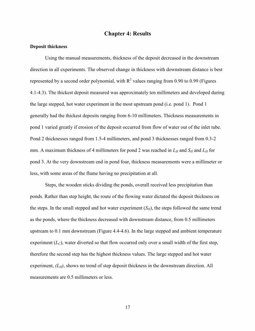
Using the manual measurements, thickness of the deposit decreased in the downstream
direction in all experiments. The observed change in thickness with downstream distance is best
represented by a second order polynomial, with R2 values ranging from 0.90 to 0.99 (Figures
4.1-4.3). The thickest deposit measured was approximately ten millimeters and developed during
the large stepped, hot water experiment in the most upstream pond (i.e. pond 1). Pond 1
generally had the thickest deposits ranging from 6-10 millimeters. Thickness measurements in
pond 1 varied greatly if erosion of the deposit occurred from flow of water out of the inlet tube.
Pond 2 thicknesses ranged from 1.5-4 millimeters, and pond 3 thicknesses ranged from 0.3-2
mm. A maximum thickness of 4 millimeters for pond 2 was reached in LH and SH and LH for
pond 3. At the very downstream end in pond four, thickness measurements were a millimeter or
less, with some areas of the flume having no precipitation at all.
Steps, the wooden sticks dividing the ponds, overall received less precipitation than
ponds. Rather than step height, the route of the flowing water dictated the deposit thickness on
the steps. In the small stepped and hot water experiment (SH), the steps followed the same trend
as the ponds, where the thickness decreased with downstream distance, from 0.5 millimeters
upstream to 0.1 mm downstream (Figure 4.4-4.6). In the large stepped and ambient temperature
experiment (LC), water diverted so that flow occurred only over a small width of the first step,
therefore the second step has the highest thickness values. The large stepped and hot water
experiment, (LH), shows no trend of step deposit thickness in the downstream direction. All
measurements are 0.5 millimeters or less.
18
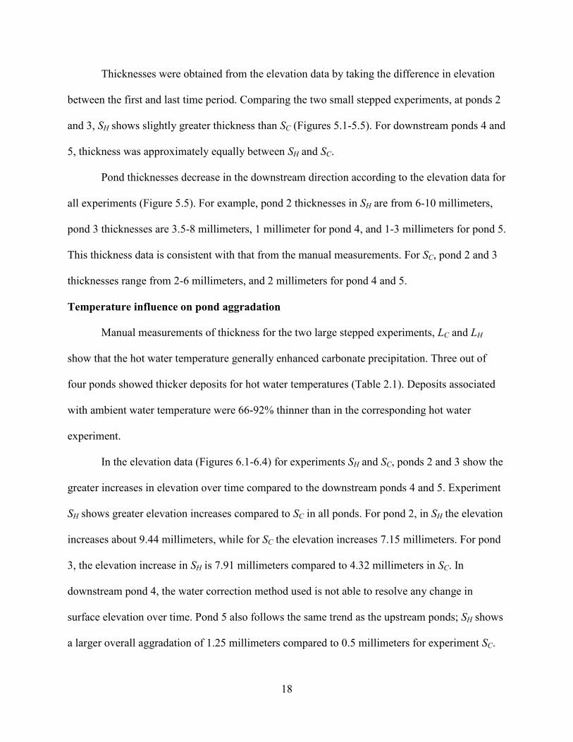
Thicknesses were obtained from the elevation data by taking the difference in elevation
between the first and last time period. Comparing the two small stepped experiments, at ponds 2
and 3, SH shows slightly greater thickness than SC (Figures 5.1-5.5). For downstream ponds 4 and
5, thickness was approximately equally between SH and SC.
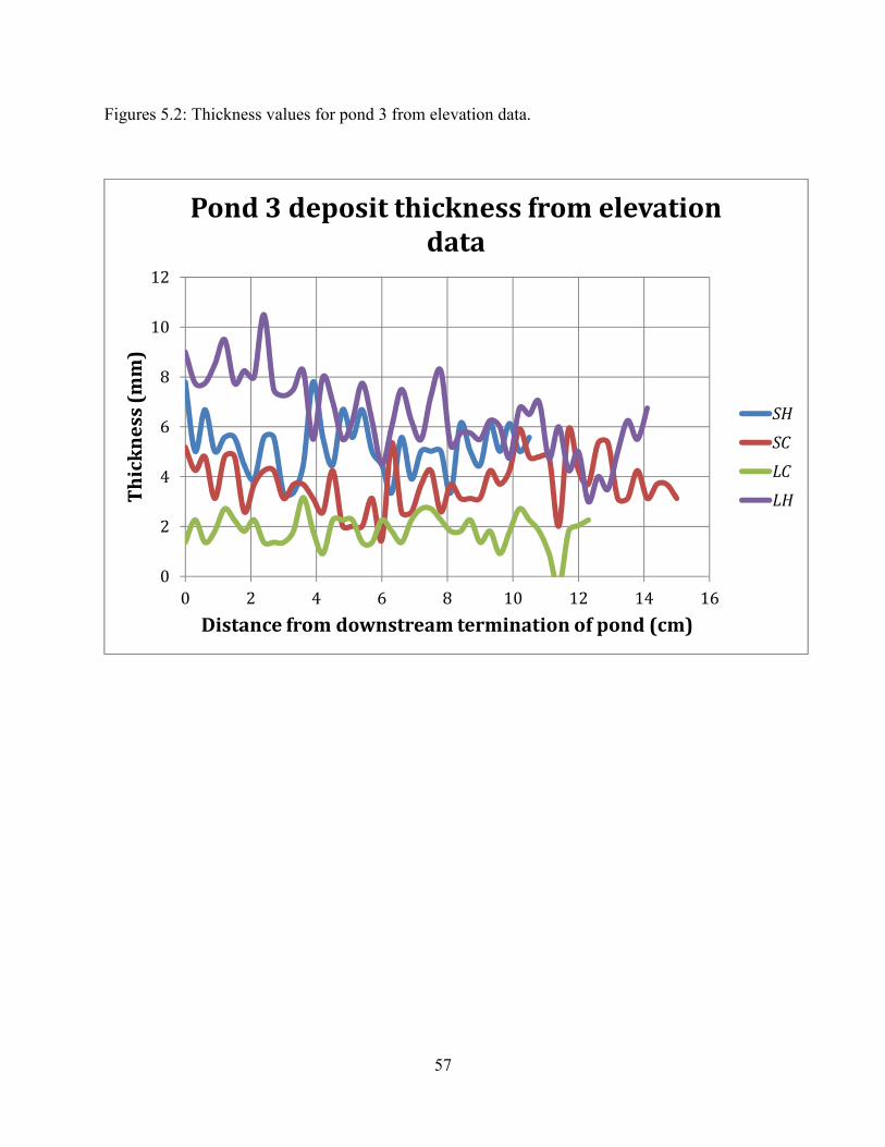
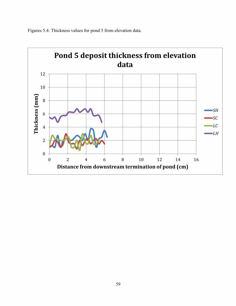
Pond thicknesses decrease in the downstream direction according to the elevation data for
all experiments (Figure 5.5). For example, pond 2 thicknesses in SH are from 6-10 millimeters,
pond 3 thicknesses are 3.5-8 millimeters, 1 millimeter for pond 4, and 1-3 millimeters for pond 5.
This thickness data is consistent with that from the manual measurements. For SC, pond 2 and 3
thicknesses range from 2-6 millimeters, and 2 millimeters for pond 4 and 5.
Temperature influence on pond aggradation
Manual measurements of thickness for the two large stepped experiments, LC and LH
show that the hot water temperature generally enhanced carbonate precipitation. Three out of
four ponds showed thicker deposits for hot water temperatures (Table 2.1). Deposits associated
with ambient water temperature were 66-92% thinner than in the corresponding hot water
experiment.
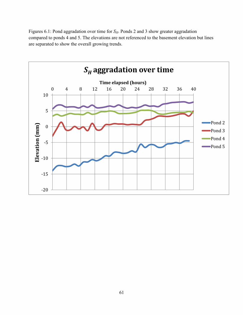
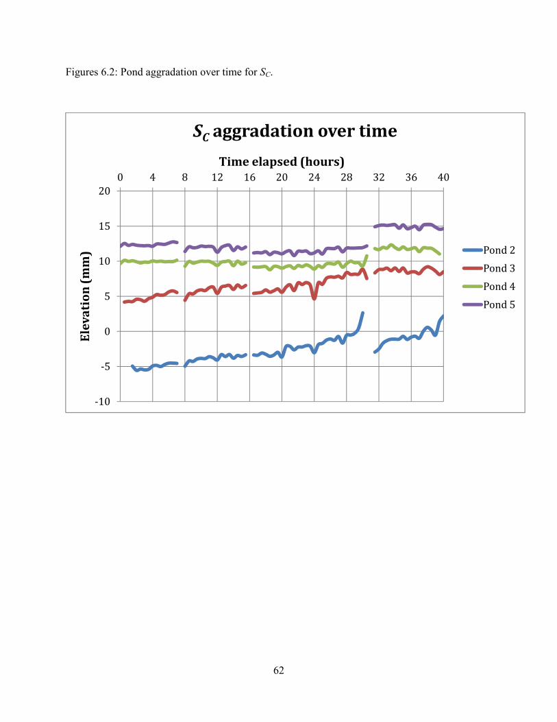
In the elevation data (Figures 6.1-6.4) for experiments SH and SC, ponds 2 and 3 show the
greater increases in elevation over time compared to the downstream ponds 4 and 5. Experiment
SH shows greater elevation increases compared to SC in all ponds. For pond 2, in SH the elevation
increases about 9.44 millimeters, while for SC the elevation increases 7.15 millimeters. For pond
3, the elevation increase in SH is 7.91 millimeters compared to 4.32 millimeters in SC. In
downstream pond 4, the water correction method used is not able to resolve any change in
surface elevation over time. Pond 5 also follows the same trend as the upstream ponds; SH shows
a larger overall aggradation of 1.25 millimeters compared to 0.5 millimeters for experiment SC.
19
Temperature influence applied equally to the results from the large step experiments. Both
manual measurements and topographic data consistently show higher aggradation rates in the hot
water experiments (Figures 6.1-6.4).
Step height influence on pond aggradation
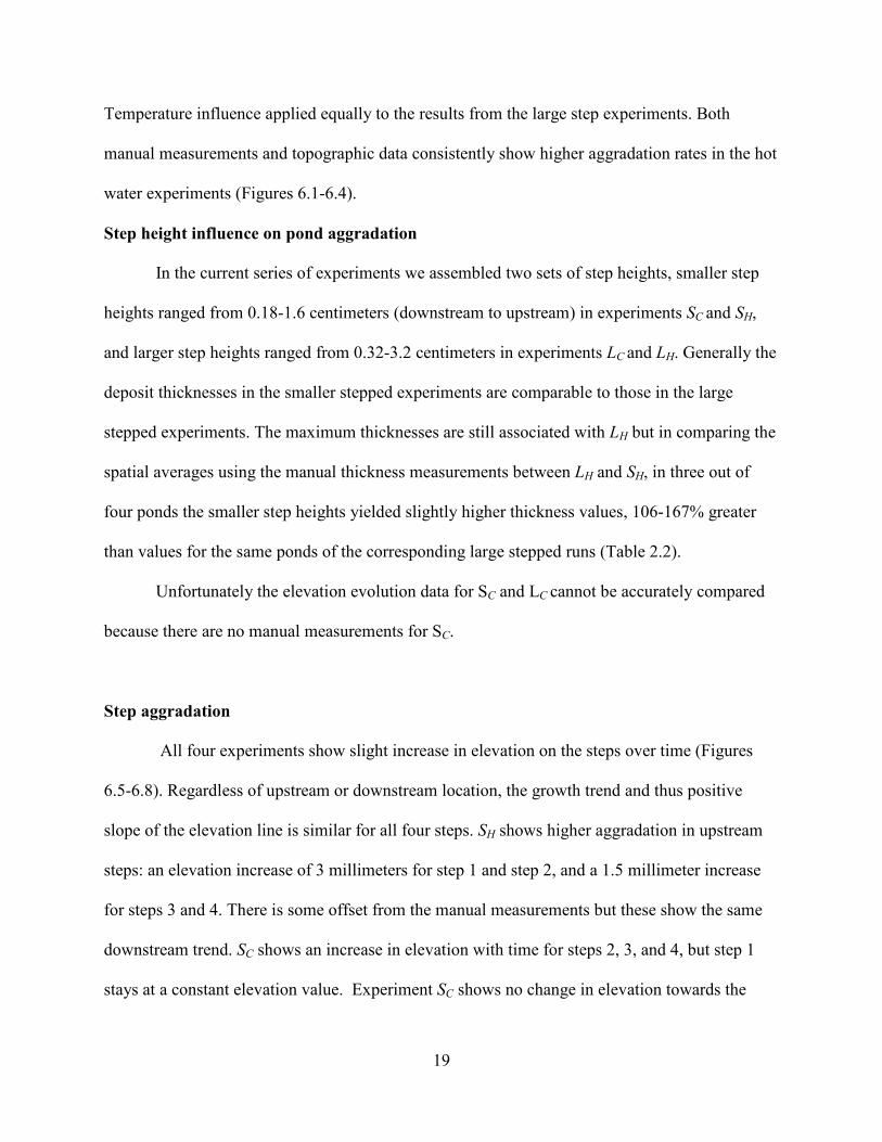
In the current series of experiments we assembled two sets of step heights, smaller step
heights ranged from 0.18-1.6 centimeters (downstream to upstream) in experiments SC and SH,
and larger step heights ranged from 0.32-3.2 centimeters in experiments LC and LH. Generally the
deposit thicknesses in the smaller stepped experiments are comparable to those in the large
stepped experiments. The maximum thicknesses are still associated with LH but in comparing the
spatial averages using the manual thickness measurements between LH and SH, in three out of
four ponds the smaller step heights yielded slightly higher thickness values, 106-167% greater
than values for the same ponds of the corresponding large stepped runs (Table 2.2).
Unfortunately the elevation evolution data for SC and LC cannot be accurately compared
because there are no manual measurements for SC.
Step aggradation
All four experiments show slight increase in elevation on the steps over time (Figures
6.5-6.8). Regardless of upstream or downstream location, the growth trend and thus positive
slope of the elevation line is similar for all four steps. SH shows higher aggradation in upstream
steps: an elevation increase of 3 millimeters for step 1 and step 2, and a 1.5 millimeter increase
for steps 3 and 4. There is some offset from the manual measurements but these show the same
downstream trend. SC shows an increase in elevation with time for steps 2, 3, and 4, but step 1
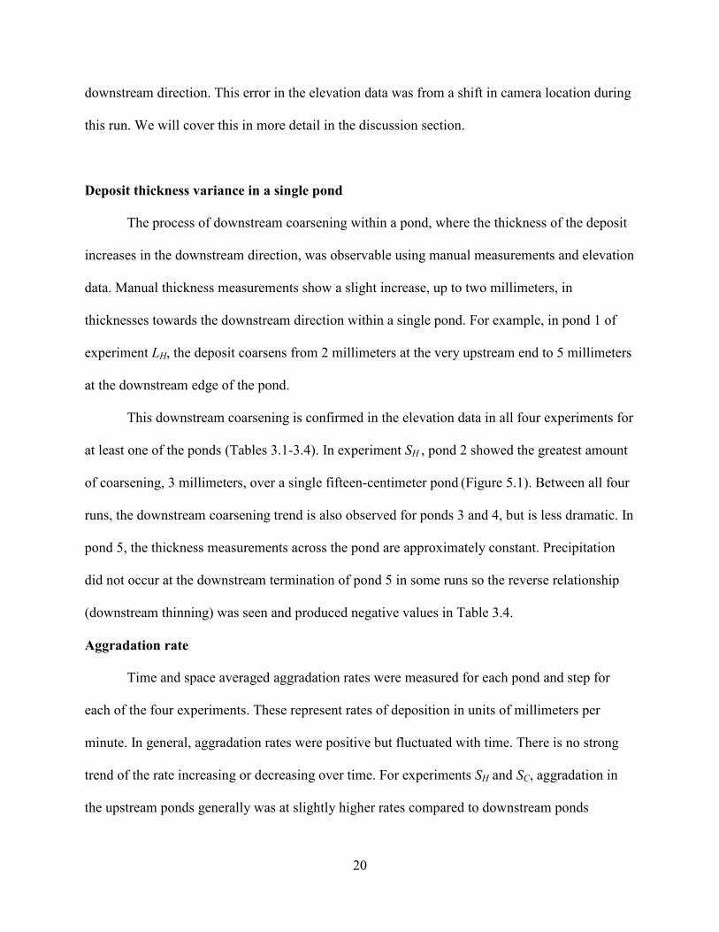
stays at a constant elevation value. Experiment SC shows no change in elevation towards the
20
downstream direction. This error in the elevation data was from a shift in camera location during
this run. We will cover this in more detail in the discussion section.
Deposit thickness variance in a single pond
The process of downstream coarsening within a pond, where the thickness of the deposit
increases in the downstream direction, was observable using manual measurements and elevation
data. Manual thickness measurements show a slight increase, up to two millimeters, in
thicknesses towards the downstream direction within a single pond. For example, in pond 1 of
experiment LH, the deposit coarsens from 2 millimeters at the very upstream end to 5 millimeters
at the downstream edge of the pond.
This downstream coarsening is confirmed in the elevation data in all four experiments for
at least one of the ponds (Tables 3.1-3.4). In experiment SH , pond 2 showed the greatest amount
of coarsening, 3 millimeters, over a single fifteen-centimeter pond (Figure 5.1). Between all four
runs, the downstream coarsening trend is also observed for ponds 3 and 4, but is less dramatic. In
pond 5, the thickness measurements across the pond are approximately constant. Precipitation
did not occur at the downstream termination of pond 5 in some runs so the reverse relationship
(downstream thinning) was seen and produced negative values in Table 3.4.
Aggradation rate
Time and space averaged aggradation rates were measured for each pond and step for
each of the four experiments. These represent rates of deposition in units of millimeters per
minute. In general, aggradation rates were positive but fluctuated with time. There is no strong
trend of the rate increasing or decreasing over time. For experiments SH and SC, aggradation in
the upstream ponds generally was at slightly higher rates compared to downstream ponds

21
(Figures 8.1-8.4 and Table 4.1 and 4.2). The majority of rates fall within an order of magnitude
of each other, the greatest magnitude difference being the increase in aggradation rate from 8.99
x 10-4 4 mm/min to 2.47 x 10
-3 mm/min from pond 5 to pond 2 in experiment SC, under ambient
water temperature and small stepped conditions. All of the other experiments showed a similar
trend, with pond 5 having the smallest aggradation rate and pond 2, the most upstream pond
measured, having the highest aggradation rate.
Comparing hot versus ambient water temperature runs, hot water runs had higher
aggradation rates. For the small stepped experiments SH and SC, the hot water experiment had
rates from 7.71 x 10⁻³ mm/min to 1.01 x 10
-3 mm/min, where as the ambient temperature
experiment had lower rates from 2.47 x 10⁻³ mm/min to 8.89 x 10
-4 mm/min (Table 4.1). The
magnitude of the fluctuation rate was higher for the hot water experiments compared to the
consistent growth shown in the ambient temperature experiments.
Comparing the aggradation rate between steps within each experiment, a similar trend
was found. Steps 1 or 2 had the highest rate of aggradation all experimental runs, and the
aggradation rate decreased towards the downstream direction in steps 3 and 4 (Table 4.2). Hot
water experiment SH also displayed higher aggradation rates on the steps compared to ambient
temperature experiments.
Comparing between ponds and steps most aggradation rates occur within the same orders
of magnitude (Table 4.1 and 4.2). Overall, the pond aggradations are slightly higher than those
on the steps. The most noticeable disparity is the rates between pond 3 and step 3, which divides
ponds 3 and 4. In experiment SC the aggradation rate in pond 3 is ten times greater than that on
step 3.
22
Chapter 5: Discussion
Temperature influence on bed aggradation
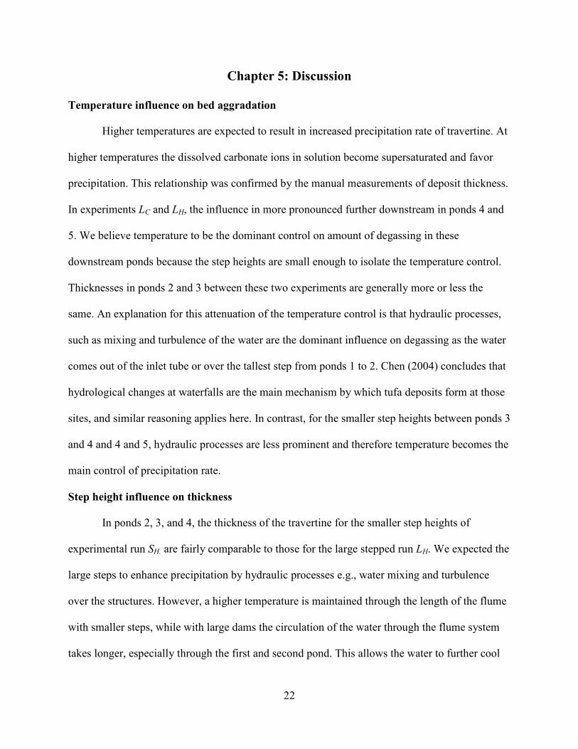
Higher temperatures are expected to result in increased precipitation rate of travertine. At
higher temperatures the dissolved carbonate ions in solution become supersaturated and favor
precipitation. This relationship was confirmed by the manual measurements of deposit thickness.
In experiments LC and LH, the influence in more pronounced further downstream in ponds 4 and
5. We believe temperature to be the dominant control on amount of degassing in these
downstream ponds because the step heights are small enough to isolate the temperature control.
Thicknesses in ponds 2 and 3 between these two experiments are generally more or less the
same. An explanation for this attenuation of the temperature control is that hydraulic processes,
such as mixing and turbulence of the water are the dominant influence on degassing as the water
comes out of the inlet tube or over the tallest step from ponds 1 to 2. Chen (2004) concludes that
hydrological changes at waterfalls are the main mechanism by which tufa deposits form at those
sites, and similar reasoning applies here. In contrast, for the smaller step heights between ponds 3
and 4 and 4 and 5, hydraulic processes are less prominent and therefore temperature becomes the
main control of precipitation rate.
Step height influence on thickness
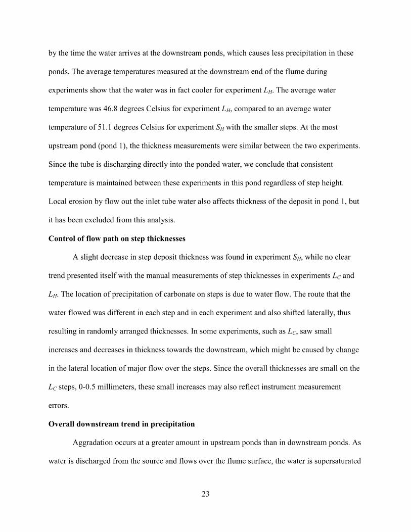
In ponds 2, 3, and 4, the thickness of the travertine for the smaller step heights of
experimental run SH. are fairly comparable to those for the large stepped run LH. We expected the
large steps to enhance precipitation by hydraulic processes e.g., water mixing and turbulence
over the structures. However, a higher temperature is maintained through the length of the flume
with smaller steps, while with large dams the circulation of the water through the flume system
takes longer, especially through the first and second pond. This allows the water to further cool
23
by the time the water arrives at the downstream ponds, which causes less precipitation in these
ponds. The average temperatures measured at the downstream end of the flume during
experiments show that the water was in fact cooler for experiment LH. The average water
temperature was 46.8 degrees Celsius for experiment LH, compared to an average water
temperature of 51.1 degrees Celsius for experiment SH with the smaller steps. At the most
upstream pond (pond 1), the thickness measurements were similar between the two experiments.
Since the tube is discharging directly into the ponded water, we conclude that consistent
temperature is maintained between these experiments in this pond regardless of step height.
Local erosion by flow out the inlet tube water also affects thickness of the deposit in pond 1, but
it has been excluded from this analysis.
Control of flow path on step thicknesses
A slight decrease in step deposit thickness was found in experiment SH, while no clear
trend presented itself with the manual measurements of step thicknesses in experiments LC and
LH. The location of precipitation of carbonate on steps is due to water flow. The route that the
water flowed was different in each step and in each experiment and also shifted laterally, thus
resulting in randomly arranged thicknesses. In some experiments, such as LC, saw small
increases and decreases in thickness towards the downstream, which might be caused by change
in the lateral location of major flow over the steps. Since the overall thicknesses are small on the
LC steps, 0-0.5 millimeters, these small increases may also reflect instrument measurement
errors.
Overall downstream trend in precipitation
Aggradation occurs at a greater amount in upstream ponds than in downstream ponds. As
water is discharged from the source and flows over the flume surface, the water is supersaturated
24
with carbonate and calcite ions, so precipitation of travertine is highly favorable. But as
degassing of CO2 and precipitation of travertine initiates, the ion concentration falls below the
saturation point, and degassing and precipitation become less favorable and will decrease
downstream. With our experimental setup, small step heights were placed downstream and
higher step heights were upstream. Since turbulence and mixing of water promotes precipitation
of travertine, our experimental set up also favors higher precipitation at the upstream end, where
higher dam height drops promote these hydraulic processes occurring.
Aggradation for steps was less than that in ponds and was steady over time. Experiment
SH shows a higher overall amount of aggradation for upstream steps compared to downstream
steps, which follows the same trend as the ponds.
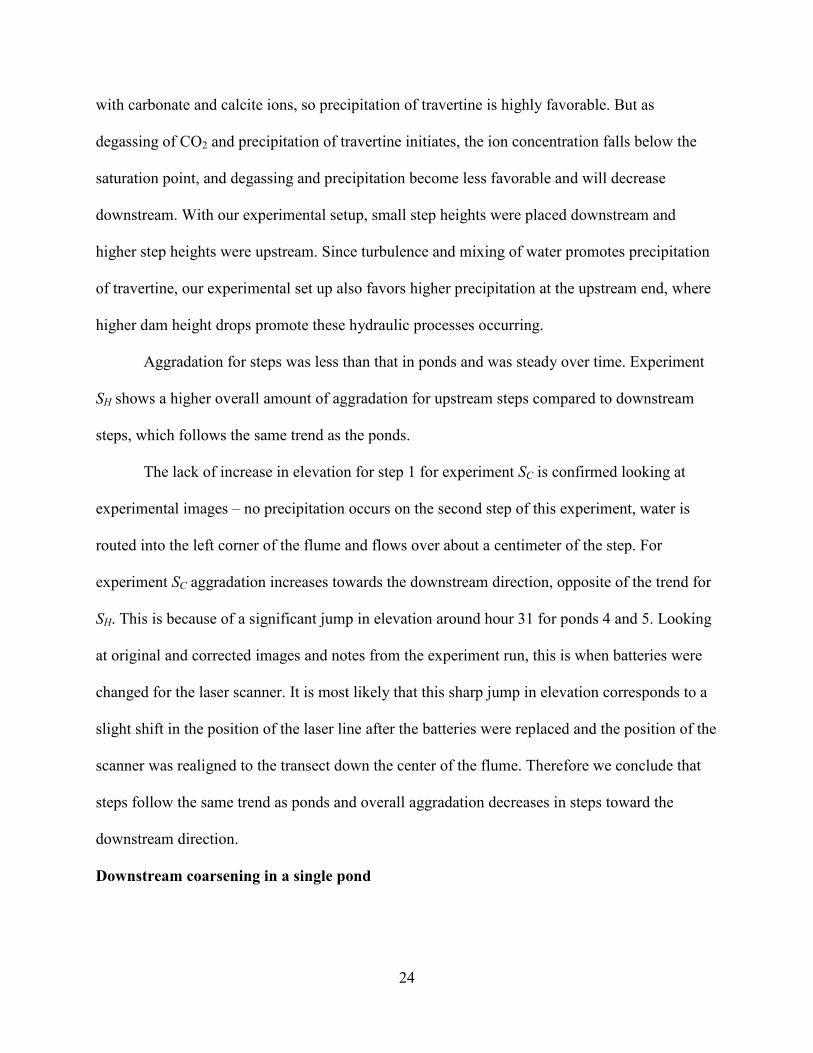
The lack of increase in elevation for step 1 for experiment SC is confirmed looking at
experimental images – no precipitation occurs on the second step of this experiment, water is
routed into the left corner of the flume and flows over about a centimeter of the step. For
experiment SC aggradation increases towards the downstream direction, opposite of the trend for
SH. This is because of a significant jump in elevation around hour 31 for ponds 4 and 5. Looking
at original and corrected images and notes from the experiment run, this is when batteries were
changed for the laser scanner. It is most likely that this sharp jump in elevation corresponds to a
slight shift in the position of the laser line after the batteries were replaced and the position of the
scanner was realigned to the transect down the center of the flume. Therefore we conclude that
steps follow the same trend as ponds and overall aggradation decreases in steps toward the
downstream direction.
Downstream coarsening in a single pond

25
The downstream coarsening trend was observable especially in upstream ponds (e.g.,
ponds 1, 2, and 3) for all four experiments. Pond 4 also shows comparably smaller, but still
positive values for downstream coarsening (Table 3.3). The mechanism for downstream
coarsening can be attributed to two processes. 1) Erosion can take place immediately after the
vertical drop of a step at the immediate upstream of a pond; at these locations turbulence of the
water can erode the existing fragile travertine precipitate from the bottom of the pond. 2) As
water travels through the length of a pond and approaches the step downstream, flow accelerates
until it reaches the downstream termination of a pond. Since the velocity of the water increases
over the length of the pond, and travertine precipitation rate increases with increasing agitation
of water, more aggradation occurs as the water travels downstream.
Fluctuations in aggradation rate with time
The pattern shown in the plots of aggradation rate in a single pond over time include
small fluctuations and large fluctuations (Figures 8.1-8.4). The small fluctuations in aggradation
rate of 0.1 millimeters are most likely resulting from instrument error of the laser scanner,
discharge inconsistencies due to tubing leaks or clogging or other complications experienced
during experimental runs, and/or image analysis. The thickness of the laser line is approximately
one millimeter, giving an instrument error of 1 mm/30 minutes or 0.03 mm/minute, so most
small fluctuations from one time period to the next fall within this error range.
For the large changes in aggradation rate, whether these are natural processes or
experimental error are unknown. However, the time variability of the aggradation rates shown is
systematically higher in the hot water experiments. LH and SH had a temperature decrease of 10-
20 degrees Celsius from the upstream to the downstream. The temperature reduction through the
26
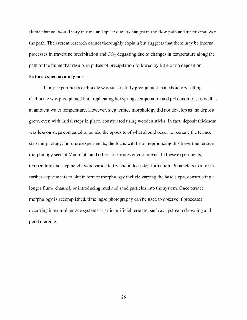
flume channel would vary in time and space due to changes in the flow path and air mixing over
the path. The current research cannot thoroughly explain but suggests that there may be internal
processes in travertine precipitation and CO2 degassing due to changes in temperature along the
path of the flume that results in pulses of precipitation followed by little or no deposition.
Future experimental goals
In my experiments carbonate was successfully precipitated in a laboratory setting.
Carbonate was precipitated both replicating hot springs temperature and pH conditions as well as
at ambient water temperature. However, step terrace morphology did not develop as the deposit
grew, even with initial steps in place, constructed using wooden sticks. In fact, deposit thickness
was less on steps compared to ponds, the opposite of what should occur to recreate the terrace
step morphology. In future experiments, the focus will be on reproducing this travertine terrace
morphology seen at Mammoth and other hot springs environments. In these experiments,
temperature and step height were varied to try and induce step formation. Parameters to alter in
further experiments to obtain terrace morphology include varying the base slope, constructing a
longer flume channel, or introducing mud and sand particles into the system. Once terrace
morphology is accomplished, time lapse photography can be used to observe if processes
occurring in natural terrace systems arise in artificial terraces, such as upstream drowning and
pond merging.
27
Chapter 6: Conclusions
While temperature and step height can influence precipitation rate, upstream versus
downstream position and vicinity to a step edge equally play a factor in how much precipitation
will occur. Water hydraulics can drastically change based on location within a terrace. Directly
after a step, with the change in height, turbulence, and mixing of the water cause erosion of the
deposited travertine substrate. As the water travels downstream within a single pond, velocity
increases until the next step “waterfall” and enhances precipitation. These hydrological
properties can dominate if step heights are large or if the inlet source of water is nearby. If
locations are far from the source, with lower velocities and calmer flow, or if step heights are
small, temperature can have a more dominate role on precipitation. Higher temperatures induce
more precipitation, so for the hot water experiments, SH and LH, more precipitation would occur
compared to the ambient temperature experiments. The conclusions are summarized as follows:
1. Carbonate thickness and overall precipitation rate in ponds are greatest upstream and
decrease downstream.
2. Aggradation rates on the top of steps are overall lower compared to adjacent ponds.
3. Temperature is a more dominant control in downstream ponds compared to upstream
ponds, where hydraulic processes play a greater role.
4. Small steps in SH induce a higher precipitation rate comparable to ones in LH, due to
loss of heat in the large stepped experiments towards the downstream. Larger steps
may have just as high of a precipitation rate as small steps in ponds right by the inlet
source of hot water.

28
5. There is no trend in aggradation rate over time. However, the magnitude of
fluctuations is higher in the hot water experiments due to a wider range of
temperature decrease over the flow through the flume.
29
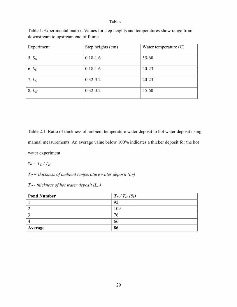
Table 1:Experimental matrix. Values for step heights and temperatures show range from
downstream to upstream end of flume.
Experiment Step heights (cm) Water temperature (C)
5, SH 0.18-1.6 55-60
6, SC 0.18-1.6 20-23
7, LC 0.32-3.2 20-23
8, LH 0.32-3.2 55-60
Table 2.1: Ratio of thickness of ambient temperature water deposit to hot water deposit using
manual measurements. An average value below 100% indicates a thicker deposit for the hot
water experiment.
% = TC / TH
TC = thickness of ambient temperature water deposit (LC)
TH - thickness of hot water deposit (LH)
Pond Number TC / TH (%)
1 92
2 109
3 76
4 66
Average 86
Tables
30
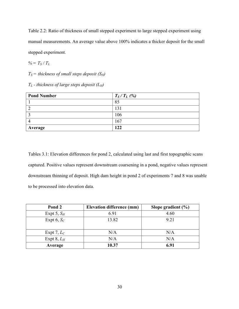
Table 2.2: Ratio of thickness of small stepped experiment to large stepped experiment using
manual measurements. An average value above 100% indicates a thicker deposit for the small
stepped experiment.
% = TS / TL
TS = thickness of small steps deposit (SH)
TL - thickness of large steps deposit (LH)
Pond Number TS / TL (%)
1 85
2 131
3 106
4 167
Average 122
Tables 3.1: Elevation differences for pond 2, calculated using last and first topographic scans
captured. Positive values represent downstream coarsening in a pond, negative values represent
downstream thinning of deposit. High dam height in pond 2 of experiments 7 and 8 was unable
to be processed into elevation data.
Pond 2 Elevation difference (mm) Slope gradient (%)
Expt 5, SH 6.91 4.60
Expt 6, SC 13.82 9.21
Expt 7, LC N/A N/A
Expt 8, LH N/A N/A
Average 10.37 6.91
31
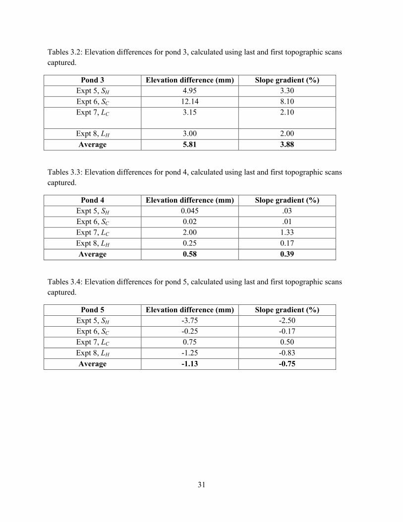
Tables 3.2: Elevation differences for pond 3, calculated using last and first topographic scans
captured.
Pond 3 Elevation difference (mm) Slope gradient (%)
Expt 5, SH 4.95 3.30
Expt 6, SC 12.14 8.10
Expt 7, LC 3.15
2.10
Expt 8, LH 3.00 2.00
Average 5.81 3.88
Tables 3.3: Elevation differences for pond 4, calculated using last and first topographic scans
captured.
Pond 4 Elevation difference (mm) Slope gradient (%)
Expt 5, SH 0.045 .03
Expt 6, SC 0.02 .01
Expt 7, LC 2.00 1.33
Expt 8, LH 0.25 0.17
Average 0.58 0.39
Tables 3.4: Elevation differences for pond 5, calculated using last and first topographic scans
captured.
Pond 5 Elevation difference (mm) Slope gradient (%)
Expt 5, SH -3.75 -2.50
Expt 6, SC -0.25 -0.17
Expt 7, LC 0.75 0.50
Expt 8, LH -1.25 -0.83
Average -1.13 -0.75
32
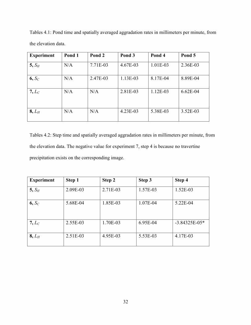
Tables 4.1: Pond time and spatially averaged aggradation rates in millimeters per minute, from
the elevation data.
Experiment Pond 1 Pond 2 Pond 3 Pond 4 Pond 5
5, SH N/A 7.71E-03 4.67E-03 1.01E-03 2.36E-03
6, SC N/A 2.47E-03 1.13E-03 8.17E-04 8.89E-04
7, LC N/A N/A 2.81E-03 1.12E-03 6.62E-04
8, LH N/A N/A 4.23E-03 5.38E-03 3.52E-03
Tables 4.2: Step time and spatially averaged aggradation rates in millimeters per minute, from
the elevation data. The negative value for experiment 7, step 4 is because no travertine
precipitation exists on the corresponding image.
Experiment Step 1 Step 2 Step 3 Step 4
5, SH 2.09E-03 2.71E-03 1.57E-03 1.52E-03
6, SC 5.68E-04 1.85E-03 1.07E-04 5.22E-04
7, LC 2.55E-03 1.70E-03 6.95E-04 -3.84325E-05*
8, LH 2.51E-03 4.95E-03 5.53E-03 4.17E-03
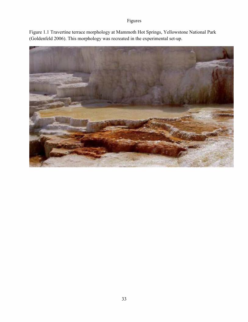
33
Figure 1.1 Travertine terrace morphology at Mammoth Hot Springs, Yellowstone National Park
(Goldenfeld 2006). This morphology was recreated in the experimental set-up.
Figures

34
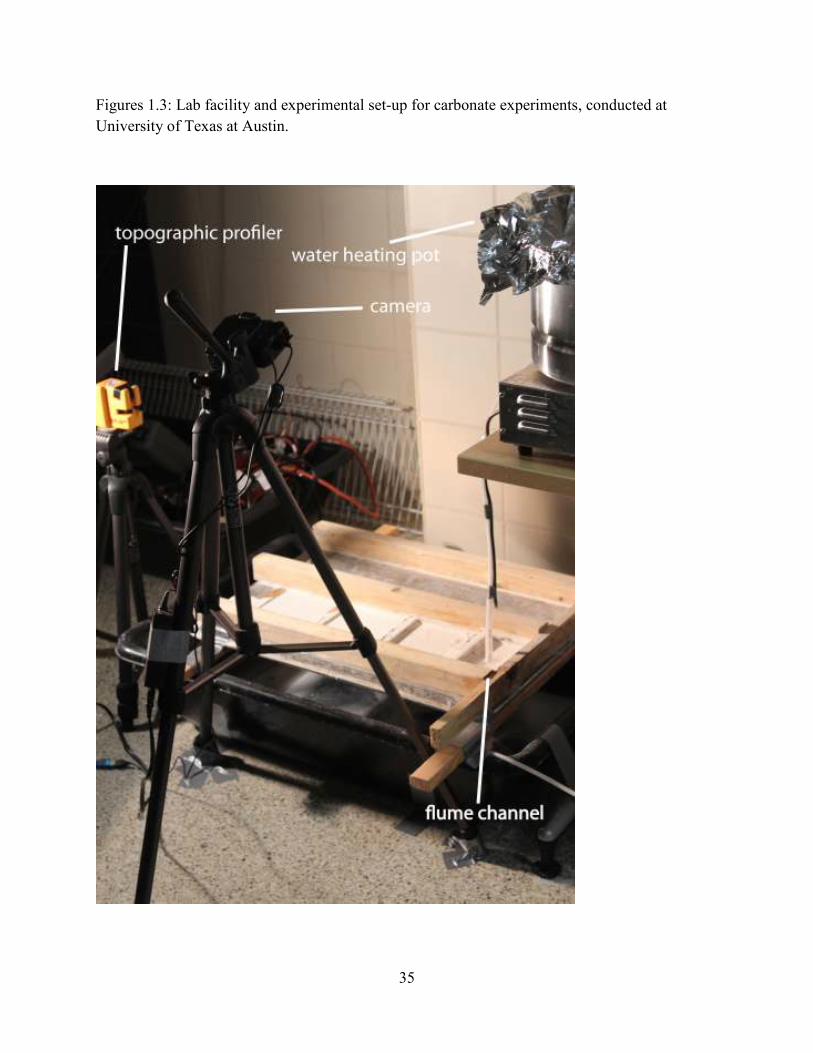
Figures 1.2: Lab facility and experimental set-up for carbonate experiments, conducted at
University of Texas at Austin.
35
Figures 1.3: Lab facility and experimental set-up for carbonate experiments, conducted at
University of Texas at Austin.

Figure 1.4: Flume design and dimensions. The flum
steps (S).
36
Figure 1.4: Flume design and dimensions. The flume was composed of five ponds (P) and foure was composed of five ponds (P) and four

37
Figures 2.1: SH temperature at the upstream and downstream ends measured every thirty minutes
over the experimental run.
45
47
49
51
53
55
57
59
61
63
65
0 4 8 12 16 20 24 28 32 36 40
Te
mp
era
ture
(C
els
ius
)
Time elapsed (hours)
SH
temperature
upstream
downstream
38
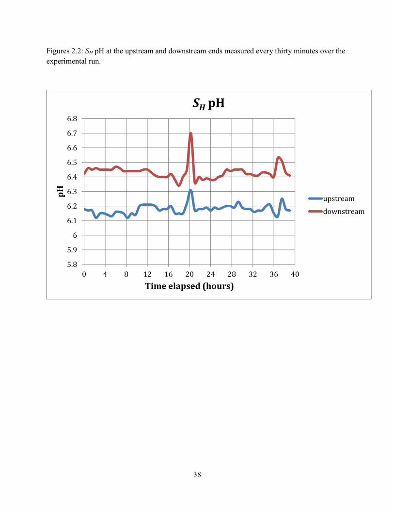
Figures 2.2: SH pH at the upstream and downstream ends measured every thirty minutes over the
experimental run.
5.8
5.9
6
6.1
6.2
6.3
6.4
6.5
6.6
6.7
6.8
0 4 8 12 16 20 24 28 32 36 40
pH
Time elapsed (hours)
SH
pH
upstream
downstream
39
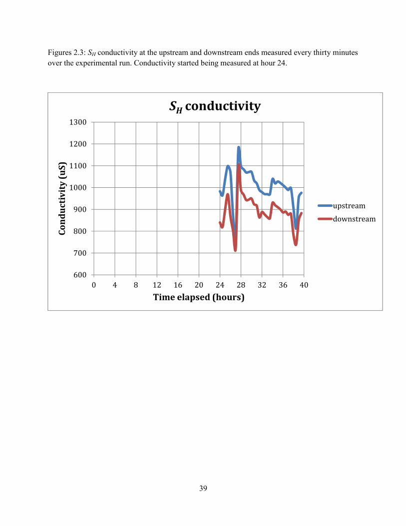
Figures 2.3: SH conductivity at the upstream and downstream ends measured every thirty minutes
over the experimental run. Conductivity started being measured at hour 24.
600
700
800
900
1000
1100
1200
1300
0 4 8 12 16 20 24 28 32 36 40
Co
nd
uc
tiv
ity
(u
S)
Time elapsed (hours)
SH
conductivity
upstream
downstream
40
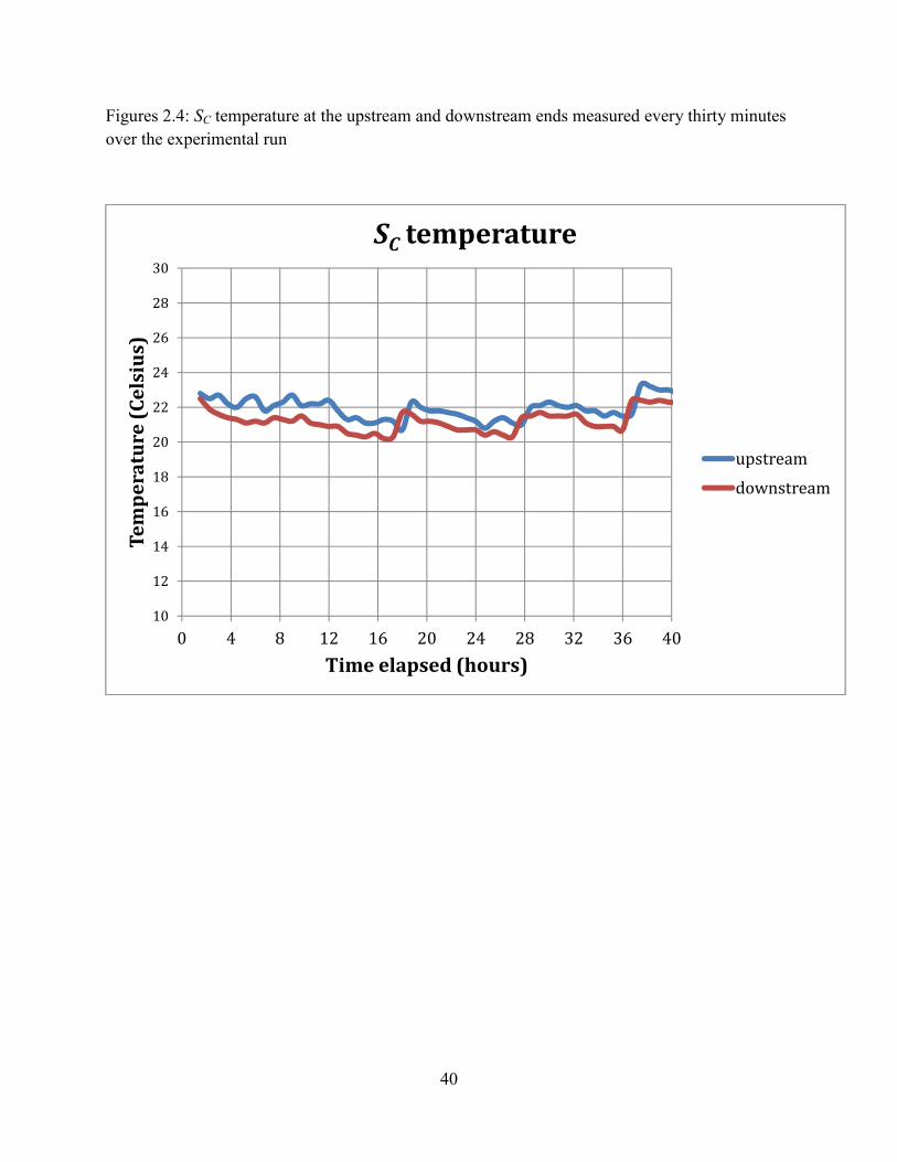
Figures 2.4: SC temperature at the upstream and downstream ends measured every thirty minutes
over the experimental run
10
12
14
16
18
20
22
24
26
28
30
0 4 8 12 16 20 24 28 32 36 40
Te
mp
era
ture
(C
els
ius
)
Time elapsed (hours)
SC
temperature
upstream
downstream

41
Figures 2.5: SC pH at the upstream and downstream ends measured every thirty minutes over the
experimental run
5.6
5.7
5.8
5.9
6
6.1
6.2
6.3
6.4
6.5
6.6
0 4 8 12 16 20 24 28 32 36 40
pH
Time elapsed (hours)
SC
pH
upstream
downstream

42
Figures 2.6: SC conductivity at the upstream and downstream ends measured every thirty minutes
over the experimental run
900
1000
1100
1200
1300
1400
1500
1600
0 4 8 12 16 20 24 28 32 36 40
Co
nd
uc
tiv
ity
(u
S)
Time elapsed (hours)
SC
conductivity
upstream
downstream
43
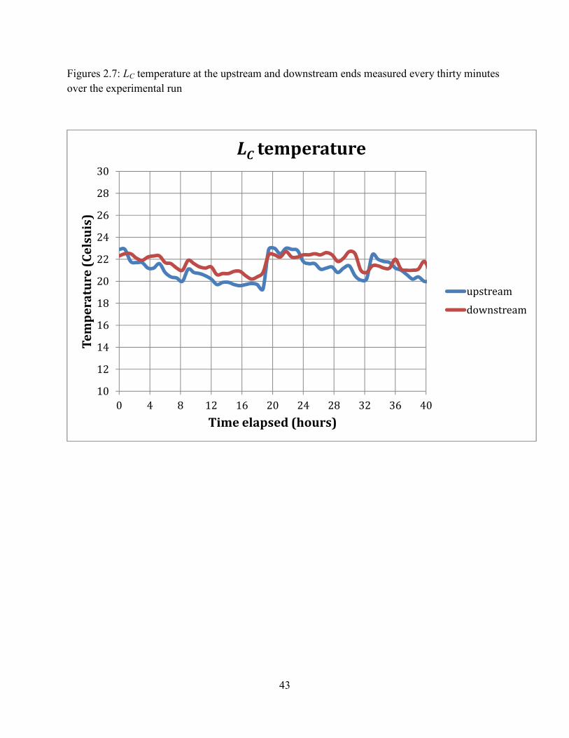
Figures 2.7: LC temperature at the upstream and downstream ends measured every thirty minutes
over the experimental run
10
12
14
16
18
20
22
24
26
28
30
0 4 8 12 16 20 24 28 32 36 40
Te
mp
era
ture
(C
els
uis
)
Time elapsed (hours)
LC
temperature
upstream
downstream

44
Figures 2.8: LC pH at the upstream and downstream ends measured every thirty minutes over the
experimental run
5.5
5.6
5.7
5.8
5.9
6
6.1
6.2
6.3
6.4
6.5
0 4 8 12 16 20 24 28 32 36 40
pH
Time elapsed (hours)
LC
pH
upstream
downstream
45
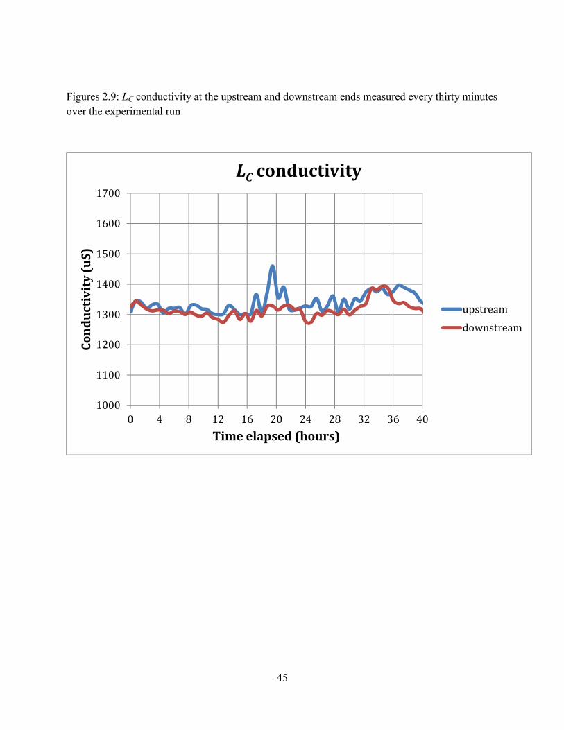
Figures 2.9: LC conductivity at the upstream and downstream ends measured every thirty minutes
over the experimental run
1000
1100
1200
1300
1400
1500
1600
1700
0 4 8 12 16 20 24 28 32 36 40
Co
nd
uc
tiv
ity
(u
S)
Time elapsed (hours)
LC
conductivity
upstream
downstream
46
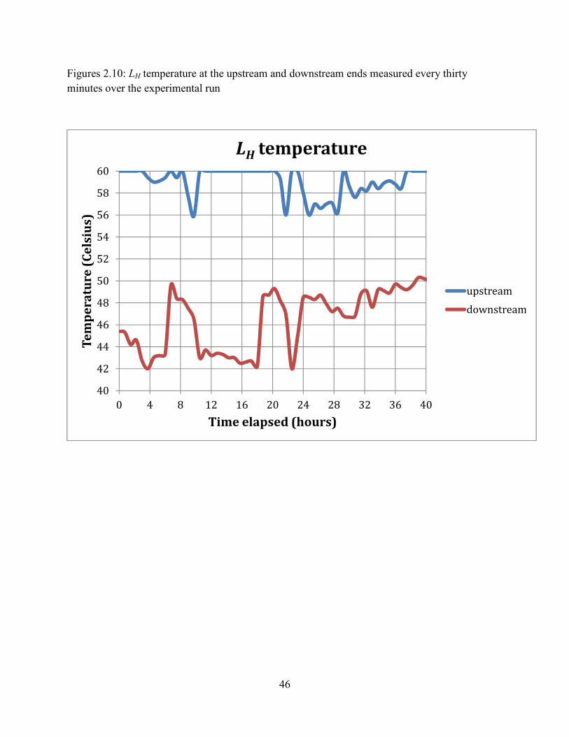
Figures 2.10: LH temperature at the upstream and downstream ends measured every thirty
minutes over the experimental run
40
42
44
46
48
50
52
54
56
58
60
0 4 8 12 16 20 24 28 32 36 40
Te
mp
era
ture
(C
els
ius
)
Time elapsed (hours)
LH
temperature
upstream
downstream
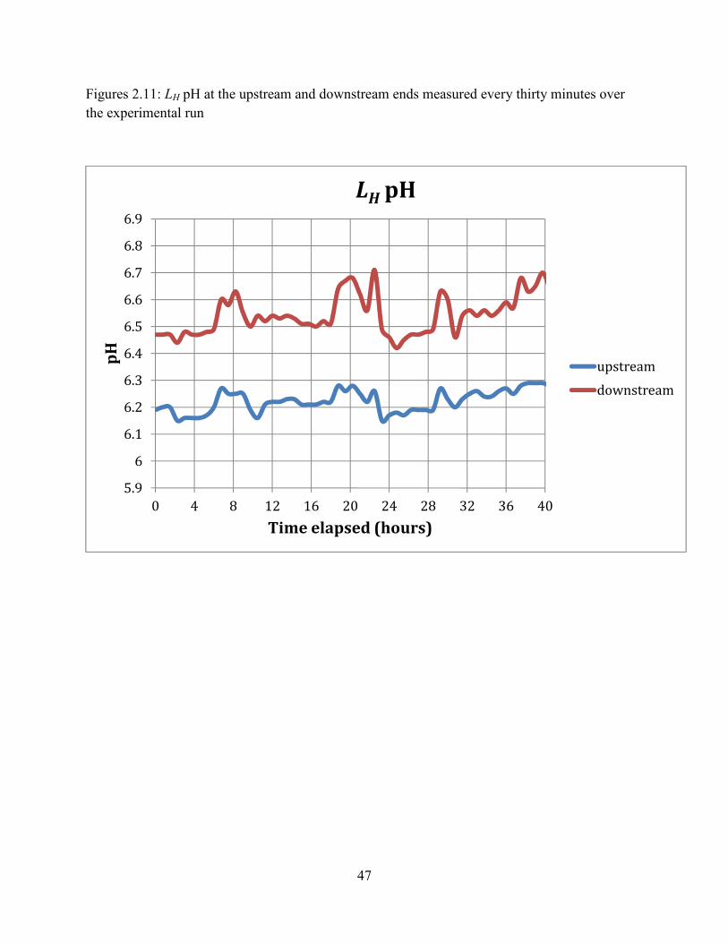
47
Figures 2.11: LH pH at the upstream and downstream ends measured every thirty minutes over
the experimental run
5.9
6
6.1
6.2
6.3
6.4
6.5
6.6
6.7
6.8
6.9
0 4 8 12 16 20 24 28 32 36 40
pH
Time elapsed (hours)
LH
pH
upstream
downstream
48
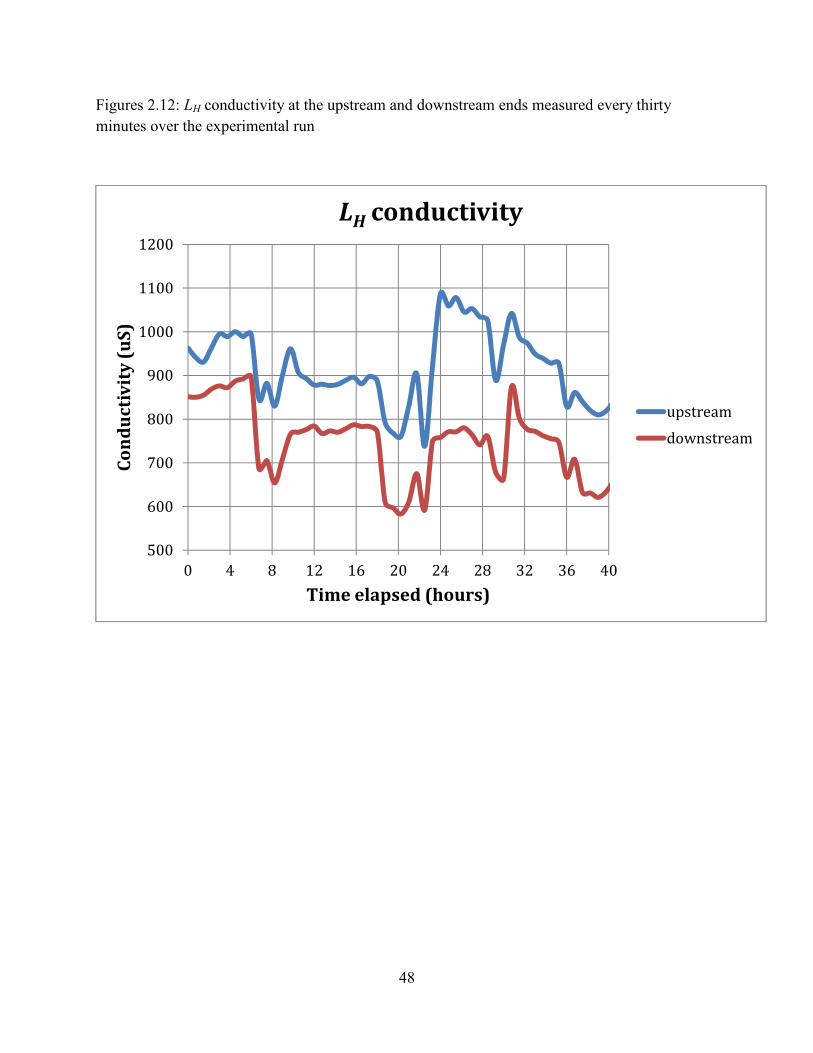
Figures 2.12: LH conductivity at the upstream and downstream ends measured every thirty
minutes over the experimental run
500
600
700
800
900
1000
1100
1200
0 4 8 12 16 20 24 28 32 36 40
Co
nd
uc
tiv
ity
(u
S)
Time elapsed (hours)
LH
conductivity
upstream
downstream
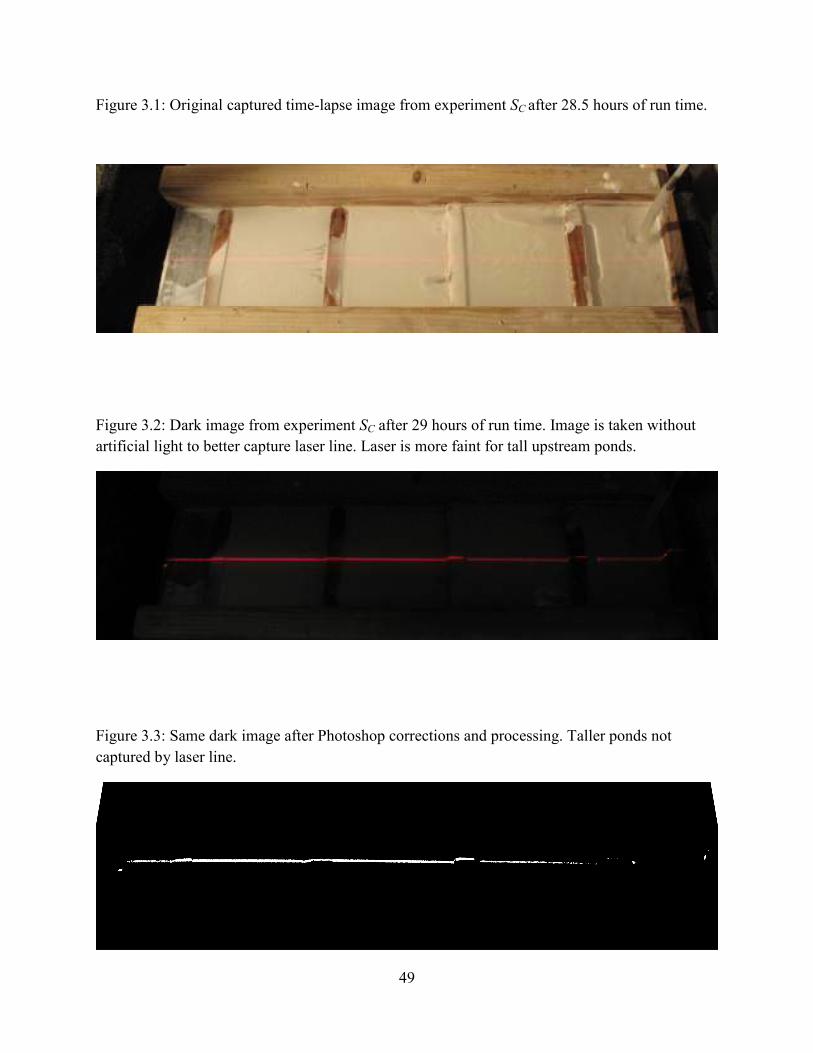
49
Figure 3.1: Original captured time-lapse image from experiment SC after 28.5 hours of run time.
Figure 3.2: Dark image from experiment SC after 29 hours of run time. Image is taken without
artificial light to better capture laser line. Laser is more faint for tall upstream ponds.
Figure 3.3: Same dark image after Photoshop corrections and processing. Taller ponds not
captured by laser line.
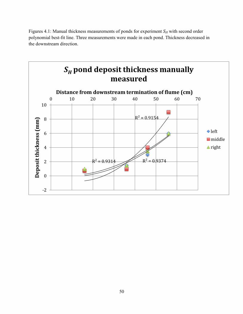
Figures 4.1: Manual thickness measu
polynomial best-fit line. Three measurements were m
the downstream direction.
-2
0
2
4
6
8
100 10 20
De
po
sit
th
ick
ne
ss
(m
m)
Distance from downstream termination of flume (cm)
SH
pond d
50
: Manual thickness measurements of ponds for experiment SH with second order
fit line. Three measurements were made in each pond. Thickness decreased in
R² = 0.9374
R² = 0.9154
R² = 0.9314
20 30 40 50 60
Distance from downstream termination of flume (cm)
pond deposit thickness manually
measured
with second order
. Thickness decreased in
70
Distance from downstream termination of flume (cm)
eposit thickness manually
left
middle
right

Figures 4.2: Manual thickness measu
polynomial best-fit line. Six measure
downstream direction.
-2
0
2
4
6
8
100 10 20
De
po
sit
th
ick
ne
ss
(m
m)
Distance from downstream termination of flume (cm)
LC
pond d
51
: Manual thickness measurements of ponds for experiment LC with second order
ix measurements were made in each pond. Thickness decreased in the
R² = 0.9403
R² = 0.9427
20 30 40 50 60
Distance from downstream termination of flume (cm)
pond deposit thickness manually
measured
with second order
. Thickness decreased in the
R² = 0.9427
R² = 0.9216
70
Distance from downstream termination of flume (cm)
eposit thickness manually
left
middle
right
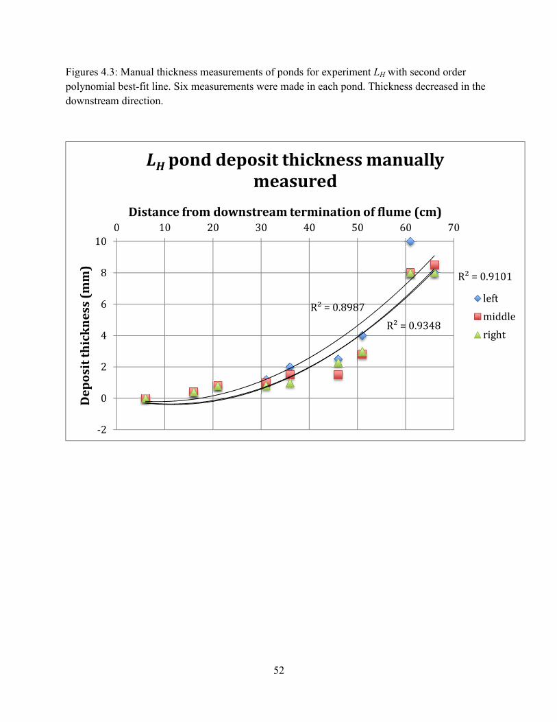
Figures 4.3: Manual thickness measur
polynomial best-fit line. Six measurements were ma
downstream direction.
-2
0
2
4
6
8
100 10 20
De
po
sit
th
ick
ne
ss
(m
m)
Distance from downstream termination of flume (cm)
LH
pond d
52
4.3: Manual thickness measurements of ponds for experiment LH with second order
ix measurements were made in each pond. Thickness decreased in the
R² = 0.8987
R² = 0.9348
20 30 40 50 60
Distance from downstream termination of flume (cm)
pond deposit thickness manually
measured
with second order
. Thickness decreased in the
R² = 0.9101
R² = 0.9348
70
Distance from downstream termination of flume (cm)
eposit thickness manually
left
middle
right
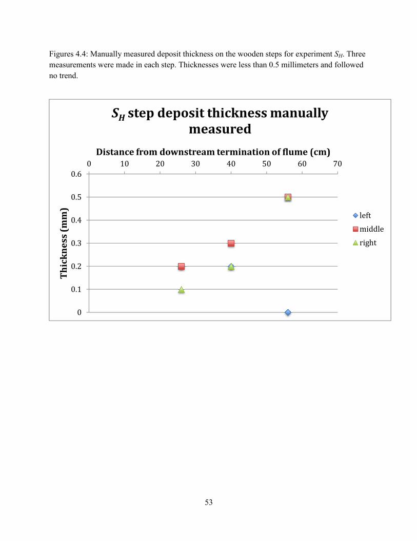
Figures 4.4: Manually measured deposit thickness on
measurements were made in each step.
no trend.
0
0.1
0.2
0.3
0.4
0.5
0.60 10 20
Th
ick
ne
ss
(m
m)
Distance from downstream termination of flume (cm)
SH
step deposit thickness manually
53
: Manually measured deposit thickness on the wooden steps for experim
measurements were made in each step. Thicknesses were less than 0.5 millimeters and followed
20 30 40 50 60
Distance from downstream termination of flume (cm)
step deposit thickness manually
measured
the wooden steps for experiment SH. Three
Thicknesses were less than 0.5 millimeters and followed
70
Distance from downstream termination of flume (cm)
step deposit thickness manually
left
middle
right

Figures 4.5: Manually measured deposit thickness on t
0
0.1
0.2
0.3
0.4
0.5
0.60 10
Th
ick
ne
ss
(m
m)
Distance from downstream termination of flume (cm)
LC
step deposit thickness manually
54
: Manually measured deposit thickness on the wooden steps for experiment
20 30 40 50 60
Distance from downstream termination of flume (cm)
step deposit thickness manually
measured
he wooden steps for experiment LC.
70
Distance from downstream termination of flume (cm)
step deposit thickness manually
left
middle
right

Figures 4.6: Manually measured deposit thickness on the wooden steps for experiment
0
0.1
0.2
0.3
0.4
0.5
0.60 10
Th
ick
ne
ss
(m
m)
Distance from downstream termination of flume (cm)
LH
step deposit thickness manually
55
asured deposit thickness on the wooden steps for experiment
20 30 40 50 60
Distance from downstream termination of flume (cm)
step deposit thickness manually
measured
asured deposit thickness on the wooden steps for experiment LH.
70
Distance from downstream termination of flume (cm)
step deposit thickness manually
left
middle
right
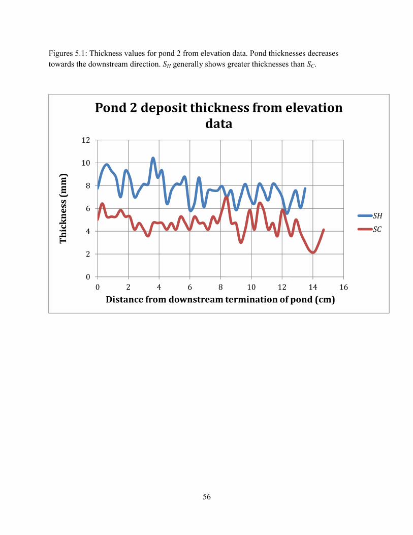
56
Figures 5.1: Thickness values for pond 2 from elevation data. Pond thicknesses decreases
towards the downstream direction. SH generally shows greater thicknesses than SC.
0
2
4
6
8
10
12
0 2 4 6 8 10 12 14 16
Th
ick
ne
ss
(m
m)
Distance from downstream termination of pond (cm)
Pond 2 deposit thickness from elevation
data
SH
SC
57
Figures 5.2: Thickness values for pond 3 from elevation data.
0
2
4
6
8
10
12
0 2 4 6 8 10 12 14 16
Th
ick
ne
ss
(m
m)
Distance from downstream termination of pond (cm)
Pond 3 deposit thickness from elevation
data
SH
SC
LC
LH

58
Figures 5.3: Thickness values for pond 4 from elevation data.
0
2
4
6
8
10
12
0 2 4 6 8 10 12 14 16
Th
ick
ne
ss
(m
m)
Distance from downstream termination of pond (cm)
Pond 4 deposit thickness from elevation
data
SH
SC
LC
LH
59
Figures 5.4: Thickness values for pond 5 from elevation data.
0
2
4
6
8
10
12
0 2 4 6 8 10 12 14 16
Th
ick
ne
ss
(m
m)
Distance from downstream termination of pond (cm)
Pond 5 deposit thickness from elevation
data
SH
SC
LC
LH
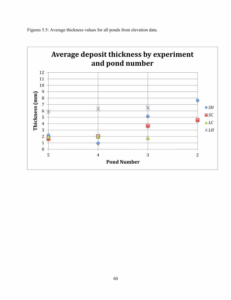
Figures 5.5: Average thickness values
0
1
2
3
4
5
6
7
8
9
10
11
12
5
Th
ick
ne
ss
(m
m)
Average deposit thickness by experiment
60
ess values for all ponds from elevation data.
34
Pond Number
Average deposit thickness by experiment
and pond number
2
Average deposit thickness by experiment
SH
SC
LC
LH
61
Figures 6.1: Pond aggradation over time for SH. Ponds 2 and 3 show greater aggradation
compared to ponds 4 and 5. The elevations are not referenced to the basement elevation but lines
are separated to show the overall growing trends.
-20
-15
-10
-5
0
5
100 4 8 12 16 20 24 28 32 36 40
Ele
va
tio
n (
mm
)
Time elapsed (hours)
SH
aggradation over time
Pond 2
Pond 3
Pond 4
Pond 5
62
Figures 6.2: Pond aggradation over time for SC.
-10
-5
0
5
10
15
200 4 8 12 16 20 24 28 32 36 40
Ele
va
tio
n (
mm
)
Time elapsed (hours)
SC
aggradation over time
Pond 2
Pond 3
Pond 4
Pond 5
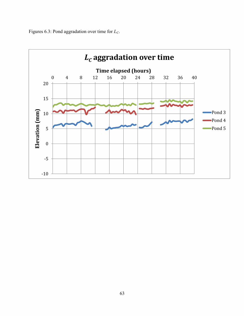
63
Figures 6.3: Pond aggradation over time for LC.
-10
-5
0
5
10
15
200 4 8 12 16 20 24 28 32 36 40
Ele
va
tio
n (
mm
)
Time elapsed (hours)
LC
aggradation over time
Pond 3
Pond 4
Pond 5

64
Figures 6.4: Pond aggradation over time for LH.
-10
-5
0
5
10
15
200 4 8 12 16 20 24 28 32 36 40
Ele
va
tio
n (
mm
)
Time elapsed (hours)
LH
pond aggradation over time
Pond 3
Pond 4
Pond 5
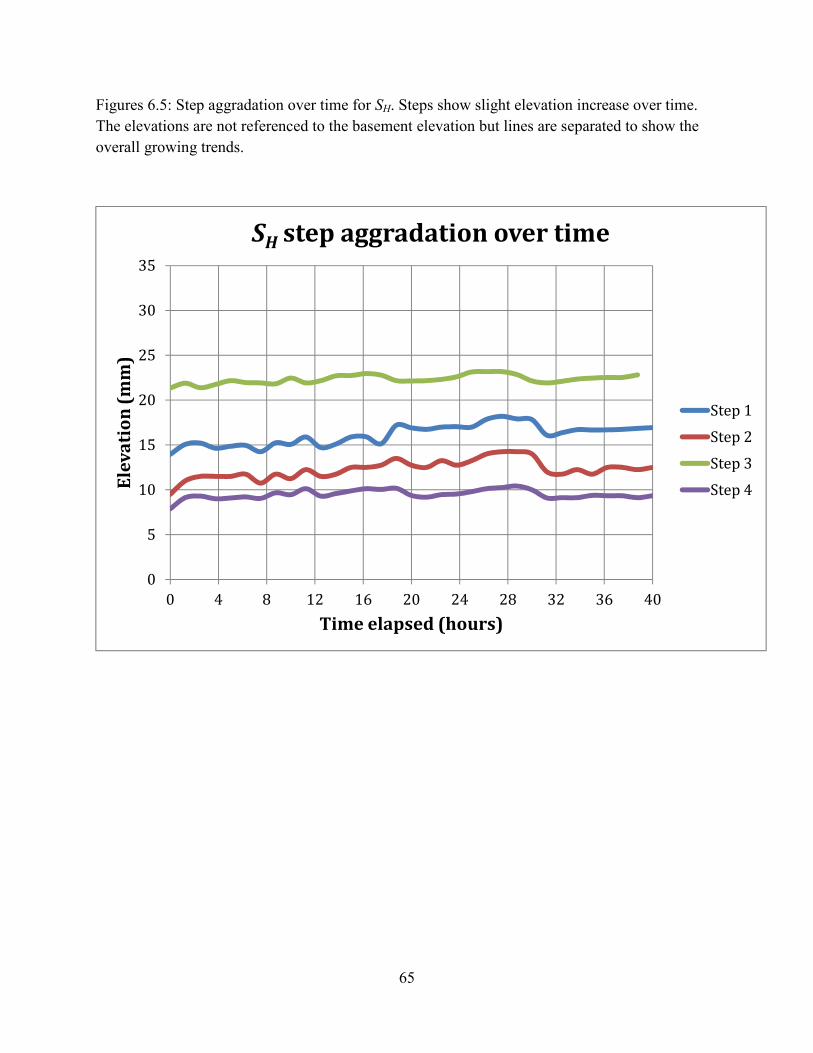
65
Figures 6.5: Step aggradation over time for SH. Steps show slight elevation increase over time.
The elevations are not referenced to the basement elevation but lines are separated to show the
overall growing trends.
0
5
10
15
20
25
30
35
0 4 8 12 16 20 24 28 32 36 40
Ele
va
tio
n (
mm
)
Time elapsed (hours)
SH
step aggradation over time
Step 1
Step 2
Step 3
Step 4

66
Figures 6.6: Step aggradation over time for SC.
0
5
10
15
20
25
30
35
0 4 8 12 16 20 24 28 32 36 40
Ele
va
tio
n (
mm
)
Time elapsed (hours)
SC
step aggradation over time
Step 1
Step 2
Step 3
Step 4
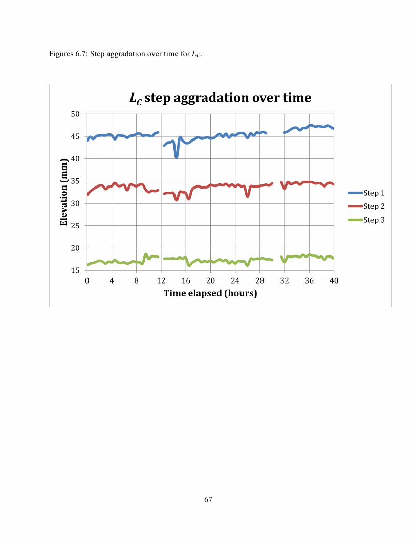
67
Figures 6.7: Step aggradation over time for LC.
15
20
25
30
35
40
45
50
0 4 8 12 16 20 24 28 32 36 40
Ele
va
tio
n (
mm
)
Time elapsed (hours)
LC
step aggradation over time
Step 1
Step 2
Step 3
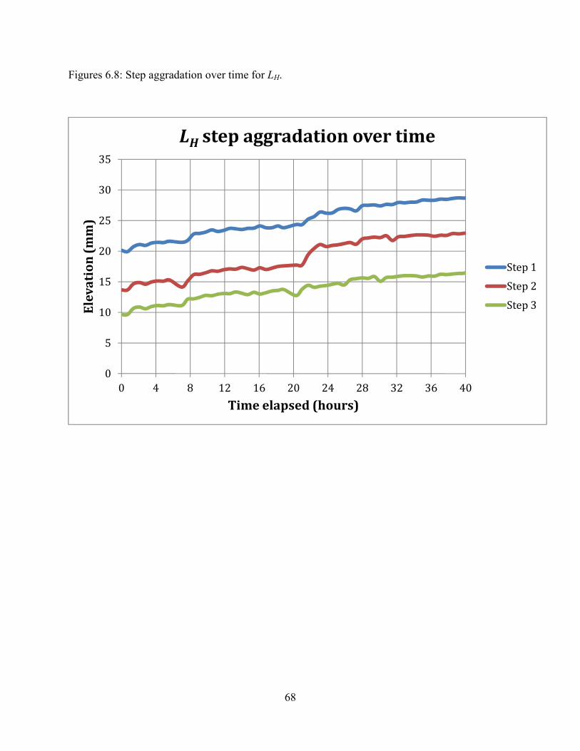
68
Figures 6.8: Step aggradation over time for LH.
0
5
10
15
20
25
30
35
0 4 8 12 16 20 24 28 32 36 40
Ele
va
tio
n (
mm
)
Time elapsed (hours)
LH
step aggradation over time
Step 1
Step 2
Step 3
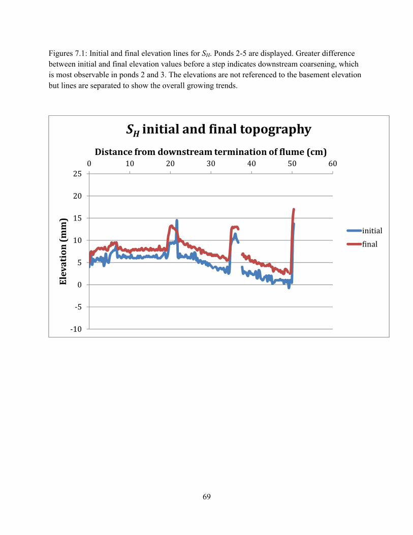
69
Figures 7.1: Initial and final elevation lines for SH. Ponds 2-5 are displayed. Greater difference
between initial and final elevation values before a step indicates downstream coarsening, which
is most observable in ponds 2 and 3. The elevations are not referenced to the basement elevation
but lines are separated to show the overall growing trends.
-10
-5
0
5
10
15
20
250 10 20 30 40 50 60
Ele
va
tio
n (
mm
)
Distance from downstream termination of flume (cm)
SH
initial and final topography
initial
final
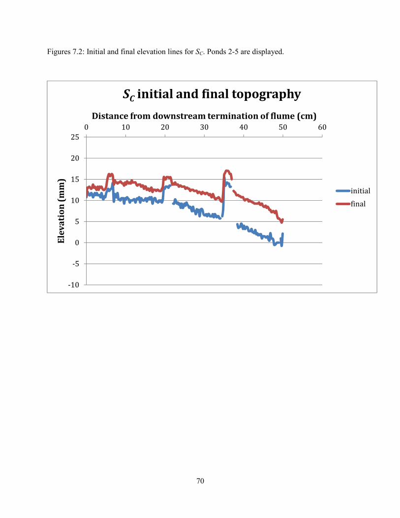
70
Figures 7.2: Initial and final elevation lines for SC. Ponds 2-5 are displayed.
-10
-5
0
5
10
15
20
250 10 20 30 40 50 60
Ele
va
tio
n (
mm
)
Distance from downstream termination of flume (cm)
SC
initial and final topography
initial
final

71
Figures 7.3: Initial and final elevation lines for LC. Ponds 3-5 are displayed.
5
10
15
20
25
30
35
400 10 20 30 40 50 60
Ele
va
tio
n (
mm
)
Distance from downstream termination of flume (cm)
LC
initial and final topography
initial
final
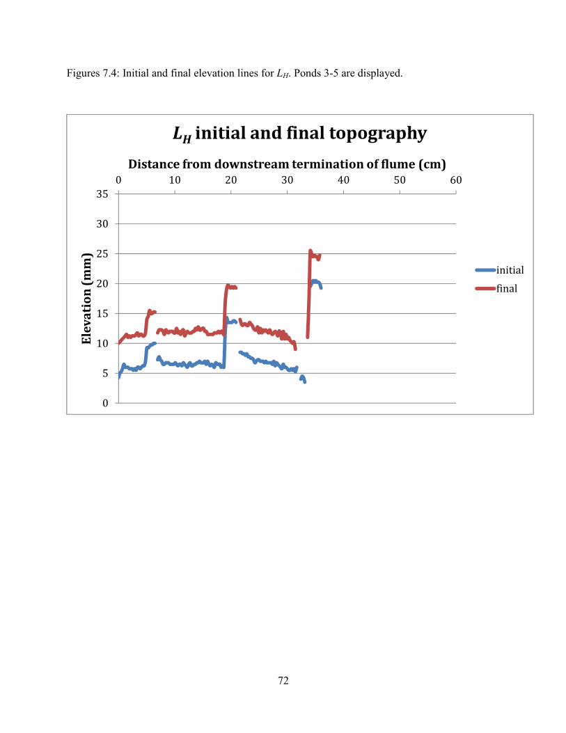
72
Figures 7.4: Initial and final elevation lines for LH. Ponds 3-5 are displayed.
0
5
10
15
20
25
30
350 10 20 30 40 50 60
Ele
va
tio
n (
mm
)
Distance from downstream termination of flume (cm)
LH
initial and final topography
initial
final
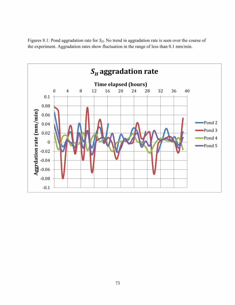
73
Figures 8.1: Pond aggradation rate for SH. No trend in aggradation rate is seen over the course of
the experiment. Aggradation rates show fluctuation in the range of less than 0.1 mm/min.
-0.1
-0.08
-0.06
-0.04
-0.02
0
0.02
0.04
0.06
0.08
0.10 4 8 12 16 20 24 28 32 36 40
Ag
grd
ati
on
ra
te (
mm
/m
in)
Time elapsed (hours)
SH
aggradation rate
Pond 2
Pond 3
Pond 4
Pond 5
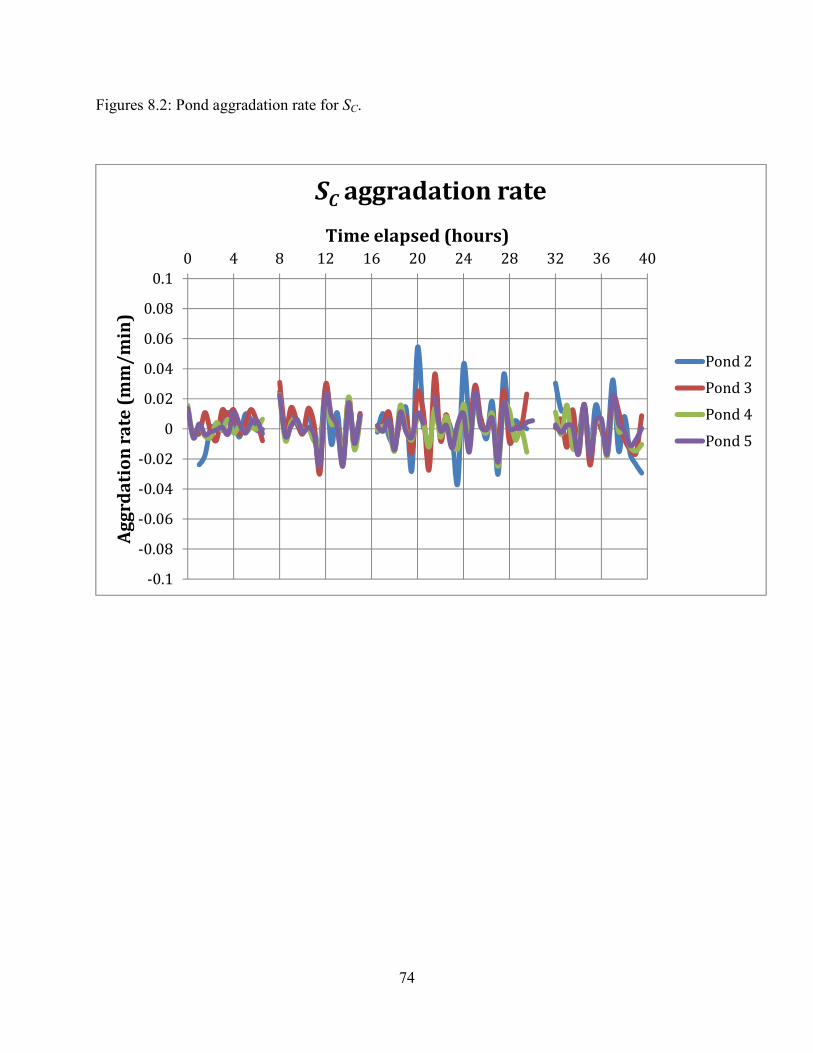
74
Figures 8.2: Pond aggradation rate for SC.
-0.1
-0.08
-0.06
-0.04
-0.02
0
0.02
0.04
0.06
0.08
0.10 4 8 12 16 20 24 28 32 36 40
Ag
grd
ati
on
ra
te (
mm
/m
in)
Time elapsed (hours)
SC
aggradation rate
Pond 2
Pond 3
Pond 4
Pond 5
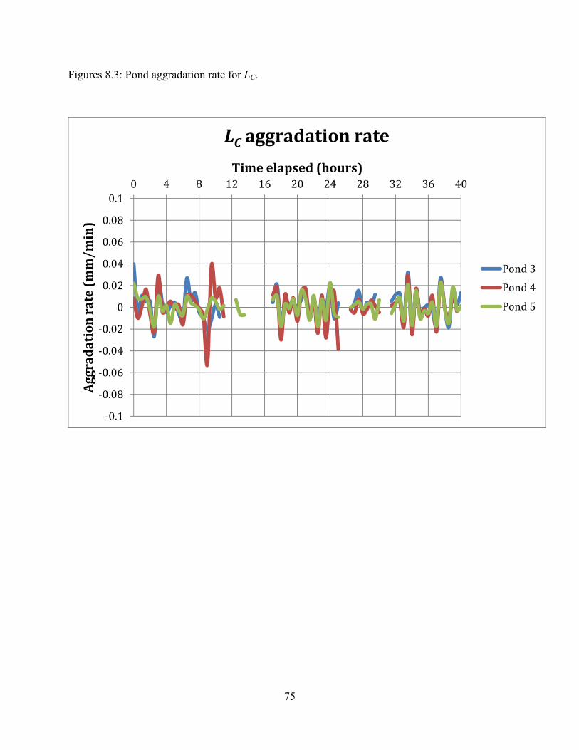
75
Figures 8.3: Pond aggradation rate for LC.
-0.1
-0.08
-0.06
-0.04
-0.02
0
0.02
0.04
0.06
0.08
0.10 4 8 12 16 20 24 28 32 36 40
Ag
gra
da
tio
n r
ate
(m
m/
min
)
Time elapsed (hours)
LC
aggradation rate
Pond 3
Pond 4
Pond 5
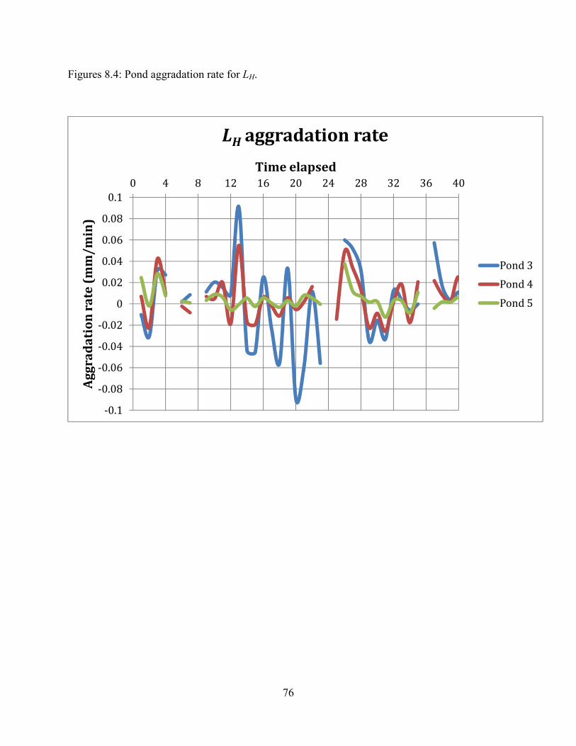
76
Figures 8.4: Pond aggradation rate for LH.
-0.1
-0.08
-0.06
-0.04
-0.02
0
0.02
0.04
0.06
0.08
0.10 4 8 12 16 20 24 28 32 36 40
Ag
gra
da
tio
n r
ate
(m
m/
min
)
Time elapsed
LH
aggradation rate
Pond 3
Pond 4
Pond 5
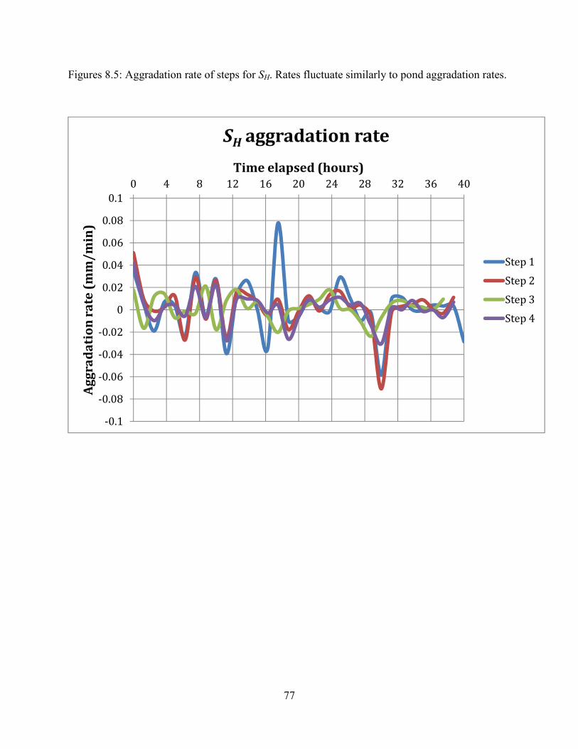
77
Figures 8.5: Aggradation rate of steps for SH. Rates fluctuate similarly to pond aggradation rates.
-0.1
-0.08
-0.06
-0.04
-0.02
0
0.02
0.04
0.06
0.08
0.10 4 8 12 16 20 24 28 32 36 40
Ag
gra
da
tio
n r
ate
(m
m/
min
)
Time elapsed (hours)
SH
aggradation rate
Step 1
Step 2
Step 3
Step 4
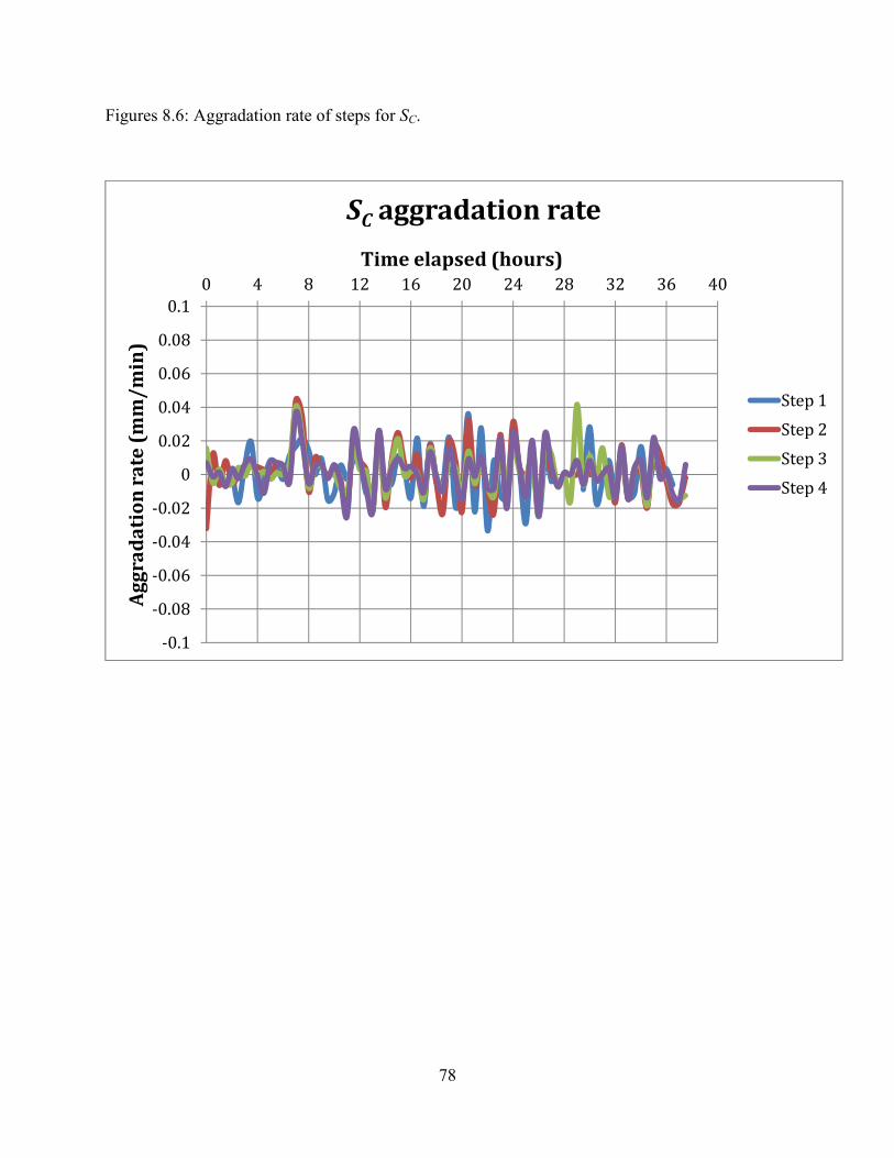
78
Figures 8.6: Aggradation rate of steps for SC.
-0.1
-0.08
-0.06
-0.04
-0.02
0
0.02
0.04
0.06
0.08
0.10 4 8 12 16 20 24 28 32 36 40
Ag
gra
da
tio
n r
ate
(m
m/
min
)
Time elapsed (hours)
SC
aggradation rate
Step 1
Step 2
Step 3
Step 4
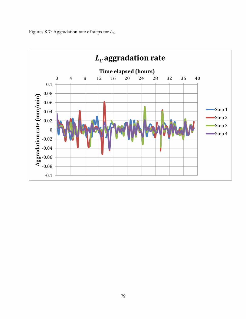
79
Figures 8.7: Aggradation rate of steps for LC.
-0.1
-0.08
-0.06
-0.04
-0.02
0
0.02
0.04
0.06
0.08
0.10 4 8 12 16 20 24 28 32 36 40
Ag
gra
da
tio
n r
ate
(m
m/
min
)
Time elapsed (hours)
LC
aggradation rate
Step 1
Step 2
Step 3
Step 4
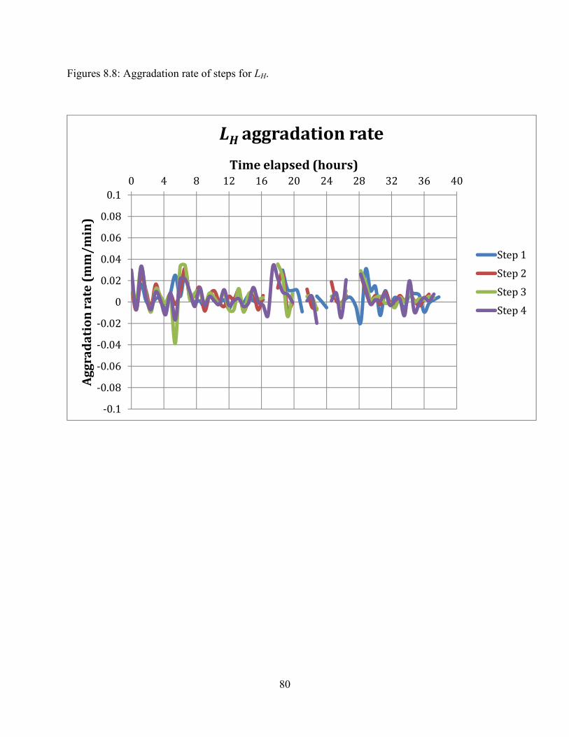
80
Figures 8.8: Aggradation rate of steps for LH.
-0.1
-0.08
-0.06
-0.04
-0.02
0
0.02
0.04
0.06
0.08
0.10 4 8 12 16 20 24 28 32 36 40
Ag
gra
da
tio
n r
ate
(m
m/
min
)
Time elapsed (hours)
LH
aggradation rate
Step 1
Step 2
Step 3
Step 4
81
References
Bargar, K.E. (1978). Geology and thermal history of Mammoth Hot Springs, Yellowstone
National Park, Wyoming, U.S. U.S. Geological Survey Bulletin, 1444, 1-54.
Buhmann, D. and Dreybrodt, W. (1984). The Kinetics of Calcite Dissolution and Preciptation in
Geologically Relevant Situation of Karst Areas. Chemical Geology, 48, 189-211.
Chafetz, H. S. and Folk, R. L. (1984). Travertines: Depositional Morphology and the Bacterially
Constructed Constituents. Journal of Sedimentary Petrology, 54, 289-316.
Chen, J., Zhang, D. D., Wang, S., Xiao, T., and Huang, R. (2004). Factors controlling tufa
deposition in natural waters at waterfall sites. Sedimentary Geology, 166, 353-366.
Fouke, B.W., Farmer, J. D., Des Marais, D. J., Pratt, L., Sturchio, N. C., Burns, P. C., Discipulo,
M.K. (2000). Depositional Facies and Aqueous-Solid Geochemistry of Travertine-
Depositing Hot Springs (Angel Terrace, Mammoth Hot Springs, Yellowstone National
Park, U.S.A.). Journal of Sedimentary Research, 70, 565-585.
Frankel, R. B, and Bazylinski, D. A. (2003). Biologically induced mineralization by bacteria;
Biomineralization. Reviews in Mineralogy and Geochemistry, 54, 95-114.
Goldenfeld, N., Chan, Y. C., and Veysey, J. (2006). Dynamics of Precipitation Pattern Formation
at Geothermal Hot Springs. Physical Review Letters, 96, 254501-1-254501-4.
Hammer, O., Dysthe, D. K., and Jamtveit, B. (2007). The dynamics of travertine dams. Earth and
Planetary Science Letters, 256, 258-263.
Hammer, O. (2008). Watch your step. Nature Physics, 4, 255-256.
Kandianis, M.T., Fouke, B. W., Veysey, J. and Inskeep, W. P. (2008). Microbial biomass; a
catalyst for CaCO3 precipitation in advection-dominated transport regimes. Geological
Society of America Bulletin, 120, 442-450.
Lu, G., Zheng, C., Donahoe, R. J., and Berry Lyons, W. (2000). Controlling processes in a
CaCO3 precipitating stream in Huanglong Natural Scenic District, Sichuan, China.
Journal of Hydrology, 230, 34-54.
82
Mann, S. (2001). Biomineralization: Principles and Concepts in Bioinorganic Materials
Chemistry. Oxford University Press, Oxford, 201 pp.
Pentecost, A. and Viles, H. (1994). A Review and Reassessment of Travertine Classification.
Geography Physique et Quaternaire, 48, 305-314.
Renaut, R. W., and Jones, B. (1997). Controls on aragonite and calcite precipitation in hot spring
travertines at Chemurku, Lake Bogoria, Kenya. Canadian Journal of Earth Sciences, 34,
801-818.
Sant’ Anna, L. G., Riccomini, C., Rodrigues-Francisco, B.H., Sial, A.N., Carvalho, M.D. and
Moura, C. A. V. (2004). The Paleocene travertine system of the Itaborai basin,
Southeastern Brazil. Journal of South American Earth Sciences, 18, 11-25.
Schlager, W. (2003). Benthic carbonate factories of the Phanerozoic. International Journal of
Earth Sciences, 92, 445-464.
Sorey, M. L., and Colvard, E. M. (1997). Hydrologic investigation in the Mammoth Corridor,
Yellowstone National Park and vicinity, U.S.A. Geothermics, 26, 221-249.
Zaihua, L., Svensson, U., Dreybrodt, W., Daoxian, Y., and Buhmann, D. (1995). Hydrodynamic
control of inorganic calcite precipitation in Huanglong Ravine, China: Field
measurements and theoretical prediction of deposit rates. Geochimica et Cosmochimica
Acta, 59, 15, 3087-3097.
Stelmach, K (2011). Thesis. 20 p. B.S. thesis, University of Illinois, Champaign-Urbana.
Vescogni, H. R. (2009). Microbial Biomarkers: Mineralogy, Crystal Fabric and Chemistry of
Calcium Carbonate Mineralization. 69 p. M.S. thesis, University of Illinois, Champaign-
Urbana.
Veysey, J. and Goldenfeld, N. (2008). Watching Rocks Grow. Nature Physics, 4, 2310-313.