Embed Size (px)
Citation preview

Copyright
by
Fei Yan
2012
The Dissertation Committee for Fei Yan Certifies that this is the approved version
of the following dissertation:
PAH Degradation and Redox Control in an Electrode Enhanced
Sediment Cap
Committee:
Danny Reible, Supervisor
Philip Bennett
Randall Charbeneau
Robert Gilbert
Howard Liljestrand
PAH Degradation and Redox Control in an Electrode Enhanced
Sediment Cap
by
Fei Yan, B.E.;M.E.;M.E.
Dissertation
Presented to the Faculty of the Graduate School of
The University of Texas at Austin
in Partial Fulfillment
of the Requirements
for the Degree of
Doctor of Philosophy
The University of Texas at Austin
August 2012

Dedication
To all who love me.

v
Acknowledgements
First and foremost, I would like to express my sincere gratitude to my PhD
advisor, Dr. Danny Reible, for his guidance, advice, encouragement and support
throughout my PhD study. His creative ideas, broad and in-depth knowledge have
inspired me and broadened my vision; his encouragement and support have been
invaluable to me as I pursue my PhD. It has been an incredible journey learning from and
working with him.
Moreover, I would like to thank the members of my committee: Dr. Philip
Bennett, Dr. Randall Charbeneau, Dr. Robert Gilbert, and Dr. Howard Liljestrand for
their support, guidance, and suggestions. I would also like to give my thanks to Dr. Mary
Jo Kirisits for her valuable advice on biodegradation and microbiology. I am always
grateful for her kindness, encouragement and willingness to help. I would like to thank
Dr. Kerry Kinney, Dr. Lynn Katz, Dr. Desmond Lawler, Dr. David Maidment, Dr.
Jeremy Meyers, and Dr. Allen Bard for their help at various stages of my PhD study.
Also, thanks to Dr. Gregory Lowry and Dr. Kelvin Gregory at Carnegie Mellon
University, and Dr. Joseph Hughes at Drexel University and Georgia Institute of
Technology for our collaboration and discussions.
I would like to acknowledge everyone who graciously provided their expertise,
time, and resources to my doctoral research including Dr. Xiaoxia Lu (general laboratory
procedures, passive sampling, HPLC trouble shooting, etc.), Charles Perego and Chia-
Chen Chen (technical supports), Tony Smith (biodegradation and microbiology),
Yongseok Hong (pH and redox behaviors), Dave Lampert (passive sampling and model
development), Nate Johnson (electrochemical application), Sungwoo Bae, Andy
vi
Hoisington, Weiwei Wu and Liming Luo (microbiology), Wei Shi and Ling Huang
(aquatic chemistry), Joaquin Rodriguez Lopez and Mei Shen (electrochemistry), Mei Sun
and Ruiling Zhang (collaboration on electrochemical application), Wu Chen and Gabe
Trejo (laboratory supports), Yachao Qi (analytical method), and every member in Dr.
Reible’s group.
Last but not the least, I would like to thank my parents, brother, sister-in-law for
their love and support; I would also like to express my gratitude to my girlfriend, Yiyi
Chu, for her love, support, patience and understanding.
vii
PAH Degradation and Redox Control in an Electrode Enhanced
Sediment Cap
Fei Yan, Ph.D
The University of Texas at Austin, 2012
Supervisor: Danny Reible
Capping is typically used to control contaminant release from the underlying
sediments. However, the presence of conventional caps often eliminates or slows natural
degradation that might otherwise occur at the surface sediment. This is primarily due to
the development of reducing conditions within the sediment that discourage hydrocarbon
degradation. The objective of this study was to develop a novel active capping method,
an electrode enhanced cap, to manipulate the redox potential to produce conditions more
favorable for hydrocarbon degradation and evaluate the approach for the remediation of
PAH contaminated sediment.
A preliminary study of electrode enhanced biodegradation of PAH in sediment
slurries showed that naphthalene and phenanthrene concentration decreased significantly
within 4 days, and PAH degrading genes increased by almost 2 orders of magnitude.
In a sediment microcosm more representative of expected field conditions,
graphite cloth was used to form an anode at the sediment-cap interface and a similar
cathode was placed a few centimeters above within a thin sand layer. With the
application of 2V voltage, ORP increased and pH dropped around the anode reflecting
water electrolysis. Various cap amendments (buffers) were employed to moderate pH
changes. Bicarbonate was found to be the most effective in laboratory experiments but a
viii
slower dissolving buffer, e.g. siderite, may be more effective under field conditions.
Phenanthrene concentration was found to decrease slowly with time in the vicinity of the
anode. In the sediment at 0-1 cm below the anode, phenanthrene concentrations
decreased to ~70% of initial concentration with no bicarbonate, and to ~50% with
bicarbonate over ~70 days, whereas those in the control remained relatively constant.
PAH degrading gene increased compared with control, providing microbial evidence of
PAH biodegradation
A voltage-current relationship, which incorporated separation distance and the
area of the electrodes, was established to predict current. A coupled reactive transport
model was developed to simulate pH profiles and model results showed that pH is
neutralized at the anode with upflowing groundwater seepage.
This study demonstrated that electrode enhanced capping can be used to control
redox potential in a sediment cap, provide microbial electron acceptors, and stimulate
PAH degradation.
ix
Table of Contents
List of Tables ..................................................................................................... xiii
List of Figures .................................................................................................... xiv
Chapter 1: Introduction .......................................................................................1
1.1 Background ...............................................................................................1
1.2 Research objectives and dissertation outline ............................................3
Chapter 2: Literature Review ..............................................................................5
2.1 PAH contamination and degradation ........................................................5
2.1.1 PAH contamination .......................................................................5
2.1.2 PAH degradation ...........................................................................6
2.1.3 PAH degradation genes.................................................................8
2.2 Electrochemical remediation for soil and sediment ..................................9
2.2.1 Electrokinetic phenomena ...........................................................10
2.2.2 Water electrolysis........................................................................11
2.2.3 Electrochemical oxidation/reduction ..........................................12
2.2.4 Electrochemical stimulation of biodegradation ..........................12
2.3 Remediation of contaminated sediments ................................................13
2.3.1 Contaminated sediments .............................................................13
2.3.2 Sediment remediation methods ...................................................15
2.3.2.1 Monitored natural attenuation .........................................15
2.3.2.2 Dredging and excavation ................................................16
2.3.2.3 In-situ capping ................................................................17
2.4 Research needs: Active capping coupling electrochemical processes with
bioremediation .....................................................................................20
Chapter 3: Electrode Enhanced Biodegradation of PAH in Sediment Slurry ..22
3.1 Introduction .............................................................................................22
3.2 Biodegradation of PAH under aerobic and nitrate reducing conditions .23
3.2.1 Materials and methods ................................................................23
x
3.2.1.1 Sediment and medium.....................................................23
3.2.1.2 Biodegradation under aerobic conditions .......................24
3.2.1.3 Biodegradation under nitrate reducing conditions ..........24
3.2.1.4 Sampling procedures .......................................................25
3.2.1.5 PAH analysis ...................................................................26
3.2.1.6 DNA extraction ...............................................................26
3.2.1.7 PCR and qPCR for PAH degrading genes ......................27
3.2.2 Results and discussion ................................................................29
3.3 Electrode enhanced biodegradation of PAH in sediment slurry .............35
3.3.1 Materials and methods ................................................................35
3.3.1.1 Experiment design and instruments ................................35
3.3.1.2 Sediment slurry preparation ............................................37
3.3.1.3 Sampling procedures .......................................................38
3.3.2 Results and discussion ................................................................39
3.4 Conclusions .............................................................................................43
Chapter 4: Electro-biodegradation of PAH and Redox Control in Sediment/Cap
Microcosms ...................................................................................................45
4.1 Introduction .............................................................................................45
4.2 PAH degradation and redox control in uncapped sediment by electrodes47
4.2.1 Materials and methods ................................................................47
4.2.1.1 Microcosm setup and operation ......................................47
4.2.1.2 pH and ORP measurement ..............................................48
4.2.1.3 Voltammetric determination of redox-sensitive species .49
4.2.1.4 Phenanthrene porewater concentration measurement by
PDMS-coated fiber ............................................................50
4.2.1.5 DNA extraction and qPCR analysis ................................51
4.2.2 Results and discussion ................................................................51
4.2.2.1 Redox control, pH changes and redox-sensitive species 51
4.2.2.2 Phenanthrene concentrations and PAH degrading genes57
4.3 PAH degradation and redox control in electrode enhanced sand caps ...63
4.3.1 Materials and methods ................................................................63
xi
4.3.2 Results and discussion ................................................................65
4.3.2.1 Redox control, pH changes and redox-sensitive species 65
4.3.2.2 PAH concentrations and PAH degrading genes .............70
4.4 PAH degradation and redox control in electrode enhanced caps with
bicarbonate amendment as a pH buffer ...............................................76
4.4.1 Materials and methods ................................................................76
4.4.2 Results and discussion ................................................................78
4.4.2.1 Redox control, pH changes and redox-sensitive species 78
4.4.2.2 Phenanthrene concentrations and PAH degrading genes83
4.4.2.3 Cost analysis ...................................................................89
4.5 Conclusions .............................................................................................91
Chapter 5: Model of Electrode Enhanced Capping ..........................................93
5.1 Introduction .............................................................................................93
5.2 Voltage-current relationship ...................................................................95
5.2.1 Model development ....................................................................95
5.2.2 Model calibration ........................................................................99
5.2.3 Voltage components analysis ....................................................102
5.2.4 Application of model in capping design ...................................104
5.3 Modeling of transport and reaction processes ......................................107
5.3.1 Modeling of transport processes ...............................................107
5.3.2 Modeling of chemical reactions ................................................110
5.3.3 Decoupling of transport and reaction processes .......................115
5.3.4 Model application for sample cases ..........................................117
5.3.4.1 Model parameters..........................................................117
5.3.4.2 Model application to no advection cases ......................123
5.2.4.2 Model application to advection cases ...........................127
5.4 Conclusions ...........................................................................................130
Chapter 6: Conclusions and Recommendations .............................................132
6.1 Conclusions ...........................................................................................132
6.2 Recommendations for future work .......................................................135
xii
6.2.1 Microbial community analysis ..................................................135
6.2.2 Characterization of oxic zone at the anode ...............................135
6.2.3 Capping performance under various conditions .......................136
6.2.4 Mineral amendment for pH control ..........................................136
Appendix A: Supporting Information for Chapter 3..........................................138
A.1 PCR amplification of PAH degrading genes by PAH-RHDα gram negative
primer .................................................................................................138
Appendix B: Supporting Information for Chapter 4 ..........................................139
B.1 Microcosm setup of PAH degradation and redox control experiments139
B.2 Uptake kinetic of fiber (210/230) for phenanthrene .............................141
B.3 ORP and pH profiles in uncapped sediment with electrodes ...............142
B.4 Profiles of redox-sensitive species in uncapped sediment with electrodes145
B.5 ORP and pH profiles in electrode enhanced sand caps (No bicarbonate
amendment)........................................................................................146
B.6 Profiles of redox-sensitive species in in electrode enhanced sand caps (No
bicarbonate amendment) ....................................................................149
B.7 ORP and pH profiles in electrode enhanced caps with bicarbonate
amendment .........................................................................................150
B.8 Profiles of redox-sensitive species in electrode enhanced caps with
bicarbonate amendment .....................................................................154
B.9 Voltage and current in the experiment of electrode enhanced caps with
bicarbonate amendment .....................................................................155
Appendix C: Supporting Information for Chapter 5 ..........................................156
C.1 Derivation of overpotential and current density relationship ...............156
References ..........................................................................................................158
Vita FY...............................................................................................................170
xiii
List of Tables
Table 3.1 Characteristics of gram negative PAH-RHDα primer ............................27
Table 4.1 ORP of platinum and Ag/AgCl reference electrode pairs in quinhydrone
dissolved in pH buffer (Sparks, 1996) ..............................................49
Table 4.2 Phenanthrene and naphthalene concentration in solid phase .................75
Table 5.1 Fitted parameters a, b and Rrstc, coefficient determination R2 and root-mean-
square-error (RMSE) ......................................................................100
Table 5.2 Transport parameters for each species in the model ............................120
Table 5.3 Chemical reaction parameters in the model .........................................121
Table 5.4 Initial concentrations in the model.......................................................122
Table 5.5 Boundary conditions in the model .......................................................123

xiv
List of Figures
Figure 1.1 Conceptual model for an electrode enhanced cap for PAH remediation
.............................................................................................................3
Figure 2.1 Schematic of electrochemical remediation of contaminated soil .....10
Figure 3.1 Naphthalene (a) and phenanthrene (b) biodegradation under aerobic
condition. Points represent the mean of triplicate supernatant samples
and error bars indicate standard deviation of triplicate data. Active
means biological active samples, and control represents killed control
samples. .............................................................................................30
Figure 3.2 Naphthalene (a) and phenanthrene (b) biodegradation under nitrate
reducing condition. Points represent the mean of triplicate supernatant
samples and error bars indicate standard deviation of triplicate data.
Active means biological active samples, and control represents killed
control samples. ................................................................................31
Figure 3.3 qPCR quantification and DNA extraction results under aerobic
condition: 1) Copy number of PAH degrading gene normalized by total
DNA; 2) Copy number of PAH degrading gene normalized by dry
sediment; 3) DNA concentration per dry sediment. .........................34
Figure 3.4 PAH degrading gene abundance by qPCR quantification under nitrate
reducing condition. The PAH-RHDα GN gene levels were normalized by
the weight of dry sediment. All the values were reported as an increase
from unincubated sediment control. .................................................34
Figure 3.5 The reactor for electrode enhanced biodegradation experiment .......35

xv
Figure 3.6 Degradation of naphthalene over time in ElectroBio reactor (RE), killed
control (KC), aerobic (AE) and anaerobic (AN) conditions. Points
represent the mean of triplicate supernatant samples and error bars
indicate standard deviation of triplicate data. ...................................40
Figure 3.7 Degradation of phenanthrene over time in ElectroBio reactor (RE),
killed control (KC), aerobic (AE) and anaerobic (AN) conditions. Points
represent the mean of triplicate supernatant samples and error bars
indicate standard deviation of triplicate data. ...................................42
Figure 3.8 PAH degrading gene abundance by qPCR quantification. The PAH-
RHDα GN gene levels were normalized by the weight of dry sediment.
All the values were reported as an increase from unincubated sediment
control. The results are the means of triplicate, and error bars represent
standard deviation. N.D. = Not Detectable. ......................................43
Figure 4.1 Vertical profiles of ORP in (a) ElecR1, (b) ElecR2 and (c) Control
reactors on selected days. ORP values were versus standard hydrogen
electrode (SHE). Depth zero was the water-sediment interface. Cathode
was at d = 0.5 cm and anode was at d = 3 cm. All the measured profiles
are in Appendix B. ............................................................................53
Figure 4.2 Vertical profiles of ORP at (a) Day 0, (b) Day 21, (c) Day 40 and (d)
Day 68. ORP values were versus standard hydrogen electrode (SHE).
Depth zero was the water-sediment interface. Cathode was at d = 0.5 cm
and anode was at d = 3 cm. ...............................................................54
xvi
Figure 4.3 Vertical profiles of pH in (a) ElecR1, (b) ElecR2 and (c) Control
reactors. Depth zero was the water-sediment interface. Cathode was at d
= 0.5 cm and anode was at d = 3 cm. All the measured profiles are in
Appendix B. ......................................................................................55
Figure 4.4 Vertical profiles of redox-sensitive species in ElecR1, ElecR2 and
Control reactors: (a) Oxygen, (b) Mn2+ and (c) Fe2+. Sulfide was not
detected. Each point represents the mean of triplicate measurements
from each electrode, and error bars are not shown for simplicity. Depth
zero was the water-sediment interface. Cathode was at d = 0.5 cm and
anode was at d = 3 cm. Figures with standard deviation are available in
Appendix B. ......................................................................................57
Figure 4.5 Phenanthrene porewater concentration at different depths for (a) ElecR1,
(b) ElecR2 and (c) Control. The results are the means of duplicate
samples, and error bars represent standard deviations. .....................59
Figure 4.6 Phenanthrene porewater concentration around the anode (d = 3 cm). The
results are the means of duplicate samples, and error bars are not shown
for simplicity. ....................................................................................60
Figure 4.7 Vertical profiles of phenanthrene porewater concentration in (a) ElecR1,
(b) ElecR2 and (c) Control reactors. Depth zero was the water-sediment
interface. Cathode was at d = 0.5 cm and anode was at d = 3 cm. The
results are the means of duplicate samples, and error bars are not shown
for simplicity. ....................................................................................61
xvii
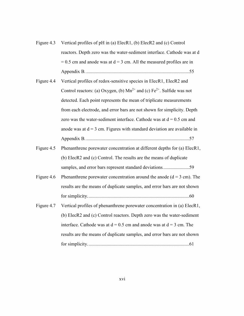
Figure 4.8 PAH degrading gene abundance by qPCR quantification at a depth of 0-
0.5 cm below the anode, 0-0.5 cm above the anode, and in the bottom
sediment in ElecR1, ElecR2, and Control. The PAH-RHDα GN gene
levels were normalized by the weight of dry sediment. All the values
were reported as an increase from the level of genes at the bottom
sediment of ElecR1. The results are the means of triplicate samples, and
error bars represent standard deviations. ..........................................63
Figure 4.9 Vertical profiles of ORP in (a) ElecCap1, (b) ElecCap2 and (c) Control
reactors. Depth zero was the water-cap interface. Cathode was at d = 0.5
cm and anode was at d = 4 cm. All the measured profiles are in
Appendix B. ......................................................................................67
Figure 4.10 Vertical profiles of pH in (a) ElecCap1, (b) ElecCap2 and (c) Control
reactors. Depth zero was the water-cap interface. Cathode was at d = 0.5
cm and anode was at d = 4 cm. All the measured profiles are in
Appendix B. ......................................................................................68
Figure 4.11 Vertical profiles of redox-sensitive species in ElecCap1, ElecCap2 and
Control reactors: (a) Oxygen, (b) Mn2+ and (c) Fe2+. Sulfide was not
detected. Each point represents the mean of triplicate measurements
from each electrode, and error bars are not shown for simplicity. Depth
zero was the water-cap interface. Cathode was at d = 0.5 cm and anode
was at d = 4 cm. Figures with standard deviation are listed in Appendix
B. .......................................................................................................70
xviii
Figure 4.12 Phenanthrene porewater concentration at different depths for (a)
ElecCap1, (b) ElecCap2 and (c) Control. The results are the means of
duplicate samples or four samples, and error bars represent standard
deviations. .........................................................................................72
Figure 4.13 Phenanthrene porewater concentration around the anode: (a) 0-1 cm
below the anode; (b) 0-1 cm above the anode. The results are the means
of duplicate samples, and error bars are not shown for simplicity. ..73
Figure 4.14 Vertical profiles of phenanthrene porewater concentration in (a)
ElecCap1, (b) ElecCap2 and (c) Control reactors. Depth zero was the
cap-sediment interface. Anode was at the interface. The results are the
means of duplicate samples, and error bars are not shown for simplicity.
...........................................................................................................74
Figure 4.15 PAH degrading gene abundance by qPCR quantification at a depth of 0-
0.5 cm below the anode in control, ElecCap1 and ElecCap2 reactors.
The PAH-RHDα GN gene levels were normalized by the weight of dry
sediment. All the values were reported as an increase from control
reactor. The results are the means of triplicate, and error bars represent
standard deviation. ............................................................................76
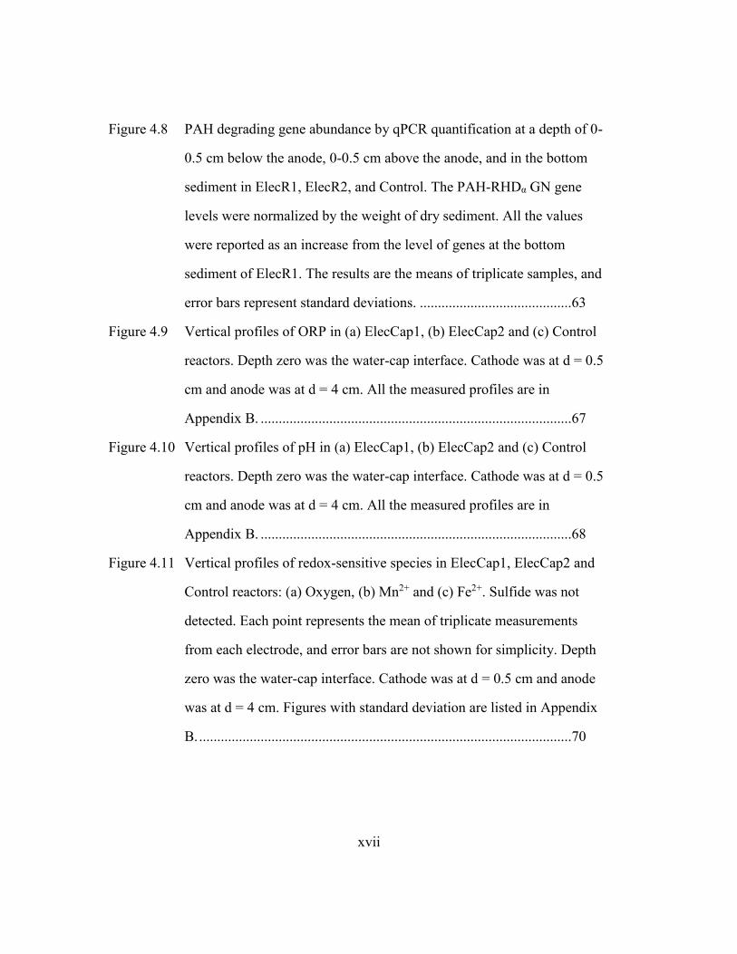
Figure 4.16 Vertical profiles of pH in (a) CtnCap1, (b) CtnCap2, (c) IntmtCap and
(d) Control reactors. Depth zero was the water-cap interface. Cathode
was at d = 0.5 cm and anode was at d = 4 cm. All the measured profiles
are in Appendix B. ............................................................................80
xix
Figure 4.17 Vertical profiles of ORP at (a) Day 20, (b) Day 28, (c) Day 40 and (d)
Day 68. ORP values were versus standard hydrogen electrode (SHE).
Depth zero was the water-sand interface. Cathode was at d = 0.5 cm and
anode was at d = 4 cm. All the measured profiles are in Appendix B.81
Figure 4.18 Vertical profiles of redox-sensitive species in CtnCap1, CtnCap2,
IntmtCap and Control reactors: (a) Oxygen, (b) Mn2+ and (c) Fe2+.
Sulfide was not detected. Each point represents the mean of triplicate
measurements from each electrode, and error bars are not shown for
simplicity. Depth zero was the water-cap interface. Cathode was at d =
0.5 cm and anode was at d = 4 cm. Figures with standard deviation are
listed in Appendix B. ........................................................................83
Figure 4.19 Phenanthrene porewater concentration at different depths for (a)
CtnCap1, (b) CtnCap2, (c) IntmtCap and (d) Control. The results are the
means of triplicate samples, and error bars represent standard deviations.
...........................................................................................................87
Figure 4.20 Phenanthrene porewater concentration at (a) 0.5–1 cm above the anode,
(b) 0-0.5 cm above the anode, (c) 0-0.5 cm below the anode and (d) 0.5-
1cm below the anode. The results are the means of triplicate samples,
and error bars are not shown for simplicity. .....................................88
Figure 4.21 PAH degrading gene abundance by qPCR quantification at a depth of 0-
0.5 cm below the anode in CtnCap1, CtnCap2, IntmtCap and control
reactors. The PAH-RHDα GN gene levels were normalized by the
weight of dry sediment. All the values were reported as an increase from
control reactor. The results are the means of triplicate, and error bars
represent standard deviation. ............................................................89
xx
Figure 5.1 Comparison of the model with experiments: (a) Exp1, (b) Exp2, (c)
Exp3, (d) All the three experiments. Dotted lines represent 95%
confidence intervals. .......................................................................101
Figure 5.2 The effect of limiting current in Exp2. Dotted line is the fitted model
excluding the last two experimental data. .......................................102
Figure 5.3 Voltage components in electrode enhanced capping in Exp2. (a) voltage
components and (b) percentage of voltage components at different input
voltage. ............................................................................................103
Figure 5.4 Voltage-current density relationship for different cap thickness. rt is the
ratio of the cap thickness to that of Exp2. .......................................105
Figure 5.5 Input voltage required to achieve the same current density with different
cap thickness. rt is the ratio of the cap thickness to that of Exp2. ...105
Figure 5.6 Sensitivity analysis of current density with respect to voltage changes
for different cap thickness. (a) current density change with respect to
voltage change (di/dV); (b) relative current density change with respect
to relative voltage change [(di/i)/(dV/V)]. ......................................107
Figure 5.7 Physical setting of an electrode enhanced capping system in vertical one
dimensional domain. d is the depth below the water sand interface.118
Figure 5.8 Triangular function of proton production rate by electrode reactions.119
Figure 5.9 Predicted pH profiles in electrode enhanced capping at different times.
.........................................................................................................124
Figure 5.10 Predicted pH profiles in electrode enhanced capping at different depths.
.........................................................................................................125
Figure 5.11 Predicted and experimental pH profiles in electrode enhanced capping at
different times. ................................................................................127
xxi
Figure 5.12 Comparison of pH profiles for different advective flow velocities (Darcy
velocity q = 0, 5*10-7 and 5*10-8 m/s): (a) Day 1; (b) Day 20; (c) Day
60; (d) Day 100. ..............................................................................129
Figure 5.13 Comparison of pH profiles at different times for advection and no
advection cases: (a) Darcy velocity q = 5*10-7 m/s; (b) Darcy velocity q
= 5*10-8 m/s; (c) Darcy velocity q = 0. ...........................................130
Figure A.1 Results of agarose gel electrophoresis of PCR amplicon by PAH-RHDα
Gram Negative (GN) primers. Lane 1 is 100bp ladder: the numbers on
the left of each band represent base pairs of preload digested DNA
fragments. Lane 2 and 3 are PCR amplicon (size = 306 bp) by PAH-
RHDα GN primer from Anacostia river sediment incubated with PAH.
Bands at other lines are PCR amplicons using other primers. ........138
Figure B.1 Microcosm setup of PAH degradation and redox control in uncapped
sediment by electrodes ....................................................................139
Figure B.2 Microcosm setup of PAH degradation and redox control in electrode
enhanced sand caps .........................................................................139
Figure B.3 Microcosm setup of PAH degradation and redox control in electrode
enhanced caps with bicarbonate amendment ..................................140
Figure B.4 T-shaped microcosm dimensions ....................................................140
Figure B.5 Uptake kinetic of fiber (210/230) for phenanthrene. Points represent the
mean of triplicate samples and error bars indicate standard deviation of
triplicate data. ..................................................................................141
Figure B.6 Vertical profiles of ORP in ElecR1. ORP values were versus standard
hydrogen electrode (SHE). Depth zero was the water-sediment interface.
Cathode was at d = 0.5 cm and anode was at d = 3 cm. .................142

xxii
Figure B.7 Vertical profiles of ORP in ElecR2. ORP values were versus standard
hydrogen electrode (SHE). Depth zero was the water-sediment interface.
Cathode was at d = 0.5 cm and anode was at d = 3 cm. .................142
Figure B.8 Vertical profiles of ORP in Control. ORP values were versus standard
hydrogen electrode (SHE). Depth zero was the water-sediment interface.
Cathode was at d = 0.5 cm and anode was at d = 3 cm. .................143
Figure B.9 Vertical profiles of pH in ElecR1. Depth zero was the water-sediment
interface. Cathode was at d = 0.5 cm and anode was at d = 3 cm. .143
Figure B.10 Vertical profiles of pH in ElecR2. Depth zero was the water-sediment
interface. Cathode was at d = 0.5 cm and anode was at d = 3 cm. .144
Figure B.11 Vertical profiles of pH in Control. Depth zero was the water-sediment
interface. Cathode was at d = 0.5 cm and anode was at d = 3 cm. .144
Figure B.12 Concentration of redox-sensitive species in ElecR1, ElecR2 and Control
reactors: (a) Oxygen, (b) Mn2+ and (c) Fe2+. Sulfide was not detected.
Each point represents the mean of triplicate measurements from each
electrode, and error bars represent standard deviations. .................145
Figure B.13 Vertical profiles of ORP in ElecCap1. ORP values were versus standard
hydrogen electrode (SHE). Depth zero was the water-cap interface.
Cathode was at d = 0.5 cm and anode was at d = 4 cm. .................146
Figure B.14 Vertical profiles of ORP in ElecCap2. ORP values were versus standard
hydrogen electrode (SHE). Depth zero was the water-cap interface.
Cathode was at d = 0.5 cm and anode was at d = 4 cm. .................146
Figure B.15 Vertical profiles of ORP in Control. ORP values were versus standard
hydrogen electrode (SHE). Depth zero was the water-cap interface.
Cathode was at d = 0.5 cm and anode was at d = 4 cm. .................147
xxiii
Figure B.16 Vertical profiles of pH in ElecCap1. Depth zero was the water-cap
interface. Cathode was at d = 0.5 cm and anode was at d = 4 cm. .147
Figure B.17 Vertical profiles of pH in ElecCap2. Depth zero was the water-cap
interface. Cathode was at d = 0.5 cm and anode was at d = 4 cm. .148
Figure B.18 Vertical profiles of pH in Control. Depth zero was the water-cap
interface. Cathode was at d = 0.5 cm and anode was at d = 4 cm. .148
Figure B.19 Concentration of redox-sensitive species in ElecCap1, ElecCap2 and
Control reactors: (a) Oxygen, (b) Mn2+ and (c) Fe2+. Sulfide was not
detected. Each point represents the mean of triplicate measurements
from each electrode, and error bars represent standard deviations. 149
Figure B.20 Vertical profiles of ORP in CtnCap1. ORP values were versus standard
hydrogen electrode (SHE). Depth zero was the water-cap interface.
Cathode was at d = 0.5 cm and anode was at d = 4 cm. .................150
Figure B.21 Vertical profiles of ORP in CtnCap2. ORP values were versus standard
hydrogen electrode (SHE). Depth zero was the water-cap interface.
Cathode was at d = 0.5 cm and anode was at d = 4 cm. .................150
Figure B.22 Vertical profiles of ORP in IntmtCap. ORP values were versus standard
hydrogen electrode (SHE). Depth zero was the water-cap interface.
Cathode was at d = 0.5 cm and anode was at d = 4 cm. .................151
Figure B.23 Vertical profiles of ORP in Control. ORP values were versus standard
hydrogen electrode (SHE). Depth zero was the water-cap interface.
Cathode was at d = 0.5 cm and anode was at d = 4 cm. .................151
Figure B.24 Vertical profiles of pH in CtnCap1. Depth zero was the water-cap
interface. Cathode was at d = 0.5 cm and anode was at d = 4 cm. .152

xxiv
Figure B.25 Vertical profiles of pH in CtnCap2. Depth zero was the water-cap
interface. Cathode was at d = 0.5 cm and anode was at d = 4 cm. .152
Figure B.26 Vertical profiles of pH in IntmtCap. Depth zero was the water-
capinterface. Cathode was at d = 0.5 cm and anode was at d = 4 cm.153
Figure B.27 Vertical profiles of pH in Control. Depth zero was the water-cap
interface. Cathode was at d = 0.5 cm and anode was at d = 4 cm. .153
Figure B.28 Concentration of redox-sensitive species in CtnCap1, CtnCap2,
IntmtCap and Control reactors: (a) Oxygen, (b) Mn2+ and (c) Fe2+.
Sulfide was not detected. Each point represents the mean of triplicate
measurements from each electrode, and error bars represent standard
deviations. .......................................................................................154
Figure B.29 Voltage and current in CtnCap1, CtnCap2 and IntmtCap reactors in the
experiment of electrode enhanced capping with bicarbonate amendment.
.........................................................................................................155
1
Chapter 1: Introduction
1.1 BACKGROUND
Contaminated sediment has become a major concern at many sites throughout the
United States and the world. A variety of organic and inorganic contaminants such as
chlorinated solvents, aromatic hydrocarbons and heavy metals have been found in
contaminated sediment and pose a risk to ecology and human health. Therefore, an
effective remediation method is needed for the management of contaminated sediment.
Generally, contaminated sediment can be treated by ex-situ or in-situ approaches.
Ex-situ approaches are based on dredging and disposal of the contaminated sediment.
Because of its high cost and limited effectiveness (Palermo et al., 1998; Reible et al.,
2003), dredging is sometimes not applicable for the treatment of contaminated sediment.
An alternative for the management of contaminated sediment is in-situ capping -
the placement of clean material (usually sand) on the sediment to isolate the contaminants
into the overlying water (Palermo et al., 1998; Wang et al., 1991). In-situ capping can be
a relatively cost-effective and noninvasive approach compared to dredging. However,
capping doesn’t necessary provide detoxification, and the risk to ecological and human
health may recur if the contaminant can migrate through the caps. Furthermore,
conventional capping usually drives the entire sediment anaerobic, hindering natural
degradation processes for some contaminants. For example, reducing conditions that
develop beneath the cap hinders the biodegradation of polycyclic aromatic hydrocarbons
(PAHs).
The use of an active capping technology has been proposed to enhance
contaminant degradation in capping layers. Unlike conventional capping, active caps can
facilitate transformations that can detoxify migrating contaminants. The primary
2
difficulty in active capping is maintaining conditions conducive to transformations, e.g.
redox conditions, sufficient nutrient or electron donor levels.
Electrochemical remediation is among the processes being investigated for their
potential application in soil and sediment remediation. Laboratory experiments and
limited field work (Renaud and Probstein, 1987; Shapiro et al., 1989; Hamed et al., 1991;
Shapiro and Probstein, 1993; Acar and Alshawabkeh, 1993; Hicks and Tondorf, 1994;
Acar at al., 1995; Lageman, 1993; Gent et al., 2009) have shown the effectiveness of this
novel approach. In most of these reported cases, decontamination of organic contaminant
was achieved by direct electrochemical oxidation and/or reduction. Some other
successful electro-remediation includes sequestration of heavy metals at the electrode and
collection of contaminants by electrokinetic process for further treatment. However,
almost all these processes are not cost-effective due to the requirement of high voltage
input, and they do not utilize the biodegradation potential of indigenous microorganisms
in soil/sediment.
In this study, electrode enhanced capping is proposed and investigated for the
bioremediation of contaminated sediment. In contrast to other electrode based
remediation technologies, this approach uses low power, and integrates biodegradation
into electrochemical process. The application of the electrodes is designed to modify
redox conditions in a thin layer in the immediate vicinity of the electrode to encourage
biodegradation of contaminants migrating through the cap (as opposed to trying to
control redox conditions in the entire contaminated sediment layer). This hybrid
remediation technology could provide an inexpensive and effective means for the
management of contaminated sediment.
In this study, PAHs were selected as typical contaminants for remediation because
of their occurrence in sediment and toxicity to ecology. Furthermore, natural attenuation
3
processes of PAHs are hindered under conventional caps. The electrode enhanced
capping technology will overcome the limitation of conventional caps for remediation of
PAH contaminated sediments.
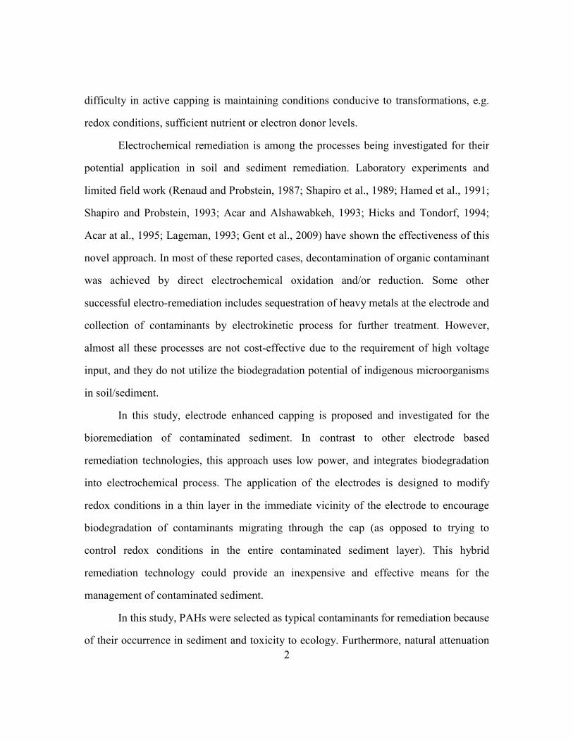
The proposed biodegradation of PAHs by electrode enhanced caps is shown in
Figure 1.1. Two graphite electrodes are placed perpendicular to contaminant transport in
the cap and polarized at low potential. By water electrolysis, oxygen is produced at the
anode, making the local sediment environment more oxidizing. Consequently, these
redox conditions changes and/or produced oxygen are expected to stimulate the activity
of PAH degrading microbes, and accelerate contaminant biodegradation.
Figure 1.1 Conceptual model for an electrode enhanced cap for PAH remediation
1.2 RESEARCH OBJECTIVES AND DISSERTATION OUTLINE
The research objective of this study is to demonstrate the feasibility of electrode
enhanced caps for the remediation of PAH contaminated sediment. To achieve the stated
goal, two types of laboratory scale experiments were conducted. The potential for this
approach was first assessed in slurry reactors under idealized conditions to demonstrate
effective enhancement of biodegradation. When success was confirmed in slurry phase,

4
the hybrid technology was then extended to microcosms to simulate capping under a
more realistic field-like condition. A mathematical model was also developed to describe
the complex physical and chemical processes for electrode enhanced capping. Based on
these specific research objectives, this dissertation is divided into the following chapters:
1) Literature review on PAH contamination and degradation, electrochemical
remediation of soil and sediment and remediation of contaminated sediments (Chapter 2).
2) Electrode enhanced biodegradation of PAH in sediment slurry. This proof of
concept experiment examined the feasibility of electrode enhanced biodegradation of
PAH in slurry phase. In a slurry reactor, mass transfer resistances can be overcome and
conditions conducive to the biological processes can be maintained (Chapter 3).
3) Electro-biodegradation of PAH and redox control in sediment/cap microcosms.
Laboratory scale reactors were used to simulate field conditions for the application of
electrode enhanced caps. The potential to accelerate biodegradation was evaluated in
simulated sediment and cap environments with electrodes, and redox conditions were
characterized (Chapter 4).
4) Model of electrode enhanced capping. A voltage-current relationship was
developed and a coupled reactive transport model was presented to describe the processes
involved in electrode enhanced capping (Chapter 5).
5) Conclusions and recommendations for future work (Chapter 6).
5
Chapter 2: Literature Review
2.1 PAH CONTAMINATION AND DEGRADATION
2.1.1 PAH contamination
Polycyclic aromatic hydrocarbons (PAHs) are chemical compounds that consist
of fused aromatic rings and do not contain heteroatoms or carry substituents. In addition
to their presence in fossil fuels, PAHs are formed by incomplete combustion of organic
materials such as wood, coal, diesel, fat, or tobacco (Page et al., 1999). They may come
from such natural sources as forest fires and volcanic eruptions or from variety of other
anthropogenic sources including fuel combustion, pyrolytic processes, spillage of
petroleum products, waste incinerators and domestic heaters (Juhasz and Naidu, 2000).
Some PAHs (e.g. naphthalene and phenanthrene) have been used for the synthesis of
organic compounds in pesticides, fungicides, mothballs, etc. (Shennan, 1984).
Many PAHs may pose a health risk to ecology and humans because of their toxic,
mutagenic and carcinogenic properties (Goldman et al., 2001; Mastrangelo et al., 1996).
The structure of many PAHs makes them highly lipid soluble and thus they can be easily
absorbed by the lungs, gut, and skin of mammals. Therefore, many PAHs are considered
to be environmental pollutants that can have a detrimental effect on the flora and fauna of
affected habitats, resulting in the uptake and accumulation of toxic chemicals in food
chains. Consequently, the US Environmental Protection Agency (US EPA) listed 16
PAHs as priority pollutants, and determined that benz[a]anthracene, benzo[a]pyrene,
benzo[b]fluoranthene, benzo[k]fluoranthene, chrysene, dibenz[a,h]anthracene, and
indeno[1,2,3-c,d]pyrene are probable human carcinogens.
PAHs can be classified into two groups: low molecular weight PAHs (2-3 rings)
and high molecular weight PAHs (4 or more rings). Low molecular weight PAHs (2-3
6
rings) are more soluble and reactive in environment. As molecular weight and ring
number increase, aqueous solubility decreases but hydrophobicity, lipophilicity and
environmental persistence increase. The genotoxicity also increases as the number of
rings increase up to 4 or 5. In addition, volatility decreases with an increasing number of
fused rings (Wilson and Jones, 1993).
The release of PAHs into the environment is widespread and PAHs have been
detected in a wide variety of environmental samples including air, soil, sediments, water,
oils, tars and food (Juhasz and Naidu, 2000). PAH contamination is frequently associated
with industrial activities such as processing, combustion and disposal of fuel/oil products
(Wilson and Jones, 1993). PAHs are found at many Superfund sites, and other petroleum-
impacted sites (Johnston et al., 1993; Menzie et al., 1992). Because creosote, a compound
containing 85% PAHs by weight, was commonly used in the wood-preserving industry,
PAHs are frequently detected in wood treatment areas (Mueller et al., 1989). Significant
levels of PAHs have been reported in sediments from many industrialized areas
throughout the world.
Due to their hydrophobicity and low solubility, PAHs concentrations in water are
very low. However, PAHs tend to accumulate in soil and sediment, especially those with
high organic carbon fraction. So in aquatic environment, most PAH contamination is
concentrated in sediment, which is considered as a reservoir for PAH accumulation.
2.1.2 PAH degradation
Microbial research in the past several decades has demonstrated that a wide
variety of bacteria, fungi and algae have the ability to metabolize PAHs. A large number
of microorganisms that can degrade PAH have been isolated from soil, sediment, sewage,
and water and characterized (Cerniglia, 1992). Generally, the rate of PAH degradation is

7
inversely proportional to the number of rings. It is believed that 2-ring and 3-ring PAHs
are readily biodegradable given optimal environmental conditions, while PAHs with
more than three rings are more resistant to biodegradation.
The microbial degradation of low molecular PAHs such as naphthalene,
phenanthrene, anthracene and acenaphthene has been well elucidated, and the pathways,
enzymes and genetics have all been reported (Cerniglia, 1992; Davies and Evans, 1964;
Gibson and Subramanian, 1984). However, less is known about the degradation of high
molecular PAHs (Kanaly and Harayama, 2000). Of the four-ring PAHs, biodegradation
of fluoranthene, pyrene, chyrsenene and benz[a]anthracene has been investigated to
various degrees (Kanaly and Harayama, 2000; Juhasz et al., 2000). In general, lower
molecular PAHs tend to oxidize completely to form CO2 and H2O while the high
molecular PAHs will degrade partially to yield various oxygenated metabolites (e.g.,
various phenolic and acid metabolites, cis-dihydrodiol, etc.) (Kanaly and Harayama,
2000).
PAHs are more readily biodegradable under aerobic conditions than with any
other terminal electron acceptor (TEA). Oxidation of aromatic ring is the principal
mechanism involved during PAH biodegradation (Cerniglia, 1992). During the first step
in the aerobic degradation of PAHs, dioxygenase incorporates oxygen atoms at two
carbon atoms of a benzene ring of a PAH resulting in the formation of cis-dihydrodiol
(Kanaly and Harayama, 2000). It undergoes rearomatization by dehydrogenases to form
dihydroxylated intermediates. Subsequently dihydroxylated intermediates undergo ring
cleavage and form tricarboxylic acid (TCA) cycle intermediates (Sabate et al., 1999).
PAH degradation in anaerobic conditions has also been reported but the rate is
much slower compared to that in aerobic conditions (Chang et al.,2002; Rothermich et
al.,2002; Rockne and Strand, 1998, 2001; Rockne et al., 2000; Johnson and Ghosh,
8
1998), and the details of metabolism pathways are very complicated and need further
elucidation (Annweiler et al., 2002).
2.1.3 PAH degradation genes
The traditional culture-dependent methods have been used to enumerate PAH
degrading bacterial population for years. However, only a small portion of
microorganisms of interests can be cultivated under standard cultivation conditions
(Amann et al., 1995). Cultivation-independent approaches have also been employed to
quantifying PAH degrading microorganisms. Recent advances in molecular microbial
technology have allowed for broader analysis of biodegradative organisms in the
environment. Quantitative polymerase chain reaction (qPCR), using primers that target
PAH ring-hydroxylating dioxygenase (PAH-RHDα) genes, has been used to estimate
copy numbers of PAH degrading gene from environmental samples. The genes encoding
PAH degradation include nah-like genes from psedudomas species (Lloyd Jones et
al.,1999; Wilson et al.,1999), phn-like genes from Burkholderia species (Laurie and
Lloyd Jones, 1999), nag-like genes from Ralstonia (Widada et al.,2002), ndo-like genes
(Gomes et al., 2007), nid-like genes (Brezna et al.,2003), pdo-like genes (Johnsen et
al.,2006), etc. Since genes coding for ring-hydroxylating dioxygenases are highly diverse,
primers to amplify a wide range of PAH-RHDα genes were developed and employed to
target majority of PAH degrading genes (Ding et al., 2010; Cebron et al., 2008). All these
primers can be employed in the study of PAH degrading genes by conventional
polymerase chain reaction (PCR) or quantitative PCR (qPCR). qPCR have been proven
to be a powerful tool to determine relative activity of PAH degrading genes. The gene
abundance revealed by qPCR results can potentially be used as an indicator for PAH
biodegradation.
9
2.2 ELECTROCHEMICAL REMEDIATION FOR SOIL AND SEDIMENT
Electrochemical remediation technology is an innovative method for in-situ
remediation for contaminated soil and sediment. Contaminants that could be treated by
this method include inorganic compounds, organic compounds and radionuclides (Acar et
al., 1995; Reddy et al., 1997). It can be performed for different soil types and is
particularly effective for fine-grained soils of low hydraulic conductivity, which are
difficult by other methods.
A typical field electrochemical remediation system is shown in Figure 2.1
(Saichek and Reddy, 2005). Electrodes are inserted at different locations at the
contaminated site and a voltage is applied across the electrodes. Several processes occur
during the application of electric field at contaminated sites to facilitate the removal of
contaminants. These processes will be discussed in more details in the following section.

10
Figure 2.1 Schematic of electrochemical remediation of contaminated soil
2.2.1 Electrokinetic phenomena
Electrokinetics is defined as the physicochemical transport of charge, action of
charged particles, and effects of applied electric potentials on formation and fluid
transport in porous media. The presence of the diffuse double layer gives rise to several
electrokinetic phenomena in soil, which may result from either the movement of different
phases with respect to each other including transport of charge, or the movement of
different phases relative to each other due to the application of an electric field (Acar and
Alshawabkeh, 1993). The electrokinetic phenomena include electroosmosis,
11
electrophoresis, electromigration, streaming potential, sedimentation potential, etc.
(Probstein and Hicks, 1993; Reddy et al., 1997). Electroosmosis is the fluid movement
with respect to solid wall under the influence of an applied electric field. Electrophoresis
is the motion of particles under influence of electric field. Electromigration refers to the
migration of ionic species under an applied potential. Streaming potential, being the
reverse of electroosmosis, is the generation of electric potential by fluid moving through
porous medium. Sedimentation potential, similar to streaming potential, is an electric
field generated by sedimenting colloid particles. Other transport processes, such as
advection, dispersion and diffusion, sometimes play important roles in electrokinetic
processes.
2.2.2 Water electrolysis
Water electrolysis can occur at the electrodes during the application of
electrochemical remediation. The standard potential of a water electrolysis cell is 1.23 V
at 25 °C based on the Nernst Equation. If the applied potential is large enough to
overcome activation barriers, water electrolysis is usually the primary reaction at the
electrodes. Protons and oxygen are produced at the anode, and hydroxyl anions and
hydrogen gas are produced at the cathode.
Anode: 2H2O = O2 + 4H+ + 4e E0 = 1.229V (2-1)
Cathode: 2H2O + 2e = H2 + 2OH− E0 =-0.827V (2-2)
Other electrochemical reactions may occur depending on the concentration of
species, their electrochemical potentials, and the reaction kinetics. For example, ferric
iron may be reduced to ferrous iron at the cathode and chloride may be oxidized to
chlorine at the anode.
12
Anode: Fe3+ + e = Fe2+ E0 = 0.771V (2-3)
Cathode: 2Cl− = Cl2 + 2e E0 = 1.3583V (2-4)
These secondary reactions usually are not favored at the anode and/or cathode
because of the low concentrations of reactants in environmental systems. So water
electrolysis is most often the dominant electrolytic reaction. As a result of water
electrolysis, oxidizing and acidic zone is developed at the anode, and reducing alkaline
zone is developed at the cathode.
2.2.3 Electrochemical oxidation/reduction
During electrochemical remediation, organic contaminants may be destroyed or
converted by either direct or indirect processes. Numerous studies have focused on the
use of direct current (DC) to oxidize or reduce organic contaminants directly
(Alshawabkeh et al., 2005; Goel et al., 2003; Petersen et al., 2007). A few studies
explored the use of alternating current (AC) to degrade organic contaminants (Chin and
Cheng, 1985; Nakamura et al., 2005). Sequential electrolytic reduction-oxidation system
was also developed to degrade energetic compounds (Gilbert and Sale, 2005).
Indirect electrolysis also contributes to contaminants removal during
electrochemical oxidation/reduction processes. During indirect anodic oxidation, strong
oxidants such as ozone, hydrogen peroxide, chlorine, etc. are generated at the anode
instead of oxygen. The contaminant is then oxidized by these strong oxidants (Goel et al.
2003).
2.2.4 Electrochemical stimulation of biodegradation
During biodegradation, microorganisms require an electron donor for reductive
degradation or an electron acceptor for oxidation process. Generally, electron donors and
13
acceptors are applied as chemicals. Electron donors commonly used for in-situ
remediation include hydrogen gas, zero valent iron and vegetable oil, and electron
acceptors in bioremediation include oxygen, nitrate, iron (III), manganese (IV), and
sulfate. A novel alternative is to supply electron donors and/or acceptors by direct
application of electricity.
Electrolysis of water is the primary reaction during electrochemical remediation
process. Hydrogen produced at the cathode can serve as an electron donor and be utilized
by consortia of anaerobic bacteria for reductive degradation, such as dechlorination or
denitrification (Sun et al., 2010; Thrash et al., 2007; Sakakibara and Nakayama, 2001).
At the anode of the reaction of water electrolysis reaction, oxygen is generated and can
serve as an electron acceptor. The produced oxygen has been proven to be effective in
stimulating bacterial growth during nitrification (Watanabe et al., 2002).
Direct electron transfer from electrodes to a bacterial cell provides another means
to stimulate microbial metabolism. Geobacter species and some other microorganisms
were shown to be able to directly transfer electrons to electrodes (Lovley, 2008; Logan,
2009). Electrodes can serve as either an electron donor or acceptor directly. It was shown
that graphite electrodes could serve as an electron acceptor for the degradation of toluene
and benzene (Zhang et al., 2010). Another study has shown the evidence of graphite
electrodes as an electron donor in anaerobic respiration (Gregory et al., 2004).
2.3 REMEDIATION OF CONTAMINATED SEDIMENTS
2.3.1 Contaminated sediments
Contaminated sediments are defined as aquatic sediments that contain chemical
substances in excess of appropriate geochemical, toxicological, or sediment quality
criteria, or are otherwise considered to pose a threat to human health or the environment
14
(US EPA, 1998). It has been estimated that approximately 10 percent of aquatic
sediments underlying United States surface waters are sufficiently contaminated to pose
potential risks to fish and to humans and wildlife that eat fish (US EPA, 1998).
Sediment is an environmental sink for many contaminants, since many pollutants
originally introduced into the water column have affinities for sediment particles. The
contaminants that introduced into the sediment are from various sources, including
municipal sewage treatment plants, combined sewer overflows, storm water discharges,
direct industrial discharges of process waste, runoff and leachate from hazardous and
solid waste sites, agricultural operations, mining operations, industrial manufacturing and
storage sites, atmospheric deposition and contaminated groundwater discharges to surface
water (Baudo and Muntau, 1990). Contaminants detected in sediments include
polychlorinated biphenyls (PCBs), heavy metals, chlorinated solvents, pesticides, PAHs,
etc. Sediments can serve as contaminant sources for transport and exposure to aquatic
biota particularly with bioaccumulative contaminants. Hydrophobic organic contaminants
such as PAHs and PCBs typically bind strongly to organic matter in sediments and these
sediment-bound pollutants serve as long-term exposure sources to aquatic ecosystems.
For instance, fish and bottom-dwelling organisms can accumulate toxic compounds like
PCBs that are passed up the food chain.
PAHs have been found to be a key contaminant at many contaminated sediment
sites (Reible et al., 2007; Perelo, 2010; Baumard et al., 1998). Because they can be
adsorbed strongly to organic matters in sediment, PAHs have been found to be
particularly persistent in sediments. Since PAHs have been reduced in many wastewater
effluents, the accumulated PAHs in the sediments will release slowly into water column
as a long-term source and pose potential threat to water quality and aquatic ecosystem via
bioaccumulation in food chains.
15
Despite the persistence of PAHs in sediments, it does not imply that PAHs may
reside in the bottom sediments indefinitely. Microbial degradation of PAHs is one of the
main processes to remove these contaminants from bottom sediments and the water
column. Both aerobic and anaerobic degradation of PAHs occurs in aquatic sediments
naturally, but anaerobic degradation occurs at a much slower rate than aerobic
degradation. Sediments are generally anaerobic except in the upper layer adjacent to
water, ranging from millimeters to centimeters. Therefore biodegradation of PAHs is
greatly hindered by oxygen shortage in sediments.
2.3.2 Sediment remediation methods
Current remediation approaches to addressing contaminated sediments include
monitored natural attenuation (MNA), dredging and excavation, and capping techniques.
2.3.2.1 Monitored natural attenuation
Monitored natural attenuation (MNA) is a technique used to monitor or test the
progress of natural attenuation processes that can degrade contaminants in sediments (US
EPA, 2005). It may be used with other remediation processes as a finishing option or as
the only remediation process if the rate of contaminant degradation is fast enough to
protect human health and the environment. Not all natural processes result in risk
reduction; some may increase or shift risk to other locations or receptors. Therefore, to
implement MNA successfully as a remedial option, those processes that contribute to risk
reduction should be identified and evaluated. Appropriate monitoring are required to
ensure acceptable risk management, and these monitoring methods include contaminant
analyses and ecological and health effects assays.
The most common natural attenuation processes occurring in sediments are
intrinsic biodegradation of the contaminants and the chemical transformation of the
16
contaminant to a less toxic form. Other important natural attenuation processes, from
most to least preferable, include (1) sorption or other binding processes to the sediment
matrix to reduce contaminant mobility and bioavailability; (2) a decrease in contaminant
concentration levels in near-surface sediment zone through burial or mixing-in-place with
cleaner sediment; (3) a decrease in contaminant concentration levels in the near-surface
sediment zone through dispersion of particle-bound contaminants or diffusive or
advective transport of contaminants to the water column. Exposure levels are reduced by
the decrease of contaminant levels through the last two natural attenuation processes.
The two primary advantages of MNA are its relatively low cost and its non-
invasive nature. The implementation cost includes monitoring, site characterization and
modeling, among which monitoring is the major cost in most cases. MNA typically has
no physical disruption to the current ecological conditions, which may be an important
advantage for sensitive environments. One major limitation of MNA is that it leaves
contaminants in place so that the risk of exposure remains. Another disadvantage of
MNA is that the rate of reducing risk is relatively slow compared to active remediation
technologies. MNA is widely considered to be the most effective remediation technique
at those sites with a low exposure risk to ecology and/or human, otherwise active
methods are required to reduce the risks posed by contaminated sediments.
2.3.2.2 Dredging and excavation
A more effective approach than MNA is preferred for contaminated sediments
with a higher risk to natural environment and human. The most common method of
remediating contaminated sediment to reduce risk is removal by dredging or excavation.
Dredging is the removal of submerged material, while excavation refers to the sediment
of which water has been diverted or drained. The processes involved in dredging of
17
contaminated sediments include sediment removal, transport, staging, treatment, and
disposal.
If cleanup goals are achieved by dredging or excavation, it minimizes the
uncertainty about long-term effectiveness by removal of contaminated sediments from
the aquatic environment. Furthermore, removal of contaminated sediment requires less
time to achieve remedial action objectives, and it has greater flexibility for future water
body use. Because of these advantages, dredging or excavation has been used for
remediation of contaminated sediment at more than 100 Superfund sites (US EPA, 2005).
The limitations of dredging or excavation compared to MNA or in-situ capping
include complexity and high cost considering the dredging itself and the processes of
transport, staging, treatment and disposal of the dredged sediment. Furthermore,
contaminant release from resuspension, and the potential risk of residual contamination
following dredging/excavation give rise to uncertainties associated with
dredging/excavation (Hong et al., 2011). Finally, the aquatic community and habitat
within the remediation area is at least temporally destroyed with the long term effect
being unknown. As a result of these limitations, Perelo (2010) examined the effectiveness
of dredging and found that half of the 20 sites studied didn’t achieve remedial goals by
dredging.
2.3.2.3 In-situ capping
In-situ capping is the placement of a covering or cap made of clean isolating
material over contaminated sediment, which remains in place. Capping materials include
clean sediment, sand, gravel, geotextiles, liners, and other permeable or impermeable
materials or the combination of above elements. In-situ capping can reduce the risk of
contaminated sediment by physical isolation of sediment to reduce direct exposure,
18
stabilization of sediment to reduce resuspension and transport to other sites, and/or
chemical isolation of sediment to reduce exposure from dissolved and colloidally bound
contaminants transported into the water column (US EPA, 2005).
In-situ capping can quickly reduce the exposure risk, and it requires less capital
cost and material handling. Also it reduced the risks of resuspension, dispersion and
volatilization of contaminants in comparison to dredging. The cap may be less disruptive
of local ecological communities, and provide clean substrate for recolonization by
bottom-dwelling organisms. In comparison to MNA, capping is considered to be a more
aggressive and effective approach.
Laboratory and field studies of capping have shown that even a simple sand cap
can reduce the risks of contaminants from contaminated sediments. Thibodeaux and
Bosworth (1990) used clean material as a capping layer to retard diffusion and reduce the
flux from PCB-contaminated sediments. Wang et al. (1991) and Thoma et al. (1993)
measured and modeled diffusion flux of some organic compounds from capped
sediments and evaluated its migration through clean sediment. Lampert et al. (2011)
demonstrated the effectiveness of thin-layer sand caps to reduce the bioaccumulation of
PAHs provided the thickness of the cap layer exceeds the depth of organism interaction
with the sediments, and contaminant migration is controlled by molecular diffusion.
Because contaminants remain in the aquatic environment, contaminants could
become exposed or be dispersed if the cap is significantly disturbed or if contaminants
move through the cap by diffusion or advection. Gidley et al. (2012) showed rapid
breakthrough of lower molecular weight PAHs with groundwater seepage in coarse sand
capping material.
To overcome the limitation that contaminants remain untreated with conventional
sand capping, an alternative - active capping has been proposed. Active capping can be
19
broadly defined as capping with materials that encourage degradation or enhance
sequestration of the contaminants. A variety of materials has been proposed and used for
sequestration of the different contaminants. Apatite, a matrix of calcium phosphate and
various other common anions, has been investigated for sequestration of metals in
sediments (Reible et al., 2007; Kaplan and Knox, 2004). Zeolite was also evaluated for
containment of metals as active barrier system (Jacobs and Forstner, 1999). Organoclay,
a modified bentonite prepared by introducing organic molecules into the clay mineral
structure, has been tested for control of non-aqueous phase liquids and other hydrophobic
organic contaminants (Reible et al., 2005; Knox et al., 2012). Organic sorbents such as
activated carbon, coke and biopolymer showed the ability to sequester hydrophobic
organic contaminants (Zimmerman et al., 2004; Murphy et al., 2006; Knox et al., 2012).
The effectiveness of a cap was greatly improved by adding an organic sorbent layer such
as activated carbon, or by mixing sorbent directly with contaminated sediment.
Commercially available active capping materials include AquaBlok™ (Adventus
Americas, Inc., Toledo, OH), which is a bentonite clay material formed around a granular
core, and organoclay materials, reactive core mat, liners, etc. from CETCO.
Being similar to conventional capping, the sequestration approach does not
degrade contaminants; it only physically sequesters them. Slight changes in the capping
environment can cause the erosion of the capping layer and resuspension of the
sequestered contaminants at high concentration. Also, surface fouling of the sorptive
materials may occur and lead to lower treatment efficiencies (Reible et al., 2007). So the
sequestration approach may not be appropriate for all the contaminated sites. These
limitations have stimulated the idea of an active capping in which contaminants are
transformed to nontoxic products by chemical, biological and/or combined processes.
Research on the application of active capping to enhance contaminant degradation has
20
not been addressed adequately and has very few successful cases. Choi et al. (2009)
developed a “reactive” cap/barrier system composited of granular activated carbon
impregnated with reactive iron/palladium (Fe/Pd) bimetallic nanoparticles (reactive
activated carbon) for PCB-contaminated sediments. 2-chlorobiphenyl was chemically
degraded via a combined process of adsorption and dechlorination with the reactive cap.
Sun et al. (2010) proposed an integrated Fe(0)–sorbent–microorganism remediation
system as an in-situ active capping technique to remediate nitrobenzene-contaminated
sediment. In the integrated capping system, Fe(0) acted to reduce nitrobenzene to aniline,
cinder served as the sorbent and support matrix, and nitrobenzene was biodegraded to
aniline by microorganisms. Himmelheber et al. (2011) demonstrated that a laboratory-
scale bioreactive in-situ sediment cap could completely dechlorinate dissolved-phase
PCE for the treatment of PCE with the amendment of a mixed, anaerobic dechlorinating
consortium and soluble electron donor. Now there is a pressing need to develop new cost-
effective active capping technologies over the long time scales for in-situ sediment
remediation.
2.4 RESEARCH NEEDS: ACTIVE CAPPING COUPLING ELECTROCHEMICAL PROCESSES
WITH BIOREMEDIATION
During recent years, electrochemical technologies have been proposed for the
remediation of soil and sediment. Numerous studies have demonstrated the effectiveness
of electrokinetic remediation in the removal of soil contaminants. However, for
hydrophobic organic compounds (HOCs) with a high tendency to be adsorbed onto soil
and sediment, electrokinetic remediation was not applicable because of their low
concentration in mobile phase. PAHs, a representative subset of HOCs, fall into this
group. Bioremediation is a reasonable alternative to treat soil and sediment polluted by
PAHs but the terminal electron acceptor in sediments even a few centimeters below the

21
sediment-water interface is typically iron or sulfate reflecting highly reduced conditions
that are not conducive to PAH degradation. Successful implementation of in-situ
bioremediation sometimes requires the presence or injection of electron acceptors into the
porous medium. A technology for a continuous introduction of electron acceptors has
been the principle bottleneck in the successful treatment for PAH contaminated soil and
sediment. Application of an electric current may be an alternative option for providing
more favorable electron acceptors. An electrode-based active capping has the potential as
a continuous pollutant remediation method for PAH contaminated sediments. Research
on active capping coupling electrochemical processes with bioremediation is needed for
the management of PAH contamination.
Although both electrochemical remediation and bioremediation have been
documented intensively for treatment of contaminated soil and sediment, the integration
of electrochemical processes and bioremediation has not been addressed adequately. The
proposed study will focus on coupling electrochemical processes with bioremediation
within an active cap for PAH contaminated sediment. This novel technology will fill the
gap between electrochemical processes and bioremediation for PAH contaminated soil
and sediment. Also, an electrode enhanced capping will be one of the few active capping
technologies that are able to enhance contaminant biodegradation.

22
Chapter 3: Electrode Enhanced Biodegradation of PAH in
Sediment Slurry
3.1 INTRODUCTION
PAHs may be naturally removed in sediments by microbial degradation.
Numerous bacterial species are capable of using PAHs as sole carbon and energy sources,
and most of these organisms can metabolize a range of PAHs (Kastner et al., 1994;
Chung and King, 2001; Hedlund and Staley, 2006; Dagher et al., 1997). The ability of
aerobic microorganisms to degrade PAHs is well known and has been observed in
laboratory and field studies with a variety of soils and sediments for many years (Bauer
and Capone, 1985; Hambrick et al., 1980; Heitkamp and Cerniglia. 1987; Boyd et al.,
2005). PAH degradation under anaerobic conditions has also been reported but it is
relatively recent, and results on the extent of anaerobic biodegradation are controversial
(Foght, 2008; Leduc et al., 1992; Johnson and Ghosh, 1998; Mihelcic and Luthy, 1988).
In general, the rate of anaerobic biodegradation is much slower than the rate of aerobic
conditions. However, the rate of PAH biodegradation in sediments is highly site specific
and varies significantly (Shuttleworth and Cerniglia, 1995).
Sediments are often anaerobic because of the high biological oxygen demand of
organic material, low solubility of oxygen, and mass transfer limitations of oxygen from
the atmosphere into the sediment. The addition of oxygen has the potential to enhance
PAH biodegradation in sediments. A novel technique to supply oxygen is by water
electrolysis in the sediment. At the anode of the reaction of water electrolysis, oxygen is
generated and it has been proven to be effective in stimulating bacterial growth
(Watanabe et al., 2002).
In this dissertation, an electrode enhanced capping was proposed and investigated
for the bioremediation of PAH contaminated sediment. In this Chapter, the potential for
23
this approach was assessed in slurry reactors under idealized conditions to demonstrate
effective enhancement of biodegradation.
Anacostia River sediment was selected as model sediment in this study because of
its historical contamination by PAHs (Lu et al., 2006). Degradation of two model PAHs
(naphthalene and phenanthrene) were studied under aerobic and nitrate reducing
conditions to evaluate PAH degradation potential in the Anacostia sediments. Electrode
enhanced biodegradation in sediment slurry was conducted, and compared with
biodegradation under aerobic and anaerobic conditions. To distinguish the effect of
abiotic loss of PAH during electrochemical processes, PAH loss in a killed control
reactor was also studied.
3.2 BIODEGRADATION OF PAH UNDER AEROBIC AND NITRATE REDUCING CONDITIONS
3.2.1 Materials and methods
3.2.1.1 Sediment and medium
PAH contaminated sediment was obtained from Anacostia River sediment and
sieved through 2mm. It was stored at 4 °C until added to slurries for these studies. The
water used to form the slurry was a low salt solution to simulate a typical freshwater
environment. The minimal salt medium (MSM) to make sediment slurry contained 4 g of
KH2PO4, 4 g of Na2HPO4, 0.5 g of NH4Cl, 0.2 g of MgCl2•6H2O, and 1 mL of trace
element solution SL-4 per 1 L of DI water. SL-4 was composed of 0.5 g of EDTA, 0.2 g
of FeSO4•7H2O and 100 mL of trace element solution SL-6 per 1 L of DI water. The
composition of SL-6 was 0.3 g of H3BO3, 0.2 g of CoCl2•6H2O, 0.1 g of ZnSO4•7H2O,
0.03 g of MnCl2•4H2O, 0.03 g of Na2MoO4•H2O, 0.02 g of NiCl•6H2O and 0.01 g of
CuCl2•2H2O per 1 L of DI water (Atlas, 2010). The pH of MSM is 6.8.
24
3.2.1.2 Biodegradation under aerobic conditions
Aerobic experiments were conducted in 250-mL amber bottles, each containing
100 mL sediment slurry (1 % solid content by weight), and 150 mL air. These bottles
were sealed with a Teflon-lined septum and secured with a screw cap.
The total oxygen demand for 100 mL sediment slurry with a solid content of 1 %
was about 5-10 mg because the biochemical oxygen demand (BOD) of sediment was
estimated as 5-10 mg/g. In each bottle, 150 mL air had 45 mg oxygen, keeping the slurry
in aerobic condition during the course of the experiment.
0.45 mg of naphthalene and 0.08 mg of phenanthrene were spiked to each bottle
at the beginning of the experiment. After establishing an appropriate gas headspace
composition (21 % oxygen as in the ambient air), the bottles were sealed and incubated in
a tumbler at room temperature. Periodically, a serum bottle from the batch samples was
sacrificed for PAH analysis and DNA extraction. Measurement of dissolved oxygen (DO)
concentration (YSI Incorporated, Model 50B) was made to assure that oxygen was not a
limiting factor for biodegradation.
Control samples were run concurrently with the test samples. Control samples
were treated by autoclaving the glassware and sediment slurry at 121 °C for 30 minutes
and then adding sodium azide such that the concentration of sodium azide in the control
samples was 10 mM. The experiments were conducted in a batch mode with test samples
and controls being prepared simultaneously.
3.2.1.3 Biodegradation under nitrate reducing conditions
Amber glass tubes of 40 mL were used for anaerobic experiment. Each tube was
filled with sediment slurry (2.5 % solid content) to zero headspace, and sealed with a
Teflon-lined septum and secured with a screw cap.
25
Nitrate reducing conditions have been generated with the addition of external
nitrate (Leduc et al., 1992; Johnson and Ghosh, 1998; Mihelcic and Luthy, 1988). In this
study, NaNO3 was added to MSM so that the initial nitrate concentration in each tube was
5.88 mM.
0.27 mg of naphthalene and 0.074 mg of phenanthrene were spiked to each tube at
the beginning of the experiment. Strict anaerobic procedures were followed during
system setup. The medium was purged with nitrogen gas immediately after autoclaving
and stored in an anaerobic chamber overnight prior to the experiment. All the sediment
slurry was prepared in an anaerobic chamber. After the setup, all the bottles were sealed
and incubated in a tumbler at room temperature. Periodically, a serum bottle from the
batch samples was sacrificed for PAH analysis and DNA extraction. Dissolved oxygen
concentration was measured at each sampling event to assure no oxygen was detected in
the sediment slurry. Control samples were prepared under anaerobic condition by
autoclaving the glassware and sediment slurry at 121 °C for 30 minutes and then adding
sodium azide at a final concentration of 10 mM.
3.2.1.4 Sampling procedures
Bottles and tubes were unloaded from tumbler and sediment slurry was allowed to
settle down for 1 hour before sampling. Triplicate supernatant samples were collected
and extracted using liquid-liquid extraction by hexane for PAH analysis.
The procedures of liquid-liquid extraction by hexane include the following steps:
1) 5 mL or 10 mL hexane was added to glass sample vials and weighed;
2) An aliquot of supernatant was collected and added to the hexane sample vials,
and weighed again. The difference of weight was used to calculate the volume
of supernatant;
26
3) The mixture was sonicated (Branson 2200 ultrasonic cleaner) for about 30
minutes in a water bath and then stored in 4 °C before the next step;
4) 2 mL hexane sample was added to a 2 mL graduated vial and concentrated
under nitrogen flow to 0.1~0.3 mL;
5) 2 mL acetonitrile was added to the graduated vial and concentrated under
nitrogen flow to a total volume of 2 mL. The graduated vial was weighed
before adding the hexane sample and after this step, and the difference was
used to calculate the final acetonitrile volume. The acetonitrile sample was
ready for PAH analysis by HPLC.
Sediment slurry was centrifuged at 3500 RPM for 30 minutes by centrifuge
(International Equipment Company, Model Size 2). The supernatant and solid were
collected and stored in 4 °C and -20 °C until further analysis, respectively.
3.2.1.5 PAH analysis
PAH concentration was measured by HPLC with a 250×4.6 mm column
(Phenomenex Luna 5u C18(2) 100A) using a mobile phase composed of 15 % water and
85 % acetonitrile at 1 mL/min. Detection was made by a fluorescence detector (Waters
2475) with an excitation wave length of 270 nm and an emission wave length of 360 nm.
3.2.1.6 DNA extraction
Solids were collected for each sacrificed sample and the solid was stored at -20 °C
until DNA extraction. DNA from an aliquot of sediment solid was extracted using
FastDNA SPIN Kit for Soil (MP Biomedicals) according to the instructions of the
manufacturer with minor changes. The water content was also measured in order to
determine the DNA concentration per weight of dry sediment.
27
Pseudomonas putida G7 (DSMZ 4476) carrying the naphthalene dioxygenase
(nahA) gene was used as a reference strain for primer test and qPCR calibration. It was
pre-grown in DSMZ medium 444, and harvested in log-phase. DNA from Pseudomonas
putida G7 (ppG7) was extracted using DNeasy Blood & Tissue Kit (Qiagen).
DNA concentrations in extracts were determined by Nanodrop ND-1000
spectrophotometer (NanoDrop Technologies, Inc). The absorbance at 260 nm was read
and converted to DNA concentration. DNA extract was diluted to a final concentration of
10 ng/μL, 1 ng/μL, 0.1 ng/μL, 0.01 ng/μL, and 0.001 ng/μL as stock solution.
3.2.1.7 PCR and qPCR for PAH degrading genes
The primer set used in PCR and qPCR targets aromatic ring-hydroxylating-
dioxygenase (RHDα) for gram negative PAH-degrading bacteria, which covers a large
range of functional genes including bphA1, phnAc, nagAc, nahAc, nahA3, etc. (Cebron
et al., 2008).
Table 3.1 Characteristics of gram negative PAH-RHDα primer
Sequence 5’-3’ Amplicon
size(bp)
Annealing
temperature(C)
Forward
primer GAG ATG CAT ACC ACG TKG GTT GGA
306 57
Reverse
primer AGC TGT TGT TCG GGA AGA YWG TGC MGT T
Conventional PCR was performed in a reaction volume of 25 μL containing 12.5
μL of DreamTaq Green PCR Master Mix (2X) (Fermentas), 2 μL of mixed forward and
reverse primer (5 μM), 2.5 μL DNA extract (2.5 μL water for negative control), 2.5 μL of
28
20X bovine serum albumin (BSA) and 5.5 μL water. It was conducted in a PTC-200
Peltier thermal cycler (MJ Research).
PCR thermal cycling includes the following steps:
Step 1: Initial dissociation: 95 °C for 5 min;
Step 2: 35 cycles of the following three steps:
Step 2.1 Denaturation: 95 °C for 30 s;
Step 2.2 Primer annealing: 57 °C for 30 s;
Step 2.3 Elongation: 72 °C for 30 s;
Step 3: 72 °C for 7 min.
qPCR was performed in 25 μL reaction volume containing 12.5 uL of Power
SYBR green PCR master mix(Applied Biosystems), 2 μL of mixed forward and reverse
primer (5 μM), 2.5 μL DNA extract (2.5 μL water for negative control), 2.5 μL of 20X
BSA and 5.5 μL water. All DNA samples were analyzed in duplicate or triplicate. qPCR
was performed in Applied Biosystems 7900HT sequence Detection System machine.
qPCR thermal cycling includes the following steps:
Step 1: Initial dissociation: 95 °C for 5 min;
Step 2: 40 cycles of the following three steps:
Step 2.1 Denaturation: 95 °C for 30 s;
Step 2.2 Primer annealing: 57 °C for 30 s;
Step 2.3 Elongation: 72 °C for 30 s;
Step 2.4 Dissociation of the primer’s dimers: 80 °C for 10 s;
Step 3: 72 °C for 7 min;
Step 4: Melting curve analysis: 0.5 °C temperature increment from 51 °C to 95°C.
Two major changes for qPCR from conventional PCR were: 1) dissociation of
primer’s dimmers at 80 °C for 10 s; 2) melting curve analysis at the end of the regular
29
thermal cycling. Both steps were added to avoid the formation of primer’s dimmers,
whose signal will interfere with PCR products. Dissociation step was to dissociate any
primer dimers during each polymerase chain reaction, and in the final step by viewing a
melting curve, it was ensured that the desired amplicon was detected and no primer
dimers were formed.
3.2.2 Results and discussion
Figure 3.1 shows the time varying concentration of naphthalene and phenanthrene
under aerobic conditions. Maintenance of aerobic conditions throughout the experiment
was confirmed with the measurement of dissolved oxygen at the end of the experiment.
Triplicate experimental samples showed an average DO of 83.1 % with a standard
deviation of 3.1 %, while DO of control samples was 96.6 % with a standard deviation of
1.0 %. Over a period of two days, considerable degradation of naphthalene and
phenanthrene was observed, while the concentration of PAH in the control sample
remained relatively constant. Naphthalene concentration decreased from ~1500 µg/L to
~10 µg/L within the first 24 hours and to no detection level (<1 µg/L) in the next 24
hours. Phenanthrene biodegradation rate was slower than naphthalene but complete
disappearance still happened within 48 hours. Phenanthrene concentration decreased
from 65 µg/L to 20 µg/L within the first 24 hours and to no detection level (<1 µg/L) in
the next 24 hours.
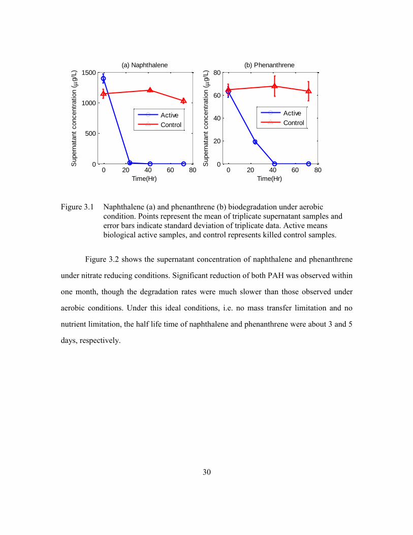
30
Figure 3.1 Naphthalene (a) and phenanthrene (b) biodegradation under aerobic
condition. Points represent the mean of triplicate supernatant samples and
error bars indicate standard deviation of triplicate data. Active means
biological active samples, and control represents killed control samples.
Figure 3.2 shows the supernatant concentration of naphthalene and phenanthrene
under nitrate reducing conditions. Significant reduction of both PAH was observed within
one month, though the degradation rates were much slower than those observed under
aerobic conditions. Under this ideal conditions, i.e. no mass transfer limitation and no
nutrient limitation, the half life time of naphthalene and phenanthrene were about 3 and 5
days, respectively.
0 20 40 60 800
500
1000
1500(a) Naphthalene
Time(Hr)
Supern
ata
nt
concentr
ation (
g/L
)
Active
Control
0 20 40 60 800
20
40
60
80(b) Phenanthrene
Time(Hr)
Supern
ata
nt
concentr
ation (
g/L
)
Active
Control
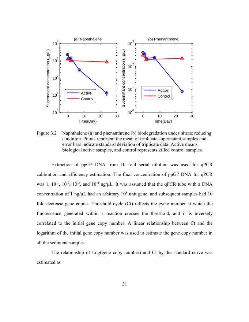
31
Figure 3.2 Naphthalene (a) and phenanthrene (b) biodegradation under nitrate reducing
condition. Points represent the mean of triplicate supernatant samples and
error bars indicate standard deviation of triplicate data. Active means
biological active samples, and control represents killed control samples.
Extraction of ppG7 DNA from 10 fold serial dilution was used for qPCR
calibration and efficiency estimation. The final concentration of ppG7 DNA for qPCR
was 1, 10-1, 10-2, 10-3, and 10-4 ng/μL. It was assumed that the qPCR tube with a DNA
concentration of 1 ng/μL had an arbitrary 108 unit gene, and subsequent samples had 10
fold decrease gene copies. Threshold cycle (Ct) reflects the cycle number at which the
fluorescence generated within a reaction crosses the threshold, and it is inversely
correlated to the initial gene copy number. A linear relationship between Ct and the
logarithm of the initial gene copy number was used to estimate the gene copy number in
all the sediment samples.
The relationship of Log(gene copy number) and Ct by the standard curve was
estimated as
0 10 20 3010
0
101
102
103
104
Time(Day)
Supern
ata
nt
concentr
ation (
g/L
)
(a) Naphthalene
Active
Control
0 10 20 3010
0
101
102
103
Time(Day)S
upern
ata
nt
concentr
ation (
g/L
)
(b) Phenanthrene
Active
Control
32
Log(gene copy numbers) = k ∗ Ct + b (3-1)
Ct value of environmental samples was estimated from amplification plot and
then converted to gene copy number by this linear relationship.
For easier comparison of PAH degrading gene populations among environmental
samples, the PAH-RHDα GN gene levels were normalized by total DNA or weight of dry
sediment. Gene copy number per DNA was an indicator of relative percentage of PAH
degrading bacteria among the entire community, while gene copy per dry sediment
reflected the absolute quantity of PAH degrading bacteria.
All values were reported as an increase from unincubated sediment, which was
stored in 4 °C until DNA extraction.
Figure 3.3 shows that under aerobic condition PAH degrading gene concentration
in the PAH spiking sediment slurry increased by two orders of magnitude at t = 4 hr
compared to unincubated sediment (t = 0), and the increase was three orders of
magnitude at t = 28 hr. After one day, the gene copies reached the plateau phase, where
gene copy number neither increased nor decreased. The killed control sampled at t = 72
hr didn’t show any changes of gene copy number compared to the unincubated sediment.
The results of two normalization methods didn’t show significant difference in
terms of gene copy increase. However, it was observed that total DNA per dry sediment
increased by 2-3 times after the incubation, which implied that the total bacterial
population increased under aerobic condition. Consequently, the increase of gene copy
number per DNA was less than the increase of gene per dry sediment.
Similarly, Figure 3.4 shows the PAH degrading gene concentration under nitrate
reducing condition. The PAH degrading gene concentration in sediment slurry increased
by one orders of magnitude after two days, and the increase was two orders of magnitude
33
at the seventh day, after which the gene copies reached the plateau phase. Although
increased gene copy numbers was observed under both aerobic and nitrate reducing
condition, the maximum increase under nitrate reducing condition was one order
magnitude less than that under aerobic condition.
The increase of gene copy number was believed to be associated with PAH
biodegradation. In the first 24 hours, it was observed that the fast growth of dioxygenase
gene and PAH disappearance occurred simultaneously. However, after all the PAH was
depleted, gene copies stopped increasing, which implied the PAH degrading bacteria
went into stationary phase.
qPCR analysis provided the evidence of PAH biodegradation under aerobic and
nitrate reducing condition, indicating that the indigenous microbial community in
Anacostia River sediment has the potential to biodegrade naphthalene and phenanthrene
in suitable environmental conditions. It was demonstrated that the occurrence of the
biodegradation process can be determined by monitoring the number of catabolic genes.
PAH-RHDα Gram Negative primer could be used for accurate qPCR quantification of
PAH degrading bacteria directly on DNA from sediment samples.

34
Figure 3.3 qPCR quantification and DNA extraction results under aerobic condition: 1)
Copy number of PAH degrading gene normalized by total DNA; 2) Copy
number of PAH degrading gene normalized by dry sediment; 3) DNA
concentration per dry sediment.
Figure 3.4 PAH degrading gene abundance by qPCR quantification under nitrate
reducing condition. The PAH-RHDα GN gene levels were normalized by the
weight of dry sediment. All the values were reported as an increase from
unincubated sediment control.
-0.5
0
0.5
1
1.5
2
2.5
3
3.5
4
0 4 28 48 72 72(Control)
Time(hr)
No
rmali
zed
Gen
e C
op
y N
um
ber
-2.0E+04
0.0E+00
2.0E+04
4.0E+04
6.0E+04
8.0E+04
1.0E+05
1.2E+05
1.4E+05
DN
A p
er
dry
sed
imen
t (n
g/g
)
Log[Gene/DNA]
Log(Gene/DrySediment)
DNA/Sediment (ng/g)
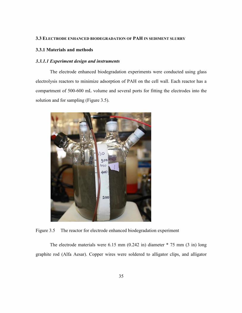
35
3.3 ELECTRODE ENHANCED BIODEGRADATION OF PAH IN SEDIMENT SLURRY
3.3.1 Materials and methods
3.3.1.1 Experiment design and instruments
The electrode enhanced biodegradation experiments were conducted using glass
electrolysis reactors to minimize adsorption of PAH on the cell wall. Each reactor has a
compartment of 500-600 mL volume and several ports for fitting the electrodes into the
solution and for sampling (Figure 3.5).
Figure 3.5 The reactor for electrode enhanced biodegradation experiment
The electrode materials were 6.15 mm (0.242 in) diameter * 75 mm (3 in) long
graphite rod (Alfa Aesar). Copper wires were soldered to alligator clips, and alligator
36
clips were connected to the graphite rods. The external power was connected only to the
copper wires for power supply.
Four out of five ports in each reactor were sealed with Teflon lined rubber
stopper. If external power was applied, copper wires went through rubber stoppers to
connect to power. Screw-caps with Mininert valve were used at the sampling port of the
reactor. By this setting, all the ports in each reactor were air tight and there was no leak to
the atmosphere.
The following four sets of experiments were conducted:
1) ElectroBio reactor (RE): Power was applied to active sediment slurry that was initially
anaerobic;
2) Killed control (KC): Power was applied to killed control sediment slurry (autoclaved)
and also initially anaerobic;
3) Aerobic control (AE): No power was applied, but the sediment slurry was maintained
in aerobic conditions during the course of the experiment. By maintaining aerobic
conditions, the PAH degradation potential of the slurries could be determined;
4) Anaerobic control (AN): No power was applied, but anaerobic conditions were
maintained. In this treatment the rate of degradation in an ineffective electrode cap could
be determined (that is, one that was ineffective at creating oxidizing conditions).
The copper wires at the electrodes were connected to Extech 382202 DC power
supply (Extech Intruments Corp, Waltham, MA). The applied power was about 3.5 V and
the current was about 15 mA.
The experiments were conducted in a period of 4 days, constantly stirred by a stir
bar, and sediment slurry were samples periodically for PAH analysis. GASTIGHT
syringe and needle (Hamilton Company) were used for sampling at each sampling time.
37
After the experiment, the slurry was centrifuged at 3500 RPM for 30 minutes and
solids were collected and store in -20 °C.
3.3.1.2 Sediment slurry preparation
PAH contaminated sediment was obtained from Anacostia River sediment and
sieved through 2 mm. It was stored at 4 °C until used.
The minimal salt medium (MSM) was used to make sediment slurry. 2 L of
anaerobic MSM was made by autoclave, deoxygenation, and stored in anaerobic chamber
(Coy Laboratories) filled with 95 % nitrogen and 5 % hydrogen. 1 L of aerobic medium
was made by oxygenation with air, and stored under atmosphere conditions.
43.3 mg naphthalene and 8.1 mg phenanthrene were dissolved in 20 mL hexane
as stock solution for spiking the sediment slurry.
To prepare the sediment slurry for RE, AE and AN, naphthalene and
phenanthrene were initially coated onto the insides of a jar by hexane delivery. 3.14 mL
PAH stock in hexane (6.79 mg naphthalene and 1.27 mg phenanthrene) was added to a
jar and distributed evenly around the bottom and sides of the jar. The hexane was allowed
to evaporate under nitrogen gas flow, leaving the PAH coated on the inside wall of the
jar. 30.20 g wet Anacostia River sediment (water content = ~50 %) was added to the jar
and diluted with 150 mL of anaerobic MSM in anaerobic chamber. The solid content of
this sediment slurry was 10 %. The sediment slurry was sealed and tumbled overnight to
make PAH dissolved and partitioned into solid phase. The next day, 45 mL of 10 % solid
slurry with PAH and 405 mL of anaerobic MSM were added to RE reactor in anaerobic
chamber, making a final sediment slurry of 450 mL with a solid content of 1 % by
weight. Similarly, 55 mL of 10 % solid slurry and 545 mL of anaerobic MSM made 600
mL final sediment slurry for AN in anaerobic condition, and 40 mL of 10 % solid slurry
38
and 360 mL of aerobic MSM made 400 mL of aerobic sediment slurry for AE in aerobic
condition. The total volume of AE reactor was 600 mL, leaving 200 mL space for air.
200 mL air had about 60 mg oxygen, which was enough to keep AE reactor in aerobic
condition during a period of several days.
To prepare the sediment slurry for KC, 11.30 g wet sediment was added to a jar
(jar-1) and diluted to 50 mL using MSM, and autoclaved at 121 °C for 30 minutes three
times. Another jar (jar-2) was autoclaved and then coated with 1.18 mL PAH stock (6.79
mg naphthalene and 1.27 mg phenanthrene). Sediment slurry in jar-1 was transferred to
jar-2 in anaerobic chamber, sealed and tumbled overnight. The next day, all the 50 mL
slurry and 450 mL autoclaved anaerobic MSM was added to reactor in anaerobic
chamber, making a final medium of 500 mL.
Following the above procedures, sediment slurry in each reactor had the same
initial concentration and solid content(1 %), and sediment slurries in RE, KC and AN
were initially oxygen free, which mimicked anaerobic condition of sediment under a
capping layer.
3.3.1.3 Sampling procedures
Stirring in reactors were stopped and sediment slurry was allowed to settle down
for 30 minutes before sampling. GASTIGHT syringe and needle were injected through
Mininert valve to sample ~1 mL supernatant from slurry. Triplicate samples were
obtained each time to minimize sampling uncertainty.
Liquid-liquid extraction by hexane was performed after the supernatant was
collected as previously described.
PAH analysis, DNA extraction, and PCR and qPCR for PAH degrading genes
followed the same procedures as previously described.
39
3.3.2 Results and discussion
Figure 3.6 represents naphthalene concentration in sediment slurry under
ElectroBio reactor (RE), killed control (KC), aerobic (AE) and anaerobic (AN)
conditions. At the end of the experiment, i.e. t= 96 hrs, naphthalene concentration under
RE, KC, and AE conditions decreased to 20-60 µg/L from an initial concentration of
about 1000 µg/L. The removal efficiency for RE, KC and AE were 96%, 93% and 97%,
respectively. However, naphthalene concentration still remained 80% of initial
concentration under anaerobic condition. These data suggested that the presence of
oxygen was critical for the degradation of naphthalene. Naphthalene had a much smaller
biodegradation rate under anaerobic conditions.
Although significant degradation of naphthalene was observed in all the three
oxygen present conditions, the pattern of the degradation was different for all the three
cases. In killed control sample, the logarithmic of naphthalene concentration decreases
linearly with time, which was equivalent to an exponential decrease with time, i.e.
C=C0*exp(-k*t). This first order reaction kinetics was consistent with the abiotic
condition in the killed control. The abiotic loss of naphthalene in the electrolytic reactor
may be a combined process of direct electrochemical oxidation at the anode, oxidation by
hydrogen peroxide, Fenton’s reagent and hydroxyl radicals (Goel et al., 2003).
Under aerobic condition, naphthalene biodegradation began several hours later
after the incubation. So there was a lag phase in the order of 10 hours for the microbial
community to degrade naphthalene. As soon as the biodegradation began, the rate of
naphthalene disappearance was significantly fast. In a period of 20 hours, naphthalene
was degraded from ~1000 µg/L to ~40 µg/L.
The degradation in the ElectroBio reactor was a combined process of abiotic
degradation and biotic degradation. The rate in the first 24 hours was in the same order of

40
magnitude as the abiotic degradation, with a half-life about 10 hours. There was a longer
lag phase (~20 hours) in this case. However, when the microbial activity started, the rate
of degradation increased significantly. Naphthalene concentration decreased from ~400
μg/L to ~50 μg/L within only 10 hours. That was about the same rate as observed under
fully aerobic conditions, suggesting that the presence of the electrodes was able to
generate and maintain aerobic degradation processes despite the initial state of the slurry
as being anaerobic.
Under both AE and RE conditions, naphthalene concentration reached a plateau
phase after about t=30 hr. Though the concentration kept decreasing, the rate was very
slow. It is implied that the bacteria in the sediment slurry stopped using naphthalene as
the carbon source.
Figure 3.6 Degradation of naphthalene over time in ElectroBio reactor (RE), killed
control (KC), aerobic (AE) and anaerobic (AN) conditions. Points represent
the mean of triplicate supernatant samples and error bars indicate standard
deviation of triplicate data.

41
Figure 3.7 represents phenanthrene concentration in sediment slurry under
ElectroBio reactor (RE), killed control (KC), aerobic (AE) and anaerobic (AN)
conditions. Phenanthrene degradation was not observed under killed control and
anaerobic condition during 4 days. The abiotic loss of phenanthrene was not as much as
naphthalene probably because of its high hydrophobicity and low aqueous concentration.
Majority of phenanthrene was adsorbed in the solid phase, and only a small fraction was
in aqueous phase and became available to direct electrochemical reaction and chemical
oxidizing reagents.
Phenanthrene degradation occurred both in ElectroBio reactor and under aerobic
condition, and the removal efficiency were 82% for RE and 86% for AE at the end of the
experiment. The lag phase of RE and AE were about 50 and 30 hours, respectively.
However, in both cases, phenanthrene degradation didn’t start until naphthalene
concentration reached the plateau phase. It is implied that the PAH degrading microbial
consortium in the slurry have a priority of naphthalene over phenanthrene, and the
bioavailability of naphthalene is higher than phenanthrene.
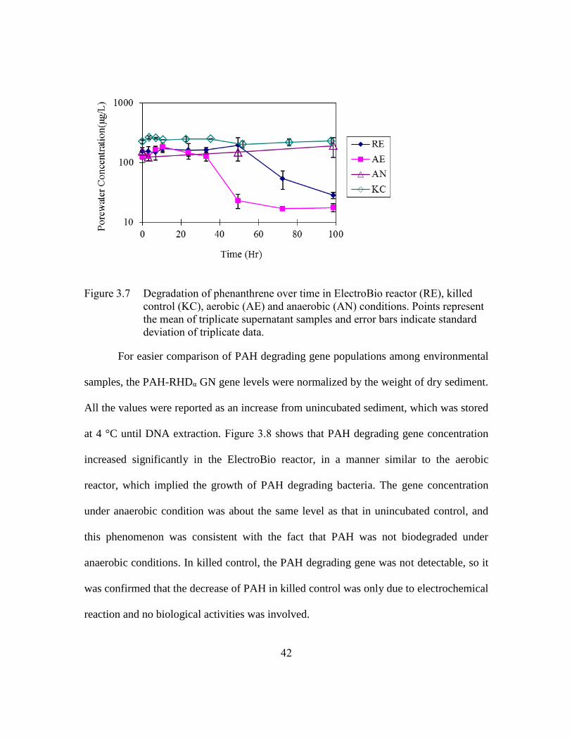
42
Figure 3.7 Degradation of phenanthrene over time in ElectroBio reactor (RE), killed
control (KC), aerobic (AE) and anaerobic (AN) conditions. Points represent
the mean of triplicate supernatant samples and error bars indicate standard
deviation of triplicate data.
For easier comparison of PAH degrading gene populations among environmental
samples, the PAH-RHDα GN gene levels were normalized by the weight of dry sediment.
All the values were reported as an increase from unincubated sediment, which was stored
at 4 °C until DNA extraction. Figure 3.8 shows that PAH degrading gene concentration
increased significantly in the ElectroBio reactor, in a manner similar to the aerobic
reactor, which implied the growth of PAH degrading bacteria. The gene concentration
under anaerobic condition was about the same level as that in unincubated control, and
this phenomenon was consistent with the fact that PAH was not biodegraded under
anaerobic conditions. In killed control, the PAH degrading gene was not detectable, so it
was confirmed that the decrease of PAH in killed control was only due to electrochemical
reaction and no biological activities was involved.
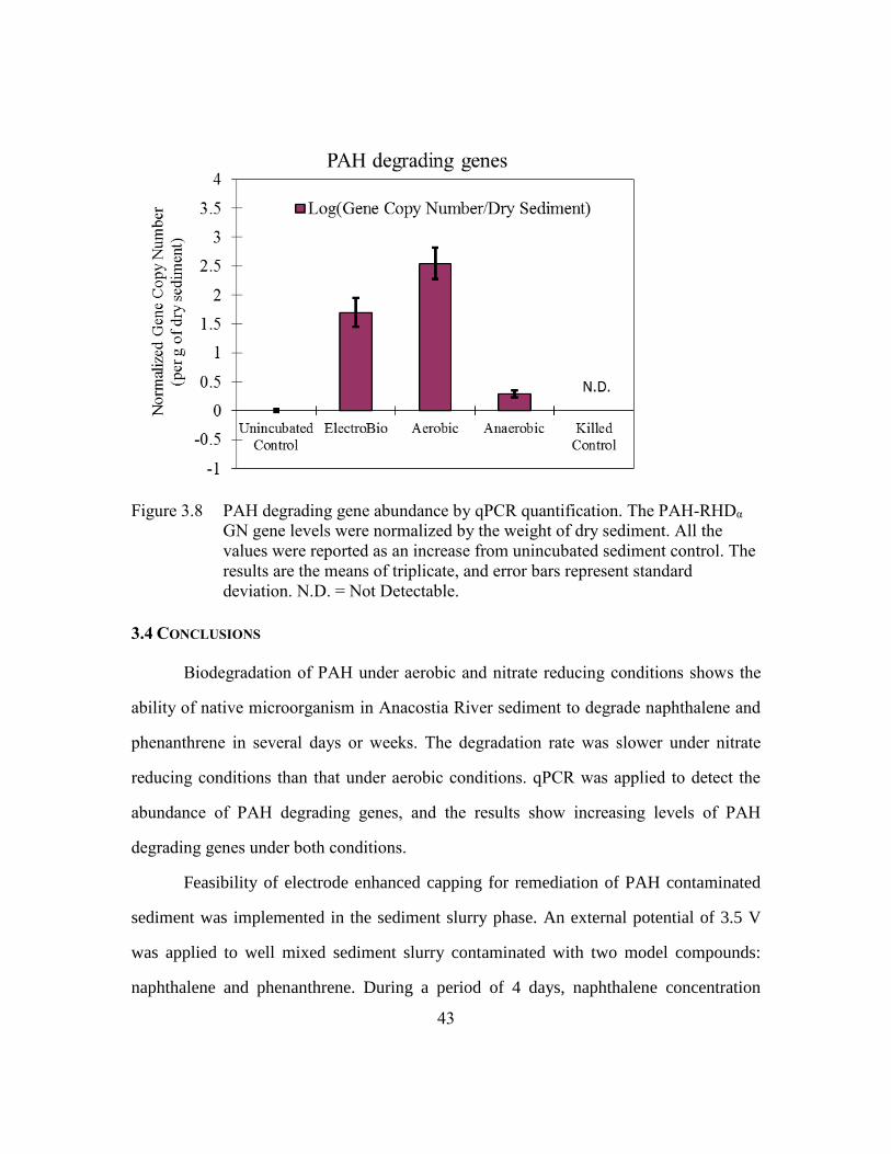
43
Figure 3.8 PAH degrading gene abundance by qPCR quantification. The PAH-RHDα
GN gene levels were normalized by the weight of dry sediment. All the
values were reported as an increase from unincubated sediment control. The
results are the means of triplicate, and error bars represent standard
deviation. N.D. = Not Detectable.
3.4 CONCLUSIONS
Biodegradation of PAH under aerobic and nitrate reducing conditions shows the
ability of native microorganism in Anacostia River sediment to degrade naphthalene and
phenanthrene in several days or weeks. The degradation rate was slower under nitrate
reducing conditions than that under aerobic conditions. qPCR was applied to detect the
abundance of PAH degrading genes, and the results show increasing levels of PAH
degrading genes under both conditions.
Feasibility of electrode enhanced capping for remediation of PAH contaminated
sediment was implemented in the sediment slurry phase. An external potential of 3.5 V
was applied to well mixed sediment slurry contaminated with two model compounds:
naphthalene and phenanthrene. During a period of 4 days, naphthalene concentration
44
decreased from ~1000 μg/L to ~50 μg/L, and phenanthrene was degraded from ~150
μg/L to ~30 μg /L in ElectroBio reactor. These rates in ElectroBio reactor were about the
same as observed under fully aerobic conditions, except a longer lag phase. By
comparison to controls, the disappearance of naphthalene was a combined process of
abiotic and biotic loss while the phenanthrene loss appeared to be solely controlled by
biotic processes. Naphthalene concentration still remained 80% of initial concentration,
and phenanthrene degradation was not observed under anaerobic condition.
The results of qPCR show significant increases of PAH degrading genes in
ElectroBio reactor and aerobic conditions, but no increase in killed control and anaerobic
conditions. qPCR analysis provided the evidence of PAH biodegradation in ElectroBio
reactor and aerobic conditions.
45
Chapter 4: Electro-biodegradation of PAH and Redox Control in
Sediment/Cap Microcosms
4.1 INTRODUCTION
Contaminated sediments cause adverse effects on aquatic life and pose a risk to
ecology and human health. Although dredging and ex-situ disposal have been used as a
remedial technology for contaminated sediment, the high cost and concern of
recontamination after dredging have led to the use of an alternative technology – in-situ
capping. In-situ capping has recently emerged as a remedial method for contaminated
sediments, and it involves the placement of clean material (usually sand) on the sediment
to isolate the contaminants into the overlying water. In-situ capping can be a relatively
cost-effective and noninvasive approach compared to dredging. However, a potential
consequence of placing a cap at the sediment-water interface is that it induces
considerable changes of biogeochemical conditions within the underlying sediment. The
anaerobic conditions induced by in-situ capping hinders PAH natural degradation, which
might otherwise occur at the surface sediment. In addition, conventional capping usually
doesn’t promote contaminant degradation or removal, and the risk to ecological and
human health may recur if the contaminant can migrate through the caps.
To overcome the limitation of conventional capping, electrode enhanced capping
was proposed and investigated for the bioremediation of PAH contaminated sediment. In
Chapter 3, the potential for this approach was assessed in completely mixed reactors to
demonstrate the effectiveness of this approach under idealized conditions. In this
Chapter, laboratory scale experiments were conducted in simulated sediments/caps to
evaluate the effect of mass transfer limitations under a realistic but controlled laboratory
environment. Phenanthrene concentration profiles in the sediments/caps were measured
at different times to determine the biodegradation rates. Important parameters to
46
characterize redox conditions, such as pH, redox potential, and concentrations of redox-
sensitive species, were determined to better understand the changes of biogeochemical
condition with the application of electricity. PAH degrading genes were quantified in the
vicinity of the anode to provide more insight on microbial biodegradation activity.
Three sets of experiments were conducted in this chapter. The experimental study
was first conducted in PAH contaminated sediment with no capping layer to identify the
key processes and parameters for further studies. The high pH buffer capacity in the
sediment would be beneficial for biodegradation with less pH shift. Second, PAH
degradation and redox control were studied in electrode enhanced caps, and upon the
finish of this study, it was expected that some degree of PAH degradation would be
observed. Third, PAH degradation and redox control were investigated in electrode
enhanced caps with bicarbonate amendment. The purpose of the last study was to test
whether PAH biodegradation could be further accelerated by providing an instant soluble
pH buffer in the system.
The goal of all of these tests was to develop a thin aerobic zone in the vicinity of
the anode. In this manner any contaminants that may migrate up out of the contaminated
sediment into the overlying water or cap layer may experience degradation. That is, the
anode is designed to serve as a biobarrier for migrating contaminants. The goal of the
effort was not to change the redox conditions or encourage degradation over a large
sediment zone. Non-migrating contaminants pose little risk to interfacial organisms or the
water column and efforts to encourage degradation over a large volume of sediment
would have substantially greater power requirements, limiting the feasibility of the
approach.
47
4.2 PAH DEGRADATION AND REDOX CONTROL IN UNCAPPED SEDIMENT BY ELECTRODES
4.2.1 Materials and methods
4.2.1.1 Microcosm setup and operation
Three 400-mL beaker reactors were used to evaluate the ability of carbon
electrodes to control the redox potential and encourage PAH degradation in simulated
static contaminated sediment. One reactor served as a no-applied electricity control
(Control) while electricity was applied to the other two (ElecR1 and ElecR2) through
cloth electrodes. In Control and ElecR1 reactors, 0.05 g/mL of siderite (Prince Agri
Products, Inc., Quincy, Illinois) was mixed with sediment to aid in buffering.
The reactors were filled with sieved (2 mm) sediment (mixture of contaminated
Anacostia River sediment and clean University Lake sediment, ratio 1:5.6). The sediment
was spiked with phenanthrene and naphthalene at a level of ~20 μg/g concentration for
both compounds.
A 5cm×5cm woven carbon cloth (Graphite felt, Wale Apparatus Co, Hellertown,
PA) was placed at 3 cm below the sediment water interface as the anode, and a second,
identical, carbon cloth was placed at 0.5 cm below the sediment-water interface as the
cathode. Deionized water was applied on top of the sediment as overlying water. Water
lost due to evaporation was periodically replenished with deionized water to maintain the
original salt composition.
The graphite electrodes were connected to copper wires by EPO-TEK® 377H
(Epoxy Technology, Billerica, MA), which is a graphite filled epoxy designed for
electronic industries. The graphite power component in the epoxy ensured its electrical
conductivity. The connections between the graphite cloth and copper wires were sealed
with Gardner Bender LTW-400 liquid electrical tape (Gardner Bender, Milwaukee, WI).

48
Powered reactors were connected to 2 V Extech 382202 DC power supply
(Extech Instruments Corp., Waltham, MA), and external power was continuously applied
for ∼12 weeks except during microelectrode measurement.
4.2.1.2 pH and ORP measurement
pH was measured by MI-405 standard pH microelectrode (Microelectrodes Inc,
Bedford, New Hampshire) and Oxidation Reduction Potential(ORP) was measured by Pt
microelectrode against Ag/AgCl reference. Vertical profiles of pH and ORP from the
sediment-water interface to a depth of 45 mm with 5 mm intervals were acquired. 2
minutes was allowed to reach equilibrium at each depth.
pH microelectrode was calibrated with pH 4, pH 7 and pH 10 standard buffer
solution (Fisher Scientific, Fair Lawn, NJ) before and after each measurement.
Pt microelectrode for ORP measurement was calibrated in pH-buffered, saturated
quinhydrone solution. Two standard solutions were prepared as follows: about 0.05 g
quinhydrone was added to 30 mL of pH 4 and pH 7 buffer solution, respectively. The
mixture was stirred and allowed at least 15 minutes to equilibrate, and then it was stirred
again. Not all of the quinhydrone would dissolve so both solutions should be saturated by
quinhydrone after equilibration. The readings of potential difference between Pt
microelectrode and Ag/AgCl reference electrode in each buffer solution were compared
to Table 4.1. If the reading was more than 10 mV from the proper value, Pt electrode was
cleaned and tested again until it met the standards. The reading was converted and
reported as versus standard hydrogen electrode (SHE).
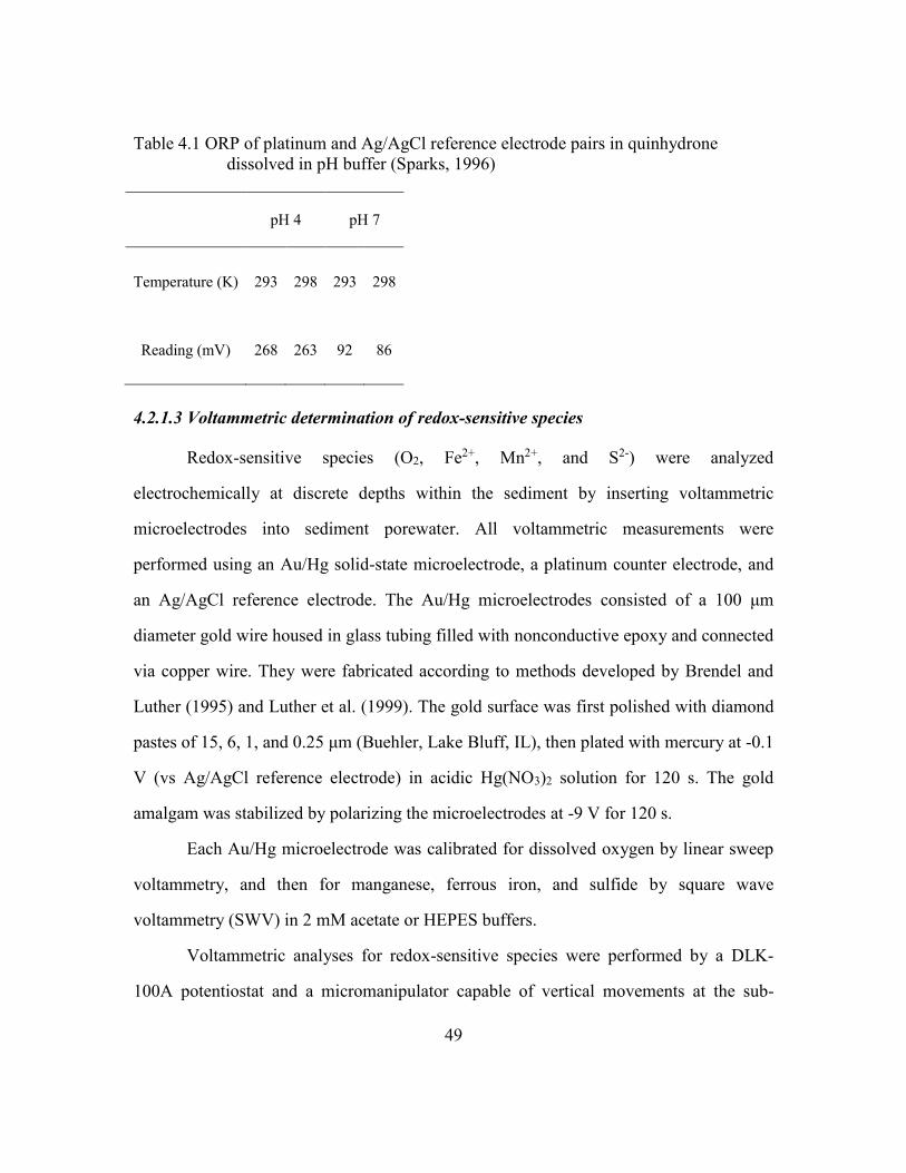
49
Table 4.1 ORP of platinum and Ag/AgCl reference electrode pairs in quinhydrone
dissolved in pH buffer (Sparks, 1996)
pH 4 pH 7
Temperature (K) 293 298 293 298
Reading (mV) 268 263 92 86
4.2.1.3 Voltammetric determination of redox-sensitive species
Redox-sensitive species (O2, Fe2+, Mn2+, and S2-) were analyzed
electrochemically at discrete depths within the sediment by inserting voltammetric
microelectrodes into sediment porewater. All voltammetric measurements were
performed using an Au/Hg solid-state microelectrode, a platinum counter electrode, and
an Ag/AgCl reference electrode. The Au/Hg microelectrodes consisted of a 100 μm
diameter gold wire housed in glass tubing filled with nonconductive epoxy and connected
via copper wire. They were fabricated according to methods developed by Brendel and
Luther (1995) and Luther et al. (1999). The gold surface was first polished with diamond
pastes of 15, 6, 1, and 0.25 μm (Buehler, Lake Bluff, IL), then plated with mercury at -0.1
V (vs Ag/AgCl reference electrode) in acidic Hg(NO3)2 solution for 120 s. The gold
amalgam was stabilized by polarizing the microelectrodes at -9 V for 120 s.
Each Au/Hg microelectrode was calibrated for dissolved oxygen by linear sweep
voltammetry, and then for manganese, ferrous iron, and sulfide by square wave
voltammetry (SWV) in 2 mM acetate or HEPES buffers.
Voltammetric analyses for redox-sensitive species were performed by a DLK-
100A potentiostat and a micromanipulator capable of vertical movements at the sub-
50
millimeter scale (Analytical Instrument Systems, Inc, Flemington, NJ). The small size of
the working microelectrode, and the precise control of vertical movement, allowed
repeated vertical profiling with high spatial resolution while minimizing bulk sediment
disturbance. Scan parameters and detection limits were the same as those reported in
Brendel and Luther (1995). Triplicate electrodes were used for the measurement and
vertical profiles from the sediment-water interface to a depth of 45 mm with 5 mm
intervals were obtained (the same location as pH and ORP profiles).
4.2.1.4 Phenanthrene porewater concentration measurement by PDMS-coated fiber
Phenanthrene profiles in the sediment interstitial water were measured by
Polydimethylsiloxane (PDMS)-coated fibers manufactured by Fiberguide Industries
(Stirling, NJ). Naphthalene could not be reliably measured by this technique due to its
relatively modest sorption onto PDMS and high volatility. The PDMS-coated fibers
(210/230) had a 210-µm core with a 10-µm PDMS coating or outer diameter of 230 µm.
The ability of the PDMS-coated fibers to quantify sediment porewater concentrations has
been tested in the laboratory (Lu et al., 2011; Mayer et al., 2000). The linear partitioning
relationship of the phenanthrene concentration between the PDMS phase (Cfiber, ng/L
PDMS) and the porewater (Cw, ng/L water) was assumed with a partition coefficient Kf
of 8912.18 (Lu et al., 2011).
For all PDMS analyses, the method described by Lu et al. (2011) was used. The
fiber was cleaned prior to deployment by sonication in hexane for a minimum of half an
hour, followed by a rinse with acetone and then deionized water.
The equilibrium time varies considerably from one fiber type to another and also
depends on the octanol-water partition coefficient (Kow) of the hydrophobic organic
compounds (Cornelissen et al., 2008; Lampert, 2010). Before using PDMS fiber for the

51
measurement of phenanthrene porewater concentration, the uptake kinetic of this type of
fiber (210/230) for phenanthrene was tested and equilibrium time was determined.
During the application of fiber for phenanthrene porewater measurement, fibers were
inserted vertically in the sediment for a period long enough to reach equilibrium. Then
fibers were pulled out from the sediment, rinsed clean (to remove any particles) with
deionized water, cut into 1 cm pieces, and placed into 2 mL HPLC vials with 1 mL of
HPLC-grade acetonitrile. Duplicate phenanthrene concentration profiles were measured
every two weeks during the course of the experiment.
4.2.1.5 DNA extraction and qPCR analysis
At the end of the experiment, sediment cores were collected and dissected into 0.5
cm or 1 cm long subsamples and stored at -20 °C until further analysis. DNA was
extracted and qPCR was performed as previously described.
4.2.2 Results and discussion
4.2.2.1 Redox control, pH changes and redox-sensitive species
When an external power of 2 V was applied to the electrodes in the sediment for
ElecR1 and ElecR2, redox potentials in the sediment around the anode changed. A 2 V of
potential was selected to ensure water electrolysis at the electrodes. A greater potential is
not preferred for stimulating biodegradation since it causes a higher rate of water
electrolysis, consequently results in severe pH changes at both the anode and the cathode.
An increment of redox potential was observed in two powered reactors compared to
control (Figure 4.1). The ORP around the anode (d = 3 cm) increased gradually from an
initial value of ~100 mV, and finally reached ~200 mV after about one month of
operation for both powered reactors. The ORP at the same depth in control reactor was
about 80 – 160 mV during the course of the experiment. The changes in redox conditions
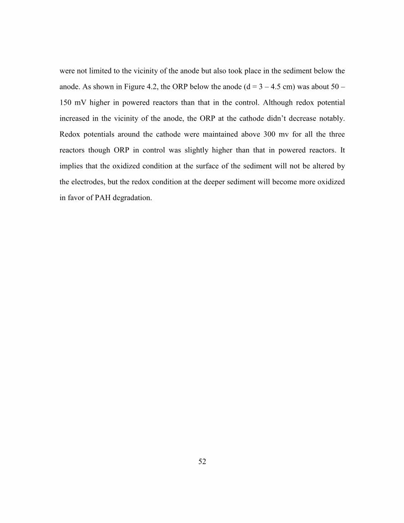
52
were not limited to the vicinity of the anode but also took place in the sediment below the
anode. As shown in Figure 4.2, the ORP below the anode (d = 3 – 4.5 cm) was about 50 –
150 mV higher in powered reactors than that in the control. Although redox potential
increased in the vicinity of the anode, the ORP at the cathode didn’t decrease notably.
Redox potentials around the cathode were maintained above 300 mv for all the three
reactors though ORP in control was slightly higher than that in powered reactors. It
implies that the oxidized condition at the surface of the sediment will not be altered by
the electrodes, but the redox condition at the deeper sediment will become more oxidized
in favor of PAH degradation.
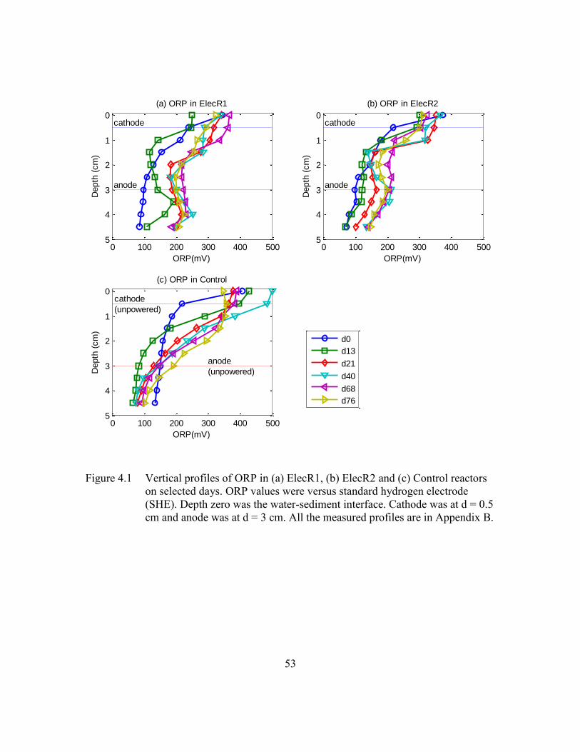
53
Figure 4.1 Vertical profiles of ORP in (a) ElecR1, (b) ElecR2 and (c) Control reactors
on selected days. ORP values were versus standard hydrogen electrode
(SHE). Depth zero was the water-sediment interface. Cathode was at d = 0.5
cm and anode was at d = 3 cm. All the measured profiles are in Appendix B.
0 100 200 300 400 500
0
1
2
3
4
5
(a) ORP in ElecR1
ORP(mV)
Depth
(cm
)
cathode
anode
0 100 200 300 400 500
0
1
2
3
4
5
(b) ORP in ElecR2
ORP(mV)
Depth
(cm
)
cathode
anode
0 100 200 300 400 500
0
1
2
3
4
5
(c) ORP in Control
ORP(mV)
Depth
(cm
)
cathode
(unpowered)
anode
(unpowered)
d0
d13
d21
d40
d68
d76
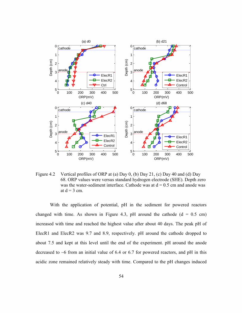
54
Figure 4.2 Vertical profiles of ORP at (a) Day 0, (b) Day 21, (c) Day 40 and (d) Day
68. ORP values were versus standard hydrogen electrode (SHE). Depth zero
was the water-sediment interface. Cathode was at d = 0.5 cm and anode was
at d = 3 cm.
With the application of potential, pH in the sediment for powered reactors
changed with time. As shown in Figure 4.3, pH around the cathode (d = 0.5 cm)
increased with time and reached the highest value after about 40 days. The peak pH of
ElecR1 and ElecR2 was 9.7 and 8.9, respectively. pH around the cathode dropped to
about 7.5 and kept at this level until the end of the experiment. pH around the anode
decreased to ~6 from an initial value of 6.4 or 6.7 for powered reactors, and pH in this
acidic zone remained relatively steady with time. Compared to the pH changes induced
0 100 200 300 400 500
0
1
2
3
4
5
(a) d0
ORP(mV)
Depth
(cm
)
cathode
anode
ElecR1
ElecR2
Ctrl
0 100 200 300 400 500
0
1
2
3
4
5
(b) d21
ORP(mV)
Depth
(cm
)
cathode
anode
ElecR1
ElecR2
Control
0 100 200 300 400 500
0
1
2
3
4
5
(c) d40
ORP(mV)
Depth
(cm
)
cathode
anode
ElecR1
ElecR2
Control
0 100 200 300 400 500
0
1
2
3
4
5
(d) d68
ORP(mV)
Depth
(cm
)
cathode
anode
ElecR1
ElecR2
Control
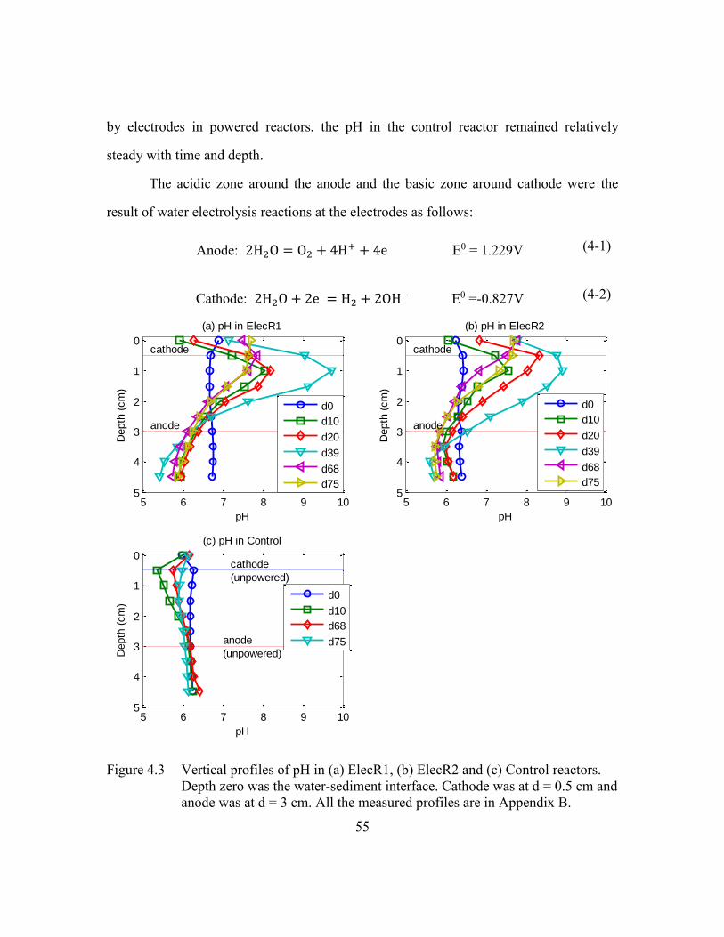
55
by electrodes in powered reactors, the pH in the control reactor remained relatively
steady with time and depth.
The acidic zone around the anode and the basic zone around cathode were the
result of water electrolysis reactions at the electrodes as follows:
Anode: 2H2O = O2 + 4H+ + 4e E0 = 1.229V (4-1)
Cathode: 2H2O + 2e = H2 + 2OH− E0 =-0.827V (4-2)
Figure 4.3 Vertical profiles of pH in (a) ElecR1, (b) ElecR2 and (c) Control reactors.
Depth zero was the water-sediment interface. Cathode was at d = 0.5 cm and
anode was at d = 3 cm. All the measured profiles are in Appendix B.
5 6 7 8 9 10
0
1
2
3
4
5
(a) pH in ElecR1
pH
Depth
(cm
)
cathode
anode
d0
d10
d20
d39
d68
d75
5 6 7 8 9 10
0
1
2
3
4
5
(b) pH in ElecR2
pH
Depth
(cm
)
cathode
anode
d0
d10
d20
d39
d68
d75
5 6 7 8 9 10
0
1
2
3
4
5
(c) pH in Control
pH
Depth
(cm
)
cathode
(unpowered)
anode
(unpowered)
d0
d10
d68
d75
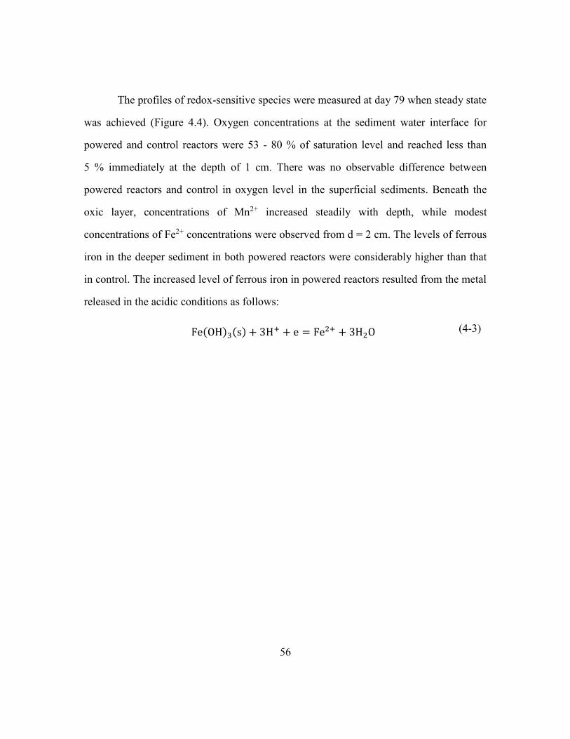
56
The profiles of redox-sensitive species were measured at day 79 when steady state
was achieved (Figure 4.4). Oxygen concentrations at the sediment water interface for
powered and control reactors were 53 - 80 % of saturation level and reached less than
5 % immediately at the depth of 1 cm. There was no observable difference between
powered reactors and control in oxygen level in the superficial sediments. Beneath the
oxic layer, concentrations of Mn2+ increased steadily with depth, while modest
concentrations of Fe2+ concentrations were observed from d = 2 cm. The levels of ferrous
iron in the deeper sediment in both powered reactors were considerably higher than that
in control. The increased level of ferrous iron in powered reactors resulted from the metal
released in the acidic conditions as follows:
Fe(OH)3(s) + 3H+ + e = Fe2+ + 3H2O (4-3)
57
Figure 4.4 Vertical profiles of redox-sensitive species in ElecR1, ElecR2 and Control
reactors: (a) Oxygen, (b) Mn2+ and (c) Fe2+. Sulfide was not detected. Each
point represents the mean of triplicate measurements from each electrode,
and error bars are not shown for simplicity. Depth zero was the water-
sediment interface. Cathode was at d = 0.5 cm and anode was at d = 3 cm.
Figures with standard deviation are available in Appendix B.
4.2.2.2 Phenanthrene concentrations and PAH degrading genes
Study on uptake kinetics of phenanthrene by fiber (210/230) revealed that the
concentration of phenanthrene in the PDMS coating reached equilibrium in about 10
0 50 100 150 200 250
0
1
2
3
4
5
(a) Oxygen
c(M)
Depth
(cm
)
0 50 100 150
0
1
2
3
4
5
(b) Mn2+
c(M)
Depth
(cm
)
0 200 400 600
0
1
2
3
4
5
(c) Fe2+
c(M)
Depth
(cm
)
ElecR1
ElecR2
Control
ElecR1
ElecR2
Control
ElecR1
ElecR2
Control
58
hours (Appendix B). In this study, 24 hours of equilibration time were used during each
measurement.
Porewater concentrations of phenanthrene were determined at different depths
every two weeks during the experiment (Figure 4.5). In the superficial sediments (d = 0
and 1 cm), phenanthrene concentration decreased with time in both powered and control
reactors due to biodegradation in oxic environment and volatilization loss. The
phenanthrene levels in powered reactors were consistently higher than those in control in
the superficial sediments because of the difference in initial conditions. Some operational
inconsistence during the setup of the experiment might cause the difference in initial
conditions.
In the control reactor, phenanthrene concentration in the anode zone (d = 3 cm)
didn’t change notably, whereas phenanthrene concentration decreased over time around
the anode in both ElecR1 and ElecR2 (Figure 4.6). The phenanthrene concentrations were
60% and 71% of their initial concentrations at the end of the experiment for ElecR1 and
ElecR2 respectively, but phenanthrene concentration still remained at 90% of initial
concentration for control.
As shown in Figure 4.5, phenanthrene concentration at the anode (d = 3 cm)
decreased with time, whereas phenanthrene concentration at 1 cm above the anode (d = 2
cm) remained almost unaffected throughout the study period in powered reactors. As a
result, phenanthrene concentrations at the anode (d = 3 cm) were lower than those at 1 cm
above the anode (d = 2 cm) after several weeks, showing a unique Z-shaped profile in the
sediment (Figure 4.7). This phenomenon was not observed in the control reactor. The
phenanthrene profile in the control reactor displayed a down gradient from the deeper
sediment toward the sediment water interface. The decrease of phenanthrene at the anode
and the unique Z-shaped profiles provided evidences that the anode placed in the
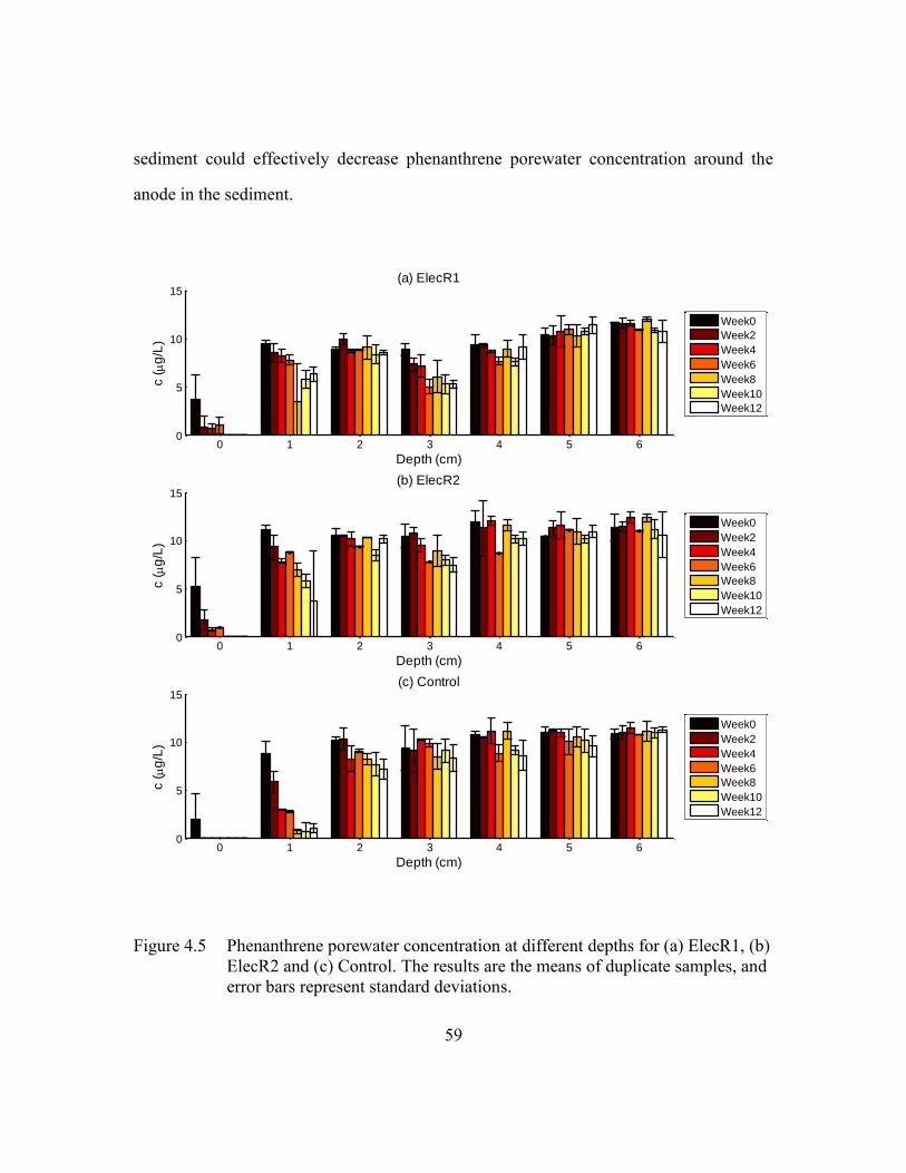
59
sediment could effectively decrease phenanthrene porewater concentration around the
anode in the sediment.
Figure 4.5 Phenanthrene porewater concentration at different depths for (a) ElecR1, (b)
ElecR2 and (c) Control. The results are the means of duplicate samples, and
error bars represent standard deviations.
0 1 2 3 4 5 60
5
10
15(a) ElecR1
Depth (cm)
c (g
/L)
0 1 2 3 4 5 60
5
10
15(b) ElecR2
Depth (cm)
c (g
/L)
0 1 2 3 4 5 60
5
10
15(c) Control
Depth (cm)
c (g
/L)
Week0
Week2
Week4
Week6
Week8
Week10
Week12
Week0
Week2
Week4
Week6
Week8
Week10
Week12
Week0
Week2
Week4
Week6
Week8
Week10
Week12
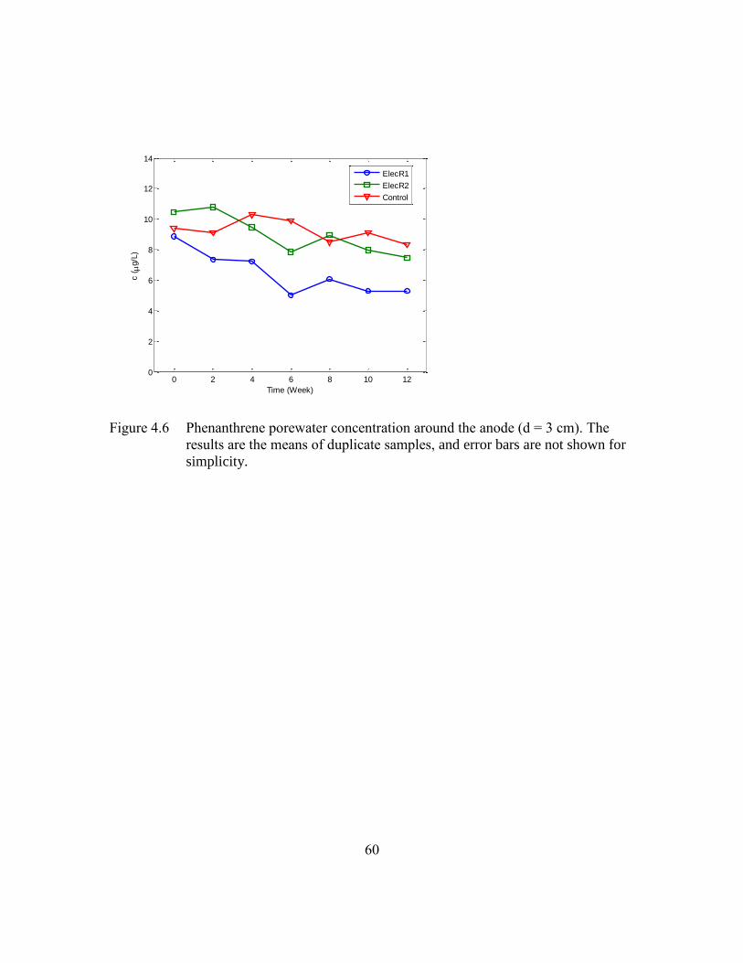
60
Figure 4.6 Phenanthrene porewater concentration around the anode (d = 3 cm). The
results are the means of duplicate samples, and error bars are not shown for
simplicity.
0 2 4 6 8 10 120
2
4
6
8
10
12
14
Time (Week)
c (
g/L
)
ElecR1
ElecR2
Control
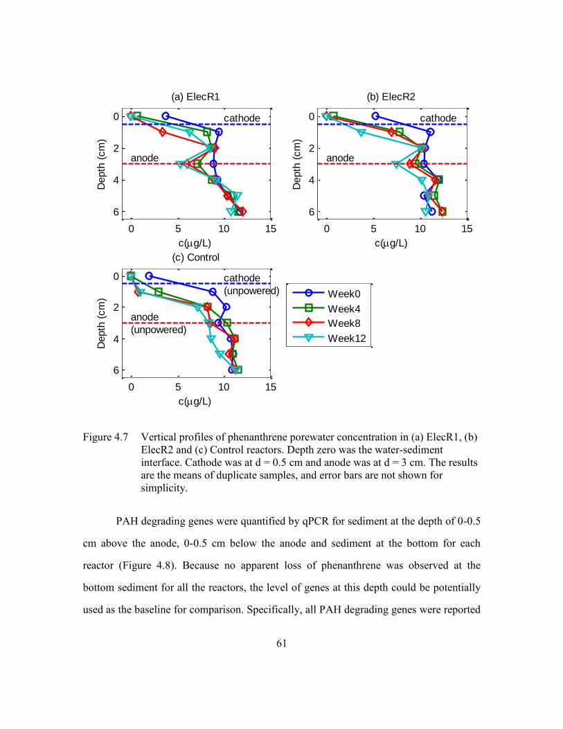
61
Figure 4.7 Vertical profiles of phenanthrene porewater concentration in (a) ElecR1, (b)
ElecR2 and (c) Control reactors. Depth zero was the water-sediment
interface. Cathode was at d = 0.5 cm and anode was at d = 3 cm. The results
are the means of duplicate samples, and error bars are not shown for
simplicity.
PAH degrading genes were quantified by qPCR for sediment at the depth of 0-0.5
cm above the anode, 0-0.5 cm below the anode and sediment at the bottom for each
reactor (Figure 4.8). Because no apparent loss of phenanthrene was observed at the
bottom sediment for all the reactors, the level of genes at this depth could be potentially
used as the baseline for comparison. Specifically, all PAH degrading genes were reported
0 5 10 15
0
2
4
6
(a) ElecR1
c(g/L)
Depth
(cm
)
cathode
anode
0 5 10 15
0
2
4
6
(b) ElecR2
c(g/L)
Depth
(cm
)
cathode
anode
0 5 10 15
0
2
4
6
(c) Control
c(g/L)
Depth
(cm
)
cathode
(unpowered)
anode
(unpowered)
Week0
Week4
Week8
Week12

62
as an increase from the level of genes at the bottom sediment of ElecR1. The results show
that the gene levels in the vicinity of the anode in ElecR1 increased by about 2 times, but
there was no significant increase of genes in ElecR2 and control reactor. It is not clear
why ElecR1 and ElecR2 behaved differently although it could be as simple as differences
in current (but not measured). The lack of current measurements may have contributed to
an inability to determine why ElecR1 performed better than ElecR2. A considerable
increase of PAH degrading genes was not observed in this study despite the decrease of
phenanthrene levels. It is possible that low PAH concentration may not provide enough
selective pressure for PAH-degrading bacteria so the growth of these bacteria was slow.
Although PAH was utilized as carbon sources, the growth of PAH-degrading bacteria
didn’t reach the exponential phase. Therefore an evident increase of gene levels was not
detected in this study.

63
Figure 4.8 PAH degrading gene abundance by qPCR quantification at a depth of 0-0.5
cm below the anode, 0-0.5 cm above the anode, and in the bottom sediment
in ElecR1, ElecR2, and Control. The PAH-RHDα GN gene levels were
normalized by the weight of dry sediment. All the values were reported as
an increase from the level of genes at the bottom sediment of ElecR1. The
results are the means of triplicate samples, and error bars represent standard
deviations.
4.3 PAH DEGRADATION AND REDOX CONTROL IN ELECTRODE ENHANCED SAND CAPS
4.3.1 Materials and methods
Three 400-mL beaker reactors were used to evaluate the ability of carbon
electrodes to control the redox potential and encourage PAH degradation in a simulated
static sand cap placed over contaminated sediment. One reactor served as a no-applied
electricity control (Control) while electricity was applied to the other two (ElecCap1 and
ElecR1 ElecR2 Control-0.4
-0.2
0
0.2
0.4
0.6
0.8
1L
og
(G
en
e C
op
y N
um
be
rs / d
ry s
ed
ime
nt)
Normalized PAH degrading genes(per g of dry sediment)
0-0.5cm above anode
0-0.5cm below anode
Bottom
64
ElecCap2) through cloth electrodes in a layer composed of sand and a 10% mixture (mass
basis) of siderite to serve as a buffer. In one of the two (ElecCap2), a 0.3-mm layer of
siderite was also applied at the sediment and anode interface to aid in buffering.
The reactors were filled with sieved (2 mm) sediment (mixture of contaminated
Anacostia River sediment and clean University Lake sediment, ratio 1:7). The sediment
was spiked with phenanthrene and naphthalene at a level of ~70 μg/g concentration for
both compounds. A 5cm×5cm woven carbon cloth (Graphite felt, Wale Apparatus Co,
Hellertown, PA) was placed on top of the sediment as the anode. A 3.5-cm layer of
sieved (0.425 mm) concrete sand (Riccelli Enterprises, Rush, NY) was placed over the
anode and a second, identical, carbon cloth was placed on the sand layer as the cathode.
A 0.5 cm sand layer was overlain on the cathode. The sand layers were saturated with
electrolyte (2 mM NaCl and 2 mM Na2SO4 mixed electrolyte) initially. Water lost due to
evaporation was periodically replenished with deionized water to maintain the original
salt composition.
The graphite electrodes were connected to copper wires and sealed with liquid
electrical tape as previously described. Powered reactors were connected to 2 V Extech
382202 DC power supply (Extech Instruments Corp., Waltham, MA), and external power
was continuously applied for ∼10 weeks except during microelectrode measurement. The
anode and cathode of ElecCap2 were switched between day 56 to day 58 and day 66 to
day 69 to test if alternating anode and cathode could reverse or reduce pH changes.
The current for ElecCap1 was initially ~200 μA and gradually dropped to ~100
μA possibly due to precipitation at the cathode (Franz et al., 2002). The current of
ElecCap2 was about 200-250 μA through the entire course of the experiment.
65
pH was measured by MI-405 standard pH microelectrode and ORP was measured
by Pt microelectrode as previously described. Vertical profiles of pH and ORP from the
water-sand interface to a depth of 60 mm with 5 mm intervals were acquired.
Redox-sensitive species (O2, Fe2+, Mn2+, and S2-) were analyzed
electrochemically as previously described.
Porewater concentration of phenanthrene was measured by PDMS-coated fiber as
previously described.
At the end of the experiment, sediment cores were collected and dissected into 0.5
cm or 1 cm long subsamples and stored at -20 °C until further analysis.
Naphthalene and phenanthrene concentration of sediment samples was
determined using a modified version of EPA Method 3550. Sediment samples were
weighed, and mixed with sodium sulfate to disperse the particles and absorb excess
water. 60 mL of hexane/acetone (volume ratio 1:1) were added to the jar and sonicated
for 30 minutes to extract the PAHs. A 2-mL aliquot of hexane/acetone was added to a 5-
mL blow down vial, and then evaporated with a Labconco (Kansas City, MO) Model
79100 RapidVap nitrogen Evaporation System to a volume of ~200 μL and reconstituted
to a volume of 2 mL with acetonitrile. The vial was mixed thoroughly, blown down to the
final volume, and analyzed.
DNA was extracted and qPCR was performed as previously described.
4.3.2 Results and discussion
4.3.2.1 Redox control, pH changes and redox-sensitive species
Figure 4.9 shows the observed changes in redox conditions after application of
power. The average ORP in the sediment layer near the unpowered anode (d = 4-6 cm) in
control reactor was ~90 mv, while those in the powered microcosms, ElecCap1 and
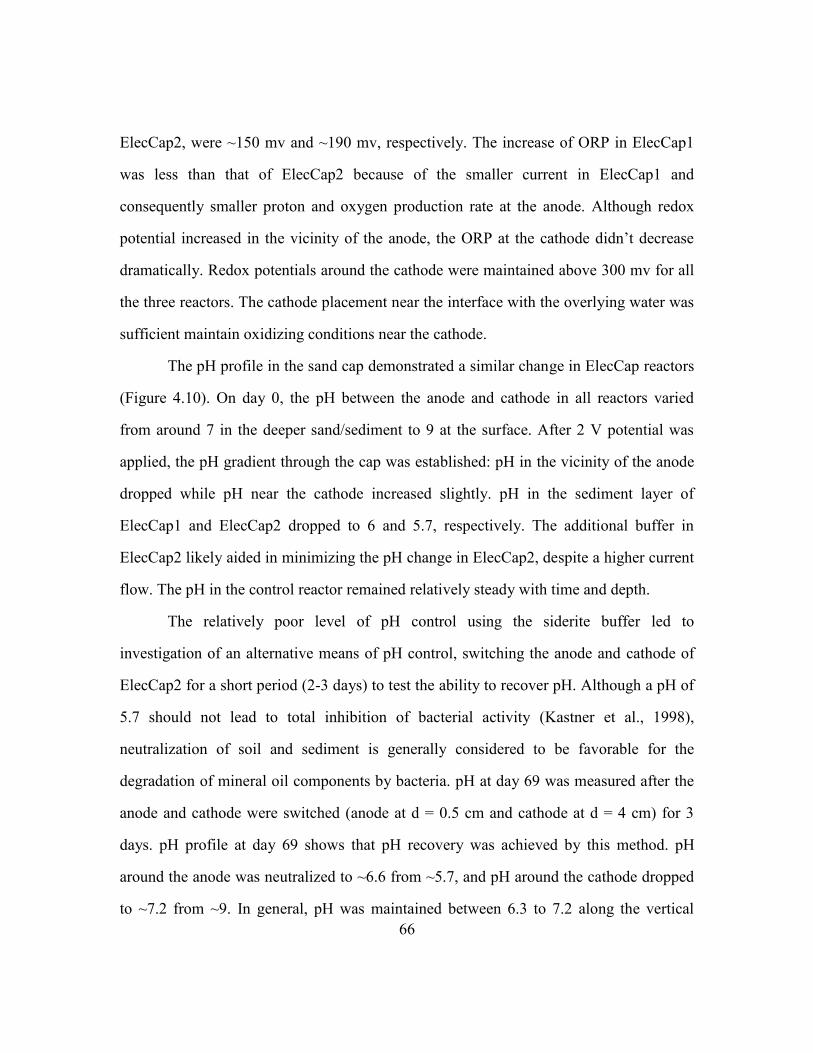
66
ElecCap2, were ~150 mv and ~190 mv, respectively. The increase of ORP in ElecCap1
was less than that of ElecCap2 because of the smaller current in ElecCap1 and
consequently smaller proton and oxygen production rate at the anode. Although redox
potential increased in the vicinity of the anode, the ORP at the cathode didn’t decrease
dramatically. Redox potentials around the cathode were maintained above 300 mv for all
the three reactors. The cathode placement near the interface with the overlying water was
sufficient maintain oxidizing conditions near the cathode.
The pH profile in the sand cap demonstrated a similar change in ElecCap reactors
(Figure 4.10). On day 0, the pH between the anode and cathode in all reactors varied
from around 7 in the deeper sand/sediment to 9 at the surface. After 2 V potential was
applied, the pH gradient through the cap was established: pH in the vicinity of the anode
dropped while pH near the cathode increased slightly. pH in the sediment layer of
ElecCap1 and ElecCap2 dropped to 6 and 5.7, respectively. The additional buffer in
ElecCap2 likely aided in minimizing the pH change in ElecCap2, despite a higher current
flow. The pH in the control reactor remained relatively steady with time and depth.
The relatively poor level of pH control using the siderite buffer led to
investigation of an alternative means of pH control, switching the anode and cathode of
ElecCap2 for a short period (2-3 days) to test the ability to recover pH. Although a pH of
5.7 should not lead to total inhibition of bacterial activity (Kastner et al., 1998),
neutralization of soil and sediment is generally considered to be favorable for the
degradation of mineral oil components by bacteria. pH at day 69 was measured after the
anode and cathode were switched (anode at d = 0.5 cm and cathode at d = 4 cm) for 3
days. pH profile at day 69 shows that pH recovery was achieved by this method. pH
around the anode was neutralized to ~6.6 from ~5.7, and pH around the cathode dropped
to ~7.2 from ~9. In general, pH was maintained between 6.3 to 7.2 along the vertical

67
profile. Although the goal of pH neutralization was achieved by this method, oxidized
redox conditions developed around the anode diminished somewhat. ORP around the
anode at day 70 decreased to ~110 mv from ~150 mv, only slightly higher than that in the
control.
Figure 4.9 Vertical profiles of ORP in (a) ElecCap1, (b) ElecCap2 and (c) Control
reactors. Depth zero was the water-cap interface. Cathode was at d = 0.5 cm
and anode was at d = 4 cm. All the measured profiles are in Appendix B.
0 200 400 600
0
2
4
6
(a) ORP in ElecCap1
ORP (mV)
Depth
(cm
)
sand
sediment
cathode
anode
0 200 400 600
0
2
4
6
(b) ORP in ElecCap2
ORP (mV)
Depth
(cm
)
sand
sediment
cathode
anode
0 200 400 600
0
2
4
6
(c) ORP in Control
ORP (mV)
Depth
(cm
)
sand
sediment
cathode
(unpowered)
anode
(unpowered)
d29
d44
d56
d70
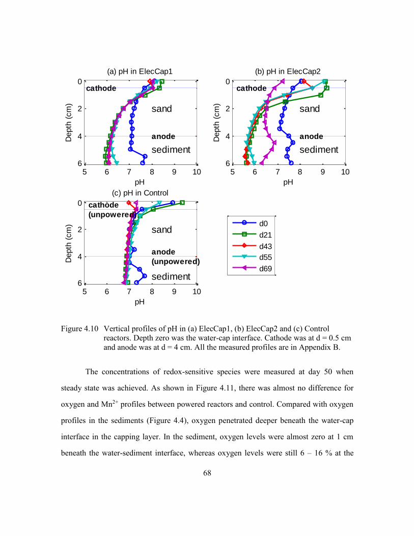
68
Figure 4.10 Vertical profiles of pH in (a) ElecCap1, (b) ElecCap2 and (c) Control
reactors. Depth zero was the water-cap interface. Cathode was at d = 0.5 cm
and anode was at d = 4 cm. All the measured profiles are in Appendix B.
The concentrations of redox-sensitive species were measured at day 50 when
steady state was achieved. As shown in Figure 4.11, there was almost no difference for
oxygen and Mn2+ profiles between powered reactors and control. Compared with oxygen
profiles in the sediments (Figure 4.4), oxygen penetrated deeper beneath the water-cap
interface in the capping layer. In the sediment, oxygen levels were almost zero at 1 cm
beneath the water-sediment interface, whereas oxygen levels were still 6 – 16 % at the
5 6 7 8 9 10
0
2
4
6
(a) pH in ElecCap1
pH
Depth
(cm
)
cathode
anode
sand
sediment
5 6 7 8 9 10
0
2
4
6
(b) pH in ElecCap2
pH
Depth
(cm
)
cathode
anode
sand
sediment
5 6 7 8 9 10
0
2
4
6
(c) pH in Control
pH
Depth
(cm
)
cathode
(unpowered)
anode
(unpowered)
sand
sediment
d0
d21
d43
d55
d69

69
same depth in the capping layer. Dissolved oxygen penetration depth in sediments is
controlled by aerobic heterotrophic activity, reoxidation of reduced compounds produced
by anaerobic mineralization, and transport by diffusion, advection and bioturbation
(Burdige, 2007). The deeper penetration depth in sand capping was mainly due to lower
organic carbon content of sand cap, and thus less microbial activities.
Similarly to the observations in the experiment of sediments with electrodes, the
concentrations of ferrous iron in the sand/sediment in both electrode enhanced capping
reactors were higher than that in control, especially in ElecCap2. Since pH of ElecCap2
was only ~5.7 compared with circumneutral pH in control, this observation confirmed
that ferrous iron was release from solid phase under acidic conditions in electrode
enhanced capping reactors.
70
Figure 4.11 Vertical profiles of redox-sensitive species in ElecCap1, ElecCap2 and
Control reactors: (a) Oxygen, (b) Mn2+ and (c) Fe2+. Sulfide was not
detected. Each point represents the mean of triplicate measurements from
each electrode, and error bars are not shown for simplicity. Depth zero was
the water-cap interface. Cathode was at d = 0.5 cm and anode was at d = 4
cm. Figures with standard deviation are listed in Appendix B.
4.3.2.2 PAH concentrations and PAH degrading genes
PAH degradation experiments in electrode enhanced cap simulators were
conducted for about 10 weeks. From week 0 to week 6, the PDMS fibers were cut into 1
cm pieces, so the spatial resolution of phenanthrene profile was 1 cm. The average
0 100 200 300
0
2
4
6
(a) Oxygen
c(M)
Depth
(cm
)
0 20 40 60
0
2
4
6
(b) Mn2+
c(M)
Depth
(cm
)
0 200 400 600
0
2
4
6
(c) Fe2+
c(M)
Depth
(cm
)
ElecCap1
ElecCap2
Control
ElecCap1
ElecCap2
Control
ElecR1
ElecR2
Control
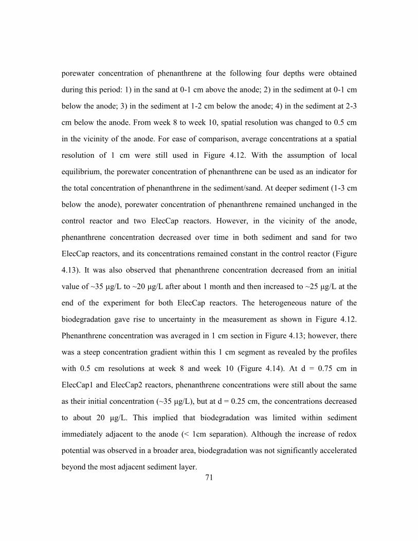
71
porewater concentration of phenanthrene at the following four depths were obtained
during this period: 1) in the sand at 0-1 cm above the anode; 2) in the sediment at 0-1 cm
below the anode; 3) in the sediment at 1-2 cm below the anode; 4) in the sediment at 2-3
cm below the anode. From week 8 to week 10, spatial resolution was changed to 0.5 cm
in the vicinity of the anode. For ease of comparison, average concentrations at a spatial
resolution of 1 cm were still used in Figure 4.12. With the assumption of local
equilibrium, the porewater concentration of phenanthrene can be used as an indicator for
the total concentration of phenanthrene in the sediment/sand. At deeper sediment (1-3 cm
below the anode), porewater concentration of phenanthrene remained unchanged in the
control reactor and two ElecCap reactors. However, in the vicinity of the anode,
phenanthrene concentration decreased over time in both sediment and sand for two
ElecCap reactors, and its concentrations remained constant in the control reactor (Figure
4.13). It was also observed that phenanthrene concentration decreased from an initial
value of ~35 μg/L to ~20 μg/L after about 1 month and then increased to ~25 μg/L at the
end of the experiment for both ElecCap reactors. The heterogeneous nature of the
biodegradation gave rise to uncertainty in the measurement as shown in Figure 4.12.
Phenanthrene concentration was averaged in 1 cm section in Figure 4.13; however, there
was a steep concentration gradient within this 1 cm segment as revealed by the profiles
with 0.5 cm resolutions at week 8 and week 10 (Figure 4.14). At d = 0.75 cm in
ElecCap1 and ElecCap2 reactors, phenanthrene concentrations were still about the same
as their initial concentration (~35 μg/L), but at d = 0.25 cm, the concentrations decreased
to about 20 μg/L. This implied that biodegradation was limited within sediment
immediately adjacent to the anode (< 1cm separation). Although the increase of redox
potential was observed in a broader area, biodegradation was not significantly accelerated
beyond the most adjacent sediment layer.
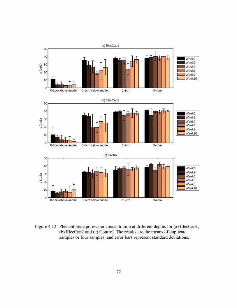
72
Figure 4.12 Phenanthrene porewater concentration at different depths for (a) ElecCap1,
(b) ElecCap2 and (c) Control. The results are the means of duplicate
samples or four samples, and error bars represent standard deviations.
0-1cm above anode 0-1cm below anode 1-2cm 3-4cm0
10
20
30
40
50(a) ElecCap1
c (
g/L
)
Week0
Week2
Week4
Week6
Week8
Week10
0-1cm above anode 0-1cm below anode 1-2cm 3-4cm0
10
20
30
40
50(b) ElecCap2
c (
g/L
)
Week0
Week2
Week4
Week6
Week8
Week10
0-1cm above anode 0-1cm below anode 1-2cm 3-4cm0
10
20
30
40
50(c) Control
c (
g/L
)
Week0
Week2
Week4
Week6
Week8
Week10
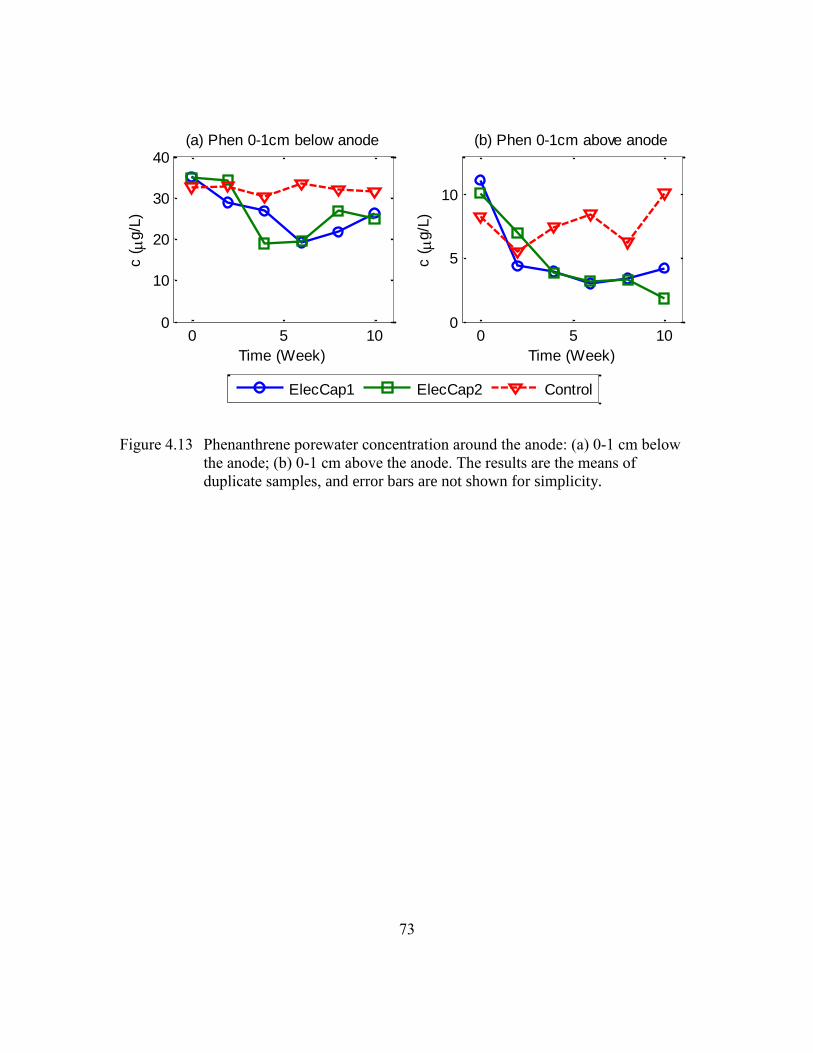
73
Figure 4.13 Phenanthrene porewater concentration around the anode: (a) 0-1 cm below
the anode; (b) 0-1 cm above the anode. The results are the means of
duplicate samples, and error bars are not shown for simplicity.
0 5 100
10
20
30
40
Time (Week)
c (
g/L
)(a) Phen 0-1cm below anode
0 5 100
5
10
Time (Week)
c (
g/L
)
(b) Phen 0-1cm above anode
ElecCap1 ElecCap2 Control
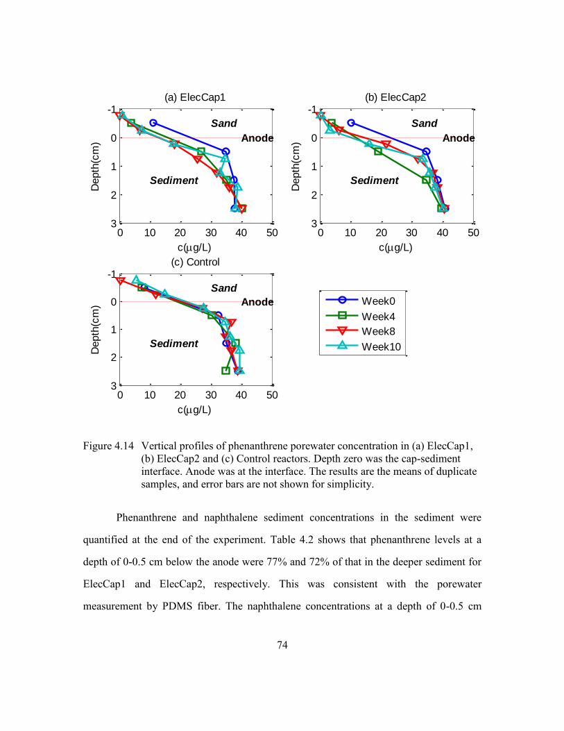
74
Figure 4.14 Vertical profiles of phenanthrene porewater concentration in (a) ElecCap1,
(b) ElecCap2 and (c) Control reactors. Depth zero was the cap-sediment
interface. Anode was at the interface. The results are the means of duplicate
samples, and error bars are not shown for simplicity.
Phenanthrene and naphthalene sediment concentrations in the sediment were
quantified at the end of the experiment. Table 4.2 shows that phenanthrene levels at a
depth of 0-0.5 cm below the anode were 77% and 72% of that in the deeper sediment for
ElecCap1 and ElecCap2, respectively. This was consistent with the porewater
measurement by PDMS fiber. The naphthalene concentrations at a depth of 0-0.5 cm
0 10 20 30 40 50
-1
0
1
2
3
c(g/L)
Depth
(cm
)(a) ElecCap1
Anode
Sand
Sediment
0 10 20 30 40 50
-1
0
1
2
3
c(g/L)
Depth
(cm
)
(b) ElecCap2
Anode
Sand
Sediment
0 10 20 30 40 50
-1
0
1
2
3
c(g/L)
Depth
(cm
)
(c) Control
Anode
Sand
Sediment
Week0
Week4
Week8
Week10
75
below the anode to that in the deeper sediment were 69% and 46% for ElecCap1 and
ElecCap2, respectively.
Table 4.2 Phenanthrene and naphthalene concentration in solid phase
Phenanthrene (μg/g dry sediment) Control ElecCap1 ElecCap2
C0: 0.5-3cm below anode 69.87 ± 4.98 78.47 ± 8.29 66.53 ± 4.80
C1: 0-0.5cm below anode 61.23 ± 3.34 60.57 ± 2.37 47.68 ± 4.15
C1/C0 88% 77% 72%
Naphthalene (μg/g dry sediment) Control ElecCap1 ElecCap2
C0: 0.5-3cm below anode 69.65 ± 13.14 77.39 ± 8.13 70.09 ± 18.35
C1: 0-0.5cm below anode 45.75 ± 8.20 53.56 ± 3.43 32.58 ± 0.71
C1/C0 66% 69% 46%
Results are average values from triplicate samples, and values after ± denote standard deviation.
PAH degrading genes were quantified by qPCR for sediment at the depth of 0-0.5
cm below the anode (Figure 4.15). An increase of PAH degrading genes was observed in
two ElecCap reactors compared to the control reactor. The normalized gene copy
numbers in ElecCap1 and ElecCap 2 reactors were 7 and 3 times greater than that in the
control reactor.
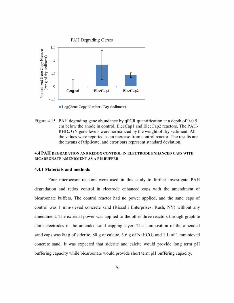
76
Figure 4.15 PAH degrading gene abundance by qPCR quantification at a depth of 0-0.5
cm below the anode in control, ElecCap1 and ElecCap2 reactors. The PAH-
RHDα GN gene levels were normalized by the weight of dry sediment. All
the values were reported as an increase from control reactor. The results are
the means of triplicate, and error bars represent standard deviation.
4.4 PAH DEGRADATION AND REDOX CONTROL IN ELECTRODE ENHANCED CAPS WITH
BICARBONATE AMENDMENT AS A PH BUFFER
4.4.1 Materials and methods
Four microcosm reactors were used in this study to further investigate PAH
degradation and redox control in electrode enhanced caps with the amendment of
bicarbonate buffers. The control reactor had no power applied, and the sand caps of
control was 1 mm-sieved concrete sand (Riccelli Enterprises, Rush, NY) without any
amendment. The external power was applied to the other three reactors through graphite
cloth electrodes in the amended sand capping layer. The composition of the amended
sand caps was 80 g of siderite, 80 g of calcite, 3.6 g of NaHCO3 and 1 L of 1 mm-sieved
concrete sand. It was expected that siderite and calcite would provide long term pH
buffering capacity while bicarbonate would provide short term pH buffering capacity.
77
The reactors were filled with sieved (2 mm) sediment (mixture of contaminated
Anacostia River sediment and clean University Lake sediment, ratio 1:6). The sediment
was spiked with phenanthrene and naphthalene at a level of ~60 μg/g concentration for
both compounds. A 13cm×6cm carbon cloth (Carbon Cloth CC6 Plain, Fuel Cell Earth
LLC, Wakefield, MA) was placed on top of the sediment as the anode. A 3.5-cm layer of
amended sand was placed over the anode and a second, identical, carbon cloth was placed
on the amended sand layer as the cathode. A 0.5 cm amended sand layer was overlain on
the cathode. The sand layers of powered and control reactors were saturated with
freshwater. Freshwater was made by diluting saltwater by a factor of 150. The saltwater
was made by dissolving 35 g of Instant Ocean® sea salts in 1 L of DI water (Stumm and
Morgan, 1996). A multi-channel peristaltic pump (Watson Marlow 205s) was used to
flow the freshwater into the microcosms.
The graphite electrodes were connected to copper wires and sealed with WEST
SYSTEM 105 epoxy resin and 206 slow hardener (WEST SYSTEM, Bay City, MI).
Powered reactors were connected to Extech 382202 DC power supply (Extech
Instruments Corp., Waltham, MA). Among all the three powered reactors, two of them
(CtnCap1 and CtnCap2) were operated in a continuous power mode: an external voltage
of ~2 V was applied continuously except during microelectrode measurement; the third
powered reactor (IntmtCap) was operated in an intermittent power mode: an external
voltage of ~2 V was applied 16 hours continuously over a 24-hour period. The applied
voltage and current for all the three reactors are available in Appendix B.
pH was measured by MI-405 standard pH microelectrode and ORP was measured
by Pt microelectrode. Vertical profiles of pH and ORP from the water-sand interface to a
depth of 55 mm with 5 mm intervals were acquired. Redox-sensitive species (O2, Fe2+,
Mn2+, and S2-) were analyzed electrochemically. Porewater concentration of
78
phenanthrene was measured by PDMS-coated fiber with 5 mm spatial resolution. At the
end of the experiment, sediment cores were collected and dissected into 0.5 cm long
subsamples and stored at -20 °C until further analysis. DNA was extracted and qPCR was
performed at the end of the experiment. The detailed experimental procedures were
described in previous sections in this dissertation.
4.4.2 Results and discussion
4.4.2.1 Redox control, pH changes and redox-sensitive species
With the aid of sodium bicarbonate buffer, pH around the anode was buffered
above 6 in all the three powered reactors (Figure 4.16). Compared with control reactor,
only a small drop of pH from 6.4 to 6 was observed in the powered reactors. With pH
maintained at circumneutral pH, PAH biodegradation rates were expected to be
accelerated by the oxygen produced at the anode with less influence of pH shift. While
the pH changes were minimized by bicarbonate buffers, the increase of ORP were not as
obvious as observed in previous experiments. As shown in Figure 4.17, only ORP in
CtnCap1 reactor was over 50 mV higher than that in control. The difference of ORP
between the other two powered reactors (CtnCap2 and IntmtCap) and the control was
only 10 – 40 mV.
This phenomenon implies that pH and ORP are strongly coupled in the sediments
under electrode enhanced capping. The coupled pH and redox changes are governed by a
complex array of biogeochemical processes.
First, proton produced at the anode not only resulted in pH drop in sediments but
also increased redox potential. This could be explained by Nernst equation of the
dominant redox couple in the sediment. Assumed the dominant redox couple was
Fe(OH)3/Fe2+ in the sediment, the redox reaction being (4-3).
79
Thus
Eh = E0 − 3pH + pFe2+ (4-4)
Where Eh is the potential of the redox reaction (ORP) and E0 is the standard redox
potential (Stumm and Morgan, 1996).
At the anode, pH drop caused by the production of proton gave rise to ORP
according to Equation (4-4). The contribution of pH on redox change might diminish if
pH changes disappear.
Second, biogeochemical reactions that involve oxygen produced at the anode also
result in the increase of redox potential and the decrease of pH. Take the dominant redox
couple Fe(OH)3/Fe2+ as an example, Fe(II) oxidization by oxygen reduced the level of
Fe(II), consequently increasing ORP according to Equation (4-4). For pH changes, many
oxidation reactions by oxygen in the sediment lead to the release of proton, such as the
organic matter oxidation process as follows (Bender and Heggie, 1984):
(CH2O)106(NH3)16(H3PO4) + 138 O2 = 106 CO2 + 16 HNO3 + H3PO4 + 122 H2O (4-5)
In this study, oxygen and proton were always produced at the same time at the
anode, and it was difficult to accurately distinguish the net effect of each species and
every process involved. Nevertheless, all the observations consistently display an
increase of ORP around the anode, indicating a possible shift in favor of PAH
biodegradation.

80
Figure 4.16 Vertical profiles of pH in (a) CtnCap1, (b) CtnCap2, (c) IntmtCap and (d)
Control reactors. Depth zero was the water-cap interface. Cathode was at d
= 0.5 cm and anode was at d = 4 cm. All the measured profiles are in
Appendix B.
5 6 7 8 9 10
0
1
2
3
4
5
(a) pH in CtnCap1
pH
Depth
(cm
)
cathode
anode
sand
sediment
5 6 7 8 9 10
0
1
2
3
4
5
(b) pH in CtnCap2
pH
Depth
(cm
)
cathode
anode
sand
sediment
d0
d20
d41
d55
d69
5 6 7 8 9 10
0
1
2
3
4
5
(c) pH in IntmtCap
pH
Depth
(cm
)
cathode
anode
sand
sediment
5 6 7 8 9 10
0
1
2
3
4
5
(d) pH in Control
pH
Depth
(cm
)cathode
(unpowered)
anode
(unpowered)
sand
sediment
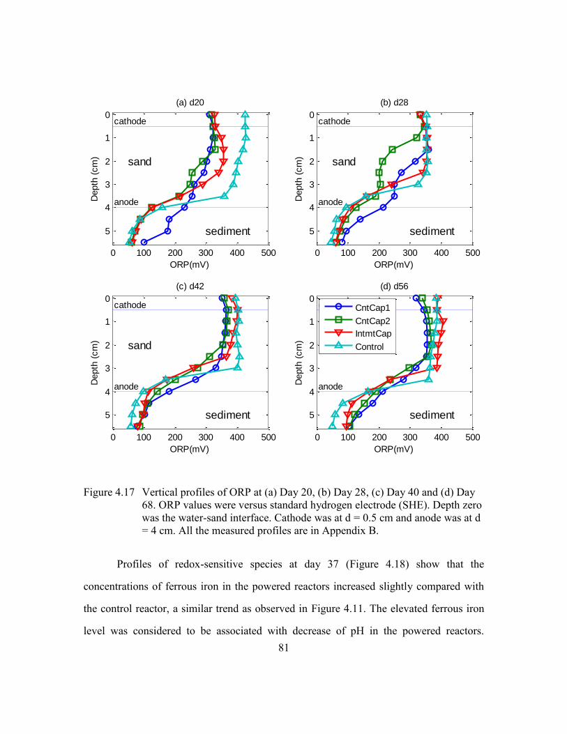
81
Figure 4.17 Vertical profiles of ORP at (a) Day 20, (b) Day 28, (c) Day 40 and (d) Day
68. ORP values were versus standard hydrogen electrode (SHE). Depth zero
was the water-sand interface. Cathode was at d = 0.5 cm and anode was at d
= 4 cm. All the measured profiles are in Appendix B.
Profiles of redox-sensitive species at day 37 (Figure 4.18) show that the
concentrations of ferrous iron in the powered reactors increased slightly compared with
the control reactor, a similar trend as observed in Figure 4.11. The elevated ferrous iron
level was considered to be associated with decrease of pH in the powered reactors.
0 100 200 300 400 500
0
1
2
3
4
5
(a) d20
ORP(mV)
Depth
(cm
)
cathode
anode
sand
sediment
0 100 200 300 400 500
0
1
2
3
4
5
(b) d28
ORP(mV)
Depth
(cm
)
cathode
anode
sand
sediment
0 100 200 300 400 500
0
1
2
3
4
5
(c) d42
ORP(mV)
Depth
(cm
)
cathode
anode
sand
sediment
0 100 200 300 400 500
0
1
2
3
4
5
(d) d56
ORP(mV)
Depth
(cm
)
cathode
anode
sand
sediment
CntCap1
CntCap2
IntmtCap
Control
82
Because of the prevalence of ferrous iron and the absence of sulfide in the sediment
beneath the capping layer, it was determined that the predominant terminal electron
accepting process (TEAP) was ferric iron reduction for all the powered reactors and
control. Although increase of redox potentials was observed in all the powered reactors,
the predominant TEAP in the sediments didn’t change with electrode enhanced caps.
The voltammetric techniques are able to detect dissolved oxygen with a detection
limit of 5 – 25 μM (Brendel and Luther, 1995). But in this study, the voltammetric
techniques failed to detect any dissolved oxygen around the anode though oxygen was
produced at the anode by water electrolysis reaction. Due to the high sediment oxygen
demand, it is unambiguous that only a very thin layer of sediment beneath the anode had
detectable levels of oxygen. The thickness of this thin layer with oxygen present
remained unknown in this study but it should be in the order of millimeters or less.
During the microelectrode measurement, all the microelectrodes were inserted through l-
cm-diameter precut openings in the graphite cloth. So it is very possible that the
microelectrodes didn’t reach the sediment with detectable levels of oxygen. These
practical or operational limitations of instruments make it very difficult for in-situ
monitoring of oxygen concentration.
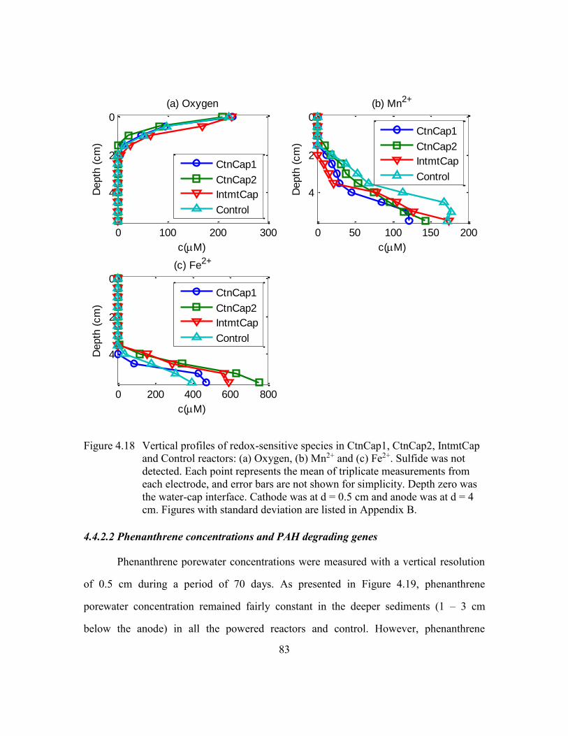
83
Figure 4.18 Vertical profiles of redox-sensitive species in CtnCap1, CtnCap2, IntmtCap
and Control reactors: (a) Oxygen, (b) Mn2+ and (c) Fe2+. Sulfide was not
detected. Each point represents the mean of triplicate measurements from
each electrode, and error bars are not shown for simplicity. Depth zero was
the water-cap interface. Cathode was at d = 0.5 cm and anode was at d = 4
cm. Figures with standard deviation are listed in Appendix B.
4.4.2.2 Phenanthrene concentrations and PAH degrading genes
Phenanthrene porewater concentrations were measured with a vertical resolution
of 0.5 cm during a period of 70 days. As presented in Figure 4.19, phenanthrene
porewater concentration remained fairly constant in the deeper sediments (1 – 3 cm
below the anode) in all the powered reactors and control. However, phenanthrene
0 100 200 300
0
2
4
(a) Oxygen
c(M)
Depth
(cm
)
CtnCap1
CtnCap2
IntmtCap
Control
0 50 100 150 200
0
2
4
(b) Mn2+
c(M)
Depth
(cm
)
CtnCap1
CtnCap2
IntmtCap
Control
0 200 400 600 800
0
2
4
(c) Fe2+
c(M)
Depth
(cm
)
CtnCap1
CtnCap2
IntmtCap
Control
84
concentration in the 1 cm vicinity of the anode displays different trends over time
between powered reactors and control (Figure 4.20). In the powered reactors, the
phenanthrene concentrations at 0.5-1 cm sand above the anode were initially at very low
concentration (< 1 μg/L) and almost non-detectable during the rest of the time; the
concentrations at 0-0.5 cm sand above the anode were initially ~ 2 μg/L and decreased to
less than 0.2 μg/L at the end. On the contrary, in the control reactor phenanthrene
concentrations increased over time in the sand above the anode (at both 0-0.5 cm and 0.5-
1 cm) due to the diffusion of phenanthrene from the underlying sediment. In the
sediments beneath the anode, phenanthrene concentrations decreased over time in
powered reactors, whereas phenanthrene concentrations increased slightly (at 0-0.5 cm
below the anode) or kept constant (at 0.5-1 cm below the anode) in the control. Not
considering the mass in the sand layer, the reduction of phenanthrene mass in the 1 cm
vicinity of sediment were 51%, 44% and 47% compared to initial mass for CtnCap1,
CtnCap2, and IntmtCap, respectively. In the experiment with no bicarbonate amendment,
a lower removal efficiency of phenanthrene (~30%) was observed during a time period of
about the same length. This difference of removal efficiency indicated that maintaining
pH at the normal range (6-8) may be a critical success factor for effective biodegradation
of PAH in electrode enhanced capping.
The low levels of phenanthrene present in the sand layer demonstrated the
effectiveness of the electrode enhanced capping as a biobarrier for remediation of
contaminated sediment. By placing the anode at the sand-sediment interface, migration of
phenanthrene from the underlying sediment was prevented or inhibited considerably.
While contaminant may breakthrough conventional sand capping over time, electrode
enhanced capping could overcome this limitation by creating a biobarrier at the cap-
sediment interface.
85
qPCR analysis confirmed increased PAH degrading genes in all the three reactors
(Figure 4.21), indicating that electrode enhanced capping stimulated microbial PAH
biodegradation. The normalized gene copy numbers increased about 2 - 6 fold in powered
reactors compared to those in control, which were comparable to the observations in the
experiments described in 4.3. Compared with the gene increase observed in the slurry
experiment, i.e., nearly 2 orders of magnitude increase, the gene increases in the
sediments under electrode enhanced capping were much less. In the slurry experiment,
the concentrations of phenanthrene and naphthalene decreased rapidly and thus
populations of PAH-degrading bacteria increased significantly. However, in the sediment
under the anode, biodegradation occurred slowly. After about 10 weeks, only
approximate 30% (no bicarbonate amendment) or 50% (with bicarbonate amendment) of
phenanthrene was degraded. It is coherent that the growth of PAH degrading bacteria in
the sediment was much slower than that in well mixed slurry systems.
The IntmtCap reactor was running in an intermittent mode: two third of the time
with power and one third of the time with no power. The results from phenanthrene
concentration show that the biodegradation rates of IntmtCap were almost the same as
those of continuous reactors. In addition, IntmtCap even shows a slightly higher level of
PAH degrading genes, though it is not conclusive to state that IntmtCap is better than
continuous reactors for PAH biodegradation. The success of IntmtCap indicates the
flexibility of electrode enhanced capping for remediation of PAH contaminated sediment.
For instance, the power can be turned off for a short period to diminish pH changes at the
anode. In the field application, if the power is accidently shut down temporally, it is very
possible that the effect is not detrimental but can be recovered when the power resumes.
The noticeable increase in PAH degrading genes between powered reactors and
control indicated that electrodes placed between sand and sediments worked by
86
increasing the population of PAH degrading bacteria. This in turn would have led to the
accelerated phenanthrene degradation rates discussed previously. This correlation
between PAH decrease and gene increase supported microbial biodegradation as a
mechanism of decay in electrode enhanced capping. However, a quantitative relationship
between PAH removal efficiency and gene increase can’t be established with limited data
in this study. For instance, the fold changes of genes were between 2 to 6 despite about
the same biodegradation rates among all the three powered reactors with bicarbonate
amendment; in addition, the results from bicarbonate amendment experiments show
relatively higher removal efficiency in the vicinity of the anode, but didn’t show
significant difference in gene increase compared with the no bicarbonate amendment
experiments. Given the uncertainty in biodegradation and the heterogamous nature of the
sediments, a correlation between biodegradation rates and gene copy numbers would
prove difficult (Baldwin et al., 2008). Nevertheless, the consistent detection of PAH
degrading gene increment was seen while PAH biodegradation occurred.
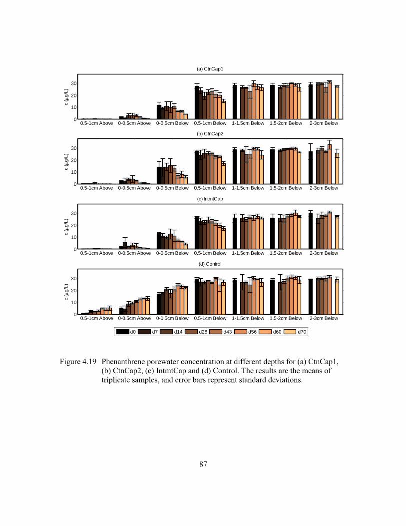
87
Figure 4.19 Phenanthrene porewater concentration at different depths for (a) CtnCap1,
(b) CtnCap2, (c) IntmtCap and (d) Control. The results are the means of
triplicate samples, and error bars represent standard deviations.
0.5-1cm Above 0-0.5cm Above 0-0.5cm Below 0.5-1cm Below 1-1.5cm Below 1.5-2cm Below 2-3cm Below0
10
20
30
(a) CtnCap1c (
g/L
)
0.5-1cm Above 0-0.5cm Above 0-0.5cm Below 0.5-1cm Below 1-1.5cm Below 1.5-2cm Below 2-3cm Below0
10
20
30
(b) CtnCap2
c (
g/L
)
0.5-1cm Above 0-0.5cm Above 0-0.5cm Below 0.5-1cm Below 1-1.5cm Below 1.5-2cm Below 2-3cm Below0
10
20
30
(c) IntmtCap
c (
g/L
)
0.5-1cm Above 0-0.5cm Above 0-0.5cm Below 0.5-1cm Below 1-1.5cm Below 1.5-2cm Below 2-3cm Below0
10
20
30
(d) Control
c (
g/L
)
d0 d7 d14 d28 d43 d56 d60 d70
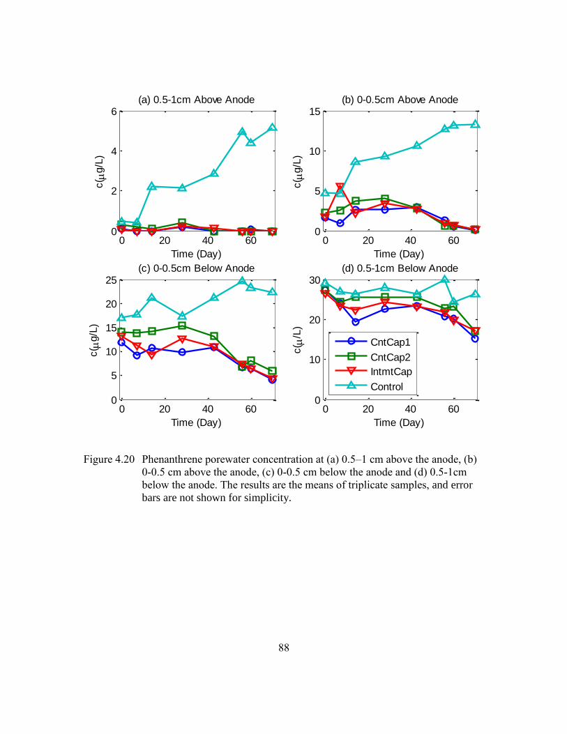
88
Figure 4.20 Phenanthrene porewater concentration at (a) 0.5–1 cm above the anode, (b)
0-0.5 cm above the anode, (c) 0-0.5 cm below the anode and (d) 0.5-1cm
below the anode. The results are the means of triplicate samples, and error
bars are not shown for simplicity.
0 20 40 600
2
4
6(a) 0.5-1cm Above Anode
Time (Day)
c(
g/L
)
0 20 40 600
5
10
15(b) 0-0.5cm Above Anode
Time (Day)
c(
g/L
)
0 20 40 600
5
10
15
20
25(c) 0-0.5cm Below Anode
Time (Day)
c(
g/L
)
0 20 40 600
10
20
30(d) 0.5-1cm Below Anode
Time (Day)
c(
/L)
CntCap1
CntCap2
IntmtCap
Control

89
Figure 4.21 PAH degrading gene abundance by qPCR quantification at a depth of 0-0.5
cm below the anode in CtnCap1, CtnCap2, IntmtCap and control reactors.
The PAH-RHDα GN gene levels were normalized by the weight of dry
sediment. All the values were reported as an increase from control reactor.
The results are the means of triplicate, and error bars represent standard
deviation.
4.4.2.3 Cost analysis
It is too early to develop verifiable cost scenarios for electrode enhanced capping
at this initial stage in the development of the technology. However, certain preliminary
estimates have been attempted to assess the potential cost-effectiveness of this
technology. The additional capital costs (compared to conventional capping) mainly
include the energy cost and the material cost of electrode materials. In the experiment of
electrode enhanced capping with bicarbonate amendment, the energy costs for three
CtnCap1 CtnCap2 IntmtCap Control
-0.4
-0.2
0
0.2
0.4
0.6
0.8
1
Lo
g (
Ge
ne
Co
py N
um
be
rs / d
ry s
ed
ime
nt)
Normalized PAH degrading genes(per g of dry sediment)
90
powered reactors ranged from 0.35 to 0.5 mW. Considering an electrode area of ~78 cm2,
the energy cost per unit area was only 45-64 mW/m2, i.e. 0.39-0.56 kWh/m2. The average
retail price of electricity to ultimate customers of US in 2011 was 9.99 cents per kWh
(US EIA, 2012). So the additional cost for energy of electrode enhanced capping is about
3.9-5.6 c/m2, i.e. $158-$227 per acre, only a very insignificant portion of the total cost of
in-situ capping. Typical costs of large-scale cap applications are approximately $17–
$21/m2 plus the cost of materials (Reible, 2004). In total, the overall placement cost of
electrode enhanced capping is about $30/m2, which is similar to the use of a reactive core
mat (McDonough et al., 2007).
The use of solar panels (photovoltaic modules) as a power supply for chemical
/electrochemical systems and remote sensors has previously been reported (Hart and
Martinez, 2006; Schafer et al., 2007; Park et al., 2008). Solar panels as a power supply
has almost zero pollution, low maintenance cost and a long life, and can be used as a
power source for electrode enhanced capping. To avoid energy fluctuations and for
working during night hours, solar panels need to be connected to a storage battery. The
output of a single solar panel with 40 solar cells ranges from 10 to 300 watts (US DOE,
2011). Because of its low power requirement, a single solar panel can power a large area
of electrode enhanced capping. If the power requirement is 45-64 mW/m2 as previously
discussed, a solar panel with a capacity of 100 W can power an area of 1560-2229 m2. So
a one-acre area needs only 2-3 solar panels of 100 W for the application of electrode
enhanced capping.
These analyses shows that electrode enhanced capping can be a cost-effective and
sustainable remediation technology for the management of contaminated sediment. Of
course, for successful application to a specific site, feasibility studies to characterize the
site hydraulics and geochemical parameters need to be performed, and operating
91
parameters will likely need to be optimized before scaling up from bench scale to field
scale.
4.5 CONCLUSIONS
The results in this study show that electrode enhanced capping can be used to
control redox potential in a sediment cap, provide microbial electron acceptor, and
stimulate PAH degradation.
Microcosm study was first implemented in the sediments with electrodes placed
horizontally at different depths. The ORP around the anode in powered reactors increased
gradually, and was 50 – 150 mV higher than that in the control. pH around the anode
decreased to ~6 from an initial value of 6.4 or 6.7 in powered reactors. Phenanthrene
concentration at the anode decreased with time, showing a unique Z-shaped profile in the
sediment in powered reactors. These observations provided evidences that the anode
placed in the sediment could effectively decrease phenanthrene porewater concentration
around the anode.
PAH biodegradation and redox control by electrode enhanced capping were
further studied in simulated microcosm reactors. Two carbon cloth electrodes were
emplaced within a sediment cap with an applied potential of 2 V. In the experiment with
no bicarbonate buffer, ORP in the vicinity of the anode increased 60 - 100 mV compared
to the control reactor, and pH dropped to 5.7 and 6 from circumneutral pH. Average
phenanthrene concentrations decreased to ~ 70% of initial concentration in the 1 cm
vicinity of the anode in 10 weeks. In the experiment with bicarbonate buffer, ORP in one
powered reactor was over 50 mV higher than that control and the other two displayed less
ORP changes. With the aid of bicarbonate buffer, only a small drop of pH from 6.4 to 6
was observed in the powered reactors. The results imply that pH and ORP are strongly

92
coupled in the sediments under electrode enhanced capping. With pH maintained at
circumneutral pH, PAH biodegradation rates were accelerated by the oxygen produced at
the anode with less influence of pH shift. The reduction of phenanthrene mass in the 1 cm
vicinity of sediment was ~ 50 % compared to initial mass in powered reactors in 10
weeks. qPCR results also show an increase of PAH degrading genes at the depth of 0 -
0.5 cm below the anode. Although these changes are confined to a small layer ( < 1 cm),
the encouragement of PAH degradation in this layer could reduce PAH migration toward
the surface and biota in the sediment and overlying water. These findings demonstrated
the capability of this novel technology for the remediation of contaminated sediment.
93
Chapter 5: Model of Electrode Enhanced Capping
5.1 INTRODUCTION
A model of the electrode enhanced capping was developed to enable prediction of
performance to a broader range of conditions than were evaluated experimentally and to
make preliminary predictions of long-term performance of an electrode enhanced cap
under field conditions. Key goals of the model were to predict performance and behavior
as well as power requirements. The application of an external potential across a capping
layer causes a very complex set of reaction and transport processes to occur within the
system. Numerical simulation of the technology requires a grasp of the physical and
chemical phenomena and mathematical formulation of these processes. These processes
include electrolysis reactions at the electrodes, geochemical reactions in aquatic
sediments and capping layer, electrokinetic processes, and contaminant transport, etc.
Water electrolysis is a major reaction with the application of an external voltage.
The production of oxygen at the anode and the generation of pH gradient in the system
are all driven by water electrolysis reaction. Their reaction rates are proportional to
current as follows (Bard and Faulkner, 2001):
Rate(mol/s) = I/nF (5-1)
Where I is the current, n is the stoichiometric number of electrons consumed in
the electrode reaction, and F is Faraday constant.
As shown in (5-1), current is an important parameter in determining the chemical
reaction rates at the electrodes. However, controlled-voltage instead of controlled-current
technique is generally employed in the application of electrode enhanced capping. So the
first step in model develop of electrode enhanced capping is to predict the current based
94
on applied voltage and other parameters, such as thickness of the capping layer and area
of the electrodes.
Once the current is determined, electrode reaction rates can be calculated and they
can serve as inputs for the model of transport and reaction processes. Coupled reactive
transport modeling simulates the distribution of all important species with time, e.g. pH
gradient.
Several mathematical models have been developed to predict transport and
reaction processes during electrokinetic remediation (Alshawabkeh and Acar, 1992;
Alshawabkeh and Acar, 1996; Shapiro et al., 1989; Shapiro and Probstein, 1993; Haran et
al., 1997; Yu and Neretnieks, 1996; Choi and Lui, 1995; Yeung and Datta, 1995; Al-
Hamdan and Reddy, 2008). However, many of these models focus on heavy metals
extraction by electrokinetic process, and do not accurately account for the geochemistry
in the sediment and/or soil. In most of these studies, pH buffering of soil/sand was not
considered, and these models are not suitable for electrode enhanced capping due to the
high pH buffer capacity of sediment. pH is one of the limiting factors have been
recognized to affect the biodegradation of PAH (Das and Chandran, 2011). Therefore it is
necessary to build a model that can accurately describe the pH of sediment/sand with the
application of an external potential across a capping layer.
In this chapter, a voltage-current relationship is developed first and then a coupled
reactive transport model is presented to describe the processes involved and this model
can serve as a design tool for electrode enhanced capping.

95
5.2 VOLTAGE-CURRENT RELATIONSHIP
5.2.1 Model development
Water electrolysis is the primary electrochemical reaction at the electrodes during
the application of external power as follows:
Anode: 2H2O = O2 + 4H+ + 4e E0 = 1.229V (5-2)
Cathode: 2H2O + 2e = H2 + 2OH− E0 =-0.827V (5-3)
The half-cell potential of the anode reaction (5-2) can be expressed by Nernst
equation as follows:
Eanode = Eanode0 +
RT
4F∗ ln {p(O2)[H
+]4} (5-4)
Where Eanode is the half-cell potential of the anode reaction, E0anode is the standard
electrode potential, R is ideal gas constant, T is absolute temperature, p(O2) is oxygen
partial pressure at the anode, and [H+] is the H+ concentration at the anode. At pH = 7 and
p(O2) = 1 atm, Eanode = 0.816 V.
The half-cell potential of the cathode reaction (5-3) can be expressed by Nernst
equation as follows:
Ecathode = Ecathode0 −
RT
2F∗ ln {p(H2)[OH−]2} (5-5)
Where Ecathodee is the half-cell potential of the cathode reaction, E0cathode is the
standard electrode potential, R is ideal gas constant, T is absolute temperature, p(H2) is
hydrogen partial pressure at the cathode, and [OH-] is the OH- concentration at the
cathode. At pH = 7 and p(H2) = 1 atm, Ecathode = -0.414 V.
The overall cell potential is written as
96
E0 = Eanode − Ecathode (5-6)
That is
E0 = Eanode0 − Ecathode
0 +RT
F∗ ln{[H+][OH−]} +
RT
4F∗ ln[p(O2)] +
RT
2F∗ ln[p(H2)] (5-7)
Although other electrochemical reactions may occur depending on the
concentration of species, their electrochemical potential, and the reaction kinetics, water
electrolysis reaction is considered the dominant reaction and thus only this reaction is
considered during the model development. This likely limits the model to the prediction
of an electrode enhanced cap to freshwater systems.
The overall applied cell voltage is composed of a number of terms, i.e.
V = EO + |ηA| + |ηC| + ηohmic (5-8)
Where V is the applied voltage, ηA and ηC are the overpotentials at the anode and
cathode, respectively, ηohmic is the ohmic loss of the system, and E0 is the thermodynamic
potential of water electrolysis. Equation (5-7) shows that E0 depends on [H+] and p(O2) at
the anode, and [OH-] and p(H2) at the cathode. Although pH may change at both cathode
and anode during the application of an extern power, it is assumed that E0 has a constant
value of 1.23 V, i.e. thermodynamic potential of water electrolysis at 25 °C at pH = 7.
Theoretically, the relationship between the current at the electrode and the
overpotential follows Butler-Volmer expressions as follows (Newman and Thomas-
Alyea, 2004):
I = Ai0 [exp (αa
F
RTη) − exp (−αc
F
RT η)] (5-9)
97
Where I is current, A is electrode active surface area, i0 is exchange current
density, F is Faraday constant, R is ideal gas constant, T is absolute temperature, η is
overpotential, αa and αc are apparent transfer coefficients, which gives the magnitude of
the potential dependence of the electrochemical reaction rates.
In most systems, αa and αc turn out to lie between 0.3 and 0.7, and they can
usually be approximated by 0.5 in the absence of actual measurement (Bard and
Faulkner, 2001).
In practice, Tafel equation is generally used to simplify the reaction kinetics as
follows (Bard and Faulkner, 2001; Pletcher and Walsh, 1990):
η = a′ + b′ ∗ log10 I (5-10)
Or
η = a′ + b′ ∗ log10(iA) = a′ + b′ ∗ log10 A + b′ ∗ log10 i (5-11)
Where a’ and b’ are empirical parameters, and i is current density (current per unit
area).
Assuming both oxygen and hydrogen generation reactions have apparent transfer
coefficients of 0.5 for αa and αc, then parameter b’ in Tafel equation will have the same
value for these two reactions (Appendix C). |ηA| + |ηC| term in Equation (5-8) can be
combined into one expression with only two empirical parameters as follows:
|ηA| + |ηC| = a + b ∗ log10(I) (5-12)
The ohmic loss ηohmic can be expressed as
ηohmic =iAL
κa=
IL
κa (5-13)
98
Where L is the distance between the anode and the cathode, κa is the effective
electrical conductivity of porous media.
Effective electrical conductivity of water-saturated soil κa can be estimated by
Archie’s empirical law (Archie, 1942; Friedman, 2005):
κa = κθm (5-14)
Where κ is the electrical conductivity of electrolyte, θ is the porosity of the sand
and m is a material-dependent empirical exponent.
The conductivity of electrolyte κ can be estimated by values of equivalent
conductances of ionic species (Bard and Faulkner, 2001)
κ = F Σ (|zi|uici) (5-15)
Where zi is charge number, ui is mobility and ci is concentration of the ith specie.
Therefore, the overall cell voltage-current relationship can be obtained by
combing Equation (5-8), (5-12), and (5-13):
V = E0 + a + b ∗ log10I +LI
κa (5-16)
It can also be written in terms of current density i instead of current I as follows:
V = E0 + a + b ∗ log10A + b ∗ log10i +LiA
κa (5-17)
Once all the parameters in Equation (5-16) or (5-17) are given, cell voltage-
current (or current density) equation is deterministic though the function to determine
current I by voltage V: I = f(V) is implicit. However, a plot of voltage V verses current I
99
can be constructed and the current I under a given value of V can be easily read from the
graph.
5.2.2 Model calibration
The input voltage by an external power and current were measured in three
beakers as described in section 4.2. The sand layers were saturated with electrolyte (2
mM NaCl and 2 mM Na2SO4 mixed electrolyte) initially though the porewater
composition would be different due to dissolution and ionic species transport. Due to
uncertainty in ionic species composition, porosity of sand θ, and empirical exponent m, a
lumped parameter Rrstc is used and Equation (5-16) is written as :
V = E0 + a + b ∗ log10(I) + RrstcI (5-18)
Where Rrstc represents the total resistance between the electrodes.
Parameter a, b and Rrstc can be obtained by fitting the model to experimental
results. The model was calibrated using three data sets, and Table 5.1 shows the
calibrated value of parameter a, b and Rrstc. Although these three beaker experiments
were conducted as replicates, measured current value at the same input voltage was
slightly different between replicates. Consequently, fitted parameters show some
variation for the different data sets. As shown in Figure 5.1, the model presented above
can be used to describe voltage-current relationship, no matter which set of calibrated
parameters is used. All the three sets of parameters gave very similar results although
each parameter may have some variation between data sets (Figure 5.1 (d)).
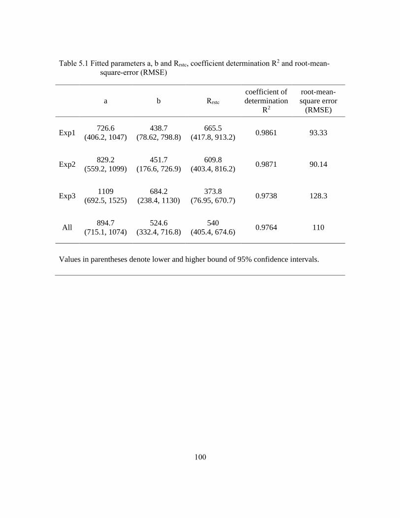
100
Table 5.1 Fitted parameters a, b and Rrstc, coefficient determination R2 and root-mean-
square-error (RMSE)
a b Rrstc
coefficient of
determination
R2
root-mean-
square error
(RMSE)
Exp1 726.6
(406.2, 1047)
438.7
(78.62, 798.8)
665.5
(417.8, 913.2) 0.9861 93.33
Exp2 829.2
(559.2, 1099)
451.7
(176.6, 726.9)
609.8
(403.4, 816.2) 0.9871 90.14
Exp3 1109
(692.5, 1525)
684.2
(238.4, 1130)
373.8
(76.95, 670.7) 0.9738 128.3
All 894.7
(715.1, 1074)
524.6
(332.4, 716.8)
540
(405.4, 674.6) 0.9764 110
Values in parentheses denote lower and higher bound of 95% confidence intervals.
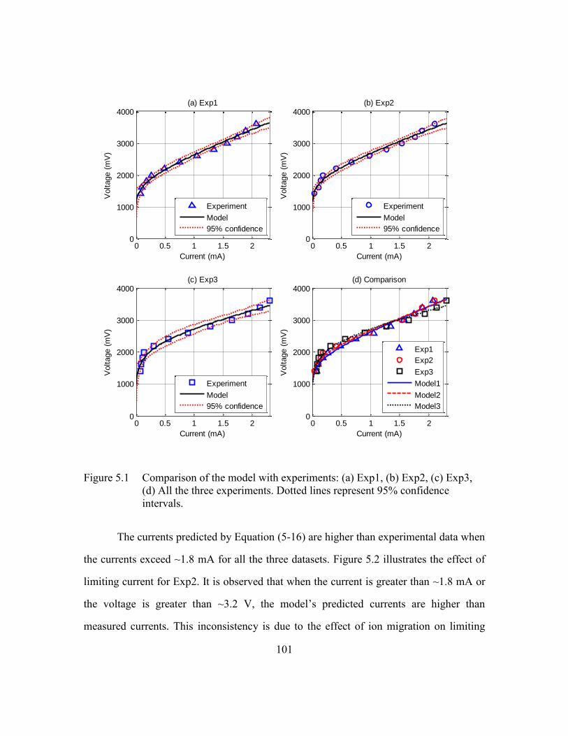
101
Figure 5.1 Comparison of the model with experiments: (a) Exp1, (b) Exp2, (c) Exp3,
(d) All the three experiments. Dotted lines represent 95% confidence
intervals.
The currents predicted by Equation (5-16) are higher than experimental data when
the currents exceed ~1.8 mA for all the three datasets. Figure 5.2 illustrates the effect of
limiting current for Exp2. It is observed that when the current is greater than ~1.8 mA or
the voltage is greater than ~3.2 V, the model’s predicted currents are higher than
measured currents. This inconsistency is due to the effect of ion migration on limiting
0 0.5 1 1.5 20
1000
2000
3000
4000
Current (mA)
Voltage (
mV
)(a) Exp1
0 0.5 1 1.5 20
1000
2000
3000
4000
Current (mA)
Voltage (
mV
)
(b) Exp2
0 0.5 1 1.5 20
1000
2000
3000
4000
Current (mA)
Voltage (
mV
)
(c) Exp3
0 0.5 1 1.5 20
1000
2000
3000
4000(d) Comparison
Current (mA)
Voltage (
mV
)
Experiment
Model
95% confidence
Experiment
Model
95% confidence
Experiment
Model
95% confidence
Exp1
Exp2
Exp3
Model1
Model2
Model3
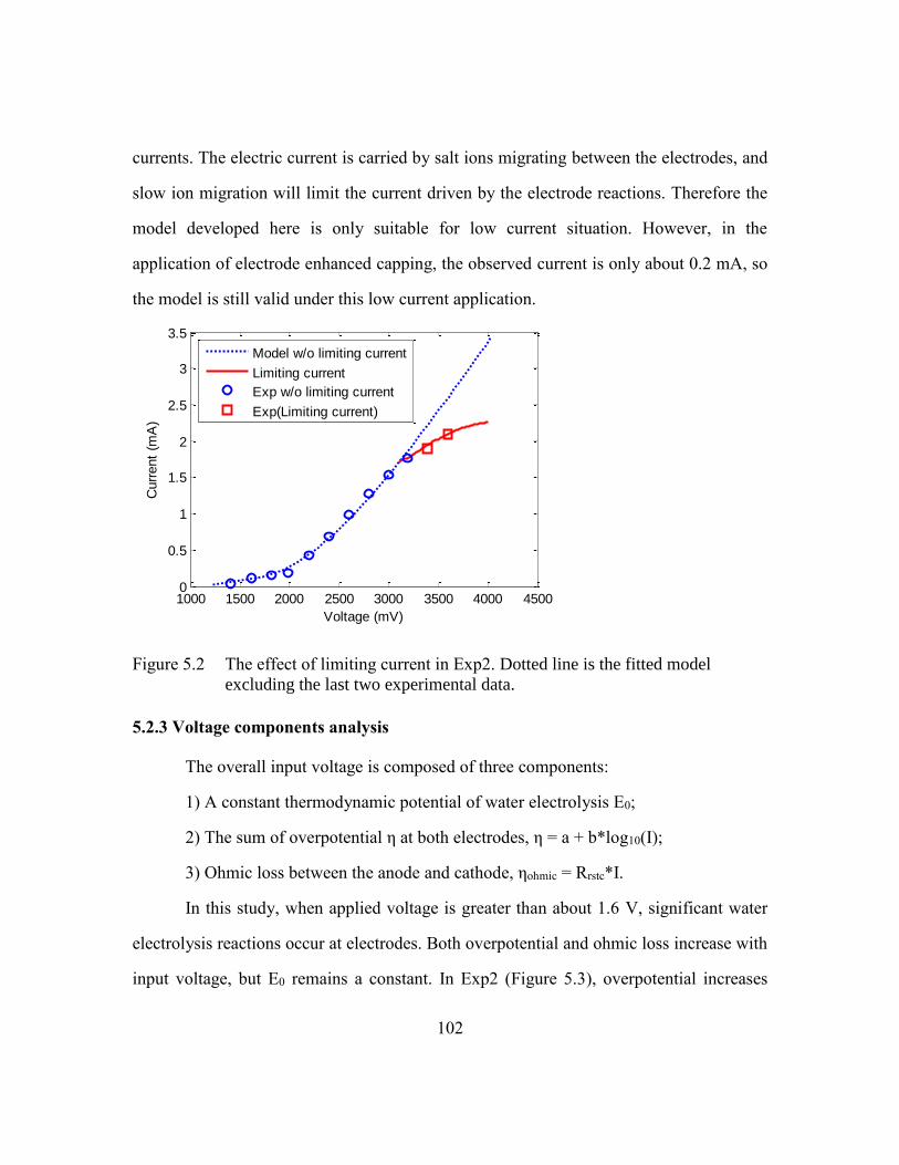
102
currents. The electric current is carried by salt ions migrating between the electrodes, and
slow ion migration will limit the current driven by the electrode reactions. Therefore the
model developed here is only suitable for low current situation. However, in the
application of electrode enhanced capping, the observed current is only about 0.2 mA, so
the model is still valid under this low current application.
Figure 5.2 The effect of limiting current in Exp2. Dotted line is the fitted model
excluding the last two experimental data.
5.2.3 Voltage components analysis
The overall input voltage is composed of three components:
1) A constant thermodynamic potential of water electrolysis E0;
2) The sum of overpotential η at both electrodes, η = a + b*log10(I);
3) Ohmic loss between the anode and cathode, ηohmic = Rrstc*I.
In this study, when applied voltage is greater than about 1.6 V, significant water
electrolysis reactions occur at electrodes. Both overpotential and ohmic loss increase with
input voltage, but E0 remains a constant. In Exp2 (Figure 5.3), overpotential increases
1000 1500 2000 2500 3000 3500 4000 45000
0.5
1
1.5
2
2.5
3
3.5
Curr
ent
(mA
)
Voltage (mV)
Model w/o limiting current
Limiting current
Exp w/o limiting current
Exp(Limiting current)
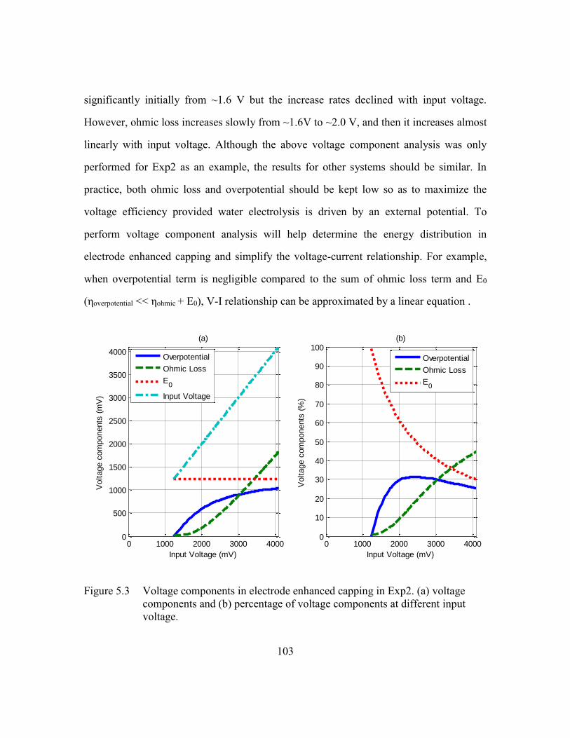
103
significantly initially from ~1.6 V but the increase rates declined with input voltage.
However, ohmic loss increases slowly from ~1.6V to ~2.0 V, and then it increases almost
linearly with input voltage. Although the above voltage component analysis was only
performed for Exp2 as an example, the results for other systems should be similar. In
practice, both ohmic loss and overpotential should be kept low so as to maximize the
voltage efficiency provided water electrolysis is driven by an external potential. To
perform voltage component analysis will help determine the energy distribution in
electrode enhanced capping and simplify the voltage-current relationship. For example,
when overpotential term is negligible compared to the sum of ohmic loss term and E0
(ηoverpotential << ηohmic + E0), V-I relationship can be approximated by a linear equation .
Figure 5.3 Voltage components in electrode enhanced capping in Exp2. (a) voltage
components and (b) percentage of voltage components at different input
voltage.
0 1000 2000 3000 40000
500
1000
1500
2000
2500
3000
3500
4000
(a)
Input Voltage (mV)
Voltage c
om
ponents
(m
V)
Overpotential
Ohmic Loss
E0
Input Voltage
0 1000 2000 3000 40000
10
20
30
40
50
60
70
80
90
100(b)
Input Voltage (mV)
Voltage c
om
ponents
(%
)
Overpotential
Ohmic Loss
E0
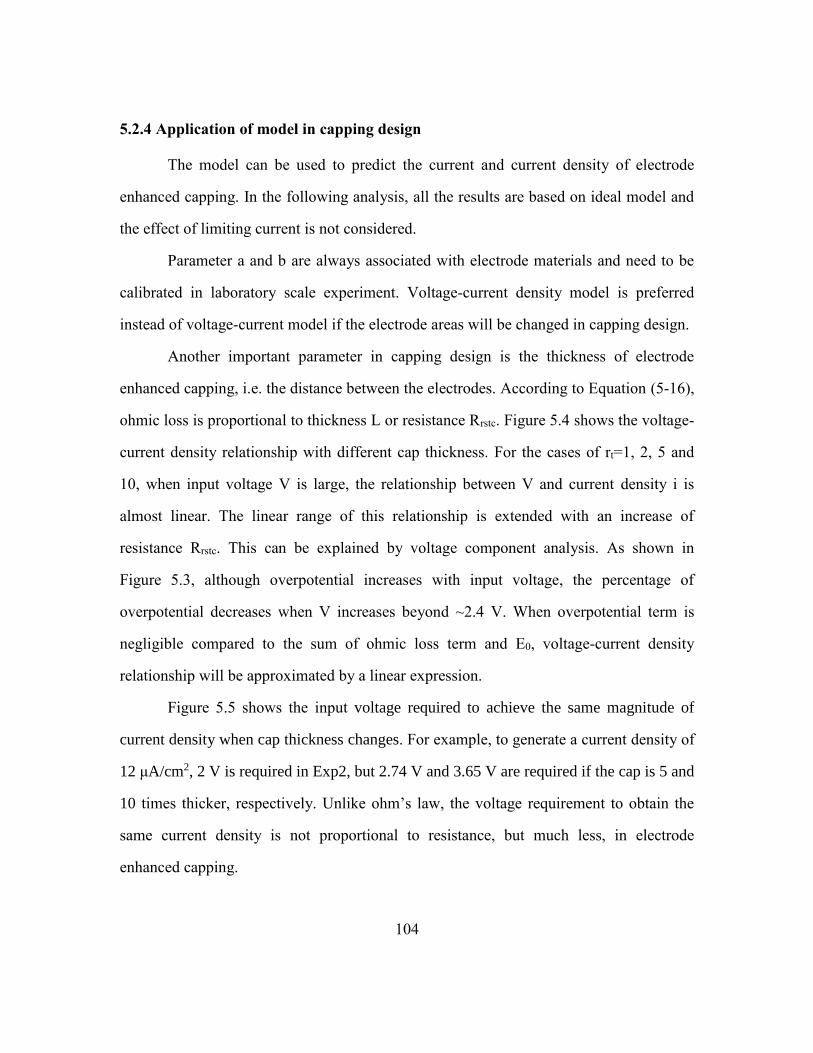
104
5.2.4 Application of model in capping design
The model can be used to predict the current and current density of electrode
enhanced capping. In the following analysis, all the results are based on ideal model and
the effect of limiting current is not considered.
Parameter a and b are always associated with electrode materials and need to be
calibrated in laboratory scale experiment. Voltage-current density model is preferred
instead of voltage-current model if the electrode areas will be changed in capping design.
Another important parameter in capping design is the thickness of electrode
enhanced capping, i.e. the distance between the electrodes. According to Equation (5-16),
ohmic loss is proportional to thickness L or resistance Rrstc. Figure 5.4 shows the voltage-
current density relationship with different cap thickness. For the cases of rt=1, 2, 5 and
10, when input voltage V is large, the relationship between V and current density i is
almost linear. The linear range of this relationship is extended with an increase of
resistance Rrstc. This can be explained by voltage component analysis. As shown in
Figure 5.3, although overpotential increases with input voltage, the percentage of
overpotential decreases when V increases beyond ~2.4 V. When overpotential term is
negligible compared to the sum of ohmic loss term and E0, voltage-current density
relationship will be approximated by a linear expression.
Figure 5.5 shows the input voltage required to achieve the same magnitude of
current density when cap thickness changes. For example, to generate a current density of
12 μA/cm2, 2 V is required in Exp2, but 2.74 V and 3.65 V are required if the cap is 5 and
10 times thicker, respectively. Unlike ohm’s law, the voltage requirement to obtain the
same current density is not proportional to resistance, but much less, in electrode
enhanced capping.
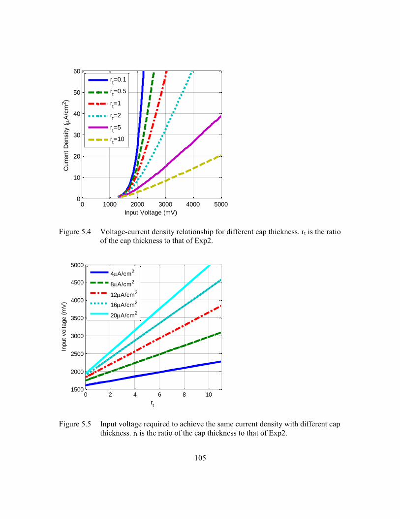
105
Figure 5.4 Voltage-current density relationship for different cap thickness. rt is the ratio
of the cap thickness to that of Exp2.
Figure 5.5 Input voltage required to achieve the same current density with different cap
thickness. rt is the ratio of the cap thickness to that of Exp2.
0 1000 2000 3000 4000 50000
10
20
30
40
50
60
Input Voltage (mV)
Curr
ent
Density (
A/c
m2)
rt=0.1
rt=0.5
rt=1
rt=2
rt=5
rt=10
0 2 4 6 8 101500
2000
2500
3000
3500
4000
4500
5000
rt
Input
voltage (
mV
)
4A/cm2
8A/cm2
12A/cm2
16A/cm2
20A/cm2
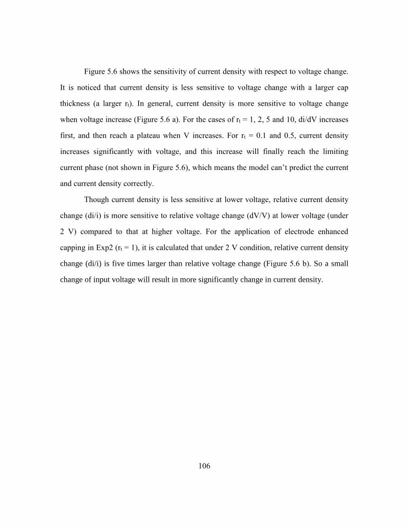
106
Figure 5.6 shows the sensitivity of current density with respect to voltage change.
It is noticed that current density is less sensitive to voltage change with a larger cap
thickness (a larger rt). In general, current density is more sensitive to voltage change
when voltage increase (Figure 5.6 a). For the cases of rt = 1, 2, 5 and 10, di/dV increases
first, and then reach a plateau when V increases. For rt = 0.1 and 0.5, current density
increases significantly with voltage, and this increase will finally reach the limiting
current phase (not shown in Figure 5.6), which means the model can’t predict the current
and current density correctly.
Though current density is less sensitive at lower voltage, relative current density
change (di/i) is more sensitive to relative voltage change (dV/V) at lower voltage (under
2 V) compared to that at higher voltage. For the application of electrode enhanced
capping in Exp2 (rt = 1), it is calculated that under 2 V condition, relative current density
change (di/i) is five times larger than relative voltage change (Figure 5.6 b). So a small
change of input voltage will result in more significantly change in current density.
107
Figure 5.6 Sensitivity analysis of current density with respect to voltage changes for
different cap thickness: (a) current density change with respect to voltage
change (di/dV); (b) relative current density change with respect to relative
voltage change [(di/i)/(dV/V)].
5.3 MODELING OF TRANSPORT AND REACTION PROCESSES
5.3.1 Modeling of transport processes
The model takes into consideration the following four transport mechanisms of
aqueous species in capping sand and sediment under the influence of DC electrical field:
(1) Advection due to the movement of groundwater under hydraulic gradient.
Jadv = cq (5-19)
Where Jadv is the advective flux, c is the concentration of species in porewater,
and q is Darcy velocity.
(2) Advection due to electroosmosis.
1000 2000 3000 4000 50000
0.02
0.04
0.06
0.08
0.1
Input Voltage (mV)
di/dV
(
A*c
m-2
/mV
)(a) di/dV
1000 2000 3000 4000 50001
2
3
4
5
6
7
8
9
Input Voltage (mV)
(di/i)/(
dV
/V)
(b) (di/i)/(dV/V)
rt=0.1
rt=0.5
rt=1
rt=2
rt=5
rt=10
108
Jeo = −θckeo∇Vep (5-20)
Where Jeo is the advective flux due to electroosmosis, θ is porosity, Vep is
electrical potential, and keo is the electroosmotic permeability which depends on the ionic
strength, viscosity and permittivity of the fluid and the properties of the porous medium
(Alshawabkeh and Acar, 1992). A simplified expression for keo is known as Helmboltz-
Smoluchowski equation (Probstein, 1989):
keo =εpζ
μ (5-21)
Where εp is permittivity of the medium, ζ is zeta potential of the porous medium,
and μ is viscosity of water.
(3) Diffusion due to concentration gradient.
Jdif = −θDef∇c (5-22)
Where Jdif is the diffusive flux due to concentration gradient, and Def is effective
diffusion coefficient.
(4) Ion migration due to ionic movement of charged ions in response to an electric field.
Jmgt = −θzuefFc∇Vep (5-23)
Where Jmgt is the ion migrational flux, z is the charge of the ion, uef is the effective
ionic mobility of the ion, and F is Faraday constant (96485 C/mol). The relationship of
the ionic mobility uef and diffusion coefficient Def is provided by Nernst-Einstein
equation:
uef =
Def
RT
(5-24)
109
Where R is ideal gas constant and T is absolute temperature.
So the total flux J is expressed as
J = cq − θckeo∇Vep − θDef∇c − θzuefFc∇Vep (5-25)
The equation for the transport of solute based on continuity equation is
∂θc
∂t+ ∇J = θRL
(5-26)
Where J is the total flux, and RL is the reaction rate of species per fluid volume
due to chemical reaction.
In this study, the following simplifying assumptions were assumed in the
transport model:
(1) The transport processes can be described by a one-dimensional model;
(2) The porosity θ is constant with time and space.
The one-dimensional equation for the solute transport and reaction is simplified as
∂c
∂t+
∂
∂x(−Def
∂c
∂x− zuefFc
∂Vep
∂x+
q
θc − keoc
∂Vep
∂x) = RL (5-27)
Similarly, the governing equation for solid species (e.g. calcite) is
∂cs
∂t+
∂
∂x(−Def
∂cs
∂x) = RS (5-28)
Where cs is the concentration of solid species (mole per weight of dry
sediment/sand), and RS is the reaction rate of solid species per weight of dry
sediment/sand due to chemical reaction.
In the case of compacted sediment and sand, particle movement such as advection
and electrophoresis is insignificant compared to solute transport processes. So it is
110
assumed that advection and electrophoresis processes are negligible in the system
(Alshawabkeh, 1994).
5.3.2 Modeling of chemical reactions
The chemical reactions occur in in electrode enhanced capping system are very
complicated due to the complex nature of sediment/sand. The major purpose of this
model is to model pH changes with time in both sediment and sand, so the model only
considers those important reactions that are related to pH changes. These reactions
include:
(1) Water electrolysis at the electrodes during the application of external power as shown
in reactions (5-2) and (5-3).
The water oxidation at the anode is the major proton source in the system, and the
water reduction at the cathode is the major hydroxyl source in the system. The reaction
rate of both reactions can be estimated by the current as in equation (5-1).
(2) Self-ionization of water
H2O = H+ + OH− (5-29)
The equilibrium constant Kw for equation (5-29) is
Kw = [H+][OH−] (5-30)
(3) Equilibrium reactions of carbonate species
H2CO3 = H+ + HCO3− (5-31)
HCO3− = H+ + CO3
2− (5-32)
111
The first and second proton dissociation constants for carbonic acid are expressed
as:
Ka1 =[H+][HCO3
−]
[H2CO3] (5-33)
Ka2 =[H+][CO3
2−]
[HCO3−]
(5-34)
The relative distribution of acid and different conjugate bases is calculated as a
function of pH:
α0 =[H2CO3]
c(TC)=
[H+]2
[H+]2+Ka1[H+] + Ka1Ka2 (5-35)
α1 =[HCO3
−]
c(TC)=
Ka1[H+]
[H+]2+Ka1[H+] + Ka1Ka2 (5-36)
α2 =[CO3
2−]
c(TC)=
Ka1Ka2
[H+]2+Ka1[H+] + Ka1Ka2 (5-37)
Where c(TC) is the concentration of total carbonate species:
c(TC) = [H2CO3] + [HCO3−] + [CO3
2−] (5-38)
(4) Acid-base reactions with surface hydroxyl groups on the surfaces of oxides
Oxides, especially those of Si, Al, and Fe, are common components of the solid
phases in natural waters, sediments, and soils (Stumm and Morgan, 1996). The various
surface hydroxyls formed on the surfaces of oxides can both associate and dissociate
protons. The acid-base reactions for oxides can be written as:
OXOH2+ = OXOH + H+ (5-39)
112
OXOH = OXO− + H+ (5-40)
Where OXOH represents a surface hydroxyl group
Similarly to carbonate species, the first and second proton dissociation constants
for surface hydroxyl groups are defined as:
Kox1 =[H+][OXOH]
[OXOH2+]
(5-41)
Kox2 =[H+][OXO−]
[OXOH] (5-42)
The relative distribution of different functional groups of surface hydroxyl is
calculated as a function of pH:
β0 =[OXOH2
+]
c(TOX)=
[H+]2
[H+]2+Kox1[H+] + Kox1Kox2 (5-43)
β1 =[OXOH]
c(TOX)=
Kox1[H+]
[H+]2+Kox1[H+] + Kox1Kox2 (5-44)
β2 =[OXO−]
c(TOX)=
Kox1Kox2
[H+]2+Kox1[H+] + Kox1Kox2 (5-45)
Where c(TOX) is the concentration of total surface hydroxyl species:
c(TOX) = [OXOH2+] + [OXOH] + [OXO−] (5-46)
(5) Acid-base reactions with proton-binding groups of humic substances
Soil organic matter is a variable and complex mixture of compounds, and the
detailed composition is usually unknown. It is assumed that the ‘active’ binding fraction
of organic matter is composed of humic substances, so the interactions between protons,
113
cations and organic matter in soils can be modeled (Tipping and Hurley, 1988; Tipping,
1994).
The sites of proton-binding groups of humic substances have a range of acidities,
and two types of site (denoted A and B) are recognized. Type A represents strong acid
groups (mainly carboxylic acid) and Type B represents weak acid groups (mainly
phenolic acid) (Stumm and Morgan, 1996; Lofts et al., 2001). It is assumed that there are
half as many Type B groups as type A groups (Tipping, 1998). Carboxylic acid groups
and phenolic groups have pK values between 4 and 6, and between 8 and 11, respectively
(Stumm and Morgan, 1996).
The acid-base reactions with proton-binding groups of Type A and Type B are
written as:
HA = H+ + A− (5-47)
HB = H+ + B− (5-48)
KHA =[H+][A−]
[HA] (5-49)
KHB =[H+][B−]
[HB] (5-50)
Where HA and HB represent proton-binding groups of Type A and Type B.
The relative distribution of acid and conjugate base for Type A and Type B
proton-binding groups is written as:
σ0 =[HA]
c(THA)=
[H+]
[H+] + KHA (5-51)

114
σ1 =[A−]
c(THA)=
KHA
[H+] + KHA (5-52)
χ0 =[HB]
c(THB)=
[H+]
[H+] + KHB (5-53)
χ1 =[B−]
c(THB)=
KHB
[H+] + KHB (5-54)
Where c(THA) and c(THB) are the concentrations of total Type A and Type B
proton-binding groups, respectively:
c(THA) = [HA] + [A−] (5-55)
c(THB) = [HB] + [B−] (5-56)
(6) Calcite precipitation and dissolution
Sediment usually contains minerals such as calcite, dolomite, siderite, etc. that
buffer the pH of porewater in sediment (Jourabchi et al., 2005). Mineral precipitation and
dissolution have an effect on sediment pH depending on concentration of minerals and
kinetics of precipitation/dissolution (Van Cappellen and Wang, 1996). In this study, only
calcite (CaCO3) is included in the model as a typical mineral commonly found in
sediment. Calcite precipitation/dissolution reaction is written as:
CaCO3(s) = Ca2+ + CO32− (5-57)
The rate of this reaction can be described by a linear model as (Archer, 1996):
Rcalcite = kdiss[CaCO3](1 − Ω) if Ω < 1 (5-58)
Rcalcite = kpctp(Ω − 1) if Ω ≥ 1 (5-59)
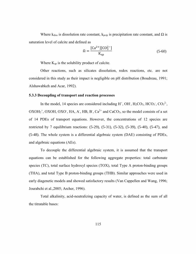
115
Where kdiss is dissolution rate constant, kpctp is precipitation rate constant, and Ω is
saturation level of calcite and defined as
Ω =[Ca2+][CO3
2−]
Ksp (5-60)
Where Ksp is the solubility product of calcite.
Other reactions, such as silicates dissolution, redox reactions, etc. are not
considered in this study as their impact is negligible on pH distribution (Boudreau, 1991;
Alshawabkeh and Acar, 1992).
5.3.3 Decoupling of transport and reaction processes
In the model, 14 species are considered including H+, OH-, H2CO3, HCO3-, CO3
2-,
OXOH2+, OXOH, OXO-, HA, A-, HB, B-, Ca2+ and CaCO3, so the model consists of a set
of 14 PDEs of transport equations. However, the concentrations of 12 species are
restricted by 7 equilibrium reactions: (5-29), (5-31), (5-32), (5-39), (5-40), (5-47), and
(5-48). The whole system is a differential algebraic system (DAE) consisting of PDEs,
and algebraic equations (AEs).
To decouple the differential algebraic system, it is assumed that the transport
equations can be established for the following aggregate properties: total carbonate
species (TC), total surface hydroxyl species (TOX), total Type A proton-binding groups
(THA), and total Type B proton-binding groups (THB). Similar approaches were used in
early diagenetic models and showed satisfactory results (Van Cappellen and Wang, 1996;
Jourabchi et al.,2005; Archer, 1996).
Total alkalinity, acid-neutralizing capacity of water, is defined as the sum of all
the titratable bases:
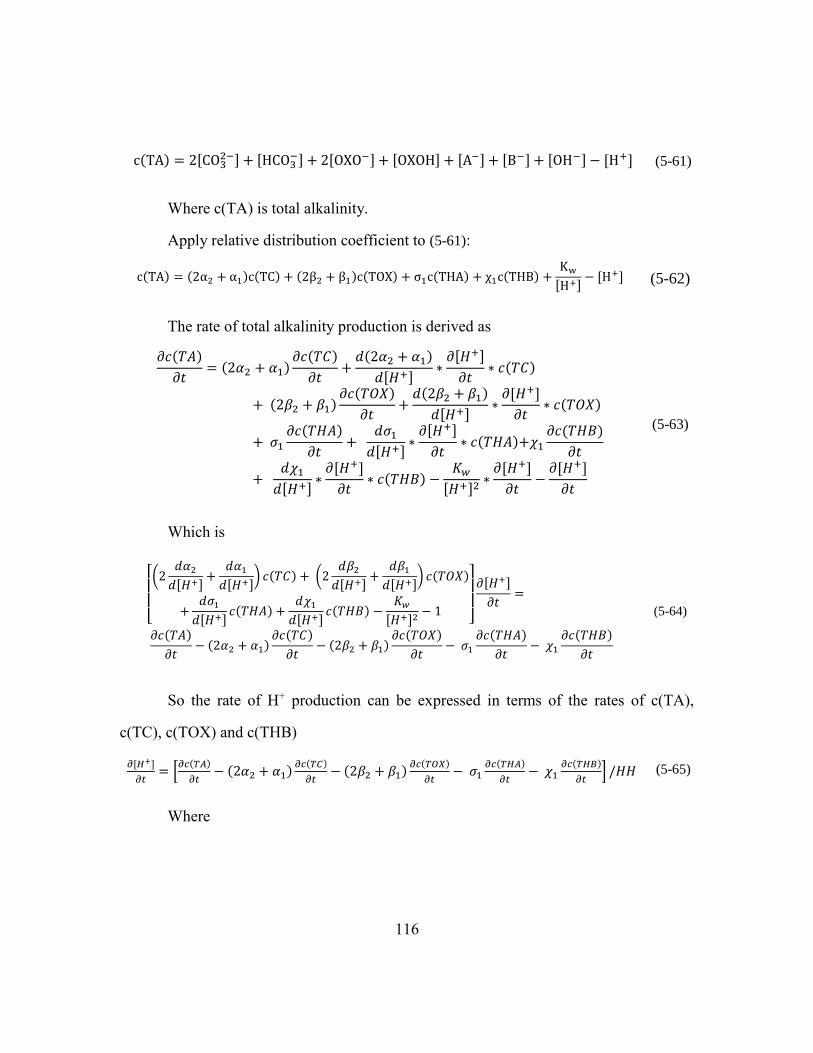
116
c(TA) = 2[CO32−] + [HCO3
−] + 2[OXO−] + [OXOH] + [A−] + [B−] + [OH−] − [H+] (5-61)
Where c(TA) is total alkalinity.
Apply relative distribution coefficient to (5-61):
c(TA) = (2α2 + α1)c(TC) + (2β2 + β1)c(TOX) + σ1c(THA) + χ1c(THB) +Kw
[H+]− [H+] (5-62)
The rate of total alkalinity production is derived as
𝜕𝑐(𝑇𝐴)
𝜕𝑡= (2𝛼2 + 𝛼1)
𝜕𝑐(𝑇𝐶)
𝜕𝑡+
𝑑(2𝛼2 + 𝛼1)
𝑑[𝐻+]∗
𝜕[𝐻+]
𝜕𝑡∗ 𝑐(𝑇𝐶)
+ (2𝛽2 + 𝛽1)𝜕𝑐(𝑇𝑂𝑋)
𝜕𝑡+
𝑑(2𝛽2 + 𝛽1)
𝑑[𝐻+]∗𝜕[𝐻+]
𝜕𝑡∗ 𝑐(𝑇𝑂𝑋)
+ 𝜎1
𝜕𝑐(𝑇𝐻𝐴)
𝜕𝑡+
𝑑𝜎1
𝑑[𝐻+]∗
𝜕[𝐻+]
𝜕𝑡∗ 𝑐(𝑇𝐻𝐴)+𝜒1
𝜕𝑐(𝑇𝐻𝐵)
𝜕𝑡
+ 𝑑𝜒1
𝑑[𝐻+]∗𝜕[𝐻+]
𝜕𝑡∗ 𝑐(𝑇𝐻𝐵) −
𝐾𝑤
[𝐻+]2∗𝜕[𝐻+]
𝜕𝑡−
𝜕[𝐻+]
𝜕𝑡
(5-63)
Which is
[ (2
𝑑𝛼2
𝑑[𝐻+]+
𝑑𝛼1
𝑑[𝐻+]) 𝑐(𝑇𝐶) + (2
𝑑𝛽2
𝑑[𝐻+]+
𝑑𝛽1
𝑑[𝐻+]) 𝑐(𝑇𝑂𝑋)
+𝑑𝜎1
𝑑[𝐻+]𝑐(𝑇𝐻𝐴) +
𝑑𝜒1
𝑑[𝐻+]𝑐(𝑇𝐻𝐵) −
𝐾𝑤
[𝐻+]2− 1
] 𝜕[𝐻+]
𝜕𝑡=
𝜕𝑐(𝑇𝐴)
𝜕𝑡− (2𝛼2 + 𝛼1)
𝜕𝑐(𝑇𝐶)
𝜕𝑡− (2𝛽2 + 𝛽1)
𝜕𝑐(𝑇𝑂𝑋)
𝜕𝑡− 𝜎1
𝜕𝑐(𝑇𝐻𝐴)
𝜕𝑡− 𝜒1
𝜕𝑐(𝑇𝐻𝐵)
𝜕𝑡
(5-64)
So the rate of H+ production can be expressed in terms of the rates of c(TA),
c(TC), c(TOX) and c(THB)
𝜕[𝐻+]
𝜕𝑡= [
𝜕𝑐(𝑇𝐴)
𝜕𝑡− (2𝛼2 + 𝛼1)
𝜕𝑐(𝑇𝐶)
𝜕𝑡− (2𝛽2 + 𝛽1)
𝜕𝑐(𝑇𝑂𝑋)
𝜕𝑡− 𝜎1
𝜕𝑐(𝑇𝐻𝐴)
𝜕𝑡− 𝜒1
𝜕𝑐(𝑇𝐻𝐵)
𝜕𝑡] /𝐻𝐻 (5-65)
Where
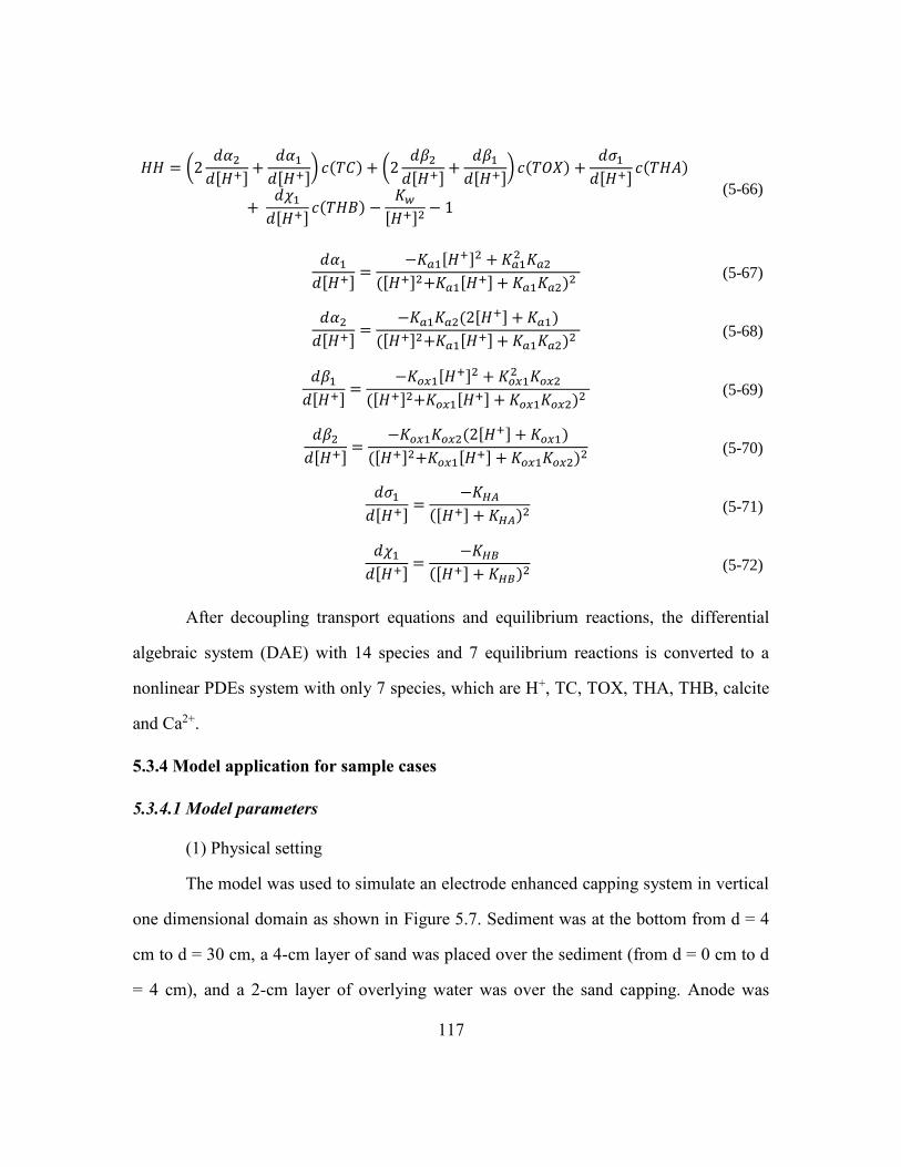
117
𝐻𝐻 = (2𝑑𝛼2
𝑑[𝐻+]+
𝑑𝛼1
𝑑[𝐻+]) 𝑐(𝑇𝐶) + (2
𝑑𝛽2
𝑑[𝐻+]+
𝑑𝛽1
𝑑[𝐻+]) 𝑐(𝑇𝑂𝑋) +
𝑑𝜎1
𝑑[𝐻+]𝑐(𝑇𝐻𝐴)
+ 𝑑𝜒1
𝑑[𝐻+]𝑐(𝑇𝐻𝐵) −
𝐾𝑤
[𝐻+]2− 1
(5-66)
𝑑𝛼1
𝑑[𝐻+]=
−𝐾𝑎1[𝐻+]2 + 𝐾𝑎1
2 𝐾𝑎2
([𝐻+]2+𝐾𝑎1[𝐻+] + 𝐾𝑎1𝐾𝑎2)
2 (5-67)
𝑑𝛼2
𝑑[𝐻+]=
−𝐾𝑎1𝐾𝑎2(2[𝐻+] + 𝐾𝑎1)
([𝐻+]2+𝐾𝑎1[𝐻+] + 𝐾𝑎1𝐾𝑎2)
2 (5-68)
𝑑𝛽1
𝑑[𝐻+]=
−𝐾𝑜𝑥1[𝐻+]2 + 𝐾𝑜𝑥1
2 𝐾𝑜𝑥2
([𝐻+]2+𝐾𝑜𝑥1[𝐻+] + 𝐾𝑜𝑥1𝐾𝑜𝑥2)
2 (5-69)
𝑑𝛽2
𝑑[𝐻+]=
−𝐾𝑜𝑥1𝐾𝑜𝑥2(2[𝐻+] + 𝐾𝑜𝑥1)
([𝐻+]2+𝐾𝑜𝑥1[𝐻+] + 𝐾𝑜𝑥1𝐾𝑜𝑥2)
2 (5-70)
𝑑𝜎1
𝑑[𝐻+]=
−𝐾𝐻𝐴
([𝐻+] + 𝐾𝐻𝐴)2 (5-71)
𝑑𝜒1
𝑑[𝐻+]=
−𝐾𝐻𝐵
([𝐻+] + 𝐾𝐻𝐵)2 (5-72)
After decoupling transport equations and equilibrium reactions, the differential
algebraic system (DAE) with 14 species and 7 equilibrium reactions is converted to a
nonlinear PDEs system with only 7 species, which are H+, TC, TOX, THA, THB, calcite
and Ca2+.
5.3.4 Model application for sample cases
5.3.4.1 Model parameters
(1) Physical setting
The model was used to simulate an electrode enhanced capping system in vertical
one dimensional domain as shown in Figure 5.7. Sediment was at the bottom from d = 4
cm to d = 30 cm, a 4-cm layer of sand was placed over the sediment (from d = 0 cm to d
= 4 cm), and a 2-cm layer of overlying water was over the sand capping. Anode was

118
placed at the sand sediment interface (d = 4 cm) and cathode was placed at d = 0.5 cm in
the sand layer. The thickness of the electrode materials was taken into consideration in
the model, and it was assumed that both the anode and cathode have a thickness of 0.5
cm. The thickness of the electrodes materials defined the range of hydrogen source and
sink term RL in the governing equation (5-27) of H+ transport and reaction. So the
hydrogen source (anode reaction) located from d = 3.75 cm to d = 4.25 cm, and hydrogen
sink (cathode reaction) located from d = 0.25 cm to d = 0.75 cm.
It was assumed that sand and sediment have the same solid density of 2.5 kg/L
and porosity of 0.5.
Figure 5.7 Physical setting of an electrode enhanced capping system in vertical one
dimensional domain. d is the depth below the water sand interface.
(2) Electrochemical reactions
In section 4.3, the current for ElecCap2 is ~ 200 μA with an electrode area of ~ 25
cm2, so the current density is 8 μA/ cm2. The rate of H+ or OH- production with ~75%
-0.2 0 0.2 0.4 0.6 0.8 1
-2
0
2
4
6
8
10
12
d(cm)
Water
Sand
Sediment
cathode
anode
119
coulombic efficiency by (5-1) is 1.55*10-9 mol/s. It is assumed that the reactions occur
within 25cm2*0.5cm (Area*Thickness) porous medium as a triangular rate function
(Figure 5.8).
Figure 5.8 Triangular function of proton production rate by electrode reactions.
(3) Electrical potential Vep
Previous studies on modeling of transport and reactions processes by electrical
field showed that electrical potential gradient varied with time, but in general the
electrical potential profile could be approximated by a linear relationship between two
electrodes (Yu and Neretnieks, 1996). In this study, it was assumed that electrical
potential Vep was linear between the anode and the cathode. The difference of Vep
between two electrodes (i.e. ohmic loss) was estimated to be 0.2 V with an external
voltage of 2 V (Figure 5.3).
(4) Transport parameters
Effective diffusion coefficient Def for aqueous species was estimated from
molecular diffusion coefficient and tortuosity factor, and Def for solid species was assume
0 2 4 6 8-1
-0.5
0
0.5
1
Depth (cm)
H+ production by electrodes
Rate
/Rate
max
Cathode
Anode

120
to be 1*10-13 m2/s (Van Cappellen and Wang, 1996). There is no established method to
measure the effective ionic mobility of an ion in porous medium. Effective ionic mobility
uef of the ion was calibrated. Transport parameters for each simulated species in the
model are listed in Table 5.2.
Table 5.2 Transport parameters for each species in the model
Def [m2/s] uef [m
2*mol/(s*C*V)] Charge number z
H+ 7*10-9 1.88*10-13 +1
TC 1*10-9 4.03*10-13 -(α1+2α2)
Ca2+ 1*10-9 4.03*10-13 +2
Calcite 1*10-13 - -
TOX 1*10-13 - -
THA 1*10-13 - -
THB 1*10-13 - -
(5) Chemical reaction parameters
Chemical reaction parameters are listed in Table 5.3. The equilibrium reaction
constant of carbonate species is well studied and known, but those of surface hydroxyl
groups and humic substances have a relative large uncertainty. So the parameters of
surface hydroxyl groups and humic substances were obtained from literature or
calibrated. Kinetic parameter of calcite dissolution and precipitation were obtained from
literature. Due to the inhibiting effect of various ions on calcite growth, the onset of
precipitation usually requires Ω to be much greater than unity (Zeebe and Sanyal, 2002;
Zeebe, 2007). So calcite precipitation was not taken into account in the model.
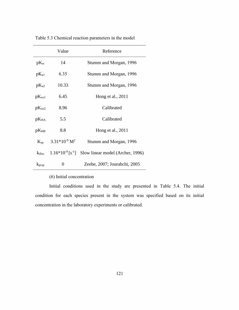
121
Table 5.3 Chemical reaction parameters in the model
Value Reference
pKw 14 Stumm and Morgan, 1996
pKa1 6.35 Stumm and Morgan, 1996
pKa2 10.33 Stumm and Morgan, 1996
pKox1 6.45 Hong et al., 2011
pKox2 8.96 Calibrated
pKHA 5.5 Calibrated
pKHB 8.8 Hong et al., 2011
Ksp 3.31*10-9 M2 Stumm and Morgan, 1996
kdiss 1.16*10-9 [s-1] Slow linear model (Archer, 1996)
kpctp 0 Zeebe, 2007; Jourabchi, 2005
(6) Initial concentration
Initial conditions used in the study are presented in Table 5.4. The initial
condition for each species present in the system was specified based on its initial
concentration in the laboratory experiments or calibrated.
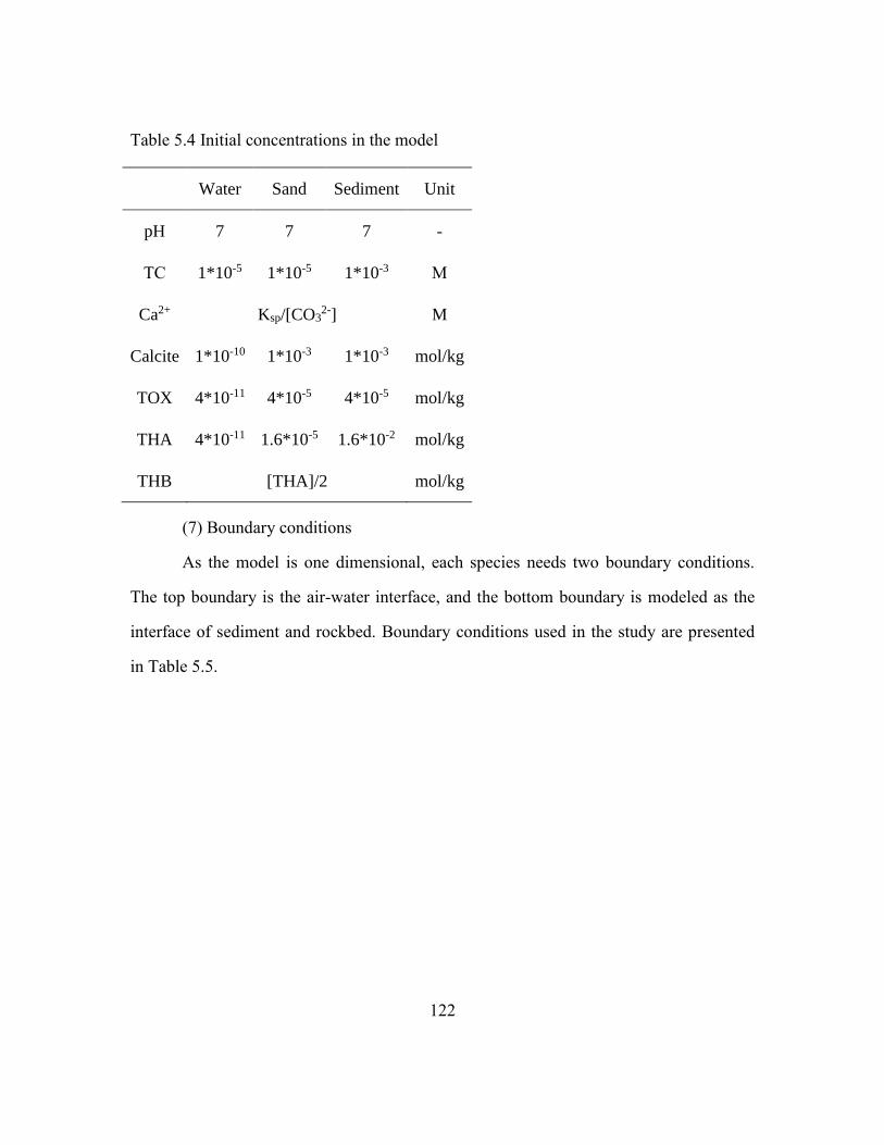
122
Table 5.4 Initial concentrations in the model
Water Sand Sediment Unit
pH 7 7 7 -
TC 1*10-5 1*10-5 1*10-3 M
Ca2+ Ksp/[CO32-] M
Calcite 1*10-10 1*10-3 1*10-3 mol/kg
TOX 4*10-11 4*10-5 4*10-5 mol/kg
THA 4*10-11 1.6*10-5 1.6*10-2 mol/kg
THB [THA]/2 mol/kg
(7) Boundary conditions
As the model is one dimensional, each species needs two boundary conditions.
The top boundary is the air-water interface, and the bottom boundary is modeled as the
interface of sediment and rockbed. Boundary conditions used in the study are presented
in Table 5.5.
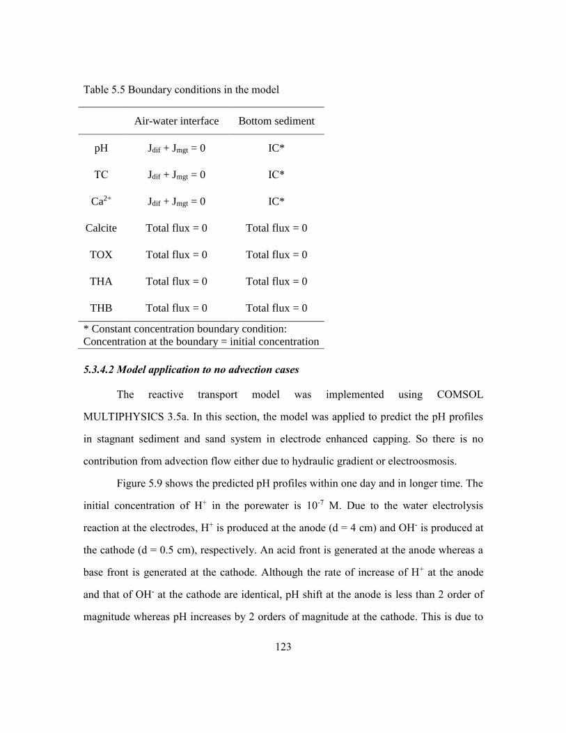
123
Table 5.5 Boundary conditions in the model
Air-water interface Bottom sediment
pH Jdif + Jmgt = 0 IC*
TC Jdif + Jmgt = 0 IC*
Ca2+ Jdif + Jmgt = 0 IC*
Calcite Total flux = 0 Total flux = 0
TOX Total flux = 0 Total flux = 0
THA Total flux = 0 Total flux = 0
THB Total flux = 0 Total flux = 0
* Constant concentration boundary condition:
Concentration at the boundary = initial concentration
5.3.4.2 Model application to no advection cases
The reactive transport model was implemented using COMSOL
MULTIPHYSICS 3.5a. In this section, the model was applied to predict the pH profiles
in stagnant sediment and sand system in electrode enhanced capping. So there is no
contribution from advection flow either due to hydraulic gradient or electroosmosis.
Figure 5.9 shows the predicted pH profiles within one day and in longer time. The
initial concentration of H+ in the porewater is 10-7 M. Due to the water electrolysis
reaction at the electrodes, H+ is produced at the anode (d = 4 cm) and OH- is produced at
the cathode (d = 0.5 cm), respectively. An acid front is generated at the anode whereas a
base front is generated at the cathode. Although the rate of increase of H+ at the anode
and that of OH- at the cathode are identical, pH shift at the anode is less than 2 order of
magnitude whereas pH increases by 2 orders of magnitude at the cathode. This is due to
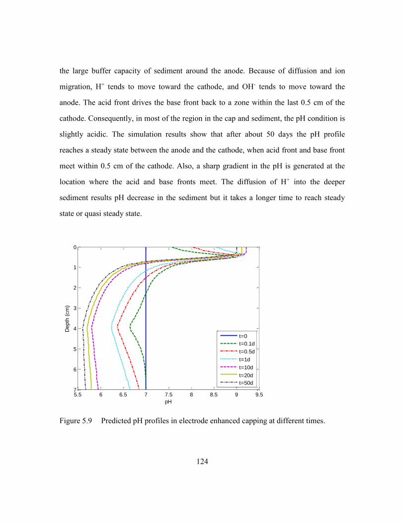
124
the large buffer capacity of sediment around the anode. Because of diffusion and ion
migration, H+ tends to move toward the cathode, and OH- tends to move toward the
anode. The acid front drives the base front back to a zone within the last 0.5 cm of the
cathode. Consequently, in most of the region in the cap and sediment, the pH condition is
slightly acidic. The simulation results show that after about 50 days the pH profile
reaches a steady state between the anode and the cathode, when acid front and base front
meet within 0.5 cm of the cathode. Also, a sharp gradient in the pH is generated at the
location where the acid and base fronts meet. The diffusion of H+ into the deeper
sediment results pH decrease in the sediment but it takes a longer time to reach steady
state or quasi steady state.
Figure 5.9 Predicted pH profiles in electrode enhanced capping at different times.
5.5 6 6.5 7 7.5 8 8.5 9 9.5
0
1
2
3
4
5
6
7
pH
Depth
(cm
)
t=0
t=0.1d
t=0.5d
t=1d
t=10d
t=20d
t=50d
125
Figure 5.10 shows the pH at different depths with time. At the cathode, pH
increase to 9 from 7 immediately after the application of power. Then pH at the cathode
decreases slowly due to influence of acid front. Similarly, pH at the anode (d = 4 cm) and
between two electrodes (d = 2 cm) decreases after the application of power. Compared
with the pH changes between two electrodes, pH outside this region changes relative
slowly. pH at the air-water interface increases to about 9.4 after 2-3 days and then
decreases slowly. pH in the deeper sediment (d= 7 cm) also has a slower response as
shown in Figure 5.10. This is because ion migration between the electrodes accelerates
the movement of H+ and other ions. However, diffusion is the only transport process
affecting ion transport outside this region.
Figure 5.10 Predicted pH profiles in electrode enhanced capping at different depths.
0 5 10 15 20 25 30 35 40 45 505.5
6
6.5
7
7.5
8
8.5
9
9.5
Time (Day)
pH
d=0 (air-water interface)
d=0.5cm (cathode)
d=2cm
d=4cm (anode)
d=7cm
126
In order to assess whether the developed model predicts pH profiles in an
electrode enhanced cap, the predictions of the model were compared with experimental
results from Chapter 4. Comparisons between the modeled and experimental pH profiles
at different times are depicted in Figure 5.11. A reasonable agreement between the
modeled and the experimental results is observed. In the deeper sediment below the
anode (d > 4 cm), the model predicted the pH profile accurately with a deviation of less
than 0.1. In the cathode region (d = 0 - 0.75 cm), the differences between the model and
experimental data were about 0.5, which are still satisfactory results. Furthermore, the
model also captured the pH decrease over time at the cathode, but with a larger rate than
that in experimental data. However, the greatest difference between the model and
experimental observations occurred in the region between the anode and cathode. The
model underestimated the pH profiles especially for the region closed to the cathode.
Both model and experimental results show a sharp gradient in pH profiles, but the
gradient in the model was sharper than that in the experimental result. The sharp pH
gradients have been observed in many electrokinetic experiments, and models were
developed to predict the pH behaviors in the system. Similarly, pH profiles predicted by
models tended to have a sharper gradient than pH observed in experiments (Shapiro and
Probstein, 1993; Haran et al., 1997; Yeung and Datla, 1995; Al-Hamdan and Reddy,
2008; Alshawabkeh and Acar, 1996; Yu and Neretnieks, 1996). Because of the complex
nature of sand and sediment, some reactions were not taken into account in the model,
e.g. some slow reactions of H+ and OH- with the surface of the sediment and sand. It is
very possible that the lack of slow reaction kinetics of H+ or OH- in the porous medium
gives rise to the inaccuracy of the model developed in this study and previous
electrokinetic models.

127
Figure 5.11 Predicted and experimental pH profiles in electrode enhanced capping at
different times.
5.2.4.2 Model application to advection cases
Many contaminated sediment sites are in shallow, near-shore areas that are
impacted by additional transport processes such as groundwater seepage and tidal driven
movement of the flow (Burnett et al., 2003; McCoy and Corbett, 2009). So advection due
to groundwater discharge and tidal movement is not uncommon and need to be addressed
for electrode enhanced capping.
Electroosmosis in a pore occurs due to the drag interaction between the bulk of
the liquid in the pore and a thin layer of charged fluid next to the pore wall, so liquid
moves under the action of the electric field in a direction parallel to it. The thin layer of
charged fluid, or electric double layer, has a typical thickness between 1 and 10 nm
(Probstein and Hicks, 1993). In the application of electrode enhanced capping, sand is
used as the capping material. Coarse sand is a very porous soil type and lacks capillary
5.5 6 6.5 7 7.5 8 8.5 9 9.5
0
1
2
3
4
5
6
7
pH
Depth
(cm
)
Exp(D21)
Exp(D28)
Exp(D33)
Exp(D43)
Model(D21)
Model(D28)
Model(D33)
Model(D43)
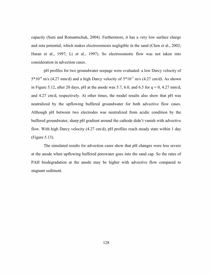
128
capacity (Suni and Romantschuk, 2004). Furthermore, it has a very low surface charge
and zeta potential, which makes electroosmosis negligible in the sand (Chen et al., 2002;
Haran et al., 1997; Li et al., 1997). So electroosmotic flow was not taken into
consideration in advection cases.
pH profiles for two groundwater seepage were evaluated: a low Darcy velocity of
5*10-8 m/s (4.27 mm/d) and a high Darcy velocity of 5*10-7 m/s (4.27 cm/d). As shown
in Figure 5.12, after 20 days, pH at the anode was 5.7, 6.0, and 6.5 for q = 0, 4.27 mm/d,
and 4.27 cm/d, respectively. At other times, the model results also show that pH was
neutralized by the upflowing buffered groundwater for both advective flow cases.
Although pH between two electrodes was neutralized from acidic condition by the
buffered groundwater, sharp pH gradient around the cathode didn’t vanish with advective
flow. With high Darcy velocity (4.27 cm/d), pH profiles reach steady state within 1 day
(Figure 5.13).
The simulated results for advection cases show that pH changes were less severe
at the anode when upflowing buffered porewater goes into the sand cap. So the rates of
PAH biodegradation at the anode may be higher with advective flow compared to
stagnant sediment.
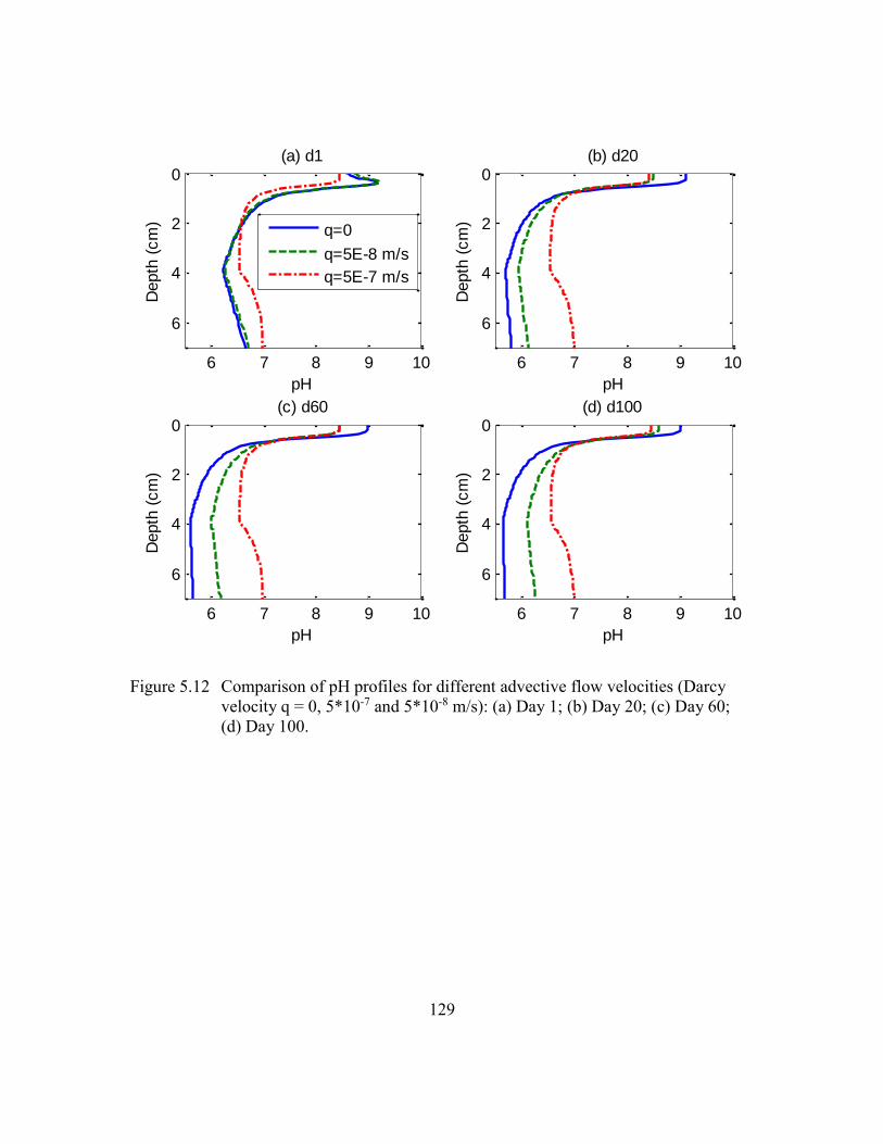
129
Figure 5.12 Comparison of pH profiles for different advective flow velocities (Darcy
velocity q = 0, 5*10-7 and 5*10-8 m/s): (a) Day 1; (b) Day 20; (c) Day 60;
(d) Day 100.
6 7 8 9 10
0
2
4
6
pH
Depth
(cm
)(a) d1
q=0
q=5E-8 m/s
q=5E-7 m/s
6 7 8 9 10
0
2
4
6
pH
Depth
(cm
)
(b) d20
6 7 8 9 10
0
2
4
6
pH
Depth
(cm
)
(c) d60
6 7 8 9 10
0
2
4
6
pH
Depth
(cm
)
(d) d100
130
Figure 5.13 Comparison of pH profiles at different times for advection and no advection
cases: (a) Darcy velocity q = 5*10-7 m/s; (b) Darcy velocity q = 5*10-8 m/s;
(c) Darcy velocity q = 0.
5.4 CONCLUSIONS
In this chapter, a voltage-current relationship of electrode enhanced capping was
developed and it incorporated several important parameters such as the thickness of
electrode enhanced capping and the area of the electrodes. The model was calibrated by
experimental dataset and empirical parameters were estimated by fitting the model to
experimental data. After calibration, current could be estimated through an implicit
voltage-current relationship. Voltage component analysis was performed to quantify the
6 7 8 9 10
0
2
4
6
pH
Depth
(cm
)(a) q=5E-7 m/s
6 7 8 9 10
0
2
4
6
pH
Depth
(cm
)
(b) q=5E-8 m/s
6 7 8 9 10
0
2
4
6
pH
Depth
(cm
)
(c) No advection
D1
D20
D40
D60
D80
D100
131
contribution of thermodynamic potential of water electrolysis, overpotentials at
electrodes, and ohmic loss. The model was applied in the design of electrode enhanced
capping, and the effect of capping thickness was investigated. Sensitivity of current with
respect to voltage changes was performed for different capping thickness.
A coupled reactive transport model was developed for multicomponent species
transport focusing on pH profiles under an electric field. In this study, transport processes
included: (1) advection due to the movement of groundwater under hydraulic gradient;
(2) advection due to electroosmosis; (3) diffusion due to concentration gradient and (4)
ion migration due to ionic movement of charged ions in response to an electric field.
Chemical reactions included water electrolysis at the electrodes, self-ionization of water,
equilibrium reactions of carbonate species, acid-base reactions with surface hydroxyl
groups on the surfaces of oxides and with proton-binding groups of humic substances,
and mineral precipitation and dissolution. The differential algebraic system (DAE) was
decoupled to a nonlinear PDEs system including seven species: H+, TC, TOX, THA,
THB, calcite and Ca2+.
The model successfully predicted the pH gradient in the application of electrode
enhanced capping, and the model predictions reasonably agreed with the experimental
results in no advection cases. pH changes under field condition with upflowing
groundwater seepage were simulated and the results shows that when buffered porewater
goes into cap from sediment, pH is neutralized at the anode.
The model can be a useful tool in the studies of transport and reaction processes
in a porous medium in an electric field and in the design of electrode enhanced capping.
132
Chapter 6: Conclusions and Recommendations
6.1 CONCLUSIONS
The purpose of this research was to develop a new active capping technology –
electrode enhanced capping to promote contaminant biodegradation for remediation of
contaminated sediment. Laboratory scale experiments were conducted in slurry reactors
and simulated sediment/cap reactors to evaluate the potential of this novel technology.
Also, mathematical models were developed to describe voltage-current characteristic and
the complex physical and chemical processes in electrode enhanced capping.
In Chapter 3, biodegradation of PAH under aerobic and nitrate reducing
conditions shows the ability of indigenous microorganisms in Anacostia River sediment
to degrade naphthalene and phenanthrene in several days or weeks. The proof of concept
experiment for electrode enhanced capping was conducted in complete mix slurry
reactors. An external potential of 3.5 V was applied to an anaerobic stirred slurry
contaminated with naphthalene and phenanthrene. During a period of 4 days, naphthalene
concentration decreased from ~1000 μg/L to ~50 μg/L, and phenanthrene was degraded
from ~150 μg/L to ~30 μg /L in ElectroBio reactor. The disappearance of naphthalene
was a result of both microbial degradation and electrochemical/chemical reactions, while
the phenanthrene loss appeared to be solely controlled by biotic processes. By comparing
with observations in aerobic and anaerobic control, it is concluded that ElectroBio reactor
could accelerate biodegradation rates from anaerobic condition, and achieve almost the
same rates as aerobic conditions. It is suggested that the presence of the electrodes was
able to maintain aerobic degradation processes despite the initial state of the slurry as
being anaerobic. qPCR analysis using PAH-RHDα Gram Negative primer shows notable
increases of PAH degrading genes in ElectroBio reactor and aerobic conditions, but no
increase in killed control and anaerobic conditions. The detection of catabolic gene
133
increase provided the microbial evidence of PAH biodegradation in ElectroBio reactor
and aerobic conditions.
In Chapter 4, the electrode approach was investigated in a more realistic and
complicated system - microcosm with mass transfer limitation. In the sediment (no
capping) microcosm study, two carbon cloth electrodes were placed horizontally in the
sediment with a separation distance of 2.5 cm. In two powered reactors, the ORP around
the anode was 50 – 150 mV higher than that in the control; pH around the anode dropped
to ~6 from an initial value of 6.4 or 6.7. Phenanthrene vertical profile displayed a unique
Z-shaped profile as the phenanthrene concentration at the anode decreased with time.
These results demonstrated that the anode placed in the sediment could effectively
decrease phenanthrene concentration, and create a more oxidized zone around the anode.
Microcosm experiments of sediment with electrode enhanced caps were conducted to
simulate a capping system. A carbon cloth anode was placed at the sediment cap
interface, and the cathode was placed 3.5 cm above the anode in the capping layer. In the
experiment with no bicarbonate buffer, ORP in the vicinity of the anode increased 60-100
mV compared to the control reactor, and pH decreased to 5.7 and 6 from circumneutral
pH. Average phenanthrene concentrations decreased to ~ 70% of initial concentration in
the 1 cm vicinity of the anode in 10 weeks whereas those in the control remained
relatively constant. In the experiment with bicarbonate buffer, only a small drop of pH
from 6.4 to 6 occurred due to the buffering capacity of bicarbonate. The increase in ORP
was not as great with less pH changes, implying the coupled phenomenon of pH and ORP
in the sediments under electrode enhanced capping. The reduction of phenanthrene
concentration in the 1 cm vicinity of sediment was ~50 %, an increase from ~30% in the
case of no bicarbonate buffer. Creating a biobarrier at the sediment cap interface,
electrode enhanced caps could effectively prevent migration of phenanthrene from the
134
underlying sediment to capping layer. The increase of PAH degrading gene compared
with control was detected at 0-0.5 cm sediment below the anode in the experiment with
and without bicarbonate buffer.
In Chapter 5, a voltage-current relationship of electrode enhanced capping was
established with the following form: V=E0+a+b*log10(I)+Rrstc*I. Parameters a, b and Rrstc
were estimated by fitting the model to experimental data. Current could be determined by
the above implicit voltage-current function. The model was applied in the design of
electrode enhanced capping, and the effect of capping thickness was investigated. A
coupled reactive transport model was built for multicomponent species transport focusing
on pH profiles for electrode enhanced capping. The model predictions and their
comparisons with the laboratory scale experimental results demonstrate that very sharp
changes in the pH profiles exist in electrode enhanced capping. The model was
implemented to simulate pH profile under field condition with upflowing groundwater
seepage, showing that pH is neutralized at the anode with buffered porewater.
In summary, a novel active capping technology – electrode enhanced capping was
proposed and tested in this study. The consistent results from slurry and microcosm
experiments demonstrated that electrode enhanced capping can be used to control redox
potential in a sediment cap, provide microbial electron acceptor, and stimulate PAH
degradation. The treatment demonstrated so far is one of the few successful active
capping technologies for the purpose of enhancing contaminant biodegradation. In
addition, this hybrid approach – coupling electrochemical process with bioremediation
was seldom used for soil and groundwater remediation. This work also bridged the gap
between electrochemical remediation and bioremediation in the field of soil and
groundwater remediation.
135
6.2 RECOMMENDATIONS FOR FUTURE WORK
6.2.1 Microbial community analysis
The ability to determine the number and types of microorganisms within a
community is fundamental to understanding the structure and function of an ecosystem.
In this study, the copy numbers of PAH degrading genes were quantified, and it
undoubtedly revealed the microbial activity of certain PAH degrading bacteria. However,
there are several limitations for this approach: 1) it doesn’t cover all the PAH degrading
bacteria; 2) it is very difficult to distinguish the contribution of each PAH degrading gene
that is amplified by the primer; 3) the shifts of microbial community in electrode
enhanced capping remains unknown. To address this issue, it is beneficial to conduct
exhaustive studies of bacterial community in order to determine the unique role that the
bacteria play in electrode enhanced capping. This will also help understand the changes
of distribution and diversity of bacteria, and ecosystem function with electrode enhanced
capping. Clone libraries and/or pyrosequencing can be two powerful tools to achieve this
goal.
6.2.2 Characterization of oxic zone at the anode
Oxygen produced at the anode created an oxic zone at the anode, which is
considered to be the most important factor to enhance PAH biodegradation. However,
several important parameters to characterize the oxic zone are still unknown. These
parameters include oxygen penetration depth, the levels of dissolved oxygen, oxygen
uptake rates by organic matter and other reduced species, oxygen fluxes at the anode, etc.
There currently exist several techniques that can be utilized for oxygen measurement, but
technical difficulties have limited their usefulness in this particular application. Under the
current microcosm setup, monitoring oxygen levels in-situ, in real time, remains a
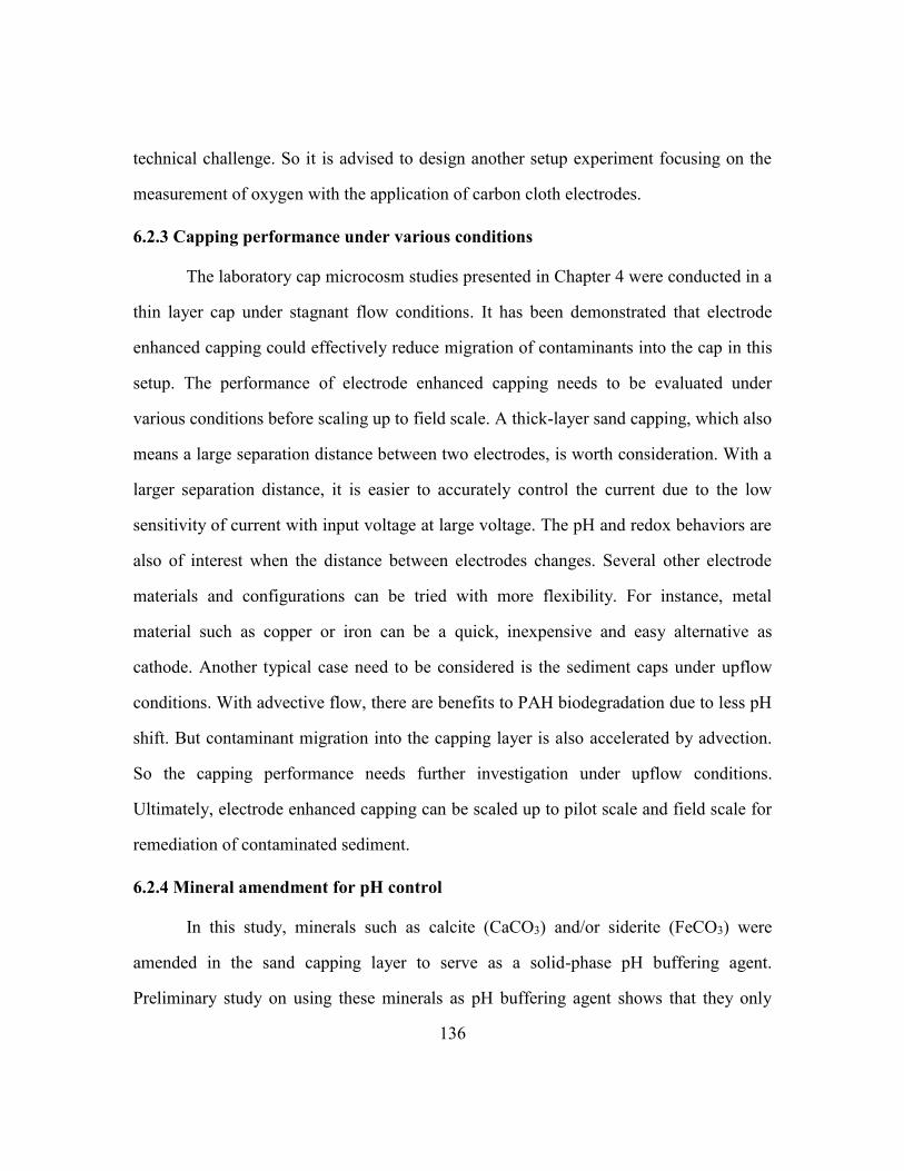
136
technical challenge. So it is advised to design another setup experiment focusing on the
measurement of oxygen with the application of carbon cloth electrodes.
6.2.3 Capping performance under various conditions
The laboratory cap microcosm studies presented in Chapter 4 were conducted in a
thin layer cap under stagnant flow conditions. It has been demonstrated that electrode
enhanced capping could effectively reduce migration of contaminants into the cap in this
setup. The performance of electrode enhanced capping needs to be evaluated under
various conditions before scaling up to field scale. A thick-layer sand capping, which also
means a large separation distance between two electrodes, is worth consideration. With a
larger separation distance, it is easier to accurately control the current due to the low
sensitivity of current with input voltage at large voltage. The pH and redox behaviors are
also of interest when the distance between electrodes changes. Several other electrode
materials and configurations can be tried with more flexibility. For instance, metal
material such as copper or iron can be a quick, inexpensive and easy alternative as
cathode. Another typical case need to be considered is the sediment caps under upflow
conditions. With advective flow, there are benefits to PAH biodegradation due to less pH
shift. But contaminant migration into the capping layer is also accelerated by advection.
So the capping performance needs further investigation under upflow conditions.
Ultimately, electrode enhanced capping can be scaled up to pilot scale and field scale for
remediation of contaminated sediment.
6.2.4 Mineral amendment for pH control
In this study, minerals such as calcite (CaCO3) and/or siderite (FeCO3) were
amended in the sand capping layer to serve as a solid-phase pH buffering agent.
Preliminary study on using these minerals as pH buffering agent shows that they only

137
have very limited buffering capacity at least in short term. A possible explanation for the
poor level of pH control using the mineral buffer is the slow kinetics of dissolution in
stagnant sediment/cap. Mineral dissolution can be surface-controlled if the adsorption of
reactant to the mineral surface is rate-limiting or transport-controlled if detached species
is transported from the surface and into the bulk solution most slowly (Furrer and Stumm,
1986). Some other geochemical reactions may also prevent or slow mineral dissolution.
Many metal oxides and oxyhydroxides, including iron oxides (i.e., ferrihydrite, goethite,
and hematite) may form in the environment as surface coatings (Nachtegaal and Sparks,
2004; Penn et al., 2001). Organic coatings may interfere with dissolution by changing the
surface characteristics, forming inner-sphere complexes, modifying the electrical
properties of the kaolinite−water interface and by masking the mineral surface from
reactant adsorption (Nachtegaal and Sparks, 2003). The mechanism why these minerals
failed to buffer pH remained unknown at this stage and the methods to improve the
dissolution kinetics needs further investigations.
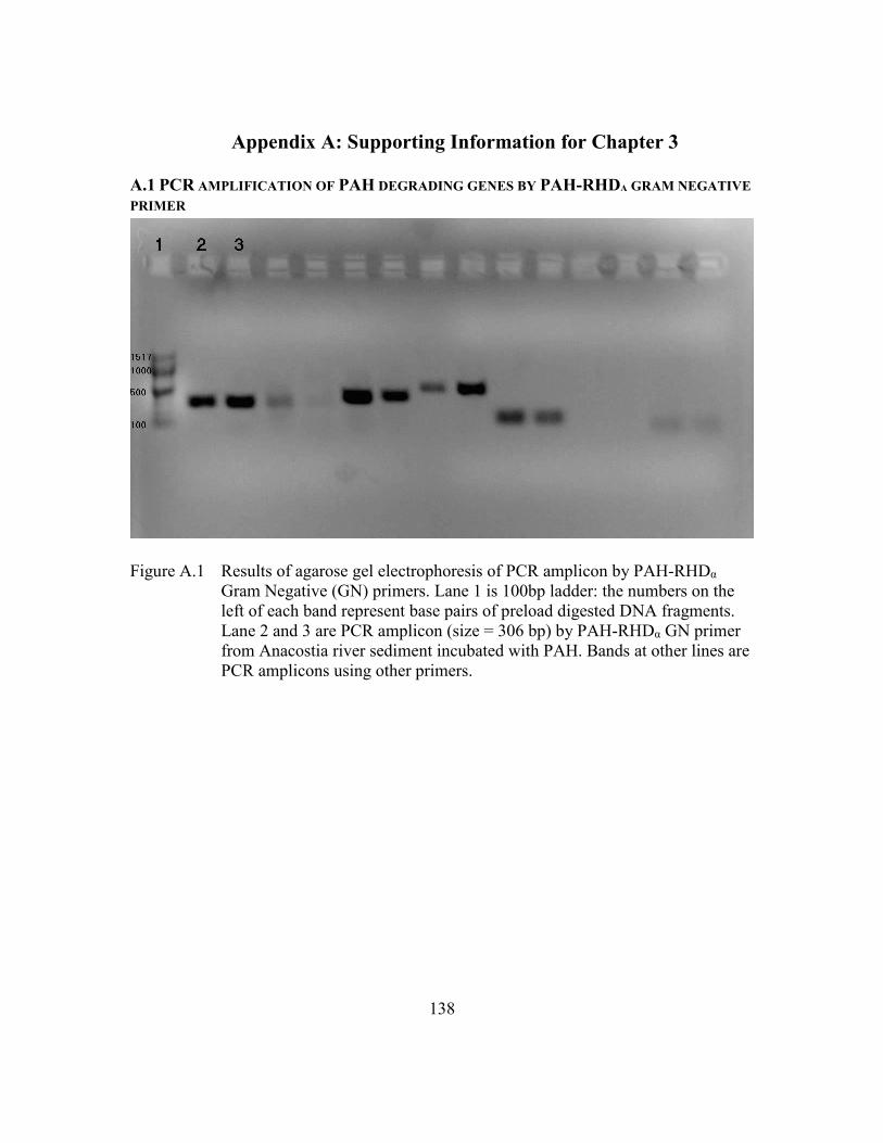
138
Appendix A: Supporting Information for Chapter 3
A.1 PCR AMPLIFICATION OF PAH DEGRADING GENES BY PAH-RHDΑ GRAM NEGATIVE
PRIMER
Figure A.1 Results of agarose gel electrophoresis of PCR amplicon by PAH-RHDα
Gram Negative (GN) primers. Lane 1 is 100bp ladder: the numbers on the
left of each band represent base pairs of preload digested DNA fragments.
Lane 2 and 3 are PCR amplicon (size = 306 bp) by PAH-RHDα GN primer
from Anacostia river sediment incubated with PAH. Bands at other lines are
PCR amplicons using other primers.
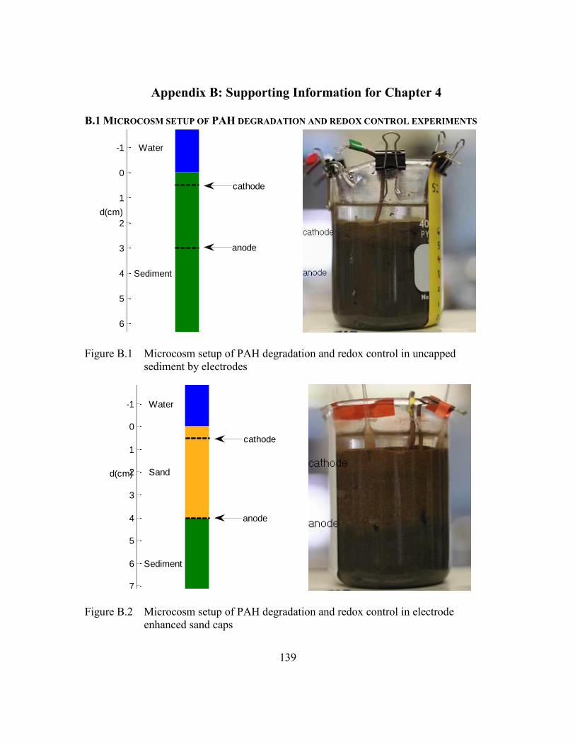
139
Appendix B: Supporting Information for Chapter 4
B.1 MICROCOSM SETUP OF PAH DEGRADATION AND REDOX CONTROL EXPERIMENTS
Figure B.1 Microcosm setup of PAH degradation and redox control in uncapped
sediment by electrodes
Figure B.2 Microcosm setup of PAH degradation and redox control in electrode
enhanced sand caps
-0.2 0 0.2 0.4 0.6 0.8 1
-3
-2
-1
0
1
2
3
4
5
6
d(cm)
Water
Sediment
cathode
anode
-0.2 0 0.2 0.4 0.6 0.8 1
-3
-2
-1
0
1
2
3
4
5
6
7
d(cm)
Water
Sand
Sediment
cathode
anode
140
Figure B.3 Microcosm setup of PAH degradation and redox control in electrode
enhanced caps with bicarbonate amendment
Figure B.4 T-shaped microcosm dimensions
-0.2 0 0.2 0.4 0.6 0.8 1
-3
-2
-1
0
1
2
3
4
5
6
7
d(cm)
Water
Sand
Sediment
cathode
anode
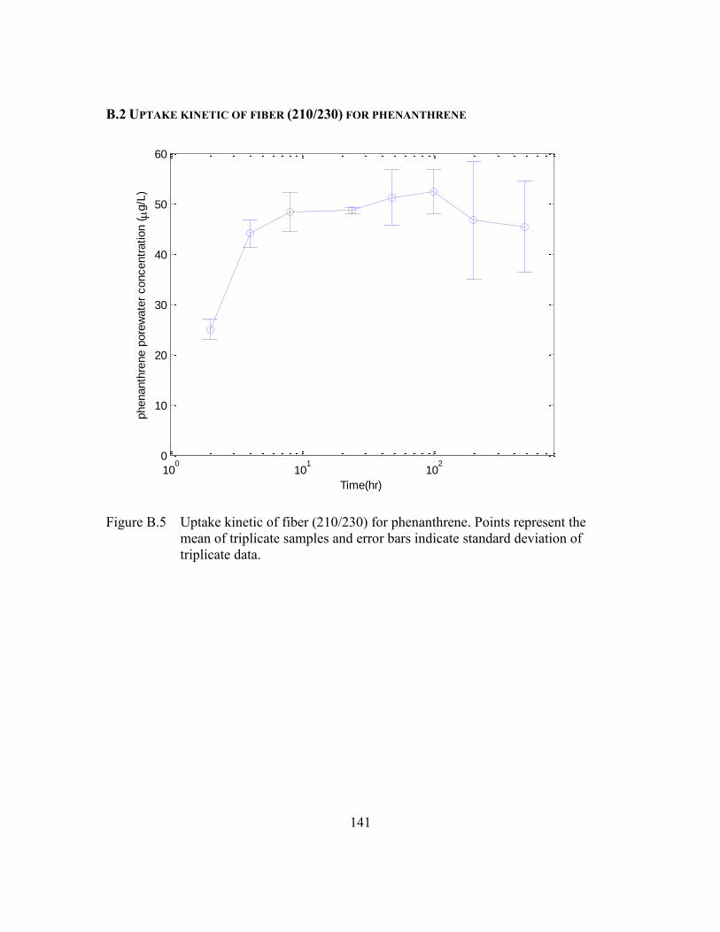
141
B.2 UPTAKE KINETIC OF FIBER (210/230) FOR PHENANTHRENE
Figure B.5 Uptake kinetic of fiber (210/230) for phenanthrene. Points represent the
mean of triplicate samples and error bars indicate standard deviation of
triplicate data.
100
101
102
0
10
20
30
40
50
60
Time(hr)
phenanth
rene p
ore
wate
r concentr
ation (
g/L
)
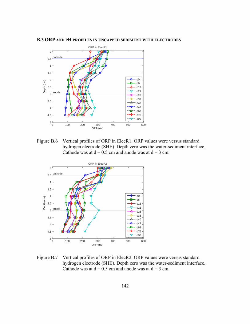
142
B.3 ORP AND PH PROFILES IN UNCAPPED SEDIMENT WITH ELECTRODES
Figure B.6 Vertical profiles of ORP in ElecR1. ORP values were versus standard
hydrogen electrode (SHE). Depth zero was the water-sediment interface.
Cathode was at d = 0.5 cm and anode was at d = 3 cm.
Figure B.7 Vertical profiles of ORP in ElecR2. ORP values were versus standard
hydrogen electrode (SHE). Depth zero was the water-sediment interface.
Cathode was at d = 0.5 cm and anode was at d = 3 cm.
0 100 200 300 400 500 600
0
0.5
1
1.5
2
2.5
3
3.5
4
4.5
5
ORP in ElecR1
ORP(mV)
Depth
(cm
)
cathode
anode
d0
d6
d13
d21
d26
d33
d40
d47
d68
d76
d90
0 100 200 300 400 500 600
0
0.5
1
1.5
2
2.5
3
3.5
4
4.5
5
ORP in ElecR2
ORP(mV)
Depth
(cm
)
cathode
anode
d0
d6
d13
d21
d26
d33
d40
d47
d68
d76
d90
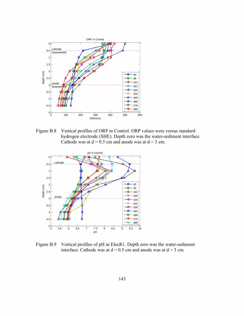
143
Figure B.8 Vertical profiles of ORP in Control. ORP values were versus standard
hydrogen electrode (SHE). Depth zero was the water-sediment interface.
Cathode was at d = 0.5 cm and anode was at d = 3 cm.
Figure B.9 Vertical profiles of pH in ElecR1. Depth zero was the water-sediment
interface. Cathode was at d = 0.5 cm and anode was at d = 3 cm.
0 100 200 300 400 500 600
0
0.5
1
1.5
2
2.5
3
3.5
4
4.5
5
ORP in Control
ORP(mV)
Depth
(cm
)
cathode
(unpowered)
anode
(unpowered)
d0
d6
d13
d21
d26
d33
d40
d68
d76
d90
5 5.5 6 6.5 7 7.5 8 8.5 9 9.5 10
0
0.5
1
1.5
2
2.5
3
3.5
4
4.5
5
pH in ElecR1
pH
Depth
(cm
)
cathode
anode
d0
d5
d10
d20
d25
d32
d39
d62
d68
d75
d89
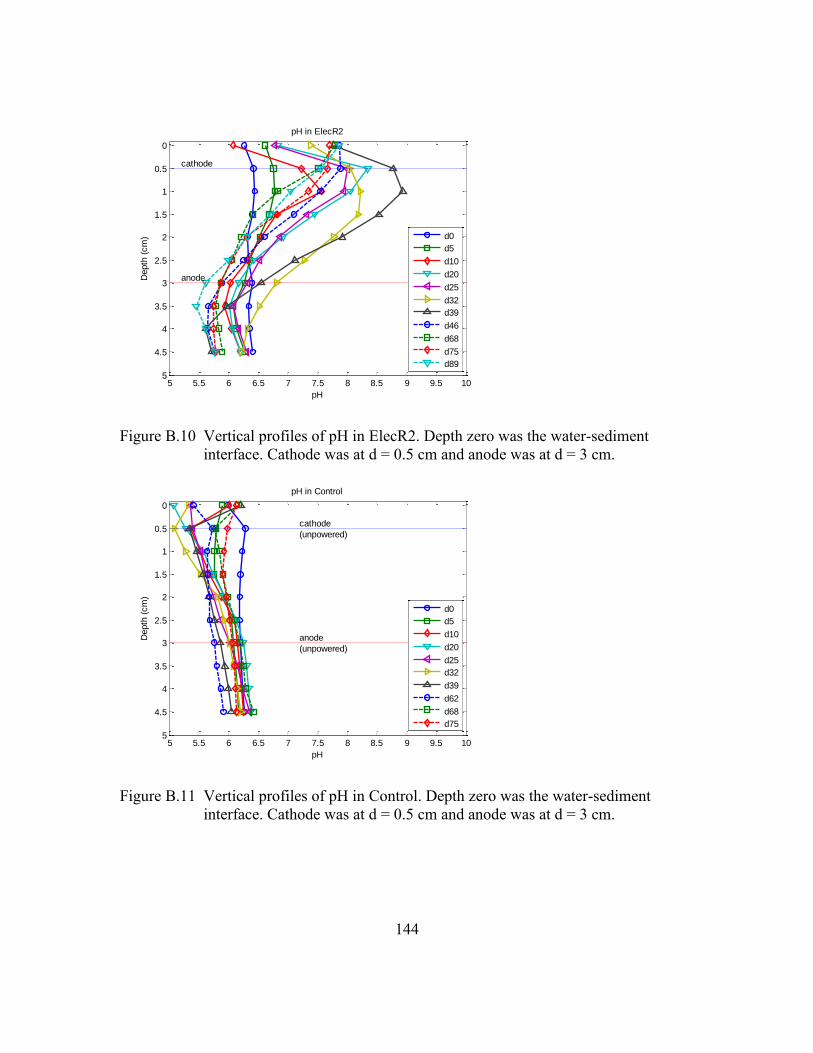
144
Figure B.10 Vertical profiles of pH in ElecR2. Depth zero was the water-sediment
interface. Cathode was at d = 0.5 cm and anode was at d = 3 cm.
Figure B.11 Vertical profiles of pH in Control. Depth zero was the water-sediment
interface. Cathode was at d = 0.5 cm and anode was at d = 3 cm.
5 5.5 6 6.5 7 7.5 8 8.5 9 9.5 10
0
0.5
1
1.5
2
2.5
3
3.5
4
4.5
5
pH in ElecR2
pH
Depth
(cm
)
cathode
anode
d0
d5
d10
d20
d25
d32
d39
d46
d68
d75
d89
5 5.5 6 6.5 7 7.5 8 8.5 9 9.5 10
0
0.5
1
1.5
2
2.5
3
3.5
4
4.5
5
pH in Control
pH
Depth
(cm
)
cathode
(unpowered)
anode
(unpowered)
d0
d5
d10
d20
d25
d32
d39
d62
d68
d75
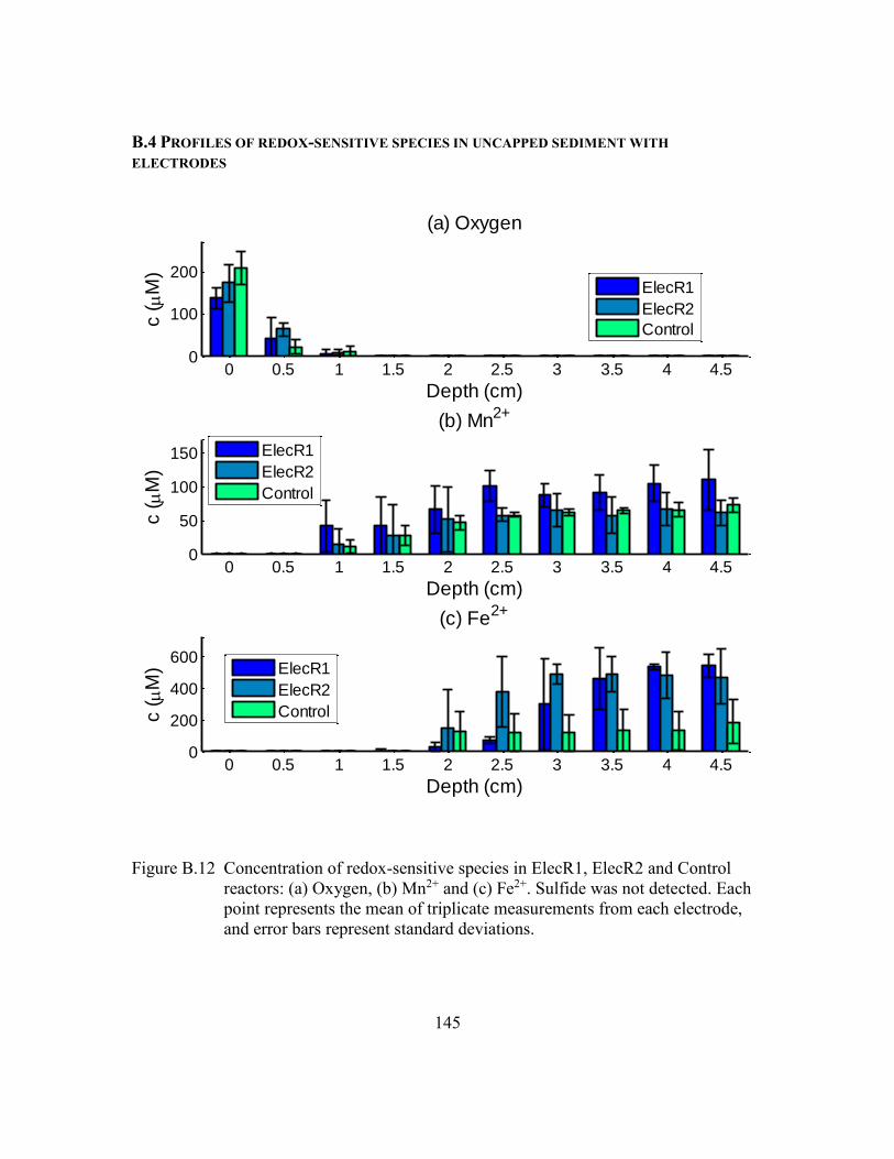
145
B.4 PROFILES OF REDOX-SENSITIVE SPECIES IN UNCAPPED SEDIMENT WITH
ELECTRODES
Figure B.12 Concentration of redox-sensitive species in ElecR1, ElecR2 and Control
reactors: (a) Oxygen, (b) Mn2+ and (c) Fe2+. Sulfide was not detected. Each
point represents the mean of triplicate measurements from each electrode,
and error bars represent standard deviations.
0 0.5 1 1.5 2 2.5 3 3.5 4 4.50
100
200
(a) Oxygen
Depth (cm)
c (M
)
ElecR1
ElecR2
Control
0 0.5 1 1.5 2 2.5 3 3.5 4 4.50
50
100
150
(b) Mn2+
Depth (cm)
c (M
)
ElecR1
ElecR2
Control
0 0.5 1 1.5 2 2.5 3 3.5 4 4.50
200
400
600
(c) Fe2+
Depth (cm)
c (M
)
ElecR1
ElecR2
Control
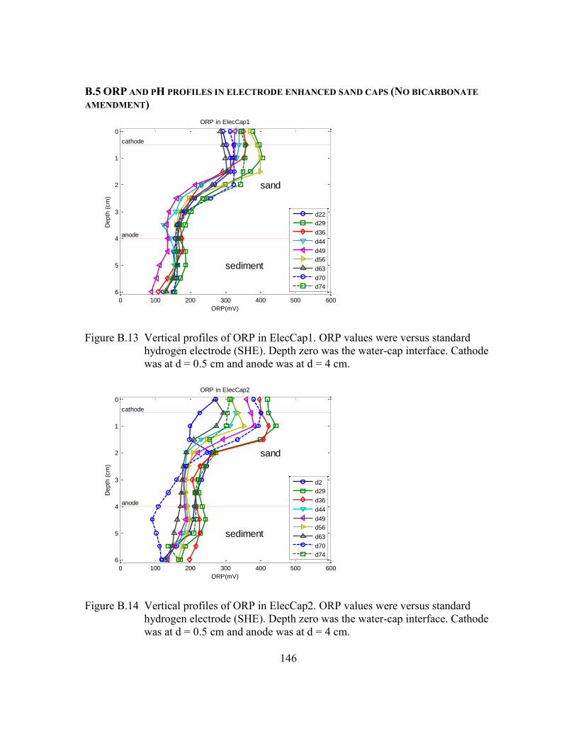
146
B.5 ORP AND PH PROFILES IN ELECTRODE ENHANCED SAND CAPS (NO BICARBONATE
AMENDMENT)
Figure B.13 Vertical profiles of ORP in ElecCap1. ORP values were versus standard
hydrogen electrode (SHE). Depth zero was the water-cap interface. Cathode
was at d = 0.5 cm and anode was at d = 4 cm.
Figure B.14 Vertical profiles of ORP in ElecCap2. ORP values were versus standard
hydrogen electrode (SHE). Depth zero was the water-cap interface. Cathode
was at d = 0.5 cm and anode was at d = 4 cm.
0 100 200 300 400 500 600
0
1
2
3
4
5
6
ORP in ElecCap1
ORP(mV)
Depth
(cm
)
cathode
anode
sand
sediment
d22
d29
d36
d44
d49
d56
d63
d70
d74
0 100 200 300 400 500 600
0
1
2
3
4
5
6
ORP in ElecCap2
ORP(mV)
Depth
(cm
)
cathode
anode
sand
sediment
d2
d29
d36
d44
d49
d56
d63
d70
d74
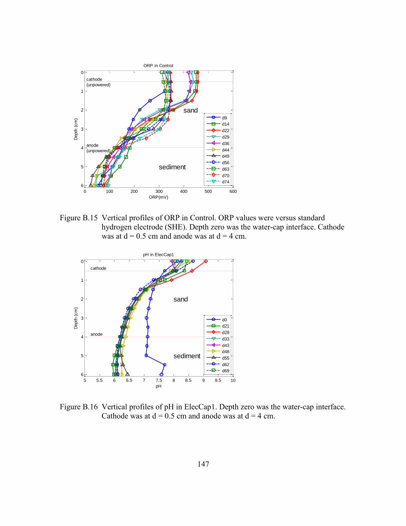
147
Figure B.15 Vertical profiles of ORP in Control. ORP values were versus standard
hydrogen electrode (SHE). Depth zero was the water-cap interface. Cathode
was at d = 0.5 cm and anode was at d = 4 cm.
Figure B.16 Vertical profiles of pH in ElecCap1. Depth zero was the water-cap interface.
Cathode was at d = 0.5 cm and anode was at d = 4 cm.
0 100 200 300 400 500 600
0
1
2
3
4
5
6
ORP in Control
ORP(mV)
Depth
(cm
)
cathode
(unpowered)
anode
(unpowered)
sand
sediment
d9
d14
d22
d29
d36
d44
d49
d56
d63
d70
d74
5 5.5 6 6.5 7 7.5 8 8.5 9 9.5 10
0
1
2
3
4
5
6
pH in ElecCap1
pH
Depth
(cm
)
cathode
anode
sand
sediment
d0
d21
d28
d33
d43
d48
d55
d62
d69
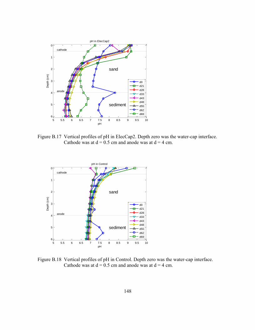
148
Figure B.17 Vertical profiles of pH in ElecCap2. Depth zero was the water-cap interface.
Cathode was at d = 0.5 cm and anode was at d = 4 cm.
Figure B.18 Vertical profiles of pH in Control. Depth zero was the water-cap interface.
Cathode was at d = 0.5 cm and anode was at d = 4 cm.
5 5.5 6 6.5 7 7.5 8 8.5 9 9.5 10
0
1
2
3
4
5
6
pH in ElecCap2
pH
Depth
(cm
)
cathode
anode
sand
sediment
d0
d21
d28
d33
d43
d48
d55
d62
d69
5 5.5 6 6.5 7 7.5 8 8.5 9 9.5 10
0
1
2
3
4
5
6
pH in Control
pH
Depth
(cm
)
cathode
anode
sand
sediment
d0
d21
d28
d33
d43
d48
d55
d62
d69

149
B.6 PROFILES OF REDOX-SENSITIVE SPECIES IN IN ELECTRODE ENHANCED SAND CAPS
(NO BICARBONATE AMENDMENT)
Figure B.19 Concentration of redox-sensitive species in ElecCap1, ElecCap2 and
Control reactors: (a) Oxygen, (b) Mn2+ and (c) Fe2+. Sulfide was not
detected. Each point represents the mean of triplicate measurements from
each electrode, and error bars represent standard deviations.
0 0.5 1 1.5 2 2.5 3 3.5 4 4.5 0 0.5 10
100
200
300
(a) Oxygen
Depth (cm)
c (M
)
ElecCap1
ElecCap2
Control
0 0.5 1 1.5 2 2.5 3 3.5 4 4.5 0 0.5 10
20
40
60
80
(b) Mn2+
Depth (cm)
c (M
)
ElecCap1
ElecCap2
Control
0 0.5 1 1.5 2 2.5 3 3.5 4 4.5 0 0.5 10
200
400
600
(c) Fe2+
Depth (cm)
c (M
)
ElecCap1
ElecCap2
Control
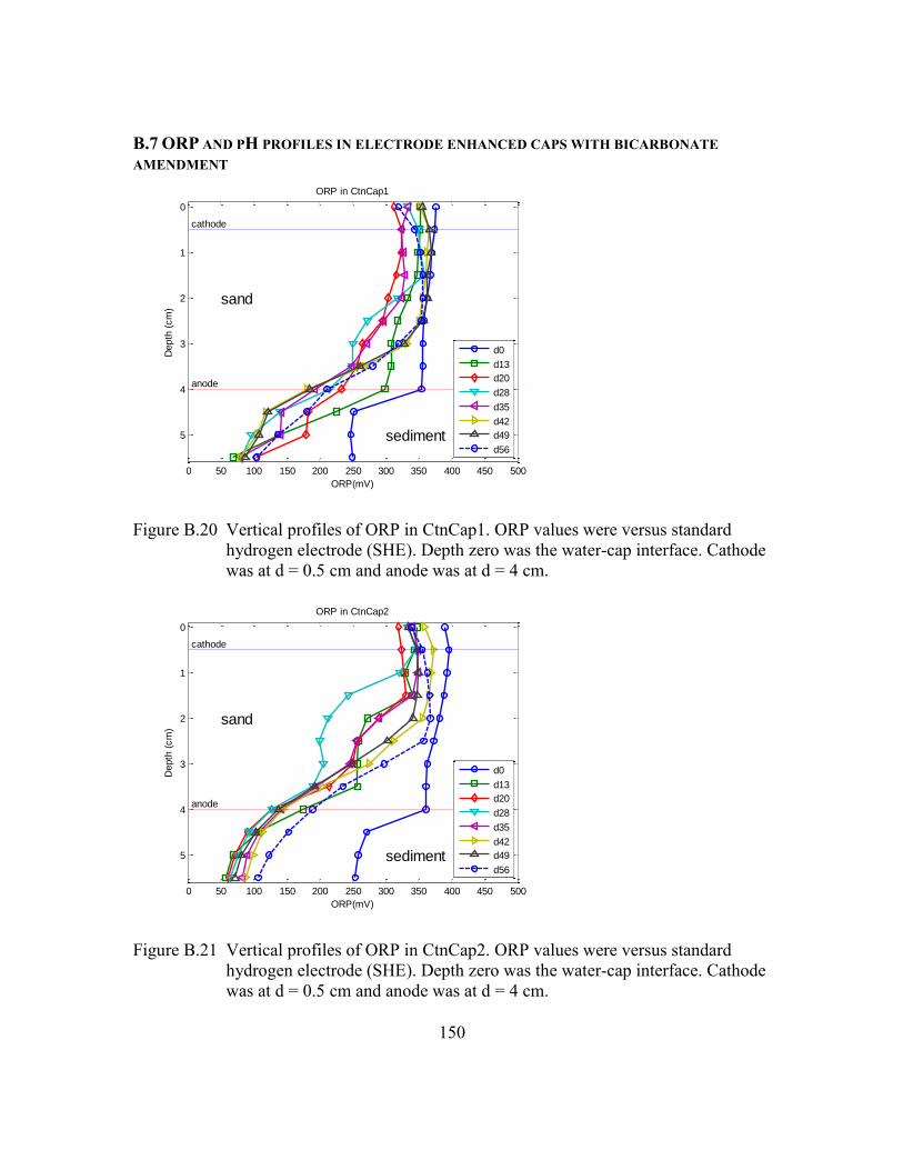
150
B.7 ORP AND PH PROFILES IN ELECTRODE ENHANCED CAPS WITH BICARBONATE
AMENDMENT
Figure B.20 Vertical profiles of ORP in CtnCap1. ORP values were versus standard
hydrogen electrode (SHE). Depth zero was the water-cap interface. Cathode
was at d = 0.5 cm and anode was at d = 4 cm.
Figure B.21 Vertical profiles of ORP in CtnCap2. ORP values were versus standard
hydrogen electrode (SHE). Depth zero was the water-cap interface. Cathode
was at d = 0.5 cm and anode was at d = 4 cm.
0 50 100 150 200 250 300 350 400 450 500
0
1
2
3
4
5
ORP in CtnCap1
ORP(mV)
Depth
(cm
)
cathode
anode
sand
sediment
d0
d13
d20
d28
d35
d42
d49
d56
0 50 100 150 200 250 300 350 400 450 500
0
1
2
3
4
5
ORP in CtnCap2
ORP(mV)
Depth
(cm
)
cathode
anode
sand
sediment
d0
d13
d20
d28
d35
d42
d49
d56
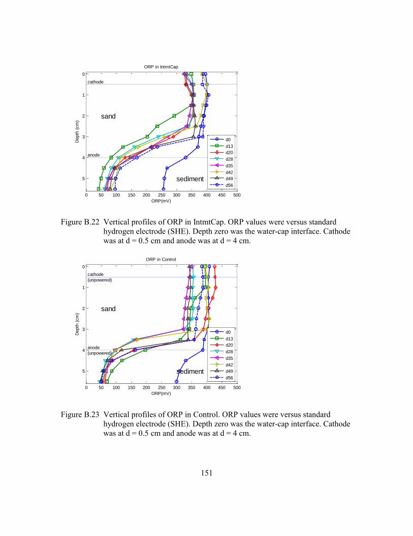
151
Figure B.22 Vertical profiles of ORP in IntmtCap. ORP values were versus standard
hydrogen electrode (SHE). Depth zero was the water-cap interface. Cathode
was at d = 0.5 cm and anode was at d = 4 cm.
Figure B.23 Vertical profiles of ORP in Control. ORP values were versus standard
hydrogen electrode (SHE). Depth zero was the water-cap interface. Cathode
was at d = 0.5 cm and anode was at d = 4 cm.
0 50 100 150 200 250 300 350 400 450 500
0
1
2
3
4
5
ORP in IntmtCap
ORP(mV)
Depth
(cm
)
cathode
anode
sand
sediment
d0
d13
d20
d28
d35
d42
d49
d56
0 50 100 150 200 250 300 350 400 450 500
0
1
2
3
4
5
ORP in Control
ORP(mV)
Depth
(cm
)
cathode
(unpowered)
anode
(unpowered)
sand
sediment
d0
d13
d20
d28
d35
d42
d49
d56

152
Figure B.24 Vertical profiles of pH in CtnCap1. Depth zero was the water-cap interface.
Cathode was at d = 0.5 cm and anode was at d = 4 cm.
Figure B.25 Vertical profiles of pH in CtnCap2. Depth zero was the water-cap interface.
Cathode was at d = 0.5 cm and anode was at d = 4 cm.
5 5.5 6 6.5 7 7.5 8 8.5 9 9.5 10
0
1
2
3
4
5
pH in CtnCap1
pH
Depth
(cm
)
cathode
anode
sand
sediment
d0
d6
d13
d20
d27
d34
d35
d41
d48
d55
d60
d69
5 5.5 6 6.5 7 7.5 8 8.5 9 9.5 10
0
1
2
3
4
5
pH in CtnCap2
pH
Depth
(cm
)
cathode
anode
sand
sediment
d0
d6
d13
d20
d27
d34
d35
d41
d48
d55
d60
d69
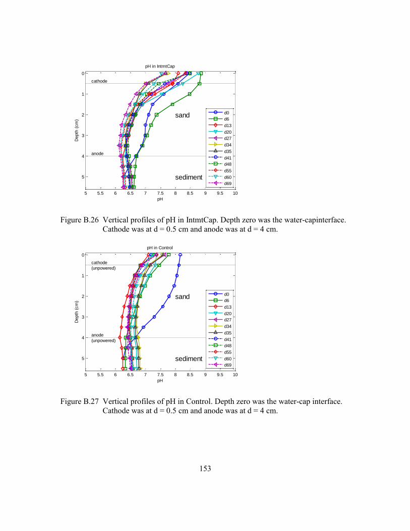
153
Figure B.26 Vertical profiles of pH in IntmtCap. Depth zero was the water-capinterface.
Cathode was at d = 0.5 cm and anode was at d = 4 cm.
Figure B.27 Vertical profiles of pH in Control. Depth zero was the water-cap interface.
Cathode was at d = 0.5 cm and anode was at d = 4 cm.
5 5.5 6 6.5 7 7.5 8 8.5 9 9.5 10
0
1
2
3
4
5
pH in IntmtCap
pH
Depth
(cm
)
cathode
anode
sand
sediment
d0
d6
d13
d20
d27
d34
d35
d41
d48
d55
d60
d69
5 5.5 6 6.5 7 7.5 8 8.5 9 9.5 10
0
1
2
3
4
5
pH in Control
pH
Depth
(cm
)
cathode
(unpowered)
anode
(unpowered)
sand
sediment
d0
d6
d13
d20
d27
d34
d35
d41
d48
d55
d60
d69
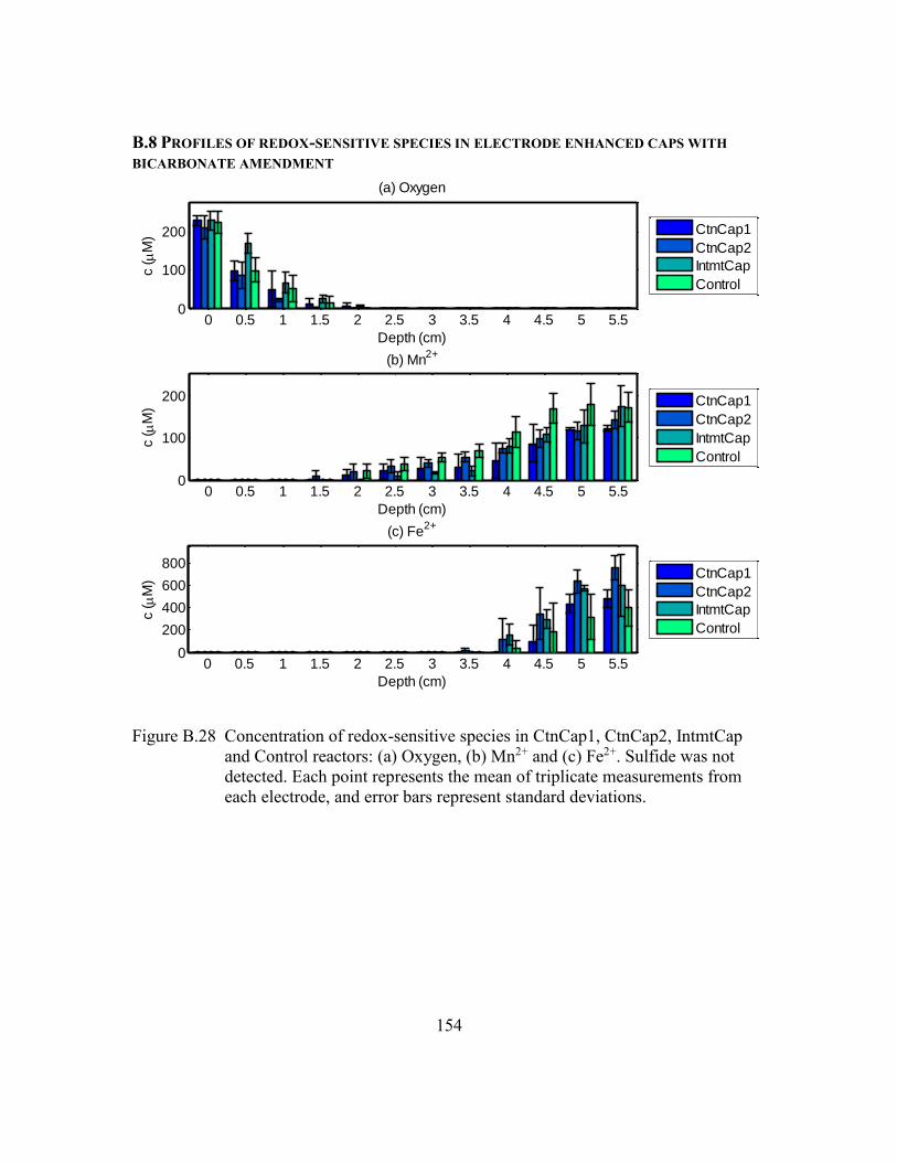
154
B.8 PROFILES OF REDOX-SENSITIVE SPECIES IN ELECTRODE ENHANCED CAPS WITH
BICARBONATE AMENDMENT
Figure B.28 Concentration of redox-sensitive species in CtnCap1, CtnCap2, IntmtCap
and Control reactors: (a) Oxygen, (b) Mn2+ and (c) Fe2+. Sulfide was not
detected. Each point represents the mean of triplicate measurements from
each electrode, and error bars represent standard deviations.
0 0.5 1 1.5 2 2.5 3 3.5 4 4.5 5 5.50
100
200
(a) Oxygen
Depth (cm)
c (
M)
CtnCap1
CtnCap2
IntmtCap
Control
0 0.5 1 1.5 2 2.5 3 3.5 4 4.5 5 5.50
100
200
(b) Mn2+
Depth (cm)
c (
M)
CtnCap1
CtnCap2
IntmtCap
Control
0 0.5 1 1.5 2 2.5 3 3.5 4 4.5 5 5.50
200
400
600
800
(c) Fe2+
Depth (cm)
c (
M)
CtnCap1
CtnCap2
IntmtCap
Control
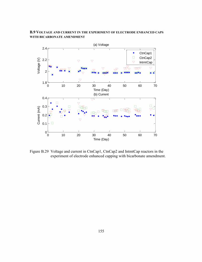
155
B.9 VOLTAGE AND CURRENT IN THE EXPERIMENT OF ELECTRODE ENHANCED CAPS
WITH BICARBONATE AMENDMENT
Figure B.29 Voltage and current in CtnCap1, CtnCap2 and IntmtCap reactors in the
experiment of electrode enhanced capping with bicarbonate amendment.
0 10 20 30 40 50 60 701.8
2
2.2
2.4(a) Voltage
Time (Day)
Voltage (
V)
CtnCap1
CtnCap2
IntmtCap
0 10 20 30 40 50 60 700
0.1
0.2
0.3
0.4(b) Current
Time (Day)
Curr
ent
(mA
)
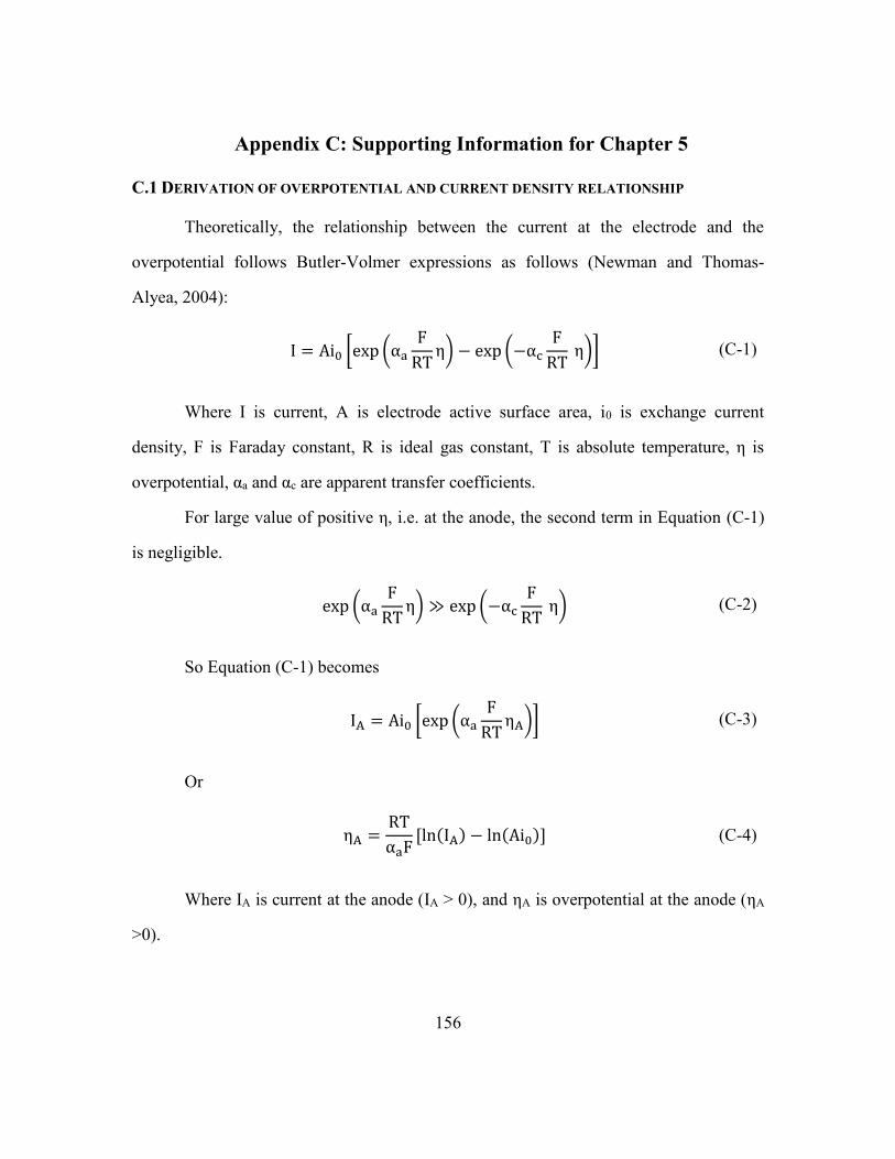
156
Appendix C: Supporting Information for Chapter 5
C.1 DERIVATION OF OVERPOTENTIAL AND CURRENT DENSITY RELATIONSHIP
Theoretically, the relationship between the current at the electrode and the
overpotential follows Butler-Volmer expressions as follows (Newman and Thomas-
Alyea, 2004):
I = Ai0 [exp (αa
F
RTη) − exp (−αc
F
RT η)] (C-1)
Where I is current, A is electrode active surface area, i0 is exchange current
density, F is Faraday constant, R is ideal gas constant, T is absolute temperature, η is
overpotential, αa and αc are apparent transfer coefficients.
For large value of positive η, i.e. at the anode, the second term in Equation (C-1)
is negligible.
exp (αa
F
RTη) ≫ exp (−αc
F
RT η) (C-2)
So Equation (C-1) becomes
IA = Ai0 [exp (αa
F
RTηA)] (C-3)
Or
ηA =RT
αaF[ln(IA) − ln(Ai0)] (C-4)
Where IA is current at the anode (IA > 0), and ηA is overpotential at the anode (ηA
>0).
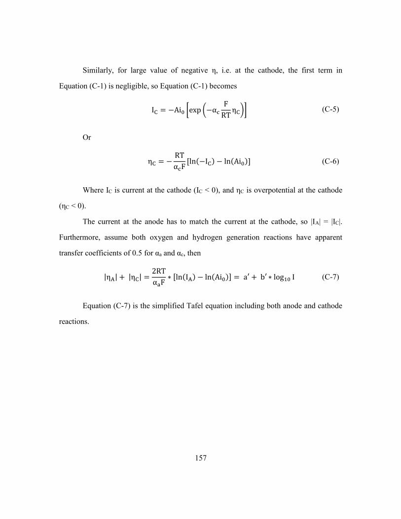
157
Similarly, for large value of negative η, i.e. at the cathode, the first term in
Equation (C-1) is negligible, so Equation (C-1) becomes
IC = −Ai0 [exp (−αc
F
RTηC)] (C-5)
Or
ηC = −RT
αcF[ln(−IC) − ln(Ai0)] (C-6)
Where IC is current at the cathode (IC < 0), and ηC is overpotential at the cathode
(ηC < 0).
The current at the anode has to match the current at the cathode, so |IA| = |IC|.
Furthermore, assume both oxygen and hydrogen generation reactions have apparent
transfer coefficients of 0.5 for αa and αc, then
|ηA| + |ηC| =2RT
αaF∗ [ln(IA) − ln(Ai0)] = a′ + b′ ∗ log10 I (C-7)
Equation (C-7) is the simplified Tafel equation including both anode and cathode
reactions.
158
References
Acar YB, Alshawabkeh AN. 1993. Principles of electrokinetic remediation.
Environmental Science & Technology 27:2638-2647.
Acar YB, Gale RJ, Alshawabkeh AN, Marks RE, Puppala S, Bricka M, Parker R. 1995.
Electrokinetic remediation - basics and technology status. Journal of Hazardous
Materials 40:117-137.
Al-Hamdan AZ, Reddy KR. 2008. Electrokinetic remediation modeling incorporating
geochemical effects. Journal of Geotechnical and Geoenvironmental Engineering
134:91-105.
Alshawabkeh AN, Acar YB. 1992. Removal of contaminants from soils by
electrokinetics - a theoretical treatise. Journal of Environmental Science and
Health Part a-Environmental Science and Engineering & Toxic and Hazardous
Substance Control A27:1835-1861.
Alshawabkeh AN. 1994. Theoretical and experimental modeling of removing
contaminants from soils by an electric field. (Doctoral dissertation). The
Louisiana State University, Baton Rouge, LA.
Alshawabkeh AN, Acar YB. 1996. Electrokinetic remediation .2. Theoretical model.
Journal of Geotechnical Engineering-Asce 122:186-196.
Alshawabkeh AN, Sarahney H. 2005. Effect of current density on enhanced
transformation of naphthalene. Environmental Science & Technology 39:5837-
5843.
Amann RI, Ludwig W, Schleifer KH. 1995. Phylogenetic identification and in-situ
detection of individual microbial-cells without cultivation. Microbiological
Reviews 59:143-169.
Annweiler E, Michaelis W, Meckenstock RU. 2002. Identical ring cleavage products
during anaerobic degradation of naphthalene, 2-methylnaphthalene, and tetralin
indicate a new metabolic pathway. Applied and Environmental Microbiology
68:852-858.
Archer D. 1996. A data-driven model of the global calcite lysocline. Global
Biogeochemical Cycles 10:511-526.
Archie GE.1942. The Electrical resistivity log as an aid in determining some reservoir
characteristics. Trans AIME 146: 54-62.
Atlas RM. 2010. Handbook of microbiological media. 4th Ed. CRC Press, Boca Raton,
FL.
Baldwin BR, Nakatsu CH, Nebe J, Wickham GS, Parks C, Nies L. 2009. Enumeration of
aromatic oxygenase genes to evaluate biodegradation during multi-phase

159
extraction at a gasoline-contaminated site. Journal of Hazardous Materials
163:524-530.
Baudo R, Muntau H. Lesser known in-place pollutants and diffuse source problems. In:
Baudo R, Giesy JP, Muntau H(eds). Sediments: Chemistry and Toxicity of In-
Place Pollutants. Lewis Publishers, Ann Arbor. pp1-14
Bard AJ, Faulkner LR. 2001. Electrochemical Methods: Fundamentals and Applications,
2nd ed..Wiley, New York.
Bauer JE, Capone DG. 1985. Degradation and mineralization of the polycyclic aromatic-
hydrocarbons anthracene and naphthalene in intertidal marine-sediments. Applied
and Environmental Microbiology 50:81-90.
Baumard P, Budzinski H, Michon Q, Garrigues P, Burgeot T, Bellocq J. 1998. Origin and
bioavailability of PAHs in the Mediterranean sea from mussel and sediment
records. Estuarine Coastal and Shelf Science 47:77-90.
Bender ML, Heggie DT. 1984. Fate of organic-carbon reaching the deep-sea floor - a
status-report. Geochimica Et Cosmochimica Acta 48:977-986.
Boudreau BP. 1991. Modeling the sulfide-oxygen reaction and associated pH gradients in
porewaters. Geochimica Et Cosmochimica Acta 55:145-159.
Boyd TJ, Montgomery MT, Steele JK, Pohlman JW, Reatherford SR, Spargo BJ, Smith
DC. 2005. Dissolved oxygen saturation controls PAH biodegradation in
freshwater estuary sediments. Microbial Ecology 49:226-235.
Brendel PJ, Luther GW. 1995. Development of a gold amalgam voltammetric
microelectrode for the determination of dissolved Fe, Mn, O2, and S(II) in
porewaters of marine and fresh-water sediments. Environmental Science &
Technology 29:751-761.
Brezna B, Khan AA, Cerniglia CE. 2003. Molecular characterization of dioxygenases
from polycyclic aromatic hydrocarbon-degrading Mycobacterium spp. FEMS
Microbiology Letters 223:177-183.
Burdige DJ. 2007. Preservation of organic matter in marine sediments: Controls,
mechanisms, and an imbalance in sediment organic carbon budgets. Chemical
Reviews 107:467-485.
Burnett WC, Bokuniewicz H, Huettel M, Moore WS, Taniguchi M. 2003. Groundwater
and pore water inputs to the coastal zone. Biogeochemistry 66:3-33.
Cebron A, Norini MP, Beguiristain T, Leyval C. 2008. Real-Time PCR quantification of
PAH-ring hydroxylating dioxygenase (PAH-RHDα) genes from Gram positive
and Gram negative bacteria in soil and sediment samples. Journal of
Microbiological Methods 73:148-159.
160
Cerniglia CE. 1992. Biodegradation of polycyclic aromatic hydrocarbons.
Biodegradation 3: 351-368.
Chang BV, Shiung LC, Yuan SY. 2002. Anaerobic biodegradation of polycyclic aromatic
hydrocarbon in soil. Chemosphere 48:717-724.
Chen JL, Al-Abed S, Ryan J, Roulier M, Kemper M. 2002. Effects of electroosmosis on
soil temperature and hydraulic head. II: Numerical simulation. Journal of
Environmental Engineering-ASCE 128:596-603.
Chin DT, Cheng CY. 1985. Oxidation of phenol with ac electrolysis. Journal of the
Electrochemical Society 132:2605-2611.
Choi H, Agarwal S, Al-Abed SR. 2009. Adsorption and Simultaneous Dechlorination of
PCBs on GAC/Fe/Pd: Mechanistic Aspects and Reactive Capping Barrier
Concept. Environmental Science & Technology 43:488-493.
Choi YS, Lui R. 1995. A mathematical-model for the electrokinetic remediation of
contaminated soil. Journal of Hazardous Materials 44:61-75.
Chung WK, King GM. 2001. Isolation, characterization, and polyaromatic hydrocarbon
degradation potential of aerobic bacteria from marine macrofaunal burrow
sediments and description of Lutibacterium anuloederans gen. nov., sp nov., and
Cycloclasticus spirillensus sp nov. Applied and Environmental Microbiology
67:5585-5592.
Cornelissen G, Pfttersen A, Broman D, Mayer P, Breedveld GD. 2008. Field testing of
equilibrium passive samplers to determine freely dissolved native polycyclic
aromatic hydrocarbon concentrations. Environmental Toxicology and Chemistry
27:499-508.
Dagher F, Deziel E, Lirette P, Paquette G, Bisaillon JG, Villemur R. 1997. Comparative
study of five polycyclic aromatic hydrocarbon degrading bacterial strains isolated
from contaminated soils. Canadian Journal of Microbiology 43:368-377.
Davies JI, Evans WC. 1964. Oxidative metabolism of naphthalene by soil pseudomonads.
Biochem J 91: 251-261.
Das N, Chandran P. 2011. Microbial Degradation of Petroleum Hydrocarbon
Contaminants: An Overview. Biotechnology Research International 2011,
doi:10.4061/2011/941810.
Ding GC, Heuer H, Zuhlke S, Spiteller M, Pronk GJ, Heister K, Kogel-Knabner I, Smalla
K. 2010. Soil Type-Dependent Responses to Phenanthrene as Revealed by
Determining the Diversity and Abundance of Polycyclic Aromatic Hydrocarbon
Ring-Hydroxylating Dioxygenase Genes by Using a Novel PCR Detection
System. Applied and Environmental Microbiology 76:4765-4771.
Foght J. 2008. Anaerobic biodegradation of aromatic hydrocarbons: Pathways and
prospects. Journal of Molecular Microbiology and Biotechnology 15:93-120.

161
Franz JA, Williams RJ, Flora JR, Meadows ME, Irwin WG. 2002. Electrolytic oxygen
generation for subsurface delivery: effects of precipitation at the cathode and an
assessment of side reactions. Water Research 36:2243-2254.
Friedman SP. 2005. Soil properties influencing apparent electrical conductivity: a review.
Computers and Electronics in Agriculture 46:45-70.
Furrer G, Stumm W. 1986. A Coordination Chemical Approach to the Kinetics of
Weathering: I. Dissolution of d-Al2O3 and BeO. Geochimica et Cosmochimica
Acta 50: 1847-1860.
Gent DB, Wani AH, Davis JL, Alshawabkah A. 2009. Electrolytic Redox and
Electrochemical Generated Alkaline Hydrolysis of Hexahydro-1,3,5-trinitro-1,3,5
triazine (RDX) in Sand Columns. Environmental Science & Technology 43:6301-
6307.
Gibson DT, Subramanian V. 1984. Microbial degradation of aromatic hydrocarbons. In
Microbial degradation of organic compounds. Marcel Dekker, New York. pp181-
252.
Gidley PT, Kwon S, Yakirevich A, Magar VS, Ghosh U. 2012. Advection Dominated
Transport of Polycyclic Aromatic Hydrocarbons in Amended Sediment Caps.
Environmental Science & Technology 46:5032-5039.
Gilbert DM, Sale TC. 2005. Sequential electrolytic oxidation and reduction of aqueous
phase energetic compounds. Environmental Science & Technology 39:9270-
9277.
Goel RK, Flora JRV, Ferry J. 2003. Mechanisms for naphthalene removal during
electrolytic aeration. Water Research 37:891-901.
Goldman R, Enewold L, Pellizzari E, Beach JB, Bowman ED, Krishnan SS, Shields PG.
2001. Smoking increases carcinogenic polycyclic aromatic hydrocarbons in
human lung tissue. Cancer Research 61:6367-6371.
Gomes NCM, Borges LR, Paranhos R, Pinto FN, Krogerrecklenfort E, Mendonca-Hagler
LCS, Smalla K. 2007. Diversity of ndo genes in mangrove sediments exposed to
different sources of polycyclic aromatic hydrocarbon pollution. Applied and
Environmental Microbiology 73:7392-7399.
Gregory KB, Bond DR, Lovley DR. 2004. Graphite electrodes as electron donors for
anaerobic respiration. Environmental Microbiology 6:596-604.
Hambrick GA, Delaune RD, Patrick WH. 1980. Effect of estuarine sediment ph and
oxidation-reduction potential on microbial hydrocarbon degradation. Applied and
Environmental Microbiology 40:365-369.
Hamed J, Acar YB, Gale RJ. 1991. Pb(II) removal from kaolinite by electrokinetics.
Journal of Geotechnical Engineering-Asce 117:241-271.
162
Haran BS, Popov BN, Zheng GH, White RE. 1997. Mathematical modeling of
hexavalent chromium decontamination from low surface charged soils. Journal of
Hazardous Materials 55:93-107.
Hart JK, Martinez K. 2006. Environmental Sensor Networks: A revolution in the earth
system science? Earth-Science Reviews 78:177-191.
Hedlund BP, Staley JT. 2006. Isolation and characterization of Pseudoalteromonas strains
with divergent polycyclic aromatic hydrocarbon catabolic properties.
Environmental Microbiology 8:178-182.
Heitkamp MA, Cerniglia CE. 1987. Effects of chemical-structure and exposure on the
microbial-degradation of polycyclic aromatic-hydrocarbons in fresh-water and
estuarine ecosystems. Environmental Toxicology and Chemistry 6:535-546.
Hicks RE, Tondorf S. 1994. Electrorestoration of metal-contaminated soils.
Environmental Science & Technology 28:2203-2210.
Himmelheber DW, Pennell KD, Hughes JB. 2011. Evaluation of a laboratory-scale
bioreactive in situ sediment cap for the treatment of organic contaminants. Water
Research 45:5365-5374.
Hong YS, Kinney KA, Reible DD. 2011. Acid volatile sulfides oxidation and metals
(Mn, Zn) release upon sediment resuspension: laboratory experiment and model
development. Environmental Toxicology and Chemistry 30:564-575.
Jacobs PH, Forstner U. 1999. Concept of subaqueous capping of contaminated sediments
with active barrier systems (ABS) using natural and modified zeolites. Water
Research 33:2083-2087.
Johnsen AR, de Lipthay JR, Reichenberg F, Sorensen SJ, Andersen O, Christensen P,
Binderup ML, Jacobsen CS. 2006. Biodegradation, bioaccessibility, and
genotoxicity of diffuse polycyclic aromatic hydrocarbon (PAH) pollution at a
motorway site. Environmental Science & Technology 40:3293-3298.
Johnson K, Ghosh S. 1998. Feasibility of anaerobic biodegradation of PAHs in dredged
river sediments. Water Science and Technology 38:41-48.
Johnston N, Sadler R, Shaw GR, Connell DW. 1993. Environmental modification of
PAH composition in coal-tar containing samples. Chemosphere 27:1151-1158.
Jourabchi P, Van Cappellen P, Regnier P. 2005. Quantitative interpretation of pH
distributions in aquatic sediments: A reaction-transport modeling approach.
American Journal of Science 305:919-956.
Juhasz AL, Naidu R. 2000. Bioremediation of high molecular weight polycyclic aromatic
hydrocarbons: a review of the microbial degradation of benzo[a] pyrene.
International Biodeterioration & Biodegradation 45:57-88.
163
Juhasz AL, Stanley GA, Britz ML. 2000. Microbial degradation and detoxification of
high molecular weight polycyclic aromatic hydrocarbons by Stenotrophomonas
maltophilia strain VUN 10,003. Letters in Applied Microbiology 30:396-401.
Kanaly RA, Harayama S. 2000. Biodegradation of high-molecular-weight polycyclic
aromatic hydrocarbons by bacteria. Journal of Bacteriology 182:2059-2067.
Kaplan DI, Knox AS. 2004. Enhanced contaminant desorption induced by phosphate
mineral additions to sediment. Environmental Science & Technology 38:3153-
3160.
Kastner M, Breuer-Jammali M, Mahro B. 1998. Impact of inoculation protocols, salinity,
and pH on the degradation of polycyclic aromatic hydrocarbons (PAHs) and
survival of PAH-degrading bacteria introduced into soil. Applied and
Environmental Microbiology 64:359-362.
Kastner M, Breuerjammali M, Mahro B. 1994. Enumeration and characterization of the
soil microflora from hydrocarbon-contaminated soil sites able to mineralize
polycyclic aromatic-hydrocarbons (PAH). Applied Microbiology and
Biotechnology 41:267-273.
Knox AS, Paller MH, Roberts J. 2012. Active Capping Technology - New Approaches
for In Situ Remediation of Contaminated Sediments. Remediation 22: 93-117
Lageman R. 1993. Electroreclamation. Environmental Science & Technology 27:2648-
2650.
Lampert DJ. 2010. An Assessment of the Design of In Situ Management Approaches for
Contaminated Sediments. (Doctoral dissertation). The University of Texas at
Austin, Austin, TX.
Lampert DJ, Sarchet WV, Reible DD. 2011. Assessing the Effectiveness of Thin-Layer
Sand Caps for Contaminated Sediment Management through Passive Sampling.
Environmental Science & Technology 45:8437-8443.
Laurie AD, Lloyd-Jones G. 1999. The phn genes of Burkholderia sp. strain RP007
constitute a divergent gene cluster for polycyclic aromatic hydrocarbon
catabolism. Journal of Bacteriology 181:531-540.
Leduc R, Samson R, Albashir B, Alhawari J, Cseh T. 1992. Biotic and abiotic
disappearance of 4 PAH compounds from flooded soil under various redox
conditions. Water Science and Technology 26:51-60.
Li ZM, Yu JW, Neretnieks I. 1997. Removal of Pb(II), Cd(II) and Cr(III) from sand by
electromigration. Journal of Hazardous Materials 55:295-304.
Lloyd-Jones G, Laurie AD, Hunter DWF, Fraser R. 1999. Analysis of catabolic genes for
naphthalene and phenanthrene degradation in contaminated New Zealand soils.
FEMS Microbiology Ecology 29:69-79.

164
Lofts S, Woof C, Tipping E, Clarke N, Mulder J. 2001. Modelling pH buffering and
aluminium solubility in European forest soils. European Journal of Soil Science
52:189-204.
Logan BE. 2009. Exoelectrogenic bacteria that power microbial fuel cells. Nature
Reviews Microbiology 7:375-381.
Lovley DR. 2008. The microbe electric: conversion of organic matter to electricity.
Current Opinion in Biotechnology 19:564-571.
Lu XX, Reible DD, Fleeger JW. 2006. Bioavailability of polycyclic aromatic
hydrocarbons in field-contaminated Anacostia River (Washington, DC) sediment.
Environmental Toxicology and Chemistry 25:2869-2874.
Lu XX, Skwarski A, Drake B, Reible DD. 2011. Predicting bioavailability of PAHs and
PCBs with porewater concentrations measured by solid-phase microextraction
fibers. Environmental Toxicology and Chemistry 30:1109-1116.
Luther GW, Reimers CE, Nuzzio DB, Lovalvo D. 1999. In situ deployment of
voltammetric, potentiometric. and amperometric microelectrodes from a ROV to
determine dissolved O2, Mn, Fe, S(-2), and pH in porewaters. Environmental
Science & Technology 33:4352-4356.
Mastrangelo G, Fadda E, Marzia V. 1996. Polycyclic aromatic hydrocarbons and cancer
in man. Environmental Health Perspectives 104:1166-1170.
Mayer P, Vaes WHJ, Wijnker F, Legierse K, Kraaij RH, Tolls J, Hermens JLM. 2000.
Sensing dissolved sediment porewater concentrations of persistent and
bioaccumulative pollutants using disposable solid-phase microextraction fibers.
Environmental Science & Technology 34:5177-5183.
McCoy CA, Corbett DR. 2009. Review of submarine groundwater discharge (SGD) in
coastal zones of the Southeast and Gulf Coast regions of the United States with
management implications. Journal of Environmental Management 90:644-651.
McDonough KM, Murphy P, Olsta J, Zhu Y, Reible D, Lowry GV. 2007. Development
and placement of a sorbent-amended thin layer sediment cap in the Anacostia
River. Soil & Sediment Contamination 16:313-322.
Menzie CA, Potocki BB, Santodonato J. 1992. Exposure to carcinogenic PAHs in the
environment. Environmental Science & Technology 26:1278-1284.
Mihelcic JR, Luthy RG. 1988. Degradation of polycyclic aromatic hydrocarbon
compounds under various redox conditions in soil-water systems. Applied and
Environmental Microbiology 54:1182-1187.
Mueller JG, Chapman PJ, Pritchard PH. 1989. Creosote-contaminated sites - their
potential for bioremediation. Environmental Science & Technology 23:1197-
1201.
165
Murphy P, Marquette A, Reible D, Lowry GV. 2006. Predicting the performance of
activated carbon-, coke-, and soil-amended thin layer sediment caps. Journal of
Environmental Engineering-Asce 132:787-794.
Nachtegaal M, Sparks DL. 2003. Nickel sequestration in a kaolinite-humic acid complex.
Environmental Science & Technology 37:529-534.
Nachtegaal M, Sparks DL. 2004. Effect of iron oxide coatings on zinc sorption
mechanisms at the clay-mineral/water interface. Journal of Colloid and Interface
Science 276:13-23.
Nakamura A, Hirano K, Iji M. 2005. Decomposition of trichlorobenzene with different
radicals generated by alternating current electrolysis in aqueous solution.
Chemistry Letters 34:802-803.
Newman J, Thomas-Alyea KE. 2004. Electrochemical Systems, 3rd ed., John Wiley &
Sons, New York.
Page DS, Boehm PD, Douglas GS, Bence AE, Burns WA, Mankiewicz PJ. 1999.
Pyrogenic polycyclic aromatic hydrocarbons in sediments record past human
activity: A case study in Prince William Sound, Alaska. Marine Pollution Bulletin
38:247-260.
Palermo M, Maynord S, Miller J, Reible D. 1998. Guidance for In-Situ Subaqueous
Capping of Contaminated Sediments," EPA 905-B96-004, Great Lakes National
Program Office, Chicago, IL.
Park H, Vecitis CD, Hoffmann MR. 2008. Solar-powered electrochemical oxidation of
organic compounds coupled with the cathodic production of molecular hydrogen.
Journal of Physical Chemistry A 112:7616-7626.
Penn RL, Zhu C, Xu H, Veblen DR. 2001. Iron oxide coatings on sand grains from the
Atlantic coastal plain: High-resolution transmission electron microscopy
characterization. Geology 29:843-846.
Perelo LW. 2010. Review: In situ and bioremediation of organic pollutants in aquatic
sediments. Journal of Hazardous Materials 177:81-89.
Petersen MA, Sale TC, Reardon KF. 2007. Electrolytic trichloroethene degradation using
mixed metal oxide coated titanium mesh electrodes. Chemosphere 67:1573-1581.
Pletcher D, Walsh FC. 1990. Industrial Electrochemistry. Chanpmand and Hall Ltd, New
York.
Probstein RF. 1989. Physicochemical Hydrodynamics.Wiley, New York.
Probstein RF, Hicks RE. 1993. REMOVAL OF CONTAMINANTS FROM SOILS BY
ELECTRIC-FIELDS. Science 260:498-503.
Reddy KR, Parupudi US. 1997. Removal of chromium, nickel and cadmium from clays
by in-situ electrokinetic remediation. Journal of Soil Contamination 6:391-407.
166
Reible D, Hayes D, Lue-Hing C, Patterson J, Bhowmik N, Johnson M, Teal J. 2003.
Comparison of the long-term risks of removal and in situ management of
contaminated sediments in the Fox River. Soil & Sediment Contamination
12:325-344.
Reible D. 2004. Cost and Feasibility of Conventional and Active Sediment Capping.
Presented at the Technology Benchmarking Workshop For Sediment and
Floodplain Remediation, Ann Arbor, MI, March 25-26.
Reible DD, Lu XX, Blishke H. 2005. Organoclay for the Control of NAPLs in
Sediments. Society of Environmental Toxicology and Chemistry 26th Annual
Meeting, Baltimore, MD.
Reible DD, Lambert D, Constant DW, Mutch RD, Zhu Y. 2007. Active capping
demonstration in the Anacostia River, Washington, DC. Remediation 17: 39-53.
Renaud PC, Probstein RF. 1987. Electroosmotic control of hazardous wastes.
Physicochemical Hydrodynamics 9:345-360.
Rockne KJ, Chee-Sanford JC, Sanford RA, Hedlund BP, Staley JT, Strand SE. 2000.
Anaerobic naphthalene degradation by microbial pure cultures under nitrate-
reducing conditions. Applied and Environmental Microbiology 66:1595-1601.
Rockne KJ, Strand SE. 1998. Biodegradation of bicyclic and polycyclic aromatic
hydrocarbons in anaerobic enrichments. Environmental Science & Technology
32:3962-3967.
Rockne KJ, Strand SE. 2001. Anaerobic biodegradation of naphthalene, phenanthrene,
and biphenyl by a denitrifying enrichment culture. Water Research 35:291-299.
Rothermich MM, Hayes LA, Lovley DR. 2002. Anaerobic, sulfate-dependent
degradation of polycyclic aromatic hydrocarbons in petroleum-contaminated
harbor sediment. Environmental Science & Technology 36:4811-4817.
Sabate J, Grifoll M, Vinas M, Solanas AM. 1999. Isolation and characterization of a 2-
methylphenanthrene utilizing bacterium: identification of ring cleavage
metabolites. Applied Microbiology and Biotechnology 52:704-712.
Saichek RE, Reddy KR. 2005. Electrokinetically enhanced remediation of hydrophobic
organic compounds in soils: A review. Critical Reviews in Environmental Science
and Technology 35:115-192.
Sakakibara Y, Nakayama T. 2001. A novel multi-electrode system for electrolytic and
biological water treatments: Electric charge transfer and application to
denitrification. Water Research 35:768-778.
Schafer AI, Broeckmann A, Richards BS. 2007. Renewable energy powered membrane
technology. 1. Development and characterization of a photovoltaic hybrid
membrane system. Environmental Science & Technology 41:998-1003.
167
Shapiro AP, Probstein RF. 1993. Removal of contaminants from saturated clay by
electroosmosis. Environmental Science & Technology 27:283-291.
Shapiro AP, Renaud PC, Probstein RF. 1989. Preliminary studies on the removal of
chemical-species from saturated porous-media by electroosmosis.
Physicochemical Hydrodynamics 11:785-802.
Shennan, JL. 1984. Hydrocarbons as substrates in industrial fermentation. In Petroleum
Microbiology Atlas. Macmillan R.M.ed. pp. 643-683.
Shuttleworth KL, Cerniglia CE. 1995. Environmental aspects of PAH biodegradation.
Applied Biochemistry and Biotechnology 54:291-302.
Sparks DL. 1996, Methods of soil analysis. Part 3, Chemical methods. Soil Science
society of America and Ameican Society of Agronomy, Madison, WI 53711.
Stumm W, Morgan JJ. 1996. Aquatic Chemistry, 3rd ed. John Wiley & Sons, New York.
Sun HW, Xu XY, Gao GD, Zhang ZZ, Yin PJ. 2010. A novel integrated active capping
technique for the remediation of nitrobenzene-contaminated sediment. Journal of
Hazardous Materials 182:184-190.
Sun M, Yan F, Zhang RL, Reible DD, Lowry GV, Gregory KB. 2010. Redox Control and
Hydrogen Production in Sediment Caps Using Carbon Cloth Electrodes.
Environmental Science & Technology 44:8209-8215.
Suni S, Romantschuk M. 2004. Mobilisation of bacteria in soils by electro-osmosis.
FEMS Microbiology Ecology 49:51-57.
Thibodeaux LJ, Bosworth WS. 1990. A Theoretical Evaluation of the Effectiveness of
Capping PCB Contaminated New Bedford Harbor Bed Sediment, Final Report.
Hazardous Waste Research Center, Louisiana State University, Baton Rouge, LA.
Thoma GJ, Reible DD, Valsaraj KT, Thibodeaux LJ. 1993. Efficiency of capping
contaminated sediments in-situ .2. Mathematics of diffusion adsorption in the
capping layer. Environmental Science & Technology 27:2412-2419.
Thrash JC, Van Trump JI, Weber KA, Miller E, Achenbach LA, Coates JD. 2007.
Electrochemical stimulation of microbial perchlorate reduction. Environmental
Science & Technology 41:1740-1746.
Tipping E. 1998. Humic ion-binding model VI: An improved description of the
interactions of protons and metal ions with humic substances. Aquatic
Geochemistry 4:3-48.
Tipping E, Hurley MA. 1988. A model of solid-solution interactions in acid organic soils,
based on the complexation properties of humic substances. Journal of Soil
Science 39:505-519.
US DOE. 2011. Energy savers - How small solar electric systems work. February 2011

168
US EPA. 1998. Contaminated Sediment Management Strategy, Office of Water, EPA-
823-R-98-001.
US EPA. 2005. Contaminated Sediment Remediation Guidance for Hazardous Waste
Sites, Office of Solid Waste and Emergency Response, EPA-540-R05-012.
US EIA. 2012. Electric Power Monthly June 2012. U.S. Energy Information
Administration, Office of Electricity, Renewables & Uranium Statistics, U.S.
Department of Energy, Washington, DC.
VanCappellen P, Wang YF. 1996. Cycling of iron and manganese in surface sediments:
A general theory for the coupled transport and reaction of carbon, oxygen,
nitrogen, sulfur, iron, and manganese. American Journal of Science 296:197-243.
Wang XQ, Thibodeaux LJ, Valsaraj KT, Reible DD. 1991. Efficiency of capping
contaminated bed sediments in situ .1. Laboratory-scale experiments on diffusion
adsorption in the capping layer. Environmental Science & Technology 25:1578-
1584.
Watanabe T, Hashimoto S, Kuroda M. 2002. Simultaneous nitrification and
denitrification in a single reactor using bio-electrochemical process. Water
Science and Technology 46:163-169.
Widada J, Nojiri H, Kasuga K, Yoshida T, Habe H, Omori T. 2002. Molecular detection
and diversity of polycyclic aromatic hydrocarbon-degrading bacteria isolated
from geographically diverse sites. Applied Microbiology and Biotechnology
58:202-209.
Wilson MS, Bakermans C, Madsen EL. 1999. In situ, real-time catabolic gene
expression: Extraction and characterization of naphthalene dioxygenase mRNA
transcripts from groundwater. Applied and Environmental Microbiology 65:80-
87.
Wilson SC, Jones KC. 1993. Bioremediation of soil contaminated with polynuclear
aromatic-hydrocarbons (PAHs) - a review. Environmental Pollution 81:229-249.
Yeung AT, Datla S. 1996. Fundamental formulation of electrokinetic extraction of
contaminants from soil: Reply. Canadian Geotechnical Journal 33:682-684.
Yu JW, Neretnieks I. 1996. Modelling of transport and reaction processes in a porous
medium in an electrical field. Chemical Engineering Science 51:4355-4368.
Zeebe RE. 2007. Modeling CO2 chemistry, delta C-13, and oxidation of organic carbon
and methane in sediment porewater: Implications for paleo-proxies in benthic
foraminifera. Geochimica Et Cosmochimica Acta 71:3238-3256.
Zeebe RE, Sanyal A. 2002. Comparison of two potential strategies of planktonic
foraminifera for house building: Mg2+ or H+ removal. Geochimica Et
Cosmochimica Acta 66:1159-1169.
169
Zhang T, Gannon SM, Nevin KP, Franks AE, Lovley DR. 2010. Stimulating the
anaerobic degradation of aromatic hydrocarbons in contaminated sediments by
providing an electrode as the electron acceptor. Environmental Microbiology
12:1011-1020.
Zimmerman JR, Ghosh U, Millward RN, Bridges TS, Luthy RG. 2004. Addition of
carbon sorbents to reduce PCB and PAH bioavailability in marine sediments:
Physicochemical tests. Environmental Science & Technology 38:5458-5464.

170
Vita FY
Fei Yan was born in Shanxi, China and attended high school in Taiyuan, Shanxi,
China. He received the degrees of Bachelor and Master from Tsinghua University, and
received the degree of Master of Engineering from the University of Florida. In 2007, he
entered the Graduate School at The University of Texas at Austin.
Permanent Address: Taiyuan, Shanxi, China
This manuscript was typed by the author.