Embed Size (px)
Citation preview

Copyright
by
Ioannis Keramidas Charidakos
2016
The Dissertation Committee for Ioannis Keramidas Charidakoscertifies that this is the approved version of the following dissertation:
Applications of Hamiltonian Theory to Plasma Models
Committee:
Philip J. Morrison, Supervisor
Francois Waelbroeck, Co-Supervisor
Claude Wendell Horton, Jr
Richard Hazeltine
Richard Fitzpatrick
Irene M. Gamba

Applications of Hamiltonian Theory to Plasma Models
by
Ioannis Keramidas Charidakos, Dipl.
DISSERTATION
Presented to the Faculty of the Graduate School of
The University of Texas at Austin
in Partial Fulfillment
of the Requirements
for the Degree of
DOCTOR OF PHILOSOPHY
THE UNIVERSITY OF TEXAS AT AUSTIN
May 2016

Acknowledgments
This dissertation is the final product of several years of work I con-
ducted at the Institute for Fusion Studies, at the University of Texas at Austin.
During my time as a doctoral student, I benefited from the invaluable pro-
fessional and moral support and guidance of my supervisors, colleagues and
friends, whose contribution I wish to hereby acknowledge. First among all, I
would like to show my appreciation for Professor Philip J. Morrison, whom I
had the privilege of having as research adviser. My enormous gratitude goes
to him: Professor Morrison’s unparalleled expertise in the field, and patient,
enthusiastic, dedication to teaching have made me the scholar I am today. I
am extremely thankful to Dr. Francois Waelbroeck, to whom I owe most of
my knowledge of tokamak-applied physics. By granting me the opportunity to
work with him, and agreeing to being my co-supervisor, Dr. Waelbroeck has
contributed to my academic success with his world-class expertise and kind
guidance.
I also would like to express my gratitude to Irene Gamba, Wendell
Horton, Richard Hazeltine and, Richard Fitzpatrick for their teachings, and
ultimately, for supporting my work by participating to this dissertation’s com-
mittee. During my last semester, I greatly benefited from my interaction with
Swadesh Mahajan and his Friday morning seminar. I am especially thankful
iv

to David Hatch who helped me with my postdoc applications. I owe a thanks
to Professor Roy Schwitters for giving me the opportunity to teach at both
an undergraduate and graduate level and for many insightful discussions on
physics I’ve had the pleasure to have with him. I would also like to thank my
first adviser, Mark G. Raizen, who agreed to take me in his group and was
supportive when I finally decided that experimental physics wasn’t for me.
My stay at both the IFS and the Department of Physics has been extremely
pleasant. I would like to thank Cathy Rapinett, James Halligan and Matt
Erwin for handling all administrative issues.
A special mention goes to my two invaluable colleagues and dear friends,
Manasvi Lingam and Ryan White. Ryan, with his acute physical intuition,
has been the provider of numerous Fermi problems spurring endless hours of
stimulating conversation among the three of us. Manasvi’s impressively prolific
intellect and broad understanding of the field has inspired me to become a
better physicist and helped me develop a finer grasp of the field’s demands. I
am also grateful to my collaborator and friend, Ehab Hassan, for our frequent
discussions and his good advice. My list of 11th floor friends would be certainly
incomplete if I didn’t acknowledge David Stark, along with my first office mate,
Chinmoy Bhattacharjee. I would also like to thank Dustin Lorshbough for the
extended, diverse conversations and the good times we shared.
In concluding my acknowledgements, I want to recognize those who,
although not related to the field, have provided for my emotional well-being
with their friendship and love. I would like to thank my fellow plasma physicist
v

Nikos Vergos, my old roommates, Giorgos Stamokostas, and Pantelis Lapas,
as well as Loukas Loumakos. I wish all of them good luck with their PhD’s.
Also, I need to mention the people who, although not physically present,
were always there for me. First the ones who live within similar time zones:
Giorgos Laskaris (Stanford), Andreas Kourouklis (UIUC) and Manos Chat-
zopoulos (UChicago). And second, my childhood friends from Greece, whom
I always bothered at odd hours but never (well... almost never) complained:
Nikos Mantalidis, Klearchos Polymeris, Christos Lamprou and, Dionysis Kara-
giannopoulos.
Finally, my deepest gratitude is for my mother, my father, and my
sister Dimitra whose care and unconditional love have encouraged me in every
step of the way. Last but not least, I would like to thank Paola for bearing
with me during the final, stressful period of my PhD and, not to forget, making
my life better.
vi

Applications of Hamiltonian Theory to Plasma Models
Publication No.
Ioannis Keramidas Charidakos, Ph.D.
The University of Texas at Austin, 2016
Supervisor: Philip J. MorrisonCo-Supervisor: Francois Waelbroeck
Three applications of Hamiltonian Methods in Plasma Physics are pre-
sented.
The first application is the development of a new, five-field, Hamiltonian
gyrofluid model. It is comprised by evolution equations for the ion density,
pressure and parallel temperature and electron density and pressure.
It contains curvature and compressibility effects. The model is shown
to satisfy a conserved energy and a Lie-Poisson bracket for it is given. Casimir
invariants are calculated and through them, the normal fields of the system
are recovered. Later, the model is linearized and shown to possess modes that
are identified with the slab ITG, toroidal ITG and KBM modes. Both an
electrostatic and an electromagnetic study are performed. Growth rates and
critical parameters for instability are computed and compared to their fluid
and kinetic counterparts. The accuracy of the model is shown to be between
the fluid and the kinetic results, as was expected. Dissipation is added to
vii

the ideal system via the use of non-local terms that mimic Landau damping.
The modes of the system are shown to undergo Kreın bifurcations and their
behavior once dissipation is turned on, strongly suggests that they are negative
energy modes. A connection between the marginal stability condition of the
ITG mode at high k⊥ and the (missing) equation of perpendicular pressure is
conjectured opening an interesting possibility for future research.
The second application is a method for the derivation of reduced fluid
models through the use of an action principle. The importance of the method
lies in the fact that since all approximations are made directly at the level of
the action, the models that result from the action minimization are guaranteed
to retain the Hamiltonian character of their parent-model. The two-fluid ac-
tion is given in Lagrangian variables and the two-fluid equations of motion are
recovered by it’s minimization. The Eulerian (field) equations of motion are re-
trieved through the Lagrange-to-Euler (L-E) map. New, single-fluid variables
are defined but instead of being implemented at the level of the equations of
motion, they are implemented directly in the action. The action is subjected
to approximations. Different approximations lead to different models with
the models of Lust, Extended MHD, Hall MHD and electron MHD being re-
trieved. The passing from Lagrangian to Eulerian variables in the single-fluid
description requires a non-trivial modification of the E-L map. A note about
the importance of quasineutrality in single-fluid models and its ramifications
in the Lagrangian framework is given. Several invariants of the models are
calculated via Noethers’ Theorem.
viii

The third application concerns the imposition of constraints in Hamil-
tonian systems. Two worked examples of the method of Dirac are presented.
The first one is on an electrostatic model which has the Hasegawa-Mima and
RMHD as distinct limits. The constraint that leads to the Hasegawa-Mima is
investigated. The calculations are demonstrated in detail and the reduced sys-
tem is produced. A brief discussion of the dispersion relation of the reduced
system concludes the first example. The second example is the imposition
of quasineutrality and divergence-free current on the bracket of the two-fluid
model. The various steps of the method are displayed and the example is
completed with the verification that the new bracket satisfies the constraints.
The possibility of performing the same calculation with single-fluid variables
remains open for future research.
ix

Table of Contents
Acknowledgments iv
Abstract vii
List of Figures xiii
Chapter 1. Introduction 1
1.1 The need for Hamiltonian models in Plasma Physics . . . . . . 1
Chapter 2. Review of Canonical and Noncanonical Hamiltoniansystems 4
2.1 Canonical Hamiltonian systems . . . . . . . . . . . . . . . . . 4
2.2 Noncanonical Hamiltonian Systems . . . . . . . . . . . . . . . 8
Chapter 3. A Hamiltonian five-field Model for ITG 12
3.1 Motivation . . . . . . . . . . . . . . . . . . . . . . . . . . . . . 13
3.2 Review of the ITG mode . . . . . . . . . . . . . . . . . . . . . 19
3.2.1 General Features of Drift Waves . . . . . . . . . . . . . 19
3.2.2 An Intuitive Picture of the ITG Mode . . . . . . . . . . 22
3.3 Ideal Five-Field Model . . . . . . . . . . . . . . . . . . . . . . 27
3.4 The Hamiltonian Form . . . . . . . . . . . . . . . . . . . . . . 31
3.5 Casimir Invariants . . . . . . . . . . . . . . . . . . . . . . . . . 33
3.6 Normal Fields . . . . . . . . . . . . . . . . . . . . . . . . . . . 36
3.7 Linear Study . . . . . . . . . . . . . . . . . . . . . . . . . . . . 38
3.7.1 Electrostatic Dispersion Relation . . . . . . . . . . . . . 41
3.7.2 Electromagnetic Dispersion Relation . . . . . . . . . . . 45
x
Chapter 4. Action Principles in Fluids and Plasmas 57
4.1 Hamilton’s Principle of least action . . . . . . . . . . . . . . . 57
4.1.1 Variational Derivatives . . . . . . . . . . . . . . . . . . . 58
4.2 Lagrangian vs Eulerian Description . . . . . . . . . . . . . . . 60
Chapter 5. Action Principles for Reduced MHD Models 66
5.1 Introduction . . . . . . . . . . . . . . . . . . . . . . . . . . . . 66
5.2 Review: Two-fluid model and action . . . . . . . . . . . . . . . 68
5.2.1 Constructing the two-fluid action . . . . . . . . . . . . . 71
5.2.2 Lagrange-Euler map . . . . . . . . . . . . . . . . . . . . 72
5.2.3 Varying the two-fluid action . . . . . . . . . . . . . . . . 74
5.3 The new one-fluid action . . . . . . . . . . . . . . . . . . . . . 76
5.3.1 New Lagrangian variables . . . . . . . . . . . . . . . . . 77
5.3.2 Ordering of fields and quasineutrality . . . . . . . . . . 78
5.3.3 Action functional . . . . . . . . . . . . . . . . . . . . . . 81
5.3.4 Nonlocal Lagrange-Euler maps . . . . . . . . . . . . . . 82
5.3.5 Lagrange-Euler maps without quasineutrality . . . . . . 85
5.3.6 Derivation of the continuity and entropy equations . . . 87
5.4 Derivation of reduced models . . . . . . . . . . . . . . . . . . . 89
5.4.1 Extended MHD . . . . . . . . . . . . . . . . . . . . . . 89
5.4.2 Hall MHD . . . . . . . . . . . . . . . . . . . . . . . . . 95
5.4.3 Electron MHD . . . . . . . . . . . . . . . . . . . . . . . 96
5.5 Noether’s theorem . . . . . . . . . . . . . . . . . . . . . . . . . 97
Chapter 6. Dirac Constraints 102
6.1 Dirac Constraints on the Hazeltine Model . . . . . . . . . . . . 104
6.1.1 Definitions . . . . . . . . . . . . . . . . . . . . . . . . . 104
6.1.2 Constraints and change of variables . . . . . . . . . . . 106
6.1.3 The Dirac Method . . . . . . . . . . . . . . . . . . . . . 108
6.1.3.1 Calculation of Matrix Elements . . . . . . . . . 108
6.1.3.2 Calculation of Inverse Matrix Elements . . . . . 110
6.1.3.3 Calculation of Integral Terms . . . . . . . . . . 113
6.1.3.4 Calculating New Equations of Motion . . . . . . 115
xi
6.1.4 Dispersion Relations . . . . . . . . . . . . . . . . . . . . 118
6.2 Dirac Constraints on the two-fluid model . . . . . . . . . . . . 120
6.2.1 The two-fluid bracket . . . . . . . . . . . . . . . . . . . 121
6.2.2 The Dirac Method on the 2-fluid bracket . . . . . . . . . 122
6.2.2.1 Constraints . . . . . . . . . . . . . . . . . . . . 122
6.2.2.2 Constraint Matrix . . . . . . . . . . . . . . . . 123
6.2.2.3 Inverse Matrix Elements . . . . . . . . . . . . . 124
6.2.2.4 Towards the Dirac bracket . . . . . . . . . . . . 125
Chapter 7. Conclusions and outline for future work 129
Bibliography 134
xii

List of Figures
3.1 Mechanism of generation of drift waves . . . . . . . . . . . . . 20
3.2 Feedback mechanism of slab ITG . . . . . . . . . . . . . . . . 24
3.3 Mechanism of toroidal ITG . . . . . . . . . . . . . . . . . . . . 25
3.4 Stability criterion with finite k⊥ . . . . . . . . . . . . . . . . . 42
3.5 Comparison of critical η . . . . . . . . . . . . . . . . . . . . . 44
3.6 Stability criterion at the ‘fluid’ limit . . . . . . . . . . . . . . . 45
3.7 Normalized growth rate as a function of τ . . . . . . . . . . . 46
3.8 Normalized growth rate vs. β . . . . . . . . . . . . . . . . . . 48
3.9 Real frequency vs. β . . . . . . . . . . . . . . . . . . . . . . . 49
3.10 Kreın bifurcation . . . . . . . . . . . . . . . . . . . . . . . . . 51
3.11 Growth rates of the ITG-KBM modes vs.k‖ . . . . . . . . . . 52
3.12 Growth rates of the ITG-KBM modes vs. k⊥ . . . . . . . . . . 54
3.13 Comparison between growth rates of the ITG mode vs. k‖ . . 55
3.14 Comparison between growth rates of the ITG mode vs. k⊥ . . 56
xiii

Μέγα βιβλίον, μέγα κακόν.
Callimachus, 4th century BC
xiv

Chapter 1
Introduction
1.1 The need for Hamiltonian models in Plasma Physics
The behavior of plasmas in tremendously different contexts, from astro-
physical environments to magnetically confined, thermonuclear plasmas inside
tokamaks, can be modeled by systems of partial differential equations that
yield the time evolution of key physical variables such as ion and electron
density, momentum, pressure, heat flux etc. One usually derives such dynam-
ical equations by taking moments of a distribution function. The equations
thus derived are fairly general since they contain the physical description of
phenomena that occur over vastly different length and time scales. As a con-
sequence, these exact moment equations are also intractable, both from an
analytical and a computational standpoint. To reduce the complexity, it is
appropriate that the exact moment equations get subsequently manipulated,
according to the particular phenomenon one wishes to model or the specific
context that the plasma in question is in, in order to filter out irrelevant time
and length scales. This phenomenological process commonly takes the form
of small parameter expansions and assumptions about the geometry of the
system under consideration. Unfortunately, there is no prescription for this
procedure and one has only his or her intuition to rely on. As a result, the sys-
1

tems of equations produced by such ad hoc procedures often comes with a host
of shortcomings. A very serious one is the loss of the Hamiltonian character
[63, 130]: The parent model, that is the system of charged particles interact-
ing with an electromagnetic field, is Hamiltonian and as a consequence, it is
desirable that any reduced description of it should retain this property. The
issue is not just a harmless question of mathematical formalism: The process
of reduction might have introduced unwanted dissipation and as a result, the
system might violate energy conservation at the ideal limit. By ideal limit, we
refer to what remains from the system once all dissipative and source terms
such as collisions, Landau damping, anomalous transport and boundary terms
have been discarded. To the contrary, a Hamiltonian system is guaranteed to
conserve energy for closed boundary conditions and the Hamiltonian formu-
lation is useful for investigating the local properties of the dynamics that are
independent of the drive.
Nonetheless, energy conservation is not the sole reason one might have
to pursue the discovery of the Hamiltonian formulation of a system. Casting a
system into its Hamiltonian form [82, 83] confers several practical advantages.
One of the most important is the existence of families of invariants, called
Casimir invariants, which are found in noncanonical Hamiltonian systems due
to the degeneracy of the cosymplectic matrix. We hope that the discussion in
the subsequent sections will make statements like the previous one explicit and
convince the reader for the importance of Casimir invariants. For now, suffice
2

it to say that the functional that results from the addition of the Casimirs
to the Hamiltonian has non-trivial equilibrium states as stationary points.
In the absence of a Poisson bracket, by contrast, the existence of non-trivial
equilibrium states is not guaranteed. For example, Ref. [135] presents an ex-
ample of a seemingly reasonable fluid model that lacks physical equilibria with
closed streamlines because the equilibrium equations imply that some fields
are multiple-valued on closed streamlines. We can also take advantage of the
Hamiltonian formulation to construct “energy principles” for the investigation
of the stability of such non-trivial equilibrium states by examining the sec-
ond variation of the aforementioned functional. The interested reader can find
the description and applications of the so-called Energy-Casimir method in
[4, 93, 131]. Another advantage is that imposing constraints on a system is
straightforward in the Hamiltonian formalism [16]. The last chapter of this
dissertation deals with this topic. Lastly, the Hamiltonian formalism can be
used to facilitate the calculation of the statistical average of the zonal flow
growth rate [66].
3

Chapter 2
Review of Canonical and Noncanonical
Hamiltonian systems
2.1 Canonical Hamiltonian systems
We will start by giving a brief reminder of the basic ideas of canonical
Hamiltonian systems. This review is by no means meant to be complete. For a
more exhaustive treatment, the reader is referred to the textbooks [57, 30, 50].
Lets start with a dynamical system that is described by generalized coordinates
qi, i = 1, . . . , n defined on the configuration space Mn. To each of these we can
associate a generalized momentum pi. If we know the Lagrangian L(q, q, t) of
the system, then these generalized momenta can be found as
pi =∂L
∂qi. (2.1)
The Euler-Lagrange equations are then written as
dpidt
=∂L
∂qi, (2.2)
dqi
dt= qi . (2.3)
After we perform a change of variables in the Lagrangian L(q, q, t)
and express it in terms of the conjugate variables (qi,pi) instead, we per-
form a Legendre transform to find the Hamiltonian of the system: H(q, p, t) =
4

piqi−L(q, p, t). In mathematical language, we say that we pass from the con-
figuration manifold Mn to the cotangent bundle T∗M. This is called the phase
space of the system. In order to be able to perform the Legendre transform,
we must be careful that the equation (2.1) is invertible. This translates into
a condition for the second derivative of L, namely thatd2L
dq26= 0. If the La-
grangian in question depends on more than one generalised coordinates, the
generalisation of the invertibility condition is that the Hessian matrix,∂2L
∂qi∂qjmust be non-singular. In terms of this new function, the above dynamical
equations can be written as:
qi =∂H
∂pi, (2.4)
pi = −∂H∂qi
. (2.5)
In this form they are known as Hamilton’s canonical equations. We remark
here that whereas the Euler-Lagrange equations are second order and define
curves in Mn, Hamilton’s equations are first order and define curves in T∗M.
This means that in phase space trajectories are separated.
A mathematical object of great importance in Hamiltonian mechanics
is the Poisson bracket ·, ·. It is a map that takes two smooth, real valued
functions of phase space (we insert them into one of the two slots) and produces
a new smooth, real valued, phase space function. If the function that goes
into the right slot is the Hamiltonian, then the Poisson bracket gives the time
evolution, under the dynamics, of the function that we insert in the left slot.
The mathematical formulation of this statement is given in (2.6) which also
5

serves as a definition of the Poisson bracket:
f = f,H =∂f
∂q
∂H
∂p− ∂f
∂p
∂H
∂q. (2.6)
In terms of the Poisson bracket Hamilton’s equations take the following
form (suppressing the subscripts)
p = p,H , q = q,H . (2.7)
The properties of the Poisson bracket are:
• bilinearity: λf, g + h = λ (f, g+ f, h) .
• antisymmetry: f, g = −g, f .
• Leibnitz rule: fg, h = f, hg + fg, h .
• Jacobi: f, g, h+ h, f, g+ g, h, f = 0 .
The next step in the development of the Hamiltonian formalism is to
define the symplectic 2-form
ω = dpi ∧ dqi . (2.8)
At first, this definition might seem a little arbitrary. The motivation be-
hind it is the following: We need a 2-form that when we contract it with the
Hamiltonian vector field1 XH = qi∂
∂qi+ pi
∂
∂pigives us the differential of the
1By the subscript of a vector field, we denote the function on which it acts. However, inthis definition, by the subscript H we mean the Hamiltonian vector field.
6

Hamiltonian, dH. In other words, we are looking for ω so that iXHω = dH,
which is the geometric form of Hamilton’s canonical equations. It turns out
that this 2-form is (2.8). Two important properties of this 2-form are:
• dω = 0 ,
• iXω = 0 iff X is a null vector field .
ω is a bilinear and antisymmetric 2-form that sends pairs of vector
fields to functions. It can locally be described by a 2n × 2n matrix of the
following form: Jc =
[0n In−In 0n
], where 0n and In are the n × n zero and
identity matrices respectively.
One of the big advantages of the Hamiltonian formalism is that it treats
both coordinates and momenta on equal footing. Therefore, we can define new
variables zi, i = 1, . . . , 2n with
zi = qi , i ∈ (1, . . . , n) , (2.9)
zi = pi−n , i ∈ (n+ 1, . . . , 2n) . (2.10)
Using these unified coordinates we can relate the Poisson bracket and
the ω 2-form by:
f, g = ω(Xf , Xg) =∂f
∂ziJ ijc
∂g
∂zj. (2.11)
with Xf and Xg being the Hamiltonian vector fields of f and g defined by the
following relation:
iXfω = df . (2.12)
7

2.2 Noncanonical Hamiltonian Systems
Many times we are confronted with dynamical systems whose time
evolution is not described by an equation such as Eq.(2.6) and we have to
decide whether they are Hamiltonian or not. Before we answer the question
of how we can tell if a dynamical system is Hamiltonian, it is instructive to
show how we can start from a canonical Hamiltonian system and perform a
transformation of variables under which, the system is no longer characterized
by the evolution equation Eq.(2.6). Lets start with a canonical Hamiltonian
system and imagine a time-independent change of variables to our canonical
coordinates
zi = zi(z) . (2.13)
The Hamiltonian undergoes the same transformation H(z) = H(z).
Taking the time derivative of Eq. (2.13), using Eq. (2.11) gives:
˙zl =∂zl
∂zizi =
∂zl
∂ziJ ijc
∂H
∂zj=
[∂zl
∂ziJ ijc
∂zm
∂zj
]∂H
∂zm. (2.14)
We see that the evolution is no longer given by Eq.(2.6) However, if we define
a new matrix J to be
J lm =∂zl
∂ziJ ijc
∂zm
∂zj, (2.15)
Hamilton’s equations take the suggestive form:
˙zl = J lm(z)∂H
∂zm= zl, H , (2.16)
with a Poisson bracket defined as:
f, g =∂f
∂zlJ lm
∂g
∂zm. (2.17)
8

J is no longer in the canonical form and, in general, depends on zi. However,
because the bracket still needs to satisfy bilinearity, antisymmetry and the
Jacobi identity, the new, noncanonical, co-symplectic matrix J needs to have
the following properties:
•
J ij = −J ji , (2.18)
•
J il∂J jk
∂zl+ J jl
∂Jki
∂zl+ Jkl
∂J ij
∂zl= 0 . (2.19)
In fact, it is the existence of a co-symplectic matrix J , satisfying prop-
erties (2.18)-(2.19), in terms of which we can write the time evolution of a
dynamical system as Eq.(2.16) that guarantees that this system is a Hamil-
tonian system. It is in the properties (2.18)-(2.19) that lies the Hamiltonian
character of a system.
One might wonder why would anyone perform such a coordinate tran-
formation and get himself in all this trouble in the first place. The answer to
this question is that usually, it is nature that has already done this. In most
cases of models describing ideal, continuous media the ‘physical’ variables are
noncanonical. However, due to a Theorem of Darboux, if we have a J that
satisfies antisymmetry and the Jacobi identity and moreover is non-singular,
there always exists a transformation that can take us back to Jc. If, on the
other hand, detJ = 0 with J having a rank 2k < 2n then, according to a
9

generalization of Darboux’s Theorem attributed to Lie [74], we can find a
transformation that takes J to:
Jc =
0k Ik 0−Ik 0k 0
0 0 02n−2k
.
By the form of the above matrix it is clear that the system looks like
a k degree of freedom, canonical Hamiltonian system with n − k extraneous
coordinates. Because of this degeneracy, there exist geometrical constants of
motion that are built-in the phase space. This makes them invariant under any
choice of Hamiltonian. They are the so-called Casimir Invariants. Because
they are invariants for any Hamiltonian, their gradients span the null space of
J as we can see by using the definition of a non-canonical Poisson bracket:
F,C = J ij∂Cα
∂zj= 0 . (2.20)
What we have discussed so far pertains to systems with finite degrees of
freedom. When we attempt to model continuous systems such as magnetoflu-
ids, we are going to have to formulate them in terms of Eulerian field variables
such as density, velocity, pressure etc. Then we necessarily need to work with
infinite-dimensional systems. The infinite-dimensional analogue of Eq.(2.17)
is:
F,G =
∫D
δF
δψiJ ij δG
δψjdµ , (2.21)
with F and G now being functionals, ψi(µ, t)’s being field variables, and µ
being Eulerian observational variables. Gradients have been replaced by func-
tional derivatives, whereas J is now an operator that needs to satisfy relations
10

(2.18)–(2.19) but for functionals. Brackets of the form Eq.(2.21) are called Lie-
Poisson brackets, under the condition that J is linear in the ψ’s. More infor-
mation about noncanonical Hamiltonian systems and their geometric structure
can be found in the review [83] on which this subsection is based.
11

Chapter 3
A Hamiltonian five-field Model for ITG
In the following chapter, we will present a Hamiltonian, five-field, gy-
rofluid model and use it to study the ITG instability. The results of this study
can be found in [60] which constitutes the backbone for this chapter. The
chapter is organized as follows: In Section 3.1 we explain the significance of
drift wave turbulence for the study of fusion plasmas and outline some ar-
guments for why one would want to study them using gyrofluid models. In
Section 3.2 we present some, mainly qualitative, features of drift waves in gen-
eral and the ITG mode in particular. In Section 3.3 we give the normalizations
of our variables, we present the ideal limit of the dynamical model and give
some connections with previous work in the field. In Section 3.4 we give the
Hamiltonian formulation of the model equations by providing a conserved en-
ergy that serves as the Hamiltonian and a Lie-Poisson bracket that satisfies
the Jacobi identity. In Section 3.5 we calculate the Casimir invariants of our
system and from them, in Section 3.6 we construct five “normal fields” which
are field variables in which the dynamical equations and the bracket take a
very simple form. Lastly, in Section 3.7 we perform a local, linear study of
the model with particular emphasis on the study of the ITG and KBM modes.
We present stability criteria for both the ideal model and a model with linear
12

dissipation terms representing the effects of parallel Landau damping and the
drift resonance. We investigate several well-known stabilizing factors of the
instability to show qualitative agreement with kinetic models.
3.1 Motivation
We believe that in Sec. 1.1 we provided ample justification for why
we desire the models we build to retain their Hamiltonian character. In this
section, we wish to explain the motivation behind studying drift waves and
why would one wish to do so using gyrofluid models in particular.
In all plasma experiments, care must be taken so that the extremely hot,
fusion-grade plasma stays confined at the core and doesn’t hit the walls of the
machine. This results in the formation of a region near the edge of the plasma
where density and temperature profiles drop abruptly, forming sharp gradi-
ents. This region is known as the pedestal. Because of the intense pedestal
gradients, instabilities are excited that tap the free energy of the configuration
seeking to straighten the profiles and diminish the gradients. These modes are
collectively called drift waves. For relevant tokamak parameters (low β and
low collisionality), the dominant mode is the Ion Temperature Gradient (ITG)
mode which gets destabilized by the presence of an ion temperature gradient.
Moreover, it is widely believed that in the parameter range that most tokamak
experiments operate, the ITG mode is always unstable. A mode however, can-
not remain unstable forever. Inevitably, at some point it reaches saturation.
From this instability-saturation cycle, a new stable equilibrium emerges which
13

we call marginal stability. It is, roughly speaking, the point where the mode is
about to go unstable. As a result of marginality, the temperature at the core
of the plasma is multiplicatively related to the temperature at the pedestal
[65, 37]. This makes the study of ITG and drift wave modes all the more
important since it is their marginal stability that sets the temperature profile
of the tokamak and determines the temperature at the core, which is what we
ultimately care about if we want to achieve fusion.
An additional reason for the interest of the plasma community in drift
waves is that they are believed to be responsible for the anomalous transport
in tokamaks. Tokamak experiments always record a level of transport, and
the concomitant heat and particle losses, that is much higher than what one
would expect from collisions or neoclassical transport. This has a direct effect
in the realization of fusion because it lowers the confinement time in Lawson’s
criterion.
A simple analysis of drift waves shows that their spatial scale is of the
size of the ion gyroradius, k⊥ρi ∼ 1, with ρi =utiΩi
and uti =
√Timi
being
the ion thermal velocity. Also, they are found to grow at the rate of the
diamagnetic frequency ω∗ =kyρiutiLn
with Ln = − 1
no
dnidr
being the ion density
scale length. If we take these two as a starting point, we can make a mixing
length estimate for the diffusivity by assuming that particles follow a random
walk with step equal to ρi and frequency of steps equal to ω∗:
D ∼ (∆x)2
∆t∼ γ
k2⊥∼ 1
k⊥ρi
ρ2iutiLn∼ ρ2
iutiLn
, (3.1)
14

which is the so-called “gyro-Bohm” diffusivity, DgB. One of the main problems
of this scaling is that the transport it predicts is usually much lower than the
one observed in actual experiments. For a more comprehensive list of problems
with the gyro-Bohm scaling of diffusivity, the interested reader is referred to
the introduction of [8] where a very thorough historical review (up to 1995) of
the field of microinstabilities research is also given.
The lesson that can be learned by the apparent failure of mixing length
arguments to predict the transport level is that turbulence is inherently non-
linear and three dimensional [8]. Therefore, attempts at calculating heat and
particle diffusivities analytically are quite challenging and severely limited. As
a consequence, our only option to comprehend these phenomena in a quanti-
tatively accurate way is to do simulations in realistic geometries with models
that incorporate all relevant effects. An obvious class of suitable models would
be kinetic in nature. Since no truncation of the moment hierarchy is taking
place, we don’t have to worry about excluding important phase space effects.
However, because curvature plays a tremendously important role in the growth
rates of drift modes, in order to draw accurate physical conclusions, we need
to carry out the simulations in realistic tokamak geometry which adds to the
complexity of kinetic simulations and makes them remarkably computation-
ally expensive. Consequently, if we want an easy to use, agile tool to gain
physical insight for microturbulence in tokamak plasmas, we need to turn to
fluid models.
Fluid models are derived by taking moments of the Vlasov equation.
15

After such an infinite number of moments is generated, a truncation at some
point of this moment hierarchy is performed. Because the equation for the n-th
moment always depends on the n + 1 moment, a closure scheme must neces-
sarily be employed. Owing to this inevitable closure problem, fluid models fail
to include many phase space effects such as Landau damping or the effect of
trapped particles. Fortunately, many attempts have been made to successfully
introduce terms in fluid models that mimic kinetic effects [34, 113, 25, 136].
By deciding upon a closure scheme for the truncation of the moment
hierarchy and further manipulation of the resulting equations in order to omit
irrelevant time and length scales we arrive at reduced fluid models. Such
models constitute versatile tools for the study of multi-scale phenomena in-
cluding, in particular, the interaction of turbulence with magnetohydrody-
namic perturbations exhibiting meso-scale structures.[133] Examples include
magnetic islands,[56, 47] edge localized modes,[140, 139] resonant magnetic
perturbations,[80, 18] as well as fishbone [101] and Alfven modes.[115, 128]
Among the several classes of fluid models, of particular importance are
the ones that retain the effects of finite ion temperature, principally for describ-
ing instabilities with growth rates comparable to the ion diamagnetic frequency
or modes with perpendicular wavelengths of the order of the ion Larmor radius.
Whereas “cold ion” models have been shown to possess noncanonical Hamil-
tonian formulations,[89, 123] the task of formulating such “hot-ion” models
that satisfy the Hamiltonian property has proven difficult. For example, ef-
forts to identify the Hamiltonian structure of the four-field model of Ref. [41]
16

were unsuccessful, even though it conserves energy.[42] The main difficulty
with such models lies in the nonlocality of the ion dynamics caused by Larmor
gyration. One way to approximate nonlocal terms is by a Taylor-series, using
k⊥ρi as a small parameter. An example of such a so-called FLR model was
given in Ref. [40], where a Hamiltonian four-field model is constructed, using
the “gyromap” technique to introduce finite ion temperature into the cold ion
limit of Ref. [41]. Unfortunately, we are unaware of any numerical implemen-
tation of this model, possibly because it requires high-order derivatives and,
consequently, additional boundary conditions.
An alternative approach for constructing fluid models with a finite ion
temperature is to truncate the moment hierarchy of the gyrokinetic equation
instead of the Vlasov equation [25, 11, 113, 112, 111]. This leads to the use of
nonlocal averaging operators that account for the full range of perpendicular
wavelengths. The resulting models are called gyrofluid models. Surprisingly,
gyrofluid models are more readily amenable to Hamiltonian formulations than
FLR models. Examples of Hamiltonian electromagnetic gyrofluid models are
given in Ref. [134] for an incompressible (three fields) and Ref. [132] for a
compressible (four fields) model. The four-field gyrofluid model advances the
first two moments of the distribution function for each species, or the ion
and electron densities and parallel momenta. Zacharias et al. have shown
that simulations of magnetic reconnection using this model are in good agree-
ment with gyrokinetic simulations,[142] and Comisso et al. have used it to
bring to light the acceleration of magnetic reconnection by nonlocal gyrofluid
17

effects.[19] Grasso et al., by contrast, have used it to examine the stabilizing
effects of ion diamagnetic drifts on the growth and saturation of tearing modes
in inhomogeneous plasma.[32]
Given the wide availability of several high-quality gyrokinetic (GK)
codes that have been verified and validated in a broad array of contexts, it
is appropriate to reflect on the value of gyrofluid (GF) models. Due to their
nature as truncated moment expansions of the GK model, GF models such
as the one presented here cannot aspire to compete with the latter in any
but three domains: speed, ease of use, and by virtue of the first two, ability
to generate physical insight. The success of the TGLF code [117, 49, 64]
demonstrates that there is a strong demand for an agile quasilinear GF code
to understand and interpret experimental observations of turbulent transport.
The motivation for the development of the Hamiltonian GF model that we will
be presenting over the next sections is similar but different: it is to provide
an equally agile tool to investigate multi-scale nonlinear problems such as
those listed above. In this context, the linear accuracy of the model is of
secondary importance compared to assuring the proper conservation laws and
providing a qualitatively correct picture of the nonlinear energy transfers. It is
worth noting, in this context, that a Poisson bracket for a gyrokinetic model,
demonstrating its Hamiltonian nature, has only recently been constructed [12]
using the newly developed technique of gauge-free lifting.[86]
18

3.2 Review of the ITG mode
3.2.1 General Features of Drift Waves
Before we give a review of the ITG mode, it is instructive to provide a
quick sketch of drift waves in general. The discussion will be based on Fig. 3.1.
There, we depict a slice of the outer midplane of a tokamak with a density
gradient. Drawing an arbitrary vertical line, we divide the plane in two areas: a
“more” dense and a “less” dense ones. We imagine an ion density perturbation
which is slow enough so that the electrons are always in equilibrium. The ion
excursion in the upper part of the picture creates a high-density patch inside
a low-density ion population. The electrons that move freely along the field
lines, rush in to restore balance creating a positive potential at that spot. The
opposite situation takes place when the perturbation creates a low-density
patch in the high-density region. Electrons leave the region, leaving behind
them an area with negative potential. The result is that an electric field is
established. This E-field, in combination with the imposed, toroidal magnetic
field, sets up an E×B drift on the particles whose direction is such as to restore
the equilibrium, pushing the high density patch back to the high-density region
and the low-density patch to the low-density region. Instability occurs when
the electron response is, for some reason, out of phase with the initial ion
perturbation.
Now, we will attempt to put the above description in mathematical
terms and do a back-of-the-envelope calculation that will reveal the basic scal-
ings of drift-wave dynamics. Because of quasineutrality, we expect the ion
19

Figure 3.1: Mechanism of generation of drift waves
20

background density plus the density perturbation to always equal the electron
(equilibrated) density:
n = noe− eφTe = no + δni , (3.2)
where we have set the Boltzmann constant, kB, equal to one for convenience.
This statement implies that the density perturbations we are considering have
a wavelength larger than the Debye length, otherwise, we would have to allow
for charge imbalance. We define the ion displacement vector ξ and, after we
express the ion density in terms of it as ni = no +∇n · ξ and Taylor expand
the electron density, we solve for the potential:
no +∇n · ξ = no
(1− eφ
Te
), (3.3)
φ = − Tenoe∇n · ξ . (3.4)
It is straightforward to calculate the electric field:
E = −∇φ =kyTee
∇nno
ξ . (3.5)
where we have used the fact that spatial variation of perturbed quantities is
of the order of wavelenght, i.e, ∇(δf) ∼ ky δf . Now, we are in a position to
compute the magnitude of the E ×B drift:
VE×B = cE ×BB2
=ckyTe∇neBno
ξ = ω∗ ξ , (3.6)
with ω∗ =ckyTeeB
∇nno
. With this simple calculation, we arrived at the diamag-
netic frequency ω∗ as the basic time scale for drift-waves.
21

3.2.2 An Intuitive Picture of the ITG Mode
Here we will give a simple picture of the ITG mode based on the de-
scription in [20]. Our analysis will be purely qualitative and will focus on
the different origins of the slab and the toroidal versions of this instability.
The five-field model that will follow, which constitutes the main subject of the
chapter, will ultimately make the description quantitative.
In the previous section we gave a qualitative picture of drift waves in
general. There, the only gradient was a density gradient. The ITG mode, as
the name suggests, is caused by a temperature gradient. The slab version of
the mode can be summarized in Fig. 3.2. Again, as in Fig. 3.1, we draw an
arbitrary line separating the plasma into a “hot” and a “cold” region because
of the temperature gradient. The ITG mode is a negative compressibility
mode. This means that somewhere in the plasma, there is a compression of
the ions and the dynamics work out in such a way that instead of opposing
the compression and restoring equilibrium, they actually enhance it. To see
how such a thing might be accomplished, consider a spot where there is an
ion density build up. Because the E ×B drift velocity is incompressible (only
when the magnetic field is uniform, as it is in the slab case) this build up can
only be caused by motion along the field lines. The electrons, being adiabatic,
respond by moving along the field lines to maintain quasineutrality, setting up
a potential. This potential, establishes an electric field which causes an E×B
drift. This drift is such that it injects cool ions into the “hot” (compressed)
region. The result is that the ion pressure is lowered locally, drawing ions
22

along the field lines by generating a u‖ to go and cover the low pressure spot.
Now, if all the phases work out correctly (which depends on many factors
such as the magnitude of the temperature and density scale lengths), since the
whole picture develops in time and moves perpendicular to both the magnetic
field and the temperature gradient, the ions that move parallel to the field
line, prompted by the lowered pressure, end up increasing the initial density
perturbation. It will be useful to keep this simplified picture of the dynamics
when considering the full dispersion relation that comes from the model. It
will give us intuition for whether different factors behave in a stabilizing or
destabilizing way.
To explain the toroidal version of the instability we use an argument
from [8] and we refer to Fig. 3.3. This instability depends on “good” and
“bad” curvature effects. Here we pause to explain what we mean by “good”
and “bad” curvature. In a tokamak, the particles follow the field lines and they
feel a centrifugal force due to their poloidal velocity. This centrifugal force, is
always pointing to the outer region of the tokamak (FCF = mω × (ω × r)). In
the outer midplane of the tokamak, this force will be in the opposite direction
of the pressure gradient. Thus, we speak about a “bad” curvature region since
FCF wants to push the particles towards the wall of the machine. In the inner
midplane, centrifugal force and pressure gradient will be parallel to each other
and we speak about a “good” curvature region, where FCF helps keep the
particles away from the wall.
Toroidicity and non-uniformity of the magnetic field, induce drifts on
23

Figure 3.2: Feedback mechanism of slab ITG
24

Figure 3.3: Mechanism of toroidal ITG at the outer midplane of the Tokamak.
25

the particles called curvature and ∇B drifts, respectively. Because the two
drifts have similar vector forms they can be combined into a single equation:
ud =u2‖ +
u2⊥2
ΩB2B×∇B . (3.7)
We will henceforth call this combined drift, the gradient drift. From the form
of the above equation we see that the gradient drift ud depends on the velocity
of the particles. Therefore, “hot” particles drift faster than “cold” ones. In the
outer midplane of the tokamak, the magnetic field gradient is such that the
gradient drift is pointing down. This gradient drift will create an ion density
perturbation because “hot” ions gradient-drift faster than cold ones, creating
increased density patches under hot patches and lowered density patches under
cold patches. As explained in the previous paragraphs, such an ion density
perturbation will lead to movement of electrons and to the establishment of a
potential and, eventually, an electric field in the direction shown in Fig. 3.3.
This electric field will cause an E ×B drift which will bring cool ions into the
already cool ion region and hot ions into the already hot ion region, driving the
mode unstable. In the inner midplane of the tokamak, the pressure gradient
reverses whereas the magnetic field gradient stays the same. In this case, the
ensuing E ×B drift will bring hot ions into the cold ion regions and cold ions
into the hot ion regions, restoring the equilibrium.
26

3.3 Ideal Five-Field Model
The model we propose is a Hamiltonian five-field electromagnetic gy-
rofluid model that is an extension of the model presented in Ref. [132]. The
new model, like its predecessor, is a truncation of a more complete one pro-
posed by Snyder and Hammett, which advances six moments for the ions and
two moments for the electron dynamics [113]. We note that Scott [112, 111]
has shown that achieving energy conservation requires modifying several of the
terms in Ref. [113] involving higher order moments. We will likewise show that
constructing a Hamiltonian model requires modifying the terms involving the
higher order moments in our model. The new model extends that in Ref. [132]
by the addition of the evolution of the ion temperature. As in the previous
model, ion compressibility effects and field curvature are also included, allow-
ing it to describe ITG, KBM, drift waves and tearing modes. To demonstrate
the properties of the model, we present a linear, local study of electrostatic
slab ITG and toroidal electromagnetic ITG modes. The results of this study
have been published in Ref. [60].
We first present the ideal portion of our model by omitting collisional
diffusion and wave-particle interaction terms, which will be examined in Sec. 3.7.
We are interested in a model that describes the destabilization of the
drift wave excited by the ion temperature gradient. Due to the acoustic na-
ture of the instability, we cannot neglect ion motion along the field lines;
therefore, we keep ion compressibility effects. Also, because we want to in-
vestigate toroidal plasma with finite β, we include electromagnetic effects.
27

Lastly, to represent the influence of toroidicity, we allow for magnetic cur-
vature. We consider the evolution of the the magnetic flux ψ, of a mag-
netic field B = z + ∇ψ × z, the ion density ni, the parallel velocity of the
ion guiding centers ui = z · vi, the electron density ne and parallel velocity
ue = z · ve, the electrostatic potential φ and the parallel ion temperature T‖.
We normalize these quantities in the following way:
(ni, ne, ψ, φ, ui, ue, T‖) =
Lnρi
(nino,neno,ψ
ρiBo
,eφ
τTi,uivti,uevti,T‖Ti
), (3.8)
where the carets denote the dimensional variables. Here no, Bo and Te are
the background density, magnetic field and electron temperature, ρi = vti/ωci
is the ion Larmor radius, where vti = (Ti/mi)12 is the ion thermal speed,
ωci = eBo/mi is the ion cyclotron frequency, Ln = no/|∇n| is the density
scale-length and τ = Te/Ti is the ratio of the species temperatures. We also
normalize the independent variables according to:
(t, k‖, k⊥) =
(tvtiLn
, k‖Ln, k⊥ρi
). (3.9)
With these normalizations, our evolution equations are as follows. The
equations that describe the ideal evolution of ion quantities are
dnidt
= −∇‖ui − 2ud∂
∂y(ni + Φ + T‖) , (3.10)
d(Ψ + ui)
dt= −∇‖T‖ −∇‖ni − 4ud
∂ui∂y
, (3.11)
dT‖dt
= −(γ − 1)∇‖ui − 2ud∂
∂y(ni + Φ + T‖) , (3.12)
28

whereas the equations describing the evolution of electron quantities are
dnedt
= −∇‖ue + 2ud∂
∂y(ne − φ) , (3.13)
d(ψ − µue)dt
=1
τ∇‖ne + 2µud
∂ue∂y
. (3.14)
In Eqs. (3.10)–(3.14), df/dt = ∂f/∂t+ [Φ, f ] and ∇‖f = ∂f/∂z − [Ψ, f ], with
[·, ·] denoting the canonical Poisson bracket, so that [f, g] = z · (∇f × ∇g).
Also, γ is the adiabatic index, ud = Ln/R is the normalized curvature drift
velocity, R is the radius of curvature of the magnetic field and Φ = Γ1/2o φ,
Ψ = Γ1/2o ψ are the gyro-averaged φ and ψ. The symbol Γ
1/2o refers to the
gyroaveraging operator introduced in Ref. [25] and is defined by
Γ1/2o ξ = exp
(1
2∇2⊥
)I1/2o
(−∇2
⊥)ξ , (3.15)
where Io is a modified Bessel function of the first kind and the result of
Eq.(3.15) should be interpreted in terms of its series expansion. At this point,
we note that only the ion guiding centers respond to the gyroaveraged value
of the electromagnetic field. Therefore, we are required to use the gyroaver-
aged value of the electrostatic potential in the E×B drift advecting the ions,
whereas electrons are advected only by the local value of their E × B drift
since we neglect the electron Larmor radius.
Equations (3.10)–(3.14) are closed by the parallel component of Ampere’s
law
2
τβe∇2⊥ψ = −j = −Γ1/2
o ui + ue, (3.16)
29

with j = z · J being the z-component of the current density, and by the
quasineutrality condition
ne = Γ1/2o ni + (Γo − 1)φ, (3.17)
with Γo =(
Γ1/2o
)2
. Here, Γ1/2o ni is the gyrophase-independent part of the real
space ion particle density and the (Γo − 1)φ term comes from the gyrophase-
dependent part of the distribution function. It represents the ion polarization
density due to the variation of the electric field around a gyro-orbit. We leave
βe unrestricted so that we can describe both “inertial” (βe µ) and “kinetic”
(βe µ) Alfven waves. Since our only temperature equation involves the
parallel temperature, from now on we will drop the subscript from T‖.
It is interesting to compare the model presented in equations (3.10)–
(3.14) to one obtained from the models of Refs. [113, 112, 111] by discarding
all the terms involving high-order moments and associated terms. By “asso-
ciated” terms, we mean for example that discarding T⊥ requires that one also
discard terms involving the gyroaveraging operator J1, since the latter terms
result from the effects on gyroaveraged quantities of the variations in the per-
pendicular temperature. The link between T⊥ and J1 is reflected in the fact
that for energy conservation, J1 terms must appear together with T⊥, as noted
in Refs. [112, 111]. The omission of the terms containing J1 means, in effect,
that we neglect ∇J0. Compared to such a truncated model, the Hamiltonian
model in Eqs. (3.10)–(3.14) lacks any trapped particle effects (terms propor-
tional to ∇‖B in Refs. [113, 112, 111]) and has a less accurate treatment of
30
FLR terms (due to the omission of the J1 terms). The two models also differ in
the coefficients of the various curvature terms. In the continuity equation, for
example, the argument of the curvature operator in the truncated version of
the model of Refs. [113, 112, 111] is Φ+p‖/2, while that in our model is Φ+p‖.
This difference is necessary in order for the five-field model to conserve energy.
In fact, we note that the curvature terms in Eqs. (3.10), (3.12) and (3.13) are
the same as the ones found in the corresponding equations of the FLR fluid
model of Ref. [143], which evolves three ion moments, as we do, and conserves
energy. Lastly, we note that the factor of four in front of the curvature term
in the momentum equation, Eq. (3.11), does match the corresponding term in
Refs. [113, 112, 111] despite the fact that for the four-field model of Ref. [132],
satisfying the Jacobi identity required halving this factor. The conclusion of
these observations is that constructing Hamiltonian models requires modifying
the truncated moment expansions, but that the correct terms are recovered as
one increases the order of the model.
3.4 The Hamiltonian Form
The system described in Sec. 3.3 conserves the following energy:
H =1
2
∫Dd2x
(n2e
τ+ n2
i +1
γ − 1T 2 + µu2
e + u2i
+ 2τβe|∇ψ|2 + Φni − φne
), (3.18)
where D denotes the spatial domain of interest and the boundary conditions
are such that surface terms vanish. The successive terms of the functional
31

of Eq.(3.18) represent, respectively, the electron and (two terms) ion thermal
energies (for an explanation about how such terms might appear in the energy
integral, the interested reader might find Ref. [43] enlightening), the parallel
component of the electron and ion kinetic energies, the magnetic energy and
the electrostatic energies of ions and electrons. Taking the energy functional
as the Hamiltonian of our 5-field model, we can write the set of equations in
a noncanonical[83] Hamiltonian form
∂ξi
∂t= ξi, H, i = 1, . . . , 5, (3.19)
with ξi being the field variables and ·, · being a noncanonical Poisson bracket.
We employ the dynamical variables ni,Mi, ne,Me, T , where Mi = Γ1/2o ψ+ui is
the canonical ion momentum andMe = ψ−µue, the electron one. Additionally,
we define ni = ni − 2udx, ne = ne − 2udx and T = T − 2udx for convenience.
32

In these variables, the bracket given by
F,G =
∫d3x(− ni([Fni , Gni ] + [FMi
, GMi]
+ [FT , GT ])−Mi([FMi, Gni ] + [Fni , GMi
]
+ ([FT , GMi] + [FMi
, GT ]))
− T ([Fni , GT ] + [FT , Gni ] + [FMi, GMi
])
+ ne([Fne , Gne ] + µ[FMe , GMe ])
+Me([FMe , Gne ] + [Fne , GMe ])
− (FMi∂zGni −GMi
∂zFni)
− (FT∂zGMi−GT∂zFMi
)
+ (FMe∂zGne −GMe∂zFne))
(3.20)
satisfies the formulation of Eq. (3.19) for the Eqs. (3.10)–(3.14), is bilinear,
antisymmetric and satisfies the Jacobi identity. In the above bracket, we have
taken γ = 2 because this is the only value of the adiabatic index that allows
the bracket to satisfy the Jacobi identity, as shown by a direct proof of the
Jacobi identity using the techinques of Ref. [82]. The Jacobi for this case will
become evident in Sec. 3.6.
3.5 Casimir Invariants
As was mentioned in Section 2.2 one of the most important properties of
noncanonical Hamiltonian systems is the existence of Casimir invariants, that
is, constants of motion for any choice of Hamiltonian. A Casimir invariant
33

C needs to satisfy the relation F,C = 0 for any field F . Here, we will set
∂z = 0. The generalization is straightforward.
Assuming a Casimir functional C(ni,Mi, T, ne,Me) and applying the
condition ξj, C = 0 with ξ1 = ni, ξ2 = Mi, ξ3 = T , ξ4 = ne, ξ5 = Me gives
the following:
[ni − 2udx,Cni ] + [Mi, CMi] + [T − 2udx,CT ] = 0 (3.21)
[ni − 2udx,CMi] + [Mi, Cni ]
+ [T − 2udx,CMi] + [Mi, CT ] = 0 (3.22)
[ni − 2udx,CT ] + [T − 2udx,Cni ] + [Mi, CMi] = 0 (3.23)
[ne − 2udx,Cne ] + [Me, CMe ] = 0 (3.24)
µ[ne − 2udx,CMe ] + [Me, Cne ] = 0 . (3.25)
For the rest of this section, we employ the previously defined variables
ni, ne, T . In addition, we observe that Fξ = Fξ. From (3.21) and (3.25) we
retrieve no information since they are automatically satisfied for any choice of
C. However, from (3.22) we get
[ni,Mi](CMiMi− Cnini − CTni)
+[Mi, T ](CniT − CMiMi+ CTT )
+[ni, T ](CMiT − CMi,ni) = 0 , (3.26)
34

from (3.23) we get
[ni, T ](CTT − Cnini)
+[T ,Mi](Cni,Mi− CMiT )
+[ni,Mi](CTMi− CMini) = 0 , (3.27)
and from (3.25) we get
[ne,Me](µCMeMe − Cnene) = 0 . (3.28)
Accordingly, we have the following set of equations:
CMiMi− Cnini − CTni = 0 (3.29)
CMiMi− CniT − CTT = 0 (3.30)
CTMi− CMini = 0 (3.31)
CTT − Cnini = 0 (3.32)
µCMeMe − Cnene = 0 , (3.33)
which must be satisfied by any Casimir invariant.
We start from Eq.(3.31) and integrate it w.r.t Mi to find Cni = CT +
f(ni, T ). By using the method of characteristics on this result, we infer that
the solution has the form C =⟨g(T + ni,Mi) + f(ni, T )
⟩, where the 〈〉 symbol
implies an integral over the volume of interest. Subsequently, we substitute
this form of the Casimir into (3.32) to obtain the wave equation ∂2ni
(f + g)−
∂2T (f + g) = 0 and by application of the method of characteristics, we recover
the other characteristic direction, C =⟨g(T + ni,Mi) + f(ni − T )
⟩. Finally,
35

employing (3.29) we arrive at the wave equation ∂2Mig−2∂2
ni+Tg = 0. Invoking
the method of characteristics once more, we derive the following general form
for the Casimir invariants corresponding to the ion piece of the bracket:
Ci =
∫d2x g±(T + ni ±
√2Mi) + f(ni − T ) . (3.34)
For the Casimir invariants that correspond to the electron part of the
bracket, we need only solve (3.33) to obtain
Ce =
∫d2x h±(Me ±
õne) . (3.35)
Thus, a general family of Casimir invariants is given by
C(ni,Mi, T, ne,Me) =
∫d2x g±(T + ni ±
√2Mi)
+ f(ni − T ) + h±(Me ±√µne) , (3.36)
where g±, f and h± are arbitrary functions.
3.6 Normal Fields
The general form of the Casimir (3.36) suggests the introduction of a
new set of variables which are called “normal fields” (see e.g. Refs. [126, 123,
122]):
Vi,± =T + ni ±√
2Mi (3.37)
Vi,f =ni − T (3.38)
Ve,± =Me ±√µne . (3.39)
36

We claim that if we express the equations of motion (3.10) – (3.14) and the
bracket of (3.20) in terms of these fields, they will take a simple form. To do
so, the following chain rule expressions for functional derivatives in terms of
these new fields are required:
Fni =FVi,+ + FVi,f + FVi,− (3.40)
FT‖ =FVi,+ + FVi,− − FVi,f (3.41)
FMi=√
2(FVi,+ − FVi,−
)(3.42)
FMe =FVe,+ + FVe,− (3.43)
Fne =√µ(FVe,+ − FVe,−
). (3.44)
Using (3.40)-(3.44) the Poisson bracket of (3.20) becomes
F,G =− 2⟨Vi,f [FVi,f , GVi,f ]
+ 2(Vi,+[FVi,+ , GVi,+ ] + Vi,−[FVi,− , GVi,− ]
)−√µ
(Ve,+[FVe,+ , GVe,+ ]− Ve,−[FVe,− , GVe,− ]
)+ 2√
2(FVi,+∂zGVi,+ − FVi,−∂zGVi,−
)−√µ
(FVe,+∂zGVe,+ − FVe,−∂zGVe,−
) ⟩. (3.45)
This simple form of the bracket is called a direct product [126], and its form im-
mediately ensures the Jacobi identity. Since the inner brackets satisfy the Ja-
cobi identity, so do their sums which constitute the larger bracket of Eq.(3.20).
Having expressed the bracket in terms of the normal fields, we can now
37

write down the equations of motion that these fields satisfy, viz.
∂Vi,±∂t
+ [Ai,±,Vi,±]±√
2∂zAi,± = 0 (3.46)
∂Ve,±∂t
+ [Ae,±,Ve,±]∓√µ∂zAe,± = 0 (3.47)
∂Vi,f∂t
+ [Ai,f ,Vi,f ] = 0 , (3.48)
where
Ai,± =Φ + ni + T ±√
2ui (3.49)
Ai,f =Φ + ni − T (3.50)
Ae,± =±(neτ− φ)
+ µ32ue (3.51)
are stream functions that simply convect the fields Vs,±/f . The latter are
therefore Lagrangian conserved quantities. Note that in a turbulent system,
equipartition results in the flattening of the profiles of Lagrangian invariants.[96]
3.7 Linear Study
In this section we linearize (3.10)–(3.14) and the two closure relations
(3.16)–(3.17) about an inhomogeneous equilibrium configuration. Then, after
deriving the dispersion relation, we study the linear stability of the ITG mode.
We assume that the densities and temperature vary linearly in the x direction,
i.e., that these quantities have the form f = x/Lf +δf with δf = fexp(ik ·x−
iωt). This may be interpreted as a local study, in the WKB sense, for modes
satisfying k⊥L⊥ 1 and k‖L‖ 1, where L⊥ and L‖ represent equilibrium
scale-lengths. Our purpose is to obtain some physical understanding of our
38

model and see how accurately it can describe the various modes of interest.
Next, we assume Φeq = 0 and ∇ψeq × z = Boyy with Boy = −∂ψ∂x
a constant
and ui,eq = 0. We note that in Fourier space, the operator Γo is Γo(b) =
e−bIo(b), where b = k2⊥ρ
2i (or b ≡ k2
⊥ in our normalized units). Even though
we mentioned that the model is Hamiltonian only for the choice γ = 2, in
the following we keep γ general to investigate its effect on the behavior of the
modes and we subsequently set γ = 2, to recover the results for our model.
Moreover, we add two dissipative terms to Eq. (3.12) that are related
to the parallel and toroidal resonances. Therefore, from now on, we make the
distinction between the non-dissipative, i.e. Hamiltonian, gyrofluid model and
the one where dissipation terms are included.
Parameters χ and ν of the added dissipative terms are tuned so that
the response function of a gyrofluid model matches the kinetic one in the slab
and the toroidal limits, respectively. Their values have been computed in
Refs. [34, 136] and found to be χ = 2√π
and ν = 2.019. Although the χ value
is exact, the numerical value of ν has not been calculated for the particular
model we are presenting but for a similar gyrofluid model. Nevertheless, we
will adopt it. The reason is that here, we are mainly concerned with the non-
dissipative, Hamiltonian part of the model and the addition of the dissipative
terms is not intended to enhance the accuracy of the results, but merely to
show the reader that such a modification is indeed possible. Correct treatment
of dissipation would require the proper study of the response function of a
kinetic model containing the same physics and the numerical minimization of
39

the error in matching it with the response function obtained by (3.10)–(3.14).
Such a study is beyond the goals of this dissertation.
The linearization of the equations of motion and the closure relations
in Fourier space result in the following system of equations:
−ωni = ω∗Γ1/20 (b)φ− kyBoyui − 2ω∗ε(ni + Γ
1/20 (b)φ+ T )− kzui , (3.52)
−ω(Γ1/20 (b)ψ + ui) =− kyBoyT − ω∗ηiΓ1/2
0 (b)ψ − kyBoyΓ1/20 (b)φ− kyBoyni
− ω∗Γ1/20 (b)ψ − 4ω∗εui − kzni − kzT − kzΓ1/2
0 (b)φ ,(3.53)
−ωT =ω∗ηiΓ1/20 (b)φ− (γ − 1)kyBoyui − 2ω∗ε(ni + Γ
1/20 (b)φ+ T )
− (γ − 1)kzui + 2iν|ω∗|εT + iχ|k‖|T , (3.54)
−ωne =ω∗rnφ− kyBoyue + 2ω∗ε
(neτ− φ)− kzue , (3.55)
−ω(ψ − µue) =− kyBoyφ+ω∗rnτ
ψ +kyτBoyne
+ 2ω∗εµue − kzφ+kzτne , (3.56)
ne = Γ1/20 (b)ni + (Γ0(b)− 1)φ , (3.57)
2
τβek2⊥ψ =− ue + Γ
1/20 (b)ui . (3.58)
Note that Γ1/20 (b)Boy = Boy and, to be clear, recall the ion and electron
density and parallel temperature gradients vary linearly, i.e., ni = x/Lni , ne =
x/Lne , and T = x/LT . We simplify the result by setting k‖ = kz + Boyky and
by defining the parameters ηi = Lni/LT , ε = udLni , and rn = Lni/Lne . Also,
ω∗ = (cTe/eBo)(ky/Ln) is the usual diamagnetic frequency. In dimensionless
variables it is expressed as ω∗ = τutiky/Ln.
40

3.7.1 Electrostatic Dispersion Relation
The electrostatic limit, which is applicable for low-β conditions, [53]
leads to a cubic dispersion relation that offers the opportunity of comparing
analytic solutions of the gyrofluid model to kinetic results. To make contact
with well-known analytic results for the slab branch of the ITG mode, we
also neglect toroidal effects. That is, we drop all toroidal terms of Eqs. (3.52)–
(3.56), set ψ = 0, and study the slab, electrostatic ITG modes, where the drive
is due to the coupling of the parallel transit of particles with the temperature
gradient. We notice that in this case, the electron and ion fields are decoupled
so we only use the ion fields of Eqs. (3.52)–(3.54), along with the quasineutral-
ity condition of (3.58) and the electron adiabatic response ne ≈ φ/τ 1. After
straightforward manipulations, we obtain a dispersion relation with real part
given by (1
τ+ 1− Γo(b)
)ω3 + γk2
‖
(Γo(b)
γ − 1
γ− 1
τ− 1
)ω
− Γo(b)ω∗ω2 + Γo(b)k
2‖ω∗ ((γ − 1)− ηi) = 0 (3.59)
and imaginary part by
k‖
(1 + (1− Γo(b))τ
τω2 + Γo(b)ω∗ω −
k2‖(1 + τ)
τ
)= 0 . (3.60)
Returning to Eq. (3.59) we can infer two stability criteria. The first
one comes from neglecting the dissipative terms, hence having just the real
1Indeed, this is a very strong assumption as can be seen in Ref. [52] where, retaining[n, φ] terms results in a much better estimate of the drift wave fluctuation level comparedto the one of Hasegawa-Mima equation.
41

part of the dispersion relation and by demanding the third-order polynomial
to have only real roots. This is done by setting the cubic discriminant equal to
zero and by that deriving a quadratic equation in ηi. To investigate the case
of finite k⊥, we obtain the stability criterion by making no approximation on
Γo(b). The result is shown in Fig. 3.4 where ηcrit (the root of the quadratic
equation mentioned above) has been plotted as a function of b for various
values of k‖. The curves depicted in Fig. 3.4 are qualitatively similar to those
kþ = 1
kþ = 0.05
0.01 0.05 0.10 0.50 1.00 5.00 10.00b
1
2
3
4
5
6
7
Ηcrit
Figure 3.4: Stability criterion with finite k⊥ as given by b. Here k‖ ranges from0.05 to 1.0
reported in Ref. [5] where a kinetic model was used.
The second stability criterion we deduce, concerns the case of perturba-
tions with very long parallel wavelengths and comes from setting the imaginary
part of the dispersion relation equal to zero, solving for ω under the condition
k‖ = 0, and eliminating it from Eq. (3.59). With this procedure we find
ηGFcrit = γ − 1 . (3.61)
42

Observe, the critical value depends on the adiabatic index. The kinetic result
for this limiting case is provided in Ref. [58] and is given by
ηKINcrit =2
1 + 2b(
1− I1(b)Io(b)
) , (3.62)
with I1(b) and I0(b) being modified Bessel functions of the first kind. Note
that the adiabatic index in the exact moment equation for the evolution of
the parallel temperature is 3. In Fig. 3.5 we plot this relation and the cor-
responding fluid approximation of it and we notice that our gyrofluid model
has the correct asymptotic behavior for perturbations with very small per-
pendicular wavelengths provided γ = 2. However, had we chosen γ = 3, we
would have gotten the correct asymptotic behavior for very large perpendicu-
lar wavelengths, at the cost of a non-Hamiltonian model. Moreover, the choice
γ = 5/3 gives ηcrit = 2/3, the result for the fluid model of Ref. [5].
The reason behind this discrepancy stems from the fact that our model
lacks an equation for the evolution of the perpendicular temperature. There-
fore, all assumptions about the correlation of T⊥ and T‖ are made by the choice
of γ (with γ = 3 meaning T⊥ and T‖ are uncorrelated and γ = 5/3 meaning
T⊥ = T‖) and remain fixed throughout the dynamics. Despite this obvious in-
flexibility of the gyrofluid model, it is evident from Fig. 3.5 that it still remains
far superior compared to its FLR counterpart.
It is helpful to study the ‘fluid’ limit of Eq. (3.59), which is obtained
by setting Γo(b) = 1 corresponding to b = 0. This is the limit of very long
perpendicular wavelengths compared to the gyroradius. Figure 3.6 shows the
43

2 4 6 8 10b
-3
-2
-1
1
2
3
Ηcrit
Hamiltonian GF
Fluid
Kinetic
Figure 3.5: Comparison of critical η for kinetic, fluid and gyrofluid results forthe case k‖ = 0
stability criterion in this fluid limit for three different values of γ, results that
were previously obtained in Ref. [5] for γ = 5/3, where a heuristic explanation
was given for the ηcrit limiting value for very long k‖.
To conclude with the electrostatic slab case, we investigated the growth
rate as a function of τ . The condition τ < 1 or, in other words, Ti > Te is
a well-known stabilizing factor for ITG, which is of particular importance for
the hot-ion cores of tokamaks.[33, 107, 24] Indeed, the behavior we found was
the expected one as we can see in Fig. 3.7. It is believed that the reason for
the stabilizing effect of high Ti is that it weakens the density perturbation and
because of that, the potential response, weaking in this fashion the feedback
mechanism of ITG.
44

Γ = 3
Γ = 2
Γ = 5/3
0.1 0.2 0.5 1.0 2.0 5.0 10.0
Ω*
kþ
1
2
3
4
5
6
Ηcrit
Figure 3.6: Stability criterion at the ‘fluid’ limit with τ = 1 for different valuesof the adiabatic index
3.7.2 Electromagnetic Dispersion Relation
To be applicable to the higher plasma pressure achieved by auxiliary
or alpha-particle heating, the theory must include the electromagnetic effect.
In fact, this effect becomes important at surprisingly low-β because of other
small parameters in the problem. It is well known that increasing β stabilizes
ITG modes [62], but leads to the onset of kinetic ballooning modes, also known
as the Alfvenic ITG modes (AITG).[144] For toroidal ITG modes, the drive
comes from the coupling of curvature and∇B-drift terms with the temperature
gradient, so that we must now keep the toroidal curvature terms. It can
be easily seen that, to lowest order, the electromagnetic effect is stabilizing.
The electromagnetic perturbation creates a small component of B that is
perpendicular to both the background magnetic field and the pressure gradient.
45

0.5 1.0 1.5 2.0
Τ
0.02
0.04
0.06
0.08
0.10
Γ
Figure 3.7: Normalized growth rate as a function of τ for ηi = 2.5, b = 0.5, k‖ =0.1
This component then leads to the development of a force on the ions, parallel
to the field lines that opposes the attraction from the pressure lowering of ITG.
In the remainder of this section, we follow the analysis of Kim, Horton
and Dong[62] and compare our gyrofluid results with their local kinetic ones.
We note, however, that complete agreement cannot be expected since Kim et
al. has one extra parameter, namely ηe. We also note that the eigenfrequencies
for the model in Ref. [113] lie within a few percent of the kinetic results, so
that comparing our model to the kinetic results is effectively equivalent to
comparing it to the Snyder and Hammett model.
Because the dispersion relation becomes unwieldy and doesn’t provide
much physical insight, we refrain from displaying it here. Instead, we solve it
numerically and present the results. Figure 3.8 shows the normalized growth
46

rates for (a) the ideal and (b) the “Landau” versions of our model as a function
of β when ηi = 2.5, b = 0.5, k‖ = 0.1, ε = 0.2, rn = 1 and τ = 1. We also pro-
vide the kinetic and fluid model results from Ref. [62] for comparison. By the
“Landau” version we mean of course the Hamiltonian model augmented by dis-
sipative terms modeling the damping caused by the wave-particle interactions.
From Fig. 3.8a, it becomes immediately clear that the nonlocal treatment of
the ion response in the gyrofluid model reproduces the main qualitative fea-
tures of the kinetic result much better than the fluid model. Compared to the
fluid result, the gyrofluid one gives stronger stabilization of the ITG modes
and lower thresholds for the excitation of KBMs. This is related to the toroidal
resonance. In both Fig. 3.8a and Fig. 3.8b we observe the close connection
between the stabilization of the ITG mode and the excitation of the Kinetic
Ballooning mode in accordance with what kinetic theory predicts. The ad-
dition of dissipative terms makes the curves shift closer to the kinetic result,
although we remark that at low growth rates the agreement is less satisfactory.
Here, we pause to explain an interesting effect, the destabilization
due to the addition of dissipation of two previously marginally stable modes
(γ = 0). For example, for the GF model it is seen in Fig. 3.8a that without
dissipation the KBM becomes unstable at β ≈ 0.010, while in Fig. 3.8b it is
seen for the same case with dissipation that this mode is destabilized for all
values of β. A similar shift from stability to instability can be observed upon
comparing these figures for the ITG mode, which is seen in Fig. 3.8a to tran-
47

ITG
F
GF
K
KBM GF
F
K
0.000 0.002 0.004 0.006 0.008 0.010 0.012 0.014Β0.0
0.1
0.2
0.3
0.4
0.5
Γ
(a) Hamiltonian model without dissipa-tive terms and comparison with kineticand fluid results.
ITG
F
KBM
K
F
GF
K
GF
0.000 0.002 0.004 0.006 0.008 0.010 0.012 0.014Β0.0
0.1
0.2
0.3
0.4
0.5
Γ
(b) Model with dissipative terms and com-parison with kinetic and fluid results.
Figure 3.8: Normalized growth rate vs. β for ηi = 2.5, b = 0.5, k‖ = 0.1, ε =0.2, rn = 1, and τ = 1. Toroidal ITG is the black line while KBM is the red.
48

0.005 0.010 0.015
8
6
4
2
2
4
βITG
KBM
ω
Figure 3.9: Real frequency vs. β. All parameters are the same as in Fig.4
sition to instability at a somewhat smaller value of β. To understand these
transitions consider Fig. 3.9, where we plot the real parts of the frequencies
versus β for four modes of the GF model without dissipation. In this figure
the two upper most modes are marginally stable for small values of β, then as
β approaches the transition value near 0.010 they collide and produce instabil-
ity. This bifurcation, which is standard in Hamiltonian systems, is called the
Hamiltonian Hopf (or Kreın) bifurcation [83, 88]. Observe, the same bifurca-
tion occurs when two marginally stable modes collide as β is decreased to a
value near to the KBM transition but closer to 0.009, producing the unstable
ITG mode. (After the transitions there are also damped modes that are not
shown in the figures.)
We can observe the Kreın bifurcation in Fig. 3.10 where we have plotted
the complex frequency of the two modes of Fig. 3.9 that bifurcate to give
the KBM mode. They correspond to the blue and green lines in the upper
49

half plane of Fig. 3.9. The two modes are shown in blue and red, the y-axis
corresponds to the imaginary part (growth rate) and the x-axis to the real part
(real frequency) of the modes complex frequency. In Fig. 3.10(a) we see initially
both modes are stable. As we let the parameter β increase, Fig. 3.10(b), they
remain stable however the “blue” mode changes real frequency and approaches
the “red” one. As β increases further, the two modes reach a point where they
are about to collide. This situation is depicted in Fig. 3.10(c). Any further
increase in β from that point on will result in the bifurcation of the two modes.
What happens is that the modes develop an imaginary component with the
imaginary part of one being the complex conjugate of the imaginary part of the
other. Indeed, this case is portrayed in Fig. 3.10(d) where the “red” mode has
become a damped mode and the “blue” mode has been destabilized. Actually,
the “blue” mode now, corresponds to the unstable KBM mode. In Fig. 3.10 we
are plotting the value of the complex frequencies for all values of the changing
β so one can see more clearly the paths that the modes trace before, during
and after the bifurcation.
The dissipative destabilization observed in Fig. 3.8b is a generic fea-
ture of Hamiltonians systems with negative energy modes (NEMs). Indeed,
in Hamiltonian systems, whenever a Hamiltonian Hopf bifurcation occurs, one
of the modes must be a NEM, and such modes have the property of getting
destabilized with the addition of dissipation (see e.g. Ref. [90] for a Hamilto-
nian version of the classical Kelvin-Tait theorem[127]). One could perform a
calculation like those of Refs. [123, 121], where the modal eigenvector is in-
50

[(a)]
2 4 6 8
Ω
-1.0
-0.5
0.5
1.0
Γ
[(b)]
2 4 6 8
Ω
-1.0
-0.5
0.5
1.0
Γ
[(c)]
1 2 3 4 5 6
Ω
-1.0
-0.5
0.5
1.0
Γ
[(d)]
1 2 3 4
Ω
-0.6
-0.4
-0.2
0.2
0.4
0.6
Γ
Figure 3.10: Kreın bifurcation
serted into the perturbation energy in order to show explicitly that it is an
NEM and then show the dissipative terms remove energy from this mode, but
such a calculation is outside the scope of the present chapter. (A similar situ-
ation occurs when energy is added to a positive energy mode.) Also note, the
previously unstable ITG and KBM modes of Fig. 3.8a become less unstable
at the onset of dissipation, as is shown in Fig. 3.8b due to the fact that it
becomes harder for a mode to grow when there is less available energy in the
system, which is consistent with this scenario.
We reiterate that the purpose of our model is to improve the nonlin-
ear fidelity of fluid models. From that perspective, we view the quality of
agreement in Fig. 3.8 as adequate.
In Fig. 3.11 we display the dependence of the growth rates of the ITG
51

and KBM modes on k‖ for various values of β for the model augmented with
the dissipative terms, with all other parameters remaining the same as in
Fig. 3.8. Values of β are in the range 0.000 − 0.012. We observe that the
stabilization through the electromagnetic effect becomes more efficient with
decreasing k‖. Further, we see again the near simultaneous stabilization of
ITG and destabilization of KBM as was noted above.
Β= 0.0
Β= 0.012
ITG
KBM
0.0 0.1 0.2 0.3 0.4 0.5
k0.00
0.05
0.10
0.15
0.20
Γ
β
β
γ
kǁ
Figure 3.11: Growth rates of the ITG-KBM modes as a function of the parallelwavenumber for the gyrofluid model with dissipative terms.
For large values of k‖ the mode is stabilized by the large parallel ion
transit term.[24, 61, 23] Intuitively, we can understand that the mode is limited
by the fact that an appreciable initial density perturbation cannot be created
within an arbitrarily small length scale. Even before this limit is reached,
though, the negative compressibility mentioned above is proportional to the
ratio of the ion diamagnetic to the sound frequency (ωpi/k‖cs), so that cou-
pling to the sound wave acts as a source of stabilization. On the other hand,
52

the initial density and potential perturbations, as well as the resulting pres-
sure lowering, are all proportional to k‖. Therefore, a finite k‖ is needed to
overcome the stabilizing effect of curvature and β. Thus, the mode becomes
most unstable at some intermediate value.
To explain the above in physical terms, we observe that the perturba-
tions’ k‖ is set by the competition of Landau Damping and phase mixing with
“good”/“bad” curvature effects. The perturbations tend to be aligned with
the field lines. This is because Landau Damping and phase mixing along the
field line quickly kills any high k‖ component. On the other hand, as the field
line rotates it samples both “good” and “bad” curvature regions. This results
in increased perturbation amplitudes in the bad curvature regions and reduced
amplitudes in good curvature regions. This phenomenon is called localization
and the resulting mode structure is known as ballooning mode. The interplay
between these two competing effects creates modes with k‖ = 1qR
where q is
the safety factor and R the major radius of the tokamak [8].
We remark that in practice a complete treatment of the effect of k‖
requires a nonlocal approach since k‖L‖ ∼ 1 normally applies, so that the
WKB approach in insufficient.
In Fig. 3.12 we illustrate the behavior of the growth rate versus k⊥
for various values of β, with the same parameters as those of the previous
figures. We notice that the peak growth rate occurs around k⊥ ≈ 0.65 and
does not change much with β. Furthermore, the stabilizing effect of β is almost
uniform for wavenumber values higher than this. This could be attributed to a
53

very high phase velocity of the wave, which leaves few particles with the right
thermal speed to resonate with it. For smaller wavenumbers, however, the
stabilization due to β becomes ineffective. This is because in this region the
parallel ion transit term becomes significantly larger than the curvature term
and becomes the dominant stabilizing effect. Another important stabilizing
effect at high k⊥ comes from FLR physics. Namely, the ions respond to the
gyroaveraged electrostatic field, thereby reducing the effective E×B velocity.
Β= 0.0
Β= 0.08
0.0 0.2 0.4 0.6 0.8 1.0 1.2 1.4
k0.00
0.02
0.04
0.06
0.08
0.10
0.12
0.14
Γ
β
β
γ
k
Figure 3.12: Growth rates of the ITG-KBM modes as a function of the per-pendicular wavenumber for the gyrofluid model with dissipative terms.
In Figs. 3.13 and 3.14 we compare the Hamiltonian model augmented
by dissipative terms and the kinetic result from Ref. [62]. Both figures suggest
some common features: again, the qualitative similarity between the Hamil-
tonian and the kinetic curves is evident. However, there is a quantitative
disparity since the Hamiltonian result is roughly three times higher than the
kinetic one at the peak value of γ. This deviation seems to be corrected by
54

taking into account the dissipative terms which lowers the results to at most
30% off from the kinetic ones at peak growth rate. This amendment, though,
doesn’t come without its own problems, namely the erratic behavior of the
dissipative model at low values of γ.
0.0 0.1 0.2 0.3 0.4 0.5 0.6k0.00
0.05
0.10
0.15
0.20
0.25
Γ
Hamiltonian gf
gf with dissipation
kinetic
Β= 0.004
γ
kǁ
β
Figure 3.13: Comparison between growth rates of the ITG mode as a functionof the parallel wavenumber for the ideal Hamiltonian model, the model withlinear wave-particle (Landau) damping, and the kinetic results.
55

0.0 0.2 0.4 0.6 0.8 1.0 1.2k
0.05
0.10
0.15
0.20
0.25
Γ
Hamiltonian gf
gf w dissipation
kinetic
Β= 0.004β
γ
k
Figure 3.14: Comparison between growth rates of the ITG mode as a functionof the perpendicular wavenumber for the ideal Hamiltonian model, the modelwith linear wave-particle (Landau) damping, and the kinetic results.
56

Chapter 4
Action Principles in Fluids and Plasmas
The second part of this dissertation presents a general method of ar-
riving at Hamiltonian reduced fluid models via the use of an action principle.
Before we start this undertaking in the next chapter, we believe it is appropri-
ate to remind the reader about Hamilton’s Principle of least action, variational
derivatives and the two equivalent descriptions of fluid dynamics. All these
are tools that we will use.
4.1 Hamilton’s Principle of least action
In Chapter 2 we showed how one could arrive at Hamilton’s equations
using the Legendre transformation if one knows the Lagrangian of the system.
In fact, the Hamiltonian description of dynamical systems is self-contained
and Hamilton’s equations, which are the equations of motion, follow naturally
from the Hamiltonian function and the form of the Lie-Poisson bracket. Now,
we are going to take the Lagrangian route where the equations of motion of
the system are not given in terms of the phase space variables q and p but in
terms of q and q. What is needed to arrive at the dynamical equations, which
in this context are called the Euler-Lagrange (E-L) equations, is an action
57

functional, S. The definition of the action is the following:
S[qi] =
∫ t2
t1
dt L(qi, qi, t) , (4.1)
where L is the Lagrangian of the system. The procedure one has to follow in
order to obtain the E-L equations is to find the path q(t) that extremizes S
when the end points q(t1), q(t2) are fixed. This procedure amounts to finding
the variational derivatives of the action with respect to qi’s and setting them
equal to zero.
4.1.1 Variational Derivatives
Because the variational principle is the main tool of this and the next
chapter, we will pause here to remind the reader about variational derivatives.
Lets start with a functional F [q] defined as follows:
F [q] =
∫ t2
t1
dt F(q, q, t) . (4.2)
The first variation of F is the first-order change in F as q(x) changes to
q(x) + εδq(x). Formally it can be written as
δF [q; δq] =d
dεF [q + εδq]
∣∣∣ε=0
:=
∫δqδF
δqdx :=
⟨δF
δq, δq
⟩. (4.3)
In the above definition, the isolated termδF
δqis known as the variational
derivative of F with respect to q.
58

The functional F depends on q and it’s derivatives. This means that
changes on F are not only induced by changes of q alone but also by changes
in q and higher derivatives. Taylor expanding F around q and it’s higher
derivatives, keeping only first order terms and then taking the derivative with
respect to ε, we are left with:
δF [q; δq] =
∫ (∂F∂q
δq +∂F∂qt
δqt +∂F∂qtt
δqtt + . . .
)dt (4.4)
=
∫δq
(∂F∂q− d
dt
∂F∂qt
+d2
dx2
∂F∂qtt− . . .
)dt , (4.5)
where in the second line we have used integration by parts and the fact that
the operations of derivation, ddx
, and variation, δ, commute.
Now, we are able to extremize the action of Eq. (4.1):
δS =
∫ t2
t1
dt
(∂L∂qi− d
dt
∂L∂qi
)δqi = 0 , (4.6)
where the surface terms arising from the integration by parts vanish owing
to the fact that the end points are fixed, therefore any variation of the path,
when evaluated on the end points must be zero. Because Eq. (4.6) needs to
hold true for any variation of the path δqi, the fundamental lemma of calculus
of variations requires that:
δSδqi
=∂L∂qi− d
dt
∂L∂qi
= 0 . (4.7)
which are the celebrated Euler-Lagrange equations.
59

4.2 Lagrangian vs Eulerian Description
In this section we will introduce and juxtapose the two equivalent ways
one can describe the motion of fluids. We will start with the lesser known
of the two, the Lagrangian. In the Lagrangian description of fluids, we first
introduce the concept of a fluid element or fluid particle. We assume that
the fluid is comprised of infinitesimal elements, each of which retains all the
properties of the original macroscopic fluid. Therefore, a complete (kinematic
at least) description of the system can be accomplished if we know the positions
of these fluid elements at all times. We define the position of a fluid element
at time t to be given by the function q(a, t). The domain of this function
is the space of all fluid elements, therefore, the variable a must somehow
specify which element’s position we want to know. The variable a serves as
the fluid element label or fluid label for the sake of brevity. In general, there
are various labeling schemes we can follow in order to uniquely specify all the
fluid elements. A straightforward one is to label each element by the three
coordinates of its initial position. Formally, a = (a1, a2, a3) = q(a, 0). In this
way, the domain of the function q becomes D, the domain of the fluid and
since, naturally, the range of q is the same, we can say that q is a D → D
map. Furthermore, unless we don’t have to deal with pathological situations
where fluid elements overlap, this map is also invertible. Because a fluid is a
continuous medium and because we can (ideally) choose our fluid elements to
be infinitesimally small, given the labeling scheme we just described, the label
a becomes a continuous label. Thus, it makes sense to define a deformation
60

matrix qi,j :=∂qi
∂ajwhich is of course the Jacobian matrix of the map that sends
fluid elements to their positions in space. We reserve the term “Jacobian” to
refer only to the determinant of qi,j. Now, the statement of invertibility of
q becomes a statement on the Jacobian, namely, J = det(qi,j) 6= 0. In case
this is true, and for the rest of this and the next chapter we will suppose that
there are no problems with the invertibility of q, the deformation matrix has
an inverse ai,j = ∂ai
∂qj. It follows then that,
qi,kak,j = ai,kq
k,j = δi,j . (4.8)
It will be useful and instructive to write the above equation in terms of the
adjoint matrix. Here, we need to remind the reader that the definition of the
adjoint of a matrix is that it is the transpose of its cofactor matrix. In that
case, we define the adjoint of qi,j to be Aj,i. According to Crammers rule, the
inverse of a matrix is the matrix adjoint divided by the determinant. From
this Eq. (4.8) can be written as:
qi,kAk,jJ
= δi,j . (4.9)
In three dimensions, J can be calculated as:
J =1
6εkjlεimnq
k,iq
j,mq
l,n , (4.10)
and Ai,j
Ai,j =1
2εjklε
imn ∂qk
∂am∂ql
∂an, (4.11)
where εijk(= εijk) is the Levi-Civita tensor. Using Eq. (4.9) one can show that
∂J∂qi,k
= Ak,i , (4.12)
61

which we could also get by diferentiating the cofactor expansion of the deter-
minant. Using the chain rule we get
∂
∂qk=
1
JAi,k
∂
∂ai= ai,k
∂
∂ai. (4.13)
Now, we can combine Eq. (4.12) and Eq. (4.13) to obtain the Euler relation
for the time derivative of J :
J =∂J∂qi,j
qi,j = J aj,iqi,j
=J ∂qi
∂qi= J∇ · u . (4.14)
For further discussions see, e.g., Refs. [83, 85, 110].
So far the only property of a fluid element we have considered has been
it’s position. A fluid element though has more properties. For example, a
fluid element can carry a certain density or magnetic flux. These properties
are known as the attributes of a fluid element and they don’t change with
time. Therefore, they are only functions of the label and we denote them with
the subscript ‘0’. A fluid element starting out with a density n0 will carry it
forever.
Although the “fluid element”, its’ position q(a, t) and its’ attributes
are the fundamental building blocks of the Lagrangian description, the most
common description in fluid dynamics is the Eulerian one. It is a field descrip-
tion. By this, we mean that we no longer view the fluid as a collection of fluid
elements that we track down their positions and attributes but as a collection
of fields that fill a space D. In other words, we no longer ask about e.g. the
62

velocity of the fluid element a but for the value of the velocity field v(x, t) at
position x. The fields of the Eulerian description that characterize the fluid
are known as the observables.
Since the Lagrangian and the Eulerian descriptions are equivalent, there
must be a way to connect the two and translate statements made about the
fluid from one description to another. To find this connection we might think
in the following way. Imagine that we have a velocity probe with which we
can map out the entire velocity field of the fluid. This can be accomplished
just by inserting our probe at the position x and measuring the velocity v(x, t)
on that point. Yet, by doing this we will have just measured the velocity
q(a, t) of whatever fluid particle happened to be passing through the point x
at the moment we stuck in the probe. A naive way of writing this formally
would be v(x, t) = q(a, t). However, upon a second look, this relation is clearly
incomplete: although we know the position x, since we know exactly the point
that we are placing the probe, the above formula doesn’t specify which fluid
element a will be there. On the other hand, we already know the function
q(a, t) and because q is a trajectory, we can learn which fluid element was at
the point x, at time t, simply by knowing which elements trajectory q was
equal to x at time t. In other words, we are trying to solve q(a, t) = x for a
which amounts to inverting the function q. Therefore, the complete statement
is:
v(x, t) = q(a, t)∣∣∣a=q−1(x,t)
. (4.15)
Equation 4.15 is known as the Lagrange-to-Euler map and serves as
63

the “dictionary” for translating statements from one description to the other
and vice versa. Of course, it is not the only map of such kind. In principle, we
should have maps relating all Eulerian observables to Lagrangian attributes.
Of particular importance is the map relating the Lagrangian attribute for mass
density ρ0 with the Eulerian mass density field ρ(x, t). The microscopic state-
ment for mass conservation would be ρd3x = ρ0d3a. Based on the definition of
the Jacobian of the deformation matrix, this amounts to ρ0 = ρJ from which
we also infer how volume elements from the space of fluid labels translate to
volume elements in real space. Again, we need to specify about which fluid el-
ement we are talking about therefore, the left hand side needs to be evaluated
at a = q−1(x, t). This last step can be written in an integral form if instead
of evaluating the Lagrangian attribute function at the inverse function of the
trajectory, we use a delta function that selects from all the fluid elements just
the right one, i.e the one that passes through x at time t:
ρ(x, t) =
∫D
d3a ρ0(a)δ(x− q(a, t)) =ρ0(a)
J
∣∣∣∣∣a=q−1(a,t)
. (4.16)
To obtain the second equation, we have evaluated the delta function. Recall
that a general property of the delta functions is that:
δ(f(x)) =∑xi
δ(x− xi)|∂f∂x|x=xi
, (4.17)
with xi being the roots of the equation f(x) = 0. In our example, we set
f(a) = x− q(a) and the second equation follows immediately.
64

In the next chapter, we will provide such Euler-Lagrange maps for all
the Eulerian observables/ Lagrangian attributes of the theory we will build.
Before we conclude this introductory section on the Eulerian and La-
grangian descriptions, we want to show how they can illuminate the definition
of the usual convective derivative used in fluid dynamics. Suppose we start
with an Eulerian function of some observable F = F (x, t). As we discussed
earlier, the value of F at point x and time t, is the value of the equivalent
Lagrangian attribute of the fluid element that happens to be at x at time t.
If we take a time derivative of F and view it as a function of q, we find
dF (q(a, t), t)
dt=∂F
∂t+ qi(a, t)
∂F
∂xi
∣∣∣∣∣a=q−1(x,t)
=∂F
∂t+ v · ∇F , (4.18)
which is the well-known convective derivative.
65

Chapter 5
Action Principles for Reduced MHD Models
5.1 Introduction
Deriving the equations of motion of fluids [125, 46, 104] and plasmas
[76, 118, 13, 26, 97, 105, 55, 85, 84] from an action principle has a rich history.
The reasons that such a formulation is pursued, even after the equations of
motion are already known, are numerous. Finding conservation laws using
Noether’s theorem [103, 102, 137, 138], obtaining variational principles for
equilibria [2, 3, 92], performing stability analyses [27, 84, 3, 59, 4, 116, 81], or
imposing constraints on a theory is straight-forward in the action functional,
but often not easily done directly in the equations of motion.
In the study of plasma physics in particular there is one more reason
to seek to derive models from a variational principle. As was mentioned in
Sec. 1.1 the ad hoc manipulations that we submit the exact moment equations
to make them tractable, more often than not, leave us with systems that have
been deprived of their Hamiltonian character. Since there is no algorithmic
procedure to restore the Hamiltonian structure in an already derived model, a
general method that allows us to derive models that are a priori Hamiltonian
would be of great benefit.
66

In the present chapter, we develop one such method where we will
attempt to derive reduced fluid models directly from an action principle thus
guaranteeing that the resulting models will be Hamiltonian (see e.g., Refs. [83,
84, 85, 92]). Such a procedure has the added advantage that the introduction
of terms in the action usually has a clear physical meaning. Furthermore, each
term of the action functional spawns several terms of the equations of motion.
Therefore, when deriving a model performing all orderings, approximations
or changes of variables directly in the action, we can immediately understand
the exact physical content of the terms that appear or disappear from the
equations of motion as a result.
In order for this procedure to work we need to utilize the Lagrangian
viewpoint since actions are naturally expressed in terms of Lagrangian vari-
ables i.e., functions of the Lagrangian trajectory q(a, t) and its derivatives as
well as Lagrangian attributes. Since equations of motion are naturally ex-
pressed in Eulerian variables, we will need a Lagrange-to-Euler map that can
take the Lagrangian result of the action extremizing to the Eulerian equations
of motion. In fact, we go one step further and we only construct actions that
can be completely expressed in terms of Eulerian observables. This general
requirement was elucidated in Refs. [85, 92], where it was termed the Eulerian
Closure Principle.
As an example of how this closure requirement for building action prin-
ciples works, we give the one found in [69]: Consider the kinetic energy term
1
2
∫D
d3aρ0(a)q2. This term can be expressed entirely in terms of the Eulerian
67

observables of mass density and velocity as1
2
∫D
d3xρv2 using the Lagrange-to-
Euler maps of Eq. (4.15) and Eq. (4.16). On the other hand, even though the
term1
2
∫D
d3a|B0(a)|2 resembles the magnetic energy, according to Eq. (5.11) it
can’t be written only in terms of Eulerian observables. Consequently, we don’t
consider actions that contain such a term as the field energy of the magnetic
field.
This chapter is organized as follows: In Sec. 5.2 we review the La-
grangian and Eulerian picture of fluid mechanics, including the derivation of
the two-fluid equations of motion through Lagrangian variations of a two-fluid
action functional. Starting from this action, we derive a new one-fluid action
functional using careful approximations, e.g., imposing quasineutrality, and a
change of variables in Sec. 5.3. Here we also introduce a new Lagrange-Euler
map and impose locality in order to derive Eulerian equations of motion in
the new variables. In Sec. 5.4 we show in detail how to derive various fluid
models, e.g., extended MHD and Hall MHD, from this new one-fluid action
functional. Sec. 5.5 contains a discussion of Noether’s theorem applied to the
new action functional. The contents of this chapter are based on the paper of
Ref. [60].
5.2 Review: Two-fluid model and action
In this section, we will briefly review the derivation of the non-dissipative
two-fluid model equations of motion from the general two-fluid action func-
tional. This action will be the starting point for deriving reduced models
68

further below. In this context we establish our notation and, later on, discuss
differences with our new procedure and results.
As we mentioned in the previous chapter, non-dissipative fluids can be
described in two equivalent ways: The Eulerian (or spatial) point of view,
which uses the physical observables of, e.g., fluid velocity v(x, t) and mass
density ρ(x, t) as its fundamental variables and describes the fluid at an ob-
servation point x in the three-dimensional domain as time passes, or the La-
grangian (or material) point of view, which considers individual fluid elements
with position q and tracks their time evolution. As described above, both
pictures are related through the standard Lagrange-Euler map.
From an action functional/variational point of view, the Lagrangian
picture is the more natural one, as it represents the infinite-dimensional gen-
eralization of the finite-dimensional Lagrangians of particle mechanics. The
equations of motion are then obtained using Hamilton’s principle as the sta-
tionary points of the action, i.e., the first variation of the action with respect
to the variables is equal to zero.
We will use the Lagrangian picture as our starting point and construct a
general two-fluid action functional. To ensure physical relevance of the theory,
we only construct actions that obey the Eulerian Closure Principle, which
states that any action functional of a physical fluid theory must be completely
expressible in Eulerian variables after the application of the Lagrange-Euler
map.
69

To simplify our notation (consistent with Ref. [83]), we will avoid ex-
plicit vector notation and define the following: qs = qs(a, t) is the position
of a fluid element (s = (i, e) is the species label) in a rectangular coordinate
system where a = (a1, a2, a3) is any label identifying the fluid element and
qs = (qs1, qs2, qs3). Here we choose a to be the initial position of the fluid par-
ticle at t = 0, although other choices are possible [4]. The Lagrangian velocity
will then be denoted by qs.
The Eulerian velocity field will be denoted by vs(x, t) with
vs = (vs1 , vs2 , vs3) where x = (x1, x2, x3) is the position in the Eulerian picture.
Similarly, we define the electric field vector E(x, t), the magnetic field vector
B(x, t), and the vector potential A(x, t). If we need to explicitly refer to
components of these vectors, we will use subscripts (or superscripts) j and k.
To simplify the equations, we will also often suppress the dependence on x, a,
and t.
The action functional described below will include integrations over
position space∫d3x and label space
∫d3a. We will not explicitly specify
the domains of integration, but assume that our functions are well-defined
on their respective domains, and that integrating them and taking functional
derivatives is allowed. In addition, we will assume that all variations on the
boundaries of the domains and any surface terms (due to integration by parts)
vanish.
70

5.2.1 Constructing the two-fluid action
The action functional of a general theory of a charged fluid interacting
with an electromagnetic field should include the following components: The
energy of the electromagnetic field, the fluid-field interaction energy, the kinetic
energy of the fluid, and the internal energy of the fluid, which describes the
fluid’s thermodynamic properties.
We will assume two independent fluids corresponding to two different
species (ions and electrons with charge es, mass ms and initial number density
of ns0(a)) which interact with the electromagnetic field, but not directly with
each other. Therefore the fluid-dependent parts of the action will naturally
split into two parts, one for each species.
The complete action functional is given by
S [qs ,A, φ] =
∫T
dt L , (5.1)
where T is a finite time interval and the Lagrangian L is given by
L =1
8π
∫d3x
[ ∣∣∣∣−1
c
∂A(x, t)
∂t−∇φ(x, t)
∣∣∣∣2 − |∇ × A(x, t)|2]
(5.2)
+∑s
∫d3a ns0(a)
∫d3x δ (x− qs(a, t))
×[escqs · A(x, t)− esφ(x, t)
](5.3)
+∑s
∫d3a ns0(a)
[ms
2|qs|2 −msUs (msns0(a)/Js, ss0)
]. (5.4)
Here we have expressed the electric and magnetic fields in terms of the
vector and scalar potential, E = −1/c (∂A/∂t)−∇φ and B = ∇×A. The first
71

term (5.2) is the electromagnetic field energy, while the next expression (5.3)
is the coupling of the fluid to the electromagnetic field, which is achieved here
by using the delta function. The last line of the Lagrangian L (5.4) represents
the kinetic and internal energies of the fluid. Note, the specific internal energy
(energy per unit mass) of species s, Us, depends on the Eulerian density as
well as a function ss0, an entropy label for each species. Also note, that the
vector and scalar potentials are Eulerian variables (i.e., functions of x).
5.2.2 Lagrange-Euler map
In accordance with the above-mentioned Eulerian Closure Principle, we
need to ensure that the action Eqs. (5.1)-(5.4) can be completely expressed
in terms of the desired set of Eulerian variables, which in turn ensures that
the resulting equations of motion will also be completely Eulerian, hence rep-
resenting a physically meaningful model.
The connection between the Lagrangian and Eulerian pictures of fluids
is the Lagrange-Euler map which we described in Sec. 4.2. Now, we will im-
plement the ideas found there to obtain relations between all of our Eulerian
observables and Lagrangian attributes for this two fluid theory. We define the
Eulerian number density ns(x, t) in terms of Lagrangian quantities as follows:
ns(x, t) =
∫d3a ns0(a) δ (x− qs(a, t)) . (5.5)
Using the property of the delta function found in 4.17, this relation can be
72

rewritten as
ns(x, t) =ns0(a)
Js
∣∣∣∣a=q−1
s (x,t)
, (5.6)
where, Js = det (∂qs/∂a) is the Jacobian determinant. Note that Eq. (5.6)
implies the continuity equation
∂ns∂t
+∇ · (nsvs) = 0 , (5.7)
which corresponds to local mass conservation if we define the mass density as
ρs = msns.
The equation for the Eulerian momentum density, Ms := msnsvs, is
Ms(x, t) =
∫d3a ns0(a, t)δ (x− qs(a, t))msqs(a, t) . (5.8)
From this one, integrating out the delta function gives us the well-known
relation for the Eulerian velocity:
vs(x, t) = qs(a, t)|a=q−1s (x,t) , (5.9)
Finally, our Eulerian entropy per unit mass, ss(x, t), is defined by
ρsss(x, t) =
∫d3a ns0(a)ss0(a)ms δ (x− qs(a, t)) , (5.10)
completing our set of fluid Eulerian variables for this theory, which is ns, ss,Ms.
It is easy to check that the closure principle is satisfied by these variables.
For the purpose of completeness, had we chosen to write the magnetic
field as a Lagrangian attribute of a fluid particle instead of a field quantity,
we would have used the following rule to define its components:
Bi(x, t) =
∫D
d3a qi,j(a, t)Bj0(a)δ(x− q(a, t)) = qi,j(a, t)
Bj0(a)
J
∣∣∣∣∣a=q−1(a,t)
. (5.11)
73
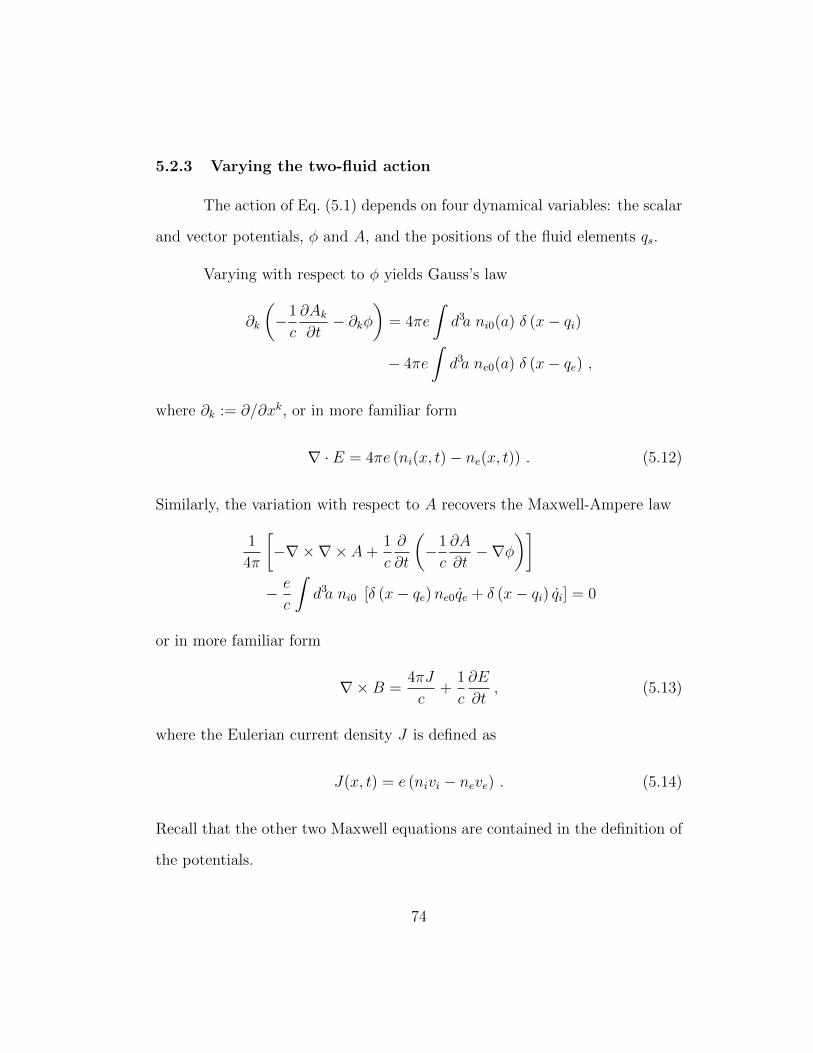
5.2.3 Varying the two-fluid action
The action of Eq. (5.1) depends on four dynamical variables: the scalar
and vector potentials, φ and A, and the positions of the fluid elements qs.
Varying with respect to φ yields Gauss’s law
∂k
(−1
c
∂Ak∂t− ∂kφ
)= 4πe
∫d3a ni0(a) δ (x− qi)
− 4πe
∫d3a ne0(a) δ (x− qe) ,
where ∂k := ∂/∂xk, or in more familiar form
∇ · E = 4πe (ni(x, t)− ne(x, t)) . (5.12)
Similarly, the variation with respect to A recovers the Maxwell-Ampere law
1
4π
[−∇×∇× A+
1
c
∂
∂t
(−1
c
∂A
∂t−∇φ
)]− e
c
∫d3a ni0 [δ (x− qe)ne0qe + δ (x− qi) qi] = 0
or in more familiar form
∇×B =4πJ
c+
1
c
∂E
∂t, (5.13)
where the Eulerian current density J is defined as
J(x, t) = e (nivi − neve) . (5.14)
Recall that the other two Maxwell equations are contained in the definition of
the potentials.
74

Variation with respect to the qs’s is slightly more complex, and we will
show a few intermediate steps. Varying the kinetic energy term is straight
forward and yields
−ns0(a)msqs(a, t) (5.15)
The j-th component of the interaction term results in
esns0(a)
[−1
c
dAj(qs, t)
dt+
1
cqks∂Ak(qs, t)
∂qjs− ∂φ(qs, t)
∂qjs
]= esns0(a)
[−1
c
∂Aj(qs, t)
∂t− 1
cqks∂Aj(qs, t)
∂qks
+1
cqks∂Ak(qs, t)
∂qjs− ∂φ(qs, t)
∂qjs
](5.16)
= esns0(a)
[E(qs, t) +
1
cqs(a, t)× (∇qs × A (qs, t))
]j
.
Note that this expression is purely Lagrangian. The fields A and E are eval-
uated at the positions qs of the fluid elements and the curl ∇qs× is taken
with respect to the Lagrangian position. Also note, since qs = qs(a, t), any
total time derivative of, e.g., A(qs, t) will result in two terms. Variation of the
internal energy term yields
−Aji∂
∂aj
ρ2s0
J 2s
∂U(ρs0Js , ss0
)∂(ρs0Js
) . (5.17)
Setting the sum of Eqs. (5.15)-(5.17) equal to zero and invoking the usual
thermodynamic relations between internal energy and pressure and tempera-
ture,
ps = (msns)2 ∂Us∂(msns)
and Ts =∂Us∂ss
, (5.18)
75

results in the well-known (non-dissipative) two-fluid equations of motion
msns
(∂vs∂t
+ vs · ∇vs)
= esns
(E +
1
cvs ×B
)−∇ps (5.19)
Further analysis (see e.g. Refs. [77, 29]) of these equations usually in-
volves the addition and subtraction of the two-fluid equations and a change of
variable transformation to
V =1
ρm(minivi +meneve)
J = e (nivi − neve)
ρm = mini +mene (5.20)
ρq = e (ni − ne) .
The resulting equations are then simplified by, e.g., making certain
assumptions (quasineutrality, v << c, etc.) and ordering to obtain two new
one-fluid equations – one often referred to as the one-fluid momentum equation
and the other as the generalized Ohm’s law.
5.3 The new one-fluid action
The first step in building an action functional for fluid models is to
decide on the relevant Eulerian observables of the model. Since we want to
derive, e.g., the two-fluid model of Lust and various reductions, our Eulerian
observables are going to be the set n, s, se, V, J, E,B, where s = (misi +
seme)/m, with m = me +mi, and n is a single number density variable.
76

Next we have to define our Lagrangian variables and with them con-
struct the action. Any additional assumption (e.g., quasineutrality etc.) and
ordering will be implemented on the action level. Varying the new action will
then result in equations of motion that, using properly defined Lagrange-Euler
maps, will Eulerianize to, e.g., Lust’s equation of motion and the generalized
Ohm’s law.
5.3.1 New Lagrangian variables
We will start by defining a new set of Lagrangian variables, inspired by
Eq. (5.20)1,
Q(a, t) =1
ρm0(a)(mini0(a)qi(a, t) +mene0(a)qe(a, t))
D(a, t) = e (ni0(a)qi(a, t)− ne0(a)qe(a, t))
ρm0(a) = mini0(a) +mene0(a) (5.21)
ρq0(a) = e (ni0(a)− ne0(a)) .
Here Q(a, t) can be interpreted as a center of mass position variable and D(a, t)
as a local dipole moment variable, connecting an ion fluid element to an elec-
tron fluid element. It is then straight-forward to take the time-derivative
of Q and D which can be interpreted as the center-of-mass velocity Q(a, t)
and a Lagrangian current D(a, t), respectively. Using appropriately defined
1First presented in A. Wurm and P.J. Morrison, Action principle derivation of one-fluidmodels from two-fluid actions, Bulletin of the Am. Phys. Soc, Vol. 54, Nr. 4 (2009).
77

Lagrange-Euler maps, Q(a, t) will map to the Eulerian velocity V (x, t) and
D(a, t) to the Eulerian current J(x, t) as defined by Eq. (5.20).
We will also need the inverse of this transformation,
qi(a, t) =ρm0(a)Q(a, t) + me
eD(a, t)
ρm0(a) + meeρq0
qe(a, t) =ρm0(a)Q(a, t)− mi
eD(a, t)
ρm0(a)− mieρq0
ni0(a) =ρm0(a) + me
eρq0(a)
m(5.22)
ne0(a) =ρm0(a)− me
eρq0(a)
m.
5.3.2 Ordering of fields and quasineutrality
Typically, reductions of the full two-fluid model are obtained by impos-
ing an auxiliary ordering on the equations of motion. In order to preserve the
variational formulation, we perform an ordering directly in the action.
To construct the action, we will start with the two-fluid action of
Eq. (5.1) and change variables to Q and D, but in light of the fluid mod-
els we are interested in, we will first make two simplifying assumptions: We
order the fields in the action so that the displacement current in Eq. (5.13)
will vanish, and we assume quasineutrality. In this section, we describe this
field ordering in detail and discuss quasineutrality in the Lagrangian variable
context, which as far as we know has not been done before.
The omission of the displacement current is allowed, when the time
78

scale of changes in the field configuration is long relative to the time it takes
for radiation to “communicate” these changes across the system [106]. We
use non-dimensional variables by introducing a characteristic scale B0 for the
magnetic field and a characteristic length scale ` for gradients. Times are
then normalized by the Alfven time tA = B0/√
4πρ and the qs’s by the Alfven
speed vA = `/tA, resulting in the following form for the sum of the field and
interaction terms of the Lagrangian (5.4):
B20
8π
∫dt
∫d3x
∣∣∣∣∣−vAc ∂A∂t − φ0
B0`∇φ
∣∣∣∣∣2
−∣∣∣∇ × A∣∣∣2
+∑s
B20
[∫dt
∫d3a n0ns0(a)es
∫d3x δ (x− qs) ×
(vA`
B0cˆqs · A−
φoB2
0
φ
)],
where φ0 and n0 are yet to be specified scales for the electrostatic potential
and the densities of both species, respectively. We also require that the two
species’ velocities are of the same scale. Requiring the two interaction terms
in the Lagrangian to be of the same order results in a scaling for φ; viz.,
φ0 ≡ B0`vA/c. Thus, both parts of the |E|2 term are of order O (vA/c).
Neglecting this term and varying with respect to A results in
∇ × B =4πen0vA
c
`
B0
(∫d3a δ(x− qi)ni0(a) ˆqi −
∫d3a δ(x− qe)ne0(a) ˆqe
),
which can be written as
B0
`∇ × B =
4πj0cJ , (5.23)
where j0 = en0vA is a scale for the current.
Varying the scaled action with respect to φ yields
0 =
∫d3a δ(x− qi)ni −
∫d3a δ(x− qe)ne ≡ ∆n . (5.24)
79

The above equation states that the difference in the two densities is zero,
i.e., the plasma is quasineutral, a property that holds locally, i.e., ni(x, t) =
ne(x, t). Using Eq. (5.6), this statement would correspond to the following in
the Lagrangian variable picture:
ni0(a)
Ji(a, t)
∣∣∣∣a=q−1
i (x,t)
=ne0(a)
Je(a, t)
∣∣∣∣a=q−1
e (x,t)
. (5.25)
In the Lagrangian picture we will make the additional assumption of
homogeneity: ni0(a) = ne0(a) = constant, which is natural for the plasma
we are modeling. It states that at t = 0 all fluid elements are identical in
the amount of density they carry. Therefore, ni0 and ne0 can be replaced by
a constant n0. Equation (5.25) then reduces to a statement about the two
Jacobians
Ji(a, t)∣∣∣a=q−1
i (x,t)= Je(a, t)
∣∣∣a=q−1
e (x,t), (5.26)
which will play a central role in our development below.
Note, that the homogeneity assumption (ni0 = ne0 = n0) does not
prohibit us from describing quasineutral plasmas with density gradients. What
we would have to do in this case, would be to pick our labeling scheme, and
hence the Jacobian, accordingly, as to reflect the initial density gradient of
the configuration. Thus there is freedom in this regard beyond what we are
assuming now.
80

5.3.3 Action functional
We are now ready to implement the change of variables discussed in
Sec. 5.3.1. Because of the homogeneity assumption ni0(a) = ne0(a) = n0, the
new variables of Eq. (5.21) reduce to
Q(a, t) =mi
mqi(a, t) +
me
mqe(a, t)
D(a, t) = en0 (qi(a, t)− qe(a, t))
ρm0(a) = mn0 (5.27)
ρq0(a) = 0
and the inverse transformation of Eq. (5.22) to
qi(Q,D) := qi(a, t) = Q(a, t) +me
men0
D(a, t)
qe(Q,D) := qe(a, t) = Q(a, t)− mi
men0
D(a, t) , (5.28)
where we choose the notation qs(Q,D) to emphasize that the qs should not be
thought of as ion/electron trajectories any more but as specific linear combi-
nations of Q(a, t) and D(a, t). In addition, we will need the ion and electron
Jacobians, Ji(Q,D) and Je(Q,D), now expressed in terms of Q and D.
81

The resulting action functional has the form:
S =− 1
8π
∫dt
∫d3x |∇ × A(x, t)|2
+
∫dt
∫d3x
∫d3a n0
δ(x− qi(Q,D))
[e
c
(Q(a, t) +
me
men0
D(a, t)
)·A(x, t)− eφ(x, t)
]
+
∫dt
∫d3x
∫d3a n0
δ(x− qe(Q,D))
[−ec
(Q(a, t)− mi
men0
D(a, t)
)·A(x, t) + eφ(x, t)
]
+1
2
∫dt
∫d3a n0
[mi|Q|2(a, t) +
mime
me2n20
|D|2(a, t)
]
−∫dt
∫d3a n0
[miUi
(min0
Ji(Q,D), (ms0 −mese0)/mi
)+meUe
(men0
Je(Q,D), se0
)],
(5.29)
where recall s0 = (misi0 +mese0)/m.
5.3.4 Nonlocal Lagrange-Euler maps
Now we define the Lagrange-Euler maps that connect the Eulerian ob-
servables V and J to the new Lagrangian variables Q and D. Referring to
Sec. 4.2, one can see that a Lagrange-Euler map is a relationship between a
Lagrangian quantity and some Eulerian observables, which holds only when
it is evaluated on a trajectory x = qs(a, t). If we apply the inverse Lagrange-
Euler maps from Eqs. (5.6) and (5.9) to Eq. (5.20) and assume quasineutrality,
82

we get
V (x, t) =mi
mqi(a, t)
∣∣∣a=q−1
i (x,t)+me
mqe(a, t)
∣∣∣a=q−1
e (x,t)
J(x, t) = e
(n0
Ji(a, t)qi(a, t)
)∣∣∣∣a=q−1
i (x,t)
−e(
n0
Je(a, t)qe(a, t)
)∣∣∣∣a=q−1
e (x,t)
n(x, t) =mi
m
(n0
Ji(a, t)
)∣∣∣∣a=q−1
i (x,t)
+me
m
(n0
Je(a, t)
)∣∣∣∣a=q−1
e (x,t)
(5.30)
s(x, t) =mi
msi0
∣∣∣a=q−1
i (x,t)+me
mse0
∣∣∣a=q−1
e (x,t)(5.31)
se(x, t) = se0
∣∣∣a=q−1
e (x,t). (5.32)
The definitions of Q(a, t) and D(a, t) in Eq. (5.27) suggest that their
time-derivatives should be associated with V and J , respectively. However,
both Q and D are nonlocal objects, since they relate the velocities of electrons
and ions which are located at different points in space. This means that neither
Q, nor D, when evaluated at the inverse maps for a, can Eulerianize to a local
velocity or current, since, in general, x = qi(Q,D) and x′ = qe(Q,D) with x 6=
x′ or, they are simultaneously evaluated at different trajectories. Therefore,
we have two different inverse functions where the Lagrangian quantities are to
be evaluated, namely, a = q−1i (x, t) and a = q−1
e (x′, t) which should be thought
of as the inverse functions of x = qi(Q,D) and x′ = qe(Q,D). To make this
83

work, we define our Lagrange-Euler maps with x = x′ as
V (x, t) =mi
m
(Q(a, t) +
me
men0
D(a, t)
)∣∣∣∣a=q−1
i (x,t)
(5.33)
+me
m
(Q(a, t)− mi
men0
D(a, t)
)∣∣∣∣a=q−1
e (x,t)
J(x, t) =en0
Ji(a, t)
(Q(a, t) +
me
men0
D(a, t)
)∣∣∣∣a=q−1
i (x,t)
− en0
Je(a, t)
(Q(a, t)− mi
men0
D(a, t)
)∣∣∣∣a=q−1
e (x,t)
.
Due to Eq. (5.26), the two Jacobian determinants are equal (as long as they
are evaluated at the respective inverse functions) and can be replaced by a
common Jacobian determinant, J .
The maps just defined are straight-forward to apply for mapping an
Eulerian statement to a Lagrangian one, but for our purpose, we have to
invert them. To keep careful track of the two inverse functions, we first invert
the intermediate relations
V (x, t) +me
men(x, t)J(x, t)
=
(Q(a, t) +
me
men0
D(a, t)
)∣∣∣∣a=q−1
i (x,t)
(5.34)
V (x, t)− mi
men(x, t)J(x, t)
=
(Q(a, t)− mi
men0
D(a, t)
)∣∣∣∣a=q−1
e (x,t)
, (5.35)
where we have used Eq. (5.6). The inverse Lagrange-Euler maps are now given
84

by
Q(a, t) =mi
m
(V (x, t) +
me
men(x, t)J(x, t)
)∣∣∣∣x=qi(Q,D)
+me
m
(V (x′, t)− mi
men(x′, t)J(x′, t)
)∣∣∣∣x′=qe(Q,D)
D(a, t) = en0
(V (x, t) +
me
men(x, t)J(x, t)
)∣∣∣∣x=qi(Q,D)
− en0
(V (x′, t)− mi
men(x′, t)J(x′, t)
)∣∣∣∣x′=qe(Q,D)
. (5.36)
Note that the construction of the maps of Eqs. (5.33) and (5.36) can be done
with any invertible linear combination of the time derivatives of our Lagrangian
variables. The only restriction is that the action should comply with the
Eulerian Closure Principle, i.e., it should be expressible entirely in terms of
the Eulerian observables. It is straightforward to show that this is true in our
case.
5.3.5 Lagrange-Euler maps without quasineutrality
Had we not assumed quasineutrality, we would have to proceed dif-
ferently: Eq. (5.20) implies that the proper Lagrangian variables that would
85

Eulerianize to velocity and current would be
V (x, t) =
mi
(ni0Ji qi(a, t)
)∣∣∣a=q−1
i (x,t)
mi
(ni0Ji
)∣∣∣a=q−1
i (x,t)+ me
(ne0Je
)∣∣∣a=q−1
e (x,t)
+me
(ne0Je qe(a, t)
)∣∣∣a=q−1
e (x,t)
mi
(ni0Ji
)∣∣∣a=q−1
i (x,t)+ me
(ne0Je
)∣∣∣a=q−1
e (x,t)
,
J(x, t) = e
(ni0Jiqi(a, t)
)∣∣∣∣a=q−1
i (x,t)
− e
(ne0Je
q(a, t)
)∣∣∣∣a=q−1
e (x,t)
.
The above equations suggest that without quasineutrality, the definitions for
Q, D, etc. should be modified to the following:
Q(a, t) =1
ρm0(a)
(miJeni0(a)qi(a, t) +meJine0(a)qe(a, t)
)D(a, t) = e
(Jeni0(a)qi(a, t)− Jine0(a)qe(a, t)
)ρm0(a) = miJeni0(a) +meJine0(a)
where Q/ (JiJe) maps to V (x, t) and D/ (JiJe) to J(x, t). In this case, how-
ever, both Q and D are implicitly defined, since Ji and Je depend on them.
This problem is absent when only manipulating the Eulerian equations of mo-
tion. It might suggest though that when quasineutrality does not hold, the
one-fluid description might not be appropriate. To see why this is so, consider
the following example: in order to satisfy the ECP for the kinetic energy term,
we swap the label volume element with the position volume element, divided
by a Jacobian. This Jacobian combines with the n0 to give the Eulerian den-
sity n(x, t). When quasineutrality does not hold, we would have instead an ni0
86

and an ne0, each needing each own Jacobian to be Eulerianized. This means,
that within the one-fluid formalism, we would still be required to keep track
of electron and ion labels, i.e., have two different label space volume elements.
This can also be seen in the most general case derived by Lust in Ref. [77]. The
resulting equations of motion in V and J still contain terms explicitly referring
to ion/electron quantities, e.g., ni and ne. In conclusion, from a variational
point of view, it is not obvious how to apply the Eulerian Closure Principle
without quasineutrality, within the context of a single fluid model. It seems
that in order to preserve it, one would need to distinguish between integrations
over ion and electron labels, so that the d3a could be related to the proper Js.
5.3.6 Derivation of the continuity and entropy equations
Before we derive the equations of motion for several different models
in the next section, we derive here the continuity equation, which all of the
models below have in common, and the entropy equations.
Due to the identity of the Jacobians from Eq. (5.26), Eq. (5.30) for n
reduces to
n(x, t) =
(n0
Ji(a, t)
)∣∣∣∣a=q−1
i (x,t)
=
(n0
Je(a, t)
)∣∣∣∣a=q−1
e (x,t)
, (5.37)
where q−1s are still the inverse functions of qs(Q,D). Inverting the equation
for the ions and taking the time derivative yields
dn
dt
∣∣∣∣x=qi(Q,D)
=d
dt
n0
Ji(a, t)= − n0
J 2i (a, t)
∂Ji∂t
.
87

To Eulerianize the equation above, we use the well-known relations d/dt =
∂/∂t+ v · ∇ and ∂J /∂t = J∇ · v that we proved in Sec. 4.2. The key here is
to use the correct Eulerian velocity, in this case the ion velocity in terms of V
and J . The result is
∂n
∂t+(V +
me
menJ)· ∇n = −n∇ ·
(V +
me
menJ)
which can be further reduced to
∂n
∂t+∇ · (nV ) +
me
me∇ · J = 0 .
However, we already know from Eq. (5.23) that ∇ · J = 0. Therefore, no
matter which equality we choose in Eq. (5.37), the continuity equation will be
the same,
∂n
∂t+∇ · (nV ) = 0 . (5.38)
Similarly, from Eq. (5.31) we obtain
∂s
∂t+ V · ∇s = 0
and from Eq. (5.32)
∂se∂t
+(V − mi
menJ)· ∇se = 0 ,
or to leading order in me/mi
∂se∂t
+
(V − 1
enJ
)· ∇se = 0 .
88

5.4 Derivation of reduced models
If we vary the action functional (5.29) with respect to Q and D and sub-
sequently apply the Lagrange-Euler map we recover the momentum equation
and generalized Ohm’s law of Lust2 (in the non-dissipative limit):
nm
(∂V
∂t+ (V · ∇)V
)(5.39)
= −∇p+J ×Bc− mime
me2(J · ∇)
(J
n
)E +
V ×Bc
=mime
me2n
(∂J
∂t+ (J · ∇)V − (J · ∇)
(J
n
)+ (∇ · V )J
)+mime
me2(V · ∇)
(J
n
)+
(mi −me)
menc(J ×B)
− mi
men∇pe +
me
men∇pi . (5.40)
We will not show this lengthy, although straightforward, calculation here, but
instead show the detailed derivation of extended MHD in the next section
which requires one more ordering in the action of Eq. (5.29).
5.4.1 Extended MHD
At this point we will make one more simplification: We define the mass
ratio µ = me/mi and order the action functional keeping terms up to first
2Note, there are typos in Eqs. (2.9) and (2.10) of Ref. [77] that prevent the term N1 fromvanishing when imposing quasineutrality, as it should.
89

order in µ. Up to first order, the change of variables is
qi(Q,D) = Q(a, t) +µ
en0
D(a, t)
qe(Q,D) = Q(a, t)− 1− µen0
D(a, t) (5.41)
and the action takes on the form
S = − 1
8π
∫dt
∫d3x |∇ × A(x, t)|2
+
∫dt
∫d3x
∫d3a n0
δ(x− qi(Q,D))
×[e
cQ(a, t) +
µ
cn0
D(a, t)·A(x, t)− eφ(x, t)
]
+
∫dt
∫d3x
∫d3a n0
δ(x− qe(Q,D))
×[−ecQ(a, t) +
(1− µ)
cn0
D(a, t)·A(x, t) + eφ(x, t)
]
+1
2
∫dt
∫d3a n0mi
((1 + µ)|Q|2(a, t) +
µ
e2n20
|D|2(a, t)
)
−∫dt
∫d3a n0
(Ue
(n0
Je(Q,D), se0
)+ Ui
(n0
Ji(Q,D), si0
)). (5.42)
where for convenience we have replaced the Us, the internal energy per unit
mass, by Us, the internal energy per particle. The pressure is obtained from
the latter according to ps = n2∂Us/∂n.
90

Varying the action with respect to Qk yields
0 = −n0mi(1 + µ)Qk(a, t)− ∂kp
+ n0
[e
c
(Qj(a, t) +
µ
en0
Dj(a, t)
)∂Aj(x, t)
∂xk−e∂kφ(x, t)− e
c
d
dtAk(x, t)
] ∣∣∣∣∣x=qi(Q,D)
+ n0
[−ec
(Qj(a, t)−
(1− µ)
en0
Dj(a, t)
)∂Aj(x, t)
∂xk+e∂kφ(x, t) +
e
c
d
dtAk(x, t)
] ∣∣∣∣∣x=qe(Q,D)
.
(5.43)
The variation of the internal energy term proceeds by varying qs through
Eqs. (5.41), giving δqs = δQ and using these expressions in the variation of the
Jacobians Js. We have given the Eulerian result since the Lagrangian one has
two terms of the form of Eq. (5.17), and it is cumbersome to carry this through
the rest of the calculation. (See Ref. [63] for a treatment that orders the Eu-
lerian equations directly.) Consistent with Dalton’s law, the total single fluid
pressure is p = pi + pe and both these pressures come in entirely at the zeroth
order of µ. Note, that the two time derivatives of A do not cancel, because
they are advected by different flows, or, since we are still in the Lagrangian
framework, they are evaluated at different arguments.
To find the Eulerian equations of motion, we start with Eq. (5.36) (up
to first order in µ) and impose locality, i.e., x = x′, such that Q maps to
V (x, t) and D to J(x, t). However, the time derivatives of Q and D have to
be treated with care as they each consist of two terms that are advected with
different velocities. We will show how to Eulerianize the equations of motion
in detail.
91

The Q in the first term of Eq. (5.43) can be re-written as
Q(a, t) (5.44)
= (1− µ)d
dt
(V (x, t) +
µ
en(x)J(x, t)
)∣∣∣∣x=qi(Q,D)
+ µd
dt
(V (x, t)− (1− µ)
en(x)J(x, t)
)∣∣∣∣x=qe(Q,D)
= (1− µ)
(∂V
∂t+∂qi∂t· ∇V +
µ
en
∂
∂t
(J
n
)(5.45)
+µ
e
∂qi∂t· ∇(J
n
))+ µ
(∂V
∂t+∂qe∂t· ∇V
−(1− µ)
en
∂
∂t
(J
n
)− (1− µ)
e
∂qe∂t· ∇(J
n
)).
From Eqs. (5.41), we can find explicit expressions for the time derivatives of
the qs(Q,D),
∂qi∂t
= Q+µ
en0
D −→ V +µ
enJ (5.46)
∂qe∂t
= Q− 1− µen0
D −→ V − 1− µen
J . (5.47)
Inserting these expression into Eq. (5.45), we find after some algebra that
Q(a, t) −→ ∂V
∂t+ (V · ∇)V +
µ(1− µ)
ne2(J · ∇)
(J
n
). (5.48)
Next we Eulerianize the interaction terms of Eq. (5.43) using Eq. (5.36)
(up to first order in µ) and Eq. (5.41). The result is
ne
c
[(Vj +
µ
enJj
) ∂Aj∂xk− c∂kφ−
∂Ak∂t− ∂qi
∂t· ∇Ak
]
+ne
c
[(−Vj +
(1− µ)
enJj
)∂Aj∂xk
+ c∂kφ+∂Ak∂t
+∂qe∂t· ∇Ak
], (5.49)
92

which, after substitution using Eqs. (5.46) and (5.47), yields
1
c
(Jj∂Aj∂xk− Jj
∂Ak∂xj
)=
(J × (∇× A))kc
. (5.50)
The full Eulerian version of the equation of motion for the velocity of
Eq. (5.43), also referred to as the momentum equation is
nm
(∂V
∂t+ (V · ∇)V
)= −∇p+
J ×Bc− me
e2(J · ∇)
(J
n
). (5.51)
Note, it was shown in Ref. [63] that the last term of Eq. (5.51) is necessary for
energy conservation.
Next, varying the action with respect to Dk yields
0 =miµ
n0e2Dk(a, t) +
(1− µ)
en0
∂kpe −µ
en0
∂kpi
+ µ
[(−1
c
d
dtAk(x, t)− ∂kφ(x, t) +
1
c
(Qj(a, t) +
µ
en0
Dj(a, t)
)∂Aj(x, t)
∂xk
)]∣∣∣∣x=qi(Q,D)
+ (1− µ)
[(−1
c
d
dtAk(x, t)− ∂kφ(x, t) +
1
c
(Qj(a, t) −
(1− µ)
en0
Dj(a, t)
)∂Aj(x, t)
∂xk
)]∣∣∣∣x=qe(Q,D)
(5.52)
This time the Jacobians of the internal energies are varied using δqe = −(1−
µ)δD/(en0) and δqi = µδD/(en0), which again follow from Eqs. (5.41). Note,
it is for this reason that only the electron pressure appears to leading order in
Ohm’s law for extended MHD.
Eulerianizing the D term in Eq. (5.52) yields
miµ
n0e2D(a, t) =
miµ
e2n
(∂J
∂t+ (J · ∇)V − (J · ∇)
(J
n
)+ (∇ · V )J
)+miµ
e2(V · ∇)
(J
n
)+miµ
e2n2J(V · ∇)n , (5.53)
93

where we have used the continuity equation Eq. (5.38) to eliminate the time
derivative of n and kept leading order in µ terms. The interaction terms in
Eq. (5.52) reduce to
E +V × (∇× A)
c− (1− 2µ)
encJ × (∇× A) . (5.54)
In Eqs. (5.53) and (5.54) we see the presence of some terms involving µ, in
front of D and J × B, respectively. However, in the latter case it occurs in
the factor (1 − 2µ) and since our ordering is µ << 1, we can drop the µ-
dependence in Eq. (5.54), to lowest order. However, in Eq. (5.53), we cannot
throw out all the terms that depend on µ since the factor µmi/(ne2) cannot
be cast into a dimensionless form, and hence one cannot invoke the ordering
µ << 1 here. Post-variation, the discrepancy in the order of the derived terms,
i.e. the existence of these anomalous terms, has also been observed elsewhere
[75].
The Eulerian version of the equation of motion of the current Eq. (5.52)
(after keeping zeroth order in µ), also known as generalized Ohm’s law, is then
E +V ×Bc
=me
e2n
(∂J
∂t+ (J · ∇)V − (J · ∇)
(J
n
)+ (∇ · V )J
)+
(J ×B)
enc− ∇pe
en+me
e2(V · ∇)
(J
n
)+
me
e2n2J(V · ∇)n . (5.55)
The last two terms on the right hand side of Eq. (5.55) can be combined to
give (me/(e2n)) (V · ∇)J and since ∇ · J = 0, we can add a V (∇ · J) term
without changing the result, and combine most terms in the divergence of the
94

tensor V J + JV to obtain the following equation:
E+V ×Bc
=me
e2n
(∂J
∂t+∇ · (V J + JV )
)−me
e2n(J ·∇)
(J
n
)+
(J ×B)
enc−∇peen
.
(5.56)
Equations (5.51) and (5.56) constitute the extended MHD model.
5.4.2 Hall MHD
Hall MHD is a limiting case, for which previous work of an action
functional nature exists [48, 141]. Here we obtain the actional functional by
expanding and retaining only terms up to zeroth order in µ, i.e., if we neglect
the electron inertia (me → 0), the action of Eq. (5.29) reduces to
S = − 1
8π
∫dt
∫d3x |∇ × A(x, t)|2
+
∫dt
∫d3a n0
[1
2m|Q|2(a, t)− Ui
(n0
Ji(Q), si0
)− Ue
(n0
Je(Q,D), se0
)]+
∫dt
∫d3x
∫d3a n0
δ
(x−Q(a, t)− 1
en0
D(a, t)
)×[−ec
(Q(a, t)− 1
en0
D(a, t)
)· A(x, t) + eφ(x, t)
]+
∫dt
∫d3x
∫d3a n0
δ (x−Q(a, t))×
[ecQ(a, t) · A(x, t)− eφ(x, t)
],
(5.57)
and Eqs. (5.41) become
qi(Q,D) = Q(a, t)
qe(Q,D) = Q(a, t)−D(a, t)/(en0) (5.58)
Observe we have also replaced mi by m in the kinetic energy term, which is
correct to leading order in µ.
95

The inverse maps required for Eulerianizing the equations of motion
reduce to
Q(a, t) = V (x, t)
∣∣∣∣x=qi=Q
D(a, t) = en0V (x, t)
∣∣∣∣x=qi=Q
− en0
(V (x′, t)− J(x′, t)
en(x′, t)
)∣∣∣∣x′=qe(Q,D)
. (5.59)
Following the procedure outlined in the previous section for extended MHD,
we arrive at what is commonly referred to as Hall MHD,
nm
(∂V
∂t+ (V · ∇)V
)= −∇p+
J ×Bc
(5.60)
E +V ×Bc
=J ×Bnec
− 1
ne∇pe , (5.61)
which are the usual forms of the momentum equation and Ohm’s law for Hall
MHD.
5.4.3 Electron MHD
Electron MHD [68, 10, 109, 55] is another limiting case where we neglect
the ion motion completely. This theory is used to describe the short time scale
motion of the electrons in a neutralizing ion background. Since the ions are
immobile, we require qi = 0 and qi = qi(a). Also, we require that there be
no electric field and, consequently, we neglect φ from the action. In this case,
using the Q, D formulation of the previous sections is redundant since there
is only a single fluid. From qi = 0 we find D = − (en0m/me) Q. (The same
relation holds between Q and D up to an additive constant which represents
the constant position of the ion). In addition, the Lagrange-Euler map takes
96

on the simple form
ve(x, t) =
(1 +
1
µ
)Q(a, t)
∣∣∣∣a=q−1
e (x,t)
, (5.62)
where
qe(a, t) = (1 +1
µ)Q(a, t) . (5.63)
The remaining terms in the action are
S = − 1
8π
∫dt
∫d3x |∇ × A(x, t)|2
+
∫dt
∫d3a n0
[1
2me|qe|2(a, t)− Ue
(n0
Je(Q)
)]−∫dt
∫d3x
∫d3a δ (x− qe)
en0
cqe · A(x, t) , (5.64)
which is essentially the same action as that of Ref. [55]. It is also straight-
forward to express this action in terms of Q using Eqs. (5.62) and (5.63).
Upon varying the action (either in terms of qe or Q) and Eulerianizing
the following equation of motion and constraint are obtained:
me
(∂ve∂t
+ ve · ∇ve)
+e
c
∂A
∂t=e
c(ve ×B)− ∇pe
n
∇×B =− 4π
cenve ,
which are the usual equations of electron MHD.
5.5 Noether’s theorem
In this section we will investigate the invariants of the action function-
als for the quasineutral Lust equations of Eq. (5.29) and the extended MHD
97

system of Eq. (5.42) using Noether’s theorem. Note that both actions can be
expressed either in terms of (Q,D) or in terms of (qi, qe), which are related
through a simple linear transformation, e.g., Eq. (5.27). Furthermore, both
sets of variables obey the Eulerian Closure Principle. Hence, it is equivalent
to work with an action expressed in terms of either set of variables. For con-
venience, we shall work with the latter set, as the Euler-Lagrange maps are
easier to apply. Noether’s theorem states that if an action is invariant under
the transformations
q′s = qs +Ks (qs, t) ; t′ = t+ τ (t) , (5.65)
i.e.,
S =
∫ t2
t1
dt
∫d3z L (qs, qs, z, t)
=
∫ t′2
t′1
dt′∫d3z′ L (q′s, q
′s, z′, t′) ,
then there exist constants of motion given by
C =
∫d3z
[τ
(∂L∂qs· qs − L
)−Ks ·
∂L∂qs
], (5.66)
where the index s represents the number of independent variables q in the
system. Our actions are mixed Lagrangian and Eulerian, so the variable z can
denote a or x.
98

1. Time translation
It is straight-forward to see that the action is invariant under time
translation with
Ks = 0; τ = 1 .
The corresponding constant of motion, the energy, is found to be
E =
∫d3x
[|∇ × A|2
8π+∑s
∫d3a
(1
2n0ms|qs|2 + n0 Us
(n0
Js, ss0
))].
Using suitable Lagrange-Euler maps to express our answer in terms of the
Eulerian variables n, V, J, we obtain
E =
∫d3x
[|B|2
8π+ nUi + nUe +mn
|V |2
2+memi
mne2
|J |2
2
], (5.67)
for the quasineutral Lust model and
E =
∫d3x
[|B|2
8π+ nUi + nUe +mn
|V |2
2+me
ne2
|J |2
2
], (5.68)
for the extended MHD model. Note that the two energies are different since
the extended MHD model includes the mass ratio ordering.
2. Space translation
Space translations correspond to
Ks = k; τ = 0 ,
where k is an arbitrary constant vector. Under space translations, the constant
of motion is the momentum, which is found to be
P = k·∫d3a (n0miqi + n0meqe) + k·
∫d3x
e
cA
∫n0 [δ (x− qi)− δ (x− qe)] d3a
.
99

Using the Lagrange-Euler maps one can show that
P = k ·∫d3x nmV
is the conserved quantity. Note that k is entirely arbitrary, and hence we see
that the total momentum
P =
∫d3x ρV (5.69)
is conserved. This is also evident from the corresponding dynamical equation
for V .
3. Rotations
The actions are also invariant under rotations which correspond to
Ks = k × qs; τ = 0 .
Following the same procedure as before, we have
L = k ·∫d3x nmr × V ,
and since we know that k is arbitrary, we conclude that the angular momentum
given by
L =
∫d3x ρ r × V (5.70)
is a constant of motion.
100

4. Galilean boosts
When discussing boosts, we have to consider that the action may remain
invariant even when the following holds
S =
∫ t2
t1
dt
∫d3z L (qs, qs, z, t)
=
∫ t′2
t′1
dt′∫d3z′ (L (q′s, q
′s, z′, t′) + ∂µλ
µ) ,
because the second term vanishes identically. In all the previous derivations
of the constants of motion, the infinitesimal transformations did not involve
time explicitly. A boost, though, corresponds to
Ks = ut; τ = 0 ,
where u is an arbitrary constant velocity. For a Galilean boost in a one-fluid
model, the corresponding invariant quantity is given by
B =
∫d3a mn (q − qt) ,
and since we have two different species, this generalizes to
B =∑s
∫d3a msns (qs − qst) .
Using the corresponding Lagrange-Euler maps, the Eulerianized expression is
given by
B =
∫d3x ρ (x− V t) . (5.71)
101

Chapter 6
Dirac Constraints
In the present chapter, we will present two worked examples of the
method of Dirac for imposing constraints on Hamiltonian systems. As we
mentioned in Sec. 1.1 oftentimes, we seek reduced descriptions of systems that
retain the fundamental physics and we desire these reduced models to retain
the Hamiltonian character of the ideal parent model. Now, we will undertake
the problem of imposing constraints to a Hamiltonian system in a way that
preserves the Hamiltonian character.
The method of Dirac is general [22] and has been applied to finite
and infinite-dimentional Hamiltonian systems [99, 100], has been used for
the derivation of incompressible fluid dynamics and magnetohydrodynamics
[16, 98], reduced fluid models of plasma physics [17], and for the description
of dynamics in fluids with free boundaries [91]. The method consists of a pro-
cedure that leads to a new bracket for the constrained system, known as the
Dirac bracket, which is bilinear, antisymmetric, satisfies the Jacobi identity
and furthermore, when one takes the bracket of anyone of the constrains with
any other quantity, the bracket vanishes. For an introduction to the method,
the interested reader might want to refer to the textbooks of [35], [120] or [119]
102

and [79]. Here, we will not formally present the method but rather illustrate
it using two worked examples relevant to reduced modelling. We will avoid
using the notions of strong and weak equality even though they are key and
should be understood before we embark on the calculation. To this effect,
we define them and we discuss briefly their ramifications. We say that two
phase space functions f and g are strongly equal when their equality holds
throughout phase space and that they are weakly equal when they are equal
only when the constraints are enforced. To make this idea concrete, we add
a brief note: Imagine that we have a system of equations for the evolution
of density and pressure. In this model, pressure and density are dynamical
variables and we have separate, yet coupled, equations that give their time
evolution. Now, lets suppose that we want to impose the constraint that the
pressure is a specific function of the density, p = f(n) and plug this equality in
the equations of motion. Of course, this can only serve as an initial condition
since the dynamics will evolve both p and n independently and after a while,
in general p 6= f(n). This would be an example of a weak equality. If we want
the condition p = f(n) to hold for all times, i.e, to be a strong equality, then
we need to impose it as a constraint. In that event, the Dirac method will
give us a new bracket and new equations of motion where additional terms
will appear. They should be understood as generalized forces, that constrain
the original system to evolve in such a way as to preserve the constraints.
103

6.1 Dirac Constraints on the Hazeltine Model
6.1.1 Definitions
For the first worked example of the Dirac method we choose a model
initially presented in Ref. [38] and shown to be Hamiltonian in Ref. [39]. The
model was used for the study of electromagnetic solitary drift waves. It is a
three field model involving the electrostatic potential φ, the parallel component
of the magnetic flux ψ and a variable χ which is defined as the departure of
the plasma density n from a constant value nc, or in other words, the density
perturbation. Also, we introduce the variables U and J which stand for the
vorticity and the parallel current density respectively, through the relations:
U =∇2⊥φ , (6.1)
J =∇2⊥ψ . (6.2)
In terms of these fields, the system of equations, when appropriate normaliza-
tions have been made, is given by:
∂U
∂t+ [φ, U ] +∇‖J = 0 , (6.3)
∂ψ
∂t+∇‖φ = ηJ + α∇‖χ , (6.4)
∂χ
∂t+ [φ, χ] +∇‖J = 0 , (6.5)
where ∇‖f = ∂f/∂z− [Ψ, f ], with [·, ·] denoting the canonical Poisson bracket,
so that [f, g] = z · (∇f × ∇g). Eq. (6.3) is the vorticity evolution equation
and is identical to the RMHD one. Eq. (6.4) is a generalized Ohm’s law where
the parallel component of the electric field is equated to the parallel current
104

plus the pressure gradient, where here, because the model is isothermal, is
only given as the gradient of the pressure perturbation. η here is a normalised
collisional resistivity which we will later drop as we are only interested in the
non-dissipative dynamics. α is a parameter defined as the squared ratio of
the ion gyroradius to transverse scale lengths, α =ρ2s
L. By transverse scale
lengths we mean the length scale of variation of quantities perpendicular to
the magnetic field, i.e., ∇−1 ∼ L. Finally, Eq. (6.5) describes the conservation
of the density. The second term is the usual E × B advection term while the
third one implies that the divergence of the electron parallel flow is the total
parallel current divergence since ion flow is very small.
The Hamiltonian of this system, as given in Ref. [39] is:
H =1
2
∫d3x((∇⊥ψ)2 + (∇⊥φ)2 + αχ2
), (6.6)
where we can clearly discern the terms for magnetic field energy, electrostatic
field energy and kinetic energy.
The Lie-Poisson bracket for the above system is:
F,G =
∫d2xU [FU , GU ] + χ[Fχ, Gχ]
+ ψ([Fψ, GU +Gχ]− [Gψ, FU + Fχ])
+ χ([Fχ, GU ]− [Gχ, FU ]) . (6.7)
Even though the system is three-dimensional, for the rest of this section, we
focus only on it’s two-dimensional limit by discarding the terms ∂φ∂z
, ∂χ∂z
, and
∂J∂z
. This is the reason that we present only the two-dimensional version of the
Lie-Poisson bracket.
105

6.1.2 Constraints and change of variables
As it can be immediately observed [38], the above model reduces to
the low-β RMHD one when α is neglected. This is appropriate when the
transverse perturbations have a scale length much larger than the gyroradius.
Also, the vorticity equation Eq. (6.3), reduces to the famous Hasegawa-Mima
[36] equation when the electrons are assumed to be adiabatic, i.e, αχ = φ.
Because this is an equation involving dynamical fields, as we know from the
introduction to this chapter, it can only be prescribed as an initial condition.
Here, we are interested in imposing electron adiabaticity as a Dirac constraint
and recovering the constrained dynamical equations through the Dirac pro-
cedure. Because the method of Dirac usually works with an even number of
constraints1, we need one more constraint. For our other constraint, we will
choose to impose that the magnetic flux is only a function of x. This is indeed
a very strong constraint yet not completely unphysical. We can imagine a
scenario where the magnetic field is imposed externally by a coil configuration
which has an active, real-time feedback loop that regulates the current in such
a way as to preserve the flux constraint. Certainly, this kind of control will
induce generalized forces that will force the system to develop on the curve of
the constraint. Therefore, the two constraints we want to impose are:
Φ1(x) =U − α∆χ = 0 , (6.8)
Φ2(x) =ψ − f(x) = 0 . (6.9)
1The reader who is interested in finding examples of the Dirac method working with anodd number of constraints is referred to Ref. [14]
106

To simplify the calculations to follow, we make the following change of vari-
ables:
U = χ , (6.10)
ψ = ψ , (6.11)
χ = U − χ . (6.12)
With this change of variables, the variational derivatives of the Hamil-
tonian (6.6) with respect to the new fields become:
HU = αU − φ , (6.13)
Hψ = −J , (6.14)
Hχ = −φ . (6.15)
where ∇2φ = U + χ and ∇2ψ = J and the transformed equations of motion
Eq. (6.3) – Eq. (6.5) are:
U =[U, φ] + [ψ, J ] , (6.16)
ψ =[ψ, φ− αU ] , (6.17)
χ =[χ, φ] . (6.18)
The Lie-Poisson bracket (6.7) becomes:
F,G =
∫d2xU [FU , GU ] + χ[Fχ, Gχ] + ψ
([Fψ, GU ] + [FU , Gψ]
), (6.19)
107

and the new constraints are given by:
Φ1(x) =U + χ− α∆U = 0 , (6.20)
Φ2(x) =ψ − f(x) = 0 . (6.21)
For the calculations that will follow, it will prove useful to define the
operators: L∆ = −1+α∆, Lξ = [ξ, ·] where ξ can be any of the U, ψ, χ. Then,
the operator L∆ is self-adjoint while all the others are anti-self-adjoint. We
also remind that when an operator is primed, it means that it acts on the x′
variable.
Finally, we note that in terms of L∆, the first constraint can be ex-
pressed as: Φ1(x) = χ− L∆U = 0.
6.1.3 The Dirac Method
The Dirac bracket for the constrained system is given by:
[F,G]DB = F,GPB −∫∫
d2xd2x′F,Φa(x)C−1ab (x,x′)Φb(x
′), G . (6.22)
where C−1ab is the inverse of the constrain matrix C, defined as Cab(x,x
′) =
Φa(x),Φb(x′), with ·, · being the Lie-Poisson bracket of the unconstrained
system. In the following, we calculate explicitly all terms needed in order to
apply Eq. (6.22).
6.1.3.1 Calculation of Matrix Elements
From now on, we drop the overbar notation. All field variables should
be understood being the barred ones and in the end, we will switch again to
108

the unbarred ones. First, we calculate the constraint matrix elements:
C11(x,x′) =Φ1(x),Φ1(x′)
=
∫d2x′′U(x′′)[δ(x− x′′)− α∆δ(x− x′′), δ(x′ − x′′)− α∆′δ(x′ − x′′)]
+ χ(x′′)[δ(x− x′′), δ(x′ − x′′)]
=
∫d2x′′−δ(x− x′′)[U(x′′), δ(x′ − x′′)] + δ(x− x′′)α∆′[U(x′′), δ(x′ − x′′)]
+ δ(x− x′′)α∆[U(x′′), δ(x′ − x′′)]− δ(x− x′′)α2∆∆′[U(x′′), δ(x′ − x′′)]
− δ(x− x′′)[χ(x′′), δ(x′ − x′′)]
=− [U, δ(x′ − x)] + α∆′[U, δ(x′ − x)] + α∆[U, δ(x′ − x)]
− α2∆∆′[U, δ(x′ − x)]− [χ, δ(x′ − x)]
=(−LU + α∆′LU + α∆LU − α2∆∆′LU − Lχ
)δ(x′ − x) , (6.23)
where in the first step we use integration by parts, in the second step we
evaluate the delta functions and in the last one, we re-express the result in
compact form, using the operators defined at the end of the previous section.
Furthermore, we observe that L∆L∆′ = (−1 + α∆)(−1 + α∆′) = (1 − α∆ −
α∆′ + α2∆∆′) which allows us to write the result in the form:
C11(x,x′) = − (L∆LUL∆′ + Lχ) δ(x′ − x) , (6.24)
since LU and L∆′ commute because they are acting on different variables.
109

We proceed by calculating C12:
C12(x,x′) =Φ1(x),Φ2(x′)
=
∫d2x′′ ψ(x′′)[δ(x− x′′)− α∆δ(x− x′′), δ(x′ − x′′)]
=
∫d2x′′−δ(x− x′′)[ψ(x′′), δ(x′ − x′′)] + δ(x− x′′)α∆[ψ(x′′), δ(x′ − x′′)]
=(−1 + α∆)[ψ, δ(x′ − x)] . (6.25)
Expressed in terms of the L-operators:
C12(x,x′) = L∆Lψδ(x′ − x) = L∆Lψδ(x− x′) . (6.26)
The calculation of C21(x,x′) is exactly the same and we will not repeat
it but simply state the result:
C21(x,x′) = −L∆′Lψ′δ(x− x′) , (6.27)
which can be easily verified using the symmetry relation:
Cab(x,x′) = −Cba(x′,x) . (6.28)
which follows from the antisymmetry of the Poisson bracket.
Finally, it is straightforward to show that:
C22(x,x′) = 0 . (6.29)
6.1.3.2 Calculation of Inverse Matrix Elements
To calculate the inverse matrix elements we use the identity:∫dx′′Cik(x,x
′′)C−1kj (x′′,x′) = δijδ(x− x′) . (6.30)
110

We start with C−112 :∫
dx′′C21(x, x′′)C−112 (x′′, x′) +
∫dx′′C22(x, x′′)C−1
22 (x′′, x′) = δ(x− x′)
−∫dx′′L∆′′Lψ′′δ(x− x′′)C−1
12 (x′′, x′) = δ(x− x′)
LψL∆C−112 (x, x′) = δ(x− x′) ,
(6.31)
where in the second step we integrated by parts twice using the fact that L∆
is self-adjoint and Lψ is anti self-adjoint and in the last step, we evaluated the
delta function. C−112 can be now calculated by inverting the result of the last
step (assuming L−1∆ ,L−1
ψ exist):
C−112 (x,x′) = L−1
∆ L−1ψ δ(x− x′) . (6.32)
Eq. (6.30) implies the symmetry relation:
C−1ab (x,x′) = −C−1
ba (x′,x) , (6.33)
for the inverse matrix elements. With the help of the above:
C−121 (x,x′) = −L−1
∆′L−1ψ′ δ(x
′ − x) = −L−1∆′L
−1ψ′ δ(x− x
′) . (6.34)
For the calculation of C−122 we will use the following trick: We assume
C−122 (x, x′) = X δ(x − x′) where X is some product of operators that we want
111

to specify. Next, we substitute in Eq. (6.30) as follows:∫dx′′C12(x, x′′)C−1
22 (x′′, x′) = −∫dx′′C11(x, x′′)C−1
12 (x′′, x′)∫dx′′L∆Lψδ(x− x′′)X δ(x′′ − x′) = −
∫dx′′C11(x, x′′)L−1
∆′′L−1ψ′′δ(x
′′ − x′)
−∫dx′′L∆Lψ′′δ(x− x′′)X δ(x′′ − x′) =
∫dx′′L−1
ψ′′L−1∆′′C11(x, x′′)δ(x′′ − x′)
−∫dx′′Lψ′′L∆δ(x− x′′)X δ(x′′ − x′) = L−1
ψ′ L−1∆′C11(x, x′)∫
dx′′X †LψL∆δ(x− x′′)δ(x′′ − x′) = L−1ψ′ L
−1∆′C
∗11δ(x− x′)
X †LψL∆δ(x− x′) = L−1ψ′ L
−1∆′C
∗11δ(x− x′) , (6.35)
where by C∗11(x, x′) we denote the operator part of C11(x, x′). A few words are
in order about this calculation. Going from the second to the third line we have
used the property Lψδ(x− x′) = −Lψ′δ(x− x′), which is elementary to prove,
given that Lψ involves only first derivatives. In the next line, we interchange
the Lψ and L∆ operators since now, they act on different arguments (therefore
they commute) and immediately afterwards, we change back the argument on
which Lψ acts. Also, we make the X operator act on the first delta function,
and in the last line, we evaluate the remaining delta function. One may wonder,
why do we have to go through all these steps and not arrive at the result in a
more straighforward way. The answer to this question is that, with hindsight,
we are looking for a particular form for our inverse element. It is well known
that infinite-dimentional operators may not have unique inverses. Any other
sequence of steps would yield a different result. Having tried several of these, it
appears that all the subsequent steps of the calculation simplify considerably
112

when we choose the particular result that arises from Eq. (6.35). In addition,
one needs to be careful about integrating X by parts. Since X is a product of
operators with some acting on primed and some acting on unprimed variables,
first we need to make all of them act on the integration variable, using the
same trick we used before in the case of Lψ. After we do that, we can integrate
by parts. Here, we have assumed that all of these operations (changing the
acting variable and integrating by parts), will add up to give us a positive sign.
After we calculate the exact form for X we can count the sign flips needed
for the described procedure, to confirm our choice. With all this in mind, we
arrive at X = L−1ψ L−1
∆ C∗†11L−1∆′L
−1ψ′ , which yields:
C−122 (x,x′) = L−1
ψ L−1∆ C∗†11L
−1∆′L
−1ψ′ δ(x− x
′) . (6.36)
To conclude with this calculation, note that the resulting form of X suggests
a number of four sign flips for the whole process of integrating by parts, which
confirms our initial guess for the choice of sign. Finally, it is easily verified
that:
C−111 (x,x′) = 0 . (6.37)
6.1.3.3 Calculation of Integral Terms
We proceed by computing the integral terms of Eq. (6.22). To do that,
we first need the Poisson brackets of the constraints with any functional F .
113

The calculation is straightforward and the result is:
F,Φ1 = −L∆LUFU − L∆LψFψ + LχFχ , (6.38)
Φ1, G = L∆′LU ′GU + L∆Lψ′Gψ − Lχ′Gχ , (6.39)
F,Φ2 = LψFU , (6.40)
Φ2, G = −Lψ′GU . (6.41)
We have only three non-zero inverse matrix elements so we calculate
three integral terms:
∫∫d2xd2x′F,Φ1C−1
12 (x,x′)Φ2, G
=
∫∫d2xd2x′ (−L∆LUFU − L∆LψFψ + LχFχ)L−1
∆ L−1ψ δ(x− x′) (−Lψ′GU)
=
∫d2x(−L−1
ψ LUFU − Fψ + L−1ψ L−1
∆ LχFχ)
(LψGU)
=
∫d2x(−FULUGU − FψLψGU + FχLχL
−1∆ GU
). (6.42)
∫∫d2xd2x′F,Φ2C−1
21 (x,x′)Φ1, G
=−∫∫
d2xd2x′ (LψFU)L−1∆′L
−1ψ′ δ(x− x
′) (L∆′LU ′GU + L∆′Lψ′Gψ − Lχ′Gχ)
=
∫d2x (LψFU)
(L−1ψ LUGU +Gψ − L−1
ψ L−1∆ LχGχ
)=
∫d2x(−FULUGU − FULψGψ + FUL
−1∆ LχGχ
). (6.43)
114

∫∫d2xd2x′F,Φ2C−1
22 (x,x′)Φ2, G
=−∫∫
d2xd2x′(LψFU)L−1ψ L−1
∆ (L∆LUL∆′ + Lχ)L−1∆′L
−1ψ′ δ(x− x
′)(Lψ′GU)
=
∫d2x(L−1
ψ LUFU + L−1ψ L−1
∆ LχL−1∆ FU)(LψGU)
=
∫d2x(FULUGU + FUL
−1∆ LχL
−1∆ GU) . (6.44)
In all the above calculations, in the third line we always take the adjoint
of the operator in front of the delta function and simultaneously, evaluate the
delta function. That’s why we end up with operators acting only on unprimed
variables. In the last step, we present the result by making all operators act
on the G functional. The reason for that is that in the next step when we will
evaluate the constrained systems equations of motion, we will have the fileds
taking up the first slot in the Dirac bracket and the Hamiltonian taking up
the second. As a result, we want to have the first slot, free of operators so that
when we plug in our fields, we will only get zeros and delta functions that will
help us evaluate the integrals.
6.1.3.4 Calculating New Equations of Motion
Now, we have everything we need to calculate the equations of motion
of the constrained system. The full Dirac bracket is rather large and not very
useful by itself to write down. As we mentioned, we arrive at it by following
the recipe of Eq. (6.22). To calculate the seperate equations of motion though,
we don’t need all the terms. We only need those terms whose first slot, i.e,
115

the F functional, has a variation with respect to the field whose equation of
motion we calculate. Otherwise, the result of the variation will be zero and
the term would be irrelevant. Also, just so that we don’t burden the reader
with unnecessary algebra, all the terms that come from the original Poisson
bracket are taken for granted and we only subtract from them the relevant
terms of the integral terms.
We start with the ψ-equation:
∂ψ
∂t= [ψ,H]DB
= [ψ, φ− αU ] +
∫dx (δ(x)[ψ, αU − φ])
= 0 . (6.45)
The first term comes from the Poisson bracket while the second is the
only term from the integral terms that has an Fψ. Evidently, this is automati-
cally evaluated to give a delta function, the bracket operator (Lψ in this case)
is written out as a bracket and in the second slot, we plug in the variational
derivative of the Hamiltonian Eq. (6.14).
We see that the result comes out to be as expected. The second con-
straint prescribes ψ to be a certain function of x, thus it can’t change by the
dynamics.
116

Next, we move to χ-equation:
∂χ
∂t= [χ,H]DB
= [χ, φ]−∫dx(δ(x)[χ, αL−1
∆ U − L−1∆ φ]
)= [χ, φ]− α[χ, L−1
∆ U ] + [χ, L−1∆ φ] . (6.46)
We observe the presence of new terms in the right hand side of the evolution
equation of χ. These new terms, amount to the generalized forces of which we
talked earlier, that force the system to preserve the constraints.
Finally, we calculate the U-equation:
∂U
∂t= [U,H]DB
= [U, φ] + [ψ, J ] +
∫dx(δ(x)[U, αU − φ])
+
∫dx(δ(x)[U, αU − φ]) +
∫dx(δ(x)[ψ,−J ])−
∫dx(δ(x)L−1
∆ [χ,−φ])
−∫dx(δ(x)[U, αU − φ])−
∫dx(δ(x)L−1
∆ [χ, L−1∆ αU − L−1
∆ φ])
= [U, φ] + [ψ, J ]− [U, φ]− [U, φ]− [ψ, J ]
+ L−1∆ [χ, φ] + [U, φ]− αL−1
∆ [χ, L−1∆ U ] + L−1
∆ [χ, L−1∆ φ]
= L−1∆ [χ, φ]− αL−1
∆ [χ, L−1∆ U ] + L−1
∆ [χ, L−1∆ φ] . (6.47)
Here, more generalized forces come into play. Their physical interpreta-
tion is not obvious and indeed, one might question the usefulness of obtaining
one. From a mathematical standpoint though, we are content that this re-
sult agrees with our first constraint. Since Φ1(x) = χ − L∆U we expect that
117

Φ1(x) = χ − L∆U . It is easily seen that if we apply −L∆ to our U -equation
and add the result to the χ-equation, we get zero as we expected.
To conclude this subsection, we should remember that all the variables
in the previous subsections were overbar variables. Now, we turn our results
into our initial variables:
U = χ+ [U − χ, φ]− α[U − χ, L−1∆ χ] + [U − χ, L−1
∆ φ] , (6.48)
χ = L−1∆ [U − χ, φ]− αL−1
∆ [U − χ, L−1∆ χ] + L−1
∆ [U − χ, L−1∆ φ] . (6.49)
6.1.4 Dispersion Relations
As we saw in the previous subsection, the initial Hazeltine model, when
constrained such that the electrons are adiabatic and magnetic flux is pre-
scribed, doesn’t reduce to the Hasegawa-Mima equation but to something
much more complicated, Eq. (6.48)-Eq. (6.49) where generalized forces per-
form the task of imposing the constraints. Therefore, we would like to know
what sort of modes does this new, constrained system possess and how do
they differ from the modes of the original one. To find out, we perform a
linear analysis of the dispersion relations assuming linear equilibria φeq = λx,
ψeq = µx which imply a linear equilibrium in χ as well, χ =λ
αx. We also
assume small perturbations of the fields of the form:
δΦ =∞∑k=0
Φkei(ωt−x·k) . (6.50)
118

We linearize the original system around the aforementioned equilibria and find
the dispersion relation to be:
ω3 − 2kyλω2 + (k2
y(1− µ)(1 + µ)− αk2⊥k
2yµ
2)ω + αµ2k2⊥k
3y = 0 . (6.51)
This equation has three roots and none of them is zero. It is interesting
to look at the limits of Eq. (6.51):
•
α = 0
This is the RMHD limit which always gives a zero mode and the mode
ω = λky ± ky√λ2 + µ2 − 1
which for λ = 0 gives an Alfven wave and for µ = 0, gives just a Doppler
shifted wave.
•
α 6= 0
This is the Hasegawa-Mima limit which gives rise to modes that can
be identified with drift waves and for µ = 0 gives only an Alfven wave
ω = 2kyλ.
Now, we proceed to give the dispersion relation of the constrained sys-
tem which is:
ω2 =
(1− αα
kyλ
(1 + αk2⊥)
+kyλ
(1 + αk2⊥)
(2 + αk2⊥) +
1− αα
∂L−1∆ x
∂xkyλ
)ω .
(6.52)
119

This one contains a zero mode and a modified drift wave
ω =
(1− αα
kyλ
(1 + αk2⊥)
+kyλ
(1 + αk2⊥)
(2 + αk2⊥)
),
which for λ = 0 it collapses only to the zero mode.
Here, we should add a remark about why we put the term
∂L−1∆ x
∂x
equal to zero. We have:
∂L−1∆ x
∂x=
∂
∂x
∫∫dx′dy′G(x, x′, y, y′)x′ =
∫∫dx′dy′
∂G(x, x′, y, y′)
∂xx′ =
−∫∫
dx′dy′∂G(x, x′, y, y′)
∂x′x′ =
∫∫dx′dy′G(x, x′, y, y′) =
δ(k)
−1 + ak2y
= 0 ,
∀k 6= 0 .
where in the last step we Fourier transformed and in the step before that, we
integrated by parts.
To sum up, we see that the constrained system contains a drift wave
mode, albeit modified. As this was an educational project on the Dirac Con-
straints method, it wasn’t in our intentions to investigate the properties of the
constrained system in more detail.
6.2 Dirac Constraints on the two-fluid model
The second worked example of the Dirac method is an attempt to
impose quasineutrality on the two-fluid model that we saw in Sec. 5.2. This
work was done in collaboration with Manasvi Lingam.
120

6.2.1 The two-fluid bracket
We know from Sec. 5.2 that the N-fluid action is comprised of three
different components:
• I. The particle component - the kinetic and internal energy densities of
the fluid particles.
• II. The field component - the electric and magnetic energy densities of
the EM fields.
• III. The particle-field interaction component - the Lagrangian for a par-
ticle in an electromagnetic field is generalized to a continuum model.
Hence, it is reasonable to assume that a N-fluid bracket must also exhibit the
same properties. Let us consider each of them in turn.
For Part I, we know that this is essentially the same as that of a neutral
fluid, albeit for each species. Hence, the bracket is
F,GI =−∑s
∫ (Ms · [(FMs · ∇)GMs − (GMs · ∇)FMs ]
+ ρs [(FMs · ∇)Gρs − (GMs · ∇)Fρs ] + σs [(FMs · ∇)Gσs − (GMs · ∇)Fσs ])d3x .
(6.53)
In the above expression, ρs denotes the mass density of each species,
Ms = ρsvs is the momentum density of each species and σs is the entropy
density of each species.
121

For Part II, the bracket for the EM fields is well known, and is given
by
F,GII = −∫
[FE · (∇×GB)−GE · (∇× FB)] d3x . (6.54)
For Part III, a mixture of guesswork and analysis is used, and it yields
F,GIII =∑s
∫κsρs [(FMs ·GE −GMs · FE) + B · (FMs ×GMs)] d
3x .
(6.55)
Note that κs = qs/ms, where the q’s and m’s represent the charges and the
masses of each species. The total bracket is given by
F,G = F,GI + F,GII + F,GIII , (6.56)
and first appeared in Ref. [114].
The Hamiltonian should be a sum of the kinetic and internal energy of
the fluid species and the energy in the electromagnetic fields:
H =
∫ (∑s
[|Ms|2
2ρs+ ρsUs (ρs, σs)
]+|E|2
2+|B|2
2
)d3x . (6.57)
The dynamical variables with which we will proceed are ρs, σs, Ms and
the EM fields E and B.
6.2.2 The Dirac Method on the 2-fluid bracket
6.2.2.1 Constraints
The two constraints we want to implement are:
Φ1(x) = ∇ · E = 0 , (6.58)
Φ2(x) = ∇ · J = 0 . (6.59)
122

Eq. (6.58) expresses quasineutrality. We have already seen that quasineutrality
is a property of charged fluids when we are interested in length scales larger
than the Debye length. The second constraint states simply that the current
needs to be divergence free, i.e, there are no sources or sinks of current within
the volume that the fluids occupy. We note that the constraint ∇ · B = 0 is
satisfied automatically.
6.2.2.2 Constraint Matrix
First we need to calculate the constraint matrix, C with Cij(x,x′) =
Φi(x),Φj(x′). This time, we won’t show explicitly all the steps of the cal-
culation.
We have the following results:
C22(x,x′) =− e2[∇′j∇′iMj(x
′)∇′i +∇j∇iMj(x)∇i
]δ(x− x′)
+ e3
(1
m3i
− 1
m3e
)∇′ · [B(x′)×∇δ(x− x′)] , (6.60)
C12(x,x′) = e2∇ · [N(x)∇δ(x− x′)] = e2Lδ(x− x′) , (6.61)
C21(x,x′) = −e2∇′ · [N(x′)∇′δ(x− x′)] = −e2L′δ(x− x′) , (6.62)
123

C11(x,x′) = 0 , (6.63)
where we have defined the vector M(x) =(
Mi(x)
m2i
+ Me(x)m2e
), the function N(x)
as N(x) =(ni(x)mi
+ ne(x)me
)and the operator L = ∇N(x) · ∇ + N(x)∇2. We
observe that Eqs. (6.61)-(6.62) satisfy the symmetry relation of Eq. (6.28).
6.2.2.3 Inverse Matrix Elements
Using the above results, we calculate the inverse matrix elements using
Eq. (6.30). We get
C−112 (x,x′) = ∇−1
(∇−1δ(x− x′)e2N(x)
)=
1
e2L−1δ(x− x′) , (6.64)
C−121 (x,x′) = −∇′−1
(∇′−1δ(x′ − x)
e2N(x′)
)= − 1
e2L′−1
δ(x− x′) , (6.65)
∇ ·[N(x)∇C−1
22 (x,x′)]
=[(L′−1
)†∇′j∇′iMj(x′)∇′i + (L′−1)†∇j∇iMj(x)∇i
]δ(x− x′)
− e(
1
m3i
− 1
m3e
)(L′−1
)†∇′ · [B(x′)×∇δ(x− x′)] ,
(6.66)
C−111 (x,x′) = 0 . (6.67)
124

It is easily verified that L−1 is the inverse of the operator L defined above.
Although the inverse nabla operators invoked in the definition of C−112 and C−1
21
may not have an inherent mathematical/physical meaning, we leave them since
their form might be useful. Once more, we point out that Eqs. (6.64)-(6.65)
obey the symmetry relation of Eq. (6.33).
6.2.2.4 Towards the Dirac bracket
We note that the two elements necessary for computing the Dirac
bracket are given below.
F,Φ1 =∑s
qs∇j
(nsFMsj
), (6.68)
F,Φ2 =−∑s
qsms
[∇j∇i
(MsiFMsj
)+∇jMsi∇jFMsi
+Msi∆FMsi
]−∑s
qsms
[∇iρs∇iFρs + ρs∆Fρs ]
−∑s
qsms
[∇iσs∇iFσs + σs∆Fσs ]
−∑s
q2s
ms
∇j
(nsFEj
)+∑s
q2s
ms
∇j
(nsεjklBkFMsl
). (6.69)
We note that the antisymmetry of the bracket allows us to easily deter-
mine Φa, G where a = 1, 2. The functional derivatives of the Hamiltonian
125

are
δH
δMsj
=Msj
ρs,
δH
δEj= Ej,
δH
δBj
= Bj
δH
δρs= −M
2s
2ρ2s
+ Us + ρs∂Us∂ρs
,δH
δσs= ρs
∂Us∂σs
. (6.70)
Instead of directly writing down the bracket, it was our aim to compute some
of the simpler dynamical equations and check whether the (numerous) calcu-
lations led us in the right direction.
On computing ∂B/∂t, we found that the Dirac bracket was the same
as the Poisson bracket, i.e., we recovered Faraday’s law and the additional
terms in the Dirac bracket did not contribute; this was consistent with the
expectations since Faraday’s law must still be preserved.
Next, we computed e(ni−ne), HDB, where the subscript DB denotes
the Dirac bracket. After some manipulation, we find that it reduces to
∂t [e(ni − ne)] = e(ni − ne), HDB = e(ni − ne), HPB +∑s
qsms
∇ ·Ms ,
and it must be noted that the very last term arises from the additional terms
within the Dirac bracket. After simplifying further, we find that
∂t [e(ni − ne)] = ∇ · J−∇ · J = 0, (6.71)
and this does indeed verify that quasineutrality is preserved, if it is satisfied
as an initial condition. Next, we determine the evolution equation for E. This
yields
∂tE = E, HDB = ∇×B−[I −N(x)∇L−1∇·
]J, (6.72)
126

and I serves as the identity operator. Note that the above expression is
reminiscent of a projection operator[15]. Let us take the divergence of the
above term. The first one identically vanishes. The second also vanishes since
we obtain [∇ · J− LL−1∇ · J], which also vanishes identically. As a result,
we conclude that ∂t∇ · E = 0, which indicates that the electric field is always
divergence free, if it is specified as an initial condition. This is in agreement
with (6.71), which is to be expected as e(ni−ne)−∇·E serves as a constraint.
Therefore, the Dirac bracket satisfies all the imposed constraints, provided
that the value of the two divergences, starts out as zero.
Our next aim was to compute the continuity equation for each species.
We obtain:
∂ρs∂t
+∇jMsj −1
m2s
∇j
[ρs∇j
(L−1 (∇kMsk)
)]= 0 , (6.73)
for each species s and L−1 was introduced in the matrix elements Cab and their
inverses. After some simplification, the above equation reduced to:
∂ρs∂t
+∇j
(ρsvsj
)−∇j
(n2svsjN
)= 0 , (6.74)
where N is the operator defined in Eqs. (6.61)-(6.62) . From this, we compute
the dynamical equation for δn = ni − ne, and find that
∂ (δn)
∂t+∇k
[(me
ne+mi
ni
)−1
(mivik −mevek)
]= 0 , (6.75)
and it is clear that the above equation is not the usual ∂ (δn) /∂t+∇ · J = 0.
However, what we should have obtained is ∂ (δn) /∂t = 0, and it is evident that
127

the above equation does not yield this condition except when pe ≡ meve =
mivi ≡ pi.
As we mentioned in the beginning of this chapter, the Dirac Constraints
method, oftentimes results in equations of motion with generalized forces which
restrict the system to evolve in a way that satisfies the constraints. At this
moment, it is unclear to us whether this failure to obtain the usual continuity
equation can be justified by those means. As a result, it remains an open
problem to explain what exactly happens when one tries to enforce Eqs. (6.58)-
(6.59) as constraints on the two-fluid bracket. In other words, is Eq. (6.74)
an equation that can tell us something physical or not, and if not, why not?
128

Chapter 7
Conclusions and outline for future work
This work has been based on three distinct projects which illustrate
the importance of Hamiltonian methods in plasma physics research and their
efficacy for generating interesting and non-trivial results.
Chapters 1, 2 and 4 are introductory while, Chapters 3, 5 and 6 contain
new results. In Chapter 1, we argued about the importance of having reduced
systems that retain their Hamiltonian character and the benefits that the
Hamiltonian formalism provides, once the Hamiltonian form of a system has
been identified.
In Chapter 2, we gave a terse review of classical mechanics from the
Hamiltonian perspective and provided a short introduction in the subject of
noncanonical Hamiltonian systems.
In Chapter 3 we presented a Hamiltonian, five-field, electromagnetic gy-
rofluid model. We gave the Hamiltonian formulation of the model and found
the families of Casimir invariants and the normal fields of it. We performed
a linear study of the dispersion relation. We began by comparing the electro-
static dispersion relation with known analytic results for a slab ITG mode. We
subsequently examined the electromagnetic properties of the model, including
129

toroidal curvature, by comparing the dependence of the growth rate on well
known stabilizing factors and comparing them with the local kinetic result of
Ref. [62]. We found good qualitative agreement.
In Chapter 4, we gave a brief reminder of the action principle of classical
mechanics and it’s use in fluid and plasma models. We also introduced and
explained the Lagrangian and Eulerean frameworks of fluid dynamics.
In Chapter 5, we derived several fluid models from a general two-fluid
action functional. All approximations, ordering schemes, and changes of vari-
ables were done in the action functional before Hamilton’s principle was in-
voked. We defined a new set of Lagrangian variables, and under the assump-
tion of quasineutrality, we constructed a new set of nonlocal Lagrange-Euler
maps assuring that our Lagrangian equations of motion can be Eulerianized.
Lastly, we derived several conservation laws for these models using Noether’s
theorem.
In Chapter 6, we presented two worked examples of the method of Dirac
for imposing constraints on Hamiltonian systems while preserving the Hamil-
tonian structure. The first example was on an electrostatic model that has
Hasegawa-Mima and RMHD as distinct limits. We imposed the constraint of
electron adiabaticity along with a constraint on the form of the poloidal flux
and displayed the reduced system. The second example we showed was the
imposition of the constraints of quasineutrality and charge conservation on the
two-fluid bracket. After following the steps of the method, although we con-
firmed that the Dirac bracket preserves the constraints, while calculating the
130
continuity equation, we stumbled upon an unphysical result. This outcome,
brought into question the validity of our approach.
The three main results of the thesis, give rise to new questions and
open up possibilities for further inquiry.
First, the five-field model presented in Chapter 3 can be extended to
include electron temperature. This straightforward improvement would make
possible a direct comparison with Ref. [62] and further enhance it’s quantita-
tive accuracy. Moreover, the fact that the value of critical η for the onset of
instability depends on the adiabatic index, strongly suggests that the inclusion
of an evolution equation for p⊥, in a manner that preserves the Hamiltonian
character, would endow the model with the correct asymptotic behavior in the
low k⊥ limit. Also, from the perspective of Hamiltonian theory, a weakly non-
linear system can be extracted from the five-field model, following the method
presented in Ref. [95].
In addition, the combination of the agility and speed of gyrofluid mod-
els with the guarantee of conservation laws that Hamiltonian systems offer,
makes the five-field model an ideal tool for the study of multi-scale, nonlinear
phenomena where correct accounting of energy transfers, past the linear stage,
is crucial. Uncertainty quantification (UQ) provides another application that
is worth mentioning. The large number of inputs to gyrokinetic codes make
comprehensive UQ impractical, but the existence of a reduced model opens up
new avenues for charting model sensitivities and subsequently using Bayesian
inference with a smaller number of runs of the GK code to selectively refine
131

the predictions and reduce the error bars. Therefore, it would be reasonable
to implement the five-field model (or future improvements of it) within an
existing framework, like BOUT++ or to develop a solver for it.
Moving on to the material of Chapter 5, we acknowledge that Extended
MHD has already been the subject of intense activity: it’s bracket structure
has been identified in Ref. [1] and in Ref. [21] from an entirely Lagrangian
standpoint. Casting Extended MHD in Hamiltonian formalism has facilitated
the study of it’s topological structures (see e.g. Ref. [70] for Extended MHD
and Ref. [7] for Hall MHD) and has elucidated connections between various
reduced MHD models [72].
Of course, the procedure of systematic orderings applied directly in the
action can be utilized to produce new reduced models. Examples where the
method has led to the formulation of hitherto unknown models (or at least,
unknown Hamiltonian versions of known models) include single fluid models
with gyroviscocity [92, 71] and the identification of a variant of Extended
MHD, called inertial MHD [73].
The novel nonlocal Lagrange-Euler map of Chapter 5 is of particular
general importance. Usual Lagrange-Euler maps (also known as momentum
maps) entail the advection of various quantities by a single velocity field and
this can be traced to the algebraic structure of the Poisson bracket written
in terms of Eulerian variables (see e.g. Ref. [83]). For single fluid models like
MHD the Poisson bracket[87] has semi-direct product structure, which occurs
in a variety of fluid contexts (e.g. Refs. [108, 51, 78]). However, many systems
132

do not possess this semi-direct product structure (e.g. Refs. [40, 31, 124, 94])
and indeed a general theory of algebraic extensions was given in Ref. [126].
It is the selection of the set of observables and the Eulerian Closure Principle
that give rise to the general algebras underlying Poisson brackets. Detailed
construction of general algebras of Ref. [126] is a topic of ongoing research.
Finally, the unusual results of Chapter 6, raise the issue of whether the
method of Dirac Constraints is the proper way of addressing the imposition of
quasineutrality and charge conservation as constraints in the two-fluid bracket.
The uncommon form of the obtained continuity equation may be the result of
unphysical generalized forces introduced by the procedure of constraining the
system. Undoubtedly, it might also be the case that there exists some “cor-
rect” way of applying the method that circumvents the problem of unphysical
generalized forces. If such a way exists, it is unknown to us and as it has often
been the case with similar issues, the point might prove highly non-trivial and
fruitful.
133

Bibliography
[1] H. M. Abdelhamid, Y. Kawazura, and Z. Yoshida. Hamiltonian for-
malism of extended magnetohydrodynamics. Journal of Physics A:
Mathematical and Theoretical, 48(23):235502, 2015.
[2] T. Andreussi, P. J. Morrison, and F. Pegoraro. MHD equilibrium varia-
tional principles with symmetry. Plasma Physics and Controlled Fusion,
52(5):5001, 2010.
[3] T. Andreussi, P. J. Morrison, and F. Pegoraro. Lagrangian, Eulerian,
and dynamically accessible stability of MHD flows. Bulletin of the
American Physical Society, 57, 2012.
[4] T. Andreussi, P. J. Morrison, and F. Pegoraro. Hamiltonian magnetohy-
drodynamics: Lagrangian, Eulerian, and dynamically accessible stability
- Theory. Phys. Plasmas, 20(9):092104, 2013.
[5] T. Antonsen, B. Coppi, and R. Englade. Inward particle transport by
plasma collective modes. Nuc. Fusion, 19(5):641, 1979.
[6] K. Araki. Differential-geometrical approach to the dynamics of dis-
sipationless incompressible Hall magnetohydrodynamics: I. Lagrangian
mechanics on semidirect product of two volume preserving diffeomor-
134

phisms and conservation laws. Journal of Physics A: Mathematical and
Theoretical, 48(17):175501, 2015.
[7] K. Araki. Helicity-based particle-relabeling operator and normal mode
expansion of the dissipationless incompressible Hall magnetohydrody-
namics. Physical Review E, 92(6):063106, 2015.
[8] M. A. Beer. Gyrofluid models of turbulent transport in tokamaks. PhD
thesis, Princeton University, 1995.
[9] P. M. Bellan. Fundamentals of plasma physics. Cambridge University
Press, 2008.
[10] S. I. Braginskii. Transport processes in a plasma. In M. Leontovich, ed-
itor, Reviews of Plasma Physics, volume 1, pages 205–311. Consultants
Bureau, New York, 1965.
[11] A. Brizard. Nonlinear gyrofluid description of turbulent magnetized
plasmas. Phys. Fluids B, 4(5):1213–1228, 1992.
[12] J. W. Burby, A. J. Brizard, P. J. Morrison, and H. Qin. Hamiltonian
formulation of the gyrokinetic Vlasov-Maxwell equations. Phys. Lett.
A, 2015.
[13] P. N. Butcher. A variational formulation of the multi-stream electrody-
namic field equations. Philosophical Magazine, 44(356):971–979, 1953.
135

[14] C. Chandre. Casimir invariants and the jacobi identity in Dirac’s theory
of constrained Hamiltonian systems. Journal of Physics A: Mathemati-
cal and Theoretical, 46(37):375201, 2013.
[15] C. Chandre, L. De Guillebon, A. Back, E. Tassi, and P. J. Morrison. On
the use of projectors for hamiltonian systems and their relationship with
Dirac brackets. Journal of Physics A: Mathematical and Theoretical,
46(12):125203, 2013.
[16] C. Chandre, P. J. Morrison, and E. Tassi. On the Hamiltonian for-
mulation of incompressible ideal fluids and magnetohydrodynamics via
Dirac’s theory of constraints. Phys. Lett. A, 376(5):737–743, 2012.
[17] C. Chandre, E. Tassi, and P. J. Morrison. Derivation of reduced two-
dimensional fluid models via Dirac’s theory of constrained hamiltonian
systems. Physics of Plasmas (1994-present), 17(4):042307, 2010.
[18] L. Comisso, D. Grasso, and F. L. Waelbroeck. Extended theory of
the Taylor problem in the plasmoid-unstable regime. Phys. Plasmas,
22(4):042109, Apr 2015.
[19] L. Comisso, D. Grasso, F. L. Waelbroeck, and D. Borgogno. Gyro-
induced acceleration of magnetic reconnection. Phys. Plasmas, 20(9):092118,
Sep 2013.
[20] S. C. Cowley, R. M. Kulsrud, and R. Sudan. Considerations of ion-
temperature-gradient-driven turbulence. Phys. Fluids, 3(10):2767–
136

2782, 1991.
[21] E. C. D’Avignon, P. J. Morrison, and M. Lingam. Derivation of the
Hall and Extended Magnetohydrodynamics brackets. arXiv preprint
arXiv:1512.00942, 2015.
[22] P. A. M. Dirac, A. Hanson, T. Regge, and C. Teitelboim. Constrained
Hamiltonian systems. Can. J. Math, 2:129, 1950.
[23] R. R. Dominguez and M. N. Rosenbluth. Local kinetic stability analysis
of the ion temperature gradient mode. Nuc. Fusion, 29(5):844, 1989.
[24] J. Q. Dong, W. Horton, and J. Y. Kim. Toroidal kinetic ηi-mode study
in high-temperature plasmas. Phys. Fluids B, 4(7):1867–1876, 1992.
[25] W. Dorland and G. W. Hammett. Gyrofluid turbulence models with
kinetic effects. Phys. Fluids B, 5(3):812–835, 1993.
[26] J. P. Dougherty. Lagrangian methods in plasma dynamics. part 2.
Construction of Lagrangians for plasmas. Journal of Plasma Physics,
11(02):331–346, 1974.
[27] K. Elsasser. Lagrangian stability of fluids and multifluid plasmas.
Physics of Plasmas, 1:3161–3173, 1994.
[28] J. P. Freidberg. Ideal MHD. Cambridge University Press, 2014.
[29] J. P. H. Goedbloed and S. Poedts. Principles of Magnetohydrodynamics.
Cambridge University Press, Cambridge, U.K., 2004.
137

[30] H. Goldstein, C. Poole, and J. Safko. Classical Dynamics. Canada:
Addison-Wesley, 1980.
[31] D. Grasso, F. Califano, F. Pegoraro, and F. Porcelli. Phase mixing and
saturation in Hamiltonian reconnection. Phys. Rev. Lett., 86:5051–
5054, 1994.
[32] D. Grasso, F. L. Waelbroeck, and E. Tassi. Ion diamagnetic effects in
gyrofluid collisionless magnetic reconnection. J. Phys.: Conf. Series,
401(1):012008, Jan 2012.
[33] T. S. Hahm and W. M. Tang. Properties of ion temperature gradient
drift instabilities in H-mode plasmas. Phys. Fluids B, 1(5):1185–1192,
1988.
[34] G. W. Hammett and F. W. Perkins. Fluid moment models for Landau
damping with application to the ion-temperature-gradient instability.
Phys. Rev. Lett., 64(25):3019, 1990.
[35] A. Hanson, T. Regge, and C. Teitelboim. Constrained Hamiltonian
systems. Accademia Nazionale dei Lincei, 1976.
[36] A. Hasegawa and K. Mima. Pseudo-three-dimensional turbulence in
magnetized nonuniform plasma. Physics of Fluids (1958-1988), 21(1):87–
92, 1978.
138

[37] D. Hatch, M. Kotschenreuther, S. Mahajan, P. Valanju, X. Liu, T. Go-
erler, F. Jenko, and D. Told. Microtearing turbulence limiting the JET-
ILW pedestal. Bulletin of the American Physical Society, 60, 2015.
[38] R. D. Hazeltine. Reduced magnetohydrodynamics and the Hasegawa–
Mima equation. Physics of Fluids, 26(11):3242, 1983.
[39] R. D. Hazeltine, D. D. Holm, and P. J. Morrison. Electromagnetic soli-
tary waves in magnetized plasmas. Journal of plasma physics, 34(01):103–
114, 1985.
[40] R. D. Hazeltine, C. T. Hsu, and P. J. Morrison. Hamiltonian four-
field model for nonlinear tokamak dynamics. Phys. Fluids, 30(10):3204,
1987.
[41] R. D. Hazeltine, M. Kotschenreuther, and P. J. Morrison. A four-field
model for tokamak plasma dynamics. Phys. Fluids, 28(8):2466, 1985.
[42] R. D. Hazeltine, M. Kotschenreuther, and P. J. Morrison. Erratum: “a
four-field model for tokamak plasma dynamics” [phys. fluids 28, 2466
(1985)]. Phys. Fluids, 29(1):341, 1986.
[43] R. D. Hazeltine, S. M. Mahajan, and P. J. Morrison. Local thermo-
dynamics of a magnetized, anisotropic plasma. Physics of Plasmas
(1994-present), 20(2):022506, 2013.
[44] R. D. Hazeltine and J. D. Meiss. Plasma Confinement. Courier Corpo-
ration, 2003.
139

[45] R. D. Hazeltine and F. L. Waelbroeck. The framework of plasma physics.
Westview, 2004.
[46] J. W. Herivel. The derivation of the equations of motion of an ideal
fluid by Hamilton’s principle. Math. Proc. Cambridge Philos. Soc,
51:344–349, 1955.
[47] P. Hill, F. Hariri, and M. Ottaviani. The effect of magnetic islands on
ion temperature gradient turbulence driven transport. Phys. Plasmas,
22(4):042308, 2015.
[48] M. Hirota, Z. Yoshida, and E. Hameiri. Variational principle for linear
stability of flowing plasmas in Hall magnetohydrodynamics. Physics of
Plasmas, 13(2):022107, Feb. 2006.
[49] C. Holland, J. E. Kinsey, J. C. DeBoo, K. H. Burrell, T. C. Luce, S. P.
Smith, C. C. Petty, A. E. White, T. L. Rhodes, L. Schmitz, E. J. Doyle,
J. C. Hillesheim, G. R. McKee, Z. Yan, G. Wang, L. Zeng, B. A. Grierson,
A. Marinoni, P. Mantica, P. B. Snyder, R. E. Waltz, G. M. Staebler, and
J. Candy. Validation studies of gyrofluid and gyrokinetic predictions
of transport and turbulence stiffness using the DIII-D tokamak. Nuc.
Fusion, 53(8):083027, 2013.
[50] D. D. Holm. Geometric mechanics, volume 2. Imperial College Press,
2008.
140

[51] D. D. Holm and B. A. Kupershmidt. Poisson brackets and Clebsch rep-
resentations for magnetohydrodynamics, multifluid plasmas, and elastic-
ity. Physica D, 6:347–363, 1983.
[52] W. Horton. Spectral distribution of drift-wave fluctuations in tokamaks.
Physical Review Letters, 37(19):1269, 1976.
[53] W. Horton, D.-I. Choi, and B.-G. Hong. Electromagnetic drift modes
driven by pressure gradients in tokamaks. Phys. Fluids (1958-1988),
26(6):1461–1466, 1983.
[54] W. Horton and Y. H. Ichikawa. Chaos and structures in nonlinear
plasmas. World Scientific, 1996.
[55] V. I. Ilgisonis and V. P. Lakhin. Lagrangean structure of hydrodynamic
plasma models and conservation laws. Plasma Physics Reports, 25:58–
69, 1999.
[56] A. Ishizawa and F. L. Waelbroeck. Magnetic island evolution in the
presence of ion-temperature gradient-driven turbulence. Phys. Plasmas,
20(12):122301, 2013.
[57] J. V. Jose and E. J. Saletan. Classical dynamics: a contemporary ap-
proach. Cambridge University Press, 1998.
[58] B. B. Kadomtsev and O. P. Pogutse. Turbulence in toroidal systems.
In Reviews of Plasma Physics, pages 249–400. Springer, 1995.
141
[59] Y. Kawazura and E. Hameiri. The complete set of Casimirs in Hall-
magnetohydrodynamics. Physics of Plasmas, 19:082513, 2012.
[60] I. Keramidas Charidakos, F. L. Waelbroeck, and P. J. Morrison. A
Hamiltonian five-field gyrofluid model. Physics of Plasmas (1994-present),
22(11):112113, 2015.
[61] J.-Y. Kim and W. Horton. Transition from toroidal to slab temperature
gradient driven modes. Phys. Fluids B, 3(5):1167–1170, 1991.
[62] J. Y. Kim, W. Horton, and J. Q. Dong. Electromagnetic effect on the
toroidal ion temperature gradient mode. Phys. Fluids B, 5(11):4030–
4039, 1993.
[63] K. Kimura and P. J. Morrison. On energy conservation in extended mag-
netohydrodynamics. Physics of Plasmas (1994-present), 21(8):082101,
2014.
[64] J. E. Kinsey, G. M. Staebler, J. Candy, R. E. Waltz, and R. V. Budny.
ITER predictions using the GYRO verified and experimentally validated
trapped gyro-Landau fluid transport model. Nuc. Fusion, 51(8):083001,
2011.
[65] M. Kotschenreuther. Gyrokinetic simulations of the ITER pedestal.
Bulletin of the American Physical Society, 60, 2015.
[66] J. A. Krommes and R. A. Kolesnikov. Hamiltonian description of
convective-cell generation. Phys. Plasmas, 11(6):L29–L32, 2004.
142

[67] L. D. Landau and J. B. Sykes. Fluid Mechanics: Vol 6. 1987.
[68] M. J. Lighthill. Studies on MHD waves and other anisotropic wave
motion. Phil. Trans. Roy. Soc., 252A:397–430, 1960.
[69] M. Lingam. Hamiltonian and Action Principle formulations of plasma
fluid models. PhD thesis, 2015.
[70] M. Lingam, G. Miloshevich, and P. J. Morrison. Concomitant Hamil-
tonian and topological structures of extended magnetohydrodynamics.
arXiv preprint arXiv:1602.00128, 2016.
[71] M. Lingam and P. J. Morrison. The action principle for generalized fluid
motion including gyroviscosity. Physics Letters A, 378(47):3526–3532,
2014.
[72] M. Lingam, P. J. Morrison, and G. Miloshevich. Remarkable con-
nections between extended magnetohydrodynamics models. Physics of
Plasmas (1994-present), 22(7):072111, 2015.
[73] M. Lingam, P. J. Morrison, and E. Tassi. Inertial magnetohydrodynam-
ics. Physics Letters A, 379(6):570–576, 2015.
[74] R. G. Littlejohn. Singular Poisson tensors. Mathematical Methods in
Hydrodynamics and Integrability in Dynamical Systems, 88:47–66, 1982.
[75] R. G. Littlejohn. Variational principles of guiding centre motion. Jour-
nal of Plasma Physics, 29:111, 1983.
143

[76] F. E. Low. A Lagrangian formulation of the Boltzmann-Vlasov equation
for plasmas. Proceedings of the Royal Society of London. Series A.
Mathematical and Physical Sciences, 248(1253):282–287, 1958.
[77] R. Lust. Uber die Ausbreitung von Wellen in einem Plasma. Fortschritte
der Physik, 7:503–558, 1959.
[78] J. E. Marsden and P. J. Morrison. Noncanonical Hamiltonian field
theory and reduced MHD. Contemp. Math., 28:133–150, 1984.
[79] J. E. Marsden and T. Ratiu. Introduction to mechanics and symmetry:
a basic exposition of classical mechanical systems, volume 17. Springer
Science & Business Media, 2013.
[80] F. Militello and F. L. Waelbroeck. Error field penetration in the presence
of diamagnetic effects. Nuc. Fusion, 49(6):065018, 2009.
[81] S. M. Moawad. Linear and nonlinear stability criteria for compressible
MHDflows in a gravitational field. J. Plasma Phys., 79:873–883, 2013.
[82] P. J. Morrison. Poisson brackets for fluids and plasmas. AIP Conf.
Proc., 88:13–46, 1982.
[83] P. J. Morrison. Hamiltonian description of the ideal fluid. Reviews of
Modern Physics, 70:467–521, 1998.
[84] P. J. Morrison. Hamiltonian and action principle formulations of plasma
physics. Physics of Plasmas, 12(5):8102, 2005.
144

[85] P. J. Morrison. On Hamiltonian and action principle formulations of
plasma dynamics. In American Institute of Physics Conference Series,
volume 1188, pages 329–344, 2009.
[86] P. J. Morrison. A general theory for gauge-free lifting. Phys. Plasmas,
20(1):012104, 2013.
[87] P. J. Morrison and J. M. Greene. Noncanonical Hamiltonian density for-
mulation of hydrodynamics and ideal magnetohydrodynamics. 45:790–
793, 1980.
[88] P. J. Morrison and G. Hagstrom. Continuum Hamiltonian Hopf bifur-
cation I. In O. Kirillov and D. Pelinovsky, editors, Nonlinear Physical
Systems - Spectral Analysis, Stability and Bifurcations, pages 247–281.
Wiley, 2014.
[89] P. J. Morrison and R. D. Hazeltine. Hamiltonian formulation of reduced
magnetohydrodynamics. Phys. Fluids, 27(4):886, 1984.
[90] P. J. Morrison and M. Kotschenreuther. The free energy principle,
negative energy modes and stability. In V. G. Baryakhtar, V. M.
Chernousenko, N. S. Erokhin, A. B. Sitenko, and V. E. Zakharov, ed-
itors, Nonlinear World: IV International Workshop on Nonlinear and
Turbulent Processes in Physics, pages 910–932. World Scientific, 1990.
[91] P. J. Morrison, N. R. Lebovitz, and J. A. Biello. The Hamiltonian de-
scription of incompressible fluid ellipsoids. Annals of Physics, 324(8):1747–
145

1762, 2009.
[92] P. J. Morrison, M. Lingam, and R. Acevedo. Hamiltonian and ac-
tion formalisms for two-dimensional gyroviscous MHD. arXiv preprint
arXiv:1405.2326, 2014.
[93] P. J. Morrison, E. Tassi, and C. Tronci. Energy stability analysis for
a hybrid fluid-kinetic plasma model. In O. Kirillov and D. Pelinovsky,
editors, Nonlinear Physical Systems - Spectral Analysis, Stability and
Bifurcations, pages 311–329. Wiley, 2014.
[94] P. J. Morrison, E. Tassi, and N. Tronko. Stability of compressible
reduced magnetohydrodynamic equilibria - analogy with magnetorota-
tional instability. Phys. Plasmas, 20:042109, 2013.
[95] P. J. Morrison and J. Vanneste. Weakly nonlinear dynamics in non-
canonical Hamiltonian systems with applications to fluids and plasmas.
arXiv preprint arXiv:1512.07230, 2015.
[96] V. Naulin, J. Nycander, and J. J. Rasmussen. Equipartition and trans-
port in two-dimensional electrostatic turbulence. Phys. Rev. Lett.,
81(19):4148, 1998.
[97] W. A. Newcomb. Lagrangian and Hamiltonian methods in magnetohy-
drodynamics. Nuclear Fusion, pages 451–463, 1962.
146

[98] S. Nguyen and L. A. Turski. Canonical description of incompressible
fluid: Dirac brackets approach. Physica A: Statistical Mechanics and
its Applications, 272(1):48–55, 1999.
[99] S. Nguyen and L. A. Turski. Examples of the Dirac approach to dy-
namics of systems with constraints. Physica A: Statistical Mechanics
and its Applications, 290(3):431–444, 2001.
[100] S. H. Q. Nguyen and L. A. Turski. Recursive properties of Dirac and
metriplectic Dirac brackets with applications. Physica A: Statistical
Mechanics and its Applications, 388(2):91–103, 2009.
[101] A. Odblom, B. N. Breizman, S. E. Sharapov, T. C. Hender, and V. P.
Pastukhov. Nonlinear magnetohydrodynamical effects in precessional
fishbone oscillations. Phys. Plasmas, 9(1):155–166, 2002.
[102] N. Padhye and P. J. Morrison. Fluid element relabeling symmetry.
Physics Letters A, 219:287–292, 1996.
[103] N. Padhye and P. J. Morrison. Relabeling symmetries in hydrodynam-
ics and magnetohydrodynamics. Plasma Physics Reports, 22:869–877,
1996.
[104] P. Penfield Jr. Hamilton’s principle for fluids. Physics of Fluids, 9:1184–
1194, 1966.
[105] P. Penfield Jr and H. A. Haus. Hamilton’s principle for electromagnetic
fluids. Physics of Fluids, 9:1195–1204, 1966.
147

[106] P. H. Roberts. An introduction to magnetohydrodynamics. Longmans,
Green and Co ltd, London, 1967.
[107] F. Romanelli. Ion temperature-gradient-driven modes and anomalous
ion transport in tokamaks. Phys. Fluids B, 1(5):1018–1025, 1989.
[108] G. Rosensteel. Rapidly rotating nuclei as Riemann ellipsoids. Ann.
Phys., 186:230–291, 1988.
[109] L. I. Rudakov, C. E. Seyler, and R. N. Sudan. Electron and Hall mag-
netohydrodynamics and magnetic field penetration in a plasma. Com-
ments Plasma Phys. Cont. Fusion, 14:171–183, 1991.
[110] R. Salmon. Hamiltonian fluid mechanics. Annual Review of Fluid
Mechanics, 20:225–256, 1988.
[111] B. Scott. Derivation via free energy conservation constraints of gyrofluid
equations with finite-gyroradius electromagnetic nonlinearities. Physics
of Plasmas (1994-present), 17(10):102306, 2010.
[112] B. D. Scott. Free-energy conservation in local gyrofluid models. Physics
of Plasmas (1994-present), 12(10):102307, 2005.
[113] P. Snyder and G. Hammett. A Landau fluid model for electromagnetic
plasma microturbulence. Phys. Plasmas, 8(7):3199–3216, 2001.
[114] R. G. Spencer and A. N. Kaufman. Hamiltonian structure of two-fluid
plasma dynamics. Physical Review A, 25(4):2437, 1982.
148

[115] D. A. Spong, B. A. Carreras, and C. L. Hedrick. Nonlinear evolution of
the toroidal Alfven instability using a gyrofluid model. Phys. Plasmas,
1(5):1503–1510, 1994.
[116] J. Squire, H. Qin, W. Tang, and C. Chandre. The Hamiltonian structure
and Euler-Poincare formulation of the Vlasov-Maxwell and gyrokinetic
systems. Physics of Plasmas, 20(2):2501, 2013.
[117] G. M. Staebler, J. E. Kinsey, and R. E. Waltz. Gyro-Landau fluid equa-
tions for trapped and passing particles. Phys. Plasmas, 12(10):102508,
2005.
[118] P. A. Sturrock. A variational principle and an energy theorem for small-
amplitude disturbances of electron beams and of electron-ion plasmas.
Annals of Physics, 4(3):306–324, 1958.
[119] E. C. G. Sudarshan and N. Mukunda. Classical Dynamics. 1983.
[120] K. Sundermeyer. Constrained dynamics with applications to Yang-Mills
theory, general relativity, classical spin, dual string model. 1982.
[121] E. Tassi and P. J. Morrison. Mode signature and stability for a Hamil-
tonian model of electron temperature gradient turbulence. Physics of
Plasmas (1994-present), 18(3):032115, 2011.
[122] E. Tassi, P. J. Morrison, D. Grasso, and F. Pegoraro. Hamiltonian
four-field model for magnetic reconnection: nonlinear dynamics and ex-
149
tension to three dimensions with externally applied fields. Nuc. Fusion,
50:034007, 2010.
[123] E. Tassi, P. J. Morrison, F. L. Waelbroeck, and D. Grasso. Hamilto-
nian formulation and analysis of a collisionless fluid reconnection model.
Plasma Phys. and Control. Fusion, 50(8):085014, 2008.
[124] E. Tassi, P. J. Morrison, F. L. Waelbroeck, and D. Grasso. Hamilto-
nian formulation and analysis of a collisionless fluid reconnection model.
Plasma Phys. and Control. Fusion, 50:085014, 2008.
[125] A. H. Taub. On Hamilton’s principle for perfect compressible fluids. In
Symposium in Applied Mathematics of American Mathematical Society,
volume 1, pages 148–157, 1949.
[126] J.-L. Thiffeault and P. J. Morrison. Classification and Casimir invariants
of Lie–Poisson brackets. Physica D: Nonlinear Phenomena, 136(3):205–
244, 2000.
[127] W. Thompson and P. G. Tait. Treatise on Natural Philosophy, volume 1.
Cambridge University Press, Cambridge, England, 1921.
[128] B. J. Tobias, I. G. J. Classen, C. W. Domier, W. W. Heidbrink, N. C.
Luhmann Jr, R. Nazikian, H. K. Park, D. A. Spong, and M. A. Van Zee-
land. Fast ion induced shearing of 2d Alfven eigenmodes measured by
electron cyclotron emission imaging. Phys Rev. Lett., 106(7):075003,
2011.
150

[129] C. Tronci and E. Camporeale. Neutral Vlasov kinetic theory of magne-
tized plasmas. Physics of Plasmas (1994-present), 22(2):020704, 2015.
[130] C. Tronci, E. Tassi, E. Camporeale, and P. J. Morrison. Hybrid Vlasov-
MHD models: Hamiltonian vs. non-Hamiltonian. Plasma Phys. Cont.
Fusion, 56:095008, 2014.
[131] C. Tronci, E. Tassi, and P. J. Morrison. Energy-Casimir stability of
hybrid Vlasov-MHD models. J. Phys. A: Mathematical and Theoretical,
48(18):185501, 2015.
[132] F. Waelbroeck and E. Tassi. A compressible Hamiltonian electromag-
netic gyrofluid model. Communications in Nonlinear Science and Nu-
merical Simulation, 17(5):2171–2178, 2012.
[133] F. L. Waelbroeck. Models for sub-Alfvenic magneto-dynamics of fusion
plasmas. Fusion Sci. Technol., 59(3):499–518, April 2011.
[134] F. L. Waelbroeck, R. D. Hazeltine, and P. J. Morrison. A Hamiltonian
electromagnetic gyrofluid model. Phys. Plasmas, 16(3):032109, 2009.
[135] F. L. Waelbroeck, P. J. Morrison, and W. Horton. Hamiltonian formu-
lation and coherent structures in electrostatic turbulence. Plasma Phys.
Control. Fusion, 46(9):1331, 2004.
[136] R. E. Waltz, R. R. Dominguez, and G. W. Hammett. Gyro-Landau
fluid models for toroidal geometry. Phys. Fluids B, 4(10):3138–3151,
1992.
151

[137] G. M. Webb and G. P. Zank. Fluid relabelling symmetries, Lie point
symmetries and the Lagrangian map in magnetohydrodynamics and gas
dynamics. Journal of Physics A: Mathematical and General, 40:545–
579, 2007.
[138] G. M. Webb, G. P. Zank, E. K. Kaghashvili, and R. E. Ratkiewicz.
Magnetohydrodynamic waves in non-uniform flows II: stress-energy ten-
sors, conservation laws and Lie symmetries. Journal of Plasma Physics,
71:811–857, 2005.
[139] P. W. Xi, X. Q. Xu, and P. H. Diamond. Phase dynamics criterion for
fast relaxation of high-confinement-mode plasmas. Phys. Rev. Lett.,
112(8):085001, 2014.
[140] X. Q. Xu, P. W. Xi, A. Dimits, I. Joseph, M. V. Umansky, T. Y. Xia,
B. Gui, S. S. Kim, G. Y. Park, T. Rhee, et al. Gyro-fluid and two-
fluid theory and simulations of edge-localized-modes. Phys. Plasmas,
20(5):056113, 2013.
[141] Z. Yoshida and E. Hameiri. Canonical Hamiltonian mechanics of Hall
magnetohydrodynamics and its limit to ideal magnetohydrodynamics.
Journal of Physics A: Mathematical and Theoretical, 46:G5502, Aug.
2013.
[142] O. Zacharias, L. Comisso, D. Grasso, R. Kleiber, M. Borchardt, and
R. Hatzky. Numerical comparison between a gyrofluid and gyrokinetic
152

model investigating collisionless magnetic reconnection. ArXiv e-prints,
June 2014.
[143] A. Zeiler, J. F. Drake, and B. Rogers. Nonlinear reduced Braginskii
equations with ion thermal dynamics in toroidal plasma. Physics of
Plasmas (1994-present), 4(6):2134–2138, 1997.
[144] F. Zonca, L. Chen, J. Q. Dong, and R. A. Santoro. Existence of ion tem-
perature gradient driven shear Alfven instabilities in tokamaks. Phys.
Plasmas, 6(5):1917–1924, 1999.
153

![Prof. Ioannis Th. Mazis, Detailed Curriculum Vitae Mazis cv.pdf · Prof. Ioannis Th. Mazis, Detailed Curriculum Vitae [Period: October 2008]. FIRST NAME: Ioannis SURNAME: Mazis FATHER’S](https://img.pdfslide.net/doc/110x75/60108c9284a7ad3545754e04/prof-ioannis-th-mazis-detailed-curriculum-mazis-cvpdf-prof-ioannis-th-mazis.jpg)


![[Nicolas Keramidas, Joann Sfar, Lewis Trondheim] D(BookFi.org)](https://img.pdfslide.net/doc/110x75/55cf9a73550346d033a1cbc3/nicolas-keramidas-joann-sfar-lewis-trondheim-dbookfiorg.jpg)