Copyright by

Jennifer Lynn Brown 2008

The Dissertation Committee for Jennifer Lynn Brown Certifies that this is the approved version of the following dissertation:

The Spread of Aggressive Corporate Tax Reporting: A Detailed

Examination of the Corporate-Owned Life Insurance Shelter

Committee:

John Robinson, Supervisor

Stephen Limberg

Linda Krull

Jay Hartzell

Roberton Williams

The Spread of Aggressive Corporate Tax Reporting: A Detailed

Examination of the Corporate-Owned Life Insurance Shelter

by

Jennifer Lynn Brown, B.B.A.; M.P.A.

Dissertation

Presented to the Faculty of the Graduate School of

The University of Texas at Austin

in Partial Fulfillment

of the Requirements

for the Degree of

Doctor of Philosophy

The University of Texas at Austin

May 2008

Dedication

To my parents, John and Ellen Bell,

my husband, Adam Brown,

and my daughter Cara Brown

v

Acknowledgements

I appreciate the helpful suggestions and insights of my dissertation committee: John Robinson

(Chair), Steve Limberg, Linda Krull, Rob Williams, and Jay Hartzell. I also thank Lil Mills,

Stephanie Sikes and workshop participants at the University of Texas Summer Brown Bag series

for valuable comments. I graciously acknowledge the financial support of the Deloitte

Foundation, the University of Texas at Austin and the McCombs School of Business.

vi

The Spread of Aggressive Corporate Tax Reporting: A Detailed

Examination of the Corporate-Owned Life Insurance Shelter

Publication No._____________

Jennifer Lynn Brown, Ph.D.

The University of Texas at Austin, 2008

Supervisor: John Robinson

This paper investigates the spread of aggressive corporate tax reporting by modeling a

firm’s decision to adopt the corporate-owned life insurance (COLI) shelter. I use a sample of

known COLI participants to examine whether certain firm characteristics are associated with the

decision to adopt a COLI shelter. I find some evidence that firms with higher performance-

matched discretionary accruals are more likely to adopt a COLI shelter, suggesting a positive

relation between aggressive financial reporting and aggressive tax reporting. I also find that firms

with greater capital market visibility are less likely to adopt a COLI shelter, consistent with a

potential reputational cost for being associated with aggressive tax avoidance activities. Further,

my results suggest that COLI adopters are generally R&D intensive firms with low leverage and

few foreign operations. In addition to firm specific characteristics, I consider two explanations

for the spread of COLI adoption motivated by theory on diffusion of innovations and institutional

isomorphism. I investigate whether firms imitate prior COLI adopters and whether COLI

adoption spreads through common auditors. My results are not consistent with an imitation

vii

explanation. Further, my results suggest that having the same auditor as a prior COLI adopter

does not increase the likelihood that a firm will adopt COLI.

viii

Table of Contents

List of Tables ......................................................................................................... vi

List of Figures ....................................................................................................... vii

INTRODUCTION..................................................................................................1

PART I 6

Chapter 1 Background on Corporate Tax Shelters ......................................................6 1.1 Recent Tax Shelter Industry Boom .........................................................6 1.2 Background on Corporate Owned Life Insurance (COLI) ......................7

1.2.1 A Tax Arbitrage Opportunity ......................................................7 1.2.2 Development of the COLI Shelter .............................................10

1.3 Accounting Treatment of COLI.............................................................14 Chapter 2 Literature Review.................................................................................17

2.1 Analytical Models of Tax Evasion ........................................................17 2.2 Archival Studies of Corporate Tax Avoidance......................................20

Chapter 3 Hypothesis Development .....................................................................28 3.1 Incentives to Report Aggressively ........................................................28 3.2 Opportunities to Report Aggressively ...................................................30 3.3 Costs of Reporting Aggressively ...........................................................32

Chapter 4 Research Methodology.........................................................................37 4.1 Data and Sample Construction ..............................................................37

4.1.1 The COLI Setting ......................................................................37 4.1.2 Identifying COLI Shelter Participants .......................................39 4.1.3 Control Samples.........................................................................42

4.2 Cross Sectional Variation in Tax Avoidance.........................................46 4.2.1 Logit Model ..............................................................................46 4.2.2 H1 Explanatory Variable ...........................................................47 4.2.3 H2 Explanatory Variables..........................................................50

ix

4.2.4 H3 Explanatory Variables..........................................................52 4.2.5 Additional Control Variables.....................................................53

4.3 Model Limitations..................................................................................56 Chapter 5 Results and Interpretation.....................................................................58

5.1 Descriptive Statistics and Univariate Results ........................................58 5.2 Cross Sectional Logit Results ................................................................59 5.3 Supplementary Analyses........................................................................64

5.3.1 Disclosure of COLI Activity .....................................................64 5.3.2 Comparison of COLI and Control Firms Over Time.................66 5.3.3 Alternative Proxies for Repuational Concern ............................68 5.3.4 Early Analysis of Tax Sheltering and Competitive Pressure.....71

PART II 72 Chapter 6 Literature Review.................................................................................74 Chapter 7 Hypothesis Development .....................................................................80

7.1 Network Influences................................................................................80 7.2 Early Versus Late Adopters ...................................................................84

Chapter 8 Research Methodology.........................................................................87 8.1 Cross Sectional Analysis........................................................................87 8.2 Event History Analysis ..........................................................................89 8.3 Discrete-time Model ..............................................................................91 8.4 Cox Proportional Hazard Model............................................................92 8.5 Split Population Model ..........................................................................93

Chapter 9 Results and Interpretation.....................................................................95 9.1 Descriptive Data.....................................................................................95 9.2 Cross Sectional Analysis Results...........................................................95 9.3 Discrete-time Logit Results ...................................................................98 9.4 Cox Proportional Model Results............................................................99 9.5 Split Population Model Results ...........................................................100 9.6 Additional Test.....................................................................................101

9.6.1 Alternative Control Samples ...................................................101

x

9.6.2 Time Variable ..........................................................................101 Chapter 10 Summary ..........................................................................................103

Appendix A Variable Definitions .......................................................................124

References............................................................................................................125

Vita .....................................................................................................................132

xi

List of Tables

Table 1: Distribution of observations across industry classifications..............105

Table 2: Descriptive statistics of regression variables .....................................107

Table 3: Likelihood of COLI adoption: Control Group A...............................109

Table 4: Likelihood of COLI adoption: Control Group B ...............................110

Table 5: Likelihood of COLI adoption: Control Group C ...............................111

Table 6: Descriptive statistics: COLI disclosers vs. COLI non-disclosers ......112

Table 7: Distribution of COLI adopters, industries and auditors across time..113

Table 8: Cross-sectional logit model of COLI adoption..................................114

Table 9: Discrete time event history analysis of COLI adoption.....................115

Table 10: Cox proportional hazard model of COLI adoption............................117

Table 11: Split-population model of COLI adoption.........................................118

xii

List of Figures

Figure 1: Financial reporting of COLI .......................................................................119

Figure 2A: Comparison of average leverage for COLI and control firms over time .............120

Figure 2B: Comparison of average ETR for COLI and control firms over time..........121

Figure 2C: Comparison of average PMDACC for COLI and control firms over time.122

Figure 2D: Comparison of average PERMDIFF for COLI and control firms over

time ............................................................................................................123

1

Introduction

During the 1990s aggressive financial reporting escalated, exemplified by the Enron and

Worldcom scandals. At the same time, the corporate tax shelter industry boomed, suggesting an

epidemic of aggressive corporate reporting. Increases in aggressive tax reporting drew coverage

from the financial press and a full-scale crackdown by the Treasury. In 1998, Forbes magazine

described a new breed of tax shelters in its cover story, “The Hustling of X-Rated Shelters”

(Novack and Saunders). The following year, the Treasury (1999) released a 164-page report

urging the adoption of numerous legislative measures to curb the growing tax shelter problem.

However, to date we have little evidence on the determinants of tax shelter participation at the

firm level. In this study, I investigate aggressive corporate tax reporting by examining firms

investing in a specific tax shelter: corporate-owned life insurance (COLI).1 In Part I of this

study, I examine the firm-specific factors associated with aggressive tax reporting and test

whether firms’ financial reporting incentives, alternative tax savings opportunities, and

reputational concerns affect the decision to adopt a tax shelter. In Part II of this study, I explore

whether theories on diffusion and institutional isomorphism help explain the spread of tax shelter

adoption among firms.

Treasury (1999) is concerned about the proliferation of tax shelter use not only because

of its impact on revenue losses, but also because corporate tax shelters breed disrespect and

threaten the voluntary tax system. Fairness, important in a voluntary tax system, is undermined

when taxpayers see that large corporations and wealthy individuals are able to get away with

sheltering significant amounts of income. Bankman (2004a) even suggests that the role played in

the tax shelter industry by large accounting firms, already tarnished by their involvement in

1 I describe the development of the corporate-owned life insurance shelter in Chapter 1, Section 2. Unless otherwise indicated by context, throughout the paper, I use the term “COLI” to refer specifically to the COLI shelter, not corporate-owned life insurance in general.

2

financial accounting scandals, could further anger taxpayers and lead to widespread

noncompliance in the more general form of overstated deductions, understated income, and

nonfiling.

The tax shelter industry also distorts allocation of economic resources. Tax shelter

activity diverts resources away from the government toward accountants, lawyers and others who

develop and promote tax shelters. Moreover, according to theories of corporate tax incidence,

engaging in a tax shelter cannot make a corporation, per se, better off. The benefits from

reducing the corporation’s tax bill will ultimately accrue to its shareholders through higher stock

prices, its employees through higher wages, or its customers through lower prices. Exactly how

the benefits will be shared is unknown, but Slemrod (2004) conjectures that the benefits of

engaging in aggressive tax shelters will primarily accrue to shareholders who may share some

with executives through incentive compensation arrangements. If so, tax shelters function

primarily to shift resources away from the government’s general citizenry and toward corporate

investors and managers. Finally, to the extent firms in a particular industry have more

opportunities to engage in sheltering taxable income, tax shelters may unduly shift the corporate

tax burden from one sector of the economy to another.

Congress and the Treasury have primarily focused on the supply side of the tax shelter

industry. In 2002, the U.S. Senate Permanent Subcommittee on Investigations launched an in-

depth inquiry into the role of accountants, lawyers and financial professionals in the U.S. tax

shelter industry with a spotlight on the public accounting firm KPMG LLP. The 2004 American

Jobs Creation Act (AJCA) enacted new rules requiring tax shelter promoters to file returns

disclosing reportable transactions and to maintain investor lists. The supply side of the tax shelter

industry is arguably easier to uncover and investigate. However, regulators charged with curbing

aggressive corporate tax reporting need to understand the underlying nature of the demand for

3

corporate tax shelters as well. This paper attempts to shed light on the demand side of the tax

shelter industry by examining firms’ decisions to adopt the COLI tax shelter.

Tax shelters can be viewed as investments whose returns are generated by tax benefits.

Treasury’s report (1999) cites the pressure to keep the firm’s effective tax rate (ETR) low and in

line with competitor benchmarks and increase shareholder value as the driving force behind the

recent wave of corporate tax shelters. To better understand aggressive corporate tax reporting

and the latest tax shelter boom, I investigate firms involved in the COLI tax shelter. I examine

firm-specific factors associated with the likelihood that a firm initially adopts COLI. I also

investigate the spread of COLI activity and test whether the firm’s social environment affects its

decision to adopt the COLI shelter.

The primary contribution of this study is the use of actual tax shelter participants to

model firms’ decisions to engage in aggressive tax reporting. Aggressive corporate tax reporting

is both difficult to define conceptually and difficult to measure.2 Most prior studies of aggressive

corporate tax reporting use ETRs or the difference between reported financial and taxable income

(book-tax differences) to proxy for tax avoidance (e.g. Rego 2003; Desai and Dharmapala 2006;

Frank et al. 2006).3 However, ETRs and book-tax differences are noisy measures of aggressive

tax reporting. ETRs vary with profitability, industry differences in the reporting of revenue and

expenses, and legitimate tax planning opportunities. Consequently, it is difficult to distinguish

lower ETRs due to better tax planning from those due to aggressive avoidance or shelter activity.

Treasury’s (1999) report suggests that the growing gap between financial statement income and

2 Many studies rely on Bankman’s (2004a) working definition of a tax shelter as a “(1) tax motivated; (2) transaction unrelated to a taxpayer’s normal business operations; that (3) under a literal reading of some relevant legal authority; (4) produces a loss for tax purposes in excess of any economic loss; (5) in a manner inconsistent with legislative intent or purpose.” See also Bankman (1999).

3 Graham and Tucker (2006) identify known tax shelter participants. However, their study focuses on firms’ debt policy decisions, not firms’ decisions to engage in aggressive tax reporting.

4

taxable income is evidence of increased corporate tax shelter activity, but Manzon and Plesko

(2002) are unable to confirm the link between the increase in book-tax differences and the

reported increase in shelter activity. Given Manzon and Plesko’s (2002) findings, Shevlin (2002)

specifically calls for the study of known tax shelter users to gain a better understanding of

corporate tax aggressiveness.

By nature, tax shelters are secretive, so developing a sample of known tax shelter users is

not a trivial endeavor. McGill and Outslay (2004) suggest the analysis of firms’ tax footnote rate

reconciliations as a one way to uncover tax shelter users. The rate reconciliation details

permanent book-tax differences. Shelters that produce permanent differences not only lower the

firm’s tax liability, they also lower the firm’s ETR, which increases earnings per share. I search

through firms’ financial statement disclosures, their tax rate reconciliations and tax footnotes, to

develop a sample of COLI shelter participants. Thus, the main advantage of this study is that I

avoid problems associated with estimating aggressive tax reporting behavior by identifying actual

tax shelter participants.

In Part I of this study, I use matched control samples to estimate a model of the cross-

sectional firm characteristics associated with tax shelter adoption. I find that performance-

matched discretionary accruals are positively related to the likelihood of adopting a COLI shelter,

suggesting a link between aggressive financial reporting and aggressive tax reporting. I also find

that firms with greater capital market visibility are less likely to adopt a COLI shelter, and

interpret this as evidence that managers perceive a reputational cost for being associated with

aggressive tax avoidance.

In Part II of this study, I discuss how theory on the diffusion of strategic innovations and

institutional isomorphism might help explain the proliferation of corporate tax shelter activity.

Drawing on these theories, I develop two hypotheses regarding the spread of COLI use and test

5

these hypotheses using both a cross-sectional regression and a discrete-time hazard model. I find

that neither the prevalence of COLI activity in a firm’s industry nor direct connections to prior

shelter adopters via auditors increases the probability of adopting the shelter. I also extend the

hypotheses developed in Part I and investigate whether the same firm characteristics hypothesized

to influence the firm’s decision to adopt a COLI shelter also influence how quickly a firm adopts

a COLI shelter. I present results from two event history models, a standard Cox proportional

hazard model and a split population model, and argue that since the number of eventual COLI

adopters is a small percentage of the overall sample the split population model is more

appropriate. Results from the split population model suggest that early COLI adopters are larger

firms with less extensive foreign operations.

This paper is organized into two parts and ten chapters. The first five chapters comprise

Part I and cover background information generally, as well as the relevant prior literature,

hypothesis development, research methodology and results related to my first research agenda.

The second five chapters comprise Part II and cover the background literature, hypothesis

development, research methodology and results related to my second research agenda, as well as

final concluding remarks.

6

PART I

Chapter 1 - Background on Corporate Tax Shelters

1.1 Recent Tax Shelter Industry Boom

Although the 1990’s witnessed a boom in the tax shelter industry, tax shelters are not a

new phenomenon. For example, Eustice (2002) traces modern lease-stripping transactions back

to the leveraged drilling fund shelters of the 1970s, and even further back to the 1958 P.G. Lake

decision which spawned the widespread use of income carve-outs by oil companies.4 As

regulators shut down one form of income-accelerating transaction, another arose. Bankman

(1999) distinguishes recent tax shelters from those shelters designed for high-income individuals

and targeted by the Tax Reform Act of 1986, stating “the new corporate tax shelter is much more

sophisticated and complex that its 1980s predecessor.” Whether the 1990’s saw an old problem

rising up again or a distinctly new and different problem, the proliferation of tax shelters

throughout the decade caught the attention of media and regulators, bringing the tax shelter

debate into the forefront once again.

A precise estimate of the size of the tax shelter industry does not exist. In March 2000,

the Joint Committee on Taxation concluded that there was a widespread and significant corporate

tax shelter problem, even though it admitted, “the data are not sufficiently refined to provide a

reliable measure of corporate tax shelter activity.”5 Bankman (1999) initially estimated that tax

shelters could cost the Treasury up to $10 billion a year. Former IRS Commissioner Charles

4 Commissioner vs. P.G. Lake, Inc., 356 U.S. 260 (1958)

5 Joint Committee on Taxation, “Testimony of the Staff of the Joint Committee on Taxation Concerning Interest and Penalties and Corporate Tax Shelters Before the Senate Finance Committee,” JCX-23-00, March 7, 2000.

7

Rossotti (2002) reported that the IRS’s amnesty program yielded $30 billion in voluntarily

disclosed shelter-related deductions.

The extent of the tax shelter market is difficult to quantify because, among other issues,

there is no precise definition for a tax shelter. Distinguishing between legitimate tax avoidance

strategies and transactions that cross the line is a challenge faced by accounting researchers, legal

scholars, regulators and perhaps even taxpayers themselves. Many scholars have referenced

Bankman (2004a) who defines a tax shelter as a “(1) tax motivated; (2) transaction unrelated to a

taxpayer’s normal business operations; that (3) under a literal reading of some relevant legal

authority; (4) produces a loss for tax purposes in excess of any economic loss; (5) in a manner

inconsistent with legislative intent or purpose.” Bankman’s (2004a) definition highlights some of

the defining characteristics of recent corporate tax shelters.

Treasury (1999) also outlined what it believed were common corporate tax shelter

characteristics: (1) lack of economic substance, (2) inconsistent financial accounting and tax

treatments, (3) presence of tax-indifferent parties, (4) complexity, (5) unnecessary steps or novel

investments, (6) promotion or marketing, (7) confidentiality, (8) high transaction costs and (9)

contingent or refundable fees and rescission or insurance arrangements. The focus of this paper,

corporate-owned life insurance, is a classic example of this new breed of corporate tax shelters, as

shown in the following section which describes its development.

1.2 Background on Corporate Owned Life Insurance (COLI)

1.2.1 A Tax Arbitrage Opportunity

The COLI shelter can be described best as a tax arbitrage transaction, similar to the

classic municipal bond arbitrage strategy. In the muni-bond arbitrage strategy, a taxpayer

borrows funds to purchase municipal bonds. The municipal bonds produce tax-exempt interest

8

income. Meanwhile, the loan gives rise to tax-deductible interest expense. The arbitrage profit is

the difference between the after-tax interest rate on the loan and the tax-exempt interest rate on

the municipal bonds.6

Like municipal bonds, life insurance policies receive preferential treatment under the

Internal Revenue Code (IRC). Among other preferences, since 1913, life insurance proceeds paid

upon the death of the insured party have been excluded from the beneficiary’s gross income (IRC

§101(a)). As in the muni-bond example, the preferential treatment of life insurance proceeds

provides an opportunity for tax arbitrage in which the taxpayer finances the purchase of an asset

which produces tax-exempt income, a life insurance policy, using proceeds from a loan that

produces tax-deductible interest expense.

There are several different forms of life insurance. To fully describe life insurance-

related tax arbitrage, it is important to distinguish between two main types of life insurance

policies: pure insurance protection policies and cash value insurance policies. Pure insurance

protection policies, traditionally referred to as term life policies, include only a death benefit. The

purchaser of a term life policy pays premiums over time, and the insurance company commits to

pay a specified sum to a beneficiary if the insured individual dies during term of the policy.

Premiums for pure protection are calculated using actuarial tables. Cash value life insurance

policies, including whole life, universal life, variable life, and variable universal life, are more

complicated. In addition to the pure insurance protection of a death benefit, cash value life

insurance policies include a savings component.

As the name indicates, a cash value life insurance contract has a cash surrender value that

the policyholder is entitled to receive if the contract is terminated. The premium paid on a cash

6 To deter this type of arbitrage, IRC §256 disallows the deduction of interest on loans used to purchase certain assets that yield tax-exempt income.

9

value policy includes: (1) a charge covering the insurance company’s cost to provide pure

insurance protection, and (2) an amount credited to the policy’s cash surrender value. Over time,

the cash value of a policy builds in two ways: (1) as premiums, in excess of the cost for pure

insurance protection, are paid, and (2) as interest is credited to the life insurance policy. For

example, consider a simplified cash value policy with a death benefit of $100,000 and an annual

premium of $1,300. Suppose the cost of the current year’s insurance protection is $200. If the

remaining $1,100 earns interest at a rate of four percent, the policy would have a $1,144 cash

value at the end of the year. The $44 of interest is commonly called the “inside interest build-

up.”

As mentioned before, under IRC §101, the proceeds paid out to a beneficiary upon the

death of an insured are excluded from the beneficiary’s taxable income. This favorable treatment

is provided for death benefits associated with cash value life policies as well as term life policies.

In addition, the investment income, or interest, earned on a cash value life insurance policy is also

accorded preferential tax treatment. Unlike other interest income which is taxed as earned, no

portion of the interest credited to the cash value of a policy (the inside buildup) is included in the

policyholder’s gross income (IRC §72). Distributions of the cash value made prior to the death of

the insured are generally includible in income; nonetheless, cash value life insurance policies

have a significant tax-deferral benefit.7 Moreover, a taxpayer can access the cash value of his

policy while still preserving the deferral benefit by borrowing against the policy because loans

secured by life insurance contracts are not treated as taxable distributions (IRC §72).

In the 1950’s insurance companies began to market leveraged insurance transactions,

designed to take advantage of the income deferral on inside buildup and the ability to borrow

7 Distributions of the cash surrender value are generally treated first as a tax-free recovery of basis, and only result in includible income when the amounts distributed exceed the taxpayer’s investment or basis in the policy (IRC §72(e)).

10

against cash value policies without triggering taxable distributions. In a leveraged insurance

transaction, the policyholder (1) pays large premiums to create the policy’s cash value quickly,

(2) strips out the investment’s cash by borrowing against the policy’s cash value, and (3) pays

tax-deductible interest back to the insurance company. The insurance company, in turn, credits

the policy’s inside build-up with investment earnings which are tax-deferred to the policyholder.

The insurance company makes a profit on the difference between the interest rate on the policy

loan and the policy’s crediting rate. The policyholder makes a tax arbitrage profit because the

tax-deferred interest credited to the policy’s cash value is greater than the after-tax cost of

deductible interest payments on policy loans. Over time, Congress has limited, but not

eliminated, the tax arbitrage opportunity created by leveraged cash value insurance transactions.8

1.2.2 Development of the COLI Shelter

Businesses have used COLI for decades. Under a COLI program, the employee is the

insured party, but the company owns the policy, pays the premiums and is the beneficiary. One

of the most widely recognized forms of COLI is “key-man” life insurance. Companies have a

legitimate business purpose for purchasing “key-man” policies, as these policies insure against

the financial cost of losing key employees to unexpected death, including the cost of recruiting

appropriately experienced replacements and the cost of redeeming the equity stake of key

employees upon their deaths. Over time, however, companies began to take out more and more

insurance on their executives, maximizing the tax arbitrage opportunity available by borrowing

against the policies and enjoying deductible interest payments while the cash value of the policies

built-up tax-free.

8 Using highly technical bright-line tests, IRC §§7702 and 7702A deny the preferential tax treatment generally accorded to inside build-up and policy loans when transactions are overly-investment oriented.

11

In the Tax Reform Act of 1986 (TRA86), Congress enacted two important changes in an

attempt to control COLI arbitrage opportunities: (1) limiting interest deductions on COLI

borrowings to $50,000 per insured life and (2) changing the criteria defining modified

endowment contracts, effectively capping the premiums that could be charged for COLI policies.

These restrictions, and their predecessors, follow a pattern of attempting to limit tax arbitrage by

narrowing the statutory definition of life insurance. For example, IRC §7702 specifically defines

life insurance for tax purposes as a contract that meets one of two actuarial tests, the cash value

accumulation test or the guideline premium/cash value corridor test. IRC §7702A further denies

preferential treatment to “modified endowment contracts,” which it defines as those life insurance

contracts that fail to meet the “seven-pay-test,” a comparison of the contract’s premium schedule

during the first seven years with a hypothetical contract with the same death benefit. Rather than

eliminating the preferential treatment for life insurance, which gives rise to the tax arbitrage

opportunity, Congress attempted to limit the extent of arbitrage by enacting a series of highly

complex bright-line rules.

TRA86 added two more bright-line restrictions, but rather than abandon the market for

tax arbitrage, insurance industry entrepreneurs responded by offering a new product: broad-based,

leveraged COLI. Broad-based, leveraged COLI was designed to work around each of the TRA86

restrictions and provide greater tax arbitrage savings than ever before. The new COLI product

used volume to make up for the arbitrage opportunity denied by the $50,000 per insured policy

loan cap. Instead of covering just key executives, the COLI shelter was designed to cover

thousands of a company’s rank and file employees.9 To provide context for the magnitude of the

9 The media has referred to COLI as “janitor’s insurance” and “dead peasant policies,” exacerbating the public’s misconception that companies using COLI benefit from the death of their employees. Originally, these policies were designed to be mortality neutral. Nonetheless, companies have been criticized for failing to adequately inform employees of their role as insured persons in COLI programs.

12

new COLI arrangements, court documents reveal that Winn-Dixie, a supermarket chain, covered

nearly all 36,000 of its employees while Wal-Mart allegedly covered 350,000 of its employees

(Winn-Dixie Stores v. C.I.R, 113 T.C. 54 (1999); Rice v. Wal-Mart Stores, Inc. 12 F. Supp. 2d

1207).

The COLI shelter was implemented using sophisticated computer programs to maximize

the $50,000 per insured deduction while ensuring that each individual policy did not exceed

allowable life insurance limits. COLI promoters also used leveraged financing arrangements to

minimize the cash outlay required to invest in the shelter and allow COLI investors to deduct

interest on policy-loans.10 The new COLI programs were designed to produce millions of

dollars in tax savings over several years. For example, court documents indicate that initial

estimates for the plan purchased by Winn-Dixie projected that COLI could produce after-tax

savings of approximately $2.7 billion, at a before-tax cost of $700 million, over sixty years.

However, while the post-1986 COLI shelter was still relatively new it came under attack by

Congress and the IRS.

By 1990, Congress was aware that corporations were using broad-based leveraged COLI,

and in 1996 Congress enacted new restrictions, limiting a corporation’s interest deductions

directly traceable to COLI to $50,000 per insured for a maximum of 20 individuals (Health

Insurance Portability and Accountability Act 1996). The IRS also began challenging pre-1996

COLI programs, successfully litigating three cases involving broad-based leveraged COLI

10IRC §264 generally disallows interest deductions on amounts systematically borrowed against insurance policies to pay premiums. However, policy loan deductions are allowed if premiums are paid using debt in only three of the first seven years of a given plan. Financing was arranged to meet the “four out of seven” safe harbor.

13

transactions (Winn-Dixie, C.M. Holdings, and AEP).11 In each case, the court denied the

claimed interest deductions on the grounds that broad-based, leveraged COLI lacked economic

substance and constituted a sham transaction.

In 2000, the IRS reported that it had identified 85 cases of COLI and was investigating 50

more cases, and in August of 2001, the IRS implemented a coordinated settlement initiative for

COLI cases. This amnesty initiative generally permitted taxpayers to settle any liability related to

COLI activity by conceding 80% of their COLI-related interest deductions. In October 2002,

after its success in litigating COLI transactions, the IRS decided to terminate its amnesty

initiative, giving taxpayers until November 18, 2002 to make settlement offers under the

agreement. The government’s victories in court effectively shut down the COLI shelter, forcing

COLI participants to unwind their investments.

Broad-based, leveraged COLI programs are a good setting to study aggressive corporate

tax reporting. For researchers, defining exactly what constitutes aggressive corporate tax

reporting is a challenging task. Where should we draw the line between less aggressive behavior

and more aggressive behavior? Even legal scholars cannot agree on a threshold. The advantage

of this study is that I do not have to define this threshold. I measure aggressive tax reporting as

participation in broad-based leveraged COLI, which the IRS and courts have already determined

crosses the line of acceptable tax reporting behavior.

Although those who developed the COLI strategy structured the transaction to meet the

“letter of the law”, COLI plans fit several of the generally accepted characteristics of a tax

11 Winn-Dixie Stores v. C.I.R., 113 T.C. 54 (1999), aff’d, 254 F.3d 1313 (11th Cir. 2001); in re C.M. Holdings, Inc., 254 B.R. 578 (Bankr D. Del. 2000), aff’d, 301 F.3d 96 (3d Cir. 2002); AEP, Inc. v. United States, 136 F.Supp. 2d 762 (S.D. Ohio 2001), aff’d, 326 F.3d 737 (6th Cir. 2003)

14

shelter.12 COLI transactions have at least three of the common indicia for defining tax shelters:

lack of business purpose, lack of profit potential apart from the tax benefits, and the prepackaged,

predetermined nature of the transaction (Eustice 2002).13 Furthermore, given the co-evolution of

life insurance products and increasing restrictions on the tax arbitrage opportunities related to life

insurance, broad-based, leveraged COLI is clearly inconsistent with the intent of the tax law.

Detailed court documents reveal that prior to Camelot’s final decision to invest in COLI, the

company’s chief financial officer was concerned about impact of possible adverse tax legislation

and wanted special provisions included in the purchase agreements allowing Camelot to rescind

its purchase if tax restrictions were enacted in 1990.14

Changes to the law, IRS court victories and the IRS’s COLI amnesty/settlement program

have brought COLI investors out of hiding. Thus, COLI represents a chance to identify and study

firms that invest in tax shelters, both those that were caught and those that voluntarily came

forward.

1.3 Accounting Treatment of COLI15

Investments in life insurance are governed by FASB Technical Bulletin No. 85-4 which

prescribes the use of the cash surrender value (CSV) method. Under the CSV method, a firm

12 Bankman (2004a), Eustice (2002), Gergen (2002), Novack and Saunders (1998)

13 While most would not challenge the business purpose of purchasing life insurance on key executives, defending the business purpose of broad-based leveraged COLI is more difficult. BOLI (bank-owned life insurance) which has flourished since the 1996 HIPAA act is marketed as a way for banks to fund their employee benefits. However, Edwards (2005) finds no correlation between the level of banks’ employee benefits and BOLI investments.

14 See in re C.M. Holdings, Inc., 254 B.R. 578 (Bankr D. Del. 2000).

15 Material for this section is drawn from Nurnberg (2004).

15

should record the CSV of the life insurance policy as an asset. Under the right of setoff, firms

can net outstanding policy loans against the CSV of the policy, rather than record a separate

liability (APB No. 10, FASB Technical Bulletin No. 88-2 and FASB Interpretation No. 39).

Since COLI shelters produce tax savings by maximizing borrowings against the CSV of the

insurance policies, firms can participate in COLI shelters with little net effect on their balance

sheets.

On the income statement, COLI expense (income) equals the premium paid less the

increase in the CSV for the period (FASB Technical Bulletin No. 85-4). In practice, net life

insurance expense (income) equals premiums paid plus interest on policy loans less increases in

the CSV of the policy less death benefits received. Figure 1 provides a detailed example of the

income statement impact of COLI.

Statement of Financial Accounting Standards (SFAS) No. 109, Accounting for Income

Taxes, requires firms to disclose a reconciliation of their ETR and the statutory tax rate, and any

material permanent book-tax difference must be reported as a separate item. SFAS No. 109 also

indicates that the excess of CSV over premiums paid results in a permanent book-tax difference if

the insurance policy is expected to be held until the death of the insured. Therefore, the excess of

taxable deductions over non-taxable income generated from participating in a COLI program, if

material, should be reported in the rate reconciliation. As an example, the tax footnote rate

reconciliation in Sonoco’s 1994 10-K shows COLI-related tax benefits of $5.09 million.

However, firms have considerable discretion over how permanent differences are netted and

aggregated into specific line items on the rate reconciliation.

Tax shelter activity is difficult to detect in the financial statements (McGill and Outslay

2004). COLI, like other shelters of the 1990’s, is characterized by its ability to create tax savings

without substantially impacting the firm’s balance sheet accounts. Because increases in CSV,

16

death benefits, premium expense and interest expense on policy loans are netted together, pre-tax

net COLI income (expense) is likely small. Moreover, the net effect itself is usually buried in

SG&A. Likewise, net COLI investment, if different from zero, is often buried in “Other Assets”

on the balance sheet.16 The level of detail, if any, disclosed in the financial statement footnotes

regarding COLI plans varies considerably from firm to firm.

16 Court documents reveal that Camelot’s COLI plan was set to maintain a zero net equity balance at the end of each year (in re C.M. Holdings, Inc., 254 B.R. 578 (Bankr D. Del. 2000).

17

Chapter 2 - Literature Review

This study is an investigation of the firm characteristics associated with aggressive

corporate tax reporting, which I capture using a sample of tax shelter participants. Although there

is scant research on the demand for tax shelters per se, this study fits broadly into the body of

literature on tax avoidance. Tax avoidance can be thought of as spectrum of strategies, with

clearly legitimate tax planning ideas on one end and egregious tax evasion on the other end. In

other words, not all tax avoidance strategies are tax shelters. However, within reason, much of

what is known about tax avoidance in general can be helpful in explaining COLI tax shelter use

specifically. In the following sections, I review several papers that exemplify extant literature on

tax avoidance. Some of these studies are directly related to the development of my hypotheses. I

review others to provide perspective on the research questions that have been addressed in prior

literature and demonstrate the incremental contribution of my study.

2.1 Analytical Models of Tax Evasion

Early studies focus on an individual’s decision to evade taxes, rather than corporate tax

avoidance. Allingham and Sandmo’s (1972) seminal paper frames tax evasion as a purely

economic decision under uncertainty. A rational taxpayer must allocate his income between a

riskless asset (reported income) and a risky asset (evasion), where the payoff to the risky asset

depends on the probability of getting caught and the size of the penalty assessed if caught, both

exogenously given. Allingham and Sandmo (1972) show analytically that given a risk-averse

taxpayer, evasion decreases as both the probability of detection and the penalty increase. The

stream of research that follows Allingham and Sandmo’s (1972) initial framework focuses on

18

how uncertainty regarding the probability of detection, the penalty structure, the tax rate, and the

tax liability, impact the individual taxpayer’s decision to evade.17

While this early body of research provides insights on individual tax evasion, a different

conceptual framework is needed to understand aggressive tax reporting by large, publicly-held

corporations (Slemrod 2004). Unlike risk-averse individuals, corporate shareholders have

diversified portfolios and should therefore be relatively risk-neutral. While shareholders are

theoretically risk-neutral, corporate tax evasion involves the coordination of multiple players,

including the shareholders’ potentially risk-averse agent, the chief financial officer. Agency

issues play an important role in thinking about corporate tax avoidance. Below, I discuss two

recent theoretical studies each of which strives to develop a new analytic framework more

appropriate for studying corporate tax evasion.

Crocker and Slemrod (2004) model corporate tax evasion in an agency context in which

the chief financial officer (CFO), who is contracted to manage the firm’s tax liability, is assumed

to possess private information regarding the extent of legally permissible reductions in taxable

income and may also engage in illegal evasion. Crocker and Slemrod (2004) characterize the

optimal incentive contract for the CFO and show that penalties imposed on the CFO directly are

more effective at reducing evasion than those imposed on shareholders. While their model is an

important first step in developing a theoretical framework for understanding corporate tax evasion

and produces results of interest to regulators attempting to curb corporate tax evasion, Crocker

and Slemrod (2004) do not investigate the determinants of cross-sectional variation in corporate

tax aggressiveness.

17 See Cuccia (1994) for a detailed review of the early tax compliance literature.

19

Chen and Chu (2005) propose a model for corporate tax evasion that incorporates a

contract between the risk-neutral owners of the firm and a risk-averse agent, responsible for filing

the tax returns. In a traditional model of individual tax evasion, the individual weighs the higher

payoff from evading taxes against the probability of being detected and the penalty imposed by

the tax authority. Chen and Chu (2005) argue that in addition to the traditional income vs. risk

trade-off, corporate tax evasion involves the trade-off between efficiency loss of internal control

and the expected gain from evasion. In their primary model, the efficiency loss comes from an

incomplete contract between the firm’s owners and the manager which induces distortions on the

manager’s effort. The incomplete contract arises from the illegal nature of tax evasion. An

efficient contract requires that the owners share risk with the manager by paying the manager a

higher wage when the illegal tax evasion is detected. However, such a contract would be

practically impossible to enforce as a court is unlikely to honor a contract based on illegal

activity.

Chen and Chu (2005) also discuss two other possible sources for inefficiency related to

tax evasion: (1) creating a vaguer contract to avoid detection, and (2) giving increased discretion

to the manager to over-report costs and under-report income. In the first, the owners trade-off an

optimally efficient contract which includes the maximum available number of informational

valuable variables on the manager’s effort with an increasing probability of being detected when

the manager’s contract is more detailed and open to the public. Since an optimal contract would

also make it easier for the tax authority to detect evasion, the owners choose to create a vaguer

contract and incur an efficiency loss in internal control. The second source of inefficiency

follows logic also outlined by Desai and Dharmapala (2006) and discussed below. Essentially,

the activities that the manager engages in to evade taxes are also activities that allow the manager

to divert the firm’s resources for himself. Chen and Chu (2005) provide a simplified example in

20

which a restaurant manger is asked to evade taxes by not issuing receipts to cash-transaction

customers (under-reporting income). However, by giving the manager discretion over recording

revenue, the owners have opened the door for the manager to simply pocket a portion of the cash

from un-reported sales for himself.

The results from Chen and Chu’s (2005) model suggest that the condition for profitable

tax evasion is more stringent for firms than for individuals because firms trade-off the higher

payoff from tax evasion against two considerations, risk and efficiency loss of internal control.

As such, their model provides some explanation for the under-sheltering puzzle. Their model is

also consistent with work by Desai and Dharmapala (2006) and suggests that cross-sectional

variation in firms’ internal control mechanisms may help explain why some firms engage in more

aggressive tax behavior than others.

2.2 Archival Studies of Corporate Tax Avoidance

Motivated by policy debate on corporate tax burdens, especially surrounding TRA86,

several studies examine the relation between firm size and tax avoidance (e.g. Shevlin and Porter

1992; Manzon and Smith 1994; Gupta and Newberry 1997). These studies measure tax

avoidance using firms’ ETRs. The political clout hypothesis suggests that larger firms are more

successful at lobbying for tax breaks, and as a result, have disproportionately lower tax burdens.

The political cost hypothesis, on the other hand, posits that large, politically sensitive firms are

more likely to be the target of regulatory actions and wealth transfers, and thus face higher ETRs

(Watts and Zimmerman 1986). Gupta and Newberry (1997) try to reconcile prior mixed findings

on the relation between firm size and ETRs by examining the variance in corporate ETRs using

panel data. They find that ETRs are not associated with firm size after controlling for cross-

sectional variation in other firm characteristics, namely capital structure, asset mix and

21

performance. Gupta and Newberry (1997) do not explicitly consider aggressive corporate tax

avoidance in the manner of recent studies. Nonetheless, their results tie variation in corporate tax

avoidance to variation in underlying firm characteristics and suggest that not all firms face the

same opportunities to avoid taxation.

Building on studies like Gupta and Newberry (1997), Rego (2003) examines the tax

avoidance opportunities of multinational firms. She finds that, ceteris paribus, larger firms have

higher ETRs. However, multinational firms, especially those with extensive foreign operations,

have relatively lower world-wide ETRs. Overall her results suggest that there are significant

economies of scale for tax planning. Like Gupta and Newberry (1997), Rego (2003) provides

evidence that ETRs vary based on differences in firms’ opportunities to engage in tax avoidance,

which in turn vary predictably with certain firm characteristics.

Gupta and Newberry (1997) and Rego (2003) both use ETRs to proxy for firms’ tax

avoidance activities. In more recent research, aggressive corporate tax reporting has been

measured using book-tax differences. This trend stems from Treasury’s (1999) report which

points to large and increasing book-tax income differences as evidence of growing tax shelter

activity. Below I discuss three studies that investigate aggressive tax reporting using book-tax

differences: Desai and Dharmapala (2006), Frank et al. (2006) and Manzon and Plesko (2002).

Desai and Dharmapala (2006) investigate the link between incentive compensation and

tax sheltering. They measure incentive compensation as the value of stock option grants to

executives as a fraction of their total compensation and measure tax sheltering as the residual

from a regression of the firm’s total book-tax difference on total accruals. To the extent tax

avoidance is pro-shareholder, one would expect managers whose incentives are more closely

aligned with shareholders would behave more like residual claimants and engage in tax avoidance

more aggressively. However, Desai and Dharmapala (2006) find that increases in incentive

22

compensation are associated with lower levels of tax sheltering. They explain this counter-

intuitive result using a model in which managers (1) have private information about true earnings

(Y), (2) choose a level of income to reveal to the shareholders (Y S) and a level of income to reveal

to the tax authorities (Y T) and (3) are assumed to gain utility from the amount of earnings, D = Y

– Y S , diverted from the shareholders. The key to the model is the possibility for a

complementary relationship between managers’ sheltering and diversion activities. Desai and

Dharmapala (2006) argue that to shelter income from taxation, managers obscure the underlying

economics of certain transactions and this obfuscation provides a shield for managers to divert

income for themselves.

In Desai and Dharmapala’s (2006) model, managers can report opportunistically to

shareholders and tax authorities and the technologies of sheltering and diversion can be

complementary. From this model, Desai and Dharmapala (2006) derive two main results. The

first result is that the relationship between tax avoidance and managerial incentives is ambiguous

and depends on the relationship between the technologies of sheltering and diversion. When the

technologies of sheltering and diversion are complementary, closely aligned managerial and

shareholder interests can result in less tax sheltering. Desai and Dharmapala (2006) describe this

result as a positive feedback effect between sheltering and diversion. The model, thus, provides

an explanation for their otherwise contrary empirical results.

The second result is that the relationship between managerial incentives and tax

sheltering is mediated by a firm’s corporate governance characteristics. In well-governed firms,

the manager responds to increases in incentives by engaging in higher levels of sheltering but not

diversion. Strong governance makes additional diversion prohibitively costly; the positive

feedback effect between sheltering and diversion will not occur when diversion is close to zero.

23

However, the positive feedback effect can occur when managers face relatively weak governance

structures.

Desai and Dharmapala (2006) interpret their basic results, a negative relationship

between increases in incentive compensation and tax sheltering, as evidence that overall (1) the

technologies between sheltering and diversion are complementary and (2) the underlying quality

of corporate governance is sufficiently low that increases in managerial incentives have the

primary effect of decreasing diversion and thereby decreasing sheltering through positive

feedback effects. Desai and Dharmapala (2006) also estimate the effect of incentive

compensation on sheltering separately for subsamples of well-governed and weakly-governed

firms. Consistent with the model’s predictions, they find that the negative effect of incentive

compensation on sheltering only exists for the weakly-governed firms; however, their interaction

term between incentive compensation and governance is not statistically significant. Overall,

Desai and Dharmapala’s (2006) study suggests that the relationship between managerial

incentives and tax sheltering is not as straightforward as one might first assume and that this

relationship is likely different for well-governed versus weakly-governed firms.

The 1990’s saw a significant increase in both corporate tax shelter activity and aggressive

financial accounting behavior. Although Desai and Dharmapala (2006) do not directly test the

relationship between aggressive financial reporting and aggressive tax reporting, their hypothesis

development relies on the notion of a complementary relationship between the technologies of

diversion and the technologies of sheltering taxable income. Earlier tradeoff literature examines

the interaction between financial reporting costs and tax costs and suggests that while neither

consideration consistently dominates managers’ decision-making, firms facing fewer financial

reporting constraints are more likely to engage in tax minimizing strategies that result in reporting

24

lower book income.18 In contrast to the decisions studied in the tradeoff literature, recent tax

avoidance strategies often produce permanent book-tax differences and provide managers with

opportunities to minimize the firm’s tax liability without lowering financial reporting income.19

Moreover, permanent book-tax differences reduce the firm’s ETR, thereby increasing financial

statement net income. This characteristic of recent tax avoidance strategies, the generation book-

tax differences, suggests a positive relationship between aggressive tax reporting and aggressive

financial reporting.

Frank et al. (2006) explore the potential relationship between aggressive financial

reporting and aggressive tax reporting, using discretionary accruals to measure aggressive

financial reporting and discretionary book-tax differences to measure aggressive tax reporting.

These two measures, discretionary accruals and discretionary book-tax differences, are analogous

in their construction. Both infer that in a regression designed to capture known causes for

variation, the residual is related to managerial opportunism.

Unlike Desai and Dharmapala (2006), Frank et al. (2006) do not develop a complex

hypothesis to explain cross-sectional variation in aggressive tax reporting. They simply posit that

some firms have an overall tendency for aggressive corporate behavior which simultaneously

affects their financial and tax reports. In general, Frank et al. (2006) find a positive correlation

18 See Shackelford and Shevlin (2001) for a review of the tradeoff literature. Examples of commonly studied tax and financial reporting tradeoff decisions include: inventory management in LIFO firms (Dhaliwal, Frankel, and Trezevant 1994; Hunt, Moyer, and Shevlin 1996), choice between qualified and non-qualified stock options (Matsunaga, Shevlin, and Shores 1992), and use of hybrid debt instruments (Engel, Erickson, and Maydew 1999).

19 It is important to note that one major source of tax savings, the use of stock option compensation, does not produce a book-tax difference per se. Employee exercises of non-qualified stock options (NQSOs) generate a deduction for the granting firm for tax purposes, but prior to SFAS. 123R firms generally recognized no expense for NQSOs for financial reporting purposes. Thus, like other permanent book-tax differences, NQSOs decreased taxable income without decreasing book income. However, APB No. 25 required that the tax benefits related to NQSOs be credited directly to additional paid-in-capital.

25

between their proxies for financial and tax aggressiveness. However, using a simultaneous

equations model to control for endogeneity, they find that firms that are aggressive for financial

reporting purposes typically have more aggressive tax reporting, but not vice versa. While their

study provides some evidence on the firm-characteristics associated with aggressive tax reporting

behavior, measuring corporate tax aggressiveness using book-tax difference is imperfect.

Motivated by Treasury’s (1999) report, Manzon and Plesko (2002) conduct a thorough

exploration of the magnitude and source of documented book-tax differences. Specifically,

Manzon and Plesko (2002) model book-tax differences as a function of variables that capture: (1)

demand for tax-favored investing and financing activities, (2) specific factors that generate timing

and permanent book-tax differences and (3) factors that may create noise in the estimation of

either financial or taxable income. Comparing R2s from the same model applied across years,

Manzon and Plesko (2002) find that the ability of these variables to predict book-tax differences

has remained fairly constant over time. Their evidence and interpretation suggests that growing

book-tax differences are not necessarily the result of increased tax shelter activity and highlight

the problems associated with using book-tax differences to proxy for tax shelter use.

In their study of corporate debt policy, Graham and Tucker (2006) are the first to employ

a sample of known tax shelter participants. Following logic developed by DeAngelo and Masulis

(1980), Graham and Tucker (2006) posit that tax shelters serve as non-debt tax shields and

substitute for the use of debt. Consistent with their hypothesis, Graham and Tucker (2006) find

that compared to firms with similar pre-shelter debt ratios, the debt ratios of their sample of tax

shelter participants fall by about 8%. While Graham and Tucker (2006) introduce the use of a

sample of tax shelter participants and contribute to our understanding of the effect of tax

sheltering on other corporate policies, their study does not directly address the determinants of tax

shelter use. I draw on Graham and Tucker’s (2006) use of actual tax shelter participants and

26

explore, in-depth, the cross-sectional firm characteristics associated with the decision to engage in

aggressive tax reporting.

Concurrent research by Wilson (2007) also examines firm characteristics associated with

tax shelter use. Wilson (2007) augments the sample used by Graham and Tucker (2006) with a

set of observations identified through a search of the Factiva Database for articles referencing tax

shelter use. Using a sample of firms identified ex post as having participated in a tax shelter,

Wilson (2007) finds that tax shelter participation is positively associated with firm size, large

book-tax differences, the existence of foreign operations, and aggressive financial reporting

practices.

On the surface, Wilson’s (2007) study is similar to mine, however important differences

distinguish the two. Wilson’s (2007) sample of 51 sheltering firms includes at least eight

different types of tax shelters. I outline the advantages and disadvantages of studying a single

shelter type, rather than multiple shelter types, in Chapter 4. Furthermore, Wilson (2007) sets out

to model identifying characteristics of tax shelter participants, while I try to model the firm’s

decision to adopt a tax shelter. For example, I hypothesize that a firm’s set of alternative tax

savings opportunities will effect its decision to adopt a shelter and find that firms with foreign

operations, measured one year prior to the year of shelter adoption, are less likely to adopt the

COLI shelter. Wilson (2007), on the other hand, finds that tax shelter participation is positively

associated with the existence of foreign operations, measured during the period of shelter use.

Wilson’s (2007) model identifies markers of current tax shelter participation, rather than

predictors of tax shelter adoption.

Chapter 3 develops my three main hypotheses. H1, that firms who report aggressively

for financial purposes are more likely to engage in a tax shelter, is similar to Wilson (2007).

Wilson (2007) finds that the incidence of tax sheltering is positively associated with long-term

27

accrual based earnings management. He also finds that the incidence of tax sheltering is

associated with book-tax differences during the sheltering period. In other words he finds that

sheltering firms have higher discretionary accruals and higher book-tax differences during the

years the shelter is being used, relative to firms who do not use shelters. In Part II, I use two

similar variables to test whether COLI participants exhibit signs of aggressive book or tax

reporting prior to adopting a shelter. I do not find a significant relationship between the level of

discretionary accruals or the level of book-tax differences over the prior three years and the

likelihood that a firm will adopt a COLI shelter.

My second hypothesis, H2, posits that a firm with fewer alternative tax savings

opportunities is more likely to adopt a tax shelter, and I include several variables designed to

capture the firm’s alternative tax savings opportunity set. Based on Graham and Tucker’s (2006)

research, Wilson (2007) includes a few of these same variables. However, in Wilson’s (2007)

model, these variables serve to capture the characteristics of the various tax shelters that his

sample includes. In contrast, I study a single tax shelter. Thus, my predictions for these variables

differ from Wilson’s. He finds that the incidence of tax sheltering is associated with lower levels

of leverage and higher levels of foreign operations. I find that COLI adoption is associated with

lower leverage and lower foreign activity in the year preceding adoption.

My third hypothesis, H3, posit that the manager’s desire to protect the firm’s reputation

will affect the decision to participate in a tax shelter, a factor not considered by Wilson (2007).

The development of H2 and H3 reflects an incremental contribution to the literature on tax

shelters. Furthermore, Part II of this study examines the spread of tax shelter use, a research

agenda not explored by Wilson (2007).

28

Chapter 3 - Hypothesis Development

Slemrod remarks that, “little is known about how and why, holding constant the chance

of getting caught and the penalty for noncompliance, corporations differ among themselves in

their aggressiveness regarding pushing the envelope of the tax law...” (2004, p. 884). Standard

economic models of tax compliance indicate that evasion is a function of the probability of

detection, penalties and the taxpayer’s risk aversion. These models focus on illegal tax evasion by

individuals. As such, predictions from these traditional models may not explain cross-sectional

differences in the adoption of corporate tax shelters. To better understand the firm characteristics

associated with tax shelter use, I investigate cross-sectional differences in firms’ incentives,

opportunities, and costs.

3.1 Incentives to Report Aggressively

Prior research finds that firms trade-off the benefit of reporting lower taxable income

with the cost of reporting lower financial statement income when managers are forced to make

conforming tax and financial reporting decisions (Shackelford and Shevlin 2001). However,

recent tax avoidance strategies produce book-tax differences and enable managers to reduce the

firm’s tax liability without reducing financial statement net income. Some strategies produce

temporary book-tax differences, but shelters that produce permanent book-tax differences are the

most sought after (Treasury 1999; Weisbach 2002). Tax shelters that permanently reduce the

firm’s ETR are a win-win for managers; these strategies simultaneously reduce taxable income

and increase after-tax financial statement income. Consequently, recent tax shelters enable

managers to simultaneously report low taxable income and high financial income.

Figure 1 details the financial income reporting of COLI transactions and uses

hypothetical numbers to depict how the tax loss produced by a COLI program can generate

29

positive after-tax financial statement income. In terms of its book income effect, the COLI

shelter is an archetype of recent corporate tax shelters. Examples of other tax shelters that

produce permanent book-tax differences include the cross-border dividend capture (CBDC)

shelter and the use of offshore intellectual proper havens (OIPH). In the CBDC shelter, a U.S.

corporation captures foreign tax credits from foreign shareholders, who have no use for the

credits, when it buys a foreign stock cum-dividend and sells the stock ex-dividend. The short-

term capital loss on the transaction offsets the dividend income, while the foreign withholding tax

credit produces a permanent reduction in the U.S. corporation’s ETR. Like transfer pricing

strategies, the purpose of an OIPH is to shift income to a foreign subsidiary in a lower-tax

jurisdiction. To the extent that the U.S. corporation designates the foreign subsidiary’s profits as

“permanently reinvested”, this strategy will produce a permanent reduction in the U.S.

corporation’s ETR. Because these tax shelters both reduce the firm’s tax liability and

simultaneously increase the firm’s after-tax book income, they likely appeal to managers who

want to avoid taxes as well as those who want to manage financial reporting income upwards,

suggesting a link between aggressive tax reporting and aggressive financial reporting.

In recent research, Desai and Dharmapala (2006) and Frank et al. (2006) both posit a link

between aggressive financial reporting and aggressive tax reporting, offering two additional lines

of reasoning. Desai (2005) and Desai and Dharmapala (2006) argue that the activities that allow

managers to shelter taxable income also create financial reporting opacity which allows managers

to divert firm resources. Essentially, Desai and Dharmapala (2006) suggest that the technologies

of sheltering income and inflating book income are complementary, and inflating book income

allows managers to garner more perquisites for themselves. Desai and Dharmapala’s (2006)

hypotheses depend on a link between aggressive tax reporting and aggressive financial reporting;

however, they do not explicitly test for a positive relationship between the two.

30

Frank et al. (2006) hypothesize that some firms have an overall tendency toward

aggressive corporate behavior, which simultaneously impacts both their financial and tax

reporting decisions. They find that firms who are aggressive for financial reporting purposes are

typically aggressive for tax reporting purposes. To measure aggressive tax reporting, Frank et al.

(2006) use the residual from a regression of permanent book-tax differences on items known to

cause permanent differences and earnings management incentives. Frank et al. (2006) try to

isolate discretionary permanent differences; however, many of their control variables (i.e.

intangibles, state taxes and pretax income) are likely correlated with the decision to engage in

aggressive tax reporting.

I formally test for a relationship between aggressive financial reporting and aggressive

tax reporting and hypothesize:

H1: Firms that report aggressively for financial statement purposes will be more likely to adopt the COLI shelter

3.2 Opportunities to Report Aggressively

Prior research finds that ETRs vary cross-sectionally with firms’ tax planning

opportunities (Gupta and Newberry 1997; Rego 2003). For example, firms with greater capital

intensity tend to have lower ETRs as a result of tax preferences associated with investments in

capital assets (Gupta and Newberry 1997). Similarly, firms with extensive foreign operations

have lower ETRs consistent with greater opportunities for tax avoidance through income-shifting

(Rego 2003). In a study of corporate multi-state tax planning, Gupta and Mills (2004) find that

firms’ state income ETRs first decrease then increase as a function of the number of states in

which they file, consistent with greater opportunities for income-shifting when firms start doing

business in multiple states. Grubert and Slemrod emphasize that, “the ability to shift income is

itself affected by the pattern of real operations” (1998, p.365). For many years, income from

31

Puerto Rican affiliates was essentially tax-free; however, Grubert and Slemrod (1998) find that

investment in Puerto Rico is dominated by firms who can take advantage of intangible income

shifting opportunities.

Both legitimate and aggressive tax avoidance opportunities vary with firm-specific

income and asset characteristics. Some firms are eligible for codified corporate tax breaks such as

R&D credits, export incentives and accelerated depreciation. The magnitude of the tax benefits

available to these firms is often evident in their tax footnote rate reconciliations. In a competitive

capital market, firms with fewer legitimate opportunities to avoid taxation or those who feel

pressured to maintain their low ETRs and have already exhausted their legitimate avenues may be

more likely to engage in aggressive tax shelters.

Furthermore, each shelter has its own technology, exploiting a different part of the Code;

and the ability of any one firm to profit from a shelter depends on whether the firm’s operations

match the shelter’s technology. For example, the contested liability acceleration strategy (CLAS)

enabled firms to accelerate the timing of tax deductions for lawsuit settlements and other legal

claims using a trust. Thus, the shelter was only beneficial to firms with significant contingent

liabilities. Recent high profile tax shelters take advantage of foreign entities, foreign operations,

intellectual property and long-lived assets.20

In early literature on the effect of taxes on capital structure, DeAngelo and Masulis

(1980) find that leverage is less in firms with alternative tax shields like depreciation, suggesting

that interest deductions and other tax shields are substitutes. Later empirical tests of the

substitution effect build on DeAnfelo and Masulis’s (1980) initial finding. MacKie-Mason

(1990) develops the tax exhaustion hypothesis, positing that the substitution effect is stronger for

20 See Bankman (1999) and Graham and Tucker (2006) for discussion of specific examples including lease-in-lease-out (LILO), transfer pricing, offshore intellectual property havens (OIPH), cross-border dividend capture (CBDC).

32

firms near the loss of their tax shields. Dhaliwal, Trezevant, and Wang (1992) test the tax

exhaustion hypothesis and find a negative association between non-debt and debt tax shields.

Trezevant (1992) examines changes in firms’ available debt tax shields and investment tax

shields surrounding the Economic Recovery Act of 1981 and finds support for both the

substitution effect and the tax exhaustion effect. These papers highlight the impact that the firm’s

tax savings opportunity set has on managers’ choices regarding capital structure.

In recent work on tax shelters, Graham and Tucker (2006) describe corporate tax shelters

as, “separate lever(s) that a corporate tax planner can pull to reduce tax obligations in any given

year.” They find that firms appear to trade-off interest deductions with non-debt tax shields (tax

shelters) as predicted by DeAngelo and Masulis (1980). By extension, I predict that the

probability that a firm will engage in one particular shelter depends on the number of other levers

available to the tax planner. Earlier literature tests whether the substitutability of debt and non-

debt tax shields helps explain managers’ financing decisions. I, on the other hand, test whether

firms’ available tax shields effect managers’ decisions to engage in an aggressive tax shelter.

Stated formally,

H2: Firms with fewer alternative shelter substitutes will be more likely to adopt the COLI shelter

3.3 Costs of Reporting Aggressively

On the surface, the cost of reporting aggressively seems obvious. If caught, the taxpayer

will have to forego any tax savings and pay penalties and interest as prescribed in the IRC and

Treasury Regulations. Indeed, early studies on taxpayer compliance model the evasion decision

in terms of costs and benefits where the cost of noncompliance is a function of the probability of

detection and the penalty structure (Allingham and Sandmo 1972; Srinivasan 1973).

Analytically, these models predict that as the probability of audit or the magnitude of penalties

33

increases, noncompliance decreases. But as Slemrod (2004) points out, these models may not be

very helpful in explaining cross-sectional differences in corporate tax aggressiveness.

First, there is little variation in the probability of detection or the penalty structure faced

by large corporations. Under its Large and Mid-Sized Business (LMSB) Division, the IRS audits

large firms, those with assets greater then $10 million, nearly every year.21 Consequently, the

probability of being audited is relatively constant across these taxpayers. Likewise, penalties for

noncompliance are a function of misstated income, not firm characteristics, and thus do not

explain cross-sectional differences in corporate tax aggressiveness. Second, since early models

focus on individual taxpayers rather than corporate taxpayers, these models do not consider the

unique costs (or benefits) of aggressive tax reporting faced by managers who, as agents, make tax

reporting decisions on behalf of their shareholders.

I investigate the impact of one such unique cost on the deterrence of corporate tax

aggressiveness, the cost of damaging the firm’s reputation. A large body of research documents

that a good reputation is an intangible asset that accrues numerous benefits including: competitive

advantage over rivals (Milgrom and Roberts 1982), easier access to capital (Stuart et al. 1999),

and superior financial performance (Roberts and Dowling 2002). Given the benefits of

possessing a good reputation, managers have ample motivation to protect this intangible asset.

Specifically, Fobrum and Shanley (1990) suggest that the desire to protect the firm’s reputation

can inhibit managers from engaging in activities that shareholders may find objectionable.

Managers may value their firms’ reputations, but it is not precisely clear whether or not

shareholders find aggressive tax avoidance objectionable. On the one hand, aggressive tax

21 Currently the LMSB Division consists of two programs, the Coordinated Industry Cases (CIC) program which audits the 1,300 largest corporations and Industry Cases (IC) program which audits approximately 50,000 more large corporations each year. The CIC was formerly known as the Coordinated Examination Program (CEP).

34

avoidance is in the best interest of shareholders because, by minimizing the firm’s tax payments,

aggressive avoidance activities maximize the after-tax value of the firm. In fact, a manager who

does not pursue every avenue to reduce taxes could be seen as a poor manager. On the other

hand, shareholders may be concerned that a manager who is aggressive in his reports to the IRS

will also be overly aggressive in his financial reports to shareholders.

While it is not clear whether shareholders themselves would find aggressive tax reporting

objectionable, like managers, shareholders have a vested interest in protecting the firm’s

reputation overall. Thus, to the extent aggressive tax avoidance is associated with being a “poor

corporate citizen,” firms with other significant constituencies, customers, employees and

suppliers, could suffer reputation costs if identified as tax shelter participants. Either way,

whether the reputation repercussions come directly from shareholders, or indirectly through the

firm’s other constituencies, concern over those repercussions could deter managers from

engaging in aggressive tax reporting.

Employee lawsuits and negative press coverage in the case of COLIs suggest that

involvement in a tax shelter scandal can hurt a firm’s reputation.22 Prior research shows that

firms suffer significant negative market reaction when their financial misdeeds are revealed

(Karpoff and Lott 1993; Dechow and Sweeney 1996; Palmrose et al. 2004). In their study of

SEC enforcement actions, Karpoff et al. (2006) find that 66% of the total market loss upon

disclosure of misconduct can be attributed to a loss in reputation and that, on average, the

reputational penalty exceeds the legal penalty by more than seven and one-half times.23 In

22 Families of decedents who were insured under broad-based COLI programs have filed suits (see Rice v. Wal-Mart Stores, Inc. 12 F. Supp. 2d 1207, Mayo v. Hartford Life Ins. Co. 220 F. Supp. 2d 714, Tillman v. Camelot Music, Inc. 408 F. 3d 1300).

23 Recent tax shelters were marketed with carefully crafted opinion letters from tax lawyers to insure against legal penalties and fines.

35

recent work, Hanlon and Slemrod (2007) find that although the reaction is smaller than for

financial accounting fraud, on average a company’s stock price does decline upon news of

involvement in a tax shelters.

The political cost hypothesis predicts that large, politically sensitive firms attempt to

avoid public scrutiny (Watts and Zimmerman 1986).24 To avoid public scrutiny, these firms are

more likely to use accounting methods that reduce financial statement income and less likely to

engage in tax avoidance behavior. Guenther (1994) tests the political cost hypothesis in a tax

setting. He finds that larger firms are more likely to have income decreasing accruals in the year

prior to the 1986 corporate tax rate reduction. In Guenther’s (1994) setting, tax savings are

exogenous; he does not directly test whether political costs curb managers’ tax avoidance

activities. Instead, Guenther (1994) shows that 1) in general, firms defer recognition of income to

take advantage of lower post-TRA86 tax rates and 2) large, politically sensitive firms

simultaneously reported lower financial statement income to defuse potential scrutiny over their

tax deferrals. The evidence presented in Guenther (1994) suggests that politically sensitive firms

will be less likely to engage in aggressive tax avoidance strategies that produce large book-tax

differences.

Regardless of the ex post repercussions of being identified as a tax avoider, I expect that

concern for the firm’s reputation to deter some managers from participating in the COLI shelter.

Similarly, I expect managers’ reputational concerns to vary depending on how visible their firm is

in the capital market. A reputational concerns effect is also consistent with the political cost

hypothesis which predicts that highly visible (politically sensitive) firms will avoid actions that

24 In contrast, the political clout hypothesis predicts that large firms are more likely to influence corporate tax policy and obtain special tax breaks relative to small firms. Results from studies examining the political cost and political clout hypotheses using firms’ ETRs as measure of political success are mixed (see Wang 1991; Gupta and Newberry 1997; Rego 2003).

36

increase the likelihood of regulators imposing wealth transfers (Watts and Zimmerman 1986).

Therefore, I hypothesize:

H3: Firms with greater reputation concerns will be less likely to adopt the COLI shelter.

37

Chapter 4 – Research Methodology

4.1 Data and Sample Construction

4.1.1 The COLI Setting

This paper investigates aggressive corporate tax reporting in a particular setting,

corporate-owned life insurance. There are both advantages and disadvantages to using this

setting. The primary advantage of this study is the use of actual tax shelter participants to model

the determinants of aggressive tax reporting. Aggressive tax avoidance can be difficult to define;

the difference between legitimate tax planning and a tax shelter is not black and white. More

appropriately, tax avoidance can be thought of as a spectrum of behaviors where the threshold

between more aggressive tax reporting and less aggressive tax reporting is subjective. Even legal

scholars have difficulty in both pinpointing the threshold and determining when an activity falls

on the illegitimate side of the threshold. In this study, I do not have to define that threshold or try

to measure which firms fall on which side; the IRS, the courts and Congress have determined that

COLI transactions cross the line and are not a legitimate tax planning strategy.

The second advantage of my setting is that I construct a sample of tax shelter adopters

that is not limited to the group of adopters whose activities were later uncovered by the IRS.

Selection bias poses a significant problem for any study of firms’ tax shelter activity. Shelters are

secretive by nature, so any sample of shelter users is naturally biased toward those participants

who got caught. Graham and Tucker (2006) use a sample of firms who were caught and/or filed

suit regarding their shelter activity. For Graham and Tucker (2006), shelter participation is a

proxy for non-debt tax shields, which they hypothesize and find influence firms’ debt structures.

Hanlon and Slemrod (2007) collect a sample of firms whose tax shelter participation is

subsequently revealed when the firm comes under IRS scrutiny. Hanlon and Slemrod (2007)

investigate the market reaction when firms’ tax reporting misconduct is revealed. Neither

38

Graham and Tucker (2006) nor Hanlon and Slemrod (2007) investigate the determinants of tax

shelter use as their primary research agenda, thus, the sample selection bias in defining shelter

firms as only those firms that got caught is not particularly problematic in these studies. On the

other hand, the purpose of my study is to model and test the influence of firm-characteristics on

the likelihood of shelter use. To understand managers’ decisions to adopt tax shelters, I ideally

need a sample that includes all firms who decide to adopt a particular tax shelter, not just the

subset of firms whose sheltering activities have been detected by tax authorities.

For several reasons, COLI represents a good opportunity to obtain a sample reflective of

the true population of shelter adopters, rather than a sample limited to firms who got caught. In

1996 Congress enacted laws to formally shut the COLI shelter down. The IRS also successfully

litigated against COLI, and given its success and the law change, in 2001 the IRS offered an

amnesty program. That amnesty program provides a chance to uncover firms who engaged in a

tax shelter but were not caught. While other shelters of the same era have been uncovered,

litigated against, and included in amnesty programs, COLI has arguably been the IRS’s most

notable success and thus represents the largest potential number of observable adopters for a

single tax shelter. Notably, COLI users make up the second largest group of tax shelter cases

identified by Wilson (2007) who builds on Graham and Tucker’s (2006) sample; the largest group

are transfer pricing cases, some of which extend back to the mid-1970s prior to the recent tax

shelter boom.

Unlike Graham and Tucker (2006), Hanlon and Slemrod (2007) and Wilson (2007), I

examine a single shelter type. The decision to use a single shelter is primarily dictated by the

research questions and hypotheses detailed in Part II of this paper. Part II addresses the spread of

tax shelter adoption. To model the spread of tax shelter use, I need to identify a specific strategy,

when it was first available and when each firm first adopted the strategy. However, the use of a

39

single shelter type has another advantage. As discussed in the development of H2, different

shelters exploit different nuances in the Code, and the ability of a particular firm to benefit from a

particular shelter depends on a match between the technology of the shelter and the nature of the

firm’s income, expenses, assets and liabilities. A single shelter type generates similar incentives.

By focusing on a single shelter, I can concentrate on identifying firm-differences in the

propensity to report aggressively and my tests are not confounded by differences among the

shelters.

The primary disadvantage of using a single shelter setting is that it results in a small

sample size. However, current working papers on corporate shelter use have similarly small

samples. For example, Hanlon and Slemrod (2007) scan over 6,000 press articles but only

identify a total of 97 firms involved in tax shelters between 1990 and 2004. Wilson’s (2007) final

sample includes 51 firms involved in several different shelters. The other major disadvantage of

using a single setting is that my results are not necessarily generalizable to participants of other

shelters or to less egregious forms of corporate tax avoidance. Using a sample of known tax

shelter participants instead of an estimated measure of aggressive tax reporting like discretionary

book-tax differences results in greater construct validity, but stronger construct validity comes at

the cost of weaker external validity.

4.1.2 Identifying COLI Shelter Participants

I use Lexis-Nexis to search company financial statements for evidence of COLI use. I

query the 1984-1995 NAARS database of financial statements using the following string:

(company or corporate) w/5 owned w/5 life w/5 insurance w/10 (tax or taxes). This search

captures any firm that mentions “corporate owned life insurance” in any portion of its 10-K filing.

For example, the following are excerpts from Marriott International’s 1995 annual report. The

40

top excerpt was included in the annual report as part of Management’s Discussion and Analysis

(MD&A), and the bottom excerpt is the reconciliation of the firm’s effective tax rate to the

statutory tax rate provided in the notes to the financial statements.

The Company's effective income tax rate declined to 40.0% from 41.5% in the preceding year, despite expiration of federal jobs tax credit programs, due to the impact of the Company's corporate-owned life insurance program and certain other investments. The effective income tax rate is expected to decline to approximately 39% in 1996… Corporate expenses increased 8% in 1994, and included costs associated with a corporate-owned life insurance program adopted late in the year.”

1995 1994 1993 U.S. statutory tax rate 35.0% 35.0% 35.0%State income taxes, net of U.S. tax benefit 5.0 5.0 6.0 Corporate-owned life insurance (1.2) - - Tax credits (1.4) (0.7) (0.8) Other, Net 2.6 2.2 2.0

40.0% 41.5% 42.2%

Since recent IRS court victories regarding the COLI shelter prompted several firms to

come forward and settle their disputes with the IRS, I also use the same text string, (company or

corporate) w/5 owned w/5 life w/5 insurance w/10 (tax or taxes), to search through news articles

and press releases for potential COLI investors. My initial search of 10-K filings and press

coverage results in 213 possible COLI adopters. I exclude 28 life insurance companies because

these firms serve as the other party in the COLI tax shelter transaction. Although corporate-

owned life insurance was effectively shut down in 1996, the restrictions enacted in 1996 left open

a loophole for bank-owned life insurance. Therefore, I exclude 32 banks from my sample of

COLI shelter participants. After excluding banks and insurance firms, my initial keyword search

of financial statements and press releases results in 153 potential COLI shelter participants.

In this study, I am interested in firms that participate in the tax shelter variety of COLI. I

examine the remaining 153 firms’ financial statements in detail to confirm participation in broad-

41

based, leveraged COLI. From the initial keyword search sample, I identify COLI shelter adopters

in one of two ways: 1) I include a firm in the shelter sample when the firm’s tax footnote rate

reconciliation includes a line item for COLI tax benefits prior to 1996, and 2) I include a firm in

the shelter sample when the firm’s post-1995 financial statements reveal involvement in the

COLI shelter prior to 1996.25 I assume that firms whose COLI programs give rise to tax benefits

material enough to warrant a line-item on the tax rate reconciliation are involved in broad-based,

leveraged COLI and include these firms in my shelter sample. I identify additional shelter

participants from their financial statement references to COLI when these firms, involved in IRS

disputes or settlements, disclose, ex post, their COLI participation.

Firms often purchase corporate-owned life insurance for legitimate business purposes,

including insuring against the loss of key executives and providing a perk for outside directors.26

Thus, I exclude firms from my shelter sample when the term corporate-owned life insurance is

only mentioned in the 10-K in reference to programs for executive or directors. After examining

the financial statements of the 213 firms from my initial search, I identify 48 firms as COLI

shelter participants. My final COLI sample includes 44 firms with data from COMPUSTAT and

CRSP necessary to calculate explanatory variables.

To examine COLI adoptions, I need to determine the first year each sample firm began

using the COLI shelter. Although the true year of adoption, t*, cannot be observed perfectly, I

25 Tax shelters are usually characterized by secrecy and using a sample of firms who openly disclose their activities in their financial statements may call into question whether these firms truly represent typical tax shelter users. However, Bankman (2002) suggests that firms who think their shelter activities would need a cloak are less likely to engage in tax shelters, while those who decide to adopt have convinced themselves that their shelter activity meets a littoral reading of the tax law.

26 In reviewing 10-Ks, I discovered several instances in which the firm purchased life insurance on its directors and designated a charitable organization of the director’s choice as the policy’s beneficiary.

42

use information in the firms’ financial statements to estimate the year of COLI adoption. I denote

the estimated year of adoption, t. When a firm discloses its COLI participation in its rate

reconciliation, unless subsequent footnote disclosures regarding COLI activity indicate otherwise,

I set t equal to the first year in which COLI appears as a line item in the income tax footnote rate

reconciliation. Managers can exercise considerable discretion in amount of detail disclosed in the

firm’s rate reconciliation; consequently, using rate reconciliation disclosures may lead to

mismeasurement of t. I also include some firms in the COLI sample based on disclosures of IRS

disputes or settlements. For these firms, I set t equal to the first year of COLI activity mentioned

in connection with an IRS dispute or settlement. Noise introduced because the true year of COLI

adoption, t*, occurs earlier than my measurement of t will bias against finding results for my

hypotheses. The year of COLI adoption ranges from 1986 to 1995.

4.1.3 Control Samples

The purpose of this study is to examine why seemingly similar firms differ in their tax

reporting aggressiveness. Thus, the objective of my research design is to identify those firms that

are “seemingly similar” to my COLI shelter firms and test whether variables capturing

hypothesized differences in the propensity to adopt a COLI shelter explain observed variation in

COLI shelter participation. I use a matched control research design as one level of control for

nonequivalence and include several continuous control variables to further reduce nonequivalence

between the COLI shelter firms and the control firms.

Initially, I follow Graham and Tucker (2006) and form a size- and industry-matched

control sample, Control Group A.27 I use industry classifications from Barth et al. (1998) and

27 Graham and Tucker (2006) employ a one-to-many match and include firms with a given sheltering firm’s 2-digit SIC code that have assets (ROA) within +/- 25% of the sheltering firm.

43

further partition durable manufacturers and retail firms following Barth et al. (2005). Control

Group A includes all firms within the matched industry whose assets are within +/- 25% of COLI

firm’s assets in year t-1. 28 A firm may appear in Control Group A more than once if the firm

matches two or more COLI firms with different start years (t) in the same industry. Control

Group A includes 416 firm-year observations consisting of 410 firms.

Matching on size and industry is a standard method for constructing a sample of control

firms that resemble one’s treatment firms. However, when I match on industry I arguably control

for the very difference that I hypothesize in H2 will influence a firm’s propensity to adopt a COLI

shelter. H2 hypothesizes that firms with fewer shelter substitutes will be more likely to engage in

a tax shelter. In particular, I note that while other tax savings opportunities are dependent on

specific types of income or assets, any firm with a sizeable workforce can obtain tax benefits

using COLI. The variables I use to capture a firm’s alternative tax savings opportunities, R&D

intensity, capital intensity, foreign operations, and intangibles, are highly correlated with industry

classification. By matching on industry, I limit the overall cross-sectional variation in these

measures. Therefore, I develop two additional control samples that are not based on industry

classification.

With Control Group B, my goal is to construct a sample of control firms that could have

adopted a COLI shelter. Again I match on size, since the scale of investment in a complex

corporate tax shelter like the COLI shelter likely precludes participation from smaller-sized firms.

In addition to size, Control Group B is based on the specific technology associated with the COLI

shelter, number of employees. While most tax shelters contemporary to the COLI shelter are

only beneficial to taxpayers with certain income or assets of a certain nature, the COLI tax shelter

28 When there is more than one COLI firm in an industry in year t, the control sample includes all nonCOLI firms whose assets are at least 75% of the smallest COLI-firm’s assets and no more than 125% of the largest COLI-firm’s assets.

44

is potentially beneficial to any firm with a reasonable-sized workforce. Therefore, to construct

Control Group B, I match on assets and workforce size. I rank all COMPUSTAT firms into

twenty groups based on assets (data 6).29 I further divide each asset rank into deciles based on

the number of employees (data 29). I identify the asset and employee ranks of each COLI firm in

year t-1. Then, I include any firms with matching asset and employee ranks in those years in

Control Group B. Similar to Control Group A, a firm may appear in Control Group B more than

once if the firm matches two or more COLI firms with different start years (t). Control Group B

includes 401 firm-year observations consisting of 354 firms.

The firms in Control Group B are similar to the COLI firms in one dimension, their

ability to reasonably benefit from the COLI shelter. However, the construction of Control Group

B does not necessarily generate a group of control firms that resemble my COLI sample

generally. Ideally, I would like the control firms to be peers of the COLI firms who decided not

to adopt the COLI shelter. To better capture the COLI firms’ peers, I form a third control sample

based on asset size and market-to-book (MTB) ratio. Stemming from Fama and French’s (1993)

three factor model, size and MTB have become standard controls for cross-sectional differences

in firms’ average stock returns. The power of MTB ratios to explain cross-sectional differences

suggests that firms with similar MTB ratios share some combination of underlying

characteristics. Furthermore, Skinner and Sloan (2002) suggest that firms with high MTB have

more to lose if they fail to meet analysts’ earnings expectations. By matching on MTB, I try to

obtain a control sample of firms under similar pressure to meet expectations.

As in the match procedure for Control Group B, I first rank all COMPUSTAT firms into

twenty groups based on assets (data 6). Then, to construct Control Group C, I subdivide each

29 I exclude firms with very small workforces (data 29 < .5), foreign incorporated firms, financial institutions (SIC codes 6000-6411), and insurance and real estate firms (6500-6999).

45

asset rank into deciles based on MTB, calculated as (data 199*data 25)/data 60. I identify the

asset and MTB ranks of each COLI firm in year t-1 and include any firms with matching asset

and MTB ranks in those years in Control Group C. As in the other two control samples, a firm

may appear in Control Group C more than once if the firm matches two or more COLI firms with

different start years (t). Control Group C includes 380 firm-year observations consisting of 344

firms.

Testing my hypotheses using three different control samples has an additional benefit.

The major contribution of my study is the use of known tax shelter participants to investigate

aggressive corporate tax reporting. Therefore, misclassification of either tax shelter participants

or non-participants could pose a significant threat to the overall validity of my results. I include a

firm in my COLI participant sample only after detailed examination of the firm’s financial

statements yields evidence of participation in broad-based, leveraged COLI. Thus, the likelihood

that I falsely identify a firm as a COLI participant is low. While the probability of a false positive

for my COLI sample is low, the probability of a false negative is significant. Given the secretive

nature of the tax shelter industry, my COLI participant sample is likely incomplete. Using three

different control samples provides some assurance that my results are not attributable to

significant bias in identifying COLI shelter participants.

My control samples could include firms who used COLI, but whose sheltering activities

have not been detected or disclosed.30 Since tax shelter activity is difficult to detect, I include as

many firms in the control samples as possible rather than using a one-to-one match technique,

increasing the likelihood that at least some of the control firms did not use COLI. Inclusion of

COLI firms in the control samples will bias against finding results. Given the method of

30 As a precaution, I exclude six firms that appear in my initial 213 COLI sample from the control sample even though I cannot confirm that these firms used broad-based, leveraged COLI.

46

construction, some firm-year observations appear in more than one control sample; however, the

overlap is small. Of the 416 firm-year observations in Control Group A, forty-six (11.2 percent)

are also in Control Group B and twenty-seven (6.5 percent) are also in Control Group C. Only 3

firm-year observations are included in all three control samples.

Table 1 shows the distribution of firm-years across industries for the COLI sample and

each of the control samples. The 44 COLI firms are concentrated in 15 industries, with some

clustering in the textiles, retail and utilities industries which comprise 13.64, 11.36 and 11.36

percent of the COLI observations. By construction, the firm-year observation in Control Group A

are also concentrated in 15 industries. The industry composition of the COLI sample and Control

Group A is consistent, indicating that the matching procedure is reasonable. Notably, Control

Groups B and C include observations in the mining and construction, pharmaceuticals, instrument

manufacturing and restaurant industries.

4.2 Cross-Sectional Variation in Tax Avoidance

4.2.1 Logit Model

This study aims to better understand the factors that influence a firm’s decision to engage

in aggressive tax reporting. To achieve that goal, I examine a particular instance of aggressive

tax reporting, participation in the COLI tax shelter. H1-H3 posit that certain firm characteristics

will affect the probability that a given firm adopts the COLI shelter. To test these hypotheses, I

match a sample of COLI shelter participants to benchmark control groups and test the effect of

cross-sectional firm characteristics on the likelihood of COLI adoption using following logistic

regression model:

Pr(COLIi,t) = β0 + β1PMDACC i,t + β2D_RDi,t-1 +β3CAPINTi,t-1 + β 4INTANGi,t-1 + (1) β5FOREIGNi,t-1 + β6VOLi,t + β7BLOCKi,t + β8ANALYSTi,t + β9lnEMPi,t-1 + β10ROAi,t-1 + β11MTBi,t-1 + β12MTRi,t-1 +

β13lnASSETSi,t + β14REL_ETRi,t + εi,t

47

where the dependent variable is an indicator equal to 1 if the firm participated in the COLI shelter

and 0 otherwise.31

4.2.2 H1 Explanatory Variable

I test whether firms that report aggressively for financial statement purposes are more

likely to report aggressively for tax purposes (H1) by including performance-matched

discretionary accruals (PMDACC) in the model (Kothari et al. 2005). H1 argues that aggressive

tax reporting and aggressive financial reporting are complementary activities and that mangers’

overall tendencies to report aggressively will impact both tax and book income. Like aggressive

tax avoidance, aggressive financial reporting is difficult to define precisely and even more

challenging to measure. PMDACC captures a spectrum of financial reporting activities, from

legitimate activities to egregiously opportunistic activities. I could use a stricter measure of

aggressive financial reporting, like SEC enforcement actions, designed to capture only egregious

behavior. However, measuring aggressive financial reporting using SEC enforcement actions,

like measuring aggressive tax reporting using IRS notices of deficiency, would capture only a

small portion of the spectrum of manager’s activities. Given the argument developed in H1, I

believe that using a broad measure of aggressive financial reporting is more appropriate than

using a measure restricted to a small set of firms.

Following Dechow et al. (1995), I define total accruals (TA) as the change in non-cash

current assets minus the change in current liabilities excluding the current portion of long-term

31 Unlike a linear probability model, using a binary response model, like the logit in Eq. (1) ensures that the estimated response probabilities are strictly between zero and one.

48

debt, minus depreciation and amortization, scaled by lagged total assets.32 I estimate modified-

Jones discretionary accruals cross-sectionally each year using all firm-year observations in the

same industry:

TAit = γ1(1/ASSETSit-1) + γ2(∆SALESit - ∆RECit) + γ3PPEit + εit (2)

where ∆SALESit is the change in sales (data 12) scaled by lagged total assets, ∆RECit is

the change in accounts receivable (data 2) lagged by total assets and PPEit is net property, plant

and equipment (data 7) scaled by lagged total assets. I classify firm-years into industries based

on the classification scheme used in Barth et al. (1998) and Barth et al. (2005). I estimate

performance-matched discretionary accruals (PMDACC) as the difference between each

observation’s discretionary accrual measure and the median discretionary accrual measure for its

ROA and industry decile, where medians are calculated excluding the observation. H1 predicts

that aggressive financial reporting firms are more likely to engage in aggressive tax reporting;

therefore I expect β1 to be positive.

While I expect PMDACC to capture firms with a tendency to report aggressively for

financial statement purposes, PMDACC does not directly measure the underlying reasons why

those firms engage in aggressive financial reporting. The earnings management literature posits a

number of motivations for aggressive financial reporting, including pressure to meet benchmarks,

pressure from analysts, poor corporate governance and excessive executive compensation. In

untabulated regressions described below I include proxies for some of these underlying

motivations for aggressive financial reporting, but I do not find significant results.

Prior research indicates that firms are penalized for an earnings decrease after a string of

consecutive earnings increases (Barth et al. 1999) and for missing earnings after consecutively

32 Referencing COMPUSTAT data items, TA = (∆data 4 - ∆data 1 - ∆data 5 + ∆data 34 – data 14)/lagged data 6.

49

meeting/beating analysts’ forecasts (Bartov et al. 2002; Kasznik and McNichols 2002).

Following Frank et al. (2006), I try to capture these incentives to engage in aggressive financial

reporting by including INC_EPS, a variable equal to the number of consecutive years the firm has

reported earnings increases over the prior five years and, POS_AFE, a variable equal to the

number of consecutive years the firm has meet/beat analysts’ forecasts over the prior five years.

Neither variable is significant in the model. I attribute the lack of significance to measurement

error; given the time frame of my COLI observations, the data necessary to construct a variable

from the five years prior to adoption is difficult to obtain. I do not focus on firms who are close

to earnings benchmarks in the year of shelter adoption because, unlike manipulating accruals,

investing in a complex tax shelter like COLI is not an earnings management strategy that can be

employed close to the end of the reporting period to temporarily boost earnings.33

Prior studies link aggressive financial reporting to poor corporate governance. For

example, Dechow et al. (1996) find that firms subject to SEC enforcement actions are more likely

to have boards of directors dominated by management, more likely to have a CEO who is also the

Chairman of the board, and less likely to have audit committees or outside blockholders. Klein

(2002) finds that abnormal accruals are negatively related to audit committee and board

independence. I include a commonly used measure of corporate governance, the g-index

(Gompers et al. 2003), in the model but do not find significant results. Again, I attribute the lack

of significance to measurement error. The g-index is a composite measure of corporate

governance and may not be a good proxy for the governance issues likely associated with

33 Studies of capital market reasons for earnings management also show that managers overstate earnings prior to equity offerings (Teo, Welch, and Wong 1998) and stock-financed acquisitions (Erickson and Wang 1998). The planning time frame for these events may be long enough to make investing in a tax shelter a feasible strategy for increasing financial income. I leave the examination of the association between earnings management in anticipation of capital market transactions and tax sheltering for future research.

50

aggressive financial or tax reporting. Furthermore, the availability of the g-index is severely

limited in earlier years. I leave examination of association between tax sheltering and specific

measure of corporate governance, like board independence, to future research.

Finally, prior studies suggest that earnings management may be linked to executive

compensation. For example, Matsunaga and Park (2001) find that CEOs’ cash bonuses are

negatively impacted when the firm’s quarterly earnings fall short of the consensus analyst

forecast and interpret their findings as evidence that CEOs have economics incentives to meet

analysts’ forecasts. Aboody and Kasznik (2000) find that CEOs make opportunistic voluntary

disclosures to maximize their stock option compensation. I include the Black-Scholes value of

the CEO’s stock grants as a measure of the CEO’s incentive to manage earnings, but do not find

that this measure is significant in the model.34 Since stock-based compensation may not have

been as prevalent in the early part of my sample period, an examination of the relation between

cash salaries or bonuses and tax sheltering may be fruitful area for future research.

4.2.3 H2 Explanatory Variables

To test H2, I include four variables that proxy for firms’ non-COLI tax savings

opportunities: D_RD, CAPINT, INTANG, and FOREIGN. Firms with different types of assets,

liabilities, revenues and expenses face different opportunities to avoid taxes, so that one shelter is

not applicable to all firms. The relation between participation in a particular shelter and the

firm’s alternative tax savings opportunities is unclear. Anecdotal evidence from tax shelter

marketers indicates the existence of a set of aggressive firms willing to invest in multiple shelters

to maintain lower ETRs, suggesting a positive relation between COLI participation and other tax

34 Execucomp data on stock compensation is first available for 1992. For years before 1992, I set the variable equal to the 1992 value.

51

avoidance opportunities. On the other hand, COLI participants may feel pressured to invest in

this particular shelter because they face limited alternatives to lower their ETRs, suggesting a

negative relation between COLI participation and alternative tax avoidance opportunities.

Compared to other codified and shelter-related tax savings strategies involving specific types of

assets, liabilities, income and expenses, COLI can be used by a broad set of firms. Therefore, I

expect negative coefficients for D_RD, CAPINT, INTANG, and FOREIGN.

Firms with significant foreign operations have more opportunities and incentives to

engage in tax planning activities (Desai et al. 2007; Rego 2003). Many recent tax shelters exploit

jurisdictional differences in the tax rules and tax rates; however, the mechanics of the COLI

shelter make it feasible for both multinational and domestic-only firms. Thus, I expect firms

with significant foreign operations are less likely to use COLI shelters. Following Rego (2003), I

measure the extent of a firm’s foreign operations as the ratio of foreign assets to total assets. I

obtain foreign assets from the geographic segment data files in COMPUSTAT.

Firms heavily engaged in research and development have several tax savings

opportunities, including the ability to shift intellectual property rights and royalty income to low-

tax jurisdictions and codified tax breaks such as the R&D tax credit. Furthermore, the use of

stock option compensation is highly correlated with R&D activity, and until recently stock

options represented a significant tax but not book expense. Given these alternative tax savings

opportunities, I expect R&D-intensive firms to be less likely to engage in a tax shelter like

COLI.35 I include two measures of R&D-related tax avoidance opportunities. The first,

D_RDt-1, is an indicator variable equal to one if the ratio of R&D expense to sales in the prior

year (RDt-1) is positive and zero otherwise. The second is the ratio of intangible assets to total

35 That is not to say that these firms are not engaged in tax shelters. Graham and Tucker (2006) include firms with deficiencies related to transfer pricing in their tax shelter sample. R&D firms are likely candidates for aggressive transfer pricing activities.

52

assets in the prior year (INTANGt-1). I expect the coefficients on these measures to be negative. I

include the prior year’s ratio of net property, plant and equipment to total assets (CAPINTt-1) to

control for tax preferences associated with capital investments (Gupta and Newberry 1997). I

expect the coefficient on CAPINT to be negative.

H2 predicts that firms with fewer alternative tax savings opportunities will be more likely

to adopt the tax shelter. I view RD, CAPINT, INTANG, and FOREIGN as collectively capturing

the firm’s non-COLI tax avoidance strategy set and expect each of these to be a substitute for the

COLI shelter. While I expect the coefficients on all of these variables to be negative, two

possibilities could give rise to mixed results. First, if some, but not all of these variables capture

COLI substitutes, only those that are truly substitutes will have negative coefficients. Second, the

variables I use to proxy for the firm’s alternative tax savings opportunities could capture other

constructs. For example, RD is often thought of as a measure of the manager’s willingness to

take on risky projects.

4.2.4 H3 Explanatory Variables

To test H3, I initially include three proxies for firms’ reputation concerns: VOL, NINST,

and ANALYST. Firms with more visibility in the capital markets should have a greater incentive

to avoid the appearance of impropriety associated with involvement in tax shelters. Prior

research indicates that institutional investors often act as additional monitors, exercising

discipline over management (Hartzell and Starks 2003; Bushee and Noe 2000). Thus, I expect

managers to be more concerned about accusations of tax shelter involvement when institutional

ownership is high. Institutional holdings are available from Thompson Financial on a quarterly

basis. I measure NINSTt-1 as the number of institutions holding the firm’s stock averaged across

the four quarters in year t-1 and expect the coefficient on this variable to be negative.

53

Initially, I included BLOCKt-1, the fraction of shares held by five-percent blockholders

averaged across the four quarters in year t-1 and expected the coefficient on this variable to be

negative. Results were not significant. However, rather than having higher values for firms with

greater information asymmetry and thus greater reputational concerns, BLOCK likely has higher

values when information asymmetry is low because a few large shareholders hold most of the

firm, are likely close to management and rely less on management’s external reports for their

assessment of the firm.36

Analysts affect the firm’s reputation by focusing investor attention on potential risks.

When analyst coverage is high, news about the firm is quickly dispersed to a broad set of

investors. Thus, I expect managers of firms with high analyst following to be more sensitive to

reputational concerns. I measure analyst coverage as the number of analysts included in the most

recent consensus forecast of annual earnings on I/B/E/S (ANALYST) and expect the coefficient on

this variable to be negative. Finally, I include average trading volume (VOL) as an additional

proxy for the firm’s capital market visibility. Like analyst coverage, I expect firms with greater

capital market visibility to be more sensitive to reputational concerns. Thus, I expect a negative

coefficient on VOL.

4.2.5 Additional Control Variables

Section 4.1.3 details the construction of three different control samples. I use a matched

control design to control for non-equivalence between the COLI and non-COLI firms at a broad

level. Limiting the sample based on asset size, as opposed to simply including size as a

continuous control variable in the regression model, is essential. Size is highly correlated with

36 I appreciate discussion with Partha Sengupta, who brought this issue to my attention.

54

many of my variables of interest and if I control for size by including it as a continuous control

variable, the explanatory power of my other variables of interest would be dominated by the

explanatory power of firm size. I include MTB, lnASSETS, and lnEMP as continuous control

variables to make the results from estimating Eq. (1) using the three different control samples

more comparable. I include ROA, MTR and REL_ETR to control for other factors likely to affect

the probability of COLI shelter adoption. I discuss the rationale for these control variables in the

following paragraphs.

Foremost, tax shelters decrease taxes due. Firms with NOL carryfowards or negative pre-

tax income are less likely to owe taxes currently, thus less likely to invest in the COLI shelter. I

include a trichotomous variable (MTRt-1) equal to zero if the firm reported a positive net operating

loss (NOL) carryforward balance and negative pre-tax income in the prior year, one if the firm

reported either an NOL carryfoward balance or negative pre-tax income in the prior year and two

if the firm reported zero NOL carryfowards and positive pre-tax income in the prior year (Mills et

al. 2003). I expect MTRt-1 to be negatively related to COLI participation. To control for

differences in profitability, I include prior year’s return on assets (ROAt-1) and expect this

measure to be positively related to COLI participation. Prior research suggests that high-growth

firms face greater incentives to meet financial reporting benchmarks (Skinner and Sloan 2002). I

control for differences in growth opportunities by including the prior year’s ratio of market equity

to book value (MTBt-1) and expect a positive coefficient on this measure.

Poor performance, relative to benchmarks based on past performance or industry

averages, increases corporate risk taking (Bromiley 1991). Treasury’s report (1999) cites

pressure to keep ETRs low and in line with competitors as a potential driving force behind the

spread of corporate tax shelter activity. In Forbes’ (1998) cover story on tax shelters, a tax

shelter promoter was quoted as saying, “A potential client once said he would hire the firm if we

55

could get their tax rate down, because it was higher than their competitors' and they were

embarrassed" (Novack and Saunders). Firms whose ETRs are high relative to their competitors

may be more likely to engage in aggressive tax shelter activity to meet industry benchmarks.

Alternatively, firms may resort to riskier tax avoidance activities to maintain low ETRs when

alternative, less aggressive tax avoidance opportunities have already been exhausted.

I control for a firm’s incentive to keep its ETR in-line with competitors by including

(REL_ETRt), the average difference between the firm’s ETR and the statutory rate over the prior

five years (REL_STR5yr) minus the median value of REL_STR5yr for firms in the same industry.

Annual ETRs are highly variable year-to-year, and in the cross-section ETRs vary by industry

and profitability.37 I am interested in controlling for the firm’s incentive to decrease their ETR

generally as well as the firm’s incentive to match its ETR to peer benchmarks. Thus, I construct a

measure of the firm’s long-term ability to keep its ETR low and in-line with competitors. By

construction, REL_ETR is highest for firms who maintain ETRs below the statutory rate and

below the median ETR for their industry.38 A negative coefficient on REL_ETR suggests that

firms engage in aggressive tax avoidance to meet competitor benchmarks, while a positive

coefficient on REL_ETR is consistent with firms engaging in tax shelter activity to sustain an

already low string of prior ETRs.

Finally, the mechanics of broad-based, leveraged COLI make this particular shelter most

profitable for firms with large workforces. For example, Wal-Mart purchased COLI policies on

approximately 350,000 of its employees (Wal-Mart Stores Inc. v. AIG Life Ins. Co., No. 126,

37 Dyreng et al. (2008) develop a measure of long-run tax avoidance based on cash taxes paid. Unfortunately, the data necessary to calculate their measure is unavailable during the time period of this study.

38 Untabulated results using a variety of alternative measures including a five-year firm ETR and the industry-median adjusted ETR for t-1 are qualitatively similar.

56

2004 (Del. Nov. 4, 2004). To control for this COLI-specific requirement, I include the log of the

number of employees in the prior year (lnEMPt-1) and expect a positive coefficient.

4.3 Model Limitations

Section 4.1.3 describes one potential selection issue; because shelter use is difficult to

detect, my control samples may include firms who participated in the COLI shelter but whose

participation was unobservable. This type of selection problem is referred to as incidental

truncation and arises when observation of the dependent variable is dependent on another

variable. In this case, observation of COLI participation depends on disclosure or detection of

COLI involvement. As I explain in Section 4.1.1, one advantage of my sample, relative to the

samples used in other recent research, is that I am able to identify both tax shelter participants

whose activities were detected by the IRS and those who came forward voluntarily. Nonetheless,

incidental truncation is still an issue. I use a one-to-many match to reduce the influence of

incorrectly coding the COLI indicator variable as a zero, rather than a one.

The other primary model misspecification concern in Eq. (1) is an omitted variable.

H1-H3 posit that certain firm characteristics will affect he probability of adopting the COLI

shelter. Treasury and the business press have emphasized the role of tax shelter promoters in the

rise of corporate tax shelter activity. I focus on the demand side of the tax shelter industry and do

not measure the potential impact of the supply side of the industry. Tax shelter promoters may

have developed predictions similar to those in H1-H3 and targeted potential clients accordingly.

Assume that the more a firm is targeted by tax shelter promoters the more likely that firm is to

adopt the COLI shelter. If the explanatory variables in Eq. (1) are positively correlated with the

likelihood of being targeted by a tax shelter promoter, my coefficient estimates will likely be

57

biased. Thus, the coefficients derived from estimating Eq. (1) may overstate the effect of the

explanatory variables on the probability of participating in the COLI shelter.

58

Chapter 5 – Results and Interpretation

5.1 Descriptive Statistics and Univariate Results

Table 2 provides descriptive statistics for both the COLI and control samples, measured

in year t. The average COLI firm has total assets of $3.7 billion and net sales of $4.3 billion,

while the average Control Group A firm has total assets of $1.7 billion and net sales of $1.9

billion. Although I construct Control Group A by matching on total assets in year t-1, the average

COLI firm is more than twice the size of the average Control Group A firm. However, average

total assets for Control Groups B and C are more similar, suggesting that COLI sample firms are

the largest firms in their industries. Consistent with H1, COLI firms have significantly (p<0.05)

higher performance-matched discretionary accruals (PMDACC) compared to Control Groups A

and C. The average COLI firm has positive PMDACC of 0.009, while the average PMDACC is

-0.007 for Control Group A and -0.006 for Control Group C. The difference in PMDACC

between the COLI sample and Control Group B is not significant.

REL_ETR compares the firm’s ETR over the prior five years to both the statutory rate

and to the median ETR for the firm’s industry. Higher values of REL_ETR indicate that a firm

consistently reports an ETR lower than the statutory rate and lower than the industry median.

The mean REL_ETR for the COLI sample is 0.028 while the mean REL_ETR for the Control

Group A is 0.011. Mean values of REL_ETR indicate COLI firms report lower ETRs than their

industry peers, despite the fact that COLI firms are more profitable during the prior year (ROAt-1)

than control firms. However, the mean difference in REL_ETR is not statistically significant.

The percentage of sample firms with R&D expenditures is greater for the COLI sample

(47.7%) than for any of the control samples (29.3%, 36.2% and 44.2%). However, only Control

Group A is statistically less R&D intensive (p<0.05). The median value of D_RDt-1 is 0.000 for

all four samples reflecting the large number of missing observations in COMPUSTAT during the

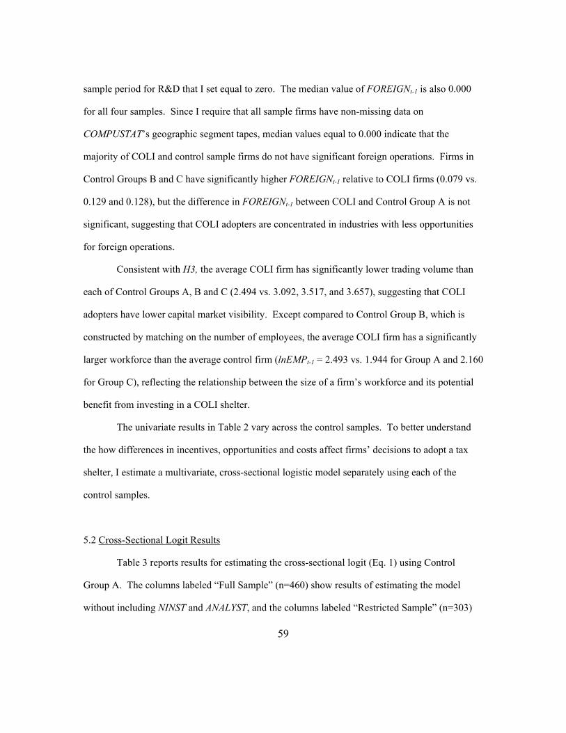
59

sample period for R&D that I set equal to zero. The median value of FOREIGNt-1 is also 0.000

for all four samples. Since I require that all sample firms have non-missing data on

COMPUSTAT’s geographic segment tapes, median values equal to 0.000 indicate that the

majority of COLI and control sample firms do not have significant foreign operations. Firms in

Control Groups B and C have significantly higher FOREIGNt-1 relative to COLI firms (0.079 vs.

0.129 and 0.128), but the difference in FOREIGNt-1 between COLI and Control Group A is not

significant, suggesting that COLI adopters are concentrated in industries with less opportunities

for foreign operations.

Consistent with H3, the average COLI firm has significantly lower trading volume than

each of Control Groups A, B and C (2.494 vs. 3.092, 3.517, and 3.657), suggesting that COLI

adopters have lower capital market visibility. Except compared to Control Group B, which is

constructed by matching on the number of employees, the average COLI firm has a significantly

larger workforce than the average control firm (lnEMPt-1 = 2.493 vs. 1.944 for Group A and 2.160

for Group C), reflecting the relationship between the size of a firm’s workforce and its potential

benefit from investing in a COLI shelter.

The univariate results in Table 2 vary across the control samples. To better understand

the how differences in incentives, opportunities and costs affect firms’ decisions to adopt a tax

shelter, I estimate a multivariate, cross-sectional logistic model separately using each of the

control samples.

5.2 Cross-Sectional Logit Results

Table 3 reports results for estimating the cross-sectional logit (Eq. 1) using Control

Group A. The columns labeled “Full Sample” (n=460) show results of estimating the model

without including NINST and ANALYST, and the columns labeled “Restricted Sample” (n=303)

60

show results of estimating the complete cross-sectional logit model for all COLI and Control

Group A firms with required data available in I/B/E/S and Thompson Financial. The regression

results indicate that both models have reasonable explanatory power with McFadden’s pseudo R2

values equal to 11.75 percent and 15.39 percent. Table 3 also reports results of a likelihood ratio

test of the hypothesis that all coefficients except the intercept are equal to zero. The chi-squared

statistics reported, 34.102 for the full sample and 31.452 for the restricted sample, indicate that

both models are reasonably well-fitted.39 Robust standard errors are estimated using the Huber

(1967)-White (1980) procedure. I begin with a discussion of the results for estimating Eq. (1) for

the full sample.

The coefficient on PMDACC is positive and significant (4.641, χ2=4.28), supporting H1.

The marginal effect indicates that, holding D_RDt-1 = 0 and all other variables at their median

values, a one standard deviation increase in PMDACC is associated with a 34 percent (from 5.9

percent to 7.9 percent) increase in the probability that a firm will adopt a COLI shelter. Firms

with higher discretionary accruals are more likely to adopt a COLI shelter, suggesting a link

between aggressive financial and aggressive tax reporting. Results for PMDACC are consistent

with Frank et al. (2006) who find that firms that have more aggressive financial reporting tend to

have more aggressive tax reporting, using discretionary accruals and discretionary permanent

book-tax differences to proxy for aggressive reporting.

Results for H2 are mixed. The coefficient on D_RDt-1 (1.240, χ2=9.92) is positive, rather

than negative as predicted. In fact, the marginal effect indicates that a change in D_RDt-1 from a

value of zero to a value of one, holding all other variables at their median values, more than

doubles (from 6.8 percent to 20 percent) the probability that a firm will adopt a COLI shelter.

39 For the full sample, the Hosmer and Lemeshow goodness-of-fit χ2 equals 11.53 with a p-value for a null hypothesis equal to 0.17. Thus the HL test also indicates that the model is reasonably well-fitted.

61

The coefficients on CAPINTt-1 (-0.652, χ2=0.27) and INTANGt-1 (-3.144, χ2=1.59) are negative but

not significant. Consistent with H2, the coefficient on FOREIGNt-1 is negative and significant

(-2.798, χ2=6.40). Firms with greater foreign assets are less likely to adopt the COLI shelter,

suggesting that firms with greater opportunities to avoid taxation by shifting income to lower-tax

jurisdictions are less likely to use the COLI shelter to obtain tax savings. The marginal effect

indicates that, holding D_RDt-1 = 0 and all other variables at their median values, a one standard

deviation increase in FOREIGNt-1 is associated with a 36 percent (from 8.5 percent to 5.4

percent) decrease in the probability that a firm will adopt a COLI shelter.

Results for the control variables are also mixed. The coefficients on MTBt-1 and MTRt-1

are negative but not significant. The coefficients on lnEMPt-1 and REL_ETR are positive but not

significant. The coefficient on ROAt-1 is positive and significant (3.252, χ2=1.93), consistent with

more profitable firms having more potential tax liability to shelter

In the full sample specification, I include VOL to proxy for the firm’s capital market

visibility and reputational concerns. Results for VOL (-0.130, χ2=2.25) support H3 and suggest

that managers with greater reputational concerns are less likely to adopt a tax shelter that

shareholders might find objectionable. In terms of the marginal effect holding D_RDt-1 = 0 and

all other variables at their median values, a one standard deviation increase in VOL is associated

with a 27 percent (from 7.9 percent to 5.8 percent) decrease in the probability that a firm will

adopt a COLI shelter. I include two additional measures for managers’ reputational concerns, the

number of institutions holding the firm’s stock (NINST) and the number of analysts covering the

firm (ANALYST). Like VOL, I expect the coefficients on these measures to be negative.

However, as Table 3 shows, using a restricted sample, the coefficients on NINST and ANALYST

are not significant. Furthermore, all else equal, COLI firms appear to be held by more

institutions, not less. While results for VOL support H3, the coefficients on NINST and ANALYST

62

are not significant. Results for the other variables of interest are qualitatively similar using both

the full sample and the restricted sample.

One possible explanation for the mixed H2 results in Table 3 (Control Group A) is that

matching on industry limits variation in the variables of interest: D_RDt-1, CAPINTt-1, INTANGt-1,

and FOREIGNt-1. To capture differences in these variables between COLI participants and non-

participants, I form two additional control samples that are not dependent on industry matching,

Control Groups B and C. Table 4 reports results using Control Group B, and Table 5 reports

results using Control Group C. The regression sample used in Table 3 includes 44 COLI firms,

but the regression samples used in Tables 4 and 5 include only 43 COLI firms. One COLI firm is

dropped when the procedures used to construct Control Groups B and C do not result in a match

for that firm.

In Tables 4 and 5, the columns labeled “Full Sample” show results of estimating the

model without including NINST and ANALYST, and the columns labeled “Restricted Sample”

show results of estimating the complete cross-sectional logit model for all COLI and control firms

with required data available in I/B/E/S and Thompson Financial. The full sample using Control

Group B consists of 444 firm-year observations, and the restricted sample using Control Group B

consists of 293 firm-year observations. The full sample using Control Group C consists of 423

firm-year observations, and the restricted sample using Control Group C consists of 268 firm-year

observations. Compared to Table 3, the pseudo R2 values in Tables 4 and 5 are lower, indicating

that the model is best specified when the matching procedure controls for industry.

Overall, the results in Tables 4 and 5 are similar to those in Table 3, demonstrating that

the results are not sensitive to the use of a particular control sample. As in Table 3, the results in

Tables 4 and 5 tend to support H1. In three of four specifications, the coefficient on PMDACC is

positive and significant, providing additional evidence that aggressive tax reporting is linked to

63

aggressive financial reporting. Likewise the results for H3 are consistent across the three control

samples. For the full sample specifications, the coefficients on VOL are negative and significant

in both Table 4 (-0.201, χ2=3.88) and Table 5 (-0.192, χ2=3.12). As in Table 3, the coefficients on

NINST are positive, rather than negative as predicted. The coefficient on ANALYST is negative

and significant (-0.083, χ2=3.03) in Table 5 but not significant in either Table 3 or 4.

Although I construct Control Groups B and C without reference to industry, Tables 4 and

5 show mixed results for H2 similar to Table 3. The coefficients on FOREIGNt-1 are negative and

significant in both Table 4 (-3.782, χ2=8.58) and Table 5 (-3.538, χ2=6.20), indicating again that

COLI firms are characterized by low foreign operations. In all three tables, the coefficients on

D_RDt-1 are positive, rather than negative as predicted. I hypothesize that firms with fewer

alternative tax savings opportunities, proxied by lower R&D expenditures, would be more likely

to engage in the COLI shelter; however, the results suggest that COLI participation is associated

with higher R&D intensity. While inconsistent with my hypothesis, a positive relation between

R&D and tax shelter use is consistent with Graham and Tucker (2006). The coefficient on

INTANGt-1 is negative and significant for the full sample in Table 5 but is not significant in any of

the other specifications.

Overall, the evidence in Tables 3, 4 and 5 suggests that COLI participation is associated

with higher performance-matched discretionary accruals, the presence of R&D expenditures,

lower foreign operations and higher trading volume. Taken together, the results support H1, but

provide mixed evidence regarding H2 and H3.

64

5.3 Supplementary Analyses

5.3.1 Disclosure of COLI Activity

Conventional wisdom holds that the tax shelter industry is very secretive; tax shelters are

designed to hide income from the IRS, many recent shelters were sold with confidentiality

agreements and shelter promoters are reticent to disclose their clients. However, of the 44 firms

that comprise my COLI sample, 31 disclose their participation, concurrent with their use of the

shelter, in their financial statements. Bankman (2002) offers one explanation for this behavior:

“Companies that purchase shelters convince themselves that they are doing nothing wrong and have a winning case under a literalist reading of the statue. Adding a cloak works against this mindset: A company that decides a cloak is necessary is a company that is more likely than not to forego the shelter (p. 458).”

In my main results, I examine firm characteristics of COLI participants relative to non-

COLI firms, but among COLI firms, I do not distinguish between disclosers and non-disclosers.

Firms who invest in COLI and choose to openly disclose their use of COLI likely differ from

those firms who invest in COLI but only reveal their investment when forced to do so. Most

importantly, those firms who invest and openly disclose may feel strongly that COLI is a

legitimate tax planning strategy. H1 predicts that some firms have an overall tendency to engage

in aggressive corporate reporting. A disclosing firm’s belief that COLI is a legitimate strategy

rather than an aggressive tax avoidance strategy should bias against finding results for H1.

Similarly, H3 predicts that firms with greater reputational concerns will be less likely to invest in

COLI and may not hold for firms that openly disclose their COLI involvement. H2 predicts that

firms with fewer alternative tax savings opportunities will be more likely to invest in COLI. I

expect this hypothesis to apply to both disclosing and non-disclosing COLI participants.

My sample includes all firms whose shelter activity is observable. Tax shelter activity is

observable if either a) the firm is a disclosing firm, b) the firm is a non-disclosing firm whose

65

activity is revealed ex post when detected by regulators, or c) the firm is a non-disclosing firm

whose activity is revealed ex post when the firm comes forward for the COLI amnesty program.

Tax shelter activity is generally not observable for non-disclosing firms whose activities are not

detected by regulators. Thus, selection bias could be an issue for my sample. Non-disclosing

firms are likely under-represented relative to the true population of non-disclosing firms. Ideally,

I would model the decision to participate in COLI and the decision to disclose that participation

separately. Unfortunately the small size of my sample does not make that feasible. Instead, I

offer some descriptive statistics on disclosers and non-disclosers.

Table 6 shows additional descriptive statistics for disclosers and non-disclosers,

measured in year t-1. On average, non-disclosers are larger than disclosers; non-disclosers have

mean assets of $6.402 billion relative to disclosers whose mean assets are $1.988 billion

(t-statistic = 1.92). Non-disclosers also have greater analyst coverage (ANALYST = 15.231 vs.

6.774, t-statistic = 2.37) and more institutional shareholders (NINST = 208.59 vs. 84.5, t-statistic

= 2.08). Although the percentage of shares held by institutional shareholders is not significantly

different between the two groups, the percentage of shares held by block shareholders is

significantly lower for non-disclosers than for disclosers (BLOCKRATIO = 0.032 vs. 0.075,

t-statistic =-1.90). Together, sample means for NINST, NBLOCK, IORATIO and

BLOCKRATIO indicate that non-disclosers are more broadly held by institutions but less of their

institutional ownership is concentrated in the hands of large blockholders. Interestingly, the

measure of reputational costs that has significant explanatory power in the multivariate model,

VOL, does not significantly vary between disclosing COLI firms and non-disclosing COLI firms.

In summarizing statistics for the full COLI sample, Panel A, I set null observations of

ANALYST, NINST, NBLOCK, IORATIO and BLOCKRATIO equal to zero. Panel B provides

summary statistics for 22 disclosers and 10 non-disclosers with non-missing data from I/B/E/S

66

and Thompson Financial. Inferences from the restricted sample are consistent with those for the

full sample.

5.3.2 Comparisons of COLI and Control Firms Over Time

Figures 2A, 2B, 2C and 2D depict the time trends before and after shelter adoption in

four variables, LEVERAGE, ETR, PMDACC and PERMDIFF. These graphs are constructed

using a sample of 37 COLI firms and 262 firms from Control Group A with all data required to

compute LEVERAGE, ETR, PMDACC and PERMDIFF every year from year t-4 to year t+4.

Figure 2A shows that relative to control firms, COLI firms have significantly lower LEVERAGE

both before and after adopting the COLI shelter (p-value < 0.05 in a one-tailed t-test for each time

period). This evidence is consistent with Graham and Tucker (2006) who find that, holding all

else equal in a logistic regression, shelter firms are less likely to issue debt. Graham and Tucker

(2006) also find that relative to firms matched on pre-shelter activity debt ratios, shelter firms’

debt ratios fall by 8% following adoption of the shelter. In contrast, Figure 2A suggests that

relative to industry and size-matched firms, shelter firms have lower debt ratios even several

years prior to adopting a shelter.

Treasury’s (1999) white paper suggests that firms engage in tax shelters under pressure to

keep their ETRs low and in line with competitor benchmarks. If so, relative to control firms, I

would expect COLI firms to have higher ETRs before adopting the shelter and lower ETRs after

adopting the shelter. Figure 2B shows some evidence of this flip in average ETRs around the

time that COLI firms start using the shelter, however, the difference in mean ETR between COLI

and non-COLI firms is not significant in any of the years t-4 to t+4 (p-value for a two-tailed

t-test is always > 0.10).

67

If shelter firms have an overall tendency toward aggressive corporate behavior which

simultaneously impacts financial earnings management activity and tax sheltering, I would expect

these firms to have higher PMDACC in general, not just in the year of shelter adoption.

However, Figure 2C shows that COLI firms do not have consistently higher levels of PMDACC.

Relative to control firms, COLI firms have significantly higher PMDACC in year t-4 (t-statistic =

1.99), significantly lower PMDACC in year t-3 (t-statistic = -2.01) and significantly higher

PMDACC in year t (t-statistic = 2.76). The mean difference in PMDACC between COLI and

Control firms is not statistically significant in any of the other years.

Large book-tax differences are often equated with aggressive tax reporting. However, large

book-tax differences can also arise because of mechanical differences in the rules used to

calculate book and taxable income or aggressive financial earnings management. To date, there

is no strong evidence to validate the use of book-tax differences as a proxy for tax shelter activity

(Shevlin 2002). Figure 2D offers some validation by comparing the book-tax differences from a

sample of known tax shelter participants to those from a matched sample.

As mentioned in Chapter 2, recent corporate tax shelters were designed to decrease taxable

income without decreasing book income, and the ideal shelter produces a permanent book-tax

difference. Unlike temporary differences, which eventually reverse over time, permanent

differences represent income (expenses) for financial (tax) purposes which will never be recorded

for tax (financial) purposes. I calculate permanent differences, PERMDIFF, following Frank et

al. (2006) as the difference between book income and taxable income, deflated by assets at the

beginning of the year (lag data 6). Book income equals pretax income (data 170) less minority

(data 49), and taxable income equals the sum of current federal tax expense (data 63) and current

68

foreign tax expense (data 64), divided by the statutory tax rate, less deferred taxes (data 50),

deflated by the statutory tax rate.40

Figure 2D shows that relative to control firms, COLI firms have significantly higher

PERMDIFF in every year except year t+1 (one-tailed t-tests each have p-value < 0.10). While

this evidence indicates that shelter users have relatively larger book-tax differences, it does not

rule out the possibility that these larger book-tax differences might also be driven by more

aggressive financial reporting. Furthermore, using discretionary book-tax differences to proxy

for tax shelter use remains problematic because as Shevlin (2002) points out, the variables used to

explain the non-discretionary portion of book-tax differences, like profitability and firm size, are

also likely variables that explain the firm’s decision to use a tax shelter.

5.3.3 Alternative Proxies for Reputational Concern

My initial three proxies for reputational concerns are based on the premise that firms with

greater capital market visibility will be more concerned about damage to their reputations and less

likely to engage in aggressive behavior than those with less visibility. However, my sample firms

are all relatively large and well-covered by financial intermediaries. Moreover, as discussed in

Section 3.3, there is no clear a priori reason that shareholders themselves would find managers’

aggressive corporate tax reports objectionable. Therefore, I consider three additional measures of

reputational concern designed to differentiate those firms which are highly visible to the public in

general because managers of more visible firms should be concerned about the negative publicity

of being associated with tax shelter use.

40 When data 63 is missing, current federal tax expense is calculated as (data 16 – data 64 – data 173 – data 50).

69

First, I construct a measure of press coverage, PRESS, equal to the number of distinct press

articles published about the firm for the two-year period, January 1, t-1 through December 31, t,

in Factiva’s database of major U.S. news and business publications. Following Barton (2005), I

only count an article if the firm’s name appears in the headline or lead paragraph and the article is

not a republished article or a recurring pricing/market data news item. I expect managers of more

visible firms to be more concerned about negative publicity associated with tax shelter scandal;

therefore I expect a negative coefficient on PRESS.

Second, I expect managers of firms with valuable brand names, especially retailers, to be

more concerned about potential customer backlash if the firm is revealed to have participated in a

tax shelter and is labeled a poor corporate citizen. Consistent with this idea, Hanlon and Slemrod

(2007) find weak evidence that the negative market reaction to news of tax shelter involvement is

greater for retail firms. I include RETAIL, an indicator variable equal to one if the firm is

associated with a brand listed in Advertising Age’s annual survey of the Top 200 Brands or has an

SIC code in the range 5000-5999, zero otherwise. I also expect a negative coefficient on

RETAIL.

Finally, I consider using the firm’s reputation score from Fortune’s American’s Most

Admired Companies list, published each year, to measure reputational concern. Since a good

reputation is valuable and hard to regain once damaged, I expect managers of firms with high

reputation rankings to be less likely to engage in a tax shelter. For over three decades, Fortune

has assigned a reputation score to each of the ten largest firms in more than thirty industries. The

reputation score has several components including investor value and corporate social

responsibility. Unfortunately, only six firms in the COLI sample appear on the list in 1986, and

only fourteen firms in the COLI sample appear in 1994. Thus, the list is not comprehensive

enough to construct a meaningful measure of reputational concern for my sample.

70

I add PRESS and RETAIL to Eq. (1) and re-estimate the model using Control Group C.

However, I find that neither the coefficient on PRESS nor the coefficient on RETAIL is

significant. PRESS is highly correlated with lnASSETS (ρ = 0.503), but the coefficient on PRESS

is not significant even when Eq. (1) is estimated without lnASSETS. Of five separate measures of

reputational concern, VOL, NINST, ANALYST, PRESS, and RETAIL, only VOL has a negative and

significant coefficient as predicted.

In developing H3 I focus on the manager’s desire to protect the firm’s reputation.

Alternatively, the manager may be reluctant to adopt a tax shelter over concern for his or her

personal reputation. For example, well entrenched CEOs or CEOs nearing retirement may be

more likely to adopt an aggressive tax strategy compared to newly appointed CEOs. Literature

on CEO reputation and style suggests that examining the relation between aggressive tax

reporting and managerial characteristics, as opposed to firm characteristics, may be a more

powerful setting. In a current study, Dyreng, Hanlon and Maydew (2007) find that individual

manager fixed effects have a significant impact on the extent of tax avoidance the firm

undertakes.

Bertrand and Schoar (2003), who track top managers across firms and over time, find that

manager fixed effects are important for a wide range of corporate decisions, including investment

and financing policies. Using observable managerial characteristics, Bertrand and Schoar (2003)

also conclude that executives from earlier birth cohorts appear to be more conservative while

executives who hold a MBA degree appear to follow more aggressive strategies. Francis et al.

(2008) examine the association between CEO reputation and earnings quality. They find that

more reputed CEOs are associated with poorer earnings quality relative to less reputed CEOs.

Francis et al. (2008) interpret their findings as evidence primarily for a matching explanation;

firms where earnings quality is inherently poor seek reputed CEOs. Milbourn (2003) examines

71

the relation between CEO reputation and stock-based compensation. His work offers four

possible observable proxies for CEO reputation: (1) CEO tenure, (2) the number of business-

related articles containing the CEO’s name, (3) whether the CEO is appointed from outside the

firm, and (4) industry-adjusted firm performance during the CEO’s tenure.

While the literature on CEO reputation and style suggests methods for testing the

relationship between managerial characteristics and aggressive tax reporting, it may be difficult to

determine which top manager is most likely associated with the decision to engage in a tax

shelter. I leave an examination of the impact of managerial reputation concerns on aggressive tax

policy choices for future research.

5.3.4 Early Analysis of Tax Sheltering and Competitive Pressure

In preliminary tests, I investigate whether competitive pressure might explain the

incidence of aggressive tax reporting. Treasury’s report (1999) emphasizes the pressure to keep

the firm’s effective tax rate (ETR) low and in line with competitor benchmarks as an explanation

for the growth in corporate tax shelters. This competitive pressure could motivate managers to

invest in increasingly more aggressive tax strategies to obtain and maintain ETRs that are low

relative to their industry. I hypothesize that firms in highly competitive industries are more likely

to engage in aggressive tax reporting. To examine this hypothesis, I look for an association

between a Herfindahl-Hirschman (HH) index of industry concentration and several measure of

tax avoidance. I construct the HH index by 2-digit SIC code; the HH index is higher for more

concentrated markets. I expect the HH index to be negatively related to industry median ETR and

positively related to industry median PERMDIFF. However, I find no relation between the HH

index and these industry measures of tax avoidance.

72

PART II

Like recent financial accounting scandals, the latest corporate tax shelter boom alarms

regulators because it signals a shift in the corporate norm toward aggressive reporting. In

outlining its concern over the proliferation of tax shelters, Treasury pointed to the following quote

from the New York Bar Association,

“The constant promotion of these frequently artificial transactions breeds significant disrespect for the tax system, encouraging responsible corporate taxpayers to expect this type of activity to be the norm, and to follow the lead of other taxpayers who have engaged in tax advantaged transactions (1999, p.3)”

This quote motivates an important question: How does a corporate practice like the use of tax

shelters spread? In particular, this quote suggests that: (1) early shelter adopters differ from later

adopters and (2) later adopters imitate early adopters because they see tax shelter use as the new

norm. A quote by Bankman, stemming from his conversations with shelter promoters, also

suggests that early shelter adopters differ from later adopters,

“Most companies are reluctant to be the first purchasers, preferring to purchase a shelter that has been vetted by others. On the other hand, since legal reform generally has prospective application only, there is a premium to getting a shelter early in its life (1999, p.1781)”

The cross-sectional model of tax shelter participation developed in Part I of this study tests

whether differences in firm-specific characteristics can explain why some firms adopt tax shelters

and other firms do not. However, variation in firm characteristics does not directly address how

aggressive tax reporting became pervasive during the late 1990’s.41 In Part II of this study, I

examine the spread of COLI activity in two ways. First, I use theory on the diffusion of strategic

innovations and institutional isomorphism to develop two additional hypotheses and predict that

41 Indirectly, variation in firm characteristics may explain a rise in aggregate tax shelter activity if the firm traits identified as determinants of the likelihood of adopting a shelter characterize an increasing proportion of firms over time.

73

factors from the firm’s social environment impact the firm’s decision to adopt the COLI shelter.

Second, I use event history analysis to investigate the timing of COLI adoptions.

74

Chapter 6 – Literature Review

To better understand how tax shelter use spread, I draw on a substantial body of literature

related to the diffusion of innovations and institutional isomorphism. The literature on diffusion

encompasses a wide variety of innovations, from the adoption of cell phones to the adoption of

kindergartens. Although tax shelters are not typical of the type of practice generally studied in

the literature, diffusion theory can provide a framework for understanding the recent proliferation

in corporate tax shelter use. In addition to covering a wide variety of innovations, diffusion

studies address a myriad of questions, for example, what characterizes innovators, how

characteristics of the innovation impact the rate of adoption, and what impacts communication

channel usage.

Rogers (2003) defines diffusion as “the process by which (1) an innovation (2) is

communicated through certain channels (3) over time (4) among the members of a social system.”

An innovation can be any new idea or practice. Certain attributes of an innovation affect its rate

of adoption. For example, observability increases the rate of adoption while complexity

decreases the rate of adoption. The easier it is for firms to see the results of an innovation, the

more likely they are to adopt. On the other hand, innovations that are perceived as difficult and

complicated to use are adopted more slowly.

The communication channel is the critical link between prior adopters and potential

adopters. Some innovations are communicated quickly through mass media channels while

others are communicated more slowly through interpersonal channels. Newness and uncertainty

make objective evaluation of an innovation’s merits costly. Thus, while objective evaluation of

the innovation is important for early adopters, later adopters rely heavily on the subjective

evaluations of prior adopters. This reliance links the study of diffusion with the study of

imitation.

75

The innovation-diffusion process takes place over time, as a firm moves from first

gaining knowledge of an innovation to forming an attitude toward the innovation to making a

decision to adopt or reject an innovation (Rogers 2003). The newness and uncertainty of an

innovation distinguish the innovation-diffusion process from other types of decision-making.

Throughout this process, the firm is trying to gain information and reduce uncertainty. One way

of reducing the uncertainty surrounding an innovation is to adopt the innovation on a partial basis.

For example, a firm may try out a new bonus scheme on a select number of employees before

implementing the scheme company-wide. When a trial period within the firm is not feasible, trial

by peers can serve as a substitute (Rogers 2003). The importance of reducing uncertainty through

trial is evident in anecdotes gathered by Bankman (1999) who reported the desire among potential

tax shelter adopters to have the shelter vetted by someone else first.

Diffusion takes place within a social system which has its own structure and norms. The

system’s communication structure can facilitate or impede the diffusion of innovations. For

example, in a system with strong opinion leaders, once those opinion leaders adopt an innovation

many others will adopt quickly thereafter. Innovations at odds with the current norms of the

social system will meet more resistance and be adopted more slowly. Again, unlike other types

of decision-making, the nature of an innovation-adoption decision requires an understanding of

the firm’s broader social environment.

Unfortunately, studies on the adoption of new business practices do not draw on a single,

well-defined theory. The ideas and intuition used to support the hypotheses developed in these

studies can be traced back to a variety of over-lapping sources. In addition to theory on the

diffusion of innovations, a related field of study, institutional isomorphism, tries to explain the

homogenization of organizational behavior.

76

DiMaggio and Powell (1985) define isomorphism as “a constraining process that forces

one unit in a population to resemble other units that face the same set of environmental

conditions.” They identify threes types of isomorphism: coercive isomorphism, mimetic

isomorphism and normative isomorphism. Coercive isomorphism stems from formal and

informal pressures exerted on an organization by the wider institutions of its environment; for

example, operating in the same legal and regulatory environment increases homogeneity among

firms. Mimetic isomorphism arises because, when faced with uncertainty, organizations tend to

model themselves on other organizations. Finally, normative isomorphism refers to the affect of

professionalization on organizations; organizations draw from the same pool of professionals,

who have similar norms and dispositions through their shared university and professional training

and membership in professional organizations. DiMaggio and Powell (1985) emphasize that their

typology is an analytic one and that these three types of isomorphism may not be empirically

distinct.

Institutional isomorphism, particularly mimetic isomorphism, can help us understand

how and why new ideas get diffused throughout an environment. Mimetic isomorphism can be a

response to uncertainty; when faced with uncertainty, organizations economize on search costs

and imitate the behavior of other organizations (Cyert and March 1963). Mimetic isomorphism

can also occur when a practice becomes institutionalized and legitimized; once enough firms

adopt a practice, the practice becomes taken-for-granted and remaining firms feel strong pressure

to join the ranks (March 1981). Mimetic organizational change can be thought of as a contagion

process that spreads fashionable practices from one firm to another (Haveman 1993).

Prior studies on diffusion of business practices and imitation among firms address a wide

variety of research questions, from how an innovation’s attributes affect its rate of adoption to

how a firm’s place within its social network impacts the likelihood that firm will eventually

77

adopt. Likewise, these studies employ a number of different research methods. Within the broad

literature on diffusion of innovations and institutional isomorphism, I focus on a branch of

management literature which examines the diffusion of corporate practices. I am particularly

interested in two main topics: (1) characteristics of early adopting firms, and (2) the network and

communication channels through which diffusion occurs. To give context for the role of theories

of diffusion and institutional isomorphism in investigating new business practices, I review three

exemplary studies below.

Haunschild (1993) examines the influence of inter-organizational imitation on corporate

acquisition activity. In particular, she examines whether board interlocks serve as the mechanism

of imitation. Haunschild (1993) posits that firm managers who sit on other firms’ boards are

exposed to the acquisition activities of those firms. For these managers, the acquisition activities

of the other firms they are “tied-to” serve as models to imitate. Consistent with an imitation

explanation, she finds that the number of current-year acquisitions made by a firm is positively

related to number of acquisitions made in the prior three years by other firms tied to the firm

through board directorships, even after controlling for firm-specific determinants of acquisition

activity tested in prior research. Haunschild’s (1993) study shows how institutional theory can

provide a more complete explanation for a wave of corporate behavior, in this instance the 1980s

wave of mergers and acquisitions, over and above the explanation provided by prevailing theories

based on firms’ cross-sectional differences.

In the context of accounting, Mezias (1990) examines the role of institutional theory in

explaining the financial reporting practices of the Fortune 200, specifically firms’ use of the

deferral method (DM) versus the flow-through method (FTM) to record investment tax credits.

He finds that the majority of variance in reporting practice explained by his model is added by

variables suggested by institutional theory. Mezias’s (1990) institutional hypotheses are drawn

78

primarily from normative isomorphism rather than mimetic isomorphism; he tests how changes in

the institutional environment, like the end to the Accounting Principles Board’s prohibition

against the FTM, affect the probability that a firm adopts a certain reporting practice. He also

develops hypotheses based on firm-characteristics designed to capture which firms are more or

less subject to pressure to achieve isomorphism; for example, Mezias (1990) finds that firms

experiencing high top management turnover were more likely to conform to prevailing practice

by adopting the FTM. Mezias (1990) makes several arguments for the relevance of institutional

theory in explaining firms’ accounting choices. In particular, Mezias (1990) points to the role of

auditors, who, as professionals, serve as an important social link between firms and lend certain

practices legitimization.

Rao and Sivakumar (1999) investigate the role of mimetic isomorphism on the diffusion

of investor relations departments. From 1984 to 1994, the percentage of Fortune 500 firms with

investor relations departments rose from 16% to 56%. Rao and Sivakumar (1999) use the

diffusion of investor relations departments to test two different models of mimetic pressure, the

cohesion model and imitation of structurally equivalent firms. Cohesion models of imitation

focus on direct ties between firms who have already adopted a practice and firms who have not

yet adopted a practice. In contrast, firms may imitate structurally equivalent peers, even in the

absence of direct ties. Although structurally equivalent firms are not directly tied to one another,

they are indirectly tied through their links with a shared environment, for example, ties to the

same suppliers, customers, or labor unions. Rao and Sivakumar (1999) find that number of board

interlocks with prior adopters is significantly and positively related to the likelihood that a firm

will create an investor relations department, but the number of prior adopters in a firm’s industry

group does not affect this likelihood. Their results suggest that the diffusion of investor relations

departments can be better described by the cohesion model than imitation of structurally

79

equivalent firms. I follow Rao and Sivakumar (1999) and develop two hypotheses for the role of

imitation on the diffusion of COLI shelter use, one based on structural equivalence and one based

on cohesion.

80

Chapter 7 – Hypothesis Development

Part I of this study investigates the effect of firm characteristics on the likelihood of

adopting a shelter. In Part II of this study, I argue that a tax shelter is essentially an innovation, a

new business practice, which each firm decides to adopt or reject. My primary research objective

in Part II is still to explain the firm’s decision to adopt a tax shelter. However, in this chapter I

draw on ideas from theory on the diffusion of innovations and institutional isomorphism to

further explain the firm’s adoption decision. Putting the firm’s tax shelter adoption decision in

the context of innovations and how innovations spread gives rise to two questions: (1) do factors

related to the firm’s social environment and its communication network influence the firm’s

decision to adopt a shelter, and (2) what factors distinguish early adopters from later adopters?

7.1 Network Influences

In this section, I develop two hypotheses related to the influence of the firm’s network on

its decision to adopt a tax shelter. As detailed in Chapter 6, unlike other decision processes, the

innovation-decision process is heavily influenced by the firm’s broader social environment. The

innovation-decision process has five stages: knowledge, persuasion, decision, implementation and

confirmation (Rogers 2003). Since I am primarily interested in explaining the firm’s decision to

adopt a tax shelter, I focus on the first three stages of the innovation-diffusion process.

In the knowledge stage, the firm is exposed to the shelter’s existence and gains an

understanding of how the shelter works. How does this occur when secrecy surrounds an

innovation? First, although conventional wisdom suggests that corporate tax shelters are highly

secretive, the evidence in Table 6 indicates there was at least some public disclosure of COLI use.

Second, even absent this public disclosure, knowledge of the shelter could have easily passed to

potential adopters through interpersonal contacts. These interpersonal contacts can be direct

81

contacts with prior adopters or indirect contacts with other change agents and aides. In the case

of COLI, knowledge may have been transmitted via shared auditors, shared tax advisors, or

shared legal counsel among others.

In the persuasion and decision stages, the firm develops either a favorable or unfavorable

attitude toward the innovation and subsequently chooses to adopt or reject the innovation (Rogers

2003). In these two stages, the firm is primarily concerned about reducing the inherent

uncertainty surrounding an innovation. Given the importance of the subjective evaluations of an

innovation on a potential adopter’s decision, Rogers (2003) argues that “the heart of the diffusion

process is the modeling and imitation by potential adopters of their near peers’ experiences with

the new idea.” The importance of vicarious trials links diffusion theory with a separately

developed line of thinking on mimetic isomorphism.

Together these theories suggest that firms imitate their peers in the adoption of new

strategies (see Haveman 1993, Haunschild 1993, and Rao and Sivakumar 1999 for example).

When uncertainty surrounding an innovation is greater, firms are less able to rely on technical

considerations, increasing the importance of social comparison (Haunschild and Miner 1997;

Abrahamson and Rosenkopf 1993). Mimetic isomorphism is a fairly broad term covering several

different types of imitative behavior, two of which I discuss below.

Under frequency-based imitation, as more and more firms adopt a practice, the practice

gains legitimacy. Eventually, the practice becomes taken-for-granted. Prior studies investigate

the role of frequency-based imitation for a wide variety of corporate decisions including:

adoption of the multidivisional form (Fligstein 1985), adoption of poison pills (Davis 1991), the

use of a particular investment banker in an acquisition deal (Haunschild and Miner 1997) and the

creation of investor relations departments (Rao and Sivakumar 1999). Evidence from these

82

studies is mixed; frequency-based imitation seems to influence some corporate decisions, but not

others.

Outcome-imitation theorizes that firms adopt strategies when they observe improvements

in the performance of peer firms using those strategies (Haunschild and Miner 1997).

Abrahamson and Rosenkopf (1993) posit that pressures on firms arising from the threat of lost

competitive advantage produce competitive bandwagons, even when the returns to an innovation

are unclear. As the number of adopters in a group increases, non-adopters face the risk of falling

farther below average if the innovation succeeds.

Frequency-based imitation is consistent with the anecdotal evidence reported by

Bankman (1999) and implies that the prevalence of a practice within a community will impact the

rate of adoption. Outcome-imitation is consistent with Treasury’s (1999) report, which identifies

pressure to keep ETRs low and in-line with competitors as a driving force behind the tax shelter

boom.

Prior literature provides support for two contagion mechanisms: structural equivalence

and cohesion (Galaskiewicz and Burt 1991; Haunschild 1993; Rao and Sivakumar 1999). The

notion of contagion mechanisms in literature on mimetic isomorphism is not strictly parallel to

the role of communications channels in diffusion theory. The term “communication channel”

generally refers to the means by which a firm first becomes aware of a new innovation, whereas

“contagion mechanism” is related to the firm’s mimicry behavior which is more closely related to

the persuasion and decision stages of the innovation-diffusion process.

Contagion via structural equivalence suggests that firms imitate other organizations that

have similar relationships with their environment, even in the absence of direct contacts.

Frequency-based imitation and outcome-based imitation are structural equivalence arguments;

83

imitation depends on potential adopters knowing about prior adopters but does not depend on

direct contacts between the two groups.

Anecdotal evidence, such as that in Forbes 1998 article, suggests that firms face

significant pressure to imitate the tax savings strategies of their peers. Therefore, I hypothesize:

H4: The greater the number of prior COLI shelter adopters in a firm’s industry, the more likely a firm is to adopt the COLI shelter.

In contrast to structural equivalence, cohesion models of imitation focus on direct

contacts between prior adopters and potential adopters. Several studies provide support for the

role of social networks in the diffusion of new corporate strategies. For example, Haunschild

(1993) finds that managers imitate the corporate acquisition activities of other firms when they

are linked through board interlocks. Similarly, Rao and Sivakumar (1999) find that board

interlocks play a role in the adoption of investor relations departments. To the extent tax shelter

activity is secretive; firms may not be able to observe the frequency of shelter use within their

peer group. Likewise, given the secrecy of tax shelters, even when a firm observes that its peers

have lower ETRs, it may not be able to trace that outcome back to the use of a particular tax

shelter. Thus, a cohesion model may better explain diffusion of tax shelter use.

Network contacts are difficult to identify and measure. Shelter participants may be

connected through common professional association memberships, common board members,

common legal advisors, common tax consultants, common auditors or others. Regulators have

focused on the role of auditor-provided tax services in the spread of the tax shelter industry,

criticizing that when a firm advises its audit client on a tax shelter transaction, the firm essentially

audits its own work (U.S. Senate Permanent Subcomittee on Investigations 2005). Because

regulators investigating the tax shelter industry have placed a spotlight on auditors, I hypothesize:

H5: A firm whose current auditor has audited prior COLI shelter adopters is more likely to adopt the COLI shelter.

84

7.2 Early Versus Late Adopter

Thinking about the firm’s shelter adoption decision in the context of the diffusion of an

innovation raises questions about the role of the firm’s social environment in the decision.

Moreover, in the diffusion process, innovators and first adopters often differ from later adopters.

The analysis in Part I of this study focuses on the likelihood that a firm will adopt a COLI shelter,

but treats the first firm to adopt a COLI shelter the same as the last firm to adopt and every firm

that adopts in between. To better understand the spread of COLI activity, I investigate whether

the firm characteristics hypothesized to affect the likelihood of COLI shelter adoption also affect

the timing of COLI shelter adoption.

Diffusion theory suggests that differences in risk propensity and the capability to generate

and adopt innovations determine the order of innovation adoption within a group of similar firms

(Rogers 2003). Early adopters may have a greater need for the practice to solve a problem or

may be embedded in a local network with norms that diverge from those held by members of the

larger social system (Massini et al. 2005). Behavioral theory of the firm suggests that managers

make strategic changes when the firm’s performance falls short of aspirations (Cyert and March

1963). Likewise, Bromiley’s (1991) work on organizational risk taking suggests that falling short

of benchmarks determined by the firm’s past performance and/or by the firm’s peer group

performance increases risk taking. In Part I, I hypothesize that certain firm characteristics affect

the firm’s decision to adopt a COLI shelter. Here, I hypothesize that a similar set of

characteristics also affect how quickly, relative to other firms, a firm decides to adopt a COLI

shelter.

H1 predicts that firms with prior indicators of aggressive financial and/or tax reporting

behavior are more likely to adopt a COLI shelter. These firms have a history of risk-taking

behavior. Diffusion theory generally suggests that innovators and early adopters have a higher

85

propensity for risk-taking. Bromiley (1991) finds that prior risk is a positive predictor of current

risk. In Chapter 1, I describe the development of the COLI shelter and suggest that although the

shelter was designed to meet the letter of the law, COLI adopters knew that investing in a broad-

based COLI program was a risky tax position. I expect early adopters to be those firms with the

highest propensity for risk. Therefore, I extend H1 and posit,

H6: All else equal, firms that report aggressively for financial reporting and/or tax purposes will adopt the COLI shelter earlier.

H2 predicts that firms with fewer alternative tax savings strategies are more likely to

adopt a COLI shelter. Treasury (1999) suggests that competitive pressure to keep the firm’s ETR

low and close to peer benchmarks was a major cause of the tax shelter boom. Treasury’s

conjecture is consistent with the idea that firms adopt new strategies and take greater risks when

their performance falls short of benchmark goals. Early adopters of an innovation are likely

those firms driven by a desire to improve performance (DiMaggio and Powell 1983). Firms look

to riskier choices when their aspired level of performance, in this case lower ETRs, cannot be

achieved under the status quo (Cyert and March 1963). In developing H2, I argue that firms may

be more inclined to adopt a risky strategy, like a COLI shelter, when faced with a limited set of

alternative tax savings strategies. I extend that hypothesis and predict,

H7: All else equal, firms with fewer non-COLI tax savings opportunities will adopt the COLI shelter earlier.

Not all firms eventually adopt tax shelters. Given the economic benefits of adopting a

COLI shelter, why do some firms reject COLI? H3 posits that firms with greater reputational

concerns are less likely to adopt a tax shelter. Concern over the firm’s reputation can inhibit

managers from adopting new strategies (Fombrun and Shanley 1990). Later adopters look to the

experiences of early adopters to reduce the risk and uncertainty surrounding an innovation. Over

86

time, as more and more firms adopt an innovation, that practice gains legitimacy. Thus, I expect

firms with greater reputational concerns to hold back on adopting the COLI shelter, preferring to

let others vet the strategy first. As Gergen (2002) points out, each additional shelter adopter

increases the risk that the government will discover the shelter and take adverse action. From the

shelter user’s perspective, the optimal number of users is one. The marginal risk of an additional

adopter is problematic for early adopters, who potentially have many years worth of tax savings

at risk, but not necessarily for the marginal firm considering adoption. Furthermore, in 1990

Congress failed to enact proposed legislation that would have limited COLI use. Congress’s

inaction could have been seen as an implicit acceptance of the COLI shelter. Gergen (2002) goes

so far as to say that COLI usage boomed after Congress failed to enact reform legislation.

Overall, I expect reputational concerns to decrease a firm’s hazard rate,

H8: All else equal, firms with greater reputational concerns will adopt the COLI

shelter later.

87

Chapter 8 – Research Methodology I first test H4 and H5 using a cross-sectional model, detailed in Section 8.1. For the

remaining tests in Part II , I employ event history analysis, which I briefly review in Section 8.2

Section 8.3 details tests of H4 and H5 using a discrete-time hazard model with time-varying

explanatory variables. I test H6, H7 and H8 using a Cox proportional hazard model, explained in

Section 8.4, and a split-population model, outlined in Section 8.5.

8.1 Cross-Sectional Analysis

First, I test H4 and H5 using a simple cross-sectional logit model, similar to the one

employed in Part I. I construct two variables designed to capture the influence of the firm’s

social environment on its decision to adopt a COLI shelter and include these variables, along with

firm-specific characteristics in the following logistic regression model:

Pr(COLIi,t) = β0 + β1 D_RDi,t-1 + β2LEVERAGEi,t-1 +β3FOREIGNi,t-1 + (3) β 4CAPINTi,t-1 + β5VOLi,t-1 + β6PMDACC3yri,t + β7BTD3yri,t + β8ROAi,t-1 + β9lnEMPi,t-1 + β10ROAi,t-1 + β11AUDITLINKi + β12NINDUSTRYi + εi,t

where the dependent variable is an indicator equal to 1 if the firm participated in a COLI shelter

and 0 otherwise.

In Part I, I hypothesize (H1) that firms that report aggressively for financial statement

purposes will be more likely to adopt a tax shelter, and I include PMDACC in the model to proxy

for aggressive financial reporting. In Eq. (3), I expand on H1 and predict that firms with a

tendency to report aggressively for either financial or tax reporting purposes will be more likely

engage in shelter activity. I test whether indicators of prior aggressive corporate reporting

increase the likelihood of adopting a COLI shelter by including a measure of prior aggressive

financial reporting behavior, PMDACC3yr, and a measure of prior aggressive tax reporting,

88

BTD3yr. As in Part I, I estimate performance-matched discretionary accruals (PMDACC). I

include the average of the absolute value of PMDACC over the prior three years (PMDACC3yr)

in Eq. (3) and expect the coefficient on this variable to be positive.

To capture prior aggressive tax reporting, I include BTD3yr, an estimate of the firm’s

permanent book-tax differences averaged over the prior three years and deflated by total assets

averaged over the prior three years. I estimate permanent differences, PERMDIFF, following

Frank et al. (2006) as the difference between book income and taxable income. Book income

equals pretax income (data 170) less minority (data 49), and taxable income equals the sum of

current federal tax expense (data 63) and current foreign tax expense (data 64), divided by the

statutory tax rate, less deferred taxes (data 50), deflated by the statutory tax rate.42 I expect a

positive coefficient on BTD3yr.

H2 posits that firms with fewer alternative shelter substitutes are more likely to adopt a

tax shelter. I include four variables in Eq. (3) to proxy for firms’ non-COLI tax savings

opportunities: D_RD, LEVERAGE, FOREIGN, and CAPINT. Graham and Tucker (2006) find

that shelter firms have lower debt ratios. In Section 5.3.2, I report that relative to control firms,

COLI firms appear to have significantly lower LEVERAGE both before and after adopting the

COLI shelter. Therefore, I add LEVERAGE as another measure of the firm’s alternative tax

savings strategy set. Consistent with H2, I expect negative coefficients for RD, LEVERAGE,

FOREIGN and CAPINT.

H3 predicts that firms with more visibility in the capital markets should have a greater

incentive to avoid the appearance of impropriety associated with involvement in tax shelters. I

42 When data 63 is missing, current federal tax expense is calculated as (data 16 – data 64 – data 173 – data 50).

89

include average trading volume (VOL) as a proxy for the firm’s capital market visibility, and

expect a negative coefficient on VOL.

I test H4 by including the total number of prior COLI adopters within a firm’s industry

group (NINDUSTYi,t-1). Industries are classified according to Barth et al. (1998).43 NINDUSTRY

varies by firm and by year but does not vary across industry. H4 predicts that the presence of

prior COLI adopters lends legitimacy to the tax shelter, thus I expect a positive coefficient on

NINDUSTRY.

I examine the impact of direct ties between prior and potential adopters via auditors by

including AUDITLINKi,t, equal to the number of prior COLI adopters audited by firm’s auditor in

year t. I use COMPUSTAT data item 149 the each firm’s auditor during the year. Consistent with

H5, I expect a positive coefficient on AUDITLINK. I also include ROA and lnEMP as additional

control variables in Eq. (3).

I estimate Eq. (3) using a matched control sample based on asset size and market-to-book

(MTB) ratio. The control sample includes 403 firm-year observations. Section 9.2 discusses the

results of estimating Eq. (3).

8.2 Event History Analysis

Diffusion is a process that occurs over time, and cross-sectional analysis does not explicitly

incorporate the influence of time on the firm’s decision-making process. Event history analysis,

on the other hand, explicitly models the time or duration that a firm spends in one state before

transitioning to another state. To examine COLI shelter adoption, I measure time to adoption, the

time from the advent of broad-based, leveraged COLI (time zero) to the date that a firm adopts

43 In Part I, I use a more detailed industry classification system based on both Barth et al. (1998) and Barth et al. (2005). Results are qualitatively similar using the more detailed industry groupings.

the COLI shelter. Let T be a positive random variable denoting adoption times where the actual

adoption time of an individual firm is a realization of T denoted as t. The possible values of T

have a probability distribution with a probability density function, f(t) and a cumulative

distribution function, F(t). Given the probability distribution of T, we can express the hazard rate

or conditional adoption rate as:

{ }t

tTttTttht Δ

≥Δ+<≤=

→Δ

|Pr)( lim0

.

In a duration model, the dependent variable is the hazard rate, or the probability that a firm will

adopt a COLI shelter at time t, given that it has not previously adopted a COLI shelter. The key

idea is that the probability that an event occurs depends, in some way, on time.

There are several types of event history models. These models differ in their assumptions

about the hazard function, the probability distribution for the time of event occurrence.

Parametric models directly specify the shape of the hazard rate. In other words, these types of

models assume that time dependency takes on a certain distribution. Alternatively, in the Cox

proportional hazard model the particular distributional form of the duration times is left

unspecified, the hazard for any particular firm is a fixed proportion of the hazard for any other

firm. Finally, a discrete-time event history model is more analogous to a parametric model.

Duration dependency can be incorporated in a discrete-time model explicitly by including a time

variable like year dummies or the natural log of time.

All duration models are fundamentally concerned with the timing of events. To assign

duration to an event, we must choose a time origin. The origin is the point at which all firms

become “at risk” of experiencing an event, and duration is the length of time from the origin until

a particular firm actually experiences the event, the length of time the firm continues to be “at

risk”. Court documents indicate that the COLI shelter was developed in 1985, and I identify at

90

91

least one firm that appears to adopt COLI in 1986. Therefore, I assume that firms are “at-risk” if

they have not adopted the COLI shelter and t is greater than 1985.

8.3 Discrete-time Model

Duration models can have either time-constant covariates or time-varying covariates.

Because the variables I use to test H4 and H5, NINDUSTRY and AUDITLINK vary over time, I

employ a duration model with time-varying covariates. Event history analysis often utilizes

continuous-time duration models. However, given discrete-time data and time-varying

covariates, a discrete-time model is useful for testing H4 and H5 (Box-Steffensmeier and Jones

1997).

In a discrete-time model, the dependent variable is a series of binary outcomes denoting

whether or not the event of interest has occurred at a given time. Each firm contributes an

observation for each year it is “at risk” of adopting a COLI shelter. While different in form than

duration, these binary outcomes convey the same information as duration time (Box-

Steffensmeier and Jones 1997). Conveniently, a discrete-time duration model can be estimated

using a familiar logit model.

The sample construction here follows that in Part I. I start with the same set of COLI firms.

However, rather than including each COLI firm only once, in the year of adoption, the sample

used in the discrete-time model described below includes yearly observations for each COLI firm

from 1986 up to and including the year that the firm adopts COLI. In the year of adoption, the

dependent variable, ADOPT, is equal to one. Prior to the year of adoption, ADOPT is equal to

zero. The sample also includes yearly observations, from 1986 to 1996, for firms in Control

Group C. For control firms, ADOPT is equal to zero in every year. The regression sample in Part

I can include more than one observation for each control firm, but only for different years (e.g.

92

control firm X may be included as a match for COLI firm A in 1988 and for COLI firm B in

1992). The regression sample used to estimate the discrete-time model below includes one

observation for each control firm for each year, regardless of the match year. The final sample

used to estimate the model has 1,905 firm-year observations, comprised of 255 firm-year

observations for 37 COLI adopters and 1,650 firm-year observations from Control Group C.

To test H4 and H5 using an event history model, I estimate the following discrete-time

logit:

Pr(ADOPTi,t) = β0 + β1D_RD i,t-1 + β2LEVERAGEi,t-1 +β3FOREIGNi,t-1 + (4) β4CAPTINTi,t-1 + β 5VOLi,t-1 + β6PMDACC3yri,+ β7BTD3yri + β8ROAi,t-1 + β9lnEMPi,t-1 + β 10NINDUSTRYi,t + β11AUDITLINKi,t + β12ln(t) + εi,t

where the dependent variable is an indicator equal to 1 if the firm adopts COLI during year t and

0 otherwise. Beyond the year of adoption, the firm is no longer included in the analysis, and

control firms that never adopt COLI are coded as 0 in every year. Results from Eq. (4) can be

interpreted in terms of the hazard probability. Section 9.3 discusses the results of estimating Eq.

(4).

8.4 Cox Proportional Hazard Model

The discrete-time model described in Section 8.3 is a particularly useful model given that

NINDUSTRY and AUDITLINK are time-varying covariates. However, a discrete-time model

requires an explicit assumption about the form of duration dependence. Moreover, the only way

to disentangle the effect of a covariate on the overall likelihood of adoption from the effect of that

covariate on the time to adoption is to interact that covariate with the explicitly modeled time

variable. Therefore, to test H6, H7 and H8, I estimate a Cox proportional hazard model:

hi(t) = exp(β1D_RDi + β2LEVERAGEi +β3FOREIGNi + β 4CAPINTi + (5) β5VOLi + β6PMDACC3yri,+ β7BTD3yri + β8ROAi + β9lnEMPi + β10ROAi) h0(t)

93

where the dependent variable is the hazard rate for firm i at time t (the probability that a firm will

adopt a COLI shelter at time t, given that it has not previously adopted a COLI shelter.)

The baseline hazard rate, h0(t), is left unspecified and captures all common factors

affecting the likelihood of adopting a COLI shelter in a particular year, while the exponential

term includes firm-specific characteristics hypothesized to affect the rate of COLI adoption. The

independent variables are all measured in 1985. To estimate Eq. (5), I set the duration to

adoption, DURi, equal to the year a firm first adopts a COLI shelter minus 1985. The

construction of the control sample for the event history analysis follows that for the cross-

sectional analysis, except that instead of matching COLI and control firms on asset and MTB

ranks in year t-1, I match firms based on asset and MTB ranks in 1985. Section 9.4 discusses the

results of estimating Eq. (5).

8.5 Split Population Model

Standard hazard models, like the Cox proportional model in Eq. (5), assume that

eventually every observation will experience the event in question (i.e. every firm will eventually

adopt a COLI shelter). This assumption makes inferences from a standard hazard model

problematic when the observed percentage of adopters in a population is low. To account for the

possibility that some portion of the population will never adopt, Schmidt and Witte (1989)

developed the “split-population” model.44 Schmidt and Witte (1989) assume there is some

unobserved variable, Zi, indicating whether or not an individual will eventually experience an

event. Let:

Pr(Zi = 1) = δi = δ(Xi) and, 44 Split population models are also known as “cure” models in the biostatistics literature, where part of the population is cured and thus has a failure rate of zero.

Pr(Zi = 0) = 1- δi = 1 – δ(Xi).

In the observation period, there is also an observable variable, Ci, indicating whether or not an

individual adopts during the observation period. For adopters, we can observe (1) Ci = 1, (2) the

time of adoption, and (3) Xi, a vector of covariates describing the individual. For nonadopters,

we can observe (1) Ci = 0, and (3) Xi. For adopters, Zi is known to equal 1; for nonadopters, either

Zi = 0 or Zi = 1 and the individual eventually adopts beyond the observation period. Letting F( ti |

Xi, Zi = 1) be the c.d.f. of adoption times for eventual adopters and f ( ti | Xi,Zi = 1) be the

corresponding p.d.f, Schmidt and Witte (1989) show that the log-likelihood function for the entire

sample is:

Log L = ∑ C=

N

i 1i [log δi + log f ( ti | Xi,Zi = 1)] +

(1- Ci) log [1- δi + δi (1 - F ( Ti | Xi,Zi = 1))]. (6)

In other words, the nonadopter’s contribution to the likelihood reflects the fact that some will

never adopt and some will adopt only after the observation period.

To test H6, H7 and H8, I estimate Eq. (6) using maximum likelihood estimation, where

Xi is a vector of the same firm-specific characteristics included in Eq. (5), δi is estimated as a logit

model, and the p.d.f. is assumed to follow a lognormal distribution.45 Section 9.5 discusses the

results of estimating Eq. (6).

94

45 Unlike the Cox proportional hazard model which requires no assumption about the functional form of the baseline hazard rate, the split population model is a variant of parametric survival models. In a preliminary stage, I estimate a standard parametric hazard model using a variety of common distributions and find that results using a lognormal specification most closely resemble the results for the Cox model in Table 10. Therefore, I use a lognormal distribution to obtain estimation results for Eq. (4) in Table 11.

95

Chapter 9 – Results and Interpretation

9.1 Descriptive Data

Table 7 shows the distribution of COLI adoption across years. Recall that broad-based,

leveraged COLI was developed in 1985 and was effectively shut down by changes in the 1996

HIPAA Act. Column (1) shows the number of new COLI adopters for each year, and Column (2)

shows the cumulative number of COLI adoptions at the end of each year. More than half of the

total COLI adoptions occur in the last three years of the sample, perhaps suggesting that firms,

anticipating a grandfather clause to proposed changes in the tax law, rushed to initiate plans

before Congress enacted new tax legislation.

Column (3) shows the number of new industries represented in the COLI sample each

year, and Column (4) shows the cumulative number of industries represented in the COLI sample

at the end of each year. The 44 COLI firms fall into 10 different industries. While over half of

new COLI adoptions occur in the last three years, those adoptions only result in the spread of

COLI use to one new industry. Column (5) shows the number of new auditors represented in the

COLI sample each year, and Column (6) shows the cumulative number of auditor represented in

the COLI sample at the end of each year. Interestingly, the first three adopters each had different

external auditors, and by 1990, COLI use had spread to clients of all of the former Big 6 auditors

as well as BDO Seidman.

9.2 Cross Sectional Analysis Results

Table 8 reports results for estimating the cross-sectional logit (Eq. 3). Column (1) show

results of estimating the model including only firm-specific characteristics. Columns (2), (3), and

(4) add the social factors, NINDUSTRY and AUDITLINK posited in H4 and H5. The regression

results indicate that all models have reasonable explanatory power with pseudo R2 values ranging

96

from 8.74 percent to 8.78 percent.46 I begin by discussing results for H1, H2, and H3 from

Column (1). In Part II, I operationalize H1, H2, and H3 using some alternative measures. I

evaluate these alternative measures by comparing the results reported in Column (1) to the results

reported in Tables 3, 4 and 5.

In Part I, I use the lag of performance-matched discretionary accruals to proxy for

aggressive financial reporting and find support for H1. However, when I use an average of

performance-matched discretionary accruals over the prior three years to proxy for the firm’s

tendency to report aggressively, I do not find support of H1. H1 predicts that firms exhibiting

prior aggressive tax or financial reporting behavior are more likely to adopt a tax shelter.

However, the coefficients on PMDACC3yr and BTD3yr are not significant.

Results for H2, while mixed, are consistent with the results reported in Part I. The

coefficient on D_RDt-1 (0.571, z=1.44) is positive, rather than negative as predicted. The

coefficient on CAPINTt-1 (-0.231, z=-0.26) is negative but not significant. Consistent with H2, the

coefficient on LEVERAGEt-1 is negative and significant (-2.591, z=-1.73). Firms with greater

leverage are less likely to adopt a COLI shelter, suggesting that the interest deductions generated

by a COLI shelter are substitutes for non-COLI debt shields. In terms of the marginal effect,

holding D_RDt-1 =0 and all other variables at their median values, a one standard deviation

increase in LEVERAGEt-1 is associated with a 30 percent decrease (from 13.3 percent to 9.3

percent) in the probability that a firm will adopt a COLI shelter. Similarly, the coefficient on

FOREIGNt-1 is negative and significant (-4.062, z=-2.67). Firms with greater foreign assets are

less likely to adopt the COLI shelter, suggesting that firms with greater opportunities to avoid

taxation by shifting income to lower-tax jurisdictions are less likely to use the COLI shelter to

46 For the full model, including NINDUSTRY and AUDITLINK, the Hosmer and Lemeshow goodness-of-fit χ2 equals 8.58 with a p-value for the null hypothesis equal to 0.38. Thus, the HL statistic also indicates that the model is reasonably well-fitted.

97

obtain tax savings. . In terms of the marginal effect, holding D_RDt-1 =0 and all other variables at

their median values, a one standard deviation increase in FOREIGNt-1 is associated with a 475

percent decrease (from 15 percent to 8.2 percent) in the probability that a firm will adopt a COLI

shelter.

I include VOL to proxy for firm’s capital market visibility and reputational concerns.

Results for VOL (-0.191, z=-1.88) support H3 and suggest that managers with greater reputational

concerns are less likely to adopt a tax shelter that shareholders might find objectionable. The

marginal effect indicates that, holding D_RDt-1 =0 and all other variables at their median values, a

one standard deviation increase in VOL is associated with a 45 percent decrease (from 15 percent

to 8.2 percent) in the probability that a firm will adopt a COLI shelter.

Results for the control variables are similar to those reported in Part I. The coefficient on

ROAt-1 is not significant, but the coefficient on lnEMPt-1 is positive and significant (0.301,

z=2.10). Even after matching on size (assets), firms with larger workforces are more likely to

adopt the COLI shelter, reflecting the specific technology of the COLI shelter.

H4 predicts that the likelihood that a firm adopts COLI during the year increases with the

number of prior adopters in its industry. H4 is based on the notion that as the number firms

participating in the COLI shelter increases, the shelter gains legitimacy, decreasing the perceived

risk associated with aggressive tax reporting behavior for firms that have not already adopted. A

positive coefficient on NINDUSTRY would imply that firms imitate their structurally equivalent

peers’ tax sheltering activities. However, as Table 8 shows, the coefficient on NINDUSTRY is not

significant in either column (3) or column (4).

Frequency and outcome-based imitation both depend on potential adopters of an

innovation observing the behavior of prior adopters. One explanation for the results for

NINDUSTRY may be that secrecy prevents peer firms from mimicking the tax savings garnered

98

by COLI participants. Another explanation is that industry does not accurately capture a firm’s

structurally equivalent peers.

H5 predicts that auditors impact the spread of COLI shelter adoption. In 1998, Forbes

ran an article on “The Hustling of X-Rated Shelters,” detailing the marketing efforts of public

accounting firms in a booming tax shelter industry. However, the coefficient on AUDITLINK is

not significant in either column (2) or column (4); suggesting that prior and potential COLI

adopters are not linked via shared auditors. By 1990, seven different auditors had audited COLI

adopters. Although the results in Table 8 cannot be generalized to other tax shelters, individual or

corporate, COLI use does not appear to have spread through the marketing efforts of any

particular public accounting firm.

Overall, the evidence in Table 8 suggests that COLI participation is associated with the

presence of R&D expenditures, lower leverage, lower foreign operations and higher trading

volume. Taken together, the results support H2 and H3 but do not support H1, H4, and H5.

9.3 Discrete-time Logit Results

Table 9 shows the results of estimating the discrete-time logit model (Eq. 4). The

discrete-time model estimates the probability of adopting a COLI shelter during the year,

conditional on not having adopted a COLI shelter in a previous year. Column (1) provides a

baseline and reports results including explanatory variables from Eq. (3). Column (2) adds ln(t)

to test for duration dependence. Columns (3) and (4) report results when NINDUSTRY and

AUDITLINK are added to the model, and Column (5) reports results for the full specification of

Eq. (4). Pseudo R2 values range from 4.54 percent to 8.78 percent. The log-likelihoods are

reported for each specification. With a chi-square statistic of 16.56 (9 degrees of freedom), a

likelihood ratio test rejects the null hypothesis that all of the coefficients other than the intercept

99

are zero. Further, the chi-square statistic from a likelihood ratio test of duration dependence (χ2 =

13.79 with one degree of freedom) suggests that a model that accounts for duration dependency is

superior to one that does not. However, likelihood ratio tests in Columns (3), (4) and (5) indicate

that relative to the specification in Column (2), including AUDITLINK and NINDUSTRY does not

appear to improve the model.

Results for H1- H3 are qualitatively similar to the cross-sectional logit results presented

in Table 8. The coefficients on PMDACC3yr and BTD3yr are not significant. As in Table 8,

results for H2 in the discrete-time logit model are mixed. The coefficients on FOREIGNt-1 are

negative and significant (p<0.05) in every specification, supporting H2. The coefficients on RDt-1

are unexpectedly positive, and the coefficients on CAPINTt-1 are not significant. Unlike Table 8,

in Table 9 the coefficients on LEVERAGEt-1 are not significant. Consistent with results in Table

8, the coefficients on VOL are negative and significant (p<0.05) in every specification, providing

additional support for H3. Similar to Table 8, the results in Table 9 do not provide support for

either H4 or H5.

9.4 Cox Proportional Model Results

Table 10 reports the results of estimating Eq. (5) for a sample of 40 COLI firms and 288

control firms with the data necessary to construct the independent variables for the year 1985. In

addition to the traditional coefficient estimates, I report the coefficients as hazard ratios. When

the hazard ratio for an independent variable is greater (less) than one, a higher value of that

variable is related to a shorter (longer) time-to-adoption. Results reported in Table 10 are similar

to those for the cross-sectional analysis presented in Table 8 and suggest that the firm

characteristics associated with the decision to adopt a COLI shelter are also associated with

100

timing of COLI adoption. Firms with greater leverage, foreign operations and capital market

visibility adopt later, while R&D intensive firms and those with larger workforces adopt sooner.

9.5 Split Population Model Results

Table 11 reports the results of estimating the split-population model in Eq. (6). I estimate

Eq. (6) using maximum likelihood and a lognormal specification for the p.d.f. for the time taken

to adopt. The columns labeled, “Adoption Propensity” show the effects of the independent

variables on the probability of eventual COLI adoption, and the columns labeled, “Duration,”

show the effects of the same independent variables on the time to COLI adoption, given eventual

adoption. Note that in Table 10, the coefficients are estimates of the effect of the independent

variables on the hazard, the probability of adopting in time t given that a firm has not yet adopted.

The coefficients in the “Duration” column of Table 11, on the other hand, are estimates of the

effect of the independent variables on the time to adoption. Therefore, we should expect the signs

on the coefficients in the two different models to be opposite.

Results from Table 11 suggest that capital market visibility affects the decision to adopt a

COLI shelter, but contrary to finding in Table 10, does not affect the timing of COLI adoption.

Three variables have statistically significant effects on the mean time to adoption: FOREIGN,

CAPINT, and lnEMP. Consistent with the results in Table 10, the evidence in Table 11 suggests

that firms with greater foreign operations are later adopters (4.576, z=3.02). Although H2

predicts that firms with greater non-COLI tax savings opportunities are less likely to adopt a

COLI shelter, the coefficient on CAPINT in Table 11 is negative and significant. One

explanation for this result is that CAPINT and lnEMP are capturing a size effect, indicating that

larger firms are earlier adopters. Overall, the results in Table 11 indicate that (1) it is possible to

separate out the effects of firm characteristics on the probability of eventual adoption from their

101

effects on the timing of adoption, and (2) when the number of eventual adopters is a small

percentage of the sample, inferences from traditional hazard models may be misleading.

9.6 Additional Tests

9.6.1 Alternative Control Samples

H4 posits that firms mimic their structurally equivalent peers which I test by including

NINDUSTRY, the number of prior COLI adopters in a firm’s industry, in a discrete-time logit

model. To avoid problems using NINDUSTRY when the control sample is matched based on

industry, I use Control Group C to estimate Eq. (4). In additional tests, I re-estimate Eq. (4) using

Control Group B. Results are qualitatively and quantitatively similar. I also estimate Eq. (4),

excluding NINDUSTRY, using Control Group A. Again, results are qualitatively and

quantitatively similar to those presented in columns 1 and 3 of Table 9. Eq. (4) does not include

MTBt-1 or lnASSETSt-1, as these variables are used to match COLI firms to firms in Control Group

C. However, inferences for H1-H5 are unchanged when MTBt-1 and lnASSETSt-1 are included.

9.6.2 Time Variable

I include ln(t) in Eq.(4) to account for duration dependence. This specification assumes

that the probability of adopting a shelter increases monotonically with time. The benefit of

including a smooth transformation of time like ln(t), relative to year dummies, is that the

coefficient gives a parsimonious characterization of the effect of time on hazard of adopting.

Including year dummies, on the other hand, allows for a more general characterization of the time

dependency of the hazard, including the possibility that the dependence on time is actually quite

lumpy. For example, Gergen (2002) reports, “that corporations that had been considering COLI

in early 1990 rushed to close the deal because they feared legislation but expected that existing

102

deals would be grandfathered” (p. 256). I re-estimate Eq. (4) using year dummies, allowing for a

more general time dependency. Results for the firm-characteristics as well as AUDITLINK and

NINDUSTRY are qualitatively similar to those reported in Table 9. Coefficients on the year

dummies are all positive and are generally increasing; however, only the coefficients for 1993

and 1994 are statistically significant.

103

Chapter 10 - Summary

Part I of this study contributes to the literature on aggressive corporate tax reporting by

modeling firm-level characteristics that affect the likelihood a firm will engage in tax shelter

activity. Recent studies use book-tax differences to identify firms engaged in aggressive tax

reporting. However, even Treasury (1999) admits, “It is very difficult to distinguish tax shelter

activity from other activity that results in a book/tax difference” (p. 21). The primary advantage

of this study over prior literature on aggressive tax reporting is that I identify a sample of known

tax shelter participants, avoiding common problems associated with estimating tax avoidance

using ETRs or book-tax differences. Using a size and industry-matched control sample, I find

that firms with higher performance-matched discretionary accruals are more likely to adopt a

COLI shelter. This finding is consistent with the idea that some firms have a general tendency

toward aggressive corporate reporting that affects their reports to both shareholders and the IRS.

I also find evidence that firms with greater reputational concerns are less likely to adopt a COLI

shelter, suggesting that managers believe disclosure of their involvement in aggressive tax

avoidance strategies could negatively impact the firm’s reputation.

Part II of this study explores whether theory developed in the management literature on

the diffusion of innovations and mimetic isomorphism can help explain the recent proliferation of

corporate tax shelter use. While corporate tax avoidance is not new, during the past decade

aggressive financial reporting and aggressive tax reporting became pervasive. This study is the

first to empirically examine whether factors stemming from the firm’s social environment help

explain the firm’s decision to engage in aggressive tax reporting.

Drawing from theory on the diffusion of strategic innovations and institutional

isomorphism, I hypothesize that as the number of prior COLI adopters increases, the shelter will

gain legitimacy, decreasing the perceived risk associated with COLI participation and increasing

104

the likelihood that more firms will adopt COLI. I examine whether imitation of structurally

equivalent peers helps explain the spread of COLI participation. However, I find that the number

of prior adopters in a firm’s industry is not related to the likelihood that it will adopt COLI.

These results are consistent with the secrecy surrounding the tax shelter industry and suggest that

COLI firms may be able to sustain above-average tax savings from their participation in COLI

because competitors are unable to mimic their strategy. I also find no evidence that firms’ direct

connections to prior COLI adopters via a shared auditor are related to the spread of COLI

adoption

Finally, this study employs event history analysis to investigate factors that affect the

timing of COLI adoptions. Results from a Cox proportional model suggest that the same

characteristics associated with the decision to adopt a COLI shelter are also associated with

timing of COLI adoption. Firms with greater leverage, foreign operations and capital markets

visibility adopt later, while R&D intensive firms and those with larger workforces adopt sooner.

The Cox model assumes that all firms will eventually adopt a tax shelter, but the percentage of

COLI adopters in my sample is quite low. Therefore, I use a split population model to distinguish

the factors related to the overall decision to adopt from those factors related to the timing of

adoption. Results from the split population model suggest that early COLI adopters are larger

firms with less extensive foreign operations.

105

Table 1

Distribution of observations across industry classifications COLI Control Group A b Control Group B c Control Group C d

Industry Description a Primary SIC Codes #

Obs. % of

Sample # Obs. % of

Sample # Obs. % of

Sample # Obs. % of

Sample Mining and construction 1000-1299, 1400-1999 3 0.75 8 2.11 Food 2000-2111 1 2.27 2 0.48 17 4.24 15 3.95 Textiles, printing and publishing 2200-2780 6 13.64 69 16.59 43 10.72 45 11.84 Chemicals 2800-2824, 2840-2899 4 9.09 18 4.33 19 4.74 16 4.21 Pharmaceuticals 2830-2836 7 1.75 15 3.95 Extractive industries 2900-2999, 1300-1399 2 4.55 25 6.01 16 3.99 14 3.68 Durable manufacturers

Rubber, plastic, leather, stone, clay and glass 3000-3299 3 6.82 18 4.33 8 2.00 11 2.89 Metal 3300-3499 4 9.09 35 8.41 18 4.49 22 5.79 Machinery 3500-3569, 3680-3699 1 2.27 10 2.40 17 4.24 12 3.16 Electrical equipment 3600-3669, 3680-3699 1 2.27 3 0.72 11 2.74 10 2.63 Transportation equipment 3700-3799 4 9.09 34 8.17 17 4.24 13 3.42 Instruments 3800-3899 14 3.49 15 3.95 Misc. manufacturers 3900-3999 5 1.25 4 1.05

Transportation 4000-4899 2 4.55 14 3.37 26 6.48 25 6.58 Utilities 4900-4999 5 11.36 51 12.26 48 11.97 53 13.95

Computers 7370-7379, 3570-3579, 3670-3679 3 6.82 14 3.37 24 5.99 33 8.68

Retail Wholesale 5000-5199 1 2.27 12 2.88 13 3.24 14 3.68 Misc. retail 5200-5799, 5900-5999 5 11.36 88 21.15 48 11.97 32 8.42 Retail 5800-5899 3 0.75 4 1.05

Services 7000-7369, 7380-8999 2 4.55 23 5.53 44 10.97 19 5.00 Total 44 416 401 380 a Industry classifications are based on Barth et al. (1998) and Barth et al. (2005) b Control Group A is based on a size (assets) and industry match.

106

c Control Group B is based on an asset and employee size match. d Control Group B is based on a size (assets) and market-to-book match.

107

Table 2

Descriptive statistics of regression variables (COLI and control samples, year t)

COLI Sample (n=44) Control Group A (n=416) Variable a Mean Q1 Median Q3 Mean Q1 Median Q3 Total Assets ($billion) 3.663 0.444 1.102 3.643 1.656 ** 0.298 0.586 *** 1.631 Net Sales ($billion) 4.297 0.534 1.333 3.185 1.879 0.396 0.694 ** 1.886 PMDACC 0.009 -0.013 0.011 0.031 -0.007 ** -0.035 -0.005 ** 0.024 D_RDt-1 0.477 0 0 1 0.293 ** 0 0 ** 1 CAPINTt-1 0.421 0.261 0.418 0.519 0.417 0.243 0.377 0.580 INTANGt-1 0.043 0 0 0.063 0.064 * 0 0.005 0.080 FOREIGNt-1 0.079 0 0 0.124 0.100 0 0 0.146 VOL 2.494 1.416 2.019 3.386 3.092 ** 1.432 2.437 3.823 lnEMPt-1 2.493 1.496 2.211 3.303 1.944 *** 1.256 1.762 *** 2.522 ROAt-1 0.096 0.059 0.097 0.133 0.079 0.035 0.074 * 0.115 MTBt-1 2.315 1.490 1.909 3.084 2.273 1.287 1.816 2.656 MTRt-1 1.773 2 2 2 1.752 2 2 2 REL_ETR 0.028 -0.014 0.033 0.055 0.011 -0.025 0.022 0.067 Control Group B (n=401) Control Group C (n=380) Mean Q1 Median Q3 Mean Q1 Median Q3 Total Assets ($billion) 3.305 0.484 1.208 2.677 2.984 0.430 1.179 2.789 Net Sales ($billion) 3.284 0.543 1.223 3.184 2.685 0.480 1.176 2.676 PMDACC 0.001 -0.032 -0.000 * 0.027 -0.006 ** -0.038 -0.001 ** 0.026 D_RDt-1 0.362 0 0 * 1 0.442 0 0 1 CAPINTt-1 0.432 0.249 0.391 0.606 0.429 0.230 0.362 0.651 INTANGt-1 0.055 0 0.004 0.086 0.068 * 0 0 0.903 FOREIGNt-1 0.129 ** 0 0 0.215 0.128 ** 0 0 0.236 VOL 3.517 *** 1.702 2.664 ** 4.054 3.657 *** 1.566 2.570 ** 4.235 lnEMPt-1 2.374 1.459 2.160 3.190 2.160 * 1.260 1.956 ** 2.830 ROAt-1 0.075 ** 0.035 0.074 ** 0.121 0.087 0.046 0.084 0.139 MTBt-1 2.351 1.252 1.750 2.745 2.536 1.497 1.996 3.109

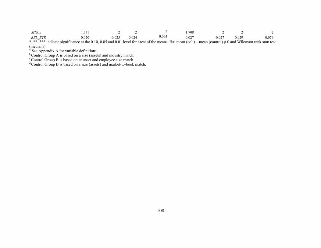
MTRt-1 1.731 2 2 2 1.708 2 2 2 REL_ETR 0.020 -0.025 0.024 0.074 0.027 -0.027 0.029 0.079

*, **, *** indicate significance at the 0.10, 0.05 and 0.01 level for t-test of the means, Ha: mean (coli) – mean (control) ≠ 0 and Wilcoxon rank sum test (medians)

108

a See Appendix A for variable definitions. b Control Group A is based on a size (assets) and industry match. c Control Group B is based on an asset and employee size match. d Control Group B is based on a size (assets) and market-to-book match.

109

Table 3

Likelihood of COLI adoption Estimated using Control Group A

Full Sample a Restricted Sample

Variable bPredicted

Sign Coefficient

Estimate Χ2statistic Coefficient

Estimate Χ2statistic

Intercept -4.437*** 11.36 -2.494 1.23

PMDACC + 4.641** 4.28 5.010** 4.12

D_RDt-1 - 1.240 9.92 1.498 8.70

CAPINTt-1 - -0.652 0.27 -0.316 0.05

INTANGt-1 - -3.144 1.59 -1.909 0.50

FOREIGNt-1 - -2.798*** 6.40 -3.681*** 5.66

VOL - -0.130* 2.25 -0.100 1.02

NINST - 0.006 2.72

ANALYST - -0.031 0.58

lnEMPt-1 + 0.268 1.35 0.127 0.19

ROAt-1 + 3.252* 1.93 3.601 1.04

MTBt-1 + -0.073 0.53 -0.141 0.98

MTRt-1 + -0.202 0.29 -0.545 1.46

lnASSETSt-1 + 0.342* 2.40 0.112 0.08

REL_ETR ? 2.645 2.40 1.091 0.25

Log-likelihood -128.043 -86.457

LR c 34.102*** 31.452***

Pseudo-R2 11.75% 15.39%

Sample size 460 303 Robust standard errors are estimated using the Huber (1967)-White(1980) procedure. ***, **, * indicate significance at 0.01, 0.05 and 0.10 levels, respectively, in two-tailed tests (one-tailed when predicted). a The full sample of firm-year observations includes 44 COLI participants and 416 firm-year observations from Control Group A, identified using a size and industry match. The restricted sample includes 32 COLI participants and 271 firm-year observations from Control Group A with data from I/B/E/S and Thompson Financial necessary to calculate ANALYST and NINST. b See Appendix A for variable definitions. c Chi-squared statistic from an LR test of the hypothesis that all coefficients other than the intercept are zero. LR test for the Full Sample has 12 degrees of freedom. LR test for the Restricted Sample has 14 degrees of freedom.

110

Table 4

Likelihood of COLI adoption Estimated using Control Group B

Full Sample a Restricted Sample

Variable bPredicted

Sign Coefficient

Estimate Χ2statistic Coefficient

Estimate Χ2statistic

Intercept -1.477 1.72 0.066 0.00

PMDACC + 1.818 1.08 3.943* 2.59

D_RDt-1 - 1.023 6.66 1.179 5.29

CAPINTt-1 - -0.494 0.24 -0.266 0.06

INTANGt-1 - -2.205 0.94 -0.875 0.09

FOREIGNt-1 - -3.782*** 8.58 -4.558*** 8.35

VOL - -0.201** 3.88 -0.155 1.56

NINST - 0.007 4.45

ANALYST - -0.045 1.08

lnEMPt-1 + 0.206 0.64 -0.032 0.01

ROAt-1 + 4.784** 4.49 4.635** 3.76

MTBt-1 + -0.058 0.58 -0.091 0.62

MTRt-1 + -0.287 0.50 -0.511 1.06

lnASSETSt-1 + -0.030 0.02 -0.187 0.29

REL_ETR ? 0.890 0.42 -0.280 0.03

Log-likelihood 128.963 86.953

LR c 24.546** 23.955**

Pseudo-R2 8.69% 12.11%

Sample Size a 444 293 Robust standard errors are estimated using the Huber (1967)-White(1980) procedure. ***, **, * indicate significance at 0.01, 0.05 and 0.10 levels, respectively, in two-tailed tests (one-tailed when predicted). a The full sample includes 43 COLI participants and 401 firm-year observations from Control Group B, identified using an asset and employee size match. The restricted sample includes 31 COLI participants and 265 firm-year observations from Control Group B with data from I/B/E/S and Thompson Financial necessary to calculate ANALYST and NINST. b See Appendix A for variable definitions. c Chi-squared statistic from an LR test of the hypothesis that all coefficients other than the intercept are zero. LR test for the Full Sample has 12 degrees of freedom. LR test for the Restricted Sample has 14 degrees of freedom.

111

Table 5

Likelihood of COLI adoption Estimated using Control Group C

Full Sample a Restricted Sample

Variable bPredicted

Sign Coefficient

Estimate Χ2statistic Coefficient

Estimate Χ2statistic

Intercept -1.343 1.46 -0.912 0.23

PMDACC + 3.928** 4.00 7.526*** 7.67

D_RDt-1 - 0.580 1.93 0.745 2.25

CAPINTt-1 - -0.616 0.38 0.042 0.00

INTANGt-1 - -2.963* 2.10 -1.093 0.00

FOREIGNt-1 - -3.538*** 6.20 -3.031** 3.80

VOL - -0.192** 3.72 -0.139 1.46

NINST - 0.004 1.49

ANALYST - -0.083** 3.03

lnEMPt-1 + 0.513** 5.02 0.568** 3.31

ROAt-1 + 1.698 0.36 1.991 0.31

MTBt-1 + -0.035 0.18 -0.111 0.40

MTRt-1 + -0.004 0.00 -0.371 0.42

lnASSETSt-1 + -0.149 0.44 -0.126 0.14

REL_ETR ? 0.077 0.00 -1.174 0.40

Log-likelihood 126.756 85.355

LR c 24.572** 21.290*

Pseudo-R2 8.84% 11.09%

Sample Size a 423 268 Robust standard errors are estimated using the Huber (1967)-White(1980) procedure. ***, **, * indicate significance at 0.01, 0.05 and 0.10 levels, respectively, in two-tailed tests (one-tailed when predicted). a The full sample includes 43 COLI participants and 380 firm-year observations from Control Group B, identified using an asset and employee size match. The restricted sample includes 31 COLI participants and 265 firm-year observations from Control Group B with data from I/B/E/S and Thompson Financial necessary to calculate ANALYST and NINST. b See Appendix A for variable definitions. c Chi-squared statistic from an LR test of the hypothesis that all coefficients other than the intercept are zero. LR test for the Full Sample has 12 degrees of freedom. LR test for the Restricted Sample has 14 degrees of freedom

Table 6

Descriptive Statistics (COLI Disclosers vs. COLI Non-Disclosers, year t-1)

Panel A: Disclosers (n=31) Non-Disclosers (n=13) Variable Mean Q1 Median Q3 Mean Q1 Median Q3 Total Assets ($billion) 1.988 0.338 0.783 2.120 6.4 * 0.869 2.755 5.652 Net Sales ($billion) 1.823 0.414 0.953 2.168 9.105 1.179 2.949 5.786 VOL 2.283 1.123 1.697 2.962 2.647 1.783 2.088 2.512 ANALYST 6.774 0 5 12 15.23 ** 6 15 24 NINST 84.500 0 60.554 132.275 208.590 * 62.277 149.356 317.559 NBLOCK 0.860 0 1 1.4 0.4 0 0 1 IORATIO 0.323 0 0.313 0.540 0.3 0.291 0.464 0.564 BLOCKRATIO 0.075 0 0.051 0.135 0.0 * 0 0 0.084

Panel B: Disclosers (n=22) Non-Disclosers (n=10) Variable Mean Q1 Median Q3 Mean Q1 Median Q3 Total Assets ($billion) 2.016 0.335 0.538 1.246 7.4 * 0.869 2.554 16.239 Net Sales ($billion) 1.356 0.351 0.774 1.838 11.136 2.275 3.409 16.703 VOL 2.586 1.495 1.979 3.032 2.824 1.672 2.255 2.671 ANALYST 9.545 4 7 14 19.80 *** 11 21.500 25 NINST 111.032 39.167 78.159 145.322 271.167 ** 90.200 225.183 498.44 NBLOCK 1.206 0 1 1.857 0.6 0 0 1.400 IORATIO 0.433 0.296 0.499 0.567 0.5 0.464 0.504 0.577 BLOCKRATIO 0.106 0 0.081 0.175 0.0 ** 0 0 0.086

Table 6 compares two groups within the COLI sample, firms that concurrently participate in COLI plans and disclose their use of COLI in their financial statements and those that do not concurrently disclose their COLI participation. Panel A describes the full COLI sample and includes 31 Disclosers and 13 Non-Disclosers. In Panel A, I set null observations equal to zero for the following variables, ANALYST, NINST, NBLOCK, IORATIO, and BLOCKRATIO. In Panel B, I restrict the sample to firms with non-missing data from I/B/E/S and Thompson Financial. Panel B includes 22 Disclosers and 10 Non-Disclosers. See Appendix A for variable definitions. Asterisks, *, **, and *** denote significance at the 10%, 5%, and 1% levels for two-tailed tests of differences in the means.

112

Table 7

Distribution of COLI adopters, industries and auditors across time

(1) (2) (3) (4) (5) (6)

Year New COLI

adopters

Cumulative # of

adopters

New industries

represented

Cumulative # of industries represented

New auditors

represented

Cumulative # of auditors represented

1986 1 1 1 1 1 1 1987 2 3 1 2 2 3 1988 0 3 0 2 0 3 1989 5 8 4 6 2 5 1990 7 15 2 8 2 7 1991 3 18 1 9 0 7 1992 3 21 0 9 1 8 1993 12 33 1 10 0 8 1994 9 42 0 10 0 8 1995 2 44 0 10 0 8 Total 44 10 8

Sample includes 44 COLI adopters with data to match based on market-to-book and assets and non-missing auditor information. Industry classifications are based on Barth, Beaver and Landsman (1998). Auditor is determined using data item 149 from COMPUSTAT.

Cumulative # of adopters, industries and auditors represented

0

5

10

15

20

25

30

35

40

45

1985 1986 1987 1988 1989 1990 1991 1992 1993 1994 1995 1996

Time

Obs

erva

tions

Industries Auditors Firms

113

114

Table 8

Cross-sectional Logit Model of COLI Adoption

Variable Predicted

Sign (1) (2) (3) (4)

Intercept -1.246 -1.288 -1.338 -1.348

(-1.59) (-1.59) (-1.60) (-1.61)

D_RDt-1 - 0.571 0.576 0.559 0.563

(1.44) (1.45) (1.40) (1.41)

LEVERAGEt-1 - -2.591** -2.616** -2.593** -2.606**

(-1.73) (-1.74) (-1.73) (-1.73)

FOREIGNt-1 - -4.062*** -4.058*** -4.096*** -4.090***

(-2.67) (-2.67) (-2.68) (-2.68)

CAPINTt-1 - -0.231 -0.202 -0.182 -0.174

(-0.26) (-0.32) (-0.20) (-0.19)

VOL - -0.191** -0.192** -0.189** -0.190**

(-1.88) (-1.89) (-1.85) (-1.86)

PMDACC3yr + -8.444 -8.388 -8.436 -8.409

(-1.38) (-1.37) (-1.37) (-1.37)

BTD3yr + -5.197 -4.991 -5.090 -5.001

(-0.69) (-0.66) (-0.67) (-0.66)

ROAt-1 + 0.324 0.263 0.397 0.356

(0.12) (0.10) (0.15) (0.13)

lnEMPt-1 + 0.301** 0.300** 0.308** 0.307**

(2.10) (2.10) (2.13) (2.12)

AUDITLINK + 0.014 0.007

(0.23) (0.11)

NINDUSTRY + 0.019 0.017

(0.34) (0.28)

Sample Size 447 447 447 447

Pseudo-R2 8.74% 8.76% 8.78% 8.78% ***, **, * indicate significance at 0.01, 0.05 and 0.10 levels, respectively, in two-tailed tests (one-tailed when predicted). The sample includes 44 COLI observations and 403 firm-year observations from a control sample matched on size (assets) and market-to-book. See Appendix A for variable definitions.

115

Table 9

Discrete-time event history analysis of COLI adoption

Variable Predicted

Sign (1) (2) (3) (4) (5)

Intercept -2.315 -4.420 -4.928 -4.564 -4.949

(-2.87) (-4.12) (-4.12) (-4.13) (-4.11)

D_RDt-1 - 0.640 0.769 0.805 0.865 0.833

(1.56) (1.83) (1.89) (1.96) (1.87)

LEVERAGEt-1 - -1.554 -1.393 -1.235 -1.238 -1.195

(-0.88) (-0.77) (-0.68) (-0.68) (-0.66)

FOREIGNt-1 - -2.826 -3.378 -3.509 -3.475 -3.530

(-1.93) (-2.27) (-2.32) (-2.32) (-2.33)

CAPINTt-1 - -0.877 -0.760 -0.959 -0.880 -0.983

(-0.90) (-0.79) (-0.99) (-0.91) (-1.00)

VOL - -0.292 -0.279 -0.263 -0.273 -0.262

(-2.18) (-2.08) (-1.98) (-2.05) (-1.97)

PMDACC3yr + -6.447 -6.479 -6.323 -6.611 -6.366

(-1.17) (-1.19) (-1.17) (-1.22) (-1.17)

BTD3yr + -6.177 -6.644 -7.242 -6.425 -7.142

(-0.83) (-0.93) (-1.02) (-0.90) (-1.00)

ROAt-1 + -1.371 -0.432 0.059 -0.464 0.015

(-0.57) (-0.17) (0.982) (-0.18) (0.01)

lnEMPt-1 + 0.129 0.136 0.125 0.114 0.119

(0.89) (0.91) (0.85) (0.76) (0.80)

ln(t) + 1.129 1.607 1.285 1.629

(3.18) (2.94) (2.99) (2.90)

AUDITLINK + -0.145 -0.136

(-1.25) (-1.08)

NINDUSTRY + -0.049 -0.016

(-0.68) (-0.20)

Log-likelihood -174.189 -167.295 -166.467 -167.052 -166.446

LR a 16.56** 13.79*** 1.66 0.49 1.70

Pseudo-R2 4.54% 8.32% 8.77% 8.45% 8.78%

116

***, **, * indicate significance at 0.01, 0.05 and 0.10 levels, respectively, in two-tailed tests (one-tailed when predicted). The sample includes 1,905 firm-year observations from 1986 to 1995, comprised of 37 COLI firms and 165 firms from Control Group C with non-missing auditor information (data 149). See Appendix A for variable definitions. a Chi-squared statistic from an LR test where LR = -2(L0 – L1). Column (1): L0 is a model where all coefficients other than the intercept are zero. Column (2): L0 = Column (1). Columns (3), (4) and (5) L0 = Column (2).

117

Table 10

Cox Proportional Hazard Model of COLI Adoption

Variable Predicted

Sign Coefficient

Estimate z Hazard Ratio

RDt-1 - 0.812 2.15 2.25

LEVERAGEt-1 - -2.978** -1.69 0.05

FOREIGNt-1 - -4.692*** -2.56 0.01

CAPINTt-1 - 0.463 0.45 1.59

VOL - -0.186* -1.55 0.83

PMDACC3yr + -2.352 -0.46 0.10

BTD3yr + -10.005 -1.39 0.00

ROAt-1 + 0.054 0.03 1.06

lnEMPt-1 + 0.196* 1.28 1.22 Sample Size = 328 firm observations LR χ2 (9 df) = -17.96, p-value = 0.03 ***, **, * indicate significance at 0.01, 0.05 and 0.10 levels, respectively, in two-tailed tests (one-tailed when predicted). The sample consists of 40 COLI participants and 288 control firms matched on size (assets) and market-to-book. The model is estimated using the exact partial likelihood method. The dependent variable is the probability of adopting a COLI shelter at time t, given that the firm had not previously adopted a COLI shelter, where t is the number of years since 1986. See Appendix A for variable definitions.

118

Table 11

Split Population Model of COLI Adoption

Adoption Propensity Equation for

Pr(ever adopt)

Duration Hazard Time to adoption, given

eventual adoption

Variable Coefficient

Estimate z Coefficient

Estimate z

Intercept 2.932 0.96 3.280 4.73

RDt-1 0.220 0.17 -0.412 -0.97

LEVERAGEt-1 4.150 0.36 3.309 1.22

FOREIGNt-1 6.522 0.86 4.576*** 3.02

CAPINTt-1 -3.388 -0.95 -1.463* -1.79

VOL -0.665** -2.13 -0.154 -1.21

PMDACC3yr 5.859 0.31 2.532 0.66

BTD3yr -43.680 -0.91 -5.897 -0.87

ROAt-1 6.997 1.00 2.321 1.14

lnEMPt-1 -0.509 -1.07 -0.264** -1.95 Sample Size = 328 firm observations Wald χ2 (9 df) = -21.20, p-value = 0.01 ***, **, * indicate significance at 0.01, 0.05 and 0.10 levels, respectively, in two-tailed tests (one-tailed when predicted). The sample consists of 40 COLI participants and 288 control firms matched on size (assets) and market-to-book. The model is estimated using maximum likelihood and a lognormal specification for the p.d.f. for the time taken to adopt. See Appendix A for variable definitions.

119

Figure 1

Financial Reporting for COLI

Book Book-Tax

Adjustment Tax

Increase in policy cash surrender value 20 (20) 0 Death benefits 0 0 0 Less: Premium expense (12) 12 0

Interest expense on policy loans (10) 0 (10)

Net COLI income (expense) (2) (8) (10)

FASB Technical Bulletin No. 85-4 prescribes the financial accounting treatment for corporate-owned life insurance. In a leveraged COLI transaction, net COLI income (expense) equals increases in the cash surrender value (interest credited to the policy) plus any death benefits received less the premium expense and the interest expense on the policy loans. Under IRC §72, the interest credited to the cash surrender value of the policy, in this example $20, is not included in the policyholder’s gross income. In other words, returns on the firm’s COLI investment are income for book purposes, but excluded from income for tax purposes. Leveraged COLI plans were designed to be mortality neutral; the profit comes from arbitraging the tax-free build up of the cash surrender value, not from tax-free death benefits. Hence, death benefits in this example are equal to zero. Because proceeds from life insurance receive preferential tax treatment, policy premiums are not deductible for tax purposes. This example shows premium expense of $12 which reduces book income, but not taxable income. However, the interest expense paid on policy-backed loans, here $10, is tax-deductible. The numbers chosen for the example here are arbitrary, but show an important feature of the COLI shelter. The transaction produces a loss for tax purposes in excess of any economic or financial statement loss. Indeed, even though this example produces a $2 pre-tax book loss, at a 35% statutory rate, the $2.80 tax benefit from $8 of net nontaxable income offsets the $2 pre-tax book loss, generating positive after-tax income of $0.80.

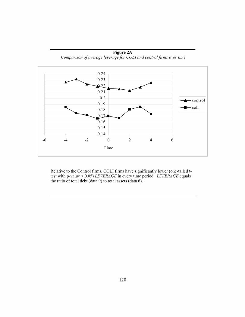
Figure 2A Comparison of average leverage for COLI and control firms over time

0.140.150.160.170.180.19

0.20.210.220.230.24

-6 -4 -2 0 2 4 6

Time

control

coli

Relative to the Control firms, COLI firms have significantly lower (one-tailed t-test with p-value < 0.05) LEVERAGE in every time period. LEVERAGE equals the ratio of total debt (data 9) to total assets (data 6).

120

Figure 2B Comparison of average ETR for COLI and control firms over time

0.3

0.32

0.34

0.36

0.38

0.4

0.42

0.44

-6 -4 -2 0 2 4 6

Time

control

coli

The difference in average ETR is not statistically significant (two-tailed t-test with p-value < 0.10) in any time period. ETR equals the ratio of total income tax expense (data 16) to pretax income (data 170).

121

________________________________________________________________________

Figure 2C Comparison of average PMDACC

for COLI and ontrol firms over time

-0.02

-0.01

0

0.01

0.02

0.03

0.04

-6 -4 -2 0 2 4 6

Time

controlcoli

PMDACC, performance-matched discretionary accruals, are calculated following Kothari et al. (2005) using an industry classification following Barth et al.(1998) and Barth et al. (2005). Relative to Control firms, COLI firms have significantly higher PMDACC in year t-4 (t-statistic = 1.99, p-value = 0.05), significantly lower PMDACC in year t-3 (t-statistic = -2.01, p-value = 0.05) and significantly higher PMDACC in year t (t-statistic = 2.76, p-value = 0.01). The mean difference in PMDACC was not statistically significant in any of the remaining years.

122

____________________________________________________________

Figure 2D Comparison of average PERMDIFF for COLI and control firms over time

-0.005

0

0.005

0.01

0.015

0.02

-6 -4 -2 0 2 4 6

Time

controlcoli

PERMDIFF, permanent book-tax differences, are calculated following Frank et al. (2005), as the difference between book income and taxable income, deflated by assets at the beginning of the year (lag data 6). Book income equals pretax income (data 170) less minority (data 49) and taxable income equals the sum of current federal tax expense (data 63) and current foreign tax expense (data 64), divided by the statutory tax rate, less deferred taxes, divided by the statutory tax rate. When data 63 is missing, current federal tax expense is calculated as (data 16 – data 64 – data 173 – data 50) Relative to Control firms, COLI firms have significantly higher (one-tailed t-test with p-value<0.10) PERMDIFF in every year except year t+1.

123

124

Appendix A – Variable Definitions

Total Assets ($billion) Data 6 / 1,000

Net Sales ($billion) Data 12 / 1,000 D_RDt-1 A dichotomous variable equal to one if the firm reports positive

research expenditures (data 46) and zero otherwise. LEVERAGEt-1 Ratio of total liabilities (data 9) / total assets (data 6) for the prior

year. CAPINTt-1 Ratio of net property, plant and equipment (data 8) / total assets

(data 6) for the prior year. FOREIGNt-1 Ratio of foreign assets / total assets for the prior year (from

COMPUSTAT Geographic Segment file). VOL Ratio of volume to shares outstanding, averaged over the year.

PMDACC3yr The absolute value of performance-matched discretionary accruals averaged over the prior 3 years.

BTD3yr Permanent book-tax differences, averaged over the prior 3 years, divided by total assets (data 6) averaged over the prior 3 years.

IORATIO The fraction of shares held by institutional owners averaged across the four quarters in the prior year

BLOCKRATIO The fraction of shares held by five-percent blockholders averaged across the four quarters in the prior year.

NINST The number of institutional owners averaged across the four quarters in the prior year.

NBLOCK The number of five-percent blockholders averaged across the four quarters in the prior year.

ANALYST The number of analysts included in the most recent consensus forecast of annual earnings on I/B/E/S.

lnEMPt-1 Log of employees (data 29) for the prior year. ROAt-1 Ratio of pre-tax book income (data 170 – data 49) / average total

assets ((data 6 + lagged data 6)/2) for the prior year. MTBt-1 Prior year’s market-to-book ratio ((data 199 * data 25)/ data 60)

NINDUSTRY The cumulative number of COLI adopters in firm i’s industry from 1986 though the end of year t-1.

AUDITLINK The number of prior COLI adopters audited by the firm’s auditor in year t.

125

References

Aboody, D. and Kasznik, R. 2000. “CEO stock option awards and the timing of corporate voluntary disclosures.” Journal of Accounting and Research, 29: 73-100.

Abrahamson, E. and Rosenkopf, L. 1993. “Institutional and competitive bandwagons: using

mathematical modeling as a tool to explore innovation diffusion.” The Academy of Management Review, 18 (3): 487-517.

Allingham, M. and Sandmo, A. 1972. “Income tax evasion: a theoretical analysis.” Journal of

Public Economics, 1 (3): 323-339. Bankman, J. 1999. “The new market for corporate tax shelters.” Tax Notes, 83 (12): 1775-1795. Bankman, J. 2002. “Commentary: modeling the tax shelter world.” Tax Law Review, 55: 455-

464. Bankman, J. 2004. “An academic’s view of the tax shelter battle.” In The Crisis in Tax

Administration, edited by H.J. Aaron and J. Slemrod. Brookings Institution, Washington D.C.

Bankman, J. 2004. “The tax shelter problem.” National Tax Journal, 57 (4): 925-936. Barth, M.E., Beaver, W.H., and Landsman, W.R. 1998. “Relative valuation roles of equity book

value and net income as a function of financial health.” Journal of Accounting and Economics, 25 (1): 1-34.

Barth, M.E., Beaver, W.H., Hand, J.R.M., and Landsman, W.R. 2005. “Accruals, accounting-

based valuation models, and the prediction of equity values.” Journal of Accounting, Auditing and Finance, 20 (4): 311-345.

Barth, M.E., Elliot, J.A., and Finn, M.W. 1999. “Market rewards associated with patterns of

increasing earnings.” Journal of Accounting Research, 37 (2): 387-413. Barton, J. 2005. “Who cares about auditor reputation?” Contemporary Accounting Research, 22

(3): 549-586. Bartov, E., Givoly, D., and Hayn, C. 2002. “The rewards to meeting or beating earnings

expectations.” Journal of Accounting and Economics, 33 (2): 173-204. Bertrand, M. and Schoar, A. 2003. “Managing with style: the effect of managers on firm

policies.” Quarterly Journal of Economics, 118 (4): 1169-1208. Box-Steffensmeier, J. and Jones, B. 1997. “Time is of the essence: event history models in

political science.” American Journal of Political Science, 41 (4): 1414-1461. Bromiley, P. 1991. “Testing a casual model of corporate risk taking and performance.” Academy

of Management Journal, 34 (1): 37-59.

126

Bushee, B. and Noe, J. 2000. “Corporate disclosure practices, institutional investors, and stock return volatility.” Journal of Accounting Research, 38 (Supp.): 171-202.

Chen, K. and Chu, C. 2005. “Internal control vs. external manipulation: a model of corporate

income tax evasion.” RAND Journal of Economics, 38 (1): 151-164. Crocker, K. and Slemrod, J. 2005. “Corporate tax evasion with agency costs.” Journal of Public

Economics, 89: 1593-1610. Cuccia, A. 1994. “The economics of tax compliance: What do we know and where do we go?”

Journal of Accounting Literature, 13: 81-116. Cyert, R. and March, J.G. 1963. A Behavioral Theory of the Firm. Englewood Cliffs, New Jersey:

Prentice-Hall. Davis, G. 1991. “Agents without principles? The spread of the poison pill through the

intercorporate network.” Administrative Science Quarterly, 36: 605-633. DeAngelo, H. and Masulis, R. 1980. “Leverage and dividend irrelevancy under corporate and

personal taxation.” Journal of Finance, 8 (1): 3-29. Dechow, P., Sloan, R., and Sweeney, A. 1995. “Detecting earnings management.” The

Accounting Review, 70: 193-226. Dechow, P., Sloan, R. and Sweeney, A. 1996. “Causes and consequences of earnings

manipulations: an analysis of firms subject to enforcement actions by the SEC.” Contemporary Accounting Research 13 (1): 1-36.

Desai, M. 2005. “The degradation of reported corporate profits.” Journal of Economic

Perspectives, 19 (4): 171-192. Desai, M., and Dharmapala, D. 2006. “Corporate tax avoidance and high-powered incentives.”

Journal of Financial Economics, 79: 145-179. Desai, M., Dyck, A., and Zingales, L. 2007. “Theft and taxes.” Journal of Financial Economics,

84 (3): 591-623. Dhaliwal, D., Frankel, M., and Trezevant, R. 1994. “The taxable and book income motivations

for a LIFO layer liquidation.” Journal of Accounting Research, 32 (2): 278-289. Dhaliwal, D., Trezevant, R. and Wang, S. 1992. “Taxes, investment related tax shields and capital

structure.” Journal of the American Taxation Association, 14 (1): 1-21. DiMaggio, P.J. and Powell, W.W. 1983. “The iron cage revisited: Institutional isomorphism and

collective rationality in organizational fields.” American Sociological Review, 48: 147-160.

Dyreng, S., Hanlon, M. and Maydew, E. 2008. “Long-run corporate tax avoidance.” The

Accounting Review, 83 (1): 61-82.

127

Dyreng, S., Hanlon, M. and Maydew, E. 2008. “The effects of managers on corporate tax avoidance.” Working paper, University of North Carolina at Chapel Hill and University of Michigan.

Edwards, C. 2005. “Do employee stock options encourage corporate tax sheltering?” Working

paper, University of North Carolina at Chapel Hill. Engel, E., Erickson, M., and Maydew, E. 1999. “Debt-equity hybrid securities.” Journal of

Accounting Research, 37 (2): 249-274. Erickson, M. and Wang, S. 1998. “Earnings management by acquiring firms in stock for stock

mergers.” Journal of Accounting and Economics, 27 (2): 149-176. Eustice, J. 2002. “Abusive tax shelters: old ‘brine’ in new bottles.” Tax Law Review, 55: 135-

174. Fama, E. and French, K. 1993. “Common risk factors in the returns on stocks and bonds.”

Journal of Financial Economics, 33: 3-56. Fligstein, N. 1985. “The spread of the multidivisional form among large firms, 1919-1979.”

American Sociological Review, 50: 377-391. Fombrun, C. and Ginsberg, A. 1990. “Shifting gears: enabling change in corporate

aggressiveness.” Strategic Management Journal, 11: 297-308.

Fombrun, C. and Shanley, M. 1990. “What’s in a name? Reputation building and corporate strategy.” Academy of Management Journal, 33 (2): 233-258.

Francis, J., Huang, A., Rajgopal, S., and Zang, A. 2008. “CEO reputation and earnings quality.”

Contemporary Accounting Research, 25 (1): 109-117. Frank, M., Lynch, L., Rego, S. 2006. “Does aggressive financial reporting accompany

aggressive tax reporting (and vice versa)?” Working paper, Universities of Virginia and Iowa.

Galaskiewicz, J. and Burt, R. 1991. “Interorganization contagion in corporate philanthropy.”

Administrative Science Quarterly, 36 (1): 88-105. Gergen, M. 2002. “The logic of deterrence: corporate tax shelters.” Tax Law Review, 55: 255-

286. Gompers, P., Ishii, J., and Metrick, A. 2003. “Corporate governance and stock prices.”

Quarterly Journal of Economics, 118 (1): 107-155. Graham, J.R. and Tucker, A.L. 2006. “Tax shelters and corporate debt policy.” Journal of

Financial Economics, 81: 563-594. Grubert, H. and Slemrod, J. 1998. “The effect of taxes on investment and income-shifting to

Puerto Rico.” Review of Economics and Statistics, 80 (3): 365-373.

128

Guenther, D. 1994. “Earnings management in response to corporate tax rate changes: evidence

from the 1986 Tax Reform Act.” The Accounting Review, 69 (1): 230-243. Gupta, S. and Mills, L. 2002. “Corporate multistate tax planning: Benefits of multiple

jurisdictions.” Journal of Accounting and Economics, 33: 117-139. Gupta, S. and Newberry, K. 1997. “Determinants of the variability in corporate effective tax

rates: evidence from longitudinal data.” Journal of Accounting and Public Policy, 16: 1-34.

Hanlon, M. and Slemrod, J. 2007. “What does tax aggressiveness signal? Evidence from stock

price reactions to news about tax aggressiveness.” Working paper, University of Michigan.

Hartzell, J. and Starks, L. 2003. “Institutional investors and executive compensation.” Journal of

Finance, 58 (6): 2351-2374. Haunschild, P. 1993. “Interorganizational imitation: the impact of interlocks on corporate

acquisition activity.” Administrative Science Quarterly, 38 (4): 564-592. Haunschild, P. and Miner, A. 1997. “Modes of interorganzational imitation: the effects of

outcome salience and uncertainty.” Administrative Science Quarterly, 42 (3): 472-500. Haveman, H. 1993. “Follow the leader: mimetic isomorphism and entry into new markets.”

Administrative Science Quarterly, 38 (4): 593-627. Huber, P.J. 1967. The behavior of maximum likelihood estimates under nonstandard conditions.

Proceedings of the Fifth Berkeley Symposium on Mathematical Statistics and Probability 1: 221-223.

Hunt, A., Moyer, S., and Shevlin, T. 1996. “Managing interacting accounting measures to meet

multiple objectives: a study of LIFO firms.” Journal of Accounting and Economics, 21 (3): 339-374.

Karpoff, J., Lee, D.S. and Martin, G. 2006. “The cost to firms of cooking the books.” Working

paper, University of Washington and Texas A&M University. Karpoff, J. and Lott, L.J. 1993. “The reputational penalty firms bear for committing fraud.”

Journal of Law and Economics, 36 (2): 757-803. Kasznik, R., and McNichols, M. 2002. “Does meeting earnings expectations matter? Evidence

from analyst forecast revisions and share prices.” Journal of Accounting Research, 40 (3): 727-759.

Klein, A. 2002. “Audit committee, board of director characteristics, and earnings management.”

Journal of Accounting and Economics, 33: 375-400.

129

Kothari, S.P., Leone, A., and Wasley, C. 2005. “Performance matched discretionary accruals.” Journal of Accounting and Economics, 39 (1): 163-197.

MacKie-Mason, J. 1990. “Do taxes affect corporate financing decisions.” Journal of Finance, 45:

1471-1493. Manzon, G. and Plesko, G. 2002. “The relation between financial and tax reporting measures of

income.” Tax Law Review, 55: 175-214. Manzon, G. and Smith, W. 1994. “The effect of the Economic Recovery Act of 1981 and the Tax

Reform Act of 1986 on the distribution of effective tax rates.” Journal of Accounting and Public Policy, 13: 349-362.

March, J.G. 1981. “Decisions in organizations and theories of choice.” In Perspectives on

Organization Design and Behavior, edited by A. Van de Ven and W.F. Joyce. Wiley: New York.

Massini, S., Lewin, A., and Greve, H. 2005. “Innovators and imitators: organizational reference

groups and adoption of organizational routines.” Research Policy, 34 (10): 1550-1569. Matsunaga, S. and Park, C. 2001. “The effect of missing a quarterly earnings benchmark on the

CEO’s annual bonus.” The Accounting Review, 76 (3): 313-332. Matsunaga, S., Shevlin, T., and Shores, D. 1992. “Disqualifying dispositions of incentive stock

options: tax benefits versus financial reporting costs.” Journal of Accounting Research, 30: 37-76.

McGill, G. and Outslay, E. 2004. “Lost in translation: detecting tax shelter activity in financial

statements.” National Tax Journal, 57 (3): 739-756. Mezias, S. 1990. “An institutional model of organizational practice: Financial reporting at the

Fortune 200.” Administrative Science Quarterly, 35 (3): 431-457. Milbourn, T. 2003. “CEO reputation and stock-based compensation.” Journal of Financial

Economics, 68: 233-262. Milgrom, P. and Roberts, J. 1982. “Predation, reputation and entry deterrence.” Journal of

Economic Theory, 27: 280-312. Mills, L., Newberry, K., and Novack, G. 2003. “How well do COMPUSTAT NOL data identify

firms with U.S. tax return loss carryovers?” Journal of the American Taxation Association, 25 (2): 1-17.

Novack, J. and Saunders, L. 1998. “The hustling of x-rated shelters.” Forbes, December 19,

1998. Nurnberg, H. 2004. “Accounting for company-owned life insurance.” Accounting Horizons, 18

(2): 109-126.

130

Palmrose, Z., Richardson, V. and Scholz, S. 2004. “Determinants of market reactions to restatement announcements.” Journal of Accounting and Economics 37: 59-89.

Rao, H. and Sivakumar, K. 1999. “Institutional sources of boundary-spanning structures: the

establishment of investor relations departments in the Fortune 500 industrials.” Organizational Science, 10 (1): 27-42.

Rego, S. 2003. “Tax-avoidance activities of U.S. multinational corporations.” Contemporary

Accounting Research, 20 (4): 805-833. Roberts, P.W. and Dowling, G.R. 2002. “Corporate reputation and sustained superior financial

performance.” Strategic Management Journal, 23 (12):1077-1093. Rogers, E. 2003. Diffusion of Innovations, 5th edition. New York: Free Press. Rogers, W.H. 1993. Regression standard errors in clustered samples. Stata Technical Bulletin 13:

19-23. Schmidt, P. and Witte, A. 1989. “Predicting criminal recidivism using ‘split-population’ survival

time models.” Journal of Econometrics, 40 (1): 141-159. Shackelford, D. and Shevlin, T. 2001. “Empirical tax research in accounting.” Journal of

Accounting and Economics, 31 (1-3): 321-387. Shevlin, T. 2002. “Commentary: corporate tax shelters and book-tax differences.” Tax Law

Review, 55: 455-464. Shevlin, T. and Porter, S. 1992. “The corporate tax comeback in 1987: Some further evidence.”

Journal of the American Taxation Association, Spring: 58-79. Skinner, D., and Sloan, R. 2002. “Earnings surprises, growth expectations, and stock returns or

Don’t let an earnings torpedo sink your portfolio.” Review of Accounting Studies, 7(2-3): 289-312.

Slemrod, J. 2004. “The economics of corporate tax selfishness.” National Tax Journal, 57 (4):

877-899. Srinivanan 1973. “Tax evasion: a model.” Journal of Public Economics, 2: 339-346. Stuart, T.E., Hoang, H. and Hybels, R.C. 1999. “Interorganizational endorsements and the

performance of entrepreneurial ventures.” Adminstrative Science Quarterly, 44: 315-349. Teo, S., Welch, I., and Wong, T. 1998. “Earnings management and the long-run

underperformance of seasoned equity offerings.” Journal of Financial Economics, 50: 63-100.

Trezevant, R. 1992. “Debt financing and tax status: tests of the substitution effect and the tax

exhaustion hypothesis using firms' responses to the Economic Recovery tax Act of 1981.” Journal of Finance, 47 (4): 1557-1568.

131

U.S. Department of the Treasury. 1999. “The problem of corporate tax shelters: discussion,

analysis, and legislative proposals.” Washington, D.C.: U.S. Government Printing Office.

U.S. Senate Permanent Committee on Investigations. 2005. “The role of professional firms in the

U.S. tax shelter industry.” S. Rep. 109-54, Washington, D.C.: U.S. Government Printing Office.

Wang, S. 1991. “The relation between firm size and effective tax rates: a test of firms’ political

success.” The Accounting Review, 66 (1): 158-169. Watts, R.L. and Zimmerman, J.L. 1986. Positive Accounting Theory. Englewood Cliffs, NJ.

Prentice Hall. Weisbach, D. 2002. “Ten truths about corporate tax shelters.” Tax Law Review, 55: 215-253. White, H. 1980. A heteroskedasticity-consistent covariance matrix estimator and a direct test for

heteroskedasticity. Econometrica (May): 817-838. Wilson, R. 2007. “An examination of corporate tax shelter participants.” Working paper,

University of Washington.

132

VITA

Jennifer Lynn Brown was born in Houston, Texas on August 21, 1975, the

daughter of Ellen Ireton Bell and John Martin Bell. After graduating from Bellaire High

School, Bellaire, Texas, in 1993, she entered the University of Texas at Austin. She

received the degrees of Bachelor of Business Administration and Masters of Professional

Accounting from the University of Texas at Austin in May 1998. During the following

years she was employed as a tax consultant with PricewaterhouseCoopers LLP. In July

2001 she entered the Graduate School of the University of Texas at Austin.

Permanent Address: 7540 E. Wolf Canyon Circle, Mesa, Arizona 85207

This dissertation was typed by the author.