Copyright by Ji Hoon Yoon 2015

Copyright

by

Ji Hoon Yoon

2015

The Dissertation Committee for Ji Hoon Yooncertifies that this is the approved version of the following dissertation:

Demand Side Load Control in Residential Buildings

with HVAC Controller for Demand Response

Committee:

Ross Baldick, Supervisor

Atila Novoselac, Co-Supervisor

Aristotle Arapostathis

Petra G. Liedl

Alexis Kwasinski



by

Ji Hoon Yoon, B.E.; M.S.E

DISSERTATION

Presented to the Faculty of the Graduate School of

The University of Texas at Austin

in Partial Fulfillment

of the Requirements

for the Degree of

DOCTOR OF PHILOSOPHY

THE UNIVERSITY OF TEXAS AT AUSTIN

May 2015

Dedicated to my parents,

Young Gun Yoon and Jae Ok Song

and to my brother,

Ji Hwan Yoon

Acknowledgments

With this dissertation, I would like to express my deepest gratitude to

my advisor, Professor Ross Baldick, for his excellent and continuing advice,

suggestions, encouragement and generosity. I have been fortunate to have an

advisor who allowed me the freedom to explore my own research topics, and

encouraged me to develop my own ideas continuously. His profound knowledge

and exemplary guidance have inspired me to mature further academically. In

addition, I gratefully appreciate my co-advisor, Dr. Atila Novoselac, for his

excellent advice and suggestions in the area of Architectural Engineering to

do research and purse my PhD degree.

Also, I would like to gratefully acknowledge the distinguished members

of my supervisory committee for their valuable help and support: Professor

Aristotle Arapostathis, and Professor Alexis Kwasinski in Department of Elec-

trical and Computer Engineering and Professor Petra G. Liedle in School of

Architecture.

Most importantly, I would like to express much gratitude and love to

my parents, Yong gun Yoon and Jae Ok Song, for their endless love and

unconditional support for me to complete my Ph.D through these difficult

years. Without their support and sacrifice, this work would never have come

into existence.

v

Finally, I appreciate the financial support from the Collaboration Project

with Electric Reliability Council of Texas and Fujitsu Laboratories of America

Inc.

vi



Publication No.

Ji Hoon Yoon, Ph.D.

The University of Texas at Austin, 2015

Supervisors: Ross BaldickAtila Novoselac

Demand Response (DR) is a key factor to increase the efficiency of the

power grid and has the potential to facilitate supply-demand balance. Demand

side load control can contribute to reduce electricity consumption through DR

programs. Especially, Heating, Ventilating and Air Conditioning (HVAC) load

is one of the major contributors to peak loads. In the United States, HVAC

systems are the largest consumers of electrical energy and a major contributor

to peak demand. In this research, the Dynamic Demand Response Controller

(DDRC) is proposed to reduce peak load as well as saves electricity cost while

maintaining reasonable thermal comfort by controlling HVAC system. To

reduce both peak load and energy cost, DDRC controls the set-point temper-

ature in a thermostat depending on real-time price of electricity. Residential

buildings are modeled with various internal loads using building energy model-

ing tools. The weather data in different climate zones are used to demonstrate

vii

that DDRC decreases peak loads and brings economic benefit in various lo-

cations. In addition, two different types of electricity wholesale markets are

used to generate DR signals. To assess the performance of DDRC, the control

algorithms are improved to consider the characteristics of building envelopes

and HVAC equipment. Also, DDRC is designed to be deployed in various ar-

eas with different electricity wholesale markets. The indoor thermal comfort

on temperature and humidity are considered based on ASHRAE standard 55.

Finally, DDRC is developed to a hardware using embedded system. The hard-

ware of DDRC is based on Advanced RISC Microcontroller (ARM) processor

and senses both indoor and outdoor environment with Internet connection

capability for DR. In addition, user friendly Graphic User Interface (GUI) is

generated to control DDRC.

viii

Table of Contents

Acknowledgments v

Abstract vii

List of Tables xiii

List of Figures xiv

Chapter 1. Introduction 1

1.1 Background . . . . . . . . . . . . . . . . . . . . . . . . . . . . 1

1.2 Motivation and Value of the Research . . . . . . . . . . . . . 7

1.3 Objectives and Scope of the Research . . . . . . . . . . . . . . 10

1.4 Contributions . . . . . . . . . . . . . . . . . . . . . . . . . . . 12

1.5 Organization of the Dissertation . . . . . . . . . . . . . . . . . 13

Chapter 2. Modeling of residential buildings and real-time priceof electricity 15

2.1 Introduction . . . . . . . . . . . . . . . . . . . . . . . . . . . . 15

2.2 Design of Single Family Houses . . . . . . . . . . . . . . . . . 22

2.3 Dynamic Retail Price of Electricity . . . . . . . . . . . . . . . 25

2.4 Simulation Cases . . . . . . . . . . . . . . . . . . . . . . . . . 33

Chapter 3. Control Algorithm of Dynamic Demand ResponseController 34

3.1 Base Control Policy with Dynamic Price of Electricity . . . . . 34

3.1.1 Estimation of Slope of Electricity Consumption by HVAC 35

3.1.2 Price Trigger and Coefficient of Price over Temperature 38

3.1.3 Control of The Thermostat . . . . . . . . . . . . . . . . 41

3.2 Improved Control Algorithm of DDRC for various circumstances 42

ix

3.2.1 Estimation of HVAC Electricity Consumption . . . . . . 43

3.2.2 Normalized Electricity Price Signal . . . . . . . . . . . . 46

3.2.3 The Change Rate of The Set-point Temperature . . . . 47

3.3 Controller Implementation . . . . . . . . . . . . . . . . . . . . 48

Chapter 4. The Results of The Performance of DDRC 51

4.1 DDRC with dynamic price of electricity . . . . . . . . . . . . . 51

4.1.1 Simulation Condition . . . . . . . . . . . . . . . . . . . 52

4.1.2 Air Conditioning Loads: August . . . . . . . . . . . . . 52

4.1.3 Heating Loads: January . . . . . . . . . . . . . . . . . . 56

4.1.4 Total Energy Savings . . . . . . . . . . . . . . . . . . . 59

4.1.5 Indoor Thermal Comfort . . . . . . . . . . . . . . . . . 61

4.2 DDRC with various price types and floor plans . . . . . . . . . 63


4.2.2 The Large House . . . . . . . . . . . . . . . . . . . . . . 64

4.2.3 The Medium House . . . . . . . . . . . . . . . . . . . . 68

4.2.4 Annual Energy Cost Savings . . . . . . . . . . . . . . . 71

4.2.5 Annual energy cost savings . . . . . . . . . . . . . . . . 73

4.2.6 Thermal Comfort . . . . . . . . . . . . . . . . . . . . . 75

4.3 DDRC with different internal loads and climate zones . . . . . 78


4.3.2 Savings of Electricity Consumption . . . . . . . . . . . . 78

4.3.3 Energy Cost Savings . . . . . . . . . . . . . . . . . . . . 84

4.3.4 The Thermal Comfort . . . . . . . . . . . . . . . . . . . 87

4.4 Summary . . . . . . . . . . . . . . . . . . . . . . . . . . . . . . 91

4.4.1 DDRC with dynamic price of electricity . . . . . . . . . 91

4.4.2 DDRC with various price types and floor plans . . . . . 92

4.4.3 DDRC with different internal loads and climate zones . 93

4.4.4 Comparison of Results . . . . . . . . . . . . . . . . . . . 93

x

Chapter 5. Development of Hardware for Dynamic Demand Re-sponse Controller 96

5.1 Arduino Due embedded controller . . . . . . . . . . . . . . . . 96

5.2 Sensing of Temperature and Humidity: HTU21D . . . . . . . . 99

5.3 Wireless Ethernet Connection . . . . . . . . . . . . . . . . . . 100

5.4 Real-Time Clock: DS3231 . . . . . . . . . . . . . . . . . . . . 102

5.5 DDRC Graphic User Interface . . . . . . . . . . . . . . . . . . 103

5.6 Assembling modules with Arduino boards . . . . . . . . . . . . 104

Chapter 6. Conclusion 106

Appendices 111

Appendix A. Thermal Comfort on Pychrometric Chart 112

Appendix B. Battery Backup System for residential buildings 119

B.1 The Layout of Battery Backup System . . . . . . . . . . . . . 119

B.2 Economics on the Battery System . . . . . . . . . . . . . . . . 122

Appendix C. Case Study: Demand Response Experiences withUtilities 124

C.1 Gulf Power . . . . . . . . . . . . . . . . . . . . . . . . . . . . . 124

C.1.1 DR Program - Energy Select . . . . . . . . . . . . . . . 124

C.1.2 Number of Customers with Energy Select . . . . . . . . 126

C.1.3 Results with Energy Select . . . . . . . . . . . . . . . . 126

C.1.4 Load Control . . . . . . . . . . . . . . . . . . . . . . . . 127

C.2 Commonwealth Edison . . . . . . . . . . . . . . . . . . . . . . 128

C.2.1 DR Program - Smart Return . . . . . . . . . . . . . . . 128

C.2.2 Real-Time Price (RTP) . . . . . . . . . . . . . . . . . . 129

C.2.3 Number of Customers . . . . . . . . . . . . . . . . . . . 130

C.3 Cincinnati Gas & Electric . . . . . . . . . . . . . . . . . . . . 130

C.3.1 DR Programs - PowerShare . . . . . . . . . . . . . . . . 131


C.4 Portland General Electric . . . . . . . . . . . . . . . . . . . . . 132

xi

C.4.1 DR Programs . . . . . . . . . . . . . . . . . . . . . . . . 132

C.4.2 Real-Time Price . . . . . . . . . . . . . . . . . . . . . . 133


C.5 Duquesne Light Company . . . . . . . . . . . . . . . . . . . . 133

C.5.1 DR Program . . . . . . . . . . . . . . . . . . . . . . . . 133

C.5.2 Real-Time Price . . . . . . . . . . . . . . . . . . . . . . 134


Bibliography 136

Vita 151

xii

List of Tables

2.1 Building geometry features of the large and medium houses . . 23

2.2 The capacities of heat pumps and COPs . . . . . . . . . . . . 26

3.1 Temperature-electricity constant for cooling (kc) and heating (kh) 44

4.1 Percentage of indoor air temperature for a year . . . . . . . . 61

4.2 Indoor air temperature in percentage of hours for a year . . . 76

4.3 Normalized thermal discomfort by days of cooling and heatingwhen DDRC is applied [Co] - The temperature difference fromthe indoor temperature without DDRC . . . . . . . . . . . . . 90

4.4 The improvement of DDRC performance by enhanced controlpolicy . . . . . . . . . . . . . . . . . . . . . . . . . . . . . . . 95

B.1 The estimate cost of the battery backup system for 16 year use 123

xiii

List of Figures

1.1 Retail Sales of Electricity to Ultimate Customers, Total by End-Use Sector(2010) − [Source] U.S. Energy Information Admin-istration, Electric Power Monthly, Table 5.1, September 2012 . 2

1.2 Residential Energy Use, Energy Use Intensity, and Energy UseFactors − [Source] DOE, Energy Efficiency and Renewable En-ergy, Trend Data: Residential Buildings Sector . . . . . . . . . 3

1.3 Residential electricity consumption by end use (2010) - [Source]DOE, Buildings Energy Data Book, Table 2.1.4, March 2012 . 4

1.4 Layout of a typical residential HVAC system . . . . . . . . . . 5

1.5 The operation of heat pump as an air conditioner or heater . . 6

1.6 Residential load changes in ERCOT grid by HVAC use (2010) 8

2.1 3D model of single family houses used in the study: large house(L) and medium size house (R) . . . . . . . . . . . . . . . . . 22

2.2 The floor plans of two single family houses: a medium houseand large house . . . . . . . . . . . . . . . . . . . . . . . . . . 25

2.3 The histogram of electricity price in Austin, TX and Chicago, IL 30

2.4 The monthly Max, Average, and Min of electricity price in twocities . . . . . . . . . . . . . . . . . . . . . . . . . . . . . . . . 31

3.1 Framework of dynamic demand response controller . . . . . . 35

3.2 Scatter plot of HVAC electricity consumption changes versusset point temperature difference . . . . . . . . . . . . . . . . . 37

3.3 Dynamic demand response controller in MATLAB/SIMULINK 49

3.4 Diagram of connection EnergyPlus with SIMULINK using BCVTB 50

4.1 Indoor air temperature changes in August . . . . . . . . . . . 53

4.2 HVAC electricity consumption during August . . . . . . . . . 54

4.3 Significant electricity peak load reduction by DDRC on August 3 55

4.4 Winter season indoor air temperature comparison, January . . 56

4.5 January HAVC electricity consumption comparison . . . . . . 57

xiv

4.6 HVAC load changes on January 20, winter season . . . . . . . 58

4.7 Comparison of annual HVAC electricity consumption . . . . . 59

4.8 Indoor thermal comfort comparison in January and August . . 62

4.9 The peak load reduction by the DDRC thermostat with RTPand DAP at a large house . . . . . . . . . . . . . . . . . . . . 66

4.10 Monthly HVAC electricity consumption of a large house . . . . 67

4.11 The contribution of DDRC thermostat with RTP and DAP todecrease peak loads at a medium house . . . . . . . . . . . . . 69

4.12 A medium house’s Monthly HVAC electricity consumption . . 70

4.13 The annual electricity savings for a large and medium house . 72

4.14 The comparison of energy cost for a large and medium house . 74

4.15 The electricity consumption of houses in Austin, TX for wholeyear . . . . . . . . . . . . . . . . . . . . . . . . . . . . . . . . 81

4.16 The comparison of annual electricity consumption by houses inChicago, IL . . . . . . . . . . . . . . . . . . . . . . . . . . . . 83

4.17 Energy cost comparisons between DDRC and fixed SP mode intwo locations . . . . . . . . . . . . . . . . . . . . . . . . . . . 86

4.18 Indoor thermal comfort of a large house with normal loads whenDDRC is applied − Austin, TX . . . . . . . . . . . . . . . . . 88

5.1 32bit ARM CPU based Arduino Due Board . . . . . . . . . . 98

5.2 Temperature and humidity senor: HTU21D . . . . . . . . . . 99

5.3 WiFi board for Arudino Due micro-controller board . . . . . . 100

5.4 Real-Time Clock (RTC): DS3231 . . . . . . . . . . . . . . . . 102

5.5 Graphic User Interface (GUI) of DDRC . . . . . . . . . . . . . 103

A.1 The indoor environment in a large house with Base Case . . . 113

A.2 The indoor environment in a large house with Case 1: Real-Time Price . . . . . . . . . . . . . . . . . . . . . . . . . . . . . 114

A.3 The indoor environment in a large house with Case 2: DayAhead Price . . . . . . . . . . . . . . . . . . . . . . . . . . . . 115

A.4 The indoor environment in a medium house with Base Case . 116

A.5 The indoor environment in a medium house with Case 1: Real-Time Price . . . . . . . . . . . . . . . . . . . . . . . . . . . . . 117

A.6 The indoor environment in a medium house with Case 2: DayAhead Price . . . . . . . . . . . . . . . . . . . . . . . . . . . . 118

xv

B.1 The layout of the battery backup system for DDRC . . . . . . 120

B.2 Absorbed Glass Mat (AGM) battery . . . . . . . . . . . . . . 121

B.3 The inverter with the battery charge and discharge function . 122

C.1 Gulf Power Service Territory . . . . . . . . . . . . . . . . . . . 125

C.2 Price Period for Residential Service with Variable Pricing (RSVP)126

C.3 Thermostat for Energy Select . . . . . . . . . . . . . . . . . . 127

C.4 Commonwealth Edison Service Territory in Chicago area . . . 128

C.5 Cincinnati Gas & Electric Service Territory in Cincinnati, Ohio 130

C.6 Portland General Electric Service Territory in Portland, Oregon 132

C.7 Duquesne Light Company Service Territory in Pittsburgh, Penn-sylvania . . . . . . . . . . . . . . . . . . . . . . . . . . . . . . 134

xvi

Chapter 1

Introduction

This chapter briefly describes background about the electricity demand

and building energy consumption. In addition, the motivation of the research is

provided. This chapter presents the scope, contribution, and the organization

of the dissertation.

1.1 Background

Residential and commercial buildings are the major contributors to

electrical energy consumption in the United States. The commercial sector

including office buildings, retail, and hotels, consumes 35.4 percent of total

electricity use in 2010. Residential buildings such as single family homes and

apartments use nearly 3 percent more electricity than the commercial sectors.

The remaining quarter of total electrical energy is consumed by industrial

and transportation sectors. About 74 percent of electrical energy is used by

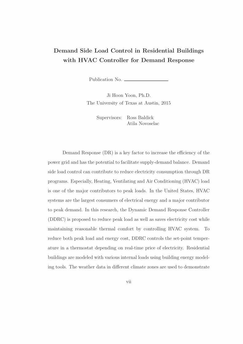
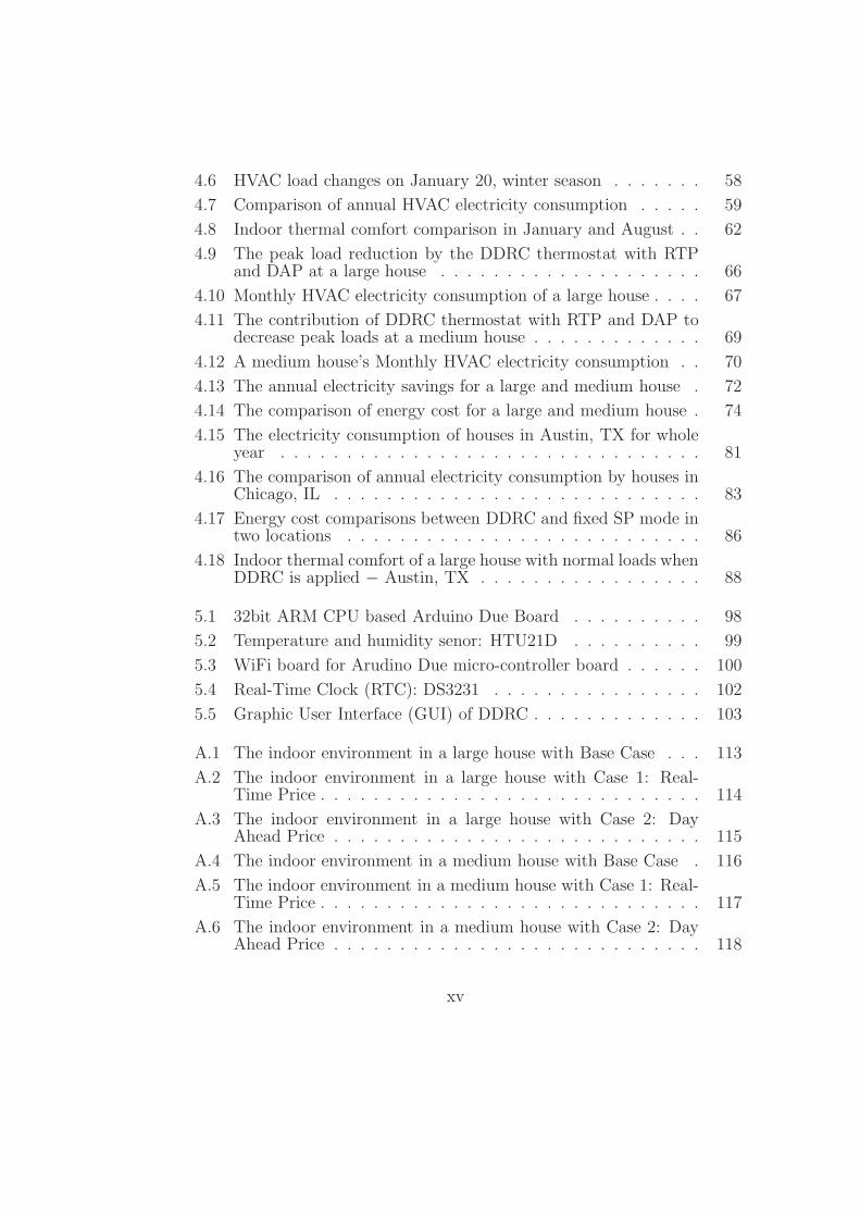
residential and commercial buildings for operations and occupations. Figure

1.1 presents the portion of electricity use by end-use sector in 2010.

The residential buildings are the largest electricity user in power grid

in the United State compared to other sectors. In addition, electricity con-

1

Transportation0.2%

Industrial25.9%

Commercial35.4%

Residential38.5%

Figure 1.1: Retail Sales of Electricity to Ultimate Customers, Total by End-Use Sector(2010) − [Source] U.S. Energy Information Administration, ElectricPower Monthly, Table 5.1, September 2012

sumption at residential buildings has on average increased during the last two

decades, even if electrical energy use in the last few years has decreased. The

size of houses in the 2000’s is bigger than in 1980’s. So, air conditioning and

heating loads to operate Heating, Ventilating, and Air Conditioning (HVAC)

system are raised. Also, the increase in numbers of electronics in households

also contributes to increase electricity use, although many appliances such as

televisions, and refrigerators have become more efficient. Figure 1.2 shows the

electrical energy use in residential sector for last twenty years.

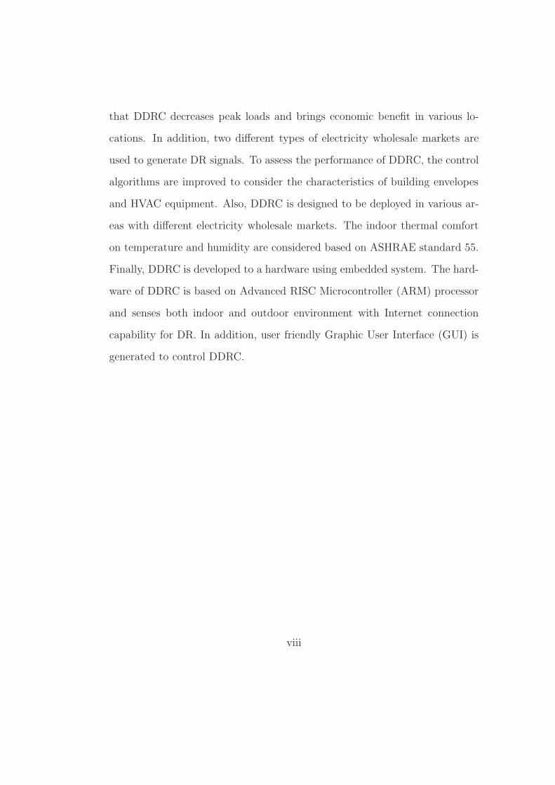
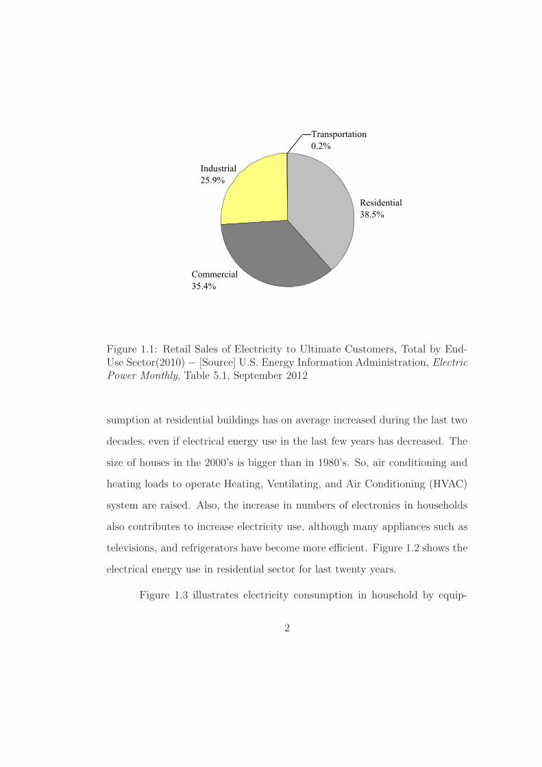
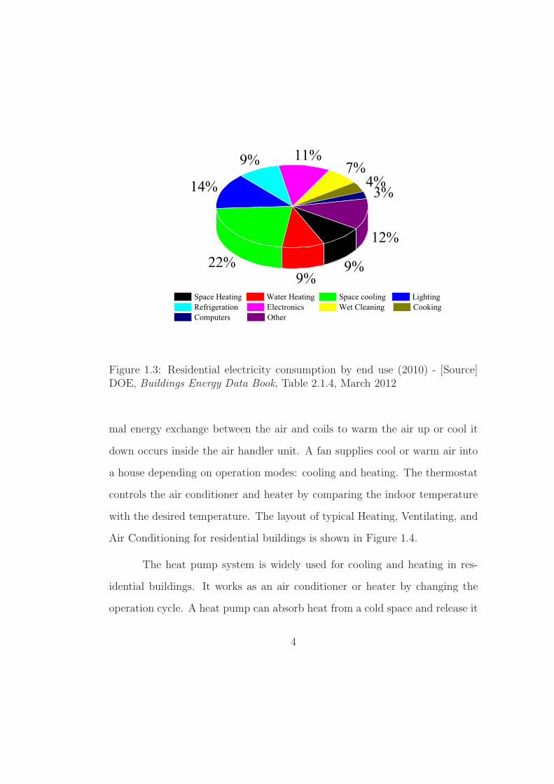
Figure 1.3 illustrates electricity consumption in household by equip-

2

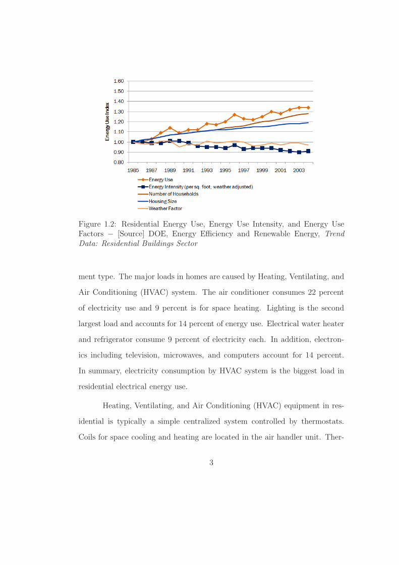
Figure 1.2: Residential Energy Use, Energy Use Intensity, and Energy UseFactors − [Source] DOE, Energy Efficiency and Renewable Energy, TrendData: Residential Buildings Sector

ment type. The major loads in homes are caused by Heating, Ventilating, and

Air Conditioning (HVAC) system. The air conditioner consumes 22 percent

of electricity use and 9 percent is for space heating. Lighting is the second

largest load and accounts for 14 percent of energy use. Electrical water heater

and refrigerator consume 9 percent of electricity each. In addition, electron-

ics including television, microwaves, and computers account for 14 percent.

In summary, electricity consumption by HVAC system is the biggest load in

residential electrical energy use.

Heating, Ventilating, and Air Conditioning (HVAC) equipment in res-

idential is typically a simple centralized system controlled by thermostats.

Coils for space cooling and heating are located in the air handler unit. Ther-

3

12%

3%4%

7%11%9%

14%

22%9%

9%

Space Heating Water Heating Space cooling Lighting Refrigeration Electronics Wet Cleaning Cooking Computers Other

Figure 1.3: Residential electricity consumption by end use (2010) - [Source]DOE, Buildings Energy Data Book, Table 2.1.4, March 2012

mal energy exchange between the air and coils to warm the air up or cool it

down occurs inside the air handler unit. A fan supplies cool or warm air into

a house depending on operation modes: cooling and heating. The thermostat

controls the air conditioner and heater by comparing the indoor temperature

with the desired temperature. The layout of typical Heating, Ventilating, and

Air Conditioning for residential buildings is shown in Figure 1.4.

The heat pump system is widely used for cooling and heating in res-

idential buildings. It works as an air conditioner or heater by changing the

operation cycle. A heat pump can absorb heat from a cold space and release it

4

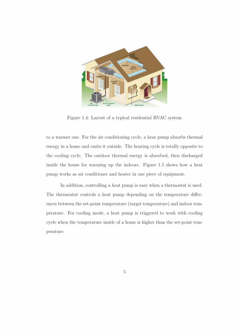
Figure 1.4: Layout of a typical residential HVAC system

to a warmer one. For the air conditioning cycle, a heat pump absorbs thermal

energy in a home and emits it outside. The heating cycle is totally opposite to

the cooling cycle. The outdoor thermal energy is absorbed, then discharged

inside the house for warming up the indoors. Figure 1.5 shows how a heat

pump works as air conditioner and heater in one piece of equipment.

In addition, controlling a heat pump is easy when a thermostat is used.

The thermostat controls a heat pump depending on the temperature differ-

ences between the set-point temperature (target temperature) and indoor tem-

perature. For cooling mode, a heat pump is triggered to work with cooling

cycle when the temperature inside of a home is higher than the set-point tem-

perature.

5

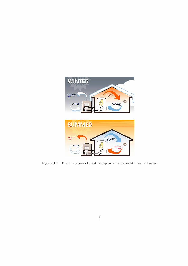
Figure 1.5: The operation of heat pump as an air conditioner or heater

6

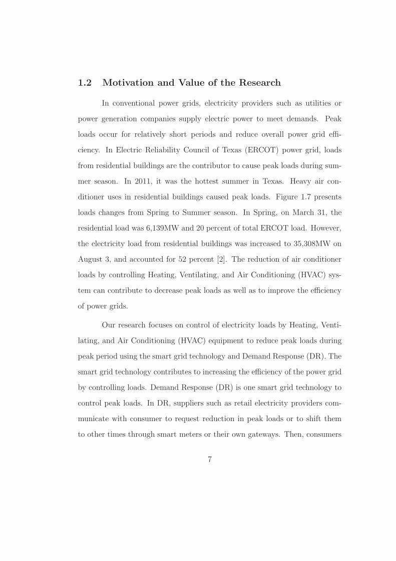
1.2 Motivation and Value of the Research

In conventional power grids, electricity providers such as utilities or

power generation companies supply electric power to meet demands. Peak

loads occur for relatively short periods and reduce overall power grid effi-

ciency. In Electric Reliability Council of Texas (ERCOT) power grid, loads

from residential buildings are the contributor to cause peak loads during sum-

mer season. In 2011, it was the hottest summer in Texas. Heavy air con-

ditioner uses in residential buildings caused peak loads. Figure 1.7 presents

loads changes from Spring to Summer season. In Spring, on March 31, the

residential load was 6,139MW and 20 percent of total ERCOT load. However,

the electricity load from residential buildings was increased to 35,308MW on

August 3, and accounted for 52 percent [2]. The reduction of air conditioner

loads by controlling Heating, Ventilating, and Air Conditioning (HVAC) sys-

tem can contribute to decrease peak loads as well as to improve the efficiency

of power grids.

Our research focuses on control of electricity loads by Heating, Venti-

lating, and Air Conditioning (HVAC) equipment to reduce peak loads during

peak period using the smart grid technology and Demand Response (DR). The

smart grid technology contributes to increasing the efficiency of the power grid

by controlling loads. Demand Response (DR) is one smart grid technology to

control peak loads. In DR, suppliers such as retail electricity providers com-

municate with consumer to request reduction in peak loads or to shift them

to other times through smart meters or their own gateways. Then, consumers

7

Figure 1.6: Residential load changes in ERCOT grid by HVAC use (2010)

respond to the request to reduce electricity use from power suppliers.

The dynamic price of electricity is a key factor for DR. Wholesale prices

change every hour or more often depending on the relation between demand

and supply of electricity in the wholesale market. The price of electricity

reflects the status of power grids. So, electricity price tends to increase with

increasing demand for electricity. When the demand for electricity is high, the

electricity price is high. Our research uses price signal based Demand Response

(DR) because the energy cost in monetary unit is more familiar to consumers

than electricity usage in kWh. So, participants are able to easily understand

how DR works to save energy and cost. In addition, their preferences can be

reflected on DR program by using a threshold price.

Electric power consumption of Heating, Ventilating, and Air Condition-

8

ing (HVAC) system is easy to manage using a thermostat. When a thermostat

is used as the controller, complicated control topologies such as variable fre-

quency drive (VFD), and refrigeration cycle control are not required to control

HVAC system. The change of set-point temperature (or target temperature)

is able to reduce electrical power consumption during peak periods having

high price of electricity possibly shifting demand to other times. Furthermore,

control of HVAC loads is an effective way to reduce peak loads because HVAC

loads account for 31 percent in total electricity use at home by end use.

In contrast, the HVAC controller described in [29] controls directly a

compressor motor in HVAC system using Variable Frequency Drive technology

(VFD). This technology is complicated so that the cost to deploy or retrofit

a controller into homes will be increased. Furthermore, VFD technology does

not guarantee the compatibility with other HVAC systems by different manu-

facturers. Thus, the proposed controller in [88] may not be feasible to install in

many buildings. Different from other controller, DDRC maintains the current

thermostat system by adding functions with sophisticated DR algorithm.

Thermal comfort is an important factor for the indoor environment. A

major reason to use Heating, Ventilating, and Air Conditioning (HVAC) sys-

tem is to keep inside of buildings in thermal comfort. Changing the set-point

temperature may cause residents to feel thermal discomfort. Our research

considers thermal comfort when changing the set-point temperature.

9

1.3 Objectives and Scope of the Research

The objective of this research is the development of a thermostat for

residential HVAC system with Demand Response (DR) capability while con-

sidering thermal comfort of the indoor environment. In this research, we pro-

pose a newly developed thermostat, Dynamic Demand Response Controller

(DDRC), to control electricity loads of HVAC equipment during peak periods.

The proposed dynamic thermostat controls the HVAC system in res-

idential buildings by changing the set-point temperatures in thermostats de-

pending on the price of electricity and the preference of occupants. The set-

point temperature will be increased or decreased for the cooling and heating

mode, respectively, when the threshold price is below the current price of elec-

tricity. The threshold price (preset price by consumers) is the baseline price

when customers want to participate in the energy saving programs. Also, the

America Society of Heating, Refrigerating, and Air-conditioning Engineers

(ASHRAE) thermal comfort is considered.

To evaluate the performance of the proposed Dynamic Demand Re-

sponse Thermostat and impact to the building, different detailed residential

buildings will be modeled using EnergyPlus, which is building energy simula-

tion software. The internal loads and detailed occupation schedules will be set

to represent various houses and building users. The dynamic thermostat will

be demonstrated for single family homes in various locations. Two different

climate zones will be chosen: Austin, TX (Climate Zone 2, hot and moist) and

Chicago, IL (Climate Zone 4, cold and moist). In addition, the real-time prices

10

of electricity are used from ERCOT (Austin, TX) and PJM (Chicago, IL). The

years of the dynamic price to evaluate the performance of the thermostat are

2011 for Austin (the hottest year) and 2013 for Chicago (the coldest year).

In an effort to evaluate the DDRC by considering different residential

building, occupants and location, the energy consumption to operate HVAC

system, the annual operation cost, and the impact on the thermal comfort will

be analyzed for cases with and without the proposed thermostat. Also different

settings of DDRC will be studied such as internal load change, location and

type of dynamic price.

The research will be divided into three phases:

A. Design control algorithm to control a thermostat

(a) Prediction of HVAC power consumption

(b) Using a threshold price to change the target temperature

(c) Set temperature change rate based on the price difference

(d) Limit temperature change rate for thermal comfort

(e) Develop residential models using EnergyPlus

B. Evaluation of performance of Dynamic Demand Response

Controller

(a) Peak loads reduction during peak time

(b) Decrease of annual electricity consumption

(c) Savings of annual energy cost to run HVAC system

11

(d) Maintain indoor environment in thermal comfort

C. Development of hardware of Dynamic Demand Response

Controller

(a) Design of graphic user interface

(b) Sensing temperature and humidity

(c) Ethernet connection for DR signal

(d) Relay control board to enable heat pump

1.4 Contributions

The Dynamic Demand Response Controller (DDRC) developed in this

work reduce peak loads in order to increase the efficiency of the electric power

grid while considering the indoor environment at residential buildings. Our

main contributions are summarized as follows.

• We estimated the electricity loads to use Heating, Ventilating, and Air

Conditioning (HVAC) equipment using linear regression of calculated

values in order to understand the building energy. Using a building

energy modeling tool, required thermal energy for cooling and heating is

predicted and converted to the electricity load of the heat pump. This

prediction provides the analysis of how much electricity loads are changed

when Demand Response signal is enabled.

12

• We proposed the Dynamic Demand Response Controller with newly de-

veloped control algorithm. The DDRC responds to price-based DR sig-

nals to reduce peak loads when the electric power grid is stressed. It

provides Demand Response and gives benefits to both retail electricity

providers for peak load reduction and end users for energy cost savings.

• We showed the performance of the proposed Dynamic Demand Response

Controller to maintain thermal comfort while it responds to the Demand

Response signal. It is important for the Heating, Ventilating, and Air

Conditioning (HVAC) system to meet criteria such as ASHRAE stan-

dard 55. Analysis of thermal discomfort contributes to ensuring that

consumers will continue to response to the Demand Response signal to

reduce peak loads.

• We developed the hardware of Dynamic Demand Response Controller for

end users. The control algorithm to respond to the Demand Response

signal is implemented into the hardware. It demonstrated that the pro-

posed Dynamic Demand Response Controller contributes to reduce peak

loads during peak period as well as provide energy cost savings to end

users.

1.5 Organization of the Dissertation

The rest of this dissertation is organized as follows. Chapter 2 presents

the modeling of single family homes using building energy modeling tools:

13

EnergyPlus/OpenStudio. Based on historical wholesale price, dynamic retail

prices of electricity are generated. Chapter 3 introduces the control algorithms

of the Dynamic Demand Response Controller (DDRC). The basic control pol-

icy implements price based Demand Response (DR). Improved control policy

of DDRC that considers attributes of building envelop is presented. In addi-

tion, different locations and wholesale market changes are considered. Chapter

4 evaluates the performance of DDRC using two proposed control algorithms

for different climate zones, internal load sizes, floor plans, and price types.

Chapter 5 illustrates the development of DDRC hardware. Conclusions are

drawn in Chapter 6. Appendix A presents the indoor thermal comfort region

on pychrometric charts to show the DDRC minimizes thermal discomfort.

14

Chapter 2

Modeling of residential buildings and

real-time price of electricity

This chapter presents the modeling of single family homes using En-

ergyPlus which is a building energy modeling tool. Based on architectural

features, two different sizes of house are designed. In addition, the dynamic

retail prices of electricity are built by analyzing the historical wholesale elec-

tricity prices at Electric Reliability of Texas (ERCOT) and Pennsylvania, New

Jersey, and Maryland (PJM) Interconnection wholesale market.

2.1 Introduction

Home electricity consumption in the United States has increased by

10% over the last two decades [1]. In addition, Electrical energy consumption

in residential buildings in the United States has generally been increasing from

2001 to 2011 except for a few years during the economic crisis. Moreover, the

average retail price of electricity has gradually increased in nominal terms over

the same period [30]. Of the total electricity consumption in homes, families

spend on average 27% of total electricity consumption for heating and air con-

ditioning [2]. The energy and peak load growth necessitates new power plants

15

and transmission lines. In hot climate zones, air conditioning (AC) loads are a

major contributor to cause peak load on the power grid. For example as shown

in Figure 1.6, in Texas where the Electric Reliability of Texas (ERCOT) man-

ages the power grid, the residential load was 6.1 GW and 20% of grid electricity

load on March 31, 2010. However, the residential load in ERCOT was tremen-

dously increased to 35.3 GW, 52% of total load, on August 3, 2010 [3] because

of the hot weather. This heavy AC load during summer on the power grids

in hot climates is the major contributor to peak load. Recently, there have

been capital expansions that will tend to increase the retail price in real terms.

Furthermore, due to heavy AC load, the cost for power generation is not only

increased but also overall grid efficiency is reduced. This research discusses

a proposed Dynamic Demand Response Controller (DDRC) and shows how

it can be used for control of the AC system depending on the retail price of

electricity. The objective of this study is to model the dynamic demand re-

sponse controller that changes set-point temperature based on the dynamic

price of electricity and occupant preferences. For dynamic price of electricity,

two types of real-time tariffs are used by some utilities in the United States:

Day Ahead Market Settlement Point Price (DAMSPP) and Real Time Market

Settlement Point Price (RTMSPP). For houses with different sizes and floor

plans, this study quantifies capacity to reduce peak loads as well as cost while

maintaining the thermal comfort inside houses within an acceptable range.

The increase of home energy usage due to Heating, Ventilating, and

Air Conditioning (HVAC) requires more generation and transmission line ca-

16

pacity to meet the high peak demand and also reduces the overall power grid

efficiency. Therefore, home energy demand increases costs for production of

electricity and for capacity. For example, the cost to increase transmission

capacity is $400/MW-mile to $3,000/MW-mile for new construction [4]. Re-

duction of Heating, Ventilation and Air Conditioning (HVAC) load during the

peak time period is important to peak load reduction, resulting in significant

savings for both utilities and customers.

Austin Energy, the municipal utility in Austin, Texas, distributed 3,000

remotely controllable thermostats for free to their customers in 2003 to reduce

HVAC loads at peak. By 2009, more than such 86,000 thermostats were in-

stalled in many customers’ residential and commercial buildings in the Austin

Energy service area. Temporarily switching off compressors brought 90MW

load reduction out of approximately 2,000MW peak load during on-peak pe-

riods [5]. Control of the thermostat is an effective way to reduce the HVAC

loads for Demand Response (DR). However, thermostats that Austin Energy

provided are not able to respond to real-time retail electricity prices due to

lack of communication and functionality. Dynamic controlled thermostats in

[6] and [7] manage HVAC operation by turning on and off based on indoor

air temperature tolerance or dead band. These thermostats are not able to

consider retail price in their HVAC control. So, HVAC load may not be cut

off during the peak price period.

In previous research related to the demand power control, large elec-

tricity loads such as commercial buildings, industries, retail and museums are

17

analyzed to reduce high demand at peak time [31]. However, residential build-

ings are also a major contributor to peak loads. To address problems related

to peak load caused by residential heating, ventilating and air conditioning

(HVAC) systems, the DDRC is modeled in this research in various residen-

tial buildings [34]. Different from other dynamic response controllers analyzed

in previous studies in [6, 8-10, 18, 26, 27, 32, 44,45], detailed house models

are developed to analyze HVAC electricity consumption under consideration

of various building geometries and physical properties that affect energy ef-

ficiency using EnergyPlus/OpenStudio energy simulation software [20,21,29].

The model developed for this study overcomes some shortcomings of previous

DDRC related research. For example, some of the previous studies related

to DDRC [8, 6, 18, 27, 32] did not have a HVAC model to control tem-

perature, and therefore, could not analyze how much electricity is saved for

cooling or heating during peak load period. Other studies related to demand

response controllers [9, 10, 26] added simple HVAC models but the oversim-

plified Equivalent Thermal Parameter (ETP) model in their controller could

not consider the impact of specific building features on the change of the set-

point temperature. Building structures such as insulation levels [11]-[13], attic

[14], and windows [15, 16, 33] considerably influence the electricity consump-

tion by HVAC. Also, geographical location and seasonal outdoor environments

[17] change HVAC loads. The performance of DDRC applied in two different

size house models with different internal loads and locations also focuses on

thermal comfort in different parts of the house.

18

Furthermore, the energy consumption by HVAC system is significantly

influenced by locations and the size of internal loads. Energy efficiency codes

are differ by climate zone [41]. So, the building behaviors to consume electricity

are different even if the buildings have the same floor plan. Previous control of

HVAC system in [34, 76] used residential models in one place with hot weather

condition only. Another factor to change energy consumption of building is the

internal load such as indoor activities and occupation schedule. Our previous

work [34, 76] used fixed internal loads. In addition, the method to estimate

internal loads in [77] connected HVAC loads to internal load changes and

another work [78] considered indoor activities. However, both researches did

not reflect the locations and characteristics of building envelope in the demand

response. So, this research uses two locations: Austin, TX for hot weather

and Chicago, IL for cold weather with two different internal load settings. In

this research, DDRC demonstrated its performance in different locations and

building environments.

Another previous study in [8] changes HVAC loads when the retail

price varies. The set-point temperature for cooling is changed when the rolling

average of price in the last 24 hours is sufficiently different from the current

price. If the retail price is sufficiently smaller than a rolling average price then

the desired cooling set-point temperature is reduced. Customers can change

desired set-point temperatures. However, the price tolerance cannot be chosen.

Another advancement of our newly developed DDRC is in innovative use of the

retail price model. Previous work related to the retail price based control [28]

19

used Critical Peak Price (CPP). However, this is partial real-time price since

the price of electricity only changes during selected peaks and stays flat rate

at other times. Similarly, the price data in [18] used the zonal market price

of ERCOT for 2006. In 2010, ERCOT market changed from a zonal market

to a nodal market where Real-Time Locational Marginal Prices are calculated

every 5 minutes. In our study, the historical wholesale price of electricity in

ERCOT’s nodal market are used together with corresponding weather file for

buildings’ cooling and heating load calculation to synthesize a real-time tariff.

Comparing to our controller that includes this real-time tariff in the decision

about the set-point temperature change, the similar controller analyzed in

the previous study [28] changes the electricity consumption by changing the

set-point temperature without using the electricity price signal as an input.

A customer specified threshold retail price is compared to the real-time

retail price of electricity. When the retail price is above the threshold price,

DDRC changes the set-point temperature of the thermostat according to the

price difference between the retail price and the threshold. For the cooling case,

DDRC increases cooling set-point temperature by one Celsius degree step.

Similarly, for heating, it decreases heating set-point temperature from original

set-point temperature. The change of thermostat set-point temperature is

done automatically after customers set their preferences for the threshold price.

One of the contributions of the analysis in this research is that it considers

both day-ahead and real-time prices for customers because many utilities in the

United States provide DR program to their customers with day ahead or real-

20

time wholesale price based tariffs [36-38]. In the ERCOT wholesale market,

the day-ahead price is calculated every hour one day before the electricity

is delivered to the customers. In contrast to the day-ahead prices, real-time

prices are calculated depending on current demand every 5 minutes. So, the

customers receive a different price of electricity in the same period depending

on whether the day-ahead or real-time prices are used.

Therefore, in the present study, two types of retail prices are used to

analyze the advantages of price type. To evaluate the performance of DDRC,

two different residential models with various internal load sizes are modeled

and two hot and cold locations are chosen to show how much energy and

cost can be saved. The price signals are input to two residential buildings’

thermostat controllers in real-time using Building Controls Virtual Test Bed

(BCVTB) [24]. DDRC, moreover, considers the thermal comfort based on

the latest ASHRAE Standard 55 [18, 39] to maintain customer comfort while

the set-point temperature changes due to the price signal. The thermostat

controller in [72] controlled a set-point temperature moved to high tempera-

ture for AC and to low temperature for heating when DR was enabled. This

big temperature difference causes thermal discomfort. Other works [79, 80]

also did not consider thermal comfort during peak load curtailment. This re-

search shows that DDRC minimizes the thermal discomfort while customers

participate in DR programs.

21

2.2 Design of Single Family Houses

We selected medium and large size of houses, common for U.S. residence

in Figure 2.1. House models are developed for using the building simulation

tools and the historical price data are collected to generate the dynamic price

of electricity as an input in the DR controller. The electricity consumption of

homes is varied depending on size, floor plan, and occupation schedule. The

house models used in this study are based on the building code for Austin, TX,

and Table 2.1 provides specific details about the two houses. Also, detailed

occupancy schedules based on typical houses in Austin are considered to model

both large and medium houses. Both house models are developed as 3D models

using EnergyPlus v7.1 and OpenStudio v0.11.0 [20, 21, 29].

Figure 2.1: 3D model of single family houses used in the study: large house(L) and medium size house (R)

Figure 2.2 presents the floor plan of the medium and large single family

houses. The medium house has 156 m2 ( 1,683 ft2) of floor area with single

story building. There are three bedrooms and one attached garage. It has

22

Table 2.1: Building geometry features of the large and medium houses

Component Medium house Large houseFloor Area 156 m²(1679 ft²) 305 m²(3283 ft²)Floor Single storey Two storiesFloor Plan 3 bedrooms, 1 garage 5 bedrooms, 1 garageOrientation South SouthWindow to wall ratio 8 % 18.1 %Internal loadsOccupant 4 Residents 4 ResidentsLighting Normal - 2.6 W/m² Normal - 2.6 W/m²

Heavy - 3.5 W/m² Heavy - 3.5 W/m²

equipment Electronics, computer, water heater,kitchen appliance, washer, dryer

Thermal Zone 3 zones 4 zonesInfiltration 0.25 ACH 0.25 ACH

Austin, TXWindows U=3.69 W/m²-K, SHGC=0.3Wall R=2.29 m²/K-WCeiling R=5.28 m²/K-W

Chicago, ILWindows U=1.99 W/m²-K, SHGC=0.3Wall R=3.52 m²/K-WCeiling R=6.69 m²/K-W

three thermal zones: living zone, garage and attic. Cooling and heating are

only applied to the main zone with one thermostat. Other zones (attic and

garage) have natural ventilation by infiltration and temperature is free floating.

We did not use detailed infiltration modeling. Since the focus of the research

is to evaluate thermostat controller we did not put effort to characterizing the

model houses for infiltration at 50Pa. So, the infiltration is constant to 0.5

Air Change per Hour (ACH) for two residential models in our research. The

23

window to wall ratio is 8.0%. The large house is twice the size of the medium

house; 305 m2 (3,280 ft2). Its floor plan has five bedrooms and one attached

garage with two levels. The thermal zones in a large single family house are 1st

floor, 2nd floor, garage and attic. Both 1st and 2nd floor are applied HVAC

with two independent thermostats [39]. So, the temperature changes in the

1st and 2nd floor are changed independently. Similar to a medium house, the

other two zones do not have HVAC system and have natural ventilation. A

large house has higher window to wall ratio, 18.1%, than a medium house so

that the influence of the sunlight and shade impacts on the large house more

than the medium house. For this reason, the capacity of cooling and heating

in a medium house is less than the large house’s. Both houses are oriented to

South. They have the same type of HVAC system, a packaged terminal heat

pump.

The internal loads are differently set to heavy and normal loads. A

heavy internal load is generated with 140% of lighting loads and 150% of in-

ternal equipment such as electronics, and appliances from a normal load. This

research aims to demonstrate that the proposed HVAC controller is effective

for the demand response in any house size and different internal loads. So,

each house model, a large and medium houses, has two different internal loads

setting to analyze how much changes of internal load impact on energy con-

sumption at homes.

Packaged terminal heat pump systems are used for both large and

medium houses. The capacity of HVAC is fixed even if the internal loads

24

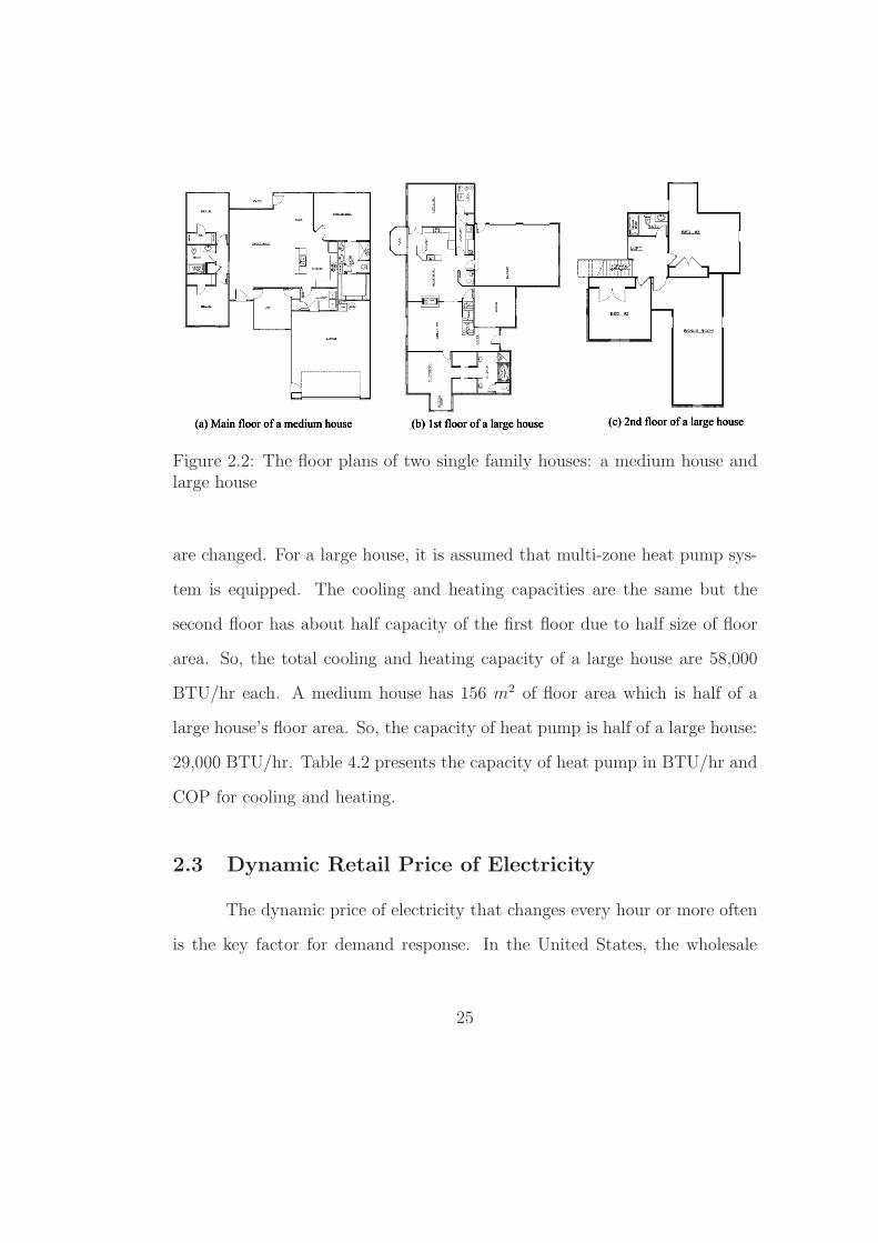
Figure 2.2: The floor plans of two single family houses: a medium house andlarge house

are changed. For a large house, it is assumed that multi-zone heat pump sys-

tem is equipped. The cooling and heating capacities are the same but the

second floor has about half capacity of the first floor due to half size of floor

area. So, the total cooling and heating capacity of a large house are 58,000

BTU/hr each. A medium house has 156 m2 of floor area which is half of a

large house’s floor area. So, the capacity of heat pump is half of a large house:

29,000 BTU/hr. Table 4.2 presents the capacity of heat pump in BTU/hr and

COP for cooling and heating.

2.3 Dynamic Retail Price of Electricity

The dynamic price of electricity that changes every hour or more often

is the key factor for demand response. In the United States, the wholesale

25

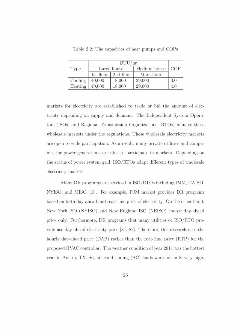
Table 2.2: The capacities of heat pumps and COPs

BTU/hrType Large house Medium house COP

1st floor 2nd floor Main floorCooling 40,000 18,000 29,000 3.0Heating 40,000 18,000 29,000 4.0

markets for electricity are established to trade or bid the amount of elec-

tricity depending on supply and demand. The Independent System Opera-

tors (ISOs) and Regional Transmission Organizations (RTOs) manage these

wholesale markets under the regulations. These wholesale electricity markets

are open to wide participation. As a result, many private utilities and compa-

nies for power generations are able to participate in markets. Depending on

the status of power system grid, ISO/RTOs adapt different types of wholesale

electricity market.

Many DR programs are serviced in ISO/RTOs including PJM, CAISO,

NYISO, and MISO [18]. For example, PJM market provides DR programs

based on both day-ahead and real-time price of electricity. On the other hand,

New York ISO (NYISO) and New England ISO (NEISO) choose day-ahead

price only. Furthermore, DR programs that many utilities or ISO/RTO pro-

vide use day-ahead electricity price [81, 82]. Therefore, this research uses the

hourly day-ahead price (DAP) rather than the real-time price (RTP) for the

proposed HVAC controller. The weather condition of year 2011 was the hottest

year in Austin, TX. So, air conditioning (AC) loads were not only very high,

26

but also the price of electricity was expensive. In contrast, Chicago suffered

the coldest weather during winter from 2013 to 2014. To maximize the effect

of DR, the year 2011 of the historical price data for Austin, TX is selected

at Austin Energy Network (AEN) [36]. For Chicago, IL, the year of 2013 at

Commonwealth Edison (ComEd) is used for the price data [54]. The unit of

electricity price at the wholesale market is $/MWh. However, retail customers

pay their electricity bill in $/kWh. Thus, the prices of electricity are converted

to $/kWh.

Many utilities in the United States provide DR programs [36-38]. Their

real-time tariffs in DR programs are based on day ahead or real-time whole-

sale price. For instance, Niagara Mohawk, New York, NY provided real-time

pricing based on day ahead wholesale price in the NY ISO market. Common-

wealth Edison in Chicago, IL also has real-time tariff for residential based on

wholesale price in the PJM market [36]. Different from these utilities, Geor-

gia and Alabama power companies offer both day ahead pricing based on day

ahead wholesale price and hour ahead price based on real-time wholesale price

[37].

Two types of retail prices are used because many utilities choose one

or use both types of prices to build their tariffs. One of the retail prices is

Day Ahead Price (DAP) and another price is Real-Time Price (RTP). For the

ERCOT simulations, these prices are based on historical wholesale electricity

price in the ERCOT wholesale market. DAP is generated using Day Ahead

Market Settlement Point Prices (DAMSPP) [42] and RTP is based on Real-

27

Time Market Settlement Point Prices (RTMSPP) in ERCOT [43]. DAMSPP

is hourly based price but RTMSPP is updated in every 15 minutes. So, RTM-

SPP is converted to hourly based price by averaging prices of RTMSPP in an

hour interval to match time scale to DAMSPP in this research. In addition,

choosing the highest prices of RTMSPP for an hour interval and the original

price of RTMSPP that has prices changing every 15 minutes are also simu-

lated. However, our preliminary analysis shows that for both the large and

the medium houses using these two types of RTMSPP (the highest and 15

minutes based prices) have little difference compared with the results using

the average price of RTMSPP. Thus, the average of RTMSPP in an hour is

chosen to convert to the hourly based hypothetical retail price.

In addition, we also model a house are located in Chicago, IL to evaluate

the performance that DDRC can work in any locations with different markets .

Thus, two different wholesale markets are chosen; ERCOT and PJM. ERCOT

(Electric Reliability Council of Texas) manages power grid in the most part

of Texas including Austin area. Its wholesale market has the energy market

(both day-ahead and real-time wholesale market), and ancillary service. PJM

Interconnection services the wholesale market in Northeast of U.S. including

Chicago area. The wholesale market in PJM has a capacity market in addition

to day-ahead, real-time, and ancillary services market. All other services in

PJM market are similar to ERCOT. The capacity market is designed to ensure

sufficient power generation can satisfy the peak demand reliably [53].

Figure 2.3 presents the histograms of the annual historical price data

28

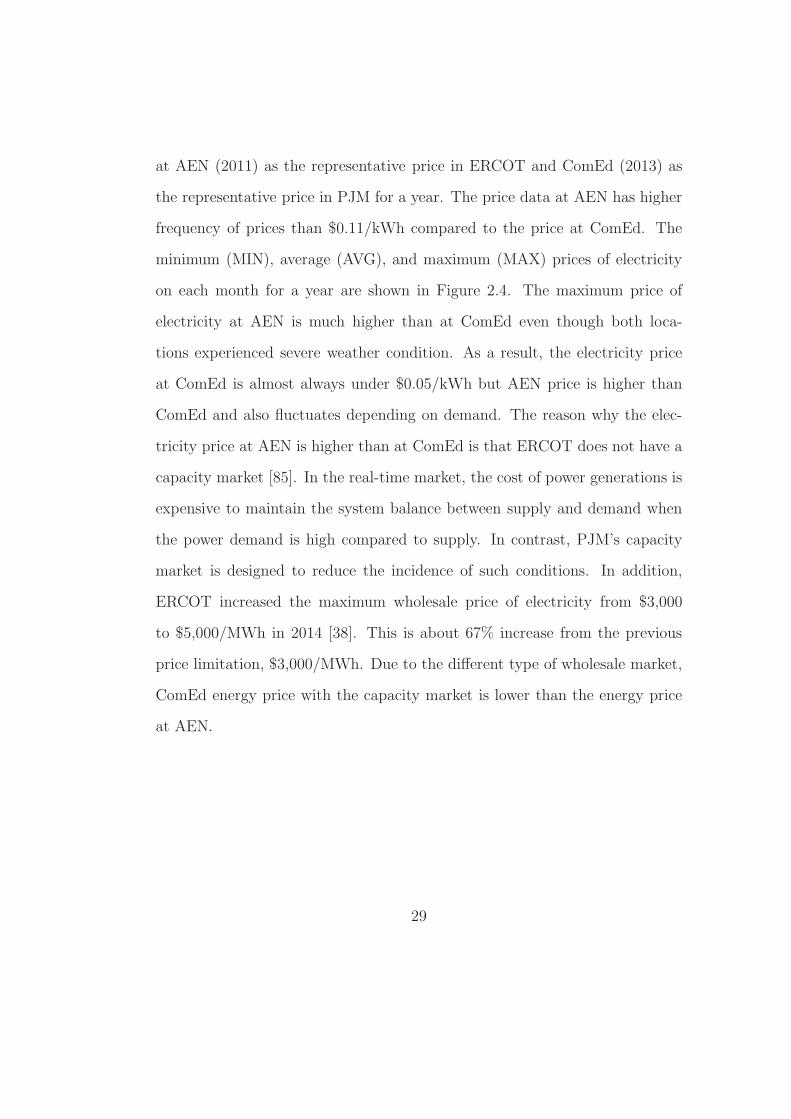
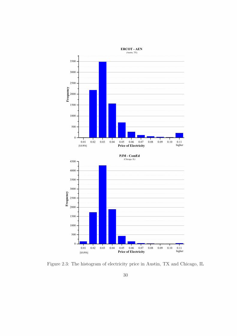
at AEN (2011) as the representative price in ERCOT and ComEd (2013) as

the representative price in PJM for a year. The price data at AEN has higher

frequency of prices than $0.11/kWh compared to the price at ComEd. The

minimum (MIN), average (AVG), and maximum (MAX) prices of electricity

on each month for a year are shown in Figure 2.4. The maximum price of

electricity at AEN is much higher than at ComEd even though both loca-

tions experienced severe weather condition. As a result, the electricity price

at ComEd is almost always under $0.05/kWh but AEN price is higher than

ComEd and also fluctuates depending on demand. The reason why the elec-

tricity price at AEN is higher than at ComEd is that ERCOT does not have a

capacity market [85]. In the real-time market, the cost of power generations is

expensive to maintain the system balance between supply and demand when

the power demand is high compared to supply. In contrast, PJM’s capacity

market is designed to reduce the incidence of such conditions. In addition,

ERCOT increased the maximum wholesale price of electricity from $3,000

to $5,000/MWh in 2014 [38]. This is about 67% increase from the previous

price limitation, $3,000/MWh. Due to the different type of wholesale market,

ComEd energy price with the capacity market is lower than the energy price

at AEN.

29

0.01 0.02 0.03 0.04 0.05 0.06 0.07 0.08 0.09 0.10 0.110

500

1000

1500

2000

2500

3000

3500

[$/kWh]

Frequency

Price of Electricity higher

ERCOT - AEN(Austin, TX)

0.01 0.02 0.03 0.04 0.05 0.06 0.07 0.08 0.09 0.10 0.110

500

1000

1500

2000

2500

3000

3500

4000

4500

Frequency

Price of Electricity higher

PJM - ComEd(Chicago, IL)

[$/kWh]

Figure 2.3: The histogram of electricity price in Austin, TX and Chicago, IL

30

1 2 3 4 5 6 7 8 9 10 11 120.00

0.02

0.04

0.06

0.08

0.10

0.12

0.14

0.16

0.5

1.0

1.5

2.0

2.5

3.0

Pric

e of

Ele

ctri

city

Month

MAX AVG MIN

ERCOT - AEN(Austin, TX)[$/kWh]

1 2 3 4 5 6 7 8 9 10 11 120.00

0.02

0.04

0.06

0.08

0.10

0.12

0.14

0.16

0.18

0.20

0.22

0.24

0.26

0.28

0.30

0.32

Pric

e of

Ele

ctri

city

Month

[$/kWh]PJM - ComEd

(Chicago, IL)

Figure 2.4: The monthly Max, Average, and Min of electricity price in twocities

31

The retail prices of electricity are based on the historical wholesale elec-

tricity price at Electric Reliability Council of Texas (ERCOT) and Pennsylvania-

New Jersey-Maryland (PJM) Interconnection. The electricity retail price is

set equal to 100% of wholesale price in $/kWh. In addition, we assume that

transmission and distribution costs are changed separately. The load zone and

year of historical wholesale electricity price used in our research are shown as

follows:

The historical data of wholesale electricity price

(a) Day Ahead Price (DAP) − YR 2011

: Austin Energy Network (AEN) − ERCOT

(b) Real Time Price (RTP) − YR 2011

: Austin Energy Network (AEN) − ERCOT

(c) Day Ahead Price (DAP) − YR 2013

: Commonwealth Edison − PJM

The aggregation through DR may impact on the electricity price in

wholesale market [86, 87]. However, this research focuses on four residential

models in different locations. This small amount of aggregation by DR from

house models does not significantly change the wholesale price. Thus, we

assume that the theoretical price data is not changed after DR.

32

2.4 Simulation Cases

In this research, two house models are simulated with different condi-

tions. The simulation conditions to estimate the performance of DDRC with

dynamic pricing have three stages:

A. DDRC with dynamic price of electricity

(a) Fixed set-point temperature setting (Normal case)

(b) Changing set-point temperature by DDRC (DDRC case)

B. DDRC with various price types and floor plans

(a) Normal and DDRC cases

(b) Two different floor plans: large and medium houses

(c) Two types of dynamic price: DAP and RTP

C. DDRC with different internal loads and climate zones

(a) Normal and DDRC cases

(b) Two different floor plans: large and medium houses

(c) Various internal loads: heavy and normal loads

(d) Different climate zones: zone 2 (Austin, TX), zone 5 (Chicago, IL)

33

Chapter 3

Control Algorithm of Dynamic Demand

Response Controller

This chapter introduces two different control algorithms for the pro-

posed controller. Linear regression estimation is used to calculate Heating,

Ventilating, and Air Conditioning (HVAC) loads when the set-point temper-

ature in a thermostat changes. Then, the price trigger as a Demand Re-

sponse (DR) signal is added to decide new set-point temperature to reduce

peak load when DR is requested. Improved DDRC control policy is also sug-

gested to enable DDRC to be used in various places with different circum-

stances. Next, the implementation of the simulations using EnergyPlus and

MATLAB/SIMULINK is illustrated in this chapter.

3.1 Base Control Policy with Dynamic Price of Elec-

tricity

The proposed Dynamic Demand Response Controller (DDRC) changes

the set-point temperature of the thermostat in 1°C increments for both cooling

and heating when the current retail price (P ) is higher than the threshold price

(Pth) that customers want to implement for energy savings. On the other hand,

if the threshold price (Pth) is above the current retail price (P ), the thermostat

34

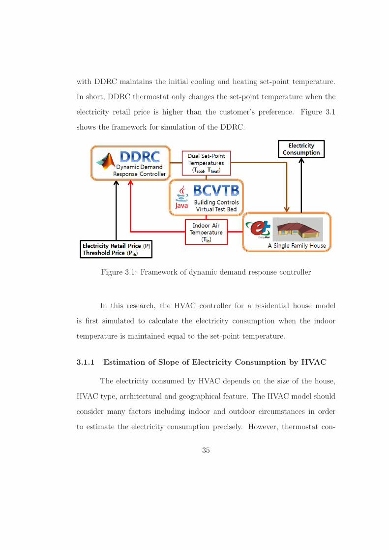
with DDRC maintains the initial cooling and heating set-point temperature.

In short, DDRC thermostat only changes the set-point temperature when the

electricity retail price is higher than the customer’s preference. Figure 3.1

shows the framework for simulation of the DDRC.

Figure 3.1: Framework of dynamic demand response controller

In this research, the HVAC controller for a residential house model

is first simulated to calculate the electricity consumption when the indoor

temperature is maintained equal to the set-point temperature.

3.1.1 Estimation of Slope of Electricity Consumption by HVAC

The electricity consumed by HVAC depends on the size of the house,

HVAC type, architectural and geographical feature. The HVAC model should

consider many factors including indoor and outdoor circumstances in order

to estimate the electricity consumption precisely. However, thermostat con-

35

trollers in [6], [18], [27],and [28] do not have an HVAC model. Thus, these

controllers cannot calculate how much electricity was consumed by HVAC nor

evaluate whether loads were shifted or curtailed during peak period compared

to normal operation.

Other thermostats in [9], [10], [26] have HVAC models to calculate

HVAC electricity consumption. Previous work reported in [10] and [26] used

the ETP model. Only outdoor air temperature impacts on the indoor air

temperature in the ETP model. An HVAC model in [9] added thermal energy

obtained from the sun. However, these models cannot reflect the outdoor

circumstance changes such as wind, precipitation, shading as well as the indoor

environments including activities, ventilation, and equipment uses.

In contrast to [9], [10], and [26], an important contribution of this

work is in using a precise HVAC model based on EnergyPlus to calculate the

electricity consumption. The indoor air temperature is not only influenced

by outdoor temperature but also by ground temperature, indoor activities,

internal load, and building size. So, these factors that impact on indoor air

temperature change should be considered to control HVAC load during peak

period. EnergyPlus considers these variables during simulation processing [29].

In our study, EnergyPlus is used to develop HVAC load functions for

the DDRC algorithm. These functions show the HVAC electricity savings

as a function of the thermostat set point temperature change. The single

family house is initially simulated with set-point temperatures fixed at 23°C

for cooling and 22°C for heating; these are the initial condition of set-point

36

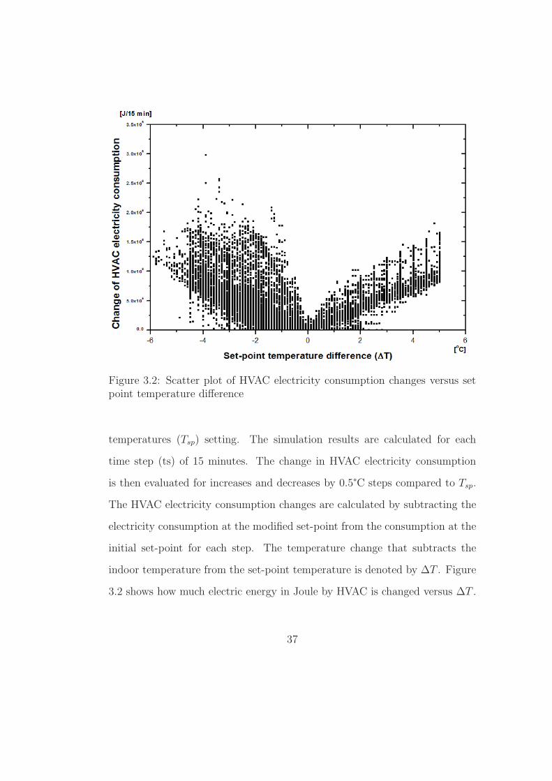
Figure 3.2: Scatter plot of HVAC electricity consumption changes versus setpoint temperature difference

temperatures (Tsp) setting. The simulation results are calculated for each

time step (ts) of 15 minutes. The change in HVAC electricity consumption

is then evaluated for increases and decreases by 0.5°C steps compared to Tsp.

The HVAC electricity consumption changes are calculated by subtracting the

electricity consumption at the modified set-point from the consumption at the

initial set-point for each step. The temperature change that subtracts the

indoor temperature from the set-point temperature is denoted by ∆T . Figure

3.2 shows how much electric energy in Joule by HVAC is changed versus ∆T .

37

The following equations represent regression the cooling and heating data

∆T = Tin − Tsp [Co] (3.1)

Ecool = −199163.34∆T + 46530.67 [J ] (3.2)

Eheat = 196204.81∆T + 13010.29 [J ] (3.3)

Electricity consumption by HVAC is calculated in Joule per 15 minute

time step. So, unit conversion should be needed to change Joule into kW by

dividing by 3.6 × 106 to provide HVAC electricity consumption equations in

kW. When the price of electricity is below Pth, the set-point temperature is

maintained at the initial value Tsp,ts. In this research, only temperature is

adjusted to control room zone. The initial set-point temperature (Tsp,ts) for

cooling is set to 23oC and for heating is set to 22oC, so that HVAC electricity

consumption is finally derived as a function of ∆T in (3.4) and (3.5):

kWHV ACcool = −0.055∆T + 0.013 [kW ] (3.4)

kWHV ACheat = 0.055∆T + 0.004 [kW ] (3.5)

3.1.2 Price Trigger and Coefficient of Price over Temperature

Previous works in [8], [27], and [28] used the average price of electricity

for the last 24 hours to trigger set-point temperature change by comparing with

38

the current price. However, using average price as a trigger is not suitable for

high fluctuation of retail price in real-time market. In addition, AC may be

turned on at time when AC load should be curtailed. The difference between

the lowest and highest price signal in [8] is about $0.021 per kWh. On the

other hand, the price difference in the ERCOT market on August 3, 2011 was

about $2.97 per kWh. The average price of electricity has a high value on this

day. Therefore, thermostat controllers in [8], [27], and [28] do not change a

set-point temperature even if the price of electricity is high since tremendous

high electricity price impacts on the average price of electricity for last 24

hours.

In contrast, the proposed DDRC uses the price difference between the

current price and a threshold price set by customers. Reference [28] considers

the chosen comfort setting in its controller but the coefficient for comfort is

unit-less. So, it is difficult for residents to choose the coefficient based on their

preference. Our DDRC reflects the preferences of occupants using a threshold

price (Pth). The threshold price (Pth) is the base price to change set-point

temperature on a thermostat. Customers choose the threshold price depending

on their preference. In this simulation, threshold price is set to $0.04 per kWh.

DDRC compares electricity retail price (P ) with threshold price (Pth) when

new retail price is updated every 15 minutes. The price difference (∆P ) is the

subtraction of electricity retail price from threshold price. When retail price

is higher than threshold price, ∆P is a positive number and DDRC starts to

work. Otherwise, ∆P is less than equal to zero so that DDRC stops working

39

immediately and maintains or returns to the initial set-point temperature.

High price difference is effective to increase set-point temperature for cooling

or to decrease it for heating at high peak load period.

∆P [$/kWh] = P − Pth (3.6)

= P − 0.04

The linear regression coefficient of temperature as a function of retail

price converts electricity price to temperature that the thermostat accepts. It

is the result of correlation between outdoor air temperature (Tout) at Mueller

AP, Austin Texas, 2011 and retail price (P ) converted from wholesale price

from ERCOT’s RTSPP, 2011. Outdoor air temperature considerably impacts

prices in the wholesale market. Wholesale price generally increases when out-

door air temperature is hot due to increment of AC load demand. On the

other hand, if outdoor environment is getting cold, retail price is also raised

due to heating demand increase. The heating and cooling loads are linearly

increased from the temperature where both cooling and heating loads are at a

minimum. Based on ERCOT data for 2011, the linear regression coefficients

of temperature with respect to to retail price for both cooling and heating are

shown in (3.7) and (3.8).

a [Co · hr/$] =

{

2.254, for cooling (3.7)

−3.683, for heating (3.8)

40

3.1.3 Control of The Thermostat

DDRC is based on based on the electricity cost to change the set-point

temperature. So, the coefficient of temperature is used to convert the elec-

tricity cost to the temperature for the thermostat. In this research, based

on experimental data, twice the price difference (∆P ) was chosen to decrease

HVAC load at on-peak. Temperature change for DDRC is calculated in (3.9)

and (3.10) below. When retail price (P ) is much higher than threshold and

desired temperatures for cooling and heating are far from current temperature

(Tin), temperature change rate is sharply increased. The maximum tempera-

ture change rate is therefore limited to 3°C in both cooling and heating mode

because sudden huge temperature change impacts on human health through

thermal shock and also gives large mechanical burden to heat pump. In ad-

dition, customers feel discomfort in high temperature difference from initial

set-point when retail price is high for an extended period. Finally, the tem-

perature change rate is discretized with 1C°steps.

∆T ratecool = a ·HVACcool · 2∆P [Co] (3.9)

∆T rateheat = a ·HVACheat · 2∆P [Co] (3.10)

New set-point temperatures at higher retail price (P ) than threshold

price (Pth) are determined by (3.11) and (3.13). DDRC thermostat remains at

initial set-point temperature when retail price is lower than threshold price. As

41

retail price increases beyond threshold price, DDRC starts increasing the set-

point temperature for cooling or delays heat pump operation time depending

on the price difference (∆P ). Conversely, set-point temperature is decreased

for heating mode, with 23°C and 22°C the initial set-point temperature for

cooling and heating, respectively:

T newsp,cool [C

o] =

{

23 + ∆T ratecool , for P > Pth (3.11)

23 for P ≤ Pth (3.12)

T newsp,heatl [C

o] =

{

22−∆T rateheat , for P > Pth (3.13)

22 for P ≤ Pth (3.14)

3.2 Improved Control Algorithm of DDRC for variouscircumstances

The DDRC described in the last section was used for several case stud-

ies. It has several drawbacks including that it is not easily adaptable to differ-

ent climate zones and markets. In this section, an improved control algorithm

is developed that is more easily adaptable.

The improved control algorithm for DDRC again takes the price signal

of electricity to participate in the utility’s DR program. Then, the set-point

temperature in a thermostat is automatically increased or decreased depending

on cooling and heating mode while considering the thermal comfort. Different

from the control policy in section 3.1, the improved algorithm is designed as

42

a universal controller that works with various type of HVAC system and in

many places with different wholesale electricity markets.

3.2.1 Estimation of HVAC Electricity Consumption

The equations to estimate HVAC power consumption when the current

indoor temperature goes to the target set-point temperature are obtained using

a statistical method. The Richardson model in [69] also estimates electricity

loads in residential houses. However, this model does not consider house size,

equipment type, and load changes. Different capacity or Coefficient of Perfor-

mance (COP) for HVAC consumes different amount of electricity. In addition,

the different set-point temperature settings also cause changes of electricity

power consumption. So, similar to section 3.1 [34, 76], this research simulates

two house models in various conditions such as different set-point temperature,

internal load changes, and weather conditions. Finally, the power consump-

tion coefficients for HVAC (k) in two locations are derived using the linear

regression method. The value of the constant term from the linear regression

results is so small that it can be ignored. So, only gradient of linear equation

is used to estimate HVAC power consumptions. This power consumption in

kW is the average power consumption for an hour because the simulation step

in this research is an hour. In addition, almost of all utilities in U.S. charge

the electricity bill to their customers in $/kWh. Table 3.1 shows that cooling

and heating coefficient (k) of power consumption are calculated for both large

and medium houses in two locations.

43

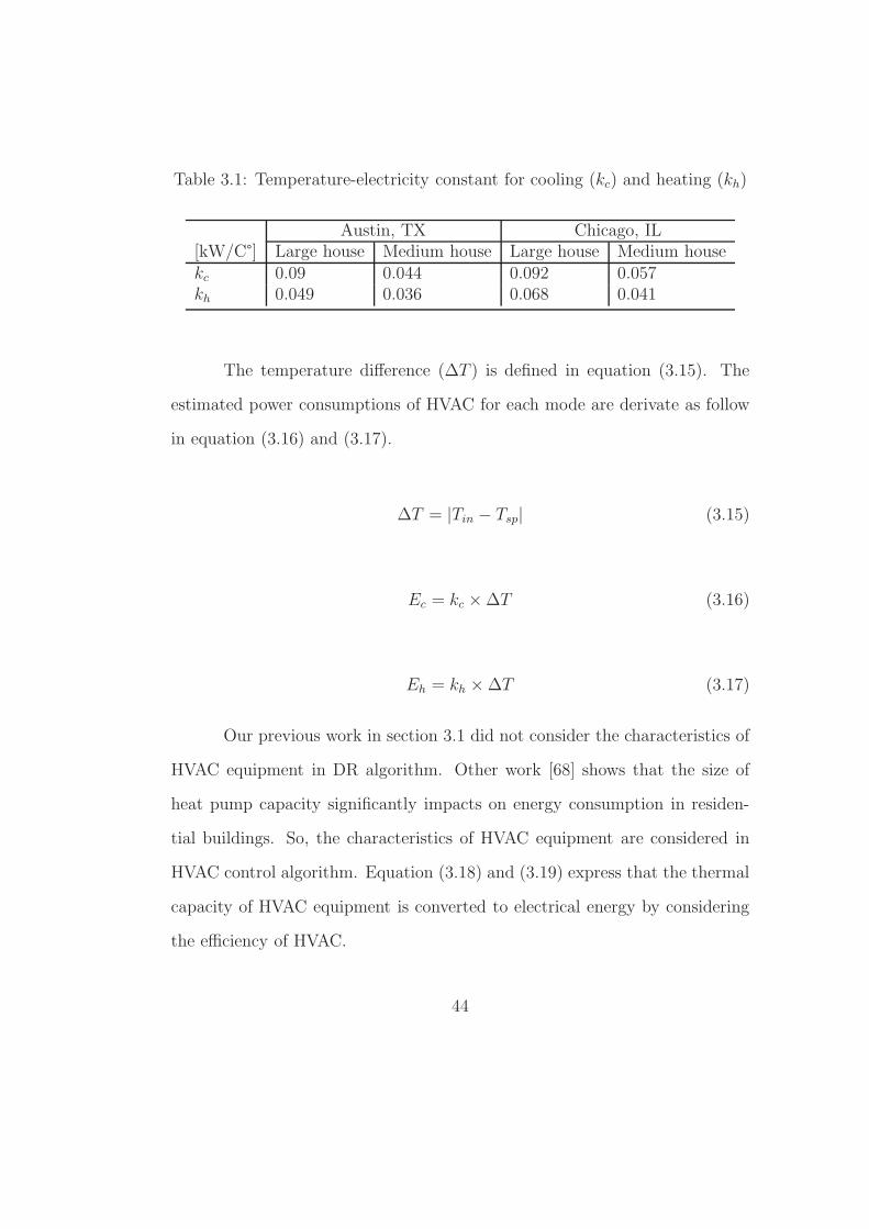
Table 3.1: Temperature-electricity constant for cooling (kc) and heating (kh)

Austin, TX Chicago, IL[kW/C°] Large house Medium house Large house Medium housekc 0.09 0.044 0.092 0.057kh 0.049 0.036 0.068 0.041

The temperature difference (∆T ) is defined in equation (3.15). The

estimated power consumptions of HVAC for each mode are derivate as follow

in equation (3.16) and (3.17).

∆T = |Tin − Tsp| (3.15)

Ec = kc ×∆T (3.16)

Eh = kh ×∆T (3.17)

Our previous work in section 3.1 did not consider the characteristics of

HVAC equipment in DR algorithm. Other work [68] shows that the size of

heat pump capacity significantly impacts on energy consumption in residen-

tial buildings. So, the characteristics of HVAC equipment are considered in

HVAC control algorithm. Equation (3.18) and (3.19) express that the thermal

capacity of HVAC equipment is converted to electrical energy by considering

the efficiency of HVAC.

44

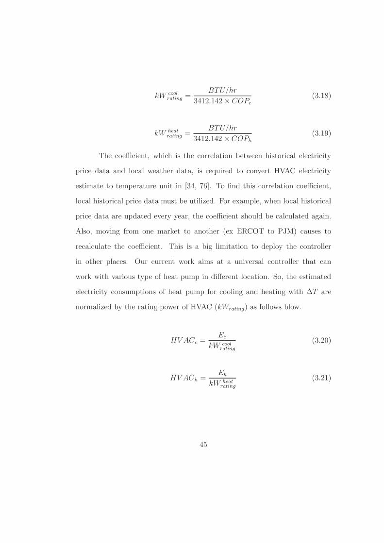
kW coolrating =

BTU/hr

3412.142× COPc

(3.18)

kW heatrating =

BTU/hr

3412.142× COPh

(3.19)

The coefficient, which is the correlation between historical electricity

price data and local weather data, is required to convert HVAC electricity

estimate to temperature unit in [34, 76]. To find this correlation coefficient,

local historical price data must be utilized. For example, when local historical

price data are updated every year, the coefficient should be calculated again.

Also, moving from one market to another (ex ERCOT to PJM) causes to

recalculate the coefficient. This is a big limitation to deploy the controller

in other places. Our current work aims at a universal controller that can

work with various type of heat pump in different location. So, the estimated

electricity consumptions of heat pump for cooling and heating with ∆T are

normalized by the rating power of HVAC (kWrating) as follows blow.

HVACc =Ec

kW coolrating

(3.20)

HV ACh =Eh

kW heatrating

(3.21)

45

3.2.2 Normalized Electricity Price Signal

The Dynamic Demand Response Controller (DDRC) takes the signal of

dynamic electricity price to change the set-point temperature for DR program.

Depending on economic situations, incomes in each household are different.

Therefore, the electricity bills that household can afford to pay are dissimilar.

The proposed DDRC considers the economic ability in household by again

utilizing threshold price (Pth) when customers participate into utility program.

Depending on demand loads, the electricity price changes. For instance, 2011

was the hottest year in Austin, TX. Air conditioning loads were significant

loads in the power grid. As a result, day-ahead price of electricity in ERCOT

wholesale market occasionally approached the maximum price, $3,000/MWh.

The fluctuation of electricity price was also very high in a same day between

on-peak and off-peak time. The previous control algorithm in section 3.1 does

not reflect the price fluctuation that causes sudden change of the set-point

temperature. To consider it, the standard deviation of electricity price for

a day (σday) is calculated based on day-ahead price which is announced a

day before. The parameter σday normalizes the price difference (Pc − Pth)

between the current price of electricity (Pc) and threshold price (Pth). The

normalized price (PN) is presented in equation (3.22) and (3.23). DTC changes

the set-point temperature when Pc is higher than Pth. Otherwise, the set-point

temperature maintains the preset temperature (Tsp)that customers set. From

Figure 2.3, the threshold price (Pth) is set to $0.04/kWh because the dynamic

prices of electricity in both Austin and Chicago maintain under $0.03/kWh

46

for most hours. Thus, DTC starts to operate itself when Pc is higher than

$0.04/kWh.

PN =

Pc − Pth

σday

for Pc > Pth (3.22)

0 for Pc ≤ Pth (3.23)

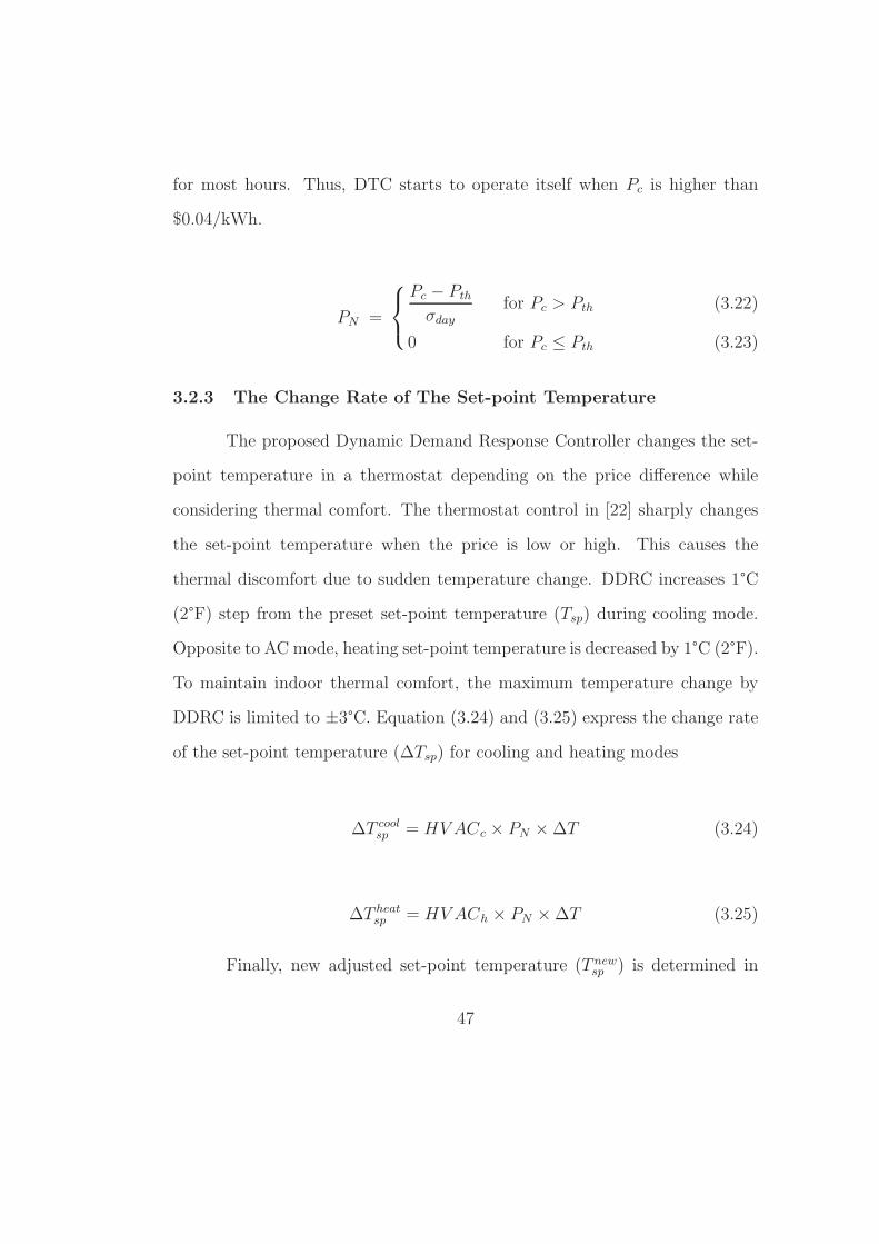
3.2.3 The Change Rate of The Set-point Temperature

The proposed Dynamic Demand Response Controller changes the set-

point temperature in a thermostat depending on the price difference while

considering thermal comfort. The thermostat control in [22] sharply changes

the set-point temperature when the price is low or high. This causes the

thermal discomfort due to sudden temperature change. DDRC increases 1°C

(2°F) step from the preset set-point temperature (Tsp) during cooling mode.

Opposite to AC mode, heating set-point temperature is decreased by 1°C (2°F).

To maintain indoor thermal comfort, the maximum temperature change by

DDRC is limited to ±3°C. Equation (3.24) and (3.25) express the change rate

of the set-point temperature (∆Tsp) for cooling and heating modes

∆T coolsp = HVACc × PN ×∆T (3.24)

∆T heatsp = HVACh × PN ×∆T (3.25)

Finally, new adjusted set-point temperature (T newsp ) is determined in

47

equation (3.26) and (3.27). When Pth is higher than Pc, ∆Tsp goes to zero.

So, DDRC maintains the preset environment for thermal comfort. Otherwise,

DDRC controls the set-point temperature depending on the difference price

between Pc and Pth. In this research, Tsp for cooling is 25°C (77°F) and heating

Tsp is 21°C (70°F).

T newsp =

Tsp +∆T coolsp for cooling mode (3.26)

Tsp −∆T heatsp for heating mode (3.27)

3.3 Controller Implementation

DDRC is implemented using MATLAB/SIMULINK. It receives two

inputs from EnergyPlus and Building Controls Virtual Test Bed (BCVTB)

and generates new set-point temperature for each cooling and heating mode.

EnergyPlus is developed and distributed by US Department of Energy. It not

only calculates annual energy from the outdoor environment and internal load

but also the annual energy consumption. A whole year of retail price based

on ERCOT’s SPP of Austin Energy Network is embedded into SIMULINK

function code. Figure 3.3 presents SIMULINK model of DDRC.

Simulation step time of EnergyPlus can be chosen from 1 minute to

1 hour. A 15 minute simulation step is used for both SIMULINK and En-

ergyPlus to match electricity retail price change interval with 15 minute in-

terval real-time price of electricity. When hourly day ahead price is chosen,

an hour time step is used to evaluate the performance of DDRC. However,

48

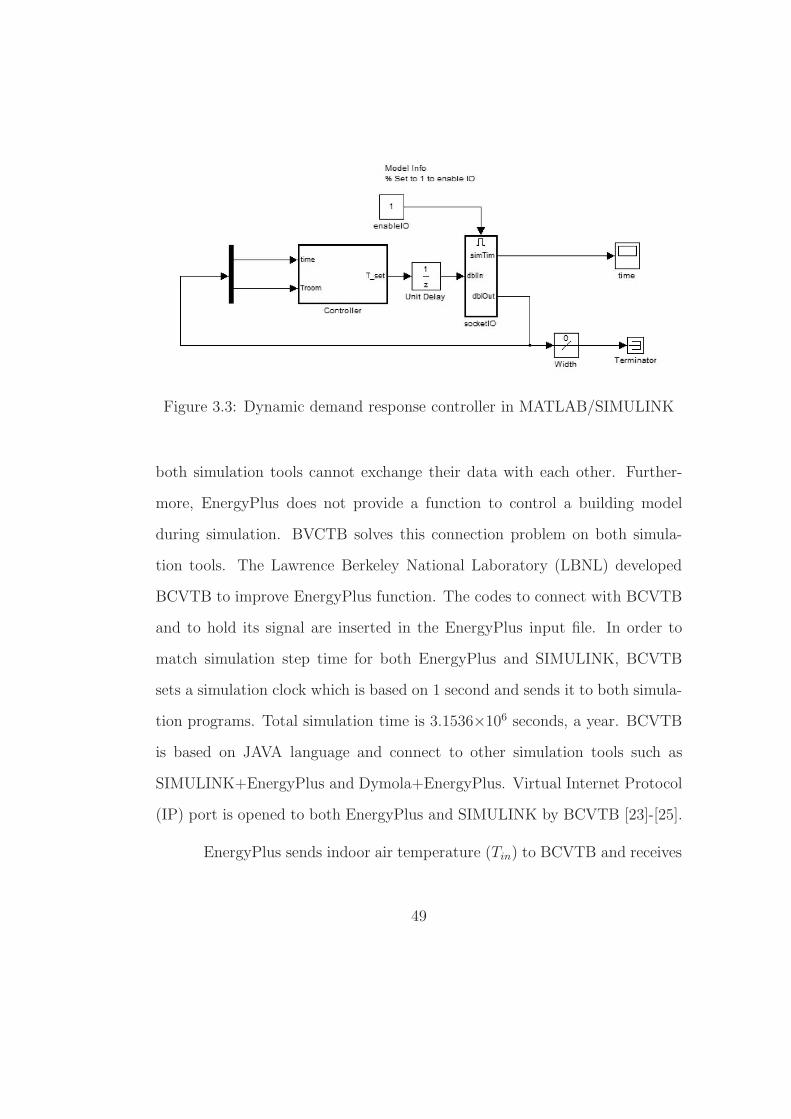
Figure 3.3: Dynamic demand response controller in MATLAB/SIMULINK

both simulation tools cannot exchange their data with each other. Further-

more, EnergyPlus does not provide a function to control a building model

during simulation. BVCTB solves this connection problem on both simula-

tion tools. The Lawrence Berkeley National Laboratory (LBNL) developed

BCVTB to improve EnergyPlus function. The codes to connect with BCVTB

and to hold its signal are inserted in the EnergyPlus input file. In order to

match simulation step time for both EnergyPlus and SIMULINK, BCVTB

sets a simulation clock which is based on 1 second and sends it to both simula-

tion programs. Total simulation time is 3.1536×106 seconds, a year. BCVTB

is based on JAVA language and connect to other simulation tools such as

SIMULINK+EnergyPlus and Dymola+EnergyPlus. Virtual Internet Protocol

(IP) port is opened to both EnergyPlus and SIMULINK by BCVTB [23]-[25].

EnergyPlus sends indoor air temperature (Tin) to BCVTB and receives

49

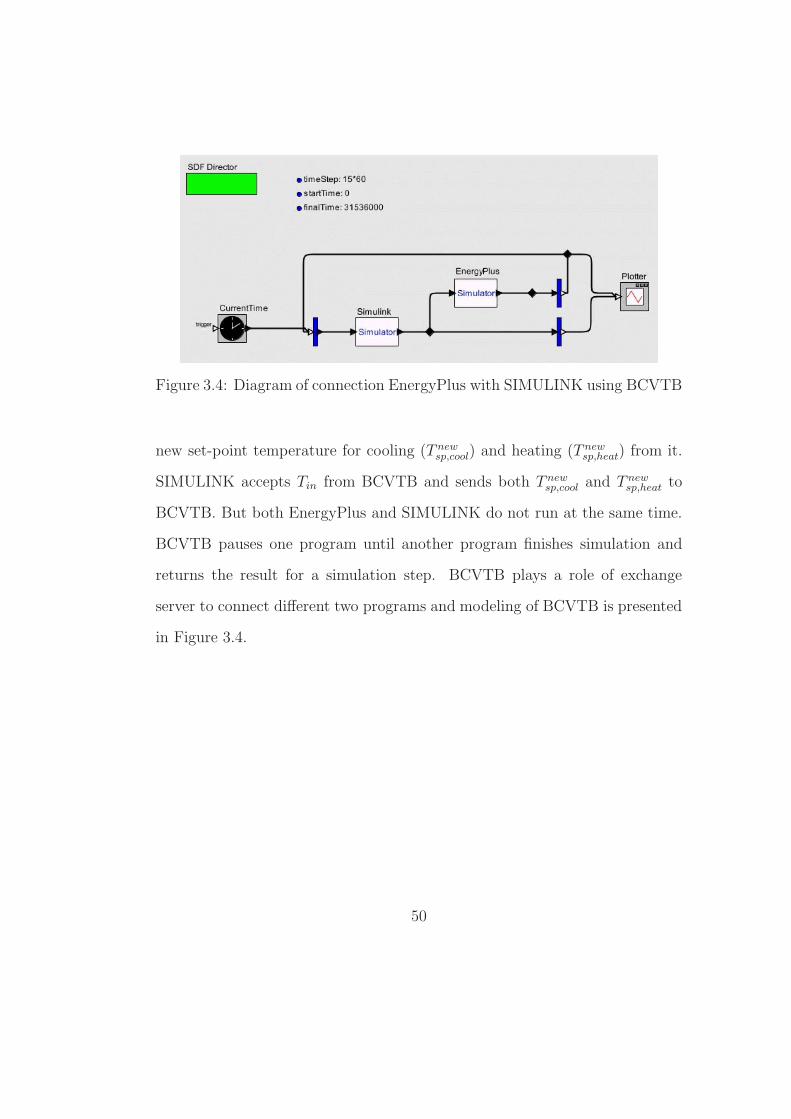
Figure 3.4: Diagram of connection EnergyPlus with SIMULINK using BCVTB

new set-point temperature for cooling (T newsp,cool) and heating (T new

sp,heat) from it.

SIMULINK accepts Tin from BCVTB and sends both T newsp,cool and T new

sp,heat to

BCVTB. But both EnergyPlus and SIMULINK do not run at the same time.

BCVTB pauses one program until another program finishes simulation and

returns the result for a simulation step. BCVTB plays a role of exchange

server to connect different two programs and modeling of BCVTB is presented

in Figure 3.4.

50

Chapter 4

The Results of The Performance of DDRC

This chapter shows the performance of the proposed Dynamic Demand

Response Controller (DDRC) under various circumstances. The target home

models have different floor plan, size, and internal loads. In addition, different

types of retail electricity prices from two wholesale markets. Furthermore,

weather data from different climate zones are used to evaluate the performance

of DDRC.

4.1 DDRC with dynamic price of electricity

In this section, the medium size of the house model and 15 minute based

real-time price (RTP) from ERCOT are used for the evaluation of DDRC per-

formance. The results are presented for energy and cost savings in cooling

(August) and heating (January) modes. Also, the thermal comfort is dis-

cussed to show that DDRC minimizes thermal discomfort while the set-point

temperature is changed.

51

4.1.1 Simulation Condition

The thermostat is set to 23°C for cooling and 22 °C for heating. Cooling

and heating are applied for all season to evaluate the performance of DDRC

with the base policy at tight HVAC operation. The medium size house with

the internal load is chosen. The dynamic price of electricity is used 15 minute

based Real-Time Price (RTP) at ERCOT wholesale market at 2011.

4.1.2 Air Conditioning Loads: August

Air conditioning load in August is the highest of the whole year due

to high outdoor air temperature. Wholesale electricity price also increases

along with high temperatures. During 2011, ERCOT limited the maximum

wholesale price to $3,000 per MWh. From the retail price policy, the maxi-

mum electricity retail price is $3/kWh. During August, retail price reaches

the maximum price for more than 6 days during peak time. DDRC changes

set-point temperature to curtail HVAC electricity as electricity retail price is

higher than the threshold price. Figure 4.1 shows indoor air temperature of a

single family house model in August for both fixed set-point temperature and

the DDRC case.

During August, indoor air temperature without DDRC thermostat

maintains initial cooling and heating temperature which are in between 22°C

and 23°C. The DDRC changes the set-point temperature so that indoor air

temperature ranges from 21°C to 26°C. When the thermostat is fixed at initial

cooling and heating set-point temperature, HVAC consumes 733.48 kWh dur-

52

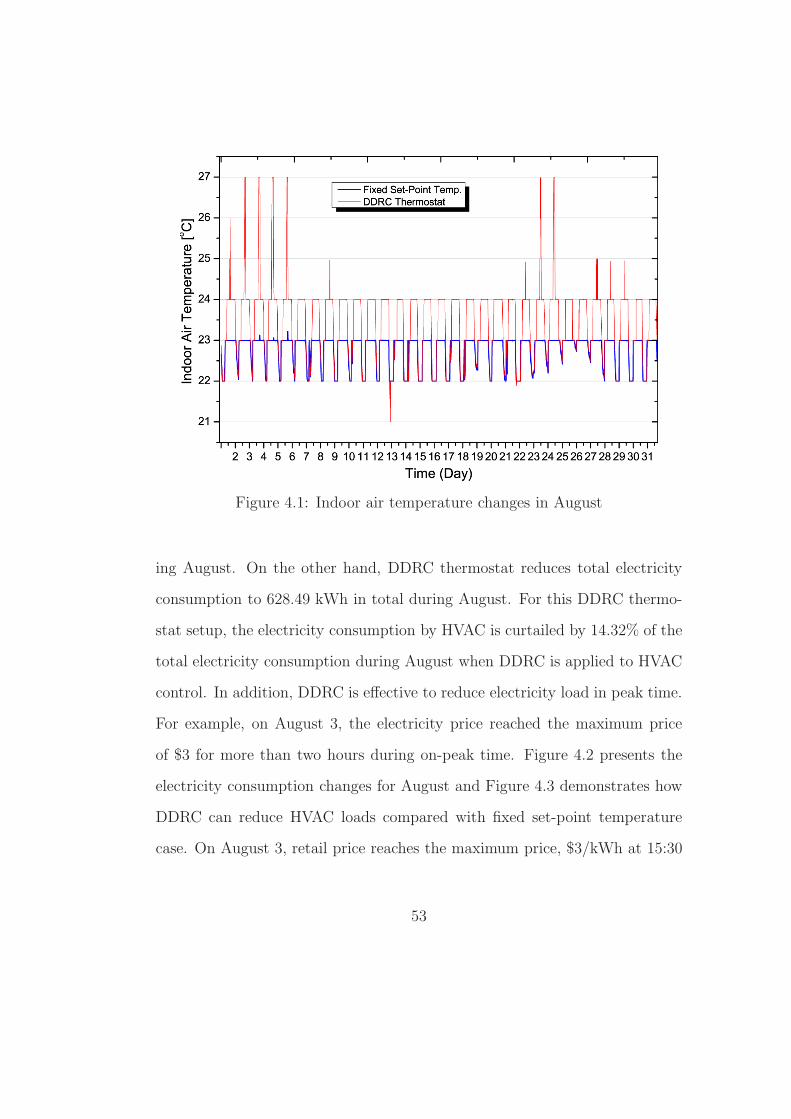
Figure 4.1: Indoor air temperature changes in August

ing August. On the other hand, DDRC thermostat reduces total electricity

consumption to 628.49 kWh in total during August. For this DDRC thermo-

stat setup, the electricity consumption by HVAC is curtailed by 14.32% of the

total electricity consumption during August when DDRC is applied to HVAC

control. In addition, DDRC is effective to reduce electricity load in peak time.

For example, on August 3, the electricity price reached the maximum price

of $3 for more than two hours during on-peak time. Figure 4.2 presents the

electricity consumption changes for August and Figure 4.3 demonstrates how

DDRC can reduce HVAC loads compared with fixed set-point temperature

case. On August 3, retail price reaches the maximum price, $3/kWh at 15:30

53

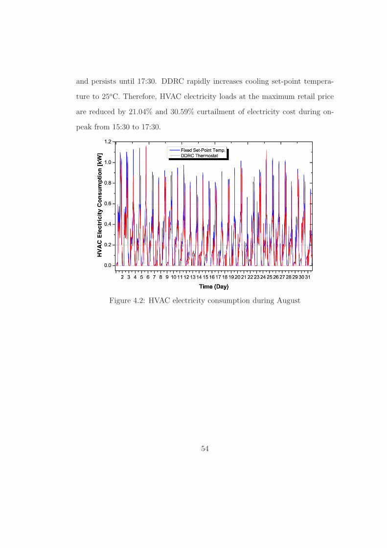
and persists until 17:30. DDRC rapidly increases cooling set-point tempera-

ture to 25oC. Therefore, HVAC electricity loads at the maximum retail price

are reduced by 21.04% and 30.59% curtailment of electricity cost during on-

peak from 15:30 to 17:30.

Figure 4.2: HVAC electricity consumption during August

54

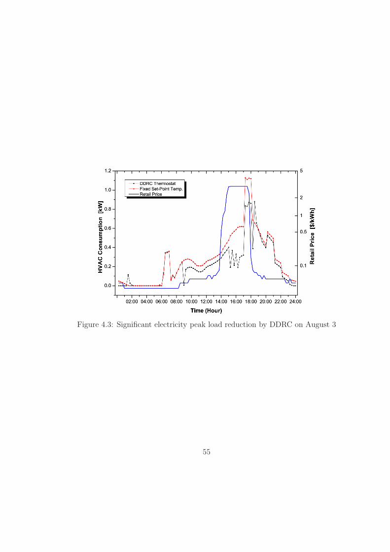
Figure 4.3: Significant electricity peak load reduction by DDRC on August 3

55

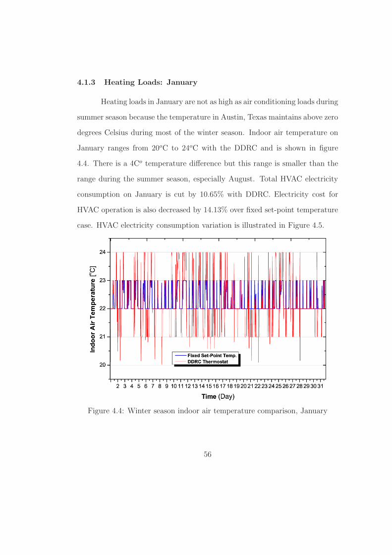
4.1.3 Heating Loads: January

Heating loads in January are not as high as air conditioning loads during

summer season because the temperature in Austin, Texas maintains above zero

degrees Celsius during most of the winter season. Indoor air temperature on

January ranges from 20oC to 24oC with the DDRC and is shown in figure

4.4. There is a 4Co temperature difference but this range is smaller than the

range during the summer season, especially August. Total HVAC electricity

consumption on January is cut by 10.65% with DDRC. Electricity cost for

HVAC operation is also decreased by 14.13% over fixed set-point temperature

case. HVAC electricity consumption variation is illustrated in Figure 4.5.

Figure 4.4: Winter season indoor air temperature comparison, January

56

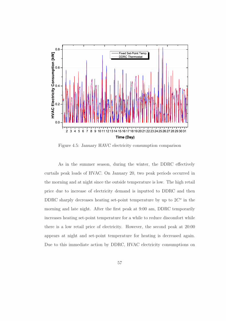
Figure 4.5: January HAVC electricity consumption comparison

As in the summer season, during the winter, the DDRC effectively

curtails peak loads of HVAC. On January 20, two peak periods occurred in

the morning and at night since the outside temperature is low. The high retail

price due to increase of electricity demand is inputted to DDRC and then

DDRC sharply decreases heating set-point temperature by up to 2Co in the

morning and late night. After the first peak at 9:00 am, DDRC temporarily

increases heating set-point temperature for a while to reduce discomfort while

there is a low retail price of electricity. However, the second peak at 20:00

appears at night and set-point temperature for heating is decreased again.

Due to this immediate action by DDRC, HVAC electricity consumptions on

57

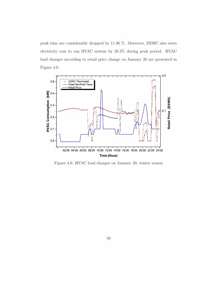
peak time are considerably dropped by 11.96 %. Moreover, DDRC also saves

electricity cost to run HVAC system by 20.3% during peak period. HVAC

load changes according to retail price change on January 20 are presented in

Figure 4.6.

Figure 4.6: HVAC load changes on January 20, winter season

58

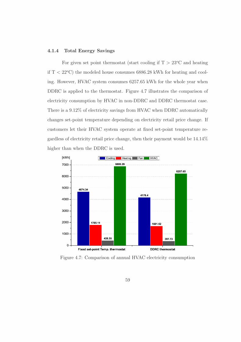
4.1.4 Total Energy Savings

For given set point thermostat (start cooling if T > 23oC and heating

if T < 22oC) the modeled house consumes 6886.28 kWh for heating and cool-

ing. However, HVAC system consumes 6257.65 kWh for the whole year when

DDRC is applied to the thermostat. Figure 4.7 illustrates the comparison of

electricity consumption by HVAC in non-DDRC and DDRC thermostat case.

There is a 9.12% of electricity savings from HVAC when DDRC automatically

changes set-point temperature depending on electricity retail price change. If

customers let their HVAC system operate at fixed set-point temperature re-

gardless of electricity retail price change, then their payment would be 14.14%

higher than when the DDRC is used.

Figure 4.7: Comparison of annual HVAC electricity consumption

59

We also considered the effect of a wider-dead band in the base case

simulation. The simulation results show that a wider thermostat dead-band

decreases the potential for energy saving with DDRC. For example, increasing

the dead-band from1 C°(start cooling if T > 23°C and heating if T < 22°C)

to 5 C°(start cooling if T > 26°C and heating if T < 21°C) decreases the total

energy saving with DDRC from 9.11% to 2.74%. Also, different house sizes

and/or thermal properties (such as insulation, glass area. etc.) may impact the

saving due to using the DDRC. An elaborate study with sensitivity analysis

that includes multiple type of houses and thermostat set-point are needed to

fully assess the economic potential of DDRC.

60

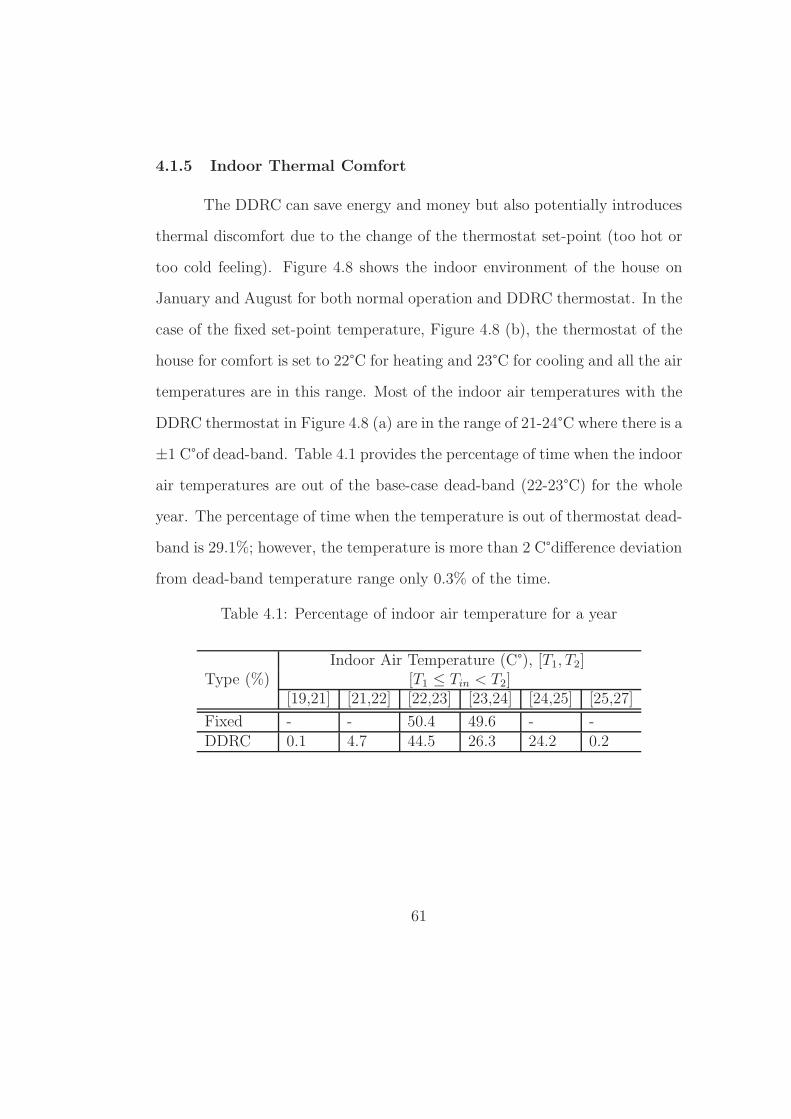
4.1.5 Indoor Thermal Comfort

The DDRC can save energy and money but also potentially introduces

thermal discomfort due to the change of the thermostat set-point (too hot or

too cold feeling). Figure 4.8 shows the indoor environment of the house on

January and August for both normal operation and DDRC thermostat. In the

case of the fixed set-point temperature, Figure 4.8 (b), the thermostat of the

house for comfort is set to 22°C for heating and 23°C for cooling and all the air

temperatures are in this range. Most of the indoor air temperatures with the

DDRC thermostat in Figure 4.8 (a) are in the range of 21-24°C where there is a

±1 C°of dead-band. Table 4.1 provides the percentage of time when the indoor

air temperatures are out of the base-case dead-band (22-23°C) for the whole

year. The percentage of time when the temperature is out of thermostat dead-

band is 29.1%; however, the temperature is more than 2 C°difference deviation

from dead-band temperature range only 0.3% of the time.

Table 4.1: Percentage of indoor air temperature for a year

Type (%)Indoor Air Temperature (C°), [T1, T2]

[T1 ≤ Tin < T2][19,21] [21,22] [22,23] [23,24] [24,25] [25,27]

Fixed - - 50.4 49.6 - -DDRC 0.1 4.7 44.5 26.3 24.2 0.2

61

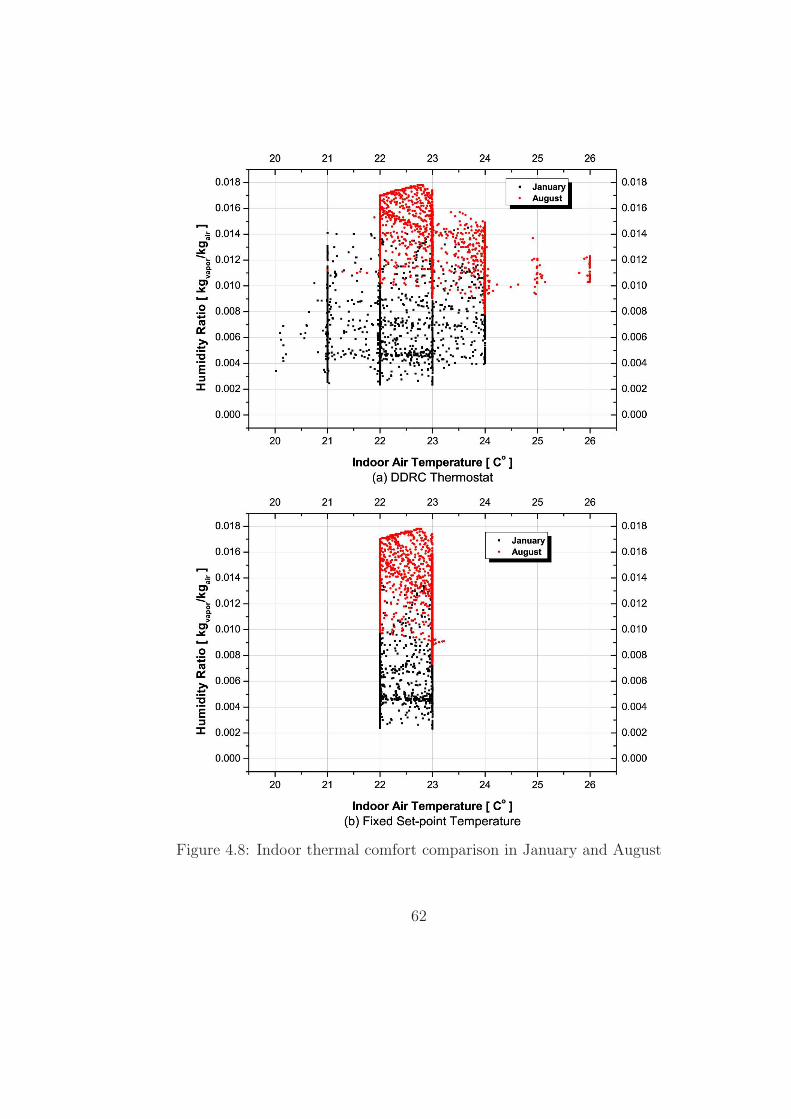
Figure 4.8: Indoor thermal comfort comparison in January and August

62

4.2 DDRC with various price types and floor plans

The performance of the proposed Dynamic Demand Response Con-

troller (DDRC) is evaluated in terms of saving energy cost and reducing peak

loads during peak time. Two different types of retail price are used; hourly

based day ahead price (DAP) and 15 minute based real-time price (RTP). In

addition, total annual electricity consumption is reduced for both the large

and medium houses when the proposed DDRC thermostats are installed. The

indoor environments in houses maintain thermal comfort during most times

compared with the base case, which has fixed set-point temperature. Ener-

gyPlus documentation recommends simulating the building with 15 minute

time-step [49-51]. However, an hour time-step is chosen in this research since

the price signal of electricity changes every hour. So, an hour simulation step

is chosen to demonstrate the performance of the proposed thermostat con-

troller to match the interval of the price signal. In additional studies, it was

verified that the results with 15 minute time-step is less than 0.5% different

from an hour based simulation results for both HVAC and total electricity

consumptions. So, the time-step does not impact on the simulation results.


In this case, The thermostat is set to 26°C for cooling and 22 °C for

heating. Cooling days is from April 1st to October 31st. During this period,

space heating is not applied. During the rest of days for a year, only space

heating is applied. So, the indoor temperature for some hours were out of

63

the thermal comfort when the indoor temperature is lower than 22 °C during

the cooling days since space heating it not applied in both with and without

DDRC cases. For heating days, the indoor environment is the same as cooling

season due to lack of air conditioning. Both the medium and large houses with

the internal load are chosen. The dynamic prices of electricity for this case are

selected 15 minute based Real-Time Price (RTP) and hourly Day Ahead Price

(DAP) at ERCOT wholesale market at 2011. DDRC adjusted the set-point

temperature with the based policy.

4.2.2 The Large House

For the large house with fixed set-point temperature, the base case

consumed 15.8 MWh of total electricity for a year. AC is turned on from

April 1st to October 31st. A heater starts to supply heat into a house when

AC mode is deactivated. HVAC electricity consumption was 7.8 MWh which

is 49% of total electricity consumption. It has a large floor plan and window

area so that high HVAC loads are demanded for cooling and heating into a

house. When the DR controller is applied, the total electricity consumptions

by HVAC are decreased to 7.5 MWh with Real Time Price (RTP) and to 7.4

MWh with Day Ahead Price (DAP). That is, 3.7% in average of energy is saved

using DR controller. Especially, on July 30, 2012, RTP reached the maximum

price of electricity, $0.61 per kWh at 16:00 to due to heavy AC use. The peak

occurred from 13:00 to 19:00 on Austin Energy Network (AEN). The average

electricity consumption of HVAC is 17 kWh during peak periods if the cooling

64

set-point temperature is not changed. However, when RTP based DDRC is

set to HVAC system, average electricity consumption for cooling was sharply

dropped to 12.7 kWh, so that 24.7% of AC load was curtailed.

65

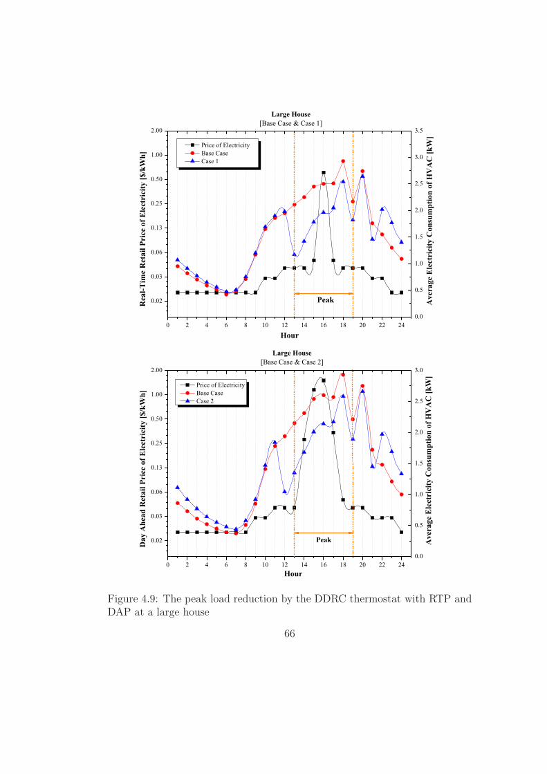
0 2 4 6 8 10 12 14 16 18 20 22 24

0.02

0.03

0.06

0.13

0.25

0.50

1.00

2.00

Price of Electricity Base Case Case 1

Rea

l-Tim

e R

etai

l Pri

ce o

f Ele

ctri

city

[$/k

Wh]

Hour

Large House[Base Case & Case 1]

Peak

0.0

0.5

1.0

1.5

2.0

2.5

3.0

3.5

Ave

rage

Ele

ctri

city

Con

sum

ptio

n of

HV

AC

[kW

]

0 2 4 6 8 10 12 14 16 18 20 22 24

0.02

0.03

0.06

0.13

0.25

0.50

1.00

2.00

Day

Ahe

ad R

etai

l Pri

ce o

f Ele

ctri

city

[$/k

Wh]

Hour


Peak

Large House[Base Case & Case 2]

0.0

0.5

1.0

1.5

2.0

2.5

3.0

Ave

rage

Ele

ctri

city

Con

sum

ptio

n of

HV

AC

[kW

]

Figure 4.9: The peak load reduction by the DDRC thermostat with RTP andDAP at a large house

66

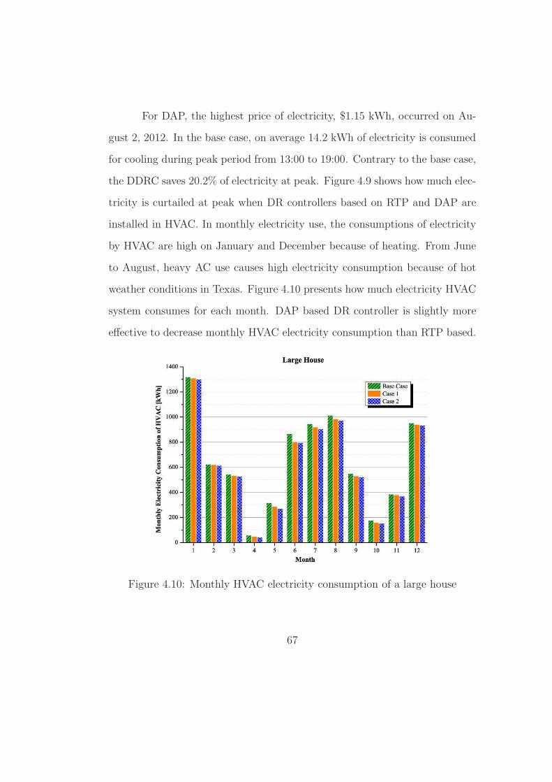
For DAP, the highest price of electricity, $1.15 kWh, occurred on Au-

gust 2, 2012. In the base case, on average 14.2 kWh of electricity is consumed

for cooling during peak period from 13:00 to 19:00. Contrary to the base case,

the DDRC saves 20.2% of electricity at peak. Figure 4.9 shows how much elec-

tricity is curtailed at peak when DR controllers based on RTP and DAP are

installed in HVAC. In monthly electricity use, the consumptions of electricity

by HVAC are high on January and December because of heating. From June

to August, heavy AC use causes high electricity consumption because of hot

weather conditions in Texas. Figure 4.10 presents how much electricity HVAC

system consumes for each month. DAP based DR controller is slightly more

effective to decrease monthly HVAC electricity consumption than RTP based.

Figure 4.10: Monthly HVAC electricity consumption of a large house

67

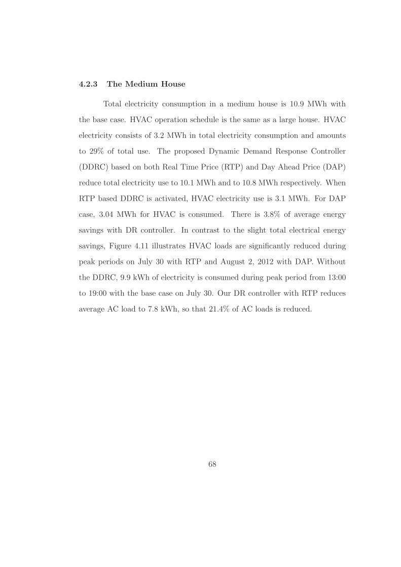
4.2.3 The Medium House

Total electricity consumption in a medium house is 10.9 MWh with

the base case. HVAC operation schedule is the same as a large house. HVAC

electricity consists of 3.2 MWh in total electricity consumption and amounts

to 29% of total use. The proposed Dynamic Demand Response Controller

(DDRC) based on both Real Time Price (RTP) and Day Ahead Price (DAP)

reduce total electricity use to 10.1 MWh and to 10.8 MWh respectively. When

RTP based DDRC is activated, HVAC electricity use is 3.1 MWh. For DAP

case, 3.04 MWh for HVAC is consumed. There is 3.8% of average energy

savings with DR controller. In contrast to the slight total electrical energy

savings, Figure 4.11 illustrates HVAC loads are significantly reduced during

peak periods on July 30 with RTP and August 2, 2012 with DAP. Without

the DDRC, 9.9 kWh of electricity is consumed during peak period from 13:00

to 19:00 with the base case on July 30. Our DR controller with RTP reduces

average AC load to 7.8 kWh, so that 21.4% of AC loads is reduced.

68

0 2 4 6 8 10 12 14 16 18 20 22 24

0.02

0.03

0.06

0.13

0.25

0.50

1.00

2.00

Rea

l-Tim

e R

etai

l Pri

ce o

f Ele

ctri

city

[$/k

Wh]

Hour


Medium House[Base Case & Case 1]

0.0

0.5

1.0

1.5

2.0

2.5

3.0

Ave

rage

Ele

ctri

city

Con

sum

ptio

n of

HV

AC

[kW

]

Peak

0 2 4 6 8 10 12 14 16 18 20 22 24

0.02

0.03

0.06

0.13

0.25

0.50

1.00

2.00

Day

Ahe

ad R

etai

l Pri

ce o

f Ele

ctri

city

[$/k

Wh]

Hour


Medium House[Base Case & Case 2]

0.0

0.5

1.0

1.5

2.0

2.5

3.0

Ave

rage

Ele

ctri

city

Con

sum

ptio

n of

HV

AC

[kW

]

Peak

Figure 4.11: The contribution of DDRC thermostat with RTP and DAP todecrease peak loads at a medium house

69

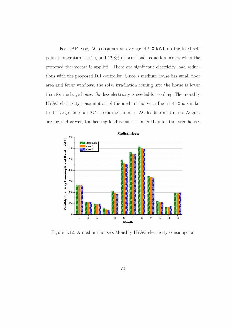
For DAP case, AC consumes an average of 9.3 kWh on the fixed set-

point temperature setting and 12.8% of peak load reduction occurs when the

proposed thermostat is applied. There are significant electricity load reduc-

tions with the proposed DR controller. Since a medium house has small floor

area and fewer windows, the solar irradiation coming into the house is lower

than for the large house. So, less electricity is needed for cooling. The monthly

HVAC electricity consumption of the medium house in Figure 4.12 is similar

to the large house on AC use during summer. AC loads from June to August

are high. However, the heating load is much smaller than for the large house.

Figure 4.12: A medium house’s Monthly HVAC electricity consumption

70

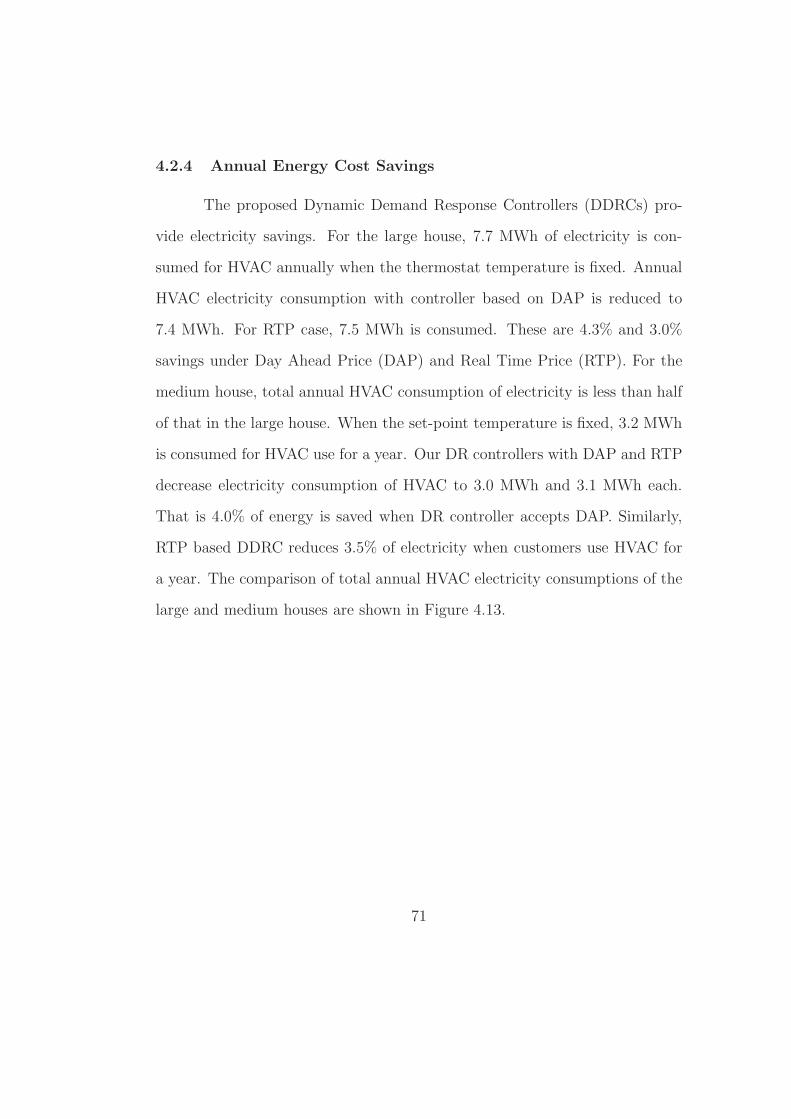
4.2.4 Annual Energy Cost Savings

The proposed Dynamic Demand Response Controllers (DDRCs) pro-

vide electricity savings. For the large house, 7.7 MWh of electricity is con-

sumed for HVAC annually when the thermostat temperature is fixed. Annual

HVAC electricity consumption with controller based on DAP is reduced to

7.4 MWh. For RTP case, 7.5 MWh is consumed. These are 4.3% and 3.0%

savings under Day Ahead Price (DAP) and Real Time Price (RTP). For the

medium house, total annual HVAC consumption of electricity is less than half

of that in the large house. When the set-point temperature is fixed, 3.2 MWh

is consumed for HVAC use for a year. Our DR controllers with DAP and RTP

decrease electricity consumption of HVAC to 3.0 MWh and 3.1 MWh each.

That is 4.0% of energy is saved when DR controller accepts DAP. Similarly,

RTP based DDRC reduces 3.5% of electricity when customers use HVAC for

a year. The comparison of total annual HVAC electricity consumptions of the

large and medium houses are shown in Figure 4.13.

71

Cooling Heating Fan HVAC0

1000

2000

3000

4000

5000

6000

7000

8000

9000

Ann

ual E

lect

rici

ty C

onsu

mpt

ion

of H

VA

C [k

Wh]

Base Case Case 1 Case 2

Large House

Cooling Heating Fan HVAC0

500

1000

1500

2000

2500

3000

3500

Ann

ual E

lect

rici

ty C

onsu

mpt

ion

of H

VA

C [k

Wh]

Base Case Case 1 Case 2

Medium House

Figure 4.13: The annual electricity savings for a large and medium house

72

4.2.5 Annual energy cost savings

The results for the DDRC demonstrate the energy costs are saved at

peak. The large house’s monthly bill to use HVAC is three times higher than

the medium house due to its size. On August, especially, heavy AC loads

occurred. So, the retail price of electricity is higher than other months. When

DR controller is applied, monthly charges are dropped to $32.9 with RTP tariff

and $46.32 with DAP. Customers who choose DAP for DR program pay a 30%

higher electricity bill than when RTP is chosen. Monetary savings are 7.7%

and 13.2%, respectively, for RTP and DAP each compared the fixed thermostat

temperature setting. For the medium house, $20.36 and $28.16 are spent to use

AC when RTP and DAP tariffs are applied in DR controller. Compared with

non-DR controller cases, DR controllers save 6.3% with RTP and 11.7% with

DAP of electricity bill on August. The annual electricity costs for cooling and

heating are presented in Figure 4.14. The large house spends twice as much

money to use HVAC system as the medium house. The DR controllers in

a large house drop costs to $220.07 with RTP and to $251.59 with DAP per

year. There are 7.7% and 10.8% of saving from the fixed set-point temperature

settings. In the case of the medium house, RTP tariff occurs $96.57 for HVAC

use and $114.8 is charged by DAP based retail price. When DR controllers

are applied, there are 8.1% and 10.47% of cost savings for each tariff from

non-DR mode. The current tariff for residential customers of Austin Energy is

an energy based tier tariff. When residential customers use more electricity in

a month beyond a tier level, they will be charged high electricity prices for the

73

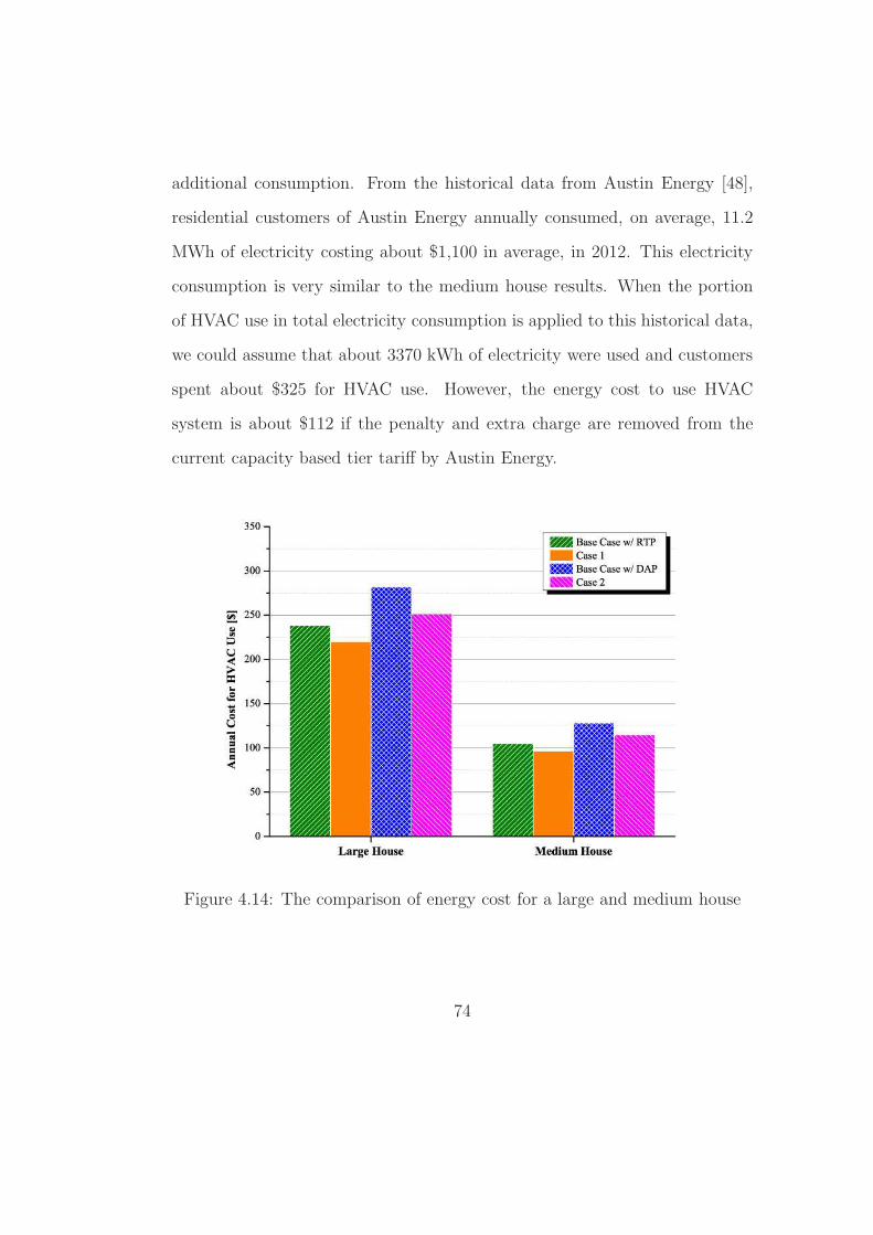
additional consumption. From the historical data from Austin Energy [48],

residential customers of Austin Energy annually consumed, on average, 11.2

MWh of electricity costing about $1,100 in average, in 2012. This electricity

consumption is very similar to the medium house results. When the portion

of HVAC use in total electricity consumption is applied to this historical data,

we could assume that about 3370 kWh of electricity were used and customers

spent about $325 for HVAC use. However, the energy cost to use HVAC

system is about $112 if the penalty and extra charge are removed from the

current capacity based tier tariff by Austin Energy.

Figure 4.14: The comparison of energy cost for a large and medium house

74

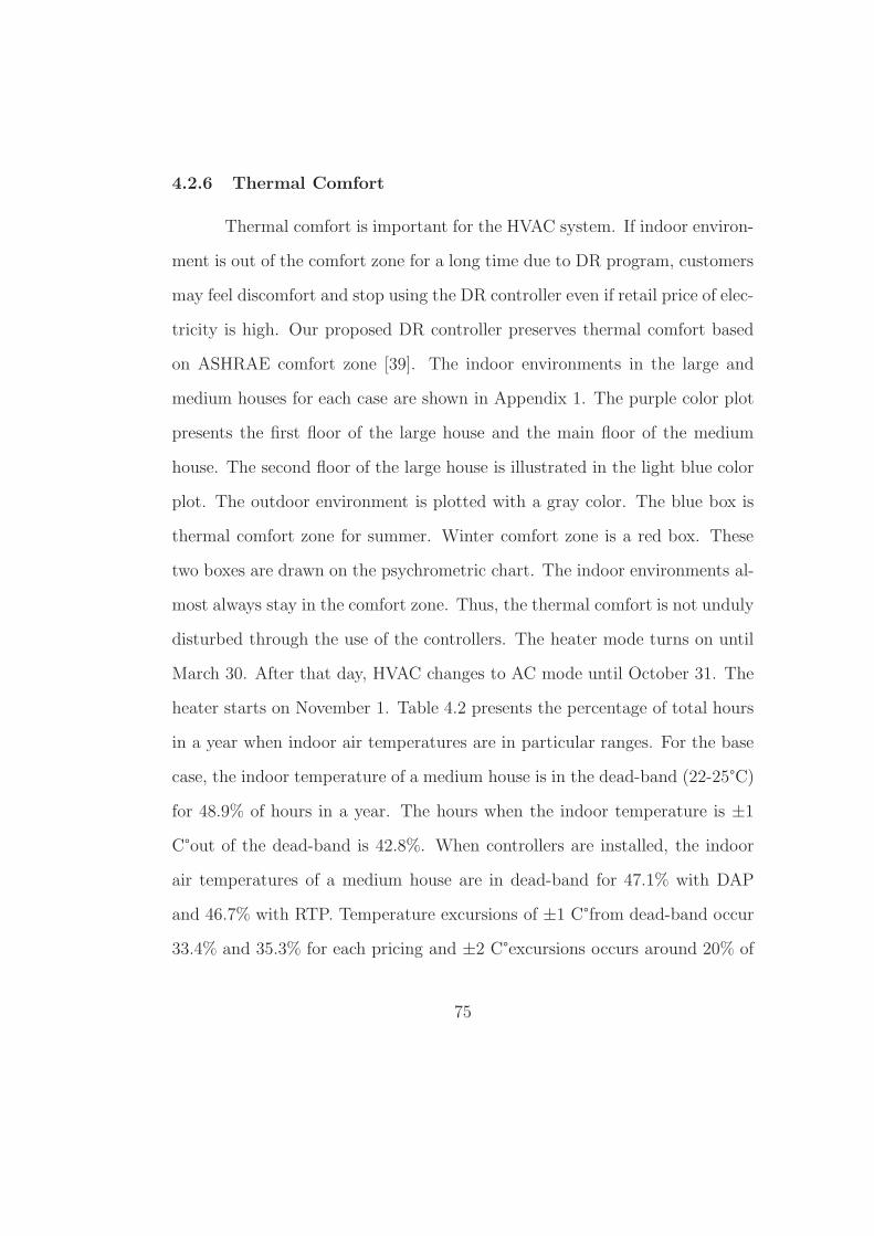
4.2.6 Thermal Comfort

Thermal comfort is important for the HVAC system. If indoor environ-

ment is out of the comfort zone for a long time due to DR program, customers

may feel discomfort and stop using the DR controller even if retail price of elec-

tricity is high. Our proposed DR controller preserves thermal comfort based

on ASHRAE comfort zone [39]. The indoor environments in the large and

medium houses for each case are shown in Appendix 1. The purple color plot

presents the first floor of the large house and the main floor of the medium

house. The second floor of the large house is illustrated in the light blue color

plot. The outdoor environment is plotted with a gray color. The blue box is

thermal comfort zone for summer. Winter comfort zone is a red box. These

two boxes are drawn on the psychrometric chart. The indoor environments al-

most always stay in the comfort zone. Thus, the thermal comfort is not unduly

disturbed through the use of the controllers. The heater mode turns on until

March 30. After that day, HVAC changes to AC mode until October 31. The

heater starts on November 1. Table 4.2 presents the percentage of total hours

in a year when indoor air temperatures are in particular ranges. For the base

case, the indoor temperature of a medium house is in the dead-band (22-25°C)

for 48.9% of hours in a year. The hours when the indoor temperature is ±1

C°out of the dead-band is 42.8%. When controllers are installed, the indoor

air temperatures of a medium house are in dead-band for 47.1% with DAP

and 46.7% with RTP. Temperature excursions of ±1 C°from dead-band occur

33.4% and 35.3% for each pricing and ±2 C°excursions occurs around 20% of

75

the year.

Table 4.2: Indoor air temperature in percentage of hours for a year

Type Indoor Air Temperature (oC), [T1, T2], where [T1 ≤ Tin < T2][20,21] [21,22] [22,25] [25,26] [26,27] [27,28]

Medium house - main floorBase 4.9 1.7 48.9 41.1 1.7 1.7Case 1 5.0 2.9 46.7 32.4 11.2 1.8Case 2 5.1 3.0 47.1 30.4 13.0 1.4

Large house - 1st floorBase 5.7 2.1 47.3 40.3 2.1 2.5Case 1 6.1 2.9 45.6 31.3 11.6 2.5Case 2 6.3 3.2 45.0 29.3 13.7 2.5

Large house - 2nd floorBase 7.3 1.9 52.3 38.5 - -Case 1 7.6 3.2 50.1 31.8 7.3 -Case 2 7.8 3.7 49.3 30.3 8.9 -

Without the DDRC, the large house is in dead-band during 47.3% and

52.3% of the time for 1st and 2nd floor respectively. The hours when the

indoor temperatures are ±1°C out of the dead-band are 42.3% and 40.4% for

1st and 2nd floors. The first floor maintains within dead-band for 45.6% and

45.0% of hours for case 1 and 2 when the DDRCs are applied. The hours when

temperature excursions of ±1°C occur are 32.5% with DAP and 34.2% with

RTP in the first floor. For second floor, temperatures are in dead-band for

50.1% and 49.3% for case 1 and 2. Temperature excursion of ±1°C from the

initial setting occur 34.0% of hours in a year with DAP and 35.0% with RTP

but over 2°C difference are about 15% for each floor.

76

Considering HVAC mode changes, the indoor environment with the

proposed controller is close to the base case but reduce consumption at crit-

ical times. About 10% of total hours in average are different from the fixed

set-point temperature setting. This small difference shows the proposed DR

controller generally maintains the thermal comfort that the customer prefers.

Comparing both tariffs based on the dynamic price, the RTP tariff is more

effective to maintain the comfort level than DAP.

77

4.3 DDRC with different internal loads and climate zones

This chapter shows the proposed controller, Dynamic Demand Re-

sponse Controller (DDRC), reduces the electricity usage to operate HVAC

system at homes even though weather conditions and prices of electricity are

different with improved control algorithm. This energy savings provide to de-

crease electricity bill for HVAC operations. In addition, the indoor thermal

discomfort is minimized while DDRC changes the set-point temperature in a

thermostat to participate DR programs.


The thermostat setting is the same as the second simulation case; 26°C

for cooling and 22 °C for heating. HVAC operation schedule setting is also

same as previous second case. Both the medium and large houses are chosen

but the internal loads are set to normal and heavy (150% of normal load)

loads. To compare the performance of DDRC in two difference locations,

the dynamic prices of electricity are used hourly Day Ahead Price (DAP)

at ERCOT wholesale market at 2011 and PJM at 2013. Improved DDRC

algorithm is implanted to adjusted the set-point temperature based on DR

signal.

4.3.2 Savings of Electricity Consumption

The summer hot weather condition in Austin, TX increases air condi-

tioning loads in residential buildings. A large house with heavy internal loads

78

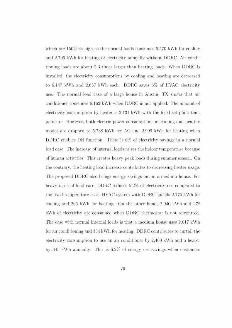
which are 150% as high as the normal loads consumes 6,570 kWh for cooling

and 2,796 kWh for heating of electricity annually without DDRC. Air condi-

tioning loads are about 2.3 times larger than heating loads. When DDRC is

installed, the electricity consumptions by cooling and heating are decreased

to 6,147 kWh and 2,657 kWh each. DDRC saves 6% of HVAC electricity

use. The normal load case of a large house in Austin, TX shows that air

conditioner consumes 6,162 kWh when DDRC is not applied. The amount of

electricity consumption by heater is 3,131 kWh with the fixed set-point tem-

perature. However, both electric power consumptions at cooling and heating

modes are dropped to 5,738 kWh for AC and 2,999 kWh for heating when

DDRC enables DR function. There is 6% of electricity savings in a normal

load case. The increase of internal loads raises the indoor temperature because

of human activities. This creates heavy peak loads during summer season. On

the contrary, the heating load increase contributes to decreasing heater usage.

The proposed DDRC also brings energy savings out in a medium house. For

heavy internal load case, DDRC reduces 5.2% of electricity use compared to

the fixed temperature case. HVAC system with DDRC spends 2,775 kWh for

cooling and 266 kWh for heating. On the other hand, 2,940 kWh and 278

kWh of electricity are consumed when DDRC thermostat is not retrofitted.

The case with normal internal loads is that a medium house uses 2,617 kWh

for air conditioning and 354 kWh for heating. DDRC contributes to curtail the

electricity consumption to use an air conditioner by 2,460 kWh and a heater

by 345 kWh annually. This is 6.2% of energy use savings when customers

79

run the HVAC system for a year. The same as the cases with a large house.

The internal load changes impact on HVAC electricity consumption since the

indoor temperature is increased or decreased by indoor activities. The elec-

tricity consumption of houses in Austin, TX for a year is presented in Figure

4.15.

80

DTC Fixed SP0

1,000

2,000

3,000

4,000

5,000

6,000

7,000El

ectr

icity

Con

sum

ptio

n

Cooling Heating

[kWh] Large house - Heavy loads(Austin, TX)

DTC Fixed SP0

1,000

2,000

3,000

4,000

5,000

6,000

7,000

Elec

tric

ity C

onsu

mpt

ion

[kWh] Large house - Normal loads(Austin, TX)

DTC Fixed SP0

500

1,000

1,500

2,000

2,500

3,000

3,500

Elec

tric

ity C

onsu

mpt

ion

[kWh] Medium house - Heavy loads(Austin, TX)

DTC Fixed SP0

500

1,000

1,500

2,000

2,500

3,000

3,500

Elec

tric

ity C

onsu

mpt

ion

[kWh] Medium house - Normal loads(Austin, TX)

Figure 4.15: The electricity consumption of houses in Austin, TX for wholeyear

81

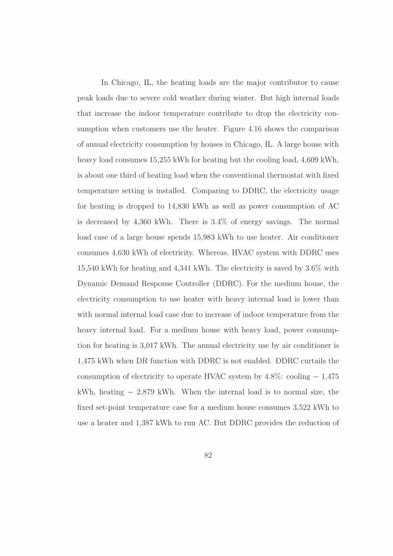
In Chicago, IL, the heating loads are the major contributor to cause

peak loads due to severe cold weather during winter. But high internal loads

that increase the indoor temperature contribute to drop the electricity con-

sumption when customers use the heater. Figure 4.16 shows the comparison

of annual electricity consumption by houses in Chicago, IL. A large house with

heavy load consumes 15,255 kWh for heating but the cooling load, 4,609 kWh,

is about one third of heating load when the conventional thermostat with fixed

temperature setting is installed. Comparing to DDRC, the electricity usage

for heating is dropped to 14,830 kWh as well as power consumption of AC

is decreased by 4,360 kWh. There is 3.4% of energy savings. The normal

load case of a large house spends 15,983 kWh to use heater. Air conditioner

consumes 4,630 kWh of electricity. Whereas, HVAC system with DDRC uses

15,540 kWh for heating and 4,341 kWh. The electricity is saved by 3.6% with

Dynamic Demand Response Controller (DDRC). For the medium house, the

electricity consumption to use heater with heavy internal load is lower than

with normal internal load case due to increase of indoor temperature from the

heavy internal load. For a medium house with heavy load, power consump-

tion for heating is 3,017 kWh. The annual electricity use by air conditioner is

1,475 kWh when DR function with DDRC is not enabled. DDRC curtails the

consumption of electricity to operate HVAC system by 4.8%: cooling − 1,475

kWh, heating − 2,879 kWh. When the internal load is to normal size, the

fixed set-point temperature case for a medium house consumes 3,522 kWh to

use a heater and 1,387 kWh to run AC. But DDRC provides the reduction of

82

electrical energy usage by 3,406 kWh for heating and 1,304 kWh for cooling.

The energy savings is 4.1% compared to a case without DDRC.

DTC Fixed SP0

2,000

4,0006,0008,000

10,000

12,00014,00016,000

Elec

tric

ity C

onsu

mpt

ion

Cooling Heating

Large house - Heavy loads[kWh] (Chicago, IL)

DTC Fixed SP0

2,000

4,0006,0008,000

10,000

12,00014,00016,000

Elec

tric

ity C

onsu

mpt

ion

Large house - Normal loads(Chicago, IL)[kWh]

DTC Fixed SP0

1,000

2,000

3,000

4,000

Elec

tric

ity C

onsu

mpt

ion

Medium house - Heavy loads[kWh](Chicago, IL)

DTC Fixed SP0

1,000

2,000

3,000

4,000

Elec

tric

ity C

onsu

mpt

ion

[kWh] Medium house - Normal loads(Chicago, IL)

Figure 4.16: The comparison of annual electricity consumption by houses inChicago, IL

The overall energy savings with the proposed Dynamic Demand Re-

sponse Controller (DDRC) are different in two locations. The absence of ca-

pacity market in the Electric Reliability Council of Texas (ERCOT) means

83

that the real-time price of electricity in Austin, TX rises to higher levels than

in Chicago, IL. As we explained in Section 2.3, Austin has higher frequency

of time when the electricity price is bigger than $0.04/kWh compared with

Chicago. As a result, DDRC which is installed at homes in Austin, TX more

often change the set-point temperature than in Chicago so that the energy

saving in Austin is higher than in Chicago.

4.3.3 Energy Cost Savings

The energy costs to run HVAC system changes depending on the price

of electricity. The energy component of the electricity price in Austin is higher

than in Chicago. So, households in Austin are charged higher electricity bills

than in Chicago. A large house with heavy internal loads pays $726.59 to use

cooling and heating annually. However, DDRC gives 11.1% of cost savings

to customers. The annual energy cost is $630.73 with heavy load. When

indoor activities are set to normal, customers pay $717.05 with the fixed set-

point temperature setting, and 12% of energy cost is saved by DDRC. Total

annual bill to run HVAC system with DDRC is $630.73. Residents who live

in a medium house pay less money for cooling and heating due to the smaller

house size. Customers spend $353.56 when the heavy internal load is set. For

DDRC case, the cost is decreased to $318.49 and 9% of electricity bill is saved.

With the normal load, the energy cost for HVAC system with DDRC is $247.74

but the conventional thermostat has an annual cost of $281.22. DDRC saves

11.9% of money by changing the set-point temperature.

84

A large house with heavy loads spends $662.31 for HVAC system while

the indoor temperature is set to maintain the set-point temperature. However,

DDRC reduces the energy cost to $621.43 and by 6.2%. For normal load

case, $684.83 of energy cost is spent when the set-point temperature is fixed.

DDRC decreases expense to use HVAC system by $642.53, 6.2%. Residents

in a medium house spend less money to use air conditioner and heater than a

large house. The operation of HVAC system requires $167.38 of annual cost

with heavy load and fixed set-point temperature setting. The energy cost that

DDRC controls HVAC system is $160.91 and it is 7.4% of cost savings. For

normal load, DDRC needs $152.15 to run air conditioner and heater for a year.

However, the fixed set-point mode requires $164.38 for cooling and heating.

DDRC gives 7% of money savings to customers. The energy cost comparisons

between DDRC and fixed SP mode in two locations are illustrated in Figure

4.17.

85

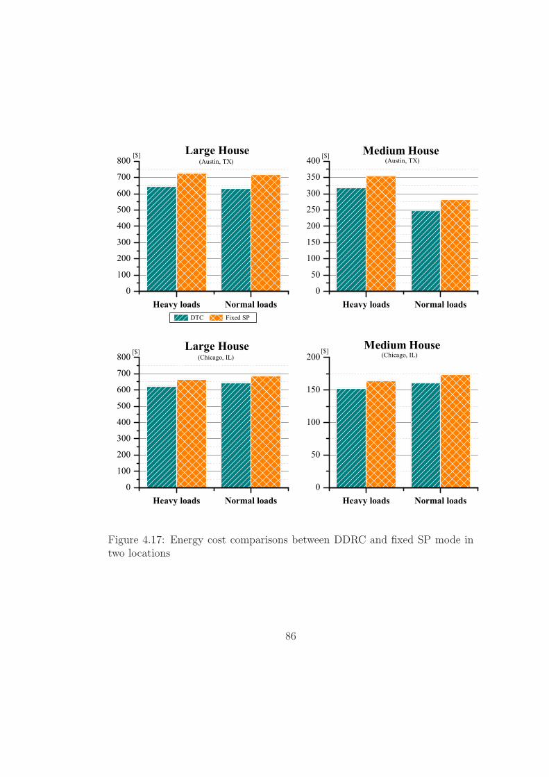
Heavy loads Normal loads0

100

200

300

400

500

600

700

800

DTC Fixed SP

Large House[$](Austin, TX)


50

100

150

200

250

300

350

400Medium House

(Austin, TX)[$]


100

200

300

400

500

600

700

800 (Chicago, IL)Large House[$]


50

100

150

200Medium House

(Chicago, IL)[$]

Figure 4.17: Energy cost comparisons between DDRC and fixed SP mode intwo locations

86

The proposed Dynamic Demand Response Controller (DDRC) provides

economic benefits to customers in Chicago even if the energy price in PJM is

lower than in ERCOT market. If utilities provide the incentive program to

their customers who want to take DR programs, the energy cost savings in

Chicago will be close to Austin. For Austin, high cost savings with DDRC

accrue to residents who live in a large or medium house no matter of internal

load size.

4.3.4 The Thermal Comfort

Thermal comfort is important for the indoor environment. If the indoor

temperature is over or under the desired temperature for a long time, people

feel discomfort. But other researches [72, 79, 80] do not reflect it on the

control methods. To minimize the thermal discomfort, the Dynamic Demand

Response Controller (DDRC) considers thermal comfort based on ASHRAE

Standard 55 [39]. The high change of the set-point temperature by high price of

electricity causes severe thermal discomfort. This may increase the resistance

of households to participation in DR programs. In this research, the preset

set-point temperature for cooling is 25°C and the heating temperature is set to

21°C. So, we assume that residents feel comfort when the indoor temperature

maintains a preset temperature (25°C) or below during AC mode. Opposite

to AC mode, the indoor temperature in heating mode remains the preset

temperature (21°C) or higher. DDRC increases or decreases the set-point

temperature when DR signal is enabled by 1°C step. Figure 4.18 shows the

87

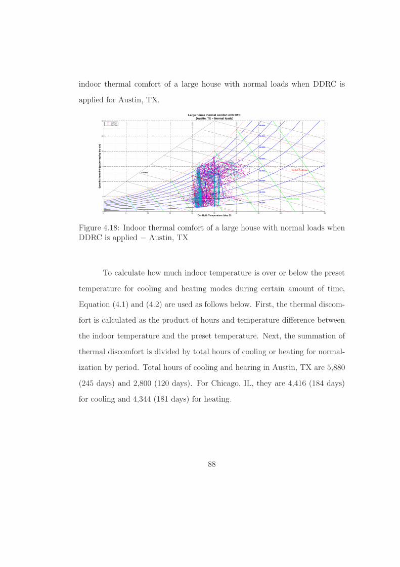
indoor thermal comfort of a large house with normal loads when DDRC is

applied for Austin, TX.

0 5 10 15 20 25 30 35 40 45 500

5

10

15

20

25

30

Dry Bulb Temperature (deg C)

Spe

cific

Hum

idity

(gr

am v

ap/k

g dr

y ai

r)

Large house thermal comfort with DTC[Austin, TX − Normal loads]

RH 10%

RH 20%

RH 30%

RH 40%

RH 50%

RH 60%

RH 70%

RH 80%

Wet Bulb Temperature

Specific Volume

Enthalpy

1st Floor2nd Floor

Figure 4.18: Indoor thermal comfort of a large house with normal loads whenDDRC is applied − Austin, TX

To calculate how much indoor temperature is over or below the preset

temperature for cooling and heating modes during certain amount of time,

Equation (4.1) and (4.2) are used as follows below. First, the thermal discom-

fort is calculated as the product of hours and temperature difference between

the indoor temperature and the preset temperature. Next, the summation of

thermal discomfort is divided by total hours of cooling or heating for normal-

ization by period. Total hours of cooling and hearing in Austin, TX are 5,880

(245 days) and 2,800 (120 days). For Chicago, IL, they are 4,416 (184 days)

for cooling and 4,344 (181 days) for heating.

88

Tdiscomfort =

Σ [(Tin − T coolsp )× hrdiscomfort]

Σ hrcoolingfor Tin > T cool

sp (4.1)

Σ [(T heatsp − Tin)× hrdiscomfort]

Σ hrheatingfor Tin < T heat

sp (4.2)

Table 4.3 explains how much DDRC causes thermal discomfort when

it changes the set-point temperature. For all cases, the indoor environment

does not exceed more than 1 C°from the preset temperature where customers

feel comfort. In results, DDRC minimizes the thermal discomfort even if the

set-point temperature is reset because of high electricity price. Furthermore,

different environments such as cold/hot weather and different internal load

sizes do not significantly impact on thermal comfort when DDRC controls

HVAC systems.

89

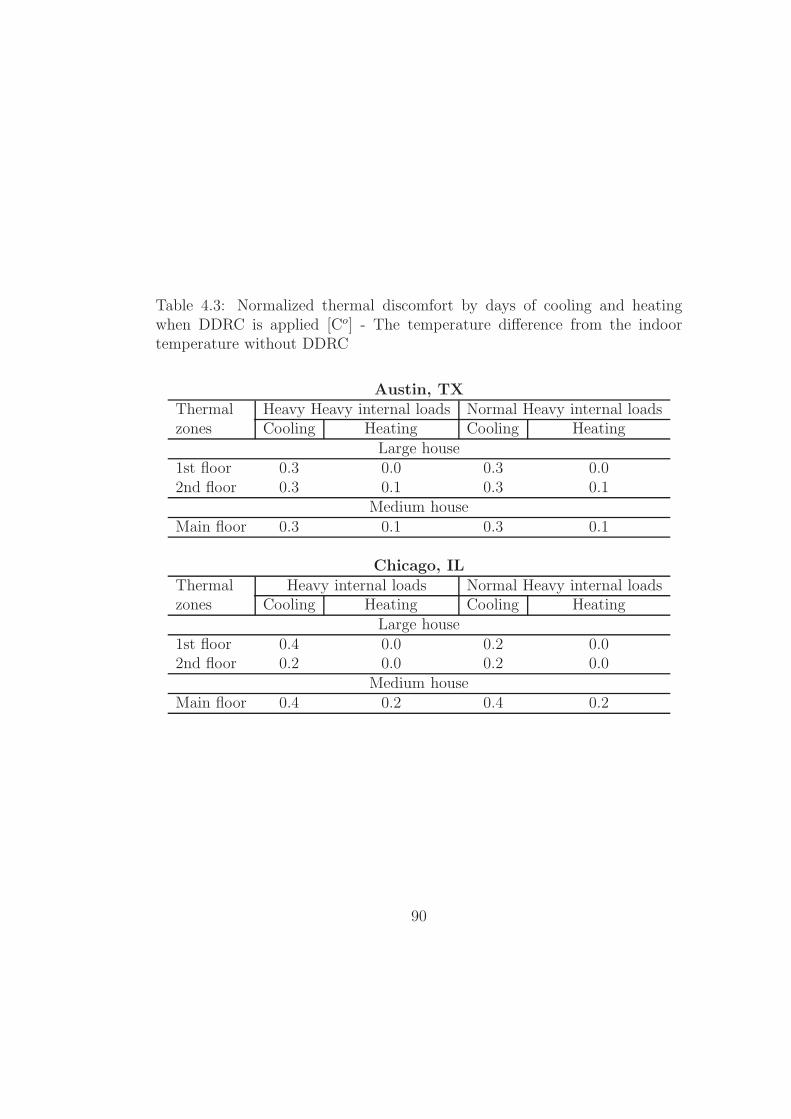
Table 4.3: Normalized thermal discomfort by days of cooling and heatingwhen DDRC is applied [Co] - The temperature difference from the indoortemperature without DDRC

Austin, TXThermal Heavy Heavy internal loads Normal Heavy internal loadszones Cooling Heating Cooling Heating

Large house1st floor 0.3 0.0 0.3 0.02nd floor 0.3 0.1 0.3 0.1

Medium houseMain floor 0.3 0.1 0.3 0.1

Chicago, ILThermal Heavy internal loads Normal Heavy internal loadszones Cooling Heating Cooling Heating

Large house1st floor 0.4 0.0 0.2 0.02nd floor 0.2 0.0 0.2 0.0

Medium houseMain floor 0.4 0.2 0.4 0.2

90

4.4 Summary

4.4.1 DDRC with dynamic price of electricity

Electricity retail price based Dynamic Demand Response Controller

(DDRC) shows that heating and cooling electricity consumption on both the

coldest month, January and the hottest month, August are considerably re-

duced by about 12% and 21% each. The electricity cost to operate for both the

coldest and hottest months are curtailed by about 29% and 31% each. In an-

nual cost savings, DDRC provides 14% electricity cost reduction to customers

with real-time retail pricing tariff. Moreover, DDRC can contribute to save

annual electricity consumption up to 9%. In respect of comfort level, indoor

air temperatures are between 22 and 24 degrees Celsius with fixed thermostat

control. The percentage of temperature which is out of thermostat dead-band

for cooling mode is 24.4% and for heating mode is 4.9%. The percentage of

time when there is more than 2 Celsius degree deviation from the temperature

dead-band is 0.3%. DDRC robustly demonstrates that HVAC loads are cur-

tailed during peak and electricity cost savings are provided to customers on

real-time tariffs. The electricity saving of AC using a thermostat controller in

[18] is 15.23% to 17.33% and cost savings are 15.54% to 34.79% for summer.

The temperature differences by the controller are about 4Co (from 23.9 to

26.1°C).

91

4.4.2 DDRC with various price types and floor plans

This case demonstrates that our proposed Dynamic Demand Response

Controller (DDRC) contributes to reduce peak loads and to saving both annual

electricity and costs. Furthermore, it minimizes thermal discomfort for houses

with different sizes and floor plans. Our DDRC brings significant peak load

curtailment of 12.8% to 24.7%. Annual electricity HVAC use is decreased by

4.3% for a large house and 4.0% for a medium house. In addition, our controller

provides advantage to customers in respect of cost savings. Customers can save

from 7.7% to 10.8% of their annual electricity bill depending on price types.

The weather condition from July 2012 to June 2013 is more moderate than

year 2011 which was the hottest year in Austin, TX. So, the electricity price at

Electric Reliability Council Of Texas (ERCOT) market at this period was lower

than in 2011. As a result, the annual electricity savings are little lower than

our previous study [16] that used 2011’s ERCOT wholesale price data. The

proposed DDRC thermostat can save a significant amount of electricity when

the price of electricity is high. The indoor air temperature mostly stays within

inside the thermal comfort zone. For 10 % of total hours of a year in average

becomes 2 C°above the AC set-point temperature. Thus, our controller avoids

significant thermal discomfort while the set-point temperature is changed due

to high price of electricity.

92

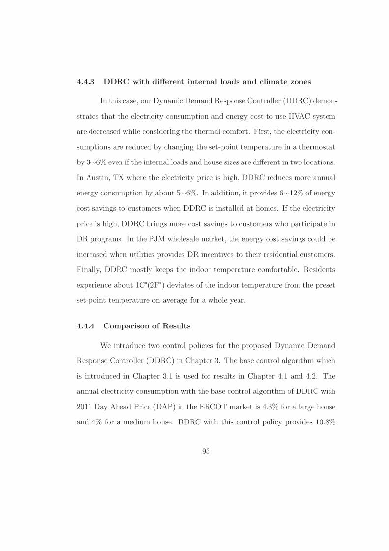
4.4.3 DDRC with different internal loads and climate zones

In this case, our Dynamic Demand Response Controller (DDRC) demon-

strates that the electricity consumption and energy cost to use HVAC system

are decreased while considering the thermal comfort. First, the electricity con-

sumptions are reduced by changing the set-point temperature in a thermostat

by 3∼6% even if the internal loads and house sizes are different in two locations.

In Austin, TX where the electricity price is high, DDRC reduces more annual

energy consumption by about 5∼6%. In addition, it provides 6∼12% of energy

cost savings to customers when DDRC is installed at homes. If the electricity

price is high, DDRC brings more cost savings to customers who participate in

DR programs. In the PJM wholesale market, the energy cost savings could be

increased when utilities provides DR incentives to their residential customers.

Finally, DDRC mostly keeps the indoor temperature comfortable. Residents

experience about 1C°(2F°) deviates of the indoor temperature from the preset

set-point temperature on average for a whole year.

4.4.4 Comparison of Results

We introduce two control policies for the proposed Dynamic Demand

Response Controller (DDRC) in Chapter 3. The base control algorithm which

is introduced in Chapter 3.1 is used for results in Chapter 4.1 and 4.2. The

annual electricity consumption with the base control algorithm of DDRC with

2011 Day Ahead Price (DAP) in the ERCOT market is 4.3% for a large house

and 4% for a medium house. DDRC with this control policy provides 10.8%

93

of cost savings for a large house and 10.5% for a medium house. However,

the base control policy is limited to Austin, TX because it requires historical

price and weather data to calculate the linear regression coefficient (a, Eq 3.7

and 3.8) which converts to temperature. So, the DDRC would require adapta-

tion to use in another location. However, the improved DDRC control policy

does not have the linear regression coefficient, which removes the limitation

of home locations. So, the DDRC can be deployed in various climate zone

and wholesale electricity market. The improve control algorithm gives 6% of

annual electricity savings for a large house with 2011 DAP in the ERCOT

market and 6.2% for a medium house. The energy cost with the improved

DDRC are reduced by 12% for both large and medium houses. The DDRC

with improved control policy has high performance compared with the DDRC

with the base algorithm. There are improvements in both annual energy cost

and electricity savings by the improved control policy. Table 4.4 presents the

comparison of the DDRC performance between the base and improved control

algorithms. The improved DDRC can reduce the HVAC electricity consump-

tion and increase the annual energy cost savings more than the DDRC with

base control algorithm.

94

Table 4.4: The improvement of DDRC performance by enhanced control policy

Control Base DDRC Improved DDRC ImprovementType [%] [%] [%]

Annual Electricity SavingsLarge house 4.3 6.0 39.5Medium house 4.0 6.2 55

Annual Energy Cost SavingsLarge house 10.8 12.0 11.1Medium house 10.5 11.9 13.3

95

Chapter 5

Development of Hardware for Dynamic

Demand Response Controller

This chapter shows the development of the proposed Dynamic Demand

Response Controller based on embedded controller including sensing environ-

ment and wireless communication capability.

5.1 Arduino Due embedded controller

Embedded micro-controllers are widely used in industries. In this re-

search, we used high performance embedded controller to build the Dynamic

Demand Response Controller (DDRC) based on the Arduino board. Arduino1

is an open-source electronics platform based on easy-to-use hardware and soft-

ware. The compiler, Arduino IDE, is provided for free to build embedded codes

based on C++ language. In hardwares, Arduino has various products with

different CPUs. Two major CPUs are used in Arduino boards; AVR and ARM

CPUs. Most Arduino boards use Atmel2 AVR 8 bit micro-controller. But, Ar-

duino Due board is 32 bit micro-controller based on Advanced RISC Machines

1http://arduino.cc2http://www.atmel.com

96

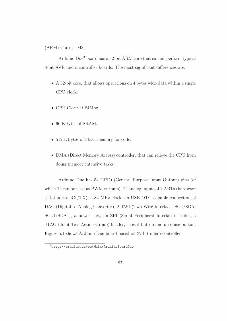
(ARM) Cortex−M3.

Arduino Due3 board has a 32-bit ARM core that can outperform typical

8-bit AVR micro-controller boards. The most significant differences are:

• A 32-bit core, that allows operations on 4 bytes wide data within a single

CPU clock.

• CPU Clock at 84Mhz.

• 96 KBytes of SRAM.

• 512 KBytes of Flash memory for code.

• DMA (Direct Memory Access) controller, that can relieve the CPU from

doing memory intensive tasks.

Arduino Due has 54 GPIO (General Purpose Input Output) pins (of

which 12 can be used as PWM outputs), 12 analog inputs, 4 UARTs (hardware

serial ports: RX/TX), a 84 MHz clock, an USB OTG capable connection, 2

DAC (Digital to Analog Converter), 2 TWI (Two Wire Interface: SCL/SDA,

SCL1/SDA1), a power jack, an SPI (Serial Peripheral Interface) header, a

JTAG (Joint Test Action Group) header, a reset button and an erase button.

Figure 5.1 shows Arduino Due board based on 32 bit micro-controller

3http://arduino.cc/en/Main/ArduinoBoardDue

97

Figure 5.1: 32bit ARM CPU based Arduino Due Board

DDRC has 7 inch resistive touch TFT (Thin Film Transistor) LCD

screen to visualize graphic interface for easy control. SPI port is allocated for

TFT LCD. Real-Time clock and temperature/humidity sensor use TWI pins

to transfer data to Arudino Due. To improve response time of DDRC, another

Arduino Due board for WiFi communication to receive demand response sig-

nal (price data) is used. The two Arduino Due boards communicate with

each other using UART (Universal Asynchronous Receiver/Transmitter) port.

Voltage level to transmit and receive is set to 3.3V from power supply with

common ground. To measure outdoor environment, 8 bit AVR based Arduino

Uno is used with 433 Mhz wireless communication for weather station.

98

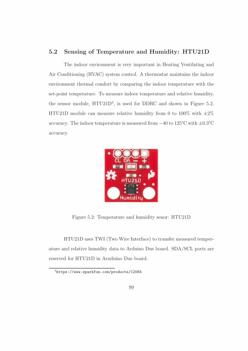
5.2 Sensing of Temperature and Humidity: HTU21D

The indoor environment is very important in Heating Ventilating and

Air Conditioning (HVAC) system control. A thermostat maintains the indoor

environment thermal comfort by comparing the indoor temperature with the

set-point temperature. To measure indoor temperature and relative humidity,

the sensor module, HTU21D4, is used for DDRC and shown in Figure 5.2.

HTU21D module can measure relative humidity from 0 to 100% with ±2%

accuracy. The indoor temperature is measured from −40 to 125°C with ±0.3°C

accuracy.

Figure 5.2: Temperature and humidity senor: HTU21D

HTU21D uses TWI (Two Wire Interface) to transfer measured temper-

ature and relative humidity data to Arduino Due board. SDA/SCL ports are

reserved for HTU21D in Aruduino Due board.

4https://www.sparkfun.com/products/12064

99

5.3 Wireless Ethernet Connection

In Demand Response, the price signal reflects the status of power grids.

When the price of electricity is high, the power grid is stressed due to peak

loads. Ethernet connection is required to get the electricity price from Electric

Reliability Council of Texas (ERCOT) website. Day Ahead wholesale price

of electricity is parsed to get the price data. Ardunio provides WiFi shield

to connect Internet via wireless technology. In our research, Arduino WiFi

Shield5 is used and supports IEEE 802.11b/g networks up to 54 Mbit/s (or

6.75 MByte/s) speed. Figure 5.3 presents Arduino WiFi shield.

Figure 5.3: WiFi board for Arudino Due micro-controller board

Arduino Due has one SPI (Serial Peripheral Interface) on the board.

5http://arduino.cc/en/Main/ArduinoWiFiShield, additional accessory boards such

as WiFi, Ethernet, and GPS are called to shield.

100

TFT LCD with touch screen uses SPI port to display information and buttons.

So, SPI port must be shared by both TFT LCD and WiFi Shield. Once

instruction by WiFi shield on queue, TFT LCD cannot use SPI port until

WiFi Shield finishes a job. Therefore, the response time to operate functions

such as changing set-point temperature and threshold price is going to be

slow. To solve slow response time, two separate Arduino Due boards are used

to improve the performance of DDRC.

101

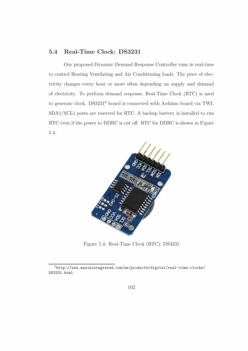
5.4 Real-Time Clock: DS3231

Our proposed Dynamic Demand Response Controller runs in real-time

to control Heating Ventilating and Air Conditioning loads. The price of elec-

tricity changes every hour or more often depending on supply and demand

of electricity. To perform demand response, Real-Time Clock (RTC) is used

to generate clock. DS32316 board is connected with Arduino board via TWI.

SDA1/SCL1 ports are reserved for RTC. A backup battery is installed to run

RTC even if the power to DDRC is cut off. RTC for DDRC is shown in Figure

5.4.

Figure 5.4: Real-Time Clock (RTC): DS3231

6http://www.maximintegrated.com/en/products/digital/real-time-clocks/

DS3231.html

102

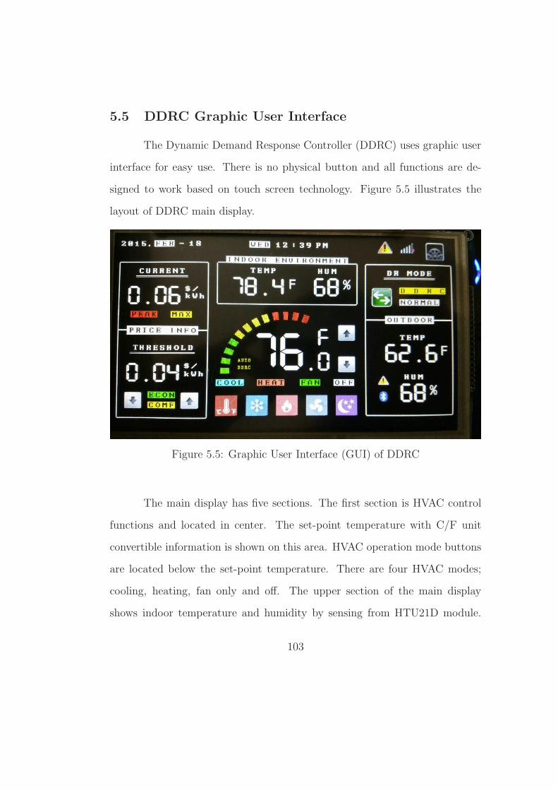
5.5 DDRC Graphic User Interface

The Dynamic Demand Response Controller (DDRC) uses graphic user

interface for easy use. There is no physical button and all functions are de-

signed to work based on touch screen technology. Figure 5.5 illustrates the

layout of DDRC main display.

Figure 5.5: Graphic User Interface (GUI) of DDRC

The main display has five sections. The first section is HVAC control

functions and located in center. The set-point temperature with C/F unit

convertible information is shown on this area. HVAC operation mode buttons

are located below the set-point temperature. There are four HVAC modes;

cooling, heating, fan only and off. The upper section of the main display

shows indoor temperature and humidity by sensing from HTU21D module.

103

Next, the right side illustrate outdoor temperature and humidity from the

weather station. Consumers can set DDRC mode when they want to partici-

pate in demand response programs. DDRC is automatically turned on when

the threshold price is below the current price of electricity. The normal mode

works as a conventional thermostat where the indoor temperature is main-

tained at the set-point temperature independent of the electricity price. The

default mode is DDRC.

The left side of the main display of DDRC presents the current price of

electricity and threshold price. Consumers can change threshold price depend-

ing on their preferences. The default value of threshold price is $0.04/kWh.

The top line shows the current time and status of WiFi. The setup menu to

change the current time and WiFi connection is located on right top corner

by clicking a setup icon.

5.6 Assembling modules with Arduino boards

Dynamic Demand Response Controller (DDRC) has several modules

to control HVAC system such as a heat pump. The main controller is Ar-

duino Due and visualizes price and environment data on the screen. Demand

response control algorithm is also implemented in the main controller. The

auxiliary controller is added to receive price data from Electric Reliability

Council of Texas (ERCOT) site. The two controllers communicate each other

via UART (RX2/TX2 port are allocated).

A power board is installed to supply 15W power for all modules includ-

104

ing Arduino boards, sensor, RTC, and relay. 12V input power is supplied to

DDRC from wall charger. Arduino boards have been limited to supply up to

5V, 1A. So, WiFi module cannot be combined with 7 inch TFT LCD screen

due to lack of power. In addition, three circuit relays to control a heat pump

consume more than 150mA to trigger relay. Since DDRC requires more than

5V with 1A, power board is added and supplies 5V, 2A and 3.3V, 1A to all

modules

Generally, a heat pump control circuit uses 24V AC system. In other

words, Arduino Due board can supply digital signal with 3.3V, 20mA from

General Purpose Input Output (GPIO) pins. Three circuits of relays are

needed to trigger air conditioner, heater and fan. Each Relay requires high

current more than 50mA so that the booster circuit to control from Arudino

GPIO pins is designed.

Temperature sensor and real-time clock are installed with the main

control board. Radio wireless (433Mhz) module is connected with auxiliary

board to receive outdoor weather data from weather station.

105

Chapter 6

Conclusion

This dissertation describes the methodology to reduce peak loads when

the power grid is stressed because of heavy electricity demand. Our research

designed the control algorithm of the Dynamic Demand Response Controller

(DDRC) and evaluated its performance using a building energy simulation

tool. Based on dynamic price of electricity at wholesale electricity markets

including Electric Reliability Council of Texas (ERCOT) and PJM Intercon-

nection, demand response signal is generated to reduce the power grid stress.

The controller reduces Heating Ventilating and Air Conditioning (HVAC)

loads by demand response. The set-point temperature in DDRC changes by

comparing the current electricity price with a threshold price for demand re-

sponse. Electricity loads during peak period are curtailed, reducing the annual

electricity consumption. In respect of energy cost, DDRC brings energy cost

savings with dynamic price tariffs in different locations. In addition, we eval-

uate the indoor thermal comfort based on ASHRAE standard 55 when DDRC

changes the set-point temperature during peak time.

In chapter 1, we introduced the background of electricity consumption

in residential buildings and general type of HVAC systems for homes. In this

106

chapter, we presented the scope and objective of our research. The proposed

Dynamic Demand Response Controller can contribute to decrease electricity

loads during peak period in order to increase the power grid efficiency as well

as to decrease the stress of the power grid due to heavy demand.

In chapter 2, we presented the modeling of two different size of single

family homes using a building energy modeling tools. Based on architectural

blueprint, house models are designed using EnergyPlus and OpenStudio. The

attributes of building envelopes such as insulation, windows, and basement

used International Energy Conservation Code (IECC) 2009 for Climate Zone

2 (Austin, TX) and Climate Zone 5&4 marine (Chicago, IL). The dynamic

retail prices of electricity were generated based on the historical wholesale

price of electricity in the Electric Reliability Council of Texas (ERCOT) and

Pennsylvania, New Jersey, and Maryland (PJM) Interconnection markets. The

two different wholesale electricity prices are used to design dynamic retail

prices; Day Ahead Price (DAP) and Real-Time Price (RTP).

In chapter 3, we suggested the control policies of the Dynamic Demand

Response Controller (DDRC). The DDRC changed the set-point temperature

by comparing the current price of electricity price with a threshold price. Two

different control algorithms were introduced; the base and improved DDRC

control algorithm. The base control policy considered the indoor environ-

ment and thermal comfort when the set-point temperature is changed during

peak periods. However, it required the linear regression coefficient to convert

price/HVAC load to temperature. This coefficient was calculated based on the

107

historical price and weather data in Austin, TX. Therefore, the DDRC with

the base control policy is limited to install at homes in Austin, TX. On the

other hand, the improved DDRC was designed to deploy in various location

and wholesale markets without the limitation. Detailed building information

such as the capacity and efficiency of heat pump were considered to change

the set-point temperature.

In chapter 4, we illustrated the performance of the Dynamic Demand

Response Controller (DDRC). The DDRC with the base control algorithm

significantly reduced the peak load by 31% during hot summer. Annual elec-

tricity consumption reduction is by 9% and cost savings is 14% with real-time

price (RTP) of electricity based tariff. The DDRC provided the energy cost

savings up to 10.8% and 4.3% of annual electricity consumption under both

RTP and DAP. In addition, the DDRC with improved control policy provided

up to 10.8% of energy cost savings with dynamic pricing in two different lo-

cations and markets while avoiding significant discomfort due to temperature

change. Also, the results present potential for saving considering peak load

by 24.7% and total electrical energy saving for HVAC in homes by 4.3% an-

nually. Comparing the base and improved control algorithm, the improved

DDRC provided better performance than the DDRC with the base control

policy. Regarding annual electricity consumption, the consumption was de-

creased by 39.5∼55% of more than the base algorithm. The improved DDRC

saved 11.1∼13.3% more energy costs.

In chapter 5, we developed the hardware for the Dynamic Demand

108

Response Controller (DDRC) based on an implemented controller. The control

algorithm of DDRC is implemented with an 32 bit ARM micro-controller.

DDRC measures indoor and outdoor temperature and relative humidity. In

addition, it has the capability to connect to the Internet for getting price

data through ERCOT price information site. DDRC can work with general

heat pump equipment by relay control. Demand response function is enabled

automatically when the current price of electricity is higher than the threshold

price.

With regard to future work, we offer the following comments.

• DDRC is developed based on an embedded controller. Generally, a hard-

ware is tested before the deployment using Hardware In the Loop (HIL)

technology. The target residential house is modeled using building energy

simulation tool, EnergyPlus. DDRC connects a target model to control

Heating, Ventilating, and Air Conditioning (HVAC) system via Ethernet

socket exchange. Using HIL test method,the hardware of DDRC will be

estimate its performance before it is installed in a real house.

• The proposed DDRC will be installed in UTest house1. The UTest house

is a fully instrumented 1,300ft2 size manufactured home which is used for

education and research in indoor environmental science and engineering.

The house has seven building rooms/zones and two heating ventilation

1http://www.caee.utexas.edu/prof/Novoselac/atila_files/Laboratories.html#

UTestHouse

109

and air-conditioning (HVAC) systems; the first one with ceiling and the

second with floor air distribution system. Even though there are several

similar test houses in the U.S., none of them is equipped to perform such

detailed monitoring of indoor air quality and energy performance. Our

DDRC hardware will be evaluate the performance of demand response

during summer season when air conditioning loads are heavy due to hot

weather.

• The retail shops and small office buildings are also contributors to cause

peak loads during summer season due to heavy air conditioner uses.

These buildings have similar HVAC system to residential buildings. Mul-

tiple heat pumps are used for cooling and heating. Therefore, DDRC is

easily retrofitted with their HVAC system for having demand response

capability. We will study energy consumption and behaviors of small

retails and office building to estimate the performance of the proposed

DDRC is not limited to residential buildings.

110

Appendices

111

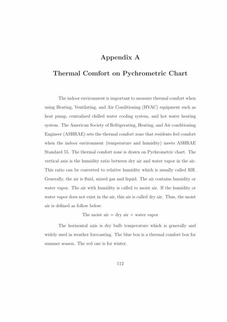
Appendix A

Thermal Comfort on Pychrometric Chart

The indoor environment is important to measure thermal comfort when

using Heating, Ventilating, and Air Conditioning (HVAC) equipment such as

heat pump, centralized chilled water cooling system, and hot water heating

system. The American Society of Refrigerating, Heating, and Air conditioning

Engineer (ASHRAE) sets the thermal comfort zone that residents feel comfort

when the indoor environment (temperature and humidity) meets ASHRAE

Standard 55. The thermal comfort zone is drawn on Pychrometric chart. The

vertical axis is the humidity ratio between dry air and water vapor in the air.

This ratio can be converted to relative humidity which is usually called RH.

Generally, the air is fluid, mixed gas and liquid. The air contains humidity or

water vapor. The air with humidity is called to moist air. If the humidity or

water vapor does not exist in the air, this air is called dry air. Thus, the moist

air is defined as follow below:

The moist air = dry air + water vapor

The horizontal axis is dry bulb temperature which is generally and

widely used in weather forecasting. The blue box is a thermal comfort box for

summer season. The red one is for winter.

112

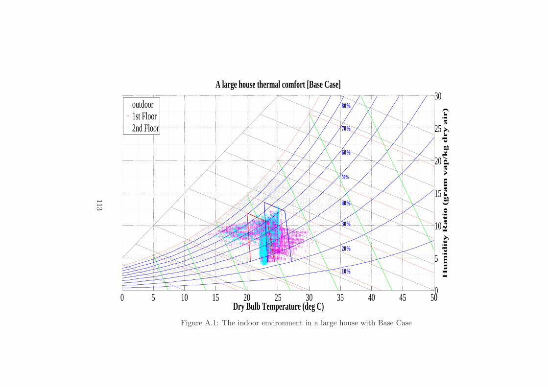
0 5 10 15 20 25 30 35 40 45 500

5

10

15

20

25

30


Hu

mid

ity R

ati

o (

gram

vap

/kg d

ry a

ir)

A large house thermal comfort [Base Case]

10%

20%

30%

40%

50%

60%

70%

80%outdoor1st Floor2nd Floor

Figure A.1: The indoor environment in a large house with Base Case

113

0 5 10 15 20 25 30 35 40 45 500

5

10

15

20

25

30


Hu

mid

ity R

ati

o (

gram

vap

/kg d

ry a

ir)

A large house thermal comfort [Case 1]

10%

20%

30%

40%

50%

60%

70%


Figure A.2: The indoor environment in a large house with Case 1: Real-Time Price

114

0 5 10 15 20 25 30 35 40 45 500

5

10

15

20

25

30


Hu

mid

ity R

ati

o (

gram

vap

/kg d

ry a

ir)

A large house thermal comfort [Case 2]

10%

20%

30%

40%

50%

60%

70%


Figure A.3: The indoor environment in a large house with Case 2: Day Ahead Price

115

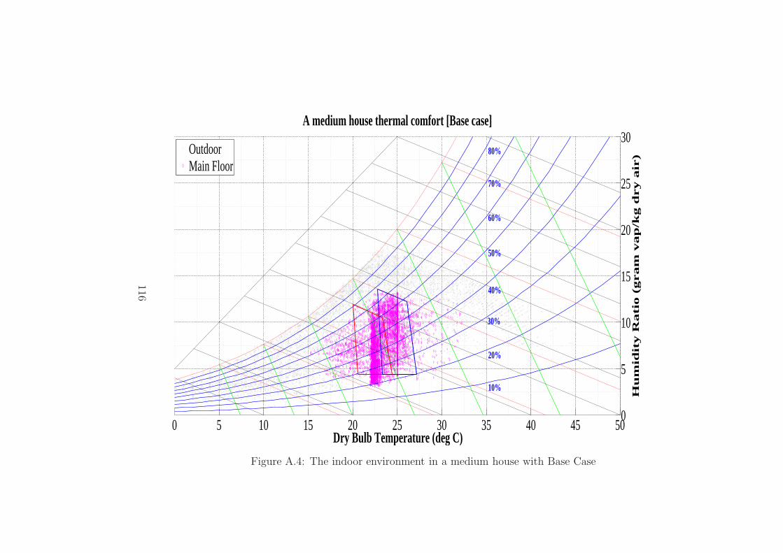
0 5 10 15 20 25 30 35 40 45 500

5

10

15

20

25

30


Hu

mid

ity R

ati

o (

gram

vap

/kg d

ry a

ir)

A medium house thermal comfort [Base case]

10%

20%

30%

40%

50%

60%

70%

80%OutdoorMain Floor

Figure A.4: The indoor environment in a medium house with Base Case

116

0 5 10 15 20 25 30 35 40 45 500

5

10

15

20

25

30


Hu

mid

ity R

ati

o (

gram

vap

/kg d

ry a

ir)

A medium house thermal comfort [Case 1]

10%

20%

30%

40%

50%

60%

70%


Figure A.5: The indoor environment in a medium house with Case 1: Real-Time Price

117

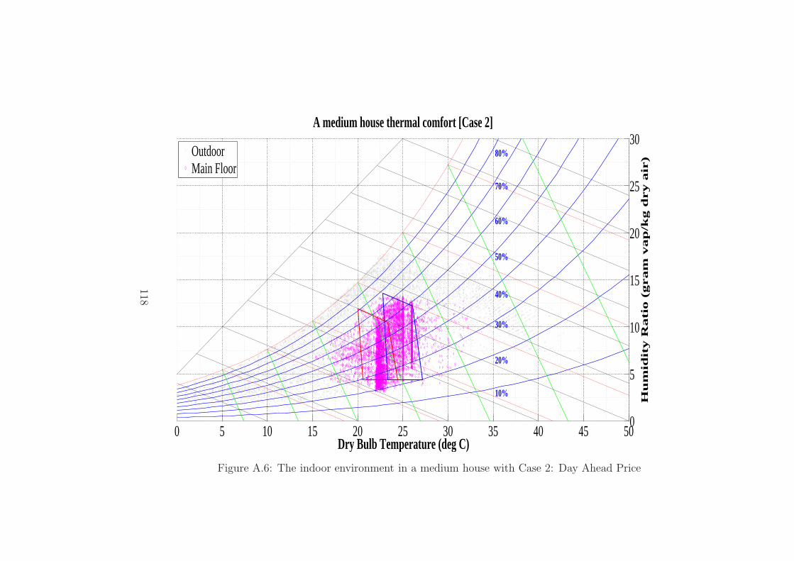
0 5 10 15 20 25 30 35 40 45 500

5

10

15

20

25

30


Hu

mid

ity R

ati

o (

gram

vap

/kg d

ry a

ir)

A medium house thermal comfort [Case 2]

10%

20%

30%

40%

50%

60%

70%


Figure A.6: The indoor environment in a medium house with Case 2: Day Ahead Price

118

Appendix B

Battery Backup System for residential

buildings

The battery backup systems are widely used with Photovoltaic (PV)

power generation system as the renewable energy source for residential build-

ings. PV system consists of three parts; PV panel, inverter, and backup bat-

tery. The solar inverter generally has the function to control of batteries with

low costs. In this appendix , we suggest the battery backup system using

AGM batteries with a solar inverter for DDRC.

B.1 The Layout of Battery Backup System

DDRC controls the battery backup system depending on the dynamic

price of electricity. When peak load is occurred, DDRC sets the battery mode

to discharge for supplying power to residential building. The batteries are

charged during the night time when the electricity price is low. The battery

backup system is not connected with utility’s grid. So, the electrical power

from batteries is consumed at residential buildings. In order to reduce the

initial investment cost, the capacity of batteries is designed to supply the

power during peak hours only. Figure B.1 shows the layout of the battery

119

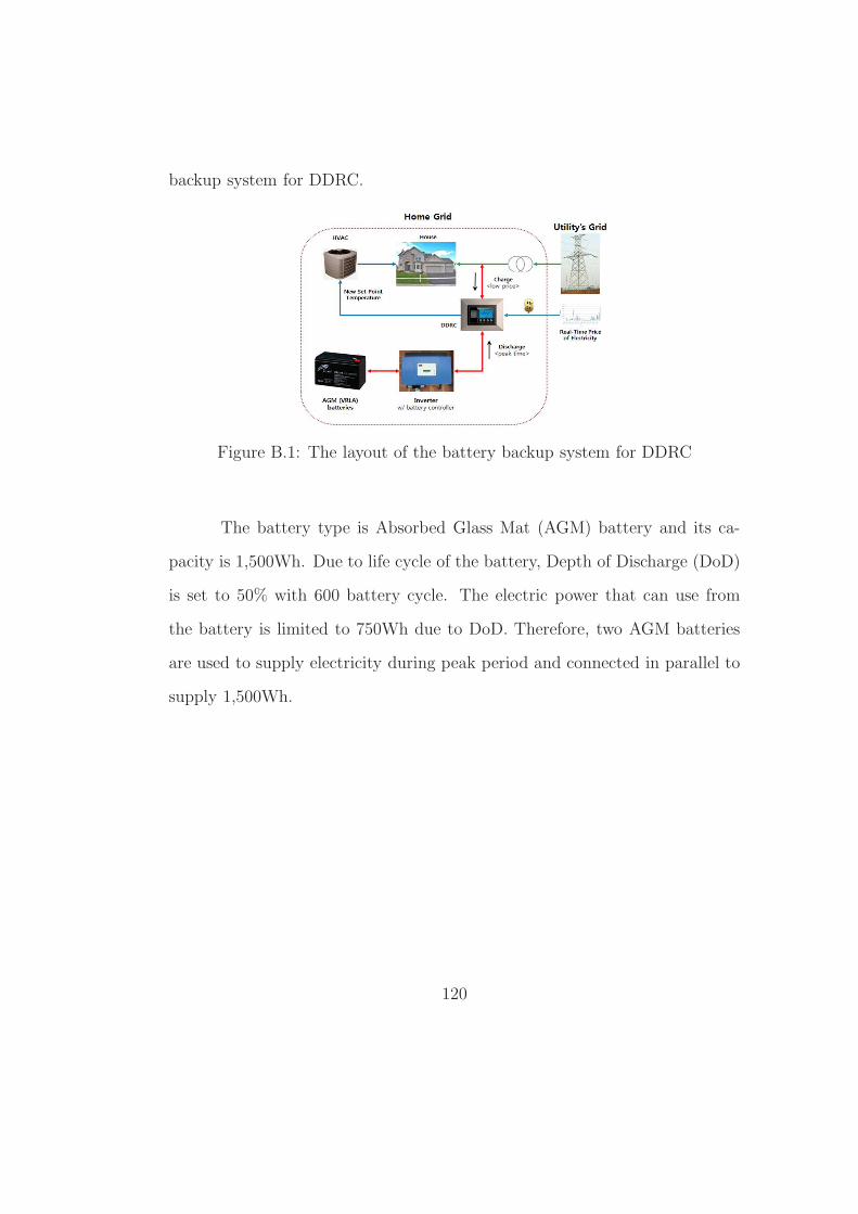
backup system for DDRC.

Figure B.1: The layout of the battery backup system for DDRC

The battery type is Absorbed Glass Mat (AGM) battery and its ca-

pacity is 1,500Wh. Due to life cycle of the battery, Depth of Discharge (DoD)

is set to 50% with 600 battery cycle. The electric power that can use from

the battery is limited to 750Wh due to DoD. Therefore, two AGM batteries

are used to supply electricity during peak period and connected in parallel to

supply 1,500Wh.

120

Figure B.2: Absorbed Glass Mat (AGM) battery

121

The solar inverter that has the battery charge and discharge function

are chosen. To charge batteries with total 1,500Wh capacity, the inverter

output is 1,500W. The inverter supplies the electric power to distribution

circuit at a residential building. So, the stored electricity in batteries are

not sent to power grid during off-peak. This electric power is reserved for

peak time.

Figure B.3: The inverter with the battery charge and discharge function

B.2 Economics on the Battery System

The battery system for DDRC is designed low cost system to assistant

the performance of DDRC. The initial investment and battery replacement

for maintenance are very important for end users. The solar inverter under

2,000Wh capacity is under $1,000 nowadays [90]. The unit cost of AGM

battery with 1,5000Wh is about $285 [91]. We assume that the batteries

discharges with 150 cycle at 50% of DoD. Two batteries are needed to replace

every 4 years. The life span of an inverter is generally 16 years. During the life

122

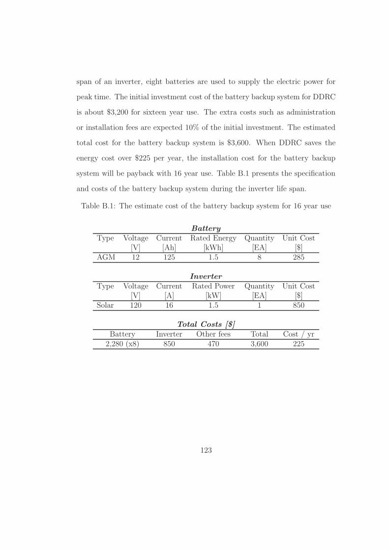
span of an inverter, eight batteries are used to supply the electric power for

peak time. The initial investment cost of the battery backup system for DDRC

is about $3,200 for sixteen year use. The extra costs such as administration

or installation fees are expected 10% of the initial investment. The estimated

total cost for the battery backup system is $3,600. When DDRC saves the

energy cost over $225 per year, the installation cost for the battery backup

system will be payback with 16 year use. Table B.1 presents the specification

and costs of the battery backup system during the inverter life span.

Table B.1: The estimate cost of the battery backup system for 16 year use

BatteryType Voltage Current Rated Energy Quantity Unit Cost

[V] [Ah] [kWh] [EA] [$]AGM 12 125 1.5 8 285

InverterType Voltage Current Rated Power Quantity Unit Cost

[V] [A] [kW] [EA] [$]Solar 120 16 1.5 1 850

Total Costs [$]Battery Inverter Other fees Total Cost / yr

2,280 (x8) 850 470 3,600 225

123

Appendix C

Case Study: Demand Response Experiences

with Utilities

Demand response (DR) programs are served in some utilities in the

United States. Their DR programs used the electricity wholesale market price

or the generation costs to design real-time price. In this appendix, we in-

troduced the experiences of DR program from several utilities in different

locations.

C.1 Gulf Power

Gulf Power is subsidiary of Southern Company and covers Northwest

Florida. Its service territory is shown in Figure C.1.

C.1.1 DR Program - Energy Select

Energy Select is residential service with variable pricing (RSVP). It

has FOUR tiers; low (off-peak), medium (partial-peak), high (on-peak), and

critical prices (emergency). When the special event is occurred (ex. emergent

peak), the critical price is served. For the normal operation, the critical price

is NOT included on the price period. These prices are decided depending on

124

Figure C.1: Gulf Power Service Territory

the power generation cost based on day ahead. This residential tariff is time

constrained rate. During the certain point of times, the price is fixed. So,

this tariff is very similar to Time of Use (TOU) from Pacific Gas and Electric

(PG&E) but the price rate in Energy Select is changed. Figure C.2 presents

price period of RSVP for summer and winter season.

The average prices for each tiers as shown below;

<Four price tiers>

Tier 1: low price ( Off-Peak) ≈ $0.079 / kWh

Tier 2: medium price (Partial-Peak) ≈ $0.092 / kWh

Tier 3: high price (On-Peak) ≈ $0.169 / kWh

Tier 4: critical price (Emergent Event) ≈ $0.696 / kWh

The percent of hours that each tier price is provided for a year is display

in Figure 3. Most of hours (87% of total hours), the current price maintained

under $0.1/kWh. High and critical prices when DR requested were about 13%.

125

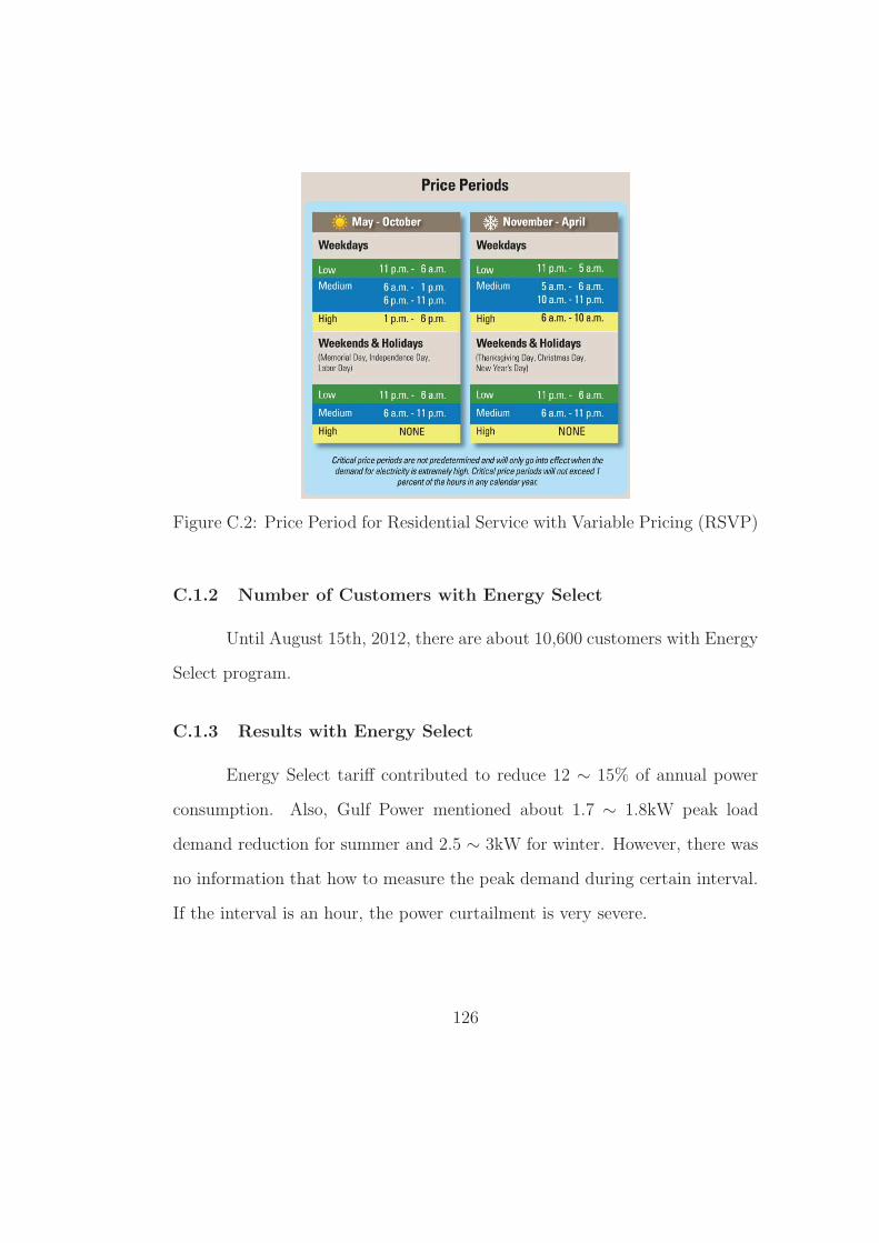
Figure C.2: Price Period for Residential Service with Variable Pricing (RSVP)

C.1.2 Number of Customers with Energy Select

Until August 15th, 2012, there are about 10,600 customers with Energy

Select program.

C.1.3 Results with Energy Select

Energy Select tariff contributed to reduce 12 ∼ 15% of annual power

consumption. Also, Gulf Power mentioned about 1.7 ∼ 1.8kW peak load

demand reduction for summer and 2.5 ∼ 3kW for winter. However, there was

no information that how to measure the peak demand during certain interval.

If the interval is an hour, the power curtailment is very severe.

126

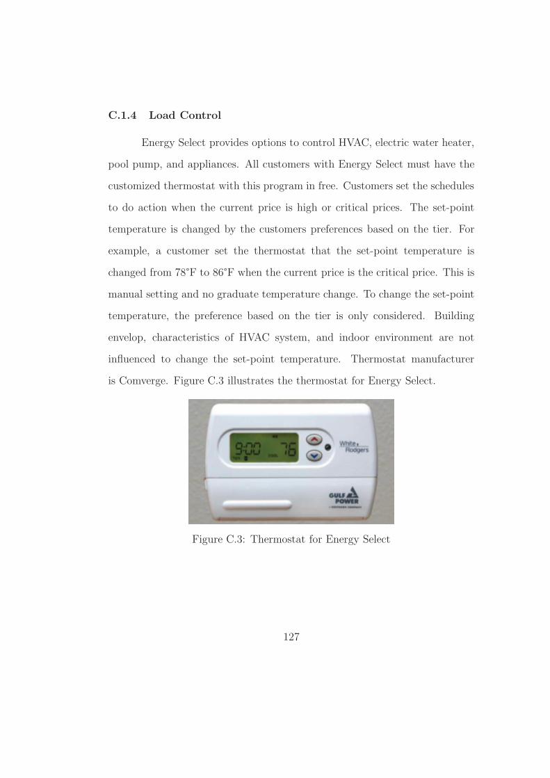
C.1.4 Load Control

Energy Select provides options to control HVAC, electric water heater,

pool pump, and appliances. All customers with Energy Select must have the

customized thermostat with this program in free. Customers set the schedules

to do action when the current price is high or critical prices. The set-point

temperature is changed by the customers preferences based on the tier. For

example, a customer set the thermostat that the set-point temperature is

changed from 78°F to 86°F when the current price is the critical price. This is

manual setting and no graduate temperature change. To change the set-point

temperature, the preference based on the tier is only considered. Building

envelop, characteristics of HVAC system, and indoor environment are not

influenced to change the set-point temperature. Thermostat manufacturer

is Comverge. Figure C.3 illustrates the thermostat for Energy Select.

Figure C.3: Thermostat for Energy Select

127

C.2 Commonwealth Edison

Commonwealth Edison is subsidiary of Exelon Corporation and cov-

ers Chicago and West Chicago Area include Naperville, Illinois. Its service

territory is shown in Figure C.4.

Figure C.4: Commonwealth Edison Service Territory in Chicago area

C.2.1 DR Program - Smart Return

Commonwealth Edison (ComEd) introduced Smart Returns program

since 1996. Smart Return has four specific programs.

(a) Voluntary Load Response (VLR)

• Nonresidential customer (C&I Commercial and Industry)

• Minimum reduction is 10kW

• $0.15/kWh incentive for load reduction

• No firm commitments and noncompliance penalties

128

(b) Early Advantage

• C&I customer

• Minimum reduction is 1MW

• Large incentive during high price or emergency events

(c) The Alliance and Energy Cooperative

• Customers who are taking service under rate 6L or 6T

• More frequent load reduction request

• Substantial incentive payment

C.2.2 Real-Time Price (RTP)

ComEd used Hourly Energy Pricing (HEP) in RTP tariff. Two pricings

are peak price and off-peak price. RTP is announced by 7 pm of the previous

day on ComEd website.

(a) Peak Price

: Used two year historical data of real-time hourly PJM West price to

generate day-ahead hourly peak price.

(b) Off-Peak Price

: Used daily transaction data of the day-ahead spot market for off-peak

prices to calculate an average of daily transaction midpoints for the preceding

month.

129

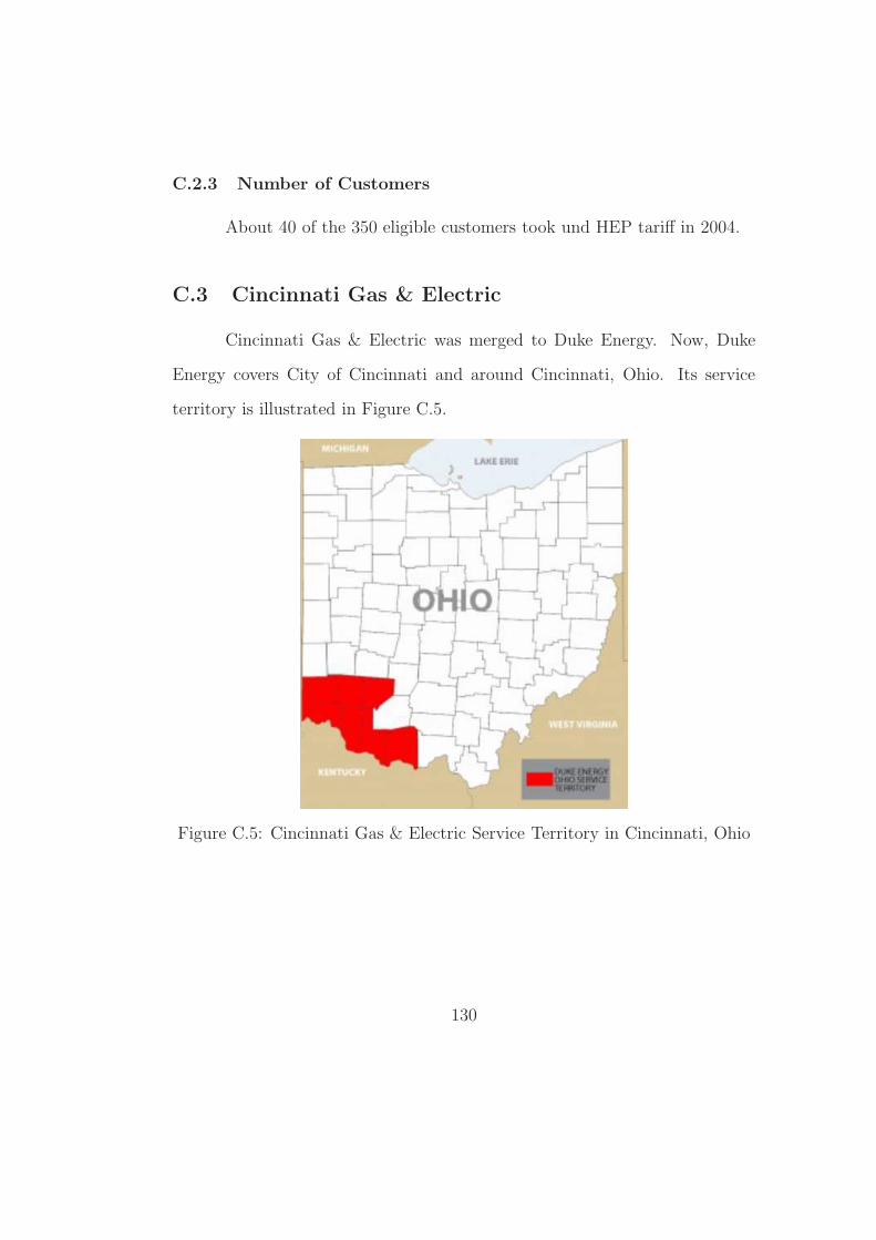
C.2.3 Number of Customers

About 40 of the 350 eligible customers took und HEP tariff in 2004.

C.3 Cincinnati Gas & Electric

Cincinnati Gas & Electric was merged to Duke Energy. Now, Duke

Energy covers City of Cincinnati and around Cincinnati, Ohio. Its service

territory is illustrated in Figure C.5.

Figure C.5: Cincinnati Gas & Electric Service Territory in Cincinnati, Ohio

130

C.3.1 DR Programs - PowerShare

Cincinnati Gas & Electric (CGE) provided voluntary RTP program

based on day-ahead price. However, Public Utility Commission (PUC) of

Ohio approved fixed price rate based on the cost of generation instead of RTP.

Therefore, CGE provided fixed rate DR programs to C&I customers.

• Voluntary program since 1996

• PowerShare: incentive based demand response

(a) Call Option

: Higher incentive payment with firm commitments and penalties for

nonperformance

(b) Quote Option

: Completely voluntary, no firm commitments and lower incentives

• PUC Ohio (PUCO) approved one-part RTP tariff

: The on-part tariff with a price floor equal the generation rates in

the fixed-prince default service. (Dispatch cost of the highest cost generation

unit/purchased power to serve CG&Es load)


About 140 customers in 2004.

131

C.4 Portland General Electric

Portland General Electric (PGE) mostly covers City of Portland, Ore-

gon. Its service territory is presented in Figure C.6.

Figure C.6: Portland General Electric Service Territory in Portland, Oregon

C.4.1 DR Programs

In 2004, Portland General Electric (PGE) provided DR programs to

non-residential customer without load demand size.

(a) Demand Buyback

: Customers pay market-based price for curtailing when called

(b) Longer-term Buybacks

: A few customers paid to reduce their electricity usage over several

months in 2001

(c) Blackout Protection

132

: Customers can avoid rotating outage by curtailing 15% of their load

when called

(d) Dispatchable Standby Generation

For residential customers, Time of Use (TOU) rates is offered. Also,

direct load controls of residential electric water heater and spacing heating

were tested.

C.4.2 Real-Time Price

Daily rate of RTP is based on the Dow Johnson Mid-C (hub) Daily on

an off peak electricity firm indenx (DJ Mid-C Firm Index) for the previous

day with the Customer Baseline Load (CBL). A CBL is derived based on each

customers historical usage.


None in 2004

C.5 Duquesne Light Company

Duquesne Light Company mostly covers City of Pittsburgh, Pennsyl-

vania. Its service territory is shown in Figure C.7.

C.5.1 DR Program

Duquesne Light Company (DLC) provided two different voluntary DR

programs.

133

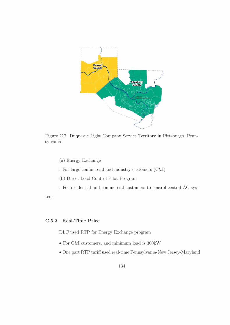
Figure C.7: Duquesne Light Company Service Territory in Pittsburgh, Penn-sylvania

(a) Energy Exchange

: For large commercial and industry customers (C&I)

(b) Direct Load Control Pilot Program

: For residential and commercial customers to control central AC sys-

tem

C.5.2 Real-Time Price

DLC used RTP for Energy Exchange program

• For C&I customers, and minimum load is 300kW

•One part RTP tariff used real-time Pennsylvania-New Jersey-Maryland

134

(PJM) Locational Marginal Price (LMP) based on the PJM daily capacity

market


59 customers took RTP tariff in April, 2005.

135

Bibliography

[1] U.S. Energy Information Administration, Household Energy Consumption

and Expenditures by End Use and Energy Source, Selected Years, 1978-

2005, U.S. Department of Energy, DC [Online] Available:

http://www.eia.gov/totalenergy/data/annual/#consumption

[2] U.S. Energy Information Administration, Residential Energy Consump-

tion Survey (RECS) 2005, U.S. Department of Energy, DC [Online]

Available:

http://www.eia.gov/consumption/residential/data/2005/index.cfm#undefined

[3] Paul Wattles (2011, Aug. 20), ERCOT Demand Response Overview &

Status Report, (AMIT-DSWG Workshop ‘AMI’s Next Frontier: Demand

Response’) [Online] Available:

http://www.ercot.com/content/meetings/dswg/keydocs/2011/0830/

3 ERCOT presentation workshop 083011.pdf

[4] R. Baldick and R. P. O’Neill, “Estimates of Comparative Costs for Uprat-

ing Transmission Capacity,” IEEE Transaction on Power Delivery, Vol.

24, No. 2, pp. 961∼969, Apr. 2009.

[5] J. Wang, M. Biviji and W. Maria Wang, “Case Study of Smart Grid

Demand Response Program in North America,” in Innovative Smart

136

Grid Technologies, ISGT, CA, 2011 IEEE PES, pp. 1∼5.

[6] M. Pipattanasomporn, M. Kuzlu and S. Rahman, “An Algorithm for

Intelligent Home Energy Management and Demand Response Analysis,”

IEEE Transaction on Smart Grid, unpublished.

[7] S. Lu, N. Samaan, R. Diao, M. Elizondo, C. Jin, E. Mayhorn, Yu Zhang

and H. Kirkham, “Centralized and Decentralized Control for Demand

Response,” in Innovative Smart Grid Technologies, ISGT , CA, 2011

IEEE/PES, pp. 1∼8.

[8] J. C. Fuller, K. P. Schneider and D. Chassin, “Analysis of Distribution

Level Residential Demand Response,” in Power Systems Conference and

Exposition (PSCE) , Phoenix, AZ, 2011 IEEE/PES, pp. 1∼7.

[9] N. Lu, D. P. Chassin, and S. E. Widergren, “Simulating Price Respon-

sive Distributed Resources,” in Power Systems Conference and Exposition

(PSCE) , 2004 IEEE/PES, pp. 1538∼1543.

[10] W. Zhang, K. Kalsi, J. Fuller, M. Elizondo, and D. Chassin, “Aggre-

gate Model for Heterogeneous Thermostatically Controlled Loads with

Demand Response,” in Power and Energy Society General Meeting, San

Diego, CA, 2012 IEEE, pp. 1∼8.

[11] W. A. Friess, K. Rakhshan, T. A. Hendawi, and S. Tajerzadeh, “Wall

insulation measures for residential villas in Dubai: A case study in energy

efficiency,” Energy and Buildings, Vol. 44, pp. 26∼32, Jan. 2012.

137

[12] J. Kosny and J. E. Christian, “Thermal evaluation of several configura-

tions of insulation and structural materials for some metal stud walls,”

Energy and Buildings, Vol. 22, pp. 157∼163, 1995.

[13] F. Stazi, A. Mastrucci, and C. di Perna, “The behaviour of solar walls

in residential buildings with different insulation levels: An experimental

and numerical study,” Energy and Buildings, Vol. 47, pp. 217∼229, Apr.

2012.

[14] K. E. Wilkes and J. L. Rucker, “Thermal Performance of Residential Attic

Insulation,” Energy and Buildings, Vol. 5, pp. 263∼277, Sep. 1983.

[15] M.K. Urbikain and J.M. Sala, “Analysis of different models to estimate

energy savings related to windows in residential buildings,” Energy and

Buildings, Vol. 41, pp. 687∼695, Jun. 2009.

[16] A. Gasparella, G. Pernigotto, F. Cappelletti, P. Romagnoni, and P. Bag-

gio, “Analysis and modeling of window and glazing systems energy per-

formance for a well-insulated residential building,” Energy and Buildings,

Vol. 43, pp. 1030∼1037, Apr. 2011.

[17] B. A. Rock, “Impact of daylight saving time on residential energy con-

sumption and cost,” Energy and Buildings, Vol. 25, pp. 63∼68, Feb.

1997.

[18] S. Tiptipakorn and W. Lee , “A Residential Consumer-Centered Load

Control Strategy in Real-Time Electricity Pricing Environment,” in Power

138

Symposium, Las Cruces, MN, 2007, NAPS, pp. 505∼510.

[19] Energy-Efficient Design of Low-Rise Residential Buildings, ANSI/ASHRAE

Standard 90.2-2007, 2007.

[20] Office of Energy Efficiency and Renewable Energy, OpenStudio— Getting

Started National Renewable Energy Laboratory of U.S Department of

Energy, Golden, CO [Online] Available: https://openstudio.nrel.gov/openstudio-

getting-started

[21] U.S. Department of Energy, Getting started with EnergyPlus: basic con-

cepts manual-essential information you need about running EnergyPlus,

U. S. Department of Energy, 2011

[22] Real-Time Settlement Point Price Display, The Electric Reliability

Council of Texas (ERCOT), Taylor, TX [Online] Available:

http://www.ercot.com/content/cdr/html/real time spp

[23] The University of Illinois and the Ernest Orlando Lawrence Berkeley Na-

tional Laboratory, External Interfaces(s) Application Guide: Guide for

using EnergyPlus with External Interface(s), U. S. Department of En-

ergy, 2011.

[24] Simulation Research Group, Building Technologies Department and En-

vironmental Energy Technologies Division Building Controls Virtual Test

Bed: User Manual Ver. 1.1.0, Lawrence Berkeley National Laboratory,

January 30, 2013.

139

[25] J. Ma, S. Joe Qin, Bo Li and T. Salsbury, “Economics Model Predic-

tive Control for Building Energy Systems,” in Innovative Smart Grid

Technologies, ISGT , 2011 IEEE PES, pp. 1∼6.

[26] K. Kalsi, M. Elizondo, J. Fuller, S. Lu, and D. Chassin, “Development

and Validation of Aggregated Models for Thermostatic Controlled Loads

with Demand Response,” in 2012 45th Hawaii International Conference

on System Sciences , 2012 IEEE Computer Society, pp. 1959∼1966.

[27] R. Roofegari Nejad and S. Masoud Moghaddas-Tafreshi, “A Novel Method

for Demand Response by Air-Conditioning Systems in A Microgrid with

Considering Wind Power Generation Variation,” in Innovative Smart

Grid Technologies, ISGT, ASIA , 2012 IEEE PES, pp. 1∼6.

[28] Pacific Northwest National Laboratory,Pacific Northwest GridWiseTM

Testbed Demonstration Projects - Part I. Olympic Peninsula Project, Pa-

cific Northwest National Laboratory and U.S. Department of Energy [On-

line] Available:

http://www.pnl.gov/main/publications/external/technical reports/PNNL-

17167.pdf

[29] The Univeristy of Illinois and the Ernest Orlando Lawrence Berkeley Na-

tional Laboratory, EnergyPlus Engineering Reference - The Reference to

EnergyPlus Calculations, U.S. Department of Energy

[30] U.S. Energy Information Administration, Table 1.2. Summary Statistics

140

for the United States, 2001 - 2011,

http://www.eia.gov/electricity/annual/html/epa 01 02.html

[31] J. L. Mathieu, D. S. Callaway, S. Kiliccote, Variability in automated re-

sponses of commercial buildings and industrial facilities to dynamic elec-

tricity prices, Energy and Buildings 43 (2011) 3322-3330

[32] M. Avci, M. Erkoc, A. Rahmani, S. Asfour, Model predictive HVAC load

control in buildings using real-time electricity pricing, Energy and Build-

ings 60 (2013) 199-209

[33] M. L. Persson, A. Roos, M. wall, Influence of window size on the energy

balance of low energy houses, Energy and Buildings 38 (2006) 181-188

[34] J. H. Yoon, R. Baldick, A. Novoselac, Dynamic demand response con-

troller based on real-time residential building, IEEE Transaction on Smart

Grid, Vol. 5, No. 1, Jan. 2014, pp 121-129

[35] G. Escriva-Escriva, I. Segura-Heras, M. Alcazar-Ortega, Application of an

energy management and control system to access the potential of different

control strategies in HVAC systems, Energy and Buildings 42 (2010) 2258-

2267

[36] U.S Department of Energy, Benefits of demand response in electricity

markets and recommendations for achieving them- a report to the United

States congress pursuant to section 1252 of the energy policy ACT of 2005,

U. S. Department of Energy, February 2006

141

[37] G. Barbose, C. Goldman, B. Neenan, A survey of utility experience with

real time pricing, Ernest Orlando Lawrence Berkeley National Laboratory,

December 2004

[38] Federal Energy Regulatory Commission (FERC), 2014 assessment of de-

mand response and advanced metering, staff report, U.S. Department of

Energy, December 2014

[39] American Society of Heating, Refrigerating and Air Conditioning Engi-

neers (ASHRAE), Thermal environmental conditions for human occu-

pancy, ANSI / ASHRAE Standard 55-2010

[40] American Society of Heating, Refrigerating and Air Conditioning Engi-

neers (ASHRAE), Energy-efficient design of low-rise residential buildings,

ANSI/ASHRAE Standard 90.2-2007, 2007

[41] Building Energy Codes Program, Residential prescriptive requirements -

2009 International Energy Conservation Code (IECC), U.S. Department

of Energy, http://energycode.pnl.gov/EnergyCodeReqs/

[42] Electricity Reliability Council Of Texas (ERCOT), Day ahead market

settlement point price display, The Electric Reliability Council of Texas,

Taylor, TX, USA

http://mis.ercot.com/misapp/GetReports.do?reportTypeId=13060&reportTitle=

Historical DAM Load Zone and Hub Prices&showHTMLView=&mimicKey

142

[43] Electricity Reliability Council Of Texas (ERCOT), Real-time market set-

tlement point price display, The Electric Reliability Council of Texas,

Taylor, TX, USA

http://mis.ercot.com/misapp/GetReports.do?reportTypeId=13061&reportTitle=

Historical RTM Load Zone and Hub Prices&showHTMLView=&mimicKey

[44] W. Surles and G. P. Henze, Evaluation of automatic priced based thermo-

stat control for peak energy reduction under residential time-of-use utility

tariffs, Energy and Buildings 49 (2012) 99 -108

[45] W.L. Leowa, R. C. Larsona, and J. L. Kirtley, Occupancy-moderated

zonal space-conditioning under a demand-driven electricity price, Energy

and Buildings 60 (2013) 453-463

[46] U.S. Energy Information Administration, CE4.4 Household Site End-Use

Consumption by Fuel in the South Region, Totals, Residential Energy

Consumption Survey, 2009

http://www.eia.gov/consumption/residential/data/2009/index.cfm?view=

consumption#undefined

[47] K. X. Perez, W. J. Cole, J. D. Rhodes, A. Ondeck, M. Baldea, M.

Webber and T. F. Edar, Nonintrusive Disaggregation of Residential Air-

Conditioning Load from Smart Meter Data, Energy and Buildings 81

(2014), page 316-325.

[48] Austin Energy, Energy Use & Sales: Residential Average Monthly kWh

and Bills, Corporate Reports & Data Library, 2012

143

http://austinenergy.com/wps/wcm/connect/88f98744-6003-4218-

8a57-2f7e7e72592a/EUS-residentialAvgBillKWH.xls?MOD=AJPERES

[49] T. Hong, F. Buhl and P. Have, EnergyPlus Run Time Analysis, Ernest

Orlando Lawrence Berkeley National Laboratory, 2008

[50] R. D. Taylor, C. Pederson and L. Lawire, Simultaneous Simulation of

Buildings and Mechanical Systems in Heat Balance based Energy Analysis

Programs, Energy and Utility Systems Division, USA-CERL, Champaign,

IL, USA

http://apps1.eere.energy.gov/buildings/energyplus/pdfs/bibliography/

simultaneous simulation taylor.pdf

[51] P. C Tabares-Velasco, Timestep considerations when simulating dynamic

behavior of high-performance homes, Buildings XII Conference, Florida,

December 2013

[52] J. D. Rhodes, B. Stephens, and M. E. Webber, Using energy audits to in-

vestigate the impacts of common air-conditioning design and installation

issues on peak power demand and energy consumption in Austin, Texas,

Energy and Buildings 43 (2011). page 3271-3278

[53] U.S. Federal Energy Regulatory Commission, Energy Primer: A Hand-

book of Energy Market Basics, July 2012, http://www.ferc.gov/market-

oversight/guide/energy-primer.pdf

144

[54] A. Faruqui, A. Hajos, R. M. Hledik and S. A. Newell, Fostering economic

demand response in the Midwest ISO, Energy 35 (2010), 1544-1552.

[55] P. Cappers, C. Goldman, and D. Kathan, Demand response in U.S. elec-

tricity markets: Empirical evidence, Energy 35 (2010), 1526-1535.

[56] R. Walawalkar, S. Fernands, N. Tharkur and K. R. Chevva, Evolution and

current status of demand response (DR) in electricity markets: Insights

from PJM and NYISO, Energy 35 (2010), 1553-1560.

[57] A. G. Vlachos, and P. N. Biskas, Demand Response in a Real-Time Bal-

ancing Market Clearing With Pay-As-Bid Pricing, IEEE Transactions on

Smart Grid, Vol. 4, No. 4 (2013), pp 1966-1975.

[58] J. Torriti, M. G. Hassan and M. Leach, Demand Response experience

in Europe: Policies, programmes and implementation, Energy 35 (2010),

1575-1583.

[59] Electricity Reliability Council of Texas (ERCOT), Demand Response

Providers , August 2014, http://www.ercot.com/content/services/

programs/load/Demand%20Response%20Providers.xls

[60] J. Kim and A. Shcherbakova, Common failures of demand response, En-

ergy 36 (2011), 873-880.

[61] S. C. Breukers, E. Heiskanen, B. Brohmann, R. M. Mourik, and C. F. J.

Feenstra, Connecting research to practice to improve energy demand-side

management (DSM), Energy 36 (2011), 2176-2185.

145

[62] U. Atikol, A simple peak shifting DSM (demand-side management) strat-

egy for residential water heaters, Energy 62 (2013), 435-400.

[63] P. Kepplinger, G. Huber and J. Petrasch, Autonomous Optimal Control

for Demand Side Management with Resistive Domestic Hot Water Heaters

Using Linear Optimization, Energy & Buildings (2014),

http://dx.doi.org/10.1016/j.enbuild.2014.12.016

[64] X. H. Li and S. H. Hong, User-expected price-based demand response

algorithm for a home-to-grid system, Energy 64 (2014), 437-449.

[65] S. H. Hong, M. Yu, and X. Huang, A real-time demand response algo-

rithm for heterogeneous devices in buildings and homes,Energy (2014),

http://dx.doi.org/10.1016/j.energy.2014.11.053

[66] H. C. Gils, Assessment of the theoretical demand response potential in

Europe, Energy 67 (2014), 1-18.

[67] J. P. Gouveia, P. Fortes and J. Seixas, Projections of energy services

demand for residential buildings: Insights from a bottom-up methodology,

Energy 47 (2012), 430-442.

[68] W. Jewell, The Effects of Residential Energy Efficiency on Electric De-

mand Response Programs, 47th Hawaii International Conference on Sys-

tem Science, IEEE Computer Society (2014), pp 2363-2372

[69] Z. Wang, and R. Paranjape, Agent-Based Simulation of Home Energy

Management System in Residential Demand Response, 27th Canadian

146

Conference on Electrical and Computer Engineering, IEEE (2014), pp

1-6.

[70] U.S. Department of Energy, EnergyPlus Energy Simulation Software,

http://apps1.eere.energy.gov/buildings/energyplus/

[71] S. Li, and D. Zhang, Developing Smart and Real-Time Demand Response

Mechanism for Residential Energy Consumers, Power System Conference,

IEEE (2014), pp 1-5.

[72] S. Li, D. Zhang, A. B. Roget, and Z. O’Neill, Integrating Home Energy

Simulation and Dynamic Electricity Price for Demand Response Study,

IEEE Transactions on Smart Grid, Vol. 5, No. 2 (2014), pp 779-778.

[73] J. J. Hirsch & Associate and Lawrence Berkeley National Laboratory,

eQUEST: the QUick Energy Simulation Tool,

http://doe2.com/equest/index.html

[74] D. Zhu, T. Hong, D. Yan, and C. Wang, A detailed loads comparison of

three building energy modeling programs: EnergyPlus, DeST and DOE-

2.1E, Building Simulation, Vol 6, No 3, pp 323-335.

[75] A. Arteconi, D. Costola, P. Hoes, and J. L. M. Hensen, Analysis of con-

trol strategies for thermally activated building systemsunder demand side

management mechanisms, Energy & Buildings 80 (2014), 384-393.

147

[76] J. H. Yoon, R. Baldick, and A. Novoselac, Demand response for residential

buildings based on dynamic price of electricity, Energy & Buildings 80

(2014), 531-541.

[77] F. McLoughlin, A. Duffy, and M. Conlon, Evaluation of time series tech-

niques to characterize domestic electricity demand, Energy 50 (2013),

120-130.

[78] S. Shosh, X. A. Sun, and X. Zhang, Consumer Profiling for Demand

Response Programs in Smart Grids, IEEE PES ISGT Asia, May 2012,

pp 1-6.

[79] A. Safdarian, M. Fotuhi-Firuzabadm and M. Lehtonen, A Distributed

Algorithm for Managing Residential Demand Response in Smart Grids,

IEEE Transactions on Industrial Informatics, Vol. 10, No. 4 (2014), pp

2385-2393.

[80] F. Fernandes, H. Morais, Z. Vale, and C. Ramos, Dynamic load manage-

ment in a smart home to participate in demand response events, Energy

& Buildings 82 (2014), 592-606.

[81] O. Sezgen, C. A. Glodman and P. Krishnarao, Option value of electricity

demand response, Energy 32 (2007), 108-119.

[82] B. Chakrabarti, D. Bullen, C. Edwards, and C. Callaghan, Demand Re-

sponse in the New Zealand Electricity Market, Transmission and Distri-

bution Conference and Exposition, IEEE PES (2012), pp 1-7.

148

[83] Electricity Reliability Council of Texas (ERCOT), Market Information:

Day-Ahead Market,

http://www.ercot.com/mktinfo/dam/index.html

[84] PJM Interconnection, Markets & Operation: Energy Market, Day-Ahead

Energy Market,

http://www.pjm.com/markets-and-operations/energy/day-ahead.aspx

[85] W. Lee, F. Quilumba, J. Shi, and S. Huang, Demand Response An

Assessment of Load Participation in the ERCOT Nodal Market, Power

and Energy Society General Meeting, IEEE (2012), pp 1-10.

[86] E. Koliou, C. Eid, J. P. Chaves-Avila, and R. A. Hakvoort, Demand

response in liberalized electricity markets: Analysis of aggregated load

participation in the German balancing mechanism, Energy 71 (2014),

245-254.

[87] P. Faria, and Z. Vale, Demand response in electrical energy supply: An

optimal real time pricing approach, Energy 36 (2011), 5374-5384

[88] V. Zois, M. Frincu, and V. Prasanna, Integrated Platform for Automated

Sustainable Demand Response in Smart Grids, IEEE International Work-

shop on Intelligent Energy Systems (2014), pp 64-69.

[89] W. H. Golove and J. H. Eto, Market Barriers to Energy Efficiency: A

Critical Reappraisal of the Rationale for Public Policies to Promote En-

ergy Efficiency, Lawrence Berkeley National Laboratory, CA, March 1996.

149

[90] Samlex America, Solar Inverter: TN 1500W, Available: http://www.

pvpower.com/samlex-tn-series-1500w-sine-wave-inverter-TN1500-112F.

aspx

[91] Vmax USA, Absorbed Glass Mat (AGM) battery: SLR125, Available:

http://www.vmaxtanks.com/SLR125-AGM-Solar-Battery-_p_38.html

150

Vita

Ji Hoon Yoon was born in Seoul, Korea. He received two Bachelor

degrees in Physics from Department of Natural Science and in Aerospace En-

gineering from Department of Aerospace Engineering at Sejong University,

Seoul, Republic of Korea in 2004. He graduated with valedictorian, College

of Natural Science. He continued his Doctor of Philosophy from Department

of Electrical and Computer Engineering at the University of Texas at Austin

from 2008 under the guidance of Professor Ross Baldick. During his PhD

program, he received Mater of Science in Electrical Engineering in 2011. His

PhD degree was received in May 2015. His primary research interests are

Energy Management System, Demand Response, Heating Ventilating and Air

Conditioning (HVAC) system control for residential and commercial buildings,

Development of Embedded System with Real-Time Operation and Power Sys-

tem Analysis for Renewable Energy.

Email address: [email protected]

This dissertation was typeset with LATEX† by the author.

†LATEX is a document preparation system developed by Leslie Lamport as a special

version of Donald Knuth’s TEX Program.

151

Documents

Copyright by Ji Hoon Yoon 2015