Copyright

by

Malathi Rao Velamuri

2004

The Dissertation Committee for Malathi Rao Velamuricertifies that this is the approved version of the following dissertation:

Health Insurance, Employment-Sector Choices and Job

Attachment Patterns of Men and Women

Committee:

Daniel S. Hamermesh, Supervisor

Maxwell B. Stinchcombe

Stephen J. Trejo

Li Gan

Robert Crosnoe

Health Insurance, Employment-Sector Choices and Job

Attachment Patterns of Men and Women

by

Malathi Rao Velamuri, B.S., M.A., M.S.

DISSERTATION

Presented to the Faculty of the Graduate School of

The University of Texas at Austin

in Partial Fulfillment

of the Requirements

for the Degree of

DOCTOR OF PHILOSOPHY

THE UNIVERSITY OF TEXAS AT AUSTIN

August 2004

Dedicated to my parents.

Acknowledgments

I completed this dissertation with the assistance and guidance of nu-

merous individuals. I would like to express my appreciation to all of them.

First, I would like to express my gratitude to my committee members

for their unwavering support, constructive feedback and guidance. I am par-

ticularly indebted to my supervisor Daniel Hamermesh for his wise counsel,

his valuable insights, his time and his infectious enthusiasm. You have, above

all, been a truly inspiring teacher. I hope I can enthuse students into ‘think-

ing’ Economics as you do! I would also like to express my heartfelt gratitude

to Maxwell Stinchcombe for his constant encouragement at every stage of my

graduate career. You have displayed infinite patience and generosity in dealing

with my weaknesses, algebraic and others. I feel privileged to have been your

student. I benefitted enormously from Stephen Trejo’s meticulous feedback,

Li Gan’s guidance and friendship and Robert Crosnoe’s refreshing perspective

on my research. My sincere thanks to all of you.

I would also like to thank all my professors at UT for sharing their

knowledge and time with me. I am grateful for the valuable advice of all the

graduate advisers - Vincent Geraci, Peter Wilcoxen and Gerald Oettinger. To

Vivian Goldman-Leffler, our graduate coordinator, I owe an enormous debt of

gratitude for her invaluable help throughout my graduate life at UT. Without

v

your constant reminders and numerous letters to people in high places, I would

have been shut out of the UT system and deported from the country a long

time ago! I thank all the staff in the Economics department for all their help

and support. I would also like to express my gratitude to Dr. Indumathi

Parthasarathy for persuading me to study Economics.

My wonderful house-mates over the years Leah, Ilke and Nithin have

been my family in Austin and have helped me cope with many a stressful sit-

uation. I cannot adequately express my affection and gratitude for your love,

friendship and support. I am very grateful to my fellow graduate students in

Economics, especially the class of 1998, for their friendship and support. I owe

special thanks to Richard Prisinzano, Leonardo Gatica, Sue Hwang Mialon,

Anne Golla, Eunsook Seo, Elaine Zimmerman, Peter Chang, Paula Hernandez-

Verme, Damien Eldridge, Mayuresh Kshetramade and Rafi Berkson for their

help, good cheer and advice. I thank Eugene Podnos for introducing me to

the intricacies of Mathematica. All the supplemental instructors I worked with

over the past few years inspired me with their youthful enthusiasm and their

desire to make a difference. It was a joy working with all of you. My numerous

friends here and in the rest of the world - Maithreyi, Aparna, Sridevi, Sree-

jata, Sarada, GB, Ganga, Nalini, Lata, Subba Reddy, Sarah, Sreenath, Bijoy,

Richard, Atietie - have provided moral support and encouragement always. I

thank you all for your friendship.

Most importantly, I wish to thank my family for believing in me, for

encouraging me in every possible way, for always being there for me, and for

vi

their prayers. Mom and Dad, I could not have done this without your spiri-

tual, emotional and financial support. Thank you for your unconditional love

and for your great reserves of patience and strength which I have shamelessly

drawn from. My siblings Gomathi, Rama and Bhaskar have always remained

steadfast in their support. I have learnt so much by observing how all of you

have followed your heart and chartered your own paths in life. I thank my

brother-in-law Gopal and my sister-in-law Prasanna for their love and encour-

agement. My wonderful nieces Srividya, Uma and Mallika and my terrific

nephew Ashwin have brought immense joy and energy into my life. Thank

you!

To Subhash and Padmaja, the cousins I lost since I started graduate

school, I just want to say that I feel your absence and miss you both.

vii

Health Insurance, Employment-Sector Choices and Job

Attachment Patterns of Men and Women

Publication No.

Malathi Rao Velamuri, Ph.D.

The University of Texas at Austin, 2004

Supervisor: Daniel S. Hamermesh

The chapters presented in this dissertation deal with two labor market

issues in the United States: (1) the impact of the cost of health insurance on

households’ choice of employment sector and (2) job attachment patterns of

men and women. Chapter 1 presents the motivation for the research. Chap-

ter 2 models the effect of employer-provided health insurance on households’

decision concerning whether to select into the wage-salary sector or the self-

employment sector. Chapter 3 provides an empirical test of this issue. Chapter

4 provides empirical support for a possible theory explaining why women might

exhibit stronger attachment to their job relative to men, early in their careers.

Chapter 5 presents the major conclusions of the dissertation and suggests di-

rections for future research.

viii

Table of Contents

Acknowledgments v

Abstract viii

List of Tables xi

List of Figures xii

Chapter 1. Introduction 1

Chapter 2. Health Insurance and Household Employment Sec-tor Choices 9

2.1 Introduction . . . . . . . . . . . . . . . . . . . . . . . . . . . . 9

2.2 Environment . . . . . . . . . . . . . . . . . . . . . . . . . . . . 12

2.2.1 Workers . . . . . . . . . . . . . . . . . . . . . . . . . . . 12

2.2.2 Firms . . . . . . . . . . . . . . . . . . . . . . . . . . . . 14

2.3 Single-person Labor Supply Problem . . . . . . . . . . . . . . 14

2.4 Married Households’ Labor Supply Problem . . . . . . . . . . 17

2.4.1 Both Spouses in self-employment . . . . . . . . . . . . . 18

2.4.2 Both Spouses in wage-salary sector . . . . . . . . . . . . 20

2.4.3 Married Households - One spouse in wage employmentand the other in self-employment . . . . . . . . . . . . . 22

2.5 Firm’s Problem . . . . . . . . . . . . . . . . . . . . . . . . . . 26

2.5.1 Comparative Statics . . . . . . . . . . . . . . . . . . . . 26

2.6 The Insurance Decision . . . . . . . . . . . . . . . . . . . . . . 28

2.6.1 Discussion . . . . . . . . . . . . . . . . . . . . . . . . . 37

2.7 Conclusions . . . . . . . . . . . . . . . . . . . . . . . . . . . . 41

ix

Chapter 3. Spousal Health Insurance and Women’s Employ-ment Sector Choices 44

3.1 Introduction . . . . . . . . . . . . . . . . . . . . . . . . . . . . 44

3.2 Theoretical Outline . . . . . . . . . . . . . . . . . . . . . . . . 48

3.2.1 Labor Supply . . . . . . . . . . . . . . . . . . . . . . . . 48

3.3 Data and Descriptive Statistics . . . . . . . . . . . . . . . . . . 52

3.4 The Self-Employment Choice . . . . . . . . . . . . . . . . . . . 55

3.5 Estimates . . . . . . . . . . . . . . . . . . . . . . . . . . . . . 58

3.6 Conclusions . . . . . . . . . . . . . . . . . . . . . . . . . . . . 65

Chapter 4. Job Attachment Patterns of Men and Women:The Role of Promotion Expectations and Experi-ence 76

4.1 Introduction . . . . . . . . . . . . . . . . . . . . . . . . . . . . 76

4.2 Data and Descriptives . . . . . . . . . . . . . . . . . . . . . . . 79

4.3 Model Specification . . . . . . . . . . . . . . . . . . . . . . . . 82

4.4 Estimates . . . . . . . . . . . . . . . . . . . . . . . . . . . . . 86

4.4.1 Basic Results . . . . . . . . . . . . . . . . . . . . . . . . 87

4.4.2 Gender-Promotion Expectation Comparisons . . . . . . 89

4.4.3 Gender-Promotion Expectation-Experience Comparisons 91

4.4.4 Early Sample . . . . . . . . . . . . . . . . . . . . . . . . 95

4.4.5 Late Sample . . . . . . . . . . . . . . . . . . . . . . . . 97

4.4.6 Individuals in Both Samples . . . . . . . . . . . . . . . . 99

4.5 Conclusions . . . . . . . . . . . . . . . . . . . . . . . . . . . . 101

Chapter 5. Conclusions 112

Bibliography 119

Vita 125

x

List of Tables

3.1 Percent Distribution of Wage-Salary and Self-Employed WomenWorkers in Non-Agricultural Occupations, by Selected Charac-teristics, 1984-85 and 1990-91 . . . . . . . . . . . . . . . . . . 68

3.2 Percent Distribution of Self-Employed and Wage-Salary Mar-ried Women Workers in Non-Agricultural Occupations, by Se-lected Characteristics . . . . . . . . . . . . . . . . . . . . . . . 69

3.3 Probit Estimates of Women’s Self-Employment Choices:Partial Effects on Response Probabilities . . . . . . . . . . . . 71

3.4 Average After-Tax Price of Health Insurance . . . . . . . . . . 72

3.5 Probit Estimates of Women’s Self-Employment Choices: PartialEffects on Response Probabilities . . . . . . . . . . . . . . . . 73

3.6 Probit Estimates of Women’s Self-Employment Choices: PartialEffects on Response Probabilities . . . . . . . . . . . . . . . . 74

3.7 Probit Estimates of Women’s Self-Employment Choices: PartialEffects on Response Probabilities . . . . . . . . . . . . . . . . 75

4.1 Self-Reported Promotion Expectations at JobBy Mobility: 1979-1983 . . . . . . . . . . . . . . . . . . . . . 104

4.2 Self-Reported Promotion Expectations at JobBy Mobility: 1996-1998 . . . . . . . . . . . . . . . . . . . . . 105

4.3 Descriptive Statistics - Entire Sample . . . . . . . . . . . . . 105

4.4 Random Effects Probit EstimationStaying on a Job, Double and Triple Difference . . . . . . . . 106

4.5 Triple Difference Marginal Effects . . . . . . . . . . . . . . . . 107

4.6 Random Effects Probit EstimationStaying on a Job by Time Period . . . . . . . . . . . . . . . . 108

4.7 Triple Difference Marginal Effects1979-1982 . . . . . . . . . . . . . . . . . . . . . . . . . . . . . 109

4.8 Triple Difference Marginal Effects1996-1998 . . . . . . . . . . . . . . . . . . . . . . . . . . . . . 110

4.9 Triple Difference Marginal EffectsIndividuals in Both Samples . . . . . . . . . . . . . . . . . . . 111

xi

List of Figures

2.1 Mass of married workers with husbands in wage-employmentand wives in self-employment . . . . . . . . . . . . . . . . . . 24

2.2 An Equilibrium Health Insurance Premium, with Adverse Se-lection . . . . . . . . . . . . . . . . . . . . . . . . . . . . . . . 39

3.1 Choice Problem of Type I and Type II Workers . . . . . . . . 67

3.2 Distribution of Weekly Hours: Married Women Covered/Not Covered, by Husband’s Health Insurance . . . . . . . . . 70

xii

Chapter 1

Introduction

In the United States, self-employment among the civilian non-agricultural

labor force declined from the 1920s to the mid-1970s. Thereafter, the trend

was reversed and the proportion of self-employed persons increased. By it-

self, this is a very interesting phenomenon since self-employment is gener-

ally associated with low levels of GDP per capita. As Blau (1987) observes,

“Even in most developing countries, where self-employment is typically a much

larger proportion of the labor force than in developed countries, the trend is

away from self-employment.” (p.446) From international comparisons of self-

employment, other important factors which are found to be highly correlated

with self-employment incidence are high marginal rates of taxation and restric-

tive labor legislation which raises the cost of layoffs to firms (OECD, 1992).

Neither of these phenomena is characteristic of the U.S. economy; marginal

rates of taxation are relatively low and have declined even further after 1986.

Moreover, the large shift from industrial employment to service sector employ-

ment since the late 1970s led to a decline of unionism, lowering the costs of

laying off workers to firms. In the light of these facts, the increasing trend of

self-employment in the U.S. invites further analysis.

1

As the incidence of self-employment rose in the U.S., there was a con-

current trend of rising health care costs. The linkage between health care costs

and the labor market comes from a unique feature of the U.S. health care sys-

tem. In the U.S., employment-based health insurance is the dominant form of

financing health care; over two-thirds of non-elderly Americans receive health

insurance through employers, either their own or that of a family member.

This is due to the fact that the tax code in the U.S. subsidizes employer pay-

ments for health insurance, by excluding these payments from income for tax

purposes. If employees are paid in wages, they must pay taxes on those wages.

On the other hand, the employer-paid portion of the health insurance premium

is exempt from income tax. Moreover, since employee contributions for health

insurance are usually paid with after-tax dollars, economic theory predicts that

employers should finance insurance premium costs rather than shifting these

costs to employees, with a corresponding decrease in wages. Moreover, group

rates of insurance offered by employers are substantially below individually-

purchased insurance rates due to adverse selection in insurance markets. All

these factors make the after-tax price of employer-provided health insurance

substantially lower than the price of individually-purchased health insurance

(Gruber and Poterba, 1994). In the second and third chapters of my disserta-

tion, I study the impact of this ‘price wedge’ on households’ incentives to select

into wage-employment vis-a-vis self-employment. My objective is to explain

the observed trend in the incidence of self-employment.

This problem is interesting and important for the following reason: the

2

U.S. labor market is considered to be a very flexible labor market, relative

to the labor markets of other industrialized countries, both in terms of the

availability of part-time jobs and access to flexible work schedules. However

employers rarely, if ever, provide health benefits to part-time workers. And as

stated above, the self-employed do not receive a tax benefit that is compara-

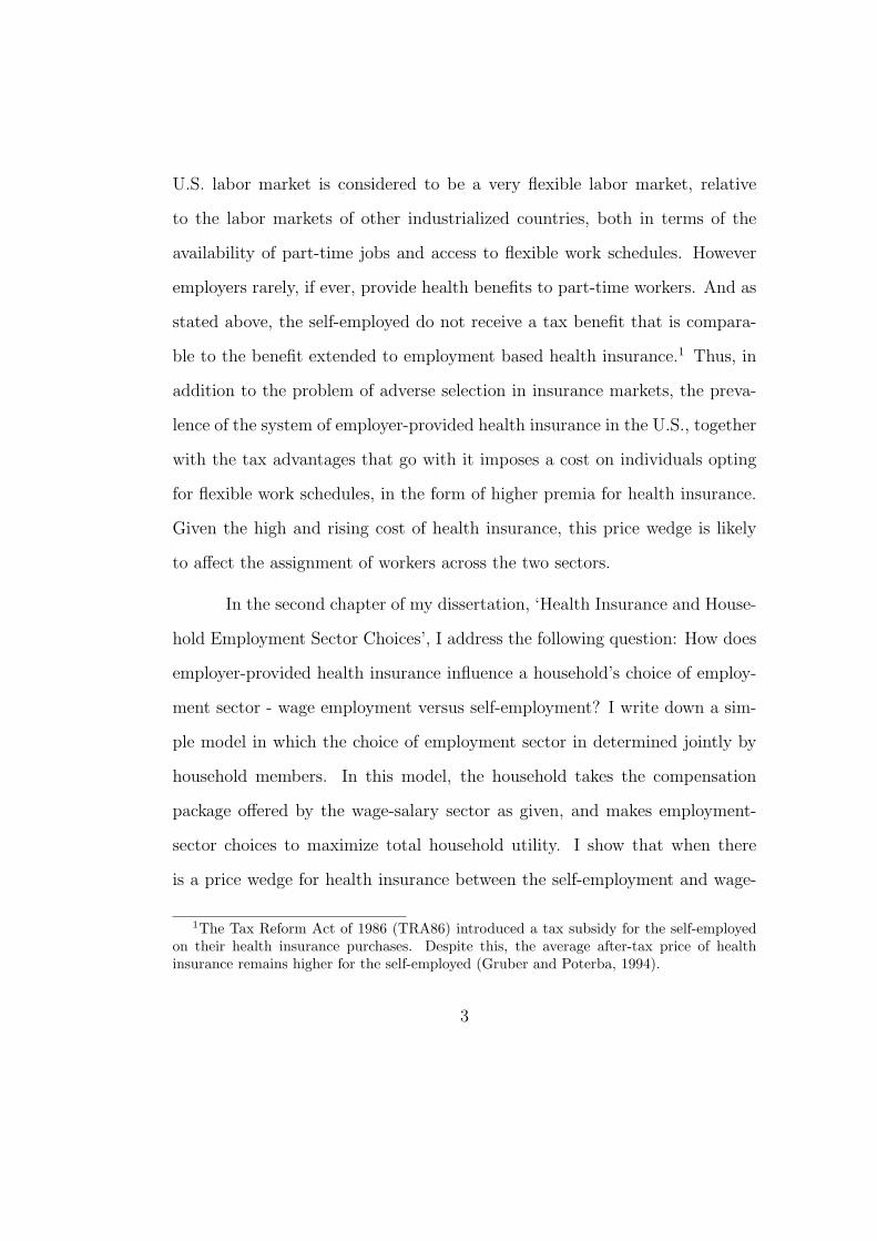
ble to the benefit extended to employment based health insurance.1 Thus, in

addition to the problem of adverse selection in insurance markets, the preva-

lence of the system of employer-provided health insurance in the U.S., together

with the tax advantages that go with it imposes a cost on individuals opting

for flexible work schedules, in the form of higher premia for health insurance.

Given the high and rising cost of health insurance, this price wedge is likely

to affect the assignment of workers across the two sectors.

In the second chapter of my dissertation, ‘Health Insurance and House-

hold Employment Sector Choices’, I address the following question: How does

employer-provided health insurance influence a household’s choice of employ-

ment sector - wage employment versus self-employment? I write down a sim-

ple model in which the choice of employment sector in determined jointly by

household members. In this model, the household takes the compensation

package offered by the wage-salary sector as given, and makes employment-

sector choices to maximize total household utility. I show that when there

is a price wedge for health insurance between the self-employment and wage-

1The Tax Reform Act of 1986 (TRA86) introduced a tax subsidy for the self-employedon their health insurance purchases. Despite this, the average after-tax price of healthinsurance remains higher for the self-employed (Gruber and Poterba, 1994).

3

employment sectors, labor supply to the self-employment sector is smaller and

to the wage-salary sector bigger, relative to the case where there is no price

wedge. Thus, the price wedge causes a distortion in the assignment of workers

between the two sectors. I also show that the extension of employer-provided

health benefits to dependents outside the firm through a family health plan

enables married couples to effectively eliminate the price wedge.

I extend this model to include the insurance-purchase decision for single

workers. In this model, in addition to choosing which sector to work in, workers

also decide whether to purchase health insurance or not. I use standard results

in the ‘adverse selection’ literature to illustrate how pooling the health risk

over the subset of workers who choose to buy insurance raises the insurance

premium, relative to the case where the risk-pooling is over all the workers in

the firm. Moreover, firms can economize on fixed costs by getting as many

workers as possible to participate in the group health insurance that they offer.

This result could explain why firms might prefer to include health benefits as

part of the compensation package to all workers, instead of making the choice

of health coverage optional.

In the third chapter of my dissertation ‘Spousal Health Insurance and

Women’s Employment Sector Choices’, I study whether the availability of

health coverage through the spouse’s health plan influences a married woman’s

decision to become self-employed. This chapter is motivated by two empirical

facts: (1) the increasing incidence of self-employment among women in the

United States since the mid-1970s - both in absolute and relative terms, and

4

(2) the prevalence of married women in self-employment. The absolute increase

in the numbers of self-employed women is not surprising in itself. This could

be a consequence of their increasing labor force participation. And the large

shift from industrial employment to service sector employment during the

1980s dramatically expanded the opportunities for self-employment and could

explain the relative increase in self-employment rates. However, this was also

a period of rising real health care costs. Thus, although the self-employment

option was easily available for women looking for flexible work schedules, it

was a costly option to exercise for those who had to purchase their own health

insurance coverage, at rates that were invariably more expensive than group

insurance rates offered by firms. On the other hand, women who had health

coverage through a spouse’s health plan could focus on other job attributes

like flexibility and non-standard work schedules. This could account for the

prevalence of married women in self-employment.

The Tax Reform Act of 1986 (TRA86) introduced a tax subsidy for

the self-employed to purchase their own health insurance. I test whether

this ‘natural’ experiment induced more women without spousal health insur-

ance coverage to select into self-employment. My estimates suggest that the

availability of health coverage through the spouse had a positive and signif-

icant effect on women’s self-employment propensities before TRA86. More-

over, the difference-in-difference estimates indicate that the incidence of self-

employment among women who did not enjoy spousal health benefits went up

in the post-TRA86 period.

5

In the fourth chapter of my dissertation ‘Job Attachment Patterns

of Men and Women: The Role of Promotion Expectations and Experience’

(joint with Richard Prisinzano), we study job turnover behavior by men and

women. Labor economists studying job turnover behavior in the 1960s and

1970s in the United States found that women exhibited substantially higher

job turnover rates compared to men. Researchers ascribed this behavior to the

long stretches of time that women spent out of the labor force. Subsequent

research has attributed the gender wage-gap to women’s lack of attachment to

the labor force. One theory that links gender differences in turnover behavior

to the gender wage gap suggests that since firms anticipate higher turnover

from women, they are not willing to invest as much in training and promoting

women as they are in men. Since firm-specific training tends to be highly cor-

related with promotions and career growth within the firm, promotion rates

for men tend to be much higher for men relative to women. These differences

in promotion rates translate into a gender wage gap.

Women’s labor force participation has increased dramatically over the

past few decades, prompting researchers to re-examine job turnover behavior

by men and women. There is evidence suggesting that more recent cohorts

of women have a higher propensity to stay on their jobs and are exhibiting a

strong attachment to the labor market.2 We would expect firms to treat these

women - the ‘stayers’ - no differently from men. However, women workers

are still a heterogenous group comprising both ‘stayers’ and ‘quitters,’ with

2See Prisinzano (2004), Light and Ureta(1992), and references therein.

6

higher average turnover rates than men. If firms cannot distinguish between

the two types of women workers based on observable characteristics, statistical

discrimination would still result in lower promotion rates for women and a

persistence of the wage gap. If, on the other hand, the women who are strongly

committed to their careers could successfully signal their intentions to stay in

the labor force and separate themselves from the quitters, they could overcome

internal labor market discrimination.

We hypothesize that women who are concerned about their careers use

job attachment as a means to signal their attachment to the labor force. This

concern is likely to be highest for women in the early stages of their career.

We therefore expect women with little or no job market experience to have

lower job turnover rates compared to men of similar experience, all else equal.

Thus, during this period we expect women to exhibit less sensitivity to expec-

tations of promotion, relative to men. This rationale also suggests that once

women have gained adequate labor market experience and revealed themselves

as stayers, their job attachment patterns should respond more closely to their

expectations of promotions. Hence, we expect women with adequate job mar-

ket experience to reveal job attachment patterns similar to those of men.

We use a longitudinal dataset to test our predictions. Specifically, we

study how the expectation of promotion affects the decision to stay on a job

and whether this pattern varies by gender and by the amount of labor mar-

ket experience. The dataset also contains information on workers’ perceived

chances of promotion in their current job. We expect workers who are con-

7

cerned about their careers to be sensitive to the potential for career growth

in their firms. We examine how turnover behavior responds to this subjective

likelihood of promotion and how this response differs by gender and experience

level. Our results suggest that individuals with low expectations of promotion

are less likely to stay on their jobs relative to those with high expectations of

promotion. We also find evidence that women are more likely than men to stay

on a job all else equal. Furthermore, women with low promotion expectations

are more likely than comparable men to stay on a job and this difference is

more pronounced early in careers. The fact that the difference diminishes with

experience supports our hypothesis.

8

Chapter 2

Health Insurance and Household Employment

Sector Choices

2.1 Introduction

Employment-based health insurance continues to be the dominant form

of financing health care in the United States; over two-thirds of non-elderly

Americans receive health insurance through employers. Group rates of in-

surance (also known as community-rated premia) offered by employers are

substantially below individual rates (also known as risk-rated premia) due to

adverse selection in insurance markets. While some self-employed individuals

enjoy group insurance coverage, the majority of those with coverage purchase

insurance on their own account (Gruber and Poterba, 1994). These individu-

als therefore face a substantially higher premium for health insurance, relative

to salaried workers. With high and rapidly rising health care costs in the

U.S., this ‘price wedge’ is likely to create a distortion in labor market out-

comes, by affecting the assignment of workers across the wage-employment

and self-employment sectors. This is the issue that I address in this chapter.

A closely related line of research explores the linkage between married

women’s labor supply choices - both hours worked and choice of employment

9

sector - and spousal health insurance. Married workers working in a firm

which provides health benefits can extend the coverage to their spouse and

other dependents outside the firm. This influences a household’s chosen bun-

dle of job attributes, offering married couples a greater latitude to substitute

health coverage for flexible hours, because of trading opportunities among

themselves (Lombard, 2001). A number of empirical papers have found sup-

port for this theory. Using cross-section data from the CPS, Buchmueller and

Valletta (1998) find a strong negative effect of health insurance coverage un-

der the husband’s health plan on wives’ work hours. Using the same data set,

Lombard (2001) finds that women’s likelihood of self-employment rises with

health coverage through the spouse. These papers treat the husband’s em-

ployment sector and compensation package as exogenous to the wife’s choice

of employment sector and hours worked.

In this chapter, I first write down a simple model in which the choice

of employment sector is determined jointly by household members. In this

model, everyone demands health insurance but the health insurance premium

differs between the two sectors. Households take the compensation package of-

fered by the wage-salary sector as given, and make employment-sector choices

to maximize total household utility. I address the following question: How

does employer-provided health insurance influence a household’s choice of em-

ployment sector - wage employment versus self-employment? I show that

when there is a price wedge for health insurance between the self-employment

and wage-employment sectors, labor supply to the self-employment sector is

10

smaller, relative to the case where there is no price wedge. Thus, the price

wedge causes a distortion in the assignment of workers between the two sectors.

I also show that the extension of employer-provided health benefits to

dependents outside the firm through a family health plan enables married cou-

ples to effectively eliminate the price wedge. I extend this model to include

the insurance-purchase decision for single workers. In this model, in addition

to choosing which sector to work in, workers also decide whether to purchase

health insurance or not. I use standard results in the ‘adverse selection’ lit-

erature to illustrate how pooling the health risk over the subset of workers

who choose to buy insurance raises the insurance premium, relative to the

case where the risk-pooling is over all the workers in the firm. This result

could explain why firms might prefer to include health benefits as part of the

compensation package to all workers, instead of making the choice of health

coverage optional.

The rest of the chapter is organized as follows: section 2 describes the

environment in which workers and firms operate, section 3 looks at the sin-

gle workers’ labor supply problem while section 4 discusses the labor supply

problem of married households. I present the firms’ problem very briefly in

section 5 and discuss some comparative statics properties. In section 6, I intro-

duce and discuss the insurance-purchase decision for single workers. Section 7

presents the conclusions.

11

2.2 Environment

2.2.1 Workers

The population in our economy consists of workers of unit mass, who

differ along two dimensions. Workers differ in their preference for flexibility,

indexed by θi which is uniformly distributed in the population along the unit

interval: θi ε (0, 1). A high realization of θ indicates a high preference for

flexibility. Flexibility can be defined along various dimensions; for our purpose,

we want to think of flexibility as the extent to which a worker has the freedom

in planning her work schedule over a specific time period.

The economy consists of two sectors of employment - the wage-salary

sector and the self-employment sector. In our model, the wage-salary sec-

tor consists of firms offering workers a compensation package in exchange for

their labor supply. The self-employment sector employs professionals like inde-

pendent owner-operators, proprietors and partners, and also includes workers

engaged in household production. For simplicity, we assume that a job in the

self-employment sector is associated with complete flexibility, while a job in

the wage-salary sector represents a completely inflexible job.

The compensation package in the wage-salary sector includes a private

health plan, which has two cost components - an average fixed cost component

Hws, associated with administrative expenses and overheads, and a variable

cost component h for every subscriber to the plan; h is small, relative to H.

The cost of the health plan for a single worker is (h + Hws). For a married

worker opting for a family health plan, the cost of the plan is (n · h + Hws),

12

where n equals the number of subscribers to the plan. The cost of a health

plan for a self-employed single worker, on the other hand, is the sum of the

variable cost and the average fixed cost, Hse, (h + Hse) while the cost of a

family health plan for a married couple who are both in self-employment is

(n · h + Hse), with Hse > Hws. This is the trade-off facing individuals and

households making the choice of working in the wage-salary sector versus the

self-employment sector. The self-employment sector offers the benefit of full

flexibility but comes with the cost of higher premium on health insurance.

The wage-salary sector offers savings on health benefits as part of the worker’s

compensation package, but requires workers to give up flexibility in exchange.

We can interpret the term (Hse −Hws) as the premium wedge or price wedge

arising out of the different prices of health insurance facing the worker in the

self-employment and wage-employment sectors. 1

I assume that the worker’s preferences can be represented by a quasi-

linear utility function, given by U(C, I) = C + V (I), where C denotes con-

sumption and I denotes health insurance . u(.) is well-behaved and has the

usual properties: u1 > 0,u2 ≥ 0, u21 = 0 and u22 ≤ 0. I also assume that

incomes are sufficiently large so that we always have an interior solution. To

1The U.S. tax system favors employer-provided health insurance over individually-purchased insurance in several respects. “Employer-provided insurance strictly dominatesinsurance purchased on own account for both itemizing and nonitemizing taxpayers, due tothe higher loading factors on individual policies, the full deductibility of employer-providedinsurance expenditures relative to the partial deductibility of own insurance expenditures,and the deductibility of employer-provided health insurance from the payroll tax as well asthe income tax.” (Gruber and Poterba, 1994). In this section, I ignore these details andsimply focus on the price difference arising out of differences in administrative costs betweenemployer-provided health insurance and individually purchased health insurance.

13

focus on the impact of the price of health insurance on the choice of employ-

ment sector, I initially assume that everyone has the same valuation for health

insurance which I denote by γ; i.e., V (I) = γ. Thus, with this simple setup, I

focus on the choice that households face between working in the wage-salary

sector and the self-employment sector.

The economy consists of a fixed fraction δ of single workers and the

remaining fraction, (1− δ) of married workers.

2.2.2 Firms

I assume that firms operate in a competitive environment, both in input and

product markets. The firm takes the market wage ω, the labor supply functions

of the two worker types as well as the health insurance prices set by the

insurance companies, as given and chooses how much labor to demand, to

maximize profits.

2.3 Single-person Labor Supply Problem

If the worker works in the self-employment sector, her indirect utility

function is given by:

uses = θi + γ − h−Hse

where Hse À h.

This gives us an alternative interpretation for θ. We can think of θ

as reflecting a person’s ability to earn outside of the wage-salary sector; the

14

higher the θ, the higher the worker’s earning potential outside the wage-salary

sector. However, I assume that θ does not affect a worker’s productivity in

the wage-salary sector.

If she works in the wage-salary sector, her utility function is given by:

uwss = ω + γ − h−Hws,

where ω is the money wage offered by the firm.

The decision rule facing the single worker is the following:

A single worker will work in the wage-salary sector iff the utility from doing

so exceeds the utility from being self-employed iff uwss ≥ use

s

ω + γ − h−Hws ≥ θi + γ − h−Hse, which implies

θi ≤ ω + Hse −Hws

Lemma 1: The mass of single workers working in the wage-salary sector, µwss

and in self-employment, µses is

µwss = ω + Hse −Hws

µses = 1− [ω + Hse −Hws]

Proof: Since µwss ε(0, 1) and µse

s ε(0, 1)

15

µwss = Pr(θi ≤ ω + Hse −Hws) = ω + Hse −Hws

µses = Pr(θi ≥ ω + Hse −Hws) = 1− [ω + Hse −Hws] ¤

If Hse−Hws is sizeable, such that ω + Hse−Hws ≥ 1, then all single workers

work in firms and µwss = 1. To focus on the more interesting case, I assume

that ω + Hse −Hws < 1 so that µwss < 1.

It is easy to observe that the price wedge for health insurance between the

wage-salary sector and the self-employment sector, Hse − Hws, affects the

assignment of workers between the two sectors. In the absence of the price

difference, the mass of workers in self-employment would be νses , where2

νses = 1− ω > 1− [ω + Hse −Hws] = µse

s

The difference between νses and µse

s is exactly the price differential for health

insurance between the self-employment and wage-employment sectors.

Note that

(i) ∂µwss /∂ω = 1 > 0,

2The Tax Reform Act of 1986 (TRA86) introduced a tax subsidy for the self-employed ontheir health insurance purchases, effectively lowering the after-tax price of health insurancefor the self-employed. Velamuri(2003) tested whether this subsidy induced more womenwithout spousal health insurance coverage to select into self-employment. Her results suggestthat the incidence of self-employment among women who did not enjoy spousal healthbenefits went up in the post-TRA86 period.

16

(ii) ∂µwss /∂h = 0

(iii) ∂µwss /∂Hws = −1 < 0

(iv) ∂µwss /∂Hse = 1 > 0.

2.4 Married Households’ Labor Supply Problem

I assume that a married worker knows not only his/her own θ but can ob-

serve the spouse’s θ as well. I also assume that the θs are independently and

identically distributed.

(θf , θm) ε (0, 1)2

If both spouses work in the wage-salary sector, they each get the benefit

of health insurance through the family health plan provided by one of their

employers. If only one spouse works in the wage-salary sector, the other spouse

gets health insurance coverage through the employer-provided family health

plan of the former.

I assume a unitary model of the household such that the utility of the household

is simply the sum of the utilities of the two spouses. The indirect utility

functions of the households are specified below.

The indirect utility function of households with both spouses in self-employment:

use,sem = θm + θf + 2γ − 2h−Hse

The utility function for households with both spouses working in wage-salary

sector : uws,wsm = 2ω + 2γ − 2h−Hws

17

The utility function for households with the husband working in wage-salary

sector and the wife in self-employment : uws,sem = ω + θf + 2γ − 2h−Hws

The utility function for households with the husband working in self-employment

sector and the wife in the wage-salary sector : use,wsm = ω +θm +2γ−2h−Hws

I now examine the decision rule facing married households.

2.4.1 Both Spouses in self-employment

Both spouses will be self-employed iff

use,sem ≥ uws,ws

m ⇔ θm + θf + 2γ − 2h−Hse ≥ 2ω + 2γ − 2h−Hws (2.1)

use,sem ≥ uws,se

m ⇔ θm + θf + 2γ − 2h−Hse ≥ ω + θf + 2γ − 2h−Hws (2.2)

use,sem ≥ use,ws

m ⇔ θm + θf + 2γ − 2h−H ≥ ω + θm + 2γ − 2h−Hws (2.3)

From condition (1) we get

θm + θf ≥ 2ω + Hse −Hws

Conditions (2) and (3) yield

18

θm ≥ ω + Hse −Hws

θf ≥ ω + Hse −Hws.

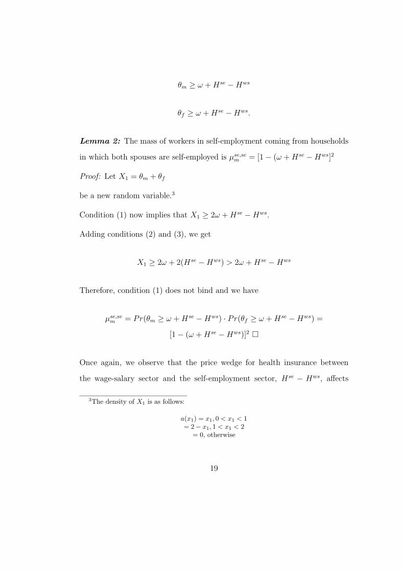
Lemma 2: The mass of workers in self-employment coming from households

in which both spouses are self-employed is µse,sem = [1− (ω + Hse −Hws]2

Proof: Let X1 = θm + θf

be a new random variable.3

Condition (1) now implies that X1 ≥ 2ω + Hse −Hws.

Adding conditions (2) and (3), we get

X1 ≥ 2ω + 2(Hse −Hws) > 2ω + Hse −Hws

Therefore, condition (1) does not bind and we have

µse,sem = Pr(θm ≥ ω + Hse −Hws) · Pr(θf ≥ ω + Hse −Hws) =

[1− (ω + Hse −Hws)]2 ¤

Once again, we observe that the price wedge for health insurance between

the wage-salary sector and the self-employment sector, Hse − Hws, affects

3The density of X1 is as follows:

a(x1) = x1, 0 < x1 < 1= 2− x1, 1 < x1 < 2

= 0, otherwise

19

the assignment of married workers between the two sectors. In the absence

of the price difference, the mass of workers in self-employment coming from

households with both spouses in self-employment would be νse,sem , where

νse,sem = [1− ω]2 > [1− (ω + Hse −Hws)]2 = µse,se

m

From µse,sem , we have

(i) ∂µse,sem /∂ω = −2[1− (ω + Hse −Hws)] < 0,

(ii) ∂µse,sem /∂h = 0

(iii) ∂µse,sem /∂Hws = 2[1− (ω + Hse −Hws)] > 0

(iv) ∂µse,sem /∂Hse = −2[1− (ω + Hse −Hws)] < 0.

2.4.2 Both Spouses in wage-salary sector

Both spouses will work in the wage-salary sector iff

uws,wsm ≥ uws,se

m ⇔ 2ω + 2γ − 2h−Hws ≥ ω − 2h−Hws + θf + 2γ (2.4)

uws,wsm ≥ use,ws

m ⇔ 2ω + 2γ − 2h−Hws ≥ ω − 2h−Hws + θm + 2γ (2.5)

uws,wsm ≥ use,se

m ⇔ 2ω + 2γ − 2h−Hws ≥ θm + θf + 2γ − 2h−Hse (2.6)

Conditions (4) and (5) yield

θf ≤ ω,

20

θm ≤ ω,

and equation (6) implies that θm + θf ≤ 2ω + Hse −Hws.

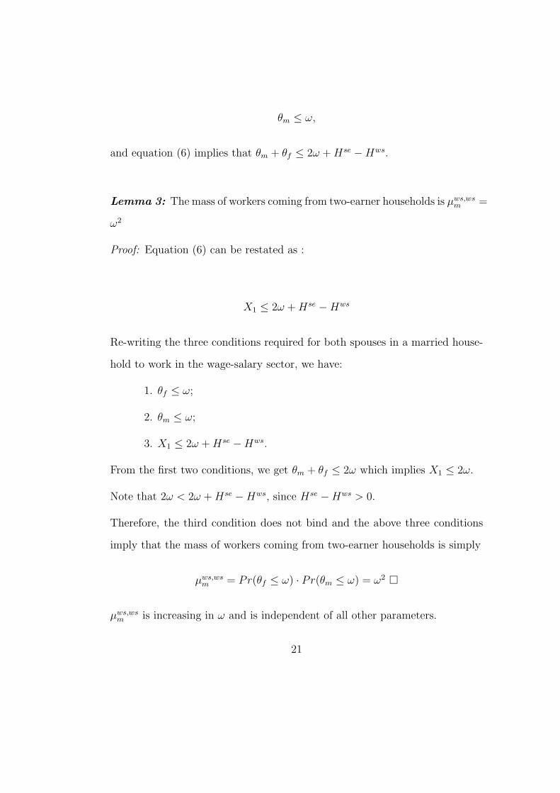
Lemma 3: The mass of workers coming from two-earner households is µws,wsm =

ω2

Proof: Equation (6) can be restated as :

X1 ≤ 2ω + Hse −Hws

Re-writing the three conditions required for both spouses in a married house-

hold to work in the wage-salary sector, we have:

1. θf ≤ ω;

2. θm ≤ ω;

3. X1 ≤ 2ω + Hse −Hws.

From the first two conditions, we get θm + θf ≤ 2ω which implies X1 ≤ 2ω.

Note that 2ω < 2ω + Hse −Hws, since Hse −Hws > 0.

Therefore, the third condition does not bind and the above three conditions

imply that the mass of workers coming from two-earner households is simply

µws,wsm = Pr(θf ≤ ω) · Pr(θm ≤ ω) = ω2 ¤

µws,wsm is increasing in ω and is independent of all other parameters.

21

2.4.3 Married Households - One spouse in wage employment andthe other in self-employment

A married worker in the wage-salary sector with the spouse in the self-

employment sector would have no incentive to choose a single coverage plan.

Opting for a family health plan would extend the health benefits to the spouse

and to other dependents, if any.

Households will have the husband in the wage employment and the wife in

self-employment iff

uws,sem ≥ uws,ws

m ⇔ ω − 2h−Hws + θf + 2γ ≥ 2ω − 2h−Hws + 2γ (2.7)

uws,sem ≥ use,ws

m ⇔ ω − 2h−Hws + θf + 2γ ≥ ω − 2h−Hws + θm + 2γ (2.8)

uws,sem ≥ use,se

m ⇔ ω − 2h−Hws + θf + 2γ ≥ θm + θf + 2γ − 2h−Hse (2.9)

These conditions yield

1. θf ≥ ω;

2. θf ≥ θm;

3. θm ≤ ω + Hse −Hws

22

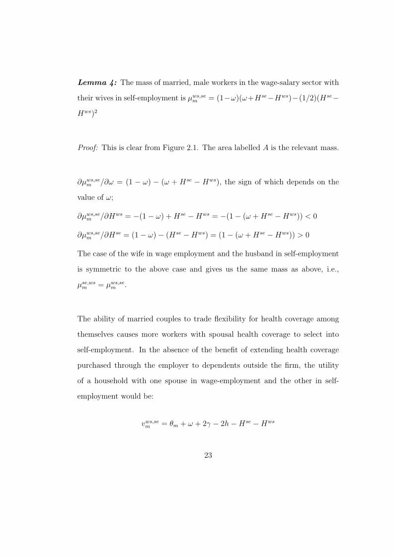
Lemma 4: The mass of married, male workers in the wage-salary sector with

their wives in self-employment is µws,sem = (1−ω)(ω+Hse−Hws)−(1/2)(Hse−

Hws)2

Proof: This is clear from Figure 2.1. The area labelled A is the relevant mass.

∂µws,sem /∂ω = (1 − ω) − (ω + Hse − Hws), the sign of which depends on the

value of ω;

∂µws,sem /∂Hws = −(1− ω) + Hse −Hws = −(1− (ω + Hse −Hws)) < 0

∂µws,sem /∂Hse = (1− ω)− (Hse −Hws) = (1− (ω + Hse −Hws)) > 0

The case of the wife in wage employment and the husband in self-employment

is symmetric to the above case and gives us the same mass as above, i.e.,

µse,wsm = µws,se

m .

The ability of married couples to trade flexibility for health coverage among

themselves causes more workers with spousal health coverage to select into

self-employment. In the absence of the benefit of extending health coverage

purchased through the employer to dependents outside the firm, the utility

of a household with one spouse in wage-employment and the other in self-

employment would be:

vws,sem = θm + ω + 2γ − 2h−Hse −Hws

23

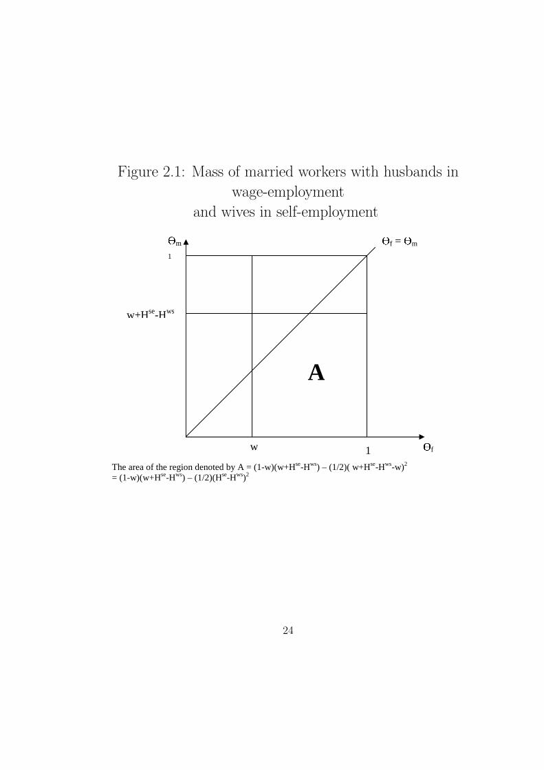
Figure 2.1: Mass of married workers with husbands in

wage-employment

and wives in self-employment

The area of the region denoted by A = (1-w)(w+Hse-Hws) – (1/2)( w+Hse-Hws-w)2 = (1-w)(w+Hse-Hws) – (1/2)(Hse-Hws)2

w

w+Hse-Hws

A

�m

1

�f

�f =

�m

1

24

and the mass of married workers,with one spouse in wage-employment and the

other is self-employment would be

νws,sem = (ω + Hse −Hws)(1− (ω + Hse −Hws)) <

(1− ω)(ω + Hse −Hws)− (1/2)(Hse −Hws)2 = µws,sem .

Thus married households with one spouse in wage-employment and the other

in self-employment effectively eliminate the difference in premia between the

two sectors, because an employer-provided family health plan offers health

coverage to the other spouse and eliminates the need for the self-employed

spouse to purchase health insurance at a higher cost.

The total labor supply to the wage-salary sector in the economy is therefore

µws = δ · µwss + (1− δ)[µws,ws

m + 2µws,sem ]

∂µws/∂ω = δ + (1 − δ)[2ω + 2 − 4ω − 2(Hse −Hws)] = δ + 2(1 − δ)[1 − ω −(Hse −Hws)] > 0

∂µws/∂Hws = −δ + (1− δ)[−2(1− ω) + 2(Hse −Hws)] = −[δ + 2(1− δ)(1−ω − (Hse −Hws)] < 0

∂µws/∂Hse = δH + (1− δ)[2(1− ω)− 2(Hse −Hws)] = δ + 2(1− δ)(1− (ω +

Hse −Hws)) > 0

25

2.5 Firm’s Problem

I normalize the price of output to 1. Firms take the labor supply

functions of the two worker types as given, and maximizes profits by choosing

ω. I denote by Z, the vector of parameters for the problem: Z = {h,Hws, Hse}.

Max∏

(ω; Z) = f(µ)− ωµ (2.10)

where I assume that f(.) is quasiconcave, differentiable and that the first-order

condition with respect to ω characterizes the firm’s labor demand as a function

of the parameters:

F ≡ f ′(.)− ω = 0

The aggregate demand for labor is simply the sum of the labor demand of all

the firms in the economy. Equating aggregate demand to the aggregate labor

supply gives us the equilibrium wage, ω∗.

2.5.1 Comparative Statics

The variable cost of health insurance h, has no effect on labor supply and

does not affect the equilibrium wage. Therefore, the only two parameters of

interest in this model are Hws and Hse. I look at the effect of changes in these

parameters on the equilibrium wage.

26

Lemma 5: An increase in the average fixed cost of health insurance in the

wage-salary sector Hse lowers the equilibrium wage ω∗.

Proof: dω/dHse = −(∂F/∂Hse)/(∂F/∂ω), while

∂F/∂Hse = f ′′(.)∂µws/∂Hse < 0 and

∂F/∂ω = f ′′(.)∂µws/∂ω − 1 < 0

Therefore, the sign of dω/dHse = −(−)/(−) = (−) ¤

The intuition for this result is straightforward. An increase in Hse increases

the cost of being self-employed and causes the labor supply to the wage-salary

sector to increase. An increase in labor supply to the wage-salary sector, all

else equal, lowers the equilibrium wage.

Lemma 6: An increase in Hws, the average fixed cost of health insurance in

the wage-salary sector, increases the equilibrium wage ω∗.

Proof: dω/dHws = −(∂F/Hws)/(∂F/∂ω)

∂F/∂Hws = f ′′(.)∂µws/∂Hws > 0

Therefore, the sign of dω/dHws = −(+)/(−) = (+) ¤

An increase in Hws, all else equal, increases the cost of health insurance to

a worker in a firm and is likely to switch some workers into self-employment,

thus lowering labor supply to the wage sector. This decrease in labor supply,

27

ceteris paribus, will cause the equilibrium wage to go up.

2.6 The Insurance Decision

So far, I have assumed that everyone has the same valuation for health insur-

ance and that everyone’s income is sufficient high for an interior solution to

exist. In reality, people have different valuations for health insurance and will

purchase health insurance only when this value exceeds the cost of purchasing

the insurance. In this section, I incorporate the insurance-purchase decision

into the above framework. I briefly discuss how this decision can lead to ‘ad-

verse selection’ when only a subset of workers chooses to purchase insurance,

causing health insurance premia to rise. Self-employed individuals acting on

their own behalf do not have the ability to pool their risk with anyone else and

consequently, face costly ‘risk-rated’ premia. This is one reason why health in-

surance premia between the two employment sectors diverge. Moreover, since

firms can lower the wages offered to workers in exchange for providing them

with health insurance, they also have an incentive of extending health coverage

to all their workers. This strategy has the effect of lowering the premium for

their workers and increases the firms’ ability to trade-off wages with health

benefits.

I restrict the analysis to single workers. In addition to differing in terms

of how much they value flexibility, workers also differ along another dimension

- in terms of how much they value health insurance. I assume that the value

28

of health insurance is also uniformly distributed in the population according

to γ, along the unit interval: γi ε (0, 1). One way to interpret γ is to assume

that it reflects expected medical costs; the higher the expected medical costs,

the more the individual values health insurance. Therefore, γ reflects the risk

types of the population, ranging from the most healthy (γ close to 0) to the

least healthy (γ close to 1).

If the worker works in the self-employment sector, her indirect utility

is one of the following: (i)use,Inss , if she chooses to purchase health insurance

or (ii) use,¬Inss if she chooses to remain uninsured:

use,Insi = θi + γi − h−Hse, (with self-insurance)

use,¬Insi = θi, (without self-insurance)

If she works in the wage-salary sector, her utility is (i)uws,Inss , if she chooses to

purchase health insurance through the employer or (ii) uws,¬Inss if she chooses

to remain uninsured:

uws,Insi = ω + γi − h−Hws, (with insurance)

uws,¬Insi = ω, (without insurance)

Now, the decision rule facing the worker is the following:

Self-Employed Workers with no Health Insurance: A worker will choose

to be self-employed, without health insurance iff

29

use,¬Insi ≥ use,Ins

i ,

use,¬Insi ≥ uws,Ins

i ,

use,¬Insi ≥ uws,¬Ins

i , which implies

γi ≤ h + Hse (2.11)

θi ≥ max(ω, ω + γi − h−Hws) (2.12)

Lemma 7: The mass of uninsured workers in self-employment is

ϕse,¬Ins = (1− ω)(h + Hse)− (1/2)(Hse −Hws)2

Proof: From (11), Pr(γi ≤ h + Hse) = h + Hse

From (12), max(ω, ω + γi − h−Hws) = ω, if γi < h + Hws.

This happens with probability (h + Hws). In this case, condition (12) reduces

to

θi ≥ ω

With probability (1−(h+Hws)), max(ω, ω+γi−h−Hws) = ω+γi−h−Hws.

In this case, condition (12) becomes

30

θi ≥ ω − h−Hws + γi

Note that when γi ≤ h+Hws, this implies that γi < h+Hse, since Hse > Hws.

In this case, condition (11) does not bind.

Therefore, the mass of uninsured workers in self-employment is given by

ϕse,noIns = (1− ω)(h + Hse)− (1/2)(Hse −Hws)2 ¤

We have

(i) ϕse,noIns/∂ω = −(h + Hse) < 0,

(ii) ϕse,noIns/∂h = (1− ω) > 0

(iii) ϕse,noIns/∂Hse = (1− ω)− (Hse −Hws) = 1− (ω + Hse −Hws) > 0

(iv) ϕse,noIns/∂Hws = Hse −Hws > 0.

In the earlier model, where all workers had the same valuation for health in-

surance, the only effect of changing prices was to shift workers across sectors.

In the present model, changing prices can affect either the insurance decision,

or the employment-sector decision or both. For instance, in the above case,

a sizeable increase in ω can not only cause workers to switch from the self-

employment to the wage-employment sector, but for γi lying between Hws and

Hse, can also cause them to purchase health insurance through their employers.

Self-Employed Workers with Health Insurance: A worker will choose

to be self-employed, with health insurance iff

31

use,Insi ≥ use,noIns

i ,

use,Insi ≥ uws,Ins

i ,

use,Insi ≥ uws,noIns

i ,

These conditions imply

γi ≥ h + Hse (2.13)

θi + γi − h−Hse ≥ max(ω, ω + γi − h−Hws) (2.14)

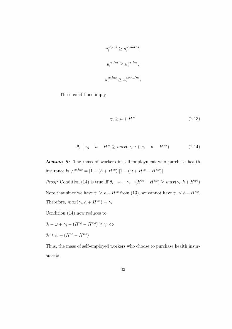
Lemma 8: The mass of workers in self-employment who purchase health

insurance is ϕse,Ins = [1− (h + Hse)][1− (ω + Hse −Hws)]

Proof: Condition (14) is true iff θi−ω + γi− (Hse−Hws) ≥ max(γi, h+Hws)

Note that since we have γi ≥ h+Hse from (13), we cannot have γi ≤ h+Hws.

Therefore, max(γi, h + Hws) = γi

Condition (14) now reduces to

θi − ω + γi − (Hse −Hws) ≥ γi ⇔

θi ≥ ω + (Hse −Hws)

Thus, the mass of self-employed workers who choose to purchase health insur-

ance is

32

ϕse,Ins = [1− (h + Hse)][1− (ω + Hse −Hws)] ¤

We have

(i) ϕse,Ins/∂ω = −[1− (h + Hse)] < 0,

(ii) ϕse,Ins/∂h = −[1− (ω + Hse −Hws)] < 0

(iii) ϕse,Ins/∂Hse = −[1− (h + Hse)]− [1− (w + Hse −Hws)] < 0

(iv) ϕse,Ins/∂Hws = [1− (h + Hse)] > 0.

Here an increase in ω, ceteris paribus, will switch more workers into wage-

employment, without changing the insurance decision. Changes in the prices

of health insurance have the expected effects.

Wage-Salary Workers with no Health Insurance: A worker will choose

to work in the wage-salary sector, and not purchase health insurance iff

uws,noInsi ≥ uws,Ins

i ,

uws,noInsi ≥ use,Ins

i ,

uws,noInsi ≥ use,noIns

i ,

These condition imply the following:

γi ≤ h + Hws (2.15)

33

ω ≥ max(θi, θi + γi − h−Hse) (2.16)

Lemma 9: The mass of workers in wage-employment who choose not to

purchase health insurance is ϕws,noIns = ω(h + Hws)

Proof: Since, from (15), we have γi ≤ h + Hws, we know that γi < h + Hse

This implies that max(θi, θi + γi − h−Hse) = θi

Therefore condition (16) reduces to

ω ≥ θi

We thus get the mass of workers in wage-employment who choose not to pur-

chase health insurance as

Pr(γi ≤ h + Hws).P r(θi ≤ ω) = ω(h + Hws) ¤

Note that

(i) ϕws,noIns/∂ω = (h + Hws) > 0,

(ii) ϕws,noIns/∂h = ω > 0

(iii) ϕws,noIns/∂Hse = 0

(iv) ϕws,noIns/∂Hws = ω > 0.

In this case again, a decrease in ω, all else equal, switches more workers into

self-employment, without affecting the insurance decision.

34

Wage-Salary Workers with Health Insurance: A worker will choose to

work in the wage-salary sector, and purchase health insurance iff

uws,Insi ≥ uws,noIns

i ,

uws,Insi ≥ use,Ins

i ,

uws,Insi ≥ use,noIns

i ,

These conditions give us

γi ≥ h + Hws (2.17)

ω + γi − h−Hws ≥ max(θi, θi + γi − h−Hse) (2.18)

Lemma 10: The mass of workers in wage-employment who purchase health

insurance is ϕws,Ins = (ω + Hse −Hws)(1− (h + Hws))− (1/2)(Hse −Hws)2

Proof: Condition (18) is equivalent to ω−θi+Hse−Hws+γi ≥ max(h+Hse, γi)

If max(h + Hse, γi) = h + Hse, condition (18) reduces to

θi ≤ ω + γi − h−Hws

If max(h + Hse, γi) = γi, condition (18) is ⇔

θi ≤ ω + Hse −Hws

35

These conditions define the mass of workers in wage-employment who pur-

chase health insurance:

ϕws,Ins = (ω + Hse −Hws)(1− (h + Hws))− (1/2)(Hse −Hws)2

Note that

(i) ϕws,Ins/∂ω = 1− h−Hws > 0,

(ii) ϕws,Ins/∂h = −(ω + Hse −Hws) < 0

(iii) ϕws,Ins/∂Hse = 1− h−Hse > 0

(iv) ϕws,Ins/∂Hws = −1− ω + h + Hws < 0.

A decrease in ω switches more workers into self-employment and all else equal,

reverses the insurance decision for those workers with γ lying between Hws and

Hse.

The total labor supply to the wage-salary sector in the economy is

ϕws = ϕws,noIns + ϕws,Ins =

ω(h + Hws) + (ω + Hse −Hws)(1− (h + Hws))− (1/2)(Hse −Hws)2

∂ϕws/∂ω = 1 > 0

ϕws/∂Hws = −1 + h + Hws < 0

36

ϕws/∂Hse = 1− h−Hse > 0

The firm’s problem is the same as in section 2.5. Once again, the aggregate

demand for labor in the economy is the sum of demands of individual firms.

Equating the aggregate demand for labor to the aggregate supply ϕws gives us

the equilibrium wage ω∗. Again, we have the same comparative static proper-

ties. An increase in the premium for health insurance in the self-employment

sector, Hse lowers the equilibrium wage, ω∗ while an increase in Hws causes

ω∗ to increase.

2.6.1 Discussion

Presumably, workers who have low expected medical costs are healthy and do

not value health insurance at its cost. Workers choosing to purchase health

insurance, on the other hand, reveal themselves as the ‘risky’ pool of workers

with high expected medical costs. Thus, when purchase of health insurance is

optional, health insurance companies will increase the premium for those who

choose to purchase it. Intuitively, as the pool of insured workers gets larger,

the average expected medical cost is less likely to vary.

Assuming that risk types can be ordered, the premium for a pool of workers

including everyone from a risk type γj to the least healthy person can be

formulated as:

P(γj→1) = E(γ|γ ≥ γj)

The premium is therefore an increasing function of γj, or equivalently,

37

a decreasing function of the mass of workers opting for health insurance.4

The expected value of medical costs to the insurance company depends on the

premium charged. As the premium increases, the healthier workers who do

not value health insurance too highly drop out of the insurance pool, and the

average medical costs of those who remain in the pool rises. The equilibrium

premium for health insurance is given by the following condition:

P ∗ = E(γ|γ ≥ P ∗)

Figure 2.2 graphs the values of E(γ|γ ≥ P ) as a function of the premium

P . The function gives the expected medical costs for workers who choose to be

insured by firms when the health insurance premium is P . It is an increasing

function of P . The equilibrium premium P ∗ is that level of P at which this

function crosses the 45-degree line, satisfying the equilibrium condition defined

above.5

Thus the health insurance premium is an increasing function of γj or

the expected medical costs. This tells us why firms might want to extend

insurance to all their workers, without making the choice of health coverage

optional; the bigger the mass of workers in the insurance pool, the lower the

4Since risk-rated insurance contacts charge a premium in proportion to the individual’sexpected medical costs during the life of the contract, premia in the individual market tendto be very high. Estimates suggest that 10% of the population accounts for 70% of totalmedical spending (Li, 2000).

5The existence of an equilibrium is not guaranteed, and if an equilibrium does exist,it need not be unique. There is a voluminous literature on this topic. For instance, seeAkerlof(1970).

38

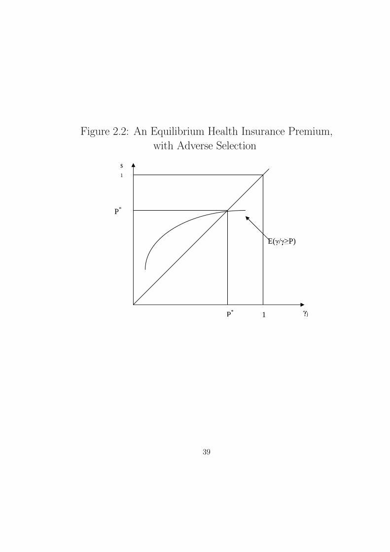
Figure 2.2: An Equilibrium Health Insurance Premium,

with Adverse Selection

$

1

γj P*

P*

E(γ /γ ≥ P)

1

39

premium charged by insurance companies. The lower the premium facing

workers in wage-employment, the wider is the potential price wedge for health

insurance between the two sectors. As the price wedge gets bigger, the labor

supply to the wage sector increases, causing the equilibrium wage to decrease

and increasing the profitability of firms. 6

When the option of not purchasing health insurance is taken away

from workers, for a given wage, those who have a high preference for flexibility

and low valuation of health insurance (the high-θ, low-γ workers) are likely

to select into self-employment. However, since θ does not affect a worker’s

productivity in the wage-salary sector, firms can still attract those workers

who have a low preference for flexibility and low valuation of health insurance

(the low-θ, low-γ types). These are the ‘healthy’ workers who will lower the

insurance premium and lower the firm’s average costs. The (low-θ, high-γ)

types have a strong incentive to select into wage-employment while the choice

of employment sector for the high-θ and high-γ type will be more senstive

to the wage, ω and the difference in health insurance premia between the

two sectors. These factors will impact how workers get sorted into the two

6The primary reason for the pre-dominance of employer-provided health insurance inthe U.S. is because it is subsidized through the tax code. If employees are paid in wages,they must pay taxes on those wages. On the other hand, the employer-paid portion of thehealth insurance premium is exempt from income tax. Moreover, employee contributionsfor health insurance are usually paid with after-tax dollars. Thus economic theory predictsthat employers should provide and finance insurance premium costs rather than shiftingthese costs to employees, with a corresponding decrease in wages (Gruber and McKnight,2002). In this section, I focus on a different though related issue: given the primary reasonfor providing health insurance to employees, why firms stand to benefit from having moreemployees participate in the group health insurance provided by them.

40

employment sectors in equilibrium.7

It is immediately apparent that the firms’ decision problem can get

very complex when θ is also an index of productivity in the wage sector and

additionally, θ is correlated with γ. Wages have to be very high to draw the

high-θ, low-γ workers into wage employment for two reasons: the reservation

wage for this type will be very high, and competition between firms to attract

this type of worker will bid wages up. If firms have differential costs to offering

health insurance to workers, then one can examine the equilibrium sorting of

different types of workers to different types of firms, and the size distribution

of firms. This is a topic for further research.

2.7 Conclusions

There is asymmetric information between individuals and health in-

surance companies over expected medical costs of those insured. This means

that individual choice over health insurance policies may result in risk-based

sorting across plans. Firms have the ability to pool the health risk of all

their workers and obtain group insurance coverage for their workers. The

self-employed, purchasing insurance for themselves, do not enjoy this leverage.

7The preferential tax treatment for employer-sponsored health insurance (see footnoteabove) suggests that firms should bear the entire premium cost for all their workers andadjust wages accordingly. In reality, not all workers in a firm value health insurance atits cost. Thus, one theory explaining why we see employee contributions to health premiasuggests that firms use employee contributions as a sorting device; by getting employeesto share in the costs of health insurance, firms provide health coverage to only those whodemand it and pass the savings back to employees in the form of higher wages (Gruber andWashington, 2003).

41

Thus, among the self-employed, the majority of those purchasing health cov-

erage pay substantially higher risk-rated insurance premia compared to group

insurance rates offered by firms. In this paper, I develop a simple model to

study the distortion arising out of this price difference, on workers’ choice

of employment sector. In this model, all workers purchase health insurance

but optimally choose whether to work in the wage-salary sector or to be self-

employed. I find that in the presence of a disparity in health insurance premia

between the two sectors, fewer workers select into the self-employment sector

relative to the case when there is no disparity. I also show that the extension

of employer-provided health benefits to dependents outside the firm through a

family health plan provided by the firm, enables married couples to effectively

eliminate this price wedge.

This model has some easily testable predictions. Changes in insurance

premia which narrow the gap between employment-based group insurance and

insurance purchased on own account will, ceteris paribus, switch more work-

ers into self-employment. Another implication of this model is that as the

premium gap between the two sectors widens, we should expect to see more

married individuals selecting into self-employment with the spouse working in

the wage-salary sector. This finding could explain the fact that self-employed

women in the U.S. are predominantly married women (Devine (1994a) and

Lombard (2001)). I test these predictions the following chapter.

I extend the above model to incorporate the insurance-purchase deci-

sion by workers. In this model, in addition to deciding which sector to work

42

in, workers also make the discrete decision on whether to purchase health in-

surance. I use standard results from the adverse selection literature to discuss

the impact of these choices on the insurance premia in both sectors. A testable

prediction arising out of this model is that as the insurance premium rises, the

pool of uninsured workers in the population expands. This prediction finds

support in a number of papers. Gruber and Poterba (1994) showed that the

demand for insurance by the self-employed went up significantly following the

Tax Reform Act of 1986, which introduced a subsidy for the self-employed on

their health insurance purchases, thus lowering their cost of insurance. Cut-

ler (2002) found that when employee costs for health insurance increased in

the United States during the 1990s, workers responded by declining to take

up insurance offered by their employers. His estimates suggest that increased

costs to employees can explain the entire decline in take-up rates in the 1990s.

These findings are highly relevant to the current debate on the state of the

health care system in the United States and the concern over the increasing

pool of uninsured individuals in the economy.

I also examine the effect of workers’ insurance-purchase decisions on

firms’ costs. I argue that firms can increase their profitability by leveraging

the premium wedge between the two sectors to lower wages. This gives us one

possible rationalization for why firms with large numbers of employees have

an incentive to extend health benefits to all their full-time employees as part

of the compensation package, without making the choice of health coverage

optional.

43

Chapter 3

Spousal Health Insurance and Women’s

Employment Sector Choices

3.1 Introduction

The incidence of self-employment has increased in the US since the mid-

1970s, both among men and women. This phenomenon is well-documented by

Blau (1987), Devine (1994a, 1994b), Evans and Leighton (1989), Lombard

(2001) and many others. While there is some controversy over whether this

represents a sustained increase for men, there seems to be a consensus that

this does signify a long-term trend for women, with the self-employment rate

increasing both absolutely and relative to total female employment.1

The absolute increase in the numbers of self-employed women is not

surprising in itself. This could be a consequence of their increasing labor force

participation. The large shift from industrial employment to service sector

employment during the 1980s dramatically expanded the opportunities for self-

employment and could explain the relative increase in self-employment rates.

1Devine (1994a) found an increasing trend in male self-employment rates in the USduring 1975-1990 while Schuetze (2000) estimated a fall, between 1980 and 1994. Some ofthis discrepancy may have to do with the data used by the two authors. Devine’s sampleincluded all civilians 16 years and older, while Schuetze’s sample was restricted to men inthe age group of 25-64. Both used data from the Current Population Survey (CPS).

44

However, this was also a period of rising real health care costs. To understand

how rapid this increase has been, it is estimated that between 1980 and 2001,

the total cost of employer-sponsored health insurance benefits has increased

four times faster than the cost of living (Employment Trends, 2003). Thus,

although the self-employment option was easily available for women looking

for flexible work schedules, it was a costly option to exercise for those who had

to purchase their own health insurance coverage, at rates that were invariably

more expensive than group insurance rates offered by firms. On the other

hand, women who had health coverage through a spouse’s health plan could

focus on other job attributes like flexibility and non-standard work schedules.

This could account for the prevalence of married women in self-employment.

A number of papers have found a linkage between married women’s la-

bor supply choices - both hours worked and choice of employment sector - and

spousal health insurance. Using cross-section data from the CPS, Buchmueller

and Valletta (1998) found a strong negative effect of health insurance cover-

age under the husband’s health plan, on wives’ work hours. Using the same

data set, Lombard(2001) found that women’s likelihood of self-employment

rises with health coverage through the spouse. From a household bargaining

perspective, this makes intuitive sense; the household takes the compensation

package offered by the wage-salary sector as given, and makes adjustments

in its labor supply choices to maximize total household utility . As Lombard

(2001) points out “Household membership influences the wife’s chosen bundle

of job attributes; for example, the wife may have greater latitude to substitute

45

pay or health coverage for desired hours because of the trading opportunities

with her husband.” (p.215, fn 4)

Employer-provided health insurance in the U.S. is subsidized through

the tax code. If employees are paid in wages, they must pay taxes on those

wages. On the other hand, the employer-paid portion of the health insurance

premium is exempt from income tax. Moreover, since employee contributions

for health insurance are usually paid with after-tax dollars, economic theory

predicts that employers should finance insurance premium costs rather than

shifting these costs to employees, with a corresponding decrease in wages.

However, firms will be constrained in their ability to lower wages if workers

do not value health insurance at its cost (Cutler and Madrian, 1996). More-

over, group rates of insurance offered by employers are substantially below

individual self-insurance rates due to adverse selection in insurance markets,

and employer-provided insurance has a lower loading factor relative to indi-

vidual policies and is fully deductible while own insurance expenditures are

only partially deductible. Furthermore, employer-provided insurance is de-

ductible from the payroll tax as well as the income tax (Gruber and Poterba,

1994). These features of employer-provided insurance make the linkage be-

tween spousal health insurance and women’s employment choices interesting

and important for a number of reasons. If we think of the cost of health in-

surance as the price of selecting into the self-employment sector, then health

coverage through the spouse’s health insurance plan creates a price wedge be-

tween women who do and who do not enjoy this benefit. Given the high cost

46

of health insurance, this price wedge is likely to create a distortion in labor

market outcomes, by either creating a mismatch between actual hours worked

and desired hours, or by affecting the assignment of women across sectors -

the self-employment sector and the wage-salary sector.

My focus in this paper is on the relationship between spousal health in-

surance and women’s choice of employment sector. The tax reform act of 1986

(TRA86) provides us with an opportunity to test this relationship. TRA86

introduced a tax subsidy for the self-employed to purchase their own health

insurance. This subsidy effectively lowered the after-tax price of health insur-

ance for the self-employed. I test whether this policy change induced more

women without health insurance coverage through their spouse to select into

self-employment. Gruber and Poterba (1994) tested the effect of TRA86 on

the (discrete) decision of the self-employed to purchase health insurance, and

found that it led to a significant increase in insurance demand among the self-

employed. In this paper, I focus my attention on another discrete decision

- the choice of employment sector - and study whether TRA86 affected the

assignment of women across sectors.

The paper is organized as follows: section 2 presents a theoretical

framework for studying the association between spousal health benefits and a

woman’s choice of work sector. Section 3 describes the data set used for the

analysis and presents some descriptive statistics. I discuss the empirical strat-

egy for testing my hypothesis in section 4 and present my results in section 5.

Section 6 presents the conclusions.

47

3.2 Theoretical Outline

3.2.1 Labor Supply

I want to describe the assignment of women workers with heterogeneous

tastes for flexibility across two sectors - the wage-salary sector and the self-

employment sector. The framework is essentially that of Rosen (1986). All

workers are assumed to be equally productive and to maximize utility defined

over two types of consumption goods:

u = u(C, φ)

where u is the utility index, C represents market consumption goods which

can be purchased with money and φ is the level of “flexibility” associated with

the job. Flexibility can be defined along many dimensions; for my purpose,

flexibility has to do the notion of the extent of freedom that a worker enjoys

in planning her work schedule over a specific time period. For simplicity, I

assume that a job in the self-employment sector is associated with a level of

φ = 0, which represents a completely flexible job. On the other hand, a job

in the wage-salary sector is associated with a level of φ = 1, representing a

completely inflexible job2. I assume that u(C, φ) is quasiconcave. Given C, I

suppose that u(C, 0) ≥ u(C, 1), i.e. all else equal, a flexible job is preferred to

an inflexible one.

2As in Rosen (1986), we can think of φ as a continuous variable such as the length oftime that a worker is required to be physically present on the job site, but make the actualchoices dicrete.

48

I modify Rosen’s framework by imagining an economy that consists

of two types of workers - women who do not have health insurance coverage

through their spouse (denoted as type I workers), and women who do (denoted

as type II workers). The population of women workers is taken as fixed and

normalized to 1, with type I workers constituting a fraction µ1 of the female la-

bor force and type II workers constituting the remaining fraction µ2 = 1−µ1. I

indicate the market value of the health benefit accruing to the worker through

her husband’s health plan by H. I make the simplifying assumption that mar-

ried women take their spouse’s employment choice and compensation package

as given in making their own decisions. In this economy, everyone has health

insurance - through their employers if they work in the wage-salary sector,

through their spouse if they are type II workers and individually purchased if

they are type I workers.

To solve for the “shadow” price of the inflexible jobs in the wage-salary

sector for these two types of women workers, I denote by C0 the market con-

sumption on a φ = 0 job for a type I worker, and by C0H = C0 +H the market

consumption for a type II worker. By construction, C0H > C0. Given C0 and

C0H , I define C∗ and C∗∗ as the consumption levels required to compensate

type I and type II workers respectively on the φ = 1 job over the φ = 0, with

C∗∗ ≥ C∗. We now have

u(C∗, 1) = u(C0, 0) and u(C∗∗, 1) = u(C0H , 0)

49

Given that all workers value flexibility, it follows that C∗ ≥ C0 and C∗∗ ≥ C0H .

I define Z0 = C∗ − C0 and Z0H = C∗∗ − C0H as the ”shadow” prices or the

willingness-to-pay for a φ = 1 job compared to a φ = 0 job.

The market is competitive but does not discriminate against either

type of worker. The self-employment sector offers a wage of w0 while the

paid employment sector offers w1. Workers take these numbers as given in

making their choices. The wage difference ∆w = w1 − w0 is defined as the

market compensating differential, or the implicit price for inflexibility. Figure

1 illustrates the choice problem facing type I and type II workers. Denoting the

market price of health insurance facing a worker by ph, the consumption and

flexibility levels of the two types of workers in the two sectors are as follows:

C0 = w0 − ph and φ = 0 for a type I worker in the self-employment

sector;

C0H = w0 and φ = 0 for a type II worker in the self-employment sector;

and

C1 = w1 and φ = 1 for both a type I and a type II worker in the paid

employment sector.

The vertical distance ab and cd measure Z0 and Z0H respectively. In effect,

type II workers have a higher reservation wage for the wage-salary sector be-

cause they enjoy health coverage through their spouse and do not have to pay

for it with their earnings. Therefore, the choice problem facing the two types

of workers can be described as follows:

50

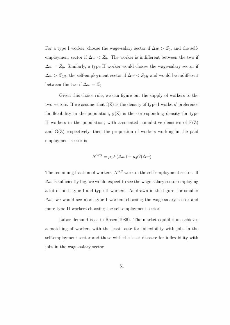
For a type I worker, choose the wage-salary sector if ∆w > Z0, and the self-

employment sector if ∆w < Z0. The worker is indifferent between the two if

∆w = Z0. Similarly, a type II worker would choose the wage-salary sector if

∆w > Z0H , the self-employment sector if ∆w < Z0H and would be indifferent

between the two if ∆w = Z0.

Given this choice rule, we can figure out the supply of workers to the

two sectors. If we assume that f(Z) is the density of type I workers’ preference

for flexibility in the population, g(Z) is the corresponding density for type

II workers in the population, with associated cumulative densities of F(Z)

and G(Z) respectively, then the proportion of workers working in the paid

employment sector is

NWS = µ1F (∆w) + µ2G(∆w)

The remaining fraction of workers, NSE work in the self-employment sector. If

∆w is sufficiently big, we would expect to see the wage-salary sector employing

a lot of both type I and type II workers. As drawn in the figure, for smaller

∆w, we would see more type I workers choosing the wage-salary sector and

more type II workers choosing the self-employment sector.

Labor demand is as in Rosen(1986). The market equilibrium achieves

a matching of workers with the least taste for inflexibility with jobs in the

self-employment sector and those with the least distaste for inflexibility with

jobs in the wage-salary sector.

51

From Figure 1, we can predict how a change in ph affects the supply of

workers to the two sectors. A decrease in ph reduces the gap between C0 and

C0H and all else equal, switches more type I workers into the self-employment

sector. This is the empirical prediction I propose to test in section IV.

3.3 Data and Descriptive Statistics

I use the Current Population Survey (CPS) data, which is a nation-

ally representative survey of over 50,000 households. Every March, the survey

collects detailed information on personal and family characteristics of respon-

dents, labor force variables and health insurance status in the previous calendar

year. However in the March files before 1989, owner-operators of incorporated

businesses were coded as wage-salary workers. This is problematic for my anal-

ysis. Fortunately, the May CPS data files contain one question pertaining to

the current job of the respondent, where both the unincorporated and incorpo-

rated self-employed are separately classified. Thus for the 1984 and 1985 years,

I match the March and May CPS files and create a sample of women workers

for the pre-TRA86 period. This way, I get all the data on labor force and per-

sonal characteristics and health insurance status from the March files and a

correct identification of self-employed workers from the May files. However the

labor force information pertains to the main job during the week prior to the

survey while the health information refers to the longest job held the previous

year. While this is likely to cause a mismatch between job characteristics and

insurance status for a subset of our sample, a number of papers (Swartz (1986)

52

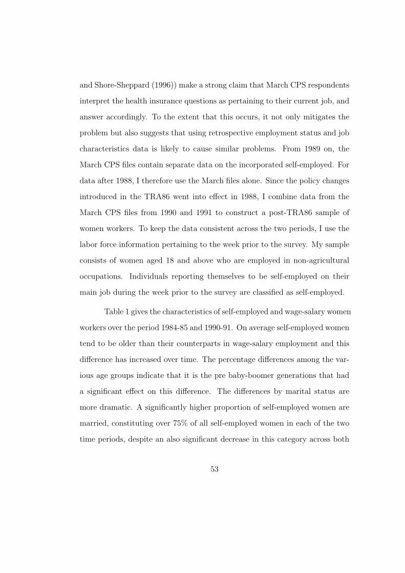
and Shore-Sheppard (1996)) make a strong claim that March CPS respondents

interpret the health insurance questions as pertaining to their current job, and

answer accordingly. To the extent that this occurs, it not only mitigates the

problem but also suggests that using retrospective employment status and job

characteristics data is likely to cause similar problems. From 1989 on, the

March CPS files contain separate data on the incorporated self-employed. For

data after 1988, I therefore use the March files alone. Since the policy changes

introduced in the TRA86 went into effect in 1988, I combine data from the

March CPS files from 1990 and 1991 to construct a post-TRA86 sample of

women workers. To keep the data consistent across the two periods, I use the

labor force information pertaining to the week prior to the survey. My sample

consists of women aged 18 and above who are employed in non-agricultural

occupations. Individuals reporting themselves to be self-employed on their

main job during the week prior to the survey are classified as self-employed.

Table 1 gives the characteristics of self-employed and wage-salary women

workers over the period 1984-85 and 1990-91. On average self-employed women

tend to be older than their counterparts in wage-salary employment and this

difference has increased over time. The percentage differences among the var-

ious age groups indicate that it is the pre baby-boomer generations that had

a significant effect on this difference. The differences by marital status are

more dramatic. A significantly higher proportion of self-employed women are

married, constituting over 75% of all self-employed women in each of the two

time periods, despite an also significant decrease in this category across both

53

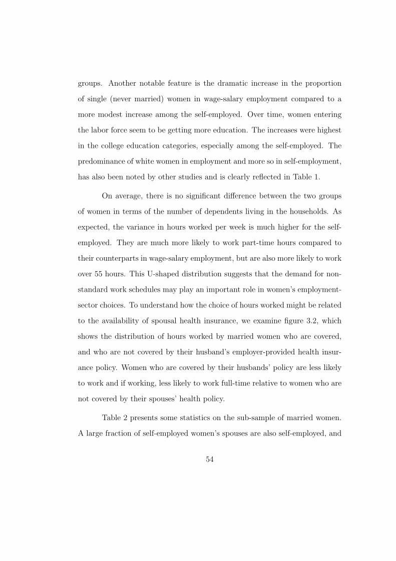
groups. Another notable feature is the dramatic increase in the proportion

of single (never married) women in wage-salary employment compared to a

more modest increase among the self-employed. Over time, women entering

the labor force seem to be getting more education. The increases were highest

in the college education categories, especially among the self-employed. The

predominance of white women in employment and more so in self-employment,

has also been noted by other studies and is clearly reflected in Table 1.

On average, there is no significant difference between the two groups

of women in terms of the number of dependents living in the households. As

expected, the variance in hours worked per week is much higher for the self-

employed. They are much more likely to work part-time hours compared to

their counterparts in wage-salary employment, but are also more likely to work

over 55 hours. This U-shaped distribution suggests that the demand for non-

standard work schedules may play an important role in women’s employment-

sector choices. To understand how the choice of hours worked might be related

to the availability of spousal health insurance, we examine figure 3.2, which

shows the distribution of hours worked by married women who are covered,

and who are not covered by their husband’s employer-provided health insur-

ance policy. Women who are covered by their husbands’ policy are less likely

to work and if working, less likely to work full-time relative to women who are

not covered by their spouses’ health policy.

Table 2 presents some statistics on the sub-sample of married women.

A large fraction of self-employed women’s spouses are also self-employed, and

54

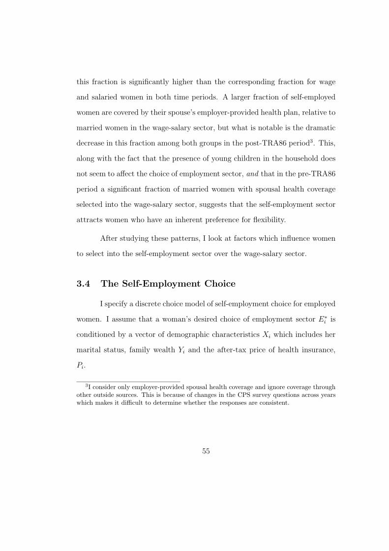
this fraction is significantly higher than the corresponding fraction for wage

and salaried women in both time periods. A larger fraction of self-employed

women are covered by their spouse’s employer-provided health plan, relative to

married women in the wage-salary sector, but what is notable is the dramatic

decrease in this fraction among both groups in the post-TRA86 period3. This,

along with the fact that the presence of young children in the household does

not seem to affect the choice of employment sector, and that in the pre-TRA86

period a significant fraction of married women with spousal health coverage

selected into the wage-salary sector, suggests that the self-employment sector

attracts women who have an inherent preference for flexibility.

After studying these patterns, I look at factors which influence women

to select into the self-employment sector over the wage-salary sector.

3.4 The Self-Employment Choice

I specify a discrete choice model of self-employment choice for employed

women. I assume that a woman’s desired choice of employment sector E∗i is

conditioned by a vector of demographic characteristics Xi which includes her

marital status, family wealth Yi and the after-tax price of health insurance,

Pi.

3I consider only employer-provided spousal health coverage and ignore coverage throughother outside sources. This is because of changes in the CPS survey questions across yearswhich makes it difficult to determine whether the responses are consistent.

55

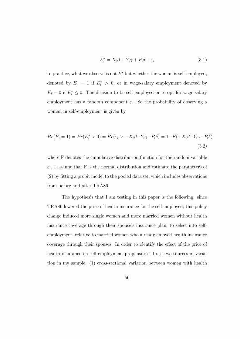
E∗i = Xiβ + Yiγ + Piδ + εi (3.1)

In practice, what we observe is not E∗i but whether the woman is self-employed,

denoted by Ei = 1 if E∗i > 0, or in wage-salary employment denoted by

Ei = 0 if E∗i ≤ 0. The decision to be self-employed or to opt for wage-salary

employment has a random component εi. So the probability of observing a

woman in self-employment is given by

Pr(Ei = 1) = Pr(E∗i > 0) = Pr(εi > −Xiβ−Yiγ−Piδ) = 1−F (−Xiβ−Yiγ−Piδ)

(3.2)

where F denotes the cumulative distribution function for the random variable

εi. I assume that F is the normal distribution and estimate the parameters of

(2) by fitting a probit model to the pooled data set, which includes observations

from before and after TRA86.

The hypothesis that I am testing in this paper is the following: since

TRA86 lowered the price of health insurance for the self-employed, this policy

change induced more single women and more married women without health

insurance coverage through their spouse’s insurance plan, to select into self-

employment, relative to married women who already enjoyed health insurance

coverage through their spouses. In order to identify the effect of the price of

health insurance on self-employment propensities, I use two sources of varia-

tion in my sample: (1) cross-sectional variation between women with health

56

insurance coverage through their spouses versus women without; and (2) time-

series variation, before versus after TRA86.

Each of these sources is likely to be correlated with other factors af-

fecting the incidence of self-employment. From the time-series variation alone,

it is difficult to disentangle other shifts that affect the attractiveness of the

self-employment sector vis-a-vis the wage-salary sector over this time period.

The cross-sectional variation may be driven by different attitudes towards risk

(Gruber and Poterba, 1994). By using both these degrees of variation how-

ever, I can eliminate spurious factors correlated with each degree of variation

individually and arrive at an estimate that denotes the effect of TRA86 on

the assignment of women across the two sectors of employment. This is the

difference-in-difference approach that I will use below.

The tax incentives for health insurance purchases by women who were

already covered through their spouse’s health plan did not change around

TRA86: “...TRA86 includes a provision disqualifying self-employed individ-

uals who are eligible for insurance coverage through a spouse from taking

advantage of the tax subsidy.” (Gruber and Poterba (1994), p. 723, fn 22).

Therefore, this group serves as a good ‘control’ group, and the difference-in-

difference estimate is given by the following equation:

∆2 = (SE1991a − SE1985

a )− (SE1991b − SE1985

b ) (3.3)

where SEt denotes the percentage self-employed at period t and the subscripts

57

a and b refer to our comparison groups - either single and married women

respectively or women without and with spousal health coverage, respectively.

3.5 Estimates

Table 3 presents results from the probit equations such as those speci-

fied in equation (2). These estimates are based on the entire sample of single

as well as married women from the pooled sample4. Each specification controls

for a detailed set of individual characteristics. The estimates presented are the

partial effects on response probabilities. For indicator variables, this estimate

reflects the effect of a discrete change of the indicator variable from 0 to 1,

on the probability of becoming self-employed. For continuous variables, this

is the estimated change in probability of becoming self-employed, due to an

infinitesimal change in the corresponding variable.

I first test for patterns observed in Table 1. The results in the first

column are broadly consistent with that of other studies, and reflect the trends

seen in Table 1. The probability of being self-employed rises with age and

education. Self-employment rates are higher for married women relative to

single women, higher for white women relative to non-whites, higher for women

4I also tried to exploit the quasi-panel structure of the CPS. In the CPS sampling rotation,households are interviewed for four consecutive months, and after a break of eight months,are interviewed again for four consecutive months. Respondents can be linked across twoyears because the second set of interviews take place in the same calendar months as the firstset of interviews (Welch, 1993). I matched individuals across the 1988 and 1989 surveys,to get a sample of women from the year before TRA86 went into effect (1987) and theconsecutive year. However, since there was little change in characteristics of the individualsacross the two years, the results were not significant, and are not reported here.

58

with children under 6 at home and residing in non-MSA areas. Women are

more likely to be self-employed in the post-TRA86 period relative to the pre-

TRA86 period5.

I next include family income from sources other than earnings as a

proxy for unearned income, to control for liquidity constraints that might

restrict women’s choice of employment sectors (Evans and Jovanovic, 1989).

This variable is measured in 2001 dollars. The results, from column 2 of Table

3, reveal that its effect is positive and significant, suggesting that family wealth

is an important determinant of entrepreneurial choice. Since TRA86 affected

the price of health insurance for the self-employed through a tax subsidy, the

subsidy was more valuable at higher tax rates. Gruber and Poterba (1994)

calculated the average after-tax price of health insurance before and after the

policy change and their calculations are presented in Table 4.

I interact the family wealth variable with the indicator for the post-

TRA86 period to test for a differential effect of the tax subsidy by wealth

status. The results are presented in column 3 of Table 3. While the wealth

effect continues to be significant, the interaction term has no effect on the self-

employment propensity.6 One explanation for this result is that the constraint

5I have not included industry and occupation controls on the grounds that the industryand occupation choices may be jointly determined with the self-employment choice.

6The TRA86 also lowered marginal tax rates significantly. Eissa (1995) showed that thelabor force participation of high-income married women increased as a result. One couldargue that it is this group that is responsible for the increased incidence of self-employmentafter TRA86. However, from the results in column 3, we cannot reject the hypothesisthat after TRA86 wealthier women were as likely to be in self-employment as in wage-employment. This suggests that increases in self-employment rates after the reform were

59

of a higher cost of health insurance is not binding for the wealthy and therefore

TRA86 made essentially no difference to them. Gruber and Poterba (1994)

provide an alternative explanation. In their view, individuals are prone to

what they term ‘recognition effects’ as far as discrete decisions are concerned.

Here, this means that the magnitude of the tax subsidy is less important than

the introduction of the subsidy itself, which leads people to reevaluate their

options and make new choices - switching from not being insured to purchasing

health insurance, moving from the wage-salary sector to the self-employment

sector and so on.

Since the core of my analysis depends on whether or not a married

woman has health coverage through her spouse’s health plan, I matched the

husband-wife pairs in the data. All persons 15 years and older in the survey

who worked in the previous calendar year were asked if they participated in

group health insurance plans offered by their employers. If they answered

in the affirmative, they were asked whether their spouse was also covered

by the plan. I used the responses to these questions to ascertain whether

a married woman had health insurance coverage through her spouse. This

variable proxies for the price of health insurance; women who benefit from their

spouse’s health plan can be thought of as paying a smaller price for selecting

into self-employment, relative to women who do not enjoy this benefit.

I present the results on self-employment propensities controlling for

not driven by changes in the marginal tax rates alone.

60

the presence of spousal health insurance coverage in column 1 of Table 5.

The health insurance variable has a positive and highly significant coefficient,

suggesting that health insurance coverage through the spouse significantly in-

fluences the probability of a woman becoming self-employed. Since we would

expect the value of an employer-provided family health plan to increase with

the number of children in the household (Buchmueller and Valletta, 1998), I

interact the health insurance dummy with the number of children under 18

in the family. The results are presented in column 2 of Table 5. While the

presence of children under 18 in the household has no influence by itself on the

self-employment decision, the positive and significant effect of the interaction

term does suggest that a family health insurance plan affects the propensity

towards self-employment, the more it is valued by the household.

In column 1 of table 6, I present probit estimates after adding controls

for husband’s employment sector. I excluded non-working husbands from the

sample on the grounds that they might be experiencing temporary, frictional

unemployment. I also excluded working husbands who did not report their

average weekly hours of work. These restrictions caused a significant drop

in the sample size. As seen in the descriptive statistics, the probability of

self-employment is significantly higher if the spouse is also self-employed. One

interpretation of this result is that it reflects positive assortative matching in

the marriage market (Becker, 1973). This explanation is also consistent with

the notion that selection into the self-employment sector reflects a preference

for flexibility, after controlling for the number of children in the household.

61

In summary, these results indicate that health coverage through the

husband’s health plan, after controlling for the husband’s employment sector,

positively affects the wife’s selection into self-employment, a point made by

Lombard (2001). I also control for hours worked by the husband to test for

possible complementarities in the family’s time allocation choices. The results

are presented in column 2 of table 6. Again, after controlling for the husband’s

sector of employment and health insurance status, we find that women whose

husbands work over 55 hours a week on average, are more likely to be self-

employed.

The results from the probit estimates above suggest that a woman’s

propensity to be self-employed is significantly affected by the availability of

health insurance coverage through her spouse. This lends strong support to the

hypothesis that the externality caused by the extension of health coverage for

the wife through the husband’s private, employer-provided health plan creates

an important price wedge between married and single women. This price

effect in turn seems to affect the assignment of women across different sectors

of the economy. Single women who wish to be self-employed may be unable to

exercise their preference because the price of selecting into their desired sector

of employment may be too high. However, there may be several other reasons

why a single woman might not select into self-employment. By comparing

single women with similar characteristics before and after the tax reform, we

can control for these other factors influencing the decision to become self-

employed that may be correlated with being single. By comparing the change

62

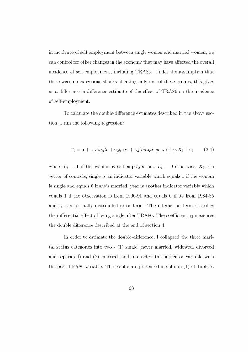
in incidence of self-employment between single women and married women, we

can control for other changes in the economy that may have affected the overall

incidence of self-employment, including TRA86. Under the assumption that

there were no exogenous shocks affecting only one of these groups, this gives

us a difference-in-difference estimate of the effect of TRA86 on the incidence

of self-employment.

To calculate the double-difference estimates described in the above sec-

tion, I run the following regression:

Ei = α + γ1single + γ2year + γ3(single.year) + γ4Xi + εi (3.4)

where Ei = 1 if the woman is self-employed and Ei = 0 otherwise, Xi is a

vector of controls, single is an indicator variable which equals 1 if the woman

is single and equals 0 if she’s married, year is another indicator variable which

equals 1 if the observation is from 1990-91 and equals 0 if its from 1984-85

and εi is a normally distributed error term. The interaction term describes

the differential effect of being single after TRA86. The coefficient γ3 measures

the double difference described at the end of section 4.

In order to estimate the double-difference, I collapsed the three mari-

tal status categories into two - (1) single (never married, widowed, divorced

and separated) and (2) married, and interacted this indicator variable with

the post-TRA86 variable. The results are presented in column (1) of Table 7.

63

Although the effect of being single is still negative and dominates the interac-

tion term, the differential effect of being single in the post-TRA86 period is

positive and statistically significant. This suggests that single women in the

post-TRA86 period are more likely to take up self-employment, as our theory

predicts. To understand what is driving these results, I re-estimated this re-

gression using the original specification of marital categories. The results are

presented in column (2) of Table 7. Its clear from these results that TRA86

affected the self-employment propensities of the divorced/widowed/separated

women, and does not seem to have affected the employment sector choices of

the never married category of women, even after controlling for age7.

Even if we acknowledge the endogeneity of spousal health insurance,

single women serve as the “uncontaminated” sub-group of our treatment group

for TRA86 since they do not have access to spousal health insurance. More-

over, as mentioned already, in addition to introducing the tax subsidy for the

self-employed, TRA86 also significantly lowered marginal tax rates; it lowered

the top marginal tax rate by 44% but the decrease was less significant for those

in the lower end of the income distribution (Feldstein, 1986). Eissa (1995)

showed that the labor force participation of high-income married women in-

creased after TRA86, as a result of the decrease in the marginal tax rate. Since

married women are believed to be more responsive to a given change in the

tax rate compared to other demographic groups, the positive and significant

differential effect of single women in the post-reform period after controlling

7On average, women who have never been married are younger than married women.

64

for any changes in labor supply of married women is a strong test of the ef-

fect of TRA86 on self-employment propensities. Besides, Gruber and Poterba

(1994) state in their paper that in 1988-89, less than one-half of self-employed

tax filers in most income classes claimed the tax subsidy (p.723, fn 23). This

suggests that the estimates presented here understate the effect of the tax

subsidy on self-employment rates.

3.6 Conclusions

In this chapter, my focus of study has been the effect of the husband’s

employer-provided family health insurance on the wife’s propensity to select

into self-employment. A number of papers have found an association between

a married woman’s labor supply behavior and spousal health insurance. A

consistent finding in the literature on women’s self-employment in the US since

the mid-1970s is the predominance of married women in this sector. While

numerous papers have remarked on the relationship between spousal health

insurance and a married woman’s propensity to select into self-employment,

no clean test of this linkage was established.

The Tax Reform Act of 1986 provides us with an opportunity to test

this linkage. The TRA86 introduced a tax subsidy for the self-employed to

purchase health insurance. At the same time, it disqualified self-employed indi-

viduals who were already enjoying health insurance benefits through a spouse

from taking advantage of the subsidy. Since the effect of the tax subsidy

was to lower the after-tax price of health insurance for those among the self-

65

employed who were purchasing their own health insurance, I predict that this

subsidy increased the incidence of self-employment among single women. My

estimates suggest that health insurance coverage through the spouse biased a

married woman’s employment sector choice strongly towards self-employment

in the pre-TRA86 period. Moreover, the incidence of single women in self-

employment went up significantly in the post-TRA86 period, after control-

ling for the effect of health insurance coverage through the spouse. This

finding supports my hypothesis that the decrease in the price of health in-

surance through the tax subsidy induced more single women to select into

self-employment in the post-TRA86 period relative to married women.

In summary, my findings suggest that in the pre-TRA86 period, the

high cost of health insurance created a price wedge between women who en-

joyed health insurance coverage through their spouse’s health plan and those

who did not. Women who had a preference for working in the self-employment

sector and who enjoyed spousal health benefits were able to exercise their pref-

erence and select into self-employment. On the other hand, for women with

a preference for the self-employment sector but constrained to purchase their

own health insurance, it was too costly to opt for this sector. For these women,

the TRA86, by narrowing this price wedge, lowered the price of selecting into

their desired sector of employment.

66

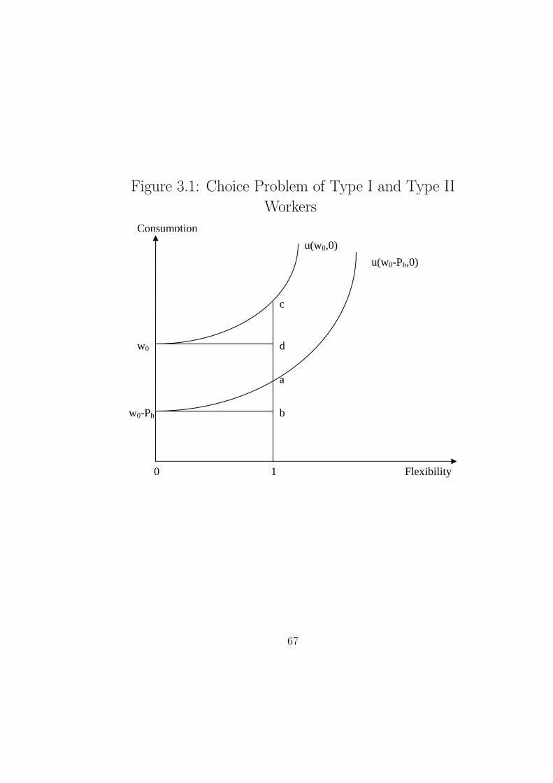
Figure 3.1: Choice Problem of Type I and Type II

Workers

Consumption

u(w0,0)

u(w0-Ph,0)

w0

w0-Ph

1 0 Flexibility

b

a

d

c

67

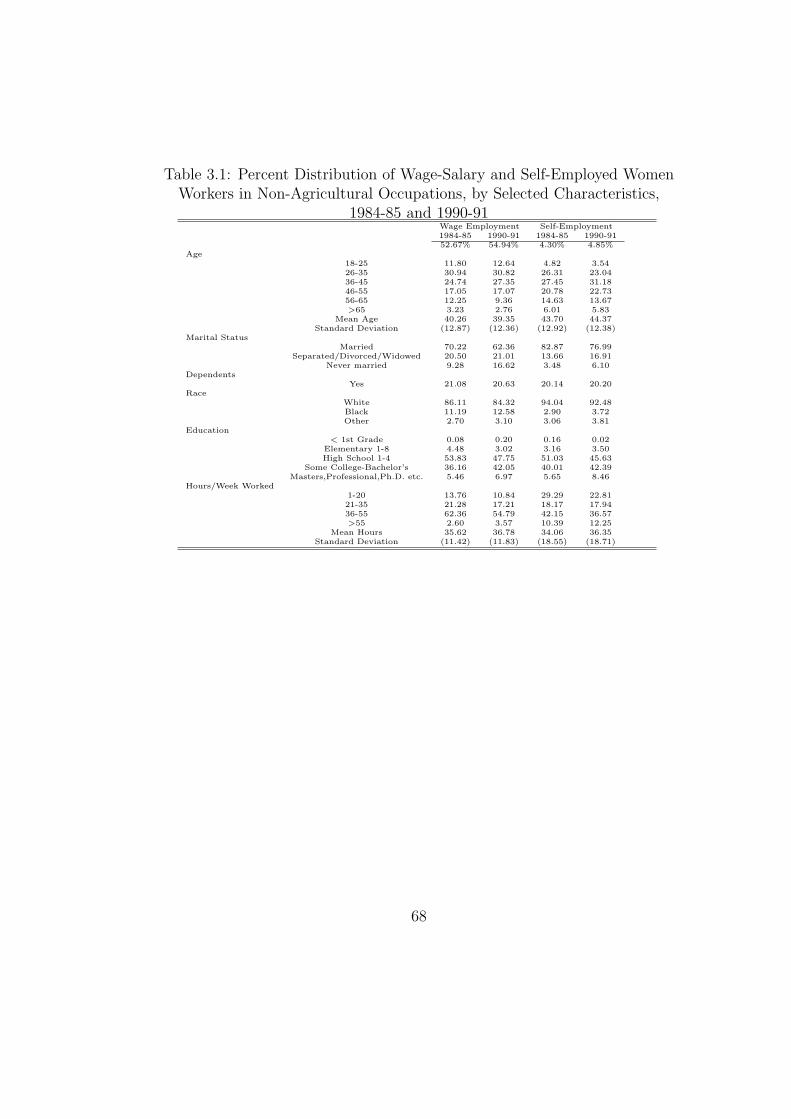
Table 3.1: Percent Distribution of Wage-Salary and Self-Employed WomenWorkers in Non-Agricultural Occupations, by Selected Characteristics,

1984-85 and 1990-91Wage Employment Self-Employment1984-85 1990-91 1984-85 1990-9152.67% 54.94% 4.30% 4.85%

Age18-25 11.80 12.64 4.82 3.5426-35 30.94 30.82 26.31 23.0436-45 24.74 27.35 27.45 31.1846-55 17.05 17.07 20.78 22.7356-65 12.25 9.36 14.63 13.67>65 3.23 2.76 6.01 5.83

Mean Age 40.26 39.35 43.70 44.37Standard Deviation (12.87) (12.36) (12.92) (12.38)

Marital StatusMarried 70.22 62.36 82.87 76.99

Separated/Divorced/Widowed 20.50 21.01 13.66 16.91Never married 9.28 16.62 3.48 6.10

DependentsYes 21.08 20.63 20.14 20.20

RaceWhite 86.11 84.32 94.04 92.48Black 11.19 12.58 2.90 3.72Other 2.70 3.10 3.06 3.81

Education< 1st Grade 0.08 0.20 0.16 0.02

Elementary 1-8 4.48 3.02 3.16 3.50High School 1-4 53.83 47.75 51.03 45.63

Some College-Bachelor’s 36.16 42.05 40.01 42.39Masters,Professional,Ph.D. etc. 5.46 6.97 5.65 8.46

Hours/Week Worked1-20 13.76 10.84 29.29 22.8121-35 21.28 17.21 18.17 17.9436-55 62.36 54.79 42.15 36.57>55 2.60 3.57 10.39 12.25

Mean Hours 35.62 36.78 34.06 36.35Standard Deviation (11.42) (11.83) (18.55) (18.71)

68

Table 3.2: Percent Distribution of Self-Employed and Wage-Salary MarriedWomen Workers in Non-Agricultural Occupations, by Selected

CharacteristicsWage Employment Self-Employment1984-85 1990-91 1984-85 1990-9152.67% 54.94% 4.30% 4.85%

Husband is Self-EmployedYes 12.47 11.43 42.19 43.91

Covered by Spouse’sEmployer-Provided Health Plan

Yes 21.00 11.05 25.69 12.57of which:

Employer Paid forAll/Part of plan 95.95 90.72 94.56 77.01

69

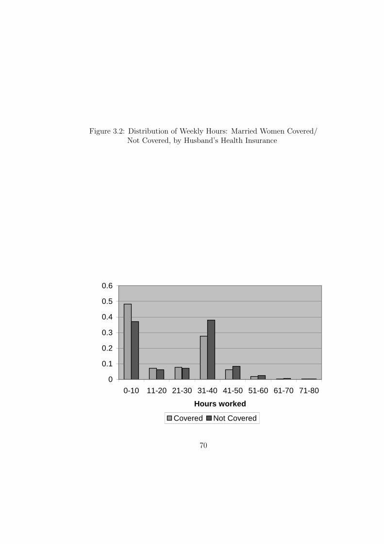
Figure 3.2: Distribution of Weekly Hours: Married Women Covered/Not Covered, by Husband’s Health Insurance

0

0.1

0.2

0.3

0.4

0.5

0.6

0-10 11-20 21-30 31-40 41-50 51-60 61-70 71-80

Hours worked

Covered Not Covered

70

Table 3.3: Probit Estimates of Women’s Self-Employment Choices:Partial Effects on Response Probabilities

(1) (2) (3)Age 0.0071*** 0.00711*** 0.00712***

(0.0002) (0.0002) (0.0002)Age squared -0.00008*** -0.00008*** -0.00008***

(0.0000) (0.0000) (0.0000)Marital status (Base=Married) Separated/divorced/ -0.01061*** -0.01028*** -0.01029***

widowed (0.0011) (0.0011) (0.0011)

Never married -0.01621*** -0.01603*** -0.01604***(0.0015) (0.0015) (0.0015)

Post-TRA86 0.00666*** 0.00664*** 0.00375***(0.0012) (0.0012) (0.0014)

Children age<6 0.0037*** 0.00375*** 0.00375***(0.0014) (0.0014) (0.0014)

Race (Base=White) Black -0.0273*** -0.02717*** -0.02717***(0.0012) (0.0012) (0.0012)

Other race -0.00439* -0.00431* -0.0043*(0.0025) (0.0025) (0.0025)

Education (Base=No school) Primary school (1-8) 0.05286*** 0.05292*** 0.05292***(0.0258) (0.0258) (0.0258)

High school (1-4) 0.0576*** 0.05716*** 0.05717***(0.0150) (0.015) (0.1499)

Upto 5 years of college .08778*** .08664*** 0.08665***(0.0237) (0.0236) (0.0236)

> 5 years of college 0.14474*** 0.14208*** 0.14209***(0.0430) (0.0426) (0426)

Non-MSA 0.00866*** 0.00874*** 0.00874***(0.0013) (0.0013) (0.0013)

Family income>50,000 0.01043*** 0.01439**(2000 dollars) (0.0032) (0.0067)Family income*Post-TRA86 -0.00403

(0.0054)

Number of observations 146,656 146,656 146,656

Note: Figures in parentheses are (robust) standard errors. All regressions include state controls.

*** - significant at the 99% level; ** - significant at the 95% level;* - significant at the 90% level

71

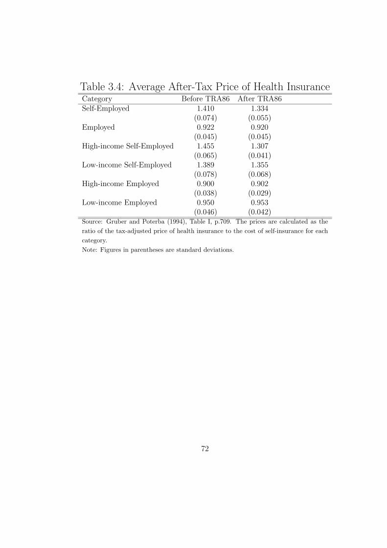
Table 3.4: Average After-Tax Price of Health InsuranceCategory Before TRA86 After TRA86Self-Employed 1.410 1.334

(0.074) (0.055)Employed 0.922 0.920

(0.045) (0.045)High-income Self-Employed 1.455 1.307

(0.065) (0.041)Low-income Self-Employed 1.389 1.355

(0.078) (0.068)High-income Employed 0.900 0.902

(0.038) (0.029)Low-income Employed 0.950 0.953

(0.046) (0.042)Source: Gruber and Poterba (1994), Table I, p.709. The prices are calculated as theratio of the tax-adjusted price of health insurance to the cost of self-insurance for eachcategory.Note: Figures in parentheses are standard deviations.

72

Table 3.5: Probit Estimates of Women’s Self-Employment Choices: PartialEffects on Response Probabilities

(1) (2)Age 0.007*** 0.00686***

(0.0002) (0.0002)Age squared -0.00008*** -0.00007***

(0.0000) (0.0000)

Marital status (Base=Married) Separated/divorced/ -0.00684*** -0.00731***widowed (0.0013) (0.0013)

Never married -0.01323*** -0.01411***(0.0016) (0.0016)

Post-TRA86 0.00376*** 0.00439***(0.0014) (0.0013)

Children age<6 0.00376***(0.0014)

Race (Base=White) Black -0.02691*** -0.02677***(0.0012) (0.0012)

Other race -0.00387 -0.0038(0.0025) (0.0025)

Education (Base=No school) Primary school (1-8) 0.05171*** 0.05137***(0.0255) (0.0255)

High school (1-4) 0.05568*** 0.05545***(0.0149) (0.0149)

Upto 5 years of college 0.08403*** 0.08347***(0.0233) (0.0232)

> 5 years of college 0.13832*** 0.13753***(0.042) (0.0419)

Non-MSA 0.00899*** 0.00896***(0.0013) (0.0013)

Family income>50,000 0.01291*** 0.01277**(2000 dollars) (0.0065) (0.0065)Family income*Post-TRA86 -0.00297 -0.00256

(0.0056) (0.0056)Covered by husband’s 0.00777*** 0.00565***health plan=yes (0.0012) (0.0015)

Children age <18 -0.00039(0.0006)

Children age <18*Family health 0.00222*insurance plan (0.0009)

Number of observations 146,656 146,656

Note: Figures in parentheses are (robust) standard errors. All regressions include state controls.

*** - significant at the 99% level; ** - significant at the 95% level;* - significant at the 90% level

73

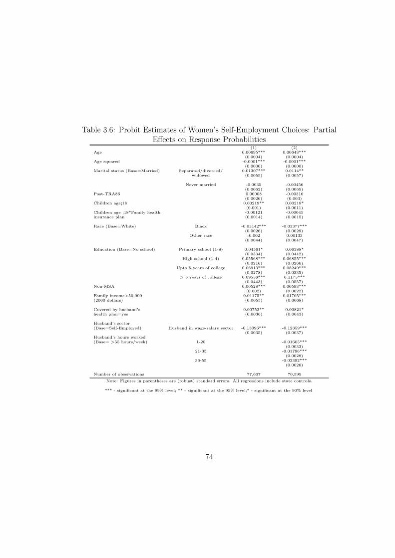
Table 3.6: Probit Estimates of Women’s Self-Employment Choices: PartialEffects on Response Probabilities

(1) (2)Age 0.00695*** 0.00643***

(0.0004) (0.0004)Age squared -0.0001*** -0.0001***

(0.0000) (0.0000)Marital status (Base=Married) Separated/divorced/ 0.01307*** 0.0114**

widowed (0.0055) (0.0057)

Never married -0.0035 -0.00456(0.0062) (0.0065)

Post-TRA86 0.00008 -0.00316(0.0026) (0.003)

Children age¡18 0.00219** 0.00218*(0.001) (0.0011)

Children age ¡18*Family health -0.00121 -0.00045insurance plan (0.0014) (0.0015)

Race (Base=White) Black -0.03142*** -0.03377***(0.0026) (0.0029)

Other race -0.002 0.00133(0.0044) (0.0047)

Education (Base=No school) Primary school (1-8) 0.04561* 0.06388*(0.0334) (0.0442)

High school (1-4) 0.05568*** 0.06855***(0.0216) (0.0266)

Upto 5 years of college 0.06913*** 0.08249***(0.0278) (0.0335)

> 5 years of college 0.09558*** 0.1175***(0.0443) (0.0557)

Non-MSA 0.00528*** 0.00593***(0.002) (0.0022)

Family income>50,000 0.01175** 0.01705***(2000 dollars) (0.0055) (0.0068)

Covered by husband’s 0.00753** 0.00821*health plan=yes (0.0036) (0.0043)

Husband’s sector(Base=Self-Employed) Husband in wage-salary sector -0.13096*** -0.12359***

(0.0035) (0.0037)Husband’s hours worked(Base= >55 hours/week) 1-20 -0.01605***

(0.0033)21-35 -0.01796***

(0.0028)36-55 -0.02392***

(0.0026)

Number of observations 77,607 70,595

Note: Figures in parentheses are (robust) standard errors. All regressions include state controls.

*** - significant at the 99% level; ** - significant at the 95% level;* - significant at the 90% level

74

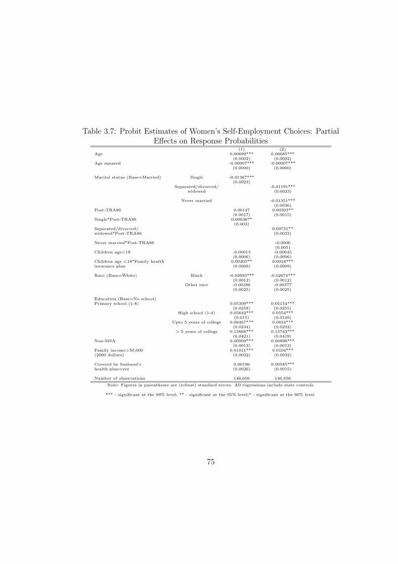
Table 3.7: Probit Estimates of Women’s Self-Employment Choices: PartialEffects on Response Probabilities

(1) (2)Age 0.00699*** 0.00685***

(0.0002) (0.0002)Age squared -0.00007*** -0.00007***

(0.0000) (0.0000)

Marital status (Base=Married) Single -0.01367***(0.0023)

Separated/divorced/ -0.01191***widowed (0.0023)

Never married -0.01351***(0.0036)

Post-TRA86 0.00147 0.00303**(0.0017) (0.0015)

Single*Post-TRA86 0.00636**(0.003)

Separated/divorced/ 0.00731**widowed*Post-TRA86 (0.0033)

Never married*Post-TRA86 -0.0006(0.005)

Children age<18 -0.00013 -0.00045(0.0006) (0.0006)

Children age <18*Family health 0.00205** 0.0024***insurance plan (0.0009) (0.0009)

Race (Base=White) Black -0.02693*** -0.02674***(0.0012) (0.0012)

Other race -0.00386 -0.00377(0.0025) (0.0025)

Education (Base=No school)Primary school (1-8) 0.05309*** 0.05154***

(0.0258) (0.0255)High school (1-4) 0.05642*** 0.0554***

(0.015) (0.0149)Upto 5 years of college 0.08467*** 0.0834***

(0.0234) (0.0232)> 5 years of college 0.13868*** 0.13743***

(0.0421) (0.0419)Non-MSA 0.00909*** 0.00896***

(0.0013) (0.0013)Family income>50,000 0.01011*** 0.0104***(2000 dollars) (0.0032) (0.0032)

Covered by husband’s 0.00196 0.00585***health plan=yes (0.0026) (0.0015)

Number of observations 146,656 146,656

Note: Figures in parentheses are (robust) standard errors. All regressions include state controls.

*** - significant at the 99% level; ** - significant at the 95% level;* - significant at the 90% level

75

Chapter 4

Job Attachment Patterns of Men and Women:

The Role of Promotion Expectations and

Experience

4.1 Introduction

In documenting the pattern of lifetime jobs in the US using data from

the 1968-1978 period, Hall(1982) found that on average, women’s jobs were of

substantially shorter duration relative to men’s jobs. According to Hall, this

higher job turnover for women was a consequence of the long stretches of time

they spent out of the labor force. Researchers have studied the implications

of these gender differences in turnover behavior on various labor market out-

comes. Ureta (1995) examined the effect of non-employment spells on wage

growth, by studying the timing and frequency of non-work spells for a sample

of young, white workers drawn from the National Longitudinal Surveys. Her

estimates suggest that 12% of the male-female wage gap can be explained by

women’s intermittent employment spells.

One channel through which gender differences in job turnover translate

into the gender wage gap is through differential rates of promotion for men

and women; some contend that women face a ‘glass ceiling’ that prevents their

upward mobility in internal labor markets (Gjerde, 2002). According to this

76

theory, since training workers is a costly activity, firms are only willing to

invest in those workers from whom they expect to recoup the costs of training.

Given that the expected time horizon to recover these costs is shorter for

women, firms are unwilling to train their women workers. And since training

is invariably a prerequisite for promotion, promotion rates for women tend

to be smaller than those for men. These differences in promotion rates then

translate into a gender wage-gap.1

A significant increase in the labor force participation of women over

the past few decades has motivated researchers to re-examine job turnover

behavior by men and women. There is evidence suggesting that more recent

cohorts of women are as concerned about their careers as men, have a higher

propensity to stay on their jobs and are exhibiting a strong attachment to the

labor market.2 We would expect firms to treat these women - the ‘stayers’

- no differently from men. However, women workers are still a heterogenous

group comprising both ‘stayers’ and ‘quitters,’ with higher average turnover

rates than men. If firms cannot distinguish between the two types of women

workers based on observables, statistical discrimination would still result in

lower promotion rates for women and a persistence of the wage gap. If, on the

other hand, the stayers could successfully signal their intentions to stay in the

labor force and separate themselves from the quitters, they could overcome

internal labor market discrimination.

1Wages usually grow with promotions; McCue’s(1996) estimates suggest that between9%-18% of wage growth is due to promotions.

2See Prisinzano (2004), Light and Ureta(1992), and references therein.

77

Prisinzano (2004) estimated a bivariate probit model of job-stays and

promotions for men and women. His results indicate that the error terms be-

tween the job-stay equation and the promotions equations are correlated for

men, suggesting that the unobservables affecting the stay decision are corre-

lated with those affecting whether they receive a promotion or not. In contrast,

the hypothesis that the estimated correlation between the error terms in the

two equations for women is equal to zero cannot be rejected, implying that

whether women receive a promotion offer or not is uncorrelated with their

job-stay decisions. This seemingly strange result is the motivation for the cur-

rent paper. It is our view that women who are concerned about their careers

are using job attachment as a signal to indicate their attachment to the la-

bor force. We expect women with little or no job market experience to have

lower job turnover rates compared to men of similar experience, all else equal.

Therefore, during this period, we expect women to exhibit less sensitivity to

expectations of promotion, relative to men. This rationale also suggests that

once women have gained adequate labor market experience and revealed them-

selves as stayers, their job attachment patterns should respond more closely to

their expectations of promotions. Hence, we expect women with adequate job

market experience to reveal job attachment patterns similar to those of men.

Accordingly, we use a longitudinal dataset to study how the expectation

of promotion affects men’s and women’s decision to stay on a job and whether

this relative pattern varies with the amount of labor market experience. The

dataset also contains information on workers’ perceived chances of promotion

78

in their current job. We expect workers who are concerned about their careers

to be sensitive to the potential for career growth in their firms. We examine

how turnover behavior responds to this subjective likelihood of promotion and

how this response differs by gender and experience level. Our results suggest

that individuals with low expectations of promotion are less likely to stay on

their jobs relative to those with high expectations of promotion. We also find

evidence that women are more likely than men to stay on a job all else equal.

Furthermore, women with low promotion expectations are more likely than

comparable men to stay on a job and this difference is more pronounced early

in careers. The fact that the difference diminishes with experience supports

our hypothesis.

The rest of the paper is organized as follows: section 4.2 gives a de-

scription of our data, the variables used in our analysis and some descriptives

for our sample. In section 4.4, we describe the empirical models we use in our

estimation, in section 4 we discuss the results and present our conclusions in

section 4.5.

4.2 Data and Descriptives

We use data from the National Longitudinal Survey of Youth (NLSY) for

the following survey years: 1979-83, 1996, 1998 and 2000.We restricted our

sample to those who exhibited a reasonable attachment to the labor market.

We eliminated respondents who worked for less than 15 weeks per year or less

than 20 hours per week in any year. We also eliminated respondents who were

79

either self-employed, working in a farming occupation or industry, or in the

armed forces. This restriction removes those individuals that face considerably

different job and promotion structures than the typical worker.

The information on job changes and the subjective perception of pro-

motion possibilities on the current job are of particular interest for the present

study. Accordingly, we identify the respondent as a ‘job-stayer’ in a particular

year if he or she reported that the main job that year was also the main job in

the previous year. In the 1979 through 1982 surveys, the NLSY includes the

respondent’s assessment of whether the chances for promotion in the current

job are good. The responses are coded as: 1. Not true at all; 2. Not too true;

3. Somewhat true and 4. Very true. In the 1996 and 1998 surveys, a similar

question is asked as follows: “Do you believe it is possible for you to get a

promotion with this employer in the next two years?”, and the respondent

replied with a yes/no. One problem in comparing these questions is that in

the 1979-82 surveys, the question does not specify a time horizon while in the

1996 and 1998, the scope of the question is limited to two years. However, we

believe that the respondents interpreted the question as referring to a short

time horizon in the 1979-82 surveys, especially given that they were all be-

tween 15 and 25 years old. We therefore combine the first two categories in

the 1979-82 survey responses - Not true at all and Not too true - into one,

and label this as “Low chances of promotion”, and combine the other two

categories - Somewhat true and Very true - into the “High chances of promo-

tion category. In the 1996 and 1998 surveys, if the response to the promotion

80

question was No, this was categorized as “Low chances of promotion” and if

it was Yes, it was categorized as “High chances of promotion.” This way, we

construct a comparable measure of subjective perception of promotion chances

on the current job.

Tables 4.1 and 4.2 present the fraction of job-stayers and job-movers

among men and women for the two time periods, categorized by their self-

perceived chances of promotion. In the 1979-82 period, among workers who

feel they have little or no chance of promotion in their current job, a signifi-

cantly larger fraction of women workers stayed on their jobs. By contrast, a

much higher fraction of men stay on in jobs in which they think that the like-

lihood of promotion is very high, relative to women. Among the job-movers,

there’s no discernible pattern among women while a significant fraction among

men, nearly 60%, move jobs even when they think they have good chances of

promotion. We observe the same pattern in the 1996-1998 period.

The summary statistics for our sample are presented in table 4.3. Women

constituted less than half the sample, as did non-whites. Although we do not

see too many differences between men and women in terms of the marital sta-

tus variables, on average, women had more children. Women were also slightly

younger and had about an extra half-year of education. This translated into

a lower average level of potential experience for women. As expected, women

had lower mean wages, compared to men. However, a higher fraction of women

stayed on their jobs from one year to the next compared to men, despite a sub-

stantially higher fraction of women reported facing low chances of promotion

81

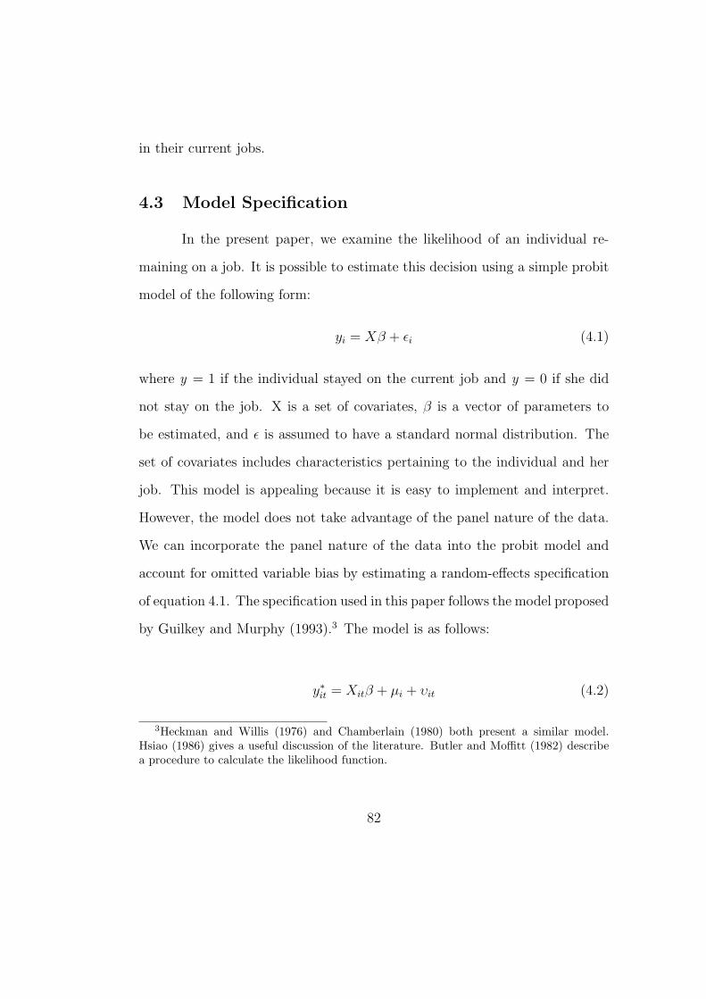
in their current jobs.

4.3 Model Specification

In the present paper, we examine the likelihood of an individual re-

maining on a job. It is possible to estimate this decision using a simple probit

model of the following form:

yi = Xβ + εi (4.1)

where y = 1 if the individual stayed on the current job and y = 0 if she did

not stay on the job. X is a set of covariates, β is a vector of parameters to

be estimated, and ε is assumed to have a standard normal distribution. The

set of covariates includes characteristics pertaining to the individual and her

job. This model is appealing because it is easy to implement and interpret.

However, the model does not take advantage of the panel nature of the data.

We can incorporate the panel nature of the data into the probit model and

account for omitted variable bias by estimating a random-effects specification

of equation 4.1. The specification used in this paper follows the model proposed

by Guilkey and Murphy (1993).3 The model is as follows:

y∗it = Xitβ + µi + υit (4.2)

3Heckman and Willis (1976) and Chamberlain (1980) both present a similar model.Hsiao (1986) gives a useful discussion of the literature. Butler and Moffitt (1982) describea procedure to calculate the likelihood function.

82

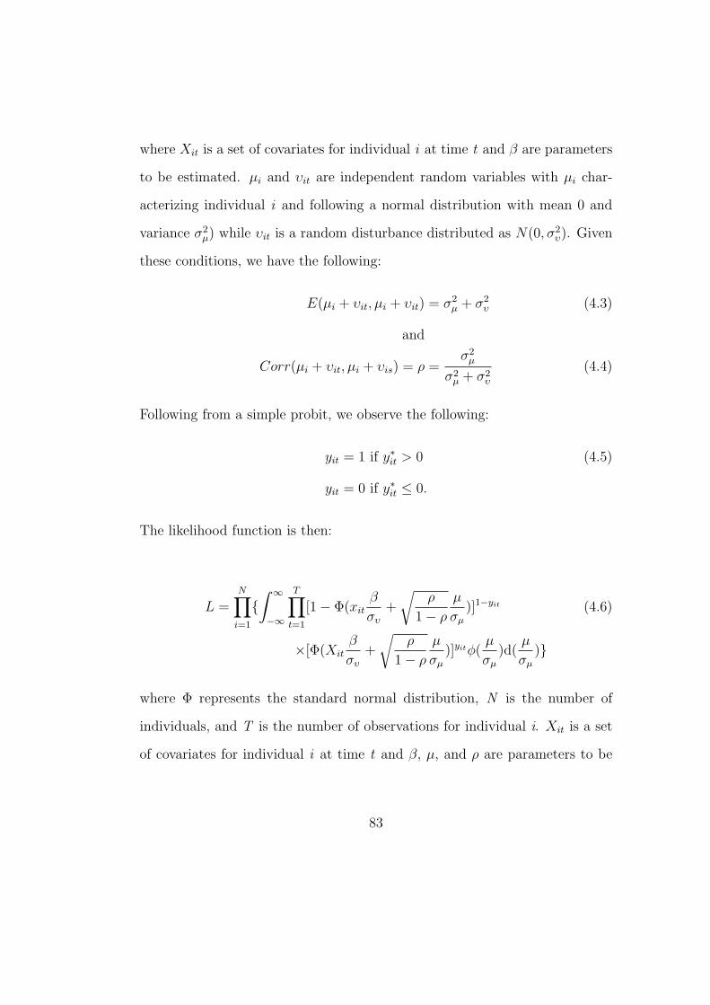
where Xit is a set of covariates for individual i at time t and β are parameters

to be estimated. µi and υit are independent random variables with µi char-

acterizing individual i and following a normal distribution with mean 0 and

variance σ2µ) while υit is a random disturbance distributed as N(0, σ2

υ). Given

these conditions, we have the following:

E(µi + υit, µi + υit) = σ2µ + σ2

υ (4.3)

and

Corr(µi + υit, µi + υis) = ρ =σ2

µ

σ2µ + σ2

υ

(4.4)

Following from a simple probit, we observe the following:

yit = 1 if y∗it > 0 (4.5)

yit = 0 if y∗it ≤ 0.

The likelihood function is then:

L =N∏

i=1

{∫ ∞

−∞

T∏t=1

[1− Φ(xitβ

συ

+

√ρ

1− ρ

µ

σµ

)]1−yit (4.6)

×[Φ(Xitβ

συ

+

√ρ

1− ρ

µ

σµ

)]yitφ(µ

σµ

)d(µ

σµ

)}

where Φ represents the standard normal distribution, N is the number of

individuals, and T is the number of observations for individual i. Xit is a set

of covariates for individual i at time t and β, µ, and ρ are parameters to be

83

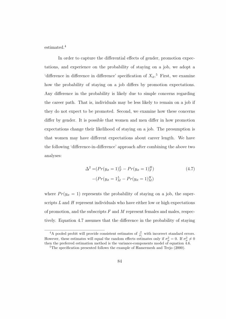
estimated.4

In order to capture the differential effects of gender, promotion expec-

tations, and experience on the probability of staying on a job, we adopt a

‘difference in difference in difference’ specification of Xit.5 First, we examine

how the probability of staying on a job differs by promotion expectations.

Any difference in the probability is likely due to simple concerns regarding

the career path. That is, individuals may be less likely to remain on a job if

they do not expect to be promoted. Second, we examine how these concerns

differ by gender. It is possible that women and men differ in how promotion

expectations change their likelihood of staying on a job. The presumption is

that women may have different expectations about career length. We have

the following ‘difference-in-difference’ approach after combining the above two

analyses:

∆2 =(Pr(yit = 1)LF − Pr(yit = 1)H

F ) (4.7)

−(Pr(yit = 1LM − Pr(yit = 1)H

M)

where Pr(yit = 1) represents the probability of staying on a job, the super-

scripts L and H represent individuals who have either low or high expectations

of promotion, and the subscripts F and M represent females and males, respec-

tively. Equation 4.7 assumes that the difference in the probability of staying

4A pooled probit will provide consistent estimates of βσε

with incorrect standard errors.However, these estimates will equal the random effects estimates only if σ2

µ = 0. If σ2µ 6= 0

then the preferred estimation method is the variance-components model of equation 4.6.5The specification presented follows the example of Hamermesh and Trejo (2000).

84

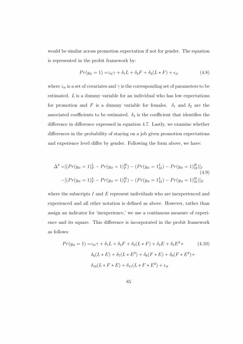
would be similar across promotion expectation if not for gender. The equation

is represented in the probit framework by:

Pr(yit = 1) =zitγ + δ1L + δ2F + δ3(L ∗ F ) + εit (4.8)

where zit is a set of covariates and γ is the corresponding set of parameters to be

estimated. L is a dummy variable for an individual who has low expectations

for promotion and F is a dummy variable for females. δ1 and δ2 are the

associated coefficients to be estimated. δ3 is the coefficient that identifies the

difference in difference expressed in equation 4.7. Lastly, we examine whether

differences in the probability of staying on a job given promotion expectations

and experience level differ by gender. Following the form above, we have:

∆3 =[(Pr(yit = 1)LF − Pr(yit = 1)H

F )− (Pr(yit = 1LM)− Pr(yit = 1)H

M)]I(4.9)

−[(Pr(yit = 1)LF − Pr(yit = 1)H

F )− (Pr(yit = 1LM)− Pr(yit = 1)H

M)]E

where the subscripts I and E represent individuals who are inexperienced and

experienced and all other notation is defined as above. However, rather than

assign an indicator for ‘inexperience,’ we use a continuous measure of experi-

ence and its square. This difference is incorporated in the probit framework

as follows:

Pr(yit = 1) =zitγ + δ1L + δ2F + δ3(L ∗ F ) + δ4E + δ5E2+ (4.10)

δ6(L ∗ E) + δ7(L ∗ E2) + δ8(F ∗ E) + δ9(F ∗ E2)+

δ10(L ∗ F ∗ E) + δ11(L ∗ F ∗ E2) + εit

85

where E and E2 are potential experience and its square, respectively while δ4

and δ5 are the associated coefficients. δ6 and δ7, and δ8 and δ9 are the pairs of

coefficients that identify the difference-in-differences for low promotion expec-

tations and inexperience, and gender and inexperience, respectively. δ10 and

δ10 are the coefficients that identify the ‘difference-in-difference-in-difference’

expressed in equation 4.9. The remaining notation is as defined above.

The above specification allows for comparisons across different groups.

We are interested in the following differences. First, we are concerned with

the difference in the likelihood of staying across gender given low promotion

expectations and the same difference given high promotion expectations. The

former difference is represented by δ2 + δ3 + δ8 + δ9 + δ10 + δ11 while the

latter difference is represented by δ2 + δ8 + δ9. Second, we are interested in

the difference in the likelihood of staying across promotion expectation given

gender. For men, this difference is represented by δ1 + δ6 + δ7. The same

difference for women is represented by δ1 + δ6 + δ7 + δ8 + δ9 + δ10 + δ11. Lastly,

we are interested in how the difference in the likelihood of staying between low

and high promotion expectation men differs from the analogous difference for

women after controlling for experience level. This difference is represented by

δ10 + δ11.

4.4 Estimates

The results from the random-effects probit models are presented in table 4.4

. The estimate of the correlation between the decision to stay on a job in

86

year t and the same decision in year t + 1, denoted by ρ, is positive and

significant. This result suggests that the random effects probit is the preferred

estimation.6 The implication of the positive sign on the correlation is that

individuals who stay on their job in year t are more likely to stay on their job

in year t + 1; in other words, certain individuals may be ‘stayers’ while others

are ‘non-stayers.’

4.4.1 Basic Results

An important determinant of staying on a job is changes in marital status. We

define changes in marital status for an individual as staying single from year t

to t + 1, remaining married from year t to t + 1, getting married between year t

and t + 1, or going from married to single between year t and t + 1. Individuals

who remain married or who get married are more likely to stay on a job than

individuals who are single, all else equal. The former group is 35% more likely

to remain on a job while the latter group is 23.5% more likely to remain on a

job.7 It is likely that this result reflects the notion that these two groups are

either more stable or desire more stability than single individuals. The stability

is likely due to the fact that individuals who are married have a dependent and

any decision is a ‘joint’ decision. The coefficient on becoming single between

two time periods is positive and significant. However, the marginal effect is

6In general, there is little difference between the pooled estimates and the random effectsestimates. However, the estimate of ρ is significantly different from zero in each modelestimated. Given this fact, we report only the results of the random effects probits.

7The predicted probability of remaining on a job at the mean levels of all continuousvariables and each dummy variable set to 0 is .5118.

87

considerably smaller than the effects associated with marriage (14%). It is not

surprising that there is a small difference in the likelihood of staying on a job

for individuals who become single and those who remain single. This difference

may reflect the fact that ‘newly’ single individuals are not that removed from

marriage and have not fully realized their single status.

Presumably, two important considerations that affect job turnover are

the wage and the potential for promotion within the firm. The former reflects

the cost to the individual of leaving the job. The coefficient on the log of the

hourly wage is positive and significant. The marginal effect associated with

the coefficient is sizable at 28.76%. This result coincides with the expectation

that the higher the wage, the higher the cost to the individual of leaving the

job. The latter is likely important to those individuals who are concerned

with a career and the associated benefits. As such, we expect individuals with

low promotion expectations to be less likely to stay on the job. Our estimate

accords with this notion; individuals who have low expectations of promotion

on their jobs are less likely to stay on their jobs.

The effect of potential experience on job turnover seems counter-intuitive;

search theory predicts that job turnover will be high at low levels of experi-

ence as workers search for a good ‘match.’ Once good job matches are made,

turnover is expected to decline. Thus, we would expect the coefficient on the

linear experience term to be positive and the one on the quadratic term to be

negative. Our results suggest the opposite pattern. A possible explanation for

this pattern is that there are differential effects of experience by gender and

88

by promotion expectation. We explore this hypothesis in subsequent specifi-

cations. However, it is important to note that the marginal effect associated

with potential experience is negligible.8

The coefficient on the gender variable is of particular interest to the

present study. Recent studies have found that women are more likely than

men to stay at jobs.9 Our result is consistent with this finding. The coefficient

on the female dummy variable is significant and positive. It suggests that

women are 12% more likely than men to stay on a job all else equal.

4.4.2 Gender-Promotion Expectation Comparisons

Column 3 of table 4.4 presents the results of the double-difference estimation.

The coefficients of particular interest are those associated with the variables

that are used in the ‘double-difference’ presented in equation 4.7. These vari-

ables are dummy variables for female and having low expectations of promo-

tion. The results from the basic specification presented in column 2 of table

4.4 suggest that women are 12% more likely to remain on a job than men all

else equal. It is not obvious why women are more likely to stay on jobs than

men. The unconditional probabilities of staying on a job are very close. In

our sample, 55.5% of men stayed on jobs while 56.9% of women stay on jobs.

This difference represents only a 2.5% increase. A reasonable explanation for

the estimated difference is that women may face a form of discrimination in

8The marginal effect of potential experience is calculated as the mean of effects in thesample.

9For example, Prisinzano (2004).

89

hiring practices. Under this condition, women may be less likely to receive

a new job offer. As such, women may hold onto jobs longer because the job

search costs they face are higher than job search costs faced by men.

If individuals are concerned with career ‘growth’, promotion expecta-

tions are likely an important consideration in the stay decision. The basic

specification supports this notion. That is, individuals with low promotion

expectations are less likely to stay on a job. The presumption is that they

will incur the costs of leaving a job in order to move to a job with more pro-

motion potential. It is also possible that individuals who have low promotion

expectations recognize they are not productive at the job. In this case, indi-

viduals may leave in order to find a job at which they are productive. The

estimation presented here does not distinguish between these possibilities but

as presented in the previous section, individuals with low promotion expec-

tations are 15% less likely to stay on a job all else equal. Considering the

magnitude of the marginal effect, it appears that promotion expectations are

an important determinant of staying on a job.

The coefficient on the interaction between female and low promotion

expectations identifies the double difference. It captures any difference in

the probability of staying on a job across promotion expectation that is due

to gender. The coefficient on the interaction is insignificant at conventional

levels. As such, it appears that women are more likely to stay on jobs than

men regardless of the promotion expectations. However, if women do need

to signal attachment to the labor market, it is likely that women with low

90

levels of experience will differ from men with low levels of experience but

women with high levels of experience will not differ from men with high levels

of experience. In order to capture this effect, we estimated the specification

presented in equation 4.10.

4.4.3 Gender-Promotion Expectation-Experience Comparisons

The results of the triple difference estimation are presented in column 6 of table

4.4 and the marginal effects of interest are in table 4.5. In the case of the control

variables, the results of the triple difference are similar to the results of the

previous specifications. In the previous estimation, we found little evidence of

‘job-shopping.’ We found that the net effect of potential experience decreased

the likelihood of staying on a job. In the current specification, we also find

this result but the inclusion of the set of interactions that identify the triple

difference changes the interpretation.10 The net effect of potential experience

differs by gender, promotion expectation, and gender-promotion expectation

group. In the case of men with high promotion expectations, the effect is

simply the net of the coefficients on the potential experience variables. The

result suggests that as potential experience increases the likelihood of staying

on a job for men with high promotion expectations decreases.11 This result

10The set of coefficients is Female, Low, Low*Female, Potential Experience, the square ofPotential Experience, Potential Experience*Low, (Potential Experience)2*Low, PotentialExperience*Female, (Potential Experience)2*Female, Potential Experience*Low*Female,and (Potential Experience)2*Low*Female. The χ2 statistic for joint significance of the fullset is 192.71 and its associated p-value is .0000.

11The χ2 statistic for joint significance of the coefficients on the potential experiencevariables is 21.99 and its associated p-value is .0000.

91

is mild evidence of negative selection for men. In the previous specifications,

we also found that individuals with low promotion expectations are less likely

to stay on a job. In the current specification, we see a different result for

men. The marginal effect associated with the coefficient on low promotion

expectations also accounts for the interaction between this variable and the

potential experience variables. The net marginal effect is .0004. This result

suggests that men with low promotion expectations are .03% more likely to

stay on a job than men with high promotion expectations.12 Even though this

result is negligible, it also reflects a negative selection of men into long tenure.

That is, men who have low promotion expectations are also less likely to find

comparable jobs in the labor market and therefore, stay on the current job.

In the double-difference specification, we found that women were 12%

more likely than men to stay on a job all else equal. In the current specification,

we also find that women are more likely to stay on a job than men. The

marginal effect associated with women also takes into account the interaction

of the potential experience variables and the female dummy variable. This

effect suggests that women who have high promotion expectations are 16.5%

more likely than men with high promotion expectations to stay on a job.13 A

possible explanation for this result is that since women are less likely to receive

a promotion, when they are likely to receive a promotion they remain on the

12The χ2 statistic for joint significance of the coefficient on low promotion expectationsand the interactions with the potential experience variables is 87.29 and its associated p-value is .0000.

13The χ2 statistic for joint significance of the coefficients on female and the interactionswith the potential experience variables is 22.61 and its associated p-value is .0000.

92

job. The presumption is that men who have high promotion expectations

may be able to find a comparable job whereas women are not able to find a

comparable job. A possible explanation for why they are not able to find a

comparable job is our signalling story. Women must signal attachment to the

labor market in order to receive promotions (and the likely wage increases).

If attachment to the labor market is observed noisily from outside a firm,

women will stay on current jobs longer than men all else equal. The difference

is highlighted when we control for promotion expectations in the estimation.

We also find that women with low promotion expectations are less likely to

stay on a job than women with high promotion expectations. The marginal

effect associated with being a women with low promotion expectations takes

into account the coefficients on the female and low promotion expectations

variables as well as each of the included interactions. The results suggest that

women with low promotion expectations are 13.8% less likely to stay on a job

than women with high promotion expectations.14 Contrary to the result for

men, it appears that there is positive selection of women into long tenure.

Given the present specification, it is possible to compare across gender

and promotion expectations. A useful comparison is women to men given low

promotion expectations. This difference in the likelihood staying on a job is

due to the turning on of the female indicator as well as the female-potential ex-

perience and female-low interactions. The marginal effect is .0122 at the mean

14The χ2 statistic for joint significance of the coefficients on low and the interactions withfemale and potential experience variables is 131.82 and its associated p-value is .0000.

93

of experience and suggests that women with low promotion expectations are

2.5% more likely to stay on job than their male counterparts.15 This differ-

ence in the likelihood of staying across gender increases if we consider men

and women with a potential experience level that is one standard deviation

below the mean. Women with low promotion expectations and ‘low’ potential

experience are 16.6% more likely than comparable men to stay on a job. This

result is of particular interest in our study. Our hypothesis is that early in

their careers women are likely to respond to promotion expectations differently

than men. Specifically, we expect women who are early in their careers to stay

on jobs for which they have low promotion expectations more often than men.

The reason for this difference is that women early in their careers must signal

an attachment to the labor market that men do not have to signal. As such,

‘job-shopping’ by women is a negative signal regarding labor force attachment.

It suggests that women who have low promotion expectations and are inexpe-

rienced are more likely to stay on a job than their male counterparts. Later

in the career, the difference in the likelihood of staying on a job between men

and women with low promotion expectations diminishes. For individuals with

a potential experience level that is one standard deviation above the mean,

women with low promotion expectations are only 12.8% more likely to remain

on a job than comparable men. Our hypothesis is that men and women’s

behavior in response to promotion expectations should be indistinguishable at

15The χ2 statistic for joint significance of the coefficients on female and the female-potential experience and female-low interactions is 43.15 and its associated p-value is .0000.

94

high levels of experience. Even though there is still a difference, this result

supports this notion.

4.4.4 Early Sample

As noted in section 4.2, the promotion expectations question in the

1979-82 surveys had four possible responses while the corresponding question

in the 1996-98 surveys had only two possible responses. In pooling the data, it

was necessary to collapse the four response categories from the earlier period

into two categories. To ensure that this restriction is not affecting our results,

we estimated the triple-difference specifications for the 1979-82 and the 1996-

1998 periods separately. In estimating the specifications for the earlier period,

we combined the two responses ‘Not true at all’ and ‘Not too true’ into one

category, ‘Low promotion expectations’ but kept the other two responses -

‘Somewhat true’ and ‘Very true’ - separate. The results are presented in

columns 2 and 3 of Table 4.6 and the marginal effects for the variables of

interest are in Table 4.7.

The results for the education, wages, children, living in MSA, race and

marital variables are all qualitatively similar to those of the pooled sample.

The coefficients on the detailed promotion expectation categories have the

expected signs; individuals who perceive their chances of promotion to be

small or moderately good are less likely to stay on the job relative to those

who believe that they have very good chances of getting promoted. Unlike in

the pooled sample, the net effect of potential experience is positive. However

95

the marginal effect still remains small and furthermore, the coefficients on the

linear and quadratic terms are not jointly significant.16

Similar to the findings in the pooled sample, we find that women are

more likely to stay on their job relative to men, regardless of promotion expec-

tations. Specifically, we find that women are 29.5%, 18.3% and 21.3% more

likely to stay on the job than their male counterparts for all low, moderate

and high promotion expectation categories, respectively. 17 Given that most of

the individuals in this sub-sample have low levels of potential experience, this

results supports our hypothesis that women stay on jobs to signal attachment

to the labor force. When we consider these marginal effects at one standard

deviation above and below the mean level of potential experience, the results

also support our hypothesis. However, we find that as potential experience

increases, the gender differences in the relative probabilities of staying on the

job also increase. This results is contrary to our expectation that as women

gain experience, their response to promotion expectations should be similar

to that of men. However, it is possible that signalling takes longer than 3.89

years.18

16The χ2 statistic for joint significance is 1.64 with a p-value of .4407.17The χ2 statistic for joint significance of the respective coefficients are 28.19, 22.02 and

11.50 with associated p-values of .0001, .0012 and .0093 respectively.18This value is the level of potential experience at one standard deviation above the mean.

96

4.4.5 Late Sample

The results of the triple difference estimation for the 1996-1998 period

are presented in column 4 and 5 of table 4.6. The marginal effects for the

variables of interest are in Table 4.8. In the case of the control variables,

these results are very similar to the results of the full sample specification.

One notable change is the coefficient on the number of children. In the full

sample estimation, the coefficient is significant and suggests that increasing

the number of children decreases the likelihood of staying on a job by 3.2%.

In the current specification, the coefficient on this variable is negative but

is insignificant and carries a considerably smaller marginal effect (-1.3%). A

possible explanation for this difference is the fact that the children in the

household are more likely to be of school age and therefore, individuals do not

have to take care of the children. One other change is the effect of experience on

the likelihood of staying on a job. In the full sample estimation, we found that

experience had a negative effect on the likelihood of staying on a job, albeit

a very small one. In this estimation, we find that experience has a positive

net effect on the likelihood of staying on a job. The effect is also considerably

larger in magnitude than the effect we found in the full sample estimation

(2.5% vs. -.6%). This result aligns with the expectation that individuals are

more likely to ‘job shop’ at low levels of experience and are more stable as

they gain experience. Similar to the result from the full sample estimation, we

find that men with low promotion expectations are 3.5% more likely to stay

on a job than men with high promotion expectations all else equal. This result

97

supports the notion that for men, there is negative selection into long tenure.

We find that women with low promotion expectations are 6.8% less

likely than women with high promotion expectations to stay on a job. In

each of the previous estimations, we found that women are more likely to stay

on jobs all else equal. This estimation yields a slightly different result. At

the mean level of potential experience (17 years), women with high promo-

tion expectations are almost 10% more likely than men with high promotion

expectations to stay on a job all else equal.19 However, women with low pro-

motion expectations are 1% less likely than their male counterparts to stay

on a job all else equal.20 This result supports our hypothesis that as women

gain experience in the labor market (and successfully signal attachment) they

will behave no differently than men. The fact that women with low promotion

expectations are less likely than their male counterparts to stay on their job

may reflect the fact that women’s careers are delayed by the need to signal

attachment to the labor force.

We find that women with low promotion expectations and potential

experience that is one standard deviation below the mean level (13.93 years)

are 2.6% more likely to stay on jobs than their male counterparts all else equal.

We also find that women with a potential experience level that is one standard

deviation above the mean level (20.7 years) and low promotion expectations

19The χ2 statistic for joint significance of the coefficient on the female indicator variableand the interactions with the potential experience variables is 9.48 with a p-value of .0235.

20The χ2 statistic for joint significance of the coefficients on female and the interactionswith low and potential experience variables is 29.97 and its associated p-value is .0000.

98

are 13% more likely to remain on a job than their male counterparts. It

appears that the gender difference in the likelihood of staying on a job given

low promotion expectations first decreases and then increases. We expect the

difference to tend toward zero and perhaps change direction as women ‘catch

up’ with men. It is possible that the result we find is due to the fact that women

may enter the labor force later than men. These women will have high levels

of potential experience but still be early in their careers. In an effort to explore

this result, we estimate the triple difference using the sample of individuals that

appear in both time periods in the following section. This sample comprises

individuals who are serious about their careers and therefore, should behave

as our signalling model suggests. It also eliminates the possibility that our

results are driven by women who know they are going to drop out of the labor

force and therefore, do not respond to promotion expectations.

4.4.6 Individuals in Both Samples

The results of the triple difference estimation are presented in columns

6 and 7 of table 4.6 while the marginal effects of the variables of interest are

presented in table 4.9. The results for the control variables do not differ sig-

nificantly from the main results presented in table 4.4 with the exception of

the coefficient on the education variable. This coefficient is insignificant in the

present specification but is significant in each of the other specifications. The

marginal effect is also considerably smaller in magnitude than other specifica-

tions at just .0025 percentage points. It also appears that experience level has

99

a negative net effect but is again relatively small at -.8% for men with high

promotion expectations.

The advantage to running the triple difference with just the sample

of individuals who appear in both time periods is that we can eliminate the

possibility that our results are driven by women who are not serious about

their careers. That is, it is likely that the full sample contains some women

who know they are going to leave the labor force and therefore, remain on

jobs despite low promotion expectations. The results presented in table 4.6

suggest that our results are not driven by this group of women. Furthermore,

the results support our signalling story. As in previous estimations, we find

that women are more likely to stay on jobs than men all else equal. Women

with high promotion expectations are 18.66% more likely to remain on jobs

than their male counterparts all else equal while women with low promotion

expectations are 2.5% more likely to remain on jobs than their male counter-

parts all else equal.21 The large difference in the likelihood of staying on a job

across gender for individuals with high promotion expectations likely reflects a

difference in the cost of finding a similar job. We also expect women to behave

more like men after they have successfully signalled attachment to the labor

force. If we consider individuals with an experience level that is one stan-

dard deviation below the mean, women with low promotion expectations are

21The χ2 statistic for joint significance of the coefficients on female and the interactionswith potential experience variables is 12.07 and its associated p-value is .0071. The χ2

statistic for joint significance of the coefficients on female and the interactions with the lowand potential experience variables is 15.74 and its associated p-value is .0076.

100

21% more likely to remain on jobs than men with low promotion expectations

all else equal. For individuals with an experience level that is one standard

deviation above the mean level, women with low promotion expectations are

only 7.5% more likely than men to remain on a job all else equal. This result

supports our explanation. It suggests that women become more responsive

to promotion expectations after they have signalled labor force attachment.

Given that our sample consists of only individuals that are attached to the

labor force, this result is strong evidence for our signalling explanation.

4.5 Conclusions

Labor economists have explained the male-female wage differential as

a consequence of women’s historic lack of attachment to the labor force. How-

ever, with a rapid rise in the female labor force participation rate over the last

few decades, the career profiles of recent cohorts of women workers has under-

gone significant changes. Studies indicate that women are now more likely to

stay on their jobs compared to men of similar characteristics. In this paper,

we examine how job turnover relates to concerns regarding a career path. We

expect to see job turnover when promotion opportunities on the job are low.

Accordingly, we study the relationship between individuals’ expectations of

promotion on their jobs and their turnover behavior. We examine how this re-

lationship varies between men and women and with experience level. It is our

hypothesis that early on in their careers, women who are strongly committed to

a career are more likely to stay on their jobs, regardless of promotion opportu-

101

nities, in a bid to signal their commitment to current and potential employers.

However, once women have acquired adequate labor market experience and

their commitment to the labor force is no longer in question, we predict that

their turnover behavior will be more responsive to career opportunities and

will be similar to that of men.

We use longitudinal data for men and women from the NLSY to test

our predictions. In order to exploit the longitudinal nature of the data, we use

a random-effects probit model to estimate the probability that an individual

will stay on a job. We estimate three models: a basic model that includes

indicator variables for female and low promotion expectations; a model that

includes an interaction between female and low promotion expectations; and a

model that includes interactions between female, low promotion expectations,

and potential experience. The results from the basic specification suggest that

as expected, individuals with low expectations of promotion are less likely

to stay on their jobs than those with high expectations of promotion. This

result is repeated in the model that allows for differences in the effect of low

promotion expectations across gender. In this model, we also find that the

tendency of women to be more likely than men to stay on a job does not

vary with promotion expectations. In the third model, we find a different

result. We find that the difference across gender in the likelihood of staying

on a job varies by potential experience. By evaluating the marginal effect of

low promotion expectations at different levels of potential experience we find

support for our hypothesis that early in their career, women are more likely

102

to stay on a job despite having low promotion expectations since they need to

signal their attachment to the labor force. Later in the career, women should

not differ from men in terms of their response to promotion expectations. Our

results suggest that while women are still more likely to remain on their job

in the face of low promotion expectations later in the career, the difference is

smaller than the difference early in the career.

We repeat the third model for three sub-samples: a 1979-82 sample, a

1996-98 sample and a sample of individuals that appear in both time periods.

The 1979-82 sample has more detailed information on promotion expectations.

This additional information strengthens our model but does not qualitatively

change the results. Similarly, the results from the 1996-98 sample do not differ

significantly from those of the pooled sample. By estimating the model using

the final sub-sample, we eliminate the possibility that our results are driven by

women who are not serious about their careers and therefore, unresponsive to

promotion expectations. These results further lend credence to our signalling

story that women at low levels of experience are more likely to stay on jobs

despite low promotion expectations than men of the same characteristics.

103

Table 4.1: Self-Reported Promotion Expectations at Job

By Mobility: 1979-1983Women

Job Stays No Stays

Response Mean Std. Dev. Mean Std. Dev.

Not True at All .1324 .339 .2484 .4322

Not True .2295 .4206 .262 .4398

True .3411 .4742 .2868 .4524

Very True .297 .4571 .2027 .4021

Observations 1586 1771

Men

Job Stays No Stays

Response Mean Std. Dev. Mean Std.Dev.

Not True at All .0874 .2826 .1639 .3703

Not True .1768 .3816 .2512 .4338

True .3654 .4817 .3288 .4699

Very True .3704 .4831 .256 .4365

Observations 1601 2074

104

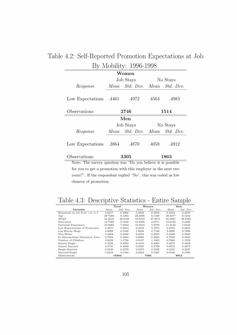
Table 4.2: Self-Reported Promotion Expectations at Job

By Mobility: 1996-1998Women

Job Stays No Stays

Response Mean Std. Dev. Mean Std. Dev.

Low Expectations .4461 .4972 .4564 .4983

Observations 2746 1514

Men

Job Stays No Stays

Response Mean Std. Dev. Mean Std. Dev.

Low Expectations .3864 .4870 .4058 .4912

Observations 3305 1863Note: The survey question was “Do you believe it is possible

for you to get a promotion with this employer in the next two

years?”. If the respondent replied “No”, this was coded as low

chances of promotion.

Table 4.3: Descriptive Statistics - Entire SampleTotal Women Men

Variable Mean Std. Dev. Mean Std. Dev. Mean Std. Dev.

Remained on job from t to t+1 0.5617 0.4962 0.5692 0.4952 0.5553 0.4970

Age 28.7269 8.1292 28.6096 8.1329 28.8277 8.1252

AFQT 44.4645 28.6104 43.8316 27.0915 45.0091 29.8462

Education 12.7589 2.1648 12.9290 2.0711 12.6126 2.2320

Potential Experience 10.9685 7.9043 10.6816 7.9769 11.2154 7.8334

Low Expectations of Promotion 0.4077 0.4914 0.4453 0.4970 0.3754 0.4843

Log Hourly Wage 2.0009 0.7648 1.8858 0.7188 2.0999 0.7890

Non-White 0.4284 0.4949 0.4352 0.4958 0.4226 0.4940

In Metropolitan Statistical Area 0.7994 0.4004 0.8066 0.3950 0.7932 0.4050

Number of Children 0.8238 1.1720 0.9137 1.1803 0.7464 1.1593

Stayed Single 0.4338 0.4956 0.4410 0.4965 0.4276 0.4948

Stayed Married 0.3745 0.4840 0.3595 0.4799 0.3873 0.4872

Single-Married 0.0549 0.2278 0.0579 0.2336 0.0523 0.2227

Married-Single 0.0218 0.1460 0.0252 0.1567 0.0188 0.1360

Observations 16394 7582 8812

105

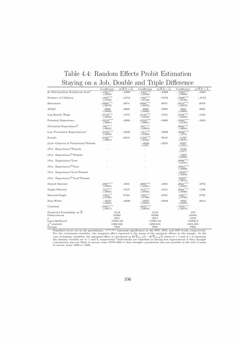
Table 4.4: Random Effects Probit Estimation

Staying on a Job, Double and Triple DifferenceCoefficient φ(Xβ) ∗ βi Coefficient φ(Xβ) ∗ βi Coefficient φ(Xβ) ∗ βi

In Metropolitan Statistical Areaa -.1251∗∗∗ -.0499 -.1251∗∗∗ -.0499 -.1223∗∗∗ -.0485(.0309) (.0309) (.0309)

Number of Children -.043∗∗∗ -.0154 -.043∗∗∗ -.0154 -.0429∗∗∗ -.0153(.0132) (.0132) (.0132)

Education .0206∗∗∗ .0074 .0206∗∗∗ .0074 .0213∗∗∗ .0076(.0079) (.0079) (.0079)

AFQT .0000 .0000 .0000 .0000 .0001 .0001(.0006) (.0006) (.0006)

Log Hourly Wage .4119∗∗∗ .1472 .4119∗∗∗ .1472 .4104∗∗∗ .1459(.0256) (.0256) (.0256)

Potential Experience -.0219∗∗∗ -.0000 -.0218∗∗∗ -.0000 -.0562∗∗∗ -.0031(.0081) (.0081) (.0124)

(Potential Experience)2 .001∗∗∗ .001∗∗∗ .0022∗∗∗(.0003) (.0003) (.0005)

Low Promotion Expectationsa -.2123∗∗∗ -.0843 -.211∗∗∗ -.0838 -.6628∗∗∗(.0239) (.0328) (.074)

Female .1548∗∗∗ .0613 .1559∗∗∗ .0618 .1138∗(.0261) (.0325) (.0647)

(Low Chances of Promotion)*Female . -.0026 -.0231 .1825∗(.047) (.1021)

(Pot. Experience)*Female . . .0162(.017)

(Pot. Experience)2*Female . . -.0007(.0008)

(Pot. Experience)*Low . . .0988∗∗∗(.0181)

(Pot. Experience)2*Low . . -.0034∗∗∗(.0008)

(Pot. Experience)*Low*Female . . -.0639∗∗(.0262)

(Pot. Experience)2*Low*Female . . .0029∗∗(.0012)

Stayed Married .4807∗∗∗ .1833 .4808∗∗∗ .1833 .4821∗∗∗ .1872(.0321) (.0321) (.0321)

Single-Married .312∗∗∗ .1219 .312∗∗∗ .1219 .3024∗∗∗ .1196(.0505) (.0505) (.0506)

Married-Single .1831∗∗ .0724 .1831∗∗ .0724 .1821∗∗ .0725(.0796) (.0796) (.0794)

Non-White -.0073 -.0029 -.0073 -.0030 .0035 .0014(.0295) (.0295) (.0295)

Constant -.9031∗∗∗ -.9037∗∗∗ -.7655∗∗∗(.0817) (.0823) (.0873)

Predicted Probability at X .5118 .5116 .479Observations 16394 16394 16394ρ .2211 .2211 .2183Log-Likelihood -10365.49 -10365.49 -10326.6

χ2 statistic 1298.822 1298.843 1353.493Groups 7903 7903 7903

Standard errors are in the parentheses. *,**,*** represent significance at the 90%, 95%, and 99% levels, respectively.For the continuous variables, the marginal effect reported is the mean of the marginal effects in the sample. In the

case of dummy variables, the marginal effect is calculated as Φ(Xd=1β)−Φ(Xd=0β) where d = 1 and d = 0 representthe dummy variable set to 1 and 0, respectively.aIndividuals are classified as having low expectations if they thoughta promotion was not likely in survey years 1979-1982 or they thought a promotion was not possible in the next 2 yearsin survey years 1996 or 1998.

106

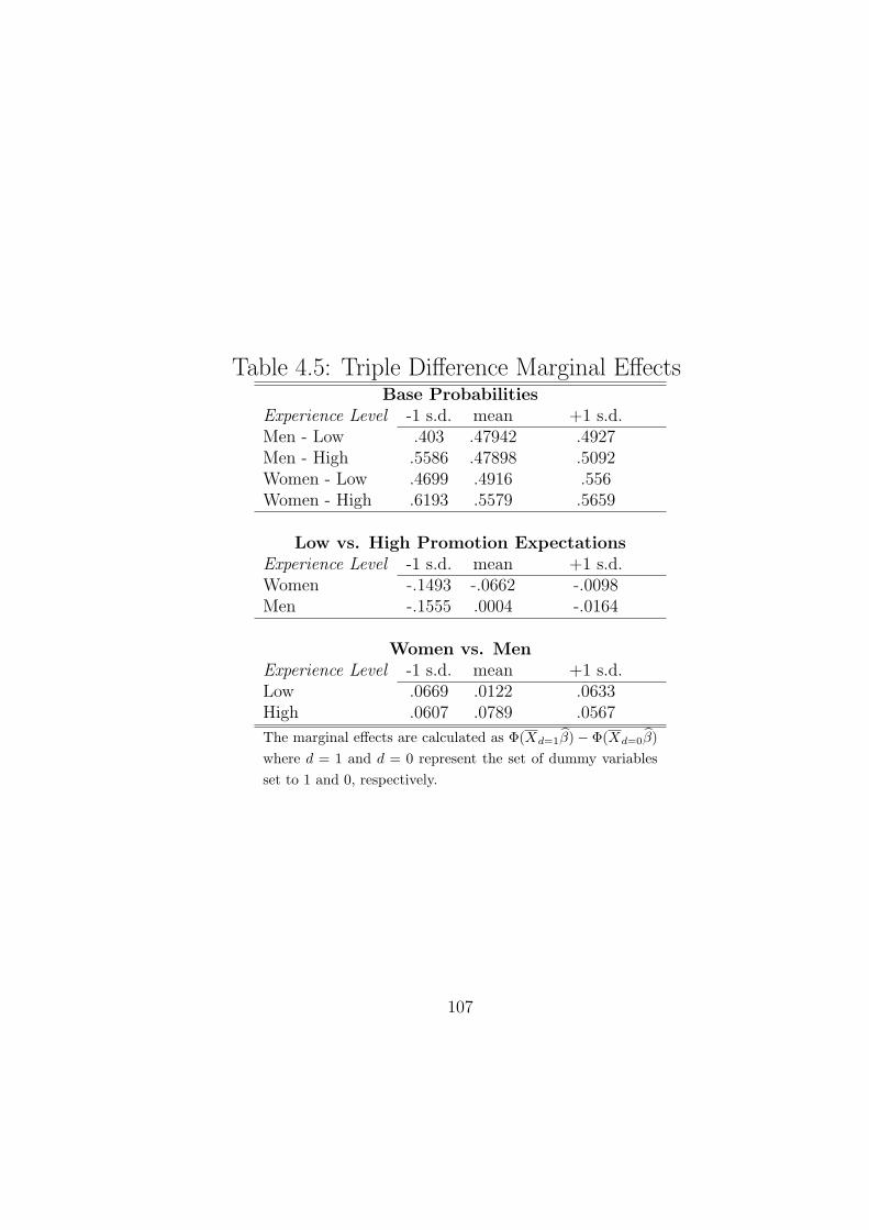
Table 4.5: Triple Difference Marginal EffectsBase Probabilities

Experience Level -1 s.d. mean +1 s.d.Men - Low .403 .47942 .4927Men - High .5586 .47898 .5092Women - Low .4699 .4916 .556Women - High .6193 .5579 .5659

Low vs. High Promotion ExpectationsExperience Level -1 s.d. mean +1 s.d.Women -.1493 -.0662 -.0098Men -.1555 .0004 -.0164

Women vs. MenExperience Level -1 s.d. mean +1 s.d.Low .0669 .0122 .0633High .0607 .0789 .0567

The marginal effects are calculated as Φ(Xd=1β)− Φ(Xd=0β)where d = 1 and d = 0 represent the set of dummy variablesset to 1 and 0, respectively.

107

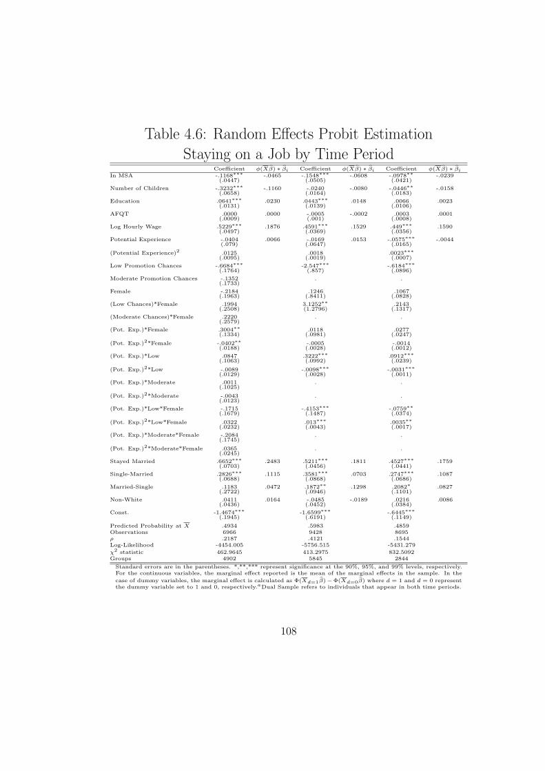
Table 4.6: Random Effects Probit Estimation

Staying on a Job by Time PeriodCoefficient φ(Xβ) ∗ βi Coefficient φ(Xβ) ∗ βi Coefficient φ(Xβ) ∗ βi

In MSA -.1168∗∗∗ -.0465 -.1548∗∗∗ -.0608 -.0978∗∗ -.0239(.0447) (.0505) (.0421)

Number of Children -.3232∗∗∗ -.1160 -.0240 -.0080 -.0446∗∗ -.0158(.0658) (.0164) (.0183)

Education .0641∗∗∗ .0230 .0443∗∗∗ .0148 .0066 .0023(.0131) (.0139) (.0106)

AFQT .0000 .0000 -.0005 -.0002 .0003 .0001(.0009) (.001) (.0008)

Log Hourly Wage .5229∗∗∗ .1876 .4591∗∗∗ .1529 .449∗∗∗ .1590(.0497) (.0369) (.0356)

Potential Experience -.0404 .0066 -.0169 .0153 -.0575∗∗∗ -.0044(.079) (.0647) (.0165)

(Potential Experience)2 .0125 .0018 .0023∗∗∗(.0095) (.0019) (.0007)

Low Promotion Chances -.6684∗∗∗ -2.547∗∗∗ -.6184∗∗∗(.1764) (.857) (.0896)

Moderate Promotion Chances -.1352 . .(.1733)

Female -.2184 .1246 .1067(.1963) (.8411) (.0828)

(Low Chances)*Female .1994 3.1252∗∗ .2143(.2508) (1.2796) (.1317)

(Moderate Chances)*Female .2220 . .(.2579)

(Pot. Exp.)*Female .3004∗∗ .0118 .0277(.1334) (.0981) (.0247)

(Pot. Exp.)2*Female -.0402∗∗ -.0005 -.0014(.0188) (.0028) (.0012)

(Pot. Exp.)*Low .0847 .3222∗∗∗ .0912∗∗∗(.1063) (.0992) (.0239)

(Pot. Exp.)2*Low -.0089 -.0098∗∗∗ -.0031∗∗∗(.0129) (.0028) (.0011)

(Pot. Exp.)*Moderate .0011 . .(.1025)

(Pot. Exp.)2*Moderate -.0043 . .(.0123)

(Pot. Exp.)*Low*Female -.1715 -.4153∗∗∗ -.0759∗∗(.1679) (.1487) (.0374)

(Pot. Exp.)2*Low*Female .0322 .013∗∗∗ .0035∗∗(.0232) (.0043) (.0017)

(Pot. Exp.)*Moderate*Female -.2084 . .(.1745)

(Pot. Exp.)2*Moderate*Female .0365 . .(.0245)

Stayed Married .6652∗∗∗ .2483 .5211∗∗∗ .1811 .4527∗∗∗ .1759(.0703) (.0456) (.0441)

Single-Married .2826∗∗∗ .1115 .3581∗∗∗ .0703 .2747∗∗∗ .1087(.0688) (.0868) (.0686)

Married-Single .1183 .0472 .1872∗∗ .1298 .2082∗ .0827(.2722) (.0946) (.1101)

Non-White .0411 .0164 -.0485 -.0189 .0216 .0086(.0436) (.0452) (.0384)

Const. -1.4674∗∗∗ -1.6599∗∗∗ -.6445∗∗∗(.1945) (.6191) (.1149)

Predicted Probability at X .4934 .5983 .4859Observations 6966 9428 8695ρ .2187 .4121 .1544Log-Likelihood -4454.005 -5756.515 -5431.279

χ2 statistic 462.9645 413.2975 832.5092Groups 4902 5845 2844

Standard errors are in the parentheses. *,**,*** represent significance at the 90%, 95%, and 99% levels, respectively.For the continuous variables, the marginal effect reported is the mean of the marginal effects in the sample. In the

case of dummy variables, the marginal effect is calculated as Φ(Xd=1β)−Φ(Xd=0β) where d = 1 and d = 0 representthe dummy variable set to 1 and 0, respectively.aDual Sample refers to individuals that appear in both time periods.

108

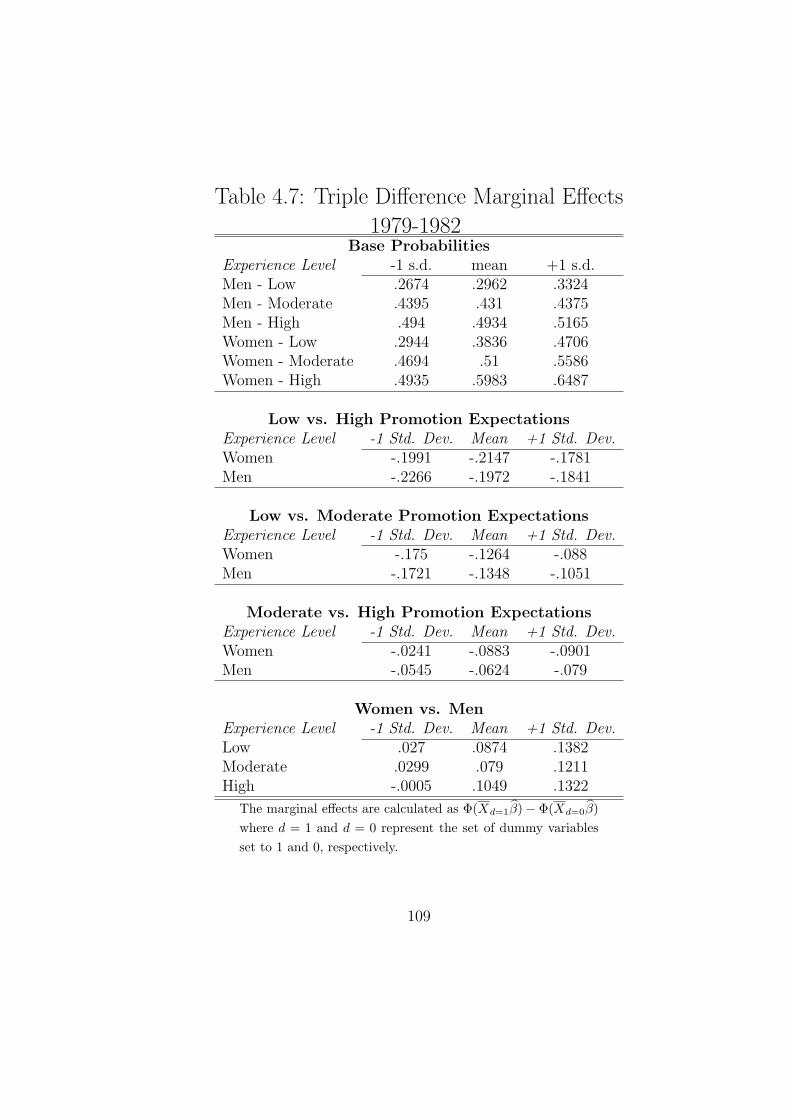
Table 4.7: Triple Difference Marginal Effects

1979-1982Base Probabilities

Experience Level -1 s.d. mean +1 s.d.Men - Low .2674 .2962 .3324Men - Moderate .4395 .431 .4375Men - High .494 .4934 .5165Women - Low .2944 .3836 .4706Women - Moderate .4694 .51 .5586Women - High .4935 .5983 .6487

Low vs. High Promotion ExpectationsExperience Level -1 Std. Dev. Mean +1 Std. Dev.Women -.1991 -.2147 -.1781Men -.2266 -.1972 -.1841

Low vs. Moderate Promotion ExpectationsExperience Level -1 Std. Dev. Mean +1 Std. Dev.Women -.175 -.1264 -.088Men -.1721 -.1348 -.1051

Moderate vs. High Promotion ExpectationsExperience Level -1 Std. Dev. Mean +1 Std. Dev.Women -.0241 -.0883 -.0901Men -.0545 -.0624 -.079

Women vs. MenExperience Level -1 Std. Dev. Mean +1 Std. Dev.Low .027 .0874 .1382Moderate .0299 .079 .1211High -.0005 .1049 .1322

The marginal effects are calculated as Φ(Xd=1β)− Φ(Xd=0β)where d = 1 and d = 0 represent the set of dummy variablesset to 1 and 0, respectively.

109

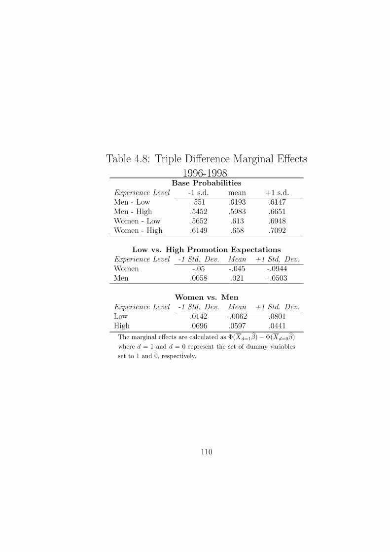
Table 4.8: Triple Difference Marginal Effects

1996-1998Base Probabilities

Experience Level -1 s.d. mean +1 s.d.Men - Low .551 .6193 .6147Men - High .5452 .5983 .6651Women - Low .5652 .613 .6948Women - High .6149 .658 .7092

Low vs. High Promotion ExpectationsExperience Level -1 Std. Dev. Mean +1 Std. Dev.Women -.05 -.045 -.0944Men .0058 .021 -.0503

Women vs. MenExperience Level -1 Std. Dev. Mean +1 Std. Dev.Low .0142 -.0062 .0801High .0696 .0597 .0441

The marginal effects are calculated as Φ(Xd=1β)− Φ(Xd=0β)where d = 1 and d = 0 represent the set of dummy variablesset to 1 and 0, respectively.

110

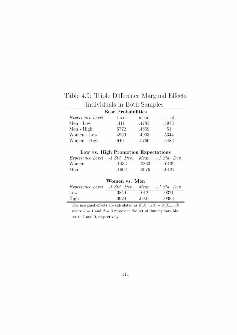
Table 4.9: Triple Difference Marginal Effects

Individuals in Both SamplesBase Probabilities

Experience Level -1 s.d. mean +1 s.d.Men - Low .411 .4783 .4973Men - High .5772 .4859 .51Women - Low .4969 .4903 .5344Women - High .6401 .5766 .5483

Low vs. High Promotion ExpectationsExperience Level -1 Std. Dev. Mean +1 Std. Dev.Women -.1432 -.0863 -.0139Men -.1662 -.0076 -.0127

Women vs. MenExperience Level -1 Std. Dev. Mean +1 Std. Dev.Low .0859 .012 .0371High .0629 .0907 .0383

The marginal effects are calculated as Φ(Xd=1β)− Φ(Xd=0β)where d = 1 and d = 0 represent the set of dummy variablesset to 1 and 0, respectively.

111

Chapter 5

Conclusions

In the United States, self-employment among the civilian non-agricultural

civilian labor force declined from the 1920s to the early 1970s. Since then, the

incidence of self-employment has been increasing. Although the rate of self-

employment is higher among men than among women, it seems clear that the

increased rate of self-employment since the 1970s is primarily a consequence

of women selecting into self-employment. This period happened to coincide

with an era of rapidly increasing health care costs.

There are two features of the health care system - one which is charac-

teristic of any health care industry in the world and another which is specific

to the economy of the United States - that suggest that there is a linkage

between health care costs and households’ choice of employment sector in the

United States. Because there is asymmetric information about expected med-

ical costs of those purchasing health insurance, individual choice over health

insurance policies may result in risk-based sorting across plans. This phe-

nomenon, called adverse selection, is a feature of any health care industry.

In the United States, health insurance is predominantly employment-based,

which allows employers to pool the health risk of their employees and obtain

112

lower health insurance premia from health insurance companies. Moreover,

employment-based health insurance enjoys a tax subsidy that is not available

to workers outside the wage-salary sector. Thus, the health insurance premia

facing workers in wage-employment tend to be significantly lower than those

facing workers in self-employment. This price wedge is likely to distort the

employment sector choices of households.

The second and third chapters of my dissertation examine how dif-

ferences in health insurance premia between the wage-employment and self-

employment sectors impact labor supply to the two sectors. The second chap-

ter is a theoretical paper. Here I describe a simple model in which the choice

of employment sector is determined jointly by household members. In this

model, everyone demands health insurance but the health insurance premium

differs between the two sectors. Households take the compensation package of-

fered by the wage-salary sector as given, and make employment-sector choices

to maximize total household utility. I address the following question: How

does employer-provided health insurance influence a household’s choice of em-

ployment sector - wage employment versus self-employment? I show that

when there is a price wedge for health insurance between the self-employment

and wage-employment sectors, labor supply to the self-employment sector is

smaller, relative to the case where there is no price wedge. Thus, the price

wedge causes a distortion in the assignment of workers between the two sec-

tors. I also show that the extension of employer-provided health benefits to

dependents outside the firm through a family health plan enables married cou-

113

ples to effectively eliminate the price wedge. I extend this model to include

the insurance-purchase decision for single workers. In this model, in addition

to choosing which sector to work in, workers also decide whether to purchase

health insurance or not. I use standard results in the ‘adverse selection’ liter-

ature to illustrate how pooling the health risk over the subset of workers who

choose to buy insurance raises the insurance premium, relative to the case

where the risk-pooling is over all the workers in the firm. Moreover, firms can

capture economies of scale by getting as many workers as possible to partici-

pate in the group health insurance that they offer. This result could explain

why firms might prefer to include health benefits as part of the compensa-

tion package to all workers, instead of making the choice of health coverage

optional.

There are two extensions to this model that I believe can give us some

interesting and testable predictions. The first is to incorporate the number

of hours worked into the worker’s decision problem and to introduce two in-

puts into the firm’s production process - the number of workers and hours per

worker. This extension will allow me to examine the effect of changes in health

insurance costs on hours worked. Another extension is to allow workers’ pref-

erence for flexibility to be correlated with their valuation of health insurance.1

If firms have differential costs to offering health insurance to workers, then one

can examine the equilibrium sorting of different types of workers to different

types of firms, and the size distribution of firms.

1For instance, a single mother with a young child is likely to be a (high θ, high γ) type.

114

In the third chapter, my focus of study has been the effect of the hus-

band’s employer-provided family health insurance on the wife’s propensity to

select into self-employment. A number of papers have found an association

between a married woman’s labor supply behavior and spousal health insur-

ance. A consistent finding in the literature on women’s self-employment in

the U.S. since the mid-1970s is the predominance of married women in this

sector. While numerous papers have remarked on the relationship between

spousal health insurance and a married woman’s propensity to select into self-

employment, no clean test of this linkage was established. The Tax Reform

Act of 1986 (TRA86) provides us with an opportunity to test this linkage.

The TRA86 introduced a tax subsidy for the self-employed to purchase health

insurance. At the same time, it disqualified self-employed individuals who

were already enjoying health insurance benefits through a spouse from taking

advantage of the subsidy. Since the effect of the tax subsidy was to lower the

after-tax price of health insurance for those among the self-employed who were

purchasing their own health insurance, I predict that this subsidy increased

the incidence of self-employment among single women.

My estimates suggest that health insurance coverage through the spouse

biased a married woman’s employment sector choice strongly towards self-

employment in the pre-TRA86 period. Moreover, the incidence of single

women in self-employment went up significantly in the post-TRA86 period,

after controlling for the effect of health insurance coverage through the spouse.

This finding supports my hypothesis that the decrease in the price of health

115

insurance through the tax subsidy induced more single women to select into

self-employment in the post-TRA86 period relative to married women. In

summary, my findings suggest that in the pre-TRA86 period, the high cost

of health insurance created a price wedge between women who enjoyed health

insurance coverage through their spouse’s health plan and those who did not.

Women who had a preference for working in the self-employment sector and

who enjoyed spousal health benefits were able to exercise their preference and

select into self-employment. On the other hand, for women with a preference

for the self-employment sector but constrained to purchase their own health in-

surance, it was too costly to opt for this sector. For these women, the TRA86,

by narrowing this price wedge, lowered the price of selecting into their desired

sector of employment.

One limitation of this chapter is that I restrict my study to women who

have chosen to be in the labor force. Although women’s labor force participa-

tion has been rising steadily over the last few decades, a substantial fraction

of working-age women still choose to stay out of the labor force. It is possi-

ble that the availability of spousal health insurance also impacts the decision

about participating in the labor force. It would therefore be fruitful to extend

the analysis in chapter 3 to a two-stage analysis: in the first stage, women

decide whether to join the labor force or not. If they decide to participate in

the labor force, they choose between self-employment and wage-employment.

This kind of analysis will address issues regarding selection, in addition to the

effect of spousal health insurance on employment sector choices.

116

In the fourth chapter (joint with Richard Prisinzano), we examine dif-

ferences in job turnover patterns between men and women. We expect to see

job turnover when promotion opportunities on the job are low. Accordingly,

we study the relationship between individuals’ expectations of promotion on

their jobs and their turnover behavior. We examine how this relationship varies

between men and women and between more and less experienced workers. It is

our hypothesis that early on in their careers, women who are strongly commit-

ted to a career are more likely to stay on in their jobs, regardless of promotion

opportunities, in a bid to signal their commitment to the labor force. How-

ever, once women have acquired adequate labor market experience and their

commitment to the labor force is no longer in question, we predict that their

turnover behavior will be more responsive to career opportunities and will be

similar to that of men. Using the 1979 National Longitudinal Survey of Youth

(NLSY), we find that men and women differ in their response to promotion

expectations. Specifically, we find that early in their career women with low

promotion expectations are more likely to stay on a job than corresponding

men. We also find that this difference diminishes with experience.

Our results suggest that women who are committed to the labor market

stay on in jobs which have little or no prospects for growth early in their career

because of the need to signal their commitment to their employer. Thus,

signalling is a costly activity and leads to inefficient outcomes; women are

under-employed on their job in the early stages of their career. An obvious

extension to this chapter is to examine whether women experience a faster

117

career growth once they have successfully signalled their attachment to the

labor market. Once firms come to believe that these women are serious about

their careers, they should respond by placing these women in positions that

match with their abilities. If this is the case, we should expect to see women

getting promoted more rapidly than men of comparable characteristics at later

stages in their career path. This is a topic that merits research.

118

Bibliography

[1] Joseph Altonji and Christina Paxson. Labor Supply, Hours Constraints

and Job Mobility. The Journal of Human Resources, 27(2):256–278, 1992.

[2] Wiji Arulampalam. “A Note on Estimated Coefficients in Random Ef-

fects Probit Models. Oxford Bullentin of Economics and Statistics”,

61(4):597–602, 1999.

[3] Gary S. Becker. A Theory of Marriage: Part I. The Journal of Political

Economy, 81(4):813–846, 1973.

[4] David Blau. A Time-Series Analysis of Self-Employment in the United

States. The Journal of Political Economy, 95(3):445–467, June 1987.

[5] James Hamilton Brown, Charles and James Medoff. Employers Large

and Small, Harvard University Press, Cambridge, Massachusetts. 1990.

[6] Thomas Buchmueller and Robert Valletta. The Effect of Health Insur-

ance on Married Female Labor Supply. The Journal of Human Resources,

34(1):42–70, 1999.

[7] J.S. Butler and Robert Moffitt. “A Computationally Efficient Quadra-

ture Procedure for the One-Factor Multinomial Probit Model”. Econo-

metrica, 50(3):761–764, May 1982.

119

[8] Gary Chamberlain. “Analysis of Covariance with Qualitative Data”.

The Review of Economic Studies, 47(1):225–238, January 1980.

[9] U.S. Dept. of Commerce, Bureau of the Census, Current Population

Survey:Annual Demographic File, 1984, 1985, 1987, 1988, 1990, 1991,

2000, 2001 [computer file], Ann Arbor, MI: Inter- university consortium

for political and social research [distributor],various years.

[10] Current Population Survey, May 1984,1985: Work Schedules,Multiple

Job-Holding and Premium Pay Supplement [machine-readable data file],

conducted by the Bureau of the Census for the Bureau of Labor Statis-

tics. washington: Bureau of the census [producer and distributor], various

years.

[11] Current Population Survey, May 2001: Work Schedules and Work at

Home Supplement [machine-readable data file], conducted by the Bureau

of the Census for the Bureau of Labor Statistics. Washington: Bureau of

the Census [producer and distributor], 2001.

[12] David Cutler and Brigitte Madrian. Rising Health Insurance Costs: Ev-

idence on Hours Worked, NBER Working Paper \5525. 1996.

[13] Theresa Devine. Characteristics of Self-Employed Women in the United

States. Monthly Labor Review, 117(3):20–34, March 1994a.

[14] Theresa Devine. Changes in Wage-and-Salary Returns to Skill and the

120

Recent Rise in Female Self-Employment. The American Economic Re-

view, 84(2):108–113, 1994b.

[15] Linda Edwards and Elizabeth Field-Hendrey. Home-Based Work and

Women’s Labor Force Decisions. Journal of Labor Economics, 20(1):170–

200, 2002.

[16] Nada Eissa. Taxation and Labor Supply of Married Women: The Tax

Reform Act of 1986 as a Natural Experiment, NBER working paper \

5023. 1995.

[17] Employment Trends. Employment Policy Foundation, January 2003.

[18] David Evans and Boyan Jovanovic. An Estimated Model of Entrepreneurial

Choice under Liquidity Constraints. The Journal of Political Economy,

97(4):808–827, 1989.

[19] David Evans and Linda Leighton. Some Empirical Aspects of Entrepreneur-

ship. The American Economic Review, 79(3):519–535, 1989.

[20] Martin Feldstein. Behavioral Responses to Tax Rates: Evidence from

the Tax Reform Act of 1986. The American Economic Review, Papers

and Proceedings, 85(2):170–174, 1995.

[21] Jonathan Gruber. The Incidence of Mandated Maternity Benefits. The

American Economic Review, 84(3):622–641, 1994.

121

[22] Jonathan Gruber and Robin McKnight. Why did Employee Health In-

surance Contributions Rise?, NBER Working Paper \8878. 2002.

[23] Jonathan Gruber and James Poterba. Tax Incentives and the Decision

to Purchase Health Insurance: Evidence from the Self-Employed. The

Quarterly Journal of Economics, 109(3):701–733, 1994.

[24] Jonathan Gruber and Ebonya Washington. Subsidies to Employee Health

Insurance Premiums and the Health Insurance Market, , NBER working

paper \ 9567. 2003.

[25] David K. Guilkey and James L. Murphy. “Estimation and Testing in the

Random Effects Probit Model”. Journal of Economterics, 59:301–317,

1993.

[26] Robert E. Hall. “The Importance of Lifetime Jobs in the U.S. Economy”.

American Economic Review, 72(3):716–724, September 1982.

[27] Daniel S. Hamermesh and Stephen J. Trejo. “The Demand for Hours of

Labor: Direct Evidence from California”. The Review of Economics and

Statistics, 82(1):38–47, February 2000.

[28] Cheng Hsiao. Analysis of Panel Data. Cambridge University Press, New

York, NY, 1986.

[29] Chu-Shiu Li. Information Costs and Health Insurance Contracts. The

Journal of Risk and Insurance, 67(2):235–247, 2000.

122

[30] Audrey Light and Manuelita Ureta. “Panel Estimates of Male and Fe-

male Job Turnover Behavior: Can Female Nonquitters be Identified?”.

Journal of Labor Economics, 10(2):156–181, April 1992.

[31] Audrey Light and Manuelita Ureta. “Early-Career Work Experience and

Gender Wage Differentials”. Journal of Labor Economics, 13(1):121–154,

1995.

[32] Karen Lombard. Female Self-Employment and Demand for Flexible,

Nonstandard Work Schedules. Economic Inquiry, 39(2):214–237, 2001.

[33] G.S. Maddala. “Limited Dependent Variables Models Using Panel Data”.

Journal of Human Resources, 22(3):307–338, Summer 1987.

[34] Employment Outlook, Chapter Four. OECD, Paris, 1992.

[35] Kathy A. Paulson Gjerde. “The Existence of Gender-Specific Promotion

Standards in the U.S.”. Managerial and Decision Economics, 23(8):447–

459, December 2002.

[36] Richard Prisinzano. “The Structure of Promotions by Gender: Address-

ing Partial Observability”. University of Texas, April 2004.

[37] Sherwin Rosen. The Theory of Equalizing Differences. Handbook of

Labor Economics, Vol. I, Eds. O. Ashenfelter and R.Layard, pages 641–

691, 1986.

123

[38] Herb Schuetze. Taxes, Economic Conditions and Recent Trends in Male

Self-Employment: a Canada-US Comparison. Labor Economics, pages

507–544, 2000.

[39] Lara Shore-Sheppard. Stemming the Tide? The Effect of Expanding

Medicaid Eligibility on Health Insurance Coverage, Working Paper ]361.

Industrial Relations Section, Princeton University, 1996.

[40] Katherine Swartz. Interpreting the Estimates from Four National Sur-

veys of the Number of People Without Health Insurance. Journal of

Economic and Social Measurement, 14:233–242, 1986.

[41] Finis Welch. Matching the Current Population Surveys. Stata Technical

Bulletin Reprints, 2:34–40, 1993.

124

Vita

Malathi Rao Velamuri was born in Dehradun, in the state of Uttar

Pradesh in India. She is the daughter of Dr. Raghavendra Rao Velamuri and

Lakshmi Velamuri. She received the Bachelor of Science degree in Mathemat-

ics in 1987 and the Master of Arts degree in Economics in 1989, from the

University of Madras. She worked as a Research Assistant and subsequently

as a Research Associate at the Institute for Financial Management and Re-

search (IFMR), Madras from 1990-98. She applied to the University of Texas

at Austin for enrollment in their Economics program. She was accepted and

started graduate studies in August, 1998.

Permanent address: 25/11 Deivasigamani Road, Royapettah,Chennai 600014, India

This dissertation was typeset with LATEX† by the author.

†LATEX is a document preparation system developed by Leslie Lamport as a specialversion of Donald Knuth’s TEX Program.

125