Embed Size (px)
Citation preview

Copyright
by
Nicholas James Durr
2010

THE DISSERTATION COMMITTEE FOR NICHOLAS JAMES DURR
CERTIFIES THAT THIS IS THE APPROVED VERSION OF THE FOLLOWING
DISSERTATION:
NONLINEAR IMAGING WITH ENDOGENOUS
FLUORESCENCE CONTRAST AND PLASMONIC
CONTRAST AGENTS
Committee:
Adela Ben-Yakar, Supervisor
Konstantin Sokolov
James Tunnell
Michael Downer
Hans Gerritsen
NONLINEAR IMAGING WITH ENDOGENOUS
FLUORESCENCE CONTRAST AND PLASMONIC
CONTRAST AGENTS
by
NICHOLAS JAMES DURR, B.S.; M.S.
DISSERTATION
Presented to the Faculty of the Graduate School of
The University of Texas at Austin
in Partial Fulfillment
of the Requirements
for the Degree of
DOCTOR OF PHILOSOPHY
THE UNIVERSITY OF TEXAS AT AUSTIN
DECEMBER 2010

iv
Acknowledgements
I would like to thank my advisor, Dr. Adela Ben-Yakar, for her enthusiasm,
support, and guidance over the course of my dissertation research. Her creativity, desire
for excellence, and boldness in venturing into new research areas have been a great
source of motivation for me. I would also like to thank all my committee members,
particularly Dr. Konstantin Sokolov for his insight in our gold nanorod collaboration, and
Dr. Hans Gerritsen, for graciously hosting me as a visiting researcher in his lab. All the
graduate students and post-docs of the Ben-Yakar Group also deserve special
acknowledgement. Whether it was standing by a chalkboard, working through the night,
or toobing down the river—just as your talents and intelligence were essential to me
finishing my degree, your camaraderie and humor were crucial to my happiness in
Austin. I had a wonderful time working with all of you and hope our friendships will be
lifelong.
v
NONLINEAR IMAGING WITH ENDOGENOUS
FLUORESCENCE CONTRAST AND PLASMONIC
CONTRAST AGENTS
Publication No._____________
Nicholas James Durr, Ph.D.
The University of Texas at Austin, 2010
Supervisor: Adela Ben-Yakar
Fluorescence from endogenous molecules and exogenous contrast agents can
provide morphological, spectral, and lifetime contrast that indicates disease state in
epithelial tissues. Recently, nonlinear microscopy has emerged as a potential tool for the
early detection, case-finding, and monitoring of epithelial cancers because it permits non-
invasive, three-dimensional fluorescence imaging of subcellular features hundreds of
microns deep. This dissertation explores the use of nonlinear microscopy for cancer
diagnostics on two fronts: (1) we examine the fundamental limitations governing the
maximum nonlinear imaging depth in epithelial tissues, and (2) we investigate the use of
a new class of nonlinear contrast agent—plasmonic gold nanoparticles—for molecularly
specific imaging of cancer cells.
We built and optimized a nonlinear microscope for deep tissue imaging, and
studied the image contrast as a function of imaging depth in ex-vivo human biopsies and
tissue phantoms. With this system we demonstrated imaging down to 370 μm deep in a
vi
human biopsy, which is significantly deeper than imaging depths achieved in comparable
studies. We found that the large scattering coefficient and homogenous fluorophore
distribution typical of epithelial tissues limit the maximum imaging depth to 3-5 mean
free scattering lengths deep in conventional nonlinear microscopy. Beyond this imaging
depth, the increasing contribution of out-of-focus emission limits the contrast to
insufficient levels for diagnostic imaging. We support these observations with time-
dependent Monte Carlo simulations.
We exploited the intense interaction of gold nanoparticles with light, enhanced by
surface plasmon resonance effects, to create extremely bright nonlinear contrast agents.
These contrast agents proved to be several orders of magnitude brighter than the brightest
organic fluorophores and at least one order of magnitude brighter than quantum dots. We
targeted gold nanoparticles to a biomarker for carcinogenesis and demonstrated
molecularly specific imaging of cancer cells. We demonstrated that unlike emission from
traditional bandgap fluorophores, nonlinear luminescence from gold nanoparticles was
weakly dependent on excitation pulse length for short pulse durations. This finding
supports the hypothesis that nonlinear excitation in plasmonic nanoparticles involves
sequential rather than simultaneous absorption of excitation photons. The remarkable
brightness of gold nanoparticles makes them an attractive contrast agent for nonlinear
diagnostics.
vii
Table of Contents
List of Tables ..................................................................................................................... xi
List of Figures ................................................................................................................... xii
Chapter 1 Introduction......................................................................................................1
1.1. Dissertation overview ........................................................................................2
Chapter 2 Background ......................................................................................................4
2.1. Epithelial tissue and carcinoma .........................................................................4
2.2. Techniques for epithelial cancer imaging ..........................................................7
2.3. Optical properties of epithelial tissues ...............................................................9
2.4. Nonlinear luminescence ...................................................................................12
2.5. Nonlinear microscopy ......................................................................................15
2.6. Sources of contrast in nonlinear optical imaging .............................................15
2.7. Plasmonic nanoparticles...................................................................................17
2.7.1. Surface plasmon resonance ..................................................................17
2.7.2. Gold nanoparticles as biomedical contrast agents ...............................19
2.7.3. Multiphoton luminescence from plasmonic nanoparticles ..................20
Chapter 3 Design and characterization of nonlinear scanning microscope for deep
tissue imaging ..........................................................................................................22
3.1. Overview ..........................................................................................................22
3.2. Excitation path .................................................................................................24
3.2.1. Excitation source ..................................................................................24
3.2.2. Laser scanning system .........................................................................25
3.2.3. Objective lens.......................................................................................26
Resolution .........................................................................................27
Field of View ....................................................................................28
Olympus XLUMPFL Objective .......................................................29
3.3. Focal volume characterization .........................................................................30
3.3.1. Spatial intensity distribution ................................................................30
viii
3.3.2. Temporal characterization ...................................................................33
3.4. Collection path .................................................................................................34
3.5. Example images ...............................................................................................37
3.5.1. Phantoms ..............................................................................................37
3.5.2. Three dimensional rendering of healthy tissue biopsies ......................38
3.5.3. Comparison of normal and cancerous biopsy ......................................39
Chapter 4 A Monte Carlo model for out-of-focus fluorescence generation in two-
photon microscopy ..................................................................................................41
4.1. Introduction ......................................................................................................41
4.2. Monte Carlo vs. analytical approach ...............................................................43
4.3. Overview of Monte Carlo model .....................................................................45
4.4. Excitation simulation .......................................................................................46
4.4.1. Focusing ...............................................................................................46
4.4.2. Temporal dependence ..........................................................................54
4.5. Collection .........................................................................................................54
4.6. Implementation ................................................................................................56
Chapter 5 Deep two-photon autofluorescence microscopy of epithelial tissues ........57
5.1. Introduction ......................................................................................................57
5.2. Methods............................................................................................................61
5.2.1. 2PAM contrast .....................................................................................61
5.2.2. 2PAM system .......................................................................................63
5.2.3. Monte Carlo model ..............................................................................65
5.2.4. Analytical model ..................................................................................65
5.2.5. Tissue phantom preparation .................................................................66
5.2.6. Biopsy preparation ...............................................................................68
5.3. Results and discussion .....................................................................................68
5.3.1. Monte Carlo simulation .......................................................................68
5.3.2. Phantom imaging .................................................................................70
5.3.3. Fluorescence decay ..............................................................................75
5.3.4. Contrast decay ......................................................................................78
ix
5.3.5. Human biopsy imaging ........................................................................80
5.3.6. Fluorescence saturation and photobleaching .......................................83
5.3.7. Maximum imaging depth .....................................................................85
5.4. Conclusions ......................................................................................................89
Chapter 6 Multiphoton-induced luminescence from gold nanoparticles ..................90
6.1. Introduction ......................................................................................................90
6.2. Nomenclature of gold nanoparticle samples ....................................................91
6.3. Physical properties ...........................................................................................92
6.4. Linear optical properties ..................................................................................96
6.4.1. Absorption and scattering cross sections .............................................96
Measurements ...................................................................................96
Simulations .......................................................................................97
6.4.2. Absorption and scattering coefficients ...............................................101
6.5. Calculation of nanoparticle concentrations ....................................................102
6.6. Nonlinear luminescence properties ................................................................104
6.6.1. Experimental setup.............................................................................104
Excitation source and power attenuator .........................................106
Pulse stretcher/compressor and autocorrelator ...............................106
Laser scanning microscope ............................................................108
Sample ............................................................................................109
Spectrometer/PMT .........................................................................110
6.6.2. Spectral features of nanoparticle luminescence .................................113
6.6.3. Dependence of MPL on excitation intensity ......................................115
6.6.4. Dependence of MPL on pulse duration .............................................124
Qualitative description ...................................................................124
Mathematical description ...............................................................126
Experimental results .......................................................................129
6.6.5. Quantification of two-photon action cross section ............................135
Theoretical development ................................................................136
Collection efficiency ......................................................................138
x
Measurement of the two-photon action cross section by reference
standard ..........................................................................................141
Results ............................................................................................143
Comparison of σTPA to previous reports .........................................147
6.6.6. Polarization dependence ....................................................................149
Setup ...............................................................................................149
Linear polarization .........................................................................150
Circular Polarization ......................................................................151
6.7. Conclusion .....................................................................................................152
Chapter 7 Nonlinear imaging of cancer cells with plasmonic contrast agents .........155
7.1. Preparation of contrast agents ........................................................................155
7.1.1. CTAB coated gold nanorods ..............................................................155
7.1.2. PEGylated gold nanorods ..................................................................156
7.1.3. Nanospheres .......................................................................................157
7.2. Sample preparation ........................................................................................158
7.2.1. Tissue phantoms.................................................................................158
7.3. Imaging systems.............................................................................................158
7.4. Single layer of labeled cancer cells ................................................................159
7.4.1. Brightness characterization ................................................................159
7.4.2. Signal from nanoparticle agglomerates .............................................161
7.4.3. Labeling with PEGylated gold nanorods ...........................................162
7.4.4. Optical properties of labeled gold nanorods ......................................164
Dependence of MPL on excitation fluence ....................................165
Dependence of MPL on excitation polarization .............................167
7.5. GNP-Labeled tissue phantoms .......................................................................167
7.6. Biocompatibility ............................................................................................171
Chapter 8 Conclusions and future directions ..............................................................174
References ........................................................................................................................179
Vita... ................................................................................................................................197
xi
List of Tables
Table 2.1: High resolution three-dimensional imaging techniques. ................................... 9
Table 4.1: Parameters for different focusing schemes. ..................................................... 52
Table 5.1: Measured decay constant compared to phantom mean free scattering length. 77
Table 6.1: Measured nanoparticle dimensions. ................................................................. 96
Table 6.2: Calculated linear absorption and scattering cross sections. ........................... 101
Table 6.3: Nanoparticle molar extinction coefficients and concentrations..................... 104
Table 6.4. Parameters used in calculating absolute emission counts for fluorescein. .... 140
Table 6.5 Two-photon action cross sections of gold nanorods and other nanoparticles. 149
xii
List of Figures
Figure 2.1: Histology of Stratified Epithelial Tissue. ......................................................... 6
Figure 2.2: Absorption and scattering mean free path length in the epithelium. .............. 12
Figure 2.3: Jablonski diagram of one and two photon excited fluorescence and second
harmonic generation.................................................................................................. 13
Figure 2.4: Surface plasmon resonance in gold nanospheres and gold nanorods. .............19
Figure 3.1: An upright laser scanning microscope for deep nonlinear imaging. .............. 23
Figure 3.2: Schematic of laser scanning system. .............................................................. 26
Figure 3.3: Layout of Olympus Objective. ....................................................................... 30
Figure 3.4: Spatial and Temporal Characterization of the Focal Spot. ............................. 32
Figure 3.5: Optimization of collection optics. .................................................................. 37
Figure 3.6: Large field of view imaging of unlabeled cancer cells and high magnification
view of gold nanorod labeled cells. .......................................................................... 38
Figure 3.7: Autofluorescence and second harmonic generation imaging in an ex-vivo
human biopsy. ........................................................................................................... 39
Figure 3.8: Two-photon autofluorescence images of normal and cancerous biopsy. ....... 40
Figure 4.1: Qualitative illustration of signal and background two-photon excited
fluorescence. ............................................................................................................. 42
Figure 4.2: Qualitative illustration of different focusing strategies. ................................. 48
Figure 4.3: Parameters describing Gaussian beam focusing in our Monte Carlo
simulation. ................................................................................................................. 50
Figure 4.4: R value vs. rs for different focusing schemes in a transparent medium. ........ 53
Figure 4.5. Collection simulation parameters. .................................................................. 56
Figure 5.1: Schematic of two-photon imaging system collection path. ............................ 64
Figure 5.2: Monte Carlo results for imaging 400 μm deep in ls = 80 μm tissue. .............. 69
Figure 5.3: XZ cross sections of phantoms and biopsy. ................................................... 72
Figure 5.4: Measured bead size vs depth. ......................................................................... 74
Figure 5.5: Fluorescence signal and background decays. ................................................. 76
Figure 5.6: Contrast decays............................................................................................... 79
Figure 5.7: Biopsy images. ............................................................................................... 81
Figure 5.8: Photobleaching test......................................................................................... 85
xiii
Figure 5.9: Maximum imaging depth summary. .............................................................. 88
Figure 6.1: TEM images of nanoparticle samples. ........................................................... 93
Figure 6.2: TEM Image processing sequence for characterizing size distribution of
GNR780. ................................................................................................................... 94
Figure 6.3: Plot of measured lengths and widths of GNR780 nanoparticles. ................... 95
Figure 6.4: Measured linear absorbance of gold nanoparticle samples. ........................... 97
Figure 6.5: Comparison of measured and simulated absorbance for GNR780. ............. 100
Figure 6.6: Nonlinear optical properties experimental setup. ......................................... 105
Figure 6.7: Focal plane pulse duration as a function of stretcher position. .................... 108
Figure 6.8: Spectrometer system response and calibration. ............................................ 112
Figure 6.9: Spectral features of MPL in nanospheres and nanorods .............................. 114
Figure 6.10: Nonlinear emission profile of fluorescein .................................................. 117
Figure 6.11: Nonlinear emission profile of GNR780 ..................................................... 119
Figure 6.12: Measured slope vs. λx for fluorescein and nanoparticle samples. .............. 122
Figure 6.13: MPL vs. average excitation power for GNR780 detected with PMT. ....... 123
Figure 6.14: Second harmonic generation signal from 160 nm diameter gold nanospheres.
................................................................................................................................. 124
Figure 6.15: Band structure of gold near the X and L symmetry points showing sequential
one photon absorption. ............................................................................................ 126
Figure 6.16: MPL vs. excitation intensity and pulse duration for fluorescein and
GNR780. ................................................................................................................. 130
Figure 6.17: Comparison of experiment and model for MPL vs τp. .............................. 131
Figure 6.18: Nonlinear order observed in GNR780 at λx = 780 nm versus pulse duration.
................................................................................................................................. 132
Figure 6.19: Nonlinear absorption coefficient (β) dependence on pulse duration. ......... 133
Figure 6.20: Simulated MPL rates vs. pulse duration and excitation power for sequential
nonlinear absorption................................................................................................ 134
Figure 6.21: Determination of effective collection angle. .............................................. 138
Figure 6.22: Measured vs. predicted emission counts of fluorescein. ............................ 140
Figure 6.23: Validation of reference fluorophore technique for calculating σTPA........... 144
Figure 6.24: Measured two-photon action cross sections of gold nanoparticles ............ 145
xiv
Figure 6.25: Absolute, area-normalized, and volume normalized σTPA of gold
nanoparticles ........................................................................................................... 147
Figure 6.26: Dependence of MPL on excitation polarization--GNR780 on coverslip. .. 151
Figure 6.27: Determining orientation of gold nanorods from polarization dependence. 152
Figure 7.1: Properties of the CTAB-coated gold nanorods used as contrast agents. ...... 156
Figure 7.2: MPL images of GNR754 labeled and unlabeled A431 cancer cells. ........... 160
Figure 7.3: Wide-field white light and MPL images of non-specifically labeled GNR754
clusters with cells. ................................................................................................... 162
Figure 7.4: GNR808p labeling of A468 cancer cells. ..................................................... 163
Figure 7.5: Sample movement correction algorithm. ..................................................... 165
Figure 7.6: MPL vs. Ip for GNR808p on a coverslip and labeled to cells. ..................... 166
Figure 7.7: Polarization dependence of GNR808p labeled to cells. ............................... 167
Figure 7.8: 2PAM and MPL images of tissue phantom.................................................. 168
Figure 7.9: Deep MPL imaging in tissue phantom. ........................................................ 170
Figure 7.10: MTT assay after incubation with GNS, GNR, and GNRp ......................... 173
1
Chapter 1 Introduction
‗Optical biopsy‘, as defined over a decade ago as ―imaging tissue microstructure
at or near the level of histopathology without the need for tissue excision,‖ [1] remains
one of the holy grails of the field of biomedical optics. The conventional excision biopsy
is an invasive technique, fraught with high failure rates, patient morbidity, and cost. A
tool to compliment, or perhaps replace, even a small fraction of the many biopsies
performed each year has the potential to make a dramatic impact on clinical medicine.
Shortly after the first demonstration of nonlinear microscopy by Denk, Strickler,
and Webb in 1990[2], its utility in the three-dimensional imaging of living skin was
realized[3]. Within the last couple of years, two-photon autofluorescence microscopy
(2PAM) has entered the clinic, and in-vivo nonlinear images of human skin are now
being explored for their diagnostic potential[4],[5]. Several naturally occurring
fluorophores provide morphological contrast of the tissue microstructure of human
skin[6],[7]. With nonlinear imaging, these fluorophores can be visualized at high
resolution, to approximately 150 μm deep[3],[8-10]. However, the epithelium can be
several hundreds of microns thick. After a decade of innovation in laser and detector
technology, imaging speed, and endoscopic techniques, the limited maximum imaging
depth of 2PAM remains as one the hurdles to its translation into a clinically relevant tool
for optical biopsy. Though the maximum imaging depth achievable in nonlinear imaging
has been studied in stained brain tissue[11], the extension of these results to samples with
more scattering and a more diffuse fluorophore distribution, such as that encountered in
2PAM of human skin, has yet to be explored. The first part of this dissertation contributes
2
to the understanding of the parameters and fundamental limitations that influence the
maximum imaging depth in 2PAM of epithelial tissues.
While tissue autofluorescence has the potential to provide some functional
contrast, the addition of molecularly-targeted contrast agents allows nonlinear imaging to
probe a wide range of important biomarkers. Furthermore, using bright contrast agents
instead of the dim endogenous fluorophores can enable imaging in less efficient, more
clinically relevant nonlinear endoscopes[12-15]. Towards this goal, the second part of
this dissertation focuses on the characterization and application of a new class of
extremely bright nonlinear probes—plasmonic contrast agents. Using gold nanoparticles,
we demonstrate that plasmonic contrast agents can be used for high-contrast,
molecularly-specific imaging of cancer cells at low excitation powers.
1.1. DISSERTATION OVERVIEW
The motivation for the project, as well as the fundamental concepts involved in
nonlinear imaging with autofluorescence contrast and with plasmonic contrast agents are
presented in Chapter 2. The anatomy and optical properties of epithelial tissue are also
discussed, along with a comparison of current imaging modalities for high resolution
non-invasive imaging of the epithelium.
Chapter 3 presents the design of a nonlinear microscope for deep imaging in
epithelial tissues. Particular attention is paid to the objective lens considerations and a
detailed optimization of the collection optics is discussed. The spatial and temporal
properties of the focal volume in our nonlinear microscope are characterized. Finally,
some example images of cancer cell phantoms and fresh human biopsies are presented.
Chapter 4 details the implementation of a Monte Carlo model to simulate the
intensity distribution resulting from a focused pulse of light in turbid media. The
3
calculated intensity distribution is used to estimate the effect of background fluorescence
on two-photon imaging contrast.
Chapter 5 experimentally demonstrates the contrast decay resulting from
increased background fluorescence as imaging depth is increased in phantoms and in a
human biopsy. These results are compared to the Monte Carlo model developed in
Chapter 4. The implications for the maximum imaging depth in conventional two-photon
autofluorescence microscopy are also discussed.
Chapter 6 presents a detailed study on the optical properties of multiphoton
luminescence from gold nanospheres and gold nanorods. The multiphoton luminescence
response to changes in excitation intensity, wavelength, polarization, and pulse duration
are explored and the relative brightness of several different gold nanoparticle samples is
quantified.
Chapter 7 puts gold nanoparticles to practical use as nonlinear contrast agents.
Gold nanorods and nanospheres are used as molecularly specific contrast agents for
imaging cultured human cancer cells. Images of single layers of cells as well as three
dimensional phantoms are presented. Finally, the biocompatibility of several species of
nanoparticles is compared.
4
Chapter 2 Background
2.1. EPITHELIAL TISSUE AND CARCINOMA
In 2007, one in eight deaths worldwide was caused by cancer, making it the
second leading cause of death after heart disease[16]. More than 85% of all cancers begin
as precancerous lesions that are confined to the superficial region of the skin, which is
typically only a few hundreds of microns thick[17]. It is well-known that the early
detection of these lesions can dramatically decrease morbidity and mortality[18].
However, of the currently used clinical imaging modalities, none have sufficient
resolution and sensitivity to detect tumors less than a few cubic centimeters in volume
(~109 cells)[19]. Optical technologies can easily exceed this resolution but are limited in
imaging depth. However, given the large prevalence of cancer in superficial regions of
the body, optical technologies have the potential to aid in case-finding and monitoring of
carcinoma.
The skin and its appendages make up the largest organ in the human body. The
outermost layer, called the epithelium, can be composed of one or many layers of cells. In
the outer layers of the body, the epithelium is most commonly stratified, and generally
composed of four layers [Figure 2.1]. The outermost layer, the stratum corneum, consists
of flat dead cells and can be many cell layers thick. This region of the tissue has high
levels of keratin filaments and lipids. The stratum granulosum is a thin layer of live cells
below the stratum corneum. Below this layer is the stratum spinosum, which synthesizes
the keratin. Both the stratum granulosum and stratum spinosum are polygonal shaped.
The deepest level of the epithelium is the stratum basale, which (in healthy tissue) is
composed of a single layer of columnar or cuboidal cells which rest on the basement

5
membrane. The epithelium is constantly being renewed, as the cells from the basal layer
differentiate outward, and dead cell layers in the stratum corneum are lost. Below this
basement membrane is the dermis, which is composed of connective tissue, including
high concentrations of collagen fibers.
6
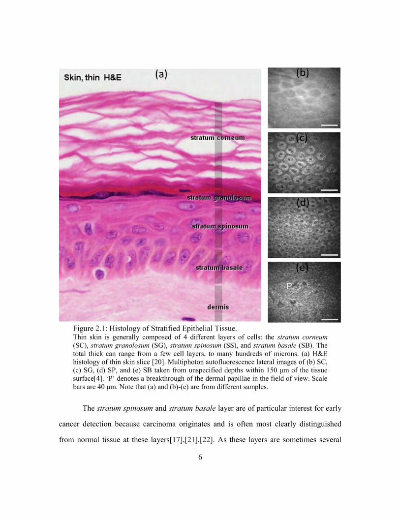
The stratum spinosum and stratum basale layer are of particular interest for early
cancer detection because carcinoma originates and is often most clearly distinguished
from normal tissue at these layers[17],[21],[22]. As these layers are sometimes several
Figure 2.1: Histology of Stratified Epithelial Tissue. Thin skin is generally composed of 4 different layers of cells: the stratum corneum
(SC), stratum granolosum (SG), stratum spinosum (SS), and stratum basale (SB). The
total thick can range from a few cell layers, to many hundreds of microns. (a) H&E
histology of thin skin slice [20]. Multiphoton autofluorescence lateral images of (b) SC,
(c) SG, (d) SP, and (e) SB taken from unspecified depths within 150 μm of the tissue
surface[4]. ‗P‘ denotes a breakthrough of the dermal papillae in the field of view. Scale
bars are 40 μm. Note that (a) and (b)-(e) are from different samples.
7
hundreds of microns below the surface, it is important for any imaging modality to be
used in cancer management to reach at least a few hundred microns deep.
2.2. TECHNIQUES FOR EPITHELIAL CANCER IMAGING
The most commonly used gold standard for carcinoma evaluation is
histopathology of a excised biopsy, usually initiated by visual inspection. This is a time-
consuming, invasive, and costly procedure. For a histology sample, the tissue is sliced so
that the histopathologist can view the depth-resolved structure of the sample. The
diagnosis is then based on both the microscopic and macroscopic structure of the tissue.
Ideally, alternative techniques for monitoring cancer would then provide three-
dimensional, or at least depth-resolved imaging, as well as microscopic resolution and
large field of views.
There are several imaging modalities in the research phase that meet these
requirements and none are without disadvantages. High frequency ultrasound (HFUS)
can image ~7 mm deep in skin, but provides a maximum resolution of hundreds of
microns. High resolution magnetic resonance imaging (MRI) can reach ~100 μm
resolution and image the entire body. However, it suffers from being an expensive, time
consuming technique, which, along with its poor resolution, make it impractical for
replacing biopsy in its current state.
Among optical technologies, confocal microscopy (CM) provides sub-μm lateral
resolution, and ~1 μm axial resolution, and allows three-dimensional imaging down to
tens of microns with autofluorescence contrast, and several hundreds of microns with
scattering or exogenous fluorescence contrast[23-26]. Mauna Kea©
has recently begun
selling a commercial device for clinical confocal endoscopy for epithelial tissue
imaging[27],[28]. High resolution optical coherence tomography (OCT) provides ~10 μm
8
lateral and sub-μm axial resolution and has the additional advantages of being extremely
fast and able to image more than 1 mm deep in epithelial tissues. OCT has found growing
success in intravascular imaging over the last decade, and is now being applied towards
epithelial tissue imaging (Michelson Diagnostics©
)[5]. However, contrast in OCT is
limited to scattering, and convincing subcellular-resolution imaging of epithelial cells has
yet to be demonstrated[5],[29]. Photoacoustic imaging (PA) can image several
millimeters deep in epithelial tissues but only reaches 50-100 μm resolution and is
limited to optical absorption contrast[30],[31].
The focus of this dissertation is on nonlinear microscopy (NM). NM can reach
several hundreds of microns deep in epithelial tissue and maintain resolutions less than 1
μm laterally and ~1 μm axially. Thus this technique exceeds the resolution of each
technique described previously with the exception of CM. In comparison to CM, NM
offers equivalent resolution and significantly deeper imaging capabilities when relying on
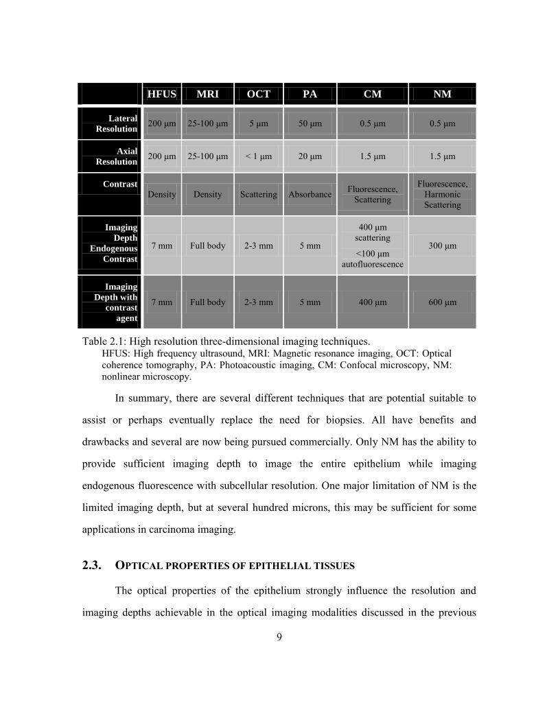
fluorescence contrast. A comparison of the 6 high resolution imaging modalities
discussed here is summarized in Table 2.1. A detailed discussion of the achievable
imaging depths in NM is presented in Chapter 5.
9
In summary, there are several different techniques that are potential suitable to
assist or perhaps eventually replace the need for biopsies. All have benefits and
drawbacks and several are now being pursued commercially. Only NM has the ability to
provide sufficient imaging depth to image the entire epithelium while imaging
endogenous fluorescence with subcellular resolution. One major limitation of NM is the
limited imaging depth, but at several hundred microns, this may be sufficient for some
applications in carcinoma imaging.
2.3. OPTICAL PROPERTIES OF EPITHELIAL TISSUES
The optical properties of the epithelium strongly influence the resolution and
imaging depths achievable in the optical imaging modalities discussed in the previous
HFUS MRI OCT PA CM NM
Lateral
Resolution 200 μm 25-100 μm 5 μm 50 μm 0.5 μm 0.5 μm
Axial
Resolution 200 μm 25-100 μm < 1 μm 20 μm 1.5 μm 1.5 μm
Contrast
Density Density Scattering Absorbance Fluorescence, Scattering
Fluorescence, Harmonic Scattering
Imaging
Depth
Endogenous
Contrast
7 mm Full body 2-3 mm 5 mm
400 μm scattering
<100 μm autofluorescence
300 μm
Imaging
Depth with
contrast
agent
7 mm Full body 2-3 mm 5 mm 400 μm 600 μm
Table 2.1: High resolution three-dimensional imaging techniques. HFUS: High frequency ultrasound, MRI: Magnetic resonance imaging, OCT: Optical
coherence tomography, PA: Photoacoustic imaging, CM: Confocal microscopy, NM:
nonlinear microscopy.
10
section. There are generally four parameters that are used to characterize the bulk optical
properties of biological tissues[32]. The index of refraction, n, describes the relative
speed of light in the sample. The scattering coefficient, μs, and absorption coefficient, μa,
describe the average number of scattering and absorption events seen by a photon per unit
length. In this dissertation, the inverse of these parameters is more commonly used—the
mean free scattering and absorption length, ls and la, which describe the average path
length a photon traverses between scattering and absorbing events, respectively. Lastly,
the scattering anisotropy, g, describes the average angle at which the scattered photon
propagates relative to its initial direction. A g of 1 means the scattered light is entirely
forward scattering while a g of 0 indicates the scattered light is scattered equally in all
directions.
For some applications, such as diffuse imaging and phototherapy, the total photon
fluence reaching a target is most important to achieve the desired outcome, regardless of
temporal or spatial coherence of the incident light. In these applications, photon scattered
at a small angle might have a similar effect as the ballistic photons, and the more relevant
scattering parameter is the transport corrected scattering length, . This
parameter describes the average length a photon travels before it is pointing in
approximately a random direction. For tissue microscopy, however, the traditional
scattering length, more intimately related to imaging performance, as even photons
scattered at a small angle will miss the micron-sized focal spot.
Each of the four bulk tissue optical parameters are wavelength dependent and
vary between tissue type, site, patient, and even by layer within the tissue. In epithelial
tissue, n typically ranges from 1.34 to 1.43 at the basal layer and upper dermis, from 1.36
to 1.43 in the intermediate epithelial layers, and from 1.45 to 1.49 in the stratum
corneum[33-35]. Scattering in epithelial tissues is typically highly forward scattering, and
11
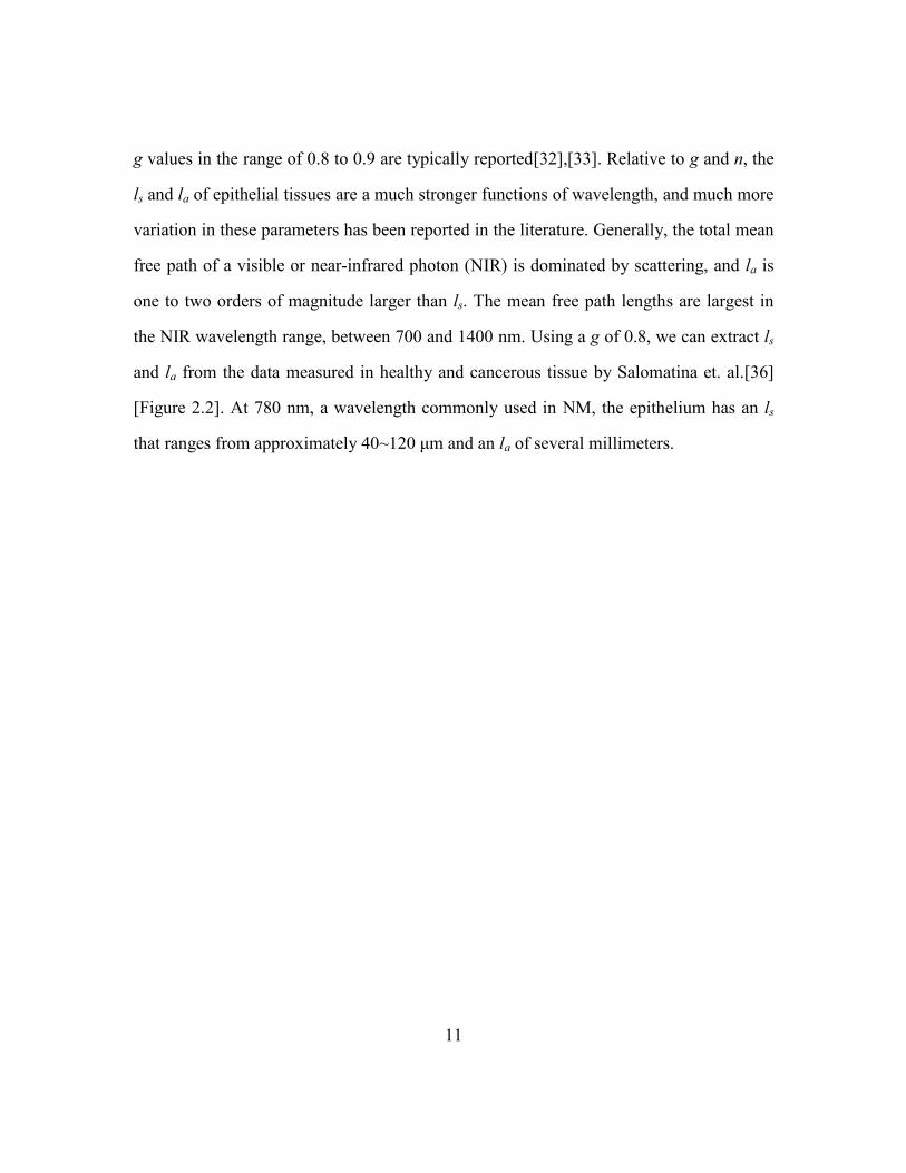
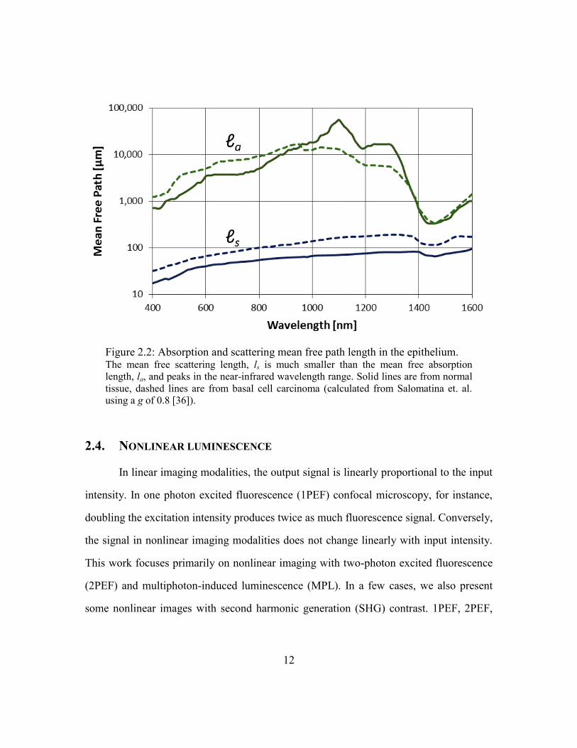
g values in the range of 0.8 to 0.9 are typically reported[32],[33]. Relative to g and n, the
ls and la of epithelial tissues are a much stronger functions of wavelength, and much more
variation in these parameters has been reported in the literature. Generally, the total mean
free path of a visible or near-infrared photon (NIR) is dominated by scattering, and la is
one to two orders of magnitude larger than ls. The mean free path lengths are largest in
the NIR wavelength range, between 700 and 1400 nm. Using a g of 0.8, we can extract ls
and la from the data measured in healthy and cancerous tissue by Salomatina et. al.[36]
[Figure 2.2]. At 780 nm, a wavelength commonly used in NM, the epithelium has an ls
that ranges from approximately 40~120 μm and an la of several millimeters.
12
2.4. NONLINEAR LUMINESCENCE
In linear imaging modalities, the output signal is linearly proportional to the input
intensity. In one photon excited fluorescence (1PEF) confocal microscopy, for instance,
doubling the excitation intensity produces twice as much fluorescence signal. Conversely,
the signal in nonlinear imaging modalities does not change linearly with input intensity.
This work focuses primarily on nonlinear imaging with two-photon excited fluorescence
(2PEF) and multiphoton-induced luminescence (MPL). In a few cases, we also present
some nonlinear images with second harmonic generation (SHG) contrast. 1PEF, 2PEF,
Figure 2.2: Absorption and scattering mean free path length in the epithelium. The mean free scattering length, ls is much smaller than the mean free absorption
length, la, and peaks in the near-infrared wavelength range. Solid lines are from normal
tissue, dashed lines are from basal cell carcinoma (calculated from Salomatina et. al.
using a g of 0.8 [36]).

13
and SHG are described in this section. MPL is introduced here, but discussed in greater
detail in Chapter 6.
The processes involved 1PEF, 2PEF, and SHG are illustrated in a Jablonski
diagram below [Figure 2.3]. In 1PEF, a high energy photon excites an electron from a
ground state, through a bandgap, to an excited state. The excited electron undergoes
nonradiative decay and, for bright fluorophores, stays in the excited state for timescales
in the nanosecond range. Some percentage of excited electrons will emit a lower energy
photon as they return to the ground state. Generally, a longer lifetime in the excited state
results in a higher fraction of emission photons produced for each excitation photon
absorbed. This fraction is called the quantum yield of the fluorophore.
In 2PEF, two lower energy excitation photons ―simultaneously‖ interact with a
ground state electron. This process can be thought of as excitation via a very short
lifetime intermediate (―virtual‖) state. The time scale of interaction necessary for
Figure 2.3: Jablonski diagram of one and two photon excited fluorescence and
second harmonic generation. One photon excited fluorescence (1PEF) involves excitation of an electron from the
ground state, s0, to an excited state, s1, from the absorbance of a high energy photon,
and the emission of a lower energy photon. Two-photon excited fluorescence (2PEF)
involves the excitation of an electron from the simultaneous absorption of two low
energy photons through a virtual intermediate state (si) and the emission of a higher
energy photons. In second harmonic generation (SHG), two photons simultaneously
interact with a sample to produce a photon with exactly twice the energy of the
excitation photons.
14
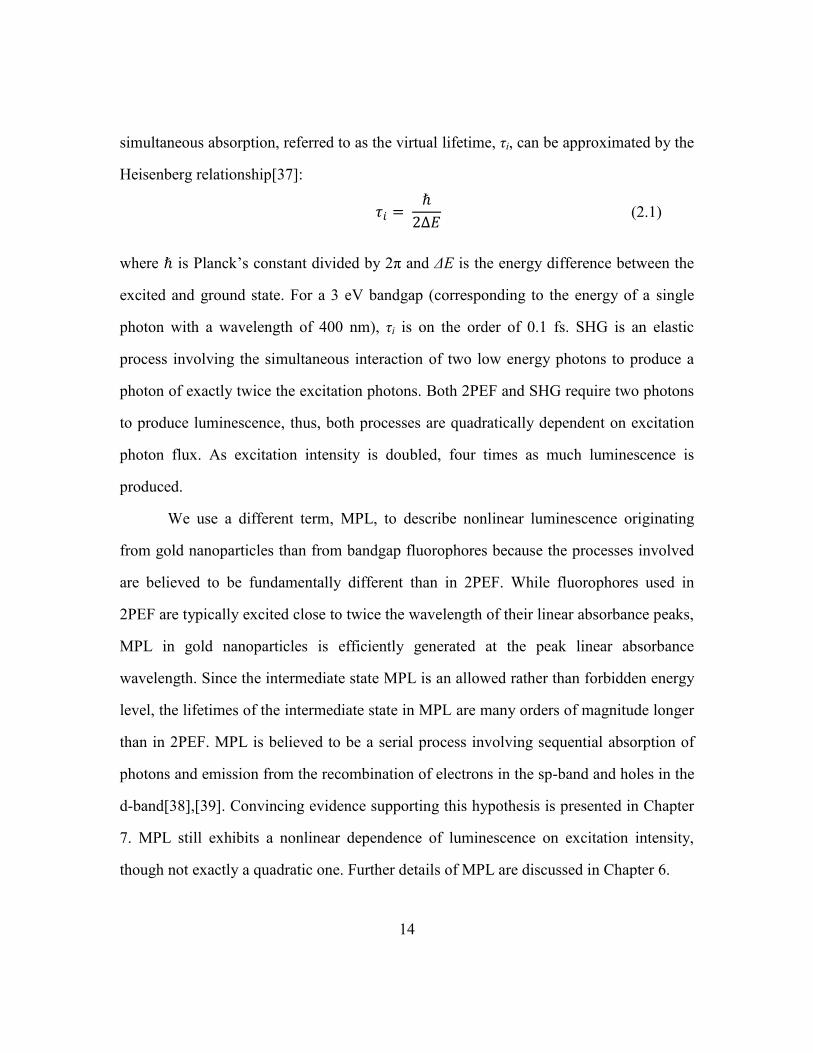
simultaneous absorption, referred to as the virtual lifetime, τi, can be approximated by the
Heisenberg relationship[37]:
(2.1)
where is Planck‘s constant divided by 2π and ΔE is the energy difference between the
excited and ground state. For a 3 eV bandgap (corresponding to the energy of a single
photon with a wavelength of 400 nm), τi is on the order of 0.1 fs. SHG is an elastic
process involving the simultaneous interaction of two low energy photons to produce a
photon of exactly twice the excitation photons. Both 2PEF and SHG require two photons
to produce luminescence, thus, both processes are quadratically dependent on excitation
photon flux. As excitation intensity is doubled, four times as much luminescence is
produced.
We use a different term, MPL, to describe nonlinear luminescence originating
from gold nanoparticles than from bandgap fluorophores because the processes involved
are believed to be fundamentally different than in 2PEF. While fluorophores used in
2PEF are typically excited close to twice the wavelength of their linear absorbance peaks,
MPL in gold nanoparticles is efficiently generated at the peak linear absorbance
wavelength. Since the intermediate state MPL is an allowed rather than forbidden energy
level, the lifetimes of the intermediate state in MPL are many orders of magnitude longer
than in 2PEF. MPL is believed to be a serial process involving sequential absorption of
photons and emission from the recombination of electrons in the sp-band and holes in the
d-band[38],[39]. Convincing evidence supporting this hypothesis is presented in Chapter
7. MPL still exhibits a nonlinear dependence of luminescence on excitation intensity,
though not exactly a quadratic one. Further details of MPL are discussed in Chapter 6.
15
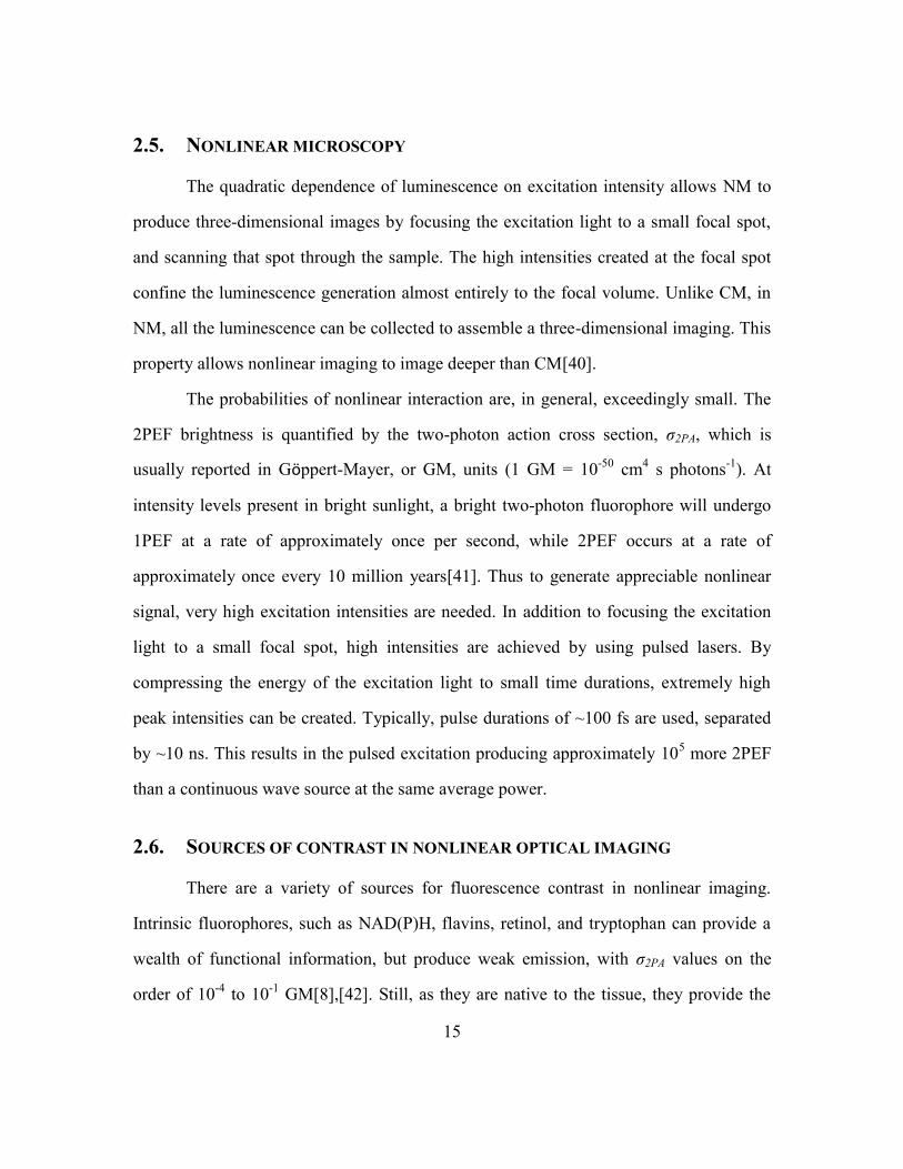
2.5. NONLINEAR MICROSCOPY
The quadratic dependence of luminescence on excitation intensity allows NM to
produce three-dimensional images by focusing the excitation light to a small focal spot,
and scanning that spot through the sample. The high intensities created at the focal spot
confine the luminescence generation almost entirely to the focal volume. Unlike CM, in
NM, all the luminescence can be collected to assemble a three-dimensional imaging. This
property allows nonlinear imaging to image deeper than CM[40].
The probabilities of nonlinear interaction are, in general, exceedingly small. The
2PEF brightness is quantified by the two-photon action cross section, σ2PA, which is
usually reported in Göppert-Mayer, or GM, units (1 GM = 10-50
cm4 s photons
-1). At
intensity levels present in bright sunlight, a bright two-photon fluorophore will undergo
1PEF at a rate of approximately once per second, while 2PEF occurs at a rate of
approximately once every 10 million years[41]. Thus to generate appreciable nonlinear
signal, very high excitation intensities are needed. In addition to focusing the excitation
light to a small focal spot, high intensities are achieved by using pulsed lasers. By
compressing the energy of the excitation light to small time durations, extremely high
peak intensities can be created. Typically, pulse durations of ~100 fs are used, separated
by ~10 ns. This results in the pulsed excitation producing approximately 105 more 2PEF
than a continuous wave source at the same average power.
2.6. SOURCES OF CONTRAST IN NONLINEAR OPTICAL IMAGING
There are a variety of sources for fluorescence contrast in nonlinear imaging.
Intrinsic fluorophores, such as NAD(P)H, flavins, retinol, and tryptophan can provide a
wealth of functional information, but produce weak emission, with σ2PA values on the
order of 10-4
to 10-1
GM[8],[42]. Still, as they are native to the tissue, they provide the
16
simplest method of functional and morphological contrast. Harmonic generation imaging
can also provide contrast to native structures in biological tissues. SHG imaging is
sensitive fibrillar structures, such as collagen, axons, muscle filaments, and microtubule
assemblies[10],[43-45]. Third harmonic generation imaging, on the other hand, is
sensitive to focal-spot sized or larger volumes which exhibit a large difference in
refractive index compared to the surrounding medium, which commonly occurs from air
bubbles and lipid droplets[46-48].
An alternative strategy to relying on endogenous contrast is to introduce contrast
agents into the sample. Though delivery of the contrast agent to the target of interest is
sometimes challenging, this technique has two important advantages: (1) a very bright
probe can be used, and (2) this probe can be targeted to a ligand of interest. Many
exogenous fluorophores used for single-photon fluorescence can also be used as two-
photon contrast agents, the brightest of which have a σ2PA on the order of 10-100 GM.
There has been some success in engineering organic dyes specifically for large σ2PA, and
values on the order of several hundreds of GM have been reported[49]. Quantum dots are
increasingly being used as two-photon contrast agents because of their extremely high
σ2PA values of up to 50,000 GM[50]. Gold nanoparticles have recently been shown to
have relatively large σ2PA values, with rough estimates ranging from 2,000 to 30,000
GM[51],[52]. Our measurements of gold nanoparticle brightness indicate even larger σ2PA
values are possible, up to 106 GM. Details of these calculations are discussed in detail in
Chapter 7.
17
2.7. PLASMONIC NANOPARTICLES
2.7.1. Surface plasmon resonance
When metals are reduced in size to lengths that are comparable to the mean free
path of their conduction band electrons (40-50 nm in gold[53]), they exhibit intense
interactions with light[54]. At these size scales, the surface electrons are resonantly
oscillated by visible and ultraviolet light. The coherent motion of these free electrons is
called the surface plasmon resonance (SPR). Depending on the geometry, orientation, and
material of the particle, the SPR leads to intense interactions of the particle with light
within a range of optical frequencies.
The interaction of light with particles can be quantified by the scattering and
absorption cross sections, Cs, and Ca respectively. The sum of these parameters is defined
as the extinction cross section, Ce. These values describe the area of light that interacts
with the particle, and can be orders of magnitude smaller or larger than the geometric
cross section of the particle. For perfectly spherical nanospheres, Mie showed[55] that
these parameters can be calculated exactly by solving Maxwell‘s equations[56],[55],[57]:
| | ∑
(2.2)
| | ∑ | |
| |
(2.3)
where,
(2.4)
(2.5)
18
Here, m is the ratio of the complex index of refraction of the particle to the real index of
refraction of the surrounding medium, k is the wave-vector, | | , where r is the
radius of the particle, and and are the Ricatti-Bessel cylindrical functions[57]. The
prime notation indicates differentiation with respect to the argument in parenthesis[57].
In general, for nonspherical particles, the cross sections must be determined numerically.
In this work we use the discrete dipole approximation (DDA) to calculate the relevant
cross sections of nonspherical particles[58]. In this method, a particle is simulated as an
array of polarizable points which become dipoles in response to an electric field. These
dipoles interact with each other and results converge to the exact analytical solution for
an increasing density of polarizable points.
From Eqs. (2.2)-(2.5), it is clear that by changing the geometry of the particle or
the optical properties of the particle or the surrounding material, the spectral shape and
magnitudes of the cross sections will also change. Thus the optical properties of metallic
particles can be ―tuned‖ to give a desired response at a particular wavelength. At the peak
SPR wavelength, metallic nanoparticles can have optical cross sections that are orders of
magnitude larger than their geometric cross sections[54],[57],[59]. Peak Ca values can be
5 orders of magnitude larger than that found in conventional absorbing dyes, and peak Cs
can be 5 orders of magnitude larger than fluorescence from strongly fluorescing dyes[59].
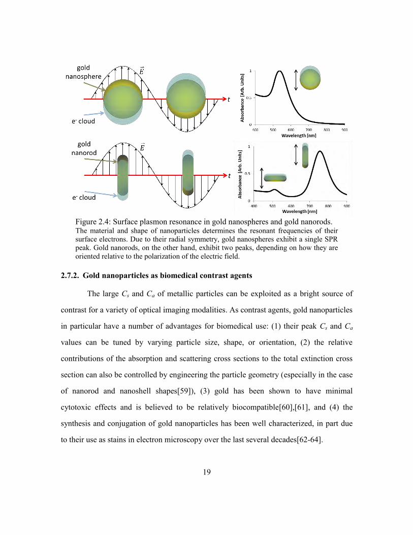
Gold nanospheres with a diameter of 70 nm exhibit a peak SPR at 530 nm when
suspended in water. Gold nanorods with a length of 50 nm and a width of 15 nm exhibit
two peaks when isotropically oriented in water—one at 510 nm when the electric field is
parallel to the short axis of the nanorod and a second at 780 nm when the electric field is
parallel to the long axis of the gold nanorod [Figure 2.4].
19
2.7.2. Gold nanoparticles as biomedical contrast agents
The large Cs and Ca of metallic particles can be exploited as a bright source of
contrast for a variety of optical imaging modalities. As contrast agents, gold nanoparticles
in particular have a number of advantages for biomedical use: (1) their peak Cs and Ca
values can be tuned by varying particle size, shape, or orientation, (2) the relative
contributions of the absorption and scattering cross sections to the total extinction cross
section can also be controlled by engineering the particle geometry (especially in the case
of nanorod and nanoshell shapes[59]), (3) gold has been shown to have minimal
cytotoxic effects and is believed to be relatively biocompatible[60],[61], and (4) the
synthesis and conjugation of gold nanoparticles has been well characterized, in part due
to their use as stains in electron microscopy over the last several decades[62-64].
Figure 2.4: Surface plasmon resonance in gold nanospheres and gold nanorods. The material and shape of nanoparticles determines the resonant frequencies of their
surface electrons. Due to their radial symmetry, gold nanospheres exhibit a single SPR
peak. Gold nanorods, on the other hand, exhibit two peaks, depending on how they are
oriented relative to the polarization of the electric field.
20
Gold nanoparticles were first demonstrated as sensitive probes for Raman
spectroscopy[65-67] and single molecule studies[68-70] in the 1990‘s. Later, Sokolov et
al. demonstrated the use of gold nanospheres for scattering contrast in vital reflectance
confocal imaging of cancer cells and tissues[71]. Since their demonstration, gold
nanospheres, nanoshells, and nanorods have also been applied as targeted contrast agents
for OCT (which uses large Cs for contrast) [72-74], and PAM (which uses large Ca for
contrast)[75-77]. There has also been important progress in using gold nanoparticles as a
therapeutic agent. These studies typically utilize the large Ca of gold nanoparticles at NIR
wavelengths for targeted thermal therapy[78-84].
2.7.3. Multiphoton luminescence from plasmonic nanoparticles
The large σ2PA values observed in metallic particles are somewhat unexpected—
traditionally, gold particles are known for their quenching of fluorescence, rather than
fluorescence emission[85]. The lifetime of excited electrons in metals is extremely fast,
on the order of tens to hundreds of femtoseconds[86],[87]. Partially due to this short
lifetime, the quantum yield of smooth metal surfaces have been measured to be extremely
low—on the order of 10-10
[38]. Nonetheless, weak luminescence can still be observed.
Single-photon-induced luminescence was first reported from bulk copper and
gold by Mooradian in 1969[88]. Later, Boyd et al. found that roughened metal surfaces
exhibited much higher single-photon-induced luminescence efficiency than smooth
surfaces. They also found that while MPL was not measurable in smooth gold films,
appreciable MPL could be observed from roughened surfaces[38]. In 2000, Mohamed et
al. found that gold nanorods offered dramatically larger quantum yield than bulk gold,
which they dubbed, the ―lightning rod‖ effect[89]. They measured an enhancement of
approximately 106 in emission yield when using excitation light at the linear absorbance
21
peak of gold nanorods. These results support the hypothesis that the presence of an SPR
in the sample is important to the efficient generation MPL. However, as we will
demonstrate in Chapter 6, the σTPA of a particle is relatively weakly dependent on the
shape of the σext—bright MPL can be observed when exciting gold nanoparticles far from
their absorbance or scattering peaks. Thus, though SPR does seem to improve the
efficiency of MPL, the complicated relationship between the spectral shapes of Cs and Ca
indicates that MPL is not simply linearly related to the absorption or scattering
enhancement from the SPR.
Gold nanoparticles have previously been used as sources of contrast in nonlinear
imaging of biological samples. Yelin et al. demonstrated MPL and harmonic nonlinear
microscopy of clusters of gold nanospheres labeled to fixed cell[90]. Unlabeled gold
nanorods were used for in vivo MPL imaging of blood vessels by Wang et al.[51]. Farrer
et al. showed that nanosphere can be bright sources of MPL when excited far from their
SPR peaks[91]. In this dissertation we expand work done by our group, which
demonstrated MPL imaging of cancer cells labeled with gold nanorods[92]. Additional
studies have also recently shown that MPL can be used for imaging nanoshells[93],
exploring the interaction of nanoparticles with cells[94-96], and even reading optically-
encoded data[97].
22
Chapter 3 Design and characterization of
nonlinear scanning microscope
for deep tissue imaging
This chapter presents the design and characterization of a laser scanning nonlinear
microscope that is optimized specifically for deep tissue autofluorescence imaging.
Several important parameters are discussed, including a characterization of excitation
source, the parameters related to objective lens performance, and the optimization of the
collection optics. A detailed presentation of the control and acquisition software, the
specific parts used, and the overall construction of the microscope can be found in the
thesis of Benjamin Holfeld[98].
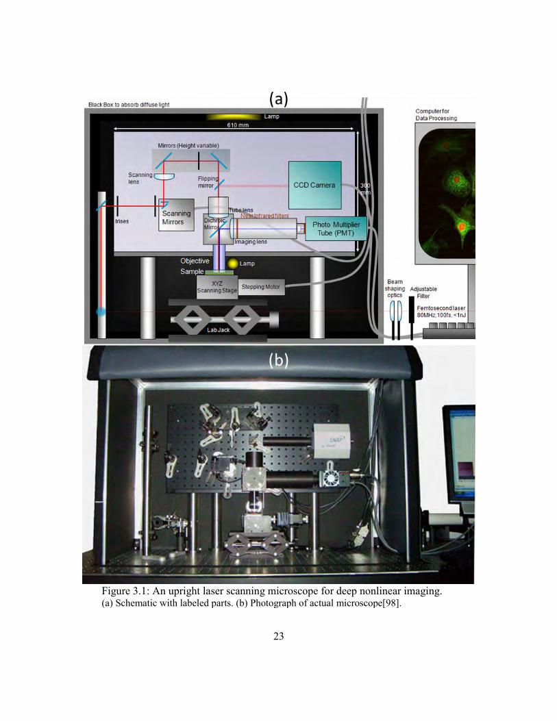
3.1. OVERVIEW
The excitation path consists of a pair of scanning mirrors, two relay lenses, and a
long working distance, large field-of-view objective lens. The emission path uses non-
descanned collection, large diameter optics, high throughput filters, and a sensitive
photomultiplier tube (PMT) to maximize visible-light sensitivity. A customized computer
program controls and synchronizes image acquisition, mirror scanning, excitation power
control, and sample position. The microscope is configured in an upright configuration—
the sample is placed under the objective—to enable the use of a water dipping objective
and to facilitate future studies involving in-vivo animal studies. Imaging throughput is
limited to 5×106 pixels per second by the data acquisition card, but imaging is typically
performed at 1×106 pixels per second to match the bandwidth of our preamplifier.
23
Figure 3.1: An upright laser scanning microscope for deep nonlinear imaging. (a) Schematic with labeled parts. (b) Photograph of actual microscope[98].
24
3.2. EXCITATION PATH
3.2.1. Excitation source
We used a Ti:Saphire, mode locked laser oscillator (Newport, MaiTai) as our
excitation source. This source has a repetition rate of 80 MHz, an excitation wavelength,
λx, tunable from 710 to 880 nm, and an average power, Pex, of 0.6 to 1.1 W across the
tuning range. We measured the full width at half maximum (FWHM) of the spectral
bandwidth, Δλ, to be 7.5 nm. Using a time-bandwidth product of 0.44, a transform
limited pulse with this bandwidth would have a FWHM pulse duration, FWHM
p of 120 fs.
The pulse duration at the imaging plane of the objective, which is more relevant to
imaging parameters, is discussed in Section 3.3.2. We measured the 1/e2 diameter of the
excitation beam to be approximately 1.5 mm in the vertical direction and 1.2 mm in the
horizontal direction at the output of the laser oscillator. The slightly larger divergence of
the smaller (horizontal) axis resulted in the beam shape being relatively circular at the
position of the objective back aperture. We used two lenses in a Galileo-configuration
beam expander with focal lengths (f) of -30 and 75 mm for a 2.5x increase in beam size.
Two sets of half wave plate (HWP) and polarizing beam cube are used to control
the excitation power. We found this solution to have several advantages over the use of
reflective neutral density filters: (1) the excitation power may be continuously adjustable
and computer controlled, (2) the dispersion introduced into the system is constant as
attenuation is changed, and (3) this approach avoids the issue of spatial beam offset
associated with the introduction of a neutral density filter at non-perpendicular angles to
the excitation beam. One HWP was adjusted by a computer controlled actuator, providing
0.01° resolution. This resolution corresponds to a worst-case attenuation resolution of
approximately ±0.08% at 780 nm (Newport, PR50PP, 10RP52-2). This value is
calculated assuming the HWP angle is adjusted at the steepest rate of transmission
25
change versus angle change. The second HWP can be manually adjusted. Combined, the
total power attenuation can be varied from less than 0.4 dB to greater than 40 dB within
the range of λx = 760-820 nm. In some cases, additional attenuation was necessary. This
was accomplished by inserting additional reflective neutral density filters in the
excitation path.
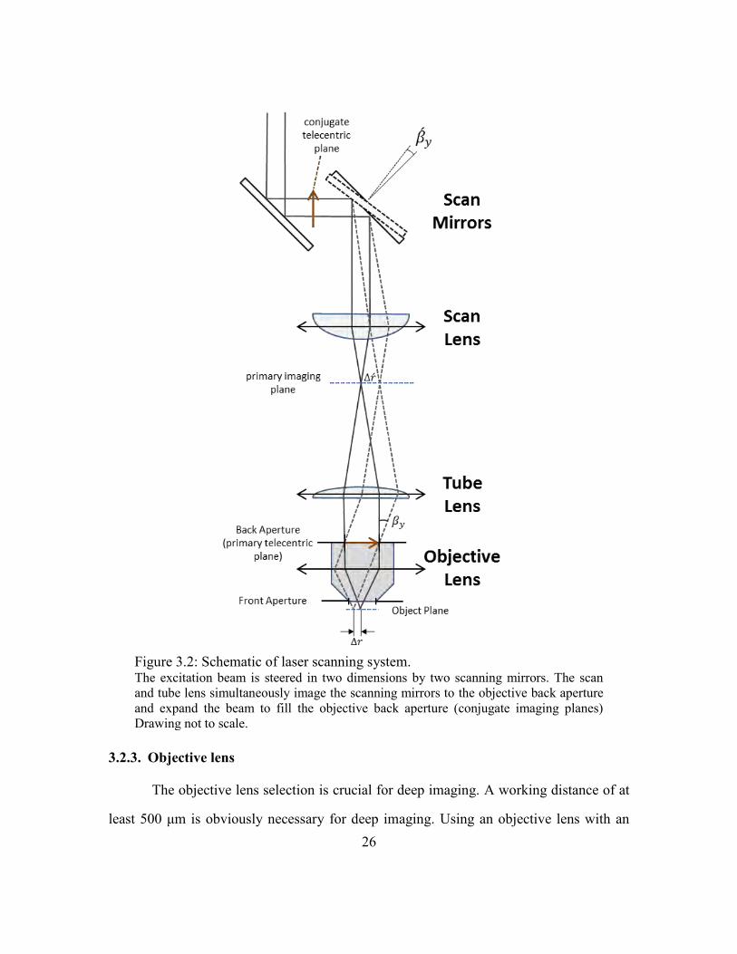
3.2.2. Laser scanning system
Two requirements of the laser scanning system are that (1) the excitation beam is
sufficiently expanded to fill the objective back aperture, allowing full use of the objective
numerical aperture (NA), and (2) that the scanning mirrors are imaged to the back
aperture, resulting in a uniform field of view at the object plane. We use a telecentric
two-lens relay system to simultaneously meet these requirements[99],[100] [Figure 3.2].
The scanning mirrors are sufficiently close together that both can be approximately
simultaneously imaged to the back aperture. We use an f = 50 mm scan lens and an f =
250 mm tube lens. The measured 1/e2 diameter of the excitation beam at the back
aperture was 12 mm.
26
3.2.3. Objective lens
The objective lens selection is crucial for deep imaging. A working distance of at
least 500 μm is obviously necessary for deep imaging. Using an objective lens with an
Figure 3.2: Schematic of laser scanning system. The excitation beam is steered in two dimensions by two scanning mirrors. The scan
and tube lens simultaneously image the scanning mirrors to the objective back aperture
and expand the beam to fill the objective back aperture (conjugate imaging planes)
Drawing not to scale.
27
immersion medium close in refractive index to the sample minimizes specimen induced
spherical aberrations, which helps maintain high intensities necessary for 2PEF[101-103].
The index of refraction of the oil, glycerol, and water used in common immersion
objectives are 1.53 (Zeiss Immersol), 1.47, and 1.33, respectively. Though the refractive
index of the stratum corneum is 1.45~1.5 it generally decreases to 1.36~1.43 closer to the
dermis[34],[35]. The tissue phantoms used in this dissertation are composed of greater
than 90% water, and are assumed to have a refractive index very close to 1.33. For these
applications, we chose a water immersion objective. Ideally, an objective with a
correction collar should be used to accommodate samples with n ≠ 1.33.
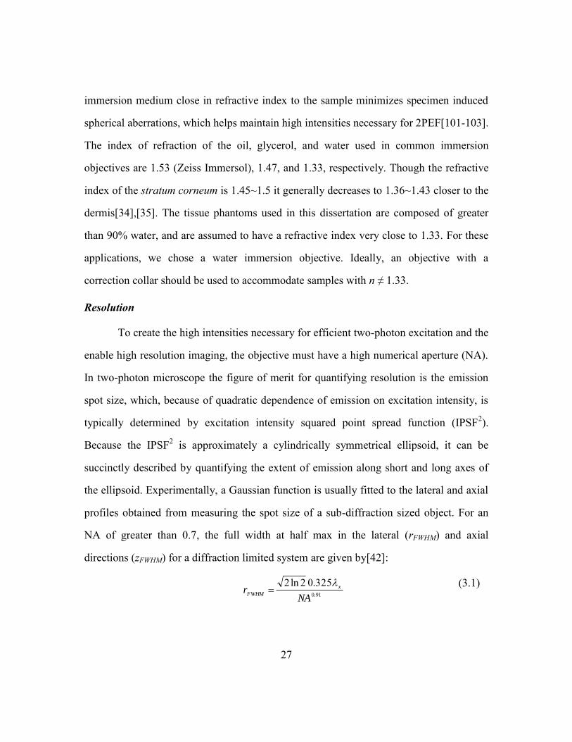
Resolution
To create the high intensities necessary for efficient two-photon excitation and the
enable high resolution imaging, the objective must have a high numerical aperture (NA).
In two-photon microscope the figure of merit for quantifying resolution is the emission
spot size, which, because of quadratic dependence of emission on excitation intensity, is
typically determined by excitation intensity squared point spread function (IPSF2).
Because the IPSF2 is approximately a cylindrically symmetrical ellipsoid, it can be
succinctly described by quantifying the extent of emission along short and long axes of
the ellipsoid. Experimentally, a Gaussian function is usually fitted to the lateral and axial
profiles obtained from measuring the spot size of a sub-diffraction sized object. For an
NA of greater than 0.7, the full width at half max in the lateral (rFWHM) and axial
directions (zFWHM) for a diffraction limited system are given by[42]:
91.0
325.02ln2NA
r x
FWHM
(3.1)
28
22
1532.02ln2NAnn
zxFWHM
(3.2)
Field of View
The objective lens field of view (FOV) is an often overlooked but important
specification that influences collection efficiency[104]. The FOV describes the maximum
lateral distance from the optical axis a small source at the focal plane can be while being
imaged by the objective lens. Since the transmission of light from a point source
gradually decreases as the point source is moved off axis, the definition is somewhat
arbitrary. In the definition used here, the FOV is defined by the radius at which 1/e of the
maximum value of a point source is transmitted, rf. Thus, in order to collect as much
scattered emission light as possible, which will appear to originate from large distances
from the optical axis, it is important to maximize rf.
In practice, the rf of an objective is not usually specified by the manufacturer, as
it is the field of view of the integrated system (
) that is important for most
microscopes. The
is usually limited by the 25 mm diameter tube lens rather than the
objectives themselves. However, in nonlinear microscopy with non-descanned detection,
the emission is collected as close as possible to the back aperture and rf is important. In
general there is an inverse relation between the magnification, M, of a lens and rf.
Intuitively, this can be inferred by looking at Figure 3.2—the distance Δr in the object
plane is related to in the primary imaging plane by: . Therefore, in
choosing an objective for deep imaging, it is important to choose an objective with a low
magnification, and ideally, for one to measure the FOV.
29
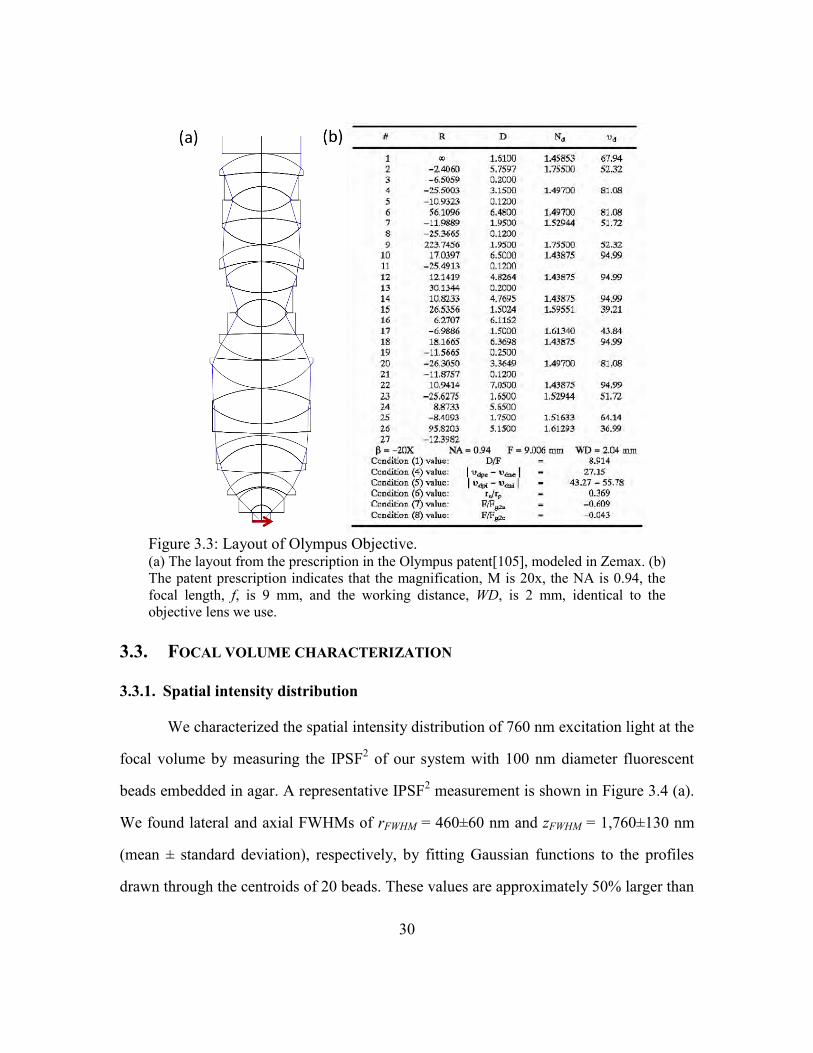
Olympus XLUMPFL Objective
We chose to use the Olympus 20x/0.95 water dipping objective lens (XLUMPFL)
for our system. In the absence of aberrations, this lens would provide an rFWHM and zFWHM
of 305 nm and 1.2 μm, respectively, at λx = 760 nm. The rf of a prototype of this
particular objective was measured to be especially large in comparison to others, with rf =
1.3 mm[104]. In comparison to a 63x/0.90 objective lens, this objective collected
approximately ten times more emission signal at large imaging depths[104]. Though the
exact layout of the objective is a trade secret, we show a prescription for an objective
with the same specifications from an Olympus patent[105]. We implemented the patent
prescription in Zemax-EE (2009 Version), and found the specifications of our objective
are met [Figure 3.3]. However, this layout should serve only as a qualitative picture of the
objective.
30
3.3. FOCAL VOLUME CHARACTERIZATION
3.3.1. Spatial intensity distribution
We characterized the spatial intensity distribution of 760 nm excitation light at the
focal volume by measuring the IPSF2 of our system with 100 nm diameter fluorescent
beads embedded in agar. A representative IPSF2 measurement is shown in Figure 3.4 (a).
We found lateral and axial FWHMs of rFWHM = 460±60 nm and zFWHM = 1,760±130 nm
(mean ± standard deviation), respectively, by fitting Gaussian functions to the profiles
drawn through the centroids of 20 beads. These values are approximately 50% larger than
Figure 3.3: Layout of Olympus Objective. (a) The layout from the prescription in the Olympus patent[105], modeled in Zemax. (b)
The patent prescription indicates that the magnification, M is 20x, the NA is 0.94, the
focal length, f, is 9 mm, and the working distance, WD, is 2 mm, identical to the
objective lens we use.
31
theoretical values expected with a diffraction-limited spot from a 0.95 NA water dipping
objective[42], and closer to what would be expected from diffraction-limited focusing
from a NA of 0.75. The difference between measured and diffraction-limited IPSF2 is too
large to be accounted for by our slight underfilling of the back aperture[106],[107], and is
likely due to lens aberrations at NIR wavelengths. Similarly large point spread functions
have been previously reported from this objective[104],[108],[109]. We found that the
PSF was independent of imaging depth through the full working distance of the lens (2
mm) in a transparent sample of 100 nm fluorescent beads embedded in an agar gel. This
result indicates that specimen-induced aberrations negligibly affect the shape of the
intensity distribution in the perifocal volume in agar phantoms, which is consistent with
other studies[110],[111].
32
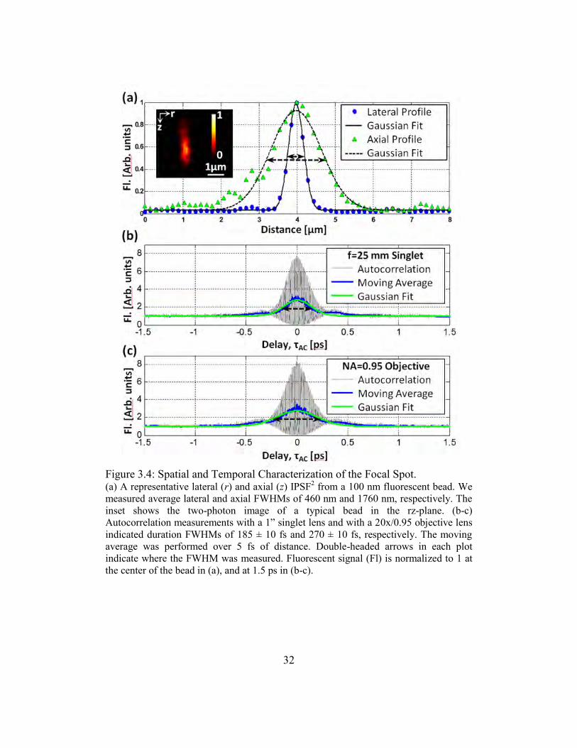
Figure 3.4: Spatial and Temporal Characterization of the Focal Spot. (a) A representative lateral (r) and axial (z) IPSF
2 from a 100 nm fluorescent bead. We
measured average lateral and axial FWHMs of 460 nm and 1760 nm, respectively. The
inset shows the two-photon image of a typical bead in the rz-plane. (b-c)
Autocorrelation measurements with a 1‖ singlet lens and with a 20x/0.95 objective lens
indicated duration FWHMs of 185 ± 10 fs and 270 ± 10 fs, respectively. The moving
average was performed over 5 fs of distance. Double-headed arrows in each plot
indicate where the FWHM was measured. Fluorescent signal (Fl) is normalized to 1 at
the center of the bead in (a), and at 1.5 ps in (b-c).
33
3.3.2. Temporal characterization
We characterized the temporal intensity distribution at the object plane of the
microscope by incorporating a Michelson interferometer with a variable delay arm in the
excitation path and measuring the autocorrelation function of the focused excitation beam
within a sample[112],[113]. We used 25 μM fluorescein in a pH 12 buffer as the sample.
We measured the autocorrelation function to estimate the pulse duration at the imaging
plane using the 0.95/20x Olympus objective lens. We also measured the autocorrelation
where the objective lens was replaced with a 1‖ diameter singlet lens with a 1‖ focal
length [Figure 3.4 (b) and (c)]. These two measurements allow us to estimate the GDD of
the objective lens (ϕo). We recorded the FWHM of a Gaussian fit, FWHM
AC , to the moving
average of our interferometric autocorrelation function over 5 measurements in each
configuration. Furthermore, we assumed the original pulse shape is a Gaussian, which
dictates that the time-bandwidth product, cB, is 0.44. The FWHM of the original pulse
shape, FWHM
p , is then related to the autocorrelation trace by:
.59.0 FWHM
AC
FWHM
p
(3.3)
We calculated the pulse duration at the sample plane to be FWHM
sp, 185 ± 8 fs with the
singlet lens and FWHM
op, 270 ± 10 fs with the objective lens from our autocorrelation
traces.
To calculate the GDD of the Olympus objective using these two measurements,
we use the equation relating the output pulse duration, Δtout, to the input pulse duration,
Δtin, for a given GDD, ϕ2, and frequency bandwidth, Δv.[114],[115]:
√
(3.4)
34
Note that this equation neglects the contribution from third and higher order dispersion.
Solving for ϕ2 and substituting the GDD of the system leading up to the focusing lens,
ϕsys, and either ϕs for ϕo the two measurements, we have:
√
( )
(3.5)
and
√
( )
(3.6)
Subtracting Eq. (3.6) from Eq. (3.5) and solving for ϕo:
(√(
)
√( )
)
(3.7)
Using the measured spectral bandwidth of 7.5 nm FWHM, our Δv is 3.7×10¹⁴
Hz at 760
nm. Assuming a modest ϕs of 250 fs2 from the 1‖ singlet lens[113], we calculate the GDD
of our objective to be ϕo ≈ 4,300 fs2 at 760 nm. This value is significantly larger than
reports of other similar-NA objectives[113], but not unexpected, given the long physical
length of this lens (75 mm long). For reference, the GDD of a 75 mm block of BK7 glass,
which has a group velocity dispersion of 50 fs2/mm at 760 nm, would be 3,750 fs
2.
3.4. COLLECTION PATH
Conventional nonlinear collection optical designs use a low f/# lens to image the
objective back aperture to the detector surface[99]. This approach maximizes emission
collection provided the emission is uniform in intensity at the back aperture and the f/# of
the collection lens fills the acceptance angle of the detector. However, neither of these
35
assumptions are appropriate in deep tissue imaging. For an infinity-corrected objective
lens, ballistic emission photons will retrace the path of the ballistic excitation light and
come out of the objective back aperture relatively collimated. There may be some
deviation between the two paths because many objective lenses are not corrected for
chromatic aberrations above ~700 nm, and so the focal planes of λx and λm can be slightly
different. But more importantly, the majority of emission light is scattered, even for
shallow imaging depths. For instance, imaging one mean free excitation path length deep
in epithelial tissue, the scattering length of emission light is typically on the order of half
that at the excitation wavelength (i.e. ls = 46 μm at λx = 760 nm and ls = 27 at λm = 500
nm[36]). Using Beer‘s Law, one can see that when imaging just 50 μm deep in these
conditions, less than 20% of the light emitted within the objective acceptance solid angle
will exit the tissue unscattered. Imaging 200 μm deep, this fraction drops to less than
0.06%. This underlies the importance of non-descanned detection in deep nonlinear
imaging.
The design of a collection system in our system is further complicated by the fact
that our detector (Hamamatsu H7422-40), which is commonly used because of its high
sensitivity, has a long tunnel surrounding the cathode which prevents high-angle photons
from being detected. Accordingly, we employed a computation model to maximize the
percentage of emission photons collected in our setup as collection lens parameters are
varied.
We optimized the collection optics for maximum emission collection for photons
from the diffusive regime using Zemax, similar to a previous approach[116]. We
launched the photons with Gaussian spatial and angular distribution with 1/e2 radii of
4.25 mm and 11.4°, respectively. This distribution was found from propagating diffuse
emission photons through the objective shown in Figure 3.3. Another approach would be
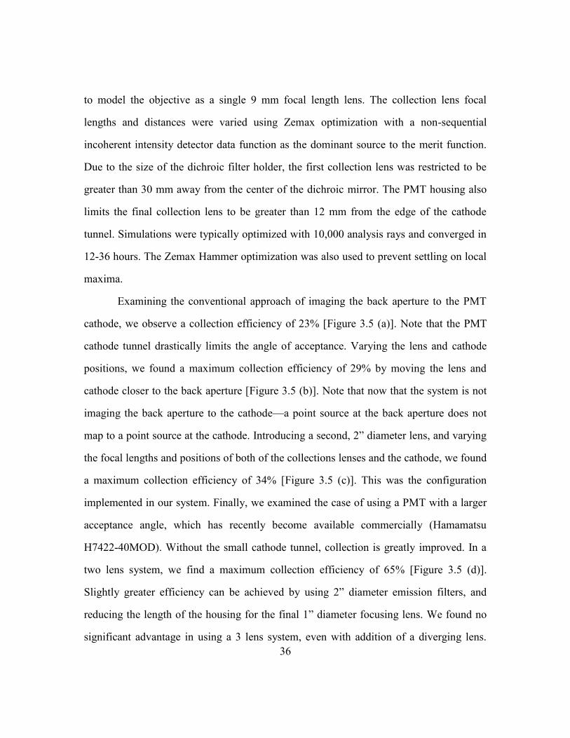
36
to model the objective as a single 9 mm focal length lens. The collection lens focal
lengths and distances were varied using Zemax optimization with a non-sequential
incoherent intensity detector data function as the dominant source to the merit function.
Due to the size of the dichroic filter holder, the first collection lens was restricted to be
greater than 30 mm away from the center of the dichroic mirror. The PMT housing also
limits the final collection lens to be greater than 12 mm from the edge of the cathode
tunnel. Simulations were typically optimized with 10,000 analysis rays and converged in
12-36 hours. The Zemax Hammer optimization was also used to prevent settling on local
maxima.
Examining the conventional approach of imaging the back aperture to the PMT
cathode, we observe a collection efficiency of 23% [Figure 3.5 (a)]. Note that the PMT
cathode tunnel drastically limits the angle of acceptance. Varying the lens and cathode
positions, we found a maximum collection efficiency of 29% by moving the lens and
cathode closer to the back aperture [Figure 3.5 (b)]. Note that now that the system is not
imaging the back aperture to the cathode—a point source at the back aperture does not
map to a point source at the cathode. Introducing a second, 2‖ diameter lens, and varying
the focal lengths and positions of both of the collections lenses and the cathode, we found
a maximum collection efficiency of 34% [Figure 3.5 (c)]. This was the configuration
implemented in our system. Finally, we examined the case of using a PMT with a larger
acceptance angle, which has recently become available commercially (Hamamatsu
H7422-40MOD). Without the small cathode tunnel, collection is greatly improved. In a
two lens system, we find a maximum collection efficiency of 65% [Figure 3.5 (d)].
Slightly greater efficiency can be achieved by using 2‖ diameter emission filters, and
reducing the length of the housing for the final 1‖ diameter focusing lens. We found no
significant advantage in using a 3 lens system, even with addition of a diverging lens.
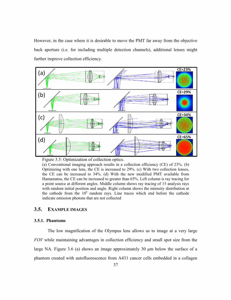
37
However, in the case where it is desirable to move the PMT far away from the objective
back aperture (i.e. for including multiple detection channels), additional lenses might
further improve collection efficiency.
3.5. EXAMPLE IMAGES
3.5.1. Phantoms
The low magnification of the Olympus lens allows us to image at a very large
FOV while maintaining advantages in collection efficiency and small spot size from the
large NA. Figure 3.6 (a) shows an image approximately 30 μm below the surface of a
phantom created with autofluorescence from A431 cancer cells embedded in a collagen
Figure 3.5: Optimization of collection optics. (a) Conventional imaging approach results in a collection efficiency (CE) of 23%. (b)
Optimizing with one lens, the CE is increased to 29%. (c) With two collection lenses,
the CE can be increased to 34%. (d) With the new modified PMT available from
Hamamatsu, the CE can be increased to greater than 65%. Left column is ray tracing for
a point source at different angles. Middle column shows ray tracing of 15 analysis rays
with random initial position and angle. Right column shows the intensity distribution at
the cathode from the 106 random rays. Line traces which end before the cathode
indicate emission photons that are not collected
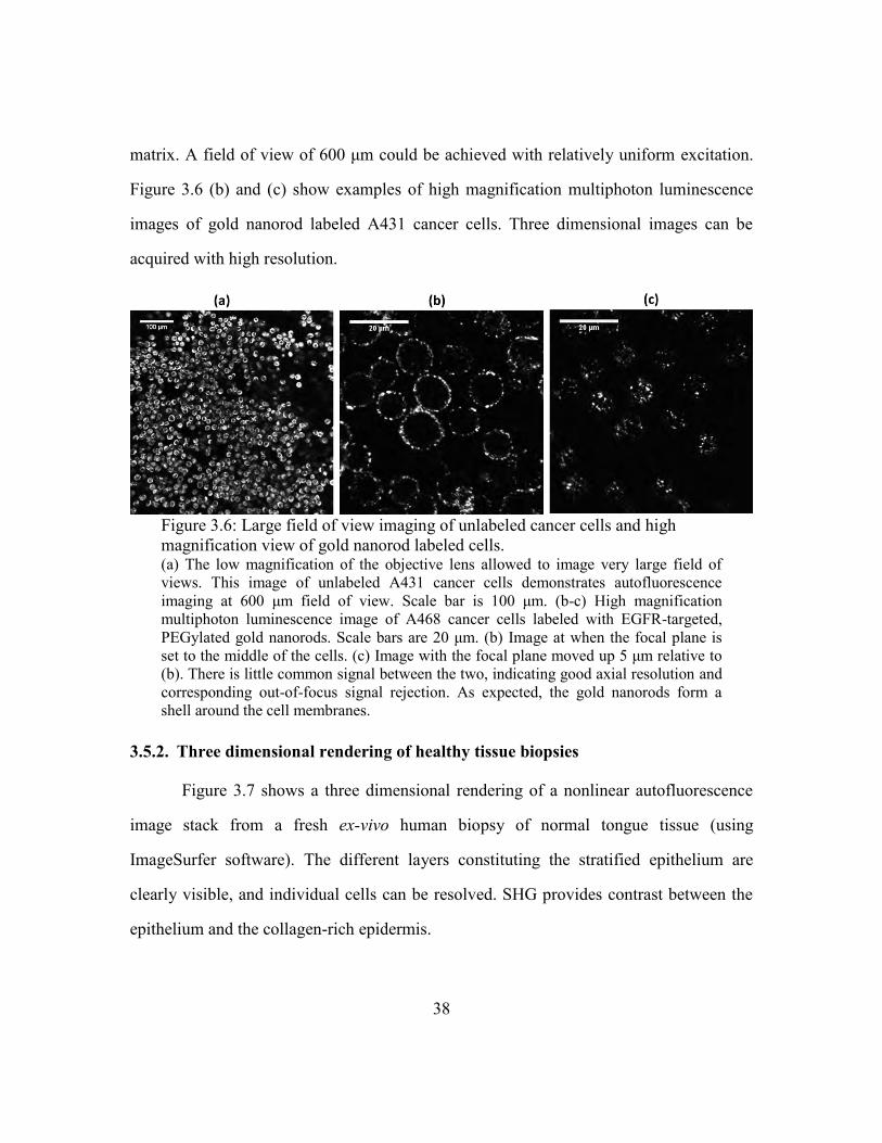
38
matrix. A field of view of 600 μm could be achieved with relatively uniform excitation.
Figure 3.6 (b) and (c) show examples of high magnification multiphoton luminescence
images of gold nanorod labeled A431 cancer cells. Three dimensional images can be
acquired with high resolution.
3.5.2. Three dimensional rendering of healthy tissue biopsies
Figure 3.7 shows a three dimensional rendering of a nonlinear autofluorescence
image stack from a fresh ex-vivo human biopsy of normal tongue tissue (using
ImageSurfer software). The different layers constituting the stratified epithelium are
clearly visible, and individual cells can be resolved. SHG provides contrast between the
epithelium and the collagen-rich epidermis.
Figure 3.6: Large field of view imaging of unlabeled cancer cells and high
magnification view of gold nanorod labeled cells. (a) The low magnification of the objective lens allowed to image very large field of
views. This image of unlabeled A431 cancer cells demonstrates autofluorescence
imaging at 600 μm field of view. Scale bar is 100 μm. (b-c) High magnification
multiphoton luminescence image of A468 cancer cells labeled with EGFR-targeted,
PEGylated gold nanorods. Scale bars are 20 μm. (b) Image at when the focal plane is
set to the middle of the cells. (c) Image with the focal plane moved up 5 μm relative to
(b). There is little common signal between the two, indicating good axial resolution and
corresponding out-of-focus signal rejection. As expected, the gold nanorods form a
shell around the cell membranes.
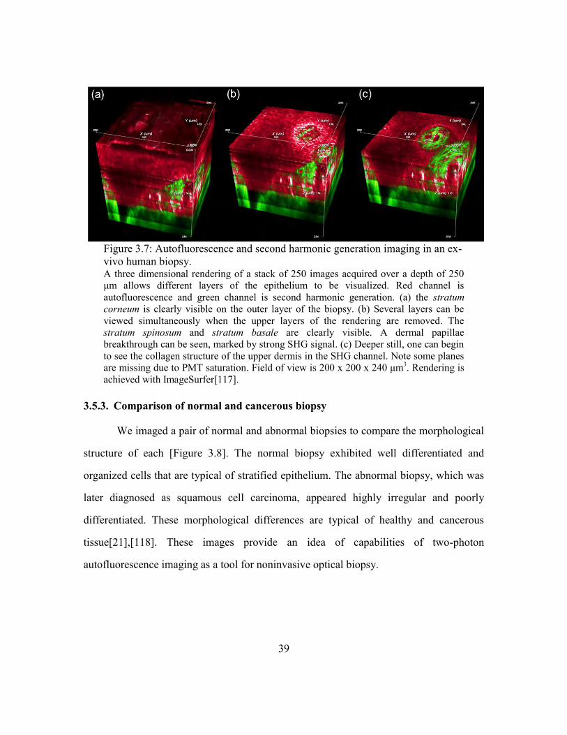
39
3.5.3. Comparison of normal and cancerous biopsy
We imaged a pair of normal and abnormal biopsies to compare the morphological
structure of each [Figure 3.8]. The normal biopsy exhibited well differentiated and
organized cells that are typical of stratified epithelium. The abnormal biopsy, which was
later diagnosed as squamous cell carcinoma, appeared highly irregular and poorly
differentiated. These morphological differences are typical of healthy and cancerous
tissue[21],[118]. These images provide an idea of capabilities of two-photon
autofluorescence imaging as a tool for noninvasive optical biopsy.
Figure 3.7: Autofluorescence and second harmonic generation imaging in an ex-
vivo human biopsy. A three dimensional rendering of a stack of 250 images acquired over a depth of 250
μm allows different layers of the epithelium to be visualized. Red channel is
autofluorescence and green channel is second harmonic generation. (a) the stratum
corneum is clearly visible on the outer layer of the biopsy. (b) Several layers can be
viewed simultaneously when the upper layers of the rendering are removed. The
stratum spinosum and stratum basale are clearly visible. A dermal papillae
breakthrough can be seen, marked by strong SHG signal. (c) Deeper still, one can begin
to see the collagen structure of the upper dermis in the SHG channel. Note some planes
are missing due to PMT saturation. Field of view is 200 x 200 x 240 μm3. Rendering is
achieved with ImageSurfer[117].
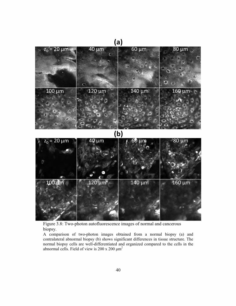
40
Figure 3.8: Two-photon autofluorescence images of normal and cancerous
biopsy. A comparison of two-photon images obtained from a normal biopsy (a) and
contralateral abnormal biopsy (b) shows significant differences in tissue structure. The
normal biopsy cells are well-differentiated and organized compared to the cells in the
abnormal cells. Field of view is 200 x 200 μm2
41
Chapter 4 A Monte Carlo model for
out-of-focus fluorescence generation
in two-photon microscopy
4.1. INTRODUCTION
One of the major advantages of two-photon imaging is that the quadratic
dependence of emission signal on excitation fluence results in nearly all the signal being
generated within the perifocal volume of a tightly focused beam. This three dimensional
confinement allows for intrinsic three-dimensional sectioning and high contrast imaging,
provided that: (1) the volume of the feature of interest, Vs, is large relative to the
excitation focal spot, and (2) that the fluorophore concentration in the feature of interest
is large compared to that in the bulk sample [Figure 4.1 (a)]. When imaging sub-
diffraction sized objects, or if the beam spot size is degraded (typically enlarged) by
aberrations, Vs is small compared to the focal volume, and the contrast suffers [Figure 4.1
(b)]. Likewise, the contrast decreases if the excitation beam is focused deep within an
attenuating sample, wherein appreciable fluorescence can be generated outside of the
perifocal volume [Figure 4.1 (c)].
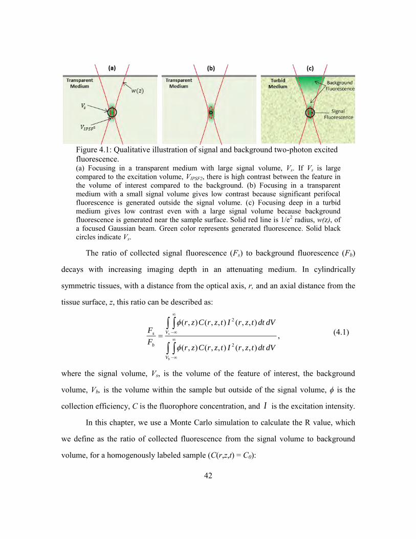
42
The ratio of collected signal fluorescence (Fs) to background fluorescence (Fb)
decays with increasing imaging depth in an attenuating medium. In cylindrically
symmetric tissues, with a distance from the optical axis, r, and an axial distance from the
tissue surface, z, this ratio can be described as:
,),,(),,(),(
),,(),,(),(
2
2
b
s
V
V
b
s
dVdttzrItzrCzr
dVdttzrItzrCzr
F
F
(4.1)
where the signal volume, Vs, is the volume of the feature of interest, the background
volume, Vb, is the volume within the sample but outside of the signal volume, ϕ is the
collection efficiency, C is the fluorophore concentration, and I is the excitation intensity.
In this chapter, we use a Monte Carlo simulation to calculate the R value, which
we define as the ratio of collected fluorescence from the signal volume to background
volume, for a homogenously labeled sample (C(r,z,t) = C0):
Figure 4.1: Qualitative illustration of signal and background two-photon excited
fluorescence. (a) Focusing in a transparent medium with large signal volume, Vs. If Vs is large
compared to the excitation volume, VIPSF2, there is high contrast between the feature in
the volume of interest compared to the background. (b) Focusing in a transparent
medium with a small signal volume gives low contrast because significant perifocal
fluorescence is generated outside the signal volume. (c) Focusing deep in a turbid
medium gives low contrast even with a large signal volume because background
fluorescence is generated near the sample surface. Solid red line is 1/e2 radius, w(z), of
a focused Gaussian beam. Green color represents generated fluorescence. Solid black
circles indicate Vs.
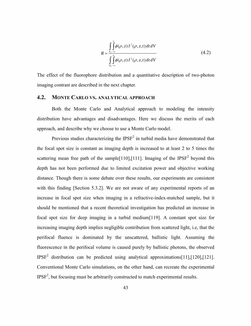
43
b
s
V
V
dVdttzIz
dVdttzIz
R
),,(),(
),,(),(
2
2
(4.2)
The effect of the fluorophore distribution and a quantitative description of two-photon
imaging contrast are described in the next chapter.
4.2. MONTE CARLO VS. ANALYTICAL APPROACH
Both the Monte Carlo and Analytical approach to modeling the intensity
distribution have advantages and disadvantages. Here we discuss the merits of each
approach, and describe why we choose to use a Monte Carlo model.
Previous studies characterizing the IPSF2 in turbid media have demonstrated that
the focal spot size is constant as imaging depth is increased to at least 2 to 5 times the
scattering mean free path of the sample[110],[111]. Imaging of the IPSF2 beyond this
depth has not been performed due to limited excitation power and objective working
distance. Though there is some debate over these results, our experiments are consistent
with this finding [Section 5.3.2]. We are not aware of any experimental reports of an
increase in focal spot size when imaging in a refractive-index-matched sample, but it
should be mentioned that a recent theoretical investigation has predicted an increase in
focal spot size for deep imaging in a turbid medium[119]. A constant spot size for
increasing imaging depth implies negligible contribution from scattered light, i.e, that the
perifocal fluence is dominated by the unscattered, ballistic light. Assuming the
fluorescence in the perifocal volume is caused purely by ballistic photons, the observed
IPSF2 distribution can be predicted using analytical approximations[11],[120],[121].
Conventional Monte Carlo simulations, on the other hand, can recreate the experimental
IPSF2, but focusing must be arbitrarily constructed to match experimental results.
44
The background fluorescence for deep nonlinear imaging is predominately
generated close to the tissue surface and extends through a few scattering lengths into the
sample[11],[122-124]. In this regime, diffraction can be neglected and the photon flux
can be accurately described by the time-dependent radiative transport equation. Exact
analytical solutions to this equation are extremely complex and do not provide relevant
utility[125]. Approximate analytical expressions have been derived to determine fluences
in this regime, but the results are inaccurate for large angle scattering and focusing,
neglect any backwards propagating component, and are more applicable at more than two
scattering lengths deep[11],[125]. Monte Carlo simulations, on the other hand, provide an
exact solution to the time-dependent radiative transport equation. In fact, analytical
approximations are generally validated against Monte Carlo methods[125].
To summarize, a Monte Carlo approach has the advantage of accurately
simulating the superficial fluorescence and the disadvantage of simulating the perifocal
volume fluorescence only after arbitrarily aiming ballistic photons to match experimental
conditions. Consequently, changes in the IPSF2 predicted from Monte Carlo models have
little bearing on the expected behavior. In comparison, an analytical approach is more
rigorous for determine perifocal fluorescence distribution, and less accurate for modeling
the superficial fluorescence generation. Given that experimental results suggest the spot
size does not appreciably change with imaging depth, we use a Monte Carlo model to
determine the R value. For an improved model, it would be possible to combine the two
approaches and use the Monte Carlo model to determine background fluorescence and an
analytical one to determine signal fluorescence, or perhaps use a Monte Carlo model that
includes diffractive effects[119].
45
4.3. OVERVIEW OF MONTE CARLO MODEL
We used two independent Monte Carlo simulations to find the spatio-temporal
distribution of the squared excitation intensity, ),,(2 tzrI , and the spatial dependence of
the collection efficiency, zr, . The corresponding results are combined using Eq. (4.2)
to determine R for a variety of sample and imaging parameters, and generally, as a
function of imaging depth, z0. Photon propagation was implemented using the same rules
as Wang et al.[126]. All simulations (excitation and collection) used a Henyey-
Greenstein scattering phase function with a scattering anisotropy set to 0.85. This is the
expected value from Mie theory for 760 nm light interacting with 1 μm diameter
polystyrene spheres[127], which are used for phantom preparation in Chapter 5. This
value is also reasonable for modeling light scattering in epithelial
tissue[33],[36],[128],[32]. For the excitation simulations, we use scattering lengths in the
range typically found in epithelial tissues at 760 nm and which are later recreated in
tissue phantoms: ls = 40, 80, and 120 μm. We assume emission photons have a
wavelength of 515 nm, which is slightly red-shifted from half of our excitation
wavelength, and close to emission peak from other 2PAM studies in epithelial
tissues[129],[130]. The ratio of scattering length at 760 nm and 515 nm was found to be
1.7 by Mie simulations for 1 μm diameter polystyrene beads. Thus, for each excitation
simulation set, we used a collection scattering length of scollection
= s / 1.7 to create a
matching collection efficiency map for each excitation scattering length. To calculate R,
the fluorescence grid created from the excitation simulation was integrated over time and
every element was multiplied by an interpolated value from the spatial collection
efficiency grid.
46
4.4. EXCITATION SIMULATION
For the excitation simulation, the photon packets were traced through a
cylindrically symmetric three-dimensional grid with coordinates for depth z, radius r, and
time t. Two grids are used to record excitation photon flux in space and time—a sparse
grid for calculating fluorescence generation outside of the focal volume (Δr = 20 μm, rmax
= 1.2 mm, Δz = 20 μm, zmax = 1.2 mm), and a fine grid within ± 20 μm of the focal plane
(Δrfocal = 200 nm, rmax = 20 μm, Δzfocal = 0.5 µm, zmax = 40 μm). Both grids had a time
spacing of one tenth the excitation pulse duration, (Δt = τp/10, tmax =3×z0/c). These grid
spacing were verified to be of sufficient resolution to capture fast changes in fluence by
running select simulations at twice the spatial and temporal resolution (resulting in eight
times more grid elements for constant total grid size). Photon packets propagate until they
exceed the maximum radius, depth, or time; their weight falls to zero (with a roulette
procedure); or they exit the tissue.
4.4.1. Focusing
Previous Monte-Carlo models of two-photon microscopy have simulated a
focused beam in one of two ways: (1) the geometric focus method, where the fluence at a
plane offset from the geometric focus that would give the same width as the diffraction
limited spot is measured [Figure 4.2 (a)][131], or (2) the spot focus method, where
initialized photons are stochastically pointed towards a radius at the focal plane such that
a lateral Gaussian distribution is created [Figure 4.2 (b)][110],[132]. The geometric focus
method suffers from a problem of creating a point of infinite fluence, as ballistic rays
transmit through an infinitely small area at the geometric focal plane. The spot focus
method effectively introduces dispersion in the simulation, as voxels in this simulation
47
will see ballistic photons pass through at different times, depending on where they are
pointed towards at the focal plane.
Our approach focuses excitation light using the hyperbolic method described by
Tycho et al. for OCT imaging [Figure 4.2 (c)][133]. By skewing the initial trajectory of
each photon off of a z-r plane by an angle depending on r, a focused Gaussian beam can
be exactly reconstructed in all three dimensions with photons that travel in straight paths.
A qualitative visualization of how straight photon rays can recreate a curved focal spot is
shown in Figure 4.2 (d). Finally, we note that the spot focus method can have a similar
shape to the hyperbolic focus method if the random radius at the focal plane is chosen
perpendicular to the initial radius, such that these photons are also skewed off axis (not
shown in Figure 4.2). For small focal spots and deep imaging depths, the temporal
dispersion introduced from variable-aiming of the initialized photons in the spot focus
method becomes negligible. Thus, we would expect similar results in modeling R for
both the hyperboloid and spot focusing methods.
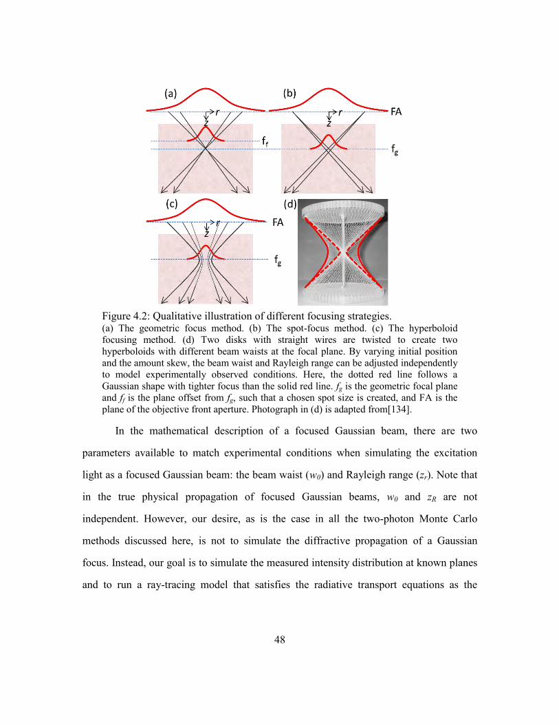
48
In the mathematical description of a focused Gaussian beam, there are two
parameters available to match experimental conditions when simulating the excitation
light as a focused Gaussian beam: the beam waist (w0) and Rayleigh range (zr). Note that
in the true physical propagation of focused Gaussian beams, w0 and zR are not
independent. However, our desire, as is the case in all the two-photon Monte Carlo
methods discussed here, is not to simulate the diffractive propagation of a Gaussian
focus. Instead, our goal is to simulate the measured intensity distribution at known planes
and to run a ray-tracing model that satisfies the radiative transport equations as the
Figure 4.2: Qualitative illustration of different focusing strategies. (a) The geometric focus method. (b) The spot-focus method. (c) The hyperboloid
focusing method. (d) Two disks with straight wires are twisted to create two
hyperboloids with different beam waists at the focal plane. By varying initial position
and the amount skew, the beam waist and Rayleigh range can be adjusted independently
to model experimentally observed conditions. Here, the dotted red line follows a
Gaussian shape with tighter focus than the solid red line. fg is the geometric focal plane
and ff is the plane offset from fg, such that a chosen spot size is created, and FA is the
plane of the objective front aperture. Photograph in (d) is adapted from[134].
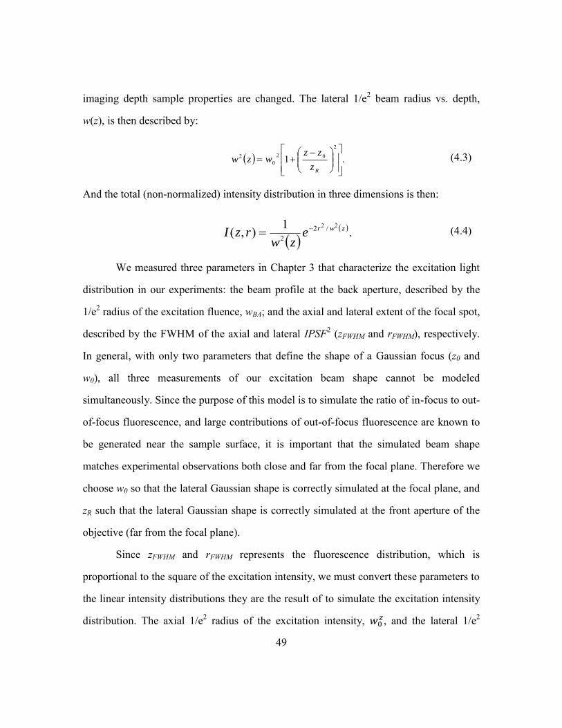
49
imaging depth sample properties are changed. The lateral 1/e2 beam radius vs. depth,
w(z), is then described by:
And the total (non-normalized) intensity distribution in three dimensions is then:
We measured three parameters in Chapter 3 that characterize the excitation light
distribution in our experiments: the beam profile at the back aperture, described by the
1/e2 radius of the excitation fluence, wBA; and the axial and lateral extent of the focal spot,
described by the FWHM of the axial and lateral IPSF2 (zFWHM and rFWHM), respectively.
In general, with only two parameters that define the shape of a Gaussian focus (z0 and
w0), all three measurements of our excitation beam shape cannot be modeled
simultaneously. Since the purpose of this model is to simulate the ratio of in-focus to out-
of-focus fluorescence, and large contributions of out-of-focus fluorescence are known to
be generated near the sample surface, it is important that the simulated beam shape
matches experimental observations both close and far from the focal plane. Therefore we
choose w0 so that the lateral Gaussian shape is correctly simulated at the focal plane, and
zR such that the lateral Gaussian shape is correctly simulated at the front aperture of the
objective (far from the focal plane).
Since zFWHM and rFWHM represents the fluorescence distribution, which is
proportional to the square of the excitation intensity, we must convert these parameters to
the linear intensity distributions they are the result of to simulate the excitation intensity
distribution. The axial 1/e2 radius of the excitation intensity,
, and the lateral 1/e2
.12
020
2
Rz
zzwzw
(4.3)
.1),(22 /2
2zwre
zwrzI
(4.4)
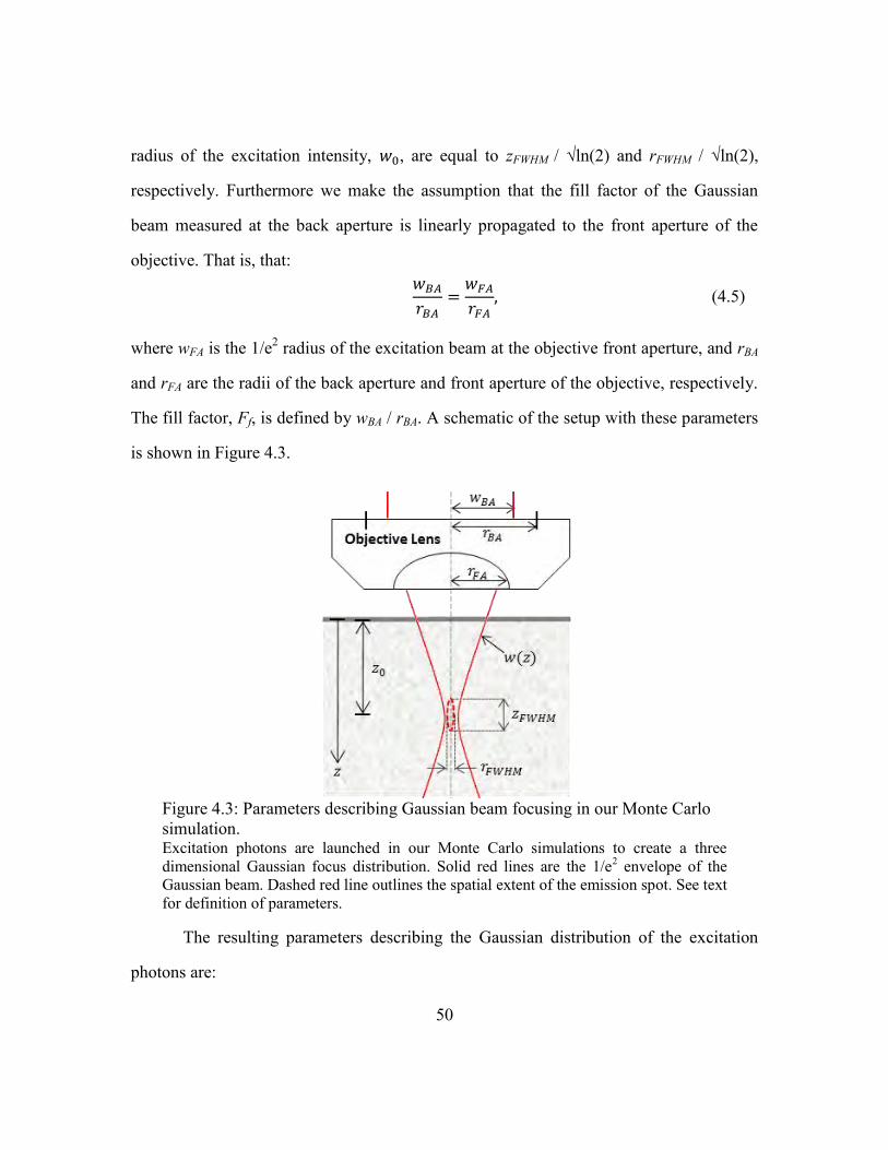
50
radius of the excitation intensity, , are equal to zFWHM / √ln(2) and rFWHM / √ln(2),
respectively. Furthermore we make the assumption that the fill factor of the Gaussian
beam measured at the back aperture is linearly propagated to the front aperture of the
objective. That is, that:
(4.5)
where wFA is the 1/e2 radius of the excitation beam at the objective front aperture, and rBA
and rFA are the radii of the back aperture and front aperture of the objective, respectively.
The fill factor, Ff, is defined by wBA / rBA. A schematic of the setup with these parameters
is shown in Figure 4.3.
The resulting parameters describing the Gaussian distribution of the excitation
photons are:
Figure 4.3: Parameters describing Gaussian beam focusing in our Monte Carlo
simulation. Excitation photons are launched in our Monte Carlo simulations to create a three
dimensional Gaussian focus distribution. Solid red lines are the 1/e2 envelope of the
Gaussian beam. Dashed red line outlines the spatial extent of the emission spot. See text
for definition of parameters.
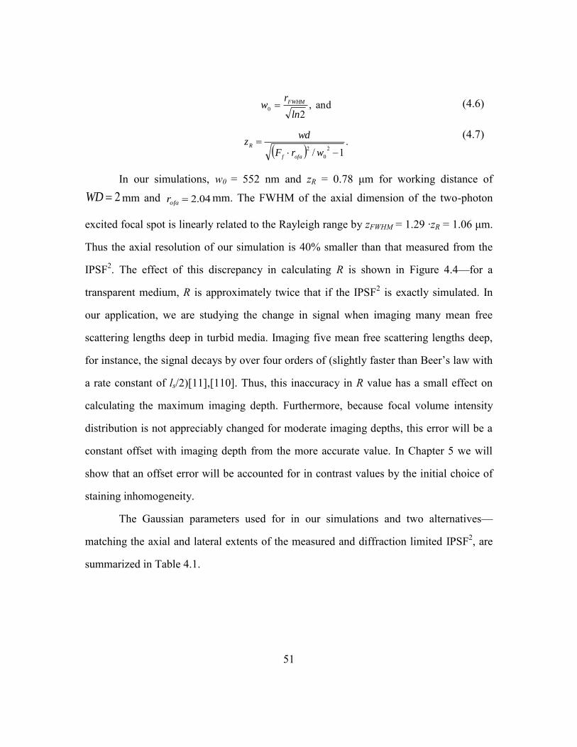
51
and ,20
ln
rw FWHM
(4.6)
.
1/ 20
2
wrF
wdz
ofaf
R
(4.7)
In our simulations, w0 = 552 nm and zR = 0.78 μm for working distance of
2WD mm and 04.2ofar mm. The FWHM of the axial dimension of the two-photon
excited focal spot is linearly related to the Rayleigh range by zFWHM = 1.29 ∙zR = 1.06 μm.
Thus the axial resolution of our simulation is 40% smaller than that measured from the
IPSF2. The effect of this discrepancy in calculating R is shown in Figure 4.4—for a
transparent medium, R is approximately twice that if the IPSF2 is exactly simulated. In
our application, we are studying the change in signal when imaging many mean free
scattering lengths deep in turbid media. Imaging five mean free scattering lengths deep,
for instance, the signal decays by over four orders of (slightly faster than Beer‘s law with
a rate constant of ls/2)[11],[110]. Thus, this inaccuracy in R value has a small effect on
calculating the maximum imaging depth. Furthermore, because focal volume intensity
distribution is not appreciably changed for moderate imaging depths, this error will be a
constant offset with imaging depth from the more accurate value. In Chapter 5 we will
show that an offset error will be accounted for in contrast values by the initial choice of
staining inhomogeneity.
The Gaussian parameters used for in our simulations and two alternatives—
matching the axial and lateral extents of the measured and diffraction limited IPSF2, are
summarized in Table 4.1.
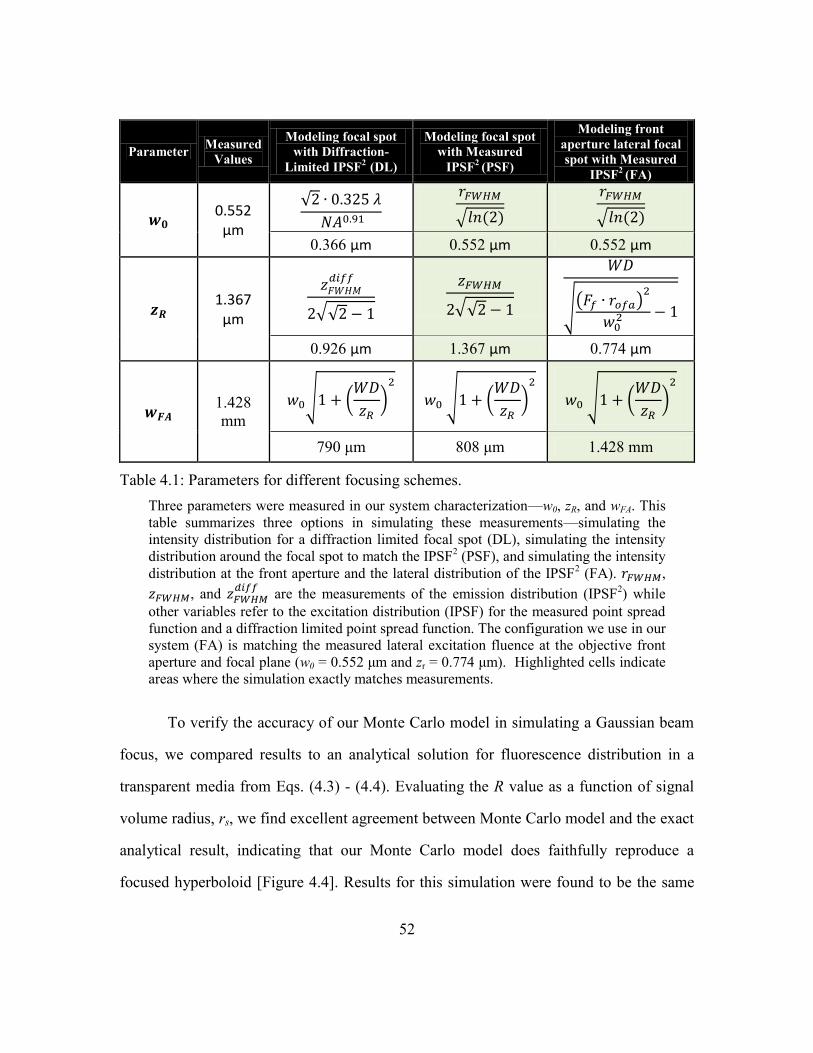
52
To verify the accuracy of our Monte Carlo model in simulating a Gaussian beam
focus, we compared results to an analytical solution for fluorescence distribution in a
transparent media from Eqs. (4.3) - (4.4). Evaluating the R value as a function of signal
volume radius, rs, we find excellent agreement between Monte Carlo model and the exact
analytical result, indicating that our Monte Carlo model does faithfully reproduce a
focused hyperboloid [Figure 4.4]. Results for this simulation were found to be the same
Parameter Measured
Values
Modeling focal spot
with Diffraction-
Limited IPSF2 (DL)
Modeling focal spot
with Measured
IPSF2 (PSF)
Modeling front
aperture lateral focal
spot with Measured
IPSF2 (FA)
0.552
μm
√
√
√
0.366 μm 0.552 μm 0.552 μm
1.367
μm
√√
√√
√( )
0.926 μm 1.367 μm 0.774 μm
1.428
mm
√ (
)
√ (
)
√ (
)
790 μm 808 μm 1.428 mm
Table 4.1: Parameters for different focusing schemes.
Three parameters were measured in our system characterization—w0, zR, and wFA. This
table summarizes three options in simulating these measurements—simulating the
intensity distribution for a diffraction limited focal spot (DL), simulating the intensity
distribution around the focal spot to match the IPSF2 (PSF), and simulating the intensity
distribution at the front aperture and the lateral distribution of the IPSF2 (FA). ,
, and
are the measurements of the emission distribution (IPSF2) while
other variables refer to the excitation distribution (IPSF) for the measured point spread
function and a diffraction limited point spread function. The configuration we use in our
system (FA) is matching the measured lateral excitation fluence at the objective front
aperture and focal plane (w0 = 0.552 μm and zr = 0.774 μm). Highlighted cells indicate
areas where the simulation exactly matches measurements.
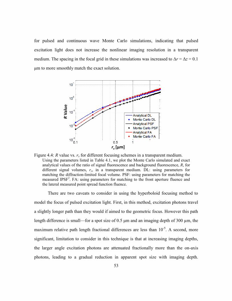
53
for pulsed and continuous wave Monte Carlo simulations, indicating that pulsed
excitation light does not increase the nonlinear imaging resolution in a transparent
medium. The spacing in the focal grid in these simulations was increased to Δr = Δz = 0.1
μm to more smoothly match the exact solution.
There are two caveats to consider in using the hyperboloid focusing method to
model the focus of pulsed excitation light. First, in this method, excitation photons travel
a slightly longer path than they would if aimed to the geometric focus. However this path
length difference is small—for a spot size of 0.5 μm and an imaging depth of 300 µm, the
maximum relative path length fractional differences are less than 10-5
. A second, more
significant, limitation to consider in this technique is that at increasing imaging depths,
the larger angle excitation photons are attenuated fractionally more than the on-axis
photons, leading to a gradual reduction in apparent spot size with imaging depth.
Figure 4.4: R value vs. rs for different focusing schemes in a transparent medium.
Using the parameters listed in Table 4.1, we plot the Monte Carlo simulated and exact
analytical values of the ratio of signal fluorescence and background fluorescence, R, for
different signal volumes, rs, in a transparent medium. DL: using parameters for
matching the diffraction-limited focal volume. PSF: using parameters for matching the
measured IPSF2. FA: using parameters for matching to the front aperture fluence and
the lateral measured point spread function fluence.
54
However, for small and moderate angular numerical apertures (< 45°) and typical
imaging depths (<5 ls), this effect is relatively subtle—at 5 scattering lengths deep with
photons aimed for a 460 nm FWHM spot size, the resulting focal volume produces ∼10
% more signal at the focal plane than expected from a Gaussian spot size of equal peak
intensity.
4.4.2. Temporal dependence
We obtained the intensity temporal impulse response of the system, ),,( tzrG , by
setting initial photon times such that ballistic photons intercept the focal plane at exactly
the same instant and counting the photons per lateral area found in each voxel. The
intensity distribution was determined by convolving the impulse response with the
Gaussian pulse envelope, f :
.)(),,(),,(
tdttftzrGtzrI (4.8)
Finally, the fluorescence generated per voxel, ℱ was calculated by multiplying the
integrated intensity squared by the volume of the voxel, Vv:
V
VdttzrIzrF
2),,(),( (4.9)
4.5. COLLECTION
We use a second Monte Carlo simulation to model the effect of heterogeneous
collection efficiency on maximum imaging depth. In this case, only detected emission is
important, so photon time-of-flight tracking, and ray tracing through lateral planes was
not necessary. Emission photons are initialized from a range of source positions (zs,rs)
with an isotropic angular distribution, for each imaging depth (z0). The escape position
(re) and angle (θe) of each photon that leaves the tissue surface is cataloged. We
55
implemented the approach outlined by Oheim et al. to determine the fraction of collected
photons[104]. The maximum acceptance radius (rm) can be derived by examining the
geometry of the system [Figure 4.5]:
,/)(0 WDrrzrrfFAfm
(4.10)
where rf is the field of view of the objective. For our 20x/0.95 objective, the field of view
was measured by previous studies to be 1.3 mm[104]. We use an effective field of view
of 1.0 mm, accounting for the limited collection angle of our PMT [Section 3.4]. The
second component of the Oheim et al. approach is to account for the coupling between
the maximum acceptance angle, θm, and rm. To conserve beam étendue, the product of θm,
and rm is assumed to be constant. The value of this constant is found by considering the
limiting case where the objective lens focuses to the sample surface, and rm = rf [135].
The resulting relation is then:
.ffmm
rr (4.11)
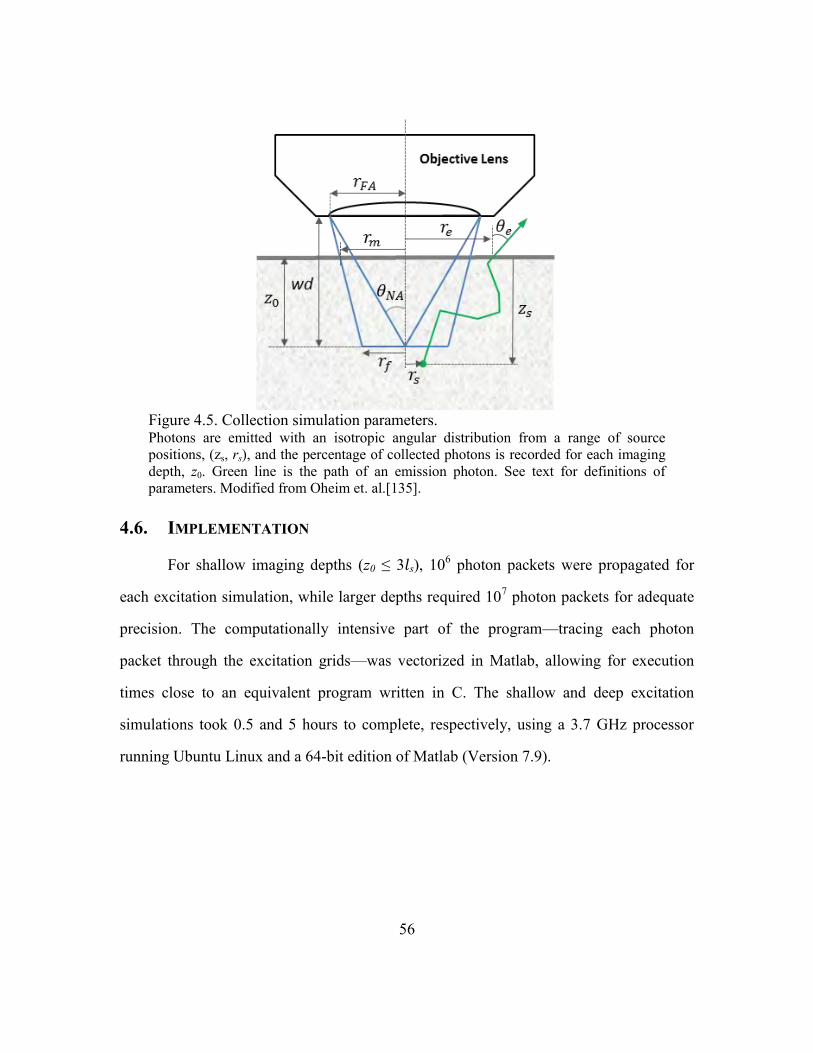
56
4.6. IMPLEMENTATION
For shallow imaging depths (z0 ≤ 3 s), 106 photon packets were propagated for
each excitation simulation, while larger depths required 107 photon packets for adequate
precision. The computationally intensive part of the program—tracing each photon
packet through the excitation grids—was vectorized in Matlab, allowing for execution
times close to an equivalent program written in C. The shallow and deep excitation
simulations took 0.5 and 5 hours to complete, respectively, using a 3.7 GHz processor
running Ubuntu Linux and a 64-bit edition of Matlab (Version 7.9).
Figure 4.5. Collection simulation parameters. Photons are emitted with an isotropic angular distribution from a range of source
positions, (zs, rs), and the percentage of collected photons is recorded for each imaging
depth, z0. Green line is the path of an emission photon. See text for definitions of
parameters. Modified from Oheim et. al.[135].
57
Chapter 5 Deep two-photon autofluorescence microscopy
of epithelial tissues
Endogenous fluorescence provides morphological, spectral, and lifetime contrast
that can indicate disease states in tissues. Previous studies have demonstrated that two-
photon autofluorescence microscopy (2PAM) can be used for non-invasive, three-
dimensional imaging of epithelial tissues down to 150 µm beneath the skin surface [136].
We report ex-vivo 2PAM images of epithelial tissue from a human tongue biopsy down
to 370 µm below the surface. At greater than 320 μm deep, the fluorescence generated
outside the focal volume degrades the image contrast to below one. We demonstrate that
these imaging depths can be reached with 160 mW of laser power (2 nJ per pulse) from a
conventional 80 MHz repetition rate ultrafast laser oscillator. We studied image contrast
as a function of depth in tissue phantoms with a range of optical properties typically
found in epithelial tissues. The phantom data agree well with the estimated contrast
decays from time-resolved Monte Carlo simulations and show maximum imaging depths
similar to that found in human biopsy results. This work demonstrates that the low
staining inhomogeneity and large scattering coefficient associated with visible-
wavelength autofluorescence limits conventional 2PAM from imaging greater than 3-5
mean free scattering lengths deep in epithelial tissue.
5.1. INTRODUCTION
Two-photon autofluorescence microscopy (2PAM) has emerged as a versatile
technique for non-invasive three-dimensional imaging of turbid biological samples with
subcellular resolution[2],[3],[8]. Spectral and morphological information obtained from
58
intravital 2PAM of unstained epithelial tissues has shown promise for diagnosing and
monitoring of carcinoma[21],[137-141]. Typically, carcinoma originates and is most
clearly distinguished from normal tissue at the basal layer, which can be many hundreds
of microns below the skin surface. Additionally, the quantification of epithelial layer
thickness can be used as an indicator of dysplasia and carcinoma[21]. Thus, in the
application of cancer diagnosis, it is particularly important to understand and extend the
maximum 2PAM imaging depth in epithelial tissues.
In general, optical imaging depth in skin can be extended by using near-infrared
(NIR) wavelengths of 700-1300 nm, which are minimally attenuated in biological
tissues[142]. Confocal microscopy can image many hundreds of microns into epithelial
tissue using NIR wavelengths and contrast from scattering or exogenous contrast
agents[23],[24]. However, the dominant fluorophores naturally present in skin have
ultraviolet and blue linear absorption bands[8],[143],[144], requiring low-visible-
wavelength excitation and emission to be imaged with confocal microscopy.
Consequently, confocal autofluorescence microscopy of has been used to obtain axial
sectioning in shallow regions of epithelial tissue but has not been reported more than a
few tens of microns below the surface[25],[144],[145]. Two-photon imaging, on the other
hand, has three working principles that make it particularly advantageous for deep
microscopy of endogenous skin fluorescence: (1) the natural fluorophores in epithelial
tissues can be excited nonlinearly with NIR light; (2) fluorescence generation in a sample
is inherently confined to the focal volume, enabling three-dimensional sectioning while
collecting both ballistic and scattered emission light; and (3) resolution is negligibly
degraded from scattering because the fluorescence in the perifocal volume is generated
almost entirely from ballistic photons[110],[111].
59
While imaging depth of confocal microscopy is limited by the challenge of
getting sufficient levels of ballistic emission photons out of the tissue, nonlinear imaging
depth is typically limited by the ability to deliver sufficient levels of ballistic excitation
photons to the focal volume. To maintain constant two-photon excited fluorescence
signal generated within the focal volume, the pulse energy delivered to the surface of the
sample must be exponentially increased with increasing imaging depth. In biological
samples, where the attenuation of NIR photons is dominated by scattering processes, the
pulse energy must be increased with an exponential length constant of approximately one
mean free scattering length, s. In practice, the excitation power delivered to the sample
surface is increased at a slightly higher rate to compensate for increased losses from
fluorescence collection and the longer path length seen by large-angle excitation photons.
Although increasing excitation power with imaging depth can maintain perifocal
fluorescence generation at arbitrarily large imaging depths, the approximation that the
two-photon excited fluorescence is generated only within the focal volume does not hold
beyond ~3 mean free scattering lengths deep[122]. Appreciable out-of-focus
(background) fluorescence can be generated by ballistic photons near the surface and by
scattered photons through several mean free scattering lengths into the tissue, gradually
reducing the image contrast[11],[131]. The ratio of collected signal fluorescence (Fs) to
background fluorescence (Fb) then decays with increasing imaging depth. In cylindrically
symmetric tissue, with a distance from the optical axis, r, and an axial distance from the
tissue surface, z, this ratio can be described as:
,),,(),,(),(
),,(),,(),(
2
2
b
s
V
V
b
s
dVdttzrItzrCzr
dVdttzrItzrCzr
F
F
(5.1)
60
where the signal volume, Vs, is the volume of the feature of interest, the background
volume, Vb, is the volume within the sample but outside of the signal volume, ϕ is the
collection efficiency, C is the fluorophore concentration, and I is the excitation
intensity.
The maximum imaging depth, zm, can be defined as the depth at which the Fs/Fb
ratio falls to one[11]. Previous studies have described the maximum imaging depth in
units of optical depths, defined as zm/ s, for homogenously stained tissue with similar
excitation parameters. Theer et al. found a zm of 3-4 scattering lengths when s = 200 µm
using an analytical model[11]. On the other hand, Leray et al. found a zm of 5-6 optical
depths when s = 350 µm using a Monte Carlo model[131]. The difference suggests that
zm is dependent on s. Experimentally, zmax has also been measured, but only in stained
brain tissue and phantoms with s ≈ 200 μm[11],[146]. Autofluorescence imaging in
epithelial tissues presents a particularly challenging set of optical properties for deep two-
photon imaging. First, the scattering length of epithelial tissues is typically in range of
40-200 μm—much smaller than those considered in previous studies. Second,
endogenous fluorophores are dimmer and more homogenously distributed than
exogenous ones. Previous 2PAM reports have not reached zm, and imaging depths have,
to the best of our knowledge, been limited to 80-150 µm below the
surface[3],[4],[129],[136],[137],[147-158]. Some previous studies have reported the
ability to image 150-200 μm deep, but either do not present these images, or show images
with no appreciable signal at these depths[3],[4].
In this paper, we present 2PAM images of a human tongue biopsy down to and
beyond zmax. We show that this limit can be reached with a few hundred milliwatts
available from conventional, high repetition rate oscillators in phantoms with optical
properties in the range typically found in epithelial tissues. We describe the gradual
61
contrast decay of 2PAM for increasing imaging depths as a function of the fluorescence
staining inhomogeneity and a ratio of integrated intensities. We examine the logarithmic
dependence of maximum imaging depth on sample scattering length, which becomes
important in imaging samples with short scattering lengths such as epithelial tissue.
Finally, the Fs/Fb ratio is calculated with time-resolved Monte Carlo simulations and
predicted contrast profiles are compared with measurements from tissue phantoms and
ex-vivo human epithelial tissue.
5.2. METHODS
5.2.1. 2PAM contrast
In the absence of fluorescence saturation, photobleaching, and sample movement,
the fluorophore concentration is independent of time. Assuming the concentration of
fluorophores within Vs is a constant, Cs, and that the out-of-focus fluorophore
concentration is diffuse enough to be approximated by the average fluorophore
concentration, Cb, we can remove the concentration terms from the integral in Eq. (5.1).
We define the staining inhomogeneity, χ, as the ratio of the fluorophore concentrations,
and a value, R, as the ratio of integrated intensities:
,b
s
C
C
(5.2)
.),,(),(
),,(),(
2
2
b
s
V
V
dVdttzrIz
dVdttzrIz
R
(5.3)
We can then express the ratio of signal to background fluorescence as the product of χ
and R:
62
.RF
F
b
s (5.4)
Though our definition for bs FF / is the same as previous reports, our definition of
χ and R differ from that described previously[11]. Our staining inhomogeneity is defined
by the absolute concentrations of fluorophores inside and outside a signal volume, and
does not depend on the perifocal intensity distribution (i.e. the numerical aperture), while
our R value is defined with the volume of the feature of interest rather than the volume of
the focal spot. Our approach has the distinction that the χ value is an intrinsic, system-
independent property of the sample that scales linearly with changes in background or
signal fluorophore concentration.
In this paper, we explore the gradual decay of image contrast, Q, versus depth due
to out-of-focus fluorescence. We define the contrast in terms of the measured signal
)(MS when the focal spot concentrically overlaps with Vs a bright feature of interest and
the measured background )(MB when the focal spot is in a volume that produces
relatively weak signal, such that:
,MB
MBMSQ
(5.5)
where, ,),,(),(),,(),( 22
s bV V
bsdVdttzrIzrCdVdttzrIzrCMS (5.6)
and .),,(),(),,(),( 22
s bV V
bbdVdttzrIzrCdVdttzrIzrCMB
(5.7)
Note that our measured background includes a fluorescence contribution from
within the defined signal volume. This term becomes important for samples where the
fluorophore is relatively homogenously distributed and there are relatively few regions
with truly dark signals. Using the definitions in Eqs. (5.2) and (5.3), and rearranging Eqs.
63
(5.5)-(5.7), we can express the contrast at a given imaging depth, 0z , as a function of χ
and R:
.)(/11
1)(0
0zR
zQ
(5.8)
This relation shows that the contrast approaches zero as the staining
inhomogeneity approaches one (i.e. a uniformly stained sample), or as R approaches zero.
If the fluorophore concentration is zero in the focal volume for the MB measurement, Q
is equal to bsFF / . In the more general case, with some fluorescent signal present in the
focal volume of the MB measurement, )( 0zQ becomes approximately equal to bsFF / for
small values of R. In this paper, we define our maximum imaging depth as the depth at
which the contrast falls to one.
We use a Monte Carlo and an analytical model to calculate )( 0zQ , and compare it
with the measured values for a variety of sample conditions. For Eq. (5.8) to be accurate,
we must choose a signal volume of approximately constant fluorophore concentration, a
condition that is closely approximated in tissue phantoms with fluorescent beads by
choosing Vs as the volume of the fluorescent bead.
5.2.2. 2PAM system
We used the nonlinear microscope described in Chapter 3 for 2PAM imaging.
Briefly, imaging was performed at 760 nm excitation wavelength because it yields the
brightest autofluorescence signal with minimal excitation light bleed-through in our
system. Two half-waveplate/polarizing beam cube pairs attenuate the excitation beam
and a pair of galvanometer scanning mirrors (Cambridge Technologies, 6215h) scans the
laser into an upright microscope. We use a high NA, water dipping objective with a large
field of view and a 2 mm working distance (0.95/20x Olympus XLUMPFL). A schematic
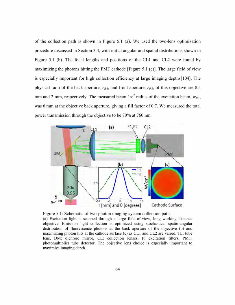
64
of the collection path is shown in Figure 5.1 (a). We used the two-lens optimization
procedure discussed in Section 3.4, with initial angular and spatial distributions shown in
Figure 5.1 (b). The focal lengths and positions of the CL1 and CL2 were found by
maximizing the photons hitting the PMT cathode [Figure 5.1 (c)]. The large field of view
is especially important for high collection efficiency at large imaging depths[104]. The
physical radii of the back aperture, rBA, and front aperture, rFA, of this objective are 8.5
mm and 2 mm, respectively. The measured beam 1/e2 radius of the excitation beam, wBA,
was 6 mm at the objective back aperture, giving a fill factor of 0.7. We measured the total
power transmission through the objective to be 70% at 760 nm.
Figure 5.1: Schematic of two-photon imaging system collection path. (a) Excitation light is scanned through a large field-of-view, long working distance
objective. Emission light collection is optimized using stochastical spatio-angular
distribution of fluorescence photons at the back aperture of the objective (b) and
maximizing photon hits at the cathode surface (c) as CL1 and CL2 are varied. TL: tube
lens, DM: dichroic mirror, CL: collection lenses, F: excitation filters, PMT:
photomultiplier tube detector. The objective lens choice is especially important to
maximize imaging depth.
65
5.2.3. Monte Carlo model
We used the Monte Carlo model developed in Chapter 4 to calculate R values,
and compare to phantom and biopsy results. We used an excitation wavelength of 760
nm, and ls values of 40, 80, and 120 μm to match phantom results. Focusing was
simulated as a Gaussian beam shape, which matched the excitation beam profile at the
front aperture of the objective and the lateral extent of the IPSF2 at the focal plane. For
the collection simulation, we used a collection scattering length of scollection
= s / 1.7, for
each of the corresponding scattering lengths at 760 nm.
5.2.4. Analytical model
We applied the analytical model developed by Theer and Denk to calculate the
fluorescence distributions for different optical system and sample parameters[120]. In
short, we consider the ballistic and scattered light distributions in turbid media
independently and then combine the resulting intensities to calculate total fluorescence.
The intensity from ballistic photons assumes an incident beam with Gaussian spatial and
temporal distributions. Using the spherical wave solution to the telegrapher‘s equation
and the Fresnel approximation, we describe the ballistic intensity as a function of a depth
dependent Rayleigh range, which reduced the effective numerical aperture with depth.
The scattered light is modeled using a small angle approximation and statistical methods
to calculate an effective temporal and transverse spatial beam width. We used a
numerical aperture of 0.75, which produces a similar spot size to that measured from our
IPSF2. All other parameters used in the analytical model were the same as those used in
the Monte Carlo model.
66
5.2.5. Tissue phantom preparation
To measure the experimental contrast decay of two-photon imaging in a turbid
media, we prepared twelve scattering agar phantoms with a range of optical properties
similar to what is typically observed in epithelial tissues. Low melting point agarose
(1.0%, Sigma) was prepared with 0.95 µm diameter polystyrene beads (Bangs Labs,
PS03N) to vary scattering coefficient, 1 µm diameter fluorescent polystyrene beads
(Invitrogen F-8823) to provide features for contrast measurements, and fluorescein
(Fluka 46955) to control staining inhomogeneity. Polystyrene beads were ultrasonicated
for 30 minutes to reduce aggregations before they were mixed into the agar phantoms. To
increase the two-photon action cross section of fluorescein, we mixed the agar solution
with 2% pH 12 buffer. Polystyrene concentrations of 1.7×10¹⁰
, 0.9×10¹⁰
, and 0.6×10¹⁰
particles per mL provided scattering mean free paths of 40, 80, and 120 µm at 760 nm
excitation, and 23, 46, and 69 µm at 515 nm emission, respectively. We determined the
scattering coefficient with a Mie calculation using polystyrene sphere and agar gel
refractive indices of 1.58 and 1.33, respectively[159]. To verify the scattering lengths of
our polystyrene solution matched Mie predictions, we measured attenuation of collimated
760 nm light through dilute solutions of polystyrene beads in a cuvette. Fluorescent beads
were added to at a constant concentration of 3.5×10⁸ particles per mL in all phantoms.
We added increasing amounts of fluorescein to get final concentrations of 0, 4,
10, and 25 μM for each scattering length tested, creating a total of 12 phantoms. This
approach allows the formation of phantoms with low staining inhomogeneities without an
increase in scattering coefficient that would result from adding high concentrations of
fluorescent polystyrene beads. Additional benefit of using this method is that we can
increase the background fluorescence immediately adjacent to the fluorescent beads. In
contrast, previous studies that varied fluorescent bead concentration could control the
67
fluorescence only in volumes many microns away from the signal volume[11]. Thus our
approach provided a more appropriate model for studying autofluorescence contrast
decay, where the local fluorophore concentration changes rapidly in short distances from
nucleus to cytoplasm to extracellular matrix. The disadvantage of our approach is that the
out-of-focus background fluorescence cannot be measured directly because there is no
region without some fluorescent signal—when the focal spot does not overlap with a
fluorescent bead, the measured background still includes some contribution from the
fluorescein in the focal volume. However, the contrast defined in Eq. (5.5) can still be
calculated, given sufficient signal to noise that fluorescent beads can be identified.
We obtained lateral phantom images at one micron depth increments from the
surface to the depth where the image contrast fell to approximately 0.1. The contrast for
each of the 16 phantoms was analyzed using an automated bead-finding script written in
Matlab. We applied a binary mask with a threshold of four standard deviations above the
mean pixel value for each lateral image. Beads were then localized by finding the three
dimensional position of the centroid of each continuously weighted connected region in
the binary stack. We only counted the connected regions of the expected single bead size
to exclude clusters and isolated noisy pixels. Beads within 10 μm of the edge of the stack
were also ignored. The MS for each bead was then calculated as the average of the
maximum 4 voxels (150 x 150 x 1000 nm/voxel) within each region and the MB was
calculated as the average pixel value of the non-connected regions at the depth
determined by the centroid of the bead. The contrast was monitored for increasing
imaging depth, while the excitation power was manually increased to maintain constant
detected signal, slightly below the saturation levels of our system.
68
5.2.6. Biopsy preparation
Human oral cavity biopsies were obtained from The University of Texas M. D.
Anderson Cancer Center as part of an ongoing project for two-photon diagnosis of oral
malignancies. The study was reviewed and approved by the internal review boards at M.
D. Anderson Cancer Center and the University of Texas at Austin. Biopsies were excised
from suspicious regions and contralateral normal tissue in the oral cavity and submitted
for histopathology. We present two-photon images from the normal biopsy in this paper.
The biopsy was approximately 3 mm in diameter and 5 mm thick, delivered in chilled
culture media (Phenol Red-free DMEM High, Fisher Scientific) and imaged within 6
hours of excision. The biopsy was stabilized on Petri dishes with low melting point agar
and imaged at room temperature in a culture media bath.
5.3. RESULTS AND DISCUSSION
5.3.1. Monte Carlo simulation
We used our Monte Carlo model to calculate R as a function of depth for each
phantom. For these calculations, Vs was set to the volume of the 1 μm diameter
fluorescent beads which provide the signal in the phantoms. Figure 4 presents the
fluorescence distribution for imaging 400 μm deep in a homogeneously labeled sample
with an s of 80 μm. In this case, the collected background fluorescence overwhelms the
signal fluorescence by approximately 30 times. The cross section of the fluorescence
generation rate shows that background fluorescence generation density peaks on the
optical axis near the focal volume [Figure 5.2 (a)]. When the fluorescence is integrated
circumferentially, we observe that the cumulative background fluorescence generation
peaks slightly off axis because the off-axis fluorescence is generated in larger volumes
[Figure 5.2 (b)]. Finally, integration of this fluorescence radially shows that the total
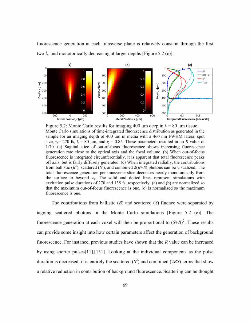
69
fluorescence generation at each transverse plane is relatively constant through the first
two s, and monotonically decreasing at larger depths [Figure 5.2 (c)].
The contributions from ballistic (B) and scattered (S) fluence were separated by
tagging scattered photons in the Monte Carlo simulations [Figure 5.2 (c)]. The
fluorescence generation at each voxel will then be proportional to (S+B)2. These results
can provide some insight into how certain parameters affect the generation of background
fluorescence. For instance, previous studies have shown that the R value can be increased
by using shorter pulses[11],[131]. Looking at the individual components as the pulse
duration is decreased, it is entirely the scattered (S2) and combined (2BS) terms that show
a relative reduction in contribution of background fluorescence. Scattering can be thought
Figure 5.2: Monte Carlo results for imaging 400 μm deep in ls = 80 μm tissue. Monte Carlo simulations of time-integrated fluorescence distribution as generated in the
sample for an imaging depth of 400 μm in media with a 460 nm FWHM lateral spot
size, τp= 270 fs, s = 80 μm, and g = 0.85. These parameters resulted in an R value of
1/70. (a) Sagittal slice of out-of-focus fluorescence shows increasing fluorescence
generation rate close to the optical axis and the focal volume. (b) When out-of-focus
fluorescence is integrated circumferentially, it is apparent that total fluorescence peaks
off axis, but is fairly diffusely generated. (c) When integrated radially, the contributions
from ballistic (B2), scattered (S
2), and combined 2(B+S) photons can be visualized. The
total fluorescence generation per transverse slice decreases nearly monotonically from
the surface to beyond z0. The solid and dotted lines represent simulations with
excitation pulse durations of 270 and 135 fs, respectively. (a) and (b) are normalized so
that the maximum out-of-focus fluorescence is one, (c) is normalized so the maximum
fluorescence is one.
70
of as a source of temporal dispersion from the sample on the scattered fluence. Thus, as
the pulse duration is increased, the dispersion of the scattered light reduces its
contribution more than for longer pulse durations, resulting in an increase in R for shorter
pulsed durations.
Though high collection efficiency is important for reaching large imaging depth
with limited excitation power, we found that heterogeneous collection efficiency
generally had a small effect on our calculations of R. In the s = 80 μm simulation
( semission
= 46 μm), the collection efficiency only reduced R by 12% at z0 = 400 μm, and
by 60% at z0 = 800 μm. The radial dependence of the collection efficiency had an
especially weak effect on R, since the majority of the fluorescence generated in the
excitation simulations was within 200 μm of the optical axis.
5.3.2. Phantom imaging
For all three sets of phantoms ( s = 40, 80, and 120 μm), we had sufficient power
to reach contrast levels below one. Typically, excitation powers smaller than 1 mW were
sufficient to image at the surface, while several hundreds of mW were required at the
largest depths. For the phantom with s = 80 μm and χ = 300, for example, the power was
increased from 0.7 mW at the surface to 483 mW at 510 μm depth. We identified an
average of 190 beads per 77×77×100 μm3 field of view in each of the 12 phantoms using
the automated bead-finding script. This number of beads corresponds to a bead
concentration of 3.2×10⁸ beads per mL, slightly less than the expected value of 3.5×10
8
beads per mL.
Figure 5.3 shows XZ images of the s = 80 μm phantom set for different staining
inhomogeneities. Each XZ reconstruction is created from a maximum projection through
15 μm (45 pixels) of Y. The accompanied biopsy images are discussed in Section 5.3.5.
71
We estimated the staining inhomogeneity of phantoms using the measured contrast at the
surface of each phantom and the R values found from Monte Carlo simulations. The R
value since it only changes slightly for shallow imaging depths in our Monte Carlo
model—a decrease from 0.51 at the surface to approximately 0.46 at one s deep.
Substituting an R value of 0.5 in Eq. (5.8), the staining inhomogeneity, χ, becomes
approximately equal to 3 times the measured contrast at shallow depths, for large values
of χ. Using this approximation, we estimate the average staining inhomogeneities to be χ
= 300, 62, 25, and 10, by using the average contrast from beads identified within the first
20-40 μm of the three phantoms at each staining inhomogeneity.
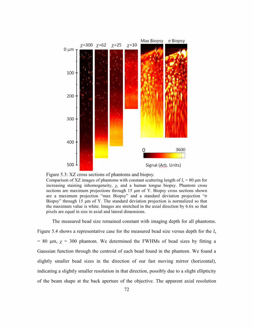
72
The measured bead size remained constant with imaging depth for all phantoms.
Figure 5.4 shows a representative case for the measured bead size versus depth for the s
= 80 μm, χ = 300 phantom. We determined the FWHMs of bead sizes by fitting a
Gaussian function through the centroid of each bead found in the phantom. We found a
slightly smaller bead sizes in the direction of our fast moving mirror (horizontal),
indicating a slightly smaller resolution in that direction, possibly due to a slight ellipticity
of the beam shape at the back aperture of the objective. The apparent axial resolution
Figure 5.3: XZ cross sections of phantoms and biopsy. Comparison of XZ images of phantoms with constant scattering length of s = 80 μm for
increasing staining inhomogeneity, χ, and a human tongue biopsy. Phantom cross
sections are maximum projections through 15 μm of Y. Biopsy cross sections shown
are a maximum projection ―max Biopsy‖ and a standard deviation projection ―σ
Biopsy‖ through 15 μm of Y. The standard deviation projection is normalized so that
the maximum value is white. Images are stretched in the axial direction by 6.6x so that
pixels are equal in size in axial and lateral dimensions.
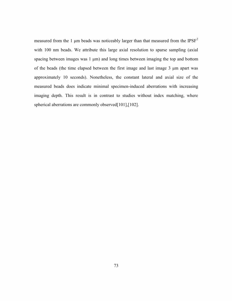
73
measured from the 1 μm beads was noticeably larger than that measured from the IPSF2
with 100 nm beads. We attribute this large axial resolution to sparse sampling (axial
spacing between images was 1 μm) and long times between imaging the top and bottom
of the beads (the time elapsed between the first image and last image 3 μm apart was
approximately 10 seconds). Nonetheless, the constant lateral and axial size of the
measured beads does indicate minimal specimen-induced aberrations with increasing
imaging depth. This result is in contrast to studies without index matching, where
spherical aberrations are commonly observed[101],[102].
74
Figure 5.4: Measured bead size vs depth. Measured sizes of 1 μm diameter fluorescent beads versus depth for the s = 40 μm, χ =
300 phantom (a), the s = 80 μm, χ = 25 phantom (b), and the s = 120 μm, χ = 10
phantom (c), in the lateral and axial directions. The trend and error bars are calculated
by the mean and standard deviations of sizes obtained by binning the beads at 50 μm
depth increments. We observed no significant increase in bead size and, thus, in system
resolution with increasing imaging depth in any of our phantoms.
75
5.3.3. Fluorescence decay
We measured the decay of the signal, background, and total fluorescence with
increasing imaging depth in our twelve phantoms. By increasing the excitation power
exponentially with imaging depth and normalizing measured signal at each imaging
depth by the expected quadratic increase with the excitation power, 20 )(/)0( zzPzP ,
we could accurately measure fluorescence decays far beyond the limited dynamic range
of our detection system.
Figure 5.5 shows the measured and calculated fluorescence decays of the three χ =
62 phantoms. Looking at the χ = 62, s = 80 μm phantom, Figure 5.5 (a) shows the decays
of the average value of the measured background at each imaging plane (MB), the
measured signal for each fluorescent bead (MS), and the difference (MS-MB). Note that
the slopes of the (MS-MB) and MB decays are approximately equal for imaging depths
down to three mean free scattering lengths. This result suggests that the contrast, defined
as the ratio of (MS-MB) to MB, is relatively constant for shallow depths. At larger
imaging depths (z > 4 s) the measured signal, which decays exponentially, is overcome by
the background, which decays with z0-1
[11]. Comparing the fluorescence decay in
phantoms with different scattering lengths, we found good agreement between the
measured data and the Monte Carlo predictions [Figure 5.5 (b) and (c)]. The decay of the
fluorescent signal from the biopsy also shown in Figure 5.5 (a), and will be discussed in
section 5.3.5.
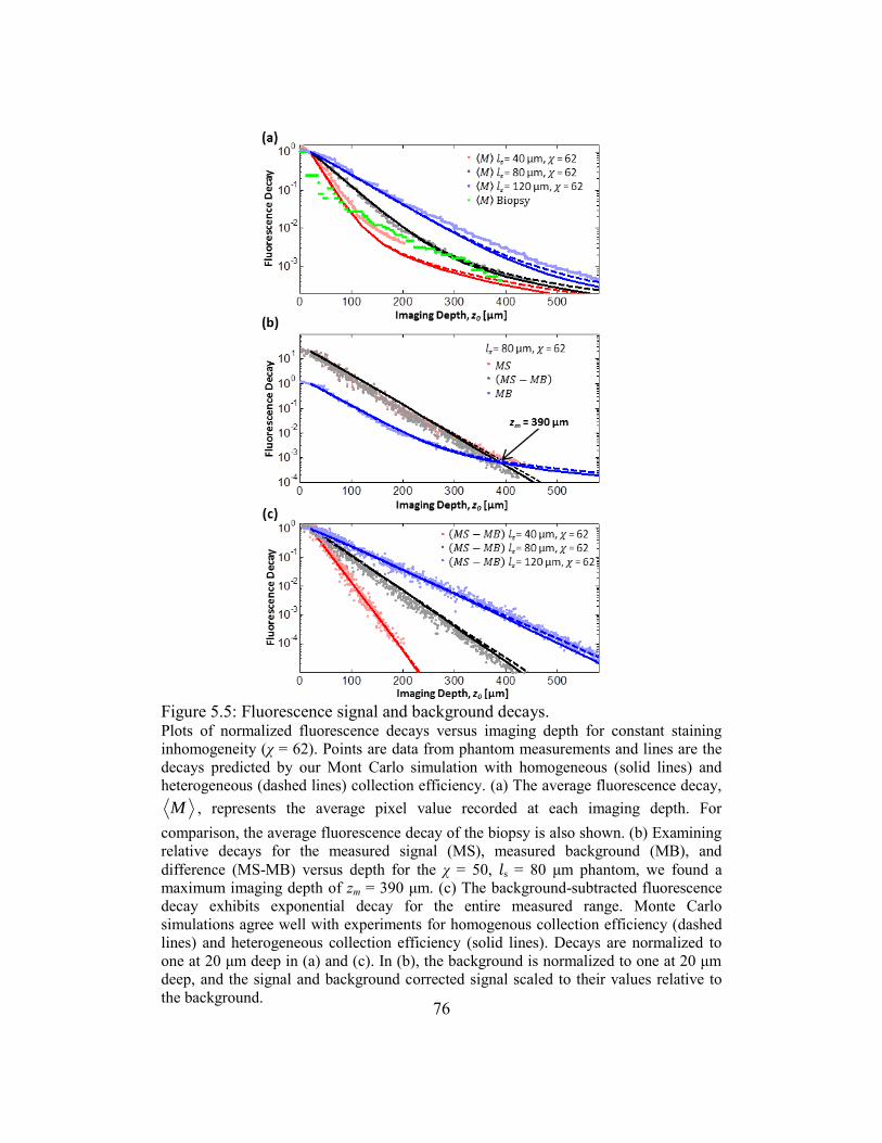
76
Figure 5.5: Fluorescence signal and background decays. Plots of normalized fluorescence decays versus imaging depth for constant staining
inhomogeneity (χ = 62). Points are data from phantom measurements and lines are the
decays predicted by our Mont Carlo simulation with homogeneous (solid lines) and
heterogeneous (dashed lines) collection efficiency. (a) The average fluorescence decay,
M , represents the average pixel value recorded at each imaging depth. For
comparison, the average fluorescence decay of the biopsy is also shown. (b) Examining
relative decays for the measured signal (MS), measured background (MB), and
difference (MS-MB) versus depth for the χ = 50, s = 80 μm phantom, we found a
maximum imaging depth of zm = 390 μm. (c) The background-subtracted fluorescence
decay exhibits exponential decay for the entire measured range. Monte Carlo
simulations agree well with experiments for homogenous collection efficiency (dashed
lines) and heterogeneous collection efficiency (solid lines). Decays are normalized to
one at 20 μm deep in (a) and (c). In (b), the background is normalized to one at 20 μm
deep, and the signal and background corrected signal scaled to their values relative to
the background.
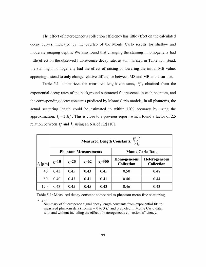
77
The effect of heterogeneous collection efficiency has little effect on the calculated
decay curves, indicated by the overlap of the Monte Carlo results for shallow and
moderate imaging depths. We also found that changing the staining inhomogeneity had
little effect on the observed fluorescence decay rate, as summarized in Table 1. Instead,
the staining inhomogeneity had the effect of raising or lowering the initial MB value,
appearing instead to only change relative difference between MS and MB at the surface.
Table 5.1 summarizes the measured length constants, m
sl , obtained from the
exponential decay rates of the background-subtracted fluorescence in each phantom, and
the corresponding decay constants predicted by Monte Carlo models. In all phantoms, the
actual scattering length could be estimated to within 10% accuracy by using the
approximation: m
ssll 3.2 . This is close to a previous report, which found a factor of 2.5
relation between m
sl and sl using an NA of 1.2[110].
s [μm]
Measured Length Constants, s
m
s
ll
Phantom Measurements Monte Carlo Data
χ=10 χ=25 χ=62 χ=300 Homogeneous
Collection
Heterogeneous
Collection
40 0.43 0.45 0.43 0.45 0.50 0.48
80 0.40 0.43 0.41 0.41 0.46 0.44
120 0.43 0.45 0.45 0.43 0.46 0.43
Table 5.1: Measured decay constant compared to phantom mean free scattering
length. Summary of fluorescence signal decay length constants from exponential fits to
measured phantom data (from z0 = 0 to 3 s) and predicted in Monte Carlo data,
with and without including the effect of heterogeneous collection efficiency.
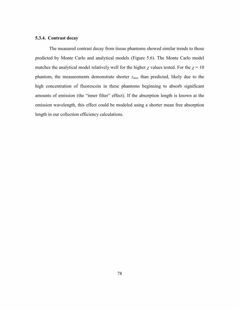
78
5.3.4. Contrast decay
The measured contrast decay from tissue phantoms showed similar trends to those
predicted by Monte Carlo and analytical models (Figure 5.6). The Monte Carlo model
matches the analytical model relatively well for the higher χ values tested. For the χ = 10
phantom, the measurements demonstrate shorter zmax than predicted, likely due to the
high concentration of fluorescein in these phantoms beginning to absorb significant
amounts of emission (the ―inner filter‖ effect). If the absorption length is known at the
emission wavelength, this effect could be modeled using a shorter mean free absorption
length in our collection efficiency calculations.
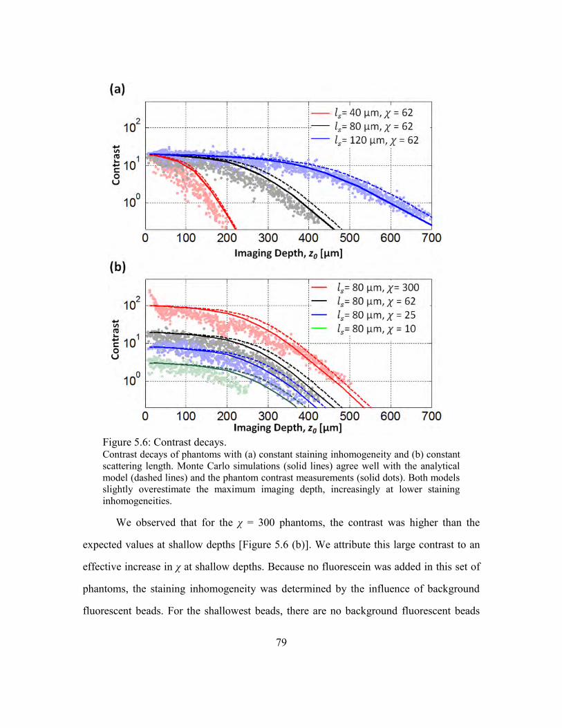
79
We observed that for the χ = 300 phantoms, the contrast was higher than the
expected values at shallow depths [Figure 5.6 (b)]. We attribute this large contrast to an
effective increase in χ at shallow depths. Because no fluorescein was added in this set of
phantoms, the staining inhomogeneity was determined by the influence of background
fluorescent beads. For the shallowest beads, there are no background fluorescent beads
Figure 5.6: Contrast decays. Contrast decays of phantoms with (a) constant staining inhomogeneity and (b) constant
scattering length. Monte Carlo simulations (solid lines) agree well with the analytical
model (dashed lines) and the phantom contrast measurements (solid dots). Both models
slightly overestimate the maximum imaging depth, increasingly at lower staining
inhomogeneities.
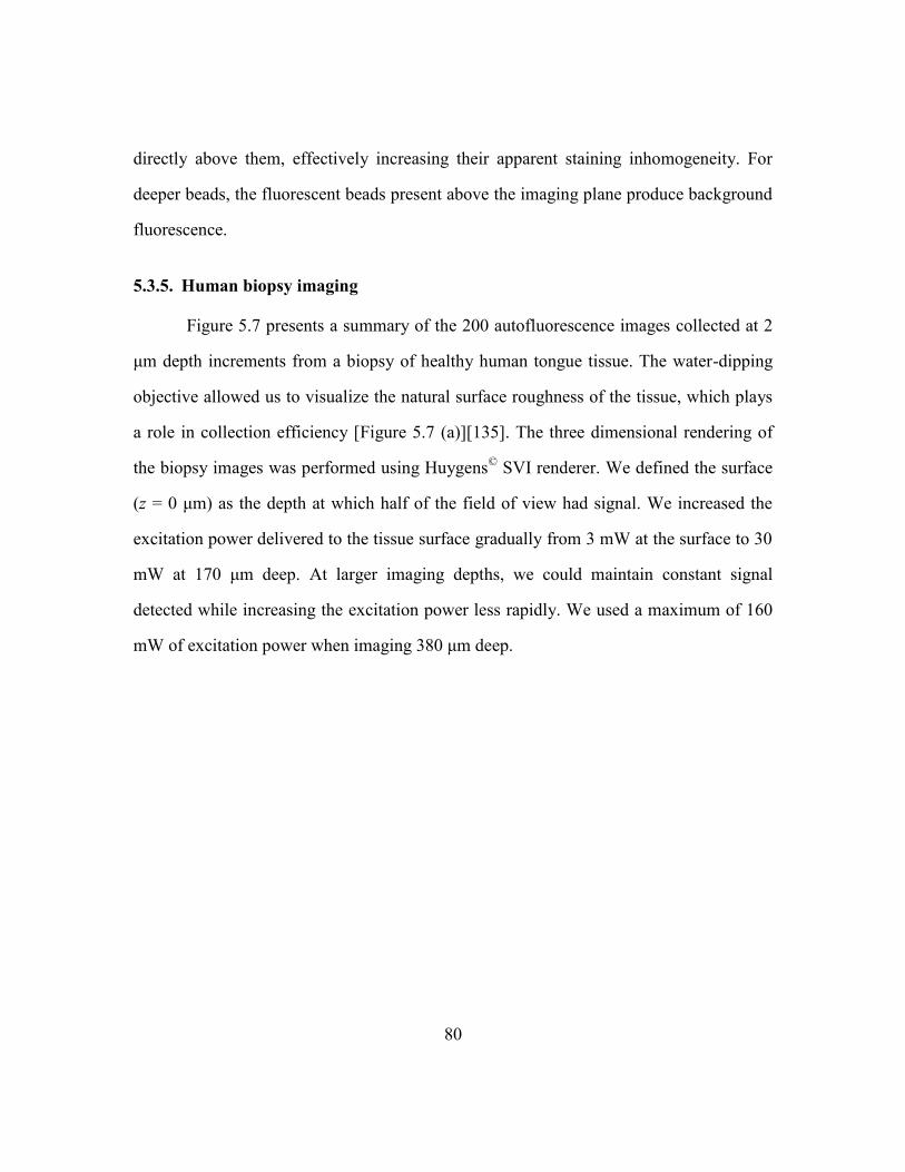
80
directly above them, effectively increasing their apparent staining inhomogeneity. For
deeper beads, the fluorescent beads present above the imaging plane produce background
fluorescence.
5.3.5. Human biopsy imaging
Figure 5.7 presents a summary of the 200 autofluorescence images collected at 2
μm depth increments from a biopsy of healthy human tongue tissue. The water-dipping
objective allowed us to visualize the natural surface roughness of the tissue, which plays
a role in collection efficiency [Figure 5.7 (a)][135]. The three dimensional rendering of
the biopsy images was performed using Huygens©
SVI renderer. We defined the surface
(z = 0 μm) as the depth at which half of the field of view had signal. We increased the
excitation power delivered to the tissue surface gradually from 3 mW at the surface to 30
mW at 170 μm deep. At larger imaging depths, we could maintain constant signal
detected while increasing the excitation power less rapidly. We used a maximum of 160
mW of excitation power when imaging 380 μm deep.
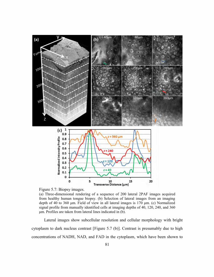
81
Lateral images show subcellular resolution and cellular morphology with bright
cytoplasm to dark nucleus contrast [Figure 5.7 (b)]. Contrast is presumably due to high
concentrations of NADH, NAD, and FAD in the cytoplasm, which have been shown to
Figure 5.7: Biopsy images. (a) Three-dimensional rendering of a sequence of 200 lateral 2PAF images acquired
from healthy human tongue biopsy. (b) Selection of lateral images from an imaging
depth of 40 to 360 μm. Field of view in all lateral images is 170 μm. (c) Normalized
signal profile from manually identified cells at imaging depths of 40, 120, 240, and 360
μm. Profiles are taken from lateral lines indicated in (b).
82
be the dominant endogenous fluorophores in confocal autofluorescence imaging of
cervical and oral epithelial tissues[160],[6], and are efficiently excited in 2PAM at 760
nm excitation[8]. We found especially high signal levels from the stratum corneum,
which, based on our Monte Carlo model, would contribute heavily to the out-of-focus
fluorescence found at large imaging depths.
A maximum XZ projection through 15 μm of Y shows that at large depths, bright
pixels in the background substantially degrade the contrast beyond 300 μm [Figure 5.3].
A normalized standard deviation projection through 15 μm of Y gives values similar to
the measured contrast—it shows bright regions where there are large changes in pixel
values. At shallow depths, this projection shows large values where there is variation
between the bright cytoplasm signal and dark nuclei. At large depths, the increase in low-
spatial-frequency, out-of-focus background fluorescence reduces the lateral variation in
signal, and the corresponding standard deviation along Y decreases.
We examined the total fluorescence decay with imaging depth to estimate the
scattering coefficient of the biopsy. Though fluorescence decay accurately predicted the
scattering coefficient in phantoms, extending this method to the biopsy can be
complicated by several effects. (1) The scattering length and fluorophore concentrations
are likely to change with depth. Previous studies have observed brighter signal coming
from the stratum corneum and basal membrane than at the intermediate epithelial
layers[6],[130]. (2) As the excised tissue dies, the autofluorescence signal levels will
gradually decay with time. We observed that the superficial regions of the tissue begin
losing fluorescence signal more rapidly than the interior regions, creating a time-
dependent change in relative fluorescence density. (3) Specimen induced aberrations
typically become more severe with increasing imaging depths[161], and would result in a
higher apparent rate of fluorescence decay. Though we verified aberrations played a
83
minimal role in degradation of signal in the phantom, without a constant-size point source
in our biopsy, we were unable to monitor our excitation spot size with depth in the
biopsy. Nevertheless, we obtain an estimate of the biopsy scattering coefficient by
comparing our measured biopsy fluorescence decay to phantom experiments [Figure 5.5
(a)]. We fit an exponential curve to the first 200 μm of fluorescence decay obtained from
the biopsy and found a length constant of 39 μm, corresponding to a scattering length of
89 μm, assuming m
ssll 3.2 [Section 5.3.3]. At larger depths, the fluorescence decayed
less rapidly, showing a similar slope to the 120sl μm phantom.
Figure 5.7 (c) presents typical contrast levels obtained from bright features at
different imaging depths. We examined the contrast in line profiles drawn through
manually identified epithelial cells marked by the lines drawn in the lateral images
displayed in Figure 5.7 (b). At 40 μm deep, the brightest signal from the cytoplasm is
approximately twenty to forty times larger than the minimum signal from within the
nucleus, while the average signal from the cytoplasm is approximately five to ten times
the average signal from the nucleus [Figure 5.7 (c)]. Using averaged signal and
background as contrast, and employing the same method used with the phantoms, we
estimate the χ of the biopsy to be 15-30. The contrast falls to one in our biopsy around
320 μm below the tissue surface, approximately 3-4 mean free scattering lengths deep.
5.3.6. Fluorescence saturation and photobleaching
The analysis presented in this paper has assumed that the intensity ranges used in
our experiments are low enough to assume negligible fluorescence saturation and
photobleaching—that is, that the fluorescence generation is quadratically dependent on
the excitation intensity and is time-independent. However, at high intensities, these
84
assumptions no longer hold. We performed a series of tests to verify that we do not
experience any saturation and photobleaching in our experiments.
Fluorescence saturation can broaden the PSF, as fluorophores in the highest
intensity regions no longer generate greater emission signal than fluorophores further
away. The resulting decrease in resolution has been previously demonstrated, but is
expected to have a significant effect only under a combination of high intensities and
especially large two-photon action cross section (> 1000 GM cross section at 1 mW of
excitation power delivered to the imaging plane)[162]. Our observation of constant
measured bead size with increasing imaging depth indicates a negligible influence of
fluorescence saturation in our phantom experiments [Figure 5.4]. To test for fluorescence
saturation in our biopsy experiments, we verified that our detected signal scales
quadratically with excitation at select imaging depths. We measured power dependencies
of 1.94, 2.00, 1.97, and 1.99 at increasing imaging depths of z0 = 290, 300, 326, and 356
μm, respectively. In phantoms, we also observed that the signal from the identified beads
scaled to the power of 1.98±0.05 at each 100 μm imaging depth increment.
We also tested for the presence of photobleaching in 2PAM of the biopsy by
measuring the ratio of the average signal of the first and last image taken at every image
plane. Each imaging plane was raster scanned 8 times at 3 frames per second. We found
an average ratio of 1.002 for the biopsy, and no trend for photobleaching at larger
imaging depths [Figure 5.8].
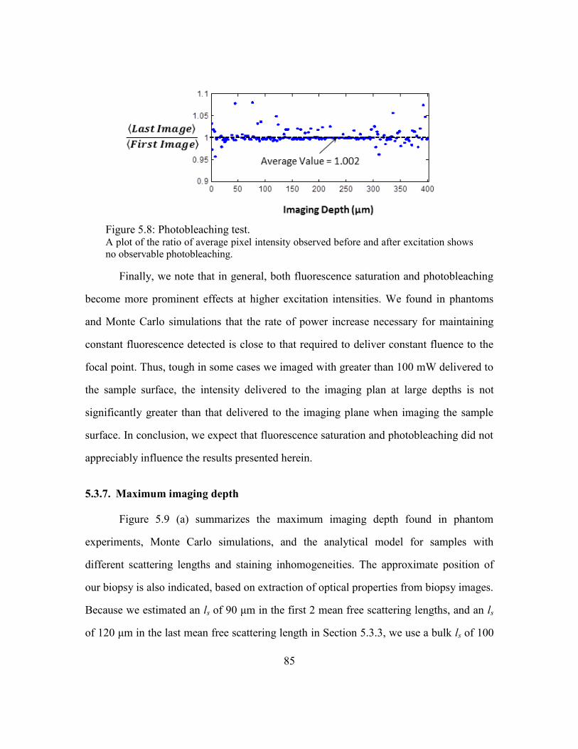
85
Finally, we note that in general, both fluorescence saturation and photobleaching
become more prominent effects at higher excitation intensities. We found in phantoms
and Monte Carlo simulations that the rate of power increase necessary for maintaining
constant fluorescence detected is close to that required to deliver constant fluence to the
focal point. Thus, tough in some cases we imaged with greater than 100 mW delivered to
the sample surface, the intensity delivered to the imaging plan at large depths is not
significantly greater than that delivered to the imaging plane when imaging the sample
surface. In conclusion, we expect that fluorescence saturation and photobleaching did not
appreciably influence the results presented herein.
5.3.7. Maximum imaging depth
Figure 5.9 (a) summarizes the maximum imaging depth found in phantom
experiments, Monte Carlo simulations, and the analytical model for samples with
different scattering lengths and staining inhomogeneities. The approximate position of
our biopsy is also indicated, based on extraction of optical properties from biopsy images.
Because we estimated an ls of 90 μm in the first 2 mean free scattering lengths, and an ls
of 120 μm in the last mean free scattering length in Section 5.3.3, we use a bulk ls of 100
Figure 5.8: Photobleaching test. A plot of the ratio of average pixel intensity observed before and after excitation shows
no observable photobleaching.
86
μm for positioning the biopsy region. We found reasonable agreement between the three
approaches, with experiments matching the models slightly better for longer scattering
lengths and higher staining inhomogeneities. This difference is likely due to the
increasing influence of small heterogeneities in our shorter scattering length phantoms,
such as spatial variations in fluorescein and polystyrene bead concentrations. The Monte
Carlo model showed a slightly weaker dependence of maximum imaging depth on
scattering length, partially due to the effect of inhomogeneous collection efficiency.
The maximum imaging depth in the biopsy was slightly less than expected from a
phantom with similar optical properties (ls = 100 μm and χ = 20). We believe this
difference is due to the presence of specimen-induced aberrations. Although we could
measure the spots size with depth in agar phantoms, there are no bright, fluorescent, sub-
diffraction limited features in human biopsies that can be used to reliably measure the
excitation spot size. But because the maximum imaging depth was within ~20% of that
measured in similar phantoms in which we demonstrate that there is no appreciable
specimen-induced aberrations, we believe that the out-of focus fluorescence is still the
dominant factor in reducing deep 2PAM imaging contrast in biopsies.
Normalizing the maximum imaging depth by n
mz = zm/ s, we observe a logarithmic
dependence of n
mz on s [Figure 5.9 (b)]. The origin of the dependence of n
mz on s comes
from the fact that as the distances are scaled down by s, the photons responsible for the
background fluorescence are confined to smaller volumes while the photons generating
focal volume signal pass through a constant size signal volume. The dependence of n
mz
on ls has not been reported before, and has significant implications in comparing
maximum achievable imaging depths among samples with different scattering lengths.
We recall that Theer et al., and Leray et al. found that two-photon imaging depth were
limited to 4.5 s and 6 s in samples with large s and small χ [11],[131]. If one were to

87
extrapolate those results to samples with scattering lengths commonly found in epithelial
tissues, the predicted maximum imaging depth would significantly overestimated [Figure
5.9 (b)].
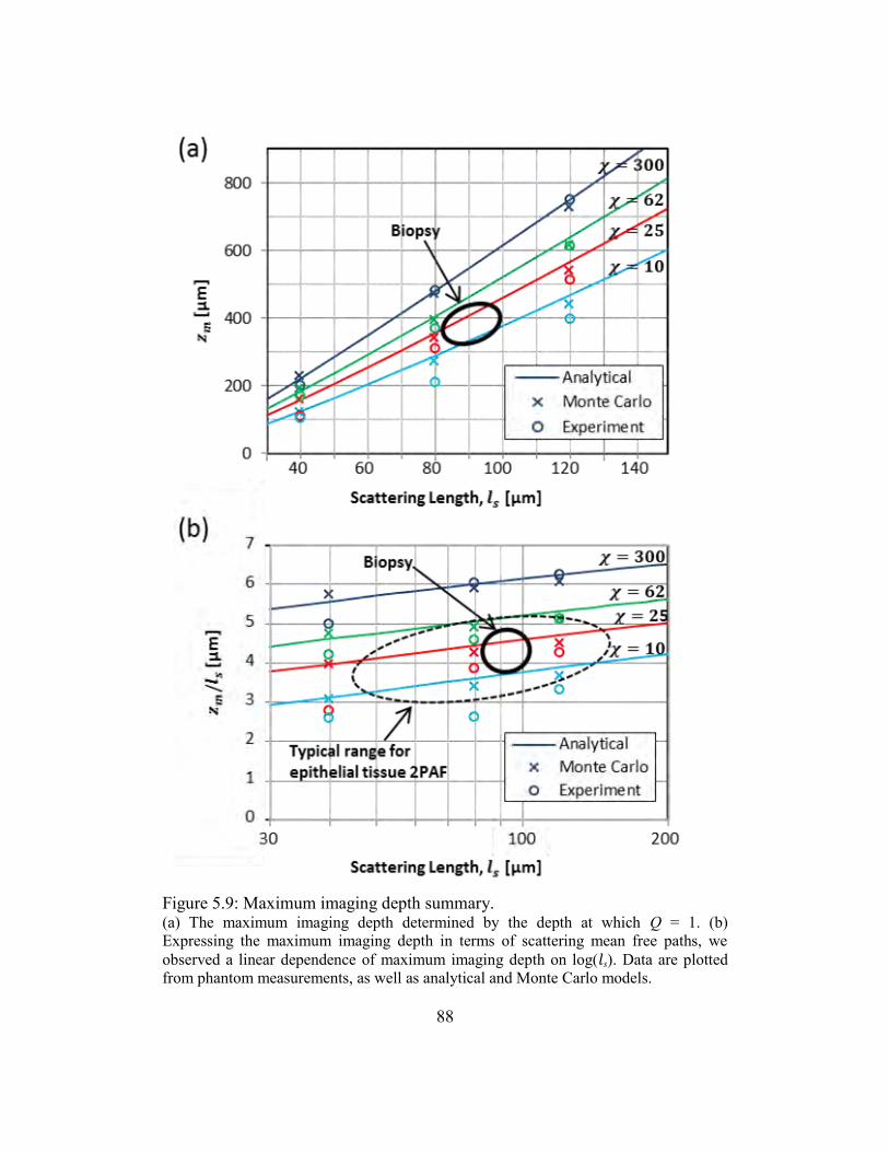
88
Figure 5.9: Maximum imaging depth summary. (a) The maximum imaging depth determined by the depth at which Q = 1. (b)
Expressing the maximum imaging depth in terms of scattering mean free paths, we
observed a linear dependence of maximum imaging depth on log( s). Data are plotted
from phantom measurements, as well as analytical and Monte Carlo models.
89
5.4. CONCLUSIONS
With recent technological advances in 2PAM, including the development of
2PAM systems more relevant for in-vivo optical biopsy[12-15], it is increasingly
important to understand how out-of-focus background fluorescence affects image
contrast and ultimately limits imaging depth. In this paper, we presented experimental
data and a computation model that describes the gradual contrast decay of two-photon
fluorescence imaging with increasing imaging depth for samples with a variety of
scattering lengths and staining inhomogeneities relevant to 2PAM of epithelial tissues.
We found maximum imaging depths significantly smaller than those observed in brain
tissue. The reasons for a shorter maximum 2PAM imaging depth in epithelial tissue are
that the maximum imaging depth decreases with decreasing scattering length, and that the
very low staining inhomogeneities typical encountered in 2PAM of epithelial tissues
leads to increased out-of-focus fluorescence generation. Based on this analysis, we expect
that given range of optical properties typical of epithelial tissue, the 2PAM image
contrast decays to one at imaging depths of approximately 160 and 500 μm for scattering
lengths of 40 and 120 μm, respectively.
In this chapter, we only considered conventional 2PAM. However, more
sophisticated approaches could extend 2PAM imaging depth and contrast by temporal
focusing[163],[164], differential aberration imaging[165], optical clearing[166],[167],
and/or spatial filtering[11],[168]. It would conceivably also be possible to extend imaging
depth by using longer wavelength excitation light[169],[170] to probe dimmer intrinsic
fluorophores that have higher wavelength absorption bands, or by using higher order
excitation (e.g. three-photon excited fluorescence).
90
Chapter 6 Multiphoton-induced luminescence
from gold nanoparticles
6.1. INTRODUCTION
This chapter presents a detailed exploration of multiphoton-induced luminescence
(MPL) from gold nanoparticles. The goal is to quantify the two-photon action cross
sections (σTPA) of a variety of gold nanoparticles and understand how σTPA relates to
various laser and sample parameters. Towards this goal, the physical properties of several
gold nanoparticle samples were characterized. The linear absorbance was modeled for
each sample using their size and aspect ratio distributions, then calculated absorbance
values were compared to measurements to accurately determine nanoparticle
concentrations. The calculated linear absorption and scattering cross sections also provide
some insight into the sample properties influencing MPL. We present a system to probe
the spectrally-resolved nonlinear optical properties of gold nanoparticles as a function of
excitation intensity, wavelength, pulse duration (τp), and polarization. The three major
findings of this chapter are: (1) gold nanoparticles can exhibit extraordinarily large σTPA
values on the order of 104-10
6 GM, which are significantly larger than any previous
reports; (2) MPL deviates from the τp-1
dependence for short pulse durations, which
provides evidence that the mechanism for MPL generation in gold nanoparticles is
sequential rather than simultaneous two-photon absorption; and (3) gold nanoparticles
exhibit third- and fourth- order luminescence generation, especially at lower emission
wavelengths and longer pulse durations.
91
6.2. NOMENCLATURE OF GOLD NANOPARTICLE SAMPLES
Gold nanoparticle samples used in this chapter are referred to as ‗GNS‘ to
indicate gold nanospheres, or ‗GNR‘ for gold nanorods, followed by the wavelength in
nanometers of the linear absorbance peak. In GNR samples, a ‗-25‘ suffix indicates 25
nm specified axial width rather than a 10 nm width, and a ‗-p‘ suffix denotes a
polyethylene glycol (PEG) coating rather than a hexadecylcetyltrimethylammonium
bromide (CTAB) coating. The PEG and CTAB coatings add a thickness of approximately
5 nm around the perimeter of the gold nanorods[171]. GNSs are surrounded by sodium
citrate ions. Stock solutions of each sample were diluted such that the peak absorbance
was approximately one. All nanoparticles were stored at room temperature, except the
GNS630, which specified storage at 4° C. We found excellent stability (evaluated by
constant absorbance spectra over time) in all samples, except the PEG-coated one, for
over a period of greater than one year.
1. GNS530: Gold nanosphere sample prepared using a citrate reduction growth method
to create a diameter of approximately 50 nm with a linear absorption centered at 530
nm. Specifically, 30 mg of gold chloride was mixed into 300 mL of ultrapure
deionized water. In a separate solution, 456 mg of tribasic sodium citrate was added
to 40 mL of ultrapure deionized water. The gold solution was stirred and heated to
boiling. 2.64 mL of the sodium citrate solution was added to the gold solution and
stirred at boiling for an additional 5 minutes to complete the reduction[172-174].
2. GNS630: Gold nanosphere sample with a specified diameter of 150 nm and a linear
absorption centered at 630 nm. Purchased from BBI Research Inc.©
(EM.GC150/4).
3. GNR750-25: Gold nanorod sample with a specified width x length of 25 x 86 nm, a
peak linear absorption centered at 750 nm, and a CTAB coating. Purchased from
Nanopartz©
.
92
4. GNR780: Gold nanorod sample with a specified width x length of 10 x 38 nm, a peak
linear absorption centered at 780 nm, and a CTAB coating. Purchased from
Nanopartz©
.
5. GNR808p: Gold nanorod sample with a specified width x length of 10 x 41 nm, a
peak linear absorption centered at 808 nm, and a PEG coating. Purchased from
Nanopartz©
.
6. GNR840: Gold nanorod sample with a specified width x length of 10 x 45 nm, a peak
linear absorption centered at 840 nm, and a CTAB coating. Purchased from
Nanopartz©
.
6.3. PHYSICAL PROPERTIES
We characterized the physical dimensions of each nanoparticle sample with high
resolution field emission scanning transmission electron microscopy (TEM). A 2 μL
volume from the stock solution of each sample was air dried on a copper grid from Grid
Tech©
(Cu-400CN). Imaging was performed on Hitachi S-5500 TEM at 150k
magnification. Representative images of each sample are shown in Figure 6.1.
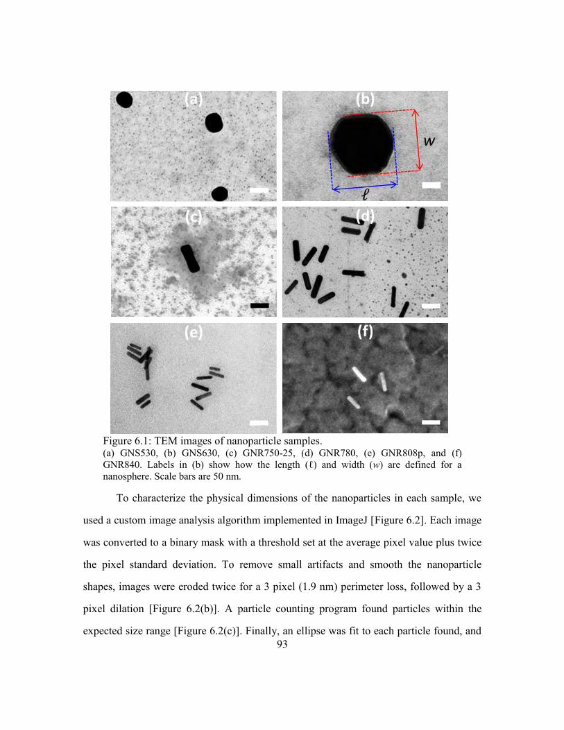
93
To characterize the physical dimensions of the nanoparticles in each sample, we
used a custom image analysis algorithm implemented in ImageJ [Figure 6.2]. Each image
was converted to a binary mask with a threshold set at the average pixel value plus twice
the pixel standard deviation. To remove small artifacts and smooth the nanoparticle
shapes, images were eroded twice for a 3 pixel (1.9 nm) perimeter loss, followed by a 3
pixel dilation [Figure 6.2(b)]. A particle counting program found particles within the
expected size range [Figure 6.2(c)]. Finally, an ellipse was fit to each particle found, and
Figure 6.1: TEM images of nanoparticle samples. (a) GNS530, (b) GNS630, (c) GNR750-25, (d) GNR780, (e) GNR808p, and (f)
GNR840. Labels in (b) show how the length (ℓ) and width (w) are defined for a
nanosphere. Scale bars are 50 nm.
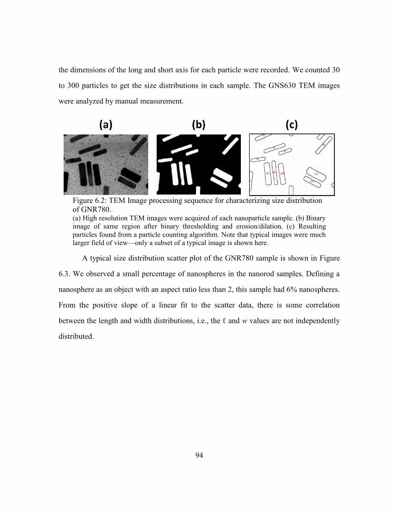
94
the dimensions of the long and short axis for each particle were recorded. We counted 30
to 300 particles to get the size distributions in each sample. The GNS630 TEM images
were analyzed by manual measurement.
A typical size distribution scatter plot of the GNR780 sample is shown in Figure
6.3. We observed a small percentage of nanospheres in the nanorod samples. Defining a
nanosphere as an object with an aspect ratio less than 2, this sample had 6% nanospheres.
From the positive slope of a linear fit to the scatter data, there is some correlation
between the length and width distributions, i.e., the ℓ and w values are not independently
distributed.
Figure 6.2: TEM Image processing sequence for characterizing size distribution
of GNR780. (a) High resolution TEM images were acquired of each nanoparticle sample. (b) Binary
image of same region after binary thresholding and erosion/dilation. (c) Resulting
particles found from a particle counting algorithm. Note that typical images were much
larger field of view—only a subset of a typical image is shown here.
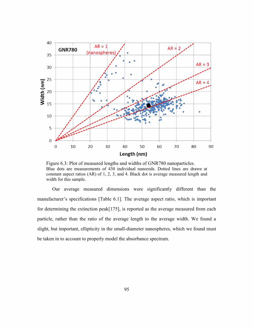
95
Our average measured dimensions were significantly different than the
manufacturer‘s specifications [Table 6.1]. The average aspect ratio, which is important
for determining the extinction peak[175], is reported as the average measured from each
particle, rather than the ratio of the average length to the average width. We found a
slight, but important, ellipticity in the small-diameter nanospheres, which we found must
be taken in to account to properly model the absorbance spectrum.
Figure 6.3: Plot of measured lengths and widths of GNR780 nanoparticles. Blue dots are measurements of 430 individual nanorods. Dotted lines are drawn at
constant aspect ratios (AR) of 1, 2, 3, and 4. Black dot is average measured length and
width for this sample.
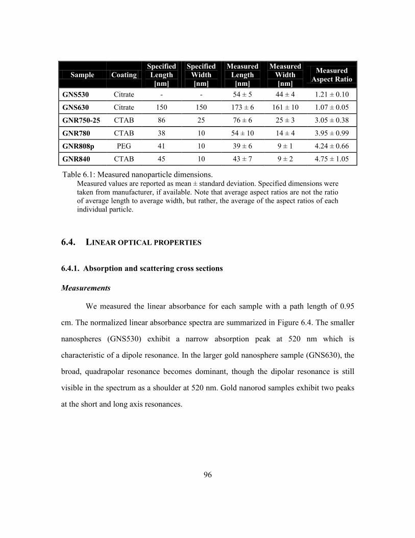
96
6.4. LINEAR OPTICAL PROPERTIES
6.4.1. Absorption and scattering cross sections
Measurements
We measured the linear absorbance for each sample with a path length of 0.95
cm. The normalized linear absorbance spectra are summarized in Figure 6.4. The smaller
nanospheres (GNS530) exhibit a narrow absorption peak at 520 nm which is
characteristic of a dipole resonance. In the larger gold nanosphere sample (GNS630), the
broad, quadrapolar resonance becomes dominant, though the dipolar resonance is still
visible in the spectrum as a shoulder at 520 nm. Gold nanorod samples exhibit two peaks
at the short and long axis resonances.
Sample Coating
Specified
Length
[nm]
Specified
Width
[nm]
Measured
Length
[nm]
Measured
Width
[nm]
Measured
Aspect Ratio
GNS530 Citrate - - 54 ± 5 44 ± 4 1.21 ± 0.10
GNS630 Citrate 150 150 173 ± 6 161 ± 10 1.07 ± 0.05
GNR750-25 CTAB 86 25 76 ± 6 25 ± 3 3.05 ± 0.38
GNR780 CTAB 38 10 54 ± 10 14 ± 4 3.95 ± 0.99
GNR808p PEG 41 10 39 ± 6 9 ± 1 4.24 ± 0.66
GNR840 CTAB 45 10 43 ± 7 9 ± 2 4.75 ± 1.05
Table 6.1: Measured nanoparticle dimensions. Measured values are reported as mean ± standard deviation. Specified dimensions were
taken from manufacturer, if available. Note that average aspect ratios are not the ratio
of average length to average width, but rather, the average of the aspect ratios of each
individual particle.
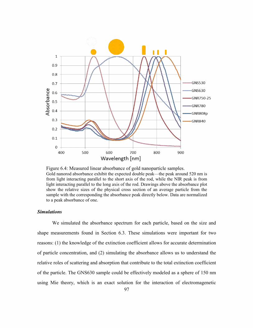
97
Simulations
We simulated the absorbance spectrum for each particle, based on the size and
shape measurements found in Section 6.3. These simulations were important for two
reasons: (1) the knowledge of the extinction coefficient allows for accurate determination
of particle concentration, and (2) simulating the absorbance allows us to understand the
relative roles of scattering and absorption that contribute to the total extinction coefficient
of the particle. The GNS630 sample could be effectively modeled as a sphere of 150 nm
using Mie theory, which is an exact solution for the interaction of electromagenetic
Figure 6.4: Measured linear absorbance of gold nanoparticle samples. Gold nanorod absorbance exhibit the expected double peak—the peak around 520 nm is
from light interacting parallel to the short axis of the rod, while the NIR peak is from
light interacting parallel to the long axis of the rod. Drawings above the absorbance plot
show the relative sizes of the physical cross section of an average particle from the
sample with the corresponding the absorbance peak directly below. Data are normalized
to a peak absorbance of one.
98
waves with spheres. We calculated the absorption and scattering cross sections of all non-
spherical shapes using a Discrete Dipole Approximation (DDA) that takes into account
the size distribution and orientation of the nanoparticles[176].
For all nanoparticle samples, the colloidal solutions were simulated at intervals of
20 nm across a range of wavelengths from 400 to 900 nm in a water environment. We
assumed the particles were far enough apart to be simulated as isolated particles in all
cases. The complex gold refractive index at the irradiation wavelength was obtained from
a curve fit to experimentally determined refractive index values for bulk gold, and then
corrected for size-related surface damping according to the Drude equation with a
modified damping constant. DDA breaks apart a simulated geometry into small cube
sections across which the induced dipole polarization from the incident light is assumed
to be constant, and is a well-established technique for simulating the SPR of colloidal
nanoparticles[59]. We observed that the GNS530 sample consisted of elliptical particles,
and thus they were simulated as spheroids with a short axis diameter of 44 nm and an
aspect ratio of 1.2.
To reproduce the features observed in the absorbance spectra of gold nanorods,
we simulated rod shapes at 4 different orientations with respect to the incident light
polarization and propagation directions. Specifically, we simulate the nanorod long axis
along the x, y, z, and [111] directions for light propagating in the z direction with linear
polarization along the x axis. We also simulate a size distribution of plus/minus one
standard deviation in the nanorod length at constant width to account for plasmonic peak
broadening due to the size distribution of the nanorods. The GNR780, GNR808p,
GNR840 samples were simulated as hemispherically-capped cylinders with aspect ratios
3.95, 4.25 and 4.75, respectively. The GNR750-25 sample was found to have an
hourglass-like shape with a tapered midsection. We simulated the particles in this sample
99
as an elliptically-capped rotationally-symmetric shape with a sinusoidally-varying
midsection. This rod had an aspect ratio of 2.77 with a diameter of 28 nm. For all
samples, we use a minimum of 48 dipoles across the diameter of the nanorod to minimize
shape discrepancy and improve the cross-sectional accuracy of the results.
The results of a typical simulation for the GNR 780 sample, in comparison to the
measured absorbance are shown in Figure 6.5. The shape around the peak absorbance
matches reasonably between the measurement and simulation, while there is a larger
error in simulating the lower wavelength peak. We believe this discrepancy is due to the
simulation only accounting for gold nanorods, while we do observe a small percentage of
nanospheres in each solution. Including a contribution from nanospheres in our
simulations would increase the absorbance at 500 to 550 nm, and simulated absorbance
would more closely match the observed values.
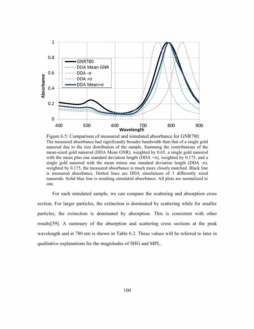
100
For each simulated sample, we can compare the scattering and absorption cross
section. For larger particles, the extinction is dominated by scattering while for smaller
particles, the extinction is dominated by absorption. This is consistent with other
results[59]. A summary of the absorption and scattering cross sections at the peak
wavelength and at 780 nm is shown in Table 6.2. These values will be referred to later in
qualitative explanations for the magnitudes of SHG and MPL.
Figure 6.5: Comparison of measured and simulated absorbance for GNR780. The measured absorbance had significantly broader bandwidth than that of a single gold
nanorod due to the size distribution of the sample. Summing the contributions of the
mean-sized gold nanorod (DDA Mean GNR), weighted by 0.65, a single gold nanorod
with the mean plus one standard deviation length (DDA +σ), weighted by 0.175, and a
single gold nanorod with the mean minus one standard deviation length (DDA -σ),
weighted by 0.175, the measured absorbance is much more closely matched. Black line
is measured absorbance. Dotted lines are DDA simulations of 3 differently sized
nanorods. Solid blue line is resulting simulated absorbance. All plots are normalized to
one.
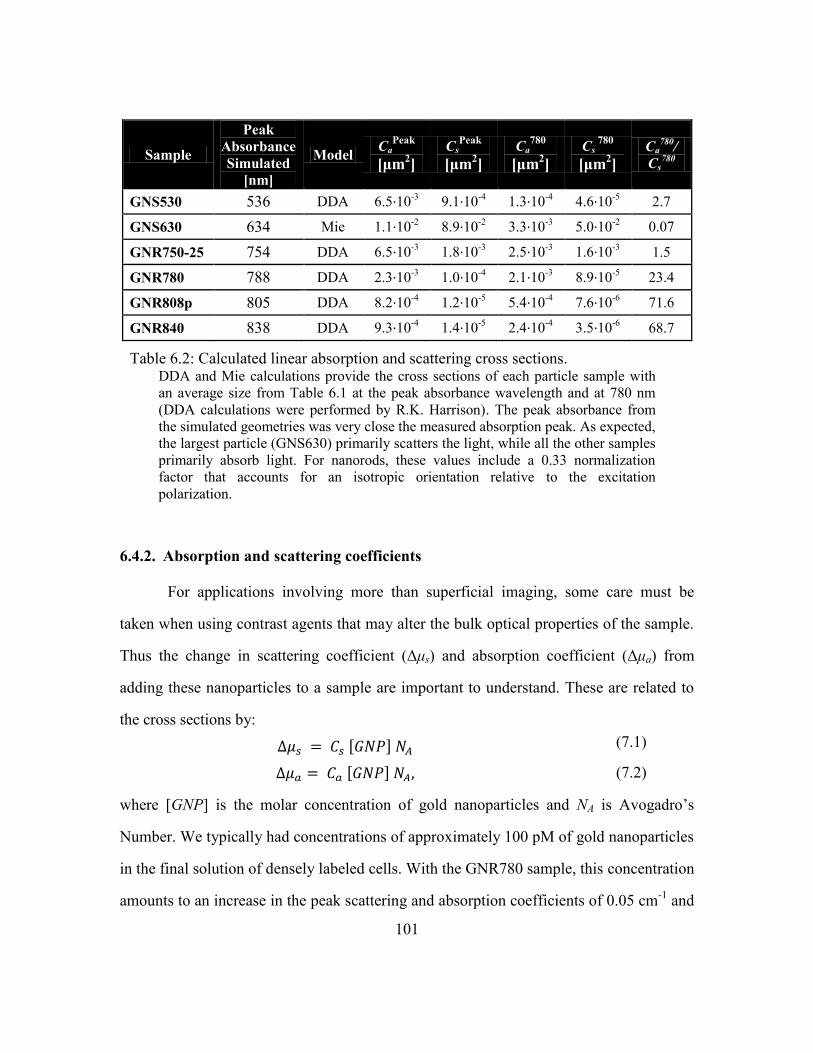
101
6.4.2. Absorption and scattering coefficients
For applications involving more than superficial imaging, some care must be
taken when using contrast agents that may alter the bulk optical properties of the sample.
Thus the change in scattering coefficient (Δμs) and absorption coefficient (Δμa) from
adding these nanoparticles to a sample are important to understand. These are related to
the cross sections by:
[ ] (7.1)
[ ] (7.2)
where [GNP] is the molar concentration of gold nanoparticles and NA is Avogadro‘s
Number. We typically had concentrations of approximately 100 pM of gold nanoparticles
in the final solution of densely labeled cells. With the GNR780 sample, this concentration
amounts to an increase in the peak scattering and absorption coefficients of 0.05 cm-1
and
Sample
Peak
Absorbance
Simulated
[nm]
Model Ca
Peak
[μm2]
CsPeak
[μm2]
Ca780
[μm2]
Cs 780
[μm2]
Ca780
/
Cs780
GNS530 536 DDA 6.5∙10-3
9.1∙10-4
1.3∙10-4
4.6∙10-5
2.7
GNS630 634 Mie 1.1∙10-2
8.9∙10-2
3.3∙10-3
5.0∙10-2
0.07
GNR750-25 754 DDA 6.5∙10-3
1.8∙10-3
2.5∙10-3
1.6∙10-3
1.5
GNR780 788 DDA 2.3∙10-3
1.0∙10-4
2.1∙10-3
8.9∙10-5
23.4
GNR808p 805 DDA 8.2∙10-4
1.2∙10-5
5.4∙10-4
7.6∙10-6
71.6
GNR840 838 DDA 9.3∙10-4
1.4∙10-5
2.4∙10-4
3.5∙10-6
68.7
Table 6.2: Calculated linear absorption and scattering cross sections. DDA and Mie calculations provide the cross sections of each particle sample with
an average size from Table 6.1 at the peak absorbance wavelength and at 780 nm
(DDA calculations were performed by R.K. Harrison). The peak absorbance from
the simulated geometries was very close the measured absorption peak. As expected,
the largest particle (GNS630) primarily scatters the light, while all the other samples
primarily absorb light. For nanorods, these values include a 0.33 normalization
factor that accounts for an isotropic orientation relative to the excitation
polarization.
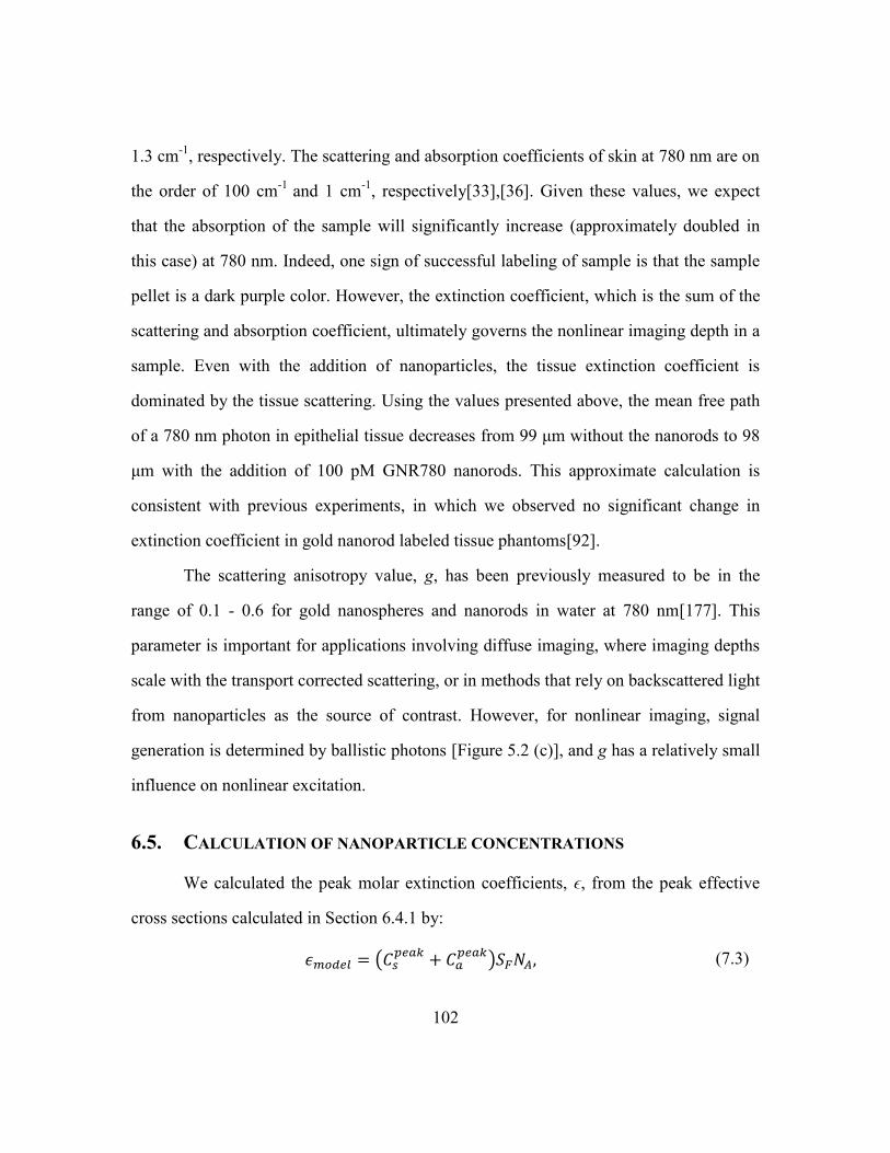
102
1.3 cm-1
, respectively. The scattering and absorption coefficients of skin at 780 nm are on
the order of 100 cm-1
and 1 cm-1
, respectively[33],[36]. Given these values, we expect
that the absorption of the sample will significantly increase (approximately doubled in
this case) at 780 nm. Indeed, one sign of successful labeling of sample is that the sample
pellet is a dark purple color. However, the extinction coefficient, which is the sum of the
scattering and absorption coefficient, ultimately governs the nonlinear imaging depth in a
sample. Even with the addition of nanoparticles, the tissue extinction coefficient is
dominated by the tissue scattering. Using the values presented above, the mean free path
of a 780 nm photon in epithelial tissue decreases from 99 μm without the nanorods to 98
μm with the addition of 100 pM GNR780 nanorods. This approximate calculation is
consistent with previous experiments, in which we observed no significant change in
extinction coefficient in gold nanorod labeled tissue phantoms[92].
The scattering anisotropy value, g, has been previously measured to be in the
range of 0.1 - 0.6 for gold nanospheres and nanorods in water at 780 nm[177]. This
parameter is important for applications involving diffuse imaging, where imaging depths
scale with the transport corrected scattering, or in methods that rely on backscattered light
from nanoparticles as the source of contrast. However, for nonlinear imaging, signal
generation is determined by ballistic photons [Figure 5.2 (c)], and g has a relatively small
influence on nonlinear excitation.
6.5. CALCULATION OF NANOPARTICLE CONCENTRATIONS
We calculated the peak molar extinction coefficients, ϵ, from the peak effective
cross sections calculated in Section 6.4.1 by:
(
) (7.3)
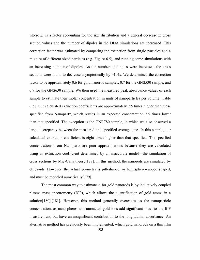
103
where SF is a factor accounting for the size distribution and a general decrease in cross
section values and the number of dipoles in the DDA simulations are increased. This
correction factor was estimated by comparing the extinction from single particles and a
mixture of different sized particles (e.g. Figure 6.5), and running some simulations with
an increasing number of dipoles. As the number of dipoles were increased, the cross
sections were found to decrease asymptotically by ~10%. We determined the correction
factor to be approximately 0.6 for gold nanorod samples, 0.7 for the GNS530 sample, and
0.9 for the GNS630 sample. We then used the measured peak absorbance values of each
sample to estimate their molar concentration in units of nanoparticles per volume [Table
6.3]. Our calculated extinction coefficients are approximately 2.5 times higher than those
specified from Nanopartz, which results in an expected concentration 2.5 times lower
than that specified. The exception is the GNR780 sample, in which we also observed a
large discrepancy between the measured and specified average size. In this sample, our
calculated extinction coefficient is eight times higher than that specified. The specified
concentrations from Nanopartz are poor approximations because they are calculated
using an extinction coefficient determined by an inaccurate model—the simulation of
cross sections by Mie-Gans theory[178]. In this method, the nanorods are simulated by
ellipsoids. However, the actual geometry is pill-shaped, or hemisphere-capped shaped,
and must be modeled numerically[179].
The most common way to estimate ϵ for gold nanorods is by inductively coupled
plasma mass spectrometry (ICP), which allows the quantification of gold atoms in a
solution[180],[181]. However, this method generally overestimates the nanoparticle
concentration, as nanospheres and unreacted gold ions add significant mass to the ICP
measurement, but have an insignificant contribution to the longitudinal absorbance. An
alternative method has previously been implemented, which gold nanorods on a thin film
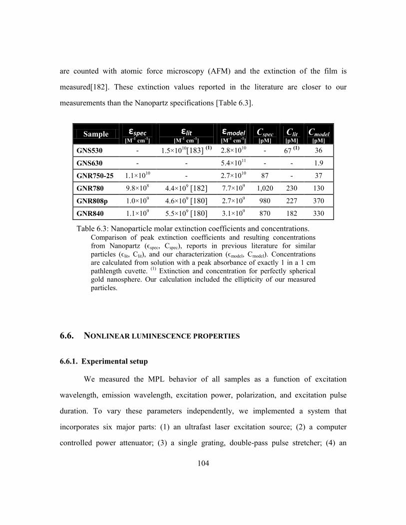
104
are counted with atomic force microscopy (AFM) and the extinction of the film is
measured[182]. These extinction values reported in the literature are closer to our
measurements than the Nanopartz specifications [Table 6.3].
6.6. NONLINEAR LUMINESCENCE PROPERTIES
6.6.1. Experimental setup
We measured the MPL behavior of all samples as a function of excitation
wavelength, emission wavelength, excitation power, polarization, and excitation pulse
duration. To vary these parameters independently, we implemented a system that
incorporates six major parts: (1) an ultrafast laser excitation source; (2) a computer
controlled power attenuator; (3) a single grating, double-pass pulse stretcher; (4) an
Sample εspec [M-1 cm-1]
εlit [M-1 cm-1]
εmodel [M-1 cm-1]
Cspec [pM]
Clit [pM]
Cmodel [pM]
GNS530 - 1.5×10¹⁰[183]
(1) 2.8×10
10 - 67
(1) 36
GNS630 - - 5.4×10¹¹
- - 1.9
GNR750-25 1.1×10¹⁰
- 2.7×10¹⁰
87 - 37
GNR780 9.8×10⁸ 4.4×10
9 [182] 7.7×10⁹ 1,020 230 130
GNR808p 1.0×10⁹ 4.6×10
9 [180] 2.7×10⁹ 980 227 370
GNR840 1.1×10⁹ 5.5×10
9 [180] 3.1×10⁹ 870 182 330
Table 6.3: Nanoparticle molar extinction coefficients and concentrations. Comparison of peak extinction coefficients and resulting concentrations
from Nanopartz (ϵspec, Cspec), reports in previous literature for similar
particles (ϵlit, Clit), and our characterization (ϵmodel, Cmodel). Concentrations
are calculated from solution with a peak absorbance of exactly 1 in a 1 cm
pathlength cuvette. (1)
Extinction and concentration for perfectly spherical
gold nanosphere. Our calculation included the ellipticity of our measured
particles.
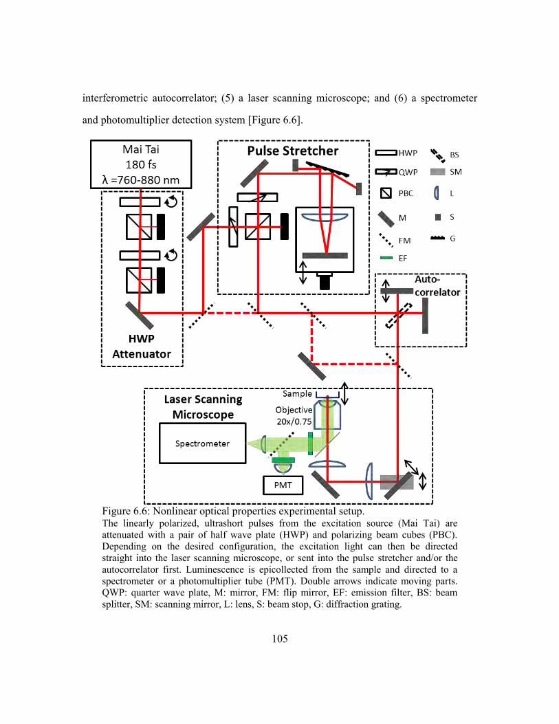
105
interferometric autocorrelator; (5) a laser scanning microscope; and (6) a spectrometer
and photomultiplier detection system [Figure 6.6].
Figure 6.6: Nonlinear optical properties experimental setup. The linearly polarized, ultrashort pulses from the excitation source (Mai Tai) are
attenuated with a pair of half wave plate (HWP) and polarizing beam cubes (PBC).
Depending on the desired configuration, the excitation light can then be directed
straight into the laser scanning microscope, or sent into the pulse stretcher and/or the
autocorrelator first. Luminescence is epicollected from the sample and directed to a
spectrometer or a photomultiplier tube (PMT). Double arrows indicate moving parts.
QWP: quarter wave plate, M: mirror, FM: flip mirror, EF: emission filter, BS: beam
splitter, SM: scanning mirror, L: lens, S: beam stop, G: diffraction grating.
106
Excitation source and power attenuator
The laser source is a Ti:Sapphire oscillator, tunable in the range of 760 to 880 nm,
with an average power of 1 W (Newport, MaiTai). At an excitation wavelength, λx, of
780 nm, the output of the laser source had a spectral bandwidth of 7.5 nm and a pulse
duration of 120 fs. The repetition rate, R, was 80 MHz. We measured the pulse duration
at the sample plane of the nonlinear microscope, τp, to be 250 fs (FWHM) when
bypassing the stretcher. The 1/e2 beam diameter is 2.1 mm exiting the cavity. To have
precise control over the laser power, we found that reflective neutral density filters were
insufficient. Instead, we used two sets of half wave plates and polarizing beam cubes to
continually adjust the power. One of the half wave plates was adjusted by a computer
controlled actuator, providing 0.01° resolution, corresponding to a worst-case attenuation
resolution of approximately ±0.08% at λx = 780 nm (Newport, PR50PP, 10RP52-2). This
value is corresponds to the change in excitation power when the HWP is adjusted at the
steepest rate of transmission change versus angle change. Using the two attenuators in
series allowed us to continuously attenuate the excitation power from less than 0.4 dB to
greater than 40 dB within the range of λx = 760-820 nm
Pulse stretcher/compressor and autocorrelator
We built a single grating, double pass pulse stretcher, similar to the designs of
[184],[185]. The grating had a line spacing of 1480 lines/mm grating with an 800 nm
wavelength blaze. We used a 2‖ diameter focusing lens (f = 200 mm) and mirror to allow
enough space for the light to reflect off the grating twice. To adjust the pulse duration, the
lens and mirror after the grating were positioned on an optical rail that could slide tens of
centimeters [Figure 6.6]. This apparatus can impart negative or positive GDD on our
excitation pulse, and vary the pulse duration at the objective focal plane from 220 fs to

107
beyond 8 ps. With proper alignment, the pulse duration could be tuned with no
observable change in system power transmission, or an significant misalignment.
To measure the autocorrelation of our excitation pulse at the sample, we used a
Michelson interferometer with a computer controlled delay arm. Changing the distance of
one arm of the interferometer changes the temporal overlap of excitation pulses at the
focal plane. The resulting autocorrelation was analyzed to find pulse duration at the
sample, as described in Section 3.3.2 and Figure 3.4 (b). We characterized the effect of
the pulse stretcher position, s, on the excitation pulse duration at the objective focal plane
using the autocorrelator and an Olympus 20x/0.75NA air objective. The pulse duration as
a function of stretcher position is shown in Figure 6.7. When not performing an
autocorrelation, we found it necessary to bypass the autocorrelator, as even with the
autocorrelator stationary, minute vibrations in the system caused the intensity at the focal
plane to fluctuate rapidly.
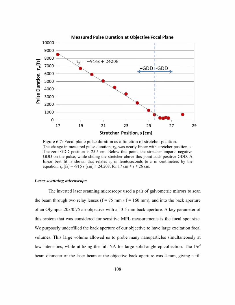
108
Laser scanning microscope
The inverted laser scanning microscope used a pair of galvometric mirrors to scan
the beam through two relay lenses (f = 75 mm / f = 160 mm), and into the back aperture
of an Olympus 20x/0.75 air objective with a 13.5 mm back aperture. A key parameter of
this system that was considered for sensitive MPL measurements is the focal spot size.
We purposely underfilled the back aperture of our objective to have large excitation focal
volumes. This large volume allowed us to probe many nanoparticles simultaneously at
low intensities, while utilizing the full NA for large solid-angle epicollection. The 1/e2
beam diameter of the laser beam at the objective back aperture was 4 mm, giving a fill
Figure 6.7: Focal plane pulse duration as a function of stretcher position. The change in measured pulse duration, τp, was nearly linear with stretcher position, s.
The zero GDD position is 25.5 cm. Below this point, the stretcher imparts negative
GDD on the pulse, while sliding the stretcher above this point adds positive GDD. A
linear best fit is shown that relates τp in femtoseconds to s in centimeters by the
equation: τp [fs] = -916 s [cm] + 24,208, for 17 cm ≤ s ≤ 26 cm.
109
factor of 0.3. At 780 nm excitation, we measured an IPSF2 of 1.4 ± 0.2 μm and 9 ± 1 μm
FWHM in the lateral and axial dimension, respectively. These numbers represent the
average ± standard deviation across measurements of ten fluorescent beads (Invitrogen,
100 nm diameter FluoSpheres) embedded in a 2% agar gel. The dimensions of the linear
intensity distribution (the IPSF) are a factor of √2 larger than the dimensions IPSF2. The
peak excitation intensity, Ip, was then calculated by using the focal spot area, Af,
calculated from the 1/e2 radius of the excitation intensity by:
(7.4)
The peak excitation intensities used were typically reported as MW/cm2, or millions of
Watts per square centimeter.
During spectra acquisitions, the scanning mirrors were rotated at 1 kHz at small
angles, which translated to maximum scanning distances of ±10 μm at the focal plane.
This scanning method minimized accumulated damage or photobleaching effects, while
minimizing any likelihood of optical trapping. Because of the large slit size in the
spectrometer, we found that this lateral movement had no effect on our measurements in
a fluorescein reference standard.
Sample
Samples were placed on a #1.5 coverslip-bottom petri dish (Matek Corp), and
adjusted relative to the objective lens with a three axis piezo actuator, first to find the
coverslip/sample interface, and then move a constant 10 μm into the sample. For aqueous
solutions, samples were concentrated to a peak optical density of 10, and 400 μL was
placed on the coverslip (resulting in a nanoparticle concentration 10x higher than those
reported in Table 6.3). For a nanoparticle concentration of 1 nM, using an ellipsoidal
110
focal volume determined by the IPSF (~25 fL), the average nanoparticle concentration is
approximately 15 particles per focal volume. In a homogenously dispersed solution at
this concentration, a nanoparticle will be separated from its nearest neighbor by an
average distance 1.2 μm.
To examine the polarization dependence of the luminescence, we analyzed
stationary particles dried on a coverslip. We prepared these samples by diluting the stock
solution five times (to a peak optical density of 0.2), depositing 5 μL of the dilute
solution on a #1.5 coverslip, and evaporating the solvent at 90° C.
Spectrometer/PMT
Nanoparticle luminescence was detected by either a spectrometer or a PMT. We
used an SRS163 nonimaging spectrometer (f/3.6) with 163 mm focal length, a 300
line/mm grating (500 nm blaze), and a 100 μm x 3 mm slit (Andor Technology). We used
an f/4 focusing lens so that no light would be lost outside of the acceptance cone of the
spectrometer, assuming perfectly collimated light from the objective (Thorlabs D = 25
mm, f = 100 mm). We verified that the small amount of focal point movement from the
scanning mirrors did not appreciably affect spectra or photon counts from a sample of
fluorescein. The 100 μm slit also played the role of a spatial filter, rejecting some of the
scattered MPL light that is not collimated out of the objective. This filtering of the
scattered light was important to our cross section measurements that are made in
reference to fluorescein, because a constant collection efficiency is required for an
accurate measurement, and fluorescein and nanoparticles scatter visible wavelength
emission quite differently. Our spectrometer was cooled with a thermoelectric cooler
(TEC) with an additional liquid cooling unit that flowed 25° C water through the TEC
heatsink. We found the liquid cooling unit to be essential for low signal measurements, as
111
it allowed us to reduce the detector temperature from -60° C to -75° C. This 15°
temperature change led to a decrease of dark current by one order of magnitude, in
agreement with the specifications.
Many previous studies on nonlinear luminescence from nanoparticles ignore the
far red regions of the luminescence spectra by using non-ideal emission filters and
dichroic mirrors[186],[97],[187]. We used ion-beam-sputtered filters that are relatively
flat up to 750 nm, while performing deep attenuation of the laser bandwidth (OD > 7
above 760 nm). Our dichroic mirror limits the spectral sensitive of our system to 380 nm
to 720 nm. We calibrated the wavelength response of our spectrometer using a NIST-
traceable Tungsten-Halogen lamp and precision current source (Optronic Laboratories,
245 and OL 65A). The actual spectrum was divided by the measured spectrum to
determine a correction factor, CF [Figure 6.8]. To get a smooth calibration, we fit a 5th
order polynomial function to the CF, resulting in:
(7.5)
All spectra presented in this chapter were multiplied by this correction factor. This
calibration ensured the shape of the luminescence we recorded reflects the actual spectral
content of the emission. Acquisitions were done over 4 accumulations at 10 second
exposures, with full vertical binning and 4 pixel horizontal binning to improve signal to
noise ratio.
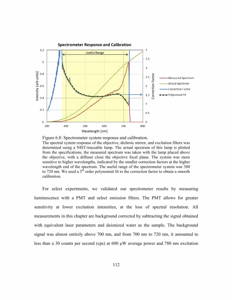
112
For select experiments, we validated our spectrometer results by measuring
luminescence with a PMT and select emission filters. The PMT allows for greater
sensitivity at lower excitation intensities, at the loss of spectral resolution. All
measurements in this chapter are background corrected by subtracting the signal obtained
with equivalent laser parameters and deionized water as the sample. The background
signal was almost entirely above 700 nm, and from 700 nm to 720 nm, it amounted to
less than a 30 counts per second (cps) at 600 μW average power and 780 nm excitation
Figure 6.8: Spectrometer system response and calibration. The spectral system response of the objective, dichroic mirror, and excitation filters was
determined using a NIST-traceable lamp. The actual spectrum of this lamp is plotted
from the specifications, the measured spectrum was taken with the lamp placed above
the objective, with a diffuser close the objective focal plane. The system was more
sensitive to higher wavelengths, indicated by the smaller correction factors at the higher
wavelength end of the spectrum. The useful range of the spectrometer system was 380
to 720 nm. We used a 5th order polynomial fit to the correction factor to obtain a smooth
calibration.
113
wavelength. Occasional 2-3 pixel signal peaks from cosmic rays were removed manually
by setting the pixel spikes to the average value of the adjacent pixels[188].
6.6.2. Spectral features of nanoparticle luminescence
This section presents a qualitative comparison of the MPL spectra of each of the
gold nanoparticle samples in solution. In general, the MPL spectra from gold
nanoparticles are very broad and significantly red-shifted compared to band-gap
fluorophores. All experiments presented in this section were performed bypassing the
pulse stretcher and autocorrelator, which resulted in a measured pulse duration of 250 fs
at the objective focal plane.
Comparing the spectral features of MPL from each nanoparticle sample, we
observe appreciable second harmonic generation (SHG) peaks only in the nanosphere
samples [Figure 6.9 (a)] and in the largest size nanorod sample [Figure 6.9 (b)]. As
expected, significant SHG signal correlates to samples with low Ca/Cs ratios summarized
in Table 6.2. As the MPL is epicollected, the harmonically generated light must scatter
backwards to be detected. Therefore the relative size of the SHG peaks to the broad MPL
outside λx/2 is a function of the scattering of the sample, and is not directly indicative of
relative magnitude of signal generated at the focal volume.
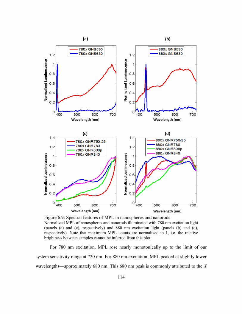
114
For 780 nm excitation, MPL rose nearly monotonically up to the limit of our
system sensitivity range at 720 nm. For 880 nm excitation, MPL peaked at slightly lower
wavelengths—approximately 680 nm. This 680 nm peak is commonly attributed to the X
Figure 6.9: Spectral features of MPL in nanospheres and nanorods Normalized MPL of nanospheres and nanorods illuminated with 780 nm excitation light
(panels (a) and (c), respectively) and 880 nm excitation light (panels (b) and (d),
respectively). Note that maximum MPL counts are normalized to 1, i.e. the relative
brightness between samples cannot be inferred from this plot.
115
symmetry point in the first Brillouin zone of gold[39],[189],[190]. One important feature,
which will be discussed more in the following section, is the presence of luminescence
below λx/2, which has also been reported by other groups[191-194]. This contrasts to
two-photon excited fluorescence, which, by energy conservation, must be at larger
wavelengths than λx/2. Thus we would expect that MPL in this spectral range should
increase at a faster than quadratic rate with increasing excitation intensity (three- or four-
photon induced luminescence). To investigate this hypothesis, we studied the dependence
of the spectrally resolved MPL on excitation intensity. This approach will also verify that
the high wavelength MPL observed here is not due to bleed through of the excitation
light[195].
6.6.3. Dependence of MPL on excitation intensity
We investigated the dependence of MPL on excitation intensity in two ways.
Using the spectrometer, we recorded MPL counts as we increased power. We also
measured the MPL response to power changes with a PMT and a variety of bandpass
emission filters. In both methods, we found that different spectral regions of the
nanoparticle MPL increased at different nonlinear rates. In all cases, we found that lower
wavelength luminescence increased at higher nonlinear orders than the higher wavelength
MPL (i.e. MPL at 400 nm increased at higher rates than MPL at 650 nm).
To start, we tested a fluorescein sample, which serves to validate our method—we
expect that all regions of the fluorescence should quadratically increase with excitation
power. We prepared a 25 μM solution of fluorescein (Fluka) in a pH 12 buffer, and
recorded spectra for increasing power. As we exponentially increased the power in
approximately 100.1
intervals, we observe that the emission shape is constant and
emission counts increase at intervals of 100.2
[Figure 6.10 (a)]. Looking at the emission
116
profiles on a logarithmic scale, we see that the emission counts are spaced at equal
increments for the exponentially increasing excitation power [Figure 6.10 (b)]. We also
visualized the nonlinear trends by taking the ratio of two full spectra at two different
excitation powers and dividing the spectral ratio by the ratio of the power increase (i.e.
~1.26). The result describes the nonlinear order at which each wavelength behaved
during the power increase. As we expected, fluorescein exhibited a quadratic dependence
on excitation power across its entire emission spectra [Figure 6.10 (c)]. We also looked at
the integration of photon counts within fixed emission wavelengths, and found a slope of
~2 on the double-logarithmic MPL vs. Ip plot, as the power was increased within each
emission window [Figure 6.10 (d) - (f)]. We tested fluorescein and rhodamine 6G in
every condition applied to gold nanoparticles, and found no deviations in these trends at
different pulse durations, excitation powers, excitation wavelengths, or emission
windows.
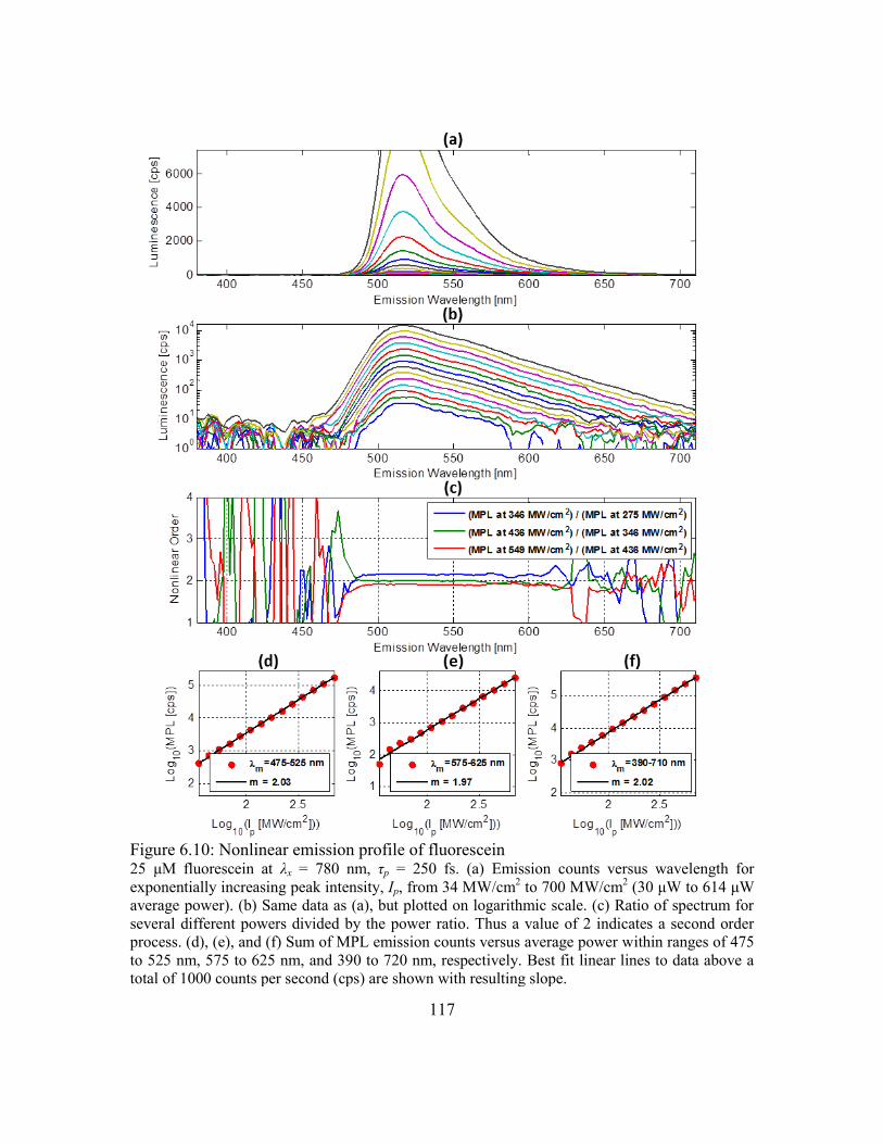
117
Figure 6.10: Nonlinear emission profile of fluorescein 25 μM fluorescein at λx = 780 nm, τp = 250 fs. (a) Emission counts versus wavelength for
exponentially increasing peak intensity, Ip, from 34 MW/cm2 to 700 MW/cm
2 (30 μW to 614 μW
average power). (b) Same data as (a), but plotted on logarithmic scale. (c) Ratio of spectrum for
several different powers divided by the power ratio. Thus a value of 2 indicates a second order
process. (d), (e), and (f) Sum of MPL emission counts versus average power within ranges of 475
to 525 nm, 575 to 625 nm, and 390 to 720 nm, respectively. Best fit linear lines to data above a
total of 1000 counts per second (cps) are shown with resulting slope.
118
Applying this analysis to the GNR780 sample, we found several interesting
deviations from the quadratic power dependence that we observed in fluorescein and
rhodamine 6G experiments [Figure 6.11]. Qualitatively, the shape of the luminescence
curve changes with excitation power, including the formation of a low wavelength peak
around 520 nm [Figure 6.11 (b)]. This shape change with varying excitation powers is
indicative of different order processes and/or saturation effects. Looking at the spectral
ratio, we observe that for constant excitation wavelength, at lower luminescence
wavelengths, the luminescence increases at nonlinear orders of up to four, while at higher
wavelengths, the nonlinear rate of increase is closer to second order [Figure 6.11 (c)].
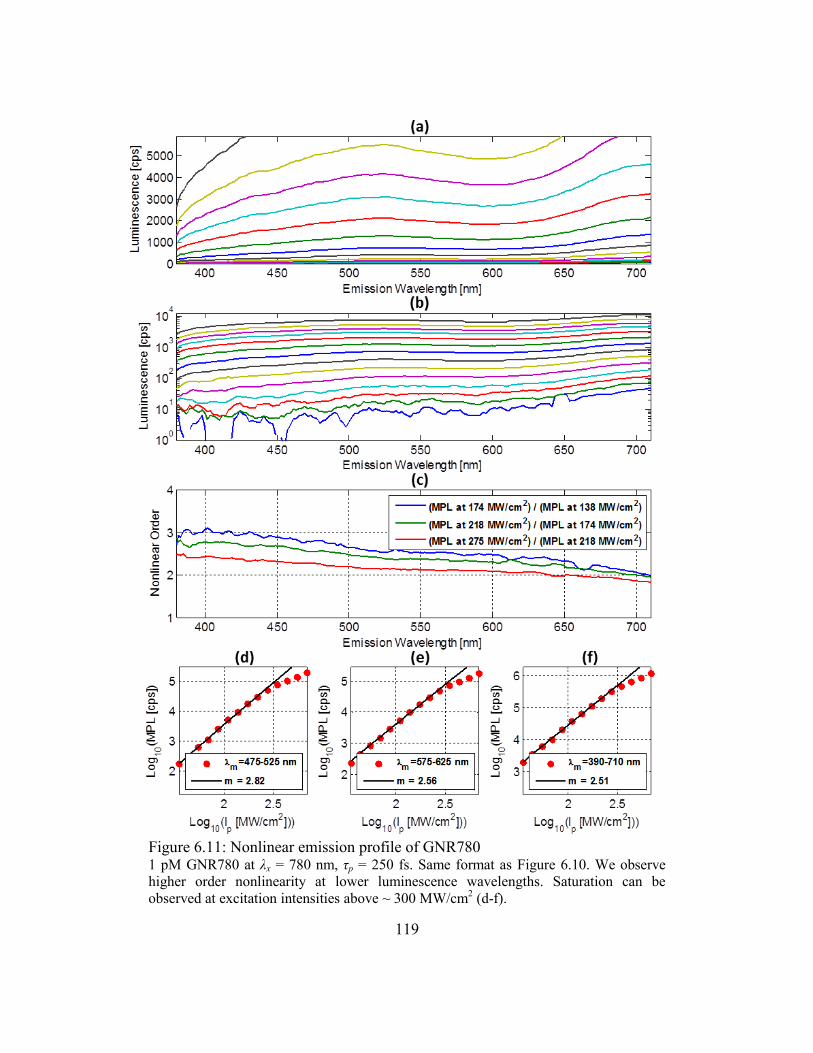
119
Figure 6.11: Nonlinear emission profile of GNR780 1 pM GNR780 at λx = 780 nm, τp = 250 fs. Same format as Figure 6.10. We observe
higher order nonlinearity at lower luminescence wavelengths. Saturation can be
observed at excitation intensities above ~ 300 MW/cm2 (d-f).
120
At peak excitation intensities greater than ~300 MW/cm2 (corresponding to an
average intensity of 61 μJ/cm2 per pulse), the luminescence begins to saturate, and lower
order power dependencies are observed. Plasmon saturation has been observed recently
in two reports. Pelton et al. observed the onset of plasmon saturation at average
intensities of approximately 32 μJ/cm2 per pulse at 800 nm excitation of similarly-sized,
single gold nanorods[196]. Park et al. found evidence of plasmon saturation in colloidal,
randomly oriented, gold nanorods[197]. They observed that when excited at resonant
wavelengths at above 1.5 nJ per pulse (approximately 1.9 GW/cm2), the absorption from
the gold nanorods begins to be dramatically reduced[197]. In both studies, though the
origin of the plasmon saturation was not fully elucidated, the saturation was attributed to
changes in the mechanisms of damping of the surface plasmon and possibly the
generation of highly energetic electrons[196],[197]. There are some differences in these
previous studies and our results. Pelton et al. probed a single gold nanorod aligned to the
electric field of the excitation light, while our setup and Park et al. probed an ensemble of
different nanorod sizes at isotropically distributed orientations with respect to the electric
field. Both Pelton et al. and Park et al. measured the transient linear transmission (and
corresponding linear absorption) rather than the multiphoton induced luminescence.
However, one would expect that the observation of a reduction in linear absorption would
correspond to a change in MPL, especially in the case where MPL is a result of
sequential linear absorption events, which we will provide evidence for in Section 6.6.4.
Though the majority of previous MPL studies with nanoparticles report a second
order dependence[92],[93],[97],[186],[198-203], the range reported is typically small,
and measurements tend to be noisy and difficult to interpret. In these studies, the peak
intensities, if indicated, are typically in the GW/cm2 range. We note that slopes taken in
our experiments at this range (above our saturation threshold) would also yield slopes
121
close to 2. We also reproduce this observation using high numerical aperture focusing in
Chapter 7. Some reports do show nonlinear dependencies that are non-integer orders,
with values that range from 2.2 to 7[191],[194],[187],[204],[205].
In Figure 6.11 (a), the different rates of increase across the luminescence spectra
result in a dramatic peak at 520 nm forming at high intensities. A similar phenomenon
was reported previously in an experiment that probed large nanorods fabricated on a
substrate with ultrafast excitation[191]. This low wavelength luminescence was attributed
to white-light supercontinuum generation, while the longer wavelength luminescence was
believed to be MPL. We will demonstrate evidence for an alternative possible origin for
this higher order dependence in Section 6.6.4.
Across all nanoparticle samples and excitation wavelengths, we observed a higher
order nonlinear dependence at the lower wavelengths of the luminescence range [Figure
6.12]. Slopes were measured by fitting lines at the lower range of Ip used in each sample.
There was no clear dependence of nonlinear slope on excitation wavelength, that is, the
slopes observed were not necessarily higher or lower when different samples were
excited with higher or lower excitation wavelengths.
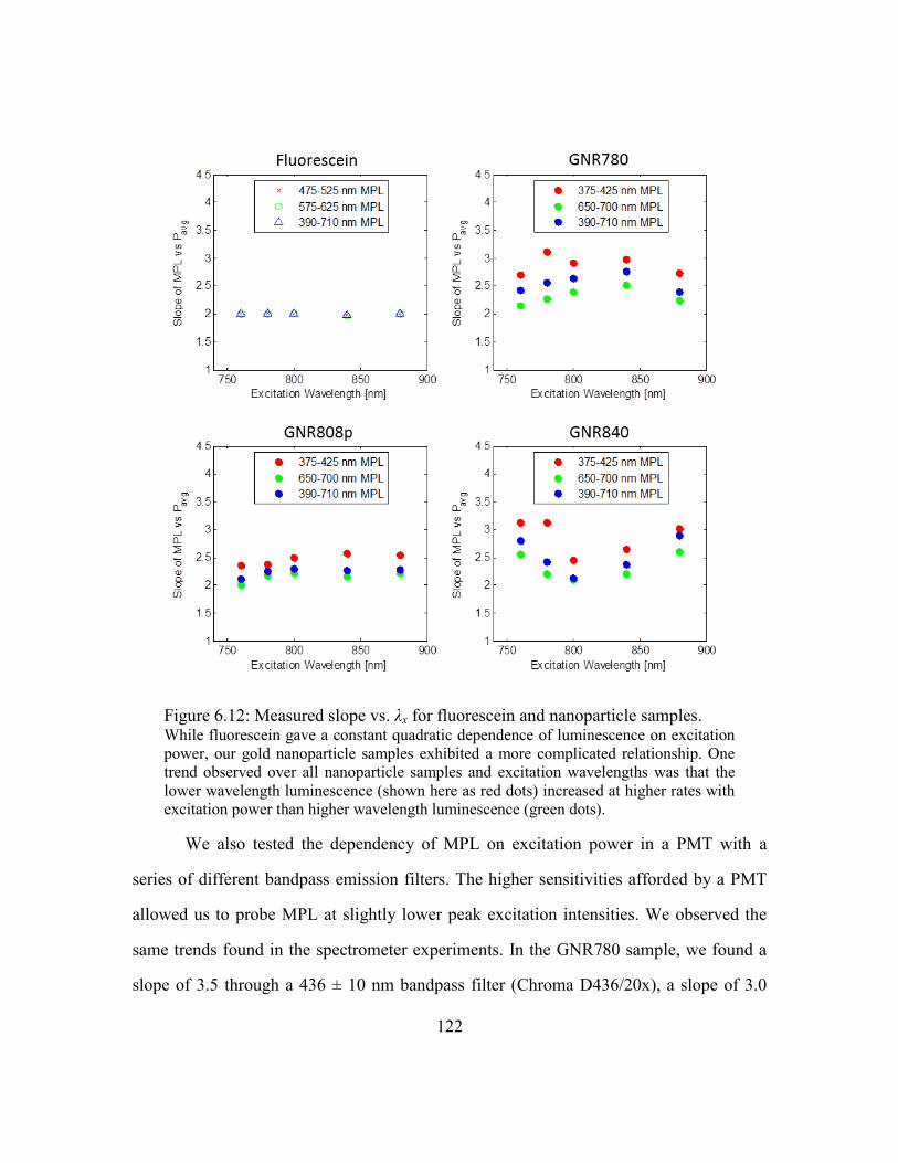
122
We also tested the dependency of MPL on excitation power in a PMT with a
series of different bandpass emission filters. The higher sensitivities afforded by a PMT
allowed us to probe MPL at slightly lower peak excitation intensities. We observed the
same trends found in the spectrometer experiments. In the GNR780 sample, we found a
slope of 3.5 through a 436 ± 10 nm bandpass filter (Chroma D436/20x), a slope of 3.0
Figure 6.12: Measured slope vs. λx for fluorescein and nanoparticle samples. While fluorescein gave a constant quadratic dependence of luminescence on excitation
power, our gold nanoparticle samples exhibited a more complicated relationship. One
trend observed over all nanoparticle samples and excitation wavelengths was that the
lower wavelength luminescence (shown here as red dots) increased at higher rates with
excitation power than higher wavelength luminescence (green dots).
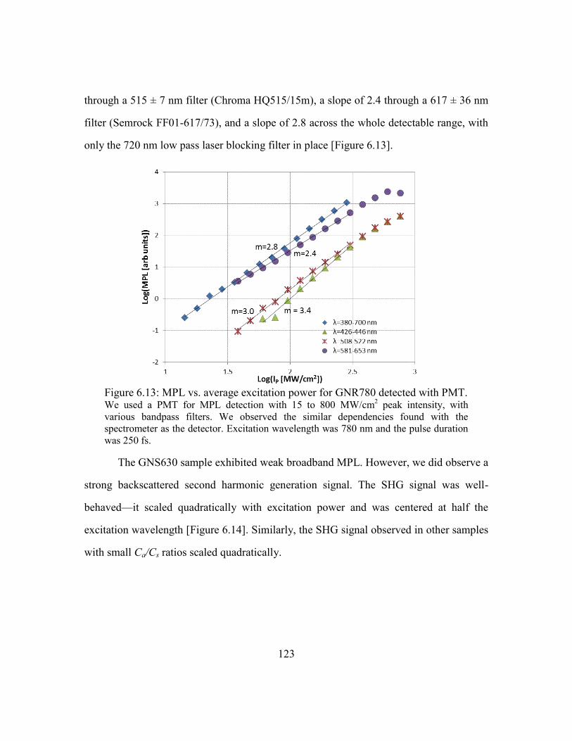
123
through a 515 ± 7 nm filter (Chroma HQ515/15m), a slope of 2.4 through a 617 ± 36 nm
filter (Semrock FF01-617/73), and a slope of 2.8 across the whole detectable range, with
only the 720 nm low pass laser blocking filter in place [Figure 6.13].
The GNS630 sample exhibited weak broadband MPL. However, we did observe a
strong backscattered second harmonic generation signal. The SHG signal was well-
behaved—it scaled quadratically with excitation power and was centered at half the
excitation wavelength [Figure 6.14]. Similarly, the SHG signal observed in other samples
with small Ca/Cs ratios scaled quadratically.
Figure 6.13: MPL vs. average excitation power for GNR780 detected with PMT. We used a PMT for MPL detection with 15 to 800 MW/cm
2 peak intensity, with
various bandpass filters. We observed the similar dependencies found with the
spectrometer as the detector. Excitation wavelength was 780 nm and the pulse duration
was 250 fs.
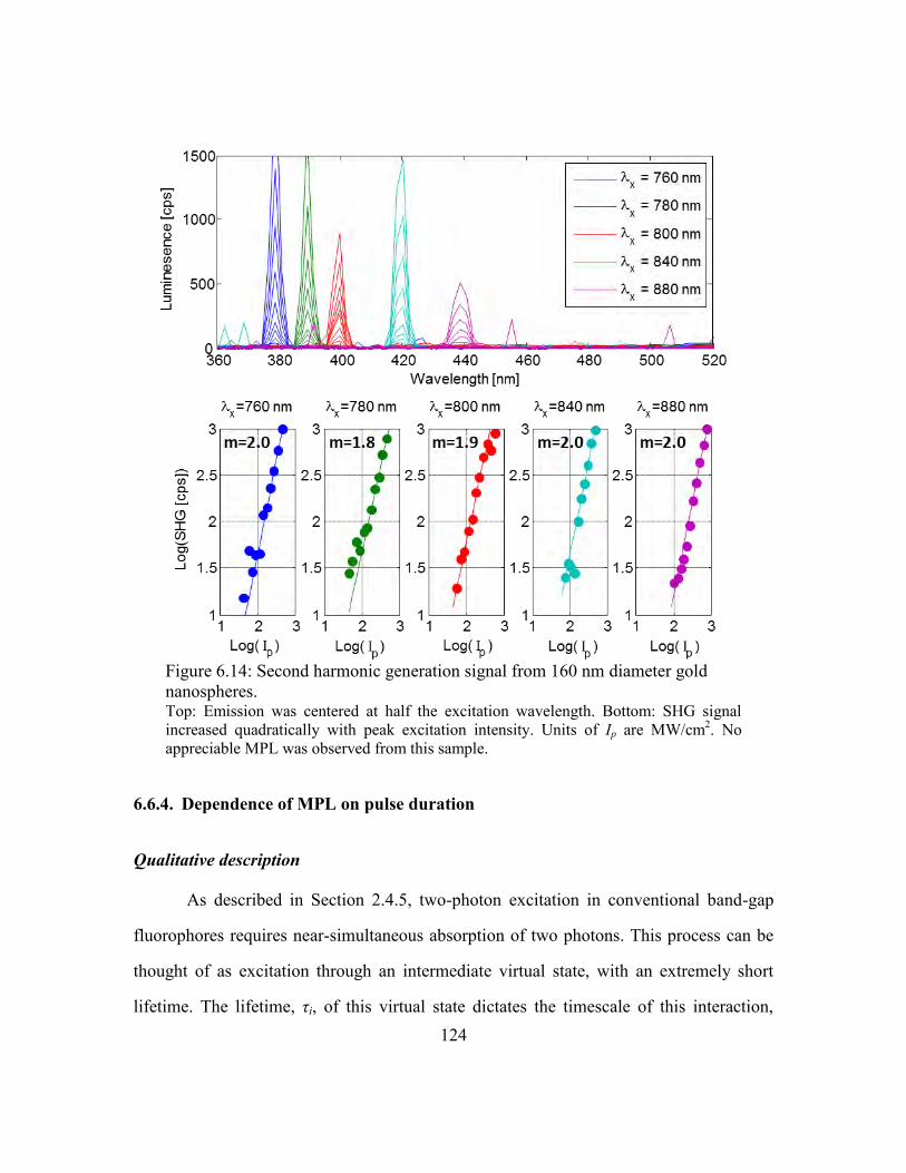
124
6.6.4. Dependence of MPL on pulse duration
Qualitative description
As described in Section 2.4.5, two-photon excitation in conventional band-gap
fluorophores requires near-simultaneous absorption of two photons. This process can be
thought of as excitation through an intermediate virtual state, with an extremely short
lifetime. The lifetime, τi, of this virtual state dictates the timescale of this interaction,
Figure 6.14: Second harmonic generation signal from 160 nm diameter gold
nanospheres. Top: Emission was centered at half the excitation wavelength. Bottom: SHG signal
increased quadratically with peak excitation intensity. Units of Ip are MW/cm2. No
appreciable MPL was observed from this sample.
125
which was approximated to be 0.1 fs in Section 2.4. For excitation pulse durations much
longer than this lifetime (τp ≫ τi), an electron sitting in this intermediate state will decay
before it sees most of the remaining photons in the excitation pulse. In this case, the
fluorescence rate will strongly depend on the pulse duration. However, as τp approaches
τi, an electron in the intermediate state stays there long enough to interact with most of
the photons in the excitation pulse. At this limit, as the pulse duration becomes shorter
and the fluorescence rate becomes independent of τp. This limit has not been explored
experimentally in band gap fluorophores because: (1) it is difficult to create excitation
pulse durations below a few femtoseconds while maintaining the short pulse durations
through a high NA objective, and (2) the spectral bandwidth of an excitation pulse grows
linearly with a decrease in pulse duration to maintain the time-bandwidth product—and
as the pulse duration drops below ~10 fs, the spectral bandwidth outgrows the two-
photon absorption linewidth of most molecular fluorophores, leading to inefficient
excitation[206].
In the case of MPL, the lifetime of the intermediate state is believed to be much
longer than 0.1 fs. Unlike multiphoton excitation with a bandgap fluorophore, MPL from
gold nanoparticles is excited at the linear absorption bands of the nanoparticle. As a
result, the intermediate state is not a forbidden one, and is not determined by the
Heisenberg relationship (i.e. ΔE is ~0 in Eq. (1)). The band structure diagram in Figure
6.15 illustrates one proposed scheme for two-photon induced luminescence in gold
nanoparticles[39],[198]. In this model, the lifetime of the intermediate state is governed
by the relaxation time of the holes created in the sp band. The lifetime of this sp hole has
been measured in nanowires and gold films to be on the order of 0.2 - 1
ps[87],[198],[207]. Because our excitation pulse duration can be varied from 200 fs to
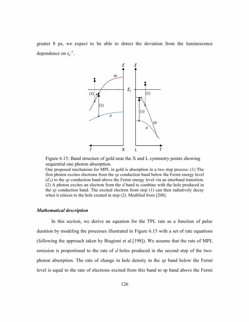
126
greater 8 ps, we expect to be able to detect the deviation from the luminescence
dependence on τp-1
.
Mathematical description
In this section, we derive an equation for the TPL rate as a function of pulse
duration by modeling the processes illustrated in Figure 6.15 with a set of rate equations
(following the approach taken by Biagioni et al.[198]). We assume that the rate of MPL
emission is proportional to the rate of d holes produced in the second step of the two-
photon absorption. The rate of change in hole density in the sp band below the Fermi
level is equal to the rate of electrons excited from this band to sp band above the Fermi
Figure 6.15: Band structure of gold near the X and L symmetry points showing
sequential one photon absorption. One proposed mechanism for MPL in gold is absorption in a two step process: (1) The
first photon excites electrons from the sp conduction band below the Fermi energy level
(EF) to the sp conduction band above the Fermi energy level via an interband transition.
(2) A photon excites an electron from the d band to combine with the hole produced in
the sp conduction band. The excited electron from step (1) can then radiatively decay
when it relaxes to the hole created in step (2). Modified from [208].
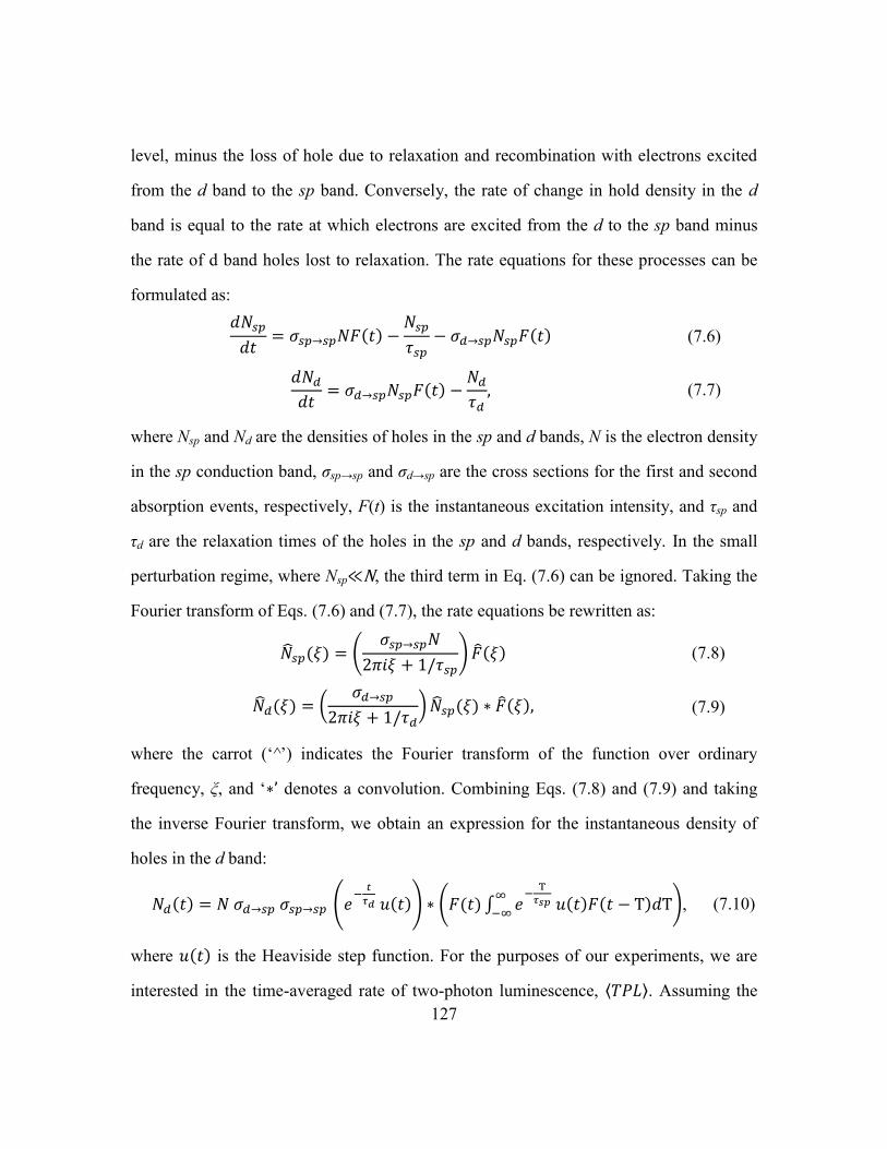
127
level, minus the loss of hole due to relaxation and recombination with electrons excited
from the d band to the sp band. Conversely, the rate of change in hold density in the d
band is equal to the rate at which electrons are excited from the d to the sp band minus
the rate of d band holes lost to relaxation. The rate equations for these processes can be
formulated as:
(7.6)
(7.7)
where Nsp and Nd are the densities of holes in the sp and d bands, N is the electron density
in the sp conduction band, σsp→sp and σd→sp are the cross sections for the first and second
absorption events, respectively, F(t) is the instantaneous excitation intensity, and τsp and
τd are the relaxation times of the holes in the sp and d bands, respectively. In the small
perturbation regime, where Nsp≪N, the third term in Eq. (7.6) can be ignored. Taking the
Fourier transform of Eqs. (7.6) and (7.7), the rate equations be rewritten as:
(
) (7.8)
(
) (7.9)
where the carrot (‗^‘) indicates the Fourier transform of the function over ordinary
frequency, ξ, and ‗ ’ denotes a convolution. Combining Eqs. (7.8) and (7.9) and taking
the inverse Fourier transform, we obtain an expression for the instantaneous density of
holes in the d band:
(
) ( ∫
), (7.10)
where is the Heaviside step function. For the purposes of our experiments, we are
interested in the time-averaged rate of two-photon luminescence, ⟨ ⟩. Assuming the
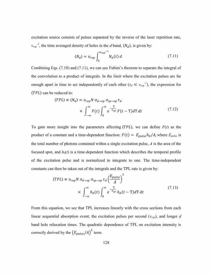
128
excitation source consists of pulses separated by the inverse of the laser repetition rate,
vrep-1
, the time averaged density of holes in the d band, ⟨ ⟩, is given by:
⟨ ⟩ ∫
(7.11)
Combining Eqs. (7.10) and (7.11), we can use Fubini‘s theorem to separate the integral of
the convolution to a product of integrals. In the limit where the excitation pulses are far
enough apart in time to act independently of each other (τd ≪ vrep-1
), the expression for
⟨ ⟩ can be reduced to:
⟨ ⟩ ⟨ ⟩
∫ ∫
(7.12)
To gain more insight into the parameters affecting ⟨ ⟩, we can define F(t) as the
product of a constant and a time-dependent function: where Epulse is
the total number of photons contained within a single excitation pulse, A is the area of the
focused spot, and hδ(t) is a time-dependent function which describes the temporal profile
of the excitation pulse and is normalized to integrate to one. The time-independent
constants can then be taken out of the integrals and the TPL rate is given by:
⟨ ⟩ (
)
∫ ∫
(7.13)
From this equation, we see that TPL increases linearly with the cross sections from each
linear sequential absorption event, the excitation pulses per second (vrep), and longer d
band hole relaxation times. The quadratic dependence of TPL on excitation intensity is
correctly derived by the ( ) term.
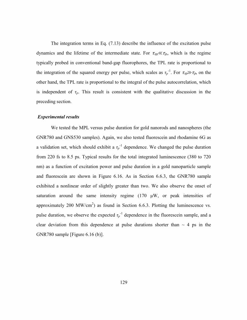
129
The integration terms in Eq. (7.13) describe the influence of the excitation pulse
dynamics and the lifetime of the intermediate state. For τsp,≪τp,, which is the regime
typically probed in conventional band-gap fluorophores, the TPL rate is proportional to
the integration of the squared energy per pulse, which scales as τp-1
. For τsp≫τp, on the
other hand, the TPL rate is proportional to the integral of the pulse autocorrelation, which
is independent of τp. This result is consistent with the qualitative discussion in the
preceding section.
Experimental results
We tested the MPL versus pulse duration for gold nanorods and nanospheres (the
GNR780 and GNS530 samples). Again, we also tested fluorescein and rhodamine 6G as
a validation set, which should exhibit a τp-1
dependence. We changed the pulse duration
from 220 fs to 8.5 ps. Typical results for the total integrated luminescence (380 to 720
nm) as a function of excitation power and pulse duration in a gold nanoparticle sample
and fluorescein are shown in Figure 6.16. As in Section 6.6.3, the GNR780 sample
exhibited a nonlinear order of slightly greater than two. We also observe the onset of
saturation around the same intensity regime (170 μW, or peak intensities of
approximately 200 MW/cm2) as found in Section 6.6.3. Plotting the luminescence vs.
pulse duration, we observe the expected τp-1
dependence in the fluorescein sample, and a
clear deviation from this dependence at pulse durations shorter than ~ 4 ps in the
GNR780 sample [Figure 6.16 (b)].
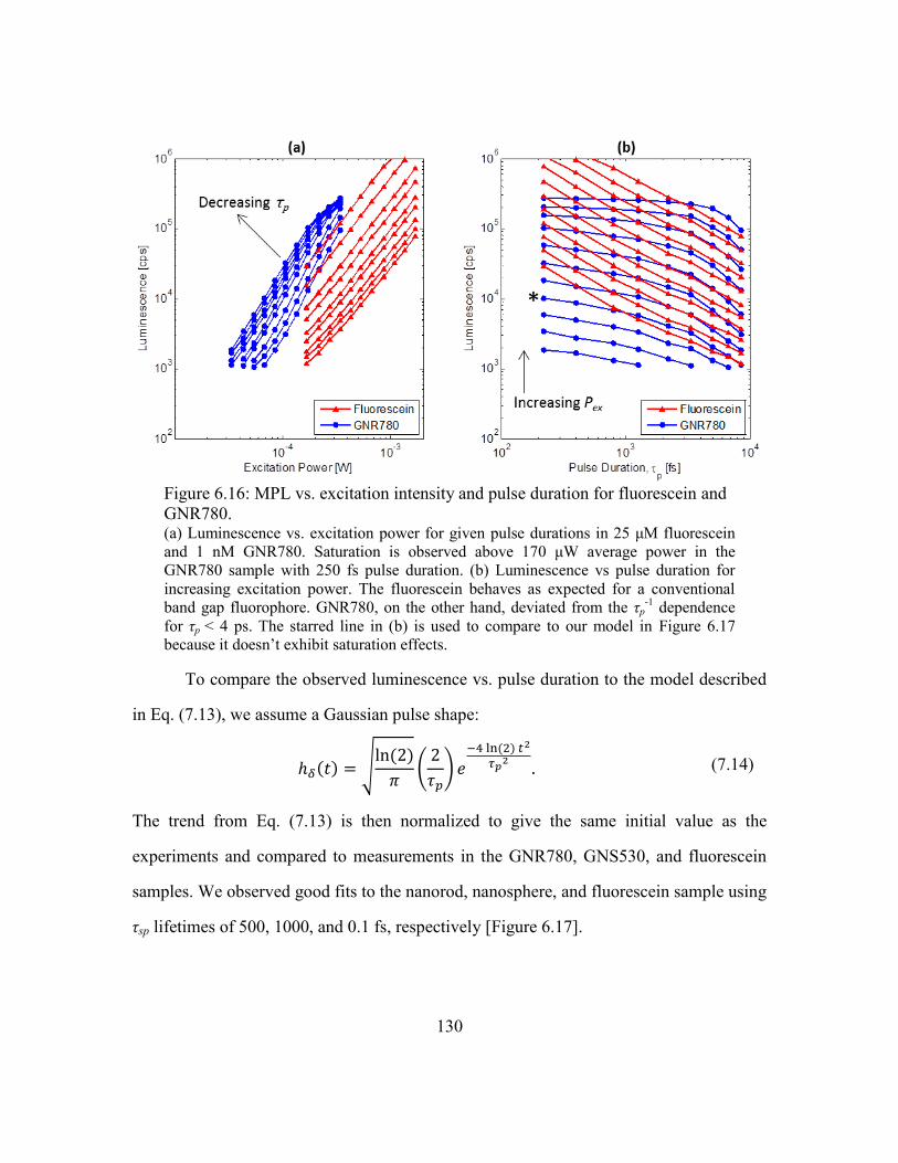
130
To compare the observed luminescence vs. pulse duration to the model described
in Eq. (7.13), we assume a Gaussian pulse shape:
√
(
)
(7.14)
The trend from Eq. (7.13) is then normalized to give the same initial value as the
experiments and compared to measurements in the GNR780, GNS530, and fluorescein
samples. We observed good fits to the nanorod, nanosphere, and fluorescein sample using
τsp lifetimes of 500, 1000, and 0.1 fs, respectively [Figure 6.17].
Figure 6.16: MPL vs. excitation intensity and pulse duration for fluorescein and
GNR780. (a) Luminescence vs. excitation power for given pulse durations in 25 μM fluorescein
and 1 nM GNR780. Saturation is observed above 170 μW average power in the
GNR780 sample with 250 fs pulse duration. (b) Luminescence vs pulse duration for
increasing excitation power. The fluorescein behaves as expected for a conventional
band gap fluorophore. GNR780, on the other hand, deviated from the τp-1
dependence
for τp < 4 ps. The starred line in (b) is used to compare to our model in Figure 6.17
because it doesn‘t exhibit saturation effects.
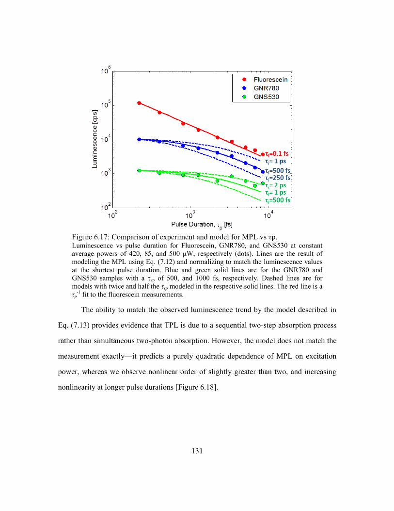
131
The ability to match the observed luminescence trend by the model described in
Eq. (7.13) provides evidence that TPL is due to a sequential two-step absorption process
rather than simultaneous two-photon absorption. However, the model does not match the
measurement exactly—it predicts a purely quadratic dependence of MPL on excitation
power, whereas we observe nonlinear order of slightly greater than two, and increasing
nonlinearity at longer pulse durations [Figure 6.18].
Figure 6.17: Comparison of experiment and model for MPL vs τp. Luminescence vs pulse duration for Fluorescein, GNR780, and GNS530 at constant
average powers of 420, 85, and 500 μW, respectively (dots). Lines are the result of
modeling the MPL using Eq. (7.12) and normalizing to match the luminescence values
at the shortest pulse duration. Blue and green solid lines are for the GNR780 and
GNS530 samples with a τsp of 500, and 1000 fs, respectively. Dashed lines are for
models with twice and half the τsp modeled in the respective solid lines. The red line is a
τp-1
fit to the fluorescein measurements.
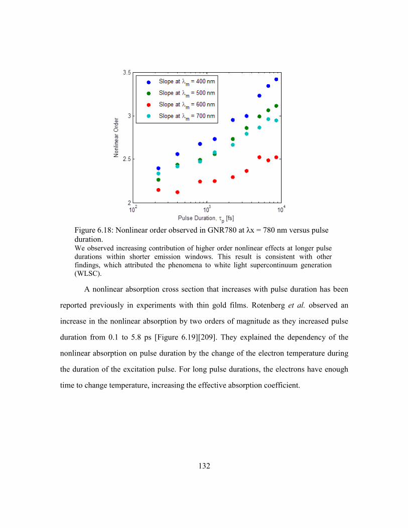
132
A nonlinear absorption cross section that increases with pulse duration has been
reported previously in experiments with thin gold films. Rotenberg et al. observed an
increase in the nonlinear absorption by two orders of magnitude as they increased pulse
duration from 0.1 to 5.8 ps [Figure 6.19][209]. They explained the dependency of the
nonlinear absorption on pulse duration by the change of the electron temperature during
the duration of the excitation pulse. For long pulse durations, the electrons have enough
time to change temperature, increasing the effective absorption coefficient.
Figure 6.18: Nonlinear order observed in GNR780 at λx = 780 nm versus pulse
duration. We observed increasing contribution of higher order nonlinear effects at longer pulse
durations within shorter emission windows. This result is consistent with other
findings, which attributed the phenomena to white light supercontinuum generation
(WLSC).
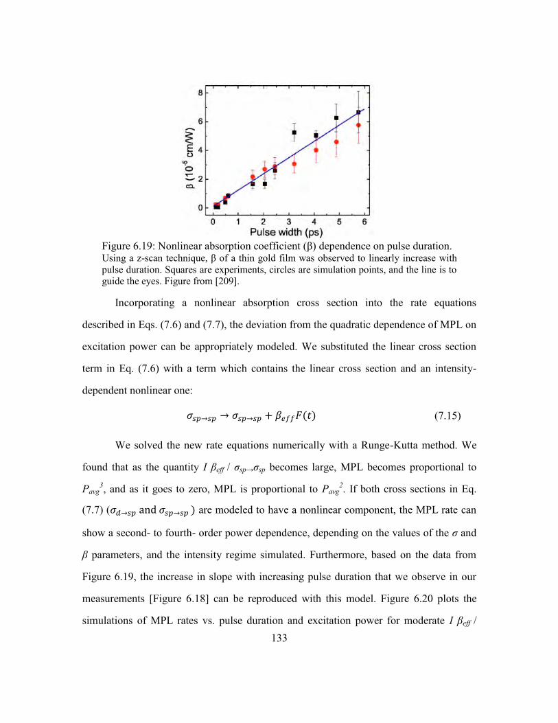
133
Incorporating a nonlinear absorption cross section into the rate equations
described in Eqs. (7.6) and (7.7), the deviation from the quadratic dependence of MPL on
excitation power can be appropriately modeled. We substituted the linear cross section
term in Eq. (7.6) with a term which contains the linear cross section and an intensity-
dependent nonlinear one:
(7.15)
We solved the new rate equations numerically with a Runge-Kutta method. We
found that as the quantity I βeff / σsp→σsp becomes large, MPL becomes proportional to
Pavg3, and as it goes to zero, MPL is proportional to Pavg
2. If both cross sections in Eq.
(7.7) ( are modeled to have a nonlinear component, the MPL rate can
show a second- to fourth- order power dependence, depending on the values of the σ and
β parameters, and the intensity regime simulated. Furthermore, based on the data from
Figure 6.19, the increase in slope with increasing pulse duration that we observe in our
measurements [Figure 6.18] can be reproduced with this model. Figure 6.20 plots the
simulations of MPL rates vs. pulse duration and excitation power for moderate I βeff /
Figure 6.19: Nonlinear absorption coefficient (β) dependence on pulse duration. Using a z-scan technique, β of a thin gold film was observed to linearly increase with
pulse duration. Squares are experiments, circles are simulation points, and the line is to
guide the eyes. Figure from [209].
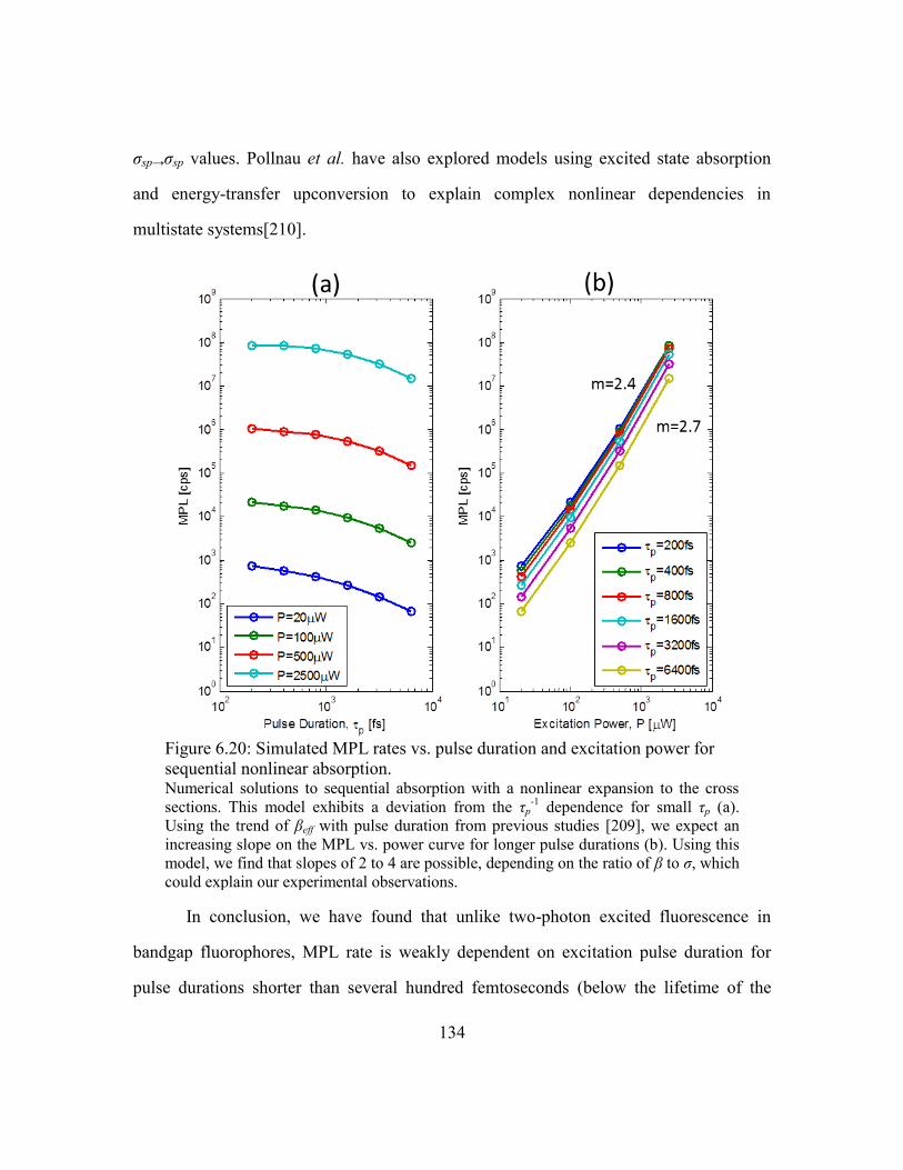
134
σsp→σsp values. Pollnau et al. have also explored models using excited state absorption
and energy-transfer upconversion to explain complex nonlinear dependencies in
multistate systems[210].
In conclusion, we have found that unlike two-photon excited fluorescence in
bandgap fluorophores, MPL rate is weakly dependent on excitation pulse duration for
pulse durations shorter than several hundred femtoseconds (below the lifetime of the
Figure 6.20: Simulated MPL rates vs. pulse duration and excitation power for
sequential nonlinear absorption. Numerical solutions to sequential absorption with a nonlinear expansion to the cross
sections. This model exhibits a deviation from the τp-1
dependence for small τp (a).
Using the trend of βeff with pulse duration from previous studies [209], we expect an
increasing slope on the MPL vs. power curve for longer pulse durations (b). Using this
model, we find that slopes of 2 to 4 are possible, depending on the ratio of β to σ, which
could explain our experimental observations.
135
intermediate state). This observation can be accurately explained by the sequential photon
absorption hypothesis[39],[198], using an intermediate state lifetime of approximately
500 fs. This lifetime value is in good agreement with previous studies, assuming the
origin is the relaxation of holes in the sp conduction band[87],[198]. The higher order
nonlinear dependencies of MPL on excitation power, which become more prevalent at
longer pulse durations, can be explained by either or both of the absorption cross sections
being modeled with a nonlinear component whose contribution increases with pulse
duration.
6.6.5. Quantification of two-photon action cross section
In Sections 6.6.3 and 6.6.4 we showed that instead of a purely second order
process, the MPL from gold nanoparticles exhibits a slightly higher order nonlinear
dependence on excitation power. At the shortest pulse durations we can achieve in our
system (220 fs), we found a log(MPL) vs log(P) slope of 2.3 to 2.5 if the whole
luminescence spectrum is considered and a slope of 2.1 to 2.3 when monitoring only the
higher luminescence wavelengths. Because MPL is a complex, non-quadratic process, the
traditional two-photon action cross section does not apply. In this section we calculate an
effective cross section by comparing measurements performed at short pulse duration and
low excitation power regions from gold nanoparticles and to a reference dye of known
two-photon action cross section (fluorescein). In these regions, the slopes observed are
relatively close to two. This measuremt, of course, is meaningful only when paired with
the excitation pulse duration, since the measured effective two-photon action cross
section will increase with increasing pulse duration for pulse durations less than the
lifetime of the intermediate state. It is also worth noting that this strategy results in a
conservative calculation of nanoparticle σTPA; using longer pulse durations or comparing
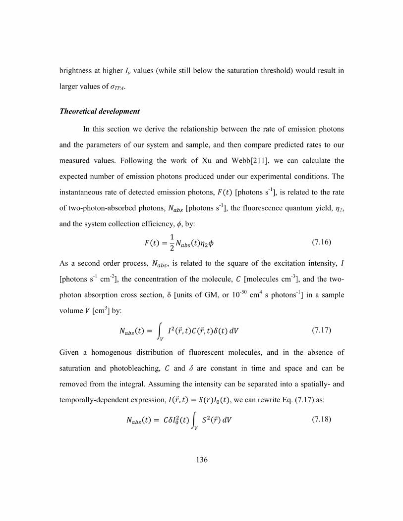
136
brightness at higher Ip values (while still below the saturation threshold) would result in
larger values of σTPA.
Theoretical development
In this section we derive the relationship between the rate of emission photons
and the parameters of our system and sample, and then compare predicted rates to our
measured values. Following the work of Xu and Webb[211], we can calculate the
expected number of emission photons produced under our experimental conditions. The
instantaneous rate of detected emission photons, [photons s-1
], is related to the rate
of two-photon-absorbed photons, [photons s-1
], the fluorescence quantum yield, η2,
and the system collection efficiency, ϕ, by:
(7.16)
As a second order process, , is related to the square of the excitation intensity,
[photons s-1
cm-2
], the concentration of the molecule, [molecules cm-3
], and the two-
photon absorption cross section, δ [units of GM, or 10-50
cm4 s photons
-1] in a sample
volume [cm3] by:
∫
(7.17)
Given a homogenous distribution of fluorescent molecules, and in the absence of
saturation and photobleaching, and δ are constant in time and space and can be
removed from the integral. Assuming the intensity can be separated into a spatially- and
temporally-dependent expression, , we can rewrite Eq. (7.17) as:
∫
(7.18)
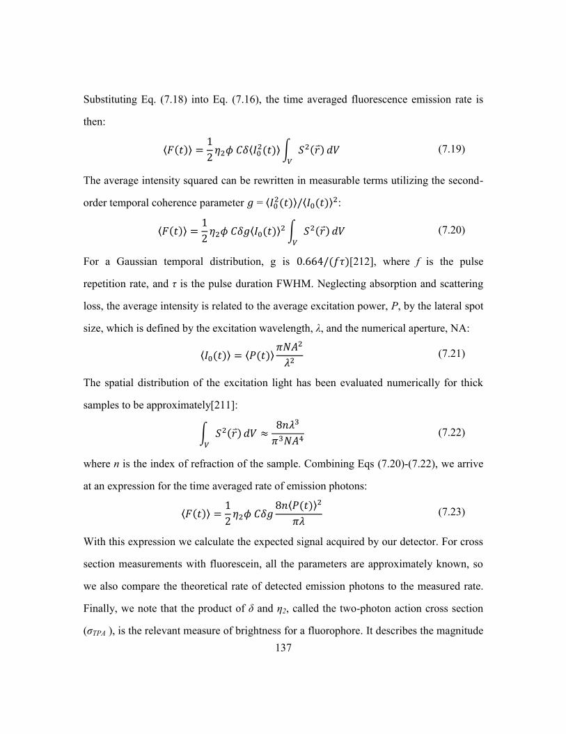
137
Substituting Eq. (7.18) into Eq. (7.16), the time averaged fluorescence emission rate is
then:
⟨ ⟩
⟨
⟩∫
(7.19)
The average intensity squared can be rewritten in measurable terms utilizing the second-
order temporal coherence parameter = ⟨ ⟩ ⟨ ⟩
:
⟨ ⟩
⟨ ⟩
∫
(7.20)
For a Gaussian temporal distribution, g is [212], where f is the pulse
repetition rate, and τ is the pulse duration FWHM. Neglecting absorption and scattering
loss, the average intensity is related to the average excitation power, P, by the lateral spot
size, which is defined by the excitation wavelength, λ, and the numerical aperture, NA:
⟨ ⟩ ⟨ ⟩
(7.21)
The spatial distribution of the excitation light has been evaluated numerically for thick
samples to be approximately[211]:
∫
(7.22)
where n is the index of refraction of the sample. Combining Eqs (7.20)-(7.22), we arrive
at an expression for the time averaged rate of emission photons:
⟨ ⟩
⟨ ⟩
(7.23)
With this expression we calculate the expected signal acquired by our detector. For cross
section measurements with fluorescein, all the parameters are approximately known, so
we also compare the theoretical rate of detected emission photons to the measured rate.
Finally, we note that the product of δ and η2, called the two-photon action cross section
(σTPA ), is the relevant measure of brightness for a fluorophore. It describes the magnitude
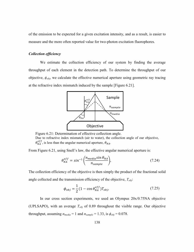
138
of the emission to be expected for a given excitation intensity, and as a result, is easier to
measure and the more often reported value for two-photon excitation fluorophores.
Collection efficiency
We estimate the collection efficiency of our system by finding the average
throughput of each element in the detection path. To determine the throughput of our
objective, ϕobj, we calculate the effective numerical aperture using geometric ray tracing
at the refractive index mismatch induced by the sample [Figure 6.21].
From Figure 6.21, using Snell‘s law, the effective angular numerical aperture is:
(
) (7.24)
The collection efficiency of the objective is then simply the product of the fractional solid
angle collected and the transmission efficiency of the objective, Tobj:
(7.25)
In our cross section experiments, we used an Olympus 20x/0.75NA objective
(UPLSAPO), with an average Tobj of 0.89 throughout the visible range. Our objective
throughput, assuming nmedia = 1 and nsample = 1.33, is ϕobj = 0.078.
Figure 6.21: Determination of effective collection angle. Due to refractive index mismatch (air to water), the collection angle of our objective,
is less than the angular numerical aperture, .
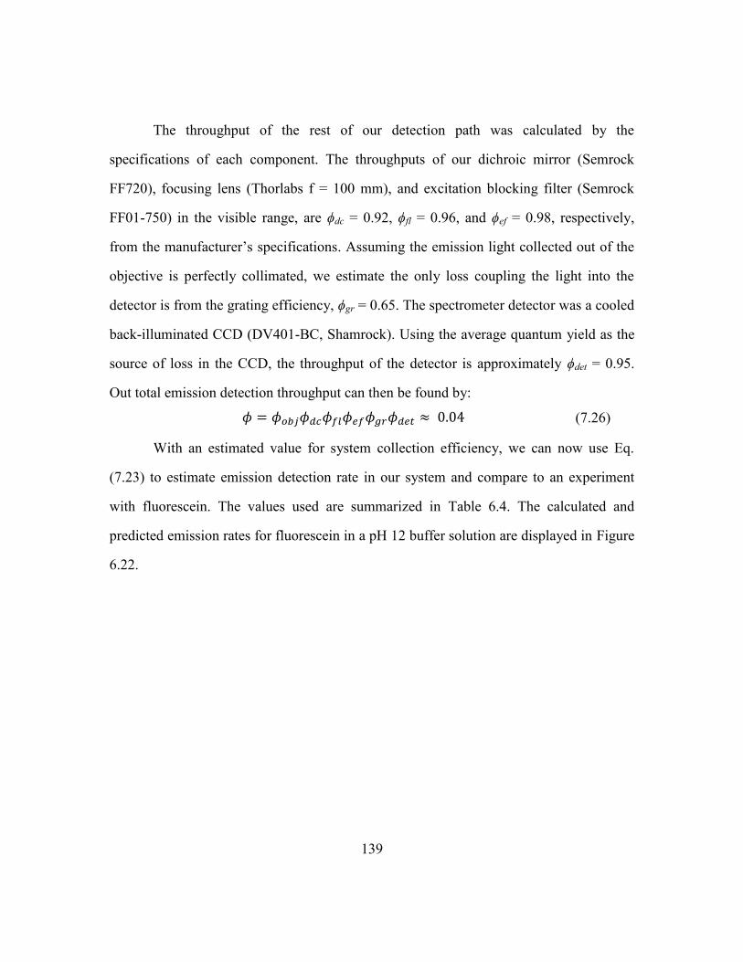
139
The throughput of the rest of our detection path was calculated by the
specifications of each component. The throughputs of our dichroic mirror (Semrock
FF720), focusing lens (Thorlabs f = 100 mm), and excitation blocking filter (Semrock
FF01-750) in the visible range, are ϕdc = 0.92, ϕfl = 0.96, and ϕef = 0.98, respectively,
from the manufacturer‘s specifications. Assuming the emission light collected out of the
objective is perfectly collimated, we estimate the only loss coupling the light into the
detector is from the grating efficiency, ϕgr = 0.65. The spectrometer detector was a cooled
back-illuminated CCD (DV401-BC, Shamrock). Using the average quantum yield as the
source of loss in the CCD, the throughput of the detector is approximately ϕdet = 0.95.
Out total emission detection throughput can then be found by:
(7.26)
With an estimated value for system collection efficiency, we can now use Eq.
(7.23) to estimate emission detection rate in our system and compare to an experiment
with fluorescein. The values used are summarized in Table 6.4. The calculated and
predicted emission rates for fluorescein in a pH 12 buffer solution are displayed in Figure
6.22.
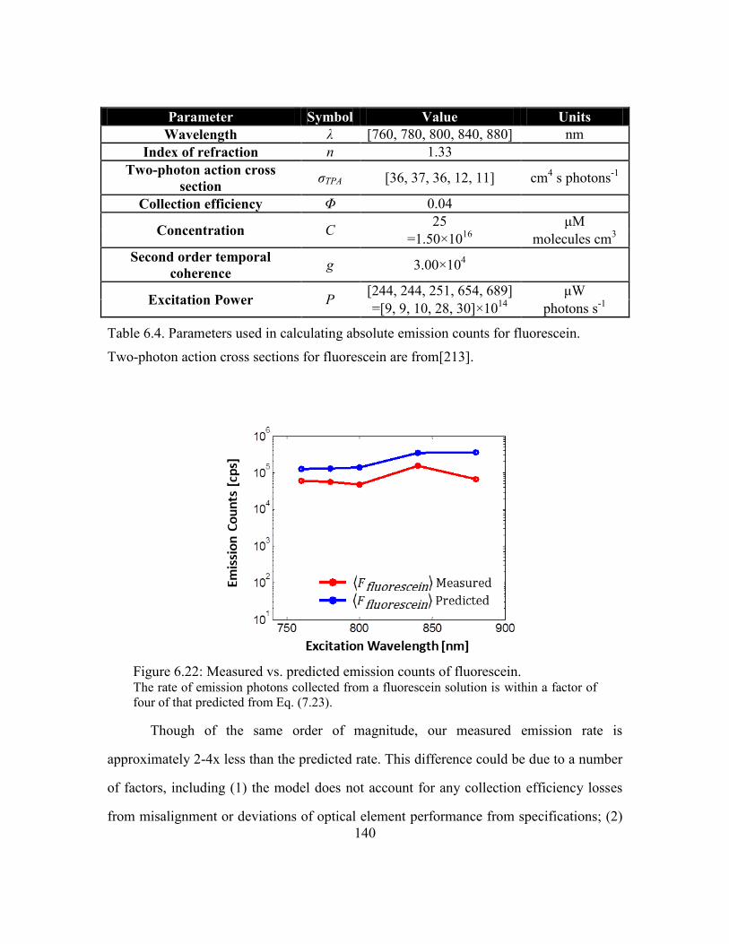
140
Though of the same order of magnitude, our measured emission rate is
approximately 2-4x less than the predicted rate. This difference could be due to a number
of factors, including (1) the model does not account for any collection efficiency losses
from misalignment or deviations of optical element performance from specifications; (2)
Parameter Symbol Value Units
Wavelength λ [760, 780, 800, 840, 880] nm
Index of refraction n 1.33
Two-photon action cross
section σTPA [36, 37, 36, 12, 11] cm
4 s photons
-1
Collection efficiency Φ 0.04
Concentration C 25 μM
=1.50×10¹⁶
molecules cm3
Second order temporal
coherence g 3.00×10
4
Excitation Power P [244, 244, 251, 654, 689] μW
=[9, 9, 10, 28, 30]×1014
photons s-1
Table 6.4. Parameters used in calculating absolute emission counts for fluorescein.
Two-photon action cross sections for fluorescein are from[213].
Figure 6.22: Measured vs. predicted emission counts of fluorescein. The rate of emission photons collected from a fluorescein solution is within a factor of
four of that predicted from Eq. (7.23).
141
the focusing lens into our spectrometer is not an achromat, so we expect some system
loss coupling into the spectrometer from chromatic aberrations; and (3) the second order
temporal coherence was calculated from a measured autocorrelation, which resulted in a
pulse duration of τFWHM = 250 fs. However, the temporal pulse shape is likely more
complicated than the smooth Gaussian assumed, but after the autocorrelation, any rapid
changes in the pulse envelope are smoothed out[114]. (4) Finally, though Eq. (7.23) is
independent of NA for perfect Gaussian focusing, an aberrated beam may introduce focal
spot dependencies—for complicated intensity distributions, it may be difficult to predict
S2.
The absolute two-photon action cross section can be measured by Eq. (7.23)
[97],[213]. However, the equation is sensitive to a number of parameters that are difficult
to characterize. As a result, given the values from measured emission rate for fluorescein,
we would have measured a two-photon action cross section that is two to four times
lower than the actual value. Consequently, we adopt a different technique that utilizes a
reference measurement to a molecule with a known two-photon action cross section,
, and is independent of focal spot geometry, g, and ϕ [214].
Measurement of the two-photon action cross section by reference standard
If the two photon action cross section for a reference molecule ( is known,
the ratio of the emission rates for an unknown sample, ⟨ ⟩, to the reference, ⟨ ⟩
eliminates some of the dependencies of Eq. (7.23). For similar emission spectra, the
collection efficiencies are approximately equal. At the same excitation wavelength, g and
λ also cancel out, leaving us with:
⟨ ⟩
⟨ ⟩
⟨ ⟩
⟨ ⟩
(7.27)
142
Rearranging Eq. (7.27), we find an expression with which we can calculate by
measuring the emission from the sample compared to a reference dye of known :
⟨ ⟩ ⟨ ⟩
⟨ ⟩⟨ ⟩ (7.28)
This equation has been used previously to calculate σTPA of different fluorophores using
fluorescein as a reference [214]. It requires that both measurements are taken within a
intensity regime where two-photon emission dominates the signal and there is no
appreciable signal from other sources, such as second harmonic generation (SHG), three-
photon excited (3PE) emission, or white light supercontinuum (WLSC) generation.
Because these phenomena have been observed from plasmonic nanoparticles under
ultrafast excitation, we use a modified approach. Instead of measuring the emission
counts at a single excitation power, which is given to the error in the power calibration
and to that inherent in a single emission measurement, we compare the intercept, β, of a
line with a slope of two fit to a plot of ⟨ ⟩ vs ⟨ ⟩. That is:
⟨ ⟩ ⟨ ⟩ (7.29)
⟨ ⟩
⟨ ⟩ . (7.30)
Now substituting Eq. (7.30) into Eq. (7.28),
( )
(7.31)
where βs and βr are the intercepts of best fit lines to the logarithmic emission vs. power
plots for the sample of interest and the reference sample, respectively.
Because we observe a deviation from a pure second order dependence of MPL on
excitation power, we take the MPL measurements at the lowest excitation intensities.
Thus, we find βs for a slope of two line that is fit at excitation intensities of 30-60
MW/cm2. We also measure all cross sections at a short pulse duration (250 fs). The cross
143
section we measure may be more appropriately described as the effective two-photon
action cross section because due to the non-quadratic relationship between MPL and Ip,
and the deviation of MPL from a τp-1
dependence, there is a small difference in measured
values when fitting βs at different intensity regimes and pulse duration. For the
measurements presented here, we took the most conservative estimates of the effective
two-photon action cross section—at short τp and small Ip, the σTPA we calculate is
significantly smaller than it would be if we used different excitation parameters.
Results
We validated our method by measuring the σTPA of fluorescein using a separate
fluorescein measurement as a reference, and comparing a rhodamine 6G σTPA
measurement to values found in the literature [214]. Fluorescein was prepared at 25 μM
concentration in a pH 12 buffer, and rhodamine 6G was prepared at a 100 μM
concentration, diluted in methanol. We found excellent agreement between consecutive
measurements of fluorescein, and with published values of rhodamine 6G [Figure 6.23].
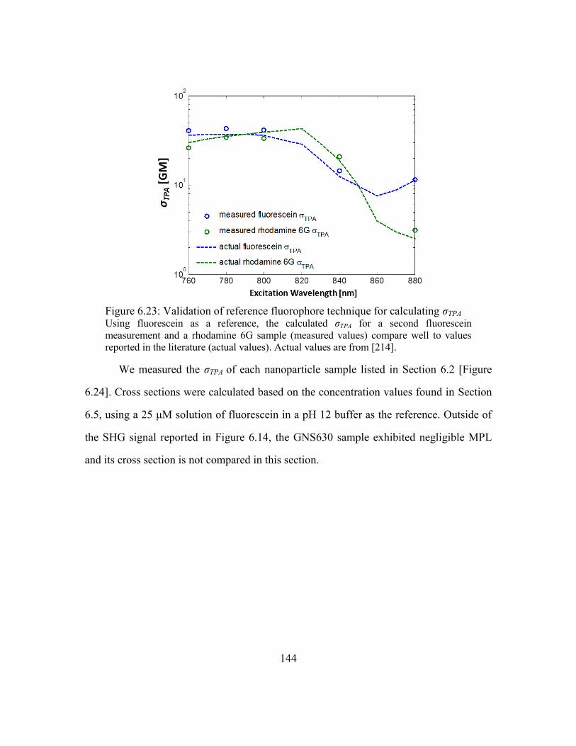
144
We measured the σTPA of each nanoparticle sample listed in Section 6.2 [Figure
6.24]. Cross sections were calculated based on the concentration values found in Section
6.5, using a 25 μM solution of fluorescein in a pH 12 buffer as the reference. Outside of
the SHG signal reported in Figure 6.14, the GNS630 sample exhibited negligible MPL
and its cross section is not compared in this section.
Figure 6.23: Validation of reference fluorophore technique for calculating σTPA Using fluorescein as a reference, the calculated σTPA for a second fluorescein
measurement and a rhodamine 6G sample (measured values) compare well to values
reported in the literature (actual values). Actual values are from [214].
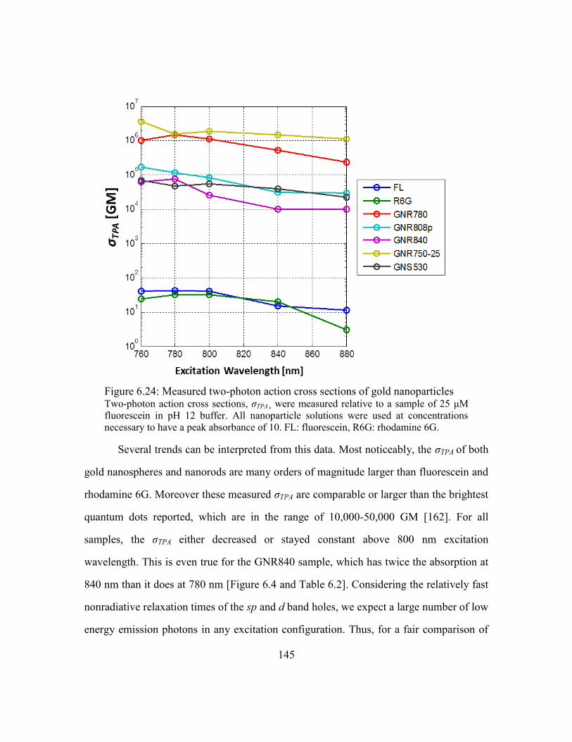
145
Several trends can be interpreted from this data. Most noticeably, the σTPA of both
gold nanospheres and nanorods are many orders of magnitude larger than fluorescein and
rhodamine 6G. Moreover these measured σTPA are comparable or larger than the brightest
quantum dots reported, which are in the range of 10,000-50,000 GM [162]. For all
samples, the σTPA either decreased or stayed constant above 800 nm excitation
wavelength. This is even true for the GNR840 sample, which has twice the absorption at
840 nm than it does at 780 nm [Figure 6.4 and Table 6.2]. Considering the relatively fast
nonradiative relaxation times of the sp and d band holes, we expect a large number of low
energy emission photons in any excitation configuration. Thus, for a fair comparison of
Figure 6.24: Measured two-photon action cross sections of gold nanoparticles Two-photon action cross sections, σTPA¸ were measured relative to a sample of 25 μM
fluorescein in pH 12 buffer. All nanoparticle solutions were used at concentrations
necessary to have a peak absorbance of 10. FL: fluorescein, R6G: rhodamine 6G.
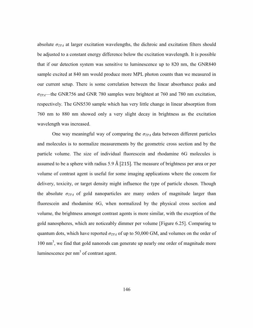
146
absolute σTPA at larger excitation wavelengths, the dichroic and excitation filters should
be adjusted to a constant energy difference below the excitation wavelength. It is possible
that if our detection system was sensitive to luminescence up to 820 nm, the GNR840
sample excited at 840 nm would produce more MPL photon counts than we measured in
our current setup. There is some correlation between the linear absorbance peaks and
σTPA—the GNR756 and GNR 780 samples were brightest at 760 and 780 nm excitation,
respectively. The GNS530 sample which has very little change in linear absorption from
760 nm to 880 nm showed only a very slight decay in brightness as the excitation
wavelength was increased.
One way meaningful way of comparing the σTPA data between different particles
and molecules is to normalize measurements by the geometric cross section and by the
particle volume. The size of individual fluorescein and rhodamine 6G molecules is
assumed to be a sphere with radius 5.9 Å [215]. The measure of brightness per area or per
volume of contrast agent is useful for some imaging applications where the concern for
delivery, toxicity, or target density might influence the type of particle chosen. Though
the absolute σTPA of gold nanoparticles are many orders of magnitude larger than
fluorescein and rhodamine 6G, when normalized by the physical cross section and
volume, the brightness amongst contrast agents is more similar, with the exception of the
gold nanospheres, which are noticeably dimmer per volume [Figure 6.25]. Comparing to
quantum dots, which have reported σTPA of up to 50,000 GM, and volumes on the order of
100 nm3, we find that gold nanorods can generate up nearly one order of magnitude more
luminescence per nm3 of contrast agent.
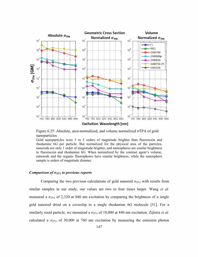
147
Comparison of σTPA to previous reports
Comparing the two previous calculations of gold nanorod σTPA with results from
similar samples in our study, our values are two to four times larger. Wang et al.
measured a σTPA of 2,320 at 840 nm excitation by comparing the brightness of a single
gold nanorod dried on a coverslip to a single rhodamine 6G molecule [51]. For a
similarly sized particle, we measured a σTPA of 10,000 at 840 nm excitation. Zijlstra et al.
calculated a σTPA of 30,000 at 760 nm excitation by measuring the emission photon
Figure 6.25: Absolute, area-normalized, and volume normalized σTPA of gold
nanoparticles Gold nanoparticles were 3 to 5 orders of magnitude brighter than fluorescein and
rhodamine 6G per particle. But normalized for the physical area of the particles,
nanorods are only 1 order of magnitude brighter, and nanospheres are similar brightness
to fluorescein and rhodamine 6G. When normalized by the contrast agent‘s volume,
nanorods and the organic fluorophores have similar brightness, while the nanosphere
sample is orders of magnitude dimmer.
148
counts of gold nanorods embedded in polyvinyl alcohol (PVA) and using Eq. (7.23) [52].
For a similarly sized particle, we measured a σTPA of 62,000 at 760 nm excitation. A
summary of previous measurements of σTPA in gold nanorods and other nanoparticles is
listed in Table 6.5.
There are a number of sources of error in the experimental methods of previous
studies that could contribute to inaccurate σTPA values. Wang et al. used average fluences
that are well above the saturation fluences we observe (many GW/cm2) [51]. This is also
corroborated by the slope of two they observe, which we can reproduce by measuring
MPL above the saturation intensity. They use rhodamine 6G and gold nanorods dried on
a coverslip, but the σTPA of each would be expected to change with in an aqueous
environment, thus their reference value may be off. Additionally, drying the gold
nanorods on a coverslip restricts their orientation relative to that expected for gold
nanorods floating in solution. It is unclear from their experiment whether they compared
brightness values when the excitation polarization was aligned to the gold nanorod, or in
some other orientation. Finally, they do not report the measured pulse duration at the
imaging plane, so, given the results of Section 6.6.4, the effective cross section could
change by an order of magnitude depending on how long their pulse duration was. The
values by Zijlstra et al. suffer from some of the same sources of error [97]. Additionally,
since they rely on a calculated system collection efficiency rather than a reference dye,
any error in their collection efficiency value linearly affects their reported σTPA. Given the
many sources of error, our values are surprisingly close to these previous reports. We
show measured values of similar nanorods and excitation parameters used by Wang et al.
and Zijlstra et al. in Table 6.5.
149
6.6.6. Polarization dependence
Setup
We tested the dependence of MPL on excitation polarization by analyzing images
of GNR780 nanorods dried on a coverslip. The excitation polarization was adjusted by
Reference Sample
[nm]
[nm]
σTPA [GM] Measurement Method
Gold Nanorods
This work GNR750-25 750 760 3,500,000 In solution, fluorescein and R6G
reference
Wang et al.
[51]
GNR
48 x 15 nm 820 830 2,320
Single particle on coverslip, R6G
reference
This work GNR840 840 840 10,000 In solution, fluorescein and R6G
reference
Zijlstra et al.
[97]
GNR
45 x 12 nm 810 760 30,000
Single particle in PVA, absolute
measurement
This work GNR840 840 760 62,000 In solution, fluorescein and R6G
reference
Other Nanoparticles
Liu et al. [216] Gold Nanodot
D = 1.3 nm -- 800 189
In solution, Coumarin 480
reference
Patel et al.
[217]
Silver Nanodot
D = 2.3 nm 400, 645 830 50,000
In solution, fluorescein and R6G
reference
Larson et al.
[50]
QD
D =7-14 nm 710 710 45,000
In solution, fluorescein
reference
Stellacci et al.
[218]
Cluster of
fluorophores
D = 10 nm
770 770 90,000 Compares cluster of 2500
fluorophores to a single one
Rahim et. al.
[219]
Conjugated
polymer
D = 8 nm
740 740 30,000 In solution, Fluorescein
reference
Table 6.5 Two-photon action cross sections of gold nanorods and other nanoparticles.
is the peak linear absorbance of the sample. λx is the excitation wavelength used.
The fluence used to probe the MPL, if reported, is indicated. The measurement method
for determining the two-photon action cross section (σTPA) values are also described.
Highlighted rows indicate measurements of similarly sized gold nanorods. We found
reasonable agreement between the two published measurements of gold nanorod σTPA and
our measurements. Sizes for nanorods are length x width. For spherical particles, sizes
are described by the particle diameter, D.
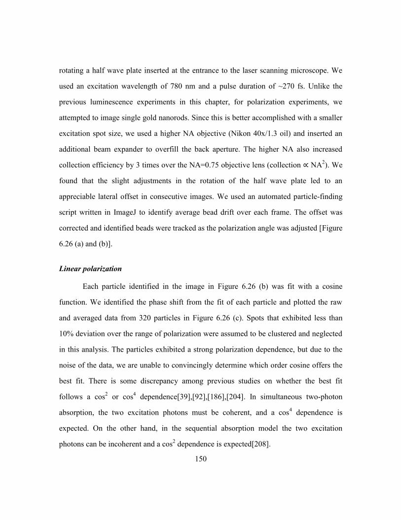
150
rotating a half wave plate inserted at the entrance to the laser scanning microscope. We
used an excitation wavelength of 780 nm and a pulse duration of ~270 fs. Unlike the
previous luminescence experiments in this chapter, for polarization experiments, we
attempted to image single gold nanorods. Since this is better accomplished with a smaller
excitation spot size, we used a higher NA objective (Nikon 40x/1.3 oil) and inserted an
additional beam expander to overfill the back aperture. The higher NA also increased
collection efficiency by 3 times over the NA=0.75 objective lens (collection NA2). We
found that the slight adjustments in the rotation of the half wave plate led to an
appreciable lateral offset in consecutive images. We used an automated particle-finding
script written in ImageJ to identify average bead drift over each frame. The offset was
corrected and identified beads were tracked as the polarization angle was adjusted [Figure
6.26 (a) and (b)].
Linear polarization
Each particle identified in the image in Figure 6.26 (b) was fit with a cosine
function. We identified the phase shift from the fit of each particle and plotted the raw
and averaged data from 320 particles in Figure 6.26 (c). Spots that exhibited less than
10% deviation over the range of polarization were assumed to be clustered and neglected
in this analysis. The particles exhibited a strong polarization dependence, but due to the
noise of the data, we are unable to convincingly determine which order cosine offers the
best fit. There is some discrepancy among previous studies on whether the best fit
follows a cos2 or cos
4 dependence[39],[92],[186],[204]. In simultaneous two-photon
absorption, the two excitation photons must be coherent, and a cos4 dependence is
expected. On the other hand, in the sequential absorption model the two excitation
photons can be incoherent and a cos2 dependence is expected[208].
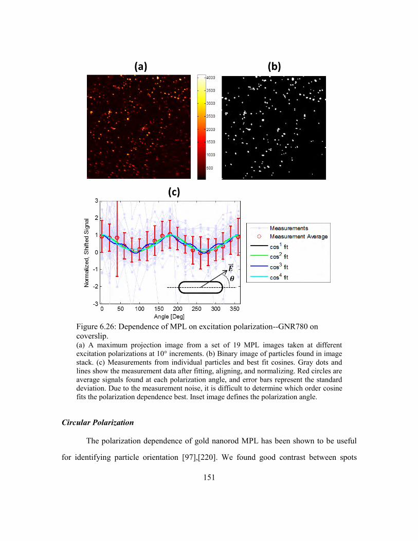
151
Circular Polarization
The polarization dependence of gold nanorod MPL has been shown to be useful
for identifying particle orientation [97],[220]. We found good contrast between spots
Figure 6.26: Dependence of MPL on excitation polarization--GNR780 on
coverslip. (a) A maximum projection image from a set of 19 MPL images taken at different
excitation polarizations at 10° increments. (b) Binary image of particles found in image
stack. (c) Measurements from individual particles and best fit cosines. Gray dots and
lines show the measurement data after fitting, aligning, and normalizing. Red circles are
average signals found at each polarization angle, and error bars represent the standard
deviation. Due to the measurement noise, it is difficult to determine which order cosine
fits the polarization dependence best. Inset image defines the polarization angle.
152
illuminated at different polarizations. As expected, all spots that were visible under either
vertical or horizontal excitation polarization were visible with circularly polarized
light[221]. The relative signal of a spot at different polarizations could presumably be
used to determine particle orientation. For example, (0, 1, 0.5) indicates a nanorod which
horizontally aligned, while (0.8, 0.9, 1.0) indicates a nanorod which is aligned at close to
45° relative to the horizontal axis [Figure 6.27].
6.7. CONCLUSION
We have measured effective σTPA values in the range 104 –10
6 GM for gold
nanospheres and nanorods. The brightest values are, to the best of our knowledge, more
Figure 6.27: Determining orientation of gold nanorods from polarization
dependence. Images of GNR780 gold nanorods dried on a coverslip under vertical (red), horizontal
(green), and circular (blue) polarized light. The three color images are overlayed
horizontally offset to visualize the response of the same spot under different
polarizations. Number sequences, X, Y, Z, represent normalized signal from vertical
(X), horizontal (Y), and circular (Z) polarization for the spot highlighted in the dotted
ovals.
153
than an order of magnitude larger than any σTPA reported before. However, given the large
size of these nanoparticles, when one normalizes σTPA by the size of the particle, the
amount of luminescence generated per nm3 is similar to that from fluorescein and
rhodamine 6G. However, in many biomedical applications, fluorescence signal is limited
to a small number of available ligands, or the fluorophore must be attached to a large
antibody. In these cases, it is advantageous to use a single bright fluorophore rather than a
large number of dimmer contrast agents.
Surprisingly, we found a strong deviation of MPL from the τp-1
dependence on
pulse durations that is commonly observed in bandgap fluorophores. MPL is nearly
constant for pulse durations below ~ 1 ps. This result has not been reported in colloidal
metal nanoparticles before, but has recently been observed recently in long gold
nanowires[86]. In addition to providing evidence for the sequential absorption
mechanism for MPL, this result has important implications for endoscopic nonlinear
microscopy, where it is often challenging to deliver short pulses and high fluences to the
sample. It is conceivable that gold nanoparticles will become useful contrast agents in
systems using picosecond pulse durations for three dimensional microscopy. This result
also highlights the importance of carefully characterizing the pulse duration at the focal
volume for MPL studies that use a reference fluorophore to calculate σTPA for metallic
nanoparticles. We also described how the non-integer and higher order nonlinear
dependencies we observe in our samples can be explained by incorporating nonlinear
affects into the sequential absorption model. Using values from previous reports, where
nonlinear absorption increases with longer pulse durations, reproduce the trends observed
in our experimental data. Thus the non-quadratic dependence of MPL on average
excitation power can be explained by sequential nonlinear absorption events.
154
Finally, we note that the results that the origin of MPL in gold nanoparticles is
sequential absorption and that the effective σTPA values are extremely large may be
directly related. Looking at Eq. (7.13), the effective σTPA in a sequential absorption
process may be described as the product of two linear absorption cross
sections: and . Linear absorption cross sections are many orders of
magnitude larger than the nonlinear ones, even under focused femtosecond excitation.
Thus, one would expect for the effective σTPA to be much larger in sequentially excited
particles than the traditional particles which require simultaneous absorption for two-
photon excitation.
155
Chapter 7 Nonlinear imaging of cancer cells
with plasmonic contrast agents
In this chapter, we demonstrate the use of gold nanospheres and gold nanorods as bright
nonlinear plasmonic contrast agents. Targeting these gold nanoparticles to epidermal
growth factor receptor (EGFR), an important biomarker for carcinogenesis, we are able to
perform molecularly specific, three-dimensional imaging of cancer cells in a single cell
layers, and formed in a tissue phantom. We note that we refer to the luminescence
observed from gold nanoparticles here as multiphoton luminescence (MPL), rather than
two-photon luminescence (TPL). In light of the findings in Chapter 6, this is the most
appropriate term, though the luminescence in gold nanoparticle labeled cells is more
commonly referred to as TPL[51],[92],[97],[193],[93],[199],[198],[222-225].
7.1. PREPARATION OF CONTRAST AGENTS
7.1.1. CTAB coated gold nanorods
CTAB-coated gold nanorods were synthesized using a seed-mediated, surfactant-
assisted growth method in a two-step procedure [226-228]. Hereafter, we call these gold
nanorods GNR754. Figure 7.1 (a) shows a TEM image of synthesized gold nanorods that
have an average aspect ratio of 3.4 ± 0.6. Figure 7.1 (b) shows that the longitudinal
plasmon mode of these nanorods is centered at 754 nm. To functionalize the GNR754
gold nanorods, the positive surface potential was converted to a negative surface potential
by coating the CTAB with polystyrene sulfonate. We used anti-EGFR antibody (clone
29.1, Sigma) for targeting to EGFR. For the control, a nonspecific antibody was used in
place of the anti-EGFR antibody (clone MOPC 21, Sigma). Details of the synthesis and
functionalization can be found in Durr et al.[92].
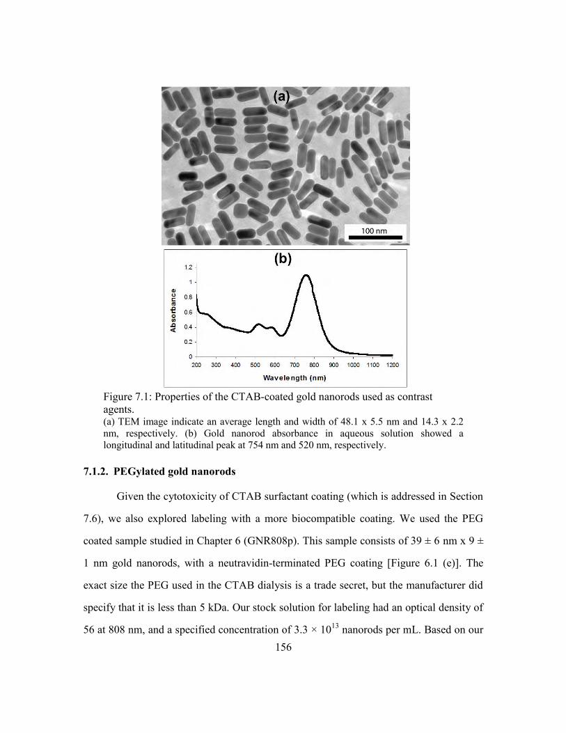
156
7.1.2. PEGylated gold nanorods
Given the cytotoxicity of CTAB surfactant coating (which is addressed in Section
7.6), we also explored labeling with a more biocompatible coating. We used the PEG
coated sample studied in Chapter 6 (GNR808p). This sample consists of 39 ± 6 nm x 9 ±
1 nm gold nanorods, with a neutravidin-terminated PEG coating [Figure 6.1 (e)]. The
exact size the PEG used in the CTAB dialysis is a trade secret, but the manufacturer did
specify that it is less than 5 kDa. Our stock solution for labeling had an optical density of
56 at 808 nm, and a specified concentration of 3.3 × 10¹³
nanorods per mL. Based on our
Figure 7.1: Properties of the CTAB-coated gold nanorods used as contrast
agents. (a) TEM image indicate an average length and width of 48.1 x 5.5 nm and 14.3 x 2.2
nm, respectively. (b) Gold nanorod absorbance in aqueous solution showed a
longitudinal and latitudinal peak at 754 nm and 520 nm, respectively.
157
characterization, we believe the actual concentration is closer to 1.2 × 10¹³
nanorods per
mL at an optical density of 56 [Section 6.5].
We conjugated the neutravidin functionalized gold nanorods to biotin labeled
antibodies for EGFR (clone 111.6, MS-378-B0, Thermo Scientific). The density of the
stock antibody solution was 200 μg/mL and the size of an individual antibody is 145kDa,
which gives an approximate antibody density of 8.3 × 10¹⁴
antibodies/mL. We mixed the
GNR808p, antibody, and 40 mM HEPES solution at a 1:1:4 volume ratio, which results
in an interaction of ~67 antibodies for every nanorod. The mixture was allowed to
interact for 20 minutes, and then centrifuged at 2,000 × g for 30 minutes to remove
unbound antibodies. We performed a second washing step, resuspending the pellet in 2
mL of 40 mM HEPES, and centrifuging at 2,000 × G for 30 minutes to further remove
unbound antibodies.
7.1.3. Nanospheres
We imaged the 54 ± 5 nm × 44 ± 4 nm nanospheres from Chapter 6 (GNS530)
labeled to cancer cells by conjugation to EGFR antibodies. 2 mL of the stock GNS530
solution were centrifuged at 2,000 × G and resuspended in 2 mL of 20 mM HEPES
buffer. 2 μL anti-EGFR monoclonoal antibodies (clone 225, 1.5 mg/mL, Sigma) were
suspended in 1.98 mL of 20 mM HEPES buffer. The gold solution was added dropwise
to the dilute antibody solution while stirring, to allow for an even coating of the
nanospheres. The mixture was allowed to interact for 45 minutes. 400 μL of 2% PEG was
added to the mixture for stability. Unbound antibodies were removed by centrifuging at
300 × G for 45 minutes. This left some nanospheres in solution, but we found that
centrifuging the nanospheres at greater force led to irreversible agglomeration. The
158
functionalized nanosphere pellet was resuspended in 300 μL DPBS without Ca2+
and
Mg2+
and stored at 4° C until use.
7.2. SAMPLE PREPARATION
We labeled MDA-MB-468 breast cancer cells and American Type Culture
Collection ATCC A431 human epidermoid carcinoma cells, both of which are known to
overexpress EGFR. Cells were cultured in DMEM supplemented with 5-10% Fetal
Bovine Serum (Sigma) and maintained at 37° C in a humidified 5% CO2 incubator. In
preparation for labeling, cells were harvested via trypsinization and resuspended in 1x
PBS. We then mixed the cell solution with varying amounts of functionalized
nanoparticles and allowed them to interact for 30-45 minutes. We separated unbound
nanoparticles from labeled cells with centrifugation at 200 × G for 5 minutes. We
deposited this solution on a #1.5 glass-bottom petri dish and incubated the sample for
approximately 1 hour for the cells to stabilize on the top of the coverslip.
7.2.1. Tissue phantoms
Three-dimensional tissue phantoms were prepared using rat tail collagen as a
scaffold. Labeled cells were centrifuged at 200 × G for 5 minutes and the resulting pellet
was resuspended in a buffered collagen solution at a concentration of 7.5 x 10⁷ cells/mL.
The collagen/cell mixture was pipetted into a 120 m spacer (Molecular Probes) and
sealed with a coverslip for imaging.
7.3. IMAGING SYSTEMS
Imaging was performed on one of two multiphoton microscopes, as indicated in
each section. We used the upright microscope described in Chapter 3 with the 20x/0.95
water dipping objective (Olympus) for deep imaging experiments with phantoms. We
159
also used an inverted microscope described in Section 6.6.1 for phantom and single cell
layer experiments with a high NA objective lens (Zeiss 63x/1.4 and Olympus 40x/1.3) for
brightness comparison and polarization experiments. Images presented with the Olympus
objective were also taken with an improved filter set that efficiently passed up to 720 nm
luminescence to the detector.
7.4. SINGLE LAYER OF LABELED CANCER CELLS
7.4.1. Brightness characterization
Figure 7.2 presents nonlinear images of a single layer of labeled and unlabeled
cells at 760 nm excitation wavelength. The images demonstrate successful labeling,
indicating the cellular distribution of EGFR. The unlabeled cells [Figure 7.2 (a)] show a
relatively uniform distribution of 2PAM signal throughout cellular cytoplasm. No signal
is associated with the nuclei, which do not have significant concentrations of endogenous
fluorophores that can be excited in the visible region. In labeled cells [Figure 7.2 (b)],
bright rings can be seen; this is a characteristic pattern of EGFR labeling and has been
also reported in confocal reflectance imaging of EGFR using spherical gold nanoparticles
[71]. The discrete bright spots in the cytoplasm of nanorod-labeled cells are indicative of
endosomal uptake of EGF receptors labeled with nanorods inside cells. The endosomal
recycling of EGFR molecules is a normal biological function of living cancer cells.26, 27
MPL images of cells treated with nonspecifically conjugated nanorods shows
agglomeration of contrast agent and little attachment to cell membranes [Figure 7.2 (d)].
Using the same excitation power of 140 W, the two-photon imaging of unlabeled cells
gave a pure background noise black image [Figure 7.2 (c)].
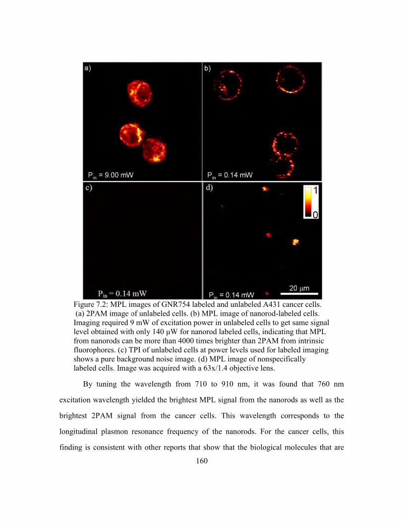
160
By tuning the wavelength from 710 to 910 nm, it was found that 760 nm
excitation wavelength yielded the brightest MPL signal from the nanorods as well as the
brightest 2PAM signal from the cancer cells. This wavelength corresponds to the
longitudinal plasmon resonance frequency of the nanorods. For the cancer cells, this
finding is consistent with other reports that show that the biological molecules that are
Figure 7.2: MPL images of GNR754 labeled and unlabeled A431 cancer cells.
(a) 2PAM image of unlabeled cells. (b) MPL image of nanorod-labeled cells.
Imaging required 9 mW of excitation power in unlabeled cells to get same signal
level obtained with only 140 μW for nanorod labeled cells, indicating that MPL
from nanorods can be more than 4000 times brighter than 2PAM from intrinsic
fluorophores. (c) TPI of unlabeled cells at power levels used for labeled imaging
shows a pure background noise image. (d) MPL image of nonspecifically
labeled cells. Image was acquired with a 63x/1.4 objective lens.
c)
161
primarily responsible for the signal in 2PAM imaging (NADH and flavins) have two-
photon cross-sections that increase with decreasing excitation wavelength from 1000 to
750 nm, and level off around 750 nm[8]. The similarity of the optimal excitation
wavelengths for both the gold nanorods and cellular autofluorescence allows a
comparison of the two imaging modalities under identical excitation conditions. We
found that MPL imaging of nanorod-labeled cells required 64 times less power than
2PAM imaging of unlabeled cells in order to achieve the similar collected intensity.
Given the quadratic dependence of emission intensity on the incident power, this
observation implies that, for equal excitation powers, MPL imaging of nanorod-labeled
cancer cells can generate more than 4000 times larger emission signal than 2PAM
imaging of unlabeled cells.
7.4.2. Signal from nanoparticle agglomerates
During functionalization, nanoparticle agglomerates are sometimes formed. We
incorporated a widefield CCD imaging system into our upright microscope to visualize
sequential images of the same field of view under MPL imaging and white-light
transmission imaging. We found that large clusters of nanoparticles that are visible under
white-light illumination are not sources of bright MPL signal. This is likely due to the
loss of surface plasmon effects as nanorods form very large aggregates.
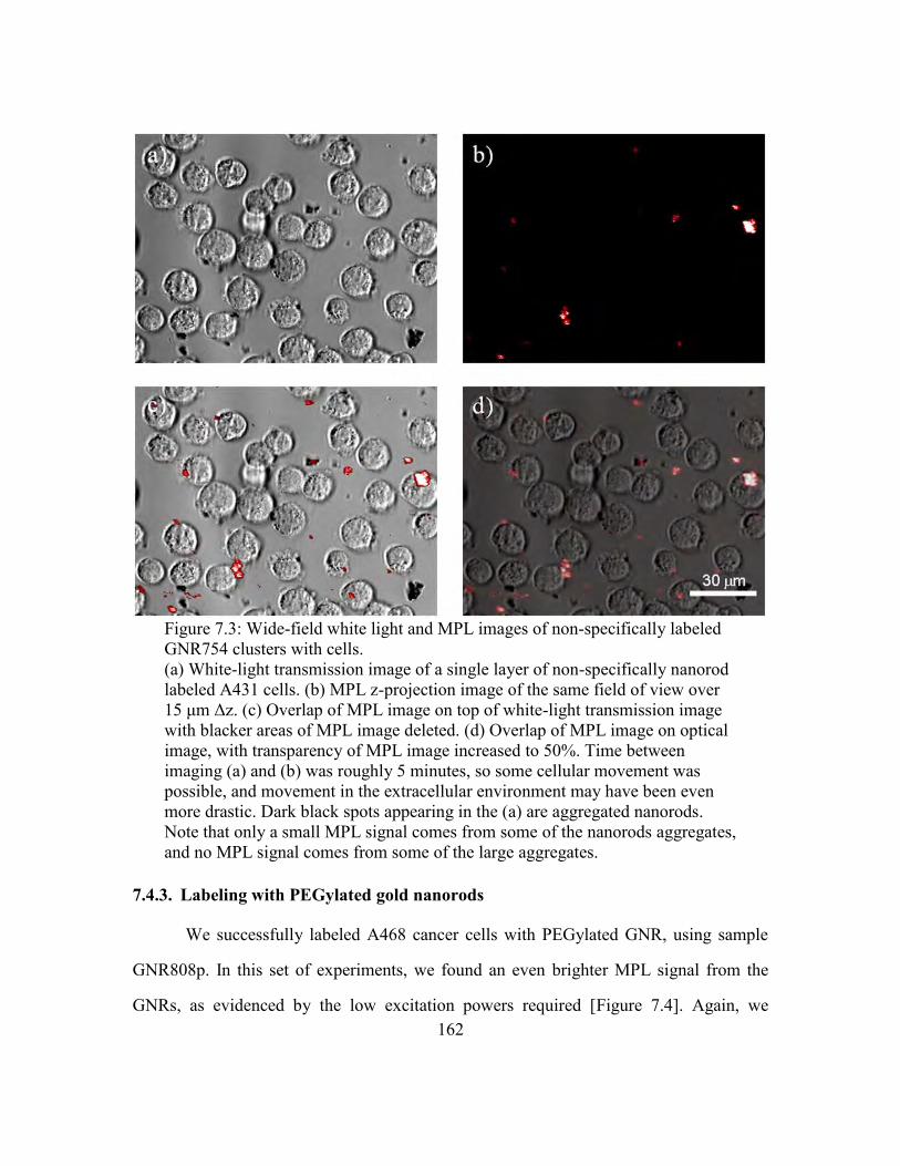
162
7.4.3. Labeling with PEGylated gold nanorods
We successfully labeled A468 cancer cells with PEGylated GNR, using sample
GNR808p. In this set of experiments, we found an even brighter MPL signal from the
GNRs, as evidenced by the low excitation powers required [Figure 7.4]. Again, we
Figure 7.3: Wide-field white light and MPL images of non-specifically labeled
GNR754 clusters with cells.
(a) White-light transmission image of a single layer of non-specifically nanorod
labeled A431 cells. (b) MPL z-projection image of the same field of view over
15 μm Δz. (c) Overlap of MPL image on top of white-light transmission image
with blacker areas of MPL image deleted. (d) Overlap of MPL image on optical
image, with transparency of MPL image increased to 50%. Time between
imaging (a) and (b) was roughly 5 minutes, so some cellular movement was
possible, and movement in the extracellular environment may have been even
more drastic. Dark black spots appearing in the (a) are aggregated nanorods.
Note that only a small MPL signal comes from some of the nanorods aggregates,
and no MPL signal comes from some of the large aggregates.
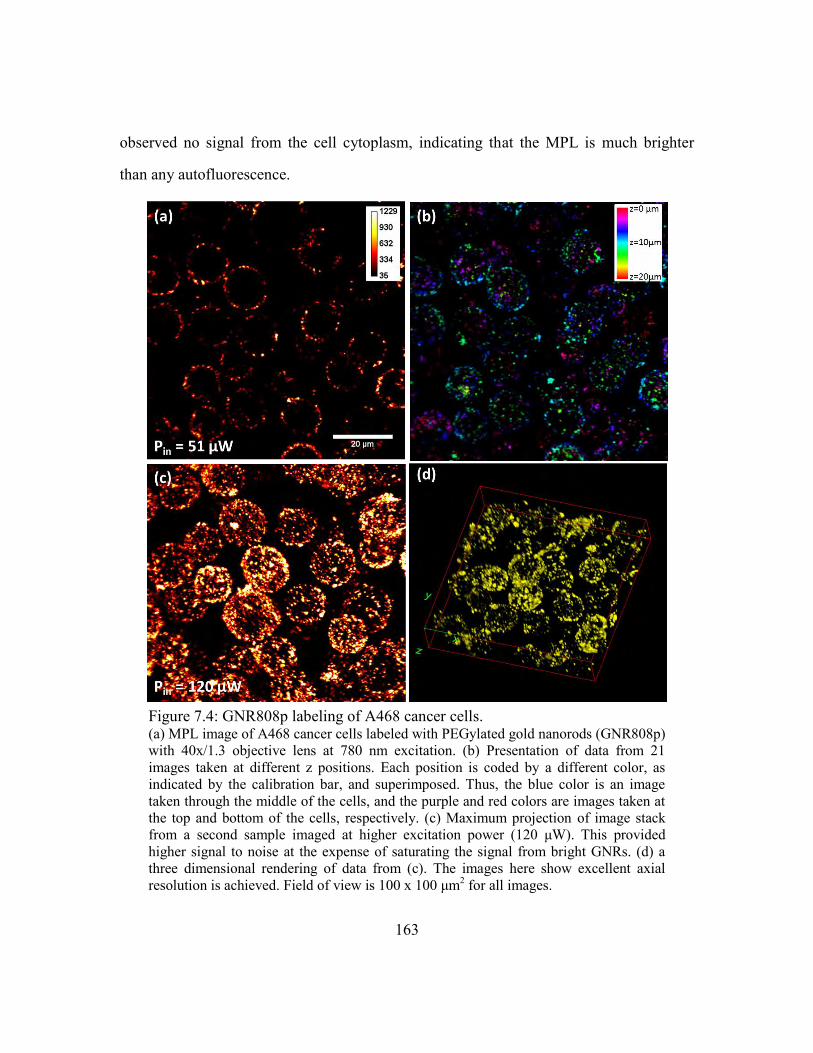
163
observed no signal from the cell cytoplasm, indicating that the MPL is much brighter
than any autofluorescence.
Figure 7.4: GNR808p labeling of A468 cancer cells. (a) MPL image of A468 cancer cells labeled with PEGylated gold nanorods (GNR808p)
with 40x/1.3 objective lens at 780 nm excitation. (b) Presentation of data from 21
images taken at different z positions. Each position is coded by a different color, as
indicated by the calibration bar, and superimposed. Thus, the blue color is an image
taken through the middle of the cells, and the purple and red colors are images taken at
the top and bottom of the cells, respectively. (c) Maximum projection of image stack
from a second sample imaged at higher excitation power (120 μW). This provided
higher signal to noise at the expense of saturating the signal from bright GNRs. (d) a
three dimensional rendering of data from (c). The images here show excellent axial
resolution is achieved. Field of view is 100 x 100 μm2 for all images.
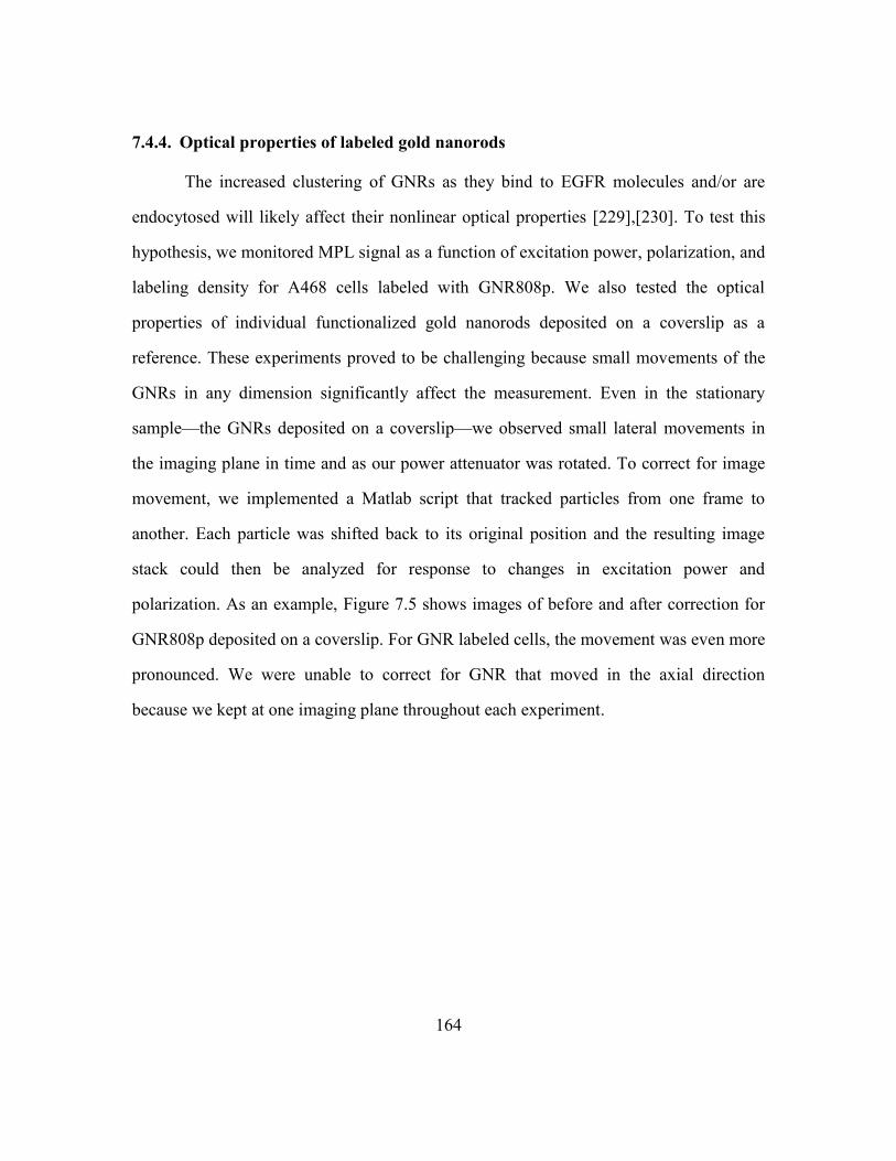
164
7.4.4. Optical properties of labeled gold nanorods
The increased clustering of GNRs as they bind to EGFR molecules and/or are
endocytosed will likely affect their nonlinear optical properties [229],[230]. To test this
hypothesis, we monitored MPL signal as a function of excitation power, polarization, and
labeling density for A468 cells labeled with GNR808p. We also tested the optical
properties of individual functionalized gold nanorods deposited on a coverslip as a
reference. These experiments proved to be challenging because small movements of the
GNRs in any dimension significantly affect the measurement. Even in the stationary
sample—the GNRs deposited on a coverslip—we observed small lateral movements in
the imaging plane in time and as our power attenuator was rotated. To correct for image
movement, we implemented a Matlab script that tracked particles from one frame to
another. Each particle was shifted back to its original position and the resulting image
stack could then be analyzed for response to changes in excitation power and
polarization. As an example, Figure 7.5 shows images of before and after correction for
GNR808p deposited on a coverslip. For GNR labeled cells, the movement was even more
pronounced. We were unable to correct for GNR that moved in the axial direction
because we kept at one imaging plane throughout each experiment.
165
Dependence of MPL on excitation fluence
We examined the dependence of MPL signal as a function of power on both
GNR-labeled cells and GNRs deposited on a coverslip. Unfortunately, we were unable to
image at the low fluences studied in Chapter 6, where we saw saturation effects above
peak intensities of 300 MW/cm2. The setup in Chapter 6 allowed for more sensitive
imaging because we used a large focal spot and simultaneously sampled many
nanoparticles, whereas in this chapter, we aim to achieve high resolution images of gold
nanoparticle labeled samples. Thus we expect that in the regimes probed here, we are
saturating the signal from the nanorods.
We demonstrate MPL from GNR808p on a coverslip and labeled to cells in
Figure 7.6. As expected, we see a smaller order nonlinear dependence than observed at
the lower Ip probed in Chapter 6. Nonetheless, we can make two important observations
Figure 7.5: Sample movement correction algorithm. Top: color images representing different excitation powers. Bottom Left: merge of all
the images taken at different powers. The smearing of the colors demonstrates that the
image moves slightly relative to the sample as the excitation power is changed. Bottom
Right: After correcting for sample movement, our data stacks show much less particle
movement.
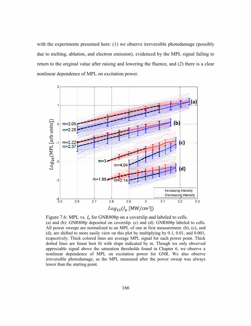
166
with the experiments presented here: (1) we observe irreversible photodamage (possibly
due to melting, ablation, and electron emission), evidenced by the MPL signal failing to
return to the original value after raising and lowering the fluence, and (2) there is a clear
nonlinear dependence of MPL on excitation power.
Figure 7.6: MPL vs. Ip for GNR808p on a coverslip and labeled to cells. (a) and (b): GNR808p deposited on coverslip. (c) and (d): GNR808p labeled to cells.
All power sweeps are normalized to an MPL of one at first measurement. (b), (c), and
(d), are shifted to more easily view on this plot by multiplying by 0.1, 0.01, and 0.001,
respectively. Thick colored lines are average MPL signal for each power point. Thick
dotted lines are linear best fit with slope indicated by m. Though we only observed
appreciable signal above the saturation thresholds found in Chapter 6, we observe a
nonlinear dependence of MPL on excitation power for GNR. We also observe
irreversible photodamage, as the MPL measured after the power sweep was always
lower than the starting point.
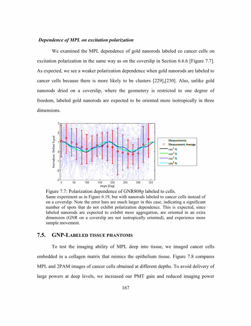
167
Dependence of MPL on excitation polarization
We examined the MPL dependence of gold nanorods labeled co cancer cells on
excitation polarization in the same way as on the coverslip in Section 6.6.6 [Figure 7.7].
As expected, we see a weaker polarization dependence when gold nanorods are labeled to
cancer cells because there is more likely to be clusters [229],[230]. Also, unlike gold
nanorods dried on a coverslip, where the geometery is restricted to one degree of
freedom, labeled gold nanorods are expected to be oriented more isotropically in three
dimensions.
7.5. GNP-LABELED TISSUE PHANTOMS
To test the imaging ability of MPL deep into tissue, we imaged cancer cells
embedded in a collagen matrix that mimics the epithelium tissue. Figure 7.8 compares
MPL and 2PAM images of cancer cells obtained at different depths. To avoid delivery of
large powers at deep levels, we increased our PMT gain and reduced imaging power
Figure 7.7: Polarization dependence of GNR808p labeled to cells. Same experiment as in Figure 6.19, but with nanorods labeled to cancer cells instead of
on a coverslip. Note the error bars are much larger in this case, indicating a significant
number of spots that do not exhibit polarization dependence. This is expected, since
labeled nanorods are expected to exhibit more aggregation, are oriented in an extra
dimension (GNR on a coverslip are not isotropically oriented), and experience more
sample movement.
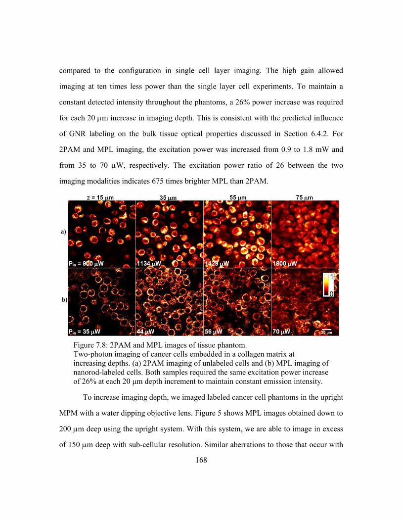
168
compared to the configuration in single cell layer imaging. The high gain allowed
imaging at ten times less power than the single layer cell experiments. To maintain a
constant detected intensity throughout the phantoms, a 26% power increase was required
for each 20 m increase in imaging depth. This is consistent with the predicted influence
of GNR labeling on the bulk tissue optical properties discussed in Section 6.4.2. For
2PAM and MPL imaging, the excitation power was increased from 0.9 to 1.8 mW and
from 35 to 70 W, respectively. The excitation power ratio of 26 between the two
imaging modalities indicates 675 times brighter MPL than 2PAM.
To increase imaging depth, we imaged labeled cancer cell phantoms in the upright
MPM with a water dipping objective lens. Figure 5 shows MPL images obtained down to
200 m deep using the upright system. With this system, we are able to image in excess
of 150 m deep with sub-cellular resolution. Similar aberrations to those that occur with
Figure 7.8: 2PAM and MPL images of tissue phantom.
Two-photon imaging of cancer cells embedded in a collagen matrix at
increasing depths. (a) 2PAM imaging of unlabeled cells and (b) MPL imaging of
nanorod-labeled cells. Both samples required the same excitation power increase
of 26% at each 20 μm depth increment to maintain constant emission intensity.

169
the oil immersion lens are observed but the onset of these aberrations occur at
approximately twice the depth. The power increase necessary to obtain similar collected
signal as imaging depth was increased was not a smooth exponential function, as
observed with the oil immersion objective. This could be due to the signal degradation
being simultaneously dependent on multiple factors such as excitation light attenuation
due to scattering, as well as optical aberrations. From the XZ image shown in Figure 6,
we can see that the point spread function become drastically larger, especially in the axial
direction, at depths greater than 150 m.
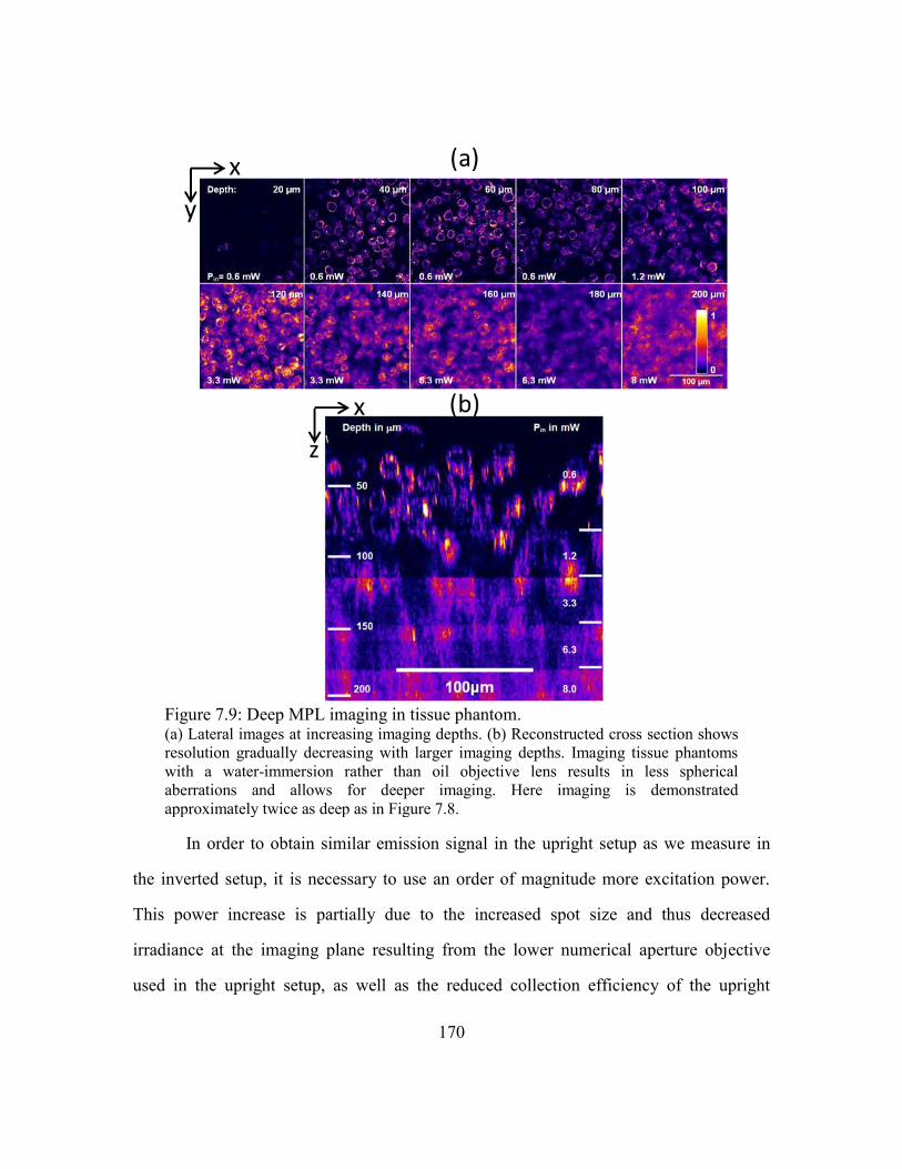
170
In order to obtain similar emission signal in the upright setup as we measure in
the inverted setup, it is necessary to use an order of magnitude more excitation power.
This power increase is partially due to the increased spot size and thus decreased
irradiance at the imaging plane resulting from the lower numerical aperture objective
used in the upright setup, as well as the reduced collection efficiency of the upright
Figure 7.9: Deep MPL imaging in tissue phantom. (a) Lateral images at increasing imaging depths. (b) Reconstructed cross section shows
resolution gradually decreasing with larger imaging depths. Imaging tissue phantoms
with a water-immersion rather than oil objective lens results in less spherical
aberrations and allows for deeper imaging. Here imaging is demonstrated
approximately twice as deep as in Figure 7.8.

171
system resulting from the large back aperture of the water immersion objective. The
measured lateral spot size of the upright setup was approximately 2.2x larger in area than
in the inverted setup. With additional optimization of the collection optics, it will be
possible to further improve the upright MPM collection efficiency.
7.6. BIOCOMPATIBILITY
CTAB is known to be cytotoxic at the concentrations used in nanorod labeling,
raising concerns about the in vivo use of nanorods for molecular imaging
[231],[222],[232],[233]. However, CTAB can be exchanged with PEG, a much more
biocompatible material, in a dialysis reaction [234]. We conducted a preliminary test of
the biocompatibility of gold nanospheres (GNS530), CTAB-coated gold nanorods
(GNR780), and PEGylated gold nanorods (GNR808p) by using an MTT assay (Promega
CellTiter Aqueous One kit). We used this assay to quantify the proliferation of A468
cancer cells when incubated with these three particle types at different concentrations for
24 and 48 hours. At each time point, the density of cells incubated with each solution was
compared to the density of cells incubated in DMEM supplemented with 5-10% Fetal
Bovine Serum (Sigma). Cells were incubated at 37° C in a humidified 5% CO2 incubator.
Concentrations in the 100 pM range are generally sufficient for dense labeling of cancer
cells. We tested incubation with concentrations of 4 to 4,000 pM of each nanoparticle
sample [Figure 7.10]. Gold nanospheres showed no significant cytotoxic effects at either
timepoint. We found that the CTAB-coated GNR780 sample at concentrations equal to
and above 400 pM exhibited significant cytoxicity within 24 hours of application to
human cancer cells. After 48 hours of incubation, even GNR780 concentrations of low as
40 pM, began to show some cytotoxic effects. On the other hand, PEGylated gold
nanorods showed very little cytotoxic effects at all concentrations after 24 hours of
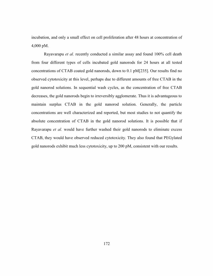
172
incubation, and only a small effect on cell proliferation after 48 hours at concentration of
4,000 pM.
Rayavarapu et al. recently conducted a similar assay and found 100% cell death
from four different types of cells incubated gold nanorods for 24 hours at all tested
concentrations of CTAB coated gold nanorods, down to 0.1 pM[235]. Our results find no
observed cytotoxicity at this level, perhaps due to different amounts of free CTAB in the
gold nanorod solutions. In sequential wash cycles, as the concentration of free CTAB
decreases, the gold nanorods begin to irreversibly agglomerate. Thus it is advantageous to
maintain surplus CTAB in the gold nanorod solution. Generally, the particle
concentrations are well characterized and reported, but most studies to not quantify the
absolute concentration of CTAB in the gold nanorod solutions. It is possible that if
Rayavarapu et al. would have further washed their gold nanorods to eliminate excess
CTAB, they would have observed reduced cytotoxicity. They also found that PEGylated
gold nanorods exhibit much less cytotoxicity, up to 200 pM, consistent with our results.
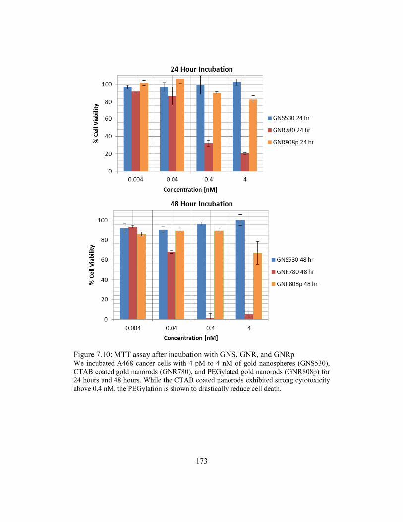
173
Figure 7.10: MTT assay after incubation with GNS, GNR, and GNRp We incubated A468 cancer cells with 4 pM to 4 nM of gold nanospheres (GNS530),
CTAB coated gold nanorods (GNR780), and PEGylated gold nanorods (GNR808p) for
24 hours and 48 hours. While the CTAB coated nanorods exhibited strong cytotoxicity
above 0.4 nM, the PEGylation is shown to drastically reduce cell death.
174
Chapter 8 Conclusions and future directions
This dissertation addressed two aspects in which nonlinear microscopy can be
extended towards clinical use—optimizing and understanding the limits of 2PAM
imaging depths in epithelial tissues, and the use of extremely bright plasmonic nonlinear
contrast agents for molecularly specific imaging of cancer cells.
We found that 2PAM imaging could be performed down to approximately 320
μm deep in a healthy human skin biopsy before the contrast was degraded to below one,
presumably by out-of-focus fluorescence generation. This result was corroborated by
tissue phantom experiments and a Monte Carlo model. As previous 2PAM studies in
mammalian skin have been limited to imaging depths of less than approximately 150 μm
deep, this represents a significant improvement in imaging depth capabilities. Our
measured maximum imaging depth is significantly less than that obtained in stained brain
tissue, even when the imaging depth is normalized by the different scattering lengths used
[11],[236]. Through Monte Carlo models and tissue phantoms, we demonstrate that the
origins for this difference are: (1) the maximum imaging depth does not scale linearly
with scattering length, and (2) the staining inhomogeneity is two orders of magnitude less
in 2PAM of epithelial tissues than typically encountered in two-photon imaging of
stained brain tissue. Fortunately, an imaging depth of 320 μm is still useful for probing
epithelial tissue disease[237]. Though 2PAM might not reach the stratum basale in some
cases, the majority of human epithelial tissues are less than a few hundred microns thick.
Still, there are several ways to improve the maximum 2PAM imaging depth.
Spherical aberrations due to refractive index mismatch can significantly degrade the spot
size in nonlinear imaging. Though we verified no significant aberrations were present in
tissue phantom experiments, the slightly larger imaging depths achieved in tissue
175
phantoms than in the biopsy may be explained by appreciable specimen-induced
aberrations by the biopsy. Future studies could use an objective lens with a correction
collar compensate for spherical aberrations to mitigate these effects, possibly moderately
increasing the maximum imaging depth in biopsies.
Alternative approaches to conventional two-photon microscopy show some
promise for reducing contributions of out-of-focus fluorescence. Temporal
focusing[163],[164], differential aberration imaging[165], optical clearing[166],[167],
and spatial filtering[11],[168] could all potentially increase maximum imaging depth.
Though these methods have shown the potential for increasing imaging depth, currently
each has only been demonstrated as a proof-of-concept for deep nonlinear imaging; larger
maximum imaging depths are generally reported using conventional two-photon
microscopes. Expected gains in imaging depths using these methods are approximately
0.5-1.0 mean free scattering length, and it is debatable whether the increased complexity
in implementing any of these methods is worth the additional ~ 50 μm in maximum
imaging depth one might achieve in epithelial tissues.
In the second part of this dissertation, we demonstrated the use of gold
nanoparticles for bright, molecularly specific imaging of cancer cells. Interestingly, we
found a deviation from the inverse relation of gold nanoparticle MPL on pulse duration.
This provides evidence that the mechanism of absorption in MPL is a sequential rather
than simultaneous one. We observed effective two-photon action cross sections that were
an order of magnitude larger than that reported from any previously reported particle,
including quantum dots. However, normalizing for the large size of gold nanoparticles,
we find that the luminescence generated per volume of particle is only slightly larger than
that from the brightest quantum dots. Still, in cases where the density of antigens is
limited, gold nanoparticles likely provide a more appealing option than quantum dots,
176
because in addition to being dimmer than gold nanoparticles, quantum dots are also well-
known to be cytotoxic. An additional advantage of nonlinear imaging with nanoparticles
compared to quantum dots is that although quantum dots are generally limited to one
emission photon per particle per excitation pulse, based on the large number of free
electrons in gold nanoparticles, it is likely that gold nanoparticles can produce more than
one emission photon per excitation pulse.
The origin of the enhanced nonlinear luminescence from gold nanoparticles is still
poorly understood. Though recent results, included those from this dissertation, point to
sequential absorption as the mechanism for MPL, the role of the plasmon resonance in
increasing MPL has only been described empirically[89], and is a poor match to ours and
others[193] observed σTPA spectra. Currently, there is no accurate model to reconcile the
disparate atomic model, from which MPL can be described as emission close to the
symmetry points in the Brillouin zone of gold, and the classical picture, where the
spectral dependency of the plasmon resonance is weakly correlated to enhanced MPL
signal. With improved understanding the mechanisms of MPL, better particle geometries
and compositions can be engineered.
We only tested commonly synthesized (and now commercially available) particle
geometries, but future studies characterizing MPL from nanorice[238], nanostars[239],
and silver nanorods[227] could yield even brighter nonlinear contrast agents because of
the sharp tips and large simulated near-field enhancements. In engineering gold
nanoparticles specifically for nonlinear imaging, it would be advantageous to create
particles with SPR peaks even further into the NIR region. For instance, at 1350 nm,
excitation light may penetrate even deeper into epithelial tissues. In moving to larger
excitation wavelengths, the disadvantage in the increased spotsize will likely be
outweighed by the increase in maximum imaging depth[170].
177
To achieve molecularly specific nonlinear imaging of tissues with plasmonic
contrast agents, several challenges remain. The biggest disadvantage of using gold
nanoparticles as contrast agents is likely their large size. Though some groups have had
success in the topical application of gold nanoparticles (notably, by using permeation
enhancers, such as chitosan[229],[240]), the delivery of gold nanoparticles, which are
orders of magnitude larger than molecular fluorophores, remains a challenge.
Additionally, more detailed studies exploring the biodistribution and clearance of gold
particles are necessary to understand the true biocompatibility of this class of contrast
agents.
The melting of gold nanoparticles has been thoroughly characterized in previous
studies, both experimentally[241],[242] and theoretically[243]. In nonlinear imaging,
where high intensities are necessary to generate appreciable signal, care must be taken to
stay below the particle damage threshold. It is possible that one may tune the excitation
wavelength for a compromise between minimizing linear absorbance of light and
maximizing the effective σTPA value. For our experiments, we found irreversible
photodamage could largely be avoided by using sub-mW excitation powers, and
typically, we could image with one order of magnitude lower intensity below the melting
threshold. However, for deep imaging, melting could become more problematic, as more
luminescence must be generated at the imaging plane to compensate from increasing
losses in collection efficiency.
There are a few notable promising applications of gold nanoparticles as nonlinear
contrast agents worth reiterating. The large size of gold nanoparticles, which makes
delivery and clearance challenging, can actually be advantageous in killing cancer
cells[78]. Because of the ―leaky vasculature‖ phenomenon, their large size may even be
beneficial in preferentially heating tumors[80]. Furthermore, gold nanoparticles can be
178
combined as a therapeutic and diagnostic (―theragnostic‖) contrast agent, or nonlinear
imaging can be used to understand the distribution of nanoparticle therapeutic agents
[93]. Finally, the large brightness of gold nanoparticles can enable molecularly specific
imaging in systems with poor collection efficiencies and/or limited excitation fluence,
such as that typically found in nonlinear endoscopic probes[12-15].
179
References
[1] G.J. Tearney, M.E. Brezinski, B.E. Bouma, S.A. Boppart, C. Pitris, J.F. Southern, and J.G. Fujimoto, “In Vivo Endoscopic Optical Biopsy with Optical Coherence Tomography,” Science, vol. 276, Jun. 1997, pp. 2037-2039.
[2] W. Denk, J. Strickler, and W. Webb, “Two-photon laser scanning fluorescence microscopy,” Science, vol. 248, Apr. 1990, pp. 73-76.
[3] B.R. Masters, P.T. So, and E. Gratton, “Multiphoton excitation fluorescence microscopy and spectroscopy of in vivo human skin.,” Biophys. J., vol. 72, Jun. 1997, pp. 2405-2412.
[4] E. Dimitrow, M. Ziemer, M.J. Koehler, J. Norgauer, K. Konig, P. Elsner, and M. Kaatz, “Sensitivity and Specificity of Multiphoton Laser Tomography for In Vivo and Ex Vivo Diagnosis of Malignant Melanoma,” J Invest Dermatol, vol. 129, Jan. 2009, pp. 1752-1758.
[5] K. König, M. Speicher, R. Bückle, J. Reckfort, G. McKenzie, J. Welzel, M.J. Koehler, P. Elsner, and M. Kaatz, “Clinical optical coherence tomography combined with multiphoton tomography of patients with skin diseases,” Journal of
Biophotonics, vol. 2, 2009, pp. 389-397. [6] I. Pavlova, M. Williams, A. El-Naggar, R. Richards-Kortum, and A. Gillenwater,
“Understanding the Biological Basis of Autofluorescence Imaging for Oral Cancer Detection: High-Resolution Fluorescence Microscopy in Viable Tissue,” Clinical
Cancer Research, vol. 14, Apr. 2008, pp. 2396-2404. [7] R. Alfano, D. Tata, J. Cordero, P. Tomashefsky, F. Longo, and M. Alfano, “Laser
induced fluorescence spectroscopy from native cancerous and normal tissue,” IEEE Journal of Quantum Electronics, vol. 20, Dec. 1984, pp. 1507-1511.
[8] W.R. Zipfel, R.M. Williams, R. Christie, A.Y. Nikitin, B.T. Hyman, and W.W. Webb, “Live tissue intrinsic emission microscopy using multiphoton-excited native fluorescence and second harmonic generation,” Proceedings of the National
Academy of Sciences, vol. 100, 2003, pp. 7075-7080. [9] C. Xu, W. Zipfel, J.B. Shear, R.M. Williams, and W.W. Webb, “Multiphoton
fluorescence excitation: new spectral windows for biological nonlinear microscopy,” Proceedings of the National Academy of Sciences of the United
States of America, vol. 93, Oct. 1996, pp. 10763 -10768. [10] P.J. Campagnola, H.A. Clark, W.A. Mohler, A. Lewis, and L.M. Loew, “Second-
harmonic imaging microscopy of living cells,” Journal of Biomedical Optics, vol. 6, Jul. 2001, pp. 277-286.
[11] P. Theer and W. Denk, “On the fundamental imaging-depth limit in two-photon microscopy,” Journal of the Optical Society of America A, vol. 23, 2006, pp. 3139-3149.
[12] K. König, A. Ehlers, I. Riemann, S. Schenkl, R. Bückle, and M. Kaatz, “Clinical two-photon microendoscopy,” Microscopy Research and Technique, vol. 70, May. 2007, pp. 398-402.
[13] B.A. Flusberg, E.D. Cocker, W. Piyawattanametha, J.C. Jung, E.L.M. Cheung, and
180
M.J. Schnitzer, “Fiber-optic fluorescence imaging,” Nature Methods, vol. 2, Dec. 2005, pp. 941-950.
[14] C.L. Hoy, N.J. Durr, P. Chen, W. Piyawattanametha, H. Ra, O. Solgaard, and A. Ben-Yakar, “Miniaturized probe for femtosecond laser microsurgery and two-photon imaging,” Optics Express, vol. 16, Jun. 2008, pp. 9996-10005.
[15] J.C. Jung and M.J. Schnitzer, “Multiphoton endoscopy,” Optics Letters, vol. 28, Jun. 2003, pp. 902-904.
[16] Garcia M, Jemal A, Ward EM, Center MM, Hao Y, Siegel RI, and Thun MJ, “Global Cancer Facts and Figures 2007,” 2007.
[17] V. Kumar, N. Fausto, and A. Abbas, Robbins & Cotran Pathologic Basis of
Disease, Seventh Edition, Saunders, 2004. [18] E.J. Kort, N. Paneth, and G.F. Vande Woude, “The Decline in U.S. Cancer
Mortality in People Born since 1925,” Cancer Research, vol. 69, 2009, pp. 6500-6505.
[19] J.V. Frangioni, “Translating in vivo diagnostics into clinical reality,” Nature
biotechnology, vol. 24, 2006, pp. 909-913. [20] “Blue Histology,” Human Thin Skin. Keratinized stratified squamous epithelium. [21] M.C. Skala, J.M. Squirrell, K.M. Vrotsos, J.C. Eickhoff, A. Gendron-Fitzpatrick,
K.W. Eliceiri, and N. Ramanujam, “Multiphoton microscopy of endogenous fluorescence differentiates normal, precancerous, and cancerous squamous epithelial tissues,” Cancer Research, vol. 65, Feb. 2005, pp. 1180-1186.
[22] I. Pavlova, K. Sokolov, R. Drezek, A. Malpica, M. Follen, and R. Richards-Kortum, “Microanatomical and Biochemical Origins of Normal and Precancerous Cervical Autofluorescence Using Laser-scanning Fluorescence Confocal Microscopy ¶,” Photochemistry and Photobiology, vol. 77, 2003, pp. 550-555.
[23] M. Rajadhyaksha, R.R. Anderson, and R.H. Webb, “Video-Rate Confocal Scanning Laser Microscope for Imaging Human Tissues In Vivo,” Applied Optics, vol. 38, Apr. 1999, pp. 2105-2115.
[24] J.T.C. Liu, M.J. Mandella, J.M. Crawford, C.H. Contag, T.D. Wang, and G.S. Kino, “Efficient rejection of scattered light enables deep optical sectioning in turbid media with low-numerical-aperture optics in a dual-axis confocal architecture,” Journal of Biomedical Optics, vol. 13, 2008, p. 034020.
[25] B.R. Masters, G. Gonnord, and P. Corcuff, “Three-dimensional microscopic biopsy of in vivo human skin: a new technique based on a flexible confocal microscope,” Journal of Microscopy, vol. 185, Mar. 1997, pp. 329-338.
[26] B.R. Masters, “Three-dimensional confocal fluorescence microscopic visualization of the living human skin,” Proceedings of SPIE, San Jose, CA, USA: 1995, pp. 188-192.
[27] J.V. Burstin, S. Eser, B. Seidler, A. Meining, M. Bajbouj, J. Mages, R. Lang, A.J. Kind, A.E. Schnieke, R.M. Schmid, G. Schneider, and D. Saur, “Highly sensitive detection of early-stage pancreatic cancer by multimodal near-infrared molecular imaging in living mice,” International Journal of Cancer, vol. 123, 2008, pp.
181
2138-2147. [28] M. Ignat, M. Aprahamian, V. Lindner, A. Altmeyer, S. Perretta, B. Dallemagne, D.
Mutter, and J. Marescaux, “Feasibility and Reliability of Pancreatic Cancer Staging Using Fiberoptic Confocal Fluorescence Microscopy in Rats,” Gastroenterology, vol. 137, 2009, pp. 1584-1592.e1.
[29] T. Gambichler, A. Orlikov, R. Vasa, G. Moussa, K. Hoffmann, M. Stücker, P. Altmeyer, and F.G. Bechara, “In vivo optical coherence tomography of basal cell carcinoma,” Journal of Dermatological Science, vol. 45, Mar. 2007, pp. 167-173.
[30] E.Z. Zhang, J.G. Laufer, R.B. Pedley, and P.C. Beard, “In vivo high-resolution 3D photoacoustic imaging of superficial vascular anatomy,” Physics in Medicine and
Biology, vol. 54, Feb. 2009, pp. 1035-1046. [31] H.F. Zhang, K. Maslov, G. Stoica, and L.V. Wang, “Functional photoacoustic
microscopy for high-resolution and noninvasive in vivo imaging,” Nature
Biotechnology, vol. 24, Jul. 2006, pp. 848-851. [32] A.J. Welch and M.J.C.V. Gemert, Optical-thermal response of laser-irradiated
tissue, Springer, 1995. [33] A.N. Bashkatov, E.A. Genina, V.I. Kochubey, and V.V. Tuchin, “Optical
properties of human skin, subcutaneous and mucous tissues in the wavelength range from 400 to 2000 nm,” Journal of Phyics-London-D Applied Physics, vol. 38, 2005, p. 2543.
[34] A. Knuttel and M. Boehlau-Godau, “Spatially confined and temporally resolved refractive index and scattering evaluation in human skin performed with optical coherence tomography,” Journal of Biomedical Optics, vol. 5, Jan. 2000, pp. 83-92.
[35] G.J. Tearney, M.E. Brezinski, J.F. Southern, B.E. Bouma, M.R. Hee, and J.G. Fujimoto, “Determination of the refractive index of highly scattering human tissue by optical coherence tomography,” Optics Letters, vol. 20, Nov. 1995, pp. 2258-2260.
[36] E. Salomatina, B. Jiang, J. Novak, and A.N. Yaroslavsky, “Optical properties of normal and cancerous human skin in the visible and near-infrared spectral range,” Journal of Biomedical Optics, vol. 11, Nov. 2006, pp. 064026-9.
[37] Michael Sheik-Bahae M and Hasselbeck MP, “Third Order Nonlinearities,” OSA
Handbook of optics, 2001. [38] Boyd, Yu, and Shen, “Photoinduced luminescence from the noble metals and its
enhancement on roughened surfaces,” Physical review. B, Condensed matter, vol. 33, Jun. 1986, pp. 7923-7936.
[39] K. Imura, T. Nagahara, and H. Okamoto, “Near-Field Two-Photon-Induced Photoluminescence from Single Gold Nanorods and Imaging of Plasmon Modes,” Journal of Physical Chemistry B, vol. 109, Jul. 2005, pp. 13214-13220.
[40] V.E. Centonze and J.G. White, “Multiphoton excitation provides optical sections from deeper within scattering specimens than confocal imaging.,” Biophysical
Journal, vol. 75, Oct. 1998, pp. 2015-2024. [41] W. Denk and K. Svoboda, “Photon upmanship: why multiphoton imaging is more
182
than a gimmick,” Neuron, vol. 18, Mar. 1997, pp. 351-357. [42] W. Zipfel, R. Williams, and W. Webb, “Nonlinear magic: multiphoton microscopy
in the biosciences,” Nature Biotechnology, vol. 21, Nov. 2003, pp. 1368-1376. [43] P.J. Campagnola, A.C. Millard, M. Terasaki, P.E. Hoppe, C.J. Malone, and W.A.
Mohler, “Three-dimensional high-resolution second-harmonic generation imaging of endogenous structural proteins in biological tissues.,” Biophysical Journal, vol. 82, Jan. 2002, pp. 493-508.
[44] E. Brown, T. McKee, E. diTomaso, A. Pluen, B. Seed, Y. Boucher, and R.K. Jain, “Dynamic imaging of collagen and its modulation in tumors in vivo using second-harmonic generation,” Nat Med, vol. 9, Jun. 2003, pp. 796-800.
[45] D.A. Dombeck, K.A. Kasischke, H.D. Vishwasrao, M. Ingelsson, B.T. Hyman, and W.W. Webb, “Uniform polarity microtubule assemblies imaged in native brain tissue by second-harmonic generation microscopy,” Proceedings of the National
Academy of Sciences of the United States of America, vol. 100, Jun. 2003, pp. 7081 -7086.
[46] D. Debarre, W. Supatto, A. Pena, A. Fabre, T. Tordjmann, L. Combettes, M. Schanne-Klein, and E. Beaurepaire, “Imaging lipid bodies in cells and tissues using third-harmonic generation microscopy,” Nat Meth, vol. 3, Jan. 2006, pp. 47-53.
[47] S. Tai, W. Lee, D. Shieh, P. Wu, H. Huang, C. Yu, and C. Sun, “In vivo optical biopsy of hamster oral cavity with epi-third-harmonic-generation microscopy,” Optics Express, vol. 14, Jun. 2006, pp. 6178-6187.
[48] D. Debarre and E. Beaurepaire, “Quantitative characterization of biological liquids for third-harmonic generation microscopy,” Biophysical journal, vol. 92, 2007, pp. 603-612.
[49] M. Albota, D. Beljonne, J. Brédas, J.E. Ehrlich, J. Fu, A.A. Heikal, S.E. Hess, T. Kogej, M.D. Levin, S.R. Marder, D. McCord-Maughon, J.W. Perry, H. Röckel, M. Rumi, G. Subramaniam, W.W. Webb, X. Wu, and C. Xu, “Design of Organic Molecules with Large Two-Photon Absorption Cross Sections,” Science, vol. 281, Sep. 1998, pp. 1653-1656.
[50] D.R. Larson, W.R. Zipfel, R.M. Williams, S.W. Clark, M.P. Bruchez, F.W. Wise, and W.W. Webb, “Water-Soluble Quantum Dots for Multiphoton Fluorescence Imaging in Vivo,” Science, vol. 300, May. 2003, pp. 1434-1436.
[51] H. Wang, T.B. Huff, D.A. Zweifel, W. He, P.S. Low, A. Wei, and J.X. Cheng, “In vitro and in vivo two-photon luminescence imaging of single gold nanorods,” Proceedings of the National Academy of Sciences, vol. 102, 2005, pp. 15752-15756.
[52] P. Zijlstra, J.W.M. Chon, and M. Gu, “Five-dimensional optical recording mediated by surface plasmons in gold nanorods,” Nature, vol. 459, May. 2009, pp. 410-413.
[53] N.W. Ashcroft and N.D. Mermin, Solid State Physics, Brooks Cole, 1976. [54] M.A. El-Sayed, “Some interesting properties of metals confined in time and
nanometer space of different shapes,” Accounts of Chemical Research, vol. 34,
183
2001, pp. 257-264. [55] G. Mie, “Beiträge zur Optik trüber Medien, speziell kolloidaler Metallösungen,”
Annalen der Physik, vol. 330, 1908, pp. 377-445. [56] U. Kreibig and M. Vollmer, Optical Properties of Metal Clusters, Springer, 1995. [57] S. Link and M.A. El-Sayed, “Shape and size dependence of radiative, non-
radiative and photothermal properties of gold nanocrystals,” International Reviews
in Physical Chemistry, vol. 19, 2000, pp. 409-454. [58] M.A. Yurkin and A.G. Hoekstra, “The discrete dipole approximation: An overview
and recent developments,” Journal of Quantitative Spectroscopy and Radiative
Transfer, vol. 106, Jul. 2007, pp. 558-589. [59] P.K. Jain, K.S. Lee, I.H. El-Sayed, and M.A. El-Sayed, “Calculated absorption and
scattering properties of gold nanoparticles of different size, shape, and composition: applications in biological imaging and biomedicine,” Journal of
Physical Chemistry B, vol. 110, 2006, p. 7238. [60] M. Abrams and B. Murrer, “Metal compounds in therapy and diagnosis,” Science,
vol. 261, Aug. 1993, pp. 725-730. [61] N. Lewinski, V. Colvin, and R. Drezek, “Cytotoxicity of nanoparticles,” Small
(Weinheim an Der Bergstrasse, Germany), vol. 4, Jan. 2008, pp. 26-49. [62] K. Sokolov, D. Nida, M. Descour, A. Lacy, M. Levy, B. Hall, S.
Dharmawardhane, A. Ellington, B. Korgel, and R. Richards[hyphen (true graphic)]Kortum, “Molecular Optical Imaging of Therapeutic Targets of Cancer,” Genomics in Cancer Drug Discovery and Development, Academic Press, 2006, pp. 299-344.
[63] M. Horisberger, “Colloidal gold : a cytochemical marker for light and fluorescent microscopy and for transmission and scanning electron microscopy,” Scanning
Electron Microscopy, 1981, pp. 9-31. [64] W. Geoghegan and G. Ackerman, “Adsorption of horseradish peroxidase,
ovomucoid and anti-immunoglobulin to colloidal gold for the indirect detection of concanavalin A, wheat germ agglutinin and goat anti-human immunoglobulin G on cell surfaces at the electron microscopic level: a new method, theory and application,” J. Histochem. Cytochem., vol. 25, Nov. 1977, pp. 1187-1200.
[65] I. Nabiev, H. Morjani, and M. Manfait, “Selective analysis of antitumor drug interaction with living cancer cells as probed by surface-enhanced Raman spectroscopy,” European Biophysics Journal, vol. 19, 1991.
[66] K. Kneipp, A.S. Haka, H. Kneipp, K. Badizadegan, N. Yoshizawa, C. Boone, K.E. Shafer-Peltier, J.T. Motz, R.R. Dasari, and M.S. Feld, “Surface-Enhanced Raman Spectroscopy in Single Living Cells Using Gold Nanoparticles,” Applied
Spectroscopy, vol. 56, Feb. 2002, pp. 150-154. [67] S. Nie and S.R. Emory, “Probing Single Molecules and Single Nanoparticles by
Surface-Enhanced Raman Scattering,” Science, vol. 275, Feb. 1997, pp. 1102-1106.
[68] R. Elghanian, J.J. Storhoff, R.C. Mucic, R.L. Letsinger, and C.A. Mirkin, “Selective Colorimetric Detection of Polynucleotides Based on the Distance-
184
Dependent Optical Properties of Gold Nanoparticles,” Science, vol. 277, Aug. 1997, pp. 1078-1081.
[69] R. Yasuda, H. Noji, M. Yoshida, K. Kinosita, and H. Itoh, “Resolution of distinct rotational substeps by submillisecond kinetic analysis of F1-ATPase,” Nature, vol. 410, Apr. 2001, pp. 898-904.
[70] S. Schultz, D.R. Smith, J.J. Mock, and D.A. Schultz, “Single-target molecule detection with nonbleaching multicolor optical immunolabels,” Proceedings of the
National Academy of Sciences of the United States of America, vol. 97, Feb. 2000, pp. 996 -1001.
[71] K. Sokolov, M. Follen, J. Aaron, I. Pavlova, A. Malpica, R. Lotan, and R. Richards-Kortum, “Real-time vital optical imaging of precancer using anti-epidermal growth factor receptor antibodies conjugated to gold nanoparticles,” Cancer Research, vol. 63, May. 2003, pp. 1999-2004.
[72] S.A. Boppart, A.L. Oldenburg, C. Xu, and D.L. Marks, “Optical probes and techniques for molecular contrast enhancement in coherence imaging,” Journal of
Biomedical Optics, vol. 10, Aug. 2005, p. 41208. [73] A.L. Oldenburg, M.N. Hansen, D.A. Zweifel, A. Wei, and S.A. Boppart,
“Plasmon-resonant gold nanorods as low backscattering albedo contrast agents for optical coherence tomography,” Optics Express, vol. 14, Jul. 2006, pp. 6724-6738.
[74] M.C. Skala, M.J. Crow, A. Wax, and J.A. Izatt, “Photothermal Optical Coherence Tomography of Epidermal Growth Factor Receptor in Live Cells Using Immunotargeted Gold Nanospheres,” Nano Letters, vol. 8, Oct. 2008, pp. 3461-3467.
[75] A.A. Oraevsky, A.A. Karabutov, and E.V. Savateeva, “Enhancement of optoacoustic tissue contrast with absorbing nanoparticles,” Hybrid and Novel
Imaging and New Optical Instrumentation for Biomedical Applications, A. Boccara and A.A. Oraevsky, Eds., Munich, Germany: SPIE, 2001, pp. 60-69.
[76] J.A. Copland, M. Eghtedari, V.L. Popov, N. Kotov, N. Mamedova, M. Motamedi, and A.A. Oraevsky, “Bioconjugated gold nanoparticles as a molecular based contrast agent: implications for imaging of deep tumors using optoacoustic tomography,” Molecular Imaging and Biology: MIB: The Official Publication of
the Academy of Molecular Imaging, vol. 6, Oct. 2004, pp. 341-349. [77] S. Mallidi, T. Larson, J. Aaron, K. Sokolov, and S. Emelianov, “Molecular specific
optoacoustic imaging with plasmonic nanoparticles,” Optics Express, vol. 15, May. 2007, pp. 6583-6588.
[78] X. Huang, I. El-Sayed, W. Qian, and M. El-Sayed, “Cancer cell imaging and photothermal therapy in the near-infrared region by using gold nanorods,” J Am
Chem Soc, vol. 128, Feb. 2006, pp. 2115-20. [79] L.R. Hirsch, R.J. Stafford, J.A. Bankson, S.R. Sershen, B. Rivera, R.E. Price, J.D.
Hazle, N.J. Halas, and J.L. West, “Nanoshell-mediated near-infrared thermal therapy of tumors under magnetic resonance guidance,” Proceedings of the
National Academy of Sciences of the United States of America, vol. 100, Nov. 2003, pp. 13549 -13554.
185
[80] D.P. O'Neal, L.R. Hirsch, N.J. Halas, J.D. Payne, and J.L. West, “Photo-thermal tumor ablation in mice using near infrared-absorbing nanoparticles,” Cancer
Letters, vol. 209, Jun. 2004, pp. 171-176. [81] C. Loo, A. Lowery, N. Halas, J. West, and R. Drezek, “Immunotargeted
Nanoshells for Integrated Cancer Imaging and Therapy,” Nano Letters, vol. 5, Apr. 2005, pp. 709-711.
[82] X. Huang, “Gold Nanoparticles Used in Cancer Cell Diagnostics, Selective Photothermal Therapy and Catalysis of NADH Oxidation Reaction,” 2006.
[83] I.H. El-Sayed, X. Huang, and M.A. El-Sayed, “Selective laser photo-thermal therapy of epithelial carcinoma using anti-EGFR antibody conjugated gold nanoparticles,” Cancer Letters, vol. 239, Jul. 2006, pp. 129-135.
[84] R.S. Norman, J.W. Stone, A. Gole, C.J. Murphy, and T.L. Sabo-Attwood, “Targeted photothermal lysis of the pathogenic bacteria, Pseudomonas aeruginosa, with gold nanorods,” Nano Lett, vol. 8, 2008, pp. 302-306.
[85] J.R. Lakowicz, Principles of Fluorescence Spectroscopy, Springer, 2006. [86] P. Biagioni, M. Celebrano, M. Savoini, G. Grancini, D. Brida, S. Matefi-Tempfli,
M. Matefi-Tempfli, L. Duo, B. Hecht, G. Cerullo, and M. Finazzi, “Dependence of the two-photon photoluminescence yield of gold nanostructures on the laser pulse duration,” Physical Review B, vol. 80, Jul. 2009, p. 045411.
[87] C. Sun, F. Vallee, L.H. Acioli, E.P. Ippen, and J.G. Fujimoto, “Femtosecond-tunable measurement of electron thermalization in gold,” Physical Review B, vol. 50, Nov. 1994, p. 15337.
[88] A. Mooradian, “Photoluminescence of Metals,” Physical Review Letters, vol. 22, 1969, pp. 185-187.
[89] M.B. Mohamed, V. Volkov, S. Link, and M.A. El-Sayed, “The 'lightning' gold nanorods: fluorescence enhancement of over a million compared to the gold metal,” Chemical Physics Letters, vol. 317, 2000, pp. 517-523.
[90] D. Yelin, D. Oron, S. Thiberge, E. Moses, and Y. Silberberg, “Multiphoton plasmon-resonance microscopy,” Opt. Express, vol. 11, 2003, pp. 1385-1391.
[91] R. Farrer, F. Butterfield, V. Chen, and J. Fourkas, “Highly Efficient Multiphoton-Absorption-Induced Luminescence from Gold Nanoparticles,” Nano Letters, vol. 5, Jun. 2005, pp. 1139-1142.
[92] N. Durr, T. Larson, D. Smith, B. Korgel, K. Sokolov, and A. Ben-Yakar, “Two-photon luminescence imaging of cancer cells using molecularly targeted gold nanorods,” Nano Letters, vol. 7, Apr. 2007, pp. 941-945.
[93] J. Park, A. Estrada, K. Sharp, K. Sang, J.A. Schwartz, D.K. Smith, C. Coleman, J.D. Payne, B.A. Korgel, A.K. Dunn, and J.W. Tunnell, “Two-photon-induced photoluminescence imaging of tumors using near-infrared excited gold nanoshells,” Optics Express, vol. 16, Feb. 2008, pp. 1590-1599.
[94] T.B. Huff, M.N. Hansen, Y. Zhao, J. Cheng, and A. Wei, “Controlling the Cellular Uptake of Gold Nanorods,” Langmuir, vol. 23, Feb. 2007, pp. 1596-1599.
[95] L. Tong, Y. Zhao, T.B. Huff, M.N. Hansen, A. Wei, and J. Cheng, “Gold Nanorods Mediate Tumor Cell Death by Compromising Membrane Integrity,”
186
Advanced materials (Deerfield Beach, Fla.), vol. 19, 2007, pp. 3136-3141. [96] L. Tong, C.M. Cobley, J. Chen, Y. Xia, and J. Cheng, “Bright Three-Photon
Luminescence from Gold/Silver Alloyed Nanostructures for Bioimaging with Negligible Photothermal Toxicity,” Angewandte Chemie International Edition, 2010, pp. NA-NA.
[97] P. Zijlstra, J.W.M. Chon, and M. Gu, “Five-dimensional optical recording mediated by surface plasmons in gold nanorods,” Nature, vol. 459, 2009, pp. 410-413.
[98] B. Holfeld, “Study of the imaging depth in turbid tissue with two-photon microscopy,” Masters Thesis, University of Texas at Austin, 2008.
[99] Tsai PS, Nishimura N, Yoder EJ, Dolnick EM, White GA, and Kleinfeld D, “Principles, design, and construction of a two-photon laser scanning microscope for in vivo brain imaging,” In vivo optical imaging of brain function, CRC Press, 2002.
[100] Stelzer EHK, “The intermediate optical system of laser-scanning confocal microscopes,” Handbook of Biological Confocal Microscopy, Springer, 2006.
[101] C.J. de Grauw, J.M. Vroom, H.T. van der Voort, and H.C. Gerritsen, “Imaging properties in two-photon excitation microscopy and effects of refractive-index mismatch in thick specimens,” Applied Optics, vol. 38, Oct. 1999, pp. 5995-6003.
[102] H. Jacobsen, P. Hanninen, and S. Hell, “Refractive-index-induced aberrations in 2-photon confocal fluorescence microscopy,” Journal of Microscopy-Oxford, vol. 176, 1994, pp. 226-230.
[103] K. Carlsson, “The influence of specimen refractive-index, detector signal integration, and nonuniform scan speed on the imaging properties in confocal microscopy,” vol. 163, 1991, pp. 167-178.
[104] M. Oheim, E. Beaurepaire, E. Chaigneau, J. Mertz, and S. Charpak, “Two-photon microscopy in brain tissue: parameters influencing the imaging depth,” Journal of
Neuroscience Methods, vol. 111, Oct. 2001, pp. 29-37. [105] T. Kasahara, “United States Patent: 6501603 - Microscope objective lens,” U.S.
Patent 6501603, December 31, 2002. [106] H. Urey, “Spot Size, Depth-of-Focus, and Diffraction Ring Intensity Formulas for
Truncated Gaussian Beams,” Applied Optics, vol. 43, Jan. 2004, pp. 620-625. [107] F. Helmchen and W. Denk, “Deep tissue two-photon microscopy,” Nat Meth, vol.
2, Dec. 2005, pp. 932-940. [108] V. Andresen, S. Alexander, W. Heupel, M. Hirschberg, R.M. Hoffman, and P.
Friedl, “Infrared multiphoton microscopy: subcellular-resolved deep tissue imaging,” Current Opinion in Biotechnology, vol. 20, Feb. 2009, pp. 54-62.
[109] C. Xu, C. Vinegoni, T.S. Ralston, W. Luo, W. Tan, and S.A. Boppart, “Spectroscopic spectral-domain optical coherence microscopy,” Optics Letters, vol. 31, Apr. 2006, pp. 1079-1081.
[110] A.K. Dunn, V.P. Wallace, M. Coleno, M.W. Berns, and B.J. Tromberg, “Influence of optical properties on two-photon fluorescence imaging in turbid samples,” Applied Optics, vol. 39, 2000, pp. 1194-1201.
187
[111] C.Y. Dong, K. Koenig, and P. So, “Characterizing point spread functions of two-photon fluorescence microscopy in turbid medium,” Journal of Biomedical Optics, vol. 8, 2003, p. 450.
[112] M. Muller, J. Squier, and G.J. Brakenhoff, “Measurement of femtosecond pulses in the focal point of a high-numerical-aperture lens by two-photon absorption,” Optics Letters, vol. 20, May. 1995, pp. 1038-1040.
[113] J.B. Guild, C. Xu, and W.W. Webb, “Measurement of group delay dispersion of high numerical aperture objective lenses using two-photon excited fluorescence,” Applied Optics, vol. 36, Jan. 1997, pp. 397-401.
[114] R. Trebino, Frequency-Resolved Optical Gating: The Measurement of Ultrashort
Laser Pulses, Springer, 2002. [115] The effects of dispersion on ultrashort pulses, Newport Corporation, . [116] J.T. Zinter and M.J. Levene, “Optimizing Fluorescence Collection in Multiphoton
Microscopy,” Biomedical Optics, OSA Technical Digest, vol. BMD70, 2008. [117] D. Feng, D. Marshburn, D. Jen, R.J. Weinberg, R.M. Taylor, and A. Burette,
“Stepping into the Third Dimension,” J. Neurosci., vol. 27, Nov. 2007, pp. 12757-12760.
[118] P. Carmeliet and R. Jain, “Angiogenesis in cancer and other diseases,” Nature, vol. 407, Sep. 2000, pp. 249-257.
[119] C.K. Hayakawa, V. Venugopalan, V.V. Krishnamachari, and E.O. Potma, “Amplitude and Phase of Tightly Focused Laser Beams in Turbid Media,” Physical Review Letters, vol. 103, Jul. 2009, p. 043903.
[120] Theer, Patrick, “On the Fundamental Imaging-Depth Limit in Two-Photon Microscopy,” Dissertation, University of Heidelberg, 2004.
[121] C.J.R. Sheppard, M. Gu, Y. Kawata, and S. Kawata, “Three-dimensional transfer functions for high-aperture systems,” Journal of the Optical Society of America A, vol. 11, 1994, pp. 593-598.
[122] J. Ying, F. Liu, and R.R. Alfano, “Spatial distribution of two-photon-excited fluorescence in scattering media,” Applied Optics, vol. 38, Jan. 1999, pp. 224-229.
[123] J. Ying, F. Liu, and R.R. Alfano, “Effect of Scattering on Nonlinear Optical Scanning Microscopy Imaging of highly scattering media,” Applied Optics, vol. 39, Feb. 2000, pp. 509-514.
[124] A. Leray, C. Odin, and Y. Le Grand, “Out-of-focus fluorescence collection in two-photon microscopy of scattering media,” Optics Communications, 2008.
[125] J.W. McLean, J.D. Freeman, and R.E. Walker, “Beam Spread Function with Time Dispersion,” Applied Optics, vol. 37, Jul. 1998, pp. 4701-4711.
[126] L. Wang, S.L. Jacques, and L. Zheng, “MCML--Monte Carlo modeling of light transport in multi-layered tissues,” Computer Methods and Programs in
Biomedicine, vol. 47, Jul. 1995, pp. 131-146. [127] E. Beaurepaire, M. Oheim, and J. Mertz, “Ultra-deep two-photon fluorescence
excitation in turbid media,” Optics Communications, vol. 188, 2001, pp. 25-29. [128] C. Simpson, M. Kohl, M. Essenpreis, and M. Cope, “Near-infrared optical
properties of ex vivo human skin and subcutaneous tissues measured using the
188
Monte Carlo inversion technique,” Phys Med Biol, vol. 43, Sep. 1998, pp. 2465-78.
[129] J.A. Palero, H.S. de Bruijn, A. van der Ploeg-van den Heuvel, H.J.C.M. Sterenborg, and H.C. Gerritsen, “In vivo nonlinear spectral imaging in mouse skin,” Optics Express, vol. 14, May. 2006, pp. 4395-4402.
[130] J.A. Palero, H.S. de Bruijn, A. van der Ploeg van den Heuvel, H.J.C.M. Sterenborg, and H.C. Gerritsen, “Spectrally Resolved Multiphoton Imaging of In Vivo and Excised Mouse Skin Tissues,” Biophys. J., vol. 93, Aug. 2007, pp. 992-1007.
[131] A. Leray, C. Odin, E. Huguet, F. Amblard, and Y.L. Grand, “Spatially distributed two-photon excitation fluorescence in scattering media: Experiments and time-resolved Monte Carlo simulations,” Optics Communications, vol. 272, 2007, pp. 269-278.
[132] C.M. Blanca and C. Saloma, “Monte carlo analysis of two-photon fluorescence imaging through a scattering medium,” Applied Optics, vol. 37, Dec. 1998, pp. 8092-8102.
[133] A. Tycho, T.M. Jørgensen, H.T. Yura, and P.E. Andersen, “Derivation of a Monte Carlo method for modeling heterodyne detection in optical coherence tomography systems,” Applied Optics, vol. 41, Nov. 2002, pp. 6676-6691.
[134] “Forming a hyperboloid with strings,” Forming a hyperboloid with strings, Jul. 2010.
[135] E. Beaurepaire and J. Mertz, “Epifluorescence collection in two-photon microscopy,” Applied optics, vol. 41, 2002, pp. 5376-5382.
[136] B. Masters, P. So, and E. Gratton, “Optical Biopsy of In Vivo Human Skin: Multi-photon Excitation Microscopy,” Lasers in Medical Science, vol. 13, Oct. 1998, pp. 196-203.
[137] P. Wilder-Smith, K. Osann, N. Hanna, N. El Abbadi, M. Brenner, D. Messadi, and T. Krasieva, “In vivo multiphoton fluorescence imaging: a novel approach to oral malignancy,” Lasers in Surgery and Medicine, vol. 35, 2004, pp. 96-103.
[138] S. Lin, S. Jee, C. Kuo, R. Wu, W. Lin, J. Chen, Y. Liao, C. Hsu, T. Tsai, Y. Chen, and C. Dong, “Discrimination of basal cell carcinoma from normal dermal stroma by quantitative multiphoton imaging,” Optics Letters, vol. 31, Sep. 2006, pp. 2756-2758.
[139] N.D. Kirkpatrick, M.A. Brewer, and U. Utzinger, “Endogenous Optical Biomarkers of Ovarian Cancer Evaluated with Multiphoton Microscopy,” Cancer
Epidemiology Biomarkers & Prevention, vol. 16, 2007, pp. 2048-2057. [140] J. Paoli, M. Smedh, A. Wennberg, and M.B. Ericson, “Multiphoton Laser
Scanning Microscopy on Non-Melanoma Skin Cancer: Morphologic Features for Future Non-Invasive Diagnostics,” Journal of Investigative Dermatology, vol. 128, 2007, pp. 1248-1255.
[141] C. Wang, F. Li, R. Wu, V.A. Hovhannisyan, W. Lin, S. Lin, P.T.C. So, and C. Dong, “Differentiation of normal and cancerous lung tissues by multiphoton imaging,” Journal of Biomedical Optics, vol. 14, 2009, p. 044034.
189
[142] R.R. Anderson and J.A. Parrish, “The Optics of Human Skin,” J Investig
Dermatol, vol. 77, Jul. 1981, pp. 13-19. [143] D.L. Heintzelman, U. Utzinger, H. Fuchs, A. Zuluaga, K. Gossage, A.M.
Gillenwater, R. Jacob, B. Kemp, and R.R. Richards-Kortum, “Optimal excitation wavelengths for in vivo detection of oral neoplasia using fluorescence spectroscopy,” Photochemistry and Photobiology, vol. 72, Jul. 2000, pp. 103-113.
[144] R. Drezek, C. Brookner, I. Pavlova, I. Boiko, A. Malpica, R. Lotan, M. Follen, and R. Richards-Kortum, “Autofluorescence Microscopy of Fresh Cervical-Tissue Sections Reveals Alterations in Tissue Biochemistry with Dysplasia¶,” Photochemistry and Photobiology, vol. 73, 2001, p. 636.
[145] B. Masters, “Three-dimensional confocal microscopy of human skin in vivo: autofluorescence of human skin,” Bioimaging, vol. 4, 1996, pp. 13-19.
[146] P. Theer, M.T. Hasan, and W. Denk, “Two-photon imaging to a depth of 1000 µm in living brains by use of a Ti: Al_2O_3 regenerative amplifier,” Optics letters, vol. 28, 2003, pp. 1022-1024.
[147] K. Koenig and I. Riemann, “High-resolution multiphoton tomography of human skin with subcellular spatial resolution and picosecond time resolution,” Journal of
Biomedical Optics, vol. 8, 2003, p. 432. [148] S. Chen, H. Wu, and C. Sun, “Three-dimensional confocal microscopy of human
skin in vivo: autofluorescence of human skin,” Journal of Biomedical Optics, vol. 14, 2009, p. 060505.
[149] R. Cicchi, D. Massi, S. Sestini, P. Carli, V. De Giorgi, T. Lotti, and F.S. Pavone, “Multidimensional non-linear laser imaging of Basal Cell Carcinoma,” Optics
Express, vol. 15, 2007, pp. 10135-10148. [150] M.B. Ericson, C. Simonsson, S. Guldbrand, C. Ljungblad, J. Paoli, and M. Smedh,
“Two-photon laser-scanning fluorescence microscopy applied for studies of human skin,” Journal of Biophotonics, vol. 1, 2008, pp. 320-330.
[151] D. Li, W. Zheng, and J.Y. Qu, “Imaging of epithelial tissue in vivo based on excitation of multiple endogenous nonlinear optical signals,” Optics Letters, vol. 34, 2009, pp. 2853-2855.
[152] B.R. Masters, P.T.C. So, and E. Gratton, “Multiphoton Excitation Microscopy of In Vivo Human Skin: Functional and Morphological Optical Biopsy Based on Three-Dimensional Imaging, Lifetime Measurements and Fluorescence Spectroscopy,” Annals of the New York Academy of Sciences, vol. 838, 1998, pp. 58-67.
[153] A.J. Radosevich, M.B. Bouchard, S.A. Burgess, B.R. Chen, and E.M.C. Hillman, “Hyperspectral in vivo two-photon microscopy of intrinsic contrast,” Optics
Letters, vol. 33, 2008, pp. 2164-2166. [154] P. So, H. Kim, and I. Kochevar, “Two-Photon deep tissue ex vivo imaging of
mouse dermal and subcutaneous structures,” Optics Express, vol. 3, Oct. 1998, pp. 339-350.
[155] J. Sun, T. Shilagard, B. Bell, M. Motamedi, and G. Vargas, “In vivo multimodal nonlinear optical imaging of mucosal tissue,” Optics Express, vol. 12, May. 2004,
190
p. 2478. [156] S. Zhuo, J. Chen, X. Jiang, S. Xie, R. Chen, N. Cao, Q. Zou, and S. Xiong, “The
layered–resolved microstructure and spectroscopy of mouse oral mucosa using multiphoton microscopy,” Physics in Medicine and Biology, vol. 52, 2007, pp. 4967-4980.
[157] S. Zhuo, J. Chen, T. Luo, X. Jiang, S. Xie, and R. Chen, “Two-layered multiphoton microscopic imaging of cervical tissue,” Lasers in Medical Science, vol. 24, 2008, pp. 359-363.
[158] J. Paoli, M. Smedh, A. Wennberg, and M.B. Ericson, “Multiphoton Laser Scanning Microscopy on Non-Melanoma Skin Cancer: Morphologic Features for Future Non-Invasive Diagnostics,” J Invest Dermatol, vol. 128, Nov. 2007, pp. 1248-1255.
[159] C. Matzler, Matlab functions for mie scattering and absorption, University of Bern: Institut fur Angewandte Physik, 2006.
[160] R. Drezek, K. Sokolov, U. Utzinger, I. Boiko, A. Malpica, M. Follen, and R. Richards-Kortum, “Understanding the contributions of NADH and collagen to cervical tissue fluorescence spectra: modeling, measurements, and implications,” Journal of Biomedical Optics, vol. 6, 2001, p. 385.
[161] S. Guldbrand, C. Simonsson, M. Smedh, and M.B. Ericson, “Point spread function measured in human skin using two-photon fluorescence microscopy,” Proceedings
of SPIE, Munich, Germany: 2009, pp. 73671R-73671R-6. [162] D.R. Larson, W.R. Zipfel, R.M. Williams, S.W. Clark, M.P. Bruchez, F.W. Wise,
and W.W. Webb, “Water-soluble quantum dots for multiphoton fluorescence imaging in vivo,” Science (New York, N.Y.), vol. 300, May. 2003, pp. 1434-6.
[163] G. Zhu, J. van Howe, M. Durst, W. Zipfel, and C. Xu, “Simultaneous spatial and temporal focusing of femtosecond pulses,” Optics Express, vol. 13, Mar. 2005, pp. 2153-2159.
[164] D. Oron, E. Tal, and Y. Silberberg, “Scanningless depth-resolved microscopy,” Optics Express, vol. 13, Mar. 2005, pp. 1468-1476.
[165] A. Leray, K. Lillis, and J. Mertz, “Enhanced background rejection in thick tissue with differential-aberration two-photon microscopy,” Biophysical Journal, vol. 94, 2008, pp. 1449-1458.
[166] G. McConnell, “Improving the penetration depth in multiphoton excitation laser scanning microscopy,” Journal of Biomedical Optics, vol. 11, 2006, p. 054020.
[167] R. Cicchi, D. Sampson, D. Massi, and F. Pavone, “Contrast and depth enhancement in two-photon microscopy of human skin ex vivo by use of optical clearing agents,” Optics Express, vol. 13, 2005, pp. 2337-2344.
[168] Y. Le Grand, A. Leray, T. Guilbert, and C. Odin, “Non-descanned versus descanned epifluorescence collection in two-photon microscopy: Experiments and Monte Carlo simulations,” Optics Communications, vol. 281, Nov. 2008, pp. 5480-5486.
[169] V. Andresen, S. Alexander, W. Heupel, M. Hirschberg, R.M. Hoffman, and P. Friedl, “Infrared multiphoton microscopy: subcellular-resolved deep tissue
191
imaging,” Current Opinion in Biotechnology, vol. 20, Feb. 2009, pp. 54-62. [170] D. Kobat, M.E. Durst, N. Nishimura, A.W. Wong, C.B. Schaffer, and C. Xu,
“Deep tissue multiphoton microscopy using longer wavelength excitation,” Optics
Express, vol. 17, 2009, pp. 13354-13364. [171] Y. Abate, A. Schwartzberg, D. Strasser, and S.R. Leone, “Nanometer-scale size
dependent imaging of cetyl trimethyl ammonium bromide (CTAB) capped and uncapped gold nanoparticles by apertureless near-field optical microscopy,” Chemical Physics Letters, vol. 474, May. 2009, pp. 146-152.
[172] J. Turkevich, P.C. Stevenson, and J. Hillier, “The Formation of Colloidal Gold,” The Journal of Physical Chemistry, vol. 57, Jul. 1953, pp. 670-673.
[173] G. Frens, “Controlled nucleation for regulation of particle-size in monodisperse gold suspensions,” Nature-Physical Science, vol. 241, 1973, pp. 22, 20.
[174] J. Kimling, M. Maier, B. Okenve, V. Kotaidis, H. Ballot, and A. Plech, “Turkevich Method for Gold Nanoparticle Synthesis Revisited,” The Journal of Physical
Chemistry B, vol. 110, 2006, pp. 15700-15707. [175] S. Link, M.B. Mohamed, and M.A. El-Sayed, “Simulation of the Optical
Absorption Spectra of Gold Nanorods as a Function of Their Aspect Ratio and the Effect of the Medium Dielectric Constant,” The Journal of Physical Chemistry B, vol. 103, Apr. 1999, pp. 3073-3077.
[176] R. Harrison and A. Ben-Yakar, “Role of near-field enhancement in plasmonic laser nanoablation using gold nanorods on a silicon substrate,” In preparation.
[177] A. Oldenburg, “Characterization of plasmon-resonant gold nanorods as near-infrared optical contrast agents investigated using a double-integrating sphere system,” Proceedings of SPIE, San Jose, CA, USA: 2005, pp. 50-60.
[178] W. Ni, X. Kou, Z. Yang, and J. Wang, “Tailoring Longitudinal Surface Plasmon Wavelengths, Scattering and Absorption Cross Sections of Gold Nanorods,” ACS
Nano, vol. 2, Apr. 2008, pp. 677-686. [179] K. Lee and M.A. El-Sayed, “Dependence of the Enhanced Optical Scattering
Efficiency Relative to That of Absorption for Gold Metal Nanorods on Aspect Ratio, Size, End-Cap Shape, and Medium Refractive Index,” The Journal of
Physical Chemistry B, vol. 109, Nov. 2005, pp. 20331-20338. [180] C.J. Orendorff and C.J. Murphy, “Quantitation of Metal Content in the Silver-
Assisted Growth of Gold Nanorods,” The Journal of Physical Chemistry B, vol. 110, Mar. 2006, pp. 3990-3994.
[181] B. Nikoobakht, J. Wang, and M.A. El-Sayed, “Surface-enhanced Raman scattering of molecules adsorbed on gold nanorods: off-surface plasmon resonance condition,” Chemical Physics Letters, vol. 366, Nov. 2002, pp. 17-23.
[182] H. Liao and J.H. Hafner, “Gold Nanorod Bioconjugates,” Chemistry of Materials, vol. 17, 2005, pp. 4636-4641.
[183] R. Jin, G. Wu, Z. Li, C.A. Mirkin, and G.C. Schatz, “What Controls the Melting Properties of DNA-Linked Gold Nanoparticle Assemblies?,” Journal of the
American Chemical Society, vol. 125, Feb. 2003, pp. 1643-1654. [184] O. Martinez, “3000 times grating compressor with positive group velocity
192
dispersion: Application to fiber compensation in 1.3-1.6 µm region,” IEEE Journal
of Quantum Electronics, vol. 23, Jan. 1987, pp. 59-64. [185] M. Lai, S.T. Lai, and C. Swinger, “Single-grating laser pulse stretcher and
compressor,” Applied Optics, vol. 33, Oct. 1994, pp. 6985-6987. [186] H. Wang, T.B. Huff, D.A. Zweifel, W. He, P.S. Low, A. Wei, and J.X. Cheng, “In
vitro and in vivo two-photon luminescence imaging of single gold nanorods,” Proceedings of the National Academy of Sciences, vol. 102, 2005, p. 15752.
[187] X. Su, M. Li, Z. Zhou, Y. Zhai, Q. Fu, C. Huang, H. Song, and Z. Hao, “Microstructure and multiphoton luminescence of Au nanocrystals prepared by using glancing deposition method,” Journal of Luminescence, vol. 128, 2008, pp. 642–646.
[188] M.J. Pelletier, “Quantitative Analysis Using Raman Spectrometry,” Applied
Spectroscopy, vol. 57, Jan. 2003, pp. 20A-42A. [189] D.J. Roaf, “The Fermi Surfaces of Copper, Silver and Gold II. Calculation of the
Fermi Surfaces,” Royal Society of London Philosophical Transactions Series A, vol. 255, Nov. 1962, pp. 135-152.
[190] K. Imura and H. Okamoto, “Properties of Photoluminescence from Single Gold Nanorods Induced by Near-Field Two-Photon Excitation,” The Journal of Physical
Chemistry C, vol. 113, 2009, pp. 11756-11759. [191] P. Muhlschlegel, “Resonant Optical Antennas,” Science, vol. 308, 2005, pp. 1607-
1609. [192] Q. Wang, J. Han, D. Guo, S. Xiao, Y. Han, H. Gong, and X. Zou, “Highly
Efficient Avalanche Multiphoton Luminescence from Coupled Au Nanowires in the Visible Region,” Nano Letters, vol. 7, 2007, pp. 723-728.
[193] D.S. Wang, F.Y. Hsu, and C.W. Lin, “Surface plasmon effects on two photon luminescence of gold nanorods,” Optics Express, vol. 17, 2009, pp. 11350–11359.
[194] H.M. Gong, Z.K. Zhou, S. Xiao, X.R. Su, and Q.Q. Wang, “Strong Near-infrared Avalanche Photoluminescence from Ag Nanowire Arrays,” Plasmonics, vol. 3, 2008, pp. 59-64.
[195] J. Pawley, Handbook of Biological Confocal Microscopy, Springer, 2006. [196] M. Pelton, M. Liu, S. Park, N.F. Scherer, and P. Guyot-Sionnest, “Ultrafast
resonant optical scattering from single gold nanorods: Large nonlinearities and plasmon saturation,” Physical Review B, vol. 73, Apr. 2006, p. 155419.
[197] S. Park, M. Pelton, M. Liu, P. Guyot-Sionnest, and N.F. Scherer, “Ultrafast Resonant Dynamics of Surface Plasmons in Gold Nanorods,” The Journal of
Physical Chemistry C, vol. 111, Jan. 2007, pp. 116-123. [198] P. Biagioni, M. Celebrano, M. Savoini, G. Grancini, D. Brida, S. Mátéfi-Tempfli,
M. Mátéfi-Tempfli, L. Duò, B. Hecht, G. Cerullo, and M. Finazzi, “Dependence of the two-photon photoluminescence yield of gold nanostructures on the laser pulse duration,” Physical Review B, vol. 80, 2009.
[199] H. Kim, C. Xiang, A.G. Güell, R.M. Penner, and E.O. Potma, “Tunable Two-Photon Excited Luminescence in Single Gold Nanowires Fabricated by Lithographically Patterned Nanowire Electrodeposition,” Journal of Physical
193
Chemistry C, vol. 112, 2008, pp. 12721-12727. [200] M. Beversluis, A. Bouhelier, and L. Novotny, “Continuum generation from single
gold nanostructures through near-field mediated intraband transitions,” Physical
Review B, vol. 68, 2003. [201] P.J. Schuck, D.P. Fromm, A. Sundaramurthy, G.S. Kino, and W.E. Moerner,
“Improving the Mismatch between Light and Nanoscale Objects with Gold Bowtie Nanoantennas,” Physical Review Letters, vol. 94, 2005.
[202] T. Kempa, R.A. Farrer, M. Giersig, and J.T. Fourkas, “Photochemical Synthesis and Multiphoton Luminescence of Monodisperse Silver Nanocrystals,” Plasmonics, vol. 1, 2006, pp. 45-51.
[203] G. Ramakrishna, O. Varnavski, J. Kim, D. Lee, and T. Goodson, “Quantum-sized gold clusters as efficient two-photon absorbers,” J. Am. Chem. Soc, vol. 130, 2008, pp. 5032–5033.
[204] A. Bouhelier, R. Bachelot, G. Lerondel, S. Kostcheev, P. Royer, and G.P. Wiederrecht, “Surface Plasmon Characteristics of Tunable Photoluminescence in Single Gold Nanorods,” Physical Review Letters, vol. 95, 2005.
[205] M. Eichelbaum, B.E. Schmidt, H. Ibrahim, and K. Rademann, “Three-photon-induced luminescence of gold nanoparticles embedded in and located on the surface of glassy nanolayers,” Nanotechnology, vol. 18, 2007, p. 355702.
[206] S. Pang, A.T. Yeh, C. Wang, and K.E. Meissner, “Beyond the ⅟T limit: two-photon-excited fluorescence using pulses as short as sub-10-fs,” Journal of
Biomedical Optics, vol. 14, 2009, p. 054041. [207] R.H.M. Groeneveld, R. Sprik, and A. Lagendijk, “Femtosecond spectroscopy of
electron-electron and electron-phonon energy relaxation in Ag and Au,” Physical
Review B, vol. 51, May. 1995, p. 11433. [208] K. Imura, T. Nagahara, and H. Okamoto, “Near-Field Two-Photon-Induced
Photoluminescence from Single Gold Nanorods and Imaging of Plasmon Modes,” The Journal of Physical Chemistry B, vol. 109, 2005, pp. 13214-13220.
[209] N. Rotenberg, A.D. Bristow, M. Pfeiffer, M. Betz, and H.M. van Driel, “Nonlinear absorption in Au films: Role of thermal effects,” Physical Review B, vol. 75, Apr. 2007, p. 155426.
[210] M. Pollnau, D.R. Gamelin, S.R. Luthi, H.U. Gudel, and M.P. Hehlen, “Power dependence of upconversion luminescence in lanthanide and transition-metal-ion systems,” Physical Review B, vol. 61, Feb. 2000, p. 3337.
[211] C. Xu and W. Webb, “Measurement of two-photon excitation cross sections of molecular fluorophores with data from 690 to 1050 nm,” Journal of the Optical
Society of America B-Optical Physics, vol. 13, Mar. 1996, pp. 481-491. [212] R. Loudon, The Quantum Theory of Light, Oxford University Press, USA, 2000. [213] C. Xu, R.M. Williams, W. Zipfel, and W.W. Webb, “Multiphoton excitation cross-
sections of molecular fluorophores,” Bioimaging, vol. 4, 1996, pp. 198-207. [214] M.A. Albota, C. Xu, and W.W. Webb, “Two-photon fluorescence excitation cross
sections of biomolecular probes from 690 to 960 nm,” Applied optics, vol. 37, 1998, pp. 7352-7356.
194
[215] Acemioglu B., Arik M., Efeoglu H., and Onganer Y., “Solvent effect on the ground and excited state dipole moments of fluorescein,” Journal of Molecular
Structure: theochem, vol. 548, Jul. 2001, pp. 165-171. [216] C. Liu, M. Ho, Y. Chen, C. Hsieh, Y. Lin, Y. Wang, M. Yang, H. Duan, B. Chen,
J. Lee, J. Hsiao, and P. Chou, “Thiol-Functionalized Gold Nanodots: Two-Photon Absorption Property and Imaging In Vitro,” The Journal of Physical Chemistry C, vol. 113, 2009, pp. 21082-21089.
[217] S.A. Patel, C.I. Richards, J. Hsiang, and R.M. Dickson, “Water-Soluble Ag Nanoclusters Exhibit Strong Two-Photon-Induced Fluorescence,” Journal of the
American Chemical Society, vol. 130, 2008, pp. 11602-11603. [218] F. Stellacci, C.A. Bauer, T. Meyer-Friedrichsen, W. Wenseleers, S.R. Marder, and
J.W. Perry, “Ultrabright Supramolecular Beacons Based on the Self-Assembly of Two-Photon Chromophores on Metal Nanoparticles,” Journal of the American
Chemical Society, vol. 125, Jan. 2003, pp. 328-329. [219] N.A.A. Rahim, W. McDaniel, K. Bardon, S. Srinivasan, V. Vickerman, P.T.C. So,
and J.H. Moon, “Conjugated Polymer Nanoparticles for Two-Photon Imaging of Endothelial Cells in a Tissue Model,” Advanced Materials, vol. 21, 2009, pp. 3492-3496.
[220] O. Schwartz and D. Oron, “Background-free third harmonic imaging of gold nanorods,” Nano Letters, vol. 9, Dec. 2009, pp. 4093-4097.
[221] J.L. Li, D. Day, and M. Gu, “Ultra-Low Energy Threshold for Cancer Photothermal Therapy Using Transferrin-Conjugated Gold Nanorods,” Advanced
Materials, vol. 20, 2008, pp. 3866-3871. [222] X. Huang, S. Neretina, and M.A. El-Sayed, “Gold Nanorods: From Synthesis and
Properties to Biological and Biomedical Applications,” Advanced Materials, vol. 21, 2009, pp. 4880-4910.
[223] T.B. Huff, M.N. Hansen, L. Tong, Y. Zhao, H. Wang, D.A. Zweifel, J.X. Cheng, and A. Wei, “Plasmon-resonant nanorods as multimodal agents for two-photon luminescent imaging and photothermal therapy,” Colloidal Quantum Dots for
Biomedical Applications II. Edited by Osinski, Marek; Jovin, Thomas M.;
Yamamoto, Kenji. Proceedings of the SPIE, 2007, p. 64480D. [224] T. Huff, M. Hansen, Y. Zhao, J. Cheng, and A. Wei, “Controlling the cellular
uptake of gold nanorods,” Langmuir, vol. 23, Feb. 2007, pp. 1596-9. [225] H. Kim, C. Xiang, A.G. Güell, R.M. Penner, and E.O. Potma, “Tunable Two-
Photon Excited Luminescence in Single Gold Nanowires Fabricated by Lithographically Patterned Nanowire Electrodeposition,” Journal of Physical
Chemistry C, vol. 112, 2008, pp. 12721-12727. [226] L. Gou and C.J. Murphy, “Fine-Tuning the Shape of Gold Nanorods,” Chemistry
of Materials, vol. 17, Jul. 2005, pp. 3668-3672. [227] N.R. Jana, L. Gearheart, and C.J. Murphy, “Wet Chemical Synthesis of High
Aspect Ratio Cylindrical Gold Nanorods,” The Journal of Physical Chemistry B, vol. 105, May. 2001, pp. 4065-4067.
[228] B. Nikoobakht and M.A. El-Sayed, “Preparation and growth mechanism of gold
195
nanorods (NRs) using seed-mediated growth method,” Chemistry of Materials, vol. 15, 2003, pp. 1957-1962.
[229] J. Aaron, N. Nitin, K. Travis, S. Kumar, T. Collier, S.Y. Park, M. Jose-Yacaman, L. Coghlan, M. Follen, and R. Richards-Kortum, “Plasmon resonance coupling of metal nanoparticles for molecular imaging of carcinogenesis in vivo,” Journal of
Biomedical Optics, vol. 12, 2007, p. 034007. [230] J. Aaron, K. Travis, N. Harrison, and K. Sokolov, “Dynamic imaging of molecular
assemblies in live cells based on nanoparticle plasmon resonance coupling,” Nano
Letters, vol. 9, Oct. 2009, pp. 3612-3618. [231] C.L. Didychuk, P. Ephrat, M. Belton, and J.J.L. Carson, “Synthesis and in vitro
cytotoxicity of mPEG-SH modified gold nanorods,” Photons Plus Ultrasound:
Imaging and Sensing 2008: The Ninth Conference on Biomedical
Thermoacoustics, Optoacoustics, and Acousto-optics, San Jose, CA, USA: SPIE, 2008, pp. 68560M-8.
[232] H. Takahashi, Y. Niidome, T. Niidome, K. Kaneko, H. Kawasaki, and S. Yamada, “Modification of gold nanorods using phosphatidylcholine to reduce cytotoxicity,” Langmuir: The ACS Journal of Surfaces and Colloids, vol. 22, Jan. 2006, pp. 2-5.
[233] L. Tong, Q. Wei, A. Wei, and J. Cheng, “Gold nanorods as contrast agents for biological imaging: optical properties, surface conjugation and photothermal effects,” Photochemistry and Photobiology, vol. 85, Feb. 2009, pp. 21-32.
[234] T. Niidome, M. Yamagata, Y. Okamoto, Y. Akiyama, H. Takahashi, T. Kawano, Y. Katayama, and Y. Niidome, “PEG-modified gold nanorods with a stealth character for in vivo applications,” Journal of Controlled Release, vol. 114, Sep. 2006, pp. 343-347.
[235] R.G. Rayavarapu, W. Petersen, L. Hartsuiker, P. Chin, H. Janssen, F.W.B. van Leeuwen, C. Otto, S. Manohar, and T.G. van Leeuwen, “In vitro toxicity studies of polymer-coated gold nanorods,” Nanotechnology, vol. 21, 2010, p. 145101.
[236] P. Theer, M.T. Hasan, and W. Denk, “Two-photon imaging to a depth of 1000 um in living brains by use of a Ti:Al2O3 regenerative amplifier,” Optics Letters, vol. 28, Jun. 2003, pp. 1022-4.
[237] H. Hong, J. Sun, and W. Cai, “Anatomical and molecular imaging of skin cancer,” Clinical, cosmetic, and investigational dermatology, vol. 1, 2008, pp. 1-17.
[238] H. Wang, D.W. Brandl, F. Le, P. Nordlander, and N.J. Halas, “Nanorice: A Hybrid Plasmonic Nanostructure,” Nano Letters, vol. 6, Apr. 2006, pp. 827-832.
[239] C.L. Nehl, H. Liao, and J.H. Hafner, “Optical Properties of Star-Shaped Gold Nanoparticles,” Nano Letters, vol. 6, Apr. 2006, pp. 683-688.
[240] B. Ghosn, A.L. van de Ven, J. Tam, A. Gillenwater, K.V. Sokolov, R. Richards-Kortum, and K. Roy, “Efficient mucosal delivery of optical contrast agents using imidazole-modified chitosan,” Journal of Biomedical Optics, vol. 15, Jan. 2010, pp. 015003-11.
[241] S. Link, C. Burda, M.B. Mohamed, B. Nikoobakht, and M.A. El-Sayed, “Laser Photothermal Melting and Fragmentation of Gold Nanorods: Energy and Laser Pulse-Width Dependence,” The Journal of Physical Chemistry A, vol. 103, Mar.

196
1999, pp. 1165-1170. [242] S. Link, C. Burda, B. Nikoobakht, and M.A. El-Sayed, “Laser-induced shape
changes of colloidal gold nanorods using Femtosecond and Nanosecond Laser Pulses,” Journal of Physical Chemistry B, vol. 104, 2000, pp. 6152-6163.
[243] O. Ekici, R. Harrison, N. Durr, D. Eversole, M. Lee, and A. Ben-Yakar, “Thermal analysis of gold nanorods heated with femtosecond laser pulses,” Journal of
Physics D: Applied Physics, vol. 41, Sep. 2008.
197
Vita
Nicholas James Durr was born in McMinnville, Oregon on March 22, 1981, the
son of Joseph and Lynn Durr. He graduated from Mckinleyville High School in 1999. He
graduated in May 2003 from the University of California, Berkeley with a degree in
Electrical Engineering and Computer Science. He was introduced to the field of
biomedical optics while employed as a research engineer in the advanced technology
development department at Nellcor from 2003 to 2004. In August 2004, he left Nellcor to
enter the Graduate School of The University of Texas at Austin as an NSF Integrative
Research and Training Fellow. He received a Master of Science in Biomedical
Engineering in the Fall of 2007.
Permanent address: 4209 Burnet Rd, Apt #209, Austin, TX, 78756
This dissertation was typed by the author