Copyright

by

Tabish Hassan Khan

2017

The Thesis Committee for Tabish Hassan Khan

Certifies that this is the approved version of the following thesis:

Designing and Testing a Relative Resiliency Framework for

Groundwater Management

APPROVED BY

SUPERVISING COMMITTEE:

Suzanne A. Pierce

David J. Eaton

Carlos Rubinstein

Supervisor:

Designing and Testing a Relative Resiliency Framework for

Groundwater Management

by

Tabish Hassan Khan, B.A.

Thesis

Presented to the Faculty of the Graduate School of

The University of Texas at Austin

in Partial Fulfillment

of the Requirements

for the Degree of

Master of Science in Energy and Earth Resources

The University of Texas at Austin

May 2017

Dedication

I dedicate this work to my best friend Max. As a dog he may not understand the contents

of this thesis but his patience and positive attitude through the long hours of writing has

been appreciated.

v

Acknowledgements

I would like to acknowledge the support of my supervisor Dr. Suzanne A. Pierce

as well as my committee members Dr. David J. Eaton and Mr. Carlos Rubinstein. I would

also like to acknowledge the support of my fellow students and EER alumni.

vi

Abstract

Designing and Testing a Relative Resilience Framework for

Groundwater Management

Tabish Hassan Khan, M.S.E.E.R.

The University of Texas at Austin, 2017

Supervisor: Suzanne A. Pierce

Groundwater enables economic growth, agriculture, and human expansion into

areas that would otherwise not support large populations due to the water supply resilience.

Underground aquifers and springs can provide water to regions and communities which

overlie them. The groundwater resources of Texas have so far proven to be relatively

resilient in most areas despite considerable pumping, anticipated population growth,

climate change, and the threat of drought which may amplify the vulnerability of these

resources. During the next 50 years, the population of Texas is expected to increase

significantly, with the majority of growth expected in the municipal sector. Texas’ Water

Plan, as published every five years by the Texas Water Development Board (TWDB) in

conjunction with Regional Water Planning Groups, aids the policy making process to meet

demands for surface and groundwater resources.

This research presents a relative resilience framework that incorporates multiple

dimensions of resilience and vulnerability using spatial and temporal variables to assess

regional water supply resilience on a relative scale. The framework is tested with an

vii

analysis of counties along the Interstate-35 corridor. Given the relative nature of the

variables and the scales upon which they are measured, the framework becomes stronger

and more accurate as additional data are added. Through this framework, a region’s relative

water supply resilience against other regions can be measured and visually represented.

The relative measurement scale, which this framework is built on, was tested with county-

level data to depict the relationships among regions. The framework is scalable and multi-

dimensional. It can be adapted for use in other settings, it facilitates discussion of resilience

components that affect groundwater resources and the regions they serve.

viii

Table of Contents

Chapter 1 Introduction ............................................................................................1

Definitions.......................................................................................................2

Background and History of Groundwater in Texas ........................................5

Scope of Research ...........................................................................................9

Chapter 2 Literature Review .................................................................................11

Introduction to Resilience and Frameworks .................................................11

Chapter 3 Introduction to the RRF........................................................................13

Summary of Methodology ............................................................................13

Indicator Selection ........................................................................................16

RRF Derivation and Framework Design ......................................................17

Proportional Metrics .....................................................................................18

Category Descriptions and Variables ............................................................18

Supply and Demand ......................................................................................19

Public Policy .................................................................................................21

Climate ..........................................................................................................23

Formation ......................................................................................................23

Quantitative Evalution ..................................................................................24

Design of RRF Graphic ................................................................................25

Proof of Concept ...........................................................................................26

Chapter 4 Results ..................................................................................................28

Discussion .....................................................................................................28

Chapter 5 Conclusions, Discussion, and Suggestions for Future Research ..........40

Assumptions and Limitations .......................................................................41

ix

Appendix 1: Previous Resilience Research ...........................................................43

Appendix 2: Tables ................................................................................................47

Bibliography ..........................................................................................................57

x

List of Tables

Table 1-1: Projected Population Growth in Texas .............................................47

Table 2-1: Overview of Scenarios and Optimized Sustainable Yield ................48

Table 2-2: Existing Resilience Frameworks.......................................................49

Table 3-1: Shortages and Scaled Values ...................................................... 50-51

Table 3-2: Climate by County ...................................................................... 52-53

Table 3-3: Aquifer Characteristics ............................................................... 54-56

xi

List of Figures

Figure 1.1: GMAs, GCDs, and Subsidence Districts...............................................6

Figure 1.2: Estimated Groundwater Declines ..........................................................7

Figure 1.3a: Extreme One-Day Precipitation Events ...............................................9

Figure 1.3b: Changing Rates of Annual Precipitation .............................................9

Figure 1.4: Major Aquifers and Population Growth in Texas ...............................10

Figure 3.1: RRF Diagram ......................................................................................13

Figure 3.2: RRF Results Sample ............................................................................14

Figure 3.3: Household Vulnerability Model ..........................................................17

Figure 3.4: Expected Water Shortages by County .................................................20

Figure 3.5: Texas Counties Regulated by GCDs ...................................................22

Figure 3.6: Study Area ...........................................................................................27

Figure 4.1: RRF Results for Hidalgo County ........................................................29

Figure 4.2: RRF Results for Dallas County ...........................................................30

Figure 4.3: RRF Results for North Texas ........................................................ 31-32

Figure 4.4: RRF Results for North Central Texas ........................................... 33-34

Figure 4.5: RRF Results for Lower Colorado Counties ........................................35

Figure 4.6: RRF Results for South Central Texas Counties ............................ 36-37

Figure 4.7: RRF Results for Rio Grande Counties ................................................38

Figure 4.8: RRF Results for Coastal Bend Counties .............................................39

xii

Equation

Equation 1: Real Value to Scale Value Conversion ..............................................25

1

Chapter 1: Introduction

Communities that depend on water resources can face stress from population growth,

climate change, and the threat of drought. Texas’ population in 2017 stands at 28,797,290

and state demographers anticipate an increase of 77.2% by 2070 (TDSHS, 2017) (TWDB,

2016). This growth holds the potential to strain the Texas’ water resources despite the

abundance of aquifers in the State.

The 2017 Texas State Water Plan estimates annual state groundwater availability will be

12.3 million acre-feet in 2020 (TWDB, 2016). Despite this abundance, Texas has actually

experienced a net loss of water from groundwater sources due to over-pumping in certain

areas of the State (George et al., 2011). Water contamination can also reduce availability

regardless of the actual quantity that is accessible.

Water availability, demand, and planning vary by countries, states, and even regions. This

research develops a relative resiliency framework, which for simplicity will be referred to

as the RRF. The RRF is an approach to constructing scalable and modifiable multi-attribute

performance measures. A framework is a conceptual tool which allows for numerous

related factors to be analyzed in a holistic manner. Such a framework can be applied to

numerous issues to identify relevant variables, their relationships, and to observe how

minor changes in specific variables can affect the system. This thesis implements an initial

test to demonstrate the RRF, to illustrate groundwater supply resilience for a region in

Texas. By testing the framework on population centers in Texas, it will be possible to scale

and expand its potential applicability to other localities.

2

Definitions

Resilience and vulnerability are defined in numerous ways throughout previous research.

Hashimoto et al., (1982) put forth the concept of quantifying the resilience of water

resource systems through the gauging of water supply reservoirs. Peters et al., (2004)

defined resilience as how quickly a system is likely to recover once a failure has occurred,

while vulnerability is the severity of the failure. Sharma and Sharma, (2006) defined

groundwater resilience as the ‘‘ability of the system to maintain groundwater reserves in

spite of major disturbances.’’ Hugman et al., (2012) identified the hydraulic properties of

an aquifer, such as transmissivity and storage capacity, as indicative of its resilience,

particularly during extreme climate events such as droughts. Ritchey et al., (2015) defined

groundwater availability as the total volume of groundwater in storage which allows for

the concepts of groundwater resiliency and buffer capacity to be explored. The Action

Research for Community Adaptation in Bangladesh (ARCAB) framework uses the

following definition of resilience:

The achievement of long term development in spite of, or in light of, climate

change. – (Dodman et al., 2009)

Several studies state a groundwater system’s resilience will fail at the point in which

discharge overwhelms recharge over the time period of concern (Theis, 1940; Alley et al.,

2002; Alley and Leake, 2004). This definition leads to the concept of vulnerability.

Vulnerability has been defined in many ways, for example, some researchers defined

vulnerability as the “average drought deficit” (Vaz, 1986; Loucks, 1997; Kjeldsen and

3

Rosbjerg, 2001). Others define it as the “maximum drought” (Moy et al., 1986). The

ARCAB framework derives its definition of vulnerability from Wisner et al., (2004):

The state that determines the ability of individuals or social groups to

respond to, recover from, or adapt to, the external stresses placed on their

livelihoods and well-being by climate hazard. – (Wisner et al., 2004)

In this definition and its overall framework, the ARCAB framework blends the definition

of resiliency into vulnerability. The “Household Vulnerability Framework” developed by

Richmond, et al., (2015) defines vulnerability as:

The inability to withstand the effects of social or environmental changes. –

(Richmond et al., 2015)

In this definition and the variables of this framework, a focus is placed on the impacts of

environmental changes on households and communities. All of these definitions relate to

groundwater’s susceptibility to change and correspond with the general definition of

vulnerability (Merriam-Webster, 2016).

Another concept is “sustainable yield,” which is related to aquifer yield. While aquifer

yield generally accounted for groundwater by what was economically recoverable,

sustainable yield accounted for:

“Recharge rates and storage conditions; water quality; discharge rates and

environmental flows; legal constraints; economic feasibility; and issues of

inter-generational equity.” (Pierce et al., 2013; Zhou, 2009; Devlin and

Sophocleous, 2005; Kalf and Wooley 2005; Alley and Leake 2004;

4

Sophocleous 2000; Alley et al. 1999; Domenico, 1972; Todd, 1959;

Kazmann, 1968, 1956; Thomas, 1951; Conkling, 1945).

Adaptive capacity is a dimension in some resilience frameworks. For example, the

Department of International Development (DFID) defines “adaptive capacity” as:

The factors that specifically enable people to anticipate, plan for and

respond to changes (for example by modifying or changing current

practices and investing in new livelihood strategies). - (DFID, 2014)

The ARCAB framework also asserts the dependence of resilience on adaptive capacity

which it defines as:

The ability to adjust to change, moderate damage, take opportunities and

respond to consequences. - (ARCAB, 2012)

Adaptive capacity can be applicable to other dimensions of personal and community

resiliency which range from assets, access to services, as well as income and food access

(DFID, 2014). This definition refers to a person or community’s ability to adapt to climate

change, which affects their access to natural resources such as water (DFID, 2014). These

definitions of resilience, vulnerability, and adaptive capacity form the basis of three types

of so-called “frameworks”: community resilience frameworks; groundwater analysis

frameworks; and groundwater resilience frameworks (see Appendix 1). For the purposes

of the Relative Resilience Framework, vulnerability and resilience will be placed on

opposing ends of the scale as antonyms of each other. Therefore, vulnerability will be

defined as “the susceptibility of the region to water shortages” and resilience is defined as

“a region’s strength against water shortages.”

5

Background and History of Groundwater in Texas

The rate at which Texas residents pump groundwater substantially increased in the 1950’s

during the drought of record. Prior to this event, Texans pumped 2 million acre-ft of

groundwater per year. Pumping jumped to 10 million acre-ft per year during the 1950’s

(George et al., 2011). Pumping rates have not returned to previous levels since the 1950’s.

Groundwater has allowed Texans to settle and even conduct large-scale agriculture in areas

that were otherwise not conducive to such activities. The “Winter Garden” region supports

year-round agriculture with water out of the Southern portion of the Carrizo-Wilcox

Aquifer (George et al., 2011). The Ogallala Aquifer has made large-scale agriculture

possible in the otherwise arid Panhandle of Texas. These aquifers contribute to the water

supply resilience of their respective areas.

Population growth presents a multitude of challenges, including how to fulfill water needs

of people without placing an inordinate strain on Texas’ natural resources. Currently, Texas

manages its water resources through the Texas Commission on Environmental Quality

(TCEQ) and the Texas Water Development Board (TWDB) (Legislative Library of Texas,

2016). Groundwater in Texas is subject to the “rule of capture,” which allows landowners

the right to capture water flowing beneath their property (Legislative Library of Texas.

2016). The TWDB has divided Texas into Groundwater Management Areas (GMA) and

the Groundwater Conservation Districts (GCD) contained within the GMA’s (TWDB,

2014). GMA’s and their respective GCD’s take part in a joint planning process in which

the districts utilize modeled available groundwater and issue pumping permits which can

meet desired future conditions (DFC). Figure 1-1 illustrates the boundaries and

6

jurisdictions of GMA’s and GCD’s. Some GMA’s follow the boundaries of aquifers. Some

GCD’s are drawn along county lines. There are also areas without GMA’s or GCD’s

(McPherson, 2008).

Groundwater supplies are influenced by the geology of the underlying aquifer. Aquifers

can be vulnerable to over-pumping; in times of heavy demand, aquifers may not be able to

sustainably supply the demand without declines in water levels (Scanlon, 2002). For

example, the TWDB in 2011 reported aquifer level declines along the I-35 corridor,

especially in the Trinity Aquifer under the Dallas, Fort Worth, and Waco area (Fig. 1.2)

(George et al., 2011).

Figure 1.1: Groundwater Management Areas, Groundwater Conservation Districts, and

Subsidence Districts

Source: Texas Water Development Board, 2016. Water for Texas, 2017 State Water

Plan.

7

The Carrizo-Wilcox has also experienced aquifer declines, particularly in the Winter

Garden Region (George et al., 2011).

Water planning in Texas utilizes the drought of record, either from the 1950’s or the more

recent 2010’s, as a baseline (TWDB, 2016). As resiliency data is drawn from regional water

plans and the Texas State Water Plan, this drought record assumption is carried into the

resiliency framework. However, tree ring records indicate that droughts even longer than

Figure 1.2: Estimated Groundwater Declines since Pre-Pumping Levels

Source: George, et al., 2011. Aquifers of Texas: Texas Water Development Board,

Numbered Reports, Report 380.

8

the 1950’s drought of record have occurred in this region’s history as recently as the 16th

century (Cleaveland et al., 2011). Droughts seem to be relatively unpredictable. It is

difficult to justify planning for a worst case scenario which has not occurred. The task of

incorporating unknown and uncertain future conditions becomes challenging as increased

mitigation measures could affect economic interests negatively.

“While Texas has recently emerged from its second-worst statewide

drought, we do not know when the next drought will occur.” – (TWDB,

2016)

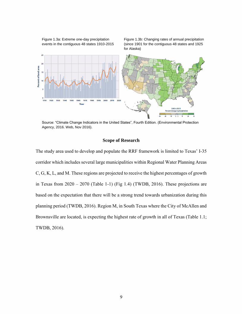
The drought which began in 2010 set drought of record conditions in some parts of Texas

and in those areas became the new baseline for water planning (TWDB, 2016). Data

indicate that most of Texas has experienced increasing average precipitation rates over

the last century and extreme precipitation events are on the rise (Fig. 1.3a & 1.3b). These

extreme precipitation events cause the average precipitation rates to rise and skew the

average to be misleading in terms of typical precipitation rates. This is especially

problematic when considering the slow recharge rates of many aquifers. Extreme

precipitation events may lead to floods and runoff, and may not contribute so

significantly to groundwater recharge.

9

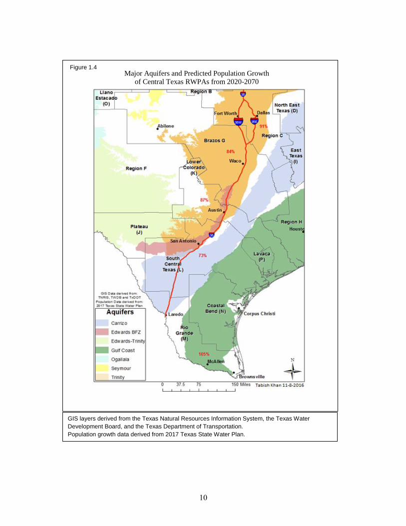
Scope of Research

The study area used to develop and populate the RRF framework is limited to Texas’ I-35

corridor which includes several large municipalities within Regional Water Planning Areas

C, G, K, L, and M. These regions are projected to receive the highest percentages of growth

in Texas from 2020 – 2070 (Table 1-1) (Fig 1.4) (TWDB, 2016). These projections are

based on the expectation that there will be a strong trend towards urbanization during this

planning period (TWDB, 2016). Region M, in South Texas where the City of McAllen and

Brownsville are located, is expecting the highest rate of growth in all of Texas (Table 1.1;

TWDB, 2016).

Figure 1.3a: Extreme one-day precipitation

events in the contiguous 48 states 1910-2015 Figure 1.3b: Changing rates of annual precipitation

(since 1901 for the contiguous 48 states and 1925

for Alaska)

Source: “Climate Change Indicators in the United States”, Fourth Edition. (Environmental Protection

Agency, 2016. Web, Nov 2016).

10

Figure 1.4

GIS layers derived from the Texas Natural Resources Information System, the Texas Water

Development Board, and the Texas Department of Transportation. Population growth data derived from 2017 Texas State Water Plan.

Major Aquifers and Predicted Population Growth

of Central Texas RWPAs from 2020-2070 Major Aquifers and Predicted Population Growth

of Central Texas RWPAs from 2020-2070

11

Chapter 2: Literature Review

Introduction to Resilience and Frameworks

Since 2011, resource analysts have produced notable resilience research on topics such as

climate change, community health, food security, and disaster relief (Table 2.2) (Schipper

and Langston, 2015). Some of this research has been led by humanitarian organizations or

non-government organizations (NGO) dedicated to international aid, reflecting the

dependence of humans and ecosystems upon this resource (Schipper and Langston, 2015)

(Steward et al., 2009). One theme is achieving inter-generational equity to ensure

groundwater availability for future use, balancing natural and man-made discharge with

recharge, through natural discharge factors such as evapotranspiration and subsurface

flows (Ritchey et al., 2015). Groundwater aquifers may be affected by climate change and

pumping by humans (Ritchey et al., 2015). Some studies conducted by the EPA and others

have reported shifts in the seasonal distribution and yearly variability of rainfall, and

therefore recharge, can be expected in the second half of the 21st century (EPA, 2016;

Stigter et al., 2011). Seasonal rainfall may increase during the winter at the expense of

lower rainfall in the spring and autumn months (Stigter et al., 2011). Stigter et al., (2011),

hypothesize that inter-annually, extreme rainfall events, and ever-longer droughts may

become more common. Hugman et al., (2012) reported that concentrated rainfall from

climate change could reduce sustainable aquifer yields by 3-5% over time, based on similar

examples of public supply withdrawals (A), aquifer storage coefficients, and locations of

public supply wells with the distribution of recharge being the test variable (Table 2-1)

(Hugman et al., 2012). The distribution of recharge variables tested two scenarios – average

12

annual value of recharge distributed uniformly over six months from October to March

against average annual value of recharge distributed two months from November to

December (Hugman et al., 2012). The first scenario depicted standard present day

conditions while the second scenario simulated an extreme version of changes in rainfall

patterns as a result of climate change (Hugman et al., 2012). Appendix 1 lists additional

community and groundwater resilience frameworks.

13

Chapter 3: Introduction to the RRF

This report develops a categorical approach to organize multi-attribute variables to provide

a concise, graphical means to evaluate difficult problems on a resilience to vulnerability

scale. This approach is scalable and repeatable in other scenarios with varying data. The

goal of this framework is to provide a visual and holistic view of an area’s relative

resilience against extreme or chronic events which threaten water supplies.

Summary of Methodology

To build a tool to visualize multiple metrics that are used to evaluate groundwater

resilience: indicators of groundwater resilience were chosen; a metric was selected to

represent the indicator; data were identified to measure the metric and tabulated (Appendix

2); the data were normalized to fit the scale by converting their real values to representative

values on a scale of 0-10 with “0” indicating high resilience and “10” indicating high

vulnerability (Appendix 2); and the scale values were plotted on the radial spoke

representing their indicator on the RRF diagram (Figure 3.1).

Figure 3.1: RRF Diagram

Layout

14

After plotting the scaled values for a particular subject located within the study area, a

polygon can then be drawn by connecting the dots and this will give a visualization of the

subject’s relative resilience categorically and overall to other subjects in the dataset (Figure

3.2).

The study area chosen for this proof of concept was the I-35 corridor in Texas. This region

was divided by individual counties for which data were collected. Six key indicators were

chosen and they are representative concepts that reflect resilience:

Average annual high temperature – These data were collected from “U.S. Climate Data”

online and indicate the average high temperature of a city located within the county for all

months in a year (Table 3-2) (USCD, 2016). The temporal range of this average is provided

on a city by city basis in Table 3-2. The city acts as a proximate representative of the

county’s annual average high temperature.

Average total annual precipitation – These data were collected from “U.S. Climate Data”

online and indicate the average total inches per year of rain that a city within the county

receives (Table 3-2) (USCD, 2016). The temporal range of this average is provided on a

Figure 3.2 RRF Results Sample

15

city by city basis in Table 3-2. The city acts as a proximate representative of the county’s

annual average high temperature.

Estimated total groundwater availability of the region’s underlying aquifer – These data

were collected from the 2007 TWDB State Water Plan and indicate the estimated

groundwater availability of the entire aquifer the county is in the territory of in acre-ft per

year for 2010 (Table 3-3) (TWDB, 2007).

Total area of the outcrop of the aquifer underlying the region – These data were collected

from the 2007 TWDB State Water Plan and indicate the area of the whole outcrop

associated with the aquifer the county is in the territory of in square miles (Table 3-3)

(TWDB, 2007).

The existence of a GCD in the region – This metric was based on a simple analysis of

whether or not the county being measured was located in the territory of a GCD or a

Subsidence District which would indicate permitting of groundwater withdrawals. This is

a metric which needs more development as there is more nuance to the factors which go

into how effective groundwater management is at the local level (Figure 3.3).

Shortage – These data were collected from the 2016 Regional Water Plans for Regions B,

C, G, K, L, M, and N. The data indicate the difference between total expected supply and

total expected demand in acre-ft. per year for each county by 2040 if water management

strategies are not executed (Table 3-1).

16

Indicator Selection

Indicators are measurable metrics which are synonymous with what Keeney and Gregory,

(2005) refer to as “attributes.” Keeney states that attributes need to be unambiguous,

comprehensive, direct, operational, and understandable (Keeney and Gregory, 2005).

These attribute characteristics build on Keeney’s research organizing attributes into three

categories: natural attributes, constructed attributes, and proxy attributes. Natural attributes

are related directly to the observation; they are the simplest to measure and the easiest to

portray (Keeney, 1992). For example, to describe the amount of water drained from a

container, a volumetric measurement of the water before and after the container is drained

would provide an exact value of how much water was lost from the container. Natural

attributes are the preferred category of attributes (Keeney and Gregory, 2005). Constructed

attributes allow for observations and measurement of a topic where no real natural attribute

exists – such as the stock market (Keeney and Gregory, 2005). The Dow Jones index was

a constructed attribute derived from a collection of stock scores to indicate the general

trend of the stock market (Keeney and Gregory, 2005). Proxy attributes do not measure the

objective of concern directly; through a relationship with the performance variable they

provide an indication of the sought-after metric. For example, the quality of a restaurant

may be measured by the number of repeat customers. This is not a direct indication of the

quality of the restaurant. However, it does provide a measure by which to gauge quality

despite many other variables which may also effect the result.

17

RRF Derivation and Framework Design

Variables from resilience frameworks listed in Appendix 1 were evaluated and included in

the RRF if they indicated regional water supply resilience and the required data was

accessible. This test of the RRF measures four categories which are divided into six

variables. The categories include: formation, which consists of outcrop area and

groundwater availability; policy, which accounts for the existence of a GCD in the region;

supply and demand, which is combined into the shortage variable; and climate, which takes

into account average annual high temperatures and average annual precipitation (Table 3-

1, Table 3-2, Table 3-3). These variables were analyzed against the qualifications for

desirable attributes given by Keeney and Gregory, (2005), to provide further validation.

The following diagram developed by Richmond, et al., (2015) was the design source for

the RRF Diagram (Fig. 3.1).

Figure 3.1: Household Vulnerability Network Model

Source: Richmond et al., 2015. Household Vulnerability

Mapping in Africa’s Rift Valley: Applied Geography, no.

63, p. 380–395.

18

Proportional Metrics

The RRF presents each variable or measure for a specific region under study as a

proportional metric. Each proportional metric is measured only against the range of data

within its variable type, which indicates its relative resilience to the other data. As

additional sets of variables are added, the maximum and minimum values can change

which would adjust the proportional values of every case study to the new range. Therefore,

each metric is plotted proportionally with respect to the maximum and minimum values

present in the dataset. For example: the availability of aquifer A is 10 acre-ft; aquifer B is

100 acre-ft; and aquifer C is 55 acre-ft. The maximum availability is set at 100 acre-ft and

the minimum will be 10 acre-ft. Therefore aquifer A will be represented with a scale value

of 10 – highly vulnerable and aquifer B will be represented with a scale value of 0 – highly

resilient. Aquifer C in this example falls directly in the middle of the range and therefore

receives a scaled value of 5.

Category Descriptions and Variables

Based on an evaluation of available data with guidance from previous research, the

following categories were selected in order to construct the proof-of-concept RRF.

Supply and Demand

Policy

Climate

Formation

Each category is then subdivided into the variables for which raw data was gathered and

converted into the scaled values for display.

19

Supply and Demand

Supply and Demand: The supply and demand data was obtained from the Texas Regional

Water Plans. Shortages can be calculated from this data by comparing projected supply

from all water sources against projected demand from all water users groups for the

planning period – which is 50 years. The data range for shortages included all values in a

given planning year for the counties within the study area outlined in Figure 3.2. The

following measure is used for the proof of concept implementation in the Supply and

Demand Category:

Shortages - measured in acre-feet/year by county within the study area (Table 3.1,

Fig 3.1).

20

Acft/Year

Shortage

-497,403

-497,402 - -450,000

-449,999 - -400,000

-399,999 - -300,000

-299,999 - -200,000

-199,999 - -100,000

-99,999 - -50,000

-49,999 - -18,000

-17,999 - 800

801 - 1,800

1,801 - 2,600

2,601 - 3,400

3,401 - 4,200

4,201 - 5,000

Figure 3.2: Shortages by County (Acre-Feet/Year)

GIS layers derived from the Texas Department of Transportation.

Shortage data derived from 2016 Region B, C, G, K, L, M, and N water plans.

21

Public Policy

Public Policy: GCD jurisdiction over a county allows permitting based on the desired

future conditions developed from modeled available groundwater. This measure can

indicate enhanced resilience, however, is not readily quantifiable and can be inconsistent.

As a constructed attribute, a value system must be assigned to quantify this variable. This

category can benefit from additional variables such as the strength of GMA cooperation,

compliance with permitting, and consistent rules between GCDs. Most counties have

GCDs which span their political boundaries while others may be conglomerates of multiple

counties (Fig 3.3). In addition, some counties such as Hidalgo, have partial GCD coverage.

The following measures are used in the Public Policy Category:

The presence of a GCD will yield a scale value of “1” or highly resilient.

The absence of a GCD will yield a scale value of “10” or highly vulnerable.

Partial jurisdiction within the county will yield a scale value of “5” or moderately

resilient.

22

Figure 3.5

GIS layers derived from the Texas Department of Transportation and the Texas Water Development

Board.

23

Climate

Climate: The climate of a region can affect groundwater recharge, surface water stability,

and regional dependence on water resources. The effects of climate on different regions

can be unique and dependent on many variables. However, variables which offer a reliable

and consistent indicator of climactic influence on a particular area were necessary. Data

for the climate category was derived from U.S. Climate Data online and records range

between 1981-2010 as well as 1961-1990 (Table 3.2; USCD, 2016). The following

measures are used in the Climate Category:

Historical record of annual precipitation rates – collected by city to indicate

proximate value for surrounding county and measured in average inches per year.

Historical annual average high temperatures – collected by city to indicate

proximate value for surrounding county and measured in degrees Fahrenheit.

Formation

Formation: The formation category contains variables which indicate the region’s access

to resilient groundwater sources. Groundwater provides a diversification factor to a

region’s water supply which reduces susceptibility to water shortages during drought. The

variables which contribute to an aquifer’s resilience must then be evaluated to gain

resolution on the aquifer’s contribution to regional resilience. Data for the formation

category were extracted from the 2007 “Water for Texas” State Water Plan (Table 3.3)

(TWDB, 2007). The availability data range reflects a range provided in the “Individual

Aquifer Data” section of the modeled groundwater availability for 2010. Outcrop surface

area is also derived from the “Individual Aquifer Data” section of the 2007 State Water

24

Plan (TWDB, 2007). The outcrop and availability range contains the data of all major and

minor aquifers which are located in, or go through, the State of Texas. The following

measures are used for the proof of concept implementation in the formation category:

Groundwater availability of the entire aquifer atop which the county is located –

measured in acre-feet.

Area of the entire outcrop of the aquifer atop which the county is located –

measured in miles2.

Quantitative Evaluation

Compilation of the data and normalization to a 1-10 scale allowed for relative measurement

of resilience by variable for each county. The following equation (Eq. 1) allowed for each

real value to be proportionally measured on a scale of 1-10 within the range of the input

dataset. The resulting “V” value can then be plotted on its respective radial line on the

circular diagram. To calculate “V”, the following equation was used where:

X = The real world value of the specific variable (i.e. area of outcrop).

XMax = The maximum value in the range of real values for the specific variable.

XMin = The minimum value in the range of real values for the specific variable.

XMax – XMin = The range of the dataset.

Therefore, the following equation provides the position of a real value on a scale of 1-10

in relation to its dataset.

25

All variables, except for temperature, equated to higher resilience with larger real world

values. Due to higher real world temperatures yielding lower resilience, the “V” value of

the temperature variable was subtracted from 10. This inverted its location on the radial

scale to follow the same direction indicating resilience as the other values.

Design of RRF Graphic

The graphic design and layout were inspired by the Household Vulnerability Diagram by

Richmond, et al., (2015). This diagram allowed the simultaneous display and comparative

analysis of multiple variables and cases at once. There are many other categories, sub-

variables, and spatial variables which can be integrated and analyzed in this framework,

however, time constraints and data availability have limited this case study. Once data for

each variable is compiled and processed into the “1-10” scaled values. It can then be plotted

on the RRF diagram. Connecting the plotted points between neighboring variables yields

a polygon which depicts a general view of the relative resilience of the county being

measured with all other counties in the dataset.

Equation 1: Real Value to Scale Value Conversion

26

Proof-of-Concept

The study area to which the framework was applied is what has been called the “I-35

corridor” (Fig. 3.6). This is not a well-defined list of counties but rather an ambiguous mass

of counties which are located along or near the path of Interstate-35 as it runs from North

to South Texas. Cities along the I-35 corridor are some of the most populous in Texas

(Table 1-1) and include major population centers such as Dallas, Fort Worth, Waco, Austin,

San Antonio, San Marcos, Brownsville, and McAllen. Brownsville and McAllen are not

along the route of I-35, however, they are relatively near the study area and statistically

significant when discussing water shortages in Texas.

27

GIS layers derived from the Texas Natural Resources Information System, the Texas Water

Development Board, and the Texas Department of Transportation.

Figure 3.6: Study Area

Tabish Khan 11-8-2016

28

Chapter 4: Results

Discussion

The lowest availability value in this dataset is 200 acre-ft/yr from the Marathon Aquifer.

The highest availability in the dataset is 5,968,260 acre-ft from the Ogallala Aquifer. The

lowest outcrop area in the dataset is 0 miles2 since multiple aquifers have no reported

outcrop. The highest outcrop area is 32,294 miles2 over the Edwards-Trinity Plateau

Aquifer (TWDB, 2007).

The lowest precipitation value in the dataset is 9.69 inches/year in El Paso (Table 3.2)

(USCD, 2016). The highest total annual precipitation dataset is 60.55 inches/year in Port

Arthur (USCD, 2016). The lowest value in the dataset is 70.9 degrees Fahrenheit in

Amarillo (USCD, 2016). The highest average maximum temperature in the dataset which

is 85.9 degrees Fahrenheit in McAllen (USCD, 2016).

29

Figures 4.1 and 4.2 depict the RRF results for Hidalgo and Dallas County along with the

values on which those results were based.

Initial analysis of this result indicates Hidalgo County is expecting extreme shortages

relative to other counties in the dataset. The dataset for this variable only included

counties along the I-35 corridor study area, so these results are spatially limited. Most

variables for Hidalgo County indicate high vulnerability and the only apparent resilience

factor appears to be partial coverage by a GCD. Most of Hidalgo County is not located

within a GCD, however a small portion is within the jurisdiction of the Red Sands GCD,

Kenedy GCD, and Brush Country GCD. This may be due to Hidalgo County’s reliance

on surface water since it and the rest of Region M obtain the majority of their water from

the Rio Grande (RGRWPG, 2015). The majority of the Gulf Coast Aquifer underlying

this area is actually brackish (RGRWPG, 2015). In addition, the median income of

Figure 4.1: RRF Results for Hidalgo County

30

Hidalgo County is $33,218, with 35% of the population living below the poverty line

(RGRWPG, 2015). Water management strategies for this area are focused on

conservation, especially in the irrigation sector which is expecting a decrease in demand

due to urbanization (RGRWPG, 2015). However, the combination of vulnerability factors

combined with the potential for drought are indicative of difficulties in the future if

conservation goals are not met.

Dallas County also scores high vulnerability rates, when viewed from a groundwater

perspective. This is due to its high dependence on surface water resources (RCWPG,

2015). Dallas County is facing significant shortages as well, however, the relativity

feature of the RRF skews this metric due to the immense shortages of other counties

evaluated in the case study. Management strategies for Region C, within which Dallas

County is located, include new surface water projects (RCWPG, 2015). This will increase

Figure 4.2: RRF Results for Dallas County

31

the resilience factor of this region if more extreme but less frequent precipitation is to be

expected. Longer and more frequent droughts, however, strain surface water resources

and can be detrimental unless a diverse water portfolio is utilized.

Figures 4.3 - 4.8 depict the RRF results of I-35 corridor counties in North Texas, North

Central Texas, the Lower Colorado, South Central Texas, the Rio Grande Region, as well

as several counties in the Coastal Bend.

Figure 4.3: RRF Results for North Texas

32

Counties in North Texas are mostly dependent upon surface water resources (RCWPG,

2015). These counties overlie the Trinity Aquifer which scored low on the resiliency

scale in relation to the Edwards-Trinity Plateau with its relatively large outcrop and the

Ogallala which is estimated to have the highest availability in this dataset (Table 3-3).

These counties do not appear to be expecting shortages in the near future, however, this

situation could change with the variability of climate. Currently, precipitation and

temperature averages appear to be relatively moderate. Most counties also appear to

reside within GCDs except Dallas and Navarro. Counties in and around the DFW

Metroplex are expecting the largest municipal growth in the region and could benefit

from diversification of their water supply.

Figure 4.3 Continued: RRF Results for North Texas

33

Figure 4.4: RRF Results for North Central Texas

34

North Central Texas counties are in many ways similar to North Texas counties. They also

overly the Trinity Aquifer are not expecting significant shortages, and are dependent on

surface water (BGRWPG, 2015). The same threats of prolonged drought and variability in

precipitation apply to these counties as well. Currently, relative temperatures and

precipitation rates are moderate in this region.

Figure 4.4 Continued: RRF Results for North Central Texas

35

The counties of the Lower Colorado Region have a wider variety of water sources. These

sources include the Lower Colorado River basin, the Edwards Aquifer, and the Trinity

Aquifer (LCRWPG, 2015). These counties are not expecting shortages in the coming

decades, are mostly covered by GCDs, and have relatively moderate temperatures and

precipitation. In addition, the sensitive Edwards Aquifer which underlies this area is

monitored and managed by the Edwards Aquifer Authority.

Figure 4.5: RRF Results for Lower Colorado Counties

36

Figure 4.6: RRF Results for South Central Texas

Counties

37

South Central Texas Counties include the San Antonio area as well as the Winter Garden

Region. These counties depend on multiple aquifers and place a heavy municipal and

agricultural demand on those formations (SCTRWPG, 2015). San Antonio’s municipal

supply is principally extracted from the Edwards Aquifer and the limitations of this

supply has caused San Antonio to ambitiously engage in conservation. In addition, San

Antonio is pursuing alternative water management strategies including aquifer storage

and recovery as well as brackish desalination. The Winter Garden agricultural region is

heavily dependent on the Carrizo-Wilcox Aquifer for year-round irrigation, however,

demand expectations for this region are shifting from agriculture to municipal in the long

term. Temperatures for this region are generally higher than areas further north and

several counties also see less average precipitation. Most of this region is under the

jurisdiction of GCDs. Given the municipal growth as well as the limited supply from

Edwards Aquifer, development of alternative supplies is ongoing to fulfill future

demands.

Figure 4.6 (Continued): RRF Results for South Central Texas

Counties

38

The counties of the Rio Grande River Basin are heavily dependent on it for their water

supply (RGRWPG, 2015). The Gulf Coast Aquifer in this region is brackish and would

require costly desalination to be suitable for municipal or agricultural use (RGRWPG,

2015). The socioeconomic conditions of this region are poor. Therefore costly water

management strategies could place vulnerable user groups at risk (RGRWPG, 2015). The

current water management strategies for this region are heavily dependent on conservation

Figure 4.7: RRF Results for Rio Grande Counties

39

and the expectation that irrigation demand will shift to municipal demand (RGRWPG,

2015). Unfortunately, like North Texas, high dependence on surface water and the potential

for droughts make this a vulnerable region. On average, this region has the highest

temperatures as well as poor precipitation levels (Table 3-2). This region is also

anticipating some of the highest shortages in the State.

The counties of the Coastal Bend region are relatively similar and have a water portfolio

mostly dependent on surface water supplies. While there is groundwater use in this

region, it is limited because sources from the Carrizo-Wilcox and Gulf Coast Aquifers

can be saline (CBRWPG, 2015). This region has relatively high temperatures and

moderate precipitation (Table 3-2). All four of the counties evaluated in this study are

covered by GCDs and do not anticipate shortages in the coming years.

Figure 4.8: RRF Results for Coastal Bend Counties

40

Chapter 5: Conclusions, Discussion, and Suggestions for Future Research

The diverse geographic conditions across Texas result in a variety of climate conditions,

resource availability, demand types, and population concentrations. This set of variables

requires prioritization when setting policy and complicates blanket approaches that affect

the entire State and its different user groups. North, Central, and South Texas regions are

all facing immense growth in their urban population centers. It has so far been ethically

acceptable if not economically harmful to deny agricultural users water in times of

shortages, however, municipal demands must be met and to withhold water from those

users would be a public policy and resource management failure. Water policy in Texas is

fractured and in many ways could benefit from a more centralized planning perspective.

The typical planning cycle of a GCD does involve a joint planning process with their

respective GMAs, however, this process seems excessively complex. A more efficient

method could involve an entity which has the authority and capacity to manage an aquifer

as a whole and not by county. Since GMAs already have boundaries more aligned with

their respective aquifers, it would make sense to elevate permitting and management

functions to the GMA level. The heavy dependence on surface water without significant

alternatives appears to be the most significant weakness in the management strategies of

several regions. Diversification and conservation will most likely aid the mitigation of

challenges brought on by population growth, drought, and climate change.

Several factors can be further broken down and researched to develop this framework. An

assessment of the factors which contribute to effective groundwater management and not

just the existence of GCDs would contribute to the framework. In addition, socioeconomic

41

variables need to be considered in order to add reinforcement to an area’s vulnerability in

the case that alternative water management strategies are needed. Refined equations could

compensate for the skewing of proportional values when analyzing availability and

shortages. The immense disparity within the ranges resulted in the minimization of

significant variables which fell out of scope. A surface water dependence variable would

have readily placed into perspective the balance of sources which each county depended

on and would reduce explanatory measures needed to convey information from the

diagram. In conclusion, there are many challenges ahead for Texas water planners but

frameworks and indicators can help bridge science and policy by making data more

accessible.

Assumptions and Limitations

Assumptions in this framework include the drought of record of the 1950’s as a minimum

benchmark for some of the data that is utilized in the framework.

Limitations of the framework include the lack of water quality indicators. Additionally, the

framework would be more accurate and meaningful if the following factors were added:

● Additional recharge variables to form a more accurate evaluation of recharge

potential.

● Dependence of an area on surface water resources would allow for mitigation of

variables which otherwise indicate strong groundwater vulnerability. This factor

would also indicate general vulnerability to drought and climate change.

● Additional data points. Due to the scale’s relative nature, as more data is entered,

more accuracy is achieved. However, the datasets must be limited to any level of

political boundaries to maintain relevance to public policy. In addition, the larger

the boundaries of the area being measured, the more data points will be needed to

achieve higher resolution.

42

Additionally, this framework and the resulting data interpretations are limited by the scope

of the entered data. Therefore, the more data that is utilized, the higher the resolution and

relative indication of resilience. Due to the fragmented nature of water planning this case

study is also based on fragmented data which reduces the accuracy of relative values.

Variables which are chosen to represent resilience and the depth of the data representing

those variables are also a potential weakness on the application side of the RRF. Lastly,

while the effects of climate change and droughts could be mitigated for by prioritizing

regional water management strategies, the exact threat levels to discrete areas of Texas are

still unknown.

43

Appendix 1: Previous Research and Related Frameworks

Community Resilience Frameworks

The ARCAB framework analyzes the effects of climate change on the resilience and

vulnerability of communities (ARCAB, 2012). ARCAB cites poverty as a critical

contributor to vulnerability since the poor are less likely to have the resources necessary to

cope with the predicted effects of climate change thereby reducing their adaptive capacity

(ARCAB, 2012). For a community, individual, household, economy, or any organization,

high adaptive capacity improves resilience against climate change (ARCAB, 2012).

Multiple organizations have adopted the concept of adaptive capacity with indicators such

as poverty levels, food security, and water security (ARCAB, 2012) (DFID, 2014).

The DFID methodology recommends that resilience indicators:

Seek to capture changes in people’s behavior or circumstances that will

make them better able to anticipate, avoid, plan for, cope with, recover

from, and adapt to the shocks and stresses that they are likely to face in the

foreseeable future - (DFID, 2014).

The focus of the DFID method is on the adaptive capacity of communities to increase

resilience by reducing dependence. When applied to water management, this would imply

conservation strategies such as drought resistance crops or the use of micro-irrigation

(DFID, 2014).

The Household Vulnerability Framework by Richmond et al., (2015) includes human

vulnerability from socioeconomic and environmental stress, which can be amplified by

increasing populations (Richmond et al., 2015). The Household Vulnerability Framework

also states the lack of appropriate resolution for individual groups when evaluating data on

44

regional scales (Richmond et al., 2015). Within a region, various groups of individuals can

be affected differently (Richmond et al., 2015). So even if an area has sufficient water

supply from proposed water management strategies it may not have high resilience.

Consideration should be given to how accessible is a water supply to different user groups

and socioeconomic levels. As the price of water increases, the poor will be at a

disadvantage, thereby reducing their resilience. The Household Vulnerability scale also

organizes indicators of vulnerability into “baskets” - an approach similar to that used by

Busby et al., (2012) (Richmond et al., 2015). The Household Vulnerability indicators were

normalized within each basket between zero and one, with zero representing the poorest

condition for a household and one being optimal (Richmond et al., 2015). Richmond et al.,

(2015) cited fieldwork, literature reviews, direct observations, and expert opinions as the

basis on which weights were given to each basket to determine vulnerability scores. After

normalization, a basket score was calculated by taking the average score for all of the

variables within the basket (Richmond et al., 2015). The basket score was multiplied by

the basket weighting metric to derive a final vulnerability score out of 100 (Richmond et

al., 2015).

Groundwater Frameworks

There are also frameworks which focus solely on water issues such as a framework

developed by the Environment Protection Agency (EPA) known as the DRASTIC method.

The DRASTIC method contains parameters such as depth to groundwater, net recharge,

aquifer media, soil media, general topography, impact of the vadose zone, and the hydraulic

conductivity of the aquifer (Bataineh et al., nd). By these measures, the DRASTIC

45

approach is highly focused on water quality issues (Bataineh et al., nd). The DPSIR

framework, developed by the European Environment Agency (EEA) for its analysis of

water-related issues, analyzes the factors which contribute to water supply and quality as

well as demand and user metrics (Kristensen, 2004). Like the DRASTIC method, DPSIR

is an acronym for the categories of variables being measured. “D” represents the driving

forces; “P” represents pressures on the environment; “S” represents the consequent state

for the environment; “I” represents impacts on the environment; and “R” represents the

responses to these effects by humans (Fig. 2.1) (Kristensen, 2004). The DPSIR framework

offers indicators and a process to evaluate water resilience, however, it does not appear to

offer a measurement system to quantify these variables.

Groundwater Resilience Frameworks and Research

The study of groundwater resilience can help to identify the circumstances which cause

high vulnerability (Stigter et al., 2011). Hashimoto et al., (1982) measured groundwater

performance through resilience, vulnerability, and reliability. Reliability conveyed the

frequency or probability that a system maintained a satisfactory state (Hashimoto et al.,

1982). Peters et al., (2004), employed Hashimoto’s performance indicators to assess

groundwater performance during drought and made calculations from precipitation,

evapotranspiration, recharge, and discharge variables. Ritchey et al., (2015) added

groundwater storage as a factor of groundwater resilience. Groundwater’s ability to provide

resilience to a community is based on its typically larger storage capacity and higher

residence times than those of typical inland surface water sources (Anderies et al., 2006)

(Hugman et al., 2012) (Katic and Grafton, 2011) (Lapworth et al., 2012) (MacDonald et

46

al., 2011) (Shah, 2009) (Sharma and Sharma, 2006) (Taylor et al., 2013). Despite the many

frameworks and analysis tools available, a method to analyze and visually present multi-

criteria resilience indicators for assessment on a relative basis was not found.

47

Appendix 2: Tables

Region 2020 2030 2040 2050 2060 2070 % GrowthA 419,000 461,000 504,000 547,000 592,000 639,000 53

B 206,000 214,000 219,000 223,000 226,000 229,000 11

C 7,504,000 8,649,000 9,909,000 11,260,000 12,742,000 14,348,000 91

D 831,000 908,000 989,000 1,089,000 1,212,000 1,370,000 65

E 954,000 1,086,000 1,208,000 1,329,000 1,444,000 1,551,000 63

F 701,000 767,000 825,000 885,000 944,000 1,003,000 43

G 2,371,000 2,721,000 3,097,000 3,495,000 3,918,000 4,351,000 84

H 7,325,000 8,208,000 9,025,000 9,868,000 10,766,000 11,743,000 60

I 1,152,000 1,234,000 1,310,000 1,389,000 1,470,000 1,554,000 35

J 141,000 154,000 163,000 171,000 178,000 185,000 31

K 1,737,000 2,065,000 2,382,000 2,658,000 2,928,000 3,243,000 87

L 3,001,000 3,477,000 3,920,000 4,336,000 4,770,000 5,192,000 73

M 1,961,000 2,379,000 2,795,000 3,212,000 3,626,000 4,029,000 105

N 615,000 662,000 693,000 715,000 731,000 745,000 21

O 540,000 594,000 646,000 698,000 751,000 802,000 4

P 50,000 52,000 53,000 54,000 55,000 56,000 12

Texas 29,508,000 33,631,000 37,738,000 41,929,000 46,353,000 51,040,000 73

Data derived

from 2017

Texas State

Water Plan

Table 1-1

Projected Population Growth in Texas by Regional Planning Areas

48

1Aia Distributed Seasonal Optimized Concentrated 73% 75.9

2Aia Concentrated Seasonal Optimized Concentrated 70% 72.8

1Aib Distributed Seasonal Optimized Distributed — —

2Aib Concentrated Seasonal Optimized Distributed — —

1Aiia Distributed Seasonal Reduced 2x Concentrated 70% 72.8

2Aiia Concentrated Seasonal Reduced 2x Concentrated 67% 69.7

1Aiiia Distributed Seasonal Reduced 5x Concentrated 40% 41.6

2Aiiia Concentrated Seasonal Reduced 5x Concentrated 35% 36.4

1Bia Distributed Constant Optimized Concentrated 79% 82.4

2Bia Concentrated Constant Optimized Concentrated 76% 79

1Bib Distributed Constant Optimized Distributed 79% 82.4

2Bib Concentrated Constant Optimized Distributed 74% 77

A = public supply withdrawal

PS = public supply

R = Recharge

Table 2-1

Table derived from

(Hugman et al., 2012) Overview of Scenarios and Optimized Sustainable Yield

Distribution

of R

Distribution

of A

Storage

coefficient

Location of PS

wells

MAR = mean annual recharge

Sustainable yield

% of MAR hm3Scenario

49

Organization Framework Title Source

Rockefeller Foundation Asian Cities Climate Change Resilience (Tyler et al., 2014)

Global Change System for Analysis, Research, and

Training

Assessments of Impacts and Adaptations of Climate Change Sustainable

Livelihood Approach(Elasha et al., 2005)

Sea Change Action Research for Community Based Adaptation (ARCAB, 2012)

Rockefeller Foundation ARUP’s City Resilience Framework (ARUP, 2014)

UK Department for International Development Resilience and Adaptation to Climate Extremes and Disasters Framework (DFID, 2014)

United Nations Development Programme Community-Based Resilience Analysis Framework (UNDP, 2013)

Food and Agricultural Organization and World Food

ProgramPrinciples of Resilience Measurement for Food Insecurity (Barret and Constas, 2013)

United Nations University - Institute for Environment and

Human SecurityCapital-Based Approach to Community Disaster Resilience (Mayunga, 2007)

Feinstein International Center Livelihood and Resilience Framework (Vaitla, 2012)

International Institute for Sustainable Development Climate Resilience and Food Security (IISD, 2013)

UN Food and Agriculture Organization’sSelf-evaluation and Holistic Assessment of Climate Resilience of

Farmers and Pastoralists Framework(Choptiany et al, 2015)

International Institute for Environment and Development Tracking Adaptation and Monitoring Development (Brooks et al., 2013)

Non-Government Organization Characteristics of a Disaster Resilient Community (Twigg, 2009)

United Nations International Strategy for Disaster Risk

ReductionDisaster Resilience Scorecard for Cities (UNISDR, 2014)

United States Agency for International Development Measurement for Community Resilience (USAID, 2013)

United States Agency for International Development Coastal Resilience (Indian Ocean Tsunami Warning System Program) (USAID, 2007)

Table 2-2

List derived from (Schipper et al., 2015) A Sampling of Existing Resilience Frameworks

50

County Shortage V Shortage V Shortage V Shortage V Shortage V Shortage V

Atascosa -171 0.11 -257 0.11 -333 0.10 -409 0.10 -484 0.10 -579 0.09

Bastrop -4,184 0.20 -11,327 0.35 -15,883 0.45 -22,596 0.59 -32,730 0.80 -47,187 1.02

Bell No data No data No data No data -16,675 0.47 No data No data No data No data -42,904 0.93

Bexar -61,851 1.52 -88,049 2.08 -112,441 2.59 -141,763 3.21 -172,269 3.84 -202,304 4.11

Blanco -48 0.11 -105 0.10 -138 0.10 -179 0.10 -209 0.09 -230 0.08

Bosque No data No data No data No data -6,955 0.25 No data No data No data No data -14,002 0.36

Brooks 1,647 0.07 1,498 0.07 1,357 0.07 1,189 0.07 1,022 0.06 848 0.06

Burnet -1,258 0.14 -2,401 0.15 -4,718 0.20 -6,850 0.24 -8,769 0.28 -10,457 0.28

Caldwell -188 0.11 -685 0.11 -1,326 0.12 -2,134 0.14 -3,024 0.15 -3,907 0.15

Cameron -206,026 4.83 -193,330 4.46 -187,351 4.25 -183,864 4.14 -182,476 4.07 -198,668 4.04

Collin -18,865 0.54 -65,722 1.58 -105,470 2.44 -145,168 3.29 -177,270 3.95 -207,655 4.22

Comal -5,153 0.23 -7,942 0.28 -14,360 0.41 -20,778 0.55 -27,492 0.69 -34,079 0.76

Cooke -849 0.13 -288 0.11 -300 0.10 -461 0.10 -1,058 0.11 -5,017 0.18

Coryell No data No data No data No data -1,577 0.13 No data No data No data No data -5,234 0.18

Dallas -42,674 1.08 -101,656 2.39 -159,703 3.64 -206,626 4.64 -248,412 5.50 -280,615 5.67

Denton -12,241 0.39 -47,075 1.16 -86,617 2.02 -128,970 2.93 -174,830 3.90 -216,283 4.39

Dimmit -8,790 0.31 -8,991 0.30 -8,203 0.28 -6,594 0.24 -4,013 0.17 -3,169 0.14

Duval 4,679 0.00 4,413 0.00 4,292 0.00 4,163 0.00 4,002 0.00 3,824 0.00

Ellis -1,611 0.14 -5,680 0.23 -14,495 0.42 -24,579 0.63 -43,984 1.05 -73,554 1.54

Falls No data No data No data No data -425 0.10 No data No data No data No data -511 0.09

Frio 0 0.11 0 0.10 0 0.10 0 0.09 0 0.09 -19 0.08

Gonzales 0 0.11 0 0.10 0 0.10 -249 0.10 -92 0.09 -373 0.08

Grayson -86 0.11 -8,106 0.28 -10,067 0.32 -13,483 0.39 -21,829 0.56 -36,244 0.80

Guadalupe -1,499 0.14 -4,244 0.20 -7,272 0.26 -11,864 0.35 -16,895 0.46 -21,910 0.51

Hamilton No data No data No data No data -175 0.10 No data No data No data No data -17 0.08

Hays -531 0.12 -2,396 0.15 -6,345 0.24 -11,412 0.34 -16,970 0.46 -23,294 0.54

Hidalgo -431,898 10.00 -439,406 10.00 -446,258 10.00 -450,263 10.00 -454,524 10.00 -497,403 10.00

Hill No data No data No data No data -32 0.10 No data No data No data No data -69 0.08

Hood No data No data No data No data 599 0.08 No data No data No data No data -827 0.09

Jim Hogg -239 0.11 -237 0.10 -244 0.10 -295 0.10 -368 0.10 -404 0.08

Johnson No data No data No data No data -6,383 0.24 No data No data No data No data -16,549 0.41

Kendall 0 0.11 0 0.10 0 0.10 -650 0.11 -1,639 0.12 -2,613 0.13

Kenedy 61 0.11 44 0.10 43 0.09 42 0.09 41 0.09 41 0.08

La Salle -4,110 0.20 -4,315 0.20 -3,979 0.18 -2,746 0.15 -851 0.11 -147 0.08

Lampasas No data No data No data No data -2,012 0.14 No data No data No data No data -2,707 0.13

Limestone No data No data No data No data -18,801 0.51 No data No data No data No data -42,346 0.92

McLennan No data No data No data No data -1,404 0.13 No data No data No data No data -13,812 0.35

McMullen 449 0.10 452 0.09 455 0.09 456 0.08 456 0.08 456 0.07

Medina -32,415 0.85 -30,285 0.78 -28,211 0.72 -26,225 0.67 -24,344 0.62 -22,738 0.53

Milam No data No data No data No data -76 0.10 No data No data No data No data -6,757 0.21

Montague -1,315 0.14 -250 0.11 -281 0.10 0 0.09 0 0.09 0 0.08

Navarro -8,000 0.29 -17,038 0.48 -17,838 0.49 -19,144 0.51 -21,055 0.55 -23,704 0.55

Parker -3,349 0.18 -6,752 0.25 -11,025 0.34 -18,031 0.49 -32,667 0.80 -51,749 1.11

Somervell No data No data No data No data -35,915 0.89 No data No data No data No data -35,864 0.79

Starr -7,992 0.29 -6,579 0.25 -5,199 0.21 -6,176 0.23 -7,140 0.24 -8,127 0.24

Tarrant -24,130 0.66 -82,442 1.96 -151,925 3.47 -207,390 4.66 -257,690 5.71 -305,928 6.18

Travis -3,199 0.18 -19,203 0.53 -27,658 0.71 -41,766 1.01 -85,617 1.95 -134,438 2.76

Table 3-1S = Shortage (Acre-Ft/Year)

Scale Value (V) = 10(SMAX-S)/(SMAX-SMIN)

Data derived

from 2016

Regional Water

Plans B, C, G, K, L,

M, and N 2060 20702020 2040 20502030

51

County Shortage V Shortage V Shortage V Shortage V Shortage V Shortage V

Uvalde -30,747 0.81 -28,756 0.75 -26,657 0.69 -24,815 0.64 -23,135 0.59 -21,744 0.51

Webb -4,294 0.21 -2,204 0.15 -2,387 0.15 -10,181 0.32 -17,998 0.48 -25,450 0.58

Willacy -49,376 1.24 -49,445 1.21 -49,529 1.19 -49,627 1.18 -50,075 1.18 -49,994 1.07

Williamson No data No data No data No data -67,836 1.60 No data No data No data No data -163,807 3.34

Wilson 0 0.11 -8 0.10 -405 0.10 -770 0.11 -1,124 0.11 -1,796 0.11

Wise -2,300 0.16 -4,261 0.20 -7,926 0.27 -14,772 0.42 -22,099 0.57 -30,339 0.68

Zapata -1,786 0.15 -1,948 0.14 -2,189 0.14 -2,502 0.15 -2,939 0.15 -3,589 0.15

Zavala -18,487 0.53 -16,805 0.48 -14,980 0.43 -13,049 0.38 -11,193 0.33 -9,443 0.26

Table 3-1 Continued2020 2030 2040 2050 2060 2070

52

County

I-35

Corridor Reference City

Average Annual High

Temperature °F Scaled Value

Adjusted

Scale Value

Average Total

Annual Scaled Value Data

Atascosa Yes Pleasanton 81.2 3.13 6.87 32.09 5.60 1981-2010 normals

Bastrop Yes Elgin 79.3 4.40 5.60 34.43 5.14 1981-2010 normals

Bell Yes Temple 77.1 5.87 4.13 35.84 4.86 1961-1990 normals

Bexar Yes San Antonio 79.8 4.07 5.93 32.91 5.43 1961-1990 normals

Blanco Yes Johnson City 78.6 4.87 5.13 33.99 5.22 1981-2010 normals

Bosque Yes Near Hill County 77.6 5.53 4.47 37.86 4.46 1981-2010 normals

Brazos County No College Station 79.3 4.40 5.60 40.09 4.02 1981-2010 normals

Brooks Yes Falfurrias 84.5 0.93 9.07 26.42 6.71 1981-2010 normals

Burnet Yes Burnet 77.4 5.67 4.33 32.97 5.42 1981-2010 normals

Caldwell Yes Lulling 79.6 4.20 5.80 35.91 4.84 1981-2010 normals

Cameron Yes Brownsville 83.7 1.47 8.53 27.37 6.52 1981-2010 normals

Collin Yes Lavon 75.8 6.73 3.27 40.52 3.94 1981-2010 normals

Comal Yes New Braunfels 78.6 4.87 5.13 33.98 5.22 1981-2010 normals

Cooke Yes Gainesville 73.8 8.07 1.93 42.8 3.49 1981-2010 normals

Coryell Yes Gatesville 79.8 4.07 5.93 33.45 5.33 1961-1990 normals

Dallas Yes Dallas 77.1 5.87 4.13 40.97 3.85 1981-2010 normals

Denton Yes Denton 76 6.60 3.40 38.08 4.42 1981-2010 normals

Dimmit Yes Carrizo Springs 83.4 1.67 8.33 19.72 8.03 1981-2010 normals

Duval Yes Benavides 83.6 1.53 8.47 24.63 7.06 1961-1990 normals

El Paso County No El Paso 77.5 5.60 4.40 9.69 10.00 1981-2010 normals

Ellis Yes Waxahachie 77.7 5.47 4.53 38.81 4.27 1961-1990 normals

Falls Yes Marlin 78.1 5.20 4.80 38.48 4.34 1981-2010 normals

Frio Yes Pearsall 83.3 1.73 8.27 24.75 7.04 1981-2010 normals

Galveston County No Galveston 76.6 6.20 3.80 43.85 3.28 1961-1990 normals

Gonzales Yes Gonzales 79.5 4.27 5.73 34.99 5.03 1981-2010 normals

Grayson Yes Sherman 72.6 8.87 1.13 43.62 3.33 1981-2010 normals

Guadalupe Yes New Braunfels 78.6 4.87 5.13 33.98 5.22 1981-2010 normals

Hamilton Yes Hamilton 76.3 6.40 3.60 28.61 6.28 1961-1990 normals

Harris County No Houston 79.7 4.13 5.87 49.58 2.16 1981-2010 normals

Hays Yes San Marcos 79.6 4.20 5.80 35.75 4.88 1981-2010 normals

Hidalgo Yes McAllen 85.9 0.00 10.00 22.24 7.53 1981-2010 normals

Hill Yes Hillsboro 77.6 5.53 4.47 37.86 4.46 1981-2010 normals

Hood Yes Granbury 76.5 6.27 3.73 37.6 4.51 1981-2010 normals

Jefferson County No Port Arthur 78.4 5.00 5.00 60.55 0.00 1981-2010 normals

Jim Hogg Yes Hebbronville 84 1.27 8.73 23.83 7.22 1981-2010 normals

Johnson Yes Cleburne 77.2 5.80 4.20 37.6 4.51 1981-2010 normals

Kendall Yes Boerne 78.3 5.07 4.93 38.12 4.41 1981-2010 normals

Kenedy Yes Sarita 82.8 2.07 7.93 29.14 6.18 1981-2010 normals

La Salle Yes Cotulla 84.1 1.20 8.80 25.05 6.98 1981-2010 normals

Lampasas Yes Lampasas 76.8 6.07 3.93 31.09 5.79 1961-1990 normals

Limestone Yes Mexia 77.3 5.73 4.27 40.35 3.97 1981-2010 normals

Lubbock County No Lubbock 74.3 7.73 2.27 19.18 8.13 1981-2010 normals

McLennan Yes Waco 77.7 5.47 4.53 36.38 4.75 1981-2010 normals

McMullen Yes Tilden 84.1 1.20 8.80 23.91 7.20 1961-1990 normals

Medina Yes Hondo 80.3 3.73 6.27 26.23 6.75 1981-2010 normals

Midland County No Midland 80 3.93 6.07 14.9 8.98 1981-2010 normals

Milam Yes Cameron 79.9 4.00 6.00 35.5 4.93 1961-1990 normals

Montague Yes Bowie 74.1 7.87 2.13 35.09 5.01 1981-2010 normals

Navarro Yes Corsicana 76.7 6.13 3.87 39.73 4.09 1981-2010 normals

Neuces County No Corpus Christi 81.5 2.93 7.07 31.7 5.67 1981-2010 normals

Parker Yes Weatherford 74.7 7.47 2.53 35.88 4.85 1981-2010 normals

Potter County No Amarillo 70.9 10.00 0.00 20.31 7.91 1981-2010 normals

Somervell Yes Glen Rose 78.7 4.80 5.20 34.8 5.06 1961-1990 normals

Starr Yes Rio Grande City 85.8 0.07 9.93 22.63 7.46 1981-2010 normals

Tarrant Yes Ft. Worth 76.7 6.13 3.87 40.97 3.85 1981-2010 normals

Taylor County No Abilene 76.2 8.64 1.36 24.83 7.55 1981-2010 normals

Tom Green County No San Angelo 78.3 5.07 4.93 21.22 7.73 1981-2010 normals

Travis Yes Austin 79.8 4.07 5.93 34.25 5.17 1981-2010 normals

Uvalde Yes Uvalde 81.4 3.00 7.00 23.41 7.30 1981-2010 normals

SMAX = 85.9

SMIN = 70.9

SMAX = 60.55

SMIN = 9.69

Table 3-2Climate by County

Scale Value (V) = 10(SMAX - S)/(SMAX-SMIN)

*Temperature scale value subtracted from 10 in order to invert position of value on scale and allow for standardized comparison with other values.

Data derived from

http://www.usclimatedata.com/

53

County

I-35

Corridor Reference City

Average Annual High

Temperature °F Scaled Value

Adjusted

Scale Value

so 1=R*

Average Total

Annual

Precipitation

(inches) Scaled Value Data

Val Verde County No Del Rio 81.8 2.73 7.27 19.52 8.07 1981-2010 normals

Victoria County No Victoria 80.7 3.47 6.53 41.22 3.80 1981-2010 normals

Webb Yes Laredo 85.1 0.53 9.47 20.15 7.94 1981-2010 normals

Willacy Yes Raymondville 85 0.60 9.40 26.05 6.78 1981-2010 normals

Williamson Yes Georgetown 78.6 4.87 5.13 37.29 4.57 1981-2010 normals

Wilson Yes Floresville 81.5 2.93 7.07 29.02 6.20 1981-2010 normals

Wise Yes Decatur 74.8 7.40 2.60 39.84 4.07 1981-2010 normals

Zapata Yes Zapata 84.6 0.87 9.13 19.53 8.07 1961-1990 normals

Zavala Yes Crystal City 83.3 1.73 8.27 20.62 7.85 1961-1990 normals

SMAX = 85.9

SMIN = 70.9

SMAX = 60.55

SMIN = 9.69

*Temperature scale value subtracted from 10 in order to invert position of value on scale and allow for standardized comparison with other values.

Table 3-2 ContinuedData derived from

http://www.usclimatedata.com/

Climate by County

Scale Value (V) = 10(SMAX - S)/(SMAX-SMIN)

54

County Region Aquifer

Area of Outcrop

(miles2)

Scale

Value

Estimated Availability

(acft-yr in 2010)

Scale

Value

Atascosa L

Bastrop K

Caldwell L

Dimmit L

Frio L

Gonzales L

Guadalupe L

La Salle L

Limestone G

McMullen N

Milam G

Webb M

Wilson L

Zavala L

Bexar L Edwards BFZ 1,560 9.52 373,811 9.37

Brooks N

Cameron M

Duval N

Hidalgo M

Jim Hogg M

Kenedy N

Starr M

Willacy M

Zapata M

SMAX = 32,294

SMIN = 0

SMAX = 5,968,260

SMIN = 200

*County to aquifer correlation based on geographic location and does not account for water transfers or other

methods by which an area can obtain water from aquifers outside its boundaries.

*Additional aquifers within Texas but not included in study area are considered to strengthen the data set.

8.30

1,825,976 6.94

6.54

10.00Gulf Coast

11,186

0

Data derived from 2007

Texas State Water Plan

Carrizo-Wilcox 1,014,753

Table 3-3Aquifer Characteristics

Scale Value (V) = 10(SMAX - S)/(SMAX-SMIN)

55

County Region Aquifer

Area of Outcrop

(miles2)

Scale

Value

Estimated Availability

(acft-yr in 2010)

Scale

Value

Blanco K

Bosque G

Burnet K

Collin C

Cooke C

Coryell G

Dallas C

Denton C

Ellis C

Falls G

Grayson C

Hamilton G

Hill G

Hood G

Johnson G

Kendall L

Lampasas G

McLennan G

Montague B

Navarro C

Parker C

Somervell G

Tarrant C

Wise C

Bell G

Comal L

Hays K/L

Medina L

Travis K

Uvalde L

Williamson G/K

SMAX = 32,294

SMIN = 0

SMAX = 5,968,260

SMIN = 200

Table 3-3 ContinuedData derived from 2007

Texas State Water Plan

Aquifer Characteristics

Scale Value (V) = 10(SMAX - S)/(SMAX-SMIN)

*County to aquifer correlation based on geographic location and does not account for water transfers or other

methods by which an area can obtain water from aquifers outside its boundaries.

*Additional aquifers within Texas but not included in study area are considered to strengthen the data set.

205,799 9.66

373,811 9.37

6.70

9.52

Trinity

Trinity/Edwards BFZ

10,652

1,560

56

County Region Aquifer

Area of Outcrop

(miles2)

Scale

Value

Estimated Availability

(acft-yr in 2010)

Scale

Value

Blaine Aquifer 3,443 8.93 315,183 9.47

Blossom Aquifer 182 9.94 2,270 10.00

Bone Spring-Victorio Peak 0 10.00 63,000 9.89

Brazos River Alluvium Aquifer 0 10.00 99,632 9.83

Capitan Reef Complex 0 10.00 52,150 9.91

Dockum Aquifer 3,519 8.91 406,138 9.32

Edwards-Trinity (High Plains) 0 10.00 4,160 9.99

Edwards-Trinity (Plateau) 32,294 0.00 572,515 9.04

Ellenburger-San Saba Aquifer 1,147 9.64 45,672 9.92

Hickory Aquifer 271 9.92 278,316 9.53

Hueco-Mesilla Bolsons 0 10.00 183,000 9.69

Igneous Aquifer 0 10.00 14,600 9.98

Lipan Aquifer 1,565 9.52 48,535 9.92

Marathon Aquifer 0 10.00 200 10.00

Marble Falls Aquifer 0 10.00 22,637 9.96

Nacatoch Aquifer 889 9.72 10,453 9.98

Ogallala Aquifer 0 10.00 5,968,260 0.00

Pecos Valley Aquifer 0 10.00 200,690 9.66

Queen City Aquifer 7,702 7.62 295,791 9.50

Rita Blanca Aquifer 0 10.00 5,419 9.99

Rustler Aquifer 309 9.90 2,492 10.00

Seymour Aquifer 0 10.00 242,226 9.59

Sparta Aquifer 1,543 9.52 50,511 9.92

West Texas Bolsons Aquifer 0 10.00 62,325 9.90

Woodbine Aquifer 1,557 9.52 37,712 9.94

Yegua-Jackson Aquifer 0 10.00 24,720 9.96

SMAX = 32,294

SMIN = 0

SMAX = 5,968,260

SMIN = 200

*County to aquifer correlation based on geographic location and does not account for water transfers or other

methods by which an area can obtain water from aquifers outside its boundaries.

*Additional aquifers within Texas but not included in study area are considered to strengthen the data set.

Not in study area

Table 3-3 Additional Aquifers Outside Study AreaData derived from 2007

Texas State Water Plan

Aquifer Characteristics

Scale Value (V) = 10(SMAX - S)/(SMAX-SMIN)

57

Bibliography

Adger, W. N., & Kelly, P. M. 1999. Social vulnerability to climate change and the

architecture of entitlements. Mitigation and Adaptation Strategies for Global

Change, 4(3-4), 253-266.

Alley W. M., Reilly T. E., Franke O. L., 1999. Sustainability of ground-water resources.

US Geological Survey Circular 1186, 79 pp.

Alley, W. M., Healy R. W., LaBaugh J. W., and Reilly T. E. 2002. Flow and storage in

groundwater systems, Sciences N. Y., 296 (5575), 1985–1990,

doi:10.1126/science.1067123.

Alley W. M., Leake S. A. 2004. The journey from safe yield to sustainability. Ground

Water 42(1): 12–16. DOI: 10.1111/j.1745-6584.2004.tb02446.x.

ARCAB, 2012. Monitoring and Evaluation Framework Paper. Draft for Feedback. Action

Research for Community Adaptation in Bangladesh.

(http://www.seachangecop.org/files/documents/2012_04_ARCAB_MandE_Fram

ework_Paper_(Draft_April_2012).pdf)

ARUP, 2014. City Resilience Index Research Report Volume 3 Urban Measurement

Report. London: ARUP International Development and the Rockefeller

Foundation.

Anderies, J. M., Ryan, P., and Walker, B. H. 2006. Loss of resilience, crisis, and

institutional change: Lessons from an intensive agricultural system in

Southeastern Australia, Ecosystems, 9(6), 865–878, doi:10.1007/s10021-006-

0017-1.

Bataineh, Siham, Curtis, Christina, and Alghwazi, Ma’in Z., nd. Groundwater Resources,

the DRASTIC Method and Applications in Jordan:

http://courses.washington.edu/cejordan/SbCcMa_Presentation.pdf (accessed July

2016)

Brazos G RWPG, Dec 2015, 2016 Brazos G Regional Water Plan, Vol 1:

http://www.twdb.texas.gov/waterplanning/rwp/plans/2016/C/Region_C_2016_R

WPV1.pdf (accessed Nov 2016).

Brazos G RWPG, Dec 2015, 2016 Brazos G Regional Water Plan, Vol 2:

http://www.twdb.texas.gov/waterplanning/rwp/plans/2016/G/Region_G_2016_R

WPV2.pdf (accessed Nov 2016).

Brooks, N., Anderson, S., Burton, I., Fisher, S., Tellam, I. 2013. An operational

framework for Tracking Adaptation and Measuring Development (TAMD).

London: IIED.

Busby, J. W., Smith, T. G., White, K. L., & Strange, S. M., 2012. Locating climate

insecurity: where are the most vulnerable places in Africa? In Climate change,

human security and violent conflict (pp. 463-511) Berlin Heidelberg: Springer.

58

Choptiany, J., Garub, B., Phillips, S., et al., 2015. Self-evaluation and Holistic

Assessment of climate Resilience of farmers and Pastoralists (SHARP). Rome:

FAO.

Cleaveland, M.K., Votteler, T.H., Stahle, D.K., Casteel, R.C., and Banner, J.L., 2011.

Extended chronology of drought in south central, southeastern and west Texas:

Texas Water Journal, v. 2, no. 1, p 54–96.

Coastal Bend RWPG, Dec 2015. Coastal Bend 2016 Regional Water Plan:

http://www.twdb.texas.gov/waterplanning/rwp/plans/2016/N/Region_N_2016_R

WP.pdf (accessed Nov 2016).

Conkling H., 1945. Utilization of groundwater storage in stream system development.

Proc Am Soc Civ Eng 33–62

Constas, M. and Barrett, C., 2013. Principles of Resilience Measurement for Food

Security: Metrics, Mechanisms, and Implementation Issues. Paper for the Expert

Consultation on Resilience Measurement Related to Food Security. Rome: Food

and Agricultural Organisation and World Food Program (FAO).

Devlin J, Sophocleous M., 2005. The persistence of the water budget myth and its

relationship to sustainability. Hydrogeology Journal v. 13 (4):549–554

DFID, 2014. Methodology for reporting against KP14 – Number of people whose

resilience has improved as a result of project support. London: Department for

International Development.

(https://www.gov.uk/government/uploads/system/uploads/attachment_data/file/32

8254/BRACED-KPI4-methodology-June2014.pdf).

Dodman, et al., 2009. Building Resilience. In Worldwatch Institute, 2009 (ed). State of

the World 2009: into a Warming World. Washington DC: Worldwatch Institute.

Domenico, P.A. 1972. Concepts and models in groundwater hydrology. McGraw-Hill,

New York.

Elasha, B., Elhassan, N., Ahmed, H., Zakieldin, S. 2005. Sustainable livelihood approach

for assessing community resilience to climate change: case studies from Sudan.

AIACC Working Paper No 17.

(http://www.start.org/Projects/AIACC_Project/working_papers/Working%20Pape

rs/AIACC_WP_No017.pdf).

Environmental Protection Agency, 2016. Climate Change Indicators in the United States,

Fourth Edition: https://www.epa.gov/sites/production/files/2016-

08/documents/climate_indicators_2016.pdf (accessed Nov 2016).

George, Peter G., Mace, Robert E., Petrossian, Rima, 2011. Aquifers of Texas: Texas

Water Development Board, Numbered Reports, Report 380,

http://www.twdb.texas.gov/publications/reports/numbered_reports/doc/R380_Aq

uifersofTexas.pdf.

59

Hashimoto, T., Stedinger, J.R., Loucks, D.P., 1982. Reliability, resiliency, and

vulnerability criteria for water resources system performance evaluation. Water

Resources Research 18 (1), 14–20.

Holling, C. S. 1973. Resilience and stability of ecological systems, Annu. Rev. Ecol.

Syst., 4, 1–23.

Hugman, R., Stigter, T. Y., Monteiro, J. P., and Nunes, L., 2012. Influence of aquifer

properties and the spatial and temporal distribution of recharge and abstraction on

sustainable yields in semi-arid regions, Hydrol. Processes, 26(18), 2791–2801,

doi:10.1002/hyp.8353.

IISD, 2013. Climate resilience and food security: A framework for monitoring and

planning. Manitoba: International Institute for Sustainable Development (IISD).

Kalf F.R., Wooley D.R., 2005. Applicability and methodology of determining sustainable

yield in groundwater systems. Hydrogeology Journal, v. 13:295–312

Katic, P., and Grafton, R. Q., 2011. Optimal groundwater extraction under uncertainty:

Resilience versus economic payoffs, J.ournal of Hydrology. V. 406(3–4), 215–

224, doi:10.1016/j.jhydrol.2011.06.016.

Kazmann, R. G., 1956. “Safe Yield’ in groundwater development, reality or illusion?

Proc Am Soc Civ Eng 82(3):12.

Kazmann, R. G., 1968. From water mining to water management. Ground Water 6(1):26–

28.

Keeney, R. L., 1992. Value Focused Thinking: A Path to Creative Decision Making.

Harvard University Press, Cambridge, MA.

Keeney, Ralph L., Gregory, Robin S., 2005. Selecting Attributes to Measure the

Achievement of Objectives. Operations Research 53(1):1-11.

http://dx.doi.org/10.1287/opre.1040.0158.

Kenedy GCD, 2016. About Us: http://www.kenedygcd.com/aboutus.aspx (accessed Nov

2016).

Kjeldsen, T.R., Rosbjerg, D., 2001. A framework for assessing the sustainability of a

water resources system. In: Schumann, A. (Ed.), Regional Management of Water

Resources (Proceedings of a Symposium Held During the Sixth IAHS Scientific

Assembly at Maastricht, The Netherlands, July 2001), vol. IAHS Publication No.

268, pp. 107–113.

Kristensen, P., 2004. The DPSIR Framework, National Environmental Research Institute,

Denmark, European Environment Agency,

http://wwz.ifremer.fr/dce/content/download/69291/913220/file/DPSIR.pdf

(accessed Mar 2016).

Lapworth, D. J., MacDonald, A. M., Tijani, M. N., Darling, W. G., Gooddy, D. C.,

Bonsor, H. C., and Araguas-Araguas, L. J., 2012. Residence times of shallow

60

groundwater in West Africa: Implications for hydrogeology and resilience to

future changes in climate, Hydrogeol. J., 21(3), 673–686, doi:10.1007/s10040-

012-0925-4.

Legislative Library of Texas, 2016. Texas Water Law Timeline:

http://www.lrl.state.tx.us/legis/watertimeline.cfm (accessed Mar 2016).

Lower Colorado RWPG, Nov 2015. 2016 Region K Water Plan, Vol 1:

http://www.twdb.texas.gov/waterplanning/rwp/plans/2016/K/Region_K_2016_R

WPV1.pdf (accessed Nov 2016).

Lower Colorado RWPG, Nov 2015. 2016 Region K Water Plan, Vol 2:

http://www.twdb.texas.gov/waterplanning/rwp/plans/2016/K/Region_K_2016_R

WPV2.pdf (accessed Nov 016).

Loucks, D.P., 1997. Quantifying trends in system sustainability. Hydrological Sciences

Journal 42 (4), 513–530.

Mayunga, J., 2007. Understanding and Applying the Concept of a Community Disaster

Resilience: A Capital-based approach. (https://www.ehs.unu.edu/file/get/3761).

MacDonald, A. M., Bonsor, H. C., Calow, R. C., Taylor, R. G., Lapworth, D. J., Maurice,

L., Tucker, J., and Dochartaigh, B. E. O, 2011. Groundwater resilience to climate

change in Africa, Br. Geol. Surv. Open Rep. OR/11/031, 25 pp.

McPherson, Mark, McPherson Law Firm, 2008. TCEQ recommends D/FW area be

designated a priority groundwater management area (PGMA):

http://www.mctexlaw.com/com-pgma.asp (accessed Nov 2016).

Merriam-Webster, 2016. Online Dictionary: http://www.merriam-webster.com/dictionary

(accessed Nov 2016).

Mitchell, A., 2013. ‘Risk and Resilience: From Good Idea to Good Practice’, OECD

Development Co-operation Working Papers, No. 13, OECD Publishing.

(http://dx.doi.org/10.1787/5k3ttg4cxcbp-en).

Moy, W.S., Cohon, J.L., ReVelle, C.S., 1986. A programming model for analysis of the

reliability, resilience and vulnerability of a water supply reservoir. Water

Resources Research 22 (4), 489–498.

Peters, E., van Lanen, H.A.J., Torfs, P.J.J.F., Bier, G., 2004. Drought in groundwater—

drought distribution and performance indicators: Journal of Hydrology, v. xx, p.

1-16.

Pierce, Suzanne A., Sharp, John M. Jr., Guillaume, Joseph H. A., Mace, Robert E., Eaton,

David J., 2013. Aquifer-yield continuum as a guide and typology for science-

based groundwater management: Hydrogeology Journal, v. 21, p. 331–340, doi

10.1007/s10040-012-0910-y.

61

Polsky, C., Neff, R., & Yarnal, B., 2007. Building comparable global change

vulnerability assessments: the vulnerability scoping diagram. Global

Environmental Change, 17(3), 472-485.

Potter, Harry G., III., 2004. History and Evolution of the Rule of Capture, in Report 361,

Conference Proceedings,

Region B RWPG, Dec 2015. Region B Regional Water Plan:

http://www.twdb.texas.gov/waterplanning/rwp/plans/2016/B/Region_B_2016_R

WP.pdf (accessed Nov 2016).

Region B RWPG, Dec 2015. 2016 Region C Regional Water Plan:

http://www.twdb.texas.gov/waterplanning/rwp/plans/2016/C/Region_C_2016_R

WPV1.pdf (accessed Nov 2016).

Richey, A. S., Thomas, B. F., Lo, M.-H., Famiglietti, J. S., Swenson, S., and Rodell, M.

2015. Uncertainty in global groundwater storage estimates in a Total

Groundwater Stress framework, Water Resour. Res., 51, 5198–5216,

doi:10.1002/2015WR017351.

Richmond, Amy Krakowka, Malcomb, Dylan, and Ringler, Kristine, 2015. Household

Vulnerability Mapping in Africa’s Rift Valley: Applied Geography, no. 63, p.

380–395.

Rio Grande RWPG, Dec 2015. 2016 Rio Grande Regional Water Plan, Vol 1:

http://www.twdb.texas.gov/waterplanning/rwp/plans/2016/M/Region_M_2016_R

WPV1.pdf (accessed Nov 2016).

Scanlon, Bridget R., Dutton, Alan, Sophocleous, Marios, 2002. Groundwater Recharge in

Texas: Bureau of Economic Geology, The University of Texas at Austin, Kansas

Geological Survey, Texas Water Development Board: Contracted Reports,

Contract Number 2000483340,

http://www.twdb.texas.gov/publications/reports/contracted_reports/doc/20004833

40.pdf.

Schipper, Lisa F., Langston, Lara, 2015. A Comparative Overview of Resilience

Measurement Frameworks – analyzing indicators and approaches: Overseas

Development Institute, Working Paper 422.

Schroter, D., Polsky, C., & Patt, A. G., 2005. Assessing vulnerabilities to the effects of

global change: an eight step approach. Mitigation and Adaptation Strategies for

Global Change, 10(4), 573-595.

Shah, T., 2009. Climate change and groundwater: India’s opportunities for mitigation and

adaptation, Environ. Res. Lett., 4(3), 035005, doi:10.1088/1748-9326/4/3/035005.

Sharma, U. C., and Sharma, V., 2006. Groundwater sustainability indicators for the

Brahmaputra basin in the northeastern region of India, in Sustainability of

Groundwater Resources and its Indicators, edited by B. Webb, IAHS Publ. 302,

IAHS Press, Foz do Iguacu, Brazil.

62

Sophocleous, M., 2000. From safe yield to sustainable development of water resources:

the Kansas experience. Journal of Hydrogeology, v. 235, (1–2):27–43

South Central Texas RWPG, Dec 2015. 2016 South Central Regional Water Plan, Vol 1:

http://www.twdb.texas.gov/waterplanning/rwp/plans/2016/L/Region_L_2016_R

WPV1.pdf (accessed Nov 2016).

South Central Texas RWPG, Dec 2015. 2016 South Central Regional Water Plan, Vol 2:

http://www.twdb.texas.gov/waterplanning/rwp/plans/2016/L/Region_L_2016_R

WPV2.pdf (accessed Nov 2016).

Stigter T., Ribeiro, L., Samper, J., Fakir, Y., Pisani, B., Li, Y., Nunes, J. P., Tomé, S.,

Oliveira, R., Hugman, R., Monteiro, J. P., Silva, A. C. F., Tavares, P. C. F.,

Shapouri, M., Cancela da Fonseca, L., El Mandour, A., Yacoubi-Khebiza, M., El

Himer, H., 2011. Assessing and Managing the Impact of Climate Change on

Coastal Groundwater Resources and Dependent Ecosystems. Final Report,

CIRCLE-Med Project. Instituto Superior Técnico, Lisbon, 187 pp.

Texas Commission on Environmental Quality, Jan 2016. Fact Sheet: "What is a

Groundwater Conservation District?”

https://www.tceq.texas.gov/assets/public/permitting/watersupply/groundwater/ma

ps/gcd_text.pdf (accessed Nov 2016).

Texas Department of State Health Services, 2017. Texas Population, 2017 Projections:

https://www.dshs.texas.gov/chs/popdat/ST2017.shtm (accessed Apr 2017).

Texas Water Development Board, 2007. Water for Texas, 2007 State Water Plan:

http://www.twdb.texas.gov/waterplanning/swp/2007/index.asp (accessed Nov

2016).

Texas Water Development Board, 2014. "Groundwater Management Areas."

http://www.twdb.texas.gov/groundwater/management_areas/ (accessed Apr

2016).

Texas Water Development Board, 2016. Water for Texas, 2017 State Water Plan:

http://www.twdb.texas.gov/waterplanning/swp/2017/index.asp (accessed Nov

2016).

Texas Water Development Board, 2016. "Desired Future Conditions."

http://www.twdb.texas.gov/groundwater/management_areas/DFC.asp (accessed

Mar 2016)

Texas Water Development Board, nd. 100 Years of Rule of Capture: From East to

Groundwater Management, p. 1–9.

Theis, C. V., 1940. The source of water derived from wells: essential factors controlling

the response of an aquifer to development. Civ Eng 10:277–280.

Thomas H.E., 1951. The conservation of groundwater. McGraw-Hill Book Company,

New York.

63

Todd, D.K., 1959. Groundwater hydrology. Wiley, New York.

Twigg, J., 2009. Characteristics of a Disaster-Resilient Community. A Guidance Note.

NGO Inter-agency group.

(http://community.eldis.org/.59e907ee/Characteristics2EDITION.pdf).

Tyler, S., Nugraha, E., Nguyen, et al., 2014. Developing Indicators of Urban Climate

Resilience. ISET. (http://i-s-e-t.org/resources/working-papers/wp2-climate-

resilience.html).

UNDP, 2013. Community Based Resilience Assessment (CoBRA) Conceptual

Framework and Methodology. United Nations Development Programme (UNDP)

Drylands Development Centre.

(http://www.disasterriskreduction.net/fileadmin/user_upload/drought/docs/CoBR

A%20Conceptual%20Framework%20and%20Methodology%20-

%20Post%20Arusha%20-%204%20April%202013.pdf).

UNISDR, 2014. Disaster Resilience Scorecard for Cities. Working Document. United

Nations International Strategy for Disaster Risk Reduction (UNISDR).

(http://www.unisdr.org/2014/campaign-

cities/Resilience%20Scorecard%20V1.5.pdf).

USAID, 2007. How resilient is your coastal community? A guide for evaluating coastal

community resilience to tsunamis and other hazards. Bangkok: U.S. Indian Ocean

Tsunami Warning System Programme.

USAID, 2013. The Resilience Agenda: Measuring Resilience in USAID.

(https://www.usaid.gov/sites/default/files/documents/1866/Technical%20Note_M

easuring%20Resilience%20in%20USAID_June%202013.pdf).

USCD, 2016, U.S. Climate Data - Texas:

http://www.usclimatedata.com/climate/texas/united-states/3213 (accessed

November 2016).

Vaitla, B., Tesfay, G., Rounseville, M., Maxwell, D., (eds.) 2012. Resilience and

Livelihoods Change in Tigray, Ethiopia. Feinstein International Center.

Vaz, A. C., 1986. Reliability in water resources planning. In: Valadares Tavares, L.,

Evaristo Da Silva, J. (Eds.), Systems Analysis Applied to Water and Related Land

Resources Proceedings of the IFAC Conference, Lisbon, Portugal, 2–4 October

1985. Pergamon Press, Tarrytown, NY.

Wisner, B., Blakie, P., Cannon, T., and Davis, I., 2004. At Risk: Natural Hazards,

People’s Vulnerability and Disasters. 2nd Edition. London: Routledge.

Zhou, Y., 2009. A critical review of groundwater budget myth, safe yield and

sustainability. Journal of Hydrogeology 370:207–213.

64

GIS Layers and Shapefiles were obtain from:

Texas Water Development Board

Texas Natural Resource Commission

Texas Department of Transportation

“Maps throughout this work were created using ArcGIS® software by Esri. ArcGIS®

and ArcMap™ are the intellectual property of Esri and are used herein under license.

Copyright © Esri. All rights reserved. For more information about Esri® software, please

visit www.esri.com.”