Transactions of the ASABE

Vol. 56(2): 681-695 © 2013 American Society of Agricultural and Biological Engineers ISSN 2151-0032 681

A SATURATION EXCESS EROSION MODEL

S. A. Tilahun, R. Mukundan, B. A. Demisse, T. A. Engda, C. D. Guzman, B. C. Tarakegn, Z. M. Easton, A. S. Collick, A. D. Zegeye,

E. M. Schneiderman, J.-Y. Parlange, T. S. Steenhuis

ABSTRACT. Scaling-up sediment transport has been problematic because most sediment loss models (e.g., the Universal Soil Loss Equation) are developed using data from small plots where runoff is generated by infiltration excess. However, in most watersheds, runoff is produced by saturation excess processes. In this article, we improve an earlier saturation ex-cess erosion model that was only tested on a limited basis, in which runoff and erosion originated from periodically satu-rated and severely degraded areas, and apply it to five watersheds over a wider geographical area. The erosion model is based on a semi-distributed hydrology model that calculates saturation excess runoff, interflow, and baseflow. In the de-velopment of the erosion model, a linear relationship between sediment concentration and velocity in surface runoff is as-sumed. Baseflow and interflow are sediment free. Initially during the rainy season in Ethiopia, when the fields are being plowed, the sediment concentration in the river is limited by the ability of the surface runoff to move sediment. Later in the season, the sediment concentration becomes limited by the availability of sediment. To show the general applicability of the Saturation Excess Erosion Model (SEEModel), the model was tested for watersheds located 10,000 km apart, in the U.S. and in Ethiopia. In the Ethiopian highlands, we simulated the 1.1 km2 Anjeni watershed, the 4.8 km2 Andit Tid water-shed, the 4.0 km2 Enkulal watershed, and the 174,000 km2 Blue Nile basin. In the Catskill Mountains in New York State, the sediment concentrations were simulated in the 493 km2 upper Esopus Creek watershed. Discharge and sediment con-centration averaged over 1 to 10 days were well simulated over the range of scales with comparable parameter sets. The Nash-Sutcliffe efficiency (NSE) values for the validation runs for the stream discharge were between 0.77 and 0.92. Sedi-ment concentrations had NSE values ranging from 0.56 to 0.86 using only four calibrated sediment parameters together with the subsurface and surface runoff discharges calculated by the hydrology model. The model results suggest that cor-rectly predicting both surface runoff and subsurface flow is an important step in simulating sediment concentrations.

Keywords. Monsoon climates, Partial area hydrology, Sediment, USLE, Variable source areas.

he success of soil and water conservation practices depends on the understanding of the processes in-volved in the generation and transport of sediment

(Ciesiolka et al., 1995). Most of existing models use the Universal Soil Loss Equation (USLE) for predicting sedi-ment loads, which assumes that rainfall intensity is one of the main driving forces causing erosion. Although this might be a reasonable assumption for areas with limited in-filtration capacity and/or extremely high-intensity storms, it is not applicable for humid climates, where soils are well structured and rainfall intensities are usually less than the infiltration capacity of the soil (Bayabil et al., 2010; Engda et al., 2011). Models that are based on USLE also assume that steep slopes produce more sediment than gentle slopes, while in humid areas runoff is generated from saturated and degraded areas of the landscape, and the amount of runoff is a function of cumulative precipitation depth and availa-ble soil storage (Liu et al., 2008; Steenhuis et al., 2009; Tilahun et al., 2012). Because of such limitations, existing models do not predict the optimal locations within the landscape for erosion control.

The limitation of USLE urged modelers to come up with alternative hillslope erosion models that are less complex than physically based models but applicable to monsoon climates. One attempt is the work of Rose et al. (1983) and Hairsine and Rose (1992). The former defined a mathemat-ical model of sediment transport from a sloping plain by

Submitted for review in March 2012 as manuscript number SW 9668;

approved for publication by the Soil & Water Division of ASABE in Janu-ary 2013. Presented at the 2011 Symposium on Erosion and LandscapeEvolution (ISELE) as Paper No. 11061.

The authors are Seifu Admassu Tilahun, Assistant Professor, Schoolof Civil and Water Resources Engineering, Bahir Dar University, BahirDar, Ethiopia; Rajith Mukundan, Research Associate, CUNY Institutefor Sustainable Cities, Hunter College, City University of New York, New York; Bezawit A. Demisse, Graduate Student, and Tegenu A. Engda,Graduate Student, Cornell Master Program in Integrated Watershed Man-agement and Water Supply, Bahir Dar, Ethiopia; Christian D. Guzman,ASABE Member, Research Assistant, Department of Biological and En-vironmental Engineering, Cornell University, Ithaca, New York, Birara C. Tarakegn, Graduate Student, Cornell Master Program in Integrated Wa-tershed Management and Water Supply, Bahir Dar, Ethiopia; Zachary M. Easton, ASABE Member, Assistant Professor, Department of BiologicalSystems Engineering, Virginia Tech, Blacksburg, Virginia; Amy S. Col-lick, Scientist, USDA-ARS Pasture Systems and Watershed ManagementResearch Unit, University Park, Pennsylvania; Assefa D. Zegeye, Re-search Assistant, Department of Biological and Environmental Engineer-ing, Cornell University, Ithaca, New York (on leave from Adet ResearchCenter, Amhara Regional State Agricultural Research Institute, Adet, Ethi-opia); Elliot M. Schneiderman, Senior Research Scientist, New York City Department of Environmental Protection, Kingston, New York; Jean-Yves Parlange, Professor Emeritus, Department of Biological and Envi-ronmental Engineering, Cornell University, Ithaca, New York; and Tam-mo S. Steenhuis, Professor, Department of Biological and EnvironmentalEngineering, Cornell University, Ithaca New York, and School of Civiland Water Resources Engineering, Bahir Dar University, Bahir Dar, Ethi-opia. Corresponding author: Tammo S. Steenhuis, 206 Riley Robb Hall,Cornell University, Ithaca, NY 14853; phone: 607-255-2489; e-mail: tss1@cornell.edu.

T

682 TRANSACTIONS OF THE ASABE

determining sediment concentration as a function of over-land flow, while the latter developed a new model to de-termine sediment concentration from physical principles that depends on the overland flow rate and a coefficient de-pendent on landscape and sediment characteristics. Models that are based on Hairsine and Rose (1992), such as Griffith University Erosion System Template (GUEST) technology, were found to be suitable for monsoonal climates (Kandel et al., 2001; Rose, 2001). Tilahun et al. (2012) further re-fined the GUEST technology and applied it to the mon-soonal humid climate in the Ethiopian highlands. For sim-plicity, the Tilahun et al. (2012) hillslope erosion model assumed that, throughout the rainy phase of the monsoon, the sediment concentration from uplands is at the transport limit (i.e., the ability of overland flow to move sediment). The model performed reasonably well in simulating sedi-ment concentration in the Anjeni watershed (1.13 km2) and Blue Nile basin (174,000 km2).

In reality, however, the sediment concentration decreas-es to the sediment source limit as sediment sources decline after a certain time during the rainy period (Ciesiolka et al., 1995). This phenomenon is well documented for the Ethio-pian highlands by Tebebu et al. (2010), Zegeye et al. (2010), and Vanmaercke et al. (2010). The objective of this article is therefore to add this detail to the erosion model of Tilahun et al. (2012) and to validate the modified model for a wider set of watersheds in Ethiopia and in New York State. At the same time, we will test the modified model to determine if it performs better for the previously tested wa-tersheds.

SATURATED EXCESS EROSION MODEL (SEEMODEL) DEVELOPMENT

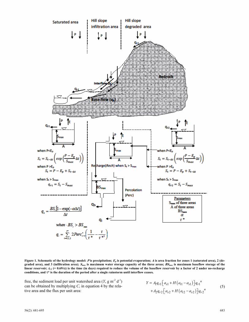
The amount of erosion is predicted as a function of the (daily) amounts of surface runoff, interflow, and baseflow. These fluxes are obtained from the relatively simple hy-drology model shown in figure 1 (Steenhuis et al., 2009; Tesemma et al., 2010) that divides the watershed into three zones. Two are runoff-producing zones: one becomes satu-rated during the wet monsoon period, and the other is the degraded hillslope. The remaining hillslope area (fig. 1) forms the third zone, where rainwater infiltrates and be-comes either interflow (zero-order reservoir) or baseflow (first-order reservoir) depending on its path to the stream. Each zone is not necessarily continuous. Parameter values are averages for each of the three zones. A daily water bal-ance is kept for each of the zones using the Thornthwaite-Mather procedure, in which actual evaporation has a linear relationship with the available water storage in the root zone. At maximum storage (Smax), actual evaporation is equal to the potential evaporation (Steenhuis and van der Molen, 1986). More information about the hydrology mod-el can be found in Steenhuis et al. (2009) and Tesemma et al. (2010). Erosion originates from the runoff-producing zones. Erosion is negligible from the non-degraded hillslopes because almost all water infiltrates before it reaches the stream.

In calculating the erosion from runoff-producing areas,

we assume that the rate of erosion depends on the stream power (Ω) per unit area. The maximum sediment concen-tration that a stream can carry (called the transport limiting capacity (Ct, g L-1) can be derived from the stream power function, as shown by Hairsine and Rose (1992), Siepel et al. (2002), Ciesiolka et al. (1995), and Yu et al. (1997):

nt t rC a q= (1)

where qr is the runoff rate per unit area from each runoff-producing area (mm d-1), and at is a variable derived from the stream power [(g L-1)(mm d-1)-n]. Variable at is a func-tion of the slope, Manning’s roughness coefficient, slope length, and effective depositability (Yu et al., 1997). As wa-ter depth increases, at essentially becomes independent of the runoff rate per unit area and can be taken as a constant (Yu et al., 1997). In this article, where the smallest water-shed considered is 113 ha, the water in the channel is suffi-ciently deep so that at is constant.

For erosion of cohesive soils, the sediment concentration will not always reach the transport limit. The sediment con-centration is at the transport limit only when rills are active-ly formed in newly plowed soils. Tebebu et al. (2010) and Zegeye et al. (2010) found that, once the rill network has been fully established, no further erosion takes place, the sediment source becomes limited, and the sediment concen-tration (C, g L-1) falls below the transport limit. For cases in which the sediment concentration becomes lower than the transport limit (Ct, g L-1), Ciesiolka et al. (1995) found, based on the work of Hairsine and Rose (1992), that the sediment concentration will not decline below the source limit (Cs, g L-1):

ns s rC a q= (2)

where as is the source limit and is assumed to be independ-ent of the flow rate for a particular watershed (as compared to plots). Introducing a new variable, H, defined as the frac-tion of the runoff-producing area with active rill formation, the sediment concentration from the runoff-producing area (Cr, g L-1) can then be written as:

( )r s t sC C H C C= + − (3)

Combining equation 3 with equations 1 and 2, the sedi-ment concentration from the runoff-producing area be-comes:

( ) nr s t s rC a H a a q = + − (4)

Finally, baseflow and interflow play an important role in the calculation of the daily sediment concentration. In a monsoon climate, baseflow at the end of the rainy season can be a significant portion of the total flow. Thus, in the last part of the rainy season, subsurface flow dilutes the peak storm sediment concentration from the runoff-producing zones when simulated on a daily basis. It is therefore important to incorporate the contribution of baseflow in the prediction of sediment concentration.

Next, we calculate the sediment concentration yield in the stream. Since the interflow and baseflow are sediment

56(2): 681-695 683

free, the sediment load per unit watershed area (Y, g m-2 d-1) can be obtained by multiplying Cr in equation 4 by the rela-tive area and the flux per unit area:

( )

( )1 1 1 1 1 1

2 2 2 2 2 2

nr s t s r

nr s t s r

Y A q a H a a q

A q a H a a q

= + −

+ + − (5)

Figure 1. Schematic of the hydrology model: P is precipitation; Ep is potential evaporation; A is area fraction for zones 1 (saturated area), 2 (de-graded area), and 3 (infiltration area); Smax is maximum water storage capacity of the three areas; BSmax is maximum baseflow storage of the linear reservoir; t1/2 (= 0.69/α) is the time (in days) required to reduce the volume of the baseflow reservoir by a factor of 2 under no-recharge conditions, and τ* is the duration of the period after a single rainstorm until interflow ceases.

684 TRANSACTIONS OF THE ASABE

where qr1 and qr2 are the runoff rates expressed in depth units for contributing area A1 (fractional saturated area) and A2 (fractional degraded area), respectively. Theoretically, for both turbulent flow and a wide field, n is equal 0.4 (Tilahun et al., 2012; Ciesiolka et al., 1995; Yu et al., 1997). The sediment concentration in the stream can be obtained by dividing the sediment load (Y in eq. 5) by the total wa-tershed discharge:

( )(( ) )

( )

1 41 1 1 1 1

1 42 2 2 2 2

1 1 2 2 3

.r s t s

.r s t s

r r b i

C A q a H a a

A q a H a a

A q A q A q q

= + −

+ + −

÷ + + +

(6)

where qb is the baseflow (mm d-1) and qi is the interflow (mm d-1) per unit area of the non-degraded hillslope (A3), where the water is being recharged to the subsurface (baseflow) reservoir.

Therefore, equation 6 was tested in four watersheds in the Ethiopian highlands (Anjeni, Andit Tid, Enkulal, and the Blue Nile basin) and one watershed in New York State (Esopus Creek), ranging in size from 1.13 to 174,000 km2. There are four parameters in equation 6 that need to be cal-ibrated (as1, at1, as2, and at2). The fraction (H) with active rill formation is not calibrated and is determined a priori based on field observations.

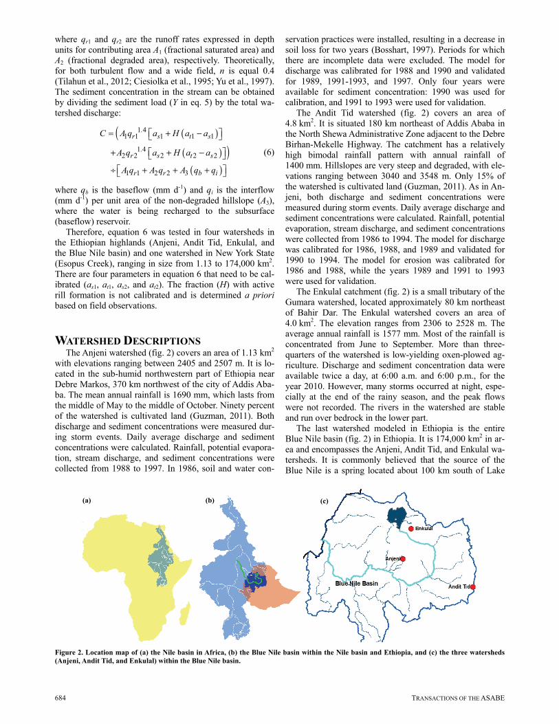
WATERSHED DESCRIPTIONS The Anjeni watershed (fig. 2) covers an area of 1.13 km2

with elevations ranging between 2405 and 2507 m. It is lo-cated in the sub-humid northwestern part of Ethiopia near Debre Markos, 370 km northwest of the city of Addis Aba-ba. The mean annual rainfall is 1690 mm, which lasts from the middle of May to the middle of October. Ninety percent of the watershed is cultivated land (Guzman, 2011). Both discharge and sediment concentrations were measured dur-ing storm events. Daily average discharge and sediment concentrations were calculated. Rainfall, potential evapora-tion, stream discharge, and sediment concentrations were collected from 1988 to 1997. In 1986, soil and water con-

servation practices were installed, resulting in a decrease in soil loss for two years (Bosshart, 1997). Periods for which there are incomplete data were excluded. The model for discharge was calibrated for 1988 and 1990 and validated for 1989, 1991-1993, and 1997. Only four years were available for sediment concentration: 1990 was used for calibration, and 1991 to 1993 were used for validation.

The Andit Tid watershed (fig. 2) covers an area of 4.8 km2. It is situated 180 km northeast of Addis Ababa in the North Shewa Administrative Zone adjacent to the Debre Birhan-Mekelle Highway. The catchment has a relatively high bimodal rainfall pattern with annual rainfall of 1400 mm. Hillslopes are very steep and degraded, with ele-vations ranging between 3040 and 3548 m. Only 15% of the watershed is cultivated land (Guzman, 2011). As in An-jeni, both discharge and sediment concentrations were measured during storm events. Daily average discharge and sediment concentrations were calculated. Rainfall, potential evaporation, stream discharge, and sediment concentrations were collected from 1986 to 1994. The model for discharge was calibrated for 1986, 1988, and 1989 and validated for 1990 to 1994. The model for erosion was calibrated for 1986 and 1988, while the years 1989 and 1991 to 1993 were used for validation.

The Enkulal catchment (fig. 2) is a small tributary of the Gumara watershed, located approximately 80 km northeast of Bahir Dar. The Enkulal watershed covers an area of 4.0 km2. The elevation ranges from 2306 to 2528 m. The average annual rainfall is 1577 mm. Most of the rainfall is concentrated from June to September. More than three-quarters of the watershed is low-yielding oxen-plowed ag-riculture. Discharge and sediment concentration data were available twice a day, at 6:00 a.m. and 6:00 p.m., for the year 2010. However, many storms occurred at night, espe-cially at the end of the rainy season, and the peak flows were not recorded. The rivers in the watershed are stable and run over bedrock in the lower part.

The last watershed modeled in Ethiopia is the entire Blue Nile basin (fig. 2) in Ethiopia. It is 174,000 km2 in ar-ea and encompasses the Anjeni, Andit Tid, and Enkulal wa-tersheds. It is commonly believed that the source of the Blue Nile is a spring located about 100 km south of Lake

Figure 2. Location map of (a) the Nile basin in Africa, (b) the Blue Nile basin within the Nile basin and Ethiopia, and (c) the three watersheds (Anjeni, Andit Tid, and Enkulal) within the Blue Nile basin.

(a) (b) (c)

56(2): 681-695 685

Tana at an elevation of 2900 m. This spring is the begin-ning of the Gilgil Abbay, which flows into Lake Tana. After Lake Tana, the Nile flows through a 1 km deep gorge, mostly over bedrock, to the Sudanese border. The Blue Nile leaves the highlands near the western border of Ethiopia and enters Sudan at an elevation of 490 m. The annual rain-fall varies from less than 1000 mm near the Sudanese bor-der to over 1800 mm in the highlands south of Lake Tana. Three years (1997, 2003, and 2004) of discharge and sedi-ment data were available at the Sudanese border. The year 1993 was used for calibration, and 2003 and 2004 were used for validation. Tesemma et al. (2010) found that the degraded soils had increased by 10% during a 25-year time span. For that reason, the degraded hillslope area was in-creased by 3% from 1997 to 2003 and 2004.

The final watershed is the Esopus Creek watershed, lo-cated in the Catskill region of New York State. This water-shed drains 493 km2 and is dominated by forests, which oc-cupy more than 90% of the watershed area. The elevation of the watershed ranges from 194 m near the watershed outlet at Coldbrook to 1275 m at the headwaters. The aver-age annual rainfall is 1450 mm. Widespread stream channel erosion of glacial clay deposits has been identified as the primary cause of high levels of turbidity. For the Esopus Creek watershed, we used measured daily stream discharge data from the USGS gauging station at the watershed outlet near Coldbrook. Turbidity measurements were taken at in-tervals between 15 min and 1 h using a YSI water quality sonde from which flow-weighted average daily values were calculated. The measured stream discharge was separated into baseflow and surface runoff components using a baseflow filter program (Arnold and Allen, 1999). The val-ues for the surface runoff region (A1) and hillslope recharge region (A3) were derived as the long-term (1931-2011) mean proportions of runoff and baseflow to total stream-flow. Degraded areas were not identified in the watershed, as the hillslope is covered by forest. The surface runoff-producing area in this watershed is the saturated zone ob-served along the streambank. Observed daily turbidity and daily stream discharge from March 2003 to March 2004 were used for calibration of sediment in the SEEModel, and a power function and data from March 2007 to March 2008 were employed for validation. Esopus Creek is at times fed

by a diversion tunnel operated from the nearby Schoharie reservoir that contributes to stream discharge. Therefore, all calculations were confined to days when the tunnel contri-bution to stream discharge was insignificant.

RESULTS AND DISCUSSION HYDROLOGY MODEL

The model calibrations over a wide range of scales have some remarkable similarities (table 1). In particular, the fraction of surface runoff zones (areas A1 and A2) in four of the watersheds is between 0.3 and 0.4. Only in the Anjeni watershed is this fraction smaller and equal to 16% of the watershed. Small changes in the relative extent of surface runoff zones and permeable hillslopes greatly affect the shape of the hydrograph (Tilahun et al., 2012). The small Ethiopian watersheds are located in the upper reaches of the Blue Nile basin, and it is likely that some of the subsur-face water passes under the gauging station and provides water for springs below. The sum of the fractional areas for the small watersheds is therefore less than one. The hillslope infiltration area is especially small for the Enkulal watershed (table 1), which is in accordance with data from piezometer readings that indicated disconnection between the top and bottom parts of the watershed (Demisse, 2011). The maximum storage of water in the root zone (Smax) and shallow aquifer (BSmax) varies among the watersheds. However, the hydrology model (fig. 1) is relatively insensi-tive to the Smax and BSmax values since they only affect the amount of surface runoff at the beginning of the rainfall season (Tilahun et al., 2012). Variations in these values be-tween watersheds are therefore not significant, with the ex-ception of the maximum storage for the hillslope infiltra-tion area and saturated area of the Blue Nile basin, which are larger.

Two parameters determine subsurface flow (fig. 1): τ* for interflow and t1/2 (= 0.69/α) for baseflow. While the baseflow contribution to streamflow decreases slowly de-pending on the amount of water in the aquifer, the interflow decreases as a linear function of time for a particular storm and stops after time τ*. As expected, τ* increases with wa-tershed size because more deep flow paths are intercepted

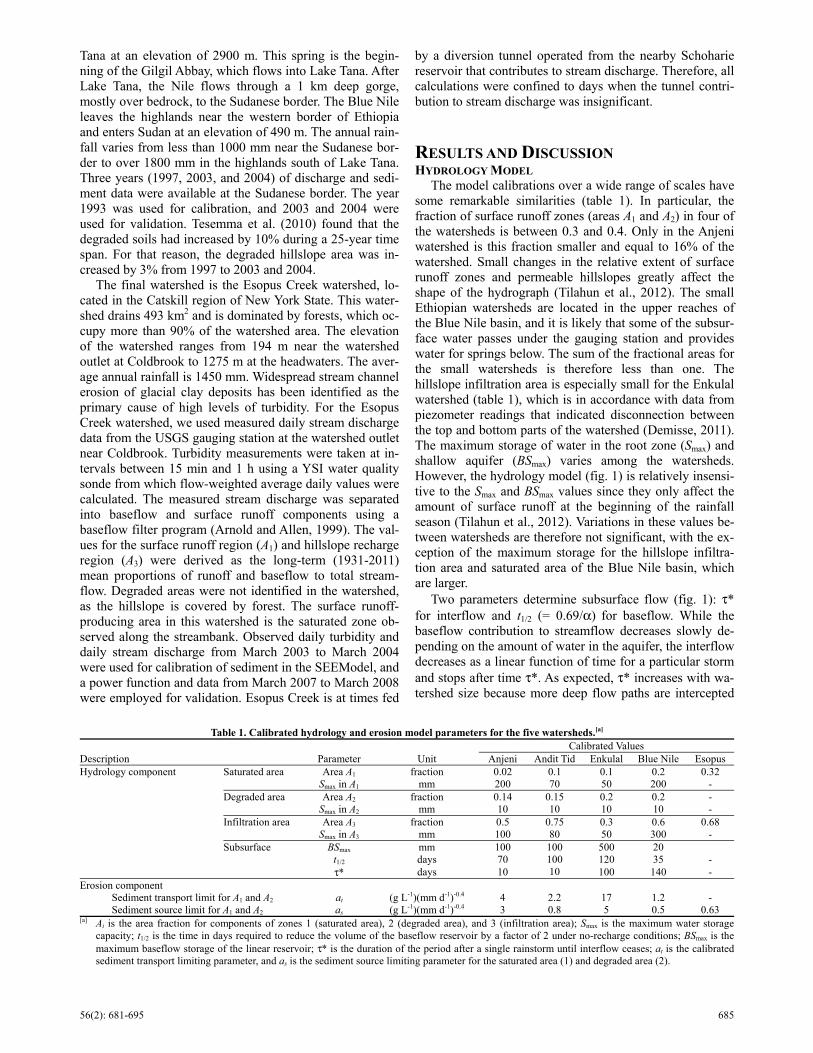
Table 1. Calibrated hydrology and erosion model parameters for the five watersheds.[a]

Description Parameter Unit Calibrated Values

Anjeni Andit Tid Enkulal Blue Nile Esopus Hydrology component Saturated area Area A1 fraction 0.02 0.1 0.1 0.2 0.32

Smax in A1 mm 200 70 50 200 - Degraded area Area A2 fraction 0.14 0.15 0.2 0.2 -

Smax in A2 mm 10 10 10 10 - Infiltration area Area A3 fraction 0.5 0.75 0.3 0.6 0.68

Smax in A3 mm 100 80 50 300 - Subsurface BSmax mm 100 100 500 20

t1/2 days 70 100 120 35 - τ* days 10 10 100 140 -

Erosion component Sediment transport limit for A1 and A2 at (g L-1)(mm d-1)-0.4 4 2.2 17 1.2 -

Sediment source limit for A1 and A2 as (g L-1)(mm d-1)-0.4 3 0.8 5 0.5 0.63 [a] Ai is the area fraction for components of zones 1 (saturated area), 2 (degraded area), and 3 (infiltration area); Smax is the maximum water storage

capacity; t1/2 is the time in days required to reduce the volume of the baseflow reservoir by a factor of 2 under no-recharge conditions; BSmax is the maximum baseflow storage of the linear reservoir; τ* is the duration of the period after a single rainstorm until interflow ceases; at is the calibrated sediment transport limiting parameter, and as is the sediment source limiting parameter for the saturated area (1) and degraded area (2).

686 TRANSACTIONS OF THE ASABE

by the river. The larger-than-expected τ* for the Enkulal watershed (table 1) is likely a consequence of missing peak flows, especially later in the rainy season, due to the sample collection timing. The half-life (t1/2) for the aquifer system is generally small (table 1) and almost independent of wa-tershed size, indicating that there is not a large aquifer. With the Nile flowing over bedrock, this should not be a surprise. Finally, the hydrology model could not be fitted very well to the Esopus Creek watershed discharge data be-cause, in a temperate climate, snowmelt requires another subroutine and because of the large elevation differences in the watershed. The proportions of surface runoff zones and permeable hillslopes were derived statistically from the discharge data. The simple hydrology SEEModel was able to simulate the discharge pattern quite well in the water-sheds with large relief and permeable soils usually over a hard pan at shallow to intermediate depths on the hillslopes.

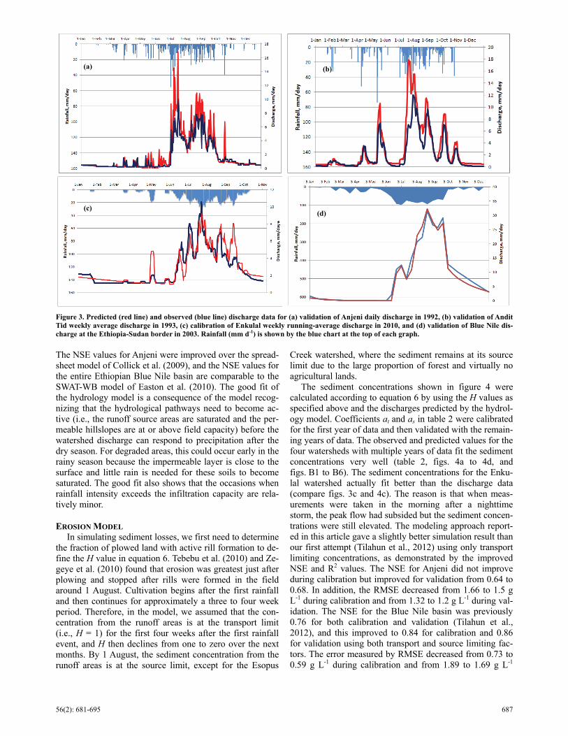
The Nash-Sutcliffe efficiencies (NSE) and coefficients of determination (R2) in table 2 for all watersheds are rea-sonably good. The NSE for validation of the daily dis-charge data in the Anjeni watershed was 0.80 (table 2). The NSE for the 7-day average discharge in Andit Tid was simi-lar at 0.78, and the NSE for the 10-day average discharge in the entire Blue Nile basin was 0.92. The SEEModel was able to simulate the discharge pattern quite well in these watersheds. The predicted and observed discharges for the

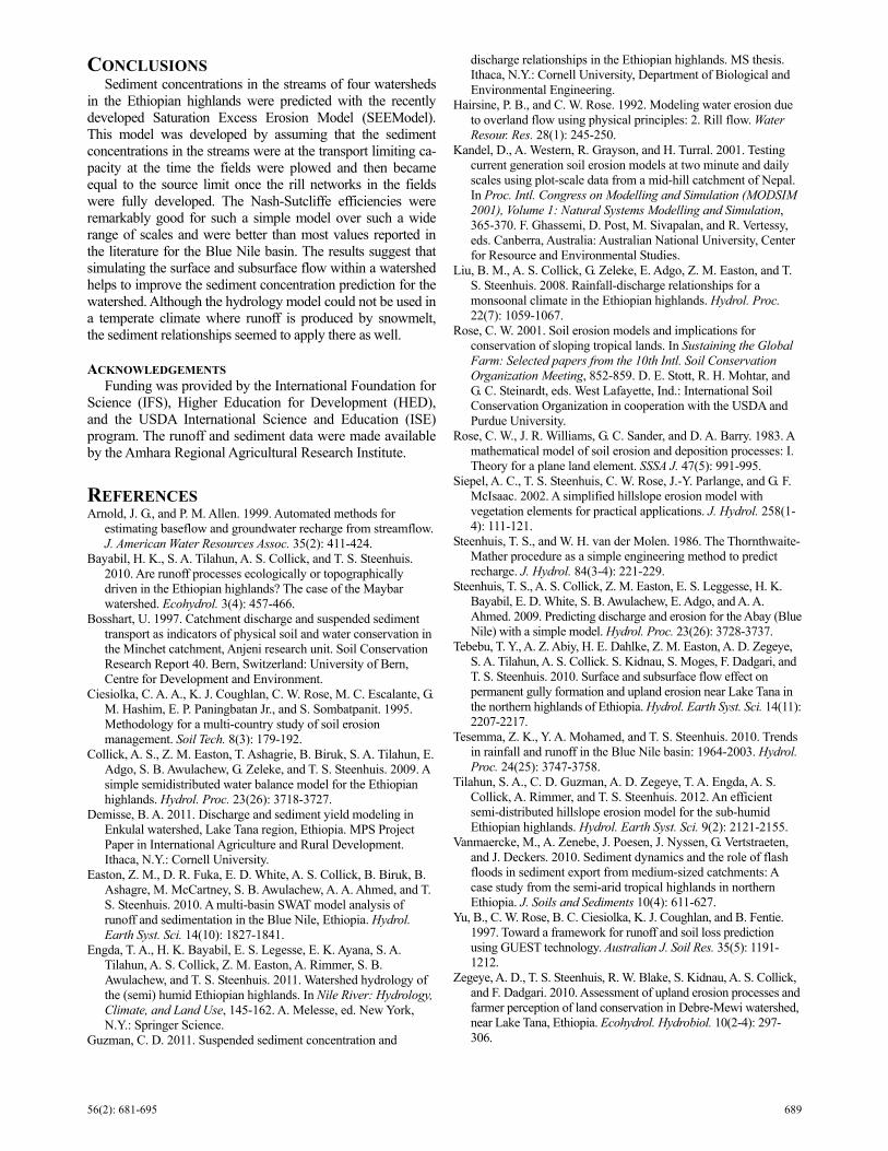
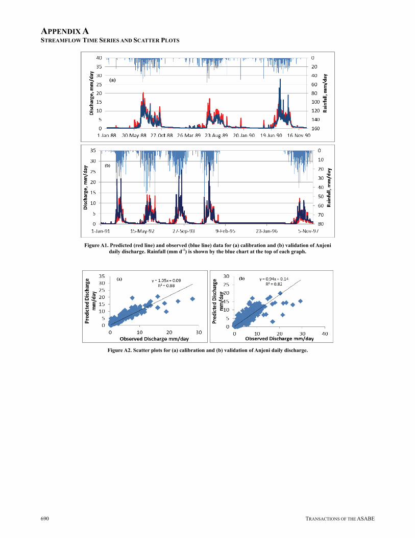
1989 validation year for the Anjeni watershed and for the 1990 validation year for Andit Tid are shown in figures 3a and 3b, respectively. Supplementary calibration and valida-tion data for all years are shown for Anjeni in figures A1 and A2 and for Andit Tid in figures A3 and A4 in Appendix A. In Anjeni, the peak daily flows were overestimated for 1988 and 1989, after the soil and water conservation prac-tices had been implemented in 1986 (Tilahun et al., 2012), and underestimated after soils had filled up behind the bunds (1990 in fig. Ala, and 1991 to 1997 in fig. A1b). In all years, the peak flows were underestimated because the model had fixed saturated areas; in reality, the saturated ar-ea expands with large storms. The years 1995 and 1996 were not simulated because the data for these periods were incomplete. The fit for Andit Tid during calibration (fig. A3) was reasonable, as shown by the NSE in table 2. The year 1987 was not included in the simulation due to missing data.

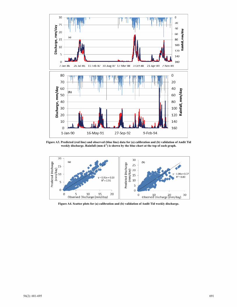
Data for the Enkulal watershed were only collected in 2010, and the weekly running-average discharges for 2010 are compared in figure 3c. The fit is not great and is partly caused by the uncertainty of the peak flows at the end of the rainy season, which likely occurred at night when man-ual measurements were not possible. The validation for the Blue Nile basin for 2003 is shown in figure 3d, and the cal-ibration and validation are shown in figures A5 and A6.

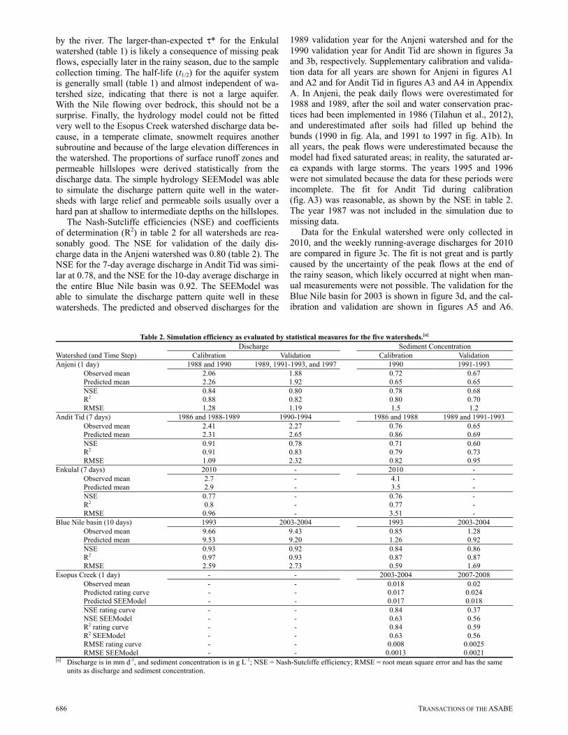
Table 2. Simulation efficiency as evaluated by statistical measures for the five watersheds.[a]

Watershed (and Time Step) Discharge

Sediment Concentration

Calibration Validation Calibration Validation Anjeni (1 day) 1988 and 1990 1989, 1991-1993, and 1997 1990 1991-1993 Observed mean 2.06 1.88 0.72 0.67 Predicted mean 2.26 1.92 0.65 0.65 NSE 0.84 0.80 0.78 0.68 R2 0.88 0.82 0.80 0.70 RMSE 1.28 1.19 1.5 1.2 Andit Tid (7 days) 1986 and 1988-1989 1990-1994 1986 and 1988 1989 and 1991-1993 Observed mean 2.41 2.27 0.76 0.65 Predicted mean 2.31 2.65 0.86 0.69 NSE 0.91 0.78 0.71 0.60 R2 0.91 0.83 0.79 0.73 RMSE 1.09 2.32 0.82 0.95 Enkulal (7 days) 2010 - 2010 - Observed mean 2.7 - 4.1 - Predicted mean 2.9 - 3.5 - NSE 0.77 - 0.76 - R2 0.8 - 0.77 - RMSE 0.96 - 3.51 - Blue Nile basin (10 days) 1993 2003-2004 1993 2003-2004 Observed mean 9.66 9.43 0.85 1.28 Predicted mean 9.53 9.20 1.26 0.92 NSE 0.93 0.92 0.84 0.86 R2 0.97 0.93 0.87 0.87 RMSE 2.59 2.73 0.59 1.69 Esopus Creek (1 day) - - 2003-2004 2007-2008 Observed mean - - 0.018 0.02 Predicted rating curve - - 0.017 0.024 Predicted SEEModel - - 0.017 0.018 NSE rating curve - - 0.84 0.37 NSE SEEModel - - 0.63 0.56 R2 rating curve - - 0.84 0.59 R2 SEEModel - - 0.63 0.56 RMSE rating curve - - 0.008 0.0025 RMSE SEEModel - - 0.0013 0.0021 [a] Discharge is in mm d-1, and sediment concentration is in g L-1; NSE = Nash-Sutcliffe efficiency; RMSE = root mean square error and has the same

units as discharge and sediment concentration.

56(2): 681-695 687

The NSE values for Anjeni were improved over the spread-sheet model of Collick et al. (2009), and the NSE values for the entire Ethiopian Blue Nile basin are comparable to the SWAT-WB model of Easton et al. (2010). The good fit of the hydrology model is a consequence of the model recog-nizing that the hydrological pathways need to become ac-tive (i.e., the runoff source areas are saturated and the per-meable hillslopes are at or above field capacity) before the watershed discharge can respond to precipitation after the dry season. For degraded areas, this could occur early in the rainy season because the impermeable layer is close to the surface and little rain is needed for these soils to become saturated. The good fit also shows that the occasions when rainfall intensity exceeds the infiltration capacity are rela-tively minor.

EROSION MODEL In simulating sediment losses, we first need to determine

the fraction of plowed land with active rill formation to de-fine the H value in equation 6. Tebebu et al. (2010) and Ze-geye et al. (2010) found that erosion was greatest just after plowing and stopped after rills were formed in the field around 1 August. Cultivation begins after the first rainfall and then continues for approximately a three to four week period. Therefore, in the model, we assumed that the con-centration from the runoff areas is at the transport limit (i.e., H = 1) for the first four weeks after the first rainfall event, and H then declines from one to zero over the next months. By 1 August, the sediment concentration from the runoff areas is at the source limit, except for the Esopus

Creek watershed, where the sediment remains at its source limit due to the large proportion of forest and virtually no agricultural lands.

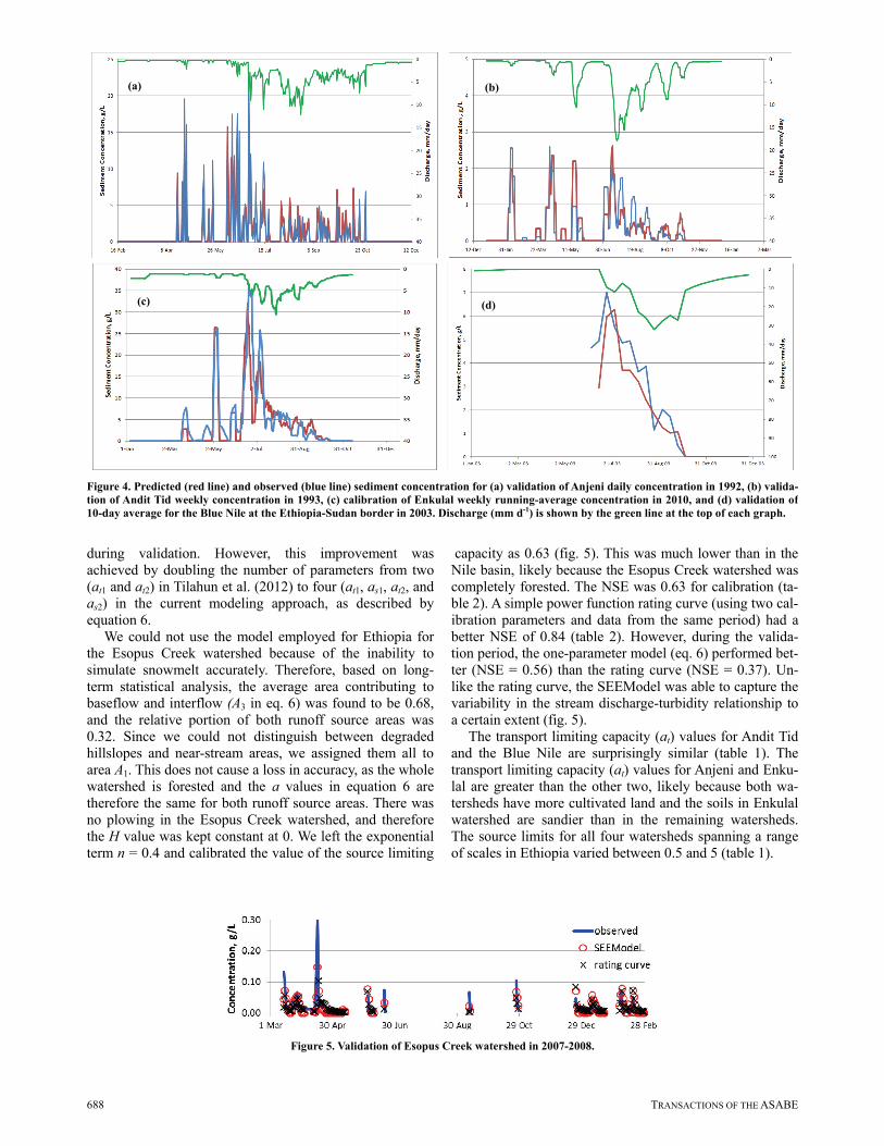
The sediment concentrations shown in figure 4 were calculated according to equation 6 by using the H values as specified above and the discharges predicted by the hydrol-ogy model. Coefficients at and as in table 2 were calibrated for the first year of data and then validated with the remain-ing years of data. The observed and predicted values for the four watersheds with multiple years of data fit the sediment concentrations very well (table 2, figs. 4a to 4d, and figs. B1 to B6). The sediment concentrations for the Enku-lal watershed actually fit better than the discharge data (compare figs. 3c and 4c). The reason is that when meas-urements were taken in the morning after a nighttime storm, the peak flow had subsided but the sediment concen-trations were still elevated. The modeling approach report-ed in this article gave a slightly better simulation result than our first attempt (Tilahun et al., 2012) using only transport limiting concentrations, as demonstrated by the improved NSE and R2 values. The NSE for Anjeni did not improve during calibration but improved for validation from 0.64 to 0.68. In addition, the RMSE decreased from 1.66 to 1.5 g L-1 during calibration and from 1.32 to 1.2 g L-1 during val-idation. The NSE for the Blue Nile basin was previously 0.76 for both calibration and validation (Tilahun et al., 2012), and this improved to 0.84 for calibration and 0.86 for validation using both transport and source limiting fac-tors. The error measured by RMSE decreased from 0.73 to 0.59 g L-1 during calibration and from 1.89 to 1.69 g L-1

Figure 3. Predicted (red line) and observed (blue line) discharge data for (a) validation of Anjeni daily discharge in 1992, (b) validation of Andit Tid weekly average discharge in 1993, (c) calibration of Enkulal weekly running-average discharge in 2010, and (d) validation of Blue Nile dis-charge at the Ethiopia-Sudan border in 2003. Rainfall (mm d-1) is shown by the blue chart at the top of each graph.

(b)(a)

(d)(c)

688 TRANSACTIONS OF THE ASABE

during validation. However, this improvement was achieved by doubling the number of parameters from two (at1 and at2) in Tilahun et al. (2012) to four (at1, as1, at2, and as2) in the current modeling approach, as described by equation 6.

We could not use the model employed for Ethiopia for the Esopus Creek watershed because of the inability to simulate snowmelt accurately. Therefore, based on long-term statistical analysis, the average area contributing to baseflow and interflow (A3 in eq. 6) was found to be 0.68, and the relative portion of both runoff source areas was 0.32. Since we could not distinguish between degraded hillslopes and near-stream areas, we assigned them all to area A1. This does not cause a loss in accuracy, as the whole watershed is forested and the a values in equation 6 are therefore the same for both runoff source areas. There was no plowing in the Esopus Creek watershed, and therefore the H value was kept constant at 0. We left the exponential term n = 0.4 and calibrated the value of the source limiting

capacity as 0.63 (fig. 5). This was much lower than in the Nile basin, likely because the Esopus Creek watershed was completely forested. The NSE was 0.63 for calibration (ta-ble 2). A simple power function rating curve (using two cal-ibration parameters and data from the same period) had a better NSE of 0.84 (table 2). However, during the valida-tion period, the one-parameter model (eq. 6) performed bet-ter (NSE = 0.56) than the rating curve (NSE = 0.37). Un-like the rating curve, the SEEModel was able to capture the variability in the stream discharge-turbidity relationship to a certain extent (fig. 5).

The transport limiting capacity (at) values for Andit Tid and the Blue Nile are surprisingly similar (table 1). The transport limiting capacity (at) values for Anjeni and Enku-lal are greater than the other two, likely because both wa-tersheds have more cultivated land and the soils in Enkulal watershed are sandier than in the remaining watersheds. The source limits for all four watersheds spanning a range of scales in Ethiopia varied between 0.5 and 5 (table 1).

Figure 4. Predicted (red line) and observed (blue line) sediment concentration for (a) validation of Anjeni daily concentration in 1992, (b) valida-tion of Andit Tid weekly concentration in 1993, (c) calibration of Enkulal weekly running-average concentration in 2010, and (d) validation of10-day average for the Blue Nile at the Ethiopia-Sudan border in 2003. Discharge (mm d-1) is shown by the green line at the top of each graph.

Figure 5. Validation of Esopus Creek watershed in 2007-2008.

(d)

(b)

(c)

(a)

56(2): 681-695 689

CONCLUSIONS Sediment concentrations in the streams of four watersheds

in the Ethiopian highlands were predicted with the recently developed Saturation Excess Erosion Model (SEEModel). This model was developed by assuming that the sediment concentrations in the streams were at the transport limiting ca-pacity at the time the fields were plowed and then became equal to the source limit once the rill networks in the fields were fully developed. The Nash-Sutcliffe efficiencies were remarkably good for such a simple model over such a wide range of scales and were better than most values reported in the literature for the Blue Nile basin. The results suggest that simulating the surface and subsurface flow within a watershed helps to improve the sediment concentration prediction for the watershed. Although the hydrology model could not be used in a temperate climate where runoff is produced by snowmelt, the sediment relationships seemed to apply there as well.

ACKNOWLEDGEMENTS Funding was provided by the International Foundation for

Science (IFS), Higher Education for Development (HED), and the USDA International Science and Education (ISE) program. The runoff and sediment data were made available by the Amhara Regional Agricultural Research Institute.

REFERENCES Arnold, J. G., and P. M. Allen. 1999. Automated methods for

estimating baseflow and groundwater recharge from streamflow. J. American Water Resources Assoc. 35(2): 411-424.

Bayabil, H. K., S. A. Tilahun, A. S. Collick, and T. S. Steenhuis. 2010. Are runoff processes ecologically or topographically driven in the Ethiopian highlands? The case of the Maybar watershed. Ecohydrol. 3(4): 457-466.

Bosshart, U. 1997. Catchment discharge and suspended sediment transport as indicators of physical soil and water conservation in the Minchet catchment, Anjeni research unit. Soil Conservation Research Report 40. Bern, Switzerland: University of Bern, Centre for Development and Environment.

Ciesiolka, C. A. A., K. J. Coughlan, C. W. Rose, M. C. Escalante, G. M. Hashim, E. P. Paningbatan Jr., and S. Sombatpanit. 1995. Methodology for a multi-country study of soil erosion management. Soil Tech. 8(3): 179-192.

Collick, A. S., Z. M. Easton, T. Ashagrie, B. Biruk, S. A. Tilahun, E. Adgo, S. B. Awulachew, G. Zeleke, and T. S. Steenhuis. 2009. A simple semidistributed water balance model for the Ethiopian highlands. Hydrol. Proc. 23(26): 3718-3727.

Demisse, B. A. 2011. Discharge and sediment yield modeling in Enkulal watershed, Lake Tana region, Ethiopia. MPS Project Paper in International Agriculture and Rural Development. Ithaca, N.Y.: Cornell University.

Easton, Z. M., D. R. Fuka, E. D. White, A. S. Collick, B. Biruk, B. Ashagre, M. McCartney, S. B. Awulachew, A. A. Ahmed, and T. S. Steenhuis. 2010. A multi-basin SWAT model analysis of runoff and sedimentation in the Blue Nile, Ethiopia. Hydrol. Earth Syst. Sci. 14(10): 1827-1841.

Engda, T. A., H. K. Bayabil, E. S. Legesse, E. K. Ayana, S. A. Tilahun, A. S. Collick, Z. M. Easton, A. Rimmer, S. B. Awulachew, and T. S. Steenhuis. 2011. Watershed hydrology of the (semi) humid Ethiopian highlands. In Nile River: Hydrology, Climate, and Land Use, 145-162. A. Melesse, ed. New York, N.Y.: Springer Science.

Guzman, C. D. 2011. Suspended sediment concentration and

discharge relationships in the Ethiopian highlands. MS thesis. Ithaca, N.Y.: Cornell University, Department of Biological and Environmental Engineering.

Hairsine, P. B., and C. W. Rose. 1992. Modeling water erosion due to overland flow using physical principles: 2. Rill flow. Water Resour. Res. 28(1): 245-250.

Kandel, D., A. Western, R. Grayson, and H. Turral. 2001. Testing current generation soil erosion models at two minute and daily scales using plot-scale data from a mid-hill catchment of Nepal. In Proc. Intl. Congress on Modelling and Simulation (MODSIM 2001), Volume 1: Natural Systems Modelling and Simulation, 365-370. F. Ghassemi, D. Post, M. Sivapalan, and R. Vertessy, eds. Canberra, Australia: Australian National University, Center for Resource and Environmental Studies.

Liu, B. M., A. S. Collick, G. Zeleke, E. Adgo, Z. M. Easton, and T. S. Steenhuis. 2008. Rainfall-discharge relationships for a monsoonal climate in the Ethiopian highlands. Hydrol. Proc. 22(7): 1059-1067.

Rose, C. W. 2001. Soil erosion models and implications for conservation of sloping tropical lands. In Sustaining the Global Farm: Selected papers from the 10th Intl. Soil Conservation Organization Meeting, 852-859. D. E. Stott, R. H. Mohtar, and G. C. Steinardt, eds. West Lafayette, Ind.: International Soil Conservation Organization in cooperation with the USDA and Purdue University.

Rose, C. W., J. R. Williams, G. C. Sander, and D. A. Barry. 1983. A mathematical model of soil erosion and deposition processes: I. Theory for a plane land element. SSSA J. 47(5): 991-995.

Siepel, A. C., T. S. Steenhuis, C. W. Rose, J.-Y. Parlange, and G. F. McIsaac. 2002. A simplified hillslope erosion model with vegetation elements for practical applications. J. Hydrol. 258(1-4): 111-121.

Steenhuis, T. S., and W. H. van der Molen. 1986. The Thornthwaite-Mather procedure as a simple engineering method to predict recharge. J. Hydrol. 84(3-4): 221-229.

Steenhuis, T. S., A. S. Collick, Z. M. Easton, E. S. Leggesse, H. K. Bayabil, E. D. White, S. B. Awulachew, E. Adgo, and A. A. Ahmed. 2009. Predicting discharge and erosion for the Abay (Blue Nile) with a simple model. Hydrol. Proc. 23(26): 3728-3737.

Tebebu, T. Y., A. Z. Abiy, H. E. Dahlke, Z. M. Easton, A. D. Zegeye, S. A. Tilahun, A. S. Collick. S. Kidnau, S. Moges, F. Dadgari, and T. S. Steenhuis. 2010. Surface and subsurface flow effect on permanent gully formation and upland erosion near Lake Tana in the northern highlands of Ethiopia. Hydrol. Earth Syst. Sci. 14(11): 2207-2217.

Tesemma, Z. K., Y. A. Mohamed, and T. S. Steenhuis. 2010. Trends in rainfall and runoff in the Blue Nile basin: 1964-2003. Hydrol. Proc. 24(25): 3747-3758.

Tilahun, S. A., C. D. Guzman, A. D. Zegeye, T. A. Engda, A. S. Collick, A. Rimmer, and T. S. Steenhuis. 2012. An efficient semi-distributed hillslope erosion model for the sub-humid Ethiopian highlands. Hydrol. Earth Syst. Sci. 9(2): 2121-2155.

Vanmaercke, M., A. Zenebe, J. Poesen, J. Nyssen, G. Vertstraeten, and J. Deckers. 2010. Sediment dynamics and the role of flash floods in sediment export from medium-sized catchments: A case study from the semi-arid tropical highlands in northern Ethiopia. J. Soils and Sediments 10(4): 611-627.

Yu, B., C. W. Rose, B. C. Ciesiolka, K. J. Coughlan, and B. Fentie. 1997. Toward a framework for runoff and soil loss prediction using GUEST technology. Australian J. Soil Res. 35(5): 1191-1212.

Zegeye, A. D., T. S. Steenhuis, R. W. Blake, S. Kidnau, A. S. Collick, and F. Dadgari. 2010. Assessment of upland erosion processes and farmer perception of land conservation in Debre-Mewi watershed, near Lake Tana, Ethiopia. Ecohydrol. Hydrobiol. 10(2-4): 297-306.

690 TRANSACTIONS OF THE ASABE

APPENDIX A STREAMFLOW TIME SERIES AND SCATTER PLOTS

Figure A1. Predicted (red line) and observed (blue line) data for (a) calibration and (b) validation of Anjeni daily discharge. Rainfall (mm d-1) is shown by the blue chart at the top of each graph.

Figure A2. Scatter plots for (a) calibration and (b) validation of Anjeni daily discharge.

(a)

56(2): 681-695 691

Figure A3. Predicted (red line) and observed (blue line) data for (a) calibration and (b) validation of Andit Tid

weekly discharge. Rainfall (mm d-1) is shown by the blue chart at the top of each graph.

Figure A4. Scatter plots for (a) calibration and (b) validation of Andit Tid weekly discharge.

692 TRANSACTIONS OF THE ASABE

Figure A5. Predicted (red line) and observed (blue line) data for (a) calibration and (b) validation of Blue Nile basin

10-day average discharge. Rainfall (mm d-1) is shown by the blue chart at the top of each graph.

Figure A6. Scatter plots for (a) calibration and (b) validation of Blue Nile basin 10-day average discharge.

(a)

(b)

56(2): 681-695 693

APPENDIX B SEDIMENT TIME SERIES AND SCATTER PLOTS

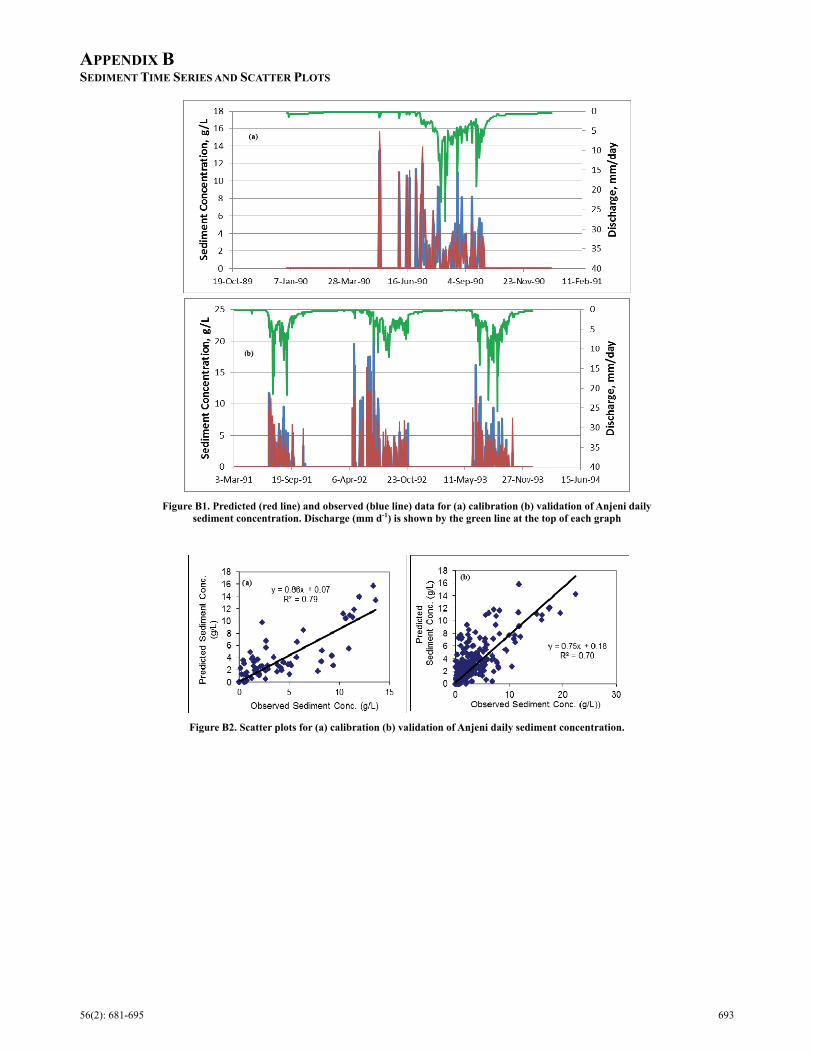
Figure B1. Predicted (red line) and observed (blue line) data for (a) calibration (b) validation of Anjeni daily

sediment concentration. Discharge (mm d-1) is shown by the green line at the top of each graph

Figure B2. Scatter plots for (a) calibration (b) validation of Anjeni daily sediment concentration.

694 TRANSACTIONS OF THE ASABE

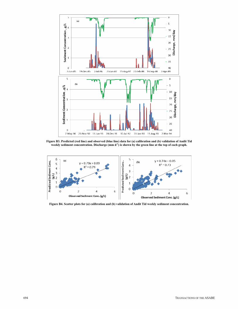
Figure B3. Predicted (red line) and observed (blue line) data for (a) calibration and (b) validation of Andit Tid

weekly sediment concentration. Discharge (mm d-1) is shown by the green line at the top of each graph.

Figure B4. Scatter plots for (a) calibration and (b) validation of Andit Tid weekly sediment concentration.

56(2): 681-695 695

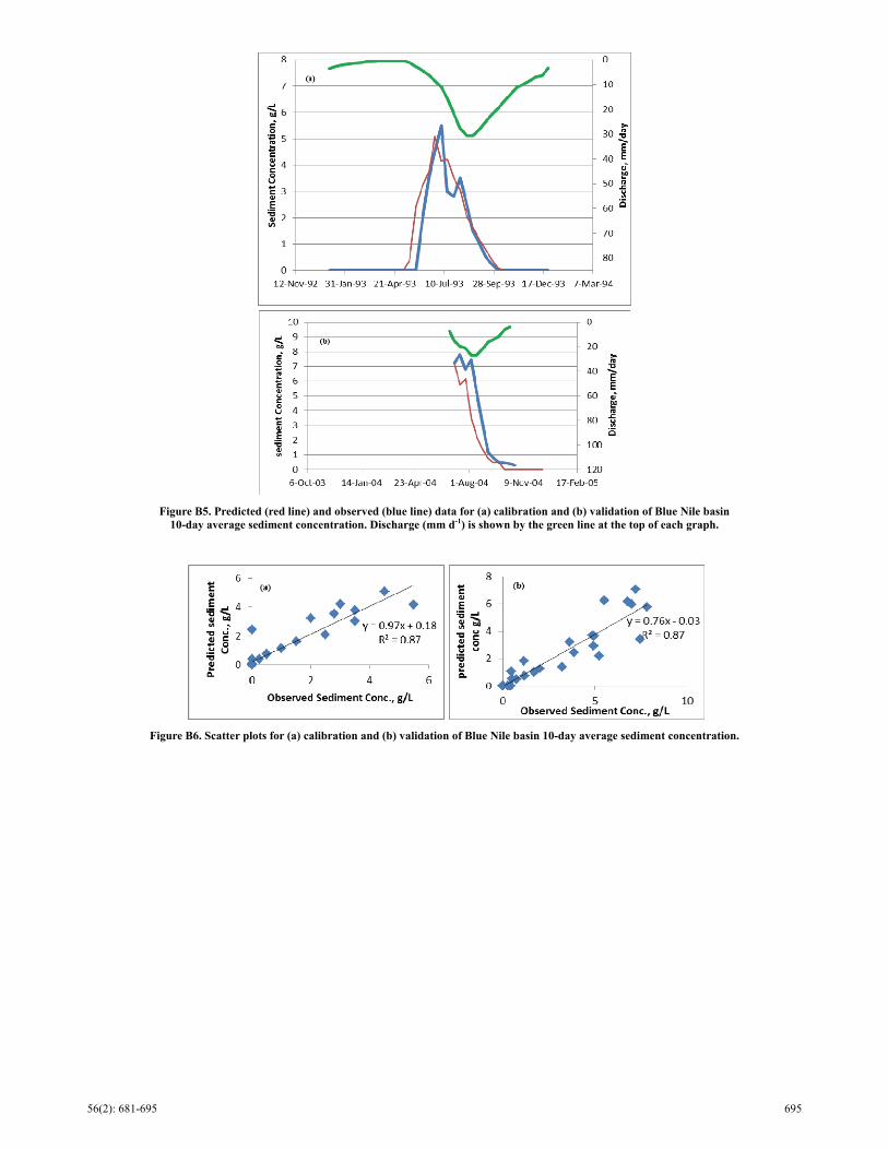
Figure B5. Predicted (red line) and observed (blue line) data for (a) calibration and (b) validation of Blue Nile basin

10-day average sediment concentration. Discharge (mm d-1) is shown by the green line at the top of each graph.

Figure B6. Scatter plots for (a) calibration and (b) validation of Blue Nile basin 10-day average sediment concentration.