Embed Size (px)
Citation preview

Copyright
by
Yu-Jeng Lin
2016
The Dissertation Committee for Yu-Jeng Lin Certifies that this is the approved
version of the following dissertation:
Modeling Advanced Flash Stripper for Carbon Dioxide Capture Using
Aqueous Amines
Committee:
Gary T. Rochelle, Supervisor
Michael Baldea
Eric Chen
Gyeong S. Hwang
David Miller

Modeling Advanced Flash Stripper for Carbon Dioxide Capture Using
Aqueous Amines
by
Yu-Jeng Lin, B.S., M.S.
Dissertation
Presented to the Faculty of the Graduate School of
The University of Texas at Austin
in Partial Fulfillment
of the Requirements
for the Degree of
DOCTOR OF PHILOSOPHY
THE UNIVERSITY OF TEXAS AT AUSTIN
August 2016

To my parents

v
Acknowledgements
Most importantly I would like to thank Mom and Dad. Pursuing Ph.D. abroad
could be much tougher without your love and encouragement. You were always there
supporting every decision I made. Thank you for giving us everything you have and make
our life better. I would not be the person I am today without you.
I would like to thank my advisor, Dr. Gary Rochelle for this incredible journey.
This work cannot be done without your consistent advising and encouragement. I am so
lucky to have the best mentor who is brilliant, motivating, patient and thoughtful. The
patience you have and the tremendous amount of time you spend on your everty student
make me want to become a better mentor when it comes to teaching. Your passion and
dedication to the work and the people you love while having a well work-life balance
become a role model I want to follow. Every weekly meeting with you was always
inspiring and motivated me to become a better engineer. I had the best learning
experience of my life.
I also appreciate my advisors in National Tsing Hua University, Dr. Shi-Shang Jang
and Dr. Shan-Hill Wong who encouraged me to step outside the comfort zone and meet
the smartest people in the world. Thank you Maeve for editing all of the progress reports
and helping me improve my writing skill. Those feedback is especially valuable for
international students.
I have learned so much from all of my current and previous groupmates not just
technical knowledge but also the way you approach and solve problems. Joining as the
same class year and the same group, Di is a perfect company to discuss qualifying exam,
course work and inevitably carbon capture. Tarun Madan was a great mentor who set
great examples on modeling work when I came in as a first-year. The previous work by

vi
David Van Wagener and Babatunde Oyenekan is an essential foundation of this work. It
was always enjoyable to have discussions with my groupmates, Peter Frailie, Lynn Li,
Brent Sherman, Matt Walters, Nathan Fine, Darshan Sachde, Eric Chen, Yang Du, Omkar
Namjoshi, Steven Fulk, Matt Beaudry, Yue Zhang, Kent Fischer, Ye Yuan, and Junyuan
Ding. Thank you for extending my vision and reminding me what I can do better. I am
grateful to have my friends whom I’ve known since college, Jerry, Island, Helen, Kaif, and
Ke-Hsun. Every trip we had always refreshed me and made me able to come back to
work with full of energy and memory. It’s been a memorable journey with all of your
participation.

vii
Modeling Advanced Flash Stripper for Carbon Dioxide Capture Using
Aqueous Amines
Yu-Jeng Lin, Ph.D.
The University of Texas at Austin, 2016
Supervisor: Gary T. Rochelle
The intensive energy use is the major obstacle to deployment of CO2 capture.
Alternative stripper configurations is one of the most promising ways to reduce the energy
consumption of CO2 regeneration and compression. The advanced flash stripper (AFS)
proposed in this work provides the best energy performance among other alternatives.
A systematic irreversibility analysis was performed instead of examining all the
possible alternatives. The overhead condenser and the cross exchanger were identified
the major sources of lost work that causes process inefficiencies. The AFS reduces the
reboiler duty by 16% and the total equivalent work by 11% compared to the simple stripper
using aqueous piperazine. The AFS was demonstrated in a 0.2 MW equivalent pilot plant
and showed over 25% of heat duty reduction compared to previous campaigns, achieving
2.1 GJ/tonne CO2 of heat duty and 32 kJ/mol CO2 of total equivalent work. The proposed
bypass control strategy was successfully demonstrated and minimized the reboiler duty.
Approximate stripper models (ASM) were developed to generalize the effect of
solvent properties on energy performance and guide solvent selections. High heat of
absorption can increase partial pressure of CO2 at elevated temperature and has potential
to reduce compression work and stripping steam heat. The optimum heat of absorption
was quantified as 70–125 kJ/mol CO2 at various conditions, which is generally higher than

viii
existing amines with 60–80 kJ/mol. The energy performance of AFS is not sensitive to
the heat of absorption.
A techno-economic analysis with process optimization that minimizes the
annualized regeneration cost was performed to demonstrate the profitability of the AFS.
The AFS reduces the annualized regeneration cost by 13% and the major savings come
from the reduction of the OPEX, which counts for over 70% of the regeneration cost. The
compressor and the cross exchanger are the major components of the CAPEX. The
optimum lean loading is around 0.22 mol CO2/mol alkalinity for PZ but is flat between
0.18 and 0.24 with less than 1% difference.
The AFS was demonstrated as a flexible system that can be applied to a wide range
of solvent properties and operating conditions while still maintaining remarkable energy
performance. Further improvement of energy efficiency by process modifications is
expected to be marginal. Increasing solvent capacity will give the most energy and cost
reduction in the future.

ix
Table of Contents
List of Tables .........................................................................................................xv
List of Figures ........................................................................................................xx
Chapter 1: Introduction ............................................................................................1
1.1 CO2 capture from coal-fired power plants ................................................1
1.2 Amine scrubbing process ..........................................................................3
1.3 Energy use for CO2 regeneration ..............................................................4
1.4 Prior work of alternative strippers ............................................................6
1.4.1 Solvent selections..........................................................................8
1.4.2 Quantifying energy performance ..................................................9
1.4.3 Demonstration of operability and profitability ...........................10
1.5 Research scope ........................................................................................11
Chapter 2: Modeling Methods ...............................................................................12
2.1 Stripper modeling in Aspen Plus® ..........................................................12
2.2 Calculating heat exchanger LMTD .........................................................14
2.3 Total equivalent work .............................................................................15
2.4 Heat-to-electricity efficiency ..................................................................16
2.5 Multi-stage compressor ...........................................................................18
2.5.1 Characteristics of CO2 compression ...........................................19
2.5.2 Updated multi-stage compressor configuration ..........................20
2.5.3 Compression work correlation ....................................................24
Chapter 3: Process Irreversibility Analysis............................................................26
3.1 Introduction .............................................................................................26
3.2 Methods...................................................................................................28
3.2.1 Process specifications .................................................................28
3.2.2 Theoretical minimum work and lost work ..................................29
3.3 Process descriptions ................................................................................31
3.3.1 Simple stripper ............................................................................31
3.3.2 Lean vapor compression .............................................................32

x
3.4 Results and discussions ...........................................................................33
3.4.1 Inefficiency of simple stripper ....................................................33
3.4.1.1 Minimum work and lost work distribution .....................33
3.4.1.2 Lost work of regeneration ...............................................35
3.4.2 Inefficiency of lean vapor compression ......................................37
3.4.3 Proposed design strategies ..........................................................38
3.4.3.1 Heat and mass transfer in the stripper .............................39
3.4.3.2 Self-contained heat integration using cold rich solvent ..40
3.4.3.3 Temperature pinch of the cross exchanger .....................41
3.4.4 Advanced flash stripper ..............................................................42
3.4.4.1 Proposed stripper configuration ......................................42
3.4.4.2 Lost work of regeneration ...............................................44
3.4.4.3 Cold and warm rich bypass .............................................48
3.4.4.4 Irreversibility of the cross exchanger ..............................50
3.4.4.5 Irreversibility of the reboiler/steam heater ......................53
3.4.5 Thermodynamic efficiency of regeneration ................................53
3.5 Conclusions .............................................................................................55
Chapter 4: Energy Performance of Advanced Stripper Configurations ................57
4.1 Introduction .............................................................................................57
4.2 Simulation methods ................................................................................59
4.2.1 Modeling stripper with updated MEA model .............................59
4.2.2 Stripping steam for PZ and MEA ...............................................61
4.2.3 Process specifications .................................................................62
4.3 Process descriptions ................................................................................64
4.3.1 Simple stripper ............................................................................64
4.3.2 Conventional alternatives............................................................65
4.3.2.1 Lean vapor compression (LVC)......................................65
4.3.2.2 Interheated stripper .........................................................66
4.3.2.3 Cold rich bypass ..............................................................67
4.3.3 Rich exchanger bypass strategy ..................................................68

xi
4.3.3.1 Simple stripper with rich exchanger bypass ...................68
4.3.3.2 Advanced reboiled stripper (ARS)..................................69
4.3.3.3 Advanced flash stripper (AFS) .......................................70
4.4 Results and discussions ...........................................................................71
4.4.1 Tradeoffs of optimum lean loading .............................................71
4.4.2 Energy performance of conventional alternatives ......................72
4.4.3 Rich exchanger bypass ................................................................74
4.4.4 Advanced reboiled/flash stripper ................................................77
4.4.5 Effect of packing height ..............................................................78
4.4.6 Effect of warm rich bypass temperature .....................................79
4.5 Overall comparisons ...............................................................................80
4.6 Conclusions .............................................................................................81
Chapter 5: Pilot Plant Test of the AFS...................................................................83
5.1 Introduction .............................................................................................83
5.2 Overview of SRP pilot plant ...................................................................84
5.3 Pilot plant results.....................................................................................88
5.3.1 Material balance ..........................................................................88
5.3.2 Enthalpy balance and heat loss ...................................................89
5.3.3 Energy performance ....................................................................90
5.3.4 Rich solvent bypass performance ...............................................94
5.3.5 Lean loading effect .....................................................................96
5.3.6 5 m PZ vs. 8 m PZ ......................................................................98
5.3.7 Heat exchanger performance ......................................................99
5.3.7.1 Cross exchangers ..........................................................100
5.3.7.2 Steam heaters ................................................................104
5.3.7.3 Cold rich exchanger ......................................................105
5.4 Modeling results....................................................................................106
5.4.1 Simulation model and data reconciliation .................................106
5.4.2 Model validation .......................................................................108
5.4.3 Rich solvent bypass optimization .............................................114

xii
5.4.4 Effect of rich and lean loading ..................................................116
5.4.5 Effect of striper packing height.................................................118
5.4.6 Effect of cross exchange area ...................................................120
5.5 Irreversibility analysis ...........................................................................122
5.6 Conclusions ...........................................................................................125
Acknowledgement ......................................................................................126
Chapter 6: Approximate Stripper Models (ASM) ...............................................127
6.1 Introduction ...........................................................................................127
6.2 Model development ..............................................................................128
6.2.1 Modeling specifications ............................................................129
6.2.1.1 Heat exchangers ............................................................130
6.2.1.2 Viscosity correction for cross exchanger ......................131
6.2.1.3 Stripper column .............................................................132
6.2.2 Solvent characterization ............................................................133
6.3 Model validation and interpretation ......................................................136
6.3.1 Comparison with rigorous Aspen Plus® model ........................136
6.3.2 Uncertainties of predicted heat capacity ...................................137
6.3.3 Model interpretation using MEA and PZ..................................139
6.3.4 Contributions to energy requirement ........................................141
6.4 Sensitivity analysis................................................................................142
6.4.1 Effect of rich loading ................................................................142
6.4.2 Effect of VLE slope ..................................................................143
6.5 Conclusions ...........................................................................................146
Chapter 7: Optimizing Heat of Absorption using the ASM ................................147
7.1 Introduction ...........................................................................................147
7.2 Modeling method ..................................................................................148
7.2.1 ASMs with generic solvent .......................................................148
7.2.2 Process specifications ...............................................................149
7.2.3 Overall energy performance .....................................................151
7.3 Results and discussions .........................................................................152

xiii
7.3.1 Tradeoffs of heat of absorption .................................................152
7.3.2 Effect of stripper configuration .................................................156
7.3.3 Effect of CO2 lean loading ........................................................158
7.3.4 Effect of reboiler temperature ...................................................159
7.3.5 Effect of compression efficiency ..............................................162
7.4 Conclusions ...........................................................................................165
Chapter 8: Optimum Design of Lean/Rich Amine Cross Exchanger ..................166
8.1 Introduction ...........................................................................................166
8.1.1 Plate-and-frame exchanger (PHE) ............................................166
8.2 Literature survey of heat transfer correlation for PHE .........................168
8.3 Viscosity effect on heat transfer coefficient .........................................172
8.4 Optimizing LMTD by shortcut method ................................................173
8.5 Optimizing fluid velocity ......................................................................175
8.5.1 Shortcut method ........................................................................176
8.5.2 Case study .................................................................................181
8.6 Conclusions ...........................................................................................183
Nomenclature ..............................................................................................183
Chapter 9: Techno-economic Analysis and Process Optimization ......................185
9.1 Introduction ...........................................................................................185
9.2 Modeling methods ................................................................................187
9.2.1 Process specifications ...............................................................187
9.2.2 Costing methods........................................................................188
9.2.3 Calculating purchased equipment cost (PEC)...........................190
9.2.4 Process optimization .................................................................196
9.3. Results and discussions ........................................................................197
9.3.1 Optimum stripper design with minimum regeneration cost .....197
9.3.2 Effect of CO2 lean loading ........................................................202
9.3.3 Effect of rich loading ................................................................206
9.3.4 Sensitivity of costing factors .....................................................208
9.3.5 5 m PZ vs. 8 m PZ ....................................................................210

xiv
9.4. Alternative supersonic compressor ......................................................214
9.5. Conclusions ..........................................................................................217
Chapter 10: Conclusions and Recommendations ................................................219
10.1 Summary .............................................................................................219
10.1.1 Advanced flash stripper ..........................................................219
10.1.2 Demonstration of the AFS ......................................................220
10.1.2.1 Pilot plant test .............................................................220
10.1.2.2 Economic analysis ......................................................221
10.1.3 Effect of solvent properties .....................................................222
10.2 Recommendations for future work .....................................................223
10.2.1 Model improvement ................................................................223
10.2.2 Heat transfer measurement .....................................................224
10.2.3 Application of the AFS ...........................................................224
Appendix A: Theoretical minimum work ............................................................225
Appendix B: Tabulated Simulation Data .............................................................227
Appendix C: Approximate Stripper Model Equations.........................................235
C.1 Simple stripper .....................................................................................235
C.2 Advanced flash stripper ........................................................................238
Nomenclature ..............................................................................................242
References ............................................................................................................244
Vita 255

xv
List of Tables
Table 1.1: Prior work on alternative strippers. ........................................................7
Table 1.2: Comparisons of solvent properties of MEA and PZ. ..............................9
Table 2.1: Multi-stage compressor specifications .................................................21
Table 3.1: Summary of modeling methods. ...........................................................28
Table 3.2: Summary of process specifications. .....................................................29
Table 3.3: Boundary conditions of minimum work calculations. ..........................30
Table 4.1: Alternative stripper configurations proposed to reduce stripping steam heat
...........................................................................................................58
Table 4.2: Process simulation specifications. ........................................................64
Table 4.3: Optimum results for 8 m PZ; rich loading: 0.4; cross exchanger ΔTLM: 5 K;
2 m packing; correction for interfacial area: 1; reboiler T: 150 °C;
optimum pressure ratio for LVC; optimum bypass rates. .................74
Table 4.4: Optimum results for 9 m MEA; rich loading: 0.5; cross exchanger ΔTLM: 5
K; 2 m packing; correction for interfacial area: 1; reboiler T: 120 °C;
optimum bypass rates. .......................................................................74
Table 4.5: Adjusted steam temperature and total equivalent work for AFS using 8 m
PZ; rich loading: 0.4; cross exchanger ΔTLM: 5 K; 2 m packing;
correction for interfacial area: 1; reboiler T: 150 °C; optimum bypass
rates. ..................................................................................................78
Table 5.1: Summary of column design and operating conditions. ........................86
Table 5.2: 2015 SRP Pilot plant operating conditions using the AFS and PZ.......87
Table 5.3: Comparisons of pilot plant results of 5 m and 8 m PZ. ........................99
Table 5.4: Heat exchanger specifications of SRP pilot plant...............................100

xvi
Table 6.1: Temperature and concentration driving force from Aspen Plus®
simulations using the AFS and 5 m PZ; 15% correction for interfacial
area; reboiler T: 150 °C; optimized bypass rates; rich loading: 0.4.133
Table 6.2: Regressed constants in Equation 6.8 for MEA and PZ. .....................136
Table 6.3: Partial heat capacity of CO2 of loaded PZ. .........................................139
Table 6.4: Process specifications for solvent evaluation. ....................................139
Table 6.5: Average slope of CO2 solubility curve at 40 °C between P*CO2 0.1 to 5 kPa.
.........................................................................................................144
Table 7.1: Regressed constants for semi-empirical Equation 6.8 for PZ. ............149
Table 7.2: Process specifications. ........................................................................151
Table 7.3: Energy performance with varied heat of absorption using simple stripper;
PZ-based generic solvent; reboiler T: 150 °C; rich solvent P*CO2 at 40
°C: 5 kPa; lean solvent P*CO2 at 40 °C: 0.15 kPa; cross exchanger ΔTLM:
5 K. ..................................................................................................155
Table 7.4: Energy performance with varied heat of absorption using AFS; PZ-based
generic solvent; reboiler T: 150 °C; rich solvent P*CO2 at 40 °C: 5 kPa;
lean solvent P*CO2 at 40 °C: 0.15 kPa; cross exchanger ΔTLM: 5 K.155
Table 8.1: Summary of empirical correlations of heat transfer and pressure drop for
PHE. ................................................................................................169
Table 8.2: Physical properties of 8 m PZ at 90 ºC and CO2 loading at 0.30. ......171
Table 8.3: Typical design parameters for PHE. ...................................................182
Table 8.4: Summary of dependence between heat transfer coefficient, pressure drop,
and viscosity by shortcut method. ...................................................183
Table 9.1: Summary of design specifications. .....................................................188
Table 9.2: Summary of costing parameters. ........................................................190

xvii
Table 9.3: Summary of equipment sizing and pricing basis. ...............................191
Table 9.4: Design specifications of multi-stage compressor. ..............................193
Table 9.5: Comparison of CAPEX of compressor from sources. ........................196
Table 9.6: Equipment table of simple stripper at 0.22 lean loading. ...................199
Table 9.7: Equipment table of AFS at 0.22 lean loading. ....................................200
Table 9.8: Energy use of simple stripper and AFS. .............................................201
Table 9.9: Comparison of absorber performance between 5 m and 8 m PZ in 2015
SRP pilot plant ................................................................................212
Table 9.10: Summary of economic analysis for 5 m and 8 m PZ. .......................213
Table 9.11: Design specifications of supersonic compressor. .............................215
Table B.1: Simple stripper using 8 m PZ; rich loading: 0.4; cross exchanger ΔTLM: 5
K; 1 m Mellapak 250X packing; correction for interfacial area: 1;
reboiler T: 150 °C. ..........................................................................227
Table B.2: Simple stripper using 8 m PZ; rich loading: 0.4; cross exchanger ΔTLM: 5
K; 2 m Mellapak 250X packing; correction for interfacial area: 1;
reboiler T: 150 °C. ..........................................................................227
Table B.3: Simple stripper using 8 m PZ; rich loading: 0.4; cross exchanger ΔTLM: 5
K; 5 m Mellapak 250X packing; correction for interfacial area: 1;
reboiler T: 150 °C. ..........................................................................228
Table B.4: Cold rich bypass using 8 m PZ; rich loading: 0.4; cross exchanger ΔTLM: 5
K; 2 m Mellapak 250X packing; correction for interfacial area: 1;
reboiler T: 150 °C; optimum bypass rate. .......................................228
Table B.5: Rich exchanger bypass using 8 m PZ; rich loading: 0.4; cross exchanger
ΔTLM: 5 K; 2 m Mellapak 250X packing; correction for interfacial area:
1; reboiler T: 150 °C; optimum bypass rate. ...................................229

xviii
Table B.6: Interheated stripper using 8 m PZ; rich loading: 0.4; cross exchanger
ΔTLM: 5 K; 2 m Mellapak 250X packing; correction for interfacial area:
1; reboiler T: 150 °C. ......................................................................229
Table B.7: Lean vapor compression using 8 m PZ; rich loading: 0.4; cross exchanger
ΔTLM: 5 K; 2 m Mellapak 250X packing; correction for interfacial area:
1; reboiler T: 150 °C; optimum pressure ratio. ...............................230
Table B.8: Lean vapor compression using 8 m PZ; rich loading: 0.4; cross exchanger
ΔTLM: 5 K; 5 m packing; correction for interfacial area: 1; reboiler T:
150 °C; optimum pressure ratio. .....................................................230
Table B.9: AFS using 8 m PZ; rich loading: 0.4; cross exchanger ΔTLM: 5 K; 2 m
Mellapak 250X packing; correction for interfacial area: 1; reboiler T:
150 °C; optimum bypass rates. .......................................................231
Table B.10: AFS using 8 m PZ; rich loading: 0.4; cross exchanger ΔTLM: 5 K; 5 m
Mellapak 250X packing; correction for interfacial area: 1; reboiler T:
150 °C; optimum bypass rates. .......................................................231
Table B.11: ARS using 8 m PZ; rich loading: 0.4; cross exchanger ΔTLM: 5 K; 2 m
Mellapak 250X packing; correction for interfacial area: 1; reboiler T:
150 °C; optimum bypass rates. .......................................................232
Table B.12: Simple stripper using 9 m MEA; rich loading: 0.5; cross exchanger
ΔTLM: 5 K; 2 m Mellapak 250X packing; correction for interfacial area:
1; reboiler T: 120 °C. ......................................................................232
Table B.13: Rich exchanger bypass using 9 m MEA; rich loading: 0.5; cross
exchanger ΔTLM: 5 K; 2 m Mellapak 250X packing; correction for
interfacial area: 1; reboiler T: 120 °C; optimum bypass rate. .........233

xix
Table B.14: Interheated stripper using 9 m MEA; rich loading: 0.5; cross exchanger
ΔTLM: 5 K; 2 m Mellapak 250X packing; correction for interfacial area:
1; reboiler T: 120 °C. ......................................................................233
Table B.15: AFS using 9 m MEA; rich loading: 0.5; cross exchanger ΔTLM: 5 K; 2 m
Mellapak 250X packing; correction for interfacial area: 1; reboiler T:
120 °C; optimum bypass rates. .......................................................234
Table B.16: ARS using 9 m MEA; rich loading: 0.5; cross exchanger ΔTLM: 5 K; 2 m
Mellapak 250X packing; correction for interfacial area: 1; reboiler T:
120 °C; optimum bypass rates. .......................................................234

xx
List of Figures
Figure 1.1: 2013 U.S. CO2 Emissions from fossil fuel combustion by sector
(replotted from Figure ES-6 in EPA report, 2015). ............................2
Figure 1.2: Post-combustion CO2 capture from coal-fired power plant. .................3
Figure 1.3: Amine scrubbing process. .....................................................................4
Figure 1.4: Advanced flash stripper. ......................................................................10
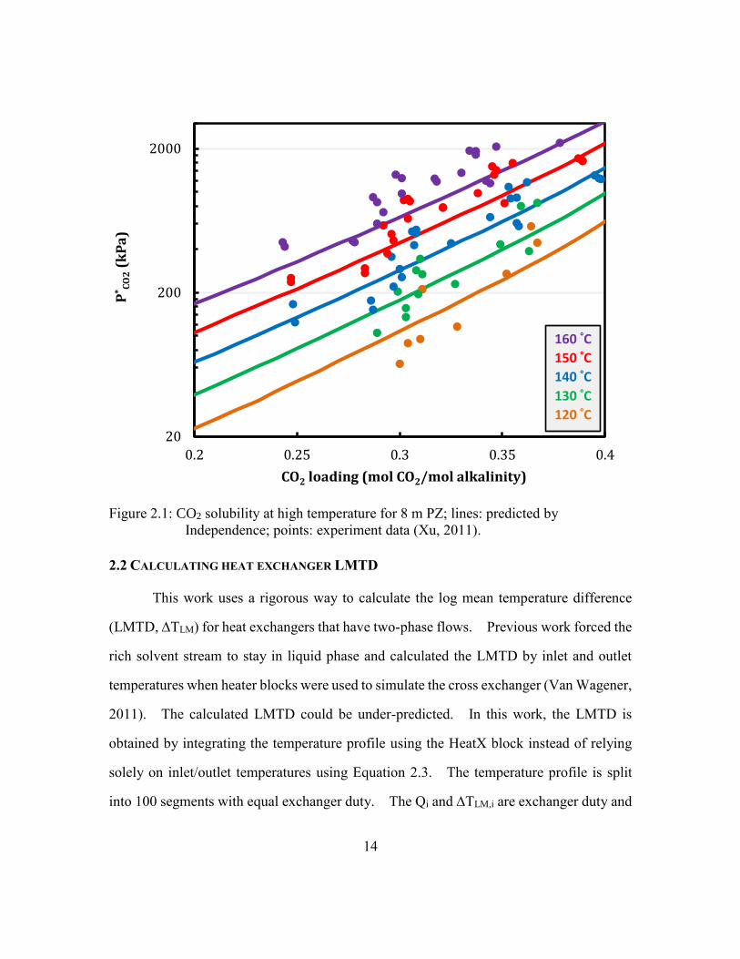
Figure 2.1: CO2 solubility at high temperature for 8 m PZ; lines: predicted by
Independence; points: experiment data (Xu, 2011). .........................14
Figure 2.2: Steam cycle integrated with CO2 regeneration....................................17
Figure 2.3: Heat-to-electricity efficiency at various steam saturation temperature.18
Figure 2.4: Density of supercritical CO2 with varied temperature. .......................20
Figure 2.5: Multi-stage compressor with supercritical pump ................................21
Figure 2.6: Compression work with updated configuration and efficiency. ..........23
Figure 2.7: Thermodynamic efficiency of CO2 compression. ...............................24
Figure 2.8: CO2 compression work with inlet pressure from 1–149 bar; final pressure
150 bar. .............................................................................................25
Figure 3.1: Simple stripper. ...................................................................................32
Figure 3.2: Lean vapor compression. .....................................................................33
Figure 3.3: Minimum work and lost work of simple stripper using 8 m PZ; rich
loading: 0.4; reboiler T: 150 °C; cross exchanger ΔTLM: 5 K; 5 m
packing; correction for interfacial area: 1. ........................................34
Figure 3.4: Lost work of regeneration of simple stripper using 8 m PZ; rich loading:
0.4; reboiler T: 150 °C; cross exchanger ΔTLM: 5 K; 5 m packing;
correction for interfacial area: 1. .......................................................36

xxi
Figure 3.5: Lost work of regeneration of lean vapor compression using 8 m PZ; rich
loading: 0.4; reboiler T: 150 °C; cross exchanger ΔTLM: 5 K; 5 m
packing; correction for interfacial area: 1; optimum pressure ratio of lean
vapor compressor at each lean loading. ............................................38
Figure 3.6: Temperature and CO2 concentration profile of stripper column for simple
stripper using 8 m PZ; lean loading: 0.24; rich loading: 0.4; reboiler T:
150 °C; cross exchanger ΔTLM: 5 K; 5 m packing; correction for
interfacial area: 1...............................................................................39
Figure 3.7: Pinch temperature approach of the cross exchanger of the simple stripper
using 8 m PZ; rich loading: 0.4; reboiler T: 150 °C; cross exchanger
ΔTLM: 5 K. .........................................................................................42
Figure 3.8: Advanced flash stripper .......................................................................43
Figure 3.9: Lost work of regeneration of advanced flash stripper using 8 m PZ; rich
loading: 0.4; reboiler T: 150 °C; cross exchanger ΔTLM: 5 K; 5 m
packing; correction for interfacial area: 1; optimum cold and warm rich
bypasses. ...........................................................................................45
Figure 3.10: Comparison of lost work of the condenser; 8 m PZ; rich loading: 0.4;
reboiler T: 150 °C; cross exchanger ΔTLM: 5 K; 5 m packing; correction
for interfacial area: 1; optimum pressure ratio for LVC; optimum cold
and warm rich bypasses for AFS. .....................................................46
Figure 3.11: Comparison of heat duty of reboiler/steam heater; 8 m PZ; rich loading:
0.4; reboiler T: 150 °C; cross exchanger ΔTLM: 5 K; 5 m packing;
correction for interfacial area: 1; optimum pressure ratio for LVC;
optimum cold and warm rich bypasses for AFS. ..............................47

xxii
Figure 3.12: Comparison of total equivalent work; 8 m PZ; rich loading: 0.4; reboiler
T: 150 °C; cross exchanger ΔTLM: 5 K; 5 m packing; correction for
interfacial area: 1; optimum pressure ratio for LVC; optimum cold and
warm rich bypasses for AFS. ............................................................48
Figure 3.13: Temperature and CO2 concentration profile of stripper column for the
advanced flash stripper; 8 m PZ; lean loading: 0.24; rich loading: 0.4;
reboiler T: 150 °C; cross exchanger ΔTLM: 5 K; 5 m packing; correction
for interfacial area: 1; optimum cold and warm rich bypasses. ........49
Figure 3.14: Flow heat capacity ratio of rich solvent to lean solvent of the cold cross
exchanger (single phase); 8 m PZ; rich loading: 0.4; reboiler T: 150 °C;
cross exchanger ΔTLM: 5 K; optimum cold and warm rich bypasses.51
Figure 3.15: Flow heat capacity ratio of rich solvent to lean solvent of the hot cross
exchanger (flashing phase); 8 m PZ; rich loading: 0.4; reboiler T: 150
°C; cross exchanger ΔTLM: 5 K; optimum cold and warm rich bypasses.
...........................................................................................................52
Figure 3.16: Comparison of thermodynamic efficiency of regeneration; 8 m PZ; rich
loading: 0.4; reboiler T: 150 °C; cross exchanger ΔTLM: 5 K; 5 m
packing; correction for interfacial area: 1; optimum pressure ratio of
LVS; optimum cold and warm rich bypasses for AFS. ....................54
Figure 4.1: CO2 partial pressure predicted by Hilliard model (dashed line) and
Phoenix model (solid line). ...............................................................60
Figure 4.2: Over-predicted stripper pressure by Hilliard model at 120 °C. ...........61
Figure 4.3: CO2 mole fraction in the vapor phase with varied lean loading predicted
by Independence for PZ and Phoenix for MEA................................62
Figure 4.4: Simple stripper. ...................................................................................65

xxiii
Figure 4.5: Lean vapor compression. .....................................................................66
Figure 4.6: Interheated stripper. .............................................................................67
Figure 4.7: Simple stripper with cold rich bypass. ................................................68
Figure 4.8: Simple stripper with cold rich exchanger bypass. ...............................69
Figure 4.9: Advanced reboiled stripper (ARS). .....................................................70
Figure 4.10: Advanced flash stripper (AFS). .........................................................71
Figure 4.11: Comparison of total equivalent work of alternative strippers using 8 m
PZ; rich loading: 0.4; cross exchanger ΔTLM: 5 K; 2 m packing;
correction for interfacial area: 1; reboiler T: 150 °C; optimum pressure
ratio for LVC; optimum bypass rates................................................72
Figure 4.12: Comparison of total equivalent work of alternative strippers using 9 m
MEA; rich loading: 0.5; cross exchanger ΔTLM: 5 K; 2 m packing;
correction for interfacial area: 1; reboiler T: 120 °C; optimum bypass
rates. ..................................................................................................73
Figure 4.13: McCabe-Thiele plot of cold rich bypass configuration using 8 m PZ; rich
loading: 0.5; lean loading; 0.28; cross exchanger ΔTLM: 5 K; 2 m
packing; correction for interfacial area: 1; reboiler T: 150 °C; optimum
bypass rates. ......................................................................................76
Figure 4.14: Total equivalent work with varied stripping packing height using 8 m
PZ; rich loading: 0.4; cross exchanger ΔTLM: 5 K; correction for
interfacial area: 1; reboiler T: 150 °C; optimum bypass rates. .........79
Figure 4.15: Total equivalent work with varied warm rich bypass temperature using 8
m PZ; rich loading: 0.4; cross exchanger ΔTLM: 5 K; 2 m packing;
correction for interfacial area: 1; reboiler T: 150 °C; optimum bypass
rates. ..................................................................................................80
xxiv
Figure 4.16: Total equivalent work of alternative stripper configurations; 8 m PZ;
lean loading: 0.26; rich loading: 0.4; cross exchanger ΔTLM: 5 K; 2 m
packing; correction for interfacial area: 1; reboiler T: 150 °C; optimum
bypass rates. ......................................................................................81
Figure 5.1: SRP CO2 capture pilot plant with advanced flash stripper. .................85
Figure 5.2: CO2 mass balance around the stripping process; average error: 2.2%.89
Figure 5.3: Heat loss and process heat duty of the AFS. .......................................91
Figure 5.4: Process heat duty of SRP pilot plant campaigns since 2011. ..............92
Figure 5.5: Total equivalent work of SRP pilot plant with the AFS......................94
Figure 5.6: Performance of rich solvent bypass; 4 runs highlighted were without
bypass control. ..................................................................................95
Figure 5.7: Effect of rich solvent bypass; run 10, 11, 17, and 18; 5 m PZ; flash tank T:
149 ºC; rich loading: 0.36; lean loading: 0.20. .................................96
Figure 5.8: Effect of lean loading; run 3, 4, 5, 11, 17, 20, and 21; 5 m PZ; flash tank
T: 149 °C; rich loading: 0.39±0.01. ..................................................97
Figure 5.9: Overall heat transfer coefficient of the cold cross exchanger. ..........101
Figure 5.10: Pressure drops of the cold cross exchanger. ....................................102
Figure 5.11: Overall heat transfer coefficient of the hot cross exchanger ...........103
Figure 5.12: Pressure drop of the hot cross exchanger. .......................................104
Figure 5.13: Overall heat transfer coefficient of the steam heaters. ....................105
Figure 5.14: Overall heat transfer coefficient of cold rich exchanger. ................106
Figure 5.15: Measured and modeled lean loading; average error: 5.4%. ............108
Figure 5.16: Measured and modeled rich loading; average error: 3.6%. .............109

xxv
Figure 5.17: Diffusivity of amine and CO2 in 5 m PZ solution predicted by
Independence model and modified Stokes-Einstein relation at stripper
conditions. .......................................................................................111
Figure 5.18: Measured and modeled process heat duty; average error: 3.0%. ....112
Figure 5.19: Stripper temperature profile; run 6; open points: measured T inside the
stripper; filled points: measured T outside the stripper; solid lines:
modeled T at operating bypass rates; dotted lines: modeled T at
optimized bypass rates. ...................................................................113
Figure 5.20: Stripper temperature profile; run 18; open points: measured T inside the
stripper; filled points: measured T outside the stripper; solid lines:
modeled T at operating bypass rates; dotted lines: modeled T at
optimized bypass rates. ...................................................................114
Figure 5.21: Process heat duty improvement after bypass re-optimization; circle: with
bypass control; triangle: without bypass control. ...........................116
Figure 5.22: Total equivalent work with various lean and rich loading; stripper T: 149
°C; packing: 2 m RSR no. 0.3; correction for interfacial area: 0.15;
constant UA; optimized bypass rates. .............................................118
Figure 5.23: Total equivalent work with various packing height and lean loading;
packing: RSR no. 0.3; correction for interfacial area: 0.15; rich loading:
0.41; stripper T: 149 °C; constant UA; optimized bypass rates. .....119
Figure 5.24: Packing utilization efficiency; packing: RSR no. 0.3; correction for
interfacial area: 0.15; rich loading: 0.41; stripper T: 149 °C; constant
UA; optimized bypass rates. ...........................................................120

xxvi
Figure 5.25: Total equivalent work with various cross exchanger UA; packing: 2 m
RSR no. 0.3; correction for interfacial area: 0.15; rich loading: 0.41;
stripper T: 149 °C; optimized bypass rates. ....................................122
Figure 5.26: Minimum work and lost work distributions of SRP pilot plant with the
AFS; average values from the runs that achieved at least 90% capture
rate and implemented bypass control. .............................................124
Figure 6.1: Approximate stripper model ..............................................................128
Figure 6.2: Simple stripper. .................................................................................130
Figure 6.3: Advanced flash stripper. ....................................................................130
Figure 6.4: Integration path of partial pressure of CO2 for solvent characterization.135
Figure 6.5: Comparison of ASM and the validated Aspen Plus® model using AFS; 5
m PZ; reboiler T: 150 °C; 5 K cross exchanger ΔTLM; 5 m RSR no. 0.3
packing; 0.15 correction factor for interfacial area used in the Aspen
Plus® model. ....................................................................................137
Figure 6.6: Approximate stripper model results of 9 m MEA and 8 m PZ with the
simple stripper and the AFS; rich loading: 0.4 for PZ and 0.5 for MEA;
cross exchanger ΔTLM: 5 K; reboiler T: 150 °C for PZ and 120 °C for
MEA. ...............................................................................................140
Figure 6.7: Breakdown of energy requirement using approximate stripper models;
lean P*CO2: 0.15 kPa; rich loading: 0.4 for PZ and 0.5 for MEA; cross
exchanger ΔTLM: 5 K; reboiler T: 150 °C for PZ and 120 °C for MEA.
.........................................................................................................142
Figure 6.8: Sensitivity to rich loading; 8 m PZ; reboiler T: 150 °C; optimized lean
loading.............................................................................................143

xxvii
Figure 6.9: Sensitivity to VLE slope, k; simple stripper with 8 m PZ-based solvent;
reboiler T: 150 °C; rich solvent P*CO2: 5 kPa; cross exchanger ΔTLM: 5
K. .....................................................................................................144
Figure 6.10: Sensible heat requirement with varied VLE slope, k (ln Pa/mol CO2);
simple stripper with 8 m PZ-based solvent; reboiler T: 150 °C; lean
P*CO2: 0.05–1 kPa; rich solvent P*
CO2: 5 kPa; cross exchanger ΔTLM: 5 K.
.........................................................................................................145
Figure 7.1: Simple stripper ..................................................................................150
Figure 7.2: Advanced flash stripper .....................................................................150
Figure 7.3: Effect of heat of absorption for simple stripper; PZ-based generic solvent;
reboiler T: 150 °C; rich solvent P*CO2 at 40 °C: 5 kPa; lean solvent P*
CO2
at 40 °C: 0.15 kPa; cross exchanger ΔTLM: 5 K. .............................153
Figure 7.4: Effect of heat of absorption for AFS; PZ-based generic solvent; reboiler
T: 150 °C; rich solvent P*CO2 at 40 °C: 5 kPa; lean solvent P*
CO2 at 40
°C: 0.15 kPa; cross exchanger ΔTLM: 5 K.......................................154
Figure 7.5: Sensitivity of total equivalent work to heat of absorption; PZ-based
generic solvent; reboiler T: 150 °C; rich solvent P*CO2 at 40 °C: 5 kPa;
lean solvent P*CO2 at 40 °C: 0.15 kPa; cross exchanger ΔTLM: 5 K.156
Figure 7.6: Comparison of total equivalent work between original and optimized heat
of absorption; PZ-based generic solvent; reboiler T: 150 °C; rich solvent
P*CO2 at 40 °C: 5 kPa; cross exchanger ΔTLM: 5 K. ........................157
Figure 7.7: Optimum heat of absorption with varied lean loading; PZ-based generic
solvent; reboiler T: 120 and 150 °C; rich solvent P*CO2 at 40 °C: 5 kPa;
cross exchanger ΔTLM: 5 K. ............................................................159

xxviii
Figure 7.8: Optimum reboiler T and total equivalent work at varied heat of
absorption; PZ-based generic solvent; rich solvent P*CO2 at 40 °C: 5 kPa;
lean solvent P*CO2 at 40 °C: 0.15 kPa; cross exchanger ΔTLM: 5 K.160
Figure 7.9: Effect of reboiler temperature on total equivalent work using AFS; PZ-
based generic solvent; average heat of absorption: 70 kJ/mol; rich
solvent P*CO2 at 40 °C: 5 kPa; lean solvent P*
CO2 at 40 °C: 0.15 kPa;
cross exchanger ΔTLM: 5 K. ............................................................162
Figure 7.10: Sensitivity of thermal and mechanical compression efficiency; PZ-based
generic solvent; reboiler T: 150 °C; rich solvent P*CO2 at 40 °C: 5 kPa;
lean solvent P*CO2 at 40 °C: 0.15 kPa; cross exchanger ΔTLM: 5 K.164
Figure 8.1: Plate-and-frame exchanger (Reppich, 1999). ....................................167
Figure 8.2: Corrugated plate and corrugation angle, . .......................................168
Figure 8.3: Nusselt number predicted by empirical correlations with varied Reynolds
number using physical properties of 8 m PZ. .................................172
Figure 8.4: The dependence of viscosity on the exchanger cost predicted by empirical
correlations with varied corrugation angle. ....................................173
Figure 8.5: Optimization of cross exchanger LMTD...........................................174
Figure 8.6: Flow pattern and geometry of a single-pass plate-and-frame exchanger.
.........................................................................................................176
Figure 8.7: The dependence of pressure drop per unit length on Nusselt number
predicted by empirical correlations with varied corrugation angle.178
Figure 8.8: Optimum velocity with varied exponent of Reynolds number, m. ...181
Figure 8.9: Optimum velocity with varied solvent viscosity. ..............................182
Figure 9.1: Economic analysis scope for the simple stripper. .............................186
Figure 9.2: Economic analysis scope for the advanced flash stripper. ................187
xxix
Figure 9.3: Multi-stage compressor with supercritical pump. .............................193
Figure 9.4: Purchased equipment cost of multi-stage compressor with supercritical
pump from Aspen Icarus® ; CO2 flow rate: 116 kg/s; 2015 cost level.194
Figure 9.5: Annualized CAPEX of multi-stage compressor; CO2 flow rate: 116 kg/s;
2015 cost level; =1. ....................................................................195
Figure 9.6: Breakdown of annualized regeneration cost at 0.22 lean loading. ....202
Figure 9.7: Effect of lean loading on annualized regeneration cost; rich loading: 0.4;
reboiler T: 150 °C; correction for interfacial area: 0.15. ................204
Figure 9.8: Breakdown of the annualized regeneration cost of AFS with varied lean
loading.............................................................................................205
Figure 9.9: Effect of rich loading on annualized regeneration cost with varied lean
loading.............................................................................................206
Figure 9.10: Effect of rich loading on annualized regeneration cost with varied ΔLdg.
.........................................................................................................207
Figure 9.11: Sensitivity of capital costing factor on annualized regeneration cost;
COE: $100/MWh. ...........................................................................208
Figure 9.12: Sensitivity of COE on annualized regeneration cost; =1. ...........209
Figure 9.13: Optimum average cross exchanger LMTD with varied COE $80 to
120/MWh and from 0.5 to 1.5. ..................................................210
Figure 9.14: Comparison of 5 m and 8m PZ; rich loading: 0.40; stripper T: 150 °C
(Freeman, 2011; Li, 2015). .............................................................211
Figure 9.15: Comparing the annualized regeneration cost of 5 m and 8 m PZ. ..213
Figure 9.16: Supersonic compressor with heat integration. .................................215
Figure 9.17: Comparison of supersonic and conventional multi-stage compressors.217
Figure A.1: Minimum work integration for CO2 regeneration process. ..............225

1
Chapter 1: Introduction
1.1 CO2 CAPTURE FROM COAL-FIRED POWER PLANTS
The coal-fired power plant is the major source of anthropogenic carbon emissions
(Figure 1.1) (EPA, 2015b). Coal-fired plants accounts for 77% of the emissions from
electricity generation and 31% of total fossil-fuel combustions in the U.S. in 2013.
Regulatory actions have been taken by the Environmental Protection Agency (EPA) to
reduce carbon emissions. The Clean Power Plan requires each state to propose a
comprehensive plan to reduce overall CO2 emissions by 10–50% before 2030 (EPA,
2015a). Those states generate more electricity from coal-fired power plants will have
higher target to achieve. Emission limits have been set as 1400 and 1000 lb/MWh-gross
for new-built coal-fired and natural gas-fired power plants while the average emission rates
are around 1800 and 800 lb/MWh, respectively. The regulation will force the power
sectors to add carbon capture and sequestration (CCS) technology to the coal-fired power
plant or shift to other low-carbon power generation such as natural gas firing and renewable
energy.
Coal is still considered the largest share (34%) of total electricity generation in 2040
because of its abundance and low price compared to other alternatives (EIA, 2015). CCS
is projected to contribute 14% of carbon reduction through 2050, and coal-fired power
plants will be the largest single application with 2/3 of them equipped with CCS (IEA,
2013). The actual scenario will depend on how cost-competitive the CCS can be and the
demonstration for commercial plants.
Figure 1.2 shows post-combustion CO2 capture for coal-fired plants. The CO2 in
the flue gas will be separated by the capture process and compressed up to 150 bar for
further storage and enhanced oil recovery (EOR).

2
Figure 1.1: 2013 U.S. CO2 Emissions from fossil fuel combustion by sector (replotted
from Figure ES-6 in EPA report, 2015).
0
1
2
CO
2e
mis
sio
ns
(bil
lio
n t
on
)
Commercial
Residential
Industry
Transportation
Electricity generation
Naturalgas
Coal-fired

3
Feedwater Preheating System
Coal+Air
HP IP LP
Boiler
CO2 CaptureCompression
System
To storageor EOR
Flue gas Treatment
Generator
HP steam
Condensate
CO2
Flue gas12% CO2
IP/LP steam Electricity
Feedwater
IP steam LP steam
Figure 1.2: Post-combustion CO2 capture from coal-fired power plant.
1.2 AMINE SCRUBBING PROCESS
Amine scrubbing is considered the most mature technology for CO2 capture and
has been successfully applied to two commercial-scale coal-fired power plants (Hirata et
al., 2014; Stéphenne, 2014). A typical amine scrubbing process includes an absorber, a
stripper, and a cross exchanger (Figure 1.3). Desulfurized flue gas is contacted with the
aqueous amine in the absorber to remove 90% of the CO2. The rich solvent carrying the
CO2 from the bottom of the absorber is sent to the stripper and heated for CO2 regeneration.
After condensing the water, the purified CO2 will be sent to the multi-stage compressor.

4
CO2
Cross Exchanger
Lean Solvent
Rich Solvent
Reboiler
Stripper
Condensate
Condenser
Trim Cooler
AbsorberFlue gas12% CO2
Vented gas
Figure 1.3: Amine scrubbing process.
1.3 ENERGY USE FOR CO2 REGENERATION
The intensive energy consumption is the major obstacle to deployment of CO2
capture (Rochelle, 2009). CO2 regeneration requires heat duty, which is usually supplied
by extracting the steam from the crossover pipe between the intermediate and low pressure
turbines in the power plant. Other major energy requirements include the pump work and
CO2 compression work. Implementing CO2 capture incurs a 20–30% penalty on
electricity output for a typical coal-fired power plant (Aroonwilas et al., 2007; Oexmann,
2011; Romeo et al., 2008). The reboiler duty provides heat of CO2 desorption, heat of
stripping steam, and sensible heat.
Heat of CO2 desorption
Absorbing CO2 by aqueous amines is exothermic. Regenerating CO2 needs to
reverse the reactions by providing heat to the rich solvent, so the heat of absorption (Habs)
determines the least amount of heat duty requirement for CO2 stripping. The heat of
absorption is dependent on solvent and which type of reactions dominates. Amine can

5
react with CO2 via carbamate and bicarbonate formation reactions. CO2 absorption
dominated by carbamate formation (primary and secondary amines) usually gives a higher
heat of absorption than bicarbonate formation (tertiary amines) (I. Kim et al., 2011).
The heat of absorption can be expressed using Equation 1.1 from Lewis and Randall
(Equation XVIII.9) (Lewis et al., 1923). Equation 1.2 integrates the partial pressure of
CO2 (P*CO2) from a reference temperature (Tref) to the operating temperature (T). The
P*CO2 at elevated temperature will increase with heat of absorption and results in a high
stripper pressure.
∆𝐻𝑎𝑏𝑠 = −𝑅 [𝜕𝑙𝑛𝑓𝐶𝑂2
𝜕(1
𝑇)
]𝑃,𝑥
≈ −𝑅 [𝜕𝑙𝑛𝑃𝐶𝑂2
∗
𝜕(1
𝑇)
]𝑃,𝑥
(1.1)
𝑃𝐶𝑂2∗(𝑇)
𝑃𝐶𝑂2∗(𝑇𝑟𝑒𝑓)
= 𝑒𝑥𝑝 [∆𝐻𝑎𝑏𝑠
𝑅(
1
𝑇𝑟𝑒𝑓−
1
𝑇)] (1.2)
Heat of stripping steam
When the rich solvent is heated in the reboiler, water is vaporized and generate
steam for stripping, which ultimately is condensed in the overhead condenser. Analogous
to the heat of absorption, the latent heat of water vaporization determines the partial
pressure of water in the stripper as shown in Equation 1.3.
∆𝐻𝑣𝑎𝑝 = −𝑅 [𝜕𝑙𝑛𝑃𝐻2𝑂
∗
𝜕(1
𝑇)
]𝑃,𝑥
(1.3)
The difference between the heat of absorption and the heat of water vaporization
determines the selectivity between CO2 and the water vapor as shown in Equation 1.4.
The heat of absorption is typically greater than the heat of vaporization (around 40 kJ/mol
H2O).
𝑃𝐶𝑂2∗(𝑇)
𝑃𝐻2𝑂∗(𝑇)
=𝑃𝐻2𝑂
∗(𝑇𝑟𝑒𝑓)
𝑃𝐶𝑂2∗(𝑇𝑟𝑒𝑓)
𝑒𝑥𝑝 [(∆𝐻𝑎𝑏𝑠−∆𝐻𝑣𝑎𝑝
𝑅) (
1
𝑇𝑟𝑒𝑓−
1
𝑇)] (1.4)

6
Sensible heat
The sensible heat is needed to heat the rich solvent from the absorber to the reboiler
temperature. The cross exchanger preheats the rich solvent by recovering enthalpy from
the hot lean solvent. The sensible heat requirement will be dependent on the solvent rate
and the cross exchanger performance.
1.4 PRIOR WORK OF ALTERNATIVE STRIPPERS
Alternative strippers have been proposed to reduce the energy use for CO2 capture.
Previous work on stripping process evaluation are summarized in Table 1.1. Most work
compared the energy performance by modeling alternative processes using conventional
solvent monoethanolamine (MEA). Rochelle’s research group have extended the
evaluation to the advanced solvent piperazine (PZ) and used total equivalent work (Weq)
to estimate the overall energy performance. Previous work approached the best
configuration by screening various alternatives. This work will apply the irreversibility
analysis to understand where the process inefficiencies come from and how much room
still left to be improved.

7
Table 1.1: Prior work on alternative strippers.
Author/year Solvent Simulation Tool Experiment
Demonstration
Performance
Indicator
Economic
Analysis
(Chang et al., 2005) DGA/MDEA Aspen Plus® N/A Heat duty No
(Oyenekan et al., 2007) K+/PZ
MDEA/PZ
Aspen Custom
Modeler® N/A Weq No
(Jassim et al., 2006) MEA Aspen Plus® N/A Weq No
(Tobiesen et al., 2006) MEA In-house code N/A Heat duty No
(Van Wagener, 2011) PZ Aspen Plus® Pilot-scale Weq No
(Le Moullec et al., 2011) MEA Aspen Plus® N/A Weq No
(Karimi et al., 2011) MEA Unisim® N/A Weq Yes
(Knudsen et al., 2011) MEA N/A Pilot-scale Heat duty No
(Fernandez et al., 2012) MEA Aspen Plus® N/A Weq Yes
(Ahn et al., 2013) MEA Unisim® N/A Weq No
(Madan, 2013) PZ Aspen Plus® N/A Weq No
(Fang et al., 2014) MEA N/A Lab-scale Heat duty No
(Jung et al., 2015) MEA Aspen Plus® N/A Weq Yes
(Liang et al., 2015) MEA ProMax® N/A Weq No
(Higgins et al., 2015) MEA Aspen Plus® N/A Heat duty No
(Stec et al., 2015) MEA N/A Pilot-scale Heat duty No
This work PZ
generic solvent
Aspen Plus®
Approximate model Pilot-scale Updated Weq Yes

8
1.4.1 Solvent selections
The energy improvement by alternative stripper configurations is also dependent
on the amine solvents used. There are four important solvent properties that have
significance on energy performance.
Absorption rate
The absorption rate determines the packing requirement in the absorber and the
CO2 rich loading, which affects not only the solvent capacity but also the mass transfer
driving force in the stripper. Higher absorption rate is always beneficial.
Heat of desorption
As discussed in Section 1.3, the heat of desorption must be provided by the reboiler
to regenerate CO2 and it also affects the partial pressure of CO2 at stripper temperature.
Higher partial pressure of CO2 can reduce compression work and improve the selectivity
between CO2 and water vapor.
CO2 capacity
The CO2 capacity is defined as the amount of CO2 can be carried per unit weight
of solvent (mol CO2/ kg solvent). It is solvent-specific and dependent on the difference
of the operating lean and rich loadings. A solvent with greater CO2 capacity needs less
solvent circulated to reach a certain removal rate and can reduce sensible heat requirement.
Thermal stability
A thermally stable solvent can be operated at a relatively higher temperature, which
contributes to a higher CO2 partial pressure while avoiding significant degradation.
Concentrated PZ has been characterized and regarded as a new standard solvent for
CO2 capture (Rochelle et al., 2011). Table 1.2 compares the solvent properties with
MEA. PZ has almost twice absorption rate and capacity and is more thermally stable than

9
MEA. The downsides of PZ are the higher viscosity and the precipitation limits at lean
loading and low temperature.
Most of this work will use PZ as solvent to demonstrate the stripper performance.
The viscosity and precipitation issues will be considered by using a lower concentration of
PZ. To generalize the effect of solvent properties on the stripper configurations,
approximate stripper models using generic solvent will be developed.
Table 1.2: Comparisons of solvent properties of MEA and PZ.
Property 7 m MEA 8 m PZ
Absorption ratea
(10-7mol/s-Pa-m2) 4.3 18.5
Capacityb
(mol CO2/mol alkalinity) 0.5 0.86
Tmaxc (°C) 122 163
Heat of absorptiond
(kJ/mol) 72 67
Viscositye (cP) 3 10.8
Solid precipitationf No Yes
a Average liquid side mass transfer rate between 0.5 and 5 kPa of P*CO2 at 40 °C (Dugas, 2009)
b Difference of lean and rich loading between 0.5 and 5 kPa of P*CO2 at 40 °C (Dugas, 2009)
c Corresponds to 2% amine loss per week (Davis, 2009; Freeman, 2011) d Differential heat of absorption at 1.5 kPa of P*
CO2 (Li, Voice, et al., 2013) e Average between 0.5 and 5 kPa of P*
CO2 at 40 °C (Amundsen et al., 2009; Freeman et al., 2011)
1.4.2 Quantifying energy performance
Some of the previous work used heat duty to indicate the energy performance
without considering the electricity loss is dependent on the steam temperature and other
energy contributors. Also, the reported energy reduction was compared at arbitrary
operating conditions and design specifications. In this work, total equivalent work will
be used to evaluate the overall energy performance with updated heat-to-work conversion
efficiency and compressor configuration that reflect current state-of-art. A thorough

10
analysis at a wide range of operating conditions and design specifications will be
conducted.
1.4.3 Demonstration of operability and profitability
Previous work were limited in process simulation without considering potential
increase in process complexities and capital cost for the alternative strippers.
Demonstrating the operability and profitability is essential to scaling up to commercial
plants in the future. This work will test the proposed configuration in a pilot-scale
experiment in order to demonstrate the energy performance and operability. A rigorous
techno-economic analysis will be performed for a commercial-scale plant in order to justify
potential cost benefit. An optimum design that minimizes the overall regeneration cost
will be provided.
Cold rich Bypass
Cold rich exchanger
Warm rich Bypass
Cold cross exchanger
Hot cross exchanger
Condenser
Absorber
Flue gas12% CO2
Vented gas
Steam heater
Stripper
Multi-stagecompressor
CO2
150 barn
Condensate
Trim cooler
Figure 1.4: Advanced flash stripper.
11
1.5 RESEARCH SCOPE
This work will simulate the stripping and compression process in Aspen Plus®
using an in-house built model “Independence” for PZ (Frailie, 2014). The absorber is out
of the scope. The best stripper configuration, the advanced flash stripper proposed in this
work is shown in Figure 1.4. The research scope will include:
Quantify minimum work and lost work using exergy analysis.
Propose new stripper configurations based on the irreversibility analysis.
Evaluate energy performance of alternative strippers with updated equivalent work
and compression work calculations.
Identify important operating parameters and design specifications by sensitivity
analyses.
Demonstrate the operability and performance of the advanced flash stripper in the
pilot plant at the UT Austin.
Validate the Independence model using the pilot plant data and further explore
optimum design using the validated model.
Develop approximate stripper models that can predict the energy performance for
amine screening and generic solvent study.
Quantify the effect solvent properties and investigate the interactions with alternative
stripper configurations.
Reduce the cost of the lean/rich solvent cross exchanger by designing at optimum
temperature approach and pressure drop.
Perform techno-economic analysis including capital and energy cost for the advanced
flash stripper.
Explore the optimum operating lean loading and process specifications that minimizes
the regeneration cost.

12
Chapter 2: Modeling Methods
2.1 STRIPPER MODELING IN ASPEN PLUS®
Simulation results were obtained from Aspen Plus® version 7.3. The Electrolyte
Non-Random Two-Liquid (e-NRTL) property method is used to describe the CO2-amine-
H2O chemistry accounting for the non-ideality in the aqueous electrolyte system (C. C.
Chen et al., 1982, 2004). For the gas-liquid contactor, Aspen Plus® RateSepTM provides
a rigorous rate-based model for heat and mass transfer using a non-equilibrium approach,
applying two-film theory. The application of the rate-based model to the amine scrubbing
process has offered accurate prediction against pilot plant data (Zhang et al., 2009).
Piperazine (PZ) will be primarily used as solvent in this work. Concentrated PZ
has been demonstrated as an advanced solvent that has higher reaction rate and CO2
capacity and is more thermally stable than MEA (Dugas, 2009). It can be used up to 150
ºC without significant thermal degradation (Freeman, 2011). The thermodynamic model
used in this work is “Independence”, which was built in-house and rigorously regressed in
Aspen Plus® with experimental data including amine volatility, heat capacity, CO2
solubility, and amine pKa over a range of amine concentration and CO2 loading. Details
of model development can be found in previous work (Frailie, 2014). Equilibrium
reactions are used in the stripper due to the relatively higher operating temperature. The
reaction set is shown in Equation 2.1.
𝑃𝑍 + 𝐶𝑂2 + 𝑃𝑍 ⇌ 𝑃𝑍𝐻+ + 𝑃𝑍𝐶𝑂𝑂− (2.1a)
𝑃𝑍𝐶𝑂𝑂− + 𝐶𝑂2 + 𝑃𝑍𝐶𝑂𝑂− ⇌ 𝑃𝑍𝐻+ + 𝑃𝑍(𝐶𝑂𝑂)22−
(2.1b)
𝑃𝑍𝐶𝑂𝑂− + 𝐶𝑂2 + 𝐻2𝑂 ⇌ 𝐻+𝑃𝑍𝐶𝑂𝑂− + 𝐻𝐶𝑂3− (2.1c)
𝑃𝑍 + 𝐻+𝑃𝑍𝐶𝑂𝑂− ⇌ 𝑃𝑍𝐻+ + 𝑃𝑍𝐶𝑂𝑂− (2.1d)

13
CO2 loading is defined as mole of total CO2 per mole of alkalinity. Equation 2.2
is a calculation example for PZ, which has two moles equivalent alkalinity for every mole
of amine.
𝐶𝑂2 𝑙𝑜𝑎𝑑𝑖𝑛𝑔 (𝑚𝑜𝑙
𝑚𝑜𝑙) =
[𝐶𝑂2]+[𝐻𝐶𝑂3−]+[𝑃𝑍𝐶𝑂𝑂−]+[𝐻+𝑃𝑍𝐶𝑂𝑂−]+2×[𝑃𝑍(𝐶𝑂𝑂)2
2−]
2×([𝑃𝑍]+[𝑃𝑍𝐶𝑂𝑂−]+[𝑃𝑍(𝐶𝑂𝑂)22−
]+[𝑃𝑍𝐻+]+[𝐻+𝑃𝑍𝐶𝑂𝑂−]) (2.2)
For the stripper modeling, CO2 solubility data is the most important data input,
which will be used to predict the equilibrium partial pressure of CO2 (P*CO2) at high
temperature 120–150 °C and lean loading conditions. The predicted P*CO2 will affect the
stripper pressure and the amount of stripping steam produced.
Figure 2.1 shows the partial pressure of CO2 with predicted by Independence with
varied CO2 loading and compares with experimental data (Xu, 2011). The predicted
P*CO2 tends to underestimate at temperature above 150 °C. However, the measured P*
CO2
data at high temperature can be scatter even at the same CO2 loading. The model will be
extrapolated when the CO2 loading is below 0.25 (mol CO2/mol alkalinity) because of
lacking of data.
14
Figure 2.1: CO2 solubility at high temperature for 8 m PZ; lines: predicted by
Independence; points: experiment data (Xu, 2011).
2.2 CALCULATING HEAT EXCHANGER LMTD
This work uses a rigorous way to calculate the log mean temperature difference
(LMTD, TLM) for heat exchangers that have two-phase flows. Previous work forced the
rich solvent stream to stay in liquid phase and calculated the LMTD by inlet and outlet
temperatures when heater blocks were used to simulate the cross exchanger (Van Wagener,
2011). The calculated LMTD could be under-predicted. In this work, the LMTD is
obtained by integrating the temperature profile using the HeatX block instead of relying
solely on inlet/outlet temperatures using Equation 2.3. The temperature profile is split
into 100 segments with equal exchanger duty. The Qi and TLM,i are exchanger duty and
20
200
2000
0.2 0.25 0.3 0.35 0.4
P* C
O2
(kP
a)
CO2 loading (mol CO2/mol alkalinity)
160 °C
150 °C
140 °C
130 °C
120 °C

15
LMTD of each segment, respectively. When the segment is small enough the TLM,i can
be calculated by inlet/outlet temperature assuming the temperature profile is linear.
∆𝑇𝐿𝑀 =∑ 𝑄𝑖
𝑛𝑖=1
∑𝑄𝑖
∆𝑇𝐿𝑀,𝑖
𝑛𝑖=1
(2.3)
When the configuration has two cross exchangers in order to extract warm rich
solvent from between, the average LMTD (TLM,avg) will be calculated by Equation 2.4,
which weights the LMTD of each exchanger (TLM,1 and TLM,2) by their exchanger duties
(Q1 and Q2). The average LMTD will be specified.
∆𝑇𝐿𝑀,𝑎𝑣𝑔 =𝑄1+𝑄2
𝑄1∆𝑇𝐿𝑀,1
+𝑄2
∆𝑇𝐿𝑀,2
(2.4)
2.3 TOTAL EQUIVALENT WORK
The total equivalent work is a more useful metric of overall energy use than reboiler
duty alone. As Equation 2.5 shows, the total equivalent work consists of pump work
(Wpump), compression work (Wcomp), and heat duty work (Wheat). Heat duty work is
obtained by converting the reboiler duty to electricity using Equation 2.6 by multiplying
the Carnot cycle efficiency and the steam turbine efficiency (ηstm-tb). The Tstm,sat is the
saturation temperature of heating steam extracted from the power plant and the sink
temperature (Tsink) is assumed as 313.15 K (40 °C). The isentropic efficiency of the steam
turbine system is set to a typical value of 90% (Bhatt, 2011; Bhatt et al., 1999). The pump
work is required to pressurize the rich solvent from atmospheric pressure to the stripper
pressure (Pstrp) as calculated using Equation 2.7. It assumes that the pump efficiency (ηp)
is 65%. The calculation of compression work will be discussed in Section 2.5.
𝑊𝑒𝑞 = 𝑊ℎ𝑒𝑎𝑡 + 𝑊𝑝𝑢𝑚𝑝 + 𝑊𝑐𝑜𝑚𝑝 (2.5)
𝑊ℎ𝑒𝑎𝑡 = η𝑠𝑡𝑚−𝑡𝑏 (𝑇𝑠𝑡𝑚,𝑠𝑎𝑡−𝑇𝑠𝑖𝑛𝑘
𝑇𝑠𝑡𝑚,𝑠𝑎𝑡) 𝑄𝑟𝑒𝑏 (2.6)

16
𝑊𝑝𝑢𝑚𝑝 = ��𝑟𝑖𝑐ℎ(𝑃𝑠𝑡𝑟𝑝−1 𝑏𝑎𝑟)
𝜂𝑝 (2.7)
2.4 HEAT-TO-ELECTRICITY EFFICIENCY
The Carnot cycle efficiency used in Equation 2.6 simplifies the conversion of heat
duty to electricity without integrating the CO2 capture process with the entire power plant.
The accuracy will be examined by comparing the heat-to-electricity efficiency (Wheat/Qreb)
with a steam cycle simulated in Aspen Plus® . Steam power plants are operated via
Rankine cycle to avoid compression and expansion of two-phase flow. Figure 2.2 shows
the steam cycle of a typical coal-fired power plant. The steam from the last stage of low
pressure turbine is totally condensed to water, pumped to high pressure, and then heated
up to above saturation temperature by the preheating system and the boiler.
A supercritical power plant integrated with CO2 capture described in DOE Case 10
(2010) is selected as the reference steam cycle. The steam flow rates, outlet pressure of
each steam turbine, and the preheating system are reproduced in the simulations. All the
steam turbines are assumed as 90% isentropic efficiency to be consistent with Equation
2.6. The steam after the last LP turbine will be condensed at 40 °C. The outlet
temperature of each heat exchanger in the feedwater preheating system will be maintained
by manipulating the preheating steam flow rate at each temperature level.
The steam extracted between the IP and LP turbines is superheated and will be de-
superheated by recycling a portion of the reboiler condensate so the sensible heat of the
steam vapor will not be wasted. The reboiler condensate can either go to the condenser
or the deaerator to return back to the steam cycle.

17
Coal+Air
HP IP LPBoiler
Condenser
Feedwater
Deaerator
Reboilerfor CO2 capture
Superheated steam
De-superheat
Reboiler condensate
(B) to deaerator(A) to condenser
Figure 2.2: Steam cycle integrated with CO2 regeneration.
Figure 2.3 compares the heat-to-electricity efficiency obtained from the steam cycle
simulations and Equation 2.6 at various steam saturation temperature. The outlet pressure
of the IP turbine was adjusted to satisfy each specified saturation temperature. The effect
of condensate return locations are compared. If the condensate is returned to the
condenser rather than the deaerator, the heat-to-electricity efficiency will increase 0.03–
0.05, which is equivalent to 11–16% increase of electricity loss because of rejecting the
sensible heat into the condenser.
The heat-to-electricity efficiency using Equation 2.6 is 0.01 lower than the actual
steam cycle at 155 °C, which implies the electricity loss is underestimated by 3%. The
difference becomes more significant with increasing steam temperature. The discrepancy
comes from the use of the saturation temperature to represent the steam temperature. The
extracted steam is superheated and is potentially more valuable. An average temperature
that weights steam temperatures by their enthalpies should be more indicative. The
amount of latent heat of saturated steam decreases with increasing saturation temperature.

18
Less contribution of enthalpy at saturation temperature makes the average steam
temperature shift away from the saturation temperature.
Generally Equation 2.6 can reasonably predict the equivalent electricity loss and
the trend with varied steam temperature.
Figure 2.3: Heat-to-electricity efficiency at various steam saturation temperature.
2.5 MULTI-STAGE COMPRESSOR
In this work, the configuration and efficiency of the multi-stage compressor will be
updated from previous work to reflect current state-of-art. Van Wagener (2011) proposed
a correlation of compression work for CO2 capture by regressing data from Aspen Plus® .
The multi-stage compressor train employed the compressors with 72% polytropic
efficiency, the intercoolers at 40 °C and water knock-out drums between stages.
0.18
0.22
0.26
0.30
0.34
120 130 140 150 160 170 180
Wh
ea
t/Q
reb
Steam saturation temperature (°C)
𝑾𝑯𝒆𝒂𝒕
𝑸𝒓𝒆𝒃= 𝟗𝟎%
𝑻𝒔𝒕𝒎,𝒔𝒂𝒕 − 𝟑𝟏𝟑𝑲
𝑻𝒔𝒕𝒎,𝒔𝒂𝒕
Steam cycle (condensate to deaerator)
Steam cycle(condensate to condenser)
Equation 2.6
19
2.5.1 Characteristics of CO2 compression
The inlet pressure of the compressor train is determined by the stripper pressure,
which is dependent on the operating lean loading and reboiler temperature. To sequester
the CO2 underground, the target pressure of the compressor has to be at least above its
supercritical pressure, 74 bar, to avoid two-phase flow. To replace the pressure loss
during transportation, 0.4–0.5 bar/km is required. In this work, the target pressure is set
at 150 bar, which has been used as a standard. (NETL, 2010). When the CO2 is in the
supercritical phase such that its density is similar to liquid, the difference between a pump
and a compressor for the compression task disappears and becomes a question of density
rather than phase. The supercritical pump is suggested for the last stage when the density
is above 500 kg/m3 (Bergamini et al., 2011).
To decrease the pipeline diameter, aftercooling can be applied to increase CO2
density and reduce volumetric flow rate (Moore et al., 2008). The aftercooler that cools
CO2 is employed before the supercritical pump to attain a density suitable for pumping and
to reduce the pump work from reduced volumetric flow rate. As shown in Figure 2.4, the
density increases dramatically around the critical region. The aftercooling temperature is
specified as 30 °C to obtain the major density increase.

20
Figure 2.4: Density of supercritical CO2 with varied temperature.
2.5.2 Updated multi-stage compressor configuration
Three types of compressor are typically used in industry: reciprocating, axial, and
centrifugal. The reciprocating compressor provides a wide range of pressure ratio but can
only accommodate inlet volume flow rate up to 7000 ft3/min. The axial compressor has
high capacity but lower pressure ratio (1.05–1.2). The pressure ratio and capacity of a
centrifugal compressor is between that of a reciprocating and axial compressor. For a
coal-fired power plant with 593 MW gross output, the CO2 volume flow rate is around
140,000 ft3/min at 1 bar inlet pressure. A centrifugal compressor with intermediate
pressure ratio and large capacity has been suggested for CO2 capture (Suri, 2007). The
maximum pressure ratio is specified as 2 due to the relatively higher molecular weight.
200
300
400
500
600
700
800
900
20 25 30 35 40
De
nsi
ty (
kg
/m
3)
Temperature (°C)
74 bar
80 bar
85 bar
90 bar

21
The configuration shown in Figure 2.5 will be simulated in Aspen Plus® . The
multi-stage compressor will compress the CO2 from the stripper pressure to 76 bar that
includes 2 bar of net positive suction head (NPSH), and the supercritical pump will
pressurize the supercritical CO2 to 150 bar. It assumes no pressure drop in the
intercoolers. The polytropic efficiency of compressors is also updated to 86% (NETL,
2010). The supercritical pump efficiency is assumed as 65%. The specifications are
shown in Table 2.1.
150 bar76 bar
PR ≤ 2
knockout water
CO2 from stripper4-13 bar
Intercooler Compressor
n stages
Supercritical pump
Figure 2.5: Multi-stage compressor with supercritical pump
Table 2.1: Multi-stage compressor specifications
Maximum pressure ratio/stage 2
Compressor polytropic efficiency (%) 86
Intercooling temperature (oC) 40
Intercoolers pressure drop (bar) 0
Aftercooling temperature (oC) 30
Supercritical pump efficiency (%) 65
Multi-stage compressor outlet P (bar) 76
Final target P (bar) 150
Figure 2.6 compares the estimated compression work from the correlation
developed by Van Wagener (2011) and the updated compressor configuration with inlet

22
pressure 1–20 bar. The minimum compression work is calculated from the difference of
Gibbs free energy between inlet pressure and 150 bar at 40 °C. The updated compression
work is about 1 kJ/mol CO2 lower, mostly due to the higher compressor efficiency, 86%
rather than 72%. This demonstrates the potential energy savings from operating at high
stripper pressure. The stripper pressure using PZ at 150 °C can be up to 10 bar, which
reduces the compression work by almost 50% compared to conventional stripper less than
2 bar.
Figure 2.7 shows the thermodynamic efficiency of CO2 compression (ηth,comp),
which is defined as the ratio of the minimum work to the actual work. The
thermodynamic efficiency for the updated compressor is around 72–74% while it was less
than 60% in previous work.

23
Figure 2.6: Compression work with updated configuration and efficiency.
3
7
11
15
19
1 2 4 8 16
Wo
rk (
kJ/
mo
l C
O2)
Inlet P (bar)
Updated compressor(this work)
Isothermal minimum work
Van Wagener (2011)

24
Figure 2.7: Thermodynamic efficiency of CO2 compression.
2.5.3 Compression work correlation
A correlation (Equation 2.8) that can be used to estimate the compression work
from 1 to 149 bar of inlet pressure is developed by regressing the simulation results shown
in Figure 2.8. The same compressor configuration and specifications described above
were used. The R-squared of regression is 99.9%.
0.5
0.6
0.7
0.8
1.0 2.0 4.0 8.0 16.0
ηth
,co
mp
Inlet P (bar)
Updated compressor(this work)
Van Wagener (2011)

25
Figure 2.8: CO2 compression work with inlet pressure from 1–149 bar; final pressure 150
bar.
𝑊𝑐𝑜𝑚𝑝 (𝑘𝐽
𝑚𝑜𝑙 𝐶𝑂2) = 15.3 − 4.6𝑙𝑛𝑃𝑖𝑛 + 0.81(𝑙𝑛𝑃𝑖𝑛)2 − 0.24(𝑙𝑛𝑃𝑖𝑛)3 + 0.03(𝑙𝑛𝑃𝑖𝑛)4
1 𝑏𝑎𝑟 ≤ 𝑃𝑖𝑛 ≤ 149 𝑏𝑎𝑟 (2.8)
0
2
4
6
8
10
12
14
16
1 4 16 64
Co
mp
ress
ion
wo
rk (
kJ/
mo
l C
O2)
Inlet P (bar)
Equation 2.8
Simulation data from Aspen Plus®

26
Chapter 3: Process Irreversibility Analysis
3.1 INTRODUCTION
Alternative stripper design is a promising means of reducing energy use. In a
conventional distillation column, alternative heat integration such as vapor recompression
and the heat-integrated distillation column have been widely investigated (Luyben, 1983;
Nakaiwa et al., 2003; Shenvi et al., 2011). The heat of condensation in the rectifying
section can be used to vaporize the liquid in the stripping section after the vapor is
compressed to high pressure. The internal heat integration strategies can significantly
reduce the reboiler duty by 20–50% (Iwakabe et al., 2006; Y. H. Kim, 2012; Luyben, 1983).
This design concept has been applied to alternative stripper design for CO2 capture.
Rochelle et al. proposed the multi-pressure stripper to recover the condensation heat of
water vapor (Jassim et al., 2006; Oyenekan et al., 2007; Van Wagener et al., 2011). The
lean vapor compression stripper recovers the waste heat after recompressing a portion of
CO2 and steam that is produced from a low pressure flashing tank (Benson et al., 1979;
Cousins et al., 2011; Fernandez et al., 2012). It has been studied and widely applied in
pilot-scale CO2 capture (Singh et al., 2014; Thimsen et al., 2014). Other stripper design
strategies such as interheated stripper, double matrix, and cold rich bypass have also been
investigated (Madan, 2013; Van Wagener et al., 2014).
Most previous work addressed the problem by comparing the energy performance
of each configuration that has been proposed. The approach does not indicate if the best
performance has been achieved and is not time-efficient since in theory infinite alternatives
could be applied. If the system is already approaching maximum thermodynamic
efficiency further process modifications will not be necessary. A systematic examination
that diagnoses the inefficiencies of the process is necessary to provide a better design that

27
maximizes energy efficiency and give the insights of maximum attainable energy
efficiency.
Instead of examining each possible configuration, exergy analysis will be used as a
tool to identify the inefficiency of the stripping process. Exergy analysis has been used
to quantify the irreversibility of the amine scrubbing process (Amrollahi et al., 2011;
Geuzebroek et al., 2004; Hanak et al., 2014; McGlashan et al., 2007; Rochedo et al., 2013).
However, these analyses did not indicate how to reduce process irreversibility and improve
energy efficiency. Also, previous work only studied a single nominal case. The
irreversibility can vary significantly with process design and operating parameters.
Exergy analysis with various process parameters is necessary to explore optimum design.
Design strategies and a new stripper configuration will be proposed to reduce the
inefficiencies based on the analysis. The conventional simple stripper will be the base
case. Lean vapor compression will be used to demonstrate why the energy improvement
using conventional approaches is limited. Important process parameters such as CO2 lean
loading, temperature approach of exchangers, and packing height will be varied to show
how they affect energy efficiency. To minimize the overall cost, economic analysis is
required but is not in the scope of this chapter. 8 m PZ will be used as solvent.
Another objective is to investigate the thermodynamic efficiency of the
regeneration process. The thermodynamic efficiency (ηth) of the separation process is
defined as the ratio of minimum work to actual work as shown in Equation 3.1. The actual
work is the sum of the minimum work and the lost work (exergy loss, irreversibility). If
a process removes all the lost work, the thermodynamic efficiency will approach 100%.
The thermodynamic efficiency of typical distillation is about 20% (Fitzmorris et al., 1980;
Y. H. Kim, 2012; Yoo et al., 1988). The thermodynamic efficiency of the stripping

28
process will be estimated to determine the efficiency of the advanced flash stripper and
show how much room is still left for improvement.
𝜂𝑡ℎ =𝑊𝑚𝑖𝑛
𝑊𝑎𝑐𝑡=
𝑊𝑚𝑖𝑛
𝑊𝑎𝑐𝑡+𝑊𝑙𝑜𝑠𝑡 (3.1)
3.2 METHODS
Simulation results were obtained from Aspen Plus® version 7.3 using
“Independence” for PZ with e-NRTL property method to describe the CO2-amine-H2O
chemistry (Frailie, 2014). The Rigorous rate-based model is used to model heat and mass
transfer with equilibrium reactions in the boundary layer. The stripper used 5 meter of
the structured packing Mellapak 250X. The Bravo Correlation was used to calculate the
mass transfer coefficient and interfacial area of the packing in the stripper (Bravo et al.,
1985). No correction of interfacial area will be applied in this chapter. Table 3.1 shows
the summary of modeling methods.
Table 3.1: Summary of modeling methods.
Solvent 8 m PZ
Process modeling tool Aspen Plus® v7.3
Thermodynamic model Independence
Stripper packing 5 m Mellapak 250X
Correction factor for
packing interfacial area 1
3.2.1 Process specifications
Process specifications used in the simulations are summarized in Table 3.2. This
work simulates the whole amine scrubbing process except the absorber. Plaza has shown
that with an intercooled absorber using 8 m PZ over the range of lean loading from 0.2 to
0.34 mol CO2/alkalinity, 90% CO2 removal can be always be attained with a finite packing

29
area (Plaza, 2011). The rich solvent is typically at 46 ºC with 0.4 CO2 rich loading over
the CO2 lean loading range. The temperature and the CO2 loading of the rich solvent were
constants.
Operating the stripper at higher temperature is usually more energy efficient.
However, the elevated temperature can result in significant thermal degradation of the
amine in the reboiler. A reasonable compromise of 150 ºC for PZ was used (Freeman,
2011). The condensing temperature of the heating steam is assumed 155 ºC, 5 K higher
than the reboiler temperature. The LMTD of the cross exchanger was specified as 5 K.
Table 3.2: Summary of process specifications.
Reboiler T (ºC) 150
Steam condensing T (ºC) 155
CO2 rich loading
(mol CO2/mol alkalinity) 0.40
Rich solvent T (ºC) 46
Cross exchanger TLM (K) 5
Cold rich exchanger TLM (K) 20
3.2.2 Theoretical minimum work and lost work
The minimum work (theoretical work, reversible work) of the whole process can
be calculated by the difference of Gibbs free energy between inlet and outlet streams
(Equation 3.2). The enthalpy (H) and entropy (S) of CO2 were obtained from the NIST
Web Book. CO2 concentration in the flue gas is assumed to be 12 mol %. Minimum
work is defined for this work, separation (Wmin,sep), compression (Wmin,comp), and
regeneration (Wmin,rgn).
𝑊𝑚𝑖𝑛 = ∆𝐺 = ∑ (𝐻 − 𝑇𝑜𝑆)𝑜𝑢𝑡 − ∑ (𝐻 − 𝑇𝑜𝑆)𝑖𝑛 (3.2)
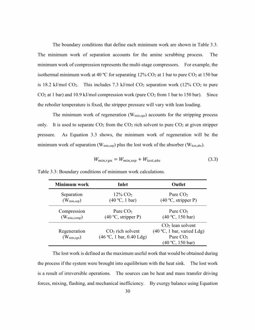
30
The boundary conditions that define each minimum work are shown in Table 3.3.
The minimum work of separation accounts for the amine scrubbing process. The
minimum work of compression represents the multi-stage compressors. For example, the
isothermal minimum work at 40 ºC for separating 12% CO2 at 1 bar to pure CO2 at 150 bar
is 18.2 kJ/mol CO2. This includes 7.3 kJ/mol CO2 separation work (12% CO2 to pure
CO2 at 1 bar) and 10.9 kJ/mol compression work (pure CO2 from 1 bar to 150 bar). Since
the reboiler temperature is fixed, the stripper pressure will vary with lean loading.
The minimum work of regeneration (Wmin,rgn) accounts for the stripping process
only. It is used to separate CO2 from the CO2 rich solvent to pure CO2 at given stripper
pressure. As Equation 3.3 shows, the minimum work of regeneration will be the
minimum work of separation (Wmin,sep) plus the lost work of the absorber (Wlost,abs).
𝑊𝑚𝑖𝑛,𝑟𝑔𝑛 = 𝑊𝑚𝑖𝑛,𝑠𝑒𝑝 + 𝑊𝑙𝑜𝑠𝑡,𝑎𝑏𝑠 (3.3)
Table 3.3: Boundary conditions of minimum work calculations.
Minimum work Inlet Outlet
Separation
(Wmin,sep)
12% CO2
(40 ºC, 1 bar)
Pure CO2
(40 ºC, stripper P)
Compression
(Wmin,comp)
Pure CO2
(40 ºC, stripper P)
Pure CO2
(40 ºC, 150 bar)
Regeneration
(Wmin,rgn)
CO2 rich solvent
(46 ºC, 1 bar, 0.40 Ldg)
CO2 lean solvent
(40 ºC, 1 bar, varied Ldg)
Pure CO2
(40 ºC, 150 bar)
The lost work is defined as the maximum useful work that would be obtained during
the process if the system were brought into equilibrium with the heat sink. The lost work
is a result of irreversible operations. The sources can be heat and mass transfer driving
forces, mixing, flashing, and mechanical inefficiency. By exergy balance using Equation

31
3.4, the lost work of the whole process or each unit operation can be calculated. The sink
temperature, To is set at 313.15 K (40 ºC). Tk is the temperature of the heat source or
sink. In this work, the heat source temperature is 155 ºC, 5 K higher than the reboiler
temperature. Q and W are the heat duty and work input/output. The enthalpy and the
entropy will be obtained from simulations in Aspen Plus® . The minimum work is the
thermodynamic limit, which is determined only by inlet and outlet conditions, but the
amount of lost work (Wlost) depends on how the process is operated. The lost work can
be reduced by a better process design that makes the operation more reversible, and leads
to less actual work requirement.
𝑊𝑙𝑜𝑠𝑡 = ∑ (1 −𝑇𝑜
𝑇𝑘) 𝑄 + ∑ 𝑊 + ∑ (𝐻 − 𝑇𝑜𝑆)𝑖𝑛 − ∑ (𝐻 − 𝑇𝑜𝑆)𝑜𝑢𝑡 (3.4)
3.3 PROCESS DESCRIPTIONS
3.3.1 Simple stripper
The simple stripper is shown in Figure 3.1. The cold rich solvent is heated by the
hot lean solvent in the cross exchanger and then sent to the top of the stripper. The
reboiler provides the sensible heat, the heat of CO2 desorption, and the heat of water
vaporization. The hot lean solvent from the reboiler is returned to the absorber after being
cooled to 40 ºC by the trim cooler. The hot CO2 vapor from the top of stripper is cooled
to 40 ºC in the overhead condenser with loss of the latent heat of the excess water vapor.

32
Cross exchanger
Condenser
Rich solvent
Lean solvent
Condensate
Multi-stagecompressor
Absorber
Flue gas12% CO2
Vented gas
Stripper
CO2
150 bar
n
Reboiler150 oC
Trim cooler
4-10 bar
Figure 3.1: Simple stripper.
3.3.2 Lean vapor compression
The lean vapor compression stripper (Figure 3.2) applies the conventional heat
integration strategy that has been used in distillation. The simple stripper is modified by
adding a flash tank and a single compressor stage. The hot lean solvent coming from the
reboiler is flashed, and produces steam and CO2 in the flash tank at lower pressure. The
flashed vapor is pressurized by the lean vapor compressor, and sent to the bottom of the
packing section in the stripper. The additional stripping steam provides a heat source for
heating the rich solvent in the stripper with packing. Compared to the simple stripper at
the same operating lean loading, the stripper pressure with lean vapor compression is
higher, and the rich solvent that goes into the top of the stripper is colder. The lean vapor
compressor is analogous to the first stage of the multi-stage compressor for CO2
compression. The stripper serves as a direct contact cooler that recovers the latent heat
of steam.

33
The temperature of the flashed vapor at the lean vapor compressor inlet is around
140 ºC. After compression the hot vapor is over 200 ºC, which might exceed the
temperature limit of typical compressor materials. The lean vapor compression work is
included in the calculation of the total equivalent work. The pressure ratio of the lean
vapor compressor for each lean loading was optimized to minimize the total equivalent
work. With a high pressure ratio, less stripping steam heat will be lost in the higher
pressure stripper but the lean vapor compression work will increase.
Cross exchanger
Condenser
Rich solvent
Low P flash
Condensate
Multi-stagecompressor
Absorber
Flue gas12% CO2
Vented gas
Stripper
CO2
150 bar
n
Trim cooler
4-10 bar
Reboiler150 oC
Lean vaporCompressor
Opt. P ratio
Figure 3.2: Lean vapor compression.
3.4 RESULTS AND DISCUSSIONS
3.4.1 Inefficiency of simple stripper
3.4.1.1 Minimum work and lost work distribution
Figure 3.3 shows the minimum work and lost work of a simple stripper using 8 m
PZ. The minimum work of separation purifies the inlet 12% CO2 at 1 bar to pure CO2 at

34
stripper pressure, which depends on the operating lean loading. The minimum work of
compression brings the pure CO2 from stripper pressure to final pressure at 150 bar. Both
these values vary with lean loading since the stripper pressure is not constant. The sum
of separation and compression minimum work is 18.2 kJ/mol CO2, which is independent
of CO2 lean and rich loading.
Figure 3.3: Minimum work and lost work of simple stripper using 8 m PZ; rich loading:
0.4; reboiler T: 150 °C; cross exchanger ΔTLM: 5 K; 5 m packing; correction
for interfacial area: 1.
The lost work from the absorber, regeneration, compression, and unrecovered
solvent pressure are also shown in Figure 3.3. The lost work of the absorber can be
regarded as from a typical intercooled absorber with finite packing area. It varies with
the CO2 lean loading since the inlet and outlet conditions of the absorber are fixed except
0
10
20
30
40
0.20 0.22 0.24 0.26 0.28 0.30 0.32 0.34
Wo
rk (
kJ/
mo
l C
O2)
Lean loading (mol CO2/mol alk)
Wmin of compression
Wlost of regeneration
Wlost of compression Unrecovered solvent pressure
Wlost of absorber
Wmin of separation
35
for the CO2 lean loading. Because the CO2 partial pressure decreases with CO2 lean
loading, a large driving force of CO2 partial pressure causes the lost work of the absorber
to increase at a lower lean loading. At higher lean loading, even though the minimum
work of regeneration required is lower, the absorber may require more packing area due to
insufficient mass transfer driving force.
The lost work of compression is obtained from the difference between the actual
work of compression and the isothermal minimum work of compression at 40 ºC. The
lost work of compression comes from the inefficiency of the compressors (86% polytropic
efficiency is used) and non-isothermal operation. The lost work of unrecovered solvent
pressure shows the amount of work that the lean solvent at the stripper pressure can
generate if it is brought to 1 bar. Practically, the unrecovered solvent pressure of the lean
solvent will be used to overcome the pressure drop through the cross exchangers, the trim
cooler, and the static head of the absorber.
The actual work required by the process is the sum of the minimum work values
and all of the lost work. The lost work of regeneration accounts for 60–70% of total lost
work. It is the major reason that the simple stripper is inefficient.
3.4.1.2 Lost work of regeneration
The lost work of regeneration can be distributed into the unit operations. Figure
3.4 shows this distribution for a simple stripper using 8 m PZ with varied lean loading.
The lost work of the reboiler reflects the amount of heat duty and the temperature
approach between the solvent and the heating steam. 5 K temperature approach between
the steam and the reboiler temperature was assumed. The lost work of the trim cooler and
the pump increases when the lean loading increases due to decreasing solvent capacity (i.e.,
increasing solvent rate) and increasing stripper pressure.

36
Figure 3.4: Lost work of regeneration of simple stripper using 8 m PZ; rich loading: 0.4;
reboiler T: 150 °C; cross exchanger ΔTLM: 5 K; 5 m packing; correction for
interfacial area: 1.
The overhead condenser and the cross exchanger are the two major lost work
sources. They account for over 70% of the lost work of regeneration. When the CO2 is
stripped out, a large amount of water vapor leaves the stripper and is removed in the
overhead condenser. The lost work of the condenser is mainly caused by the loss of latent
heat of the stripping steam. From the Gibbs-Helmholtz equation of CO2 desorption
reaction (Equation 3.5), either increasing the regeneration temperature or using solvents
that have higher heat of absorption (Habs) will increase the partial pressure of CO2 (P*CO2),
providing better selectivity of CO2 over the water vapor. However, elevated regeneration
0
3
6
9
12
15
0.20 0.22 0.24 0.26 0.28 0.30 0.32 0.34
Lo
st w
ork
(k
J/m
ol
CO
2)
Lean loading (mol CO2/mol alk)
Cross exchanger
Condenser
Reboiler
Stripper PumpTrim cooler

37
temperature will cause more solvent degradation and a higher pressure heating steam
requirement.
𝑑(𝑙𝑛𝑃𝐶𝑂2∗ )
𝑑𝑇=
∆𝐻𝑎𝑏𝑠
𝑅𝑇2 (3.5)
The lost work of the cross exchanger is the temperature difference times the amount
of heat exchanged between the cold rich solvent and the hot lean solvent. Even with a
small LMTD of 5 K, the lost work of the cross exchanger is significant because of the large
exchanger duty, which is 2 to 5 times the reboiler duty. It is sensitive to the lean loading
because of the change in solvent cyclic capacity. For example, the solvent circulation rate
at 0.28 lean loading is around 50% of that at 0.34 lean loading. The lower solvent flow
rate results in a lower heat duty in the cross exchanger, so the lost work of the cross
exchanger decreases with decreasing lean loading.
3.4.2 Inefficiency of lean vapor compression
There are two reasons that the lean vapor compression gives better energy
performance than the simple stripper. First, additional stripping steam is produced in the
low pressure flash tank, providing the opportunity for the rich solvent to capture the extra
heat in the stripper. However, the stripping steam has to be pressurized before the heat is
recovered, which requires additional compression work. Second, similar to the multi-
pressure stripper and double matrix stripper (Jassim et al., 2006; Oyenekan et al., 2007;
Van Wagener et al., 2011), the stripper is operated at higher pressure compared to the
simple stripper at the same lean loading, which inherently reduces the stripping steam.
Figure 3.5 shows the lost work of regeneration with lean vapor compression. The
lost work of the condenser is only reduced by 1/3. This implies that this stripper design
is not capable of fully recovering the waste heat from the stripping steam. A portion of
the lost work is shifted from the reboiler to the stripper column since the superheated

38
stripping steam is delivered into the stripper and preheats the rich solvent. The lean vapor
compressor and the flash tank also result in lost work.
Figure 3.5: Lost work of regeneration of lean vapor compression using 8 m PZ; rich
loading: 0.4; reboiler T: 150 °C; cross exchanger ΔTLM: 5 K; 5 m packing;
correction for interfacial area: 1; optimum pressure ratio of lean vapor
compressor at each lean loading.
3.4.3 Proposed design strategies
The significant lost work from the condenser and the cross exchanger is the primary
reason that the simple stripper is not energy efficient. To reduce the irreversibility,
analysis of heat and mass transfer in the stripper and the cross exchanger will be explored.
Alternative design strategies can be proposed accordingly.
0
3
6
9
12
15
0.20 0.22 0.24 0.26 0.28 0.30 0.32 0.34
Lo
st w
ork
(k
J/m
ol
CO
2)
Lean loading (mol CO2/mol alk)
Cross exchanger
Condenser
Reboiler
Stripper
PumpTrim coolerFlash tank+LV compressor

39
3.4.3.1 Heat and mass transfer in the stripper
The lost work of the stripper column of the simple stripper is relatively low. It
can be explained by the temperature profile and the CO2 concentration profile of the
stripper column shown in Figure 3.6. For the simple stripper, the bottom is the reboiler
that heats the solvent up to 150 ºC. The temperature of the rich solvent going into the top
of the stripper is around 140 ºC, only 10 ºC higher than the bottom reboiler temperature.
Since the liquid is hot, it cannot condense any stripping steam from the vapor phase. The
temperature profile shows that the pinch at the top of the stripper and most of the packing
is wasted.
Figure 3.6: Temperature and CO2 concentration profile of stripper column for simple
stripper using 8 m PZ; lean loading: 0.24; rich loading: 0.4; reboiler T: 150
°C; cross exchanger ΔTLM: 5 K; 5 m packing; correction for interfacial area:
1.
0.2
0.4
0.6
0.8
1.0
100
110
120
130
140
150
0.0 0.2 0.4 0.6 0.8 1.0
yC
O2
or
y* C
O2
Te
mp
era
ture
(°C
)
Z/Ztotal
Vapor T
Liquid T
yCO2
y*CO2
Bot Top

40
The CO2 concentration profile shows the stripping conditions using the CO2 mole
fraction in the vapor phase (yCO2) and the equilibrium CO2 mole fraction in the liquid phase
(y*CO2), which is the ratio of equilibrium partial pressure of CO2 to the stripper pressure.
The vapor coming from the reboiler contains 30% CO2 and 70% H2O, and it leaves the
stripper with 60% CO2 and 40% H2O. The equilibrium CO2 partial pressure of the solvent
depends on the CO2 loading and the solvent temperature. Before the rich solvent goes
into the stripper, the hot solvent flashes out a portion of CO2, so the rich solvent at the top
is at 0.34 CO2 loading instead of 0.4. This lower CO2 loading causes a low equilibrium
mole fraction of CO2. The CO2 concentration also pinches at the top. The appearance
of pinches for both heat and mass transfer implies that the simple stripper is a poor design
that could not effectively condense the stripping steam and strip CO2. To improve the
stripper, both heat and mass transfer performance should be considered. The rich solvent
that goes to the stripper should be at or below its bubble point to avoid flashing.
3.4.3.2 Self-contained heat integration using cold rich solvent
The reasons for limited energy reduction of the lean vapor compression are clear
from Figure 3.5. First, the lost work of the condenser has not been fully recovered. Over
60% of that is still left. Second, additional recompression work has to be provided before
the stripping steam heat is recovered. In fact, the vapor only needs to be compressed for
heat integration if its dew point temperature is lower than the bubble point of the heat sink.
If a low temperature heat sink is available, the waste heat from the vapor can still be
recovered without being “upgraded”.
Therefore, it is straightforward to use the cold rich solvent at 46 ºC as the heat sink
to recover the rest of the stripping steam heat. However, direct contact should be avoided.
When the solvent is cold, the equilibrium partial pressure of CO2 could be lower than that
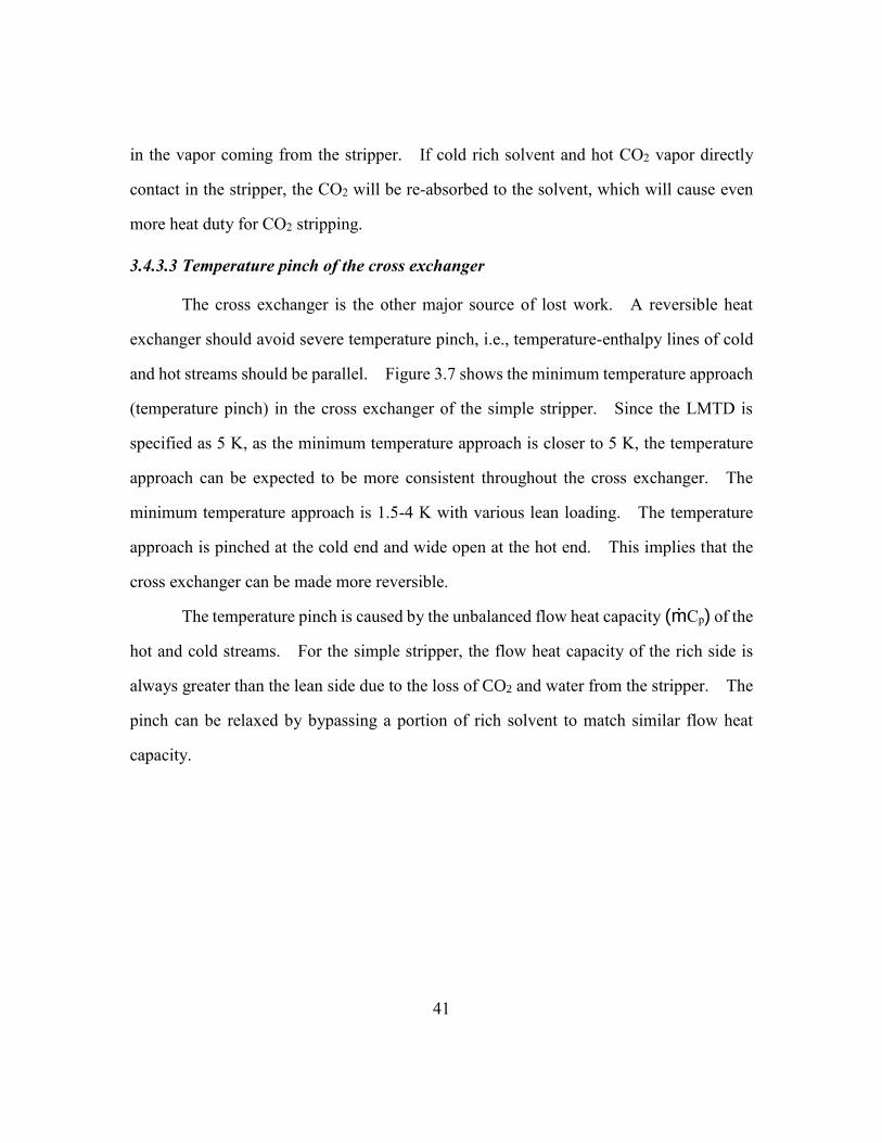
41
in the vapor coming from the stripper. If cold rich solvent and hot CO2 vapor directly
contact in the stripper, the CO2 will be re-absorbed to the solvent, which will cause even
more heat duty for CO2 stripping.
3.4.3.3 Temperature pinch of the cross exchanger
The cross exchanger is the other major source of lost work. A reversible heat
exchanger should avoid severe temperature pinch, i.e., temperature-enthalpy lines of cold
and hot streams should be parallel. Figure 3.7 shows the minimum temperature approach
(temperature pinch) in the cross exchanger of the simple stripper. Since the LMTD is
specified as 5 K, as the minimum temperature approach is closer to 5 K, the temperature
approach can be expected to be more consistent throughout the cross exchanger. The
minimum temperature approach is 1.5-4 K with various lean loading. The temperature
approach is pinched at the cold end and wide open at the hot end. This implies that the
cross exchanger can be made more reversible.
The temperature pinch is caused by the unbalanced flow heat capacity (mCp) of the
hot and cold streams. For the simple stripper, the flow heat capacity of the rich side is
always greater than the lean side due to the loss of CO2 and water from the stripper. The
pinch can be relaxed by bypassing a portion of rich solvent to match similar flow heat
capacity.

42
Figure 3.7: Pinch temperature approach of the cross exchanger of the simple stripper
using 8 m PZ; rich loading: 0.4; reboiler T: 150 °C; cross exchanger ΔTLM: 5
K.
3.4.4 Advanced flash stripper
3.4.4.1 Proposed stripper configuration
Based on the design strategies, a new stripper configuration, the advanced flash
stripper, is proposed and shown in Figure 3.8. The major modifications are the warm rich
bypass and the cold rich bypass with the cold rich exchanger.
The cross exchanger is split into two exchangers. The warm rich bypass is
extracted and fed to the top of the stripper after mixing with the cold rich bypass. The
temperature was selected as the bubble point at the stripper operating pressure. The
temperature at bubble point without flashing will maximize the equilibrium partial pressure
1
2
3
4
5
6
0.20 0.22 0.24 0.26 0.28 0.30 0.32
Pin
ch
T (
K)
CO2 lean loading (mol CO2/mol alk)
TLM=5 K

43
of CO2 for stripping, while still condensing a portion of stripping steam from the vapor
phase.
Cold rich Bypass
Cold rich exchanger
Warm rich Bypass
Cold cross exchanger
Hot cross exchanger
Condenser
Absorber
Flue gas12% CO2
Vented gas
Steam heater
Stripper
Multi-stagecompressor
CO2
150 barn
Condensate
Trim cooler
Rich solvent
Lean solvent 150 oC
4-10 bar
Figure 3.8: Advanced flash stripper
The cold rich solvent serves as a low temperature heat sink to recover the rest of
the stripping steam heat. The heat is recovered by the rich exchanger instead of by direct
contact in the stripper to avoid re-absorption. The rich exchanger preheats a portion of
the cold rich solvent by hot vapor coming out of the stripper. The cold and warm rich
bypass also help relax the temperature pinch in the cross exchanger.
The optimized cold and warm rich bypass rate will maximize the potential benefits
from the stripping steam heat recovery, the CO2 stripping performance in the stripper
column, and the cross exchanger performance. For each lean loading the bypasses are
optimized to minimize the total equivalent work. Higher bypass rates are required at low
lean loading as more stripping steam needs to be recovered.

44
After cold and warm rich solvent bypasses, the rest of the rich solvent is heated by
a steam heater and fed into the bottom of the stripper. The regeneration temperature of
the stream coming from the flash tank was 150 ºC. The reboiler in a typical stripper is
replaced by a steam heater, which has the same function as the reboiler except the solvent
is heated convectively. Since the amine tends to thermally degrade at high temperature,
the convective steam heater with less solvent hold-up and residence time will minimize
thermal degradation.
3.4.4.2 Lost work of regeneration
Figure 3.9 shows the lost work of regeneration of the advanced flash stripper using
8 m PZ. The lost work of the condenser is almost eliminated compared to the simple
stripper and the lean vapor compression. The water vapor content from the rich
exchanger is only around 5 mol % over the lean loading range. Figure 3.10 shows that
the lost work of the condenser with the advanced flash stripper is 50% less than with lean
vapor compression. The proposed design strategies significantly reduce the
irreversibility of the condenser.

45
Figure 3.9: Lost work of regeneration of advanced flash stripper using 8 m PZ; rich
loading: 0.4; reboiler T: 150 °C; cross exchanger ΔTLM: 5 K; 5 m packing;
correction for interfacial area: 1; optimum cold and warm rich bypasses.
0
3
6
9
12
15
0.20 0.22 0.24 0.26 0.28 0.30 0.32 0.34
Lo
st w
ork
(k
J/m
ol
CO
2)
Lean loading (mol CO2/mol alk)
Cross exchanger
Condenser+Cold rich exchanger
Steam heaterStripper
PumpTrim cooler

46
Figure 3.10: Comparison of lost work of the condenser; 8 m PZ; rich loading: 0.4;
reboiler T: 150 °C; cross exchanger ΔTLM: 5 K; 5 m packing; correction for
interfacial area: 1; optimum pressure ratio for LVC; optimum cold and
warm rich bypasses for AFS.
Figure 3.11 compares the heat duty of the reboiler/steam heater. The lean vapor
compression reduces the heat duty by 8.4% and the advanced flash stripper reduces it by
16.1% at the optimum lean loading compared to the simple stripper. Figure 3.12
compares the total equivalent work, which includes the compression work, pump work,
equivalent work of reboiler duty, and the lean vapor compression work. The advanced
flash stripper reduces the total equivalent work by 11.2% at optimum lean loading while
the lean vapor compression reduces it by only 3.4%.
0
2
4
6
0.20 0.22 0.24 0.26 0.28 0.30 0.32 0.34
Wlo
sto
f co
nd
en
ser
(kJ/
mo
l C
O2)
Lean loading (mol CO2/mol alk)
Simple stripper
Lean vapor compression
Advanced flash stripper
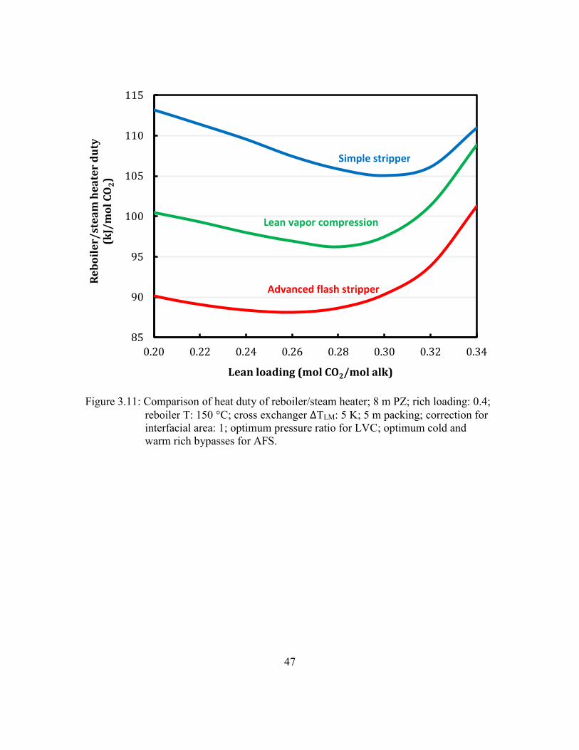
47
Figure 3.11: Comparison of heat duty of reboiler/steam heater; 8 m PZ; rich loading: 0.4;
reboiler T: 150 °C; cross exchanger ΔTLM: 5 K; 5 m packing; correction for
interfacial area: 1; optimum pressure ratio for LVC; optimum cold and
warm rich bypasses for AFS.
85
90
95
100
105
110
115
0.20 0.22 0.24 0.26 0.28 0.30 0.32 0.34
Re
bo
ile
r/st
ea
m h
ea
ter
du
ty
(kJ/
mo
l C
O2)
Lean loading (mol CO2/mol alk)
Simple stripper
Advanced flash stripper
Lean vapor compression

48
Figure 3.12: Comparison of total equivalent work; 8 m PZ; rich loading: 0.4; reboiler T:
150 °C; cross exchanger ΔTLM: 5 K; 5 m packing; correction for interfacial
area: 1; optimum pressure ratio for LVC; optimum cold and warm rich
bypasses for AFS.
3.4.4.3 Cold and warm rich bypass
The temperature and the CO2 concentration profile of the stripper shown in Figure
3.13 explain the energy improvement. The pinch shown in the simple stripper (Figure
3.6) has disappeared. The advanced flash stripper avoids heat and mass transfer pinches
and provides more opportunity for the stripper packing to recover the stripping steam heat
and strip CO2 from the rich solvent. The adjustable warm rich bypass rate can change the
slope of the operating line (CO2 concentration and temperature of vapor) to match the
equilibrium line. With optimum bypasses that minimize the reboiler duty, the
30
32
34
36
0.20 0.22 0.24 0.26 0.28 0.30 0.32 0.34
We
q (
kJ/
mo
l C
O2)
Lean loading (mol CO2/mol alk)
Simple Stripper
Advanced flash stripper
Lean vapor compression

49
temperature profiles of the vapor and the liquid are nearly parallel. Both heat and mass
transfer show consistent driving force throughout the column, which implies that the
packing is utilized more efficiently.
Figure 3.13: Temperature and CO2 concentration profile of stripper column for the
advanced flash stripper; 8 m PZ; lean loading: 0.24; rich loading: 0.4;
reboiler T: 150 °C; cross exchanger ΔTLM: 5 K; 5 m packing; correction for
interfacial area: 1; optimum cold and warm rich bypasses.
The temperature of the rich solvent that goes to the stripper is determined by both
cold rich bypass and warm rich bypass. The adjustable bypass rates give the flexibility
to determine the temperature. At low temperature, more stripping steam can be recovered
in the stripper but re-absorption may occur as the CO2 is absorbed from the vapor. In the
0.2
0.4
0.6
0.8
1
100
110
120
130
140
150
0.0 0.2 0.4 0.6 0.8 1.0
yC
O2
or
y* C
O2
Te
mp
era
ture
(°C
)
Z/Ztotal
Vapor T
Liquid TyCO2
y*CO2
Bot Top

50
CO2 concentration profile in Figure 3.13, the re-absorption can be seen at the top of the
stripper. Even with re-absorption, this case gives the minimum reboiler duty by
recovering more stripping steam.
3.4.4.4 Irreversibility of the cross exchanger
The reversibility of the cross exchanger can be understood by following the ratio
of the flow heat capacity (mCp) of the rich and lean streams. The cross exchanger will be
reversible if the flow heat capacity between rich and lean solvent is well-matched. To
maximize the performance of the cross exchanger, the ratio of the flow heat capacity should
be close to unity.
Figure 3.14 shows the ratio of the flow heat capacity of rich to lean stream in single
phase before the rich solvent vaporizes. Since the specific heat capacity is similar over
the operating conditions, the flow heat capacity is mainly affected by the solvent flow rate.
For the simple stripper, the ratio is greater than unity, around 1.01–1.09. The loss of water
vapor and CO2 from the stripper results in lean solvent flow that is less than the rich solvent.
For the advanced flash stripper, the ratio of flow heat capacity is reduced to 0.96–0.99.
The cold rich bypass reduces the flow rate of rich solvent that goes to the cross exchanger.
At optimized bypass rate, the flow rate of the rich solvent is even lower than the lean
solvent, so the ratio of the flow heat capacity is less than unity. The fact that the ratio is
not exactly at unity implies that it is worthwhile extracting more solvent to recover the
stripping steam heat rather than balancing the temperature approach of the cross exchanger.

51
Figure 3.14: Flow heat capacity ratio of rich solvent to lean solvent of the cold cross
exchanger (single phase); 8 m PZ; rich loading: 0.4; reboiler T: 150 °C;
cross exchanger ΔTLM: 5 K; optimum cold and warm rich bypasses.
When the rich solvent starts vaporizing, the heat of vaporization makes the specific
heat capacity at the rich side much higher than the lean side that stays in single phase.
Figure 3.15 shows the ratio of the flow heat capacity with vaporization. The ratio of the
simple stripper is around 1.4–1.8, far from the desired unity. For the advanced flash
stripper, the ratio is reduced to 1.1–1.3. The extraction of cold and warm rich bypass help
balance the flow heat capacity with lower rich solvent rate in the cross exchanger.
Generally, the advanced flash stripper provides a more reversible cross exchanger than the
simple stripper.
0.90
0.95
1.00
1.05
1.10
0.20 0.22 0.24 0.26 0.28 0.30 0.32 0.34
Ra
tio
of
flo
w h
ea
t ca
pa
city
Lean loading (mol CO2/mol alk)
Simple stripper
Advanced flash stripper

52
Figure 3.15: Flow heat capacity ratio of rich solvent to lean solvent of the hot cross
exchanger (flashing phase); 8 m PZ; rich loading: 0.4; reboiler T: 150 °C;
cross exchanger ΔTLM: 5 K; optimum cold and warm rich bypasses.
The lost work of the cross exchanger can be potentially reduced by using a tight
temperature approach or increasing the solvent capacity. However, an excessively small
temperature difference should be avoided due to the prohibitive cost of the cross exchanger.
Operating at lower CO2 lean loading will increase the cyclic capacity because less solvent
will be circulating between the absorber and the stripper. Figure 3.9 showed that
significant lost work of the cross exchanger is avoided at low loading. With the simple
stripper this strategy will not be effective, as the lost work of the condenser will offset the
reduction (Figure 3.4), but for the advanced stripper, the low lean loading region is exactly
where the advanced flash stripper reduces the lost work of the condenser the most.
0.7
1.0
1.3
1.6
1.9
0.20 0.22 0.24 0.26 0.28 0.30 0.32 0.34
Ra
tio
of
flo
w h
ea
t ca
pa
city
Lean loading (mol CO2/mol alk)
Simple stripper
Advanced flash stripper

53
3.4.4.5 Irreversibility of the reboiler/steam heater
The lost work of the reboiler (steam heater for advanced flash stripper) will increase
with increasing steam temperature. The relationship can be expressed by the heat duty-
equivalent work conversion factor in the total equivalent work calculation. When the
steam is extracted from the power plant, steam at higher temperature will cause more
electricity loss. For example, using steam at 180 ºC leads to an additional 15% electricity
penalty compared to that at 155 ºC with equivalent reboiler duty.
In this work, 5 K temperature difference is used for the reboiler. Ideally, using
steam with temperature as low as possible can minimize the lost work of the reboiler.
However, an excessively small temperature approach should be avoided.
3.4.5 Thermodynamic efficiency of regeneration
The thermodynamic efficiency can be used to quantify the potential for energy
improvement by comparing the actual work to the minimum work, which is defined in
Equation 3.1. The thermodynamic efficiency of CO2 compression is around 73% over
the range of inlet pressure from 1 to 20 bar.
Since this work focuses on developing the design strategies for the stripping
process, the thermodynamic efficiency of regeneration will more adequately represent the
performance of the regeneration process only. Equation 3.6 defines the thermodynamic
efficiency of regeneration (ηth,rgn) as the ratio of the minimum work of regeneration to the
actual work of regeneration. The minimum work of regeneration is defined in Table 3.2.
The actual work of regeneration (Wact,rgn) includes the heat provided to the reboiler/steam
heater and the pump work of the rich solvent pump. This work used feasible design
parameters to demonstrate the maximum energy efficiency that can be attained in practice.
Unrealistic assumptions such as infinite heat/mass transfer area are avoided.

54
𝜂𝑡ℎ,𝑟𝑔𝑛 =𝑊𝑚𝑖𝑛,𝑟𝑔𝑛
𝑊𝑎𝑐𝑡,𝑟𝑔𝑛 (3.6)
Figure 3.16: Comparison of thermodynamic efficiency of regeneration; 8 m PZ; rich
loading: 0.4; reboiler T: 150 °C; cross exchanger ΔTLM: 5 K; 5 m packing;
correction for interfacial area: 1; optimum pressure ratio of LVS; optimum
cold and warm rich bypasses for AFS.
Figure 3.16 compares the thermodynamic efficiency of regeneration. The
efficiency of the simple stripper is 50–60% and the advanced flash stripper is 55–74% in
the range of operating lean loading. For the simple stripper, the low efficiency at high
lean loading is mainly due to the dominating lost work of the cross exchanger. At lower
lean loading where the lost work of the condenser dominates, the efficiency is relatively
flat because the minimum work also increases. The advanced flash stripper is nearly
50%
55%
60%
65%
70%
75%
0.20 0.22 0.24 0.26 0.28 0.30 0.32 0.34
ηth
,rg
n
Lean loading (mol CO2/mol alk)
Simple stripper
Lean vapor compression
Advanced flash stripper

55
stripping steam free, so the efficiency is mainly driven by the lost work of the cross
exchanger for the entire lean loading range. The advanced flash stripper improves the
most at lower lean loading where the stripping steam is significant.
The advanced flash stripper gives the maximum thermodynamic efficiency at 74%.
It is remarkable compared to typical distillation with heat integration that is only around
20% (Fitzmorris et al., 1980; Y. H. Kim, 2012; Yoo et al., 1988). The remaining lost
work from the cross exchanger is difficult to reduce since PZ has already provided a
superior solvent capacity compared to other solvents (Li, Voice, et al., 2013). Therefore,
the energy efficiency of the regeneration process with the advanced flash stripper using 8
m PZ is approaching the thermodynamic limit from which further improvement is expected
to be marginal.
3.5 CONCLUSIONS
The lost work of the condenser and the cross exchanger were identified as the two
major reasons that the simple stripper is not energy efficient. The advanced flash
stripper using cold and warm rich bypasses is proposed to reduce the lost work.
The warm rich bypass reduces the work loss associated with condensing water vapor
resulting from the stripping steam.
The cold rich bypass recovers the rest of the stripping steam heat by providing a low
temperature heat sink while avoiding CO2 re-absorption.
The advanced flash stripper overcomes the weaknesses of lean vapor compression and
almost eliminates the lost work of the condenser. The cold and warm rich bypasses
also make the cross exchanger more reversible by balancing the flow heat capacity
between the rich and lean streams.

56
The advanced flash stripper reduces the reboiler duty by 16.1% and the total
equivalent work by 11.2% compared to the simple stripper.
The advanced flash stripper reaches a remarkable thermodynamic efficiency at 55–
74% over a range of operating lean loading.
The regeneration process is close to a reversible operation compared to common
distillation. Further improvement of energy efficiency is expected to be limited.

57
Chapter 4: Energy Performance of Advanced Stripper Configurations
4.1 INTRODUCTION
The irreversibility of the condenser has been identified as the major reason that
makes the amine scrubbing process inefficient and is responsible for over 50% of the lost
work in the regeneration process. Several alternative stripper configurations have been
proposed to reduce the stripping steam heat loss. The configurations mainly applied two
approaches: heat integration and isothermal stripping. Table 4.1 summarizes the
alternative stripper configurations proposed by previous work.
The heat integration approach uses the latent heat of the stripping steam to preheat
the rich solvent, which needs to be heated from the absorber temperature up to the reboiler
temperature at 120–150 °C. Representative configurations include rich solvent bypass,
interheated stripper, and vapor recompression. The rich solvent bypass extracts a portion
of rich solvent to be contacted with the hot CO2 vapor in the stripper, where the stripping
steam is condensed with releasing the latent heat. The interheated stripper integrates the
lean/rich cross exchanger into the stripper column and results in a colder stripper feed than
the conventional simple stripper. Vapor recompression applies the heat integration
strategy that has been used for conventional distillation. The hot CO2 vapor with steam
from the stripper is compressed by a multi-stage compressor to elevate the condensing
temperature of the stripping steam. A part of reboiler duty can be provided by the heat
integration with the compressor intercoolers. Most of the waste heat is obtained from the
latent heat of water vapor so the energy improvement will be limited if the stripping steam
has been already recovered by other approaches before entering the compressor train.
Isothermal stripping aims at regenerating CO2 at the highest temperature possible
throughout the stripping process. The maximum stripping temperature is usually limited
by the thermal degradation of the amine. When the CO2 is stripped from rich loading to

58
lean loading, operating the stripper isothermally will lead to the highest partial pressure of
CO2, which can improve the selectivity of CO2 over stripping steam and reduce the
mechanical compression work. The overall performance will depend on the efficiencies
of thermal compression and mechanical compression. The multi-pressure stripper
integrates the CO2 compressor with the stripper column and operates at different pressure
levels. Additional compression work is required to compress the stripping steam. The
matrix stripper and the multi-stage flash attain high stripper pressure by providing reboiler
duty at each stage instead compressing the CO2 vapor. Theoretically, an isothermal
stripper can be achieved if infinite stages are used.
Table 4.1: Alternative stripper configurations proposed to reduce stripping steam heat
Type Configuration Sources
Heat integration
Rich solvent bypass
(Eisenberg et al., 1979)
(Soave et al., 2002)
(Van Wagener et al., 2014)
(Madan, 2013)
Interheated stripper
(Leites et al., 1993)
(Oyenekan et al., 2007)
(Van Wagener et al., 2011)
Vapor recompression (Jassim et al., 2006)
Isothermal stripping
Multi-pressure stripper (Jassim et al., 2006)
(Oyenekan et al., 2007)
Lean vapor compression (Ebnson et al., 1979)
(Reddy et al., 2009)
Matrix stripper (Oyenekan et al., 2007)
Multi-stage flash (Van Wagener et al., 2011)
This work propose new configurations that apply rich exchanger bypass. The
energy performance will be compared to other alternatives previously proposed using the

59
same metric. In order to show the improvement with different solvent properties, the
stripper configurations will be modeled using two common solvents, PZ and MEA in
Aspen Plus® . The overall energy performance will be indicated by the total equivalent
work in a wide range of operating lean loading.
4.2 SIMULATION METHODS
8 m PZ and 9 m MEA were chosen as solvents. The thermodynamic models used
for MEA and PZ in this work were “Phoenix” and “Independence”, respectively.
Modeling details can be found in Frailie (2014) and Plaza (2011). These models have
been regressed in Aspen Plus® with experimental data including amine volatility, heat
capacity, CO2 solubility, and amine pKa over a range of amine concentration and CO2
loading.
4.2.1 Modeling stripper with updated MEA model
Van Wagener (2011) predicted the stripper performance for 9 m MEA using the
thermodynamic model developed by Hilliard (Hilliard, 2008). The Hilliard model tends
to overestimate the partial pressure of CO2 (P*CO2) as amine concentration and temperature
increase. The error can have significant effect on predicting the stripper pressure and the
overall energy performance. “Phoenix” is an updated model that has fixed the problem
and was regressed by including more high temperature data. It showed an adequate fit
that matches experimental data and can predict the partial pressure of CO2 over the
temperature range from 40 to 160 °C (Plaza, 2011). Figure 4.1 compares the partial
pressure of CO2 predicted by the two models. The predicted P*CO2 by the Hilliard model
is almost twice that predicted by the Phoenix model at 120 °C where the stripper is typically
operated for MEA. The stripper pressure at 120 °C can be over-predicted by 1 to 4 bar in
the lean loading range as shown in Figure 4.2. The over-prediction of P*CO2 not only

60
underestimated the compression work and the stripping steam heat but also misjudged the
optimum lean loading. This work will demonstrate the energy performance of alternative
strippers with an updated model for MEA.
Figure 4.1: CO2 partial pressure predicted by Hilliard model (dashed line) and Phoenix
model (solid line).
0.001
0.01
0.1
1
10
100
0.1 0.2 0.3 0.4 0.5
P* C
O2
(k
Pa)
CO2 loading (mol CO2/mol alkalinity)
40°C
120°C
60°C
80°C
100°C

61
Figure 4.2: Over-predicted stripper pressure by Hilliard model at 120 °C.
4.2.2 Stripping steam for PZ and MEA
The amount of stripping steam generated will be determined by the vapor-liquid
equilibrium between CO2, water, and amine at high temperature. Figure 4.1 shows the
mole fraction of CO2 in the vapor phase at stripper temperature predicted by Aspen
models® . The vapor phase consists of CO2 and steam since amine is relatively less
volatile and its mole fraction is lower than 1%. The CO2 product coming up from the
reboiler will contain 20–80% stripping steam before being counter-currently contacted
with solvent in the stripper.
As indicated by Equation 1.4, the selectivity of CO2 and steam can be improved by
higher heat of absorption and operating temperature. Even though MEA can only be
2
4
8
0.25 0.3 0.35 0.4 0.45
Stri
pp
er P
(b
ar)
Lean loading (mol CO2/mol alkalinity)
Hilliard model(120 °C)
Phoenix model(120 °C)

62
operated at 120 °C, it still provides a relatively higher CO2 mole fraction than PZ at 150
°C since it has a higher heat of absorption. Operating at a higher lean loading will
significantly reduce the stripping steam but the lean loading also has impact on other
contributors to energy use. Exploring optimum lean loading that minimizes the total
equivalent work will compromise between these energy tradeoffs.
𝑃𝐶𝑂2∗(𝑇)
𝑃𝐻2𝑂∗(𝑇)
=𝑃𝐻2𝑂
∗(𝑇𝑟𝑒𝑓)
𝑃𝐶𝑂2∗(𝑇𝑟𝑒𝑓)
𝑒𝑥𝑝 [(∆𝐻𝑎𝑏𝑠−∆𝐻𝑣𝑎𝑝
𝑅) (
1
𝑇𝑟𝑒𝑓−
1
𝑇)] (1.4)
Figure 4.3: CO2 mole fraction in the vapor phase with varied lean loading predicted by
Independence for PZ and Phoenix for MEA.
4.2.3 Process specifications
Process specifications used in the simulations are shown in Table 4.2. Because
the absorber was not simulated, typical rich solvent conditions including rich loading and
0
0.2
0.4
0.6
0.8
1
50 500
yC
O2
Lean solvent P*CO2 at 40 °C (Pa)
8 m PZ(120 °C)
8 m PZ(150 °C)
9 m MEA(120 °C)
9 m MEA(150 °C)

63
temperature were fixed as constants. The total packing height in the stripper is fixed at 2
m except for the configurations with two packing sections where 1 m is used for each
section. The Bravo Correlation was used to calculate the mass transfer coefficient and
interfacial area of the packing in the stripper (Bravo et al., 1985). Rich solvent was set at
46 °C with CO2 loading (mol CO2/mol alkalinity) of 0.5 for MEA and 0.4 for PZ according
to typical results with an intercooled absorber (Plaza, 2011).
Reboiler temperature involves the tradeoff between energy efficiency and
degradation rate. A reasonable compromise of 150 °C for PZ and 120 °C for MEA was
used (Davis, 2009; Freeman, 2011). The steam temperatures used to calculate the
equivalent work were 155 °C and 125 °C for PZ and MEA, respectively assuming a 5 K
temperature approach.
The LMTD of the heat exchanger was calculated rigorously as described in Chapter
2. For the cross exchanger and the interheated exchanger, the LMTD was specified as 5 K.
For the cold rich exchanger, which has poorer heat transfer between vapor and liquid, the
LMTD was set at 20 K.

64
Table 4.2: Process simulation specifications.
Solvent 8 m PZ 9 m MEA
Process modeling tool Aspen Plus® v7.3
Thermodynamic model Independence Phoenix
Rich loading
(mol CO2/mol alkalinity) 0.40 0.50
Reboiler T (°C) 150 120
Steam T (°C) 155 125
Stripper packing 2 m Mellapak 250X
Correction factor for
packing interfacial area 1
Rich solvent T (°C) 46
Cross exchanger LMTD (K) 5
Cold rich exchanger LMTD (K) 20
Interheated exchanger LMTD (K) 5
4.3 PROCESS DESCRIPTIONS
4.3.1 Simple stripper
The simple stripper shown in Figure 4.4 is the base case. The rich solvent is
preheated in the cross exchanger and then sent to the top of stripper. The hot lean solvent
from the reboiler is returned to the absorber through the cross exchanger. The hot CO2
rich vapor from the top of stripper is cooled to 40 °C in the overhead condenser with loss
of the latent heat of the excess water vapor.

65
Cross exchanger
Condenser
Rich solvent
Lean solvent
Condensate
Multi-stagecompressor
Absorber
Flue gas12% CO2
Vented gas
Stripper
CO2
150 bar
n
Reboiler150 oC
Trim cooler
4-10 bar
Figure 4.4: Simple stripper.
4.3.2 Conventional alternatives
4.3.2.1 Lean vapor compression (LVC)
The lean vapor compression (Figure 4.5) can reduce the stripping steam heat by
operating the stripper at a higher pressure at a given lean loading compared to the simple
stripper. The hot lean solvent is flashed in a flash tank at lower pressure. The flashed
vapor is then pressurized by the lean vapor compressor, and sent to the bottom of the
packing section in the stripper. The stripper serves as a direct contact cooler that recovers
the latent heat of steam by a cooler stripper feed. The lean vapor compression was
demonstrated in pilot plant tests and showed the savings of reboiler duty can be up to 20%
(Knudsen et al., 2011).
In this work the pressure ratio of the lean vapor compressor for each lean loading
will be optimized to minimize the total equivalent work. With a high pressure ratio, less
stripping steam heat will be lost in the higher pressure stripper but the lean vapor

66
compression work will increase. The additional lean vapor compression work will be
included in the total equivalent work.
Cross exchanger
Condenser
Rich solvent
Low P flash
Condensate
Multi-stagecompressor
Absorber
Flue gas12% CO2
Vented gas
Stripper
CO2
150 bar
n
Trim cooler
Reboiler
Lean vaporCompressor
Opt. P ratio
Figure 4.5: Lean vapor compression.
4.3.2.2 Interheated stripper
The interheated stripper was proposed by Leites (1993) and has been studied by
Rochelle et al. (Oyenekan et al., 2007; Van Wagener et al., 2011). All the solvent is
extracted from the middle of stripper, heated by the hot lean solvent in the interheated
exchanger, and sent back to next section of the stripper. Van Wagener showed that the
interheated stripper offers the best energy savings among several alternatives including
two-stage flash, double matrix, and multi-pressure using MEA and PZ.

67
Cross exchanger
Condenser
Rich solvent
Lean solvent
Condensate
Multi-stagecompressor
Absorber
Flue gas12% CO2
Vented gas
Stripper
CO2
150 bar
n
Reboiler
Trim cooler
Interheated exchanger
Figure 4.6: Interheated stripper.
4.3.2.3 Cold rich bypass
Figure 4.7 shows the simple stripper with cold rich bypass. A portion of the cold
rich solvent is bypassed and sent to the top of the stripper without being heated by the cross
exchanger. The bypassed solvent will be preheated in the stripper by condensing the
stripping steam out of the CO2 vapor. A pilot plant test in UT Austin applied the cold
rich bypass to a two-stage flash stripper and showed over 20% of heat duty reduction
(Madan et al., 2013). The concept can be extended by extracting the rich solvent at
different temperature levels and feeding into appropriate locations in the stripper to match
the heat and mass transfer driving force. In theory the stripper column can approach
reversible operation if infinite feeds of rich solvent are applied. However, a diminishing
return of energy savings was observed with an increasing number of bypasses and more
stripper packing is required to fully realize the benefits (Madan, 2013).

68
Cross exchanger
Condenser
Rich solvent
Lean solvent
Condensate
Multi-stagecompressor
Absorber
Flue gas12% CO2
Vented gas
Stripper
CO2
150 bar
n
Reboiler
Trim cooler
Cold rich bypass
Figure 4.7: Simple stripper with cold rich bypass.
4.3.3 Rich exchanger bypass strategy
4.3.3.1 Simple stripper with rich exchanger bypass
The rich exchanger bypass strategy is proposed in this work to improve the cold
rich bypass configuration by avoiding CO2 re-absorption in the stripper. Figure 4.8 shows
the simple stripper with rich exchanger bypass. An exchanger is used to recover the
stripping steam heat instead direct contacting with the CO2 vapor in the stripper. After
being heated, the bypass rich solvent is mixed with the hot rich solvent and fed to the top
of the stripper. The cold rich bypass rate will be optimized with a minimum total
equivalent work.

69
Cross exchanger
Condenser
Rich solvent
Lean solvent
Multi-stagecompressor
Absorber
Flue gas12% CO2
Vented gas
Stripper
CO2
150 bar
n
Reboiler
Trim cooler
Cold rich exchanger
Cold rich bypass
Figure 4.8: Simple stripper with cold rich exchanger bypass.
4.3.3.2 Advanced reboiled stripper (ARS)
Figure 4.7 shows the advanced reboiled stripper proposed in this work. A
combination of the rich exchanger bypass and the warm rich bypass is applied. The warm
rich bypass is drawn from the cross heat exchanger and fed to the top of stripper. The
temperature was selected as the bubble point temperature, which will maximize the
equilibrium partial pressure of CO2 and increase the mass transfer driving force for CO2
and water transfer. The cold rich solvent serves as a low temperature heat sink to recover
the rest of the stripping steam heat while avoiding CO2 re-absorption. As discussed in
Chapter 3, the cold and warm rich bypass also help relax the temperature pinch in the cross
exchanger.
The combination of cold and warm rich bypass is expected to work more
efficiently. The optimized cold and warm rich bypass rate will maximize the potential
benefits from the stripping steam heat recovery, the CO2 stripping performance in the
stripper column, and the cross exchanger performance.

70
Cold rich Bypass
Cold rich exchanger
Warm rich BypassTbp
Cold cross exchanger
Hot cross exchanger
Condenser
Absorber
Flue gas12% CO2
Vented gas
Stripper
Multi-stagecompressor
CO2
150 barn
Condensate
Trim cooler
Rich solvent
Lean solventReboiler
Figure 4.9: Advanced reboiled stripper (ARS).
4.3.3.3 Advanced flash stripper (AFS)
In the advanced flash stripper (Figure 4.10), the reboiler is replaced by a convective
steam heater in order to minimize the residence time at higher temperature, where the
amine tends to thermally degrade the most. The rich solvent will be heated by the steam
heater and the vapor and liquid will be separated in the stripper sump. The separated
vapor will go up along the stripper and counter-currently contacted with the warm rich
bypass while condensing stripping steam.

71
Cold rich Bypass
Cold rich exchanger
Warm rich Bypass
Cold cross exchanger
Hot cross exchanger
Condenser
Absorber
Flue gas12% CO2
Vented gas
Steam heater
Stripper
Multi-stagecompressor
CO2
150 barn
Condensate
Trim cooler
Rich solvent
Lean solvent
Figure 4.10: Advanced flash stripper (AFS).
4.4 RESULTS AND DISCUSSIONS
4.4.1 Tradeoffs of optimum lean loading
Figures 4.11 and 4.12 compare the total equivalent work of alternative strippers at
varied lean loading using 8 m PZ and 9 m MEA, respectively. The optimum lean loading
is around 0.28–0.30 for PZ and 0.36–0.38 for MEA. Results at optimum lean loading are
summarized in Tables 4.3 and 4.4.
The lean loading is one of the most important operating parameters that affect the
energy performance. As lean loading varies, energy tradeoffs involve the stripping steam
heat, sensible heat, compression work, and pump work. Since the rich loading is constant
in the simulations, the difference between the lean and the rich loading determines the
cyclic capacity and the solvent circulation rate. Higher lean loading can reduce the
stripping steam heat and the compression work by enhancing the partial pressure of CO2,
but the sensible heat increases due to reduced solvent capacity.

72
4.4.2 Energy performance of conventional alternatives
The conventional alternatives including the lean vapor compression, the cold rich
bypass, and the interheated stripper provide 4–7% energy savings compared to the simple
stripper. The improvement is limited at higher loading because the stripping steam is
suppressed by higher partial pressure of CO2. The interheated stripper has the best
performance among the conventional alternatives previously proposed. Since a portion
of the sensible heat from the hot lean solvent is already recovered in the interheated
exchanger, the stripper feed becomes colder and results in a similar effect of warm rich
bypass, which reduces the flashing at the top of the stripper.
Figure 4.11: Comparison of total equivalent work of alternative strippers using 8 m PZ;
rich loading: 0.4; cross exchanger ΔTLM: 5 K; 2 m packing; correction for
interfacial area: 1; reboiler T: 150 °C; optimum pressure ratio for LVC;
optimum bypass rates.
30
32
34
36
0.20 0.22 0.24 0.26 0.28 0.30 0.32 0.34
Weq
(k
J/m
ol C
O2)
Lean loading (mol CO2/mol alk)
Simple stripper
LVC
ARS
AFS
Cold rich BPS
Rich Ex. BPS
Interheated

73
Figure 4.12: Comparison of total equivalent work of alternative strippers using 9 m
MEA; rich loading: 0.5; cross exchanger ΔTLM: 5 K; 2 m packing;
correction for interfacial area: 1; reboiler T: 120 °C; optimum bypass rates.
36
37
38
39
40
41
0.30 0.32 0.34 0.36 0.38 0.40 0.42 0.44
Weq
(k
J/m
ol C
O2)
Lean loading (mol CO2/mol alk)
Simple stripper
Rich Ex. BPSInterheated
ARS
AFS

74
Table 4.3: Optimum results for 8 m PZ; rich loading: 0.4; cross exchanger ΔTLM: 5 K; 2
m packing; correction for interfacial area: 1; reboiler T: 150 °C; optimum
pressure ratio for LVC; optimum bypass rates.
Opt. ldg
(mol/mol)
Pstrp
(bar)
CBPS
(%)
WBPS
(%)
Energy (kJ/mol CO2)
Qreb Wheat Wcomp Weq
Simple stripper 0.30 8.6 - - 105 25.4 7.4 34.0
LVC 0.30 8.6 - - 98 23.6 7.7 32.5
Cold rich BPS 0.30 8.6 5 - 96 23.2 7.4 31.8
Interheated stripper 0.28 7.4 - - 94 22.7 7.9 31.5
Rich Ex. BPS 0.30 8.6 7 - 94 22.7 7.4 31.3
ARS 0.28 7.4 6 15 89 21.5 7.9 30.2
AFS 0.28 7.4 6 20 89 21.6 7.9 30.3
Table 4.4: Optimum results for 9 m MEA; rich loading: 0.5; cross exchanger ΔTLM: 5 K;
2 m packing; correction for interfacial area: 1; reboiler T: 120 °C; optimum
bypass rates.
Opt. ldg
(mol/mol)
Pstrp
(bar)
CBPS
(%)
WBPS
(%)
Energy (kJ/mol CO2)
Qreb Wheat Wcomp Weq
Simple stripper 0.38 3.0 - - 144 27.7 11.0 39.2
Interheated stripper 0.38 3.0 - - 134 25.7 11.0 37.2
Rich Ex. BPS 0.38 3.0 10 - 136 26.0 11.0 37.5
ARS 0.36 2.8 8 24 129 24.7 11.3 36.4
AFS 0.36 2.8 7 24 129 24.9 11.3 36.5
4.4.3 Rich exchanger bypass
The drawback of the cold rich bypass is that the CO2 has potential to be re-absorbed
back to the solvent since the partial pressure of CO2 at the cold rich temperature is low.
Figure 4.13 shows the McCabe-Thiele plot of the stripper using the cold rich bypass. The

75
CO2 loading increases from the rich loading at 0.4 to 0.44 at the top by absorbing CO2 from
the vapor. The highlighted area indicates the re-absorption region where the CO2 transfer
is from vapor to solvent. Then the CO2 loading gradually reduces to the specified lean
loading 0.28 at the bottom. Additional heat duty is required to regenerate the CO2 that
was unnecessarily re-absorbed. The rich exchanger bypass addresses the problem while
still providing an adequate heat sink for heat recovery.
Herrin proposed to use a heat exchanger to preheat the hot rich solvent by the
overhead vapor (Herrin, 1989). However, rich solvent at high temperature does not have
the issue of CO2 re-absorption. Feeding the hot rich solvent into the stripper should give
a better energy performance since the CO2 can be stripped at the same time while the
stripping steam is condensed. The cold rich solvent is a better candidate to recover the
stripping steam heat using a heat exchanger.

76
Figure 4.13: McCabe-Thiele plot of cold rich bypass configuration using 8 m PZ; rich
loading: 0.5; lean loading; 0.28; cross exchanger ΔTLM: 5 K; 2 m packing;
correction for interfacial area: 1; reboiler T: 150 °C; optimum bypass rates.
The cold rich exchanger bypass shows 2–4% less total equivalent work compared
the cold rich bypass using PZ. It should be noted that the performance of the heat
recovery depends on the specified cold rich exchanger LMTD and stripper packing height.
The reboiler duty can be reduced with a smaller temperature approach or more packing by
increasing heat transfer area. An optimum design should be determined by economic
analysis that considers the capital cost and energy cost together.
0
0.2
0.4
0.6
0.8
1
0.28 0.30 0.32 0.34 0.36 0.38 0.40 0.42 0.44
yC
O2
or
y* C
O2
CO2 loading (mol/mol alk)
Operating line
Equilibrium line
Bot Top
CO2
Re-absorptionregion

77
4.4.4 Advanced reboiled/flash stripper
The proposed advanced reboiled/flash stripper gives the best energy performance
among all the alternatives. The heat duty/total equivalent work is reduced by 15%/11%
and 10%/7%, respectively for PZ and MEA at optimum lean loading. The ARS is slightly
better than the AFS since it contains an extra stripper feed, which makes the stripper operate
more counter-currently. The difference of the total equivalent work is around 1%.
The steam temperature was assumed as 155 °C for PZ in the equivalent work
calculation for the AFS. However, the actual steam temperature will depend on the actual
solvent temperature in the steam heater. Since 150 °C was specified at the stripper sump,
where the hot rich solvent and solvent bypass mix, the solvent temperature at the steam
heater outlet must exceed 150 °C. Adjusted steam temperature that takes account of the
actual operating temperature of the steam heater is calculated.
Table 4.5 shows the adjusted steam temperature needed to satisfy a 5 K LMTD and
compares the total equivalent work that calculated by assumed steam temperature (155 °C )
and by adjusted steam temperature. When the bypass rate becomes higher as lean loading
decreases, the main rich solvent stream needs to be heated to a higher temperature by the
steam heater to achieve 150 °C at the stripper sump. The adjusted steam temperature is
153–157 °C in the lean loading range and results in less than 1% difference of total
equivalent work.

78
Table 4.5: Adjusted steam temperature and total equivalent work for AFS using 8 m PZ;
rich loading: 0.4; cross exchanger ΔTLM: 5 K; 2 m packing; correction for
interfacial area: 1; reboiler T: 150 °C; optimum bypass rates.
Lean loading 0.20 0.24 0.28 0.32
Total bypass rate (%) 61 44 26 14
Solvent T in
(°C) 145 142 141 141
Solvent T out
(°C) 155 154 153 151
Adjusted steam T
(°C) 157 155 154 153
Weq at Tstm=155 °C
(kJ/mol CO2) 32.2 31.0 30.4 31.4
Weq at adjusted Tstm
(kJ/mol CO2) 32.5 31.0 30.3 31.1
4.4.5 Effect of packing height
The sensitivity of stripper packing height is tested for the simple stripper and the
AFS in Figure 4.14. The AFS can obtain more energy savings by increasing packing
height than the simple stripper. Increasing the stripper packing height enhances the
stripper performance and leads to less cold rich bypass. Little energy reduction is
obtained as the packing height increases from 5 to 10 m, which implies the driving force
in the stripper is almost pinched. The advanced reboiled/flash stripper with two
adjustable bypasses is a flexible system that can maximize energy performance at various
design specifications and operating conditions.

79
Figure 4.14: Total equivalent work with varied stripping packing height using 8 m PZ;
rich loading: 0.4; cross exchanger ΔTLM: 5 K; correction for interfacial area:
1; reboiler T: 150 °C; optimum bypass rates.
4.4.6 Effect of warm rich bypass temperature
A sensitivity analysis of the warm rich bypass temperature is tested in Figure 4.15.
The base case is at bubble point and two other testing cases were specified at 5 K and 10
K subcooling. The bypass rates were optimized for each case. In real operations, the
temperature will be determined by the cross exchanger performance. A colder stripper
feed might result in CO2 re-absorption. However, since the warm rich bypass is mixed
with the cold rich bypass before entering the stripper, the AFS has the degree of freedom
to self-adjust the actual feed temperature by the mixing ratio and reduces the impact of re-
30
32
34
36
38
0.20 0.22 0.24 0.26 0.28 0.30 0.32 0.34
We
q(k
J/m
ol
CO
2)
Lean loading (mol CO2/mol alk)
Simple Stripper
AFS
2 m packing
5 m packing
10 m packing

80
absorption. The total equivalent work at bubble point outperforms the subcooling cases
at lower lean loading but the difference is less than 3%.
Figure 4.15: Total equivalent work with varied warm rich bypass temperature using 8 m
PZ; rich loading: 0.4; cross exchanger ΔTLM: 5 K; 2 m packing; correction
for interfacial area: 1; reboiler T: 150 °C; optimum bypass rates.
4.5 OVERALL COMPARISONS
Figure 4.16 compares the the total equivalent work of simple stripper, conventaionl
stripper alternatives and the AFS, and the ARS proposed in this work. Most the
configurations target at reducing stripping steam heat but using different ways. A major
reduction can be seen between the simple stripper and any alternatives. The AFS and the
ARS provide another break through. The ARS that has an additional stripper feed can
give additional improvement but is marginal. The diminishing returns suggests that
30
31
32
33
34
35
0.20 0.22 0.24 0.26 0.28 0.30 0.32 0.34
We
q(k
J/m
ol
CO
2)
Lean loading (mol CO2/mol alkalinity)
AFS(Warm BPS@Tbp)
AFS(Warm BPS@Tbp -10 K)
AFS (Warm BPS@Tbp -5 K)

81
further improvement by process modifications will be limited. Overall, the AFS reduces
the total equivalent work by 13% using 8 m PZ.
Figure 4.16: Total equivalent work of alternative stripper configurations; 8 m PZ; lean
loading: 0.26; rich loading: 0.4; cross exchanger ΔTLM: 5 K; 2 m packing;
correction for interfacial area: 1; reboiler T: 150 °C; optimum bypass rates.
4.6 CONCLUSIONS
The cold rich bypass configuration was improved by the rich exchanger bypass to
avoid CO2 re-absorption using a heat exchanger.
Compared to other alternative strippers that have been proposed to reduce the
stripping steam heat, the advanced reboiled/flash stripper provides the best energy
30
31
32
33
34
35
Weq
(kJ/
mo
l CO
2)
Stripper configurations
Simple Stripper
AFS
Conventional alternatives
ARS

82
performance. It uses 11% less total equivalent work with 8 m PZ and 7% less with
9 m MEA compared to the simple stripper.
The optimum lean loading that minimizes the total equivalent work is 0.28–0.30 for
8 m PZ and 0.36–0.38 for 9 m MEA at constant rich loading. The energy
improvement is more significant at lower lean loading where the stripping steam is
excessive.
The AFS needs to use a relatively higher steam temperature than the ARS when the
bypass rate is high but the impact on the total equivalent work is less than 1% in a
typical lean loading range.

83
Chapter 5: Pilot Plant Test of the AFS
5.1 INTRODUCTION
Pilot plant tests for advanced solvents and configurations are crucial as
steppingstones to commercial-scale plants. Several studies have tested new solvents in
pilot-scale experiments and show over 10% energy reduction compared to the standard
solvent, 30 wt % MEA (Bumb et al., 2014; Knudsen et al., 2009; Mangalapally et al., 2012;
Nakamura et al., 2014; Ohashi et al., 2011). Aqueous PZ has been considered a new
standard solvent with twice the absorption rate and greater CO2 capacity than MEA
(Rochelle et al., 2011). PZ has the potential to minimize the energy requirement and
environmental impact of CO2 capture. 8 m PZ has been tested at the Separations Research
Program (SRP) of The University of Texas at Austin (UT Austin) (E. Chen et al., 2013;
Plaza et al., 2013; Van Wagener et al., 2013) and the Tarong CO2 capture pilot plant in
Australia (Cousins et al., 2015). The lowest reboiler duty in the Tarong test was 2.9
GJ/tonne CO2, 15% lower than 30 wt % MEA using the same facility. The EVN power
plant in Austria using 7 m PZ found 14% heat duty savings (Rabensteiner et al., 2015). 5
m PZ (30 wt %) has sparked interest since it has a wider solid solubility window, lower
viscosity, and greater rate of CO2 absorption than 8 m PZ (E. Chen et al., 2014). 5 m PZ
has potential to be used at an over-stripping lean loading that gives greater CO2 absorption
rate, mass transfer driving force, and cyclic CO2 capacity.
Previous work on alternative stripper configurations focused on process
development evaluated by computational simulations but such configurations have rarely
been demonstrated in pilot-scale experiments. The lean vapor compression and the
interheated stripper have been applied in pilot plants using 30 wt % MEA with heat duty
of 2.9–3.5 GJ/tonne CO2 (Knudsen et al., 2011; Stec et al., 2015). UT Austin

84
demonstrated the two-stage flash with cold rich solvent bypass in 2011 and the heat duty
was 2.7 GJ/tonne CO2 using 8 m PZ (Madan et al., 2013).
Chapter 3 has shown that the advanced flash stripper (AFS) can effectively recover
most of the stripping steam heat loss. A lower rich solvent flow rate in the cross
exchanger will also help balance the flow heat capacity between the lean and the rich
solvent, and relieve the temperature pinch. The improvement of energy performance
comes from reducing the irreversibility in the overhead condenser, the stripper, and the
cross exchanger.
The first pilot plant test of the AFS was carried out at UT Austin in March 2015,
and lasted 3 weeks. The objectives of this campaign were to demonstrate reliable
operation and energy performance using PZ. This work will present and interpret the
pilot plant results. The “Independence” model for PZ developed by Frailie (Frailie, 2014)
will be validated using pilot plant data and used to explore the optimum design and
operating conditions.
5.2 OVERVIEW OF SRP PILOT PLANT
The CO2 capture pilot plant is located at the Pickle Research Campus in north
Austin, Texas. The integrated absorption and stripping process treats synthetic flue gas
equivalent to a 0.1–0.2 MW coal-fired power plant, capturing around 3 tonne CO2/day. A
simplified flowsheet is shown in Figure 5.1.
The flue gas was synthesized by mixing air with the CO2 recycled from the stripper
overhead. The CO2 inlet concentration is controlled by adjusting a CO2 makeup flow
rate. The absorber is packed with 6 meters of Raschig Super-Pak (RSP-250) structured
packing divided into two beds. The solvent is intercooled between the two beds with the
flexibility to turn the cooling on and off. The CO2-rich solvent from the absorber is
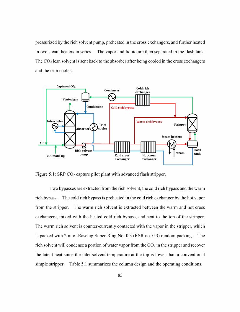
85
pressurized by the rich solvent pump, preheated in the cross exchangers, and further heated
in two steam heaters in series. The vapor and liquid are then separated in the flash tank.
The CO2 lean solvent is sent back to the absorber after being cooled in the cross exchangers
and the trim cooler.
Stripper
Cold rich bypass
Steam heaters
Condensate
CondenserCold rich
exchanger
Warm rich bypass
Flash tank
Captured CO2
Cold cross exchanger
Hot cross exchanger
Intercooler
Absorber
Air
CO2 make up
Trim cooler
Rich solvent pump
Vented gas
Steam
Figure 5.1: SRP CO2 capture pilot plant with advanced flash stripper.
Two bypasses are extracted from the rich solvent, the cold rich bypass and the warm
rich bypass. The cold rich bypass is preheated in the cold rich exchanger by the hot vapor
from the stripper. The warm rich solvent is extracted between the warm and hot cross
exchangers, mixed with the heated cold rich bypass, and sent to the top of the stripper.
The warm rich solvent is counter-currently contacted with the vapor in the stripper, which
is packed with 2 m of Raschig Super-Ring No. 0.3 (RSR no. 0.3) random packing. The
rich solvent will condense a portion of water vapor from the CO2 in the stripper and recover
the latent heat since the inlet solvent temperature at the top is lower than a conventional
simple stripper. Table 5.1 summarizes the column design and the operating conditions.

86
Table 5.1: Summary of column design and operating conditions.
Column design
Absorber diameter (m) 0.43
Absorber packing type/height (m) RSP-250/6.1
Stripper diameter (m) 0.15
Stripper packing type/height (m) RSR no. 0.3/2
Operating conditions
CO2 in flue gas (%) 6 and 12
PZ (molality) 5 and 8
Flue gas rate (kg/hr) 1700–3500
Solvent rate (kg/hr) 700–1100
L/G (kg/kg) 2.3–4.9
Capture rate (%) 68–97
Stripper T (ºC) 135–149
Stripper P (bara) 4.2–7.0
Rich loading (mol CO2/mol alkalinity) 0.20–0.27
Lean loading (mol CO2/mol alkalinity) 0.35–0.41
The 3-week 2015 campaign included 17 runs with 5 m PZ and 4 runs with 8 m PZ.
The test matrix is shown in Table 5.2, which included variations of flue gas rate, solvent
flow rate, stripper temperature, stripper pressure, bypass rate, and intercooling on/off.
The CO2 concentration of the synthetic flue gas was controlled at 12% by manipulating the
CO2 make up flow, except in Run 19 which was at 6%. The flue gas to solvent ratio is
2.9–4.3 (kg/kg) and the CO2 capture rate is 68–97%. The CO2 lean loading was varied
by manipulating the stripper pressure while the flash tank temperature was automatically
controlled by adjusting the steam rate. The absorber performance determined the CO2
rich loading, which directly affected the energy performance.

87
Table 5.2: 2015 SRP Pilot plant operating conditions using the AFS and PZ.
Run PZ
(m)
Flue gas rate
(kg/hr)
Solvent rate
(kg/hr)
Capture
rate (%)
Cold BPS
ratio (%)
Warm BPS
ratio (%)
Pstrp
(bar)
Tstrp
(°C)
1 4.7 749 2265 85 8 38 4.2 140
2 4.9 744 2489 97 7 30 4.2 140
3 4.9 728 2491 94 10 37 5.9 149
4 4.9 753 2490 94 10 32 5.9 149
5 5.0 752 2491 94 10 32 5.9 149
6 5.0 730 2957 89 7 23 5.9 145
7 5.3 726 3442 80 6 19 5.9 145
8 5.1 736 3443 96 8 19 5.9 145
9 5.1 1042 3442 80 8 19 5.9 145
10 5.0 1059 3168 87 11 19 5.9 149
11 5.0 732 2262 89 10 31 5.9 149
12 4.9 730 3441 94 7 18 5.9 145
13 7.4 1039 3507 68 7 18 5.9 145
14 8.0 1041 3539 75 8 17 5.9 145
15 7.8 719 3534 93 8 17 5.9 145
16 8.0 740 2574 91 8 21 6.5 149
17 5.0 716 2482 93 11 28 6.0 149
18 5.0 717 2485 96 0 29 6.0 148
19 5.0 733 1721 92 6 41 4.2 135
20 4.9 737 2080 84 13 33 5.7 149
21 4.9 759 2507 75 5 23 7.0 149

88
The steady-state value of each operating condition was determined as the average
over a 30-minute period. Lean and rich solvent samples were taken in each run. PZ was
determined by manual acid titration of the lean solvent. Total CO2 in the solvent was
determined by manual titration in methanol and by estimation from on-line density
measurements using the correlation developed by Freeman (Freeman et al., 2011). The
second method shows more consistent lean loading at the same stripper temperature and
pressure throughout the campaign and also gives better CO2 mass balance closure (see
Section 5.3.1). The density-predicted CO2 loading is considered more reliable and will
be used in this analysis as the measured CO2 loading.
5.3 PILOT PLANT RESULTS
5.3.1 Material balance
The CO2 mass balance around the stripper can be quantified by comparing the CO2
regenerated on the gas side and the liquid side. The CO2 regenerated on the gas side was
measured from the stripper overhead. The CO2 regenerated on the liquid side (mCO2,L)
was calculated using Equation 5.1, which depends on the mass flow rate (mrich, mlean) and
the CO2 mass fraction (xCO2,rich , xCO2,lean) of the lean and the rich solvent. Figure 5.2
shows a good CO2 balance closure throughout the campaign with a 2.2% average error.
��𝐶𝑂2,𝐿 = ��𝑟𝑖𝑐ℎ𝑥𝐶𝑂2,𝑟𝑖𝑐ℎ − ��𝑙𝑒𝑎𝑛𝑥𝐶𝑂2,𝑙𝑒𝑎𝑛 (5.1)

89
Figure 5.2: CO2 mass balance around the stripping process; average error: 2.2%.
5.3.2 Enthalpy balance and heat loss
The enthalpy balance can be calculated around the stripping process including two
cross exchangers, the steam heater, the stripper, the flash tank, the cold rich exchanger, the
condenser, and the condensate separator. The material streams across the boundary
include the rich solvent entering the cold cross exchanger, the lean solvent leaving the cold
cross exchanger, the CO2 vapor, and the condensate leaving the condensate separator.
The enthalpy of the material streams were obtained from the Independence model for PZ,
which provides the predictions of heat capacity and heat of CO2 absorption at measured
temperature, pressure, and composition. Heat input and output include the steam heater
duty, the condenser cooling duty and the system heat loss. The steam heater duty was
50
70
90
110
130
150
50 70 90 110 130 150
Ove
rhea
d C
O2
flo
w r
ate
(kg/
hr)
CO2 regenerated from solvent (kg/hr)

90
calculated using the heating steam flow rate and the evaporated enthalpy at measured steam
temperature and pressure. The condenser cooling duty was calculated from the cooling
water flow rate and the temperature at the inlet and outlet of the condenser. The heat loss
can be calculated by enthalpy balance using Equation 5.2 for each run.
��𝑙𝑜𝑠𝑠 = (��𝑟𝑖𝑐ℎ − ��𝑙𝑒𝑎𝑛 − ��𝐶𝑂2− ��𝐻2𝑂) + ��𝑠𝑡𝑚 − ��𝑐𝑜𝑛𝑑 (5.2)
where:
��𝑟𝑖𝑐ℎ: enthalpy of the rich solvent entering the cold cross exchanger
��𝑙𝑒𝑎𝑛: enthalpy of the lean solvent leaving the cold cross exchanger
��𝐶𝑂2: enthalpy of the CO2 leaving the condensate separator
��𝐻2𝑂: enthalpy of the condensate leaving the separator
��𝑠𝑡𝑚: measured steam heater duty
��𝑐𝑜𝑛𝑑: measured condenser cooling duty
The calculated heat loss can be correlated with the temperature gradient between
the flash tank temperature (Th) and the ambient temperature (Tamb) using Equation 5.3.
The heat loss constant, Chloss, represents the product of the exposed area and the overall
heat transfer coefficient of heat loss. The average Chloss of 21 runs is 102.7 W/K with
7.5% standard deviation. The heat loss was also calculated in the pre-start up test with
water before the campaign. The average Chloss during the water test is 100.8 W/K. The
consistent heat loss constant of the amine and the water system assures the validity of the
calculated heat loss.
��𝑙𝑜𝑠𝑠 = 𝐶ℎ𝑙𝑜𝑠𝑠(𝑇ℎ − 𝑇𝑎𝑚𝑏) (5.3)
5.3.3 Energy performance
The process heat duty is obtained by subtracting the heat loss from the measured
steam heater duty. Figure 5.3 shows the heat loss and the process heat duty. The process

91
heat duty of the AFS is 2.1–3.0 GJ/tonne CO2 including 17 runs below 2.5 GJ/tonne CO2.
Figure 5.4 compares the process heat duty of the 2015 campaign with previous SRP
campaigns in 2011 using a two-stage flash and 8 m PZ (Madan et al., 2013; Van Wagener
et al., 2013). The AFS reduces the heat duty by over 25%.
Figure 5.3: Heat loss and process heat duty of the AFS.
0
1
2
3
4
5
1 5 9 13 17 21
He
at
du
ty (
GJ/
ton
ne
CO
2)
Run
Heat loss
Process heat duty

92
Figure 5.4: Process heat duty of SRP pilot plant campaigns since 2011.
The total equivalent work (Weq) described in Chapter 2 (Equation 2.5–2.7) is used
to indicate the overall energy performance for CO2 capture and compression, which
includes pump work, compression work and heat duty work.
𝑊𝑒𝑞 = 𝑊ℎ𝑒𝑎𝑡 + 𝑊𝑝𝑢𝑚𝑝 + 𝑊𝑐𝑜𝑚𝑝 (2.5)
Heat duty work (Equation 2.6) converts the heat duty to electricity by multiplying
the turbine efficiency, 90%, and the Carnot cycle efficiency. Tstm is the heating steam
condensing temperature, which is around 10 K higher than the flash tank temperature in
this campaign. The Qp is the process heat duty. The pump work is calculated using
Equation 2.7. Vrich is the rich solvent volume flow rate and the Prp is the rich solvent
pump outlet pressure. The head provided by the rich pump was used to overcome the
2
3
4
5
6
0 10 20 30 40
Pro
cess
he
at
du
ty (
GJ/
ton
ne
CO
2)
Run
2011 Jan.Two-stage flash
2011 Oct.Two-stage flash w/ cold rich BPS
DOE Case 10 (2010)MEA w/ simple stripper
2015 Mar.Advanced flash stripper

93
pressure drop of the cross exchangers and the steam heaters, and reach stripper pressure.
The total pressure drop of the heat exchangers is around 2 bar. The pump efficiency, ηp,
is assumed as 65%. The compression work to 150 bar is estimated using the correlation
(Equation 2.8) as a function of stripper pressure.
𝑊𝐻𝑒𝑎𝑡 = 90% (𝑇𝑠𝑡𝑚−313𝐾
𝑇𝑠𝑡𝑚) 𝑄𝑝 (2.6)
𝑊𝑝𝑢𝑚𝑝 = ��𝑟𝑖𝑐ℎ(𝑃𝑟𝑝−1 𝑏𝑎𝑟)
𝜂𝑝 (2.7)
𝑊𝑐𝑜𝑚𝑝 (𝑘𝐽
𝑚𝑜𝑙 𝐶𝑂2) = 15.3 − 4.6𝑙𝑛𝑃𝑖𝑛 + 0.81(𝑙𝑛𝑃𝑖𝑛)2 − 0.24(𝑙𝑛𝑃𝑖𝑛)3 + 0.03(𝑙𝑛𝑃𝑖𝑛)4
1 𝑏𝑎𝑟 ≤ 𝑃𝑖𝑛 ≤ 149 𝑏𝑎𝑟 (2.8)
The breakdown of total equivalent work is shown in Figure 5.5. Since the stripper
pressure only varied from 4 to 7 bar, the compression work and the pump work are nearly
constant. The total work requirement is dominated by the heat duty work. The lowest
total equivalent work achieved was 32.0 kJ/mol CO2.
The U.S. Department of Energy (DOE) reviewed amine scrubbing for CO2 capture
and developed base cases (NETL, 2010). The Case 10 uses MEA with a simple stripper
at 1.6 bar to capture CO2 from coal-fired power plants. The reported heat duty is around
3.6 GJ/tonne CO2. The total equivalent work calculated is 45 kJ/mol CO2, including 31.8
kJ/mol heat duty work and 13.2 kJ/mol projected compression work. Compared to
DOE Case 10, the AFS with PZ reduces the total equivalent work by over 20%.
Reduction of compression work is around 5 kJ/mol CO2 because PZ is more thermally
stable, so the stripper can be operated at higher temperature and pressure without
significant thermal degradation.

94
Figure 5.5: Total equivalent work of SRP pilot plant with the AFS.
5.3.4 Rich solvent bypass performance
The heat recovery performance was maintained by manually adjusting the cold and
warm rich bypass rates for each run. The cold and warm rich bypasses are used to recover
the stripping steam heat from the CO2 vapor. The vapor temperatures indicate the amount
of stripping steam that has been condensed. The analysis in Chapter 3 concluded that the
optimum bypass rates usually give a consistent temperature approach between vapor and
liquid throughout the stripper column.
The temperature difference between the liquid that enters the stripper and the vapor
at the top was maintained at around 7 K in this campaign. The cold rich bypass rate was
adjusted to ensure the cold rich exchanger performance by keeping the cold rich exchanger
0
10
20
30
40
50
1 5 9 13 17 21
We
q(k
J/m
ol
CO
2)
Run
Heat duty work
Pump work
Compression work
DOE Case 10 (2010)MEA w/ simple stripper

95
vapor outlet temperature at 50–70 °C. Figure 5.6 shows the results of rich solvent bypass
control. The total bypass ratio includes the cold and the warm rich bypass. The water
content from the flash tank is estimated using the Independence model at a given
temperature and pressure. Lower lean loading and lower flash tank temperature that
reduce partial pressure of CO2 will result in higher water vapor content in the stripped
vapor. The results show that higher water content requires more bypass to maintain the
vapor outlet temperature. Four runs highlighted in Figure 5.6 used relatively low bypass
rates at given water content and therefore resulted in higher vapor outlet temperature.
Figure 5.6: Performance of rich solvent bypass; 4 runs highlighted were without bypass
control.
40
80
120
160
200
240
0%
10%
20%
30%
40%
50%
55% 60% 65% 70% 75% 80%
Co
ld r
ich
X v
apo
r T
(°C
)
To
tal b
ypas
s ra
tio
H2O content in flash tank vapor
Cold richX vapor out T
Total bypass ratio
No bypass control

96
Figure 5.7 further demonstrates the effect of bypass on the energy performance.
There are 4 runs at identical operating conditions except the bypass ratio. The water
content in the vapor phase should be similar at the same flash tank temperature and lean
loading. The two runs on the left side of the plot that did not deliver enough bypass to
condense the stripping steam led to a 15% increase of heat duty.
Figure 5.7: Effect of rich solvent bypass; run 10, 11, 17, and 18; 5 m PZ; flash tank T:
149 ºC; rich loading: 0.36; lean loading: 0.20.
5.3.5 Lean loading effect
The lean loading is one of the most important operating parameters that determine
minimum heat duty. Chapter 4 has shown a quadratic relationship between lean loading
40
70
100
130
160
2.2
2.4
2.6
2.8
25% 30% 35% 40%C
old
ric
h X
vap
or
ou
t T
(°C
)
Pro
cess
hea
t d
uty
(G
J/to
nn
e C
O2)
Total bypass ratio
Cold rich X vapor out T
Process heat duty

97
and heat duty at constant rich loading. Optimum lean loading was found to minimize the
energy requirement. Figure 5.8 shows 7 runs at identical operating conditions except the
CO2 lean loading. Since the rich loading is approximately constant, lower lean loading
provides better cyclic capacity (i.e., the difference between rich and lean loading, Ldg)
and less sensible heat requirement. However, lower lean loading will cause more
stripping steam to be generated and thus lower the ratio of CO2 to H2O in the stripping
vapor. Heat duty trade-offs between the sensible heat and the stripping steam heat are
expected when the lean loading varies. Diminishing returns of heat duty can be seen at
lean loading between 0.23 and 0.25. Based on this, it is inferred that the heat duty is
approaching the minimum at the operating lean loadings.
Figure 5.8: Effect of lean loading; run 3, 4, 5, 11, 17, 20, and 21; 5 m PZ; flash tank T:
149 °C; rich loading: 0.39±0.01.
0.10
0.12
0.14
0.16
0.18
2.0
2.5
3.0
0.19 0.21 0.23 0.25 0.27
L
dg
(m
ol
CO
2/
mo
l a
lka
lin
ity
)
Pro
cess
he
at
du
ty (
GJ/
ton
ne
CO
2)
Lean loading (mol CO2/mol alkalinity)
Process heat duty
Ldg

98
5.3.6 5 m PZ vs. 8 m PZ
It has been demonstrated that 5 m PZ provides better solid solubility and lower
viscosity than 8 m PZ. Solvents with lower viscosity can provide better mass and heat
transfer performance. This campaign consisted of 4 runs using 8 m PZ, so direct
comparisons can be made. Table 5.3 shows that two comparisons are made at the same
flash tank temperature and lean loading. Each comparison has similar solvent capacity
and bypass ratio. Even though 5 m PZ has a lower equilibrium capacity (mol alkalinity/kg
solution) than 8 m, higher liquid side mass transfer rate results in higher rich loading and
greater cyclic capacity (Ldg). These runs end up with approximately the same ratio of
solvent rate to the CO2 capture rate. The sensible heat requirement and the heat recovery
performance are expected to be similar in each comparison. The only reason that 5 m PZ
outperformed 8 m PZ with a lower heat duty is the cross exchanger performance. The
temperature approach of the cold cross exchanger at the cold end indicates the amount of
sensible heat recovered from the lean solvent. A lower temperature approach implies
higher heat transfer coefficient. The cross exchanger performance can be quantified by
the number of heat transfer units (NTU). The NTU of the cold cross exchanger using 5
m PZ is 20% greater than 8 m PZ because of lower viscosity.

99
Table 5.3: Comparisons of pilot plant results of 5 m and 8 m PZ.
Comparison 1
(145 °C 0.24 lean Ldg)
Comparison 2
(145 °C 0.24 lean Ldg)
Run 8 15 9 14
PZ (m) 5 8 5 8
Viscosity at 40 °C (cP) 3.3 9.5 3.3 9.5
Equilibrium capacity
(mol alkalinity/kg solution) 7.0 9.5 7.0 9.5
Rich loading
(mol CO2/mol alkalinity) 0.37 0.34 0.39 0.36
Total bypass ratio (%) 25 24 26 24
Cold end T of cold cross X
(°C) 6.5 8.4 6.4 8.7
NTU of cold cross X 19.2 15.9 18.9 15.8
Heat duty
(GJ/tonne CO2) 2.36 2.51 2.21 2.41
5.3.7 Heat exchanger performance
The heat transfer coefficient of heat exchangers in the stripping process is
evaluated. The log mean temperature difference (LMTD) is calculated from measured
inlet/outlet temperatures even for the flashing exchangers with non-linear temperature
profiles. The heat transfer coefficient could be under-estimated by under-predicting the
LMTD. The heat duty of the cross exchangers is calculated from the lean solvent side
with the heat capacity predicted by Aspen Plus® . The steam heater heat duty is dependent
on where the heat loss occurs and how much latent heat of steam is actually transferred to
the solvent. This analysis will report a conservative heat transfer coefficient by using the
process heat duty as steam heater duty. Table 5.4 summarizes the heat exchanger
specifications and the operating temperature approaches.

100
Table 5.4: Heat exchanger specifications of SRP pilot plant.
Heat exchanger Type Service
(hot/cold)
Area
(m2)
LMTD
(K)
Cold cross exchanger Plate-and-frame solvent/solvent 40.0 3–6
Hot cross exchanger Plate-and-frame solvent/solvent 20.4 2–5
Low T steam heater Shell-and-tube steam/solvent 1.3 12–17
High T steam heater Shell-and-tube steam/solvent 1.0 8–13
Cold rich exchanger Plate-and-frame CO2 vapor/solvent 3.2 21–34
5.3.7.1 Cross exchangers
Figures 5.9 and 5.10 show the overall heat transfer coefficient of the cold cross
exchanger, which is expected to have single phase on both sides. The heat transfer
coefficient increases with the solvent rate with a power of 1.15, which is higher than the
empirical value 0.6–0.75 for plate-and-frame exchangers (Ayub, 2003). This
demonstrates that the heat transfer coefficient can be enhanced by a higher fluid velocity.
However, the turbulence also creates higher pressure drop as shown in Figure 5.10. A
cross exchanger optimization that determines the optimum fluid velocity by considering
the pumping cost and the heat exchanger cost will be performed in Chapter 8.

101
Figure 5.9: Overall heat transfer coefficient of the cold cross exchanger.
y = 0.15 x1.15
500
800
1100
1400
1700
1500 2000 2500 3000 3500
U (
W/
K-m
2)
Avg solvent flow rate (kg/hr)
5 m PZ8 m PZ

102
Figure 5.10: Pressure drops of the cold cross exchanger.
The rich solvent is likely to flash in the hot cross exchanger when it exceeds the
bubble point. In this case, both convection and nucleate boiling will contribute to the heat
transfer at the rich side. Figure 5.11 shows that the heat transfer coefficient is not as
sensitive as the cold cross exchanger to the solvent flow rate since the effectiveness of the
nucleate boiling is mainly determined by the temperature approach while the single phase
all relies on convective heat transfer.
y = 510.71 x0.67
500
800
1100
1400
1700
1 3 5 7
U (
W/
K-m
2)
Avg pressure drop (psi)
5 m PZ8 m PZ

103
Figure 5.11: Overall heat transfer coefficient of the hot cross exchanger
y = 642.40 x0.09
800
1100
1400
1700
1000 1500 2000 2500 3000 3500
U (
W/
K-m
2)
Avg solvent flow rate (kg/hr)
5 m PZ
8 m PZ

104
Figure 5.12: Pressure drop of the hot cross exchanger.
5.3.7.2 Steam heaters
Figure 5.13 shows the heat transfer coefficient of the steam heaters, which has no
strong correlation with the solvent rate. This implies that nucleate boiling is the dominant
heat transfer mechanism. In the nucleate boiling regime, higher heat transfer coefficient
can be achieved as the temperature difference between the heating surface and saturation
temperature increases. Even though the high temperature steam heater has a relatively
lower temperature approach (8–13 K) than the low temperature steam heater (12–17 K),
the effective temperature difference between the steam temperature and the bubble point
temperature can be actually greater due to the pressure drop. More bubbles generated at
y = 630.92 x0.45
800
1000
1200
1400
1600
2 3 4 5 6 7
U (
W/
K-m
2)
Avg P drop (psi)
5 m PZ
8 m PZ

105
lower pressure creates more turbulence and leads to a higher heat transfer coefficient for
the high temperature steam heater.
Figure 5.13: Overall heat transfer coefficient of the steam heaters.
5.3.7.3 Cold rich exchanger
The cold rich exchanger has the condensing steam and CO2 vapor at the hot side
and the rich solvent in single phase at the cold side. The heat transfer coefficient is around
250 W/K-m2 because of the poor heat transfer performance of vapor as shown in Figure
5.14. Condensing steam can make heat transfer more effective than the vapor itself.
Generally, CO2 vapor at higher temperature contains more steam that can be condensed in
the cold rich exchanger so results in a higher heat transfer coefficient.
1000
2000
3000
4000
5000
900 1400 1900 2400 2900
U (
W/
K-m
2)
Solvent rate (kg/hr)
Low T steam heater
High T steam heater
Avg
Avg

106
Figure 5.14: Overall heat transfer coefficient of cold rich exchanger.
5.4 MODELING RESULTS
5.4.1 Simulation model and data reconciliation
The Independence model was rigorously regressed in Aspen Plus® with
experimental data including amine volatility, heat capacity, CO2 solubility, and amine pKa
over a range of amine concentration and CO2 loading (Frailie, 2014). The electrolyte
Non-Random Two-Liquid (e-NRTL) property method is used to describe the CO2-amine-
H2O chemistry accounting for the non-ideality in the aqueous electrolyte system. Aspen
Plus® RateSepTM provides a rigorous, rate-based model for heat and mass transfer with
equilibrium reactions in the boundary layer. Mass transfer and area models used in the
50
150
250
350
105 115 125 135
U (
W/K
-m2)
Vapor inlet T (°C)
Stripper P= 4 bar
Stripper P= 6-7 bar

107
stripper were developed specifically for RSR no. 0.3 packing by regression of experimental
data collected using a pilot-scale column (Wang, 2015).
The data reconciliation was implemented in Aspen Plus® using the Data-Fit tool.
Data-Fit minimizes the error of result variables between measured and modeled values by
adjusting model-input variables. The objective function in data reconciliation is shown
in Equation 5.4. The resulting variables of interest are the process heat duty and the CO2
production rate, which indicate the energy performance and CO2 mass balance,
respectively.
The model-input variables from pilot plant measurements include the temperature
and pressure of the rich solvent, PZ concentration, the lean side outlet temperature of the
cold and hot cross exchanger, the temperature and pressure of the flash tank, the liquid side
outlet temperature of the cold rich exchanger, and the condenser temperature. The
temperature and pressure measurement inputs are considered consistent and reliable, and
so will not be adjusted. Two adjustable parameters in the data reconciliation are the CO2
concentration in the rich solvent (rich loading) and the correction of packing interfacial
area for the stripper. The rich loading was adjusted for each run and the packing
interfacial area factor is a global parameter that uniformly applies to the whole campaign.
Generally, the adjustment of the CO2 rich loading is responsible for CO2 mass balance
closure, and the packing area factor will be adjusted to match the process heat duty.
𝑀𝑖𝑛 ∑ (𝑀𝑒𝑎𝑠𝑢𝑟𝑒𝑑𝑖−𝑀𝑜𝑑𝑒𝑙𝑒𝑑𝑖
𝜎𝑖)
2𝑛𝑖=1 (5.4)
where:
Measuredi: pilot plant measurement of variable i
Modeledi: model prediction of variable i
𝜎𝑖: standard deviations of pilot plant measurement of variable i

108
n: number of result variables
5.4.2 Model validation
Figures 5.15 and 5.16 compare the modeled and density-predicted CO2 loading.
The modeled lean loading was determined by the vapor-liquid equilibrium at given
temperature and pressure of the flash tank. The modeled lean and rich loadings are 5.4%
and 3.6% higher, respectively.
Figure 5.15: Measured and modeled lean loading; average error: 5.4%.
0.0
0.1
0.2
0.3
1 5 9 13 17 21
Le
an
lo
ad
ing
(m
ol
CO
2/
mo
l a
lk)
Run
Measured
Modeled

109
Figure 5.16: Measured and modeled rich loading; average error: 3.6%.
The regressed correction factor for the packing interfacial area is 15.2%±0.17%
within 95% confidence interval. The correction accounts for the actual column
performance and potential model errors. The actual effective area could be less than the
model prediction due to liquid maldistribution that causes un-wetted packing. Model
errors could also result from over-predicting the mass transfer coefficient of the liquid and
gas side. All the potential errors were reflected on a single correction factor.
The 6-in ID (150 mm) stripper was packed with the random packing RSR no. 0.3
that has the packing size of 15 mm. The diameter-to-packing size ratio of the SRP stripper
is 10 while the packing performance data were measured using a column with a ratio of
30.(Wang, 2015) The wall effect is more significant for a small column and will reduce
0.0
0.1
0.2
0.3
0.4
0.5
1 5 9 13 17 21
Ric
h l
oa
din
g (
mo
l C
O2/
mo
l a
lk)
Run
Measured
Modeled

110
the effective packing area. It is expect that a large scale plant will reduce the wall effect
and increase the packing wetted area.
The diffusion coefficient of amine and reaction product predicted by the model is
the most uncertain parameter used in the mass transfer coefficient model. Figure 5.17
compares the diffusivity of amine in amine solution predicted by the Independence model
and by the Stokes-Einstein relation, which applies an analogy of viscosity as shown in
Equation 5.5 (Snijder et al., 1993; Versteeg et al., 1988). The diffusivity data of amine in
water is needed (Dam-water). The Independence model uses the same analogy to estimate
the diffusivity of CO2 in amine solution with a power of 0.8. The diffusion coefficient of
amine is expected to be about half of CO2 at the stripper temperature using the modified
Stokes-Einstein relation. However, the predicted diffusion coefficient of amine in the
model is 4 times greater than expected. The over-prediction of the diffusion coefficient
is compensated for by a small correction factor applied to the interfacial area.
𝐷𝑎𝑚−𝑎𝑚
𝐷𝑎𝑚−𝐻2𝑂= (
𝜇𝑤𝑎𝑡𝑒𝑟
𝜇𝑎𝑚)
0.6
(5.5)

111
Figure 5.17: Diffusivity of amine and CO2 in 5 m PZ solution predicted by Independence
model and modified Stokes-Einstein relation at stripper conditions.
Figure 5.18 shows that the model predicts well the process heat duty for the whole
campaign with a 3.0% average error. Two typical temperature profiles of this campaign
are shown in Figures 5.19 and 5.20, representing with and without bypass control,
respectively. The open points were measured inside the stripper and the filled points were
measured from the liquid or vapor that go into the stripper. Solid lines are model-
predicted temperatures. The two measurements at the stripper bottom consistently reflect
the liquid temperature but other were more inclined to vapor temperature.
2.0E-05
4.0E-05
8.0E-05
1.6E-04
120 125 130 135 140
Dif
fusi
vity
(cm
2/s
)
Temperature (°C)
DPZ-PZ
(Independence)
DCO2-PZ
(Independence)
DPZ-PZ
(Stokes-Einstein relation)

112
Figure 5.18: Measured and modeled process heat duty; average error: 3.0%.
0
1
2
3
1 5 9 13 17 21
Prc
oes
s h
eat
du
ty (
GJ/
ton
ne
CO
2)
Run
Measured
Modeled

113
Figure 5.19: Stripper temperature profile; run 6; open points: measured T inside the
stripper; filled points: measured T outside the stripper; solid lines: modeled
T at operating bypass rates; dotted lines: modeled T at optimized bypass
rates.
110
120
130
140
0 1
Stri
pp
er T
(°C
)
Z/Ztotal
Vapor T (modeled)
Liquid T(modeled)
Measured T
TOP BOT
Liquid in
Vapor in
Operating BPS Optimized BPS

114
Figure 5.20: Stripper temperature profile; run 18; open points: measured T inside the
stripper; filled points: measured T outside the stripper; solid lines: modeled
T at operating bypass rates; dotted lines: modeled T at optimized bypass
rates.
5.4.3 Rich solvent bypass optimization
The temperature approaches at the top and the bottom of the stripper (the difference
between the open and the filled points in Figures 5.19 and 5.20) were controlled to be
approximately equal to each other by adjusting the rich solvent bypass during the test.
The cold and the warm rich bypass were re-optimized using the validated model to assure
the performance of the bypass control strategy. First, the product of the overall heat
transfer coefficient and the exchanger area (UA) of the cross exchangers and the cold rich
105
120
135
150
0 1
Stri
pp
er (
°C)
Z/Ztotal
Vapor T (modeled)
Liquid T(modeled)
Measured T
TOP BOT
Liquid in
Vapor in
Operating BPS Optimized BPS

115
exchanger was found for each run at operating conditions. Second, bypass rates were
varied to minimize the heat duty while UA was kept constant.
Figure 5.21 shows the improvement of the heat duty and the absolute change of the
total bypass ratio after optimizing the rich solvent bypass. The changes of heat duty and
bypass ratio will approach zero as the operating rich solvent bypass is at optimum. The
heat duty was kept within 2% of the minimum when the bypass rates were adequately
controlled. The change of total bypass ratio is less than 10%. Four other runs without
bypass control needed the bypass ratio to be increased by around 20% to minimize the heat
duty. Figure 5.21 also suggests that energy performance can be easily guaranteed as long
as the bypass ratio is in the optimum range. This demonstrates the operability and
flexibility of a complex system by implementing a simple control strategy.
To further justify the control strategy, temperature profiles before and after bypass
optimization are compared in Figures 5.19 and 5.20. The dotted lines are the modeled
temperature profiles at optimum bypass ratio. The operating bypass ratio of Run 6
(Figure 5.19) was already close to optimum so the temperature profile shows little change.
Run 18 (Figure 5.20) did not deliver enough bypass to the stripper so the temperature
approach was different between the top (30 K) and the bottom (5 K). The temperature
profile becomes nearly parallel after re-optimizing the bypasses.

116
Figure 5.21: Process heat duty improvement after bypass re-optimization; circle: with
bypass control; triangle: without bypass control.
5.4.4 Effect of rich and lean loading
A base case with the minimum total equivalent work of the campaign was selected
for further studies that extended the operating conditions. Run 21 using 5 m PZ achieved
an equivalent work of 32.6 kJ/mol CO2 with 0.27 lean loading, 0.41 rich loading
(modeled value), and 149 °C flash tank temperature. The UA of the cross exchangers and
the cold rich exchanger were fixed in the following simulations. The rich solvent
bypasses were optimized in all of the cases.
Figure 5.22 shows the total equivalent work with various rich and lean loading.
The rich loading reflects the absorber performance and is affected by the liquid to gas ratio
0%
5%
10%
15%
0% 5% 10% 15% 20% 25% 30%
Hea
t d
uty
red
uct
ion
Absolute change of total bypass ratio
No bypass control
With bypass control

117
(L/G), the intercooling, and the operating lean loading. The rich loading in this campaign
was 0.37–0.41 mol CO2/mol alkalinity. Higher rich loading is always beneficial because
greater cyclic capacity requires a lower solvent rate for CO2 regeneration.
The optimum lean loading to minimize total equivalent work can be found at each
rich loading. The stripping steam heat and sensible heat are dominant at low and high
lean loading, respectively. The optimum lean loading shifts with rich loading but the
optimum Ldg is approximately constant at 0.11 mol CO2/mol alkalinity. The difference
of total equivalent work between the base case and the minimum is less than 1%, which
confirms the inference in Section 5.3.3 that the best energy performance has been reached
using the existing facility.

118
Figure 5.22: Total equivalent work with various lean and rich loading; stripper T: 149 °C;
packing: 2 m RSR no. 0.3; correction for interfacial area: 0.15; constant UA;
optimized bypass rates.
5.4.5 Effect of striper packing height
The packing height determines the heat recovery performance in the stripper.
Figure 5.23 shows the total equivalent work with varied packing height from 1 to 5 m. A
correction of interfacial area, 15%, is applied in Aspen Plus® to match the pilot plant data,
so that the model had to use 0.8 m of packing to represent 5 m of real packing. Adding
packing has more effect at low lean loading where excessive stripping steam needs to be
recovered. The reduction of the total equivalent work by increasing packing from 2 m to
5 m is 7% at 0.22 lean loading but 2% at 0.28 lean loading.
31
34
37
40
0.22 0.24 0.26 0.28 0.30 0.32
Weq
(k
J/m
ol C
O2)
Lean loading (mol CO2/mol alkalinity)
Rich ldg= 0.41
Rich ldg= 0.37
Rich ldg= 0.39
Base case (Run 21)

119
Figure 5.23: Total equivalent work with various packing height and lean loading;
packing: RSR no. 0.3; correction for interfacial area: 0.15; rich loading:
0.41; stripper T: 149 °C; constant UA; optimized bypass rates.
Efficiency of packing utilization can be quantified using Equation 5.6. The
maximum (Weq,max) and the minimum (Weq,min) total equivalent work are defined as using
1 m packing and infinite packing, respectively. 1 m is assumed to be the least packing
height needed for a packed stripper. The difference between Weq,max and Weq,min is the
maximum amount of energy that can theoretically be reduced by adding packing. When
the packing utilization efficiency is approaching 100%, little energy improvement will be
obtained from increasing packing height.
𝑃𝑎𝑐𝑘𝑖𝑛𝑔 𝑢𝑡𝑖𝑙𝑖𝑧𝑎𝑡𝑖𝑜𝑛 𝑒𝑓𝑓𝑖𝑐𝑖𝑒𝑛𝑐𝑦 =𝑊𝑒𝑞,𝑚𝑎𝑥−𝑊𝑒𝑞
𝑊𝑒𝑞,𝑚𝑎𝑥−𝑊𝑒𝑞,𝑚𝑖𝑛 (5.6)
31
33
35
37
0.22 0.24 0.26 0.28 0.30 0.32
Weq
(k
J/m
ol C
O2)
Lean loading (mol CO2/mol alkalinity)
2 m RSR #0.3
5 m RSR #0.3
1 m RSR #0.3
Base case(Run 21)

120
Figure 5.24 shows the total equivalent work and the packing efficiency with
increasing packing height at 0.22 and 0.28 lean loading. The greatest reduction of total
equivalent work is between 1 m and 5 m. After 5 m, adding packing improves the energy
performance by less than 2%. The packing utilization efficiency reaches 88% with 5 m
packing and then approaches 99% after 10 m. The packing efficiency varies with packing
height but not with lean loading.
Figure 5.24: Packing utilization efficiency; packing: RSR no. 0.3; correction for
interfacial area: 0.15; rich loading: 0.41; stripper T: 149 °C; constant UA;
optimized bypass rates.
5.4.6 Effect of cross exchange area
The sensible heat recovered from the hot lean solvent in the cross exchanger is
typically 3–5 times the reboiler/steam heater duty. Increasing the cross exchanger area
0%
20%
40%
60%
80%
100%
30
32
34
36
38
0 5 10 15 20P
ack
ing
uti
liza
tio
n e
ffic
ien
cy
Weq
(kJ/
mo
l CO
2)
Packing height (m)
Weq
(lean ldg=0.28)
Weq
(lean ldg=0.22)
Efficiency(lean ldg=0.22)
Efficiency(lean ldg=0.28)

121
can effectively reduce the heat duty requirement. The size and performance of the
specific heat exchanger in the pilot plant directly affects the measured energy performance.
Figure 5.25 shows the total equivalent work as the cross exchanger area is varied
from 50% to 125% of the UA relative to the pilot plant. The reduction of the total
equivalent work by increasing the cross exchanger area is more pronounced at higher lean
loading where the cyclic capacity is deteriorating. An additional 25% cross exchanger
area added to the base case reduces the total equivalent work by 4% at 0.28 lean loading.
The cross exchanger in the SRP pilot plant is large, resulting in the minimum temperature
approach as 2 K. Increasing cross exchanger area will not significantly reduce the heat
duty since the exchanger has been practically pinched.
The average LMTD (TLM) is also indicated in Figure 5.25. The LMTD of the
base case is 4.3 K. Lin and Rochelle suggest that the economic optimum cross exchanger
LMTD is between 5 and 10 K using 8 m PZ (Lin & Rochelle, 2014). The large exchanger
in the existing pilot plant may result in excessive capital cost.

122
Figure 5.25: Total equivalent work with various cross exchanger UA; packing: 2 m RSR
no. 0.3; correction for interfacial area: 0.15; rich loading: 0.41; stripper T:
149 °C; optimized bypass rates.
5.5 IRREVERSIBILITY ANALYSIS
Irreversibility analysis has been used to quantify process inefficiency and potential
energy improvement for amine scrubbing processes in Chapter 3. By exergy balance
using Equation 3.4, the minimum work and the lost work of each unit operation can be
calculated. The sink temperature, To, is set at 313.15 K (40 ºC). Tk is the steam
temperature. Q and W are the heat duty and work input/output. The enthalpy, H and
the entropy, S were obtained from the validated Aspen Plus® model.
𝑊𝑙𝑜𝑠𝑡 = ∑ (1 −𝑇𝑜
𝑇𝑘) 𝑄 + ∑ 𝑊 + ∑ (𝐻 − 𝑇𝑜𝑆)𝑖𝑛 − ∑ (𝐻 − 𝑇𝑜𝑆)𝑜𝑢𝑡 (3.4)
31
33
35
37
39
0.22 0.24 0.26 0.28 0.30 0.32
Weq
(kJ/
mo
l CO
2)
Lean loading (mol CO2/mol alkalinity)
100% UA
(TLM= 4.3 K)
50% UA
(TLM= 8.4 K)
75% UA
(TLM= 5.7 K)
125% UA
(TLM= 3.5 K)
Base case(Run 21)

123
Figure 5.26 shows the minimum work and the lost work averaged by the runs that
achieved at least 90% capture rate and implemented bypass control. The minimum work
of separation (Wmin,sep) and the minimum work of compression (Wmin,comp) are the
theoretical work required to separate CO2 from flue gas to pure CO2 at stripper pressure
and to compress pure CO2 isothermally at 40 °C from stripper pressure to 150 bar,
respectively.
The lost work of each unit operation indicates irreversible operations. The lost
work of the absorber reflects the mass transfer driving force between the flue gas and the
CO2-loaded solvent. The lost work of the heat exchanger is proportional to the exchanger
duty and the temperature approach. The cross exchanger and the steam heater are
responsible for most of the lost work from heat exchangers. The exchanger duty of the
steam heater is about 25% of the cross exchanger, however the temperature approach is
greater. The compressor with intercooling is at 72% overall thermodynamic efficiency.
Other contributions include the rich pump, the stripper column, the cold rich exchanger,
the condenser, the trim cooler, and the un-recovered lean solvent pressure.

124
Figure 5.26: Minimum work and lost work distributions of SRP pilot plant with the AFS;
average values from the runs that achieved at least 90% capture rate and
implemented bypass control.
The overall thermodynamic efficiency including CO2 separation and compression
is about 50%, which is remarkable compared to 20% for conventional separation processes
such as distillation (Fitzmorris et al., 1980; Y. H. Kim, 2012; Yoo et al., 1988). The
remaining lost work is simply due to the mass and heat transfer driving force, which is
inevitable if finite capital is used. Further energy reduction by process modifications will
be marginal.
Solvents that provide greater absorption rate and capacity will be the key to better
performance. The lost work of the cross exchanger can only be reduced by increasing
solvent capacity (i.e., reducing solvent circulation rate and exchanger duty) because the
Wlost,absorber
Wlost,cross X
Wlost,reboiler
Wlost,comp
Wlost,others
Wmin,comp
Wmin,sep

125
existing cross exchanger has already achieved a small temperature approach as indicated
in Section 5.4.6. A higher absorption rate can effectively reduce the driving force in the
absorber with finite packing height.
5.6 CONCLUSIONS
Findings of pilot plant test:
The CO2 mass balance was closed with 2.2% average error. Process heat duty and
heat loss were identified using enthalpy balance around the stripping process.
17 runs have process heat duty 2.1–2.5 GJ/tonne CO2 and 4 runs without enough rich
solvent bypass are 2.5–2.9 GJ/tonne CO2. The lowest Weq is 32.0 kJ/mol CO2.
The AFS shows over 25% heat duty reduction compared to previous SRP campaigns,
and over 30% compared to the DOE base case.
Cold and warm rich solvent bypass were manually controlled to recover the stripping
steam heat by maintaining the stripper vapor outlet temperature and the cold rich
exchanger vapor outlet temperature. Four runs that did not achieve the temperature
target increased the process heat duty by 15%.
5 m PZ provides 20% greater number of heat transfer units than 8 m PZ on the cold
cross exchanger and results in a lower process heat duty because of lower viscosity.
Findings of simulations:
The “Independence” model was validated using the pilot plant data and accurately
represents the performance of the pilot plant. The modeled lean loading and rich
loading show 5.4% and 3.6% average error compared to the density-predicted loading.
The modeled and the measured process heat duty has 3% average error.
The validated model was used to re-optimize the bypass rates. It confirmed that the
bypass control strategy used during the test successfully minimized the heat duty.

126
Increasing the stripper packing height has a more significant effect at low lean
loading. The packing utilization efficiency can reach 88% using 5 m of RSR no. 0.3.
The existing cross exchanger performed well on recovering the sensible heat from the
lean solvent, giving around 2 K pinch temperature approach and 4.3 K TLM.
Energy improvement by using more exchanger area will not be significant for the
existing pilot plant.
The irreversibility analysis showed that the thermodynamic efficiency of the SRP pilot
plant using the AFS is about 50%. The absorber and the cross exchanger are the two
major sources of lost work and can only be addressed by greater absorption rate and
solvent capacity, respectively.
ACKNOWLEDGEMENT
The pilot plant data presented in this work was contributed by all of the hard work
by the staff in SRP and graduate students from Rochelle’s group including Dr. Rochelle
and Dr. Eric Chen who planned the campaign and manufactured the AFS, and Dr. Frank
Seibert, Micah Perry, Steve Briggs, Robert Montgomery, Di Song, Steven Fulk, Matt
Walters, Yue Zhang, Matt Beaudry, Kent Fischer, Paul Nielsen, Darshan Sachde, and
Nathan Fine.

127
Chapter 6: Approximate Stripper Models (ASM)
6.1 INTRODUCTION
Solvent selection is one of important ways to reduce the energy requirement and
capital cost for CO2 capture. Solvent screening has been used to identify important
solvent properties such as absorption rate, CO2 solubility, and thermal stability (Li, 2015).
These measured data can be used to quantify individual energy contributions and capital
requirement such as cyclic capacity, maximum stripper temperature, absorber packing
requirement, and the size of cross exchanger. Process models incorporated with solvent
characteristics are necessary in order to evaluate the overall energy performance that
reflects the process specifications, operating conditions, and the integration effect of
various solvent properties. Rigorous Aspen Plus® models have been developed by
regressing thermodynamic and kinetic data over a range of amine concentration and CO2
loading, and used to simulate advanced processes and scale up (Frailie, 2014; Plaza, 2011;
Sherman, 2016) . However, rigorous models require extensive experimental data and are
time-consuming to create.
For the purpose of estimating energy performance for promising amines, shortcut
models that can reasonably predict energy performance should be adequate. Notz
proposed a shortcut method that applies Kremser’s equilibrium stage approach, but the
model was less accurate at higher lean loading due to the assumption of an isothermal
stripper (Notz et al., 2011). Kim developed an enthalpy balance around a simple stripper
to approximate the regeneration heat duty assuming that the partial pressure of CO2 and
water is equilibrium with the hot rich solvent that enters the top of the stripper (H. Kim et
al., 2015). The assumption does not apply to the low lean loading region since the stripper
pinch is no longer at the top. This previous work were all based on the conventional
simple stripper.
128
The goal of this work is to develop an approximate stripper model (ASM) that
captures the characteristics of the advanced flash stripper (AFS), which has shown
remarkable energy performance and can be regarded as a representative of a highly
reversible regeneration process. The model will be developed in MATLAB® with limited
input data required. It will be validated with existing models that were developed
rigorously in Aspen Plus® .
As shown in Figure 6.1, the ASM will be used to predict the overall energy
performance for existing solvent candidates with inputs of by measured solvent properties
and process specifications. The prediction can provide a quantitative indicator for solvent
selections. The model can also be treated as a generic solvent model. Desired solvent
properties and process operating conditions that minimize the energy requirement can be
identified. A guidance for future solvent screening can be provided.
Approximate
Stripper Model
Solvent Properties
Process Specs
Solvent Properties
Process Specs
Overall Energy
Performance
Overall Energy
Performance
Existing solvent evaluation
Generic solvent modeling
Figure 6.1: Approximate stripper model
6.2 MODEL DEVELOPMENT
The ASMs were developed for the simple stripper and the AFS. The simple
stripper serves as the base case so the interactions between solvent properties and stripper
configurations can be investigated. The absorber is not in the scope of this paper and will

129
not be included in the model. Typical rich solvent conditions will be used as input to the
model. The ASM is algebraic-equation-based and is solved in MATLAB® . The model
calculates material balance, enthalpy balance, and vapor liquid equilibrium but does not
include the rigorous mass and heat transfer calculations of the rate-based model in Aspen
Plus® . Instead, the ASM specifies the mass and heat transfer driving force between vapor
and liquid at both the top and the bottom of the stripper. The major inputs are the CO2
solubility relationship (i.e., vapor liquid equilibrium of CO2 in loaded amine) and the heat
capacity. The system includes three components: CO2, amine, and water. It assumes
that the amine is non-volatile and CO2 is not condensable. The CO2 equilibrium is
described by a relation between partial pressure of CO2 and CO2 loading in solution, which
can be obtained from experimental measurements. The flash calculation of water applies
Raoult’s law assuming ideal solution and ideal gas. The saturation pressure and the heat
of vaporization of water are obtained from the DIPPR database.
6.2.1 Modeling specifications
The simple stripper and the AFS are shown in Figures 6.2 and 6.3, respectively.
Since the absorber is not included, the rich loading and temperature are specified for typical
intercooled absorber. The partial pressure of CO2 of the lean solvent (lean P*CO2) was
varied from 0.05 to 1 kPa. Detailed equations are shown in Appendix C. General
modeling specifications are described in this section.

130
Cross exchanger
Condenser
Rich solvent
Lean solvent
yH2O, top
Ttop
yH2O, bot
Tbot
Condensate
Captured CO2
Absorber
Flue gas12% CO2
Vented gas
Stripper
TrebTcrossX, hotTcrossX, cold
Figure 6.2: Simple stripper.
Cold rich Bypass
Cold rich exchanger
Warm rich BypassTbp
Cold cross exchanger
Hot cross exchanger
Rich solvent
Lean solvent
Condenser
ytop
Ttop
Treb
Tbp
ybot
Tbot
QcrossX, 1
TLM,crossX, 1
QcrossX, 2
TLM,crossX, 2
Absorber
Flue gas12% CO2
Vented gas
Captured CO2
Condensate
Steam heater
Stripper
TcrossX, wrm
TcrossX, cold
TcrossX, hot
TCRX, hotTCRX, cold
Figure 6.3: Advanced flash stripper.
6.2.1.1 Heat exchangers
The heat exchangers are specified by the log mean temperature difference (LMTD,
TLM), which is a log mean average of temperature approaches at the cold end and the hot
end assuming a linear temperature-enthalpy profile.

131
The rich solvent usually flashes and becomes two phases in the cross exchanger
when it reaches the bubble point. To minimize the error caused by the nonlinear
temperature-enthalpy profile due to flashing, the LMTD calculation of the cross exchanger
is split into two regions: the liquid phase region and the flashing region. The heat duty
and the LMTD of each region are calculated. The average LMTD (TLM,crossX,avg) is then
obtained using Equation 6.1, which weights the LMTD of each region by its exchanger
duties. For the advanced flash stripper, the temperature of the warm rich bypass is
specified as bubble point temperature, which makes the LMTD calculation approach
identical to the simple stripper.
∆𝑇𝐿𝑀,𝑐𝑟𝑜𝑠𝑠𝑋,𝑎𝑣𝑔 =𝑄𝑐𝑟𝑜𝑠𝑠𝑋,1+𝑄𝑐𝑟𝑜𝑠𝑠𝑋,2
𝑄𝑐𝑟𝑜𝑠𝑠𝑋,1∆𝑇𝐿𝑀,𝑐𝑟𝑜𝑠𝑠𝑋,1
+𝑄𝑐𝑟𝑜𝑠𝑠𝑋,2
∆𝑇𝐿𝑀,𝐶𝑟𝑜𝑠𝑠𝑋,2
(6.1)
6.2.1.2 Viscosity correction for cross exchanger
The heat transfer performance of the cross exchanger can be affected by the solvent
viscosity. The optimum cross exchanger LMTD is a function of viscosity with a power
of 0.175 for plate-and-frame exchanger (Li, 2015). Viscous solvent should be designed
with a greater LMTD to avoid the excessive capital cost of cross exchanger due to the
degraded heat transfer coefficient. Details of cross exchanger optimization can be found
in Chapter 8. To differentiate the viscosity effect on the cross exchanger performance,
the specified cross exchanger LMTD can be adjusted based on the solvent viscosity at 40
°C as Equation 6.2 shows. The viscosity of 30 wt% MEA will be used as the reference
(ref) and 5 K will be the reference LMTD of the cross exchanger (TLM,ref).
∆𝑇𝐿𝑀,𝑐𝑟𝑜𝑠𝑠𝑋,𝑎𝑣𝑔 = ∆𝑇𝐿𝑀,𝑟𝑒𝑓 (𝜇
𝜇𝑟𝑒𝑓)
0.175
(6.2)

132
6.2.1.3 Stripper column
The model approximates the mass and heat transfer of the stripper by specifying
the concentration and temperature driving force between the vapor and the liquid. The
log mean temperature difference (TLM,strp) and the log mean concentration difference
(yLM,strp) are calculated using Equations 6.3 and 6.4, respectively. Since the amine is
assumed to be non-volatile, the yLM,strp of CO2 will be the same as H2O.
∆𝑇𝐿𝑀,𝑠𝑡𝑟𝑝 =∆𝑇𝑡𝑜𝑝−∆𝑇𝑏𝑜𝑡
𝑙𝑛(∆𝑇𝑡𝑜𝑝
∆𝑇𝑏𝑜𝑡)
(6.3)
∆𝑦𝐿𝑀,𝑠𝑡𝑟𝑝 =∆𝑦𝑡𝑜𝑝−∆𝑦𝑏𝑜𝑡
𝑙𝑛(∆𝑦𝑡𝑜𝑝
∆𝑦𝑏𝑜𝑡)
(6.4)
The temperature and concentration difference indicate the heat recovery
performance of the stripper and both are affected by the stripper packing height. Table
6.1 shows average temperature (Tstrp) and concentration (ystrp) driving force in the AFS
obtained from a rigorous Aspen Plus® model that has been validated by the pilot plant data
in Chapter 5. A 15% correction factor was applied to the interfacial area of the stripper
packing in order to match the plant performance. More packing used will reduce the
driving forces and attain better energy performance. 5 meter of Raschig Super-Ring
(RSR) no. 0.3 packing in the stripper will result in 5–10% yLM,strp and 5–7 K TLM,strp
using 5 m PZ.
The stripper pressure was determined at the specified reboiler temperature and lean
loading, and then the bubble point temperature of the rich solvent can be calculated. The
cold rich bypass temperature at the cold rich exchanger outlet and the warm rich bypass
were specified at bubble point temperature. The cold rich bypass ratio was determined
by the enthalpy balance around the cold rich exchanger at a given LMTD. The warm rich

133
bypass ratio was optimized to minimize the total heat duty. Greater bypass rates will be
required at low lean loading because more stripping steam needs to be recovered.
Table 6.1: Temperature and concentration driving force from Aspen Plus® simulations
using the AFS and 5 m PZ; 15% correction for interfacial area; reboiler T:
150 °C; optimized bypass rates; rich loading: 0.4.
Lean loading
(mol CO2/mol alk) 0.22 0.24 0.26 0.28 0.30 0.32
2 m RSR no. 0.3 stripper packing
Avg Tstrp (K) 11.5 12.1 11.6 10.9 9.9 8.7
Avg ystrp (%) 16.2 15.2 13.4 11.5 9.6 7.7
5 m RSR no. 0.3 stripper packing
Avg Tstrp (K) 7.0 6.8 6.5 6.1 5.6 5.0
Avg ystrp (%) 9.5 8.7 7.8 6.8 5.9 5.0
10 m RSR no. 0.3 stripper packing
Avg Tstrp (K) 4.3 4.2 4.0 3.8 3.5 3.2
Avg ystrp (%) 6.3 5.8 5.3 4.8 4.2 3.7
6.2.2 Solvent characterization
The cyclic capacity and the heat of absorption are the most important solvent
properties that determine energy performance. The heat of absorption can be measured
directly by calorimetric experiments or obtained from the temperature derivative of the
CO2 solubility measurement (I. Kim et al., 2007, 2011). This model determines the
differential heat of absorption (Habs) in Equation 6.5 from Lewis and Randall (Equation
XVIII.9) (Lewis et al., 1923). The fugacity of CO2 (fCO2) is approximated by its partial
pressure (P*CO2). Equation 6.5 has been validated in predicting the calorimetric data for
CO2 absorption in aqueous MEA at typical operating conditions (Mathias et al., 2012). In
this work it will be applied to a higher stripper pressure. The fugacity coefficient of CO2
at 150 °C is 0.95–0.99 at 1–30 bar and 0.9–0.95 at 30–60 bar (Spycher et al., 1988). The

134
heat of absorption used in this model is only a function of CO2 loading but is not
temperature dependent. It represents an average heat of absorption across the operating
temperature range.
∆𝐻𝑎𝑏𝑠 = −𝑅 [𝜕𝑙𝑛𝑓𝐶𝑂2
𝜕(1
𝑇)
]𝑃,𝑥
≈ −𝑅 [𝜕𝑙𝑛𝑃𝐶𝑂2
∗
𝜕(1
𝑇)
]𝑃,𝑥
(6.5)
The slope of the solubility curve, k, will affect the cyclic capacity and is defined in
Equation 6.6. A flat solubility curve will increase the loading difference between the lean
and the rich solvent at given rich and lean partial pressure of CO2.
𝑘(𝑇, 𝛼) =𝜕𝑙𝑛𝑃𝐶𝑂2
∗
𝜕𝛼 (6.6)
The partial pressure of CO2 is characterized by the slope of the solubility curve and
the heat of absorption as shown in Equation 6.7. The partial pressure is integrated from
a reference temperature (Tr) and CO2 loading (r) to the final statevia the CO2 loading
dependence and the temperature dependence. Figure 6.4 shows the integrating path.
𝑙𝑛𝑃𝐶𝑂2
∗ (𝑇, 𝛼) = 𝑙𝑛𝑃𝐶𝑂2,𝑟∗ (𝑇𝑟 , 𝛼𝑟) + ∫ 𝑘(𝑇𝑟 , 𝛼)𝑑𝛼
𝛼
𝛼𝑟+ ∫ −
∆𝐻𝑎𝑏𝑠(𝛼)
𝑅𝑑 (
1
𝑇)
𝑇
𝑇𝑟 (6.7)
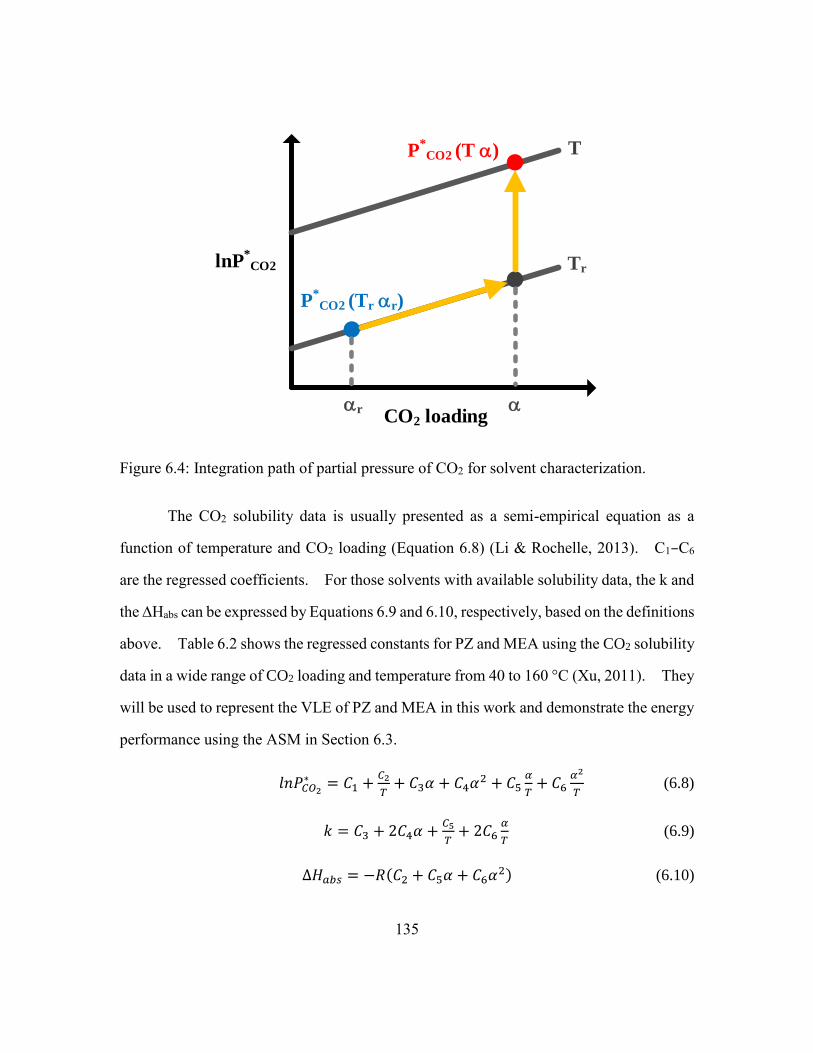
135
CO2 loading
lnP*CO2 Tr
T
r
P*
CO2 (Tr r)
P*
CO2 (T )
Figure 6.4: Integration path of partial pressure of CO2 for solvent characterization.
The CO2 solubility data is usually presented as a semi-empirical equation as a
function of temperature and CO2 loading (Equation 6.8) (Li & Rochelle, 2013). C1–C6
are the regressed coefficients. For those solvents with available solubility data, the k and
the Habs can be expressed by Equations 6.9 and 6.10, respectively, based on the definitions
above. Table 6.2 shows the regressed constants for PZ and MEA using the CO2 solubility
data in a wide range of CO2 loading and temperature from 40 to 160 °C (Xu, 2011). They
will be used to represent the VLE of PZ and MEA in this work and demonstrate the energy
performance using the ASM in Section 6.3.
𝑙𝑛𝑃𝐶𝑂2
∗ = 𝐶1 +𝐶2
𝑇+ 𝐶3𝛼 + 𝐶4𝛼2 + 𝐶5
𝛼
𝑇+ 𝐶6
𝛼2
𝑇 (6.8)
𝑘 = 𝐶3 + 2𝐶4𝛼 +𝐶5
𝑇+ 2𝐶6
𝛼
𝑇 (6.9)
∆𝐻𝑎𝑏𝑠 = −𝑅(𝐶2 + 𝐶5𝛼 + 𝐶6𝛼2) (6.10)

136
Table 6.2: Regressed constants in Equation 6.8 for MEA and PZ.
Amine C1 C2 C3 C4 C5 C6 R2
MEA 38.6 -12379 0 -16 3556 8702 0.994
PZ 35.3 -11054 0 -18.9 4958 10163 0.993
The heat capacity of the CO2 loaded solution is needed to calculate the enthalpy
balance around the heat exchangers, which will affect the sensible heat requirement. The
heat capacity of the mixture is estimated by a weight fraction average of pure components
shown in Equation 6.11 as a function of temperature. Any enthalpy of mixing is ignored.
The heat capacity of aqueous PZ is predicted from a group contribution model (Rayer et
al., 2012). The partial heat capacity of CO2 is assumed to be zero in this model and the
sensitivity will be discussed in Section 6.3.
𝐶𝑝,𝑚𝑖𝑥(𝑇) = 𝐶𝑝,𝑎𝑚(𝑇)𝑋𝑎𝑚 + 𝐶𝑝,𝐻2𝑂(𝑇)𝑋𝐻2𝑂 + 𝐶𝑝,𝐶𝑂2(𝑇)𝑋𝐶𝑂2
(6.11)
6.3 MODEL VALIDATION AND INTERPRETATION
6.3.1 Comparison with rigorous Aspen Plus® model
The ASM is compared with the rigorous Aspen Plus® model that has been validated
by the pilot plant data from the 2015 campaign at UT Austin using the AFS and 5 m PZ.
Figure 6.5 shows the total equivalent work at varied lean loading. The LMTDs of the
cross exchanger and the cold rich exchanger are 5 K and 20 K, respectively. The TLM,strp
and the yLM,strp of the stripper specified in the ASM were obtained from the Aspen Plus®
results using 5 meters of RSR no. 0.3 packing.
The results show a 5% systematic bias between the ASM and the Aspen Plus®
model, but have the same trend with varied lean loading. The bias is mainly due to the
difference in the predicted heat capacity of CO2 loaded solvent between models. The

137
approximate model matches the Aspen Plus® model if the partial heat capacity of CO2 is
increased from 0 to 3 kJ/kg-K, which is close to the value predicted by Aspen Plus® .
Figure 6.5: Comparison of ASM and the validated Aspen Plus® model using AFS; 5 m
PZ; reboiler T: 150 °C; 5 K cross exchanger ΔTLM; 5 m RSR no. 0.3
packing; 0.15 correction factor for interfacial area used in the Aspen Plus®
model.
6.3.2 Uncertainties of predicted heat capacity
The sensible heat required depends on the temperature approach of the cross
exchanger and is sensitive to the ratio of the heat capacity of the lean and the rich solvent.
The temperature change of the lean and the rich solvent in the cross exchanger is around
100 K (approximately from 50 °C to 150 °C). A 1% difference of the heat capacity
between the lean or the rich solution will lead to a 1 K difference on the temperature
31
32
33
34
35
36
0.22 0.24 0.26 0.28 0.30 0.32
Weq
(k
J/m
ol C
O2)
Lean loading (mol CO2/mol alk)
Approx. Model(Cp,CO2=0 kJ/kg-K,Cp,rich/Cp,lean=1.00)
Validated Aspen Plus® Model
(Cp,CO2=1.5 kJ/kg-K,Cp,rich/Cp,lean=1.01)
(Cp,CO2=3 kJ/kg-K,Cp,rich/Cp,lean=1.02)

138
approach, which is 20% of sensible heat when the LMTD is 5 K. This shows that the
consistency of the heat capacity between lean and rich solvent is important to the cross
exchanger design and the sensible heat estimate, especially when the cross exchanger has
a large number of transfer units (i.e., a large temperature change and a small temperature
approach). The heat capacity will mainly affect the sensible heat requirement.
The heat capacity of CO2-loaded PZ solution were measured using Differential
Scanning Calorimeter (DSC) by Hilliard and Nguyen over a range of PZ concentration,
CO2 loading, and temperature (Hilliard, 2008; Nguyen, 2013). The Independence model
attempted to predict these data but had limited success (Frailie, 2014).
To compare the predicted partial heat capacity of CO2, which is the main factor that
determines the heat capacity ratio of lean and rich solvent, Equation 6.11 is used as a simple
model. Table 6.3 compares the partial heat capacity predicted by experiment data and the
Independence model. The reproducibility of the experiments was obtained by running
duplicates with DSC using water. Hilliard’s data is more consistent than Nguyen’s,
which potentially has up to 10% of error. The predicted partial heat capacity of PZ are in
the same range among the predictions by experiments and the Independence model. But
the predicted partial heat capacity of CO2 by the Independence model is about 10 times the
Hilliard’s data and 1.5-3 times the Nguyen’s data. Improving the consistency of the
experiment measurement and the model predictions is recommended for future work in
order to accurately predict the sensible heat.

139
Table 6.3: Partial heat capacity of CO2 of loaded PZ.
Hilliard (2008) Nguyen (2013) Independence
model
Data reproducibility (%) ±1% ±10% N/A
PZ (m) 2 and 3.6 8, 10, and 12 5 and 8
CO2 loading
(mol CO2/mol alk) 0.16–0.4 0.2–0.4 0.2–0.4
Temperature (°C) 40–120 40 150 40–150
Partial Cp of CO2
(kJ/kg-K) 0.3–0.5 1–2.9 3.6–4
Partial Cp of PZ
(kJ/kg-K) 1.8–2.9 2.4–3.1 2.6–3
6.3.3 Model interpretation using MEA and PZ
The ASM is demonstrated using 9 m MEA and 8 m PZ with the simple stripper and
the AFS in Figure 6.6. Table 6.4 shows the process specifications. The rich loadings
are specified as 0.5 and 0.4 mol CO2/mol alkalinity for MEA and PZ, respectively, which
are typical with an intercooled absorber (Plaza, 2011). The reboiler for MEA is at 120
°C, lower than PZ since it is less thermally stable.
Table 6.4: Process specifications for solvent evaluation.
Amine 9 m MEA 8 m PZ
Reboiler temperature (°C) 120 150
Rich loading (mol CO2/mol alkalinity) 0.5 0.4
Rich solvent temperature (°C) 46
TLM,crossX,avg (K) 5
TLM,strp (K) 5
yLM,strp (%) 5
Cold rich exchanger TLM (K) 5

140
8 m PZ requires 13% less equivalent work than 9 m MEA, mainly a result of the
higher capacity of PZ, which is amplified at higher lean loading where a higher circulation
rate is required. The AFS further reduces the total equivalent work by over 10%
compared to the simple stripper, and the reduction is significant at lower lean loading,
where more stripping steam heat is required. The results show the same trends as
previous modeling results using rigorous Aspen Plus® models (Lin, Madan, et al., 2014),
suggesting that the ASMs are capable of differentiating between solvents and between
stripper configurations, and reflecting the effects of lean loading and reboiler temperature.
Figure 6.6: Approximate stripper model results of 9 m MEA and 8 m PZ with the simple
stripper and the AFS; rich loading: 0.4 for PZ and 0.5 for MEA; cross
exchanger ΔTLM: 5 K; reboiler T: 150 °C for PZ and 120 °C for MEA.
30
34
38
42
50 500
Weq
(kJ/
mo
l CO
2)
Lean P*CO2 at 40°C
9 m MEASimple stripper
8 m PZ Simple stripper
8 m PZAFS

141
6.3.4 Contributions to energy requirement
The ASMs also quantify each contribution to the total equivalent work. The heat
duty work can be split into the heat of absorption (Wheat,abs), the sensible heat (Wheat,sen),
and the stripping steam heat (Wheat,stm). The average heat of absorption is defined in
Equation 6.12, which integrates the differential heat of absorption from lean to rich loading.
The stripping steam heat accounts for the latent heat of the remaining steam coming from
the stripper (for the simple stripper) or from the cold rich exchanger (for the AFS).
∆𝐻𝑎𝑏𝑠,𝑎𝑣𝑔 =∫ ∆𝐻𝑎𝑏𝑠
𝛼𝑟𝑖𝑐ℎ𝛼𝑙𝑒𝑎𝑛
𝑑𝛼
𝛼𝑟𝑖𝑐ℎ−𝛼𝑙𝑒𝑎𝑛 (6.12)
Figure 6.7 shows the breakdown of the total equivalent work at lean P*CO2 of 0.15
kPa at 40 °C, which is used as a surrogate for lean loading. When comparing PZ and
MEA with the simple stripper at the same reboiler temperature, 120 °C, the major energy
savings of PZ are from the sensible heat due to the greater capacity of PZ. When the
reboiler temperature is elevated to 150 °C, higher stripper pressure reduces the
compression work but the work value of the heat duty increases with temperature. The
saving of compression work is almost offset by the increase in heat work, and the total
equivalent work is about the same. The AFS almost eliminates the stripping steam heat
with a slight increase in the sensible heat. When the rich solvent is bypassed to recover
the stripping steam heat, less sensible heat can be recovered from the hot lean solvent.
These tradeoffs were considered in optimizing the bypass rates that minimize the total
equivalent work.

142
Figure 6.7: Breakdown of energy requirement using approximate stripper models; lean
P*CO2: 0.15 kPa; rich loading: 0.4 for PZ and 0.5 for MEA; cross exchanger
ΔTLM: 5 K; reboiler T: 150 °C for PZ and 120 °C for MEA.
6.4 SENSITIVITY ANALYSIS
6.4.1 Effect of rich loading
Since the absorber was not modeled in this work, a sensitivity analysis of the rich
P*CO2 was performed. Figure 6.8 shows the total equivalent work and the Ldg (i.e., the
difference between the rich and the lean loading) using 8 m PZ with a rich P*CO2 of 3 to 7
kPa. The lean loading was optimized at each rich loading to minimize the total equivalent
work. The optimum lean loading will track the rich loading so the Ldg is almost
constant. The AFS has a greater optimum Ldg than the simple stripper since it makes
use of the additional stripping steam at lower lean loading.
0
10
20
30
We
q(k
J/m
ol
CO
2)
Wheat,abs
Wcomp
Wpump
Wheat,sen
Wheat,stm
MEA (120°C)
Simple stripper
PZ (120°C)
Simple stripper
PZ (150°C)
AFS
PZ (150°C)
Simple stripper

143
The difference in the total equivalent work between the stripper configurations is
nearly constant in this rich loading range, which suggests that the energy savings of the
AFS will not be affected by the absorber performance at optimum lean loadings. The rich
loading mainly affects the cyclic capacity and the sensible heat requirement.
Figure 6.8: Sensitivity to rich loading; 8 m PZ; reboiler T: 150 °C; optimized lean
loading.
6.4.2 Effect of VLE slope
The sensitivity to the slope of CO2 solubility curve is tested by manipulating the k
defined in Equations 6.6 and 6.7. Table 6.5 lists the average slope of common amine
solvents at 40 °C calculated from the semi-empirical equations regressed by Xu (2011)
between P*CO2 from 0.1 to 5 kPa. Typically blending with tertiary and hindered amines
0.04
0.06
0.08
0.10
0.12
29
32
35
38
3000 4000 5000 6000 7000
Op
tim
um
L
dg
(mo
l CO
2/m
ol a
lk)
Weq
(kJ/
mo
l CO
2)
Rich P*CO2 at 40 °C (Pa)
Weq
(Simple stripper)
Weq
(AFS)
Ldg(Simple stripper)
Ldg(AFS)

144
can reduce the VLE slope and improves the solvent capacity (Li, Voice, et al., 2013).
More solvent capacity interpreted by VLE data can be found.
Table 6.5: Average slope of CO2 solubility curve at 40 °C between P*CO2 0.1 to 5 kPa.
Amine Average slope, k (𝒍𝒏(𝑷𝒂)
𝒎𝒐𝒍 𝑪𝑶𝟐 𝒎𝒐𝒍 ⁄ 𝒂𝒍𝒌)
PZ 24.5
MEA 21.9
DGA 23.5
MDEA/PZ (5m/5m) 18.7
MDEA//PZ (7m/2m) 16.6
Figure 6.9: Sensitivity to VLE slope, k; simple stripper with 8 m PZ-based solvent;
reboiler T: 150 °C; rich solvent P*CO2: 5 kPa; cross exchanger ΔTLM: 5 K.
33
34
35
36
37
100 1000
Weq
(k
J/m
ol C
O2)
Lean solvent P*CO2 (Pa)
Base case
Slope k+5
Slope k-5

145
Figure 6.9 shows the total equivalent with varied VLE slope (k) by ±5 using the
simple stripper. 8 m PZ is used as the base solvent. The rich solvent P*CO2 is fixed at 5
kPa and the lean P*CO2 varies from 0.05 to 1 kPa. The cross exchanger LMTD was
specified as 5 K. When the slope changes, both rich and lean loadings will shift with the
same direction to satisfy the specified P*CO2. A steeper slope will result in a tighter
window between the rich and lean loadings and increases the solvent circulation rate
needed to attain a certain CO2 removal. The total equivalent work across the lean loading
range systematically increases and decreases when the VLE slope changes.
Figure 6.10: Sensible heat requirement with varied VLE slope, k (ln Pa/mol CO2); simple
stripper with 8 m PZ-based solvent; reboiler T: 150 °C; lean P*CO2: 0.05–1
kPa; rich solvent P*CO2: 5 kPa; cross exchanger ΔTLM: 5 K.
10
15
20
25
30
35
40
0 50 100 150 200 250
Sen
sib
le h
eat
(kJ/
mo
l CO
2)
Solvent rate ⨯ Tcross,cold (kg/kg CO2-K)
Base case
Slope k +5
Slope k -5

146
The sensible heat requirement is mainly determined by the solvent rate and the cold
side temperature approach of the cross exchanger, which is caused by the unbalance solvent
rate between rich and lean. The VLE slope will ultimately reflect on the solvent
circulation rate. Figure 6.10 shows that the sensible heat requirement of different VLE
slopes are almost fall on the same line. This suggests that predicting the sensible heat
requirement is straightforward and can be simply estimated by the cyclic capacity and the
temperature approach of the cross exchanger.
6.5 CONCLUSIONS
Approximate stripper models (ASM) were developed to predict the energy
performance for the simple stripper and the AFS.
The total equivalent work is sensitive to the predicted heat capacity of solvent
especially when the cross exchanger has a large heat transfer unit. Generally the
ASM showed a similar trend that was predicted by the rigorous Aspen Plus® model.
The ASMs are capable of differentiating between solvents and between stripper
configurations, and reflecting the effects of lean loading and reboiler temperature.
As the rich loading varies from 3 to 7 kPa, a constant optimum Ldg was found and
the energy savings by the AFS is not affected.

147
Chapter 7: Optimizing Heat of Absorption using the ASM
7.1 INTRODUCTION
Important solvent properties that affect energy performance include absorption rate,
cyclic capacity, heat of absorption, and thermal stability. A higher absorption rate can
reduce the packing in the absorber and make the solvent CO2 richer, which increases the
mass transfer driving force in the stripper. The cyclic capacity determines the solvent
required to achieve a certain removal. The sensible heat needed to heat the solvent to the
reboiler temperature will be proportional to the circulation rate. The heat of absorption is
used to reverse the chemical reactions and strip the CO2 from the rich solvent. A
thermally stable solvent can be operated at a relatively high reboiler temperature and
stripper pressure. High absorption rate, greater cyclic capacity, and good thermal stability
are always desirable.
Typically the solvent performance has been represented as the reboiler duty based
on experimental measurements at limiting conditions. Low heat of absorption has been
considered advantageous in some previous solvent screening (Chowdhury et al., 2013;
Goto et al., 2009). However, several researchers have suggested that a lower heat of
absorption does not always reduce overall energy use since it can affect other contributions
(Oexmann et al., 2010; Rochelle et al., 2011). The solvents with higher heat of absorption
will have higher CO2 partial pressure at stripper temperature, and so will have the potential
to reduce the stripping steam heat and the compression work. The stripping steam heat
has been identified as one of the major causes of irreversibility of the amine scrubbing
process, and accounts for 30–50% of the lost work from the regeneration in Chapter 3.
Higher CO2 partial pressure can improve the selectivity of CO2 to H2O and reduce stripping
steam heat. The compression work typically accounts for 1/3 of the total energy

148
requirement. Determining the desirable heat of absorption is not as straightforward as
determining other properties.
The objective of this work is to quantify the optimum heat of absorption, and
identify favorable operating conditions and stripper configurations that minimize the total
energy requirement. Understanding the effect of the heat of absorption will facilitate
solvent screening. The effect of the heat of absorption was evaluated using shortcut
models of the simple stripper. Oyenekan and Rochelle tested the sensitivity using generic
solvent with heat of absorption from 60 to 170 kJ/mol (Oyenekan et al., 2006). Heat
equivalent work and compression work were used to indicate energy performance.
Bhown noted that the work value of the extracted steam can have a significant impact on
the selection of heat of absorption (Heberlea et al., 2014). Kim indicated the optimum
heat of absorption is 60–80 kJ/mol by minimizing the reboiler duty at a constant stripper
pressure at 1–3 bar (H. Kim et al., 2016). However, using only the reboiler duty as the
indicator of energy performance and limiting the stripper pressure might not fully reflect
the actual performance. Most previous work focused mainly on the conventional simple
stripper but the energy requirement can be highly influenced by alternative configurations.
Approximate stripper models (ASM) developed in Chapter 6 will be used to explore
the effect of heat of absorption by estimating the total equivalent work. Concentrated PZ
will serve as the base solvent.
7.2 MODELING METHOD
7.2.1 ASMs with generic solvent
The ASMs for the simple stripper and the AFS that have been validated were
described in Chapter 6. PZ-based generic solvent will be used in this work. By using
Equation 6.7 to calculate the partial pressure of CO2, the heat of absorption can be

149
manipulated by varying the Habs while keeping the slope of VLE curve (k) unchanged at
given temperature and CO2 loading so the solvent capacity will not be affected. The Habs
and k of base solvent are obtained from Equation 6.9 and 6.10, which are derived from the
semi-empirical equation (Equation 6.8). Table 7.1 shows the regressed constants for PZ
using the CO2 solubility data in a wide range of CO2 loading and temperature from 40 to
160 °C (Xu, 2011).
𝑙𝑛𝑃𝐶𝑂2
∗ (𝑇, 𝛼) = 𝑙𝑛𝑃𝐶𝑂2,𝑟∗ (𝑇𝑟 , 𝛼𝑟) + ∫ 𝑘(𝑇𝑟 , 𝛼)𝑑𝛼
𝛼
𝛼𝑟+ ∫ −
∆𝐻𝑎𝑏𝑠(𝛼)
𝑅𝑑 (
1
𝑇)
𝑇
𝑇𝑟 (6.7)
𝑙𝑛𝑃𝐶𝑂2
∗ = 𝐶1 +𝐶2
𝑇+ 𝐶3𝛼 + 𝐶4𝛼2 + 𝐶5
𝛼
𝑇+ 𝐶6
𝛼2
𝑇 (6.8)
𝑘 = 𝐶3 + 2𝐶4𝛼 +𝐶5
𝑇+ 2𝐶6
𝛼
𝑇 (6.9)
∆𝐻𝑎𝑏𝑠 = −𝑅(𝐶2 + 𝐶5𝛼 + 𝐶6𝛼2) (6.10)
Table 7.1: Regressed constants for semi-empirical Equation 6.8 for PZ.
Amine C1 C2 C3 C4 C5 C6 R2
PZ 35.3 -11054 0 -18.9 4958 10163 0.993
7.2.2 Process specifications
The simple stripper and the AFS shown in Figures 7.1 and 7.2 are representative of
a conventional and a highly reversible regeneration process, respectively. They will be
compared in order to investigate the effect of alternative stripper configurations.

150
Cross exchanger
Condenser
Rich solventP*
CO2=5 kPaTrich=46°C
Lean solventP*
CO2=0.05-1 kPa
yH2O, top
Ttop
yH2O, bot
Tbot
Condensate
Captured CO2
Absorber
Flue gas12% CO2
Vented gas
Stripper
Treb
Figure 7.1: Simple stripper
Cold rich Bypass
Cold rich exchanger
Warm rich BypassTbp
Cold cross exchanger
Hot cross exchanger
Rich solventP*
CO2=5 kPaTrich=46°C
Lean solventP*
CO2=0.05-1 kPa
Condenser
ytop
Ttop
Treb
Tbp
ybot
Tbot
QcrossX, 1
TLM,crossX, 1
QcrossX, 2
TLM,crossX, 2
Absorber
Flue gas12% CO2
Vented gas
Captured CO2
Condensate
Steam heater
Stripper
Figure 7.2: Advanced flash stripper
Table 6.2 shows the process specifications. The partial pressure of CO2 of the rich
solvent (rich P*CO2) is fixed as 5 kPa at 40 °C assuming a reasonable driving force in the
absorber that treats the flue gas at 12% from coal-fired power plants. The rich solvent
temperature is assumed to be 46 °C, a typical temperature with an intercooled absorber.

151
The partial pressure of CO2 of the lean solvent (lean P*CO2) at 40 °C was varied from 0.05
to 1 kPa. The specification method of the stripper and the heat exchangers were described
in Chapter 6. The TLM,strp and the yLM,strp of H2O were specified as 5 K and 5%,
respectively. The average cross exchanger LMTD is 5 K.
Table 7.2: Process specifications.
Rich solvent temperature (°C) 46
Reboiler T (°C) 150
Rich P*CO2 of generic solvents (kPa) 5
Lean P*CO2 of generic solvents (kPa) 0.05-1
TLM,crossX,avg (K) 5
TLM,strp (K) 5
yLM,strp (%) 5
Cold rich exchanger TLM (K) 5
7.2.3 Overall energy performance
The total equivalent work is a more useful metric of energy use than heat duty
alone. The total equivalent work consists of pump work (Wpump), compression work
(Wcomp), and heat duty work (Wheat). It assumes that the pump efficiency (ηpump) is 65%
and the lean solvent pressure can be recovered by a hydro-turbine with 90% efficiency
(ηhydro-tb). The average heat of absorption is defined in Equation 6.12, which integrates
the differential heat of absorption from lean to rich loading. The stripping steam heat
accounts for the latent heat of the remaining steam coming from the stripper (for the simple
stripper) or from the cold rich exchanger (for the AFS).
∆𝐻𝑎𝑏𝑠,𝑎𝑣𝑔 =∫ ∆𝐻𝑎𝑏𝑠
𝛼𝑟𝑖𝑐ℎ𝛼𝑙𝑒𝑎𝑛
𝑑𝛼
𝛼𝑟𝑖𝑐ℎ−𝛼𝑙𝑒𝑎𝑛 (6.12)

152
7.3 RESULTS AND DISCUSSIONS
7.3.1 Tradeoffs of heat of absorption
Figure 7.3 shows the effect of the heat of absorption on the total equivalent work
using the simple stripper. The lean P*CO2 is 0.15 kPa and reboiler temperature is 150 °C.
The original average heat of absorption of PZ is around 70 kJ/mol and was manually
increased up to 100 kJ/mol. The sensible heat stays constant since the solvent capacity
was kept unchanged. When the heat of absorption increases, the compression work and
the stripping steam heat decrease due to the elevated partial pressure of CO2 and stripper
pressure. The strategy depends on whether the savings can compensate for the increase
in the heat of absorption. The energy reductions show diminishing returns and the pump
work begins to dominate at 100 kJ/mol CO2 heat of absorption. The compression work
decreases linearly with heat of absorption while the pump work increases exponentially.
The optimum heat of absorption that minimizes the total equivalent work is around 90
kJ/mol for the simple stripper. If only the heat duty is considered, the optimum is between
70–80 kJ/mol.
Figure 7.4 shows the total equivalent work of the AFS as the heat of absorption
varies within the same range from 70 to 100 kJ/mol CO2. The stripping steam heat is
significantly reduced by the rich solvent bypasses and makes the total equivalent work flat
at low heat absorption. The optimum heat of absorption is pushed toward a lower value.
The slight increase of the sensible heat is due to the unbalanced temperature approach of
the cross exchanger when cold rich bypass is extracted.
Tables 7.3 and 7.4 are the tabulated representations of Figure 7.3 and 7.4,
respectively including the stripper pressure and reboiler duty.

153
Figure 7.3: Effect of heat of absorption for simple stripper; PZ-based generic solvent;
reboiler T: 150 °C; rich solvent P*CO2 at 40 °C: 5 kPa; lean solvent P*
CO2 at
40 °C: 0.15 kPa; cross exchanger ΔTLM: 5 K.
0
10
20
30
70 80 90 100
We
q(k
J/m
ol
CO
2)
Habs,avg (kJ/mol CO2)
Wheat,abs
Wcomp
Wpump
Wheat,sen
Wheat,stm

154
Figure 7.4: Effect of heat of absorption for AFS; PZ-based generic solvent; reboiler T:
150 °C; rich solvent P*CO2 at 40 °C: 5 kPa; lean solvent P*
CO2 at 40 °C: 0.15
kPa; cross exchanger ΔTLM: 5 K.
0
10
20
30
70 80 90 100
We
q(k
J/m
ol
CO
2)
Habs,avg (kJ/mol CO2)
Wheat,abs
Wcomp
Wpump
Wheat,sen
Wheat,stm

155
Table 7.3: Energy performance with varied heat of absorption using simple stripper; PZ-
based generic solvent; reboiler T: 150 °C; rich solvent P*CO2 at 40 °C: 5 kPa;
lean solvent P*CO2 at 40 °C: 0.15 kPa; cross exchanger ΔTLM: 5 K.
Heat of absorption
(kJ/mol CO2) 70 80 90 100
Stripper P (bar) 6.8 11.6 24.9 60.7
Equivalent work (kJ/mol CO2)
Weq 34.5 32.4 31.7 33.2
Wheat 26.0 25.5 26.6 28.8
Wcomp 8.2 6.4 3.9 1.4
Wpump 0.3 0.5 1.2 3.0
Reboiler duty (kJ/mol CO2)
Qreb 107.7 105.5 110.1 119.0
Qstm 21.1 10.1 5.1 3.9
Table 7.4: Energy performance with varied heat of absorption using AFS; PZ-based
generic solvent; reboiler T: 150 °C; rich solvent P*CO2 at 40 °C: 5 kPa; lean
solvent P*CO2 at 40 °C: 0.15 kPa; cross exchanger ΔTLM: 5 K.
Heat of absorption
(kJ/mol CO2) 70 80 90 100
Stripper P (bar) 6.8 11.6 24.9 60.7
Equivalent work (kJ/mol CO2)
Weq 30.6 30.4 30.6 32.4
Wheat 22.1 23.5 25.5 28.0
Wcomp 8.2 6.4 3.9 1.4
Wpump 0.3 0.5 1.2 3.0
Reboiler duty (kJ/mol CO2)
Qreb 91.6 97.1 105.6 115.9
Qstm 1.1 0.8 0.5 0.3

156
7.3.2 Effect of stripper configuration
The stripping steam heat can be avoided by the AFS using rich solvent bypasses or
by solvents with higher heat of absorption, which suppress the partial pressure of water.
Figure 7.5 compares the optimum heat of absorption of both stripper configurations at 0.15
kPa of lean P*CO2. The optimum heat of absorption of the AFS is around 80 kJ/mol,
around 10 kJ/mol less than the simple stripper. The simple stripper has higher total
equivalent work than the AFS especially at 60-80 kJ/mol that most current solvents have.
The total equivalent work of the AFS is less sensitive to heat of absorption, implying that
it is a flexible system that can be applied to a wide range of heat of absorption while still
minimizing the energy use.
Figure 7.5: Sensitivity of total equivalent work to heat of absorption; PZ-based generic
solvent; reboiler T: 150 °C; rich solvent P*CO2 at 40 °C: 5 kPa; lean solvent
P*CO2 at 40 °C: 0.15 kPa; cross exchanger ΔTLM: 5 K.
30
32
34
36
38
60 70 80 90 100
Weq
(kJ/
mo
l CO
2)
Habs,avg (kJ/mol CO2)
Simple stripper
Advanced flash stripper

157
Using the solvent at optmimum heat of absorption can be seen as the best-case
scenario that minimize the energy requirement if the “perfect” solvent can be found.
Figure 7.6 quantifies the potential energy improvement by comparing the total equivalent
work of the base solvent with 70 kJ/mol and the generic solvent with an optimum heat of
absorption. The energy reduction by optimizing the heat of the absorption can be up to
10% for the simple stripper but the improvement is limited for the AFS since the stripping
steam has been already reduced by the rich solvent bypasses. The AFS does not need a
solvent with the optimum heat of absorption to achieve remarkable energy performance.
Figure 7.6: Comparison of total equivalent work between original and optimized heat of
absorption; PZ-based generic solvent; reboiler T: 150 °C; rich solvent P*CO2
at 40 °C: 5 kPa; cross exchanger ΔTLM: 5 K.
30
32
34
36
50 500
Weq
(kJ/
mo
l CO
2)
Lean P*CO2 at 40°C (Pa)
Simple stripper
(Habs of PZ)
AFS
(Habs of PZ)
Simple stripper
(Opt. Habs)
AFS
(Opt. Habs)

158
7.3.3 Effect of CO2 lean loading
Lean loading is the most important operating parameter. The absorber
performance is better at lower lean loading because of enhanced absorption rate and mass
transfer driving force. To achieve optimal stripper performance, the selected lean loading
needs to compromise on the stripping steam heat, the compression work, and the cyclic
capacity. In Figure 7.6, the total equivalent work is improved more at lower lean loading
where the stripping steam heat and the compression work are the major energy
requirement.
Figure 7.7 shows the optimum heat of absorption ranges from 70 to 125 kJ/mol,
which varies with the lean loading, reboiler temperature, and stripper configurations.
Generally, the desirable heat of absorption is higher than current solvents such as MEA
and PZ. The average heat of absorption of the current solvent is typically 60–80 kJ/mol,
depending on which type of reaction dominates. Amine can react with CO2 via carbamate
and bicarbonate formation reactions. CO2 absorption dominated by carbamate formation
(primary and secondary amines) usually gives a higher heat of absorption than bicarbonate
formation (tertiary amines) (I. Kim et al., 2011).
The simple stripper and the operating conditions at low reboiler temperature and
low lean loading will generate significant stripping steam and should have a higher heat of
absorption to boost the partial pressure of CO2.

159
Figure 7.7: Optimum heat of absorption with varied lean loading; PZ-based generic
solvent; reboiler T: 120 and 150 °C; rich solvent P*CO2 at 40 °C: 5 kPa; cross
exchanger ΔTLM: 5 K.
7.3.4 Effect of reboiler temperature
Elevating the reboiler temperature is an alternative way to maximize the partial
pressure of CO2 and further reduce the stripping steam heat and the compression work.
This strategy determines if the weakness of a low heat of absorption can be compensated
by elevating the reboiler temperature. The reboiler duty will always decrease with
increasing reboiler temperature but the equivalent work is not necessarily reduced because
extracting high pressure/temperature steam will incur a greater electricity penalty. The
value of equivalent work depends on the Carnot cycle efficiency.
65
85
105
125
50 500
Op
tim
um
H
ab
s(k
J/m
ol
CO
2)
Lean P*CO2 at 40°C (Pa)
Simple stripper (120°C)
AFS(120°C)
AFS(150°C)
MEA
PZ
Simple stripper (150°C)

160
The reboiler temperature is optimized at 120–170 °C with a range of heat of
absorption from 65 to 110 kJ/mol in Figure 7.8. Higher reboiler temperature is needed to
minimize the total equivalent work for the solvents with lower heat of absorption. The
simple stripper also needs a relatively high reboiler temperature compared to the AFS, but
they converge to the same temperature as the heat of absorption approaches 100 kJ/mol.
The difference of total equivalent work between the simple stripper and the AFS still exists,
even at optimum reboiler temperature.
Figure 7.8: Optimum reboiler T and total equivalent work at varied heat of absorption;
PZ-based generic solvent; rich solvent P*CO2 at 40 °C: 5 kPa; lean solvent
P*CO2 at 40 °C: 0.15 kPa; cross exchanger ΔTLM: 5 K.
30
32
34
36
38
110
130
150
170
65 80 95 110
Weq
(kJ/
mo
l CO
2)
Op
tim
um
Tre
b(°
C)
Habs,avg (kJ/mol CO2)
Opt. Treb
(Simple stripper)
Weq
(Simple stripper)
Opt. Treb
(AFS)
Weq
(AFS)

161
However, the energy savings from optimizing the reboiler temperature is
insignificant. Figure 7.9 shows the tradeoffs. The reduction of the compression work is
almost the same as the increasing heat duty work when the reboiler temperature increases.
The difference is less than 1% from 120 to 180 °C, a typical range of steam temperature
from the IP/LP crossover pipe of a power plant. Unlike the heat of absorption strategy,
elevating the reboiler temperature will make the whole heat duty more expensive as work
instead of just the heat of absorption itself. This strategy will not be as effective as
utilizing heat of absorption. The capture plant will be flexible enough to use any available
IP/LP steam from the existing power plant without degrading the energy performance.
The thermal stability of the solvent will be the only limitation. Higher stripper pressure
will still be cost-effective because of the reduced size of the compressor train.

162
Figure 7.9: Effect of reboiler temperature on total equivalent work using AFS; PZ-based
generic solvent; average heat of absorption: 70 kJ/mol; rich solvent P*CO2 at
40 °C: 5 kPa; lean solvent P*CO2 at 40 °C: 0.15 kPa; cross exchanger ΔTLM: 5
K.
7.3.5 Effect of compression efficiency
In this process, the CO2 can be pressurized thermally or mechanically. The
optimum heat of absorption is determined by compromising between thermal compression
and mechanical compression. Thermal compression pressurizes and heats up the solvent
to attain a high stripper pressure. The efficiency is determined by the heat-to-electricity
conversion factor and the pump efficiency. The mechanical compression compresses the
CO2 from the stripper pressure to 150 bar by a multi-stage compressor and the efficiency
depends on the polytropic efficiency of the compressor and the intercooling between
0
10
20
30
120 135 150 165 180
We
q(k
J/m
ol
CO
2)
Treb (°C)
Wheat,abs
Wcomp
Wpump
Wheat,sen
Wheat,stm

163
stages. Using a solvent with higher heat of absorption or increasing the reboiler
temperature will increase the thermal compression and reduce the mechanical compression.
Optimizing heat of absorption will maximize the overall compression efficiency.
A sensitivity analysis was performed by accounting for a wide range of thermal and
mechanical compression efficiencies. The base case assumes 86% compressor polytropic
efficiency (ηcomp,poly) and 90% steam turbine isentropic efficiency (ηstm-tb). The analysis
covers the practical range from 72 to 99% for both the compressor and steam turbine. The
pump work is considered a part of thermal compression so the same discounting factor of
steam turbine efficiency is applied to the pump.
Figure 7.10 shows the optimum heat of absorption as a function of the product of
the thermal and the mechanical efficiency. The efficiencies of the base case serve as the
reference. Two extreme cases are indicated on the plot. The case at 72% polytropic
compressor efficiency and 72% steam turbine efficiency will favor thermal compression
because the heat is relatively cheap and mechanical compression is the least efficient.
Applying a high heat of absorption is worthwhile to increase the stripper pressure and
reduce the mechanical compression. On the other hand when the compressor efficiency
and the steam turbine efficiency are both at 99%, it is advantageous to switch to mechanical
compression. The electricity penalty caused by the extracted steam becomes more
pronounced when the steam turbine is more efficient. The heat of absorption will be too
costly to pursue high stripper pressure, so it results in a low optimum heat of absorption.

164
Figure 7.10: Sensitivity of thermal and mechanical compression efficiency; PZ-based
generic solvent; reboiler T: 150 °C; rich solvent P*CO2 at 40 °C: 5 kPa; lean
solvent P*CO2 at 40 °C: 0.15 kPa; cross exchanger ΔTLM: 5 K.
The AFS always has a lower optimum heat of absorption than the simple stripper
since less benefit can be obtained from increasing the heat of absorption. At high steam
turbine efficiency, the AFS does not need high heat of absorption but can still effectively
reduce the stripping steam. If the efficiency of the turbine and the compressor are
improved, the heat of absorption of existing solvents can be closer to the optimum,
especially for the AFS.
70
75
80
85
90
95
0.5 0.6 0.7 0.8 0.9 1
Op
tim
um
H
abs,
avg
(kJ/
mo
l CO
2)
ηcomp,polyηstm-tb
Base caseηcomp,poly= 86%ηstm-tb= 90%
ηcomp,poly= 72%ηstm-tb= 72%
ηcomp,poly= 99%ηstm-tb= 99%
Simple stripper
AFS

165
7.4 CONCLUSIONS
Using solvents with high heat of absorption can increase the partial pressure of CO2
and effectively reduce the stripping steam heat and the compression work. Optimum
heat of absorption can be found when the energy reductions show diminishing returns
and the increase in the pump work is dominant.
The optimum heat of absorption varies from 70 to 125 kJ/mol. The simple stripper
and the operating conditions at low reboiler temperature and low lean loading will
need a higher optimum heat of absorption to boost the partial pressure of CO2.
By increasing the heat of absorption, the total equivalent work can be reduced by 10%
for the simple stripper and less than 1% for the AFS.
The AFS always has a lower optimum heat of absorption than the simple stripper since
the stripping steam heat is already eliminated by the rich solvent bypasses.
The AFS is a flexible system that can be applied to a wide range of heat of absorption
while still minimizing the energy requirement. Further reduction by increased heat
of absorption is marginal.
Increasing the partial pressure of CO2 by reboiler temperature will not effectively
reduce the total equivalent work. The savings of compression work is almost offset
by the increase in the heat duty work.
Improving the efficiency of the steam turbine and compressor will favor mechanical
compression rather than thermal compression, and results in an optimum heat of
absorption as low as 70–85 kJ/mol, which is close to that of available solvents.

166
Chapter 8: Optimum Design of Lean/Rich Amine Cross Exchanger
8.1 INTRODUCTION
In the amine scrubbing process, the lean/rich amine cross exchanger is used to
recover the sensible heat from the hot lean solvent. The exchanger heat duty is 3 to 5
times the actual reboiler duty input. Since a large amount of heat is transferred, the capital
cost of the cross exchanger is one of the cost centers, accounting for 20–30% of capital
cost (Lin & Rochelle, 2014).
To reduce the cross exchanger cost, the most important design parameter, the
LMTD should be optimized. Furthermore, the heat transfer performance can be enhanced
by increasing the pressure drop and using a less viscous solvent. This chapter aims at
investigating the pressure drop and viscosity effect on the cross exchanger performance
and reducing the capital cost by providing an optimum design. The plate-and-frame
exchanger will be considered to be the type used for the cross exchanger. Mechanical
and structure design will not be in the scope of this work.
8.1.1 Plate-and-frame exchanger (PHE)
The plate-and-frame type exchanger (PHE) has become a commonly used heat
exchanger because of the advantages over the conventional shell-and-tube exchanger: the
compactness, high thermal efficiency, and easy maintenance and reconfiguration. A
typical PHE is shown in Figure 8.1. The hot and cold fluids flow between thin plates
where the heat transfer area is provided. The ports on the corner of plates serve as fluid
collectors or distributors. The plates are sealed by gaskets or welding to avoid fluid
mixing and leakage. Typical maximum pressure and temperature rating for gasketed
PHE is 20–28 bar and 100–200 °C depending on the gasket material. Higher pressure
and temperature can be tolerated with a welded PHE.

167
Figure 8.1: Plate-and-frame exchanger (Reppich, 1999).
The heat transfer performance can be enhanced by corrugated plates, which
produces additional turbulence. Turbulent flow can be attained even at a low Reynolds
number (Re) from 100 to 300 relative to 104 for a smooth tube. As shown in Figure 8.2,
the corrugation angle, , is the primary geometry variable, which can be selected between
0 and 90º. As the corrugation angle increases, better heat transfer coefficient can be
obtained but the pressure drop also increases.

168
Figure 8.2: Corrugated plate and corrugation angle, .
8.2 LITERATURE SURVEY OF HEAT TRANSFER CORRELATION FOR PHE
Empirical correlations developed from experimental data can be used to estimate
the heat transfer coefficient and the pressure drop. Table 8.1 summarizes the correlations
from literature for the heat transfer coefficient and the pressure drop for PHE. Two
dimensionless groups, Nusselt number (Nu) and Fanning friction factor (f) are used to
calculate the heat transfer coefficient (h) and the total pressure drop (P), respectively, as
shown in Equations 8.1 and 8.2.
ℎ = 𝑁𝑢𝐷𝑒
𝑘 (8.1)
∆𝑃 =2𝑓𝐿𝑇𝜌𝑢2
𝐷𝑒 (8.2)

169
Table 8.1: Summary of empirical correlations of heat transfer and pressure drop for PHE.
Author/year Fluid Heat transfer Pressure drop
(Okada et al., 1972) Water 𝑁𝑢 = 0.327𝑅𝑒0.65𝑃𝑟0.4 (𝜃 = 60)
𝑁𝑢 = 0.157𝑅𝑒0.66𝑃𝑟0.4 (𝜃 = 30)
(Rosenblad et al., 1975) Water 𝑁𝑢 = 0.289𝑅𝑒0.697𝑃𝑟0.33
(Vaie, 1975) Water 𝑁𝑢 = 0.298(𝜙)1−0.646𝑅𝑒0.646𝑃𝑟0.316 𝑓 = (36𝜙𝑅𝑒−1 + 0.2)𝜙
(Kumar, 1984) Water
𝑁𝑢 = 0.348𝑅𝑒0.663𝑃𝑟0.33 (𝜇
𝜇𝑤
)0.17
(𝜃 = 60)
𝑁𝑢 = 0.108𝑅𝑒0.703𝑃𝑟0.33 (𝜇
𝜇𝑤
)0.17
(𝜃 = 30)
𝑓 = 2.99𝑅𝑒−0.183(𝜃 = 60)
𝑓 = 0.76𝑅𝑒−0.215(𝜃 = 30)
(Heavner et al., 1993) Water
𝑁𝑢 = 0.308𝑅𝑒0.667𝑃𝑟0.33 (𝜇
𝜇𝑤
)0.17
(𝜃𝑎𝑣𝑔 = 56.5)
𝑁𝑢 = 0.118𝑅𝑒0.720𝑃𝑟0.33 (𝜇
𝜇𝑤
)0.17
(𝜃𝑎𝑣𝑔 = 33.5)
𝑓 = 1.441𝑅𝑒−0.1353(𝜃𝑎𝑣𝑔 = 56.5)
𝑓 = 0.545𝑅𝑒−0.1555(𝜃𝑎𝑣𝑔 = 33.5)
(Roetzel et al., 1994) Water 𝑁𝑢 = 0.371𝑅𝑒0.703𝑃𝑟0.33
(Thonon et al., 1995) 𝑁𝑢 = 0.2946𝑅𝑒0.7𝑃𝑟0.33 (𝜃 = 60) 𝑁𝑢 = 0.2267𝑅𝑒0.631𝑃𝑟0.33 (𝜃 = 30)
𝑓 = 0.37𝑅𝑒−0.172(𝜃 = 60) 𝑓 = 0.572𝑅𝑒−0.217(𝜃 = 30)
(Talik et al., 1995) Propylene
glycol/water 𝑁𝑢 = 0.2𝑅𝑒0.75𝑃𝑟0.4(𝜃 = 60) 𝑓 = 48.26𝑅𝑒−0.74(𝜃 = 60)
(Manglik et al., 1995) Water 𝑁𝑢 = 0.105𝑅𝑒0.755𝑃𝑟0.33 (𝜇
𝜇𝑤
)0.14
(𝜃 = 45) 𝑓 = 1.274𝑅𝑒−0.15(𝜃 = 45)
(Muley et al., 1999) Water 𝑁𝑢 = 𝐶1(𝜃)𝐶2(𝜙)𝑅𝑒𝑎(𝜃)𝑃𝑟0.33 (𝜇
𝜇𝑤
)0.14
𝑓 = 𝐶3(𝜃)𝐶4(𝜙)𝑅𝑒−𝑏(𝛽𝜃)
(Warnakulasuriya et al., 2008) Salt solution 𝑁𝑢 = 0.292𝑅𝑒0.725𝑃𝑟0.35 (𝜇
𝜇𝑤
)0.14
(𝛽 = 60) 𝑓 = 23.8𝑅𝑒−0.205(𝜃 = 60)
(Khan et al., 2010) Water
𝑁𝑢 = 0.1368𝑅𝑒0.7424𝑃𝑟0.35 (𝜇
𝜇𝑤
)0.14
𝛽 = 30
𝑁𝑢 = 0.1449𝑅𝑒0.8414𝑃𝑟0.35 (𝜇
𝜇𝑤
)0.14
𝛽 = 60
170
Most literature used water as the working fluid in experiments and reported heat
transfer coefficient and pressure drop with varied fluid flow rate. The Nusselt number
and the Fanning friction factor are typically regressed by Equations 8.3 and 8.4 as a
function of Reynolds number and Prandtl number (Pr). The exponent of the Prandtl
number, n, was typically fixed at 0.33 from the boundary layer theory, and the experimental
data were regressed to determine the CNu and m. The friction factor is inversely
proportional to the Reynolds number with an exponent, p. The most common corrugation
angles tested were 30º and 60º.
𝑁𝑢 = 𝐶𝑁𝑢𝑅𝑒𝑚𝑃𝑟𝑛 (8.3)
𝑓 = 𝐶𝑓𝑅𝑒−𝑝 (8.4)
The empirical correlations are applied to amine solutions to predict the potential
performance of the cross exchanger for amine scrubbing. The physical properties of 8 m
PZ at typical operating conditions in the cross exchanger are shown in Table 8.2. The
physical properties were estimated at 90 ºC, around the average temperature of the cross
exchanger from 50 to 140 ºC. Applying the correlations that were regressed by
experiment data of water to the amine system assumes the same dependence of heat transfer
coefficient on fluid velocity even the amines are more viscous. To understand the
viscosity effect on the PHE, measuring the heat transfer coefficient and pressure drop for
viscous solvent is necessary in the future. The Prandtl number for 8 m PZ is around 70,
which is an order of magnitude higher than water due to the viscosity. The plate spacing
(δ) is assumed to be 2 mm so the hydraulic diameter (De) is 4 mm.

171
Table 8.2: Physical properties of 8 m PZ at 90 ºC and CO2 loading at 0.30.
Viscosity
(cP) 3
Thermal conductivity
(W/m-K) 0.15
Heat capacity
(kJ/kg-K) 3.5
Figure 8.3 shows the Nusselt number predicted by the empirical equations at varied
Reynolds number with two common corrugation angles, 30º and 60º. The Dittus-Boelter
equation (Dittus et al., 1985) for smooth tube is also plotted. The corrugated plates can
enhance the heat transfer coefficient by 2–10 times at the same Reynolds number. The
PHE with 60º generally provides a higher heat transfer coefficient, which is almost twice
of that with 30º. At the same corrugation angle, the difference of the Nusselt number
between correlations can vary more than 50% but the dependence on the Reynolds number
is similar.

172
Figure 8.3: Nusselt number predicted by empirical correlations with varied Reynolds
number using physical properties of 8 m PZ.
8.3 VISCOSITY EFFECT ON HEAT TRANSFER COEFFICIENT
The heat transfer coefficient can be enhanced by using a less viscous solvent.
Based on the form of Equation 8.3, the dependence of heat transfer coefficient on viscosity
is m-n. Figure 8.4 shows the dependence predicted by the empirical correlations with
varied corrugation angle. Most of the viscosity dependence is between 0.30 and 0.40,
which implies that reducing viscosity by 50% can save on cross exchanger cost by 20–
25%.
10
100
200 2000
Nu
Re
Smooth tube
PHE
( =60° )
PHE
( =30° )

173
Figure 8.4: The dependence of viscosity on the exchanger cost predicted by empirical
correlations with varied corrugation angle.
8.4 OPTIMIZING LMTD BY SHORTCUT METHOD
The LMTD of the cross exchanger (TLM) has the most impact on the capital cost.
The capital cost of the cross exchanger is sensitive to the LMTD especially for the system
that has a large number of heat transfer units (NTU). The temperature change across the
cross exchanger is typically around 100 K so the NTU will be 20 if the LMTD is 5 K.
The optimum LMTD is tradeoff of energy cost and capital cost. Li adjusted the solvent
capacity by taking account of the viscosity effect on the cross changer cost at optimum
LMTD (Li, Voice, et al., 2013). A shortcut method that determines the optimum cross
exchanger LMTD was derived with the following assumptions:
0.30
0.35
0.40
20 30 40 50 60 70
m-n

174
The temperature change across the cross exchanger (TcrX), heat capacity (Cp), and
steam temperature (Tstm) are independent of TLM
Assume the temperature change in the reboiler is the same as TLM
Cross exchanger
Condenser
Rich solventfrom absorber
Stripper
Reboiler
To compressor
Lean solventto absorber
TcrX
TLM
Treb
Steam
Tstm
Figure 8.5: Optimization of cross exchanger LMTD.
The optimization includes the CAPEX and OPEX of the cross exchanger and the
reboiler as shown in Figure 8.4. The area of the cross exchanger and the reboiler are
calculated:
𝐴𝑐𝑟𝑋 =𝑄𝑐𝑟𝑋
𝑈𝑐𝑟𝑋∆𝑇𝐿𝑀=
��𝐶𝑝∆𝑇𝑐𝑟𝑋
𝑈𝑐𝑟𝑋∆𝑇𝐿𝑀 (8.5)
𝐴𝑟𝑒𝑏 =𝑄𝑟𝑒𝑏
𝑈𝑟𝑒𝑏(𝑇𝑠𝑡𝑚−𝑇𝑟𝑒𝑏)=
��𝐶𝑝∆𝑇𝐿𝑀
𝑈𝑟𝑒𝑏(𝑇𝑠𝑡𝑚−𝑇𝑟𝑒𝑏) (8.6)
The CAPEX and the OPEX are calculated:
𝐶𝐴𝑃𝐸𝑋 = 𝐶𝑃𝐸𝐶,𝑐𝑟𝑋𝐴𝑐𝑟𝑋 + 𝐶𝑃𝐸𝐶,𝑟𝑒𝑏𝐴𝑟𝑒𝑏 (8.7)

175
𝑂𝑃𝐸𝑋 = 𝐶𝐶𝑂𝐸𝜂𝑡𝑏 (𝑇𝑠𝑡𝑚−𝑇𝑠𝑖𝑛𝑘
𝑇𝑠𝑡𝑚) 𝑄𝑟𝑒𝑏 = 𝐶𝐶𝑂𝐸𝜂𝑡𝑏 (
𝑇𝑠𝑡𝑚−𝑇𝑠𝑖𝑛𝑘
𝑇𝑠𝑡𝑚) ��𝐶𝑝∆𝑇𝐿𝑀 (8.8)
𝑇𝑜𝑡𝑎𝑙 𝑐𝑜𝑠𝑡 = 𝐶𝑃𝐸𝐶,𝑐𝑟𝑋��𝐶𝑝∆𝑇𝑐𝑟𝑋
𝑈𝑐𝑟𝑋∆𝑇𝐿𝑀+ 𝐶𝑃𝐸𝐶,𝑟𝑒𝑏
��𝐶𝑝∆𝑇𝐿𝑀
𝑈𝑟𝑒𝑏(𝑇𝑠𝑡𝑚−𝑇𝑟𝑒𝑏)+ 𝐶𝐶𝑂𝐸𝜂𝑡𝑏 (
𝑇𝑠𝑡𝑚−𝑇𝑠𝑖𝑛𝑘
𝑇𝑠𝑡𝑚) ��𝐶𝑝∆𝑇𝐿𝑀 (8.9)
𝜕(𝑇𝑜𝑡𝑎𝑙 𝑐𝑜𝑠𝑡)
𝜕∆𝑇𝐿𝑀= −𝐶𝑃𝐸𝐶,𝑐𝑟𝑋
��𝐶𝑝∆𝑇𝑐𝑟𝑋
𝑈𝑐𝑟𝑋∆𝑇𝐿𝑀2 + 𝐶𝑃𝐸𝐶,𝑟𝑒𝑏
��𝐶𝑝
𝑈𝑟𝑒𝑏(𝑇𝑠𝑡𝑚−𝑇𝑟𝑒𝑏)+ 𝐶𝐶𝑂𝐸 (
𝑇𝑠𝑡𝑚−𝑇𝑠𝑖𝑛𝑘
𝑇𝑠𝑡𝑚) ��𝐶𝑝 (8.10)
At optimum LMTD (TLM,opt), the first derivative of total cost is equal to zero:
∆𝑇𝐿𝑀,𝑜𝑝𝑡 = √𝐶𝑃𝐸𝐶,𝑐𝑟𝑋∆𝑇𝑐𝑟𝑋
𝑈𝑐𝑟𝑋[
𝐶𝑃𝐸𝐶,𝑟𝑒𝑏
𝑈𝑟𝑒𝑏(𝑇𝑠𝑡𝑚−𝑇𝑟𝑒𝑏)+ 𝐶𝐶𝑂𝐸𝜂𝑡𝑏 (
𝑇𝑠𝑡𝑚−𝑇𝑠𝑖𝑛𝑘
𝑇𝑠𝑡𝑚)]
−0.5
(8.11)
∆𝑇𝐿𝑀,𝑜𝑝𝑡 ∝ √𝐶𝑃𝐸𝐶,𝑐𝑟𝑋∆𝑇𝑐𝑟𝑋
𝑈𝑐𝑟𝑋 (8.12)
Equation 8.12 shows that the optimum LMTD is a function of heat transfer
coefficient, temperature change and the cost of heat exchanger. A greater LMTD should
be used to prevent excessive capital cost when the NTU is large and the heat transfer
coefficient is small. If the heat transfer performance can be enhanced, a smaller cross
exchanger LMTD that increases the thermal efficiency can be applied.
8.5 OPTIMIZING FLUID VELOCITY
When the physical properties of the fluid are given, the only degree of freedom that
determines the heat transfer coefficient and the pressure drop is the fluid velocity. The
optimum fluid velocity will trade off the enhanced heat transfer performance and the
penalty from the pressure drop. An economic optimization can be performed by
considering the tradeoffs including the capital cost of the cross exchanger and the cost
associated with the pressure drop including the pumping cost and the capital cost of the
pump (Martin, 1999). A shortcut method that determines the optimum fluid velocity will
be developed for the cross exchanger.

176
8.5.1 Shortcut method
Figure 8.6 shows the flow pattern and the geometry of a PHE with a single-pass.
The fluid velocity is determined by the cross-sectional area that is perpendicular to the flow
direction.
L
d
WP
Figure 8.6: Flow pattern and geometry of a single-pass plate-and-frame exchanger.
If the plate spacing (d is fixed, the fluid velocity can be varied by adjusting the
total plate width (WT), which is the width of each plate (Wp) multiplied by the total plate
number. The mass velocity of each side can be determined by Equation 8.13. The m
is the mass flow rate of one side.
𝐺 = 𝜌𝑢 =��
𝛿×𝑊𝑇
2
(8.13)
Equations 8.3 and 8.4 are used to calculate the heat transfer coefficient and the
pressure drop with the empirical parameters: m, n, and p. The pressure drop per unit
length (P/L) is proportional to the Reynolds number with exponent 2-p (Equation 8.14).
177
Substituting the Reynolds number for pressure drop per unit length shows that the
dependence of the pressure drop per unit length on Nusselt number is m/(2-p) (Equation
8.15). The dependence will determine the heat transfer enhancement by increasing the
pressure drop. The empirical m and p can be obtained from literature that measured heat
transfer coefficient and pressure drop with the same experiment set. Figure 8.7 shows the
dependence is between 0.35 and 0.40 as predicted by empirical correlations. This implies
that increasing the pressure drop per unit length by twice can enhance the heat transfer
coefficient by about 30%. The total pressure drop (P) will also depend on the total flow
length (LT).
∆𝑃
𝐿=
2𝑓𝜌𝑢2
𝐷𝑒∝ 𝑅𝑒2−𝑝 (8.14)
ℎ ∝ 𝑅𝑒𝑚 ∝ (∆𝑃
𝐿)
𝑚
2−𝑝 (8.15)

178
Figure 8.7: The dependence of pressure drop per unit length on Nusselt number predicted
by empirical correlations with varied corrugation angle.
To optimize the fluid velocity (u) the total cost associated with the cross exchanger
is derived. All the dimensionless groups are taken apart and expressed as a function of
the fluid velocity, the physical properties and the constants and exponents from the
empirical correlations. Equation 8.16 and 8.17 show the expression of the heat transfer
coefficient and the total pressure drop, respectively.
ℎ =𝑘
𝐷𝑒𝐶𝑁𝑢𝑅𝑒𝑚𝑃𝑟𝑛 = 𝐶𝑁𝑢𝜌𝑚𝐷𝑒
𝑚−1𝑘1−𝑛𝐶𝑝𝑛𝑢𝑚𝜇𝑛−𝑚 (8.16)
∆𝑃 =2𝑓𝑓𝐿𝜌𝑢2
𝐷𝑒= 2𝐶𝑓𝜌1−𝑝𝐷𝑒
−𝑝−1𝑢2−𝑝𝜇𝑝𝐿𝑇 (8.17)
0.30
0.35
0.40
0.45
20 30 40 50 60 70
m/
(2-p
)

179
If the total width is used to determine the fluid velocity, the total flow length will
be determined by the total heat transfer area, A. The total flow length can be related to
the heat transfer area and the fluid velocity using Equation 8.18. The equivalent diameter
(De) is 2 times the plate spacing.
𝐿𝑇 =𝐴
𝑊𝑇=
𝐴��
𝜌𝛿𝑢
=𝜌𝐷𝑒𝑢
2��𝐴 (8.18)
The overall heat transfer coefficient, U, is approximated as one half of the heat
transfer coefficient on one side assuming negligible thermal resistance of the plate.
Equation 8.19 is used to relate the heat transfer area and the overall heat transfer coefficient.
𝐴 =𝑄
𝑈∆𝑇𝐿𝑀=
��𝐶𝑝∆𝑇𝑐𝑟𝑋
𝑈∆𝑇𝐿𝑀 (8.19)
By rearranging Equations 8.16–19, the heat transfer area and the total pressure drop
can be expressed by Equations 8.20 and 8.21. The exchanger area is inversely
proportional to the fluid velocity with a power of m, which is around 0.6–0.75 for PHE as
literature indicated. The magnitude of m will determine potential heat transfer
enhancement by increasing the fluid velocity. The dependence of the fluid velocity on
the total pressure drop (P) is 3-m-p. The p affects the friction factor and the m indirectly
determines the total flow length. A longer flow length will cause more total pressure
drop.
𝐴 = ��∆𝑇
∆𝑇𝐿𝑀
2
𝐶𝑁𝑢𝜌−𝑚𝐷𝑒
1−𝑚𝑘𝑛−1𝐶𝑝1−𝑛𝑢−𝑚𝜇𝑚−𝑛 (8.20)
∆𝑃 =∆𝑇
∆𝑇𝐿𝑀
2𝐶𝑓
𝐶𝑁𝑢𝜌2−𝑚−𝑝𝐷𝑒
1−𝑚−𝑝𝑘𝑛−1𝐶𝑝1−𝑛𝑢3−𝑚−𝑝𝜇𝑚−𝑛+𝑝 (8.21)
The total cost associated with the cross exchanger optimization includes the energy
cost of pump work and the capital cost of the pump and the cross exchanger. The pump
work can be calculated using Equation 8.22. After adding the pricing parameters,

180
Equation 8.24 shows the total cost associated with the cross exchanger, which should be
minimized. The optimum velocity is mainly driven by the empirical parameters m and p,
the equipment purchased cost of the exchanger and the pump (CPEC,ex, CPEC,p), the capital
scaling and the annualizing factor, and , and the cost of electricity, CCOE as shown in
Equation 8.25.
𝑊𝑝𝑢𝑚𝑝 =��∆𝑃
𝜂𝑝=
��∆𝑃
𝜌𝜂𝑝 (8.22)
𝐶𝑜𝑠𝑡𝑡𝑜𝑡𝑎𝑙 = (𝐶𝐶𝑂𝐸 + 𝛼𝛽𝐶𝑃𝐸𝐶,𝑝)2𝐶𝑓
𝐶𝑁𝑢
��
𝜂𝑝
∆𝑇
∆𝑇𝐿𝑀𝜌1−𝑚−𝑝𝐷𝑒
1−𝑚−𝑝𝑘𝑛−1𝐶𝑝1−𝑛𝑢3−𝑚−𝑝𝜇𝑚−𝑛+𝑝
+𝛼𝛽𝐶𝑃𝐸𝐶,𝑐𝑟𝑋��∆𝑇
∆𝑇𝐿𝑀
2
𝐶𝑁𝑢𝜌−𝑚𝐷𝑒
1−𝑚𝑘𝑛−1𝐶𝑝1−𝑛𝑢−𝑚𝜇𝑚−𝑛 (8.24)
At optimum fluid velocity (uopt), 𝜕𝐶𝑜𝑠𝑡𝑡𝑜𝑡𝑎𝑙
𝜕𝑢= 0
𝑢𝑜𝑝𝑡 = (𝑚
𝐶𝑓(3−𝑚−𝑝)
𝛼𝛽𝐶𝑃𝐸𝐶,𝑐𝑟𝑋
𝐶𝐶𝑂𝐸+𝛼𝛽𝐶𝑃𝐸𝐶,𝑝𝜂𝑝𝜌𝑝−1𝐷𝑒
𝑝𝜇−𝑝)
1
3−𝑝 (8.25)
The optimum velocity is independent of the solvent rate, the temperature change of
the cross exchanger, and the cross exchanger LMTD. To maintain at optimum fluid
velocity, the plate number needs to increase as the solvent rate increases while the plate
length will increase as the NTU increases. Viscous solvent will result in a lower optimum
velocity since it causes higher pressure drop.

181
8.5.2 Case study
The optimum velocity in Equation 8.25 is demonstrated using typical design
parameters shown in Table 8.3 and plotted with varied m and viscosity in Figures 8.8 and
8.9, respectively. Typical optimum fluid velocity is at 0.32–0.42 m/s. The exponent of
the Reynolds number, m determines the heat transfer enhancement with increasing fluid
velocity. The greater the m is, it is more efficient to reduce the heat exchanger area by
utilizing high the pressure drop so a greater optimum velocity is obtained. The net effect
of viscosity on optimum velocity is with a power of –p/(3-p), which is around 0.08 for the
base case. Viscous solvent should apply a lower fluid velocity to minimize the total cost.
Figure 8.8: Optimum velocity with varied exponent of Reynolds number, m.
0.32
0.34
0.36
0.38
0.40
0.42
0.5 0.6 0.7 0.8
Op
tim
um
ve
loci
ty (
m/
s)
m

182
Table 8.3: Typical design parameters for PHE.
m 0.66
p 0.21
Cf 1.44
ηp 0.65
(kg/m3) 1000
De (m) 0.004
𝛼𝛽𝐶𝑃𝐸𝐶,𝑐𝑟𝑋
𝐶𝐶𝑂𝐸 + 𝛼𝛽𝐶𝑃𝐸𝐶,𝑝
100
(cP) 3
Figure 8.9: Optimum velocity with varied solvent viscosity.
0.32
0.36
0.40
0.44
0.5 1 2 4 8
Op
tim
um
ve
loci
ty (
m/
s)
Viscosity (cP)

183
8.6 CONCLUSIONS
To minimize the cross exchanger cost, shortcut methods that determine optimum
LMTD and fluid velocity were developed. The optimum fluid velocity is at 0.32–0.42
m/s. Table 8.4 summarizes the dependence between the cross exchanger LMTD, fluid
velocity, heat transfer coefficient, and pressure drop. The cross exchanger optimization
will be applied to the economic analysis in Chapter 9.
Table 8.4: Summary of dependence between heat transfer coefficient, pressure drop, and
viscosity by shortcut method.
Dependence x Empirical value
∆𝑇𝐿𝑀,𝑜𝑝𝑡 ∝ ℎ𝑥 0.5 -
ℎ ∝ 𝑢𝑥 m 0.6–0.75
ℎ ∝ (∆𝑃
𝐿)
𝑥
m/(2-p) 0.35–0.4
ℎ ∝ ∆𝑃𝑥 m/(3-m-p) 0.3–0.35
𝑢𝑜𝑝𝑡 ∝ 𝜇𝑥 -p/(3-p) -0.04– -0.08
ℎ𝑜𝑝𝑡 ∝ 𝜇𝑥 m-n 0.3–0.4
∆𝑃𝑜𝑝𝑡 ∝ 𝜇𝑥 m-n+p 0.3–0.6
NOMENCLATURE
𝐴 Heat exchanger area (m2)
𝐶𝐶𝑂𝐸 Cost of electricity ($/W-yr) 𝐶𝑓 Constant in pressure drop correlation
𝐶𝑁𝑢 Constant in heat transfer correlation
𝐶𝑝 Heat capacity (kJ/kg-K)
𝐶𝑃𝐸𝐶,𝑐𝑟𝑋 Purchased equipment cost ($/m2)
𝐶𝑃𝐸𝐶,𝑝 Purchased equipment cost ($/W)
𝐷𝑒 Equivalent diameter(= 2𝛿)
𝑓 Fanning friction factor
ℎ Heat transfer coefficient (W/K-m2)
𝑘 Thermal conductivity (W/K-m2)
𝐿𝑇 Total length of flow path (m)
𝑁𝑢 Nusselt number (= ℎ𝐷𝑒/𝑘)

184
𝑚 Exponent of Re
�� Solvent mass flow rate
𝑛 Exponent of Pr
𝑝 Exponent in pressure drop correlation
𝑄 Exchanger heat duty (W)
𝑅𝑒 Reynolds number (= 𝜌𝑢𝐷𝑒/𝜇)
𝑇𝑠𝑡𝑚 Steam temperature (K)
𝑇𝑟𝑒𝑏 Reboiler temperature (K)
𝑈 Overall heat transfer coefficient (W/K-m2)
�� Solvent volume flow rate (m3/s)
𝑢 fluid velocity (m/s)
𝑊𝑝 Width of each plate (m)
𝑊𝑇 Total width of plates (m)
Greek
𝛼 Scaling factor (-)
𝜃 Corrugation angle
𝛽 Annualizing factor (1/yr)
∆𝑃 Total pressure drop (Pa)
∆𝑃 𝐿⁄ Pressure drop per unit length (Pa/m)
∆𝑇𝐿𝑀 Log mean temperature difference (K)
𝛿 Plate spacing (m)
𝜂𝑝 Pump efficiency
𝜂𝑡𝑏 Steam turbine efficiency
𝜇 Solvent viscosity (Pa-s))
𝜌 Solvent density (kg/m3)
Subscript
crX Cross exchanger
reb Reboiler
p Pump

185
Chapter 9: Techno-economic Analysis and Process Optimization
9.1 INTRODUCTION
Energy has been used as the primary performance indicator in previous studies of
alternative stripper configurations. However, the overall cost benefit is not guaranteed
without considering the capital cost. In order to demonstrate the potential cost benefit
that can be brought by the advanced flash stripper (AFS), a techno-economic analysis
accounting for both operating cost (OPEX) and capital cost expenses (CAPEX) must be
performed.
The major objective of previous economic analyses was to show the
competitiveness and economic feasibility of amine scrubbing by comparing the cost of CO2
avoided (Abu-Zahra et al., 2007; Hammond et al., 2011; Hasan et al., 2012; Huang et al.,
2010). Abu-Zahra (2007) studied the effect of lean loading, amine concentration, and
removal rate on the overall economics using a non-intercooled absorber and a simple
stripper. Most studies were focused on conventional process configurations and solvent
(MEA), and there are few direct comparisons to advanced solvents and processes.
Several studies compared the capital cost of alternative strippers (Karimi et al.,
2011; Lin & Rochelle, 2014; Schach et al., 2010). Schach (2010) demonstrated the cost
savings using absorber intercooling and the matrix stripper but the parametric study of lean
loading was at a constant stripper pressure, which limits the possibility to reduce the
compressor cost. Karimi (2011) concluded that the lean vapor compression gives the
lowest capture cost among five stripper alternatives. However, the effect of lean loading
and process optimization regarding capital-energy tradeoffs were not considered. Lin and
Rochelle (2014) evaluated the operating and capital cost for the most promising stripper
configuration, the advanced flash stripper (AFS) at varied lean loading and stripper
pressure. A parametric study was performed to investigate the effect of the cross

186
exchanger LMTD and the CO2 lean loading. Little study has been conducted for
advanced stripper configurations with a complete process economic optimization.
The objective of this work is to quantify the benefit of AFS by considering OPEX
and CAPEX and compare to the conventional simple stripper. A process optimization
that minimizes the annualized cost will be explored to guide selection of the optimum
equipment design and operating conditions. The simple stripper and the AFS will be
modeled in Aspen Plus® using 8 m PZ. The scope of the economics analysis includes the
CO2 regeneration and compression highlighted in Figures 9.1 and 9.2 for the simple
stripper and the AFS, respectively. Since the absorber is not included, the rich solvent
conditions will be the input to the simulation. The rich loading will reflect the absorber
performance.
Cross exchanger
Condenser
Rich solvent
Lean solvent
Condensate
Multi-stagecompressor
Absorber
Flue gas12% CO2
Vented gas
Stripper
CO2
150 bar
n
Reboiler
Trim cooler
Regeneration and compression
4-10 bar
Figure 9.1: Economic analysis scope for the simple stripper.

187
Cold rich Bypass
Cold rich exchanger
Warm rich BypassTbp
Cold cross exchanger
Hot cross exchanger
Condenser
Absorber
Flue gas12% CO2
Vented gas
Steam heater
Stripper
Multi-stagecompressor
CO2
150 barn
Condensate
Trim cooler
Regeneration and compression
4-10 bar
Figure 9.2: Economic analysis scope for the advanced flash stripper.
9.2 MODELING METHODS
9.2.1 Process specifications
The capture plant is designed to capture 3.3 million tonnes of CO2 per year, which
corresponds to a 500 MWe (gross output) coal-fired power plant with 90% removal (Fisher,
2007). The process specifications used in the simulations are shown in Table 9.1. The
rich solvent loading and temperature are assumed as 0.4 mol CO2/mol alkalinity and 46
°C, respectively, which are typical results for an intercooled absorber with 1.1–1.2 L/G and
finite packing (Plaza, 2011). The effect of rich loading will be tested in Section 9.3.3
Simulation results were obtained from Aspen Plus® version 7.3 using the
Independence model, which was rigorously regressed for PZ (Frailie, 2014). The
rigorous rate-based calculation is used in the stripper for heat and mass transfer with
equilibrium reactions. The interfacial area is corrected by a factor of 0.15 to agree with

188
2015 SRP pilot plant data as described in Chapter 5. This is probably a result of an
inaccurate value of the amine diffusion coefficient predicted by Independence model.
Table 9.1: Summary of design specifications.
CO2 capture rate (kg/s) 115.7
Solvent 8 m PZ
Process modeling tool Aspen Plus® v7.3
Thermodynamic model Independence
Packing type RSR no. 0.3
Correction factor of interfacial area 0.15
Regeneration temperature (°C) 150
Rich loading (mol CO2/mol alk) 0.4
Rich solvent temperature (°C) 46
9.2.2 Costing methods
The annualized cost of CO2 captured in $/tonne CO2 will be used to quantify the
capital-energy tradeoffs and justify the cost benefits. The annualized regeneration cost
will include the OPEX and the annualized CAPEX of unit operations included in the scope
of Figures 9.1 and 9.2.
CAPEX
The capital cost needs to be converted to $/tonne CO2 so it can be compared with
energy cost. A simplified estimation method was proposed by Frailie (2014) using
Equation 9.1. The scaling factor converts the purchased equipment cost (PEC) to total
capital investment (TCI) and the annualizing factor annualizes the TCI. The scaling
factor includes the direct and indirect installation cost, contingency, contractor’s fee, and
auxiliary facilities. Typical scaling factor for chemical processes was indicated as 4–6,

189
which depends on types of process and unit operation (Seider et al., 2003; Turton et al.,
2012).
Various estimation methods for CO2 capture process have been reviewed by Frailie
(2014). It was concluded that typical scaling factor is 2–10 and annualizing factor is 0.1–
0.3. The annualizing factor takes into account return on investment (10%), taxes (35% of
return on investment), depreciation, and maintenance (2–3%). The andare
recommended as 5 and 0.2, respectively and will be used in this work.
𝐴𝑛𝑛𝑢𝑎𝑙𝑖𝑧𝑒𝑑 𝐶𝐴𝑃𝐸𝑋 ($
𝑡𝑜𝑛𝑛𝑒 𝐶𝑂2) =
𝛼×𝛽×𝑃𝐸𝐶
𝑡𝑜𝑛𝑛𝑒 𝐶𝑂2 𝑐𝑎𝑝𝑡𝑢𝑟𝑒𝑑 𝑝𝑒𝑟 𝑦𝑒𝑎𝑟 (9.1)
OPEX
Total equivalent work (Weq) is used to calculate the OPEX by accounting for the
electricity penalty due to the steam extraction from the power plant, the CO2 compression
work, and the solvent pumping work. The rich pump work is required to overcome the
pressure drops through heat exchangers and move the solvent from the absorber to the
pressure of the stripper. The lean solvent is typically at 4–10 bar at 150 °C using PZ.
The available pressure will be taken into account when calculating the pump work
requirement for the lean solvent.
The operating cost is calculated using Equation 9.2. The cost of electricity (COE)
with post-combustion CO2 capture will increase $41/MWh due to the increased capital and
energy consumption for capture process (IEA, 2013). A typical levelized COE,
$100/MWh will be used in the analysis. The levelized COE is expected to improve as
more commercial capture plants are built due to learning effects. Advanced solvents and
processes also have potential to reduce the cost. A sensitivity analysis on and COE
will be performed in Section 9.3.4. Table 9.2 summarizes the costing parameters used in
this work.

190
𝐴𝑛𝑛𝑢𝑎𝑙𝑖𝑧𝑒𝑑 𝑂𝑃𝐸𝑋 ($
𝑡𝑜𝑛𝑛𝑒 𝐶𝑂2) =
𝑊𝑒𝑞×COE
𝑡𝑜𝑛𝑛𝑒 𝐶𝑂2 𝑐𝑎𝑝𝑡𝑢𝑟𝑒𝑑 𝑝𝑒𝑟 𝑦𝑒𝑎𝑟 (9.2)
Table 9.2: Summary of costing parameters.
Capital scaling factor, 5
Capital annualizing factor, 0.2
COE ($/MWh) 100
CEPCI (2015 April) 563
Operational time (days/yr) 329
9.2.3 Calculating purchased equipment cost (PEC)
The unit operations are sized using the simulation data such as pressure,
temperature, flow rate, heat duty, and heat exchanger LMTD (TLM) obtained from Aspen
Plus® . The PEC of unit operations were acquired either from vendor quotes or empirical
correlations, and then scaled to 2015 cost level by the Chemical Engineering Plant Cost
Index (CEPCI). Table 9.3 summarizes the equipment sizing and pricing basis.
Heat exchangers
Sizing heat exchangers requires the exchanger duty, LMTD and the overall heat
transfer coefficient (U). The exchanger duty and LMTD are obtained from Aspen Plus®
simulations. The U of the cross exchangers will be optimized by considering pressure
drop cost and the exchanger cost as described in Chapter 8. The U of the cold rich
exchanger and the steam heater are calculated from the 2015 SRP pilot plant results. The
condenser and the reboiler are considered to have the same heat transfer mechanism of the
cold rich exchanger and the steam heater, respectively so the same values will be used.
Stripper column
The stripper height consists of one packing section, a sump with 1 min residence
time, and 2 meter auxiliary height for distributor and liquid feed. The diameter is
determined by 80% flooding approach.

191
Table 9.3: Summary of equipment sizing and pricing basis.
Class Name Type Material Sizing basis Cost source
Column Stripper Packed tower 316SS
80% flooding
Auxiliary height: 2 m
Residence time: 1 min
(Tsai, 2010)
Heat
exchanger
Cross
exchanger Plate-and-frame 316SS Optimized U and TLM Vendor quote
Cold rich
exchanger Plate-and-frame 316SS
U: 250 W/K-m2
OptimizedTLM Vendor quote
Trim cooler Plate-and-frame 316SS U: 1500 W/K-m2
Cooling water Tin/Tout: 16/25 °C Vendor quote
Condenser Plate-and-frame 316SS U: 250 W/K-m2
Cooling water Tin/Tout: 16/25 °C Vendor quote
Reboiler Kettle type
Shell-and-tube 316SS
U: 2500 W/K-m2
Optimizedsteam
(Seider et al.,
2003)
Steam heater Fixed-head type
Shell-and-tube
Tube: SS
Shell: CS
U: 2500 W/K-m2
Optimized steam Vendor quote
Pump
Rich pump Centrifugal 316SS Efficiency: 65% Vendor quote
Lean pump Centrifugal 316SS Efficiency: 65% Vendor quote
CO2 pump Centrifugal 316SS Efficiency: 65%
Final P: 150 bar Vendor quote
Compressor Multi-stage
compressor Centrifugal 316SS
Pressure ratio per stage ≤2
Intercooling to 40 °C
Polytropic efficiency: 86%
Final P: 76 bar
Aspen Icarus®
Pressure
vessel
Condensate
tank Vertical 316SS Residence time: 5 mins (Tsai, 2010)

192
Pumps
The PEC of pump is mainly determined by the pump work, which is calculated
based on the volumetric flow rate of solvent and the head requirement. The rich solvent
pumps provide the head to move the solvent from 1 bar to the stripper pressure and the
pressure drops across the heat exchangers. A pump for the lean solvent is not necessary
when the stripper pressure is sufficient to get the solvent through the cross exchangers, the
trim cooler and the absorber. The pressure drops of the steam heater and the trim cooler
are assumed as 10 psi (0.7 bar) for each, and the static head of the absorber is assumed as
30 m. The pump efficiency is assumed as 65%.
Multi-stage compressor
The capital cost of the multi-stage compressor consists of compressors,
intercoolers, a motor drive, and a CO2 supercritical pump as shown in Figure 9.3. The
CO2 is compressed from stripper pressure to above critical pressure using the multi-stage
compressor and further pressurized to 150 bar using the CO2 supercritical pump. The
CO2 is intercooled to 40 °C and aftercooled to 30 °C before entering the pump to reduce
the volumetric flow rate. Table 9.4 summarizes the design specifications of the multi-
stage compressor. The configuration and specifications are identical to the simulations
used to acquire compression work described in Chapter 2.
The sizing uses the simulation results from Aspen Plus® with CO2 flow rate at 116
kg/s. The PEC of the compressor and motor are obtained from Aspen Icarus® as a
function of inlet volume flow rate, pressure rating, and compression work.

193
150 bar76 bar
PR ≤ 2
knockout water
CO2 from stripper4-13 bar
Intercooler Compressor
n stages
Supercritical pump
Figure 9.3: Multi-stage compressor with supercritical pump.
Table 9.4: Design specifications of multi-stage compressor.
Maximum pressure ratio/stage 2
Compressor polytropic efficiency (%) 86
Intercooling temperature (oC) 40
Aftercooling temperature (oC) 30
Supercritical pump efficiency (%) 65
Multi-stage compressor outlet P (bar) 76
Final target P (bar) 150
Figure 9.4 shows the PEC of the multi-stage compressor with varied inlet pressure.
The capital cost is mainly driven by the cost of the compressor. Step changes can be seen
when the number of stages varies, which depends on the specified maximum pressure ratio.
The stripper pressure for MEA at 120 °C is typically 1–4 bar and for PZ at 150 °C is 4–10
bar. PZ only requires 3 or 4 stages compared to MEA that that requires 5–7 stages at
the typical operating lean loadings. This demonstrates the potential benefit of PZ with
higher thermal stability that can be operated at elevated temperature providing higher
stripper pressure.

194
Figure 9.4: Purchased equipment cost of multi-stage compressor with supercritical pump
from Aspen Icarus® ; CO2 flow rate: 116 kg/s; 2015 cost level.
The total compressor PEC data is annualized and smoothed by a regressed
correlation (Equation 9.3) with 0.98 of R-squared as shown in Figure 9.5. The smooth
curve eliminates the discontinuities and reduces the uncertainties from the specified
maximum pressure ratio that can vary among manufacturers but still predicts the general
trend with varied inlet pressure.
𝐴𝑛𝑛𝑢𝑎𝑙𝑖𝑧𝑒𝑑 𝐶𝑜𝑚𝑝𝑟𝑒𝑠𝑠𝑜𝑟 𝐶𝐴𝑃𝐸𝑋 ($
𝑡𝑜𝑛𝑛𝑒 𝐶𝑂2) = −2.05 𝑙𝑛(𝑃𝑖𝑛) + 0.17𝑙𝑛2(𝑃𝑖𝑛) + 6.76
1 𝑏𝑎𝑟 ≤ 𝑃𝑖𝑛 ≤ 13 𝑏𝑎𝑟 (9.3)
Table 9.5 compares the compressor CAPEX calculated by Equation 9.3 and from
other sources including DOE Case 10 (NETL, 2010) and a vendor quote at corresponding
$0
$5
$10
$15
$20
1 2 3 4 5 6 7 8 9 10 11 12 13
PE
C (
MM
$)
Inlet pressure (bar)
Intercoolers
Compressor
Motor
Supercritical pump

195
inlet pressures. The cost from DOE case is slightly higher than prediction because it
included a dehydration unit. In general Equation 9.3 can adequately predict the
compressor CAPEX.
Figure 9.5: Annualized CAPEX of multi-stage compressor; CO2 flow rate: 116 kg/s;
2015 cost level; =1.
2
3
4
5
6
7
1 2 4 8 16
An
ua
uli
zed
CA
PE
X (
$/
ton
ne
CO
2)
Inlet P (bar)
Equation 9.3
DOE case 10 (2010)MEA at 120 °C
Vendor quotePZ 150 °C
Simulation data from Aspen Icarus®

196
Table 9.5: Comparison of CAPEX of compressor from sources.
DOE Case 10 Vendor quote
Configuration
6 stages centrifugal
compressor
+intercooling
4 stages centrifugal
compressor
+intercooling
+CO2 supercritical pump
CO2 flow rate (kg/s) 152.6 137.6
Inlet P (bar) 1.6 5.9
Final P (bar) 153 150
Annualized CAPEX
($2015/tonne CO2) 6.4 3.5
Annualized CAPEX by Eq. 9.3
($2015/tonne CO2) 6.0 3.6
9.2.4 Process optimization
The CAPEX and OPEX calculations are built in the Aspen Plus® and are calculated
simultaneously with simulations. The optimization problem shown in Equations 9.4 and
9.5 are solved for the simple stripper and the AFS, respectively at specified lean loading,
rich loading, and reboiler temperature. The decision variables include heat exchanger
LMTD (TLM), stripper packing height (Hpkg), cold and warm rich bypass rates (Fcbp, Fwbp),
steam saturation temperature (Tstm) and pressure drops of the cross exchangers (Pcrx). The
lean loading will optimized by a parametric study.
minimize∆𝑇𝐿𝑀,𝐻𝑝𝑘𝑔,𝑇𝑠𝑡𝑚,∆𝑃𝑐𝑟𝑥
𝑎𝑛𝑛𝑢𝑎𝑙𝑖𝑧𝑒𝑑 𝑂𝑃𝐸𝑋 + 𝐶𝐴𝑃𝐸𝑋 (9.4)
Subject to: specified lean loading, rich loading, and Treb
minimize∆𝑇𝐿𝑀,𝐻𝑝𝑘𝑔,𝐹𝑐𝑏𝑝 ,𝐹𝑤𝑏𝑝,𝑇𝑠𝑡𝑚,∆𝑃𝑐𝑟𝑥
𝑎𝑛𝑛𝑢𝑎𝑙𝑖𝑧𝑒𝑑 𝑂𝑃𝐸𝑋 + 𝐶𝐴𝑃𝐸𝑋 (9.5)
Subject to: specified lean loading, rich loading, and Treb
197
The cross exchanger optimization has been discussed in Chapter 8. The heat
transfer coefficient can be enhanced by increasing the fluid velocity. The optimization
considers the tradeoffs of the reduction of cross exchanger area and the increase of pumping
cost. An optimum heat transfer coefficient can be found. Equations 9.6 and 9.7 were
recommended to estimate the heat transfer coefficient and the fanning friction factor for
plate-and-frame exchanger (Ayub, 2003). Even though the rich solvent will become a
two-phase flow after it reaches the bubble point, the heat transfer calculations will assume
single phase. Only liquid properties are used to calculate Reynolds (Re) and Prandtl
number (Pr).
𝑁𝑢 = 0.3𝑅𝑒0.66𝑃𝑟0.33 (9.6)
𝑓 = 1.44𝑅𝑒−0.21 (9.7)
9.3. RESULTS AND DISCUSSIONS
9.3.1 Optimum stripper design with minimum regeneration cost
Both the simple stripper and the AFS were simulated and optimized using 8 m PZ.
Tables 9.6 and 9.7 summarize the equipment tables for the simple stripper and the AFS at
0.22 lean loading, respectively.
The stripper diameter of the AFS is smaller than the simple stripper since less
solvent is fed to the stripper. The warm rich bypass provides a greater driving force for
stripping steam recovery and CO2 stripping so the optimum packing height of AFS is twice
that of simple stripper.
The exchanger duty of the cross exchanger is typically 3–5 times the reboiler duty
so even a few degrees change of the cross exchanger LMTD can affect the energy
performance significantly. To determine the temperature approach of the cross

198
exchanger, the tradeoffs involve the capital cost and the steam use in the reboiler/steam
heater. The AFS has a relatively smaller LMTD of the cross exchanger than the simple
stripper, which implies that the sensible heat from the hot lean solvent is recovered in a
more efficient way. Previous work showed that the cold and warm rich bypass of AFS
can help relax the temperature pinch of the cross exchangers by balancing the mass flow
rate between lean and rich solvent and make it more reversible (Lin et al., 2016).
The optimum steam saturation temperatures for the simple stripper and the AFS are
164 °C and 157 °C, respectively. Higher steam saturation temperature can increase the
temperature approach between the heating medium and the solvent but will lose more
electricity per unit steam usage. The exchanger area of the reboiler/steam heater is
directly proportional to the heat duty and the LMTD. The higher heat duty and capital
cost of kettle-type reboiler make the simple stripper require a higher steam temperature in
order to reduce the reboiler CAPEX.

199
Table 9.6: Equipment table of simple stripper at 0.22 lean loading.
Class Name Design spec Annualized CAPEX
($/tonne CO2)
Column Stripper
Diameter: 10 m
Packing H: 3.9 m
Column H: 7.2 m
0.4
Heat
exchanger
Cross exchanger
U: 1520 W/K-m2
TLM: 9.8 K
Plean: 3.0 bar
Prich: 2.1 bar
1.8
Reboiler TLM: 13.6 K
Steam°C1.5
Condenser TLM: 69 K 0.2
Trim cooler TLM: 26 K 0.1
Pump Rich pump Head: 8.2 bar 0.5
Lean pump Head: 1.3 bar 0.2
Compressor Multi-stage
compressor Net output: 23.5 MW 3.6
Pressure vessel Condensate tank Diameter: 2.3 m
Height: 4.6 m <0.1
Annualized CAPEX
($/tonne CO2) 8.3

200
Table 9.7: Equipment table of AFS at 0.22 lean loading.
Class Name Design spec Annualized CAPEX
($/tonne CO2)
Column Stripper
Diameter: 8.4 m
Packing H: 9.8 m
Column H: 13.6 m
0.6
Heat
exchanger
Cold cross
exchanger
U: 1449 W/K-m2
TLM: 7.9 K
Plean: 1.8 bar
Prich: 2.7 bar
1.5
Hot cross
exchanger
U: 1831 W/K-m2
TLM: 6.9 K
Plean: 0.7 bar
Prich: 1.5 bar
0.6
Steam heater TLM: 10.2 K
Steam°C0.8
Cold rich
exchanger TLM: 18 K 0.3
Condenser TLM: 35 K 0.1
Trim cooler TLM: 27 K 0.1
Pump Rich pump Head: 9.4 bar 0.6
Lean pump Head: 1.7 bar 0.2
Compressor Multi-stage
compressor Net output: 23.5 MW 3.6
Pressure vessel Condensate tank Diameter: 3.5 m
Height: 1.8 m <0.1
Annualized CAPEX
($/tonne CO2) 8.3
The comparison of energy use is shown in Table 9.8. The AFS reduces the heat
duty by 20% compared to the simple stripper. Higher steam temperature makes the
difference as equivalent work even greater. The pump work and the compression work
are approximately the same at the same lean loading, which gives the same stripper
pressure.

201
Table 9.8: Energy use of simple stripper and AFS.
Simple stripper AFS
Lean loading
(mol CO2/mol alk) 0.22 0.22
Stripper P
(bar) 5.5 5.5
Tsteam
(°C) 164 157
Heat duty
(kJ/mol CO2) 120.2 95.7
Wheat
(kJ/mol CO2) 30.5 23.1
Wpump
(kJ/mol CO2) 0.8 1.0
Wcomp
(kJ/mol CO2) 8.2 8.2
Weq
(kJ/mol CO2) 39.5 32.3
Energy cost
($/tonne CO2) 25.4 21.1
Figure 9.6 shows the contributions to the annualized regeneration cost at 0.22 lean
loading. The annualized regeneration cost is $33.7 and $29.4/tonne CO2 for the simple
stripper and the AFS, respectively including 70% of OPEX and 30% of CAPEX. The
compressor and the cross exchanger are the cost centers of CAPEX. The AFS reduces
the annualized regeneration cost by 13% and the major savings come from the reduction
of the steam cost. The AFS has the same CAPEX as the simple stripper. Even though
the AFS splits the cross exchanger, the total exchanger area does not necessarily increase.
Multiple plate-and-frame exchangers are needed for a full-scale plant so the exchanger
price per unit area is not affected. The cold rich exchanger can be simply seen as a part
of the condenser, which is responsible to condense the stripping steam and cool the CO2
vapor to 40 °C. The only difference is that the temperature approach using the cold rich

202
solvent is not as large as using cooling water. The cost savings by the AFS is equivalent
to $12.7 million per year for a 500 MWe coal-fired power plant.
Figure 9.6: Breakdown of annualized regeneration cost at 0.22 lean loading.
9.3.2 Effect of CO2 lean loading
CO2 lean loading is the most important operating parameter that should be
determined and optimized. At fixed stripper temperature, lean loading can be varied by
manipulating the stripper pressure. Figure 9.7 shows the annualized regeneration cost at
varied lean loading. The simple stripper (SS) base case specifies 5 K LMTD for the cross
exchanger and 2 m stripper packing while optimizing other decision variables as shown in
0
5
10
15
20
25
30
35
Simple stripper AFS
An
nu
ali
zed
co
st (
$/
ton
ne
CO
2)
Steam
Compression+pump work
Compressor
Heat exchangers
Others
OPEX
CAPEX

203
Equation 9.4. Another two cases with optimum packing height and cross exchanger
LMTD are also presented to show each individual effect.
The improvement from optimizing packing height becomes more significant with
decreasing lean loading but has little effect at the higher lean loading. Increasing packing
height provides heat transfer area for heat recovery from the stripping steam especially at
low lean loading region where stripping steam is significant. 2 m of packing is excessive
for lean loadings above 0.24 and will saturate the heat and mass transfer at the top of the
stripper so little improvement is observed.
The optimum cross exchanger LMTD is primarily affected by solvent capacity (i.e.,
solvent circulation rate) when the lean loading varies. The annualized regeneration cost
is expected to be less sensitive to the cross exchanger LMTD at lower lean loadings because
the cross exchanger CAPEX and the sensible heat requirement have less contributions at
lower solvent rate. Because excessive stripping steam is still left with the simple stripper,
a greater cross exchanger LMTD makes the stripper feed colder and able to condense a
portion of stripping steam in the stripper. A similar effect of warm rich bypass can be
attained by adjusting the LMTD of the cross exchanger for the simple stripper.
The AFS consistently reduces cost by $3–4/tonne CO2 compared to the simple
stripper throughout the lean loading range. The optimum lean loading that minimizes the
annualized regeneration cost is at 0.22 mol CO2/mol alkalinity. The cost is flat for both
configurations between lean loadings 0.18 and 0.26 with a difference less than $0.3/tonne
CO2. It should be noted that lower lean loading always gives better absorption
performance and reduces the absorber packing requirement. If the absorber CAPEX is
included, the optimum lean loading should shift even lower. Other considerations such

204
as PZ solid solubility, amine volatility, aerosol growth should be taken into account when
determining the optimum lean loading.
Figure 9.7: Effect of lean loading on annualized regeneration cost; rich loading: 0.4;
reboiler T: 150 °C; correction for interfacial area: 0.15.
Figure 9.8 shows the contributions to the annualized regeneration cost with the AFS
with varied lean loading. The compression work is driven by the stripper pressure, which
varies from 4.6 to 10.2 bar in this lean loading range. The CAPEX and OPEX of the
compressor can be reduced by 32% ($3.2/tonne CO2) as the lean loading increases from
0.16 to 0.32 mol CO2/mol alkalinity. However, the savings from the compressor CAPEX
and OPEX are not enough to compensate the increase of the sensible heat requirement and
29
31
33
35
37
39
0.16 0.18 0.20 0.22 0.24 0.26 0.28 0.30 0.32
An
nu
aliz
ed c
ost
($/
ton
ne
CO
2)
Lean loading (mol CO2/mol alk)
SS base case(5K LMTD/2m pkg)
AFS optimum case
SS(5K LMTD/Opt PKG)
SS(Opt LMTD/2m PKG)
SS optimum case

205
the cross exchanger CAPEX. The CAPEX of the cross exchanger increases from $1.4 to
$5.5/tonne CO2 and is the cost most sensitive to lean loading.
The optimum lean loading for the AFS is lower than the optimum lean loading
considering only the total equivalent work. Even though the OPEX accounts for over
70% of the annualized regeneration cost, the CAPEX is more sensitive to lean loading.
The low solvent capacity at high lean loading deteriorates both energy and capital cost, so
the optimum is forced to lower lean loading until the compression cost and the heat loss of
stripping steam dominate.
Figure 9.8: Breakdown of the annualized regeneration cost of AFS with varied lean
loading.
0
5
10
15
20
25
30
35
0.16 0.18 0.20 0.22 0.24 0.26 0.28 0.30 0.32
An
nu
ali
zed
co
st (
$/
ton
ne
)
Lean loading (mol CO2/mol alk)
OPEX-Steam+pump
OPEX-Compression
CAPEX- Others
CAPEX- Compressor
CAPEX-Cross exchangers

206
9.3.3 Effect of rich loading
Since the absorber is not simulated, a sensitivity analysis of rich loading that
represents the absorber performance is performed. Figure 9.9 plots the annualized
regeneration cost with varied rich loading from 0.36 to 0.40 mol CO2/mol alkalinity.
Increasing the rich loading from 0.38 to 0.40 reduces the annualized regeneration cost by
5–10% depending on the lean loading. The rich loading mainly affects the cyclic capacity
and the solvent circulation rate, which is inversely proportional to the difference of rich
and lean loading (i.e., Ldg). The rich loading makes the most significance at higher lean
loading where the sensible heat requirement and the cross exchanger CAPEX dominate.
Figure 9.9: Effect of rich loading on annualized regeneration cost with varied lean
loading.
29
33
37
41
0.16 0.18 0.20 0.22 0.24 0.26 0.28 0.30 0.32
An
nu
aliz
ed c
ost
($/
ton
ne
CO
2)
Lean loading (mol CO2/mol alk)
Rich ldg=0.38
Rich ldg=0.40
Rich ldg=0.36

207
The cyclic capacity is isolated by plotting the annualized regeneration cost versus
Ldg in Figure 9.10. The Ldg increases with decreasing lean loading at a constant rich
loading. The costs between rich loadings converge at lower Ldg (i.e., higher lean
loading) but there are still differences at low lean loading region. The secondary effect
of the rich loading is on the stripper performance. Richer solvent with a higher partial
pressure facilitates CO2 stripping and water condensation in the stripper by providing a
greater driving force between solvent and vapor. Better stripper performance reduces not
only the stripper packing height but also the cold rich bypass and prevents a severe pinch
in the cross exchanger. The effects of solvent capacity and stripper performance
dominate at higher and lower lean loadings, respectively.
Figure 9.10: Effect of rich loading on annualized regeneration cost with varied ΔLdg.
29
33
37
41
0.05 0.10 0.15 0.20 0.25
An
nu
aliz
ed c
ost
($/
ton
ne
CO
2)
Ldg (mol CO2/mol alk)
Rich ldg=0.38
Rich ldg=0.40
Rich ldg=0.36
Decreasing lean loading

208
9.3.4 Sensitivity of costing factors
The annualized regeneration cost depends on the capital scaling factor, annualizing
factor, and COE, which not only affect the cost value but also the emphasis of CAPEX or
OPEX. A sensitivity analysis was performed for the AFS by adjusting the and the
COE, which are 1 and $100/MWh, respectively for the base case.
Figures 9.11 and 9.12 show the annualized regeneration cost with ±50% change of
and ±20% change of COE, respectively. The change results in $4–5/tonne CO2
systematic increase or decrease across the lean loading range. All the cases have similar
trends and optimum lean loadings as the base case.
Figure 9.11: Sensitivity of capital costing factor on annualized regeneration cost; COE:
$100/MWh.
24
29
34
39
0.16 0.18 0.20 0.22 0.24 0.26 0.28 0.30 0.32
An
nu
aliz
ed c
ost
($/
ton
ne
CO
2)
Lean loading (mol CO2/mol alk)
=1.5
=0.5
=1

209
Figure 9.12: Sensitivity of COE on annualized regeneration cost; =1.
Figure 9.13 shows an example of how the optimum design is adjusted to adapt to
different emphasis on CAPEX and OPEX. The optimum cross exchanger LMTD
decreases from 10 to 5 K when the ratio of COE to increases from 50 to 240 (i.e., from
80 of COE and 1.5 of to 120 of COE and 0.5 of ). Increasing the cross exchanger
area is worthwhile to reduce steam consumption when the price of steam is high and the
annualized capital cost is relatively cheaper.
24
29
34
39
0.16 0.18 0.20 0.22 0.24 0.26 0.28 0.30 0.32
An
nu
aliz
ed c
ost
($/
ton
ne
CO
2)
Lean loading (mol CO2/mol alk)
COE=$120/MWh
COE=$100/MWh
COE=$80/MWh

210
Figure 9.13: Optimum average cross exchanger LMTD with varied COE $80 to
120/MWh and from 0.5 to 1.5.
9.3.5 5 m PZ vs. 8 m PZ
The optimum lean loading will be lower than 0.22 if the absorber CAPEX is
included. However, lean loading of 0.22 for 8 m PZ may not be operationally attractive
because of the potential precipitation of PZ·6H2O solid at upset conditions or during
shutdown when the solvent cools below 40 °C. This possibility may require additional
capital cost to heat trace lines and provide other means to recover from an upset. 5 m PZ
is considered an option to extend the solid solubility window while still providing superior
performance due to lower viscosity.
5
6
7
8
9
10
50 100 150 200 250
Avg
cro
ss e
xch
ange
r
TL
M(K
)
COE/ab ($-yr/MWh)

211
Figure 9.14 shows the transition temperature of precipitation for 5 m and 8 m PZ
from prvious experimental measurement (Freeman, 2011; Li, 2015). By assuming the
lowest temperature that the process would encounter, the solubility line corresponds to the
lower limit of lean loading. The lower limit of lean loading is 0.19 for 5 m and 0.24 for
8 m PZ assuming 25 °C is the cooling water temperature that will be used in the trim cooler,
which is the coldest spot in the process for the lean solvent. 5 m PZ also has no rich
solubility limit unlike 8 m.
Figure 9.14: Comparison of 5 m and 8m PZ; rich loading: 0.40; stripper T: 150 °C
(Freeman, 2011; Li, 2015).
Both 5 and 8 m PZ were tested in the 2015 SRP pilot plant campaign using an
intercooled absorber and the AFS. Table 9.5 summarizes the absorber performance.
0
10
20
30
40
50
0.00 0.05 0.10 0.15 0.20 0.25 0.30 0.35 0.40 0.45
Tra
nsi
tio
n T
em
pe
ratu
re (
°C)
CO2 loading (mol CO2/mol alk)
5 m PZ
8 m PZ
Solution
PZ∙6H2O (s)

212
The comparisons show that at the same solvent to flue gas ratio (L/G) and lean loading 5
m PZ outperformed 8 m with a higher rich loading, which offsets the drawback in capacity
due to lower amine concentration. The absorber performance will be taken into account
in the economic analysis by assuming a higher rich loading for 5 m PZ. According to the
pilot plant results, two sets of comparisons are made: 0.41/0.38 and 0.39/0.36 of rich
loading for 5 m/8 m PZ.
Table 9.9: Comparison of absorber performance between 5 m and 8 m PZ in 2015 SRP
pilot plant
Comparison 1 Comparison 2
PZ concentration (m) 5 8 5 8
Absorber L/G
(kg/kg) 4.7 5 3.3 3.4
Lean loading
(mol CO2/mol alkalinity) 0.24 0.24 0.24 0.24
Rich loading
(mol CO2/mol alkalinity) 0.37 0.34 0.39 0.36
Figure 9.15 shows the annualized regeneration cost of 5 m and 8 m PZ at two
sets of rich loading. 5 m PZ reduces the annualized regeneration cost by 6% compared to
8 m in both comparisons. The savings mainly come from higher rich loading and better
heat transfer performance. As discussed in Section 9.3.3, higher rich loading benefits the
stripper performance and result in less cold rich bypass required to recover the stripping
steam heat. 5 m PZ also reduces the cross exchanger CAPEX by a greater heat transfer
coefficient. The viscosity of 5 m PZ is 30–50% that of 8 m, which increases the transfer
coefficient by around 40%.

213
Figure 9.15: Comparing the annualized regeneration cost of 5 m and 8 m PZ.
Table 9.10: Summary of economic analysis for 5 m and 8 m PZ.
5 m PZ 8 m PZ
Lean loading
(mol CO2/mol alkalinity) 0.22 0.22
Rich loading
(mol CO2/mol alkalinity) 0.39 0.36
Solvent rate (kg/s) 2482 2284
Cold rich BPS (%) 8 12
Warm rich BPS (%) 28 31
Cross exchanger U
(W/K-m2) 2358 1615
Avg cross exchanger TLM
(K) 6.1 7.7
28
32
36
40
0.16 0.18 0.20 0.22 0.24 0.26 0.28 0.30 0.32
An
nu
aliz
ed c
ost
($/
ton
ne
CO
2)
Lean loading (mol CO2/mol alk)
5m PZRich ldg=0.41
8m PZRich ldg=0.36
8m PZRich ldg=0.38
5m PZRich ldg=0.39

214
9.4. ALTERNATIVE SUPERSONIC COMPRESSOR
The Ramgen Company has been developing the Supersonic Shock Wave
Compressor with a blade tip not limited by Mach number, so the pressure ratio can be up
to 10 per stage (Lawlor et al., 2005). The physical size of the compressor is smaller and
only 1–2 stages are required. It has been claimed that the Supersonic Shock Wave
Compressor can save 40–50% of capital cost by reducing the physical size of the
compressor and provide higher compression efficiency (Lupkes, 2012). Also, the higher
discharge temperature makes heat recovery from the intercoolers easier to implement.
The design allows the discharge temperature to be up to 260 °C compared to 120–140 °C
for a conventional compressor. A single-stage supersonic compressor has been
demonstrated with 7.7 pressure ratio, and a commercial size will be tested in the future
(Lupkes, 2012).
This section will simulate the compressor with the same configuration as shown in
Figure 9.3 except with a higher pressure ratio up to 10 per stage and a higher polytropic
efficiency 90% claimed by Ramgen Company. With various inlet pressure, the overall
pressure ratio will be distributed evenly to each stage. Table 9.11 shows the design
specifications for the supersonic compressor.

215
Table 9.11: Design specifications of supersonic compressor.
Supersonic compressor
Maximum pressure ratio/stage 10
Compressor polytropic efficiency (%) 90
Intercooling temperature (oC) 40
Aftercooling temperature (oC) 30
Supercritical pump efficiency (%) 65
Multi-stage compressor outlet P (bar) 76
Final target P (bar) 150
Supersonic compressor integrated with AFS
Intercooler LMTD (K) 20
Cold rich bypass out T (°C) 150
A greater pressure ratio implies CO2 will contain more enthalpy after each
compressor stage. Recovering the waste heat by a heat integration with the AFS is
proposed in this work. As shown in Figure 9.16, the heat in the CO2 vapor will be used
to heat the cold rich solvent bypass from 46 °C up to 150 °C, which is assumed to be limited
by thermal degradation. The cold rich bypass rates are adjusted to meet the specified 20
K LMTD of the intercooler.
150 bar76 bar
PR ≤ 10PR ≤ 10Cold rich BPSCold rich BPS
CO2 from stripper
Figure 9.16: Supersonic compressor with heat integration.

216
Figure 9.17 compares the compression work of the conventional and the supersonic
compressors. In the loading range from 0.20 to 0.34 (5–13 bar), only one or two stages
are required for the supersonic compressor. A significant increase of compression work
around 8 bar is due to the transition from two stages to one stage. The increase in pressure
ratio causes the elevated discharge temperature and further departure from isothermal
operation. Since the conventional compressor intercools more frequently, the more
isothermal compression requires less work. The waste heat from the intercoolers of the
supersonic compressor can be recovered by the process itself using the cold rich bypass.
The compression work of the supersonic compressor with heat integration is also
presented. The total equivalent work is calculated with and without heat integration, and
the difference is considered the reduction of compression work. With heat recovery, the
supersonic compressor can have the same energy performance as the conventional
compressor. This demonstrates that the supersonic compressor has potential to reduce the
overall cost from the net savings of capital and installation costs due to the compact design.

217
Figure 9.17: Comparison of supersonic and conventional multi-stage compressors.
9.5. CONCLUSIONS
The annualized regeneration cost is $33.7–33.9/tonne CO2 and $29.4–30.2/tonne CO2
for the simple stripper and the AFS, respectively with lean loading from 0.16 to 0.0.28
using 8 m PZ.
The AFS reduces the annualized regeneration cost by 13% and the major savings
come from the reduction of the steam cost. The AFS has the same CAPEX as the
simple stripper.
The OPEX accounts for over 70% of the annualized regeneration cost. The
compressor and the cross exchanger are the major components of the CAPEX.
5
6
7
8
9
10
5 7 9 11 13
Wo
rk (
kJ/
mo
l C
O2)
Inlet P (bar)
Supersonic
Conventional
Supersonic with heat recovery (8 m PZ)

218
The annualized regeneration cost is flat between lean loadings 0.18 and 0.24 but
increases 13% from 0.28 to 0.32 because the reduced solvent capacity increases the
sensible heat requirement and the CAPEX of cross exchanger, which is the most
sensitive cost when lean loading varies.
Rich loading that reflects the absorption performance can affect the solvent capacity
and the stripper performance, which dominate at higher and lower lean loadings,
respectively.
5 m PZ not only extends the solid solubility window but also reduces the annualized
regeneration cost by 6% when compared to 8 m because of better absorption
performance and a higher heat transfer coefficient of the cross exchanger.
The supersonic compressor with heat integration has the same energy performance as
the conventional multi-stage compressor and potentially can reduce the capital cost
due to the compact design.

219
Chapter 10: Conclusions and Recommendations
10.1 SUMMARY
10.1.1 Advanced flash stripper
The lost work of the condenser and the cross exchanger were identified as the two
major sources of lost work for the simple stripper.
The AFS using cold and warm rich bypasses is proposed to reduce the lost work.
The warm rich bypass reduces the work loss associated with condensing water vapor
resulting from the stripping steam. The cold rich bypass recovers the rest of the
stripping steam heat by providing a low temperature heat sink while avoiding CO2 re-
absorption.
The rich bypasses also make the cross exchanger more reversible by balancing the
flow heat capacity between the rich and lean streams.
Compared to other alternative strippers that have been proposed to reduce the
stripping steam heat, the advanced reboiled/flash stripper provides the best energy
performance. It uses 11% less total equivalent work with 8 m PZ and 7% less with
9 m MEA compared to the simple stripper.
The AFS reduces the reboiler duty by 16.1% and the total equivalent work by 11.2%
compared to the simple stripper.
The AFS reaches a remarkable thermodynamic efficiency at 55–74% over a range of
operating lean loading.
The optimum lean loading that minimizes the total equivalent work is 0.28–0.30 for
8 m PZ and 0.36–0.38 for 9 m MEA at constant rich loading. The energy
improvement is more significant at lower lean loading where the stripping steam is
excessive.

220
10.1.2 Demonstration of the AFS
10.1.2.1 Pilot plant test
17 runs have process heat duty 2.1–2.5 GJ/tonne CO2 and 4 runs without adequate rich
solvent bypass are 2.5–2.9 GJ/tonne CO2. The lowest Weq is 32.0 kJ/mol CO2.
The AFS shows over 25% heat duty reduction compared to previous SRP campaigns,
and over 30% compared to the DOE base case.
Cold and warm rich solvent bypass were manually controlled to recover the stripping
steam heat by maintaining the stripper vapor outlet temperature and the cold rich
exchanger vapor outlet temperature. Four runs that did not achieve the temperature
target increased the process heat duty by 15%.
5 m PZ provides 20% greater number of heat transfer units than 8 m PZ on the cold
cross exchanger and results in a lower process heat duty because of lower viscosity.
The “Independence” model was validated using the pilot plant data and accurately
represents the performance of the pilot plant. The modeled lean loading and rich
loading show 5.4% and 3.6% average error compared to the density-predicted loading.
The modeled and the measured process heat duty has 3% average error.
The validated model was used to re-optimize the bypass rates. It confirmed that the
bypass control strategy used during the test successfully minimized the heat duty.
Increasing the stripper packing height has a more significant effect at low lean
loading. The packing utilization efficiency can reach 88% using 5 m of RSR no. 0.3.
The irreversibility analysis showed that the thermodynamic efficiency of the SRP pilot
plant using the AFS is about 50%. The absorber and the cross exchanger are the two
major sources of lost work and can only be addressed by greater absorption rate and
solvent capacity, respectively.

221
10.1.2.2 Economic analysis
The regeneration and compression costs are $33.7–37/tonne CO2 and $29.4–
33.8/tonne CO2 for the simple stripper and the AFS, respectively with lean loading
from 0.16 to 0.32 using 8 m PZ.
The AFS reduces 13% of the annualized cost from the steam cost with the same
CAPEX as the simple stripper.
The OPEX accounts for over 70% of the regeneration and compression cost. The
compressor and the cross exchanger are the major costs of the CAPEX.
The annualized cost is flat between lean loadings 0.18 and 0.24 but increases 13%
from 0.28 to 0.32 because the reduced solvent capacity increases the sensible heat
requirement and the CAPEX of cross exchanger, which is the most sensitive cost
when lean loading varies.
Rich loading that reflects the absorption performance can affect the solvent capacity
and the stripper performance, which dominate at higher and lower lean loadings,
respectively.
5 m PZ not only extends the solid solubility window but also reduces the annualized
cost by 6% when compared to 8 m because of better absorption performance and a
higher heat transfer coefficient of the cross exchanger.
The supersonic compressor with heat integration has the same energy performance as
the conventional multi-stage compressor and potentially can reduce the capital cost
due to the compact design.

222
10.1.3 Effect of solvent properties
Approximate stripper model (ASM) were developed to predict the energy
performance for the simple stripper and the AFS.
The total equivalent work is sensitive to the predicted heat capacity of solvent
especially when the cross exchanger has a large heat transfer unit. Generally the
ASM showed a similar trend that was predicted by the rigorous Aspen Plus® model.
As the rich loading varies from 3 to 7 kPa, a constant optimum Ldg was found and
the energy savings by the AFS is not affected.
Using solvents with high heat of absorption can increase the partial pressure of CO2
and effectively reduce the stripping steam heat and the compression work. Optimum
heat of absorption can be found when the energy reductions show diminishing returns
and the increase in the pump work is dominant.
The optimum heat of absorption ranges from 70 to 125 kJ/mol. The simple stripper
and the operating conditions at low reboiler temperature and low lean loading will
need a higher optimum heat of absorption to boost the partial pressure of CO2.
By increasing the heat of absorption, the total equivalent work can be reduced by 10%
for the simple stripper and less than 1% for the AFS.
The AFS always has a lower optimum heat of absorption than the simple stripper since
the stripping steam heat is already eliminated by the rich solvent bypasses.
The AFS is a flexible system that can be applied to a wide range of heat of absorption
while still minimizing the energy requirement. Further reduction by increased heat
of absorption is marginal.

223
Increasing the partial pressure of CO2 by reboiler temperature will not effectively
reduce the total equivalent work. The savings of compression work is almost offset
by the increase in the heat duty work.
Improving the efficiency of the steam turbine and compressor will favor mechanical
compression rather than thermal compression, and result in a heat of absorption as
low as 70–85 kJ/mol, which is close to that of available solvents.
10.2 RECOMMENDATIONS FOR FUTURE WORK
10.2.1 Model improvement
1. This work concluded that over-stripping lean loading is more cost-efficient. The
partial pressure of CO2 at high temperature and low lean loading predicted by
Independence model was extrapolated because of lacking data below 0.25 mol
CO2/mol alkalinity. More CO2 solubility data at high temperature and over-stripping
conditions should be measured and confirmed with model.
2. This work showed that the heat capacity can have significant impact on predicting the
sensible heat especially for a cross exchanger with a large number of heat transfer
units. The uncertainties of the predicted heat capacity come from the inconsistency
of measurement data and a poor fit of the Independence model. These should be
improved in the future in order to accurately predict the sensible heat.
3. The diffusion coefficient of amine predicted by Independence is overestimated by
about 4 times. It should be fixed otherwise a 0.15 correction for packing area needs
to be used.

224
10.2.2 Heat transfer measurement
1. Most literature that predicted the heat transfer coefficient for plate-and-frame
exchanger used water as fluid. Viscous fluid should be considered in the future
measurement in order to investigate the viscosity effect.
2. Pilot plant tests showed that the heat transfer coefficient is not sensitive to flow rate
when the solvent starts flashes. The nucleate boiling heat transfer is inferred as the
dominant mechanism. The operating regime should be confirmed by experiments.
10.2.3 Application of the AFS
1. At over-stripping lean loading, the AFS becomes less energy-efficient due to the
excessive stripping steam. The ARS that has an additional hot rich bypass is
recommended. The marginal effect of increasing number of bypasses should be
investigated in the future.
2. 5 m PZ with lower viscosity was found more cost-efficient than 8 m since better
absorber and cross exchanger performance. Other PZ concentrations should be
explored in the future.
3. Besides coal-fired power plants, other major emission sources include steel/iron plant,
cement plant, and olefin cracking. These CO2 concentration of these industrial
emissions is from 3% to 20%.
The performance of AFS should be re-evaluated at various rich loadings that are
determined by the absorber performance. The optimum design and operating
conditions of the applications should be determined.
The solvent performance will differ from applications because of the shifting
VLE at various CO2 concentration range. Solvent selections should be re-
evaluated at a wider range of CO2 concentration.

225
Appendix A: Theoretical minimum work
Enthalpy and entropy balance
For a steady state flow system:
𝐻𝑖𝑛 − 𝐻𝑜𝑢𝑡 + 𝑄 + 𝑊𝑠 = 0 (A.1)
𝑆𝑖𝑛 − 𝑆𝑜𝑢𝑡 + (𝑄𝑟𝑒𝑣
𝑇+ 𝑆𝑖𝑟𝑟) = 0 (A.2)
Minimum work occurs when process is reversible:
𝑄 = 𝑄𝑟𝑒𝑣 (A.3)
𝑆𝑖𝑟𝑟 = 0 (A.4)
𝑊𝑚𝑖𝑛 = 𝑊𝑠 = ∆𝐻 − 𝑄𝑟𝑒𝑣 = ∆𝐻 − 𝑇∆𝑆 + 𝑇𝑆𝑖𝑟𝑟 = ∆𝐺 + 𝑇𝑆𝑖𝑟𝑟 (A.5)
𝑊𝑚𝑖𝑛 = ∆𝐺 (A.6)
Minimum work for CO2 regeneration and compression
The CO2 regeneration and compression for minimum work calculation is simplified
in Figure A.1. The minimum work accounts for compressing CO2 from the equilibrium
partial pressure of CO2 in the lean/rich solvent to the final pressure 150 bar. The process
is assumed isothermal at 40 °C.
From Absorber
Rich solventPi = P*
CO2,rich
Back to AbsorberLean solventPi =P*
CO2,lean
Pf =150 bar
Wmin
Figure A.1: Minimum work integration for CO2 regeneration process.

226
Assuming ideal gas, the minimum work can be calculated by initial pressure and
final pressure:
𝑊𝑚𝑖𝑛 = ∆𝐺 = 𝑅𝑇𝑙𝑛𝑃𝑓 − 𝑅𝑇𝑙𝑛𝑃𝑖 = 𝑛𝐶𝑂2𝑅𝑇𝑙𝑛𝑃𝑓
𝑃𝑖 (A.7)
Since the partial pressure of CO2 changers with CO2 loading in the solvent. The
equation is integration from rich to lean.
𝑑𝑊𝑚𝑖𝑛 = 𝑑(∆𝐺) = 𝑅𝑇𝑙𝑛𝑃𝑓
𝑃𝑖𝑑𝑛𝐶𝑂2
(A.8)
𝑇𝑜𝑡𝑎𝑙 𝑊𝑚𝑖𝑛 = ∫ 𝑑(∆𝐺) = ∫ 𝑅𝑇𝑙𝑛𝑃𝑓
𝑃𝐶𝑂2∗ 𝑑𝑛𝐶𝑂2
𝐿𝑒𝑎𝑛
𝑅𝑖𝑐ℎ
𝐿𝑒𝑎𝑛
𝑅𝑖𝑐ℎ (A.9)
𝑊𝑚𝑖𝑛 =∫ 𝑅𝑇𝑙𝑛
𝑃𝑓
𝑃𝐶𝑂2∗ 𝑑𝑛𝐶𝑂2
𝐿𝑒𝑎𝑛𝑅𝑖𝑐ℎ
∫ 𝑑𝑛𝐶𝑂2𝐿𝑒𝑎𝑛
𝑅𝑖𝑐ℎ
=𝑅𝑇 ∫ 𝑙𝑛𝑃𝑓𝑑𝑛𝐶𝑂2
𝐿𝑒𝑎𝑛𝑅𝑖𝑐ℎ
∫ 𝑑𝑛𝐶𝑂2𝐿𝑒𝑎𝑛
𝑅𝑖𝑐ℎ
−𝑅𝑇 ∫ 𝑙𝑛𝑃𝐶𝑂2
∗ 𝑑𝑛𝐶𝑂2𝐿𝑒𝑎𝑛
𝑅𝑖𝑐ℎ
∫ 𝑑𝑛𝐶𝑂2𝐿𝑒𝑎𝑛
𝑅𝑖𝑐ℎ
(A.10)
The CO2 transferred is equal to the change of loading, 𝛼
𝑑𝑛𝐶𝑂2 = 𝑑𝛼 (A.11)
𝑊𝑚𝑖𝑛 =𝑅𝑇
∫ 𝑑𝛼𝛼𝑙𝑒𝑎𝑛
𝛼𝑟𝑖𝑐ℎ
(∫ 𝑙𝑛𝑃𝑓𝑑𝛼𝛼𝑙𝑒𝑎𝑛
𝛼𝑟𝑖𝑐ℎ− ∫ 𝑙𝑛𝑃𝐶𝑂2
∗ 𝑑𝛼𝛼𝑙𝑒𝑎𝑛
𝛼𝑟𝑖𝑐ℎ)
=𝑅𝑇
(𝛼𝑙𝑒𝑎𝑛−𝛼𝑟𝑖𝑐ℎ)[𝑙𝑛𝑃𝑓(𝛼𝑙𝑒𝑎𝑛 − 𝛼𝑟𝑖𝑐ℎ) − ∫ 𝑙𝑛𝑃𝐶𝑂2
∗ 𝑑𝛼𝛼𝑙𝑒𝑎𝑛
𝛼𝑟𝑖𝑐ℎ] (A.12)
The equilibrium partial pressure of CO2 can be expressed by the semi-empirical
equation as a function of temperature and loading to get analytical solution.

227
Appendix B: Tabulated Simulation Data
Table B.1: Simple stripper using 8 m PZ; rich loading: 0.4; cross exchanger ΔTLM: 5 K; 1
m Mellapak 250X packing; correction for interfacial area: 1; reboiler T: 150
°C.
Lean ldg
(mol/mol) 0.20 0.22 0.24 0.26 0.28 0.30 0.32 0.34
P
(bar) 5.1 5.4 5.9 6.5 7.4 8.6 10.1 12.3
Energy performance (kJ/mol CO2)
Qreb 121.1 115.4 111.3 108.1 106.0 105.1 106.4 111.0
Wheat 29.28 27.90 26.90 26.14 25.63 25.41 25.73 26.84
Wpump 0.3 0.4 0.5 0.6 0.9 1.2 1.9 3.1
Wcomp 9.2 9.0 8.7 8.3 7.9 7.4 6.8 6.1
Weq 38.8 37.3 36.1 35.1 34.4 34.0 34.4 36.1
Table B.2: Simple stripper using 8 m PZ; rich loading: 0.4; cross exchanger ΔTLM: 5 K; 2
m Mellapak 250X packing; correction for interfacial area: 1; reboiler T: 150
°C.
Lean ldg
(mol/mol) 0.20 0.22 0.24 0.26 0.28 0.30 0.32 0.34
P
(bar) 5.1 5.4 5.9 6.5 7.4 8.6 10.1 12.3
Energy performance (kJ/mol CO2)
Qreb 114.9 112.1 109.7 107.6 106.0 105.1 106.0 110.9
Wheat 27.8 27.1 26.5 26.0 25.6 25.4 25.6 26.8
Wpump 0.3 0.4 0.5 0.6 0.9 1.2 1.9 3.1
Wcomp 9.2 9.0 8.7 8.3 7.9 7.4 6.8 6.1
Weq 37.3 36.5 35.7 35.0 34.4 34.0 34.3 36.0

228
Table B.3: Simple stripper using 8 m PZ; rich loading: 0.4; cross exchanger ΔTLM: 5 K; 5
m Mellapak 250X packing; correction for interfacial area: 1; reboiler T: 150
°C.
Lean ldg
(mol/mol) 0.20 0.22 0.24 0.26 0.28 0.30 0.32 0.34
P
(bar) 5.1 5.4 5.9 6.5 7.4 8.6 10.1 12.3
Energy performance (kJ/mol CO2)
Qreb 113.2 111.4 109.6 107.5 105.8 105.0 106.1 110.9
Wheat 27.4 26.9 26.5 25.0 25.6 25.4 25.7 26.8
Wpump 0.3 0.4 0.5 0.6 0.9 1.2 1.9 3.1
Wcomp 9.2 9.0 8.7 8.3 7.9 7.4 6.8 6.1
Weq 36.9 36.3 35.7 34.0 34.4 34.0 34.3 36.0
Table B.4: Cold rich bypass using 8 m PZ; rich loading: 0.4; cross exchanger ΔTLM: 5 K;
2 m Mellapak 250X packing; correction for interfacial area: 1; reboiler T:
150 °C; optimum bypass rate.
Lean ldg
(mol/mol) 0.20 0.22 0.24 0.26 0.28 0.30 0.32 0.34
P
(bar) 5.1 5.4 5.9 6.5 7.4 8.6 10.1 12.3
Cold BPS
(%) 18 14 11 9 7 5 3 2
Energy performance (kJ/mol CO2)
Qreb 106.3 102.1 99.0 96.9 95.8 96.0 98.2 104.4
Wheat 25.7 24.7 23.9 23.4 23.2 23.2 23.7 25.2
Wpump 0.3 0.4 0.5 0.7 0.9 1.2 1.9 3.1
Wcomp 9.2 9.0 8.7 8.3 7.9 7.4 6.8 6.1
Weq 35.2 34.0 33.1 32.4 31.9 31.8 32.4 34.5

229
Table B.5: Rich exchanger bypass using 8 m PZ; rich loading: 0.4; cross exchanger
ΔTLM: 5 K; 2 m Mellapak 250X packing; correction for interfacial area: 1;
reboiler T: 150 °C; optimum bypass rate.
Lean ldg
(mol/mol) 0.20 0.22 0.24 0.26 0.28 0.30 0.32 0.34
P
(bar) 5.1 5.4 5.9 6.5 7.4 8.6 10.1 12.3
Cold BPS
(%) 25 21 17 13 10 7 5 3
Energy performance (kJ/mol CO2)
Qreb 100.3 97.9 95.9 94.3 93.5 93.9 96.4 102.8
Wheat 24.2 23.7 23.2 22.8 22.6 22.7 23.3 24.8
Wpump 0.3 0.4 0.5 0.6 0.9 1.2 1.9 3.1
Wcomp 9.2 9.0 8.7 8.3 7.9 7.4 6.8 6.1
Weq 33.8 33.0 32.4 31.8 31.4 31.3 32.0 34.1
Table B.6: Interheated stripper using 8 m PZ; rich loading: 0.4; cross exchanger ΔTLM: 5
K; 2 m Mellapak 250X packing; correction for interfacial area: 1; reboiler T:
150 °C.
Lean ldg
(mol/mol) 0.20 0.22 0.24 0.26 0.28 0.30 0.32 0.34
P
(bar) 5.1 5.4 5.9 6.5 7.4 8.6 10.1 12.3
Energy performance (kJ/mol CO2)
Qreb 100.7 97.6 95.5 94.2 93.9 95.0 98.2 105.5
Wheat 24.3 23.6 23.1 22.8 22.7 23.0 23.7 25.5
Wpump 0.3 0.4 0.5 0.7 0.9 1.2 1.9 3.1
Wcomp 9.2 9.0 8.7 8.3 7.9 7.4 6.8 6.1
Weq 33.9 33.0 32.3 31.7 31.5 31.6 32.4 34.7

230
Table B.7: Lean vapor compression using 8 m PZ; rich loading: 0.4; cross exchanger
ΔTLM: 5 K; 2 m Mellapak 250X packing; correction for interfacial area: 1;
reboiler T: 150 °C; optimum pressure ratio.
Lean ldg
(mol/mol) 0.20 0.22 0.24 0.26 0.28 0.30 0.32 0.34
Stripper P
(bar) 5.5 6.1 6.9 8.0 9.4 11.0 12.9 14.6
Flash P
(bar) 3.2 3.6 4.1 4.7 5.5 6.9 8.6 11.2
Energy performance (kJ/mol CO2)
Qreb 101.7 99.8 98.2 96.9 96.2 97.5 100.4 107.9
Wheat 24.6 24.1 23.7 23.4 23.3 23.6 24.3 26.1
Wpump 0.3 0.4 0.5 0.7 0.9 1.2 1.9 3.1
Wcomp 8.9 8.6 8.1 7.6 7.0 6.5 6.0 5.5
WLV comp 1.5 1.5 1.5 1.5 1.4 1.1 0.9 0.4
Weq 35.4 34.6 33.9 33.2 32.6 32.5 33.0 35.1
Table B.8: Lean vapor compression using 8 m PZ; rich loading: 0.4; cross exchanger
ΔTLM: 5 K; 5 m packing; correction for interfacial area: 1; reboiler T: 150
°C; optimum pressure ratio.
Lean ldg
(mol/mol) 0.20 0.22 0.24 0.26 0.28 0.30 0.32 0.34
Stripper P
(bar) 5.5 6.1 6.9 8.0 9.4 11.0 12.4 13.8
Flash P
(bar) 3.2 3.6 4.1 4.7 5.5 6.9 8.8 11.5
Energy performance (kJ/mol CO2)
Qreb 100.5 99.3 98.0 96.9 96.2 97.5 101.4 108.9
Wheat 24.3 24.0 23.7 23.4 23.3 23.6 24.5 26.3
Wpump 0.4 0.5 0.6 0.8 1.2 1.6 2.3 3.5
Wcomp 8.9 8.6 8.1 7.6 7.0 6.5 6.1 5.7
WLV comp 1.5 1.5 1.5 1.5 1.4 1.1 0.6 0.2
Weq 35.1 34.6 33.9 33.3 32.9 32.9 33.6 35.8

231
Table B.9: AFS using 8 m PZ; rich loading: 0.4; cross exchanger ΔTLM: 5 K; 2 m
Mellapak 250X packing; correction for interfacial area: 1; reboiler T: 150
°C; optimum bypass rates.
Lean ldg
(mol/mol) 0.20 0.22 0.24 0.26 0.28 0.30 0.32 0.34
P
(bar) 5.1 5.4 5.9 6.5 7.4 8.6 10.1 12.3
Cold BPS
(%) 14 12 10 8 6 5 4 2
Warm BPS
(%) 46 41 34 27 20 14 10 5
Energy performance (kJ/mol CO2)
Qreb 93.8 91.6 90.1 89.3 89.4 90.7 94.1 101.2
Wheat 22.7 22.1 21.8 21.6 21.6 21.9 22.8 24.5
Wpump 0.3 0.4 0.5 0.7 0.9 1.2 1.9 3.1
Wcomp 9.2 9.0 8.7 8.3 7.9 7.4 6.8 6.1
Weq 32.2 31.5 31.0 30.6 30.4 30.6 31.4 33.7
Table B.10: AFS using 8 m PZ; rich loading: 0.4; cross exchanger ΔTLM: 5 K; 5 m
Mellapak 250X packing; correction for interfacial area: 1; reboiler T: 150
°C; optimum bypass rates.
Lean ldg
(mol/mol) 0.20 0.22 0.24 0.26 0.28 0.30 0.32 0.34
P
(bar) 5.1 5.4 5.9 6.5 7.4 8.6 10.1 12.3
Cold BPS
(%) 11 10 9 7 6 4 3 2
Warm BPS
(%) 44 36 28 22 16 12 8 6
Energy performance (kJ/mol CO2)
Qreb 90.1 89.0 88.4 88.1 88.6 90.3 93.8 101.3
Wheat 21.8 21.5 21.4 21.3 21.4 21.8 22.7 24.5
Wpump 0.3 0.4 0.5 0.7 0.9 1.2 1.9 3.1
Wcomp 9.2 9.0 8.7 8.3 7.9 7.4 6.8 6.1
Weq 31.3 30.9 30.5 30.3 30.2 30.5 31.4 33.7

232
Table B.11: ARS using 8 m PZ; rich loading: 0.4; cross exchanger ΔTLM: 5 K; 2 m
Mellapak 250X packing; correction for interfacial area: 1; reboiler T: 150
°C; optimum bypass rates.
Lean ldg
(mol/mol) 0.20 0.22 0.24 0.26 0.28 0.30 0.32 0.34
P
(bar) 5.1 5.4 5.9 6.5 7.4 8.6 10.1 12.3
Cold BPS
(%) 14 11 9 8 6 5 4 2
Warm BPS
(%) 41 35 28 21 15 10 5 2
Energy performance (kJ/mol CO2)
Qreb 92.2 90.4 89.2 88.6 88.9 90.3 93.8 100.9
Wheat 22.3 21.8 21.6 21.4 21.5 21.8 22.7 24.4
Wpump 0.3 0.4 0.5 0.7 0.9 1.2 1.9 3.1
Wcomp 9.2 9.0 8.7 8.3 7.9 7.4 6.8 6.1
Weq 31.8 31.2 30.7 30.4 30.3 30.4 31.3 33.6
Table B.12: Simple stripper using 9 m MEA; rich loading: 0.5; cross exchanger ΔTLM: 5
K; 2 m Mellapak 250X packing; correction for interfacial area: 1; reboiler T:
120 °C.
Lean ldg
(mol/mol) 0.30 0.32 0.34 0.36 0.38 0.40 0.42 0.44
P
(bar) 2.3 2.4 2.6 2.8 3.0 3.3 3.8 4.5
Energy performance (kJ/mol CO2)
Qreb 147.9 146.3 145.1 144.4 144.4 145.6 148.8 157.5
Wheat 28.4 28.1 27.9 27.7 27.7 28.0 28.6 30.3
Wpump 0.2 0.2 0.3 0.3 0.4 0.6 0.9 1.5
Wcomp 11.9 11.8 11.6 11.3 11.0 10.7 10.2 9.6
Weq 40.5 40.1 39.7 39.4 39.2 39.2 39.7 41.4
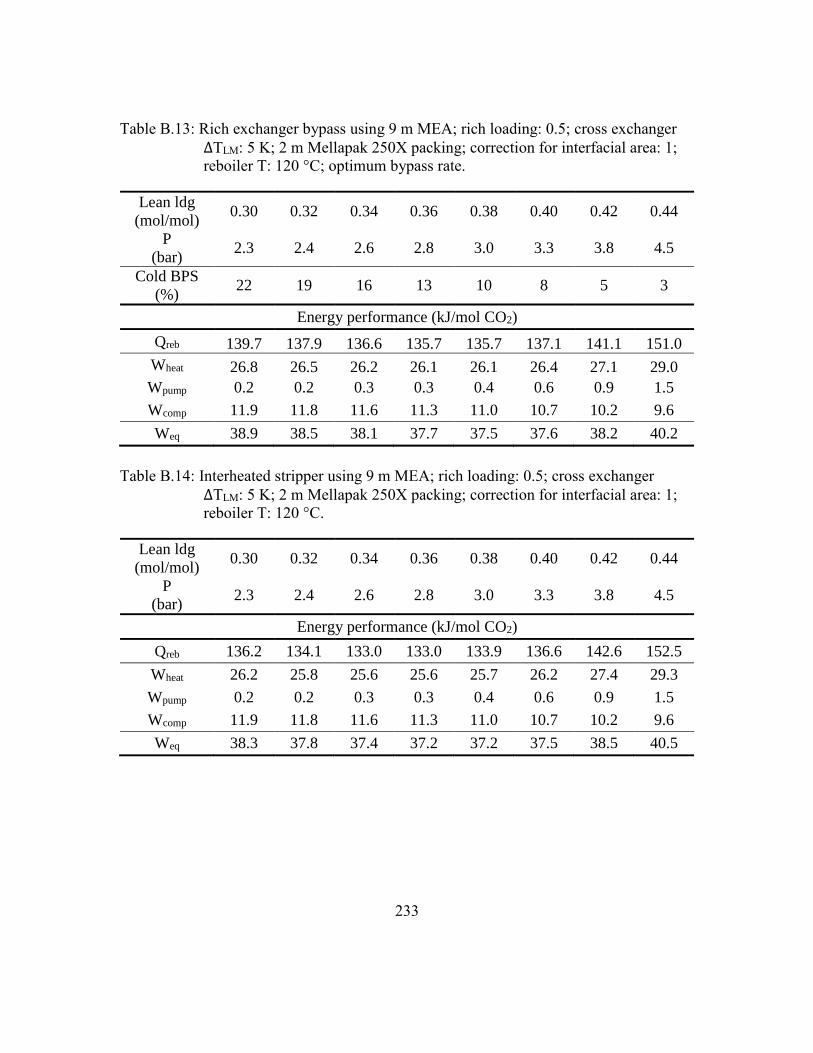
233
Table B.13: Rich exchanger bypass using 9 m MEA; rich loading: 0.5; cross exchanger
ΔTLM: 5 K; 2 m Mellapak 250X packing; correction for interfacial area: 1;
reboiler T: 120 °C; optimum bypass rate.
Lean ldg
(mol/mol) 0.30 0.32 0.34 0.36 0.38 0.40 0.42 0.44
P
(bar) 2.3 2.4 2.6 2.8 3.0 3.3 3.8 4.5
Cold BPS
(%) 22 19 16 13 10 8 5 3
Energy performance (kJ/mol CO2)
Qreb 139.7 137.9 136.6 135.7 135.7 137.1 141.1 151.0
Wheat 26.8 26.5 26.2 26.1 26.1 26.4 27.1 29.0
Wpump 0.2 0.2 0.3 0.3 0.4 0.6 0.9 1.5
Wcomp 11.9 11.8 11.6 11.3 11.0 10.7 10.2 9.6
Weq 38.9 38.5 38.1 37.7 37.5 37.6 38.2 40.2
Table B.14: Interheated stripper using 9 m MEA; rich loading: 0.5; cross exchanger
ΔTLM: 5 K; 2 m Mellapak 250X packing; correction for interfacial area: 1;
reboiler T: 120 °C.
Lean ldg
(mol/mol) 0.30 0.32 0.34 0.36 0.38 0.40 0.42 0.44
P
(bar) 2.3 2.4 2.6 2.8 3.0 3.3 3.8 4.5
Energy performance (kJ/mol CO2)
Qreb 136.2 134.1 133.0 133.0 133.9 136.6 142.6 152.5
Wheat 26.2 25.8 25.6 25.6 25.7 26.2 27.4 29.3
Wpump 0.2 0.2 0.3 0.3 0.4 0.6 0.9 1.5
Wcomp 11.9 11.8 11.6 11.3 11.0 10.7 10.2 9.6
Weq 38.3 37.8 37.4 37.2 37.2 37.5 38.5 40.5

234
Table B.15: AFS using 9 m MEA; rich loading: 0.5; cross exchanger ΔTLM: 5 K; 2 m
Mellapak 250X packing; correction for interfacial area: 1; reboiler T: 120
°C; optimum bypass rates.
Lean ldg
(mol/mol) 0.30 0.32 0.34 0.36 0.38 0.40 0.42 0.44
P
(bar) 2.3 2.4 2.6 2.8 3.0 3.3 3.8 4.5
Cold BPS
(%) 13 11 10 8 7 6 4 3
Warm BPS
(%) 52 46 39 31 24 16 10 5
Energy performance (kJ/mol CO2)
Qreb 131.4 129.9 129.3 129.4 130.6 133.2 138.3 149.1
Wheat 25.2 25.0 24.8 24.9 25.1 25.6 26.6 28.6
Wpump 0.2 0.2 0.3 0.3 0.4 0.6 0.9 1.5
Wcomp 11.9 11.8 11.6 11.3 11.0 10.7 10.2 9.6
Weq 37.3 36.9 36.7 36.5 36.6 36.9 37.7 39.8
Table B.16: ARS using 9 m MEA; rich loading: 0.5; cross exchanger ΔTLM: 5 K; 2 m
Mellapak 250X packing; correction for interfacial area: 1; reboiler T: 120
°C; optimum bypass rates.
Lean ldg
(mol/mol) 0.30 0.32 0.34 0.36 0.38 0.40 0.42 0.44
P
(bar) 2.3 2.4 2.6 2.8 3.0 3.3 3.8 4.5
Cold BPS
(%) 13 11 10 8 7 6 4 3
Warm BPS
(%) 46 39 32 24 16 9 4 1
Energy performance (kJ/mol CO2)
Qreb 130.0 128.8 128.4 128.7 129.9 132.6 137.7 148.4
Wheat 25.0 24.7 24.7 24.7 25.0 25.5 26.5 28.5
Wpump 0.2 0.2 0.3 0.3 0.4 0.6 0.9 1.5
Wcomp 11.9 11.8 11.6 11.3 11.0 10.7 10.2 9.6
Weq 37.1 36.7 36.5 36.4 36.4 36.8 37.6 39.7

235
Appendix C: Approximate Stripper Model Equations
C.1 SIMPLE STRIPPER
Equilibrium partial pressure of CO2 For generic solvent
𝑃𝐶𝑂2
∗ (𝑇, 𝛼) = 𝑒𝑥𝑝 [𝑙𝑛𝑃𝐶𝑂2,𝑟∗ (𝑇𝑟 , 𝛼𝑟) + ∫ 𝑘(𝑇𝑟 , 𝛼)𝑑𝛼
𝛼
𝛼𝑟+ ∫ −
∆𝐻𝑎𝑏𝑠(𝛼)
𝑅𝑑 (
1
𝑇)
𝑇
𝑇𝑟] (C.1)
Stripper pressure calculation
𝑃𝑠𝑡𝑟𝑝 = 𝑃𝐶𝑂2
∗ (𝑇𝑟𝑒𝑏 , 𝛼𝑙𝑒𝑎𝑛) + 𝑃𝐻2𝑂𝑠𝑎𝑡 (𝑇𝑟𝑒𝑏)𝑥𝐻2𝑂,𝑙𝑒𝑎𝑛 (C.2)
Overall mass balance
𝑚𝑟𝑖𝑐ℎ = 𝑚𝑙𝑒𝑎𝑛 + 𝑚𝑠𝑡𝑟𝑝𝑉 + 𝑚𝑟𝑖𝑐ℎℎ𝑉 (C.3)
𝑚𝑖,𝑟𝑖𝑐ℎ = 𝑚𝑖,𝑙𝑒𝑎𝑛 + 𝑚𝑖,𝑠𝑡𝑟𝑝𝑉 + 𝑚𝑖,𝑟𝑖𝑐ℎℎ𝑉 𝑖 = 𝐻2𝑂, 𝐶𝑂2, 𝑎𝑚 (C.4)
𝑚𝑗 = ∑ 𝑚𝑖,𝑗𝑖 𝑖 = 𝐻2𝑂, 𝐶𝑂2, 𝑎𝑚 𝑗 = 𝑎𝑛𝑦 𝑠𝑡𝑟𝑒𝑎𝑚 (C.5)
∑ 𝑦𝑖,𝑗 = 1𝑖 𝑖 = 𝐻2𝑂, 𝐶𝑂2, 𝑎𝑚 𝑗 = 𝑎𝑛𝑦 𝑣𝑎𝑝𝑜𝑟 𝑠𝑡𝑟𝑒𝑎𝑚 (C.6)
∑ 𝑥𝑖,𝑗 = 1𝑖 𝑖 = 𝐻2𝑂, 𝐶𝑂2, 𝑎𝑚 𝑗 = 𝑎𝑛𝑦 𝑙𝑖𝑞𝑢𝑖𝑑 𝑠𝑡𝑟𝑒𝑎𝑚 (C.7)
𝑚𝑎𝑚,𝑗 = 𝑦𝑖,𝑗 = 0 𝑗 = 𝑎𝑛𝑦 𝑣𝑎𝑝𝑜𝑟 𝑠𝑡𝑟𝑒𝑎𝑚 (C.8)
Warm rich solvent flashing
𝑃𝐶𝑂2
∗ (𝑇𝑟𝑖𝑐ℎ𝑤, 𝛼𝑟𝑖𝑐ℎ) + 𝑃𝐻2𝑂𝑠𝑎𝑡 (𝑇𝑟𝑖𝑐ℎ𝑤)𝑥𝐻2𝑂,𝑟𝑖𝑐ℎ = 𝑃𝑠𝑡𝑟𝑝 (C.9)
Hot rich solvent flashing mass balance
𝑚𝑟𝑖𝑐ℎ = 𝑚𝑟𝑖𝑐ℎℎ𝑉 + 𝑚𝑟𝑖𝑐ℎℎ𝐿 (C.10)
𝑚𝑖,𝑟𝑖𝑐ℎ = 𝑚𝑖,𝑟𝑖𝑐ℎℎ𝑉 + 𝑚𝑖,𝑟𝑖𝑐ℎℎ𝐿 𝑖 = 𝐻2𝑂, 𝐶𝑂2, 𝑎𝑚 (C.11)
𝑃𝐶𝑂2
∗ (𝑇𝑟𝑖𝑐ℎℎ, 𝛼𝑟𝑖𝑐ℎℎ) + 𝑃𝐻2𝑂𝑠𝑎𝑡 (𝑇𝑟𝑖𝑐ℎℎ)𝑥𝐻2𝑂,𝑟𝑖𝑐ℎℎ𝐿 = 𝑃𝑠𝑡𝑟𝑝 (C.12)
Stripper mass balance
𝑚𝑖,𝑠𝑡𝑟𝑝𝐿 = 𝑚𝑖,𝑟𝑖𝑐ℎℎ𝐿 𝑖 = 𝐻2𝑂, 𝐶𝑂2, 𝑎𝑚 (C.13)
𝑚𝑠𝑡𝑟𝑝𝑡𝑜𝑝𝐿 + 𝑚𝑠𝑡𝑟𝑝𝑏𝑜𝑡𝑉 = 𝑚𝑠𝑡𝑟𝑝𝑏𝑜𝑡𝐿 + 𝑚𝑠𝑡𝑟𝑝𝑡𝑜𝑝𝑉 (C.14)
𝑚𝑖,𝑠𝑡𝑟𝑝𝑡𝑜𝑝𝐿 + 𝑚𝑖,𝑠𝑡𝑟𝑝𝑏𝑜𝑡𝑉 = 𝑚𝑖,𝑠𝑡𝑟𝑝𝑏𝑜𝑡𝐿 + 𝑚𝑖,𝑠𝑡𝑟𝑝𝑡𝑜𝑝𝑉 (C.15)

236
Stripper top liquid flashing
𝛼𝑠𝑡𝑟𝑝𝑡𝑜𝑝𝐿 = 𝛼𝑟𝑖𝑐ℎℎ (C.16)
𝑇𝑠𝑡𝑟𝑝𝑡𝑜𝑝𝐿 = 𝑇𝑟𝑖𝑐ℎℎ (C.17)
(𝑇𝑠𝑡𝑟𝑝𝑡𝑜𝑝𝐿 , 𝛼𝑠𝑡𝑟𝑝𝑡𝑜𝑝𝐿) + 𝑃𝐻2𝑂𝑠𝑎𝑡 (𝑇𝑠𝑡𝑟𝑝𝑡𝑜𝑝𝐿)𝑥𝐻2𝑂,𝑠𝑡𝑟𝑝𝑡𝑜𝑝𝐿 = 𝑃𝑠𝑡𝑟𝑝 (C.18)
𝑦𝐶𝑂2,𝑠𝑡𝑟𝑝𝑡𝑜𝑝𝐿∗ =
𝑃𝐶𝑂2∗ (𝑇𝑠𝑡𝑟𝑝𝑡𝑜𝑝𝐿,𝛼𝑠𝑡𝑟𝑝𝑡𝑜𝑝𝐿)
𝑃𝑠𝑡𝑟𝑝 (C.19)
𝑦𝐻2𝑂,𝑠𝑡𝑟𝑝𝑡𝑜𝑝𝐿∗ =
𝑃𝐻2𝑂𝑠𝑎𝑡 (𝑇𝑠𝑡𝑟𝑝𝑡𝑜𝑝𝐿)𝑥𝐻2𝑂,𝑠𝑡𝑟𝑝𝑡𝑜𝑝𝐿
𝑃𝑠𝑡𝑟𝑝 (C.20)
Stripper bottom liquid flashing
𝑃𝐶𝑂2
∗ (𝑇𝑠𝑡𝑟𝑝𝑏𝑜𝑡𝐿 , 𝛼𝑠𝑡𝑟𝑝𝑏𝑜𝑡𝐿) + 𝑃𝐻2𝑂𝑠𝑎𝑡 (𝑇𝑠𝑡𝑟𝑝𝑏𝑜𝑡𝐿)𝑥𝐻2𝑂,𝑠𝑡𝑟𝑝𝑏𝑜𝑡𝐿 = 𝑃𝑠𝑡𝑟𝑝 (C.21)
𝑦𝐶𝑂2,𝑠𝑡𝑟𝑝𝑏𝑜𝑡𝐿∗ =
𝑃𝐶𝑂2∗ (𝑇𝑠𝑡𝑟𝑝𝑏𝑜𝑡𝐿 ,𝛼𝑠𝑡𝑟𝑝𝑡𝑏𝑜𝑡𝐿)
𝑃𝑠𝑡𝑟𝑝 (C.22)
𝑦𝐻2𝑂,𝑠𝑡𝑟𝑝𝑏𝑜𝑡𝐿∗ =
𝑃𝐻2𝑂𝑠𝑎𝑡 (𝑇𝑠𝑡𝑟𝑝𝑏𝑜𝑡𝐿)𝑥𝐻2𝑂,𝑠𝑡𝑟𝑝𝑏𝑜𝑡𝐿
𝑃𝑠𝑡𝑟𝑝 (C.23)
Stripper reboiler flashing
𝑇𝑠𝑡𝑟𝑝𝑏𝑜𝑡𝑉 = 𝑇𝑟𝑒𝑏 (C.24)
𝑦𝐶𝑂2,𝑠𝑡𝑟𝑝𝑏𝑜𝑡𝑉 =𝑃𝐶𝑂2
∗ (𝑇𝑟𝑒𝑏,𝛼𝑙𝑒𝑎𝑛)
𝑃𝑠𝑡𝑟𝑝 (C.25)
𝑦𝐻2𝑂,𝑠𝑡𝑟𝑝𝑏𝑜𝑡𝑉 =𝑃𝐻2𝑂
𝑠𝑎𝑡 (𝑇𝑟𝑒𝑏)𝑥𝐻2𝑂,𝑙𝑒𝑎𝑛
𝑃𝑠𝑡𝑟𝑝 (C.26)
Enthalpy balance around cross exchanger
��𝑟𝑖𝑐ℎ𝑐(𝑇𝑟𝑖𝑐ℎ𝑐) − ��𝑟𝑖𝑐ℎ𝑤(𝑇𝑟𝑖𝑐ℎ𝑤) = ��𝑙𝑒𝑎𝑛𝑐(𝑇𝑙𝑒𝑎𝑛𝑐) − ��𝑙𝑒𝑎𝑛𝑤(𝑇𝑙𝑒𝑎𝑛𝑤) (C.27)
��𝑟𝑖𝑐ℎ𝑤(𝑇𝑟𝑖𝑐ℎ𝑤) − ��𝑟𝑖𝑐ℎℎ(𝑇𝑟𝑖𝑐ℎℎ) = ��𝑙𝑒𝑎𝑛𝑤(𝑇𝑙𝑒𝑎𝑛𝑤) − ��𝑙𝑒𝑎𝑛ℎ(𝑇𝑙𝑒𝑎𝑛ℎ) (C.28)
Enthalpy balance around stripper
��𝑠𝑡𝑟𝑝𝑡𝑜𝑝𝐿(𝑇𝑠𝑡𝑟𝑝𝑡𝑜𝑝𝐿) − ��𝑠𝑡𝑟𝑝𝑏𝑜𝑡𝐿(𝑇𝑠𝑡𝑟𝑝𝑏𝑜𝑡𝐿) = ��𝑠𝑡𝑟𝑝𝑡𝑜𝑝𝑉(𝑇𝑠𝑡𝑟𝑝𝑡𝑜𝑝𝑉) − ��𝑠𝑡𝑟𝑝𝑏𝑜𝑡𝑉(𝑇𝑠𝑡𝑟𝑝𝑏𝑜𝑡𝑉) (C.29)
Cross LMTD calculation

237
𝑄𝑐𝑟𝑜𝑠𝑠𝑋,1 = ��𝑙𝑒𝑎𝑛𝑤 − ��𝑙𝑒𝑎𝑛𝑐 (C.30)
𝑄𝑐𝑟𝑜𝑠𝑠𝑋,2 = ��𝑙𝑒𝑎𝑛ℎ − ��𝑙𝑒𝑎𝑛𝑤 (C.31)
∆𝑇𝐿𝑀,𝑐𝑟𝑜𝑠𝑠𝑋,1 =(𝑇𝑟𝑖𝑐ℎ𝑐−𝑇𝑙𝑒𝑎𝑛𝑐)−(𝑇𝑟𝑖𝑐ℎ𝑤−𝑇𝑙𝑒𝑎𝑛𝑤)
𝑙𝑛[(𝑇𝑟𝑖𝑐ℎ𝑐−𝑇𝑙𝑒𝑎𝑛𝑐)
(𝑇𝑟𝑖𝑐ℎ𝑤−𝑇𝑙𝑒𝑎𝑛𝑤)]
(C.32)
∆𝑇𝐿𝑀,𝑐𝑟𝑜𝑠𝑠𝑋,2 =(𝑇𝑟𝑖𝑐ℎℎ−𝑇𝑙𝑒𝑎𝑛ℎ)−(𝑇𝑟𝑖𝑐ℎ𝑤−𝑇𝑙𝑒𝑎𝑛𝑤)
𝑙𝑛[(𝑇𝑟𝑖𝑐ℎℎ−𝑇𝑙𝑒𝑎𝑛ℎ)
(𝑇𝑟𝑖𝑐ℎ𝑤−𝑇𝑙𝑒𝑎𝑛𝑤)]
(C.33)
∆𝑇𝐿𝑀,𝑐𝑟𝑜𝑠𝑠𝑋,𝑎𝑣𝑔 =𝑄𝑐𝑟𝑜𝑠𝑠𝑋,1+𝑄𝑐𝑟𝑜𝑠𝑠𝑋,2
𝑄𝑐𝑟𝑜𝑠𝑠𝑋,1∆𝑇𝐿𝑀,𝑐𝑟𝑜𝑠𝑠𝑋,1
+𝑄𝑐𝑟𝑜𝑠𝑠𝑋,2
∆𝑇𝐿𝑀,𝐶𝑟𝑜𝑠𝑠𝑋,2
(C.34)
Stripper temperature and concentration driving force
∆𝑇𝑠𝑡𝑟𝑝𝑡𝑜𝑝 = 𝑇𝑠𝑡𝑟𝑝𝑡𝑜𝑝𝑉 − 𝑇𝑠𝑡𝑟𝑝𝑡𝑜𝑝𝐿 (C.35)
∆𝑇𝑠𝑡𝑟𝑝𝑏𝑜𝑡 = 𝑇𝑠𝑡𝑟𝑝𝑏𝑜𝑡𝑉 − 𝑇𝑠𝑡𝑟𝑝𝑏𝑜𝑡𝐿 (C.36)
∆𝑦𝑠𝑡𝑟𝑝𝑡𝑜𝑝 = 𝑦𝑖,𝑠𝑡𝑟𝑝𝑡𝑜𝑝𝑉 − 𝑦𝑖,𝑠𝑡𝑟𝑝𝑡𝑜𝑝𝐿∗ (C.37)
∆𝑦𝑠𝑡𝑟𝑝𝑏𝑜𝑡 = 𝑦𝑖,𝑠𝑡𝑟𝑝𝑏𝑜𝑡𝑉 − 𝑦𝑖,𝑠𝑡𝑟𝑝𝑏𝑜𝑡𝐿∗ (C.38)
∆𝑇𝐿𝑀,𝑠𝑡𝑟𝑝 =∆𝑇𝑠𝑡𝑟𝑝𝑡𝑜𝑝−∆𝑇𝑠𝑡𝑟𝑝𝑏𝑜𝑡
𝑙𝑛(∆𝑇𝑠𝑡𝑟𝑝𝑡𝑜𝑝
∆𝑇𝑠𝑡𝑟𝑝𝑏𝑜𝑡)
(C.39)
∆𝑦𝐿𝑀,𝑠𝑡𝑟𝑝 =∆𝑦𝑠𝑡𝑟𝑝𝑡𝑜𝑝−∆𝑦𝑠𝑡𝑟𝑝𝑏𝑜𝑡
𝑙𝑛(∆𝑦𝑠𝑡𝑟𝑝𝑡𝑜𝑝
∆𝑦𝑠𝑡𝑟𝑝𝑏𝑜𝑡)
(C.40)
Overall enthalpy balance
��𝑟𝑒𝑏 = ��𝑙𝑒𝑎𝑛𝑐(𝑇𝑙𝑒𝑎𝑛𝑐) − ��𝑟𝑖𝑐ℎ(𝑇𝑟𝑖𝑐ℎ𝑐) + ��𝑠𝑡𝑟𝑝𝑉(𝑇𝑠𝑡𝑟𝑝𝑉) (C.41)

238
C.2 ADVANCED FLASH STRIPPER
Equilibrium partial pressure of CO2 For generic solvent
𝑃𝐶𝑂2
∗ (𝑇, 𝛼) = 𝑒𝑥𝑝 [𝑙𝑛𝑃𝐶𝑂2,𝑟∗ (𝑇𝑟 , 𝛼𝑟) + ∫ 𝑘(𝑇𝑟 , 𝛼)𝑑𝛼
𝛼
𝛼𝑟+ ∫ −
∆𝐻𝑎𝑏𝑠(𝛼)
𝑅𝑑 (
1
𝑇)
𝑇
𝑇𝑟] (C.42)
Stripper pressure calculation
𝑃𝑠𝑡𝑟𝑝 = 𝑃𝐶𝑂2
∗ (𝑇𝑟𝑒𝑏 , 𝛼𝑙𝑒𝑎𝑛) + 𝑃𝐻2𝑂𝑠𝑎𝑡 (𝑇𝑟𝑒𝑏)𝑥𝐻2𝑂,𝑙𝑒𝑎𝑛 (C.43)
Overall mass balance
𝑚𝑟𝑖𝑐ℎ = 𝑚𝑙𝑒𝑎𝑛 + 𝑚𝑠𝑡𝑟𝑝𝑉 (C.44)
𝑚𝑖,𝑟𝑖𝑐ℎ = 𝑚𝑖,𝑙𝑒𝑎𝑛 + 𝑚𝑖,𝑠𝑡𝑟𝑝𝑉 + 𝑚𝑖,𝑟𝑖𝑐ℎℎ𝑉 𝑖 = 𝐻2𝑂, 𝐶𝑂2, 𝑎𝑚 (C.45)
𝑚𝑗 = ∑ 𝑚𝑖,𝑗𝑖 𝑖 = 𝐻2𝑂, 𝐶𝑂2, 𝑎𝑚 𝑗 = 𝑎𝑛𝑦 𝑠𝑡𝑟𝑒𝑎𝑚 (C.46)
∑ 𝑦𝑖,𝑗 = 1𝑖 𝑖 = 𝐻2𝑂, 𝐶𝑂2, 𝑎𝑚 𝑗 = 𝑎𝑛𝑦 𝑣𝑎𝑝𝑜𝑟 𝑠𝑡𝑟𝑒𝑎𝑚 (C.47)
∑ 𝑥𝑖,𝑗 = 1𝑖 𝑖 = 𝐻2𝑂, 𝐶𝑂2, 𝑎𝑚 𝑗 = 𝑎𝑛𝑦 𝑙𝑖𝑞𝑢𝑖𝑑 𝑠𝑡𝑟𝑒𝑎𝑚 (C.48)
𝑚𝑎𝑚,𝑗 = 𝑦𝑖,𝑗 = 0 𝑗 = 𝑎𝑛𝑦 𝑣𝑎𝑝𝑜𝑟 𝑠𝑡𝑟𝑒𝑎𝑚 (C.49)
Rich solvent bypass mass balance
𝑚𝑟𝑖𝑐ℎ = 𝑚𝑟𝑖𝑐ℎ𝑐 + 𝑚𝑐𝑏𝑝𝑠 (C.50)
𝑚𝑟𝑖𝑐ℎ𝑐 = 𝑚𝑟𝑖𝑐ℎ𝑤 + 𝑚𝑤𝑏𝑝𝑠 (C.51)
Warm rich solvent flashing
𝑃𝐶𝑂2
∗ (𝑇𝑟𝑖𝑐ℎ𝑤, 𝛼𝑟𝑖𝑐ℎ) + 𝑃𝐻2𝑂𝑠𝑎𝑡 (𝑇𝑟𝑖𝑐ℎ𝑤)𝑥𝐻2𝑂,𝑟𝑖𝑐ℎ = 𝑃𝑠𝑡𝑟𝑝 (C.52)
Hot rich solvent flashing mass balance
𝑚𝑟𝑖𝑐ℎ𝑤 = 𝑚𝑟𝑖𝑐ℎℎ𝑉 + 𝑚𝑟𝑖𝑐ℎℎ𝐿 (C.53)
𝑚𝑖,𝑟𝑖𝑐ℎ𝑤 = 𝑚𝑖,𝑟𝑖𝑐ℎℎ𝑉 + 𝑚𝑖,𝑟𝑖𝑐ℎℎ𝐿 𝑖 = 𝐻2𝑂, 𝐶𝑂2, 𝑎𝑚 (C.54)
𝑃𝐶𝑂2
∗ (𝑇𝑟𝑖𝑐ℎℎ, 𝛼𝑟𝑖𝑐ℎℎ) + 𝑃𝐻2𝑂𝑠𝑎𝑡 (𝑇𝑟𝑖𝑐ℎℎ)𝑥𝐻2𝑂,𝑟𝑖𝑐ℎℎ𝐿 = 𝑃𝑠𝑡𝑟𝑝 (C.55)
Stripper mass balance
𝑚𝑖,𝑠𝑡𝑟𝑝𝐿 = 𝑚𝑖,𝑤𝑏𝑝𝑠 𝑖 = 𝐻2𝑂, 𝐶𝑂2, 𝑎𝑚 (C.56)
𝑚𝑠𝑡𝑟𝑝𝑡𝑜𝑝𝐿 + 𝑚𝑠𝑡𝑟𝑝𝑏𝑜𝑡𝑉 = 𝑚𝑠𝑡𝑟𝑝𝑏𝑜𝑡𝐿 + 𝑚𝑠𝑡𝑟𝑝𝑡𝑜𝑝𝑉 (C.57)

239
𝑚𝑖,𝑠𝑡𝑟𝑝𝑡𝑜𝑝𝐿 + 𝑚𝑖,𝑠𝑡𝑟𝑝𝑏𝑜𝑡𝑉 = 𝑚𝑖,𝑠𝑡𝑟𝑝𝑏𝑜𝑡𝐿 + 𝑚𝑖,𝑠𝑡𝑟𝑝𝑡𝑜𝑝𝑉 (C.58)
Cold rich exchanger mass balance
𝑚𝑠𝑡𝑟𝑝𝑉 = 𝑚𝑐𝑟𝑥𝑉 + 𝑚𝑐𝑟𝑥𝐿 (C.59)
𝑚𝑖,𝑠𝑡𝑟𝑝𝑉 = 𝑚𝑖,𝑐𝑟𝑥𝑉 + 𝑚𝑖,𝑐𝑟𝑥𝐿 𝑖 = 𝐻2𝑂, 𝐶𝑂2, 𝑎𝑚 (C.60)
Stripper top liquid flashing
𝛼𝑠𝑡𝑟𝑝𝑡𝑜𝑝𝐿 = 𝛼𝑟𝑖𝑐ℎ (C.61)
𝑇𝑠𝑡𝑟𝑝𝑡𝑜𝑝𝐿 = 𝑇𝑟𝑖𝑐ℎ𝑤 (C.62)
(𝑇𝑠𝑡𝑟𝑝𝑡𝑜𝑝𝐿 , 𝛼𝑠𝑡𝑟𝑝𝑡𝑜𝑝𝐿) + 𝑃𝐻2𝑂𝑠𝑎𝑡 (𝑇𝑠𝑡𝑟𝑝𝑡𝑜𝑝𝐿)𝑥𝐻2𝑂,𝑠𝑡𝑟𝑝𝑡𝑜𝑝𝐿 = 𝑃𝑠𝑡𝑟𝑝 (C.63)
𝑦𝐶𝑂2,𝑠𝑡𝑟𝑝𝑡𝑜𝑝𝐿∗ =
𝑃𝐶𝑂2∗ (𝑇𝑠𝑡𝑟𝑝𝑡𝑜𝑝𝐿,𝛼𝑠𝑡𝑟𝑝𝑡𝑜𝑝𝐿)
𝑃𝑠𝑡𝑟𝑝 (C.64)
𝑦𝐻2𝑂,𝑠𝑡𝑟𝑝𝑡𝑜𝑝𝐿∗ =
𝑃𝐻2𝑂𝑠𝑎𝑡 (𝑇𝑠𝑡𝑟𝑝𝑡𝑜𝑝𝐿)𝑥𝐻2𝑂,𝑠𝑡𝑟𝑝𝑡𝑜𝑝𝐿
𝑃𝑠𝑡𝑟𝑝 (C.65)
Stripper bottom liquid flashing
𝑃𝐶𝑂2
∗ (𝑇𝑠𝑡𝑟𝑝𝑏𝑜𝑡𝐿 , 𝛼𝑠𝑡𝑟𝑝𝑏𝑜𝑡𝐿) + 𝑃𝐻2𝑂𝑠𝑎𝑡 (𝑇𝑠𝑡𝑟𝑝𝑏𝑜𝑡𝐿)𝑥𝐻2𝑂,𝑠𝑡𝑟𝑝𝑏𝑜𝑡𝐿 = 𝑃𝑠𝑡𝑟𝑝 (C.66)
𝑦𝐶𝑂2,𝑠𝑡𝑟𝑝𝑏𝑜𝑡𝐿∗ =
𝑃𝐶𝑂2∗ (𝑇𝑠𝑡𝑟𝑝𝑏𝑜𝑡𝐿 ,𝛼𝑠𝑡𝑟𝑝𝑡𝑏𝑜𝑡𝐿)
𝑃𝑠𝑡𝑟𝑝 (C.67)
𝑦𝐻2𝑂,𝑠𝑡𝑟𝑝𝑏𝑜𝑡𝐿∗ =
𝑃𝐻2𝑂𝑠𝑎𝑡 (𝑇𝑠𝑡𝑟𝑝𝑏𝑜𝑡𝐿)𝑥𝐻2𝑂,𝑠𝑡𝑟𝑝𝑏𝑜𝑡𝐿
𝑃𝑠𝑡𝑟𝑝 (C.68)
Stripper sump flashing
𝑇𝑠𝑡𝑟𝑝𝑏𝑜𝑡𝑉 = 𝑇𝑟𝑒𝑏 (C.69)
𝑦𝐶𝑂2,𝑠𝑡𝑟𝑝𝑏𝑜𝑡𝑉 =𝑃𝐶𝑂2
∗ (𝑇𝑟𝑒𝑏,𝛼𝑙𝑒𝑎𝑛)
𝑃𝑠𝑡𝑟𝑝 (C.70)
𝑦𝐻2𝑂,𝑠𝑡𝑟𝑝𝑏𝑜𝑡𝑉 =𝑃𝐻2𝑂
𝑠𝑎𝑡 (𝑇𝑟𝑒𝑏)𝑥𝐻2𝑂,𝑙𝑒𝑎𝑛
𝑃𝑠𝑡𝑟𝑝 (C.71)
Cold rich exchanger flashing
𝑇𝑐𝑏𝑝𝑠 = 𝑇𝑟𝑖𝑐ℎ𝑐 (C.72)

240
𝑃𝐻2𝑂𝑠𝑎𝑡 (𝑇𝑐𝑟𝑥) = 𝑃𝑠𝑡𝑟𝑝 (C.73)
Enthalpy balance around cross exchangers
��𝑟𝑖𝑐ℎ𝑐(𝑇𝑟𝑖𝑐ℎ𝑐) − ��𝑟𝑖𝑐ℎ𝑤(𝑇𝑟𝑖𝑐ℎ𝑤) = ��𝑙𝑒𝑎𝑛𝑐(𝑇𝑙𝑒𝑎𝑛𝑐) − ��𝑙𝑒𝑎𝑛𝑤(𝑇𝑙𝑒𝑎𝑛𝑤) (C.74)
��𝑟𝑖𝑐ℎ𝑤(𝑇𝑟𝑖𝑐ℎ𝑤) − ��𝑟𝑖𝑐ℎℎ(𝑇𝑟𝑖𝑐ℎℎ) = ��𝑙𝑒𝑎𝑛𝑤(𝑇𝑙𝑒𝑎𝑛𝑤) − ��𝑙𝑒𝑎𝑛ℎ(𝑇𝑙𝑒𝑎𝑛ℎ) (C.75)
Enthalpy balance around stripper
��𝑠𝑡𝑟𝑝𝑡𝑜𝑝𝐿(𝑇𝑠𝑡𝑟𝑝𝑡𝑜𝑝𝐿) − ��𝑠𝑡𝑟𝑝𝑏𝑜𝑡𝐿(𝑇𝑠𝑡𝑟𝑝𝑏𝑜𝑡𝐿) = ��𝑠𝑡𝑟𝑝𝑡𝑜𝑝𝑉(𝑇𝑠𝑡𝑟𝑝𝑡𝑜𝑝𝑉) − ��𝑠𝑡𝑟𝑝𝑏𝑜𝑡𝑉(𝑇𝑠𝑡𝑟𝑝𝑏𝑜𝑡𝑉) (C.76)
Enthalpy balance around cold rich exchanger
��𝑠𝑡𝑟𝑝𝑉(𝑇𝑠𝑡𝑟𝑝𝑡𝑜𝑝𝑉) − ��𝑐𝑟𝑥𝑉(𝑇𝑐𝑟𝑥) − ��𝑐𝑟𝑥𝐿(𝑇𝑐𝑟𝑥) = ��𝑐𝑏𝑝𝑠(𝑇𝑐𝑏𝑝𝑠) − ��𝑐𝑏𝑝𝑠𝑜𝑢𝑡(𝑇𝑐𝑏𝑝𝑠𝑜𝑢𝑡) (C.77)
Cross LMTD calculation
𝑄𝑐𝑟𝑜𝑠𝑠𝑋,1 = ��𝑙𝑒𝑎𝑛𝑤 − ��𝑙𝑒𝑎𝑛𝑐 (C.78)
𝑄𝑐𝑟𝑜𝑠𝑠𝑋,2 = ��𝑙𝑒𝑎𝑛ℎ − ��𝑙𝑒𝑎𝑛𝑤 (C.79)
∆𝑇𝐿𝑀,𝑐𝑟𝑜𝑠𝑠𝑋,1 =(𝑇𝑟𝑖𝑐ℎ𝑐−𝑇𝑙𝑒𝑎𝑛𝑐)−(𝑇𝑟𝑖𝑐ℎ𝑤−𝑇𝑙𝑒𝑎𝑛𝑤)
𝑙𝑛[(𝑇𝑟𝑖𝑐ℎ𝑐−𝑇𝑙𝑒𝑎𝑛𝑐)
(𝑇𝑟𝑖𝑐ℎ𝑤−𝑇𝑙𝑒𝑎𝑛𝑤)]
(C.80)
∆𝑇𝐿𝑀,𝑐𝑟𝑜𝑠𝑠𝑋,2 =(𝑇𝑟𝑖𝑐ℎℎ−𝑇𝑙𝑒𝑎𝑛ℎ)−(𝑇𝑟𝑖𝑐ℎ𝑤−𝑇𝑙𝑒𝑎𝑛𝑤)
𝑙𝑛[(𝑇𝑟𝑖𝑐ℎℎ−𝑇𝑙𝑒𝑎𝑛ℎ)
(𝑇𝑟𝑖𝑐ℎ𝑤−𝑇𝑙𝑒𝑎𝑛𝑤)]
(C.81)
∆𝑇𝐿𝑀,𝑐𝑟𝑜𝑠𝑠𝑋,𝑎𝑣𝑔 =𝑄𝑐𝑟𝑜𝑠𝑠𝑋,1+𝑄𝑐𝑟𝑜𝑠𝑠𝑋,2
𝑄𝑐𝑟𝑜𝑠𝑠𝑋,1∆𝑇𝐿𝑀,𝑐𝑟𝑜𝑠𝑠𝑋,1
+𝑄𝑐𝑟𝑜𝑠𝑠𝑋,2
∆𝑇𝐿𝑀,𝐶𝑟𝑜𝑠𝑠𝑋,2
(C.82)
Cold rich exchanger LMTD
𝑄𝑐𝑟𝑥 = ��𝑐𝑏𝑝𝑠𝑜𝑢𝑡 − ��𝑐𝑏𝑝𝑠 (C.83)
∆𝑇𝐿𝑀,𝑐𝑟𝑥 =(𝑇𝑐𝑏𝑝𝑠−𝑇𝑐𝑟𝑥)−(𝑇𝑐𝑏𝑝𝑠𝑜𝑢𝑡−𝑇𝑠𝑡𝑟𝑝𝑉)
𝑙𝑛[(𝑇𝑐𝑏𝑝𝑠−𝑇𝑐𝑟𝑥)
(𝑇𝑐𝑏𝑝𝑠𝑜𝑢𝑡−𝑇𝑠𝑡𝑟𝑝𝑉)]
(C.84)
Stripper temperature and concentration driving force
∆𝑇𝑠𝑡𝑟𝑝𝑡𝑜𝑝 = 𝑇𝑠𝑡𝑟𝑝𝑡𝑜𝑝𝑉 − 𝑇𝑠𝑡𝑟𝑝𝑡𝑜𝑝𝐿 (C.85)
∆𝑇𝑠𝑡𝑟𝑝𝑏𝑜𝑡 = 𝑇𝑠𝑡𝑟𝑝𝑏𝑜𝑡𝑉 − 𝑇𝑠𝑡𝑟𝑝𝑏𝑜𝑡𝐿 (C.86)

241
∆𝑦𝑠𝑡𝑟𝑝𝑡𝑜𝑝 = 𝑦𝑖,𝑠𝑡𝑟𝑝𝑡𝑜𝑝𝑉 − 𝑦𝑖,𝑠𝑡𝑟𝑝𝑡𝑜𝑝𝐿∗ (C.87)
∆𝑦𝑠𝑡𝑟𝑝𝑏𝑜𝑡 = 𝑦𝑖,𝑠𝑡𝑟𝑝𝑏𝑜𝑡𝑉 − 𝑦𝑖,𝑠𝑡𝑟𝑝𝑏𝑜𝑡𝐿∗ (C.88)
∆𝑇𝐿𝑀,𝑠𝑡𝑟𝑝 =∆𝑇𝑠𝑡𝑟𝑝𝑡𝑜𝑝−∆𝑇𝑠𝑡𝑟𝑝𝑏𝑜𝑡
𝑙𝑛(∆𝑇𝑠𝑡𝑟𝑝𝑡𝑜𝑝
∆𝑇𝑠𝑡𝑟𝑝𝑏𝑜𝑡)
(C.89)
∆𝑦𝐿𝑀,𝑠𝑡𝑟𝑝 =∆𝑦𝑠𝑡𝑟𝑝𝑡𝑜𝑝−∆𝑦𝑠𝑡𝑟𝑝𝑏𝑜𝑡
𝑙𝑛(∆𝑦𝑠𝑡𝑟𝑝𝑡𝑜𝑝
∆𝑦𝑠𝑡𝑟𝑝𝑏𝑜𝑡)
(C.90)
Overall enthalpy balance
��𝑟𝑒𝑏 = ��𝑙𝑒𝑎𝑛𝑐(𝑇𝑙𝑒𝑎𝑛𝑐) − ��𝑟𝑖𝑐ℎ(𝑇𝑟𝑖𝑐ℎ𝑐) + ��𝑐𝑟𝑥𝑉(𝑇𝑐𝑟𝑥) + ��𝑐𝑟𝑥𝐿(𝑇𝑐𝑟𝑥) (C.91)

242
NOMENCLATURE
��𝑗: enthalpy of stream j
𝑚𝑗: total mass flow rate of stream j
𝑚𝑖,𝑗: mass flow rate of component i in stream j
𝑃𝑠𝑡𝑟𝑝: stripper pressure
𝑃𝑖,𝑗: partial pressure of component i in vapor stream j
𝑃𝑖,𝑗∗ : equilibrium partial pressure of component i in liquid stream j
𝑃𝐻2𝑂𝑠𝑎𝑡 (𝑇): saturation pressure of water at temperature T
𝑇𝑗: temperature of stream j
𝑥𝑖,𝑗: mole fraction of component i in liquid stream j
𝑦𝑖,𝑗: mole fraction of component i in vapor stream j
Greek letter:
𝛼𝑗: CO2 loading of stream j
∆𝐻𝑎𝑏𝑠(𝛼): heat of absorption at CO2 loading
∆𝑇: temperature approach
∆𝑇𝐿𝑀: log mean temperature difference
∆𝑦: concentration difference between y and y*
Stream name j:
cbps: cold rich bypass
cbpsout: cold rich bypass at cold rich exchanger outlet
crxL: liquid phase at cold rich exchanger out
crxV: vapor phase at cold rich exchanger out
lean: lean solvent
leanc: cold lean solvent

243
leanh: hot lean solvent
leanw: warm lean solvent
rich: rich solvent
richc: cold rich solvent
richh: hot rich solvent
richhV: vapor in hot rich solvent
richhL: liquid in hot rich solvent
richw: warm rich solvent
strpbotL: liquid at bottom of stripper
strpbotV: vapor at bottom of stripper
strptopL: liquid at top of stripper
strptopV: vapor at top of stripper
strpV: total stripping vapor of stripping process
wbps: warm rich bypass

244
References
Abu-Zahra, M. R. M., Niederer, J. P. M., Feron, P. H. M., & Versteeg, G. F. (2007). CO2
capture from power plants. Part II. A parametric study of the economical
performance based on mono-ethanolamine. International Journal of Greenhouse
Gas Control, 1(2), 135–142.
Ahn, H., Luberti, M., Liu, Z., & Brandani, S. (2013). Process configuration studies of the
amine capture process for coal-fired power plants. International Journal of
Greenhouse Gas Control, 16, 29–40.
Amrollahi, Z., Ertesvåg, I. S., & Bolland, O. (2011). Thermodynamic analysis on post-
combustion CO2 capture of natural-gas-fired power plant. International Journal of
Greenhouse Gas Control, 5(3), 422–426.
Amundsen, T. G., Ø i, L. E., & Eimer, D. A. (2009). Density and viscosity of
monoethanolamine + water + carbon dioxide from (25 to 80) °C. Journal of
Chemical and Engineering Data, 54(11), 3096–3100.
Aroonwilas, A., & Veawab, A. (2007). Integration of CO2 capture unit using single- and
blended-amines into supercritical coal-fired power plants: Implications for emission
and energy management. International Journal of Greenhouse Gas Control, 1(2),
143–150.
Ayub, Z. H. (2003). Plate Heat Exchanger Literature Survey and New Heat Transfer and
Pressure Drop Correlations for Refrigerant Evaporators. Heat Transfer Engineering,
24(5), 3–16.
Benson, H., & Mccrea, D. (1979). Removal of acid gases from hot gas mixtures.
Bergamini, L., Vescovo, C., & Milone, F. (2011). Centrifugal pumps for CO2
applications. In Proceedings of the Twenty-Seventh International Pump User
Symposium (pp. 45–49). Houston, TX, USA.
Bhatt, M. S. (2011). Enhancement of energy efficiency and loading of steam turbines
through retrofitting 2-d designs with 3-d designs. Journal of Scientific and Industrial
Research, 70, 64–70.
Bhatt, M. S., & Rajkumar, N. (1999). Performance enhancement in coal fired thermal
Power plants. Part II: steam turbines. International Journal of Energy Research, 23,
489–515.
Bravo, J. L., Rocha, J. A., & Fair, J. R. (1985). Mass transfer in gauze packings.
Hydrocarbon Processing, 64(1), 91–95.
Bumb, P., Kumar, R., Khakharia, P., & Goetheer, E. (2014). Demonstration of Advanced
APBS Solvent at TNO’s CO2 Capture Pilot Plant. Energy Procedia, 63, 1657–1666.
245
Chang, H., & Shih, C. M. (2005). Simulation and optimization for power plant flue gas
CO2 absorption-stripping systems. Separation Science and Technology, 40(4), 877–
909.
Chen, C. C., Britt, H., Boston, J., & Evans, L. (1982). Local composition model for
excess Gibbs energy of electrolyte systems. Part I: Single solvent, single completely
dissociated electrolyte systems. AIChE Journal, 28(4), 588–596.
Chen, C. C., & Song, Y. (2004). Generalized electrolyte-NRTL model for mixed-solvent
electrolyte systems. AIChE Journal, 50(8), 1928–1941.
Chen, E., Fulk, S. M., Sachde, D., Lin, Y. J., & Rochelle, G. T. (2014). Pilot Plant
Activities with Concentrated Piperazine. Energy Procedia, 63, 1376–1391.
Chen, E., Madan, T., Sachde, D., Walters, M. S., Nielsen, P. T., & Rochelle, G. T.
(2013). Pilot Plant Results with Piperazine. Energy Procedia, 37, 1572–1583.
Chowdhury, F. A., Yamada, H., Higashii, T., Goto, K., & Onoda, M. (2013). CO2
capture by tertiary amine absorbents: A performance comparison study. Industrial &
Engineering Chemistry Research, 52(24), 8323–8331.
Cousins, A., Huang, S., Cottrell, A., Feron, P. H. M., Chen, E., & Rochelle, G. T. (2015).
Pilot-scale parametric evaluation of concentrated piperazine for CO2 caputre at an
australian coal-fired power station. Greenhouse Gases: Science and Technology,
2(6), 408–418.
Cousins, A., Wardhaugh, L. T., & Feron, P. H. M. (2011). Preliminary analysis of
process flow sheet modifications for energy efficient CO2 capture from flue gases
using chemical absorption. Chemical Engineering Research and Design, 89(8),
1237–1251.
Davis, J. D. (2009). Thermal Degradation of Aqueous Amines Used for Carbon Dioxide
Capture. Ph.D. Dissertation. The University of Texas at Austin.
Dittus, F., & Boelter, L. (1985). Heat transfer in automobile radiators of the tubular type.
International Communications in Heat and Mass …, 12, 3–22.
Dugas, R. E. (2009). Carbon Dioxide Absorption, Desorption, and Diffusion in Aqueous
Piperazine and Monoethanolamine. Ph.D. Dissertation. The University of Texas at
Austin.
Ebnson, H. E., & McCrea, D. H. (1979). Removal of acid gases from hot gas mixtures.
US.
EIA. (2015). Annual Energy Outlook 2015.
Eisenberg, B., & Johnson, R. R. (1979). Amine regeneration process. US.
EPA. (2015a). Clean Power Plan proposal.

246
EPA. (2015b). Inventory of U.S. Greenhouse Gas Emissions and Sinks 1990-2013.
Washington, DC.
Fang, M., Xiang, Q., Wang, T., Moullec, Y. Le, Lu, J., Jiang, W., Zhou, X., Zhang, J., &
Chen, G. (2014). Experimental Study on the Novel Direct Steam Stripping Process
for Postcombustion CO 2 Capture.
Fernandez, E. S., Bergsma, E. J., de Miguel Mercader, F., Goetheer, E. L. V., & Vlugt, T.
J. H. (2012). Optimisation of lean vapour compression (LVC) as an option for post-
combustion CO2 capture: Net present value maximisation. International Journal of
Greenhouse Gas Control, 11, S114–S121.
Fisher, K. S. (2007). Advanced Amine Solvent Formulations and Process Integration for
Near-Term CO2 Capture Success. Grant No: DE-FG02-06ER84625.
Fitzmorris, R. E., & Mah, R. S. H. (1980). Improving distillation column design using
thermodynamic availability analysis. AIChE Journal, 26(2), 265–273.
Frailie, P. T. (2014). Modeling of Carbon Dioxide Absorption/Stripping by Aqueous
Methyldiethanolamine/Piperazine. Ph.D. Dissertation. The University of Texas at
Austin.
Freeman, S. A. (2011). Thermal Degradation and Oxidation of Aqueous Piperazine for
Carbon Dioxide Capture. Ph.D. Dissertation. The University of Texas at Austin.
Freeman, S. A., & Rochelle, G. T. (2011). Density and viscosity of aqueous (piperazine +
carbon dioxide) solutions. Journal of Chemical and Engineering Data, 56, 574–581.
Geuzebroek, F. H., Schneiders, L. H. J. M., Kraaijveld, G. J. C., & Feron, P. H. M.
(2004). Exergy analysis of alkanolamine-based CO2 removal unit with AspenPlus.
Energy, 29(9-10), 1241–1248.
Goto, K., Okabe, H., Shimizu, S., Onoda, M., & Fujioka, Y. (2009). Evaluation method
of novel absorbents for CO2 capture. Energy Procedia, 1(1), 1083–1089.
Hammond, G. P., Akwe, O., & Williams, S. (2011). Techno-economic appraisal of fossil-
fuelled power generation systems with carbon dioxide capture and storage. Energy,
36(2), 975–984.
Hanak, D. P., Biliyok, C., Yeung, H., & Białecki, R. (2014). Heat integration and exergy
analysis for a supercritical high-ash coal-fired power plant integrated with a post-
combustion carbon capture process. Fuel, 134, 126–139.
Hasan, M., & Baliban, R. (2012). Modeling, simulation, and optimization of
postcombustion CO2 capture for variable feed concentration and flow rate. 1.
Chemical absorption and membrane processes. Industrial & Engineering Chemistry
Research, 51, 15642−15664.

247
Heavner, R. L., Kumar, H., & Wanniarachchi, A. S. (1993). Performance of an Industrial
Heat Exchanger: Effect of Chevron Angle. AIChE Symposium Series, 89, 262–267.
Heberlea, J. R., & Bhown, A. (2014). Absorption system modeling to identify desirable
solvent properties. Energy Procedia, 63, 1135–1143.
Herrin, J. P. (1989). Process sequencing for amine regeneration. United States.
Higgins, S. J., & Liu, Y. A. (2015). CO2 Capture Modeling, Energy Savings, and Heat
Pump Integration. Industrial & Engineering Chemistry Research, 54(9), 2526–2553.
Hilliard, M. D. (2008). A Predictive Thermodynamic Model for an Aqueous Blend of
Potassium Carbonate, Piperazine, and Monoethanolamine for Carbon Dioxide
Capture from Flue Gas. Ph.D. Dissertation. The University of Texas Austin.
Hirata, T., Nagayasu, H., Yonekawa, T., Inui, M., Kamijo, T., Kubota, Y., Tsujiuchi, T.,
Shimada, D., Wall, T., & Thomas, J. (2014). Current status of MHI CO2 capture
plant technology, 500 TPD CCS demonstration of test results and reliable
technologies applied to coal-fired flue gas. Energy Procedia, 63, 6120–6128.
Huang, B., Xu, S., Gao, S., Liu, L., Tao, J., Niu, H., Cai, M., & Cheng, J. (2010).
Industrial test and techno-economic analysis of CO2 capture in Huaneng Beijing
coal-fired power station. Applied Energy, 87(11), 3347–3354.
IEA. (2013). Technology Roadmap- Carbon Capture and Storage. France.
Iwakabe, K., Nakaiwa, M., Huang, K., Nakanishi, T., Røsjorde, A., Ohmori, T., Endo, A.,
& Yamamoto, T. (2006). Energy saving in multicomponent separation using an
internally heat-integrated distillation column (HIDiC). Applied Thermal
Engineering, 26, 1362–1368.
Jassim, M., & Rochelle, G. T. (2006). Innovative absorber/stripper configurations for
CO2 capture by aqueous monoethanolamine. Industrial & Engineering Chemistry
Research, 45(8), 2465–2472.
Jung, J., Jeong, Y. S., Lee, U., Lim, Y., & Han, C. (2015). New Configuration of the CO
2 Capture Process Using Aqueous Monoethanolamine for Coal-Fired Power Plants.
Industrial & Engineering Chemistry Research, 54(15), 3865–3878.
Karimi, M., Hillestad, M., & Svendsen, H. F. (2011). Capital costs and energy
considerations of different alternative stripper configurations for post combustion
CO2 capture. Chemical Engineering Research and Design, 89(8), 1229–1236.
Khan, T. S., Khan, M. S., Chyu, M.-C., & Ayub, Z. H. (2010). Experimental
investigation of single phase convective heat transfer coefficient in a corrugated
plate heat exchanger for multiple plate configurations. Applied Thermal
Engineering, 30, 1058–1065.

248
Kim, H., Hwang, S. J., & Lee, K. S. (2015). Novel shortcut estimation method for
regeneration energy of amine solvents in an absorption-based carbon capture
process. Environmental Science & Technology, 49(3), 1478–1485.
Kim, H., & Lee, K. S. (2016). Design guidance for an energy-thrift absorption process for
carbon capture: Analysis of thermal energy consumption for a conventional process
configuration. International Journal of Greenhouse Gas Control, 47, 291–302.
Kim, I., & Svendsen, H. F. (2007). Heat of absorption of carbon dioxide (CO2) in
monoethanolamine (MEA) and 2-(aminoethyl) ethanolamine (AEEA) solutions.
Industrial & Engineering Chemistry Research, 5803–5809.
Kim, I., & Svendsen, H. F. (2011). Comparative study of the heats of absorption of post-
combustion CO2 absorbents. International Journal of Greenhouse Gas Control,
5(3), 390–395.
Kim, Y. H. (2012). Energy saving and thermodynamic efficiency of a double-effect
distillation column using internal heat integration. Korean Journal of Chemical
Engineering, 29(12), 1680–1687.
Knudsen, J. N., Andersen, J., Jensen, J. N., & Biede, O. (2011). Evaluation of process
upgrades and novel solvents for the post combustion CO2 capture process in pilot-
scale. Energy Procedia, 4, 1558–1565.
Knudsen, J. N., Jensen, J. N., Vilhelmsen, P. J., & Biede, O. (2009). Experience with
CO2 capture from coal flue gas in pilot-scale: Testing of different amine solvents.
Energy Procedia, 1(1), 783–790.
Kumar, H. (1984). The Plate Heat Exchanger: Construction and Design. In Institute of
Chemical Engineering Symposium Series (pp. 1275–1288).
Lawlor, S., & Baldwin, P. (2005). Conceptual design of a supersonic CO2 compressor. In
Proceedings of ASME Turbo Expo: Power for Land, Sea and Air.
Le Moullec, Y., & Kanniche, M. (2011). Screening of flowsheet modifications for an
efficient monoethanolamine (MEA) based post-combustion CO2 capture.
International Journal of Greenhouse Gas Control, 5(4), 727–740.
Leites, I. L., & Berchenko, V. M. (1993). Application of the Second Law of
Thermodynamics for Optimization of Absorption Processes to Decrease the Energy
Consumption. In Energy Systems and Ecology Conference 93. Cracow, Poland.
Lewis, G. N., & Randall, M. (1923). Thermodynamics and the Free Energy of Chemical
Substances (1st ed.). McGraw-Hill Book Company, Inc. New York and London.
Li, L. (2015). Carbon Dioxide Solubility and Mass Transfer in Aqueous Amines for
Carbon Capture. Ph.D. Dissertation. The Univerisity of Texas at Austin.

249
Li, L., & Rochelle, G. T. (2013). Absorption rate and CO2 solubility in new PZ blends.
Energy Procedia, 37, 370–385.
Li, L., Voice, A. K., Li, H., Namjoshi, O., & Nguyen, T. (2013). Amine blends using
concentrated piperazine, 00, 1–17.
Liang, Z., Gao, H., Rongwong, W., & Na, Y. (2015). Comparative studies of stripper
overhead vapor integration-based configurations for post-combustion CO2 capture.
International Journal of Greenhouse Gas Control, 34, 75–84.
Lin, Y. J., Madan, T., & Rochelle, G. T. (2014). Regeneration with rich bypass of
aqueous piperazine and monoethanolamine for CO2 capture. Industrial and
Engineering Chemistry Research, 53(10), 4067–4074.
Lin, Y. J., & Rochelle, G. T. (2014). Optimization of Advanced Flash Stripper for CO2
Capture using Piperazine. Energy Procedia, 63, 1504–1513.
Lin, Y. J., & Rochelle, G. T. (2016). Approaching a reversible stripping process for CO2
capture. Chemical Engineering Journal, 283, 1033–1043.
Lupkes, K. (2012). Ramgen Supersonic Shock Wave Compression and Engine
Technology. Grant no: FE0000493.
Luyben, W. L. (1983). Comparison of Energy Consumption in Five Heat-Integrated
Distillation Configurations. Ind. Eng. Chem. Process Des. Dev., 22, 175–179.
Madan, T. (2013). Modeling of Stripper Configurations for CO2 Capture using Aqueous
Piperazine. M.S. Thesis. The University of Texas at Austin.
Madan, T., Van Wagener, D. H., Chen, E., & Rochelle, G. T. (2013). Modeling pilot
plant results for CO2 stripping using piperazine in two stage flash. Energy Procedia,
37, 386–399.
Mangalapally, H. P., Notz, R., Asprion, N., Sieder, G., Garcia, H., & Hasse, H. (2012).
Pilot plant study of two new solvents for post combustion carbon dioxide capture by
reactive absorption and comparison to MEA. Chemical Engineering Science, 8(22),
205–216.
Manglik, R. M., & Muley, A. (1995). Thermal–hydraulic behavior of a mixed chevron
single-pass plate-and-frame heat exchanger. In Proceedings of the 30th National
Heat Transfer Conference, ASME-Heat Transfer Division (Vol. 314, pp. 89–96).
Martin, H. (1999). Economic optimization of compact exchangers. EF-Conference on
Compact Heat Exchangers and Enhancement Technology for the Process Industries,
0(1), 1–6.
Mathias, P. M., & O’Connell, J. P. (2012). The gibbs-helmholtz equation and the
thermodynamic consistency of chemical absorption data. Industrial and Engineering
Chemistry Research, 51(13), 5090–5097.

250
McGlashan, N. R., & Marquis, A. J. (2007). Availability analysis of post-combustion
carbon capture systems: Minimum work input. Proceedings of the Institution of
Mechanical Engineers, Part C: Journal of Mechanical Engineering Science, 221(9),
1057–1065.
Moore, J., & Nored, M. (2008). Novel concepts for the compression of large volumes of
Carbon Dioxide. In Proceedings of ASME Turbo Expo: Power for Land, Sea and
Air. Berlin,Germany.
Muley, A., & Manglik, R. (1999). Experimental study of turbulent flow heat transfer and
pressure drop in plate heat exchanger with chevron plates. Journal of Heat Transfer,
121, 110–117.
Nakaiwa, M., Huang, K., Endo, a., Ohmori, T., Akiya, T., & Takamatsu, T. (2003).
Internally Heat-Integrated Distillation Columns: A Review. Chemical Engineering
Research and Design, 81, 162–177.
Nakamura, S., Yamanaka, Y., Matsuyama, T., Okuno, S., Sato, H., Iso, Y., & Huang, J.
(2014). Effect of Combinations of Novel Amine Solvents, Processes and Packing at
IHI’s Aioi Pilot Plant. Energy Procedia, 63, 687–692.
NETL. (2010). Cost and Performance Baseline for Fossil Energy Plants Volume 1:
Bituminous Coal and Natural Gas to Electricity.
Nguyen, B.-T. N. (2013). Amine Volatility in CO2 Capture. Ph.D Dissertation. The
Univerisity of Texas at Austin.
Notz, R., Tönnies, I., Mangalapally, H. P., Hoch, S., & Hasse, H. (2011). A short-cut
method for assessing absorbents for post-combustion carbon dioxide capture.
International Journal of Greenhouse Gas Control, 5(3), 413–421.
Oexmann, J. (2011). Post-Combustion CO2 Capture: Energetic Evaluation of Chemical
Absorption Processes in Coal-Fired Steam Power Plants. Ph.D. Dissertation.
Technischen Universität Hamburg‐Harburg.
Oexmann, J., & Kather, A. (2010). Minimising the regeneration heat duty of post-
combustion CO2 capture by wet chemical absorption: The misguided focus on low
heat of absorption solvents. International Journal of Greenhouse Gas Control, 4(1),
36–43.
Ohashi, Y., Ogawa, T., & Egami, N. (2011). Development of carbon dioxide removal
system from the flue gas of coal fired power plant. Energy Procedia, 4, 29–34.
Okada, K., Ono, M., Tomimura, T., Okuma, T., Konno, H., & Ohtani, S. (1972). Design
and Heat Transfer Characteristics of a New Plate Heat Exchanger. Heat Transfer
Japanese Research, 1, 90–95.

251
Oyenekan, B. A., & Rochelle, G. T. (2006). Energy performance of stripper
configurations for CO2 capture by aqueous amines. Industrial & Engineering
Chemistry Research, 2457–2464.
Oyenekan, B. A., & Rochelle, G. T. (2007). Alternative stripper configurations for CO2
capture by aqueous amines. AIChE Journal, 53(12), 3144–3154.
Plaza, J. M. (2011). Modeling of Carbon Dioxide Absorption using Aqueous
Monoethanolamine, Piperazine and Promoted Potassium Carbonate. Ph.D.
Dissertation. The University of Texas at Austin.
Plaza, J. M., & Rochelle, G. T. (2013). Modeling of pilot plant results for CO2 capture by
aqueous piperazine. Energy Procedia, 4, 1593–1600.
Rabensteiner, M., Kinger, G., Koller, M., Gronald, G., & Hochenauer, C. (2015).
Investigation of carbon dioxide capture with aqueous piperazine on a post
combustion pilot plant–Part I: Energetic review of the process. International Journal
of Greenhouse Gas Control, 39, 79–90.
Rayer, A. V., Henni, A., & Tontiwachwuthikul, P. (2012). Molar heat capacities of
solvents used in CO2 capture: A group additivity and molecular connectivity
analysis. The Canadian Journal of Chemical Engineering, 90(2), 367–376.
Reddy, S., Gillmartin, J., & Francuz, V. (2009). Integrated Compressor/Stripper
Configurations and Methods. US.
Rochedo, P. R. R., & Szklo, A. (2013). Designing learning curves for carbon capture
based on chemical absorption according to the minimum work of separation.
Applied Energy, 108, 383–391.
Rochelle, G. T. (2009). Amine scrubbing for CO2 capture. Science (New York, N.Y.),
325(5948), 1652–1654.
Rochelle, G. T., Chen, E., Freeman, S. A., Van Wagener, D. H., Xu, Q., & Voice, A. K.
(2011). Aqueous piperazine as the new standard for CO2 capture technology.
Chemical Engineering Journal, 171(3), 725–733.
Roetzel, W., Das, S., & Luo, X. (1994). Measurement of the heat transfer coefficient in
plate heat exchangers using a temperature oscillation technique. International
Journal of Heat and Mass Transfer, 37, 325–331.
Romeo, L. M., Espatolero, S., & Bolea, I. (2008). Designing a supercritical steam cycle
to integrate the energy requirements of CO2 amine scrubbing. International Journal
of Greenhouse Gas Control, 2(4), 563–570.
Rosenblad, G., & Kullendorff, A. (1975). Estimating heat transfer rates from mass
transfer studies on plate heat exchanger surfaces. Wärme-Und Stoffübertragung, 8,
187–191.

252
Schach, M. O., Schneider, R., Schramm, H., & Repke, J. U. (2010). Techno-economic
analysis of postcombustion processes for the capture of carbon dioxide from power
plant flue gas. Industrial and Engineering Chemistry Research, 49(5), 2363–2370.
Seider, W. D., Seader, J. D., & Lewin, D. R. (2003). Product and proces design
principles (2nd ed.). Wiley.
Shenvi, A. a., Herron, D. M., & Agrawal, R. (2011). Energy efficiency limitations of the
conventional heat integrated distillation column (HIDiC) configuration for binary
distillation. Industrial and Engineering Chemistry Research, 50, 119–130.
Sherman, B. (2016). Thermodynamic and Mass Transfer Modeling of Aqueous Hindered
Amines for Carbon Dioxide Capture. The Univerisity of Texas at Austin.
Singh, A., & Stéphenne, K. (2014). Shell Cansolv CO2 capture technology: Achievement
from first commercial plant. In Energy Procedia (Vol. 63, pp. 1678–1685). Austin,
TX, USA.
Snijder, E. D., te Riele, M. J. M., Versteeg, G. F., & van Swaaij, W. P. M. (1993).
Diffusion coefficients of several aqueous alkanolamine solutions. Journal of
Chemical & Engineering Data, 38(3), 475–480.
Soave, G., & Feliu, J. a. (2002). Saving energy in distillation towers by feed splitting.
Applied Thermal Engineering, 22(8), 889–896.
Spycher, N. F., & Reed, M. H. (1988). Fugacity coefficients of H2, CO2, CH4, H2O and
of H2O-CO2-CH4 mixtures: a virial equation treatment for moderate pressures and
temperatures applicable to calculations of hydrothermal boiling. Geochimica et
Cosmochimica Acta, 52(3), 739–749.
Stec, M., Tatarczuk, A., Więcław-Solny, L., Krótki, A., Ściążko, M., & Tokarski, S.
(2015). Pilot plant results for advanced CO2 capture process using amine scrubbing
at the Jaworzno II Power Plant in Poland. Fuel, 151, 50–56.
Stéphenne, K. (2014). Start-up of world’s first commercial post-combustion coal fired ccs
project: Contribution of shell cansolv to saskpower boundary dam iccs project.
Energy Procedia, 63, 6106–6110.
Suri, R. (2007). CO2 Compression for Capture-Enabled Power Systems. University of
Waterloo.
Talik, A. C., Fletcher, L. S., Anand, N. K., & Swanson, L. W. (1995). Heat Transfer and
Pressure Drop Characteristics of a Plate Heat Exchanger. Proceedings of the
ASME/JSME Thermal Engineering Conference, 4, 321–329.
Thimsen, D., Maxson, A., Smith, V., Cents, T., Falk-Pedersen, O., Gorset, O., &
Hamborg, E. (2014). Results from MEA testing at the CO2 Technology Centre
Mongstad. Part I: Post-Combustion CO2 capture testing methodology. Energy
Procedia, 63, 5938–5958.

253
Thonon, B., Vidil, R., & Marvillet, C. (1995). Recent research and developments in plate
heat exchangers. Journal of Enhanced Heat Transfer, 2, 149–155.
Tobiesen, F. A., & Svendsen, H. F. (2006). Study of a Modified Amine-Based
Regeneration Unit. Industrial & Engineering Chemistry Research, 45(8), 2489–
2496.
Tsai, R. E. (2010). Mass Transfer Area of Structured Packing. The University of Texas at
Austin.
Turton, R., Bailie, R. C., Whiting, W. B., Shaeiwitz, J. A., & Bhattacharyya, D. (2012).
Analysis, Synthesis, and Design of Chemical Processes (4th ed.). Prentice Hall.
Vaie, C. (1975). The Performance of Plate Heat Exchanger. Ph.D. Dissertation.
University of Bradford.
Van Wagener, D. H. (2011). Stripper Modeling for CO2 Removal Using
Monoethanolamine and Piperazine Solvents. Ph.D. Dissertation. The University of
Texas at Austin.
Van Wagener, D. H., & Rochelle, G. T. (2011). Stripper configurations for CO2 capture
by aqueous monoethanolamine. Chemical Engineering Research and Design, 89(9),
1639–1646.
Van Wagener, D. H., & Rochelle, G. T. (2014). Cold Rich Bypass to Strippers for CO2
Capture by Concentrated Piperazine. Chemical Engineering & Technology, 37(1),
149–156.
Van Wagener, D. H., Rochelle, G. T., & Chen, E. (2013). Modeling of pilot stripper
results for CO2 capture by aqueous piperazine. International Journal of Greenhouse
Gas Control, 12, 280–287.
Versteeg, G. F., & Van Swaaij, W. P. M. (1988). Solubility and diffusivity of acid gases
(carbon dioxide, nitrous oxide) in aqueous alkanolamine solutions. Journal of
Chemical and Engineering Data, 33(1), 29–34.
Wang, C. (2015). Mass Transfer Coefficients and Effective Area of Packing. Ph.D.
Dissertation. The University of Texas at Austin.
Warnakulasuriya, F. S. K., & Worek, W. M. (2008). Heat transfer and pressure drop
properties of high viscous solutions in plate heat exchangers. International Journal
of Heat and Mass Transfer, 51, 52–67.
Xu, Q. (2011). Thermodynamics of CO2 Loaded Aqueous Amines. Ph.D Dissertation.
The Univerisity of Texas at Austin.
Yoo, K. P., Lee, K. S., Lee, W. H., & Park, H. S. (1988). Diagnosis of thermodynamic
efficiency in heat integrated distillation. Korean Journal of Chemical Engineering,
5(2), 123–130.

254
Zhang, Y., Chen, H., & Chen, C. (2009). Rate-based process modeling study of CO2
capture with aqueous monoethanolamine solution. Industrial & Engineering
Chemistry Research, 48, 9233–9246.

255
Vita
Yu-Jeng Lin was born in Taipei, Taiwan in 1987. After receiving a B.S in
Chemical Engineering from National Taiwan University in May 2009, he entered National
Tsing Hua University for graduate school. In May 2011, he received a M.S. in Chemical
Engineering. After serving one year in Taiwan Army, he began his graduate studies in
Chemical Engineering at the University of Texas at Austin in the fall of 2012. He has
accepted a full-time position at Mitsubishi Heavy Industries in Yokohama, Japan upon
graduation with his Ph.D. degree.
Permanent email: [email protected]
This dissertation was typed by Yu-Jeng Lin.