Embed Size (px)
Citation preview
Copyright © Cengage Learning. All rights reserved.
Differentiation2
2.12.22.32.42.52.6

The Derivative and the Tangent Line Problem
Copyright © Cengage Learning. All rights reserved.
2.1
3
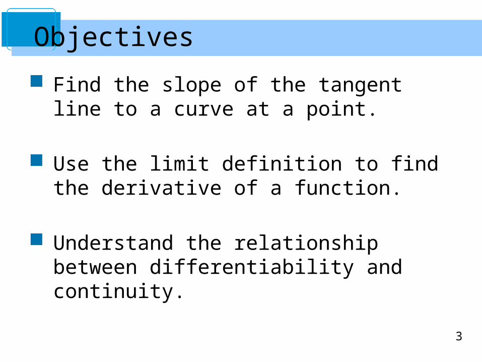
Find the slope of the tangent line to a curve at a point.
Use the limit definition to find the derivative of a function.
Understand the relationship between differentiability and continuity.
Objectives

4
The Tangent Line Problem

5
Calculus grew out of four major problems that European mathematicians were working on during the seventeenth century.
1. The tangent line problem
2. The velocity and acceleration problem
3. The minimum and maximum problem
4. The area problem
Each problem involves the notion of a limit, and calculus can be introduced with any of the four problems.
The Tangent Line Problem

6
Essentially, the problem of finding the tangent line at a point P boils down to the problem of finding the slope of the tangent line at point P.
You can approximate this slope using a secant line through the point of tangency and a second point on the curve, as shown in Figure 2.3.
Figure 2.3
The Tangent Line Problem

7
If (c, f(c)) is the point of tangency and is a second point on the graph of f, the slope of the secant line through the two points is given by substitution into the slope formula.
The Tangent Line Problem
8
The Tangent Line Problem
The right-hand side of this equation is a difference quotient.
The denominator x is the change in x, and the numerator y = f(c + x) – f(c) is the change in y.

9
The Tangent Line Problem
The slope of the tangent line to the graph of f at the point (c, f(c)) is also called the slope of the graph of f at x = c.

10
Example 1 – The Slope of the Graph of a Linear Function
Find the slope of the graph of f(x) = 2x – 3 at the point (2, 1).
Solution:To find the slope of the graph of f when c = 2, you can applythe definition of the slope of a tangent line, as shown.

11
Example 1 – Solution
Figure 2.5
cont’d
The slope of f at (c, f(c)) = (2, 1) is m = 2, as shown in Figure 2.5.

12
The definition of a tangent line to a curve does not cover the possibility of a vertical tangent line.
For vertical tangent lines, you can use the following definition.
If f is continuous at c and
the vertical line x = c passing through (c, f(c)) is a vertical tangent line to the graph of f.
The Tangent Line Problem

13
For example, the function shown in Figure 2.7 has a vertical tangent line at (c, f(c)).
Figure 2.7
The Tangent Line Problem

14
If the domain of f is the closed interval [a, b], you can extend the definition of a vertical tangent line to include the endpoints by considering continuity and limits from the right (for x = a) and from the left (for x = b).
The Tangent Line Problem

15
The Derivative of a Function

16
The Derivative of a Function
The limit used to define the slope of a tangent line is also used to define one of the two fundamental operations of calculus—differentiation.

17
The Derivative of a Function
Be sure you see that the derivative of a function of x is also a function of x.
This “new” function gives the slope of the tangent line to the graph of f at the point (x, f(x)), provided that the graph has a tangent line at this point.
The process of finding the derivative of a function is called differentiation.
A function is differentiable at x if its derivative exists at x and is differentiable on an open interval (a, b) if it is differentiable at every point in the interval.

18
In addition to f′(x), which is read as “f prime of x,” other notations are used to denote the derivative of y = f(x). The most common are
The notation dy/dx is read as “the derivative of y with respect to x” or simply “dy, dx.” Using limit notation, you can write
The Derivative of a Function

19
Example 3 – Finding the Derivative by the Limit Process
Find the derivative of f(x) = x3 + 2x.
Solution:

20
Example 3 – Solution
Remember that the derivative of a function f is itself a function, which can be used to find the slope of the tangent line at the point (x, f(x)) on the graph of f.
cont’d

21
Differentiability and Continuity

22
Differentiability and Continuity
The following alternative limit form of the derivative is useful in investigating the relationship between differentiability and continuity. The derivative of f at c is
provided this limit exists (see Figure 2.10).
Figure 2.10

23
Differentiability and Continuity
Note that the existence of the limit in this alternative formrequires that the one-sided limits
exist and are equal.
These one-sided limits are called the derivatives from the left and from the right, respectively.
It follows that f is differentiable on the closed interval [a, b] if it is differentiable on (a, b) and if the derivative from the right at a and the derivative from the left at b both exist.
24Figure 2.11
Differentiability and Continuity
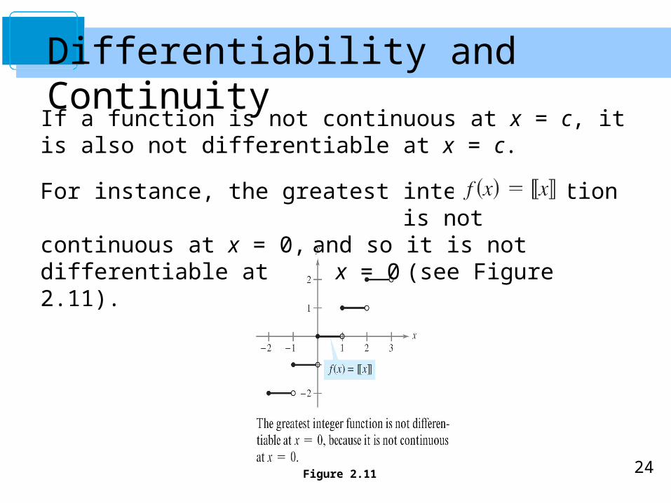
If a function is not continuous at x = c, it is also not differentiable at x = c.
For instance, the greatest integer function is not continuous at x = 0, and so it is not differentiable at x = 0 (see Figure 2.11).

25
Differentiability and Continuity
You can verify this by observing that
and
Although it is true that differentiability implies continuitythe converse is not true.
That is, it is possible for a function to be continuous at x = c and not differentiable at x = c.

26
The function shown in Figure 2.12 is continuous at x = 2.
Example 6 – A Graph with a Sharp Turn
Figure 2.12

27
However, the one-sided limits
and
are not equal.
So, f is not differentiable at x = 2 and the graph of f does not have a tangent line at the point (2, 0).
cont’dExample 6 – A Graph with a Sharp Turn

28
Differentiability and Continuity
The following statements summarize the relationship
between continuity and differentiability.
1. If a function is differentiable at x = c, then it is continuous at x = c. So, differentiability implies continuity.
2. It is possible for a function to be continuous at x = c and not be differentiable at x = c. So, continuity does not imply differentiability.

29
Basic Differentiation Rules and Rates of Change
Copyright © Cengage Learning. All rights reserved.
2.2
30
Find the derivative of a function using the Constant Rule.
Find the derivative of a function using the Power Rule.
Find the derivative of a function using the Constant Multiple Rule.
Objectives

31
Find the derivative of a function using the Sum and Difference Rules.
Find the derivatives of the sine function and of the cosine function.
Use derivatives to find rates of change.
Objectives

32
The Constant Rule

33
The Constant Rule
Figure 2.14

34
Example 1 – Using the Constant Rule

35
The Power Rule

36
The Power Rule
Before proving the next rule, it is important to review the procedure for expanding a binomial.
The general binomial expansion for a positive integer n is
This binomial expansion is used in proving a special case of the Power Rule.

37
The Power Rule

38
When using the Power Rule, the case for which n = 1 is best thought of as a separate differentiation rule. That is,
This rule is consistent with the fact that the slope of the line y = x is 1,as shown in Figure 2.15.
Figure 2.15
The Power Rule

39
Example 2 – Using the Power Rule
In Example 2(c), note that before differentiating, 1/x2 was rewritten as x-2. Rewriting is the first step in many differentiation problems.

40
The Constant Multiple Rule

41
The Constant Multiple Rule

42
Example 5 – Using the Constant Multiple Rule

43
The Constant Multiple Rule and the Power Rule can be combined into one rule. The combination rule is
The Constant Multiple Rule

44
The Sum and Difference Rules

45
The Sum and Difference Rules

46
Example 7 – Using the Sum and Difference Rules
47
Derivatives of the Sine and Cosine Functions

48
Derivatives of the Sine and Cosine Functions

49
Example 8 – Derivatives Involving Sines and Cosines

50
Rates of Change
51
You have seen how the derivative is used to determine slope.
The derivative can also be used to determine the rate of change of one variable with respect to another.
Applications involving rates of change occur in a wide variety of fields.
A few examples are population growth rates, production rates, water flow rates, velocity, and acceleration.
Rates of Change

52
A common use for rate of change is to describe the motion of an object moving in a straight line.
In such problems, it is customary to use either a horizontal or a vertical line with a designated origin to represent the line of motion.
On such lines, movement to the right (or upward) is considered to be in the positive direction, and movement to the left (or downward) is considered to be in the negative direction.
Rates of Change

53
The function s that gives the position (relative to the origin)
of an object as a function of time t is called a position
function.
If, over a period of time t, the object changes its position by the amount s = s(t + t) – s(t), then, by the familiar formula
the average velocity is
Rates of Change

54
If a billiard ball is dropped from a height of 100 feet, its height s at time t is given by the position function
s = –16t2 + 100 Position function
where s is measured in feet and t is measured in seconds. Find the average velocity over each of the following time intervals.
Example 9 – Finding Average Velocity of a Falling Object
a. [1, 2] b. [1, 1.5] c. [1, 1.1]

55
For the interval [1, 2], the object falls from a height of
s(1) = –16(1)2 + 100 = 84 feet to a height of
s(2) = –16(2)2 + 100 = 36 feet.
Example 9(a) – Solution
The average velocity is

56
Example 9(b) – Solution
For the interval [1, 1.5], the object falls from a height of 84 feet to a height of 64 feet.
The average velocity is
cont’d

57
For the interval [1, 1.1], the object falls from a height of 84 feet to a height of 80.64 feet.
The average velocity is
Note that the average velocities are negative, indicating that the object is moving downward.
Example 9(c) – Solution cont’d

58
In general, if s = s(t) is the position function for an object moving along a straight line, the velocity of the object at time t is
In other words, the velocity function is the derivative of the position function.
Velocity can be negative, zero, or positive.
The speed of an object is the absolute value of its velocity. Speed cannot be negative.
Rates of Change

59
The position of a free-falling object (neglecting air resistance) under the influence of gravity can be represented by the equation
where s0 is the initial height of the object, v0 is the initial velocity of the object, and g is the acceleration due to gravity.
On Earth, the value of g is approximately –32 feet per second per second or –9.8 meters per second per second.
Rates of Change

60
Example 10 – Using the Derivative to Find Velocity
At time t = 0, a diver jumps from a platform diving board that is 32 feet above the water(see Figure 2.21). The position of the diveris given by
s(t) = –16t2 + 16t + 32 Position function
where s is measured in feet and t is measured in seconds.
a. When does the diver hit the water?
b. What is the diver’s velocity at impact?
Figure 2.21

61
Example 10(a) – Solution
To find the time t when the diver hits the water, let s = 0 and solve for t.
–16t2 + 16t + 32 = 0 Set position function equal to 0.
–16(t + 1)(t – 2) = 0 Factor.
t = –1 or 2 Solve for t.
Because t ≥ 0, choose the positive value to conclude that
the diver hits the water at t = 2 seconds.

62
Example 10(b) – Solution
The velocity at time t is given by the derivative
s(t) = –32t + 16.
So, the velocity at time is t = 2 is s(2) = –32(2) + 16
= –48 feet per second.
cont’d

63
Product and Quotient Rules and Higher-Order Derivatives
Copyright © Cengage Learning. All rights reserved.
2.3

64
Find the derivative of a function using the Product Rule.
Find the derivative of a function using the Quotient Rule.
Find the derivative of a trigonometric function.
Find a higher-order derivative of a function.
Objectives

65
The Product Rule

66
The Product Rule

67
Example 1 – Using the Product Rule
Find the derivative of
Solution:

68
The Quotient Rule

69
The Quotient Rule

70
Example 4 – Using the Quotient Rule
Find the derivative of
Solution:

71
Derivatives of Trigonometric Functions

72
Derivatives of Trigonometric Functions
Knowing the derivatives of the sine and cosine functions, you can use the Quotient Rule to find the derivatives of the four remaining trigonometric functions.

73
Example 8 – Differentiating Trigonometric Functions

74
Derivatives of Trigonometric Functions

75
Higher-Order Derivatives

76
Higher-Order Derivatives
Just as you can obtain a velocity function by differentiating a position function, you can obtain an acceleration function by differentiating a velocity function.
Another way of looking at this is that you can obtain an acceleration function by differentiating a position function twice.

77
The function given by a(t) is the second derivative of s(t) and is denoted by s"(t).
The second derivative is an example of a higher-order derivative.
You can define derivatives of any positive integer order. For instance, the third derivative is the derivative of the second derivative.
Higher-Order Derivatives

78
Higher-Order Derivatives
Higher-order derivatives are denoted as follows.

79
Example 10 – Finding the Acceleration Due to Gravity
Because the moon has no atmosphere, a falling object on the moon encounters no air resistance. In 1971, astronaut David Scott demonstrated that a feather and a hammer fall at the same rate on the moon. The position function for each of these falling objects is given by
s(t) = –0.81t2 + 2
where s(t) is the height in meters and t is the time in seconds. What is the ratio of Earth’s gravitational force to the moon’s?

80
Example 10 – Solution
To find the acceleration, differentiate the position function twice.
s(t) = –0.81t2 + 2 Position function
s'(t) = –1.62t Velocity function
s"(t) = –1.62 Acceleration function
So, the acceleration due to gravity on the moon is –1.62 meters per second per second.

81
Example 10 – Solution
Because the acceleration due to gravity on Earth is –9.8
meters per second per second, the ratio of Earth’s
gravitational force to the moon’s is
cont’d

82
The Chain Rule
Copyright © Cengage Learning. All rights reserved.
2.4

83
Find the derivative of a composite function using the Chain Rule.
Find the derivative of a function using the General Power Rule.
Simplify the derivative of a function using algebra.
Find the derivative of a trigonometric function using the Chain Rule.
Objectives

84
The Chain Rule

85
The Chain Rule
This text has yet to discuss one of the most powerful differentiation rules—the Chain Rule.
This rule deals with composite functions and adds a surprising versatility to the rules discussed in the two previous sections.

86
For example, compare the functions shown below.
Those on the left can be differentiated without the Chain Rule, and those on the right are best differentiated with the Chain Rule.
Basically, the Chain Rule states that if y changes dy/du times as fast as u, and u changes du/dx times as fast as x, then y changes (dy/du)(du/dx) times as fast as x.
The Chain Rule

87
Example 1 – The Derivative of a Composite Function
A set of gears is constructed, as shown in Figure 2.24, such that the second and third gears are on the same axle.
As the first axle revolves, it drives the second axle, which in turn drives the third axle.
Let y, u, and x represent the numbers of revolutions per minute of the first, second, and third axles, respectively. Find dy/du, du/dx, and dy/dx ,and show that
Figure 2.24

88
Example 1 – Solution
Because the circumference of the second gear is three times that of the first, the first axle must make three revolutions to turn the second axle once.
Combining these two results, you know that the first axle must make six revolutions to turn the third axle once.
Similarly, the second axle must make two revolutions to turn the third axle once, and you can write

89
So, you can write
In other words, the rate of change of y with respect to x is the product of the rate of change of y with respect to u and the rate of change of u with respect to x.
cont’dExample 1 – Solution

90
The Chain Rule

91
Example 2 – Decomposition of a Composite Function

92
The General Power Rule

93
The General Power Rule
One of the most common types of composite functions,
y = [u(x)]n.
The rule for differentiating such functions is called the General Power Rule, and it is a special case of the Chain Rule.

94
The General Power Rule

95
Example 4 – Applying the General Power Rule
Find the derivative of f(x) = (3x – 2x2)3.
Solution:
Let u = 3x – 2x2.
Then f(x) = (3x – 2x2)3 = u3
and, by the General Power Rule, the derivative is

96
Simplifying Derivatives

97
Simplifying Derivatives
The next three examples illustrate some techniques for simplifying the “raw derivatives” of functions involving products, quotients, and composites.

98
Example 7 – Simplifying by Factoring Out the Least Powers

99
Example 8 – Simplifying the Derivative of a Quotient
100
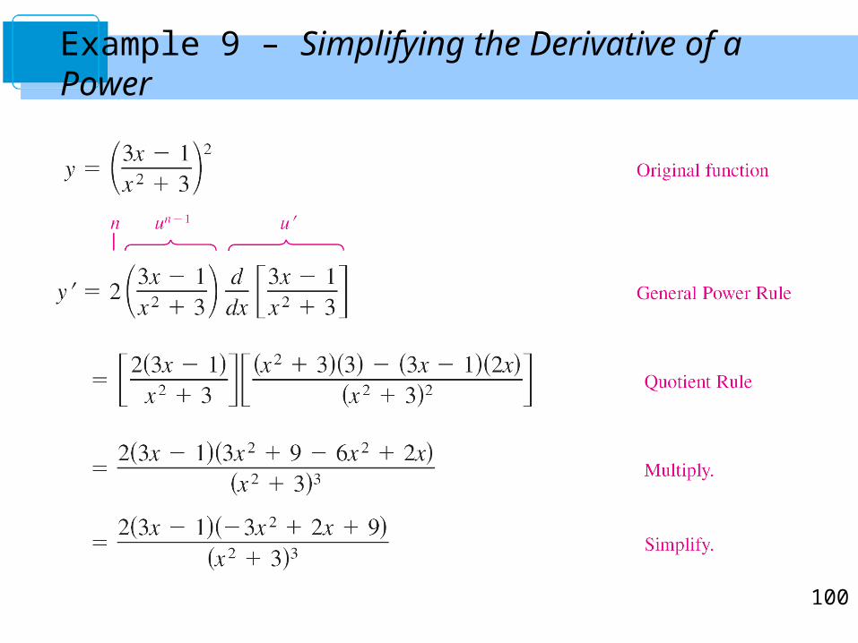
Example 9 – Simplifying the Derivative of a Power

101
Trigonometric Functions and the Chain Rule

102
Trigonometric Functions and the Chain Rule
The “Chain Rule versions” of the derivatives of the six trigonometric functions are as follows.

103
Example 10 – Applying the Chain Rule to Trigonometric Functions

104
Trigonometric Functions and the Chain Rule

105
Implicit Differentiation
Copyright © Cengage Learning. All rights reserved.
2.5
106
Distinguish between functions written in implicit form and explicit form.
Use implicit differentiation to find the derivative of a function.
Objectives

107
Implicit and Explicit Functions

108
Implicit and Explicit Functions
Most functions have been expressed in explicit form. For example, in the equation
the variable y is explicitly written as a function of x.
Some functions, however, are only implied by an equation. For instance, the function y = 1/x is defined implicitly by the equation xy = 1.
Explicit form

109
Suppose you were asked to find dy/dx for this equation. You could begin by writing y explicitly as a function of x and then differentiating.
This strategy works whenever you can solve for the function explicitly.
You cannot, however, use this procedure when you are unable to solve for y as a function of x.
Implicit and Explicit Functions

110
For instance, how would you find dy/dx for the equation
where it is very difficult to express y as a function of x
explicitly? To do this, you can use implicit differentiation.
Implicit and Explicit Functions

111
To understand how to find dy/dx implicitly, you must realize
that the differentiation is taking place with respect to x.
This means that when you differentiate terms involving x
alone, you can differentiate as usual.
However, when you differentiate terms involving y, you
must apply the Chain Rule, because you are assuming that
y is defined implicitly as a differentiable function of x.
Implicit and Explicit Functions

112
Example 1 – Differentiating with Respect to x

113
cont’dExample 1 – Differentiating with Respect to x

114
Implicit Differentiation

115
Implicit Differentiation

116
Example 2 – Implicit Differentiation
Find dy/dx given that y3 + y2 – 5y – x2 = –4.
Solution:
1. Differentiate both sides of the equation with respect to x.

117
2. Collect the dy/dx terms on the left side of the equation and move all other terms to the right side of the equation.
3. Factor dy/dx out of the left side of the equation.
4. Solve for dy/dx by dividing by (3y2 + 2y – 5).
cont’dExample 2 – Solution

118
To see how you can use an
implicit derivative, consider
the graph shown in Figure 2.27.
From the graph, you can see that y is not a function of x. Even so, the derivative found in Example 2 gives a formula for the slope of the tangent line at a point on this graph.The slopes at several points on thegraph are shown below the graph.
Figure 2.27
Implicit Differentiation
119
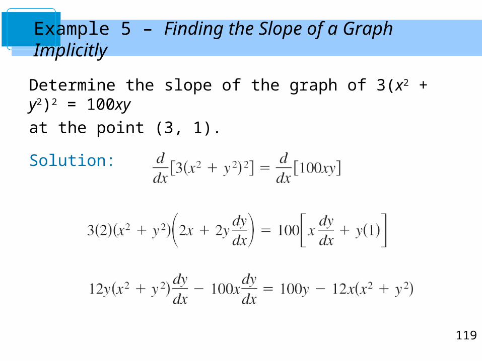
Example 5 – Finding the Slope of a Graph Implicitly
Determine the slope of the graph of 3(x2 + y2)2 = 100xy
at the point (3, 1).
Solution:

120
Example 5 – Solutioncont’d

121
At the point (3, 1), the slope of the graph is as shown in
Figure 2.30. This graph is called a lemniscate.
Figure 2.30
Example 5 – Solutioncont’d

122
Related Rates
Copyright © Cengage Learning. All rights reserved.
2.6

123
Find a related rate.
Use related rates to solve real-life problems.
Objectives
124
Finding Related Rates

125
Finding Related Rates
The Chain Rule can be used to find dy/dx implicitly.
Another important use of the Chain Rule is to find the rates
of change of two or more related variables that are
changing with respect to time.

126
For example, when water is drained out of a conical tank (see Figure 2.33), the volume V, the radius r, and the height h of the water level are all functions of time t.
Knowing that these variables are related by the equation
Figure 2.33
Finding Related Rates

127
you can differentiate implicitly with respect to t to obtain the related-rate equation
From this equation you can see that the rate of change of
V is related to the rates of change of both h and r.
Finding Related Rates
128
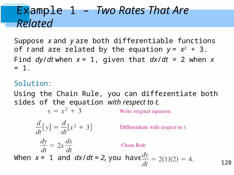
Example 1 – Two Rates That Are Related
Suppose x and y are both differentiable functions of t and are related by the equation y = x2 + 3.
Find dy/dt when x = 1, given that dx/dt = 2 when x = 1.
Solution:
Using the Chain Rule, you can differentiate both sides of the equation with respect to t.
When x = 1 and dx/dt = 2, you have

129
Problem Solving with Related Rates

130
Problem Solving with Related Rates

131
Example 3 – An Inflating Balloon
Air is being pumped into a spherical balloon (see Figure 2.35) at a rate of 4.5 cubic feet per minute. Find the rate of change of the radius when the radius is
2 feet.
Figure 2.35

132
Example 3 – Solution
Let V be the volume of the balloon and let r be its radius.
Because the volume is increasing at a rate of 4.5 cubic feet per minute, you know that at time t the rate of change of the volume is
So, the problem can be stated as shown.
Given rate: (constant rate)
Find: when r = 2

133
Example 3 – Solution
To find the rate of change of the radius, you must find an equation that relates the radius r to the volume V.
Equation:
Differentiating both sides of the equation with respect to t produces
cont’d

134
Example 3 – Solution
Finally, when r = 2, the rate of change of the radius is
cont’d