Embed Size (px)
Citation preview

Copyright is owned by the Author of the thesis. Permission is given for a copy to be downloaded by an individual for the purpose of research and private study only. The thesis may not be reproduced elsewhere without the permission of the Author.

Performance Study of IEEE 802.11p for Vehicle to
Vehicle Communications Using OPNET
A thesis presented in partial fulfilment of the
requirements for the degree of
Master of Engineering
in
Telecommunications and Network
at
Massey University,
Auckland, New Zealand
Ning Sun
November 2011

I
Abstract
IEEE 802.11p is the recently finalised protocol located at the bottom of the Dedicated Short
Range Communication (DSRC) protocol suite, which supports Intelligent Transportation
System (ITS) applications for both road safety and added value communication purposes. It
has evolved from widely applied Wireless Local Area Network (WLAN) standards and it
cooperates with peculiar higher layer protocols in order to carry out inter-vehicle
communication. In this thesis, we focus on the performance study of road safety
communication as being the vital application in ITS, which is very necessary not only
because IEEE 802.11p is a relatively new protocol but also because it heavily relies on
broadcast mode, thus distinguishing itself from other 802.11 counterparts. With the aid of
OPNET, a powerful commercial simulator, different scenarios have been deployed in which
one or more variable factors are involved, such as vehicle number, data packet size,
communication distance, vehicle fleet topology, etc., in order to find out their impacts on
DSCR and characteristics of 802.11p.
After analysing results data collected from hundreds of simulations, we found out that
802.11p represented a desirable performance in terms of latency and priority-oriented
services throughout our simulation scenarios. However, packet collision caused by either
media contention or hidden nodes turned out to be a relatively serious issue of vehicle
communication and 802.11p seems in shortage of an effective mechanism to deal with it.
What we can only hope is that under practical application, the media should always be lightly
occupied and that there are few ACs with high priorities trying to contend resources
simultaneously at any given time. Meanwhile, our analyses indicate that current 802.11p
protocol might still need further modifications in order to address its inherent issues and
enhance the communication performance.

II
Acknowledgements
First and foremost, I would like to thank my supervisor, Dr. Frakhul Alam, whose patience
and kindness, as well as his academic attainments, have been invaluable to me. As the
proverb goes, a single conversation across the table with a wise person is worth a month's
study of books. This appropriately expresses the feelings I had every time I consulted with
him about any confusion during the research. I have thoroughly enjoyed working under his
guidance and I greatly appreciated his continuous support and advice in all aspects of my
thesis work.
I would also like to thank Dr. Suhaimi Abd Latif who helped me develop my skills in
OPNET usage and who often provided precious opinions on my deployment of simulations
through his rich experience in this field.
I am also indebted to Mr. Yu Xue Feng, who specialised in road traffic modeling and who
provided me with helpful advice, as well as Mr. Dmitri Roukin, who provided software
technical support and system maintenance to facilitate my research. I have to give a special
mention to the encouragement given by my two friends, YongZhu Zheng and HuiMing Xu.
Most importantly, this thesis would not have been at all possible without the constant support
and care of my parents, as they always love and trust me. I would like to express my heart-
felt gratitude to them.

III
TABLES OF CONTENTS
Abstract
Acknowledgements
Chapter 1 Introduction
1.1 Backgrounds ........................................................................................................ 1
1.2 Justification for ITS in New Zealand ................................................................... 2
1.3 Vehicular Ad-Hoc Network (VANET) ................................................................ 4
1.4 Objectives and Outline of the Thesis ................................................................... 5
Chapter 2 Communication Technology for VANET
2.1 Overview .............................................................................................................. 7
2.2 Dedicated Short Range Communications (DSRC) .............................................. 7
2.3 Other Communication Technologies for VANET ............................................... 9
2.4 Necessity of 802.11p Performance Study .......................................................... 11
2.5 Summary ............................................................................................................ 12
Chapter 3 Physical Layer Technology of 802.11p
3.1 Overview of Physical Layer............................................................................... 14
3.2 Introduction of OFDM ....................................................................................... 14
3.3 Comparison between 802.11a and 802.11p ....................................................... 16
3.4 OFDM PLCP ..................................................................................................... 18
3.4.1 Functions of PLCP ......................................................................................... 18
3.4.2 OFDM PPDU Format .................................................................................... 20
3.5 Spectrum Allocation for 802.11p ....................................................................... 22
3.5.1 Industrial, Scientific, and Medical Bands ...................................................... 23
3.5.3 DSRC Channel Arrangement ......................................................................... 25
IV
3.6 Transmission Power ........................................................................................... 27
3.6.1 WLAN Transmit Power Regulation .............................................................. 27
3.6.2 Transmit Power Limit on 802.11p ................................................................. 29
3.7 Wireless Channel Characteristics ...................................................................... 30
3.7.1 Overview ........................................................................................................ 30
3.7.2 Channel Models for 802.11p.......................................................................... 31
3.8 Summary ............................................................................................................ 33
Chapter 4 Medium Access Control and Quality of Service
4.1 MAC Protocol for IEEE 802.11 Standards ........................................................ 34
4.1.1 Overview ........................................................................................................ 34
4.1.2 Collision Avoidance Mechanism ................................................................... 34
4.2 Enhanced Distributed Channel Access (EDCA) ............................................... 37
4.2.1 Introduction of EDCA Mechanism ................................................................ 37
4.2.2 EDCA for 802.11p ......................................................................................... 41
4.3 MAC Protocol Data Unit of 802.11p ................................................................. 45
4.4 Summary ............................................................................................................ 48
Chapter 5 VANET Topology and WAVE Short Message
5.1 Multi-Channel Operation` .................................................................................. 49
5.2 Characteristics of VANET Topology ................................................................ 50
5.2.1 Broadcast Mechanism on CCH ...................................................................... 50
5.2.2 WAVE Basic Service Set (WBSS) ................................................................ 51
5.3 WAVE Short Message Protocol (WSMP) ......................................................... 53
5.3.1 Introduction .................................................................................................... 53
5.3.2 Frame Format of WSA................................................................................... 55
5.3.3 Frame Format of WSM .................................................................................. 58
V
5.4 Summary ............................................................................................................ 61
Chapter 6 Simulation Elements Configuration and Fundamental Scenarios
6.1 Introduction of 802.11p Simulation ................................................................... 62
6.2 Workstation Configuration and Explanation ..................................................... 63
6.3 A Simple Simulation Scenario ........................................................................... 68
6.3.1 Deployment and Performance of Scenario -1 ................................................ 68
6.3.2 Performance Analysis .................................................................................... 71
6.4 Study of Distance Impact on CCH Performance ............................................... 72
6.4.1 Deployment of Stationary Scenario-2 and Performance ............................... 72
6.4.2 Performance Analysis of Scenario-2 ............................................................. 76
6.4.2.1 Analysis within Effective Coverage ................................................... 76
6.4.2.2 Analysis Outside of Effective Coverage ............................................. 77
6.4.3 Deployment of Dynamic Scenario-3 and Performance ................................. 79
6.4.3 Performance Analysis of Scenario-3 ............................................................. 81
6.5 Study of Packet Size Impact on VANET ........................................................... 84
6.5.1 Introduction and Deployment of Scenario-4.................................................. 84
6.5.2 Analysis of Instance-1.................................................................................... 85
6.5.3 Analysis of Instance-2.................................................................................... 87
6.5.4 Analysis of Four Sub-Instances of Instance-3 ............................................... 89
Chapter 7 Advanced Scenarios and Performance Analysis
7.1 Study of Vehicle Number Impact on VANET ................................................... 93
7.1.1 Deployment and Performance of Instance-4.................................................. 93
7.1.2 Analysis of Instance-4.................................................................................... 94
7.2 Study of Multiple AC Types Impact ................................................................ 104
7.2.1 Introduction and Performance of Instance-5................................................ 104
7.2.2 Analysis of Instance-5.................................................................................. 107

VI
7.3 Comprehensive Performance Study in Dynamic Environment ....................... 108
7.3.1 Deployment and Performance of Scenario-5 ............................................... 108
7.3.2 Performance Study of Testing Node 01 ....................................................... 110
7.3.3 Analysis of Testing Node 00/02 .................................................................. 114
Chapter 8 Conclusion and Future Work
8.1 Conclusion ....................................................................................................... 119
8.2 Future Work ..................................................................................................... 120
REFERENCES
Appendix

VII
LIST OF FIGURES
Figure 1-1 Number of Fatal Crashes from 1975-2009 ..................................................... 1
Figure 1-2 VANET Communication Scenario ................................................................ 4
Figure 2-1 Protocol Architecture for DSRC .................................................................... 8
Figure 2-2 DSRC allocation in different regions or entities ............................................ 9
Figure 3-1 Block diagram of OFDM System ................................................................ 15
Figure 3-2 ICI and ISI ..................................................................................................... 16
Figure 3-3 PLCP transmit function ................................................................................. 19
Figure 3-4 Format of OFDM PPDU ................................................................................ 20
Figure 3-5 802.11p PLCP Preamble Structure ............................................................... 21
Figure 3-6 Structure of Signal Field ............................................................................... 22
Figure 3-7 Wi-Fi signal test in Auckland CBD .............................................................. 24
Figure 3-8 Frequency spacing of 802.11a ....................................................................... 25
Figure 3-9 DSRC channel arrangement .......................................................................... 26
Figure 3-10 Transmit spectrum mask, and side band interference ................................. 28
Figure 3- 11 5 GHz Power IR regulations ...................................................................... 28
Figure 3-12 Two Ray Path Loss Model .......................................................................... 32
Figure 4- 1 Overview of Different MAC Protocols ....................................................... 34
Figure 4-2 RTS/CTS Mechanism addressing hidden node problem .............................. 36
Figure 4- 3 MAC Protocols Relationship ....................................................................... 37
Figure 4-4 EDCA mechanism at MAC layer .................................................................. 40
Figure 4- 5 AIFS and Backoff Time Contend for Channel Access in EDCF ................. 41

VIII
Figure 4-6 EDCA at 802.11p MAC ............................................................................... 42
Figure 4-7 AIFS and Backoff Time for CCH and SCH ................................................. 44
Figure 4- 8 Overall MPDU Format of 802.11p/e ........................................................... 45
Figure 4- 9 Sub-fields of Frame Control......................................................................... 46
Figure 5-1 1609.4 Alternating Channel Access Mechanisms ......................................... 49
Figure 5-2 Channel access options: (a) continuous, (b) alternating, (c) immediate, and (d)
extended .................................................................................................................. 50
Figure 5-3 Broadcast Storm in Wired and Wireless Networks....................................... 51
Figure 5-4 Non-WBSS and WBSS Topology ................................................................ 52
Figure 5- 5 WSMP and IPv6 working on different channels.......................................... 54
Figure 5- 6 Simple Procedure Flow of WBSS Joining ................................................... 55
Figure 5- 7 Format of Wave Service Advertisement Sub-Field ..................................... 55
Figure 5- 8 Service Info Format...................................................................................... 56
Figure 5- 9 Format of Channel Info ................................................................................ 57
Figure 5- 10 Format of WAVE Routing Advertisement ................................................ 58
Figure 5- 11 Generation of WSM Package ..................................................................... 59
Figure 6-1 PHY and EDCA Configuration for AC 3 ..................................................... 65
Figure 6-2 Contention and Backoff Mechanisms in Two Situations .............................. 67
Figure 6-3 Topology of Scenario-1................................................................................. 68
Figure 6-4 OPNET Setting for AC 3 Packet Generation ................................................ 70
Figure 6-5 Delay of ACs in Scenario-1 .......................................................................... 70
Figure 6-6 Average Delay of ACs in Scenario-1 ............................................................ 71
IX
Figure 6-7 Topology of Scenario-2 for Distance Impact Study ..................................... 73
Figure 6-8 AC 3 Average Delay for Testing Nodes 00-05 ............................................. 73
Figure 6-9 AC 3 Bit Error Rate for Testing Nodes 00-05 .............................................. 74
Figure 6-10 AC 3 Packet Receiving Rate for Testing Nodes 00-05 ............................... 74
Figure 6-11 SNR of Node 01/06/07 in Scenario-2 ......................................................... 75
Figure 6-12 AC 3 Delay of Node 01/06/07 on Scenario-2 ............................................. 75
Figure 6-13 Average BER of AC 01/06/07 on Scenario-2 ............................................. 76
Figure 6-14 Topology for Scenario-3 ............................................................................. 80
Figure 6-15 Overall Delay and Delay of ACs in Discrete Pattern .................................. 80
Figure 6-16 BER of Node 08 .......................................................................................... 81
Figure 6-17 Packet Reception Rate and SNR in dB ....................................................... 81
Figure 6-18 Reception Distance Under One OFDM Symbol ......................................... 83
Figure 6-19 Topology of Scenario-4............................................................................... 85
Figure 6-20 Average Delay for Instance-1 ..................................................................... 85
Figure 6-21 Average Delay of ACs for Instance-2 ......................................................... 88
Figure 6-22 Impact of Packet Size of AC 0 on VANET (sub-instance 0) ...................... 89
Figure 6-23 Impact of Packet Size of AC 1 on VANET (sub-instance 1) ...................... 90
Figure 6-24 Impact of Packet Size of AC 2 on VANET (sub-instance 2) ...................... 90
Figure 6-25 Impact of Packet Size of AC 3 on VANET (sub-instance 3) ...................... 90
Figure 7-1 Topology of Instance-4 under 10 Vehicle Condition .................................... 93
Figure 7-2: Average Delay Based on Vehicle Number and Packet Size in 3D Mesh
Format ..................................................................................................................... 94

X
Figure 7-3 Packet Loss Rate of AC 0 and AC 3 ............................................................. 97
Figure 7-4 Division of Overall Waiting Duration ......................................................... 100
Figure 7-5 Turning Off Impact on Packet Loss at Initial Stage .................................... 101
Figure 7-6 Average Delay of ACs under (48 768) bits/packet (Instance-5) ............... 105
Figure 7-7 Average Bit Loss Rate of ACs (48 768) bits/packet (Instance-5) ............. 105
Figure 7-8 Average Packets/s of AC 0 and AC 1/2/3 under 1400 bits/packet ............. 106
Figure 7-9 Delay of ACs under 1400 bits/packet ......................................................... 106
Figure 7-10 Average AC 0 Packet Dropped Per Second under 1400 bits/packet ........ 107
Figure 7-11 Topology of Scenario-5............................................................................. 109
Figure 7-12 Delay of Each AC for Scenario-5 in Discrete Format .............................. 109
Figure 7-13 Moving Average Throughput of Testing Node 01 .................................... 110
Figure 7-14 Illustration of Vehicle Merge .................................................................... 111
Figure 7-15 Vehicle Group Merge Procedure .............................................................. 113
Figure 7-16 Throughput peaks of AC 3 at Testing Nodes 00 and 02 ........................... 114
Figure 7-17 Eleven Stages of Vehicle Group Mergence .............................................. 115
Figure 7-18 Rotation and Shift of Testing Node 02 Throughput Diagram ................... 117
Figure 7-19 Throughput of Testing Node 00/01/02 in One Chart ................................ 117
Figure 7-20 Reception Throughput of Vehicle 01/10/15/20......................................... 118

XI
LIST OF TABLES
Table 1-1 Passenger cars per 1,000 people by country ..................................................... 2
Table 1-2 Crash parameters between NZ and USA with derivative results ..................... 3
Table 3-1 Comparison between 802.11a and 802.11p .................................................... 16
Table 3-2 IR and EIRP combination at 2.4 GHz UNII of PtP ........................................ 29
Table 3-3 Max Power for IR and EIRP .......................................................................... 30
Table 4-1 UP’s map to ACs ............................................................................................ 39
Table 4-2 EDCA parameter for CCH ............................................................................ 43
Table 4-3 EDCA parameter for SCH .............................................................................. 43
Table 4-4 Type Field Instance ........................................................................................ 46
Table 6-1 Packet Generation Parameter ......................................................................... 69
Table 6-2 Data for Delay of Each AC ............................................................................ 71
Table 6-3 Increased delay per 100 Bits Added (ms/100 bits) of Instance 0 ................... 86
Table 6-4 Packet Size Configuration for Four Sub-Instances ........................................ 87
Table 6-5 Delay Increase per 100 Bits Added ................................................................ 88
Table 6-6 Average Increased Delay /100 bits for Four Sub-instances ........................... 90
Table 7-1 Delay Ratio between AC3 and AC0 ............................................................... 95
Table 7-2 Packet Loss Rate for AC 0 and AC 3 ............................................................. 96
Table 7-3 Collision Rate Comparison AC 3/AC 0 ....................................................... 102

XII
GLOSSARY
3G Third Generation
AC Access Category
ACK Acknowledgement
ADSL Asymmetric Digital Subscriber Line
AGC Automatic Gain Control
AIFS Arbitrary Inter-frame Space
AIFSN Arbitration Inter-Frame Space Number
AP Access Point
ASTM American Society for Testing and Materials
BCH Basic Channel
BEB Binary Exponential Backoff
BER Bit Error Rate
BS Base Station
BSS Basic Service Set
BTS Base Transreceiver Station
CCA Clear Channel Assessment
CCH Control Channel
CDMA Code Division Multiple Access
CRC Cyclic Redundancy Code
CSMA/CA Carrier Sense Multiple Access with Collision Avoidance
CTS Clear to Send
CW Contention Window
DCF Distributed Coordination Function
D-MAC Directional MAC
DSRC Dedicated Short Range Communications
EDCA Enhanced Distributed Channel Access
EDCAF Enhanced Distributed Channel Access Function
EDCF Enhanced DCF

XIII
EIFS Extended Inter-frame Space
EIRP Equivalent Isotropically Radiated Power
ERP Extended Rate PHY
ESOP End of Service Period
FCC Federal Communications Commission
FEC Forward Error Correction
FI Frame Information
GI Guard Interval
GPS Global Positioning System
GSM Global System for Mobile Communications
HCCA HCF Controlled Channel Access
HCF Hybrid Coordination Function
HR/DSSS High-Rate Direct Sequence
IANA Internet Assigned Numbers Authority
IBSS Independent BSS
ICI Inter Carrier Interference
IFFT Inverse Fast Fourier Transform
IFS Interframe Spaces
IR Intentional Radiator
ISI Intern Symbol Interference
ISM Industrial, Scientific and Medical
ISTEA Intermodal Surface Transportation Efficiency Act
ITS Intelligent Transport System
ITU International Telecommunication Union
LOS Line of Sight
MAC Media Access Control
MANET Mobile Ad-Hoc Network
MIB Management Information Base
MIMO Multiple-input and Multiple-output
MPDU MAC Protocol Data Unit
XIV
MS Mobile Station
MSDU MAC Service Data Unit
MTU Maximum Transmission Unit
NAT Network Address Translation
NHTSA National Traffic Safety Administration
NLOS Non-LOS
OBU Onboard Unit
OFDM Orthogonal Frequency-Division Multiplexing
OSI Open Systems Interconnection
PCF Point Coordination Function
PER Packet Error Rate
PHY Physical Layer
PLCP Physical Layer Convergence Procedure
PMD Physical Medium Dependent
PPDU PLCP Protocol Data Unit
PSDU PLCP Service Data Unit
PSID Provider Service ID
PtMP Point to Multipoint
PtP Point to Point
QoS Quality of Service
RIR Regional Internet Registries
RR-ALOHA Reliable Reservation-ALOHA
RSU Roadside Unit
RTS Request to Send
SAP Service Access Point
SC Sub-Carrier
SCH Service Channel
SIFS Short Interframe Spaces
SNR Signal to Noise Ratio
STA Station

XV
TDMA Time Division Multiple Access
TG Task Group
TID Traffic Identifier
TSID Traffic Stream Identifier
TXOP Transmission Opportunity
UNII Unlicensed national Information Infrastructure Band
UP User Priority
USDOT U.S. Department of Transportation
V2I Vehicle to Infrastructure
V2V Vehicle to Vehicle
V2X V2V and V2I
VANET Vehicular Ad-Hoc Network
WAVE Wireless Access in Vehicular Environment
WBSS WAVE Basic Service Set
WG Working Group
WIBSS WAVE IBSS
Wimax Worldwide Interoperability for Microwave Access
WLAN Wireless LAN
WME WAVE Management Entity
WRA WAVE Routing Advertisement
WSA WAVE Service Advertisement
WSM WAVE Short Message
WSM WAVE Short Message
WSMP WAVE Short Message Protocol

1
Chapter 1 Introduction
1.1 Backgrounds According to Traffic Safety Facts published by the United States National Traffic Safety
Administration (NHTSA) in 2009, there were 5,505,000 vehicular crashes in that year,
which resulted in a direct economic loss of $230.06 billion [1]. The numbers of fatalities,
injuries and property damage were 30,797, 1,517,000 and 3,957,000, respectively [2]. Even
though great effort has been made by car manufacturers to enhance the safety of severe crash
accidents, the fatal number of crashes has not significantly declined in the last two decades;
see Figure 1-1.
Figure 1-1 Number of Fatal Crashes from 1975-2009 [2] For the sake of enhancing the efficiency, safety and convenience of transportation, the US
Intermodal Surface Transportation Efficiency Act (ISTEA) of 1991 launched the national US
(Intelligent Transport System) ITS programme, with US$660 million funding over six years.
The core of ITS research conducted by the U.S. Department of Transportation (USDOT) has
been clearly defined as connected vehicle research-“ – a multimodal initiative that aims to
enable safe, interoperable networked wireless communications among vehicles, the

2
infrastructure, and passengers’ personal communications devices. [1]”. Among multi-year
research, there are two aspects out of six in their main priorities, namely: Vehicle-to-Vehicle
(V2V) Communications for Safety, and Vehicle-to-Infrastructure (V2I) Communications for
Safety.
1.2 Justification for ITS in New Zealand Even though ITS, V2V and V2I seem driven by the US industry, we should expect the
deployment of ITS in New Zealand in the near future based on two facts; this is despite its
population being only 1.3% of the United States’ and its territory being only as big as the
state of California.
Firstly, we compare the indicator from the World Bank: Passenger cars (per 1,000 people) [3]
in 2008. Table 1-1 provides ranks of this indicator.
Table 1-1 Passenger cars per 1,000 people by country
Rank Country name 2006 2007 2008 1 Monaco 748 732 2 Luxembourg 673 3 Iceland 667 661 4 New Zealand 609 615 616 5 Italy 591 596 ……
21 United States 451 451
It is important to understand the feasibility of deploying ITS, which does not depend on how
big the country is, since smaller coverage in most cases requires less investment on related
devices. From the table above, we surprisingly find that New Zealand ranks in the top 4 and
is the only country whose population is over one million. Meanwhile, every 1,000
Americans generally own 451 cars, yet it only ranks 21st, thus indicating around 32% lower
than New Zealand. Given that the USA has invested billions of dollars on ITS, it is logical to
assume that New Zealand, with a very close condition, could do it as well.
Secondly, it is necessary to compare traffic accidents between these two countries according
3
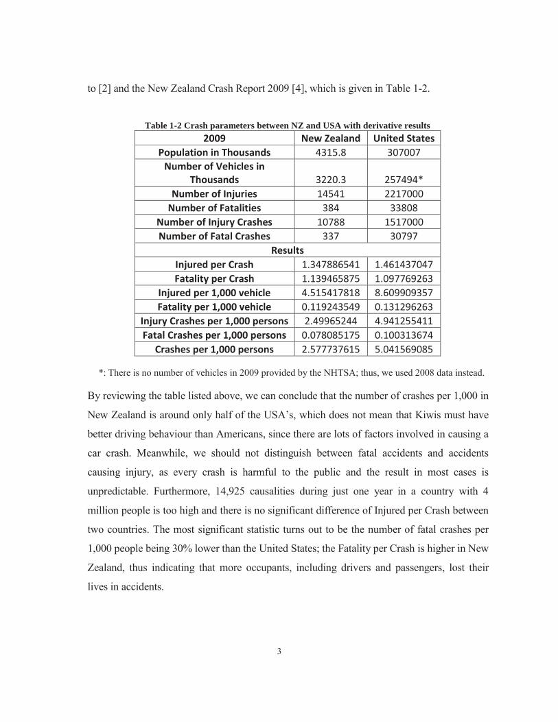
to [2] and the New Zealand Crash Report 2009 [4], which is given in Table 1-2.
Table 1-2 Crash parameters between NZ and USA with derivative results
2009 New Zealand United States Population in Thousands 4315.8 307007
Number of Vehicles in Thousands 3220.3 257494*
Number of Injuries 14541 2217000 Number of Fatalities 384 33808
Number of Injury Crashes 10788 1517000 Number of Fatal Crashes 337 30797
Results Injured per Crash 1.347886541 1.461437047 Fatality per Crash 1.139465875 1.097769263
Injured per 1,000 vehicle 4.515417818 8.609909357 Fatality per 1,000 vehicle 0.119243549 0.131296263
Injury Crashes per 1,000 persons 2.49965244 4.941255411 Fatal Crashes per 1,000 persons 0.078085175 0.100313674
Crashes per 1,000 persons 2.577737615 5.041569085 *: There is no number of vehicles in 2009 provided by the NHTSA; thus, we used 2008 data instead.
By reviewing the table listed above, we can conclude that the number of crashes per 1,000 in
New Zealand is around only half of the USA’s, which does not mean that Kiwis must have
better driving behaviour than Americans, since there are lots of factors involved in causing a
car crash. Meanwhile, we should not distinguish between fatal accidents and accidents
causing injury, as every crash is harmful to the public and the result in most cases is
unpredictable. Furthermore, 14,925 causalities during just one year in a country with 4
million people is too high and there is no significant difference of Injured per Crash between
two countries. The most significant statistic turns out to be the number of fatal crashes per
1,000 people being 30% lower than the United States; the Fatality per Crash is higher in New
Zealand, thus indicating that more occupants, including drivers and passengers, lost their
lives in accidents.
4
1.3 Vehicular Ad-Hoc Network (VANET) A VANET is a form of mobile ad-hoc network, which provides communications to nearby
vehicles with fixed equipment in order to improve road safety [5]. In fact, VANET is a very
special case of Mobile Ad-Hoc Network (MANET) and shares lots of similarities with it.
Concerning ITS, which is actually a very abstract term and a concept with many substantial
research areas involved, the VANET is the most vital part of ITS research, thus proving the
platforms of V2V and V2I communication as being two key components in ITS. The former
is defined as a dynamic wireless exchange of data, at least including position, speed and
location of vehicles, in order to sense threats and hazards, calculate risk, and issue driver
advisories or warnings. On the other hand, V2I for safety focus on the exchange of critical
safety and operational data between vehicles and highway infrastructure intended to
primarily avoid or mitigate motor vehicle crashes, as well as enable a wide range of other
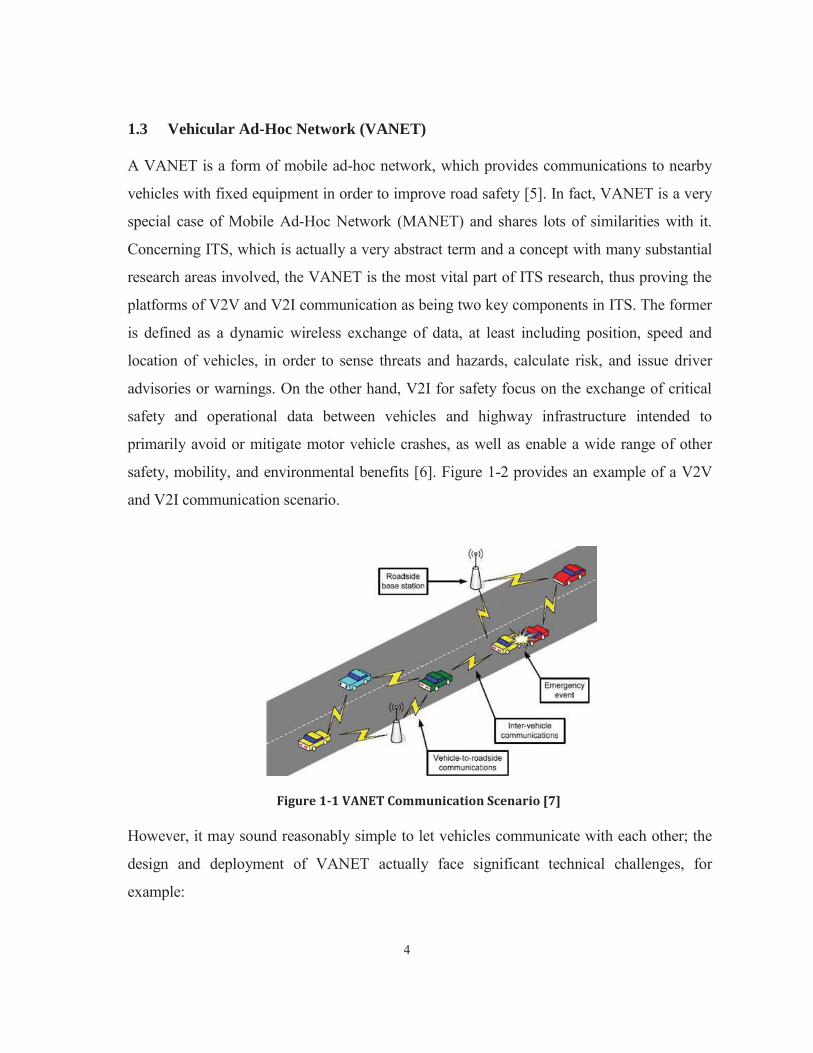
safety, mobility, and environmental benefits [6]. Figure 1-2 provides an example of a V2V
and V2I communication scenario.
Figure 1-1 VANET Communication Scenario [7] However, it may sound reasonably simple to let vehicles communicate with each other; the
design and deployment of VANET actually face significant technical challenges, for
example:

5
1. Unpredictable Wireless Communication Environment: VANET has to cope with
unfavourable characteristics of wireless communication, such as multi-path
propagation, fading and the Doppler effect.
2. Decentralised and self-organised Topology: The highly dynamic changes in VANET
and the mobility of vehicles make it hard to synchronise and manage the transmission
events, thus resulting in channel efficiency and frame collision.
3. Security and Privacy Issue: As we will see in the following chapters, many potential
protocols for VANET are heavily based on broadcasts and are without a normal
authentication mechanism for a time-critical application purpose. These attributes will
inevitably bring about security issues, such as a broadcast storm.
1.4 Objectives and Outline of the Thesis The main objective of the thesis is to present and evaluate the control channel (CCH)
performance of VANET, based on IEEE 802.11p. As a recently finalised standard, current
research of its performance is only at initial stage .Our literature review indicates that a
comprehensive study of the standard that takes complex network topologies and high
dynamic environment into consideration, is not available. As a result the work undertaken
for this project was quite necessary, whereby we concentrate on its physical layer (PHY)
technology and protocol of media access control (MAC) layer. Different simulations will be
made in order to evaluate different characteristics of VANET for each access category (AC),
such as delay, collision rate, reaction to changing vehicle numbers, and packet size, etc. We
also provide an outline of this thesis through chapters, which are as follows:
Chapter 1 points out the necessity of ITS for the main purpose of enhancing road safety and
it also introduces the concept of VANET, which provides a platform for V2V and V2I
communication.
Chapter 2 depicts the development history of short range communications (DSRC), based on
IEEE 802.11p and advantages in contrast with other VANET communication technologies.
Chapter 3 describes the PHY characteristics of IEEE 802.11p, including its radio link

6
technology, spectrum, channel bandwidth, format of PHY data unit, transmission power and
propagation modelling.
Chapter 4 introduces the MAC protocol for the 802.11 family and focuses on the mechanism
of Enhanced Distributed Channel Access, which is adopted by IEEE 802.11p for the purpose
of providing Quality of Service (QoS).
Chapter 5 examines the special topology of VANET under 802.11p, a mechanism of a multi-
channel operation and a frame format of the WAVE Short Message (WSM) protocol, which
is the very one that differs 802.11p from other WLAN standard counterparts.
Chapter 6 details simulation principles and element configuration of OPNET. Meanwhile,
some fundamental phenomena, such as delay, distance and packet size impacts, will be
analysed, thus acting as a basis and an indispensible one for Chapter 7.
Chapter 7 involves more complex simulation scenarios under multiple variables and dynamic
changing network topology, in order to review the overall performance of VANET and
further study the characteristics of each AC.
Chapter 8 provides conclusions of our study and recommends the enhancement of the
software simulator as well as protocols for further study.

7
Chapter 2 Communication Technology for VANET 2.1 Overview
As mentioned previously, VANET is just a platform for vehicle communication, where
different technologies are capable of being applied. Generally speaking, communication
technologies can be divided into two categories in terms of topology, namely centralised and
decentralised [8]. The mobile network, whether 2G or 3G, is the most typical example of a
centralised technology. However, concerning requirements for safety-critical applications,
such as latency and priority service, it turns out to be unsuitable to VANET. Thus, almost all
efforts are made on the development of decentralised or Ad-Hoc communication technology
for vehicle communication.
Meanwhile, the communication technology can be divided into two major parts: radio link
technology and protocol, which are tightly dependent on each other. The former includes
channel access method, modulation scheme, bandwidth, etc. A protocol is a set of rules for
how information is exchanged over the network, which exists in every layer of a
communication system, whereby Media Access Control (MAC) and Physical Layer (PHY)
protocols are the most important ones.
2.2 Dedicated Short Range Communications (DSRC)
Dedicated Short Range Communications (DSRC) are defined as one-way or two-way short-
to medium-range wireless communication channels, which are specifically designed for
automotive use and are a corresponding set of protocols and standards involving everything
from PHY to application layer for VANET [9]. The standardisation of DSRC began within
the American Society for Testing and Materials (ASTM) subcommittee, E17.51, which takes
charge of reviewing issues related to vehicle roadside communications [10]. In July 2003, it
published the last standard version, E2213-03 (ASTM 2003), for DSRC, which is heavily
based on the 802.11a standard by combining slightly changed PHY and MAC layers
specified in IEEE 1999 and 2003, respectively.
After 2003, the task of developing DSRC standards has been put in the hands of two working

8
groups (WG) of IEEE, namely P1609 WG and 802.11p WG. The former focus on standards
from higher MAC layers to application layers and also developed a P 1690 protocol suite
called Wireless Access in Vehicular Environment (WAVE) [11]. The latter concentrates on
lower MAC and PHY. The drafts of 802.11p were developed based on ASTM 2003 between
2005 and 2009, according to the latest IEEE WLAN standard, and it was finally approved on
July 15, 2010. Therefore, DSRC contains both WAVE and 802.11p. Figure 2-1 illustrates
protocol architecture for DSRC.
Figure 2-1 Protocol Architecture for DSRC [12]
In respect to the spectrum, a 75 MHz band from 5.850-5.925 GHz has been allocated by the
Federal Communications Commission (FCC) in the United States. However, the EU made
the decision for the DSRC spectrum much later than the USA, who allocated a 30 MHz band
from 5.875-5.905 GHz on August 2008, thus sitting at the central of the USA band and now
much narrower. It is apparently other countries that have their own decisions about what
spectrum should be allocated to DSRC, whose statuses can be “in use”, “allocated”
or ”potential”. Figure 2-2 illustrates the DSRC band allocations in different regions or
entities.

9
Figure 2-2 DSRC allocation in different regions or entities [13] *The frequency band 5795-5815 MHz is designated for Road Transport and Traffic Telematics (RTTT) applications by CEPT/ECC Decision (02)01. 2.3 Other Communication Technologies for VANET
Nowadays, DSRC based on IEEE 802.11p is considered as the most promising one for
VANET but it is definitely not the only choice. Throughout years of research, a considerable
amount of technology has been proposed, whereby there are two draws of our attention;
these will be introduced in the following:
The Reliable Reservation-ALOHA (RR-ALOHA) protocol is the key component of
ADHOC MAC, a novel MAC architecture proposed by European Project CarTALK2000
[14]. Corresponding technology for a physical layer uses (Time Division Multiple Access) a
TDMA mechanism in a distributed method. The media under RR-ALOHA is divided into
fixed time frames and, like ALOHA, each node will occupy one time slot of a frame called
Basic Channel (BCH) for sending its frame information (FI), which is a vector with M
entries held by each member to indicate the sensing status in the previous frame. Each node
is allowed to transmit only at its own BCH interval and listens for the remaining time slots,
whose FIs will be marked as reserved or busy once successful transmissions have been
detected, together with vehicle IDs. Thus, we can predict that if there is a new member
10
joining in, it has to listen for an intact time frame before transmitting on a time slot
considered as unoccupied. Therefore, if the time slot is marked by its ID in the whole FIs of
the next frame, it indicates that this BCH is reserved for it in a two-hop neighbourhood for
the purpose of hidden node avoidance.
Meanwhile, a Directional Antenna-based MAC protocol is another kind of VANET. As its
name implies, the vehicle can transmit data in a desired direction by dividing 360 degrees
into N sectors with a 360/N angle span each, which might sound like a very bizarre
technology but is one that substantially exists with advantages of fewer transmission
collisions and higher channel reuse efficiency [15]. The Directional MAC (D-MAC) is the
most typical one for this kind. The adoption of D-MAC requires each vehicle to know
geographic positions of themselves and neighbours by using GPS. Meanwhile, the media
access mechanism is similar to 802.11, through involving Request to Send (RTS), Clear to
Send (CTS) and Acknowledgement (ACK), which are sent to one or all sectors of 360
degrees. Any vehicles receiving such management messages are prohibited from transmitting
until the initial node finishes its communication process. However, other vehicles outside the
communication sectors will not be affected and will be able to conduct their own
communication, namely simultaneous communication on the same frequency band used in
different sectors.
However, it is necessary to point out some disadvantages of the above-mentioned two
protocols. Concerning RR-ALOHA, it is based on the TDMA mechanism, which is difficult
to meet relevant requirements of time-critical services provided by VANET, for example:
1. The number of time slots (N) is based on vehicle numbers in VANET and changes
rapidly. Thus, it is hard to choose the value of N since too big a value will heavily
shorten the transmission period for each vehicle and will waste bandwidth in cases
with fewer vehicles in the network. Meanwhile, small N will cause BCH allocation
failure, which often refers to Allocation Failure in (Global System for Mobile
Communications) the GSM term.
2. The allocation of the time slot is mandatory regardless of vehicles going to send or
not. Furthermore, at the same time, the topology swiftly changes, which generates a

11
lot of overheads - consequently in the data communication procedure. Also, each
vehicle has to wait its turn for transmitting and a new joining member is unable to
transmit at least one frame period, which are all fatal flaws for safety-oriented and
delay-sensitive communication.
3. Synchronisation is essential for RR-ALOHA in order to coordinate the
communication between vehicles, by letting them transmit between a very precious
time span. Unlike the GSM network, where the base transreceiver station (BTS) will
synchronise all mobile stations in a centralised manner, it is difficult and will bring
about security issues for Ad-Hoc networks carrying out this task, whereby Time
Advancement and multipath fading may cause chaos in communication.
In respect to protocol D-MAC:
1. First of all, it is very difficult to deal with the edge effect in wireless communication,
which is supposed to happen in different sections, as the transmission energy will leak
more or less to adjacent sections. Moreover, there is no definition of how many
sections should be chosen for D-MAC. A vehicle might be located between two
sections indicating that many vehicles will be unnecessarily informed and blocked
from transmission.
2. This technology appears costly, and is therefore requesting many advanced antennae
in order to fulfil this task.
3. Vehicles need to keep collecting geographical position information of all nearby
counterparts and then decide which direction to transmit under a highly dynamic
topology. For safety purposes, the Global Positioning System (GPS) coordinates will
need to be sent in a broadcast manner, therefore wasting much more bandwidth. This
is also very complex in terms of computation.
2.4 Necessity of 802.11p Performance Study
IEEE 802.11p has many advantages on other technology counterparts, due to three main
reasons, as follows:
1. It is the groundwork for DSRC focused by USDOT.

12
2. The devices required by DSRC, which are based on 802.11p, are less costly than
either RR-ALOHA or D-MAC. Meanwhile, it does not adopt the TDMA mechanism
in order to provide more flexibility.
3. 802.11p applies the latest technologies on both PHY and MAC, such as Orthogonal
Frequency-Division Multiplexing (OFDM) and Enhanced Distributed Channel Access
(EDCA) in order to cope with rapidly changing communication environments and to
provide priority-oriented services.
On the other hand, it is very necessary to further study the performance of VANET under
802.11p standards, mainly due to several reasons. First and foremost, it has just been
finalised in the middle of 2011. Although for years in DSRC standard development, many
research papers have been published, their standards that are inevitably being studied have
some discrepancies with current 802.11p. For instance, in [16] and [17], Decentralized-
TDMA and third generation (3G) cellular networks for mobile communication were studied
for VANET communication. Secondly, the simulations for the VANET performance study
nowadays are primarily conducted by NS-3 or OMNET++, which are public-source discrete-
event network simulators based on C++. However, they are generally lacking systematic and
complete documentations and version control support [18]. Besides that, the study of
VANET requires us to deploy relatively complex scenarios, including attributes of vehicles
(velocity, trajectory and number), PHY (frequency, modulation mechanism and transmission
power), MAC (EDCA, higher layers (Packet Generation Frequency, size and traffic type),
etc., which are either not included or are guaranteed by these contributed open-source
simulators. Thus, in this thesis, we adopt OPNET as a full-featured commercial simulator,
which is specialised for network research and development in order to better study and
analyse the performance in VANET.
2.5 Summary
In this chapter, we introduced DSRC as the most promising communication technology for
VANET. Recently finalised IEEE 802.11p is the basis of DSRC and is supposed to
overcome many disadvantages of traditional vehicular communication technologies. It is

13
very necessary to further study the performance of 802.11p, which will be conducted by
commercial simulator, OPNET.

14
Chapter 3 Physical Layer Technology of 802.11p
3.1 Overview of Physical Layer
PHY is the lowest layer of the Open Systems Interconnection (OSI) model of a
communication network ,whose functionality of PHY is transmitting raw bits through the
network medium. Most of the time, the PHY layer of 802.11 or other wireless
communication standards can be divided into two sub-layers, namely the Physical Layer
Convergence Procedure (PLCP) sublayer and the Physical Medium Dependent (PMD)
sublayer. The former works between the MAC layer and PMD layer, whereby it maps the
bits into symbols and adds its own head to create PLCP Protocol Data Units (PPDUs). The
PMD layer, on the other hand, is in charge of transmitting these symbols into the medium.
In respect to PHY design, two factors are generally taken into consideration. These are the
medium type and end user expectation, which involve but are not limited to wired or wireless,
working frequency, sending rate, throughput, modulation technology, etc [19]. Concerning
wireless communication, which is more complex than its wired counterpart, it requires more
effort on this layer, especially in elements, such as channel modeling and high reliability, in
order to fulfill the proper operation of communication.
Current Wireless LAN (WLAN) technology largely depends on three PHY types defined by
IEEE, namely OFDM PHY, High-Rate Direct Sequence (HR/DSSS) PHY, and Extended
Rate PHY (ERP) adopted by 802.11a,p/b/g, respectively, which remarkably distinguish
between each other by including multiplexing, modulation, and framing mechanisms.
3.2 Introduction of OFDM
Within the three PHYs mentioned above, OFDM PHY is the very one that draws our
attention. It is the one which 802.11a/p and other latest technologies are dependent on, such
as Asymmetric Digital Subscriber Line (ADSL) and Worldwide Interoperability for
Microwave Access (Wimax). The OFDM-based transmission scheme can provide high rate
transmission while maximising spectrum efficiency in tough channel environments, whereby

15
a high bit stream is divided into several low bit streams and is transmitted by orthogonal
overlapped sub-carriers (SCs). Figure 3-1 shows a block diagram of the OFDM system.
Figure 3-1 Block diagram of OFDM System [20] Based on the figure given above, some attributes of the OFDM mechanism will be briefly
introduced, as follows:
1. There are three kinds of forward error correction (FEC) options in OFDM wireless
systems 1/2, 2/3 and 3/4.
2. There are four kinds of modulation mechanisms provided in 802.11 OFDM systems
(BPSK, QPSK, 16 QAM and 64 QAM), which cooperate with different coding rates
in order to provide appropriate bit rates called dynamic rate shifting.
3. A lower baud rate modulation should be used in tough environments and modulations,
such as 16 or 64 QAM, which need more power in order to transmit and to be applied
in a relatively ideal condition.
4. A cyclic prefix, which is a copy of the last portion of the data symbol appended to the
front of the symbol during the guard interval, acting as a Guard Interval will be put on
each OFDM symbol in order to overcome Inter Symbol Interference (ISI) and Inter
Carrier Interference (ICI). The former is often caused by time dispersive

16
environments in the form of multipath propagation. On the other hand, ICI may
happen due to the Doppler effect or an asynchronisation between transmitter and
receiver. Figure 3-2 provides illustrations of ICI and ISI.
Figure 3-2 ICI and ISI 3.3 Comparison between 802.11a and 802.11p
As mentioned above, both 802.11a and p adopt OFDM technology. Since 802.11p is an
amended version of the 802.11a standard, only minor changes have been made. Table 3-1
gives a comparison between these two standards [21].
Table 3-1 Comparison between 802.11a and 802.11p
Parameters IEEE 802.11a IEEE 802.11p Changes
Bit rate(Mbit/s) 6, 9, 12, 18, 24, 36, 48, 54
3, 4.5, 6, 9, 12, 18, 24, 27 Half
Modulation mode BPSK, QPSK, BPSK, QPSK,
No Change 16QAM, 64QAM 16QAM, 64QAM
Code rate 1/2, 2/3, 3/4 1/2, 2/3, 3/4 No Change
Number of active subcarriers 52 52 No Change
Symbol duration 4 μs 8 μs Double Guard time 0.8 μs 1.6 μs Double FFT period 3.2 μs 6.4 μs Double
Preamble duration 16 μs 32 μs Double
Subcarrier spacing 0.3125 MHz 0.15625 MHz Half
We can see 802.11p differs itself from 802.11a on many PHY parameters, although all these

17
changes are actually caused by merely halving the bandwidth of 802.11a to 10 MHz, since
OFDM parameters, such as preamble duration, symbol duration, and bit rate, have a linear
relationship with subcarrier spacing. The three most important parameters will be introduced,
as follows:
1. Number of Subcarriers:
We can see that the number of active subcarriers for both standards is the same (52).
The reason to call it active is that the number of SCs defined by them is 64, whilst in
a status of being either active or inactive [22]. Thus, it is not very accurate to say
802.11a or p has 52 or 48 subcarriers. However, for the purpose of avoiding
neighbouring mask interference, the lower-end six SCs and upper-end five SCs are set
as inactively reserved for the guard band, together with a central Direct Conversion
band (DC-band). It causes the remaining number of SCs in active status to be 52.
Since channel widths of 802.11a and p are 20 and 10 MHz, respectively, the spacing
for each SC becomes 0.3125 MHz for 802.11a and half that value for 802.11p.
Furthermore, 4 SCs out of 52 are pilot SCs that carry no information from an input
data stream, except timing and frequency information for the purpose of
synchronisation. Therefore, the total number of SCs used to carry “useful”
information is only 48.
2. Subcarrier frequency spacing (Δf) and FFT period
Δf = channel bandwidth/total subcarrier number (including inactive ones). Thus, Δf
for 802.11p will be 10 MHz/64=156.25 kHz, which is half the value of 802.11a.
defines the sampling duration of FFT for each subcarrier equal to 1/Δf. Thus,
will be 3.2μs and 6.4μs for 802.11 a and p, respectively. The following attributes
are all dependent on but we need to know that the root is subcarrier spacing.
3. Data Rate
The reason the code bit rate of 802.11p is only half of its 802.11a counterpart is due to
doubling of the symbol duration to 8μs, which makes 6 MBd for 802.11p, rather than
12 MBd as in the 802.11a case. This characteristic further indicates that the data rate
of 802.11p, whilst under the same modulation and coding rate as 802.11a, will only
18
get half of its rate level. It is actually very reasonable for VANET, based on several
facts. Firstly, standards, such as 802.11p, for vehicular communication are mainly for
safety purposes involving lots of short message communications rather than
continuous communication for home or office usage. Thus, the driver will experience
no difference to the latency of receiving a message around several Kbs by lowering
the capacity from 54 Mbps to 27 Mbps. On the other hand, the data rate provided by
each standard of 802.11 is in a very ideal condition. Concerning VANET, a highly
dynamic environment and a vehicle number within a communication zone effectively
contribute to throughput much more than sending a data rate. Also, of major
importance is that it is worthy to sacrifice some high data rates, namely 36, 48, and 54
Mbps in general for very good conditions, which are rarely able to be met in the V2V
case, in order to provide a more robust transmission mechanism by doubling its
symbol duration. Additionally, only 3, 6 and 12 Mbps are compulsory for applying 10
MHz OFDM PHY; the rest are optional [23].
3.4 OFDM PLCP
3.4.1 Functions of PLCP As mentioned at the beginning of this chapter, PHY of 802.11 standards can be sub-divided
into PLCP and PDM sub layers. PLCP communicates with MAC through a service access
point (SAP) and its main function is further processing MAC protocol data units (MPDUs),
whilst often referring to PLCP service data units (PSDU) in PHY for transmission
preparation. To be specific, when the PLCP layer receives PSDU from MAC, it will add
three additional parts to it (preamble, a PLCP header and trailer) in order to form a PLCP
frame, which is the same ideal from the 7 layer OSI model, whereby a MAC packet moves
down to PHY to become a frame. Then, PLCP will provide data rate and transmit power
information to the PMD sublayer, which further carries out an OFDM modulation task,
including an inverse fast fourier transform (IFFT), a cyclic prefix attachment, and DAC, etc.
Meanwhile, although the frame structure at the PLCP layer would be different, according to

19
transmission technology, it would generally perform the same three functions. The first is
called a Carrier Sense function. PLCP will ask PMD to continually check the status of the
medium. If there are desired signals detected, PLCP will try to synchronise with the receiver
by reading its preamble. On the other hand, when transmitting, PLCP will provide medium
status information called PHY-CCA (Clear Channel Assessment) to MAC, which makes a
further decision on transmission based on it. Concerning the transmit function, PLCP will
direct PMD to be in the transmitting mode after having a TXSTART.request primitive,
together with PSDU ranging from 0-4095 bytes, from the MAC layer. Within 20
microseconds, the PMD should send a preamble to antennae at the lowest rate of
corresponding standards [14]. For 802.11p, the data rate will be 3 Mbps (actual gross rate is
6 MBd) in BPSK modulation in order to provide the most robust mechanism. Then, PDM
will switch to maybe a different rate defined in PSDU for the rest of the frame. After the
transmission, PLCP will send a PHY-TXSTEND.confirm primitive to the MAC layer, while
asking PMD to go back to receive the status. Figure 3-3 illustrates the mechanism.
Figure 3-3 PLCP transmit function

20
Concerning the receive function, the situation becomes a bit more complex, as many more
primitives will be involved. Firstly, if the PLCP learns from PMD that the channel is busy at
the signal power level at at least -82 dBm [24], it will try to read the incoming frame
preamble and synchronise with the receiver. Then, PLCP will send a PHY-
RXSTART.indicate primitive as well as frame length & data rate information in the frame
head to MAC, in order to let it know that there is a frame coming. Meanwhile, there is a
bytes counter set in PLCP against the information received from the frame header helping it
know when the receiving can be considered as completed, while also sending bytes of PSDU
to MAC via PHY-DATA.indicate messages. After receiving the procedure, PLCP will
further send a PHY-RXEND.indicate primitive to MAC [25].
3.4.2 OFDM PPDU Format The frame format of the OFDM PLCP Data Unit (PPDU), whether 802.11a or p, is the same
but with a different length. OFDM PPDU can be divided into three main parts: Preamble,
Signal and Data Fields, which are shown in Figure 3-4.
Figure 3-4 Format of OFDM PPDU One thing needs to be noted here. Unlike TCP/UDP or an IP protocol, whose frame format
can be defined exactly in bits, PPDU adopts both time duration and bits to express itself as
some sub-parts, rather than being Data filed; these are variable in length but have a fixed
duration.
The PLCP preamble field actually consists of three sub-parts: 10 short training sequences, a
guard interval II (GI2), as well as 2 long training sequences. Figure 3-5 shows the detailed
structure of the PLCP Preamble of 802.11p.

21
Figure 3-5 802.11p PLCP Preamble Structure In respect to 802.11p, the duration of short training sequence equals 1/4 of at 0.8μs;
therefore, the total duration of ten μs. The first 7 ones are used for signal detection,
automatic gain control (AGC) and antenna diversity selection. The remaining three from t7
to t10 help to provide synchronisation as well as coarse frequency acquisition [26]. Since the
PLCP preamble contributes a lot to successful transmission, it is worthy of putting a guard
interval (GI2) between short and long sequences, which is 1/2 of , twice the value of
OFDM GI duration. Following two long training sequences, a doubled value of is
deployed for estimating channel impulse responses and a frequency offset. Thus, the total
duration of the PLCP Preamble reaches 32μs for 802.11p. One thing needed to be noted is
that the clear channel assessment (CCA) of PLCP is required to inform MAC that the
medium is busy within the time after five short training sequences have been read.
The signal is a 24 bits long field. There is a misinterpretation by marking it “one OFDM
symbol” in many places. As different modulations provide various baud rates, each OFDM
symbol contains different bits. Even if we know that the Signal field is always sent in the
most robust modulation mechanism, BPSK, when referring to 802.11a and p, to call Signal
one OFDM symbol, is still not correct. According to what is mentioned above, there are 48
active subcarriers and one OFDM symbol representing 48 bits under BPSK. Thus, the Signal
field is merely 1/2 of the OFDM symbol (under BPSK) in the PLCP frame. Considering a
1/2 coding rate at a PMD sublayer, it is more accurate to say that Signal field needs one
OFDM symbol duration to be sent. Figure 3-6 gives a detailed structure of the Signal field.

22
Figure 3-6 Structure of Signal Field The first part contains 4 bits that are used to inform PMD which rates should apply to the
Data field. For instance, 1101 means 6 Mbps, and 1001 indicates 16 QAM. Followed by 1
bit, the reserved subfield is always set to 0. The Length field represents how long PSDU is in
bytes, which on the other hand indicates that any PSDU should not be over 4095 bytes as
(2^12-1=4095). Actually, it is not practical to currently set PSDU that high for wired
networks, as Ethernet frames only allow 1518 bytes at maximum [27], such as PPPoE and
not to mention wireless networks, whose communication conditions are often worse than
wired counterparts. Like the PLCP preamble, the importance of a Signal field is worthy of
setting one parity bit for error detection of only the first 17 bits out of 24. Finally, the 4 bits
at the Tail field are reserved and are all set to 0.
The Data field is composed of 4 sub fields. The first one is called Service field with 16 bits
all set to be 0s, whereby the lower 7 bits are used for synchronisation at the receiver side and
the upper 9 bits also are reserved. PSDU is the heaviest part of the PLCP frame, and for
WLAN, whose size is on average 1024 bytes, generally. In the following 6 bits at the Tail
field, all 0s are applied for improving the error probability of the decoder by returning the
“zero state”. We know that the PLCP frame will be sent to PMD for constellation mapping.
In order to keep the integrity, the size of the frame must be the integer number of the OFDM
symbol based on different modulation mechanisms. Therefore, the last Pad field of at least
six bits long is used for this purpose.
3.5 Spectrum Allocation for 802.11p

23
3.5.1 Industrial, Scientific, and Medical Bands They are license-free and often refer to ISM bands [28], which are defined by the
International Telecommunication Union-Telecommunication Standardization Sector (ITU-T).
In the United States, the FCC controls the use of the ISM bands but it may differ in other
countries due to local regulations. The ISM bands can be sub-divided into three categories as
follows:
1. 1902-928 MHz (26 MHz wide, Industrial)
2. 2.4000-2.4835 GHz (83.5 MHz wide, Scientific)
3. 5.725-5.875GHz (150 MHz wide Medical)
As we mentioned previously, 5.850-5.925 GHz has been allocated for DSRC by the FCC in
the United States, which is slightly overlapping with the medical band. The reasons for
choosing a 5 GHz band rather than its two lower frequency counterparts in ISM are based on
two facts:
4. Concerning the 900 MHz industrial band, although it has a stronger penetration
capability due to a relatively low frequency, the bandwidth seems too narrow to be
applied to V2X (V2V and V2I) communication and is already partially occupied by
the widely deployed GSM 900 Network.
5. In respect to the 2.4 GHz scientific band, as most 802.11 standards, such as
802.11b/g/n, operate on this frequency, the interference turns out to be severe and
makes it infeasible to be adopted by DSRC. For example, Figure 3-7 shows 802.11b/g
signal interference in the CBD area of Auckland at 8:00 PM Saturday, 11th June 2011.
More than a hundred Wi-Fi signals had been detected by a 14 dBi gain directional
antenna.

24
Figure 3-7 Wi-Fi signal test in Auckland CBD
3.5.2 Unlicensed National Information Infrastructure Bands The Unlicensed National Information Infrastructure Bands (UNII) is where 802.11a is
frequency located. Although DSRC does not operate on exact frequencies defined by these
bands but are close, it is worthy of being reviewed and analysed. UNII can be categorised
into three discrete bands with a 100 MHz width each, as follows:
1 UNII-1 Lower 5.15-5.25 GHz
2 UNII-2 Middle 5.25-5.35 GHz
3 UNII-3 Upper 5.725-5.825 GHz
The IEEE defines the UNII-1 for indoor usage only and the maximum transmit power of 40
mW, followed by UNII-2 for either indoor or outdoor use at a maximum of 200 mW, as well
as UNII-3 for outdoor point-to-point at 800 mW. The 802.11a works on all these three bands
with 12 sub channels spaced at 20 MHz each, in which 8 channels are located at UNII-1/2,
and the remaining 4 sit at UNII-3. Figure 3-8 illustrates the channel allocation of 802.11a.

25
Figure 3-8 Frequency spacing of 802.11a The channel at 5 GHz is much “cleaner” than its 2.4 GHz counterpart, due to the prevalence
of 802.11b/g and the lesser adoption of 802.11a. Actually, a spectrum between 5-6 GHz is
one of the most promising candidates for 802.11p standards. First, the Line of Sight (LOS)
almost dominates the overall performance of wireless communication above 6 GHz. Below
that, LOS and (non-LOS) NLOS both play important roles. Concerning V2I in vehicular
communication, the roadside units (RSUs) can be densely deployed to mount tall enough but
to only cover a relatively short range, such as 1 Km at a highway, where the clear sight
environment often can be met. Secondly, the 2.4 GHz band is not only congested but is also
not very helpful to vehicle communication as there is merely 7.66 dB extra loss through the
use of 5.8 GHz, and the use of a free space loss calculation. Through comparing with the
industrial band, if ISM can be simply overcome by using antenna gain technology, a 5.8
GHz signal would reach -77.66 dBm based on 30 dBm maximum transmit power, which is
suitable for most sensitivity requirements. Thirdly, such a frequency can provide a higher
data rate for time-critical communication, such as V2V.
3.5.3 DSRC Channel Arrangement When we mention DSRC or 802.11p, the emphasis is on DSRC regulation in the US, due to
the maturity and stability consideration. 802.11p works at a frequency band of 5.850-5.925
26
GHz, which overlaps with the Medical band of ISM. Considering a sideband phenomenon
and the avoidance of interference to 802.11a, the lower 5 MHz out of the 75 MHz bandwidth
is reserved as a guard band. The rest of the 70 MHz is sub-divided into seven 10 MHz
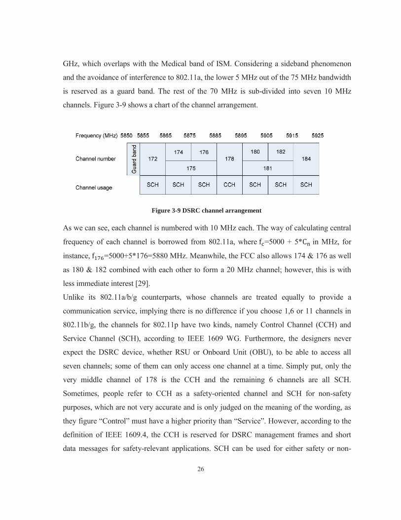
channels. Figure 3-9 shows a chart of the channel arrangement.
Figure 3-9 DSRC channel arrangement As we can see, each channel is numbered with 10 MHz each. The way of calculating central
frequency of each channel is borrowed from 802.11a, where =5000 + 5* in MHz, for
instance, =5000+5*176=5880 MHz. Meanwhile, the FCC also allows 174 & 176 as well
as 180 & 182 combined with each other to form a 20 MHz channel; however, this is with
less immediate interest [29].
Unlike its 802.11a/b/g counterparts, whose channels are treated equally to provide a
communication service, implying there is no difference if you choose 1,6 or 11 channels in
802.11b/g, the channels for 802.11p have two kinds, namely Control Channel (CCH) and
Service Channel (SCH), according to IEEE 1609 WG. Furthermore, the designers never
expect the DSRC device, whether RSU or Onboard Unit (OBU), to be able to access all
seven channels; some of them can only access one channel at a time. Simply put, only the
very middle channel of 178 is the CCH and the remaining 6 channels are all SCH.
Sometimes, people refer to CCH as a safety-oriented channel and SCH for non-safety
purposes, which are not very accurate and is only judged on the meaning of the wording, as
they figure “Control” must have a higher priority than “Service”. However, according to the
definition of IEEE 1609.4, the CCH is reserved for DSRC management frames and short
data messages for safety-relevant applications. SCH can be used for either safety or non-
27
safety purposes. On July 20, 2006, the FCC further defined services for 172 and 184
channels, which are the two ones located at the edges of the DSRC band. Under FCC 06-110
2006, channel 172 was sued “exclusively for v2v safety communications for accident
avoidance and mitigation, and safety of life and property applications.” Meanwhile, channel
184 is designated as “exclusively for high-power, long-distance communications to be used
for public safety applications involving safety of life and property, including road
intersection collision mitigation”. Through these definitions, at least we cannot use these two
channels for road map updating or travel guide purposes.
3.6 Transmission Power
3.6.1 WLAN Transmit Power Regulation
It is important to understand that there is a transmit power limit on any communication
system, either by regional regulation or public health consideration. For instance, the
maximum transmit power for a GSM base station (BS) and mobile station (MS) are 20 W
and 2 W. One of the most important reasons to put restrictions on MAX PTx (Maximum
Power Transmitted) is due to interference. This conception has been heavily deployed in
mobile networks, whereby inappropriate transmit power often causes handover failure, cross
section coverage or even an isolated island effect. Meanwhile, although we often define a
channel in certain precise frequency ranges, which is actually very ideal, all hardware
working at a certain carrier frequency will generate a sideband lobe beyond its intentional
frequency band. The IEEE defines a transmit frequency mask for the 802.11 family, under
which the first sideband lobe, which is ±11 MHz with a width of 22 MHz from the centre
frequency of the main carrier frequency, must be at least 30 dB less than the main lobe. Also,
any other sideband lobes ± 22 MHz from the central main lobe must be 50 dB lower [30].
Figure 3-10 gives an illustration of a transmit spectrum mask and sideband lobe interference.

28
Figure 3-10 Transmit spectrum mask, and side band interference The term of transmit power limit has dual meanings, including power generated and power
transmitted. The former often refers to the power of Intentional Radiator (IR), including all
components from transmitter to antenna, but excludes antenna. The latter has a much more
popular term (Equivalent Isotropically Radiated Power (EIRP)), which means the highest RF
signal strength transmitted from a particular antenna. We can conclude that, if there is no
gain for antenna, the power of IR will be equal to EIRP.
The FCC in the United States and controlling entities in other countries set limitations both
on power of IR and EIRP for 802.11 standard suites, depending on frequency band and
communication methods, i.e. Point to Multipoint (PtMP) or Point-to-Point (PtP). It indicates
that the RF designers need to pay attention not only to power emitted by an antenna but also
the amount sent to it. Concerning ISM 2.4 GHz band and 5 GHz UNII band for PtMP, the
FCC allows maximum power of IR to be 1 W (30 dBm) and EIRP to be 4 W (36 dBm).
Figure 3-11 gives an illustration of the power of IR of 5 GHz PtMP regulations.
Figure 3- 11 5 GHz Power IR regulations For 2.4 GHz PtP, the maximum power of IR is still 1 W but the maximum EIRP flexibly
29
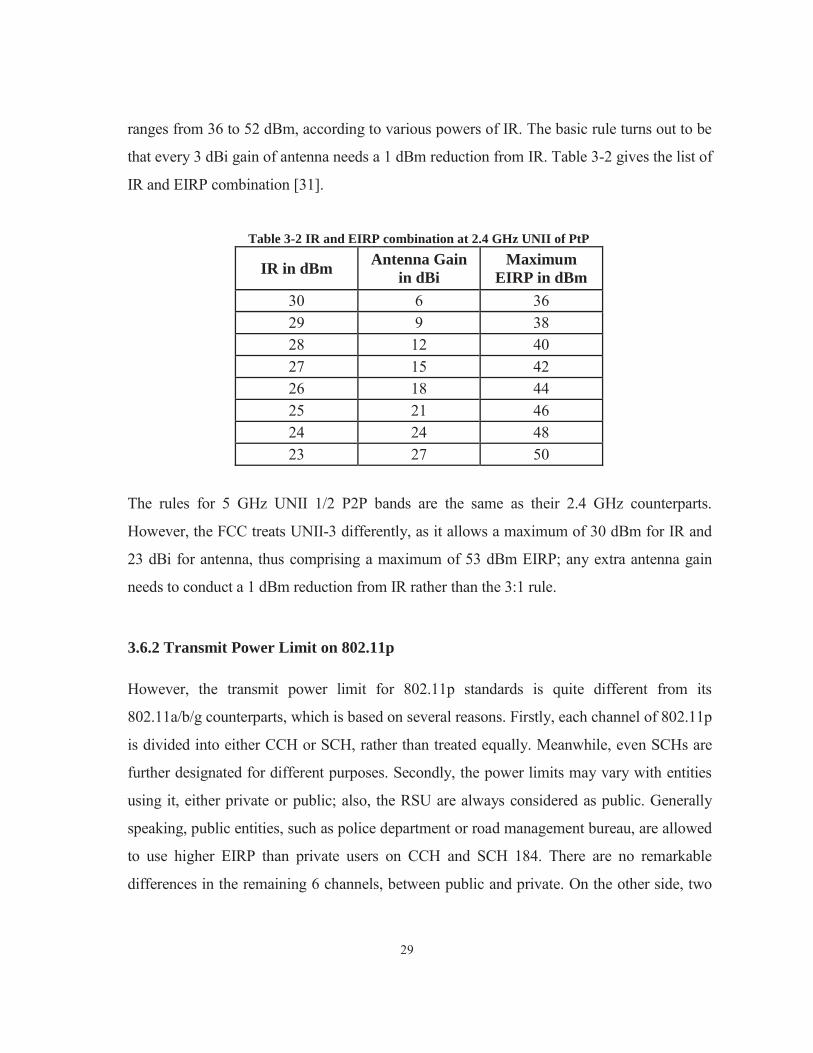
ranges from 36 to 52 dBm, according to various powers of IR. The basic rule turns out to be
that every 3 dBi gain of antenna needs a 1 dBm reduction from IR. Table 3-2 gives the list of
IR and EIRP combination [31].
Table 3-2 IR and EIRP combination at 2.4 GHz UNII of PtP
IR in dBm Antenna Gain in dBi
Maximum EIRP in dBm
30 6 36 29 9 38 28 12 40 27 15 42 26 18 44 25 21 46 24 24 48 23 27 50
The rules for 5 GHz UNII 1/2 P2P bands are the same as their 2.4 GHz counterparts.
However, the FCC treats UNII-3 differently, as it allows a maximum of 30 dBm for IR and
23 dBi for antenna, thus comprising a maximum of 53 dBm EIRP; any extra antenna gain
needs to conduct a 1 dBm reduction from IR rather than the 3:1 rule.
3.6.2 Transmit Power Limit on 802.11p However, the transmit power limit for 802.11p standards is quite different from its
802.11a/b/g counterparts, which is based on several reasons. Firstly, each channel of 802.11p
is divided into either CCH or SCH, rather than treated equally. Meanwhile, even SCHs are
further designated for different purposes. Secondly, the power limits may vary with entities
using it, either private or public; also, the RSU are always considered as public. Generally
speaking, public entities, such as police department or road management bureau, are allowed
to use higher EIRP than private users on CCH and SCH 184. There are no remarkable
differences in the remaining 6 channels, between public and private. On the other side, two

30
channels for short distance communication 180 and 182 have lower power limits than other
channels. Private OBUs working on them are allowed a higher power of IR than RSUs and
there are no limits defined on public OBUs, which is understandable, since antennae on
OBUs generally have less gain than RSUs. Table 3-3 lists detailed power limits for channels
of 802.11p standards [32].
Table 3-3 Max Power for IR and EIRP
All in dBm
Channel
Public RSU Private RSU Public OBU Private OBU Max
Power of IR
Max EIRP
Max Power of IR
Max EIRP
Max Power of IR
Max EIRP
Max Power of IR
Max EIRP
172 28.8 33 28.8 33 28.8 33 28.8 33 174 28.8 33 28.8 33 28.8 33 28.8 33 176 28.8 33 28.8 33 28.8 33 28.8 33 178 28.8 44.8 28.8 33 28.8 44.8 28.8 33
180 10 23 10 23 not defined
not defined 20 23
182 10 23 10 23 not defined
not defined 20 23
184 28.8 40 28.8 33 28.8 40 28.8 33
One more thing that needs to be mentioned here is the RSU height. There is restriction on the
height of RSU at a maximum of 15 meters. However, the above table is just for height equal
or lower than 8 meters, whose excess requests reduction of EIRP correspondingly.
3.7 Wireless Channel Characteristics
3.7.1 Overview The design of a wireless network requires much more effort compared to the wired ones. The
transmission medium for the latter one is generally stable and scalable. For instance, the
coated fiber cable definitely would provide extremely high throughput, while affected little
by environmental changes. On the other hand, although the cost-free wireless medium is

31
almost everywhere, a designer has to take many more aspects into consideration. The three
main factors dominating wireless communication are attenuation, fading and the Doppler
effect. The main reason leading to wireless communication complexity is the channel
characteristics not just varying according to different radio link technologies, such as
working frequency, modulation mechanism, and bandwidth, but also different application
environments. That indicates that the overall channel characteristics are the interaction
between the nature of transmission systems and changing environments. In short, there is no
absolute solution for any wireless system but only better refined approximate ones.
The three factors mentioned above are mainly used to describe the effects based on different
attributes of a communication environment. Under fixed radio link technology, attenuation
indicates signal loss being mainly due to transmission distance and absorption. Meanwhile,
fading subdivided into small and large scale ones is caused by a multipath propagation
phenomenon related to surrounding objects. The last Doppler effect happens when there is a
relative speed difference between Tx and Rx. They have remarkable impacts on the overall
performance of wireless communication but are not always harmful. For instance, in respect
to multipath propagation, some Fresnel zones will increase signal strength, thus helping to
overcome some path loss [33]. Therefore, different channel models have been brought out
and kept in modification in order to better describe the channel characteristics for given
wireless communication systems.
802.11p needs to be deployed in a highly dynamic environment and is also time-critical.
Therefore, even a channel model fitting 802.11a mainly under a stationary environment for
regular home & office usage cannot be applied on 802.11p directly. Although, it is only a
modified version of 802.11a; in most cases, there is a noticeable difference between them.
3.7.2 Channel Models for 802.11p There are various channel models for different types of wireless communication-based and
working environments. For instance, the fading component analysis can mainly be divided
into Rayleigh and Rician; the former one is for propagation without dominant LOS, and the

32
latter one is used for the opposite case. Empirical path loss models widely adopted in Mobile
Phone Networks, such as Okumura-Hata or Walfish-Ikegami, cannot be used for 802.11p
directly, due to significant differences in operation frequencies or modulation mechanisms.
Among all the proposed models for VANET, two models will be introduced, as follows:
The main general model for the empirical study of VANET channel characteristics can be
expressed as follows in dB unit [34],
P(d)= (Equation 3-1)
is the transmission power at reference distance which is often used in WLAN link
budget calculation, normally 1 meter distance away from the transmitter antenna. n refers to
pathloss exponent. and Y contribute to large and small scale fading, respectively. The
former one has a Gaussian distribution with when modeling in a
log-normal variant. Y can be modeled either Rican or Rayleigh..
A Two Ray Path Loss Model takes a LOS dominant signal into consideration. We use the
V2V scenario for instance. The received signal is the combination of LOS and reflected
signal by the ground. Figure 3-14 illustrates the situation of this model.
Figure 3-12 Two Ray Path Loss Model Based on free space path loss, the received signal strength of the two ray model can be
refined as follows [35]:
= [ (Equation 3-2)
Where the path length of LOS and reflection are annotated as . , L and represent

33
reflection, the coefficient, absorption factor and phase rotation of reflected signal.
3.8 Summary
In this chapter, we gave the reason why IEEE 802.11p is allocated a 5GHz spectrum and
analysed its attributes by using 10 MHz for a channel bandwidth. It shows that the
modification of PHY and adoption of the OFDM scheme enhance its capability of
overcoming undesirable and dynamic communication environments on VANET.

34
Chapter 4 Medium Access Control and Quality of Service
4.1 MAC Protocol for IEEE 802.11 Standards
4.1.1 Overview The MAC, as its name implies, refers to the mechanism of accessing the communication
medium when there are multiple stations (STAs) operating in the same channel. On the other
hand, Quality of Service (QoS) indicates the control mechanism in data networks that tries to
ensure a certain level of performance to a data flow, which is in accordance with requests
from the application program. These two terms are actually tightly related. In wireless
networks, due to their remarkable distinguishing feature, as oppose to their wired counterpart,
people makes much more effort on a MAC mechanism in order to achieve better
performance.
Generally, MAC protocols can be divided into two main classes: deterministic and random,
whose protocols may be either under centralised or decentralised control. Since 802.11p is
for a highly dynamic and unpredictable environment, its MAC protocol can only be chosen
from a random class rather than a deterministic one. Figure 4-1 provides an overview of
various MAC protocols.
Figure 4- 1 Overview of Different MAC Protocols [36] 4.1.2 Collision Avoidance Mechanism

35
IEEE 802.11 standards adopt a Carrier Sense Multiple Access with Collision Avoidance
(CSMA/CA) protocol to ensure only one device transmits at any one time, in order to reduce
that eliminating collisions within their CSMA mechanisms are the same as each other but
CA mechanisms might still vary according to different standards. In general, there are three
kinds of elements incorporated into each other to perform CA: Interframe Spaces (IFS),
contention window (CW) and binary exponential backoff (BEB), and RTS/CTS. The first
two are used to provide a double collision guard by letting STA wait for an IFS interval,
when sensing the medium is idle rather than transmitting immediately, and extra contention
window time for further collision avoidance. The last one is actually optionally deployed to
address hidden node problems in WLAN. When STA gains the rights of accessing the
medium, instead of sending data frames immediately, it will send RTS in which there is a
Duration sub-field to indicate how long the whole process of transmission will last, including
at least three intervals of Short IFS (SIFS), one CTS, one Data Duration and one ACK. This
makes all STAs in the communication domain of the transmitting device obtain the
information about how long the medium will be occupied. The destination STA then sends a
CTS also containing duration information of one SIFS and CTS shorter than its RTS
counterpart, which will be received by all STAs in the communication domain of the
receiving device. The combination of the above-mentioned two procedures eliminates the
hidden node problem. Figure 4-2 illustrates these mechanisms.

36
Figure 4-2 RTS/CTS Mechanism addressing hidden node problem After deciding the CSMA/CA is a basic MAC protocol for 802.11p, from Figure 4-1, we can
further see that there are two choices for MAC protocol: 802.11 Distributed Coordination
Function (DCF) and 802.11e EDCA. The fact is that, in original 802.11 standards, there are
only two medium access coordination functions defined: DCF and Point Coordination
Function (PCF). The former is contention-based and is mandatory for a basic service set
(BSS) and independent BSS (IBSS) applying 802.11 standards. On the other hand, PCF is an
optional, contention-free mode, but it requests centralised topology. Concerning the QoS,
802.11 standards are designed to merely provide a best effort service and also when in
shortage of a built-in mechanism for real-time services, which can hardly be used for either
throughput or delay-sensitive applications. It implies that both DCF and PCF are not directly
suitable to DSRC. Such a situation changed when the Enhancement Task Group in 2005
brought up an approved amendment standard (IEEE 802.11e), in which a set of QoS
enhancements for WLAN applications were made by modifying the MAC layer in order to
provide differentiated classes of services. In 802.11e, both DCF and PCF enhancements have
been made through a new coordination function called the Hybrid Coordination Function
(HCF) with two types of channel access mechanisms, EDCA and HCF Controlled Channel
Access (HCCA), which evolved from DCF and PCF, respectively [37]. All the above-
mentioned became the very reasons why 802.11p chose EDCA to be a MAC protocol for

37
QoS purposes. However, we need to notice that the EDCA is absolutely not an isolated
protocol but instead shares lots of similarities with its ancestor. Figure 4-3 illustrates a brief
relationship between these protocols.
Figure 4- 3 MAC Protocols Relationship 4.2 Enhanced Distributed Channel Access (EDCA)
4.2.1 Introduction of EDCA Mechanism As mentioned previously, IEEE 802.11 standard was designed to provide experience of an
Ethernet-like service over wireless, which is often referred to wireless Ethernet by virtue of
supporting a best-effort service. On the other side, the 802.11p MAC layer for QoS purposes
should focus on the prioritisation of important safety and time-critical messages, whereby
making the application of normal 802.11 standards impractical. Since 802.11p is a cross-
layer protocol, its PHY is similar to 802.11a and the MAC layer adopting EDCA proposed
by IEEE 802.11e for QoS guarantee. Note that the term of enhanced DCF (EDCF) is used
instead of EDCA, as it evolved from DCF in an earlier version of 802.11e draft [38].
The 802.11e is an approved amendment standard which was brought up by the Enhancement
Task Group (TG) in 2005, whereby a set of QoS enhancements for WLAN applications was
provided by modifying the MAC layer and also offering differentiated classes of service.
Actually, the most well-known technology adopting 802.11e is Wimax. Besides providing an
enhanced MAC mechanism, there are also two kinds of QoS defined in 802.11e, namely
prioritised and parameterised QoS [39]. The parameterised one is also a strict requirement

38
quantitatively, and obviously 802.11p is only capable of providing former ones, under which
frames arriving at the MAC layer would be labeled as different user priorities by the upper
layer and differentiated channel access will be performed. It is understandable that the frame
with the highest priority will be sent through the channel first. There are two main
remarkable conceptions in 802.11e, thus distinguishing it from DCF or PCF, which is stated
as follows:
A Traffic Identifier (TID) is a value in a MAC service data unit (MSDU) ranging from 0 to
15. The value from 0 to 7 indicates user priority of the frame, whereby 7 is the lowest
priority. Meanwhile, the value from 8 to 15 is used to identify which traffic stream the frame
belongs to and these are often called traffic stream identifiers (TSIDs). There are eight
different TSIDs that can be assigned on each traffic stream, which means that 8 TSs per
station can be achieved [40].
Transmission Opportunity (TXOP) is a bounded time interval when STA is permitted to
send a series of frames which define when STA can transmit and what the maximum
transmitting duration is (TXOP limit). A TXOP obtained from EDCA contention is called
EDCA TXOP. The value of a TXOP limit is determined by the AP, according to the rules of
the channel access schemes and is informed to all STAs through beacons. In short, TXOP
adoption makes the transmission time for each STA more controllable and predictable,
together with the enhancement on protocol.
As mentioned earlier, there are eight respective values ranging from 0 to 7 of user priority
(UP) in each MSDU. The MAC layer will categorise each frame into its corresponding
access category (AC) according to its UP value. The AC acts as a banner for the common set
of EDCA parameters adopted by STAs for channel contention purposes.
The EDCA defines four ACs, namely AC_BK (Background), AC_BE (Best Effort), AC_VI
(Video) and AC_VO (Voice traffic) [41]. The mapping relationships between eight UPs and
four ACs can be found in Table 4-1, as follows:

39
Table 4-1 UP’s map to ACs
Priority User Priority (UP) Access Category Designation
(Informative)
Lowest 1 AC_BK Background
2 AC_BK Background
0 AC_BE Best Effort
3 AC_BE Best Effort
4 AC_VI Video
5 AC_VI Video
6 AC_VO Voice
Highest 7 AC_VO Voice
There is an interesting fact drawing our attention when reviewing the table; UP 0 is the
default UP value with the lowest priority within eight value groups. However, its
corresponding AC priority is higher than its counterparts of UP 1 and UP 2, which are for
background services providing support to applications without the need to process the data
immediately and thus possess the lowest priority. On the other hand, AC_VO is with the
highest priority and should be used for all management frames. Figure 4-4 illustrates the
EDCA mechanism at a MAC layer.
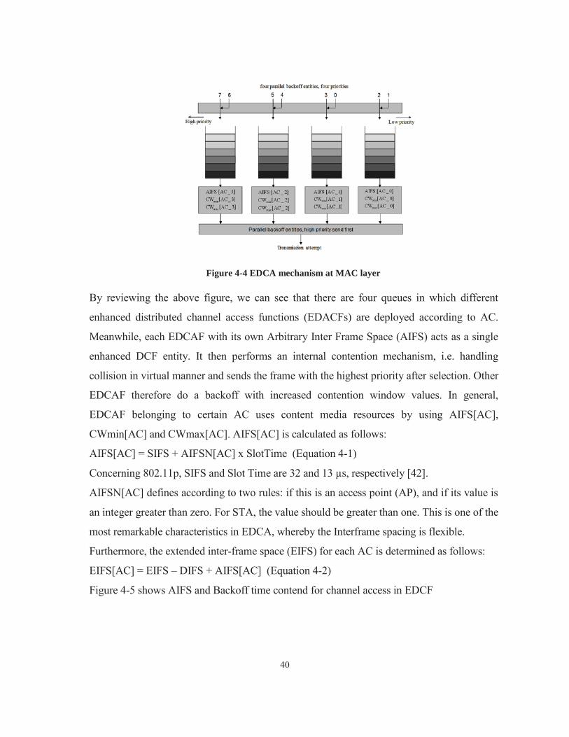
40
Figure 4-4 EDCA mechanism at MAC layer By reviewing the above figure, we can see that there are four queues in which different
enhanced distributed channel access functions (EDACFs) are deployed according to AC.
Meanwhile, each EDCAF with its own Arbitrary Inter Frame Space (AIFS) acts as a single
enhanced DCF entity. It then performs an internal contention mechanism, i.e. handling
collision in virtual manner and sends the frame with the highest priority after selection. Other
EDCAF therefore do a backoff with increased contention window values. In general,
EDCAF belonging to certain AC uses content media resources by using AIFS[AC],
CWmin[AC] and CWmax[AC]. AIFS[AC] is calculated as follows:
AIFS[AC] = SIFS + AIFSN[AC] x SlotTime (Equation 4-1)
Concerning 802.11p, SIFS and Slot Time are 32 and 13 μs, respectively [42].
AIFSN[AC] defines according to two rules: if this is an access point (AP), and if its value is
an integer greater than zero. For STA, the value should be greater than one. This is one of the
most remarkable characteristics in EDCA, whereby the Interframe spacing is flexible.
Furthermore, the extended inter-frame space (EIFS) for each AC is determined as follows:
EIFS[AC] = EIFS – DIFS + AIFS[AC] (Equation 4-2)
Figure 4-5 shows AIFS and Backoff time contend for channel access in EDCF

41
Figure 4- 5 AIFS and Backoff Time Contend for Channel Access in EDCF 4.2.2 EDCA for 802.11p As IEEE 802.11p is designed exclusively for a Vehicle Environment, it adopts EDCA, while
maintaining some modifications. Multi-channel operation is the main difference of 802.11p
at a MAC layer from its counterparts, where all channels (CCH and SCH) are provided a set
of traffic categories for QoS guarantee purposes. Figure 4-6 provides an illustration of an
EDCA mechanism at 802.11p MAC layer.

42
Figure 4-6 EDCA at 802.11p MAC [43] There are still four ACs labeled from AC[0] to AC[3]. Under the CCH interval, each one can
be possibly explained, as follows:
AC[3]: with the highest priority, it is used for emergency information, especially for collision
avoidance application. Other instances can be obstacles, e.g. wet road surface, traffic light
break down.
AC[2]: concerns presence and speed information broadcasted by vehicles.
AC[1]: concerns the information from other vehicles for help, but is not strictly related to
safety issues.
AC[0]: concerns information aimed at establishing new non-safety-related connections via
SCHs.
However, we need to notice that the 802.11p standard was just finalised and that its
application is still being processed. The definition of each AC, either on CCH or SCH, will
largely rely on upper layers, especially the application layer designed by different
manufacturers and thus may be various.
Meanwhile, as 802.11p is used for time-sensitive application for safety purposes mainly and
because CCH and SCH are all allowed to perform real-time traffic, it is obviously beneficial

43
if we assign more time to CCH. However, for the sake of overall satisfaction, the tradeoff of
time allocation of the QoS guarantee mechanism has to be made in order to cope with large
and regular data traffic on SCHs, whilst meanwhile keeping CCH delay at an acceptable
range. According to what is mentioned above, each AC represents a specific EDCAF at the
MAC layer, which is further defined by corresponding parameters. Apparently, these EDCA
parameters, even with the same AC, will vary in different channel types. There are two
adaptive forms at IEEE 1609.4 for CCH and SCH, respectively, as shown in Table 4-2 and
Table 4-3.
Table 4-2 EDCA parameter for CCH [44]
AC Traffic Type CWmin CWmax AIFSN
AC1 background 15 511 9
AC0 best effort 7 15 6
AC2 video 3 7 3
AC3 voice 3 7 2
We can see from the above table that the AC1 is actually with the lowest priority not only
with the biggest CWmin and CWmax within the whole table but also the highest AIFSN,
which indicates its AIFS and backoff window will be the longest one. Meanwhile, AC0 is at
the middle priority among its counterparts, whose CWmin is just the CWmax of AC2 and
AC3 but AIFSN is doubly comparing with AC2. Concerning AC2 and AC3, with the same
contention windows, their AIFSN has only 1 slight difference ensuring AC3 is the top
priority.
Table 4-3 EDCA parameter for SCH [44]
AC Traffic Type CWmin CWmax AIFSN
AC1 background 15 511 7
AC0 best effort 15 511 3 AC2 video 7 15 2 AC3 voice 3 7 2

44
In contrast to Table 4-2, we can see that the EDCA parameter for SCH is more loosened than
what is applied on CCH. However, the AC3 for SCH at the highest priority is exactly the
same as its counterpart of CCH, maybe because SCH sometimes involves safety-oriented
application. There is a tradeoff between AIFSN and the contention window made in SCH.
As the AIFSN in SCH are all lower than their corresponding ones in CCH, it indicates that
all AIFS in SCH will be shorter than CCH, except AC0. Such a mechanism makes nodes get
ready to send frames by quickly entering into the backoff stage. By shortening the AIFS, the
collision probability might increase but it will be accepted as the deployment happens in
SCH, rather than strictly related to time-critical transmission. At the same time, the
contention windows, both min and max for SCH ranging from AC1 to AC2, are all greater
than CCH, which compensates for the shortcoming, due to the related lower AIFSN. For
instance, The CWmax value of AC0 in SCH proving the best effort traffic type is set at 511,
which means that EDCAF here is willing to ensure transmission reliability by doing
retransmission and waiting longer, in order to have ACK. To be more specific, Figure 4-7
illustrates the AIFS plus minimum backoff time for each AC in both channels.
Figure 4-7 AIFS and Backoff Time for CCH and SCH [43]

45
Since the channel environment for transmission is unpredictable, only minimum backoff
time can be given, since it is irreverent to the transmitting situation. The time parameter on
the chart matches what was mentioned previously. The time intervals of AIFS and backoff
time for the highest priority in both channels are the same. Followed by the AC2 and AC1,
their AIFS values in CCH are longer than SCH but backoff times are in a contrary situation,
which makes the total time interval shorter than SCH. The last AC0 turned out to be a bit
different, due to the same minimum backoff time in these two channels.
4.3 MAC Protocol Data Unit of 802.11p
The structure of a MAC protocol Data Unit (MPDU) is quite a delicate and complex part of
802.11 standards, based on the fact that a MAC layer carries out most functions in WLAN
communication, which generate a MPDU by wrapping MSDU received from LLC and then
handing to the PLCP sublayer in PHY, as mentioned previously.
In fact, there are four types of frames in 802.11, namely management, control, data and
reserved; however, an overall MPDU format is generally given regardless of frame type,
since the structure remains the same across all frames, even though not all parts are used in
every specific type. Meanwhile, the MPDU format can be further divided into two kinds -
QoS supportive and non-supportive - which implies that the format of 802.11p will be the
same as 802.11e, with an additional QoS field than normal 802.11 a/b/g standards. Figure 4-
8 illustrates the overall MPDU format.
Figure 4- 8 Overall MPDU Format of 802.11p/e A brief introduction for important fields/subfields shown above will be given as follows:
Frame Control: This 2 bytes long field is the most complex one in MPDU and can be further

46
divided into several sub fields shown in Figure 4-9.
Figure 4- 9 Sub-fields of Frame Control Currently, the protocol version is 00 and the remaining possibilities are reserved for future
use. Frame types are used to indicate four types of frames, as mentioned above. Table 4-4
details the type field instance.
Table 4-4 Type Field Instance
Bits Frame Type Example
0,0 Management Association, Authentication, Probe
0,1 Control ACK, CTS, RTS
1,0 Data
1,1 Reserved
Furthermore, the sub type field indicates the specific type of frame, for instance, 0000, 1010
and 0001, mean association request, Power Save (PS)-Poll and Data +CF-ACK, respectively.
As we know, fragmentation can be used in WLAN communication to support the division of
MSDUs into smaller elements carried out by More Frag Field set to 1, if there is a fragment
subsequently belonging to the same MSDU. However, it is necessary to point out that only
unicast frames will be fragmented rather than broadcast or multicast frames. In this case, the
MAC protocol will use the aFragmentationThreshold parameter in its management
information base (MIB) to judge whether the size of generated MPDU will exceed the
threshold by merely passing the whole MSDU to the MAC layer. If the answer is true, then

47
fragmentation will be conducted in order to break down MSDU and send each one separately.
1. Duration/ID and Address Fields: The former field lasting 16 bits long contains
information of NAV or short ID alternately. However, since only the power-save poll
(PS-Poll) uses a short ID tightly related to the PCF mechanism, this field is generally
representing duration for 802.11p application, under which Bit 15 is set to 0 and
maximum value 32767 in microseconds can be obtained by manipulating Bit from 0-
14. The four MAC address fields in MPDU are selectively used according to different
types of frames. In most cases, only addresses 1-3 contribute wireless communication
and address-4 is only for special situations, such as DS, which is also the reason why it
does not adjoin with the other three counterparts in MPDU. In short, Addresses-1/2 are
always the recipient/ destination addresses or the under ToDS/ FromDS addresses of
AP, respectively. Address-3 is generally the missing address, since under BSS, merely
indicating an address of AP is not enough and an extra field needs to be used for the
source or destination address. However, we can predict that in case there are two APs
in DS, the communication has to account for the full usage of four address fields.
Beyond that, a higher layer address mechanism, such as IP, will be needed. Under the
802.11p scenario, only addresses 1 and 2 join the procedure of communication in most
cases.
2. Frame Body and QoS Control Fields: The frame body often referred to MSDU is
passed from higher layer LLC. In fact, it is a bit difficult to find the maximum size of
MSDU in 802.11 standards, due to the evolution and advancement. This can be
explained twofold. Firstly, the 802.11-2007 standard defines that the maximum size for
MSDU is 2304 bytes for non-security mechanisms applied or 2312 (WEP)/2324
(TKIP) [45] as overheads are increased. Thus, the derived max length has three
possibilities, namely 2338 (non-security), 2346 (WEP), and 2358 (TKIP). Under the
QoS supported Frame structure, another 2 bytes need to be added on the above results,
thus making the theoretical maximum length 2360. On the other side, PSDU allows a
4095 maximum in length [46], although MPDU can only reach half of the size. It is not
correct to mark MSDU at 4095, as it violates the 802.11-2007 definition. Secondly, the

48
latest 802.11n brought up two novel schemes - aggregate MSDU and MPDU (A-
MSDU, A-MPDU) – which extended the maximum sizes to 3839/7935 and 65,535
octets, respectively [47]. Based on what is stated above, we can conclude that the max
MSDU for 802.11p should be less than 2304, due to no authentication mechanism
required. Concerning the QoS control field, which is 16 bits long and which bit 7 is
reserved, the first 3 bits are used to indicate TID and bit 4 is for End of service period
(EOSP) purposes, through setting 1 for transmission/ retransmissions, or 0 otherwise.
Bits 5-6 define the acknowledgement policy under different communication
procedures. Finally, multi-functions are carried out by Bits 8-15, in general, TXOP
limit, QAP PS Buffer State, TXOP duration requested and Queue size.
4.4 Summary
In this chapter, we introduced the mechanisms of MAC protocols for IEEE 802.11 standards.
Meanwhile, 802.11p adopts EDCA as a more advanced one revolving from DCF, which is
not only for collision avoidance but also for concentrating on providing QoS. Its traffic
stream is granted different EDCAF according to its TID out of four kinds or channel types
(CCH or SCH) in order to provide a priority-oriented service. Also, the structure of MPDU
of 802.11p has been reviewed.

49
Chapter 5 VANET Topology and WAVE Short Message
5.1 Multi-Channel Operation`
Due to the nature of DSRC, it needs to tune to CCH and SCHs alternately. By reviewing the
DSRC protocol suite given in Chapter 2, we can see that the MAC layer of DSRC is divided
into two sub-layers. The upper MAC layer, which is defined by IEEE 1609.4, is mainly used
for three functions related to multi-channel operation, namely channel coordination, channel
routing and User Priority. The lower one focuses on wireless medium access. Such division
is a very unique characteristic of DSRC, thus distinguishing itself from its counterparts, such
as 802.11a/g, as they only work in certain operational channels, whose MAC structures are
relatively simpler than their DSRC counterparts.
Even though IEEE Std 1609.4-2010 allows one or more PHY devices to be equipped on
vehicles, it only provides examples and guidelines for a single-PHY device case under one
CCH and SCH. Figure 5-1 gives an illustration of the 1609.4 channel access mechanism.
Figure 5-1 1609.4 Alternating Channel Access Mechanisms [48] The combination of CCH and SCH intervals is called Sync interval, as defined by 50ms each.
Moreover, we notice that there is a guard interval (2ms) used to address radio switching and
timing inaccuracies among different devices. In VANET, CCH is used for the exchanging of
management information, such as WAVE Short Message (WSM) and Service
Advertisements. Therefore, it is mandatory for all RF devices to monitor this channel at the
same time in most cases. However, it is apparent that such an even division access
mechanism cannot meet the requirements of relatively heavy data transmission, as there is no

50
need to always allocate half the length of Sync to CCH for short message exchange. On the
other hand, SCH can also be used for traffic safety communication rather than CCH only.
Therefore, IEEE 1609.4 actually gives four possible access choices: continuous, alternating,
immediate and extended, thus representing different combination types of CCH and SCH
according to different applying environments. The first access choice refers to always
monitoring either CCH or SCH, which is a special scenario because, at that time, SCH is
capable of sending WSM, despite it being optional. Meanwhile, the last two choices will
prolong the SCH interval, while also shortening the CCH interval. Figure 5-2 shows these
four access mechanisms.
Figure 5-2 Channel access options: (a) continuous, (b) alternating, (c) immediate, and (d) extended 5.2 Characteristics of VANET Topology
5.2.1 Broadcast Mechanism on CCH Due to the multi-channel operation nature of WAVE communication as well as its highly
dynamic environment, its network topology is quite different from 802.11 standards and is

51
much more complex. Meanwhile, we should selectively adopt traditional WLAN topologies
in order to understand VANET, rather than just matching them with each other. First and
foremost, 802.11p std-2011 clearly defines “communicating data frames outside the context
of a BSS” and that the main purpose of V2X communication is for traffic safety that is based
on the broadcasting on CCH in general, which indicates that every RF device nearby can
exchange such messages. It is irrelevant as to whether OBUs or RSUs should consist of a
service set first or not, as the broadcasting uses a wildcard MAC address by setting
0xFFFFFFFFFFFF [49] . The conception of broadcasting may be popular in wired networks,
since routers are able to filter the broadcast packets for safety issues. However, the wireless
medium is a typical shared medium, which is analogous to a hub rather than a switch, not to
mention a router. Heavy broadcasting will cause broadcast storms and will severely impact
the throughput of networks. Therefore, the normal IEEE 802.11 standard places a restriction
on the broadcasting functionality, which can be only used for beacon or probe purposes.
Figure 5-3 provides an example of a broadcast storm in both wired and wireless networks.
Figure 5-3 Broadcast Storm in Wired and Wireless Networks 5.2.2 WAVE Basic Service Set (WBSS)
As long as we remember that the nature of WAVE communication is for broadcasting on
CCH generally, the remaining communication for services rather than safety purposes can

52
additionally happen on SCHs. In this case, RF devices equipped on OBUs or RSUs have to
consist of a WAVE Basic Service Set (WBSS) [50]. From this point-of-view, we should
realise that the V2X communication can be based on non-WBSS and WBSS, which are able
to exist simultaneously. The non-WBSS is the main topology category for broadcasting
purposes only, whereby STAs may consist of a WBSS for SCH communication; however, it
is not mandatory. Figure 5-4 depicts this situation.
Figure 5-4 Non-WBSS and WBSS Topology Concerning WBSS, we should not use traditional WLAN to understand it. In some journals,
there is usage of the term ‘WAVE IBSS’ (WIBSS), whereby the author tries to analog
WBSS and WIBSS to BSS and ad-hoc networks, respectively [51]. Personally, I do not quite
agree that methods, such as the inner mechanism of VANET, are remarkably different from
normal WLAN topology. This is based on several facts:
1. There is no access point in VANET, but only service provider and client. Since RSU
is a stationary device and is often with high throughput, people often mistakenly take
it as an AP. However, in a distribution system, all STA traffic should go through a
portal device, i.e. AP, which is totally not the case in VANET. In a WBSS, even RSU
acts as a service provider, while OBUs can still perform point-to-point
communication. Meanwhile, the communication duration between RSU and OBU is
actually very short, whose mean estimate is only 3.6 seconds [52]. Thus, it is more
appropriate that we treat RSU and OBU equally in order to be all SATs without

53
differentiation.
2. There is no authentication or association procedure in WAVE Communication [53].
In a normal WLAN scenario, there are a lot of procedures in association, and much
more in authentication. For instance, under passive scanning, the AP will keep
sending a beacon at an interval around 0.1 or 0.2 seconds. STA captures this beacon
and sends an association request. AP then sends back an association confirmation
frame and awaits ACK from STA. Such a procedure is too time-consuming and is not
compatible with WAVE Communication. Security issues brought up by eliminating
such a procedure are expected to be addressed by a higher layer rather than PHY or
MAC.
3. WBSS is ephemeral and is a dynamically organised topology. Unlike BSS or even
IBSS, whose network topologies are quite stable and rarely change, WBSS is
occasionally generated when a SAT would like to be a service provider by sending a
WAVE Service Advertisement frame on CCH. Other SATs receive this frame and
hand it to an upper layer in order to decide whether it joins or not. Meanwhile, even
STA would have already become a member of certain WBSS; the termination of
membership is allowed to happen anytime, without any interaction with the service
provider. Since the formation of WBSS is just for services in a very short-term
duration and because every STA has the right to be a service provider for a certain
application, the WBSS is thus a very unstable and loose topology without any
restriction on the number of members and lasting period.
5.3 WAVE Short Message Protocol (WSMP)
5.3.1 Introduction From Figure 2-1, we can see that there are two kinds of protocol suites sitting in the higher
layer, namely WSMP and IPv6 suites [54]. The former is exclusively for time-critical and
safety-oriented communication in WAVE, without the need for an IP addressing mechanism,
since it is always broadcasted on either CCH or SCH. On the other side, the latter (IPv6) can
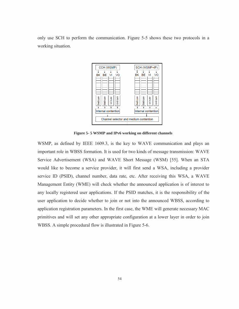
54
only use SCH to perform the communication. Figure 5-5 shows these two protocols in a
working situation.
Figure 5- 5 WSMP and IPv6 working on different channels WSMP, as defined by IEEE 1609.3, is the key to WAVE communication and plays an
important role in WBSS formation. It is used for two kinds of message transmission: WAVE
Service Advertisement (WSA) and WAVE Short Message (WSM) [55]. When an STA
would like to become a service provider, it will first send a WSA, including a provider
service ID (PSID), channel number, data rate, etc. After receiving this WSA, a WAVE
Management Entity (WME) will check whether the announced application is of interest to
any locally registered user applications. If the PSID matches, it is the responsibility of the
user application to decide whether to join or not into the announced WBSS, according to
application registration parameters. In the first case, the WME will generate necessary MAC
primitives and will set any other appropriate configuration at a lower layer in order to join
WBSS. A simple procedural flow is illustrated in Figure 5-6.

55
Figure 5- 6 Simple Procedure Flow of WBSS Joining 5.3.2 Frame Format of WSA There are two kinds of WSA formats: secured and unsecured. Concerning the unsecured one,
it consists of three fields, namely Protocol Version, Type and Wave Service Advertisement.
Meanwhile, there are an additional two fields (Security Header and Trailer) for the secured
WSA format. Within all fields, the Wave Service Advertisement is the most complicated part,
including many sub-fields with various lengths in octets. In general, this field can be
subdivided into four smaller parts: header, service info, channel info and WAVE Routing
Advertisement [56]. Figure 5-7 shows the format.
Figure 5- 7 Format of Wave Service Advertisement Sub-Field The header includes one mandatory octet field, together with optional extension fields.
Within one octet, the first five bites are used to indicate the WSA version, which is currently
set to 1, and the last two bytes, as change count is used by numbering the WSA frame in
order to let the receiver decide whether this is the repeated WSA. The extension field is not
mandatory but should not exceed 255 octets, as restricted by IEEE 1609.3-2010. The first is
the repeat rate, which is 8 bits long and which indicates the sending rate of WSA for a

56
broadcasting service every 5 seconds. The receiver should use this field to evaluate link
quality, which is followed by “Transmit Power Used”, “2DLocation”,
“3DLocationAndConfidence”, “Advertiser Identifier” and “Country String”, which function
as their names imply.
Referring to the Service Info field, it provides information of an application service, with a
unique PSID for each one, which implies that this field can be repeated when more than one
application is provided. 1609.3 allows 0 through 32 instances of this field in the WSA.
Figure 5-8 illustrates the format of this field.
Figure 5- 8 Service Info Format As we know, DSRC is a typical priority-oriented communication; channel access and service
evaluation, both at Rx and TX, are all based on it. Thus, the “ServicePriority” field is
adopted for this purpose, which is 8 bits long and which provides 64 degrees of priority level
– 0 being the lowest. Moreover, there are some interesting fields in the extension field (also
not exceeding 255 octets). For instance, there is a 128 bits IPv6 address and Provider MAC
address for traditional IP-based communication. Concerning the RCPI Threshold field in 1
octet long borrowed from IEEE802.11k, it ranges from 0 to -110 in dBm and provides a
recommendation to be received for a discarding decision.
The Channel Info field is a relatively fixed-length segment; 6 out of its 7 sub fields are all 1
octet in length and only have exception in the extension field. Furthermore, there shall be 0
to 32 instances of Channel Info segments in the WSA. Each indicates the characteristics of
one channel, which is associated with zero or more Service Info and which contains the
fields. Within these sub fields, some of them are especially important to WAVE

57
communication. Figure 5-9 provides the format of Channel Info.
Figure 5- 9 Format of Channel Info For instance, the Channel Number indicates the number of the channel to which the
accompanying information pertains. As we know, DSRC is a multi-channel operation; the
procedure of joining WBSS only relies on receiving WSA without any further interaction.
The STA, belonging to certain WBSS, has to know which SCH out of six is used to provide
the application service and therefore can monitor this channel at its interval. Meanwhile, the
Transmit Power Level represents the actual power in the output of the antenna connector for
transmission on associated channels. The extension field of Channel Info contains two sub
fields. The first one (EDCA Parameter Set) is adopted for QoS purposes. Since there is an
inner contention mechanism at MAC of DSRC, this field will include important parameters,
such as AIFSN, CWmax, CWmin and TXOP Limit, for each application provided. The
second segment of the extension field is Channel Access, which indicates the times in terms
of channel interval, during which the provider is on the associated SCH. If set to 0, it will be
considered as continuous access, both on a CCH or SCH interval. Otherwise, if set to 1, the
provider will be on an SCH interval, only as alternating access.
The final segment of WSA is WAVE Routing Advertisement (WRA), which is also an
optional choice. As its name implies, WRA is used to provide information about
infrastructural internetwork connectivity, in order to let receivers join the advertised IPv6
network. The adoption of IPv6 is one of the remarkable characteristics of WAVE
communication, which can be divided into two logical parts. The first 64 bits, which
represent the global routing prefix, and the remaining 64 bits are called host interface

58
identifiers, which are created by using the MAC address of a host interface or random
generation number if privacy is concerned. More than a decade ago, network engineers
started worrying about the exhaustion of IPv4 addresses and were thus researching a 128 bit
long IPv6 addressing mechanism, which was supposed to provide 3.4 X and ultimately
provide a resolution to that issue. In February 2011, the Internet Assigned Numbers
Authority (IANA) assigned the last top level (/8) block of IPv4 to 5 regional internet
registries (RIR). However, since the prediction of exhaustion was largely relying on the stage
of internet development, the recent and future explosive increase of internet users and
providers drastically shortened that deadline. According to the research of the UN’s
Telecommunications Agency, there were two billion internet users in 2011, not including
other industrial regions that require IP addresses, such as GPRS. If we had not adopted
technologies, such as classless routing or network address translation (NAT), the exhaustion
would happen. Figure 5-10 illustrates the format of WAVE Routing Advertisement.
Figure 5- 10 Format of WAVE Routing Advertisement The Router Lifetime is two bytes long and indicates the duration of validity of the Default
Gateway and associated information. Meanwhile, the Default Gateway contains a 128 bits
long IPv6 address of the router for SCH communication. The extension field contains a
Secondary DNS and Gateway MAC address, which all allow the service to function. All
these structures mentioned are for the purpose of providing regular IP connectivity and for
eliminating the boundary between data communication for WAVE and internet access.
5.3.3 Frame Format of WSM The WAVE Short Message is exclusively used for CCH control information, which is

59
related to traffic safety purposes and which should be distinguished from WSA. The
generation of WSM is from a high layer to MAC, via different primitives with different
headers and tails at different layers. However, due to the nature of WAVE, this mechanism
will be quite different from traditional WLAN standards. Figure 5-11 shows the generation
of the WSM package.
Figure 5- 11 Generation of WSM Package [56] As we can see from the above figure, the header of the WSM package is the same at a
different layer starting from a higher layer; this is unlike a normal WLAN lower layer, which
will put its own header and will wrap a higher layer frame into its payload area. This
phenomenon is due to important information, such as Destination Address, priority and
TxPow_Level, which are decided by the application and which are sent down as separate
parameters in the primitive form, rather than as part of WSM. The WSM passing through
LLC will finally be put in the LLC Data segment of the MAC Data field, together with an
LLC header and SNAP header.

60
The WSM can be further divided into six segments, whereby the extension field is optional
and the length of WSM Data varies. The one octet version field includes a first 4 bits
reserved for future usage and the remaining indicate the WSMP version, followed by the
PSID field, like WSA. Actually, since WSA and WSM both rely on a WSM protocol, their
format structures share lots of similarities. In the WSMP header extension field, it also
includes segments, such as channel number, Data Rate and Transmit Power Used, in order to
increase the communication performance in WAVE. Concerning the length field, which is
16 bits long and which indicates the WSM size in length, only 12 out of 16 bits are used
currently and the remaining 4 bits are reserved. Based on this, we can conclude that the
current maximum length of WSM is 4095 bytes, which is actually pretty long compared to
most wired and wireless standards. Generally, the TCP/IP protocol, which is based on
Ethernet, can only allow 1500 bytes at most and is called the maximum transmission unit
(MTU); it totals 1518 bytes when adding a header and the Cyclic Redundancy Code (CRC)
[56]. There is no problem for the 802.11 family to handle this, as their payload can take 2304
bytes and is big enough for a distribution system. Meanwhile, people would like to increase
the wireless MTU; it can hardly be carried out not only because of current applications
counting on the TCP/IP suite for networking but also the infeasibility of setting the MTU too
long, especially for wireless communication.
The mechanism of how many maximum bytes are contained in each frame is called
fragmentation. Most of the time, we are not allowed to adjust it on RF devices for several
reasons. If the MTU is set too small, we will have lots of overheads in communication,
interframe spacing and ACKs, which are definitely inefficient to usage of bandwidth and
which are harmful to throughput, since atomic procedure in wireless is a three-way
handshake. On the other side, setting a very big MTU seems to overcome these problems
previously mentioned; however, it is worse than setting a small fragmentation in most cases.
Firstly, even though each device in a wireless communication domain still has a fair right to
content for the medium, it may occupy too long a time for sending frames in big sizes, as
other STAs have to wait throughout the period. Secondly, attenuation and corruption of
packet data will require the retransmission of long bit frames rather than just parts of them.

61
Therefore, such a setting also drastically reduces wireless throughput and ultimately wastes
bandwidth. Just like most designing tasks, it is important to find a tradeoff between MTU
and overheads for certain wireless communication environments, rather than having an
absolute solution that is good for all cases.
5.4 Summary
In this chapter, we reviewed a higher MAC layer protocol (IEEE 1609.4) for the multi-
channel operation of DSRC, which is based on CCH and SCH further adopting WSM and
IPv6, respectively, at higher layers of transmission. Such a mechanism brings STAs in
VANET form either a unique WBSS or non-WBSS topology on different channel intervals.
Meanwhile, formats of WSM and WSA, which are exclusively for the CCH broadcast mode,
have been carefully studied.

62
Chapter 6 Simulation Elements Configuration and Fundamental Scenarios
The OPNET Modeler Wireless Suite provides high fidelity modeling, simulation, and
analysis of a broad range of wireless networks. Given that OPNET is the de facto standard
for wireless network simulation, we decided to use OPNET. However since OPNET does
not have IEEE 802.11p modeling yet, we had to modify the current 802.11a protocol for our
study.
6.1 Introduction of 802.11p Simulation
All simulations conducted for the 802.11p performance study on following chapters will
base on OPNET 14.0 with wireless suite, which is a comprehensive analyzing tool for both
wired and wireless networks. Since the unique characteristics of 802.11p standards
distinguish themselves from other WLAN standards, many aspects, including but not limited
to operating frequency, bandwidth, broadcasting nature on CCH, QoS mechanism that is
based on EDCA, and road traffic situations, will have to be considered. One of the most
important things, which is needed to be noticed, is that we should not take 802.11p
simulation as a bunch of laptops equipped with 802.11a in movement. Instead, it should be
considered an absolutely different wireless standard exclusively for vehicular application.
By virtue of OPNET, most characteristics of 802.11p can be carried out in order to facilitate
relevant researches in this thesis. However, it is necessary to mention that the simulation
would not be able to cover every aspect of 802.11p but rather prove our best efforts to
approach it, due to two facts briefly stated as follows:
Firstly, 802.11p has just been finalised in July this year. Thus, there is no immediate module
able to be adopted from OPNET. As 802.11p is a modified standard of 802.11a, the
simulation inevitably relies on the amendment of its PHY and MAC parameters. Meanwhile,
even though OPNET is very professional software for wireless network research, its
limitation in functionalities makes it difficult to fulfil all mechanisms of 802.11p application.
For instance, there is no frequency switch function between CCH and SCH. Furthermore,

63
OPNET does not allow the deployment of multiple access categories on a single WLAN
workstation.
Secondly, as 802.11p will be applied to dynamically changing environments as well as the
main objective of this thesis being to focus on the analysis of performance based on its PHY
and MAC mechanisms, some factors, such as propagation model, terrain, and road traffic
situations, have to be chosen either ideally or empirically. Otherwise, the simulation results
will be affected by too many random factors and will handicap the general analysis.
Despite the disadvantages mentioned above, these are actually the very factors bringing
challenges and interests to the 802.11p simulation performance study, as most difficulties
and software limitations could be overcome by alternative ways.
The simulations and analyses in this thesis mainly focus on CCH performance of 802.11p, as
it is the most important and critical part of VANET application, which can be further divided
into several subsections in order to study the impacts, such as distance, packet size and
vehicle traffic flow on VANET individually. Finally, a comprehensive performance under a
dynamic environment will be studied.
6.2 Workstation Configuration and Explanation
The OPNET configuration for the node workstation is the key part of our simulation, which
contains necessary parameters for further topology deployment. Each main parameter is
explained as follows:
1. Min Frequency: Concerning CCH simulation, all vehicles should work at a central
frequency numbered 178 and should be between 5885 -5895 MHz. Therefore, Min
frequency should be 5885 MHz.
2. Bandwidth: All simulations choose 10 MHz, as standardised, and disregard the 20
MHz situation.
3. Physical Characteristics: 802.11p is a modification of 802.11a, which is the only
approximate choice in OPNET and which expects to bring the closest performance.

64
4. Data Rate: The data type of Data Rate in OPNET is double. As 3/6/12 Mbps are three
mandatory rates in 802.11p standards as well as the first two rates being adopted
under poor wireless communication, 6 Mbps will be used for CCH simulation, which
is a reasonable and popular choice for most IEEE papers related to 802.11p.
5. Transmission Power: We know that 802.11p is supposed to provide communication
within one kilometre, which will be adopted in simulations. Meanwhile, as OPNET
does not provide a power self-adjustment function, it is necessary to calculate precise
transmission power as a very important parameter, not only according to data rate but
also as the internal mechanism of OPNET. After reviewing and reading different
research papers, they show that different transmission power settings have been used,
such as 20, 40, or even 3 dBm, which cannot all be applied to my simulation directly.
A brief introduction of transmission power estimation is stated as an Appendix and
the result showing 0.01939555 W (12.877 dBm) is needed.
6. EDCA Configuration: Throughout our simulation, there are four kinds of access
categories (ACs) that will be applied, namely Background (AC 0), Best Effort (AC
1), Interactive Voice (AC 2) and Reserved (AC 3), whose related AIFSN and CW will
be set according to Table 4-2, which is listed in Chapter 4. Figure 6-1 gives an
example of PHY and EDCA settings for AC 3 setting.

65
Figure 6-1 PHY and EDCA Configuration for AC 3
There is one thing which needs to be explained here. Due to the OPNET limitation
mentioned previously, namely there being only one AC for each workstation, the
consideration of an OPNET workstation equal to a vehicle should vary with real applications,
whereby one vehicle might temporally broadcast one or more AC on its CCH. In the former
case, they will be equal to each other; however, things will be relatively complex when more
than one AC exists in one vehicle. An immediate thought might be to combine multiple
workstations to represent one vehicle. As such, an alternative solution has been widely used
in other research papers, for EDCA performance studies and also in this thesis. However,
some clarification and analysis need to be provided before we adopt it.
1. It will not always be equal to the vehicle, when sending multiple ACs. At first glance,
these ACs seem like content media simultaneously and would be the same if more
workstations were added to represent them. Indeed, they are equal when there is no
collision happening in VANET. However, in case of collision, whose types, namely
internal or external, differ depending on whether two collided signals come from

66
workstations belonging to the same vehicle or not, there are a further two sub-cases
under which external collision still maintains the equalisation for an alternative
solution. However, in case of internal collision, the EDCA standard requires a packet
from comparatively low priority AC to perform exponential backoff, which cannot be
carried out by OPNET due to two reasons: firstly, despite being called internal
collision, it actually happens in external collision form in OPNET, as the collided
signals come from different workstations and are taken as “Noise/Interference” at the
receiver end. On the other hand, due to the lack of CTS/RTS mechanisms under the
broadcast mode, a collision will not be detected by transmitter and no corresponding
backoff will be made.
2. An alternative solution will bring a sort of statistical inaccuracy but will be
acceptable. As we mentioned previously, in case of internal collision, the AC with
higher priority will be sent first, which means that, in real practice, AC 3 will never
suffer from collision backoff under the CCH broadcast mode. By reviewing OPNET
simulation, we can see that the same situation happens and, in fact, AC 3 might
perform worse in comparison to the real situation. For instance, imagining there are
AC 3 and AC 2 with lower priority, which are all sending packets numbered P-0, if a
collision happens, P-0 of AC 3 will send, and its AC 2 counterpart will not only wait 3
time slots but will also choose a contention window from [0 7] rather than [0 3] (i.e.
higher probability of waiting longer to gain media access). Since OPNET does not
provide broadcast backoff functionality, in this case, both P-0 of AC 3 and 2 will
disappear and P-1 of AC 3 will try to compete with its counterpart of AC 2, which
still uses an initial CW range [0 3]. Figure 6-2 illustrates this example.

67
Figure 6-2 Contention and Backoff Mechanisms in Two Situations
Therefore, in OPNET, we actually would get a higher delay and lower throughput for
AC 3, which underestimates real situation performance. On the other hand, the
performance of lower ACs might be overestimated. The reason we say it is acceptable
is due to our simulation focus being on the study of AC 3 performance in a relatively
nasty environment, whose feasibility will not be affected by underestimation as long
as it meets pre-defined criteria.
3. Since there is no exponential backoff mechanism under CCH simulation, inter-AC
collision should theoretically never happen on some pairs under an ideal propagation
mode and saturated network as long as
( + AIFSN < AIFS
Therefore, these non-collision groups can be summarised as follows:
[AC 3, AC 1]; [AC 3, AC 0]; [AC 2, AC 0]; Meanwhile, [AC 2, AC 1] have a very
slight possibility of having a collision unless value 0 is chosen for CW of AC 1.
What is stated above provides a fundamental conception and justification of our
simulation. Meanwhile, each of our simulation scenarios focus on the impact of
different aspects on VANET performance, whose relevant deployment and theoretical
foundations will be given in more detail in the following sections.
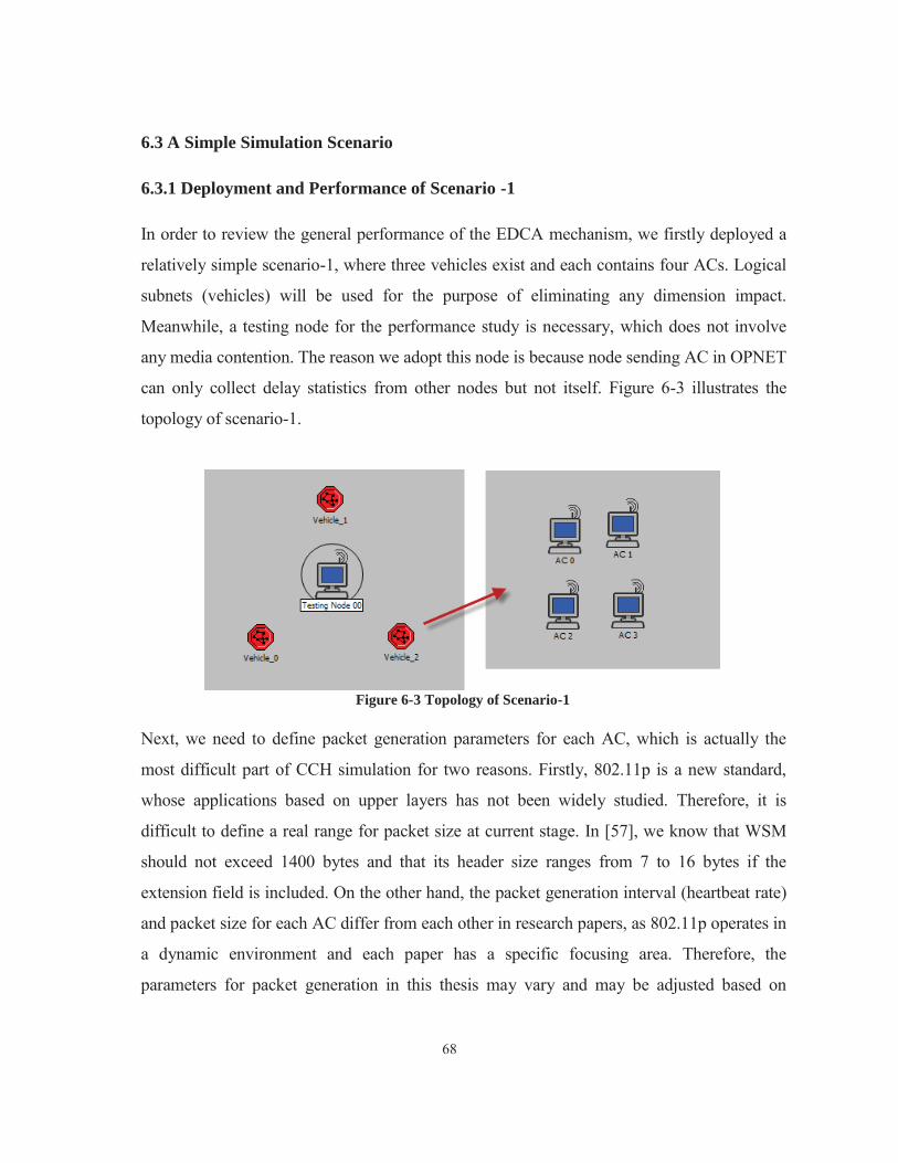
68
6.3 A Simple Simulation Scenario 6.3.1 Deployment and Performance of Scenario -1 In order to review the general performance of the EDCA mechanism, we firstly deployed a
relatively simple scenario-1, where three vehicles exist and each contains four ACs. Logical
subnets (vehicles) will be used for the purpose of eliminating any dimension impact.
Meanwhile, a testing node for the performance study is necessary, which does not involve
any media contention. The reason we adopt this node is because node sending AC in OPNET
can only collect delay statistics from other nodes but not itself. Figure 6-3 illustrates the
topology of scenario-1.
Figure 6-3 Topology of Scenario-1
Next, we need to define packet generation parameters for each AC, which is actually the
most difficult part of CCH simulation for two reasons. Firstly, 802.11p is a new standard,
whose applications based on upper layers has not been widely studied. Therefore, it is
difficult to define a real range for packet size at current stage. In [57], we know that WSM
should not exceed 1400 bytes and that its header size ranges from 7 to 16 bytes if the
extension field is included. On the other hand, the packet generation interval (heartbeat rate)
and packet size for each AC differ from each other in research papers, as 802.11p operates in
a dynamic environment and each paper has a specific focusing area. Therefore, the
parameters for packet generation in this thesis may vary and may be adjusted based on
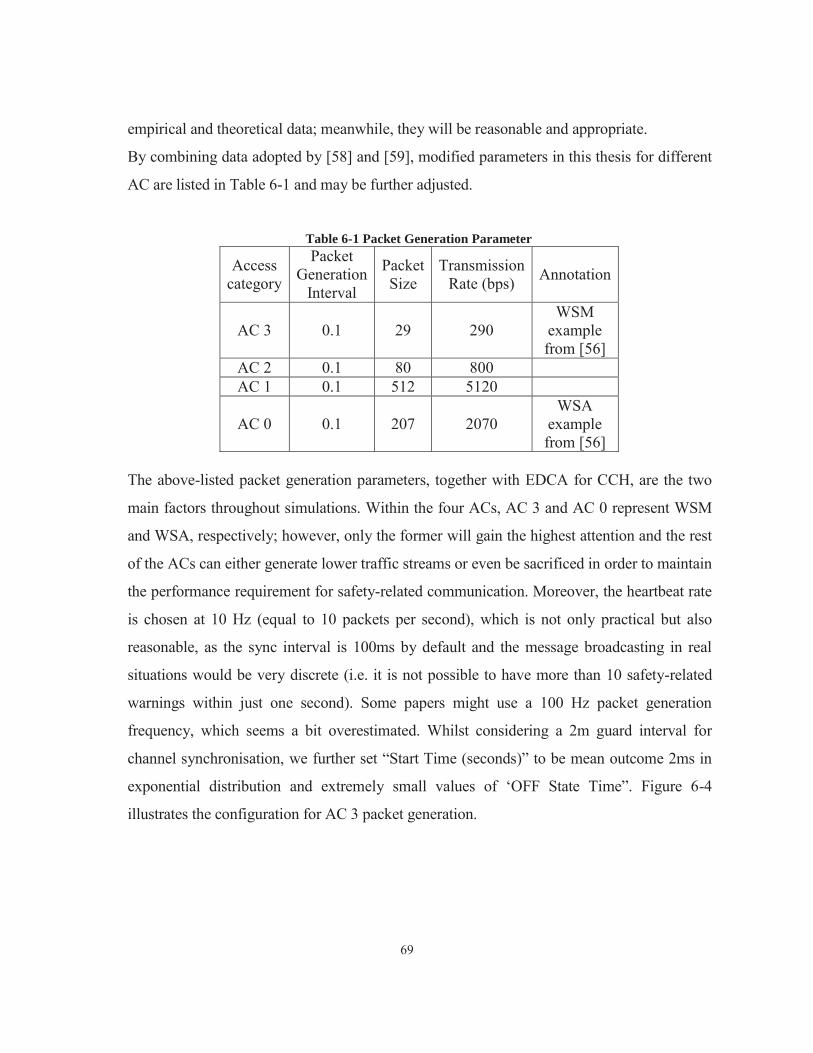
69
empirical and theoretical data; meanwhile, they will be reasonable and appropriate.
By combining data adopted by [58] and [59], modified parameters in this thesis for different
AC are listed in Table 6-1 and may be further adjusted.
Table 6-1 Packet Generation Parameter
Access category
Packet Generation
Interval
Packet Size
Transmission Rate (bps) Annotation
AC 3 0.1 29 290 WSM
example from [56]
AC 2 0.1 80 800 AC 1 0.1 512 5120
AC 0 0.1 207 2070 WSA
example from [56]
The above-listed packet generation parameters, together with EDCA for CCH, are the two
main factors throughout simulations. Within the four ACs, AC 3 and AC 0 represent WSM
and WSA, respectively; however, only the former will gain the highest attention and the rest
of the ACs can either generate lower traffic streams or even be sacrificed in order to maintain
the performance requirement for safety-related communication. Moreover, the heartbeat rate
is chosen at 10 Hz (equal to 10 packets per second), which is not only practical but also
reasonable, as the sync interval is 100ms by default and the message broadcasting in real
situations would be very discrete (i.e. it is not possible to have more than 10 safety-related
warnings within just one second). Some papers might use a 100 Hz packet generation
frequency, which seems a bit overestimated. Whilst considering a 2m guard interval for
channel synchronisation, we further set “Start Time (seconds)” to be mean outcome 2ms in
exponential distribution and extremely small values of ‘OFF State Time”. Figure 6-4
illustrates the configuration for AC 3 packet generation.

70
Figure 6-4 OPNET Setting for AC 3 Packet Generation
We ran this simulation in OPNET for 10 minutes. Meanwhile, since a 10 Hz packet
generation interval is very discrete to OPNET, we therefore set “Values per statistic” to be
10000 in order to obtain better statistical observation. The delay of each AC for this
simulation is given in Figure 6-5 under overlaid presentation.
Figure 6-5 Delay of ACs in Scenario-1

71
6.3.2 Performance Analysis Analysis: Since 802.11p is not supposed to provide a regular internet access purpose, we
mainly focus on the performance of delay. Through reviewing the above results, no fixed
delay parameter could be obtained. However, its range and all statistic points scattered with
different scales, although each AC densely locates at a certain band, which is expected to be
the average delay value for them. In order to facilitate our analysis, this data has been
exported to a spreadsheet in Table 6-2 and the average delay is shown in Figure 6-6 below:
Table 6-2 Data for Delay of Each AC
Access category Max Delay in ms Average Delay Max/Avg. Ratio AC 3 0.323 0.1742 0.539318885 AC 2 0.395 0.3089 0.782025316 AC 1 2.838 1.87 0.658914729 AC 0 4.401 2.52 0.572597137
Figure 6-6 Average Delay of ACs in Scenario-1
72
By reviewing the diagram, we can see that EDCA is quite a robust MAC mechanism, in
terms of it maintaining priority as the layout of delay for each AC. In particular, even the
packet size of AC 1 is doubled, compared to that of AC 0; its average delay is still smaller
than AC 0. On the other hand, AC 3 not only suffers the lowest delay but also the most stable
one, compared with its counterparts, as its Max/Avg. Ratio is only 53.9%, which is similar to
the 57.2% of AC 0. Meanwhile, AC 2 and AC 1 had approximately 78% and 65.8%,
respectively. It can be concluded that within four ACs, the ones with either the highest or
lowest priority will experience a smaller delay fluctuation than others. Furthermore, it looks
like these four ACs can be mainly divided into two major groups, namely AC3/2 and AC 1/0,
whose delay gaps are remarkably noticeable on the above diagram. However, at this moment,
we cannot analyse the delay difference between members of the same group, as different
packet sizes have been deployed in ACs; although, we predict that AC3/2 should always
have a smaller internal delay difference than AC1/0, which will be proved in the following
subsection of this thesis.
6.4 Study of Distance Impact on CCH Performance
6.4.1 Deployment of Stationary Scenario-2 and Performance
Previous simulations could actually only prove that EDCA works and that priority for each
AC is apparent. However, the average delay for each AC obtained was under an ideal
situation and could therefore not be adopted directly, since, in practice, whether or not
communication distance and vehicle velocity will impact 802.11p performance needs to be
further examined.
For this purpose, we created scenario-2, which is based on the previous one, by deploying a
5x1 km map in which the logical subnet containing three vehicles is located at 500,500 m.
One (numbered as 00) of eight testing nodes is placed in the logical subnet and the rest are
each spaced at 200m. Figure 6-7 shows the topology of scenario-2.

73
Figure 6-7 Topology of Scenario-2 for Distance Impact Study
As previous designed, the transmission power in our simulation covers 1 Km effective
distance judging by throughput. Testing Node 06/07 will be out of the 1 Km range and will
therefore be used for further study. It is assumed that the distance will affect almost every
aspect of wireless communication, including delay, throughput, bit error rate (BER), signal-
to-noise ratio (SNR), etc. Various performances of AC 3 for different testing nodes are given
by Figure 6-8 13.
Figure 6-8 AC 3 Average Delay for Testing Nodes 00-05

74
Figure 6-9 AC 3 Bit Error Rate for Testing Nodes 00-05
Figure 6-10 AC 3 Packet Receiving Rate for Testing Nodes 00-05

75
Figure 6-11 SNR of Node 01/06/07 in Scenario-2
Figure 6-12 AC 3 Delay of Node 01/06/07 on Scenario-2

76
Figure 6-13 Average BER of AC 01/06/07 on Scenario-2
6.4.2 Performance Analysis of Scenario-2 6.4.2.1 Analysis within Effective Coverage Analysis: Since the distance impact to communication performance is pretty complex,
merely judging from the average delay of each node will not be enough. Instead, we observe
three indicators for our performance study, namely average delay, BER and packet receiving
rate. Firstly, we can see that, within a 1Km distance, all nodes have almost the same average
delay and are slightly increased according to distance from data source. This can be
explained by an increased BER, which is acceptably given in Figure 6-9, due to a relatively
greater attenuation by distance. Since the delay is a compositive performance, including
hardware efficiency, propagation, processing, etc., in this case, we can consider the slight
increase in node 05 delay being down to more processing time taken by correcting received

77
bits as well as propagation delay. Furthermore, we know that the relationship between SNR
and BER under QPSK from [60] is as follows:
BER= (Equation 6-1)
SNR= (Equation 6-2)
Where is carrier-to-noise ratio, and B represent data rate and bandwidth, respectively.
The two equations above actually indicate that the BER will be dynamically affected by
SNR according to distance change (i.e. lower SNR results in higher BER). In real application,
with the purpose of extending coverage, vehicles should switch to a lower data rate (i.e. a
simpler modulation mechanism to obtain a lower sensitivity requirement or to intelligently
increase its transmission power, together with more advanced hardware components, such as
an equalizer, in order to cope with multipath propagation and a fading phenomenon).
Meanwhile, there is an abrupt packet receiving rate drop at Node 05, from 98.92 packets/s to
92.45 packets/s, due to an edge effect related to a sensitivity issue, which will be explained in
detail later on.
6.4.2.2 Analysis Outside of Effective Coverage Next, we observe the performance of testing nodes 06 and 07, in contrast with 01, based on
their SNR, delay and bit error rates from Figure 6-(11 13). It can be observed from Figure
6-12 that the longer distance has the larger swing range of delay and thus more scarce
sampling nodes on the diagram. Through comparing the BER between nodes 06 /07 and 00,
they increased almost by 213% and 100% on average. What we need to focus on is the peak
AC 3 delay for each testing node, rather than their average values, as we found that the peak
delay for node 00 is around 0.323 ms, compared with 0.766 ms for node 07, which can be
explained by the same reason for a processing delay (mentioned above). Although the delay
has increased by 137% outside of coverage, under VANET with only three vehicles, it might
seem acceptable. However, on the other side, the scarcity observed actually impacts on the
performance at the highest level and is the very reason for causing the effective pre-design

78
coverage. Firstly, we know that CCH always works on the broadcast model and that there is
no retransmission sent differently from normal WLAN applications, in which a user will
experience extremely slow throughput and frequent disconnection, but can still feel “useful”.
A typical case might be that your wireless adapter detects weak Wi-Fi signals without
encryption leaking from your neighbour’s house; you can take advantage of slowly opening
some web pages rather than watching YouTube smoothly. However, in traffic safety
application, almost all messages on CCH are expected to be received without exemption and
there is no selective or occasional receiving that is tolerated. Secondly, the cause of lower
receiving rates is mainly the sensitivities of receivers; the turning point in communication
performance is varying the different modulation schemes. According to Equitation 7-2, the
SNR will increase under a higher data rate. Most of the time, the receiving status will
abruptly deteriorate when the signal strength is below the sensitivity, thus causing a great
amount of data which cannot ultimately be decoded and dropped. Here, we need to
distinguish the difference between receiver sensitivity and the packet reception-power
threshold. The hard figure of the former is provided by a few manufacturers but is a measure
of the minimum threshold at which a device can properly detect and interpret a signal, which
implies two facts: firstly, under this threshold, a device is still allowed and might be able to
detect signals. On the other hand, even though it can detect the signal, the interpretation will
perform improperly without any guarantee. The latter (reception-power threshold), however,
is a very precise value under which a signal will not be sensed nor decoded. Therefore, by
setting this parameter with a smaller value, we can see that the signal is being ‘cut off”
immediately without any exemption, even if it can still be properly decoded by a receiver.
Since the sensitivity is merely hardware-related and cannot be changed, the power threshold
actually has a great meaning to vehicle communication under the two scenarios stated below:
1. If the data source would like to confine the transmission range within certain
coverage or eliminate receivers under a poor communication environment, it can
define the fixed value of the power threshold in its packet header rather than just
merely increasing its transmission power. This is based on several reasons: firstly, not
all vehicles have to receive data, especially in the SCH case. Secondly, since VANET

79
operates in a highly dynamic environment, merely changing the transmission power
would not always help to better the performance but rather increase interference.
Furthermore, by informing receivers of the threshold, we actually handle the rights of
decisions of acceptance rather than forcing the communication.
2. As we know, under the broadcast mode, CSMA/CA will still be involved in media
access contention, which contributes to most of the delay. Generally speaking, how
long a certain node needs to wait in order to gain access to the media is dependent on
the number of nodes within the effective communication coverage. At the edges of
broadcast distances or even further, even though the signal strength is much lower
than sensitivity, nodes there might be content with redundant counterparts, which are
not supposed to be taken into consideration. For instance, based on common sense,
we know that the pre-crash messages are generally only meaningful to the vehicles
behind the sending source; this is in order to let drivers brake as soon as possible.
However, since mainly isotropic antenna will be adopted in VANET, these messages
will inevitably send to the vehicle not only in front but also outside of pre-defined
coverage and will thus make receivers try to sense them. Therefore, if vehicles are
able to set a reception threshold according to distance and dynamic environment, their
performance will not be affected by vehicles outside of their coverage and will look
better due to the receivers ignoring signals below their threshold. In fact, in a long
queue of vehicles in a traffic congestion period, most vehicles can be considered at
the edge of certain effective communication coverage. Thus, this parameter will
improve the overall network performance rather than several members of it.
6.4.3 Deployment of Dynamic Scenario-3 and Performance Furthermore, in order to demonstrate the analysis stated above and to obtain the dynamic
distance impact to network performance, we set another testing node (08), which is moving
at a low velocity of 1 Km/h, in order to eliminate the Doppler effect from 500,500 to
2500,500. Topology for this mobile scenario-3 is given in Figure 6-14.

80
Figure 6-14 Topology for Scenario-3 After running this simulation, related performances are given below:
Figure 6-15 Overall Delay and Delay of ACs in Discrete Pattern
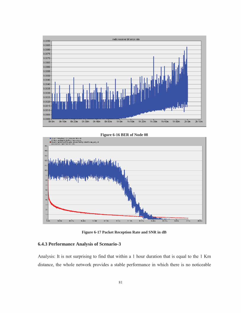
81
Figure 6-16 BER of Node 08
Figure 6-17 Packet Reception Rate and SNR in dB
6.4.3 Performance Analysis of Scenario-3 Analysis: It is not surprising to find that within a 1 hour duration that is equal to the 1 Km
distance, the whole network provides a stable performance in which there is no noticeable

82
change of delay and packet reception rate, and the BER only slightly increases. On the other
hand, the related performance abruptly deteriorates when out of coverage, due to sensitivity
issues mentioned previously and the SNR below being around 10 dB.
What drew our attention turned out to be the gradually reduced overall delay, which
combined all four ACs. However, as mentioned previously, according to distance and BER
increase, the delay should slightly increase. Such a phenomenon can be explained by the
reserve proportional relationship between packet size and reception distance; as can be
observed from Figure 6- 15, AC 2 with the highest packet size of 512 bites can only be
received at the shortest duration due to two reasons stated below:
1. Under the same modulation scheme, a packet containing more bits requires more
OFDM symbols to be transmitted. For instance, the PHY layer of 802.11p at 6 Mbps
adopts QPSK, whereby data bits per OFDM symbol is 48. When signal strength is
below the sensitivity, one or several OFDM symbols belonging to certain packets
could neither be sensed nor decoded, thus making an incomplete packet reception that
is dropped by the PHY layer. Therefore, a packet with a bigger size will generally
experience an extremely higher symbol loss probability. This can be proved if we
confine the packet size within one OFDM symbol by resetting the size of AC 3 to 10
bits and AC 2 to 20 bits. In this case, the PHY layer of transmitter will pad the
remaining bits for this packet in order to consistently place it into a complete OFDM
symbol. Figure 6-18 shows the results.

83
Figure 6-18 Reception Distance Under One OFDM Symbol
From the above diagram, we can see that AC 3 and AC 2 can be received almost at
the same distance, which proves our previous assumption.
2. Furthermore, the packet error rate (PER) will not evenly allocate on different ACs
with various packet sizes, according to [61]
=1-(1- (Equation 6-3)
.
The above equation indicates that the PER has an exponential relationship with
packet size. Therefore, AC 1 with 512 will experience an extremely high PER
reaching 100% very quickly when out of coverage. One thing needed to be mentioned
here is that the observed BER from OPNET cannot be used to calculate directly,
since it has been defined on OPNET as BER for bits of the packet, which is
completing arrival at the receiver channel, and the real BER is actually much higher
than that. The continued increasing PER, which is due to abruptly deteriorated BER,
when outside of coverage causes packets to be dropped by PHY, as we can see from
Figure 6-17.
The reasons given above explain why the overall delay decreases rather than
increases; as with the four ACs, packets containing relatively high bits and a lower

84
priority will first experience dropping, which further makes AC 3 become the
dominant one at the receiver end, according to distance increase.
6.5 Study of Packet Size Impact on VANET
6.5.1 Introduction and Deployment of Scenario-4 This subsection is the key part of this thesis and the most important component of our
simulation, as the impacts of packet size and vehicle number on VANET are pretty complex,
which, in most cases, cooperate with each other in order to dominate network performance.
At first glance, it is obvious that the increase of either packet size or vehicle number will
lower the performance, namely a longer delay, higher interference, etc. Moreover, increasing
a packet size is somewhat similar to increasing vehicle number but they will never be equal,
just like the time spent picking up a bag of wheat being tremendously different from picking
up thousands of grains of wheat, despite being at the same weight. Thus, the delay of two
nodes sending 1000 bits/packet will be different from four nodes sending 500 bits/packet.
Due to the complexity mentioned above, we will first study the packet size impact on
VANET independently, which is a 2D pattern. After that, the factor of the number of
vehicles will be added into our study and will finally form a 3D pattern, namely packet size,
vehicle number and performance. Since each vehicle might carry one or more ACs, the study
of the relationship between packet size and performance itself requires a lot of work. After
careful consideration, three instances will be examined in this subsection, which are based on
three vehicles of topology; a brief introduction is given as follows:
1. Only one kind of AC exists in VANET. This is used to study packet size impact on individual ACs.
2. Based on 1, we added another three ACs into VANET, which helps to study the MAC contention mechanism’s impact on certain kinds of AC.
3. Based on 2, we checked the performance of the added three ACs in order to study how one kind of AC impacts on the whole system performance.
Scenario-4 was created in which there are four subnets numbered from 00 to 04, which are
spacing at least 1Km each. Each of them is used to study a certain AC containing three

85
vehicles and one testing node, whose category is the same as the subnet number. For instance,
subnet02 only focuses on the performance study of AC 2 and subnet04 is reserved for future
usage. Also, the packet reception power threshold is reset to -80 dB in order to eliminate
possible interference. Figure 6-19 illustrates the topology of scenario-4.
Figure 6-19 Topology of Scenario-4
6.5.2 Analysis of Instance-1 We deploy the same kind of AC in each subnet and turn off the other three ACs. Then, the
packet size for each workstation will be increased to the power of 2 based on 48 bits till 768
bits, together with a special instance of 1400 bits as the maximum allowed size for CCH.
After running the simulation eight times, the diagram for the average delay of each AC is
given in Figure 6-20. Detailed data can be found in the Appendix.
Figure 6-20 Average Delay for Instance-1

86
Analysis: Firstly, we can observe from the above chart that, according to the increase of
packet size, the delay for each AC will also increase, whereby AC 3 and AC 2 are almost
overlapping each other as well as AC 0 and AC 1 being slightly higher. Such a phenomenon
can be explained by breaking up overall delay into two parts: constant and variable from the
view of packet size. The former refers to media access delay, including frame spacing period
and Backoff, propagation delay that is irrelevant with packet size but is mainly dependent on
the number of ACs, packet generation frequency and transmission distance. The latter is the
process and queuing delay at both the transmitter and receiver end, which is immediately
affected by the size of packet.
Since our previous simulation only involves three vehicles and that there is no collision
happening when checking “collision status” from OPNET, the overall delay is completely
dominated by packet size, and the impact of AC priority will be diluted by the increase of
packet size. For instance, at 48 bits/packet, the delay of AC 0 is 1.5 times that of AC 3, but is
only 1.138 times in the 1400 bits/packet situation. Furthermore, by analysing collected delay
data, we found that there are approximately 0.23ms increases per every 100 bits added on
packets, despite what the kind of AC or base packet size is. Table 6-3 shows a detailed ration
for each AC.
Table 6-3 Increased delay per 100 Bits Added (ms/100 bits) of Instance 0
Delay Added (ms) 96 192 384 768 1400
AC 3 0.26672917 0.18927708 0.23186146 0.23210938 0.23167563
AC 2 0.26666667 0.18822917 0.23239583 0.23239583 0.23275316
AC 1 0.24291667 0.22197917 0.24802083 0.24804688 0.24844937
AC 0 0.23020833 0.25822917 0.25838542 0.25835938 0.25878165
One thing needed to be pointed out here is that it is pretty hard to get delay increase per bit

87
value, since suddenly stepping up may happen due to the padding mechanism of the OFDM
symbol. For example, under QPSK (48 bits per symbol), there will be no delay difference
between 20 bits/packet and 40 bits/packet, and an abrupt surge might be seen when
deploying 50 bits/packet.
In general, we can conclude that increasing the packet size in batch has an approximately
linear impact on network delay. Meanwhile, the higher packet size is the smaller difference
of delay performance between ACs.
6.5.3 Analysis of Instance-2 Concerning instance 2 and 3, their statistical data can actually be obtained from the same
simulation scenario and just two different study aspects, i.e. one AC to three other ACs; three
ACs to one AC. In order to study the impact of bother packet size and the media contention
mechanism on VANET performance, we alternately set one AC range from 48 to 1400
bits/packet and the remaining three ACs to contain 384 bits/packet. Table 6-3 briefly
introduces four sub-instances of our study.
Table 6-4 Packet Size Configuration for Four Sub-Instances
Packet Size (bits) Sub-Instance No. AC 3 AC 2 AC 1 AC 0
0 48-1400 384 384 384 1 384 48-1400 384 384 2 384 384 48-1400 384 3 384 384 384 48-1400
After running simulation around 24 times, detailed data for each sub-instance is put in the
Appendix, whereby each average delay data is obtained from at least the thousand sampling
points. Meanwhile, they provide great help for our comprehensive study of packet size
impact on VANET performance.
Firstly, we examine the delay of each AC, along with an increased packet size under the

88
media contention mechanism. Figure 6-21 illustrates the performance of each AC.
Figure 6-21 Average Delay of ACs for Instance-2
Analysis: By comparing with Figure 6-20, it can be seen that each AC expends its spacing
with one another, especially AC 3 and AC 2, which are almost overlapping in Figure 6-20,
yet represent a noticeable distance in Figure 6-21. Such spacing is mainly due to media
access delay varying with AC types under contention. As we know, under the EDCA
mechanism, AC with higher priority will suffer smaller frame spacing and contention
backoff, thus resulting in AC 3 starting from a low Y axis value, in contrast to its counterpart
(AC 0). On the other hand, unlike previous instances, the same amount of bits added to
different ACs under media contention generated variable extra delay, whereby AC 3
experiences the lowest delay increase at around 0.168 ms per 100 bits, in comparison with
the 0.269 ms of AC 0. Detailed rates are listed in Table 6-4, as follows:
Table 6-5 Delay Increase per 100 Bits Added
Delay Added (ms) 96 192 384 768 1400 Average AC 3 0.160625 0.156979 0.166094 0.181276 0.178307 0.168656 AC 2 0.180208 0.2225 0.190417 0.233724 0.236978 0.212765 AC 1 0.217708 0.2375 0.240052 0.252526 0.259351 0.241428 AC 0 0.2925 0.229896 0.247708 0.283594 0.294636 0.269667
All these phenomena indicate one principle, which is that EDCA is a quite robust mechanism
under media contention, under which AC with higher priority will be less affected by the
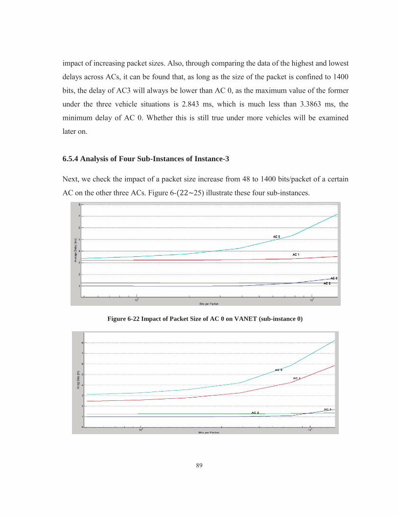
89
impact of increasing packet sizes. Also, through comparing the data of the highest and lowest
delays across ACs, it can be found that, as long as the size of the packet is confined to 1400
bits, the delay of AC3 will always be lower than AC 0, as the maximum value of the former
under the three vehicle situations is 2.843 ms, which is much less than 3.3863 ms, the
minimum delay of AC 0. Whether this is still true under more vehicles will be examined
later on.
6.5.4 Analysis of Four Sub-Instances of Instance-3 Next, we check the impact of a packet size increase from 48 to 1400 bits/packet of a certain
AC on the other three ACs. Figure 6- 25) illustrate these four sub-instances.
Figure 6-22 Impact of Packet Size of AC 0 on VANET (sub-instance 0)

90
Figure 6-23 Impact of Packet Size of AC 1 on VANET (sub-instance 1)
Figure 6-24 Impact of Packet Size of AC 2 on VANET (sub-instance 2)
Figure 6-25 Impact of Packet Size of AC 3 on VANET (sub-instance 3) Analysis: These four diagrams together illustrate some interesting phenomena of the impacts
of packet size of different AC on VANET performance. Table 6-5 gives an overview of the
average increased delay/100 bits for these four sub-instances.
Table 6-6 Average Increased Delay /100 bits for Four Sub-instances
Average Increased Delay (ms)
Sub-Instance 0
Sub-Instance 1
Sub-Instance 2
Sub-Instance 3
AC 3 0.022829509 0.024183544 0.075627044 0.168656184 AC 2 0.002476332 0.010266812 0.212765361 0.067404931 AC 1 0.022600672 0.241427545 0.273015164 0.212292524

91
AC 0 0.269666799 0.357498945 0.306356013 0.251460509
These rules can be summarised and explained based on the data collected from our
simulation, as follows:
1. Increasing the packet size of the different AC will lead to a higher delay for all ACs.
However, the magnitude and sensitivity turn out to be unevenly due to the domination
of the EDCA mechanism.
2. The packet size of AC 0 impacts on the delay of itself at the greatest magnitude, at an
average of 0.269 ms/100 bits, yet impacts a little on AC 2. Concerning AC 3 and AC
1, there would be a noticeable delay increase when the packet size of AC 0 reaches
384 bits/packet, and AC 3 would suffer a relatively bigger delay increase than AC 2,
even though it might seem out of expectation, since AC 3 is with the highest priority
and would be the most resistant one against impacts of other ACs. Such a
phenomenon could be attributed to the shielding effect. Although AC 0 is with the
lowest priority, it still has a minor opportunity to gain media access, which is actually
bigger under the fact of a low packet generation frequency in VANET. When its
packet exceeds a certain level, the process time will be remarkably increased, which
causes two results: firstly, one or more AC 2/1 packets might be generated and will
compete with AC 3. Secondly, a newly generated AC 3 packet cannot process backoff
countdown, but will instead wait in the queue. The issue is that AC 3 ranks at the
highest priority, whose queue delay is comparatively smaller than counterparts of
other ACs, but is vulnerable to an increasing process delay caused by other ACs. In
short, when there is a negative impact on network performance, the AC with the
higher priority will stand on the front line, in order to digest such impacts, e.g. like a
shield or cushion.
3. The packet size of AC 1 has the greatest impact on the delay of AC 0 at an average
0.3575 ms/100 bits, due to these two ACs being relatively competitive in the EDCA
mechanism. Also, it has the second largest impact on itself, followed by AC 3, and
has almost no effect on AC 2, due to the shield effect.
92
4. The packet sizes of AC 3 and 2 have a similar and most prominent impact on all ACs
in VANET. If we divide ACs into high and priority groups, which contain AC3/2 and
AC 1/0, respectively, the rule can be described that increasing the packet size of one
AC in a higher priority group always affects AC 0 at the largest scale, as well as has
the smallest impact on its counterpart in the same group, namely AC 3 or AC 2.
Meanwhile, there is also a considerable delay increase of itself, as in our simulation,
AC 3 and AC 2 reach 0.1686 ms and 0.212 ms per 100 bits, respectively.
What is stated above provides a practical mean to our practical application of
802.11p, in which we realise that the immediate approach to improved network
performance of certain ACs turns out to be reducing the packet size of itself,
especially AC 0 and AC 3. Meanwhile, the packet size of the former has the faintest
overall impact on the overall performance of ACs, and the latter, however, has the
greatest impact, followed by AC 2 and AC 1. Therefore, concerning 802.11p, it would
be very helpful if advanced compression was adopted on high priority ACs and thus
eliminated non-safety critical information from either their MPDU header or payload
area.

93
Chapter 7 Advanced Scenarios and Performance Analysis 7.1 Study of Vehicle Number Impact on VANET
7.1.1 Deployment and Performance of Instance-4 Next, we study the number of vehicle impacts on VANET based on Instance 1, whereby
only three ACs of the same kind are involved. It has to be pointed out that, although we call
the factor “Number of Vehicle”, we actually mean the number of ACs carried by vehicles,
since there might be one or more ACs for each vehicle in the real world. Considering our
topic of VANET performance, it would be better to keep using the term “Number of
Vehicle”, with further annotation on the number and kind of ACs.
In our following simulation (Instance -4), the vehicle number was chosen from 10 to 100,
whereby their packet size for AC is based on Instance 1. Therefore, we can predict that the
Table of Instance -1 will expand to four larger tables for each kind of AC exclusively.
However, whilst studying the impact on individual types of AC, we chose AC 3 and AC 0
only, since it is apparently the performances of AC 2 and AC 1 that will locate between their
counterparts at the edge of priority. Furthermore, as mentioned at the beginning of this
chapter, through the increase of vehicle numbers, we will monitor not only delay but also the
signal collision status on our instance in order to judge the accuracy of data collected. Figure
7-1 illustrates an example topology for AC 0 in a 10 vehicles condition.
Figure 7-1 Topology of Instance-4 under 10 Vehicle Condition

94
After running the simulation 120 times under different configuration, we obtained data for
both average delay as well as time average collision status, which can be found in the
Appendix. The data for average delay of each AC has been picked out and processed by
Matlab, in order to represent two 3D diagrams in mesh format in Figure 7-2.
Figure 7-2: Average Delay Based on Vehicle Number and Packet Size in 3D Mesh Format 7.1.2 Analysis of Instance-4 In Figure 7-2, we can see that two non-overlapping curved surfaces for AC 3 and AC 0
respectively exist. From previous analysis, it shows that the packet size of AC has a
nonlinear impact on the delay of VANET. In this simulation, we found that, under the same
packet size, the vehicle number also contributes to a nonlinear impact on network. These two
impacts result in each AC representing themselves in a curved surface in 3D, whereby lots of
interesting phenomena can be observed and explained, as below:
1. At any point of (x, y), the value of AC 0 is always higher than that of AC 3. This
means that, whilst under the same packet size and vehicle number, the delay of AC 3
is always lower than AC 0. Table 7-1 shows the ratio of delay between these two ACs.

95
Table 7-1 Delay Ratio between AC3 and AC0
Vehicle Number
Packet Size (bits) 48 96 192 384 768 1400
% of
% of
% of
% of
% of
% of
10 45.30805% 52.68987% 49.07003% 49.49728% 43.52806% 53.43127% 20 26.46045% 27.95734% 32.36207% 33.54552% 30.38885% 36.13730% 30 20.33726% 22.89531% 25.94399% 23.62221% 24.32868% 27.70663% 40 17.79008% 24.93669% 22.19527% 20.34183% 19.67183% 23.45120% 50 15.55578% 24.08680% 17.61468% 18.72852% 19.63963% 21.65888% 60 17.08029% 20.63362% 15.45850% 18.11852% 18.58024% 21.32377% 70 16.51185% 18.39700% 13.74920% 14.61118% 17.94289% 20.94330% 80 14.36548% 14.82191% 13.95019% 14.97769% 17.59218% 20.54308% 90 16.03093% 16.75482% 14.60256% 14.97141% 17.18188% 19.54115% 100 15.31146% 15.66473% 14.58648% 14.69202% 18.23769% 22.53833%
It can be seen that, when at the lowest vehicle number and whatever the packet size,
the difference of delay between these turns out to be the smallest, whereby AC 3
accounts for around half that of AC 0. On the other side, through the general increase
of vehicle numbers, the gap is reduced gradually from around 50% to 15 or 22%.
Such a phenomenon is because, when media is heavily occupied by the same kind of
AC type, AC 3, although with the smallest AIFSN, has to process more deferred
access.
2. The collision phenomenon is another complex issue of WLAN and is sometimes
considered more important than VANET delay. OPNET provides some indicators,
such as “collision status” and “packet marked noise by power stage”, which are all
Boolean value and which are recommended to be reviewed in a time average filter;
they are also used to examine whether they occur at a certain time point. However, in
VANET, every vehicle sends packets in a very discrete manner; such indicators can
only show collision increase rather than how exact packet loss will be due to
collision. Considering our simulation is always under a free space propagation mode,
the number of packets difference between transmitters and receiver must therefore be

96
caused by collision, which also provides a quantitative method for our study.
Meanwhile, DES indicates that, when even under the most condense instances,
namely a 100 vehicles at 1400 bits/packet, each vehicle still sends at 10 packets/s
equally. After calculating based on Appendix data, the packet loss rate due to collision
is listed in Table 7-2 and Figure 7-3 illustrates this data in 3D format.
Table 7-2 Packet Loss Rate for AC 0 and AC 3 Only one AC 0 for each Vehicle
Vehicle Number
Packet Size (bits) 48 96 192 384 768 1400
Loss Rate Loss Rate Loss Rate Loss Rate Loss Rate Loss Rate 10 12.18167% 15.65781% 15.75667% 23.23333% 28.28333% 31.34000% 20 32.14000% 36.06165% 43.02165% 50.78008% 54.85500% 56.69834% 30 45.02000% 48.47223% 55.86223% 62.63667% 66.47333% 67.83000% 40 53.27875% 57.12250% 63.00668% 68.98418% 73.16000% 74.16168% 50 56.01000% 62.36334% 68.22866% 73.65934% 77.07066% 78.14866% 60 57.46388% 67.63278% 72.93000% 77.32445% 80.06222% 81.05833% 70 62.31547% 69.73953% 73.56286% 78.84047% 82.45096% 83.22904% 80 66.70729% 69.55875% 75.19791% 76.99688% 84.27291% 84.98959% 90 69.26297% 71.70186% 77.32222% 79.10186% 85.23241% 86.19074% 100 72.28917% 74.78167% 79.72250% 81.13250% 85.01667% 85.42500%
Only one AC 3 for each Vehicle
Vehicle Number
Packet Size (bits) 48 96 192 384 768 1400
Loss Rate Loss Rate Loss Rate Loss Rate Loss Rate Loss Rate
10 21.55667% 32.14000% 40.32500% 51.97120% 58.14600% 66.02500% 20 47.36335% 54.40667% 63.74584% 74.36667% 82.74828% 85.94167% 30 51.92110% 59.99333% 70.86113% 79.78333% 87.35278% 90.62223% 40 56.53750% 66.80418% 75.62708% 82.92085% 88.72292% 91.86458% 50 60.30534% 68.38134% 77.49000% 84.56500% 90.72823% 93.41334% 60 62.12167% 71.71667% 79.85278% 86.70417% 92.39167% 94.47502% 70 66.28286% 75.03286% 81.70119% 87.80833% 92.75239% 95.09040% 80 72.24479% 78.81146% 84.59584% 89.61041% 93.89896% 95.78080% 90 73.07314% 80.63519% 85.40000% 89.88333% 94.18981% 95.88056% 100 75.76167% 82.98250% 86.25083% 90.23750% 94.17333% 95.35167%

97
Figure 7-3 Packet Loss Rate of AC 0 and AC 3
It looks like the packet loss rate of either AC 0 or AC 3 at any given packet size and
vehicle number might be too high to be feasible for real application. Indeed, there is
little possibility of having 100 vehicles sending 1400 bits/packet AC 3 at a frequency
of 10 Hz within 2 ms as a guard interval. However, it is necessary to understand that
our simulation is only based on an extremely undesirable situation, in which the upper
limit boundary and many characteristics of 802.11p for VANET can be observed and
studied. Otherwise, we could set two vehicles to send one small size packet every 60
seconds; however, it definitely doesn’t help to evaluate the performance.
On the other hand, the mechanism of collision can hardly be explained by several
sentences, although we could simply say that a larger number of vehicles or packet
sizes of VANET will increase the packet loss rate; however, it is worthy of examining
in detail and is provided as follows:
First and foremost, it is important to understand that there are two kinds of network
models for a collision study - saturated and non-saturated - whose difference relies on
whether each node always has packets to be sent from a queue [62]. There is
remarkable research of the former by Giuseppe Bianchi, which was published in 2000
and which was widely adopted. Concerning the non-saturated network, it has only
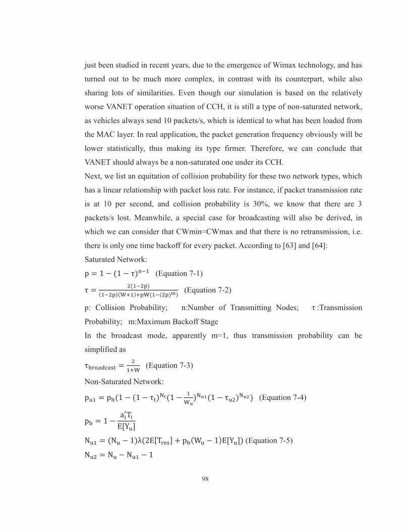
98
just been studied in recent years, due to the emergence of Wimax technology, and has
turned out to be much more complex, in contrast with its counterpart, while also
sharing lots of similarities. Even though our simulation is based on the relatively
worse VANET operation situation of CCH, it is still a type of non-saturated network,
as vehicles always send 10 packets/s, which is identical to what has been loaded from
the MAC layer. In real application, the packet generation frequency obviously will be
lower statistically, thus making its type firmer. Therefore, we can conclude that
VANET should always be a non-saturated one under its CCH.
Next, we list an equitation of collision probability for these two network types, which
has a linear relationship with packet loss rate. For instance, if packet transmission rate
is at 10 per second, and collision probability is 30%, we know that there are 3
packets/s lost. Meanwhile, a special case for broadcasting will also be derived, in
which we can consider that CWmin=CWmax and that there is no retransmission, i.e.
there is only one time backoff for every packet. According to [63] and [64]:
Saturated Network:
(Equation 7-1)
(Equation 7-2)
p: Collision Probability; n:Number of Transmitting Nodes; :Transmission
Probability; m:Maximum Backoff Stage
In the broadcast mode, apparently m=1, thus transmission probability can be
simplified as
(Equation 7-3)
Non-Saturated Network:
(Equation 7-4)
(Equation 7-5)

99
: Collision probability of first backoff attempt
: Number of saturated nodes
: Initial contention window
: Average number of packets on their retransmission attempts from other non-
saturated stations
: Probability that a non-saturated station attempts to retransmit in a given slot
Other symbol meanings can be found in [64] and are left out here.
Referring to the broadcast mode, and should be zero. Thus, the above
equation can be written as:
[Equation 7-6]
Although these equations provided seem delicate and complex, especially for a non-
saturated network, their characteristics can generally be described as follows:
In a saturated network, the collision probability is dominated by CW and the number
of nodes, rather than AIFSN or packet size, although it sounds odd. We have proved
this in OPNET by setting the packet generation frequency to be 1MHz in two packet
size instances: 48 bits and 480 bits/packet (10 vehicles) and two AIFSN instances: 2
and 5; the results are exactly the same at a packet loss rate of around 85.26%. The
reason for such characteristics is because the overall duration for obtaining media
access can be divided into three parts: start time, deferred access and CW backoff.
These are illustrated in Figure 7-4.

100
Figure 7-4 Division of Overall Waiting Duration
It might look like a simple diagram; however, it contains essential information for a
collision mechanism. The first part (start time) can be subdivided into an initial
transmitter turning off duration as well as an interval for a packet arriving at the
queue. Apparently, in a saturated network, the latter is always zero. Meanwhile, if we
make the former higher, i.e. allocating less overlapping time slots for each vehicle,
there should be fewer collisions happening equal to reducing vehicle numbers. In a
saturated network, where a queue interval is almost zero for every AC, the overall
waiting duration would rely more on turning off duration, deferred access and CW
backoff. On the other side, since there is always a packet in the queue for
transmission, the turning off duration can only help packets from different vehicles to
space each other in a very short duration, due to quick consumption, which is the
reason why we see there being fluctuation at an initial stage of our simulation. Figure
7-5 shows such a phenomenon.
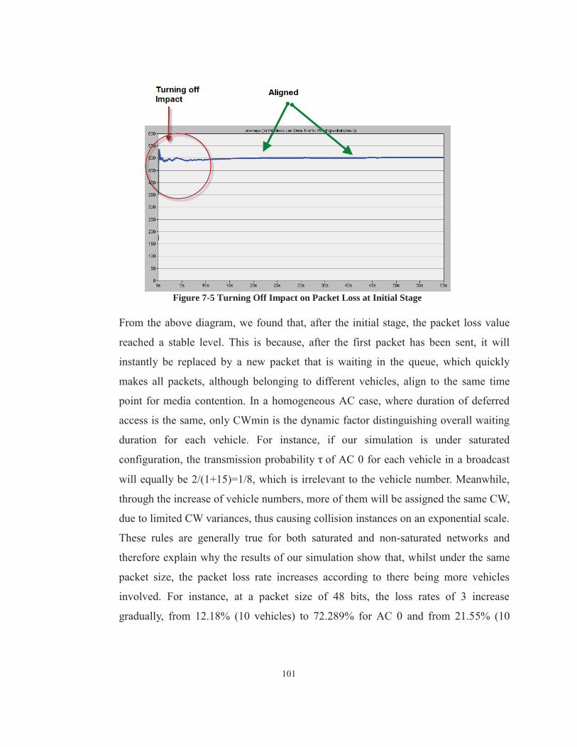
101
Figure 7-5 Turning Off Impact on Packet Loss at Initial Stage
From the above diagram, we found that, after the initial stage, the packet loss value
reached a stable level. This is because, after the first packet has been sent, it will
instantly be replaced by a new packet that is waiting in the queue, which quickly
makes all packets, although belonging to different vehicles, align to the same time
point for media contention. In a homogeneous AC case, where duration of deferred
access is the same, only CWmin is the dynamic factor distinguishing overall waiting
duration for each vehicle. For instance, if our simulation is under saturated
configuration, the transmission probability of AC 0 for each vehicle in a broadcast
will equally be 2/(1+15)=1/8, which is irrelevant to the vehicle number. Meanwhile,
through the increase of vehicle numbers, more of them will be assigned the same CW,
due to limited CW variances, thus causing collision instances on an exponential scale.
These rules are generally true for both saturated and non-saturated networks and
therefore explain why the results of our simulation show that, whilst under the same
packet size, the packet loss rate increases according to there being more vehicles
involved. For instance, at a packet size of 48 bits, the loss rates of 3 increase
gradually, from 12.18% (10 vehicles) to 72.289% for AC 0 and from 21.55% (10
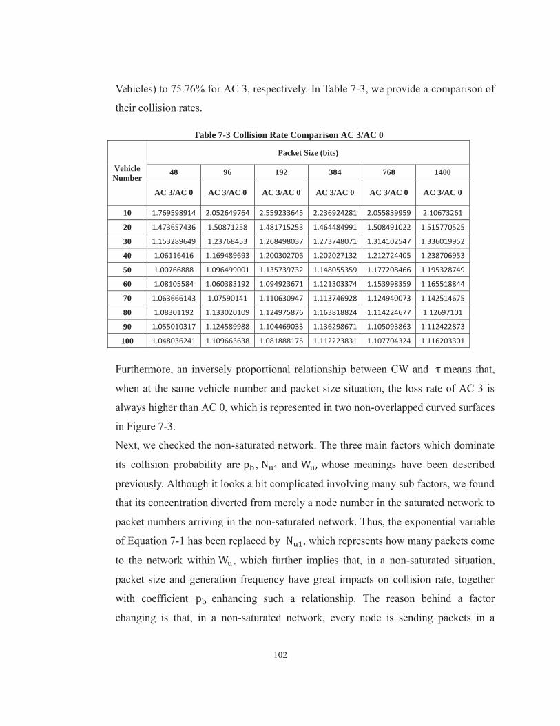
102
Vehicles) to 75.76% for AC 3, respectively. In Table 7-3, we provide a comparison of
their collision rates.
Table 7-3 Collision Rate Comparison AC 3/AC 0
Vehicle Number
Packet Size (bits)
48 96 192 384 768 1400
AC 3/AC 0 AC 3/AC 0 AC 3/AC 0 AC 3/AC 0 AC 3/AC 0 AC 3/AC 0
10 1.769598914 2.052649764 2.559233645 2.236924281 2.055839959 2.10673261
20 1.473657436 1.50871258 1.481715253 1.464484991 1.508491022 1.515770525
30 1.153289649 1.23768453 1.268498037 1.273748071 1.314102547 1.336019952
40 1.06116416 1.169489693 1.200302706 1.202027132 1.212724405 1.238706953
50 1.00766888 1.096499001 1.135739732 1.148055359 1.177208466 1.195328749
60 1.08105584 1.060383192 1.094923671 1.121303374 1.153998359 1.165518844
70 1.063666143 1.07590141 1.110630947 1.113746928 1.124940073 1.142514675
80 1.08301192 1.133020109 1.124975876 1.163818824 1.114224677 1.12697101
90 1.055010317 1.124589988 1.104469033 1.136298671 1.105093863 1.112422873
100 1.048036241 1.109663638 1.081888175 1.112223831 1.107704324 1.116203301
Furthermore, an inversely proportional relationship between CW and means that,
when at the same vehicle number and packet size situation, the loss rate of AC 3 is
always higher than AC 0, which is represented in two non-overlapped curved surfaces
in Figure 7-3.
Next, we checked the non-saturated network. The three main factors which dominate
its collision probability are , and whose meanings have been described
previously. Although it looks a bit complicated involving many sub factors, we found
that its concentration diverted from merely a node number in the saturated network to
packet numbers arriving in the non-saturated network. Thus, the exponential variable
of Equation 7-1 has been replaced by , which represents how many packets come
to the network within , which further implies that, in a non-saturated situation,
packet size and generation frequency have great impacts on collision rate, together
with coefficient enhancing such a relationship. The reason behind a factor
changing is that, in a non-saturated network, every node is sending packets in a

103
discrete manner and does not involve media contention all the time, i.e. active or
inactive, thus making it impossible to simply use an overall node number for the
collision study. In general, a longer duration will be required to send larger packets,
which can cause more vehicles to have packets in their queues for transmission and
content media after a certain node finishes the sending. One thing which needs to be
pointed out is that the initial CW contributes to both base and exponential factors of
Equation 7-6, and thus performs a slight offset impact on bigger CW. For instance,
although the CWmin of AC 0 is 15 resulting in a base value of 1/15, it might
encounter more new packets arriving due to a longer backoff duration, i.e. bigger
which is different from the saturated situation. However, such an offset impact
can be quickly overwhelmed by an increasing value of vehicle numbers, which is the
reason why we still see there are two exponential functions, like 3D diagrams, in
Figure 7-3. All these stated above explain why, in the same 10 vehicles instance, AC 0
with 1400 bits/packet experiences a 2.57 times loss probability as big as 48
bits/packet. Moreover, even though there is a considerable AIFSN and CWmin
difference between AC 0 and AC 3, their collision performances are getting closer
when we increase the value of the number of vehicles, as can be seen in Table 7-3.
3. There was an interesting phenomenon in our simulation; through reviewing delay
data collected in the same packet size, occasionally the delay of a higher vehicle
number was smaller than its counterpart of a smaller number. For instance, with 192
bits/packet, the delay of 30 vehicles and 40 vehicles was 0.7054 and 0.6376 ms,
respectively, and such a situation only happens once at AC 0 at vehicle 30/40 with 96
bits/packet. At first glance, it might seem very confusing and can be blamed on
incorrect configuration. However, after I spent a week simulating sub instances more
than 360 times on OPNET, I noticed that it can always happen in certain different
areas of the data collection table. After recalling the collision mechanism discussed
previously as well as the higher value of “packet marked as noise by power stage”
observed from OPNET DES, it is believed that such a phenomenon is due to collided
packets, which causes a combined signal either at a higher or lower power.

104
Concerning the latter instance, if the power is lower than the packet reception
threshold, transmitters in VANET will consider the media to be free and will conduct
a media access procedure. On the other hand, we review the statement of “increasing
vehicle numbers”, which are expected to bring more contention nodes and ultimately
dilute the transmission probability. However, for AC with a high priority, especially
AC 3 with only 4 kinds of CW variances on the CCH mode, for the small start time,
which we set as 2 ms, the number of vehicles encountering collisions is predicted to
happen in batches, i.e. there are a high percentage of vehicles transmitting
simultaneously. Since VANET on CCH is a typical non-saturated network, after these
vehicles send their packets, they might have no more packets in the queues for
transmission, thus resulting in actually less vehicle content in the media at the next
stage. Finally, the collision also causes there to be a scarce amount of data collected,
as we can see from the Appendix, whereby, for instance, only 46.8 packets have been
received per packet, thus making a sort of inevitable accuracy in the data analysis.
The points stated above explained the observed abnormal phenomenon and it is
supposed to appear in a random manner. However, we assure it will appear at a higher
probability on AC 3 than its lower priority counterparts.
7.2 Study of Multiple AC Types Impact
7.2.1 Introduction and Performance of Instance-5 Previous simulation instances generally take single AC types for study. However, in real
practice, since each vehicle is able to carry multiple ACs, we developed instance-5, which
was based on scenario-4, in order to further study the performance in this situation, while
also taking real traffic flow into consideration.
As in Auckland, New Zealand, most highways have three lanes for each direction, which is
the base of the instance-5 simulation. Meanwhile, according to [65], in a traffic congestion
period, one direction is fed at a rate of 6000 vehicles/h and the speed is around 60 Km/h,
which is in contrast to the opposite direction of 2000 vehicles/h (100 Km/h). Thus, we

105
estimate that, during this period, there are 133 vehicles within a 1 Km effective coverage.
Concerning packet size, it will be chosen at the same pacing as with instance-4. After
running the simulation, the collected data is provided in the Appendix. Figure 7-(6
gave the performances.
Figure 7-6 Average Delay of ACs under (48 768) bits/packet (Instance-5)
Figure 7-7 Average Bit Loss Rate of ACs (48 768) bits/packet (Instance-5)

106
Figure 7-8 Average Packets/s of AC 0 and AC 1/2/3 under 1400 bits/packet
Figure 7-9 Delay of ACs under 1400 bits/packet

107
Figure 7-10 Average AC 0 Packet Dropped Per Second under 1400 bits/packet
7.2.2 Analysis of Instance-5 It seems that, from 768 bits to 1400 bits per packet, the network reaches a saturated status.
Thus, we individually give the performances two major packet size categories, namely
48 768 bits/packet and 1400 bits/packet. Meanwhile, unlike the signal type of the AC
situation, instance-5 with multiple ACs represents in a more complex manner.
In respect to 48-768 bits/packet, we can see that there is a linear relationship between packet
size and delay that is similar to instance-4, where lower priority AC will suffer a higher delay.
On the other hand, since OPNET is not capable of providing how many packets are received
for each AC under multiple AC types, we have to use a bit loss rate instead, although it will
be a bit lower than the packet loss rate under the same condition. It is surprising to find that
the bit loss rates of AC 0/1 decrease under a packet size increasing from 48 to 368
bits/packet and reach a plateau after that, whereas AC 2/3 gave completely opposite
performances. This is because, with the same packet transmission rate for each AC being at
10 packets/s, AC with a lower priority has a greater probability of colliding with other types
of AC. For instance, the Packet of AC 1 tends to collide with its counterparts from AC 2/3
and itself, rather than AC 0, due to distinguishing EDCAFs. Meanwhile, from table 7-2, we

108
can see that AC with a higher priority is more sensitive to the increase of packet size in terms
of collision, which indicates that packets of AC 2/3 are supposed to collide with the same
types of AC as well as with themselves. Thus, such a mechanism is equal to the release of a
sort of media resource to a lower priority AC 0/1 and it will decrease their collision
probabilities. Moreover, the observed plateaus are due to a much less impact of packet size to
the collision rate of AC 0/1.
The performances of VANET under 1400 bits/packet are significantly different from that of
48 768 bits/packet because the network becomes saturated, whereby AC 1/2/3 tend to
continue the rules and performances of previous packet size categories. However, there is an
abrupt deterioration of AC 0, as not only its packet transmission rate reduces to an average of
6 packets/s; there is also an increasing packet dropped rate due to overflow after 7.5s. All of
these phenomena are due to heavily occupied media by AC 1/2/3 in which AC with the
lowest priority gains a very faint transmission opportunity and has to drop increasingly
accumulated packets in its queue, together with a definitely unacceptable average delay
value of around 3.5s.
7.3 Comprehensive Performance Study in Dynamic Environment
7.3.1 Deployment and Performance of Scenario-5 In this sub-section, we are going to extend our simulation into a dynamic environment. The
reason we are doing this is merely that 802.11p does not apply to the vehicle network, since
it theoretically can resist a velocity of up to 350 Km/h and also every dynamic duration can
be divided into thousands of snapshots; however, it can facilitate our study by observing
mixed changeable factors in one scenario. In order to do this, we set up simulation scenario-5,
which contains two vehicle groups (01 and 02). These groups contain 40 vehicles each with
four ACs (48 bits/packet), whose other is identical with scenario-4. Furthermore, in order to
avoid a possible edge effect, the dimension of each vehicle group is set at 2000*10 m,
whereby vehicles are almost evenly spaced and three testing nodes are deployed (two at the
edges and one in the middle, which are marked as 00/02 and 01). The trajectory ranges from

109
(1000, 100) to (9000, 100) and is only attached to vehicle group 01 at a relative speed of 120
Km/h. Also, vehicle group 02 is fixed at the middle of the trajectory for the purpose of
accelerating the OPNET simulation speed. Figure 7-11 illustrates the topology for scenario-5.
Figure 7-11 Topology of Scenario-5
After running the above simulation, the performances collected from testing node 01 in the
middle of the vehicle group are given in Figures 7-12/13.
Figure 7-12 Delay of Each AC for Scenario-5 in Discrete Format
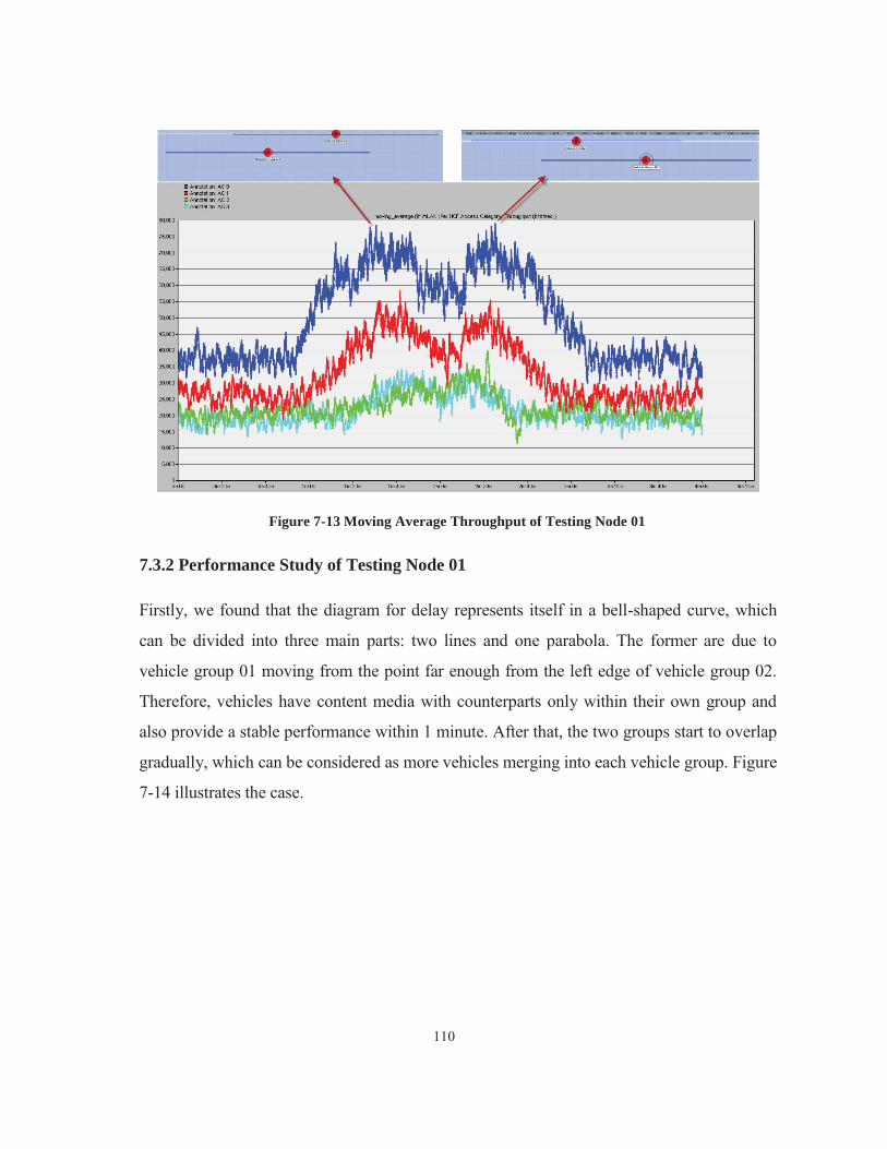
110
Figure 7-13 Moving Average Throughput of Testing Node 01 7.3.2 Performance Study of Testing Node 01 Firstly, we found that the diagram for delay represents itself in a bell-shaped curve, which
can be divided into three main parts: two lines and one parabola. The former are due to
vehicle group 01 moving from the point far enough from the left edge of vehicle group 02.
Therefore, vehicles have content media with counterparts only within their own group and
also provide a stable performance within 1 minute. After that, the two groups start to overlap
gradually, which can be considered as more vehicles merging into each vehicle group. Figure
7-14 illustrates the case.

111
Figure 7-14 Illustration of Vehicle Merge
From the view at the centre of effective communication coverage, vehicles there will
experience a greater traffic feed externally, i.e. more vehicles come inside. In our scenario,
only group 02 can fill with a 2 Km long effective communication coverage. Thus, the peak
delay we saw happened in the 80 vehicles per group situation. Such a phenomenon might
look simple, but has an important meaning, which implies two different VANET
performances in congested and loosened traffic situations. Concerning the first case, where
vehicles are almost continuously fed into certain coverage, the delay would be relatively low
but would maintain at a stable level, which helps vehicles in this range precisely evaluate the
situation more and also conducts AC adjustment accordingly, such as packet size or
generation frequency, for the purpose of enhancing some AC communication quality. On the
other hand, the latter instance subsequently causes large-scale fluctuation and jitter. It is
necessary to be understood that, since CCH works in the broadcast mode, it is hardly
possible to obtain information about a communication environment during that period, but
would count in the SCH period, whose establishment, however, completely depends on the
successful communication of WSA at AC 0, i.e. a deteriorative process. On the other side, it
can be observed that, through the increase of vehicle numbers, the delay of all ACs increase
at approximately the same pace and also maintain the spacing with each other just like the
previous two vehicle group merge, which proves the effectiveness of the EDCA mechanism

112
and the relatively independent behavior of each AC in VANET.
Besides the delay in the dynamic environment, Figure 7-14 discloses a more critical issue in
practical application, which is a hidden node problem that is rarely mentioned in WLAN
nowadays, due to the successful CTS/RTS mechanism. It has never been brought out or
found in previous scenarios because they are generally set in either a neglectable dimension
or a logical subnet, in order to better study other factors impacting on VANET. However, in
scenario 5, we found that there are always two throughput peaks happening at approximately
97s and 137s for each AC at testing node 01. After comparing to previous scenarios, I
conclude that such a phenomenon is due to a hidden node issue, as there is no CTS/RTS
mechanism in the broadcast mode. Apparently, vehicles in previous scenarios contend media
with each other either in a logical subnet or an extreme dimension, in order to better study
other changeable factors, thus never experiencing the hidden node problem.
However, in practical application, we need to divide collisions into two types: media
contention collision and hidden node collision, which are combined in order to degrade
VANET performance. In scenario-4, the packet received per second keeps increasing unless
the loss rate reaches nearly 100%, although adding a vehicle number results in a higher
collision rate. Concerning scenario-5, every node joining the effective communication
coverage of testing node 01 will arouse a higher rate of both kinds of collision, which at
some stage will overwhelm the impact of adding ACs. Simply put, even though more
packets have been transmitted every second, the collision rate increases much faster and
results in fewer packets being successfully received. Figure 7-15 provides the procedure of a
vehicle group merge from the view of testing node 01.

113
Figure 7-15 Vehicle Group Merge Procedure
In fact, the mechanism concerning dimension is very complex, although the above diagram
looks simple. I will try my best to explain it by using AC 03 as an example. In our scenario,
it shows one peak happening at stage 03. Firstly, from the view of testing node 01, we divide
its effective communication coverage into two parts (01 and 02), whereby there is no hidden
node collision within the same part due to pre-defined 1 Km coverage. When two vehicle
groups start to merge with each other from stage 01 to 02, the overall packet transmission
rate in part 01 increases, while the rate in part 02 remains the same, according to the
conclusion from scenario-4 and the nature of a non-saturated network. Thus, at these stages,
even with the number of hidden node collisions, testing node 01 can still receive more
packets within a given time. Simply put, vehicles in part 01 outnumber its counterparts of 02.
However, when vehicle group 02 pierces the middle line of group 01, where testing node 01
is located, the vehicle number in part 02 will increase, while the number in 01 does not
change. At that time, a collision due to hidden node increases is due to more vehicles being
fed into part 02, which act as antagonists against their counterparts in part 01. However, at
the initial stage after piercing, a higher packet transmission rate may still be able to offset the
impact of a greater overall collision rate; however, it loses its domination at a certain point in
time.
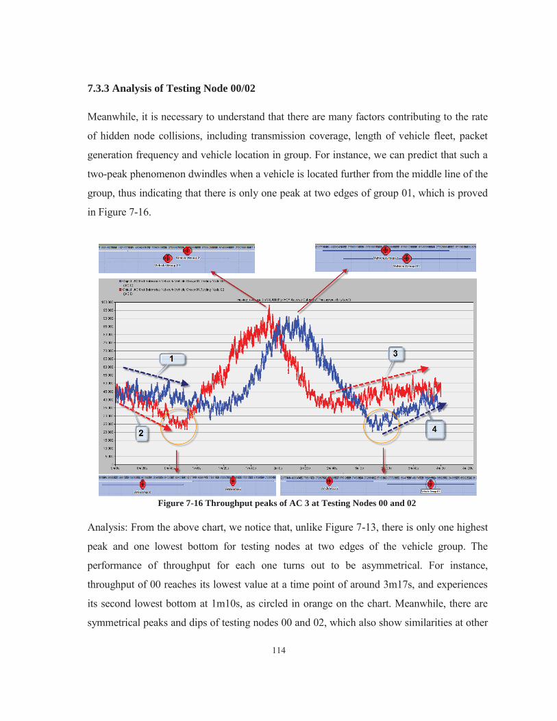
114
7.3.3 Analysis of Testing Node 00/02 Meanwhile, it is necessary to understand that there are many factors contributing to the rate
of hidden node collisions, including transmission coverage, length of vehicle fleet, packet
generation frequency and vehicle location in group. For instance, we can predict that such a
two-peak phenomenon dwindles when a vehicle is located further from the middle line of the
group, thus indicating that there is only one peak at two edges of group 01, which is proved
in Figure 7-16.
Figure 7-16 Throughput peaks of AC 3 at Testing Nodes 00 and 02
Analysis: From the above chart, we notice that, unlike Figure 7-13, there is only one highest
peak and one lowest bottom for testing nodes at two edges of the vehicle group. The
performance of throughput for each one turns out to be asymmetrical. For instance,
throughput of 00 reaches its lowest value at a time point of around 3m17s, and experiences
its second lowest bottom at 1m10s, as circled in orange on the chart. Meanwhile, there are
symmetrical peaks and dips of testing nodes 00 and 02, which also show similarities at other

115
points.
In order to explain and prove these statements and assumptions, it is necessary to further
illustrate all eleven stages of vehicle group mergence in Figure 7-17.
Figure 7-17 Eleven Stages of Vehicle Group Mergence
Parts 01 and 02 here are effective communication coverage for testing nodes 00 and 02,
respectively. As we mentioned in previous analysis, due to the two types of collision existing
in VANET, the packet receiving rate not only depends on how many vehicles are in
coverage but also their locations. In our scenario, using testing node 02 as an example, part
02 can be sub-divided into left and right parts. Then, we define the vehicle number ration
between left and right part as . Before the vehicle number changes in part 02, is
always 20/0 {Stage 01}, followed by 20/ (1-20) {Stage 01-02}, (21-40)/20 {Stage 02-04},
40/(20-0) {Stage 04-06} and (40-20)/0 {Stage 06-08}. Thus, we can see that within these
eight stages mostly affecting the performance of testing node 02, no pair can be considered
symmetric. For instance, if 36/20 at Stage 03, we can never find 20/36 throughout all
stages, due to the initial being 20/0 in an asymmetric manner. That explains why
throughput performance for 02 looks asymmetric and why there is only one highest peak and

116
one lowest bottom happening at Stages 05 and 01, respectively.
Next, we study two less fluctuated trend lines of testing node 02, namely 2 and 3 marked by
a dashed arrow line in Figure 7-16. Concerning the first trend, it happens when two vehicles
get close to each other until a little portion of vehicles in group 02 enters into effective
coverage of testing node 02 (Stage 01). Meanwhile, trend line 3 comes under an opposite
situation when vehicles of group 02 are further away from the coverage (Stage 09). Most of
the time, there are no vehicle number changes within part 02 throughout these two trend lines,
which indicates that such a phenomenon is mainly due to the impact of vehicles outside of
the testing node 02 effective coverage. According to the conclusion of scenario-2, packets
transmitted by vehicles located more than 1 Km, even if they can be harder decoded or
sensed along with distance, will arouse a higher probability of a sensed busy period, thus
reducing the throughput of testing node 02. A similar mechanism causes trend line 03, where
out of coverage vehicles, to gradually have a lower negative impact on part 02. However, the
reason that the lowest bottom is found on trend line 2 rather than 3 is because there are still
hidden node collisions on time periods of trend lines 2 and 3. Also, the former instance
turned out to represent a much more balanced pattern on two sides of part 02, namely lower
. Thus, hidden node collisions in trend line 02 will be higher than their counterparts of 03.
By reviewing Figure 7-17 again, we notice that there are symmetric patterns in this chart,
which are based on middle Stage 06. For instance, Stage 02/10 can be considered as a
rotated pair. However, it requests us to change the view from testing node 02 to 00;
otherwise, it cannot be considered as equal. Combining what we studied previously, we can
conclude that every stage experience by testing node 02 will not repeat itself but will still be
a counterpart of 00 in a reversed sequence, due to the location and relative movement of
these two vehicle groups. Therefore, we predict that their throughput patterns need to be both
rotated and shifted based on a time axle, which is proved in Figure 7-18.

117
Figure 7-18 Rotation and Shift of Testing Node 02 Throughput Diagram
From what is stated above, it reveals that throughout the procedure of an approaching vehicle
group at any given time point, every vehicle in the group will contribute a different
performance. Their delays will all be presented in a bell-shaped curve but will have space
between one another due to location difference. On the other side, the performance of
throughput turns out to be more complex, whereby every node evolves based on the
counterpart in the middle of the vehicle group. Figures 7-19 and 7-20 demonstrate the
evolution.
Figure 7-19 Throughput of Testing Node 00/01/02 in One Chart
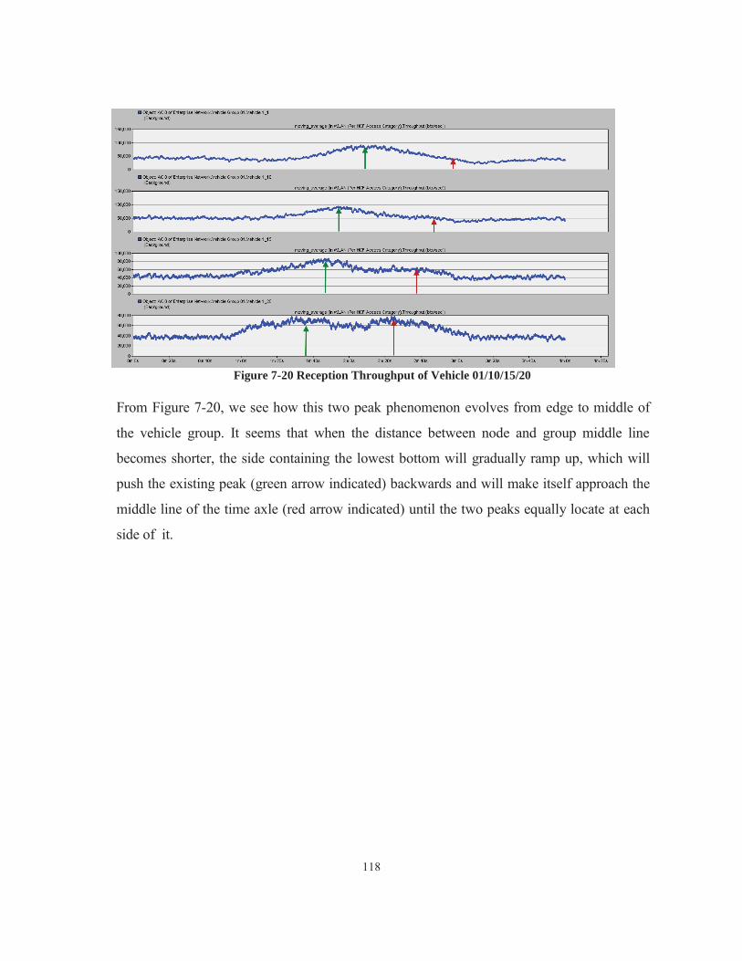
118
Figure 7-20 Reception Throughput of Vehicle 01/10/15/20
From Figure 7-20, we see how this two peak phenomenon evolves from edge to middle of
the vehicle group. It seems that when the distance between node and group middle line
becomes shorter, the side containing the lowest bottom will gradually ramp up, which will
push the existing peak (green arrow indicated) backwards and will make itself approach the
middle line of the time axle (red arrow indicated) until the two peaks equally locate at each
side of it.

119
Chapter 8 Conclusion and Future Work
8.1 Conclusion
In previous chapters, we simulated different scenarios for a CCH performance study under
801.11p. The results indicate that various factors cooperating with each other will impact on
the performance duo of a dynamically changing communication environment and can be
summarised as follows:
1 According to [66], the latencies for pre-crash and collision risk warning should not be
more than 50ms and 100ms, respectively. The results of all instances in our simulations
meet that requirement very well. For example, under instance-5 of scenario-4, whereby
133 vehicles start to contend media within 2 ms and each AC carries 1400 bits/packet,
the delay of AC 3 only reaches 7.25 ms, which indicates that 802.11p is capable
enough of meeting the latency requirement for road safety applications.
2 EDCA is an effective protocol to assign distinguishing media access priorities to
different types of ACs throughout our simulations. Especially under the situation where
media resources are heavily occupied, the mechanism tends to sacrifice the
transmission opportunity of ACs starting from the lowest priority in order to maintain
the operation of ACs with higher priorities.
3 Under the CCH broadcast mode, the packet collision caused by media contention
might be an issue. In general, the performance of AC with higher priority is more
sensitive to the number of vehicles transmitting within a guard interval and packet size.
In instance-4 of our simulation, where only ten vehicles carrying AC 3 data stream at
48 bits/packet, the collision rate can reach 21.55% and can seem too high to be
feasible, when two factors previously mentioned further increase.
4 The VANET adopted 802.11p protocol might be under risk of a broadcast storm and is
not very capable of dealing with an occasionally heavy load of higher priority AC
streams, since it eliminates the TXOP mechanism and evolves from the IEEE 802.11
family, which are all for unicast most of the time and are in shortage of an effective
mechanism for broadcasting or multicasting. Meanwhile, in these situations, not only

120
the CCH interval will be affected but also its SCH counterpart, due to a high collision
rate and latency of AC 0, which is supposed to provide information for WBSS
association.
5 Throughout the process of vehicle fleet mergence, the performance of each vehicle will
fluctuate significantly, which also distinguishes each other according to the position of
its fleet, due to the combined effects of communication coverage (including effective
and edge) as well as collision, due to hidden nodes. The latter one is inevitable under
the CCH broadcast mode since there is no RTS/CTS mechanism.
8.2 Future Work
In this thesis, we studied the performance of CCH in VANET in various situations with the
aid of OPNET. There are several recommendations we would like to provide for further
study of IEEE 802.11p, as follows:
1 It is hard to predict when an immediate 802.11p module will be available on OPNET.
Thus, within a relatively long-term period, the performance study still needs to rely on
the modification of current available WLAN modules. To be specific, the objective of a
wireless station needs to be to contain more than one wlan_mac_intf in order to
support multiple ACs and carry out and facilitate an internal contention mechanism
based on a single wireless_lan_mac.
2 Furthermore, although SCH will not directly be involved in road safety applications, its
performance might still need to be reviewed based on two reasons. Firstly,
communication on SCH is not an isolated procedure from its counterpart of CCH but
completely depends on it due to the reasons of AC 0 mentioned in previous
conclusions. Secondly, a STA is only able to estimate the communication conditions
during an SCH interval for the purpose of adjusting its transmission power, data rate,
packet size, etc., since the broadcast mode on CCH is a one-way transmission
mechanism and no feedback can be obtained during that period. In short,
communications on CCH and SCH are dependable on each other in some cases and

121
cooperate together to intelligently adjust themselves in order to enhance the overall
performance.
3 The impacts of geographic terrains, multipath propagation and fading on VANET
performance might need to be taken into consideration, as well as dynamically
changing vehicle topology, through the development of an exclusive propagation
modelling module for IEEE 802.11p. Current modelling in OPNET, like HATA,
Longley Rice, and Walfisch-Ikegami, cannot all be applied on the 5 GHz band directly.
4 The current 802.11p standard might demand further enhancement to address two main
prominent issues: broadcast storm and packet collision. The solution for the former
could be multi-hop forwarding or restoration of TXOP. The latter seems more difficult
to deal with and we advise researchers to consider modifying PHY of DSRC by adding
the latest multiple-input and multiple-output (MIMO) technology, together with
frequency hopping for some ACs with relatively high priorities.

122
REFERENCES [1] http://www.its.dot.gov/its_program/about_its.htm (2010)
[2] NHTSA (2009), "Traffic Safety Facts 2009,” www-nrd.nhtsa.dot.gov/pubs/811402ee.pdf
[3]http://data.worldbank.org/indicator/IS.VEH.PCAR.P3?order=wbapi_data_value_2008+wbapi_data
_value+wbapi_data_value-last&sort=desc
[4] Ministry of Transport, New Zealand (2010), "MOTOR VEHICLE CRASHES IN NEW
ZEALAND 2009,” http://www.transport.govt.nz/research/Motor-Vehicle-Crashes-in-New-Zealand-
2009/
[5] K.Prasanth, Dr.K.Duraiswamy, K.Jayasudha, Dr. C.Chandrasekar, "IMPROVED PACKET
FORWARDING APPROACH IN VEHICULAR AD HOC NETWORKS USING RDGR
ALGORITHM,” International Journal of Next Generation Network (IJNGN), Vol.2, No.1, pp.14,
March 2010
[6] http://www.its.dot.gov/research/v2v.htm (2010)
[7] Mainak Ghosh & Sumit Goswami (2009),"Intelligent Transportation using VANET,”IIT,
Kharagpur, http://pcquest.ciol.com/content/technology/2009/109020101.asp
[8] Den Hengst,M.,Sol, H.G., “The impact of information and communication technology on
interorganizational coordination,” The 34th Annual Hawaii International Conference, 10 pp., 3-6 Jan.
2001
[9] Hannes Hartenstein, Kenneth Laberteaux (2010),"VANET: vehicular applications and inter-
networking technologies,” John Wiley & Sons Ltd, IBSN 978-0-470-74056-9
[10] Harvey J. Miller and Shih-Lung Shaw (2001),"Geographic Information Systems for
Transportation,” Oxford University Press, ISBN 0195123948

123
[11] Yasser L. Morgan, “Managing DSRC and WAVE Standards Operations in a V2V Scenario,”
International Journal of Vehicular Technology, vol. 2010
[12]Daniel Jiang, Luca Delgrossi, "IEEE 802.11p: Towards an International Standard for Wireless
Access in Vehicular Environments,” Vehicular Technology Conference, 2008. VTC Spring 2008.
IEEE, Singapore, pp. 2036-2040
[13] Martin Muller (2009), "WLAN 802.11p Measurements for Vehicle to Vehicle (V2V) DSRC
Application Note," ROHDE & SCHWARZ
[14] Martin Koubek, Susan Rea, and Dirk Pesch , "Reliable Delay Constrained Multihop
Broadcasting in VANETs,” URASIP Journal on Advances in Signal Processing, vol.2010
[15]Benslimane, A., Taleb, T., Sivaraj, R., "Dynamic Clustering-Based Adaptive Mobile Gateway
Management in Integrated VANET — 3G Heterogeneous Wireless Networks " Selected Areas in
Communications, IEEE Journal, vol.29, pp.559-570, March 2011
[16] Mathieu LENOBLE, Kenji ITO (2011), "Throughput Improvement Technique for D-TDMA-
Based Vehicular Ad-Hoc Networks,” IEICE TRANSACTIONS on Communications Vol. E94-B,
No.10, pp.2776-2784
[17] Lequerica, I., Ruiz, P.M., Cabrera, V., "Improvement of vehicular communications by using 3G
capabilities to disseminate control information,” Network, IEEE, Vol. 23, Issue: 1, pp. 32-38, Jan.-
Feb. 2010
[18] Jianli Pan, (2008),"A Survey of Network Simulation Tools: Current Status and Future
Developments,” Washington University in St.Louis
[19] Rolf Kraemer, Marcos D. Katz (2009),"Short-range wireless communications: emerging
technologies and applications,” John Wiley & Sons Ltd, ISBN 978-0-470-69995-9
[20] Ramjee Prasad (2004) "OFDM for wireless communications systems,” Artech House Publishers,
IBSN 978-1580537964

124
[21] Arijit Khan, Shatrugna Sadhu, and Muralikrishna Yeleswarapu (2010), "A comparative analysis
of DSRC and 802.11 over Vehicular Ad hoc Networks,” Dept. of Computer Science, University of
California, Santa Barbara
[22] Ivan, I., Besnier, P., Crussiere, M., Drissi, M., Le Danvic, L., Huard, M., Lardjane, E., "Physical
layer performance analysis of V2V communications in high velocity context," Intelligent Transport
Systems Telecommunications, 2009 9th International Conference, pp. 409-414, 20-22 Oct. 2009
[23]Gukhool, B.S., Cherkaoui, S., "IEEE 802.11p modeling in NS-2,” Local Computer Networks,
2008. LCN 2008. 33rd IEEE Conference, Montreal, Que, pp.622-626, 14-17 Oct. 2008
[24] Scalia, Luca, Widmer, Joerg, Aad, Imad, "On the side effects of packet detection sensitivity in
IEEE 802.11 interference management,” World of Wireless Mobile and Multimedia Networks
(WoWMoM), 2010 IEEE International Symposium, Montreal, QC, Canada, pp. 1-7, 14-17 June 2010
[25] Tinnirello, I., Bianchi, G., Yang Xiao, "Refinements on IEEE 802.11 Distributed Coordination
Function Modeling Approaches,” IEEE Transactions on Vehicular Technology, vol. 59, issue 3, pp.
1055-1067, March 2010
[26] Dalton, D., Kwet Chai, Evans, E., Ferriss, M., Hitchcox, D., Murray, P., Selvanayagam, S.,
Shepherd, P., DeVito, L., "A 12.5-mb/s to 2.7-Gb/s continuous-rate CDR with automatic frequency
acquisition and data-rate readback,” Solid-State Circuits, IEEE Journal, vol. 40, issue 12,pp.2713-
2725, Dec.2005
[27] Hao Hu, Areal, J.L., Palushani, E., Oxenlowe, L.K., Clausen, A., Berger, M.S., Jeppesen, P.,
"Optical Synchronization of a 10-G Ethernet Packet and Time-Division Multiplexing to a 50-Gb/s
Signal Using an Optical Time Lens," Photonics Technology Letters, IEEE, vol. 22, issue 21, pp.1583-
1585, Nov. 2010
[28] Ramjee Prasad and Luis Munoz, “WLANs and WPANs Towards 4G Wireless,” Artech House,
ISBN 978-1580530903

125
[29] Ghassan M. T. Abdalla, Mosa Ali Abu-Rgheff and Sidi Mohammed Senouci (2010), "Current
Trends in Vehicular Ad Hoc Networks," University of Plymouth – School of Computing,
Communications & Electronics, Ubiquitous Computing and Communication Journal
[30] Li, P., Scalabrino, N., Fang, Y., Gregori, E., Chlamtac, I., "Channel Interference in IEEE
802.11b Systems," Global Telecommunications Conference, 2007. GLOBECOM '07. IEEE,
Washington, DC, pp.887-891,26-30 Nov.2007
[31] David D. Coleman, David A. Westcott (2009), "CWNA Certified Wireless Network
Administrator Official Study Guide,” Wiley Publishing, Inc., ISBN 978-0072255386
[32]Hannes Hartenstein, Kenneth Laberteaux (2010), "VANET Vehicular Applications and Inter-
Networking Technologies,” John Wiley & Sons Ltd., ISBN 978-0-470-74056-9
[33] David D. Coleman, David A. Westcott, Ben Miller, Peter Mackenzie (2004), "CWAP Certified
Wireless Analysis Professional Official Study Guide,” Sybex, ISBN 978-0072255850
[34] Mecklenbrauker, C. F., Molisch, A. F., Karedal, J., Tufvesson, F., Paier, A., Bernado, L., Zemen,
T., Klemp, O., Czink, N. (2011), "Vehicular Channel Characterization and Its Implications for
Wireless System Design and Performance,” Proceedings of the IEEE, vol.99, issue 7, pp.1189-1212,
July 2011
[35] Mahdi Abbasi (2008), "Characterization of a 5GHz Modular Radio Frontend for WLAN Based
on IEEE 802.11p,” University of Gavle
[36] Bernhard H. Walke,Stefan Mangold,Lars Berlemann, (2006), "IEEE 802 Wireless Systems:
Protocols, Multi-hop Mesh/Relaying, Performance and Spectrum Coexistence,” John Wiley & Sons
Ltd
[37] Jong-Moon Chung, Minseok Kim, Yong-Suk Park, Myungjun Choi, Sangwoo Lee, Hyun Seo
Oh, (2011), "Time Coordinated V2I Communications and Handover for WAVE Networks,” Selected
Areas in Communications, IEEE Journal, vol. 29, issue 3, pp.545-558, March 2011

126
[38] Gaurav Sharma, Ayalvadi Ganesh, Peter Key, (2006), "Performance Analysis of Contention
Based Medium Access Control Protocols,” School of Electrical and Computer Engineering
[39] Inanc Inan,Feyza Keceli,Ender Ayanoglu, "Analysis of the 802.11e Enhanced Distributed
Channel Access Function,” IEEE TRANSACTIONS ON COMMUNICATIONS, VOL. 57, NO. 6,
JUNE 2009
[40] Kamal Gakhar, Annie Gravey, Alain Leroy, "IROISE: A New QoS Architecture for IEEE 802.16
and IEEE 802.11e Interworking,” Department Of Computer Science, ENST Bretagne, Broadband
Networks, 2005. BroadNets 2005. 2nd International Conference, Boston, MA, pp.607-612, Oct. 2005
[41] Prof. R.S.Uppal, Shubhla Puri, (2010), "Performance and Evaluation of IEEE 802.11e using
QUALNET,” Department of Electronics and Communication Engineering of Baba Banda Singh
Bahadur Engineering College and GGS College of Modern Technology
[42] Der-Jiunn Deng, Hsin-Chin Chen, Han-Chieh Chao and Yueh-Min Huang (2011), “A Collision
Alleviation Scheme for IEEE 802.11p VANETs,” Wireless Personal Communications, Volume 56,
Number 3
[43] Sebastian Grafling, Petri Mahonen, Janne Riihijarvi, (2010), "Performance Evaluation of IEEE
1609 WAVE and IEEE 802.11p for Vehicular Communications,” Ubiquitous and Future Networks
(ICUFN), 2010 Second International Conference, Jeju Island, Korea, pp.344-348,16-18 June 2010
[44] Jelena Misic, Ghada Badawy, Vojislav B. Misic, "Performance characterization for IEEE
802.11p network with single channel devices,” Vehicular Technology, IEEE Transactions, vol.60,
issue 4, pp.1775-1787, May 2011
[45] Md.Abdul Based (2010), "A Survey about IEEE 802.11e for better QoS in WLANs,”
Department of Telematics, NTNU, Norway

127
[46] Das, S., Chakraborty, K., Rajamani, K., Dural, O., Soliman, S.S., "Scalable PLCP header
extension within PSDU,” Ultra-Wideband, 2009. ICUWB 2009. IEEE International Conference on,
Vancouver, BC, pp.570-574, 9-11 Sept. 2009
[47] Byeong Gi Lee, Sunghyun Choi ,(2008),"Broadband Wireless Access and Local Networks
Mobile WiMAX and WiFi,” Artech House Publishers, ISBN 978-1596932937
[48] IEEE Vehicular Technology Society, "IEEE Standard for Wireless Access in Vehicular
Environments (WAVE)—Multi-channel Operation", E-ISBN: 978-0-7381-6489-2, Feb. 2011
[49] Bin Hu, Hamid Gharavi, "A Joint Vehicle-Vehicle/Vehicle-Roadside Communication Protocol
for Highway Traffic Safety,” International Journal of Vehicular Technology, vol. 2011
[50] Sajjad Akbar Mohammad, Asim Rasheed, Amir Qayyum (2011), "VANET Architectures and
Protocol Stacks: A Survey ,” Communication Technologies for Vehicles, Lecture Notes in Computer
Science, 2011, Volume 6596/2011, 95-105, DOI: 10.1007/978-3-642-19786-4_9
[51] Shie-Yuan Wang, Chih-Che Lin, Kuang-Che Liu, Wei-Jyun Hong, (2009), "On multi-hop
forwarding over WBSS-based IEEE 802.11(p)/1609 networks,” Personal, Indoor and Mobile Radio
Communications, 2009 IEEE 20th International Symposium, Tokyo, pp.3040-3044,13-16 Sept. 2009
[52] Y. L. Morgan, (2010), "Notes on DSRC & WAVE Standards Suite: Its Architecture, Design, and
Characteristics,” Communications Surveys & Tutorials, IEEE, vol. 12, issue 4,pp. 504-518, Fourth
Quarter 2011
[53] Ching-Ling Huang, Fallah, Y.P., Sengupta, R., Krishnan, H., "Adaptive Intervehicle
Communication Control for Cooperative Safety Systems,” Network, IEEE, vol.24, issue 1, pp.6-13.
Jan.-Feb. 2010
[54] Kenney, J.B., "Dedicated Short-Range Communications (DSRC) Standards in the United States,”
Proceedings of the IEEE, vol.99, issue 7, pp.1162-1182, July 2011

128
[55] Olivia Brickley, Martin Koubek, Susan Rea, Dirk Pesch, (2010), "A Network Centric Simulation
Environment for CALM-based Cooperative Vehicular Systems,” SIMUTools '10 Proceedings of the
3rd International ICST Conference on Simulation Tools and Techniques, ISBN: 978-963-9799-87-5
[56] IEEE Vehicular Technology Society, "IEEE Standard for Wireless Access in Vehicular
Environments (WAVE)— Networking Services, IEEE Std 1609.3™-2010"
[57] Johan Englund, (2010), "Determining suitability of the IEEE1609 standard for PRT systems"
[58] Campolo, C., Vinel, A., Molinaro, A., Koucheryavy, Y.,(2011),"Modeling Broadcasting in IEEE
802.11p/WAVE Vehicular Networks,” Communications Letters, IEEE, vol. 15, issue 2, pp.199-201,
Feb. 2011
[59] Huibin Wang, Yang Hu, Lili Zhang, Wei Xia, (2010),"A New Adaptive EDCA Approach to QoS
of Wireless Communications,” College of Computer and Information Engineering, Hohai University,
Nanjing, China
[60] Antonio Peinado, Jose Segura, (2006), "Speech Recognition over Digital Channels: Robustness
and Standards,” Wiley, ISBN: 978-0-470-02400-3
[61] Ralph El Khoury and Rachid El-Azouzi, (2007), "Modeling the Effect of Forwarding in a Multi-
hop Ad Hoc Networks with Weighted Fair Queueing,” LIA/CERI, Universite d'Avignon, France
[62] Ralph El Khoury and Rachid El-Azouzi, "Modeling the Effect of Forwarding in a Multi-hop Ad
Hoc Networks with Weighted Fair Queueing,” Mobile Ad-Hoc and Sensor Networks, Lecture Notes
in Computer Science, 2007, Volume 4864/2007, 5-18, DOI: 10.1007/978-3-540-77024-4_3
[63] Giuseppe Bianchi, "Performance Analysis of the IEEE 802.11 Distributed Coordination
Function,” IEEE JOURNAL ON SELECTED AREAS IN COMMUNICATIONS, VOL. 18, NO. 3,
MARCH 2000

129
[64] Suong H. Nguyen, Hai L. Vu, and Lachlan L. H. Andrew, "Performance analysis of 802.11e
EDCA WLANs with saturated and non-saturated sources,” Swinburne University, Melbourne,
Australia
[65] John T Hughes,(2002),"AIMSUN2 Simulation of a Congested Auckland Freeway,” Transit New
Zealand, Auckland, New Zealand
[66] Ikbal Chammakhi Msadaa, Pasquale Cataldi and Fethi Filali, (2010), "A Comparative Study
between 802.11p and Mobile WiMAX-based V2I Communication Networks,” Next Generation
Mobile Applications, Services and Technologies (NGMAST), 2010 Fourth International Conference,
Amman, pp.186-191, 27-29 July 2010

130
Appendix
Transmission Power Estimation
Objects: One fixed node, one mobile node, 4 Km trajectory
Parameter Setting: 801.11p, 10 Km/h for mobile node (very low speed), 6 Mbps, 0.005 W
for transmission power
The above results only indicate a 364.5 second stable transmission and show that 0.005 W is
not enough for 1 Km coverage, as it has to last 720 seconds (1 Km at each side of fixed
node). According to the free space loss formula, we define N in dBm at a critical point (at
537 seconds). Thus,
N= 7 – {32.45+ 20*lg5885+20*lg(2-537*2.777777/1000)} (7 dBm here equals to 0.005W)

131
Thus, N≈-95 dBm. In the case of there being 1 Km coverage, we can get transmission power
to be 12.87702108 dBm, which is equal to 0.01939555W.
The result actually perfectly matches our expectation, as a 12 minute stable communication
can be observed after applying the above transmission power.

132
Simulation Results
Table of Average Delay under three same kind ACs only of Instance 1
Access Category
Packet Size (bits) 48 96 192 384 768 1400
Average Delay (ms) AC 3 0.2073 0.33533 0.517036 0.96221 1.85351 3.3177 AC 2 0.2162 0.3442 0.5249 0.9711 1.8635 3.3345 AC 1 0.2611 0.3777 0.5908 1.067 2.0195 3.5897 AC 0 0.3041 0.4146 0.6625 1.1586 2.1507 3.7862
Tables of Sub-Instance for Study of Packet Size Impact
sub-instance 0 Packet Size of AC 0 Access
Category 48 96 192 384 768 1400
Average Delay (ms) AC 3 1.0093 0.9964 0.9919 1.019 1.2534 1.6993 AC 2 1.2637 1.2782 1.2526 1.2664 1.2691 1.2751 AC 1 3.2003 3.2205 3.2169 3.2642 3.3401 3.5314 AC 0 3.3863 3.5267 3.7474 4.223 5.312 7.1741
sub-instance 0 Packet Size of AC 1 Access
Category 48 96 192 384 768 1400
Average Delay (ms) AC 3 0.9895 0.9853 0.986 1.0192 1.0844 1.6827 AC 2 1.2357 1.2455 1.2502 1.2662 1.2939 1.3601 AC 1 2.4634 2.5679 2.7959 3.2568 4.2265 5.8656 AC 0 3.1017 3.2537 3.5753 4.2077 5.8533 8.2417
sub-instance 0 Packet Size of AC 2 Access
Category 48 96 192 384 768 1400
Average Delay (ms) AC 3 0.75 0.7501 0.809 1.0205 1.3572 2.1076 AC 2 0.6057 0.6922 0.9058 1.2714 2.1689 3.6666 AC 1 2.3965 2.3746 2.6681 3.266 4.6692 7.3751 AC 0 3.3079 3.3232 3.6358 4.234 5.9344 8.5882

133
sub-instance 0 Packet Size of AC 3 Access
Category 48 96 192 384 768 1400
Average Delay (ms) AC 3 0.4733 0.5504 0.7011 1.02 1.7161 2.843 AC 2 1.0595 1.0792 1.1371 1.2756 1.5824 2.111 AC 1 2.5956 2.6927 2.8584 3.2059 4.1028 5.8219 AC 0 3.6067 3.6813 3.8686 4.2196 5.3499 8.0651

134
Vehicle Number Impact on VANET Performance under a single type of AC.

135
VANET Performance under Multiple-AC Types