Embed Size (px)
Citation preview

Copyright is owned by the Author of the thesis. Permission is given for a copy to be downloaded by an individual for the purpose of research and private study only. The thesis may not be reproduced elsewhere without the permission of the Author.
------- --
Flow and Diffusion
Measurements
on Complex Fluids
Using
Dynamic NMR Microscopy
A thesis presented in partial fulfilment of the requirements for the degree of Doctor of Philosophy in �hysics
at Massey U ni versi ty
Bertram Manz 1996
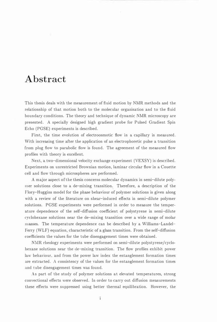
Abstract
This thesis deals with the measurement of fluid motion by NMR methods and the
relationship of that motion both to the molecular organisation and to the fl uid
boundary conditions. The theory and technique of dynamic NMR microscopy are
presented . A specially designed high gradient probe for Pulsed Gradient Spin
Echo ( PGSE) experiments is described .
First, the time evolution of electroosmotic flow in a capillary is measured .
With increasing time after the application of an electrophoretic pulse a transition
from plug flow to parabolic flow is found . The agreement of the measured flow
profiles with theory is excellent.
Next, a two-dimensional velocity exchange experiment (VEXSY) is described .
Experiments on u nrestricted Brownian motion , laminar circular flow in a Couette
cell and flow th rough microspheres are performed .
A major aspect o f t he thesis concerns molecular dynamics in semi-di lute poly
mer solutions close to a de-mixing transition.,
Therefore, a description of the
Flory-Huggins model for the phase behaviour of polymer solutions is given along
with a review of the literature on shear-induced effects in semi-di lute polymer
solutions. PGSE experiments were performed in order to measure the temper
ature dependence of the self-diffusion coefficient of polystyrene in semi-di lute
cyclohexane solutions near the de-mixing transition over a wide range of molar
masses. The temperature dependence can be described by a Williams-Landel
ferry (WLF) equation , characteristic of a glass transition. From the self-diffusion
coefficients the values for the tube disengagement times were obtained .
NMR rheology experiments were performed on semi-dilute polystyrene/cyclo
hexane solutions near the de-mixing transition . The flow profiles exhibit power
law behaviour , and from the power law index the entanglement formation times are ext racted . A consistency of the values for the entanglement formation times
and tube disengagement times was found .
As part of the study of polymer solutions at elevated temperatu res, strong
convectional effects were observed . In order to carry out diffusion measurements
these effects were suppressed using better thermal equili bration . However, the
11 ABSTRACT
convection process itself was subject to NMR investigation . Convectional flow
in a capi l lary was measured using PGSE NMR, VEXSY and dynamic NMR mi
croscopy. The VEXSY experiment shows that the flow is stationary. The velocity
propagator measured using dynamic NMR microscopy was used to calculate the
echo attenuation function E(q). It was found that the pronounced minima and
maxima in the Stejskal-Tanner plots agree well with the measured E(q) values.
Flow profiles of lyotropic liquid crystals are presented . Using deuterium NMR
spectroscopy it i s shown that the shear-induced alignment of molecules can be
measured using NMR microscopy.
--------------- -- --
Acknowledgements
The fol lowing people have helped me with th is work . It is a pleasure to thank
them here.
Prof. Paul T. Callaghan , my fi rst supervisor, for his constant support, enthu
siasm and expertise.
Assoc. Prof. Rod K. Lambert, my second supervisor, for support and d iscus
sions.
The staff of the electronics workshop who bui lt the shift register wh ich enabled
me to sleep at night while the experiments were running, and for helping me with
many little problems.
The staff of the mechanical workshop for building a driving system for the
Couette system and count less other items.
Grant P latt for build i ng the dewars of the PGSE probe and for cutting and
seal ing my sample tubes.
Dr. Ph i l Back for designing and building the PGSE probe.
Dr. Bas Smeulders for supplying me with information about the DobanoljWa
ter system .
D r . Joe Seymour who i nspired me with h is enthusLasm and gave me permission
to use some of his data.
My fel low graduate students Andrew, Craig, Lucy and all other i nhabitants of
the NMR lab for being friends and colleagues.
The secretaries for their help with administration .
Al l members of the Physics department for maintain ing a pleasant working
environment.
The German Academic Exchange Service (DAAD ) and the New Zealand Foun
dation for Research. Science and Technology for financial support .
Anna for putting up with me.
III

IV AC[{NO WLEDG EMENTS
Contents
Abstract
Acknowledgements
Table of Contents
List of Figures
List of Tables
1 Introduction
1 . 1
1 .2
Introduction .
Organisation of the Thesis .
2 Introduction to NMR and Imaging
2.1 NMR Theory . . . . . . . . . . . . . . . . . . . . . . . . . .
2. 1 . 1 The Quantum Mechanical Description . . . . . . . .
2. 1 . 1 . 1 Quantum Mechanical States and Operators
2.1 . 1 .2 Angu'lar Momentum Operators . .
2. 1 . 1 .3 Nuclear Spins in a Magnetic Field
2. 1 .1.-1 The Ensemble Average
2. 1 .1.5 Time Evolution
2.1.2 The Semi-Classical Picture . .
2.1.2.1 The Rotating Frame .
2.1.2.2 Excitation
2. 1 .2.3 Relaxation
2.1.2...l Free Induction Decay
2.2 Nuclear Interactions . . . . . . . . . .
2.2.1
2.2.2
2.2.3
i\Iagnetic F ield Inhomogeneity
Chemical Shift .
Dipolar Coupling
v
111
v
Xl
XV
1
1
2
5
6
6
6
7
7
8
9
10
10
1 1
13
14
15
15
15
16
VI CONTENTS
2.2 .4 Quadrupolar Coupling
2 .3 Spin Manipu lations . . . . . .
2 . 3 . 1 The Spin Echo . . . .
2 . :3 .2 The Stimulated Echo .
2 .3 .3 The Quadrupole Echo
2 .3 . .! Two- Dimensional Spectroscopy .
2 .3 .5 Signal Averaging and Phase Cycling
2.3 .6 The Effect of Magnetic Field Gradients
2 .4 I ntroduction to NMR Imaging .
2 .4 . 1 k- Space Imaging . . . .
2 .4 .2 Selective Excitation . .
2 .4 .3
2 .4 .4
2 .4 .5
2 .4 .2 . 1 Hard Pulses and Soft Pulses
2 .4 .2 .2 Slice Selection . . . . . . .
Fourier Imaging i n Two Dimensions
Measuring Self- Diffusion : The Pulsed Gradient Spin Echo .
Dynamic NMR Imaging . . . . . .
2 .4 .5 . 1 Introduction to q- Space .
2 .4 .5 .2 The Dynamic Spin Echo
2 .5 Hardware and Software . . . . . . . . . .
2 .5 . 1 The Bruker AMX300 Spectrometer .
2 .5 .2 The FX60 Spectrometer . . .
2 .5 .3 The High-Gradient Probe . .
2 .5 .3 . 1 The Gradient Coils
2 .5 .3 .2 Gradient Calibration
2 .5 .3 .3 Gradient Eddy Currents .
2 .5 .3 .4 Temperature Control
2 .5 .3 .5 d. Stage
2 .5 .4 Data Processing .
3 Imaging of Electroosmotic Flow
3 . 1 Introduction . . . . . . . . . . .
3 .1 .1 Electrophoresis and NMR
:3 .1 .2 Electroosmosis
3 .2 Theory . . . . . . . . .
3 .3 Experimental Section .
3. .! Results . .
3 .5 Discussion
1 7
1 7
1 7
21
2 1
22
23
25
25
25
26
27
28
28
30
32
32
32
34
34
35
35
36
37
38
38
39
40
43
43
43
45
45
49
5 1
55
CO rvTEN TS
4 Velocity Exchange Spectroscopy
-1 . 1 Introduction . . . . . . . . .
4 .2 Theoretical Considerations . . . . -1.3 Experimental . . . . . . . . . . .
-1 . 3 . 1 Unrestricted Brownian Motion
-L3 . 2 Laminar Newtonian Flow in a Couette Cell
-1.3.2.1 Calculation of the V EXSY Spectra .
-1.3.2.2 Measu rement of the V EXSY Spectra
4.3.3 Flow Th rough Micropores
4.4 Concl usions
5 Polymer Physics
.5 . 1 Introduction .
5 . 1 . 1 Defi nition of a Polymer
5 . 1 .2 Molecu lar Weights and Polydispersity
5 . 1 .3 Polystyrene . . . . . . . . . . . . .
5 .2 Dynamics of Polymer Chains in Solution .
5 .2 . 1 Random Coils i n Dilute Solutions .
5 .2 .2 Thermodynamics of Polymer Solutions .
VIl
57
57
58
60
60
6 1
6 1
64
68
70
73
73
73
73
74
74
75
76
5 .2 .3 Osmotic Pressure and the F lory Temperature 78
5 .2.4 Phase Equi l ibria . . . . 78
5 .2 .5 Concentration Regimes 8 1
5 .2 .6 The Reptation Model 83
5 .3 Rheology of Polymer Solutions 87
5 .3 . 1 Introduction and Definitions 87
5 .3 .2 Dependence of Non-Newtonian Viscosity on Shear Rate 88
5 .3 .3 The Glass Transition . . . . . . . . . . . .5 .4 Flow-Induced Structures in Polymer Solutions
5.-!. 1 Shear-Induced Phase Transitions . . .
.5 .-! .2 Enhanced Concentration Fluctuations
5 . 4 .3 Shear-Induced Orderi ng
5.5 Rheo-NMR
5.6 Rheometers . . . . . .
6 Diffusion Nleasurements
6 .1 Polystyrene in Cyclohexane
6 .2 Experimental Section . . . .
6 .2 . 1 Sam ple Preparation
6 .2 .2 Measurement of the Self-Diffusion Coefficient
9 1
92
92
93
94
94
9.5
97
97
98
98
99
vii i CONTENTS
6 .3 Results . . . . . . . . . . . . . . . . . . . . . . . . . . . . . . . . . . 1 0 1
6 .3 . 1 The Temperature Dependence of Ds at Different Molar Masses 10 1
6 .3 .2 The Temperature Dependence of Ds at Different Concen-
trations
6.4 Discussion . . .
6 . 4 . 1
6 .4 .2
Reptation Times
Concentration F luctuations
6 .4 .2 . 1 Some Calculations
102
104
104
106
1 08
6 .4 .2 .2 Comparison With the Experimental Values 1 10
6 .4 .3 Glass Transition
6.5 Conclusions . . . . . . .
7 Flow Measurements on Polymer Solutions
7 . 1 Instrumentation . . . . .
7 . 1 . 1 The Couette Cell
7 . 1 .2 Data Analysis . .
7 .2 Experimental . . . . . .
7 .2 . 1 Sample P reparation
7 .2 .2 F low Measurements
7 .3 Results . . . . . . . . . . . .
7 .4 Discussion . . . . . . . . . .
7.4 . 1 Shear-Induced Phase Transitions
7 .4 .2 Entanglement Formation Times .
7 .4 .3 Glass Transition
7.5 Conclusions . . . . . . .
8 Convection in a Capillary
8 . 1 Introduction . . . . . . .
8.2 Experimental . . . . . .
8 .2 . 1 The PGSE Experiment
8 .2 .2 The Flow Imaging Experiment
8 .2 .3 The VEXSY Experiment
8.3 Conclusions . . . . . . . . . . . .
1 1 1
1 13
1 1 5
1 15
1 1 5
1 17
1 17
1 1 7
1 1 8
1 2 1
122
122
123
125
126
1 29
129
13 1
132
133
135
137
9 Shear-Induced Order in Liquid Crystals 139
9 . 1 Lyotropic Systems . . . . . . . . . . . . . . . . . . . . . . . . 139
9 . 1 . 1 Introduction . . . . . . . . . . . . . . . . . . . . . . . 139 9 . 1 .2 Rheology on Lyotropic Systems in the Lamellar Phase 1-n
9 . 1 .3 NMR on Lyotropic Systems in the Lamellar Phase . . 1�2
CONTENTS
9.2 Experimental Section . . . . . . .
9 .2 . 1 Sample Preparation . . .
9 .2 . 1 . 1 Dobanol/Water
9.2 . 1 . 2 Aerosol OT /Water .
----- - -- -----
9.2 .2 Measurement of Flow Profiles
9 .2 .3 Measurement of Order Parameters
9 .3 Resu lts . . . . . . . . . . . . . . .
9 .3 . 1 Flow Profiles . . . . . . .
9 .3 . 1 . 1 Dobanol/Water
9 .3 . 1 .2 AOT /Water . .
9 .3 .2 Deuterium NMR Spectra
9 .4 Discussion .
9 .5 Conclusions
IX
143
143
143
143
143
145
146
146
146
147
148
149
150
10 Conclusion 153
1 0 . 1 Summary . . . . . . . . . 153
10 .2 Outlook on Future Work . 154
Bibliography 1 57
A The P GSE Probe 167
B The Pulse Sequences 179
B . 1 Pu lse Sequence to Send Trigger Pulses to External Shift Register 1 79
B .2 Dynamic Spin Echo Soft Soft . . . . . . . . . . . . . . . . . 1 79
B .3 Pulsed Gradient Spin Echo . . . . . . . . . . . . . . . . . . . 18 1
B .4 Pulsed Gradient Spin Echo With Ramped Gradient Pulses . . 183
B .5 Dynamic Stimulated Echo with Electroosmosis Trigger Pu lse 1 84
B .6 V EXSY . . . . . . . . . . . . . . 186
B .7 V EXSY with Carr-Purcell Train 188
C The AV Programs 191
C. 1 Program to Send Trigger Pulses to External Shift Register . 191
C.2 AU Program for a Set of Experiments with Different Temperatures 192
C.:3 AL Program for a Set of Experiments with Different Motor Speeds 192

x CONTENTS
List of Figures
2 . 1 Decomposition of an Oscillating Field 12
2 . 2 The Free Induction Decay . . 15
2.3 The NMR Spectrum . . . . . 1 6
2.4 The Quadrupolar Interaction 18
2 . 5 Spin Echo Pu lse Sequence . . 18
2 . 6 Formation of a Spin Echo . . 20
2 .7 Stimulated Echo Pulse Sequence 2 1
2.8 Quadrupole Echo Pu lse Sequence 22
2 . 9 Two-Dimensional Spectroscopy 22
2 . 1 0 Phase Cycling . . . . . . . . . . 24
2 . 1 1 Slice Selection . . . . . . . . . . 27
2 . 1 2 The Spin Warp Pu lse Sequence 29
2 . 1 3 The Pulsed Gradient Spin Echo . 3 1
2 . 1 4 The Dynamic Spin Echo Pu lse Sequence 33
2 . 15 Circuit Diagram to Show the Connection of Primary and Secondary
Coils . . . . . . . . . . . . . . . . . . . . 36
2 . 1 6 Calibration of the H igh Gradient P robe . . . . . . . . 37
2 . 17 "Switch-off" Test of the High Gradient Probe . . . . . 39
2 . 1 8 Temperature Cal ibration of the High Gradient Probe . 40
2 . 19 Circuit Diagram of the d. Stage . -10
2.20 Photos of the High Gradient Probe 42
3.1 Poiseuil le Flow in a Capi l lary . . .
:3 .2 Pu lse Cycle of the Electric Field Gradient
3.3 The Electroosmotic Cell . . . . . . . . . .
3.-1 The Pulse Sequence for the Electroosmosis Experiments
3 . .5 Velocity Images of the Electroosmotic Cell .
3.6 Velocity Profiles of the Electroosmotic Cell
-1 . 1 The Basic VEXSY Pu lse Sequence
XI
46
49
.50
51
·53
5 -1
59
XII
4.2
4.3 4.4 -L . 5
4.6
4.7 4.8
.5.1
.5.2
5.3
5.4
5.5
5.6
5.7
5.8
5.9
5.10
5.11
5.12
5.13
6.1
6.2
6.3
6.4
6.5
6.6
6.7
6.8
6.9
6.10
6.11
i.1
i.2
i.3
7.4 7.5
LIST OF FIGURES
Two Types of Displacements that Cannot Be Distinguished 60
VEXSY Spectrum of Diffusion . . . . . . . . . . . 61
Motion in the Complex Plane . . . . . . . . . . . . 62
The VEXSY Pulse Sequence Using a CPMG Train 65
VEXSY Spectra of Laminar Couette Flow . . . . . 67
Flow Th rough a Porous Medium . . . . . . . . . . 68
VEXSY Spectra of Flow Through a Porous Medium 71
Polystyrene . . . . . 74
Random Coils . . . . 76
Polymers in Solution 7i
Diagrams of the Free Energy 79
Phase Diagrams . . . 81
Cloud Point Curves . 82
c* vs. iV1w . . . . . . 84
The Reptation Model 85
A Velocity Profile of F luid Flowing Along a Boundary 87
Shear Stress vs. Shear Rate Diagram . . . . . . . . . 88
Viscosity vs. Shear Rate Diagram . . . . . . . . . . . 89
Viscosity And Power Law Exponent vs. Shear Rate . 90
Cone and Plate Rheometer and Couette Rheometer 96
Cydohexane . . . . . . . . . . . . . . 97
Stejskal-Tanner Plots . . . . . . . . 102
Ds vs. T at Different Molar Masses . 103 -1/2
Tp, Tc and <Pc vs. N1w . . . . . . . 104
log Ds vs. log N1w at Different Temperatures . 105
Ds vs. T at Different Concentrations . . . 106
log Ds vs. log <P at Different Temperatu res 107
Id vs. l'vlw at Different Temperatures . . . 108
Concentration Fluctuations . . . . . . . . 109
Ds vs. T at Different Molar Masses With F itted Curves 111
T:J' Tp and Tc vs. Mw ' . . . . . . . . . . . . . . . . . . . 113
The Couette Cell Used For the Experiments i n This Thesis 116
The Pulse Sequence molo/'step . . . . . . . . . . . . . 116
NMR Image of the COllette Cell . . . . . . . . . . . . . 118
Resolu tion Enhancement Using Double Slice Selection 119
Dynamic Spin Echo With Double Slice Selection . . . 120
LIST OF FIGURES xiii
7 . 6 Velocity Profiles in the Couette Cell at Different Temperatures 122
7 .7 n vs. T . . . . 123
7 .8 log i' vs. log r 124
7 .9 'll \'s. J[w . . 125
7 . 1 0 aT vs. T with WLF Fit 126
8 . 1 Convection . . . . . . . 129
8.2 Benard Cells . . . . . . 130
8 .3 PGSE Experiment of a Polymer Solution Undergoing Convectional
Flow . . . . . . . . . . . . . . . . . . . 133
8 .4 Velocity Image of a Convectional Cell . . . . . . . 134
8 .5 Three Different Types of Motion . . . . . . . . . . 135
8 .6 The Fourier Transform of the Velocity Propagator 136
8 .7 VEXSY Images of a Polymer Solution Undergoing Convectional F low 137
9 . 1 Nematic and Smectic Liquid Crystals . . . . . . . . . . .
9 .2 The Lamellar Phase of a L ipid/Water System . . . . . .
9 .3 Velocity P rofiles of Dobanol/Water i n the Couette Cell .
9 .4 Velocity P rofiles of AOT /Water i n the Couette Cell
9 .5 i' vs . r for Dobanol/Water i n the Couette Cell
9 .6 T and TJ vs . i' for Dobanol/Water . . . . . . . . . .
9 .7 '1 vs . r for AOT /Water i n the Couette Cell . . . .
9 .8 Deuter ium NMR Spectra of Sheared Dobanol/D20
9 .9 Deuterium NMR Spectra of Sheared AOT /D20 . .
140
14 1
144
145
147
148
149 150
1 5 1

XIV LIST OF FIGURES
List of Tables
2 . 1 Gradient Coil Specifications . . . 36
5 . 1 Specifications o f the PS samples . 75
6 . 1 P hysico-chemical Parameters of Cyclohexane . . . . . . . . . . . . 98
6 .2 Parameters for the PG SE Experiments at Different Mw . . . . . . 1 00
6 .3 Parameters for the PGSE Experiments at Different Concentrations 1 0 1
6 . 4 Parameters for t h e WLF Fit . . . . . . . . . . . . . . . . . . 1 12
7 . 1 Parameters for the Flow Imaging Experiments 1 2 1
9 . 1 Parameters for the Flow Imaging Experiments 1 45
xv

XVI LIST OF T.-tBLES
Chapter 1
Introd uction
1.1 Introduction
Pulsed Gradient Sp in Echo ( PGSE) NMR is a well-established techn ique for mea
suring molecular displacements. In combination with NMR microscopy it provides
a powerful and non-invasive tool to monitor flow and d iffusion . A particular fea
ture is the possibi l i ty of observing the dependence of flow or displacements on
other physical parameters u nder i nvestigation . An emphasis of this thesis i s the
measurement of the dependence of molecular displacements on t ime and on tem
peratu re i n different systems.
Changes of molecular properties with time can be measured i n d ifferent ways.
If the parameter of i nterest is non-stationary, the easiest approach is s imply to
measure th is parameter at d ifferent times. In the case of molecular d isplacements
the time evolution of flow profiles provides a characteristic example. One particu
lar case is the behaviour of electroosmotic flow after the application of an electric
field . This flow can constitute a major d isturbance in electrophoresis experiments.
Knowledge of the flow profiles provides a test for theoretical models and thereby
insight wh ich may be used to compensate the disturbance. Using dynamic NMR
microscopy we were able to measure the time evolution of electroosmotic flow .
Even in stationary flow , changes of molecular velocities can exist . A particu lar
example is the laminar flow of a l iquid between two rotating cylinders, where
the flu id elements undergo circu lar motion . In such cases, the time dependence of molecu lar yelocities can be monitored by a two-dimensional velocity exchange
(>xperiment. This method can also be used to extract the characteristic timescales
of flow through a porous medium .
Polymer solutions are well-characterised model systems where many physical
parameters can be chosen with ease, for example by varying the polymer chain
1
2 CHAPTER 1. INTROD UCTION
length, the concentration or the solvent quality. The latter property is strongly
temperature dependent in the vici nity of the "theta" or de-mixing transition .
A number of physical properties show significant changes in th is vicin i ty and i n
th is thesis we focus on changes in bu lk hyd rodynamic and microscopic Brown ian
dynamics. The PGSE method is widely used to measure the self-d iffusion of
polymers. The dependence of the polymer self-diffusion on parameters such as
molar mass, concentration and time has been measured extensively. To the best
of our knowledge, no measurements of the temperature dependence of the self
diffusion have been reported so far , and no theoretical model exists. We wil l
describe such measurements at temperatures near the de-mixing transition . We
wil l show that the temperature dependence of the self-diffusion coefficient can be
described by a glass transition .
The entanglement concept has been highly successful i n describing physical
properties of polymers . A field which still lacks u nderstanding is the shear rate
dependence of the viscosity of polymers. It can often be described phenomeno
logically by one parameter , the so-cal led power law index. Theories for the non
l inear viscoelastic behaviour state that th is power law index is governed by en
tanglements . The characteristic relaxation time for entanglements shows a simple
relationsh ip to the self-diffusion coefficient. By measuring the power law i ndex
we have extracted this relaxation time and compared it to that obtained from
measurements of the self-diffusion coefficient. Good agreement has been found .
The fact that shear rate changes influence the viscosity of polymer solutions
raises the question of what happens on a molecular level . One hypothesis is that
the molecules align in the flow field . With deuterium NMR spectroscopy one can d irectly measure the orientation of molecules. We show that in principle it
is possible to measure the shear rate dependence of molecular orientations using
NMR.
1.2 Organisation of t he Thesis
All the experiments described in th is thesis were performed using NMR. Therefore \\'e i ntroduce i n chapter 2 the Ntv[R phenomenon and review the basic theoretical
a.nd experimental concepts which will be required to understand the experiments
descri bed in later chapters . The pri nciples of q-space, flow imaging and PGSE
wi l l be discussed .
In chapter 3 the flow imaging method will be applied to measure the time
evolution of electroosmotic flow in a capillary. The experimental f low profi les are
compared with a theoretical model .
1.2. ORGANISATION OF THE THESIS 3
:-\ new two-d imensional exchange experiment is demonstrated in chapter 4. The VEXS'{ experiment correlates molecular displacements at one instant to the
displacement of the same molecule at a later time. This method is demonstrated
on u nrestricted Brownian motion, laminar flow in a Couette cel l , and flow through
a bed of microspheres.
The next four chapters deal with polymer solutions. Chapter.5 introduces
the basic polymer physics concepts and gives a review of the present l iterature on
polymer solutions. In chapter 6 the PGSE method is used to measure the polymer
self-diffusion coefficient of polystyrene/cyclohexane solutions. From th is the tube
d isengagement times can be determined .
I n chapter 7 a different approach is used . Here, the flow profiles of polymer
solutions i n the Couette cell are measured . Using a theoretical model for non
linear viscoelasticity the entanglement formation times for polymer coils can be
obtained from the shape of these profiles. These times are compared with the
values for the tube d isengagement times obtained in chapter 6.
Chapter 8 deals with a problem which occurred during the early stages of the
PGSE experiments described in chapter 6 . At elevated temperatures , convectional
motion can be a major problem when measuring self-diffusion . The timescale
of convectional flow is investigated with three d ifferent techniques : PGSE, flow
imaging and VEXSY. Lyotropic l iquid crystals also show interesting rheological behaviour . In chap
ter 9 flow profiles of such systems are measured . With deuter ium NMR spec
troscopy it is also shown that shear stress changes the orientation of molecules in
the sample.
In chapter 10 we give some concluding remarks and discuss potential future
work .

4 CHA.PTER 1. INTROD UCTION
Chapter 2
Introd uction to NMR and
Imaging
The fi rst nuclear magnetic resonance (NMR) experiments were performed just
over 50 years ago independently by the groups of Purcell [ 1] and B loch [2] . In
the early days, NMR served mainly as a tool for measuring relaxation t imes .
Hahn d iscovered the spin echo [3] in 1 950, and when Ernst [4] pointed out that
by the use of Fourier transformation (F T) the more efficient pulsed approach ,
which was pioneered by Hahn [5] , could give the same multi-line spectra as the continuous wave (CW) method , a new tool for chemical analysis was born . Stejskal
and Tanner [6] implemented the pulsed gradient spin echo ( PGSE) method to
measure molecular self-diffusion . In 1 973, Mansfield [7] and Lauterbur [8] showed
that proton density images can be obtained from a sample using magnetic field
gradients. This d iscovery was the basis of a whole new field of research called
magnetic resonance imaging (MRI) or NMR imaging. By combining the PGSE
method with the NMR imaging method , one can obtain images of local velocity
distributions in heterogeneous systems. This method is known as dynamic NMR
imaging and was implemented by Callaghan et al. i n 1 988 [9] . The experiments
of chapters 3 , 7 and 9 were performed using the dynamic NMR imaging method ,
whi le chapter 6 deals with PGSE experiments. I n chapter 4, we introduce a new exchange experiment. which bases on the dynamic imaging method . In chapter 8,
we combine all th ree methods to measure convectional flow in a capil lary.
In section 2 . 1 , we wil l give a brief introduction to NMR. In section 2.2, we
discuss some nuclear interactions which are important for the experiments later in
th is thesis . Section 2 . 3 describes basic spin manipulations which wil l be needed in
section 2.-1 to understand the imaging techniques. F inally, in section 2 .5 we wi l l
give a brief description of the spectrometer and a specially designed probe for our
.5
6 CHAPTER 2. INTROD UCTION TO NMR A.ND IMA.GING
PGSE experiments described in chapter 6 .
2.1 NMR Theory
There are many text books which deal with the topic of NMR theory. We refer
to only a few of them [10]-[16] here.
Atomic nuclei are inherently quantum mechanical in their behaviour and are
thus characterised by a set of quantum numbers. One quantum mechanical degree
of freedom, which has no representation in the classical theory, is the spi n . The
spin quantum number J can only have integer or half-integer values. There are
NMR experiments which can only be explained by a fu l l quantum mechanical
treatment [ 16] but , in many cases , a semi-classical treatment is sufficient . We
wi l l therefore give a brief quantum mechanical description of the nature of n uclear
magnetisation , before proceeding with the semi-classical macroscopic description .
2.1.1 The Quantum Mechanical Description
2.1.1.1 Quantum Mechanical States and Operators
In quantum mechanics, the state of a particle can be described by a H i lbert vector
IIji(t)). All observables are represented by hermitian operators A. A state Ip) is
called an eigenstate of A if
Alp) = al<P)· (2.1)
a is known as the eigenvalue of the state I<p)· Two states Ipm) and Ipn) are called
degenerate under A, if they are both eigenstates of A with the same eigenvalue.
The eigenvalues of any hermitian operator are real numbers, and the eigenstates
I<p) form a complete and orthogonal set. This means that any state 11ji) can be expressed as a l inear combination of the eigenstates I<p):
(2.2) n
with
(2 .3 )
If a particle is in a state 11ji), which is not an eigenstate of the operator A, but
given by the superposition in equation 2 .2, the result of the measu rement of the
observable A represented by the operator A is given by
(ljiIAIIji) (2 .4 ) nt,n
(2 .5) m,n
2.1. lYJ',1IR THEORY 7
(2 .6 ) n
The meaning of this result is as fol lows . If we perform a single experiment on
one particle, then the measurement wil l return the value en with a probability
lanl2. If we have a large number of identically prepared particles, then equation
2.6 represents an average of eigenvalues weighted by their respective probabilities .
We wi l l return to this so-called ensemble average at the end of this section .
2.1.1.2 Angular Momentum Operators
A quantum mechanical vector operator I is called an angular momentum operator,
if its components Ix , Iy and 1= are observables satisfying the fol lowing relations
[ 17 ] :
(2 .7 )
It fol lows that the three components of I cannot be observed at the same time.
However , it is possible to show that
(2 .8)
In NMR, it is common to work in the basis where 12 and Iz commute. The
eigenvalues of 12 are I(I + 1 ) , where I is an i nteger or half-integer .
For example, a 1 H hydrogen nucleus ( proton ) has a value of 1 = 1/2 , whereas
a 2 H deuterium nucleus has I = 1. The eigenvalue m of Iz has 2 1 + 1 possible
values, being m = -I, -I + 1, . . . , 1 - 1 , I. For example, for protons m can have
the two values of m = -1/2 and m = 1/2 .
The quantum state of a nucleus , l!]i), can be described as a combination of the
basis states 11, m). Most of the time, we are deal ing with nuclei for which I is the
same and l!]i) can be expressed as
J l!]i) = L amlm) .
m=-J
2.1.1.3 Nuclear Spins in a Magnetic Field
(2 .9)
A particle spin is always l inked with an angular momentum . The operator L of
the angular momentum is just proportional to the spin operator I:
L = hI. (2 .10 )
h i s Planck's constant divided by 27l'. Although the fol lowing model i s wrong, i t helps our intuition to imagine a nucleus as a spherical d istribution of charged parti
cles which rotates around its axis. Charged particles undergoing a circular motion
8 CHAPTER 2. INTROD UCTION TO NMR AND IMAGING
create a magnetic moment. which is proportional to the angular momentum :
J.L=�( L. ( 2 . 1 1 )
�( is known as the gyromagnetic ratio and is dependent on the nucleus in q uestion .
For protons, for example, �( has a value of 2 .68 . 108 Hz T-l , whi le for deuterons,
�( is eq ual to 4 . 1 1 · 10' Hz T-I . Our intuitive model fails for point-like particles,
such as electrons, but equation 2 . 1 1 still remains correct.
The energy of a quantum mechanical state is characterised by the eigenvalues
of the Hamilton (or energy) operator H. For a particle with a magnetic moment
J.L which is placed i n a magnetic field B, the associated Hamiltonian is
( 2 . 12 )
It i s common to fix a coordinate system so that the z aXIs IS along B. Then
equation 2 . 1 1 becomes
(2 . 13 )
Note that J.lz i s sti l l a quantum mechanical operator . Substitut ing equations 2 . 1 0
and 2 . 1 1 i nto equation 2 . 1 3 , we obtain
(2 . 14 )
lz has the eigenvalues m. This gives the d iscrete energy levels
(2 . 15 )
These d iscrete energy levels are called Zeeman levels.
The quantum mechanical selection ru les state that there exist on ly fi rst order
transitions from the states Im) to states Im ± 1) . This corresponds to energy
spEttings of
(2 . 16 )
which i s known as the Zeeman splitting. The frequency
WL = ",,'B� ( 2 . 1 7 )
i s called the Larmor frequency.
2.1.1.4 The Ensemble Average
So far, our quantum mechanical treatment has referred to only one single particle.
In an NMR experiment, we measure the signal of an ensemble of nuclei , which can be in different states ItJi). We therefore have to average equation 2.6 over
2.1. Ni"fR THEORY 9
the whole ensemble. This is done by splitting the ensemble into subensembles, i n
which all nuclei are in the same state \IP). ptJi i s the probabili ty that a nucleus is
in the state \IP). The ensemble average of equation 2.6 is denoted by (A), and we
obtain
(A) = (IP\A\IP) = LPtJi(IP\A\IP). ( 2 . 1 8 ) tJi
The bar denotes the ensemble average.
At this point . we define the density operator p, which is very useful for calcu
lati ng the ensemble average. p is defined as [ 17 , 18]
(2 . 1 9 )
The ensemble average o f the expectation value o f A, (A), can then be written as [17]
(A) = tr(Ap) . (2 .20)
2 . 1 . 1 .5 Time Evolution
The dynamics of a quantu m mechanical system is described by the Schrodinger
equation [ 1 7, 18] :
in %t
\1P(t)) = ti \lP (t)) . (2 .21 )
ti is again the Hamilton operator . If ti is constant i n time, the solution of equation
2 .2 1 can be written as
\1P(t)) = U(t)\IJi(O)) (2 .22)
with
U(t) = e-i1it/n. (2 .23)
U(t) is known as the evolution operator . Equations 2.22 and 2 .23 can be used to
calculate the t ime dependence of a state, i f the i nitial state and the i nteraction
are known .
The time evolu tion of the density operator p can be deduced from the Schro
d inger eq uation and is given by the Liouvil le equation :
in � = [ti, p] .
If ti is constant in time. the sol ution of equation 2.2-1 is
p(t) U(t)p(0)U-1(t)
e -i1it/ h p(O) ei1it/it.
(2 .24)
(2.25)
(2 .26)
10 CHAPTER 2. INTRODUCTION TO NMR AND IMAGING
As an example, we calculate the time evolution of the expectation value of the
operator Ix under a constant Hamiltonian . We assume p(O) = Ix . We obtain
(2.27)
Finally, we can define a classical magnetisation vector M as
(2.28)
N is the number of spins per unit volume. With the density matrix, it can be
shown [ 16] that in thermal equ il ibri um at temperatures such that k8T � ',(hBz,
the average value (1"\11;.) of the magnetisation along the magnetic field is
(2 .29)
where k8 is the Boltzmann constant, and T is the absolute temperature . Th is
macroscopic magnetisation vector M allows us for a classical pictu re of the quan
tum mechanical NMR phenomenon , which we will use from now on u nless stated
otherwise.
2.1.2 The Semi-Classical Picture
2 . 1 .2 .1 The Rotating Frame
The important parameter i n the classical representation is the magnetisation vec
tor M. From classical electrodynamics it is known that a magnetic field B exerts
a torque M x B on the magnetisation vector M. From classical mechan ics, we
know that the torque is equal to the change in angular momentum :
dL Tt = M x B. (2 .30)
Since L = -y-1 M (equation 2 . 1 1 ) , we get
dM Tt = M x (-yB) . (2 . 3 1 )
This equation holds, regardless of whether B is time dependent o r not. We wil l
now assume that B is constant i n time. Then it is very useful to transform
equation 2 .31 into a coordinate frame, which rotates with as yet an arbitrary
angular velocity n. Equation 2 .31 then reads:
dM Tt = M x (-yB+n) . (2.32)
2.1. NMR THEORY 1 1
Equation 2.32 tells us that the motion of M i n the rotating frame obeys the same
equation as in the stationary frame, provided the magnetic field B is replaced by
an effective magnetic field Be! r
n Be!! = B +-.
I (2.33)
It is most convenient now to choose as our rotating frame the frame, which ro
tates with the angular velocity n = -,B around B. I n th is frame, M remains
stationary. This means that in the stationary frame, M rotates with the Larmor
freq uency around the static field B.
2.1.2.2 Excitation
All modern pulse NMR spectrometers are equipped with a coil around the sample
which is used to create an oscillating magnetic field perpendicular to the static
field. Because the frequency of this oscillation is in the radio frequency range, th is
coil is called radio frequency ( r .f. ) coi l . The same coil is also used as a detector
for the change of magnetisation in the sample after the excitation of the nuclei ,
with which we wil l deal now.
In our stationary frame we defi ne a coordinate frame with the unit vectors i, j, and k along the x, y, z axes , respectively, so that the z axis points along the
static field B and the x axis along the alternating field . The static field can then
be wri tten as B = Bok. The alternating field BI is assumed to oscil late with the
Larmor frequency WL: (2.34)
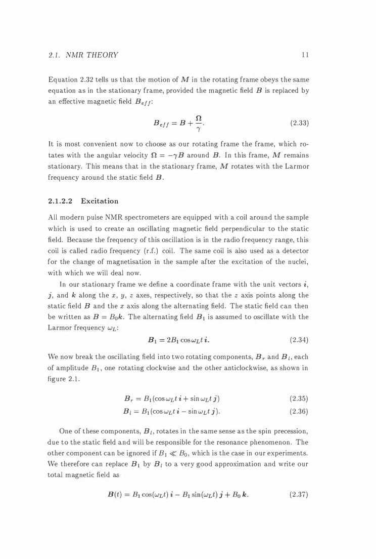
We now break the oscillating field i nto two rotating components, Br and Bl, each
of amplitude BI, one rotating clockwise and the other anticlockwise, as shown in
figure 2 . 1 .
B,. = BI (coswLti + sinwLtj)
Bl = BI (coswLt i - sinwLtj).
(2.35)
(2.36)
One of t hese components, BI, rotates in the same sense as the spin precession ,
due to the static field and wi l l be responsible for the resonance phenomenon . The
other component can be ignored if BI � Ba, which is the case in our experiments.
We therefore can replace BI by BI to a very good approximation and write our
total magnetic field as
(2.37)
12 CHAPTER 2. INTRODUCTION TO NMR AND IMAGING
Figure 2.1: An osci l lat ing magnetic field Bl(t) can be decomposed into the superposition of two counterrotat ing magnetic fields B/(t) and Br(t).
Equation 2.31 gives for each component :
dMx dt
dMy dt
dMz dt
(2.38)
(2.39)
(2.40)
U nder the i nitial condition M(O) = Mok, the solution for these equations is :
where Wl = "BI·
Mosin wltsin wLt
Mo sin Wltcos wLt
Mo cos wlt,
(2.41)
(2.42)
(2.43)
The magnetisation vector M therefore precesses simultaneously around Ba with the Larmor freq uency and around B 1 with the freq uency Wl. In the rotating frame, where BI is stationary, M just precesses around BI with the frequency
WI . By varying the duration of the oscil lating magnetic field , one can ti lt the
magnetisation vector by an arbitrary angle. For example, if WIt = IT /2, M is
fl ipped by 900 from in itially along the z axis into the xy plane. If WI t = IT , M is
fl ipped by 1800• By changing the phase of the oscillating field , the axis, around
which M i s rotated , can be changed . Usual ly, M i s rotated around the x (or y)
axis by 900 or 1800, and we denote these pulses as 90x (90y) or 180x (180x) pu lses.
Because the frequency of these pulsed signals is normally in the range of radio
frequencies, these pu lses are called radio frequency ( r .f. ) pu lses.
2.1. NlvIR THEORY 13
The application of an d. pulse to a spin system can also be described using
the quantum mechan ical time eyolution operator U(t) defined in equation 2.23 .
The Hamiltonian describing an d. pulse which rotates the magnetisation around
the :1: axis is given by [ 16] :
(2.44)
For a pulse which rotates the magnetisation around the y axis, Ix only has to be
replaced by Iy in equation 2 .44.
2.1.2.3 Relaxation
Equation 2 .29 i nd icates that the thermal equi l ibr ium magnetisation Mo is along
the direction of the magnetic field Ba. By d. pulse excitation , the spins are
flipped from th is thermal equi l ibri um position into positions which are energet
ically less favourable. According to equation 2 .31 the spins would remain in a
non-equi l ibri um position . Of course, there exists a characteristic timescale TI ,
which depends on factors such as sample, temperature and strength of the static
field Ba, in which the spins relax back to their thermal equilibrium position . Th is
timescale TI is called longitudinal or spin-lattice relaxation time. As the name
implies, the process involves an exchange with the reservoir, which is called lattice.
We therefore want to add a term to the equation for d�;, , so that the solution
for this term goes to Ala for t» TI , regardless of the value of Mz(O) . This can be
ach ieved by the following term:
The solution is:
dMz
dt (2 .45 )
(2 .46)
The x and y components of M wil l decay to zero by the same relaxation process.
The spins, however , interact with each other and tend to get to thermal equ il ibri um
amongst themselves . This process is called spin-spin relaxation, and its timescale,
T2, is equal to or shorter than Tl. vVe therefore want to add to the transverse
components of equation 2.31 a term which ensures that the solutions l'vIx,y(t ) decay
to zero for t »T2. Because the decay is dominated by the faster process, it is
justified to omit the term with Tt . The phenomenological description for spin-spin relaxation can be written as:
(2 .47)
1 --1 CHAPTER 2. INTROD UCTION TO N1VIR AND IMAGING
Combining equations 2 .4.5 and 2.47 with equation 2 .31 gives the Bloch equations
[ 10] :
rl/'v!x dt
dAly dt
dMz elt
lv!x Al (M x B)x -
T2 My
, ( M x B)y -
T2
A( (M X B);; - MO;1 lvf,.
(2 .48)
( 2 .49)
(2 .50)
From the values for Tl and T2 relaxation , one can extract useful i nformation about
the Hamiltonian and dynamics of a spin system. We wi l l use the B loch equations
now to calculate the evolution of the magnetisation vector after applying a 90x d. pulse.
2.1.2.4 Free Induction Decay
With the help of equations 2 .41 - 2 .43 we saw, that the magnetisation vector can
be fl ipped from initially along the z axis i nto the xy plane by applying a.n d. pulse
of the right duration . The solutions to the Bloch equations for the magnetisation
d irectly after a 90x pulse, when M = N1oi , are:
Mo sin (wLt)e-t/T2
Mo COs (wLt)e-t/T2
Mo(l - e-t/T1 ) .
(2 .5 1 )
(2 .52)
(2 .53)
The oscillating and decaying magnetisation in the xy plane is called free induction
decay (FID) and is detected by the d. coi l . A typical FID is shown i n figure
2 .2 for both x and y magnetisation . A complex Fourier transformation (FT)
of this signal yields the absorption and d ispersion spectrum of the sample [4] .
The FT of the signal in figure 2.2 is a Lorentzian line with a width of 1 /rrT2 .
With the usual heterodyne detection , the peak will be centred at the frequency
8w = WL - wr • where Wr is the reference frequency of the mixing stage. The real part of the spectrum displayed in figure 2 .3 (a) is the absorption spectrum , while
the imaginary part displayed in ( b) is the d ispersion spectrum.
In practice, the signal i s digitally sampled using N discrete sampling points
in a time interval T. The spectrum obtained after a numerical FT then has a
bandwidth of l iT, and the separation of the points in the frequency domain is
liNT.
-- - -- --- --------------
2. 2. NUCLEAR INTERACTIONS 15
(a) 90x
r. f. � • + begin acquisition time
(b) : J l a
real · - - -!.a.�a _____ � • signal ::::::" Y.· "'·�
. " (C) •
• - a . Imagmary ---46.& .... a ______ • signal ::::::;Vvv ..... _.4/,.
. , . t
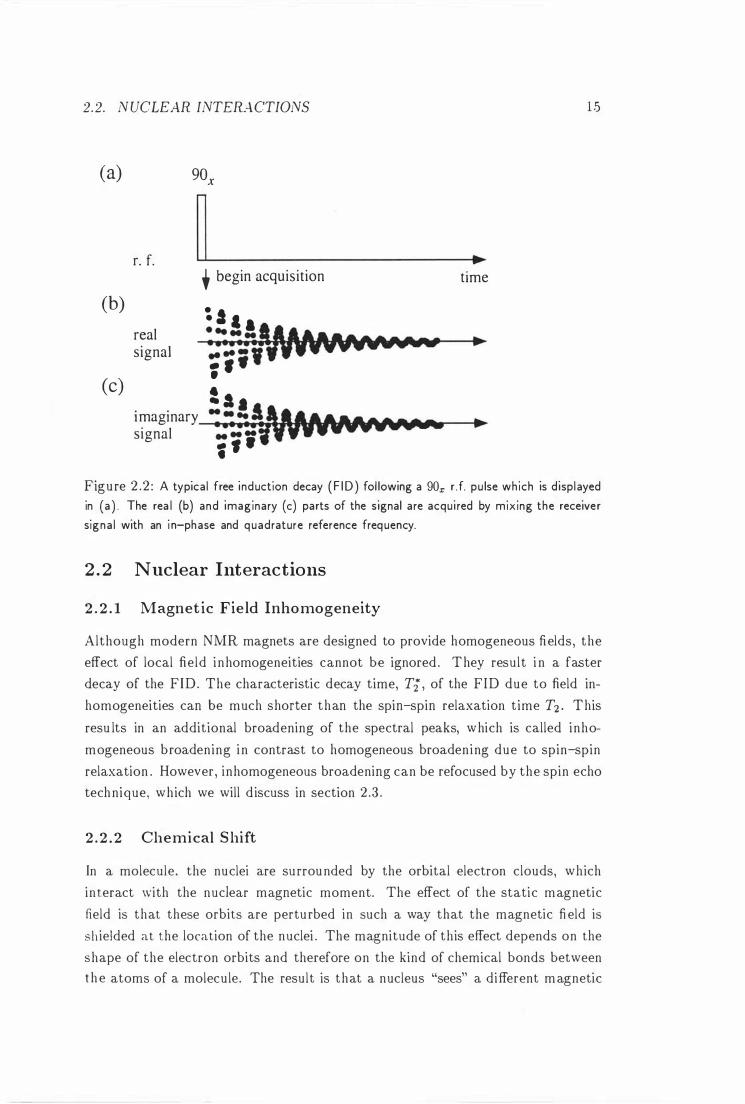
Figure 2.2: A typica l free induction decay ( F ID ) fol lowing a 90x r .f. pu lse which is displayed
in (a ) . The rea l (b) and imaginary (c) parts of the signal are acqui red by mixing the receiver
signa l with an i n-phase and quadrature reference frequency.
2.2 Nuclear Interactions
2 . 2 . 1 Magnet ic Field Inhomogeneity
Although modern NMR magnets are designed to provide homogeneous fields , the
effect of local field inhomogeneities cannot be ignored . They result i n a faster
decay of the FID. The characteristic decay time, Ti , of the FID due to field in
homogeneities can be much shorter than the spin-spin relaxation time T2 . This
resu lts in an additional broadening of the spectral peaks, which is called inho
mogeneous broadening i n contrast to homogeneous broaden ing due to spin-spin
relaxation . However , inhomogeneous broadening can be refocused by the spin echo
technique, which we will d iscuss in section 2.3.
2 . 2 . 2 Chemical Shift
In a molecule. the nuclei are su rrounded by the orbital electron clouds, which
interact with the nuclear magnetic moment. The effect of the static magnetic
field is that these orbits are pertu rbed in such a way that the magnetic field is
sh ielded at the location of the nuclei . The magnitude of this effect depends on the
shape of the electron orbits and therefore on the kind of chemical bonds between t h e atoms of a molecule. The result is that a nucleus "sees" a different magnetic
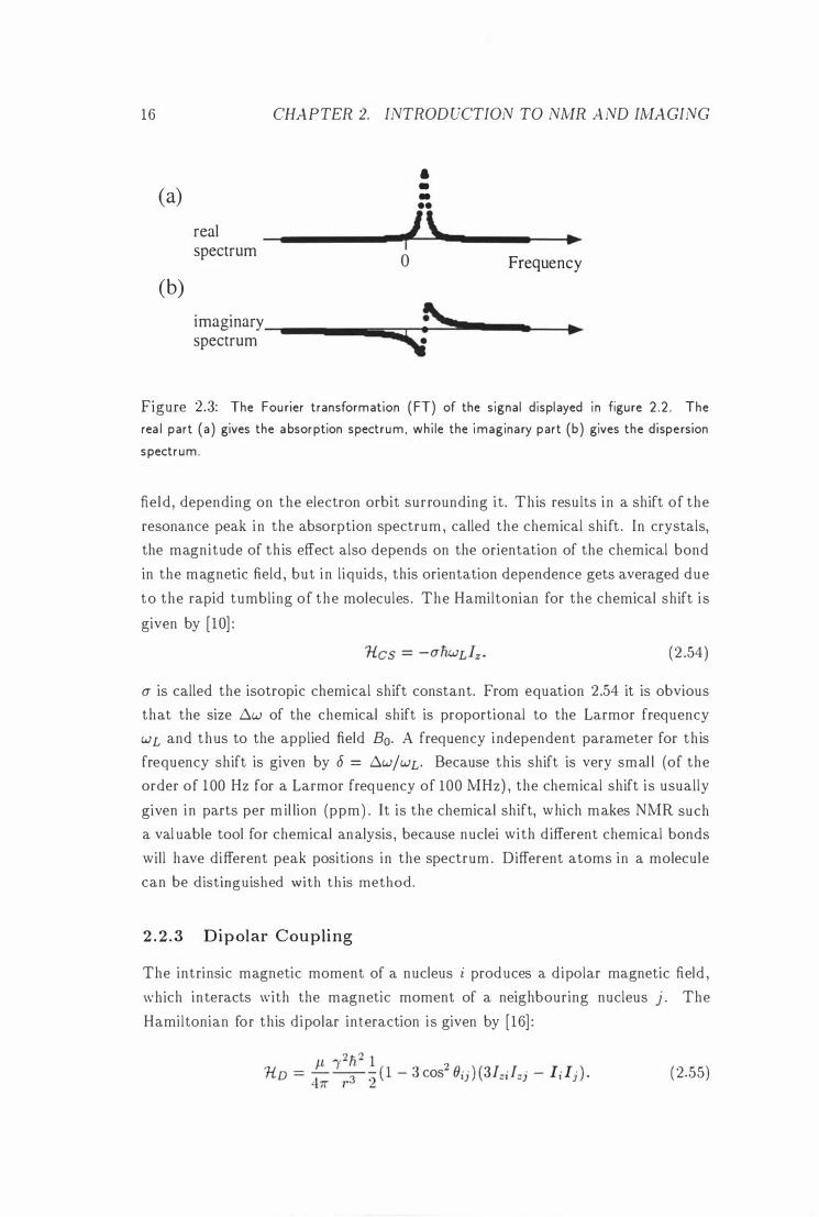
16
(a) real spectrum
(b) Imagmary spectrum
CHAPTER 2. INTROD UCTION TO NMR AND IMAGING
a • -••
IL 0 Frequency
!\." 'i Figure 2.3: The Fourier transformation ( FT) of the s ignal displayed i n figure 2 .2 . The
rea l part (a) gives the absorption spectrum , whi le the imaginary part (b) gives the dispersion
spectrum .
field , depending on the electron orbit surrounding it . Th is results i n a shift of the
resonance peak i n the absorption spectrum , called the chemical shift . In crystals,
the magnitude of th is effect also depends on the orientation of the chemical bond
in the magnetic field , but i n l iquids, this orientation dependence gets averaged due
to the rapid tumbling of the molecules . The Hamiltonian for the chemical shift i s
given by [ 10] :
(2.54)
(j is called the isotropic chemical shift constant. From equation 2.54 it is obvious
that the size b.w of the chemical shift is proportional to the Larmor frequency
WL and thus to the applied field Bo. A frequency i ndependent parameter for th is
frequency shift is given by (j = b.W/WL. Because this shift is very smal l (of the
order of 1 00 Hz for a Larmor frequency of 100 MHz) , the chemical shift is usually
given i n parts per m il lion (ppm). It is the chemical shift, which makes NMR such
a val uable tool for chemical analysis , because nuclei with d ifferent chemical bonds
will have different peak positions in the spectrum . Different atoms in a molecule
can be distinguished with t h is method.
2 . 2 . 3 D i p olar Coupling
The intrinsic magnetic moment of a nucleus i produces a d ipolar magnetic field ,
which interacts with the magnetic moment of a neighbouring nucleus j . The
Hamiltonian for this d ipolar interaction is given by [ 16] :
(2.55)
2 . .'3. SPIN MANIP ULATIONS 1 7
Oij is the angle between the connecting line o f nuclei i and j and the static magnetic
field .
Due to the rapid tumbling of the molecules , the dipolar coupling is usually very
small in liquids . In solids , however, where the molecules are at fixed positions, the
orientation dependence of the dipolar interaction leads to a significant broadening
of the resonances.
2.2.4 Quadrupolar Coupling
Another interaction , which is important for nuclei with I > 1/2 , is the quad rupo
lar coupling. It arises from the coupling of the nuclear quadrupole moment Q with the tensor of the electric field gradient caused by the electronic orbits. The
Hamiltonian is given by [ 16] :
1i = e2Qq ( 3 COS2 0 - 1 ) (31 _ [2 ) . Q 4/ (21 - 1 ) 2
z (2 .56)
e is the electron charge, q is called the electric field gradient, and e is the angle
between the bond direction of the atom and the static magnetic field Bo. It is
common to define the order parameter s and the quadrupolar splitting constant
CQ as:
s ( 3 cos:e - 1 ) (2.57) e2qQ
41i' CQ = ( 2 .58)
For a given I , the quadrupolar interaction shifts the energy levels with different
m. For example, for a deuterium nucleus 1 = 1, and the energy levels are shifted
as shown in figure 2.4 (a) . The resulting absorption spectrum consists of a pair of
lines , as shown in figure 2.4 (b ) . The amplitude of the line splitting is proportional
t o the order parameter s, which depends on the orientation of the molecu le in the
static magnetic field . The quadrupolar coupling therefore enables us to measure
molecular orientations . We will use this method in chapter 9 to measure alignment
of molecules in shear flow.
2.3 Spin Manipulations
2 . 3 . 1 The Spin Echo
The spin echo was first discovered by Hahn in 1950 [3] . Consider the pulse sequence
shown in figure 2 .5. The magnetisation vector for different times is shown in
18 CHAPTER 2. INTROD UCTION TO NMR AND IMAGING
Ca) Zeeman In level
- I
o
+ quadrupole interaction
---- - - --'----
Cb)
o sCQ Frequency
Figure 2 .4 : (a ) The shift of the Zeeman levels due to the quadrupolar i nteraction is shown for a nucleus with I = 1. The two possible tra nsitions are displayed by a r rows. (b ) The
corresponding absorption spectrum consists of a pa i r of peaks separated by 2sCQ .
90x 1 8q,
��: 'r
.�. � . .. ..... FID
'r
,-.. .. . .....
• • . .
• •
•
� . .. .....
Spin Echo
• time
Figure 2 .5 : The spin echo pu lse sequence . The F ID decays exponentia l l y with the t ime
constant Ti . If after the time T a 1800 r .f. pu lse is applied , the echo s ignal a ppears at a time
T after the 1800 r .f. pu lse.
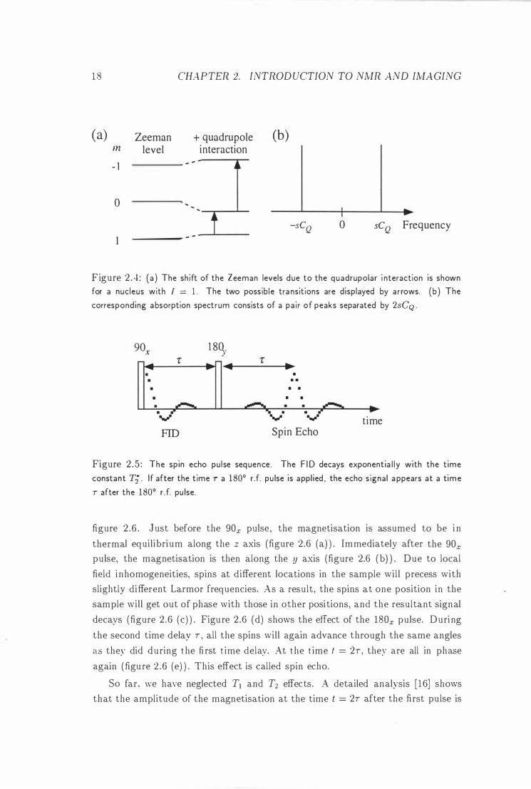
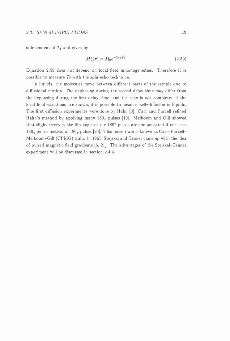
figure 2 .6 . J ust before the 90x pulse , the magnetisation is assumed to be i n
thermal equi l i bri um along the z axis (figure 2.6 (a) ) . Immediately after the 90x pulse, the magnetisation is then along the y axis (figure 2.6 ( b) ) . Due to local
field i nhomogeneities, spins at different locations in the sample wi l l precess with slightly different Larmor frequencies. As a result , the spins at one position in the
sample wil l get out of phase with those in other positions, and the resultant signal
decays (figure 2 .6 (c) ) . Figu re 2.6 (d) shows the effect of the 180x pu lse. During
the second time delay T , all the spins wil l again advance through the same angles
as they did du ring the fi rst t ime delay. At the time t = 2T, the�' are all in phase
again (figu re 2 .6 (e) ) . This effect is called spin echo.
So far, we have neglected TJ and T2 effects. A detailed analysis [ 16] shows
that the amplitude of the magnetisation at the time t = 2T after the fi rst pulse is
2.3. SPIN !vIANIPULATIONS 19
independent of Tt and given by
(2 .59)
Equation 2 .59 does not depend on local field inhomogeneities . Therefore it is
possible to measure T2 with the spin echo technique.
In l iquids, the molecu les move between different parts of the sample d ue to
diffusional motion . The dephasing du ri ng the second delay time may differ from
the dephasing du ring the first delay time, and the echo is not complete. If the
local field variations are known , it is possible to measure self-diffusion in liqu ids.
The first diffusion experiments were done by Hahn [3] . Carr and Purcell refined
Hahn 's method by applying many 1 80x pulses [ 19] . Meiboom and Gi l l showed
that slight errors in the flip angle of the 1 800 pulses are compensated if one uses
180y pulses i nstead of 180x pulses [20] . This pulse train is known as Carr-Purcell
Meiboom-Gil l (CPMG) train . In 1965, Stejskal and Tanner came up with the idea
of pulsed magnetic field gradients [6, 2 1 ] . The advantages of the Stejskal-Tanner
experiment wil l be d iscussed in section 2.4.4.
20 CHAPTER 2. INTROD UCTION TO NMR AND IMAGING
(a) (b)
(c)
I ,
I
,
z z
y
(d) z z
- - -,') y
(e) z
y
- - -,
\
y
y
Figure 2 .6 : Formation of a spin echo by means of a 90x - r - 1 80x - r pu lse sequence. (a) At the start, the magnetisation vector is paral le l to the static magnetic field . (b) The 90x d. pu lse fl i ps the magnetisation vector a long the y axis. (c) The spi ns start to dephase due to local field i nhomogeneities . (d) The 180x r .f. pulse fl i ps a l l spins by 1800 around the x axis.
(e) After the delay r after the 1 80.r r . f. pu Ise all spi ns are in phase agai n .
2 . .1. SPIN J'vIANIPULATIONS
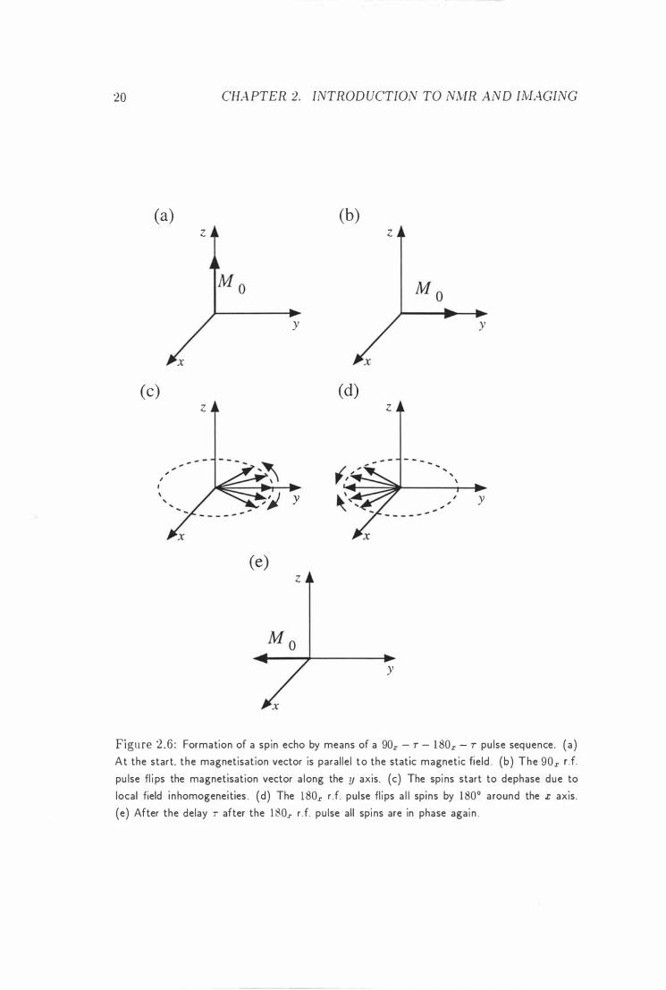
2.3 . 2 The Stimulated Echo
2 1
I n h is original paper. Hahn also discussed the th ree pulse sequence shown i n figure
2 .7 . There are th ree spin echoes at times 271 , 2TI + 2T2, and 71 + 272 after the
first rJ. pulse. They are the spin echoes of the fi rst and second , first and th i rd ,
and second and third d. pulse, respectively. Hahn found a fourth echo at time
t = 2TI + T2 after the first d. pulse. This is called the stimulated echo.
90x 90x 1"2
90x 1"1
��: 1"1
.�� .�� •
• • •
•
.. � ,,-.. .. � . . rr .. • • rr ..... V ..... time FID Stimulated Echo
Figure 2.7 : The stimu lated echo pulse sequence. The stimu lated echo appears at a time TI after the th i rd r . f. pu lse.
In many samples, the spin-spin relaxation time T2 is much shorter than the
spin-lattice relaxation time T1 • I n the stimulated echo pulse sequence, the trans
verse magnetisation is stored along the z direction by the second r . f. pulse before
being tipped back i nto the t ransverse plane for detection . During the time 72 , the
magnetisation is aligned along the z axis and suffers only from Tl relaxation . Th is
can allow the echo formation over time i ntervals which would not be accessible
by the spin echo. A clear d isadvantage of the stimulated echo is the formation of
multiple echoes due to the spin echoes of the three pu lses, which can i nterfere with
the stimulated echo . By applying a "crusher" gradient pulse between the second
and th ird r .f. pulse, these unwanted spin echoes can be made to d isappear .
Because of the problems with unwanted spin echo i nterferences, we use the
stimulated echo method only i n cases where we want particu larly long delay times for the echo formation .
2.3.3 The Quadrupole Echo
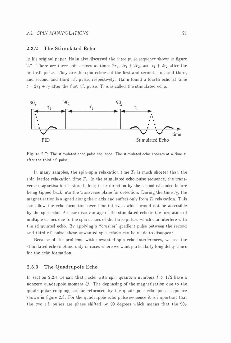
In section 2 .2 .-1 we saw that nuclei with spin quantum numbers I > 1/2 have a
nonzero quad rupole moment Q . The dephasing of the magnetisation due to the
quadrupolar coupling can be refocused by the quadrupole echo pulse sequence
shown in figure 2 .8 . For the quadrupole echo pulse sequence it is important that
the two rJ. pu lses are phase shifted by 90 degrees which means that the 90.r
22 CHAPTER 2. INTROD UCTION TO NMR A ND IMAGING
excitation pulse needs to be followed by a gOy refocusing pulse. The magnetisation
is refocused at the time 2T after the first r .f. pu lse.
90x 90y
�.�: ,
.�. ,-..... • J' V
FID
,
..",...,. .. • .....
•
• •
•
,-..... . J' V
Quadrupole Echo
• time
Figure 2 .8 : The quad rupole echo pu lse sequence consists of two 90° d. pulses, wh ich are out of phase by 90° . The echo signa l appears at a time T after the second 90° r .f. pulse.
The quadrupole echo pulse sequence wil l be used in chapter 9 to measure
alignment of molecules i n shear flow .
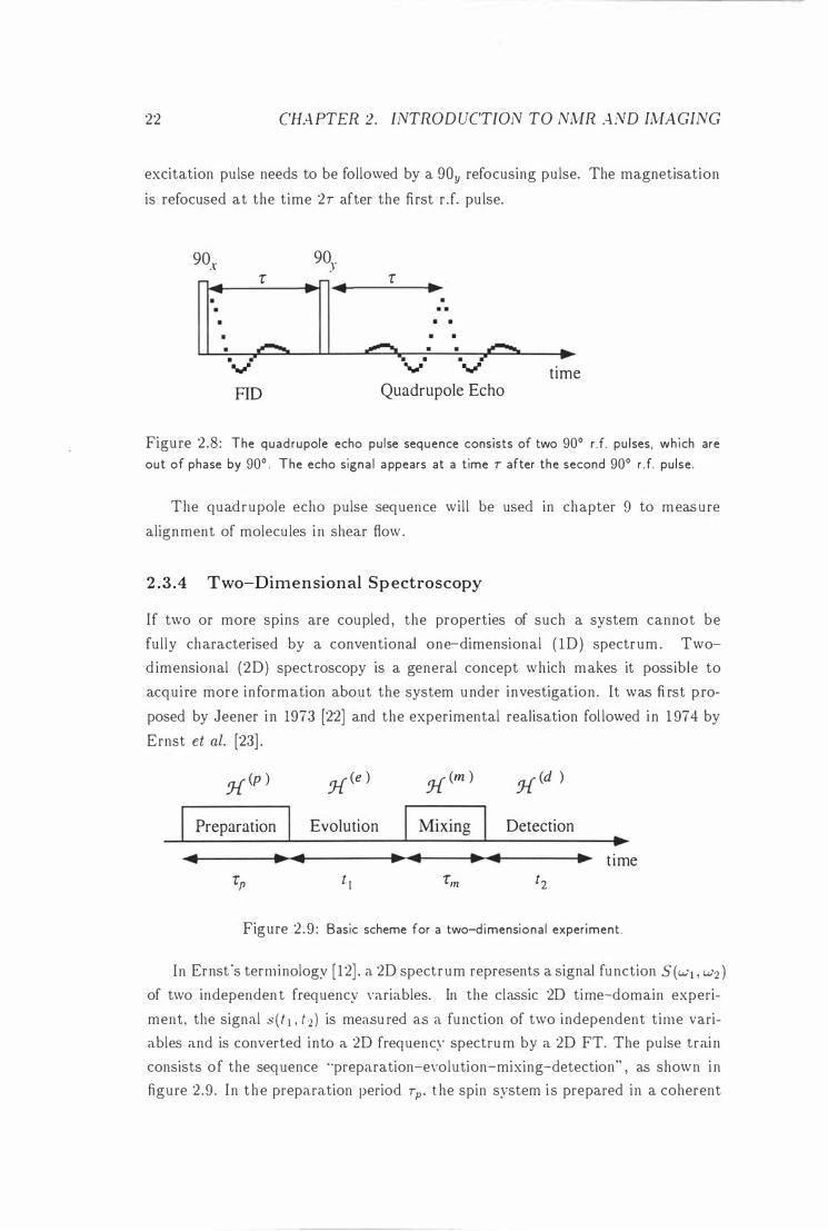
2.3 .4 Two-Dimensional Spectroscopy
If two or more spins are coupled , the properties of such a system cannot be
fu lly characterised by a conventional one-dimensional ( ID) spectrum . Two
d imensional (2D) spectroscopy is a general concept which makes it possible to
acqu i re more information about the system under investigation . It was fi rst p ro
posed by Jeener i n 1973 [22] and the experimental realisation fol lowed i n 1 974 by
Ernst et al. [23] .
j{ (P ) j{ (e ) j{ (m ) j{ (d )
Preparation Evolution Detection
• • • • • • • • time
'p t I 'm t2
Figure 2 .9 : Basic scheme for a two-dimensiona l experiment.
In Ernst "s terminology [ 12] . a 2D spectrum represents a signal function S (Wt , W2 ) of two independent frequency variables. In the classic 2D time-domain experi
ment, the signal s(t 1 , t }. ) is measu red as a function of two independent t ime vari
ables and is converted into a 2D frequenc�' spectrum by a 2D FT. The pulse train
consists of the sequence '·preparation-evolution-mixing-detection" , as shown i n
figure 2 .9 . I n the preparation period Tp . t he spin system i s prepared in a coherent
2 . .3. SPIN MANIPULA.TIONS 23
non-equi l ibri um state, which will evolve in the subsequent periods. In the simplest
case, the preparation period is just one d. pulse . During the evolution period t l ,
the spin system evolves freely under the infl uence of a specific Hamiltonian . The
evolution du ring t l determines the frequencies in the wl-domain . The t l -domain
i s sampled by carrying out a series o f experiments with systematic incrementa
tion of t 1 . The mixing period Tm may consist of one or more pulses separated
by intervals . During the mixing period , the spins may change their magnetisa
tion , orientation or other parameters which are characteristic of the system u nder
investigation . The evolution of the spins du ring the detection period t2 finally
determines the frequencies in the w2-domain .
Ernst distinguishes between th ree types of 2D NMR spectroscopy: separation
of interactions, correlation methods and exchange. If the Hamiltonian is com posed
of terms of different physical origin , it is often possible to decompose the complex
ID spectr um by the choice of two suitable effective Hamiltonians 1{(e) and 1{(d)
for the evolution and detection period . I n the 2D spectrum, the spectrum due
to 1{(e) i s then along the Wl axis, while the spectrum due to 1{(d) i s along the
W2 axis . With correlation methods, one can measure the interaction between
spins. The simplest experiment is based on the sequence 90x-t l-(,8)-t2 . This
experiment is termed correlation spectroscopy (COSY) . The transfer of coherence
is induced by the pu lse of flip angle {J. From the appearance of cross-peaks in the
2D correlation spectra the coupling parameters can be identified . With exchange spectroscopy, dynamic processes, such as chemical exchange or spin d iffusion, can
be measured . The fundamental idea is the label l ing of spins before exchange takes
place, such that after the mixing time, the magnetisation can be traced back.
One particu lar 2D exchange experiment, due to Spiess et al. [24, 25, 26] ' provides
a relevant example. Here the Wl and W2 dimensions are dominated by dipolar
or quadrupolar interactions in which the frequency offset relates directly to local
bond angle. The mixing period consists of the storage of Zeeman order along the
magnetic field direction so that the recall of magnetisation at a later t ime reveals angular correlations arising from the angular reorientation of polymer segments
which occurred over the mixing time Tm . I n chapter 4 this idea o f exchange will be extended to a different frequency
space. The equ ivalent Wt and W2 dimensions correspond to the movements Zt and
Z2 over two well defi ned time intervals, which are separated by the mixing time.
2 . 3 . 5 Signal Averaging and Phase Cycling
In many cases the signal acquired in one NMR experiment is not strong enough to ext ract meaningfu l data. One repeats therefore one experiment N times, adding
24 CHAPTER 2. INTROD UCTION TO NMR AND nvfAGING
up the signal from the individual scans. This i ncreases the signal amplitude by a
factor of N, while the noise level increases by a factor of Nl/2 . Thus, the signal
to-noise ratio increases by a factor of Nl/2 • Between two scans, one has to wait
for the magnetisation to come to thermal equil ibri um . This is usually the case
after times of 2-3 Tl . The Tl value for protons in most liquids used i n th is thesis
is less than 1 s . Therefore, repetition times of 1-1 .5 s are considered long enough
for the experiments i n this thesis.
The NMR signal is usually overlapped by background interferences . These
i nterferences can have various sources, such as d .c . offset i n the amplifier of the
receiver . By changing the phases of the d. pulses between different scans and
adding or subtracting the signal in the correct way, one can suppress these i n
terferences. Hoult and Richards [27] describe a four-step phase cycl ing which
nul l ifies artifacts l ike d.c. offset in the receiver stage and imperfect phase settings
of the rJ. pulses. For most experiments i n th is thesis, it was sufficient to employ
a two-step phase cycle, which only nul l ifies the d .c . offset in the receiver. T his
two-step phase cycling is shown in figure 2 . 1 0 .
•
. ..
(b) 90_x
:. •
•
•
(c)
. ..
.. . . .... . . . ....... ....... . ............. .
. ' .... .... . ..
••
.. . .
. .. . .
. . ...
.... " . .
' ....... . ........................ . . .
•••
• ••
•• le
••••• •••••• • •••••
cc ••••••
time
time
time
Figure 2 . 10 : (a ) The F ID after a 90x r . f. pulse is acqu i red with a d .c . offset on the receiver.
( b) The F ID after a 90_x r .f. pu lse. (c) Subtraction of the signals acqui red i n (a ) a nd (b) cancels out the d . c . offset , but adds the F IDs .
2.4. INTROD UCTION TO ;V/VIR /J'vIA.GING 25
2.3 . 6 The E ffect of Magnetic Field Gradients
In NMR spectroscopy, one is usually concerned to get the magnetic field i nside
the sample as homogeneous as possible. Several layers of shim coils and specially
designed pu lse sequences ensu re that the broadening due to field i nhomogeneities
is smaller that the natu ral li newid th . However, if one wants to extract the spatial
dependence of molecu les in the sample, one deliberately has to vary the magnetic
field across the sam pie. These magnetic field variations are created by specially
designed gradient coils through which large, switch able currents can be passed .
Because the field variations due to the switch able gradients are much smaller
than the static field Ba, only the component of the gradient paral lel to Ba needs
to be considered . The components of the field gradient can then be written as
Gx oBz
(2.60) ox
Gy oBz
(2.61) ay
Gz oBz
(2.62) = --
oz
Because the magnetic field varies across the sample, the Larmor frequency wi l l
depend on the spatial coordinate r . The local Larmor frequency w(r) is given by
w(r) = ,Bo + ,G · r . (2.63)
Equation 2.63 is the basic equation for NMR imaging. In the next section we wi l l
use th is equation to calculate the NMR signal of a sample i n a l inearly varying
magnetic field .
2 .4 Introd uction to NMR Imaging
2.4. 1 k-Space Imaging
Consider a sam pie of local spin density p( r) . If we neglect relaxation effects , the
complex NMR signal dS of a small volume element dV is given by
dS = p(r)eiw( rJ tdV. (2.64)
Using equation 2 .63, we obtain
( 2 .65)
I n the receiver. the radio-frequency signal is mixed with a reference frequency.
This process is known as heterodyne mixing. If one chooses as a reference freq uency �( Bo , the signa l osci l lates only with a frequency ,G · r , which is i n the
26 CHAPTER 2. INTROD UCTION TO NMR AND IMAGING
audio-frequency range. Equation 2.65 can then be rewritten as
(2 .66)
I ntegration across the whole sample yields:
(2 .67)
Equation 2 .67 has the form of a Fourier transformation . To make th is relationship
more clear, we define a reciprocal space vector k as [28]
(2 . 68)
The magnitude k of k therefore depends on both the duration and the magnitude
of the gradient. The direction of k is given by the direction of G.
With the reciprocal space vector k. equation 2.67 can be written as
(2 .69)
The local spin density p(r) can be obtained from equation 2.69 by inverse Fou rier
t ransformation :
(2 .70)
Equations 2.69 and 2.70 state that S and p are mutually conjugate parameters.
Th is is the fundamental relationship for NMR imaging. In practice, one scans
the signal stepping the magnitude of all three components of G i ndependently.
A subsequent numerical FT yields p(r) . However, for a ful l three-dimensional
image, this process is very time consuming. I n many cases, one is only interested
in the two-dimensional projection of one or a few th in planar slices through the
sample, comparable to the slice of a micrograph . The key to this method is the excitation of a single, predetermined , layer of spins, a process known as selective
excitation .
2.4.2 Selective Excitation
In order to select a thin layer (slice) of spins, we need to do two things. F i rstly,
we need to apply a gradient perpendicular to our selected slice. Then we need a
method to excite the spins within a certain frequency range, which corresponds
to the thickness of our slice, as shown in figure 2 . 1 1 . We discuss the latter fi rst.
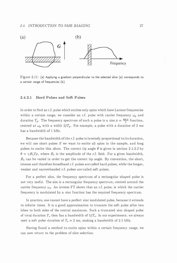
2.4 . INTRODUCTION TO NMR INIAGING
(a) (b)
27
Frequency
Figure 2 . 1 1 : (a) Applyi ng a gradient perpend icu la r to the selected slice (a) corresponds to
a certain range of frequencies (b ) .
2 .4 .2 .1 Hard Pulses and Soft Pulses
I n order to find an rJ. pulse which excites only spins which have Larmor frequencies
within a certain range, we consider an rJ. pulse with carrier frequency wp and
d uration Tp . The frequency spectrum of such a pulse is a sinc x = si�x function ,
centred at wp with a width 21Tp . For example, a pulse with a duration of 2 ms
has a bandwidth of 1 kHz.
Because the bandwidth of the rJ. pulse is inversely proportional to i ts d uration , we wi l l use short pulses if we want to excite all spins in the sample, and long
pulses to excite thin slices. The correct t ip angle (J is given in section 2 . 1 .2 .2 by
(J = ,BI Tp , where BI is the amplitude of the d. field . For a given bandwidth ,
BI can be varied i n order to get the correct t ip angle. By convention , the short,
i ntense and therefore broadband rJ. pulses are called hard pulses, whi le the longer,
weaker and narrow banded r.f. pu lses are called soft pulses.
For a perfect slice, the frequency spectrum of a rectangular shaped pulse is
not very usefu l . The aim is a rectangular frequency spectrum , centred around the
carrier frequency WS ' An inverse FT shows that an rJ. pulse, in wh ich the carrier
frequency is modulated by a sinc function has the required frequency spectrum .
In practice, one cannot have a perfect sinc modulated pulse, because i t extends
to infin i te times. It is a good approximation to truncate the soft pu lse after two
lobes to both sides of the central maximum. Such a truncated si nc shaped pulse
of total du ration Ts then has a ba.ndwidth of 51Ts . In our experiments. we always
used a soft pulse du ration of Ts = 2 ms, making a bandwidth of 2 .5 kHz .
Having found a method to excite spins within a certain frequency range, we
can now return to the problem of slice selection .
28 CHA.PTER 2. INTROD UCTION TO NMR AND IMAGING
2.4 .2 .2 Slice Selection
To select a slice of a given thickness �=, we apply a gradient perpendicular to the
slice. The strength G s of this gradient is given by the thickness of the slice and
the bandwidth 6.w of the soft pu lse :
_ l 6.w Cs = I 6.z · (2 .7 1 )
I t can be shown [ 1 1] that the spins dephase duri ng a 900 slice selective soft
pu lse due to the gradient. They can subsequently be rephased if a gradient pu lse
with amplitude -Cs and duration Ts/2 is applied . A 1800 soft pulse in a spin
echo sequence does not need any refocusing.
We now return to equation 2.70 and take into account that we excite only th in
slices i n one direction . This leads us to the two-dimensional imaging method .
2.4 . 3 Fourier Imaging i n Two D imensions
Having established a method to l imit our experiment to two d imensions, we must
encode the signal for these remain ing directions. If the slice gradient is applied i n
the direction of the static field ( z direction) , equation 2 .69 simplifies to
(2 .72)
Now we can imagine k-space as a plane with kx and ky axes, and we wi l l sample a
finite n umber N2 of points (grid) i n that plane. I f th is grid is based on Cartesian
coordinates, the sampling method is called Fou rier imaging (FI ) [29] .
Because of the time dependence of equation 2.68, we can obtain points along
one l ine in k-space if we sample the signal i n the presence of a gradient. Th is
gradient is called the read grad ient. Unless otherwise stated , th is direction always
corresponds to the x direction i n our experiments. This l ine i n k-space being
sampled i n the presence of a read gradient now has to be moved up and down
the ky axis . This can be achieved by applying the gradient Gy for a period before sampling. This so-called phase gradient causes a phase shift which varies l inearly
with position along the y axis , whi le the read gradient causes a frequency shift
along the x axis.
In order to sample along the fu l l grid in k-space, it is necessary to sample
for positive as well as negative I.-values. ky can easily be reversed by reversing
the gradient. As for the read gradient, however, it is not obvious how to obtain
negative times. By using the spin echo method we can shift the time origin . The echo appears
with a delay T after the 1800 pulse and from that time on the signal resembles
2.4 . INTROD UCTION TO N1VIR IMAGING 29
the FID. Therefore we assign negative times to times before the echo appears.
We usually set the sampling interval so that the echo appears in the centre of the
acquisition time.
hard pulse
r.f.
read gradient
� • •
Tl2
I 80y soft pulse
Vv • time
• • • T
• phase -1I1111�----------------------------------� gradient
s lice gradient
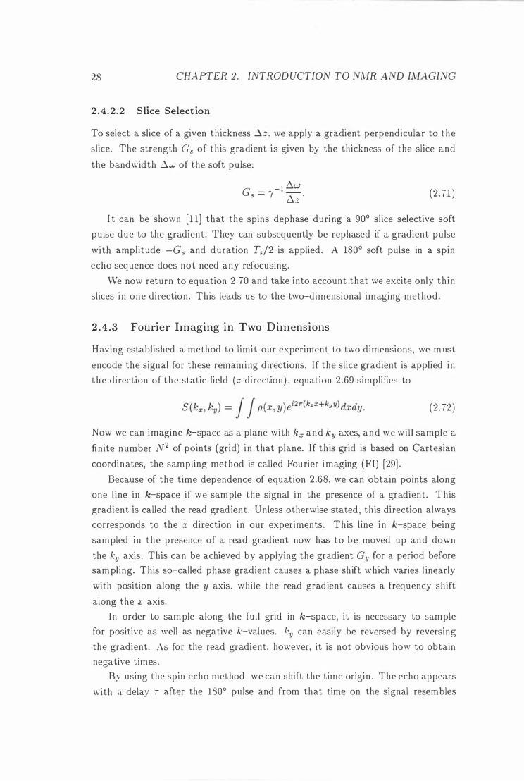
Figure 2 . 1 2 : The spin warp pu lse sequence for Fourier imagi ng. The read gradient is on du r ing signa l acquis it ion. The phase gradient is i ncremented between each scan .
The pulse sequence for F I , called spin warp [30] , i s shown i n figure 2. 12 . The
sp in echo sequence consists of a hard 900 excitation pulse and a slice selective soft
1 800 soft pulse. In principle, we could also use a soft 900 and a hard 1800 pu lse.
However , we favou r the first method , because i nhomogeneities in the rJ. field can
lead to leakages of the hard 1800 pulse. A soft 1800 pulse refocuses only spins
from a small region , in which the rJ. field is expected to be more homogeneous
than across the whole sample. Spins in regions outside the slice can create an FID
when using the (soft 90)-(hard 180) sequence if the 1 800 pu lse i s not perfect but ,
say, only a 1600 pulse.
The read gradient between the 900 and the 1 800 pulses is called precursor read gradient. It dephases the spins in order to sh ift the echo maximum to the cent re
of the acquisition time. The phase gradient is increased in N steps from - Gp to
Gp between different scans . N is the number of encoding steps in each direction .
The acquisition time T was defi ned in section 2 . 1 .2 .4 .
A typical experiment has N = 128 steps for encoding i n each di rection of k
space. vVith a repetition time T,. and Nav signal averages, the total experiment
30 CHAPTER 2. INTROD UCTION TO N1VIR AND IMAGING
time is Texp = Nav NTr . Normal ly, we choose Tr = 1 s and Nav = 2, giving
a typical experiment time of Texp = 2.56 s, which is just over 4 minutes for a
two-dimensional image.
We saw that with the spin warp method we can obtain images of the spin
density distribution p(x, y) in a sample. It does not matter, whether the molecu les
are stationary or not. In the next section , we wil l discuss the PGSE method which
is sensitive to d isplacements of molecules, but has not the spatial resolution of the
spin warp. In section 2 .4.5 we combine the spin warp and the PGSE techniques to
form a three-dimensional experiment , with which we can obtain flow and d iffusion
maps.
2.4.4 Measuring Self-Diffusion: The Pulsed Gradient Spin Echo
The fi rst NMR measurements of molecular displacements were reported by Hahn
i n 1 950 [3] . He observed a decrease of the echo signal due to self-diffusion i n an
i nhomogeneous static magnetic field . The idea is that the dephasing of the spins
due to local field i nhomogeneities does not get refocused by the 1 800 pulse if the
spins change position during the echo delay. This method is stil l i n use. With
superconducting magnets, where one coi l is reversed , self-diffusion coefficients of
polymers can be measured down to 2 . 10-15 m2 s-l [3 1] .
A big d isadvantage of the steady gradient method is that the gradient is on
the whole time, especially during the d. pulses and acquisition . Th is broadens
the spectrum, and the bandwidth of transmitter and receiver therefore limit the
strength of the gradient which can be applied . McCall et at. suggested i n 1963
to switch the gradient off during the d. pulses and acquisition , but have h igh
gradients i n the delays between [32] . In 1965 , Stejskal and Tanner performed the
fi rst practical implementation of this idea, the so-called pulsed grad ient spin echo
( PGSE) method [6] . The pulse sequence is shown in figure 2 . 13 . A review of
different techniques to measure self-diffusion based on the PGSE method is given
in [33] .
We expect that t he echo signal depends on both relaxation and gradient. The
effects of T2 relaxation can be removed by normalising the echo signal 5 (g , 8, .D ) to its value 5(0 ) with no gradient applied . The ratio 5 (g , 8 , Ll)/5 (0) i s called echo attenuation E(g, 8, �) . It can be shown [6 , 2 1] that E(g , 8, Ll) is given by
( 2 ./3)
which is the Stejskal-Tanner equation . 0 is the self-diffusion coefficient of the
sample. A plot of log E(g, 8, ....1 ) vs . -y2g282 (Ll - 8/3 ) is called a Stejskal-Tanner
plot and is expected to give a straight line with slope - D. An example for a
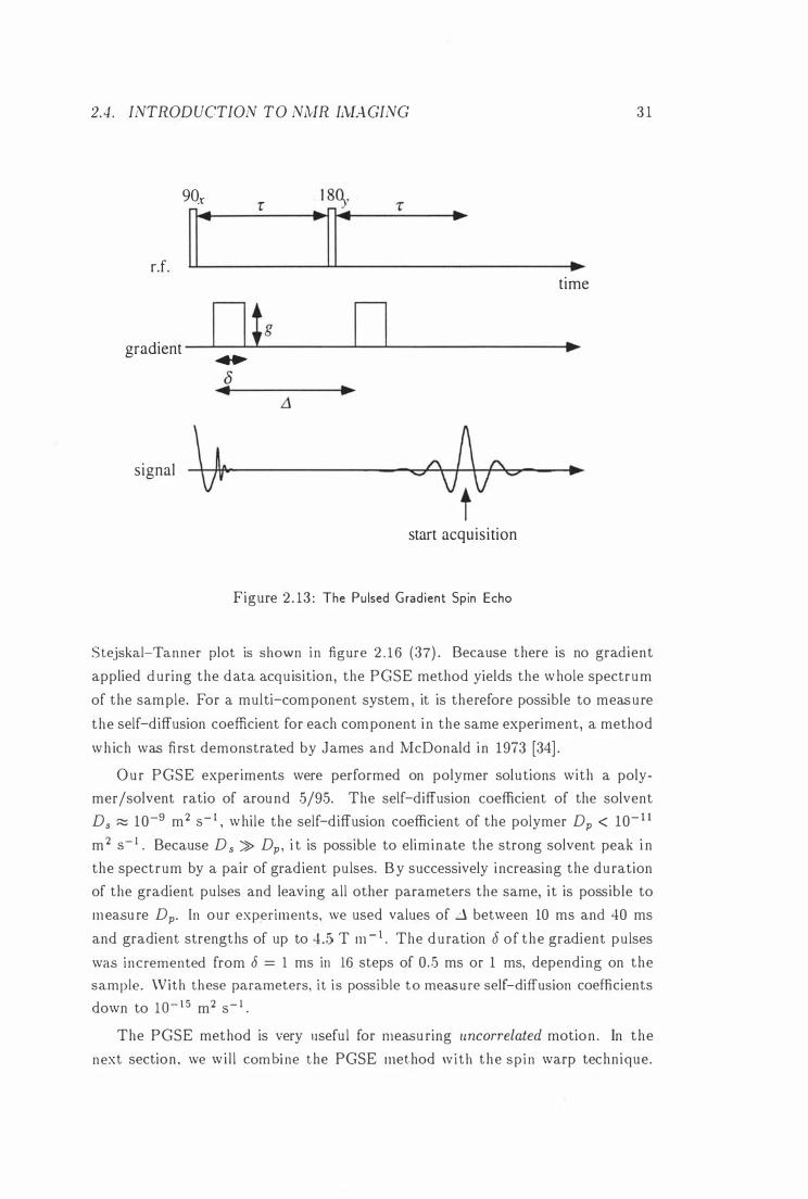
2.4 . INTRODUCTION TO NMR IlvIAGING
90x r 1 8�.
�� .�� r.f.
gradient ntg n ....
8 • •
signal 1 !. VV'
•
A A c c>' \JV t start acquisition
Figure 2 . 13 : The Pu lsed Gradient Spin Echo
3 1
• time
•
•
S tejskal-Tan ner plot is shown i n figure 2 . 1 6 (37) . Because there is no gradient
applied d uring the data acquisition, the PGSE method yields the whole spectrum
of the sample. For a multi-component system , it is therefore possible to measure
the self-diffusion coefficient for each component in the same experiment, a method
wh ich was first demonstrated by James and McDonald in 1973 [34] .
Ou r PGSE experiments were performed on polymer solutions with a poly
mer/solvent ratio of around 5/95. The self-diffusion coefficient of the solvent
Ds � 1 0-9 m2 S- I , while the self-diffusion coefficient of the polymer Dp < 10- 1 1
m2 S- I . Because D s � Dp, i t is possible to eliminate the strong solvent peak i n
the spectrum by a pair of gradient pulses. By successively increasing the duration
of the gradient pulses and leaving all other parameters the same, it is possible to
measu re Dp. In our experiments, we used values of d between 10 ms and 40 ms
and gradient strengths of up to .. 1 .5 T m - I . The duration 8 of the gradient pulses
was incremented from [) = 1 ms in 16 steps of 0 .5 ms or 1 ms, depending on the sample. With these parameters, i t i s possible t o meas u re self-diffusion coefficients
down to 10- 1 5 m2 S- I .
The PGSE method is very usefu l for measu ring tmcorrelated motion . In the
n ext section, we wi l l com bi ne the PGSE method w i t h the s p i n warp technique.
32 CHAPTER 2. INTROD UCTION TO NMR AND IMAGING
This gives us a techn ique to measure correlated motion as well . Because th is is
an imaging method , we have the same spatial resolution as with the spin warp
method .
2 .4 .5 Dynamic NMR Imaging
2 .4.5 .1 Introduction to q-Space
In order to discuss the phase shift of moving molecules due to gradient pulses, we
need to i ntroduce some new parameters. A molecule i can be characterised by the
function ri (t) which describes its position at any time t . In t he PGSE experiment
shown i n figure 2 . 1 3 , the phase shift �qJ is given by
�qJ = ,bg · (r - r') . (2 .74)
The total signal is an ensemble average aver the whole sample in which each
phase term is weighted by the average propagator Ps ( R, t) [35] which gives the
probability that a molecule moves the d istance R = r' - r du ring the time t. The
echo signal E£.l (g) is then
(2 .75)
Signal attenuations due to T2 relaxation can be removed by normalising E.t:. (g) to
E£.l (g = O) = l .
Equation 2 .75 is again a Fou rier relationship . We therefore define a reciprocal
'space vector q such that [1 1]
(2 .76)
Equation 2 .75 can then be written as
E.t:. (q) = J Ps (R, L1)ei27rqoRdR. (2 .77)
Equation 2.77 gives the normalised echo signal in a PGSE experiment. In the next
section we combine the PGSE and spin warp techniques. This will enable us to
obtain velocity and diffusion maps.
2.4.5 .2 The Dynamic Spin Echo
The dynamic spin echo pu lse sequence is shown in figure 2 . 1-! . It is the same as the
spin warp pulse sequence in figure 2.12 with a pair of gradient pu lses added , which
is stepped i n amplitude. The dynamic spin echo is therefore a th ree-dimensional
experiment. The echo signal S ( k, q ) is now given by
S (k, q ) = J p(r)ei2"kor J Ps (R, t1)ei2rrq.RdRdr. (2 .78)
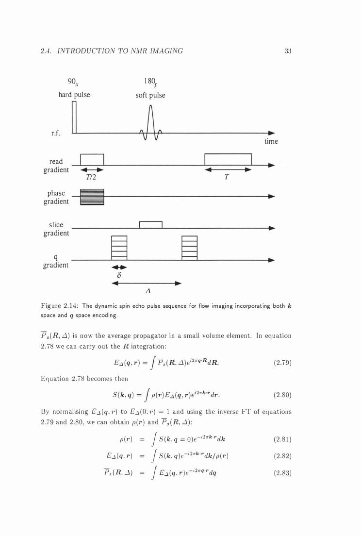
2.4. INTROD UCTION TO NlvIR IMAGING
90x l 80y
hard pul se soft pulse
r.f. � JL VV
read gradient • •
TI2
phase gradient
sl ice gradient
S S q gradient ....
8 • •
L1
33
• time
• • • T
•
•
Figure 2 . 14 : The dynamic spin echo pu lse sequence for flow imaging i ncorporat ing both k space and q space encod ing .
Ps (R, .1 ) is now the average propagator i n a small volume element . In equation
2 . 78 we can carry out the R integration :
(2 .79)
Equation 2 .78 becomes t hen
(2 .80)
By normal isi ng E.j ( q , r) to E..1 ( O , r ) = 1 and using the inverse FT of equations
2 .79 and 2 .80 , we can obtain p(r ) and Ps (R, Ll) :
p(r ) J S (k . q = 0 ) e-i27rk.r elk (2 .8 1 )
E..1 (q , r ) J S ( k , q ) e-i27rk .r elk/ p (r ) (2 .82)
Ps (R, ...1 ) J Ed ( q , r ) e - i27rq.relq (2 .83)
34 CHAPTER 2. INTROD UCTION TO NlvIR AND IMAGING
For purely Brownian motion with d i ffusion coefficient D, the propagator Ps ( R, ,1)
is a Gaussian with wid th 2D,1. I f the molecules are also undergoing coherent
motion with velocity t· , the peak of the propagator is shifted by vLl [ 1 1 ] .
The dynamic spin echo enables us to measure correlated and uncorrelated
displacements of molecules , with a velocity resolution of a few microns per second
and a spatial resolution on the order of 10 microns.
The dynamic spin echo and the pulsed gradient spin echo are methods to mea
sure changes in position of molecules. In chapter 4 we will demonstrate the VEXSY
pulse sequence which enables us to monitor changes i n molecular velocities .
2.5 Hardware and S oftware
So far , we have looked at the different techniques to obtain information about the
spatial d istribution of molecules or their d isplacements. In th is section we wi l l
briefly describe the hardware and software used for the experiments i n th is thesis.
2.5.1 The B ruker AMX300 Spectrometer
All the experiments in this thesis were performed using a commercial Bruker
AMX300 spectrometer . Unless stated otherwise, the experiments were performed
i n a superconducting magnet with a magnetic field strength of 7 T, corresponding
to a Larmor frequency of 300 MHz for protons.
A variety of I' J. coils is available with the Bruker microimaging probe. In our
experiments we used either a 15 mm diameter cavity resonator coil or a 5 mm
diameter saddle coi l . The power of the d. transmitter is 50 W, giving 900 pu lse
durations of 15 J.Ls and .5 J.LS, respectively. The Bruker m icroimaging gradient coil
provides magnetic field gradients in all th ree d irections. The currents are provided
by Bruker AFPA30 power supplies and can go up to 30 A. At maximum current,
gradient strengths of 0 .35 T m- l in the x and y directions, and 1 .2 T m-I i n the
z direction are available. Al l gradient coils are actively shielded and have eddy
current ringdown times of less than 1 ms.
The temperature can be control led i n the range between -500 C and +2000 C
by a Bruker VT2000 temperature control un it . Compressed air is blown past a
heating coil and then along the sample. The temperature is measured by a copper
constantan thermocouple sitting in the air stream just below the sample. Cooling
below room temperature can be achieved by using cold nitrogen gas from the
evaporation of l iquid nitrogen . With this setup , the temperature can be control led
with an accuracy of ±O. l 0 C.
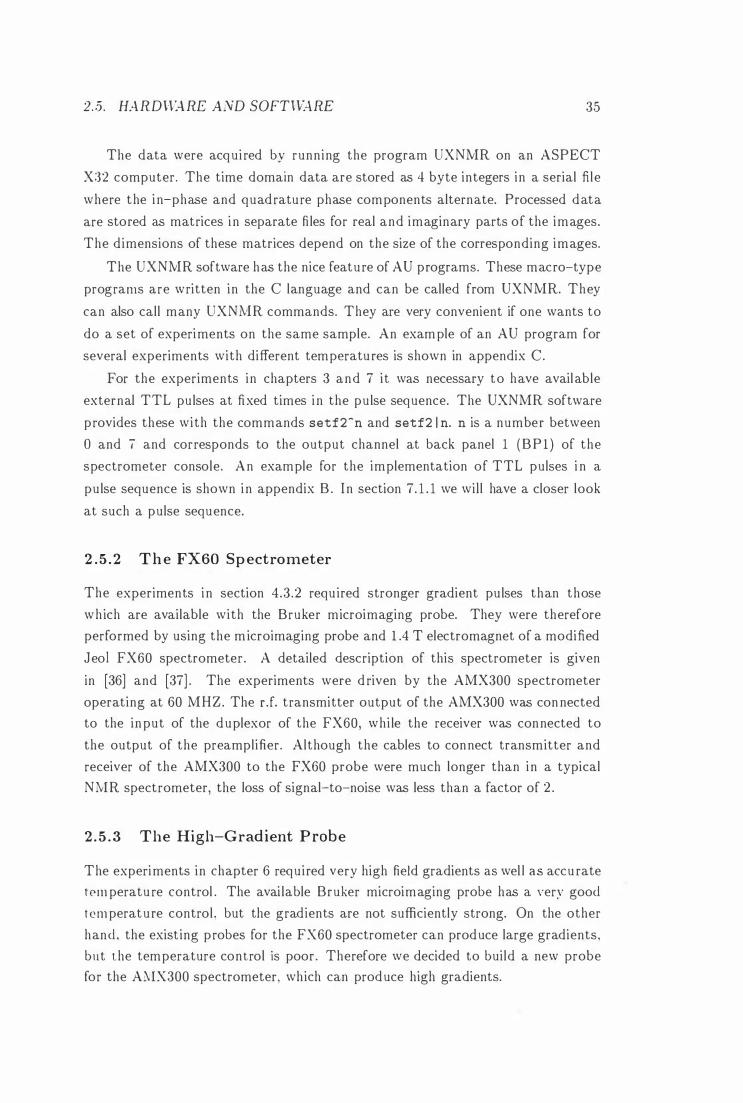
2 . . 5. HARDWARE AND SOFTWARE 35
The data were acqui red by running the program UXNMR on an ASPECT
X32 computer. The time domain data are stored as 4 byte integers in a serial fi le
where the i n-phase and quadrature phase components alternate. Processed data
are stored as matrices i n separate fi les for real and imaginary parts of the images.
The dimensions of these matrices depend on the size of the corresponding images.
The UXNMR software has the nice featu re of AU programs. These macro-type
programs are written in the C language and can be called from UXNMR. They
can also call many UXNMR commands. They are very convenient if one wants to
do a set of experiments on the same sample. An example of an AU program for
several experiments with different temperatures is shown in appendix C.
For the experiments in chapters 3 and 7 it was necessary to have available
external TTL pulses at fixed times i n the pulse sequence. The UXNMR software
provides these with the commands setf2-n and setf2 1 n. n is a number between
o and 7 and corresponds to the output channel at back panel 1 (BP 1 ) of the
spectrometer console. An example for the implementation of TTL pulses i n a
pulse sequence is shown i n appendix B . I n section 7. 1 . 1 we will have a closer look
at such a pulse sequence.
2.5.2 The FX60 Spectrometer
The experiments i n section 4.3 .2 requ ired stronger gradient pulses than those
wh ich are available with the Bruker microimaging probe. They were therefore
performed by using the m icroimaging probe and 1 .4 T electromagnet of a modified
Jeol FX60 spectrometer . A detailed description of this spectrometer is given
in [36] and [37] . The experiments were d riven by the AMX300 spectrometer
operating at 60 MHZ. The d. transmitter output of the AMX300 was connected to the in put of the duplexor of the FX60, whi le the receiver was connected to
the output of the preamplifier. Although the cables to connect transmitter and
receiver of the AMX300 to the FX60 probe were much longer than i n a typical NMR spectrometer, the loss of signal-to-noise was less than a factor of 2 .
2.5.3 The High-G radient Probe
The experiments in chapter 6 required very high field gradients as wel l as accu rate tem peratu re control . The avai lable Bruker microimaging probe has a very good
temperature control . but the gradients are not sufficiently strong. On the other
hand , the exist ing probes for the FX60 spectrometer can produce large gradients,
but the temperature control is poor . Therefore we decided to build a new probe for the AMX300 spectrometer, which can produce high gradients.
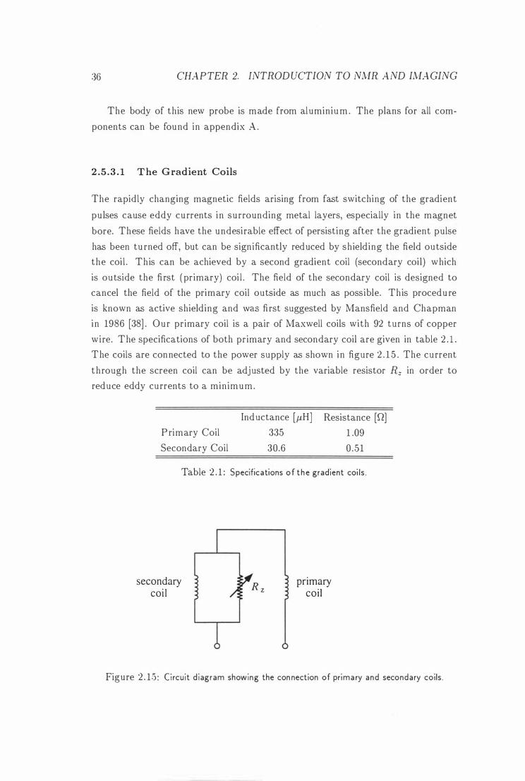
36 CHAPTER 2. INTROD UCTION TO NMR AND IMAGING
The body of this new probe is made from aluminiu m . The plans for all com
ponents can be found in appendix A.
2 .5 .3 .1 The Gradient Coils
The rapidly changing magnetic fields arising from fast switching of the gradient
pulses cause eddy currents i n su rrounding metal layers, especially in the magnet
bore. These fields have the undesirable effect of persisting after the gradient pulse
has been tu rned off, but can be significantly reduced by shield ing the field outside
the coi l . Th is can be achieved by a second gradient coil (secondary coil) which
is outside the fi rst ( primary) coi l . The field of the secondary coil is designed to
cancel the field of the primary coil outside as much as possible. This procedu re
is known as active shielding and was fi rst suggested by Mansfield and Chapman
i n 1986 [38] . Our primary coil is a pair of Maxwell coils with 92 turns of copper
wire. The specifications of both primary and secondary coil are given in table 2 . l .
The coils are connected to the power supply as shown i n figure 2 . 1 5 . The current
through the screen coil can be adjusted by the variable resistor Rz in order to
reduce eddy currents to a min imum .
P rimary Coil
Secondary Coil
Ind uctance [J.LH]
335
30.6
Resistance [n]
1 .09
0 .51
Table 2 . 1 : Specifications of the gradient coi ls .
secondary coi l
primary coil
Figure 2 . 15 : Circu it d iagram showing the connection of primary and secondary coils.
2.5. HARDvVARE AND SOFTWARE 37
2.5.3.2 Gradient Calibration
The gradient was calibrated by measuring the self-diffusion coefficient of water
at an ambient temperature of 20° C with the PGSE method . A plot of log E
vs. �(252 J2P .1,. is shown in figure 2 . 16 (a) . Using the literature value for the -JP'" self-di ffusion coefficient of water of 2 .04 m2 S- I [39] , we can work out the gradient
strength to be 0 . . 50 ± 0 .05 T m-I A- I . This calibration method is considered to
be very accurate, but does not yield any information about the homogeneity of the
gradient. Therefore, the magnetic field inside the gradient coil was also mapped
using a Hall probe. A graph of field strength vs. distance is shown in figure 2 . 1 6
( b) . I t shows that t he gradient is constant within a range o f ± 5 mm from the
centre . A l inear regression in this region yields again a gradient of 0 . 5 T m-I A- I
which is the same as we obtained by the self-diffusion method .
(a)
� ell
..2
(b)
,....., Eo--E
.......
=
0.0
-0.5
- \ .O
- 1 .5
-2.0
-2.5 0
6 4 2 0
-2 -4 -6
-20
1 * 1 09 2* 1 09 3 * 1 09 4* 1 09 5* 1 09
- 1 0
y2 8 2 F.1, [A2STo2]
o Distance [mm]
1 0 20
Figu re 2 . 16 : ( a ) A Stejskal-Ta1ner plot of doped water i n the high gradient probe. By
using the l iterature va l ue of 2 .04·'fr, - s- I . we ca l ibrate the gradient to be 0 . 5 T m - I A- I . (b) The magnetic field a long the coil ax is for a cu rrent of 1 A , measured with a Ha l l probe. The fu l l ci rcles indicate the range of constant gradient. The l i ne is a regression of these poi nts and yields a gradient of 0 . 5 T m - I A- I .
38 CHAPTER 2. INTROD UCTION TO lVi'vIR AND ll'vIAGING
2 .5 .3 .3 Gradient Eddy Currents
I n order to be able to optimise the parameters for our PGSE experiments, it is
important to know how long the eddy currents wil l persist after the gradient is
turned off. This can be achieved by recording the FID after a variable delay T after turning off the gradient, as shown in figure 2 . 1 7 (a) . This procedure is known
as pre-emphasis test. We recorded 8 FIDs after delay times T of T = 0 . 15 , 0 .3 ,
0 . . 5 . 1 .0 . 2 .0 . . 5 . 0 , 10 .0 and 20 .0 ms after switch ing off the gradient pu lse. These
are shown in figure 2 . 1 7 ( b ) and (c) for two d ifferent gradient strengths. For short
delay times T , the fields due to eddy currents distort the FID significantly, but we
can see that the eddy cu rrents have decayed after 2 ms even for gradients as large
as 7.5 T m-I . This means that we need to have a delay of at least 2 ms each time
the gradient is turned off. A delay of 2 ms is considered short and does not cause
any problems in our experiments.
I t was also fou nd that none of the F IDs changed when repeating the same
experiment. From this we conclude that the eddy currents are coherent . Signal
averaging wou ld therefore add the d istorted FIDs in phase.
I n the PGSE experiments, the echo signal becomes u nstable for gradients larger
than 4 .5 T m- I . It was found that th is effect is incoherent between d ifferent scans.
As we could see from the "switch-off" test, i nstabilities due to eddy currents
are coherent. Therefore we believe that sample movement, which is expected
to be more randomised than eddy currents, causes these i nstabilities. A possible
improvement would be a stronger sample support than the one used at the moment
which wil l be described i n the next section . Alternatively, the PGSE-MASSEY
method [40] could be used . However, for our experiments in chapter 6 a maximum
gradient o f 4 . 5 T m-I , which could be achieved without any changes, was sufficient.
2 .5 .3 .4 Temperature Control
The sample temperature is controlled by the Bruker VT2000 temperature control
un it . Heater and ai r tube fit on an adaptor which d irects the air flow to the
sample. The temperature is monitored by a copper-constantan thermocouple
which sits permanently in the ai r stream 8 cm below the sample. With a plug connector it can be connected to the VT2000 unit . Because the temperatu re is
monitored below the sample. we calibrated the sample temperature for different
readings of the thermocou pie. This was done by using a thermocouple of a F luke
80Th: thermocouple module inside an NMR tube at the centre of the d. coil . The
calibration curve is sho\\' n i n figure 2 . 18 .
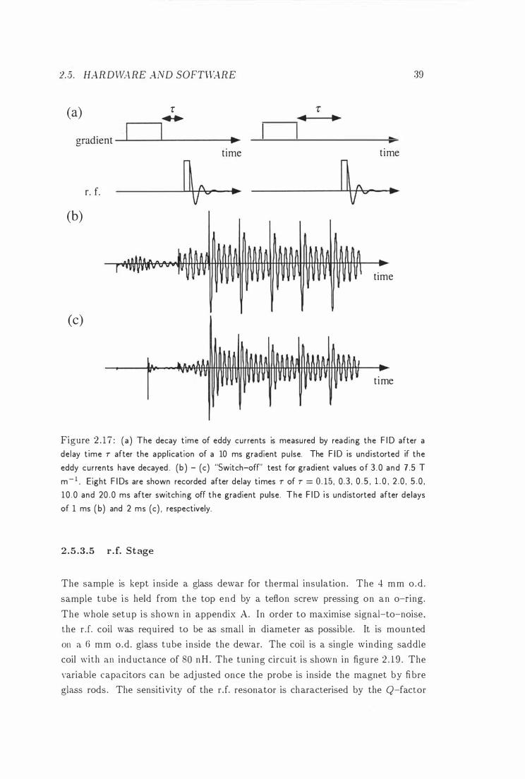
------------------
2. 5 . HARDWARE AND SOFTWARE
(a) r .. r-----'I gradient --�----�----------�.�
time
r. f.
(b)
(c)
time
time
time
39
Figure 2 . 1 7 : ( a ) The decay t ime of eddy currents is measured by read ing the F ID after a
de lay t ime r after the application of a 10 ms gradient pu lse. The F ID is undistorted if the
eddy cur rents have decayed . (b ) - (c) "Switch-off" test for gradient values of 3 . 0 and 7.5 T
m- I Eight F IDs are shown recorded after delay times r of T = 0 . 15 , 0 .3 , 0 . 5 , l . 0 , 2 .0 , 5 . 0 , 1 0 . 0 and 20 .0 ms after switch i ng off t he gradient pulse. The F ID i s und istorted after delays
of 1 ms ( b) and 2 ms (c) , respectively.
2 . 5 . 3 . 5 r . f. Stage
The sample is kept i nside a glass dewar for thermal insulation. The 4 mm o .d .
sample tube i s held from the top end by a teflon screw pressing on an o-ring.
The whole setup is shown i n appendix A. In order to maximise signal-to-noise ,
the rJ. coil was required to be as smal l in diameter as possible. It is mounted
on a 6 mm o.d . glass tube inside the dewar. The coil is a single winding saddle
coil with an inductance of 80 nH . The tuning circuit is shown in figure 2 . 19 . The
variable capacitors can be adjusted once the probe is inside the magnet by fi bre
glass rods . The sensitivity of the r .f. resonator is characterised by the Q-factor
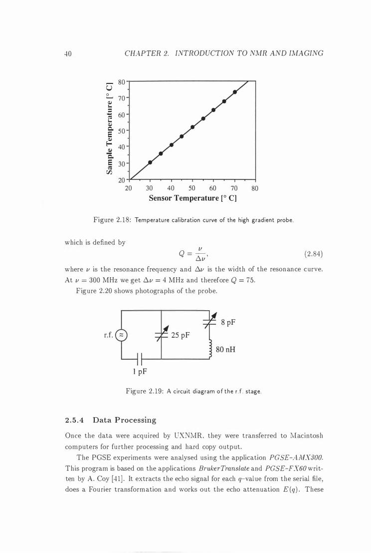
40
,........, 80 U 0
70 ........ QJ I. := ..... 60 c: I. QJ Co 50 E QJ Eo- 40 QJ Q.. E 30 c:
rJJ 20
CHAPTER 2. INTRODUCTION TO NMR AND IMAGING
20 30 40 50 60 70 80 Sensor Temperature [0 Cl
Figure 2. 18 : Temperatu re cal ibration cu rve of the high gradient probe.
which is defined by /J
Q = 6.// ' (2 .84)
where v is the resonance frequency and 6.v is the width of the resonance curve.
At v = 300 MHz we get 6.v = 4 MHz and therefore Q = 75.
Figure 2.20 shows photographs of the probe.
8 pF
rJ. 25 pF
1 pF
Figure 2 . 19 : A ci rcuit diagram of the r . f . stage.
2 . 5 . 4 Data Processing
Once the data were acquired by UXNMR, they were transferred to Macintosh
computers for fu rther processing and hard copy output.
The PGSE experiments were analysed using the application PGSE-i!.ivIX300. This program is based on the applications BrukerTranslate and PGSE-FX60 written by A. Coy [4 1] . It extracts the echo signal for each q-value from the serial file,
does a Fou rier transformation and works out the echo attenuation E (q) . These
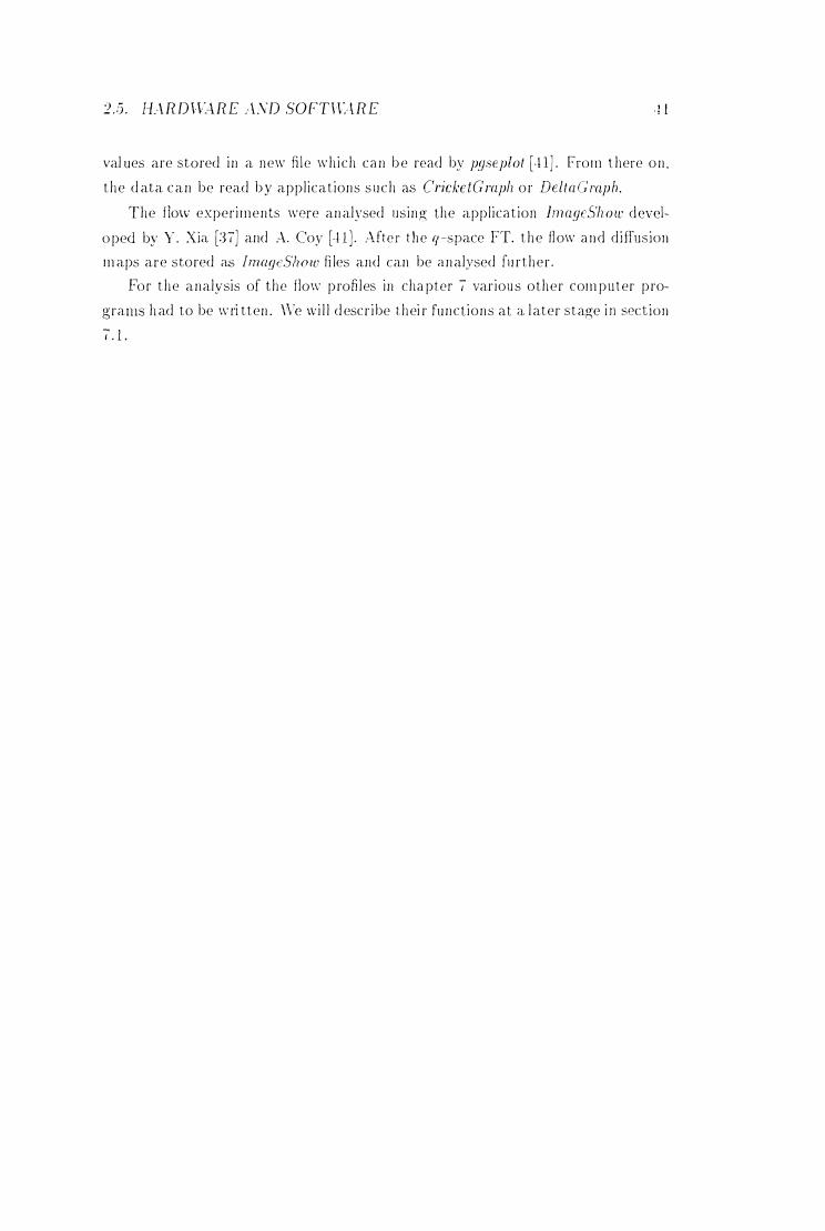
2.5 . l-L\RD\U.RE :\.VD SOFTH�·�RE
val ues are stored i n a n ew f1 le w h i c h c a n b e read by pgseplot [.l l ] . from t here o n .
t h e d ata c a n be read b y appl icat ions s u c h as CricketGraph o r DcltaGmph.
The flo\v experi m e n ts were an alysed lls i n g the appl icat ion InwgeS'hoU' devel
o ped by 't' . Xia [TI] and A. Coy [.I l J . After the q -s pace FT. t h e fl ow a nd d iffusion
m aps are stored as ImaqcShow fi les and can be a n alysed fu rther .
For t h e analysis of the flow p rofi les in c ha pter 7 varioll s other com p u t er p ro
grams h ad to be w ri tten . \Vc vii l l d escr i be t h ei r fu nct ions at CL l ater stage i n section
7. 1 .
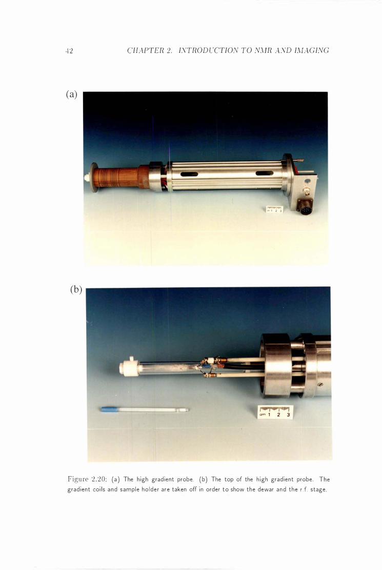
-l 2
Ca)
Cb)
CHAPTER 2. I.YTROD UCTION TO NiVIR A ;VD IAJAGING
Figu re 2 .20 : (a ) The h igh gradient probe. (b) The top of the h igh gradient probe The
grad ient coi ls a nd sample ho lde r a re taken off in order to show the dewar and the d. stage.
C hapter 3
Imaging of Electroosmotic Flow
3 . 1 Intro duction
I n t h is chapter we w i l l descr ibe m ic roimaging measurements o n flow wh ich is vary
i n g i n spa.ce as wel l as in t ime . \Ve i nvestigate the t ime evol u tion of electroosmotic
flow in a capi l lary fol low ing the application of pu lsed electric fields i n a weak ion ic
sol ut ion .
3 . 1 . 1 Electrophoresis a n d NlVIR
\Vhen an electric field of rnagn i tude Edc is present in an electrolyte solu tion , ions
d ri ft along the electr ic field l ines . This ion transport is know n as electrophoresis.
In m olec ular biology, electrophoresis is one of t he most important methods of
analysis of t ransport properties. Because of ion ic col l is ions and solvent friction ,
ions of a part icu lar s pecies reach a term inal velocity v of
(3 . 1 )
where It is the elect rophoret ic mobi l i ty of the molecu le u n der i nvestigation i n a
pa.rt icu lar env ironment . It depends on the shape and size of the molecu le as well as its charge and temperat u re . For molecu la.r ions. mobi l i t ies usual ly l ie i n t h e
range of 1 to 5 . 1 0 -8 m2 S- 1 V- I H:2] . Thus . for elec t ric fields w i t h magn i tudes u p to l O O V cm- I . the u pper l im i t fo r d ri ft velocit ies is abou t 0 .5 m m s- I .
For microscopical ly visi ble pa rt icles. t he electrophoretic mobi l i t ies can be mea
su red d i rec t ly by observ ing ( h e moving part icles \vi t h a microscope. I f they canno t 1)(' o bs('['v('d d i rec t l:;. t h ey m u st ('i t h er b e ad sorbed o n m i c roscopical ly v i s i bl e carrier particles to permi t d i rect mobi l i ty measurement . or st1J(l ipd i nd i rect ly by t ech
n iq ues i n wh ich the movement of macroscopic amou nts of material i ll the elec t ric
field is detected . Zone methods h ave been widely ad apted for t his pu rpose. A st r ip
· 1 -1 CHAPTER :]. I.\L\GISG OF ELECTROOSMOTIC FLOW
of fi lter paper i s sat u rated wi th bu ffer solut ion , and a smal l amount of a sol ut ion
of the material u nder i nvestigation is applied as a narrow band . On application
of a potential d i fference between t he ends of the str ip , each component migrates
at a rate wh ich is main ly determined by its mobi l ity. After an appropriate t ime .
the str ip i s removed . d r ied and developed to show the posit ions and concentra
t ions of the d i fferent components. These techniques are descri bed i n textbooks on
electrophoresis . for example in [-13] .
I n section 2 . -1 . 5 we saw that wi th the dynamic s p i n echo method i t i s poss ible
to measu re flow profiles with a resolu tion down to a few m icrons per second . By
taking advantage of chem ical sh i ft sensit ivity one can also resolve d ifferent compo
nents in a mixtu re . The combination of N1\lR with electrophoresis i s called elec
trophoretic NivIR ( EN MR) . I n pr inc iple it is possible to determ i ne electrophoretic
mobi l it ies and d iffusion coefficients for each l ine in the NlvlR spectr u m .
T he fi rst observations o f electrophoretic dr i ft v i a NrvIR were reported b y Packer
et al. [44] in 1972 . They found t hat the echo envelope in a modified Carr-Purcell
sequence depended on the c urrent densi ty with and without grad ient p ulses , b u t
t he effects were enhanced by the g radient pulses. I t was s uggested that t h e ef
fects were associated wi th magnetic fi eld grad ients res u lt ing from electr ical cu rrent
t h rough the sample and the sp iral motion of ions under the influence of the ma in
magnetic fi eld . Later experiments are referred to i n a review by Johnson [42] .
One might fear t hat the movement of charged particles would i n terfere w i t h
t he static magnet ic fi eld . Two p roblems m ight occur . F irstly, moving charged
par ticles create a magnetic fi eld . I f the movement is along the static magnetic
field (z d irection) , as it i s in the nat ural arrangement in a superconduct ing mag
net , the magnetic fi eld created by th is cu r rent h as components only i n the x y plane. T herefore t here i s no magnetic field created i n the z d i rect ion . When an
electromagnet is used . t h e ionic cu r rent creates a magnetic fi eld wh ich cannot be
ignored . However , i t can be com pensated for by external s h im coi ls .
The other effect wh ich has to be d iscussed is the perturbed orbit of charged
particles in a m agnetic field . S i nce the force on a charged particle moving in a magnetic fi eld is perpend icular to both velocity and fi eld . no e ffect is expected
\vhen t he cu rrent a.nd the main magnetic field are paral lel . I n fact . molecu la r
coll is ions randomise t he d i rect ion and magnitude of the veloc ities apart froIn a
smal l polarisat ion resu l t i ng from the appl ied electric field . and there is l i tt le effect
for an�' or ien t ation of cu rrent and main magnetic field .
However . t here is another effect which can be Cl severe problem i n electrophores is experiments. \Ye wil l deal with th is so-called electroosmosis in the next sect io n .
3.2 . THEOH1 ' . [ .)
3 . 1 . 2 Electroosmosis
The electrophoretic migration of ions resu lts in ionic coll isions \v i th the neutra l
solvent molecu les which t ra nsfer momentum in the d i rection of ion flow . However .
for an ion ic sol u t ion in wh ich the charge distr ibution is homogeneous. the oppo
sitely d i rected flow of anions and cations causes local cancellation of such effects so
t hat ion migration occu rs against a stationary solvent . Because th is cancellation
is dependent on local charge neutral ity, any i nhomogeneity in charge d istr ib ll t ion
can d rastica.lly alter the loca.l balance in electrophoretic d rag forces . The resu l t ing
fl u id t ransport is k nown as electl'oosmosis [· 1 2 . ·1.5 . .JG] . The velocities associated
\vi t h electroosmosis a re com parable to or even larger t han the electrophoretic d ri ft
veloci ties.
U ntreated glass or plastic: surfaces In contact with electrolyte solut ions are al
ways charged , and the positive and negat i ve ions in sol u tion are d istr ibuted u nder
the i n fl uence of the electric field . Close to t he su rface, a layer with CL high concen
t ration of coun terioll s , k nown as the Debye layer. is the resu l t . As a consequence ,
the application of an electric field causes i n homogeneous electrophoretic c urrents.
Because the Debye l ayer is generally very th in , the electroosmotic d rag wil l resu l t
i n an apparent s l ip of the fl uid along the boundary. Outside th is layer t he flow
profile wil l be determ ined by the hydrodynamics of a ne ll t ral fl uid experienc ing
t lte electroosmotic flow as a boundary condit ion .
Electroosmotic flow can be reduced by i ncreasing the v iscosity of the fl ui d o r by red ucing the charge on the su rface by coat ing i t w i th a polymer . I n cases w here
i t is not possible to red uce the elect roosmotic flow significantly, it is i mportant
to k now the shape and t ime dependence of the f low profile . Electroosmotic flow
can be measured by observing a boundary layer i n the electrophoretic cell with
a microscope. However, th is method requ i res the solut ion to be doped wi th m i
croscopical ly visi ble particles . With dynamic NMR microscopy i t is possible to
observe the movement of the solvent d i rectly and non�invasively. In this chapter \ve measure the time evolu tion of electroosrnosic flow with the dynam ic sp in echo
method and com pare our resu lts with theoretical pred ictions.
3 . 2 Theory
Consider t he case of a capillar:-' of rad ius Ho in wh ich elcctroosmo t ic flow develops
at the \vall . I f the fl u id is incompressi ble and confi ned then the su rface flow
lll l lst be balanced by a cou llt er flow. r n der eq ui l ibri u m . const an t electric fi eld
cond it ions, and g iven a ;\ewton ian fl uid , we expect that t h e rate of strai n , [J tljor ,
wil l vary l ine arly w i th rad ius , resul t. ing i n a quad ratic vclori ty profi le . (· ( r ) . T he
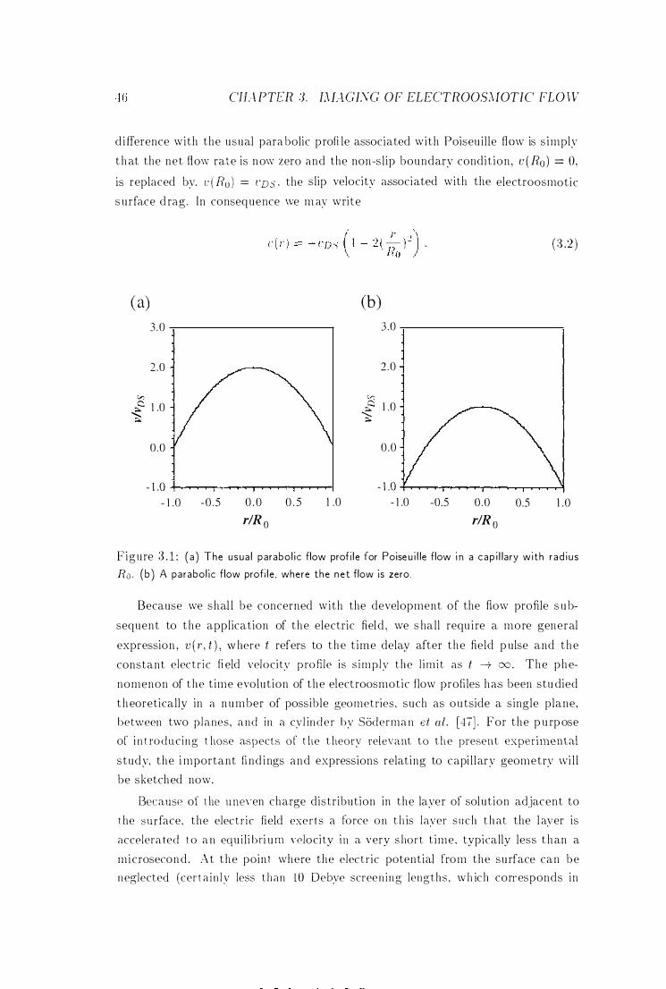
CIU PTER 3. nHGISG OF ELEC'TROOSMOTIC FLOPv'
d ifference with the usual para bolic p rofi le associated with Poiseu i l le flmv is s imply
t hat the net How rate is now zero and the non-s l ip boundary condit ion , u ( Ro) = 0, is replaced by, v ( Ro l = ( 'DS , the sl ip velocity associated with the electroosmotic
s u rface d rag . In consequence \ve m ay write
(:3,2)
(a) (b) 3 .0 3 .0
2.0 2 .0
v: '" c 1 .0 c 1 .0 t < ;:.
0.0 0 .0
- LO - J .O - 1 .0 -0 .5 0 . 0 0 . 5 1 .0 - 1 .0 -0.5 0 .0 0.5 1 .0
rlR o rlR o
Figure 3 . 1 : ( a ) The usua l parabol ic flow prof i le for Poiseu i l le flow i n a cap i l lary w ith r ad i u s
Ro . (b ) A parabol ic flow profi le . where the ne t flow is zero.
Because we shal l be concerned with the development of the flow profile s u b
sequent to the appl ication of the electric fiel d , we s hal l requ i re a more general
expression , v ( 1' , t ) , w here t refers to the t ime delay after the field p ulse and the
constant elec t r i c field velocity p rofile is s i m p l y t h e l i m i t as t -+ 00 . The phe
nomenon of t h e t ime evolut ion of the e1ectroosmotic flow profiles has been stu died
t heoretically in a number of possible geo met ries, such as ou tside a single plane, between two p l anes, and in a cy l in d e r by S6derman et al . [47] . For the p u rpose oC i n t ro d u c i n g t hose aspects o e t he t heory relevant to t h e presen t exp(;rimental study, the i mportant fi nd i ngs and expressions relat ing to capi l lary geometry \vi l I
be sketched now.
Because of the U1\E'\'en charge distr ibution in the layer of sol ut ion adjacent to
the surface, the elec t r i c field exe r t s a force o n t h is l ayer s u c h t h at the l ayer is
accelerated t o a n eq u i l i b ri u m \'e locity i n a very s ho r t t ime , typically less t han a
m ic rosecond . At the poin1 where the elec t r i c potential from the su rface can be n e�lectecl (cer t a i n l :v less t h a n 10 Debye scree n i n g lengt h s , \v h ic h corresponds in
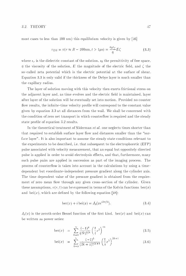
3 .2. THEOHY
most cases to less than 100 n m ) th is equ i l i b ri u m velocity is given by [46]
( ) to tr , . L'DS ::= V /. � R - 100nm, t > Ills = -- E � '7
where E r is the d ielectric constant of the sol ut ion , EO the permitt iv i ty of free space .
'7 the viscos i ty of the sol u tion , E the magnitude of the e lectr ic field , and ( the
so-called zeta potential wh ich i s the electric potential at the surface of shear .
Equation :3 . :3 is only valid i f the t h ickness of the Debye layer is much smal ler than
the capil lary rad i us .
T he layer of solution moving with t h is velocity then exerts frict ional stress on
the adjacent layer and , as t ime evolves and the electr ic field is maintained . layer
afte r l ayer of t he sol u tion wi l l be eventually set i nto motion . Provided no counter
1low results , the i n fi n i te-t ime velocity p rofile w il l correspond to the constant valu e
given by equ ation ;3 .3 a t all distances from the wal l . We shal l be concerned w i t h
t h e cond i tion of zero net t ransport i n wh ich counter1low i s requ ired and the steady
state profi le of equation :3 .2 results .
I n t he theoretical treatment of Sc:iderman et a!. one neglects t imes shorter than
t h at requ i red to establish su rface layer flow and d istances smaller than the "su r
fa ce l ayer" . I t is also i mportant to assu me the steady state condit ions relevant to
the experiments to b e descr ibed , i .e . t hat subsequent to the electrophoretic (EFP)
pu lse associated wi th veloc i ty meas u rement , t hat an equal but oppositely d irected
pulse is applied in order to avoid electrolysis effects, and that , fu rthermore, m any
such pu lse pairs are appl ied i n succession as part o f t he imaging p rocess . The
process of counterflovv' is taken i nto account i ll t he calcu lations by using a t ime
dependent but coordinate-independent p ress u re grad ient along the cyl inder axis .
The t ime dependent value of the p ress u re g radient i s obtai ned from t he requ ire
ment of zero mean flow t h rough any given c ross-section of the cyl inder . G ive n
these assumptions, v ( r, t ) can b e expressed i n terms o f the Kelv in fu nctions ber ( .r)
and bei ( .c ) , w hich are defi ned b�r the fo llmving equation
ber ( x ) + i bei ( :c ) = Jo (;cci3rr/4 ) . ( 3 .4)
Jo ( :r ) is the zeroth order Bessel function of the fi rst k ind . ber ( :e ) and bei ( .r ) can
be w ritten as power series:
ber (.r ) ( 3 .5 )
bei ( .7: ) ( :3 .G )
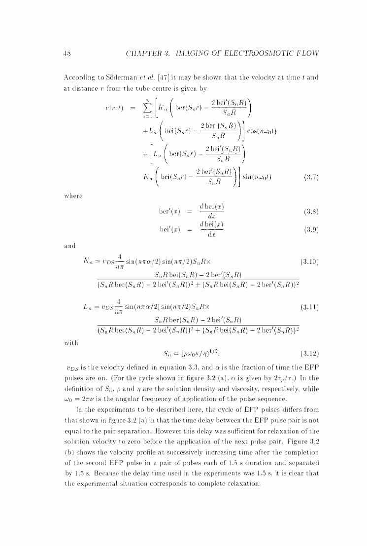
CHAPTER. 3 . L\[:lGEVG OF ELECTROOS,\[OTfC FLOW
Accord i ng to Soderman e t al. Hi] i t may be shown that the velocity at t ime t and
at d istance r from t h e t u be centre is given by
where
and
w i th
bel" ( :1: )
bei' ( :1: )
d be r ( J; )
cb: d bei
d:r
.+ [(n == ('DS - si n ( nr.('I'/2) s in ( nr. / 2 )SnRx n rr
SnR bei ( SnR) - 2 ber ' (SnR)
(SnR ber (Sn R) - '2 bei' (SnR) ) 2 + (SnR bei (SnR ) - 2 ber' ( Sn R ) ) 2
( 3 .8)
( 3 .9 )
( 3 . 10 )
L n == VDS � sin ( nr.u/2) s i n ( nr. /2 ) Sn R x (3 . 1 1 ) 7lr. Sn R ber (SnR) - 2 bej ' (Sn R)
( 3 . 1 2 )
IJDS i s t h e velocity defi ned i n equation :3 . :3 , and Cl' i s the fraction o f t ime t h e EFP
pu lses are on . ( For t he cycle s hown i n figure 3 . 2 (a) , Cl' i s given b y '2Tp/T . ) I n the
defi n it ion of Sn , (J and 77 are the sol n tion density and viscosity, respect ive ly, wh i l e Wo =: 2r.v i s t h e angu lar freq uency o f applicat ion of t he p u lse seq uence .
In the experiments to be described here , the cycle of EFP pu lses d iffers from
t h at shown i n fig u re :3.:2 ( a) i n t h at the t ime delay bet\veen t h e EFP p u lse pa ir i s not
eq ua l t o the pa i r separation . However th is de lay was su fficient for relaxation of the
so l u t i o n \'e!ocity t o zero before t h e application of t h e next p u lse pa i r . Figure :3 . 2
( b ) shows t h e \'elocity profi le at successively increasing t ime a fter t he com plet ion
o f t he second EFP pu lsp i n a pair of p u lses pach o f l . .5 s durat ion and separatpc\
b�' 1 .5 s. Bec;lusP t he de la:,.' t ime used in t h e experi men ts was L5 s, it is c lear t hat
t h e e x peri m e n t a l si t u ation corresponds to comp lete relaxation .
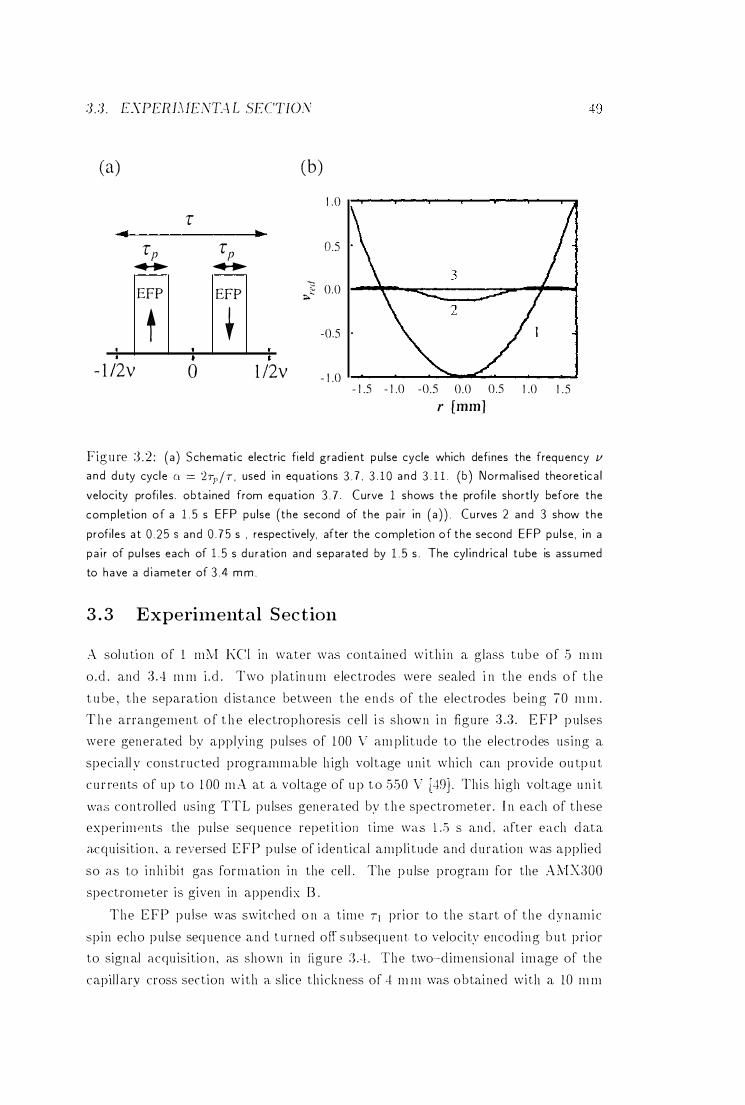
3.3 . EXPERBIE;,\TA L SECTlO;\T
(a) (b) 1 .0
'! 1II1II ......
'!p '!p 0.5 .............. ..............
-::: 0.0 EFP EFP "" ;;."
t t -0.5
- 1 /2v 0 1 I2v - 1 .0 - 1 .5 - 1 .0 -0.5 0.0 0.5 1 .0 1 . 5
r [mm]
Figu re :3 .2 : ( a ) Schemati c electric f ie ld grad ient pu lse cycle which defi nes the frequency v
a n d d u ty cycle Cl := '2rp/T . used i n eq uat ions 3 . 7 . 3 . 1 0 a n d 3 . 1 1 . (b) Norma l ised theoretic a l
velocity profi les . obta i ned from equat ion 3 . 7 Curve 1 shows t h e profi l e short ly before the
completion of a 1 . 5 s EFP pu lse (the second of the pa i r i n ( a ) ) . Cu rves 2 and 3 show the
prof i les a t 0 .25 $ and 0 . 7 5 s . respectively. after the complet ion of the second EFP pu lse , i n a
pa i r of pu l ses each of 1 . 5 s d u r at ion and separa ted by 1 . 5 s . The cyl i nd rica l tube is ass umed
to have a d i ameter of 3 .4 m m .
3 . 3 Experinlental S ection
A sol u tion o f 1 mM KCI in water was contained wi th in a g lass tube o f 5 m m
o.cI . ancl 3 .4 m m i .cI . Two p lat in u m e lectrodes were sealed i n the ends o f t he
t u be , t he separation d istance between t he ends o f the electrodes being 70 m m .
T h e arrangement o f t h e electrophoresis ce l l i s shmvn i n figure 3 .:3 . EFP pu lses
were generated by applying pu lses of 1 00 V am pl i tude to the electrodes us ing a
specia. l l y constructed programmable h igh vol tage u n it which can provide ou t p u t
cu rn' llts o f up t o 1 00 mA at a voltage of u p t o 550 V H9J . This high voltage u n i t
was contro l led lls ing TTL pu lses generated by t h e spectrorneter . I n each of these
experiments the pu lse seq uence repeti t io)) time was L5 s and , after each data
acquisition . a reversed EFP pu lse of identical ampl i tude and du ration was appl ied
so as t o i n h i bi t gas formation in the cel l . The pu lse program for the A'\[X�)O()
spectrometer is given in appendix B .
The EFP pu lse was switched o n it t ime Tl prior to the start o f the dynamic
Spi ll echo pu lse seq uence and t u rned o ff subsequent to velocity encod ing bu t prior
to sign al acqu isition , as shown in figure : >A. The two·-d imensional image of the
capil l ary cross section with a sl ice th ickness of Ll m m was obtai ned with a 10 m m
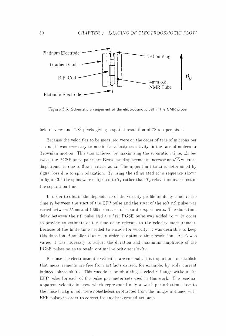
50 CHAPTER 3. L\U G ISG OF ELECTROOSMO TIC FLOW
Platinum E lectrode � Teflon Plug
Gradient Coils �
R.F. Coil
Platinum Electrode ------------4mm o.d. NMR Tube
Figure :3 . 3 : Schematic ar rangement of the electroosmotic cel l in the N M R probe.
field of view and 1 282 pixels giving a spatial reso lu tion of 78 pm per pixel .
Because the velocities to be measu red were on the order of tens of m icrons per
second , i t was necessary to maximise velocity sensitivity i n the face of molecu lar
B rownian motion . Th is \vas ach ieved by maximising the separat ion t ime, d, be
tween the PGSE pu lse pair s ince B rownian d isplacements i n crease as Vii w hereas
cl isplacements cl ue to flow increase as d . The u pper l im i t to d is determined by
signal loss due to spin relaxation . By using the stimu lated echo sequence s hown
i n figure 3 . 4 t he spins were su bjected to T1 rat her than 12 relaxation over m ost of
the separation t ime .
In order to obtain the dependence of the velocity profile on de lay t ime, t , the
t ime '11 between the start of the EFP p ulse and the start of the soft r J. p ulse was
varied between 25 ms and 1 000 ms in a set of separate experiments. The short t ime
delay between the rJ. pulse and the fi rst PGSE pu lse was added to '11 i n order
to p rovide an est imate of the t ime delay relevant to the velocity measu rement .
Because of the fi n ite t ime needed to encode for velocity. i t was desirable to keep
th is du ration d smal ler than '11 in order to opt imise t ime resolut ion . As d was
varied it was necessary to adjust the du ration and maxim u m amp l i tude of the
PGSE pu lses so as to retain opt ima l velocity sensit ivity.
Because the electroosmotic n�locities are so smal l . it is important t o establish
that measn rements a re free from artifacts caused . for exam ple , b�' eddy c u rrent
induced phase sh ifts. This \Vas done b�' obtain ing a velocit�· image \vi thout the
EFP p ulse for each of the pu lse pa ramet er sets used in t h is work . The resid ua l
apparent veloc ity images, which represented on ly it \vea k pert u rbation c lose to
the noise background . were nO lletheless subt racted from the images obtained w i th
EFP pu lses i n order to correct for any ba.ckground artifacts .
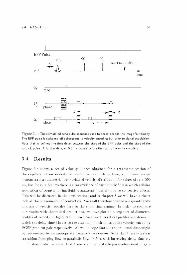
3. 1 . H ES ULTS .5 1
EFP Pul se
start acquis i tion
L f. t time
c, Cl read
c.y i 0 0 phase
g � ��. 8 C� rI 0
s l ice LJ .... .1 ...
F i g u re 3 .4 : The st im u lated echo pu l se seq uence used to phase-encode the image for velocity.
The E F P pu lse is switched off subsequent to velocity encod ing but pr ior to sign a l acquis it ion .
Note tha t T) defines t he time de l ay between t he start of t he EFP pu l se and the start of t he
soft r .f. pu l se . A fu rther de lay of 5 . 3 ms occurs before the start of velocity encod i ng .
3 . 4 Results
F i g u n� 3 . .5 shows a set o f velocity i mages o btained for a t ransve rse sec t i o n o f
t h e capil l ary a t s u ccessi vely i nc reas i n g val u es of delay t i m e , TI . T h ese i m ages
d e m onst rate a sym metr ic , wel l-beh aved velocity d is t ri b u ti o n for val u es of Tl < 500
ms, b u t fo r T1 > .500 ms there is clear evidence of asym metric flow i n wh ich cel l u lar
se paration of co u n terfl mv i n g fl u id is ap paren t . possibly d ue to convective effects.
T h is w i l l be discussed in t he next sect io n , a n d in c h apter 8 we wi l l h ave a c loser
look at t h e p h e n o m e n o n o f convection . vVe s h al l t h erefore con fi n e Oll r q u an t i tative
an alysis o f velocit:., profi les here to the short time regi me. I n order to com pare
o u r res u l ts w i t h t h eoretical pred i ct i o n s , we h ave plotted a seq u e n ce of d i amet ral
profi les o f wdocity in figure :3 . 6 . I n each case two t heoretical p rofi les are shown i n
w h ich t h e delay t i m e t i s spt t o t h e s t ar t and fi n ish t i mes o f t h e velocity encodi n g
PGSE gradient p a i r res pective l ,\', \Ve wo uld h o p e t h at t h e experimen ta.l d ata m ig h t
be rt' prese n t ('d b�' a n appropri ate mean of t hese c u rves. Note t h at t h(,1'e i s a clear
t ransit io n frolll p l ug flo\\' to para.bol ic flow p ro fi les \v i t h i n creas i n g delay time TI ' I t s h o u l d a lso be n oted t h a t t here are n o adj ustable parameters u sed i n gen-
52 CIL\ PTEH :3. L\ L\G E\G OF ELECTROOS�JOTIC FLOW
erat ing the theoretical profi les, save for the scal i ng constant , VDS . The val ue of
this constant \vas dete rmined by adjust ing i ts value so that the t heoretical p rofil es
best agreed with the data i n flgu re :3 .6 (al . T he val ue so o btai ned , t:DS == 0 .095
mm s- l , \vas then used i ll generat ing al l other profi l es . From the va l ue of UD S we may calcu late ( to be 80 mV ( us ing the val ue is . S for ( 1' ) ' a value wh ich i s q uite
reason able for glass HS, 50] .
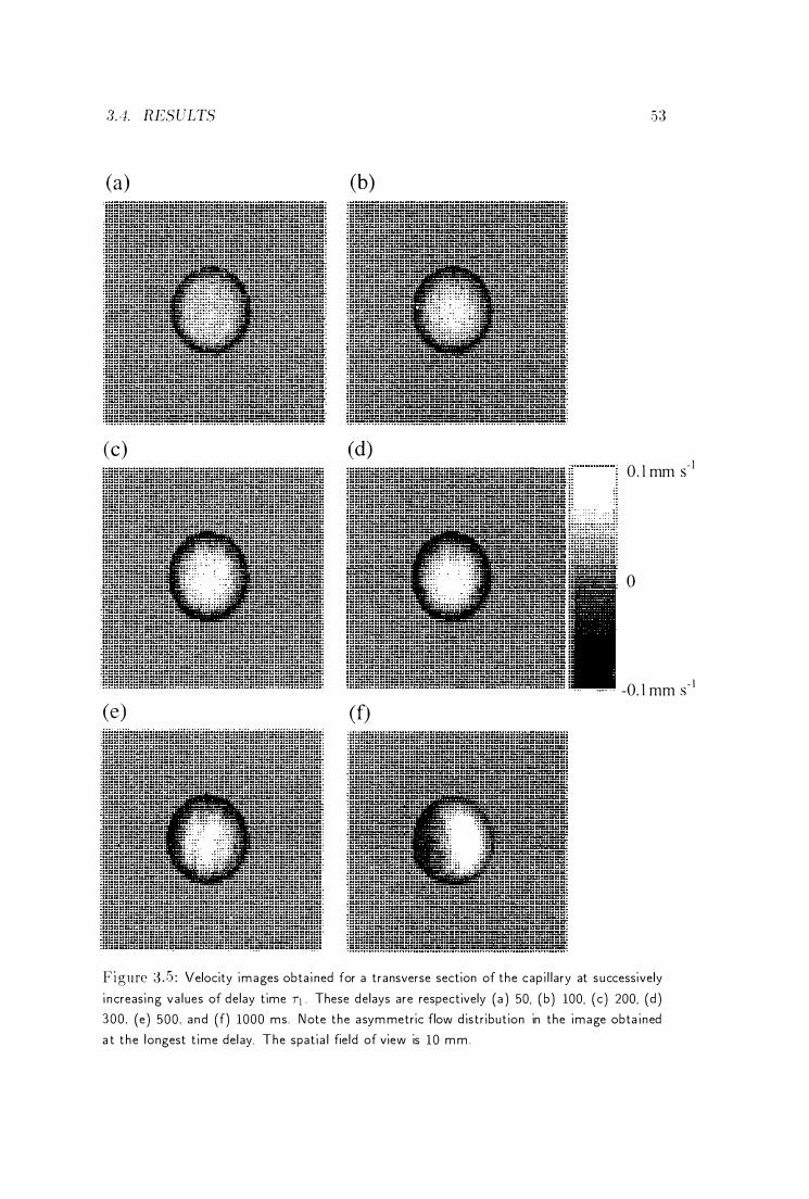
:1,,1. RESULTS 53
(a) (b)
(c) (d) O. l mm s·1
o
-O. l mm S· I
(e) (t)
Figure ;� .5 : Velocity images obta i ned for a transverse section of the cap i l lary at successively
i n creasi ng va l ues of delay time Tl . These delays are respectively (a ) 50, (b) 100, (c ) 200, (d ) 300 , (e ) 500 , and (f) 1000 ms. Note the asymmetric flow distr ibut ion in the image obta ined
a t the longest t ime del ay. The spati a l fie ld of view is 10 mm.
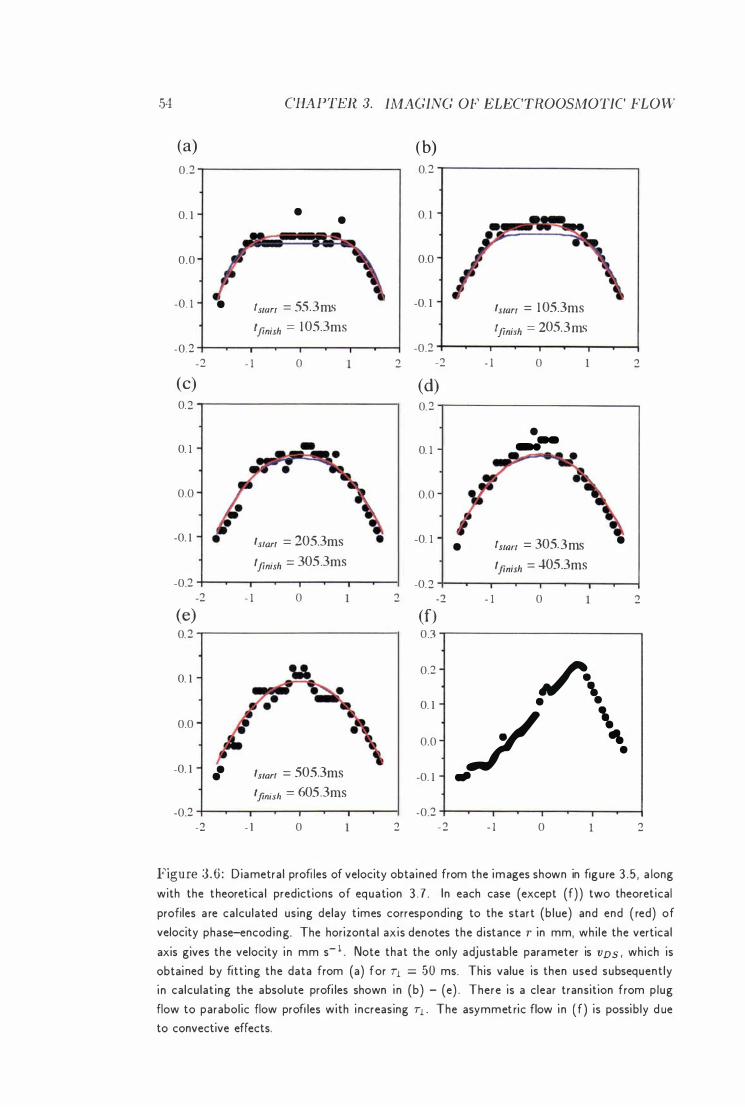
54
(a) 0.2
0. 1
0.0
-0. 1
-0 .2 -2
(C) 0.2
0. 1
0.0
-0. 1
-0.2 -2
(e) 0. 2
0. 1
0.0
-0. 1
-0.2 -2
•
- 1
- 1
••
- 1
CHAPTER 3.
• •
ts/art = 55.3ms {finish = 1 05.3ms
0
-
Is/art = 205.3ms lfinish = 305.3ms
0
Is/art = 505.3ms tfinish = 605.3ms
0
IMAGING OF ELECTROOSMOTIC FLOW
(b) 0. 2
0. 1
0.0
-0. 1
-0.2 2 -2
(d) 0. 2
0. 1
0.0
-0. 1
-0. 2 2 -2
(t) 0.3
0.2
0. 1
0.0
-0. 1
-0.2 2 - 2
- I
•
- 1
Is/art = 1 05.3ms [finish = 205.3ms
0
• --
tS/art = 305.3ms lfinish = 405.3ms
0
/-, • •
•
/ \ � •
.-
- I 0
2
2
2
Figure 3 .6 : Diametra l profi les of velocity obtained from the images shown in figure 3 .5 , a long
with the theoretica l predictions of equation 3 . 7 . In each case (except (f) ) two theoretical
profiles a re calculated using delay times corresponding to the start (b lue) and end ( red) of velocity phase-encoding. The horizontal axis denotes the distance r in mm, whi le the vertica l
axis gives the velocity in mm s- l Note that the only adjustable parameter is VDS , which is
obtained by fitting the data from (a) for 71 = 50 ms. This value is then used subsequently
in calculating the absolute profi les shown in (b) - (e) . There is a clear transition from plug
flow to parabolic flow profi les with increasing 71 . The asymmet ric flow in (f) is possibly d ue to convective effects.
3 .5 . DISC[!SSlO;\i 5.)
3 . 5 D iscussion
A l t h o u g h t h e experi menta l flow profi les agree very wel l with t h e pred ictions . i t
s h o u l d be n oted t h at resistive heat ing of the sample i s a serious problem i n E 0" M R
experiments . I n o r d e r t o w o r k o u t t h e tem peratu re i nc reCkse, w e consider a sample
h av i n g electr ic cond uct iv ity h el , length d and cross-sectional a rea A . \Vh e n a
potent ial d i fference U is appl ied across the sam ple for a period t l , t h e energy �Vel de posited i n the sam ple is
( :3 . 1 3 )
w h e re R ::::: 1/ "pl . l is t h e elect rical resis t ance. T he t hermal energy lVth req ui red
to h eat t h e sam ple by 81' is given by
( :3 . H)
w here p and cp are the d ensi ty and specific h eat of t h e sam ple. If n o heat i s
exc hanged w i t h t h e environment , both energies m ust be equ al :
( 3 . 1 5 )
T h e tem perat u re i n crease 8T is t h e n given by
(3 . 16)
w h ere E :::: U / d is the strength o f t he electr ic field p u lse. In o u r experim ents we
u sed val u es o f U = 100 V and d ::::: 7 cm . For a solu tion o f 1 m M KCI i n water
Kel ::::: 0 . 0 1 47 $1- 1 m - l [5 1] at a temperat u re of 25° C . With these values, alon g
v,-i t h t he l i terat u re values for p ::::: 996 .9 k g m -3 and cp ::::: 4 1 80 J K- 1 m -3 o f w ater
at 2,5° C [5 1) , we obtain a temperat u re i n crease of 8T ::::: 7 m K for an EFP p u lse
o f 1 s d u r ation . Because t h is temperat u re i n crease is expected to be h om ogenous
ac ross t h e w hole sam ple and . for short EFP p u lses. s m al ler t h an temperatu re
fl u ct.u at ions cl u e to o t her effects (e .g . heat ing of t h e gradient coi l , absorpt ion o f
r J. power) , w e c o n c l u d e t h at convective effects are n ot i m portant for o u r analysis ,
except for t h e longest T] val ue u sed in our experiments.
In order to est i mate t he m i n i m u m vertical tem perat u re grad ient �T across t h e
sam ple. for wh ich convection w i l l OCC ll r . we assume now t h at t h e asy m metr ic flow
d is1 ri bu t iOI1 in figure :L :3 ( f ) is callsed b:-' convection . In chapter 8 t h e p h enomenon
of cO Il vection w i l l be disc u ssed i n d etai l . Con vection can only occ u r i f the Rayle igh
n u m ber R dt' fi n (1d i n t'(j ll at ion 8 . 1 exceeds t he cr i tical val u e Rc w h ic h strongly
i n creases with decreas ing aspect rat io defined as the ratio of t h e w i d t h L of the
fl u id layer to its d e pth d . For the esti m ations here , we assume as in c h apter 8
56 CHAPTER 3. IMAGING OF ELECTROOSI\,lOTIC FLOW
the value of Rc to be Rc ;:::;:; 107 [or our setu p . We set R = R c for t ] = 1 s . With
the l itera tu re va lues of volu me expansion Cl = l .G · 1 0- -\ I\- l . t hermal d iffusivity
� t h = l A - 10-7 m2 S- I , and kinematic v iscosity v = 8 .0 · 1 0-7 m2 s- 1 [5 1] we
obtain a m in imum tem perature d ifference of �T = 2 E . :\s stated above, these
calcu lations neglect any hecLt exchange with the environment , but i t is clear that
convection due to resistive heat ing governs the upper l imit of the TI values for
w h ich electroosmotic flow can be observed i n our experiments.
Because the c rit ical Rayleigh number Rc strongly increases with decreas ing
aspect ratio of t he cell u nder i nvestigation , the most efficient way to avoid con
vection is to red uce the aspect ratio. This can be achieved by eit her reduc ing
the width L of the fl u id layer or by i ncreasing its depth d. Equation 8 . 1 states
that R ex: (p , and therefore Rc can be increased without c hanging R by reduc ing
L. This means t hat the onset of cOllvection is red uced most efficiently by us ing a
smal ler tube d iameter.
\Vi th the cu rrent t he lower l imit of T] is determined by t h e available
gradient s t rength in order to get a reasonable velocity reso lution . Wu e t al. [.52] demonstrated t hat it is poss ible to reconstruct the velocity profi le i n a system w i th
cyl indrical symmetry by using on ly one grad ient wh i ch is oriented along t he flow
d i rection . By using the h igh grad ient probe described i n section 2 . 5 . 3 i t would
t herefore be possible to measure flow profiles for values of Tl < .50 ms. The lowest
l imit of Tl is reached when the d isplacements of t h e molecules due to electric field
pulses are smal le r t h an the d isplacements due to Brownian motion .
In t h is chapter we have demonstrated t hat N1vIR m icroscopy is a powerful tool
to monitor t he t ime evolution of electroosmosis. \Ve cou ld measu re flow profiles
with a velocity resolu tion of around 1 5 jlm s- 1 . We h ave shown t hat elect roosmotic
flow velocit ies are of the same magnitude as the ionic electrophoretic motion ,
bu t t hat electroosmotic velocities typically reach a steady state d istr ibu tion i n a
capi l lary geom etry on a t imescale of 1 00 mil liseconds, rather than at the su b-nanosecond relaxation t imes pert inent to t he ionic electrophoretic response. A
pleasing aspect is the good agreement between theory and experiment .
Chapter 4
Velocity Exchange
S p ectroscopy
I n t he previous chapters we i nt rod uced some methods which may be used to image
flow p rofiles. In c hapter :3 we saw that t here is an easy method to measu re t h e
t ime variation of velocity profiles with a t ime resol u tion T o f the order of T � 50-
L O O IllS and a spatial resol u tion of t he order o f 1 00 pIll . I n chapter 7 we wi l l
red uce the pixel size i n one d imension down to 30 fim by us ing two s l i ce select ive
rJ. p u lses i n t he imaging plane. I n t his chapter we demonstrate a 2D velocity
pxchange experiment , w hich has a time reso lut ion of less t han 5 ms and wh ic h
correlates molecu l ar velocities i n t he whole sample and i s therefore no t restricted
by the pixel size.
4 . 1 Introduction
I II sect ion 2 .3 .4 \ve gave a brief i ntroduction to 2D spectroscopy. I n t h is chap
ter we \vi l l demonstrate a somewhat analogous experiment performed i n a v(:�ry
d i fferent frequency space. H ere, the equ ivalent 11 and 12 domains correspond to
the movements Zr and Z2 over two wel l defi ned t ime i ntervals , w hich are them
selves separated by a fu rther t ime delay, Tm l the equivalen t of the " m ixing" t ime
i n Oll r experimen t . The conj ugate "preparation" and "detection" domains are the
q space of the PGSE method . The PGSE grad ient pu lse pairs are stepped so as to
ph (\se�encode the spi ns for molecu la r translational motion . Both pai rs of q�pulses
are appl ied in the same d i rection so that a spin isoch romat (a set of molecu les
t ravel l ing at constant velocity) wi l l have identical Z1 and Z2 d isplacements. t hus
con t ri b u ting to poin ts on the d iagona l i n ( Z1 ) Z2 ) space. On the othe r h and a
migration of spins from one region of the displacement spectru m to another over
.57
.) CHA PTER 4. VELOCITY EXCHA.NGE SPECTROSCOP Y
the t i m e Tm will lead to c ross-peaks . [ n this man ner the molecu lar velocities may
be correlated . [ n E rnst's term inology [ 12] th is experiment can be classified as
an exchange experiment and h as been termed Velocity EXchange S pectroscopY
( V EXSY) [.53] . The idea has some featu res i n common with two p u lse sequences
proposed by Cory, Gar roway and Miller [54] , for the measurement of d iffusion
based o n compartment size selection . In the fi rst , these authors suggested apply
ing two P G S E p u lse pai rs separated by a delay time so that the echo attenuation
d ue to the second pair would be weighted by attenuation which was caused by
the fi rst pai r of gradient pu lses. When applied to the diffusion of spins in porous
media, th is could lead to a fi n al echo amplitude w h ich would indicate leakage from
pores. In the second they suggested that applying two orthogonally-d irected gra
dient p u lse pairs i n q u ick succession could be used to measure pore eccentricity
if the spins were com partmentalised i nto regions of differing pore shape. By con
t rast VEXSY is a two-di mensional experiment i n w hich correlations are observed
between d ifferi ng isoch rom ats of t he motional spectru m corresponding to a single
d i rection of displacement .
An obvious q uestion w h ich arises concerns what possible advantage t h is veloc
ity correlation approach m ight have over d i rect velocity i maging. The i m aging of
velocity p rofiles uses some applied contrast in the imagi ng pulse sequence w h ic h
i s sensitive t o fl u id velocity. However, such a method i s always l imited i n sensi
tivity by the available signal-to-noise ratio in the chosen volume element. The
advantage of correlation s pectroscopy over sim ply imaging the velocity field , is the
benefi t derived from long range homogeneity i n the fl uid behaviou r . T h is is p re
cisely t h e same advantage i mplicit i n the COSY experiment. I t is not necessary to
carry out the COSY on a single molecule if the behaviou r i n q uestion is common
to the entire ensemble of such molecules. S imi larly, if t here is a local heterogeneity
of the t ranslational motion spect ru m , which is homogeneous over the wider fl uid
sam ple, then i t is possible to perform the two-di mensional spectroscopy without
the usual signal-to-noise l imitation of the voxel . This permits a m uch higher s pa
tial resolu tion than is commonly available. Fu rthermore it is possible to perfo r m
t h is spectroscopy with chemical shift selectiv ity.
4 . 2 Theoret ical Considerations
Consider the dou ble PGSE pu lse seq uence shown 111 figu re .. 1: . 1 . Following the
fi rst 90.z: pu lse. the t ransverse magnetisation is phase encoded accord ing to the
displacement RI w h ich occ urs over the d u ration D between the fi rst PG S E p u lse
pair . \Vith the notation from section 2 .4 .5 , the average propagator for motion
,1 . 2. THEORETICAL CO;YSlDERATIO;YS
IS given by P" ( RI , .:1 ) . Then the normalised magnetisation remain ing after the
second grad ient pu lse is given by equation 2 .11 :
l� ( ) J -/J ( R ' ) i2r:Ql ·R l lR ': ...1 q l ::::: " 1 . -...l e L l ·
begin acquisi tion
t
r. f. f\ (\ A 8 .......
v V-t ime
I I ..
I I Figure 4 . 1 : RF and grad ient pu lse seq uence for velocity exchange spectroscopy (VEXSY) i n which s uccessive P G S E pu lse pa i rs (fl l a n d fl, J a re appl ied separated by a de lay t ime Tm ·
Following a t ime delay T m , spins associated with molecules wh ich d isplaced by
RI d uring the fi rst phase-encoding period , may h ave moved to a d i fferent part of t he d isplacement spectru m . To account for t h is we i ntroduce a condit ional
probabil ity distr ibu tion P ( Rl , Tm I R2 ' Ll) wh ich is assu med to be com mo n to the
entire molecu lar ensemble. This propagator gives the condit ional probabil i ty that
a molecu le wh ich moved by RI over the t ime delay .:1 , wiI l d isplace by R2 over Ll
when th is l atter measurement is m ade after the delay Tm . Following the appl ication of the second grad ient pu lse pair (q2 ) the remain ing t ransverse magnetisation is
Let us su ppose t hat ql is applied along d irection Z and q2 along Y . Then i n
verse Fourier transformation with respect to (q l ' q2 ) returns the two-di mensional
FOll rier spectrum Ps ( ZI , ,,:,\ ) P (Zl ' Tm 1Y2 ' ..:.\ ) . Clearly we are faced with an ambigu
ity where Y is not col l inear with Z since we could not distingu ish molecu les whose
motion had the same com ponents ZI and }z along the q l and q2 d i rections d u ring
each pu lse pa i r . from those which changed du ring de lay Tm from a Zl motion along
60 CHAPTEH , 1 . FELOCITY EXCHASGE SPECTHOSCOPY
q l to a lz d isp lacement a long q:.: . For example w e could n o t d ist i ngu ish between
constant obl ique veloci ty and a velocity w h ich changed in d irectio n . T h is is shown
more c lear ly i n f1gure �1 . 2 . Conseq uently, we shal l consider an exchange experi
ment in wh ich q l and q2 are parallel and def1ne a u n ique d isplacement d i rection
Z. Thus the t\vo-dirnensional spect rum becomes
(4 .2 )
Here we note . i n relation to t h e second experiment of Cory e t al. , t h at w h e n
molecu les are com partmentalised i n pores of differ ing shape, P ( Zl ' Tm I Z2 ' .1) i s
n o t common t o the molecu lar ensemble . For example, for spher ical pores w i th
variable d iameters cl, P (ZI ' Tm I Z2 ' .1) i s zero for pores w i th d < ZI or d < Z2 , but
fi n ite for pores \vi t h Z1 < cl and Z2 < rl. \Ve shal l not consider t h is poss ib i l i ty
here and i nstead deal w i th a u n ique cond i t ional probabil i ty funct ion .
Ca) Cb)
1 ...
~ ~ Z1
after Tm Z2 Z1 after Tm
Z2
Figure 4 .2 : The two types of d isp lacement i n ( a ) a nd i n (b ) ca n not be d i st i ngui shed if the
fi rst q-grad ient encodes i n vertica l d i rection and the second i n horizonta l d i rection .
4 . 3 Experinlental
4 . 3 . 1 Unrestricted Brownian Motion
In the special case of u n restricted Brown ian motion , ZI and Z2 are ent i re ly U Il
correlated and bot h fJ, ( ZI ' .1 ) and P ( ZI , Tm I Z2 . .1) are independent Gaussians .
T herefore we get with equation �1 . 2
)/lD.J
The experiment was ca.rried out us ing t he :'-l�lR signal of water doped w i th
0 . 1 % CUSO.l to red uce T1 • The q-space pha.se encod i ng was ca.rr ied out i n 6.12
steps us ing q-pu lses of du ration i5 1 2 ms, separation .1 1 2 ms and ampl i tude
9 = 0 . 9 T m 1 . The delay t ime Tm was 42 ms . The two-d imensional VEXS'{
4 .3. KYPERIMENTA L 6 1
spect r um S (ZI ' Z2 ) i s shown i n figure 4 . :3 , both as a n i ntensity map and as two profiles taken across orthogonal d i rections . The standard deviat ion of the the
c i rcu lar-- sym metric Gallssian is
(12 =: 2 Dd (4 .4)
�With a meas ured width or 7 pm we get 1) 2 .0 · lO-9 m2 S-1, w hich i s in excellent
a.greement with the expected val ue of D = 2 .04 . JO-9 rn2 S- l [39] .
F igure ;L3 : A two-d imensiona l VEXSY spectrum 5'(Z1 ) for u n restricted B rown i an motion of water molecu les a n d orthogona l s l ice prof i les th rough this image showi ng the Ga ussia n
d isp lacement spectrum associated with self-diffusion .
4 . 3 . 2 L am.inar Newt onian Flow i n a C o uette C e l l
4.3.2.1 Calculation of t he VEXSY Spectra
For a sta.t ionary velocity d istri buti on , P(Zj , Im I Z2 , d) is t.he D irac delta funct ion 5 (Z1 - Zz ) . and eq ua.tion 4 .'2 becomes
(4 .5 )
This corresponds to a purely d ia.gonal spectrum w i th d istr ibut ion Fs ( Zj , d) along each orthogonal axis .
\Ve now calculate the two -d imensional spectrum of a Newtoll ian fl u i d u nder
going c i rc nlar lllot ion in a Couette cell w h ich wi l l be considered i n chapter 7 ,
sta.rt ing w i t h the d istr i but ion of velocity com ponents on a c i rcu la r ann u lus w i th a.
62 CHAPTER 4. VELOCITY EXCHANGE 8PECTR08COPY
given rad i us l' and a fi xed angu lar velocity w . At t h is stage it is easier to do the
calcu lat ions i n t he complex representation . v , VI and V2 are the complex velocities,
and v"" v1I ' VLr , V111 and V2x ) v211 are the real and imaginary parts of v ) VI and V2 ) such t hat
V V'B + £v1l ( 4 .6)
VI VLr: + iVl11 (4 .7 )
112 V2x + £V211 ( 4 .8 )
III the experiment , we on ly m easure the velocity component a.!ong t he grad ien t
d irect ion , wh ich we can represent by the real part of the complex velocity. The
velocity component in t h is d i rection for an element of flu id subtending an angle e
is givell by
Vx = Iv l cos e = wr cos e . (4 .9)
Since t he angular d istr ibution Pie) is u n iform and p(e)dO = P(vx ) dv�. , the veloc
ity distr ibution is given by
V" P V;1' = -- 1 - --1 ( 2 ) - 1 / 2
( ) 27rW7' W2T2
(4 , 10)
vVhen the s ubst itution Zl
fol lows d i rectly.
vx.1 IS m ade, the average p ropagator Ps ( Zl , .1)
Figu re 4 .4 : With the representat ion of the c i rcu l a r motion i n the complex p l a n e i t i s easy t o
work out the probab i l i ty d i st r ibutions P(va· ) and P ( VL '" Im . Ll)
vVe now h ave to work out the condit ional probabil i ty P ( VIx ) Im ! V2.T , ..1) t h at a
flu id element w hich h as the velocity component VL); wi l l h ave the velocity compo
nent V2x along the same d i rection if t h t� m easurement is m ade at a t ime Im later.
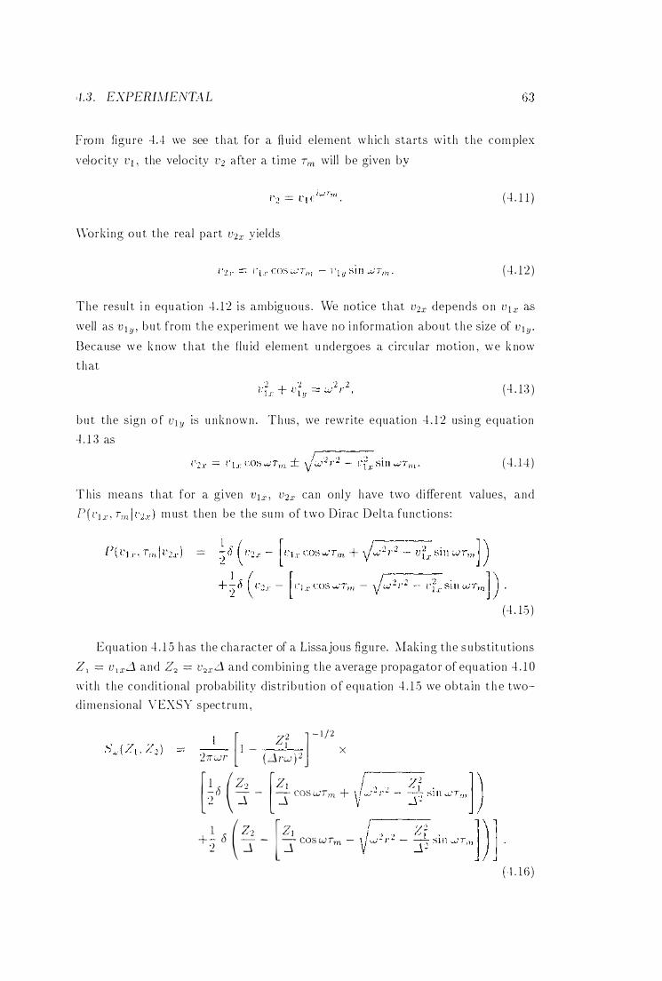
- 1 .3 . EXPERLHENT.'tL
From figu re 4 . .1 we see that for a fl u id element wh ich starts wi th the com plex
veloc ity VI , the velocity V2 a fter a t ime Tm will be given by
(4 . 1 1 )
Work ing ou t the real part U2r y ields
( 4 . 1 2 )
The resu l t i n equ ation "1 . 1 2 is ambiguous . We notice that V2r depends on V I r as well as V l y , but from the experiment we h ave no i n formation about the size of V l y ' Because we k now that the flu id element u ndergoes a circu lar motion , \ve k now
that
(4 . 1 :3 )
but the s ign o f Vl y IS u nknown . Thus , we rewr ite equation 4 . 1 2 usin g equation
"1 . 1 :3 as
( 4 .H )
T his means t hat for a g iven v!x , V2x can only have two different values, and
1' ( /' l x , Tm I m ust then be the su m of two Dirac Delta functions:
(4 . 15 )
Equation 4 . 1 .5 h as the character of a Lissajous figu re. Making the s u bstit u tions Z, = l],x-1 and Z2 = u2X.1 and com bin i ng the average propagator of equ ation 4 . 1 0
with the condit ional p robabi l i ty d istr i bu tion o f equ ation 4 . 1 5 we obtain t h e two� d imensional V EXSY spectru m ,
J - I X [ ZZ ] - 1/2
27TWr (.Jl'w ) 2 [ 1 _ (Z? - (J -- -'2 .J [ZI -:I COS lw'Tm +
, 1 ( 22 [Zl T <5 -.- - - COS WTm 2 .J .J
(UG)
CHAPTER , 1 . VELOCITY EXCIL\NGE SPECTROSCOPY
Th is is t he displacement spectr u m for flow i n a circular annu lus wi th rad ius r . I n the case of the Couette flow between concentric cyl inders , i n w hich the ou te r
cyl inder of radi us 1'0 i s stationary and t h e cent ral cyl inder o f rad ius r i rotates w i t h
the angular veloci ty ",,'0 , t h e fl u id angular velocity varies across the gap. Apply ing
no-sl i p boundary conditions on each s ide , the VEXSY spect rum 8 ( Z1 1 Z2 ) can be
obtai n ed from equ ation cL 16 by i ntegrat ing with respect to the appropr iate angular
velocity d istr ibut ion . A l ternatively, \ve may rewrite equation � . 1 6 in terms of the
local tangential speed u , so t hat [ Z2 ] - 1 /2
1 . 1 -- 1 - -- X 27fV2 (L\v) 2
[ 1 _ (z) [Zl 2b ; - L\ COs(vim jr) +
1 _ ( Z2 [Zl -1- _. b -. - - COS (VT jr) I :2 .:1 .:1 m
The velocity field for a Newtonian fl u id is given by [55]
(4 . 1 8)
S ince the normalised rad ial weigh i ng function is given by f ( r ) == 2rj (r� - rn , t h e
V EXSY spectr u m is
(4 . 1 9)
Such a spect rum contains a complex ridge st ructure rem i niscent of the pat terns
for med by the sharp edged Pale patterns [56] i n 2D separated field spectra of
pmvders pu bl ished by Ernst [ 12] and 2D exchange spectra by S piess et al . [26] . I n
t hese examples , t he patterns arise from the d istr ibution of molecu lar or ientations in powder sam ples, while in the examples shown below . the patterns arises fro m
t h e distr ibution o f these edges as t h e rotation angle varies from zero t o a fi n i te
va l ue across t he Couette f low.
4 . 3 . 2 . 2 Meas urement o f t he VEXSY S p ectra
The pu lse sequence shown in figure e1 . l is a l i t t le naive . I n particu lar i t makes
no allowance for t he d i fficu l ty wh ich arises from i n homogeneous local fie lds. A ny
such va riation can lead to i ncomplete echo refocusing when t h e t1 u id motion causes
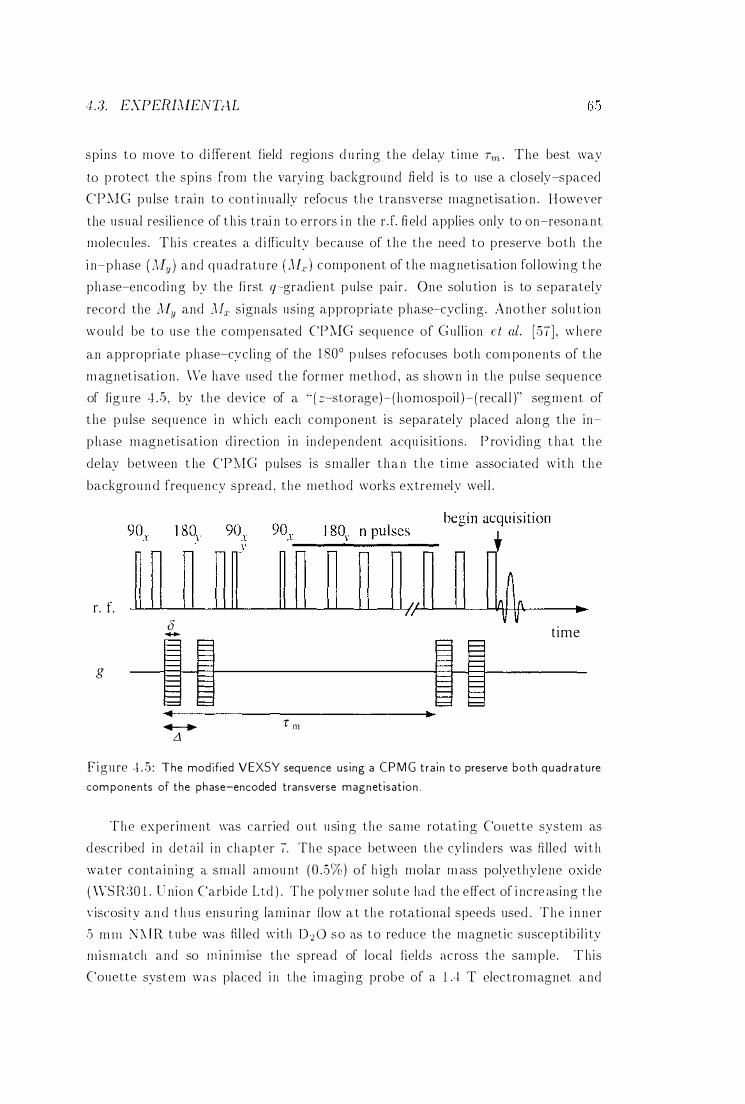
:1 .3. EXPERLUENTAL
sp ins to move to d ifferent field regions d u ri ng the delay t ime Tm . The best way
to p rotect the sp ins from the vary ing background fi eld is to use a c losely-spaced
CP.\lG pu lse t rai n to con t i nual ly refocus t he t ransverse magnet isat io n . However
the usual res i l ience of t h is trai n to errors i n the rJ. fi eld applies only to on-resonant
molecu les . Th i s creates a d i fficu l ty because of the t he need to preserve both the
i n-phase (AI!! ) and quad ratu re ( Jlc ) component of the magnetisation fol lowi ng t he
phase-encod i ng by the fi rst q-grad ient p u lse pair . One sol u tion i s to separately
record the JIy and M�. s ignals us ing appropr iate phase-cycl ing . Another solu t ion
wou ld be to use the compensated CPMG sequence of G ul l ion et al. [51] , where
an appropriate phase-cycl ing of the 1 800 p ulses refocuses both com ponents of t he
m agnet isat ion . \Ve have used the former method , as shown i n the pu lse sequence
of fig u re cl.5 , by the device of a " ( z-storage)- (homospoil ) - ( recal l )" segment of
the p u lse sequence i n w h ich each component is separately placed along the in
phase magnetisat ion d i rect ion i n independent acqu is it ions . P rov id ing t hat t he
delay between t he CP?v[G pulses is smaller t han t he t ime assoc iated w i th t he
backgrou nd frequency spread , the method works extremely wel l .
r. f. (j
-
g H ... ....-.
L1
1 1 r m
...
t ime
Figu re �L5 : The modified VEXSY seq uence us ing a CPMG t ra in to preserve both q u ad ratu re
components of the phase-encoded transverse magnetisation .
The exper iment was carried ou t usi ng the same rotat i ng Couette system as
d escr i bed i n deta i l i n chapter I. The space between the cy l i nders was fi lled Ivi t h
water conta i n i ng (1, smal l amou nt ( 0 .5%) o f h igh molar m ass polyethylene oxide
( WS ltW l . U nion Carbide Lld ) . The poly mer sol u te had the e ffect of i nc re as ing t h e
\' iscosi ty and t h us ensu ri ng lam inar flow a t t he rotational speeds used . The i n ner .) m ill :\'\IR t u be was fi l led with D '2 0 so as to reduce the magnetic suscept ib i l i ty
m ismatch and so m i n im ise the spread of local fields across the sample . T his
Couette system was placed i ll the imaging probe of a l A T electromagnet and
G6 CHAPTER �1 . VELOCITY EXCHANGE SPECTROSCOP'r'
the exper iment was performed usi ng the A::'IX300 spectrometer operat ing at 60
:YIHz . as described in sect ion 2 .5 .2 . Because of the need to work w i th Trn val ues
much larger than the rec iprocaJ l ine\vidt h (around 200- 1 Hz- 1 ) . i t was necessary
to employ the CP:YIG sequence of figure 4 . ·5 .
A sin gle rotation speed o f 1 0 cyc les per second was used a nd Tm was varied
by changing the nu m ber of CP::'IG loops in the period between the two q-pulse
pairs. The correspond ing val ues of '-'J Tm (expressed in cycles) were 0 . 1 5 . 0 . 50 , 1 .00
and 2 .00 . The measurements were carried out lls ing va l ues of 8 = 1 ms, ....l 2 .58
ms and w i th a repetit ion time of 1 s . I n each case 642 q --steps were used and fou r
steps o f p hase cyc l ing were performed , each experiment l asti ng 4 . 5 hou rs . These
results are shown as V EXSY spectra in figu re 4 .G along w i th the corresponding
t heoretical V EXSY maps calcu lated by assuming a constant velocity grad ient .
The agreement is excellent .
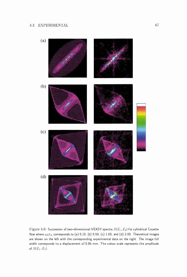
4.3. EXPERiMENTAL 67
(a)
(b)
(c)
(d)
Figure 4.6 : Succession of two-dimensiona l VEXSY spectra S(Zl ' Z2) for cyl indrical (ouette
flow where WOT.n corresponds to (a ) 0 . 15 , (b) 0.50 , (c) l .00 , and (d) 2 .00 . Theoretical images
are shown on the left with the correspond ing experimental data on the right. The image fu l l width corresponds to a displacement o f 0 .85 mm . The colou r scale represents t h e amplitude
of S(Zl , Z2 ) '
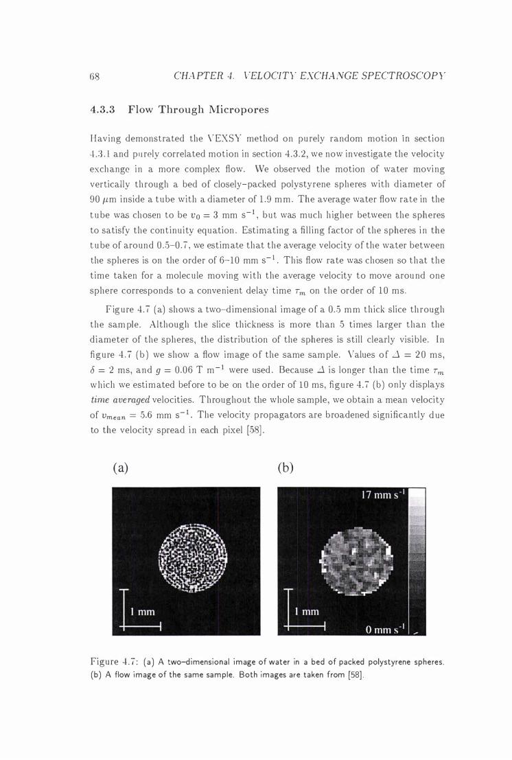
68 CHA PTER 4 . VELOCITY EXCHA iVGE SPECTROSCOPY
4.3.3 Flow Through Micropores
H aving demonstrated the V EXSY method o n pu rely random motion 111 section
4 .3 . 1 and pu rely correlated motion in section 4 .3 .2 , we now investigate the velocity
exch ange i n a more com plex flow. vVe observed the motion of water movi ng
vertically th rough a bed of closely-packed polystyrene spheres with d iameter of
90 /-l m i nside a t u be with a diameter of 1 .9 m m . The average water flow rate in the
t u be was chosen to be Vo = 3 mm S- I , but was much h igher between the spheres
to satisfy the cont inu ity equation . Est imating a fi l l ing factor of the spheres i n the
t u be of around 0 .5-0 . 7 , we estim ate that the average velocity of the water between
the spheres is on the order of 6-1 0 mm S- l . Th is flow rate was chosen so t h at t h e
t ime taken for a molec u le moving w i t h t he average velocity t o move arou nd one
sphere corresponds to a convenient delay t ime Tm on the order of 1 0 ms .
F ig u re 4 .7 ( a) shows a two-d imensional image of a 0 .5 m m t h ick slice th rough
the sam ple . Although the slice th ickness is more than 5 times larger t han the
d i ameter of the spheres the d istribution of the spheres is sti l l clearly visi ble. I n
fi g u re 4 . 7 ( b ) we show a flow image o f the same sam ple. Values o f L1 = 2 0 ms ,
8 = 2 ms, and g = 0.06 T m - I were used . Because L1 i s longer than the t ime Tm w hich we esti m ated before to be on the order of 1 0 ms, fi g u re 4.7 (b ) o n ly d isplays
time averaged velocities. T h roughout the whole sample, we obtain a mean velocity
of Vmean = 5.6 mm S- 1 . The velocity p ropagators are b roadened sign ificantly d ue
to the velocity spread i n each pixel [58J .
(a) (b)
Figu re 4 . 7 : (a ) A two-dimensiona l image of water in a bed of packed polystyrene spheres. (b) A flow image of the same sample. Both images are taken from [58] .
4 .3 . EXPERLVIENTAL 69
Having used the dynamic spin echo method to obtain i n formation about the
average velocity of a fl u id in a porous medi u m . \ve now use the VEXSY method to
o btain i n formation about the change of veloci ties with time. Because we expect
the correlation t ime to be short ( 1 0 IllS or less ) . it is necessary to have the delays
8 and ..J as short as possible . T his requ i res la rge gradients. Therefore, we used
the h igh gradient p robe wh ich is descri bed in section 2 .5 .3 for the experiments i n
t h is section . I n t h e experiment ()c12 q-steps were used \vith a maximum grad ient
am pl itude of ;3 T m - I , a grad ient pu lse d urat ion cS of 1 ms and a delay d of , 1
ms . The choice of these parameters ensu res t hat the d istance the molecu les move
due to B rownian motion d u ri ng the t ime Ll ( J(.1:2) ::::: J2DLl ::::: 4 . 2I1m) is much
smal ler t han the d istance a molecu le moves with the average velocity d ur ing the
same t ime Ll ( z = vavLl ::::::: ;3211. m ) . In other words , the broaden i ng of the VEXSY
spect rum is not d ue to B rownian motion , but to d ispersion i n the velocities.
I n figure 4 .8 we show some experimental VEXSY spectra. Figu re 4.8 ( a)
d isp lays the VEXSY spectrum of the stationary fl u id . As expected , we get a
spectru m with Gaussian p rofiles, s imilar to the one i n figure 4 . :3 . The spectra i n
figu re 4 . 8 ( b ) - ( d ) were recorded w i t h a flow rate of ;3 m m S - I i n the t ube and
d i fferent mixing t imes. There is a clear transition from moderately station ary
flow for short mix ing t imes to correlated randomised flow as the mix ing t ime is
i ncreased . The spectra are confined to the fi rst quad rant because of the dominan t m ot ion o f t h e water molecu les along t h e t u be .
Note also t hat t h e posit ion of t h e peak m axi m u m shifts from t he cent re ( zero
velocity ) i n figu re 4 .8 ( a) by 3 pixels (correspond ing to a velocity value of v = 3
m m s - l ) i n ( b)- (d ) . A lthough most of the molecu les are moving with v = 3 m m S- 1 , there arc some molecules, which are moving wi th velocities of u p t o Vmax = 24
m m s-l . Th is i n formation was not obtainable with the spin vvarp pu lse sequence
d iscussed before, because the large spread of velocities in one pixel broadens the
velocity propagators and thus makes i t impossib le to use large grad ients . In order
to get a good velocity reso lu tion . one has to use a long delay 21. H owever, th is
means t hat one meas ures on ly the t ime averaged velocity.
O ne might \'londer why the VEXSY spectra don ' t shmv a stronger correlation
for a mixing time wh ich corresponds to the time taken for a molecu le moving with
the average veloc ity to move a round one sphere. This t imescale is 20 ms i n o ll r
experiment . I n t h e VEXS'{ experiment . w e do a n i nstantaneous velocity encod ing , \\'a i t a delay t ime Tm , and do anot.her instantaneous velocity encod ing . The spectra in fi gu re -1 . 8 (b )- (d ) slimV' that the molecu les cha.nge their veloci ties very quickly
on a t imescale of t o ms and lose memory about their p revio lls velocities after t hat
t imp . I n a s im ple PCSE experiment wi th the same setup , strong d isp lacement
70 CHAPTER 4 . VELOCITY EXCHANGE SPECTROSCOP'{
correlations have been observed [58] . The PGSE experiment encodes for location
of the molecu les, waits a delay t ime J . a,nd encodes again for location . The PGSE
experiment therefore measures the a vemge velocity of a molecu le d u ri ng the t ime
....l . whi le the VEXSY experiment correlates two velocities of the same molecu le
obta.ined at d i fferen t , short . t ime i ntervals. In this case , the VEXSY method is
less susceptible to t ime averaging .
4 . 4 Conclusions
In th is chapter , we demonstrated a new 2D exchange experiment where the fre
quency d imensions h and 12 are not the usual chemical sh ift or d ipolar coup l ing ,
but the d isplacements Zl and Z2 of molecules over well defi ned t ime i ntervals . By
applyin g the V EXSY pulse sequence to systems with known behaviou r we could
show the rel iabi l i ty of this method. The VEXSY spectrum of a sample of water
undergoing u nr estricted diffusion is a 2D Gaussian . From the width of th is Gaus
sian we could work ou t the self-diffusion coefficient wh ich is i n excellent agreement
with the l i terat u re val ue . The VEXSY spectra of l am inar Newtonian flow in a
Couette cel l are also i ll good agreement with the sim ulations.
Of cou rse , in these cases t here are methods wh ich can provide i n formation
about the velocity fie ld more d i rectly. With the dynamic spin echo method i t
i s possible to obtain velocity and d iffusion m aps . However , m any modern NMR spectrometers on ly have one grad ient available for d iffusion studies . \lYe h ave
shown here that with the V EXSY method it is possible to obtain i n formation
about the velocity fie ld with only one gradient .
From the experiments i n section 4 .3 .3 we could see that the dynamic sp in echo
m easu res the d istrib ution of velocities averaged over the time d. As a contrast ,
the VEXSY method correlates velocities of t he same molecu le over the m ixing
t ime Tm . Both yie ld the same resu l t for stationary fl ow , but can be very d ifferent
for H uctuat ing flows, as \ve have shown above. The VEXSY method is therefore
a powerfu l tool for the i nvestigation of fl uctuat ing velocity fields. However , t h e
l imits are also obvious . Beca.use the VEXSY method uses t\vo phase-encodi ng
gradients , the acqu isition t ime for one exper iment i s usual ly on the order o f 1 or 2 hou rs . I f only one gradient d i rection i s avai labl(� . t h e stim ulated echo cannot be
\lsed due to m ult i ple spin echo i nterferences. and the exchange t imes which can
be lIsed in the experiments are l imited by Tz relaxation rather than Tl relaxation .
I n chapter 8 we wi l l use the VEXSY method t o investigate the t10w field caused
by cOllvection in a capillary.
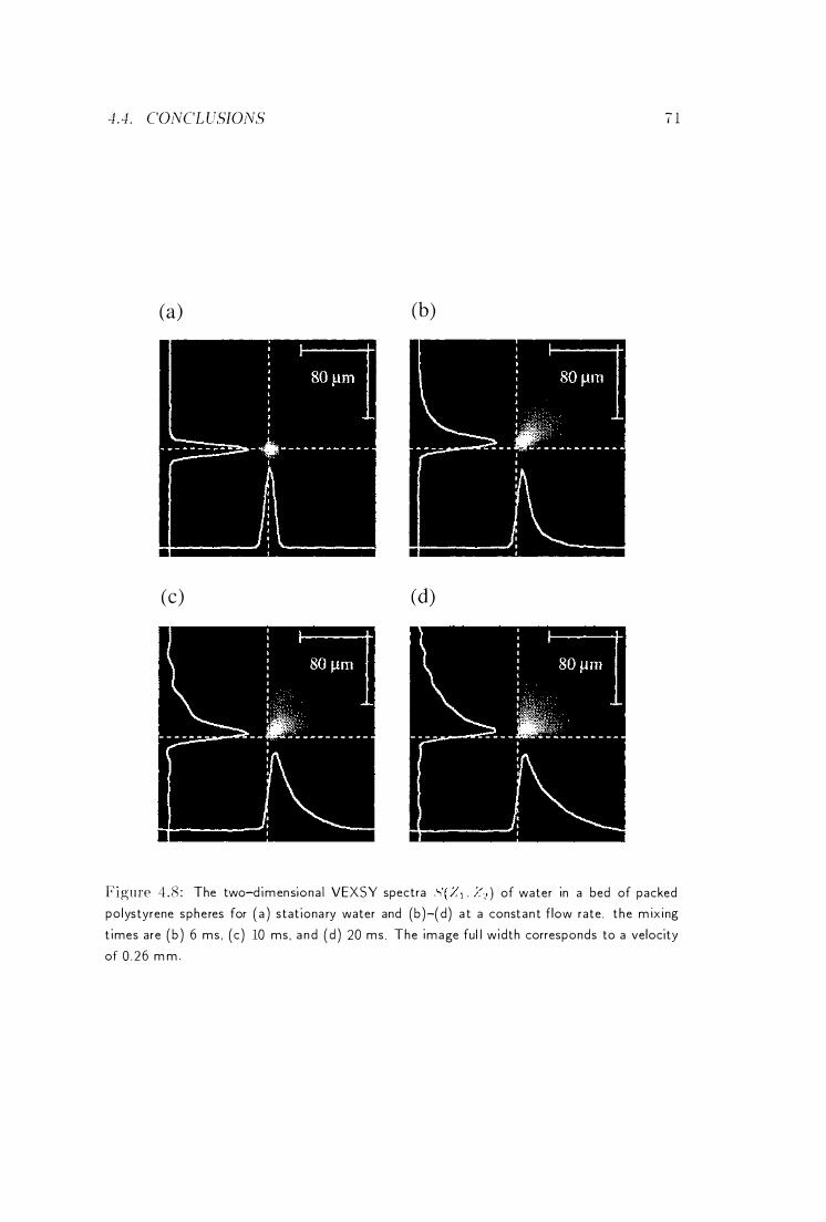
4 .4 . CONCL USIONS 7 1
Ca) Cb)
Cc) Cd)
Figure :l .B : The two-d imensiona l VEXSY spectra ) of water in a bed of packed po lystyrene spheres for ( a ) stat iona ry water and (b )-( d) a t a constant f low rate. the m ix ing
t imes are ( b ) 6 ms, (c) 10 ms, a n d ( d ) 20 ms. The image ful l width corresponds to a velocity
of 0 .26 m m
72 CILtPTER 4 . VELOCIT'l EXCHANGE SPECTROSCOPY
Chapter 5
Polymer Physics
I n t h is chapter t he basic ideas o f polymer physics are int rod uced as far a s they
are needed to understand the experiments i n chapters 6 and 7 .
5 . 1 Introd uction
5 . 1 . 1 Definition of a Polymer
Polymers are large molecules m ade up of m any atoms l inked together by covalent
bonds . They usual ly contain carbon and other atoms such as hydrogen , oxygen ,
and n i t rogen . A s the name suggests , groups of simpler b locks ( monomers ) are
l i nked together in some system atic way. Although t he fi nal molec u le does not
need to be ent i re ly l i near , it is usual ly the case t hat the final l inking process
resu lts in a chain-l ike structu re of the polymer molecu le . Many textbooks are
available which deal with polymer physics , for example [59J-[G6J .
5 . 1 . 2 Molecular vVeights and Polydispersity
I n a real polymer sample, the degree of polymer isation varies from one polymer
molec u le to another . lVi denotes the number of polymer molecules i n the sam ple
with the molecu lar m ass Ali . T he average molecu lar mass for the sam ple can be
defi n ed as n umber average
L NiJIi ; = 1 J [" = '-----'::0'-:--- (5 . 1 )
L :Y, i== 1
or weight average
Y ' \I2 • t � I
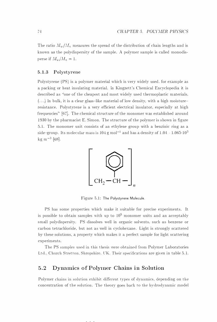
CHAPTER 5 . POLYMER PHYSICS
The ratio .i!w/:i!" m easu res the spread of the d istr ibu tion of chain lengt hs and is
k nown as the polydispersi ty of the sample. A polymer sample is called monodis
p erse if Mw /M" = 1 .
5 . 1 . 3 Polystyrene
Polystyrene ( PS) is a polymer material which is very widely used . for exam ple as
a packing or h eat insu lat ing m aterial . In Kingzett 's Chemical Encyclopedia it is
descri bed as ;'one o f the cheapest and most widely used t he r moplastic m aterials.
( . . . ) In bu lk , i t is a clear glass-like material of low density, with a high moistu re
resistance. Polystyrene is a very efficient electrical insu lator, especial ly at h i g h
frequencies" [67J . The chemical struct u re o f the monomer w as established around
1 930 by the pharmacist E . S imon . The struct u re of t he polym e r i s s hown i n figure
.5 . 1 . The monomer un i t consists of an ethylene grou p \vi th a benz in ic r ing as a
side--group . Its m olecular m ass i s 104 g mol- I and h as a density of 1 .04 1 .06.5 , 1 03
k g m -3 [68] .
CH,., - CH -.... n
Figure .5 . 1 : The Polystyrene Molecu le .
PS has some properties wh ich make i t s uitable for p recise exper iments . It
is possible to obtain sam ples \vi th u p to 1 05 monomer u nits and an acceptably
s m al l polydispersity. PS d issolves wel l in organ ic sol vents. such as benzene or
carbon tetrachloride. but not as \vel l in cyclohexane . Light is strongly scattered
by these sol u tions, a p roperty wh ich makes it a perfect sample for l ight scatter i ng
experi m ents .
The PS s a m ples used i n t h is t hesis \vere obtained fro m Polym er Laboratories
L t d . . C h u rc h S t ret t o n . S h ro ps h i re . Ch:. Thei r speci fications are given i n table 5 . 1 .
5 . 2 Dynalnics o f PolYlner C hains i n Solution
Polymer c h ai n s i n solu t ion exh i bit d i fferent ty pes of d y n a.mics , dependi ng on t h e
concentration of t h e sol ution . T h e theo ry goes back t o t h e hyd rod y n a m i c model
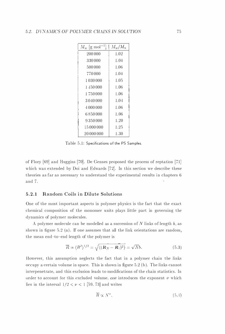
5.2. Dy"v.,DHCS OF POLYMEH CILU:\,S IN SOL UTION
J1w [g mol - I ] J1w/i'vIn 200 000 1 .02
3:30 000 1 . 04
500 000 1 .06
770 000 1 .04
1 030 000 1 .05
1 c1 50 000 l . O6
1 750 000 l .O6
:3 040 000 1 .04
4 000 000 1 .06
6 850 000 1 . 06
9 350 000 1 .20
15 000 000 1.25
20 000 000 1 .30
Table 5 . 1 : Specificat ions of the PS Samples .
75
of Flory [69] and H uggins [70J . De Gennes proposed the process of reptation [7 1]
w hich was extended by Doi and Edwards [72] . In th i s section we descr ibe these
t heories as far as necessary to u nderstand the exper imental resu l ts i n c hapters 6 and 7 .
5 . 2 . 1 Random Coils i n D ilute Solut ions
One of the most i m portant aspects in polymer physics is the fact t hat the exact
chemical composit ion of the monomer u n its p lays l i tt le part in govern ing t he
dynam ics of polymer molecu les .
A polymer molecu le can be model led a.s a succession o f N l i n ks o f length b , as
shown i n figu re 5 .2 (a) . If one assu mes that all the l i n k orientations are random .
t he mean end -to -end length of the polymer is
( 5 . 3 )
However . t h is ass umption neglects the fact that i n a polymer chai n t he l i n ks
occ u py a certa in vol u me i n space. Th is is shown i n figure 5 . 2 ( b ) . The l i n ks can not
i n terpenet rate, and th is excl usion leads to modifications of the chain statistics. In
order to accoun t fo r th is pxc ludpd vol ume. OIle i n t rod uces the exponent 1/ \\O h ich
l ips i n the i n terva l 1 /2 < v < 1 [59 . 7:�1 and wr ites
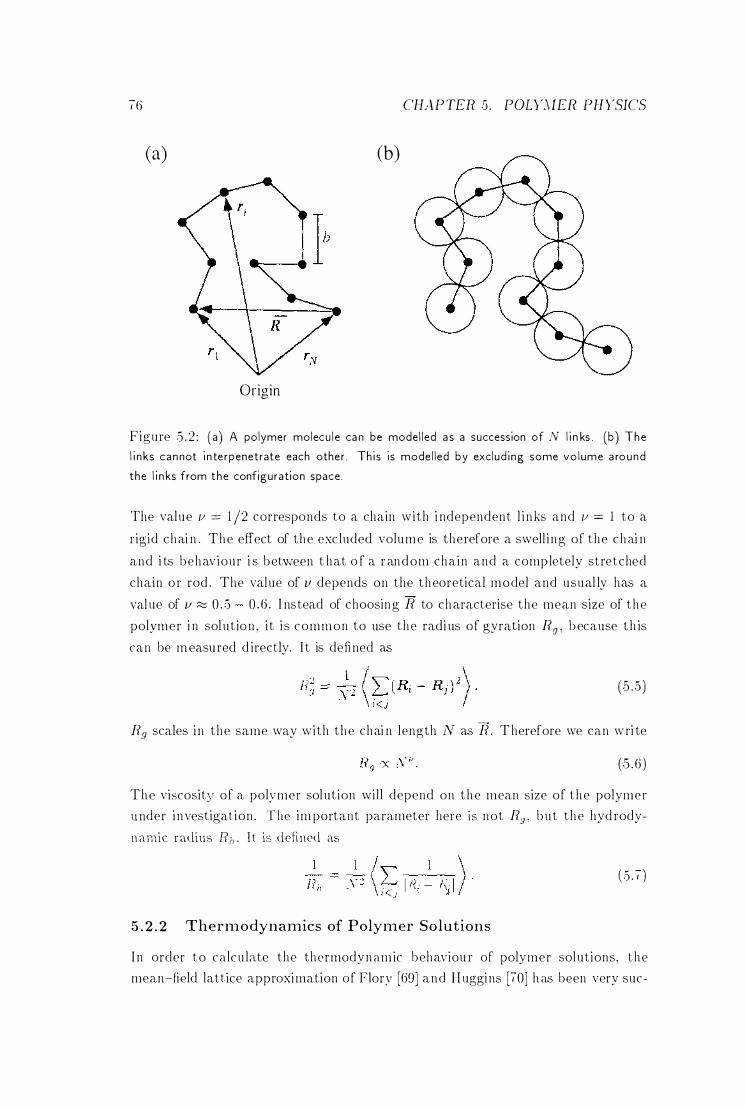
76 CHAPTER 5. POLYMER PHYSICS
(a) (b)
Origin
Figure 5 .2 : (a) A polymer molecu le ca n be model led a s a succession of N l i n ks . (b ) The
l i n ks cannot i n te rpenetrate each othe r . Th is is model led by exclud ing some vo lume a round
the l i n ks from the configuration space.
The value 1/ == 1 /2 corresponds to a chain with i ndependent l i nks and 1/ = 1 to a
rigid chai n . The effect of the exc luded volume is therefore a swell i ng of the chai n
and i ts behaviour i s betvleen t hat o f a r andom chain and a comp letely stretched
chain o r rod . The value of 1/ depends on the theoretical model and usual ly has a
value of 1/ � 0 . 5 0 .6 . I nstead of choosing R to characterise the mean size of the
polymer i n solut ion , i t i s common to use the radi us of gyration Rg , because t h is
can be m easured d irectly. I t is defi ned as
(5 .5)
Rg scales i n the same way with the chai n length 1\/ as R. T herefore we can wri te
(.5 . 6 )
The viscosity of a polymer solution wil l depend on the mean size of the polymer under i nvestigat ion . The im portant parameter here is not R:J 1 but the hyd rody
n a mic radius Rh . I t is defi ned as
;\\ /2:-1 ) , \ 1 <.1 5 . 2 . 2 Thermodynamics of Polymer So lutions
(5 .7 )
I n order to ca lcu late the thermodynam ic behaviou r of polymer solutions, the mean-field lattice approximation of FIory [69] and Huggins [70] h as been very suc-
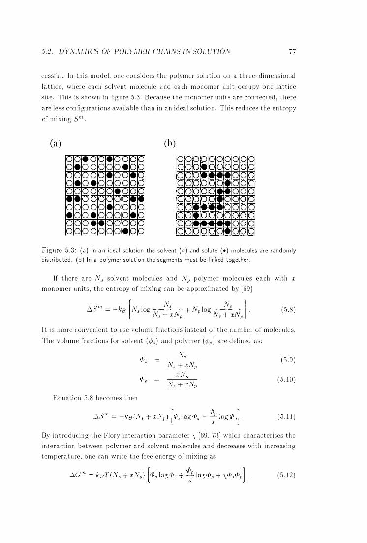
5 .2. D LYAJIICS OF POLY.HER CHAINS IN SOL UTIO;\' 1 1
cessfu l . I n th is model . one considers the polymer sol u tion on a th ree�dimensional
lattice, w here each solvE'nt molecule a.nd ea.ch monomer un i t occ upy one lattice
site . This is shown in fig u re .5 . 3 . Because the monomer u n its are con nec ted , there
are less configurat ions available t han i n an ideal solu t io n . Th is reduces the entropy
of m ixi ng srn .
(a) 0 0 • 0 0 • 0 • 0 0 0 0 0 0 0 0 0 • 0 • 0 • 0 0 0 0 0 0 0 0 • • 0 ) 0 0 0 0 0 • • 0 0 • 0 0 0 0 0 • • 0 0 0 0 0 0 0
0 0 0 • 0 0 0 0 • 0 )IV 0 0 0 0 0 0 0 •
O lr 0 0 • 0 0 0 0 10 • • 0 0 • 0 0 0 0 0
(b) 0 00 0 0 0 0 0 0 0 0 0 0 . 0 0 0 0 0 0 0 0 0 0 0 0 0 0 0 0 0 0 0 0 0 0 0 014� 0 0 0 IV J ) 'V .-JIO,'V J1'-..I 1'-0 0 - - 0 0 0 0 O O t O O O O O O O 0 0 1--1- - 0 0 0 0 0 0 0 0 0 . 0 0 0
Figure 5 . 3 : ( a ) I n a n idea l solution the solvent (0 ) a nd sol u te ( .) molecules a re randomly
d istr i b u ted . ( b ) I n a polymer solut ion the segments must be l i nked together .
If t here are Ns solvent molecules and Np polymer molecules each with x monomer u n its , the entropy of mixing can be approx imated by [69]
[ Ns N 1 6Srn = - kB Ns log N TV + Np log r.y' p TV . s + :1: 1 p i ' s + Xl p ( 5 .8 )
I t i s more convenient to use volume fractions i nstead o f t h e n umber of molecules.
The vol ume fractions for solvent (4;05) and polymer (q)p ) are defined as:
Equation 5 .8 becomes t hen
Ns + �:Np x
( 5 . 9 )
( .5 . 1 0 )
( 5 . 1 1 )
By i n t roduc ing t he Flory interaction parameter \: [69 . 7:)] which characterises the
i n te raction bet\veen polymer and solvent molecu les and decreases with i nc reasing
tem peratu re . one can write the free energy of mixing as
( 5 . 1 2 )
78 CHAPTER 5. POLYi\I[ER PHYSICS
5 . 2 . 3 Osmotic P ressure a n d t h e Flory Tem p erature
From equation 5 . 1 2 i t is possible to obtain the osmotic pressu re JI of the polymer
solut ion [7:3J . . kG T [ ([>D 1 2 ] n :::: --::::-- -' + ( ;- - \)t:P + . . . .
L's .1: 2 p ( 5 . 1 3 )
T h is i s a v i r ial expansion o f van ' t Hoff's law [74] . The term ( � - .\ ) i s k nown
as the second v i rial coeffic ient . I f t h is term is zero , the polymer solu tion behaves
l i ke an ideal solu t io n . Because of the tem perature dependence of x, t h is occurs
at a part icu lar tem perature which is called the F!ory, or theta, temperatu re e . A
solvent is called a t heta solvent i f X :::: � . At the theta temperat u re , the polymer
coi l takes on i ts " natu ral size" , and excluded volume effects are cancelled out .
Above the t heta temperatu re , X < � and polymer-solvent contacts are favou red .
The coi l expands i n t h is region . Below the theta tem perature , X > � and t he
co i l col lapses i n to a globule. Th is coil-to-globule t ransit ion has been a topic of
extensive research in recent years [75]-[82] .
T heta temperatures can vary widely. depend i ng on the part icu lar polymer and
solvent . For example. for polystyrene i n cyclohexane , i t is :35° C [83] , \vh ile for
polystyrene i n benzene i t is 50° C [68] and 22° C for polystyrene i n d ioctyl
ph thalate (DOP) [8-t] .
The interact ion paxameter X d oes not depend on t he tem perature alone , bu t
also on other parameters such as <Pp and x . Strict ly speaking , the t heta tem
perat u re is defined for an i nfin i tely long chain in a solut ion with i nfini tesim al
concentration .
5 . 2 . 4 P hase Equilibria
For the formation of a s ingle phase solution 6Cm of equation .5 . 1 2 m ust always
be negat ive . However , t h is is not the only condit ion , as is i l l ustrated in figure 5 . 4 .
The cu rve i n figure 5 A (a ) is always concave upwards , and t h is means that any
poin t Q on the cu rve has a lower free energy than a two phase syste m of the same overa l l composi tion . Howewr. i f the free energy cu rve has a shape such as t hat
shown in figure ;) .-1 ( b ) . the free energy is smaller if a two-phase system is formed .
i f the polymer concentration i s between ifJp1 and t:Pp2 ' T h e poin ts PI and P2 can
be connected by a. l ine wh ic h is a tangent at both points. Th is l ine represents the free energy of a phase ::;eparatpc! m ixture . and each posit ion on the l i ne represents
d i fferent propor t ions of t he two phase separated m ixtures. Any hypothetical s ingle
phase mixtu re between these com positions h as a larger free energy t han the phase
separated mixture . so that the system is imm iscible over th is composit ion range. The composit ion range where phase separation occu rs is defined by the poin ts of
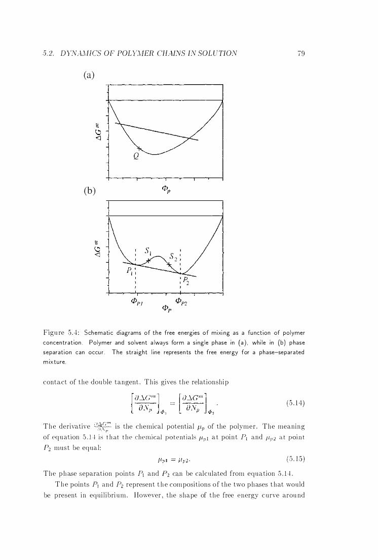
.5 . 2. DYNAMICS OF POLL\[ER CHATvS IN SOL UTION
Ca)
Cb)
7D
Figu re 5 .4 : Schemati c diagrams of the free energies of mixi ng as a fu nction of polymer
concentrat ion . Polymer and solvent a lways form a s i ngle phase in (a ) , whi le in (b) p hase
separat ion can occu r . The stra ight l ine represen ts the free energy for a phase-separated
m ixture.
contact of the dou ble tangent . Th is gives the relationsh i p
( 5 . 1 4)
The derivative is the chemical potential �tp of the polymer . The meaning of ("q u ation ,') . 1 ·1 i s t h at t h e c h e m i cal potentials jlp ! at poin t P! a nd /'p2 at poi n t
P::. must be equal : (5 . 1 5)
Tht' p h ase separation points Pt and P2 C<1.n be calcu lated from equa.tion S . U . T h e points F\ and Pz represent t h e com positions o f the two phases t hat wou ld
be present i n equ i l i bri u m . HO\w�ver , the shape of t he free t'nergy cu rve arou nd
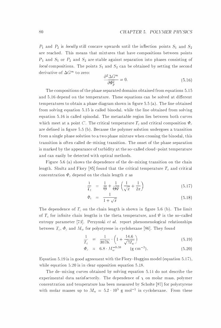
80 CHAPTER 5 . POLY.\IER PHYSICS
P1 and P2 is locally st i l l concave u pwards u nt i l the inflection points 51 and 52 are reached . Th is means that mixt ures that have compositions between points
Pl and 51 or P2 and S2 are stable against separation i nto phases consist ing of
local com posi t ions . The points SI and S2 can be obtained by sett ing the secon d
der ivative o f �cm t o zero: ;p ::'Cm
Dp2 == o . p
( .5 . 16 )
The composit ions of t he pha.<;;e separated domains obtained from equ ations .5 . 1 5
and 5 . 1 6 depend o n the tem peratu re . These equations can be solved at d ifferent
temperatu res to obtain a phase diagram shown in figure 5 .5 (a) . The l ine obtained
from solv ing equation 5 . 1 5 is called binodaL \vhi le the l ine obtained from solv ing
equ ation 5 . 1 6 is called spinodal . The metastable region l ies between both c urves
w hich meet at a point C. The cr itical temperature Te and cr i tical composit ion Pc are defined i n figu re .5 . 5 (b ) . Because the polymer sol ution undergoes a transit ion
from a single phase sol u tion to a two phase mixture when c rossing the b inoclal , t h is
t ransition is often cal led de-mixing t ransit ion . The onset of the phase separation
is marked by the a ppearance of tu rbidity at the so-called cloud-point temperature
and can easi ly be detected wi th optical methods.
F igure 5.6 (a) shows the dependence of the de-mixing t ransition on the chain
lengt h . S hu l t z and F lory [8.5] found that the cr it ical temperature Te and c r it ical
concentration Pe depend on the chain length x as
1 1 ( 1 1 ) e + e!f! jX
+ 2x
( 5 . 1 7 )
1 1 +
(5 . 18 )
The dependence o f Te on the chai n length is shmvn i n figure 5 .6 (b ) . The l im i t
of Te for i nfinite cha in lengt hs i s t he theta temperatu re, and !Ji i s t he so-called
entropy pa rameter [i:�] . Perzynski et al. report phenomenological relationsh ips
between T� , (Pc and JIw for polystyrene i n cyclohexane [86] . They found
1 Tc Pc
-- . 1 + --1 ( 14 .6 ) 30ih: jMw 6 8 . U-O .38
• .. tU (g cm-3 ) .
( .5 . 1 9 )
(.5 .20)
Equation 5 . 1 9 is i n good agreement with the Flory-H uggins model (eq uation 5 . 1 i) ,
whi le equ ation 5 .20 is i n clear opposi tion equation .5 . 1S . The de-mixing curves obtained by solv ing equation 5 . 1 "1 do not describ e the
experimenta l da ta satisfactorily. The dppendence of \ on mola.r mass , polymer
concentration and tem peratu re has been measu red by Scholte [8i) for polystyrene with molar masses up to iUW = 5.2 . 105 g mol - 1 i n cyclohexane . From t hese
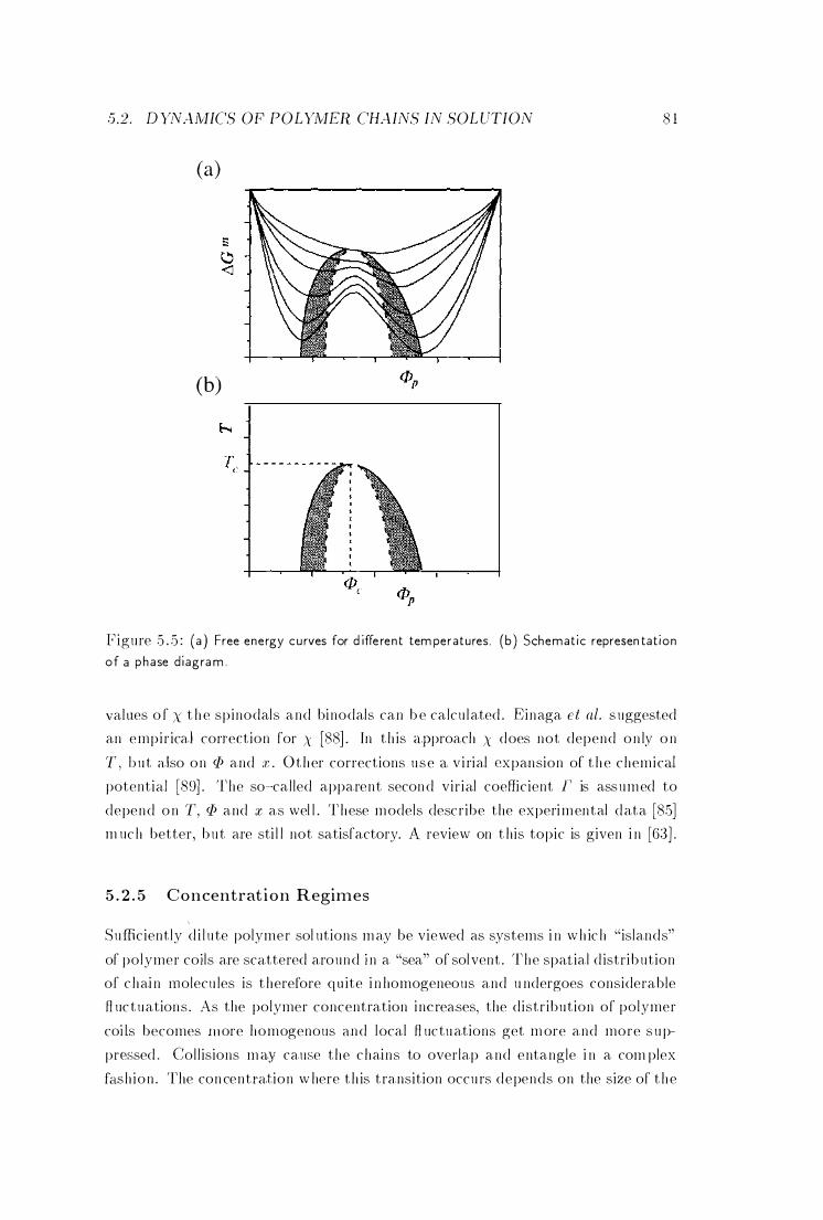
5.2. D YNAMICS OF POLYMER CHAINS IN SOL UTION
(a)
(b)
8 1
Figure 5 . 5 : (a ) Free energy curves for d iffe rent tem peratures . (b ) Schemat ic represen tat ion
of a phase d iagra m .
val ues o f X t h e spinodals and binodals can b e calcu lated . Einaga et al. s uggested
an e mpirical correction for X [88] . In t h is approach X d oes not depend o n ly o n
T , b u t also on c{! and :r . O t h er corrections u s e a. virial t:�xpansion of t h e chemical
potentia.1 [89] . The so� called apparent secon d viria.l coefficient r is ass u m ed to
depend o n T, c{! and x as wel l . These m odels describe the experi m ental d ata [85} m uc h better, b u t are sti l l not satisfactory. A review on t his topic is given i n [63} .
5 . 2 . 5 Concentrat i o n Regimes
Sufficiently d i l u te polymer sol utions m ay be viewed as systems i n w h ic h "islands"
of polymer coils are sca.ttered around i n a "sea" of sol vent . The spatial d istrib ution
of c h ai n molecu les is t herefore q u ite i n homogeneous and u ndergoes considerable
fl uctuations . As the polymer concentration increases, the distribution of polymer
coi ls becomes m ore homogenous a,nd local fl uctu ations get m ore and more s u p�
pr�;ssed . Collisions m ay cause the chains to overlap and entangle i n a com plex
fash ion . The con centration w here t h is transition occu rs d e pends on the size of t h e
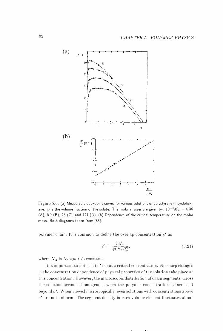
82
Ca)
Cb)
11 C l
1 0
. 1 .2
CHAPTER 5. POL'r?vIER PH}rSICS
Figure 5.6 : (a ) Measu red c loud-point cu rves for var ious sol ut ions of polystyrene i n cyclohex
a ne . 'P i s t he vol ume fract ion of the solute. The molar masses are given by: 1 0-4 Mw :::: 4 .36 (A) , 8 .9 (B ) , 25 (C), a n d 127 ( D) . (b) Dependence of the cr iti ca l temperatu re on the mo l a r
mass . Both d i agrams ta ken from [85] .
polymer chai n . I t is com mon to define the overlap concentration c* as
(5 . 2 1 )
w here NA i s Avogadro's constant .
I t i s important to note t hat c * i s not a. cr i tical concentrat ion . No sharp changes
in the concentration dependence of physical properties of the solu tion take place at
t h is concentration . However, the macroscopic d istr ibut ion of c hai n segments a.cross
the solu tion becomes homogenous when the polymer concentration is i nc reased
beyond c* . \Vhen vie\ved mic roscopical ly, even sol u tions w i th concentrations above
c* are not u ni form . The segment density in each vol ume element fl uctuates abou t
5 .2. D Y.\'.·L\lICS OF POLY.\IER CHAINS IN SOL UTION 83
a mean val ue c. Because of the chain con nectivity, these fl uc tuations can not take
place independen tly. They have been observed by l ight scatteri n g [90. 9 1] and can
be enhanced by external shear and lead to shear-induced phase transitions. vVe
wi l l come back to th is effect later i n section .5 .4 .
From eq uation 5 .2 1 i t follows that if Alw is suffi cient ly h ig h , there is a rather
wide range where the concentration is h igher than c* , but i ts absol u te val u e is st i l l
low. S uch solu tions are d i lu te i n the sense that the concentration of polymer is
smal l , but concentrated enough for coils to overlap. They are called sem i-d i l u te .
As the concentration increases, the polymer solution enters a reg ime where the
chains overlap extensively. Density fl uctuations are m ain ly screened . The concen
t ration where the t ransition from semi-d i l u te to concentrated solu tions occu rs is
termed e X" and i s i ndependent of Alw '
Equation .5 . 2 1 allows us to estimate the dependence of c" on A[w ' Because of
relationsh ip ·5 . 6 Ry scales as A[:'u . Therefore
" \[ 1 -31/ C CX l ' w . ( .5 . 22 )
Adam and Delsant i [92] measu red Ry of PS i n a t heta solvent at d i f1'erent m olar
m asses and obtained the phenomenological relationshi p
" - � 1 �1- 1 /2 c - b . lv w
w hich is i n agreement with relationship .5 . 22 for v
.5 .23 is shown i n fig u re .5 .7 .
5 . 2 . 6 The Reptation Model
( .5 .23 )
1/2 . A graph of equ at ion
I f the polymer concent ration is h igh enough for entanglements to take place, the
mot ion of each polymer chai n is restricted by neighbour ing chains. This effect
d ue to chain u llcrossabil ity is cal led topological constraint and shown in figu re
.5 .8 (a ) . B rochard and de Gen nes [9:3] s uggested replac ing the chain by a wire
t rapped i n a cu rv i l inear t ube fixed i n space ( figure .5 .8 ( b ) ) . I t can only move along its own path . Figure ;') .8 (c) shows the prim i tive path which is given by the
shortest pat.h between the ends of the polymer and has the same topology relative
to the obstac les a s the chai n . A p rim i tive chain can then be used to descri be the sim pl i fi ed motion of the polymer moving along the pr im i t ive path by neglect ing sma l l scale fl uctuations across the path . Do i and Echva rds [72] extended th is idea
by a pproximating the cha in of d iscrete molecu le's by a cont inuolls cha in . The�r
ca lcu lated di fferent t ime scale regimes of polymer reptation [G l . 72] . I f the t ime
over \vh ich d i ffusion i s measu red i s longer than the longest relaxation t ime Td of the Doi-Edwards model , the d iffusion is a long range centre-of-mass d i ffusion
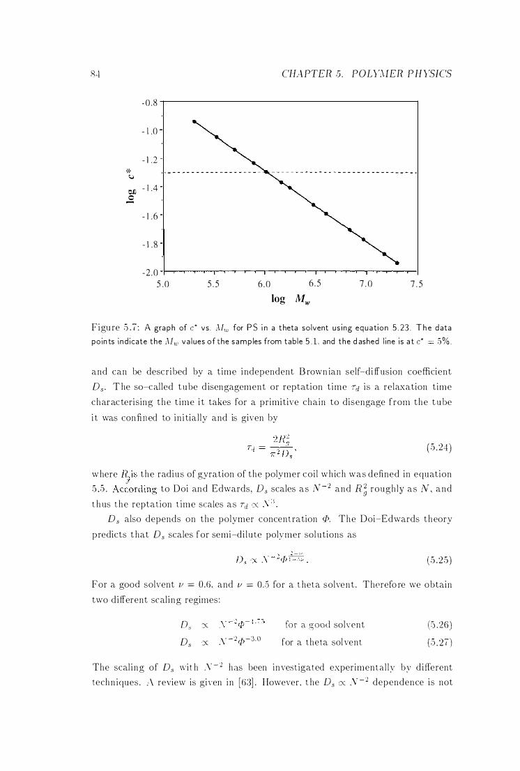
;.:q
-0 . 8
- 1 .0
- 1 .2 *
(..)
eJl - l A .$
- 1 . 6
- 1 .8
-2 .0 5 .0 5 . 5
CHAPTER. 5. POLYMER. PHYSICS
6 .0 6 . 5
log Mw 7 . 0 7 . 5
Figu re .5 .7 : A gra ph of c ' vs . M," for P S i n a t heta solvent us i ng equa tion 5 . 23 . T h e d ata
poin ts i nd icate the Mw va lues of the samp les from table 5 . 1 , and the d ashed l ine is a t c* .5% .
and can be descr ibed by a t ime i ndependent B rown ian self-di ffusion coefficient
Ds. T he so-called tube d isengagement or reptation t ime Td i s a relaxation t ime
characteris ing the t ime i t takes for a pr imitive chain to disengage from the t ube
i t was conflIled to i n i tial ly and is given by
( 5 . 24)
w here � i s the radius of gyration of the polymer coi l wh ich was defined in equation
5 .5 . Ac�ording to Doi and Edwards, Ds scales as N-2 and R; roughly as iV , and
t hus the reptation t ime scales as Tei ':x Ds also depends on the polymer concentration <1>. The Doi-Edwards theory
predicts t hat Ds scales for semi-d i lu te polymer solutions as
(5 .25)
For a gooe! solvent lJ = O.G, and v = 0.:3 for a t heta solvent . Therefo re we obtain
two d i fferent scal ing regimes:
D .\" - 2 (1'.- 1 . 75 s x e
Ds :X ;\" -2 ([>-3.0 for (L good solH'nt
for a theta sol vent
(� ')(' ) 0) . - )
( .5 . 27)
The scal i ng of Ds \\"i t h ;\" - 2 hils been investigated exper imenta l ly by d i fferent
techn iques. :\ review is gi \Oen in [G3] . However . t he Ds lX S -2 dependence is not
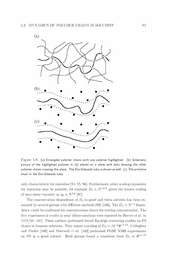
5 .2. D )'t\:\MICS OF POLL\IE'R CHAISS I:V SOL UTIOIV
Ca)
(b) • - - - - - - - ...
•
Cc) • - - - - - - - .... ....
- - - - - - -. "
•
•
•
•
•
•
•
- ,
• i- - - - _ _ _ - " .
I •
85
F igure 5 .8 : ( a ) E n ta ngled polymer cha i ns w i t h one polymer h igh l ighted . ( b ) Schemat ic
p icture of the h igh l ighted polymer in (a) p l aced on a p l ane with dots s howing the other
polymer c h a i ns cross ing th is p l ane . The Doi-Edwards tube is shown as wel l . (c) The pr im itive
cha i n in the Doi-Edwards tube .
only chara.cteristic for reptation [9el, 95 . 96] . Furthermore, other scali ng exponents
for reptation m ay be possible, for exam ple Ds 0( N-2A, given the k nown scal i ng
of zero shear viscosity as ')0 0( 1V3. 1 [97] .
The concentration dependence of Ds i n good and t heta solvents h as been ex
am i ned by severa l groups with d i fferent methods [98]-[ 1 06J . The Ds ':x: N- 2 depen
dence could be confi rmed for concentrations above the overlap concentratio n . The
fi rst experimenta l resu l ts in semi -d i l u te sol u tions were reported by Hervet et al. i n
l () i�) [DS . 1 0i l These authors perfo rmed forced Rayleigh scattering st.ud ies on PS
ch ains i n benzene sol ut.ions. They report a scal ing of Ds 0( A/-2p-L75 . Callaghan
a nd Finder [ l OO] and :"leenval l et al . [ 1 02J performed PGSE NMR experiments
on PS in a good solvent . Both grou ps found a transition from Ds 0( p- 1 .75
86 CHAPTER ·5 . POLY1\[ER PHYSICS
to Ds 'X <[>-3.0 with increasing concentration . However . th is transition is verv
smooth over a wide concentration range. Wesson et al. [ 1 0 1] and K im et al. [ 1 04J
m easu red t h e polymer and tracer d iffusion in good solvents via forced Rayleigh
scatter ing . T hey also fou nd a smooth transition from Ds ex <[>- 1 .75 to Ds ex p-3.0 behaviour . A mis e t al. [99] and Wheeler e t al. [ 1 05] measured the self-diffusion
coefficients of PS in theta sol u tions via l ight scattering. These authors also re
port a smooth transition between the two scal ing regimes. Nemoto et al. ( 1 03)
re-analysed the Ds data reported in [ l O lJ using a concentration and temperat u re
dependent local v iscosity correction . With th is correction term the data reported
in [ 1 0 1] fit better into the scal ing predictions of the Doi-Edwards modeL Fleischer
e t al. [ 106] performed PG SE NMR exper iments on PS i n deuterated benzene and
i n deu terated chloroform in sem i-d il u te concentration . The scalin g l aw Ds ex 1\11;;2
could be confirmed , but no l inear region with a concentration exponent of - 1 . 7.5
could be found . The concentration exponent of the m aster curve decreased fro m
about - 1 .8 t o - :3 .0 a t t h e e n d o f t h e sem i-d i l u te region . and then exhi bited a
fu rther d ramatic decrease.
Because t here seems to be no sharp transitions between scal i ng in good and
t h eta solvents , the question arises w hether t here is a u n iversal scali ng law for
Ds (p) . Ph i l lies suggests i n a series of papers [ 108)- [ 1 1 1) t hat reptation i s not an
i mporta.nt process in polymer sol utions. I n stea.d he suggests a u niversal scali ng
l aw for the concentration dependence of Ds :
(5 . 28 )
w here Do , Q and ;\ a.re adjustable parameters. \Vith t his empir ical equ at ion , he can obtain a good fi t to the experimental data mentioned above. A m ajor cr iticism of t h is description is t hat the apparent success of equ ation 5 . 28 reflects more the flexibi l i ty of the stretched exponential form than the un i versali ty of
d i ffusion mechanisms i n semi-d i l u t e polymer sol u tions [ 1 0.'5] .
Tb o ll r knowledge, there have so far been no studies of the temperatu re de
pendence of Ds near the de-mixing t ransitions of polymer solu tions . I n chapter
6 we report on PGSE :'-i:\;IR measu rements of the tem perature dependence of Ds for polymer solu t ions at different chain lengths and d i fferent concent rations. \Ve wi l l show then t hat t here exists a single temperatu re scal ing dependence.
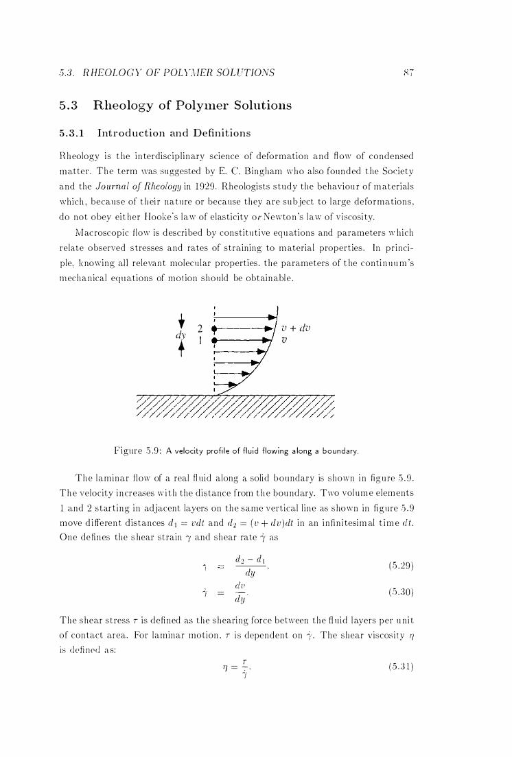
5.3 . RHEOLOG Y OF POLY.HER SOU)TIONS
5 . 3 Rheology of PolYlner Solutions
5 . 3 . 1 Int r o d uction an d Definitions
Rheology is t he i n terdisc ip l inary science of deformation and flow of condensed
matter . The term \vas suggested by E. C. Bingham who also founded t he Society
and the JO llrnal of Rheology in 1 929 . Rheologists study the behaviou r of m aterials
which , because of t hei r nature or because they are su bject to large deformations .
do not obey eit her Hooke's law of elasticity or Newton 's law of v iscosi ty.
Mac roscopic f low is descri bed by constitu tive equ ations and parameters w hich
relate observed stresses and rates of straining to m aterial properties . In pr inci
ple. k nowing all relevant molecu lar properties . t he parameters of t he conti n uu m 's
mechan ical eq llations of mot ion shou ld be obtainable .
, dv +
2 ... ---11 .. , 1
v + dv V
Figure 5 .9 : A velocity profi l e of fl u id flowing a long a boundary
The laminar flow of a real fl u id along Cl solid boundary is shown i n fig u re 5 . 9 .
The velocity i n creases w i t h the d istance from t h e bou ndary. Two vol ume elements
1 and :2 star t ing i n adjacent layers on the same vertical l ine as shown in figure 5 . 9
move d i fferen t d istances cl l :::::: vdl and d2 :::::: ( v + dv )dt in an i nfin i tesim al t ime elt. One defines the s hear strain Ai and shear rate '1' as
d2 - d l I dy ( 5 .:29 )
clu AI -dy ( .') .:30)
The shear stress T is defi ned as the shearing force between the fl u id l ayers per u n i t
of contact area. For laminar motion . T i s dependent on "':( . The shear viscosi ty Tl is den !led as:
T I) = -;- . !
( .5 . :3 1 )
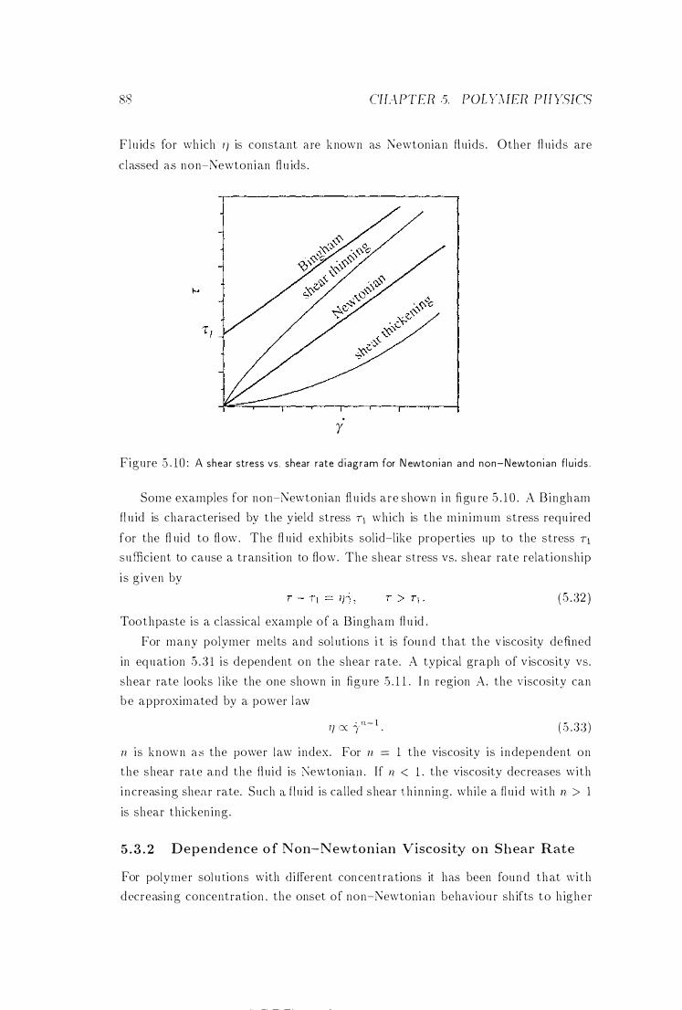
88 CHAPTER ·5. POL '(:\fER PHYSICS
Flu ids for wh ich 1) is constant a re k nown as Newtonian fl u ids . Other fl u ids are
c lassed as non-Newtonian fl u ids .
.
r
Figure .5 . 10 : A shear stress vs. shear rate d i agram for N ewton i an and non-Newton i an fl u ids .
Some examples for non-Newtonian fl u ids are shovvn i n figu re 5 . 1 0 . A Bingham
fl u id is characterised by the yield stress '1 which is the m in imum stress requ ired
for the fl uid to fl ow . The fl u id exhibits solid-like properties up to the stress '1 su fficient to cause a transit ion to flow. The shear stress vs. shear rate relat ionship
i s given by
( 5 . 32 )
Toothpaste is a c lassical example of a Bingham flu id .
For many polymer melts and sol utions i t is fou nd t hat the v iscosity defined
in equation 5 . 3 1 is dependent on the shear rate. A typical graph of v iscosity vs.
shear rate looks l ike the one shown in figu re 5 . 1 1 . I n region A, the viscosity can
be approximated by a power l aw
17 ex 1,,- 1 . ( 5 . :33)
n is known as the power l aw index. For n = 1 the viscosity is i ndependent on
the shear rate and the fl u id is �ewtoniall . I f n < 1 . the viscosity decreases with
i n creas ing shear rate. Such cL f lu id is called shear th i nn ing . whi le a fl u id with n > 1
is shear th icken ing .
5 . 3 . 2 D e p e ndence o f Non-Newtonian Viscosity on Shear Rate
For polymer sol u tions with d i fferent concen t rations it has been found that \vi th decreasing concentration , the onset of non-Newtonian behaviou r sh ifts to h igher
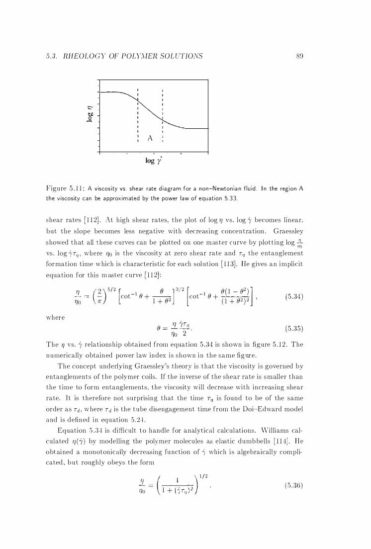
5 .3. nHEOLOG Y OF POLYMEn SOL UTIONS
A
log y.
89
Figure 5 . 1 1 : A viscos ity vs . shear rate d ia gram for a non-Newtonia n f luid . I n the reg',on A the v iscosity can be a pproximated by the power law of equat ion 5 . 33 .
shear rates [ 1 1 2] . At h igh shear rates, the plot of log 1,1 vs. log "':! becomes l inear .
but the s lope becomes less negative with dec reas ing concentration . G raessley
showed t hat all t.h ese curves can be plotted on one m aster curve by plott ing log 7): vs . log )'T71 , where 770 is the viscosity at zero shear rate and T,/ the entanglement
for mation time w hich is characteristic for each solution ( 1 1 3) . He gives an i m pl ic it
equation for this m aster cu rve [ 1 1 2] :
where
77
170
( 2 ) 5/2 [ - 1 () ] 3/2 [ -1 (} ( 1 _ (}2 ) ] ;;: cot e +
1 + e2 cot (} + ( 1 + (}2 ) 2 ' (} =
!l "':(TI) . 1,10 2
(5 .34)
(5 .35)
The 17 vs. l' relationsh ip obtained from equation 5 .34 is shown in figure 5 . 1 2 . The
n umerical ly obtained power law index i s shown i n t he same figure .
The concept underlying G raessley's theory is t hat the viscosity i s governed by entanglements of the polY'mer coils. I f the inverse of the shear rate is smal ler than
the t ime to form entanglements, the viscosity wi l l decrease w i th increas ing shear
rate. I t is therefore not su rprising that the time T7) is found to bt� of the same
order as Tei , w here Td is the t ube d isengagement time from the Doi-Edward model
a nd is defined i n equation 5 .n.
Equation 5 .:}"! is d ifficult to handle for analytica l calcu l ations. 'vVil l iams cal
cu lated 17b) by model l ing the poly'mer molecu les as elastic d umb bel ls [ 1 1 4] . He
obtai ned a monotonica l ly decreasing fu nction of 1 which i s algebraical ly com plicated , bu t rough ly obeys the form
I) 170 ( 1 + (�T� ) 2 ) 1 /2 ( 5 . :}6 )
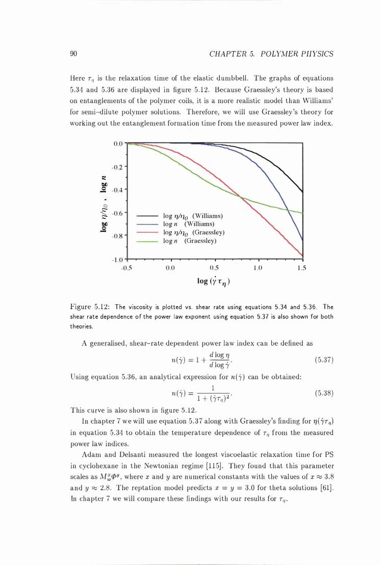
90 CHAPTER 5. POLYMER PHYSICS
Here T'I is the relaxation time of the elastic dumbbell . The graphs of equations
5 .34 and 5.36 are displayed in figure 5 . 12 . Because Graessley's theory is based
on entanglements of the polymer coils, it is a more realistic model than Williams'
for semi-dilute polymer solutions. Therefore, we will use Graessley 's theory for
working out the entanglement formation time from the measured power law index.
0.0
-0.2
� � Q -0.4 -
C) � � -0.6
� Q --0.8
- 1 .0 -0.5
log 111110 (Williams) log n (Willi am s) log 111110 (Graessley) log n
0.0
(Graessley)
0.5
log (r 1:11 )
1 .0 1 .5
Figure 5 .12 : The viscosity is plotted vs. shear rate using equat ions 5 . 34 and 5 .36 . The shear rate dependence of the power law exponent using equation 5.37 is a lso shown for both theories.
A generalised , shear-rate dependent power law index can be defined as
. d log 7] n(t) = 1 + -
d l . ' (5 .37)
og t
Using equation 5.36, an analytical expression for n (-y) can be obtained:
. 1 n (t) = 1 + (-YT'I ) 2 . (5 .38)
This curve is also shown in figure 5 . 12 .
In chapter 7 we will use equation 5 .37 along with Graessley's finding for 7]( -YT'I)
in equation 5 .34 to obtain the temperature dependence of T'I from the measured
power law indices.
Adam and Delsanti measured the longest viscoelastic relaxation time for PS
in cyclohexane in the Newtonian regime [1 15] . They found that this parameter
scales as M�pY , where x and y are numerical constants with the values of x :::::; 3.8 and y :::::; 2 .8 . The reptation model predicts x = y = 3 .0 for theta solutions [61] . In chapter 7 we will compare these findings with our results for T'I '
5 .3. RHEOLOG Y OF POLl?vIER SOL UTIONS
5 . 3 . 3 The Glas s Transition
9 1
When a polymeric m aterial i s cooled from the l iq u id o r r u bbery state, i t becomes
m uch st iffer as i t goes th rough a certai n tern peratu re range . This s t i ffen ing is
the resu l t of one of two possible events: crystal l isat ion or glass t rans i tion . For
crystall isat ion to occur , the polymer molecules must be sufficiently regular along
their length to allow formation of crystal l isation lattices, and the coo l ing rate m ust
be s low enough . When a polymer fai ls to crystall ise, the amorphous , l iqu id l i ke
struct u re of the polymer is retained , bu t the molecular motion frozen , and the
m aterial t u rns i nto a glass. Such a glass transit ion occu rs over a fin i te tem peratu re
interval , bu t is st i l l real ised abruptly enough to mer i t the term transit ion . I t can
be recognised by the change in many properties of the m aterial , such as an i ncrease
i n v iscosity or a change of the specific heat and thermal expansion .
The val ues o f the glass transition tem peratu re Tg reported for a certain poly
mer often d i ffer by as m uch as 1 0 20° C, because the glass transit ion occu rs over
a temperat u re range rather than at a s ingle , sharply defined temperatu re , and be
cause the observed Tg varies somewhat depend ing on the method of meas u rement
used and the thermal h istory of the sample . For polystyrene, 1� h as a l i teratu re
value of :373 K [68J . I f the polymer is i n solut ion , Tg can be much lower. Th is
decrease can be attr ibu ted to the in t rod uction of add it ional free vol u me with the
solvent [ 1 1 6J . For example, for polystyrene i n cyclohexane a Tg of around 280 K
h as been reported [ 1 1 7] .
Near the g lass t ransition , the self-diffusion coefficient Ds (T) can be descr ibed by a law named after Wil l iams, Landel and Ferry (WLF) [ 1 1 8, 1 1 9 , 1 20J :
Ds (T) = Doe ( .5 .39 )
The ratio (tT (T) of mechan ical and electrical relaxation t imes at temperatu re T
to t heir values at a reference temperatu re Ts can be expressed by the equation
[ 1 18 , 1 20]
T - T log aT (T) = - C l r S
T C2 + T - s
where Cl and 1'2 are ('onst a n ts which deppnd on the choice of Ts .
( 5 .40 )
I n chapter G we w i l l measure the t emperat u re dependence of D s of PSjCYH
solu t ions near i he de-mix ing transi tion . \\'(' wil l show that i t can be descri bed by
equation 5 .39 . I n chapter I we wil l DW<lSU re the pO\ver law exponent n (T) in order to obtain TT) (T) for the same sam pIes. \Ve wil l show that the behaviou r of T,lT) Ileal' the de-mixi ng t ransition ca.n be described by equation 5 .40 .
92 CHAPTER 5. POLYMER PI-f'lSICS
5 . 4 Flow-Induced Structures in PolYluer S olutions
W hen a polymer sol ution is subjected to shear , the free energy of mixing given
by equat ion .5 . 12 m ust be adjusted by an add it ional term wh ich accounts for
t he entropy change due to flow. A large n umber of d ifferent p henomena h as
been observed , ranging from macroscopic phase separations t h rough mesoscopic
concentration fl uctuations to microscopic alignment of molecu les. Reviews on t h is
topic have been pu bl ished by Rangel�Nafail e e t al. [ 1 2 1 J and Larson [ 1 22] . A
recently p ubl ished book by Nakatani [ 1 2:3] contains several detailed articles with
a large n umber of references . I n th is section we wi l l g ive a short review on t his
topic.
5 . 4 . 1 S he ar-Ind uced P hase Transitions
The fi rst systematic i nvestigations on shear�induced phase transit ions iNere per
formed by Kuhn and Silberberg i n 1 9.52 ( 124) . They observed that a solu tion of polystyrene and ethyl cel l u lose i n benzene, which was phase separated at room
temperat u re , resu l ted i n a homogenous one�phase sol u tion when a velocity gra
d ient was appl ied . After the velocity grad ient was t u rned off, t he sol u tion phase
separated again . The shift in the phase transition temperature was found to be
dependent on the shear rate.
Vel' Strate and P hi l i ppoff reported in 191·1 [ 1 2.5] on experiments where a c lear
polymer sol ution , PS i n d ioctyl phthalate (DOP) , was pumped from a reservoir
t h rough a capi l lary i nto a second reservoir . Above a certain shear rate wh ich was
fou n d to depend on polymer, solvent , temperatu re and concentrat ion , the sol u tion
t u rned c loudy upon passing i nto the capil lary and clear when leav ing i t . This effect
was i nterpreted as a phase separation induced by a shear rate dependent change
i n free energy. This phase separation was found to be reversible .
An i r reversi ble shear�ind Hced change i n the refract ive i ndex has been observed
in PSjCYH solut ions by Debeauvais et al. and h as been i nterpreted as degradation
of the polymer coi ls [ 1 26] . Because th is was found to happen at shear rates h igher
than we used i n the experiments of chapter I , th is degradation ,vas not i mportant
for our experiments.
Rangel�� afai le et al. obser\'ed a shear�dependent i ncr ease in t.he cloud�poin t
t emperat u re of PSjDOP sol u tions. They found a. sh ift o f u p t o 28° C i n t h e phase
t ransition temperat u re at a shear rate of 220 S- 1 [ 1 2 1] . In a review they also s ummar ised a whole variety of shear-induced changes in the degree of mixing of
polymer sol u tions. These effects inc lude shear�ind uced cloudiness, p recipitation
of gel�l ike particles and flow-ind uced crystal lisat ion .
5 . e1 . FLOW-IND UCED STR UCTURES [V POLYJ'vIER SOL UTIONS 9:3
Barham and I\el ler reported Oil t h e existence of d i fferent d isti nct types of
rheological behaviou r in h igh molecu la r weigh t P?v['ylA sol u tions , depend ing on t he
shear rate. These types were attr ibu ted to the formation o f layers formed by the
mu tual entanglement of molecu les i n the flowing sol u tion and those adsorbed along
the rheometer su rfaces. They can be much t hicker t han the rad i us of gyration and
are cal led adsorption-entanglement layers . With i nc reasing shear rate, t hese layers
grow , and wild fl uctuations in shear stress are observed . At h igher shear rates,
sponta.neous local phase separations occu r , and fi nal ly t hese phase separations
grow u nt i l a stable two-phase system h as been established [ 1 27] . Link and Spri nger
also reported the o nset of shear-induced phase separations in very d i l u te PS/DOP
sol u tions [ 1 28] .
A theoretical model for these shear -induced sh ifts in t he phase transition tem
peratu re has been s uggested independently by Rangeh\;afaile et al. [ 1 2 1J and
\Volf ( 1 29] . These authors add a shear -dependent term to the free energy of m ix
ing Q..Gm i n eq uation .5 . 1 2 which corresponds to the elastic free energy stored i n
t he system d ue to chain deformation and i s proport ional t o t h e shear stress tensor
T .
5 . 4 . 2 Enhanced Concentration Fl uctuations
The thermodyn amic approach by Rangel-Nafaile e t al. has been cr it icised by
Hel fand and Fred rickson [ 1:30] , and by Onuki [ 1 3 1 ) ' who h ave considered t h is
problem from the poin t of view of the growth of concentration fl uctuations u po n
t h e application of shear. I n their t reatment , t h e F lofY interaction parameter X is
assumed to be shear-dependent . lvIi /ner extended the Helfand-Fredrickson model
to the case of entangled polymers [ 1 32] . The shear-dependence of X has been
measu red by Ha.mmouda et al. [ 1 :33J for PS/DOP solutions. A steep i ncrea.se of
\: was found when the shear rate l' exceeded a cr it ical val ue wh ich was below
the spinodal val ue where phase separatioll occu r red .
Hashimoto et al. performed l ight scattering experiments on a b inary polymer
sol ut ion u nder shear [ 1 3-1J . With increasing shear rate. t hey report on five d ifferent
regimes of concentration fl uctuations, inc lud ing the formation of polymer-rich
d roplets wh ich elongate with i nc reasing shear rate .
\Vu e t al. have stud ied the orientation dependence of the enhanced concentra
tion fl uct uations i n t he Couet te geometry [ 1 35] . They showed that the st ructu res were a l igned i n t h e p l a n e d efi ned by t he d i rection of flow an d t h e di rection of shear .
;\s the shear rate \vas i ncreased . the structu res rotated by 90° i n this plane. Thei r
l e n g t h was fou nd to be o f order 1000 A . For high shear rates, Yanase e t al. fou n d t h e d ichroism � n/l t o b e t ime-dependent [ 1 :36J . This e ffect i s believed t o b e caused
94
by a shear-induced phase t ransit io n .
CHA.PTEH 5. POL 'y'.\IEH PH'{SICS
The d irect v isualisation of enhanced concentrat ion f l uctuations i n semi-d i l u te
polymer sol utions h as been reported by Moses e t a!. [ 1 37] . With a mic roscope,
periodic structu res with a length scale of approx imately 10 {lm could be see n .
These structu res are in quali tative agreement with t h e ones fou nd from t he c har
acteristic butterfly patterns i n l ight scat ter ing [ l 34] and neutron scatteri ng [ 1 38]
experiments . .1 i and Helfand calcu lated the polymer struc tu re factor us ing a phe
nomenological approach to write down a coupled set of Langevi n equations for
polymer concentratio n , velocity and strain [ 139] . The calcu lated but terfly pat
terns were fou nd to be i n q ual itative agreement with the exper iments by \Vu e t a l . [ 1 35] .
5 . 4 . 3 S hear-Induced Orderi ng
So far , we have on ly considered shear effects on scales much larger than the size of
the molecu les. However , for randomly oriented chain molecu les, one expects t hat
an i n homogeneous flow field somehow alters the configuration of the molecu les.
Nakatani e t al . [ 140] performed NMR experiments on sheared polymer melts .
I n the next section we wi l l descr ibe these exper iments in more detai l .
L i n k and Spr inger and M u ller e t al. measured t h e shear dependence of a l l
t h ree rad i i of gyration of PS coils i n D O P via l ight scatterin g [ 128] and of polymer
melts via neutron scattering [ 1 4 1] . Both groups fou n d t hat t he coi ls elongate i n
the plane defined by the flow and shear d i rections, i n q uali tative agreement w i th
the t heory.
5 . 5 Rheo-NMR
In chapter 2 vve showed that NMR spectroscopy is a techn ique to measu re interac
t ions on a molecu lar level . For exam ple, the d ipolar and quadrupolar i nteract ions
are both dependent on the orientation of the molecu le i n the magnetic field, w hi le the relaxation t imes 1'1 and T2 revea.l i n formation abo u t the dynamics of the
m olecu le u nder i nws tigation . 0i�IR is t herefore an ideal t ech nique t o monitor
changes on a molecu l a r level due to macroscopic shear . Such a combinat ion of rheo logical experiments with )iMR was fi rst demonstrated by Nakatani e t al . and
termed rheo-0i;\[ R [ 1 ,1OJ . These a.uthors designed a. cone and plate rheometer to
operate i nside a s tandard )iMR probe. Th is apparatus was used to mon i tor the
proton l i newidt h of polymer melts u nder shear . An i ncrease i n the l inewidth was
fonnd with i nc reasing shear which h as been attr ibuted to a redistr ibu tion of the
i n i tial l y isotropic d ipolar coupl ing .
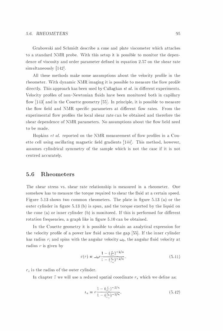
5. 6. RHEO;\[ETEnS
G rabowski and Schmidt desc ribe a cone and plate viscometer wh ich attaches
t o a standard NMR probe. With th is setu p it is possible to monitor the depen
dence of viscosity and order parameter defined in equation 2 .57 on the shear rate
sim u ltaneously [ 1 "12J .
Al l t hese methods make some assumptions about the velocity profi le i n the
rheometer . With dynamic NMR imaging i t is possible to meas u re the f low proft le
d irectly. This approach h as been used by Cal laghan et al. i n d i fferent experiments .
Velocity profi les of non-Newtonian fl u ids have been monito red both in capil lary
flow [H3] and i n the Couette geometry [55] . In principle, i t is possible to meas u re
t he How field and 0JMR specifi c parameters at d i fferent flow rates . From the
experimental flow profiles the local shear rate can be obtained and therefore the
shear dependence of NMR parameters. No assumptions abou t the flow f ie ld need
to be m ade .
Hopkins et al. reported on the N]\IR measurement of flow p ro fi les i n a Cou
ette cel l using osci l lat ing magnetic field gradients [ 144] . This method , however ,
assu mes cyl ind rical sym metry of the sam ple which is not the case if i t is not
centred accu rately.
5 . 6 RheOlneters
The s hear stress vs. shear rate relationsh ip is measu red in a rheometer . One
somehmv h as to measu re the torque requ i red to shear the fl u id at a certain speed .
F ig u re 5 . 1 3 shows two common r heometers. The p late i n figure 5 . 1 3 ( a) or the
o u te r cyl inder i n figure .5 . 1 3 (b ) i s spun , and the torque exerted by the l iqu id on
the cone (a) or i n ner cyl inder ( b) is mon itored . I f th i s is performed for d ifferent
rotation frequencies, a graph l i ke in fig u re .5 . 1 0 can be obtai ned .
I n the Couette geometry it is possible to obtain an analytical expression for the velocity profile of a power law flu id across the gap [.5S] . I f the i n ner cyl inder has rad i us l'i and spins with the angular velocity Wo , the angular fl u id veloci ty at
rad ius I ' is given by
1' ( 1' ) (5A l )
1'0 i s the rad ius o f the ou ter cyl inder .
rn ch apter I' we wi l l use a red uced spat ial coord inate l's which we def i ne as:
I' s ( 5 . 12 )
96 CHAPTER 5. POLYMER PHYSICS
Ca)
.....---------- cone
L...-----;;ro sample fluid
L...-__ ........-, .---------' �""IIr__ ____ _ CV plate
(b)
inner cyl i nder
'�f-------- sample fl u i d
..... �-----. - outer cyl inder
CV Figure 5 . 1 3 : Two of the most widely used rheometers are ( a ) the cone a n d p l a te rheometer
and (b) the Couette rheometer.
The shear rate in a system with cyli nd rical sym metry is g iven by [ 145]
;, = r 0 ( v ( r) I Or I'
\Vith the velocity profi le of eq u ation 5 .4 1 this gives
. 2....,'0 ( I
= --"----,-n 1 - ( � )
, 0
( 5 .43 )
( .5 .44 )
These equations wi l l be used i ll chapter / . The velocity profi le v ( r) wi l l be measu red t here, and n wi l l be obtained by a least squares fi t of equ ation 5 .4 1 .
From equat ion .5 . · 14 fol lows t ha t a graph of log ;( vs. log /' is a st raight l ine with
slope - 2/n for a power law fl u id . This a l ternative method of measur ing n wi l l be
used i n chapter 9 .
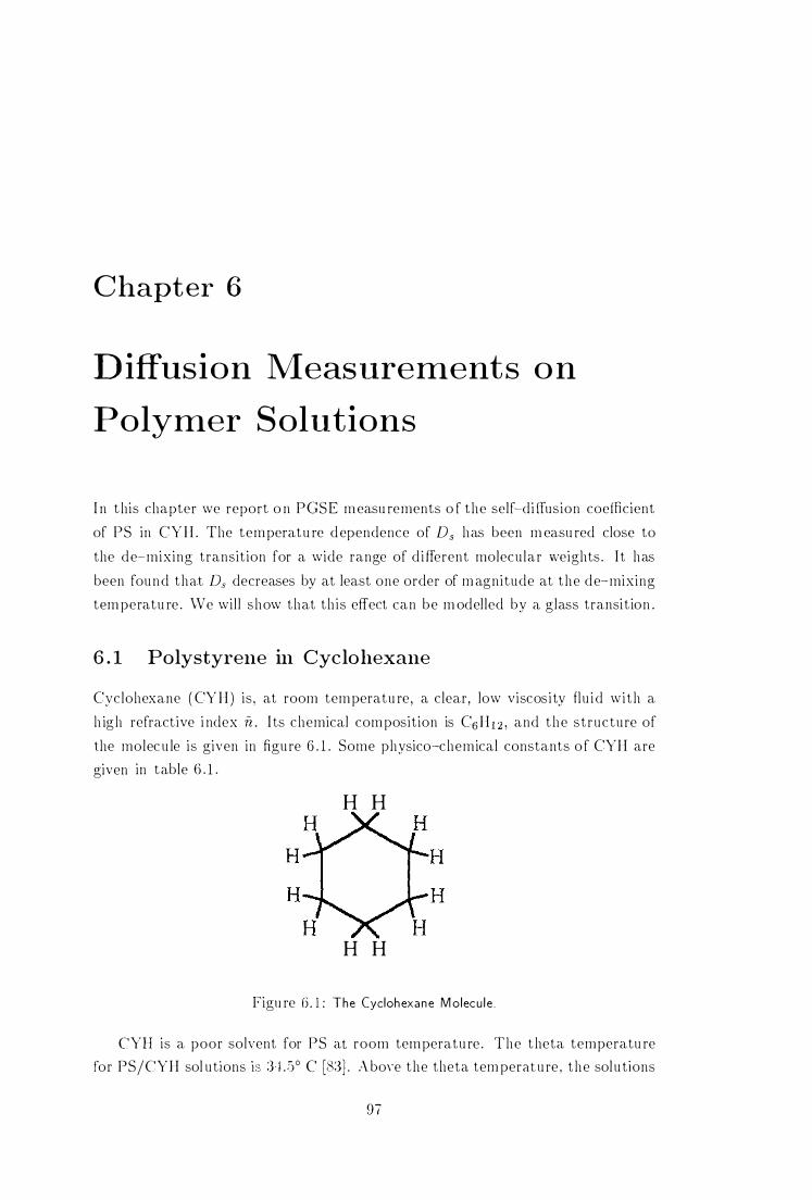
Chapter 6
D iffusion MeaSllrements o n
Polymer Solutions
I n this chapter we report o n PGSE measu rements o f the self-di ffusion coefficient
of PS in CYH . The temperatu re d ependence of Ds has been m easu red close to
the de-mixing transition for a wide range of d ifferent molecular 'vveights . I t has
been found that Ds decreases by at least one order of m agnitude at the de-mixing
tem peratu re . We wil l show that th is effect can be m odelled by a, glass transi t ion .
6 . 1 Polystyrene in Cyclohexane
Cyclohexane ( CYH) is , at room temperatu re , a clear, low viscos ity flu i d wi th a
h igh refract ive i ndex n . I ts chemical composition is C6H 1 2 , and the structure of
the molecu le is given in figure 6 . 1 . Some physico-chemical constants of CYH are
given in table 6 . 1 .
H H
H H
Figu re G. 1 : The Cyclohexane Molecu le .
CYB is a poor solvent for PS at room temperatu re . The theta temperatu re
for PS/CYH sol utions is :3 1 .5° C [8:3J . A bo\'e the theta tem peratu re , the solu tions
9,
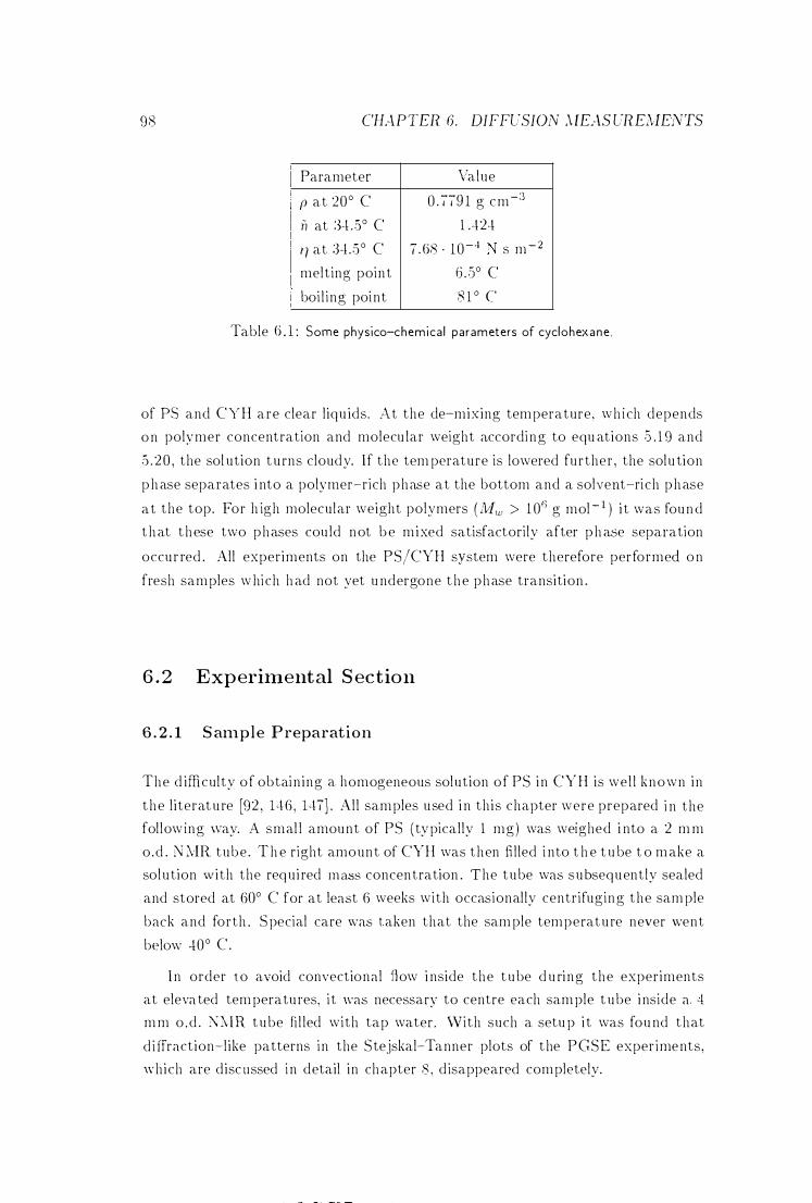
98 CHAPTER 6. DIFFUSION MEAS URElvIEjVTS
Parameter Value
p at 20° C 0 . 779 1 g c m -:3
ii at :)LSo C 1 .424
17 at :34 .5° C 7.68 . 10-.1 � s m - 2
melting point 6 .:3° C
boi l ing poi nt 8 1 ° C
Table 6 . l : Some physico-chemica l parameters of cyclohexane .
of PS and CYH are clear liqu ids. At the de-mixing temperature , wh i ch depends
o n polymer concentration and molecu lar weight a.ccordi ng to equ ations .5 . 1 9 and
5 . 20 , the sol ution t u rns cloudy. If the tem perature is lowered fu rther , the solu tion
p h ase separates i nto a polymer-rich phase at the bottom and a solvent-rich p h ase
at the top. For h igh molecular weight polymers (i'vItu > 1 06 g mol - I ) i t was fou n d
t h at t h ese two phases cou ld not b e mixed satisfactorily after p h ase separation
occu r red . All experiments on the PS/CYH system were therefore performed o n
fresh samples w hich h ad not yet u ndergone t h e phase transition .
6 . 2 Experhnental S ection
6 . 2 . 1 S am p l e P reparation
The d ifficulty of obtain ing a homogeneous solution of PS i n CYH is we l l known in
t h e l iterat u re [92 , H6 , Hi] . All samples u sed i n th is chapter were prepared i n the
following \vay. A smal l amount of PS (ty pically 1 mg) was weighed i nto a 2 m m
o.d . N MR tube . T h e r ight amount of CYH was then fi l led i nto t h e t u be t o m ake a
solu tion with the requ i red m <1..'3S concentration . The tube was subsequ ently sealed
and stored at 60° C for at least 6 weeks with occasionally centr ifug ing the sam ple
back and forth . S pecial care \vas t aken that the sam ple temperat u re never \vent
belmv 40° C.
I n order to avoid convectional flow i nside the t u be d u ring the experiments
at eleva ted tem peratu res, i t was necessary to centre each sam ple t ube i nside a , cl m m o . d . :\"\IR t u be fi l led with tap water. With such a setu p i t was fou nd that
d i ffraction-like patterns in the Stejskal-Tanner plots of t he PGSE exper iments.
\\' h ich are d isc llssed i n detail in chapter 8 , d isappeared completely.
6.2. EXPERIAIENT-\ L SECTION
6 . 2 . 2 lVleasurement o f the S elf-Diffusion Co efficient
99
T h e tem peratu re dependence of Ds w as m easu red for t h e P S sam ples from table
5 . 1 w i t h a m ass concentration of 5 <:i{ i ll CYH . In a second set of expe r i m e n ts ,
t h e tem pera t u re dependence of Ds was Ill NSlucd for t h e P S sample w i t h .\IlL' =
1 . 7:3 · l OG g m ol - 1 at d i fferent concent rations.
The experiments were performed using the high grad ie n t probe described i n
sect i o n 2 . 5 .3 . D u e to artifacts i n t h e echo signal for h igh grad i e n t c u rrents ( which
cou ld be d u e to sam ple v i bration or eddy c u rre n ts) , t h e PGSE p u lse seq uence from
sect i o n 2 A A h ad to be mod i fied s l ightly. Instead of using rectangular s haped
grad i e n t p u lses, ram ped grad ie n t p u lses were appl ied . Each ram p step h ad a
d uration of 50 JLS a n d a c u rrent ampl itude of u p to 1 A. The pulse p rogram
j){}Scmmp is given in appendix B. Although i t is possible to obtain an equ ation for
t h e echo atte n u ation us ing ramped grad ie n t p u lses [ 148] , i t was fou n d t hat s u c h
corrections w e r e not n ecessary i n o u r case w h ere t h e ram p t i m e is s h o r t com pared
to t h e d u ration of t h e gradient p ulse.
I n a m ul t i -com ponent system it is , in pr inc ip le , possible to m easu re the self
d i ffusion coefficient of each com pone n t i n one sin gl e P G S E experi m e n t by sim pl y
meas u ri n g t h e echo atte n u ation o f each peak i n t h e NMR spec t r u m . I n o u r c ase ,
h oweve r , t h e solvent s ignal is m uch l arger i n am pli t u de than t h e signal comi n g
fro m t h e polymer a n d w i l l dom i n ate t h e spec t r um . Because t h e solvent a n d s u r
rou nd i n g water d iffuse m u c h faster t h an t h e pol y m e r , i t is possible to attenuate
the solve n t and water s ignal completely by a pair of PGSE pulses. The only signal
rem ai n i n g is from the polymer . By now successi vely i n c reasing t h e d uration of
t h e PGSE p u lses one can meas u re t he self-di ffusion of t h e polymer w i t h o u t any
solven t i nterferences.
D u e to t h e l arge range of molecu l ar weights investigated (2 . 105 g m ol - 1 2 . 1 07 g m o l- I ) , Ds is expec ted to vary by 4 orders of m agnitude accordi n g to equation
;") . 25 . The short T2 valu e of P S l i mits the d iffusion time d to a m axi m u m valu e of
clQ m s . T h erefore t h e experimental pa.rameters h ad to be adj usted indiv idual ly for
each sample . T his was done as fol lows. The grad ie n t pu lse d u ration 6min for t h e
fi rst q sl ice was c hosen to be between 0 . :") a n d :3 ms, depending o n t h e sam ple . T h e
g r ad i e n t a m p l i t u d e 9 w a s then adj ust�:d s u c h t h at t h e �::'IR sign a.! of t h e water
and the sol ven t \vere att e n u ated com pletely. The only sign al left \vas the pol�' m e r
sign aL T h e i n c rement o f the gradien t p u l se d u ration between each q sl ice was
t h e n chosen such t hat t h e atten uation of t h e poly m e r sign al i n t h e fi nal q slice was
arou nd 0 . 1 at a. t em perat u re of ·l·2° C . The echo t i m e .:..\ was between 20 ms and
LlO ms. \Vith t h i s proced ure . t h e grad i e n t d u ration was i ncremented i n 16 steps
w i t h a step size (S ine between 0 .25 Ill S ;). lld 1 Ins . T h e grad i e n t ampl itude was left
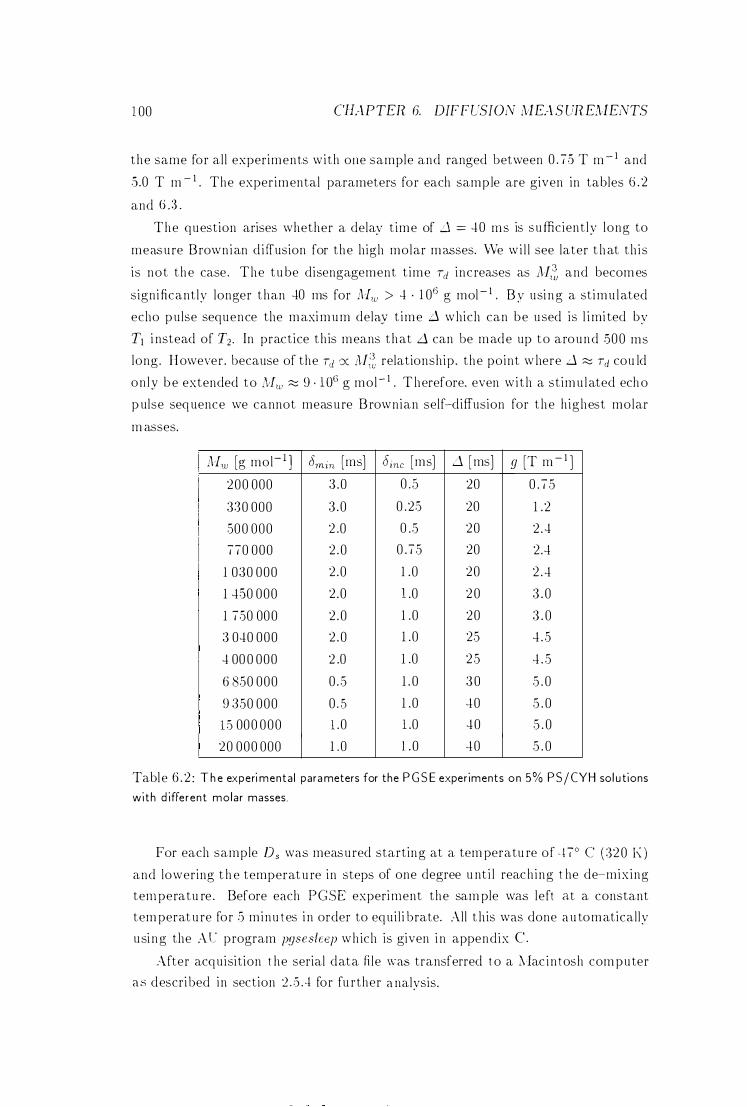
1 00 CHAPTER 6. DIFFL'SION ;'vlEA S URElvIENTS
the same for al l experiments with ol le sample and ranged between 0 . 7.5 T m - I and
.5.0 T m - I . The exper imental parameters for each samp le are given in tables 6 . 2
and 6 . :3 . The question arises whether a delay t ime of .J = 40 ms is su fficient ly long to
measure Brownian d i ffusion for the high molar masses. vVe wi l l see later t hat th is
is not the case . The tu be disengagement t ime Td increases as AJ1� and becomes
significantly longer t han 40 ms for Mw > 4 . 1 06 g mol - I . B y usi ng a stimu lated
echo pu lse sequence the maximum delay t ime .J which can be used is l imi ted by
TI i nstead of T2• In practice t h is means that d can be made up to around .s00 ms
long. However . because of the TeI ex: AJ�� relationship . the point where d � Td cou ld
on ly be extended to Afw � 9 · l OG g mol- I . Therefore. even with a stimu lated echo
p ulse seq uence we cannot measure B rownian self-diffusion for the h ighest molar
m asses.
Mw [g mol- 1 J
200 000
3:30 000
,500 000
770 000
1 030 000
1 4.50 000
1 7,50 000
3 040 000
4 00 0 000
6 850 000
9 :350 000 1 ,5 000 000
20 000 000
()min [ms]
3 .0
3 .0
2 .0
2 . 0
2 .0
2 .0
2 . 0
2 . 0
2 .0
0 . 5
0 . .5 1 .0
1 .0
Sine [ms] .J [ms] 9 [T m - I ]
0 . .5 20 0 . 75
0 .2 ,5 20 1 .2 0 .5 20 2 .4 0 .75 20 2.4
1 .0 20 2 . 4
l .0 2 0 3 . 0
1 .0 20 3 . 0 1 .0 25 4 . 5
1 .0 25 4 . 5
1 . 0 3 0 5 . 0
1 .0 40 5 . 0 l .0 40 5 . 0
l . 0 40 5 . 0
Table 6 . 2 : T h e experimenta l parameters for the P G S E exper iments on 5% PS/CYH sol u tions
with d ifferent molar masses.
For each sample Ds was measured starting at a tem peratu re of ·1'iO C ( 32 0 E )
and lowering t h e temperat u re in steps of one degree u nt i l reach ing t he de-mixing
tem peratu re . Before each PGSE experiment the sam ple was left at a constant
tem perat u re for 5 minu tes i n order to equi l i brate. All t h is was done a u tomatically
usi ng the At" program pgseshep which is given i n appendix C .
.\fter acquisit ion t he serial data fi le \\'a3 transferred t o a ;"lac in tosh com puter as described in section 2 . .5A for fu rther a nalysis.
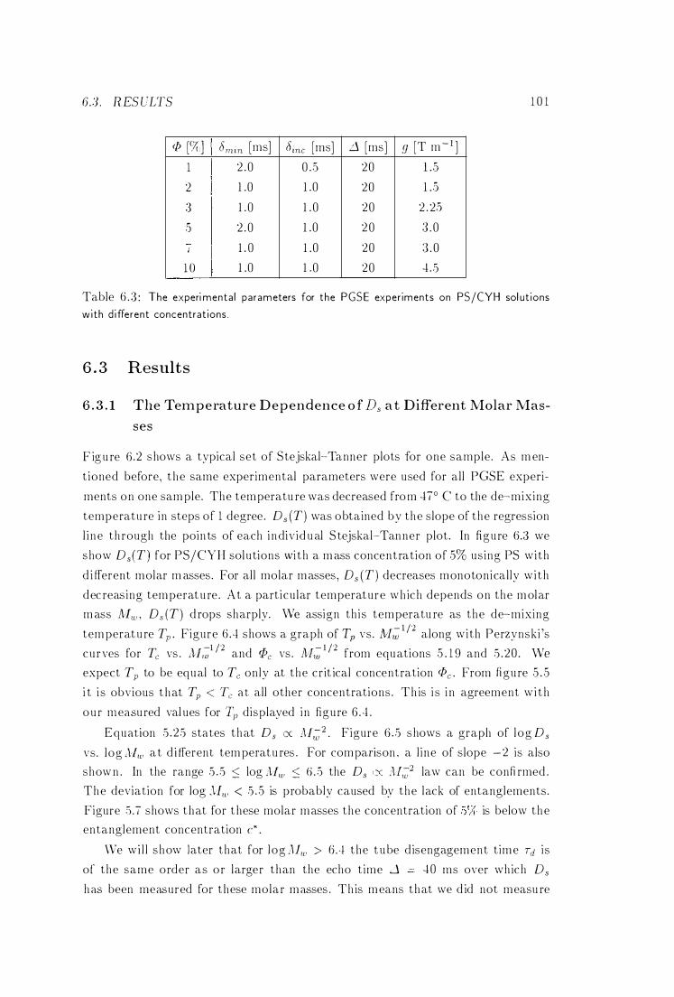
6 .3 . RES ULTS 1 0 1
P [(iq Omin [ms] Oine [ms] ...1 [ms] g [T m - I ]
i 2 . 0 0 . . 5 20 1..5 2 1 .0 1 .0 20 1 .:')
:3 1 . 0 1 . 0 20 2 . 25
:) 2 . 0 1 .0 2 0 :3 . 0 - 1 . 0 1 .0 20 :3 . 0 I
i O 1 .0 1.0 20 4 .5
Table 6 . :3 : The experi menta l parameters for the PGSE exper iments on PS/CYH sol ut ions
with d i fferent concentrat ions .
6 . 3 Results
6 . 3 . 1 The Tem p e rature D e p endence o f Ds a t Different Molar Mas-
ses
F ig u re 6.2 shows a typical set of Stejskal-Tanner plots for one sample . As m en
t ioned before, t h e same experimental parameters were used for all PGSE experi
ments on one sam ple. The temperatu re was decreased from 47° C to the de-mix ing
tem perat u re in steps of 1 degree . D s (T) was obtained by the slope of the regression
l i ne th rough the poin ts of each i ndiv id u al S tejskal-Tanner plot. In figure 6.3 we
show Ds(T) for PS/CYH sol utions ivi th a m ass concentration of 5% us ing PS with
d i fferent molar m asses . For all molar masses , D s (T) decreases monoton ically w i th
dec reas ing temperat u re . At a part icu lar temperature wh ich depends on the molar
m ass IvIu! ' Ds (T) d rops sharply. We assign th is temperatu re as the de-mixing
tem perat u re Tp . Figure 6 .4 shows a graph of Tp vs. lvI;;; 1 /2 along wi th Perzynski 's
cu rves for Tc vs . lvI,-;/ /2 and Pe vs . lH;;; 1 /2 from equations 5 . 1 9 and 5 .20 . We expect Tp to be equal to Tc only at the cr it ical concentration Pc . From figu re 5 . 5
i t i s obvious t h at Tp < Te at all other concentrations . Th is i s i n agreement w i t h
ou r measured val ues for '1�) displayed in figure 6 . 4 .
Equation 5 .25 states that Ds ex M,"';/ . Figure 6 .5 shows a graph of l og Ds vs. log j1w at d i fferent tem peratu res . For comparison . a l ine of slope -2 is also
show n . In the range 5 . 5 ::; log ;Hw ::; G . 5 the Ds IX ;\1,"';/ law can be confi rmed .
The deviation for log .\Iw < 5 . 5 is probably caused by the lack of entanglements.
Figure 5.7 shows t hat for t hese molar masses the concentration of entanglement concentration c* .
is below the
\Ve w i l l show Jater that for log "Iw > GA the t ube d isengagement t ime Td i s
of the same order as o r larger than the echo t ime .J 40 ms over wh ich Ds has been measured for these molar masses . Th is means that we d id not measu re
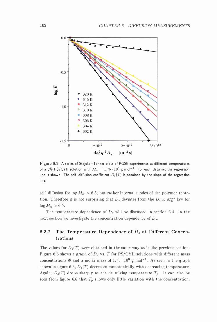
1 02
� ell 0
-
-0.5
- 1 .0
• 320 K • 3 16 K D 3 1 2 K • 3 10 K • 308 K o 306 K
304 K A 302 K
A
CHAPTER 6. DIFFUSION MEASUREMENTS
A A
- 1 .5 +---...---T"'"""--..----.------...--...... ---l o
Figure 6 .2 : A series of Stejskal-Tanner plots of PGSE experiments at d ifferent temperatures
of a 5% PS/CYH solution with Mw = 1 . 75 · 1 06 g mol- I For each data set the regression l ine is shown . The self-diffusion coefficient D$ ( T) is obtained by the slope of the regression
l i ne.
self-diffusion for log Mw > 6 .5 , but rather internal modes of the polymer repta
tion. Therefore it is not surprising that Ds deviates from the Ds ex M;;;2 law for
log Mw > 6 .5 .
The temperature dependence of Ds will be discussed in section 6.4 . In the
next section we investigate the concentration dependence of Ds .
6 . 3 . 2 The Temperature Dependence of Ds at Different Concen
trations
The values for Ds (T) were obtained in the same way as in the previous section .
Figure 6 .6 shows a graph of Ds vs. T for PS/CYH solutions with different mass
concentrations if> and a molar mass of 1 .75 . 106 g mol- i . As seen in the graph
shown in figure 6 .3 , Ds (T) decreases monotonically with decreasing temperature.
Again, Ds (T) drops sharply at the de-mixing temperature Tp . It can also be
seen from figure 6.6 that Tp shows only little variation with the concentration .
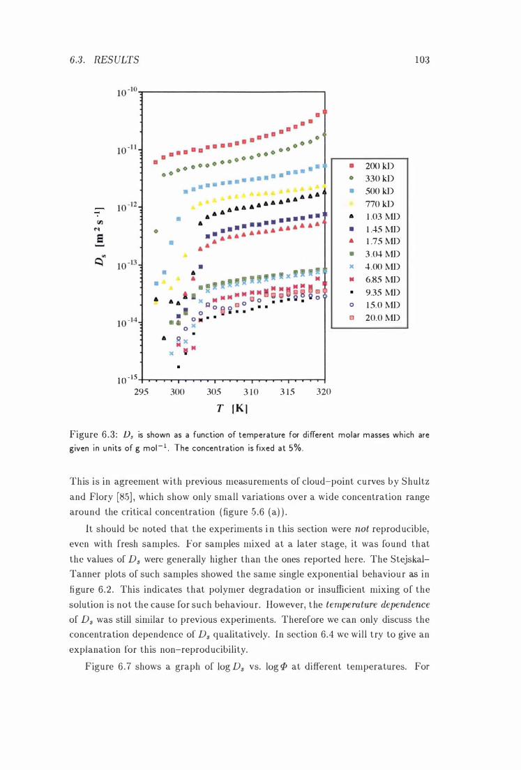
6.3. RESULTS
,..-, -,
1
0 - 1 0 ..,......-----------------.
•
• 10 - 15 +-r-T'-
-'-"""--'-'T""T"'T"''T''''''"'''T'''T'''''I-'''''''-'r-T''''T'''"T'''T''''T'''"T'''''I'-I 295 300 305 3 1 0 3 15 320
T [ K ]
a
o
•
A
•
.to
IB
)(
..
•
o
200 kD 330 kD 500 kD 770 kD 1 .03 MD 1 .45 MD 1 .75 MD 3 .04 MD 4.00 MD 6.85 MD 9.35 MD 1 5.0 MD 20.0 MD
1 03
Figure 6 .3 : Ds is shown as a function of temperature for different molar masses which are
given in u nits of g mol- i , The concentration is fixed at 5%.
This is in agreement with previous measurements of cloud-point curves by Shultz
and Flory [85] , which show only small variations over a wide concentration range
around the critical concentration (figure 5 .6 (a) ) .
It should be noted that the experiments i n this section were not reproducible,
even with fresh samples. For samples mixed at a later stage, it was found that
the values of Ds were generally higher than the ones reported here. The Stejskal
Tanner plots of such samples showed the same single exponential behaviour as in
figure 6.2. This indicates that polymer degradation or insufficient mixing of the
solution is not the cause for such behaviour. However, the temperature dependence
of Ds was still similar to previous experiments. Therefore we can only discuss the
concentration dependence of Ds qualitatively. In section 6.4 we will try to give an
explanation for this non-reproducibility.
Figure 6 .7 shows a graph of 10g Ds vs. 10g P at different temperatures. For
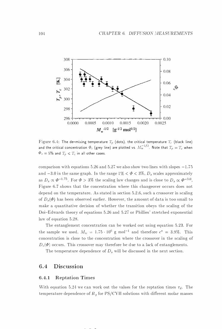
1 04 CHAPTER. 6. DIFFUSION ,\IEASUR.EivIENTS
308 0. 1 0
306 0.08
,....... 304 � 0.06
Eo .... ; ... 302 ,,'6<
� 0 .04 Eo-. ">.. 300
298 0.02
296 0.00 0.0000 0.0005 0.00 1 0 0.00 1 5 0.0020 0.0025
M ·1/2 w
[g- 1I2 moP/2]
Figure 6 .4 : The de-mixi ng temperature Tp (dots) , t he cr it ica l temperatu re (b lack l i ne) a n d the cr it ica l concentration rJ>c (grey l i ne) a re plotted vs. Aft� 1 / 2 Note that Tp = Tc when
rJ> c = 5% and Tp < Tc i n a l l other cases.
com parison wi th equ ations .5 .26 and 5 .27 we also show two l ines w i th slopes - 1 .75
and -3 . 0 i n the same graph . I n the range 1 % < qi < 3% , Ds scales approxim ately
as D s (x qi-l .75 . For qi > 3% the scal ing law changes and is close to D s ex qi-3.0 . Figure 6 .7 shows t hat the concentration w here t his changeover occurs does not
depend on the temperatu re . As stated in section 5 .2 .6 , such a crossover in scal i ng of Ds (qi) h as been observed earlier . However , the amount of data is too smal l to
make a q uantitat ive decision of whether the t ransi t ion obeys the scal i ng of the
Doi-Edwards theory of equations 5 . 26 and 5 .27 or Ph il l ies ' stretched exponential
law of equ ation 5 .28 . The entanglement concentration can be worked out us ing equ ation 5 .23 . For
the sample we used . Mw 1 . 75 . 1 06 g mol- 1 and therefore c* = 3 .9%. This concentration is close to the concentration where the crossover i n the scal i ng of
Ds (qi) occu rs . Th is crossover may therefore be d ue to a lack of entanglements . The temperat u re dependence of Ds wi l l be discussed in the next sect ion .
6 . 4 Discussion
6 . 4 . 1 Reptation T imes
With equ ation 5 .2cl we can \vork out the valu es for the reptation t imes Td . The
tem peratu re dependence of Rg for PS/CYH sol u tions with d i fferent molar masses
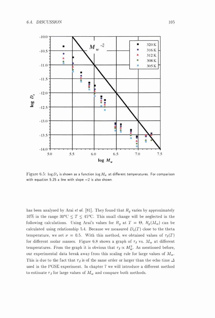
6.4. DISCUSSION
- 1 0.0
• - 1 0.5 •
- 1 1 .0
- 1 1 .5
., - 1 2.0 Cl Cl;)
oS - 1 2.5
- 13.0
- 13.5
- 14.0 5.0 5.5
•
6.0 6.5
log Mw
• • • • •
7.0
320 K 3 1 6 K 3 1 2 K 308 K 305 K
7.5
105
Figure 6.5 : log D3 is shown as a function log Mw at different temperatures. For comparison with equation 5 .25 a line with slope -2 is a lso shown .
has been analysed by Arai et al. [8 1] . They found that Rg varies by approximately
10% in the range 30°C :S T :S 45°C. This small change will be neglected in the
following calculations. Using Arai's values for Rg at T = 0, Rg (Mw) can be
calculated using relationship 5.4. Because we measured Ds (T) close to the theta
temperature, we set v = 0 .5 . With this method, we obtained values of T.;l (T)
for different molar masses. Figure 6.8 shows a graph of TJ vs . Mw at different
temperatures . From the graph it is obvious that Tj, ex: M�. As mentioned before,
our experimental data break away from this scaling rule for large values of Mw ' This is due to the fact that Tj, is of the same order or larger than the echo time .d used in the PGSE experiment. In chapter 7 we will introduce a different method
to estimate T.;l for large values of Mw and compare both methods.
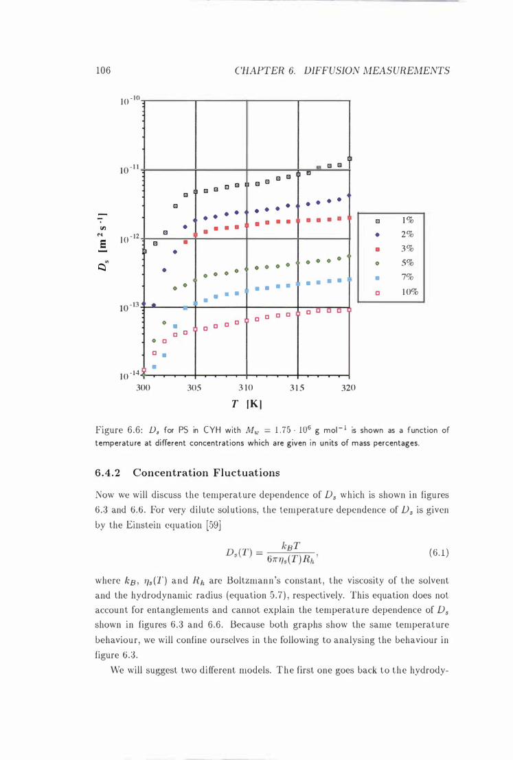
106
.--. fIJ
N
e ........ '"
�
10 - 10
1 0 -12
1 0 -14 300
13
B
•
•
0
0 c
c •
•
13 13 13 El
13
• • •
• a • •
• •
0 0 0
0 0
• • • -
• c c c c c
305
CHAPTER 6. DIFFUSION MEAS UREMENTS
El 13
• •
a a
0 0
• •
c c
3 10
T [K ]
13
•
a
0
•
c
13 13
• •
• •
0 0
• •
c c
3 1 5
J:I El
• •
a a
0 0
• •
c c
13 13
• •
•
0 0
• •
c c
320
El 1 %
• 2%
a 3%
o 5%
• 7%
c 1 0%
Figure 6 .6 : D. for PS in CYH with Mw = 1 . 75 . 1 06 g mol - 1 is shown as a function of temperatu re at different concentrations which a re given i n un its of mass percentages.
6 . 4 . 2 Concentration Fluctuations
Now we will discuss the temperature dependence of Ds which is shown in figures
6 .3 and 6.6 . For very dilute solutions, the temperature dependence of Ds is given
by the Einstein equation [59]
(6 . 1)
where kB , "ls (T) and Rh are Boltzmann's constant , the viscosity of the solvent
and the hydrodynamic radius (equation 5.7) , respectively. This equation does not
account for entanglements and cannot explain the temperature dependence of Ds
shown in figures 6 .3 and 6 .6 . Because both graphs show the same temperature
behaviour, we will confine ourselves in the following to analysing the behaviour in
figure 6 .3 . We will suggest two different models. The first one goes back to the hydrody-
6.4 . DISCUSSION
- 1 0 . 5
• 320 K
• 3 1 6 K
- 1 1 .0 .. 3 12 K • 308 K
• 304 K
- 1 1 .5 .. • - 1 .75
... • • Q t)() - 12 .0 • 0
-
• • ..
- ] 2.5
•
•
- 1 3 . 0
- 13.5 +--...--4---.--+--...--4---.--+--r---l 0.0 0.2 0.4 0.6
log cP
0.8 1 .0
107
Figure 6 .7 : log Ds is shown as a function of log tP at different temperatu res. For comparison with equations 5 .26 and 5 .27 two l i nes with slope - 1 . 75 and -3 . 0 are a lso shown .
namic model and is based on the concentration fluctuations in polymer solutions
mentioned in section 5.2 .5 . The second model suggests that Ds (T) can be de
scribed by a glass transition which has been introduced in section 5 .3 .3 . We will
see that the latter model gives a much better description.
Spatial fluctuations in the polymer concentration result, according to equation
5.25, in spatial fluctuations of the self-diffusion coefficient. It is known that near
the critical point these fluctuations increase both in amplitude Pa and correlation
length � [149] . If concentration fluctuations govern the behaviour of Ds (T) near
the de-mixing transition , it should be possible to find values of Pa (T) and �(T) .
We will show here that the effect of concentration fiuctuations alone is too small
to explain the behaviour of Ds (T) shown in figures 6.3 and 6.6 .
108 CHAPTER 6. DIFFUSIO MEASUREMENTS
1 0 0�-----------,------------�----------�
1 0 - 1 +------------4--------*---��--------�
10 -2 +-__________ --I __ ----,#-......a ____ +-__________ --I
..-, (IJ 10 -3 '-'
... � • 320 K • 3 1 6 K
1 0 -4 A 3 1 2 K • 308 K • 305 K
1 0 -5
1 0 -6�--�����--�-,����--����� 1 0 5
Figure 6 .8 : Td is shown as a function Mw at d ifferent temperatu res. For comparison with equation 5 .24 a l ine showing the Td ex M� relationsh ip is a lso d rawn.
6.4.2.1 Some Calculations
For simplicity we assume that the concentration fluctuations are one-dimensional
along the z direction and sinusoidal around a mean value Po with a wavelength ).
as shown in figure 6.9 (a) and (b) . The amplitude of the fluctuations is Pa :
(27rZ ) <p( z) = <Po + <Pa cos T . (6 .2)
The Stejskal-Tanner plots in figure 6 .2 show no curvature . This means that ,
although the self-diffusion coefficient Ds ( z ) is not constant across the sample,
it can be described by an effective constant De!! which is some sort of average
diffusion constant . This implies that the mean square displacement (z2) = DeJ J11
of the polymer molecules over the time 11 must be much larger than the square of
the wavelength of the fluctuations:
(6 .3)
6 .'1 . DISCUSSION
z (b)
<P - - - - - - -o
(�_s (_z) _A ____ A __
1 09
Figu re 6 .9: ( a ) The spati a l d istr ibution of polymer coi l s assum ing one-dimensiona l s i nusoida l
concent rat ion fl uctuat ions . ( b) T h e function <p ( z ) . (c) The spati a l d istr ibut ion of D " (z )
assum ing s i nusoida l concentration fluctuat ions .
vVe now assume that Ds scales as in a theta solvent l ike Ds ex <P-3 • The
funct ion Ds ( z ) is shown schemat ically i n figure 6 . 9 (c) . The t ime t taken for a
m olecu le to move over distances m uch smal ler than A is then proportion al to (j)3 .
For d istances m uch larger than A we therefore find
(6 .4 )
\vh ere (j)�� is the average of <j)3 :
<j)3 = � r\ <j)3 ( z ) d z . /\ la (6 .5 )
Csing equ ation 6 .2 , th is average can be calculated . Expanding (j)3 ( z) and taking
i n to accou nt t hat
( 6 .6) and
( 6 . 7 )
1 1 0 CHA PTER. 6. DIFF L'SIO;\f l\IEAS UR.EMENTS
\ve obtain
Using relationshi p 6..1 and De!! = (:;2 ) / t . we get
1 Def f = Do . 3 p2 ,
1 + '2 ;pt
where Do is the val ue of Def f for {Po = O .
o
( 6 .8)
( 6 .9)
I t is i mportant to note that Def f does not depend on the wavelength >- of the concentration fl uctuations. However . for ou r calcu lat ions it was essent ial t hat
>-2 < De] f .6 . Th is means that a molecu le has to move over many wavelengths i n
o rder t o b e able t o descr ibe i t by a n effect ive d iffusion constant . T h e act ual valu e
o f >- i s n o t i mportant u nder these cond i tions .
6 . 4 . 2 . 2 Comparison W i t h t he Experimental Values
\Ve now compare the resu l ts of equ ation 6 .9 with our values of Ds(T) from figure
6 . 3 . \Ve st i l l assume that the wavelength /\ of the concentration fl uctuations is
smal l compared to t he mean squ are d isplacement of the polymer m olecules over
the t ime .6. Then the ampl itude Wo is the only adjustable parameter i n equ at ion
6 . 9 .
Because Ds (T) i n figure 6 . 3 decreases w i t h decreasing temperat u re , we expec t ,
from equ ation 6 .9 , Wo to increase w i th decreas ing temperatu re . Because Wo must
be in the range 0 :s; Wo :s; Wo , De!! is restr icted to values between � Do :s; De!] :s; Do. However , close to the de-m ix ing temperatu re we observe a sharp decrease
of Ds(T) by at least a factor of 5. Th is i mp lies that the effect of concentration
fl u ct uations alone is too weak to explain our exper imenta.l resu lts .
One might wonder whether our resu l ts wou ld be more real ist ic if we chose Ds (1)) to vary in our calcu lations a s Ds (1)) ex 1> - 1 .75 i nstead of Ds (1)) ex 1>-3.0 . The resu l t is t hat the variation of Ds ( p) would be smaller , and De] f would be
even c loser to Do for large fl uctuations than i n equation 6 .9 .
\Ye therefore conclude that o ll r s imple model of concentration fl uctuations
a lone can not explain the measu red Ds(T) values shown in figu re G .3 . The fact
that experiments are not reprod ucible ind icates that changes occ u r i n the sample
when de-mixing takes place, which take a long t ime to relax . Th is suggests that
the polymer enters some kind of glassy state at the de-mixing t ransit io n . Th is wi l l be d iscussed i n the next section .
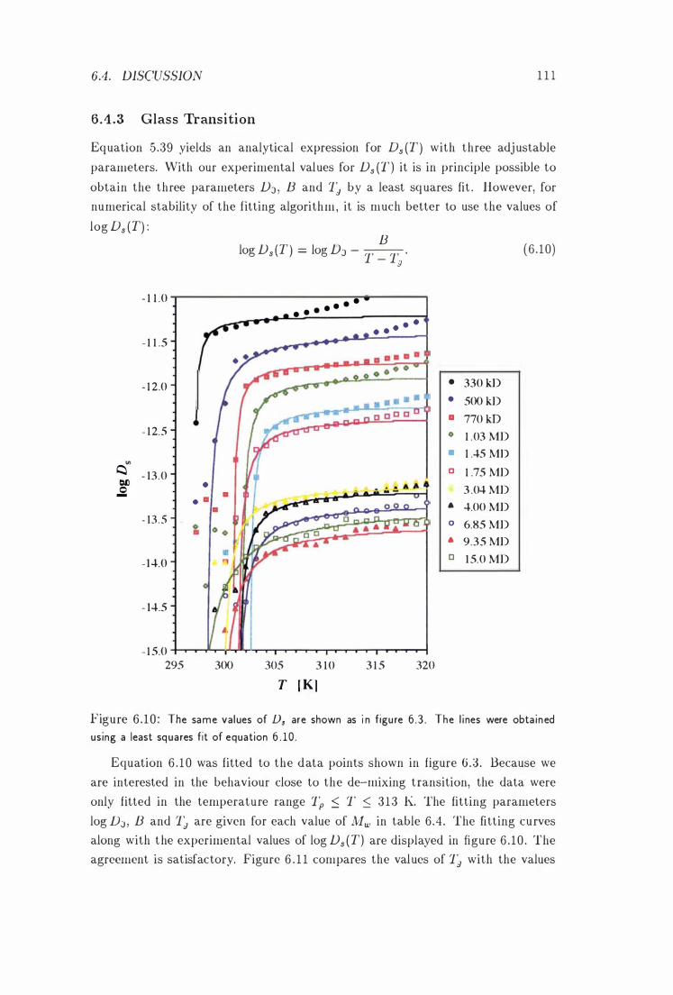
6.4. DISCUSSION 1 1 1
6.4.3 Glass Transition
Eq uation 5.39 yields an analytical expression for D s (T) with three adjustable
parameters. With our experimental values for Ds (T) it is in principle possible to
obtain the three parameters DJ B and Tg by a least squares fit . However, for
numerical stability of the fitting algorithm, it is much better to use the values of
log Ds (T) :
'"
� � 0
-
- 1 1 .0
- 1 1 .5
- 1 2.0
- 1 2.5
- 13.0 •
. 11 11
- 13.5 :
- 1 4.0
- 14.5
11
B log Ds (T) = log DJ - T _ T g
• • • • • • •
• • • • •
- 1 5.0 ;.....,r-T""-."-t-yL..,Ja,..J-r-.....,--.-...-.--.-r-T"".....-.r-T"" ......... -r--r--T--j 295 300 305 3 1 0 3 1 5 320
T [ K]
• 330 kD • 500 kD
11 770 kD
o 1 .03 MD 11 1 .45 MD
c 1 .75 MD
3 .04 MD 6 4.00 MD
o 6.85 MD 6 9.35 MD
c 1 5.0 MD
(6 . 10)
Figure 6 . 10 : The same values of D8 are shown as i n figure 6 .3 . The l i nes were obta ined
using a least squares fit of equation 6 . 10 .
Equation 6 . 1 0 was fitted to the data points shown in figure 6.3 . Because we
are interested in the behaviour close to the de-mixing transition, the data were
only fitted in the temperature range Tp ::; T ::; 313 K. The fitting parameters
log DJ , B and Tg are given for each value of Mw in table 6.4 . The fitting curves
along with the experimental values of log Ds ( T) are displayed in figure 6 . 10 . The
agreement is satisfactory. Figure 6 . 1 1 compares the values of Tg with the values
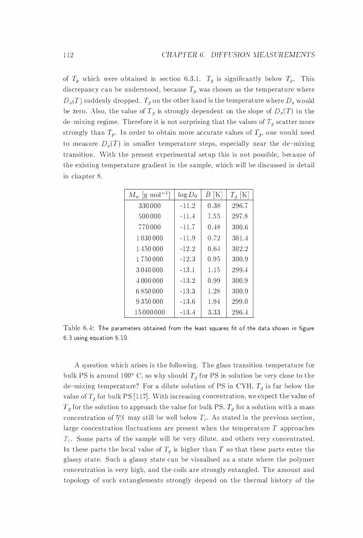
1 12 CILlPTER 6 . DIFFUSION .UEAS UREAIENTS
of Tp \vhich were o btained in sec tion 6 .3 . 1 . Tg is sign i fican tly below Tp . This
d iscrepancy can be u nderstood , because Tp was chosen as the temperat u re where
DsCT ) suddenly d ropped . T:; on the other hand is the temperat u re where Ds would
be zero. A lso, the val ue of Tg is strongly dependent on the slope of Ds (T) i n t he
de-mixing regime. Therefore i t is not su rprising that the values of Tg scatter m ore
st rongly than Tp . I n o rder to obtain more accu rate values of T:;, o ne \vou ld need
to measu re Ds (T) in smaller temperatu re steps, especial ly near the de-mix ing
transit ion . With the p resent experimental set u p th is is not possible , because of
the existi ng temperatu re gradient i n the sample, which wi l l be d iscussed in detai l
in chapter 8.
ly[w [g mol - i ] log Do B [K] Tg [K] 330 000 - 1 1 .2 0 .38 296 .7
500 000 - 1 1 .4 1..5 5 297.8
770 000 - 1 1 .7 0 .48 300 .6
1 0:30 000 - 1 1 . 9 o -.) . 1 � :30 1 .4
1 1.50 000 - 12 . 2 0 . 6-1 302 .2
1 7 .50 000 - 1 2 . 3 0 .95 300 .9
3 040 000 - 1 :3 . 1 1 . 15 299 .4
4 000 000 - 1 3 .2 0 .99 300 .9
6 850 000 - 1 3 . :3 1 .28 300 .9
9 3.50 000 13 . 6 1 .94 299 . 0
1 5 000 000 - 1 3 . 4 3 .33 296 .4
Table 6 .4 : The parameters obta i ned from the least squ ares fit of the d ata s hown i n figure
6 . 3 using equ at ion 6 . 1 0 .
A question wh ich arises i s t h e fol lowing . The glass transition temperatu re for
b u l k PS is around 1 00° C, so why shou ld Tg for PS in sol u tion be very dose to the
de-mixing temperat u re? For a d i l u te sol u tion of PS i n CYH, Tg i s far below the
value of Tg for bu l k P S [ 1 17] . With i ncreasi ng concentrat ion , we expect the value of
1� for the sol u tion to approach the value for bu lk PS . Tg for a solut ion wi th a m ass
concentration of may sti l l be well below Tc . As stated i n the previous sect ion ,
large concentration fl uctuations are presen t when the tem peratu re T approaches
Te . Some parts of the sample wil l be very d i l u te . and others very concentrated .
1n t hese parts t he local value of Tg is h igher than T so that t hese parts enter the glassy state. S uch a glassy state can be visualised as a state where the polymer
concentration is very h igh , and the coils are strongly entangled . The amount and
topology of such entanglements strongly depend O il the thermal h istory of the
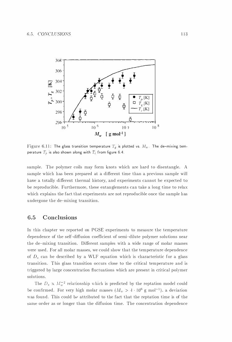
6 . 5 . CONCL US/ONS
308�------------------------------�
306
� 304 '--'
�e" 302
�",. 300
298
• Tp [K] o T� [K]
- Tc (K]
296 +-�����--���������� 1 0 5 1 0 6 1 0 7 1 0 8
Mw [ g mol-l ]
1 1 :3
Figure 6. 1 1 : The g lass t ransit ion temperat u re Tg is p lotted vs. Mu, ' The de-mixing tem
pera t u re Tp i s a lso shown a long with Tc from figu re 6 . 4 .
sample . The polymer coils may form k nots which are hard to disentangle. A
sample which h as been p repared at a d i fferent t ime than a previous sample wi l l
have a totally d ifferent thermal h istory, and experiments cannot be expected to
be reproducib le . Fu rthermore , these entan glements can take a long t ime to relax
which expl ai ns the fact that experiments are not reprod ucible once the sample h as
u ndergone the de-mixing transitio n .
6.5 C onclusions
I n t h is chapter we reported on PGSE experiments to measu re the temperatu re
dependence of the self-diffusion coefficient of semi-d i l u te polymer sol u tions near
the de-mixing transit ion . Different samples with a wide range of molar masses
were used . For al l molar masses, we could show that the tem peratu re dependence
of Ds can be described by a WLF eq uation wh ich is characteristic for a glass
transit io n . T his gl ass transition occurs close to the critical tem peratu re and is
t riggered by large concentration fl uctuations which are presen t in cri t ical polymer
sol u tions.
The Ds Je J [,� 2 rel ationsh i p w hich is pred icted by the reptation model could
be confirmed . For very h igh molar masses ( .\Iw > ·f · l OG g mol- I ) . a deviation
was fou nd . This could bi:' attr ibu ted to the fact that the reptation t ime is of the
SaJlle order as or longer t han t he d iffusion t ime. The concentration dependence
CHAPTER 6. DIFFUSIO,\[ MEASUREMENTS
of Ds appears to show a cross�over from Ds ex cp- 1 .7 ,S behaviou r to Ds ex (p�3.0
behaviou r with i ncreasing concentration . However , i t cou ld not be decided whether
the appa.rent exponent varies smooth ly as in P hi ll ies' model or shO\vs a \vel l�defined
c ross-over between asymptotic behaviou r as i n the reptation model .
From the experimental values for Ds the reptation t imes cou ld be extracted .
I n chapter I we introd llce an independent method to obtain these parameters . \Ve
\vi l l t hen compare these values with the ones reported i n th is chapter .
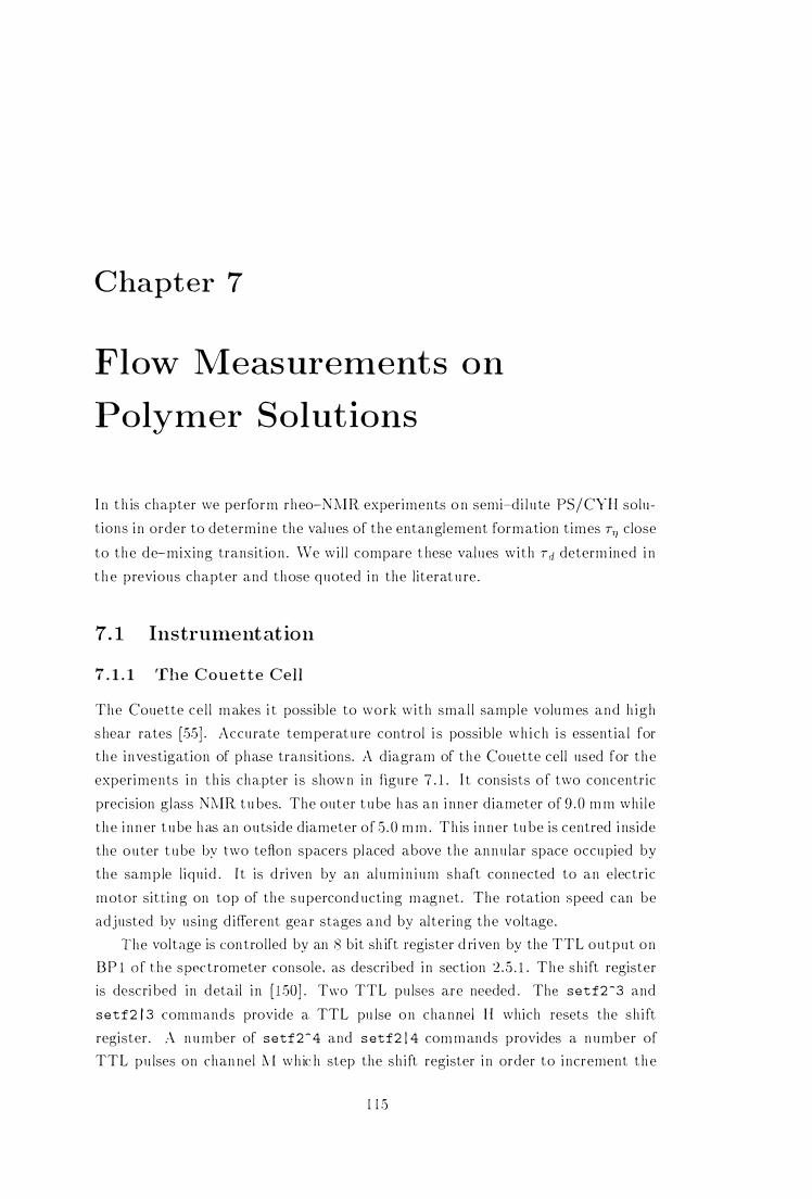
Chapter 7
Flow Measurements on
Polymer Solutions
I n t h is chapter we perform rheo-NMR experiments o n semi-di l u te PS/CYH solu
t ions i n order to determine the val ues of the entanglement formation t imes TT) close
to the de-mixing transit ion . We wi l l compare t hese values with Td determ ined i n
t h e previous chapter and those quoted i n the l iterat u re .
7. 1 Instrument at ion
7 . 1 . 1 The C o u e t t e Cell
The Couette ce l l makes i t possible to work with smal l sample volumes and h igh
s hear rates [SS] . Accurate temperat u re control i s possible wh i ch i s essential for
the investigation of phase transitions. A diagram of the Couette cell used for the
experiments i n t h is cha,pter i s shown in figure 7 . 1 . I t consists of two concentric
precision glass NMR tu bes. The outer t u be has an i nner diameter of 9 . 0 m m whi le
t he i nner t u be has an outside diameter of ,5 . 0 m m . Th is i nner tu be is centred i nside
the ou ter t u be by two teflon spacers placed above the annu lar space occupied by
the sample l iqu id . I t is d riven by an al um in i um shaft connected to an electr ic
motor sitti ng on top of the supercond ucting magnet. The rotation speed can be
adjusted by using d ifferent gea r stages and by alter ing the voltage .
The volta.ge is control led by an 8 bit sh ift register d riven by the TTL output on
BP 1 of the s !)('ctrometer console, as descri bed i n section 2 . 05 . 1 . The sh ift register
is d('scri b('d in detail i n [ I SO] . T\\'o TTL puls('s are needed . The setf2-3 and
setf2 / 3 commands provide a TTL pu ls(' on chanl1('1 H which resets the sh i ft
register. A nu mber of setf 2 - 4 and s etf2 [ 4 com m ands provides a n umber of TTL pu lses on chan nel I'll whic h step the sh i ft register i n order to i ncrement t he
L L !)
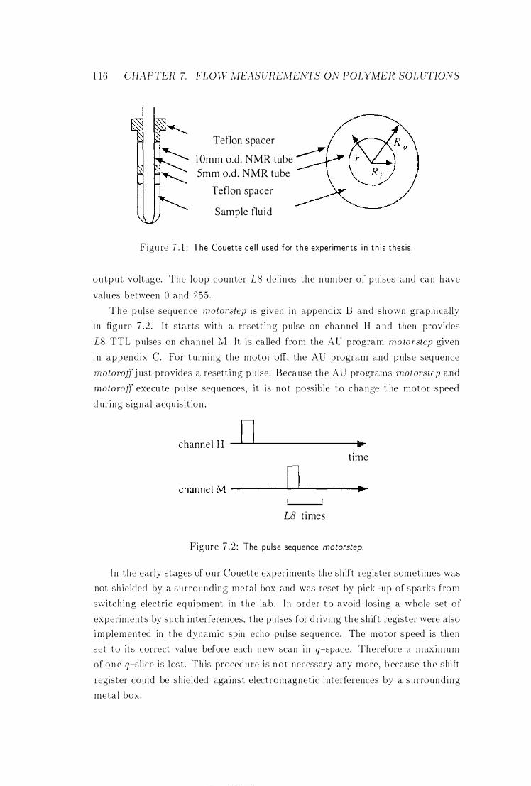
1 1 6 CHAPTER 7. FLOW AIEAS URE;\IENTS ON POLYl'vIER SOL UTIONS
Teflon spacer
l Omm o.d. NMR tube � 5mm o.d. NMR tube
Teflon spacer
S ample flu i d
Figu re 7 . l : The (ouette ce l l used for t he exper iments i n t h i s thesis .
output voltage. The loop counter L8 defi nes the n umber of pulses and can h ave
values between 0 and 255 .
The pulse sequence motoT'step is given i n append ix B and shown graphically
III figure 7 .2 . I t starts with a resett ing pu lse on channel H and then provides
L8 TTL pulses on channel Iv1. It is called from the AU program rno toT'step given
i n appendix C. For t urn ing the motor off, the AD program and pulse sequence
moto1'Off j ust provides a resett i ng pulse. Because the AD programs motoT'step and
m.otoroff execu te p u lse sequences , it is not poss ible to c hange t he motor speed
d ur ing signal acqu is i t ion .
channel H D time
channel M ____ --LD--I-____ -1 .........
L8 t imes
Figure 7 .2 : The pu lse seq uence motorstep.
I n the early stages of ou r Couette exper iments the sh ift registe r sometimes was
not sh ielded by a su rrounding metal box and \vas reset by pick-up of sparks from
s\vitch i ng electr ic equ ipment i n t he lab. I n order to avoid los ing a whole set o f
experiments by such interferences. t he pu lses for d riv ing the sh ift register were also im plemented in t he dynamic spin echo pu lse sequence. The motor speed is then
set to i ts correct va l ue before each new scan i n q-space. Therefore a maximum
of one q-sl ice is lost. Th is procedu re is no t necessary any more, b ecause the shi ft
register could be shielded aga.inst electromagnetic i nterferences by a su rround ing
metal box.
7.2. EXPERIMENTAL 1 17
7. 1 . 2 Data A nalysis
Although our Couette cel l does not measu re the torque (and t herefore the v iscos
i ty ) , we can st i l l extract i m portant rheological i n formation from ou r data. The
power law i ndex n can be extracted from the experimental velocity profi les lls ing
equ at ion 5 .4 1 , where n is t he on ly adjustable parameter and can be fi tted us ing a.
least squares fi t . The computer prograrn PowerLawFit was 'vvri t ten for th i s p u r
pose. I t reads the exper imental v vs. r data and fits 11 from equ at ion 5 . 4 1 by a
least squares fi t , where ri, r 0 and Wo are given parameters . 1'he data a.re then
d isplayed as v vs. 1' ( 1 - (r/ro) -2/n. n i s i ndependent of r i f a straight l i ne resu lts .
O therwise n depends on ,. and t herefore on -y , and the data h ave to be analysed
with a different method.
The local shear rate -yer) can be calcu lated us ing equ at ion 5 .43 . The compu ter
p rogram Der'illa live n urnerical ly ca lc u lates the derivative of a :r:y data set lls i ng a
regression l i ne th rough 11 p to n ine neighbouri ng points . It fol lows from equation
5J14 t hat a graph d isplay ing log -y vs. log r h as the s lope -2/71 . A change i n
s lope o f such a graph therefore i ndicates a shear rate dependence o f n . None of
t,hp experilm;nts reported in t h is chapter showed t h is effect . Because a llumer ical
der ivative of noisy data is not very accu rate , n was obtainE�d by a least squares fit
w hich is n u merically much more robust .
7 . 2 Experinlental
7 . 2 . 1 S a nlple Preparation
Each sample used for the experiments i ll t h is chapter was p repa.red in a. la m m
o .d . N M R t u be w hich was subsequent ly 1lsed as t he ou ter cyl i nder of the Couette
cel l s hown in fig u re 7 . 1 . A pproximately 50 mg of PS was weighed i nto the NMR tu be, and the r ight amount of CYE was added to rnake a solu tion wi th a m ass
concentration of PS sam ples wi th 1O-G A1w 1 .75 , G .85 , 9 . 35 and 1 5 .0 g
rnol- [ were used . The molecu lar weight d istri butions are g iven i n table 5 . 1 . 1'be
t u be was subsequent ly closed with a p lastic cap and stored i n a glass bottle i nside
a wa.ter bath at 600 C for at least 6 weeks. I n order to speed u p t he m ixin g
process, t h e sam plE'S were occasionally st irred . T h e glass bottles were fil led w i th
smal l amounts of CYH to reduce solvent evaporation from the sample t ubes.
A fter the m ix ing period , a 5 m m o . d . NMR t ube with the tefl on spacers was
i n serted into the sa.mple t u be and connected to the Bruker NMR probe. Al l i tems
in contact with the sample were pre--heated at 60° C to prevent thE' sam ple from
dp mix ing .
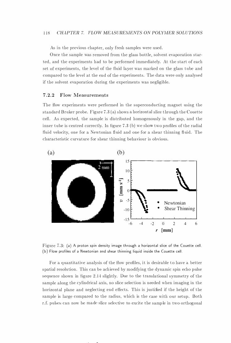
1 18 CHAPTER 7. FLOW IVIEASURE1'vlENTS ON POLYMER SOL UTIONS
As i n the previous chapter , only fresh samples were used .
O nce the sample was removed from the glass bottle , solvent evapo ration star
ted , and the experiments had to be performed i mmediately. At the start of each
set of experiments, the level of the flu id layer was marked on the glass t u be and
compared to the level at the end of the experiments. The data were on ly analysed
if the solvent evaporation d u ring the experiments was negligible .
7 . 2 . 2 F l ow M e as urements
The flow experiments were performed Jll the supercondu cting magnet using the
standard B r uke r probe. F igure 7 .3 ( a) s hows a horizontal sl ice t hrough the Couette
cell . As expected , the sample is d istr ibuted homogenously i n the gap, and the
i nner t u be is centred correctly. In figure 7 .3 ( b) we show two p rofiles of the rad ial flu i d velocity, one for a Newtonian fl uid and one for a shear t h i nn i ng fl uid . The
characteristic curvature for shear th inn ing behaviou r is obvious.
Ca) Cb) 1 5
1 0 ,......,
5 ..... fn El El 0 I--'
t:::. -5 • Newtonian
- 1 0 • Shear Thinning
- 1 5 -6 -4 -2 0 2 4 6
r [mm]
Figure 7 .3 : (a ) A proton sp in dens ity image th rough a horizonta l s l i ce of the (ouette cel l . ( b ) F low profi les of a N ewton i an a nd shear th i nn i ng l i qu id i ns ide the (ouette cel l .
For a q uantitative analysis of the flow profi les, i t is desirable t o have a better
spati al resolu tion . This can b(� ach ieved by modify ing the dynamic spin echo pulse
sequence shown in figu re 2 . 14 slightly. Due to the t ranslational symmetry of the
sample along the cyl ind rical axis, no slice selection is needed when imaging in the
horizontal plane and neglect ing end e ffects. Th is is j ustified if the height of t he
sample is large com pared to the radius , which is the Case with o u r set up . Both
r . f. p u lses can now be made slice selective to excite t he samp le in two orthogonal
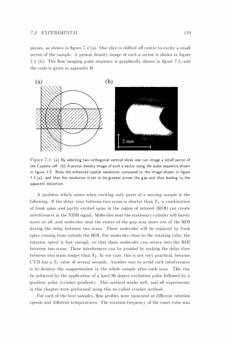
7.2. EXPERLVfENrr�4L L 1 9
planes, as show n i n figure 7.4 ( a) . One sl ice i s sh i fted off centre to excite a smal l
sector of the sam ple. A p roton density i m age of such a sector is shown i n fig u re
7 .4 (b ) . T h e flow i m aging p u lse seq uence is graphically shown i n fig u re 7 .5 , and
the code is given i n append i x B .
(a) Cb)
Figure 7 ./1 : (a ) By selecti ng two orthogona l vert ica l s l ices one can image a sma l l sector of
the Couette cel l . (b) A proton d ensity image of such a sector us ing the pu lse seq uence shown
i n fig u re 7 .5 . Note the enha nced s pati a l resol ut ion compared to the i mage shown i n f igure 7 . 3 (a ) , and that the resol ut ion is set to be greater across the gap and thus leading to the
a pparent distortion .
A problem which arises w hen excit i ng only parts of a moving sample is the
foll owing. If t h e delay t ime between two scans is shorter t h an T] , a , com bination
of fresh spins and partly excited spins i ll t h e region of interest (ROI) can create
i ntprferenceR in t h e NNLR Rignal . Molecu les near t h e stationary cyl inder wi l l barely
m ove at all , and molecu les near the centre of the gap m ay m ove o u t of the ROI
d tui ng t h e delay between t.wo scans . These molecu les wi l l be replaced by fresh
s pi n R coming from o u tside t h e ROL For molecu les dose to the rotat ing t u be, the
rotation speed is fast enough , so t h at these m olecu les can retur n i nto t h e ROI
between two scans. 'fhese in terferences can b e avoided by making t h e delay t ime
between two scans longer t han 1'1' In ou r case, t h is is not very pra.ctical , because
CYH h as a TI val ue of several seconds. Anot h er way to avoid such i nterferenceR
is to dE�stroy the magnetisation i n the w hole sample after each scan . This ca.n
be ach ieved by the application of a llard 90 degree excitation p ulse followed by a
grad ient. pu lse (crusher gradient) . This m et h od works well , and all experiments
i n t h is chapter were performed using t h is so�call ed crusher m ethod .
For each of t h e fou r sampleR, flow profi les were rneas u red at d i fferent rotation
s peeds and d iffeH�nt tem perat ures. The rotation frequency of the i nner t u be was
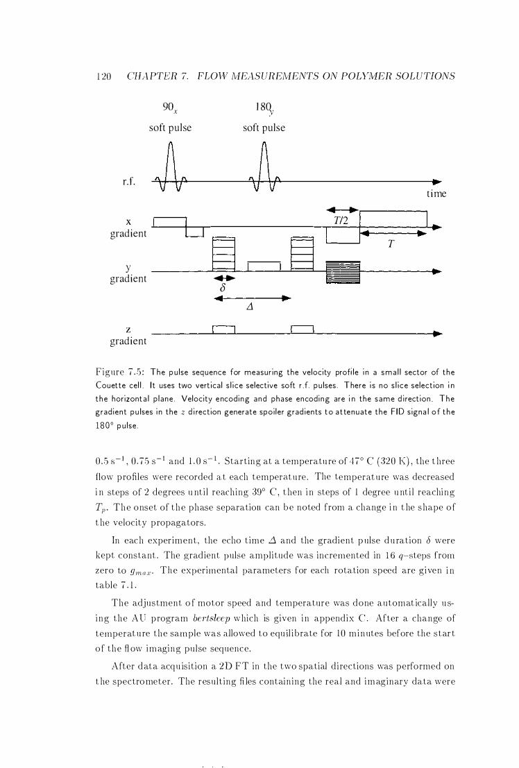
1 20 CHA PTER 7. FLOW MEASUREMENTS ON POLYlvlER SOL UTIONS
d.
x gradient
Y gradient
z gradient
90x soft pulse
�� V V
b ...
8 ..
I I
1 8�. soft pulse
�� VV
... L1
I I
• t i me
.. . TI2 I I .
.. I .. T
.-
Figure 7 .5 : The p u lse sequence for measur ing the velocity profi le i n a sma l l sector of the
(ouette cel l . I t uses two vert ica l s l i ce selective soft r .f. p u lses . There i s no s l i ce selection i n
t he horizont a l p l ane . Velocity encodi ng and phase encodi ng are i n the same d i rect ion . The
grad ient pu lses i n the z d i rection generate spoi ler grad ients to attenuate the F ID s igna l of t he
1800 p u lse .
0 .5 8-1 , 0 . 75 s- 1 and 1 . 0 8- 1 . Starting at a temperatu re of 47° C ( 320 K) , the t hree
flow profiles were recorded a.t each tempera.t u re . The temperatu re was decreased
i n steps of 2 degrees u nt i l reach ing 39° C , t hen i n steps of 1 degree u nt i l reachi ng
Tp . The onset of t he phase separatioll can be noted from a change i n t he s hape o f
t he velocity p ropagators.
In each exper iment , the echo t ime .6 and the gradient p ulse d u ration [j were
kept constant . The grad ient pulse ampl itude was incremented in 1 6 q-steps from
zero to gmax' The experimental parameters for each rotation speed are g iven i n table 7 . 1 .
The adjustment o f motor speed and temperature was done automat ically u s
i ng the AU program bertsleep which is given i n append ix C . After a change of
temperat u re the sample was a.llowed to equ il i b rate for 10 minutes before the star t
of the fl ow imaging pu lse sequence.
After data acqu isit ion a 2D FT in the two spatial d i rections was performed on
t he spectro meter. The resu l t ing fi les contain ing the real and imaginary data were
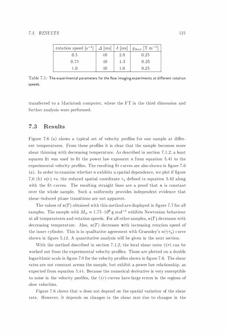
1. 3. RES ULTS
rotation speed [S- l ] L1 [ms]
0 . 5 4 0
0 . 75 4 0
l .0 , 10
J [ms]
2 . 0
l . :3
1 .0
9max [T m-I ]
0 .25
0 . 2·5
0 .2 5
1 2 1
Table 1 . 1 : The exper imenta l parameters for the flow i maging experiments a t d ifferent rotat ion
speeds .
transferred to a ;\[acin tosh computer , where the FT i n the th i rd d imension and
fu rther analysis were performed .
7 . 3 Results
Figure 1.6 (a ) shows a typical set of velocity p rofiles for one sample at d iffer
ent temperat u res . From these profi les it is clear that the sample becomes more
shear th i nn ing with decreasing temperat u re . As descri bed i n section 1. 1 . 2 , a least
squares fit was used to fi t the power l aw exponent n from equ ation 5 . 4 1 to the
experimental velocity profiles. The resu lt ing fi t c urves are also shown i n figure 7 .6
(a ) . I n order to examine whether n exhibits a spatial dependence, we plot i f figu re
7 .6 ( b ) v (r ) vs. the reduced spat ial coord i nate rs defined i n equ at ion 5 .42 along
with the fi t c u rves . The resu lt ing straight l ines are a proof that n is constant over the whole sample. Such a u ni formity provides independent evidence that
shear-induced p hase t ransi t ions are not apparent .
The values of n (T) obtained with th i s method are displayed in figure 7 .7 for all
samples . The sample with Mw == 1 . 75 . 1 06 g m o]- l exhib i ts Newtoni an behaviou r
at all temperatu res and rotation speeds. For all other samples, n (T) decreases with
decreasing temperat u re . Also , n (T) decreases vvi th increasin g rotation speed of
the i nner cyl inder . Th is is i n qual itative agreement with Graessley 's n ()T1) ) c urve
shown in figure 5 . 1 2 . A quant itative analysis wi l l be given in the next section .
With the method described i n sect ion 7 . 1 .2 , the local shear rates 1' ( r) can be
worked out from the experimental veloc ity profiles. Those are plotted on a double
logar ithmic scale in figu re 7.8 for the veloc i ty profiles shown in figu re 7 . 6 . The shear
rates are not constant across the sam ple, bu t exh ib i t a, power l aw relationsh i p , as
expected from equation :') .1 .1 . Because the n umerical derivative is very s ll scepti ble
to noise in the veloci ty profi les, the 1' ( 1' ) cu rves have large er ro rs in the regions of
slow velocities .
Figu re 7 .G shows that n does not depend on the spatial variation of the shear rate. H owever , it depends on changes i ll the shear rate d ue to ch anges in the
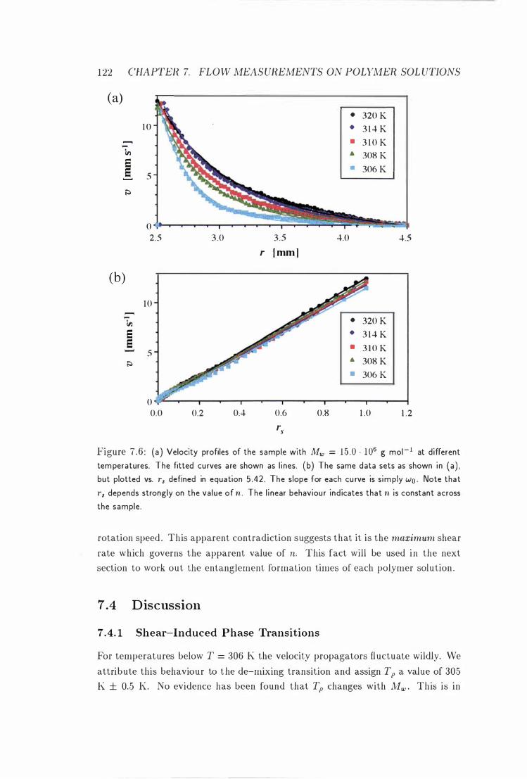
122 CHAPTER 7. FLO W MEAS UREME TS ON POLYMER SOL UTIONS
(a) • 320 K
1 0 • 3 1 4 K ,....., • 3 1 0 K -
ill .. 308 K a • 306 K e 5 .......
i;:l
0 2.5 3.0 3.5 4.0 4.5
r [ mm ]
(b) 1 0
.- • 320 K ill e • 3 1 4 K e • 3 1 0 K ....... 5 i;:l .. 308 K
• 306 K
0 0.0 0.2 0.4 0.6 0.8 1 .0 1 .2
rs
Figure 7 .6 : (a ) Velocity profiles of the sample with Mw = 1 5 . 0 . 1 06 g mol- 1 at different
temperatures. The fitted curves are shown as l i nes. (b) The same data sets as shown in (a) ,
but plotted vs. r3 defined in equation 5.42. The slope for each cu rve is simply Wo . Note that
r 3 depends strongly on the value of n . The l i near behaviour indicates that n is constant across
the sample.
rotation speed . This apparent contradiction suggests that it is the maximum shear
rate which governs the apparent value of n. This fact will be used in the next
section to work out the entanglement formation times of each polymer solution .
7.4 Discussion
7.4.1 Shear-Induced Phase Transitions
For temperatures below T = 306 K the velocity propagators fl uctuate wildly. We
attribute this behaviour to the de-mixing transition and assign Tp a value of 305 K ± 0.5 K. No evidence has been found that Tp changes with Mw . This is in
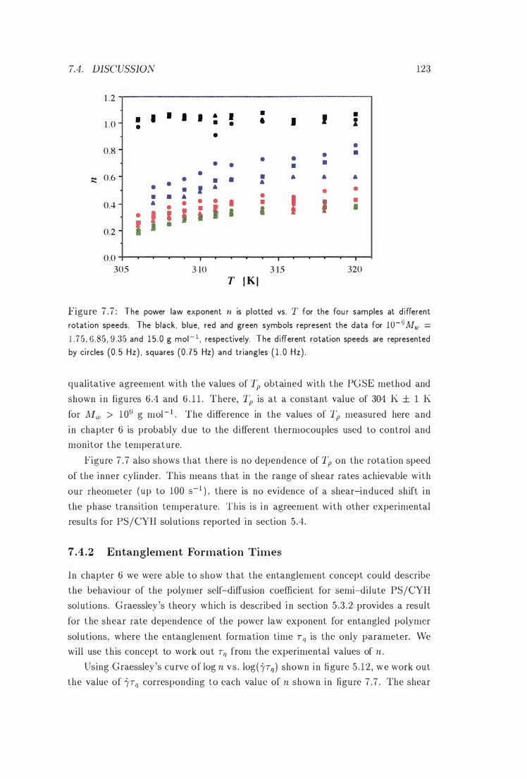
7.4 . DISCUSSION 123
1 .2
• • • • A I • I • • • • •
1 .0 • • A • •
• 0.8 • •
• • • • • • 0.6
• • A • • ;:: • • • • • • • I • • • • • • • I • • • • I • I •
0.4 • • I I • • I I I t I I •
0.2
0.0 305 3 10 3 15 320
T [ K]
Figure 7 . 7 : The power law exponent n is plotted vs. T for the fou r samples at different
rotation speeds. The black, blue, red and green symbols represent the data for 1 0 - 6 Mw =
1 . 75 , 6.85, 9 .35 and 15 .0 g mol - I , respectively. The different rotation speeds are represented by ci rcles (0 .5 Hz) , squares (0 .75 Hz) and tr iangles ( 1 . 0 Hz) .
qualitative agreement with the values of Tp obtained with the PG SE method and
shown in figures 6.4 and 6 . 1 1 . There, Tp is at a constant value of 304 K ± 1 K
for Mw > 106 g mol-I . The difference in the values of Tp measured here and
in chapter 6 is probably due to the different thermocouples used to control and
monitor the temperature.
Figure 7 .7 also shows that there is no dependence of Tp on the rotation speed
of the inner cylinder. This means that in the range of shear rates achievable with
our rheometer (up to 100 S- I ) , there is no evidence of a shear-induced shift in
the phase transition temperature. This is in agreement with other experimental
results for PS/CYH solutions reported in section 5.4.
7.4.2 Entanglement Formation Times
In chapter 6 we were able to show that the entanglement concept could describe
the behaviour of the polymer self-diffusion coefficient for semi-dilute PS/CYH
solutions. G raessley's theory which is described in section 5.3 .2 provides a result
for the shear rate dependence of the power law exponent for entangled polymer
solutions, where the entanglement formation time TI/ is the only parameter. We
will use this concept to work out TI/ from the experimental values of n . Using G raessley's curve of log n vs . log( 1'TI/ ) shown in figure 5 . 12 , we work out
the value of 'YTI/ corresponding to each value of n shown in figure 7 .7 . The shear
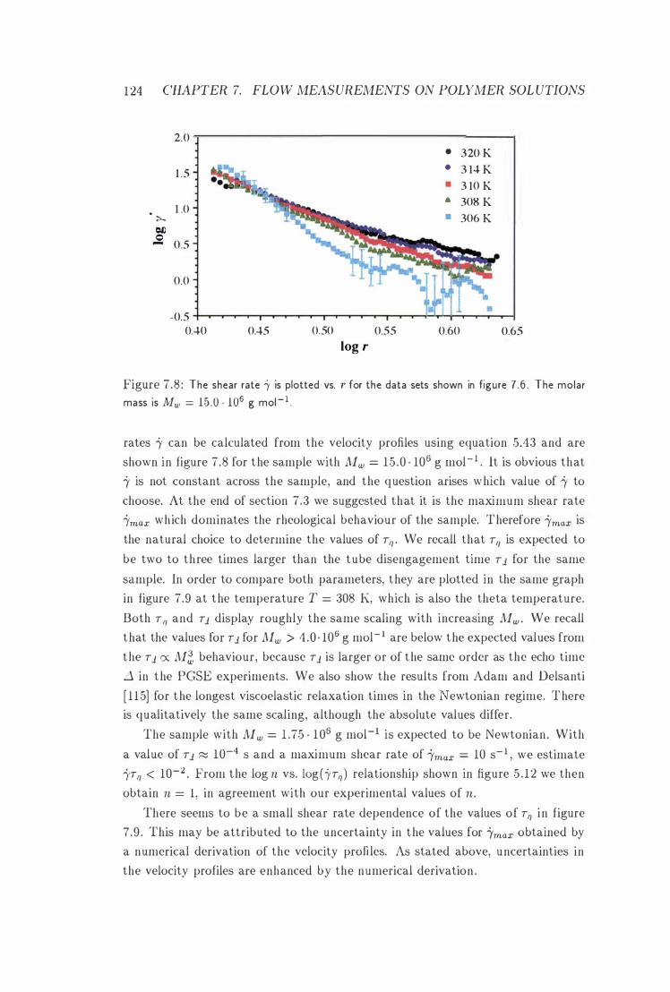
1 24 CHAPTER 7. FLO W MEAS UREMENTS ON POLYMER SOL UTIONS
2.0 • 320 K
1 .5 • 3 14 K • 3 10 K
1 .0 • 308 K
>- • 306 K Cl) 0
0.5 -
0.0
-0.5 0.40 0.45 0.50 0.55 0.60 0.65
log r
Figure 7 .8 : The shear rate '1 is plotted vs. r for the data sets shown in figure 7 .6 . The molar
mass is Mw = 15 . 0 . 106 g mol - l .
rates l' can be calculated from the velocity profiles using equation 5.43 and are
shown in figure 7 .8 for the sample with Mw = 15 .0 . 106 g mol- i . It is obvious that l' is not constant across the sample, and the question arises which value of l' to
choose. At the end of section 7 .3 we suggested that it is the maximum shear rate
1'max which dominates the rheological behaviour of the sample. Therefore 1'max is
the natural choice to determine the values of TI) ' We recall that TI) is expected to
be two to three times larger than the tube disengagement time TJ for the same
sample. In order to compare both parameters, they are plotted in the same graph
in figure 7 .9 at the temperature T = 308 K, which is also the theta temperature.
Both TI) and TJ display roughly the same scaling with increasing Mw. We recall
that the values for TJ for Mw > 4 .0 . 106 g mol- 1 are below the expected values from
the TJ ex: M� behaviour, because TJ is larger or of the same order as the echo time
Ll in the PGSE experiments. We also show the results from Adam and Delsanti
[ l l5] for the longest viscoelastic relaxation times in the ewtonian regime. There is qualitatively the same scaling, although the absolute values differ.
The sample with Mw = 1 .75 . 1 06 g mol-1 is expected to be Newtonian. With
a value of TJ ;:::;; 10-4 s and a maximum shear rate of 1'max = 10 S- I , we estimate 1'TI) < 10-2 • From the log n vs. 10g (1TI) ) relationship shown in figure 5 . 12 we then
obtain n = 1, in agreement with our experimental values of n. There seems to be a small shear rate dependence of the values of TI) in figure
7 .9 . This may be attributed to the uncertainty in the values for 1'max obtained by
a numerical derivation of the velocity profiles. As stated above, uncertainties in
the velocity profiles are enhanced by the numerical derivation .
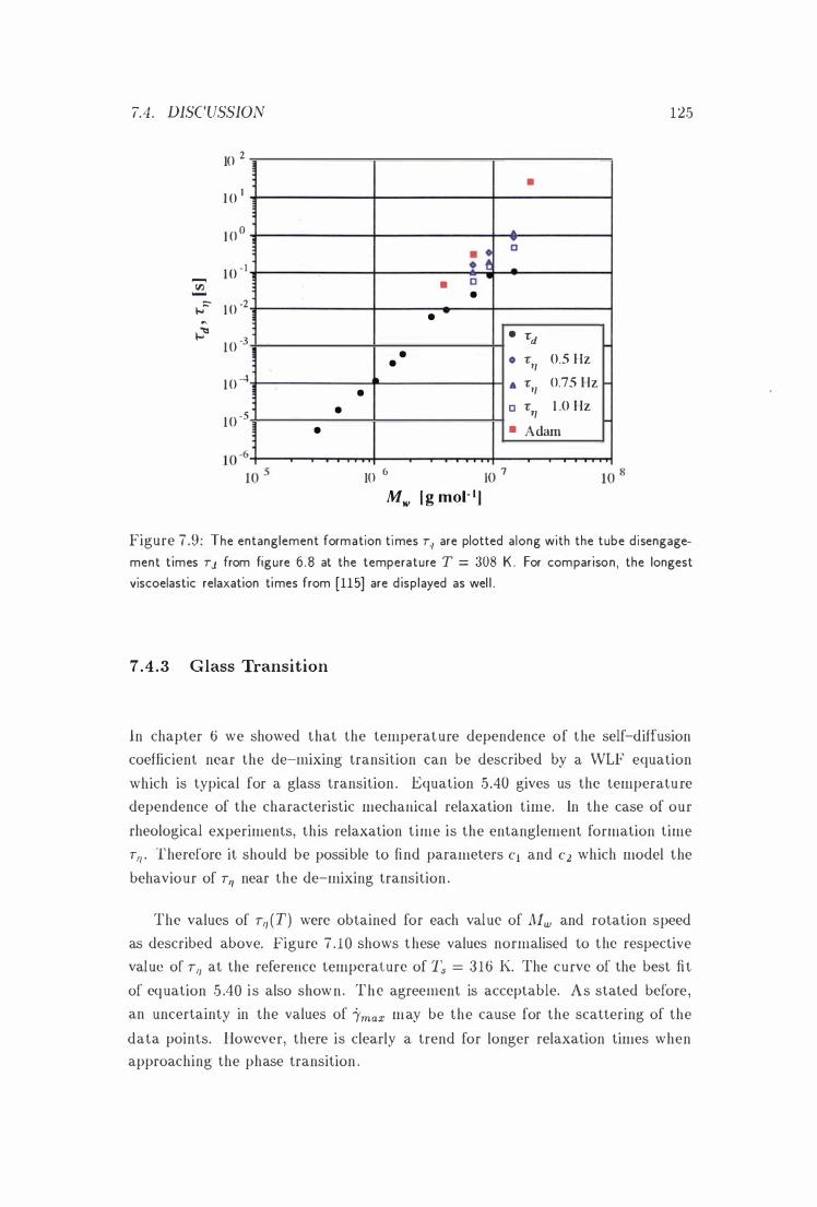
7.4 . DISCUSSION
10 2
1 0 1
1 0 °
....... lO -1 [/) ......
f-o"" lO -2 �
f-o� 10 -3
10 -4
10 -5 •
•
: t • C
• •
• •
•
10 6 la 7 Mw [ g moP]
125
•
.. -c
...
• 1:d o 1:YI 0.5 Hz
A 1:1) 0.75 Hz
C 1:1) 1 .0 Hz
• Adam
Figure 7.9 : The entanglement formation times T./ are plotted along with the tube d isengage
ment times TJ from figure 6 .8 at the temperature T = 308 K . For comparison , the longest viscoelastic relaxation times from [115] are d isplayed as wel l .
7.4.3 Glass Transition
In chapter 6 we showed that the temperature dependence of the self-diffusion coefficient near the de-mixing transition can be described by a WLF equation
which is typical for a glass transition . Equation 5.40 gives us the temperature dependence of the characteristic mechanical relaxation time. In the case of our
rheological experiments, this relaxation time is the entanglement formation time Tf/ ' Therefore it should be possible to find parameters Cl and C2 which model the
behaviour of Tf/ near the de-mixing transition .
The values of Tf/ (T) were obtained for each value of Mw and rotation speed as described above. Figure 7 . 10 shows these values normalised to the respective value of Tf/ at the reference temperature of Ts = 316 K. The curve of the best fit
of eq uation 5 .40 i s also shown. The agreement is acceptable. As stated before, an uncertainty in the values of "Ymax may be the cause for the scattering of the
data points. However, there is clearly a trend for longer relaxation times when approaching the phase transition .
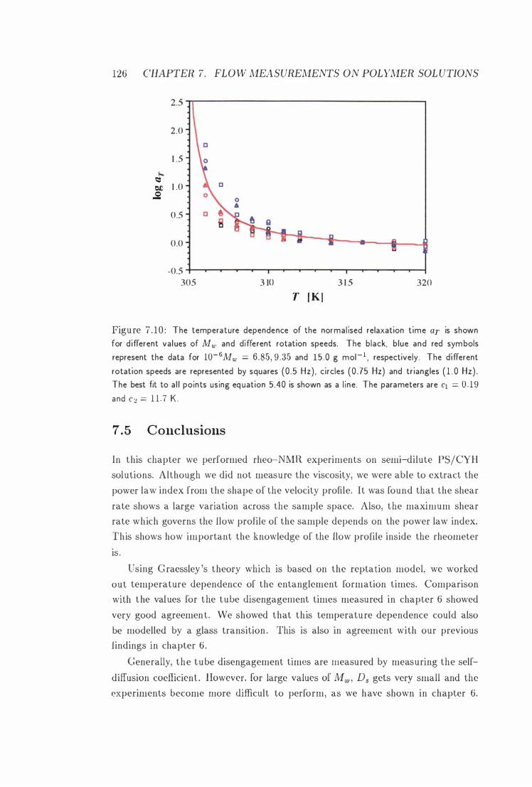
126 CHAPTER 7. FLO W MEASUREMENTS ON POLYMER SOL UTIONS
2.5�--------------------------------------�
2.0
1 .5
e-. � OIl 1 .0
.s 0.5
0.0
-0.5 305 3 10 3 1 5 320
T fK l
Figure 7 . 10 : The temperature dependence of the normal ised relaxation t ime aT is shown for different values of Mw and different rotation speeds. The black, blue and red symbols
represent the data for 10- 6 Mw :::: 6.85, 9 . 35 and 15 .0 g mol- I , respectively. The different
rotation speeds are represented by squares (0 .5 Hz) , circles (0 . 75 Hz) and triangles ( l . 0 Hz) . The best fit to a l l points using equation 5.40 is shown as a l ine . The parameters are Cl :::: 0 . 1 9
and C 2 :::: 1 1 . 7 K .
7.5 Conclusions
In this chapter we performed rheo-NMR experiments on semi-dilute PS/CYH
solutions. Although we did not measure the viscosity, we were able to extract the
power law index from the shape of the velocity profile. It was found that the shear
rate shows a large variation across the sample space. Also, the maximum shear rate which governs the flow profile of the sample depends on the power law index.
This shows how important the knowledge of the flow profile inside the rheometer
is .
Using G raessley 's theory which is based on the reptation model, we worked
out temperature dependence of the entanglement formation times. Comparison
with the values for the tube disengagement times measured in chapter 6 showed
very good agreement . We showed that this temperature dependence could also
be modelled by a glass transition . This is also in agreement with our previous findings in chapter 6.
Generally, the tube disengagement times are measured by measuring the self
diffusion coefficient . However, [or large values of Mw , Ds gets very small and the
experiments become more difficult to perform, as we have shown in chapter 6.
I . ·) . COSCL L'SIOXS 1 27
The m ethod descri bed in th is chapter p rovides an alternative . We h ave shown
that this method works partic ularly wel l for long T1]' For short TT) very h igh
shear rates are req u i red to find non-Newtonian behaviou r . Thus we h ave two
com plementary methods which can be used to measure the disentanglement t imes
of polymer sol u tions: For short T'7 and smal l val ues of lHw , the m easurement of
the self-di ffusion coefficient us ing the PGSE method p rovides better res u l ts . With
i n creasing J\;!w , the PGSE experiments become harder to perform , and the flow
imaging method provides better resu lts . I t is also important to note t hat the latter method measu res the NNIR sign al of the solvent and is t herefore not l imi ted by
the generally short T2 relaxation t ime of the polymer molecu les.

1 28 CHAPTER I. FLO\V ;HEAS URKHESTS ON POLYMER SOL UTIONS
C hapter 8
Convection in a Capillary
8 . 1 Intro duction
Consider a horizontal layer of an incompressible fl u id , wh ich i s heated from below ,
as shown i n figure 8 . 1 . The flu id at the bottom wil l be less dense tha.n the ft uid
at the top. This potentially u nstable arrangement wi l l have the tendency to re
d istr ibute itself i n such a way that the denser layer tends to m ove to the bottom .
H owever, t h is tendency of t he fl uid to move wi l l be i n h ib i ted by i ts own viscosity.
We expect therefore that the temperature gradient must exceed a crit ical value
before the i nstabili ty can manifest i tself. The flow caused by th is i nstabil ity i s known as convection . Convection i n general means fl uid motions caused by tem
perature d ifferences with t he temperat u re gradient pointing in any d i rection , bu t
i n t h is work we wil l o nly consider the case, where the fl uid i s heated from below .
cool , denser l iquid at top subsides
warm, less dense l iquid at bottom is driven up
Heater
Figure 8 . 1 : If a n i ncompressible f luid is heated from below, the warmer and less dense l ayer
at the bottom tends to rise. whi le the cooler a nd denser layer at the top tends to s ink . The res u lt i ng flow is known as convection .
The earliest systematic experiments on convectiona.l flow are those of Benard
I l1 1 900 [ 1 52, 153) . He shov,red that a certain tem perature gradient must be ex
ceeded before instabil i ty can set i n , and t hat the motions have a stationary cel lu lar
129
130 CHAPTER 8. CONVECTION EV A CAPILLARY
Figure 8 .2 : Origi n a l photograph showing Benard cel ls a t natu ra l size i n a l ayer of whale o i l .
Taken from [151] .
character with a remarkable symmetry. I f t h e experiment i s performed with s uffi
cient care, t h e cells al ign themselves in a hexagonal structure . A photograph from
Benard 's work is shown i n figure 8 .2 . Lord Rayleigh [ 154] showed a few years later
t hat t he onset of i nstabil i ty is characterised by the numerical valu e of the non
d imensional parameter R, \vh ich is known as the Rayleigh n umber and defined as fol lows:
R - go:6.T 13 - ( . Kt h V
(8 . 1 )
9 denotes the acceleration due to grav ity, d the depth of the layer , 6.T is t he
temperatu re d ifference across the sample, and 0: , Kth , and v are the coefficients o f
volume expansion , t hermal diffusivity, and k inematic v iscosity, respectively, and
defined in the fol lowing way :
0:
Kt h
1/ =
V- I (DV ) DT p ,.\
pCp 7]
P
( 8 . 2)
(8 . 3 )
(8 .4)
cp , 7] . ,.\ and p are the speci fic heat at constant pressure . the viscosity. t hermodyn amic cond uctivity and density, respectively.
Rayleigh 's t reatment of the Benard problem neglects surface e ffects . He i nt ro
d uced what we now call the Rayleigh-Benard problem , \vh ich refers to convection
caused by heating from below which is not affected by su rface tension effects.
Rayleigh a.\so showed t hat when R j ust exceeds a cr it ical va.lu e Rc . a stat ionary
pattern must exist . Chandrasekhar calculated the t heoretical value of Rc to be
1 708 [ 1 .55) , which com pares well with Si lverston 's exper imental val ue of 1 700 ± .5 1
[ t 5G] . These calcu lations assumed that the width of the fl uid layer is much larger
than its depth , so t hat end effects can be neglected . The width can be charac-
8.2. EXPERL\IEi\iTAL 1 :3 1
terised b y the nondimensiona l aspect ratio r == L l d which i s the ratio o f the width
L o f the fl uid layer d i vided by its depth d . '\lost stud ies of convectional flow deal
wi th large aspect ratios. For small values of r the non-sli p boundary condit ions
tend to damp the onset of cr it ical flow. The theoretical treatments of convection
in c i rcu lar containers by C h a r l so n and Sani [ 1 57] and by Catton and Edwards
[ 1 58] both show a sharp i ncrease of Rc for smal l aspect ratios. For example, for
I' = 0 .06 , a value of Rc > 1 0 ' has been reported [ 1 .58] , whereas Rc decreases
rapid ly to Rc J 708 for I' > 5 [ 1 57J .
Good review a rt ic les a bo u t recen t experi m ents o n t he r m al convection have
been pu bl ished by ;\Jorm and et al. [ 1 59J and by C['oss and Hohenberg [ 1 60] . )VIany
references can be found i n l\:oschmieder's book [ 1 5 1J .
Usually, the convectional cells are m ade visible by smal l particles of metal
powder i n the fl u id . Because NMR is a non-invasive techn ique , it is possible to
image the velocity profi les d i rectly. To our k nowledge , t here is only one MRI study
[ 1 6 1J on convect ion . The authors of th is study fou nd steady convective states of
Rayleigh-Benard convection in porous media . These states, which have not yet
been fu l ly u nderstood , depend in a complex manner on the pore packing . We wil l
show t hat such convective states also exist i n a s imple NlvlR t ube and give a more
q uantitative analysis of the velocity profiles .
I n t his chapter , We t ry to answer the q uestion of what happens i f we perform
a PGSE experiment to measure self-diffusion i n a sample where convection i s
present . I n chapter 6 we mentioned that convection causes problems, and we had
to find a special setu p to overcome this . I n the following sections, we wi l l h ave a c lose look at these problems. We will u se th ree d ifferent techniques to measu re
mo lecu lar d isplacements: The PGSE pu lse sequence i ntroduced i n section 2 .4 .4 ,
the spin warp flow imaging pu lse sequence from section 2 .4 . 5 , and the VEXSY
pulse sequence from chapter 4 .
8 .2 Experinlental
For all the exper iments in this section we used a sol ution of 5% polystyrene ( j1w =
1 27 000 ) i n cyclohexane . The sam ple was fl lled i nside a .+ m m o.d . N:\IR t ube .
T h e h ei g h t of t h e silm ple i nside the tube was 25 m m and therefore larger than the h e i g h t of t he r . f. coi l ( 1 :5 m m ) . :\"0 s l i c e select ion was llsed i n either experiment .
The sample \vilS heated i nside the r J. c o i l by a stream of 50° C hot ai r from
below. T h e tem perat u re di fference was .+ I\: across a sample length of 2 . 5 c m . \Ve now t ry to est imate the Rayleigh n um ber for o u r setup . The viscosity T) of
polysty ren e/cyclohex a n e sol u ti ons at 50° C has been measu red by Papazian [ 1 62] .
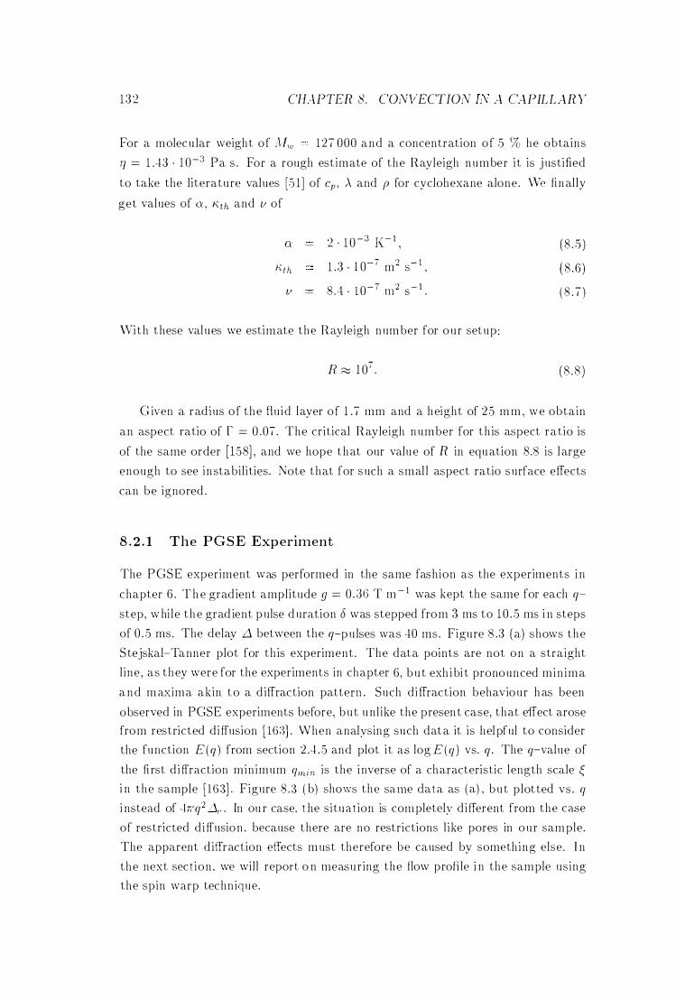
132 CHAPTER 8. CONVECT/Oi'v' IS A CAPILLARY
For a molecu lar weight of ,Hw 127 000 and a concentration of 5 % he obtains
77 = 1 A:3 . 1 0-3 Pa s . For a rough est imate of the Rayleigh n umber i t is j ustified
to take the l iteratu re values [5 1] of cp , A and p for cyclohexane alone . \Ve fi nal ly
get values of 0: , Kth and 1/ of
0:
f),th
IJ
2 ' 1 0 -3 1(- 1 ,
1 .3 · 1 0-' m2 s- l ,
8 .1 . 1 0-7 m2 s- 1 .
\Vi t h t hese val ues we estimate the Rayleigh n um ber for ou r setup :
R ::::::: 1 0' .
( 8 . 5 )
(8 .6 )
( 8 . 7 )
( 8 . 8 )
G iven a radius of the flu id layer of 1 .7 mm and a height of 25 m m , we obtain
an aspect ratio of r = 0 .07 . The cr itical Rayleigh n umber for t h is aspect rat io is
of the same order [ 1.58] , and we hope t hat our value of R in equ ation 8.8 is l arge
enough to see i nstabi l i ties. Note that for such a smal l aspect ratio surface effects
can be ignored .
8 . 2 . 1 The P G S E Exp eriment
The PGSE experiment was performed in the same fash ion as the experiments i n
chapter 6 . T h e grad ient ampl itude 9 = 0 . :.36 T m - I was kept the same for each q
step, w hi le t he grad ient pulse d uration 5 was stepped from 3 ms to 1 0 . 5 ms i n steps
of 0 . 5 ms. The delay .:.1 between the q-pu lses was 40 ms. Figu re 8 .3 (a) shows the
Stejskal-Tanner plot for th is experiment . The data points are not on a straight
l i ne , as they were for the experiments in chapter 6, b u t exh i bi t pronounced m i n ima
and m axima akin t o a d iffraction pattern . Such d iffraction behaviou r h as been
observed in PGSE experiments before, bu t u n l ike the presen t case, that effect arose from restricted d i ffusion [163] . When analysing such data it is hel pful to consider
the function E (q ) from section 2A .5 and plot i t as log E ( q ) vs. q . The q-value of
the fi rst d i ffraction m in imum qmin is the i nverse of a characteristic length scale � i n the sample [ 16 ;)] . Figure 8 . ;) ( b) shows the same data. as (a) , bu t plot ted vs . q
i nstead of ·1r.q2 ..:.l, . . In ou r case. t he s itua t ion is com pletely d ifferent from the case
of restricted d i ffusion . because there are no restrictions l i ke pores in o u r sam ple.
The apparent d iffraction effects m ust therefore be caused by someth ing else. I n
the next sec t ion , we wil l report o n measu ring the flow profi le i n the sample us ing
the spin warp techn ique.
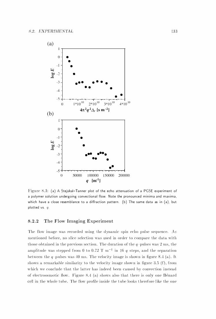
8.2. EXPEHIMENTAL
(a)
(b)
�
o • •
- 1 •
-3
-4 • • • • • • •
• • •
• • -5 +---��---r--�--��--�--�
o 1 * 1 0 10 2* 1 0 10 3* 1 0 10 4* 1 0 10
o •
- I
4n:2q 2,1r [8 m -2]
• •
gf -2 • -
-3
-4 ... . ... •• •
•• -5 ���rT������-r�-r�
o 50000 1 00000 1 50000 200000 q [m-l]
t :3 3
Figll re 8. :3 : ( a ) A Stejskal-Tan ner p lot of the echo atte n uation of a PGSE exper iment of
a polymer sol ut ion u ndergoi ng convection a l flow. Note the pronounced m in ima a nd maxima ,
wh ich have a c lose resemb l ance to a d iffraction pattern . ( b ) The same data as i n ( a ) , but
p lotted vs . q.
8. 2 . 2 The F l ow Imaging Experiment
The flow image was rt�corded using the d ynamic Spi ll echo pu l se sequ ence. As
mentioned before, no s l ice select ion was nSf'd in order to compare the d ata with
t hose obtained i n the p revious section . The d u ration of the q - pu lses was 2 ms, the
am p l i tude was stepped from 0 to 0 . 72 T m-I i n 16 q -steps, and the separation
between the q - p u lses was 11 0 ms. The veloc ity image is show n in figure 8 .4 (a) . It
shows a remarkabl e s imilari ty to the velocity image show n in figu re :� . 5 (0 , from
w hich we concl ude t hat t he l atter h as i ndeed been caused by convection i nst€:'ad
of c1ectroosmotic How . Figure 8.'1 (a) shows also that t here is on ly one Benard
cel l i ll the >vho le t u be. The flow profi le i nside the t u be looks t herefore l ike the one
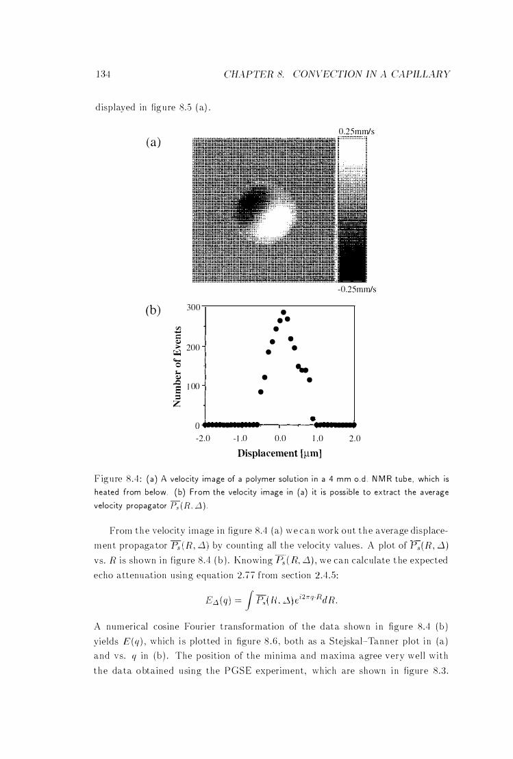
184 CHAPTER 8. CONVECTION IN A CAPILLARY
d isplayed in fig u re 8.5 ( a) .
0.25mm/s (a)
-0.25mm/s
(b) 300 • • •
en • ..... ::: • Q.I • ... 200 • � •
� 0 .. ;... Q.I • • ..Q 5 1 00 • := Z
• O ........ --.-�� .... -2.0 - 1 .0 0.0 1 .0 2 .0
Displacement [)..lm]
F igu re 8 .4 : ( a ) A velocity image of a polymer sol u tion i n a 4 mm o .d . N M R tube , which is
heated from below. ( b) From the velocity image i n (a) it i s poss ib le to extract the a verage
velocity propagator Ps (R, LJ ) .
From t h e velocity image i n figure 8.4 ( a) w e c a n work ou t t h e avera.ge displace
m ent propagator Ps (R , Ll) by count ing all the velocity values . A plot of Ps (R , Ll) vs. R i s shown i n figu re 8 .4 ( b ) . Knowing P s CR, Ll) , we can calcu late t he expected
echo attenua tion usi ng equat ion 2 .77 from section 2 .4 .5 :
E' ( ) - I-p (I') "' ) , £27Cq·R lR .JLl q - . s l , u e (. .
A numerical cosine Fourier t ransformation of the data shown i n figure 8.4 ( b )
yields E(q) , which i s plotted i n figure 8 . 6 , both as a Stejskal�Tanner plot i n (a )
and vs . q i n ( b ) . The posit ion of the m in ima and m ax ima a.gree very wel l w i t h
t he data o btained usi ng the PGSE exper iment , wh ich are shmvn i n figure 8 .3 .
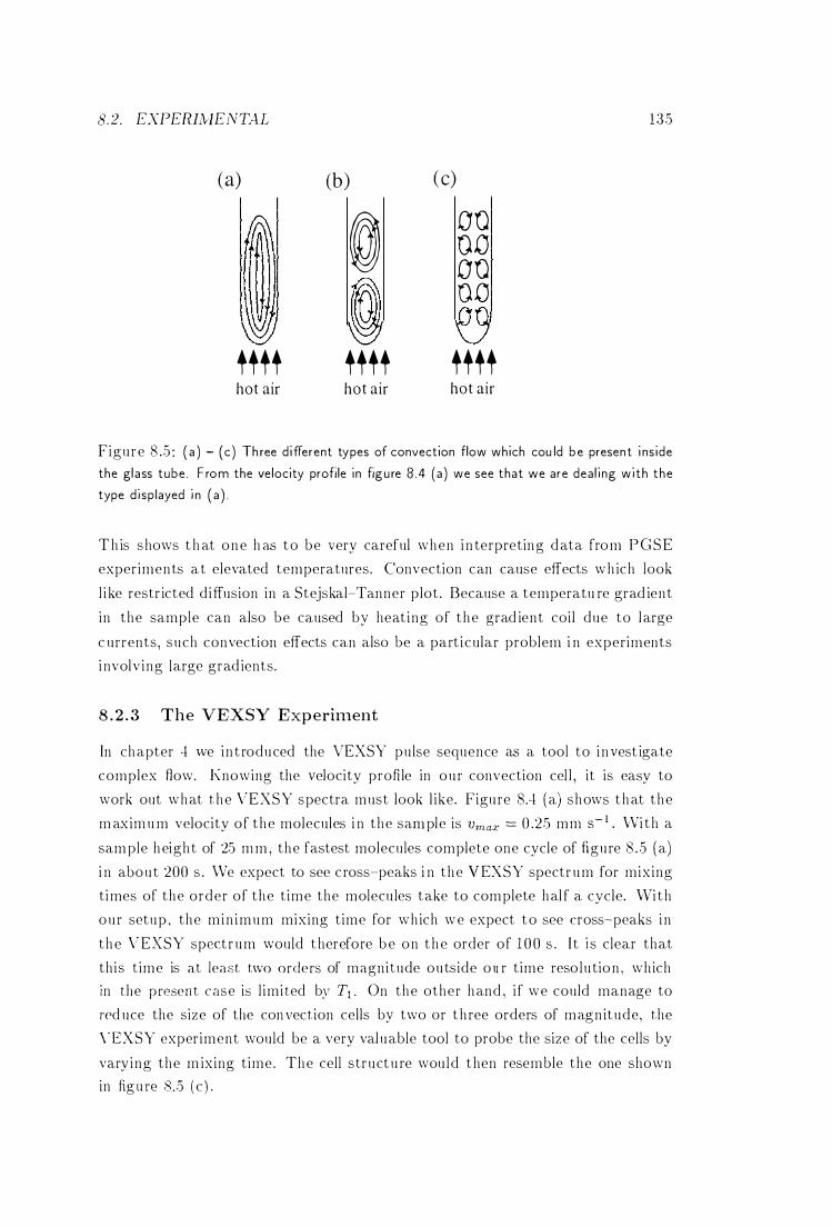
8. 2. EXPERII'vlENTAL
(a)
tttt hot air
(b)
@ � tttt hot air
(c) 00 00 00 00
tttt hot air
135
Figure 8 . . 5 : ( a ) - (c) Th ree d i fferent types of convection flow which cou ld be presen t i ns ide
the gl ass tube . F rom the velocity profile in figu re 8 .4 (a) we see that we are dea l ing with the
type d isp layed i n ( a ) .
T h is shows t h at one h as to be very careful when i n terpreting data from PGSE
exper iments a t elevated temperatures. Convection can cause effects wh ich look
l i ke restr icted d iffusion in a Stejskal-Tanner plot . Because a temperatu re grad ient
in the sample can also be caused by heat ing of the grad ient coi l due to large
c urrents , such convection effects can also be a part i cular problem i n experiments
i nvolv ing large grad ients.
8 . 2 . 3 The VEXSY Exp eriment
In chapter 4 ,'le i n t roduced the VEXSY pulse sequence as a tool to i nvest igate
complex flow. Knowing the velocity profile in ou r convection cel l , it is easy to
work out what the VEXSY spectra must look l ike. Figu re 8,4 (a) shows t hat the
m axim u m velocity of the molecules i n the sam ple is 1)max == 0 .25 mm S- 1 . vVi t h a
sam ple height of 25 m m , the fastest molecules complete one cycle of figure 8 . 5 (a) i n about 200 s . We expect to see c ross-peaks i n the VEXSY spectr um for mix ing
t imes of the order of the t ime the molecu les take to complete hal f a cycle. vVi t h
ou r setup , the m in imum mixing t ime for wh ich we expect to see cross-peaks i n
t he VEXSY spe.ct r um would t herefore be on t h e order of 1 00 s . I t i s clear that
th is t ime is at least two orders of magnitude outside o ll r t ime reso lu tio n , wh ich in the p resen t case is l im i ted by Tr • On the other hand , i f we could manage to
red uce the size of the con vection cells by two or t h ree orders of magn itude, the
\ -EXSY exper iment would be a very val uable tool to probe the size of the cells by
vary ing the m ixing t ime. The cell struct u re wou ld t hen resemble the one shown in f1gUH� 8.5 ( c ) .
1 36
(a)
� 0Jl ..9
(b)
� 0Jl
.£
0
- 1
-2
-3
-4
-5
0
- 1
-2
-3
-4
-5
0
0
CIL-\PTEH 8. CONVECTION IN A CAPILLAR'{
1 * 1 0 10 2* 1 0 10 3* 1 0 10 4* 1 0 10
4n2q 2L1r [s m o2]
50000 100000 1 50000 200000
q [mol]
Figure 8 . 6 : The Four ier t ransform of the velocity propagator disp layed i n figu re 8 .4 (b)
p lotted vs . 41T2 q2 Dr (a) and vs. q(b) .
The V EXSY experiments were performed using the h igh g radient probe de
scr ibed i n section 2 . .5.3 in order to m aximise velocity sensit ivity. The spectra were
recorded us ing 642 phase encoding steps with a grad ient pu lse d uration of !5 = 2 .5
ms, grad ient pu lse ampl itude g = 2.2.') T m 1 and pulse separation Li = 15 ms.
F igure 8 . 7 (a ) and ( b ) d isplay the VEXSY spectra of the solvent for two d ifferent
m ixi ng t imes of Tm = 2.5 ms and Tm = 12.5 ms, respectively. Both spectra are essent i al ly ident ical . The broadening of the spectra is d ue to B rownian motio n . T h is
becomes evident when com pari ng the profi les i n fi gu re 8 . 7 ( a) and 8 .7 (c ) , wh ich
is the two-di mensional VEXSY plot for the polymer. The polymer h as a m uch
smal ler self-d i ffusion coefficient than the solvent , and thus the VEXSY spectrum
i s less broadened . \Ve can estim ate the self-d iffusion coefficients us ing equ ation
8.3. CONCUJSIONS 1 37
(a) (b)
(c)
Fig u re 8 .7 : The two-d imens iona l VEXSY spectra 8(Z1 ) Z2) of a polymer solut ion u nd ergoing
convectiona l flow. The d i sp lacement fie ld of view is 133 Ilm . (a ) The VEXSY spect rum of
the solvent for a short mixi ng t ime ( Tm 25 ms) . (b ) The VEXSY spectrum of the solvent
for a long mixing time ( Tm 1 25 ms) . (c) The VEXSY spectrum of the polymer for a s hort
mix ing t ime (Tm = 25 ms) .
4 .4 . With w id t hs of 1 5 Ilm and 4 Ilm we get val ues of DSolv = 4 . �) . W-9 m 2 s- 1
and Dpo1y = :3 . 5 . 1 0- 10 m 2 s-1 for the self-diffusion coefficient of the solvent and
polymer , respectively.
8.3 Conclusions
In this chapter we examined convectional flow wi th t hree d ifferent methods. I n the sim ple geoll1etry we were using, the velocity field t u rned ou t to be stationary.
I n t h is case , one dynamic spin echo experiment p rovides fu l l i nformation abou t
t h e flow profi le i n th(� sample. From t his flow profile, o n e can extract t h e E(g) function w hich we also obtai ned from the PG SE experiment . For a stat ionary flow p rofile we know that the V EXSY spectr um does not show a.ny cross- peaks .
CHAPTER 8. CONVECTION IN A CAPILLARY
Therefore we can extract the complete i n formation about the flow profile from one
dynamic spin echo experiment if we assume that the velocity field is stationary.
If the molecu lar veloci ties are changing on a t imescale of order 1 0-100 ms,
one h as to perform several experiments with variable delay L1 i n order to probe
these changes . As stated before i n section 4 .3 .3 , the PGSE and dynamic spin
echo methods on ly measure average d isplacements d u ring the delay t ime d. A
set of V EXSY experiments on the other hand yields i n formation about changes i n
veloc i ty more d i rectly.
The dynamic spin echo techn ique requ i res grad ients i n all t hree spatial di
rections. Many modern spectrometers. however, are on ly equ ipped with j ust one
grad ient for d iffusion studies. In th is case, fl ow profi les with a cylind rical geometry
GUl be reconstructed using the PGSE method (.52) . Th is reconstruct ion method
fails when the fl ow is more complex as th is is the case i n ou r convection cell . Then
the VEXSY method , wh ich also uses one gradient d i rection , h as to be used III order to obtain m axim u m information abou t the fl ow profile .
Figu re 8 .7 shO\vs the lim i ts of t he VEXSY method . The spectra i n ( a) and
( b ) are significantly broadened which cou ld be due to self-d iffusion or to changes
in veloci ty. There could be smal l cross-peaks h idden somewhere u nder the broad
spect r u m . The spectr um i n figure 8 .7 (c) demonstrates that th is problem can be
avoided by doping the sample with large molecu les wh ich h ave a m uch smaller self
d iffusion coefficient than the solvent molecules. I t is much narrower and shows no
c ross-peaks. The l imitations of th is doping method are also obvious. I n part icu lar ,
the s ignal-to-noise is generally poor and T2 short wh ich l imits the valu es for t he
possible exchange times.
In t h is chapter we measured the convectional fl ow in a glass t u be . The fl ow
profile could be obtained using the dynam ic spin echo method . From the veloci ty
image we calcu lated the E(q) function and showed t hat i t exhibits pronounced
m in ima and maxima akin to a diffraction pattern . T hese m in ima and m axim a
agree very well with the ones fou nd with PGSE experiments on the same cel l .
With the V EXSY method we could show that the flow field i n the convection cell is stationary.
Chapter 9
S hear-Induced Order in Liquid
Crystals
9 . 1 Lyotropic Systelns
9 . 1 . 1 Intro duction
I n a c rystal the bu i ld ing blocks (atoms or molecules) are arranged in a regu lar
periodic struct u re k nown as a lattice. Translational m otion is m ai n ly frozen ou t .
I n a l iqu id , on the other hand , the bu i ld i ng blocks are completely d isordered
and move rapidly. In section 5 . 3 . 3 we in t roduced the glassy state as a state of
a s upe rcooled l iqu id , where the t ranslational motion is frozen . A nother s tate of
organisation is the mesomorphic state . Such a state shows less symmetry than a c rystal , but more symmetry than a l iqu id . Because t ranslational motion can take
place qu ite easily, these phases are also k nown as l iquid crystals .
L ike crystal latt ices , l iqu id crystal phases are characterised by t heir sym metry.
The m ai n types are nemat ics and smectics and are shown i n figure 9 . 1 .
• Nematics are flu ids of rod l ike molecu les with their centres d isordered , bu t
w i t h a com mon axis o f alignment for t he rods ( figure 9 . 1 (a ) ) .
• S mectics are layered systems. each layer behaving l i ke a two-di mensional
l iq u id . The smectic A type is opt ically u n iaxial ( figure 9 . 1 ( b) , whereas the C type is biaxial ( figure 9 . 1 (c ) . Smect ics are also k nown as lamellar systems.
There are many more phases wh ich are not i mportant for th is thesis . They are
descri bed in references [ l G4, 1 65J .
There m ay be phase t ransitions between d ifferent types of a l iqu id c rystal
when physical parameters are changed . A l iqu id c rystal is called thermotropic i f
the tem peratu re is the on ly variable to im pose phase transitions . Pu re m aterial s
139
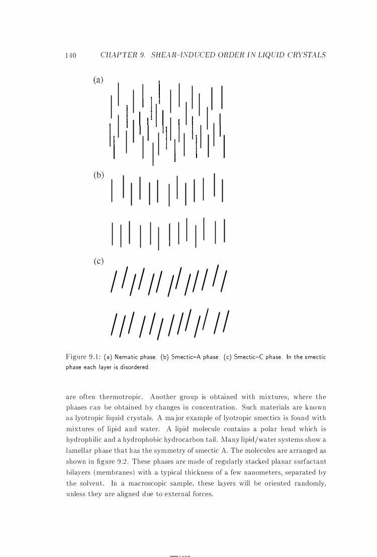
1 "10 CHAPTER D. SHEA R-EVD UCED ORDER IN LIQ UID CR'lSTALS
Ca)
(b)
(c)
I III II II II I II II I I II I II II I I
Figure 9 . 1 : ( a ) Nematic phase . (b) Smectic-A phase . (c ) Smectic-C phase . I n the smectic
phase each l ayer is d i sordered .
are often thermotropic . Another group is obtai ned with mixtures , w here t h e phases can be obtai ned by changes in concentration . S uch materials are k nown as lyotropic l iqu id c rystals. A major example of lyotropic smect ics is found w i th
mixtures of l i pid and water . A l ip id molecu le contains a polar head wh ich is
hyd roph il ic and a hyd rophobic hydrocarbon ta.il . l\Iany l ipid/vlater systems show a
l amel l a r phase that h a..s the sym metry of smectic A . The molecu les are arranged as shown i n fi gu re 9 .2 . These phases a re made of regu la rly stacked planar surfactant
b i layers ( membranes) with a typical t h ickness of a few nanometers, separated by
the solvent . In a macroscopic sample, these layers wi l l be or iented randomly, u nless t hey are a.ligned d ue to external forces.
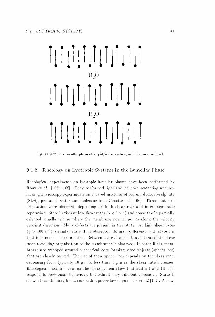
9. 1 . O'OTRDPIC SYSTE,\JS
Figu re 9 .2 : The l ame l l a r phase of a l ip id/water system . i n th is case smectic-A .
9. 1 . 2 Rheology o n Lyotropic Systems i n t h e Lamellar P hase
1 4 1
Rheological experiments on lyotropic lamellar phases have been performed by
Roux et al. [ 166}-[ 1 68} . They performed l ight and neut ron scatterin g and po
laris ing microscopy experiments on sheared m ixtures of sod i um dodecyl-su lphate
(SDS) , pentanol, water and dodecane in a Couette cell [ 166} . Three states of
orientation were observed , depend ing on both shear rate and i n ter-membrane
separat io n . State I exists at low shear rates b < 1 s- l ) and consists of a partial ly
o riented lamellar phase where the mem brane normal points along the velocity grad ient d i rection . Many defects are present in t hi s state. At h igh shear rates
(";( > 1 00 S- 1 ) a s imi lar state I I I is observed . Its main d ifference with state I is
that it is much better oriented . Between states I and I ll , at intermed iate shear
rates a stri k ing organisation of the membranes is observed . In state r r the mem
branes are wrapped around it spherical core forming large objects (spheru l i tes)
that are c losely packed . The ::;ize of these spherul ites depends on the shear rate .
dec reas ing from typica.l ly 10 It nl t.o les::; than 1 pm as the shear rate increases.
Rheological measu rements on the same ::;ystem show that states I and I I I correspond to Newtonian behaviou r . but exh ibit very d i fferent viscosit ies . State I I
shows shear th inn ing behaviou r with a. power law exponent n :::;:; 0 .2 [ 1 67} . A new .
142 CHAPTER g . SHEA R.-EVD UCED ORDER IN LIQ UID CRYSTALS
h igh ly o rganised state h as been found for a mixtu re of SDS, octanol and water at
high shear rates [ 16S] . \Vith increasing shear rate the spherul ites stop changing
the ir s ize and organ ise t hemselves into long-range ordered plane structures sl id
ing over each other. The spherul ites are h exagonal shaped and c losely packed on
tr iangular lattices .
9 . 1 . 3 NMR on Lyotropic S ystems in the Lamellar P hase
T he layered structure and dynamics of lyotropic systems i n the lamel lar p h ase
h ave been exami ned extensively by l\'MR. Here , we are only i nterested i n the
orientation and mobi l ity of the ,vater molecules between the bi layers. Callaghan
et at. performed PGSE experiments on a l ip idjD20 system and s hO\ved t h at t he
water molecules are aligned between the bi layers. T hey also showed that t here
exists an anisotropy i n the self-diffusion coefficient . The water molecu les are much
more mobi le i n the p lane parallel to t he bi layer s urface t han perpend icu lar to i t .
Rheo-NMR experiments on lyotropic l iq u id c rystals have been performed by
Lukaschek e t al. [ 1 69 , 1 70] . For a mixtu re of a nonionic su rfactant with D20 i n
t h e h exagonal phase i t was found that t h e deuteri u m l\'wIR spectra depend o n
t h e shear strain �( . Alignment occ u rs along t h e flow d irection [ 169] . A t t he same
t ime, the v iscosity decreases with increasing shear strai n . Experiments on a m ix
t u re of non ion ic s urfactants with D20 in the lamellar phase revealed a s hear rate
dependence of the deuteri u m l\'M R spectra. Two of the t h ree states of orientat ion
discussed by Rou x et al. , which were described in the previous section , could be
identified [ 170] . At low shear rates, the lamellar layers were found to be oriented
along t he velocity gradient . The deuter iu m N M R spectra also s howed the pres
ence of many defects i n these layers . At h igher shear rates the total l i n e w idth of
the deuteri u m spectra becomes smaller wh ich was found to be consistent w i th the
formation of spheru l ites i n state I l described by ROllX et a t .
The experiments of Roux et al. and Lukaschek et al. show t hat shear stress
causes align ment of the lamellae wh ich red uces the v iscosity of the sample . This
is expected to be reflected i n the velocity profiles i n the Couette cel l . wh ic h wi l l
be reported i n section 9 . 2 . 2 .
:0. 1any othe r :\,),[R experiments on lyotropic l iqu id c rystals h ave been per
formed . for exam ple relaxation t ime and l ine shape measurements. References
to those can be fou nd in [ 1 65]- [ t i2] . H O\vever , they are not i m portant for ou r
rheo-N?\IR experiments.
9.2. EXPERL\[E.\iTAL SECTION
9 . 2 Experilnental S ection
9 . 2 . 1 Sample Preparation
Two d i fferent systems \,/ere used for the experiments descri bed in th is chapter.
Both are s l1 r factants and form a lamel lar phase i ll water at room tem peratu re .
9 . 2 . 1 . 1 Dobanol/vVater
Dobanol h as the chem ical composition C 1 4 H29 ( EOh , w here EO stands for ethylene
oxide (-CnrCHrO-) . The phase d iagram of Dobanol/water mixtures exh i bi ts
a l ame llar phase between concentrations of roughly (l5% and 85% and between
room temperatu re and 85° C. A bove 85° C the sample enters the isotropic phase
[17:3] . The samples were p repared by add ing Dobanol and water i n a 3 : 1 m ass ratio
in a 10 m m o .d . NMR tube. The m ixtu res were then heated i nto the isotropic
phase for mix ing and the 5 mm o .d . NMR tube along with the tenon spacers was
i nserted i nto the sam pIe t ube .
For the experiments described i n section 9 .2 . 3 a Dobanol/D20 sample with
the same m ass concentration was p repared .
9 . 2 . 1 . 2 Aerosol OT /Water
Aerosol OT ( bis ( 2-ethyl hexyl ) sod i um su l fonsucc in ate) ( AOT) is known to form a
lamel lar phase with water at room temperatu re over a wide range of concentrations
[ 174] . At a m ass ratio of 1 ; 1 the phase transit ion to the isotropic phase occ u rs at
a temperatu re of 1 40° C. The samples were prepared by addi ng AOT and water
at a 1 : 1 m ass ratio in a glass t ube which was subsequently sealed and stored at a
tem peratu re of (lO° C for at least two weeks . Duri ng th is period the sample t ubes
were occasionally centrifuged back and forth to ensu re m ixing .
A sample of AOT /D20 with the same m ass concentrat ion was prepared for
the experiments described i n section 9 .2 .3 .
For the NMR measu rements the samples were then transferred i nto a 1 0 m m
o . d . NMR tu b(" , and the .) m m o . d . tube with the teflon spacers was inserted .
Entrapped air bubbles could be reduced by centrifuging the w hole Couette cel l .
9 . 2 . 2 lVleasurem.ent of Flow Profiles
The fl ow pro fi les for the Dobanol/water sa.mple were measured usi ng the same
techn ique as descri bed in chapter I . the experimental parameters being given i n
t h e fi rst l ine o f table 9. 1 . These flow profiles are shown i n figu re 9 . 3 (a) . They
144 CHAPTER 9. SHEA R-iND UCED ORDER iN LiQ UiD CRYSTALS
display a large velocity gradient close to the rotating tube. Further away from
the rotating tube the velocity seems to be almost constant and at the outer wall
the sample appears to slip. In order to monitor this behaviour more closely a
second set of experiments was carried out with a h igher velocity resolution . The
spatial resolution had to be reduced because the echo time L1 was limited by the
transverse relaxation time.
The parameters for the flow imaging are given in the second line of table 9 . 1 ,
while the corresponding flow profiles are shown in figure 9 .3 (b) . ote that the
velocity profiles give accurate values only in the regions of low velocities. Close to
the spinning tube the propagators are broadened significantly due to shear in one pixel.
(a)
,.....-, -
ill
� ........ t::>
(b)
,.....-, ..... � e e ........ t::>
1 6 ,.
14 • 1 .0 Hz 1 2 .- • A A 0.75 Hz • 1 0
8 .-
A • 0.5 Hz A,.
6
4
2
0
-2 2.0 2.5 3.0 3.5 4.0 4.5 5.0
r [ mm ] 2.0
• 1 .0 Hz
1 .5 a 0.75 Hz
.a • • 0.5 Hz •
1 .0 A • • •
A • • • • • • • • •
0.5
• • • • • A A aA a A A A A • • A A A A AA A A A A • • • • • • • • • • • • • • • • • • • • • •
O.O �� .. ��--,-�--���,-������ 2.0 2.5 3.0 3.5 4.0
r [ mm ] 4.5 5.0
Figure 9 .3 : (a) Velocity profiles of Dobanol/Water at different rotation speeds of the inner tube . The arrows mark the calcu lated speeds of the rotating tube. (b) Same profiles as in
(a ) , but measured with a higher velocity resolution . The s l ip at the outer wa l l is obvious.
9.2. EXPERIMENTAL SECTION
Sample Ll [ms]
Dobanol/H2O 15
Dobanol/H2O 20
AOT/ I-bO 15
o [ms]
3 .0
5 .0
2 .0
gmax [T m-I ]
0 .25
0 .25
0.35
Table 9 . 1 : The experimental parameters for the flow imaging experiments.
145
A difficulty arose for the AOT /water sample. It was found that the transverse
relaxation time T2 was on the order of 5 ms. Such a value of T2 is too short
to apply the modified dynamic spin echo pulse sequence from figure 7.5 with an acceptable signal-to-noise ratio. Therefore the velocity profiles for this sample
had to be measured using the normal dynamic spin echo pulse sequence shown in
figure 2 . 14 . The velocity profiles obtained with this method are shown in figure
9 . 4 , while the experimental parameters are given in the bottom line of table 9 . 1 .
1 6
1 4
1 2
10
8
6
4
2
• 1 .0 Hz • • � " 0.75 Hz " • 0.5 Hz " . .
� . " . . " . .
• •• • • • •
• • "" ,, ·. - Itt l· • • • • • • • • • • " t •• • • •
O +-�--r-�����--�-r--���� 2.0 2.5 3.0 3.5 4.0 4.5 5.0
r [ mm ]
Figure 9 . 4 : Velocity profiles of AOT /Water a t different rotation speeds of the i nner tube. The arrows mark the calcul ated speeds of the rotating tube.
For both samples the rotation frequency of the inner tube was 0.5 S - 1 , 0 .75
s-1 and 1 .0 s-1 . All experiments were performed at an ambient temperature of
22° C .
9 .2 .3 Measurement o f Order Parameters
Molecular orient at ions are often measured by selectively replacing some protons of
the molecule under investigation by deuterium nuclei . As stated in section 2.2 .4 .
these deuterium nuclei have a nonzero quadrupole moment . Because deuterium
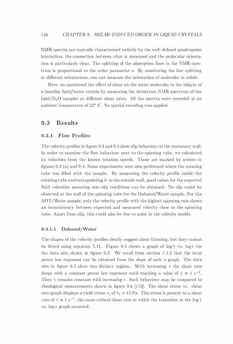
14G CH/\PTER 9. SHEAR-ISD uCED ORDER IN LIQ UID CRYSTALS
NivIR spectra a re typica l ly characterised entirely by t he well-defined q uad r upolar
i n teractio n . the con nection between \vhat is measured and t he molecu lar or ienta
t ion is particu larly clear. The spl i tt ing of the abso rption l ines i n the NMR spec
t r um is proportional to the order parameter s. By mon itoring the l ine spl itt ing
at d ifferent orientations . one can measu re the orientation of molecu les in sol ids .
Here , we monitored the effect of shear o n the water molecules i n the bi layer of
a l amel lar l ip id/water system by measur ing t he deuter i um NlvlR spectr um of the
l i pid/D2 0 samples at d ifferent shear rates. Al l the spectra were recorded at an
ambient tem peratu re of 22° C. No spatial encoding was applied .
9 . 3 Results
9 . 3 . 1 F l ow Profiles
The velocity profi les i n figure 9 .3 and 9 .4 show s l ip behaviou r at t he stationary wal l .
I n order t o examine t h e flow behaviou r next t o t h e spi nn ing t u be, we calcu lated
its velocities from the known rotation speeds . Those are marked by arrows i n
figures 9 . 3 ( a) and 9 . 4 . Some experiments were also performed where t h e rotating
t u be was fi lled with the sample. By meas ur ing the velocity profile i nside the
rotat ing t u be and extrapolati ng i t to the outside wall , good values for the expected
flu i d velocities assum ing non-sli p condit ions can be obtai ned . No slip cou l d be
observed at the wall of the spin ni ng t u be for the Dobanol/Water sample . For t h e
AOT /Water sample, o n l y the velocity profile with t h e h ighest spi nn i ng rate shows an i nconsistency between expected and measu red velocity c lose to the spi nn i ng
t u be. Apart from sl ip , th is cou ld also be d ue to noise i n t he velocity profile .
9 . 3 . 1 . 1 Dobanol/Water
T he shapes of the velocity profiles clearly suggest shear th inn ing , but they cannot
be fitted using equ at ion 5 .4 1 . Figure 9 .5 s hows a graph of log ;f vs . tog r for
the data sets shmvn in f igu re 9 .3 . We recall from sect ion 7 . 1 .2 t h at t he local
power law exponent can be obtained from the slope of such a graph . The d ata sets i n figu re 9 . 5 shmv two d ist inct regions. \Vi th increas ing r the shear rate
d rops with a constant pmver law exponent u nt i l reaching a value of "y ;::::; 1 s- l . Then "I remains constant with increasing r . Such behaviou r may be compared to
rheological measu rements shmvn in figure 9 . 6 [ 1 73] . The shear stress vs. shear
rate graph d isplays a y ield st ress 71 of 71 = 1 5 Pa. This stress is present to a shear
r ate of ;( ;::::; 1 s- l . the same c rit ical shear rate at wh ich the t ransition i n the log "y vs. log r graph occu r red .
9.3. RES ULTS
(a)
......., -� ...... . ;:...,
(b)
• >-
Cl) 0 -
60
50
40
30
20
10
0 2.5
2
0
- 1
-2
-3
.. • 1 .0 Hz A 0.75 Hz A I • 0.5 Hz A • A ·
•• t •• • • . A
• A .. • A • • ... A .. �
3 .0 3.5 4.0 r [ mm]
I,. • • ••• ••• • 1 .0 Hz •• AA •• A 0.75 Hz ·.!AA •• • AAA� • 0.5 Hz •• AAI .. •• A __ -;-" • AA • A & A • • • • • A & -,/ A • A A &
• • • • • & • & • A • • •
• •
0.40 0.45 0.50 0.55 0.60 log r
147
4.5
0.65
Figure 9 .5 : (a) 7 vs. r and (b) log 7 vs. log r for Dobanol/Water at d ifferent rotation speeds
of the i n ner tube.
9.3 . 1 . 2 AOT/Water
As mentioned previously, the transverse relaxation time TJ. is too short to obtain
a good signal-to-noise ratio in the velocity profiles. Therefore we can give only a
qualitative analysis of the profiles shown in figure 9 .4 .
As observed with the Dobanol/Wa\,er sample, the velocity profiles reveal slip
behaviour at the stationary wall. A graph of log l' vs. log r is shown in figure 9 .7 .
The shear rate drops again with increasing r and reaches a constant value at l' � 2
S- 1 .
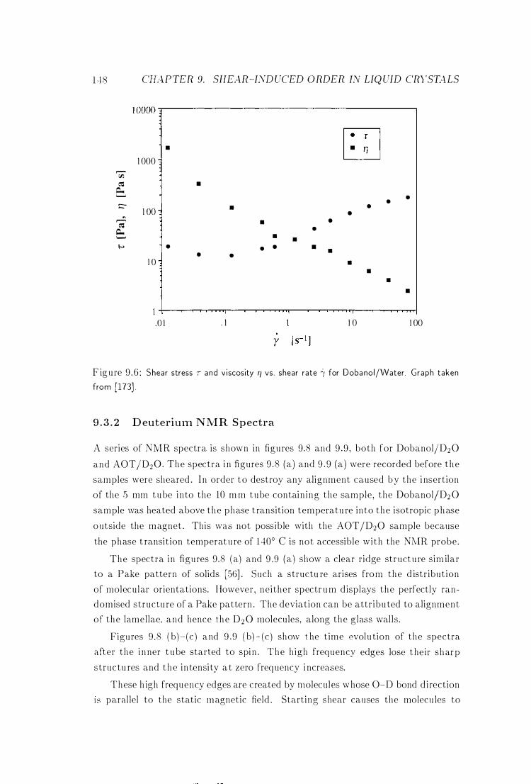
1 e18 CIL1PTER 9. SHEAR-ISD UCED ORDER I.'v' LIQ UID CRYST:1LS
1 0000�--------------------------------------�
..--V'J c: ,.. -........
::::-� ,......, c:
Q.. ........ \->
•
1 000
1 00
•
1 0
.0 1
•
•
• •
. 1
• • •
• • • • • •
I-7l �
• •
• •
1 0
• •
• •
1 00
F igu re 9 . 6 : Shear stress r and viscosity T) vs. shear rate 1 for Doba nol/Water. Graph taken
from [173] .
9 . 3 . 2 D euteriUlTl N M R S p ectra
A series of N:t\/[R spectra is shown in figu res 9.8 and 9 . 9 , both for Dobanol/D20
and AOT/D20. The spectra i n figures 9 .8 (a) and 9 . 9 (a) were recorded before t he
samples were sheared . I n order to destroy any alignment caused by the i nsertion
of the 5 mm t ube i nto the 10 m m tube contain ing the sample, the DobanoljD20
sample was heated above the phase t ransition temperatu re into the isotropic p hase
outside the magnet . This was not possib le with the AOT /D20 sample because
the phase t ransition temperat u re of 1 400 C is not accessible w i th the NMR probe.
The spectra i n figu res 9.8 ( a) and 9 .9 (a ) show a clear ridge struct u re sim ilar
to a Pake pattern of solids [56] . Such a structu re arises from the d istr ibut ion
of molecu lar orientations. However , ne ither spectr u m d isplays the perfectly randomised struct u re of a Pake pattern . The deviation can be attr ibu ted to alignment
of the lamel lae. and hence t he D20 molecu les, along the g lass wal ls .
Figu res 9 .8 ( b)- (c ) a.nd 9 .9 ( b) (c ) shO\v t he t ime evol u tion of the spectra
after the i n ner t u be started to spi n . The h igh frequency edges lose t heir sharp
structu res and t h e i n tensity a t zero frequency i ncreases.
These h igh frequency edges are created by molecu l t:s w hose O-D bond d i rection
I S paral lel to the static magnetic field . Starting shear causes the molecu les to
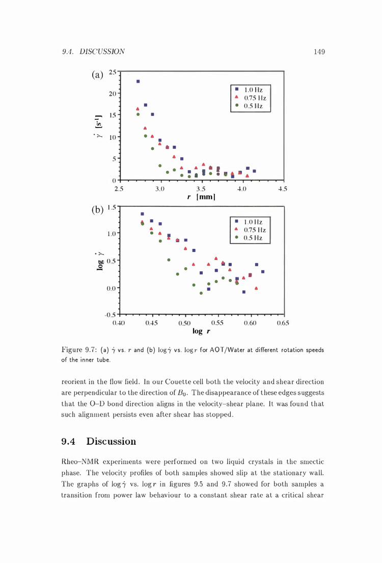
9.4 . DISCUSSION
(a) 25 •
• 1 .0 Hz 20 .. 0.75 Hz
• • 0.5 Hz .. ....... 1 5 • • -fI.l .......... ..
. � 10 . .. • .. * • • 5 .. •
• .. .. .. * ! • • • : • • • • I • • • • 0 2.5 3.0 3 .5 4.0 4.5
r [ mm] (b) 1 .5
• • • • • 1 .0 Hz
.. .. 0.75 Hz l .0 · .. 1 * . • 0.5 Hz • ..
. � • � 0.5 • .. 0 a .. • • •
- • • .. • • • • • • • • • I ..
0.0 • a • •
-0.5 +-........ .....,.... .......... r-r.....,....-.--T"""T.....,....-.--........ --.......-........r.....,....-r-.......-T.....,............., 0.40 0.45 0.50 0.55
log r 0.60 0.65
149
Figure 9 .7 : (a) 1 vs . r and (b) log 1 vs . log r for AOT /Water at different rotation speeds
of the i nner tube.
reorient in the flow field . In our Couette cell both the velocity and shear direction
are perpendicular to the direction of Bo . The disappearance of these edges suggests
that the O-D bond direction aligns in the velocity-shear plane. It was found that
such alignment persists even after shear has stopped .
9.4 Discussion
Rheo-NMR experiments were performed on two liquid crystals in the smectic
phase. The velocity profiles of both samples showed slip at the stationary wall.
The graphs of log i' vs. log r in figures 9.5 and 9.7 showed for both samples a
transition from power law behaviour to a constant shear rate at a critical shear
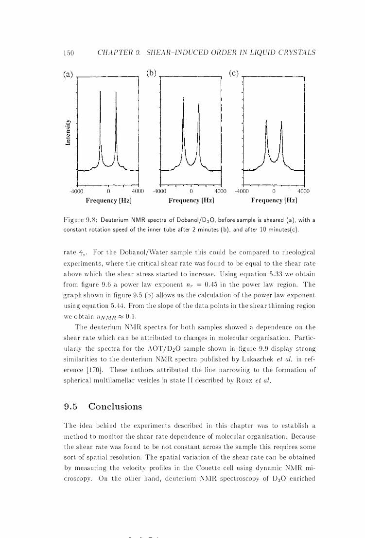
1 .50 CHA PTER. D. SHEAR.-iJ'iDUCED OR.DER. IN LIQ UID CR.YSTALS
(a) ..,-____ -,
-4000 0 4000 Frequency [Hz]
(b) ..,-___ ----, (c) -r--------,
-4000 0 4000 -4000 0 4000 Frequency [Hz] Frequency [Hz]
Figure 9 . 8 : Deuteri um N M R spectra of Dobanol /D20 . before s ample is sheared ( a ) , with a
consta n t rotat ion speed of the i n ner t ube after 2 minutes ( b) , a nd after 1 0 minu tes(c) .
rate . For t h e Dobanol/Water sample t his could be compared to rheological
experiments , where t he critical shear rate was found to be equal to the shear rate
above w hich the shear stress started to increase. Using equation .5 . 33 we obtai n
from figure 9 .6 a power law exponent n,. = 0 .45 i n the power law region . The
graph shown i n figure 9 .5 (b ) allows us the calculat ion of the power l aw exponent
usin g equation 5.4-1 . From the slope of the data points i n the shear t h i nn i ng region
we o btai n nlVM R ;::::;: O. l .
The deu teriu m NMR spectra for both samples showed a dependence on the
shear rate which can be attr ibuted to changes i n molecu lar organisation . Partic
u larly the spectra for the AOT /D20 sample shown in figu re 9 . 9 display strong
s imi lar it ies to the deuteri um N:tvlR spectra publ ished by Lukaschek et al. in ref
eren ce [ 1 70) . These authors attr ibu ted the l i ne n arrowing to the formation of
spherical mu l ti lamellar vesicles in state I I descri bed by Roux et al .
9 . 5 Conclusions
The idea behi nd the experiments descri bed i n th is chapter was to establ ish a
method to mon i tor the shear rate dependence of molecu lar o rganisation . Because
t he shear rate was fou nd to be not constant across the sample th is requ ires some
sort of spatia l resol ut ion . The spatial variation of the shear rate can be obtained
by measur ing the velocity profi les i n the CoueUe cell us ing dynam ic N:YIR mi
croscopy. On the other hand . deuteriu m NMR spectroscopy of D20 en riched
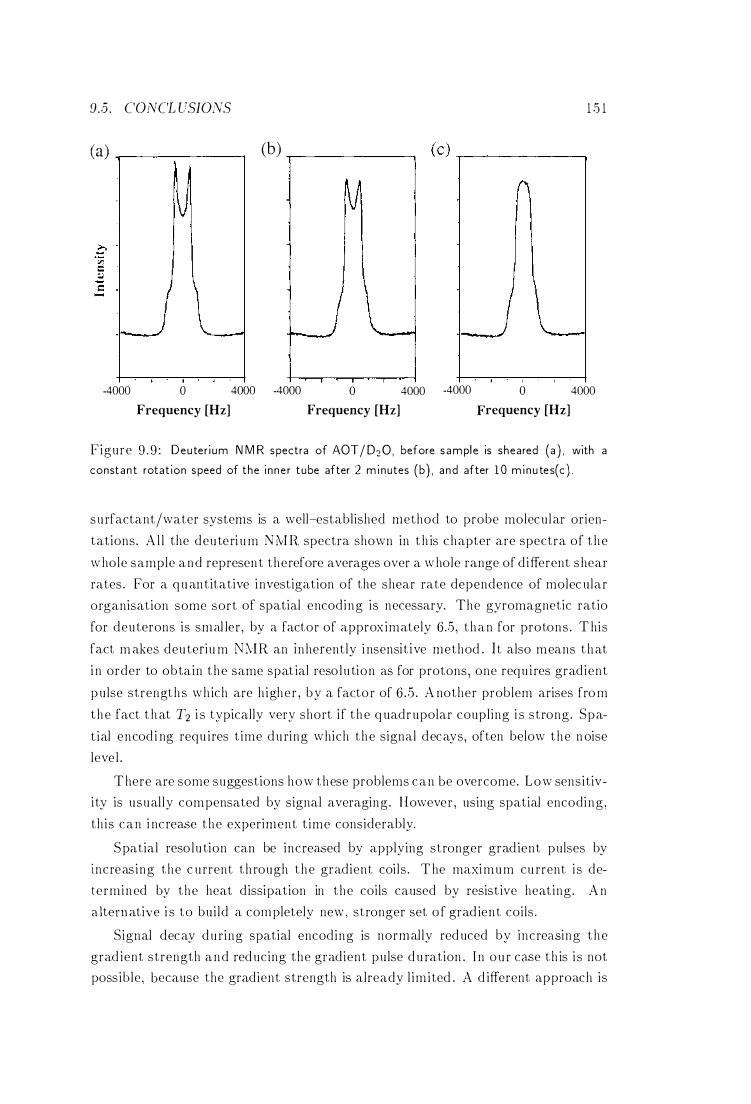
9.5 . CONCL USIO;\iS 1 5 1
Ca) -r-------, (b) -r--------, (c) ,--____ -,
v
-4000 o Frequency [Hz]
4000 -4000 o Frequency [Hz]
4000 -4000 o 4000 Frequency [Hz]
Figure 9 .9 : Deuter i um N M R spectra of AOT / 020 , before s ample is sheared (a ) , with a
constant rotat ion speed of the i nne r tube after 2 minutes (b) , a nd after 10 minu tes(c ) .
su rfactant/water systems is a well-established method to probe molecu lar orien
tations. A l l the deute ri u m NMR spectra shown in t h is chapter are spectra of t he
w hole sample and represen t therefore averages over a w hole range of d ifferent shear
rates . For a q uant itative i nvestigation of the shear rate dependence of molec u lar
organisation some sort of spatial encoding is necessary. The gyromagnetic ratio
for deuterons is smal ler , by a factor of approximately 6.5, than for protons . T his
fact m akes deu teriu m NMR an inherently i nsensit ive method . It also means t hat
i n order to obtain the same spat ial reso l u tion as for protons, one requ i res gradient
pu lse strengths wh ich are h igher , by a factor of 6 .5 . A nother problem arises fro m
the fact t hat T2 i s typically very short i f t he q uadrupolar coupl ing i s strong. Spa
t ial encod i ng requ ires t ime du ring which the signal decays, often below the n oise
leve l .
T here are some suggestions how these problems can be overcome. Low sensitivi ty is usual ly compensated by signal averaging . However , using spatial encoding ,
th is can i ncrease the experiment t ime considerably.
Spatial reso lu tion can be increased by applying stronger grad ient pulses by
increas ing the c u rrent t h rough the gradient coi ls . T he maximum cu rrent i s de
termined by the heat d issipation in the coils caused by resist ive heat ing. A n
altern ative i s to bui ld a completely new . stronger set o f grad ient coils .
Signal decay du ring spatial encoding is normally red uced by increasing the
grad ient strength and red ucing the gradient pu lse d u ration . I n o u r case th is i s not possib le , because the gradient strength is already l im ited . A d ifferent approach is
1.52 CHAPTER g. SHEAR-IND UCED ORDER u,,' LIQUID CRYSTALS
to use some kind of spatial encoding wh ich on ly suffers from Tl relaxation , which
is m uch slower in l iquid crystals . Th is can be ach ieved by using, for example, the
S PACE [ 1 75] or DIGGER [ 1 76) pu lse t rains suggested by Doddrel l et al. wh ich
select ively destroy the magnetisation i n the whole sample except i n the region
u nder i nvestigation .
A l l these points show that deuteri u m N?vl R spectroscopy is hard to perform
with a spatial reso lution on a m icroscopic scale. However, the experimen ts de
scribed above also show that t here is a lot of potential for fu t u re work .
Chapter 1 0
Conclusion
10 .1 S ummary
In th is thesis we i nvestigated how NMR microscopy could be used to obtain i n for
mation about heterogenous properties of flu ids, in particular the time evolution
of flow, and the dependence of hydrodynamic behaviour and Brownian motion
of molecular organisation. Pulsed Gradient Spin Echo NMR and the concept of
q-space analysis played a key role i n the experiments.
By measuring flow profiles i n an electroosmotic capillary at d ifferent t imes after turn ing on the electric field we were able to demonstrate that the shape
of the profile changes with increasing time from plug flow to the well-known
parabolic profile. A steady state is reached in the capill ary geometry on a timescale
of 100 ms, and the electroosmotic flow velocities are of the same order as the
ionic electrophoretic d rift velocities. The agreement with a theoretical model was
excellent .
In stationary flow, changes of molecular velocities can be observed by using
a two-dimensional velocity exchange experiment (VEXSY) . This experiment was
demonstrated on Brownian motion , on laminar circular flow in a Couette cell and
on flow through a bed of closely-packed microspheres. In the latter case, the
VEXSY spectrum showed a transition from stationary to a more randomised flow
with increasing mixing time.
Molecu lar velocities due to convectional flow were monitored with different
methods. The VEXSY experiments showed that this flow is stationary The echo
attenuation function E (q) of a PGSE experiment revealed pronounced min ima
and maxima. Comparison with the function E(q) obtained from the measured
velocity propagator showed good agreement.
The temperature dependence of molecular displacement parameters was mea-
153
1 54 CHAPTER 10. CONCL USION
sured for semi-dilute polymer solutions near the de-mixing transition. The tem
peratu re dependence of the self-diffusion coefficient could be described by a WLF
equation which is characteristic of a glass transition . Using the reptation model
for polymers, the tube d isengagement times Td were calcu lated . From the shape of
the velocity profiles in the Couette cell the entanglement formation times T1J were
obtained using a theory for non-linear viscoelasticity based on the entanglement
concept. Good agreement between Td and T1J was found, as expected .
With deuterium NMR spectroscopy we showed that shear-induced alignment
can be measured . This result has some potential for future work which will be
d iscussed in the next section .
10 .2 Outlook on Future Work
It is not surprising that many new questions can be raised from all aspects of th is
thesis. We mention a few of them here.
The measurements of the flow profiles in the electroosmosis cell showed ex
cellent agreement with the theory for one particular geometry. The theory of
S6derman et al . has been applied to a number of d ifferent geometries. I t would
be i nteresting to measure the time evolution of electroosmotic velocity profiles i n
geometries d ifferent from that o f the capillary used here. One particular example
is the flow between parallel plates, a geometry which could best be investigated
using the new horizontal magnet which has been recently installed in the NMR
lab.
Investigation of complex flow using the PGSE NMR method is one of the key
research areas in our grou p. It is of particular i nterest , because of its d irect analogy
with scattering methods and because only one gradient is requi red . Oscillations
in the echo attenuation function E (q) have been observed in d ifferent flowing
systems, such as convectional flow and flow through micropores. At the stage of
writing of this thesis experiments on Taylor vortices [ 151 , 1 55] are i n p rogress.
Not much is known so far about the temperature dependence of the polymer
self-diffusion coefficients for semi-dilute solutions near the de-mixing transition .
The PSjCYH system has been examined extensively in the l iteratu re , but it is
very difficult to handle. Another system on which many references are available
is PS in DOP. It also shows some interesting features when sheared . A project for the future would be to repeat the diffusion and rheo-NMR experiments on
semi-dilute PSjDOP solutions.
We showed that the local shear rate can be obtained from the velocity profiles. Rabin and Samulski [177] suggested the use of deuterium labelli ng to measure
1 0. 2. O UTLOOK ON FUTURE WORK 155
shear-induced alignment of molecules i n polymer solutions. Because the shear
rate varies across the sample, the deuterium spectrum has to be recorded in dif
ferent regions of the sample using selective excitation. A different approach to
measuring shear-ind uced alignment has been suggested by Callaghan and Samul
ski [178] . Their so-called "beta function" measures the dipolar i nteraction d irectly
and shows a strong orientation dependence. The advantage of the beta function
is that no expensive and difficult deuter ium labelling is required . Using NMR mi
croscopy the spatial (and therefore shear) dependence of other NMR parameters,
such as relaxation times, can also be measured .
The question of whether reptation is an important process i n polymer solutions
still remains to be answered . With a new quadrupolar gradient coil developed i n
our group gradient strengths of u p to 50 T m-I are achievable. Th is should
allow the measurement of internal motion of the polymer chains and clarify the
mechanisms i nvolved in molecu lar dynam ics of polymer coils i n solution .

1 .56 CHAPTER 10. CONCL USION
Bibliography
[1 ] E . M . Purcel l , H . C . Torrey, and R. V . Pound. Phys. Rev. , 69, 37-38 ( 1946) .
[2] F . Bloch , W . W. Hansen , and M . Packard . Phys. Rev. , 70, 474-485 ( 1946 ) .
[3] E . L . Hahn . Phys. Rev. , 8 0 , 580-594 ( 1950) .
[4] R. R. Ernst and W. A . Anderson . Rev. Sci. Instrum. , 37, 93-102 ( 1966) .
[5] E . L . Hahn . Phys. Rev. , 80, 580 ( 195 1 ) .
[6] E . O . Stejskal and J . E . Tanner. J. Chem. Phys. , 42, 288-292 ( 1965 ) .
[7] P . Mansfield and P. K . GranneII . J. Phys. C: Sol. St. Phys. , 6, L422-L426
( 1973) .
[8] P. C . Lauterbur . Nature, 242, 190-19 1 ( 1973) .
[9] P. T . Cal laghan , C. D . Eccles, and Y . Xia. J. Phys. E: Sci. Instrum. , 2 1 ,
820-822 ( 1988) .
[ 10] A . Abragam. The Principles of Nuclear Magnetism. Clarendon Press, Ox
ford , ( 1961 ) .
[ 1 1] P. T . Cal laghan . Principles of Nuclear Magnetic Resonance Microscopy.
Clarendon Press, Oxford , ( 1 99 1 ) .
[ 12] R . R . Ernst, G . Bodenhausen , and A . Wokaun . Principles of Nuclear Mag
netic Resonance in One and Two Dimensions. Clarendon P ress, Oxford ,
( 1987) .
[ 13] E . Fukushima and S. B . W . Roeder. Experimental Pulse NMR. A Nuts and
Bolts Approach. Addison-Wesley, Reading (Massachusetts) , ( 198 1 ) .
[ 14] W . W . Paudler. Nuclear Magnetic Resonance. John Wiley & Sons, New
York, ( 1987) .
157
1.58 BIBLIOGRAPHY
[ 15] D. Shaw . Fourier Transform N1VlR Spectroscopy. Elsevier Publish ing Com
pany, Inc . , Amsterdam, ( 1984) .
[ 1 6] C. P. Slichter. Principles of Magnetic Resonance. Springer-Verlag, Heidel
berg, ( 1990) .
[ 17] A. Messiah . Quantum Mechanics. John Wiley & Sons, New York, ( 1 966) .
[ 18] L . 1 . Schiff. Quantum Mechanics. McGraw Hil l , New York, ( 1955) .
[ 19] H . Y. Carr and E . M . Purcell . Phys. Rev. , 94, 630-638 ( 1954) .
[20] S. Meiboom and D . Gi l l . Rev. Sci. Instrum., 29, 688-691 ( 1958) .
[2 1 ] E. O . Stejskal. J. Chem. Phys . , 43, 3597-3603 ( 1965) .
[22] J . Jeener. Ampere I nternational Summer School , Basko Polje, Yugoslavia,
( 1973) .
[23] L . Mii ller, A . Kumar, and R. R . Ernst. J. Chem. Phys. , 63, 5490-5491 .
( 1975) .
[24] C. Schmidt, B . Bl iimich , and H . W . Spiess. J. Magn . Reson. , 79, 269-290
( 1988) .
[25] S . Wefing and H . W. Spiess. J. Chem. Phys. , 89, 12 19-1233 ( 1988) .
[26] S . Wefing, S . Kaufmann , and H . W . Spiess. J. Chem. Phys. , 89 , 1 234-1244
( 1988) .
[27] D. 1. Hoult and R. E. Richards. Proc. R . Soc. London A , 344, 3 1 1-340
( 1975) .
[28] P. Mansfield and P. K . Grannel l . Phys. Rev. B, 12 , 3618-3634 ( 1975) .
[29] A. Kumar, D . Welti , and R. R. Ernst. J. Magn. Reson., 18 , 69-83 ( 1975) .
[30] G. Johnson , J . M . S . Hutchison , T . W. Redpath , and L . M . Eastwood . J. Il'l agn. Reson. , 54, 374-384 ( 1983) .
[3 1] M . Appel, G . Fleischer, J . Karger, F . Fujara, and I . Chan. Macromolecules,
27 , 4274-4277 ( 1994) .
[32] D. W. McCal l , D . C. Douglass, and E . W. Anderson . Ber. Bunsenges. , 67,
336-340 ( 1963 ) .
[33] J . Karger, H . Pfeifer, and W. Heink. Adv. Magn. Reson . , 12 , 1-89 ( 1988) .
BIBLIOGRAPHY 159
[34] T. L . James and G . G . McDonald . J. i\l!agn. Reson. , 1 1 , .58-61 ( 1973) .
[35] J . IG.rger and W. Heink . J. Magn. Reson., 51 , 1-7 ( 1983) .
[36] C. D . Eccles . Microscopic NMR Imaging. PhD thesis, Massey University,
( 1987) .
[37] Y. Xia. Dynamic NMR Microscopy. PhD thesis, Massey University, ( 1992 ) .
[38] P. Mansfield and B . Chapman . J. Magn. Reson. , 66, 573-576 ( 1986 ) .
[39] R. Mil ls . J. Phys. Chem. , 77, 685-688 ( 1973) .
[40] P. T . Callaghan. J. Magn. Reson. , 88, 493-500 ( 1990) .
[4 1 ] A . Coy. q-Space, Restricted Diffusion and Pulsed Gradient Spin Echo Nu
clear Magnetic Resonance. PhD thesis, Massey University, ( 1995) .
[42] C. S . Johnson and Q. He. Adv. Magn. Reson., 13 , 13 1-159 ( 1989 ) .
[43] D . J . Shaw. Electrophoresis. Academic Press, London , ( 1969) .
[44] J . Packer , C . Rees, and D . J . Tomlinson . Adv. Mol. Relaxation Processes,
3 , 1 19-1 3 1 ( 1972) .
[45] R. J . Hunter. Zeta Potential in Colloid Science. Academic Press, London ,
( 1981 ) .
[46] R . J . Hunter. Foundations of Colloid Science. Clarendon Press, Oxford ,
( 1987 ) .
[47] O . Soderman and B . Jonsson . Journal of Chemical Physics (submit
ted) ( 1996 ) .
[-t8] M . Abramowitz and 1 . A. Stegun . Handbook of Mathematical Functions.
Dover Publications, New York, ( 1970 ) .
[49] T. R. Saarinen and W. S . Woodward . Rev. Sci. Instrum. , 59 , 761-763
( 1988) .
[50] P. J . Scales , F. Grieser, T. W . Healey, L . R. White, and D . Y . C . Chan . Langmuir, 8 , 965 ( 199:2 ) .
[5 1 ] D. R . Lide. Handbook of Chemistry and Physics. CRC Press, New York,
( 1995) .
1 60 BIBLIOGRAPHY
[52] D . Wu , A. Chen , and C. S . Johnson Jr . J. Magn. Reson. A , 1 1 5 , 123-126
( 199.5 ) .
[.53] P . T . Callaghan and B . Manz. J . Magn. Reson. A , 1 06 , 260-265 ( 1994 ) .
[.54] D . G . Cory, A . N . Garroway, and J . B . Miller. Polymer Preprints, 3 1 ,
149-150 ( 1990 ) .
[.55] C . J . Rofe, R. K . Lambert , and P . T . Callaghan . J. Rheol. , 38 , 857-887
( 1994) .
[56] G . E. Pake. J. Chem. Phys . , 16 , 327-336 ( 1948) .
[57] T . Gu ll ion , D . B . Baker, and M. S . Conradi . J. Magn. Reson. , 89, 479-484
( 1 990) .
[58] J . D . Seymour and P. T . Cal laghan . J. Magn. Reson. A , (in press ) ( 1 996 ) .
[59] P . G . de Gennes. Scaling Concepts i n Polymer Physics. Comel! University
P ress, Ithaca, ( 1979) .
[60] M . Kurata. Thermodynamics of Polymer Solutions. Harwood Academic
P ubl ishers, Chur , ( 1982) .
[6 1 ] M . Doi and S . F . Edwards. The Theory of Polymer Dynamics. Clarendon
P ress, Oxford, ( 1986 ) .
[62] J . des Cloizeaux and G . Jan nink . Polymers in Solution. Clarendon P ress,
Oxford , ( 1990 ) .
[63] H . Fuj ita. Polymer Solutions. Elsevier Publishing Company, Inc . , Amster
dam, ( 1990 ) .
[64] U . Eisele. Introduction to Polymer Physics. Springer-Verlag, Berl in , ( 1990) .
[65] R. H . Boyd and P. J . Phi l l ips. The Science of Polymer Molecules. Cambridge
U niversity Press, Cambridge, ( 1993 ) .
[66] J . S . Higgins and H. C . Benoit . Polymers and Neutron Scattering. Clarendon
Press, Oxford , ( 1994) .
[67] D. H . Hey. J{ing::ett 's Chemical Encyclopedia. Bailliere, Tindal l and Cassell
Ltd . , London , ( 1966 ) .
[68] J . Brandrup and E. H . Immergut . Polymer Handbook. John Wiley & Sons,
New York, ( 1989) .
BIBLIOGRAPHY 1 6 1
[69] P . J . Flory. J. Chem. Phys. , 10 , 5 1 ( 1942) .
[70] M . L . Huggins. J. Phys. Chem. , 64, 1712-1719 ( 1942) .
[7 1] P. G . de Gennes. J. Chem. Phys. , 55, 572-.579 ( 1971 ) .
[72] M . Doi and S . F . Edwards. J. Chem. Soc. Faraday Trans. 2, 74, 1789-1801
( 1 978) .
[73] P. J . Flory. Principles of Polymer Chemistry. Cornell University P ress,
Ithaca, ( 1953) .
[74] L . D . Landau and E. M. Lifshitz . Statistical Physics. Pergamon Press,
London , ( 1958) .
[75] A . Z. Akcasu and C. C . Han . Macromolecules, 12 , 276-280 ( 1979) .
[76] J .-P. Munch , G . Hild , and S. Candau . Macromolecules, 16 , 71-75 ( 1983) .
[77] I . H . Park, Q .-W. Wang, and B . Chu . Macromolecules, 20, 1965-1975 ( 1987) .
[78] A . Y. Grosberg and D . V . Kuznetsov. Macromolecules, 25, 1 996-2003
( 1992) .
[79] J . Vu , Z . Wang, and B . Chu . Macromolecules, 25, 1618-1620 ( 1992) .
[80] H . Yamakawa, F . Abe, and Y. Einaga. Macromolecules, 27 , 5704-5712
( 1994) .
[8 1] T . Arai , F . Abe, T. Yoshizaki , Y. Einaga, and H . Yamakawa. Macro
molecules, 28, 5458-.5464 ( 1995) .
[82] B . Chu , Q . Ying, and A . Y. Grosberg. Macromolecules, 28, 180-189 ( 1995) .
[83] C . Strazielle and H . Benoit. Macromolecules, 8 , 203-205 ( 1975) .
[84] G . C. Berry. J. Chem. Phys. , 46, 1338-1352 ( 1967) .
[85] A . R. Shultz and P. J . Flory. J. Am. Chem. Soc. , 74, 4760-4767 ( 1952) .
[86] R. Perzynski, M . Delsanti , and M . Adam . J. Physique, 48 , 1 1 5-124 ( 1987 ) .
[87] T . G . Scholte. J. Polym. Sci. A -2, 9 , 1553-1577 ( 1971 ) .
[88] Y . Einaga, S . Ohashi, Z . Tong, and H . Fujita. Macromolecules, 1 7, 527-534
( 1984) .
162 BIBLIOGRAPHY
[89] R. Konigsveld, W. H . Stockmayer , J . W. Kennedy, and L . A . Kleintjens.
lv! acromolecules, 7 , 73-79 ( 1974) .
[90] M. Takahashi and T. Nose. Polymer, 27, 1071-1077 ( 1986) .
[9 1] C . H . Wang and X . Q. Zhang. Macromolecules, 28, 2288-2296 ( 1995) .
[92] M . Adam and M. Delsanti. Macromolecules, 18, 1 760-1770 ( 1985) .
[93] F . Brochard and P. G . de Gennes. Macromolecules, 10 , 1 157- 1 1 6 1 ( 1977) .
[94] W. Hess. Macromolecules, 19 , 1 395-1404 ( 1986) .
[95] J . Skolnick, R. Yaris, and A . Koli nski . J. Chem. Phys . , 88, 1407-1417
( 1988) .
[96] J . Skolnick and R. Yaris. J. Chem. Phys. , 88, 1418-1442 ( 1988) .
[97] M . Doi . Introduction to Polymer Physics. Clarendon Press, Oxford , ( 1996 ) .
[98] L . Leger, H . Hervet , and F . Rondolez . Macromolecules, 1 4 , 1 732-1 738
( 1 98 1 ) .
[99] E . J . Amis, C . C . Han, and Y . Matsushita. Polymer, 25, 650-658 ( 1984 ) .
[ 100] P. T . Callaghan and D . N . Pinder. Macromolecules, 17 , 431-437 ( 1984) .
[ 1 0 1] J . A . Wesson , 1 . Noh , T . Kitano, and H . Yu . Macromolecules, 1 7, 782-792
( 1984) .
[ 102] E. von Meerwall , E. J . Amis, and J . D . Ferry. Macromolecules, 18 , 260-266
( 1985) .
[ 103] N . Nemoto, M . R. Landry, 1 . Noh , T. Kitano, J . A . Wesson , and H . Yu .
Macromolecules, 18 , 308-3 10 ( 1985) .
[ 104] H . Kim, T. Chang, J . M. Yohanan , L . Wang, and H . Yu . Macromolecules,
19 , 2737-27-t4 ( 1986) .
[ 1 05] L. M. Wheeler, T . P. Lodge, B . Hanley, and M. Tirrell . Macromolecules, 20 ,
1 120- 1 129 ( 1987) .
[ 1 06] G . Fleischer, O . E. Zgadzai , V . D . Skirda, and A . I . Maklakov. Colloid
Polym. Sci. , 266, 201-207 ( 1 988 ) .
[ 107] H . Hen'et, L . Leger , and F . Rondolez . Phys. Rev. Let . , 42, 1681 ( 1979) .
BIBLIOGRAPHY
[ 1 08] G. D . J . Phi llies. Macromolecules, 19 , 2367-2376 ( 1986) .
[109] G . D. J . Ph i ll ies. Macromolecules, 20, 558-564 ( 1987) .
[ 1 10] G . D . J . Phil lies. Macromolecules, 21 , 310 1-3 106 ( 1988) .
[ 1 1 1 ] G . D . J . Phil l ies. Macromolecules, 2 1 , 214-220 ( 1988) .
[1 12] W . W. G raessley. Adv. Polym. Sci. , 16 ( 1974) .
[ 1 1 3] W . W. G raessley. J. Chem. Phys. , 47, 1942-1953 ( 1967) .
[ 1 14] M . C . Williams. A IChE J. , 12 , 1064-1070 ( 1966 ) .
[ 1 15] M . Adam and M . Delsanti . J. Physique, 4 5 , 1513-1521 ( 1984) .
163
[ 1 16] J . D . Ferry. Viscoelastic Properties of Polymers. John Wiley & Sons, New
York, ( 1980) .
[1 17] W . Brown and P. Stepanek. Macromolecules, 24, 5484-5486 ( 1 99 1 ) .
[ 1 18] M . 1 . Will iams, R . F . Landel, and J . D . Ferry. J. A m. Chem. Soc. , 77,
3701-3707 ( 1955) .
[ 1 19] S . F . Edwards and T . Vilgis. Physica Scripta, T13 , 7-16 ( 1 986) .
[120] S . F . Edwards. Polymer, 35, 3827-3830 ( 1994 ) .
[121] C . Rangel-Nafaile, A . B . Metzner, and K. F . Wissbrun . Macromolecules,
1 7, 1 187- 1 1 95 ( 1984) .
[ 122] R. G . Larson . Rheol. Acta, 3 1 , 497-520 ( 1992) .
[123] A . 1 . Nakatani and M. D . Dadmun . Flow-Induced Structure im Polymers.
American Chemical Society, Washington, ( 1995) .
[124] A . Silberberg and W. Kuhn . Nature, 1 70 , 450-451 ( 1952 ) .
[125] G . Ver Strate and W. Philippoff. J. Polym. Sci. Polym. Let. Ed. , 12 , 267-
275 ( 1974 ) .
[ 1 26] F . Debeauvais , P. G ramain , and J . Leray. J. Polym. Sci. C, 16 , 3993-3999
( 1968) .
[ 1 27] P. J . Barham and A . Keller. Macromolecules, 23, 303-309 ( 1990 ) .
[ 1 28] A . Link and J . Springer. Macromolecules, 26, 464-471 ( 1993 ) .
164 BIBLIOGRAPHY
[ 129] B. A. Wolf. Macromolecules, 1 7, 6 1.5-6 18 ( 1984) .
[ 130] E . Helfand and G . H . Fredrickson . Phys. Rev. Let . , 62, 2468-2471 ( 1989) .
[ 131 ] A . Onuk i . Phys. Rev. Let. , 62, 2472-2475 ( 1989) .
[ 132] S . T . Milner. Phys. Rev. Let . , 66, 1477-1480 ( 1991 ) .
[ 1 33] B . Hammouda, A . I . Nakatani, D . A . Waldow, and C . C . Han . Macro
molecules, 25, 2903-2906 ( 1992) .
[ 134] T . Hashimoto, T . Takebe, and S . Suehiro. J. Chem. Phys . , 88, 5874-588 1
( 1988) .
[135] X .-L . Wu , D . J . Pine, and P. K. Dixon . Phys. Rev. Let. , 66, 2408-241 1
( 199 1 ) .
[ 136] H . Yanase, P. Moldenaers, J . Mewis, V . Abetz , J . van Egmond , and G . G .
Ful ler . Rheol. Acta, 30, 89-97 ( 1991 ) .
[ 137] E . Moses, T . Kume, and T . Hashimoto. Phys. Rev. Let. , 72 , 2037-2040
( 1994 ) .
[ 138] E . Mendes, P. L indner, M . B uzier, F . Boue, and J . Bastide. Phys. Rev. Let . ,
66, 1595-1598 ( 1991 ) .
[ 139] H . J i and E . Helfand . Macromolecules, 28, 3869-3880 ( 1995) .
[ 140] A . I . Nakatani , M . D . Poliks, and E . T. Samulski . Macromolecules, 23 ,
2686-2692 ( 1 990) .
[ 14 1] R. Muller, J . J . Pesce, and C. P icot . Macromolecules, 26, 4356-4362 ( 1993 ) .
[ 142] D . A . G rabowski and C . Schmidt . Macromolecules, 27, 2632-2634 ( 1 994) .
[ 143] Y . Xia and P. T. Callaghan . Macromolecules, 24, 4777-4786 ( 1991 ) .
[ 144] J . A . Hopkins, R. E . Santin i , and J . B . Grutzner. J. Magn. Reson. A , 1 1 7 ,
1 50-163 ( 1995) .
[ 1 -15] R. G . C . Arridge. A n Introduction to Polymer Mechanics. Taylor & Francis,
London , ( 1985) .
[ 1 -16] A . -1\ 1 . Hecht, H . B . Bohidar, and E. Geissler. J. Physique Lett. , 45 . L 12 1-
L 126 ( 1984 ) .
[ 1 -1 7] W . Brown and P. Stepanek. Macromolecules, 2 5 , 4359-4363 ( 1992) .
BIBLIOGRAPHY 165
[148] W. S . Price and P. W. Kuchel . .J. Magn. Reson. , 94, 1 33-139 ( 1991 ) .
[ 149] N . Miyashita and T . Nose. J. Chem. Phys. , 100, 6028-6037 ( 1994) .
[ 1 .50] C . .J . Rofe. PhD thesis, Massey University (to be published).
[ 151] E. L. Koschmieder. Benard Cells and Taylor Vortices. Cambridge University
P ress, Cambridge, ( 1993) .
[ 152] H . Benard . Rev. Sci. Pures Appl. , 1 1 , 1261-1271 and 1 309-1328 ( 1900 ) .
[ 153] H . Benard . A nn. Chim. Phys. , 23, 62-144 ( 1 90 1 ) .
[ 154] Lord Rayleigh . Philos. Mag. , 32, 529-546 ( 1916) .
[ 155] S . Chandrasekhar. Hydrodynamic and Hydromagnetic Stability. Clarendon
P ress, Oxford , ( 1961 ) .
[ 156] P. L . Siverston . Forsch. Ing. Wes. , 24, 29-32 and 59-69 ( 1958) .
[ 157] G . S . Charlson and R. L . Sani . Int. J. Heat Mass Transfer, 13 , 1479-1496
( 1970 ) .
[158] I . Catton and D . K. Edwards. AIChE J. , 16 , 594-601 ( 1 970) .
[ 159] C . Normand, Y. Pomeau, and M . Velarde. Rev. Mod. Phys. , 49, 581-624
( 1977) .
[ 160] M . C. Cross and P. C. Hohenberg. Rev. Mod. Phys. , 65, 851 ( 1993) .
[ 16 1] M . D . Shattuck, R. P. Behringer, G . A . Johnson, and J . G . Georgiadis. Phys.
Rev. Let. , 75, 1934-1937 ( 1995) .
[162] L . A. Papazian . Polymer, 10 , 399-420 ( 1969) .
[ 163] P. T . Callaghan , A . Coy, D . MacGowan , K . J . Packer , and F . O . Zelaya.
Nature, 351 , 467-469 ( 199 1 ) .
[ 16-i] P. G . d e Gennes and J . Prost . The Physics of Liquid Crystals. Clarendon
Press, Oxford , ( 1993 ) .
[ 165] R . Y . Dong. Nuclear Magnetic Resonance of L iq'uid Crystals. Springer
Verlag, Berl in , ( 1994) .
[166] O . Diat , D . Roux, and F. Nal let . J. Physique Il, 3 , l-i27-1452 ( 1 993) .
[167] D . Roux, F. Nallet, and O . Diat. Ellrophys. Lett. , 24, 53-58 ( 1993 ) .
166 BIBLIOGRAPHY
[ 1 68] O. Diat , D . Roux, and F . Nallet. Phys. Rev. E, 51 , 3296-3299 ( 199.5 ) .
[ 169] M. Lukaschek, D . A . Grabowski, and C. Schmidt . LANGMUIR, 1 1 , 3590-
3.594 ( 1995) .
[1 70] M. Lukaschek, S . Muller, A . Hasenhindl , D . A . Grabowski, and C . Schmidt .
Colloid Polym. Sci. , 274, 1-7 ( 1 996) .
[ 1 7 1] C. L . Khetrapal , A . C. Kunwar, A . S . Tracey, and P. Diehl . Nuclear Magnetic
Resonance Studies in Lyotropic Liquid Crystals. Springer-Verlag, Berlin ,
( 1975) .
[172] O. Soderman and P. Sti lbs . Progress in NMR Spectroscopy, 26, 445-482
( 1994 ) .
[173] B. Smeulders. (private communication).
[174] J . Rogers and P. A. Winsor. Nature, 216 , 477-479 ( 1967 ) .
[ 175] D . M . Doddrell, W. M. B rooks, J . M . Bulsing, J . Field , M . G . Irving, and
H. Baddeley. J. Magn. Reson. , 68 , 367-372 ( 1986) .
[ 176] D. M . Doddrell , J . M. Bu lsing, G . J . Galloway, W. M . B rooks, J . F ield ,
M. G . Irving, and H . Baddeley. J. Magn. Reson . , 70 , 319-326 ( 1986) .
[177] U . Rabin and E . T. Samulski . Macromolecules, 25, 2985-2987 ( 1992) .
[ 178] P. T. Callaghan and E. T. Samulsk i . (to be published)( 1996 ) .
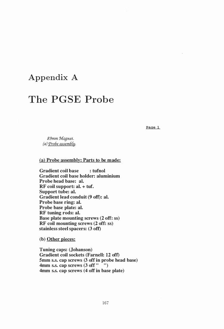
Appendix A
The PGSE Probe
89mm Magnet. (a) Prove assemMy.
(a) Probe assembly: Parts to be made:
Gradient coil base : tufnol Gradient coil base holder: aluminium Probe head base: al. RF coil support: al. + tuf. Support tube: al. Gradient lead conduit (9 oft): al. Probe base ring: al. Probe base plate: al. RF tuning rods: al. Base plate mounting screws (2 off: ss) RF coil mounting screws (2 off: ss) stainless steel spacers: (3 oft)
(b) Other pieces:
Tuning caps: (Johanson) Gradient coil sockets (Farnell: 12 off) 5mm s.s. cap screws (3 off in probe head base) 4mm s.s. cap screws (3 off 1 1
" ) 4mm s.s. cap screws (4 off in base plate)
167
Page 1
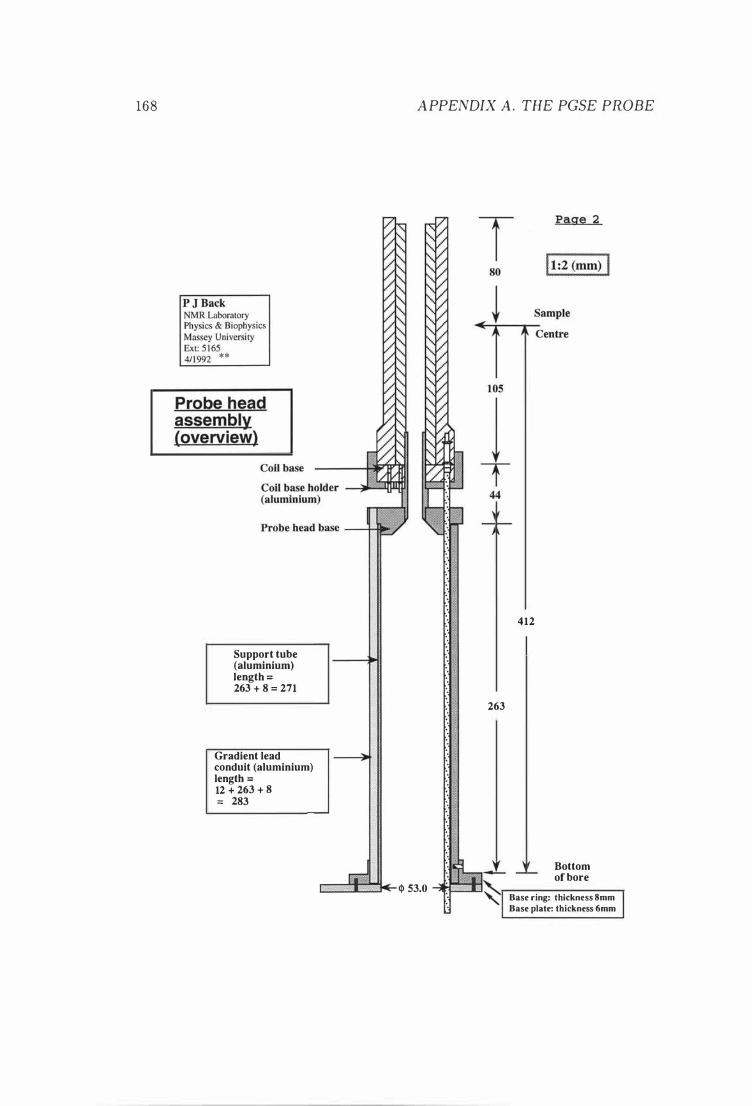
168
Support tube (aluminium) length =
263 + 8 = 271
Gradient lead conduit (aluminium) length =
12 + 263 + 8 = 283
APPENDIX A . THE PGSE PROBE
263
<P 53.0
412
Bottom of bore
Base ring: thickness 8mm
Base plate: thickness 6mm
A PPENDIX A . THE PGSE PROBE
Probe head .
Johanson 5642 (1-30 pF)
(non-magnetic)
Burndy
(non-magnetic)
Pins: Farnell 1 50-623
Sockets: Farnell ] 50-626.
Pin clearance 3mm
Gradient lead conduit: 6.4mm OD, 4mm ID.
T 25
IiliJ-o--- cl> 53 --�
I�·---- cl> 72 ---_0" I
169
Page 3
1 1 : 1 (mm) I
Plan A r
T 'j r
n B
T 263
170 APPENDIX A . THE PGSE PROBE
Page 4 2: 1
Probe head base
I RF coil support I /- 15 -1
5.5
t 1-------- $ 53 ---------j;�
1---------- $ 64
.... 1. __________ $ 72 ·1
APPENDIX A. THE PGSE PROBE
Probe head support tube
90 1 1 0
160
180 0 �;+------�-------4�---160
- 1 10 -70 -90
Grooves: 0.25 inch diam. to depth 3.0mm
171
Page 5
11 :2 (mm) 1
172
Probe head assembly
Page 6
1 1 :2 (mm) I
APPENDIX A . THE PGSE PROBE
I- ( pO -l
80
1 105
T 44
412 to probe base
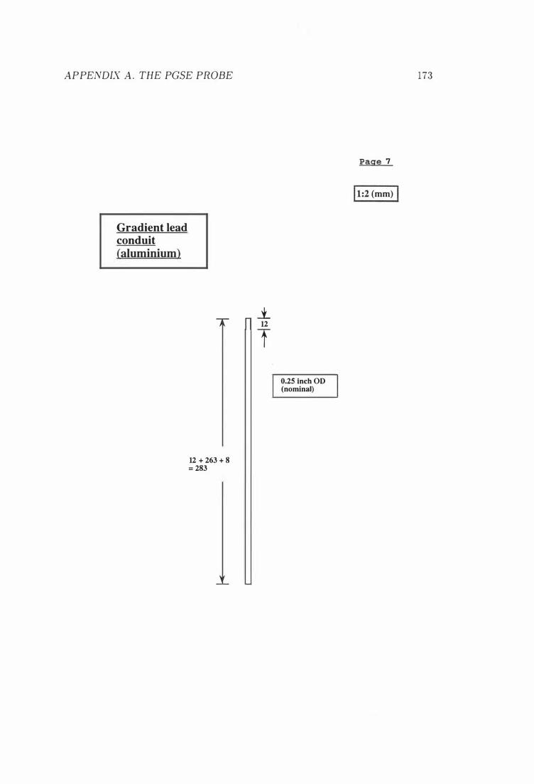
APPENDIX A . THE PGSE PROBE
Gradient lead conduit (aluminium)
12 + 263 + 8 = 283
..t. 12
T 0.25 Inch OD (nominal)
Page 7
11 :2 (mm) 1
173
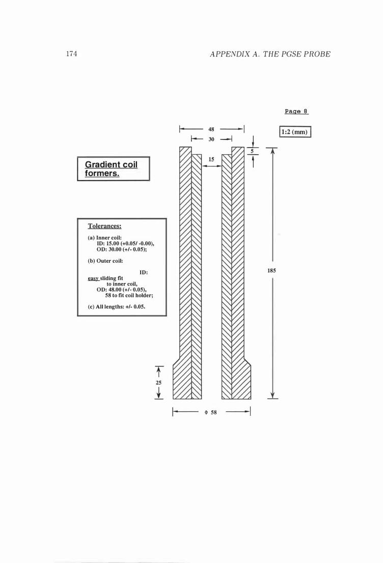
174
G radient coil formers.
Tolerances: (a) Inner coil:
ID: 15.00 (+0.05/ -0.00), OD: 30.00 (+/- 0.05);
(b) Outer coil:
ID: �sliding fit
to inner coil, OD: 48.00 (+/- 0.05),
58 to fit coil holder;
(c) All lengths: +/- 0.05.
25
1
APPENDIX A . THE PGSE PROBE
Page 8
-- I 48
I- 30 -l � 11 :2 (mm) I
5
-,
185
� 58
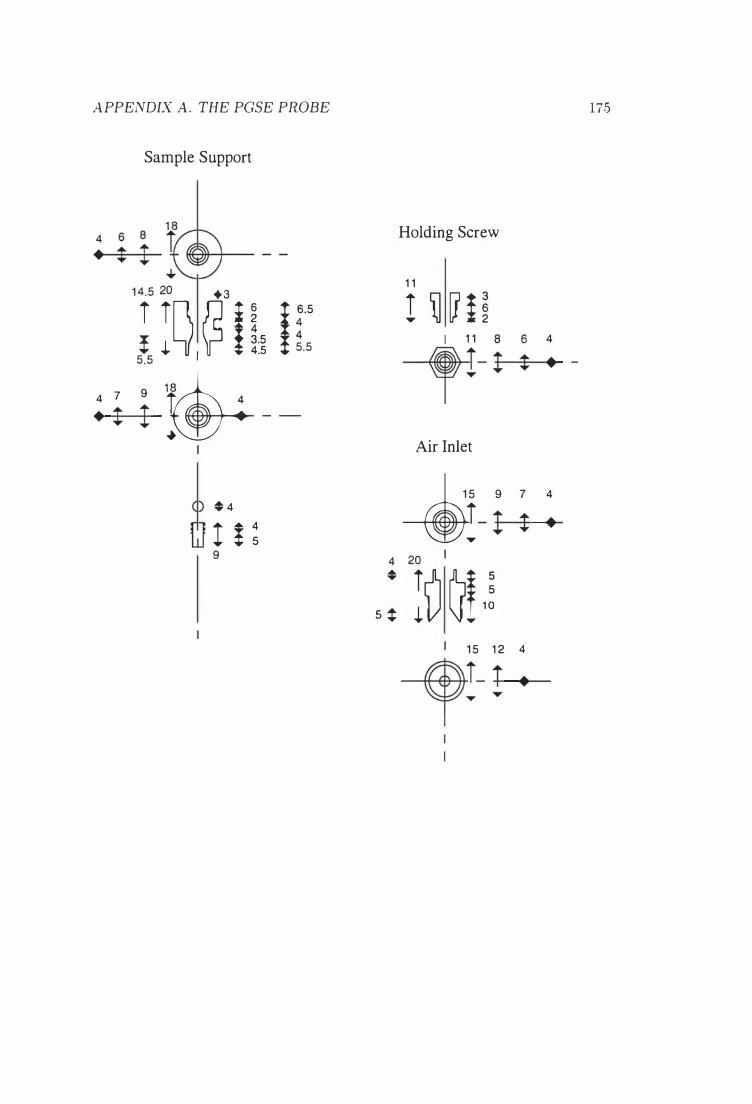
APPENDIX A . THE PGSE PROBE
4 •
4 7
• t
Sample Support
1 4.5 20 + 3
i iQ � ! � ! ,j. I t� 5.5 i :5
5.5
9 1� ! t 4 _ _
....
* 4
! ! � 9 4 *
s t
175
Holding Screw
1 1
! � � i i I 1 1 8 6 4 ---t1- ! $ . -
Air Inlet
-4)5 9 7 4 T- ! t • ....
20 I
�� � ,� I 1 5 1 2 4
-,!- ! .
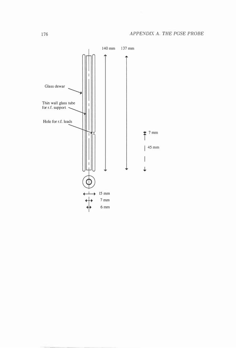
176 APPENDIX A . THE PGSE PROBE
Glass dewar
Thin wal l glass tube for rJ. support
1 40 mm 1 37 mm
15 mm
7 mm
6 mm
45 mm
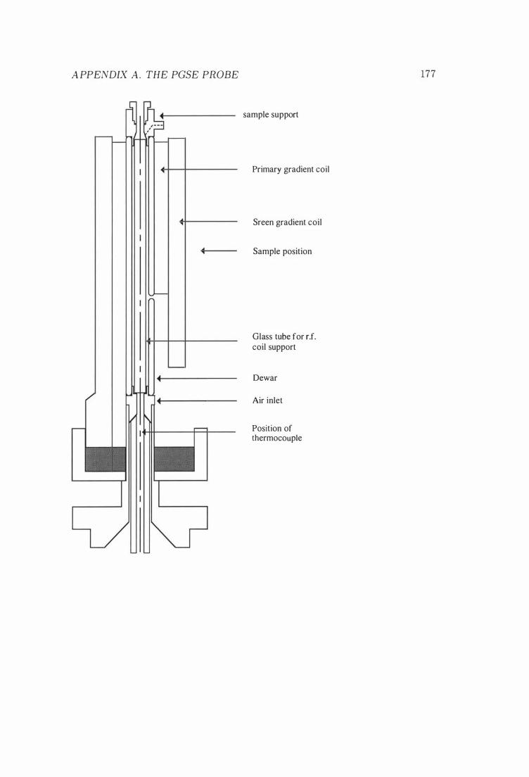
A PPENDIX A. THE PGSE PROBE
sample support
Primary gradient coil
Sreen gradient coil
Sample position
Glass tube for r.f. coil support
Dewar
Air inlet
Position of thermocouple
177

178 APPENDIX A . THE PGSE PROBE
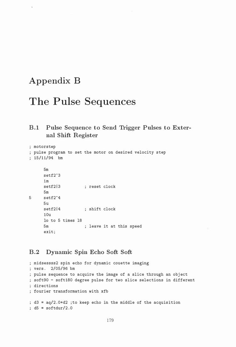
Appendix B
The Pulse Sequences
B . l Pulse Sequence t o Send Trigger Pulses t o Exter
nal S hift Register
S
motorstep
pulse program to set the motor on desired velocity step 15/ 1 1/94 bm
5m
setf2-3 lm setf2 1 3 reset clock 5m s etf2-4 Su setf2 1 4 shift clock
10u
10 to 5 t imes 18
Srn leave it at this speed exit ;
B . 2 Dynamic Spin Echo S oft S oft
rnidsessss2 spin echo for dynamic couette irnaging vers o 2/05/96 bm
pulse sequence to acquire the image of a slice through an obj ect soft90 - soft 180 degree pulse for two slice selections in different
directions fourier transformation with xfb
d3 = aq/2 . 0+d2 ; to keep echo in the middle of the acquis ition d5 = softdur/2 . 0
1 79
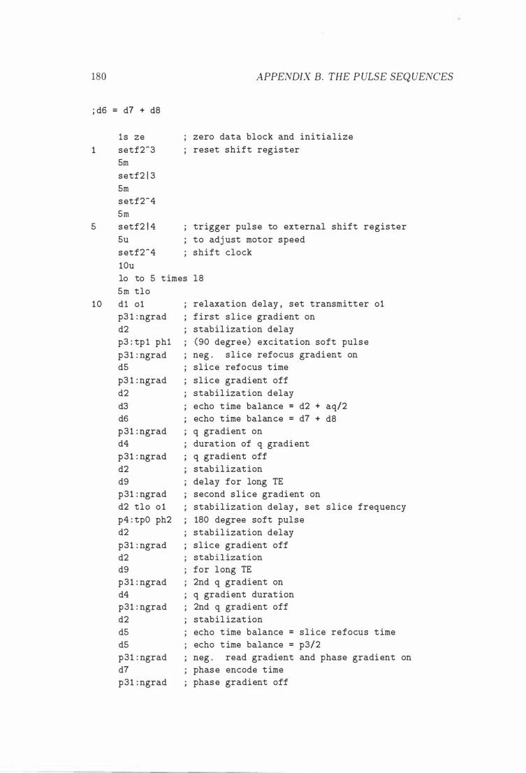
180 APPENDIX B. THE P ULSE SEQ UENCES
j d6 = d7 + d8
1
S
ls ze
setf2-3 Srn
setf2 1 3
Srn
setf2-4
Srn
setf2 1 4
Su
setfT4
10u
zero data block and initialize
reset shift register
trigger pulse to external shift register
to adj ust motor speed
shift clock
10 to S t imes 18
Srn tlo
10 dl 01 relaxat ion delay , set transmitter 01
p3 1 : ngrad first slice gradient on
d2 stabil ization delay
p3 : tp l phl (90 degree) excitation soft pulse
p31 : ngrad neg . slice refocus gradient on dS slice refocus time
p3 1 : ngrad slice gradient off
d2 stabil izat ion delay
d3 d6 p31 : ngrad d4
p31 : ngrad
d2 d9 p31 : ngrad
d2 tlo 0 1
p4 : tpO ph2 d2
p31 : ngrad d2 d9 p31 : ngrad d4 p31 : ngrad
d2 dS dS p31 : ngrad
d7
p31 : ngrad
echo t ime balance = d2 + aq/2 echo time balance = d7 + d8 q gradient on durat ion of q gradient q gradient off
stabilization
delay for long TE second slice gradient on
stabilization delay , set slice frequency
180 degree soft pulse stabilization delay
slice gradient off stabilization for long TE 2nd q gradient on q gradient durat ion 2nd q gradient off
stabil izat ion
echo t ime balance = slice refocus time echo t ime balance = p3/2
neg . read gradient and phase gradient on phase encode time phase gradient off
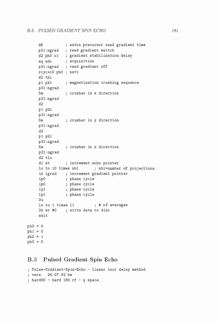
B.3 . PULSED GRA.DIENT SPIN ECHO
d8
p3 1 : ngrad
d2 ph3 0 1
aq adc
p31 : ngrad
rcyc=10 phO d2 thi p 1 ph1 p31 : ngrad Srn
p31 : ngrad
d2
p 1 ph1
p31 : ngrad
Srn
p3 1 : ngrad
d2 p 1 ph1
p31 : ngrad Srn
p31 : ngrad
d2 tlo
extra precursor read gradient time
read gradient switch gradi ent stabil ization delay
acquis it ion
read gradient off
ns= 1
magnetization crushing sequence
crusher in x direct ion
crusher in y direct ion
crusher in z direction
d1 st ; increment echo pointer 10 to 10 t imes nbl ; nbl=nurnber of proj ect ions 1s igrad ipO ipO ip1 ip1
3u
increment gradient pointer phase cycle phase cycle phase cycle phase cycle
10 to 1 t imes 1 1 ; # o f averages 2s wr #0 write data to disc
exit
phO = 0 ph1 = 0 ph2 = 1 ph3 0
B . 3 Pulsed Gradient Spin Echo
Pulse-Gradient-Spin-Echo - linear incr delay method vers o 26 . 07 . 93 brn hard90 - hard 180 rf - q space
181
182 APPENDIX B. THE PULSE SEQUENCES
; ! ! ! in memory acquisition ! ! !
l s ze zero data block and init ial ize
Sm thi
10 dl 01 relaxation delay , set transmitter 0 1
2 0 d3 loop of dummy gradient pulses
phO =
phl =
ph2 =
ph3 =
p31 : ngrad dummy gradient pulse on
d4 p31 : ngrad dS
dummy gradient pulse off
10 to 20 times 12
p l phl (90 degree) excitation hard pulse d3 rf-grad delay p31 : ngrad first q pulse
d4 q durat ion p31 : ngrad q gradients off
dS delay for big DELTA
p2 ph2 180 degree hard pulse d3 rf-grad delay
p31 : ngrad second q gradient on
d4 q durat ion delta
p31 : ngrad
dS 0 1
q gradients off
delay for DELTA
aq adc acquisition
rcyc=10 phO ns= l
dl st increment echo pointer
delay Sm id4 increment Sm ddS decrement delay 10 to 10 t imes nbl Sm rd4 reset Sm rdS reset Sm ipO phase Sm ipO phase Sm ip l phase
Sm ip l phase 3u 10 to 10 t imes 1 1 d l wr #0 ; write
exit
0 0 1
0
nbl=number of proj ections
delay delay
cycle cycle cycle
cycle
; # of averages data to disc
pw=rd=O
B.4. PULSED GRADIENT SPIN ECHO WITH RAMPED GRADIENT PULSES183
• I I I , . . . in memory acquisit ion I I I
B .4 P ulsed Gradient Spin Echo With Ramped Gradi
ent P ulses
Pulse-Gradient-Spin-Echo - linear incr delay method with ramped gradients
vers o 7/9/95 bm
hard90 - hard 180 rf - q space
• I I I , . . . in memory acquisit ion ! ! !
ls ze
5m thi
zero data block and initialize
10 dl 0 1 1 1 d3
relaxation delay , set transmitter 0 1 rf-grad delay
12 p31 : ngrad
d 1 1
step gradient up , start of loop for dummy puls es
10 to 12 t imes 13
p3 1 : ngrad f irst q pulse
d4 q durat ion 13 p31 : ngrad step gradient down
d 1 1
1 0 to 1 3 t imes 13
p31 : ngrad ; q gradients off d5 ; delay for b ig DELTA 10 to 1 1 t imes 15 ; end of loop for dummy pulses
pl phl (90 degree) excitat ion hard pulse d3 rf-grad delay
30 p3 1 : ngrad step gradient up d l l 10 t o 3 0 t imes 1 3
p31 : ngrad f irst q pulse
d4 q duration 40 p31 : ngrad step gradient down
d 1 1 10 t o 40 t imes 13
p31 : ngrad q gradients off d5 delay for big DELTA
p2 ph2 180 degree hard pulse d3 rf-grad delay
50 p31 : ngrad d 1 1
step gradient up
10 to 50 t imes 13
184 APPENDIX B. THE PULSE SEQUENCES
60
p31 : ngrad
d4
p31 : ngrad
d l l
second q gradient on
q duration delta
step gradient down
10 to 60 t imes 13
p31 : ngrad q gradients off
d8 ph3 0 1 delay for echo
acquisition
ns=l aq adc
rcyc=10 phO
dl st
Srn id4 Srn ddS
increment echo pointer
increment delay decrement delay
Srn dd8 10 to 10 t imes nbl nbl=number of proj ect ions
Srn rd4 reset delay
Srn rdS reset delay
Srn rd8
Srn ipO phase cycle
Srn ipO phase cycle
Srn ipl phase cycle
Srn ipl phase cycle
3u
10 to 10 t imes 1 1 ; # of averages
dl wr #0 ; write data to disc
exit
phO = 0
phl = 0
ph2 = 1 ph3 = 0
; pw=rd=O
; ! ! ! in memory acquisit ion ! ! !
B . 5 Dynamic Stimulated Echo with Electroosmosis Trig
ger P ulse
midsteshhep for Dynamic Spin-Echo-Mult i-q-Sl ice with electrophores is trigger pulse vers o 16/1 1/93 bm pulse sequence to acquire the image of a slice through an obj ect soft90 - hard 90 ste 90 degree pulse fourier transformat ion with tf3 tf2
B.5. DYNAMIC STIMULATED ECHO WITH EO PULSE 185
mult i q data set
l s ze
10 dl tlo
setf2-3
dl0
setf2 1 3
d l l
setf2-2 d13 p31 : ngrad
d2 0 1
p3 : tpO phl
p31 : ngrad
d3 thi p31 : ngrad
d2 0 1
p 3 1 : ngrad
d4 p31 : ngrad d2
d5 p2 ph2
d2 p31 : ngrad d4 p31 : ngrad
d7 p2 ph2 d2 p3 1 : ngrad d4 p31 : ngrad d2 d5 d6
p3 1 : ngrad d2 ph3 setf2 1 2 aq adc p3 1 : ngrad rcyc=10 phO setf2-3 d10 setf2 1 3 2s
zero data block and init ial ize
relaxat ion delay , set transmitter 0 1
trigger pulse on channel H on BP l for gradient
duration
pulse off
delay
trigger pulse on channel C on BP l for EP delay
slice gradient on
stabil izat ion delay
90 degree excitat ion soft pulse
dephasing read gradient and phase increment
gradient and slice rephase gradient on
all gradients off
stabilizat ion delay
q-gradient on
durat ion of q-gradient q-gradient off stabil izat ion
TE and DELTA separation-d4-d2-p2
hard 90 degree pulse
stabilizat ion crusher on
durat ion crusher off
storage along z-axis second hard 90 pulse stabilization 2nd q gradient on duration of q-gradient
2nd q grad off stabilizat ion delay 2nd TE and DELTA sepn-d4-d2-p2 trim delay approx p3/2 read gradient on
gradient stabilizat ion delay EP pulse off acquis it ion read gradient off acquis it ion second gradient pulse on durat ion second gradient pulse off dummy ep for negat ive voltage
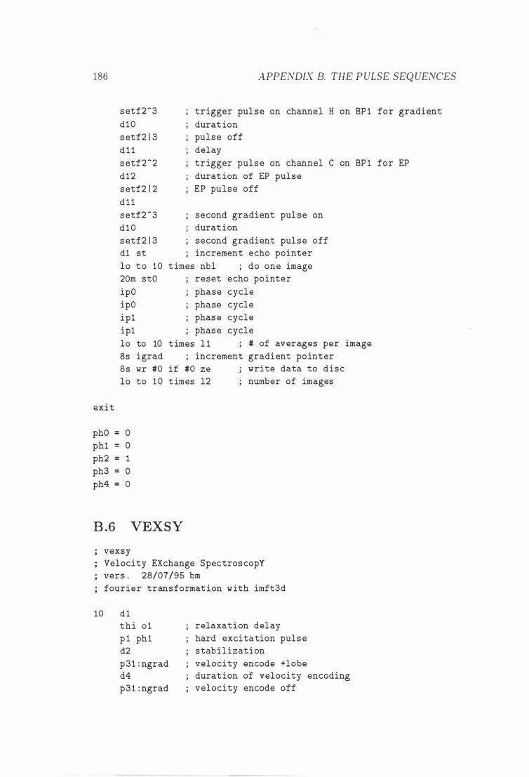
186
exit
phO =
phl =
ph2 =
ph3 =
ph4 =
APPENDIX B. THE P ULSE SEQ UENCES
setf2-3
dl0
setf2 1 3
d l l
setf2-2
d12
setf2 1 2
d l l
setf2-3
dl0
setf2 1 3
trigger pulse on channel H on BP l for gradient
durat ion pulse off
delay
trigger pulse on channel C on BP l for EP
durat ion of EP pulse EP pulse off
second gradient pulse on durat ion
second gradient pulse off dl st increment echo pointer
10 to 10 t imes nbl ; do one image
20m stO reset echo pointer
ipO phase cycle
ipO phase cycle
ipl phase cycle
ipl phase cycle
10
8s 8s 10
0 0
1
0
0
to 10 t imes 1 1 # of averages per image
igrad ; increment gradient pointer
wr #0 if #0 ze write data to disc
to 10 t imes 12 number of images
B .6 VEXSY
vexsy Velocity EXchange SpectroscopY vers o 28/07/95 bm
fourier transformat ion with imft3d
10 dl thi 0 1 p l phl d2
p31 : ngrad d4 p31 : ngrad
relaxation delay
hard excitation pulse stabilization
velocity encode +lobe durat ion of velocity encoding velocity encode off
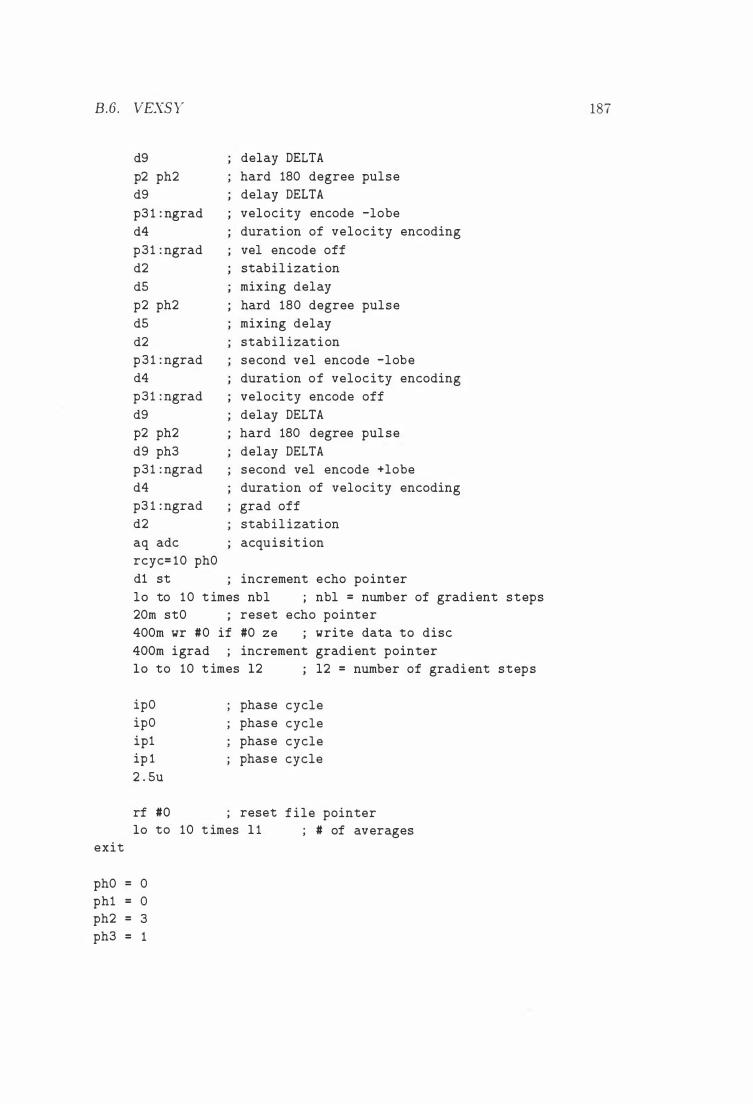
B.6. VEXSY
exit
phO =
phl = ph2 =
ph3 =
d9
p2 ph2 d9
p3 1 : ngrad
d4
p31 : ngrad
d2
dS
p2 ph2
dS
d2 p31 : ngrad
d4
p31 : ngrad
d9
p2 ph2
d9 ph3 p31 : ngrad
d4
p3 1 : ngrad
d2
delay DELTA
hard 180 degree pulse delay DELTA
velocity encode -lobe
duration of velocity encoding
vel encode off stabilization
mixing delay
hard 180 degree pulse
mixing delay
stabilization
second vel encode -lobe
duration of velocity encoding
velocity encode off
delay DELTA
hard 180 degree pulse
delay DELTA second vel encode +lobe
duration of velocity encoding
grad off stabil izat ion
aq adc acquisit ion rcyc= 10 phO
dl st increment echo pointer
10 to 10 t imes nbl ; nbl = number of gradient steps 20m stO reset echo pointer 400m wr #0 if #0 ze write data to disc
400m igrad ; increment gradient pointer 10 to 10 t imes 12 12 = number of gradient steps
ipO phase cycle ipO phase cycle ipl phase cycle ip l phase cycle 2 . Su
rf #0 ; reset f ile pointer 10 to 10 t imes 1 1 ; # of averages
0 0 3 1
187
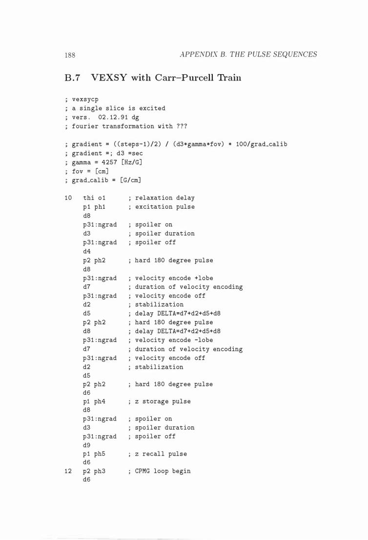
188 APPENDIX B. THE PULSE SEQ UENCES
B . 7 VEXSY with Carr-Purcell Train
10
12
vexsycp
a s ingle slice is excited
vers o 02 . 12 . 9 1 dg
fourier transformation with ? ? ?
gradient = ( ( steps- l ) /2 ) / (d3*gamma*fov) * 100/grad_cal ib
gradient = ; d3 =sec
gamma = 4257 [Hz/G]
fov = [cm] grad_cal ib = [G/cm]
thi 0 1
p l phl
d8 p31 : ngrad
d3 p31 : ngrad
d4
p2 ph2
d8 p31 : ngrad d7
p31 : ngrad d2
d5
p2 ph2
d8 p31 : ngrad
d7
p31 : ngrad
d2 d5 p2 ph2 d6 pl ph4 d8 p31 : ngrad
d3 p31 : ngrad
d9 p l ph5 d6
p2 ph3 d6
relaxat ion delay
excitation pulse
spoiler on
spoiler durat ion spoiler off
hard 180 degree pulse
velocity encode +lobe durat ion of velocity encoding
velocity encode off stabilization
delay DELTA=d7+d2+d5+d8 hard 180 degree pulse
delay DELTA=d7+d2+d5+d8 velocity encode -lobe
duration of velocity encoding velocity encode off
stabilization
hard 180 degree pulse
z storage pulse
spoiler on
spoiler durat ion spoiler off
z recall pulse
CPMG loop begin
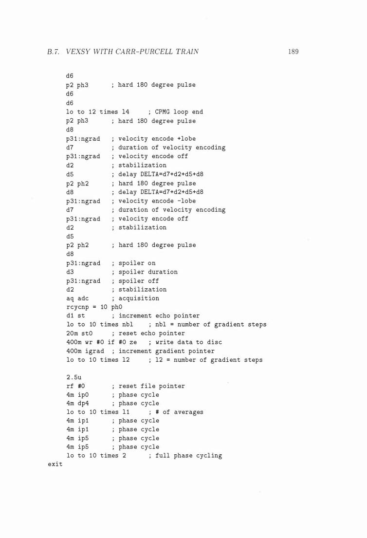
B. 7. VEXSY WITH CARR-PURCELL TRAIN
exit
d6
p2 ph3 d6
d6
hard 180 degree pulse
10 to 12 t imes 14 ; CPMG loop end p2 ph3 hard 180 degree pulse d8
p3 1 : ngrad d7 p31 : ngrad
d2
dS
p2 ph2 d8
p31 : ngrad d7
p3 1 : ngrad
d2 dS p2 ph2
d8
p31 : ngrad d3
velocity encode +lobe durat ion of velocity encoding velocity encode off
stabilization
delay DELTA=d7+d2+dS+d8
hard 180 degree pulse delay DELTA=d7+d2+dS+d8
velocity encode -lobe
durat ion of velocity encoding
velocity encode off stabilization
hard 180 degree pulse
spoiler on
spoiler durat ion
p31 : ngrad spoiler off d2 stabilizat ion
aq adc acquisit ion rcycnp = 10 phO d l st ; increment echo pointer 10 to 10 t imes nbl ; nbl = number of gradient steps
20m stO reset echo pointer
400m wr #0 if #0 ze write data to disc
400m igrad ; increment gradient pointer 10 to 10 t imes 12 12 = number of gradient steps
2 . Su rf #0 reset file pointer 4m ipO phase cycle 4m dp4 phase cycle 10 to 10 t imes 1 1 ; # of averages 4m ipl phase cycle
4m ip l phase cycle
4m ip5 phase cycle 4m ip5 phase cycle 10 to 10 t imes 2 ; full phase cycl ing
189
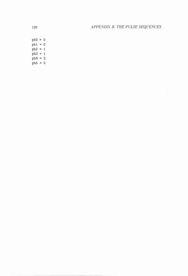
190
phO = 0
ph1 = 0
ph2 = 1 ph3 = 1 ph4 = 2 ph5 = 0
APPENDIX B. THE P ULSE SEQ UENCES
Appendix C
The A U Programs
C . l Program to Send Trigger P ulses to External S hift
Register
motorstep
15/1 1/94 bm
char s25 [25J ;
char save�ame [20J , save_user [20J ; int save_expno , save_procno ; int helpi ;
getcurdat a ;
ShmLstatus ( " AU program motorstep " ) ; (void) strcpy ( save-llame , name ) ;
(void) strcpy ( save_user , user) ;
save_expno = expno ; save_procno= procno ; fetchpar ( " L 8 " , &helpi ) ;
/* Go to the dataset motor */
DATASET ( "motor" , 1 , 1 , disk , user ) ;
read standard parameters rpar ( " standardim1d" , "al l " ) ;
/* change pulse sequence */ storepar ( " PULPROG" , "motorstep " ) ;
/* store counter */ storepar ( " L 8" , help i ) ;
/ * send pulses t o shift register */
191
192 APPENDIX C. THE A U PROGRAMS
ZG ;
1 * return to previous data * 1 DATASET ( save�ame , save_expno , save_procno , disk , save_user ) ;
1 * print message on screen * 1 Show-status ( " Au program motorstep finished" ) ;
1 * quit ;
quit AU program
C .2 AV Program for a Set of Experiments with D if
ferent Temperatures
char s35 [35] ;
getcurdata ;
uselastpars ; rvtl ist ;
t imes ( l 1 )
pgsesleep
03/05/95 bm
1* all expts . with
1 * read VT l ist
1 * begin loop Procerr (O , "Sett ing Temperature" ) ;
vt ; 1 * set temperature
the same parameters * 1 * 1 * 1
1 * wait for temperature to settle
teready (300 , 0 . 3 ) ; sprintf (s35 , "Experiment number Yed \n" , expno ) ;
1 * print message on screen
Proc_err (O , s35 ) ;
zg ; iexpno ; ivtlist ;
1 * Acquisit ion 1* next experiment 1 * read next temperature from l ist
end ; 1 * end loop sprintf ( s35 , "Experiments f inished . Bye . . . \n" ) ;
1 * print message on screen Proc_err (O , s35) ;
quit ; 1 * quit AU program
C . 3 AV Program for a Set o f Experiments with Dif
ferent Motor Speeds
bertsleep
C.3. DIFFERENT l'vIOTOR SPEEDS 193
15/4/94 bm
char s35 [35J ;
getcurdata ;
usecurpars ;
t imes (4)
1 * all expts . with different parameters * 1 1 * begin loop * 1
sprintf ( s35 , "Experiment number 'l.d\n" , expno) ;
1 * print message on screen Proc_err (O , s35 ) ;
1 * execute AU program motorstep
xau ( "motorstep " ) ;
zg ; 1 * Acquisition
iexpno ; 1 * next experiment end ; 1 * end loop sprintf ( s35 , "Experiments f inished . Bye . . . \n" ) ;
Proc_err (O , s35 ) ; 1* print message on screen
quit ; 1 * quit AU program