Copyright Warning & Restrictions

The copyright law of the United States (Title 17, United States Code) governs the making of photocopies or other

reproductions of copyrighted material.

Under certain conditions specified in the law, libraries and archives are authorized to furnish a photocopy or other

reproduction. One of these specified conditions is that the photocopy or reproduction is not to be “used for any

purpose other than private study, scholarship, or research.” If a, user makes a request for, or later uses, a photocopy or reproduction for purposes in excess of “fair use” that user

may be liable for copyright infringement,

This institution reserves the right to refuse to accept a copying order if, in its judgment, fulfillment of the order

would involve violation of copyright law.

Please Note: The author retains the copyright while the New Jersey Institute of Technology reserves the right to

distribute this thesis or dissertation

Printing note: If you do not wish to print this page, then select “Pages from: first page # to: last page #” on the print dialog screen

The Van Houten library has removed some ofthe personal information and all signatures fromthe approval page and biographical sketches oftheses and dissertations in order to protect theidentity of NJIT graduates and faculty.

ABSTRACT

MULTI-SPECTRAL LIGHT INTERACTION MODELINGAND IMAGING OF SKIN LESIONS

bySachin Vidyanand Patwardhan

Nevoscope as a diagnostic tool for melanoma was evaluated using a white light source

with promising results. Information about the lesion depth and its structure will further

improve the sensitivity and specificity of melanoma diagnosis. Wavelength-dependent

variable penetration power of monochromatic light in the trans-illumination imaging

using the Nevoscope can be used to obtain this information. Optimal selection of

wavelengths for multi-spectral imaging requires light-tissue interaction modeling. For

this, three-dimensional wavelength dependent voxel-based models of skin lesions with

different depths are proposed. A Monte Carlo simulation algorithm (MCSVL) is

developed in MATLAB and the tissue models are simulated using the Nevoscope optical

geometry. 350-700nm optical wavelengths with an interval of 5nm are used in the study.

A correlation analysis between the lesion depth and the diffuse reflectance is then used to

obtain wavelengths that will produce diffuse reflectance suitable for imaging and give

information related to the nevus depth and structure. Using the selected wavelengths,

multi-spectral trans-illumination images of the skin lesions are collected and analyzed.

An adaptive wavelet transform based tree-structure classification method

(ADWAT) is proposed to classify epi-illuminance images of the skin lesions obtained

using a white light source into melanoma and dysplastic nevus images classes. In this

method, tree-structure models of melanoma and dysplastic nevus are developed and

semantically compared with the tree-structure of the unknown image for classification.

Development of the tree-structure is dependent on threshold selections obtained from a

statistical analysis of the feature set. This makes the classification method adaptive. The

true positive value obtained for this classifier is 90% with a false positive of 10%. The

Extended ADWAT method and Fuzzy Membership Functions method using combined

features from the epi-illuminance and multi-spectral images further improve the

sensitivity and specificity of melanoma diagnosis. The combined feature set with the

Extended-ADWAT method gives a true positive of 93.33% with a false positive of

8.88%. The Gaussian Membership Functions give a true positive of 100% with a false

positive of 17.77% while the Bell Membership Functions give a true positive of 100%

with a false positive of 4.44%.

MULTI-SPECTRAL LIGHT INTERACTION MODELINGAND IMAGING OF SKIN LESIONS

bySachin Vidyanand Patwardhan

A DissertationSubmitted to the Faculty of

New Jersey Institute of TechnologyIn Partial Fulfillment of the Requirements for the Degree of

Doctor of Philosophy in Electrical Engineering

Department of Electrical and Computer Engineering

January 2004

Copyright © by Sachin Vidyanand Patwardhan

ALL RIGHTS RESERVED

APPROVAL PAGE

MULTI-SPECTRAL LIGHT INTERACTION MODELINGAND IMAGING OF SKIN LESIONS

Sachin Vidyanand Patwardhan

Dr. Atam P. Dhawan, Dissertation Advisor DateProfessor of Electrical and Computer Engineering, NJIT

Dr. Nirwan Ansari, Committee Member DateProfessor of Electrical and Computer Engineering, NJIT

Dr. Timothy Mang, Comm tee Member DateAssociate Professor of Elect . cal and Computer Engineering, NJIT

Dr. John F. Federici, Committee Member gatefessor of Physics, NJIT

Dr. Stanley Reiman, Committee Member DateProfessor of Biomedical Engineering, NJIT

BIOGRAPHICAL SKETCH

Author: Sachin Vidyanand Patwardhan

Degree: Doctor of Philosophy

Date: January 2004

Undergraduate and Graduate Education:

• Doctor of Philosophy in Electrical EngineeringNew Jersey Institute of Technology, Newark, NJ, 2004.

• Master of Technology in Biomedical EngineeringIndian Institute of Technology, Mumbai, India, 1993.

• Bachelor of Engineering in Electrical EngineeringGovernment College of Engineering, Pune, India, 1990.

Major: Electrical Engineering

Presentations and Publications:

Sachin V. Patwardhan, Atam P. Dhawan and Patricia A. Relue, Tree-structured WaveletTransform Signature for Classification of Melanoma, Proc. SPIE MedicalImaging: Image Processing, Vol. 4684, p. 1085-1091, 2002.

Amit Nimunkar, Atam P. Dhawan, Patricia A. Relue and Sachin V. Patwardhan,Wavelet and Statistical Analysis for Melanoma Classification, Proc. SPIEMedical Imaging: Image Processing, Vol. 4684, p. 1346-1353, 2002.

iv

Sachin V. Patwardhan, Atam P. Dhawan and Patricia A. Relue, Classification ofMelanoma Using Tree-Structured Wavelet Transforms, Computer Methods andPrograms in Biomedicine, Vol. 72, p. 223-239, 2003.

Sachin V. Patwardhan, Atam P. Dhawan and Patricia A. Relue, Wavelength Selection forMulti-Spectral Imaging of Skin Lesions, Proc. IEEE 29 th Annual NortheastBioengineering Conference, p. 327-328, 2003.

Sachin V. Patwardhan, Atam P. Dhawan and Patricia A. Relue, Monte Carlo Simulationof Light-Tissue Interaction — Part I: Three-Dimensional Voxel Based Simulationfor Optical Imaging, IEEE Transactions on Biomedical Engineering, underrevision, 2003.

Sachin V. Patwardhan, Atam P. Dhawan and Patricia A. Relue, Monte Carlo Simulationof Light-Tissue Interaction — Part II: Three-Dimensional Simulation for Trans-illumination based Imaging of Skin Lesions, IEEE Transactions on BiomedicalEngineering, under revision, 2003.

Atam P. Dhawan, Sachin V. Patwardhan and Patricia A. Relue, Multi-Spectral LightTissue Interaction Modeling For Skin Lesion Imaging, 25th Annual InternationalConference of the IEEE Engineering in Medicine and Biology Society, submitted,2003.

Ketan Patel, Ronn Walvick, Sachin V. Patwardhan and Atam P. Dhawan, Classificationof Melanoma using Wavelet Transform-based Optimal Fearure Set, SPIEInternational Symposium: Medical Imaging, submitted, 2004.

Sachin V. Patwardhan, Shuangshuang Dai and Atam P. Dhawan, Multi-spectral ImageAnalysis and Classification of Melanoma Using Crisp and Fuzzy Partitions,Computerized Medical Imaging and Graphics, submitted, 2003

IN THE MEMORIES OF MY GRANDFATHERS

VINAYAK D. PATWARDHAN AND CHANTIMANI P. DAMLE

WHOSE BLESSINGS WILL ALWAYS GIVE ME STRENGTH

AND SHOW ME THE RIGHT PATH

vi

ACKNOWLEDGEMENT

It is with great pleasure; I express my indebtness and gratitude to Dr. Atam P. Dhawan

for his guidance, suggestions and supervision of my dissertation work. Without his

support, encouragement and reassurance completion of this work was not possible. I am

also thankful to Dr. Patricia A. Relue for her advice and suggestions as my unofficial co-

advisor. Special thanks are also given to Dr. Stanley Reisman, Dr. Nirwan Ansari and Dr.

Timothy Chang and Dr. John Federici for actively participating in my committee.

I would like to thank the Whitaker Foundation for providing partial funding for

this research under the Whitaker Foundation Research Grant RG-99-0127 and to all the

patients whose data was used in this study, The Medical College of Ohio, Toledo and Dr.

Prabir Chaudhari for his contribution in the data collection. I am also thankful H. Zeng,

C. MacAulay, B. Palcic and D. McLean for sharing their data of diffuse reflectance

measurements using the spectroanalyser system.

Many of my fellow graduate students and friends in the Signal and Image

Processing Laboratory deserve recognition for their support and valuable inputs. Thanks

are given to Shuangshuang, Amit, Denver, Yash, and Kristin.

I would like to thank my parents Vidyanand and Vinita and my wife's parents

Jayant and Jyoti for supporting and encouraging me during my Ph.D. work. This work

was possible only because my wife Swati encouraged me to pursue my dreams and took

care of our daughter Sneha and me while I was busy with my studies and research work.

Special thanks are due to Swati and Sneha for being supportive and understanding and

bearing the hardship of student life with me.

vi'

TABLE OF CONTENTS

Chapter

1 INTRODUCTION

Page

1

1.1 Motivation 1

1.2 Problem Statement and Objectives 2

1.3 Proposed Approach 3

1.4 Organization of the Report 6

2 LITERATURE REVIEW 8

2.1 Spatial/Frequency and Texture Analysis 8

2.2 Modeling of Light-Tissue Interaction 10

3 METHODOLOGY 16

3.1 Classification of the Epi-illuminance Images... 16

3.1.1 Epiluminesence Image Data 16

3.1.2 Image Decomposition 17

3.1.3 Tree Structure Classification Method 18

3.1.4 Adaptive Wavelet-based Tree-Structure Classification Method 20

3.2 Light-Tissue Interaction Modeling 24

3.2.1 Photon Random Walk 25

3.2.2 Tissue Models and Voxel Library 34

3.2.3 Optical Properties 36

3.2.4 Verification of the Algorithm 41

3.2.5 Skin Lesion Models 46

3.2.6 Nevoscope Optical Geometry 47

viii

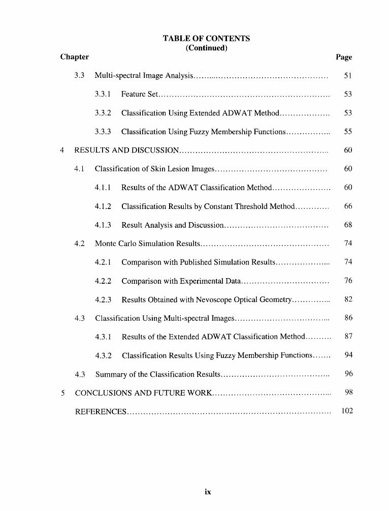
TABLE OF CONTENTS(Continued)

Chapter

3.3 Multi-spectral Image Analysis

3.3.1 Feature Set

3.3.2 Classification Using Extended ADWAT Method

3.3.3 Classification Using Fuzzy Membership Functions

Page

51

53

53

55

4 RESULTS AND DISCUSSION 60

4.1 Classification of Skin Lesion Images 60

4.1.1 Results of the ADWAT Classification Method 60

4.1.2 Classification Results by Constant Threshold Method 66

4.1.3 Result Analysis and Discussion 68

4.2 Monte Carlo Simulation Results 74

4.2.1 Comparison with Published Simulation Results 74

4.2.2 Comparison with Experimental Data 76

4.2.3 Results Obtained with Nevoscope Optical Geometry 82

4.3 Classification Using Multi-spectral Images 86

4.3.1 Results of the Extended ADWAT Classification Method 87

4.3.2 Classification Results Using Fuzzy Membership Functions 94

4.3 Summary of the Classification Results 96

5 CONCLUSIONS AND FUTURE WORK 98

REFERENCES 102

ix

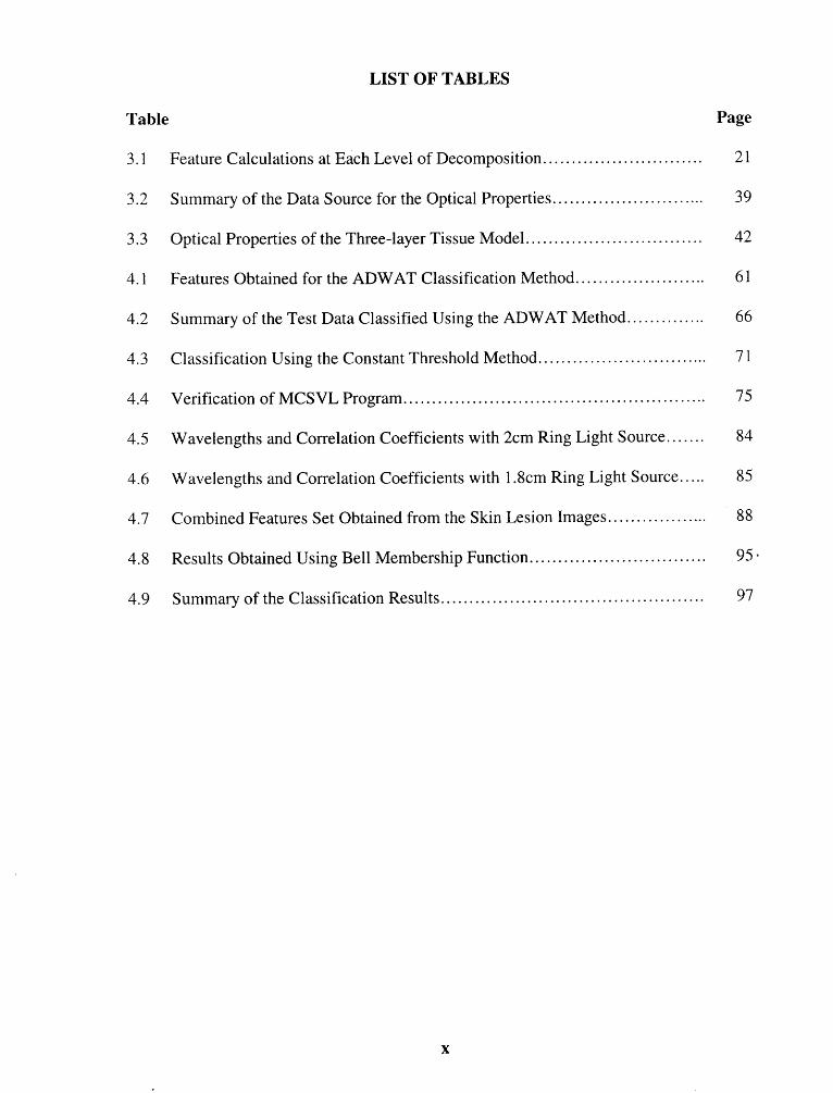
LIST OF TABLES

Table Page

3.1 Feature Calculations at Each Level of Decomposition 21

3.2 Summary of the Data Source for the Optical Properties 39

3.3 Optical Properties of the Three-layer Tissue Model 42

4.1 Features Obtained for the ADWAT Classification Method 61

4.2 Summary of the Test Data Classified Using the ADWAT Method 66

4.3 Classification Using the Constant Threshold Method 71

4.4 Verification of MCSVL Program 75

4.5 Wavelengths and Correlation Coefficients with 2cm Ring Light Source 84

4.6 Wavelengths and Correlation Coefficients with 1.8cm Ring Light Source 85

4.7 Combined Features Set Obtained from the Skin Lesion Images 88

4.8 Results Obtained Using Bell Membership Function 95

4.9 Summary of the Classification Results 97

x

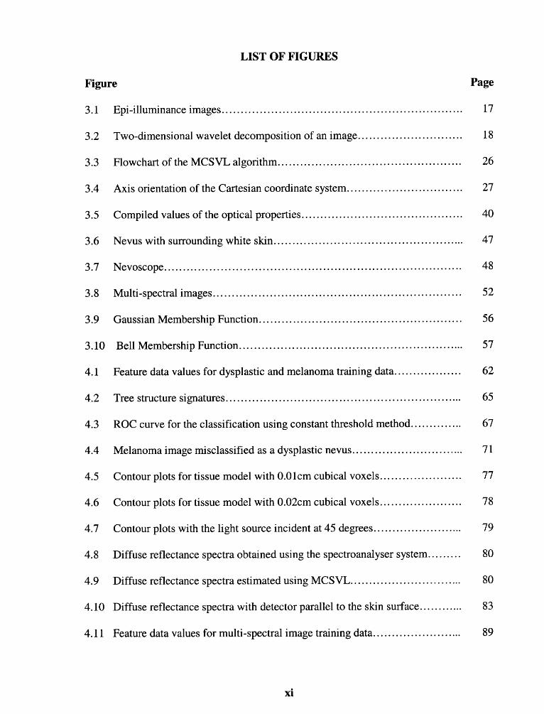
LIST OF FIGURES

Figure Page

3.1 Epi-illuminance images 17

3.2 Two-dimensional wavelet decomposition of an image 18

3.3 Flowchart of the MCSVL algorithm 26

3.4 Axis orientation of the Cartesian coordinate system 27

3.5 Compiled values of the optical properties 40

3.6 Nevus with surrounding white skin 47

3.7 Nevoscope 48

3.8 Multi-spectral images 52

3.9 Gaussian Membership Function 56

3.10 Bell Membership Function 57

4.1 Feature data values for dysplastic and melanoma training data 62

4.2 Tree structure signatures 65

4.3 ROC curve for the classification using constant threshold method 67

4.4 Melanoma image misclassified as a dysplastic nevus 71

4.5 Contour plots for tissue model with 0.01cm cubical voxels 77

4.6 Contour plots for tissue model with 0.02cm cubical voxels 78

4.7 Contour plots with the light source incident at 45 degrees 79

4.8 Diffuse reflectance spectra obtained using the spectroanalyser system 80

4.9 Diffuse reflectance spectra estimated using MCSVL 80

4.10 Diffuse reflectance spectra with detector parallel to the skin surface 83

4.11 Feature data values for multi-spectral image training data 89

xi

CHAPTER 1

INTRODUCTION

1.1 Motivation

The rising rate of skin cancer is a growing concern worldwide [1]. Skin cancer is the

most common form of cancer in the human population [2]. Mass screening for melanoma

and other cutaneous malignancies has been advocated for early detection and effective

treatment [3]. Dermatologists use the ABCD rule (Asymmetry, Border, Colors, and

Dermoscopic structures) to characterize skin lesions [4-7]. To calculate the ABCD score,

the criteria are assessed semi-quantitatively. Each of the criteria is then multiplied by a

given weight factor to yield a total dermoscopy score [8]. The ABCD rule works well

with thin melanocytic lesions. The sensitivity of the ABCD rule is reported to vary from

59% to 88% [9-10]. The features used in the ABCD rule suggest that changes in the

surface characteristics of the nevus occur as it progresses towards melanoma. In the early

stages of melanoma the features used in visual examination are hardly visible and may

lead to a false diagnosis. However, if images of skin lesions can be collected that contain

spatial/frequency and texture information, then a non-invasive method of lesion

classification based on these surface characteristics may be developed. The lesion for

biopsy can then be selected utilizing computer-aided analysis for improving the

sensitivity and specificity of skin cancer detection. Thus, the development of a non-

invasive imaging and analysis method could be beneficial in the early detection of

cutaneous melanoma.

1

2

Malignant melanoma is the most lethal skin cancer in which melanocytes in the

epidermis undergo malignant transformation. The two phases in the growth of melanoma

are the superficial spreading phase, during which the lesion increases in size within the

epidermis, and the vertical growth phase when the cells begin to move into the dermis

[11-12]. The level of the spread of melanoma within the epidermis and then the dermis is

determined as the Clark level, which indicates the stage (i.e. the severity) of the spread of

melanoma. The best prognostic factor is the vertical thickness of the suspected nevus [12-

13]. But due to lack of non-invasive diagnostic techniques, excision and histological

sectioning of the suspected nevus is the only method used for the vertical thickness

measurement. Lesion excision could be painful and people with a false diagnosis

unnecessarily suffer and get a scar in place of the excised lesion. A non-invasive

technique that can characterize the lesion depth information will increase the diagnostic

sensitivity and also save the patients from pain and unnecessary scars.

1.2 Problem Statement and Objectives

Dhawan [14-15] introduced the concept of Nevoscope; a noninvasive trans-illumination

based imaging modality for analysis and diagnosis of melanoma. The Nevoscope is being

evaluated as a dermatological tool for improving visual examination of suspected lesions.

It has shown promising results using image analysis techniques such as 3D reconstruction

[15-16], segmentation [17-18] and texture and spatial-frequency information [14, 19-20]

for quantitative analysis of diagnostic parameters.

Visible light introduced onto the skin area surrounding a lesion by the ring light

source of the Nevoscope [14-15] penetrates the skin and undergoes scattering and

3

absorption within the various skin layers. A significant part of the unabsorbed multiply

scattered light re-emerges from the skin's surface as diffuse reflectance. This reflectance

forms an image of the trans-illuminated lesion when viewed from above. Although the

trans-illumination images give information from within the skin, it is hard to quantify the

depth from where this information is obtained. So far, Nevoscope as a diagnostic tool for

melanoma was evaluated using a white light source, but it can be easily adapted to a

monochromatic light source of a specific wavelength. The depth of penetration of

monochromatic light in the skin depends on its wavelength, with higher wavelengths

having more depth of penetration. This wavelength-dependent variable penetration power

of monochromatic light in the trans-illumination imaging using the Nevoscope can be

used to obtain information for characterizing the skin lesion depth.

The objectives of this study are

• To analyze the epi-illuminance images of the skin lesion, extract features andclassify the images into melanoma, dysplastic nevus images classes.

• To find optical wavelengths which when used in the trans-illumination imaging ofthe Nevoscope could give information for characterizing melanoma.

• To collect multi-spectral images of the skin lesions using the selected opticalwavelengths and to analyze them for the diagnosis of melanoma.

1.3 Proposed Approach

The features used in the ABCD rule suggest that changes in the spatial/frequency and

textural characteristics can be used for classifying the skin lesions. Among the different

methods used for the analysis of spatial/frequency and textural information, the Gaussian

Markov random field [21-23] and Gibbs distribution texture models [24-25] characterize

the gray levels between nearest neighboring pixels by a certain stochastic relationship.

4

The weakness in these methods is that they focus on the coupling between image pixels

on a single spatial scale and fail to characterize different scales of texture effectively.

Wavelet transform [26-29], Gabor transforms [30-33] and Wigner distribution [30-33]

are good multi-resolution analytical tools and help to overcome this limitation. Tree-

structured wavelet decomposition determines important frequency channels dynamically

based on image energy calculations within the different frequency bands and can be

viewed as an adaptive multi-channel method [34].

To analyze the epi-illuminance images of the skin lesions and to classify them

into melanoma and dysplastic nevus images the wavelet transform analysis is used. An

adaptive wavelet transform based tree-structure classification method (ADWAT) is

proposed. In this method tree-structure models of the different image classes are

developed using a known set of images. The tree-structure models of melanoma and

dysplastic nevus are then semantically compared with the tree-structure of the unknown

skin lesion image for classification. Development of the tree-structure is dependent on

threshold selections obtained from a statistical analysis of the feature set. This makes the

classification method adaptive.

To select optimal wavelengths for multi-spectral imaging, study and

understanding of light-tissue interaction is necessary. For modeling the light-tissue

interaction, Kubelka-Munk, radiative transport theory and Monte Carlo methods are the

three most common methods used [35]. The Kubelka-Munk description is applicable to

one-dimensional geometries and accounts for propagation of diffuse fluxes only [36].

Hence, the results are not valid for measurement systems employing collimated or finite

aperture light sources. Also, it is difficult to incorporate effects of diffuse reflectance at

5

the medium boundaries into models based on Kubelka-Munk theory. Exact analytical

solutions of the radiative transport equations have been found only for a few special cases

[37]. The numerical computation of the right equation with discrete ordinate method is a

formidable task even for simple geometries. Techniques such as diffusion approximation

[38-40] and Beer's law [41] have been used, which are valid for highly scattering and

non-scattering materials. Photon interaction with matter is stochastic in nature and can be

described using computer simulation with appropriately weighted random absorption and

scattering events. Monte Carlo simulation is a statistical technique for simulating light-

tissue interaction under a wide variety of situations [42-44].

To find optical wavelengths in the visible range, which when used with the

Nevoscope can discriminate skin lesions based on their depths, the Monte Carlo

simulation technique is used. Three-dimensional voxel based models of skin lesions with

different depths and models of different skin types based on their epidermal melanin

concentration are proposed. A voxel library is compiled using the wavelength dependent

optical properties of tissue reported by various research groups. Voxels from the voxel

library are used in the development of the tissue models. The optical properties of the

voxels used in the models change according to the wavelength of the monochromatic

light source used in the simulation. This makes the models wavelength dependent. A

Monte Carlo simulation algorithm (MCSVL) for models generated using the voxel

library is developed. The tissue models are simulated for diffuse reflectance

measurements with an interval of 5 nm over the optical wavelength range of 350-700 nm.

A correlation analysis between the lesion depth and the diffuse reflectance is then used to

obtain wavelengths that produce high correlation coefficient values.

6

Multi-spectral skin lesion images using the selected wavelengths are collected.

Using an analysis similar to the ADWAT method, wavelet transform based features are

extracted from the multi-spectral trans-illumination images of the skin lesion. These

features are combined with those obtained from the epi-illuminance images of the skin

lesion using a white light source. The ADWAT classification method is extended to

handle this combined feature set for improving the sensitivity and specificity of

melanoma diagnosis. Most of the features used in the ADWAT classification method

have a bimodal distribution with overlapping feature values between the image classes.

Hence, fuzzy membership functions based method is also used to compare the

classification results.

1.4 Organization of the Report

The report is divided in to five main parts: (1) Introduction and problem statement, (2)

Background and literature review, (3) Methodology and implementation, (4) Results and

discussion and (5) Conclusion and future work. Chapter 2 presents a brief review of the

literature. In Section 2.1 the various approaches used in the analysis of spatial/frequency

information and textural information are discussed. Section 2.2 describes the various

methods used for modeling light-tissue interaction. The advantages and disadvantages of

the methods described in Chapter 2, leads into the methods proposed in this study.

The implementations of the proposed methods are described in Chapter 3.

Section 3.1 describes the ADWAT classification method while Section 3.2 describes the

MCSVL algorithm, the concept of voxel library, the tissue models and the correlation

analysis for optimal wavelength selection. In section 3.3 the multi-spectral images of the

7

skin lesion collected using the selected optimal wavelengths are analyzed. Wavelet

transform based feature extraction and their significance is discussed in this section. The

combined feature set obtained from the epi-illuminance and trans-illumination images is

used for improving the classification of the melanoma. An Extended-ADWAT

classification method and Fuzzy Membership Functions based method are employed for

this purpose and the classification results are compared.

The results obtained are presented and analyzed in Chapter 4. Classification

results of epi-illuminance images of skin lesions obtained using the ADWAT method are

discussed in Section 4.1. Estimates of the diffuse reflectance obtained for the tissue

models proposed and the results of the correlation analysis between lesion depth and

diffuse reflectance are presented in Section 4.2. Section 4.3 presents the classification

results obtained using the combined features from multi-spectral trans-illumination

images and epi-illuminance images of the skin lesion. In Chapter 5, conclusions drawn

from the work done so far towards development of the Nevoscope and improving the

sensitivity and specificity of melanoma diagnosis are presented. Methods for further

improving the Nevoscope capabilities as a diagnostic tool for melanoma are suggested

based on these conclusions.

CHAPTER 2

LITERATURE REVIEW

2.1 Spatial/Frequency And Texture Analysis

It is very difficult to give the precise definition of texture that could be used in image

analysis. It should describe local neighborhood properties of the gray levels, but also

include some intuitive properties like roughness, granularity and regularity. Texture is

defined in [45] as the feature, which describes spatial ordering of pixel intensities in a

region. According to Jain [46], the term texture generally refers to repetition of basic

texture elements called texels. Their placement can be periodic, quasi-periodic or

random. Texture can be characterized using statistical properties of the region in an

image that has a set of local statistics, or other local properties that are constant, slowly

varying or approximately periodic [47-48].

The application of wavelet orthogonal representation to texture discrimination and

fractal analysis has been discussed by Mallat [49]. Feature extraction for texture analysis

and segmentation using wavelet transforms has been applied by Chang and Kuo [34],

Laine and Fan [50], Unser [51], and Porter and Canagarajah [52]. The tree-structured

wavelet transform decomposes a signal into a set of frequency channels that have

narrower bandwidths in the lower frequency region. Decomposition of just the lower

frequency region, as is performed in conventional wavelet transforms, may not be

effective for image classification [30], [53-54]. This is suitable for signals consisting

primarily of smooth components with information concentrated in the low frequency

regions, but is not suitable for quasi-periodic signals whose dominant frequency channels

8

9

are located in the mid-frequency region. The most significant spatial and frequency

information that characterizes an image often appears in the mid-frequency region. Thus,

to analyze these types of signals wavelet packets are used [34]. In the wavelet packet

analysis the decomposition is no longer applied to the low frequency channels

recursively, but can be applied to the output of any channel.

Chang and Kuo [34] proposed a method for the development of wavelet

transform-based tree structure decomposition. In this method, a set of known images used

during the learning phase is decomposed using a two-dimensional wavelet transform to

obtain the energy map and the dominant frequency channels. Decomposition of a channel

is determined based on the ratio of the average energy of that channel to the highest

average energy of a channel at the same level of decomposition. If the energy ratio

exceeds a pre-determined threshold value, the channel is decomposed. The dominant

frequency channels are then used as features for classification. Chang and Kuo [34] have

suggested that the filter selection dose not have much influence on the texture

classification. On the other hand experiments preformed by Unser [51] imply that the

choice of a filter bank in the wavelet texture characterization could be an important issue.

DeBrunner and Kadiyala [55] and Mojsilovic, Popovic and Rackov [56] have studied the

effect of wavelet bases in texture classification using the method suggested by Chang and

Kuo [34] and agree with the results obtained by Unser [51].

The tree structure method suggested by Chang and Kuo [34] has several major

limitations, mainly, the selection of the threshold value used for subsequent

decomposition and the assumption that high average energy is a good discrimination

criterion. To overcome these limitations, an adaptive wavelet-based tree-structure

10

(ADWAT) analysis method is proposed. In the adaptive method, the channels that are

decomposed are selected based on a statistical analysis of the feature data. The threshold

is selected to give the best separation of features for channels that contain information

useful for discrimination. Based on these thresholds the tree structure models for each of

the image classes is obtained. In this study, the ADWAT method is used for a model-

based classification of epi-illuminance images of skin lesions. The tree structure models

of melanoma and dysplastic nevus are developed and are semantically compared with the

tree structure of the unknown skin lesion image for classification. This method is

compared with the one suggested by Chang and Kuo [34]. The ADWAT classification

method is further extended to analyze and classify the multi-spectral trans-illumination

image data.

2.2 Modeling Of Light-Tissue Interaction

Light-tissue interaction has many applications in medical diagnostics and therapeutic

procedures such as photodynamic therapy [57], laser surgery [58], laser Doppler

velocimetry [59] and pulse oximetry [60]. Controlled experimental studies to understand

light interaction with tissue and measurements of optical properties are difficult to

perform. Mathematical models of light propagation in tissue have been developed and

studied over decades for this purpose. The exact assessment of light propagation in tissue

would require a model that characterizes the spatial distribution and the size distribution

of tissue structures, their absorbing properties and their refractive indices. However for

real tissue, such as skin, the task of creating a precise representation either as a phantom

or as a computer simulation is formidable. Tissue is mostly represented as an absorbing

11

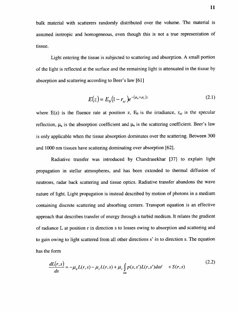
bulk material with scatterers randomly distributed over the volume. The material is

assumed isotropic and homogeneous, even though this is not a true representation of

tissue.

Light entering the tissue is subjected to scattering and absorption. A small portion

of the light is reflected at the surface and the remaining light is attenuated in the tissue by

absorption and scattering according to Beer's law [61]

where E(z) is the fluence rate at position z, E0 is the irradiance, r sc is the specular

reflection, p is the absorption coefficient and IA, is the scattering coefficient. Beer's law

is only applicable when the tissue absorption dominates over the scattering. Between 300

and 1000 nm tissues have scattering dominating over absorption [62].

Radiative transfer was introduced by Chandrasekhar [37] to explain light

propagation in stellar atmospheres, and has been extended to thermal diffusion of

neutrons, radar back scattering and tissue optics. Radiative transfer abandons the wave

nature of light. Light propagation is instead described by motion of photons in a medium

containing discrete scattering and absorbing centers. Transport equation is an effective

approach that describes transfer of energy through a turbid medium. It relates the gradient

of radiance L at position r in direction s to losses owing to absorption and scattering and

to gain owing to light scattered from all other directions s' in to direction s. The equation

has the form

12

where p is the phase function and S is the source of power generated at r in direction s

[63]. The transport theory is often used in the diffusion approximation [64], i.e., at every

point outside the incident beam radiative transfer is described only by the photon number

density and the net photon flux. This is allowed if the light is scattered many times and as

a result has an almost uniform angular distribution. The transport theory in the diffusion

approximation or the diffusion theory was used by Reynolds et al. [65] to determine the

relative reflectance by a whole blood medium.

Since the light propagation model must accurately simulate samples with arbitrary

scattering to absorption ratios, anistropic scattering and boundaries, no analytical and few

numerical options exist. Diffusion equation [63] is one of the common approximations.

Kubelka-Munk (K-M) [66-68] is another approximation proposed. The K-M model was

derived for diffuse incident flux with isotropic scattering and matched boundaries. The

interior flux is divided in to two streams: a forward stream of strength I(z) and a

backward stream of strength J(z). Each stream is scattered and absorbed according to the

linear coefficients S and K respectively. The functions I(z) and J(z) are easily obtained by

solving two simultaneous, first order differential equations:

where d is the depth of the layer, T is the transmission coefficient equal to I(z=d) / I(z=0),

R is the reflection coefficient equal to J(z=0) / I(z=0) and b=√[(K/S)(K/S+2)]. The K-M

model can be extended to stacked layers by a straightforward ray-tracing analysis [63].

13

For situations where diffusion theory breaks down, the most useful method has

been to apply Monte Carlo modeling [63] to simulate photon transport. In this

computational technique, the multiple-scattering trajectories of individual photons are

traced through the medium, each interaction being governed by the random process of

absorption or scattering. Physical quantities of interest are scored within the statistical

uncertainties of the finite number of photons simulated. The power of Monte Carlo

method lies in its ability to handle virtually any source, detector and tissue boundary

conditions, as well as any combination of tissue optical properties. However, it has the

fundamental limitation that the physical parameter space is sampled only one point at a

time, so that any single Monte Carlo simulation gives little insight into the functional

relationships between measurable quantities and the optical properties. It also requires a

large computational time.

Laser irradiation of skin using homogeneous [42] and layered geometries [43-44]

has been effectively simulated using the Monte Carlo method. Flock, Wilson and

Patterson [69] have compared the results of diffusion theory and Monte Carlo models for

propagation of light in highly scattering tissue-like media. The Monte Carlo approach

provided close agreement with the results of independent radiative transfer calculations

[70], while the diffusion models examined [65,74] were inaccurate for predicting some of

the characteristics of the light fluence distributions. Treatment of port wine stain

combined with simple geometric shapes to approximate skin components have been

simulated [42, 72-74]. Lucassen et al. [74] and Smithies et al. [73] have used layers, long

cylinders and curved vessels to simulate the microstructure of skin. Wang, Jacques and

Zheng [75], Prahl, Keijzer, Jacques and Welch [76] and Gardner and Welch [77] are

14

among the groups to estimate total diffuse reflectance and total transmittance in a semi-

infinite layered medium for different optical conditions using independent Monte Carlo

codes. Instead of using the typical layered geometry and cylindrical blood vessels, Pfefer

et al [78] have used imaging techniques to define actual tissue geometry. Optical low

coherence reflectometry images of rat skin were used to specify a 3D material array, with

each entry assigned a label to represent the type of tissue in that particular voxel.

Layered tissue models in which the individual layers are assumed to be

homogeneous are most commonly used by researchers. Although simple and easy to

implement, a modular representation is more appropriate for modeling geometrically

complex non-homogeneous tissue. There are two primary methods to represent an object

in a mathematical simulation: a shape-based method [79] and a voxel-based method [80].

The shape-based approach describes the boundaries of each object by mathematical

equations. Using this approach it is difficult to describe irregular boundaries. The voxel-

based approach represents an object by a union of the voxels. The accuracy with which

irregular boundaries can be described using the voxel-based approach depends on the size

of the voxels. Once the object description is done, using several physical and

probabilistic features such as absorption coefficient, scattering coefficient, anisotropy

factor and refractive index, the photon random walk is simulated repeatedly until an

acceptable variance is obtained.

The Monte Carlo method takes into account the changes in the value of the

refractive index between two tissue layers or tissue components. This is used to establish

the boundaries where the photon would be reflected or refracted. The Monte Carlo

program needs specific modifications for every model, to take into account the changes in

15

the medium with respect to the boundaries of the absorbing tissue from one model to

another. A concept of voxel library and its use in developing complex homogeneous and

non- homogeneous tissue models is presented here. The voxel library offers flexibility of

independently changing the physical and optical properties of the voxels. Models

developed using the voxel-based method require no alterations in the Monte Carlo

program. A Monte Carlo simulation algorithm (MCSVL) for models generated using the

voxel library is developed. The simulation results obtained using MCSVL are compared

with published data for verification of the algorithm. Skin models of different skin types

[81] based on the epidermal melanin concentration are presented. Tissue reflectance

spectra for the skin models developed using the voxel library are presented for optical

wavelengths with an interval of 5 nm over the range of 350-700 nm. Nevus models of

various depths are formed and incorporated into the skin models. These models are

simulated using the Nevoscope optical geometry. A correlation analysis is performed

between the lesion depths and tissue reflectance to obtain wavelengths with maximum

correlation coefficient values.

CHAPTER 3

METHODOLOGY

3.1 Classification of the Epi-illuminance Images

In this section the ADWAT method and the tree structure classification method with

constant threshold suggested by Chang and Kuo [34] are described in detail. Also, the

epi-illuminance image data and the channel designation used for the wavelet

decomposition of an image are described.

3.1.1 Epi-illuminance Image Data

Epi-illuminance images of skin lesions of individuals from various age groups and gender

were collected using the Nevoscope [14-15]. A 100W halogen light source was used for

illumination. Images were collected with an Agfa digital camera (ePhoto-1280) and were

16-bits, 1024 x 768 pixels in size. The lesion images were collected over a period of one

year by imaging suspicious lesions on 173 individuals under the observation of a cancer

specialist. From these image data, 25 cases of melanoma were confirmed by biopsy and

histological examination. Images were split into two sets for classification. The learning

(known) set consisted of 15 images of melanoma and 15 images of dysplastic nevus. The

testing (unknown) set used in the classification consisted of 10 images of melanoma and

20 images of dysplastic nevus. The same set of images was used for each classification

method. Sample images of melanoma and dysplastic nevus from the data set and an

image of normal skin are shown in Figure 3.1.

16

17

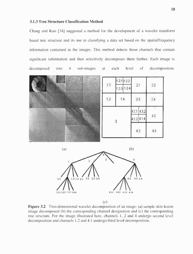
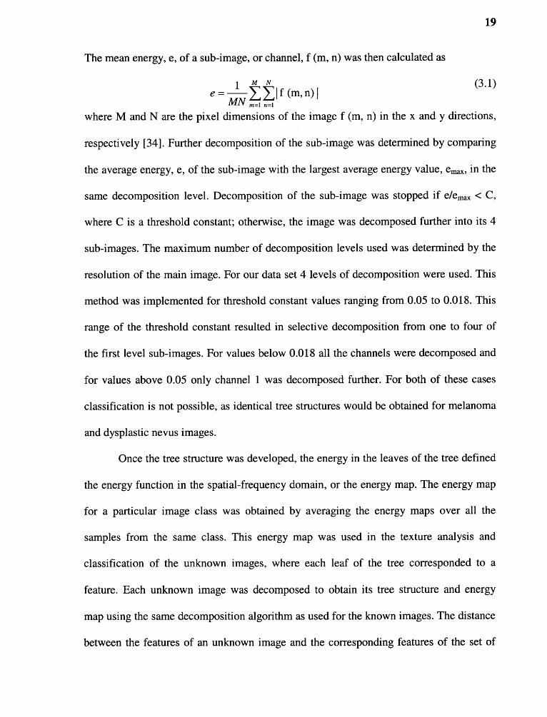
3.1.2 Image Decomposition

All images were decomposed in Matlab using the Daubechies-3 (db3) wavelet. The

channel designation used in this study for the wavelet decomposition of an image and the

resulting sub-images is the same for both tree structure methods. The main image is

numbered as 0 and its low-low, low-high, high-low and high-high filter channels are

numbered 1, 2, 3 and 4, respectively, for the first level of decomposition. The channels

for the second level of decomposition of channel 1 are numbered 1.1, 1.2, 1.3 and 1.4,

and so on for the other channels and further levels of decomposition. An example of

wavelet decomposition of a sample skin lesion image with the corresponding channel

designation and tree structure are given in Figure 3.2. According to the method suggested

by Chang and Kuo [34], in this figure channels 1.2.1-1.2.4 and 4.1.1-4.1.4 would be

considered as dominant frequency channels. After the channels are decomposed their

mean energy is calculated as described below to obtain the features for classification.

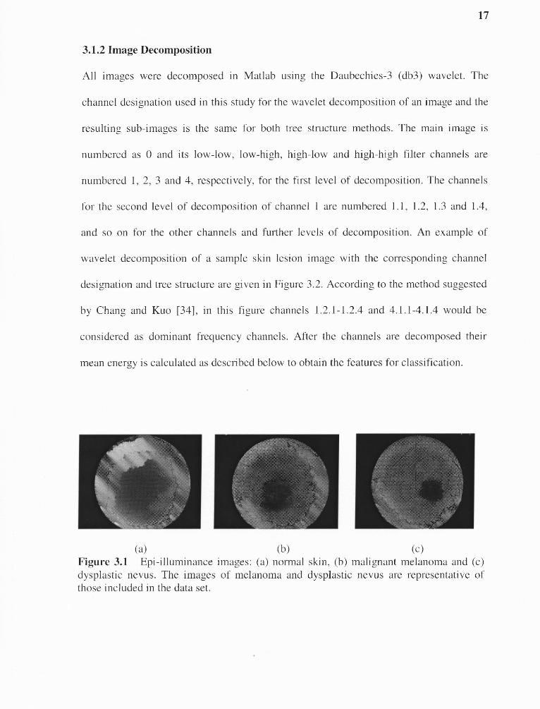
(a) (b) (c)Figure 3.1 Epi-illuminance images: (a) normal skin, (b) malignant melanoma and (c)dysplastic nevus. The images of melanoma and dysplastic nevus are representative ofthose included in the data set.

18

3.1.3 Tree Structure Classification Method

Chang and Kuo [34] suggested a method for the development of a wavelet transform

based tree structure and its use in classifying a data set based on the spatial/frequency

information contained in the images. This method detects those channels that contain

significant information and then selectively decomposes them further. Each image is

decomposed into 4 sub-images at each level of decomposition.

Figure 3.2 Two-dimensional wavelet decomposition of an image: (a) sample skin lesionimage decomposed (b) the corresponding channel designation and (c) the correspondingtree structure. For the image illustrated here, channels 1, 2 and 4 undergo second leveldecomposition and channels 1.2 and 4.1 undergo third level decomposition.

19

The mean energy, e, of a sub-image, or channel, f (m, n) was then calculated as

where M and N are the pixel dimensions of the image t (m, n) in the x and y directions,

respectively [34]. Further decomposition of the sub-image was determined by comparing

the average energy, e, of the sub-image with the largest average energy value, emax, in the

same decomposition level. Decomposition of the sub-image was stopped if e/emax < C,

where C is a threshold constant; otherwise, the image was decomposed further into its 4

sub-images. The maximum number of decomposition levels used was determined by the

resolution of the main image. For our data set 4 levels of decomposition were used. This

method was implemented for threshold constant values ranging from 0.05 to 0.018. This

range of the threshold constant resulted in selective decomposition from one to four of

the first level sub-images. For values below 0.018 all the channels were decomposed and

for values above 0.05 only channel 1 was decomposed further. For both of these cases

classification is not possible, as identical tree structures would be obtained for melanoma

and dysplastic nevus images.

Once the tree structure was developed, the energy in the leaves of the tree defined

the energy function in the spatial-frequency domain, or the energy map. The energy map

for a particular image class was obtained by averaging the energy maps over all the

samples from the same class. This energy map was used in the texture analysis and

classification of the unknown images, where each leaf of the tree corresponded to a

feature. Each unknown image was decomposed to obtain its tree structure and energy

map using the same decomposition algorithm as used for the known images. The distance

between the features of an unknown image and the corresponding features of the set of

20

known images was used to classify the candidate image to either the melanoma or

dysplastic lesion class. The Mahanalobis distance [82], Di , was used as the discrimination

function for classification of each unknown image. D i was calculated for each unknown

image as

where xi denotes the mean energy of the j th dominant channel for the unknown image, mil

denotes the corresponding mean energy value of the j th channel for the image class i, and

cij represents the variance of channel j for image class i. The first 8 dominant frequency

channels were used in this analysis, so the value of J used was 8. For our data with only

two-image classes, melanoma and dysplastic nevus, the value of i was either 1 or 2. An

unknown image was assigned to image class 1 if D1 < D2; otherwise, the image was

assigned to image class 2.

3.1.4 Adaptive Wavelet-based Tree-Structure (ADWAT) Classification Method

A new Adaptive Wavelet-Based Tree-Structure (ADWAT) method is presented here to

address two major limitations of the tree structure classification method described in

Section 3.1.3. First, additional features are selected so that channels are decomposed as a

result of their discrimination content and not solely on maximum energy. Porter and N.

Canagarajah [87] proposed the ratio of the mean energy in the low-frequency channels to

the mean energy in the middle-frequency channels as a criterion for optimal feature

selection. These low to middle frequency ratios of channel energies emphasize the

spatial/frequency differences in an image. Second, the threshold value used for selecting

the decomposition channels is selected adaptively based on a statistical analysis of the

21

feature data. Thus, various ratios of channel energies or their combination over a given

decomposition level are used as additional features and a statistical analysis of the feature

data is used to find the threshold values that optimally partitions the image-feature space

for classification. The ADWAT method for classification is described below.

3.1.4.1 Feature Set. Features are computed so that channels are decomposed as a

result of their discrimination content and not only on maximum energy. For each level of

decomposition, four sub-images are created and the average energy of each channel is

calculated according to Equation (3.l).

Table 3.1 Feature Calculations at Each Level of Decomposition: Illustrated withdecomposition of channel l. At each level of decomposition, the average energy of eachsub-image is calculated with the corresponding energy ratios. These features are used in astatistical analysis to select the optimal feature set for image classification.Sub-image or

Channel

Features

Average

Energy

Maximum Energy

Ratio

Fractional Energy Ratio

l.1 el.l el.l/emax el.l/(el.2+el.3+el.4)

l.2 el.2 el.2/emax el.2/(el.l+el.3+el.4)

l.3 el.3 el.3/emax el.3/(el.l+el.2+el.4)

l.4 el.4 el.4/emax el.4/(el.l+el.2+el.3)

1. Of the four average energies calculated, the greatest is designated emax.2. Since emax is the maximum average energy (either ell, e 1.2, el.3, or e 1.4) only three of the ratios tomaximum energy are used as features; the fourth ratio is always 1.

In addition several energy ratios are also calculated and used as features as shown

in Table 3.l. The average energies and energy ratios generate 11 features per channel,

resulting in 11 features from the first level of decomposition, 44 features from the second

level of decomposition, and 176 features from the third level of decomposition.

22

3.1.4.2 Threshold Selection. The mean, variance and the histogram of the feature

values for each of the target classes are used to determine if a feature generated a

unimodal distribution or segregated into a bimodal distribution between the image

classes. The sample mode (most frequently occurring value) was used as an estimator for

the population mode. The descriptive Statistics tool in Microsoft Excel was used for this

purpose. This analysis tool generated a report of univariate statistics for the data in the

input range, providing information about the central tendency and variability of the data.

Based on the histogram of the data values, the number of modes present in the data was

estimated and the mean and variance of the data was calculated.

During the learning phase the known set of melanoma and dysplastic nevus

images were used. For the classification of skin images, all images were decomposed up

to 4 levels using the Daubechies-3 (db3) wavelet. Thresholds for channel decomposition

were obtained by performing a statistical analysis on the feature values derived from the

average channel energies.

All pooled feature values that generated unimodal distributions were rejected. Out

of the total 231 features, 214 features were rejected for this reason. For all features that

segregated into bimodal distributions between image classes, thresholds were calculated.

If more than one feature within a particular channel were distributed bimodally, then the

feature that generated linearly separable pure clusters for the two classes was used in the

analysis. For all such features, energy ratio thresholds were calculated by averaging the

highest value from the lowest valued class with the lowest value from the highest valued

class. According to the minimum distance classifier, taking the average value of the

means of the two classes as a threshold would be optimum in the Bayes sense [83]. This

23

requires that the distance between the means is large compared to the spread or

randomness of each class with respect to its mean. Since this is not true for any of the

linearly separable features, average of the separation between the two classes was used as

a threshold. For all the remaining channels having features with bimodal distribution that

did not produce linearly separable pure clusters, the feature with greater separation of the

two class means compared to the variance of the two classes was used in the analysis. All

such features were assumed to follow a Gaussian distribution with each of the two image

classes having the same probability of occurrence equal to 0.5. The optimal energy ratio

threshold for these features with the minimal classification error was calculated as the

average of the means of the two Gaussian distributions [83].

3.1.4.3 Development of Tree Structure Signatures. Based on the thresholds

selected above, the image decomposition algorithm was developed to obtain the tree

structure for each of the image classes. Decomposition was stopped for a channel if all of

its features for the two classes followed unimodal distributions. Each channel that had at

least one feature that was bimodally distributed was decomposed further if its feature

value satisfied the corresponding energy ratio threshold. Since the thresholds were

selected to optimally partition the two image classes, one of the two image classes was

preferentially decomposed. In this analysis, many more dysplastic nevus images were

available than melanoma images. Thus, the dysplastic nevus class was used as the

reference group and the thresholds were set such that images of this type were not

decomposed. The tree structures that resulted from this decomposition form the

signatures of the melanoma and dysplastic nevus image classes.

24

3.1.4.4 Classification Phase. During the classification phase the tree structure of

the candidate image obtained using the same decomposition algorithm described

previously was semantically compared with the tree structure signatures of melanoma

and dysplastic nevus. A classification variable, CV, is used to rate the tree structure of the

candidate image. CV is set to a value of 1 when the main image is decomposed. The

value of CV is incremented by one for each additional channel decomposition. When the

algorithm decomposes a dysplastic nevus image, only one level of decomposition should

occur (channel 0). Thus, for values of CV equal to l, a candidate image was assigned to

the dysplastic nevus class. A value of CV greater than 1 indicates further decomposition

of the candidate image, and the image was accordingly assigned to the melanoma class.

3.2 Light-Tissue Interaction Modeling

In this section the MCSVL algorithm and the development of tissue models using the

concept of voxel library are described. This is followed by the description of the

simulation setups used for verification of the algorithm and simulations of the skin lesion

models with the Nevoscope optical geometry. Finally, the correlation analysis between

the lesion depth and diffuse reflectance is described. Optical wavelengths for multi-

spectral imaging of the skin lesions are selected based on the correlation analysis.

3.2.1 Photon Random Walk

The MCSVL algorithm for simulating light-tissue interaction using Monte Carlo

techniques is implemented in the MATLAB environment. Figure 3.3 shows the flowchart

of the MCSVL algorithm. The flowchart can be divided into four sections: l. launching

the photon, 2. photon movement within the tissue and the photon tissue interaction, 3.

25

photon hitting a boundary and 4. photon termination. These sections are marked with

dotted boxes on the flowchart and are briefly describe below.

The presented method is based on the approach presented by Wang, Jacques and

Zheng [75]. Their program, MCML, works with homogeneous layered-tissue models. A

boundary between two layers where the refractive index changes occurs only along the

depth of the tissue in a homogeneous layered-tissue model. However in the voxel-based

approach for non-homogeneous tissue models this boundary can occur between two

adjacent voxels. These two voxels with different refractive indices could be side by side

or one above the other. The calculations related to the photon hitting the boundary from

the MCML program are therefore extended to handle boundaries between adjacent voxels

of the voxel-based model in the MCSVL program.

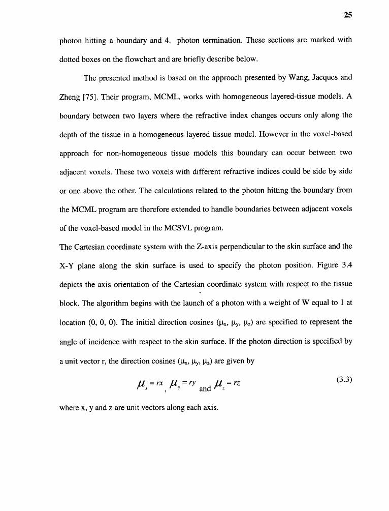
The Cartesian coordinate system with the Z-axis perpendicular to the skin surface and the

X-Y plane along the skin surface is used to specify the photon position. Figure 3.4

depicts the axis orientation of the Cartesian coordinate system with respect to the tissue

block. The algorithm begins with the launch of a photon with a weight of W equal to 1 at

location (0, 0, 0). The initial direction cosines (la x , μy , μz ) are specified to represent the

angle of incidence with respect to the skin surface. If the photon direction is specified by

a unit vector r, the direction cosines (μx, µy, 11) are given by

where x, y and z are unit vectors along each axis.

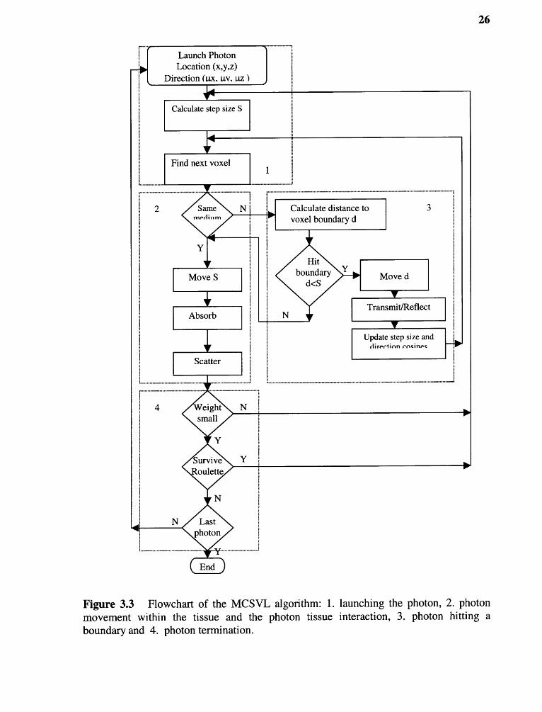
Figure 3.3 Flowchart of the MCSVL algorithm: l. launching the photon, 2. photonmovement within the tissue and the photon tissue interaction, 3. photon hitting aboundary and 4. photon termination.

Figure 3.4 Axis orientation of the Cartesian coordinate system.

If a refractive index mismatch occurs between the ambient and the tissue then specular

reflection Rs is subtracted from the initial photon weight W. R s is computed using theFresnel's

equation

where the refractive index of the ambient is n1 and that of the tissue is n2. After

accounting for specular reflection, the photon step size S is calculated using

L. J

where is the local absorption coefficient, II, is the scattering coefficient and E is a

random number uniformly distributed in the interval [0, l]. The current photon location

(x, y, z), the direction cosines (4, μy, p) and the path length S are then used to determine

the next potential location of the photon-tissue interaction using

28

where x1, y1 and z 1 are the coordinates of the new location. If the photon is still within the

same medium it is moved to this new location and its weight is decreased by an amount

ΔW, due to absorption within the tissue. The change in weight is given by

where IA is the tissue interaction coefficient equal to the sum of the local absorption

coefficient μa and the scattering coefficient µ s .

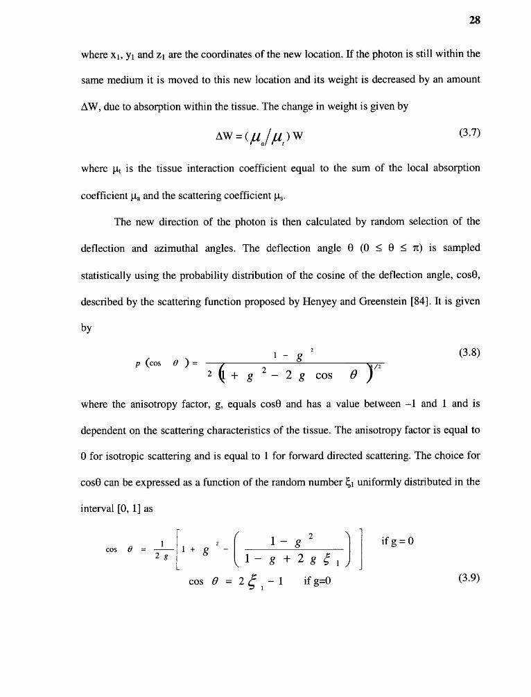
Thenew direction of the photon is then calculated by random selection of the

deflection and azimuthal angles. The deflection angle 0 (0 5_ 0 5_ it) is sampled

statistically using the probability distribution of the cosine of the deflection angle, cosθ,

described by the scattering function proposed by Henyey and Greenstein [84]. It is given

by

where the anisotropy factor, g, equals cosθ and has a value between —l and 1 and is

dependent on the scattering characteristics of the tissue. The anisotropy factor is equal to

0 for isotropic scattering and is equal to 1 for forward directed scattering. The choice for

cosh can be expressed as a function of the random number ξ1 uniformly distributed in the

interval [0, l] as

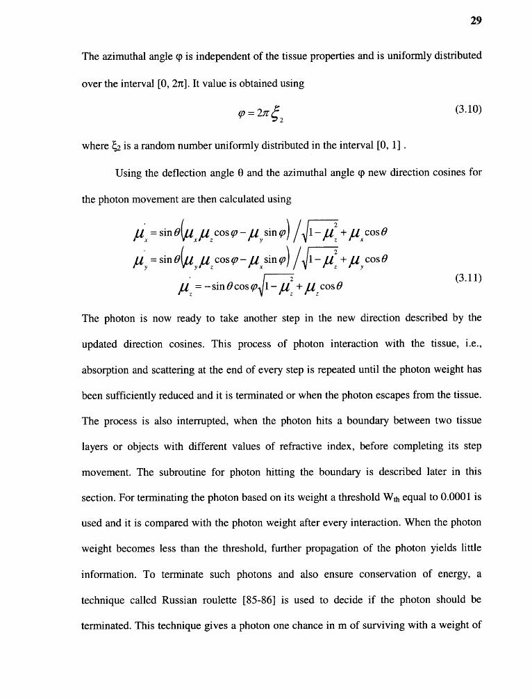
29

The azimuthal angle φ is independent of the tissue properties and is uniformly distributed

over the interval [0, 27]. It value is obtained using

where is a random number uniformly distributed in the interval [0, 1] .

Using the deflection angle 0 and the azimuthal angle φ new direction cosines for

the photon movement are then calculated using

The photon is now ready to take another step in the new direction described by the

updated direction cosines. This process of photon interaction with the tissue, i.e.,

absorption and scattering at the end of every step is repeated until the photon weight has

been sufficiently reduced and it is terminated or when the photon escapes from the tissue.

The process is also interrupted, when the photon hits a boundary between two tissue

layers or objects with different values of refractive index, before completing its step

movement. The subroutine for photon hitting the boundary is described later in this

section. For terminating the photon based on its weight a threshold Wth equal to 0.0001 is

used and it is compared with the photon weight after every interaction. When the photon

weight becomes less than the threshold, further propagation of the photon yields little

information. To terminate such photons and also ensure conservation of energy, a

technique called Russian roulette [85-86] is used to decide if the photon should be

terminated. This technique gives a photon one chance in m of surviving with a weight of

30

mW„ were Wr is the present weight of the photon. A value of m equal to ten is used, thus

giving a photon one-tenth chance of survival with a weight of 10W r. A random number

uniformly distributed in the interval [0, l] is compared with l/m and the photon survives

if the random number is less than or equal to l/m. This method conserves energy, yet

terminates photons in an unbiased manner.

If the photon hits the boundary between two tissue layers or objects with different

values of refractive index before completing the step, it may be either internally reflected

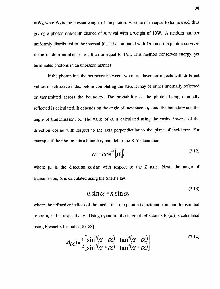
or transmitted across the boundary. The probability of the photon being internally

reflected is calculated. It depends on the angle of incidence, onto the boundary and the

angle of transmission, a t. The value of αi is calculated using the cosine inverse of the

direction cosine with respect to the axis perpendicular to the plane of incidence. For

example if the photon hits a boundary parallel to the X-Y plane then

where μ z is the direction cosine with respect to the Z axis. Next, the angle of

transmission, at is calculated using the Snell's law

where the refractive indices of the media that the photon is incident from and transmitted

to are ni and n t respectively. Using αi and at, the internal reflectance R () is calculated

using Fresnel's formulas [87-88]

31

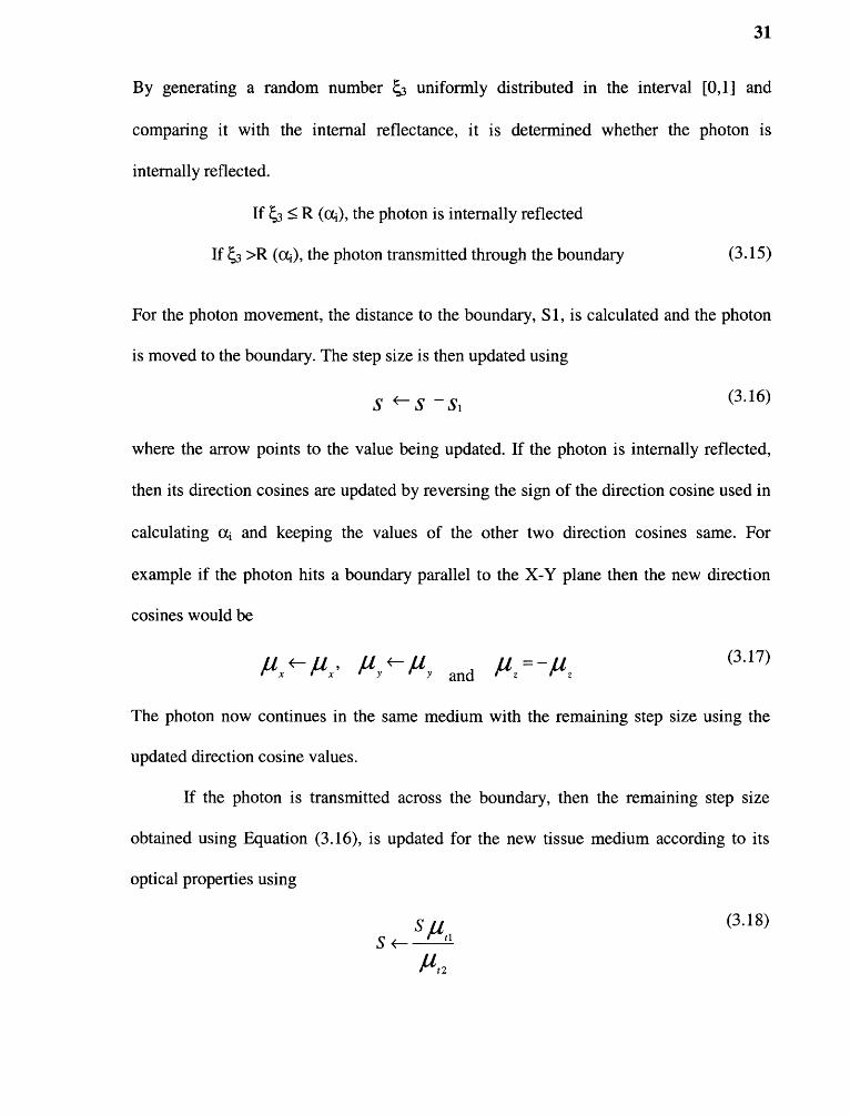
By generating a random number uniformly distributed in the interval [0,l] and

comparing it with the internal reflectance, it is determined whether the photon is

internally reflected.

For the photon movement, the distance to the boundary, Si, is calculated and the photon

is moved to the boundary. The step size is then updated using

where the arrow points to the value being updated. If the photon is internally reflected,

then its direction cosines are updated by reversing the sign of the direction cosine used in

calculating αi and keeping the values of the other two direction cosines same. For

example if the photon hits a boundary parallel to the X-Y plane then the new direction

cosines would be

The photon now continues in the same medium with the remaining step size using the

updated direction cosine values.

If the photon is transmitted across the boundary, then the remaining step size

obtained using Equation (3.16), is updated for the new tissue medium according to its

optical properties using

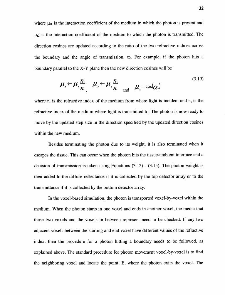
32

where μt1 is the interaction coefficient of the medium in which the photon is present and

μt2 is the interaction coefficient of the medium to which the photon is transmitted. The

direction cosines are updated according to the ratio of the two refractive indices across

the boundary and the angle of transmission, a t . For example, if the photon hits a

boundary parallel to the X-Y plane then the new direction cosines will be

where ni is the refractive index of the medium from where light is incident and n t is the

refractive index of the medium where light is transmitted to. The photon is now ready to

move by the updated step size in the direction specified by the updated direction cosines

within the new medium.

Besides terminating the photon due to its weight, it is also terminated when it

escapes the tissue. This can occur when the photon hits the tissue-ambient interface and a

decision of transmission is taken using Equations (3.12) - (3.15). The photon weight is

then added to the diffuse reflectance if it is collected by the top detector array or to the

transmittance if it is collected by the bottom detector array.

In the voxel-based simulation, the photon is transported voxel-by-voxel within the

medium. When the photon starts in one voxel and ends in another voxel, the media that

these two voxels and the voxels in between represent need to be checked. If any two

adjacent voxels between the starting and end voxel have different values of the refractive

index, then the procedure for a photon hitting a boundary needs to be followed, as

explained above. The standard procedure for photon movement voxel-by-voxel is to find

the neighboring voxel and locate the point, E, where the photon exits the voxel. The

33

distance, d, between this point and the initial position of the photon is calculated and

compared with the step size S. If the step size S is greater than the distance d, the photon

is moved to the exit point and S is reduced by an amount d. If the refractive indices of the

current voxel and the next voxel are the same then the photon either moves the remaining

step size or moves to the boundary of the next voxel depending upon the minimum

distance between the two. If the refractive index of the adjacent voxel is different then the

photon may be internally reflected within the same voxel or transmitted to the next voxel.

The decision of internal reflection or transmission is made using Equations (3.12) —

(3.15). If internally reflected the photon can move the remaining step size given by

Equation (3.16) in the direction specified by the updated direction cosines obtained using

Equation (3.17). If the photon is transmitted through the boundary it can move the

updated step size given by Equation (3.18) in the direction specified by the updated

direction cosines obtained using Equation (3.19).

Most of the photon movement is within a uniform medium and the neighboring

voxels along the photon path have the same refractive index. Checking the boundary

conditions at every voxel interface is not required as is done in the voxel-by-voxel

calculations explained above. The photon accelerating method suggested by Sato and

Ogawa [89] for the photon transport is used in the MCSVL code to improve the

simulation efficiency. In this method, the layer or object boundary is checked by

comparing the refractive indices of all the voxels within the photon path. If all these

voxels have the same refractive index then the photon is free to move and interact with

the tissue. On the other hand if the refractive index changes along the photon path, an

object boundary is present and its distance from the existing photon location is calculated

34

and compared with the step size. If the step size is smaller than this distance the photon

can take this step, otherwise the photon is moved to the boundary and it is decided

whether it will be reflected or refracted. Thus the calculation of the exit point E and its

distance d from the initial position is omitted at each and every voxel interface along the

path. By using this method, instead of having checkpoints at every voxel interface along

the path, only two checkpoints are required before the photon-tissue interaction and this

improves the simulation efficiency.

3.2.2 Tissue Models and Voxel Library

The tissue material grid corresponds in size one-to-one with the grid that accumulates the

absorbed photon weights. Voxels representing the different tissue media are grouped

together to form a three-dimensional tissue block. The position of a particular voxel in

this tissue block is dependent on the tissue model. The dimensions of the voxel (Ax, Ay,

Az) and the number of voxels in each direction are used to establish the grid skeleton.

The photon location in this three-dimensional array forming the tissue material grid is

specified using Cartesian coordinates (x, y, z) or voxel indices (i, j, k). If all the voxels

are of the same size and shape a simple routine can be used to convert from Cartesian

location to voxel index and vice versa. All the voxels are assigned a voxel type number

corresponding to their media type. For example in a three-layer skin model the media

types could be stratum corneum, epidermis and dermis and l, 2 and 3 could be the voxel

type numbers assigned to the voxels of these media type respectively. So the three-

dimensional material grid array corresponding to this three-layer skin model will have

only these three numbers. The MCSVL algorithm, based on the photon location gets the

voxel type number and then reads a text file corresponding to this voxel type number to

35

obtain its physical and optical properties. The physical properties are the size and shape

of the voxel and the optical properties are the absorption and scattering coefficients,

anisotropy factor and index of refraction. A collection of all these text files is the voxel

library. Since the optical properties of a particular medium are wavelength dependent,

editing the optical properties in these text files according to the wavelength used in the

study is one option. Instead, different text files are formed, one for every wavelength, is

containing the optical properties of the medium for a given wavelength. These text files

are then assigned to different voxel type numbers, although they all represent the same

medium. Now if the wavelength studied is changed one only needs to change the voxel

type numbers in the three-dimensional material grid array. The voxel library offers the

flexibility of updating the optical properties of the voxel or adding new media types into

the library as new experimental results are reported.

All voxels in the library are rectangular in shape. The voxel dimensions (Ax, Ay,

Az) can be selected based on the object to be described and the resolution required in the

study. Cubical voxels with all dimensions equal to 10μm are used in this study. Computer

memory is an important factor affecting the time required for completing a simulation. In

the MCSVL algorithm the three-dimensional material grid array is split into two-

dimensional arrays parallel to the skin surface. The processor accesses three of these two-

dimensional arrays, one containing the voxel in which the photon is present and one array

above and below it at a given time. Thus the computer can read the voxel in which the

photon is present and all its 6 neighboring voxels and is free from any unwanted

information related to the material grid above and below these arrays. This saves the

computer memory and helps to improve the computational speed.

36

3.2.3 Optical Properties

Based on the experimental and analytical results reported by various researchers, so far

355 types of voxels based on the difference in the medium or the difference in the optical

properties of a medium for different wavelengths are compiled.

The values for refractive index for tissue used by various researchers range from

the value of refractive index of water to value slightly higher than 1.5. Bolin et al. [90]

used fiber optic cladding method to find the refractive index of tissue. Refractive index

was measured over the range of 390-700nm. From these experiments it can be concluded

that the refractive index of the tissue changes slightly over the visible spectrum and hence

can be approximated by a constant value. The values of refractive indices used in this

study are l.45, l.4 and l.4 for the stratum corneum, epidermis and dermis respectively.

The value of refractive index for air is taken equal to l. Zeng et al. [91] also used these

values in their tissue model.

For the optical properties of the stratum corneum the data reported by Gernert et

al. [95] is used. They used collimated and diffuse transmission and diffuse reflection

measurements obtained using a 10μm thick sample of 90% pure stratum corneum

reported by Everett et al. [92] to analyze the values of μa and μs of the stratum corneum

as a function of wavelength. They have published the values for a wavelength range of

250-400nm. These values are extrapolated up to 700nm using least square approximation

techniques. For the anisotropy factor the data published by Bruls [93] using goniometer

measurements of in- vitro stratum corneum is used.

For the epidermal scattering coefficient the data reported by Gernert et al. [95] is

used. They have obtained the wavelength dependent values of is for epidermis using the

37

values of g deduced from Brul's [93] experiment and the epidermal diffuse integrating

sphere measurements reported by Wan et al. [36].

The absorption coefficients for the epidermis are approximated using the

analytical formulas given by Jacques [81]. The absorption coefficient value is given as a

function of wavelength and the volume fraction of the epidermis occupied by

melanosomes. The epidermal absorption coefficient is a combination of the skin baseline

absorption coefficient, aμ Baseline, and the absorption coefficient of a single melanosome,

μ melanosome• The analytical equation for the skin baseline absorption coefficient (cm ^-1) is

given by

The absorption coefficient of a single melanosome (cm ^-1) is approximated using

expression

The absorption coefficient for the epidermis (cm^-1) combines the skin baseline absorption

and the melanosome absorption and is approximated using the following formula

where A is the wavelength in nm and fmel is the volume fraction of the epidermis occupied

by melanosomes. According to Jacques [81] fmel ranges from l.3-6.3% for white color

skin, 11-16% for brown/olive color skin and 18-43% for black color skin. Using the

average volume fraction of melanosomes within the tissue color range, the values for

epidermal absorption coefficients for 71 wavelengths in the range of 350-700 nm with

5nm interval are calculated using Equations (3.20) — (3.22). The values of the average

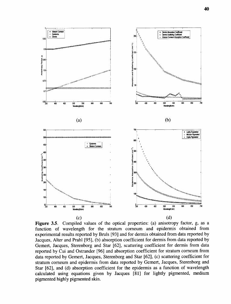
38

volume fraction of melanosomes used are 3.8% for white skin, 13.5% for brown/olive

skin and 30.5% for the black skin type.

For the scattering coefficients of the dermis the values reported by Gemert et al.

[95] are used. They have used the Kubelka-Munk coefficients of the dermal tissue

obtained from integrating sphere measurements reported by Anderson and Parrish [94]

along with the values of g given by Jacques et al. [95] to calculate the scattering

coefficient values for the dermis as a function of wavelength. The absorption coefficient

for the dermis is a combination of the oxy and deoxy-hemoglobin absorption. Cui and

Ostrander [96] have reported these values as a function of wavelength based on diffusion

theory and experimental results.

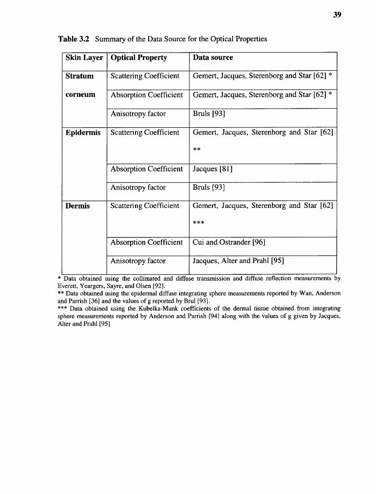
The experimental and analytical results mentioned above were used to obtain the

optical properties of the voxels in the voxel library. Table 3.2 gives summary of the data

source for the optical properties of the tissue used in this study. For the data on which no

analytical equations are reported, the measurement and scaling tools in Adobe Photoshop

are used to approximate the values from the scanned images of these published results.

Values were obtained for 71 different wavelengths, every 5nm in the wavelength range of

350-700nm. Figure 3.5 shows the scatter plots of these optical properties as a function of

wavelength.

The values of the absorption coefficient, the scattering coefficient and the

anisotropy factor form a set of the optical properties. 71 sets of values each for the optical

properties of the skin layers, stratum corneum and dermis, corresponding to the 71

wavelengths used in this study are compiled. The epidermal tissue is classified into the

three skin color types using the values of the average volume fraction of melanosomes

39

Table 3.2 Summary of the Data Source for the Optical Properties

Skin Layer Optical Property Data source

Stratum

corneum

Scattering Coefficient Gemert, Jacques, Sterenborg and Star [62] *

Absorption Coefficient Gemert, Jacques, Sterenborg and Star [62] *

Anisotropy factor Bruls [93]

Epidermis Scattering Coefficient Gemert, Jacques, Sterenborg and Star [62]

**

Absorption Coefficient Jacques [81]

Anisotropy factor Bruls [93]

Dennis Scattering Coefficient Gernert, Jacques, Sterenborg and Star [62]

***

Absorption Coefficient Cui and Ostrander [96]

Anisotropy factor Jacques, Alter and Prahl [95]

* Data obtained using the collimated and diffuse transmission and diffuse reflection measurements byEverett, Yeargers, Sayre, and Olsen [92].** Data obtained using the epidermal diffuse integrating sphere measurements reported by Wan, Andersonand Parrish [36] and the values of g reported by Brul [93].*** Data obtained using the Kubelka-Munk coefficients of the dermal tissue obtained from integratingsphere measurements reported by Anderson and Parrish [94] along with the values of g given by Jacques,Alter and Prahl [95]

40

Figure 3.5. Compiled values of the optical properties: (a) anisotropy factor, g, as afunction of wavelength for the stratum corneum and epidermis obtained fromexperimental results reported by Bruls [93] and for dermis obtained from data reported byJacques, Alter and Prahl [95], (b) absorption coefficient for dermis from data reported byGernert, Jacques, Sterenborg and Star [62], scattering coefficient for dermis from datareported by Cui and Ostrander [96] and absorption coefficient for stratum corneum fromdata reported by Gernert, Jacques, Sterenborg and Star [62], (c) scattering coefficient forstratum corneum and epidermis from data reported by Gernert, Jacques, Sterenborg andStar [62], and (d) absorption coefficient for the epidermis as a function of wavelengthcalculated using equations given by Jacques [81] for lightly pigmented, mediumpigmented highly pigmented skin.

41

given by Jacques [81]. The three skin color types can also be classified as lightly

pigmented, medium pigmented and highly pigmented. By combining the epidermal

absorption coefficients obtained using Equations (3.20) - (3.22) for these three types of

epidermal tissue with the values for the scattering coefficient and the anisotropy factor,

213 sets of values for the epidermal tissue are obtained. A different voxel type number is

assigned to all these sets of optical properties. Thus, 71 different types of voxels for the

stratum corneum, lightly pigmented, medium pigmented and highly pigmented epidermis

and dermis each are formed. All these voxels put together form the voxel library with a

total of 355 voxels.

3.2.4. Verification of the Algorithm

The first step in algorithm verification is to verify that the calculations and iterations

preformed by the MCSVL code for the photon transport within the tissue and its

interaction with the tissue are correct. For this purpose the tissue model and the optical

geometry of Gardner [77] and Wang and Jacques [43] is used and simulation results are

compared. They both used a three-layer tissue model with a point light source incident

perpendicular to the skin surface and measured the total diffuse reflectance and

transmittance. Gardner [77] used 100,000 photons in his simulations while Wang and

Jacques [43] used 1,000,000 photons to test their Monte Carlo code, MCML. The optical

properties and the layer thickness used in this three-layer model are given in Table 3.3.

The refractive indices of the top and the bottom ambient media were set to 1.0.

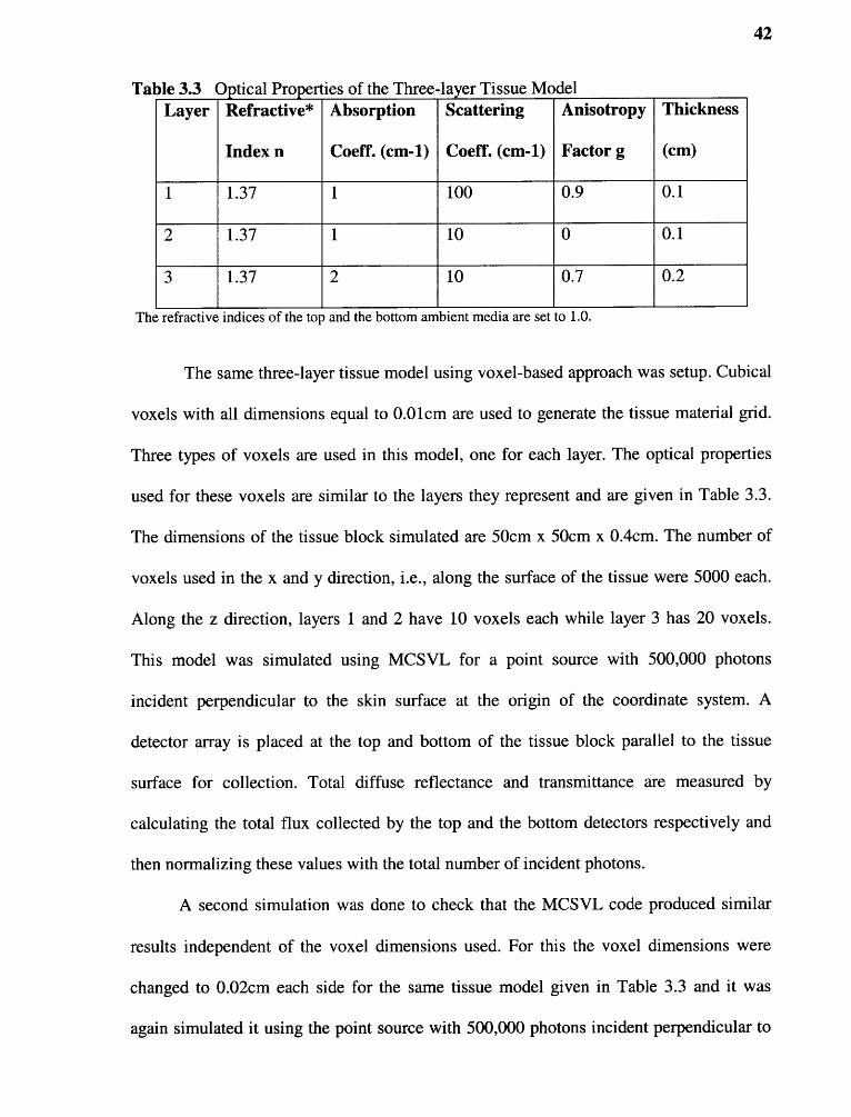
42

Table 3.3 Optical Properties of the Three-layer Tissue ModelLayer Refractive*

Index n

Absorption

Coeff. (cm-1)

Scattering

Coeff. (cm-1)

Anisotropy

Factor g

Thickness

(cm)

1 l.37 1 100 0.9 0.l

2 l.37 1 10 0 0.l

3 l.37 2 10 0.7 0.2

The refractive indices of the top and the bottom ambient media are set to 1.0.

The same three-layer tissue model using voxel-based approach was setup. Cubical

voxels with all dimensions equal to 0.0lcm are used to generate the tissue material grid.

Three types of voxels are used in this model, one for each layer. The optical properties

used for these voxels are similar to the layers they represent and are given in Table 3.3.

The dimensions of the tissue block simulated are 50cm x 50cm x 0.4cm. The number of

voxels used in the x and y direction, i.e., along the surface of the tissue were 5000 each.

Along the z direction, layers 1 and 2 have 10 voxels each while layer 3 has 20 voxels.

This model was simulated using MCSVL for a point source with 500,000 photons

incident perpendicular to the skin surface at the origin of the coordinate system. A

detector array is placed at the top and bottom of the tissue block parallel to the tissue

surface for collection. Total diffuse reflectance and transmittance are measured by

calculating the total flux collected by the top and the bottom detectors respectively and

then normalizing these values with the total number of incident photons.

A second simulation was done to check that the MCSVL code produced similar

results independent of the voxel dimensions used. For this the voxel dimensions were

changed to 0.02cm each side for the same tissue model given in Table 3.3 and it was

again simulated it using the point source with 500,000 photons incident perpendicular to

43

the skin surface. Now the number of voxels used in the x and y direction i.e. along the

surface of the tissue are 2500 each. Layers 1 and 2 have 5 voxels each and layer 3 has 10

voxels along the z direction. In order to study the change in the beam profile and the light

diffusion within the tissue, for the same tissue model, a third simulation was done. The

angle of incidence of the illuminating point source was changed so that it is at 45 degrees

with respect to the tissue normal and the X-axis and is at 90 degrees with respect to the

Y-axis. 500,000 photons were used in this third simulation also. For all these models

contour maps of the energy distribution in the material grid along different horizontal

tissue planes and the two vertical planes passing through the point of light incidence were

used to check the beam profile and the uniformity of the light diffusion in the tissue.

Zeng et al. [97-98] have published diffuse reflectance data measured on Asian volunteers

using their spectroanalyser system. They used two fused silica fibers having 1 mm core

diameter, one to deliver the illuminating light at 5 degrees and the other to collect the

reflected light at 30 degrees with respect to the tissue normal. Diffuse reflectance values

were measured over the wavelength range of 400-780nm. The next step of our algorithm

verification is to develop a wavelength dependent tissue model using the voxel library

and to simulate it using the optical geometry similar to the spectroanalyser system. The

diffuse reflectance values were then estimated for various wavelengths and compared

them with the experimental results published by Zeng et al.[97-98].

For spectroanalyser system optical geometry setup, a fiber optic cable with 1mm

core diameter and a collection angle of 30 degrees with respect to the tissue normal are to

be simulated. Light is conducted through an optical fiber only if it flows into the fiber

within its acceptance angle Oa [99]. The acceptance angle Oa of the fiber is given by

where no, n1 and n2 are the refractive indices of the medium surrounding the fiber, the

fiber core and the fiber cladding respectively. With air as the medium surrounding the

fiber no would be equal to 1. It was assumed that the fiber has a glass core with n1 equal

to 1.5 and a polymer cladding with n2 equal to 1.47. This gives an acceptance angle of

17.4 degrees. A circular disc with 1mm diameter is placed on the tissue surface with an

angle of 30 degrees between the axis normal to the disc and the tissue normal (Z-axis) to

simulate the collecting optical fiber. Any photon escaping the tissue surface and hitting

the disc with an angle less than 17.4 degrees with respect to the disc normal will be

conducted through the optical fiber. Weight of all such photons is accumulated towards

the total diffuse reflectance. A point source incident at an angle of 5 degrees with respect

to the tissue normal is simulated by choosing the initial direction cosines 1.1x , lay and μz of

the photon beam equal to 0.08716, 0 and 0.9962 respectively. This point source is

incident at the origin of the coordinate system, which is also the focus of the collection

fiber.

A three-layer tissue model is used with the stratum corneum of 50μm, epidermis

of 100μm and dermis of 200μm in thickness. For the epidermis there are three types of

voxels in the voxel library according to the level of pigmentation. Out of these lightly

pigmented, medium pigmented and highly pigmented epidermal voxels; the medium

pigmented type voxels are used in this model. Thus, a medium pigmented or Asian skin

type model was formed. By replacing the medium pigmented epidermal voxels in the

45

Asian skin type model with the lightly pigmented and highly pigmented epidermal

voxels, white and black color skin type models were formed respectively.

For all these models, the dimensions of the tissue block used were 5cm x 5cm x

0.035cm. Cubical voxels with each side equal to 10μm were used, forming the material

grid array of 5000 voxel x 5000 voxel x 35 voxel. As explained in Section 2.2, for all the

three skin layers there are 71 voxel types each in the voxel library corresponding to the

71 different wavelengths in the range of 350-700nm with an interval of 5nm. Let's say

for the stratum corneum we have voxel type number 1 corresponding to 350nm

wavelength, voxel type number 2 corresponding to 355nm wavelength and so on. When

simulating the tissue with a 350nm wavelength, we use voxel type number 1 to form the

stratum corneum material grid and change it to voxel type number 2 for a 355nm

wavelength. Thus voxels having the optical properties of the tissue at a particular

wavelength are used to form the material grid when the tissue model is to be simulated

using that particular wavelength. In this way three-layer wavelength dependent tissue

models are obtained.

These models were simulated using a point source with 100,000 photons each for

all the wavelengths. The total diffuse reflectance was estimated by normalizing the total

diffuse flux collected with the total number of photons used in the simulation for every

wavelength. The variance of the simulation results can be minimized either by using a

large number of photons or by carrying out multiple independent simulations and

averaging the results of all these simulations. The latter method for variance reduction is

chosen. Results were obtained by taking the average value of diffuse reflectance from

three independent runs for each wavelength.

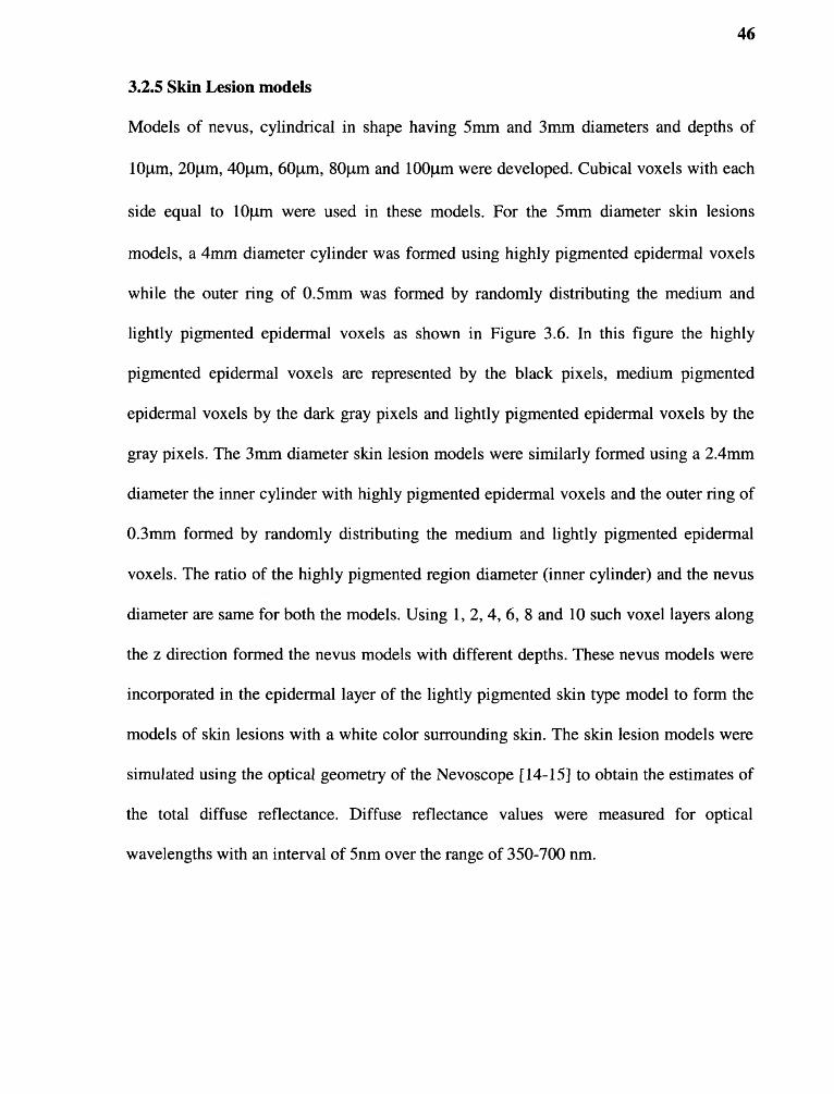
46

3.2.5 Skin Lesion models

Models of nevus, cylindrical in shape having 5mm and 3mm diameters and depths of

1011m, 20μm, 4011m, 60μm, 801,1m and 100μm were developed. Cubical voxels with each

side equal to lOμm were used in these models. For the 5mm diameter skin lesions

models, a 4mm diameter cylinder was formed using highly pigmented epidermal voxels

while the outer ring of 0.5mm was formed by randomly distributing the medium and

lightly pigmented epidermal voxels as shown in Figure 3.6. In this figure the highly

pigmented epidermal voxels are represented by the black pixels, medium pigmented

epidermal voxels by the dark gray pixels and lightly pigmented epidermal voxels by the

gray pixels. The 3mm diameter skin lesion models were similarly formed using a 2.4mm

diameter the inner cylinder with highly pigmented epidermal voxels and the outer ring of

0.3mm formed by randomly distributing the medium and lightly pigmented epidermal

voxels. The ratio of the highly pigmented region diameter (inner cylinder) and the nevus

diameter are same for both the models. Using 1, 2, 4, 6, 8 and 10 such voxel layers along

the z direction formed the nevus models with different depths. These nevus models were

incorporated in the epidermal layer of the lightly pigmented skin type model to form the

models of skin lesions with a white color surrounding skin. The skin lesion models were

simulated using the optical geometry of the Nevoscope [14-15] to obtain the estimates of

the total diffuse reflectance. Diffuse reflectance values were measured for optical

wavelengths with an interval of 5nm over the range of 350-700 nm.

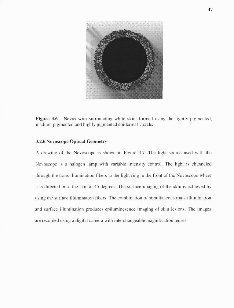
47

Figure 3.6 Nevus with surrounding white skin: formed using the lightly pigmented,medium pigmented and highly pigmented epidermal voxels.

3.2.6 Nevoscope Optical Geometry

A drawing of the Nevoscope is shown in Figure 3.7. The light source used with the

Nevoscope is a halogen lamp with variable intensity control. The light is channeled

through the trans-illumination fibers to the light ring in the front of the Nevoscope where

it is directed onto the skin at 45 degrees. The surface imaging of the skin is achieved by

using the surface illumination fibers. The combination of simultaneous trans-illumination

and surface illumination produces epiluminesence imaging of skin lesions. The images

are recorded using a digital camera with interchangeable magnification lenses.

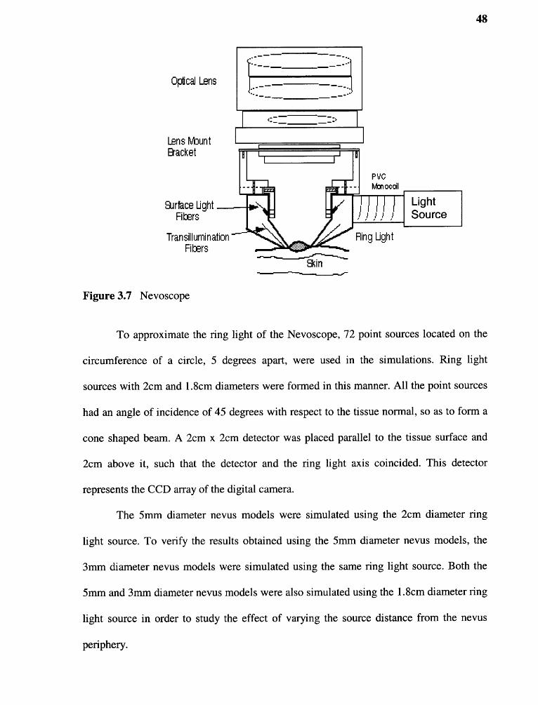
"8

To approximate the ring light of the Nevoscope, 72 point sources located on the

circumference of a circle, 5 degrees apart, were used in the simulations. Ring light

sources with 2cm and 1.8cm diameters were formed in this manner. All the point sources

had an angle of incidence of 45 degrees with respect to the tissue normal, so as to form a

cone shaped beam. A 2cm x 2cm detector was placed parallel to the tissue surface and

2cm above it, such that the detector and the ring light axis coincided. This detector

represents the CCD array of the digital camera.

The 5mm diameter nevus models were simulated using the 2cm diameter ring

light source. To verify the results obtained using the 5mm diameter nevus models, the

3mm diameter nevus models were simulated using the same ring light source. Both the

5mm and 3mm diameter nevus models were also simulated using the 1.8cm diameter ring

light source in order to study the effect of varying the source distance from the nevus

periphery.

49

The models of different skin types based on their epidermal melanin

concentration described earlier were also simulated using the Nevoscope optical

geometry in order to estimate their diffuse reflectance spectra. 125,000 photons per point

source of the Nevoscope optical geometry setup were used in all the simulations. The

tissue reflectance as a function of wavelength was measured for all the tissue models with

an interval of 5nm for the optical range of 350-700nm. The diffused reflectance values

were obtained by normalizing the total flux collected by the detector with the total

number of photons used in the simulation.

3.2.6.1 Simulations Of Tissue Models. The skin lesion models described above and

the models of different skin types based on their epidermal melanin concentration were

simulated using the Nevoscope optical geometry. For the Nevoscope, 100,000 photons

per point source approximating the Nevoscope optical geometry were used in all the

simulations. The skin lesion models were also simulated using the optical geometry of the

spectroanalyser system [97-98]. 100,000 photons were used in all the simulations with

the spectroanalyser system. For the spectroanalyser system simulations, three

independent runs using 100,000 photons each were done. The tissue reflectance as a

function of wavelength was measured for all the tissue models with an interval of 5nm

for the optical range of 350-700nm. The diffused reflectance values were normalized by

dividing the total flux collected by the detectors by the total number of photons used in

the simulation. For the spectroanalyser system, results were obtained by taking the

average of the diffuse reflectance values obtained from the three independent simulations.

50

3.2.6.2. Wavelength Selection By Correlation Analysis. For two random variables

X and Y the correlation coefficient is defined by

where COV(X,Y) is the covariance of X and Y, E[.] represents the expected value of the

variable and E[X], σx and E[Y], ay are the expected values and standard deviations of X

and Y respectively [100]. The correlation coefficient is a number that is at most 1 in

magnitude. The extreme values of px,y are achieved when X and Y are related linearly

i.e. Y=AX + B. px,y is equal to 1 if A is greater than zero and is equal to -1 if A is less

than zero. px,y can be viewed as a statistical measure of the extent to which Y can be

predicted by a linear function of X. Variables X and Y are uncorrelated if px,y equals

zero [100].

Four different sets of simulations were conducted using a combination of skin

lesion models and ring light source with different diameters. The different combinations

used were: 5mm diameter skin lesion and 2cm diameter ring light, 5mm diameter skin

lesion and 1.8cm diameter ring light, 3mm diameter skin lesion and 2cm diameter ring

light and 3mm diameter skin lesion and 1.8cm diameter ring light. In each set of

simulations lesion models with different depths were simulated using optical wavelengths

with an interval of 5nm over the optical range of 350-700nm. Since there are 6 different

lesion depths, 6 simulations were performed in each set. The measured diffuse reflectance

values from a particular set of simulations were grouped together in to arrays according

to the wavelengths used in the simulation. Say for the set of 5mm diameter skin lesion

with a 2cm diameter ring light, models with 10, 20, 40, 60, 80 and 100 pm lesion depth

51

were simulated. Then the array DR1 corresponding to 350nm wavelength will have the

diffuse reflectance values corresponding to the 5mm diameter skin lesion models with

increasing depth. Since 6 different lesion depths were used, every set will have 6 diffuse

reflectance values. 71 such sets were formed for wavelengths with an interval of 5nm

over the optical range of 350-700nm. Another set ND was formed containing the values

of the nevus depths. Using DRj (1 j 71) and ND as the variables, correlation

coefficient values Cj (1 j 5_ 71) were calculated for all the sets of simulations. A

correlation coefficient threshold, CT was set equal to 0.7. Wavelengths for which the

absolute value of the correlation coefficient was greater than CT were obtained for the

5mm and 3mm diameter nevus models simulated with a 2cm diameter ring light source.

Out of these, wavelengths that were common for both the models were selected for the

multi-spectral imaging of the skin lesions. The effect of changing the ring light source

diameter was studied by comparing the results with those obtained from the 5mm and

3mm diameter nevus models simulated with a 1.8cm diameter ring light source.

3.3 Multi-spectral Image Analyses

Multi-spectral trans-illuminance images of skin lesions of individuals from various age

groups and gender were collected using the Nevoscope [14-15]. A 100W halogen light

source along with narrow band-pass interference filters of the wavelengths selected from

the mathematical modeling of light-tissue interaction were used for illumination. Images

were collected with an Agfa digital camera (ePhoto-1280) and were 16-bits, 1024 x 768

pixels in size. The lesion images were collected over a period of two years by imaging

suspicious lesions on 250 individuals under the observation of a cancer specialist. From

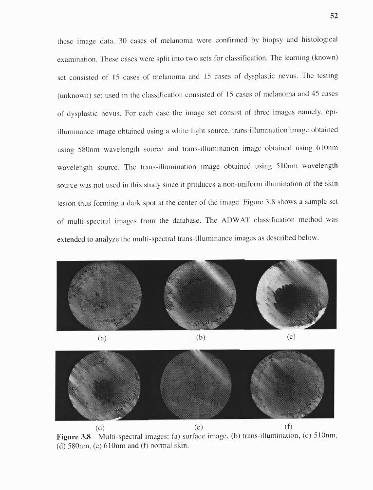
52

these image data, 30 cases of melanoma were confirmed by biopsy and histological

examination. These cases were split into two sets for classification. The learning (known)

set consisted of 15 cases of melanoma and 15 cases of dysplastic nevus. The testing

(unknown) set used in the classification consisted of 15 cases of melanoma and 45 cases

of dysplastic nevus. For each case the image set consist of three images namely,

epi-illuminance image obtained using a white light source, trans-illumination image obtained

using 580nm wavelength source and trans-illumination image obtained using 610nm

wavelength source. The trans-illumination image obtained using 510nm wavelength

source was not used in this study since it produces a non-uniform illumination of the skin

lesion thus forming a dark spot at the center of the image. Figure 3.8 shows a sample set

of multi-spectral images from the database. The ADWAT classification method was

extended to analyze the multi-spectral trans-illuminance images as described below.

k•-'1

Figure 3.8 Multi-spectral images: (a) surface image, (b) trans-illumination, (c) 510nm,(d) 580nm, (e) 610nm and (f) normal skin.

53

3.3.1. Feature Set

Features were derived from the multi-spectral images using similar analysis that was used

in the ADWAT classification method. All images of a particular wavelength from the

learning set are decomposed up to three levels in Matlab using the Daubechies-3 (db3)

wavelet. After the channels are decomposed their mean energy is calculated using

Equation (3.1). Channel energies and various ratios of channel energies similar to those

given in Table 3.1 are used as features. Statistical analysis is used to reduce the

dimensions of the feature space by selecting on those features that produce a bi-modal

distribution between the two image classes, namely, melanoma and dysplastic nevus. For

all these features energy thresholds were obtained in the same manner as described in

Section 3.1.4. All pooled feature values that generated unimodal distributions were

rejected. Features were obtained for the 580nm and 610nm wavelength images. These

features were combined with the features obtained from the epi-illuminance images to

form the feature set.

3.3.2. Classification Using Extended-ADWAT Method

The Extended-ADWAT method is a two-step classification process. In the first step only

the epi-illuminance images are used and classification is carried out in the same manner

as the ADWAT method described in Section 3.1.4. The only difference between the first

step of the Extended-ADWAT method and the ADWAT method is, instead of having

only two image classes, the Extended-ADWAT method has three image classes. Images

are now classified as melanoma, dysplastic nevus or suspicious lesion. In the ADWAT

method all the images that produced a tree structure similar to the tree structure model of

the dysplastic nevus were assigned to the dysplastic nevus image class and the rest were

54

assigned to the melanoma image class. In the Extended-ADWAT method images are

classified as melanoma only if the tree structure completely matches the melanoma tree

structure model. All the images that produce incomplete tree structures are assigned to

the suspicious lesion class. The multi-spectral trans-illuminance images of these skin

lesions are then analyzed in the second step of the classification process. The following

procedure is involved in classification at this step:

a. Decompose the epi-illuminance image using the threshold-based algorithm.

b. Count the number of channels (CV1) that satisfied the energy threshold criteriaand were decomposed further.

c. If CV1 = 1 then image is assigned to the Dysplastic nevus class.If CV1 = 6 then image is assigned to the Melanoma class.If 1 < CV1 < 6 then image is assigned to the suspicious lesion class.

d. Suspicious skin lesion images are further analyzed in the second step of theclassification process.

In the second step of the classification process multi-spectral trans-illuminance

images of the suscipious lesions are analyzed. The following procedure is involved in this

setp:

a. The multi-spectral trans-illuminance images of all the skin lesion that are markedas suspicious in the first step of the classification are decomposed up to 3 levelsusing db3 wavelet.

b. Channel energies or energy ratios are calculated for all the channels for whichbimodal distribution was obtained during the learning phase and thresholds werecalculated.

c. Total number of channels (CV2) that satisfy their respective energy thresholdcriteria from both the multi-spectral images is calculated. If all the energythreshold criteria were satisfied then the value of CV2 would be equal to themaximum value CVmax•

d. Melanoma probability (MP) is calculated as the ratio CV2 CVmax•

55

e. For the value of MP greater than or equal to Melanoma Probability Threshold(MPT) the lesion is classified as melanoma otherwise it is classified as adysplastic nevus.

3.3.3. Classification Using Fuzzy Membership Functions

Conventional classification approaches always assign a new unidentified object into

exactly one category by means of classifier constructed from the training data set. Even

though they are suitable for various applications and have proven to be an important tool,

they do not reflect the nature of human concepts and thoughts, which tend to be abstract

and imprecise. In real world, to set a crisp boundary often makes the result intuitively

unreasonable. If the selected features have an overlapping distribution among the classes,

introduction of fuzzy logic for classification becomes necessary. Another better

justification for employing fuzzy logic is to represent via membership functions the

extent to which a candidate belongs to the different classes [104].

A fuzzy set is a set without a crisp boundary. If 0 is a collection of objects denoted

generically by X, then a fuzzy set A in 0 is defined as a set of ordered pairs:

where / μ A (o) is called the membership function (MF) for the fuzzy set A and its value

ranges from 0 to 1. In short, a membership function can be viewed as a curve that

defines how each point in the input space is mapped to a membership value (or degree of

membership) between 0 and 1. The input space, or 0 in the definition, is sometimes

referred to as universe of discourse, which may consist of discrete objects or continuous

space. The classes of parameterized functions used to define membership functions

include the following: Triangular MF, Trapezoidal MF, Gaussian MF and Bell MF.

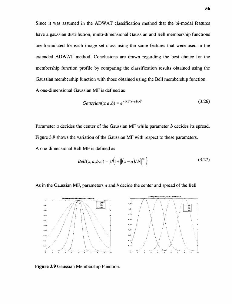
56

Since it was assumed in the ADWAT classification method that the bimodal features

have a gaussian distribution, multi-dimensional Gaussian and Bell membership functions

are formulated for each image set class using the same features that were used in the

extended ADWAT method. Conclusions are drawn regarding the best choice for the

membership function profile by comparing the classification results obtained using the

Gaussian membership function with those obtained using the Bell membership function.

A one-dimensional Gaussian MF is defined as

Parameter a decides the center of the Gaussian MY while parameter b decides its spread.

Figure 3.9 shows the variation of the Gaussian MF with respect to these parameters.

A one-dimensional Bell MF is defined as

As in the Gaussian MF, parameters a and b decide the center and spread of the Bell

Figure 3.9 Gaussian Membership Function.

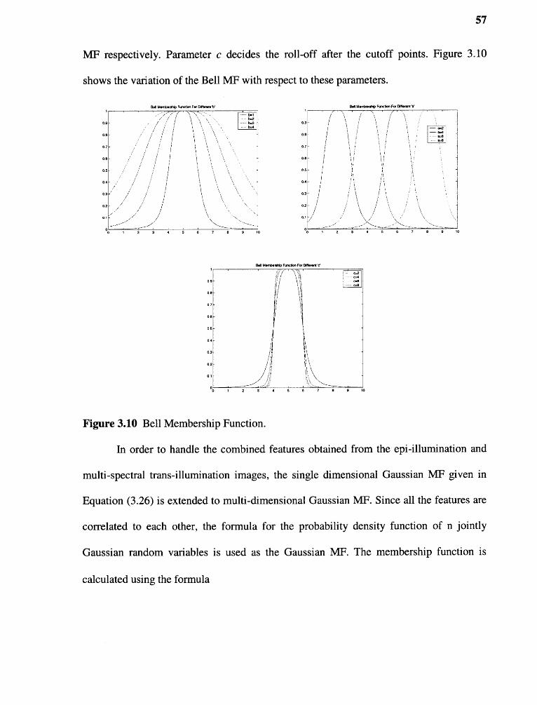
57

MF respectively. Parameter c decides the roll-off after the cutoff points. Figure 3.10

shows the variation of the Bell MF with respect to these parameters.

Figure 3.10 Bell Membership Function.

In order to handle the combined features obtained from the epi-illumination and

multi-spectral trans-illumination images, the single dimensional Gaussian MF given in

Equation (3.26) is extended to multi-dimensional Gaussian MF. Since all the features are

correlated to each other, the formula for the probability density function of n jointly

Gaussian random variables is used as the Gaussian MF. The membership function is

calculated using the formula

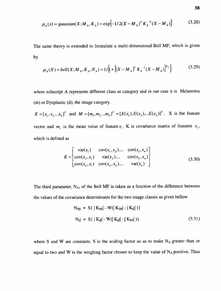
The same theory is extended to formulate a multi-dimensional Bell MF, which is given

by

where subscript A represents different class or category and in our case it is Melanoma

(m) or Dysplastic (d); the image category.

X is the feature

vector and m i is the mean value of feature xi . K is covariance matrix of features xi ,

which is defined as

The third parameter, NA, of the Bell MF is taken as a function of the difference between

the values of the covariance determinants for the two image classes as given bellow

where S and W are constants. S is the scaling factor so as to make NA greater than or

equal to two and W is the weighing factor chosen to keep the value of NA positive. Thus

59

the shape of the Bell MF for the two classes will be the same only if their covariance

matrices are the same.

The values of the parameters defining the membership functions are calculated using the

learning data set. These values are used in Equations (3.28) and (3.29) to formulate the

Gaussian and the Bell membership functions respectively. The value of scaling constant

S in Equation (3.31) was taken equal to 10 23 and NA was calculated for different discrete

values of weighing constant W. During the classification phase, for a candidate image the

feature vector X is obtained using wavelet decomposition and channel energy feature

calculations. This X is then plugged in to Equations (3.28) and (3.29) respectively to

calculate the membership function values for the melanoma and dysplastic nevus image

class. The candidate image is then assigned to the image class with higher membership

function value using the criteria 'winner takes all'.

CHAPTER 4

RESULTS AND DISCUSSION

4.1 Classification Of Skin Lesion Images

The diagnostic accuracy of a test is measured by the sensitivity and specificity of correct

classification [101]. For the classification of skin lesions in this study, the sensitivity, or

true positive fraction (TPF), indicates the fraction of melanoma lesions correctly

classified as melanoma. The specificity, or true negative fraction (TNF), indicates the

fraction of dysplastic or non-melanoma lesions correctly classified as non-melanoma.

The relationship between sensitivity and specificity calculated for all possible threshold

values of the discriminant function, or for this case the threshold constant, is represented

graphically as the Receiver operating characteristic (ROC). The vertical axis of the graph

represents the sensitivity or TPF, while the horizontal axis represents the false-positive

fraction, FPF, which is 1-TNF [101]. Results obtained from the ADWAT classification

method are presented and are then compared with those obtained using the method

proposed by Chang and Kuo [34].

4.1.1 Results of the ADWAT Classification Method

For the tree structure development, 11 features were considered for each channel

decomposed. From these features, threshold values were calculated for those features that

segregated into bimodal distributions between lesion classes. If more than one feature

within a particular channel segregated between lesion classes, then the feature for which

the separation between the mean values of the two classes was maximum compared to the

variance of each class was used in the analysis. The feature set and threshold values used

60

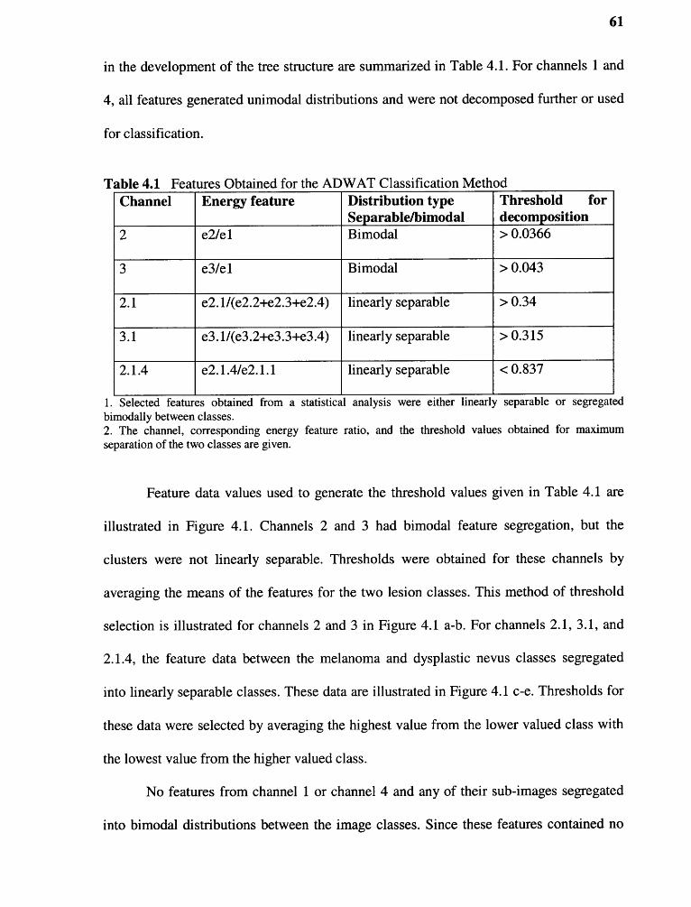
61

in the development of the tree structure are summarized in Table 4.1. For channels 1 and

4, all features generated unimodal distributions and were not decomposed further or used

for classification.

Table 4.1 Features Obtained for the ADWAT Classification MethodChannel Energy feature Distribution type

Separable/bimodalBimodal

Threshold fordecomposition> 0.03662 e2/el

3 e3/el Bimodal > 0.043

2.1 e2. 1/(e2.2+e2.3+e2.4) linearly separable > 0.34

3.1 e3.1/(e3.2+e3.3+e3.4) linearly separable > 0.315

2.1.4 e2.1.4/e2.1.1 linearly separable < 0.837

1. Selected features obtained from a statistical analysis were either linearly separable or segregatedbimodally between classes.2. The channel, corresponding energy feature ratio, and the threshold values obtained for maximumseparation of the two classes are given.

Feature data values used to generate the threshold values given in Table 4.1 are

illustrated in Figure 4.1. Channels 2 and 3 had bimodal feature segregation, but the

clusters were not linearly separable. Thresholds were obtained for these channels by

averaging the means of the features for the two lesion classes. This method of threshold

selection is illustrated for channels 2 and 3 in Figure 4.1 a-b. For channels 2.1, 3.1, and

2.1.4, the feature data between the melanoma and dysplastic nevus classes segregated

into linearly separable classes. These data are illustrated in Figure 4.1 c-e. Thresholds for

these data were selected by averaging the highest value from the lower valued class with

the lowest value from the higher valued class.

No features from channel 1 or channel 4 and any of their sub-images segregated

into bimodal distributions between the image classes. Since these features contained no

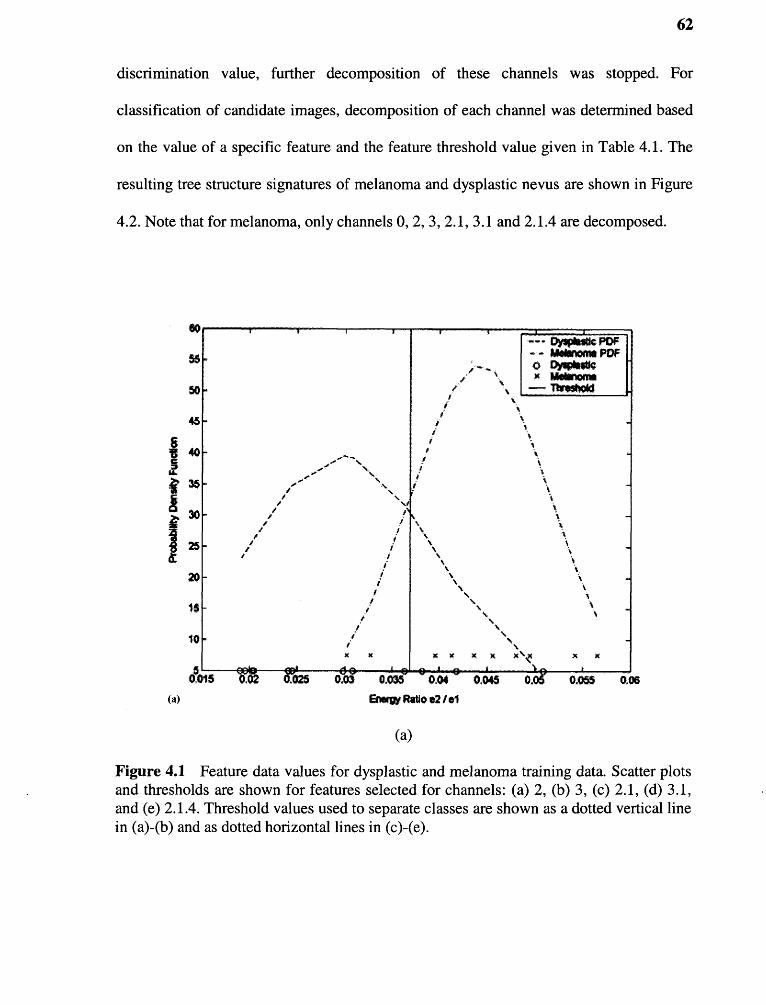
62

discrimination value, further decomposition of these channels was stopped. For

classification of candidate images, decomposition of each channel was determined based

on the value of a specific feature and the feature threshold value given in Table 4.1. The

resulting tree structure signatures of melanoma and dysplastic nevus are shown in Figure

4.2. Note that for melanoma, only channels 0, 2, 3, 2.1, 3.1 and 2.1.4 are decomposed.

Figure 4.1 Feature data values for dysplastic and melanoma training data. Scatter plotsand thresholds are shown for features selected for channels: (a) 2, (b) 3, (c) 2.1, (d) 3.1,and (e) 2.1.4. Threshold values used to separate classes are shown as a dotted vertical linein (a)-(b) and as dotted horizontal lines in (c)-(e).

63

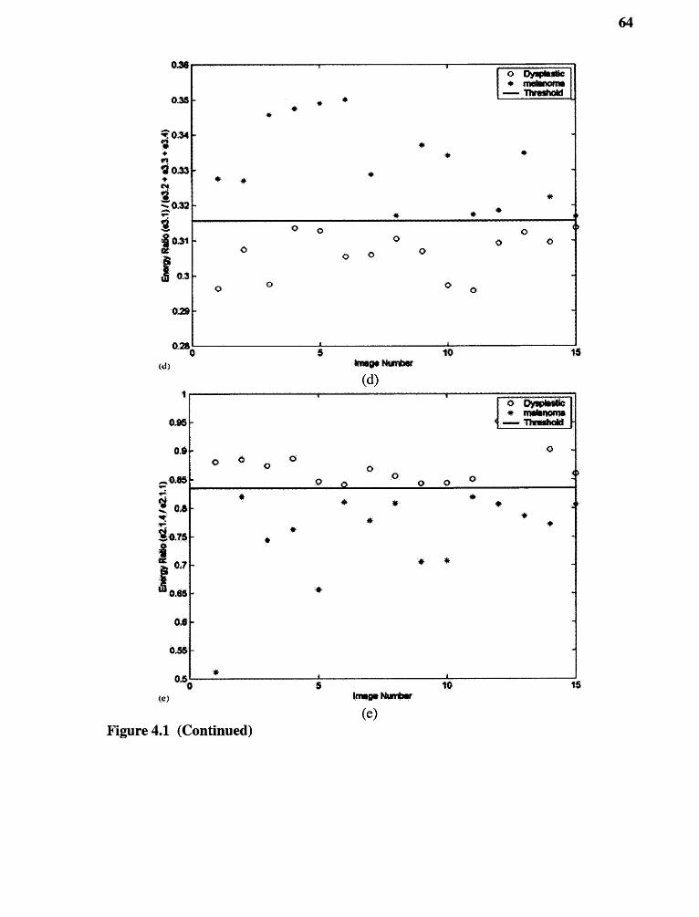
/ A

65

The decomposition of all the other channels was stopped since these features produced

unimodal distributions between the lesion classes. Also note that due to the selection of

the thresholds, the algorithm does not decompose dysplastic nevus images beyond the

first level. A dysplastic nevus will thus generate a tree structure with only one level of

decomposition as shown in Figure 4.2 b.

The results of the classification of the test data using the ADWAT method are

summarized in Table 4.2. For the ten images of melanoma used during the classification

phase, the algorithm was able to correctly classify nine images to the melanoma nevus

class. Histological evaluation had confirmed that all of these ten lesions were melanoma.

Figure 4.2 Tree structure signatures: (a) melanoma and (b) dysplastic nevus. Based onthe threshold values given in Table 3.3, several channels are decomposed for themelanoma creating a distinct tree structure. The dysplastic nevus is not decomposedbeyond the first level because of the selection of the threshold values.

66

For the 20 images of dysplastic nevus, 18 were correctly classified to the dysplastic nevus

class while two images were incorrectly classified to the melanoma nevus class. The

resulting true positive fraction (TPF) obtained for this classifier was 90% with a false

positive fraction (FPF) of 10%.

4.1.2 Classification Results By Constant Threshold Method

The results from this classification method are summarized in Table 4.3. The number of

melanoma and dysplastic nevus correctly classified and the resulting TPF and FPF are

given. The resulting ROC curve obtained for the tree structure wavelet transform analysis

method is shown in Figure 4.3. This tree structure method gives a maximum true positive

value of 70% and a false positive value of 20% for a threshold constant value of 0.026.

Table 4.2 Summary of the Test Data Classified Using the ADWAT MethodLesiontype

Number classified CV Classification Channel decompositionerror

Melanoma 8 6 Melanoma ---

Melanoma 1 5 Melanoma no decomposition of 3.1

Melanoma 1 1 Dysplastic no decomposition of 2, 3

Dysplastic 18 1 Dysplastic ---

Dysplastic 2 2 Melanoma decomposition of 2

Note: The lesions with a value of the classification variable (CV) greater than 1 are classified as melanoma;those with CV equal to 1 are classified as dysplastic nevus. The resulting TPF is 90% with a FPF of 10%.

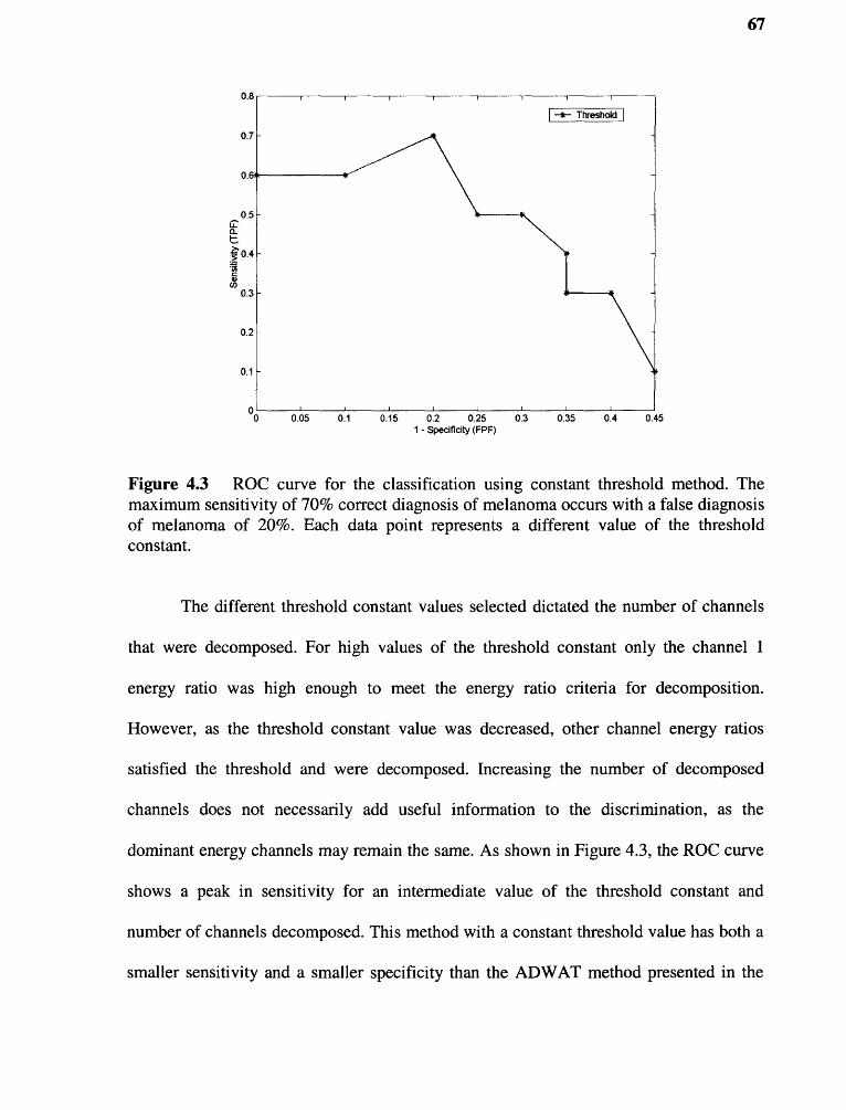
67

Figure 4.3 ROC curve for the classification using constant threshold method. Themaximum sensitivity of 70% correct diagnosis of melanoma occurs with a false diagnosisof melanoma of 20%. Each data point represents a different value of the thresholdconstant.

The different threshold constant values selected dictated the number of channels

that were decomposed. For high values of the threshold constant only the channel 1

energy ratio was high enough to meet the energy ratio criteria for decomposition.

However, as the threshold constant value was decreased, other channel energy ratios

satisfied the threshold and were decomposed. Increasing the number of decomposed

channels does not necessarily add useful information to the discrimination, as the

dominant energy channels may remain the same. As shown in Figure 4.3, the ROC curve

shows a peak in sensitivity for an intermediate value of the threshold constant and

number of channels decomposed. This method with a constant threshold value has both a

smaller sensitivity and a smaller specificity than the ADWAT method presented in the

68

previous section. Thus, by adaptively selecting the threshold based on the discrimination

content of the data, a better classification can be achieved with the same data.

4.1.3 Result Analysis and Discussion

In this section, the advantage of adaptively selecting the threshold values for image

decomposition is discussed in relation to the energy distribution and the information

within the channels. Result analysis and interpretation are also presented followed by

pointing out the potential applications of the ADWAT method.

4.1.3.1 Threshold Selection. For the epiluminesence images used in this study,

the energy is non-uniformly distributed among the channels. At the first level of

decomposition, the image total energy is distributed with about 82-87% in channel 1, 3-

4% in channel 2, 4-5% in channel 3 and 4-11% in channel 4. The energy in channel 1, the

low-low frequency channel, primarily corresponds to the skin surrounding the lesion and

is of no significance in the lesion classification. Channels 2 and channel 3, the mid

frequency channels, correspond to the nevus-skin boundary and some portions of the

nevus itself. These two channels are important from the classification point of view as

they contain most of the information that would allow discrimination between lesions

according to the ABCD rule. The energy in channel 4, the high-high frequency channel,

corresponds to portions of the lesion boundary where the boundary is well defined and

also to regions of uneven reflection from the surface due to air gaps and skin layering.

In the method proposed by Chang and Kuo [34], a threshold value is selected and

the ratio of channel energy to maximum channel energy within a decomposition level is

calculated. The decomposition of channels 2 and 3, which contain most of the relevant

discrimination information, is dependent on the value of the threshold constant. Selecting

69

a threshold constant value higher than the average e2/e1 or e3/e 1 energy ratio for a lesion

class will thus result in a loss of this information. For the test images, an e3/e1 ratio of

0.043 and an e2/e 1 ratio of 0.0366 optimally segregate the melanoma and dysplastic

nevus classes. For a threshold value greater than this e3/e1 ratio value, the tree structure

developed for many candidate melanoma images results in decomposition of only the

low-low frequency channel. This method will thus produce identical tree structure and

energy maps for the melanoma and dysplastic image classes, resulting in nearly all the

images from the data set being classified as dysplastic. For values of the threshold

constant below 0.043, the tree structure and the energy maps are highly dependent on the

value of the threshold constant. Hence, rather than randomly selecting a threshold value

without any criterion, this classification could be improved by using an adaptive method

for selecting the threshold value.

Obtaining the threshold values from a statistical analysis of the channel energies

and their ratios provides the required adaptivity to the tree structure development.

Statistical selection of the thresholds at each level of decomposition makes the ADWAT

method more robust and a good candidate method for surface characterization and texture

representation. It should be noted that since the thresholds were obtained from bimodal

distributions, reversing the inequalities on the thresholds would reverse the tree structure

signatures developed for the two classes. The dysplastic nevus was a logical choice as a

basis for classification instead of the melanoma since more dysplastic nevus data was

available. The number of images used during the learning phase is the same for both the

classes, although the number of dysplastic nevus images used in the classification phase

70

is more. Also the natural population of dysplastic nevus class is very large compared to

melanoma, hence no risk of obtaining any bias is seen.

4.1.3.2 Analysis of ADWAT Classification. In the ADWAT method, it is

necessary for either channel 2 or channel 3 to be decomposed in order to generate a value

of CV > 1 and to classify a lesion as melanoma. A summary of the decomposition of the

test images is given in Table 4.3. Among the nine images classified as melanoma, eight

images developed the complete tree structure signature of melanoma with the value of

CV equal to 6. The remaining image correctly classified as melanoma produced a value

of CV equal to 5, failing to decompose channel 3.1. The melanoma image that was

misclassified as non-melanoma is shown in Figure 4.4. This lesion is a late stage

melanoma that was easily diagnosed by the physician. As can be seen in the image, a

significant amount of reflection is contained in the image as a result of flaking skin on the

lesion and skin surface. As a result, more energy was distributed in channel 4, while the

energy in channels 2 and 3 decreased below the threshold values needed for

decomposition. The algorithm failed in this case due to this change in the energy

distribution. The imaging artifact resulting from non-uniform reflection can be minimized

by use of a polarizing filter or by applying a lotion to the skin prior to imaging to

minimize refractive index mismatch.

The two images of dysplastic nevi that were incorrectly classified as melanoma

were decomposed beyond the first level. For both of these images, channel 2 was

decomposed one level. These images produced a value of CV equal to 2 and were thus

classified as melanoma. The tree structure developed for these two images is different

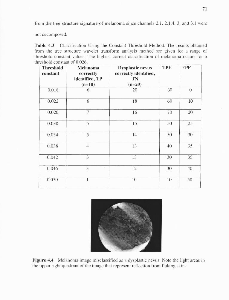
71

from the tree structure signature of melanoma since channels 2.1, 2.1.4, 3, and 3.1 were

not decomposed.

Table 4.3 Classification Using the Constant Threshold Method. The results obtainedfrom the tree structure wavelet transform analysis method are given for a range ofthreshold constant values. The highest correct classification of melanoma occurs for athreshold constant of 0.026.

Thresholdconstant

Melanomacorrectly

identified, TP

Dysplastic nevuscorrectly identified,

TN

TPF FPF

(n=10) (n=20)0.018 6 20 60 0

0.022 6 18 60 10

0.026 7 16 70 20

0.030 5 15 50 25

0.034 5 14 50 30

0.038 4 13 40 35

0.042 3 13 30 35

0.046 3 12 30 40

0.050 1 10 10 50

Figure 4.4 Melanoma image misclassified as a dysplastic nevus. Note the light areas inthe upper right quadrant of the image that represent reflection from flaking skin.

72

This misclassification can be interpreted in two primary ways. One level of

decomposition beyond the main level is a result of the closely valued features between

the melanoma and dysplastic in channel 2. As a result, it may be worthwhile to reconsider

the definition of the classification variable or to increase the classification variable to a

value greater than 1 to delineate the melanoma and dysplastic nevus class boundary. An

alternate interpretation of the misclassification of these dysplastic nevi may be that these

two nevi are in the early stages of malignant transformation, but are not showing any

visible features to be identified as melanoma by a physician. Since none of the lesions

visually diagnosed as dysplastic nevus were biopsied, these two lesions could potentially

be at the very early stage of melanoma. This possibility deserves further consideration as

it may show that the ADWAT method is more sensitive than the ABCD rule in making

diagnosis of early melanoma. Further investigation and patient follow-up is needed

before this hypothesis can be confirmed or disproved.

The ADWAT classification method requires approximately 15-20 seconds for

image decomposition, computing the feature values and making a decision about the

image class of the unknown. The method suggested by Chang and Kuo [34] requires

more time due to the distance calculations involved in the classification phase.

The same set of features used during the training phase of the ADWAT

classification method were used to train a three layer feed-forward neural network with

back-propagation training algorithm [102-103]. The back-propagation training algorithm

is an iterative gradient algorithm designed to minimize the mean square error between the

actual outputs of a multiplayer feed forward perceptron and the desired output. The first

and second hidden layers of the network had ten and six neurons respectively while the

73

output layer had one neuron. The two hidden layers had a nonlinear log-sigmoid transfer

function while the output layer had a linear transfer function. It required 957 cycles of

iterations through the training set for the error to go below 0.00001. The feature set used

in the classification phase of the ADWAT classification method was then presented to

this trained network. It produced a true positive fraction (TPF) of 90% with a false

positive fraction (FPF) of 25%.

The sensitivity of the ADWAT classification method is better then the sensitivity

of the ABCD rule [4-7]. The TPF and FPF values are much improved as compared to the

method suggested by Chang and Kuo [34]. Compared to the neural network

backpropagation method [102-103], the ADWAT classification method has better

specificity. Also the physicians find more information in the epiluminesence images

obtained using the Nevoscope [14-15] than normal visual examination. But, more data

needs to be analyzed before the ADWAT classification method can be used in a clinical

setting.

4.1.3.3 Potential Applications. The ADWAT classification method is especially

effective and fast as compared to that of Chang and Kuo [34] when images with different

surface characteristics but similar dominant frequency channels are to be classified.

Instead of measuring the distance between features and iteratively adding new features

into the classification process, the images can be classified by using a semantic

comparison of the tree structure signatures, making the classification process simpler.

Although the ADWAT method has been illustrated here with two image classes, it can be

adapted easily to accommodate more classes. Instead of using a single threshold, multiple

thresholds and tree structures will be obtained, depending upon the number of classes.

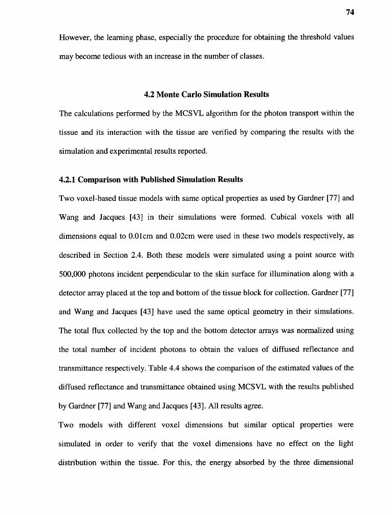
74

However, the learning phase, especially the procedure for obtaining the threshold values

may become tedious with an increase in the number of classes.

4.2 Monte Carlo Simulation Results

The calculations performed by the MCSVL algorithm for the photon transport within the

tissue and its interaction with the tissue are verified by comparing the results with the

simulation and experimental results reported.

4.2.1 Comparison with Published Simulation Results

Two voxel-based tissue models with same optical properties as used by Gardner [77] and

Wang and Jacques [43] in their simulations were formed. Cubical voxels with all

dimensions equal to 0.01cm and 0.02cm were used in these two models respectively, as

described in Section 2.4. Both these models were simulated using a point source with

500,000 photons incident perpendicular to the skin surface for illumination along with a

detector array placed at the top and bottom of the tissue block for collection. Gardner [77]

and Wang and Jacques [43] have used the same optical geometry in their simulations.

The total flux collected by the top and the bottom detector arrays was normalized using

the total number of incident photons to obtain the values of diffused reflectance and

transmittance respectively. Table 4.4 shows the comparison of the estimated values of the

diffused reflectance and transmittance obtained using MCSVL with the results published

by Gardner [77] and Wang and Jacques [43]. All results agree.

Two models with different voxel dimensions but similar optical properties were

simulated in order to verify that the voxel dimensions have no effect on the light

distribution within the tissue. For this, the energy absorbed by the three dimensional

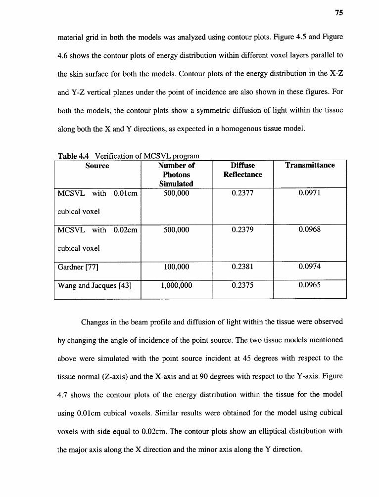
75

material grid in both the models was analyzed using contour plots. Figure 4.5 and Figure

4.6 shows the contour plots of energy distribution within different voxel layers parallel to

the skin surface for both the models. Contour plots of the energy distribution in the X-Z

and Y-Z vertical planes under the point of incidence are also shown in these figures. For

both the models, the contour plots show a symmetric diffusion of light within the tissue

along both the X and Y directions, as expected in a homogenous tissue model.

Table 4.4 Verification of MCSVL programSource Number of

PhotonsSimulated

DiffuseReflectance

Transmittance

MCSVL with 0.01cm

cubical voxel

500,000 0.2377 0.0971

MCSVL with 0.02cm

cubical voxel

500,000 0.2379 0.0968

Gardner [77] 100,000 0.2381 0.0974

Wang and Jacques [43] 1,000,000 0.2375 0.0965

Changes in the beam profile and diffusion of light within the tissue were observed

by changing the angle of incidence of the point source. The two tissue models mentioned

above were simulated with the point source incident at 45 degrees with respect to the

tissue normal (Z-axis) and the X-axis and at 90 degrees with respect to the Y-axis. Figure

4.7 shows the contour plots of the energy distribution within the tissue for the model

using 0.01cm cubical voxels. Similar results were obtained for the model using cubical

voxels with side equal to 0.02cm. The contour plots show an elliptical distribution with

the major axis along the X direction and the minor axis along the Y direction.

76

4.2.2 Comparison with Experimental Data

A three layer, wavelength-dependent voxel-based tissue model of the medium pigmented

or the Asian skin color type was developed. This model was simulated using the optical

geometry of the spectroanalyser system [98]. Zeng et al [97-98] have used the

spectroanalyser system for diffuse reflectance measurements on Asian volunteers. In the

spectroanalyser system the light is incident at an angle of 5 degrees with respect to the

tissue normal and the collection angle is 30 degrees. This optical geometry was setup in

the simulations as explained in Section 3.2.4. White and black skin color type models

were also developed and simulated using the same optical geometry. For all these

models, diffuse reflectance was estimated for optical wavelengths with an interval of 5nm

over the range of 350-700nm. Results were obtained by taking an average value of the

diffuse reflectance obtained from three independent runs using 100,000 photons each.

Figure 4.8 shows the diffuse reflectance spectra obtained by direct measurement at

different body locations using the spectroanalyser system [97-98]. Figure 4.9 shows the

diffuse reflectance spectra obtained using MCSVL for the three skin color type models.

All the spectra show the two characteristic oxy-hemoglobin absorption valleys between

520nm and 600nm. The characteristic oxy-hemoglobin absorption valleys become less

prominent as the level of pigmentation in the skin increases. This reduction in the

characteristic oxy-hemoglobin absorption valleys from the lightly pigmented to highly

pigmented skin type spectra can be attributed to the absorption due to melanin becoming

more prominent than the oxy-hemoglobin absorption. Comparing the three diffuse

reflectance spectra in Figure 4.9, one can observe a drop in the diffuse reflectance values

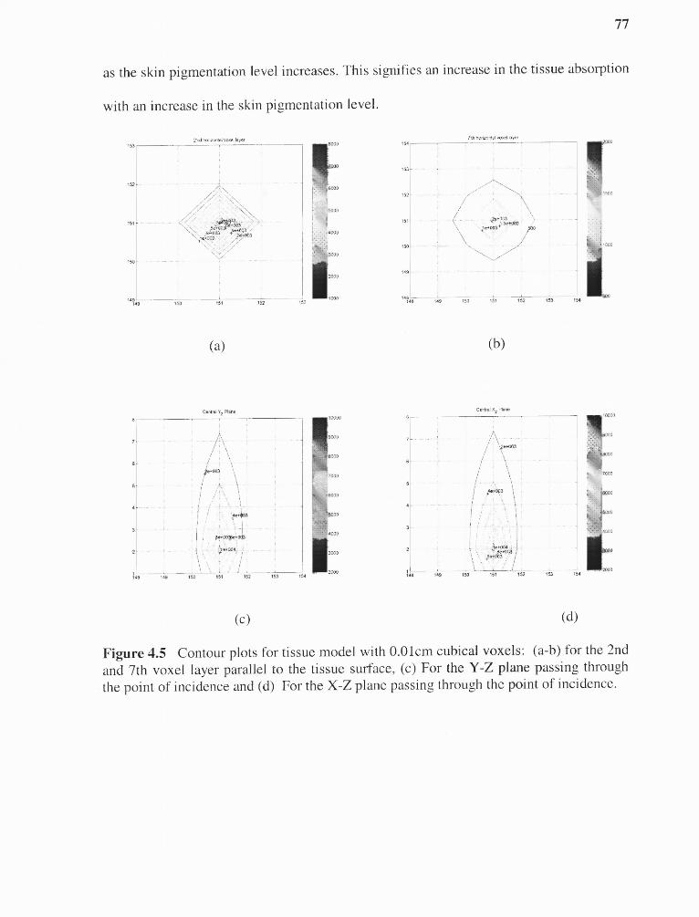
77

as the skin pigmentation level increases. This signifies an increase in the tissue absorption

with an increase in the skin pigmentation level.

(c) (d)

Figure 4.5 Contour plots for tissue model with 0.01cm cubical voxels: (a-b) for the 2ndand 7th voxel layer parallel to the tissue surface, (c) For the Y-Z plane passing throughthe point of incidence and (d) For the X-Z plane passing through the point of incidence.

Figure 4.6 Contour plots for tissue model with 0.02cm cubical voxels: (a-b) for the 2ndand 5th voxel layer parallel to the tissue surface, (c) For the Y-Z plane passing throughthe point of incidence and (d) For the X-Z plane passing through the point of incidence.

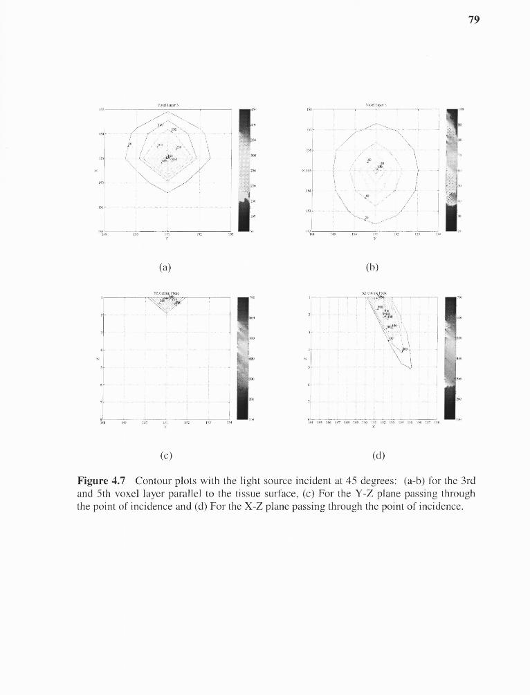
Figure 4.7 Contour plots with the light source incident at 45 degrees: (a-b) for the 3rdand 5th voxel layer parallel to the tissue surface, (c) For the Y-Z plane passing throughthe point of incidence and (d) For the X-Z plane passing through the point of incidence.

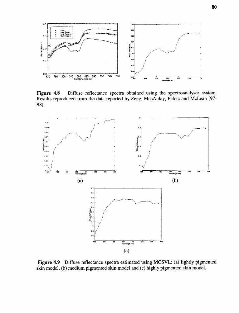
Figure 4.8 Diffuse reflectance spectra obtained using the spectroanalyser system.Results reproduced from the data reported by Zeng, MacAulay, Palcic and McLean [97-98].

Figure 4.9 Diffuse reflectance spectra estimated using MCSVL: (a) lightly pigmentedskin model, (b) medium pigmented skin model and (c) highly pigmented skin model.

81

Although the diffuse reflectance spectra obtained using the MCSVL code has

similar characteristics to those measured experimentally using the spectroanalyser

system, the values differ. This is attributed to the difference in the method of

normalization and the difference between the measurement set-up used in the simulations

and actual measurements. A point light source is used in the MCSVL simulations where

as the spectroanalyser system uses a 1 mm core diameter fused silica fiber for

illumination. The method of normalizing the collected flux to obtain the values of the

diffuse reflectance is different in our simulations from the method used by Zeng et al

[97-98]. For the spectroanalyser system measurements, the diffuse reflectance spectrum

obtained using a standard disc with constant reflectance, independent of wavelength, was

used as a reference. This spectrum was used to normalize the measured skin spectrum.

For MCSVL estimates, the diffuse reflectance values were normalized by dividing the

collected flux by the number of photons used in the simulation.

The diffuse reflectance spectra from different body locations of the Asian

Volunteer are different in details except for the two characteristic oxy-hemoglobin

absorption valleys. This signifies that the diffuse reflectance values vary with the skin

thickness and the concentration of the chromophores associated with it. The classification

of skin is based on the volume fraction of the epidermis occupied by melanosomes, fmel,

which for white color skin is equal to 1.3-6.3%, 11-16% for brown/olive color skin and

18-43% for black color skin, according to Jacques [81]. The average values of these fmel

ranges were used in calculating the epidermal absorption coefficient for the three skin

color type models.

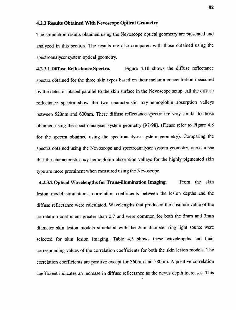
82

4.2.3 Results Obtained With Nevoscope Optical Geometry

The simulation results obtained using the Nevoscope optical geometry are presented and

analyzed in this section. The results are also compared with those obtained using the

spectroanalyser system optical geometry.

4.2.3.1 Diffuse Reflectance Spectra. Figure 4.10 shows the diffuse reflectance

spectra obtained for the three skin types based on their melanin concentration measured

by the detector placed parallel to the skin surface in the Nevoscope setup. All the diffuse

reflectance spectra show the two characteristic oxy-hemoglobin absorption valleys

between 520nm and 600nm. These diffuse reflectance spectra are very similar to those

obtained using the spectroanalyser system geometry [97-98]. (Please refer to Figure 4.8

for the spectra obtained using the spectroanalyser system geometry). Comparing the

spectra obtained using the Nevoscope and spectroanalyser system geometry, one can see

that the characteristic oxy-hemoglobin absorption valleys for the highly pigmented skin

type are more prominent when measured using the Nevoscope.

4.2.3.2 Optical Wavelengths for Trans -illumination Imaging. From the skin

lesion model simulations, correlation coefficients between the lesion depths and the

diffuse reflectance were calculated. Wavelengths that produced the absolute value of the

correlation coefficient greater than 0.7 and were common for both the 5mm and 3mm

diameter skin lesion models simulated with the 2cm diameter ring light source were

selected for skin lesion imaging. Table 4.5 shows these wavelengths and their

corresponding values of the correlation coefficients for both the skin lesion models. The

correlation coefficients are positive except for 360nm and 580nm. A positive correlation

coefficient indicates an increase in diffuse reflectance as the nevus depth increases. This

83

is significant from the imaging point of view for a better characterization of the nevus

depth. At 360nm the absorption of light due to melanin is very high, also the scattering by

the superficial skin layers (Stratum corneum) would be high at this wavelength,

preventing it form penetrating any deeper. Due to this 360nm light will not be able to

sample nevus depths effectively resulting in a negative correlation coefficient value.

580nm would sample the nevus depths more effectively than 360nm due to more

penetration in the tissue. But, at this wavelength the absorption due to hemoglobin would

be very high. This may have resulted into a negative correlation coefficient value at this

(c)Figure 4.10 Diffuse reflectance spectra with detector parallel to the skin surface: (a)lightly pigmented, (b) medium pigmented and (c) highly pigmented.

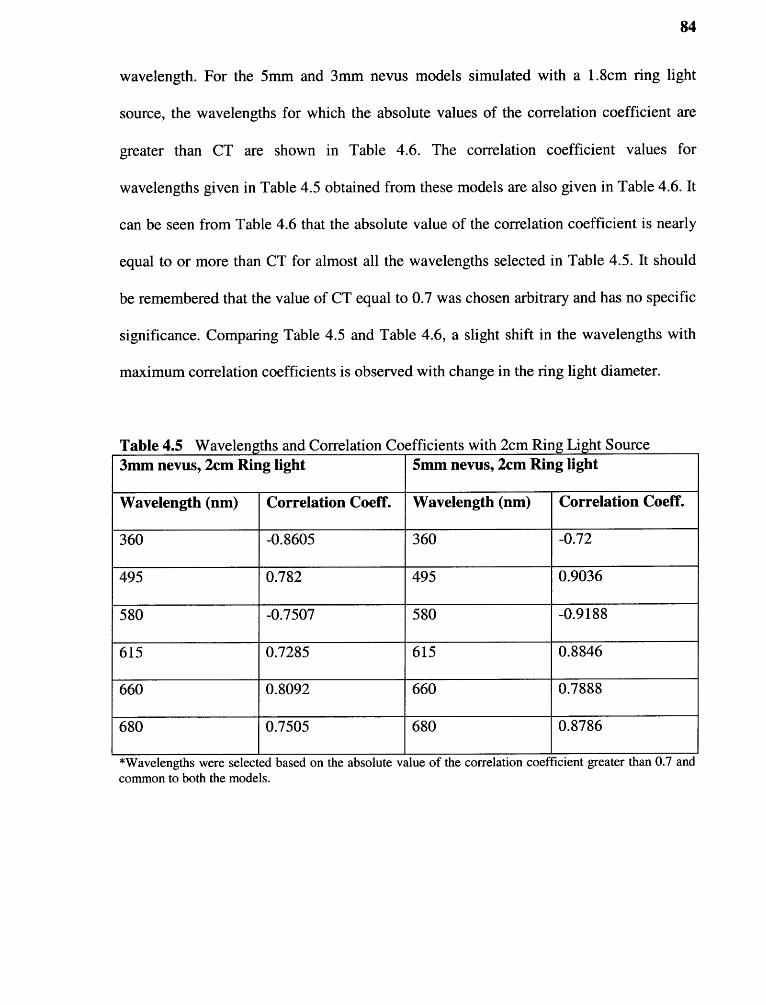
84

wavelength. For the 5mm and 3mm nevus models simulated with a 1.8cm ring light

source, the wavelengths for which the absolute values of the correlation coefficient are

greater than CT are shown in Table 4.6. The correlation coefficient values for

wavelengths given in Table 4.5 obtained from these models are also given in Table 4.6. It

can be seen from Table 4.6 that the absolute value of the correlation coefficient is nearly

equal to or more than CT for almost all the wavelengths selected in Table 4.5. It should

be remembered that the value of CT equal to 0.7 was chosen arbitrary and has no specific

significance. Comparing Table 4.5 and Table 4.6, a slight shift in the wavelengths with

maximum correlation coefficients is observed with change in the ring light diameter.

Table 4.5 Wavelengths and Correlation Coefficients with 2cm Ring Light Source3mm nevus, 2cm Ring light 5mm nevus, 2cm Ring light

Wavelength (nm) Correlation Coeff. Wavelength (nm) Correlation Coeff.

360 -0.8605 360 -0.72

495 0.782 495 0.9036

580 -0.7507 580 -0.9188

615 0.7285 615 0.8846

660 0.8092 660 0.7888

680 0.7505 680 0.8786

*Wavelengths were selected based on the absolute value of the correlation coefficient greater than 0.7 andcommon to both the models.

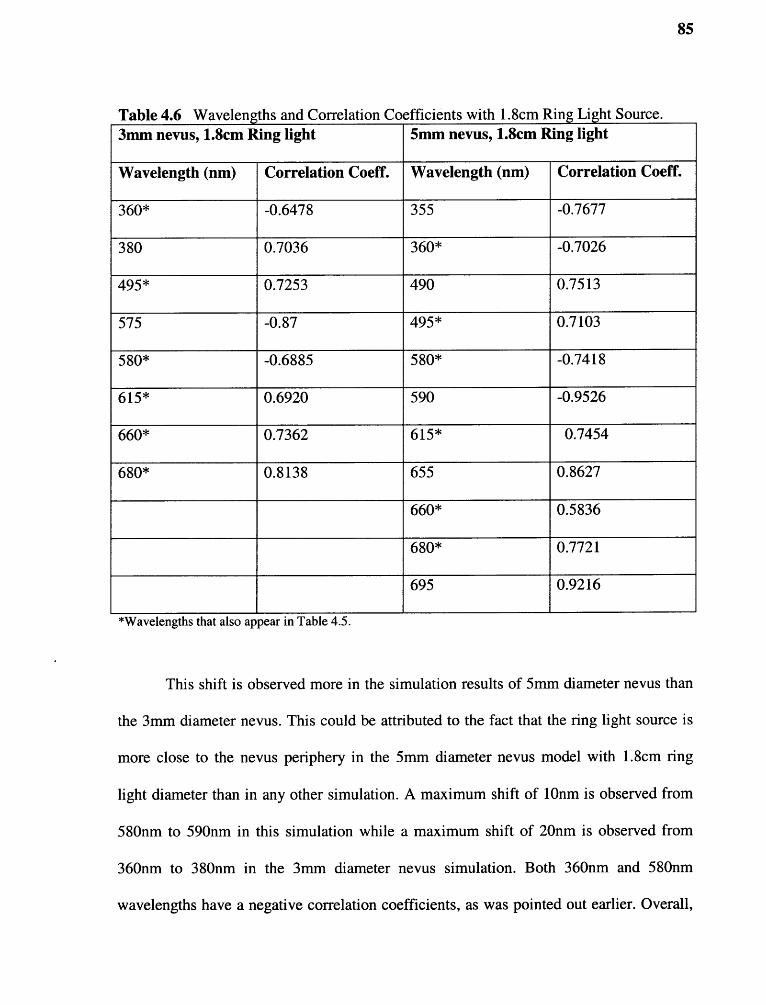
Table 4.6 Wavelengths and Correlation Coefficients with 1.8cm Ring Light Source.3mm nevus, 1.8cm Ring light 5mm nevus, 1.8cm Ring light

Wavelength (nm) Correlation Coeff. Wavelength (nm) Correlation Coeff.

360* -0.6478 355 -0.7677

380 0.7036 360* -0.7026

495* 0.7253 490 0.7513

575 -0.87 495* 0.7103

580* -0.6885 580* -0.7418

615* 0.6920 590 -0.9526

660* 0.7362 615* 0.7454

680* 0.8138 655 0.8627

660* 0.5836

680* 0.7721

695 0.9216

*Wavelengths that also appear in Table 4.5.

This shift is observed more in the simulation results of 5mm diameter nevus than

the 3mm diameter nevus. This could be attributed to the fact that the ring light source is

more close to the nevus periphery in the 5mm diameter nevus model with 1.8cm ring

light diameter than in any other simulation. A maximum shift of l0nm is observed from

580nm to 590nm in this simulation while a maximum shift of 20nm is observed from

360nm to 380nm in the 3mm diameter nevus simulation. Both 360nm and 580nm

wavelengths have a negative correlation coefficients, as was pointed out earlier. Overall,

85

86

lesser shift in wavelength and a better correlation between the nevus depths and the

diffuse reflectance is obtained for wavelengths above 600nm. This is the region where the

absorption due to both melanin and hemoglobin is less and also the scattering of light in

the epidermal and dermal layers is less.

From the results, it can be said that optical wavelengths of 495, 580, 615, 660 and

680nm can be used for multi-spectral imaging and characterization of the skin lesions

using the Nevoscope. For wavelength below —450nm there would be secondary

emissions from natural fluorophores inside the skin due to auto-fluorescence [23] which

is not taken in to account in the simulations performed. A certain amount of uncertainty

is involved in selecting the wavelength for multi-spectral imaging of the skin lesions due

to auto-fluorescence.

4.3 Classification Using Multi-spectral Images

The ADWAT classification method uses the epi-illuminance images of the skin lesion

obtained using a white light source. These images contain the superficial skin lesion

features that are used by a physician for diagnosis using the ABCD rule. The ADWAT

classification method uses the spatial-frequency information in these images that

correspond to these superficial skin lesion features. The suspicious skin lesions are

removed and analyzed in the histo-pathology lab where the information about the lesion

depth and architecture is obtained. Based on this information a case of melanoma is

confirmed.

Multi-spectral trans-illuminance images of the skin lesion give information about

the lesion depth and architecture, hence analysis of these images would improve the

87

sensitivity of melanoma diagnosis. In this section classification results obtained using the

Extended ADWAT method and Fuzzy Membership functions are presented and

discussed.

4.3.1 Results of the Extended ADWAT Classification Method

The multi-spectral images obtained using 580nm and 610nm were analyzed using the

technique described in the ADWAT classification method. Statistical analysis of the

channel energy and energy ratio features of these images was used to obtain features that

segregated into bimodal distributions between lesion classes. Threshold values were

calculated for these features to obtain maximum separation between the two image

classes. The feature set and their corresponding threshold values obtained from the multi-

spectral images are summarized in Table 4.7. Feature set and threshold values obtained

from the epi-illuminance images are also given in Table 4.7 to present the combined

feature set. Feature data values used to generate the threshold values given in Table 4.7

are illustrated in Figure 4.11. All the features obtained from the multi-spectral images had

bimodal feature segregation. Thresholds were obtained for these channels by averaging

the means of the features for the two lesion classes. Figure 4.11 a-e illustrate the features

for the 580nm wavelength image and Figure 4.11 f-h illustrate the features for the 610nm

wavelength image.

In the first step of the classification decision about the image class is taken based

on the value of CV1, which counts the number of channels in the epi-illuminance image

that satisfy the threshold criteria and are decomposed further. If CV1 is equal to 1 then the

image is assigned to the dysplastic nevus class; for CV1 = 6 the image is assigned to the

melanoma class and for any other value of CV1 the image is assigned to the suspicious

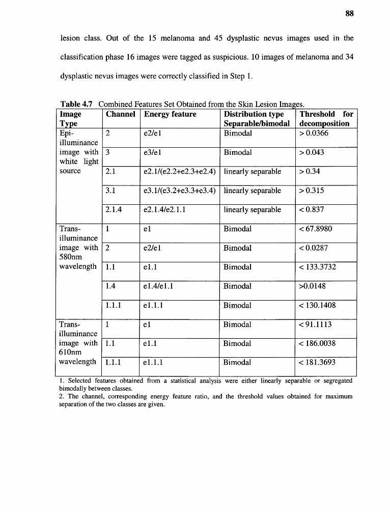
88

lesion class. Out of the 15 melanoma and 45 dysplastic nevus images used in the

classification phase 16 images were tagged as suspicious. 10 images of melanoma and 34

dysplastic nevus images were correctly classified in Step 1.

Table 4.7 Combined Features Set Obtained from the Skin Lesion 'mans.ImageType

Channel Energy feature Distribution typeSeparable/bimodal

Threshold fordecomposition

Epi-illuminanceimage withwhite lightsource

2 e2/e1 Bimodal > 0.0366

3 e3/e1 Bimodal > 0.043

2.1 e2. 1/(e2.2+e2.3+e2.4) linearly separable > 0.34

3.1 e3.1/(e3.2+e3.3+e3.4) linearly separable > 0.315

2.1.4 e2.1.4/e2.1.1 linearly separable < 0.837

Trans-illuminanceimage with580nmwavelength

1 e1 Bimodal < 67.8980

2 e2/e1 Bimodal < 0.0287

1.1 e1.1 Bimodal < 133.3732

1.4 e1.4/e1.1 Bimodal >0.0148

1.1.1 e1.1.1 Bimodal < 130.1408

Trans-illuminanceimage with610nmwavelength

1 e1 Bimodal < 91.1113

1.1 ell Bimodal < 186.0038

1.1.1 e1.1.1 Bimodal < 181.3693

1. Selected features obtained from a statistical analysis were either linearly separable or segregatedbimodally between classes.2. The channel, corresponding energy feature ratio, and the threshold values obtained for maximumseparation of the two classes are given.

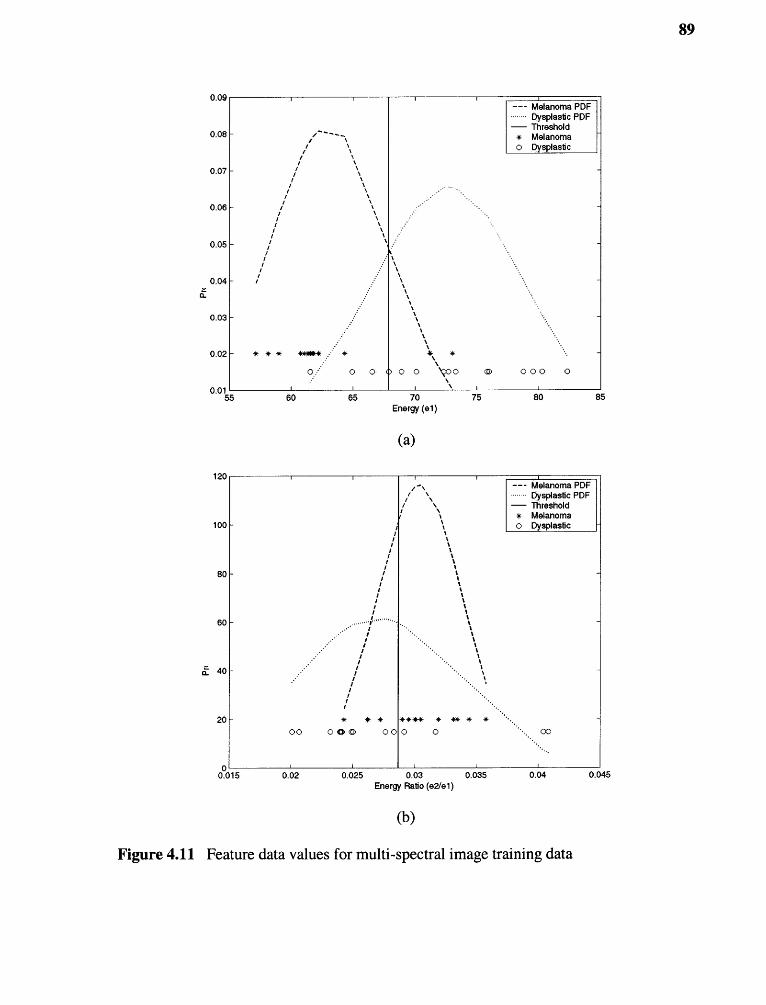
Figure 4.11 Feature data values for multi-spectral image training data

89

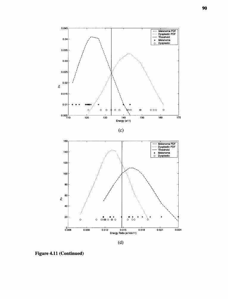
90

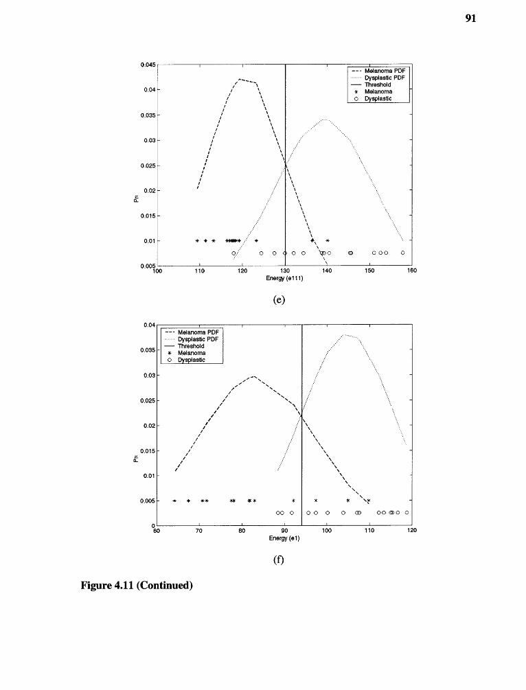
91

140 160120 220200 240180Energy (ell)

180Energy (e111)

(h)

120 140 160 200 220 240

(g)

Figure 4.11 (Continued)

92

0.022

0.018

0.014

0.01

0.006

0.002

0.022

0.018

0.014

0.01

0.006

0.002

--- Melanoma PDF Dysplastic PDF- Threshold

* Melanomao Dysplastic

* *

0 0 0 0 no 0 COO 0 00 0

--- Melanoma PDF Dysplastic PDF- Threshold* Melanomao Dysplastic

*

op 0 0

•

CD 0 000 0 00 0

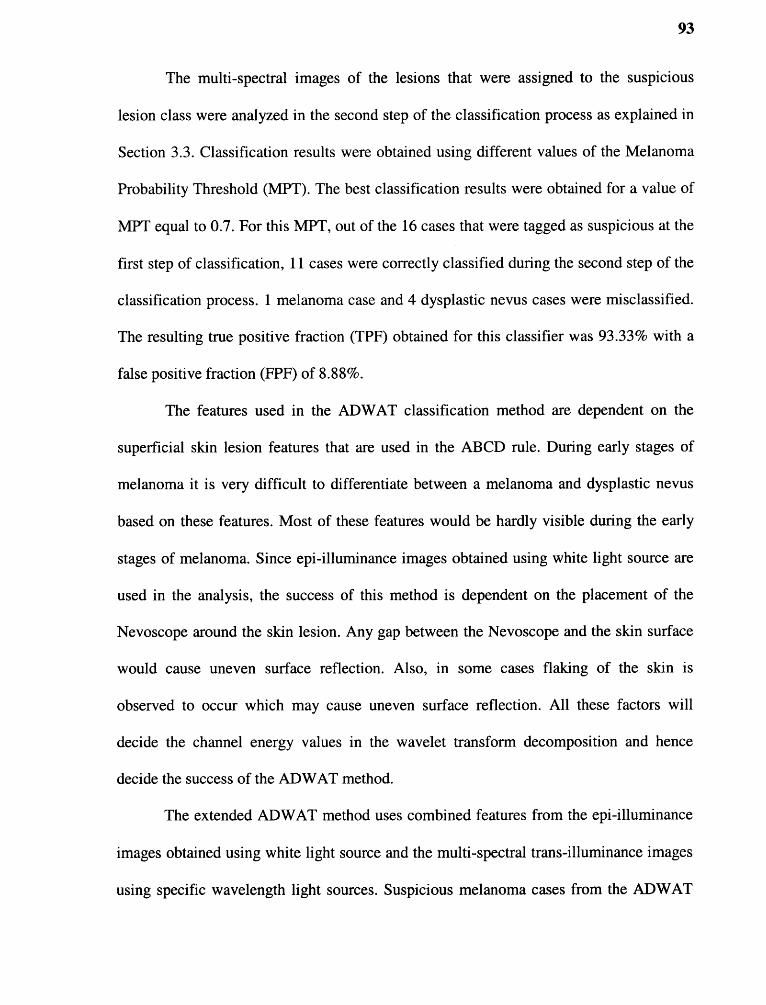
93

The multi-spectral images of the lesions that were assigned to the suspicious

lesion class were analyzed in the second step of the classification process as explained in

Section 3.3. Classification results were obtained using different values of the Melanoma

Probability Threshold (MPT). The best classification results were obtained for a value of

MPT equal to 0.7. For this MPT, out of the 16 cases that were tagged as suspicious at the

first step of classification, 11 cases were correctly classified during the second step of the

classification process. 1 melanoma case and 4 dysplastic nevus cases were misclassified.

The resulting true positive fraction (TPF) obtained for this classifier was 93.33% with a

false positive fraction (FPF) of 8.88%.

The features used in the ADWAT classification method are dependent on the

superficial skin lesion features that are used in the ABCD rule. During early stages of

melanoma it is very difficult to differentiate between a melanoma and dysplastic nevus

based on these features. Most of these features would be hardly visible during the early

stages of melanoma. Since epi-illuminance images obtained using white light source are

used in the analysis, the success of this method is dependent on the placement of the

Nevoscope around the skin lesion. Any gap between the Nevoscope and the skin surface

would cause uneven surface reflection. Also, in some cases flaking of the skin is

observed to occur which may cause uneven surface reflection. All these factors will

decide the channel energy values in the wavelet transform decomposition and hence

decide the success of the ADWAT method.

The extended ADWAT method uses combined features from the epi-illuminance

images obtained using white light source and the multi-spectral trans-illuminance images

using specific wavelength light sources. Suspicious melanoma cases from the ADWAT

94

classification method due to less developed superficial features of uneven surface

reflection are taken to the next step of analysis. Multi-spectral trans-illuminance images

are analyzed in this step. These images give information related to the nevus architecture

and depth and are less affected from the uneven surface reflection. Hence the extended

ADWAT method will give more accurate results and the variance in the overall success

of this method will be less compared to the ADWAT method.

4.3.2 Classification Results Using Fuzzy Membership Functions

Bimodal features were obtained from the epi-illumination images and the multi-

spectral trans-illumination images using wavelet decomposition and statistical analysis of

the channel energy and energy ratios for the Extended ADWAT classification method.

All these features were combined to form a composite feature set. In this composite

feature set the dynamic range of the channel energy ratio features is far less compared to

the dynamic range of the channel energy features. For classification it is necessary to

normalize the feature set so that all the features have similar dynamic range. In the

Extended ADWAT method each feature was compared with the corresponding feature

value of the candidate images independently and hence normalization was not necessary.

Using linear transformations all the features in the composite feature set were normalized

so that they have a dynamic range between zero and one. Using the values of MA, KA and

NA that were calculated from the learning data set, the values of the dysplastic and

melanoma membership functions were calculated for the unknown image sets using

Equations (3.28) and (3.29). Decision as to whether the unknown image set belongs to

the melanoma or dysplastic nevus class was taken based on the "winner takes all"

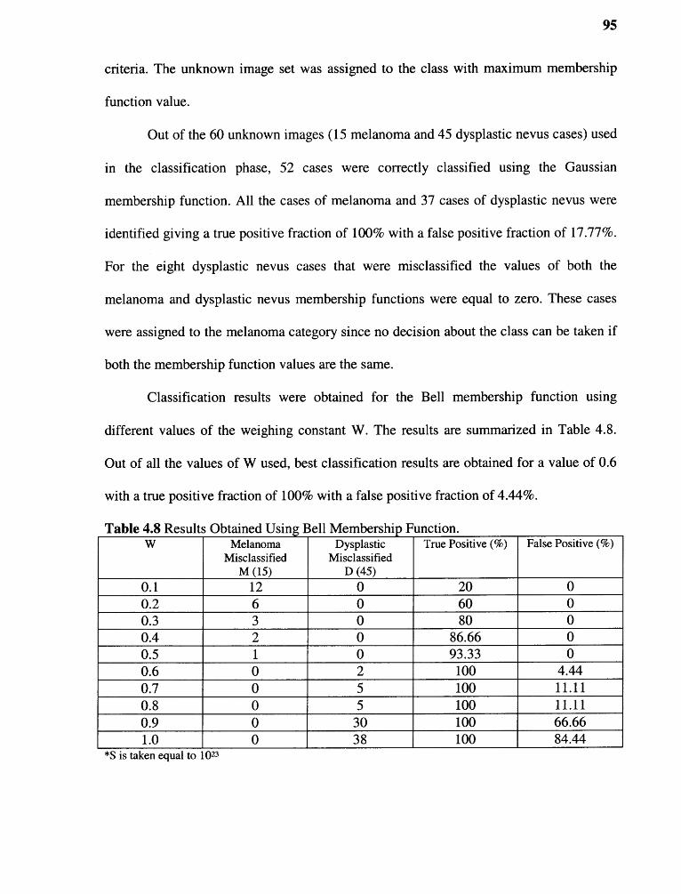
95

criteria. The unknown image set was assigned to the class with maximum membership

function value.

Out of the 60 unknown images (15 melanoma and 45 dysplastic nevus cases) used

in the classification phase, 52 cases were correctly classified using the Gaussian

membership function. All the cases of melanoma and 37 cases of dysplastic nevus were

identified giving a true positive fraction of 100% with a false positive fraction of 17.77%.

For the eight dysplastic nevus cases that were misclassified the values of both the

melanoma and dysplastic nevus membership functions were equal to zero. These cases

were assigned to the melanoma category since no decision about the class can be taken if

both the membership function values are the same.

Classification results were obtained for the Bell membership function using

different values of the weighing constant W. The results are summarized in Table 4.8.

Out of all the values of W used, best classification results are obtained for a value of 0.6

with a true positive fraction of 100% with a false positive fraction of 4.44%.

Table 4.8 Results Obtained Using Bell Membership Function.W Melanoma

MisclassifiedM (15)

DysplasticMisclassified

D (45)

True Positive (%) False Positive (%)

0.1 12 0 20 00.2 6 0 60 00.3 3 0 80 00.4 2 0 86.66 00.5 1 0 93.33 00.6 0 2 100 4.440.7 0 5 100 11.110.8 0 5 100 11.110.9 0 30 100 66.661.0 0 38 100 84.44

*S is taken equal to 1023

96

4.4 Summary of the Classification Results

The skin lesion images obtained using the Nevoscope were classified using different

techniques into two classes, melanoma and dysplastic nevus. The epi-illuminance images

obtained using a white light source were classified using the Constant Threshold Method,

Neural Network with back-propagation training algorithm and ADWAT method. The

results presented in Section 4.1 were obtained using 10 melanoma images and 20

dysplastic nevus images as candidate images for classification.

The combined set of epi-illuminance and multi-spectral trans-illuminance images

was classified using the Extended ADWAT method and the Fuzzy Membership

Functions Method. 15 melanoma images and 45 dysplastic nevus images were used as

candidate images for classification. The epi-illuminance images from this data set were

also classified using the classification methods applied on epi-illuminance image data

alone. The results obtained from all these classification techniques are summarized in

Table 4.9. By comparing the classification results it can be said that combining the

information obtained from the multi-spectral trans-illuminance images with the

information obtained from the epi-illuminance images, improves the classification of the

skin lesions.

97

Table 4.9 Summary of the Classification Results.Type of Images

Used

Method Images Correctly Classified True

Positive

False

PositiveMelanoma Dysplastic

Epi-illuminance

Images

Constant

Threshold

11/15 36/45 73.33% 20%

Neural Network 13/15 34/45 86.66% 24.44%

ADWAT 13/15 40/45 86.66% 11.11%

Multi-spectral and

Epi-illuminance

Images

Extended

ADWAT

14/15 41/45 93.33% 8.88%

Gaussian

Membership

Functions

15/15 37/45 100% 17.77%

Bell Membership

Functions

15/15 43/45 100% 4.44%

CHAPTER 5

CONCLUSIONS AND FUTURE WORK

The first objective of this study was to analyze the epi-illuminance images of the skin

lesion, extract features and classify the images into melanoma and dysplastic nevus

image classes. For this an adaptive wavelet transform based tree structure classification

method (ADWAT) was proposed. In this method tree structure signatures of the different

image classes are formed using statistical analysis of the feature set. Semantic

comparison of the tree structure produced by the unknown image with the signatures of

the different image classes is then used for classification. The ADWAT method using the

mean energy ratios with statistically selected threshold values is effective and simple for

classification of the images based on their spatial and frequency information. The tree

structure model developed by using this method is more robust than the one employing a

fixed threshold of the maximum energy ratio. This work also shows that the

epi-illuminance images of the skin lesions obtained using the Nevoscope capture the features

used in the ABCD rule effectively and hence are promising in the early diagnosis of

melanoma.

The second objective of this study was to find optimal optical wavelengths in the

visible range which when used in the trans-illumination imaging could give information

for characterizing melanoma depth and architecture. A Monte Carlo simulation program

(MCSVL) was developed to simulate the tissue models built using a voxel library.

Verification of the algorithm shows that MCSVL can give results that agree with the

reported experimental and simulation data. Also, with some modifications in the photon

launching and detection subroutines more complicated illumination and detection

98

99

geometries for estimation and characterization of tissue optical properties can be handled

using the MCSVL program. The voxel-based approach offers flexibility in developing

complex non-homogeneous tissue models. Also the use of voxel library in generating

these models offers the flexibility of updating the physical and optical properties of the

voxel corresponding to a medium or adding new media types into the models as new

experimental results are reported.

Skin lesion models of different depths and diameters were formed and simulated

using the Nevoscope optical geometry. Correlation analysis was used to find optimal

optical wavelengths for multi-spectral imaging of the skin lesions. The simulation results

indicate that combining the wavelength dependent penetration of monochromatic light in

the trans-illumination imaging using the Nevoscope, the skin lesion depth and

architectural information can be characterized.

To collect multi-spectral images of the skin lesions using the selected optical

wavelengths and to analyze them for the diagnosis of melanoma was the last objective of

this study. Skin lesion data is being collected using the selected wavelengths with high

correlation coefficient values between the lesion depth and the diffuse reflectance. The

multi-spectral trans-illumination images were analyzed for feature extraction. Derived

features giving spatial / frequency and textural information were obtained using wavelet

decomposition and statistical analysis. The combined feature set obtained from the epi-

illuminance and multi-spectral trans-illuminance images was used in the classification.

Two different classification techniques namely, Extended ADWAT method and Fuzzy

Membership Functions method were applied and the results were compared. The results

obtained from these two methods are better than those obtained using ADWAT method

100

with features from the epi-illuminance images alone. The Fuzzy Membership Function

method gives much better results than the Extended-ADWAT method since it dose not

use crisp partitions to separate the two image classes that have overlapping features.

Results indicate that the multi-spectral trans-illuminance images add more information in

the diagnosis of melanoma and hence improve its sensitivity and specificity. Although

promising results were obtained from this analysis, more data needs to be collected and

analyzed before the classification methods can be employed in a clinical setup.

Although six different wavelengths were selected from the correlation analysis

for multi-spectral imaging, data was collected only using three of them. Wavelengths

above 650nm may give more information related to the lesion architecture due to more

penetration power. For smaller wavelengths around 510nm the ring light illumination of

the skin lesion is non-uniform thus forming a dark spot at the center of the image. It is

due to this reason that the images obtained using the blue wavelength were not used in

the multi-spectral analysis. A radial enhancement function can be calculated using the

intensity variation measurements along the ring light diameter. Monte Carlo simulations

can also be used for this purpose to obtain the diffuse reflectance and photon detection

probability profile along the ring light diameter.

The simulations have shown a slight variation in the wavelengths with maximum

correlation coefficients as the ring light diameter is changed. This effect should be

studied further. Perhaps a variable diameter ring light source should be used for

collecting the skin lesion images. Smaller ring light diameters at lower wavelengths

would make the lesion illumination more uniform and eliminate the dark spot at the

image center.

101

The possibility of three-dimensional reconstruction of the skin lesion using the

multi-spectral images should be explored. Based on Monte Carlo simulations the optical

penetration depths of different wavelengths can be estimated. This information can be

coupled with the multi-spectral images for 3D reconstruction. A time correlation study to

compare the various stages of melanoma development can also be useful in improving

the diagnosis. Overall it can be said that the Nevoscope has an immense potential as an

optical modality for imaging and analyzing skin lesions. Mass screening for melanoma

using the Nevoscope and computer aided diagnosis for early detection and treatment

would soon be possible.

REFERENCES

[1] A. Kopf, D. Rigel and R. Friedman, The rising incidence and mortality rates ofmalignant melanoma, J. Dermatol. Surg. Oncol., vol. 8, pp. 760-761, 1982.

[2] A. Kopf, T. Saloopek, J. Slade, A. Marghood and R. Bart, Techniques of cutaneousexamination for the detection of skin cancer, Cancer Supplement, vol. 75 (2), pp.684-690, 1994.

[3] H. Koh, R. Lew and M. Prout, Screening for melanoma/skin cancer: Theoretical andpractical considerations, J. Am. Acad. Dermatol., vol. 20, pp. 159-172, 1989.

[4] W. F. Dial, ABCD rule aids in preoperative diagnosis of malignant melanoma,Cosmetic Dermatol., vol. 8(3), pp. 32-34, 1995.

[5] D. S. Rigel and R.J. Friedman, The rationale of the ABCDs of early melanoma, J.Am.Acad. Dermatol., vol. 29(6), pp. 1060-1061, 1993.

[6] J. S. Lederman, T. B. Fitzpatrick and A. J. Sober, Skin markings in the diagnosisand prognosis of cutaneous melanoma, Arch. Dermatol., vol. 120, pp. 1449-1452,1984.

[7] M. M. Wick, A. J. Sober, T. B. Fitzpatrick, M. C. Mihm, A. W. Kopf, W. H. Clarkand M. S. Blois, Clinical characteristics of early cutaneous melanoma, Cancer,vol. 45, pp. 2684-2686, 1980.

[8] Stolz, ABCD Rule, Euro. J Dermatol, http://www.dermoscopy.org, 1994.

[9] R. J. Friedman, D. S. Rigel and A. W. Kopf, Early detection of malignantmelanoma: the role of physician examination and self-examination of the skin,CA Cancer J. Clin., vol. 35(3), pp. 130-151, 1985.

[10] C. Grin, A. Kopf, B. Welkovich, R. Bart, M. Levenstein, Accuracy in the clinicaldiagnosis of melanoma, Arch Dermatol., vol. 126, pp. 763-766, 1990.

[11] T. Dougherty, J. Kaufman, A. Goldfarb, K. Weishaupt, D. Boyle and A. Mittlemn,Photoradiation therapy for the treatment of malignant tumors, Cancer Res., vol.38, pp. 2628-2635, 1978.

[12] K. Arndt and J. Noe, Cutaneous Laser Therapy, S. Rosen, Ed. London: Wiley,1983.

[13] R. Bonner, T. Clem, P. Bowen, R. Bowman, Laser-Doppler continuous real-timemonitor of pulsatile and mean blood flow in tissue microcirculation, ScatteringTechniques Appiles to Supramolecular and Non-Equilibrium Systems, S. Chen,B. Chu and R. Nossal, Ed. New York : Plenum, 1981, pp. 685-702.

102

103

[14] A. P. Dhawan, Early detection of cutaneous malignant melanoma by threedimensional nevoscopy, Computer Methods and Programs in Biomedicine, vol.21, pp. 59-68, 1985.

[15] A. P. Dhawan, R. Gordon and R. M. Rangayyan, Nevoscopy: three-dimensionalcomputed tomography of nevi and melanomas in situ by transillumination, IEEETrans. Med. Imag., vol. 3(2), pp. 54-61, June 1984.

[16] P. Kini and A. P. Dhawan, Three-Dimensional Imaging and Reconstruction of Skin-Lesions, Computerized Medical Imaging and Graphics, vol. 16(3), pp. 153-162,1992.

[17] L. Xu, M. Jackowski, A. Goshtasby, C. Yu, D. Roseman, A. P. Dhawan, and S.Bines, Segmentation of Skin Cancer Images, Image and Vision Computing, vol.17, pp. 65-74, 1999.

[18] A. P. Dhawan and A. Sicsu, Segmentation of images of skin-lesions using color andsurface pigmentation, Computerized Medical Imaging and Graphics, vol. 16(3)pp. 163-177, 1992.

[19] P. Kini and A. P. Dhawan, Non-invasive imaging and analysis of skin lesions forearly detection of cutaneous malignant melanoma, Biomedical Instrumentationand Technology, vol. 28, pp. 209-219, 1994.

[20] A. P. Dhawan, An expert system for early detection of malignant melanoma usingthe knowledge-based image analysis, International Journal on Analytical andQuantitative Cytology and Histology, vol. 10(6), pp. 405-416, 1988.

[21] R. Chellappa, Two-dimensional discrete Gaussian Markov random field models forimage processing, Pattern Recognition, vol. 2, pp. 79-122, 1985.

[22] G. R. Cross and A. K. Jain, Markov random field texture models, IEEE Trans.Pattern Anal. And Machine Intell., vol. 5, pp. 25-39, Jan. 1983.

[23] J. W. Woods, S. Dravida and R. Mediavilla, Image estimation using doublystochastic Gaussian random field models, IEEE Trans. Pattern Anal. AndMachine Intell., vol. 9, pp. 245-253, Mar. 1987.

[24] H. Derin, Segmentation of textured images using Gibbs random fields, Computer,Vision, Graphics and Image Processing, vol. 35, pp. 72-98, 1986.

[25] H. Derin and H. Elliott, Modeling and segmentation of noisy and textured imagesusing Gibbs random fields, IEEE Trans. Pattern Anal. And Machine Intell., vol. 9,pp. 39-55, Jan. 1987.

104

[26] I. Daubechies, Orthonormal bases of compactly supported wavelets,Communications on Pure and Applied Mathematics, vol. 41, pp. 909-996, Nov.1988.

[27] I. Daubechies, The wavelet transform, time-frequency localization and signalanalysis, IEEE Trans. Info. Theory, vol. 36, pp. 961-1005, Sept. 1990.

[28] C. E. Heil and D. F. Walnut, Continuous and discrete wavelet transforms, SIAMReview, vol. 31, pp. 628-666, Dec. 1989.

[29] S. G Mallat, A theory for multi-resolution signal decomposition: the waveletrepresentation, IEEE Trans. Pattern Anal. And Machine Intell., vol. 11, pp.674-693, July 1989.

[30] T. R. Reed and H. Wechsler, Segmentation of textured images and Gestaltorganization using spatial/spatial-frequency representations, IEEE Trans. PatternAnal. And Machine Intell., vol. 12, pp. 1-12, Jan. 1990.

[31] A. C. Bovik, Analysis of multichannel narrow band filters for image texturesegmentation, IEEE Trans. Signal Processing, vol. 39, pp. 2025-2043, Sept. 1991.

[32] A. C. Bovik, M. Clark and W. S. Geisler, Multichannel texture analysis usinglocalized spatial filters, IEEE Trans. Pattern Anal. And Machine Intell., vol. 12,pp. 55-73, Jan. 1990.

[33] R. R. Coifman and M. V. Wickerhauser, Entropy based algorithms for best basisselection, IEEE Trans. Info. Theory, vol. 38, pp. 713-718, Mar. 1992.

[34] Tianhorng Chang and C. C. Jay Kuo, Texture analysis and classification with tree-structured wavelet transform, IEEE Trans. Image processing, vol. 2, No. 4, pp.429-441, Oct. 1993.

[35] J. M. Schmitt, G. X. Zhou and E. C. Walker, Multilayer model of photon diffusionin skin, J. Opt. Soc. Am. A, vol. 7, No. 11, pp. 2141-2153, 1990.

[36] S. Wan, R. Anderson and J. Parrish, Analytical Modeling for the Optical Propertiesof Skin with in Vitro and in Vivo Applications, Photochem. Photobiol., vol. 34,pp. 493-499, 1981.

[37] S. Chandrasekhar, Radiative Transfer, New York Dover, 1960.

[38] A. Ishimaru, Wave Propagation andScattering in Random Media, vol. 1, New York:Academic, 1978.

105

[39] B. Kim, S. Jacques, S. Rastegar, S. Thomsen and M. Motamedi, The Role ofDynamic Changes in Blood Perfusion and Optical Properties in ThermalCoagulation of the Prostate, Proc. SPIE, vol. 2391, pp. 443-450, 1995.

[40] B. Anvari, S. Rastegar and M. Motamedi, Modeling of Intraluminal Heating ofBiological Tissue : Implications for Treatment of Benign Prostatic Hyperplasia,IEEE Trans. Biomed. Eng., vol. 41, No. 9, pp. 854-864, 1994.

[41] A. Sagi, A Shitzer, A. Katzir and S. Akselrod, Heating of Biological Tissue byLaser Irradiation : Theoretical Model, Optical Eng., vol. 31, No. 7, pp. 1417-1424, 1992.

[42] R. Hemenger, Optical Properties of Turbid Media with Specularly ReflectingBoundaries : Applications to Biological Problems, Appl. Optics, vol. 16, pp.2007-2012, 1977.

[43] L. Wang and S. Jacques, Monte Carlo Modeling of Light Transport in Multi-layered Tissues in standard C, Univ. Texas, M.D. Anderson Cancer Center, 1992.

[44] M. Keijzer, S. Jacques, A. Prahl, and A. Welch, Light Distributions in ArteryTissue : Monte Carlo Simulations for Finite-diameter Laser Beams, Laser Surg.Med., vol. 9, pp. 148-154, 1989.

[45] IEEE Standard 610.4-1990, IEEE Standard Glossary of Image Processing andPattern Recognition Terminology, New York: IEEE press, 1990.

[46] A. K. Jain, Fundamentals of Digital Image Processing, Englewood Cliffs, NJ:Prentice Hall, 1989.

[47] J. Sklansky, Image segmentation and feature extraction, IEEE. Trans. Syst. Man.Cybern., vol. 8, pp. 237-247, 1978.

[48] R. M. Haralick, Statistical and structural approaches to texture, Proc. IEEE, vol. 67,No. 5, pp. 768-804, 1979.

[49] S. Mallat, A Theory for Multisolution Signal Decomposition: The WaveletRepresentation, IEEE Trans. Pattern Anal. And Machine Intell., vol. 11, pp. 674-693, July 1989.

[50] A. Laine and J. Fan, Texture classification by wavelet packet signatures, IEEETrans. Pattern Anal. And Machine Intell., vol. 15(11), pp. 1186-1191, 1993.

[51] M. Unser, Texture classification and segmentation using wavelet frames, IEEETrans. Image Processing., vol. 4(11), pp. 1549-1560, 1993.

106

[52] R. Porter and N. Canagarajah, A robust automatic clustering scheme for imagesegmentation using wavelets, IEEE Trans. Image Processing., vol. 5(4), pp. 662-665, 1996.

[53] H. I. Choi and W. J. Williams, Improved time-frequency representation ofmulticomponent signals using exponential kernels, IEEE Trans. Acoust., Speech,and Signal Processing, vol. 37, pp. 862-871, June 1989.

[54] L. Cohen, Time-frequency distributions — a review, Proc. IEEE, vol. 77, pp. 941-981, July 1989.

[55] M. Kadiyala and V. DeBrunner, Effect of wavelet bases in texture classificationusing a tree-structured wavelet transform, Conference Record of the Thirty-ThirdAsilomar Conference on Signals, Systems, and Computers, vol. 2, pp. 1292-1296,1999.

[56] A. Mojsilovic, M. V. Popovic and D. M.Rackov, On the selection of an optimalwavelet basis for texture characterization, IEEE Trans. Image Processing, vol. 9,No. 12, pp. 2043-2050, 2000.

[57] T. Dougherty, J. Kaufman, A. Goldfarb, K. Weishaupt, D. Boyle and A. Mittlemn,Photoradiation therapy for the treatment of malignant tumors, Cancer Res., vol.38, pp. 2628-2635, 1978.

[58] K. Arndt and J. Noe, Cutaneous Laser Therapy, S. Rosen, Ed. London: Wiley, 1983.

[59] R. Bonner, T. Clem, P. Bowen, R. Bowman, Laser-Doppler continuous real-timemonitor of pulsatile and mean blood flow in tissue microcirculation, ScatteringTechniques Appiles to Supramolecular and Non-Equilibrium Systems, S. Chen,B. Chu and R. Nossal, Ed. New York : Plenum, 1981, pp. 685-702.

[60] K. Tremper and S. Barker, Pulse Oximetry, Anesthesiology, vol. 70, pp. 98-109,1989.

[61] A. Ishimaru, Wave propagation and scattering in random media: single scatteringand Transport theory, Academic press, New York, 1978.

[62] M. Van Gemert, S. Jacques, H. Sterenborg and W. Star, Skin Optics, IEEE Trans.Biomed. Eng., vol. 36, No. 12, pp. 1146-1154, 1989.

[63] Laser, photonics and electro-optics, edt. A. J. Welch and M. J. C. van Gemert,Plenum Press, New York, 1995.

[64] R. A. J. Groenhuis, H. A. Ferwerda and J. J. Ten Bosch, Scattering and absorptionof turbid materials determined from reflection measurements I: theory, App. Opt.,vol. 22, No. 16, pp. 2456-2462, 1983.

107

[65] L. Reynolds, C. Johnson and A. Ishimaru, Diffuse Reflectance from a Finite BloodMedium : Applications to Modeling of Fiber Optic Catheters, Appl. Optics, vol.15, pp. 2059-2067, 1976.

[66] P. Kubelka and F. Munk, Ein Beitrag zur optik der farbanstriche, Z. TechnichsePhysik, vol. 12, pp. 593-601, 1931.

[67] P. Kubelka, New contributions to the optics of intensely light scattering materialspart I, J. Opt. Soc. Am., vol. 38, pp. 448-457, 1948.

[68] P. Kubelka, New contributions to the optics of intensely light scattering materialspart non-homogeneous layers, J. Opt. Soc. Am., vol. 44, pp. 330-335, 1954.

[69] S. T. Flock, M. S. Patterson, B. C. Wilson and D. R. Wyman, Monte Carlomodeling of light propagation in highly scattering tissue-I: Model predictions andcomparison with diffusion theory, IEEE Trans. Biomed. Eng., vol. 36, pp. 1162-1168, 1989.

[70] H. C van de Hulst, Multiple Light Scattering Tables, Formulas and Applications,New York: Academic, 1980.

[71] I. Miller and A. Veitch, Optical Modeling of Light Distributions in Skin TissueFollowing Laser Radiation, Laser Surg. Med., vol. 13, pp. 565-571, 1993.

[72] M. vanGemert, A. Welch, J. Pickering, 0. Tan and G. Gijsbers, Wavelengths ofLaser Treatment of Port Wine Stains and Telangiectasia, Laser Surg. Med., vol.16, pp. 147-155, 1995.

[73] D. Smithies and P. Butler, Modeling the Distribution of Laser Light in Port WineStains with Monte Carlo Method, Phys. Med. Biol., vol. 40, pp. 701-731, 1995.

[74] G. Lucassen, W. Verkruysse, M. Keijzer and M. vanGemert, Light Distributions inPort Wine Stains Model Containing Multiple Cylindrical and Curved BloodVessels, Laser Surg. Med., vol. 18, pp. 345-357, 1996.

[75] L. Wang, S. Jacques and L. Zheng, MCML - Monte Carlo Modeling of LightTransport in Multi-layered Tissues, Compu. Metd. And Prog. in Biomed., vol. 47,pp. 131-146, 1995.

[76] S. Prahl, M. Keijzer, S. Jacques and A. Welch, A Monte Carlo Model of LightPropagation in Tissue, Proc. SPIE, vol. 5, pp. 102-111, 1989.

[77] C. Gardner and A. Welch, Monte Carlo Simulation of Light Transport in Tissue:unscattered absorption events, Appl. Opt., vol. 33, pp. 2743-2745, 1994.

108

[78] T. J. Pfefer, J. K. Barton, M. T. Ducros, T.E. Milner, J. S. Nelson and A. J. Welch,Adaptable three-dimensional Monte Carlo modeling of imaged blood vessels inskin, SPIE Proc., vol. 2975, pp. 2-13, 1997.

[79] W. Snyder, M. Ford, G. Warnerand H. Fisher, Estimates of absorbed fractions forMonoenergetic Photon Sources Uniformly Distributed in Various Organs of aHetrogeneous Phantom, J. Nucl. Med., pp. 5-52, 1969.

[80] I. Zubal and C. Harrell, Voxel based Monte Carlo Calculations of Nuclear MedicineImages and Applied Variance Reduction Techniques, Inf. Proc. In Med. Ima.Proc., 12th Int. Conf., pp. 23-33, 1991.

[81] S. Jacques, Skin Optics Summary, Oregon Medical Laser Center News, Jan 1998.

[82] J. W. Wang, C. H. Chen, W. M. Chien and C. M. Tsai, Texture classificationusing non-separable two-dimensional wavelets, Pattern Recognition Letters, vol.19, pp. 1225-1234, 1998.

[83] R. C. Gonzalez and R. E. Woods, Digital image processing, pp.443-458,Addison-Wesley publishing company, 1992.

[84] L. Henyey and J. Greenstein, Diffuse radiation in the Galaxy, Astrophys. J., vol. 93,pp. 70-83, 1941.

[85] J. Hendricks and T. Booth, MCNP Variance Reduction Overview, Lect. Notes Phys.vol. 240, pp. 83-92, 1985.

[86] L. Carter and E. Cashwell, Particle-Transport Simulation With Monte CarloMethod, USERDA Tech. Info. Center, Oak Ridge, TN, 1975.

[87] M. Born and E. Wolf, Principles of Optics: Electromagnetic Theory of Propagation,Interference and Diffraction of Light, 6th ed., Pergamon Press, 1986.

[88] E. Hecht, Optics, 2nd ed., Addison & Wesley Publishing Company, Inc., 1987.

[89] S. Tokiko and K. Ogawa, New Accelerating Method for Photon Transport in MonteCarlo Simulation, IEEE Trans. Nucl. Sc., vol. 46, No. 6, pp. 2197-2201, 1999.

[90] F. Bolin, L. Preuss, R. Taylor and R. Ference, Refractive Index of SomeMammalian Tissues Using a Fiber Optic Cladding Method, App. Optics, vol. 28,No. 12, pp. 2297-2302, 1989.

[91] H. Zeng, C. MacAulay, D. McLean and B. Palcic, Reconstruction of in Vivo SkinAutofluorescence Spectrum from Microscopic Properties by Monte CarloSimulation, Photochem. Photobiol., vol. 38, pp. 234-240, 1997.

109

[92] M. Everett, E. Yeargers, R. Sayre, and R. Olsen, Penetration of Epidermis byUltraviolet Rays, Photochem. Photobiol., vol. 5, pp. 533-542, 1966.

[93] W. Bruls and J van der Leun, Forward Scattering Propertiec of Human EpidermalLayers, Photochem. Photobiol., vol. 40, pp. 231-242, 1984.

[94] R. Anderson and J. Parrish, Optical Properties of Human Skin, The Science ofPhotomedicine, J. Regan and J. Parrish Ed., New York: Plenum, 1982, pp. 147-194.

[95] S. Jacques, C. Alter and S. Prahl, Angular Dependence of He-Ne Laser LightScattering by Human Dermis, Laser Life Sci., vol. 1, pp. 309-333, 1987.

[96] W. Cui, L. Ostrander and B. Lee, In Vivo Reflectance of Blood and Tissue as aFunction of Light Wavelength, IEEE Trans. Biomed. Eng., vol. 37, No. 6, pp.632-639, 1990.

[97] H. Zeng, C. MacAulay, D. McLean and B. Palcic, Spectroscopic and MicroscopicCharacteristics of Human Skin Autofluorescence Emission, Photochem.Photobiol., vol. 61, No. 6, pp. 639-645, 1995.

[98] H. Zeng, C. MacAulay, B. Palcic and D. McLean, A ComputerizedAutofluorescence and Diffuse Reflectance Spectroanalyser System for in VivoSkin Studies, Phys. Med. Biol., vol. 38, pp. 231-240, 1993.

[99] S. L. Jacques and S. A. Prahl, Collection by an optical fiber, Oregon GraduateInstititute, http://omlc.ogi.edu/classroom/ece532/classl/collect fiber.html,1998.

[100] Alberto Leon-Garcia, Probability and random processes for electrical engineering,2nd ed., Addison-Wesley Publishing Company, Inc., pp. 233-234, 1994.

[101] A. R. van Erkel and P. M. Th. Pattynama, Receiver operating characteristic(ROC) analysis: Basic principles and applications in radiology, EuropeanJournal of Radiology, vol. 27, pp. 88-94, 1998.

[102] R. P. Lippmann, An introduction to computing with neural nets, IEEE ASSPMagazine, pp. 4-22, April 1987.

[103] B. Widrow and M. A. Lehr, 30 years of adaptive neural networks: Perceptron,Madaline, and backpropagation, Proc. IEEE, vol. 78, No. 9, pp. 1415-1442,Sept. 1990.

[104] Shuangshuang Dai and Atam P. Dhawan, PC-based Fuzzy Classification ofTurbine Blade Damage, 40 th AIAA/ASME/SEE/ASEE Joint Conference,Florida, 2004, submitted.