Embed Size (px)
Citation preview

Core Statistics
Simon N. Wood

iii iv
Contents
Preface viii
1 Random variables 11.1 Random variables 11.2 Cumulative distribution functions 11.3 Probability (density) functions 21.4 Random vectors 31.5 Mean and variance 61.6 The multivariate normal distribution 91.7 Transformation of random variables 111.8 Moment generating functions 121.9 The central limit theorem 131.10 Chebyshev, Jensen and the law of large numbers 131.11 Statistics 16
Exercises 16
2 Statistical models and inference 182.1 Examples of simple statistical models 192.2 Random effects and autocorrelation 212.3 Inferential questions 252.4 The frequentist approach 262.5 The Bayesian approach 362.6 Design 442.7 Useful single-parameter normal results 45
Exercises 47
3 R 483.1 Basic structure of R 493.2 R objects 503.3 Computing with vectors, matrices and arrays 533.4 Functions 623.5 Useful built-in functions 66
v
vi Contents
3.6 Object orientation and classes 673.7 Conditional execution and loops 693.8 Calling compiled code 723.9 Good practice and debugging 74
Exercises 75
4 Theory of maximum likelihood estimation 784.1 Some properties of the expected log likelihood 784.2 Consistency of MLE 804.3 Large sample distribution of MLE 814.4 Distribution of the generalised likelihood ratio statistic 824.5 Regularity conditions 844.6 AIC: Akaike’s information criterion 84
Exercises 86
5 Numerical maximum likelihood estimation 875.1 Numerical optimisation 875.2 A likelihood maximisation example in R 975.3 Maximum likelihood estimation with random effects 1015.4 R random effects MLE example 1055.5 Computer differentiation 1125.6 Looking at the objective function 1205.7 Dealing with multimodality 123
Exercises 124
6 Bayesian computation 1266.1 Approximating the integrals 1266.2 Markov chain Monte Carlo 1286.3 Interval estimation and model comparison 1426.4 An MCMC example: algal growth 1476.5 Geometry of sampling and construction of better proposals 1516.6 Graphical models and automatic Gibbs sampling 162
Exercises 176
7 Linear models 1787.1 The theory of linear models 1797.2 Linear models in R 1897.3 Extensions 201
Exercises 204
Appendix A Some distributions 207A.1 Continuous random variables: the normal and its relatives 207A.2 Other continuous random variables 209
Contents vii
A.3 Discrete random variables 211
Appendix B Matrix computation 213B.1 Efficiency in matrix computation 213B.2 Choleski decomposition: a matrix square root 215B.3 Eigen-decomposition (spectral-decomposition) 218B.4 Singular value decomposition 224B.5 The QR decomposition 225B.6 Sparse matrices 226
Appendix C Random number generation 227C.1 Simple generators and what can go wrong 227C.2 Building better generators 230C.3 Uniform generation conclusions 231C.4 Other deviates 232References 235Index 238
Preface
This book is aimed at the numerate reader who has probably taken an in-troductory statistics and probability course at some stage and would likea brief introduction to the core methods of statistics and how they are ap-plied, not necessarily in the context of standard models. The first chapteris a brief review of some basic probability theory needed for what fol-lows. Chapter 2 discusses statistical models and the questions addressed bystatistical inference and introduces the maximum likelihood and Bayesianapproaches to answering them. Chapter 3 is a short overview of the R pro-gramming language. Chapter 4 provides a concise coverage of the largesample theory of maximum likelihood estimation and Chapter 5 discussesthe numerical methods required to use this theory. Chapter 6 covers thenumerical methods useful for Bayesian computation, in particular Markovchain Monte Carlo. Chapter 7 provides a brief tour of the theory and prac-tice of linear modelling. Appendices then cover some useful informationon common distributions, matrix computation and random number genera-tion. The book is neither an encyclopedia nor a cookbook, and the bibliog-raphy aims to provide a compact list of the most useful sources for furtherreading, rather than being extensive. The aim is to offer a concise coverageof the core knowledge needed to understand and use parametric statisticalmethods and to build new methods for analysing data. Modern statistics ex-ists at the interface between computation and theory, and this book reflectsthat fact. I am grateful to Nicole Augustin, Finn Lindgren, the editors atCambridge University Press, the students on the Bath course ‘Applied Sta-tistical Inference’ and the Academy for PhD Training in Statistics course‘Statistical Computing’ for many useful comments, and to the EPSRC forthe fellowship funding that allowed this to be written.
viii
1
Random variables
1.1 Random variables
Statistics is about extracting information from data that contain an inher-ently unpredictable component. Random variables are the mathematicalconstruct used to build models of such variability. A random variable takesa different value, at random, each time it is observed. We cannot say, inadvance, exactly what value will be taken, but we can make probabilitystatements about the values likely to occur. That is, we can characterisethe distribution of values taken by a random variable. This chapter brieflyreviews the technical constructs used for working with random variables,as well as a number of generally useful related results. See De Groot andSchervish (2002) or Grimmett and Stirzaker (2001) for fuller introductions.
1.2 Cumulative distribution functions
The cumulative distribution function (c.d.f.) of a random variable (r.v.), X ,is the function F (x) such that
F (x) = Pr(X ≤ x).
That is, F (x) gives the probability that the value of X will be less thanor equal to x. Obviously, F (−∞) = 0, F (∞) = 1 and F (x) is mono-tonic. A useful consequence of this definition is that if F is continuous thenF (X) has a uniform distribution on [0, 1]: it takes any value between 0 and1 with equal probability. This is because
Pr(X ≤ x) = PrF (X) ≤ F (x) = F (x)⇒ PrF (X) ≤ u = u
(if F is continuous), the latter being the c.d.f. of a uniform r.v. on [0, 1].Define the inverse of the c.d.f. as F−(u) = min(x|F (x) ≥ u), which is
just the usual inverse function of F if F is continuous. F− is often calledthe quantile function of X . If U has a uniform distribution on [0, 1], then
1
2 Random variables
F−(U) is distributed as X with c.d.f. F . Given some way of generatinguniform random deviates, this provides a method for generating randomvariables from any distribution with a computable F−.
Let p be a number between 0 and 1. The p quantile of X is the valuethat X will be less than or equal to, with probability p. That is, F−(p).Quantiles have many uses. One is to check whether data, x1, x2, . . . , xn,could plausibly be observations of a random variable with c.d.f. F . The xiare sorted into order, so that they can be treated as ‘observed quantiles’.They are then plotted against the theoretical quantiles F−(i − 0.5)/n(i = 1, . . . , n) to produce a quantile-quantile plot (QQ-plot). An approx-imately straight-line QQ-plot should result, if the observations are from adistribution with c.d.f. F .
1.3 Probability (density) functions
For many statistical methods a function that tells us about the probabilityof a random value taking a particular value is more useful than the c.d.f. Todiscuss such functions requires some distinction to be made between ran-dom variables taking a discrete set of values (e.g. the non-negative integers)and those taking values from intervals on the real line.
For a discrete random variable, X , the probability function (or probabil-ity mass function), f(x), is the function such that
f(x) = Pr(X = x).
Clearly 0 ≤ f(x) ≤ 1, and since X must take some value,∑
i f(xi) = 1,where the summation is over all possible values of x (denoted xi).
Because a continuous random variable, X , can take an infinite numberof possible values, the probability of taking any particular value is usuallyzero, so that a probability function would not be very useful. Instead theprobability density function, f(x), gives the probability per unit interval ofX being near x. That is, Pr(x−∆/2 < X < x+∆/2) ≃ f(x)∆. Moreformally, for any constants a ≤ b,
Pr(a ≤ X ≤ b) =
∫ b
a
f(x)dx.
Clearly this only works if f(x) ≥ 0 and∫∞−∞ f(x)dx = 1. Note that∫ b
−∞ f(x)dx = F (b), so F ′(x) = f(x) when F ′ exists. Appendix A pro-vides some examples of useful standard distributions and their probability(density) functions.
1.4 Random vectors 3
x
−0.5
0.0
0.5
1.0
1.5
y
−0.5
0.0
0.5
1.0
1.5
f(x,y
)
0.0
0.5
1.0
1.5
2.0
2.5
3.0
x
0.20.4
0.60.8
y
0.2
0.4
0.6
0.8
f(x,y
)
0.0
0.5
1.0
1.5
2.0
2.5
3.0
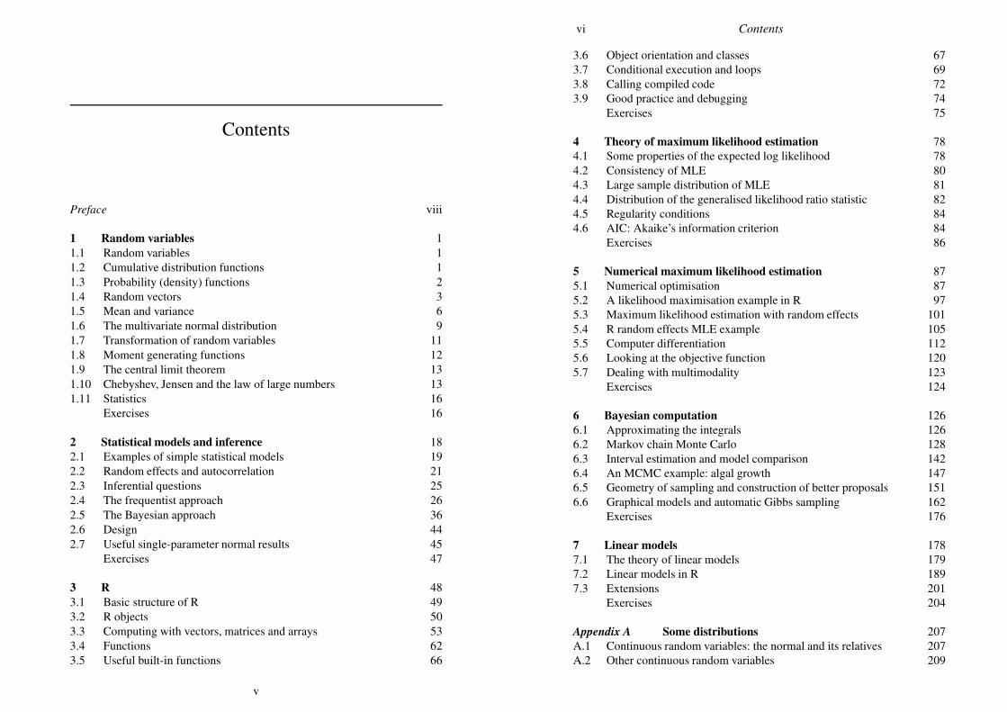
Figure 1.1 The example p.d.f (1.2). Left: over the region[−0.5, 1.5]× [−0.5, 1.5]. Right: the nonzero part of the p.d.f.
The following sections mostly consider continuous random variables,but except where noted, equivalent results also apply to discrete randomvariables upon replacement of integration by an appropriate summation.For conciseness the convention is adopted that p.d.f.s with different argu-ments usually denote different functions (e.g. f(y) and f(x) denote differ-ent p.d.f.s).
1.4 Random vectors
Little can usually be learned from single observations. Useful statisticalanalysis requires multiple observations and the ability to deal simultane-ously with multiple random variables. A multivariate version of the p.d.f.is required. The two-dimensional case suffices to illustrate most of the re-quired concepts, so consider random variables X and Y .
The joint probability density function of X and Y is the function f(x, y)such that, if Ω is any region in the x− y plane,
Pr(X,Y ) ∈ Ω =∫∫
Ω
f(x, y)dxdy. (1.1)
So f(x, y) is the probability per unit area of the x − y plane, at x, y. Ifω is a small region of area α, containing a point x, y, then Pr(X,Y ) ∈ω ≃ fxy(x, y)α. As with the univariate p.d.f. f(x, y) is non-negative andintegrates to one over R2.
4 Random variables
x
0.0
0.2
0.4
0.6
0.8
1.0
y
0.0
0.2
0.4
0.6
0.8
1.0
f(x,y
)
0.0
0.5
1.0
1.5
2.0
2.5
3.0
x
0.0
0.2
0.4
0.6
0.8
1.0
y
0.0
0.2
0.4
0.6
0.8
1.0
f(x,y
)
0.0
0.5
1.0
1.5
2.0
2.5
3.0
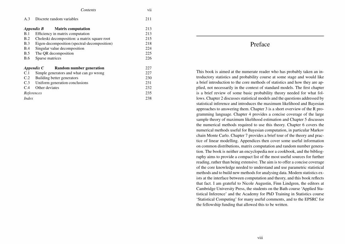
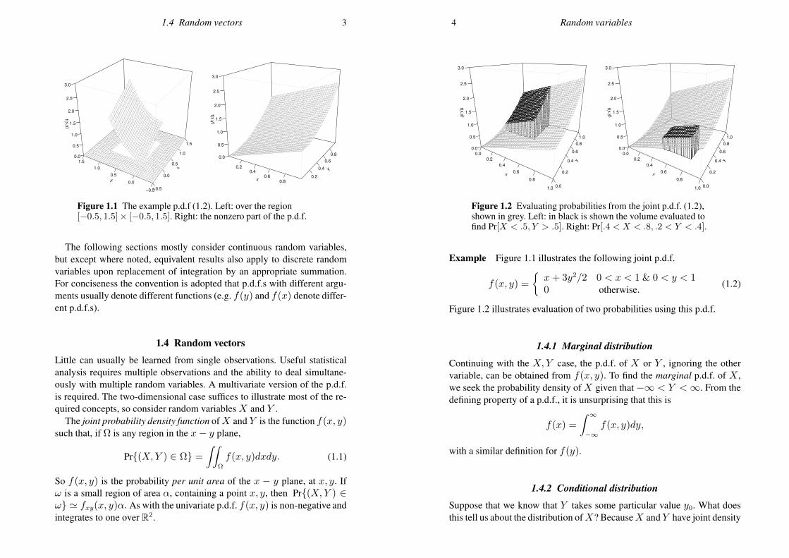
Figure 1.2 Evaluating probabilities from the joint p.d.f. (1.2),shown in grey. Left: in black is shown the volume evaluated tofind Pr[X < .5, Y > .5]. Right: Pr[.4 < X < .8, .2 < Y < .4].
Example Figure 1.1 illustrates the following joint p.d.f.
f(x, y) =
x+ 3y2/2 0 < x < 1 & 0 < y < 10 otherwise.
(1.2)
Figure 1.2 illustrates evaluation of two probabilities using this p.d.f.
1.4.1 Marginal distribution
Continuing with the X,Y case, the p.d.f. of X or Y , ignoring the othervariable, can be obtained from f(x, y). To find the marginal p.d.f. of X ,we seek the probability density of X given that−∞ < Y <∞. From thedefining property of a p.d.f., it is unsurprising that this is
f(x) =
∫ ∞
−∞f(x, y)dy,
with a similar definition for f(y).
1.4.2 Conditional distribution
Suppose that we know that Y takes some particular value y0. What doesthis tell us about the distribution of X? BecauseX andY have joint density
1.4 Random vectors 5
x
−0.5
0.0
0.5
1.0
1.5
y
−0.5
0.0
0.5
1.0
1.5
f(x,y
)
0.0
0.5
1.0
1.5
2.0
2.5
3.0
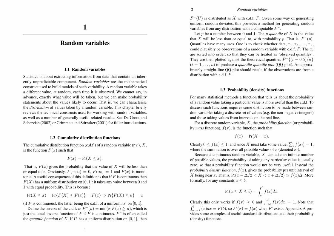
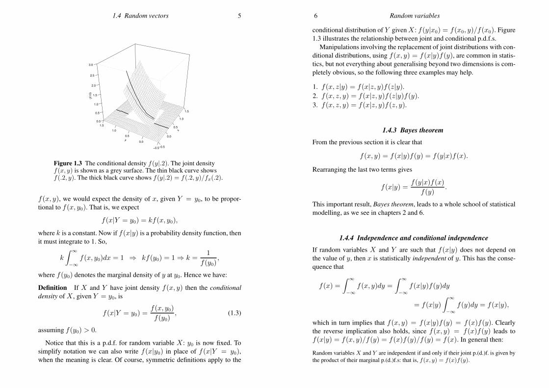
Figure 1.3 The conditional density f(y|.2). The joint densityf(x, y) is shown as a grey surface. The thin black curve showsf(.2, y). The thick black curve shows f(y|.2) = f(.2, y)/fx(.2).
f(x, y), we would expect the density of x, given Y = y0, to be propor-tional to f(x, y0). That is, we expect
f(x|Y = y0) = kf(x, y0),
where k is a constant. Now if f(x|y) is a probability density function, thenit must integrate to 1. So,
k
∫ ∞
−∞f(x, y0)dx = 1 ⇒ kf(y0) = 1⇒ k =
1
f(y0),
where f(y0) denotes the marginal density of y at y0. Hence we have:
Definition If X and Y have joint density f(x, y) then the conditionaldensity of X , given Y = y0, is
f(x|Y = y0) =f(x, y0)
f(y0), (1.3)
assuming f(y0) > 0.
Notice that this is a p.d.f. for random variable X: y0 is now fixed. Tosimplify notation we can also write f(x|y0) in place of f(x|Y = y0),when the meaning is clear. Of course, symmetric definitions apply to the
6 Random variables
conditional distribution of Y given X: f(y|x0) = f(x0, y)/f(x0). Figure1.3 illustrates the relationship between joint and conditional p.d.f.s.
Manipulations involving the replacement of joint distributions with con-ditional distributions, using f(x, y) = f(x|y)f(y), are common in statis-tics, but not everything about generalising beyond two dimensions is com-pletely obvious, so the following three examples may help.
1. f(x, z|y) = f(x|z, y)f(z|y).2. f(x, z, y) = f(x|z, y)f(z|y)f(y).3. f(x, z, y) = f(x|z, y)f(z, y).
1.4.3 Bayes theorem
From the previous section it is clear that
f(x, y) = f(x|y)f(y) = f(y|x)f(x).Rearranging the last two terms gives
f(x|y) = f(y|x)f(x)f(y)
.
This important result, Bayes theorem, leads to a whole school of statisticalmodelling, as we see in chapters 2 and 6.
1.4.4 Independence and conditional independence
If random variables X and Y are such that f(x|y) does not depend onthe value of y, then x is statistically independent of y. This has the conse-quence that
f(x) =
∫ ∞
−∞f(x, y)dy =
∫ ∞
−∞f(x|y)f(y)dy
= f(x|y)∫ ∞
−∞f(y)dy = f(x|y),
which in turn implies that f(x, y) = f(x|y)f(y) = f(x)f(y). Clearlythe reverse implication also holds, since f(x, y) = f(x)f(y) leads tof(x|y) = f(x, y)/f(y) = f(x)f(y)/f(y) = f(x). In general then:
Random variables X and Y are independent if and only if their joint p.(d.)f. is given bythe product of their marginal p.(d.)f.s: that is, f(x, y) = f(x)f(y).
1.5 Mean and variance 7
Modelling the elements of a random vector as independent usually sim-plifies statistical inference. Assuming independent identically distributed(i.i.d.) elements is even simpler, but much less widely applicable.
In many applications, a set of observations cannot be modelled as inde-pendent, but can be modelled as conditionally independent. Much of mod-ern statistical research is devoted to developing useful models that exploitvarious sorts of conditional independence in order to model dependent datain computationally feasible ways.
Consider a sequence of random variablesX1,X2, . . . Xn, and letX−i =(X1, . . . ,Xi−1,Xi+1, . . . ,Xn)
T. A simple form of conditional indepen-dence is the first order Markov property,
f(xi|x−i) = f(xi|xi−1).
That is, Xi−1 completely determines the distribution of Xi, so that givenXi−1, Xi is independent of the rest of the sequence. It follows that
f(x) = f(xn|x−n)f(x−n) = f(xn|xn−1)f(x−n)
= . . . =n∏
i=2
f(xi|xi−1)f(x1),
which can often be exploited to yield considerable computational savings.
1.5 Mean and variance
Although it is important to know how to characterise the distribution of arandom variable completely, for many purposes its first- and second-orderproperties suffice. In particular the mean or expected value of a randomvariable, X, with p.d.f. f(x), is defined as
E(X) =
∫ ∞
−∞xf(x)dx.
Since the integral is weighting each possible value of x by its relative fre-quency of occurrence, we can interpret E(X) as being the average of aninfinite sequence of observations of X .
The definition of expectation applies to any function g of X:
Eg(X) =∫ ∞
−∞g(x)f(x)dx.
Defining µ = E(X), then a particularly useful g is (X − µ)2, measuring
8 Random variables
the squared difference between X and its average value, which is used todefine the variance of X:
var(X) = E(X − µ)2.The variance of X measures how spread out the distribution of X is. Al-though computationally convenient, its interpretability is hampered by hav-ing units that are the square of the units of X . The standard deviation isthe square root of the variance, and hence is on the same scale as X .
1.5.1 Mean and variance of linear transformations
From the definition of expectation it follows immediately that if a and b arefinite real constants E(a + bX) = a + bE(X). The variance of a + bXrequires slightly more work:
var(a+ bX) = E(a+ bX − a− bµ)2= Eb2(X − µ)2 = b2E(X − µ)2 = b2var(X).
If X and Y are random variables then E(X + Y ) = E(X) + E(Y ).To see this suppose that they have joint density f(x, y); then,
E(X + Y ) =
∫(x+ y)f(x, y)dxdy
=
∫xf(x, y)dxdy +
∫yf(x, y)dxdy = E(X) + E(Y ).
This result assumes nothing about the distribution of X and Y . If wenow add the assumption that X and Y are independent then we find thatE(XY ) = E(X)E(Y ) as follows:
E(XY ) =
∫xyf(x, y)dxdy
=
∫xf(x)yf(y)dxdy (by independence)
=
∫xf(x)dx
∫yf(y)dy = E(X)E(Y ).
Note that the reverse implication only holds if the joint distribution of Xand Y is Gaussian.
Variances do not add as nicely as means (unless X and Y are indepen-dent), and we need the notion of covariance:
cov(X,Y ) = E(X − µx)(Y − µy) = E(XY )−E(X)E(Y ),
1.6 The multivariate normal distribution 9
where µx = E(X) and µy = E(Y ). Clearly var(X) ≡ cov(X,X),and if X and Y are independent cov(X,Y ) = 0 (since then E(XY ) =E(X)E(Y )).
Now let A and b be, respectively, a matrix and a vector of fixed finitecoefficients, with the same number of rows, and let X be a random vector.E(X) = µx = E(X1), E(X2), . . . , E(Xn)T and it is immediate thatE(AX + b) = AE(X) + b. A useful summary of the second-orderproperties of X requires both variances and covariances of its elements.These can be written in the (symmetric) variance-covariance matrix Σ,where Σij = cov(Xi,Xj), which means that
Σ = E(X − µx)(X− µx)T. (1.4)
A very useful result is that
ΣAX+b = AΣAT, (1.5)
which is easily proven:
ΣAX+b = E(AX + b−Aµx − b)(AX+ b−Aµx − b)T= E(AX −Aµx)(AX−Aµx)
T)
= AE(X − µx)(X− µx)TAT = AΣAT.
So if a is a vector of fixed real coefficients then var(aTX) = aTΣa ≥ 0:a covariance matrix is positive semi-definite.
1.6 The multivariate normal distribution
The normal or Gaussian distribution (see Section A.1.1) has a central placein statistics, largely as a result of the central limit theorem covered in Sec-tion 1.9. Its multivariate version is particularly useful.
Definition Consider a set of n i.i.d. standard normal random variables:Zi ∼
i.i.dN(0, 1). The covariance matrix for Z is In and E(Z) = 0. Let B
be an m× n matrix of fixed finite real coefficients and µ be an m- vectorof fixed finite real coefficients. The m-vector X = BZ+µ is said to havea multivariate normal distribution. E(X) = µ and the covariance matrixof X is just Σ = BBT. The short way of writing X’s distribution is
X ∼ N(µ,Σ).
In Section 1.7, basic transformation theory establishes that the p.d.f. for
10 Random variables
this distribution is
fx(x) =1√
(2π)m|Σ|e−
12 (x−µ)TΣ−1(x−µ) for x ∈ Rm, (1.6)
assumingΣ has full rank (if m = 1 the definition gives the usual univariatenormal p.d.f.). Actually there exists a more general definition in which Σ ismerely positive semi-definite, and hence potentially singular: this involvesa pseudoinverse of Σ.
An interesting property of the multivariate normal distribution is thatif X and Y have a multivariate normal distribution and zero covariance,then they must be independent. This implication only holds for the normal(independence implies zero covariance for any distribution).
1.6.1 A multivariate t distribution
If we replace the random variables Zi ∼i.i.d
N(0, 1) with random variables
Ti ∼i.i.d
tk (see Section A.1.3) in the definition of a multivariate normal, we
obtain a vector with a multivariate tk(µ,Σ) distribution. This can be use-ful in stochastic simulation, when we need a multivariate distribution withheavier tails than the multivariate normal. Note that the resulting univariatemarginal distributions are not t distributed. Multivariate t densities with tdistributed marginals are more complicated to characterise.
1.6.2 Linear transformations of normal random vectors
From the definition of multivariate normality, it immediately follows thatif X ∼ N(µ,Σ) and A is a matrix of finite real constants (of suitabledimensions), then
AX ∼ N(Aµ,AΣAT). (1.7)
This is because X = BZ + µ, so AX = ABZ +Aµ, and hence AXis exactly the sort of linear transformation of standard normal r.v.s thatdefines a multivariate normal random vector. Furthermore it is clear thatE(AX) = Aµ and the covariance matrix of AX is AΣAT.
A special case is that if a is a vector of finite real constants, then
aTX ∼ N(aTµ,aTΣa).
For the case in which a is a vector of zeros, except for aj , which is 1, (1.7)implies that
Xj ∼ N(µj ,Σjj) (1.8)
1.6 The multivariate normal distribution 11
(usually we would write σ2j for Σjj). In words:
If X has a multivariate normal distribution, then the marginal distribution of any Xj isunivariate normal.
More generally, the marginal distribution of any subvector of X is multi-variate normal, by a similar argument to that which led to (1.8).
The reverse implication does not hold. Marginal normality of the Xj
is not sufficient to imply that X has a multivariate normal distribution.However, if aTX has a normal distribution, for all (finite real) a, then Xmust have a multivariate normal distribution.
1.6.3 Multivariate normal conditional distributions
Suppose that Z and X are random vectors with a multivariate normal jointdistribution. Partitioning their joint covariance matrix
Σ =
[Σz Σzx
Σxz Σx
],
then
X|z ∼ N(µx +ΣxzΣ−1z (z− µz),Σx −ΣxzΣ
−1z Σzx).
Proof relies on a result for the inverse of a symmetric partitioned matrix:
[A CCT B
]−1
=
[A−1 +A−1CD−1CTA−1 −A−1CD−1
−D−1CTA−1 D−1
]
where D = B−CTA−1C (this can be checked easily, if tediously). Nowfind the conditional p.d.f. of X givenZ. Defining Q = Σx−ΣxzΣ
−1z Σzx,
z = z − µz, x = x− µx and noting that terms involving only z are partof the normalising constant,
f(x|z) = f(x, z)/f(z)
∝ exp
− 1
2
[zx
]T [Σ−1
z + Σ−1z ΣzxQ
−1ΣxzΣ−1z −Σ−1
z ΣzxQ−1
−Q−1ΣxzΣ−1z Q−1
] [zx
]
∝ exp−xTQ−1x/2 + xTQ−1ΣxzΣ
−1z z+ z terms
∝ exp−(x − ΣxzΣ
−1z z)TQ−1(x − ΣxzΣ
−1z z)/2 + z terms
,
which is recognisable as a N(µx+ΣxzΣ−1z (z−µz),Σx−ΣxzΣ
−1z Σzx)
p.d.f.
12 Random variables
1.7 Transformation of random variables
Consider a continuous random variable Z , with p.d.f. fz. Suppose X =g(Z) where g is an invertible function. The c.d.f of X is easily obtainedfrom that of Z:
Fx(x) = Pr(X ≤ x)
=
Prg−1(X) ≤ g−1(x) = PrZ ≤ g−1(x), g increasingPrg−1(X) > g−1(x) = PrZ > g−1(x), g decreasing
=
Fzg−1(x), g increasing1− Fzg−1(x), g decreasing
To obtain the p.d.f. we simply differentiate and, whether g is increasing ordecreasing, obtain
fx(x) = F ′x(x) = F ′
zg−1(x)∣∣∣∣dz
dx
∣∣∣∣ = fzg−1(x)∣∣∣∣dz
dx
∣∣∣∣ .
If g is a vector function and Z and X are vectors of the same dimension,then this last result generalises to
fx(x) = fzg−1(x) |J| ,
where Jij = ∂zi/∂xj (again a one-to-one mapping between x and z is as-sumed). Note that if fx and fz are probability functions for discrete randomvariables then no |J| term is needed.
Example Use the definition of a multivariate normal random vector toobtain its p.d.f. Let X = BZ+ µ, where B is an n× n invertible matrixandZ a vector of i.i.d. standard normal random variables. So the covariancematrix of X is Σ = BBT, Z = B−1(X − µ) and the Jacobian here is|J| = |B−1|. Since the Zi are i.i.d. their joint density is the product of theirmarginals, i.e.
f(z) =1√2π
n e−zTz/2.
Direct application of the preceding transformation theory then gives
f(x) =|B−1|√2π
n e−(x−µ)TB−TB−1(x−µ)/2
=1√
(2π)n|Σ|e−(x−µ)TΣ−1(x−µ)/2.
1.8 Moment generating functions 13
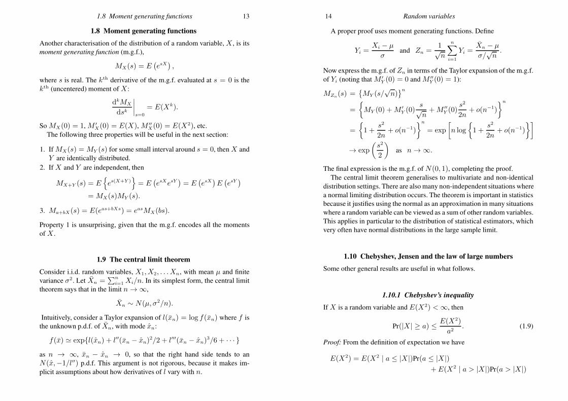
1.8 Moment generating functions
Another characterisation of the distribution of a random variable, X , is itsmoment generating function (m.g.f.),
MX(s) = E(esX),
where s is real. The kth derivative of the m.g.f. evaluated at s = 0 is thekth (uncentered) moment of X:
dkMX
dsk
∣∣∣∣s=0
= E(Xk).
So MX(0) = 1, M ′X(0) = E(X), M ′′
X(0) = E(X2), etc.The following three properties will be useful in the next section:
1. If MX(s) = MY (s) for some small interval around s = 0, then X andY are identically distributed.
2. If X and Y are independent, then
MX+Y (s) = Ees(X+Y )
= E
(esXesY
)= E
(esX)E(esY)
= MX(s)MY (s).
3. Ma+bX(s) = E(eas+bXs) = easMX(bs).
Property 1 is unsurprising, given that the m.g.f. encodes all the momentsof X .
1.9 The central limit theorem
Consider i.i.d. random variables, X1,X2, . . . Xn, with mean µ and finitevariance σ2. Let Xn =
∑ni=1 Xi/n. In its simplest form, the central limit
theorem says that in the limit n→∞,
Xn ∼ N(µ, σ2/n).
Intuitively, consider a Taylor expansion of l(xn) = log f(xn) where f isthe unknown p.d.f. of Xn, with mode xn:
f(x) ≃ expl(xn) + l′′(xn − xn)2/2 + l′′′(xn − xn)
3/6 + · · · as n → ∞, xn − xn → 0, so that the right hand side tends to anN(x,−1/l′′) p.d.f. This argument is not rigorous, because it makes im-plicit assumptions about how derivatives of l vary with n.
14 Random variables
A proper proof uses moment generating functions. Define
Yi =Xi − µ
σand Zn =
1√n
n∑
i=1
Yi =Xn − µ
σ/√n
.
Now express the m.g.f. of Zn in terms of the Taylor expansion of the m.g.f.of Yi (noting that M ′
Y (0) = 0 and M ′′Y (0) = 1):
MZn(s) =
MY (s/
√n)n
=
MY (0) +M ′
Y (0)s√n+M ′′
Y (0)s2
2n+ o(n−1)
n
=
1 +
s2
2n+ o(n−1)
n= exp
[n log
1 +
s2
2n+ o(n−1)
]
→ exp
(s2
2
)as n→∞.
The final expression is the m.g.f. of N(0, 1), completing the proof.The central limit theorem generalises to multivariate and non-identical
distribution settings. There are also many non-independent situations wherea normal limiting distribution occurs. The theorem is important in statisticsbecause it justifies using the normal as an approximation in many situationswhere a random variable can be viewed as a sum of other random variables.This applies in particular to the distribution of statistical estimators, whichvery often have normal distributions in the large sample limit.
1.10 Chebyshev, Jensen and the law of large numbers
Some other general results are useful in what follows.
1.10.1 Chebyshev’s inequality
If X is a random variable and E(X2) <∞, then
Pr(|X| ≥ a) ≤ E(X2)
a2. (1.9)
Proof: From the definition of expectation we have
E(X2) = E(X2 | a ≤ |X|)Pr(a ≤ |X|)+ E(X2 | a > |X|)Pr(a > |X|)
1.10 Chebyshev, Jensen and the law of large numbers 15
and because all the terms on the right hand side are non-negative it followsthat E(X2) ≥ E(X2 | a ≤ |X|)Pr(a ≤ |X|). However if a ≤ |X|, thenobviously a2 ≤ E(X2 | a ≤ |X|) so E(X2) ≥ a2Pr(|X| ≥ a) and (1.9)is proven.
1.10.2 The law of large numbers
Consider i.i.d. random variables, X1, . . . Xn, with mean µ, and E(|Xi|) <∞. If Xn =
∑ni=1 Xi/n then the strong law of large numbers states that,
for any positive ǫ
Pr(limn→∞
|Xn − µ| < ǫ)= 1
(i.e. Xn converges almost surely to µ).Adding the assumption var(Xi) = σ2 < ∞, it is easy to prove the
slightly weaker result
limn→∞
Pr(|Xn − µ| ≥ ǫ
)= 0,
which is the weak law of large numbers (Xn converges in probability toµ). A proof is as follows:
Pr(|Xn − µ| ≥ ǫ
)≤ E(Xn − µ)2
ǫ2=
var(Xn)
ǫ2=
σ2
nǫ2
and the final term tends to 0 as n → ∞. The inequality is Chebyshev’s.Note that the i.i.d. assumption has only been used to ensure that var(Xn) =σ2/n. All that we actually needed for the proof was the milder assumptionthat limn→∞ var(Xn) = 0.
To some extent the laws of large numbers are almost statements of theobvious. If they did not hold then random variables would not be of muchuse for building statistical models.
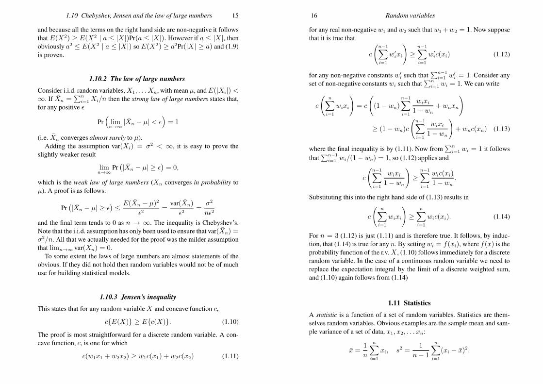
1.10.3 Jensen’s inequality
This states that for any random variable X and concave function c,
cE(X) ≥ Ec(X). (1.10)
The proof is most straightforward for a discrete random variable. A con-cave function, c, is one for which
c(w1x1 + w2x2) ≥ w1c(x1) + w2c(x2) (1.11)
16 Random variables
for any real non-negative w1 and w2 such that w1+w2 = 1. Now supposethat it is true that
c
(n−1∑
i=1
w′ixi
)≥
n−1∑
i=1
w′ic(xi) (1.12)
for any non-negative constants w′i such that
∑n−1i=1 w′
i = 1. Consider anyset of non-negative constants wi such that
∑ni=1 wi = 1. We can write
c
(n∑
i=1
wixi
)= c
((1−wn)
n−1∑
i=1
wixi1− wn
+ wnxn
)
≥ (1− wn)c
(n−1∑
i=1
wixi1− wn
)+ wnc(xn) (1.13)
where the final inequality is by (1.11). Now from∑n
i=1 wi = 1 it followsthat
∑n−1i=1 wi/(1− wn) = 1, so (1.12) applies and
c
(n−1∑
i=1
wixi1− wn
)≥
n−1∑
i=1
wic(xi)
1− wn.
Substituting this into the right hand side of (1.13) results in
c
(n∑
i=1
wixi
)≥
n∑
i=1
wic(xi). (1.14)
For n = 3 (1.12) is just (1.11) and is therefore true. It follows, by induc-tion, that (1.14) is true for any n. By setting wi = f(xi), where f(x) is theprobability function of the r.v. X , (1.10) follows immediately for a discreterandom variable. In the case of a continuous random variable we need toreplace the expectation integral by the limit of a discrete weighted sum,and (1.10) again follows from (1.14)
1.11 Statistics
A statistic is a function of a set of random variables. Statistics are them-selves random variables. Obvious examples are the sample mean and sam-ple variance of a set of data, x1, x2, . . . xn:
x =1
n
n∑
i=1
xi, s2 =1
n− 1
n∑
i=1
(xi − x)2.
Exercises 17
The fact that formal statistical procedures can be characterised as functionsof sets of random variables (data) accounts for the field’s name.
If a statistic t(x) (scalar or vector) is such that the p.d.f. of x can bewritten as
fθ(x) = h(x)gθt(x),where h does not depend on θ and g depends on x only through t(x),then t is a sufficient statistic for θ, meaning that all information about θcontained in x is provided by t(x). See Section 4.1 for a formal definitionof ‘information’. Sufficiency also means that the distribution of x givent(x) does not depend on θ.
Exercises1.1 Exponential random variable, X ≥ 0, has p.d.f. f(x) = λ exp(−λx).
1. Find the c.d.f. and the quantile function for X.2. Find Pr(X < λ) and the median of X.3. Find the mean and variance of X.
1.2 Evaluate Pr(X < 0.5, Y < 0.5) if X and Y have joint p.d.f. (1.2).1.3 Suppose that
Y ∼ N
([1
2
],
[2 1
1 2
]).
Find the conditional p.d.f. of Y1 given that Y1 + Y2 = 3.1.4 If Y ∼ N(µ, Iσ2) and Q is any orthogonal matrix of appropriate dimension,
find the distribution of QY. Comment on what is surprising about this result.1.5 If X and Y are independent random vectors of the same dimension, with
covariance matrices Vx and Vy , find the covariance matrix of X+Y.1.6 Let X and Y be non-independent random variables, such that var(X) = σ2
x,var(Y ) = σ2
y and cov(X,Y ) = σ2xy . Using the result from Section 1.6.2,
find var(X + Y ) and var(X − Y ).1.7 Let Y1, Y2 and Y3 be independent N(µ, σ2) r.v.s. Somehow using the matrix
1/3 1/3 1/3
2/3 −1/3 −1/3
−1/3 2/3 −1/3
show that Y =∑3i=1 Yi/3 and
∑3i=1(Yi − Y )2 are independent random
variables.1.8 If log(X) ∼ N(µ, σ2), find the p.d.f. of X.1.9 Discrete random variable Y has a Poisson distribution with parameter λ if
its p.d.f. is f(y) = λye−λ/y!, for y = 0, 1, . . .
18 Random variables
a. Find the moment generating function for Y (hint: the power series repre-sentation of the exponential function is useful).
b. If Y1 ∼ Poi(λ1) and independently Y2 ∼ Poi(λ2), deduce the distribu-tion of Y1 + Y2, by employing a general property of m.g.f.s.
c. Making use of the previous result and the central limit theorem, deducethe normal approximation to the Poisson distribution.
d. Confirm the previous result graphically, using R functions dpois, dnorm,plot or barplot and lines. Confirm that the approximation improveswith increasing λ.
2
Statistical models and inference
Statistics aims to extract information from data: specifically, informationabout the system that generated the data. There are two difficulties withthis enterprise. First, it may not be easy to infer what we want to knowfrom the data that can be obtained. Second, most data contain a componentof random variability: if we were to replicate the data-gathering processseveral times we would obtain somewhat different data on each occasion.In the face of such variability, how do we ensure that the conclusions drawn
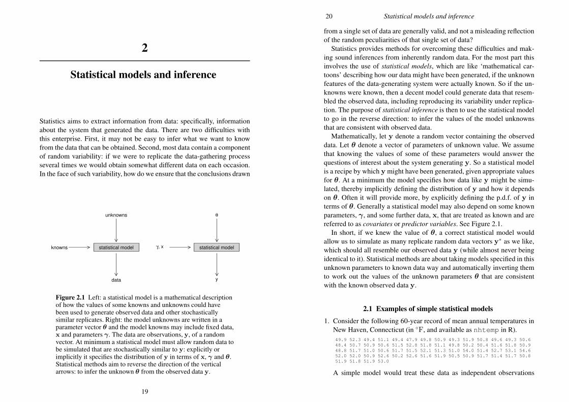
statistical modelknowns
unknowns
data
statistical modelγ, x
θ
y
Figure 2.1 Left: a statistical model is a mathematical descriptionof how the values of some knowns and unknowns could havebeen used to generate observed data and other stochasticallysimilar replicates. Right: the model unknowns are written in aparameter vector θ and the model knowns may include fixed data,x and parameters γ. The data are observations, y, of a randomvector. At minimum a statistical model must allow random data tobe simulated that are stochastically similar to y: explicitly orimplicitly it specifies the distribution of y in terms of x, γ and θ.Statistical methods aim to reverse the direction of the verticalarrows: to infer the unknown θ from the observed data y.
19
20 Statistical models and inference
from a single set of data are generally valid, and not a misleading reflectionof the random peculiarities of that single set of data?
Statistics provides methods for overcoming these difficulties and mak-ing sound inferences from inherently random data. For the most part thisinvolves the use of statistical models, which are like ‘mathematical car-toons’ describing how our data might have been generated, if the unknownfeatures of the data-generating system were actually known. So if the un-knowns were known, then a decent model could generate data that resem-bled the observed data, including reproducing its variability under replica-tion. The purpose of statistical inference is then to use the statistical modelto go in the reverse direction: to infer the values of the model unknownsthat are consistent with observed data.
Mathematically, let y denote a random vector containing the observeddata. Let θ denote a vector of parameters of unknown value. We assumethat knowing the values of some of these parameters would answer thequestions of interest about the system generating y. So a statistical modelis a recipe by which y might have been generated, given appropriate valuesfor θ. At a minimum the model specifies how data like y might be simu-lated, thereby implicitly defining the distribution of y and how it dependson θ. Often it will provide more, by explicitly defining the p.d.f. of y interms of θ. Generally a statistical model may also depend on some knownparameters, γ, and some further data, x, that are treated as known and arereferred to as covariates or predictor variables. See Figure 2.1.
In short, if we knew the value of θ, a correct statistical model wouldallow us to simulate as many replicate random data vectors y∗ as we like,which should all resemble our observed data y (while almost never beingidentical to it). Statistical methods are about taking models specified in thisunknown parameters to known data way and automatically inverting themto work out the values of the unknown parameters θ that are consistentwith the known observed data y.
2.1 Examples of simple statistical models
1. Consider the following 60-year record of mean annual temperatures inNew Haven, Connecticut (in F, and available as nhtemp in R).49.9 52.3 49.4 51.1 49.4 47.9 49.8 50.9 49.3 51.9 50.8 49.6 49.3 50.648.4 50.7 50.9 50.6 51.5 52.8 51.8 51.1 49.8 50.2 50.4 51.6 51.8 50.948.8 51.7 51.0 50.6 51.7 51.5 52.1 51.3 51.0 54.0 51.4 52.7 53.1 54.652.0 52.0 50.9 52.6 50.2 52.6 51.6 51.9 50.5 50.9 51.7 51.4 51.7 50.851.9 51.8 51.9 53.0
A simple model would treat these data as independent observations
2.1 Examples of simple statistical models 21
from an N(µ, σ2) distribution, where µ and σ2 are unknown param-eters (see Section A.1.1). Then the p.d.f. for the random variable corre-sponding to a single measurement, yi, is
f(yi) =1√2πσ
e−(yi−µ)2
2σ2 .
The joint p.d.f. for the vector y is the product of the p.d.f.s for theindividual random variables, because the model specifies independenceof the yi, i.e.
f(y) =60∏
i=1
f(yi).
2. The New Haven temperature data seem to be ‘heavy tailed’ relative toa normal: that is, there are more extreme values than are implied by anormal with the observed standard deviation. A better model might be
yi − µ
σ∼ tα,
where µ, σ and α are unknown parameters. Denoting the p.d.f. of a tαdistribution as ftα , the transformation theory of Section 1.7, combinedwith independence of the yi, implies that the p.d.f. of y is
f(y) =60∏
i=1
1
σftα(yi − µ)/σ.
3. Air temperature, ai, is measured at times ti (in hours) spaced half anhour apart for a week. The temperature is believed to follow a dailycycle, with a long-term drift over the course of the week, and to besubject to random autocorrelated departures from this overall pattern.A suitable model might then be
ai = θ0 + θ1ti + θ2 sin(2πti/24) + θ3 cos(2πti/24) + ei,
where ei = ρei−1 + ǫi and the ǫi are i.i.d. N(0, σ2). This model im-plicitly defines the p.d.f. of a, but as specified we have to do a littlework to actually find it. Writing µi = θ0 + θ1ti + θ2 sin(2πti/24) +θ3 cos(2πti/24), we have ai = µi + ei. Because ei is a weightedsum of zero mean normal random variables, it is itself a zero meannormal random variable, with covariance matrix Σ such that Σi,j =ρ|i−j|σ2/(1− ρ2). So the p.d.f. of a,1 the vector of temperatures, must
1 For aesthetic reasons I will use phrases such as ‘the p.d.f. of y’ to mean ‘the p.d.f. of therandom vector of which y is an observation’.
22 Statistical models and inference
be multivariate normal,
fa(a) =1√
(2π)n|Σ|e−
12 (a−µ)TΣ−1(a−µ),
whereΣ depends on parameter ρ and σ, whileµ depends on parametersθ and covariate t (see also Section 1.6).
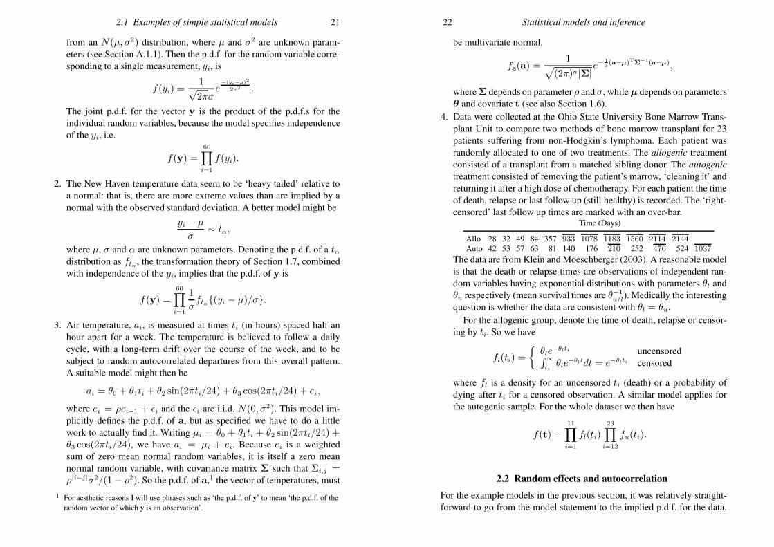
4. Data were collected at the Ohio State University Bone Marrow Trans-plant Unit to compare two methods of bone marrow transplant for 23patients suffering from non-Hodgkin’s lymphoma. Each patient wasrandomly allocated to one of two treatments. The allogenic treatmentconsisted of a transplant from a matched sibling donor. The autogenictreatment consisted of removing the patient’s marrow, ‘cleaning it’ andreturning it after a high dose of chemotherapy. For each patient the timeof death, relapse or last follow up (still healthy) is recorded. The ‘right-censored’ last follow up times are marked with an over-bar.
Time (Days)
Allo 28 32 49 84 357 933 1078 1183 1560 2114 2144Auto 42 53 57 63 81 140 176 210 252 476 524 1037
The data are from Klein and Moeschberger (2003). A reasonable modelis that the death or relapse times are observations of independent ran-dom variables having exponential distributions with parameters θl andθu respectively (mean survival times are θ−1
u/l). Medically the interestingquestion is whether the data are consistent with θl = θu.
For the allogenic group, denote the time of death, relapse or censor-ing by ti. So we have
fl(ti) =
θle
−θlti uncensored∫∞ti
θle−θltdt = e−θlti censored
where fl is a density for an uncensored ti (death) or a probability ofdying after ti for a censored observation. A similar model applies forthe autogenic sample. For the whole dataset we then have
f(t) =11∏
i=1
fl(ti)23∏
i=12
fu(ti).
2.2 Random effects and autocorrelation
For the example models in the previous section, it was relatively straight-forward to go from the model statement to the implied p.d.f. for the data.
2.2 Random effects and autocorrelation 23
Often, this was because we could model the data as observations of in-dependent random variables with known and tractable distributions. Notall datasets are so amenable, however, and we commonly require morecomplicated descriptions of the stochastic structure in the data. Often werequire models with multiple levels of randomness. Such multilayered ran-domness implies autocorrelation in the data, but we may also need to in-troduce autocorrelation more directly, as in Example 3 in Section 2.1.
Random variables in a model that are not associated with the indepen-dent random variability of single observations,2 are termed random effects.The idea is best understood via concrete examples:
1. A trial to investigate a new blood-pressure reducing drug assigns malepatients at random to receive the new drug or one of two alternativestandard treatments. Patients’ age, aj , and fat mass, fj , are recordedat enrolment, and their blood pressure reduction is measured at weeklyintervals for 12 weeks. In this setup it is clear that there are two sourcesof random variability that must be accounted for: the random variabilityfrom patient to patient, and the random variability from measurement tomeasurement made on a single patient. Let yij represent the ith blood-pressure reduction measurement on the jth patient. A suitable modelmight then be
yij = γk(j)+β1aj+β2fj+bj+ǫij, bj ∼ N(0, σ2b ), ǫij ∼ N(0, σ2),
(2.1)where k(j) = 1, 2 or 3 denotes the treatment to which patient j hasbeen assigned. The γk, βs and σs are unknown model parameters. Therandom variables bj and ǫij are all assumed to be independent here.
The key point is that we decompose the randomness in yij into twocomponents: (i) the patient specific component, bj , which varies ran-domly from patient to patient but remains fixed between measurementson the same patient, and (ii) the individual measurement variability, ǫij ,which varies between all measurements. Hence measurements takenfrom different patients of the same age, fat mass and treatment will usu-ally differ more than measurements taken on the same patient. So theyij are not statistically independent in this model, unless we conditionon the bj .
On first encountering such models it is natural to ask why we donot simply treat the bj as fixed parameters, in which case we would beback in the convenient world of independent measurements. The rea-
2 and, in a Bayesian context, are not parameters.
24 Statistical models and inference
son is interpretability. As stated, (2.1) treats patients as being randomlysampled from a wide population of patients: the patient-specific effectsare simply random draws from some normal distribution describing thedistribution of patient effects over the patient population. In this setupthere is no problem using statistics to make inferences about the pop-ulation of patients in general, on the basis of the sample of patients inthe trial. Now suppose we treat the bj as parameters. This is equivalentto saying that the patient effects are entirely unpredictable from patientto patient — there is no structure to them at all and they could take anyvalue whatsoever. This is a rather extreme position to hold and impliesthat we can say nothing about the blood pressure of a patient who is notin the trial, because their bj value could be anything at all. Another sideof this problem is that we lose all ability to say anything meaningfulabout the treatment effects, γk, since we have different patients in thedifferent treatment arms, so that the fixed bj are completely confoundedwith the γk (as can be seen by noting that any constant could be added toa γk, while simultaneously being subtracted from all the bj for patientsin group k, without changing the model distribution of any yij).
2. A population of cells in an experimental chemostat is believed to growaccording to the model
Nt+1 = rNt exp(−αNt + bt), bt ∼ N(0, σ2b ),
where Nt is the population at day t; r, α, σb and N0 are parameters;and the bt are independent random effects. A random sample of 0.5%of the cells in the chemostat is counted every 2 days, giving rise toobservations yt, which can be modelled as independent Poi(0.005Nt).In this case the random effects enter the model nonlinearly, introducinga complicated correlation structure into Nt, and hence also the yt.
The first example is an example of a linear mixed model.3 In this case itis not difficult to obtain the p.d.f. for the vector y. We can write the modelin matrix vector form as
y = Xβ + Zb+ ǫ, b ∼ N(0, Iσ2b ), ǫ ∼ N(0, Iσ2), (2.2)
where βT = (γ1, γ2, γ3, β1, β2). The first three columns of X contain0, 1 indicator variables depending on which treatment the row relates to,
3 It is a mixed model because it contains both fixed effects (the γ and β terms in theexample) and random effects. Mixed models should not be confused with mixturemodels in which each observation is modelled as having some probability of beingdrawn from each of a number of alternative distributions.
2.2 Random effects and autocorrelation 25
and the next two columns contain the age and fat mass for the patients. Zhas one column for each subject, each row of which contains a 1 or a 0depending on whether the observation at this data row relates to the subjector not. Given this structure it follows (see Section 1.6.2) that the covariancematrix fory is Σ = Iσ2+ZZTσ2
b and the expected value of y isµ = Xβ,so that y ∼ N(µ,Σ), with p.d.f. as in (1.6). So in this case the p.d.f. for yis quite easy to write down. However, computing with it can become verycostly if the dimension of y is beyond the low thousands. Hence the mainchallenge with these models is to find ways of exploiting the sparsity thatresults from having so many 0 entries in Z, so that computation is feasiblefor large samples.
The second example illustrates the more usual situation in which themodel fully specifies a p.d.f. (or p.f.) for y, but it is not possible to writeit down in closed form, or even to evaluate it exactly. In contrast, the jointdensity of the random effects, b, and data, y, is always straightforward toevaluate. From Sections 1.4.2 and 1.4.3 we have that
f(y,b) = f(y|b)f(b),and the distributions f(y|b) and f(b) are usually straightforward to workwith. So, for the second example, let f(y;λ) denote the p.f. of a Poissonrandom variable with mean λ (see Section A.3.2). Then
f(y|b) =∏
t
f(yt;Nt/200),
while f(b) is the density of a vector of i.i.d. N(0, σ2b ) deviates.
For some statistical tasks we may be able to work directly with f(y,b)without needing to evaluate the p.d.f. of y: this typically applies when tak-ing the Bayesian approach of Section 2.5, for example. However, often wecannot escape the need to evaluate f(y) itself. That is, we need
f(y) =
∫f(y,b)db,
which is generally not analytically tractable. We then have a number ofchoices. If the model has a structure that allows the integral to be bro-ken down into a product of low-dimensional integrals then numerical in-tegration methods (so-called quadrature) may be feasible; however, thesemethods are usually impractical beyond somewhere around 10 dimensions.Then we need a different approach: either estimate the integral statisticallyusing stochastic simulation or approximate it somehow (see Section 5.3.1).
26 Statistical models and inference
2.3 Inferential questions
Given some data, y, and a statistical model with parameters θ, there arefour basic questions to ask:
1. What values for θ are most consistent with y?
2. Is some prespecified restriction on θ consistent with y?
3. What ranges of values of θ are consistent with y?
4. Is the model consistent with the data for any values of θ at all?
The answers to these questions are provided by point estimation, hypoth-esis testing, interval estimation and model checking, respectively. Ques-tion 2 can be somewhat generalised to: which of several alternative mod-els is most consistent with y? This is the question of model selection(which partly incorporates question 4). Central to the statistical way of do-ing things is recognising the uncertainty inherent in trying to learn about θfrom y. This leads to another, often neglected, question that applies whenthere is some control over the data-gathering process:
5. How might the data-gathering process be organized to produce data thatenables answers to the preceding questions to be as accurate and preciseas possible?
This question is answered by experimental and survey design methods.There are two main classes of methods for answering questions 1-4,
and they start from different basic assumptions. These are the Bayesianand frequentist approaches, which differ in how they use probability tomodel uncertainty about model parameters. In the frequentist approach,parameters are treated as having values that are fixed states of nature, aboutwhich we want to learn using data. There is randomness in our estimationof the parameters, but not in the parameters themselves. In the Bayesianapproach parameters are treated as random variables, about which we wantto update our beliefs in the light of data: our beliefs are summarised byprobability distributions for the parameters. The difference between theapproaches can sound huge, and there has been much debate about whichis least ugly. From a practical perspective, however, the approaches havemuch in common, except perhaps when it comes to model selection. Inparticular, if properly applied they usually produce results that differ byless than the analysed models are likely to differ from reality.
2.4 The frequentist approach 27
2.4 The frequentist approach
In this way of doing things we view parameters, θ, as fixed states of nature,about which we want to learn. We use probability to investigate what wouldhappen under repeated replication of the data (and consequent statisticalanalysis). In this approach probability is all about how frequently eventswould occur under this imaginary replication process.
2.4.1 Point estimation: maximum likelihood
Given a model and some data, then with enough thought about what theunknown model parameters mean, it is often possible to come up with away of getting reasonable parameter value guesses from the data. If thisprocess can be written down as a mathematical recipe, then we can call theguess an estimate, and we can study its properties under data replicationto get an idea of its uncertainty. But such model-by-model reasoning istime consuming and somewhat unsatisfactory: how do we know that ourestimation process is making good use of the data, for example? A generalapproach for dealing with all models would be appealing.
There are a number of more or less general approaches, such as themethod of moments and least squares methods, which apply to quite wideclasses of models, but one general approach stands out in terms of practicalutility and nice theoretical properties: maximum likelihood estimation. Thekey idea is simply this:
Parameter values that make the observed data appear relatively probable are more likelyto be correct than parameter values that make the observed data appear relatively im-probable.
For example, we would much prefer an estimate of θ that assigned a prob-ability density of 0.1 to our observed y, according to the model, to anestimate for which the density was 0.00001.
So the idea is to judge the likelihood of parameter values using fθ(y),the model p.d.f. according to the given value of θ, evaluated at the ob-served data. Because y is now fixed and we are considering the likelihoodas a function of θ, it is usual to write the likelihood as L(θ) ≡ fθ(y). Infact, for theoretical and practical purposes it is usual to work with the loglikelihood l(θ) = logL(θ). The maximum likelihood estimate (MLE) ofθ is then
θ = argmaxθ
l(θ).
28 Statistical models and inference
There is more to maximum likelihood estimation than just its intuitive ap-peal. To see this we need to consider what might make a good estimate, andto do that we need to consider repeated estimation under repeated replica-tion of the data-generating process.
Replicating the random data and repeating the estimation process resultsin a different value of θ for each replicate. These values are of course ob-servations of a random vector, the estimator or θ, which is usually alsodenoted θ (the context making clear whether estimate or estimator is beingreferred to). Two theoretical properties are desirable:
1. E(θ) = θ or at least |E(θ) − θ| should be small (i.e. the estimatorshould be unbiased, or have small bias).
2. var(θ) should be small (i.e. the estimator should have low variance).
Unbiasedness basically says that the estimator gets it right on average: along-run average of the θ, over many replicates of the data set, would tendtowards the true value of the parameter vector. Low variance implies thatany individual estimate is quite precise. There is a tradeoff between thetwo properties, so it is usual to seek both. For example, we can alwaysdrive variance to zero if we do not care about bias, by just eliminating thedata from the estimation process and picking a constant for the estimate.Similarly it is easy to come up with all sorts of unbiased estimators thathave enormous variance. Given the tradeoff, you might reasonably wonderwhy we do not concern ourselves with some direct measure of estimationerror such as E(θ−θ)2, the mean square error (MSE). The reason is thatit is difficult to prove general results about minimum MSE estimators, sowe are stuck with the second-best option of considering minimum varianceunbiased estimators.4
It is possible to derive a lower limit on the variance that any unbiased es-timator can achieve: the Cramér-Rao lower bound. Under some regularityconditions, and in the large sample limit, it turns out that maximum like-lihood estimation is unbiased and achieves the Cramér-Rao lower bound,which gives some support for its use (see Sections 4.1 and 4.3). In addition,under the same conditions,
θ ∼ N(θ,I−1), (2.3)
4 Unless the gods have condemned you to repeat the same experiment for all eternity,unbiasedness, although theoretically expedient, should not be of much intrinsic interest:an estimate close to the truth for the data at hand should always be preferable to one thatwould merely get things right on average over an infinite sequence of data replicates.
2.4 The frequentist approach 29
where Iij = −E(∂2l/∂θi∂θj) (and actually the same result holds substi-tuting Iij = −∂2l/∂θi∂θj for Iij).
2.4.2 Hypothesis testing and p-values
Now consider the question of whether some defined restriction on θ isconsistent with y?
p-values: the fundamental ideaSuppose that we have a model defining a p.d.f., fθ(y), for data vector yand that we want to test the null hypothesis, H0 : θ = θ0, where θ0is some specified value. That is, we want to establish whether the datacould reasonably be generated from fθ0(y). An obvious approach is to askhow probable data like y are under H0. It is tempting to simply evaluatefθ0(y) for the observed y, but then deciding what counts as ‘probable’ and‘improbable’ is difficult to do in a generally applicable way.
A better approach is to assess the probability, p0 say, of obtaining dataat least as improbable as y under H0 (better read that sentence twice). Forexample, if only one dataset in a million would be as improbable as y,according to H0, then assuming we believe our data, we ought to seriouslydoubt H0. Conversely, if half of all datasets would be expected to be at leastas improbable as y, according to H0, then there is no reason to doubt it.
A quantity like p0 makes good sense in the context of goodness offit testing, where we simply want to assess the plausibility of fθ0 as amodel without viewing it as being a restricted form of a larger model.But when we are really testing H0 : θ = θ0 against the alternative H1 :‘θ unrestricted’ then p0 is not satisfactory, because it makes no distinctionbetween y being improbable under H0 but probable under H1, and y beingimprobable under both.
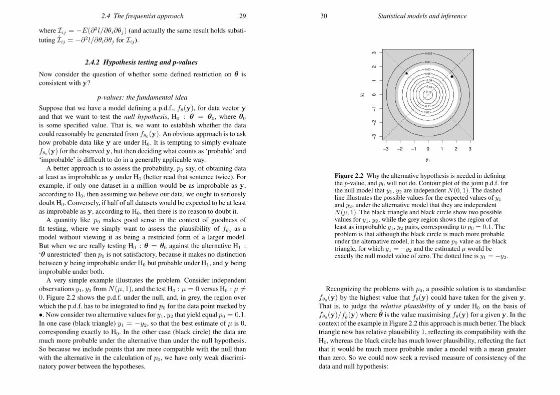
A very simple example illustrates the problem. Consider independentobservations y1, y2 from N(µ, 1), and the test H0 : µ = 0 versus H0 : µ 6=0. Figure 2.2 shows the p.d.f. under the null, and, in grey, the region overwhich the p.d.f. has to be integrated to find p0 for the data point marked by•. Now consider two alternative values for y1, y2 that yield equal p0 = 0.1.In one case (black triangle) y1 = −y2, so that the best estimate of µ is 0,corresponding exactly to H0. In the other case (black circle) the data aremuch more probable under the alternative than under the null hypothesis.So because we include points that are more compatible with the null thanwith the alternative in the calculation of p0, we have only weak discrimi-natory power between the hypotheses.
30 Statistical models and inference
−3 −2 −1 0 1 2 3
−3
−2
−1
01
23
y1
y2
0.002
0.01
0.03
0.05
0.07
0.09
0.11
0.13
0.15
Figure 2.2 Why the alternative hypothesis is needed in definingthe p-value, and p0 will not do. Contour plot of the joint p.d.f. forthe null model that y1, y2 are independent N(0, 1). The dashedline illustrates the possible values for the expected values of y1and y2, under the alternative model that they are independentN(µ, 1). The black triangle and black circle show two possiblevalues for y1, y2, while the grey region shows the region of atleast as improbable y1, y2 pairs, corresponding to p0 = 0.1. Theproblem is that although the black circle is much more probableunder the alternative model, it has the same p0 value as the blacktriangle, for which y1 = −y2 and the estimated µ would beexactly the null model value of zero. The dotted line is y1 = −y2.
Recognizing the problems with p0, a possible solution is to standardisefθ0(y) by the highest value that fθ(y) could have taken for the given y.That is, to judge the relative plausibility of y under H0 on the basis offθ0(y)/fθ(y) where θ is the value maximising fθ(y) for a given y. In thecontext of the example in Figure 2.2 this approach is much better. The blacktriangle now has relative plausibility 1, reflecting its compatibility with theH0, whereas the black circle has much lower plausibility, reflecting the factthat it would be much more probable under a model with a mean greaterthan zero. So we could now seek a revised measure of consistency of thedata and null hypothesis:
2.4 The frequentist approach 31
p is the probability, under the null hypothesis, of obtaining data at least as relativelyimplausible as that observed.
Actually the reciprocal of this relative plausibility is generally known asthe likelihood ratio fθ(y)/fθ0(y) of the two hypotheses, because it is ameasure of how likely the alternative hypothesis is relative to the null, giventhe data. So we have the more usual equivalent definition:
p is the probability, under the null hypothesis, of obtaining a likelihood ratio at least aslarge as that observed.
p is generally referred to as the p-value associated with a test. If the nullhypothesis is true, then from its definition, the p-value should have a uni-form distribution on [0, 1] (assuming its distribution is continuous). Byconvention p-values in the ranges 0.1 ≥ p > 0.05, 0.05 ≥ p > 0.01,0.01 ≥ p > 0.001 and p ≤ 0.001 are sometimes described as providing,respectively, ‘marginal evidence’, ‘evidence’, ‘strong evidence’ and ‘verystrong evidence’ against the null model, although the interpretation shouldreally be sensitive to the context.
GeneralisationsFor the purposes of motivating p-values, the previous subsection consid-ered only the case where the null hypothesis is a simple hypothesis, speci-fying a value for every parameter of f , while the alternative is a compositehypothesis, in which a range of parameter values are consistent with thealternative. Unsurprisingly, there are many situations in which we are in-terested in comparing two composite hypotheses, so that H0 specifies somerestrictions of θ, without fully constraining it to one point. Less commonly,we may also wish to compare two simple hypotheses, so that the alternativealso supplies one value for each element of θ. This latter case is of theo-retical interest, but because the hypotheses are not nested it is somewhatconceptually different from most cases of interest.
All test variants can be dealt with by a slight generalisation of the like-lihood ratio statistic to fθ(y)/fθ0(y) where fθ0(y) now denotes the max-imum possible value for the density of y under the null hypothesis. If thenull hypothesis is simple, then this is just fθ0(y), as before, but if not thenit is obtained by finding the parameter vector that maximises fθ(y) subjectto the restrictions on θ imposed by H0.
In some cases the p-value can be calculated exactly from its definition,and the relevant likelihood ratio. When this is not possible, there is a largesample result that applies in the usual case of a composite alternative witha simple or composite null hypothesis. In general we test H0 : R(θ) = 0
32 Statistical models and inference
against H1 : ‘θ unrestricted’, where R is a vector-valued function of θ,specifying r restrictions on θ. Given some regularity conditions and in thelarge sample limit,
2log fθ(y) − log fθ0(y) ∼ χ2r, (2.4)
under H0. See Section 4.4.fθ(y)/fθ0(y) is an example of a test statistic, which takes low values
when the H0 is true, and higher values when H1 is true. Other test statisticscan be devised in which case the definition of the p-value generalises to:
p is the probability of obtaining a test statistic at least as favourable to H1 as that ob-served, if H0 is true.
This generalisation immediately raises the question: what makes a goodtest statistic? The answer is that we would like the resulting p-values to beas small as possible when the null hypothesis is not true (for a test statisticwith a continuous distribution, the p-values should have a U(0, 1) distribu-tion when the null is true). That is, we would like the test statistic to havehigh power to discriminate between null and alternative hypotheses.
The Neyman-Pearson lemmaThe Neyman-Pearson lemma provides some support for using the likeli-hood ratio as a test statistic, in that it shows that doing so provides thebest chance of rejecting a false null hypothesis, albeit in the restricted con-text of a simple null versus a simple alternative. Formally, consider testingH0 : θ = θ0 against H1 : θ = θ1. Suppose that we decide to rejectH0 if the p-value is less than or equal to some value α. Let β(θ) be theprobability of rejection if the true parameter value is θ — the test’s power.
In this accept/reject setup the likelihood ratio test rejects H0 if y ∈ R =y : fθ1(y)/fθ0(y) > k and k is such that Prθ0(y ∈ R) = α. It isuseful to define the function φ(y) = 1 if y ∈ R and 0 otherwise. Thenβ(θ) =
∫φ(y)fθ(y)dy. Note that β(θ0) = α.
Now consider using an alternative test statistic and again rejecting if thep-value is ≤ α. Suppose that the test procedure rejects if
y ∈ R∗ where Prθ0(y ∈ R∗) ≤ α.
Let φ∗(y) and β∗(θ) be the equivalent of φ(y) and β(θ) for this test. Hereβ∗(θ0) = Prθ0(y ∈ R∗) ≤ α.
The Neyman-Pearson Lemma then states that β(θ1) ≥ β∗(θ1) (i.e. thelikelihood ratio test is the most powerful test possible).
2.4 The frequentist approach 33
Proof follows from the fact that
φ(y) − φ∗(y)fθ1(y)− kfθ0(y) ≥ 0,
since from the definition of R, the first bracket is non-negative wheneverthe second bracket is non-negative, and it is non-positive whenever the sec-ond bracket is negative. In consequence,
0 ≤∫φ(y) − φ∗(y)fθ1(y)− kfθ0(y)dy
= β(θ1)− β∗(θ1)− kβ(θ0)− β∗(θ0) ≤ β(θ1)− β∗(θ1),
since β(θ0) − β∗(θ0) ≥ 0. So the result is proven. Casella and Berger(1990) give a fuller version of the lemma, on which this proof is based.
2.4.3 Interval estimation
Recall the question of finding the range of values for the parameters thatare consistent with the data. An obvious answer is provided by the rangeof values for any parameter θi that would have been accepted in a hypoth-esis test. For example, we could look for all values of θi that would haveresulted in a p-value of more than 5% if used as a null hypothesis for theparameter. Such a set is known as a 95% confidence set for θi. If the set iscontinuous then its endpoints define a 95% confidence interval.
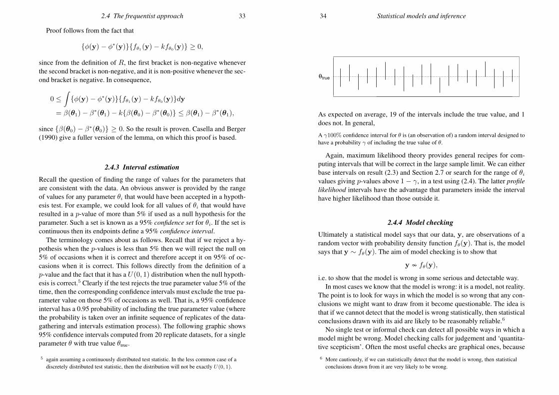
The terminology comes about as follows. Recall that if we reject a hy-pothesis when the p-values is less than 5% then we will reject the null on5% of occasions when it is correct and therefore accept it on 95% of oc-casions when it is correct. This follows directly from the definition of ap-value and the fact that it has a U(0, 1) distribution when the null hypoth-esis is correct.5 Clearly if the test rejects the true parameter value 5% of thetime, then the corresponding confidence intervals must exclude the true pa-rameter value on those 5% of occasions as well. That is, a 95% confidenceinterval has a 0.95 probability of including the true parameter value (wherethe probability is taken over an infinite sequence of replicates of the data-gathering and intervals estimation process). The following graphic shows95% confidence intervals computed from 20 replicate datasets, for a singleparameter θ with true value θtrue.
5 again assuming a continuously distributed test statistic. In the less common case of adiscretely distributed test statistic, then the distribution will not be exactly U(0, 1).
34 Statistical models and inference
θtrue
As expected on average, 19 of the intervals include the true value, and 1does not. In general,
A γ100% confidence interval for θ is (an observation of) a random interval designed tohave a probability γ of including the true value of θ.
Again, maximum likelihood theory provides general recipes for com-puting intervals that will be correct in the large sample limit. We can eitherbase intervals on result (2.3) and Section 2.7 or search for the range of θivalues giving p-values above 1− γ, in a test using (2.4). The latter profilelikelihood intervals have the advantage that parameters inside the intervalhave higher likelihood than those outside it.
2.4.4 Model checking
Ultimately a statistical model says that our data, y, are observations of arandom vector with probability density function fθ(y). That is, the modelsays that y ∼ fθ(y). The aim of model checking is to show that
y ≁ fθ(y),
i.e. to show that the model is wrong in some serious and detectable way.In most cases we know that the model is wrong: it is a model, not reality.
The point is to look for ways in which the model is so wrong that any con-clusions we might want to draw from it become questionable. The idea isthat if we cannot detect that the model is wrong statistically, then statisticalconclusions drawn with its aid are likely to be reasonably reliable.6
No single test or informal check can detect all possible ways in which amodel might be wrong. Model checking calls for judgement and ‘quantita-tive scepticism’. Often the most useful checks are graphical ones, because6 More cautiously, if we can statistically detect that the model is wrong, then statistical
conclusions drawn from it are very likely to be wrong.
2.4 The frequentist approach 35
when they indicate that a model is wrong, they frequently also indicatehow it is wrong. One plot that can be produced for any model is a quantile-quantile (QQ) plot of the marginal distribution of the elements of y, inwhich the sorted elements of y are plotted against quantiles of the modeldistribution of y. Even if the quantile function is not tractable, replicate yvectors can be repeatedly simulated from fθ(y), and we can obtain empir-ical quantiles for the marginal distribution of the simulated yi. An approxi-mately straight line plot should result if all is well (and reference bands forthe plot can also be obtained from the simulations).
But such marginal plots will not detect all model problems, and more isusually needed. Often a useful approach is to examine plots of standardisedresiduals. The idea is to remove the modelled systematic component of thedata and to look at what is left over, which should be random. Typicallythe residuals are standardised so that if the model is correct they should ap-pear independent with constant variance. Exactly how to construct usefulresiduals is model dependent, but one fairly general approach is as follows.Suppose that the fitted model implies that the expected value and covari-ance matrix of y areµθ and Σθ. Then we can define standardised residuals
ǫ = Σ−1/2
θ(y − µθ),
which should appear to be approximately independent, with zero mean andunit variance, if the model is correct. Σ−1/2
θis any matrix square root of
Σ−1
θ, for example its Choleski factor (see Appendix B). Of course, if the
elements of y are independent according to the model, then the covariancematrix is diagonal, and the computations are very simple.
The standardised residuals are then plotted against µθ, to look for pat-terns in their mean or variance, which would indicate something missing inthe model structure or something wrong with the distributional assumption,respectively. The residuals would also be plotted against any covariates inthe model, with similar intention. When the data have a temporal elementthen the residuals would also be examined for correlations in time. The ba-sic idea is to try to produce plots that show in some way that the residualsare not independent with constant/unit variance. Failure to find such plotsincreases faith in the model.
2.4.5 Further model comparison, AIC and cross-validation
One way to view the hypothesis tests of Section 2.4.2 is as the comparisonof two alternative models, where the null model is a simplified (restricted)
36 Statistical models and inference
version of the alternative model (i.e where the models are nested). Themethods of Section 2.4.2 are limited in two major respects. First, they pro-vide no general way of comparing models that are not nested, and second,they are based on the notion that we want to stick with the null model untilthere is strong evidence to reject it. There is an obvious need for modelcomparison methods that simply seek the ‘best’ model, from some set ofmodels that need not necessarily be nested.
Akaike’s information criterion (AIC; Akaike, 1973) is one attempt tofill this need. First we need to formalise what ‘best’ means in this context:closest to the underlying true model seems sensible. We saw in Section2.4.2 that the likelihood ratio, or its log, is a good way to discriminatebetween models, so a good way to measure model closeness might be touse the expected value of the log likelihood ratio of the true model and themodel under consideration:
K(fθ, ft) =
∫log ft(y) − log fθ(y)ft(y)dy
where ft is the true p.d.f. of y. K is known as the Kullback-Leibler di-vergence (or distance). Selecting models to minimise an estimate of theexpected value of K (expectation over the distribution of θ) is equivalentto selecting the model that has the lowest value of
AIC = −2l(θ) + 2dim(θ).
See Section 4.6 for a derivation.Notice that if we were to select models only on the basis of which has
the highest likelihood, we would encounter a fundamental problem: even ifa parameter is not in the true model, the extra flexibility it provides meansthat adding it never decreases the maximised likelihood and almost alwaysincreases it. So likelihood almost always selects the more complex model.AIC overcomes this problem by effectively adding a penalty for addingparameters: if a parameter is not needed, the AIC is unlikely to decreasewhen it is added to the model.
An alternative recognises that the KL divergence only depends on themodel via−
∫log fθ(y)ft(y)dy, the expectation of the model maximised
log likelihood, where the expectation is taken over data not used to estimateθ. An obvious direct estimator of this is the cross-validation score
CV = −∑
i
log fθ[−i](yi),
where θ[−i] is the MLE based on the data with yi omitted (i.e. we measure
2.5 The Bayesian approach 37
the average ability of the model to predict data to which it was not fitted).Sometimes this can be computed or approximated efficiently, and variantsare possible in which more than one data point at a time are omitted fromfitting. However, in general it is more costly than AIC.
2.5 The Bayesian approach
The other approach to answering the questions posed in Section 2.3 is theBayesian approach. This starts from the idea that θ is itself a random vec-tor and that we can describe our prior knowledge about θ using a priorprobability distribution. The main task of statistical inference is then to up-date our knowledge (or at any rate beliefs) about θ in the light of data y.Given that the parameters are now random variables, it is usual to denotethe model likelihood as the conditional distribution f(y|θ). Our updatedbeliefs about θ are then expressed using the posterior density
f(θ|y) = f(y|θ)f(θ)f(y)
, (2.5)
which is just Bayes theorem from Section 1.4.3 (again f with different ar-guments are all different functions here). The likelihood, f(y|θ), is speci-fied by our model, exactly as before, but the need to specify the prior, f(θ),is new. Note one important fact: it is often not necessary to specify a properdistribution for f(θ) in order for f(θ|y) to be proper. This opens up thepossibility of using improper uniform priors for θ; that is, specifying thatθ can take any value with equal probability density.7
Exact computation of (2.5) is rarely possible for interesting models, butit is possible to simulate from f(θ|y) and often to approximate it, as wesee later. For the moment we are interested in how the inferential questionsare answered under this framework.
2.5.1 Posterior modes
Under the Bayesian paradigm we do not estimate parameters: rather wecompute a whole distribution for the parameters given the data. Even so,we can still pose the question of which parameters are most consistentwith the data. A reasonable answer is that it is the most probable value of
7 This is not the same as providing no prior information about θ. e.g. assuming that θ hasan improper uniform prior distribution is different from assuming the same for log(θ).
38 Statistical models and inference
θ according to the posterior: the posterior mode,
θ = argmaxθ
f(θ|y).
More formally, we might specify a loss function quantifying the loss as-sociated with a particular θ and use the minimiser of this over the poste-rior distribution as the estimate. If we specify an improper uniform priorf(θ) = k, then f(θ|y) ∝ f(y|θ) and the posterior modes are exactlythe maximum likelihood estimates (given that f(y) does not depend onθ). In fact, for data that are informative about a fixed dimension parametervector θ, then as the sample size tends to infinity the posterior modes tendto the maximum likelihood estimates in any case, because the prior is thendominated by the likelihood.
2.5.2 Model comparison, Bayes factors, prior sensitivity, BIC, DIC
Hypothesis testing, in the sense of Section 2.4.2, does not fit easily withthe Bayesian approach, and a criterion somehow similar to AIC is alsonot straightforward. The obvious approach to Bayesian model selectionis to include all possible models in the analysis and then to compute themarginal posterior probability for each model (e.g. Green, 1995). Thissounds clean, but it turns out that those probabilities are sensitive to thepriors put on the model parameters, which is problematic when these are‘priors of convenience’ rather than well-founded representations of priorknowledge. Computing such probabilities is also not easy. This section ex-amines the issue of sensitivity to priors and then covers two of the attemptsto come up with a Bayesian equivalent to AIC. See Section 6.6.4 for analternative approach based on posterior simulation.
Marginal likelihood, the Bayes factor and sensitivity to priorsIn the Bayesian framework the goal of summarising the evidence for oragainst two alternative models can be achieved by the Bayes factor (whichtherefore plays a somewhat similar role to frequentist p-values). A naturalway to compare two models, M1 and M0, is via the ratio of their prob-abilities.8 As a consequence of Bayes theorem, the prior probability ratiotransforms to the posterior probability ratio as
Pr(M1|y)Pr(M0|y)
=f(y|M1)Pr(M1)
f(y|M0)Pr(M0)= B10
Pr(M1)
Pr(M0),
8 If M1 and M0 are the only two possibilities then the probability ratio is also the odds ofM1; that is, the probability of M1 over the probability of not M1.
2.5 The Bayesian approach 39
by definition of B10, which is known as the Bayes factor for comparingM1 with M0. So B10 measures the amount by which the data have shiftedthe prior probability ratio in favour of M1. As with p-values, there areconventions about how to describe the degree of evidence that differentmagnitudes of Bayes factor represent (Kass and Raftery, 1995). Workingwith 2 logB10 (for comparability with the log likelihood ratio) we have
2 logB10 Evidence against M0
0− 2 Barely worth mentioning2− 6 Positive6− 10 Strong> 10 Very strong
To actually compute B10 we need to obtain the marginal density of ygiven each model, also known as the marginal likelihood. For example,
f(y|M1) =
∫f(y|θ1)f(θ1)dθ1, (2.6)
where θ1 denotes the parameters of M1. The need to integrate over all pos-sible parameter values is a major difference between the Bayes factor andthe likelihood ratio statistic for model comparison, but integration givesthe Bayes factor some advantage. The likelihood ratio statistic is a ratio ofmaximised likelihoods evaluated at both models’ best fit parameters, givingthe larger model an inevitable advantage, which we then have to allow forin interpreting the ratio; hence the need for p-values or AIC. By integratingover all possible parameter values, the marginal likelihood does not sufferfrom this bias towards large models — irrelevant flexibility can decreasethe marginal likelihood. Computing (2.6) is generally not straightforward,with two main lines of attack being via stochastic simulation (see Section6.3.1), or Laplace approximation of the integral. However, there is also amore fundamental problem to consider.
Examination of (2.6) indicates an immediate problem with the use ofvague, uninformative or improper priors (i.e. with any prior that is chosento represent a broad statement of ignorance, rather than a precise character-isation of prior knowledge). The difficulty is that the value of (2.6) is verysensitive to the prior. It is easy to see the problem by example. Suppose thelikelihood indicates that a single parameter θ is almost certain to lie in theinterval (0, 1), but because we had no real prior information on θ, we useda U(−100, 100) prior, obtaining a value for the marginal likelihood of k.Now suppose that we replace the prior with U(−1000, 1000). This pro-
40 Statistical models and inference
duces a negligible change in the posterior for θ, but reduces the marginallikelihood to approximately k/10 (corresponding to a ‘positive’ change inthe Bayes factor in the earlier table). If we had used an improper priorthen it would only have been possible to compute the marginal likelihoodto within an arbitrary multiplicative constant, rendering the Bayes factorcompletely useless unless the same improper priors apply to both models.
Another way of seeing the problem with the marginal likelihood is torecognise that it is the likelihood for the fixed parameters of the prior (thatis, for those parameter values we chose during model specification), allother parameters having been integrated out. Choosing between models onthe basis of the relative likelihood of the fixed parameters of the prior is notalways a natural approach. Indeed it is completely arbitrary if those valueswere selected merely to be as uninformative as possible about θ.
In summary, because the prior is inescapably part of the model in theBayesian approach, marginal likelihoods, Bayes factors and posterior modelprobabilities are inescapably sensitive to the choice of prior. In conse-quence, it is only when those priors that differ between alternative mod-els are really precise and meaningful representations of prior knowledgethat we can justify using Bayes factors and posterior model probabilitiesfor model selection. Even then, the computation of the marginal likelihoodis often difficult. These difficulties are part of the motivation for attempt-ing to produce AIC-like model selection criteria (see Section 2.4.5) in theBayesian setting. But before looking at these, let us consider fixing theBayes Factor.
Intrinsic, fractional and partial Bayes factors
Given that Bayes factors require meaningfully informative priors, whichare often not available at the model formulation stage, it is worth consid-ering the alternative of using part of the data to generate priors. The basicidea is to split the data y into two parts x and z, and to use f(θ|x) as theprior for computing the marginal likelihood based on z. That is, marginallikelihoods of the form
f(z|Mi,x) =
∫f(z|θi,x)f(θi|x)dθi
are used to form a sort of partial Bayes factor. To see why this improvesmatters, substitute f(θi|x) = f(x|θi)f(θi)/
∫f(x|θi)f(θi)dθi into the
2.5 The Bayesian approach 41
preceding expression to get
f(z|Mi,x) =
∫f(z|θi,x)f(x|θi)f(θi)dθi∫
f(x|θi)f(θi)dθi
=
∫f(y|θi)f(θi)dθi∫f(x|θi)f(θi)dθi
. (2.7)
Since we have the same prior on the top and bottom of this last expres-sion, the sensitivity to priors seen in the full marginal likelihood is muchreduced.
Two variants of this basic idea are intrinsic and fractional Bayes factors.Intrinsic Bayes factors (Berger and Pericchi, 1996) use a subset x just largeenough to ensure that f(θi|x) is proper, and then average the resulting par-tial Bayes factors over all such subsets to remove the arbitrariness attendanton any particular choice of x. The required averaging can be somewhatcomputationally costly. Hence fractional Bayes factors (O’Hagan, 1995)use the fact that if b = dim(x)/dim(y), then f(x|θi) ≈ f(y|θi)b (at leastfor large dimensions and exchangeable observations) and this approxima-tion can be plugged into (2.7). Note that if the fractional Bayes factors areto select the right model in the large sample limit, then b → 0 as the sam-ple size tends to infinity. This consistency is automatic for intrinsic Bayesfactors. Hence the Bayesian cross-validation approach of setting x to ywith one datum omitted, and then averaging the results over each possiblez, will not give consistent model selection, but then neither does AIC (seeSection 4.6). See Section 6.3.1 for fractional Bayes factor computation.
BIC: the Bayesian information criterion
An older approach, avoiding the difficulties of sensitivity to priors, is dueto Schwarz (1978). Dropping the notation relating to particular models inthe interests of clarity, the computation of the Bayes factor requires theevaluation of the marginal likelihood,
P =
∫f(y|θ)f(θ)dθ,
for each model. Let n be the dimension of y and p be the dimension of θ,and define fp(θ) = f(y|θ)f(θ) (y is the observed data vector here). Let
42 Statistical models and inference
θ be the value of θ maximising fp. A Taylor expansion gives
log fp(θ) ≃ log fp(θ)−1
2(θ − θ)T
(−∂2 log fp
∂θ∂θT
)(θ − θ)
⇒ fp(θ) ≃ fp(θ) exp
−1
2(θ − θ)T
(−∂2 log fp
∂θ∂θT
)(θ − θ)
.
Recognising the term in from the multivariate normal p.d.f., we have
P =
∫fp(θ)dθ ≃ fp(θ)(2π)
p/2
∣∣∣∣−∂2 log fp∂θ∂θT
∣∣∣∣−1/2
.
Now assume, at least in the n → ∞ limit, that −∂2 log fp/∂θ∂θT =
nI0, where I0 is a matrix such that |I0|, is bounded above and below byfinite positive constants, independent of n (and ideally close to 1). In thecase of i.i.d. data, then I0 is the (fixed) information matrix for a singleobservation. Under this assumption we have
∣∣∣∣−∂2 log fp∂θ∂θT
∣∣∣∣ = np|I0|
and so
log P ≃ log f(y|θ) + log f(θ) +p
2log(2π) − p
2log n− 1
2log |I0|.
Now as n→∞, θ → θ (the MLE) while the terms that do not depend onn become negligible compared to those that do. So we arrive at
BIC = −2 log f(y|θ) + p log n (≈ −2 log P ).
Hence the difference in BIC between two models is a crude approximationto twice the log Bayes factor, and all other things being equal, we wouldselect the model with the lowest BIC. Notice some arbitrariness here: thereis really nothing in the preceding derivation to stop us from multiplying nin BIC by the finite positive constant of our choice. One interesting featureof BIC is that because it drops the prior, it is not susceptible to the problemwith sensitivity to priors that affects the Bayes factor itself, but on the otherhand the justification for dropping the prior seems somewhat artificial.
DIC: the deviance information criterionIn complex Bayesian models it is not always clear how to count the numberof free parameters in the model. For example, the distinction between ran-dom effects and parameters in models is really terminological rather thanformal in the Bayesian setting. This makes application of BIC problematic,
2.5 The Bayesian approach 43
as does BIC’s dependence on knowledge of the posterior modes, which arenot directly available via simulation.
In essence, the problem with counting free parameters is the introductionof priors. A prior restricts the freedom of a parameter to vary. In the limit inwhich the prior was a Dirac delta function, then the corresponding param-eter would behave as a fixed constant, insensitive to the data, and shouldclearly not count in the tally of free parameters at all. Moving smoothlyfrom this extreme to the other extreme of a fully uninformative prior, itseems reasonable that the contribution of the corresponding parameter tothe free parameter count should increase smoothly from 0 to 1. This idealeads us to the notion of effective degrees of freedom.
Spiegelhalter et al. (2002) suggest a measure of the effective degreesof freedom of a Bayesian model that is readily computed from simulationoutput. They first define the deviance as
D(θ) = −2 log f(y|θ) + c,
where c is a neglectable constant depending only on the y (and hence notvarying between models of a given y). Using the notation x for ‘mean ofx’, the proposed definition of the effective degrees of freedom is
pD = D(θ)−D(θ).
The definition is appealing because in the large sample limit in which thelikelihood dominates the prior and the posteriors are approximately Gaus-sian, then D(θ) − DE(θ) ∼ χ2
r, by the same argument that leads to(2.4). But pD is a direct estimate of E[D(θ)−DE(θ)], andE(χ2
r) = r.The deviance information criterion is then
DIC = D(θ) + 2pD,
which clearly has a somewhat similar form to AIC. Derivation of DIC in thecontext of approximately Gaussian posteriors is relatively straightforward,but it is applied much more widely, with some associated controversy. Inany case the DIC cannot be justified if pD is not small relative to the num-ber of data in y. It has the pragmatic appeal of being readily computablefrom simulation output, while being much less sensitive to the choice ofvague priors than the marginal likelihood.
2.5.3 Interval estimation
The Bayesian approach to answering the question of what range of param-eter values is consistent with the data is to pick out the range of values with
44 Statistical models and inference
high posterior probability. For example, a γ100% credible set for θi is
Ω = θi :∫
Ω
f(θi|y)dθi = γ; f(θi ∈ Ω|y) > f(θi 6∈ Ω|y)
(i.e. it is the set containing the γ100% of θi values with highest posteriorprobability). If the set is continuous then its endpoints define a γ100%credible interval. Notice the difference from frequentist confidence inter-vals. Here the interval is fixed and the parameter is random, which is theopposite of the frequentist interpretation. Despite this difference, in thelarge sample limit, with informative data, Bayesian credible intervals andfrequentist confidence intervals coincide.
2.5.4 Model checking
A particularly extreme Bayesian argument states that you should not checkmodels, because doing so implies that you did not properly specify youruncertainty when setting up the Bayesian analysis and are therefore being‘incoherent’. This argument is somewhat impractical, and it is usually morepragmatic to view both models and priors as approximate representationsof reality that it would be wise to check for gross infelicities. In part thischecking can be done as in Section 2.4.4, but it is also wise to check thesensitivity of results to the specification of the prior, especially if it waschosen more or less arbitrarily, as is often the case. Simulation of replicatedata implied by draws from the posterior distribution of the parameterscan also be helpful, in order to check whether the posterior simulated datadeviate in some systematic way from the observed data, indicating a prob-lematic model (see e.g. Section 6.6.4).
2.5.5 The connection to MLE
We have already seen the large sample coincidence between posterior modesand MLEs and the large sample correspondence of Bayesian credible in-tervals and frequentist credible intervals. In fact, in many circumstances, inthe large sample limit,
θ|y ∼ N(θ,I−1),
where θ and I are as in (2.3).
2.6 Design 45
2.6 Design
Statistical design theory is concerned with the design of surveys and ex-periments so as to obtain data that will be best able to answer the statisticalquestions of interest. This is a large topic with a rich theory, and much isknown about how to go about producing practically useful designs. Thissection simply introduces two important design ideas.
The first key idea is randomisation. To make things concrete, considerthe example of conducting an experiment to test whether a drug is effectiveat reducing blood pressure, relative to a standard treatment. In addition tothe drug there are many other variables that may control blood pressure,such as age, percentage body fat, sex and so on. Because these factors arenot of direct interest here, they are referred to as confounding variables.Strictly, a confounding variable is any variable that is associated with boththe response variable and other predictor variables of interest, but in prac-tice it is often difficult to rule out confounding for any variable that mightaffect the response. To know what the effect of the drug is, we must al-low for the presence of the confounders. To see why, imagine we treatedalmost all women in the study with the new drug, and almost all the menwith the standard treatment: now try to work out how you would disentan-gle the effect of sex from the effect of the drug. One solution is to measurethe confounders and include them in the statistical model used to analysethe data. This is useful, but we cannot measure all possible confounders,because we do not even know what some of them might be. In the face ofunmeasured confounders, how can we hope to make valid inferences aboutthe effect of the drug?
The answer is randomisation. If patients are randomly allocated to drugtype, then we break all possible association between the treatment the pa-tient receives and the value of the confounding variables, so they cease tobe confounders. In effect the part of the patient’s blood pressure changethat is due to these other variables can now be treated as patient-specificrandom error. This random error can easily be accounted for in the statisti-cal modelling, and valid conclusions can be drawn about the drug’s effect.
The key point is that the randomisation of experimental units (e.g. pa-tients) to experimental treatments (e.g. drug treatment) turns the effects ofunmeasured confounder variables into effects that can be modelled as ran-dom noise. It is this effect of randomisation that allows experiments to beused to test for causal effects in a way that is impossible with observa-tional or survey data, where we cannot eliminate the systematic effects ofunmeasured (and possibly unknown) confounders.
46 Statistical models and inference
The second big idea in design is that we can adjust how experiments orsurveys are done to improve the parameter estimates made using the result-ing data. The idea is often to try to optimise some measure of the averagevariance of the parameter estimators (or of θ|y for a Bayesian analysis).If we are using maximum likelihood estimation then the approximate co-variance matrix for θ is I−1. The leading diagonal elements of this matrixgive the approximate estimator variances. Two of the most common designcriteria are then as follows:
1. A-optimality, which seeks to minimise the average estimator variance,which is equivalent to minimising tr(I−1).
2. D-optimality, which seeks to minimise the determinant of the approxi-mate covariance matrix, |(I−1| = 1/|I |.
The idea is that the design is adjusted to minimise the chosen criterion.Sometimes this can be achieved analytically, but otherwise a numerical op-timisation may be required. See Cox (1992) for an introduction to design.
2.7 Useful single-parameter normal results
The approximate normality of many estimators, as a result of the centrallimit theorem and large sample maximum likelihood results, means thatsome basic computations involving single normally distributed estimatorsare required repeatedly.
Suppose we know that θ ∼ N(θ, σ2θ), where σθ is known, but θ is not.
We might want to test H0 : θ = θ0 versus H1 : θ 6= θ0, for some specifiedvalue θ0. A moment’s thought, or contemplation of the likelihood ratiostatistic, leads to the test statistic
θ − θ0σθ
,
which will obviously have a N(0, 1) distribution if H0 is true.9 Since thenull distribution is symmetric, and large magnitude values of the statisticsupport H1, the p-value is
p = Pr
(|Z| ≥
∣∣∣∣∣θ − θ0σθ
∣∣∣∣∣
)where Z ∼ N(0, 1). (2.8)
In obvious notation, here is some R code to compute this (three variants,giving identical results):9 With even shorter contemplation of the likelihood ratio we could equally have used
(θ − θ0)2/σ2θ , which has a χ2
1 distribution under H0: the p-value is unchanged.
2.7 Useful single-parameter normal results 47
z.obs <- (theta.hat - theta.0)/sigmapnorm(abs(z.obs),lower.tail=FALSE) + pnorm(-abs(z.obs))pnorm(-abs(z.obs))*2 ## use symmetry of N(0,1)pchisq(z.obs^2,lower.tail=FALSE,df=1) ## equivalent
In fact we seldom know σθ, and it is much more common that θ ∼N(θ, c2σ2), where c is a known constant and σ2 is unknown but can beestimated by σ2. One option is just to plug cσ in place of σθ and use (2.8).This is fine in the large sample limit, but at finite sample sizes we canusually do a bit better by not ignoring the variability in σ2.
Suppose that σ2 is statistically independent of θ and that σ2/σ2 ∼ χ2k/k
for some positive integer k. In that case, from the definition of the tk dis-tribution (see Section A.1.3),
θ − θ0cσ
∼ tk.
The p-value computation for H0 : θ = θ0 versus H1 : θ 6= θ0 now uses
p = Pr
(|T | ≥
∣∣∣∣∣θ − θ0cσ
∣∣∣∣∣
)where T ∼ tk.
In R something like the following would be used:
t.obs <- (theta.hat - theta.0)/(const*sigma.hat)pt(-abs(z.obs),df=k)*2 ## use symmetry of t_k
The assumptions about σ2 may look restrictive, but there are quite wideclasses of model estimation problems for which they hold. For example,they hold exactly in the case of linear regression models (see Chapter 7),and approximately for generalised linear models (in these cases k is thenumber of data less the number of estimated parameters, excluding σ2).Even when the conditions only hold approximately, use of tk is usually animprovement on simply ignoring the variability in σ2 and using N(0, 1).In any case as k →∞, tk tends to N(0, 1).
Now consider confidence interval (CI) estimation, first in the knownvariance case. Suppose that we would accept H0, above, for any θ0 re-sulting in a p-value≥ α. In that case we would have accepted all θ0 valuessuch that
zα/2 ≤θ − θ0σθ
≤ z1−α/2,
where zφ is the φ quantile of the N(0, 1) distribution: the value such thatPr(Z ≤ zφ) = φ. By symmetry zα/2 = −z1−α/2 (zα/2 will be negative).
48 Statistical models and inference
Rearrangement of the inequality leads to
θ + zα/2σθ < θ0 < θ − zα/2σθ
(i.e. a (1 − α)100% confidence interval for θ is θ ± zα/2σθ). Here is onepossible piece of R code, implementing this for a 95% CI:theta.hat + qnorm(c(.025,.975))*sigma
When the variance is estimated, the derivation is identical, except thatthe tk distribution is used in place of N(0, 1). Letting tk,α/2 denote theα/2 quantile of tk, the endpoints of the (1 − α)100% CI for θ becomeθ ± tk,α/2cσ. R code to implement this might be
theta.hat + qt(c(.025,.975),df=k)*const*sigma.hat
Although the results here all relate to single parameters, nothing in thepreceding arguments requires that the model only contains one unknownparameter. θ could be a single element from a parameter vector.
Exercises2.1 Find the maximum likelihood estimates of µ and σ for Example 1, Section
2.1. Find an exact 95% confidence interval for µ. Compare it to the approxi-mation based on (2.3). Compute an approximate confidence interval for σ.
2.2 By appropriate use of the qnorm, sort, plot and abline functions in R,check the model fit produced in question 2.1. Is the model adequate?
2.3 Using R, produce a contour plot of the log likelihood for the second modelfor the temperature data in Section 2.1, against µ and σ for α = 3. Approxi-mately find the MLE of µ and σ for the given α.
2.4 Using R, write a function to evaluate the log likelihood of θl for Example4 in Section 2.1 (hint: see ?dexp). Plot the log likelihood against θl over asuitable range, and by making use of (2.4) and the definition of a confidenceinterval, find a 95% confidence interval for θl (pchisq is also useful).
2.5 Write an R function to evaluate the log likelihood of model (2.2) in Section2.2 by making use of the chol function in R (see Section B.2).
2.6 Consider simulated data x <-rnorm(10)+1, for which the Bayesian modelxi ∼ N(µ, 1), µ ∼ U(−k, k) (i.e. the prior for µ is a uniform distributionon [−k, k]). Making use of the R function integrate, investigate the sen-sitivity of the marginal likelihood for this model, when k is changed from 2to 20. Vectorize may be useful for converting your joint density functionto a form suitable for integrate.
2.7 Show that if independent observations xi have an exponential distributionwith parameter λ, and λ has a gamma distribution as a prior, then the poste-rior distribution of λ is also a gamma distribution (see Section A.2.2).
3
R
Statistical analysis of interesting datasets is conducted using computers.Various specialised computer programmes are available to facilitate statis-tical work. For using general statistical theory directly with custom-builtmodels, R is probably the most usefully flexible of such programmes.
R (R Core Team, 2012) is a progamming language and environment de-signed for statistical analysis. It is free (see http://cran.r-project.orgto obtain a copy) and is written and maintained by a community of statisti-cians. A major design feature is extendibility. R makes it very straightfor-ward to code up statistical methods in a way that is easy to distribute andfor others to use. The first place to look for information on getting startedwith R is http://cran.r-project.org/manuals.html. I will assumethat you have installed R, can start it to obtain a command console, andhave at least discovered the function q() for quitting R.1
The following web resources provide excellent guides to the R languageat different levels.
• http://cran.r-project.org/doc/contrib/Short-refcard.pdf
is a four page summary of key functions and functionality.• http://cran.r-project.org/doc/contrib/R_language.pdf
is a very concise introduction to and reference for the structure of thelanguage.
• http://cran.r-project.org/doc/manuals/R-lang.html
is the main reference manual for the language.
A huge amount of statistical functionality is built into R and its extensionpackages, but the aim of this chapter is simply to give a brief overview ofR as a statistical programming language.
1 When you quit R, it will ask you if you want to save the workspace image. If you reply‘yes’ then all the objects created and not subsequently destroyed in your session will besaved to disk and reloaded next time you start R. Usually you do not want to do this.
49
50 R
3.1 Basic structure of R
When you start R (interactively) two important things are created: a com-mand prompt at which to type commands telling R what to do, and anenvironment, known interchangeably as the ‘global environment’ or ‘userworkspace’ to hold the objects created by your commands. Unlike the com-mand prompt, you do not see the global environment directly, but it is thereas an extendible chunk of computer memory for holding your data, com-mands and other objects.
Generically in R an ‘environment’ consists of two things. The first,known in R jargon as a frame, is a set of symbols used to refer to ob-jects, along with the data defining those objects. The second is a pointer toan enclosing environment. As we will see, R makes use of different envi-ronments arranged in a tree structure when organising the evaluation andmanipulation of objects. In a slightly Zen manner, the base environmentof the tree contains nothing at all. For the most part environments act asseamless computational infrastructure that the programmer is largely un-aware of, but for some purposes it is important to know about them.
Everything in R is an object living in an environment, including R com-mands themselves. Here is a line of R code to create an object called ‘a’and to assign it the value 2 (using the assignment operator <-):
> a <- 2
As soon as I press return, the text “a <-2” is sent to the parser to bechecked for correctness (i.e. whether it is a valid statement in R) and tobe converted to an internal representation for evaluation, known as an ex-pression object. The expression is then evaluated, which has the effect ofcreating an object in the user workspace referred to by the symbol a andcontaining the single number 2.
Once an object is created, it can be referred to by name and used tocreate other objects. For example,
> b <- 1/a
Having created objects you often need to check their contents. Just typ-ing the name of an object causes R to print it (actually to call the print
function for the class of object concerned):
> b[1] 0.5
ls() lists all the objects in the global environment and rm(b) would re-move the object called b.
3.2 R objects 51
R is a functional programming language: it is structured around func-tions that take objects as arguments and produce other objects as results.Even basic operators such as + and * are actually implemented as func-tions. Within R we can create objects that are functions. Suppose we wantto create a function foo that takes arguments a and b and returns the valueof b log(a)− 1/2. Here is how to define such a function object:
foo <- function(a,b) b * log(a) - 0.5
The curly brackets and enclose the R commands defining how the ar-guments a and b are converted into the result returned by the function.Whatever is evaluated on the last line of the function is taken to be itsreturn value. So
> foo(2,3)[1] 1.579442
prints the value of foo evaluated at a = 2, b = 3.R evaluates commands once they appear complete and a line end has
been encountered. Commands can be split over several lines, but you thenneed to be careful that they could not be interpreted as being complete atthe end of one of the lines, before they really are. Conversely, if severalcomplete commands are to be included on a single line then they must beseparated by ‘;’. Commands can be grouped using curly brackets, and. Once you have started a group of commands with a , it will not becomplete and ready to be parsed and evaluated until you close it with a .
You will have noticed from this discussion that R is an interpreted lan-guage. Commands are interpreted and executed as they are encountered(rather than being converted en masse into binary instructions and thenexecuted, as in a compiled language, such as C). This has two importantconsequences. First, we will have to worry about achieving efficiency inrepetitive tasks, to ensure that interpretation of what we want R to do doesnot take longer than actually doing it. Second, it means that it is possibleto write R code that itself writes R code and runs it.
3.2 R objects
Objects in R are either language objects of some sort or are the result of afunction call. Therefore, in contrast to many programming languages, wedo not need to explicitly declare the type of a variable before using it: thetype is determined by the function creating the variable. There are a number
52 R
of basic object types (classes) in R, of which the most important for datahandling are vectors and arrays. Lists are used to create objects containingseveral different sorts of object.
As well as their class, objects in R carry around information about thebasic type of thing that they are made up of. Somewhat confusingly, theyactually carry around three different classifications of the sort of basic thingthey are made up of: their type, mode and storage mode. The followingcode illustrates this by creating the vector (1, 2, 3, 4) and examining itstype, mode and storage mode:> b <- 1:4> typeof(b)[1] "integer"> mode(b)[1] "numeric"> storage.mode(b)[1] "integer"
Usually it is not necessary to worry much about the modes and type ofan object: for example, the conversion between real and integer numbersis automatic and need seldom concern the programmer. The exception iswhen calling code written in other languages, when it is essential to knowthe storage mode of data being passed to the external code from R.
Objects can also carry a variety of extra information as attributes. At-tributes have a name and can be an object of any type. They behave ratherlike a whole bunch of notes stuck onto the object and carried around withit. The attributes function lets you access all the attributes of an ob-ject, whereas the attr function allows individual attributes to be set andextracted. As an example, let’s give the vector b, above, an attribute con-sisting of a 2× 2 matrix (and then print it):> attr(b,"mat") <- matrix(1:4,2,2)> attr(b,"mat")
[,1] [,2][1,] 1 3[2,] 2 4
You can add as many attributes as you like, and they are used by R itselfin many ways, including in the implementation of matrices and higher di-mensional arrays. The class of an object is somewhat like a special attributeand is used in R’s basic object orientation mechanism (see Section 3.6).
Here are the basic sorts of objects that are needed for manipulating datain R. For a complete list see the sources listed at the start of the chapter.
• Vectors are the default structures for storing real, complex, integer, log-ical and character data. Scalars are simply vectors of length 1. Here is
3.2 R objects 53
some code to create a numeric vector d, check how many elements ithas, and print the third element:
> d <- c(1,3.56,9)> length(d)[1] 3> d[3][1] 9
• Arrays are vectors with a dim attribute and are of class "array". Thefollowing creates a three dimensional array, displays its dim attribute,and prints its element 2, 1, 3:
> b <- array(1:24,c(2,3,4))> attributes(b)$dim[1] 2 3 4> b[2,1,3][1] 14
Array elements can be accessed by providing an index for each dimen-sion, as just shown, or by providing a single index for accessing elementsof the underlying vector. Arrays are stored in the underlying vector in‘column major’ order, so if d is the dim attribute b[i, j, k] is equivalentto b[i+ (j − 1)d1 + (k − 1)d1d2]; that is b[2,1,3] refers to the samelocation as b[14], in this case.
• Matrices are two dimensional arrays of class "matrix". They are treatedas a separate class to facilitate numerical linear algebra with matrices.
• Factors are, conceptually, vectors of labels that serve to group other data.They have a special place in statistical modelling (see e.g. Chapter 7)and as such require special handling. In R, factors have class "factor"and another attribute "levels", which is a vector of the unique labelsoccurring in the factor object. If you print a factor variable, then what isprinted is the label given in each element of the vector. However, what isactually stored is a set of integers indexing the "levels" attribute, andit is the print function that is actually doing the conversion from storedinteger to corresponding label.
• Data.frames are matrices of data, where each column has a name, but notnecessarily the same type. (e.g. having a mixture of logical, numeric,factor and character columns is no problem). This format is a naturalway of storing statistical datasets. Here is a short example:
> dat <- data.frame(y=5:7,lab=c("um","er","er"))> daty lab
1 5 um
54 R
2 6 er3 7 er
By default the character vector lab was converted to a factor variable.2
Data frames can be accessed like any other matrix, but also by variablename and as a list (see next). In consequence, dat[2,1], dat$y[2] anddat[[1]][2] all access the same entry (6).
• Lists are the basic building blocks for all sorts of complicated objectsin R. Lists consist of any number of numbered, and optionally named,items, each of which can be an object of any type. For example,
> li <- list(a="fred",1:3,M=matrix(1,2,2))
Elements can be accessed by number, starting from 1, using doublesquare brackets (e.g. li[[1]] accesses "fred"). If the item has a namethen this provides an alternative access method using $. For example,li$a also accesses "fred".
3.3 Computing with vectors, matrices and arrays
Data manipulation in R is vector based. That is, wherever possible we workwith whole vectors, rather than with individual elements of vectors, be-cause the former is much more efficient in an interpreted language. Sostandard operators and mathematical functions in R are defined in a vectororiented manner, as best illustrated by an example.
Suppose we have vectors x and y and want to evaluate the vector z, theelements of which are defined as zi = sin(xi)yi − yxi
i / exp(xi). If x andy are the vectors in R, then
> z <- sin(x)*y - y^x/exp(x)
computes z. The key point is that the functions and operators are operatingelementwise on the vector components.
There are built-in functions for a number of common vector operationsthat are not purely elementwise. For example:
sum(x) to evaluate∑
i xi.prod(x) to evaluate
∏i xi.
cumsum(x) to evaluate zi =∑i
j=1 xj .cumprod(x) to evaluate zi =
∏ij=1 xj .
2 See ?data.frame for how to turn off this conversion.
3.3 Computing with vectors, matrices and arrays 55
3.3.1 The recycling rule
When working with vectors we often want to perform operations involvinga scalar and a vector (such as multiplying all the elements of a vector bytwo). In R, scalars are simply vectors of length one: there is nothing specialabout them. However, R has a recycling rule, which is a vector-orientedgeneralisation of what happens when a scalar is multiplied by a vector. Therecycling rule states that when two vectors of different length appear in anoperation, then the shorter is replicated as many times as is necessary toproduce a vector of the length of the longer vector, and this recycled vectoris what is used in computation.
So conceptually if x <-c(1,2,3), then z <-2*x results in 2 being re-cycled three times to produce a vector of three 2s, which is then multipliedby x elementwise to produce z. Here is an example of recycling in action:
> a <- 1:4> b <- 1:2> a + b[1] 2 4 4 6
Recycling can be very useful once you get used to it. For example, supposethat we want to form A = WX where W is a diagonal matrix with diag-onal elements w, and X is some n×n matrix. One option for doing this isto form W explicitly and then multiply X by it:
W <- diag(w); A <- W%*%X
This uses something like 2n3 arithmetic operations, most of which involveproducts with zero, and make no contribution to the final result. But recall-ing that matrices are actually stored columnwise in vectors, we can simplyexploit the recycling rule to compute the result with n2 operations and nowasted products with zero:
A <- w * X
R will produce a warning if the number of elements in the longer vector isnot an integer multiple of the number of elements in the shorter vector. Itwill also refuse to recycle vectors with a dimension attribute.
3.3.2 Matrix algebra
Clearly, vectorised elementwise operations mean that A*B does not performmatrix multiplication and A/B does not produce AB−1. Instead these andother matrix operations have special functions and operators:
56 R
• %*% is the matrix multiplication operator. A %*%B performs the matrixmultiplication AB, checking for compatible dimensions. This is alsoused for matrix-vector multiplication.
• %x% is the Kronecker product. So A %x% B produces A⊗B.• t(A) returns the transpose of its argument.• solve(A,B) formsA−1B. To formAB−1 use t(solve(t(B),t(A)))
since AB−1 = (B−TAT)T. solve(A) returns A−1, but should rarelybe used, because it is usually more expensive and less stable to computethe inverse explicitly.
• crossprod(A) produces ATA at least twice as quickly as t(A)%*%A
would do.
When computing with these basic operations you need to be very carefulabout the ordering of operations. An interesting feature of numerical linearalgebra is that many expressions can be evaluated in a number of differentorders, all of which give the same result, but can differ in their compu-tational speed by several orders of magnitude. To see this, consider com-puting BCy, where, from left to right the matrix dimensions are n ×m,m× n and n× 1 (a vector). R function system.time lets us examine theeffect of operation ordering, while n and m are set to 1000 and 2000.
> system.time(z <- B%*%C%*%y)user system elapsed2.706 0.009 2.720
> system.time(z <- B%*%(C%*%y))user system elapsed0.013 0.000 0.013
Both lines compute the same quantity here, but the second is much faster.Why? In the first case R simply evaluates the expression left to right: thematrix produced by BC is formed first at the cost of 2n2m arithmeticoperations, after which the result is multiplied by y at a further cost of 2n2
operations. In the second case the brackets force R to compute the vectorCy first using 2mn operations, and then to multiply it by B at the costof 2mn more operations. So the latter approach involves something likea factor of n fewer operations.3. This is clearly an issue that can not beignored, but it is also rather straightforward to deal with (see Appendix B)
Functions chol, qr,4 eigen and svd produce the Choleski, QR, eigenand singular value decompositions of their arguments, respectively. In thecase of qr the decomposition is returned in a compact form, which can
3 We do not see quite that speed up here because of other overheads in both calculations.4 Beware of the default tol argument for qr in R: it is set quite high for some purposes.
3.3 Computing with vectors, matrices and arrays 57
then be manipulated with helper functions (see ?qr). forwardsolve andbacksolve are versions of solve to use with, respectively, lower and up-per triangular first arguments: for an n × n argument they are a factorof n more efficient than using solve in these cases. Functions det anddeterminant are also provided for evaluating determinants, but for manystatistical applications determinants should rather be computed directlyfrom the triangular QR or Choleski factor, which is likely to be needed any-way. Appendix B provides more information on matrix decompositions.
Functions ncol and nrow return the number of rows or columns of theirargument, whereas rowSums and colSums return vectors of sums for eachrow or each column, respectively. kappa efficiently estimates the conditionnumber of a matrix (see Section B.3.3), and norm computes various matrixnorms. apply and its relatives, covered next, are also useful with matrices.
Matrices consisting mainly of zeroes are known as sparse matrices. TheMatrix package supplied with R provides the facilities for working withsparse matrices, but be warned that you need to understand pivoting andthe issue of infil in order to make good use of it (see Davis, 2006).
3.3.3 Array operations and apply
Beyond matrices, many array operations are accomplished using vectorarithmetic and the indexing and subsetting facilities to be covered next.However, there are two common array-oriented tasks that deserve specialmention: applying a function to some margins of an array, using the applyfunction, and forming array products by ‘summing over array indices’, us-ing Jonathon Rougier’s tensor5 package.
The apply function takes a single array as its first argument, a vector ofdimension indices as the next argument, and then a function to be appliedto the data given by the indices. Here is a simple example using apply tosum over the rows and columns of a 2×3 matrix (a two dimensional array).
> A <- matrix(1:6,2,3);A[,1] [,2] [,3]
[1,] 1 3 5[2,] 2 4 6> apply(A,1,sum)[1] 9 12> apply(A,2,sum)[1] 3 7 11
5 In physics and geometry a vector has a magnitude and an associated direction, requiringa one-dimensional array of numbers to represent it. A tensor has a magnitude and d
associated directions, and it requires a d-dimensional array of numbers to represent it.
58 R
The first call to apply specifies that the sum function should be applied toeach row (the first dimension) of A in turn, and the results returned. Thesecond call applies sum to each column (the second dimension) of A. To beclear about what apply is doing, it helps to see what happens if we specifyrows and columns in the second argument:
> apply(A,c(1,2),sum)[,1] [,2] [,3]
[1,] 1 3 5[2,] 2 4 6
So apply has taken the data given by each combination of row and columnindex (a single number in the case of a two dimensional array) and appliedsum to that, giving the matrix result shown, which is just the original A here.
apply can be used in the same way with arrays of any dimension: see?apply for more. Furthermore there are versions of apply for lists (see?lapply), and for applying functions over subsets of vectors (see ?tapply).Related functions aggregate and sweep are also useful.
Now consider array products. We have a c-dimensional array A and ad-dimensional array B and want to find the array that results by forminginner products of some of their dimensions. For example,
Cipqvw =∑
jkl
AijklpqBkjlvw .
If we write some indices as superscripts, then this can be written more com-pactly using Einstein’s summation convention as C ipq
vw = AijklpqBkjlvw .The idea is that we sum over the product of the elements given by sharedindices. Here is a concrete example forming AijkBkjl in R:
> A <- array(1:24,c(2,3,4))> B <- array(1:72,c(4,3,5))> require(tensor) ## load the tensor library> tensor(A,B,c(2,3),c(2,1))
[,1] [,2] [,3] [,4] [,5][1,] 1090 2818 4546 6274 8002[2,] 1168 3040 4912 6784 8656
tensor takes the arrays as arguments, followed by two vectors giving thedimensions to be summed over.
3.3.4 Indexing and subsetting
Operations often have to be applied to only a subset of a vector or arrayor to only some dimensions of an array. To facilitate this efficiently, R has
3.3 Computing with vectors, matrices and arrays 59
a rich variety of indexing and subsetting operations that can be applied toarrays and vectors. First let us consider vectors.
Vectors can be indexed using a vector of integers giving the locationsof the required elements within the indexed vector, or by a logical arrayof the same length as the indexed vector, having a TRUE for each requiredelement. Here is an example:> x <- c(0,-1,3.4,2.1,13)> ii <- c(1,4,5)> x[ii][1] 0.0 2.1 13.0> il <- c(TRUE,FALSE,FALSE,TRUE,TRUE)> x[il][1] 0.0 2.1 13.0
The index version is somewhat more flexible than the logical version, inthat elements can be selected more than once and in any order. For example,> ii <- c(5,4,1,1)> x[ii][1] 13.0 2.1 0.0 0.0
However, the logical version is better for extracting values according tosome condition. For example, the values of x less than 2.5 can be extractedas follows:> il <- x < 2.5> il[1] TRUE TRUE FALSE TRUE FALSE> x[il][1] 0.0 -1.0 2.1
or with the single command x[x < 2.5]. It is often helpful to convert thelogical version to the index version, and the which function does this:> ii <- which(x < 2.5); ii[1] 1 2 4
(ii <-(1:5)[x < 2.5] is equivalent).Index vectors of either type can also appear on the ‘left-hand side’ of an
assignment6. This example resets any element of x to 1 if it is less than 2:> x[x < 2] <- 1; x[1] 1.0 1.0 3.4 2.1 13.0
The examples so far have involved only simple conditions, but oftenmore complicated subsetting is required. This can be achieved using ele-mentwise logical ‘or’ and ‘and’ operators, ‘|’ and ‘&’. For example, con-sider selecting the elements of a vector z that are between -1 and 2:6 Actually the assignment arrow can point in either direction, so this really means ‘at the
pointy end of the assignment operator’.
60 R
> z <- c(3.6,-1.2,1,1.6,2,20)> z[z >= -1 & z <= 2][1] 1.0 1.6 2.0
z[z < -1 | z > 2] extracts the complement of this subset, as does thealternative z[!(z >= -1 &z <= 2)], which uses the ‘not’ operator, ‘!’.
Another common task is to apply some function to all of several non-overlapping subsets of a vector, a task which tapply accomplishes. Thevector of data, X, is its first argument, followed by a vector or list of vectors,INDEX, containing one or more factor variables, each of the same length asX. All elements of X sharing the same combination of factor levels fromINDEX are in the same group, and the subvectors containing these groupssupply the argument to tapply’s third argument, the function FUN. Forexample, suppose that the means of the first two, the next three and thefinal element of z are required:> fac <- factor(c(1,1,2,2,2,3))> tapply(z,fac,mean)
1 2 31.200000 1.533333 20.000000
Matrices and arrays generally require one further sort of subsetting: theextraction of particular rows and columns. Actually this works by mak-ing use of the fact that the absence of an indexing array is taken to meanthat the whole vector is required. For example, x and x[] both return thewhole vector, x. Similarly, X[i,] and X[,j] extract, respectively, row i
and column j of matrix X.Indexing vectors and missing indices can be mixed in any way you like;
for example,> a <- array(1:24,c(2,3,4))> a[1,,2:3]
[,1] [,2][1,] 7 13[2,] 9 15[3,] 11 17
Notice, however, that the task of extracting scattered elements of a ma-trix or array is more difficult. Suppose I want to extract the three elements(1, 3), (4, 2) and (2, 1) from a 4× 3 matrix B. Naively I might try> B <- matrix(1:12,4,3)> i <- c(1,4,2); j <- c(3,2,1)> B[i,j]
[,1] [,2] [,3][1,] 9 5 1[2,] 12 8 4[3,] 10 6 2
3.3 Computing with vectors, matrices and arrays 61
. . . not what is required at all (but completely consistent with the precedingdescription of how indexing works). Here the underlying vector storageof arrays comes to the rescue. Recalling that arrays are stored in columnmajor order, we can create an appropriate vector indexing the underlyingvector storage in order to extract the required elements:> B[i+(j-1)*4][1] 9 8 2
One important detail of array subsetting is that if a subset results in asingle vector, then dimension attributes are dropped by default. This cancause problems in code designed for the case where we do not know inadvance whether an array or a vector will be returned by an operation. Inthis case we can force dimension attributes to be retained, as follows:> B[1,] ## vector result[1] 1 5 9> B[1,,drop=FALSE] ## 1 by 3 matrix result
[,1] [,2] [,3][1,] 1 5 9
3.3.5 Sequences and grids
Many computations require the production of regular sequences of num-bers (or occasionally other variables). The simplest is a sequence of num-bers incrementing or decrementing by 1. a:b produces a sequence startingat a and finishing at a+k where k is the largest integer such that a+ k ≤ b
if a < b or such that a − k ≥ b otherwise. Usually a and b are integers.For example,> i <- 1:10; i[1] 1 2 3 4 5 6 7 8 9 10
Function seq produces sequences with increments that need not be unity.Its first two arguments specify endpoints, while argument by specifies anincrement to apply, or alternatively length specifies how many elementsthe sequence should have. For example> x <- seq(0,1.5,length=4); x[1] 0.0 0.5 1.0 1.5
Frequently, sequences should repeat in some way and rep facilitatesthis. Its first argument is a ‘base sequence’, and the second argument spec-ifies how its elements are to be repeated. Here are some examples:> rep(x,2) ## whole sequence repeat[1] 0.0 0.5 1.0 1.5 0.0 0.5 1.0 1.5
62 R
> rep(x,each=2) ## element-wise repeat[1] 0.0 0.0 0.5 0.5 1.0 1.0 1.5 1.5> rep(x,rep(2,4)) ## element-wise (more flexible)[1] 0.0 0.0 0.5 0.5 1.0 1.0 1.5 1.5
For the last form, the second argument is a vector of the same length as xspecifying how many times each element of x is to be repeated (its elementsmay differ, of course).
Regular sequences in more than one dimension are also useful: grids.One option for generating a grid is to use rep. However, it is often easierto use the function expand.grid, which takes named arguments definingthe mesh points in each dimension, and returns a data frame with columnscorresponding to each margin, expanded so that the points fall on a regulargrid. For example,
> z <- seq(-1,0,length=3)> expand.grid(z=z,x=x)
z x1 -1.0 0.02 -0.5 0.03 0.0 0.04 -1.0 0.5. . .12 0.0 1.5
Any dimension of grid can, in principle, be generated. Often a grid is gener-ated in order to evaluate a function of several variables over some domain.In that case it can be more convenient to use the function outer whichgenerates the evaluation grid internally, and returns the function values,evaluated on the grid, as an array.
3.3.6 Sorting, ranking, ordering
sort will return its argument sorted into ascending order (set the secondargument decreasing to TRUE to get descending order). For example,
> set.seed(0); x <- runif(5); x[1] 0.8966972 0.2655087 0.3721239 0.5728534 0.9082078> sort(x)[1] 0.2655087 0.3721239 0.5728534 0.8966972 0.9082078
Often it is necessary to apply the reordering implied by sorting one vari-able to some other variables. order will return an appropriate index vectorfor doing this (see also ?sort.int), illustrated here by resorting x itself:
> io <- order(x); io[1] 2 3 4 1 5
3.4 Functions 63
> xs <- x[io]; xs[1] 0.2655087 0.3721239 0.5728534 0.8966972 0.9082078
A related task is to find the rank of data in a vector, and rank does this.In the absence of ties, then rank is the inverse function of order in thefollowing sense:> ir <- rank(x); ir[1] 4 1 2 3 5> xs[rank(x)][1] 0.8966972 0.2655087 0.3721239 0.5728534 0.9082078
Another way of ‘inverting’ io is with> um <- rep(0,5)> um[io] <- 1:5; um[1] 4 1 2 3 5
Similarly, using ir on the left-hand side results in um being io. This sort ofconstruction is useful when dealing with matrix pivoting (as used, option-ally, in qr and chol, for example).
3.4 Functions
Functions were introduced in Section 3.1, but some more detail is requiredto write them effectively. Formally a function consists of an argument list,a body (the code defining what it does), and an environment (which is theenvironment where it was created). Generally, functions take objects asarguments and manipulate them to produce an object, which is returned.There are two caveats to this general principle.
1. A function may have side effects, such as printing some output to theconsole or producing a plot. Indeed a function may only produce a sideeffect, and no return object. Generally side effects that modify objectsthat are external to the function are to be avoided, if code is to be cleanand easy to debug.
2. A function may make use of objects not in its argument list: if R en-counters a symbol not in the function argument list and not previouslycreated within the function, then it searches for it, first in the environ-ment in which the function was defined7 (which is not necessarily theenvironment from which it was called). If that fails it looks in the envi-ronments returned by function search(). A benign use of this mech-anism is to call other functions not in a function’s argument list, or to
7 This is known as ‘lexical scoping’, because the parent environment of the function iswhere it was written down.
64 R
access constants such as those stored in .Machine. Using this mech-anism to provide a function with other objects that you have createdis generally bad practice, because it makes for complex hard-to-debugcode. Generally all objects that a function needs should be provided asits arguments. If this gets unwieldy, then group the arguments into asmaller number of list arguments.
Here is an example of a function definition. It generalises one-to-onereal functions with power series representations to symmetric matrices:mat.fun <- function(A,fun=I) ea <- eigen(A,symmetric=TRUE)ea$vectors %*% (fun(ea$values)*t(ea$vectors))
‘function(A,fun=I)’ indicates that a function is to be created with ar-guments A and fun. In this case the function created is given the namemat.fun, but functions are sometimes used without being given a name(for example, in the arguments to other functions). The argument list givesthe names by which the function arguments will be referred to within thefunction body. Arguments may be given default values to be used in theevent that the function is called without providing a value for that argu-ment. This is done using name = default in the argument list. fun=I isan example of this, setting the default value of fun to the identity function.
Next comes the body of the function given by the R expressions withinthe curly brackets ... (if the function body consists of a single ex-pression, then the brackets are not needed). The function body can containany valid R expressions. The object created on the last line of the functionbody is the object returned by the function. Alternatively the object canbe returned explicitly using the return function. For mat.fun, the eigendecomposition of the first argument is obtained and then used to producethe generalised version of fun.
Now let us use the function, with a random matrix. First a sanity check:> set.seed(1)> m <- 3; B <- crossprod(matrix(runif(m*m),m,m))> B; mat.fun(B)
[,1] [,2] [,3][1,] 0.5371320 0.8308333 0.8571082[2,] 0.8308333 1.6726210 1.5564220[3,] 0.8571082 1.5564220 1.7248496
[,1] [,2] [,3][1,] 0.5371320 0.8308333 0.8571082[2,] 0.8308333 1.6726210 1.5564220[3,] 0.8571082 1.5564220 1.7248496
3.4 Functions 65
which confirms that the default behaviour is to return the first argument.Now consider what actually happened when the function was called (by
mat.fun(B)). R first matches the arguments of the function to those ac-tually supplied, adopting a rather permissive approach to so doing. First itmatches on the basis of exact matches to argument names (‘A’ and ‘fun’ inthe example). This does not mean that R is looking for B to be called A inthe example; rather it is looking for statements of the form A=B, specifyingunambiguously that object B is to be taken as argument ‘A’ of mat.fun.After exact matching, R next tries partial matching of names on the re-maining arguments; for example mat.fun(B,fu=sqrt) would cause thesqrt function to be taken as the object to be used as argument fun. Aftermatching by name, the remaining arguments are matched by position inthe argument list: this is how R has actually matched B to A earlier. Anyunmatched argument is matched to its default value.
R next creates an evaluation frame: an extendible piece of memory inwhich to store copies of the function arguments used in the function, aswell as the other objects created in the function. This evaluation frame hasthe environment of the function as its parent (which is the environmentwhere the function was defined, remember).
Having matched the arguments, R does not actually evaluate them im-mediately, but waits until they are needed to evaluate something in the func-tion body: this is known as lazy evaluation. Evaluation of arguments takesplace in the environment from which the function was called, except forarguments matched to their default values, which are evaluated in the func-tion’s own evaluation frame.
Preliminaries over, R then evaluates the commands in the function body,and returns a result.
Notice that arguments are effectively copied into the function’s eval-uation frame, so nothing that is done to a function argument within thefunction has any effect on the object that supplied that argument ‘outside’the function. Within the body of mat.mod argument A could have been re-placed by some poetry, and matrix B would have remained unaltered.
Here is an example of calling mat.mod to find a matrix inverse:
> mat.fun(A = B, fun = function(x) 1/x)[,1] [,2] [,3]
[1,] 10.108591 -2.164337 -3.070143[2,] -2.164337 4.192241 -2.707381[3,] -3.070143 -2.707381 4.548381
In this case both arguments were supplied by their full name, and a functiondefinition was used to supply argument fun.
66 R
3.4.1 The ‘...’ argument
Functions can also have a special argument ‘...’, which is used to createfunctions that can have variable numbers of arguments. It is also used topass arguments to a function that may in turn be passed on to other func-tions, without those arguments having to be declared as arguments of thecalling function: this is useful for passing arguments that control settingsof plotting functions, for example.
Any arguments supplied in the call to a function, that are not in the argu-ment list in the function definition, are matched to its ‘...’ argument, if ithas one.8 The elements of ‘...’ can be extracted into a list. The followingsimple function’s only purpose is to do this, and thereby show you all youneed to know to work with ‘...’:dum <- function(...) arg <- list(...)arg.names <- as.list(substitute(list(...)))[-1]names(arg) <- arg.namesarg
The first line of the function body extracts the arguments and puts them ina list. The next line extracts the names of the arguments (in the calling en-vironment, obviously). Look up ?substitute to understand exactly howit works. The names are then given to the elements of the list. Here it is inunexciting action, with just two arguments:> a <- 1; b <- c("um","er")> dum(a,b)$a[1] 1$b[1] "um" "er"
As mentioned, a major use of ‘...’ is to pass arguments to a function forit to pass on to another function. R’s optimisation function optim uses thismechanism to pass arguments to the function that it is minimising. optimis designed to minimise functions with respect to their first argument (avector). The function to be optimised may have many other arguments,of no concern to optim, except that values for them have to be supplied.optim does not ‘know’ what these are called nor how many of them thereare: it does not need to because they can be provided as named argumentsmatched to ‘...’ and passed to the function that way. For example, here isa function for optim to minimise, and the call to do so:8 This has the slightly unfortunate side effect that mistyped argument names do not
generate obvious warnings.
3.5 Useful built-in functions 67
ff <- function(x,a,b) (x[1]-a/(x[2]+1))^2 + (x[2]-b/(x[1]+1))^2
optim(c(0,0),ff,a=.5,b=.2)
optim minimises ff w.r.t. the elements of x. It passes 0.5 and 0.2 to ff asthe values for a and b. Of course, we are not restricted to passing simpleconstants: almost any R object could also be passed as an argument.
One irritation is worth being aware of.ff <- function(res=1,...) res;f(r=2)
will return the answer 2 as a result of partial matching of argument names,even if you meant r to be part of the ‘...’ argument. It is easy to be caughtout by this. If you want ‘...’ to be matched first, then it has to precede thearguments it might be confused with. So the following gives the answer 1:ff <- function(...,res=1) res;f(r=2)
3.5 Useful built-in functions
The purpose of this chapter is to provide an introductory overview, nota reference, for R. So this section simply provides the information onwhere to locate the documentation for some useful standard built-in func-tions. R has an extensive help system, which can be accessed by typinghelp.start() at the command prompt, to obtain help in navigable HTMLform, or by typing ?foo at the command line, where foo is the function orother topic of interest.
Help topic Subject covered
?Arithmetic Standard arithmetic operators?Logic Standard logical operators?sqrt Square root and absolute value functions?Trig Trigonometric functions (sin, cos, etc.)?Hyperbolic Hyperbolic functions (tanh, etc.)?Special Special mathematical functions (Γ function, etc.)?pgamma Partial gamma function?Bessel Bessel functions?log Logarithmic functions?max Maximum, minimum and vectorised versions?round Rounding, truncating, etc.?distributions Statistical distributions built into R
68 R
The ?distributions topic requires some more explanation. R has built-in functions for the beta, binomial, cauchy, chisquared, exponential, f,gamma, geometric, hypergeometric, lnormal (log-normal), multinomial,nbinomial (negative binomial), normal, poisson, t, uniform and weibulldistributions. The R identifying names for these are shown in courier fontin this list.
For each distribution, with name dist, say, there are four functions:
1. ddist is the probability (density) function of dist.2. pdist is the cumulative distribution functions of dist.3. qdist is the quantile function of dist.4. rdist generates independent pseudorandom deviates from dist.
3.6 Object orientation and classes
Objects in R have classes, and R contains a mechanism by which differentversions of a function may be used depending on an object’s class. Forexample, the somewhat complicated list object returned from the linearmodelling function lm has class "lm":
> set.seed(0); n <- 100> x <- runif(n); y <- x + rnorm(n)> b <- lm(y~x)> class(b)[1] "lm"
This is why if we just type b or equivalently print(b) at the commandprompt, then rather than getting a dull and lengthy printout of everything b
contains (the default for a list), we get the much prettier result:
> print(b)
Call:lm(formula = y ~ x)
Coefficients:(Intercept) x
-0.05697 0.92746
What has happened here is that the print method function appropriate tothe "lm" class has been invoked to do the printing. This function is calledprint.lm (type stats:::print.lm at the command prompt if you wantto see what it looks like). The mechanism by which this happens involvesmethod dispatch via a generic print function. If we examine the printfunction then it turns out to contain only a single line:
3.6 Object orientation and classes 69
> printfunction (x, ...)UseMethod("print")
which tells R to use a function print.foo based on the class foo of thefirst argument x: there is a print.default to use if no print.foo methodis found. Common uses of this sort of approach are for print, summary andplot functions.
At first sight it might appear that the existence of print methods is anuisance if you want to know exactly what is inside an object, but actuallyit is no handicap. You can always call the default print method directly (e.g.print.default(b) prints out the contents of b in tedious and overwhelm-ing detail). str(b) is usually a better bet, giving a summary of the structureof its argument. names(b) simply tells you the names of b’s elements.
Many object classes are quite closely related to other object classes. Forexample, generalised linear models share many features of linear models,and as a result there is much overlap in the structure of the objects returnedby lm and glm. This overlap immediately raises the question of whethersome lm methods could be used directly with glm objects without needingto be rewritten. The idea of inheritance of classes facilitates this. An objectof one class can inherit from one or more other classes, and any methodfunctions missing for this class can then default to the versions for theclasses from which it inherits. For example,
> b1 <- glm(y~x)> class(b1)[1] "glm" "lm"
indicates that class "glm" inherits from class "lm", which could also betested using inherits(b1,"lm"). In the case of b1 there is a print.glm
method, but no plot.glm, so plot(b1) will actually use plot.lm(b1).We are free to add methods for existing generic functions and to create
our own generics. As an example, the following code creates a version ofthe ‘+’ operator that concatenates lines of poetry, which are given class"poetry", and creates a print method for the class:
"+.poetry" <- function(a,b) d <- paste(a,b,sep="\n")class(d) <- "poetry"d
print.poetry <- function(x) cat(x,"\n")
Note that paste is a function for pasting together character strings and cat
70 R
is a basic text output function. Having provided these methods for objectsof class "poetry", here they are in action:> a <- "twas brillig and the slithy toves"> b <- "Did gyre and gimble in the wabe"> d <- "All mimsy were the borogroves"> class(a) <- class(b) <- class(d) <- "poetry"> a + b + dtwas brillig and the slithy tovesDid gyre and gimble in the wabeAll mimsy were the borogroves
The mechanisms described here are a quite weak form of object orienta-tion, known as S3 classes and methods. A much fuller form of object ori-entation is provided by S4 classes and methods in the R package methods.The ?Methods help file contains very clear information on both approaches.
3.7 Conditional execution and loops
It is often necessary to evaluate different sets of R commands dependingon whether some condition holds or not. When working with elements ofvectors and arrays the efficient way to evaluate conditionally is to use thelogical indexing methods of Section 3.3.4; otherwise R offers this structure:
if (condition) statements 1
else statements 2
If the expression condition evaluates to TRUE then the expressions cor-responding to statements 1 are evaluated; otherwise statements 2 areevaluated. The else ... part is optional: if it is omitted then nothingis evaluated when condition is FALSE, and R simply moves on to the nextinstruction. Nested if statements can be constructed in the obvious way(see also ?switch):if (condition 1) statements 1
else if (condition 2) statements 2
else statement 3
Here is a simple example to simulate the tossing of a coin:if (runif(1) > 0.5) cat("heads\n") else cat("tails\n")
3.7 Conditional execution and loops 71
Statements such as a <-if (condition) foo else bar are also com-monly used.
Another essential programming task is looping. In R it is important toavoid looping over array elements whenever possible: the methods detailedin Section 3.3 are usually much more efficient. However, there are manylegitimate uses of looping (where each iteration of the loop is doing lotsof work), and R has five commands for loop implementation: for, while,repeat, break and next.
for is perhaps the most commonly used. It repeats a set of R commandsonce for each element of a vector. The syntax isfor (a in vec) R code
where the R code in brackets is repeated for a set equal to each element ofvec in turn. For example,> vec <- c("I","am","bored")> for (a in vec) cat(a," ")I am bored
The commonest use of for is to loop over all integers between some limits.For example, for (i in 1:10) ... evaluates the commands in ...for i = 1, 2, . . . , 10.
while executes a loop until a condition is no longer met. The syntax iswhile (condition) R code
So it repeatedly evaluates R code until condition no longer evaluates toTRUE. The following example iterates a simple ecological population modeluntil some threshold population is exceeded:N <- 2while (N < 100) N <- N * exp(rnorm(1)*.1)
Notice that this is an example of a case where we cannot avoid looping byvectorizing: the computation is fundamentally iterative.
break and next are commands for modifying the looping behaviourfrom within the code being looped over. break causes an immediate exitfrom the loop. next causes the loop to skip directly to the next iteration.The existence of break facilitates R’s simplest looping instruction repeat,which simply repeats a set of instructions until a break is encountered.Here is a rewrite of the while population model example, using repeat.The logic is identical.
72 R
N <- 2repeat N <- N * exp(rnorm(1)*.1)if (N >= 100) break
Note the indentation of code within the loop: this is generally consideredto be good practice because it improves readability.
3.7.1 Loop efficiency
The key to efficient programming in R is to make sure that each iterationof a loop is doing lots of work (with relatively little code). Looping overelements of arrays, and doing only a little work on each element, is usuallyvery inefficient. To emphasise this, consider the example of multiplyingtwo square matrices. The following R code compares the timings of a naiveloop in R with use of ‘%*%’ for the same task.
> n <- 100L> A <- matrix(runif(n^2),n,n)> B <- matrix(runif(n^2),n,n)> C <- B*0> system.time(+ for (i in 1:n) for (j in 1:n) for (k in 1:n)+ C[i,j] <- C[i,j] + A[i,k] * B[k,j])
user system elapsed11.213 0.012 11.223> system.time(C <- A%*%B)
user system elapsed0.004 0.000 0.002
The reason that the loop is so slow is that R is an interpreted language. Ateach iteration of the nested loop, C[i,j] <-C[i,j] + A[i,k] *B[k,j]
has to be interpreted and evaluated, which takes far longer than the oneaddition and one multiplication that the expression actually results in. Ofcourse, the naive loop is particularly boneheaded. We could much improvematters by replacing the inner loop with something vector oriented, therebyincreasing the work done at each iteration while reducing the interpretationand evaluation overheads by a factor of around 100:
> system.time(+ for (i in 1:n) for (j in 1:n)+ C[i,j] <- sum(A[i,] * B[,j]))
user system elapsed0.224 0.000 0.223
This is better, but still around 50 times slower than the single line version.
3.8 Calling compiled code 73
When lengthy looping is unavoidable, as in truly iterative computations,then some improvements can be obtained by byte-compilation of R, usingthe standard package compiler. Here is an example of creating a byte-compiled function out of the second R loop using the cmpfun function:
> require(compiler)> bad.loop <- cmpfun(function(A,B) + C <- A*0+ for (i in 1:n) for (j in 1:n)+ C[i,j] <- sum(A[i,] * B[,j])+ C+ )> system.time(C <- bad.loop(A,B))
user system elapsed0.108 0.000 0.108
A modest improvement, but still much slower than A%*%B.
3.8 Calling compiled code
There exist tasks for which R is simply inefficient, but this inefficiency isoften easy to overcome by calling external compiled code from R. Inter-faces exist for Fortran, C and C++, and it is possible to call back into Rfrom compiled code. This section only considers the most basic interfacefor calling C code from R. Windows users will need the extra software pro-vided at http://cran.r-project.org/bin/windows/Rtools/. Mostsystems based on some variety of Unix should already have the requiredtools available.
Consider the example of writing C code to implement the matrix mul-tiplication loop from the previous section. Suppose that such a function iscontained in matmult.c, as follows:
#include <math.h>#include "matmult.h"
void matmult(double *A, double *B, double *C, int *n) int i,j,k;for (i=0;i < *n;i++) for (j=0;j < *n;j++) C[i + *n * j] = 0;for (k=0;k < *n;k++)C[i + *n * j] += A[i + *n * k] * B[k + *n * j];
Notice the assumption that the matrices are stored columnwise in vectors,corresponding to R’s underlying storage convention for matrices. There isa corresponding header file, matmult.h, containing
74 R
void matmult(double *A, double *B, double *C, int *n);
In the directory containing these files, the command line version of R cancreate a compiled version of this code, suitable for calling from R:
R CMD SHLIB matmult.c
will produce a shared object file matmult.so (matmult.dll on Windows).From within R we can now load this compiled object (either giving the fullpath to the file or using setwd to set the working directory to the directorycontaining it).
> dyn.load("matmult.so")
The routine itself can now be called, via R function .C:
> res <- .C("matmult",A=as.double(A),B=as.double(B),+ C=as.double(C*0),n=as.integer(n))> C <- matrix(res$C,n,n)
The arguments are explicitly converted to the type that the C code is expect-ing, using as.double, etc. For the matrices, what is passed to C is a pointerto the underlying vector of values (stored one column after another). .C ac-tually copies all the objects that are its arguments, before passing pointersto these copies to the C code. .C then returns a list containing the copiedarguments, with any modification of the copies that the C code has made.9
For this example, the copy of C has been modified. In the above call, eachargument has been given a name; for example, by using A=as.double(A)
to name the first argument A. If names are omitted, then the elements ofthe return list are accessed by number in the usual way. Finally, notice thatres$C had to be explicitly converted from a vector back to a matrix.
Applying system.time to the call to matmult reveals that it takes aboutthree times as long as A%*%B. The speed penalty occurs because the givenC code is itself inefficiently written: speeding it up by a factor of threeis fairly easy, but also beyond the scope of this book. However, even thisinefficient C code is much faster than anything we achieved using R loopsfor this task.
See http://cran.r-project.org/doc/manuals/R-exts.html formuch more detail on this topic, but note that there are numerous oppor-tunities to call R routines from C if the header file R.h is included in thecode. For example, unif_rand() and norm_rand() give access to R’suniform and standard normal pseudorandom number generators.
9 Hence the C code does not modify the original R objects passed as arguments to .C

3.9 Good practice and debugging 75
3.9 Good practice and debugging
R is enormously flexible: so flexible that it is easy to code in a very sloppyway that is likely to create hard-to-trace errors. For this reason it is worthimposing some self discipline when coding. Top of the list is to code forlegibility. There are four obvious aspects to this:
1. Use meaningful object names, but try to keep them concise. For exam-ple, if coding up a model that you wrote down in terms of parametersα, β and γ, then refer to those parameters as alpha, beta and gamma
in your code.2. White space costs almost nothing, so use it to space out your expres-
sions for readability. It is good practice to use white space around oper-ators to avoid ambiguity. For example, a <- 2 is unambiguous, whereasa<-2 could be assignment or could be the logical result of testing if a isless than -2 (R would choose assignment, but code is clearer if you donot have to known that).
3. Use comments to explain code. Comments start with # and continueuntil a line end. Use them freely.
4. When coding a complex task, take care to structure your code carefully.Break the task down into functions, each performing a discrete, well-defined and comprehensible part of the overall work.
The second component of self-discipline is to resist the temptation to doeverything interactively at the command prompt. R code for anything re-motely complex should be coded up in a text file (which can be saved) andthen pasted or source’d into R. Various R-based computing environmentsexist to make this way of working easier.
Finally, a word about debugging. Anyone writing remotely interestingcode makes mistakes. Being very careful about writing down exactly whatyou want to do on paper before coding it can minimise the number of cod-ing bugs, but will not eliminate them. It is good practice to assume thatcode is buggy until, after strenuous effort, you fail to find any more bugs.The temptation when confronted with a stubborn bug is to spend hoursgazing at the code. This is usually a waste of time: if you were going tosee the bug that way, you would probably have done so when first writingthe code. It is more effective to apply the approach of scientific investiga-tion to your code. Formulate hypotheses about what might be wrong (oreven what should be right), and design experiments to test these hypothe-ses. When doing this it is helpful to print out intermediate values of com-puted quantities. However, to avoid wasting time, you should also learn
76 R
how to use a debugger. In R the default debugging facilities are providedby debug and trace (see their help files for more information). However,I find the mtrace debugger from Mark Bravington’s debug package to bemuch more useful.
You can also debug C (and other) code called from R using the GNUgdb debugger. For C/C++ on Linux, nemiver is somewhat easier to usethan gdb (and in some respects more powerful). The valgrind mem-ory error debugger can also be used for compiled code in R. Again, seehttp://cran.r-project.org/doc/manuals/R-exts.html for details.
Exercises3.1 Computers do not represent most real numbers exactly. Rather, a real number
is approximated by the nearest real number that can be represented exactly(floating point number), given some scheme for representing real numbersas fixed-length binary sequences. Often the approximation is not noticeable,but it can make a big difference relative to exact arithmetic (e.g., imagine thatyou want to know the difference between two distinct real numbers that areapproximated by the same binary sequence). One consequence of working infinite precision arithmetic is that for any number x, there is a small numberǫ such that for all e, |e| ≤ |ǫ|, x+ e is indistinguishable from x.
a. Try out the following code to find the size of this number, when x = 1:
eps <- 1x <- 1while (x+eps != x) eps <- eps/2eps/x
b. Confirm that the final eps here is close to the largest ǫ for which x andx+ ǫ give rise to the same floating point number.
c. 2*eps is stored in R as .Machine$double.eps. Confirm this.d. Confirm that eps/x is the same for x = 1/8,1/4,1/2,1,2, 4 or 8.e. Now try some numbers that are not exactly representable as modest pow-
ers of 2, and note the difference.f. In terms of decimal digits, roughly how accurately are real numbers be-
ing represented here?
3.2 Rewrite the following to eliminate the loops, first using apply and thenusing rowSums:
X <- matrix(runif(100000),1000,100); z <- rep(0,1000)for (i in 1:1000) for (j in 1:100) z[i] <- z[i] + X[i,j]

Exercises 77
Confirm that all three versions give the same answers, but that your rewritesare much faster than the original. (system.time is a useful function.)
3.3 Rewrite the following, replacing the loop with efficient code:
n <- 100000; z <- rnorm(n)zneg <- 0;j <- 1for (i in 1:n) if (z[i]<0) zneg[j] <- z[i]j <- j + 1
Confirm that your rewrite is faster but gives the same result.3.4 Run the following code:
set.seed(1); n <- 1000A <- matrix(runif(n*n),n,n); x <- runif(n)
Evaluate xTAx, tr(A) and tr(ATWA) where W is the diagonal matrixsuch that Wii = xi.
3.5 Consider solving the matrix equation Ax = y for x, where y is a known n
vector and A is a known n×n matrix. The formal solution to the problem isx = A−1y, but it is possible to solve the equation directly, without actuallyforming A−1. This question explores this direct solution. Read the help filefor solve before trying it.
a. First create an A, x and y satisfying Ax = y.
set.seed(0); n <- 1000A <- matrix(runif(n*n),n,n); x.true <- runif(n)y <- A%*%x.true
The idea is to experiment with solving Ax = y for x, but with a knowntruth to compare the answer to.
b. Using solve, form the matrix A−1 explicitly and then form x1 =
A−1y. Note how long this takes. Also assess the mean absolute differ-ence between x1 and x.true (the approximate mean absolute ‘error’ inthe solution).
c. Now use solve to directly solve for x without forming A−1. Note howlong this takes and assess the mean absolute error of the result.
d. What do you conclude?
3.6 The empirical cumulative distribution function for a set of measurementsxi : i = 1, . . . n is
F (x) =#xi < x
n
where #xi < x denotes ‘number of xi values less than x’. When an-swering the following, try to ensure that your code is commented, clearly
78 R
structured, and tested. To test your code, generate random samples usingrnorm, runif, etc.
a. Write an R function that takes an unordered vector of observations x
and returns the values of the empirical c.d.f. for each value, in the ordercorresponding to the original x vector. See ?sort.int.
b. Modify your function to take an extra argument plot.cdf, that whenTRUE will cause the empirical c.d.f. to be plotted as a step function overa suitable x range.
3.7 Try out the debug function on your function from the previous question.Then install the debug package from CRAN and see how using the mtracefunction compares. To get started, take a look at the html help for the debugpackage.
3.8 In an R session containing nothing important, run the following code.
rm(list=ls())hello2 <- function(name=NULL,n=3,dum=0) txt <- paste(paste(rep("hello ",n),collapse=""),
name,"\n",sep="")cat(txt)
hello2(foo,2)hello2("simon",2,foo)
Why does the first call to hello2 generate an error, but not the second?3.9 Work out the reasons for the differences and similarities in the results of
calling foo and bar in the following code:
foo <- function() print(parent.env(environment()))print(parent.frame())
bar <- function() foo()foo()bar()
4
Theory of maximum likelihood estimation
The use of maximum likelihood estimation rests on some general the-ory about log likelihoods and maximum likelihood estimates. This chapterbriefly covers the derivation of the key results at a level suitable for ensur-ing their reliable application. See Cox and Hinkley (1974), Silvey (1970)and Davison (2003) for more detail.
4.1 Some properties of the expected log likelihood
Large sample theory for maximum likelihood estimators relies on some re-sults for the expected log likelihood and on the observed likelihood tendingto its expected value as the sample size tends to infinity. The results for theexpected log likelihood are derived here. Recall that l(θ) = log fθ(y), andlet θt be the vector of true parameter values.
1.
E
(∂l
∂θ
∣∣∣∣θt
)= 0, (4.1)
where the expectation is taken at θt. Proof is straightforward providedthat there is sufficient regularity to allow the order of differentiation andintegration to be exchanged:
E
∂
∂θlog fθ(y)
=
∫1
fθ(y)
∂fθ∂θ
fθ(y)dy =
∫∂fθ∂θ
dy
=∂
∂θ
∫fθ(y)dy =
∂1
∂θ= 0.
2.
cov
(∂l
∂θ
∣∣∣∣θt
)= E
(∂l
∂θ
∣∣∣∣θt
∂l
∂θT
∣∣∣∣θt
), (4.2)
79
80 Theory of maximum likelihood estimation
which follows directly from the previous result and the definition of acovariance matrix, (1.4). Recall here that ∂l/∂θ is a column vector and∂l/∂θT a row vector.
3.
I = E
(∂l
∂θ
∣∣∣∣θt
∂l
∂θT
∣∣∣∣θt
)= −E
(∂2l
∂θ∂θT
∣∣∣∣θt
). (4.3)
I , is known as the Fisher information matrix. The terminology relatesto the fact that a likelihood containing lots of information about θ willbe sharply peaked (I will have large magnitude eigenvalues), whereasa less informative likelihood will be less sharply peaked.
Proof is straightforward. From (4.1) we have
∫∂ log fθ∂θ
fθ(y)dy = 0
⇒∫
∂2 log fθ∂θ∂θT
fθ(y) +∂ log fθ∂θ
∂fθ∂θT
dy = 0,
but∂ log fθ∂θT
=1
fθ
∂fθ∂θT
, so∫
∂2 log fθ∂θ∂θT
fθ(y)dy = −∫
∂ log fθ∂θ
∂ log fθ∂θT
fθ(y)dy,
and the result is proven.4. The expected log likelihood has a global maximum at θt. i.e.
El(θt) ≥ El(θ) ∀ θ. (4.4)
Since log is a concave function, Jensen’s inequality (1.10) implies that
E
[log
fθ(y)
fθt(y)
]≤ log
[E
fθ(y)
fθt(y)
]
= log
∫fθ(y)
fθt(y)fθt(y)dy = log
∫fθ(y)dy = log(1) = 0,
and the result is proven.5. The Cramér-Rao lower bound. I−1 provides a lower bound on the vari-
ance matrix of any unbiased estimator θ, in the sense that cov(θ)−I−1
is positive semi-definite.
4.2 Consistency of MLE 81
Proof: Since f∂ log f/∂θ = ∂f/∂θ, ∂θt/∂θTt = I and θ is unbi-
ased,∫θfθt(y)dy = θt ⇒
∫θ∂ log fθt∂θT
t
∣∣∣∣θt
fθt(y)dy = I.
Hence, given (4.1), the matrix of covariances of elements of θt withelements of ∂ log fθt/∂θt can be obtained:
cov
(θ,
∂ log fθt∂θt
∣∣∣∣θt
)
= E
(θ∂ log fθt∂θT
t
∣∣∣∣θt
)− E(θ)E
(∂ log fθt∂θT
t
∣∣∣∣θt
)= I.
Combining this with (4.2) we obtain the variance-covariance matrix,
cov
[θ
∂ log fθt∂θt
∣∣∣θt
]=
[cov(θ) I
I I],
which is positive semi-definite by virtue of being a variance-covariancematrix. It follows that
[I −I−1
] [ cov(θ) II I
] [I
−I−1
]= cov(θ)− I−1
is positive semi-definite, and the result is proven.If the sense in which I−1 is a lower bound is unclear, consider the
variance of any linear transformation of the form aTθ. By the result justproven, and the definition of positive semi-definiteness,
0 ≤ aTcov(θ)− I−1a = var(aTθ)− aTI−1a,
⇒ var(aTθ) ≥ aTI−1a. For example, the lower bound on var(θi) isgiven by the ith element on the leading diagonal of I−1.
4.2 Consistency of MLE
Maximum likelihood estimators are usually consistent, meaning that as thesample size tends to infinity, θ tends to θt (provided that the likelihoodis informative about the parameters). This occurs because in regular situa-tions l(θ)/n→ El(θ)/n as the sample size, n, tends to infinity, so thateventually the maximum of l(θ) and El(θ)must coincide at θt by (4.4).The result is easy to prove if the log likelihood can be broken down into a
82 Theory of maximum likelihood estimation
sum of independent components (usually one per observation), so that thelaw of large numbers implies convergence of the log likelihood to its ex-pectation. Consistency can fail when the number of parameters is growingalongside the sample size in such a way that, for at least some parameters,the information per parameter is not increasing with sample size.
4.3 Large sample distribution of MLE
Taylor’s theorem implies that
∂l
∂θ
∣∣∣∣θ
≃ ∂l
∂θ
∣∣∣∣θt
+∂2l
∂θ∂θT
∣∣∣∣θt
(θ − θt)
with equality in the large sample limit, for which θ − θt → 0. From thedefinition of θ, the left-hand side is 0. So assuming I/n is constant (atleast in the n→∞ limit), then as the sample size tends to infinity,
1
n
∂2l
∂θ∂θT
∣∣∣∣θt
→ −In, while
∂l
∂θ
∣∣∣∣θt
is a random vector with mean 0 and covariance matrix I by (4.2) and(4.1).1 Therefore in the large sample limit,
θ − θt ∼ I−1 ∂l
∂θ
∣∣∣∣θt
,
implying that E(θ − θt) = 0 and var (θ − θt) = I−1. Hence in regularsituations in the large sample limit, maximum likelihood estimators areunbiased and achieve the Cramér-Rao lower bound. This partly accountsfor their popularity.
It remains to establish the large sample distribution of θ − θt. In thecase in which the likelihood is based on independent observations, thenl(θ) =
∑i li(θ), where li denotes the contribution to the log likelihood
from the ith observation. In that case ∂l/∂θ =∑
i ∂li/∂θ, so that ∂l/∂θis a sum of independent random variables. Hence, under mild conditions,the central limit theorem applies, and in the large sample limit
θ ∼ N(θt,I−1). (4.5)
In any circumstance in which (4.5) holds, it is also valid to use−∂2l/∂θ∂θT
1 In the limit the random deviation of n−1∂2l/∂θ∂θT from its expected value, n−1I, isnegligible relative to n−1I itself (provided it is positive definite). This is never the casefor the ∂l/∂θ, because its expected value is zero.
4.4 Distribution of the generalised likelihood ratio statistic 83
in place of I itself. When the likelihood is not based on independent ob-servations, it is very often the case that ∂l/∂θ has a limiting normal distri-bution so that (4.5) holds anyway. The key is that the expected informationincreases without limit with increasing sample size. In any case, achieve-ment of the Cramér-Rao lower bound does not depend on normality.
4.4 Distribution of the generalised likelihood ratio statistic
Consider testing:
H0 : R(θ) = 0 vs. H1 : R(θ) 6= 0,
where R is a vector-valued function of θ, such that H0 imposes r restric-tions on the parameter vector. If H0 is true, then in the limit as n→∞,
2λ = 2l(θ)− l(θ0) ∼ χ2r, (4.6)
where l is the log-likelihood function and θ is the MLE of θ. θ0 is thevalue of θ maximising the likelihood subject to the constraint R(θ) = 0.This result is used to calculate approximate p-values for the test.
To derive (4.6), first re-parameterise so that θT = (ψT,γT), whereψ isr dimensional and the null hypothesis can be rewritten H0 : ψ = ψ0. Suchre-parameterisation is always possible, but is only necessary for deriving(4.6), not for its use.
Let the unrestricted MLE be (ψT, γT), and let (ψT0 , γ
T0 ) be the MLE
under the restrictions defining the null hypothesis. To make progress, γ0
must be expressed in terms of ψ, γ and ψ0. Taking a Taylor expansion ofl around the unrestricted MLE, θ, yields
l(θ) ≃ l(θ)− 1
2
(θ − θ
)TH(θ − θ
), (4.7)
where Hi,j = − ∂2l/∂θi∂θj |θ. Exponentiating produces
L(θ) ≃ L(θ) exp
[−(θ − θ
)TH(θ − θ
)/2
]
(i.e. the likelihood can be approximated by a function proportional to thep.d.f. of an N(θ,H−1) random vector). So, in the large sample limit anddefining Σ = H−1, the likelihood is proportional to the p.d.f. of
N
([ψγ
],
[Σψψ Σψγ
Σγψ Σγγ
]).
84 Theory of maximum likelihood estimation
If ψ = ψ0 then this p.d.f. will be maximised by2 γ0 = E(γ|ψ0), which,from the results of Section 1.6.3, is
γ0 = γ +ΣγψΣ−1ψψ(ψ0 − ψ). (4.8)
If the null hypothesis is true, then in the large sample limit ψ → ψ0 (inprobability) so that the approximate likelihood tends to the true likelihood,and we can expect (4.8) to hold for the maximisers of the true likelihood.
It helps to express (4.8) in terms of the partitioned version of H. WritingΣH = I in partitioned form
[Σψψ Σψγ
Σγψ Σγγ
] [Hψψ Hψγ
Hγψ Hγγ
]=
[I 00 I
],
and multiplying out, results in two useful equations:
ΣψψHψψ +ΣψγHγψ = I and ΣψψHψγ +ΣψγHγγ = 0. (4.9)
Rearranging (4.9) while noting that, by symmetry,HTψγ = Hγψ andΣT
ψγ =Σγψ, yields
Σ−1ψψ = Hψψ −HψγH
−1γγHγψ (4.10)
and −H−1γγHγψ = ΣγψΣ
−1ψψ. Substituting the latter into (4.8), we obtain
γ0 = γ +H−1γγHγψ(ψ −ψ0). (4.11)
Now provided that the null hypothesis is true so that ψ is close toψ0, wecan reuse the expansion (4.7) and write the log likelihood at the restrictedMLE as
l(ψ0, γ0) ≃ l(ψ, γ)− 1
2
[ψ0 − ψγ0 − γ
]TH
[ψ0 − ψγ0 − γ
].
Hence
2λ = 2l(ψ, γ)− l(ψ0, γ0) ≃[ψ0 − ψγ0 − γ
]TH
[ψ0 − ψγ0 − γ
].
Substituting for γ0 from (4.11) and writing out H in partitioned form gives
2λ ≃[
ψ0 − ψH−1γγHγψ(ψ −ψ0)
]T [Hψψ Hψγ
Hγψ Hγγ
] [ψ0 − ψ
H−1γγHγψ(ψ −ψ0)
]
= (ψ −ψ0)T[Hψψ −HψγH
−1γγHγψ
](ψ −ψ0)
= (ψ −ψ0)TΣ−1
ψψ(ψ −ψ0),
2 See Section 1.4.2 and Figure 1.3 if this is unclear.
4.5 Regularity conditions 85
where the final equality follows from (4.10). If H0 is true, then as n→∞this expression will tend towards exactness as ψ → ψ0. Furthermore,provided H → I as n → ∞, then Σ tends to I−1, and hence Σψψ
tends to the covariance matrix of ψ, by (4.5). Hence, by the asymptoticnormality of the MLE ψ, 2λ ∼ χ2
r, under H0.
4.5 Regularity conditions
The preceding results depend on some assumptions.
1. The densities defined by distinct values of θ are distinct. If this is not thecase the parameters need not be identifiable, and there is no guaranteeof consistency.
2. θt is interior to the space of possible parameter values. This is neces-sary in order to be able to approximate the log likelihood by a Taylorexpansion in the vicinity of θt.
3. Within some neighbourhood of θt, the first three derivatives of the loglikelihood exist and are bounded, while the Fisher information matrixsatisfies (4.3) and is positive definite and finite. The various Taylor ex-pansions and the arguments leading to (4.5) depend on this.
When these assumptions are met the results of this section are very generaland apply in many situations well beyond the i.i.d setting. When they arenot met, some or all of the results of Sections 4.2 to 4.4 will fail.
4.6 AIC: Akaike’s information criterion
As briefly introduced in Section 2.4.5, an appealing approach to modelselection is to select the model that appears to be as close to the truth aspossible, in the Kullback-Leibler sense of minimising
K(fθ, ft) =
∫log ft(y) − log fθ(y) ft(y)dy, (4.12)
where ft is the true density of y and fθ is the model approximation to it.To make this aspiration practical, we need to choose some version of Kthat can be estimated, and it turns out that the expected value of K(fθ, ft)
is tractable, where θ is the MLE.Although we cannot compute it, consider the value of θ that would min-
86 Theory of maximum likelihood estimation
imise (4.12), and denote it by θK . Now consider the Taylor expansion
log fθ(y) ≃ log fθK(y) + (θ − θK)T∂ log fθ∂θ
∣∣∣∣θK
+1
2(θ − θK)T
∂2 log fθ∂θ∂θT
∣∣∣∣θK
(θ − θK). (4.13)
If θK minimises K then∫∂ log fθ/∂θ|θKftdy = 0, so substituting (4.13)
into K(fθ, ft), while treating θ as fixed3 results in
K(fθ, ft) ≃ K(fθK , ft) +1
2(θ − θK)TIθK (θ − θK), (4.14)
where IθK is the information matrix at θK . Now assume that the model issufficiently correct that E(θ) ≃ θK and cov(θ) ≃ IθK , at least for largesamples. In this case, and reusing results from the end of Section 4.4,
El(θ)− l(θK) ≃ E
1
2(θ − θK)TIθK (θ − θK)
≃ p/2 (4.15)
where p is the dimension of θ. So taking expectations of (4.14) and substi-tuting an approximation from (4.15),
EK(fθ, ft) ≃ K(fθK , ft) + p/2. (4.16)
Since this still involves the unknownable ft, consider
E−l(θ) = E[−l(θK)− l(θ)− l(θK)]≃ −
∫logfθK (y)ft(y)dy − p/2 by (4.15)
= K(fθK , ft)− p/2−∫
logft(y)ft(y)dy.
Using this result to eliminate K(fθK , ft) from (4.16) suggests the estimate
EK(fθ, ft) = −l(θ) + p+
∫logft(y)ft(y)dy.
Since the last term on the right-hand side only involves the truth, this lastestimate is minimised by whichever model minimises
AIC = −2l(θ) + 2p,
where the factor of 2 is by convention, to put AIC on the same scale as 2λ
3 By treating θ as fixed we are effectively assessing the expected likelihood ratio betweenmodel and truth for new data.
Exercises 87
from Section 4.4. A possible concern here is that (4.15) is not justified ifthe model is oversimplified and hence poor, but in practice this is unprob-lematic, because the log likelihood decreases sharply as the approximationdeteriorates. See Davison (2003) for a fuller derivation.
An objection to AIC is that it is not consistent: as n → ∞, the proba-bility of selecting the correct model does not tend to 1. For nested models(4.6) states that the difference in −2l(θ) between the true model and anoverly complex model follows a χ2
r distribution, where r is the number ofspurious parameters. Neither χ2
r nor 2p depends on n, so the probability ofselecting the overly complex model by AIC is nonzero and independent ofn (for n large). The same objection could also be made about hypothesistesting, unless we allow the accept/reject threshold to change with n.4
Exercises4.1 The double exponential distribution has p.d.f. f(x) = e−|x−µ|/σ/(2σ) where
µ and σ are parameters. Obtain maximum likelihood estimates of µ and σ,given observations x1, x2, . . . , xn. (assume that n is even, the xi are uniqueand xi 6= µ). Comment on the uniqueness of your estimates.
4.2 A random variable X has p.d.f. f(x) = (b − a)−1 if a ≤ x ≤ b and 0otherwise. Given observations x1, x2, . . . , xn, find the maximum likelihoodestimates of a and b. Are the corresponding estimators unbiased? Why is(4.5) inapplicable in this case?
4.3 Random variables X and Y have joint p.d.f. f(x, y) = kxαyβ 0 ≤ x ≤1, 0 ≤ y ≤ 1. Assume that you have n independent pairs of observations(xi, yi). (a) Evaluate k in terms of the α and β. (b) Find the maximum like-lihood estimators of α and β. (c) Find approximate variances of α and β
4.4 Suppose that you have n independent measurements of times between majoraircraft disasters, ti, and believe that the probability density function for theti’s is of the form: f(t) = ke−λt
2
t ≥ 0 where λ and k are the same for alli. (a) By considering the normal p.d.f., show that k =
√4λ/π. (b) Obtain a
maximum likelihood estimator for λ. (c) Given observations of Ti (in days)of: 243, 14, 121, 63, 45, 407 and 34 use a generalised likelihood ratio test totest H0 : λ = 10−4 against the alternative of no restriction on λ at the 5%significance level. Note that if V ∼ χ2
1 then Pr[V ≤ 3.841] = 0.95.
4 The inconsistency of AIC is not in itself the reason for the empirical observation thatAIC tends to select increasingly complex models as n increases. If the true model isamong those considered then (4.6) does not imply that the probability of rejecting itincreases with sample size. However, if all the models under consideration are wrong,then we will tend to select increasingly complex approximations as the sample sizeincreases and the predictive disadvantages of complexity diminish.
5
Numerical maximum likelihood estimation
The theory of maximum likelihood estimation provides very general toolsfor inference using statistical models, provided we can evaluate the loglikelihood and its first two derivatives and maximise the likelihood withrespect to its parameters. For most interesting models we can not do thisentirely analytically, and must use numerical methods for parts of the en-terprise. The second-order Taylor expansion is again pivotal.1
5.1 Numerical optimisation
Most optimisation literature and software, including in R, concentrates onthe minimisation of functions. This section follows this convention, bearingin mind that our goal of maximising log likelihoods can always be achievedby minimising negative log likelihoods. Generically, then, we are interestedin automatic methods for finding
θ = argminθ
f(θ). (5.1)
There are some very difficult problems in this class, so some restrictionsare needed. Specifically, assume that the objective function, f , is a suffi-ciently smooth function, bounded below, and that the elements of θ areunrestricted real parameters. So f might be a negative log likelihood, forexample. f may also depend on other known parameters and data, but thereis no need to clutter up the notation with these. The assumption that θ isunrestricted means that, if we want to put restrictions on θ, we need to beable to implement them by writing θ = r(θr), where r is a known func-tion and θr is a set of unrestricted parameters. Then the problem becomesminθr fr(θr).
Even given these assumptions, it is not possible to guarantee finding a
1 Some numerical matrix algebra is also taken for granted here, but Appendix Bintroduces most of what is needed.
88
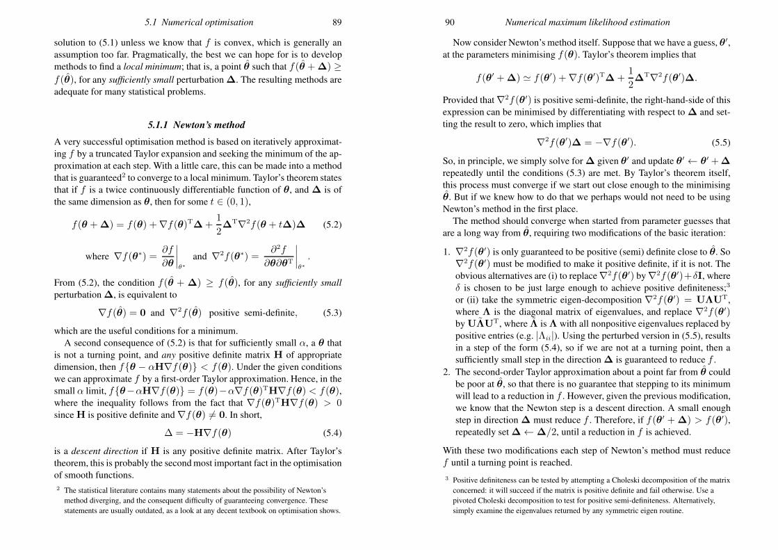
5.1 Numerical optimisation 89
solution to (5.1) unless we know that f is convex, which is generally anassumption too far. Pragmatically, the best we can hope for is to developmethods to find a local minimum; that is, a point θ such that f(θ +∆) ≥f(θ), for any sufficiently small perturbation ∆. The resulting methods areadequate for many statistical problems.
5.1.1 Newton’s method
A very successful optimisation method is based on iteratively approximat-ing f by a truncated Taylor expansion and seeking the minimum of the ap-proximation at each step. With a little care, this can be made into a methodthat is guaranteed2 to converge to a local minimum. Taylor’s theorem statesthat if f is a twice continuously differentiable function of θ, and ∆ is ofthe same dimension as θ, then for some t ∈ (0, 1),
f(θ +∆) = f(θ) +∇f(θ)T∆+1
2∆T∇2f(θ + t∆)∆ (5.2)
where ∇f(θ∗) =∂f
∂θ
∣∣∣∣θ∗
and ∇2f(θ∗) =∂2f
∂θ∂θT
∣∣∣∣θ∗.
From (5.2), the condition f(θ + ∆) ≥ f(θ), for any sufficiently smallperturbation ∆, is equivalent to
∇f(θ) = 0 and ∇2f(θ) positive semi-definite, (5.3)
which are the useful conditions for a minimum.A second consequence of (5.2) is that for sufficiently small α, a θ that
is not a turning point, and any positive definite matrix H of appropriatedimension, then fθ − αH∇f(θ) < f(θ). Under the given conditionswe can approximate f by a first-order Taylor approximation. Hence, in thesmall α limit, fθ−αH∇f(θ) = f(θ)−α∇f(θ)TH∇f(θ) < f(θ),where the inequality follows from the fact that ∇f(θ)TH∇f(θ) > 0since H is positive definite and∇f(θ) 6= 0. In short,
∆ = −H∇f(θ) (5.4)
is a descent direction if H is any positive definite matrix. After Taylor’stheorem, this is probably the second most important fact in the optimisationof smooth functions.2 The statistical literature contains many statements about the possibility of Newton’s
method diverging, and the consequent difficulty of guaranteeing convergence. Thesestatements are usually outdated, as a look at any decent textbook on optimisation shows.
90 Numerical maximum likelihood estimation
Now consider Newton’s method itself. Suppose that we have a guess, θ′,at the parameters minimising f(θ). Taylor’s theorem implies that
f(θ′ +∆) ≃ f(θ′) +∇f(θ′)T∆+1
2∆T∇2f(θ′)∆.
Provided that∇2f(θ′) is positive semi-definite, the right-hand-side of thisexpression can be minimised by differentiating with respect to ∆ and set-ting the result to zero, which implies that
∇2f(θ′)∆ = −∇f(θ′). (5.5)
So, in principle, we simply solve for ∆ given θ′ and update θ′ ← θ′ +∆repeatedly until the conditions (5.3) are met. By Taylor’s theorem itself,this process must converge if we start out close enough to the minimisingθ. But if we knew how to do that we perhaps would not need to be usingNewton’s method in the first place.
The method should converge when started from parameter guesses thatare a long way from θ, requiring two modifications of the basic iteration:
1. ∇2f(θ′) is only guaranteed to be positive (semi) definite close to θ. So∇2f(θ′) must be modified to make it positive definite, if it is not. Theobvious alternatives are (i) to replace∇2f(θ′) by∇2f(θ′)+δI, whereδ is chosen to be just large enough to achieve positive definiteness;3
or (ii) take the symmetric eigen-decomposition ∇2f(θ′) = UΛUT,where Λ is the diagonal matrix of eigenvalues, and replace ∇2f(θ′)by UΛUT, where Λ is Λ with all nonpositive eigenvalues replaced bypositive entries (e.g. |Λii|). Using the perturbed version in (5.5), resultsin a step of the form (5.4), so if we are not at a turning point, then asufficiently small step in the direction ∆ is guaranteed to reduce f .
2. The second-order Taylor approximation about a point far from θ couldbe poor at θ, so that there is no guarantee that stepping to its minimumwill lead to a reduction in f . However, given the previous modification,we know that the Newton step is a descent direction. A small enoughstep in direction ∆ must reduce f . Therefore, if f(θ′ +∆) > f(θ′),repeatedly set ∆←∆/2, until a reduction in f is achieved.
With these two modifications each step of Newton’s method must reducef until a turning point is reached.3 Positive definiteness can be tested by attempting a Choleski decomposition of the matrix
concerned: it will succeed if the matrix is positive definite and fail otherwise. Use apivoted Choleski decomposition to test for positive semi-definiteness. Alternatively,simply examine the eigenvalues returned by any symmetric eigen routine.
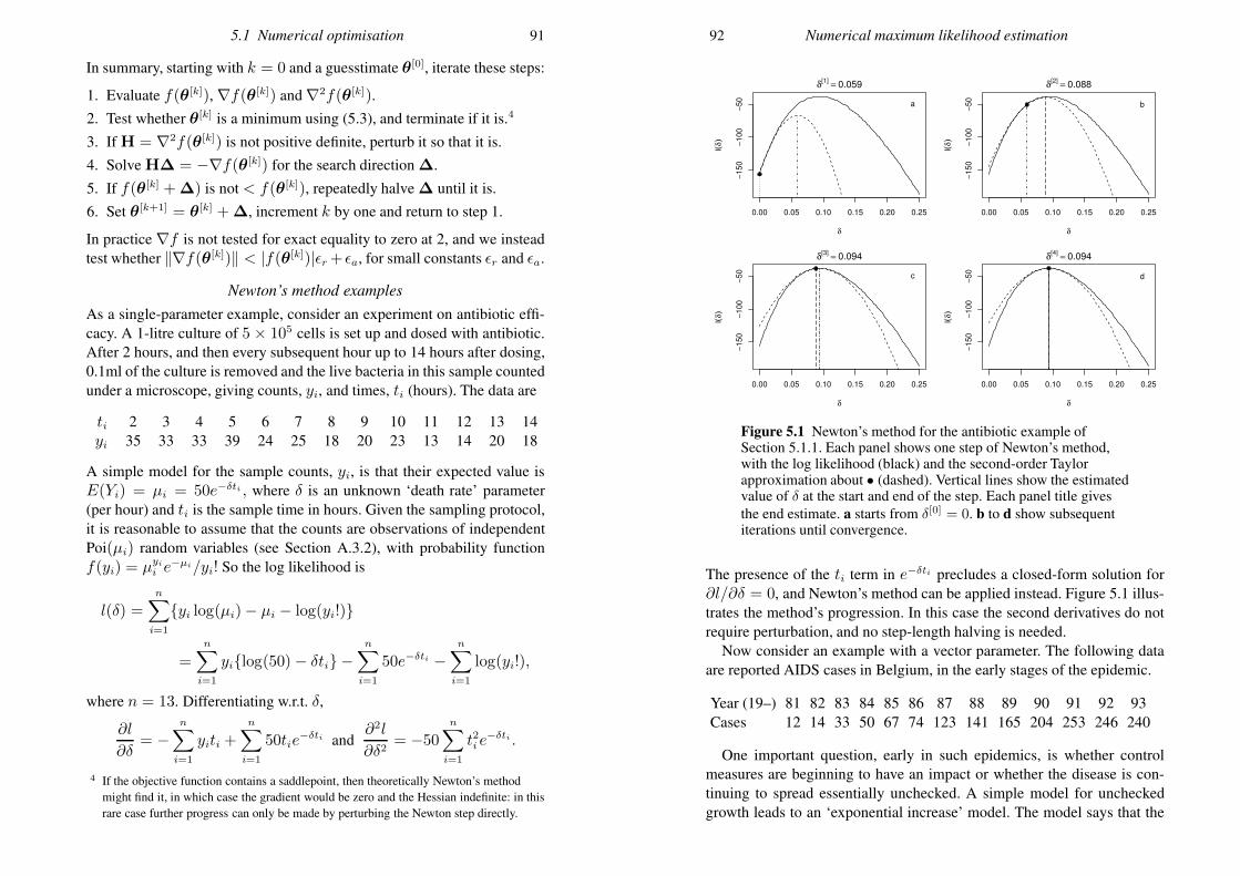
5.1 Numerical optimisation 91
In summary, starting with k = 0 and a guesstimate θ[0], iterate these steps:
1. Evaluate f(θ[k]),∇f(θ[k]) and∇2f(θ[k]).2. Test whether θ[k] is a minimum using (5.3), and terminate if it is.4
3. If H = ∇2f(θ[k]) is not positive definite, perturb it so that it is.4. Solve H∆ = −∇f(θ[k]) for the search direction ∆.
5. If f(θ[k] +∆) is not < f(θ[k]), repeatedly halve ∆ until it is.6. Set θ[k+1] = θ[k] +∆, increment k by one and return to step 1.
In practice∇f is not tested for exact equality to zero at 2, and we insteadtest whether ‖∇f(θ[k])‖ < |f(θ[k])|ǫr+ ǫa, for small constants ǫr and ǫa.
Newton’s method examplesAs a single-parameter example, consider an experiment on antibiotic effi-cacy. A 1-litre culture of 5 × 10⁵ cells is set up and dosed with antibiotic.After 2 hours, and then every subsequent hour up to 14 hours after dosing,0.1ml of the culture is removed and the live bacteria in this sample countedunder a microscope, giving counts, yi, and times, ti (hours). The data are
ti 2 3 4 5 6 7 8 9 10 11 12 13 14yi 35 33 33 39 24 25 18 20 23 13 14 20 18
A simple model for the sample counts, yi, is that their expected value isE(Yi) = µi = 50e−δti , where δ is an unknown ‘death rate’ parameter(per hour) and ti is the sample time in hours. Given the sampling protocol,it is reasonable to assume that the counts are observations of independentPoi(µi) random variables (see Section A.3.2), with probability functionf(yi) = µyii e
−µi/yi! So the log likelihood is
l(δ) =n∑
i=1
yi log(µi)− µi − log(yi!)
=n∑
i=1
yilog(50)− δti −n∑
i=1
50e−δti −n∑
i=1
log(yi!),
where n = 13. Differentiating w.r.t. δ,
∂l
∂δ= −
n∑
i=1
yiti +n∑
i=1
50tie−δti and
∂2l
∂δ2= −50
n∑
i=1
t2i e−δti .
4 If the objective function contains a saddlepoint, then theoretically Newton’s methodmight find it, in which case the gradient would be zero and the Hessian indefinite: in thisrare case further progress can only be made by perturbing the Newton step directly.
92 Numerical maximum likelihood estimation
0.00 0.05 0.10 0.15 0.20 0.25
−150
−100
−50
δ
l(δ)
δ[1]
= 0.059
a
0.00 0.05 0.10 0.15 0.20 0.25
−150
−100
−50
δ
l(δ)
δ[2]
= 0.088
b
0.00 0.05 0.10 0.15 0.20 0.25
−150
−100
−50
δ
l(δ)
δ[3]
= 0.094
c
0.00 0.05 0.10 0.15 0.20 0.25
−150
−100
−50
δ
l(δ)
δ[4]
= 0.094
d
Figure 5.1 Newton’s method for the antibiotic example ofSection 5.1.1. Each panel shows one step of Newton’s method,with the log likelihood (black) and the second-order Taylorapproximation about • (dashed). Vertical lines show the estimatedvalue of δ at the start and end of the step. Each panel title givesthe end estimate. a starts from δ[0] = 0. b to d show subsequentiterations until convergence.
The presence of the ti term in e−δti precludes a closed-form solution for∂l/∂δ = 0, and Newton’s method can be applied instead. Figure 5.1 illus-trates the method’s progression. In this case the second derivatives do notrequire perturbation, and no step-length halving is needed.
Now consider an example with a vector parameter. The following dataare reported AIDS cases in Belgium, in the early stages of the epidemic.
Year (19–) 81 82 83 84 85 86 87 88 89 90 91 92 93Cases 12 14 33 50 67 74 123 141 165 204 253 246 240
One important question, early in such epidemics, is whether controlmeasures are beginning to have an impact or whether the disease is con-tinuing to spread essentially unchecked. A simple model for uncheckedgrowth leads to an ‘exponential increase’ model. The model says that the
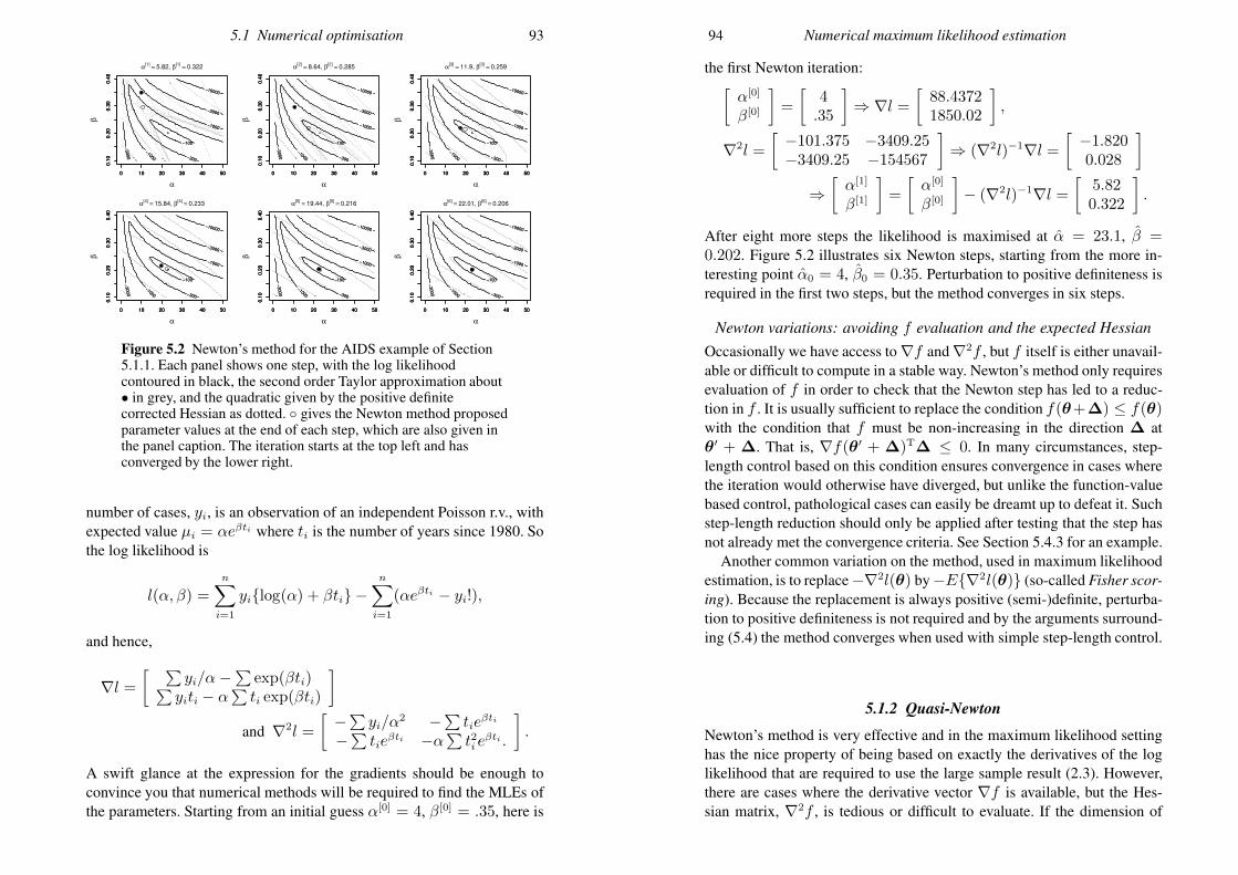
5.1 Numerical optimisation 93
α
β −10000
−3000
−3000
−1000
−1000
−300
−100
0 10 20 30 40 50
0.1
00
.20
0.3
00
.40
0 10 20 30 40 50
0.1
00
.20
0.3
00
.40
−10000
−3000
−3000
−1000
−1000
−300
−100
0 10 20 30 40 50
0.1
00
.20
0.3
00
.40
α[1]
= 5.82, β[1]
= 0.322
α
β
−10000
−3000
−3000
−1000
−1000
−300
−100
0 10 20 30 40 50
0.1
00
.20
0.3
00
.40
0 10 20 30 40 50
0.1
00
.20
0.3
00
.40
−10000
−3000
−3000
−1000
−1000
−300
−100
0 10 20 30 40 50
0.1
00
.20
0.3
00
.40
α[2]
= 8.64, β[2]
= 0.285
α
β
−10000
−3000
−3000
−1000
−1000
−300
−100
0 10 20 30 40 50
0.1
00
.20
0.3
00
.40
0 10 20 30 40 50
0.1
00
.20
0.3
00
.40
−10000
−3000
−3000
−1000
−1000
−300
−100
0 10 20 30 40 50
0.1
00
.20
0.3
00
.40
α[3]
= 11.9, β[3]
= 0.259
α
β
−10000
−3000
−3000
−1000
−1000
−300
−100
0 10 20 30 40 50
0.1
00
.20
0.3
00
.40
0 10 20 30 40 50
0.1
00
.20
0.3
00
.40
−10000
−3000
−3000
−1000
−1000
−300
−100
0 10 20 30 40 50
0.1
00
.20
0.3
00
.40
α[4]
= 15.84, β[4]
= 0.233
α
β
−10000
−3000
−3000
−1000
−1000
−300
−100
0 10 20 30 40 50
0.1
00
.20
0.3
00
.40
0 10 20 30 40 50
0.1
00
.20
0.3
00
.40
−10000
−3000
−3000
−1000
−1000
−300
−100
0 10 20 30 40 50
0.1
00
.20
0.3
00
.40
α[5]
= 19.44, β[5]
= 0.216
α
β
−10000
−3000
−3000
−1000
−1000
−300
−100
0 10 20 30 40 50
0.1
00
.20
0.3
00
.40
0 10 20 30 40 50
0.1
00
.20
0.3
00
.40
−10000
−3000
−3000
−1000
−1000
−300
−100
0 10 20 30 40 50
0.1
00
.20
0.3
00
.40
α[6]
= 22.01, β[6]
= 0.206
Figure 5.2 Newton’s method for the AIDS example of Section5.1.1. Each panel shows one step, with the log likelihoodcontoured in black, the second order Taylor approximation about• in grey, and the quadratic given by the positive definitecorrected Hessian as dotted. gives the Newton method proposedparameter values at the end of each step, which are also given inthe panel caption. The iteration starts at the top left and hasconverged by the lower right.
number of cases, yi, is an observation of an independent Poisson r.v., withexpected value µi = αeβti where ti is the number of years since 1980. Sothe log likelihood is
l(α, β) =n∑
i=1
yilog(α) + βti −n∑
i=1
(αeβti − yi!),
and hence,
∇l =[ ∑
yi/α−∑
exp(βti)∑yiti − α
∑ti exp(βti)
]
and ∇2l =
[ −∑ yi/α2 −∑ tie
βti
−∑ tieβti −α∑ t2i e
βti .
].
A swift glance at the expression for the gradients should be enough toconvince you that numerical methods will be required to find the MLEs ofthe parameters. Starting from an initial guess α[0] = 4, β[0] = .35, here is
94 Numerical maximum likelihood estimation
the first Newton iteration:[α[0]
β[0]
]=
[4.35
]⇒ ∇l =
[88.43721850.02
],
∇2l =
[ −101.375 −3409.25−3409.25 −154567
]⇒ (∇2l)−1∇l =
[ −1.8200.028
]
⇒[α[1]
β[1]
]=
[α[0]
β[0]
]− (∇2l)−1∇l =
[5.820.322
].
After eight more steps the likelihood is maximised at α = 23.1, β =0.202. Figure 5.2 illustrates six Newton steps, starting from the more in-teresting point α0 = 4, β0 = 0.35. Perturbation to positive definiteness isrequired in the first two steps, but the method converges in six steps.
Newton variations: avoiding f evaluation and the expected HessianOccasionally we have access to∇f and∇2f , but f itself is either unavail-able or difficult to compute in a stable way. Newton’s method only requiresevaluation of f in order to check that the Newton step has led to a reduc-tion in f . It is usually sufficient to replace the condition f(θ+∆) ≤ f(θ)with the condition that f must be non-increasing in the direction ∆ atθ′ + ∆. That is, ∇f(θ′ + ∆)T∆ ≤ 0. In many circumstances, step-length control based on this condition ensures convergence in cases wherethe iteration would otherwise have diverged, but unlike the function-valuebased control, pathological cases can easily be dreamt up to defeat it. Suchstep-length reduction should only be applied after testing that the step hasnot already met the convergence criteria. See Section 5.4.3 for an example.
Another common variation on the method, used in maximum likelihoodestimation, is to replace−∇2l(θ) by−E∇2l(θ) (so-called Fisher scor-ing). Because the replacement is always positive (semi-)definite, perturba-tion to positive definiteness is not required and by the arguments surround-ing (5.4) the method converges when used with simple step-length control.
5.1.2 Quasi-Newton
Newton’s method is very effective and in the maximum likelihood settinghas the nice property of being based on exactly the derivatives of the loglikelihood that are required to use the large sample result (2.3). However,there are cases where the derivative vector ∇f is available, but the Hes-sian matrix, ∇2f , is tedious or difficult to evaluate. If the dimension of
5.1 Numerical optimisation 95
θ is large, numerically solving for the Newton direction can also becomeprohibitively costly. These considerations raise the question of what can bedone based only on f and∇f .
The obvious approach is to apply the strategy that led to Newton’s methodagain, but based on the first-order Taylor expansion of f . However, the re-sulting steepest descent method is really a nonstarter. The problem is thatthe first-order Taylor expansion ceases to be a good model of f at exactlythe point we are most interested in. At the minimum of f , ∇f = 0 andwe lose all justification for having neglected the second-order terms in theTaylor expansion in favour of the first order terms, since the latter have van-ished. This theoretical concern is borne out in practice: the steepest descentmethod often becomes excruciatingly slow as it approaches a minimum.
A less obvious approach is to build up a local quadratic model of f fromthe first derivative information accumulated as the optimisation proceeds.This leads to quasi-Newton methods, which update an approximation tothe Hessian, ∇2f , based entirely on evaluations of ∇f . In principle, thisapproximation can be used instead of the Hessian in Newton’s method, butit is also possible to work directly on an approximation to the inverse ofthe Hessian, thereby reducing the cost of calculating the step, ∆. It is alsopossible to ensure that the approximate Hessian is always positive definite.
Quasi-Newton methods were invented in the mid 1950s by W. C. Davi-don (a physicist). In the mathematical equivalent of not signing the Beat-les, his paper on the method was rejected (it was eventually published in1991). There are now many varieties of the quasi-Newton method, but themost popular is the BFGS variant,5 which is briefly covered here.
Suppose that H[k+1] is the approximate positive definite Hessian at the(k + 1)th step, so that
f(θ) ≃ f(θ[k+1]) +∇f(θ[k+1])T(θ − θ[k+1])
+1
2(θ − θ[k+1])TH[k+1](θ − θ[k+1]).
The basic requirement of a quasi Newton method is that this approximationshould exactly match∇f(θ[k]); that is, it should get the gradient vector atthe previous point, θ[k], exactly right. So
∇f(θ[k+1]) +H[k+1](θ[k] − θ[k+1]) = ∇f(θ[k]),
5 BFGS is named after Broyden, Fletcher, Goldfarb and Shanno all of whom discoveredand published it, independently, around 1970. ‘Big Friendly Giant Steps’ is the way allRoald Dahl readers remember the name, of course (M. V. Bravington, pers. com.).
96 Numerical maximum likelihood estimation
which can be compactly re-written as
H[k+1]sk = yk, (5.6)
where sk = θ[k+1]−θ[k] andyk = ∇f(θ[k+1])−∇f(θ[k]). Equation (5.6)will only be feasible for positive definite H[k+1] under certain conditionson sk and yk, but these can always be met by choosing the step-length tomeet the Wolfe conditions, covered shortly.
Now let us work in terms of the inverse approximate Hessian, B[k] ≡(H[k]
)−1. Equation (5.6) alone does not define a unique B[k+1], and some
extra conditions are needed. A B[k+1] is sought that
1. satisfies (5.6) so that B[k+1]yk = sk;2. is as close as possible to B[k];3. is positive definite.
‘Close’ in condition 2 is judged using a particular matrix norm, that is notcovered here. The unique solution to this problem is the BFGS update
B[k+1] = (I− ρkskyTk )B
[k](I− ρkyksTk ) + ρksks
Tk ,
where ρ−1k = sTk yk. The BFGS method then works exactly like Newton’s
method, but with B[k] in place of the inverse of ∇2f(θ[k]), and withoutthe need for evaluation of second derivatives or for perturbing the Hessianto achieve positive definiteness. A finite difference approximation to theHessian is often used to start the method (see Section 5.5.2).
The only detail not required by Newton’s method is that step-length se-lection must now be carried out more carefully. We must ensure that thestep-length is such that ∆ satisfies the sufficient decrease condition
f(θ[k] +∆) ≤ f(θ[k]) + c1∇f(θ[k])T∆,
c1 ∈ (0, 1), and the curvature condition
∇f(θ[k] +∆)T∆ ≥ c2∇f(θ[k])T∆,
c2 ∈ (c1, 1). Collectively these conditions are known as the Wolfe con-ditions. The first seeks to ensure that the step results in a decrease that isreasonable relative to the gradient of f in the direction of ∆ and guardsagainst overly long steps. The second says that there should have been asufficient decrease in the gradient of the function along ∆ (otherwise whynot take a longer step, given that the function is still decreasing fast inthis direction). For a full discussion see Nocedal and Wright (2006, §3.1),where c1 = 10−4 and c2 = 0.9 are suggested as typical.
When performing maximum likelihood estimation, it is tempting to use
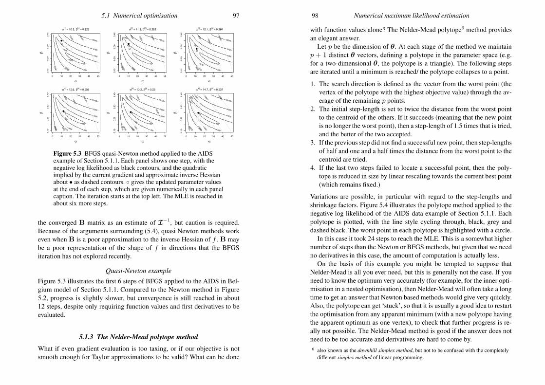
5.1 Numerical optimisation 97
α
β
100
300
1000
1000
3000
3000
10000
0 10 20 30 40 50
0.1
00
.20
0.3
00
.40
1000
3000
10000
10000
30000
α[1]
= 10.3, β[1]
= 0.323
α
β
100
300
1000
1000
3000
3000
10000
0 10 20 30 40 50
0.1
00
.20
0.3
00
.40
300
1000
3000
3000
10000
10000
30000
α[2]
= 11.3, β[2]
= 0.282
α
β
100
300
1000
1000
3000
3000
10000
0 10 20 30 40 50
0.1
00
.20
0.3
00
.40
300
1000 3000 3
000 10000
30000
α[3]
= 12.1, β[3]
= 0.264
α
β
100
300
1000
1000
3000
3000
10000
0 10 20 30 40 50
0.1
00
.20
0.3
00
.40
300
1000
3000
3000
10000
10000
30000
α[4]
= 12.6, β[4]
= 0.256
α
β
100
300
1000
1000
3000
3000
10000
0 10 20 30 40 50
0.1
00
.20
0.3
00
.40
300
1000
1000
3000
3000
10000
10000
30000
α[5]
= 13.2, β[5]
= 0.25
α
β
100
300
1000
1000
3000
3000
10000
0 10 20 30 40 50
0.1
00
.20
0.3
00
.40
300
1000
1000
3000
3000
10000
10000
30000
α[6]
= 14.7, β[6]
= 0.237
Figure 5.3 BFGS quasi-Newton method applied to the AIDSexample of Section 5.1.1. Each panel shows one step, with thenegative log likelihood as black contours, and the quadraticimplied by the current gradient and approximate inverse Hessianabout • as dashed contours. gives the updated parameter valuesat the end of each step, which are given numerically in each panelcaption. The iteration starts at the top left. The MLE is reached inabout six more steps.
the converged B matrix as an estimate of I−1, but caution is required.Because of the arguments surrounding (5.4), quasi Newton methods workeven when B is a poor approximation to the inverse Hessian of f . B maybe a poor representation of the shape of f in directions that the BFGSiteration has not explored recently.
Quasi-Newton exampleFigure 5.3 illustrates the first 6 steps of BFGS applied to the AIDS in Bel-gium model of Section 5.1.1. Compared to the Newton method in Figure5.2, progress is slightly slower, but convergence is still reached in about12 steps, despite only requiring function values and first derivatives to beevaluated.
5.1.3 The Nelder-Mead polytope method
What if even gradient evaluation is too taxing, or if our objective is notsmooth enough for Taylor approximations to be valid? What can be done
98 Numerical maximum likelihood estimation
with function values alone? The Nelder-Mead polytope6 method providesan elegant answer.
Let p be the dimension of θ. At each stage of the method we maintainp + 1 distinct θ vectors, defining a polytope in the parameter space (e.g.for a two-dimensional θ, the polytope is a triangle). The following stepsare iterated until a minimum is reached/ the polytope collapses to a point.
1. The search direction is defined as the vector from the worst point (thevertex of the polytope with the highest objective value) through the av-erage of the remaining p points.
2. The initial step-length is set to twice the distance from the worst pointto the centroid of the others. If it succeeds (meaning that the new pointis no longer the worst point), then a step-length of 1.5 times that is tried,and the better of the two accepted.
3. If the previous step did not find a successful new point, then step-lengthsof half and one and a half times the distance from the worst point to thecentroid are tried.
4. If the last two steps failed to locate a successful point, then the poly-tope is reduced in size by linear rescaling towards the current best point(which remains fixed.)
Variations are possible, in particular with regard to the step-lengths andshrinkage factors. Figure 5.4 illustrates the polytope method applied to thenegative log likelihood of the AIDS data example of Section 5.1.1. Eachpolytope is plotted, with the line style cycling through, black, grey anddashed black. The worst point in each polytope is highlighted with a circle.
In this case it took 24 steps to reach the MLE. This is a somewhat highernumber of steps than the Newton or BFGS methods, but given that we needno derivatives in this case, the amount of computation is actually less.
On the basis of this example you might be tempted to suppose thatNelder-Mead is all you ever need, but this is generally not the case. If youneed to know the optimum very accurately (for example, for the inner opti-misation in a nested optimisation), then Nelder-Mead will often take a longtime to get an answer that Newton based methods would give very quickly.Also, the polytope can get ‘stuck’, so that it is usually a good idea to restartthe optimisation from any apparent minimum (with a new polytope havingthe apparent optimum as one vertex), to check that further progress is re-ally not possible. The Nelder-Mead method is good if the answer does notneed to be too accurate and derivatives are hard to come by.6 also known as the downhill simplex method, but not to be confused with the completely
different simplex method of linear programming.
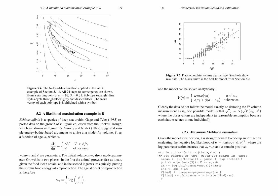
5.2 A likelihood maximisation example in R 99
α
β
100
300
1000
1000
3000
3000
10000
0 10 20 30 40 50
0.1
00.1
50.2
00.2
50.3
00.3
50.4
0
Figure 5.4 The Nelder-Mead method applied to the AIDSexample of Section 5.1.1. All 24 steps to convergence are shown,from a starting point at α = 10, β = 0.35. Polytope (triangle) linestyles cycle through black, grey and dashed black. The worstvertex of each polytope is highlighted with a symbol.
5.2 A likelihood maximisation example in R
Echinus affinis is a species of deep sea urchin. Gage and Tyler (1985) re-ported data on the growth of E. affinis collected from the Rockall Trough,which are shown in Figure 5.5. Gurney and Nisbet (1998) suggested sim-ple energy-budget based arguments to arrive at a model for volume, V , asa function of age, a, which is
dV
da=
γV V < φ/γφ otherwise,
where γ and φ are parameters. The initial volume is ω, also a model param-eter. Growth is in two phases: in the first the animal grows as fast as it can,given the food it can obtain, and in the second it grows less quickly, puttingthe surplus food energy into reproduction. The age at onset of reproductionis therefore
am =1
γlog
(φ
γω
),
100 Numerical maximum likelihood estimation
0 5 10 15 20 25
05
10
15
20
25
30
35
age
vol
Figure 5.5 Data on urchin volume against age. Symbols showraw data. The black curve is the best fit model from Section 5.2.
and the model can be solved analytically:
V (a) =
ω exp(γa) a < amφ/γ + φ(a− am) otherwise.
Clearly the data do not follow the model exactly, so denoting the ith volumemeasurement as vi, one possible model is that
√vi ∼ N(
√V (ai), σ
2)where the observations are independent (a reasonable assumption becauseeach datum relates to one individual).
5.2.1 Maximum likelihood estimation
Given the model specification, it is straightforward to code up an R functionevaluating the negative log likelihood of θ = log(ω, γ, φ, σ)T , where thelog parameterisation ensures that ω, γ, φ and σ remain positive:
urchin.vol <- function(theta,age) ## get volumes at ‘age’ given log params in ‘theta’omega <- exp(theta[1]); gamma <- exp(theta[2])phi <- exp(theta[3]); V <- age*0am <- log(phi/(gamma*omega))/gammaind <- age < amV[ind] <- omega*exp(gamma*age[ind])V[!ind] <- phi/gamma + phi*(age[!ind]-am)V
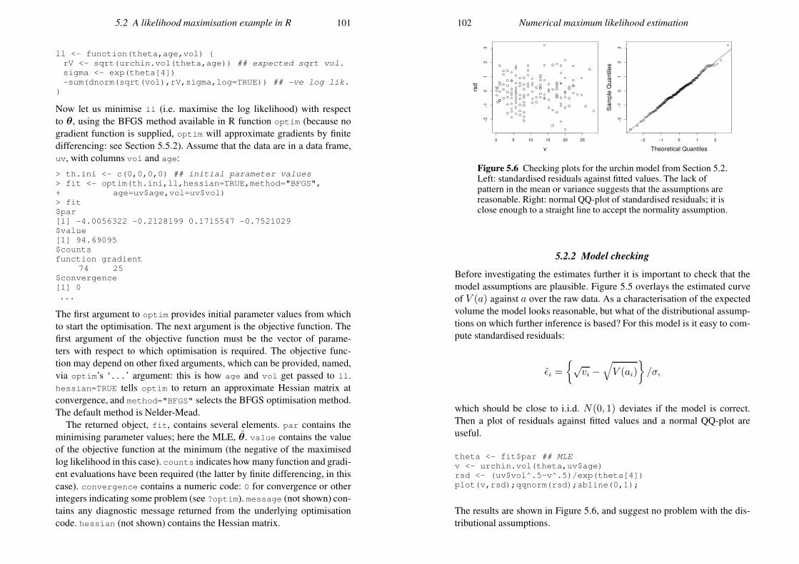
5.2 A likelihood maximisation example in R 101
ll <- function(theta,age,vol) rV <- sqrt(urchin.vol(theta,age)) ## expected sqrt vol.sigma <- exp(theta[4])-sum(dnorm(sqrt(vol),rV,sigma,log=TRUE)) ## -ve log lik.
Now let us minimise ll (i.e. maximise the log likelihood) with respectto θ, using the BFGS method available in R function optim (because nogradient function is supplied, optim will approximate gradients by finitedifferencing: see Section 5.5.2). Assume that the data are in a data frame,uv, with columns vol and age:
> th.ini <- c(0,0,0,0) ## initial parameter values> fit <- optim(th.ini,ll,hessian=TRUE,method="BFGS",+ age=uv$age,vol=uv$vol)> fit$par[1] -4.0056322 -0.2128199 0.1715547 -0.7521029$value[1] 94.69095$countsfunction gradient
74 25$convergence[1] 0...
The first argument to optim provides initial parameter values from whichto start the optimisation. The next argument is the objective function. Thefirst argument of the objective function must be the vector of parame-ters with respect to which optimisation is required. The objective func-tion may depend on other fixed arguments, which can be provided, named,via optim’s ‘...’ argument: this is how age and vol get passed to ll.hessian=TRUE tells optim to return an approximate Hessian matrix atconvergence, and method="BFGS" selects the BFGS optimisation method.The default method is Nelder-Mead.
The returned object, fit, contains several elements. par contains theminimising parameter values; here the MLE, θ. value contains the valueof the objective function at the minimum (the negative of the maximisedlog likelihood in this case). counts indicates how many function and gradi-ent evaluations have been required (the latter by finite differencing, in thiscase). convergence contains a numeric code: 0 for convergence or otherintegers indicating some problem (see ?optim). message (not shown) con-tains any diagnostic message returned from the underlying optimisationcode. hessian (not shown) contains the Hessian matrix.
102 Numerical maximum likelihood estimation
0 5 10 15 20 25
−2
−1
01
23
v
rsd
−2 −1 0 1 2
−2
−1
01
23
Theoretical Quantiles
Sam
ple
Quantile
s
Figure 5.6 Checking plots for the urchin model from Section 5.2.Left: standardised residuals against fitted values. The lack ofpattern in the mean or variance suggests that the assumptions arereasonable. Right: normal QQ-plot of standardised residuals; it isclose enough to a straight line to accept the normality assumption.
5.2.2 Model checking
Before investigating the estimates further it is important to check that themodel assumptions are plausible. Figure 5.5 overlays the estimated curveof V (a) against a over the raw data. As a characterisation of the expectedvolume the model looks reasonable, but what of the distributional assump-tions on which further inference is based? For this model is it easy to com-pute standardised residuals:
ǫi =
√vi −
√V (ai)
/σ,
which should be close to i.i.d. N(0, 1) deviates if the model is correct.Then a plot of residuals against fitted values and a normal QQ-plot areuseful.
theta <- fit$par ## MLEv <- urchin.vol(theta,uv$age)rsd <- (uv$vol^.5-v^.5)/exp(theta[4])plot(v,rsd);qqnorm(rsd);abline(0,1);
The results are shown in Figure 5.6, and suggest no problem with the dis-tributional assumptions.
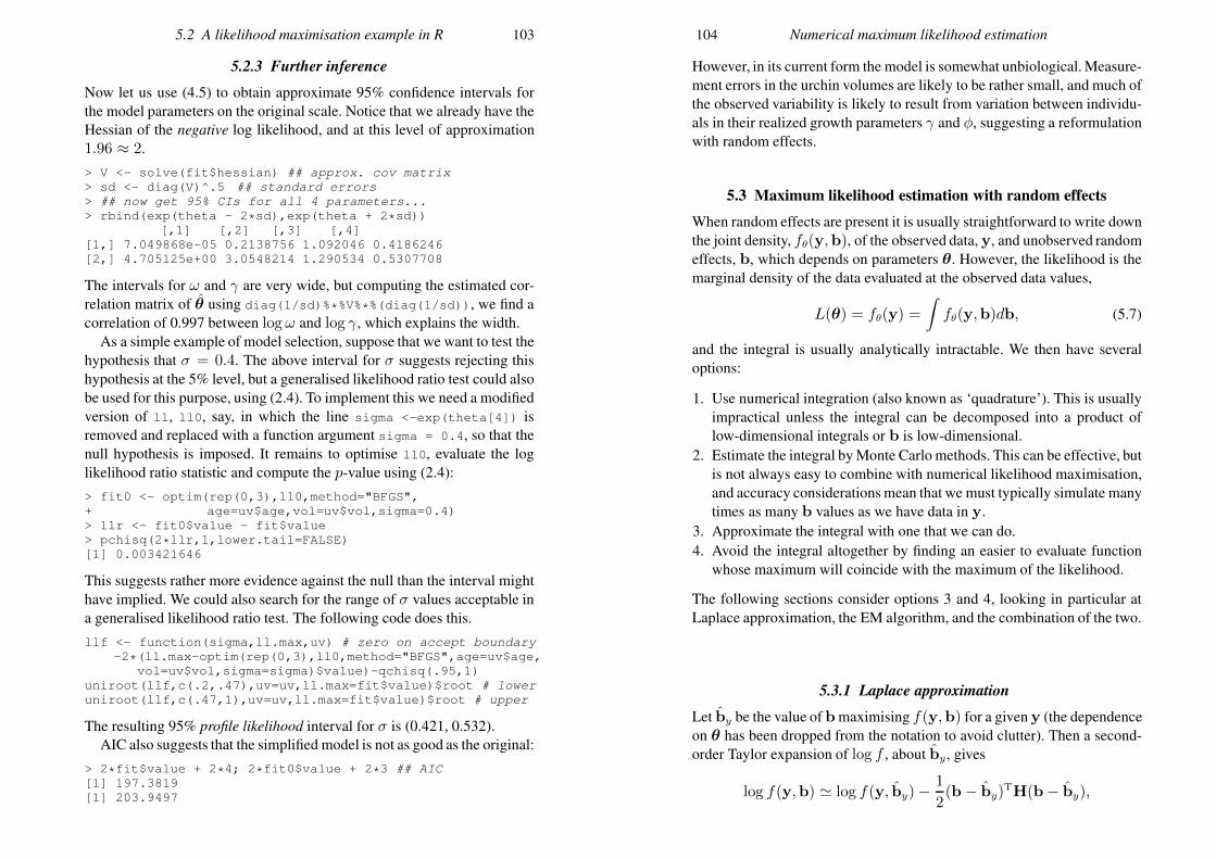
5.2 A likelihood maximisation example in R 103
5.2.3 Further inference
Now let us use (4.5) to obtain approximate 95% confidence intervals forthe model parameters on the original scale. Notice that we already have theHessian of the negative log likelihood, and at this level of approximation1.96 ≈ 2.
> V <- solve(fit$hessian) ## approx. cov matrix> sd <- diag(V)^.5 ## standard errors> ## now get 95% CIs for all 4 parameters...> rbind(exp(theta - 2*sd),exp(theta + 2*sd))
[,1] [,2] [,3] [,4][1,] 7.049868e-05 0.2138756 1.092046 0.4186246[2,] 4.705125e+00 3.0548214 1.290534 0.5307708
The intervals for ω and γ are very wide, but computing the estimated cor-relation matrix of θ using diag(1/sd)%*%V%*%(diag(1/sd)), we find acorrelation of 0.997 between logω and log γ, which explains the width.
As a simple example of model selection, suppose that we want to test thehypothesis that σ = 0.4. The above interval for σ suggests rejecting thishypothesis at the 5% level, but a generalised likelihood ratio test could alsobe used for this purpose, using (2.4). To implement this we need a modifiedversion of ll, ll0, say, in which the line sigma <-exp(theta[4]) isremoved and replaced with a function argument sigma = 0.4, so that thenull hypothesis is imposed. It remains to optimise ll0, evaluate the loglikelihood ratio statistic and compute the p-value using (2.4):
> fit0 <- optim(rep(0,3),ll0,method="BFGS",+ age=uv$age,vol=uv$vol,sigma=0.4)> llr <- fit0$value - fit$value> pchisq(2*llr,1,lower.tail=FALSE)[1] 0.003421646
This suggests rather more evidence against the null than the interval mighthave implied. We could also search for the range of σ values acceptable ina generalised likelihood ratio test. The following code does this.
llf <- function(sigma,ll.max,uv) # zero on accept boundary-2*(ll.max-optim(rep(0,3),ll0,method="BFGS",age=uv$age,
vol=uv$vol,sigma=sigma)$value)-qchisq(.95,1)uniroot(llf,c(.2,.47),uv=uv,ll.max=fit$value)$root # loweruniroot(llf,c(.47,1),uv=uv,ll.max=fit$value)$root # upper
The resulting 95% profile likelihood interval for σ is (0.421, 0.532).AIC also suggests that the simplified model is not as good as the original:
> 2*fit$value + 2*4; 2*fit0$value + 2*3 ## AIC[1] 197.3819[1] 203.9497
104 Numerical maximum likelihood estimation
However, in its current form the model is somewhat unbiological. Measure-ment errors in the urchin volumes are likely to be rather small, and much ofthe observed variability is likely to result from variation between individu-als in their realized growth parameters γ and φ, suggesting a reformulationwith random effects.
5.3 Maximum likelihood estimation with random effects
When random effects are present it is usually straightforward to write downthe joint density, fθ(y,b), of the observed data, y, and unobserved randomeffects, b, which depends on parameters θ. However, the likelihood is themarginal density of the data evaluated at the observed data values,
L(θ) = fθ(y) =
∫fθ(y,b)db, (5.7)
and the integral is usually analytically intractable. We then have severaloptions:
1. Use numerical integration (also known as ‘quadrature’). This is usuallyimpractical unless the integral can be decomposed into a product oflow-dimensional integrals or b is low-dimensional.
2. Estimate the integral by Monte Carlo methods. This can be effective, butis not always easy to combine with numerical likelihood maximisation,and accuracy considerations mean that we must typically simulate manytimes as many b values as we have data in y.
3. Approximate the integral with one that we can do.4. Avoid the integral altogether by finding an easier to evaluate function
whose maximum will coincide with the maximum of the likelihood.
The following sections consider options 3 and 4, looking in particular atLaplace approximation, the EM algorithm, and the combination of the two.
5.3.1 Laplace approximation
Let by be the value of b maximising f(y,b) for a giveny (the dependenceon θ has been dropped from the notation to avoid clutter). Then a second-order Taylor expansion of log f , about by, gives
log f(y,b) ≃ log f(y, by)−1
2(b− by)
TH(b− by),
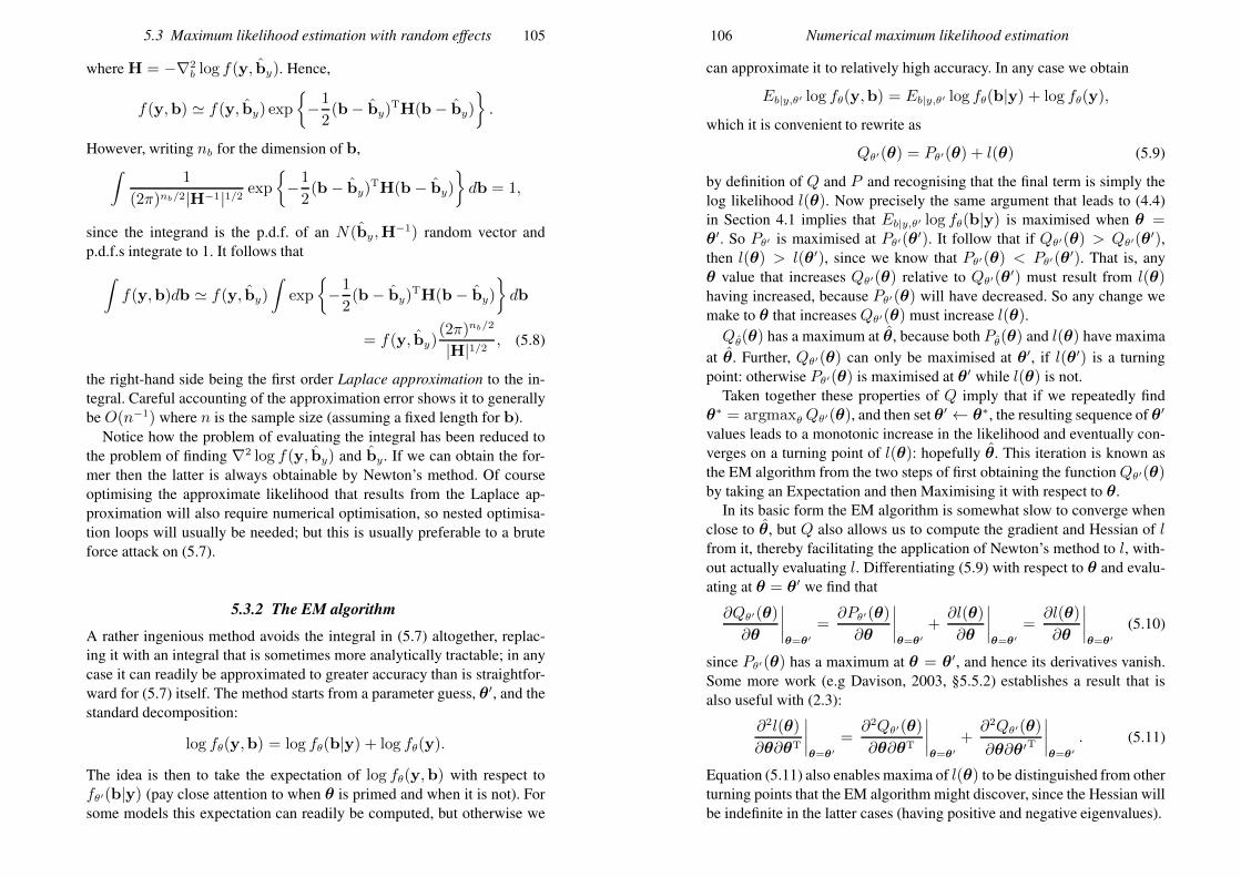
5.3 Maximum likelihood estimation with random effects 105
where H = −∇2b log f(y, by). Hence,
f(y,b) ≃ f(y, by) exp
−1
2(b− by)
TH(b− by)
.
However, writing nb for the dimension of b,∫
1
(2π)nb/2|H−1|1/2 exp−1
2(b− by)
TH(b− by)
db = 1,
since the integrand is the p.d.f. of an N(by,H−1) random vector and
p.d.f.s integrate to 1. It follows that∫
f(y,b)db ≃ f(y, by)
∫exp
−1
2(b− by)
TH(b− by)
db
= f(y, by)(2π)nb/2
|H|1/2 , (5.8)
the right-hand side being the first order Laplace approximation to the in-tegral. Careful accounting of the approximation error shows it to generallybe O(n−1) where n is the sample size (assuming a fixed length for b).
Notice how the problem of evaluating the integral has been reduced tothe problem of finding ∇2 log f(y, by) and by. If we can obtain the for-mer then the latter is always obtainable by Newton’s method. Of courseoptimising the approximate likelihood that results from the Laplace ap-proximation will also require numerical optimisation, so nested optimisa-tion loops will usually be needed; but this is usually preferable to a bruteforce attack on (5.7).
5.3.2 The EM algorithm
A rather ingenious method avoids the integral in (5.7) altogether, replac-ing it with an integral that is sometimes more analytically tractable; in anycase it can readily be approximated to greater accuracy than is straightfor-ward for (5.7) itself. The method starts from a parameter guess, θ′, and thestandard decomposition:
log fθ(y,b) = log fθ(b|y) + log fθ(y).
The idea is then to take the expectation of log fθ(y,b) with respect tofθ′(b|y) (pay close attention to when θ is primed and when it is not). Forsome models this expectation can readily be computed, but otherwise we
106 Numerical maximum likelihood estimation
can approximate it to relatively high accuracy. In any case we obtain
Eb|y,θ′ log fθ(y,b) = Eb|y,θ′ log fθ(b|y) + log fθ(y),
which it is convenient to rewrite as
Qθ′(θ) = Pθ′(θ) + l(θ) (5.9)
by definition of Q and P and recognising that the final term is simply thelog likelihood l(θ). Now precisely the same argument that leads to (4.4)in Section 4.1 implies that Eb|y,θ′ log fθ(b|y) is maximised when θ =θ′. So Pθ′ is maximised at Pθ′(θ′). It follow that if Qθ′(θ) > Qθ′(θ
′),then l(θ) > l(θ′), since we know that Pθ′(θ) < Pθ′(θ
′). That is, anyθ value that increases Qθ′(θ) relative to Qθ′(θ
′) must result from l(θ)having increased, because Pθ′(θ) will have decreased. So any change wemake to θ that increases Qθ′(θ) must increase l(θ).
Qθ(θ) has a maximum at θ, because both Pθ(θ) and l(θ) have maximaat θ. Further, Qθ′(θ) can only be maximised at θ′, if l(θ′) is a turningpoint: otherwise Pθ′(θ) is maximised at θ′ while l(θ) is not.
Taken together these properties of Q imply that if we repeatedly findθ∗ = argmaxθQθ′(θ), and then set θ′ ← θ∗, the resulting sequence of θ′
values leads to a monotonic increase in the likelihood and eventually con-verges on a turning point of l(θ): hopefully θ. This iteration is known asthe EM algorithm from the two steps of first obtaining the function Qθ′(θ)by taking an Expectation and then Maximising it with respect to θ.
In its basic form the EM algorithm is somewhat slow to converge whenclose to θ, but Q also allows us to compute the gradient and Hessian of lfrom it, thereby facilitating the application of Newton’s method to l, with-out actually evaluating l. Differentiating (5.9) with respect to θ and evalu-ating at θ = θ′ we find that
∂Qθ′(θ)
∂θ
∣∣∣∣θ=θ′
=∂Pθ′(θ)
∂θ
∣∣∣∣θ=θ′
+∂l(θ)
∂θ
∣∣∣∣θ=θ′
=∂l(θ)
∂θ
∣∣∣∣θ=θ′
(5.10)
since Pθ′(θ) has a maximum at θ = θ′, and hence its derivatives vanish.Some more work (e.g Davison, 2003, §5.5.2) establishes a result that isalso useful with (2.3):
∂2l(θ)
∂θ∂θT
∣∣∣∣θ=θ′
=∂2Qθ′(θ)
∂θ∂θT
∣∣∣∣θ=θ′
+∂2Qθ′(θ)
∂θ∂θ′T
∣∣∣∣θ=θ′
. (5.11)
Equation (5.11) also enables maxima of l(θ) to be distinguished from otherturning points that the EM algorithm might discover, since the Hessian willbe indefinite in the latter cases (having positive and negative eigenvalues).
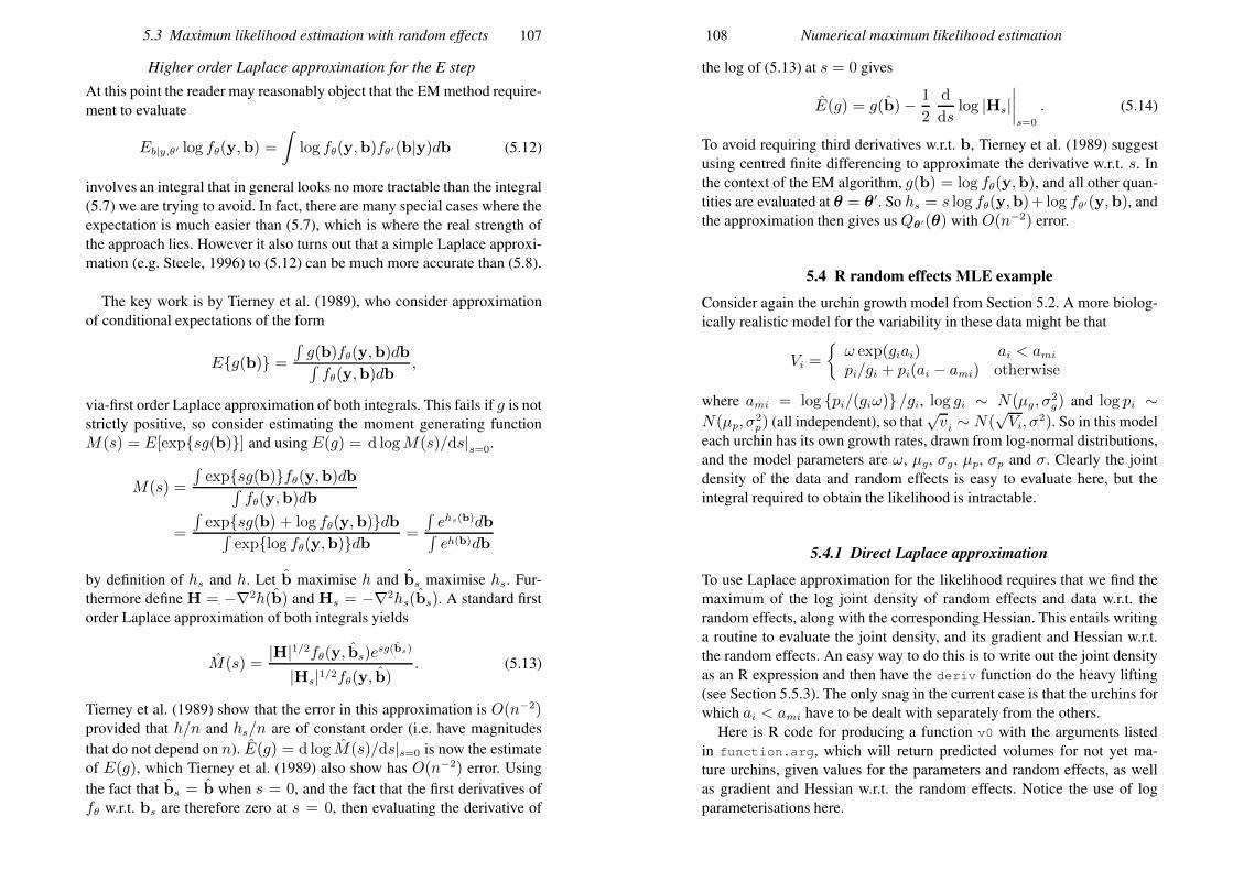
5.3 Maximum likelihood estimation with random effects 107
Higher order Laplace approximation for the E stepAt this point the reader may reasonably object that the EM method require-ment to evaluate
Eb|y,θ′ log fθ(y,b) =
∫log fθ(y,b)fθ′(b|y)db (5.12)
involves an integral that in general looks no more tractable than the integral(5.7) we are trying to avoid. In fact, there are many special cases where theexpectation is much easier than (5.7), which is where the real strength ofthe approach lies. However it also turns out that a simple Laplace approxi-mation (e.g. Steele, 1996) to (5.12) can be much more accurate than (5.8).
The key work is by Tierney et al. (1989), who consider approximationof conditional expectations of the form
Eg(b) =∫g(b)fθ(y,b)db∫fθ(y,b)db
,
via-first order Laplace approximation of both integrals. This fails if g is notstrictly positive, so consider estimating the moment generating functionM(s) = E[expsg(b)] and using E(g) = d logM(s)/ds|s=0.
M(s) =
∫expsg(b)fθ(y,b)db∫
fθ(y,b)db
=
∫expsg(b) + log fθ(y,b)db∫
explog fθ(y,b)db=
∫ehs(b)db∫eh(b)db
by definition of hs and h. Let b maximise h and bs maximise hs. Fur-thermore define H = −∇2h(b) and Hs = −∇2hs(bs). A standard firstorder Laplace approximation of both integrals yields
M(s) =|H|1/2fθ(y, bs)esg(bs)
|Hs|1/2fθ(y, b). (5.13)
Tierney et al. (1989) show that the error in this approximation is O(n−2)provided that h/n and hs/n are of constant order (i.e. have magnitudesthat do not depend on n). E(g) = d log M (s)/ds|s=0 is now the estimateof E(g), which Tierney et al. (1989) also show has O(n−2) error. Usingthe fact that bs = b when s = 0, and the fact that the first derivatives offθ w.r.t. bs are therefore zero at s = 0, then evaluating the derivative of
108 Numerical maximum likelihood estimation
the log of (5.13) at s = 0 gives
E(g) = g(b)− 1
2
d
dslog |Hs|
∣∣∣∣s=0
. (5.14)
To avoid requiring third derivatives w.r.t. b, Tierney et al. (1989) suggestusing centred finite differencing to approximate the derivative w.r.t. s. Inthe context of the EM algorithm, g(b) = log fθ(y,b), and all other quan-tities are evaluated at θ = θ′. So hs = s log fθ(y,b)+ log fθ′(y,b), andthe approximation then gives us Qθ′(θ) with O(n−2) error.
5.4 R random effects MLE example
Consider again the urchin growth model from Section 5.2. A more biolog-ically realistic model for the variability in these data might be that
Vi =
ω exp(giai) ai < amipi/gi + pi(ai − ami) otherwise
where ami = log pi/(giω) /gi, log gi ∼ N(µg, σ2g) and log pi ∼
N(µp, σ2p) (all independent), so that
√vi ∼ N(
√Vi, σ
2). So in this modeleach urchin has its own growth rates, drawn from log-normal distributions,and the model parameters are ω, µg, σg , µp, σp and σ. Clearly the jointdensity of the data and random effects is easy to evaluate here, but theintegral required to obtain the likelihood is intractable.
5.4.1 Direct Laplace approximation
To use Laplace approximation for the likelihood requires that we find themaximum of the log joint density of random effects and data w.r.t. therandom effects, along with the corresponding Hessian. This entails writinga routine to evaluate the joint density, and its gradient and Hessian w.r.t.the random effects. An easy way to do this is to write out the joint densityas an R expression and then have the deriv function do the heavy lifting(see Section 5.5.3). The only snag in the current case is that the urchins forwhich ai < ami have to be dealt with separately from the others.
Here is R code for producing a function v0 with the arguments listedin function.arg, which will return predicted volumes for not yet ma-ture urchins, given values for the parameters and random effects, as wellas gradient and Hessian w.r.t. the random effects. Notice the use of logparameterisations here.
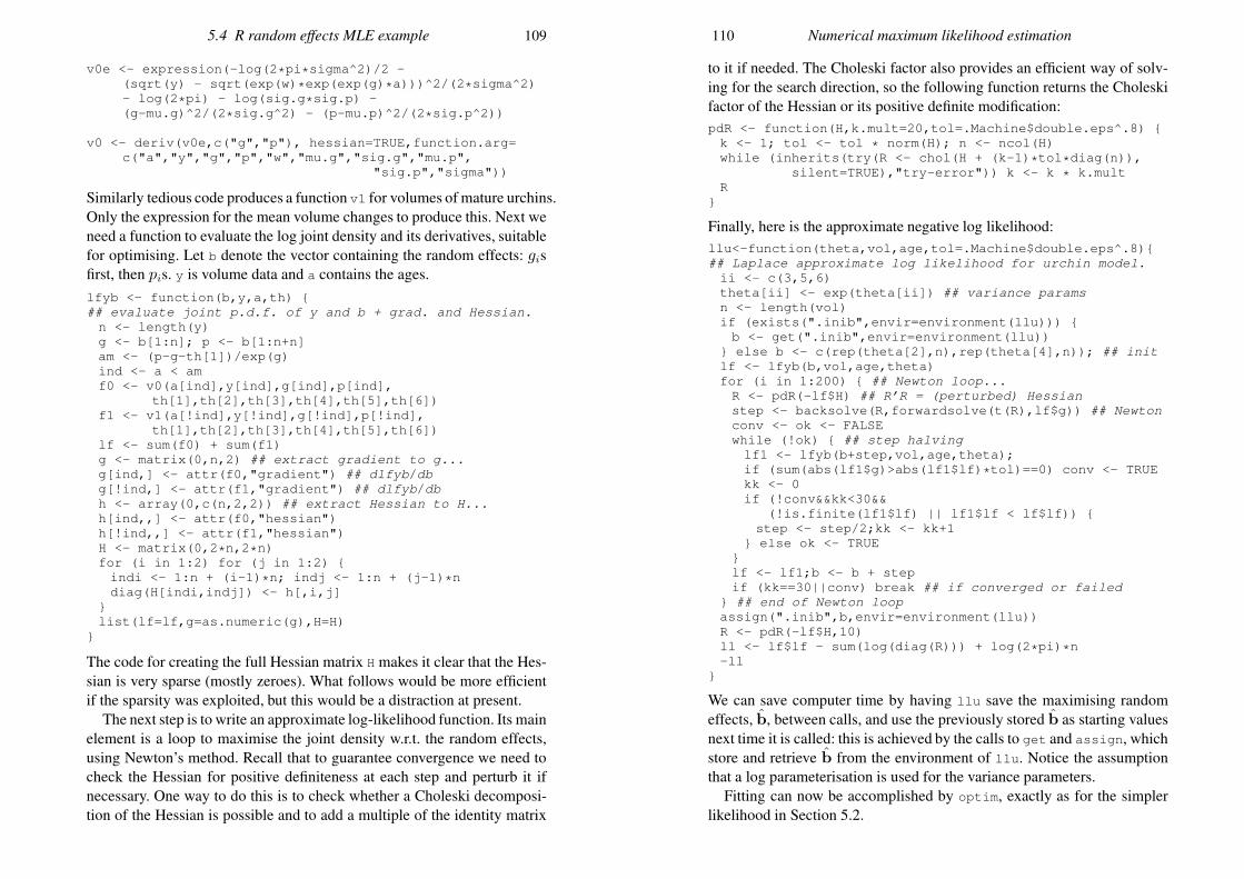
5.4 R random effects MLE example 109
v0e <- expression(-log(2*pi*sigma^2)/2 -(sqrt(y) - sqrt(exp(w)*exp(exp(g)*a)))^2/(2*sigma^2)- log(2*pi) - log(sig.g*sig.p) -(g-mu.g)^2/(2*sig.g^2) - (p-mu.p)^2/(2*sig.p^2))
v0 <- deriv(v0e,c("g","p"), hessian=TRUE,function.arg=c("a","y","g","p","w","mu.g","sig.g","mu.p",
"sig.p","sigma"))
Similarly tedious code produces a function v1 for volumes of mature urchins.Only the expression for the mean volume changes to produce this. Next weneed a function to evaluate the log joint density and its derivatives, suitablefor optimising. Let b denote the vector containing the random effects: gisfirst, then pis. y is volume data and a contains the ages.lfyb <- function(b,y,a,th) ## evaluate joint p.d.f. of y and b + grad. and Hessian.n <- length(y)g <- b[1:n]; p <- b[1:n+n]am <- (p-g-th[1])/exp(g)ind <- a < amf0 <- v0(a[ind],y[ind],g[ind],p[ind],
th[1],th[2],th[3],th[4],th[5],th[6])f1 <- v1(a[!ind],y[!ind],g[!ind],p[!ind],
th[1],th[2],th[3],th[4],th[5],th[6])lf <- sum(f0) + sum(f1)g <- matrix(0,n,2) ## extract gradient to g...g[ind,] <- attr(f0,"gradient") ## dlfyb/dbg[!ind,] <- attr(f1,"gradient") ## dlfyb/dbh <- array(0,c(n,2,2)) ## extract Hessian to H...h[ind,,] <- attr(f0,"hessian")h[!ind,,] <- attr(f1,"hessian")H <- matrix(0,2*n,2*n)for (i in 1:2) for (j in 1:2) indi <- 1:n + (i-1)*n; indj <- 1:n + (j-1)*ndiag(H[indi,indj]) <- h[,i,j]
list(lf=lf,g=as.numeric(g),H=H)
The code for creating the full Hessian matrix H makes it clear that the Hes-sian is very sparse (mostly zeroes). What follows would be more efficientif the sparsity was exploited, but this would be a distraction at present.
The next step is to write an approximate log-likelihood function. Its mainelement is a loop to maximise the joint density w.r.t. the random effects,using Newton’s method. Recall that to guarantee convergence we need tocheck the Hessian for positive definiteness at each step and perturb it ifnecessary. One way to do this is to check whether a Choleski decomposi-tion of the Hessian is possible and to add a multiple of the identity matrix
110 Numerical maximum likelihood estimation
to it if needed. The Choleski factor also provides an efficient way of solv-ing for the search direction, so the following function returns the Choleskifactor of the Hessian or its positive definite modification:pdR <- function(H,k.mult=20,tol=.Machine$double.eps^.8) k <- 1; tol <- tol * norm(H); n <- ncol(H)while (inherits(try(R <- chol(H + (k-1)*tol*diag(n)),
silent=TRUE),"try-error")) k <- k * k.multR
Finally, here is the approximate negative log likelihood:llu<-function(theta,vol,age,tol=.Machine$double.eps^.8)## Laplace approximate log likelihood for urchin model.ii <- c(3,5,6)theta[ii] <- exp(theta[ii]) ## variance paramsn <- length(vol)if (exists(".inib",envir=environment(llu))) b <- get(".inib",envir=environment(llu))
else b <- c(rep(theta[2],n),rep(theta[4],n)); ## initlf <- lfyb(b,vol,age,theta)for (i in 1:200) ## Newton loop...R <- pdR(-lf$H) ## R’R = (perturbed) Hessianstep <- backsolve(R,forwardsolve(t(R),lf$g)) ## Newtonconv <- ok <- FALSEwhile (!ok) ## step halvinglf1 <- lfyb(b+step,vol,age,theta);if (sum(abs(lf1$g)>abs(lf1$lf)*tol)==0) conv <- TRUEkk <- 0if (!conv&&kk<30&&
(!is.finite(lf1$lf) || lf1$lf < lf$lf)) step <- step/2;kk <- kk+1
else ok <- TRUElf <- lf1;b <- b + stepif (kk==30||conv) break ## if converged or failed
## end of Newton loopassign(".inib",b,envir=environment(llu))R <- pdR(-lf$H,10)ll <- lf$lf - sum(log(diag(R))) + log(2*pi)*n-ll
We can save computer time by having llu save the maximising randomeffects, b, between calls, and use the previously stored b as starting valuesnext time it is called: this is achieved by the calls to get and assign, whichstore and retrieve b from the environment of llu. Notice the assumptionthat a log parameterisation is used for the variance parameters.
Fitting can now be accomplished by optim, exactly as for the simplerlikelihood in Section 5.2.
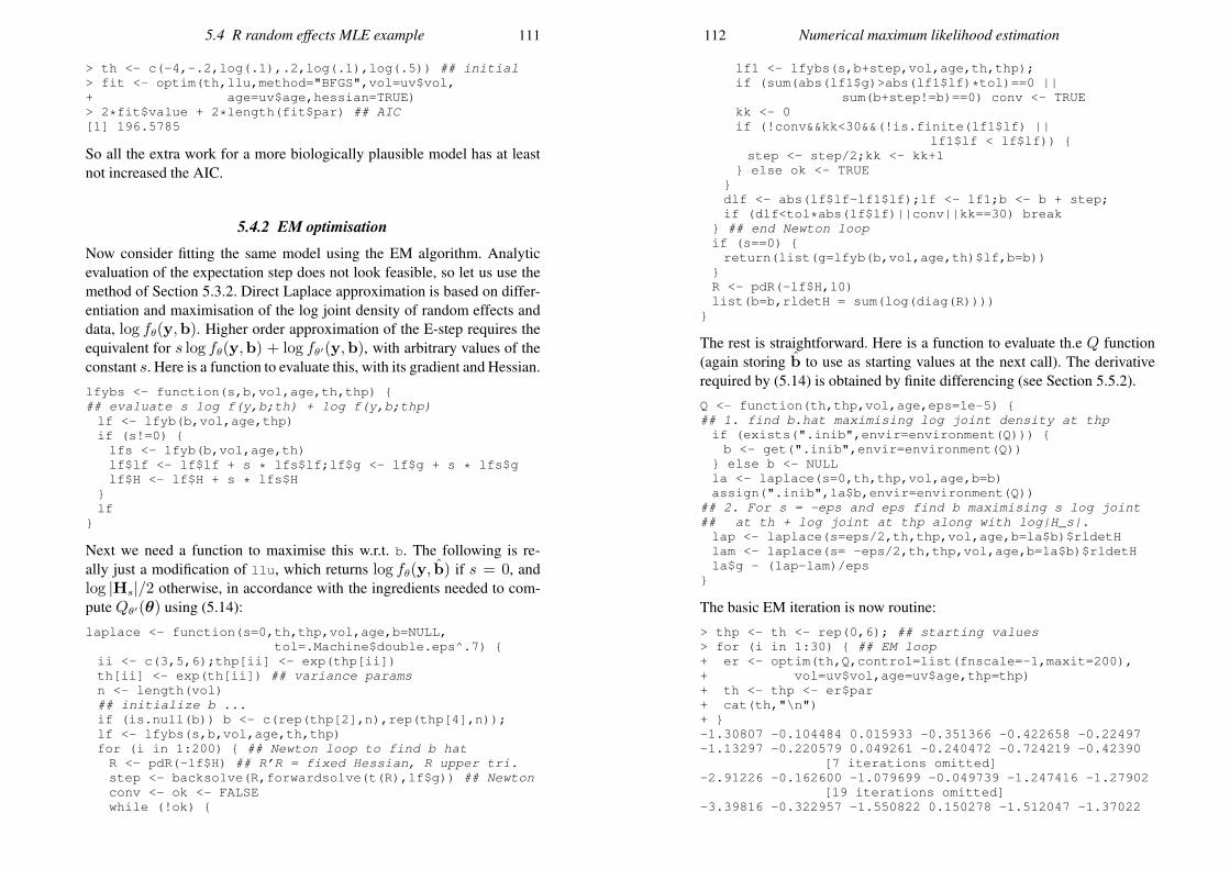
5.4 R random effects MLE example 111
> th <- c(-4,-.2,log(.1),.2,log(.1),log(.5)) ## initial> fit <- optim(th,llu,method="BFGS",vol=uv$vol,+ age=uv$age,hessian=TRUE)> 2*fit$value + 2*length(fit$par) ## AIC[1] 196.5785
So all the extra work for a more biologically plausible model has at leastnot increased the AIC.
5.4.2 EM optimisation
Now consider fitting the same model using the EM algorithm. Analyticevaluation of the expectation step does not look feasible, so let us use themethod of Section 5.3.2. Direct Laplace approximation is based on differ-entiation and maximisation of the log joint density of random effects anddata, log fθ(y,b). Higher order approximation of the E-step requires theequivalent for s log fθ(y,b) + log fθ′(y,b), with arbitrary values of theconstant s. Here is a function to evaluate this, with its gradient and Hessian.
lfybs <- function(s,b,vol,age,th,thp) ## evaluate s log f(y,b;th) + log f(y,b;thp)lf <- lfyb(b,vol,age,thp)if (s!=0) lfs <- lfyb(b,vol,age,th)lf$lf <- lf$lf + s * lfs$lf;lf$g <- lf$g + s * lfs$glf$H <- lf$H + s * lfs$H
lf
Next we need a function to maximise this w.r.t. b. The following is re-ally just a modification of llu, which returns log fθ(y, b) if s = 0, andlog |Hs|/2 otherwise, in accordance with the ingredients needed to com-pute Qθ′(θ) using (5.14):
laplace <- function(s=0,th,thp,vol,age,b=NULL,tol=.Machine$double.eps^.7)
ii <- c(3,5,6);thp[ii] <- exp(thp[ii])th[ii] <- exp(th[ii]) ## variance paramsn <- length(vol)## initialize b ...if (is.null(b)) b <- c(rep(thp[2],n),rep(thp[4],n));lf <- lfybs(s,b,vol,age,th,thp)for (i in 1:200) ## Newton loop to find b hatR <- pdR(-lf$H) ## R’R = fixed Hessian, R upper tri.step <- backsolve(R,forwardsolve(t(R),lf$g)) ## Newtonconv <- ok <- FALSEwhile (!ok)
112 Numerical maximum likelihood estimation
lf1 <- lfybs(s,b+step,vol,age,th,thp);if (sum(abs(lf1$g)>abs(lf1$lf)*tol)==0 ||
sum(b+step!=b)==0) conv <- TRUEkk <- 0if (!conv&&kk<30&&(!is.finite(lf1$lf) ||
lf1$lf < lf$lf)) step <- step/2;kk <- kk+1
else ok <- TRUEdlf <- abs(lf$lf-lf1$lf);lf <- lf1;b <- b + step;if (dlf<tol*abs(lf$lf)||conv||kk==30) break
## end Newton loopif (s==0) return(list(g=lfyb(b,vol,age,th)$lf,b=b))
R <- pdR(-lf$H,10)list(b=b,rldetH = sum(log(diag(R))))
The rest is straightforward. Here is a function to evaluate th.e Q function(again storing b to use as starting values at the next call). The derivativerequired by (5.14) is obtained by finite differencing (see Section 5.5.2).
Q <- function(th,thp,vol,age,eps=1e-5) ## 1. find b.hat maximising log joint density at thpif (exists(".inib",envir=environment(Q))) b <- get(".inib",envir=environment(Q))
else b <- NULLla <- laplace(s=0,th,thp,vol,age,b=b)assign(".inib",la$b,envir=environment(Q))
## 2. For s = -eps and eps find b maximising s log joint## at th + log joint at thp along with log|H_s|.lap <- laplace(s=eps/2,th,thp,vol,age,b=la$b)$rldetHlam <- laplace(s= -eps/2,th,thp,vol,age,b=la$b)$rldetHla$g - (lap-lam)/eps
The basic EM iteration is now routine:
> thp <- th <- rep(0,6); ## starting values> for (i in 1:30) ## EM loop+ er <- optim(th,Q,control=list(fnscale=-1,maxit=200),+ vol=uv$vol,age=uv$age,thp=thp)+ th <- thp <- er$par+ cat(th,"\n")+ -1.30807 -0.104484 0.015933 -0.351366 -0.422658 -0.22497-1.13297 -0.220579 0.049261 -0.240472 -0.724219 -0.42390
[7 iterations omitted]-2.91226 -0.162600 -1.079699 -0.049739 -1.247416 -1.27902
[19 iterations omitted]-3.39816 -0.322957 -1.550822 0.150278 -1.512047 -1.37022
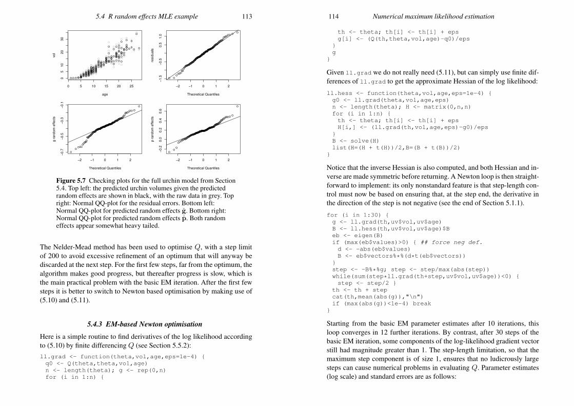
5.4 R random effects MLE example 113
0 5 10 15 20 25
05
10
20
30
age
vol
−2 −1 0 1 2
−1
.5−
0.5
0.5
1.0
Theoretical Quantiles
resid
ua
ls
−2 −1 0 1 2
−0
.7−
0.5
−0
.3−
0.1
Theoretical Quantiles
g r
an
do
m e
ffe
cts
−2 −1 0 1 2−
0.2
0.0
0.2
0.4
0.6
Theoretical Quantiles
p r
an
do
m e
ffe
cts
Figure 5.7 Checking plots for the full urchin model from Section5.4. Top left: the predicted urchin volumes given the predictedrandom effects are shown in black, with the raw data in grey. Topright: Normal QQ-plot for the residual errors. Bottom left:Normal QQ-plot for predicted random effects g. Bottom right:Normal QQ-plot for predicted random effects p. Both randomeffects appear somewhat heavy tailed.
The Nelder-Mead method has been used to optimise Q, with a step limitof 200 to avoid excessive refinement of an optimum that will anyway bediscarded at the next step. For the first few steps, far from the optimum, thealgorithm makes good progress, but thereafter progress is slow, which isthe main practical problem with the basic EM iteration. After the first fewsteps it is better to switch to Newton based optimisation by making use of(5.10) and (5.11).
5.4.3 EM-based Newton optimisation
Here is a simple routine to find derivatives of the log likelihood accordingto (5.10) by finite differencing Q (see Section 5.5.2):ll.grad <- function(theta,vol,age,eps=1e-4) q0 <- Q(theta,theta,vol,age)n <- length(theta); g <- rep(0,n)for (i in 1:n)
114 Numerical maximum likelihood estimation
th <- theta; th[i] <- th[i] + epsg[i] <- (Q(th,theta,vol,age)-q0)/eps
g
Given ll.grad we do not really need (5.11), but can simply use finite dif-ferences of ll.grad to get the approximate Hessian of the log likelihood:
ll.hess <- function(theta,vol,age,eps=1e-4) g0 <- ll.grad(theta,vol,age,eps)n <- length(theta); H <- matrix(0,n,n)for (i in 1:n) th <- theta; th[i] <- th[i] + epsH[i,] <- (ll.grad(th,vol,age,eps)-g0)/eps
B <- solve(H)list(H=(H + t(H))/2,B=(B + t(B))/2)
Notice that the inverse Hessian is also computed, and both Hessian and in-verse are made symmetric before returning. A Newton loop is then straight-forward to implement: its only nonstandard feature is that step-length con-trol must now be based on ensuring that, at the step end, the derivative inthe direction of the step is not negative (see the end of Section 5.1.1).
for (i in 1:30) g <- ll.grad(th,uv$vol,uv$age)B <- ll.hess(th,uv$vol,uv$age)$Beb <- eigen(B)if (max(eb$values)>0) ## force neg def.d <- -abs(eb$values)B <- eb$vectors%*%(d*t(eb$vectors))
step <- -B%*%g; step <- step/max(abs(step))while(sum(step*ll.grad(th+step,uv$vol,uv$age))<0) step <- step/2
th <- th + stepcat(th,mean(abs(g)),"\n")if (max(abs(g))<1e-4) break
Starting from the basic EM parameter estimates after 10 iterations, thisloop converges in 12 further iterations. By contrast, after 30 steps of thebasic EM iteration, some components of the log-likelihood gradient vectorstill had magnitude greater than 1. The step-length limitation, so that themaximum step component is of size 1, ensures that no ludicrously largesteps can cause numerical problems in evaluating Q. Parameter estimates(log scale) and standard errors are as follows:
5.5 Computer differentiation 115
> th;diag(-ll.hess(th,uv$vol,uv$age)$B)^.5[1] -3.39180 -0.36804 -1.69383 0.18609 -1.50680 -1.35400[1] 0.712693 0.188591 0.168546 0.039671 0.188626 0.257298
For practical purposes these results are indistinguishable from the first-order Laplace approximation results. So in this case the extra effort of us-ing higher order approximations to the log-likelihood is of little benefit,other than to confirm the results of the first order Laplace approximation.Actually, given that the difference between the MLE and the true parame-ters is typically O(n−1/2) for the exact likelihood, it is not really surprisingthat we often see no substantial improvement in using an O(n−2) approx-imation in place of an O(n−1) approximation when computing the MLE.
Some model checking plots are shown in Figure 5.7. The random ef-fects appear somewhat heavy tailed relative to normal: perhaps they shouldbe modelled as t distributed. Otherwise the model appears fairly convinc-ing, with much of the variability explained by urchin-to-urchin growth ratevariability. The main practical objection is that the residual error is still alittle high to be explicable as measurement error. The way to make furtherprogress on this might be to seriously estimate the measurement error byseparate calibration measurements and to include this measured measure-ment error in the model specification.
5.5 Computer differentiation
The preceding sections rely on a great deal of differentiation. If carried outby hand this can rapidly become tedious, and anyone whose sense of selfworth is not reliant on carefully performing enormously lengthy routinecalculations will quickly find themselves looking for automated alterna-tives. There are three possibilities:
1. Use a computer algebra system, such as Mathematica, Maple or Max-ima7 to help with the differentiation. This works well for relatively sim-ple models, although the results often require a certain amount of ‘handsimplification’ before use.
2. Approximate the derivatives using finite differences. This is always pos-sible, but is less accurate than the other methods.
3. Use automatic differentiation (AD), which computes numerically exactderivatives directly from the computer code implementing the functionto be differentiated, by automatic application of the chain rule. Relativeto approach 1, this is feasible for much more complicated situations.
7 Maxima is free software.
116 Numerical maximum likelihood estimation
5.5.1 Computer algebra
A general discussion of computer symbolic algebra is beyond the scopeof this chapter. However, it is worth illustrating the basic symbolic differ-entiation available in R function D, which will symbolically differentiateR expressions with respect to single variables. As an example, considerdifferentiating g(a, x) = sin(ax)x2−1 w.r.t. x:> dx <- D(expression(1/(sin(a*x)*x^2)),"x"); dx-((cos(a * x) * a * x^2 + sin(a * x) * (2 * x))/
(sin(a * x) * x^2)^2)
The expression defined by the first argument is differentiated by the vari-able identified in the second argument (a character string). A ‘call’ isreturned, which can in turn be differentiated by D. For example, let us eval-uate ∂2g/∂a∂x:> D(dx,"a")-(((cos(a * x) - sin(a * x) * x * a) * x^2 + cos(a * x)
* x * (2 * x))/(sin(a * x) * x^2)^2 - (cos(a * x) * a* x^2 + sin(a * x) * (2 * x)) * (2 * (cos(a * x) * x* x^2 * (sin(a * x) * x^2)))/((sin(a * x) * x^2)^2)^2)
This result would clearly benefit from some simplification.
5.5.2 Finite differences
Consider differentiating a sufficiently smooth function f(x) with respectto the elements of its vector argument x. f might be something simple likesin(x) or something complicated like the mean global temperature pre-dicted by an atmospheric global circulation model, given an atmosphericcomposition, forcing conditions and so on. A natural way to approximatethe derivatives is to use the finite difference (FD) approximation:
∂f
∂xi≃ f(x+∆ei)− f(x)
∆, (5.15)
where ∆ is a small constant and ei is a vector of the same dimension asx, with zeroes for each element except the ith, which is 1. How big should∆ be? As small as possible, right? Wrong. The difficulty is that computersonly store real numbers to finite precision (usually equivalent to about 16places of decimals for a 64-bit double precision floating point number).This means that if ∆ is too small, there is a danger that the computedvalues of f(x + ∆ei) and f(x), will be identical and (5.15) will be inerror by 100%. Even in less extreme situations, almost all precision can belost. The following code snippet illustrates the issue:
5.5 Computer differentiation 117
> a <- 1e16; b <- a + pi> b-a; pi[1] 4[1] 3.141593
Clearly the exact value of b−a should be π, not 4, but π is a tiny proportionof 1016. Hence when storing 1016 + π with about 16 places of decimals,we lose all the information from 3.141593 after the decimal point.8. Suchloss of precision is known as cancellation error
It is possible to obtain a bound on the cancellation error involved in(5.15). Suppose that we can calculate f to one part in ǫ−1 (the best wecan hope for here is that ǫ is the machine precision). Now let Lf be anupper bound on the magnitude of f , and denote the computed value of fby comp(f). We have |compf(x+∆ei) − f(x+∆ei)| ≤ ǫLf and|compf(x) − f(x)| ≤ ǫLf which combine to imply that
∣∣∣∣compf(x+∆ei)− f(x)
∆− f(x+∆ei)− f(x)
∆
∣∣∣∣ ≤2ǫLf∆
.
So the right hand side is an upper bound on the cancellation error resultingfrom differencing two very similar quantities in finite precision arithmetic.
The cancellation error bound implies that we would like ∆ to be as largeas possible, but that would cause (5.15) to deteriorate as an approximation.To investigate this we need a bound on the error in (5.15) that occurs even ifall the components on its right hand side are computed exactly. In a slightlysloppy notation, Taylor’s theorem tells us that
f(x+∆ei) = f(x) +∇f(x)Tei∆+1
2∆2eT
i ∇2fei.
Rearranging while noting that∇f(x)Tei = ∂f/∂xi we have
f(x+∆ei)− f(x)
∆− ∂f
∂xi=
1
2∆eT
i ∇2fei.
Now suppose that L is an upper bound on the magnitude of eTi ∇2fei =
∂2f/∂x2i . It follows that
∣∣∣∣f(x+∆ei)− f(x)
∆− ∂f
∂xi
∣∣∣∣ ≤L∆
2.
8 b-a is 4 rather than 3 as a result of representing numbers using binary, rather thandecimal.
118 Numerical maximum likelihood estimation
That is to say, we have an upper bound on the finite difference truncation9
error.So we want ∆ to be as small as possible to minimise truncation error,
and as large as possible to minimise cancellation error. Given that the totalerror is bounded as follows,
err.fd ≤ L∆
2+
2ǫLf∆
,
it makes sense to choose ∆ to minimise the bound. That is, we shouldchoose
∆ ≈√
4ǫLfL
.
If the typical sizes of f and its second derivatives are similar, then
∆ ≈ √ǫ
will not be too far from optimal. This is why the square root of the machineprecision is often used as the finite difference interval. If Lf 6≈ L or f isnot calculable to a relative accuracy that is a small multiple of the machineprecision, then consult §8.6 of Gill et al. (1981).
Other FD formulaeThe finite difference approach just considered is forward differencing. Cen-tred differences are more accurate, but more costly:
∂f
∂xi≃ f(x+∆ei)− f(x−∆ei)
2∆.
In the well-scaled case ∆ ≈ ǫ1/3 is about right.Higher order derivatives can also be useful. For example,
∂2f
∂xi∂xj≃ f(x+∆ei +∆ej)− f(x+∆ei)− f(x+∆ej) + f(x)
∆2,
which in the well-scaled case will be most accurate for ∆ ≈ ǫ1/4. Obvi-ously if exact first derivatives are available it would be preferable to differ-ence those.
9 So called because it is the error associated with truncating the Taylor seriesapproximation to the function.
5.5 Computer differentiation 119
5.5.3 Automatic differentiation
Automatic differentiation (AD) operates by differentiating a function baseddirectly on the computer code that evaluates the function. There are sev-eral approaches, but the most elegant use the features of object-orientedprogramming languages to achieve the desired end. The key feature of anobject-oriented language, from the AD perspective, is that every data struc-ture, or object, in such a language has a class and the meaning of opera-tors such as +, -, *, etc. depends on the class of the objects to which theyare applied. Similarly the action of a function depends on the class of itsarguments. See Section 3.6.
Suppose then, that we would like to differentiate
f(x1, x2, x3) = x1x2 sin(x3) + ex1x2 /x3
w.r.t. its real arguments x1, x2 and x3.10 In R the code
(x1*x2*sin(x3)+ exp(x1*x2))/x3
would evaluate the function, if x1, x2 and x3 were initialised to be floatingpoint numbers.
Now define a new type of object of class "ad" that has a value (a float-ing point number) and a "grad" attribute. In the current case this "grad"attribute will be a 3-vector containing the derivatives of the value w.r.t. x1,x2 and x3. We can now define versions of the arithmetic operators andmathematical functions that will return class "ad" results with the correctvalue and "grad" attribute, whenever they are used in an expression.
Here is an R function to create and initialise a simple class "ad" object:
ad <- function(x,diff = c(1,1)) ## create class "ad" object. diff[1] is length of grad## diff[2] is element of grad to set to 1.grad <- rep(0,diff[1])if (diff[2]>0 && diff[2]<=diff[1]) grad[diff[2]] <- 1attr(x,"grad") <- gradclass(x) <- "ad"x
Here it is in use, initialising x1 to 1, giving it a three dimensional "grad"attribute, and setting the first element of grad to 1, since ∂x1/∂x1 = 1:
> x1 <- ad(1,c(3,1))> x1[1] 1attr(,"grad")
10 This example function is taken from Nocedal and Wright (2006).
120 Numerical maximum likelihood estimation
[1] 1 0 0attr(,"class")[1] "ad"
Now the interesting part. We define versions of mathematical functionsand operators that are specific to class "ad" objects and correctly propagatederivatives alongside values. Here is a sin function for class "ad":
sin.ad <- function(a) grad.a <- attr(a,"grad")a <- as.numeric(a) ## avoid infinite recursion!d <- sin(a)attr(d,"grad") <- cos(a) * grad.a ## chain ruleclass(d) <- "ad"d
Here is what happens when it is applied to x1:
> sin(x1)[1] 0.841471attr(,"grad")[1] 0.5403023 0.0000000 0.0000000attr(,"class")[1] "ad"
So the value of the result is sin(x1) and the first element of its "grad"
contains the derivative of sin(x1) w.r.t. x1 evaluated at x1 = 1.Operators can also be overloaded in this way. For example, here is the
multiplication operator for class "ad":
"*.ad" <- function(a,b) ## ad multiplicationgrad.a <- attr(a,"grad")grad.b <- attr(b,"grad")a <- as.numeric(a)b <- as.numeric(b)d <- a*b ## evaluationattr(d,"grad") <- a * grad.b + b * grad.a ## chain ruleclass(d) <- "ad"d
Continuing in the same way we can provide a complete library of mathe-matical functions and operators for the "ad" class. Given such a library, wecan obtain the derivatives of a function directly from the code that wouldsimply evaluate it, given ordinary floating point arguments. For example,here is some code evaluating the example function:
> x1 <- 1; x2 <- 2; x3 <- pi/2> (x1*x2*sin(x3)+ exp(x1*x2))/x3[1] 5.977259
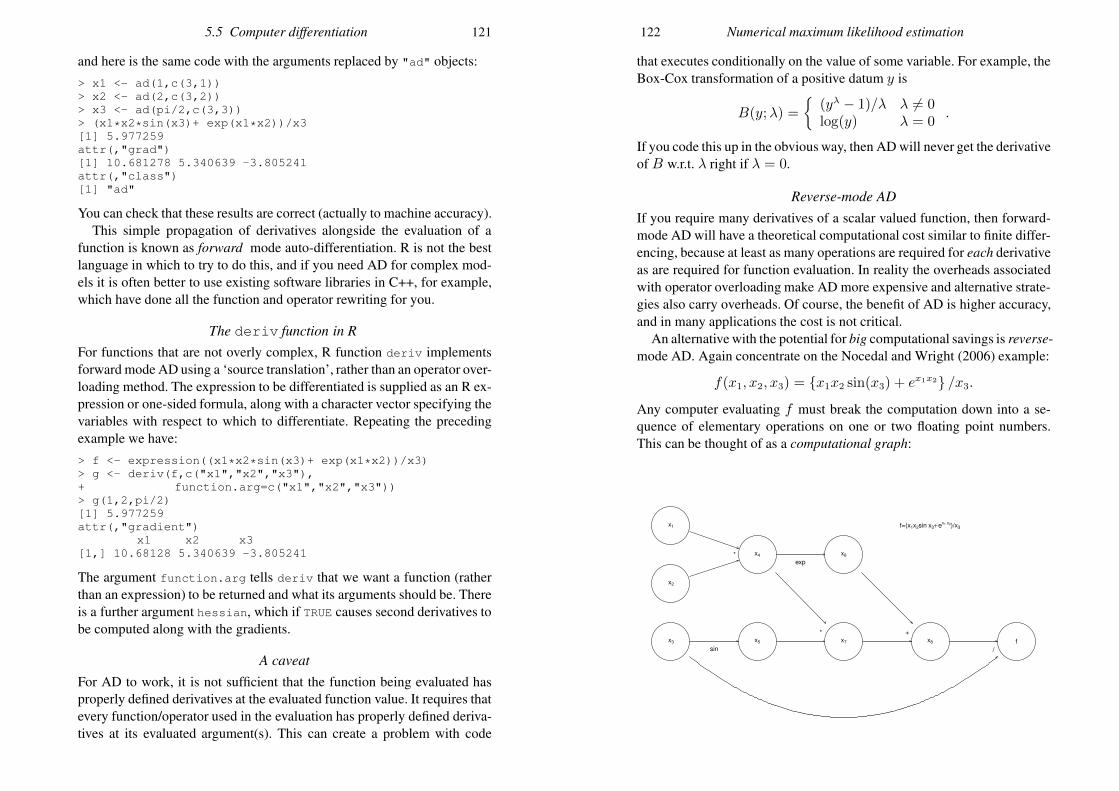
5.5 Computer differentiation 121
and here is the same code with the arguments replaced by "ad" objects:
> x1 <- ad(1,c(3,1))> x2 <- ad(2,c(3,2))> x3 <- ad(pi/2,c(3,3))> (x1*x2*sin(x3)+ exp(x1*x2))/x3[1] 5.977259attr(,"grad")[1] 10.681278 5.340639 -3.805241attr(,"class")[1] "ad"
You can check that these results are correct (actually to machine accuracy).This simple propagation of derivatives alongside the evaluation of a
function is known as forward mode auto-differentiation. R is not the bestlanguage in which to try to do this, and if you need AD for complex mod-els it is often better to use existing software libraries in C++, for example,which have done all the function and operator rewriting for you.
The deriv function in RFor functions that are not overly complex, R function deriv implementsforward mode AD using a ‘source translation’, rather than an operator over-loading method. The expression to be differentiated is supplied as an R ex-pression or one-sided formula, along with a character vector specifying thevariables with respect to which to differentiate. Repeating the precedingexample we have:
> f <- expression((x1*x2*sin(x3)+ exp(x1*x2))/x3)> g <- deriv(f,c("x1","x2","x3"),+ function.arg=c("x1","x2","x3"))> g(1,2,pi/2)[1] 5.977259attr(,"gradient")
x1 x2 x3[1,] 10.68128 5.340639 -3.805241
The argument function.arg tells deriv that we want a function (ratherthan an expression) to be returned and what its arguments should be. Thereis a further argument hessian, which if TRUE causes second derivatives tobe computed along with the gradients.
A caveatFor AD to work, it is not sufficient that the function being evaluated hasproperly defined derivatives at the evaluated function value. It requires thatevery function/operator used in the evaluation has properly defined deriva-tives at its evaluated argument(s). This can create a problem with code
122 Numerical maximum likelihood estimation
that executes conditionally on the value of some variable. For example, theBox-Cox transformation of a positive datum y is
B(y;λ) =
(yλ − 1)/λ λ 6= 0log(y) λ = 0
.
If you code this up in the obvious way, then AD will never get the derivativeof B w.r.t. λ right if λ = 0.
Reverse-mode ADIf you require many derivatives of a scalar valued function, then forward-mode AD will have a theoretical computational cost similar to finite differ-encing, because at least as many operations are required for each derivativeas are required for function evaluation. In reality the overheads associatedwith operator overloading make AD more expensive and alternative strate-gies also carry overheads. Of course, the benefit of AD is higher accuracy,and in many applications the cost is not critical.
An alternative with the potential for big computational savings is reverse-mode AD. Again concentrate on the Nocedal and Wright (2006) example:
f(x1, x2, x3) = x1x2 sin(x3) + ex1x2 /x3.
Any computer evaluating f must break the computation down into a se-quence of elementary operations on one or two floating point numbers.This can be thought of as a computational graph:
f=(x1x2sin x3+ ex1 x2)/x3
x1
x2
x3
sin
x4
exp
x5
x6
x7 x8 f
*
* +
/
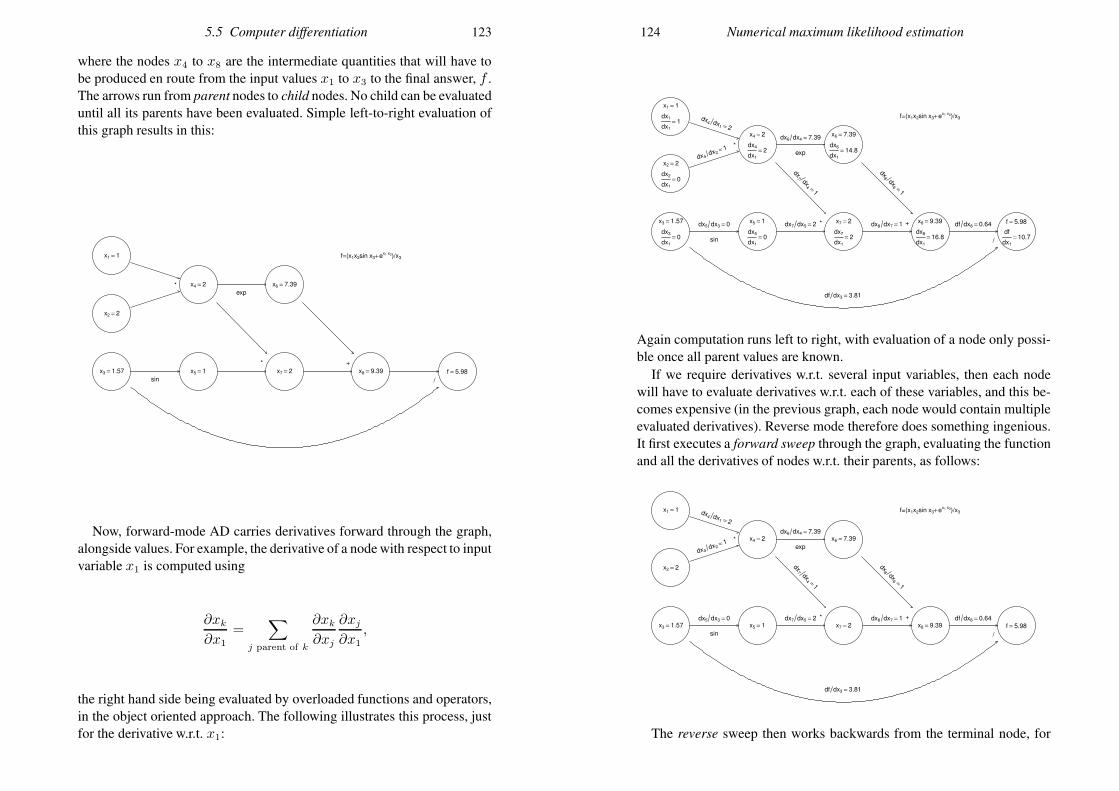
5.5 Computer differentiation 123
where the nodes x4 to x8 are the intermediate quantities that will have tobe produced en route from the input values x1 to x3 to the final answer, f .The arrows run from parent nodes to child nodes. No child can be evaluateduntil all its parents have been evaluated. Simple left-to-right evaluation ofthis graph results in this:
f=(x1x2sin x3+ ex1 x2)/x3x1 = 1
x2 = 2
x3 = 1.57
sin
x4 = 2
exp
x5 = 1
x6 = 7.39
x7 = 2 x8 = 9.39 f = 5.98
*
* +
/
Now, forward-mode AD carries derivatives forward through the graph,alongside values. For example, the derivative of a node with respect to inputvariable x1 is computed using
∂xk∂x1
=∑
j parent of k
∂xk∂xj
∂xj∂x1
,
the right hand side being evaluated by overloaded functions and operators,in the object oriented approach. The following illustrates this process, justfor the derivative w.r.t. x1:
124 Numerical maximum likelihood estimation
f=(x1x2sin x3+ ex1 x2)/x3
x1 = 1
dx1
dx1
= 1dx
4 dx1 = 2
x2 = 2
dx2
dx1
= 0
dx4dx2
= 1
x3 = 1.57
dx3
dx1
= 0 sin
dx5 dx3 = 0
df dx3 = 3.81
x4 = 2
dx4
dx1
= 2 exp
dx6 dx4 = 7.39
dx7dx
4 =1
x5 = 1
dx5
dx1
= 0
dx7 dx5 = 2
x6 = 7.39
dx6
dx1
= 14.8
dx8dx
6 =1
x7 = 2
dx7
dx1
= 2
dx8 dx7 = 1x8 = 9.39
dx8
dx1
= 16.8
df dx8 = 0.64 f = 5.98
df
dx1
= 10.7
*
* +
/
Again computation runs left to right, with evaluation of a node only possi-ble once all parent values are known.
If we require derivatives w.r.t. several input variables, then each nodewill have to evaluate derivatives w.r.t. each of these variables, and this be-comes expensive (in the previous graph, each node would contain multipleevaluated derivatives). Reverse mode therefore does something ingenious.It first executes a forward sweep through the graph, evaluating the functionand all the derivatives of nodes w.r.t. their parents, as follows:
f=(x1x2sin x3+ ex1 x2)/x3x1 = 1 dx
4 dx1 = 2
x2 = 2
dx4dx2
= 1
x3 = 1.57
sin
dx5 dx3 = 0
df dx3 = 3.81
x4 = 2
exp
dx6 dx4 = 7.39
dx7dx
4 =1
x5 = 1dx7 dx5 = 2
x6 = 7.39
dx8dx
6 =1
x7 = 2dx8 dx7 = 1
x8 = 9.39df dx8 = 0.64
f = 5.98
*
* +
/
The reverse sweep then works backwards from the terminal node, for
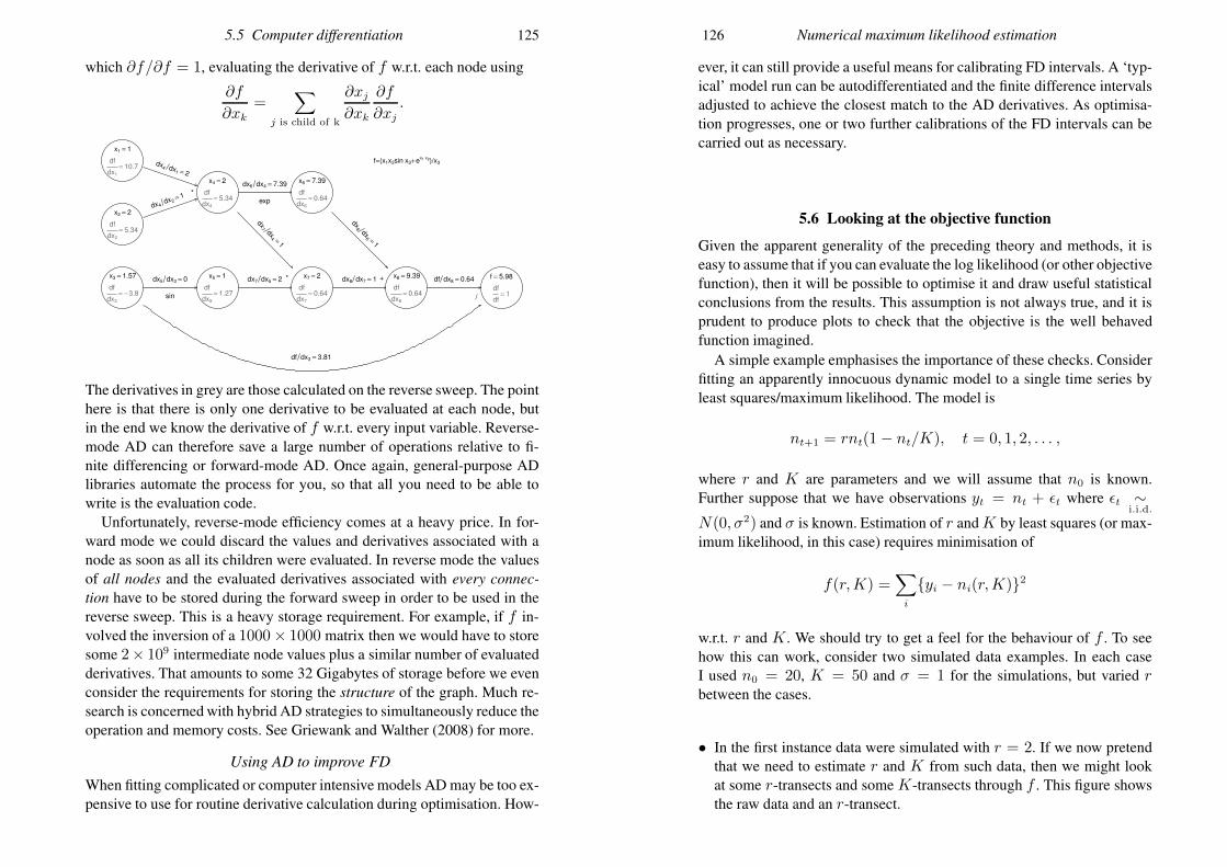
5.5 Computer differentiation 125
which ∂f/∂f = 1, evaluating the derivative of f w.r.t. each node using
∂f
∂xk=
∑
j is child of k
∂xj∂xk
∂f
∂xj.
f=(x1x2sin x3+ ex1 x2)/x3
x1 = 1
df
dx1
= 10.7dx
4 dx1 = 2
x2 = 2
df
dx2
= 5.34
dx4dx2
= 1
x3 = 1.57
df
dx3
= − 3.8 sin
dx5 dx3 = 0
df dx3 = 3.81
x4 = 2
df
dx4
= 5.34 exp
dx6 dx4 = 7.39
dx7dx
4 =1
x5 = 1
df
dx5
= 1.27
dx7 dx5 = 2
x6 = 7.39
df
dx6
= 0.64
dx8dx
6 =1
x7 = 2
df
dx7
= 0.64
dx8 dx7 = 1x8 = 9.39
df
dx8
= 0.64
df dx8 = 0.64 f = 5.98
df
df= 1
*
* +
/
The derivatives in grey are those calculated on the reverse sweep. The pointhere is that there is only one derivative to be evaluated at each node, butin the end we know the derivative of f w.r.t. every input variable. Reverse-mode AD can therefore save a large number of operations relative to fi-nite differencing or forward-mode AD. Once again, general-purpose ADlibraries automate the process for you, so that all you need to be able towrite is the evaluation code.
Unfortunately, reverse-mode efficiency comes at a heavy price. In for-ward mode we could discard the values and derivatives associated with anode as soon as all its children were evaluated. In reverse mode the valuesof all nodes and the evaluated derivatives associated with every connec-tion have to be stored during the forward sweep in order to be used in thereverse sweep. This is a heavy storage requirement. For example, if f in-volved the inversion of a 1000× 1000 matrix then we would have to storesome 2× 10⁹ intermediate node values plus a similar number of evaluatedderivatives. That amounts to some 32 Gigabytes of storage before we evenconsider the requirements for storing the structure of the graph. Much re-search is concerned with hybrid AD strategies to simultaneously reduce theoperation and memory costs. See Griewank and Walther (2008) for more.
Using AD to improve FDWhen fitting complicated or computer intensive models AD may be too ex-pensive to use for routine derivative calculation during optimisation. How-
126 Numerical maximum likelihood estimation
ever, it can still provide a useful means for calibrating FD intervals. A ‘typ-ical’ model run can be autodifferentiated and the finite difference intervalsadjusted to achieve the closest match to the AD derivatives. As optimisa-tion progresses, one or two further calibrations of the FD intervals can becarried out as necessary.
5.6 Looking at the objective function
Given the apparent generality of the preceding theory and methods, it iseasy to assume that if you can evaluate the log likelihood (or other objectivefunction), then it will be possible to optimise it and draw useful statisticalconclusions from the results. This assumption is not always true, and it isprudent to produce plots to check that the objective is the well behavedfunction imagined.
A simple example emphasises the importance of these checks. Considerfitting an apparently innocuous dynamic model to a single time series byleast squares/maximum likelihood. The model is
nt+1 = rnt(1− nt/K), t = 0, 1, 2, . . . ,
where r and K are parameters and we will assume that n0 is known.Further suppose that we have observations yt = nt + ǫt where ǫt ∼
i.i.d.
N(0, σ2) and σ is known. Estimation of r and K by least squares (or max-imum likelihood, in this case) requires minimisation of
f(r,K) =∑
i
yi − ni(r,K)2
w.r.t. r and K . We should try to get a feel for the behaviour of f . To seehow this can work, consider two simulated data examples. In each caseI used n0 = 20, K = 50 and σ = 1 for the simulations, but varied rbetween the cases.
• In the first instance data were simulated with r = 2. If we now pretendthat we need to estimate r and K from such data, then we might lookat some r-transects and some K-transects through f . This figure showsthe raw data and an r-transect.
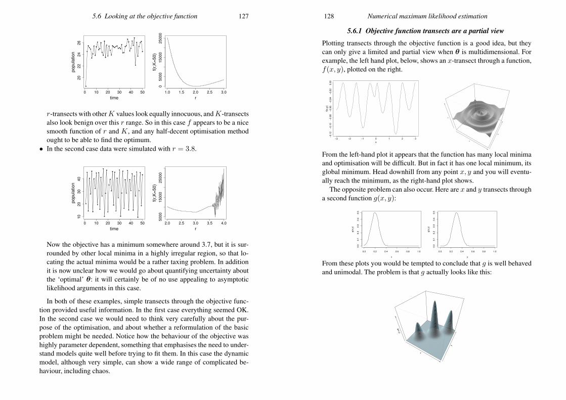
5.6 Looking at the objective function 127
0 10 20 30 40 50
20
22
24
26
time
popula
tion
1.0 1.5 2.0 2.5 3.0
05000
15000
25000
r
f(r,
K=
50)
r-transects with otherK values look equally innocuous, andK-transectsalso look benign over this r range. So in this case f appears to be a nicesmooth function of r and K , and any half-decent optimisation methodought to be able to find the optimum.
• In the second case data were simulated with r = 3.8.
0 10 20 30 40 50
10
20
30
40
time
popula
tion
2.0 2.5 3.0 3.5 4.0
5000
15000
25000
r
f(r,
K=
50)
Now the objective has a minimum somewhere around 3.7, but it is sur-rounded by other local minima in a highly irregular region, so that lo-cating the actual minima would be a rather taxing problem. In additionit is now unclear how we would go about quantifying uncertainty aboutthe ‘optimal’ θ: it will certainly be of no use appealing to asymptoticlikelihood arguments in this case.
In both of these examples, simple transects through the objective func-tion provided useful information. In the first case everything seemed OK.In the second case we would need to think very carefully about the pur-pose of the optimisation, and about whether a reformulation of the basicproblem might be needed. Notice how the behaviour of the objective washighly parameter dependent, something that emphasises the need to under-stand models quite well before trying to fit them. In this case the dynamicmodel, although very simple, can show a wide range of complicated be-haviour, including chaos.
128 Numerical maximum likelihood estimation
5.6.1 Objective function transects are a partial view
Plotting transects through the objective function is a good idea, but theycan only give a limited and partial view when θ is multidimensional. Forexample, the left hand plot, below, shows an x-transect through a function,f(x, y), plotted on the right.
−3 −2 −1 0 1 2 3
−0
.12
−0
.10
−0
.08
−0
.06
−0
.04
−0
.02
0.0
0
x
f(x,y
)
x
y
z
From the left-hand plot it appears that the function has many local minimaand optimisation will be difficult. But in fact it has one local minimum, itsglobal minimum. Head downhill from any point x, y and you will eventu-ally reach the minimum, as the right-hand plot shows.
The opposite problem can also occur. Here are x and y transects througha second function g(x, y):
0.0 0.2 0.4 0.6 0.8 1.0
0.0
0.1
0.2
0.3
0.4
0.5
x
g(x
,y)
0.0 0.2 0.4 0.6 0.8 1.0
0.0
0.1
0.2
0.3
0.4
0.5
y
g(x
,y)
From these plots you would be tempted to conclude that g is well behavedand unimodal. The problem is that g actually looks like this:
x
y
g(x,y)
5.7 Dealing with multimodality 129
So, generally speaking, it is a good idea to plot transects through the ob-jective function before optimisation, and to plot transects passing throughthe apparent optimum after optimisation. However, bear in mind that tran-sects only give partial views.
5.7 Dealing with multimodality
There is no universal prescription for dealing with multimodality, but thefollowing approaches may help:
• A common recommendation is to repeat optimisation a number of timesfrom radically different starting values, perhaps randomly generated.This can help to indicate multimodality and to find the dominant mode.
• For relatively small-scale local optima, a bootstrapping approach can behelpful. Suppose we have a log likelihood, l(θ), based on data vector y.Start with a parameter guess, θ0, and iterate the following steps:
1. Starting at θ0, seek θ = argmaxθ l(θ), by numerical optimisation.2. Resample your data with replacement to produce a resampled data
vector y∗ and corresponding log-likelihood function l∗(θ).3. Starting at θ, seek θ0 = argmaxθ l
∗(θ), by numerical optimisation.
Any auxiliary data are resampled alongside y (so that auxilliary datastay with the datum to which they belong). The idea is that by randomlyperturbing the objective, it may be possible to escape local optima. Forgreater perturbation, smaller re-samples can be used.
• It the objective appears pathologically multimodal, it is probably time toreformulate the question being addressed.
Exercises5.1 Rosenbrock’s function f(x, z) = a(z − x2)2 + (b − x)2 is a classic test
function for optimisation methods. Usually a = 100 and b = 1.
a. Write a function Rosenbrockwith vector arguments x and z and scalararguments a and b, with default values of 10 and 1, respectively. Usingcontour and outer, produce a contour plot of f for −1.5 ≤ x ≤ 1.5
and −0.5 ≤ z ≤ 1.5.b. Write a modified version of Rosenbrock, suitable for optimisation us-
ing optim. Optimise Rosenbrock using optim with starting valuesx = −1, z = 1, and compare results using Nelder-Mead and BFGS.
c. Repeat the optimisation using nlm and nlminb.
130 Numerical maximum likelihood estimation
5.2 Write your own code to optimise Rosenbrock’s function by Newton’s method.Optionally use R’s symbolic or automatic differentiation functions to obtainthe required gradient and Hessian.
5.3 Write your own code to optimise Rosenbrock’s function by BFGS.5.4 Write functions suitable for use with optim to evaluate the negative log
likelihood and its gradient for the cell count example in Section 5.1.1. Hence,find the MLE of δ using optim. Compute and compare 95% confidenceintervals for δ based on the Hessian of the log likelihood and generalisedlikelihood ratio test inversion.
5.5 Write a function suitable for use with optim to evaluate the negative loglikelihood of the AIDS cases model of Section 5.1.1 (use dpois with thelog=TRUE option). Write a second function evaluating the negative log like-lihood of an extended version of the model in which the dependence of thelog case rate on time is quadratic, rather than linear. Use a generalised likeli-hood ratio test (GLRT) to compare the models, and also compute their AICvalues. What aspect of the GLRT might be suspect here?
5.6 R package MASS contains a dataframe geyser where geyser$waiting
gives the waiting times between eruptions of the Old Faithful geyser in Yel-lowstone National Park. A possible model is that that the waiting times, ti,are independently drawn from a mixture of two normal distributions, withp.d.f.
f(ti) =φ√2πσ1
e− 1
2σ21(ti−µ1)
2
+1− φ√2πσ2
e− 1
2σ22(ti−µ2)
2
,
where parameter φ is bounded between 0 and 1. Find MLEs for the param-eters and test whether p = 0.5. Are there any theoretical caveats on thisanalysis? Produce appropriate model checking plots (not ‘residual’ plots!).
5.7 R package faraway contains data from an experiment on balance in humansubjects. There were 40 subjects, and the experiment was repeated a numberof times on each, standing on two different surfaces under three differentdegrees of restriction of vision. Sex, age, height and weight of the subjectswere recorded. The following code loads the data, creates a variable indicat-ing whether subjects were judged fully stable (1) or not (0), and convertsthe subject identifiers to a factor variable:
library(faraway)ctsib$stable <- ifelse(ctsib$CTSIB==1,1,0)ctsib$Subject <- factor(ctsib$Subject)
Interest lies is in explaining stability in terms of the other variables. A pos-sible model for the data involves a vector of subject-specific random effectsb, and is as follows:
stablei|b ∼ Bernoulli(µi) µi = eηi/(1 + eηi ),
where if measurement i if for subject j, of sex k, on surface m, and with
Exercises 131
vision restriction q, then
ηi = α+ γk + δm + φq + βHeighti + bj ,
where bj ∼ N(0, σ2b ) (independent). The subject-specific random effects are
important, because we would expect subject-to-subject variability in theirbalancing ability. More generally we can write the model for ηi in vectormatrix form as
η = Xβ + Zb, b ∼ N(0, Iσ2b ).
X contains a column of Height data and columns of zeroes and ones iden-tifying measurements to particular groups (Sex, Vision, etc.). Z containszeroes and ones in order to pick out the correct bj for each data row. Thefollowing code creates suitable matrices:
X <- model.matrix(~ Sex+Height+Surface+Vision,ctsib)Z <- model.matrix(~ Subject-1,ctsib)
a. Write an R function to evaluate the joint probability/density of stableand the subject-specific random effects, along with its gradient and theleading diagonal of its Hessian w.r.t. b. Only the leading diagonal of theHessian is required, as it turns out to be a diagonal matrix.
b. Write an R function to evaluate the negative log likelihood of the modelparameters, integrating out b by Laplace approximation.
c. Fit the model using optim to find the MLE.
6
Bayesian computation
Recall that the Bayesian approach to statistics views the model parameters,θ, as random variables with prior p.d.f., f(θ), and then answers the basicquestions of statistical inference using the posterior p.d.f.
f(θ|y) = f(y|θ)f(θ)f(y)
,
(see Section 2.5). The principal practical challenges are that
f(y) =
∫f(y|θ)f(θ)dθ (6.1)
is usually intractable for interesting models and that it is usually equallyintractable integrals of f(θ|y) that are of direct interest. There are thentwo main strategies for making progress: either approximate the requiredintegrals or find a way of simulating from f(θ|y) without requiring suchintegrals. The latter strategy is based on the fact that, for many statisticalpurposes, the ability to simulate from a density is as good as being ableto evaluate the density, and sometimes better. Hybrid strategies are alsouseful. For much more on the topics covered here see Gamerman and Lopes(2006), Robert and Casella (2009), Gelman et al. (2013) and, at a moreadvanced level, Robert (2007).
6.1 Approximating the integrals
One possibility is to evaluate the normalising constant (6.1), and other in-teresting integrals, using Laplace approximation. For example, integrateout θ in exactly the same way as b was integrated out in Section 5.3.1.This relies on the integrand having only one important mode and, in thecontext of (6.1), is unlikely to result in an exactly proper posterior f(θ|y).
Another approximation is based on recognising, from (6.1), that f(y) =
132
6.1 Approximating the integrals 133
Eθf(y|θ), and to approximate this expectation using the simulationtechnique known as importance sampling. The idea is simple. Suppose wewant to estimate α = Efφ(X) where X ∼ f(x). An obvious unbiasedestimator is obtained by simulating n deviates, xi, from f(x) and settingα′ =
∑i φ(xi)/n. The problem is that φ(xi) may be very close to zero for
many of the xi, so that our estimate is really based only on the few pointsfor which φ was non-negligible, making the approximation inaccurate andhighly variable. If we have access to a p.d.f. g(z) that has high probabilitywhere φ(z) is high, and low probability otherwise, then we could use thefact that α = Efφ(X) = Egφ(Z)f(Z)/g(Z) to obtain the alterna-tive unbiased estimator:
α =1
n
n∑
i=1
φ(zi)f(zi)/g(zi) where zi ∼ g(z).
This importance sampling estimator tends to improve on the naive version,by placing the zi in better locations w.r.t. φ. The f(zi)/g(zi) are known asimportance weights. A problem in Bayesian analysis is that f(zi) is oftenan un-normalised density, so it is necessary to normalise the importanceweights, leading to the modified importance sampling estimator,
α =
∑ni=1 φ(zi)f(zi)/g(zi)∑n
i=1 f(zi)/g(zi)where zi ∼ g(z),
which can also be used directly for other integrals of more immediate in-terest than (6.1).
In the context of (6.1), it can be attractive to use the p.d.f. of
N(θ, −∇2θ log f(y, θ)−1) (6.2)
as g(θ), where θ is the maximiser of f(y,θ). This is motivated by theLaplace approximation. Alternatively, to reduce the risk of extreme weightsin the tails of the distribution, tk(θ, −∇2
θ log f(y, θ)−1) can be used forg, with k set to a small integer (see Section 1.6.1). Similar proposals canbe constructed for other integrals of interest.
Usually the quantities required from the posterior are expectations offunctions of θ according to the posterior distribution. That is, we requireintegrals of the form
∫φ(θ)f(θ|y)dθ =
∫φ(θ)f(y|θ)f(θ)dθ∫f(y|θ)f(θ)dθ ,
and these can be estimated by direct application of (5.14) in Section 5.3.2.
134 Bayesian computation
6.2 Markov chain Monte Carlo
The approximation methods just described are useful when we know thatthe posterior distribution has a relatively simple form, preferably with a sin-gle mode. However, these assumptions are doubtful in many cases wherethe Bayesian approach is appealing, and more general methods are thenrequired. The key is to use the fact that
f(θ|y) ∝ f(θ,y) (= f(y|θ)f(θ)) ,to devise methods for simulating from f(θ|y), which only require evalu-ation of f(θ,y) with the observed data values plugged in for y. The re-sulting Markov chain Monte Carlo (MCMC) methods simulate (correlated)samples from the distribution of the model unknowns (parameters and anyrandom effects), given the data. Based on the unknowns at one step, a newset of unknowns is generated in such a way that the stable distribution ofthe resulting Markov chain is the distribution of interest. The developmentof MCMC methods relies on being able to generate apparently randomnumbers by computer: Appendix C discusses the extent to which this ispossible.
6.2.1 Markov chains
To use MCMC we do not require much theoretical background on Markovchains, but some basic concepts are needed. A sequence of random vectors,X1,X2,X3, . . ., constitutes a Markov chain if, for any j,
f(xj |xj−1,xj−2, . . . ,x1) = f(xj |xj−1).
For notational convenience let us rewrite the density of xj given xj−1 asP (xj |xj−1), the transition kernel of the Markov chain. If there exists adensity fx such that
fx(xj) =
∫P (xj |xj−1)fx(xj−1)dxj−1
(where fx denotes the same density on both sides), then this is the station-ary distribution of the chain. Existence of a stationary distribution dependson P being irreducible, meaning that wherever we start the chain, there isa positive probability of visiting all possible values of X. If the chain isalso recurrent, meaning that if its length tends to infinity it will revisit anynon-negligible set of values an infinite number of times, then its station-ary distribution is also its limiting distribution. This means that the chaincan be started from any possible value of X, and its marginal distribution
6.2 Markov chain Monte Carlo 135
will eventually converge on fx. In consequence as the simulation length,J , tends to infinity,
1
J
J∑
j=1
φ(Xj)→ Efxφ(X)
(also known as ergodicity). This extension of the law of large numbers (seeSection 1.10.2) to this particular sort of correlated sequence is what makesMCMC methods useful, so the methods discussed in this chapter will beset up to produce chains with the required properties.
6.2.2 Reversibility
Now we turn to the issue of constructing Markov chains to generate se-quences θ1,θ2, . . . from f(θ|y). An MCMC scheme will generate sam-ples from f(θ|y), if it satisfies the detailed balance condition (also termedreversibility). Let P (θi|θj) be the p.d.f. of θi given θj , according to thechain. We require
P (θj |θj−1)f(θj−1|y) = P (θj−1|θj)f(θj |y). (6.3)
The left hand side of (6.3) is the joint p.d.f. of θj ,θj−1 from the chain,if θj−1 is from f(θ|y). Integrating w.r.t. θj−1 gives the correspondingmarginal density of θj ,
∫P (θj |θj−1)f(θj−1|y)dθj−1 =
∫P (θj−1|θj)f(θj |y)dθj−1
= f(θj |y).That is, given θj−1 from f(θ|y), the chain generates θj also from f(θ|y)as result of (6.3). So provided that we start with a θ1 that is not impossibleaccording to f(θ|y), then the chain will generate from the target distribu-tion. How quickly it will converge to the high-probability region of f(θ|y)is another matter.
6.2.3 Metropolis Hastings
The Metropolis-Hastings method constructs a chain with an appropriateP .It works as follows:
1. Pick a proposal distribution q(θj |θj−1) (e.g. a normal centred on θj−1).Then pick a value θ0, set j = 1 and iterate steps 2 and 3:
136 Bayesian computation
2. Generate θ′j from q(θj |θj−1).
3. Set θj = θ′j with probability
α = min
1,
f(y|θ′j)f(θ
′j)q(θj−1|θ′
j)
f(y|θj−1)f(θj−1)q(θ′j |θj−1)
, (6.4)
otherwise setting θj = θj−1. Increment j.
Note that the q terms cancel if q depends only on the magnitude of θj −θj−1 (e.g. if q is a normal centred on θj−1). The same goes for the priordensities, f(θ), if they are improper uniform. If both of these simplifica-tions hold then we have α = min
1, L(θ′
j)/L(θj−1), so that we are
accepting or rejecting on the basis of the likelihood ratio.An important consideration is that θ1 may be very improbable so that
the chain may take many iterations to reach the high-probability regionof f(θ|y). For this reason we usually need to discard a burn-in periodconsisting of the first few hundred or thousand θj vectors simulated.
6.2.4 Why Metropolis Hastings works
As we saw in Section 6.2.2, the Metropolis-Hastings (MH) method willwork if it satisfies detailed balance. It does, and proof is easy. To simplifynotation let π(θ) = f(θ|y) ∝ f(y|θ)f(θ), so that the MH acceptanceprobability from θ to θ′ is
α(θ′,θ) = min
1,
π(θ′)q(θ|θ′)
π(θ)q(θ′|θ)
.
We need to show that π(θ)P (θ′|θ) = π(θ′)P (θ|θ′). This is trivial ifθ′ = θ. Otherwise we know that P (θ′|θ) = q(θ′|θ)α(θ′,θ), from whichit follows that
π(θ)P (θ′|θ) = π(θ)q(θ′|θ)min
1,
π(θ′)q(θ|θ′)
π(θ)q(θ′|θ)
= min π(θ)q(θ′|θ), π(θ′)q(θ|θ′) = π(θ′)P (θ|θ′),
where the final equality is by symmetry of the third term above.
6.2.5 A toy example with Metropolis Hastings
To illustrate the basic simplicity of the approach, consider an example forwhich simulation is certainly not required. Suppose we have 20 indepen-dent observations xi, that can each be modelled as N(µ, σ2) random vari-
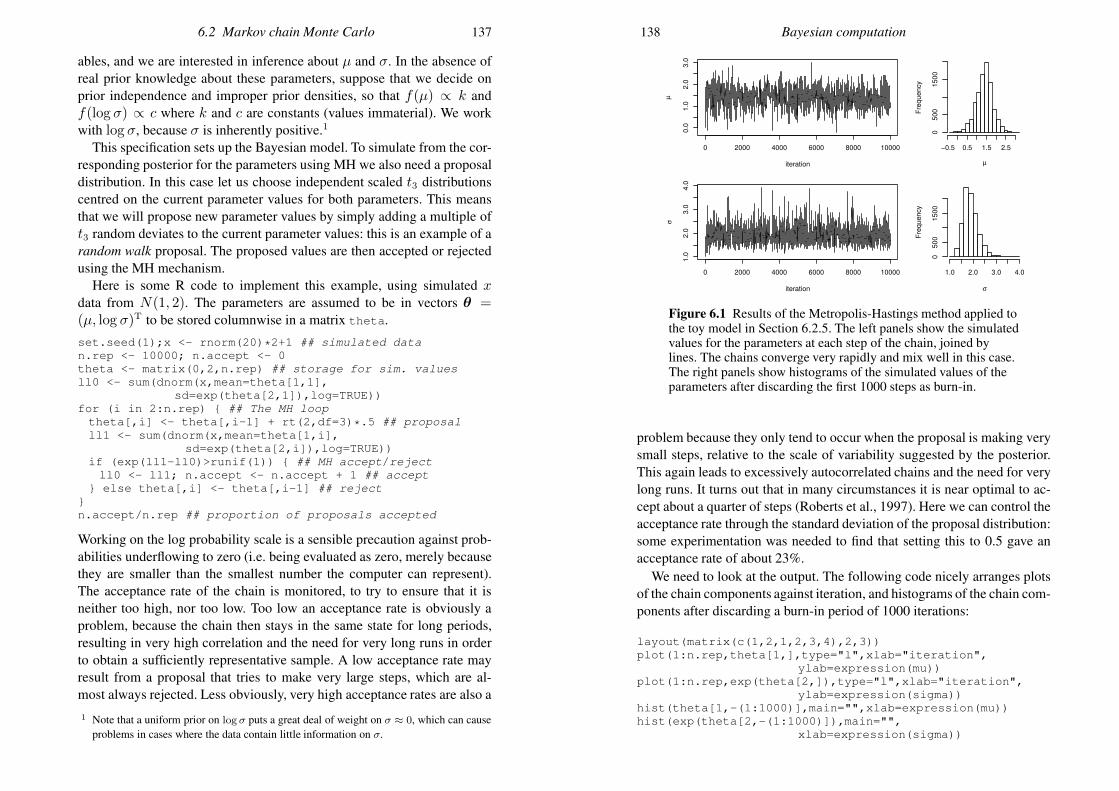
6.2 Markov chain Monte Carlo 137
ables, and we are interested in inference about µ and σ. In the absence ofreal prior knowledge about these parameters, suppose that we decide onprior independence and improper prior densities, so that f(µ) ∝ k andf(log σ) ∝ c where k and c are constants (values immaterial). We workwith log σ, because σ is inherently positive.1
This specification sets up the Bayesian model. To simulate from the cor-responding posterior for the parameters using MH we also need a proposaldistribution. In this case let us choose independent scaled t3 distributionscentred on the current parameter values for both parameters. This meansthat we will propose new parameter values by simply adding a multiple oft3 random deviates to the current parameter values: this is an example of arandom walk proposal. The proposed values are then accepted or rejectedusing the MH mechanism.
Here is some R code to implement this example, using simulated xdata from N(1, 2). The parameters are assumed to be in vectors θ =(µ, log σ)T to be stored columnwise in a matrix theta.
set.seed(1);x <- rnorm(20)*2+1 ## simulated datan.rep <- 10000; n.accept <- 0theta <- matrix(0,2,n.rep) ## storage for sim. valuesll0 <- sum(dnorm(x,mean=theta[1,1],
sd=exp(theta[2,1]),log=TRUE))for (i in 2:n.rep) ## The MH looptheta[,i] <- theta[,i-1] + rt(2,df=3)*.5 ## proposalll1 <- sum(dnorm(x,mean=theta[1,i],
sd=exp(theta[2,i]),log=TRUE))if (exp(ll1-ll0)>runif(1)) ## MH accept/rejectll0 <- ll1; n.accept <- n.accept + 1 ## accept
else theta[,i] <- theta[,i-1] ## rejectn.accept/n.rep ## proportion of proposals accepted
Working on the log probability scale is a sensible precaution against prob-abilities underflowing to zero (i.e. being evaluated as zero, merely becausethey are smaller than the smallest number the computer can represent).The acceptance rate of the chain is monitored, to try to ensure that it isneither too high, nor too low. Too low an acceptance rate is obviously aproblem, because the chain then stays in the same state for long periods,resulting in very high correlation and the need for very long runs in orderto obtain a sufficiently representative sample. A low acceptance rate mayresult from a proposal that tries to make very large steps, which are al-most always rejected. Less obviously, very high acceptance rates are also a1 Note that a uniform prior on log σ puts a great deal of weight on σ ≈ 0, which can cause
problems in cases where the data contain little information on σ.
138 Bayesian computation
0 2000 4000 6000 8000 10000
0.0
1.0
2.0
3.0
iteration
µ
0 2000 4000 6000 8000 10000
1.0
2.0
3.0
4.0
iteration
σ
µ
Fre
quency
−0.5 0.5 1.5 2.5
0500
1500
σ
Fre
quency
1.0 2.0 3.0 4.0
0500
1500
Figure 6.1 Results of the Metropolis-Hastings method applied tothe toy model in Section 6.2.5. The left panels show the simulatedvalues for the parameters at each step of the chain, joined bylines. The chains converge very rapidly and mix well in this case.The right panels show histograms of the simulated values of theparameters after discarding the first 1000 steps as burn-in.
problem because they only tend to occur when the proposal is making verysmall steps, relative to the scale of variability suggested by the posterior.This again leads to excessively autocorrelated chains and the need for verylong runs. It turns out that in many circumstances it is near optimal to ac-cept about a quarter of steps (Roberts et al., 1997). Here we can control theacceptance rate through the standard deviation of the proposal distribution:some experimentation was needed to find that setting this to 0.5 gave anacceptance rate of about 23%.
We need to look at the output. The following code nicely arranges plotsof the chain components against iteration, and histograms of the chain com-ponents after discarding a burn-in period of 1000 iterations:
layout(matrix(c(1,2,1,2,3,4),2,3))plot(1:n.rep,theta[1,],type="l",xlab="iteration",
ylab=expression(mu))plot(1:n.rep,exp(theta[2,]),type="l",xlab="iteration",
ylab=expression(sigma))hist(theta[1,-(1:1000)],main="",xlab=expression(mu))hist(exp(theta[2,-(1:1000)]),main="",
xlab=expression(sigma))
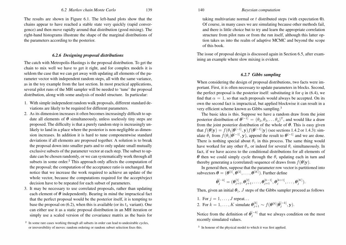
6.2 Markov chain Monte Carlo 139
The results are shown in Figure 6.1. The left-hand plots show that thechains appear to have reached a stable state very quickly (rapid conver-gence) and then move rapidly around that distribution (good mixing). Theright-hand histograms illustrate the shape of the marginal distributions ofthe parameters according to the posterior.
6.2.6 Designing proposal distributions
The catch with Metropolis-Hastings is the proposal distribution. To get thechain to mix well we have to get it right, and for complex models it isseldom the case that we can get away with updating all elements of the pa-rameter vector with independent random steps, all with the same variance,as in the toy example from the last section. In most practical applications,several pilot runs of the MH sampler will be needed to ‘tune’ the proposaldistribution, along with some analysis of model structure. In particular:
1. With simple independent random walk proposals, different standard de-viations are likely to be required for different parameters.
2. As its dimension increases it often becomes increasingly difficult to up-date all elements of θ simultaneously, unless uselessly tiny steps areproposed. The difficulty is that a purely random step is increasingly un-likely to land in a place where the posterior is non-negligible as dimen-sion increases. In addition it is hard to tune componentwise standarddeviations if all elements are proposed together. A solution is to breakthe proposal down into smaller parts and to only update small mutuallyexclusive subsets of the parameter vector at each step. The subset to up-date can be chosen randomly, or we can systematically work through allsubsets in some order.2 This approach only affects the computation ofthe proposal; the computation of the acceptance ratio is unchanged. Butnotice that we increase the work required to achieve an update of thewhole vector, because the computations required for the accept/rejectdecision have to be repeated for each subset of parameters.
3. It may be necessary to use correlated proposals, rather than updatingeach element of θ independently. Bearing in mind the impractical factthat the perfect proposal would be the posterior itself, it is tempting tobase the proposal on (6.2), when this is available (or its tk variant). Onecan either use it as a static proposal distribution in an MH iteration orsimply use a scaled version of the covariance matrix as the basis for
2 In some rare cases working through all subsets in order can lead to undesirable cycles,or irreversibility of moves: random ordering or random subset selection fixes this.
140 Bayesian computation
taking multivariate normal or t distributed steps (with expectation 0).Of course, in many cases we are simulating because other methods fail,and there is little choice but to try and learn the appropriate correlationstructure from pilot runs or from the run itself, although this latter op-tion takes us into the realm of adaptive MCMC and beyond the scopeof this book.
The issue of proposal design is discussed again in Section 6.5, after exam-ining an example where slow mixing is evident.
6.2.7 Gibbs sampling
When considering the design of proposal distributions, two facts were im-portant. First, it is often necessary to update parameters in blocks. Second,the perfect proposal is the posterior itself: substituting it for q in (6.4), wefind that α = 1, so that such proposals would always be accepted. On itsown the second fact is impractical, but applied blockwise it can result in avery efficient scheme known as Gibbs sampling.3
The basic idea is this. Suppose we have a random draw from the jointposterior distribution of θ[−1] = (θ2, θ3, . . . θq)
T, and would like a drawfrom the joint posterior distribution of the whole of θ. This is easy giventhat f(θ|y) = f(θ1|θ[−1],y)f(θ[−1]|y) (see sections 1.4.2 or 1.4.3): sim-ulate θ1 from f(θ1|θ[−1],y), append the result to θ[−1] and we are done.There is nothing special about θ1 in this process. The same thing wouldhave worked for any other θi, or indeed for several θi simultaneously. Infact, if we have access to the conditional distributions for all elements ofθ then we could simply cycle through the θi updating each in turn andthereby generating a (correlated) sequence of draws from f(θ|y).
In general then, suppose that the parameter row vector is partitioned intosubvectors θ = (θ[1],θ[2], . . . ,θ[K]). Further define
θ[−k]j = (θ
[1]j+1,θ
[2]j+1, . . . ,θ
[k−1]j+1 ,θ
[k+1]j , . . . ,θ
[K]j ).
Then, given an initial θ1, J steps of the Gibbs sampler proceed as follows
1. For j = 1, . . . , J repeat. . .2. For k = 1, . . . ,K simulate θ[k]
j+1 ∼ f(θ[k]|θ[−k]j ,y).
Notice from the definition of θ[−k]j that we always condition on the most
recently simulated values.
3 In honour of the physical model to which it was first applied.
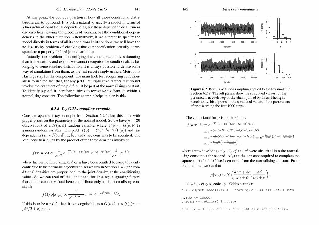
6.2 Markov chain Monte Carlo 141
At this point, the obvious question is how all those conditional distri-butions are to be found. It is often natural to specify a model in terms ofa hierarchy of conditional dependencies, but these dependencies all run inone direction, leaving the problem of working out the conditional depen-dencies in the other direction. Alternatively, if we attempt to specify themodel directly in terms of all its conditional distributions, we will have theno less tricky problem of checking that our specification actually corre-sponds to a properly defined joint distribution.
Actually, the problem of identifying the conditionals is less dauntingthan it first seems, and even if we cannot recognise the conditionals as be-longing to some standard distribution, it is always possible to devise someway of simulating from them, as the last resort simply using a MetropolisHastings step for the component. The main trick for recognising condition-als is to use the fact that, for any p.d.f., multiplicative factors that do notinvolve the argument of the p.d.f. must be part of the normalising constant.To identify a p.d.f. it therefore suffices to recognise its form, to within anormalising constant. The following example helps to clarify this.
6.2.8 Toy Gibbs sampling example
Consider again the toy example from Section 6.2.5, but this time withproper priors on the parameters of the normal model. So we have n = 20observations of a N(µ, φ) random variable, where 1/φ ∼ G(a, b) (agamma random variable, with p.d.f. f(y) = baya−1e−by/Γ(a)) and (in-dependently) µ ∼ N(c, d). a, b, c and d are constants to be specified. Thejoint density is given by the product of the three densities involved:
f(x, µ, φ) ∝ 1
φn/2e−
∑i(xi−µ)2/(2φ)e−(µ−c)2/(2d) 1
φa−1e−b/φ
where factors not involving x, φ or µ have been omitted because they onlycontribute to the normalising constant. As we saw in Section 1.4.2, the con-ditional densities are proportional to the joint density, at the conditioningvalues. So we can read off the conditional for 1/φ, again ignoring factorsthat do not contain φ (and hence contribute only to the normalising con-stant):
f(1/φ|x, µ) ∝ 1
φn/2+a−1e−
∑i(xi−µ)2/(2φ)−b/φ.
If this is to be a p.d.f., then it is recognisable as a G(n/2 + a,∑
i(xi −µ)2/2 + b) p.d.f.
142 Bayesian computation
0 2000 4000 6000 8000 10000
01
23
iteration
µ
0 2000 4000 6000 8000 10000
1.0
2.0
3.0
4.0
iteration
σ
µ
Fre
quency
0 1 2 3 4
01000
3000
σ
Fre
quency
1.0 2.0 3.0 4.0
0500
1500
Figure 6.2 Results of Gibbs sampling applied to the toy model inSection 6.2.8. The left panels show the simulated values for theparameters at each step of the chain, joined by lines. The rightpanels show histograms of the simulated values of the parametersafter discarding the first 1000 steps.
The conditional for µ is more tedious,
f(µ|x, φ) ∝ e−∑
i(xi−µ)2/(2φ)−(µ−c)2/(2d)
∝ e−(nµ2−2xnµ)/(2φ)−(µ2−2µc)/(2d)
= e−1
2φd (dnµ2−2xdnµ+φµ2−2µφc) = e−
dn+φ2φd (µ2−2µ dnx+φc
dn+φ )
∝ e−dn+φ2φd (µ− dnx+φc
dn+φ )2
,
where terms involving only∑
i x2i and c2 were absorbed into the normal-
ising constant at the second ‘∝’, and the constant required to complete thesquare at the final ‘∝’ has been taken from the normalising constant. Fromthe final line, we see that
µ|x, φ ∼ N
(dnx+ φc
dn+ φ,
φd
dn+ φ
).
Now it is easy to code up a Gibbs sampler:n <- 20;set.seed(1);x <- rnorm(n)*2+1 ## simulated data
n.rep <- 10000;thetag <- matrix(0,2,n.rep)
a <- 1; b <- .1; c <- 0; d <- 100 ## prior constants
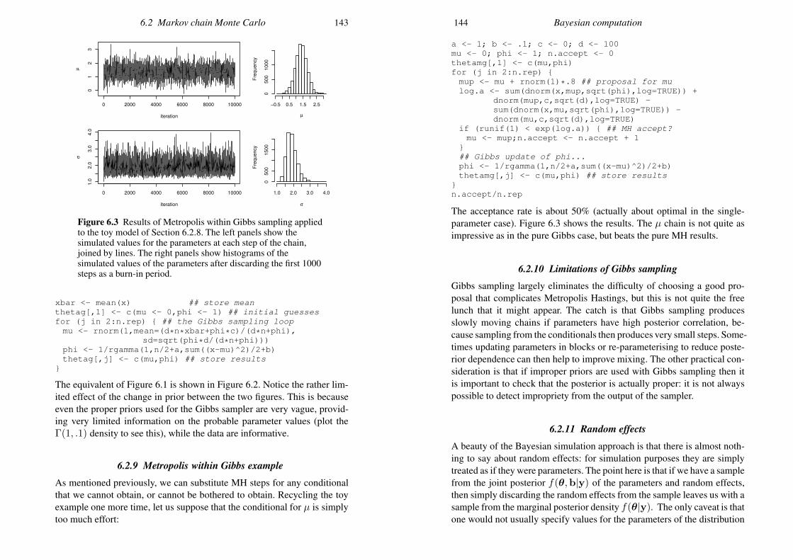
6.2 Markov chain Monte Carlo 143
0 2000 4000 6000 8000 10000
01
23
iteration
µ
0 2000 4000 6000 8000 10000
1.0
2.0
3.0
4.0
iteration
σ
µ
Fre
quency
−0.5 0.5 1.5 2.5
0500
1000
σ
Fre
quency
1.0 2.0 3.0 4.0
0500
1500
Figure 6.3 Results of Metropolis within Gibbs sampling appliedto the toy model of Section 6.2.8. The left panels show thesimulated values for the parameters at each step of the chain,joined by lines. The right panels show histograms of thesimulated values of the parameters after discarding the first 1000steps as a burn-in period.
xbar <- mean(x) ## store meanthetag[,1] <- c(mu <- 0,phi <- 1) ## initial guessesfor (j in 2:n.rep) ## the Gibbs sampling loopmu <- rnorm(1,mean=(d*n*xbar+phi*c)/(d*n+phi),
sd=sqrt(phi*d/(d*n+phi)))phi <- 1/rgamma(1,n/2+a,sum((x-mu)^2)/2+b)thetag[,j] <- c(mu,phi) ## store results
The equivalent of Figure 6.1 is shown in Figure 6.2. Notice the rather lim-ited effect of the change in prior between the two figures. This is becauseeven the proper priors used for the Gibbs sampler are very vague, provid-ing very limited information on the probable parameter values (plot theΓ(1, .1) density to see this), while the data are informative.
6.2.9 Metropolis within Gibbs example
As mentioned previously, we can substitute MH steps for any conditionalthat we cannot obtain, or cannot be bothered to obtain. Recycling the toyexample one more time, let us suppose that the conditional for µ is simplytoo much effort:
144 Bayesian computation
a <- 1; b <- .1; c <- 0; d <- 100mu <- 0; phi <- 1; n.accept <- 0thetamg[,1] <- c(mu,phi)for (j in 2:n.rep) mup <- mu + rnorm(1)*.8 ## proposal for mulog.a <- sum(dnorm(x,mup,sqrt(phi),log=TRUE)) +
dnorm(mup,c,sqrt(d),log=TRUE) -sum(dnorm(x,mu,sqrt(phi),log=TRUE)) -dnorm(mu,c,sqrt(d),log=TRUE)
if (runif(1) < exp(log.a)) ## MH accept?mu <- mup;n.accept <- n.accept + 1
## Gibbs update of phi...phi <- 1/rgamma(1,n/2+a,sum((x-mu)^2)/2+b)thetamg[,j] <- c(mu,phi) ## store results
n.accept/n.rep
The acceptance rate is about 50% (actually about optimal in the single-parameter case). Figure 6.3 shows the results. The µ chain is not quite asimpressive as in the pure Gibbs case, but beats the pure MH results.
6.2.10 Limitations of Gibbs sampling
Gibbs sampling largely eliminates the difficulty of choosing a good pro-posal that complicates Metropolis Hastings, but this is not quite the freelunch that it might appear. The catch is that Gibbs sampling producesslowly moving chains if parameters have high posterior correlation, be-cause sampling from the conditionals then produces very small steps. Some-times updating parameters in blocks or re-parameterising to reduce poste-rior dependence can then help to improve mixing. The other practical con-sideration is that if improper priors are used with Gibbs sampling then itis important to check that the posterior is actually proper: it is not alwayspossible to detect impropriety from the output of the sampler.
6.2.11 Random effects
A beauty of the Bayesian simulation approach is that there is almost noth-ing to say about random effects: for simulation purposes they are simplytreated as if they were parameters. The point here is that if we have a samplefrom the joint posterior f(θ,b|y) of the parameters and random effects,then simply discarding the random effects from the sample leaves us with asample from the marginal posterior density f(θ|y). The only caveat is thatone would not usually specify values for the parameters of the distribution
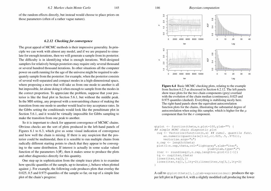
6.2 Markov chain Monte Carlo 145
of the random effects directly, but instead would choose to place priors onthose parameters (often of a rather vague nature).
6.2.12 Checking for convergence
The great appeal of MCMC methods is their impressive generality. In prin-ciple we can work with almost any model, and if we are prepared to simu-late for enough iterations, then we will generate a sample from its posterior.The difficulty is in identifying what is enough iterations. Well-designedsamplers for relatively benign posteriors may require only several thousandor several hundred thousand iterations. In other situations all the computerpower on earth running for the age of the universe might be required to ade-quately sample from the posterior: for example, when the posterior consistsof several well-separated and compact modes in a high-dimensional space,where proposing a move that will take us from one mode to another is allbut impossible, let alone doing it often enough to sample from the modes inthe correct proportion. To appreciate the problem, suppose that your pos-terior is like the final plot in Section 5.6.1, but without the middle peak.In the MH setting, any proposal with a nonvanishing chance of making thetransition from one mode to another would lead to tiny acceptance rates. Inthe Gibbs setting the conditionals would look like the penultimate plot inSection 5.6.1, and it would be virtually impossible for Gibbs sampling tomake the transition from one peak to another.
So it is important to check for apparent convergence of MCMC chains.Obvious checks are the sort of plots produced in the left-hand panels ofFigures 6.1 to 6.3, which give us some visual indication of convergenceand how well the chain is mixing. If there is any suspicion that the pos-terior could be multimodal, then it is sensible to run multiple chains fromradically different starting points to check that they appear to be converg-ing to the same distribution. If interest is actually in some scalar valuedfunction of the parameters h(θ), then it makes sense to produce the plotsand other diagnostics directly for this quantity.
One step up in sophistication from the simple trace plots is to examinehow specific quantiles of the sample, up to iteration j, behave when plottedagainst j. For example, the following code produces plots that overlay the0.025, 0.5 and 0.975 quantiles of the sample so far, on top of a simple lineplot of the chain’s progress:
146 Bayesian computation
0 2000 4000 6000 8000 10000
0.0
1.0
2.0
3.0
iter
µ
0 10 20 30 40
0.0
0.4
0.8
Lag
AC
F
0 2000 4000 6000 8000 10000
1.0
2.0
3.0
4.0
iter
σ
0 10 20 30 40
0.0
0.4
0.8
Lag
AC
F
Figure 6.4 Basic MCMC checking plots, relating to the examplefrom Section 6.2.5 as discussed in Section 6.2.12. The left panelsshow trace plots for the two chain components (grey) overlaidwith the evolution of the chain median (continuous), 0.025 and0.975 quantiles (dashed). Everything is stabilising nicely here.The right-hand panels show the equivalent autocorrelationfunction plots for the chains, illustrating the substantial degree ofautocorrelation when using this sampler, which is higher for the µcomponent than for the σ component.
qtplot <- function(theta,n.plot=100,ylab="") ## simple MCMC chain diagnostic plotcuq <- Vectorize(function(n,x) ## cumul. quantile func.
as.numeric(quantile(x[1:n],c(.025,.5,.975))),vectorize.args="n")
n.rep <- length(theta)plot(1:n.rep,theta,col="lightgrey",xlab="iter",
ylab=ylab,type="l")iter <- round(seq(1,n.rep,length=n.plot+1)[-1])tq <- cuq(iter,theta)lines(iter,tq[2,])lines(iter,tq[1,],lty=2);lines(iter,tq[3,],lty=2)
A call to qtplot(theta[1,],ylab=expression(mu)) produces the up-per left plot in Figure 6.4, with a slightly modified call producing the lower
6.2 Markov chain Monte Carlo 147
left plot. In both cases it appears that the median and both the other quan-tiles stabilise rapidly.
For slightly more formal checking it helps to have some idea of the effec-tive sample size of the chains. Roughly speaking, what size of independentsample from f(θ|y) would be equivalent to the correlated sample from ourMCMC scheme? Or, if we were to retain only every kth sample from thechain, how large would k have to be before we could reasonably treat theresulting thinned sample as approximately independent? To answer thesequestions it is helpful to examine the autocorrelation function (ACF) of thechain components, as shown in the plots on the right hand side of Figure6.4, which are produced by, for example, acf(theta[1,]) in R. Appar-ently retaining every 25th µ value and every 20th σ value from the chainwould give us almost independent samples.
Actually the acf function also returns the estimated correlations at eachlag (silently). For example,
> mu.ac <- acf(theta[1,])[[1]][,,1];mu.ac[1] 1.0000000 0.8831924 0.7777484 0.6863556 0.6096274[6] 0.5406225 0.4834136 0.4303171 0.3796966 0.3389512. . . . . .
The autocorrelation length associated with a chain is defined as twice thesum of the correlations minus 1. The summation is strictly over all lagsup to infinity, but in practice we can sum over the lags up to the point atwhich autocorrelation appears to have vanished (see R package coda for abetter method). The corresponding effective sample size is then defined asthe sequence length divided by the autocorrelation length. For example,
> acl <- 2*sum(mu.ac)-1; acl[1] 16.39729> n.rep/acl ## effective sample size[1] 609.8569
So the effective sample size for the µ component is about 600 (althoughusually we would discard the burn-in period before computing this). Re-peating the exercise for σ gives an autocorrelation length of around 10 andan effective sample size of about 1000. For the Metropolis within Gibbssampler, considered previously, the autocorrelation length is only 6 for µand 1.3 for σ. For pure Gibbs the figure for µ drops to close to 1.
Armed with this information, more formal tests are possible. For ex-ample, given multiple chains, we can subsample to obtain approximatelyindependent samples between each chain and then apply ANOVA meth-ods to see if there appear to be variance components associated with thedifference between chains. With a single chain, we might want to divide
148 Bayesian computation
the apparently converged chain into two parts and formally test whetherthe two samples appear to come from the same distribution. A two-sampleKolmogorov-Smirnov test is appropriate here, provided that the two sam-ples are of independent draws from the two distributions, so again sub-sampling is needed. Here is an example, for the simple µ chain:
> th0 <- theta[1,1001:5500]> th1 <- theta[1,5501:10000]> ind <- seq(1,4500,by=16) ## subsampling index> ks.test(th0[ind],th1[ind])
Two-sample Kolmogorov-Smirnov test
data: th0[ind] and th1[ind]D = 0.0745, p-value = 0.4148alternative hypothesis: two-sided
With a p-value of 0.4 there is no evidence for a difference in distributionbetween the two halves of the chain, so this result provides no reason todoubt convergence. The exact choice of sampling interval is not important:increasing the sampling interval to 25, as might be implied by simply ex-amining the ACF, leads to the same conclusion. However, using a muchlower sampling rate is a disaster: failure to subsample at all completelyviolates the independence assumption of the test, resulting in a computedp-value around 10−13, and even a sampling interval of five results in anerroneously low p-value of 0.016.
This section only scratches the surface of convergence checking. SeeRobert and Casella (2009, Ch. 8) for more information, and the coda pack-age in R for an extensive set of checking functions (Plummer et al., 2006).
6.3 Interval estimation and model comparison
Given reliable posterior simulations from a chain, interval estimates andquantities for model comparison can be computed. The former is straight-forward, because intervals can be based directly on the observed quantilesof the simulated parameters. For example, with the simple toy model ofSection 6.2.9, it is easy to produce 95% credible intervals (CIs) for µ andσ, as follows (discarding the first 1000 samples as burn-in):
quantile(thetamg[1,-(1:1000)],c(0.025,0.975)) ## CI muquantile(thetamg[2,-(1:1000)]^.5,c(0.025,0.975)) # CI sig
which yields 0.52 < µ < 2.22 and 1.39 < σ < 2.67. The next subsectiondiscusses model comparison.
6.3 Interval estimation and model comparison 149
6.3.1 Computing the marginal likelihood and DIC
As discussed in Section 2.5.2 Bayesian model comparison presents somefundamental difficulties, which it is important to be aware of before com-puting anything. For now, suppose that our models are specified with mean-ingful priors, so that marginal likelihood can form a meaningful basis formodel comparison. In that case importance sampling, as introduced in Sec-tion 6.1, provides a reasonable way to compute the marginal likelihood,f(y) =
∫f(y|θ)f(θ)dθ, which is the basis for computing the Bayes
factor (introduced in Section 2.5.2) for model comparison. Recall that theidea of importance sampling is to generate n random vectors θi from somesuitable density ∝ g(θ), and then use the estimate
f(y) =
∑i f(y|θi)f(θi)/g(θi)∑
i f(θi)/g(θi),
where the denominator is simply replaced by n if the density g is properlynormalised. It is tempting to use the results of MCMC sampling directlyhere, and set g(θi) = f(y|θi)f(θi), in which case
f(y) =n∑
i 1/f(y|θi),
which is the harmonic mean of the likelihood over the simulations. Un-fortunately this simple estimate is of poor quality. It need not have finitevariance, and its realised behaviour is often bizarre.4 The problem is thatthe harmonic mean is dominated by the smallest values of f(y|θi) in thesample, and the greater the sample, the smaller the smallest values become.In consequence this estimate can depend strongly and systematically onthe simulation length n. This problem would not occur if we simply setg(θi) = f(θi), but in the case of a highly informative likelihood and/ordiffuse priors such a scheme would put most of the simulated θi where theintegrand is negligible, resulting in high estimator variance.
An obvious solution is to base sampling on a mixture of the two ap-proaches; that is, we simulate a sample from the prior and a sample fromthe posterior and treat the combined sample as coming from the mixturedistribution g(θ) = αf(θ|y) + (1 − α)f(θ), where 0 < α < 1 and g isnow properly normalised. The difficulty, of course, is that f(θ|y) involvesthe very normalising constant that we are trying to find, but plugging the
4 The poor performance is initially confusing, since from basic importance samplingtheory the proposal distribution appears to be ideal, but the pathology creeps in becauseof the need to normalise the importance weights in this case.
150 Bayesian computation
estimate of f(y) into the importance sampling estimate yields
f(y) =1
n
n∑
i=1
f(y|θi)f(θi)αf(y|θi)f(θi)/f(y) + (1− α)f(θi)
, (6.5)
which can be solved, numerically, for f(y).5
To use this importance sampling based estimate in practice requires thatsome care is taken to avoid underflow or overflow problems. Letting c =log f(y) and ai = log f(y|θi), (6.5) can be rewritten as
logn∑
i
αe−β + (1− α)ec−ai−β)
−1 − β − log n = 0,
where β is an arbitrary constant, which can be set to a nonzero value, ifnecessary, to avoid overflow problems. Note that in practice the root c of(6.5) may be unbounded below computationally, if the posterior probabilityof the draws from the prior is vanishingly small computationally. This canoccur in high-dimensional settings and when using vague or uninforma-tive priors, but in the latter case the marginal likelihood and Bayes factorsshould anyway not be computed for the reasons given in Section 2.5.2.
To see this in action, suppose that we have generated 20,000 samplesusing the Gibbs sampling code in Section 6.2.8, and that these samples arestored in the two row matrix thetag. Now add 20,000 samples from theprior, and compute the log likelihood for each sample:
n.prior <- 20000thetap <- matrix(0,2,n.prior)thetap[1,] <- rnorm(n.prior,c,sqrt(d))thetap[2,] <- rgamma(n.prior,a,b)th <- cbind(thetag,thetap) ## combined samplealpha=ncol(thetag)/ncol(th)lfy.th <- colSums(matrix(dnorm(x,rep(th[1,],each=n),
rep(sqrt(th[2,]),each=n),log=TRUE),n,n.rep+n.prior))
With these ingredients we can now solve for c = log f(y). The followingfunction implements the stabilised version of (6.5), computing a value forβ that should reduce underflow or overflow, if this is necessary:
5 It is easy to prove that the equation always has a single finite root by definingk = 1/f(y) and then considering where the curve of 1/k versus k cuts the (monotonic)curve of the right hand side against k. That the root is the marginal likelihood in thelarge sample limit follows from the unbiasedness and consistency of importancesampling when the true f(y) is substituted in the right hand side.
6.3 Interval estimation and model comparison 151
fyf <- function(lfy,lfy.th,alpha,big=280) ## log f(y) - log f(y|theta_i) = c - a_i ...ac <- lfy - lfy.thif (min(ac) < -big||max(ac) > big) ## overflow?beta <- sum(range(ac))/2if (beta > big) beta <- bigif (beta < -big) beta <- -big
else beta <- 0n <- length(lfy.th)ac <- ac - betaind <- ac < big ## index non-overflowing ac valueslog(sum(1/(alpha*exp(-beta) + (1-alpha)*exp(ac[ind]))))-
beta - log(n)
The uniroot function in R can be used to solve for the log of f(y), asfollows:
>uniroot(fyf,interval=c(-100,0),lfy.th=lfy.th,alpha=alpha)$root[1] -44.64441
So the log of the marginal likelihood is approximately -44.6 here.6 If wehad two models to compare, then we could compute the log marginal likeli-hood for the second model in the same way, form the log Bayes factor, andthen refer to Section 2.5.2 for interpretation of the result. Note, however,that this example is really only useful for illustrating the computations: thevague priors in this model cannot be treated as the sort of meaningful priorinformation that would justify use of the Bayes factor for serious modelcomparison.
Computations for the fractional Bayes factorRecall from (2.7) in Section 2.5.2 that to compute the fractional Bayesfactor requires that the (estimated) marginal likelihood be divided by (anestimate of)
∫f(y|θ)bf(θ)dθ where b is constant in (0, 1). Let us call
the resulting quantity the ‘fractional marginal likelihood’ here. Given thepreceding computations it is easy to reuse (6.5) and estimate the requiredintegral using
∫f(y|θ)bf(θ)dθ ≃ 1
n
n∑
i=1
f(y|θi)bαf(y|θi)/f(y) + (1− α)
6 This example can also be used to illustrate the problem with the harmonic meanestimator based on the chain samples alone: running the chain for 10 times as manyiterations increases the harmonic mean estimate of the marginal likelihood by a factor ofaround 10.
152 Bayesian computation
Setting b = 0.3, here is some R code for the computation:lfy <- uniroot(fyf,interval=c(-100,0),lfy.th=lfy.th,
alpha=alpha)$rootlfyb <- log(mean(exp(.3 * lfy.th -
log(.5 * exp(lfy.th-lfy) + .5))))frac.ml <- lfy - lfyb ## log ’fractional ML’
The result is−29.3. To illustrate the robustness of the fractional approach,the prior parameters in this example can be changed to b=0.01 and d=1000(making the priors more vague). The marginal likelihood then drops from−44.6 to −47.4, whereas the fractional version only drops to −29.4.
A crude Laplace approximate marginal likelihood estimateIn the large sample limit with informative data, the posterior covariancematrix is the inverse Hessian of the log likelihood, which dominates thelog prior. Hence if Σ is the estimated covariance matrix of θ from thechain, while f is the largest value of f(y|θ)f(θ) observed in the chain,then applying a Laplace approximation as in Section 5.3.1 yields the roughapproximation
log f(y) ≃ log f + p log(2π)/2 + log |Σ|/2,where p = dim(θ). This approximation is computable directly from a sam-ple from the posterior. For example, continuing the example from the pre-vious subsection,> V <- cov(t(thetag))> lfyth <- lfy.th[1:n.rep] ++ dnorm(thetag[1,],c,sqrt(d),log=TRUE) ++ dgamma(thetag[2,],a,b,log=TRUE)> max(lfyth) + log(2*pi) + sum(log(diag(chol(V))))[1] -44.44495
which is comparable with the previous estimate. This approach only worksin circumstances in which a Laplace approximation is expected to work,so it will only be useful when the posterior has a single important mode,which can be reasonably approximated by a Gaussian.
Neither of the simple methods presented here is likely to work wellin very complex modelling situations. In such cases (and again assumingthat meaningful priors have been used) more sophisticated methods will beneeded: Friel and Pettitt (2008) is a good place to start.
Computing the DICRelative to the marginal likelihood, computing the DIC is very easy, and itcan legitimately be used with vague priors. Continuing the same example,
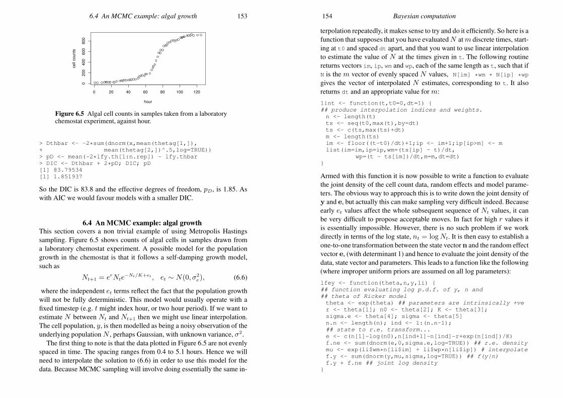
6.4 An MCMC example: algal growth 153
0 20 40 60 80 100 120
0200
400
600
800
hour
cell
counts
Figure 6.5 Algal cell counts in samples taken from a laboratorychemostat experiment, against hour.
> Dthbar <- -2*sum(dnorm(x,mean(thetag[1,]),+ mean(thetag[2,])^.5,log=TRUE))> pD <- mean(-2*lfy.th[1:n.rep]) - lfy.thbar> DIC <- Dthbar + 2*pD; DIC; pD[1] 83.79534[1] 1.851937
So the DIC is 83.8 and the effective degrees of freedom, pD, is 1.85. Aswith AIC we would favour models with a smaller DIC.
6.4 An MCMC example: algal growthThis section covers a non trivial example of using Metropolis Hastingssampling. Figure 6.5 shows counts of algal cells in samples drawn froma laboratory chemostat experiment. A possible model for the populationgrowth in the chemostat is that it follows a self-damping growth model,such as
Nt+1 = erNte−Nt/K+et , et ∼ N(0, σ2
e), (6.6)
where the independent et terms reflect the fact that the population growthwill not be fully deterministic. This model would usually operate with afixed timestep (e.g. t might index hour, or two hour period). If we want toestimate N between Nt and Nt+1 then we might use linear interpolation.The cell population, y, is then modelled as being a noisy observation of theunderlying population N , perhaps Gaussian, with unknown variance, σ2.
The first thing to note is that the data plotted in Figure 6.5 are not evenlyspaced in time. The spacing ranges from 0.4 to 5.1 hours. Hence we willneed to interpolate the solution to (6.6) in order to use this model for thedata. Because MCMC sampling will involve doing essentially the same in-
154 Bayesian computation
terpolation repeatedly, it makes sense to try and do it efficiently. So here is afunction that supposes that you have evaluatedN at m discrete times, start-ing at t0 and spaced dt apart, and that you want to use linear interpolationto estimate the value of N at the times given in t. The following routinereturns vectors im, ip, wm and wp, each of the same length as t, such that ifN is the m vector of evenly spaced N values, N[im] *wm + N[ip] *wp
gives the vector of interpolated N estimates, corresponding to t. It alsoreturns dt and an appropriate value for m:
lint <- function(t,t0=0,dt=1) ## produce interpolation indices and weights.n <- length(t)ts <- seq(t0,max(t),by=dt)ts <- c(ts,max(ts)+dt)m <- length(ts)im <- floor((t-t0)/dt)+1;ip <- im+1;ip[ip>m] <- mlist(im=im,ip=ip,wm=(ts[ip] - t)/dt,
wp=(t - ts[im])/dt,m=m,dt=dt)
Armed with this function it is now possible to write a function to evaluatethe joint density of the cell count data, random effects and model parame-ters. The obvious way to approach this is to write down the joint density ofy and e, but actually this can make sampling very difficult indeed. Becauseearly et values affect the whole subsequent sequence of Nt values, it canbe very difficult to propose acceptable moves. In fact for high r values itis essentially impossible. However, there is no such problem if we workdirectly in terms of the log state, nt = logNt. It is then easy to establish aone-to-one transformation between the state vectorn and the random effectvector e, (with determinant 1) and hence to evaluate the joint density of thedata, state vector and parameters. This leads to a function like the following(where improper uniform priors are assumed on all log parameters):
lfey <- function(theta,n,y,li) ## function evaluating log p.d.f. of y, n and## theta of Ricker modeltheta <- exp(theta) ## parameters are intrinsically +ver <- theta[1]; n0 <- theta[2]; K <- theta[3];sigma.e <- theta[4]; sigma <- theta[5]n.n <- length(n); ind <- 1:(n.n-1);## state to r.e. transform...e <- c(n[1]-log(n0),n[ind+1]-n[ind]-r+exp(n[ind])/K)f.ne <- sum(dnorm(e,0,sigma.e,log=TRUE)) ## r.e. densitymu <- exp(li$wm*n[li$im] + li$wp*n[li$ip]) # interpolatef.y <- sum(dnorm(y,mu,sigma,log=TRUE)) ## f(y|n)f.y + f.ne ## joint log density
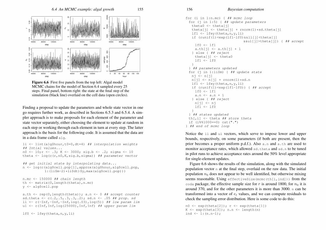
6.4 An MCMC example: algal growth 155
40000 80000 120000
0.1
00.2
00
.30
step
r
40000 80000 120000
51
01
52
0
step
n0
40000 80000 120000
50
00
15
00
02
50
00
step
K
40000 80000 120000
0.0
50
.10
0.1
50
.20
0.2
5
step
σe
40000 80000 120000
10
12
14
16
18
20
step
σ
0 20 40 60 80 100 120
02
00
40
06
00
80
0
hour
cell.
pop
Figure 6.6 First five panels from the top left: Algal modelMCMC chains for the model of Section 6.4 sampled every 25steps. Final panel, bottom right: the state at the final step of thesimulation (black line) overlaid on the cell data (open circles).
Finding a proposal to update the parameters and whole state vector in onego requires further work, as described in Sections 6.5.3 and 6.5.4. A sim-pler approach is to make proposals for each element of the parameter andstate vector separately, either choosing the element to update at random ineach step or working through each element in turn at every step. The latterapproach is the basis for the following code. It is assumed that the data arein a data frame called alg.
li <- lint(alg$hour,t0=0,dt=4) ## interpolation weights## Intial values...n0 <- 10;r <- .3; K <- 3000; sig.b <- .2; sigma <- 10theta <- log(c(r,n0,K,sig.b,sigma)) ## parameter vector
## get initial state by interpolating data...n <- log(c(alg$cell.pop[1],approx(alg$hour,alg$cell.pop,
1:(li$m-2)*li$dt)$y,max(alg$cell.pop)))
n.mc <- 150000 ## chain lengthth <- matrix(0,length(theta),n.mc)y <- alg$cell.pop
a.th <- rep(0,length(theta)); a.n <- 0 ## accept countersd.theta <- c(.2,.5,.3,.3,.2); sd.n <- .05 ## prop. sdll <- c(-Inf,-Inf,-Inf,log(.03),log(5)) ## low param limul <- c(Inf,Inf,log(25000),Inf,Inf) ## upper param lim
lf0 <- lfey(theta,n,y,li)
156 Bayesian computation
for (i in 1:n.mc) ## mcmc loopfor (j in 1:5) ## update parameterstheta0 <- theta[j]theta[j] <- theta[j] + rnorm(1)*sd.theta[j]lf1 <- lfey(theta,n,y,li)if (runif(1)<exp(lf1-lf0)&&ll[j]<theta[j]
&&ul[j]>theta[j]) ## acceptlf0 <- lf1a.th[j] <- a.th[j] + 1
else ## rejecttheta[j] <- theta0lf1 <- lf0
## parameters updatedfor (j in 1:li$m) ## update statenj <- n[j]n[j] <- n[j] + rnorm(1)*sd.nlf1 <- lfey(theta,n,y,li)if (runif(1)<exp(lf1-lf0)) ## acceptlf0 <- lf1a.n <- a.n + 1
else ## rejectn[j] <- njlf1 <- lf0
## states updatedth[,i] <- theta ## store thetaif (i%%1000==0) cat(".")
## end of mcmc loop
Notice the ll and ul vectors, which serve to impose lower and upperbounds, respectively, on some parameters (if both are present, then theprior becomes a proper uniform p.d.f.). Also a.n and a.th are used tomonitor acceptance rates, which allowed sd.theta and sd.n to be tunedin pilot runs to achieve acceptance rates around the 50% level appropriatefor single-element updates.
Figure 6.6 shows the results of the simulation, along with the simulatedpopulation vector n at the final step, overlaid on the raw data. The initialpopulation n0 does not appear to be well identified, but otherwise mixingseems reasonable. Using effectiveSize(mcmc(th[i,ind])) from thecoda package, the effective sample size for r is around 1800, for n0 it isaround 370, and for the other parameters it is more than 3000. n can betransformed into a vector of et values, and we can compute residuals tocheck the sampling error distribution. Here is some code to do this:
n0 <- exp(theta[2]); r <- exp(theta[1])K <- exp(theta[3]); n.n <- length(n)ind <- 1:(n.n-1);
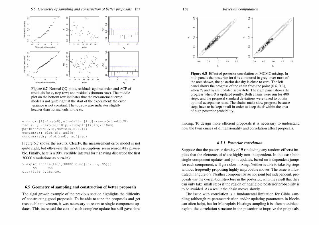
6.5 Geometry of sampling and construction of better proposals 157
−2 −1 0 1 2
−0
.2−
0.1
0.0
0.1
0.2
Theoretical Quantiles
Sam
ple
Quantile
s
0 5 10 15 20 25 30
−0
.2−
0.1
0.0
0.1
0.2
Index
e
0 5 10 15
−0
.20
.20
.61
.0
Lag
AC
F
−2 −1 0 1 2
−3
0−
10
01
02
03
0
Theoretical Quantiles
Sam
ple
Quantile
s
0 10 20 30 40 50 60
−3
0−
10
01
02
03
0
Index
rsd
0 5 10 15
−0
.20
.20
.61
.0
Lag
AC
F
Figure 6.7 Normal QQ-plots, residuals against order, and ACF ofresiduals for et (top row) and residuals (bottom row). The middleplot on the bottom row indicates that the measurement errormodel is not quite right at the start of the experiment: the errorvariance is not constant. The top row also indicates slightlyheavier than normal tails in the et.
e <- c(n[1]-log(n0),n[ind+1]-n[ind]-r+exp(n[ind])/K)rsd <- y - exp(n[li$ip]*li$wp+n[li$im]*li$wm)par(mfrow=c(2,3),mar=c(5,5,1,1))qqnorm(e); plot(e); acf(e)qqnorm(rsd); plot(rsd); acf(rsd)
Figure 6.7 shows the results. Clearly, the measurement error model is notquite right, but otherwise the model assumptions seem reasonably plausi-ble. Finally, here is a 90% credible interval for r (having discarded the first30000 simulations as burn-in):> exp(quantile(th[1,30000:n.mc],c(.05,.95)))
5% 95%0.1689796 0.2817391
6.5 Geometry of sampling and construction of better proposals
The algal growth example of the previous section highlights the difficultyof constructing good proposals. To be able to tune the proposals and getreasonable movement, it was necessary to resort to single-component up-dates. This increased the cost of each complete update but still gave slow
158 Bayesian computation
θ1
θ2
0.1
0.1
0.5
1
1.5
0.0 0.5 1.0 1.5 2.0
0.0
0.5
1.0
1.5
2.0
θ1
θ2
0.1
0.1
0.5
1
1.5
0.0 0.5 1.0 1.5 2.0
0.0
0.5
1.0
1.5
2.0
Figure 6.8 Effect of posterior correlation on MCMC mixing. Inboth panels the posterior for θ is contoured in grey: over most ofthe area shown, the posterior density is close to zero. The leftpanel shows the progress of the chain from the point (0.5, 0.5),when θ1 and θ2 are updated separately. The right panel shows theprogress when θ is updated jointly. Both chains were run for 400steps, and the proposal standard deviations were tuned to obtainoptimal acceptance rates. The chains make slow progress becausesteps have to be kept small in order to keep the θ within the areaof high posterior probability.
mixing. To design more efficient proposals it is necessary to understandhow the twin curses of dimensionality and correlation affect proposals.
6.5.1 Posterior correlation
Suppose that the posterior density of θ (including any random effects) im-plies that the elements of θ are highly non-independent. In this case bothsingle-component updates and joint updates, based on independent jumpsfor each component, will give slow mixing. Neither is able to take big stepswithout frequently proposing highly improbable moves. The issue is illus-trated in Figure 6.8. Neither componentwise nor joint but independent, pro-posals use the correlation structure in the posterior, with the result that theycan only take small steps if the region of negligible posterior probability isto be avoided. As a result the chain moves slowly.
The issue with correlation is a fundamental limitation for Gibbs sam-pling (although re-parameterisation and/or updating parameters in blockscan often help), but for Metroplois-Hastings sampling it is often possible toexploit the correlation structure in the posterior to improve the proposals.
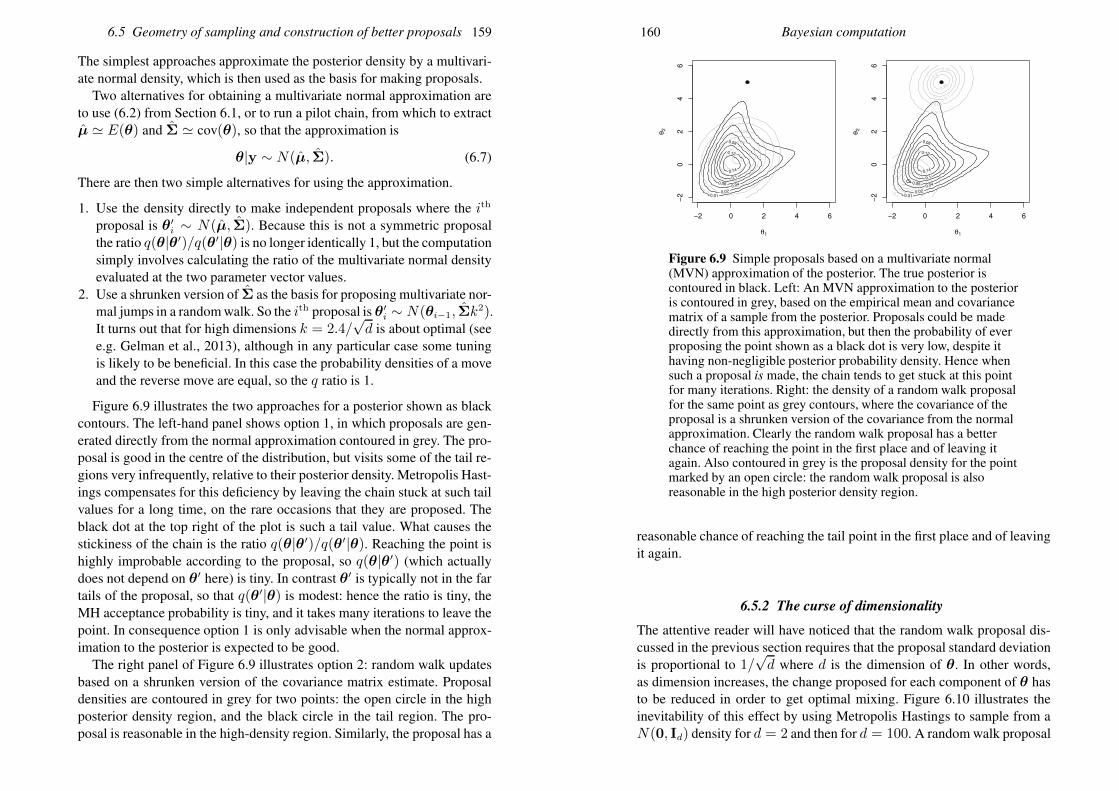
6.5 Geometry of sampling and construction of better proposals 159
The simplest approaches approximate the posterior density by a multivari-ate normal density, which is then used as the basis for making proposals.
Two alternatives for obtaining a multivariate normal approximation areto use (6.2) from Section 6.1, or to run a pilot chain, from which to extractµ ≃ E(θ) and Σ ≃ cov(θ), so that the approximation is
θ|y ∼ N(µ, Σ). (6.7)
There are then two simple alternatives for using the approximation.
1. Use the density directly to make independent proposals where the ith
proposal is θ′i ∼ N(µ, Σ). Because this is not a symmetric proposal
the ratio q(θ|θ′)/q(θ′|θ) is no longer identically 1, but the computationsimply involves calculating the ratio of the multivariate normal densityevaluated at the two parameter vector values.
2. Use a shrunken version of Σ as the basis for proposing multivariate nor-mal jumps in a random walk. So the ith proposal is θ′
i ∼ N(θi−1, Σk2).It turns out that for high dimensions k = 2.4/
√d is about optimal (see
e.g. Gelman et al., 2013), although in any particular case some tuningis likely to be beneficial. In this case the probability densities of a moveand the reverse move are equal, so the q ratio is 1.
Figure 6.9 illustrates the two approaches for a posterior shown as blackcontours. The left-hand panel shows option 1, in which proposals are gen-erated directly from the normal approximation contoured in grey. The pro-posal is good in the centre of the distribution, but visits some of the tail re-gions very infrequently, relative to their posterior density. Metropolis Hast-ings compensates for this deficiency by leaving the chain stuck at such tailvalues for a long time, on the rare occasions that they are proposed. Theblack dot at the top right of the plot is such a tail value. What causes thestickiness of the chain is the ratio q(θ|θ′)/q(θ′|θ). Reaching the point ishighly improbable according to the proposal, so q(θ|θ′) (which actuallydoes not depend on θ′ here) is tiny. In contrast θ′ is typically not in the fartails of the proposal, so that q(θ′|θ) is modest: hence the ratio is tiny, theMH acceptance probability is tiny, and it takes many iterations to leave thepoint. In consequence option 1 is only advisable when the normal approx-imation to the posterior is expected to be good.
The right panel of Figure 6.9 illustrates option 2: random walk updatesbased on a shrunken version of the covariance matrix estimate. Proposaldensities are contoured in grey for two points: the open circle in the highposterior density region, and the black circle in the tail region. The pro-posal is reasonable in the high-density region. Similarly, the proposal has a
160 Bayesian computation
−2 0 2 4 6
−2
02
46
θ1
θ2
0.01 0.02
0.04 0.06
0.08
0.1
0.12
0.14
0.01
0.01
0.02
0.04
0.06
0.08
0.1
−2 0 2 4 6
−2
02
46
θ1
θ2
0.01 0.02
0.04 0.06
0.08
0.1
0.12
0.14
0.01
0.05
0.1
0.15
0.2
0.25
0.01
0.05
0.1
0.1
0.15
0.2
0.2
5
Figure 6.9 Simple proposals based on a multivariate normal(MVN) approximation of the posterior. The true posterior iscontoured in black. Left: An MVN approximation to the posterioris contoured in grey, based on the empirical mean and covariancematrix of a sample from the posterior. Proposals could be madedirectly from this approximation, but then the probability of everproposing the point shown as a black dot is very low, despite ithaving non-negligible posterior probability density. Hence whensuch a proposal is made, the chain tends to get stuck at this pointfor many iterations. Right: the density of a random walk proposalfor the same point as grey contours, where the covariance of theproposal is a shrunken version of the covariance from the normalapproximation. Clearly the random walk proposal has a betterchance of reaching the point in the first place and of leaving itagain. Also contoured in grey is the proposal density for the pointmarked by an open circle: the random walk proposal is alsoreasonable in the high posterior density region.
reasonable chance of reaching the tail point in the first place and of leavingit again.
6.5.2 The curse of dimensionality
The attentive reader will have noticed that the random walk proposal dis-cussed in the previous section requires that the proposal standard deviationis proportional to 1/
√d where d is the dimension of θ. In other words,
as dimension increases, the change proposed for each component of θ hasto be reduced in order to get optimal mixing. Figure 6.10 illustrates theinevitability of this effect by using Metropolis Hastings to sample from aN(0, Id) density for d = 2 and then for d = 100. A random walk proposal
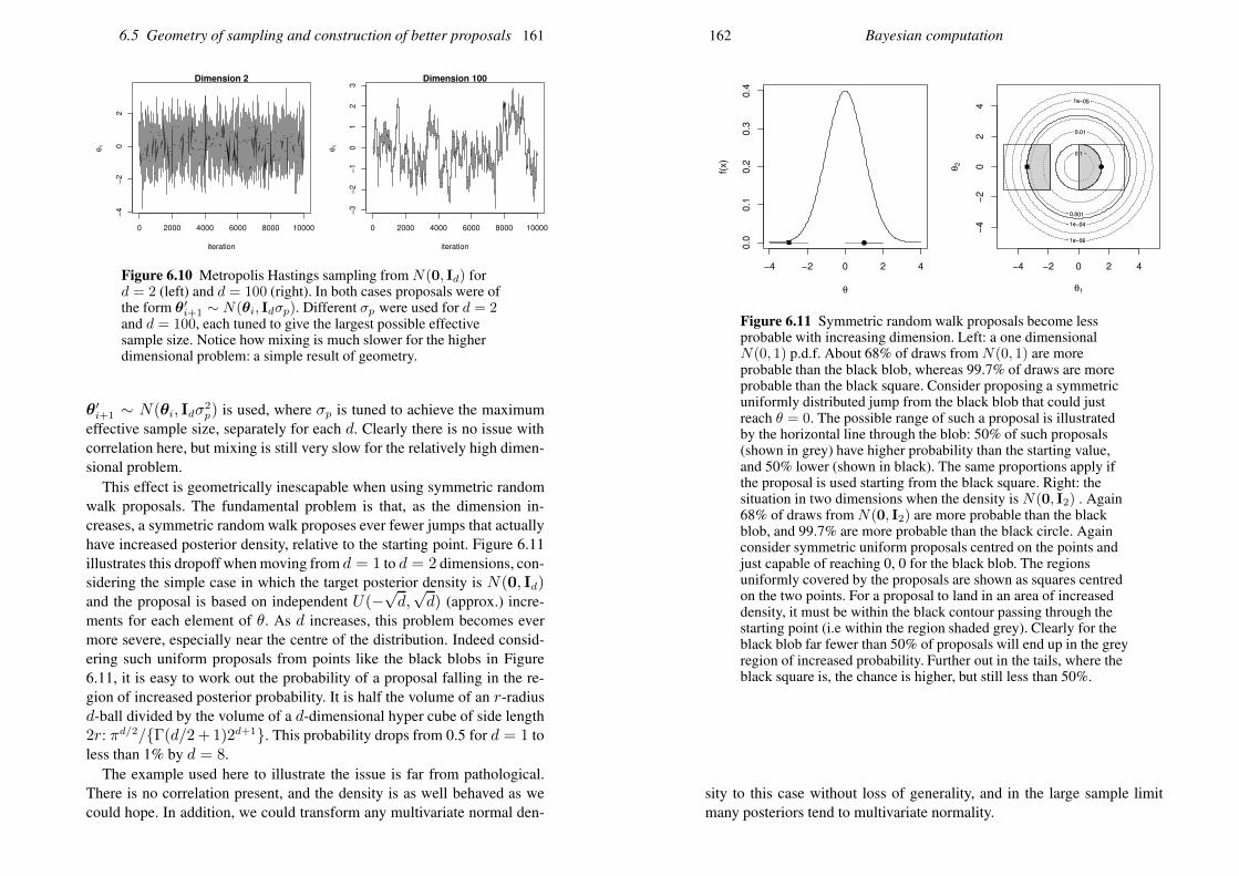
6.5 Geometry of sampling and construction of better proposals 161
0 2000 4000 6000 8000 10000
−4
−2
02
Dimension 2
iteration
θ1
0 2000 4000 6000 8000 10000
−3
−2
−1
01
23
Dimension 100
iteration
θ1
Figure 6.10 Metropolis Hastings sampling from N(0, Id) ford = 2 (left) and d = 100 (right). In both cases proposals were ofthe form θ′i+1 ∼ N(θi, Idσp). Different σp were used for d = 2and d = 100, each tuned to give the largest possible effectivesample size. Notice how mixing is much slower for the higherdimensional problem: a simple result of geometry.
θ′i+1 ∼ N(θi, Idσ
2p) is used, where σp is tuned to achieve the maximum
effective sample size, separately for each d. Clearly there is no issue withcorrelation here, but mixing is still very slow for the relatively high dimen-sional problem.
This effect is geometrically inescapable when using symmetric randomwalk proposals. The fundamental problem is that, as the dimension in-creases, a symmetric random walk proposes ever fewer jumps that actuallyhave increased posterior density, relative to the starting point. Figure 6.11illustrates this dropoff when moving from d = 1 to d = 2 dimensions, con-sidering the simple case in which the target posterior density is N(0, Id)and the proposal is based on independent U(−
√d,√d) (approx.) incre-
ments for each element of θ. As d increases, this problem becomes evermore severe, especially near the centre of the distribution. Indeed consid-ering such uniform proposals from points like the black blobs in Figure6.11, it is easy to work out the probability of a proposal falling in the re-gion of increased posterior probability. It is half the volume of an r-radiusd-ball divided by the volume of a d-dimensional hyper cube of side length2r: πd/2/Γ(d/2+1)2d+1. This probability drops from 0.5 for d = 1 toless than 1% by d = 8.
The example used here to illustrate the issue is far from pathological.There is no correlation present, and the density is as well behaved as wecould hope. In addition, we could transform any multivariate normal den-
162 Bayesian computation
−4 −2 0 2 4
0.0
0.1
0.2
0.3
0.4
θ
f(x)
θ1
θ2
1e−06
1e−05
1e−04
0.001
0.01
0.1
−4 −2 0 2 4
−4
−2
02
4
1e−06
1e−05
1e−04
0.001
0.01
0.1
Figure 6.11 Symmetric random walk proposals become lessprobable with increasing dimension. Left: a one dimensionalN(0, 1) p.d.f. About 68% of draws from N(0, 1) are moreprobable than the black blob, whereas 99.7% of draws are moreprobable than the black square. Consider proposing a symmetricuniformly distributed jump from the black blob that could justreach θ = 0. The possible range of such a proposal is illustratedby the horizontal line through the blob: 50% of such proposals(shown in grey) have higher probability than the starting value,and 50% lower (shown in black). The same proportions apply ifthe proposal is used starting from the black square. Right: thesituation in two dimensions when the density is N(0, I2) . Again68% of draws from N(0, I2) are more probable than the blackblob, and 99.7% are more probable than the black circle. Againconsider symmetric uniform proposals centred on the points andjust capable of reaching 0, 0 for the black blob. The regionsuniformly covered by the proposals are shown as squares centredon the two points. For a proposal to land in an area of increaseddensity, it must be within the black contour passing through thestarting point (i.e within the region shaded grey). Clearly for theblack blob far fewer than 50% of proposals will end up in the greyregion of increased probability. Further out in the tails, where theblack square is, the chance is higher, but still less than 50%.
sity to this case without loss of generality, and in the large sample limitmany posteriors tend to multivariate normality.

6.5 Geometry of sampling and construction of better proposals 163
6.5.3 Improved proposals based on approximate posterior normality
These basic issues have given rise to a great deal of work on adaptiveMetropolis-Hastings schemes that use nonsymmetric proposals with an im-proved tendency to make moves that will increase the posterior, while tak-ing relatively large steps. Most of this work is well beyond our scope here.Instead let us consider developing some simple improved schemes, basedon the preceding insights.
The big advantage of the fixed multivariate normal proposal is that ittends to propose more points near the centre of the distribution than in thetails, but its disadvantage is that it may not visit poorly approximated tailsoften enough, so it gets stuck in them when it does visit. The advantage ofthe random walk is that it can get into the tails without getting stuck there,but does so by making many proposals into low-probability regions. Anobvious hybrid strategy is to propose moves from a mixture distribution.With tunable probability γ propose from N(µ, Σ) otherwise propose fromN(θi, Σk2). The probability density for the proposal and its reverse nowhave to be computed from the mixture distribution to compute the MH qratio, but this is unproblematic.
A simpler alternative that directly addresses the tendency of symmetricrandom walks to propose improbable moves in high dimensions is to movethe centre of such proposals from θi, in the direction of µ. Defining ‖θ −µ‖2
Σ= (θ − µ)TΣ−1(θ − µ) and
m(θ) =
θ − γ(θ − µ)/‖θ − µ‖Σ ‖θ − µ‖Σ > γθ otherwise
,
the proposal density becomes N(m(θ), Σk2). We must choose γ and cantypically afford to increase k somewhat.
6.5.4 Improved proposals for the algal population example
The samplers constructed in Section 6.4 have rather disappointing perfor-mance, in terms of effective sample size for computational effort. 150,000iterations still only gave an effective sample size of around 370 for n0, andeach of those updates required an accept/reject computation for each ele-ment of θ and n separately. This section compares the simple improvedupdates discussed in the previous subsection based on the covariance ma-trix of the parameters according to the first run.
If the state vectors n for each iteration are stored as columns of a matrix
164 Bayesian computation
0 10000 30000 50000
0.1
50
.20
0.2
50
.30
0.3
5
step
r
0 10000 30000 50000
51
01
52
0
step
n0
0 10000 30000 50000
50
00
10
00
01
50
00
step
K
0 10000 30000 50000
0.0
60
.10
0.1
40
.18
step
σb
0 10000 30000 50000
10
12
14
16
18
step
σ
0 20 40 60 80 100 120
02
00
40
06
00
80
0
hour
cell.
pop
Figure 6.12 Algal model MCMC output equivalent to Figure 6.6,for 50000 iterations using a fixed multivariate normal proposal,based on the mean and covariance matrix from a pilot run. Noticehow the chain becomes stuck where the posterior density ismoderate but the proposal density is very low; it then takes a largenumber of iterations to become unstuck: see the discussionaround Figure 6.9 for an explanation of this phenomenon.
nn, then the first step is to compute the mean and covariance matrix for thevector b = (θT,nT)T:
## tn is params and state, discarding burn-in...tn <- rbind(th,nn)[,-(1:20000)]mu <- rowMeans(tn) ## mu hatV <- cov(t(tn)) ## Sigma hat
Before going further it is important to look at pairs plots of the rows oftn to see whether N(µ, Σ) can be expected to capture anything usefulabout the posterior. In this case it can, so first consider using N(µ, Σ) as afixed proposal. All proposals can be generated up front, using, for examplemvrnorm from the MASS library in R:
library(MASS)sp <- mvrnorm(n.mc,mu,V)
so sp contains one proposal per row. The q ratio in the MH acceptanceprobability requires the density of each proposal, and the following willevaluate the log of these for all rows of sp:
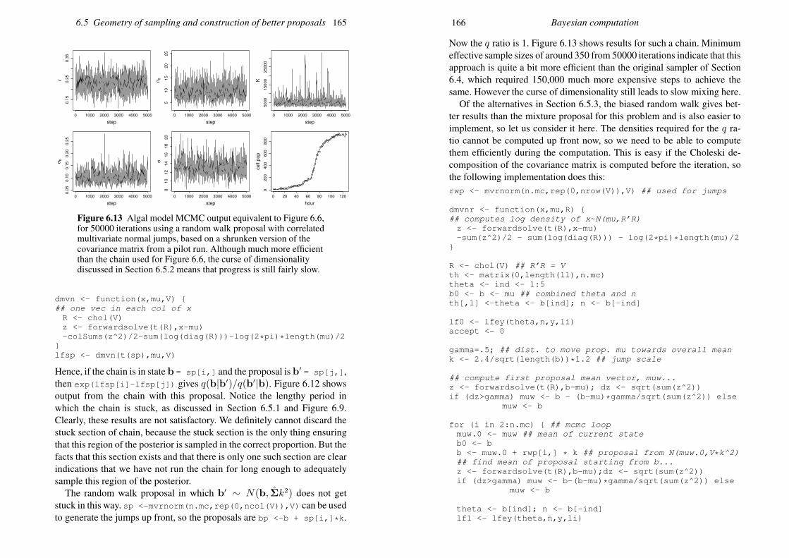
6.5 Geometry of sampling and construction of better proposals 165
0 1000 2000 3000 4000 5000
0.1
50
.25
0.3
5
step
r
0 1000 2000 3000 4000 5000
51
01
52
02
5
step
n0
0 1000 2000 3000 4000 5000
50
00
15
00
02
50
00
step
K
0 1000 2000 3000 4000 5000
0.0
50
.10
0.1
50
.20
0.2
5
step
σb
0 1000 2000 3000 4000 5000
81
01
21
41
61
82
0
step
σ
0 20 40 60 80 100 120
02
00
40
06
00
80
0
hour
cell.
pop
Figure 6.13 Algal model MCMC output equivalent to Figure 6.6,for 50000 iterations using a random walk proposal with correlatedmultivariate normal jumps, based on a shrunken version of thecovariance matrix from a pilot run. Although much more efficientthan the chain used for Figure 6.6, the curse of dimensionalitydiscussed in Section 6.5.2 means that progress is still fairly slow.
dmvn <- function(x,mu,V) ## one vec in each col of xR <- chol(V)z <- forwardsolve(t(R),x-mu)-colSums(z^2)/2-sum(log(diag(R)))-log(2*pi)*length(mu)/2
lfsp <- dmvn(t(sp),mu,V)
Hence, if the chain is in state b = sp[i,] and the proposal is b′ = sp[j,],then exp(lfsp[i]-lfsp[j]) gives q(b|b′)/q(b′|b). Figure 6.12 showsoutput from the chain with this proposal. Notice the lengthy period inwhich the chain is stuck, as discussed in Section 6.5.1 and Figure 6.9.Clearly, these results are not satisfactory. We definitely cannot discard thestuck section of chain, because the stuck section is the only thing ensuringthat this region of the posterior is sampled in the correct proportion. But thefacts that this section exists and that there is only one such section are clearindications that we have not run the chain for long enough to adequatelysample this region of the posterior.
The random walk proposal in which b′ ∼ N(b, Σk2) does not getstuck in this way. sp <-mvrnorm(n.mc,rep(0,ncol(V)),V) can be usedto generate the jumps up front, so the proposals are bp <-b + sp[i,]*k.
166 Bayesian computation
Now the q ratio is 1. Figure 6.13 shows results for such a chain. Minimumeffective sample sizes of around 350 from 50000 iterations indicate that thisapproach is quite a bit more efficient than the original sampler of Section6.4, which required 150,000 much more expensive steps to achieve thesame. However the curse of dimensionality still leads to slow mixing here.
Of the alternatives in Section 6.5.3, the biased random walk gives bet-ter results than the mixture proposal for this problem and is also easier toimplement, so let us consider it here. The densities required for the q ra-tio cannot be computed up front now, so we need to be able to computethem efficiently during the computation. This is easy if the Choleski de-composition of the covariance matrix is computed before the iteration, sothe following implementation does this:rwp <- mvrnorm(n.mc,rep(0,nrow(V)),V) ## used for jumps
dmvnr <- function(x,mu,R) ## computes log density of x~N(mu,R’R)z <- forwardsolve(t(R),x-mu)-sum(z^2)/2 - sum(log(diag(R))) - log(2*pi)*length(mu)/2
R <- chol(V) ## R’R = Vth <- matrix(0,length(ll),n.mc)theta <- ind <- 1:5b0 <- b <- mu ## combined theta and nth[,1] <-theta <- b[ind]; n <- b[-ind]
lf0 <- lfey(theta,n,y,li)accept <- 0
gamma=.5; ## dist. to move prop. mu towards overall meank <- 2.4/sqrt(length(b))*1.2 ## jump scale
## compute first proposal mean vector, muw...z <- forwardsolve(t(R),b-mu); dz <- sqrt(sum(z^2))if (dz>gamma) muw <- b - (b-mu)*gamma/sqrt(sum(z^2)) else
muw <- b
for (i in 2:n.mc) ## mcmc loopmuw.0 <- muw ## mean of current stateb0 <- bb <- muw.0 + rwp[i,] * k ## proposal from N(muw.0,V*k^2)## find mean of proposal starting from b...z <- forwardsolve(t(R),b-mu);dz <- sqrt(sum(z^2))if (dz>gamma) muw <- b-(b-mu)*gamma/sqrt(sum(z^2)) else
muw <- b
theta <- b[ind]; n <- b[-ind]lf1 <- lfey(theta,n,y,li)
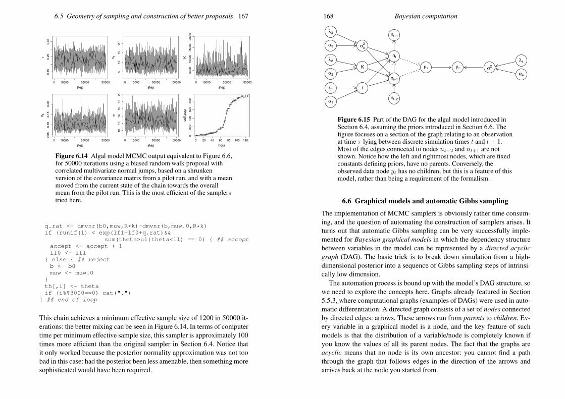
6.5 Geometry of sampling and construction of better proposals 167
0 10000 30000 50000
0.1
50
.25
0.3
5
step
r
0 10000 30000 50000
51
01
52
0
step
n0
0 10000 30000 50000
50
00
10
00
01
50
00
20
00
0
step
K
0 10000 30000 50000
0.0
50
.10
0.1
50
.20
step
σb
0 10000 30000 50000
10
12
14
16
18
20
step
σ
0 20 40 60 80 100 120
02
00
40
06
00
80
0
hour
cell.
pop
Figure 6.14 Algal model MCMC output equivalent to Figure 6.6,for 50000 iterations using a biased random walk proposal withcorrelated multivariate normal jumps, based on a shrunkenversion of the covariance matrix from a pilot run, and with a meanmoved from the current state of the chain towards the overallmean from the pilot run. This is the most efficient of the samplerstried here.
q.rat <- dmvnr(b0,muw,R*k)-dmvnr(b,muw.0,R*k)if (runif(1) < exp(lf1-lf0+q.rat)&&
sum(theta>ul|theta<ll) == 0) ## acceptaccept <- accept + 1lf0 <- lf1
else ## rejectb <- b0muw <- muw.0
th[,i] <- thetaif (i%%3000==0) cat(".")
## end of loop
This chain achieves a minimum effective sample size of 1200 in 50000 it-erations: the better mixing can be seen in Figure 6.14. In terms of computertime per minimum effective sample size, this sampler is approximately 100times more efficient than the original sampler in Section 6.4. Notice thatit only worked because the posterior normality approximation was not toobad in this case: had the posterior been less amenable, then something moresophisticated would have been required.
168 Bayesian computation
x x
α1
λ1
α2
λ2
α3
λ3
r
K
σe
2
nt−2
nt−1
nt
nt+1
µτ yτ σ2
α4
λ4
Figure 6.15 Part of the DAG for the algal model introduced inSection 6.4, assuming the priors introduced in Section 6.6. Thefigure focuses on a section of the graph relating to an observationat time τ lying between discrete simulation times t and t+ 1.Most of the edges connected to nodes nt−2 and nt+1 are notshown. Notice how the left and rightmost nodes, which are fixedconstants defining priors, have no parents. Conversely, theobserved data node yt has no children, but this is a feature of thismodel, rather than being a requirement of the formalism.
6.6 Graphical models and automatic Gibbs sampling
The implementation of MCMC samplers is obviously rather time consum-ing, and the question of automating the construction of samplers arises. Itturns out that automatic Gibbs sampling can be very successfully imple-mented for Bayesian graphical models in which the dependency structurebetween variables in the model can be represented by a directed acyclicgraph (DAG). The basic trick is to break down simulation from a high-dimensional posterior into a sequence of Gibbs sampling steps of intrinsi-cally low dimension.
The automation process is bound up with the model’s DAG structure, sowe need to explore the concepts here. Graphs already featured in Section5.5.3, where computational graphs (examples of DAGs) were used in auto-matic differentiation. A directed graph consists of a set of nodes connectedby directed edges: arrows. These arrows run from parents to children. Ev-ery variable in a graphical model is a node, and the key feature of suchmodels is that the distribution of a variable/node is completely known ifyou know the values of all its parent nodes. The fact that the graphs areacyclic means that no node is its own ancestor: you cannot find a paththrough the graph that follows edges in the direction of the arrows andarrives back at the node you started from.
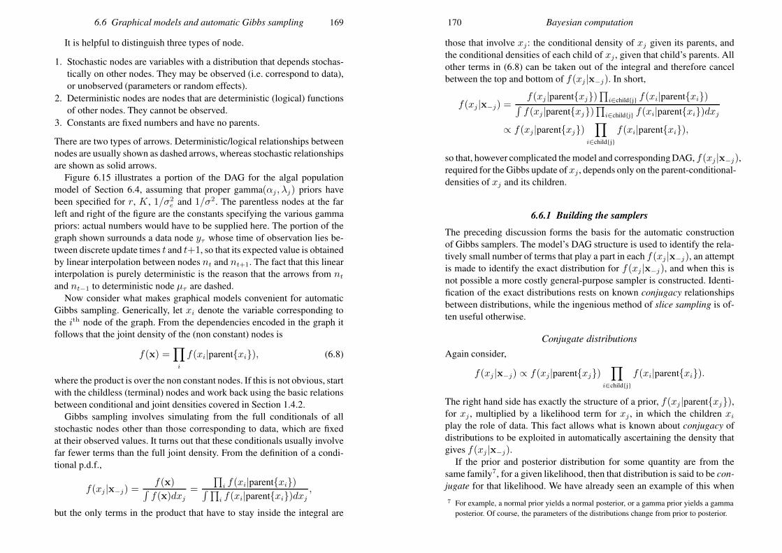
6.6 Graphical models and automatic Gibbs sampling 169
It is helpful to distinguish three types of node.
1. Stochastic nodes are variables with a distribution that depends stochas-tically on other nodes. They may be observed (i.e. correspond to data),or unobserved (parameters or random effects).
2. Deterministic nodes are nodes that are deterministic (logical) functionsof other nodes. They cannot be observed.
3. Constants are fixed numbers and have no parents.
There are two types of arrows. Deterministic/logical relationships betweennodes are usually shown as dashed arrows, whereas stochastic relationshipsare shown as solid arrows.
Figure 6.15 illustrates a portion of the DAG for the algal populationmodel of Section 6.4, assuming that proper gamma(αj , λj) priors havebeen specified for r, K , 1/σ2
e and 1/σ2. The parentless nodes at the farleft and right of the figure are the constants specifying the various gammapriors: actual numbers would have to be supplied here. The portion of thegraph shown surrounds a data node yτ whose time of observation lies be-tween discrete update times t and t+1, so that its expected value is obtainedby linear interpolation between nodes nt and nt+1. The fact that this linearinterpolation is purely deterministic is the reason that the arrows from ntand nt−1 to deterministic node µτ are dashed.
Now consider what makes graphical models convenient for automaticGibbs sampling. Generically, let xi denote the variable corresponding tothe ith node of the graph. From the dependencies encoded in the graph itfollows that the joint density of the (non constant) nodes is
f(x) =∏
i
f(xi|parentxi), (6.8)
where the product is over the non constant nodes. If this is not obvious, startwith the childless (terminal) nodes and work back using the basic relationsbetween conditional and joint densities covered in Section 1.4.2.
Gibbs sampling involves simulating from the full conditionals of allstochastic nodes other than those corresponding to data, which are fixedat their observed values. It turns out that these conditionals usually involvefar fewer terms than the full joint density. From the definition of a condi-tional p.d.f.,
f(xj |x−j) =f(x)∫f(x)dxj
=
∏i f(xi|parentxi)∫ ∏i f(xi|parentxi)dxj
,
but the only terms in the product that have to stay inside the integral are
170 Bayesian computation
those that involve xj : the conditional density of xj given its parents, andthe conditional densities of each child of xj , given that child’s parents. Allother terms in (6.8) can be taken out of the integral and therefore cancelbetween the top and bottom of f(xj|x−j). In short,
f(xj |x−j) =f(xj |parentxj)
∏i∈childj f(xi|parentxi)∫
f(xj|parentxj)∏i∈childj f(xi|parentxi)dxj
∝ f(xj |parentxj)∏
i∈childj
f(xi|parentxi),
so that, however complicated the model and corresponding DAG, f(xj |x−j),required for the Gibbs update of xj , depends only on the parent-conditional-densities of xj and its children.
6.6.1 Building the samplers
The preceding discussion forms the basis for the automatic constructionof Gibbs samplers. The model’s DAG structure is used to identify the rela-tively small number of terms that play a part in each f(xj |x−j), an attemptis made to identify the exact distribution for f(xj|x−j), and when this isnot possible a more costly general-purpose sampler is constructed. Identi-fication of the exact distributions rests on known conjugacy relationshipsbetween distributions, while the ingenious method of slice sampling is of-ten useful otherwise.
Conjugate distributionsAgain consider,
f(xj |x−j) ∝ f(xj|parentxj)∏
i∈childj
f(xi|parentxi).
The right hand side has exactly the structure of a prior, f(xj |parentxj),for xj , multiplied by a likelihood term for xj , in which the children xiplay the role of data. This fact allows what is known about conjugacy ofdistributions to be exploited in automatically ascertaining the density thatgives f(xj |x−j).
If the prior and posterior distribution for some quantity are from thesame family7, for a given likelihood, then that distribution is said to be con-jugate for that likelihood. We have already seen an example of this when7 For example, a normal prior yields a normal posterior, or a gamma prior yields a gamma
posterior. Of course, the parameters of the distributions change from prior to posterior.
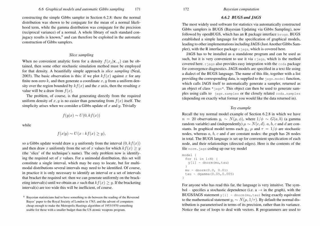
6.6 Graphical models and automatic Gibbs sampling 171
constructing the simple Gibbs sampler in Section 6.2.8: there the normaldistribution was shown to be conjugate for the mean of a normal likeli-hood term, while the gamma distribution was conjugate for the precision(reciprocal variance) of a normal. A whole library of such standard con-jugacy results is known,8 and can therefore be exploited in the automaticconstruction of Gibbs samplers.
Slice sampling
When no convenient analytic form for a density f(xj|x−j) can be ob-tained, then some other stochastic simulation method must be employedfor that density. A beautifully simple approach is slice sampling (Neal,2003). The basic observation is this: if we plot kf(x) against x for anyfinite non-zero k, and then generate a coordinate x, y from a uniform den-sity over the region bounded by kf(x) and the x axis, then the resulting xvalue will be a draw from f(x).
The problem, of course, is that generating directly from the requireduniform density of x, y is no easier than generating from f(x) itself. Thesimplicity arises when we consider a Gibbs update of x and y. Trivially
f(y|x) ∼ U(0, kf(x))
while
f(x|y) ∼ U(x : kf(x) ≥ y),
so a Gibbs update would draw a y uniformly from the interval (0, kf(x))and then draw x uniformly from the set of x values for which kf(x) ≥ y(the ‘slice’ of the technique’s name). The only problem now is identify-ing the required set of x values. For a unimodal distribution, this set willconstitute a single interval, which may be easy to locate, but for multi-modal distributions several intervals may need to be identified. Of course,in practice it is only necessary to identify an interval or a set of intervalsthat bracket the required set: then we can generate uniformly on the brack-eting interval(s) until we obtain an x such that kf(x) ≥ y. If the bracketinginterval(s) are too wide this will be inefficient, of course.
8 Bayesian statisticians had to have something to do between the reading of the ReverendBayes’ paper to the Royal Society of London in 1763, and the advent of computerscheap enough to make the Metropolis Hastings algorithm of 1953/1970 somethingusable for those with a smaller budget than the US atomic weapons program.
172 Bayesian computation
6.6.2 BUGS and JAGS
The most widely used software for statistics via automatically constructedGibbs samplers is BUGS (Bayesian Updating via Gibbs Sampling), nowfollowed by openBUGS, which has an R package interface brugs. BUGSestablished a simple language for the specification of graphical models,leading to other implementations including JAGS (Just Another Gibbs Sam-pler), with the R interface package rjags, which is covered here.
JAGS has to be installed as a standalone program and can be used assuch, but it is very convenient to use it via rjags, which is the methodcovered here. rjags also provides easy integration with the coda packagefor convergence diagnostics. JAGS models are specified in a text file usinga dialect of the BUGS language. The name of this file, together with a listproviding the corresponding data, is supplied to the jags.model function,which calls JAGS itself to automatically generate a sampler, returned asan object of class "jags". This object can then be used to generate sam-ples using calls to jags.samples or the closely related coda.samples
(depending on exactly what format you would like the data returned in).
Toy exampleRecall the toy normal model example of Section 6.2.8 in which we haven = 20 observations yi ∼ N(µ, φ), where 1/φ ∼ G(a, b) (a gammarandom variable) and (independently) µ ∼ N(c, d). a, b, c and d are con-stants. In graphical model terms each yi, µ and τ = 1/φ are stochasticnodes, whereas a, b, c and d are constant nodes: the graph has 26 nodesin total. The BUGS language is set up for convenient specification of eachnode, and their relationships (directed edges). Here is the contents of thefile norm.jags coding up our toy model
model for (i in 1:N) y[i] ~ dnorm(mu,tau)
mu ~ dnorm(0.0, 0.01)tau ~ dgamma(0.05,0.005)
For anyone who has read this far, the language is very intuitive. The sym-bol ~ specifies a stochastic dependence (i.e. a → in the graph), with theBUGS/JAGS statement y[i] ~ dnorm(mu,tau) being exactly equivalentto the mathematical statement yi ∼ N(µ, 1/τ). By default the normal dis-tribution is parameterised in terms of its precision, rather than its variance.Notice the use of loops to deal with vectors. R programmers are used to
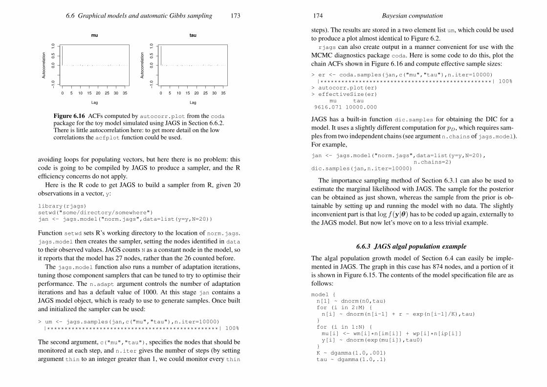
6.6 Graphical models and automatic Gibbs sampling 173
0 5 10 15 20 25 30 35
−1.0
0.0
0.5
1.0
Lag
Auto
corr
ela
tion
mu
0 5 10 15 20 25 30 35
−1.0
0.0
0.5
1.0
Lag
Auto
corr
ela
tion
tau
Figure 6.16 ACFs computed by autocorr.plot from the codapackage for the toy model simulated using JAGS in Section 6.6.2.There is little autocorrelation here: to get more detail on the lowcorrelations the acfplot function could be used.
avoiding loops for populating vectors, but here there is no problem: thiscode is going to be compiled by JAGS to produce a sampler, and the Refficiency concerns do not apply.
Here is the R code to get JAGS to build a sampler from R, given 20observations in a vector, y:
library(rjags)setwd("some/directory/somewhere")jan <- jags.model("norm.jags",data=list(y=y,N=20))
Function setwd sets R’s working directory to the location of norm.jags.jags.model then creates the sampler, setting the nodes identified in data
to their observed values. JAGS counts N as a constant node in the model, soit reports that the model has 27 nodes, rather than the 26 counted before.
The jags.model function also runs a number of adaptation iterations,tuning those component samplers that can be tuned to try to optimise theirperformance. The n.adapt argument controls the number of adaptationiterations and has a default value of 1000. At this stage jan contains aJAGS model object, which is ready to use to generate samples. Once builtand initialized the sampler can be used:
> um <- jags.samples(jan,c("mu","tau"),n.iter=10000)|*************************************************| 100%
The second argument, c("mu","tau"), specifies the nodes that should bemonitored at each step, and n.iter gives the number of steps (by settingargument thin to an integer greater than 1, we could monitor every thin
174 Bayesian computation
steps). The results are stored in a two element list um, which could be usedto produce a plot almost identical to Figure 6.2.
rjags can also create output in a manner convenient for use with theMCMC diagnostics package coda. Here is some code to do this, plot thechain ACFs shown in Figure 6.16 and compute effective sample sizes:
> er <- coda.samples(jan,c("mu","tau"),n.iter=10000)|*************************************************| 100%
> autocorr.plot(er)> effectiveSize(er)
mu tau9616.071 10000.000
JAGS has a built-in function dic.samples for obtaining the DIC for amodel. It uses a slightly different computation for pD, which requires sam-ples from two independent chains (see argument n.chains of jags.model).For example,
jan <- jags.model("norm.jags",data=list(y=y,N=20),n.chains=2)
dic.samples(jan,n.iter=10000)
The importance sampling method of Section 6.3.1 can also be used toestimate the marginal likelihood with JAGS. The sample for the posteriorcan be obtained as just shown, whereas the sample from the prior is ob-tainable by setting up and running the model with no data. The slightlyinconvenient part is that log f(y|θ) has to be coded up again, externally tothe JAGS model. But now let’s move on to a less trivial example.
6.6.3 JAGS algal population example
The algal population growth model of Section 6.4 can easily be imple-mented in JAGS. The graph in this case has 874 nodes, and a portion of itis shown in Figure 6.15. The contents of the model specification file are asfollows:
model n[1] ~ dnorm(n0,tau)for (i in 2:M) n[i] ~ dnorm(n[i-1] + r - exp(n[i-1]/K),tau)
for (i in 1:N) mu[i] <- wm[i]*n[im[i]] + wp[i]*n[ip[i]]y[i] ~ dnorm(exp(mu[i]),tau0)
K ~ dgamma(1.0,.001)tau ~ dgamma(1.0,.1)
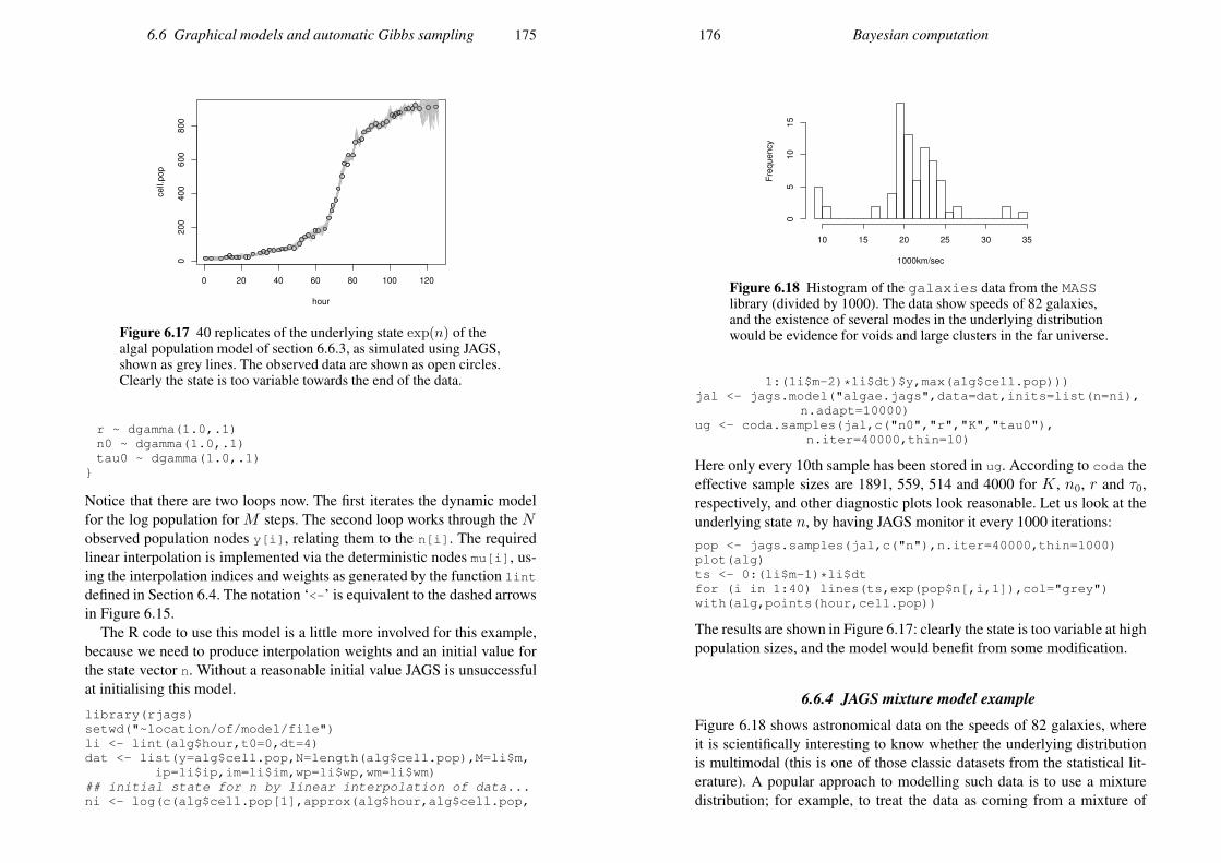
6.6 Graphical models and automatic Gibbs sampling 175
0 20 40 60 80 100 120
0200
400
600
800
hour
cell.
pop
Figure 6.17 40 replicates of the underlying state exp(n) of thealgal population model of section 6.6.3, as simulated using JAGS,shown as grey lines. The observed data are shown as open circles.Clearly the state is too variable towards the end of the data.
r ~ dgamma(1.0,.1)n0 ~ dgamma(1.0,.1)tau0 ~ dgamma(1.0,.1)
Notice that there are two loops now. The first iterates the dynamic modelfor the log population for M steps. The second loop works through the Nobserved population nodes y[i], relating them to the n[i]. The requiredlinear interpolation is implemented via the deterministic nodes mu[i], us-ing the interpolation indices and weights as generated by the function lint
defined in Section 6.4. The notation ‘<-’ is equivalent to the dashed arrowsin Figure 6.15.
The R code to use this model is a little more involved for this example,because we need to produce interpolation weights and an initial value forthe state vector n. Without a reasonable initial value JAGS is unsuccessfulat initialising this model.
library(rjags)setwd("~location/of/model/file")li <- lint(alg$hour,t0=0,dt=4)dat <- list(y=alg$cell.pop,N=length(alg$cell.pop),M=li$m,
ip=li$ip,im=li$im,wp=li$wp,wm=li$wm)## initial state for n by linear interpolation of data...ni <- log(c(alg$cell.pop[1],approx(alg$hour,alg$cell.pop,
176 Bayesian computation
1000km/sec
Fre
quency
10 15 20 25 30 35
05
10
15
Figure 6.18 Histogram of the galaxies data from the MASSlibrary (divided by 1000). The data show speeds of 82 galaxies,and the existence of several modes in the underlying distributionwould be evidence for voids and large clusters in the far universe.
1:(li$m-2)*li$dt)$y,max(alg$cell.pop)))jal <- jags.model("algae.jags",data=dat,inits=list(n=ni),
n.adapt=10000)ug <- coda.samples(jal,c("n0","r","K","tau0"),
n.iter=40000,thin=10)
Here only every 10th sample has been stored in ug. According to coda theeffective sample sizes are 1891, 559, 514 and 4000 for K , n0, r and τ0,respectively, and other diagnostic plots look reasonable. Let us look at theunderlying state n, by having JAGS monitor it every 1000 iterations:pop <- jags.samples(jal,c("n"),n.iter=40000,thin=1000)plot(alg)ts <- 0:(li$m-1)*li$dtfor (i in 1:40) lines(ts,exp(pop$n[,i,1]),col="grey")with(alg,points(hour,cell.pop))
The results are shown in Figure 6.17: clearly the state is too variable at highpopulation sizes, and the model would benefit from some modification.
6.6.4 JAGS mixture model example
Figure 6.18 shows astronomical data on the speeds of 82 galaxies, whereit is scientifically interesting to know whether the underlying distributionis multimodal (this is one of those classic datasets from the statistical lit-erature). A popular approach to modelling such data is to use a mixturedistribution; for example, to treat the data as coming from a mixture of
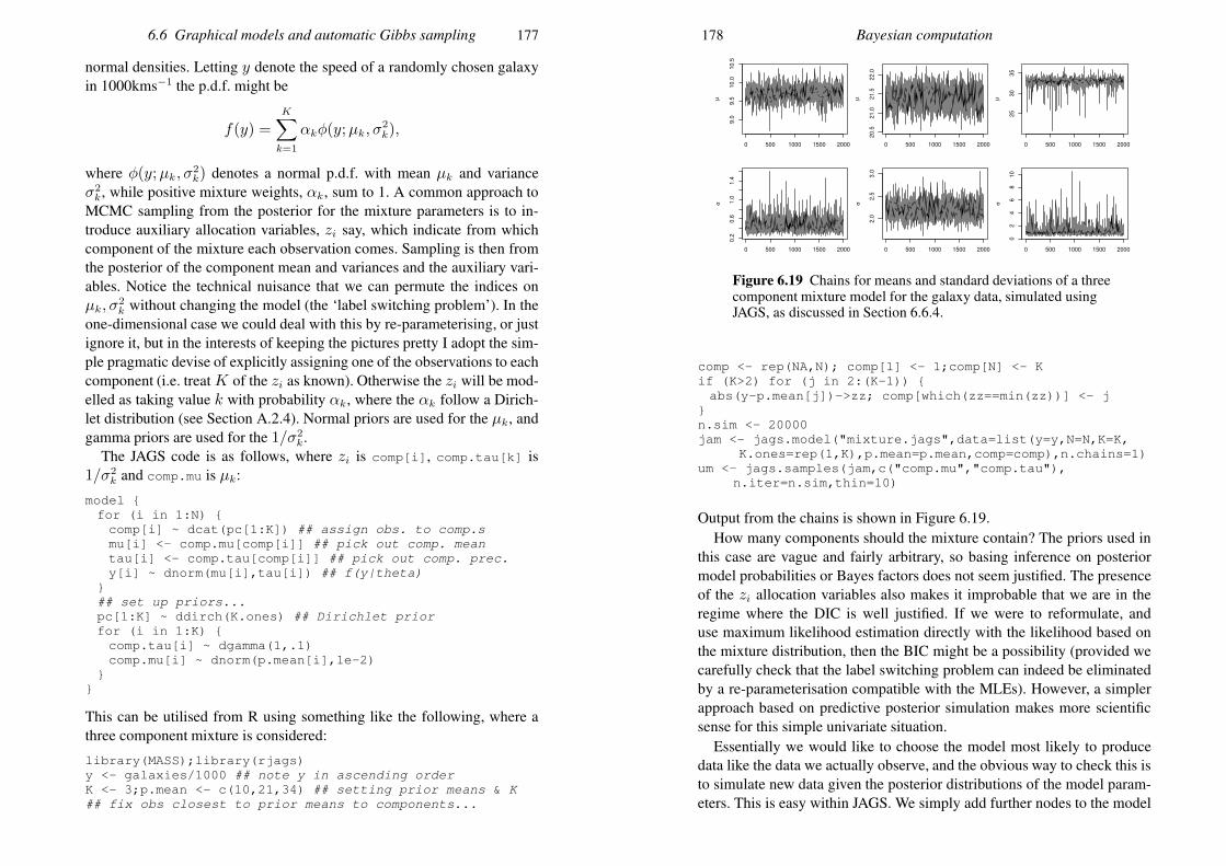
6.6 Graphical models and automatic Gibbs sampling 177
normal densities. Letting y denote the speed of a randomly chosen galaxyin 1000kms−1 the p.d.f. might be
f(y) =K∑
k=1
αkφ(y;µk, σ2k),
where φ(y;µk, σ2k) denotes a normal p.d.f. with mean µk and variance
σ2k, while positive mixture weights, αk, sum to 1. A common approach to
MCMC sampling from the posterior for the mixture parameters is to in-troduce auxiliary allocation variables, zi say, which indicate from whichcomponent of the mixture each observation comes. Sampling is then fromthe posterior of the component mean and variances and the auxiliary vari-ables. Notice the technical nuisance that we can permute the indices onµk, σ
2k without changing the model (the ‘label switching problem’). In the
one-dimensional case we could deal with this by re-parameterising, or justignore it, but in the interests of keeping the pictures pretty I adopt the sim-ple pragmatic devise of explicitly assigning one of the observations to eachcomponent (i.e. treat K of the zi as known). Otherwise the zi will be mod-elled as taking value k with probability αk, where the αk follow a Dirich-let distribution (see Section A.2.4). Normal priors are used for the µk, andgamma priors are used for the 1/σ2
k.The JAGS code is as follows, where zi is comp[i], comp.tau[k] is
1/σ2k and comp.mu is µk:
model for (i in 1:N) comp[i] ~ dcat(pc[1:K]) ## assign obs. to comp.smu[i] <- comp.mu[comp[i]] ## pick out comp. meantau[i] <- comp.tau[comp[i]] ## pick out comp. prec.y[i] ~ dnorm(mu[i],tau[i]) ## f(y|theta)
## set up priors...pc[1:K] ~ ddirch(K.ones) ## Dirichlet priorfor (i in 1:K) comp.tau[i] ~ dgamma(1,.1)comp.mu[i] ~ dnorm(p.mean[i],1e-2)
This can be utilised from R using something like the following, where athree component mixture is considered:
library(MASS);library(rjags)y <- galaxies/1000 ## note y in ascending orderK <- 3;p.mean <- c(10,21,34) ## setting prior means & K## fix obs closest to prior means to components...
178 Bayesian computation
0 500 1000 1500 2000
9.0
9.5
10.0
10.5
µ
0 500 1000 1500 2000
0.2
0.6
1.0
1.4
σ
0 500 1000 1500 2000
20.5
21.0
21.5
22.0
µ
0 500 1000 1500 2000
2.0
2.5
3.0
σ
0 500 1000 1500 2000
25
30
35
µ
0 500 1000 1500 2000
02
46
810
σ
Figure 6.19 Chains for means and standard deviations of a threecomponent mixture model for the galaxy data, simulated usingJAGS, as discussed in Section 6.6.4.
comp <- rep(NA,N); comp[1] <- 1;comp[N] <- Kif (K>2) for (j in 2:(K-1)) abs(y-p.mean[j])->zz; comp[which(zz==min(zz))] <- j
n.sim <- 20000jam <- jags.model("mixture.jags",data=list(y=y,N=N,K=K,
K.ones=rep(1,K),p.mean=p.mean,comp=comp),n.chains=1)um <- jags.samples(jam,c("comp.mu","comp.tau"),
n.iter=n.sim,thin=10)
Output from the chains is shown in Figure 6.19.How many components should the mixture contain? The priors used in
this case are vague and fairly arbitrary, so basing inference on posteriormodel probabilities or Bayes factors does not seem justified. The presenceof the zi allocation variables also makes it improbable that we are in theregime where the DIC is well justified. If we were to reformulate, anduse maximum likelihood estimation directly with the likelihood based onthe mixture distribution, then the BIC might be a possibility (provided wecarefully check that the label switching problem can indeed be eliminatedby a re-parameterisation compatible with the MLEs). However, a simplerapproach based on predictive posterior simulation makes more scientificsense for this simple univariate situation.
Essentially we would like to choose the model most likely to producedata like the data we actually observe, and the obvious way to check this isto simulate new data given the posterior distributions of the model param-eters. This is easy within JAGS. We simply add further nodes to the model
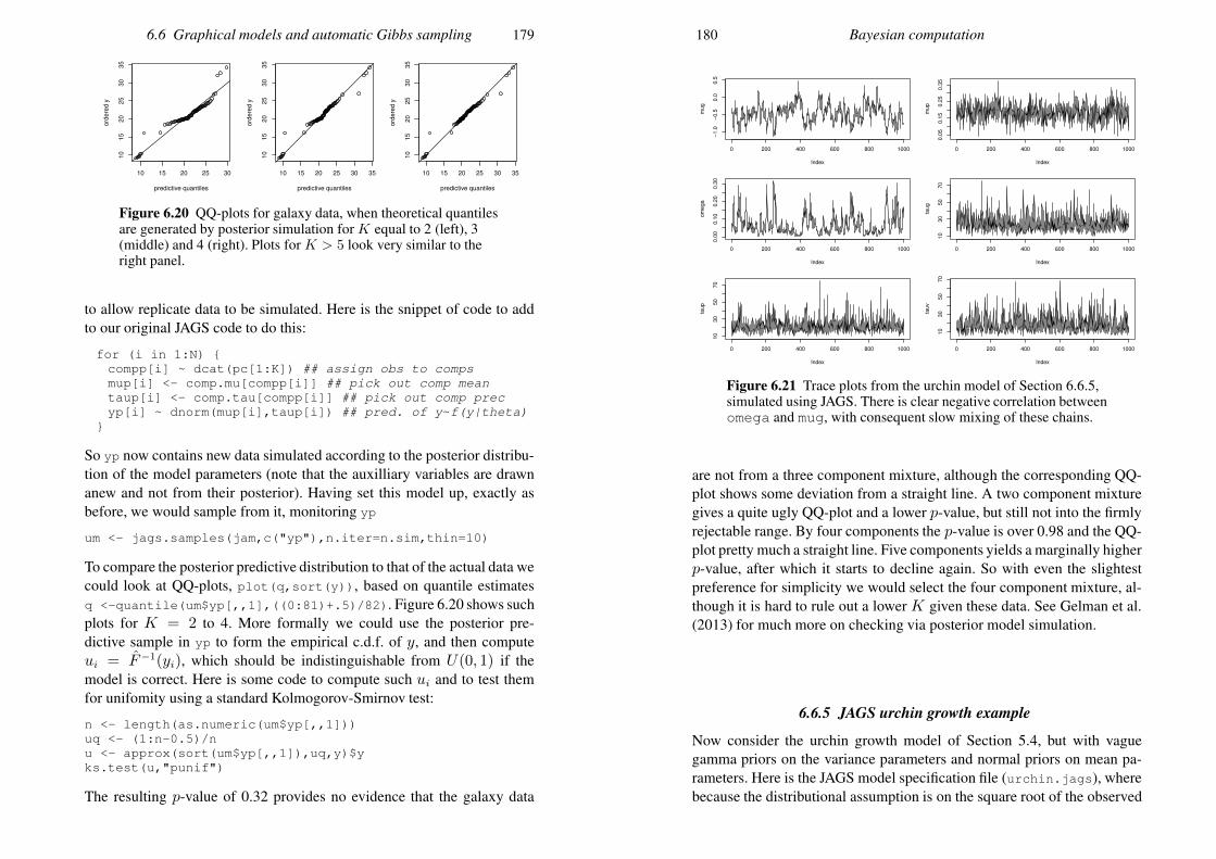
6.6 Graphical models and automatic Gibbs sampling 179
10 15 20 25 30
10
15
20
25
30
35
predictive quantiles
ord
ere
d y
10 15 20 25 30 35
10
15
20
25
30
35
predictive quantiles
ord
ere
d y
10 15 20 25 30 35
10
15
20
25
30
35
predictive quantiles
ord
ere
d y
Figure 6.20 QQ-plots for galaxy data, when theoretical quantilesare generated by posterior simulation for K equal to 2 (left), 3(middle) and 4 (right). Plots for K > 5 look very similar to theright panel.
to allow replicate data to be simulated. Here is the snippet of code to addto our original JAGS code to do this:
for (i in 1:N) compp[i] ~ dcat(pc[1:K]) ## assign obs to compsmup[i] <- comp.mu[compp[i]] ## pick out comp meantaup[i] <- comp.tau[compp[i]] ## pick out comp precyp[i] ~ dnorm(mup[i],taup[i]) ## pred. of y~f(y|theta)
So yp now contains new data simulated according to the posterior distribu-tion of the model parameters (note that the auxilliary variables are drawnanew and not from their posterior). Having set this model up, exactly asbefore, we would sample from it, monitoring yp
um <- jags.samples(jam,c("yp"),n.iter=n.sim,thin=10)
To compare the posterior predictive distribution to that of the actual data wecould look at QQ-plots, plot(q,sort(y)), based on quantile estimatesq <-quantile(um$yp[,,1],((0:81)+.5)/82). Figure 6.20 shows suchplots for K = 2 to 4. More formally we could use the posterior pre-dictive sample in yp to form the empirical c.d.f. of y, and then computeui = F−1(yi), which should be indistinguishable from U(0, 1) if themodel is correct. Here is some code to compute such ui and to test themfor unifomity using a standard Kolmogorov-Smirnov test:
n <- length(as.numeric(um$yp[,,1]))uq <- (1:n-0.5)/nu <- approx(sort(um$yp[,,1]),uq,y)$yks.test(u,"punif")
The resulting p-value of 0.32 provides no evidence that the galaxy data
180 Bayesian computation
0 200 400 600 800 1000
−1.0
−0.5
0.0
0.5
Index
mug
0 200 400 600 800 1000
0.0
50.1
50.2
50.3
5
Index
mup
0 200 400 600 800 1000
0.0
00.1
00.2
00.3
0
Index
om
ega
0 200 400 600 800 1000
10
30
50
70
Index
taug
0 200 400 600 800 1000
10
30
50
70
Index
taup
0 200 400 600 800 1000
10
30
50
70
Index
tauv
Figure 6.21 Trace plots from the urchin model of Section 6.6.5,simulated using JAGS. There is clear negative correlation betweenomega and mug, with consequent slow mixing of these chains.
are not from a three component mixture, although the corresponding QQ-plot shows some deviation from a straight line. A two component mixturegives a quite ugly QQ-plot and a lower p-value, but still not into the firmlyrejectable range. By four components the p-value is over 0.98 and the QQ-plot pretty much a straight line. Five components yields a marginally higherp-value, after which it starts to decline again. So with even the slightestpreference for simplicity we would select the four component mixture, al-though it is hard to rule out a lower K given these data. See Gelman et al.(2013) for much more on checking via posterior model simulation.
6.6.5 JAGS urchin growth example
Now consider the urchin growth model of Section 5.4, but with vaguegamma priors on the variance parameters and normal priors on mean pa-rameters. Here is the JAGS model specification file (urchin.jags), wherebecause the distributional assumption is on the square root of the observed
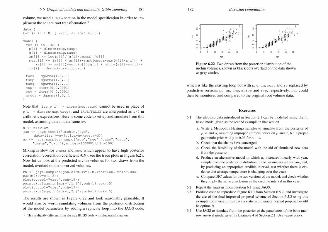
6.6 Graphical models and automatic Gibbs sampling 181
volume, we need a data section in the model specification in order to im-plement the square root transformation:9
data for (i in 1:N) rv[i] <- sqrt(v[i])model for (i in 1:N) p[i] ~ dlnorm(mup,taup)g[i] ~ dlnorm(mug,taug)am[i] <- log(p[i]/(g[i]*omega))/g[i]murv[i] <- (a[i] < am[i])*sqrt(omega*exp(g[i]*a[i])) +
(a[i] >= am[i])*sqrt(p[i]/g[i] + p[i]*(a[i]-am[i]))rv[i] ~ dnorm(murv[i],tauv)
tauv ~ dgamma(1.0,.1)taup ~ dgamma(1.0,.1)taug ~ dgamma(1.0,.1)mup ~ dnorm(0,0.0001)mug ~ dnorm(0,0.0001)omega ~ dgamma(1.0,.1)
Note that log(p[i]) ~ dnorm(mup,taup) cannot be used in place ofp[i] ~ dlnorm(mup,taup), and TRUE/FALSE are interpreted as 1/0 inarithmetic expressions. Here is some code to set up and simulate from thismodel, assuming data in dataframe uv:N <- nrow(uv)jan <- jags.model("urchin.jags",
data=list(v=uv$vol,a=uv$age,N=N))um <- jags.samples(jan,c("mup","mug","taup","taug",
"omega","tauv"),n.iter=100000,thin=100)
Mixing is slow for omega and mug, which appear to have high posteriorcorrelation (correlation coefficient -0.9): see the trace plots in Figure 6.21.Now let us look at the predicted urchin volumes for two draws from themodel, overlaid on the observed volumes:rn <- jags.samples(jan,c("murv"),n.iter=1001,thin=1000)par(mfrow=c(1,2))plot(uv,col="grey",pch=19);points(uv$age,rn$murv[,1,]^2,pch=19,cex=.5)plot(uv,col="grey",pch=19);points(uv$age,rn$murv[,2,]^2,pch=19,cex=.5)
The results are shown in Figure 6.22 and look reasonably plausible. Itwould also be worth simulating volumes from the posterior distributionof the model parameters by adding a replicate loop into the JAGS code,9 This is slightly different from the way BUGS deals with data transformation.
182 Bayesian computation
0 5 10 15 20 25
05
10
20
30
age
vol
0 5 10 15 20 25
05
10
20
30
age
vol
Figure 6.22 Two draws from the posterior distribution of theurchin volumes, shown as black dots overlaid on the data shownas grey circles.
which is like the existing loop but with p, g, am, murv and rv replaced bypredictive versions pp, gp, amp, murvp and rvp, respectively. rvp couldthen be monitored and compared to the original root volume data.
Exercises6.1 The nhtemp data introduced in Section 2.1 can be modelled using the tα
based model given as the second example in that section.
a. Write a Metropolis Hastings sampler to simulate from the posterior ofµ, σ and α, assuming improper uniform priors on µ and σ, but a propergeometric prior with p = 0.05 for α− 1.
b. Check that the chains have converged.c. Check the feasibility of the model with the aid of simulated new data
from the posterior.d. Produce an alternative model in which µi increases linearly with year,
sample from the posterior distribution of the parameters in this case, and,by producing an appropriate credible interval, test whether there is evi-dence that average temperature is changing over the years.
e. Compare DIC values for the two versions of the model, and check whetherthey imply the same conclusion as the credible interval in this case.
6.2 Repeat the analysis from question 6.1 using JAGS.6.3 Produce code to reproduce Figure 6.10 from Section 6.5.2, and investigate
the use of the final improved proposal scheme of Section 6.5.3 using thisexample (of course in this case a static multivariate normal proposal wouldbe optimal!)
6.4 Use JAGS to simulate from the posterior of the parameters of the bone mar-row survival model given in Example 4 of Section 2.1. Use vague priors.
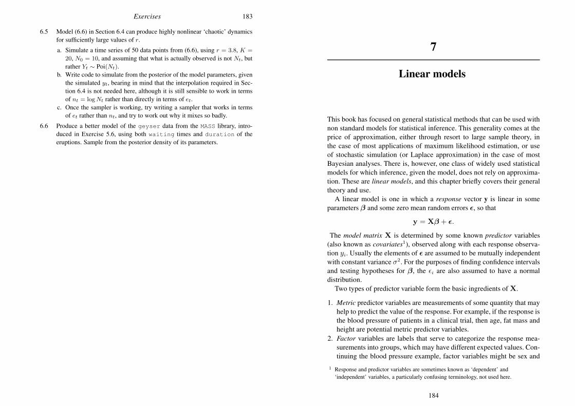
Exercises 183
6.5 Model (6.6) in Section 6.4 can produce highly nonlinear ‘chaotic’ dynamicsfor sufficiently large values of r.
a. Simulate a time series of 50 data points from (6.6), using r = 3.8, K =
20, N0 = 10, and assuming that what is actually observed is not Nt, butrather Yt ∼ Poi(Nt).
b. Write code to simulate from the posterior of the model parameters, giventhe simulated yt, bearing in mind that the interpolation required in Sec-tion 6.4 is not needed here, although it is still sensible to work in termsof nt = logNt rather than directly in terms of et.
c. Once the sampler is working, try writing a sampler that works in termsof et rather than nt, and try to work out why it mixes so badly.
6.6 Produce a better model of the geyser data from the MASS library, intro-duced in Exercise 5.6, using both waiting times and duration of theeruptions. Sample from the posterior density of its parameters.
7
Linear models
This book has focused on general statistical methods that can be used withnon standard models for statistical inference. This generality comes at theprice of approximation, either through resort to large sample theory, inthe case of most applications of maximum likelihood estimation, or useof stochastic simulation (or Laplace approximation) in the case of mostBayesian analyses. There is, however, one class of widely used statisticalmodels for which inference, given the model, does not rely on approxima-tion. These are linear models, and this chapter briefly covers their generaltheory and use.
A linear model is one in which a response vector y is linear in someparameters β and some zero mean random errors ǫ, so that
y = Xβ + ǫ.
The model matrix X is determined by some known predictor variables(also known as covariates1), observed along with each response observa-tion yi. Usually the elements of ǫ are assumed to be mutually independentwith constant variance σ2. For the purposes of finding confidence intervalsand testing hypotheses for β, the ǫi are also assumed to have a normaldistribution.
Two types of predictor variable form the basic ingredients of X.
1. Metric predictor variables are measurements of some quantity that mayhelp to predict the value of the response. For example, if the response isthe blood pressure of patients in a clinical trial, then age, fat mass andheight are potential metric predictor variables.
2. Factor variables are labels that serve to categorize the response mea-surements into groups, which may have different expected values. Con-tinuing the blood pressure example, factor variables might be sex and
1 Response and predictor variables are sometimes known as ‘dependent’ and‘independent’ variables, a particularly confusing terminology, not used here.
184
7.1 The theory of linear models 185
drug treatment received (drug A, drug B or placebo, for example). Some-what confusingly, the groups of a factor variable are referred to as levelsalthough the groups generally have no natural ordering, and even if theydo, the model structure ignores it.
To understand the construction of X it helps to consider an example. Sup-pose that along with yi we have metric predictor variables xi and zi andfactor variable gi, which contains labels dividing yi into three groups. Sup-pose further that we believe the following model to be appropriate:
yi = γgi + α1xi + α2zi + α3z2i + α4zixi + ǫi, i = 1, . . . , n,
where there is a different γ parameter for each of the three levels of gi.Collecting the γ and α parameters into one vector, β, we can rewrite themodel in matrix-vector form as
y1y2y3y4....yn
=
1 0 0 x1 z1 z21 z1x1
1 0 0 x2 z2 z22 z2x2
1 0 0 x3 z3 z23 z3x3
0 1 0 x4 z4 z24 z4x4
. . . . . . .
. . . . . . .
. . . . . . .
. . . . . . .0 0 1 xn zn z2n znxn
γ1γ2γ3α1
α2
α3
α4
+
ǫ1ǫ2ǫ3ǫ4....ǫn
where y1 - y3 are in group 1, y4 is in group 2, and yn is in group 3 ofthe factor g. Notice how the factor levels/groups each get a dummy in-dicator column in the model matrix, with elements showing whether thecorresponding yi belongs to the group or not. Notice also how the metricvariables can enter the model nonlinearly: the model is linear in the param-eters and error term, but not necessarily in the predictors.
7.1 The theory of linear models
This section shows how the parameters, β, of the linear model
µ = Xβ, y ∼ N(µ, Inσ2) (7.1)
can be estimated by least squares. It is assumed that X is a matrix, withn rows, p columns and rank p (n > p). It is also shown that the resultingestimator, β, is unbiased and that, given the normality of the data, β ∼N(β, (XTX)−1σ2). Results are also derived for setting confidence limits
186 Linear models
on parameters and for testing hypotheses about parameters: in particularthe hypothesis that several elements of β are simultaneously zero.
In this section it is important not to confuse the length of a vector withits dimension. For example (1, 1, 1)T has dimension 3 and length
√3. Also
note that no distinction has been made notationally between random vari-ables and particular observations of those random variables: it is usuallyclear from the context which is meant.
7.1.1 Least squares estimation of β
Point estimates of the linear model parameters, β, can be obtained by themethod of least squares; that is, by minimising the residual sum of squares
S =n∑
i=1
(yi − µi)2,
with respect to β, where µ = Xβ. This fitting objective follows directlyfrom the log likelihood for the model, but even without the assumption ofnormality, the Gauss-Markov theorem says that minimising S w.r.t. β willproduce the minimum variance linear unbiased estimator of β.
To use least squares with a linear model, written in general matrix-vectorform, first recall the link between the Euclidean length of a vector and thesum of squares of its elements. If v is any vector of dimension, n, then‖v‖2 ≡ vTv ≡∑n
i=1 v2i . Hence
S = ‖y − µ‖2 = ‖y −Xβ‖2.
Since S is simply the squared (Euclidian) length of the vector y−Xβ,its value will be unchanged if y −Xβ is rotated or reflected. This obser-vation is the basis for a practical method for finding β and for developingthe distributional results required to use linear models.
Specifically, as with any real matrix, X can always be decomposed
X = Q
[R0
]= QfR, (7.2)
where R is a p×p upper triangular matrix,2 and Q is an n×n orthogonalmatrix, the first p columns of which form Qf . Recall that orthogonal ma-trices rotate/reflect vectors, but do not change their length. Orthogonalityalso means that QQT = QTQ = In. Multiplying y−Xβ by QT implies
2 That is, Ri,j = 0 if i > j. See also Section B.5.
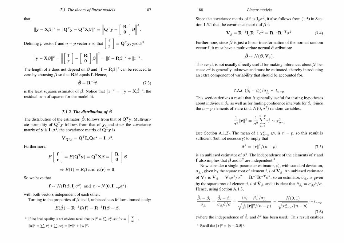
7.1 The theory of linear models 187
that
‖y −Xβ‖2 = ‖QTy −QTXβ‖2 =∥∥∥∥QTy −
[R0
]β
∥∥∥∥2
.
Defining p vector f and n− p vector r so that[fr
]≡ QTy, yields3
‖y −Xβ‖2 =∥∥∥∥[fr
]−[R0
]β
∥∥∥∥2
= ‖f −Rβ‖2 + ‖r‖2.
The length of r does not depend on β and ‖f −Rβ‖2 can be reduced tozero by choosing β so that Rβ equals f . Hence,
β = R−1f (7.3)
is the least squares estimator of β. Notice that ‖r‖2 = ‖y − Xβ‖2, theresidual sum of squares for the model fit.
7.1.2 The distribution of β
The distribution of the estimator, β, follows from that of QTy. Multivari-ate normality of QTy follows from that of y, and since the covariancematrix of y is Inσ2, the covariance matrix of QTy is
VQTy = QTInQσ2 = Inσ2.
Furthermore,
E
[fr
]= E(QTy) = QTXβ =
[R0
]β
⇒ E(f) = Rβ and E(r) = 0.
So we have that
f ∼ N(Rβ, Ipσ2) and r ∼ N(0, In−pσ
2)
with both vectors independent of each other.Turning to the properties of β itself, unbiasedness follows immediately:
E(β) = R−1E(f) = R−1Rβ = β.
3 If the final equality is not obvious recall that ‖x‖2 =∑i x
2i , so if x =
[v
w
],
‖x‖2 =∑i v
2i +
∑i w
2i = ‖v‖2 + ‖w‖2.
188 Linear models
Since the covariance matrix of f is Ipσ2, it also follows from (1.5) in Sec-tion 1.5.1 that the covariance matrix of β is
Vβ = R−1IpR−Tσ2 = R−1R−Tσ2. (7.4)
Furthermore, since β is just a linear transformation of the normal randomvector f , it must have a multivariate normal distribution:
β ∼ N(β,Vβ).
This result is not usually directly useful for making inferences aboutβ, be-cause σ2 is generally unknown and must be estimated, thereby introducingan extra component of variability that should be accounted for.
7.1.3 (βi − βi)/σβi ∼ tn−p
This section derives a result that is generally useful for testing hypothesesabout individual βi, as well as for finding confidence intervals for βi. Sincethe n− p elements of r are i.i.d. N(0, σ2) random variables,
1
σ2‖r‖2 = 1
σ2
n−p∑
i=1
r2i ∼ χ2n−p
(see Section A.1.2). The mean of a χ2n−p r.v. is n − p, so this result is
sufficient (but not necessary) to imply that
σ2 = ‖r‖2/(n− p) (7.5)
is an unbiased estimator of σ2. The independence of the elements of r andf also implies that β and σ2 are independent.4
Now consider a single-parameter estimator, βi, with standard deviation,σβi
, given by the square root of element i, i of Vβ . An unbiased estimatorof Vβ is Vβ = Vβσ
2/σ2 = R−1R−Tσ2, so an estimator, σβi, is given
by the square root of element i, i of Vβ , and it is clear that σβi= σβi
σ/σ.Hence, using Section A.1.3,
βi − βiσβi
=βi − βiσβi
σ/σ=
(βi − βi)/σβi√1σ2 ‖r‖2/(n− p)
∼ N(0, 1)√χ2n−p/(n − p)
∼ tn−p
(7.6)(where the independence of βi and σ2 has been used). This result enables
4 Recall that ‖r‖2 = ‖y −Xβ‖2.
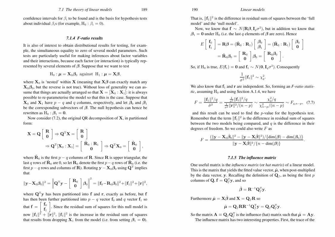
7.1 The theory of linear models 189
confidence intervals for βi to be found and is the basis for hypothesis testsabout individual βis (for example, H0 : βi = 0).
7.1.4 F-ratio results
It is also of interest to obtain distributional results for testing, for exam-ple, the simultaneous equality to zero of several model parameters. Suchtests are particularly useful for making inferences about factor variablesand their interactions, because each factor (or interaction) is typically rep-resented by several elements of β. Suppose that we want to test
H0 : µ = X0β0 against H1 : µ = Xβ,
where X0 is ‘nested’ within X (meaning that Xβ can exactly match anyX0β0, but the reverse is not true). Without loss of generality we can as-sume that things are actually arranged so that X = [X0 : X1]: it is alwayspossible to re-parameterise the model so that this is the case. Suppose thatX0 and X1 have p − q and q columns, respectively, and let β0 and β1
be the corresponding subvectors of β. The null hypothesis can hence berewritten as H0 : β1 = 0.
Now consider (7.2), the original QR decomposition of X, in partitionedform:
X = Q
[R0
]⇒ QTX =
[R0
]
⇒ QT[X0 : X1] =
[R0 : R1
0
]⇒ QTX0 =
[R0
0
],
where R0 is the first p− q columns of R. Since R is upper triangular, thelast q rows of R0 are 0, so let R0 denote the first p− q rows of R0 (i.e. thefirst p− q rows and columns of R). Rotating y−X0β0 using QT impliesthat
‖y−X0β0‖2 =∥∥∥∥QTy−
[R0
0
]β0
∥∥∥∥2
= ‖f0−R0β0‖2+‖f1‖2+‖r‖2,
where QTy has been partitioned into f and r, exactly as before, but fhas then been further partitioned into p − q vector f0 and q vector f1 so
that f =
[f0f1
]. Since the residual sum of squares for this null model is
now ‖f1‖2 + ‖r‖2, ‖f1‖2 is the increase in the residual sum of squaresthat results from dropping X1 from the model (i.e. from setting β1 = 0).
190 Linear models
That is, ‖f1‖2 is the difference in residual sum of squares between the ‘fullmodel’ and the ‘null model’.
Now, we know that f ∼ N(Rβ, Ipσ2), but in addition we know that
β1 = 0 under H0 (i.e. the last q elements of β are zero). Hence
E
[f0f1
]= Rβ = (R0 : R1)
[β0
β1
]= (R0 : R1)
[β0
0
]
= R0β0 =
[R0
0
]β0 =
[R0β0
0
].
So, if H0 is true, E(f1) = 0 and f1 ∼ N(0, Iqσ2). Consequently
1
σ2‖f1‖2 ∼ χ2
q.
We also know that f1 and r are independent. So, forming an F-ratio statis-tic, assuming H0 and using Section A.1.4, we have
F =‖f1‖2/q
σ2=
1σ2 ‖f1‖2/q
1σ2 ‖r‖2/(n − p)
∼ χ2q/q
χ2n−p/(n − p)
∼ Fq,n−p, (7.7)
and this result can be used to find the p-value for the hypothesis test.Remember that the term ‖f1‖2 is the difference in residual sum of squaresbetween the two models being compared, and q is the difference in theirdegrees of freedom. So we could also write F as
F =(‖y −X0β0‖2 − ‖y −Xβ‖2)/dim(β)− dim(β0)
‖y −Xβ‖2/n − dim(β).
7.1.5 The influence matrix
One useful matrix is the influence matrix (or hat matrix) of a linear model.This is the matrix that yields the fitted value vector, µ, when post-multipliedby the data vector, y. Recalling the definition of Qf , as being the first pcolumns of Q, f = QT
f y, and so
β = R−1QTf y.
Furthermore µ = Xβ and X = QfR so
µ = QfRR−1QTf y = QfQ
Tf y.
So the matrix A ≡ QfQTf is the influence (hat) matrix such that µ = Ay.
The influence matrix has two interesting properties. First, the trace of the
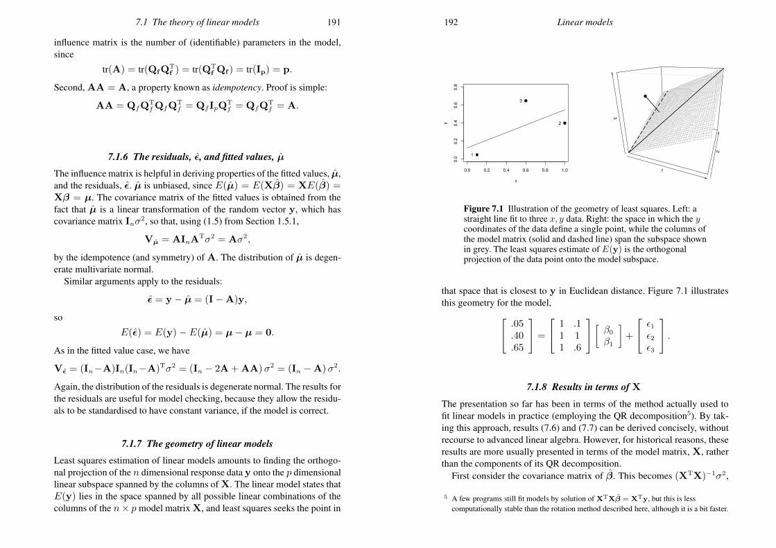
7.1 The theory of linear models 191
influence matrix is the number of (identifiable) parameters in the model,since
tr(A) = tr(QfQTf ) = tr(QT
f Qf ) = tr(Ip) = p.
Second, AA = A, a property known as idempotency. Proof is simple:
AA = QfQTfQfQ
Tf = QfIpQ
Tf = QfQ
Tf = A.
7.1.6 The residuals, ǫ, and fitted values, µ
The influence matrix is helpful in deriving properties of the fitted values, µ,and the residuals, ǫ. µ is unbiased, since E(µ) = E(Xβ) = XE(β) =Xβ = µ. The covariance matrix of the fitted values is obtained from thefact that µ is a linear transformation of the random vector y, which hascovariance matrix Inσ
2, so that, using (1.5) from Section 1.5.1,
Vµ = AInATσ2 = Aσ2,
by the idempotence (and symmetry) of A. The distribution of µ is degen-erate multivariate normal.
Similar arguments apply to the residuals:
ǫ = y − µ = (I−A)y,
so
E(ǫ) = E(y) − E(µ) = µ− µ = 0.
As in the fitted value case, we have
Vǫ = (In−A)In(In−A)Tσ2 = (In − 2A+AA) σ2 = (In −A)σ2.
Again, the distribution of the residuals is degenerate normal. The results forthe residuals are useful for model checking, because they allow the residu-als to be standardised to have constant variance, if the model is correct.
7.1.7 The geometry of linear models
Least squares estimation of linear models amounts to finding the orthogo-nal projection of the n dimensional response data y onto the p dimensionallinear subspace spanned by the columns of X. The linear model states thatE(y) lies in the space spanned by all possible linear combinations of thecolumns of the n× p model matrix X, and least squares seeks the point in
192 Linear models
0.0 0.2 0.4 0.6 0.8 1.0
0.0
0.2
0.4
0.6
0.8
x
y
1
2
3
1
2
3
Figure 7.1 Illustration of the geometry of least squares. Left: astraight line fit to three x, y data. Right: the space in which the ycoordinates of the data define a single point, while the columns ofthe model matrix (solid and dashed line) span the subspace shownin grey. The least squares estimate of E(y) is the orthogonalprojection of the data point onto the model subspace.
that space that is closest to y in Euclidean distance. Figure 7.1 illustratesthis geometry for the model,
.05
.40
.65
=
1 .11 11 .6
[β0
β1
]+
ǫ1ǫ2ǫ3
.
7.1.8 Results in terms of X
The presentation so far has been in terms of the method actually used tofit linear models in practice (employing the QR decomposition5). By tak-ing this approach, results (7.6) and (7.7) can be derived concisely, withoutrecourse to advanced linear algebra. However, for historical reasons, theseresults are more usually presented in terms of the model matrix, X, ratherthan the components of its QR decomposition.
First consider the covariance matrix of β. This becomes (XTX)−1σ2,
5 A few programs still fit models by solution of XTXβ = XTy, but this is lesscomputationally stable than the rotation method described here, although it is a bit faster.
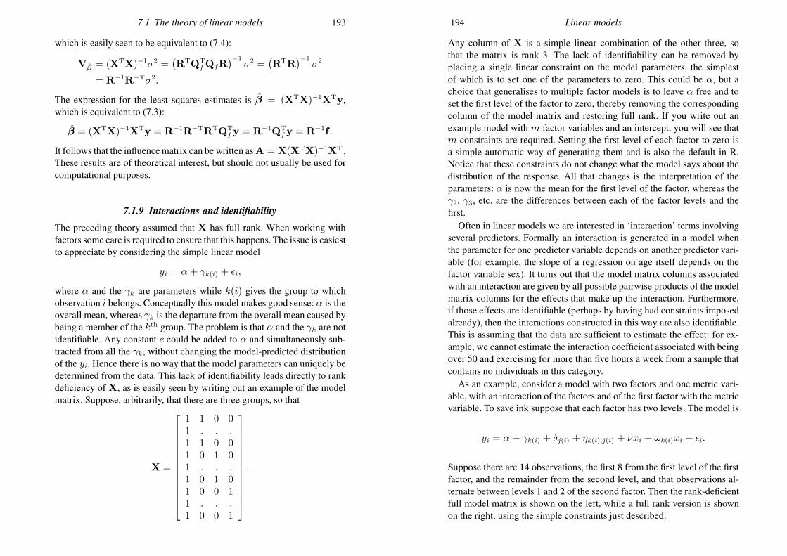
7.1 The theory of linear models 193
which is easily seen to be equivalent to (7.4):
Vβ = (XTX)−1σ2 =(RTQT
fQfR)−1
σ2 =(RTR
)−1σ2
= R−1R−Tσ2.
The expression for the least squares estimates is β = (XTX)−1XTy,which is equivalent to (7.3):
β = (XTX)−1XTy = R−1R−TRTQTf y = R−1QT
f y = R−1f .
It follows that the influence matrix can be written as A = X(XTX)−1XT.These results are of theoretical interest, but should not usually be used forcomputational purposes.
7.1.9 Interactions and identifiability
The preceding theory assumed that X has full rank. When working withfactors some care is required to ensure that this happens. The issue is easiestto appreciate by considering the simple linear model
yi = α+ γk(i) + ǫi,
where α and the γk are parameters while k(i) gives the group to whichobservation i belongs. Conceptually this model makes good sense: α is theoverall mean, whereas γk is the departure from the overall mean caused bybeing a member of the kth group. The problem is that α and the γk are notidentifiable. Any constant c could be added to α and simultaneously sub-tracted from all the γk, without changing the model-predicted distributionof the yi. Hence there is no way that the model parameters can uniquely bedetermined from the data. This lack of identifiability leads directly to rankdeficiency of X, as is easily seen by writing out an example of the modelmatrix. Suppose, arbitrarily, that there are three groups, so that
X =
1 1 0 01 . . .1 1 0 01 0 1 01 . . .1 0 1 01 0 0 11 . . .1 0 0 1
.
194 Linear models
Any column of X is a simple linear combination of the other three, sothat the matrix is rank 3. The lack of identifiability can be removed byplacing a single linear constraint on the model parameters, the simplestof which is to set one of the parameters to zero. This could be α, but achoice that generalises to multiple factor models is to leave α free and toset the first level of the factor to zero, thereby removing the correspondingcolumn of the model matrix and restoring full rank. If you write out anexample model with m factor variables and an intercept, you will see thatm constraints are required. Setting the first level of each factor to zero isa simple automatic way of generating them and is also the default in R.Notice that these constraints do not change what the model says about thedistribution of the response. All that changes is the interpretation of theparameters: α is now the mean for the first level of the factor, whereas theγ2, γ3, etc. are the differences between each of the factor levels and thefirst.
Often in linear models we are interested in ‘interaction’ terms involvingseveral predictors. Formally an interaction is generated in a model whenthe parameter for one predictor variable depends on another predictor vari-able (for example, the slope of a regression on age itself depends on thefactor variable sex). It turns out that the model matrix columns associatedwith an interaction are given by all possible pairwise products of the modelmatrix columns for the effects that make up the interaction. Furthermore,if those effects are identifiable (perhaps by having had constraints imposedalready), then the interactions constructed in this way are also identifiable.This is assuming that the data are sufficient to estimate the effect: for ex-ample, we cannot estimate the interaction coefficient associated with beingover 50 and exercising for more than five hours a week from a sample thatcontains no individuals in this category.
As an example, consider a model with two factors and one metric vari-able, with an interaction of the factors and of the first factor with the metricvariable. To save ink suppose that each factor has two levels. The model is
yi = α+ γk(i) + δj(i) + ηk(i),j(i) + νxi + ωk(i)xi + ǫi.
Suppose there are 14 observations, the first 8 from the first level of the firstfactor, and the remainder from the second level, and that observations al-ternate between levels 1 and 2 of the second factor. Then the rank-deficientfull model matrix is shown on the left, while a full rank version is shownon the right, using the simple constraints just described:
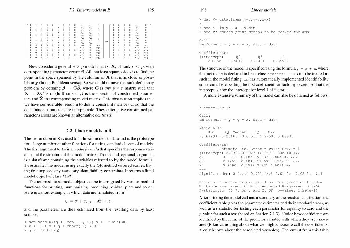
7.2 Linear models in R 195
1 1 0 1 0 1 0 0 0 x1 x1 01 1 0 0 1 0 0 1 0 x2 x2 01 1 0 1 0 1 0 0 0 x3 x3 01 1 0 0 1 0 0 1 0 x4 x4 01 1 0 1 0 1 0 0 0 x5 x5 01 1 0 0 1 0 0 1 0 x6 x6 01 1 0 1 0 1 0 0 0 x7 x7 01 1 0 0 1 0 0 1 0 x8 x8 01 0 1 1 0 0 1 0 0 x9 0 x91 0 1 0 1 0 0 0 1 x10 0 x101 0 1 1 0 0 1 0 0 x11 0 x111 0 1 0 1 0 0 0 1 x12 0 x121 0 1 1 0 0 1 0 0 x13 0 x131 0 1 0 1 0 0 0 1 x14 0 x14
→
1 0 0 0 x1 01 0 1 0 x2 01 0 0 0 x3 01 0 1 0 x4 01 0 0 0 x5 01 0 1 0 x6 01 0 0 0 x7 01 0 1 0 x8 01 1 0 0 x9 x91 1 1 1 x10 x101 1 0 0 x11 x111 1 1 1 x12 x121 1 0 0 x13 x131 1 1 1 x14 x14
Now consider a general n × p model matrix, X, of rank r < p, withcorresponding parameter vector β. All that least squares does is to find thepoint in the space spanned by the columns of X that is as close as possi-ble to y (in the Euclidean sense). So we could remove the rank-deficiencyproblem by defining β = Cβ, where C is any p × r matrix such thatX = XC is of (full) rank r. β is the r vector of constrained parame-ters and X the corresponding model matrix. This observation implies thatwe have considerable freedom to define constraint matrices C so that theconstrained parameters are interpretable. These alternative constrained pa-rameterisations are known as alternative contrasts.
7.2 Linear models in R
The lm function in R is used to fit linear models to data and is the prototypefor a large number of other functions for fitting standard classes of models.The first argument to lm is a model formula that specifies the response vari-able and the structure of the model matrix. The second, optional, argumentis a dataframe containing the variables referred to by the model formula.lm estimates the model using exactly the QR method covered earlier, hav-ing first imposed any necessary identifiability constraints. It returns a fittedmodel object of class "lm".
The returned fitted model object can be interrogated by various methodfunctions for printing, summarizing, producing residual plots and so on.Here is a short example in which data are simulated from
yi = α+ γk(i) + δxi + ǫi,
and the parameters are then estimated from the resulting data by leastsquares:
> set.seed(0);g <- rep(1:3,10); x <- runif(30)> y <- 1 + x + g + rnorm(30) * 0.5> g <- factor(g)
196 Linear models
> dat <- data.frame(y=y,g=g,x=x)>> mod <- lm(y ~ g + x,dat)> mod ## causes print method to be called for mod
Call:lm(formula = y ~ g + x, data = dat)
Coefficients:(Intercept) g2 g3 x
2.0362 0.9812 2.1461 0.8590
The structure of the model is specified using the formula y ~ g + x, wherethe fact that g is declared to be of class "factor" causes it to be treated assuch in the model fitting. lm has automatically implemented identifiabilityconstraints here, setting the first coefficient for factor g to zero, so that theintercept is now the intercept for level 1 of factor g.
A more extensive summary of the model can also be obtained as follows:
> summary(mod)
Call:lm(formula = y ~ g + x, data = dat)
Residuals:Min 1Q Median 3Q Max
-0.64293 -0.26466 -0.07511 0.27505 0.89931
Coefficients:Estimate Std. Error t value Pr(>|t|)
(Intercept) 2.0362 0.2023 10.067 1.84e-10 ***g2 0.9812 0.1873 5.237 1.80e-05 ***g3 2.1461 0.1849 11.605 8.76e-12 ***x 0.8590 0.2579 3.331 0.0026 **---Signif. codes: 0 ’***’ 0.001 ’**’ 0.01 ’*’ 0.05 ’.’ 0.1
Residual standard error: 0.411 on 26 degrees of freedomMultiple R-squared: 0.8436, Adjusted R-squared: 0.8256F-statistic: 46.75 on 3 and 26 DF, p-value: 1.294e-10
After printing the model call and a summary of the residual distribution, thecoefficient table gives the parameter estimates and their standard errors, aswell as a t statistic for testing each parameter for equality to zero and thep-value for such a test (based on Section 7.1.3). Notice how coefficients areidentified by the name of the predictor variable with which they are associ-ated (R knows nothing about what we might choose to call the coefficients;it only knows about the associated variables). The output from this table
7.2 Linear models in R 197
can also be used to compute confidence intervals for the model coefficientsusing the results from Section 2.7. The Residual standard error is σ,and the F-statistic is the F-ratio for testing the null hypothesis that aconstant is as good a model for the mean response as the model actuallyfitted. The associated p-value suggests not, in this case.
The R-squared statistics are measures of how closely the model fits theresponse data. The idea is that, after fitting, the part of the variability leftunexplained is the variability of the residuals, so the proportion of variabil-ity unexplained is the ratio of the residual variance to the original varianceof the yi. One minus the unexplained variance is the explained variance
r2 = 1−∑
i ǫ2i/n∑
i(yi − y)2/n.
This conventional definition (from which the n’s can be cancelled) usesbiased variance estimators. As a result r2 tends to overestimate how well amodel is doing. The adjusted r2 avoids this overestimation to some extentby using unbiased estimators,
r2adj = 1−∑
i ǫ2i/(n− p)∑
i(yi − y)2/(n− 1),
where p is the number of model parameters. r2adj can be negative.6
High r2 values (close to 1) indicate a close fit, but a low r2 is not neces-sarily indicative of a poor model: it can simply mean that the data containa substantial random component.
7.2.1 Model formulae
In R, model formulae are used to specify the response variable and modelstructure. Consider the example
y ~ x + log(z) + x:z
The variable to the left of ~ specifies the response variable, whereas every-thing to the right specifies how to set up the model matrix. ‘+’ indicatesto include the variable to the left of it and the variable to the right of it (itdoes not mean that they should be summed). ‘:’ denotes the interaction ofthe variables to its left and right. So if x is a metric variable then the aboveformula specifies:
yi = β1 + β2xi + β3 log(zi) + β4xizi + ǫi
6 This occurs when the fit of the model to data is purely imaginary.
198 Linear models
whereas if x is a factor variable the model is
yi = β1 + γk(i) + β2 log(zi) + αk(i)zi + ǫi.
Notice how an intercept term is included by default.In addition to ‘+’ and ‘:’ several other symbols have special meanings
in model formulae:
• ‘*’ means to include main effects and interactions, so a * b is the sameas a + b + a:b.
• ‘^’ is used to include main effects and interactions up to a specified level.So (a+b+c)^2 is equivalent to a + b + c + a:b + a:c + b:c, forexample, while (a+b+c)^3 would also add a:b:c. Notice that this oper-ator does not generate all the second-order terms you might be expectingfor metric variables.
• ‘-’ excludes terms that might otherwise be included. For example, -1excludes the intercept otherwise included by default, and x * z - z
would produce x + x:z.
As we have seen, you can use simple mathematical functions in modelformulae to transform variables, but outside the argument to a function theusual arithmetic operators all have special meanings. This means that if wewant to restore the usual arithmetic meaning to an operator in a formula,then we have to take special measures to do this, by making the expressionthe argument of the identity function I(). For example, y ~I(x+z) wouldspecify the model yi = α+β(xi+zi)+ǫi. Occasionally the model matrixshould include a column for which the corresponding β coefficient is fixedat 1. Such a column is known as an offset: offset(z) would include acolumn, z, of this type. See ?formula in R for more details.
7.2.2 Model checking
As with all statistical modelling it is important to check the plausibility ofa linear model before conducting formal statistical inference. It is pointlesscomputing AIC, testing hypotheses or obtaining confidence intervals for amodel that is clearly wrong, because all these procedures rest on the modelbeing at least plausible. For linear models the key assumptions are those ofconstant variance and independence, and the residuals should be examinedfor any evidence that these have been violated. Normality of the residualsshould also be checked, if the other assumptions are viable, but the centrallimit theorem tends to mean that normality is of only secondary importanceto the other assumptions.
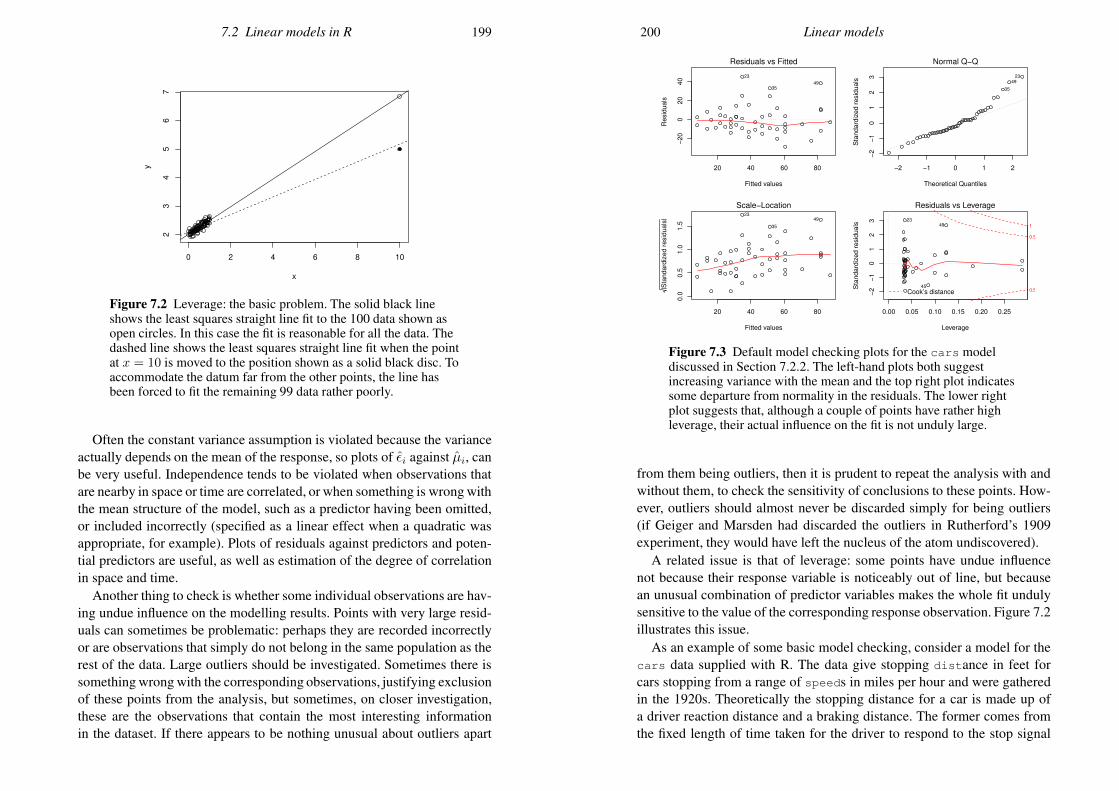
7.2 Linear models in R 199
0 2 4 6 8 10
23
45
67
x
y
Figure 7.2 Leverage: the basic problem. The solid black lineshows the least squares straight line fit to the 100 data shown asopen circles. In this case the fit is reasonable for all the data. Thedashed line shows the least squares straight line fit when the pointat x = 10 is moved to the position shown as a solid black disc. Toaccommodate the datum far from the other points, the line hasbeen forced to fit the remaining 99 data rather poorly.
Often the constant variance assumption is violated because the varianceactually depends on the mean of the response, so plots of ǫi against µi, canbe very useful. Independence tends to be violated when observations thatare nearby in space or time are correlated, or when something is wrong withthe mean structure of the model, such as a predictor having been omitted,or included incorrectly (specified as a linear effect when a quadratic wasappropriate, for example). Plots of residuals against predictors and poten-tial predictors are useful, as well as estimation of the degree of correlationin space and time.
Another thing to check is whether some individual observations are hav-ing undue influence on the modelling results. Points with very large resid-uals can sometimes be problematic: perhaps they are recorded incorrectlyor are observations that simply do not belong in the same population as therest of the data. Large outliers should be investigated. Sometimes there issomething wrong with the corresponding observations, justifying exclusionof these points from the analysis, but sometimes, on closer investigation,these are the observations that contain the most interesting informationin the dataset. If there appears to be nothing unusual about outliers apart
200 Linear models
20 40 60 80
−2
00
20
40
Fitted values
Re
sid
ua
ls
Residuals vs Fitted
23
4935
−2 −1 0 1 2
−2
−1
01
23
Theoretical Quantiles
Sta
nd
ard
ize
d r
esid
ua
ls
Normal Q−Q
2349
35
20 40 60 80
0.0
0.5
1.0
1.5
Fitted values
Sta
nd
ard
ize
d r
esid
ua
ls
Scale−Location23
49
35
0.00 0.05 0.10 0.15 0.20 0.25
−2
−1
01
23
Leverage
Sta
nd
ard
ize
d r
esid
ua
ls
Cook’s distance 0.5
0.5
1
Residuals vs Leverage
4923
45
Figure 7.3 Default model checking plots for the cars modeldiscussed in Section 7.2.2. The left-hand plots both suggestincreasing variance with the mean and the top right plot indicatessome departure from normality in the residuals. The lower rightplot suggests that, although a couple of points have rather highleverage, their actual influence on the fit is not unduly large.
from them being outliers, then it is prudent to repeat the analysis with andwithout them, to check the sensitivity of conclusions to these points. How-ever, outliers should almost never be discarded simply for being outliers(if Geiger and Marsden had discarded the outliers in Rutherford’s 1909experiment, they would have left the nucleus of the atom undiscovered).
A related issue is that of leverage: some points have undue influencenot because their response variable is noticeably out of line, but becausean unusual combination of predictor variables makes the whole fit undulysensitive to the value of the corresponding response observation. Figure 7.2illustrates this issue.
As an example of some basic model checking, consider a model for thecars data supplied with R. The data give stopping distance in feet forcars stopping from a range of speeds in miles per hour and were gatheredin the 1920s. Theoretically the stopping distance for a car is made up ofa driver reaction distance and a braking distance. The former comes fromthe fixed length of time taken for the driver to respond to the stop signal
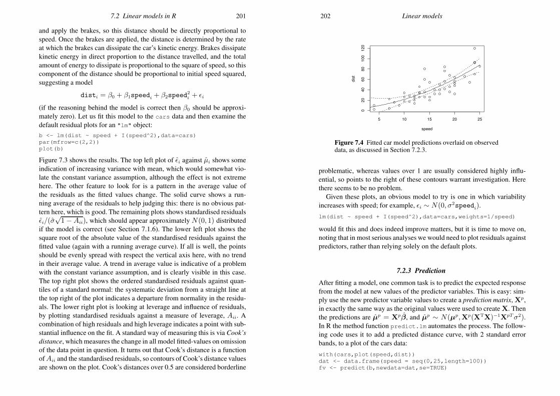
7.2 Linear models in R 201
and apply the brakes, so this distance should be directly proportional tospeed. Once the brakes are applied, the distance is determined by the rateat which the brakes can dissipate the car’s kinetic energy. Brakes dissipatekinetic energy in direct proportion to the distance travelled, and the totalamount of energy to dissipate is proportional to the square of speed, so thiscomponent of the distance should be proportional to initial speed squared,suggesting a model
disti = β0 + β1speedi + β2speed2i + ǫi
(if the reasoning behind the model is correct then β0 should be approxi-mately zero). Let us fit this model to the cars data and then examine thedefault residual plots for an "lm" object:b <- lm(dist ~ speed + I(speed^2),data=cars)par(mfrow=c(2,2))plot(b)
Figure 7.3 shows the results. The top left plot of ǫi against µi shows someindication of increasing variance with mean, which would somewhat vio-late the constant variance assumption, although the effect is not extremehere. The other feature to look for is a pattern in the average value ofthe residuals as the fitted values change. The solid curve shows a run-ning average of the residuals to help judging this: there is no obvious pat-tern here, which is good. The remaining plots shows standardised residualsǫi/(σ
√1−Aii), which should appear approximately N(0, 1) distributed
if the model is correct (see Section 7.1.6). The lower left plot shows thesquare root of the absolute value of the standardised residuals against thefitted value (again with a running average curve). If all is well, the pointsshould be evenly spread with respect the vertical axis here, with no trendin their average value. A trend in average value is indicative of a problemwith the constant variance assumption, and is clearly visible in this case.The top right plot shows the ordered standardised residuals against quan-tiles of a standard normal: the systematic deviation from a straight line atthe top right of the plot indicates a departure from normality in the residu-als. The lower right plot is looking at leverage and influence of residuals,by plotting standardised residuals against a measure of leverage, Aii. Acombination of high residuals and high leverage indicates a point with sub-stantial influence on the fit. A standard way of measuring this is via Cook’sdistance, which measures the change in all model fitted-values on omissionof the data point in question. It turns out that Cook’s distance is a functionof Aii and the standardised residuals, so contours of Cook’s distance valuesare shown on the plot. Cook’s distances over 0.5 are considered borderline
202 Linear models
5 10 15 20 25
020
40
60
80
100
120
speed
dis
t
Figure 7.4 Fitted car model predictions overlaid on observeddata, as discussed in Section 7.2.3.
problematic, whereas values over 1 are usually considered highly influ-ential, so points to the right of these contours warrant investigation. Herethere seems to be no problem.
Given these plots, an obvious model to try is one in which variabilityincreases with speed; for example, ǫi ∼ N(0, σ2speedi).
lm(dist ~ speed + I(speed^2),data=cars,weights=1/speed)
would fit this and does indeed improve matters, but it is time to move on,noting that in most serious analyses we would need to plot residuals againstpredictors, rather than relying solely on the default plots.
7.2.3 Prediction
After fitting a model, one common task is to predict the expected responsefrom the model at new values of the predictor variables. This is easy: sim-ply use the new predictor variable values to create a prediction matrix, Xp,in exactly the same way as the original values were used to create X. Thenthe predictions are µp = Xpβ, and µp ∼ N(µp,Xp(XTX)−1XpTσ2).In R the method function predict.lm automates the process. The follow-ing code uses it to add a predicted distance curve, with 2 standard errorbands, to a plot of the cars data:
with(cars,plot(speed,dist))dat <- data.frame(speed = seq(0,25,length=100))fv <- predict(b,newdata=dat,se=TRUE)
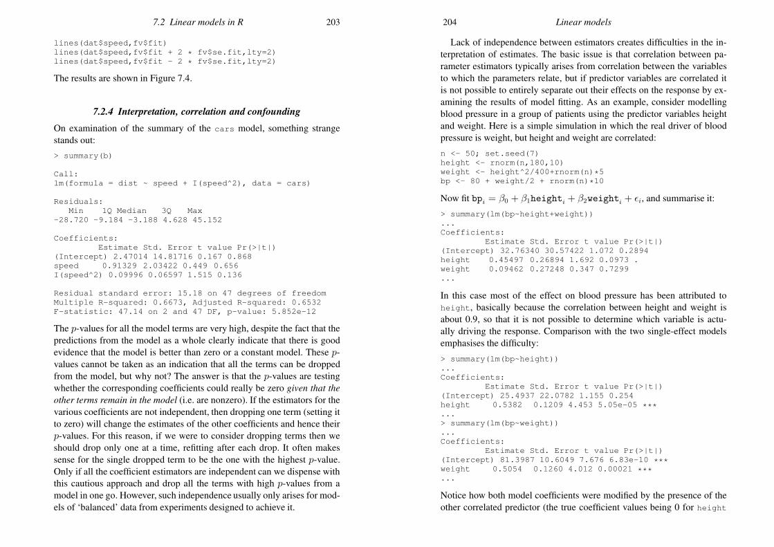
7.2 Linear models in R 203
lines(dat$speed,fv$fit)lines(dat$speed,fv$fit + 2 * fv$se.fit,lty=2)lines(dat$speed,fv$fit - 2 * fv$se.fit,lty=2)
The results are shown in Figure 7.4.
7.2.4 Interpretation, correlation and confounding
On examination of the summary of the cars model, something strangestands out:
> summary(b)
Call:lm(formula = dist ~ speed + I(speed^2), data = cars)
Residuals:Min 1Q Median 3Q Max
-28.720 -9.184 -3.188 4.628 45.152
Coefficients:Estimate Std. Error t value Pr(>|t|)
(Intercept) 2.47014 14.81716 0.167 0.868speed 0.91329 2.03422 0.449 0.656I(speed^2) 0.09996 0.06597 1.515 0.136
Residual standard error: 15.18 on 47 degrees of freedomMultiple R-squared: 0.6673, Adjusted R-squared: 0.6532F-statistic: 47.14 on 2 and 47 DF, p-value: 5.852e-12
The p-values for all the model terms are very high, despite the fact that thepredictions from the model as a whole clearly indicate that there is goodevidence that the model is better than zero or a constant model. These p-values cannot be taken as an indication that all the terms can be droppedfrom the model, but why not? The answer is that the p-values are testingwhether the corresponding coefficients could really be zero given that theother terms remain in the model (i.e. are nonzero). If the estimators for thevarious coefficients are not independent, then dropping one term (setting itto zero) will change the estimates of the other coefficients and hence theirp-values. For this reason, if we were to consider dropping terms then weshould drop only one at a time, refitting after each drop. It often makessense for the single dropped term to be the one with the highest p-value.Only if all the coefficient estimators are independent can we dispense withthis cautious approach and drop all the terms with high p-values from amodel in one go. However, such independence usually only arises for mod-els of ‘balanced’ data from experiments designed to achieve it.
204 Linear models
Lack of independence between estimators creates difficulties in the in-terpretation of estimates. The basic issue is that correlation between pa-rameter estimators typically arises from correlation between the variablesto which the parameters relate, but if predictor variables are correlated itis not possible to entirely separate out their effects on the response by ex-amining the results of model fitting. As an example, consider modellingblood pressure in a group of patients using the predictor variables heightand weight. Here is a simple simulation in which the real driver of bloodpressure is weight, but height and weight are correlated:
n <- 50; set.seed(7)height <- rnorm(n,180,10)weight <- height^2/400+rnorm(n)*5bp <- 80 + weight/2 + rnorm(n)*10
Now fit bpi = β0 + β1heighti + β2weighti + ǫi, and summarise it:
> summary(lm(bp~height+weight))...Coefficients:
Estimate Std. Error t value Pr(>|t|)(Intercept) 32.76340 30.57422 1.072 0.2894height 0.45497 0.26894 1.692 0.0973 .weight 0.09462 0.27248 0.347 0.7299...
In this case most of the effect on blood pressure has been attributed toheight, basically because the correlation between height and weight isabout 0.9, so that it is not possible to determine which variable is actu-ally driving the response. Comparison with the two single-effect modelsemphasises the difficulty:
> summary(lm(bp~height))...Coefficients:
Estimate Std. Error t value Pr(>|t|)(Intercept) 25.4937 22.0782 1.155 0.254height 0.5382 0.1209 4.453 5.05e-05 ***...> summary(lm(bp~weight))...Coefficients:
Estimate Std. Error t value Pr(>|t|)(Intercept) 81.3987 10.6049 7.676 6.83e-10 ***weight 0.5054 0.1260 4.012 0.00021 ***...
Notice how both model coefficients were modified by the presence of theother correlated predictor (the true coefficient values being 0 for height
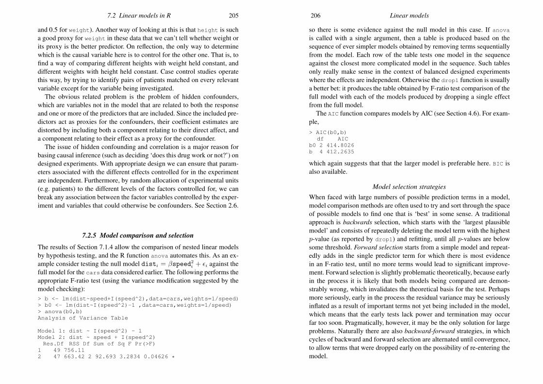
7.2 Linear models in R 205
and 0.5 for weight). Another way of looking at this is that height is sucha good proxy for weight in these data that we can’t tell whether weight orits proxy is the better predictor. On reflection, the only way to determinewhich is the causal variable here is to control for the other one. That is, tofind a way of comparing different heights with weight held constant, anddifferent weights with height held constant. Case control studies operatethis way, by trying to identify pairs of patients matched on every relevantvariable except for the variable being investigated.
The obvious related problem is the problem of hidden confounders,which are variables not in the model that are related to both the responseand one or more of the predictors that are included. Since the included pre-dictors act as proxies for the confounders, their coefficient estimates aredistorted by including both a component relating to their direct affect, anda component relating to their effect as a proxy for the confounder.
The issue of hidden confounding and correlation is a major reason forbasing causal inference (such as deciding ‘does this drug work or not?’) ondesigned experiments. With appropriate design we can ensure that param-eters associated with the different effects controlled for in the experimentare independent. Furthermore, by random allocation of experimental units(e.g. patients) to the different levels of the factors controlled for, we canbreak any association between the factor variables controlled by the exper-iment and variables that could otherwise be confounders. See Section 2.6.
7.2.5 Model comparison and selection
The results of Section 7.1.4 allow the comparison of nested linear modelsby hypothesis testing, and the R function anova automates this. As an ex-ample consider testing the null model disti = βspeed2i + ǫi against thefull model for the cars data considered earlier. The following performs theappropriate F-ratio test (using the variance modification suggested by themodel checking):> b <- lm(dist~speed+I(speed^2),data=cars,weights=1/speed)> b0 <- lm(dist~I(speed^2)-1 ,data=cars,weights=1/speed)> anova(b0,b)Analysis of Variance Table
Model 1: dist ~ I(speed^2) - 1Model 2: dist ~ speed + I(speed^2)Res.Df RSS Df Sum of Sq F Pr(>F)
1 49 756.112 47 663.42 2 92.693 3.2834 0.04626 *
206 Linear models
so there is some evidence against the null model in this case. If anova
is called with a single argument, then a table is produced based on thesequence of ever simpler models obtained by removing terms sequentiallyfrom the model. Each row of the table tests one model in the sequenceagainst the closest more complicated model in the sequence. Such tablesonly really make sense in the context of balanced designed experimentswhere the effects are independent. Otherwise the drop1 function is usuallya better bet: it produces the table obtained by F-ratio test comparison of thefull model with each of the models produced by dropping a single effectfrom the full model.
The AIC function compares models by AIC (see Section 4.6). For exam-ple,> AIC(b0,b)
df AICb0 2 414.8026b 4 412.2635
which again suggests that that the larger model is preferable here. BIC isalso available.
Model selection strategiesWhen faced with large numbers of possible prediction terms in a model,model comparison methods are often used to try and sort through the spaceof possible models to find one that is ‘best’ in some sense. A traditionalapproach is backwards selection, which starts with the ‘largest plausiblemodel’ and consists of repeatedly deleting the model term with the highestp-value (as reported by drop1) and refitting, until all p-values are belowsome threshold. Forward selection starts from a simple model and repeat-edly adds in the single predictor term for which there is most evidencein an F-ratio test, until no more terms would lead to significant improve-ment. Forward selection is slightly problematic theoretically, because earlyin the process it is likely that both models being compared are demon-strably wrong, which invalidates the theoretical basis for the test. Perhapsmore seriously, early in the process the residual variance may be seriouslyinflated as a result of important terms not yet being included in the model,which means that the early tests lack power and termination may occurfar too soon. Pragmatically, however, it may be the only solution for largeproblems. Naturally there are also backward-forward strategies, in whichcycles of backward and forward selection are alternated until convergence,to allow terms that were dropped early on the possibility of re-entering themodel.
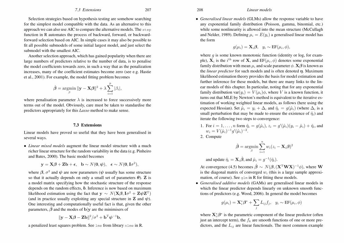
7.3 Extensions 207
Selection strategies based on hypothesis testing are somehow searchingfor the simplest model compatible with the data. As an alternative to thisapproach we can also use AIC to compare the alternative models. The stepfunction in R automates the process of backward, forward, or backward-forward selection based on AIC. In simple cases it may also be possible tofit all possible submodels of some initial largest model, and just select thesubmodel with the smallest AIC.
Another selection approach, which has gained popularity when there arelarge numbers of predictors relative to the number of data, is to penalisethe model coefficients towards zero, in such a way that as the penalizationincreases, many of the coefficient estimates become zero (see e.g. Hastieet al., 2001). For example, the model fitting problem becomes
β = argminβ
‖y −Xβ‖2 + λp∑
i=1
|βi|,
where penalisation parameter λ is increased to force successively moreterms out of the model. Obviously, care must be taken to standardise thepredictors appropriately for this Lasso method to make sense.
7.3 Extensions
Linear models have proved so useful that they have been generalised inseveral ways.
• Linear mixed models augment the linear model structure with a muchricher linear structure for the random variability in the data (e.g. Pinheiroand Bates, 2000). The basic model becomes
y = Xβ + Zb+ ǫ, b ∼ N(0,ψ), ǫ ∼ N(0, Iσ2),
where β, σ2 and ψ are now parameters (ψ usually has some structureso that it actually depends on only a small set of parameters θ). Z isa model matrix specifying how the stochastic structure of the responsedepends on the random effects, b. Inference is now based on maximumlikelihood estimation using the fact that y ∼ N(Xβ, Iσ2 + ZψZT)(and in practice usually exploiting any special structure in Z and ψ).One interesting and computationally useful fact is that, given the otherparameters, β and the modes of b|y are the minimisers of
‖y −Xβ − Zb‖2/σ2 + bTψ−1b,
a penalized least squares problem. See lme from library nlme in R.
208 Linear models
• Generalised linear models (GLMs) allow the response variable to haveany exponential family distribution (Poisson, gamma, binomial, etc.)while some nonlinearity is allowed into the mean structure (McCullaghand Nelder, 1989). Defining µi = E(yi) a generalised linear model hasthe form
g(µi) = Xiβ, yi ∼ EF(µi, φ),
where g is some known monotonic function (identity or log, for exam-ple), Xi is the ith row of X, and EF(µi, φ) denotes some exponentialfamily distribution with mean µi and scale parameterφ. Xβ is known asthe linear predictor for such models and is often denoted η. Maximumlikelihood estimation theory provides the basis for model estimation andfurther inference for these models, but there are many links to the lin-ear models of this chapter. In particular, noting that for any exponentialfamily distribution var(yi) = V (µi)φ, where V is a known function, itturns out that MLE by Newton’s method is equivalent to the iterative es-timation of working weighted linear models, as follows (here using theexpected Hessian). Set µi = yi + ∆i and ηi = g(µi) (where ∆i is asmall perturbation that may be made to ensure the existence of ηi) anditerate the following two steps to convergence:
1. For i = 1, . . . , n form ηi = g(µi), zi = g′(µi)(yi − µi) + ηi, andwi = V (µi)
−1g′(µi)−2.
2. Compute
β = argminβ
n∑
i=1
wi(zi −Xiβ)2
and update ηi = Xiβ, and µi = g−1(ηi).
At convergence (4.5) becomes β ∼ N(β, (XTWX)−1φ), where Wis the diagonal matrix of converged wi (this is a large sample approxi-mation, of course). See glm in R for fitting these models.
• Generalised additive models (GAMs) are generalised linear models inwhich the linear predictor depends linearly on unknown smooth func-tions of predictors (e.g. Wood, 2006). In general the model becomes
g(µi) = X∗iβ
∗ +∑
j
Lijfj , yi ∼ EF(µi, φ)
where X∗iβ
∗ is the parametric component of the linear predictor (oftenjust an intercept term), the fk are smooth functions of one or more pre-dictors, and the Lij are linear functionals. The most common example
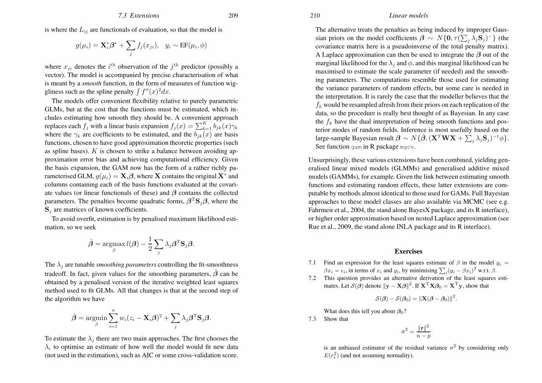
7.3 Extensions 209
is where the Lij are functionals of evaluation, so that the model is
g(µi) = X∗iβ
∗ +∑
j
fj(xji), yi ∼ EF(µi, φ)
where xji denotes the ith observation of the jth predictor (possibly avector). The model is accompanied by precise characterisation of whatis meant by a smooth function, in the form of measures of function wig-gliness such as the spline penalty
∫f ′′(x)2dx.
The models offer convenient flexibility relative to purely parametricGLMs, but at the cost that the functions must be estimated, which in-cludes estimating how smooth they should be. A convenient approachreplaces each fj with a linear basis expansion fj(x) =
∑Kk=1 bjk(x)γk
where the γk are coefficients to be estimated, and the bjk(x) are basisfunctions, chosen to have good approximation theoretic properties (suchas spline bases). K is chosen to strike a balance between avoiding ap-proximation error bias and achieving computational efficiency. Giventhe basis expansion, the GAM now has the form of a rather richly pa-rameterised GLM, g(µi) = Xiβ, where X contains the originalX∗ andcolumns containing each of the basis functions evaluated at the covari-ate values (or linear functionals of these) and β contains the collectedparameters. The penalties become quadratic forms, βTSjβ, where theSj are matrices of known coefficients.
To avoid overfit, estimation is by penalised maximum likelihood esti-mation, so we seek
β = argmaxβ
l(β)− 1
2
∑
j
λjβTSjβ.
The λj are tunable smoothing parameters controlling the fit-smoothnesstradeoff. In fact, given values for the smoothing parameters, β can beobtained by a penalised version of the iterative weighted least squaresmethod used to fit GLMs. All that changes is that at the second step ofthe algorithm we have
β = argminβ
n∑
i=1
wi(zi −Xiβ)2 +
∑
j
λjβTSjβ.
To estimate the λj there are two main approaches. The first chooses theλi to optimise an estimate of how well the model would fit new data(not used in the estimation), such as AIC or some cross-validation score.
210 Linear models
The alternative treats the penalties as being induced by improper Gaus-sian priors on the model coefficients β ∼ N0, τ(∑j λjSj)
− (thecovariance matrix here is a pseudoinverse of the total penalty matrix).A Laplace approximation can then be used to integrate the β out of themarginal likelihood for the λj and φ, and this marginal likelihood can bemaximised to estimate the scale parameter (if needed) and the smooth-ing parameters. The computations resemble those used for estimatingthe variance parameters of random effects, but some care is needed inthe interpretation. It is rarely the case that the modeller believes that thefk would be resampled afresh from their priors on each replication of thedata, so the procedure is really best thought of as Bayesian. In any casethe fk have the dual interpretation of being smooth functions and pos-terior modes of random fields. Inference is most usefully based on thelarge-sample Bayesian result β ∼ Nβ, (XTWX +
∑j λjSj)
−1φ.See function gam in R package mgcv.
Unsurprisingly, these various extensions have been combined, yielding gen-eralised linear mixed models (GLMMs) and generalised additive mixedmodels (GAMMs), for example. Given the link between estimating smoothfunctions and estimating random effects, these latter extensions are com-putable by methods almost identical to those used for GAMs. Full Bayesianapproaches to these model classes are also available via MCMC (see e.g.Fahrmeir et al., 2004, the stand alone BayesX package, and its R interface),or higher order approximation based on nested Laplace approximation (seeRue et al., 2009, the stand alone INLA package and its R interface).
Exercises7.1 Find an expression for the least squares estimate of β in the model yi =
βxi = ǫi, in terms of xi and yi, by minimising∑i(yi − βxi)
2 w.r.t. β.7.2 This question provides an alternative derivation of the least squares esti-
mates. Let S(β) denote ‖y −Xβ‖2. If XTXβ0 = XTy, show that
S(β)− S(β0) = ‖X(β − β0)‖2.
What does this tell you about β0?7.3 Show that
σ2 =‖r‖2n− p
is an unbiased estimator of the residual variance σ2 by considering onlyE(r2i ) (and not assuming normality).
Exercises 211
7.4 Show that, in the usual linear modelling notation, XTy = XTµ. Hence if alinear model contains an intercept term, show what the sum of the residuals,∑i ǫi, must be.
7.5 Write out the following three models in the form y = Xβ + ǫ (note: y, βand ǫ are always vectors, whereas X is a matrix). In all cases y is the re-sponse variable, ǫ the residual ‘error’ and other Greek letters indicate modelparameters.
a. The ‘balanced one-way ANOVA model’, yij = βi+ǫij , where i = 1 . . . 3
and j = 1 . . . 2.b. A model with two explanatory variables: a factor variable and a continu-
ous variable, x:
yi = βj + γxi + ǫi if obs. i is from factor level j
Assume that i = 1 . . . 6, that the first two observations are for factor level1 and the remaining four for factor level 2, and that the xi’s are 0.1, 0.4,0.5, 0.3, 0.4 and 0.7.
c. A model with two explanatory factor variables and only one observationper combination of factor variables: yij = α + βi + γj + ǫij . The firstfactor (β) has three levels and the second factor has four levels.
7.6 A statistician has fitted two alternative models to response data yi. Thefirst is yi = β0 + β1xi + ǫi and the second is yi = β0 + β1xi + γj +
ǫi if yi from group j. In R the factor variable containing the group labels istrt. The statistician wants to test the null hypothesis that the simpler modelis correct. To do this, both models are fitted in R, and a fragment of thesummary for each is shown here:
> summary(b0)lm(formula = y ~ x)...Resid standard error: 0.3009 on 98 degrees of freedom> summary(b1)lm(formula = y ~ x + trt)...Resid standard error: 0.3031 on 95 degrees of freedom
In R this test could be conducted via anova(b0,b1), but instead performthe test using just the information given (and pf in R).
7.7 Consider the cars model of Section 7.2.2. This question is about the me-chanics of estimating that model using the QR decomposition.
a. Create a model matrix X, for the model, using the data in the cars dataframe and the model.matrix.
b. Now form the QR decomposition of X as follows
qrx <- qr(X) ## returns a QR decomposition objectQ <- qr.Q(qrx,complete=TRUE) ## extract QR <- qr.R(qrx) ## extract R
212 Linear models
c. Look at R to confirm its structure. Confirm that Q is an orthogonal matrix.Confirm that ‖Qx‖2 = ‖x‖2 for any x of appropriate dimension, bytrying some example x’s (why does this happen?).
d. Obtain f and r (in the notation of Section 7.1.1).e. Evaluate β using R and f .f. Confirm that ‖r‖2 = ‖y −Xβ‖2 for this model.g. Estimate σ2 as σ2 = ‖r‖2/(n− p).h. Using σ2 and R, obtain an estimate of the estimator covariance matrix
Vβ
corresponding to β.
7.8 A material of unknown volume is divided into four roughly equal parts bycutting it in two first and then cutting the resulting pieces in two. Two alterna-tive methods of estimating the (different) volumes of each part are suggested
A. Make two estimates of the volume of each section.B. Make two estimates of the volume of each of the 2 parts formed first, and
one estimate of the volume of the each of the 4 final pieces.
Assuming that each estimate is independent and unbiased with variance σ2,show that the variances of the least squares estimates of the four volumesare 0.5σ2 by method A and 0.6σ2 by method B. Hint: use the (XTX)−1σ2
form of the parameter estimator covariance matrix.7.9 A distillery sets up and sponsors a hill race dubbed the ‘Whisky Challenge’,
for promotional purposes. To generate extra interest from elite fell runnersin the first year, it is proposed to offer a prize for every runner who com-pletes the course in less than a set time, T0. The organisers need to set T0high enough to generate a big field of participants, but low enough that theydo not bankrupt the distillery. To this end they approach you to come upwith a predicted winning time for the race. To help you do this, the hillsdata frame in R package MASS provides winning times for 35 Scottish hillraces. To load the data and examine it, type library(MASS);hills inR. Find and estimate a suitable linear model for predicting winning times(minutes) in terms of race distance dist (miles) and the total height climbedclimb (feet). If you are not sure where to start look up ‘Naismith’s Rule’on Wikipedia. The Whisky Challenge is to be a 7-mile race, with 2400 feetof ascent.
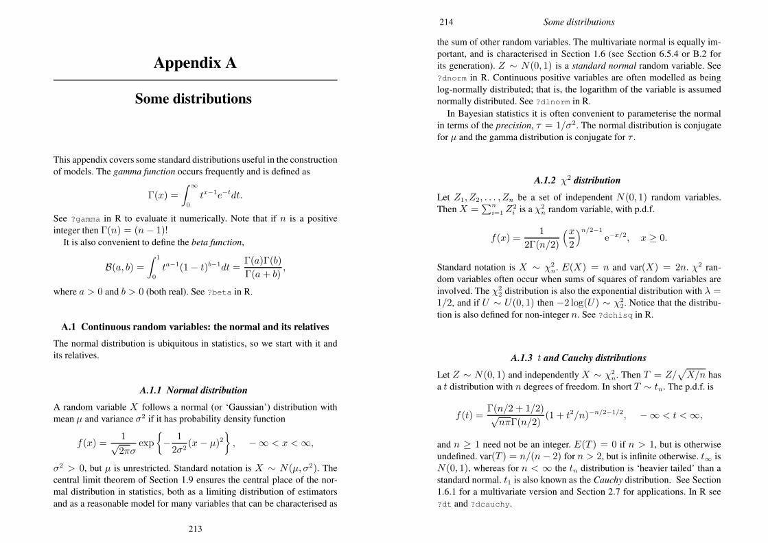
Appendix A
Some distributions
This appendix covers some standard distributions useful in the constructionof models. The gamma function occurs frequently and is defined as
Γ(x) =
∫ ∞
0
tx−1e−tdt.
See ?gamma in R to evaluate it numerically. Note that if n is a positiveinteger then Γ(n) = (n− 1)!
It is also convenient to define the beta function,
B(a, b) =∫ 1
0
ta−1(1− t)b−1dt =Γ(a)Γ(b)
Γ(a+ b),
where a > 0 and b > 0 (both real). See ?beta in R.
A.1 Continuous random variables: the normal and its relatives
The normal distribution is ubiquitous in statistics, so we start with it andits relatives.
A.1.1 Normal distribution
A random variable X follows a normal (or ‘Gaussian’) distribution withmean µ and variance σ2 if it has probability density function
f(x) =1√2πσ
exp
− 1
2σ2(x− µ)2
, −∞ < x <∞,
σ2 > 0, but µ is unrestricted. Standard notation is X ∼ N(µ, σ2). Thecentral limit theorem of Section 1.9 ensures the central place of the nor-mal distribution in statistics, both as a limiting distribution of estimatorsand as a reasonable model for many variables that can be characterised as
213
214 Some distributions
the sum of other random variables. The multivariate normal is equally im-portant, and is characterised in Section 1.6 (see Section 6.5.4 or B.2 forits generation). Z ∼ N(0, 1) is a standard normal random variable. See?dnorm in R. Continuous positive variables are often modelled as beinglog-normally distributed; that is, the logarithm of the variable is assumednormally distributed. See ?dlnorm in R.
In Bayesian statistics it is often convenient to parameterise the normalin terms of the precision, τ = 1/σ2. The normal distribution is conjugatefor µ and the gamma distribution is conjugate for τ .
A.1.2 χ2 distribution
Let Z1, Z2, . . . , Zn be a set of independent N(0, 1) random variables.Then X =
∑ni=1 Z
2i is a χ2
n random variable, with p.d.f.
f(x) =1
2Γ(n/2)
(x2
)n/2−1
e−x/2, x ≥ 0.
Standard notation is X ∼ χ2n. E(X) = n and var(X) = 2n. χ2 ran-
dom variables often occur when sums of squares of random variables areinvolved. The χ2
2 distribution is also the exponential distribution with λ =1/2, and if U ∼ U(0, 1) then −2 log(U) ∼ χ2
2. Notice that the distribu-tion is also defined for non-integer n. See ?dchisq in R.
A.1.3 t and Cauchy distributions
Let Z ∼ N(0, 1) and independently X ∼ χ2n. Then T = Z/
√X/n has
a t distribution with n degrees of freedom. In short T ∼ tn. The p.d.f. is
f(t) =Γ(n/2 + 1/2)√
nπΓ(n/2)(1 + t2/n)−n/2−1/2, −∞ < t <∞,
and n ≥ 1 need not be an integer. E(T ) = 0 if n > 1, but is otherwiseundefined. var(T ) = n/(n− 2) for n > 2, but is infinite otherwise. t∞ isN(0, 1), whereas for n < ∞ the tn distribution is ‘heavier tailed’ than astandard normal. t1 is also known as the Cauchy distribution. See Section1.6.1 for a multivariate version and Section 2.7 for applications. In R see?dt and ?dcauchy.
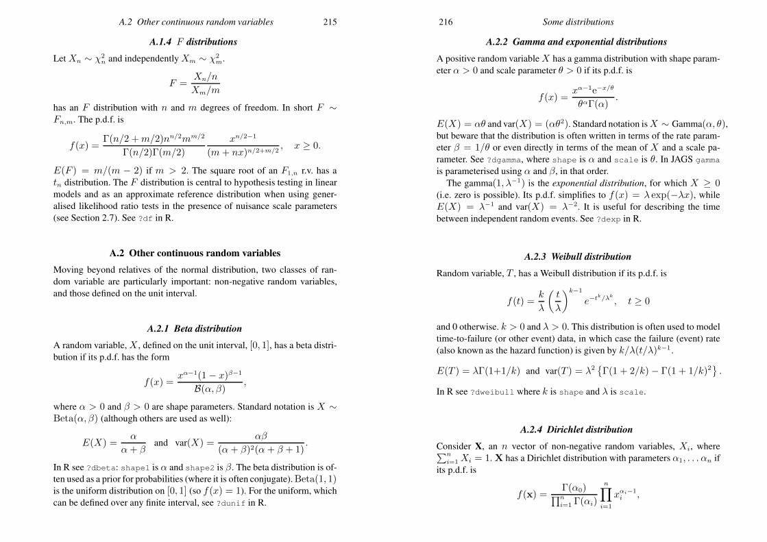
A.2 Other continuous random variables 215
A.1.4 F distributions
Let Xn ∼ χ2n and independently Xm ∼ χ2
m.
F =Xn/n
Xm/m
has an F distribution with n and m degrees of freedom. In short F ∼Fn,m. The p.d.f. is
f(x) =Γ(n/2 +m/2)nn/2mm/2
Γ(n/2)Γ(m/2)
xn/2−1
(m+ nx)n/2+m/2, x ≥ 0.
E(F ) = m/(m − 2) if m > 2. The square root of an F1,n r.v. has atn distribution. The F distribution is central to hypothesis testing in linearmodels and as an approximate reference distribution when using gener-alised likelihood ratio tests in the presence of nuisance scale parameters(see Section 2.7). See ?df in R.
A.2 Other continuous random variables
Moving beyond relatives of the normal distribution, two classes of ran-dom variable are particularly important: non-negative random variables,and those defined on the unit interval.
A.2.1 Beta distribution
A random variable, X , defined on the unit interval, [0, 1], has a beta distri-bution if its p.d.f. has the form
f(x) =xα−1(1− x)β−1
B(α, β) ,
where α > 0 and β > 0 are shape parameters. Standard notation is X ∼Beta(α, β) (although others are used as well):
E(X) =α
α+ βand var(X) =
αβ
(α+ β)2(α+ β + 1).
In R see ?dbeta: shape1 is α and shape2 is β. The beta distribution is of-ten used as a prior for probabilities (where it is often conjugate).Beta(1, 1)is the uniform distribution on [0, 1] (so f(x) = 1). For the uniform, whichcan be defined over any finite interval, see ?dunif in R.
216 Some distributions
A.2.2 Gamma and exponential distributions
A positive random variable X has a gamma distribution with shape param-eter α > 0 and scale parameter θ > 0 if its p.d.f. is
f(x) =xα−1e−x/θ
θαΓ(α).
E(X) = αθ and var(X) = (αθ2). Standard notation isX ∼ Gamma(α, θ),but beware that the distribution is often written in terms of the rate param-eter β = 1/θ or even directly in terms of the mean of X and a scale pa-rameter. See ?dgamma, where shape is α and scale is θ. In JAGS gamma
is parameterised using α and β, in that order.The gamma(1, λ−1) is the exponential distribution, for which X ≥ 0
(i.e. zero is possible). Its p.d.f. simplifies to f(x) = λ exp(−λx), whileE(X) = λ−1 and var(X) = λ−2. It is useful for describing the timebetween independent random events. See ?dexp in R.
A.2.3 Weibull distribution
Random variable, T , has a Weibull distribution if its p.d.f. is
f(t) =k
λ
(t
λ
)k−1
e−tk/λk
, t ≥ 0
and 0 otherwise. k > 0 and λ > 0. This distribution is often used to modeltime-to-failure (or other event) data, in which case the failure (event) rate(also known as the hazard function) is given by k/λ(t/λ)k−1 .
E(T ) = λΓ(1+1/k) and var(T ) = λ2Γ(1 + 2/k)− Γ(1 + 1/k)2
.
In R see ?dweibull where k is shape and λ is scale.
A.2.4 Dirichlet distribution
Consider X, an n vector of non-negative random variables, Xi, where∑ni=1 Xi = 1. X has a Dirichlet distribution with parameters α1, . . . αn if
its p.d.f. is
f(x) =Γ(α0)∏ni=1 Γ(αi)
n∏
i=1
xαi−1i ,
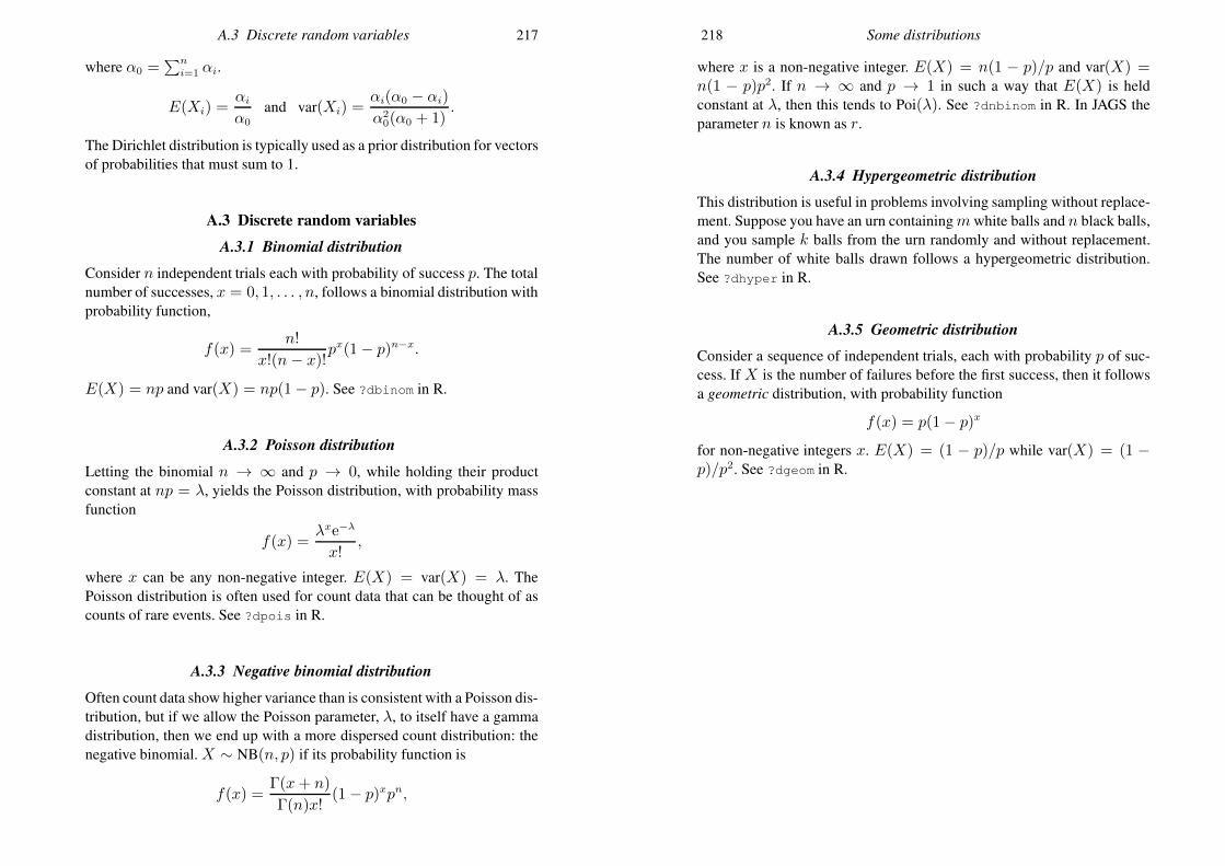
A.3 Discrete random variables 217
where α0 =∑n
i=1 αi.
E(Xi) =αiα0
and var(Xi) =αi(α0 − αi)
α20(α0 + 1)
.
The Dirichlet distribution is typically used as a prior distribution for vectorsof probabilities that must sum to 1.
A.3 Discrete random variables
A.3.1 Binomial distribution
Consider n independent trials each with probability of success p. The totalnumber of successes, x = 0, 1, . . . , n, follows a binomial distribution withprobability function,
f(x) =n!
x!(n − x)!px(1− p)n−x.
E(X) = np and var(X) = np(1− p). See ?dbinom in R.
A.3.2 Poisson distribution
Letting the binomial n → ∞ and p → 0, while holding their productconstant at np = λ, yields the Poisson distribution, with probability massfunction
f(x) =λxe−λ
x!,
where x can be any non-negative integer. E(X) = var(X) = λ. ThePoisson distribution is often used for count data that can be thought of ascounts of rare events. See ?dpois in R.
A.3.3 Negative binomial distribution
Often count data show higher variance than is consistent with a Poisson dis-tribution, but if we allow the Poisson parameter, λ, to itself have a gammadistribution, then we end up with a more dispersed count distribution: thenegative binomial. X ∼ NB(n, p) if its probability function is
f(x) =Γ(x+ n)
Γ(n)x!(1− p)xpn,
218 Some distributions
where x is a non-negative integer. E(X) = n(1 − p)/p and var(X) =n(1 − p)p2. If n → ∞ and p → 1 in such a way that E(X) is heldconstant at λ, then this tends to Poi(λ). See ?dnbinom in R. In JAGS theparameter n is known as r.
A.3.4 Hypergeometric distribution
This distribution is useful in problems involving sampling without replace-ment. Suppose you have an urn containing m white balls and n black balls,and you sample k balls from the urn randomly and without replacement.The number of white balls drawn follows a hypergeometric distribution.See ?dhyper in R.
A.3.5 Geometric distribution
Consider a sequence of independent trials, each with probability p of suc-cess. If X is the number of failures before the first success, then it followsa geometric distribution, with probability function
f(x) = p(1− p)x
for non-negative integers x. E(X) = (1 − p)/p while var(X) = (1 −p)/p2. See ?dgeom in R.
Appendix B
Matrix computation
Statistical computation often involves numerical computation with matri-ces. It is quite easy to get this wrong, producing code that is orders of mag-nitude less efficient or less stable than could be achieved. This appendix in-troduces the basics of stability and efficiency in matrix computation, alongwith some standard matrix decompositions useful in statistics. See Goluband Van Loan (2013) or Watkins (1991) for more detail.
B.1 Efficiency in matrix computation
Consider this simple example in R.
n <- 2000A <- matrix(runif(n*n),n,n)B <- matrix(runif(n*n),n,n)y <- runif(n)system.time(f0 <- A%*%B%*%y) ## case 1user system elapsed31.50 0.03 31.58system.time(f1 <- A%*%(B%*%y)) ## case 2user system elapsed0.08 0.00 0.08
f0 and f1 are identical to machine precision, but f1 took much less time tocompute. Why? The answer is to do with how the multiplications were or-dered in the two cases, and the number of floating point operations (flops)required by the two alternative orderings.
1. In the first case AB was formed first, and the resulting matrix used topre-multiply the vector y.
2. In the second case, the vector By was formed first and was then pre-multiplied by A.
The first case took more time because the number of floating point opera-tions (+, -, *, /) required to multiply A and B was about 2n3, whereas the
219
220 Matrix computation
number of flops required to multiply an n × n matrix by an n vector isonly about 2n2. Hence f0 cost about 2n3 + 2n2 operations, whereas f1cost only 4n2. So the first alternative required about n/2 times as manyoperations as the second.1
Another simple matrix operation is the evaluation of the trace of a matrixproduct. Again different ways of computing the same quantity lead to rad-ically different computation times. Consider the computation of tr(AB)where A is 5000 × 100 and B is 100 × 5000:
n <- 5000;m <- 100A <- matrix(runif(n*m),n,m)B <- matrix(runif(n*m),m,n)system.time(sum(diag(A%*%B)))user system elapsed10.46 0.11 10.58system.time(sum(diag(B%*%A)))user system elapsed0.2 0.0 0.2
system.time(sum(A*t(B)))user system elapsed0.02 0.00 0.02
1. The first method forms AB, at a flop cost of 2n2m and then extractsthe leading diagonal and sums it.
2. The second method uses the fact that tr(AB) = tr(BA). It forms BAat flop cost of 2nm2 and then extracts the leading diagonal of the resultand sums it.
3. The third method makes direct use of the fact that tr(AB) =∑
ij AijBji,at a cost of 2nm. It is the fastest because no effort is wasted in calcu-lating unused off-diagonal matrix elements.
Notice that method 1 is not just wasteful of flops, but also requires storageof an n× n matrix, which is much larger than either A or B.
Unfortunately, it is not generally possible to automatically choose themost efficient alternative when computing with matrices. Even the appar-ently simple problem of choosing the best order in which to perform matrixmultiplication is difficult to automate. However, for many statistical com-puting problems, a small amount of effort in identifying the best orderingat the coding stage pays big dividends in terms of improved computing
1 The ratio of timings observed is not exactly 1000 here, because R also spends timeinterpreting the instructions, setting up storage and so on, which is a significant part ofthe cost of producing f1; low level optimisation also has an impact on timing.
B.2 Choleski decomposition: a matrix square root 221
speeds. In general, the important thing is to be constantly aware of the po-tential for careless coding with matrices to be hugely inefficient, and toconsider flop count in all matrix computations.
Generally when flop counting it is important to know whether the countis proportional to n2 or to n3 (for example), as n → ∞, but much lessimportant to know whether it is 2n2 or 4n2, say. For this reason, it is oftensufficient to simply consider how the cost scales with the problem size, inthe n→∞ limit, without worrying about exact constants of proportional-ity. So we simply consider whether an algorithm is O(n2) or O(n3) (‘ordern2 or order n3’), for example.
B.2 Choleski decomposition: a matrix square root
Positive definite matrices are the ‘positive real numbers’ of matrix alge-bra. They have particular computational advantages and occur frequentlyin statistics, because covariance matrices are usually positive definite (andalways positive semi-definite). So let’s start with positive definite matrices,and their matrix square roots. To see why matrix square roots might beuseful, consider the following.
Example Generating multivariate normal random variables. There existvery quick and reliable methods for simulating i.i.d. N(0, 1) random de-viates, but suppose that N(µ,Σ) random vectors are required. Clearly wecan generate vectors z from N(0, I). If we could find a matrix R such thatRTR = Σ, then y ≡ RTz + µ ∼ N(µ,Σ), because the covariancematrix of y is RTIR = RTR = Σ and E(y) = E(RTz+ µ) = µ.
In general the square root of a positive definite matrix is not uniquelydefined, but there is a unique upper triangular square root of any positivedefinite matrix: its Choleski factor. The algorithm for finding the Choleskifactor is easily derived. Consider a 4×4 example first. The defining matrixequation is
R11 0 0 0R12 R22 0 0R13 R23 R33 0R14 R24 R34 R44
R11 R12 R13 R14
0 R22 R23 R24
0 0 R33 R34
0 0 0 R44
=
A11 A12 A13 A14
A12 A22 A23 A24
A13 A23 A33 A34
A14 A24 A34 A44
.
222 Matrix computation
If the component equations of this expression are written out and solvedin the right order, then each contains only one unknown, as the followingillustrates (unknowns are in bold):
A11 = R112
A12 = R11R12
A13 = R11R13
A14 = R11R14
A22 = R212 +R22
2
A23 = R12R13 +R22R23
.
.
Generalising to the n×n case, and using the convention that∑0
k=1 xi ≡ 0,we have
Rii =
√√√√Aii −i−1∑
k=1
R2ki, and Rij =
Aij −∑i−1
k=1 RkiRkj
Rii
, j > i.
Working through these equations in row order, from row one, and startingeach row from its leading diagonal component, ensures that all right-hand-side quantities are known at each step. Choleski decomposition requiresn3/3 flops and n square roots. In R it is performed by function chol, whichcalls routines in LAPACK or LINPACK.2
Example (continued) The following simulates 1000 random draws from
N
1−13
,
2 −1 1−1 2 −11 −1 2
and checks their observed mean and covariance:
V <- matrix(c(2,-1,1,-1,2,-1,1,-1,2),3,3)mu <- c(1,-1,3)R <- chol(V) ## Choleski factor of VZ <- matrix(rnorm(3000),3,1000) ## 1000 N(0,I) 3-vectorsY <- t(R)%*%Z + mu ## 1000 N(mu,V) vectors
## and check that they behave as expected...rowMeans(Y) ## observed mu
2 Actually, numerical analysts do not consider the Choleski factor to be a square root inthe strict sense, because of the transpose in A = RTR.
B.2 Choleski decomposition: a matrix square root 223
[1] 1.0924086 -0.9694124 2.9926779
(Y-mu)%*%t(Y-mu)/1000 ## observed V[,1] [,2] [,3]
[1,] 2.066872 -1.039062 1.003980[2,] -1.039062 2.054408 -0.980139[3,] 1.003980 -0.980139 1.833971
As a second application of the Choleski decomposition, consider evalu-ating the log likelihood of µ and Σ:
l = −n
2log(2π)− 1
2log(|Σ|)− 1
2(y − µ)TΣ−1(y − µ).
If we were simply to invert Σ to evaluate the final term, it would cost 2n3
flops, and we would still need to evaluate the determinant. A Choleski-based approach is much better. It is easy to see that Σ−1 = R−1R−T,where R is the Choleski factor of Σ. So the final term in the log likelihoodcan be written as zTz where z = R−T(y − µ). Notice that we do notactually need to evaluate R−T, but simply to solve RTz = y − µ for z.To see how this is done, consider a 4× 4 case again:
R11 0 0 0R12 R22 0 0R13 R23 R33 0R14 R24 R34 R44
z1z2z3z4
=
y1 − µ1
y2 − µ2
y3 − µ3
y4 − µ4
.
If this system of equations is solved from the top down, then there is onlyone unknown (shown in bold) at each stage:
R11z1 = y1 − µ1
R12z1 +R22z2 = y2 − µ2
R13z1 +R23z2 +R33z3 = y3 − µ3
R14z1 +R24z2 +R34z3 +R44z4 = y4 − µ4
The generalisation of this forward substitution process to n dimensions isobvious, as is the fact that it costs O(n2) flops: much cheaper than explicitformation of R−T, which would involve applying forward substitution tofind each column of the unknown R−T in the equation RTR−T = I, atO(n3) cost.
In R there is a routine forwardsolve for doing forward substitutionwith a lower triangular matrix (and a routine backsolve for performing theequivalent back substitution with upper triangular matrices). Before usingit, we still need to consider |Σ|. Again the Choleski factor helps. From
224 Matrix computation
the general properties of determinants we know that |RT||R| = |Σ|, butbecause R is triangular |RT| = |R| = ∏n
i=1 Rii. So given the Choleskifactor, the calculation of the determinant is O(n).
Example The following evaluates the log likelihood of the covariancematrix V and mean vector mu, from the previous example, given an observedyT = (1, 2, 3):y <- 1:3; n <- length(y)z <- forwardsolve(t(R),y-mu)logLik <- -n*log(2*pi)/2-sum(log(diag(R)))-sum(z*z)/2logLik
[1] -6.824963
Note that Choleski decomposition of a matrix that is not positive def-inite will fail. Positive semi-definite is no better, because in that case aleading diagonal element of the Choleski factor will become zero, so thatcomputation of the off-diagonal elements on the same row is impossible.Positive semi-definite matrices are reasonably common, so this is a prac-tical problem. For the positive semi-definite case, it is possible to modifythe Choleski decomposition by pivoting; that is, by reordering the rowsand columns of the original matrix so that the zeroes end up at the end ofthe leading diagonal of the Choleski factor, in rows that are all zero. Thisis not pursued further here. Rather let us consider a more general matrixdecomposition, that provides matrix square roots along with much else.
B.3 Eigen-decomposition (spectral-decomposition)
Any symmetric matrix, A can be written as
A = UΛUT, (B.1)
where the matrix U is orthogonal and Λ is a diagonal matrix, with ith
leading diagonal element λi (conventionally λi ≥ λi+1). Post-multiplyingboth sides of the decomposition by U we have
AU = UΛ.
Considering this system one column at a time and writing ui for the ith
column of U we have
Aui = λiui.
So the λi are the eigenvalues of A, and the columns of U are the cor-responding eigenvectors. (B.1) is the eigen-decomposition or spectral de-composition of A.
B.3 Eigen-decomposition (spectral-decomposition) 225
State-of-the-art schemes for eigen-decomposition are fairly intricate, butdo not use the determinant and characteristic equation of A. One practicalscheme is as follows: (i) the matrix A is first reduced to tri-diagonal formusing repeated pre- and post-multiplication by simple rank-one orthogonalmatrices called Householder rotations, and (ii) an iterative scheme calledQR-iteration3 then pre-and post-multiplies the tri-diagonal matrix by evensimpler orthogonal matrices, in order to reduce it to diagonal form. Atthis point the diagonal matrix contains the eigenvalues, and the product ofall the orthogonal matrices gives U. Eigen-decomposition is O(n3), but agood symmetric eigen routine is around 10 times as computationally costlyas a Choleski routine.
An immediate use of the eigen-decomposition is to provide an alterna-tive characterisation of positive (semi-) definite matrices. All the eigenval-ues of a positive (semi-) definite matrix must be positive (non-negative) andreal. This is easy to see. Were some eigenvalue, λi to be negative (zero),then the corresponding eigenvector ui would result in uT
i Aui being neg-ative (zero). At the same time the existence of an x such that xTAx isnegative (zero) leads to a contradiction unless at least one eigenvalue isnegative (zero).4
B.3.1 Powers of matrices
Consider raising A to the power m.
Am = AAA · · ·A = UΛUTUΛUT · · ·UΛUT
= UΛΛ · · ·ΛUT = UΛmUT,
where Λm is just the diagonal matrix with λmi as the ith leading diagonalelement. This suggests that any real valued function, f , of a real valuedargument, which has a power series representation, has a natural generali-sation to a symmetric matrix valued function of a symmetric matrix argu-ment; that is
f ′(A) ≡ Uf ′(Λ)UT,
where f ′(Λ) denotes the diagonal matrix with ith leading diagonal elementf(λi). For example, exp(A) = U exp(Λ)UT.
3 Not to be confused with QR decomposition.4 We can write x = Ub for some vector b. So xTAx < 0 ⇒ bTΛb < 0 ⇒
∑b2iΛi < 0
⇒ Λi < 0 for some i.
226 Matrix computation
B.3.2 Another matrix square root
For matrices with non-negative eigenvalues we can generalise to non-integerpowers. For example, it is readily verified that
√A = U
√ΛUT has the
property that√A√A = A. Notice (i) that
√A is not the same as the
Choleski factor, emphasizing the non-uniqueness of matrix square rootsand (ii) that, unlike the Choleski factor,
√A is well defined for positive
semi-definite matrices (and can therefore be computed for any covariancematrix).
B.3.3 Matrix inversion, rank and condition
Continuing in the same vein we can investigate matrix inversion by writing
A−1 = UΛ−1UT,
where the diagonal matrix Λ−1 has ith leading diagonal element λ−1i .
Clearly we have a problem if any of the λi are zero, for the matrix inversewill be undefined. A matrix with no zero eigenvalues is termed full rank.A matrix with any zero eigenvalues is rank deficient and does not have aninverse. The number of nonzero eigenvalues is the rank of a matrix.
For some purposes it is sufficient to define a generalised inverse or pseu-doinverse when faced with rank deficiency, by finding the reciprocal of thenonzero eigenvalues, but setting the reciprocal of the zero eigenvalues tozero. This is not pursued here.
It is important to understand the consequences of rank deficiency quitewell when performing matrix operations involving matrix inversion/matrixequation solving. This is because near rank deficiency is rather easy toachieve by accident, and in finite precision arithmetic it is as bad as rankdeficiency. First consider trying to solve
Ax = y
for x when A is rank deficient. In terms of the eigen-decomposition thesolution is
x = UΛ−1UTy.
So y is rotated to become y′ = UTy, the elements of y′ are then dividedby the eigenvalues, λi, and the reverse rotation is applied to the result. Theproblem is that y′
i/λi is not defined if λi = 0. This is just a differentway of showing something that you already know: rank-deficient matricescannot be inverted. But the approach also helps in understanding near rankdeficiency and ill conditioning.
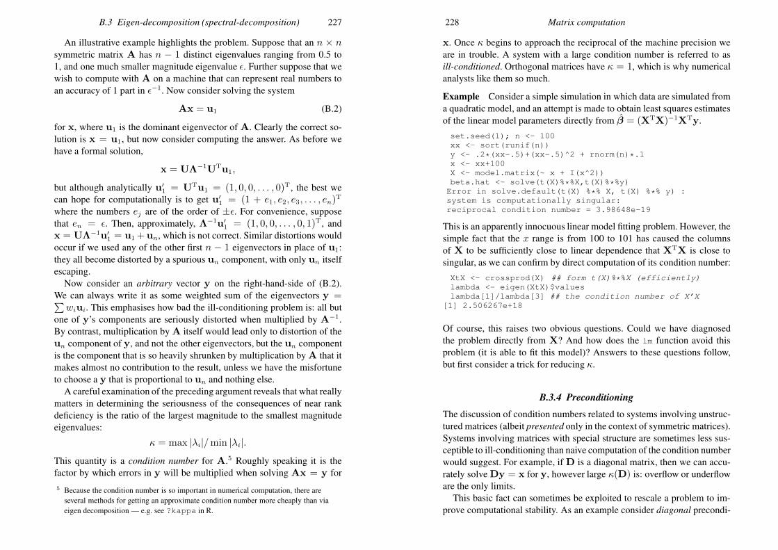
B.3 Eigen-decomposition (spectral-decomposition) 227
An illustrative example highlights the problem. Suppose that an n × nsymmetric matrix A has n − 1 distinct eigenvalues ranging from 0.5 to1, and one much smaller magnitude eigenvalue ǫ. Further suppose that wewish to compute with A on a machine that can represent real numbers toan accuracy of 1 part in ǫ−1. Now consider solving the system
Ax = u1 (B.2)
for x, where u1 is the dominant eigenvector of A. Clearly the correct so-lution is x = u1, but now consider computing the answer. As before wehave a formal solution,
x = UΛ−1UTu1,
but although analytically u′1 = UTu1 = (1, 0, 0, . . . , 0)T, the best we
can hope for computationally is to get u′1 = (1 + e1, e2, e3, . . . , en)
T
where the numbers ej are of the order of ±ǫ. For convenience, supposethat en = ǫ. Then, approximately, Λ−1u′
1 = (1, 0, 0, . . . , 0, 1)T , andx = UΛ−1u′
1 = u1 +un, which is not correct. Similar distortions wouldoccur if we used any of the other first n − 1 eigenvectors in place of u1:they all become distorted by a spurious un component, with only un itselfescaping.
Now consider an arbitrary vector y on the right-hand-side of (B.2).We can always write it as some weighted sum of the eigenvectors y =∑
wiui. This emphasises how bad the ill-conditioning problem is: all butone of y’s components are seriously distorted when multiplied by A−1.By contrast, multiplication by A itself would lead only to distortion of theun component of y, and not the other eigenvectors, but the un componentis the component that is so heavily shrunken by multiplication by A that itmakes almost no contribution to the result, unless we have the misfortuneto choose a y that is proportional to un and nothing else.
A careful examination of the preceding argument reveals that what reallymatters in determining the seriousness of the consequences of near rankdeficiency is the ratio of the largest magnitude to the smallest magnitudeeigenvalues:
κ = max |λi|/min |λi|.This quantity is a condition number for A.5 Roughly speaking it is thefactor by which errors in y will be multiplied when solving Ax = y for5 Because the condition number is so important in numerical computation, there are
several methods for getting an approximate condition number more cheaply than viaeigen decomposition — e.g. see ?kappa in R.
228 Matrix computation
x. Once κ begins to approach the reciprocal of the machine precision weare in trouble. A system with a large condition number is referred to asill-conditioned. Orthogonal matrices have κ = 1, which is why numericalanalysts like them so much.
Example Consider a simple simulation in which data are simulated froma quadratic model, and an attempt is made to obtain least squares estimatesof the linear model parameters directly from β = (XTX)−1XTy.
set.seed(1); n <- 100xx <- sort(runif(n))y <- .2*(xx-.5)+(xx-.5)^2 + rnorm(n)*.1x <- xx+100X <- model.matrix(~ x + I(x^2))beta.hat <- solve(t(X)%*%X,t(X)%*%y)Error in solve.default(t(X) %*% X, t(X) %*% y) :system is computationally singular:reciprocal condition number = 3.98648e-19
This is an apparently innocuous linear model fitting problem. However, thesimple fact that the x range is from 100 to 101 has caused the columnsof X to be sufficiently close to linear dependence that XTX is close tosingular, as we can confirm by direct computation of its condition number:
XtX <- crossprod(X) ## form t(X)%*%X (efficiently)lambda <- eigen(XtX)$valueslambda[1]/lambda[3] ## the condition number of X’X
[1] 2.506267e+18
Of course, this raises two obvious questions. Could we have diagnosedthe problem directly from X? And how does the lm function avoid thisproblem (it is able to fit this model)? Answers to these questions follow,but first consider a trick for reducing κ.
B.3.4 Preconditioning
The discussion of condition numbers related to systems involving unstruc-tured matrices (albeit presented only in the context of symmetric matrices).Systems involving matrices with special structure are sometimes less sus-ceptible to ill-conditioning than naive computation of the condition numberwould suggest. For example, if D is a diagonal matrix, then we can accu-rately solve Dy = x for y, however large κ(D) is: overflow or underfloware the only limits.
This basic fact can sometimes be exploited to rescale a problem to im-prove computational stability. As an example consider diagonal precondi-
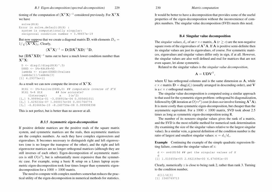
B.3 Eigen-decomposition (spectral-decomposition) 229
tioning of the computation of (XTX)−1 considered previously. For XTXwe havesolve(XtX)
Error in solve.default(XtX) :system is computationally singular:reciprocal condition number = 3.98657e-19
But now suppose that we create a diagonal matrix D, with elements Dii =1/√(XTX)ii. Clearly,
(XTX)−1 = D(DXTXD)−1D,
but (DXTXD)−1 turns out to have a much lower condition number thanXTX:D <- diag(1/diag(XtX)^.5)DXXD <- D%*%XtX%*%Dlambda <- eigen(DXXD)$valueslambda[1]/lambda[3]
[1] 4.29375e+11
As a result we can now compute the inverse of XTX:XtXi <- D%*%solve(DXXD,D) ## computable inverse of X’XXtXi %*% XtX ## how accurate?
(Intercept) x I(x^2)[1,] 9.999941e-01 -3.058910e-04 0.005661011[2,] 1.629232e-07 1.000017e+00 0.001764774[3,] -6.816663e-10 -8.240750e-08 0.999998398
This is not perfect, but is better than no answer at all.
B.3.5 Asymmetric eigen-decomposition
If positive definite matrices are the positive reals of the square matrixsystem, and symmetric matrices are the reals, then asymmetric matricesare the complex numbers. As such they have complex eigenvectors andeigenvalues. It becomes necessary to distinguish right and left eigenvec-tors (one is no longer the transpose of the other), and the right and lefteigenvector matrices are no longer orthogonal matrices (although they arestill inverses of each other). Eigen-decomposition of asymmetric matri-ces is still O(n3), but is substantially more expensive than the symmet-ric case. For example, using a basic R setup on a Linux laptop asym-metric eigen-decomposition took four times longer than symmetric eigen-decomposition for a 1000 × 1000 matrix.
The need to compute with complex numbers somewhat reduces the prac-tical utility of the eigen-decomposition in numerical methods for statistics.
230 Matrix computation
It would be better to have a decomposition that provides some of the usefulproperties of the eigen-decomposition without the inconvenience of com-plex numbers. The singular value decomposition (SVD) meets this need.
B.4 Singular value decomposition
The singular values, di, of an r× c matrix, A (r ≥ c) are the non-negativesquare roots of the eigenvalues of ATA. If A is positive semi-definite thenits singular values are just its eigenvalues, of course. For symmetric matri-ces, eigenvalues and singular values differ only in sign, if at all. However,the singular values are also well defined and real for matrices that are noteven square, let alone symmetric.
Related to the singular values is the singular value decomposition,
A = UDVT,
where U has orthogonal columns and is the same dimension as A, whilec× c matrix D = diag(di) (usually arranged in descending order), and Vis a c× c orthogonal matrix.
The singular value decomposition is computed using a similar approachto that used for the symmetric eigen problem: orthogonal bi-diagonalization,followed by QR iteration atO(rc2) cost (it does not involve formingATA).It is more costly than symmetric eigen-decomposition, but cheaper than theasymmetric equivalent. For a 1000 × 1000 matrix, SVD took about 2.5times as long as symmetric eigen-decomposition using R.
The number of its nonzero singular values gives the rank of a matrix,and the SVD is the most reliable method for numerical rank determination(by examining the size of the singular values relative to the largest singularvalue). In a similar vein, a general definition of the condition number is theratio of largest and smallest singular values: κ = d1/dc.
Example Continuing the example of the simple quadratic regression fit-ting failure, consider the singular values of X:
d <- svd(X)$d ## get the singular values of Xd
[1] 1.010455e+05 2.662169e+00 6.474081e-05
Clearly, numerically X is close to being rank 2, rather than rank 3. Turningto the condition number,
d[1]/d[3][1] 1560769713
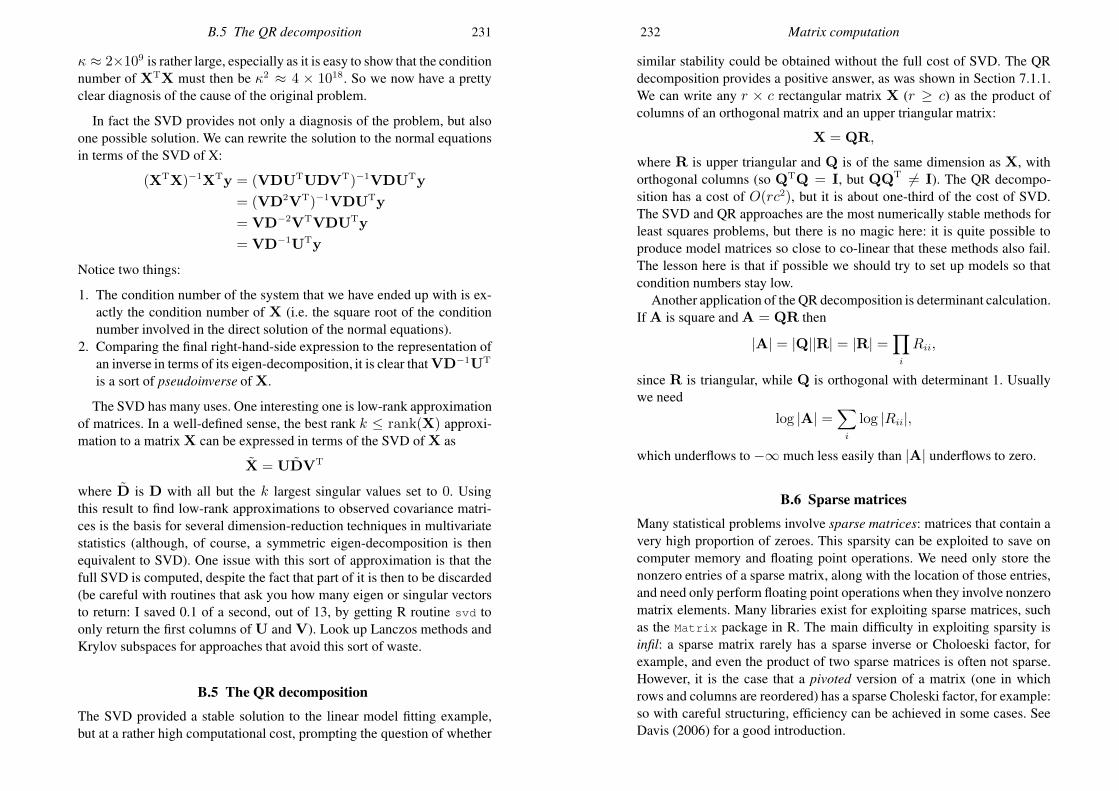
B.5 The QR decomposition 231
κ ≈ 2×10⁹ is rather large, especially as it is easy to show that the conditionnumber of XTX must then be κ2 ≈ 4 × 10¹⁸. So we now have a prettyclear diagnosis of the cause of the original problem.
In fact the SVD provides not only a diagnosis of the problem, but alsoone possible solution. We can rewrite the solution to the normal equationsin terms of the SVD of X:
(XTX)−1XTy = (VDUTUDVT)−1VDUTy
= (VD2VT)−1VDUTy
= VD−2VTVDUTy
= VD−1UTy
Notice two things:
1. The condition number of the system that we have ended up with is ex-actly the condition number of X (i.e. the square root of the conditionnumber involved in the direct solution of the normal equations).
2. Comparing the final right-hand-side expression to the representation ofan inverse in terms of its eigen-decomposition, it is clear thatVD−1UT
is a sort of pseudoinverse of X.
The SVD has many uses. One interesting one is low-rank approximationof matrices. In a well-defined sense, the best rank k ≤ rank(X) approxi-mation to a matrix X can be expressed in terms of the SVD of X as
X = UDVT
where D is D with all but the k largest singular values set to 0. Usingthis result to find low-rank approximations to observed covariance matri-ces is the basis for several dimension-reduction techniques in multivariatestatistics (although, of course, a symmetric eigen-decomposition is thenequivalent to SVD). One issue with this sort of approximation is that thefull SVD is computed, despite the fact that part of it is then to be discarded(be careful with routines that ask you how many eigen or singular vectorsto return: I saved 0.1 of a second, out of 13, by getting R routine svd toonly return the first columns of U and V). Look up Lanczos methods andKrylov subspaces for approaches that avoid this sort of waste.
B.5 The QR decomposition
The SVD provided a stable solution to the linear model fitting example,but at a rather high computational cost, prompting the question of whether
232 Matrix computation
similar stability could be obtained without the full cost of SVD. The QRdecomposition provides a positive answer, as was shown in Section 7.1.1.We can write any r × c rectangular matrix X (r ≥ c) as the product ofcolumns of an orthogonal matrix and an upper triangular matrix:
X = QR,
where R is upper triangular and Q is of the same dimension as X, withorthogonal columns (so QTQ = I, but QQT 6= I). The QR decompo-sition has a cost of O(rc2), but it is about one-third of the cost of SVD.The SVD and QR approaches are the most numerically stable methods forleast squares problems, but there is no magic here: it is quite possible toproduce model matrices so close to co-linear that these methods also fail.The lesson here is that if possible we should try to set up models so thatcondition numbers stay low.
Another application of the QR decomposition is determinant calculation.If A is square and A = QR then
|A| = |Q||R| = |R| =∏
i
Rii,
since R is triangular, while Q is orthogonal with determinant 1. Usuallywe need
log |A| =∑
i
log |Rii|,
which underflows to −∞ much less easily than |A| underflows to zero.
B.6 Sparse matrices
Many statistical problems involve sparse matrices: matrices that contain avery high proportion of zeroes. This sparsity can be exploited to save oncomputer memory and floating point operations. We need only store thenonzero entries of a sparse matrix, along with the location of those entries,and need only perform floating point operations when they involve nonzeromatrix elements. Many libraries exist for exploiting sparse matrices, suchas the Matrix package in R. The main difficulty in exploiting sparsity isinfil: a sparse matrix rarely has a sparse inverse or Choloeski factor, forexample, and even the product of two sparse matrices is often not sparse.However, it is the case that a pivoted version of a matrix (one in whichrows and columns are reordered) has a sparse Choleski factor, for example:so with careful structuring, efficiency can be achieved in some cases. SeeDavis (2006) for a good introduction.
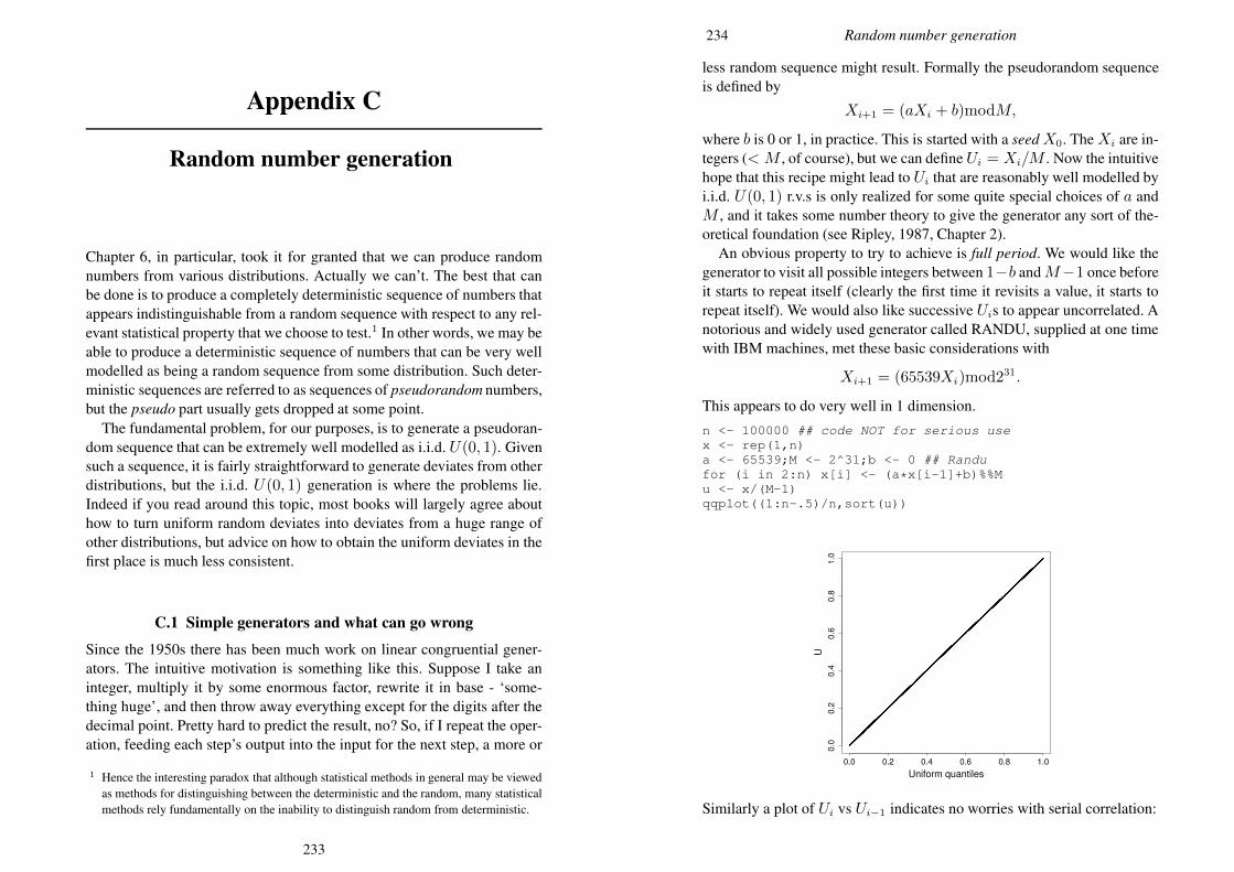
Appendix C
Random number generation
Chapter 6, in particular, took it for granted that we can produce randomnumbers from various distributions. Actually we can’t. The best that canbe done is to produce a completely deterministic sequence of numbers thatappears indistinguishable from a random sequence with respect to any rel-evant statistical property that we choose to test.1 In other words, we may beable to produce a deterministic sequence of numbers that can be very wellmodelled as being a random sequence from some distribution. Such deter-ministic sequences are referred to as sequences of pseudorandom numbers,but the pseudo part usually gets dropped at some point.
The fundamental problem, for our purposes, is to generate a pseudoran-dom sequence that can be extremely well modelled as i.i.d. U(0, 1). Givensuch a sequence, it is fairly straightforward to generate deviates from otherdistributions, but the i.i.d. U(0, 1) generation is where the problems lie.Indeed if you read around this topic, most books will largely agree abouthow to turn uniform random deviates into deviates from a huge range ofother distributions, but advice on how to obtain the uniform deviates in thefirst place is much less consistent.
C.1 Simple generators and what can go wrong
Since the 1950s there has been much work on linear congruential gener-ators. The intuitive motivation is something like this. Suppose I take aninteger, multiply it by some enormous factor, rewrite it in base - ‘some-thing huge’, and then throw away everything except for the digits after thedecimal point. Pretty hard to predict the result, no? So, if I repeat the oper-ation, feeding each step’s output into the input for the next step, a more or
1 Hence the interesting paradox that although statistical methods in general may be viewedas methods for distinguishing between the deterministic and the random, many statisticalmethods rely fundamentally on the inability to distinguish random from deterministic.
233
234 Random number generation
less random sequence might result. Formally the pseudorandom sequenceis defined by
Xi+1 = (aXi + b)modM,
where b is 0 or 1, in practice. This is started with a seed X0. The Xi are in-tegers (< M , of course), but we can define Ui = Xi/M . Now the intuitivehope that this recipe might lead to Ui that are reasonably well modelled byi.i.d. U(0, 1) r.v.s is only realized for some quite special choices of a andM , and it takes some number theory to give the generator any sort of the-oretical foundation (see Ripley, 1987, Chapter 2).
An obvious property to try to achieve is full period. We would like thegenerator to visit all possible integers between 1−b and M−1 once beforeit starts to repeat itself (clearly the first time it revisits a value, it starts torepeat itself). We would also like successive Uis to appear uncorrelated. Anotorious and widely used generator called RANDU, supplied at one timewith IBM machines, met these basic considerations with
Xi+1 = (65539Xi)mod231.
This appears to do very well in 1 dimension.
n <- 100000 ## code NOT for serious usex <- rep(1,n)a <- 65539;M <- 2^31;b <- 0 ## Randufor (i in 2:n) x[i] <- (a*x[i-1]+b)%%Mu <- x/(M-1)qqplot((1:n-.5)/n,sort(u))
0.0 0.2 0.4 0.6 0.8 1.0
0.0
0.2
0.4
0.6
0.8
1.0
Uniform quantiles
USimilarly a plot of Ui vs Ui−1 indicates no worries with serial correlation:
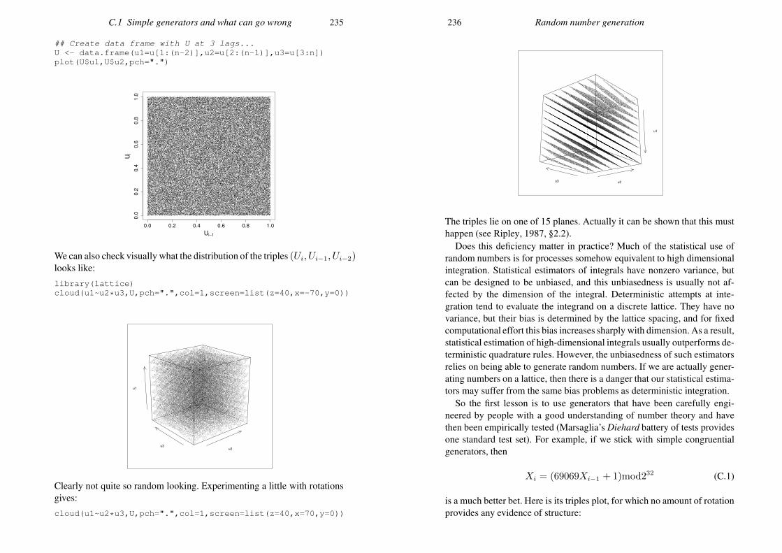
C.1 Simple generators and what can go wrong 235
## Create data frame with U at 3 lags...U <- data.frame(u1=u[1:(n-2)],u2=u[2:(n-1)],u3=u[3:n])plot(U$u1,U$u2,pch=".")
0.0 0.2 0.4 0.6 0.8 1.0
0.0
0.2
0.4
0.6
0.8
1.0
Ui−1
Ui
We can also check visually what the distribution of the triples (Ui, Ui−1, Ui−2)looks like:
library(lattice)cloud(u1~u2*u3,U,pch=".",col=1,screen=list(z=40,x=-70,y=0))
u2u3
u1
Clearly not quite so random looking. Experimenting a little with rotationsgives:
cloud(u1~u2*u3,U,pch=".",col=1,screen=list(z=40,x=70,y=0))
236 Random number generation
u2u3
u1
The triples lie on one of 15 planes. Actually it can be shown that this musthappen (see Ripley, 1987, §2.2).
Does this deficiency matter in practice? Much of the statistical use ofrandom numbers is for processes somehow equivalent to high dimensionalintegration. Statistical estimators of integrals have nonzero variance, butcan be designed to be unbiased, and this unbiasedness is usually not af-fected by the dimension of the integral. Deterministic attempts at inte-gration tend to evaluate the integrand on a discrete lattice. They have novariance, but their bias is determined by the lattice spacing, and for fixedcomputational effort this bias increases sharply with dimension. As a result,statistical estimation of high-dimensional integrals usually outperforms de-terministic quadrature rules. However, the unbiasedness of such estimatorsrelies on being able to generate random numbers. If we are actually gener-ating numbers on a lattice, then there is a danger that our statistical estima-tors may suffer from the same bias problems as deterministic integration.
So the first lesson is to use generators that have been carefully engi-neered by people with a good understanding of number theory and havethen been empirically tested (Marsaglia’s Diehard battery of tests providesone standard test set). For example, if we stick with simple congruentialgenerators, then
Xi = (69069Xi−1 + 1)mod232 (C.1)
is a much better bet. Here is its triples plot, for which no amount of rotationprovides any evidence of structure:
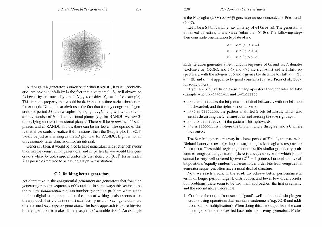
C.2 Building better generators 237
u2u3
u1
Although this generator is much better than RANDU, it is still problem-atic. An obvious infelicity is the fact that a very small Xi will always befollowed by an unusually small Xi+1 (consider Xi = 1, for example).This is not a property that would be desirable in a time series simulation,for example. Not quite so obvious is the fact that for any congruential gen-erator of period M , then k-tuples, Ui, Ui−1, . . . , Ui−k+1 will tend to lie ona finite number of k − 1 dimensional planes (e.g. for RANDU we saw 3-tuples lying on two dimensional planes.) There will be at most M1/k suchplanes, and as RANDU shows, there can be far fewer. The upshot of thisis that if we could visualize 8 dimensions, then the 8-tuple plot for (C.1)would be just as alarming as the 3D plot was for RANDU. Eight is not anunreasonably large dimension for an integral.
Generally then, it would be nice to have generators with better behaviourthan simple congruential generators, and in particular we would like gen-erators where k-tuples appear uniformly distributed on [0, 1]k for as high ak as possible (referred to as having a high k-distribution).
C.2 Building better generators
An alternative to the congruential generators are generators that focus ongenerating random sequences of 0s and 1s. In some ways this seems to bethe natural fundamental random number generation problem when usingmodern digital computers, and at the time of writing it also seems to bethe approach that yields the most satisfactory results. Such generators areoften termed shift-register generators. The basic approach is to use bitwisebinary operations to make a binary sequence ‘scramble itself’. An example
238 Random number generation
is the Marsaglia (2003) Xorshift generator as recommended in Press et al.(2007).
Let x be a 64-bit variable (i.e. an array of 64 0s or 1s). The generator isinitialised by setting to any value (other than 64 0s). The following stepsthen constitute one iteration (update of x):
x← x ∧ (x >> a)
x← x ∧ (x << b)
x← x ∧ (x >> c)
Each iteration generates a new random sequence of 0s and 1s. ∧ denotes‘exclusive or’ (XOR), and >> and << are right-shift and left shift, re-spectively, with the integers a, b and c giving the distance to shift. a = 21,b = 35 and c = 4 appear to be good constants (but see Press et al., 2007,for some others).
If you are a bit rusty on these binary operators then consider an 8-bitexample where x=10011011 and z=01011100:
• x<<1 is 00110110: the bit pattern is shifted leftwards, with the leftmostbit discarded, and the rightmost set to zero.
• x<<2 is 01101100: the pattern is shifted 2 bits leftwards, which alsoentails discarding the 2 leftmost bits and zeroing the two rightmost.
• x>>1 is 01001101: shift the pattern 1 bit rightwards.• x^z is 11000111:a 1 where the bits in x and z disagree, and a 0 where
they agree.
The Xorshift generator is very fast, has a period of 264−1, and passes theDiehard battery of tests (perhaps unsurprising as Marsaglia is responsiblefor that too). These shift-register generators suffer similar granularity prob-lems to congruential generators (there is always some k for which [0, 1]k
cannot be very well covered by even 264 − 1 points), but tend to have allbit positions ‘equally random’, whereas lower order bits from congruentialgenerator sequences often have a good deal of structure.
Now we reach a fork in the road. To achieve better performance interms of longer period, larger k-distribution, and fewer low-order correla-tion problems, there seem to be two main approaches: the first pragmatic,and the second more theoretical.
1. Combine the output from several ‘good’, well-understood, simple gen-erators using operations that maintain randomness (e.g. XOR and addi-tion, but not multiplication). When doing this, the output from the com-bined generators is never fed back into the driving generators. Prefer-
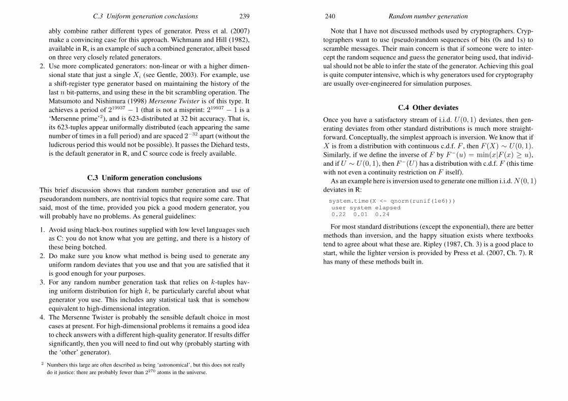
C.3 Uniform generation conclusions 239
ably combine rather different types of generator. Press et al. (2007)make a convincing case for this approach. Wichmann and Hill (1982),available in R, is an example of such a combined generator, albeit basedon three very closely related generators.
2. Use more complicated generators: non-linear or with a higher dimen-sional state that just a single Xi (see Gentle, 2003). For example, usea shift-register type generator based on maintaining the history of thelast n bit-patterns, and using these in the bit scrambling operation. TheMatsumoto and Nishimura (1998) Mersenne Twister is of this type. Itachieves a period of 219937 − 1 (that is not a misprint: 219937 − 1 is a‘Mersenne prime’2), and is 623-distributed at 32 bit accuracy. That is,its 623-tuples appear uniformally distributed (each appearing the samenumber of times in a full period) and are spaced 2−32 apart (without theludicrous period this would not be possible). It passes the Diehard tests,is the default generator in R, and C source code is freely available.
C.3 Uniform generation conclusions
This brief discussion shows that random number generation and use ofpseudorandom numbers, are nontrivial topics that require some care. Thatsaid, most of the time, provided you pick a good modern generator, youwill probably have no problems. As general guidelines:
1. Avoid using black-box routines supplied with low level languages suchas C: you do not know what you are getting, and there is a history ofthese being botched.
2. Do make sure you know what method is being used to generate anyuniform random deviates that you use and that you are satisfied that itis good enough for your purposes.
3. For any random number generation task that relies on k-tuples hav-ing uniform distribution for high k, be particularly careful about whatgenerator you use. This includes any statistical task that is somehowequivalent to high-dimensional integration.
4. The Mersenne Twister is probably the sensible default choice in mostcases at present. For high-dimensional problems it remains a good ideato check answers with a different high-quality generator. If results differsignificantly, then you will need to find out why (probably starting withthe ‘other’ generator).
2 Numbers this large are often described as being ‘astronomical’, but this does not reallydo it justice: there are probably fewer than 2270 atoms in the universe.
240 Random number generation
Note that I have not discussed methods used by cryptographers. Cryp-tographers want to use (pseudo)random sequences of bits (0s and 1s) toscramble messages. Their main concern is that if someone were to inter-cept the random sequence and guess the generator being used, that individ-ual should not be able to infer the state of the generator. Achieving this goalis quite computer intensive, which is why generators used for cryptographyare usually over-engineered for simulation purposes.
C.4 Other deviates
Once you have a satisfactory stream of i.i.d. U(0, 1) deviates, then gen-erating deviates from other standard distributions is much more straight-forward. Conceptually, the simplest approach is inversion. We know that ifX is from a distribution with continuous c.d.f. F , then F (X) ∼ U(0, 1).Similarly, if we define the inverse of F by F−(u) = min(x|F (x) ≥ u),and if U ∼ U(0, 1), then F−(U) has a distribution with c.d.f. F (this timewith not even a continuity restriction on F itself).
As an example here is inversion used to generate one million i.i.d.N(0, 1)deviates in R:
system.time(X <- qnorm(runif(1e6)))user system elapsed0.22 0.01 0.24
For most standard distributions (except the exponential), there are bettermethods than inversion, and the happy situation exists where textbookstend to agree about what these are. Ripley (1987, Ch. 3) is a good place tostart, while the lighter version is provided by Press et al. (2007, Ch. 7). Rhas many of these methods built in.
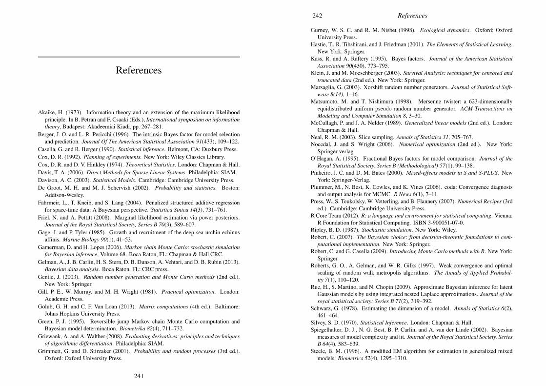
References
Akaike, H. (1973). Information theory and an extension of the maximum likelihoodprinciple. In B. Petran and F. Csaaki (Eds.), International symposium on informationtheory, Budapest: Akadeemiai Kiadi, pp. 267–281.
Berger, J. O. and L. R. Pericchi (1996). The intrinsic Bayes factor for model selectionand prediction. Journal Of The American Statistical Association 91(433), 109–122.
Casella, G. and R. Berger (1990). Statistical inference. Belmont, CA: Duxbury Press.Cox, D. R. (1992). Planning of experiments. New York: Wiley Classics Library.Cox, D. R. and D. V. Hinkley (1974). Theoretical Statistics. London: Chapman & Hall.Davis, T. A. (2006). Direct Methods for Sparse Linear Systems. Philadelphia: SIAM.Davison, A. C. (2003). Statistical Models. Cambridge: Cambridge University Press.De Groot, M. H. and M. J. Schervish (2002). Probability and statistics. Boston:
Addison-Wesley.Fahrmeir, L., T. Kneib, and S. Lang (2004). Penalized structured additive regression
for space-time data: A Bayesian perspective. Statistica Sinica 14(3), 731–761.Friel, N. and A. Pettitt (2008). Marginal likelihood estimation via power posteriors.
Journal of the Royal Statistical Society, Series B 70(3), 589–607.Gage, J. and P. Tyler (1985). Growth and recruitment of the deep-sea urchin echinus
affinis. Marine Biology 90(1), 41–53.Gamerman, D. and H. Lopes (2006). Markov chain Monte Carlo: stochastic simulation
for Bayesian inference, Volume 68. Boca Raton, FL: Chapman & Hall CRC.Gelman, A., J. B. Carlin, H. S. Stern, D. B. Dunson, A. Vehtari, and D. B. Rubin (2013).
Bayesian data analysis. Boca Raton, FL: CRC press.Gentle, J. (2003). Random number generation and Monte Carlo methods (2nd ed.).
New York: Springer.Gill, P. E., W. Murray, and M. H. Wright (1981). Practical optimization. London:
Academic Press.Golub, G. H. and C. F. Van Loan (2013). Matrix computations (4th ed.). Baltimore:
Johns Hopkins University Press.Green, P. J. (1995). Reversible jump Markov chain Monte Carlo computation and
Bayesian model determination. Biometrika 82(4), 711–732.Griewank, A. and A. Walther (2008). Evaluating derivatives: principles and techniques
of algorithmic differentiation. Philadelphia: SIAM.Grimmett, G. and D. Stirzaker (2001). Probability and random processes (3rd ed.).
Oxford: Oxford University Press.
241
242 References
Gurney, W. S. C. and R. M. Nisbet (1998). Ecological dynamics. Oxford: OxfordUniversity Press.
Hastie, T., R. Tibshirani, and J. Friedman (2001). The Elements of Statistical Learning.New York: Springer.
Kass, R. and A. Raftery (1995). Bayes factors. Journal of the American StatisticalAssociation 90(430), 773–795.
Klein, J. and M. Moeschberger (2003). Survival Analysis: techniques for censored andtruncated data (2nd ed.). New York: Springer.
Marsaglia, G. (2003). Xorshift random number generators. Journal of Statistical Soft-ware 8(14), 1–16.
Matsumoto, M. and T. Nishimura (1998). Mersenne twister: a 623-dimensionallyequidistributed uniform pseudo-random number generator. ACM Transactions onModeling and Computer Simulation 8, 3–30.
McCullagh, P. and J. A. Nelder (1989). Generalized linear models (2nd ed.). London:Chapman & Hall.
Neal, R. M. (2003). Slice sampling. Annals of Statistics 31, 705–767.Nocedal, J. and S. Wright (2006). Numerical optimization (2nd ed.). New York:
Springer verlag.O’Hagan, A. (1995). Fractional Bayes factors for model comparison. Journal of the
Royal Statistical Society. Series B (Methodological) 57(1), 99–138.Pinheiro, J. C. and D. M. Bates (2000). Mixed-effects models in S and S-PLUS. New
York: Springer-Verlag.Plummer, M., N. Best, K. Cowles, and K. Vines (2006). coda: Convergence diagnosis
and output analysis for MCMC. R News 6(1), 7–11.Press, W., S. Teukolsky, W. Vetterling, and B. Flannery (2007). Numerical Recipes (3rd
ed.). Cambridge: Cambridge University Press.R Core Team (2012). R: a language and environment for statistical computing. Vienna:
R Foundation for Statistical Computing. ISBN 3-900051-07-0.Ripley, B. D. (1987). Stochastic simulation. New York: Wiley.Robert, C. (2007). The Bayesian choice: from decision-theoretic foundations to com-
putational implementation. New York: Springer.Robert, C. and G. Casella (2009). Introducing Monte Carlo methods with R. New York:
Springer.Roberts, G. O., A. Gelman, and W. R. Gilks (1997). Weak convergence and optimal
scaling of random walk metropolis algorithms. The Annals of Applied Probabil-ity 7(1), 110–120.
Rue, H., S. Martino, and N. Chopin (2009). Approximate Bayesian inference for latentGaussian models by using integrated nested Laplace approximations. Journal of theroyal statistical society: Series B 71(2), 319–392.
Schwarz, G. (1978). Estimating the dimension of a model. Annals of Statistics 6(2),461–464.
Silvey, S. D. (1970). Statistical Inference. London: Chapman & Hall.Spiegelhalter, D. J., N. G. Best, B. P. Carlin, and A. van der Linde (2002). Bayesian
measures of model complexity and fit. Journal of the Royal Statistical Society, SeriesB 64(4), 583–639.
Steele, B. M. (1996). A modified EM algorithm for estimation in generalized mixedmodels. Biometrics 52(4), 1295–1310.

References 243
Tierney, L., R. Kass, and J. Kadane (1989). Fully exponential Laplace approximationsto expectations and variances of nonpositive functions. Journal of the AmericanStatistical Association 84(407), 710–716.
Watkins, D. S. (1991). Fundamentals of matrix computation. New York: Wiley.Wichmann, B. and I. Hill (1982). Efficient and portable pseudo-random number gener-
ator. Applied Statistics 31, 188–190.Wood, S. N. (2006). Generalized Additive Models: An Introduction with R. CRC press. Index
AIC, 36, 206, 207and cross-validation, 36computation, 104derivation, 85inconsistent, 87
algae, 153, 169, 174backward selection, 206backward substitution, 223Bayes
and importance sampling, 133and random effects, 144, 153approximation methods, 132computation, 132confidence interval, 44factor, 39, 149
fractional, 41, 152intrinsic, 41
information criterion, 42MCMC, 134theorem, 6, 37versus frequentist, 26, 44
beta function, 213BFGS, 95, 101
example, 97bias, 28BIC, 42BUGS, 172cancellation error, 117case control study, 205central limit theorem, 13Chebyshev’s inequality, 14Choleski decomposition, 110, 221coda, 172, 174computational graph, 122concavity, 15conditional distribution, 6conditional independence, 7confidence interval, 26, 33, 47
Bayesian, 148computation, 103definition, 34linear model, 189profile likelihood, 34, 103
confounder, 45conjugate distribution, 170covariance, 8covariance matrix, 9covariate, 20Cramér-Rao bound, 28
and maximum likelihood, 82derivation, 80
CRAN, 49credible interval, 44
computation, 148, 157cross validation, 36
Bayesian, 41cumulative distribution function, 1
DAG, 168data, 19design, 26, 45
optimality, 46detailed balance, 135DIC, 43
computation, 153, 174differentiation, 116
automatic, 119caveat, 122
automatic, in R, 121computational graph, 122D in R, 116deriv, 121finite differences, 116reverse mode automatic, 122symbolic, 116
distributionbeta, 215
244

Index 245
binomial, 217Cauchy, 214χ2, 188, 214Dirichlet, 177, 217exponential, 22, 216F, 190, 215gamma, 141, 216geometric, 218hypergeometric distribution, 218multivariate normal, 10, 165, 222multivariate t, 10negative binomial, 218normal, 213Poisson, 24, 217proposal, 139standard normal, 214t, 10, 21, 47, 188, 214uniform, 215Weibull, 216
eigen-decomposition, 224EM algorithm
computation, 111speeding up, 106, 113using Laplace approximation, 107, 111
estimator, 28Euclidean norm, 186expected value, 7F-ratio statistic, 190factor variable, 185finite difference
interval size, 118finite differences, 116
second derivatives, 118Fisher information, 80Fisher scoring, 94fitted values
distribution of, 191forward selection, 206forward substitution, 223frequentist, 27
confidence interval, 33versus Bayes, 26, 44
galaxies data, 177gamma function, 213generalised additive mixed model, 210generalised additive model, 208generalised likelihood ratio test, 32
computation, 103derivation, 83
generalised linear mixed model, 210
generalised linear model, 208graph, 169graphical models, 168hat matrix, 190hypothesis test, 26, 29, 38, 83
power, 32single parameter, 46
hypothesis testinglinear model, 188, 189
idempotent matrix, 191ill-conditioned, 226importance sampling, 133, 149independence, 7inequality
Chebyshev’s, 14Jensen’s, 15
inferenceAIC, 36, 85basic questions, 26Bayesian, 37confidence interval, 33, 47frequentist, 27hypothesis test, 29likelihood, 27maximum likelihood, 28Neyman-Pearson lemma, 32p value, 30point estimation, 27single parameter normal, 46
influence matrix, 190properties, 190
interactions, 194JAGS, 172
algae example, 174data transformation, 181deterministic node, 175toy example, 172urchin example, 181
Jensen’s inequality, 15, 80joint density, 3Kullback-Leibler divergence, 36, 85Laplace approximation, 39, 105
and EM algorithm, 107computation, 108equivalent normal density, 133of posterior expectation, 107, 133
law of large numbers, 15least squares, 186, 231
estimators, 186likelihood, 27
246 Index
marginal, 39profile, 34, 103properties of expected log, 79
likelihood ratio, 31compared to Bayes factor, 39Neyman-Pearson, 32
linear interpolation, 154linear mixed model, 24, 207linear model, 184
AIC, 206ANOVA, 189confounding, 203contrasts, 193estimator distribution, 187F test, 206F-ratio, 189fitted values, 191identifiability constraint, 193identifiability constraints, 194influence, 200interactions, 194least squares, 186leverage, 200model matrix, 185, 194prediction, 203R, 195R formula, 198R residual plots, 202residuals, 191selection, 206t-ratio, 188theory, 185traditional results, 192
lm, 195anova, 205drop1, 206plot, 202predict, 203step, 207summary, 196
log likelihoodcovariance matrix of derivative, 80expected derivative, 79information matrix, 80properties of expected, 79urchin model, 101
marginal density, 4marginal likelihood
computation, 149Markov chain, 7, 135Markov chain Monte Carlo, 134
autocorrelation, 147convergence checking, 145convergence testing, 147effective sample size, 147, 174extended example, 156Gibbs sampling, 140
automatic, 168example, 141finding conditionals, 141limitations, 144R code, 142slice sampling, 171
Metropolis Hastings, 135blocking, 139example, 137optimal acceptance rate, 138proposal distribution, 136, 139R code, 137reversibility, 136
Metropolis within Gibbs, 143multiple chains, 147reversibility, 135
Markov property, 7matrix
computation stability, 226condition number, 227determinant, 224, 232efficiency, 56eigen decomposition, 224function, 225generalised inverse, 226, 231idempotent, 191ill-conditioned, 226inverse of partitioned, 11preconditioning, 228singular value decomposition, 230solving triangular system, 223sparse, 232square root, 226
maximum likelihood estimation, 28, 79and Cramér-Rao bound, 82computation, 101consistency, 81large sample distribution, 29, 83numerical, 88, 92random effects, 110regularity conditions, 85using EM algorithm, 105with random effects, 104
mean, 7mixture model, 177

Index 247
model, 19AIDS in Belgium, 92algae, 153, 174annual mean temperature, 21autocorrelated temperatures, 21bacteria, 91bone marrow, 22cars, 201checking, 26, 34, 44, 102, 115, 157comparison, 26, 36
Bayesian, 38galaxies, 177linear, 184mixed, 23mixture, 177random effects, 23selection, 36survival, 22urchin, 99, 108, 181
moment, 13generating function, 13
multivariate normal, 9, 42, 83, 163conditional density, 11, 83linear transformation, 10marginal density, 11p.d.f., 10, 12
Newton’s method, 89examples, 91Fisher scoring, 94modifications, 90step, 90via EM algorithm, 106without function evaluation, 94, 114
Neyman-Pearson lemma, 32proof, 33
objective function, 88plotting, 128
odds, 38optim, 101optimisation, 88
and multimodality , 128, 129BFGS, 95conditions for optimum, 89descent direction, 89EM algorithm, 105Nelder-Mead, 98Newton’s method, 89quasi-Newton, 95second most important fact, 89step-length control, 90, 96with random effects, 104
Wolfe conditions, 96over fitting, 36
p-value, 30computation, 46general definition, 32
parameter, 19, 27point estimation, 26, 27posterior
density, 37mode, 38simulation, 139
posterior predictive simulation, 44, 178postive definite
test, 110power, 32precision, 214predictor variable, 20prior, 37
improper, 37, 137probability density function, 2
conditional, 6joint, 3marginal, 4
probability function, 2probability mass function, 2proposal distribution, 139pseudoinverse, 226, 231QQ-plot, 2, 35QR decomposition, 186, 232quantile, 2, 48quantile function, 2quasi-Newton, 95
R, 49acf, 147apply, 58arithmetic, 54array, 53, 57array indexing, 59assignment, 50attributes, 52bitwise logical operators, 59byte compilation, 73C interface, 73class, 52, 68
inheritance, 69compiled code, 73conditional execution, 70data frame, 54debugging, 76deriv, 108, 121
248 Index
diagonal matrix, 55dim attribute, 53distributions, 47, 68efficiency, 51, 54, 56, 72environment, 50evaluation, 50, 51
lazy, 65evaluation frame, 65factors, 53frame, 50functions, 51, 63
. . . argument, 66argument list, 64argument matching, 65body, 64built in, 67definition, 64method, 68variable number of arguments, 66
grids, 61if statements, 70interpreted language, 51language reference, 49lexical scoping, 63linear models, 195list, 54logical subsetting, 59loops, 71, 72matrix, 53, 55, 60
algebra, 55decomposition, 57efficiency, 56solve, 55sparse, 57subsetting, 60transpose, 56
method functions, 68, 120mode, 52model formula, 198object orientation, 52, 68, 119object structure, 69objects, 52operator overloading, 69, 120optim, 66, 101parser, 50partial matching, 65random numbers, 68rank, 62recycling rule, 55sequences, 61shared object file, 74
sort, 62storage mode, 52subsetting, 57, 59symbolic differentiation, 116tapply, 60tensor contraction, 58type, 52vector, 53, 54vectorize, 54Vectorize, 146which, 59workspace, 50
r2, 197random effects, 23, 26, 153
and Bayesian simulation, 144and optimisation, 104computation, 108EM algorithm, 105Laplace approximation, 105
random number generation, 233Mersenne Twistor, 239RANDU, 234Xorshift, 238
random variable, 1discrete, 2
random vectorlinear transformation, 9
randomisation, 45, 205residual sum of squares, 187residuals, 35, 102, 198
distribution of, 191linear model, 191standardised, 191
rjags, 172sea urchins, 99slice sampling, 171spectral decomposition, 224standard deviation, 8statistic, 17
sufficient, 17Taylor expansion, 42, 83, 86, 104Taylor’s theorem, 89transformation, 12truncation error, 118urchins, 99, 108, 181variance, 8, 28variance covariance matrix, 9