Embed Size (px)
Citation preview
CORIOLIS MASS FLOW RATE METERS
FOR LOW FLOWS
Promotiecommissie: Voorzitter, secretaris prof.dr.ir. J. van Amerongen, Universiteit Twente Promotor prof.dr.ir. P.P.L. Regtien, Universiteit Twente Deskundigen ir. J.M. Zwikker, Demcon ir. W. Jouwsma, Bronkhorst High Tech Leden prof.dr.ir. S. Stramigioli, Universiteit Twente prof.dr.ir. C.H. Slump, Universiteit Twente prof.ir. R.H. Munnig Schmidt, TU Delft dr.ir. D.M. Brouwer, Universiteit Twente Coriolis Mass Flow Rate Meters for Low Flows A. Mehendale Ph.D Thesis, University of Twente, Enschede, The Netherlands ISBN: 978-90-365-2727-9 Cover: Toy gyro top. Photograph by Adam Hart-Davis, via http://gallery.hd.org Rear: A parallel between a gyro and a Coriolis mass-flowmeter Printing: Print Partners Ipskamp, Enschede, The Netherlands © Aditya Mehendale, 2008
CORIOLIS MASS FLOW RATE METERS
FOR LOW FLOWS
DISSERTATION
to obtain
the degree of doctor at the University of Twente,
on the authority of the rector magnificus,
prof.dr. W.H.M. Zijm,
on account of the decision of the graduation committee,
to be publicly defended
on Thursday the 2nd of October, 2008 at 13:15
by
Aditya Mehendale
born on the 2nd of June 1976
in Pune, India

This dissertation has been approved by: Prof.dr.ir. P.P.L. Regtien (promotor)
i
Summary
The accurate and quick measurement of small mass flow rates (~10 mg/s) of fluids is
considered an “enabling technology” in semiconductor, fine-chemical, and food & drugs
industries. Flowmeters based on the Coriolis effect offer the most direct sensing of the mass
flow rate, and for this reason do not need complicated translation or linearization tables to
compensate for other physical parameters (e.g. density, state, temperature, heat capacity,
viscosity, etc.) of the medium that they measure. This also makes Coriolis meters versatile –
the same instrument can, without need for factory calibration, measure diverse fluid media –
liquids as well as gases. Additionally, Coriolis meters have a quick response, and can
principally afford an all-metal-no-sliding-parts fluid interface.
A Coriolis force is a pseudo-force that is generated when a mass is forced to travel along a
straight path in a rotating system. This is apparent in a hurricane on the earth (a rotating
system): when air flows towards a low-pressure region from surrounding areas, instead of
following a straight path, it “swirls” (in a towards + sideways motion). The sideways motion
component of the swirl may be attributed to the Coriolis (pseudo)force. To harness this force
for the purpose of measurement, a rotating tube may be used. The measurand (mass flow
rate) is forced through this tube. The Coriolis force will then be observed as a sideways force
(counteracting the swirl) acting upon this tube in presence of mass-flows. The Coriolis mass
flow meter tube may thus be viewed as an active measurement – a “modulator” where the
output (Coriolis force) is proportional to the product of the excitation (angular velocity of the
tube) and the measurand (mass flow rate).
From a constructional viewpoint, the Coriolis force in a Coriolis meter is generated in an
oscillating (rather than a continuously rotating) meter-tube that carries the measurand fluid.
In such a system (typically oscillating at a chosen eigenfrequency of the tube-construction),
besides the Coriolis force, there are also inertial, dissipative and spring-forces that act upon
the meter tube. As the instrument is scaled down, these other forces become significantly
larger than the generated Coriolis force. Several “tricks” can be implemented to isolate these
constructional forces from the Coriolis force, based on orthogonality – in the time domain, in
eigenmodes and in terms of position (unobservable & uncontrollable modes, symmetry, etc.).
Being an active measurement, the design of Coriolis flowmeters involves multidisciplinary
elements - fluid dynamics, fine-mechanical construction principles, mechanical design of the
oscillating tube and surroundings, sensor and actuator design, electronics for driving, sensing
and processing and software for data manipulation & control. This nature lends itself well to a
mechatronic system-design approach. Such an approach, combined with a “V-model” system
development cycle, aids in the realization of a Coriolis meter for low flows.
Novel concepts and proven design principles are assessed and consciously chosen for
implementation for this “active measurement”. These include:
- shape and form of the meter-tube
- a statically determined affixation of the tube
- contactless pure-torque actuator for exciting the tube
- contactless position-sensing for observing the (effect of) Coriolis force
- strategic positioning of the sensor & actuator to minimize actuator crosstalk and to
maximize the position sensor ratio-gain
- ratiometric measurement of the (effect of) the Coriolis force to identify the measurand
(i.e. the mass flow rate)
- multi-sensor pickoff and processing based solely on time measurement – this is
tolerant to component gain mismatch and any drift thereof
- measurement of temperature and correction for its effect of tube-stiffness
ii
The combined effect of these and other choices is the realization of a fully working prototype.
Such prototype devices are presented as a test case in this thesis to assess the effectiveness
of these choices.
A “V-model” system-development cycle involves the critical definition of requirements at the
beginning and a detailed evaluation at the end to verify that these are met. To reduce
ambiguity of intent, several test methods are defined right at the beginning with this model in
mind. These end-tests complete the “cycle” – a loop that began with the concepts and with
the definition of requirements. However, a V-model also entails shorter iterative cycles that
help refine concepts and components during the intermediate design phases. Such “inner
loops” are also presented to illustrate design at subsystem and component levels.
A Coriolis flowmeter prototype with an all-steel fluid-interface is demonstrated, that has a
specified full-scale (“FS”) mass flow rate of 200 g/h (~55 mg/s) of water. This instrument has
a long-term zero-stability better than 0.1% FS and sensitivity stability better than 0.1%,
density independence of sensitivity (within 0.2% for liquids), negligible temperature effect on
drift & sensitivity, and a 98% settling time of less than 0.1 seconds. For higher and/or negative pressure drops, these instruments have been seen to operate from –50×FS to
+50×FS (i.e. from –10 kg/h to +10 kg/h) without performance degradation – particularly
important in order to tolerate flow-pulsations in dosing applications.
Finally, the results of the present work are discussed, and recommendations are made for
possible future research that would add to it. Two important recommendations are made -
about the possibility to seek, by means of an automated optimization algorithm, an improved
tube shape for sensing the flow, and about constructional improvements to make the
measuring instrument more robust against external vibrations.
iii
Samenvatting
De nauwkeurige en snelle meting van kleine massastromen (~10 mg/s) wordt in de
halfgeleider-, fijnchemische, voedingsmiddelen- en medische industrie als een technologie
gezien welke vernieuwende processen mogelijk maken. De op het Coriolis-effect gebaseerde
massastroommeters meten direct de massastroom, dus zonder omrekeningen om andere
fysische parameters (bijvoorbeeld dichtheid, aggregratietoestand, temperatuur,
warmtecapaciteit, viscositeit, enz.) van de te meten grootheid te compenseren. Hierdoor zijn
deze instrumenten veelzijdig; hetzelfde instrument kan, zonder noodzaak van
mediumspecifieke kalibratie, diverse vloeistoffen en gassen meten. Bovendien hebben deze
meters een korte reactietijd en het vloeistofcontact kan volledig in RVS uitgevoerd worden,
zonder glijdende delen.
De Coriolis-kracht is een pseudo-kracht die optreedt wanneer een massa in een roterend
systeem loodrecht op de rotatierichting beweegt. Dit treedt bijvoorbeeld op in een orkaan
wanneer op de draaiende aarde de lucht die naar een lage druk regio stroomt, begint af te
buigen en daardoor de bekende spiraalvorm krijgt. Deze lucht ondervindt een zijwaartse
pseudo-kracht die veroorzaakt wordt door het Coriolis-effect. Om deze kracht te kunnen
beheersen en daarmee te meten, kan een roterende buis worden gebruikt. De te meten
vloeistof (of het te meten gas) wordt gedwongen door deze buis te stromen. De Coriolis-
kracht kan nu worden waargenomen als een kracht die afbuiging van deze stromende vloeistof
tegenwerkt. De Coriolis-buis van de massastroommeter kan worden beschouwd als een actief
meetprincipe, ofwel modulator, waarbij de Coriolis-kracht evenredig is aan het product van de
excitatie (hoeksnelheid van de buis) en de massastroomsnelheid.
De benodigde hoeksnelheid van de vloeistofdragende buis wordt gerealiseerd door een
oscillerende (in plaats van continu roterende, zoals de aarde) beweging; dit om glijdende
delen te vermijden. De oscillatie van de buis vindt plaats op een eigenfrequentie van de
buisconstructie. Door deze oscillatie ontstaan krachten tengevolge van inertiële, verende en
dempende eigenschappen van de buisconstructie. Naarmate de meetbuis verkleind
(geschaald) wordt, worden deze krachten vele malen groter ten opzichte van de Coriolis-
kracht. Verschillende “trucs” kunnen gebruikt worden om deze krachten afkomstig van de
constructie te isoleren van de Coriolis-kracht. Deze “trucs” zijn gebaseerd op orthogonaliteit
zowel in het tijddomein als met betrekking tot eigenmodes en de positionering van
componenten.
Juist omdat het een actief meetprincipe is, is het ontwerp van een Coriolis-massastroommeter
multidisciplinair. Vloeistofdynamica, fijnmechanische en constructieprincipes, elektronica voor
de aansturing, sensoren, signaalbewerking en informatica voor regelen en sturen, spelen een
rol in de prestaties van het uiteindelijke meetinstrument. Daarom is dit ontwerp geschikt voor
een mechatronische ontwerp-aanpak. Deze aanpak heeft er samen met een
systeemontwerpcyclus volgens het “V-model” aan bijgedragen om een voor zeer lage
massastromen bedoelde Coriolis-massastroommeter te realiseren.
Zowel nieuwe concepten als bewezen ontwerpregels zijn overwogen en steeds is een bewuste
keuze gemaakt bij aspecten van de implementatie van de actieve meting:
- Vorm van de meetbuis
- Statisch bepaalde buisfixatie en omgevingsconstructie
- Contactloze ‘zuiver-koppel’ aanstoting van de buis
- Contactloos meetprincipe om het effect van de Coriolis-kracht te meten
- Strategische positionering van de actuator en sensoren om de overspraak van de
actuatiekracht naar de Coriolis-beweging te minimaliseren en tegelijk de Coriolis-
beweging zo groot mogelijk te maken ten opzichte van de actuatiebeweging
- Ratiometrische bepaling van de Coriolis-kracht op de buis om de massastroom te ijken
iv
- Opname door middel van meerdere, uitsluitend op tijdmeting gebaseerde sensoren,
waardoor de opname ongevoelig is voor ongelijke signaalamplitudes of veranderingen
daarvan.
- Meten van een correctie voor de door temperatuur beïnvloede eigenschappen van het
buismateriaal
Bovenstaande concepten hebben tezamen bijgedragen aan het realiseren van volledig
werkende prototypes. Deze prototypes zijn onderworpen aan een aantal testen om de
doeltreffendheid van de gemaakte keuzes aan te tonen.
De systeemontwerpcyclus volgens het “V-model” eist het kritisch vastleggen van systeemeisen
(requirements) tijdens de beginfase en een evaluatie in de eindfase om aan te tonen dat de
eisen gehaald zijn. Om onduidelijkheid met betrekking tot meetmethoden te voorkomen,
moeten deze tijdens de beginfase vastgelegd worden. De eindmetingen voltooien de lus die
begon met het vastleggen van de systeemeisen. Binnen het V-model kunnen ook meerdere
kleinere iteratieve lussen gemaakt worden gedurende de systeemontwikkeling om tussendoor
de concepten te verbeteren. Naast de grotere lus zijn in dit verslag ook enkele kleinere lussen
gepresenteerd om het subsysteem en het ontwerp op componentniveau toe te lichten.
Een Coriolis-massastroommeter met een “Full Scale” (FS) bereik van 200 g/uur water wordt in
deze thesis beschreven. Deze meter heeft een nulpunts-stabiliteit beter dan 0.1% FS en een
gevoeligheidsverandering kleiner dan 0.1%. De invloed van de vloeistofdichtheid op de
gevoeligheid leidt tot een fout kleiner dan 0.2%. De invloed van de temperatuur op de
gevoeligheid en het nulpuntsverloop is verwaarloosbaar klein. Verder is de reactietijd,
gedefinieerd als de benodigde tijd om 98% van de eindwaarde door te geven, minder dan 0.1
seconden.
Tot slot worden de resultaten van het huidige onderzoek besproken en zijn er aanbevelingen
gedaan voor mogelijk vervolgonderzoek. Twee belangrijke aanbevelingen zijn gedaan,
namelijk om door een geautomatiseerd optimalisatie-algoritme een verbeterde buisvorm voor
het meten van de flow te ontdekken en om door constructieve verbeteringen de meetbuisvorm
ongevoelig te maken voor externe trillingen.
v
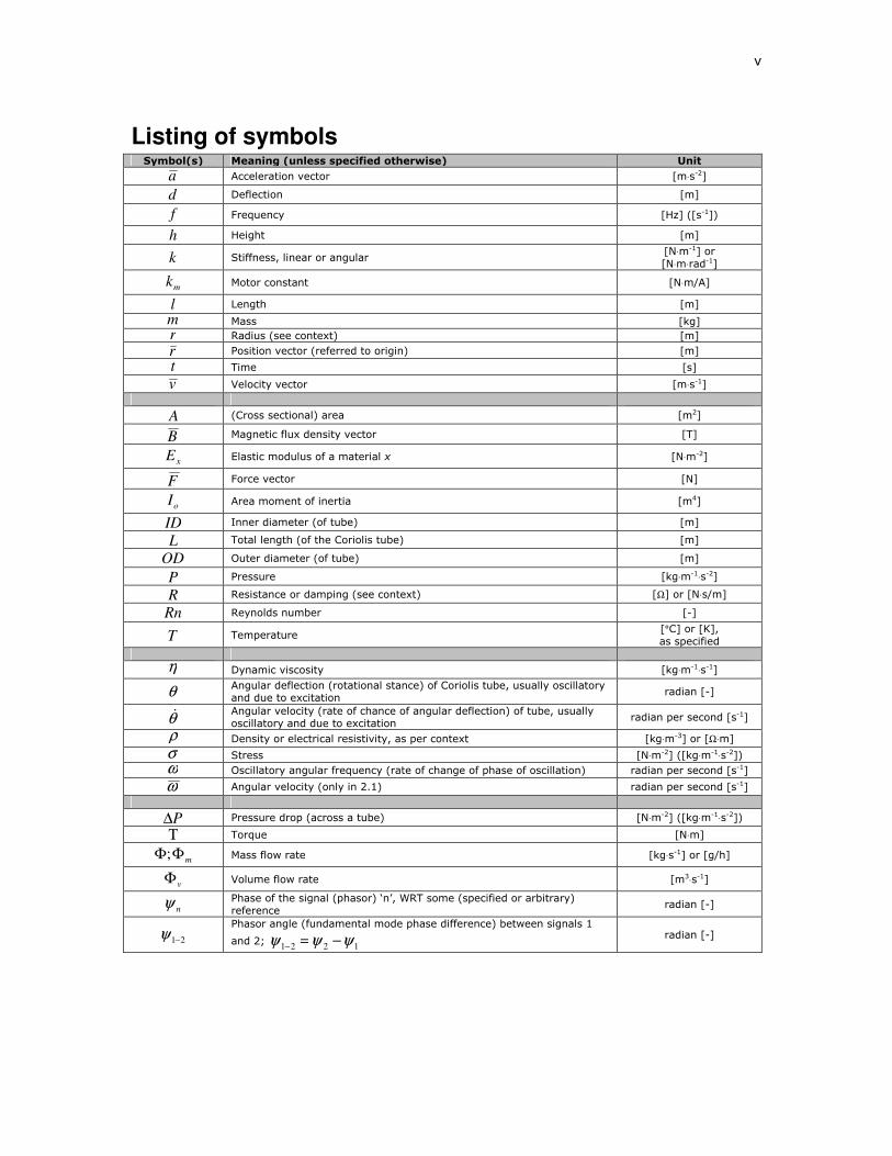
Listing of symbols Symbol(s) Meaning (unless specified otherwise) Unit
a Acceleration vector [m⋅s-2]
d Deflection [m]
f Frequency [Hz] ([s-1])
h Height [m]
k Stiffness, linear or angular [N⋅m-1] or
[N⋅m⋅rad-1]
mk Motor constant [N⋅m/A]
l Length [m]
m Mass [kg]
r Radius (see context) [m]
r Position vector (referred to origin) [m]
t Time [s]
v Velocity vector [m⋅s-1]
A (Cross sectional) area [m2]
B Magnetic flux density vector [T]
xE Elastic modulus of a material x [N⋅m-2]
F Force vector [N]
oI Area moment of inertia [m4]
ID Inner diameter (of tube) [m]
L Total length (of the Coriolis tube) [m]
OD Outer diameter (of tube) [m]
P Pressure [kg⋅m-1⋅s-2]
R Resistance or damping (see context) [Ω] or [N⋅s/m]
Rn Reynolds number [-]
T Temperature [°C] or [K],
as specified
η Dynamic viscosity [kg⋅m-1⋅s-1]
θ Angular deflection (rotational stance) of Coriolis tube, usually oscillatory and due to excitation
radian [-]
θ& Angular velocity (rate of chance of angular deflection) of tube, usually oscillatory and due to excitation
radian per second [s-1]
ρ Density or electrical resistivity, as per context [kg⋅m-3] or [Ω⋅m]
σ Stress [N⋅m-2] ([kg⋅m-1⋅s-2])
ω Oscillatory angular frequency (rate of change of phase of oscillation) radian per second [s-1]
ω Angular velocity (only in 2.1) radian per second [s-1]
P∆ Pressure drop (across a tube) [N⋅m-2] ([kg⋅m-1⋅s-2])
Τ Torque [N⋅m]
mΦΦ; Mass flow rate [kg⋅s-1] or [g/h]
vΦ Volume flow rate [m3⋅s-1]
nψ Phase of the signal (phasor) ‘n’, WRT some (specified or arbitrary)
reference radian [-]
21−ψ Phasor angle (fundamental mode phase difference) between signals 1
and 2; 1221 ψψψ −=−
radian [-]
vi
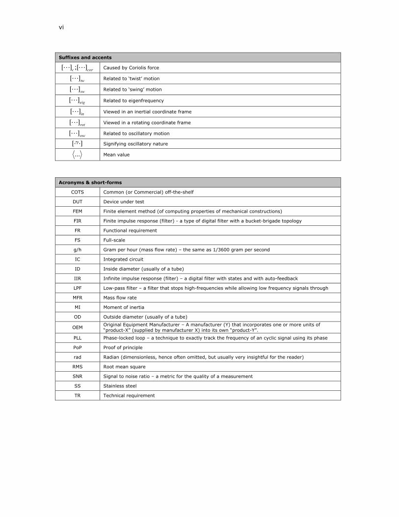
Suffixes and accents
corc ][;][ LL Caused by Coriolis force
tw][L Related to ‘twist’ motion
sw][L Related to ‘swing’ motion
eig][L Related to eigenfrequency
in][L Viewed in an inertial coordinate frame
rot][L Viewed in a rotating coordinate frame
osc][L Related to oscillatory motion
]~[L Signifying oscillatory nature
... Mean value
Acronyms & short-forms
COTS Common (or Commercial) off-the-shelf
DUT Device under test
FEM Finite element method (of computing properties of mechanical constructions)
FIR Finite impulse response (filter) - a type of digital filter with a bucket-brigade topology
FR Functional requirement
FS Full-scale
g/h Gram per hour (mass flow rate) – the same as 1/3600 gram per second
IC Integrated circuit
ID Inside diameter (usually of a tube)
IIR Infinite impulse response (filter) – a digital filter with states and with auto-feedback
LPF Low-pass filter – a filter that stops high-frequencies while allowing low frequency signals through
MFR Mass flow rate
MI Moment of inertia
OD Outside diameter (usually of a tube)
OEM Original Equipment Manufacturer – A manufacturer (Y) that incorporates one or more units of “product-X” (supplied by manufacturer X) into its own “product-Y”.
PLL Phase-locked loop – a technique to exactly track the frequency of an cyclic signal using its phase
PoP Proof of principle
rad Radian (dimensionless, hence often omitted, but usually very insightful for the reader)
RMS Root mean square
SNR Signal to noise ratio – a metric for the quality of a measurement
SS Stainless steel
TR Technical requirement
vii
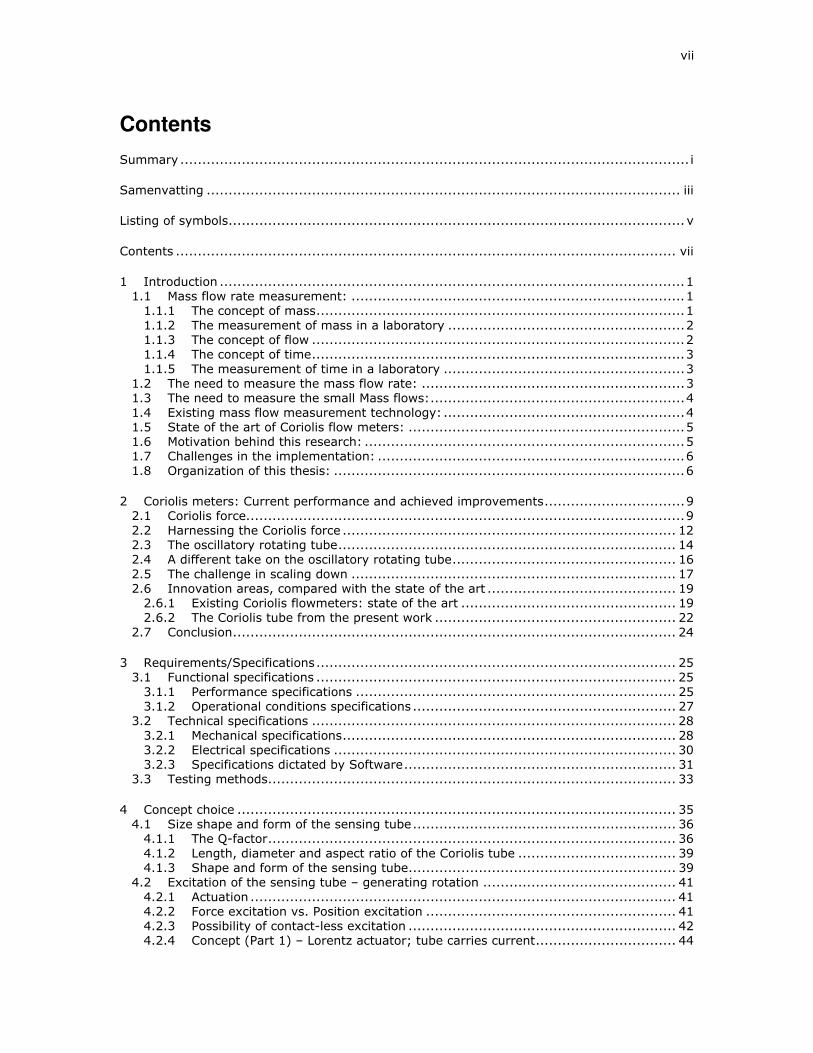
Contents
Summary .................................................................................................................... i
Samenvatting ............................................................................................................ iii
Listing of symbols........................................................................................................ v
Contents .................................................................................................................. vii
1 Introduction ..........................................................................................................1 1.1 Mass flow rate measurement: ............................................................................1
1.1.1 The concept of mass....................................................................................1 1.1.2 The measurement of mass in a laboratory ......................................................2 1.1.3 The concept of flow .....................................................................................2 1.1.4 The concept of time.....................................................................................3 1.1.5 The measurement of time in a laboratory .......................................................3
1.2 The need to measure the mass flow rate: ............................................................3 1.3 The need to measure the small Mass flows:..........................................................4 1.4 Existing mass flow measurement technology: .......................................................4 1.5 State of the art of Coriolis flow meters: ...............................................................5 1.6 Motivation behind this research: .........................................................................5 1.7 Challenges in the implementation: ......................................................................6 1.8 Organization of this thesis: ................................................................................6
2 Coriolis meters: Current performance and achieved improvements................................9 2.1 Coriolis force....................................................................................................9 2.2 Harnessing the Coriolis force ............................................................................ 12 2.3 The oscillatory rotating tube............................................................................. 14 2.4 A different take on the oscillatory rotating tube................................................... 16 2.5 The challenge in scaling down .......................................................................... 17 2.6 Innovation areas, compared with the state of the art ........................................... 19
2.6.1 Existing Coriolis flowmeters: state of the art ................................................. 19 2.6.2 The Coriolis tube from the present work ....................................................... 22
2.7 Conclusion..................................................................................................... 24
3 Requirements/Specifications.................................................................................. 25 3.1 Functional specifications .................................................................................. 25
3.1.1 Performance specifications ......................................................................... 25 3.1.2 Operational conditions specifications ............................................................ 27
3.2 Technical specifications ................................................................................... 28 3.2.1 Mechanical specifications............................................................................ 28 3.2.2 Electrical specifications .............................................................................. 30 3.2.3 Specifications dictated by Software.............................................................. 31
3.3 Testing methods............................................................................................. 33
4 Concept choice .................................................................................................... 35 4.1 Size shape and form of the sensing tube............................................................ 36
4.1.1 The Q-factor............................................................................................. 36 4.1.2 Length, diameter and aspect ratio of the Coriolis tube .................................... 39 4.1.3 Shape and form of the sensing tube............................................................. 39
4.2 Excitation of the sensing tube – generating rotation ............................................ 41 4.2.1 Actuation ................................................................................................. 41 4.2.2 Force excitation vs. Position excitation ......................................................... 41 4.2.3 Possibility of contact-less excitation ............................................................. 42 4.2.4 Concept (Part 1) – Lorentz actuator; tube carries current................................ 44
viii
4.2.5 Concept (Part 2) – Galvanic isolation of excitation current............................... 44 4.2.6 Pure torque actuation ................................................................................ 44
4.3 Observation of the sensing tube ....................................................................... 45 4.3.1 Observing the Coriolis force........................................................................ 45 4.3.2 Optical position sensing ............................................................................. 46 4.3.3 Electrical representation of optical signals..................................................... 47
4.4 Ratiometric sensing in terms of phasors............................................................. 48 4.4.1 Choice of phase detection method ............................................................... 48 4.4.2 Overview - Dual quadrature demodulation .................................................... 49
4.5 Digital representation of electrical signals (and vice versa) ................................... 50 4.6 Summary ...................................................................................................... 50
5 Detailed design.................................................................................................... 51 5.1 The meter tube - Shape and dimensions ............................................................ 51
5.1.1 Diameter of meter tube ............................................................................. 51 5.1.2 Wall thickness of meter tube....................................................................... 52 5.1.3 Shape of meter tube: choosing eigenfrequencies ........................................... 54 5.1.4 Conclusion ............................................................................................... 54
5.2 Excitation - The oscillating tube ........................................................................ 55 5.2.1 Q-factor................................................................................................... 55 5.2.2 Actuation of the Coriolis tube ...................................................................... 56 5.2.3 Tolerances essential for the actuator............................................................ 57 5.2.4 Temperature dependent variation of (stainless steel) material properties .......... 59 5.2.5 Medium density and eigenfrequency ............................................................ 62 5.2.6 Oscillator: Actuation at eigenfrequency ........................................................ 63
5.3 Sensing the Coriolis effect................................................................................ 65 5.3.1 Magnitudes .............................................................................................. 66 5.3.2 Variation in sensitivity ............................................................................... 68
5.4 Processing - Ratiometric measurement from phasor angles................................... 72 5.4.1 Sources of errors ...................................................................................... 75 5.4.2 Correction for rotation-pole shift using multiple sensors.................................. 78 5.4.3 Noise on ratiometric measurement due to noise on position sensor signals ........ 81
5.5 Summary ...................................................................................................... 83
6 Evaluation and measurement results ...................................................................... 85 6.1 Evaluation: The tube shape and dimensions ....................................................... 85
6.1.1 Pressure drop across tube .......................................................................... 85 6.1.2 Eigenfrequencies of the meter tube ............................................................. 85
6.2 Evaluation: the oscillation properties ................................................................. 87 6.2.1 The Q factor and its relation to mass flow and the environment ....................... 87 6.2.2 Actuation - power requirement and relation to the Q-factor ............................. 88 6.2.3 Effects of a non-ideal actuator .................................................................... 90 6.2.4 Temperature and tube eigenfrequencies ....................................................... 91 6.2.5 Medium density and the tube eigenfrequencies.............................................. 92
6.3 Evaluation: the Coriolis effect........................................................................... 93 6.3.1 Density-related variation in the instrument sensitivity .................................... 93 6.3.2 Temperature-related variation in the instrument sensitivity ............................. 95
6.4 Evaluation: ratiometric measurement ................................................................ 96 6.4.1 Inherent phase delays and mismatch in the instrument-construction ................ 96 6.4.2 Pole shift estimation algorithm.................................................................... 96
6.5 Measurements ............................................................................................... 97 6.5.1 Flow ranges ............................................................................................. 98 6.5.2 Uncertainty (in measuring flow) .................................................................. 98 6.5.3 Temperature effects: Drift and sensitivity ................................................... 101 6.5.4 Measurement of medium density............................................................... 103 6.5.5 Medium density: effect on sensitivity ......................................................... 104 6.5.6 Long-duration test of drift and sensitivity ................................................... 104 6.5.7 Noise on the measured flow...................................................................... 105 6.5.8 Meter response time................................................................................ 105
ix
6.5.9 Pressure drop and effects of absolute pressure on sensitivity......................... 106 6.5.10 Influence of instrument attitude on offset and sensitivity............................ 107
6.6 Conclusion................................................................................................... 108
7 Conclusions and recommendations ....................................................................... 109 7.1 The output of the project ............................................................................... 109 7.2 Conclusions at the system-level...................................................................... 109 7.3 Conclusions at the subsystem level ................................................................. 109 7.4 Conclusions at the component-level ................................................................ 109 7.5 Recommendations ........................................................................................ 110
Appendix A - Ratiometric measurement with phasors ................................................ 113
Appendix B - Lorentz actuation............................................................................... 115 B.1 Dimensioning of the stator yoke of the Lorentz actuator .................................. 115 B.2 Dimensioning of current inducing transformer ................................................ 119
Appendix C - Transimpedance amplifiers.................................................................. 121
Appendix D - Commercial Coriolis flowmeters ......................................................... 123
References ............................................................................................................. 125
Literature ............................................................................................................... 125
Patents .................................................................................................................. 126
Acknowledgements.................................................................................................. 129
About the author ..................................................................................................... 131

1 Introduction
1.1 Mass flow rate measurement: Mass flow rate measurement, as the name suggests, is the measurement of the rate at which
a quantity of a fluid, (expressed in terms of mass) crosses an imaginary boundary – for
example the outlet of a tank. Before discussion of mass flow rate measurement, let us first
consider measurement, in general. Measurement is process of associating numbers with
physical quantities; but often this association has prerequisites and pitfalls.
As the “Guide to the expression of uncertainty in measurement – 1995”, Paragraph 3.4.8 puts
it (for measurement uncertainty – though the same principles hold for measurement, in
general):
“Although this guide provides a framework for assessing (uncertainty), it cannot substitute for critical
thinking, intellectual honesty, and professional skill. The (evaluation of uncertainty) is neither a routine
task nor a purely mathematical one; it depends on detailed knowledge of the nature of the measurand
and of the measurement. The quality and utility (of the uncertainty) quoted for the result of a
measurement therefore ultimately depend on the understanding, critical analysis, and integrity of those
who contribute to the assignment of its value.”
For the sake of critical analysis, in order to get a clear understanding of the nature of the
measurand before delving into the measurement of mass flow rate, the individual elements
are first discussed:
1.1.1 The concept of mass Mass is a fundamental concept in physics, roughly corresponding to the intuitive idea of "how
much matter there is in an object". Mass can be generally quantitatively expressed on the
basis of two physical (observable) phenomena (see [1]):1
Inertia:
Inertial mass is a measure of an object's resistance to changing its state of motion when a
force is applied. An object with small inertial mass changes its motion more readily, and an
object with large inertial mass does so less readily.
Gravitation: Every mass exerts a gravitational force of attraction on every other mass. The force of
attraction between any one pair of masses is proportional to each of the masses in the pair
and the inverse of the square of the distance separating the two. Under similar conditions, an
object with a larger mass will exert a proportionately larger force of mutual attraction.
The inertial definition of mass is useful for predicting the behavior of tuning forks, billiard balls
and deep-space rocket propulsion, while the gravitational definition of mass is useful in the
context of bathroom weigh-scales and orbits of planets.
In the context of pendulums and free-fall, both definitions are simultaneously relevant – the
comparison (and equivalence) of these definitions has been the subject of numerous
experiments since Galileo. As of 2008, no proof of non-equivalence has been found (see [1]).2
The kilogram is the unit of mass, and is one of seven base units defined by the SI system. It
is, to date, based upon a prototype (the international prototype kilogram “IPK”) - a cylinder
made of a platinum-iridium alloy and stored in a vault in the International Bureau of Weights and Measures in Sevres, France. Prior to this cylinder, the definition of a kilogram was based
upon a liter of pure water at either the triple point (0’C) or the maximum-density point (4’C)
1 See also: http://en.wikipedia.org/wiki/Mass 2 See also: http://en.wikipedia.org/wiki/Mass (Equivalence of inertial and gravitational masses)
2 Coriolis mass flow rate meters for low flows
1.1.2 The measurement of mass in a laboratory Though by no means the most accurate manner, it is convenient to measure mass in a
laboratory indirectly in terms of weight. Assuming that the Earth’s gravitational acceleration is
constant and known in the laboratory, the mass of an object is proportional to its weight – the
downward ‘pull’ force exerted by the Earth upon the object. For the purpose of this thesis, for
liquids, weight measurements made by means of laboratory weigh-scales are treated as the
reference3. The veracity of the meter may be checked by placing a reference calibration-mass
upon the weigh-scales: this way, possible errors in the weigh-scales due to sensor gain, the
definition of “down”, and the local variation in earth’s gravitational acceleration (together
typically contributing to around +/- 0.2% error) can be eliminated.
Buoyancy effects due to local atmospheric pressure must be critically included in such
measurements.
With laboratory-grade equipment and proper procedure, it is not challenging to estimate the
mass of a liquid - from its weight - with a relative error smaller than 0.01%.
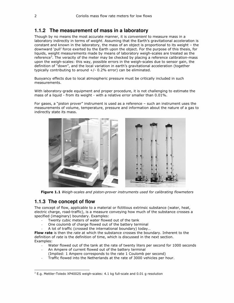
For gases, a “piston prover” instrument is used as a reference – such an instrument uses the
measurements of volume, temperature, pressure and information about the nature of a gas to
indirectly state its mass.
Figure 1.1 Weigh-scales and piston-prover instruments used for calibrating flowmeters
1.1.3 The concept of flow The concept of flow, applicable to a material or fictitious extrinsic substance (water, heat,
electric charge, road-traffic), is a measure conveying how much of the substance crosses a
specified (imaginary) boundary. Examples:
- Twenty cubic meters of water flowed out of the tank
- One coulomb of charge flowed out of the battery terminal
- A lot of traffic (crossed the international boundary) today…
Flow rate is then the rate at which the substance crosses the boundary. Inherent to the
definition of rate is the definition of time, which is discussed in the next section.
Examples:
- Water flowed out of the tank at the rate of twenty liters per second for 1000 seconds
- An Ampere of current flowed out of the battery terminal
(Implied: 1 Ampere corresponds to the rate 1 Coulomb per second)
- Traffic flowed into the Netherlands at the rate of 3000 vehicles per hour.
3 E.g. Mettler-Toledo XP4002S weigh-scales: 4.1 kg full-scale and 0.01 g resolution
Introduction 3
Usually, a conduit is associated with a flow. This can be, for example, a tube, a conductor, or a
road. While defining flow, it is often (unrealistically) assumed that the flow rate into a conduit
(i.e. at its imaginary “inlet” boundary) is equal to the flow rate out of the conduit (i.e. at its
“outlet” boundary). This may not be the case due to changing circumstances and capacity of
the conduit, and should be critically considered while defining/interpreting flow and flow-rate.
1.1.4 The concept of time The concept of time (see [2]) is too fundamental and philosophical in nature to discuss here.
Practically, time is the representation of duration between two events. Time, like mass, has a
unit (the second) that is one of the seven base units defined by the SI. Since 1967, the
International System of Measurements bases the second on the properties of cesium atoms.
SI defines the second (see [4]) as 9,192,631,770 cycles of the radiation that corresponds to
the transition between two electron spin-energy levels of the ground state of the 133Cs atom.
The term “rate” is used to express how much of something happens per unit time. As the
passage of time is continuous4 (i.e. not discrete or granular, but smooth) for all practical
purposes, a “constant rate” stays constant despite the small-ness of the time interval chosen
to determine the rate.
1.1.5 The measurement of time in a laboratory Time can be conveniently measured in a laboratory or within instruments by counting the
oscillations of a crystal (usually quartz) resonator. The relative error with which large-scale
time (a day or a year) can be measured in this manner is better than 10 parts per million. On
a smaller time-scale, the error in the measurement of time (cycle-to-cycle jitter brought about
due to thermal and other effects) has a standard deviation less than 10 picoseconds.
In a laboratory, mass flow rate measurement (measurement of the mass crossing a boundary
per unit time i.e. dtdm ) is conveniently approximated by dividing accumulated mass by the
elapsed time (i.e. tm
∆∆ ), in a small time interval. As the measurement of time over practical
time intervals (e.g. 1 s) has a relative error that is orders of magnitude smaller than that of
the measurement of mass, the error of the time-base of the reference instrument can be
neglected.
1.2 The need to measure the mass flow rate: As accepted by the SI, in its definition of the mole, the “amount of substance” can be
compared in terms of its mass. That’s to say – since the proposition of Avogadro’s number,
the following statement has not been disproved:
Equal “quantities” of the same substance (i.e. the same number of identical molecules) have the same
mass.
Practically this means – barring the case of unknown isotopes – that for chemical reactions of
any kind, it is advantageous to know the mass of reagents. In a batch-process, this (mixing
reagents in a ratio of masses) can be done using weigh-scales. In a continuous process, mass-
flow rate meters become essential5.
Volume flow (rate) measurement is often an acceptable description of the quantity or flow-rate
of a substance. Water in a utilities meter and petrol and diesel fuel at a pumping station are
de-facto expressed as a volume flow or a volume flow rate. Volume flow-rate measurement is
generally simpler (and thus cheaper) than mass flow rate measurement. However typical
causes of error when expressing the quantity of substance, when volume is measured instead
of mass, are:
4 Down to Planck time (~5.4e-44 s), where physical theories are believed to fail 5 In modern times, mass flow rate controllers (meter + control-valve) are also used for batch operations
(like bottle-filling or reagent dosing) due to their ease of automation, speed of operation, and inherent
safety (no spillage or contamination during handling)
4 Coriolis mass flow rate meters for low flows
- Density change
Cooler fluids are generally denser – i.e. have more substance per unit volume. Also,
while dealing with compressible fluids (gases) the density is dependent on pressure.
- Phase change
Reagents such as ethylene or carbon dioxide may change phase (gas/liquid) during
handling due to supercritical nature under pressure.
1.3 The need to measure the small Mass flows: The measurement and control of small fluid flow-rates (‘small’ in this context is between 1 and
1000 g/h) is required in several applications in continuous reactors and batch operations in
- Semiconductor processing plants (dopants – silane, arsine, phosphine)
- Pilot-plants for petrochemical industries (ethylene)
- Pharmaceutical and food-and-beverage industry
The meters for such applications typically measure corrosive (titanium tetrachloride, hydrogen
chloride) and hazardous (ethylene, arsine, phosphine) fluids and contamination-sensitive
pharmaceutical agents.
1.4 Existing mass flow measurement technology: Direct (i.e. not based upon volume measurements) and continuous mass flow rate meters
available as standard industrial instruments are based on just one of two technologies:
- Thermal mass flow meters:
In these meters, the heat capacity of a known fluid medium is used in conjunction with
its flow rate to transport heat towards or away from a sensor or heater. As such, the
meters have to be calibrated per fluid medium, and are not suitable for unknown
media and also not suitable if the medium properties change considerably (e.g. due to
temperature, pressure, physical state, etc.).
- Coriolis mass flow meters:
In these meters, the Coriolis force generated by a fluid flowing in a rotating conduit is
used to estimate the mass-flow.
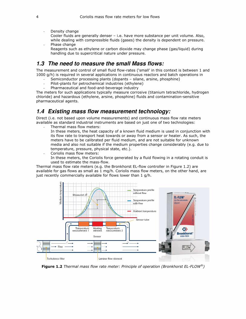
Thermal mass flow rate meters (e.g. the Bronkhorst EL-flow controller in Figure 1.2) are
available for gas flows as small as 1 mg/h. Coriolis mass flow meters, on the other hand, are
just recently commercially available for flows lower than 1 g/h.
Figure 1.2 Thermal mass flow rate meter: Principle of operation (Bronkhorst EL-FLOW®)
Introduction 5
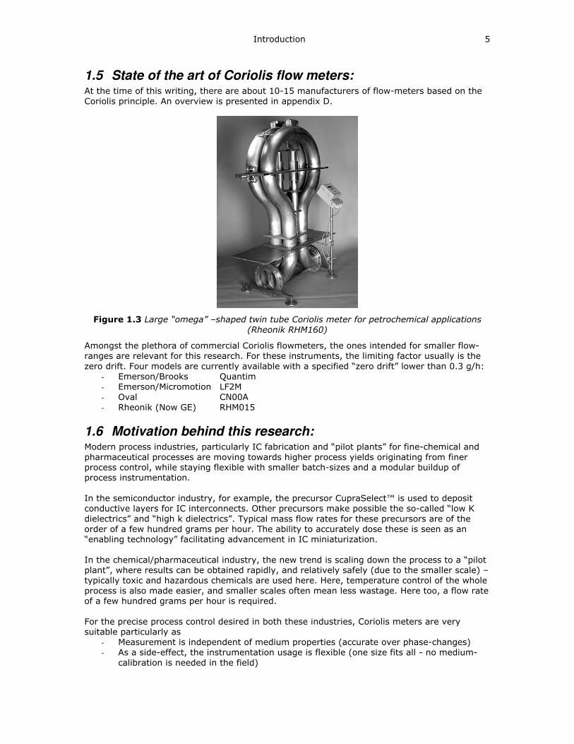
1.5 State of the art of Coriolis flow meters: At the time of this writing, there are about 10-15 manufacturers of flow-meters based on the
Coriolis principle. An overview is presented in appendix D.
Figure 1.3 Large “omega” –shaped twin tube Coriolis meter for petrochemical applications (Rheonik RHM160)
Amongst the plethora of commercial Coriolis flowmeters, the ones intended for smaller flow-
ranges are relevant for this research. For these instruments, the limiting factor usually is the
zero drift. Four models are currently available with a specified “zero drift” lower than 0.3 g/h:
- Emerson/Brooks Quantim
- Emerson/Micromotion LF2M
- Oval CN00A
- Rheonik (Now GE) RHM015
1.6 Motivation behind this research: Modern process industries, particularly IC fabrication and “pilot plants” for fine-chemical and
pharmaceutical processes are moving towards higher process yields originating from finer
process control, while staying flexible with smaller batch-sizes and a modular buildup of
process instrumentation.
In the semiconductor industry, for example, the precursor CupraSelect™ is used to deposit
conductive layers for IC interconnects. Other precursors make possible the so-called “low K
dielectrics” and “high k dielectrics”. Typical mass flow rates for these precursors are of the
order of a few hundred grams per hour. The ability to accurately dose these is seen as an
“enabling technology” facilitating advancement in IC miniaturization.
In the chemical/pharmaceutical industry, the new trend is scaling down the process to a “pilot
plant”, where results can be obtained rapidly, and relatively safely (due to the smaller scale) –
typically toxic and hazardous chemicals are used here. Here, temperature control of the whole
process is also made easier, and smaller scales often mean less wastage. Here too, a flow rate
of a few hundred grams per hour is required.
For the precise process control desired in both these industries, Coriolis meters are very
suitable particularly as
- Measurement is independent of medium properties (accurate over phase-changes)
- As a side-effect, the instrumentation usage is flexible (one size fits all - no medium-
calibration is needed in the field)

6 Coriolis mass flow rate meters for low flows
- Accuracy remains high over product lifetime – no clogging or wear
- Rapid meter response to flow-change
The mass-flow meters currently available are aimed at mass-flow of typically several hundred
kg/hour and as such unsuitable for the smaller scales.
To this end, in collaboration with the University of Twente (formal theoretical background),
Demcon (mechatronic design), and TNO (fluid dynamics), this research project has been
undertaken.
1.7 Challenges in the implementation: Coriolis meters scale poorly. That is to say, that generally speaking, their performance
degrades as the overall size decreases. This scaling aspect is discussed further in Chapter 2.
As with all flowmeters, it is desirable to make an instrument with high repeatability and small
offset-drift. To avoid the need for characterization, linearity is also desirable. Due to the
nature of measurement (discussed in the following chapters), unwanted forces of relatively
large magnitudes interfere with the intermediate measurand, i.e. the Coriolis force, leading to
large drift in the meter-offset. Designing a meter (for a small flow-rate) with an acceptably
small drift is the most challenging task. The technical as well as the organizational aspects
have been tackled with the ‘Mechatronics-approach’6, for example, by means of a statically
determined construction (see [3]), orthogonality of modes, constructional symmetries,
strategic sensor and actuator placement and separation in frequency-domain. Processing
(compensation for higher order physical effects) is also required in order to reduce sensitivity
errors to less than 1%. This is done by means of purely time-domain measurements,
correction using multiple position sensors, and (sensitivity) correction for medium density and
temperature.
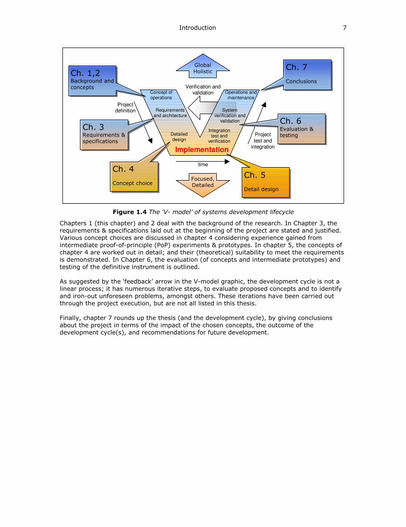
1.8 Organization of this thesis: The organization of this thesis is loosely based on the steps in a V-model of a systems
development lifecycle [4], [8]. This is not merely a subjective choice. This project at the
backbone of this thesis deals with the entire ‘Mechatronic design cycle’ (see [8]) of developing
a state-of-the-art mechatronic measurement system. Rather than basing the chapter-
segmentation on subsystems or on chronological order of research, the V-model approach is
taken due to the nature of tasks involved from start to the finish.
6 Mechatronics has come to mean the synergistic use of precision engineering, control theory, computer
science, and sensor and actuator technology to design improved products and processes; insight into the
mechatronics approach and also the Mechatronics design process is to be found in [8]
Introduction 7
Ch. 3 Requirements & specifications
Ch. 1,2 Background and concepts
Ch. 4 Concept choice
Ch. 5 Detail design
Ch. 6 Evaluation & testing
Ch. 7 Conclusions
Global Holistic
Focused, Detailed
Verification and validation
time
Project definition
Project test and
integration
Concept of operations
Requirements and architecture
Detailed design
Implementation
Integration test and
verification
System verification and
validation
Operations and maintenance
Figure 1.4 The ‘V- model’ of systems development lifecycle
Chapters 1 (this chapter) and 2 deal with the background of the research. In Chapter 3, the
requirements & specifications laid out at the beginning of the project are stated and justified.
Various concept choices are discussed in chapter 4 considering experience gained from
intermediate proof-of-principle (PoP) experiments & prototypes. In chapter 5, the concepts of
chapter 4 are worked out in detail; and their (theoretical) suitability to meet the requirements
is demonstrated. In Chapter 6, the evaluation (of concepts and intermediate prototypes) and
testing of the definitive instrument is outlined.
As suggested by the ‘feedback’ arrow in the V-model graphic, the development cycle is not a
linear process; it has numerous iterative steps, to evaluate proposed concepts and to identify
and iron-out unforeseen problems, amongst others. These iterations have been carried out
through the project execution, but are not all listed in this thesis.
Finally, chapter 7 rounds up the thesis (and the development cycle), by giving conclusions
about the project in terms of the impact of the chosen concepts, the outcome of the
development cycle(s), and recommendations for future development.

2 Coriolis meters: Current performance and achieved improvements
Target setting: Coriolis meters are available as standard products for about 40 years; patents are to be found
from as far back as the 1950s. Patents and literature refer for the most part to tube shapes
and actuation, sensing and processing configurations. Literally hundreds of tube-shapes are to
be found, many of them with immediately visible advantages and drawbacks. The one
common factor in them all is, naturally, the generation and measurement of Coriolis force. In
this chapter, we look at the basic operation of a Coriolis meter without implementation details,
and form a generic model representative of the fundamental working. Subsequently, the
current state of the art is considered (various existing Coriolis meters), their possible
shortcomings are listed and the innovative elements of this work are presented against this
background.
2.1 Coriolis force Coriolis force, like centrifugal force is a pseudo-force (fictitious force) that appears to act on
masses moving in a rotating reference-frame (see [1]). In a rotating coordinate frame,
fictitious acceleration can be brought about due to the rotation of the reference frame.
The Coriolis force is named after Gaspard-Gustave de Coriolis, a French scientist who
described it in 1835 in a paper titled “Sur les équations du mouvement relatif des systèmes de corps (On the equations of relative motion of a system of bodies)” This paper deals with the
transfer of energy in rotating systems like waterwheels. Coriolis's name began to appear in
meteorological literature (in the context of weather systems) at the end of the 19th century,
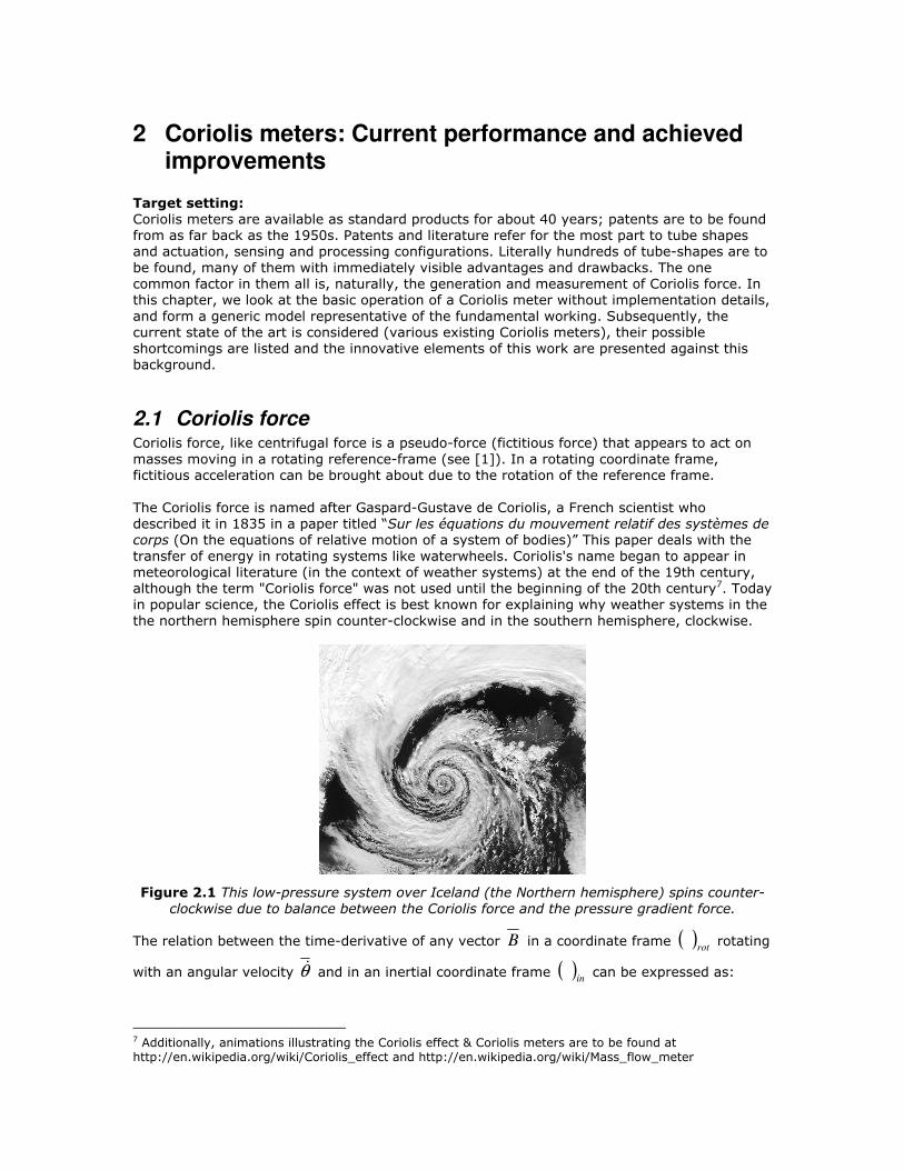
although the term "Coriolis force" was not used until the beginning of the 20th century7. Today
in popular science, the Coriolis effect is best known for explaining why weather systems in the
the northern hemisphere spin counter-clockwise and in the southern hemisphere, clockwise.
Figure 2.1 This low-pressure system over Iceland (the Northern hemisphere) spins counter-clockwise due to balance between the Coriolis force and the pressure gradient force.
The relation between the time-derivative of any vector B in a coordinate frame ( )rot
rotating
with an angular velocity θ& and in an inertial coordinate frame ( )in
can be expressed as:
7 Additionally, animations illustrating the Coriolis effect & Coriolis meters are to be found at
http://en.wikipedia.org/wiki/Coriolis_effect and http://en.wikipedia.org/wiki/Mass_flow_meter
10 Coriolis mass flow rate meters for low flows
in
rot
in
in
Bdt
Bd
dt
Bd×+
=
ω (2.1)
If we express acceleration a as the time-derivative of velocity v ,
in
rot
inin v
dt
vda ×+
= ω (2.2)
Similarly, if we express the velocity as the time-derivative of the position vector r
rvv rotin ×+= ω (2.3)
(As there’s only the rotation and no translation, rotin rr = )
The acceleration can now be expressed as
)()(
rvdt
rvda rot
rot
rotin ×+×+
×+= ωω
ω (2.4)
Or equivalently, as rotrot a
dt
vd= and rotv
dt
rd=
)(2 rvrdt
daa rotrotin ××+×+×+= ωωω
ω (2.5)
The “coordinate acceleration” in the rotating frame is thus
44444444 344444444 21
4342143421321
framecoordinaterotatingatoduefictitious
onacceleratilcentrifugaonacceleratiCoriolis
rot
onacceleratiEuleronacceleratiphysical
inrot rvrdt
daa
;
)(2 ××−×−×−= ωωωω
(2.6)
which is the physical acceleration, exerted by external forces on the object, plus additional
terms associated with the geometry of the rotating reference frame.
For an object having mass m in this rotating reference-frame, the fictitious acceleration terms
bring about:
- Centrifugal force:
( ) rrmrmF lcentrifuga ˆ)()( 2ωωω =××−⋅=
in the radial direction
- Coriolis force:
)2( rotCoriolis vmF ×−= ω
in a direction perpendicular to the rotation and velocity
Coriolis meters: Current performance and achieved improvements 11
- Euler force:
)( rdt
dmF Euler ×−=
ω
caused by the angular acceleration of the coordinate frame
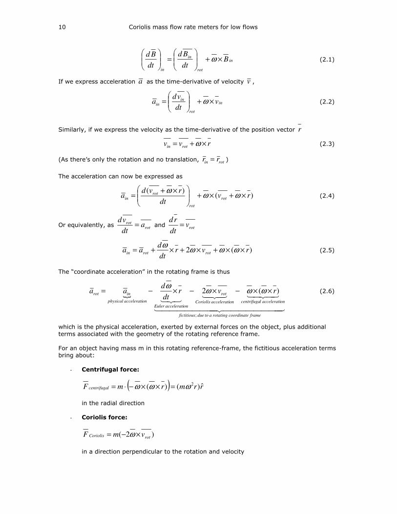
Going a step further, if instead of a mass, we have a continuous flow (e.g. water in a rotating
tube), the individual flowing elements (globs of water) can be thought of as masses together
contributing to the fictitious forces.
ω
dt
dω
v
Centrifugal.. Coriolis.. and Euler
forces on fluid globs in a rotating tube carrying the stream of fluid
ω
Figure 2.2 Pseudo-forces acting upon fluid in a rotating tube
For the particular case of the Coriolis force, where the velocity plays a role, consider a glob of
fluid with mass dm , taken as a thin slice of the tube of total length L ; the thickness of the
slice is dl , the sectional area is A and the density of the fluid is ρ . The tube rotates with an
angular velocity ω
Summing over all globs:
∫=
⋅⋅⋅×−=L
l
fluidofgloba
rottotalCoriolis dlAvF0
2)(48476
ρω (2.7)
Notice, however, that Avrot ⋅ is the volume flow rate and Avrot ⋅⋅ ρ is actually the mass-flow-
rate mΦ . We can rewrite the expression for Coriolis force as:
)(22)(0
m
L
l
mtotalCoriolis ldlF Φ×⋅−=⋅Φ×−= ∫=
ωω (2.8)
This relation forms the basis for all Coriolis mass flow rate meters8.
8 For a more intuitive explanation about the generation of Coriolis force, see [9].
[6] gives thorough treatment of rotating reference frames and gyroscopes.
12 Coriolis mass flow rate meters for low flows
2.2 Harnessing the Coriolis force
From equation 2.8, is seen that in order to generate Coriolis force, a conduit of length L
carrying mass-flow (with MFR Φ ) is needed. When this conduit is rotated with an angular rate
of ω (henceforth referred to as θ& to avoid confusion with the symbol for eigenfrequency), it
will result in a Coriolis force corF proportional to Φ . The following illustrative construction has
these components (mass-flow, length and angular rate) and is perhaps the simplest possible
usable Coriolis MFR meter.
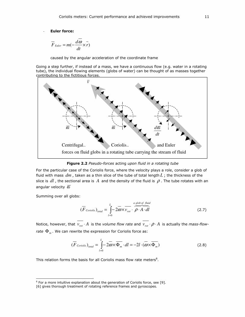
Figure 2.3 An illustrative rotating-tube Coriolis MFR meter
In this construction, fluidic mass-flow is introduced into a so called “active tube length” by
means of two slip-couplings and (compliant) bellows. The inlet and outlet are fixed, while the
tube construction in between is driven to rotate by means of an external engine, such as an
electromotor. A stiff frame couples the feeding sections of pipe so that the inlet and outlet
“elbows”, together with the frame, form a stiff rotating construction. A (stiff) force sensor is
positioned between the rigid frame and the central straight piece of ‘sensor’ tube between the
two bellows (constituting the active tube-length).
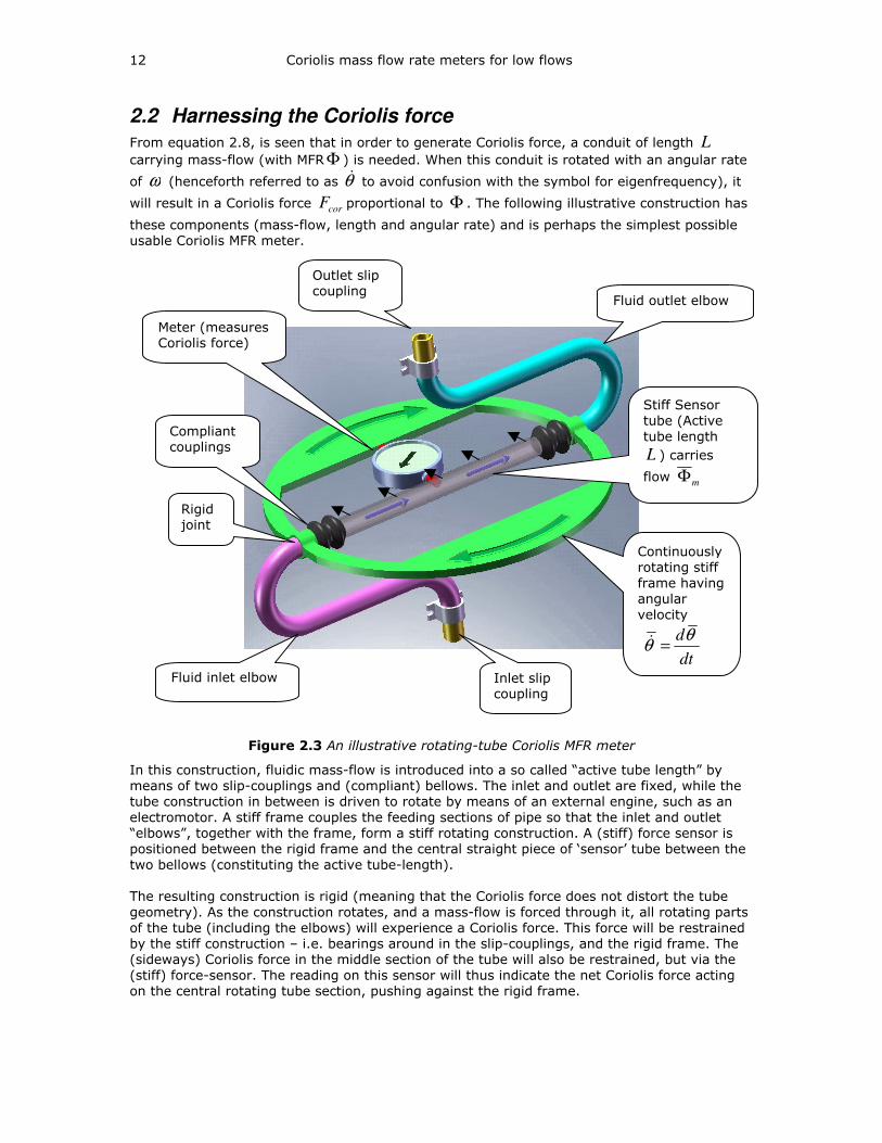
The resulting construction is rigid (meaning that the Coriolis force does not distort the tube
geometry). As the construction rotates, and a mass-flow is forced through it, all rotating parts
of the tube (including the elbows) will experience a Coriolis force. This force will be restrained
by the stiff construction – i.e. bearings around in the slip-couplings, and the rigid frame. The
(sideways) Coriolis force in the middle section of the tube will also be restrained, but via the
(stiff) force-sensor. The reading on this sensor will thus indicate the net Coriolis force acting
on the central rotating tube section, pushing against the rigid frame.
Inlet slip coupling
Continuously
rotating stiff
frame having
angular
velocity
dt
dθθ =&
Fluid inlet elbow
Fluid outlet elbow
Meter (measures Coriolis force)
Outlet slip coupling
Compliant couplings
Stiff Sensor
tube (Active
tube length
L ) carries
flow mΦ
Rigid joint
Coriolis meters: Current performance and achieved improvements 13
To get an idea about the magnitudes involved, let us consider for the construction in Figure
2.3 a tube of length 0.2 m and cross-section 1 sq.cm (irrelevant) rotating at 300 RPM (i.e.
5Hz, or 31.4 rad/sec). Consider water flowing through this tube at the rate of 0.1 kg/s – about
a liter in 10 seconds.
The Coriolis force this tube will generate is:
][25.11.04.312.02)(2 NlF mCoriolis ≅×××=Φ×⋅−= θ& (2.9)
This is small compared to the centrifugal force due to water column in one half of the tube
(about 5 N per half) and somewhat larger than the rate-of-change of momentum in each of
the elbows (about 0.2 N per elbow)
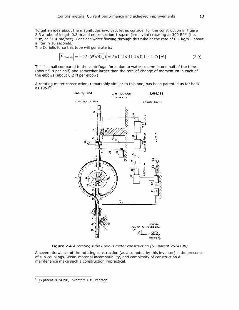
A rotating meter construction, remarkably similar to this one, has been patented as far back
as 19539.
Figure 2.4 A rotating-tube Coriolis meter construction (US patent 2624198)
A severe drawback of the rotating construction (as also noted by this inventor) is the presence
of slip-couplings. Wear, material incompatibility, and complexity of construction &
maintenance make such a construction impractical.
9 US patent 2624198, Inventor: J. M. Pearson
14 Coriolis mass flow rate meters for low flows
An approach taken by several inventors in the 50’s is one where the “sensing element” in the
tube undergoes oscillatory –rather than continuous- rotation. This “twist” motion, similar to
the dance style invented around the same period, is still used in the present day. The basic
idea is that a small angular deflection (though with high angular rates, as will be seen) is
brought about by means of elastic deformation of the fluid-carrying conduit. This deflection is
oscillatory in nature. As such, the need for slip-couplings is eliminated. Of course, this means
that the generated Coriolis force too is oscillatory in nature. Possible ill effects of this (aliasing
of fast-changing flow due to pulsating readout) can be avoided by choosing a sufficiently high
oscillation frequency.
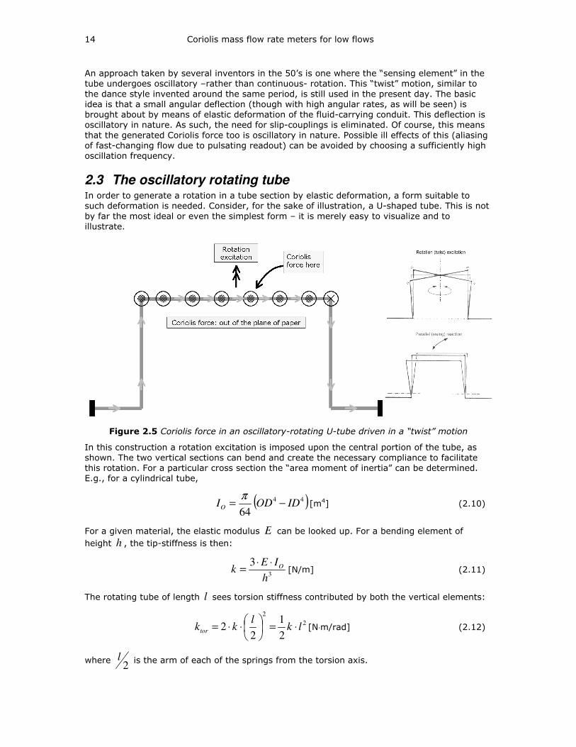
2.3 The oscillatory rotating tube In order to generate a rotation in a tube section by elastic deformation, a form suitable to
such deformation is needed. Consider, for the sake of illustration, a U-shaped tube. This is not
by far the most ideal or even the simplest form – it is merely easy to visualize and to
illustrate.
Figure 2.5 Coriolis force in an oscillatory-rotating U-tube driven in a “twist” motion
In this construction a rotation excitation is imposed upon the central portion of the tube, as
shown. The two vertical sections can bend and create the necessary compliance to facilitate
this rotation. For a particular cross section the “area moment of inertia” can be determined.
E.g., for a cylindrical tube,
( )44
64IDODIO −=
π[m4] (2.10)
For a given material, the elastic modulus E can be looked up. For a bending element of
height h , the tip-stiffness is then:
3
3
h
IEk O⋅⋅
= [N/m] (2.11)
The rotating tube of length l sees torsion stiffness contributed by both the vertical elements:
2
2
2
1
22 lk
lkktor ⋅=
⋅⋅= [N⋅m/rad] (2.12)
where 2
l is the arm of each of the springs from the torsion axis.
Coriolis meters: Current performance and achieved improvements 15
This is by no means an exact estimate of the stiffness. The torsion in the inlet and outlet tubes
(which decreases the overall stiffness), the torsion in the rotating length that couples the left
and right bending elements (which increases the overall stiffness), and other higher order
effects have been neglected. It does give fair estimates for order-of-magnitude calculations.
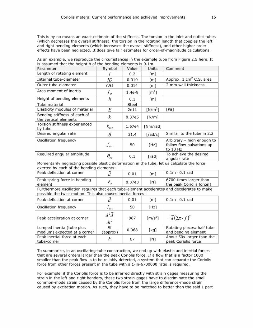
As an example, we reproduce the circumstances in the example tube from Figure 2.5 here. It
is assumed that the height h of the bending elements is 0.1m.
Parameter Symbol Value Units Comment
Length of rotating element l 0.2 [m]
Internal tube-diameter ID 0.010 [m] Approx. 1 cm2 C.S. area
Outer tube-diameter OD 0.014 [m] 2 mm wall thickness
Area moment of inertia OI 1.4e-9 [m4]
Height of bending elements h 0.1 [m]
Tube material Steel
Elasticity modulus of material E 2e11 [N/m2] [Pa]
Bending stiffness of each of
the vertical elements k 8.37e5 [N/m]
Torsion stiffness experienced
by tube tork 1.67e4 [Nm/rad]
Desired angular rate θ& 31.4 [rad/s] Similar to the tube in 2.2
Oscillation frequency
oscf 50 [Hz]
Arbitrary – high enough to
follow flow pulsations up
to 10 Hz
Required angular amplitude twθ 0.1 [rad]
To achieve the desired
angular rate
Momentarily neglecting possible plastic deformation in the tube, let us calculate the force
exerted by each of the bending elements:
Peak deflection at corner d~
0.01 [m] 0.1m ⋅ 0.1 rad
Peak spring-force in bending
element bF 8.37e3 [N] 6700 times larger than
the peak Coriolis force!!
Furthermore oscillation requires that each tube-element accelerates and decelerates to make
possible the twist motion. This also causes inertial forces:
Peak deflection at corner d~
0.01 [m] 0.1m ⋅ 0.1 rad
Oscillation frequency oscf 50 [Hz]
Peak acceleration at corner 2
2 ~
dt
dd 987 [m/s2] ( )2
2~
fd ⋅= π
Lumped inertia (tube plus
medium) expected at a corner
m
(approx) 0.068 [kg]
Rotating pieces: half tube
and bending element
Peak inertial-force at each
tube-corner iF 67 [N] About 50x larger than the
peak Coriolis force
To summarize, in an oscillating-tube construction, we end up with elastic and inertial forces
that are several orders larger than the peak Coriolis force. If a flow that is a factor 1000
smaller than the peak flow is to be reliably detected, a system that can separate the Coriolis
force from other forces present in the tube with a 1-in-6700000 ratio is required.
For example, if the Coriolis force is to be inferred directly with strain gages measuring the
strain in the left and right benders, these two strain-gages have to discriminate the small
common-mode strain caused by the Coriolis force from the large difference-mode strain
caused by excitation motion. As such, they have to be matched to better than the said 1 part
16 Coriolis mass flow rate meters for low flows
in 6.7 million10. This requirement can be avoided by measuring motion instead of strain – near
the rotation axis, the excitation motion is very small, and thus the Coriolis (swing) motion is
relatively larger.
Furthermore, to create the oscillatory rotation motion, an actuator that can deliver a peak
torque Τ of 1.67e3 N⋅m (peak power: 26 kW
⋅Τ= peakpeak θ&
2
111) Such a brute-force
approach can be avoided, for example, by using resonance. Such systems and constructions
are presented in chapter 4.
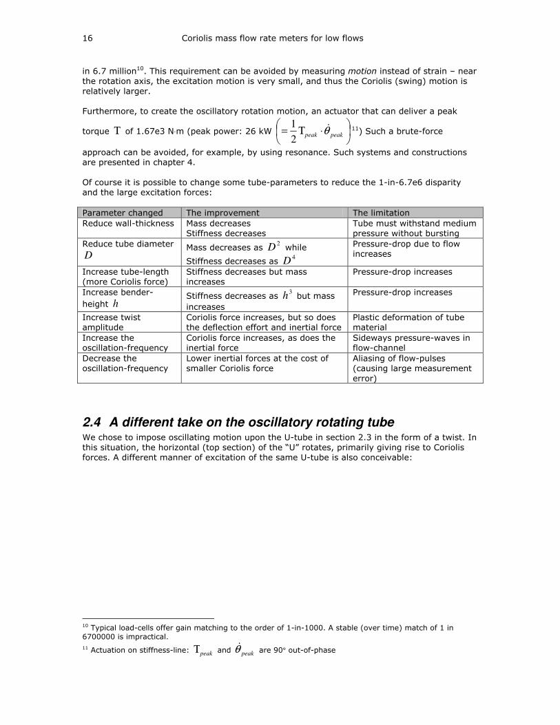
Of course it is possible to change some tube-parameters to reduce the 1-in-6.7e6 disparity
and the large excitation forces:
Parameter changed The improvement The limitation
Reduce wall-thickness Mass decreases
Stiffness decreases
Tube must withstand medium
pressure without bursting
Reduce tube diameter
D Mass decreases as
2D while
Stiffness decreases as 4
D
Pressure-drop due to flow
increases
Increase tube-length
(more Coriolis force)
Stiffness decreases but mass
increases
Pressure-drop increases
Increase bender-
height h Stiffness decreases as
3h but mass
increases
Pressure-drop increases
Increase twist
amplitude
Coriolis force increases, but so does
the deflection effort and inertial force
Plastic deformation of tube
material
Increase the
oscillation-frequency
Coriolis force increases, as does the
inertial force
Sideways pressure-waves in
flow-channel
Decrease the
oscillation-frequency
Lower inertial forces at the cost of
smaller Coriolis force
Aliasing of flow-pulses
(causing large measurement
error)
2.4 A different take on the oscillatory rotating tube We chose to impose oscillating motion upon the U-tube in section 2.3 in the form of a twist. In
this situation, the horizontal (top section) of the “U” rotates, primarily giving rise to Coriolis
forces. A different manner of excitation of the same U-tube is also conceivable:
10 Typical load-cells offer gain matching to the order of 1-in-1000. A stable (over time) match of 1 in
6700000 is impractical.
11 Actuation on stiffness-line: peakΤ and peakθ& are 90° out-of-phase
Coriolis meters: Current performance and achieved improvements 17
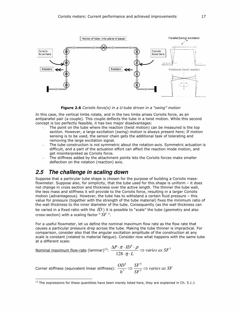
Figure 2.6 Coriolis force(s) in a U-tube driven in a “swing” motion
In this case, the vertical limbs rotate, and in the two limbs arises Coriolis force, as an
antiparallel pair (a couple). This couple deflects the tube in a twist motion. While this second
concept is too perfectly feasible, it has two major disadvantages:
- The point on the tube where the reaction (twist motion) can be measured is the top
section. However, a large excitation (swing) motion is always present here; If motion
sensing is to be used, the sensor chain gets the additional task of tolerating and
removing the large excitation signal.
- The tube construction is not symmetric about the rotation-axis. Symmetric actuation is
difficult, and a part of the actuation effort can affect the reaction mode motion, and
get misinterpreted as Coriolis force.
- The stiffness added by the attachment points lets the Coriolis forces make smaller
deflection on the rotation (reaction) axis.
2.5 The challenge in scaling down Suppose that a particular tube shape is chosen for the purpose of building a Coriolis mass-
flowmeter. Suppose also, for simplicity, that the tube used for this shape is uniform – it does
not change in cross section and thickness over the active length. The thinner the tube wall,
the less mass and stiffness it will provide to the Coriolis force, resulting in a larger Coriolis
motion (advantageous). However, the tube has to withstand a certain fluid pressure – this
value for pressure (together with the strength of the tube material) fixes the minimum ratio of
the wall thickness to the inner diameter of the tube. Consequently (as the wall thickness can
be varied in a fixed ratio with the ID ) it is possible to “scale” the tube (geometry and also
cross-section) with a scaling factor “ SF ”.
For a useful flowmeter, let us define the nominal maximum flow rate as the flow rate that
causes a particular pressure drop across the tube. Making the tube thinner is impractical. For
comparison, consider also that the angular excitation amplitude of the construction at any
scale is constant (related to material fatigue). Consider now what happens with the same tube
at a different scale:
Nominal maximum flow-rate (laminar)12: 3
4
128SFasriesva
L
IDP⇒
⋅⋅
⋅⋅⋅∆
η
ρπ
Corner stiffness (equivalent linear stiffness): SFasriesvaSF
SF
h
OD⇒⇒
3
4
3
4
12 The expressions for these quantities have been merely listed here, they are explained in Ch. 5.1.1
18 Coriolis mass flow rate meters for low flows
Excitation - linear excursion (of corner): SFasariesv
Excitation force (=stiffness × excitation): 2
SFasariesv
Tube inertia: 3
SFasariesv (related to the volume)
Tube eigenfrequency: SF
asriesvaSF
SF
m
k 13⇒⇒=ω
Active tube length: SFasariesvL ⇒
Flow-rate per excitation-force: SFasriesvaSF
SFFpE ⇒⇒
2
3
Coriolis force per excitation force: )(
)(2
forceexcitation
Ltemassflowra
forceCoriolis
exc
4444 84444 76&θ⋅⋅⋅
( ) SFasriesvaSF
SFSFLFpE
velangularpeak
eigexc ⇒⋅⋅⋅⋅⇒⋅⋅⋅⋅⇒1
12)(248476
ωθ
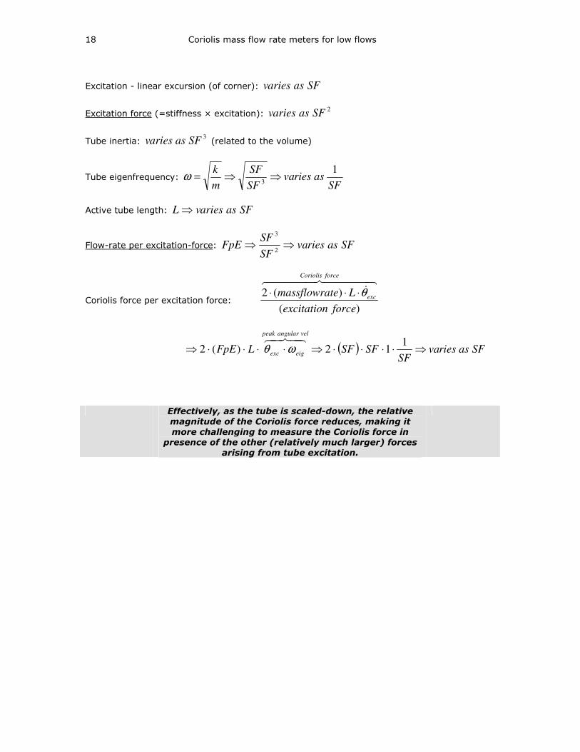
Effectively, as the tube is scaled-down, the relative
magnitude of the Coriolis force reduces, making it
more challenging to measure the Coriolis force in
presence of the other (relatively much larger) forces
arising from tube excitation.
Coriolis meters: Current performance and achieved improvements 19
2.6 Innovation areas, compared with the state of the art
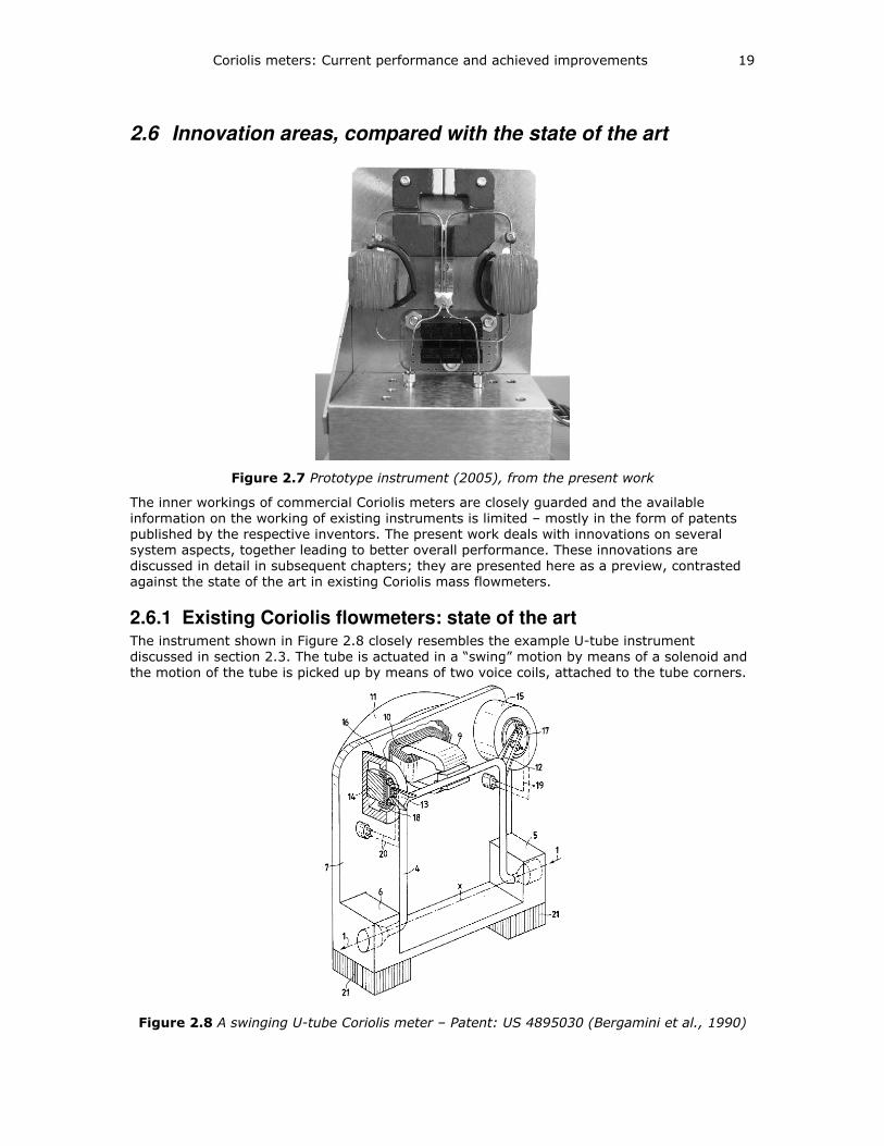
Figure 2.7 Prototype instrument (2005), from the present work
The inner workings of commercial Coriolis meters are closely guarded and the available
information on the working of existing instruments is limited – mostly in the form of patents
published by the respective inventors. The present work deals with innovations on several
system aspects, together leading to better overall performance. These innovations are
discussed in detail in subsequent chapters; they are presented here as a preview, contrasted
against the state of the art in existing Coriolis mass flowmeters.
2.6.1 Existing Coriolis flowmeters: state of the art The instrument shown in Figure 2.8 closely resembles the example U-tube instrument
discussed in section 2.3. The tube is actuated in a “swing” motion by means of a solenoid and
the motion of the tube is picked up by means of two voice coils, attached to the tube corners.
Figure 2.8 A swinging U-tube Coriolis meter – Patent: US 4895030 (Bergamini et al., 1990)

20 Coriolis mass flow rate meters for low flows
This form has several disadvantages. Here the tube ends (fixed to the chassis at points 5 and
6) are away from each other. This structure is susceptible to distortion under a thermal
gradient (a warm fluid medium). There are heavy and paddle-like (having large wind
resistance) attachments upon the tube. Coriolis forces being in phase with damping forces; will
be indistinguishable, and influenced by the windage.
The actuation is achieved by means of applying a force in the middle of the tube. If the force is
not exactly in the middle, the tube will see it as a combination - force plus torque. Based on
phase relations, most of this torque can be eliminated, but is nonetheless undesirable. The
actuator is a solenoid (9, 10). Magnetization of the ferromagnetic components may cause out-
of-phase actuation (can be mistaken for Coriolis force).
In addition to the arguments mentioned in section 0, the vertical limbs of the U-shape are
subjected to bending, and the Coriolis force is generated in these very limbs. The Coriolis
force, dependent on the local angular velocity will then be not uniform over the entire tube-
length, but concentrated at the parts with the most deflection. Imagine now that the nature of
bending changes slightly; this will affect the instrument sensitivity.
The sensors used to measure the position of the tube and thereby the Coriolis force, also see
all the excitation motion. The (small) Coriolis motion is buried in a large common-mode signal
corresponding to the excitation. This is avoidable.
This particular instrument consists of a single tube on a heavy chassis. The tube vibration will
cause a chassis-shake. If the chassis is not sufficiently heavier than the tube, the chassis
motion may be misinterpreted as Coriolis motion.
The form shown in Figure 2.9 has two tubes usually carrying exactly the same mass flow (as
they are connected in series).
Figure 2.9 A twin-tube Coriolis meter – Patent: US 4192184 (Cox et al., 1980)
This configuration, though generally the same as the previous one, offers some advantages.
The double tube reduces the problem of the chassis shake. Also, notice that the actuation and
the position sensing is done as a relative measurement – between the two tubes; this makes
external vibrations invisible (or less visible) to the position sensors. The numerous
attachments for the purpose of actuation and sensing also seem smaller than the previous
example.
For the rest, this instrument has all the drawbacks of the instrument in the previous example.
Additionally, the double-tube construction has some problems – the assumption behind the
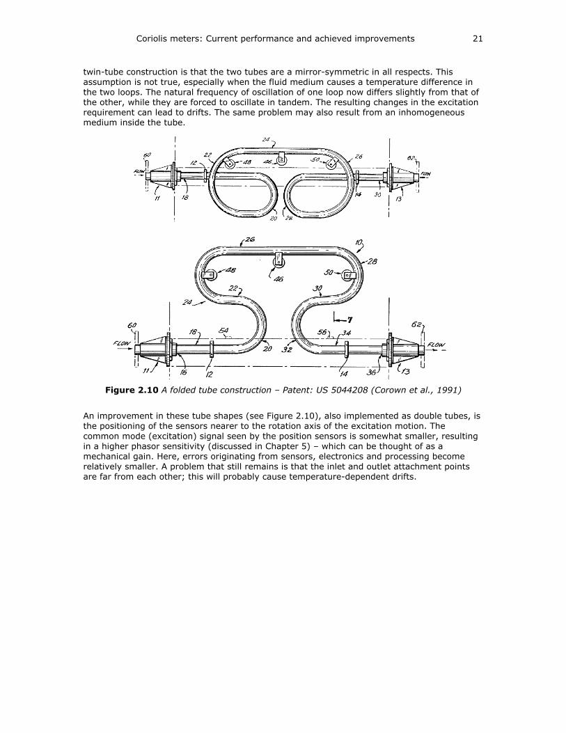
Coriolis meters: Current performance and achieved improvements 21
twin-tube construction is that the two tubes are a mirror-symmetric in all respects. This
assumption is not true, especially when the fluid medium causes a temperature difference in
the two loops. The natural frequency of oscillation of one loop now differs slightly from that of
the other, while they are forced to oscillate in tandem. The resulting changes in the excitation
requirement can lead to drifts. The same problem may also result from an inhomogeneous
medium inside the tube.
Figure 2.10 A folded tube construction – Patent: US 5044208 (Corown et al., 1991)
An improvement in these tube shapes (see Figure 2.10), also implemented as double tubes, is
the positioning of the sensors nearer to the rotation axis of the excitation motion. The
common mode (excitation) signal seen by the position sensors is somewhat smaller, resulting
in a higher phasor sensitivity (discussed in Chapter 5) – which can be thought of as a
mechanical gain. Here, errors originating from sensors, electronics and processing become
relatively smaller. A problem that still remains is that the inlet and outlet attachment points
are far from each other; this will probably cause temperature-dependent drifts.
22 Coriolis mass flow rate meters for low flows
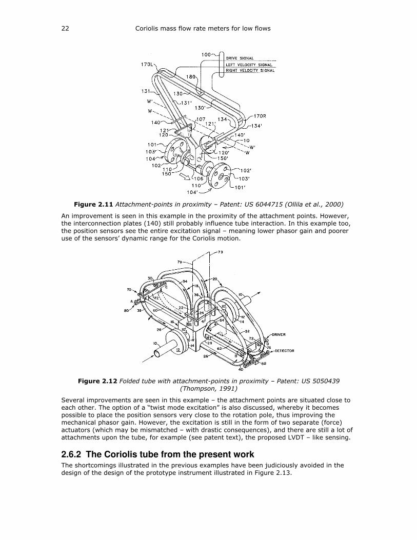
Figure 2.11 Attachment-points in proximity – Patent: US 6044715 (Ollila et al., 2000)
An improvement is seen in this example in the proximity of the attachment points. However,
the interconnection plates (140) still probably influence tube interaction. In this example too,
the position sensors see the entire excitation signal – meaning lower phasor gain and poorer
use of the sensors’ dynamic range for the Coriolis motion.
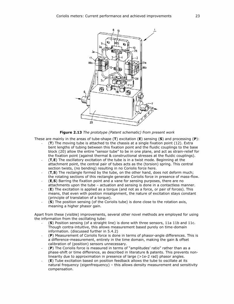
Figure 2.12 Folded tube with attachment-points in proximity – Patent: US 5050439 (Thompson, 1991)
Several improvements are seen in this example – the attachment points are situated close to
each other. The option of a “twist mode excitation” is also discussed, whereby it becomes
possible to place the position sensors very close to the rotation pole, thus improving the
mechanical phasor gain. However, the excitation is still in the form of two separate (force)
actuators (which may be mismatched – with drastic consequences), and there are still a lot of
attachments upon the tube, for example (see patent text), the proposed LVDT – like sensing.
2.6.2 The Coriolis tube from the present work The shortcomings illustrated in the previous examples have been judiciously avoided in the
design of the design of the prototype instrument illustrated in Figure 2.13.
Coriolis meters: Current performance and achieved improvements 23
Figure 2.13 The prototype (Patent schematic) from present work
These are mainly in the areas of tube-shape (T) excitation (E) sensing (S) and processing (P):
- (T) The moving tube is attached to the chassis at a single fixation point (12). Extra
bent lengths of tubing between this fixation point and the fluidic couplings to the base
block (20) allow the entire “sensor tube” to be in one plane, and act as strain-relief for
the fixation point (against thermal & constructional stresses at the fluidic couplings).
- (T,E) The oscillatory excitation of the tube is in a twist mode. Beginning at the
attachment point, the central pair of tubes acts as the (torsion) spring. This central
section twists, (no bending) resulting in no Coriolis force here.
- (T,S) The rectangle formed by the tube, on the other hand, does not deform much;
the rotating sections of this rectangle generate Coriolis force in presence of mass-flow.
- (E,S) Barring the fixation point and a vane for sensing purposes, there are no
attachments upon the tube – actuation and sensing is done in a contactless manner.
- (E) The excitation is applied as a torque (and not as a force, or pair of forces). This
means, that even with position misalignment, the nature of excitation stays constant
(principle of translation of a torque).
- (S) The position sensing (of the Coriolis tube) is done close to the rotation axis,
meaning a higher phasor gain.
Apart from these (visible) improvements, several other novel methods are employed for using
the information from the oscillating tube:
- (S) Position sensing (of a straight line) is done with three sensors, 11a 11b and 11c.
Though contra-intuitive, this allows measurement based purely on time-domain
information. (discussed further in 5.4.2)
- (P) Measurement of Coriolis force is done in terms of phasor-angle differences. This is
a difference-measurement, entirely in the time domain, making the gain & offset
calibration of (position) sensors unnecessary.
- (P) The Coriolis force is measured in terms of “amplitudes’ ratio” rather than as a
phase-shift or time difference, as described in literature & patents. This prevents non-
linearity due to approximation in presence of large (>1e-2 rad) phasor angles.
- (E) Tube excitation based on position feedback allows the tube to oscillate at its
natural frequency (eigenfrequency) – this allows density measurement and sensitivity
compensation.
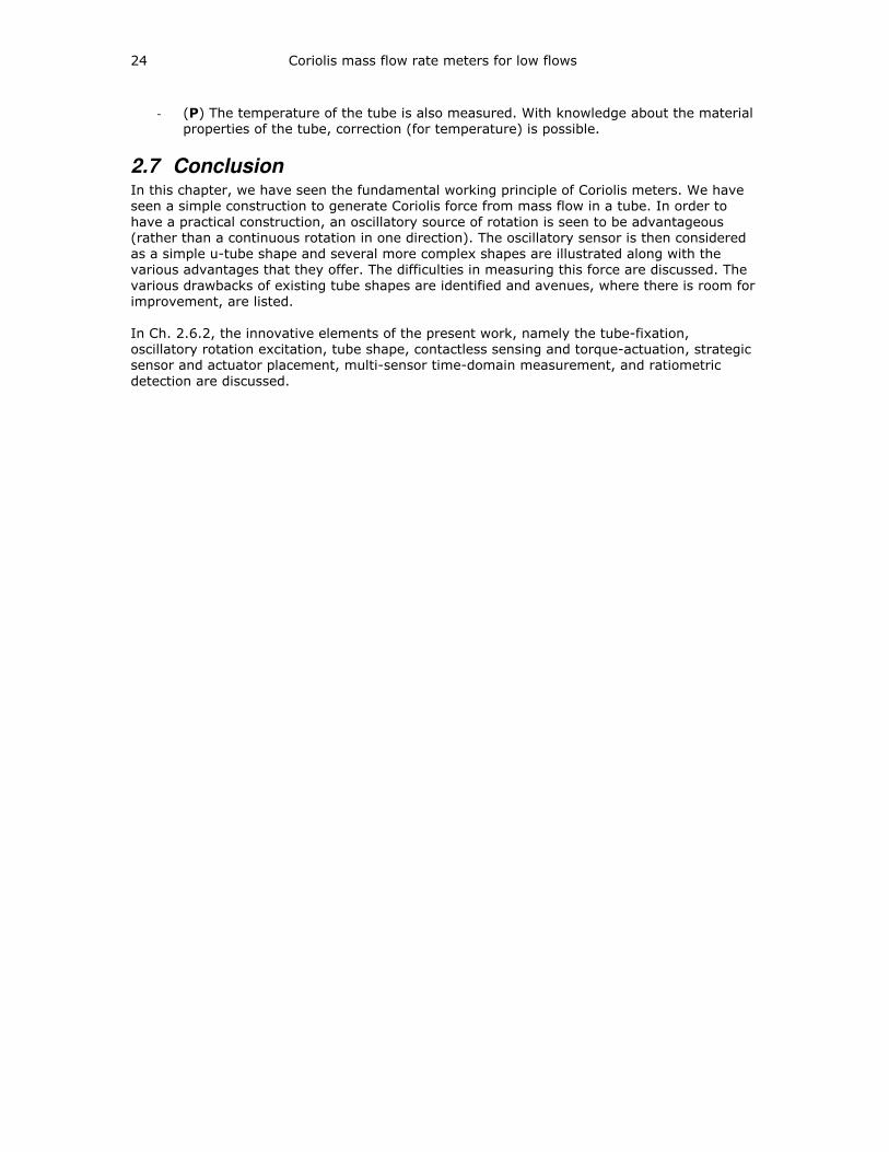
24 Coriolis mass flow rate meters for low flows
- (P) The temperature of the tube is also measured. With knowledge about the material
properties of the tube, correction (for temperature) is possible.
2.7 Conclusion In this chapter, we have seen the fundamental working principle of Coriolis meters. We have
seen a simple construction to generate Coriolis force from mass flow in a tube. In order to
have a practical construction, an oscillatory source of rotation is seen to be advantageous
(rather than a continuous rotation in one direction). The oscillatory sensor is then considered
as a simple u-tube shape and several more complex shapes are illustrated along with the
various advantages that they offer. The difficulties in measuring this force are discussed. The
various drawbacks of existing tube shapes are identified and avenues, where there is room for
improvement, are listed.
In Ch. 2.6.2, the innovative elements of the present work, namely the tube-fixation,
oscillatory rotation excitation, tube shape, contactless sensing and torque-actuation, strategic
sensor and actuator placement, multi-sensor time-domain measurement, and ratiometric
detection are discussed.
3 Requirements/Specifications Target setting The objective of the project behind this research was to develop a range of mass flow (rate)
meters, based on the Coriolis principle, and controllers based on it, to measure and control low
flow rates in liquids and gases. It was proposed to have a number of variants of the
instrument to cater to specific flow ranges, each variant measuring flow-rates a decade (x10)
smaller than the previous one.
3.1 Functional specifications The functional specifications are typically the specifications that are presented in a 'product folder' to a customer who views the instrument as a black box. The functional specs may be
subdivided into performance specifications (how well the instrument performs) and operational conditions specifications (what the instrument can withstand). Additionally there may be
technical specifications for the dimensions, footprints, interfaces, appearances etc. The
Functional specifications are a good starting point to enumerate the measurement steps
needed to qualify the outcome of the project; the qualification tests and performance metrics
(expectations) may be planned in advance.
Specifications are the result of requirements defined at the beginning of a project. In the
following text, the functional requirements (FR) are enumerated, with an identifier number of
the format FR x.y, where x is the serial number identifying the requirement and y is the
instrument type number. Only those requirements that are relevant from a scientific
standpoint are listed, together with a brief example or a description of the implications
thereof.
3.1.1 Performance specifications
FR 1 to FR 3: Flow range A wide range of flow rates is to be measured - the ratio between the smallest and largest
(expected application full-scale) is about 1:1000. In order to better utilize the dynamic range
it is proposed to distribute the flow ranges over multiple types of instruments:
- FR 1.1 Type I- Flow range: 10 … 200 g/h full scale (FS) - FR 1.2 Type II- Flow range: 100 … 2000 g/h FS - FR 1.3 Type III- Flow range: 1000 … 20000 g/h FS
In general, a Coriolis mass flow rate meter senses mass flow by means of translating the
Coriolis force generated in a meter-tube into a “measurable quantity” – e.g. strain in a strain-
gage or displacement in an elastic member. This (small) Coriolis force has to be measured in
presence of (unwanted) disturbances that, in an absolute sense, scale with geometry (the
larger the meter tube, the more the disturbance). This pushes the design in favor of a smaller
construction. In contradiction to this is the pressure drop across the tube. The acceptable
pressure drop across a commercial flow meter is about 1 bar, i.e. 1e5 Pa13, while that across a
controller is ~3 bar (3e5 Pa). The pressure drop P∆ in a fluid, of density ρ and viscosity η ,
flowing through a tube having a diameter d and length L , may be determined by the Hagen
Poiseuille equation (see section 5.1.1). In general, the smaller the tube, the larger is the
pressure-drop, for a given flow-rate. This pushes the design in favor of a larger tube diameter.
In the requirements FR1.y above, two values are specified for each type of instrument. For
example, in the type-I instrument, the smaller of the two (i.e. 10 g/h) is intended for gases
13 This comes about as the commonly available driving-pressure in a fluidic system is about 10 bar. A 1-
bar drop across the meter corresponds to 10% of this supply-pressure. In flow controllers, for rapid
control, it is essential that more than 50% of the pressure drops across the control-valve (see [10]); the 3
bar specification for controllers accounts for this extra drop across the valve. See also: FR 14
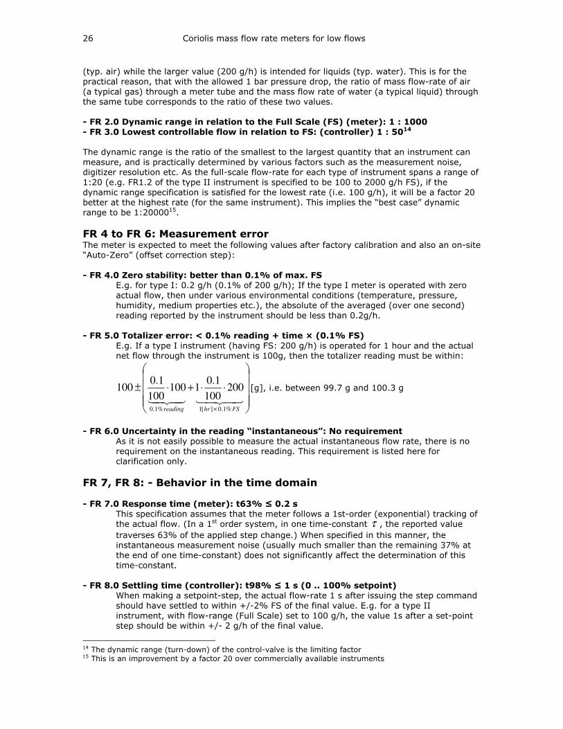
26 Coriolis mass flow rate meters for low flows
(typ. air) while the larger value (200 g/h) is intended for liquids (typ. water). This is for the
practical reason, that with the allowed 1 bar pressure drop, the ratio of mass flow-rate of air
(a typical gas) through a meter tube and the mass flow rate of water (a typical liquid) through
the same tube corresponds to the ratio of these two values.
- FR 2.0 Dynamic range in relation to the Full Scale (FS) (meter): 1 : 1000
- FR 3.0 Lowest controllable flow in relation to FS: (controller) 1 : 5014
The dynamic range is the ratio of the smallest to the largest quantity that an instrument can
measure, and is practically determined by various factors such as the measurement noise,
digitizer resolution etc. As the full-scale flow-rate for each type of instrument spans a range of
1:20 (e.g. FR1.2 of the type II instrument is specified to be 100 to 2000 g/h FS), if the
dynamic range specification is satisfied for the lowest rate (i.e. 100 g/h), it will be a factor 20
better at the highest rate (for the same instrument). This implies the “best case” dynamic
range to be 1:2000015.
FR 4 to FR 6: Measurement error The meter is expected to meet the following values after factory calibration and also an on-site
“Auto-Zero” (offset correction step):
- FR 4.0 Zero stability: better than 0.1% of max. FS E.g. for type I: 0.2 g/h (0.1% of 200 g/h); If the type I meter is operated with zero
actual flow, then under various environmental conditions (temperature, pressure,
humidity, medium properties etc.), the absolute of the averaged (over one second)
reading reported by the instrument should be less than 0.2g/h.
- FR 5.0 Totalizer error: < 0.1% reading + time × (0.1% FS)
E.g. If a type I instrument (having FS: 200 g/h) is operated for 1 hour and the actual
net flow through the instrument is 100g, then the totalizer reading must be within:
⋅⋅+⋅±
×
4342143421FShrreading %1.0][1%1.0
200100
1.01100
100
1.0100 [g], i.e. between 99.7 g and 100.3 g
- FR 6.0 Uncertainty in the reading “instantaneous”: No requirement As it is not easily possible to measure the actual instantaneous flow rate, there is no
requirement on the instantaneous reading. This requirement is listed here for
clarification only.
FR 7, FR 8: - Behavior in the time domain
- FR 7.0 Response time (meter): t63% ≤ 0.2 s This specification assumes that the meter follows a 1st-order (exponential) tracking of
the actual flow. (In a 1st order system, in one time-constant τ , the reported value
traverses 63% of the applied step change.) When specified in this manner, the
instantaneous measurement noise (usually much smaller than the remaining 37% at
the end of one time-constant) does not significantly affect the determination of this
time-constant.
- FR 8.0 Settling time (controller): t98% ≤ 1 s (0 .. 100% setpoint) When making a setpoint-step, the actual flow-rate 1 s after issuing the step command
should have settled to within +/-2% FS of the final value. E.g. for a type II
instrument, with flow-range (Full Scale) set to 100 g/h, the value 1s after a set-point
step should be within +/- 2 g/h of the final value.
14 The dynamic range (turn-down) of the control-valve is the limiting factor 15 This is an improvement by a factor 20 over commercially available instruments
Requirements 27
3.1.2 Operational conditions specifications While not as visible as the performance specifications, the operational condition specifications
play an important role in the design choices and choices of operating principles. If neglected at
the outset, these may lead to expensive redesign & delays during later stages.
FR 9 to FR 11: Temperature - FR 9.0 Ambient temperature range: -10 to +70°°°°C; sterilization (fluid at 150°°°°C) for
15 minutes
Survivability: The said temperature range precludes the use of certain materials, e.g.
plastics and certain types of permanent magnets. The power dissipation budget of the
instrument too should consider the upper temperature. The lower temperature range
does not apply to media like water that would freeze, thereby possibly damaging the
instrument.
Function: The ambient temperature has an effect on pickup-sensor characteristics and on (tube) material properties (see [9]). The impact of the wide (80°C) temperature
range on the performance should be accounted for.
- FR 10.0 Rate of change of instrument temperature (survivability): 1°°°°C-per-second
- FR 11.0 Drift due to change in fluid medium temperature: ± 0.01% reading/°°°°C
The drift is to be interpreted as a linear parameter, which means that after calibration
at the instantaneous temperature of e.g. 20 °C, for a rise to e.g. 30 °C an error in the
instantaneous reading of 10 × 0.01 = 0.1% is allowed. This is to be added to the sum
of previously mentioned errors.
FR 12 to FR 17: Pressure and media properties
- FR 12.0 Fluid types: All clean, homogeneous fluids compatible with AISI 316
AISI 316 stainless steel is the material of choice for typical applications of Coriolis
mass flow rate meters (semiconductors, medicines, foods & beverages etc.). This
seems a roundabout way of specifying that the Coriolis meter tube should be made of
a material that can withstand media that are a superset of media that AISI 316 can
withstand. The material choice is limited to AISI316 itself, and a few others like
titanium and Hastelloy. Materials such as Kalrez may be used in couplings.
- FR 13.0 Viscosity: Up to 0.1 Pa.s The nominal viscosity of water is 0.001 Pa⋅s. This is considered when specifying
pressure drop over the instruments. It is understood that fluids with higher viscosity
shall not achieve the rated flow-per-pressure-drop specification.
- FR 14.0 Pressure drop: < 1 bar at nominal water flow (meter); 3 bar (controller) From experience (see [10]), it is recommended that in order to achieve specified
speed in a controller, the pressure drop across the control valve should be at least
50% of the total pressure drop for liquid media (and >75% for gases).
- FR 15.0 Pressure sensitivity: ≤ 0.01 % reading per bar input pressure
Similar to FR 11.0, this allows for errors due to minor deformations in tube-geometry
due to fluid pressure.
- FR 16.0 Maximum system pressure: 100 bar The tube should survive and operate normally at this pressure. This specification will
dictate the minimum wall thickness of a particular tube.
- FR 17.0 Density measurement error: <10 kg/m3
The density of the medium affects the inertia of the Coriolis tube and can be inferred
from instrument variables, primarily the eigenfrequency of oscillation of the tube. The
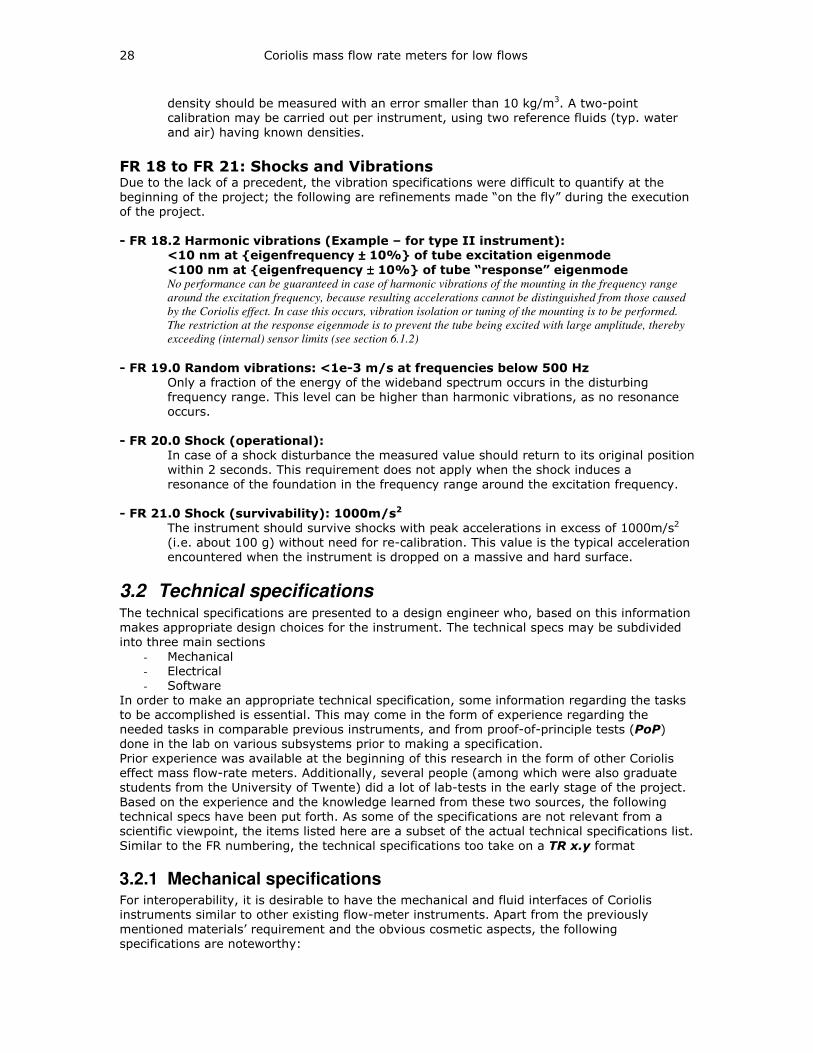
28 Coriolis mass flow rate meters for low flows
density should be measured with an error smaller than 10 kg/m3. A two-point
calibration may be carried out per instrument, using two reference fluids (typ. water
and air) having known densities.
FR 18 to FR 21: Shocks and Vibrations Due to the lack of a precedent, the vibration specifications were difficult to quantify at the
beginning of the project; the following are refinements made “on the fly” during the execution
of the project.
- FR 18.2 Harmonic vibrations (Example – for type II instrument): <10 nm at eigenfrequency ±±±± 10% of tube excitation eigenmode
<100 nm at eigenfrequency ±±±± 10% of tube “response” eigenmode No performance can be guaranteed in case of harmonic vibrations of the mounting in the frequency range
around the excitation frequency, because resulting accelerations cannot be distinguished from those caused
by the Coriolis effect. In case this occurs, vibration isolation or tuning of the mounting is to be performed.
The restriction at the response eigenmode is to prevent the tube being excited with large amplitude, thereby
exceeding (internal) sensor limits (see section 6.1.2)
- FR 19.0 Random vibrations: <1e-3 m/s at frequencies below 500 Hz
Only a fraction of the energy of the wideband spectrum occurs in the disturbing
frequency range. This level can be higher than harmonic vibrations, as no resonance
occurs.
- FR 20.0 Shock (operational): In case of a shock disturbance the measured value should return to its original position
within 2 seconds. This requirement does not apply when the shock induces a
resonance of the foundation in the frequency range around the excitation frequency.
- FR 21.0 Shock (survivability): 1000m/s2
The instrument should survive shocks with peak accelerations in excess of 1000m/s2
(i.e. about 100 g) without need for re-calibration. This value is the typical acceleration
encountered when the instrument is dropped on a massive and hard surface.
3.2 Technical specifications The technical specifications are presented to a design engineer who, based on this information
makes appropriate design choices for the instrument. The technical specs may be subdivided
into three main sections
- Mechanical
- Electrical
- Software
In order to make an appropriate technical specification, some information regarding the tasks
to be accomplished is essential. This may come in the form of experience regarding the
needed tasks in comparable previous instruments, and from proof-of-principle tests (PoP)
done in the lab on various subsystems prior to making a specification.
Prior experience was available at the beginning of this research in the form of other Coriolis
effect mass flow-rate meters. Additionally, several people (among which were also graduate
students from the University of Twente) did a lot of lab-tests in the early stage of the project.
Based on the experience and the knowledge learned from these two sources, the following
technical specs have been put forth. As some of the specifications are not relevant from a
scientific viewpoint, the items listed here are a subset of the actual technical specifications list.
Similar to the FR numbering, the technical specifications too take on a TR x.y format
3.2.1 Mechanical specifications For interoperability, it is desirable to have the mechanical and fluid interfaces of Coriolis
instruments similar to other existing flow-meter instruments. Apart from the previously
mentioned materials’ requirement and the obvious cosmetic aspects, the following
specifications are noteworthy:
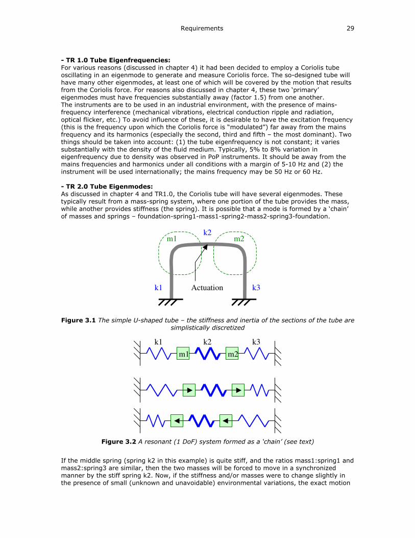
Requirements 29
- TR 1.0 Tube Eigenfrequencies:
For various reasons (discussed in chapter 4) it had been decided to employ a Coriolis tube
oscillating in an eigenmode to generate and measure Coriolis force. The so-designed tube will
have many other eigenmodes, at least one of which will be covered by the motion that results
from the Coriolis force. For reasons also discussed in chapter 4, these two ‘primary’
eigenmodes must have frequencies substantially away (factor 1.5) from one another.
The instruments are to be used in an industrial environment, with the presence of mains-
frequency interference (mechanical vibrations, electrical conduction ripple and radiation,
optical flicker, etc.) To avoid influence of these, it is desirable to have the excitation frequency
(this is the frequency upon which the Coriolis force is “modulated”) far away from the mains
frequency and its harmonics (especially the second, third and fifth – the most dominant). Two
things should be taken into account: (1) the tube eigenfrequency is not constant; it varies
substantially with the density of the fluid medium. Typically, 5% to 8% variation in
eigenfrequency due to density was observed in PoP instruments. It should be away from the
mains frequencies and harmonics under all conditions with a margin of 5-10 Hz and (2) the
instrument will be used internationally; the mains frequency may be 50 Hz or 60 Hz.
- TR 2.0 Tube Eigenmodes:
As discussed in chapter 4 and TR1.0, the Coriolis tube will have several eigenmodes. These
typically result from a mass-spring system, where one portion of the tube provides the mass,
while another provides stiffness (the spring). It is possible that a mode is formed by a ‘chain’
of masses and springs – foundation-spring1-mass1-spring2-mass2-spring3-foundation.
k1
k2
k3
m2 m1
Actuation
Figure 3.1 The simple U-shaped tube – the stiffness and inertia of the sections of the tube are simplistically discretized
m1 m2
k1 k2 k3
Figure 3.2 A resonant (1 DoF) system formed as a ‘chain’ (see text)
If the middle spring (spring k2 in this example) is quite stiff, and the ratios mass1:spring1 and
mass2:spring3 are similar, then the two masses will be forced to move in a synchronized
manner by the stiff spring k2. Now, if the stiffness and/or masses were to change slightly in
the presence of small (unknown and unavoidable) environmental variations, the exact motion
30 Coriolis mass flow rate meters for low flows
of the masses in such a construction would slightly non-symmetric and hence unpredictable.
Hence, such a ‘chain’ should be avoided for the excitation mode. The primary energy-storing-
element pairs (k1, m1 and k2, m2) should be combined into a single physical pair
(k,m) if possible.
- TR 3.0 Chassis Eigenfrequencies:
The vibrating Coriolis tube will be mounted on a chassis, which should ideally appear as an
infinitely stiff support for the tube. If not, the modes introduced in the chassis might adversely
affect (interfere with) the measurement of motion of the tube. Practically, the chassis should
be such that its lowest eigenfrequency should be several times higher than the excitation
frequency of the tube.
- TR 4.0 statically determined construction: Due to non-ideal construction (e.g. unavoidable constructional asymmetries), there always
exists coupling (leakage of power) between eigenmodes. In presence of damping, (leading to
phase-shift), such leaked power can result in forces indistinguishable from Coriolis forces. It is
possible, from experience from PoP tests, to calibrate-out a small amount of leakage.
However, for the calibration to be effective, the imperfections must stay constant over time. A
statically determined construction (see [3]) is essential. Furthermore, the fixed ends of fluid-
carrying tube(s) should be as close to each other as possible, avoiding mechanical ‘bridges’ in
order to minimize deformation of the tube in the event of (unavoidable) thermal gradients.
3.2.2 Electrical specifications - TR 5.0 Digital or analog processing:
In previous PoP studies (see [9]) it has been demonstrated that digital processing is feasible
for processing sensor signals to translate them to a flow measurement. Due to advancement
in analog to digital signal converter and processing techniques in recent years, especially due
to the maturation and widespread use of PC audio, analog signals can be represented and
processed in the digital domain with high resolution with reasonably low cost and effort. A
digital system offers flexibility (e.g. internal rerouting of signals and tweaking of functional
blocks), transparency for debugging and observation of system behavior, upgradeability of
features, robustness (the travel-path of analog information is much shorter, and consequently,
less susceptible to external disturbance or internal noise). A few COTS digital parts can
emulate the function of several specialized analog parts, making a digital system attractive. If
desired, a layered approach can be taken towards the engineering of the digital processing,
where several sub-iterations of the “V-model” can be made without time-consuming rewiring
of analog parts. The details are dealt with in section 3.2.3.
- TR 6.0 Power consumption and heat dissipation: For compatibility reasons, and dissipation possibilities (ability to get rid of generated heat), it
is a requirement that the instrument, as a whole, should not consume or dissipate more than
about 8 Watt power. This translates to about 333 mA current consumption at 24V supply
voltage. (Note: As the meter does not export any power, almost all consumed power is
converted to heat in the instrument.)
In a particular PoP implementation, it has been demonstrated that in order to have the Coriolis
tube oscillate with sufficient amplitude, it needs about 6 mW of mechanical power to sustain
oscillations. This value will of course change with a particular form or size of tube used.
However, this specification gives an order-of-magnitude for the requirement.
- TR 7.0 Uncertainty due to time reference:
It has been demonstrated from calculations and a set of PoP instruments that an achievable
amplitudes’ ratio between the excitation motion and the response motion due to Coriolis forces
is about 100:1. At the smallest resolvable flow (0.01% of the nominal) this ratio leads to a
phase-shift (between sensor signals) that corresponds to a time-delay to the order of about 1
ns. A jitter in the clock signal will lead to noise in the measurement. The details of the effects
Requirements 31
of clock jitter and inaccuracy are dealt with in chapter 5.4.3. The SONET16 specification, for
example, defines Jitter as “the short-term variations of a digital signal’s significant instants from their ideal positions in time”. Clocks jitter in the order of picoseconds is achievable with
commercial clock generators. Relative error of such clock generators, on the other hand, is
usually a few PPM. Both of these are several times better than required.
- TR 8.0 General sensor quality requirements: Position sensors are to be used to determine the motion of the Coriolis tube to analyze it for
determining the extent of the generated Coriolis force. For the same reasons as in TR 7.0, it is
crucial that these motion sensors have as small time delays as possible; in the worst case,
they should be matched with each other. The estimate for allowable variation (over time) in
delay mismatch is a few tens of nanoseconds. Matching the gain of each sensor is not critical,
as a ratiometric and time-referenced measurement is adopted.
- TR 9.0 Galvanic isolation & current through the instrument: If physical principles are employed in the CMFM that make it susceptible to stray current
return paths, especially in industrial environments, the sensitive components must be
galvanically isolated from such paths. Typically, a PoP instrument employed a Lorentz actuator
for excitation of the meter tube. A stray (unwanted) 50 Hz current flowing through this tube
would create indeterministic forces that may interfere with the meter principle.
3.2.3 Specifications dictated by Software As mentioned in TR10.0, the meter (soft) function, the communications interface and
calibration intelligence is to be handled by a separate proven processor unit. This primarily
leaves over the core functionality of:
- Excitation of the tube at a predetermined amplitude
- Determination of amplitudes’ ratio by analyzing the effect of Coriolis force on the
motion of the tube
And secondarily
- The determination of the (natural) frequency of oscillation of the meter tube
In previous PoP studies, the meter functionality has been implemented and tested on an
industrial PC platform; the software that drives this PoP gives insight into the needed
processing power. The software on the PoP platform was structured in a manner so as to be
driven by timer interrupt ticks. Each “time slice” (time between two successive interrupt
“ticks”) has the full functionality – input + processing + output – contained within it. This
functionality is repeated at the rate of timer ticks. This means, that if a target CPU is able to
perform all tasks that are in one “slice” within one time-slice in the PoP setup, it is sufficient
for the required operation.
- TR 10.0 Processing power: Determination of needed processing power:
All the instructions executed in one time slice in the PoP are collected together. In case an
operation runs in a loop, the instructions within that operation are repeated the number of
times that the loop repeats. [The instructions running in the time-slice on the industrial PC in
the PoP were coded directly in (5x86) assembly. Most of the instructions were coded as FPU
assembly, (which is surprisingly powerful and non-tedious) on a 5x86 platform]. Next, the
instructions are categorized by complexity of implementation. As the final target platform (i.e.,
the processor on which the instrument firmware shall be implemented) is probably not a 5x86
processor, the PoP instructions are factorized in terms of possible instructions on a candidate
target processor. As an illustration, the following equivalence may be drawn:
16 Short for Synchronous Optical Network, a standard for connecting fiber-optic transmission systems.
SONET was proposed by Bellcore in the middle 1980s and is now an ANSI standard.
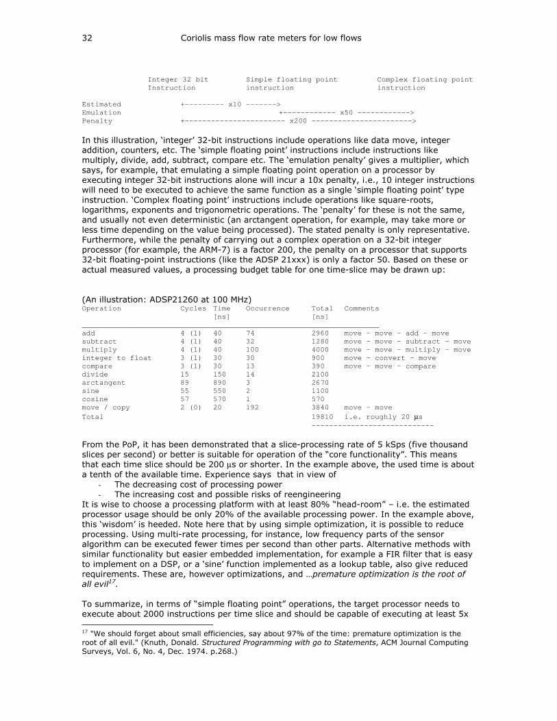
32 Coriolis mass flow rate meters for low flows
Integer 32 bit Simple floating point Complex floating point
Instruction instruction instruction
Estimated +--------- x10 ------->
Emulation +------------ x50 ------------>
Penalty +----------------------- x200 ----------------------->
In this illustration, ‘integer’ 32-bit instructions include operations like data move, integer
addition, counters, etc. The ‘simple floating point’ instructions include instructions like
multiply, divide, add, subtract, compare etc. The ‘emulation penalty’ gives a multiplier, which
says, for example, that emulating a simple floating point operation on a processor by
executing integer 32-bit instructions alone will incur a 10x penalty, i.e., 10 integer instructions
will need to be executed to achieve the same function as a single ‘simple floating point’ type
instruction. ‘Complex floating point’ instructions include operations like square-roots,
logarithms, exponents and trigonometric operations. The ‘penalty’ for these is not the same,
and usually not even deterministic (an arctangent operation, for example, may take more or
less time depending on the value being processed). The stated penalty is only representative.
Furthermore, while the penalty of carrying out a complex operation on a 32-bit integer
processor (for example, the ARM-7) is a factor 200, the penalty on a processor that supports
32-bit floating-point instructions (like the ADSP 21xxx) is only a factor 50. Based on these or
actual measured values, a processing budget table for one time-slice may be drawn up:
(An illustration: ADSP21260 at 100 MHz) Operation Cycles Time Occurrence Total Comments
[ns] [ns]
____________________________________________________________________
add 4 (1) 40 74 2960 move – move – add – move
subtract 4 (1) 40 32 1280 move – move – subtract – move
multiply 4 (1) 40 100 4000 move – move – multiply – move
integer to float 3 (1) 30 30 900 move – convert – move
compare 3 (1) 30 13 390 move – move – compare
divide 15 150 14 2100
arctangent 89 890 3 2670
sine 55 550 2 1100
cosine 57 570 1 570
move / copy 2 (0) 20 192 3840 move – move
Total 19810 i.e. roughly 20 µs ----------------------------
From the PoP, it has been demonstrated that a slice-processing rate of 5 kSps (five thousand
slices per second) or better is suitable for operation of the “core functionality”. This means
that each time slice should be 200 µs or shorter. In the example above, the used time is about
a tenth of the available time. Experience says that in view of
- The decreasing cost of processing power
- The increasing cost and possible risks of reengineering
It is wise to choose a processing platform with at least 80% “head-room” – i.e. the estimated
processor usage should be only 20% of the available processing power. In the example above,
this ‘wisdom’ is heeded. Note here that by using simple optimization, it is possible to reduce
processing. Using multi-rate processing, for instance, low frequency parts of the sensor
algorithm can be executed fewer times per second than other parts. Alternative methods with
similar functionality but easier embedded implementation, for example a FIR filter that is easy
to implement on a DSP, or a ‘sine’ function implemented as a lookup table, also give reduced
requirements. These are, however optimizations, and …premature optimization is the root of all evil17.
To summarize, in terms of “simple floating point” operations, the target processor needs to
execute about 2000 instructions per time slice and should be capable of executing at least 5x
17 "We should forget about small efficiencies, say about 97% of the time: premature optimization is the
root of all evil." (Knuth, Donald. Structured Programming with go to Statements, ACM Journal Computing
Surveys, Vol. 6, No. 4, Dec. 1974. p.268.)
Requirements 33
as many. Measurements or simulations on candidate target processors to satisfy this
condition takes away guesswork and prevents the risk of hardware redesign.
- TR 11.0 Processing precision: From PoP tests, it is seen that the processing precision of 24 bits18, and the high dynamic
range due to an 8-bit exponent, offered by the IEEE 754 32-bit floating point representation is
sufficient to carry out trigonometric calculations and implement IIR digital filters for phase-
detection. As such, a typical 32-bit signal-processor (with a 32 bit FPU) is recommended.
3.3 Testing methods Generally speaking there are four methods19 (see [11]) to verify (prove) a requirement:
- Testing: prove compliance by means of a well-defined procedure.
- Analysis: prove compliance by means of calculations.
- Demonstration: prove compliance by means of a demonstration, for qualitative
requirements.
- Inspection: prove compliance by means of studying the product, for visible design features.
Each of the functional requirements defined above is to be proven by means of testing. Most of
the technical requirements need not be tested, but can be proven by means of inspection or
demonstration. The test methods (TM) are summarized below with an identifier (number)
TM 1.1 1.2 and 1.3: Range The measurement must determine the flow range in which the (stationary) error requirements
are fulfilled. These requirements are to be measured for a number of flow rates within each of
the flow ranges of the instrument, using weighing scales as a reference.
TM 2.0 Error and uncertainty The static zero-error (offset) of the reference instrument is to be nulled beforehand
The zero stability is to be measured without flow, under normal process conditions: with filled
tube, under pressure.
Test practices:
- Sensitivity measurements are to be done from 0 to 100% of full-scale flow with 25% steps.
Before the measurement the zero offset is eliminated. The dominant error is usually not the
non-linearity, but a shift of the sensitivity line.
- Errors and repeatability are related to the totalizer, defined over 1 hour measuring time with
constant flow and a ‘flying start’ and also a ‘flying stop’. The actual measuring time depends
on the flow rate and the measurement range of the scales: for a smaller flow it will take more
time to achieve a measurement having a comparable relative error due to the readout of the
scales.
- Meter noise or jitter causes high-frequency fluctuations of the readout. These may be
suppressed by filtering of the measured data, e.g. by an exponential smoothing filter (simple
first order digital filter), as long as this filtering does not conflict with other requirements.
Since the above definition is related to the totalizer reading a constant flow, fluctuations or
filtering do not affect the totalizer reading, as the measurement interval is much longer than
the filter time-constants.
- The scenario for measuring the repeatability has not been specified. For the flow meter this
may be defined as doing a statistically significant number of measurements for a fixed flow at
realistic time intervals. As the repeatability applies to the totalizer at full flow, it is tested at
100 g/h for a period of 1 hour.
18 IEEE 754, Single-precision 32-bit representation: 23 bit fraction + 1 implicit bit 19 MIL-STD-961E
34 Coriolis mass flow rate meters for low flows
TM 3.0 Temperature Ambient temperature testing requires a temperature-controlled environment. A programmable
environment chamber shall be used to create predefined temperature ramp for dynamic
temperature tests. A reference temperature sensor shall monitor the environment temperature
to qualify the built-in temperature sensors.
TM 4.0 Pressure - Measurements on pressure drop can be performed with water, at normal system pressure.
- As the minimum system (over)pressure is 3 bar, and the instrument pressure-drop is about
1 bar, an additional resistance (e.g. a partly closed valve) will be needed downstream.
TM 5.0 Response and settling time
- To be measured for a number of different steps, for both increasing and decreasing flows.
- To be measured at minimum specified system pressure, because this is the most critical
(worst-case).
- As the performance is not related to measurement error, no accurate reference instrument is
needed; the output of the tested instrument itself can be used. Internal filtering is to be
switched off where this affects the speed of response.
- The device used for switching during the response time measurement may not add any
capacity, resistance or time lag.
- Before the settling time measurement the valve must be bled form air possibly trapped
inside.
TM 6.0 Vibrations - All vibration and shock tests are to be performed on a softly suspended rigid platform that
can be given a defined acceleration in any translational or rotational direction. Harmonic or
random vibration can be applied by means of an excitation coil; shock excitation by means of
a hammer pendulum with well-defined tip stiffness.
TM 7.0 Immunity for medium density - Is to be tested using different media (water, IPA, air) in a thermally well-conditioned
environment using accurate scales as a reference, with sufficient measurement (totalizer)
time.
4 Concept choice Target setting The concept choices in the course of this project were, to a large extent, based upon proof-of-
principle studies, simulations and ‘thought experiments’ carried out since 2001. Aspects of
Coriolis mass-flow rate meters published in patents & other literature are used as a benchmark
- a comparison for concepts implemented or chosen in this particular project.
Peculiarity of the measurement principle Coriolis mass-flow rate meters, those tested in the PoP and also the vast array presented in
various patents shows a peculiar parallel to a well-known measurement instrument, the
moving-coil galvanometer; here, the Lorentz force is the cross product of current and
magnetic field, whereas in Coriolis force is the result of the cross product of the mass flow and
angular velocity vectors. Being based on an active measurement principle, a CMFM thus
necessarily has moving parts. The analogy is as follows:
Galvanometer:
• Tiny current flows through coil
• Multiple turns increase sensitivity (force per unit current)
• Coil is strategically placed (in a piece-wise linear magnetic field)
• Force (or torque) causes the coil to move perpendicular to the flow and field
• Pushes a spring with a stiffness k
• Needle moves following xkF ⋅= or k
Fx =
• Sensitivity is thus also determined by stiffness
• Weak spring helps to increase sensitivity
• Spring must have constant stiffness and magnetic field must have constant flux
density and coil must have constant number of turns for all allowed values of current if
the meter is to be linear.
• Nothing else (other than the Lorentz force) should move the coil
Coriolis Mass flow rate meter:
• Tiny flow through tube
• Single turn for simple construction and low pressure drop
• Tube is strategically placed in a ‘rotation field’
• DC rotation field is difficult to implement, hence AC rotation field is used
• The Coriolis effect generates a (Coriolis) force that relates the bias (AC rotation field)
and the response (AC deflection) depending on the mass-flow rate.
• The Coriolis force deflects spring to an extent k
1 (or mass to an extent
2
1
sm ⋅,
depending on implementation) hence lower stiffness (or lower mass) results in larger
deflection.
• External actuation is essential to create a ‘rotation field’; this actuation may not
interfere with the instrument response (analogy: in a galvanometer, the coil itself may
not be moved by the magnetic field, and hence is designed using non-magnetic
materials)
• Parasitic couplings must be minimized; nothing else (other than the Coriolis force)
should deflect the tube
This analogy helps to make some concept choices. The challenge in Coriolis meters lies in:
• How to generate a defined angular velocity or how to make measurements insensitive
to unknown variations in the angular velocity
• How to measure a periodic (oscillatory) force
• How to make (force) measurements that are insensitive to variations in sensitivity of
the force sensor
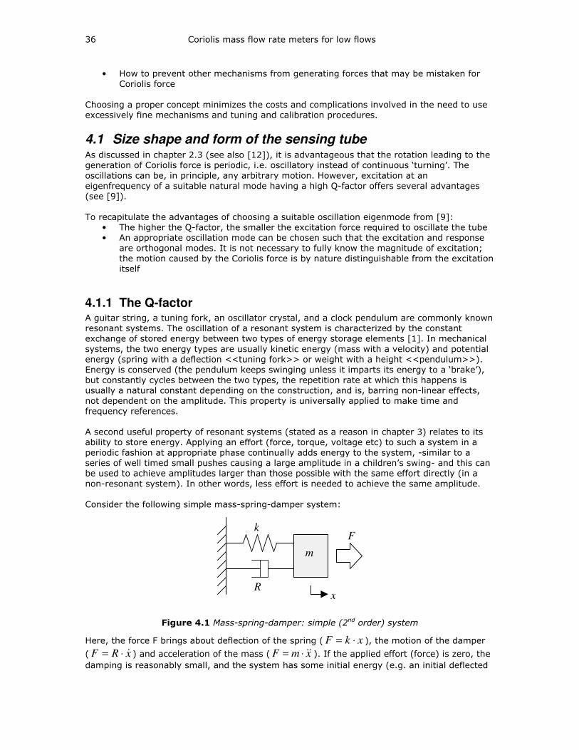
36 Coriolis mass flow rate meters for low flows
• How to prevent other mechanisms from generating forces that may be mistaken for
Coriolis force
Choosing a proper concept minimizes the costs and complications involved in the need to use
excessively fine mechanisms and tuning and calibration procedures.
4.1 Size shape and form of the sensing tube As discussed in chapter 2.3 (see also [12]), it is advantageous that the rotation leading to the
generation of Coriolis force is periodic, i.e. oscillatory instead of continuous ‘turning’. The
oscillations can be, in principle, any arbitrary motion. However, excitation at an
eigenfrequency of a suitable natural mode having a high Q-factor offers several advantages
(see [9]).
To recapitulate the advantages of choosing a suitable oscillation eigenmode from [9]:
• The higher the Q-factor, the smaller the excitation force required to oscillate the tube
• An appropriate oscillation mode can be chosen such that the excitation and response
are orthogonal modes. It is not necessary to fully know the magnitude of excitation;
the motion caused by the Coriolis force is by nature distinguishable from the excitation
itself
4.1.1 The Q-factor A guitar string, a tuning fork, an oscillator crystal, and a clock pendulum are commonly known
resonant systems. The oscillation of a resonant system is characterized by the constant
exchange of stored energy between two types of energy storage elements [1]. In mechanical
systems, the two energy types are usually kinetic energy (mass with a velocity) and potential
energy (spring with a deflection <<tuning fork>> or weight with a height <<pendulum>>).
Energy is conserved (the pendulum keeps swinging unless it imparts its energy to a ‘brake’),
but constantly cycles between the two types, the repetition rate at which this happens is
usually a natural constant depending on the construction, and is, barring non-linear effects,
not dependent on the amplitude. This property is universally applied to make time and
frequency references.
A second useful property of resonant systems (stated as a reason in chapter 3) relates to its
ability to store energy. Applying an effort (force, torque, voltage etc) to such a system in a
periodic fashion at appropriate phase continually adds energy to the system, -similar to a
series of well timed small pushes causing a large amplitude in a children’s swing- and this can
be used to achieve amplitudes larger than those possible with the same effort directly (in a
non-resonant system). In other words, less effort is needed to achieve the same amplitude.
Consider the following simple mass-spring-damper system:
k
m
x
F
R
Figure 4.1 Mass-spring-damper: simple (2nd order) system
Here, the force F brings about deflection of the spring ( xkF ⋅= ), the motion of the damper
( xRF &⋅= ) and acceleration of the mass ( xmF &&⋅= ). If the applied effort (force) is zero, the
damping is reasonably small, and the system has some initial energy (e.g. an initial deflected

Concept choice 37
position), the mass will continue to describe a so-called “simple harmonic motion”. The
eigenfrequency (natural frequency, eigf ) [Hz] of this motion is given by:
m
kf eigeig ==⋅ ωπ2 (4.1)
Also, given the force-balance
xmxRxkF &&& ⋅+⋅+⋅= (4.2)
the system transfer function (Bode plot of deflection-per-applied-force, normalized for unit
stiffness) looks like:
-40
-20
0
20
40
60
80
Magnitu
de (
dB
)
10-1
100
101
-180
-135
-90
-45
0
Phase (
deg)
Bode Diagram
Frequency (rad/sec)
-40
-20
0
20
40
Magnitu
de (
dB
)
100
101
102
-180
-135
-90
-45
0
Phase (
deg)
Bode Diagram
Frequency (rad/sec)
Figure 4.2 Illustrative transfer functions (x/F) of 2nd order systems: Q=1000 (top pair) and Q=10 (bottom pair)
Notice the sharp phase transition & narrow peak in the system with the high Q-factor
38 Coriolis mass flow rate meters for low flows
The magnitude plot can be subdivided into three distinct parts, named “the stiffness line”, “the
resonance peak” and “the mass line”.
The stiffness line is the flat line to the left (lower frequencies) of the peak. Here, the stiffness
is dominant, and the deflection x follows the rule
xkF ⋅= , or in other words, kF
x 1= . Here, xR &⋅ and xm &&⋅ are negligibly small as the
frequency is low. Furthermore, the phase is zero. This signifies that the deflection directly
tracks the force.
To the right of the resonance peak, the mass (inertia) is dominant and the relation between
the deflection and the applied force predominantly follows the relation:
xmF &&⋅= , or in other words, 2
1
smF
x
⋅
−= . Here the magnitude drops as the square of the
frequency, inversely proportional to the mass – hence the name “mass-line”. The phase is -
180°, indicating that the mass moves in an opposite sense than the applied force – logical
considering that the force directly causes acceleration, which must be integrated twice in time
to get deflection.
Resonance occurs at the eigenfrequency. The magnitude of the resonance peak is determined
by the magnitude of the damper, in relation to the mass and spring. It is Q times larger than
the magnitude of the stiffness line, where Q is the “quality factor” of the mass spring system;
the lower the damping, the higher the ‘quality’.
In terms of m , k and r , the peak multiplier (quality factor Q ) is given by:
R
kmQ
⋅= (4.3)
In other words,
k
m
RkQ
F
x
peak
11=⋅=
(4.4)
The term “quality” originates from resonant devices such as tuning forks or oscillator crystals,
where the higher the peak, the better the quality of the device (precise frequency; better
rejection of nearby frequencies etc.)
It is important that exactly at the eigenfrequency, the phase-shift between the applied force
and the resulting (large) deflection is exactly 90°. This means that the velocity x& is exactly in-
phase with the force; that the system appears purely resistive to the applied effort. This phase
relation can be used to drive a mass-spring system into oscillation; the effort must be in-
phase with the velocity, or 90’ leading the deflection (analogy: push the swing hardest when it
is at the null position).
Often, the stiffness k and mass m of a resonant system are easy to determine, by simple
calculations or modeling. The (unintentional) damping is often very small and difficult to
estimate. However, the Q-factor can be experimentally determined in the following (simple)
manner:
• Give an initial energy to a resonator (e.g. - hit the tuning fork)
• Observe the excursion of the system; this will be sinusoidal, with a frequency eigf ,
beginning with large amplitude, and then will gradually decay, with a decay time-
constant, decayτ .
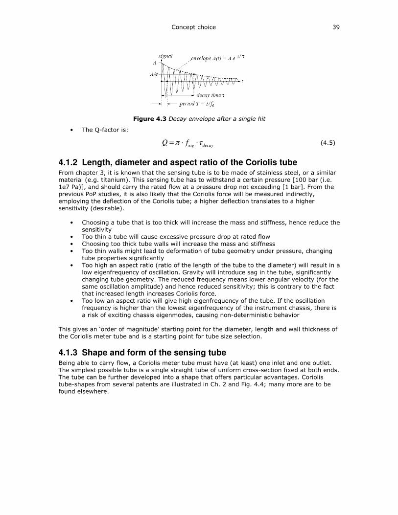
Concept choice 39
Figure 4.3 Decay envelope after a single hit
• The Q-factor is:
decayeigfQ τπ ⋅⋅= (4.5)
4.1.2 Length, diameter and aspect ratio of the Coriolis tube From chapter 3, it is known that the sensing tube is to be made of stainless steel, or a similar
material (e.g. titanium). This sensing tube has to withstand a certain pressure [100 bar (i.e.
1e7 Pa)], and should carry the rated flow at a pressure drop not exceeding [1 bar]. From the
previous PoP studies, it is also likely that the Coriolis force will be measured indirectly,
employing the deflection of the Coriolis tube; a higher deflection translates to a higher
sensitivity (desirable).
• Choosing a tube that is too thick will increase the mass and stiffness, hence reduce the
sensitivity
• Too thin a tube will cause excessive pressure drop at rated flow
• Choosing too thick tube walls will increase the mass and stiffness
• Too thin walls might lead to deformation of tube geometry under pressure, changing
tube properties significantly
• Too high an aspect ratio (ratio of the length of the tube to the diameter) will result in a
low eigenfrequency of oscillation. Gravity will introduce sag in the tube, significantly
changing tube geometry. The reduced frequency means lower angular velocity (for the
same oscillation amplitude) and hence reduced sensitivity; this is contrary to the fact
that increased length increases Coriolis force.
• Too low an aspect ratio will give high eigenfrequency of the tube. If the oscillation
frequency is higher than the lowest eigenfrequency of the instrument chassis, there is
a risk of exciting chassis eigenmodes, causing non-deterministic behavior
This gives an ‘order of magnitude’ starting point for the diameter, length and wall thickness of
the Coriolis meter tube and is a starting point for tube size selection.
4.1.3 Shape and form of the sensing tube Being able to carry flow, a Coriolis meter tube must have (at least) one inlet and one outlet.
The simplest possible tube is a single straight tube of uniform cross-section fixed at both ends.
The tube can be further developed into a shape that offers particular advantages. Coriolis
tube-shapes from several patents are illustrated in Ch. 2 and Fig. 4.4; many more are to be
found elsewhere.
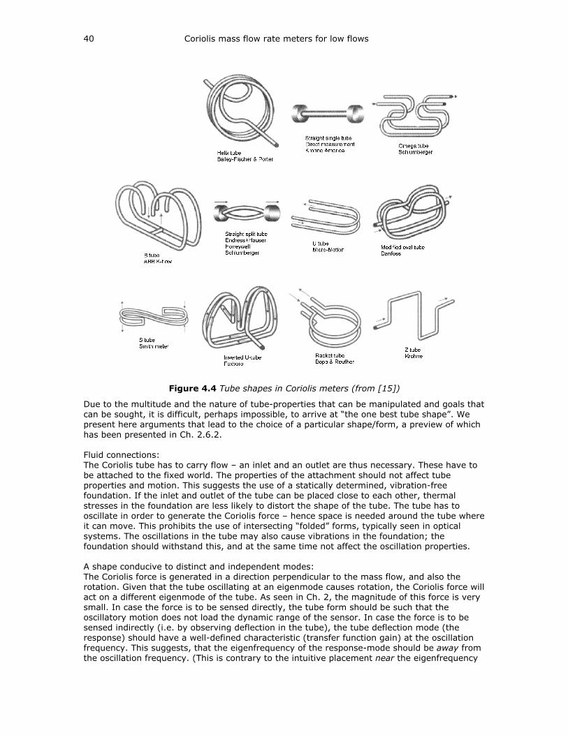
40 Coriolis mass flow rate meters for low flows
Figure 4.4 Tube shapes in Coriolis meters (from [15])
Due to the multitude and the nature of tube-properties that can be manipulated and goals that
can be sought, it is difficult, perhaps impossible, to arrive at “the one best tube shape”. We
present here arguments that lead to the choice of a particular shape/form, a preview of which
has been presented in Ch. 2.6.2.
Fluid connections:
The Coriolis tube has to carry flow – an inlet and an outlet are thus necessary. These have to
be attached to the fixed world. The properties of the attachment should not affect tube
properties and motion. This suggests the use of a statically determined, vibration-free
foundation. If the inlet and outlet of the tube can be placed close to each other, thermal
stresses in the foundation are less likely to distort the shape of the tube. The tube has to
oscillate in order to generate the Coriolis force – hence space is needed around the tube where
it can move. This prohibits the use of intersecting “folded” forms, typically seen in optical
systems. The oscillations in the tube may also cause vibrations in the foundation; the
foundation should withstand this, and at the same time not affect the oscillation properties.
A shape conducive to distinct and independent modes:
The Coriolis force is generated in a direction perpendicular to the mass flow, and also the
rotation. Given that the tube oscillating at an eigenmode causes rotation, the Coriolis force will
act on a different eigenmode of the tube. As seen in Ch. 2, the magnitude of this force is very
small. In case the force is to be sensed directly, the tube form should be such that the
oscillatory motion does not load the dynamic range of the sensor. In case the force is to be
sensed indirectly (i.e. by observing deflection in the tube), the tube deflection mode (the
response) should have a well-defined characteristic (transfer function gain) at the oscillation
frequency. This suggests, that the eigenfrequency of the response-mode should be away from
the oscillation frequency. (This is contrary to the intuitive placement near the eigenfrequency
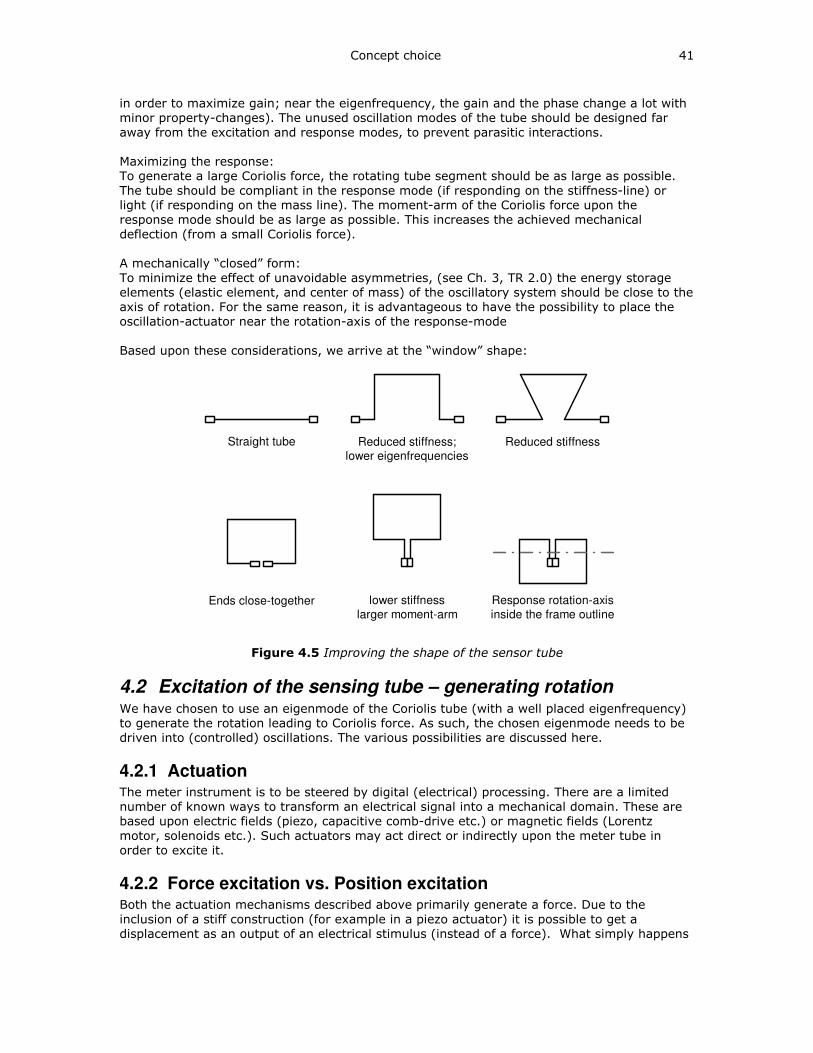
Concept choice 41
in order to maximize gain; near the eigenfrequency, the gain and the phase change a lot with
minor property-changes). The unused oscillation modes of the tube should be designed far
away from the excitation and response modes, to prevent parasitic interactions.
Maximizing the response:
To generate a large Coriolis force, the rotating tube segment should be as large as possible.
The tube should be compliant in the response mode (if responding on the stiffness-line) or
light (if responding on the mass line). The moment-arm of the Coriolis force upon the
response mode should be as large as possible. This increases the achieved mechanical
deflection (from a small Coriolis force).
A mechanically “closed” form:
To minimize the effect of unavoidable asymmetries, (see Ch. 3, TR 2.0) the energy storage
elements (elastic element, and center of mass) of the oscillatory system should be close to the
axis of rotation. For the same reason, it is advantageous to have the possibility to place the
oscillation-actuator near the rotation-axis of the response-mode
Based upon these considerations, we arrive at the “window” shape:
Straight tube Reduced stiffness;lower eigenfrequencies
Reduced stiffness
Ends close-together lower stiffness
larger moment-arm
Response rotation-axis
inside the frame outline
Figure 4.5 Improving the shape of the sensor tube
4.2 Excitation of the sensing tube – generating rotation We have chosen to use an eigenmode of the Coriolis tube (with a well placed eigenfrequency)
to generate the rotation leading to Coriolis force. As such, the chosen eigenmode needs to be
driven into (controlled) oscillations. The various possibilities are discussed here.
4.2.1 Actuation The meter instrument is to be steered by digital (electrical) processing. There are a limited
number of known ways to transform an electrical signal into a mechanical domain. These are
based upon electric fields (piezo, capacitive comb-drive etc.) or magnetic fields (Lorentz
motor, solenoids etc.). Such actuators may act direct or indirectly upon the meter tube in
order to excite it.
4.2.2 Force excitation vs. Position excitation Both the actuation mechanisms described above primarily generate a force. Due to the
inclusion of a stiff construction (for example in a piezo actuator) it is possible to get a
displacement as an output of an electrical stimulus (instead of a force). What simply happens
42 Coriolis mass flow rate meters for low flows
here is that if the material stiffness of the piezo element is k , and the force generated by
applying an electric field across the piezo element is F , we see a displacement x across the
element such that k
Fx = . The crucial point here is that the piezo stiffness is much higher
than the stiffness of the body (tube) being excited, and hence dominant. A similar explanation
also holds true if a (force) actuation principle is used to drive an inertial mass that is several
times larger than a secondary body (tube) that is coupled to it. The large mass imposes
position excitation upon the tube (see the Rheonik “omega” tube in Appendix D). We choose,
if possible, direct (force) actuation for the following reasons:
• A minimum force is required as no extra mass or stiffness is involved. In case of an
imperfect construction, less force is present to ‘leak’ onto the Coriolis mode.
• In absence of extra mass, the effect of the density of fluid medium is clear by means
of the eigenfrequency of oscillation of the tube. This aids in the computation of
medium density and thereby volume flow-rate.
4.2.3 Possibility of contact-less excitation “It is common to all mass flow meters which work according to the Coriolis principle that the Coriolis
forces caused by the mass flow and to be evaluated are very small in relation to the other forces
involved in the motion of the conduit. This leads to the fact that the Coriolis forces change the basic
motion only slightly. In the case of the known mass flow measurement devices, the basic motion of the
conduit is changed by other different influences in addition to the Coriolis forces. For example, these
changes appear because of the transducers and oscillation generators attached to the conduit in the
case of all known mass flow meters. These additional masses mounted on the conduit, on the one hand,
reduce the influence of the Coriolis forces on the motion of the conduit because of their own mass, and,
on the other hand, lead to the fact that the conduits are changed mechanically in an insufficiently
defined way by the attachment of the masses, for example by soldering or welding. Both influences lead
to a reduction of the measurement effect, a lower measurement accuracy, and hard-to-define long-term
behavior, and play a role, in particular in the case of mass flow devices of small rated mass flow, i.e.,
smaller design and thus less conduit mass. In particular, a high mass of conduit including attachments,
i.e., of the system capable of oscillation, leads to a lower resonance frequency, equivalent to lower
Coriolis forces, and thus a reduced measurement effect. Moreover, in the case of masses symmetrically
mounted on the conduit, such as, for example, the transducers in general, very precise mechanical
tolerances are to be maintained. This requirement leads to an expensive production process.”
– Ronald van der Pol, Meter for flowing media, US Patent 5 747 704, May 5, 1998
For several reasons, it is advantageous to be able to actuate the Coriolis meter tube without
any attached components. In the event that there are attached components, they should be
positioned in such a way that the forces caused by a possibly imperfect construction should be
separable (in mechanics, or in the time domain) from generated Coriolis forces.
Bearing this in mind, some concepts were explored before & during the initial PoP tests:
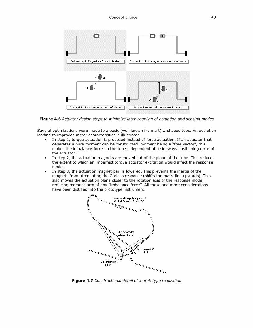
Concept choice 43
Figure 4.6 Actuator design steps to minimize inter-coupling of actuation and sensing modes
Several optimizations were made to a basic (well known from art) U-shaped tube. An evolution
leading to improved meter characteristics is illustrated.
• In step 1, torque actuation is proposed instead of force actuation. If an actuator that
generates a pure moment can be constructed, moment being a “free vector”, this
makes the imbalance-force on the tube independent of a sideways positioning error of
the actuator.
• In step 2, the actuation magnets are moved out of the plane of the tube. This reduces
the extent to which an imperfect torque actuator excitation would affect the response
mode.
• In step 3, the actuation magnet pair is lowered. This prevents the inertia of the
magnets from attenuating the Coriolis response (shifts the mass-line upwards). This
also moves the actuation plane closer to the rotation axis of the response mode,
reducing moment-arm of any “imbalance force”. All these and more considerations
have been distilled into the prototype instrument.
Figure 4.7 Constructional detail of a prototype realization
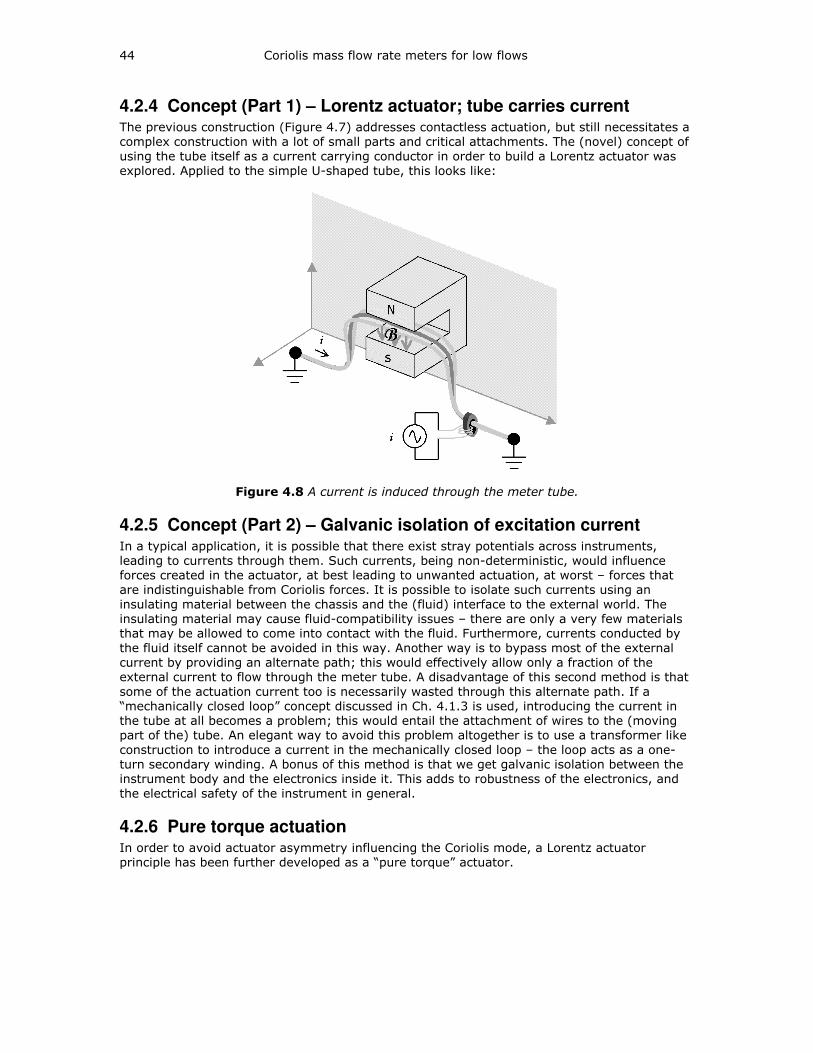
44 Coriolis mass flow rate meters for low flows
4.2.4 Concept (Part 1) – Lorentz actuator; tube carries current The previous construction (Figure 4.7) addresses contactless actuation, but still necessitates a
complex construction with a lot of small parts and critical attachments. The (novel) concept of
using the tube itself as a current carrying conductor in order to build a Lorentz actuator was
explored. Applied to the simple U-shaped tube, this looks like:
Figure 4.8 A current is induced through the meter tube.
4.2.5 Concept (Part 2) – Galvanic isolation of excitation current In a typical application, it is possible that there exist stray potentials across instruments,
leading to currents through them. Such currents, being non-deterministic, would influence
forces created in the actuator, at best leading to unwanted actuation, at worst – forces that
are indistinguishable from Coriolis forces. It is possible to isolate such currents using an
insulating material between the chassis and the (fluid) interface to the external world. The
insulating material may cause fluid-compatibility issues – there are only a very few materials
that may be allowed to come into contact with the fluid. Furthermore, currents conducted by
the fluid itself cannot be avoided in this way. Another way is to bypass most of the external
current by providing an alternate path; this would effectively allow only a fraction of the
external current to flow through the meter tube. A disadvantage of this second method is that
some of the actuation current too is necessarily wasted through this alternate path. If a
“mechanically closed loop” concept discussed in Ch. 4.1.3 is used, introducing the current in
the tube at all becomes a problem; this would entail the attachment of wires to the (moving
part of the) tube. An elegant way to avoid this problem altogether is to use a transformer like
construction to introduce a current in the mechanically closed loop – the loop acts as a one-
turn secondary winding. A bonus of this method is that we get galvanic isolation between the
instrument body and the electronics inside it. This adds to robustness of the electronics, and
the electrical safety of the instrument in general.
4.2.6 Pure torque actuation In order to avoid actuator asymmetry influencing the Coriolis mode, a Lorentz actuator
principle has been further developed as a “pure torque” actuator.
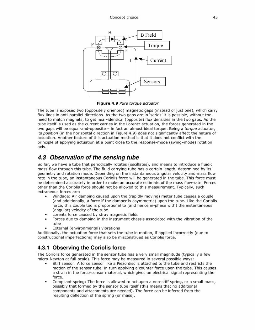
Concept choice 45
Figure 4.9 Pure torque actuator
The tube is exposed two (oppositely oriented) magnetic gaps (instead of just one), which carry
flux lines in anti-parallel directions. As the two gaps are in ‘series’ it is possible, without the
need to match magnets, to get near-identical (opposite) flux densities in the two gaps. As the
tube itself is used as the current carries in the Lorentz actuation, the forces generated in the
two gaps will be equal-and-opposite – in fact an almost ideal torque. Being a torque actuator,
its position (in the horizontal direction in Figure 4.9) does not significantly affect the nature of
actuation. Another feature of this actuation method is that it does not conflict with the
principle of applying actuation at a point close to the response-mode (swing–mode) rotation
axis.
4.3 Observation of the sensing tube So far, we have a tube that periodically rotates (oscillates), and means to introduce a fluidic
mass-flow through this tube. The fluid carrying tube has a certain length, determined by its
geometry and rotation mode. Depending on the instantaneous angular velocity and mass flow
rate in the tube, an instantaneous Coriolis force will be generated in the tube. This force must
be determined accurately in order to make an accurate estimate of the mass flow-rate. Forces
other than the Coriolis force should not be allowed to this measurement. Typically, such
extraneous forces are:
• Windage: Air damping caused upon the (rapidly moving) meter tube causes a couple
(and additionally, a force if the damper is asymmetric) upon the tube. Like the Coriolis
force, this couple too is proportional to (and hence in-phase with) the instantaneous
(angular) velocity of the tube.
• Lorentz force caused by stray magnetic fields
• Forces due to damping in the instrument chassis associated with the vibration of the
tube
• External (environmental) vibrations
Additionally, the actuation force that sets the tube in motion, if applied incorrectly (due to
constructional imperfections) may also be misconstrued as Coriolis force.
4.3.1 Observing the Coriolis force The Coriolis force generated in the sensor tube has a very small magnitude (typically a few
micro-Newton at full-scale). This force may be measured in several possible ways:
• Stiff sensor: A force sensor like a Piezo disc is attached to the tube and restricts the
motion of the sensor tube, in turn applying a counter force upon the tube. This causes
a strain in the force-sensor material, which gives an electrical signal representing the
force.
• Compliant spring: The force is allowed to act upon a non-stiff spring, or a small mass,
possibly that formed by the sensor tube itself (this means that no additional
components and attachments are needed). The force can be inferred from the
resulting deflection of the spring (or mass).
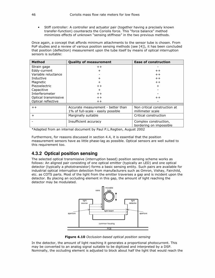
46 Coriolis mass flow rate meters for low flows
• Stiff controller: A controller and actuator pair (together having a precisely known
transfer-function) counteracts the Coriolis force. This “force balance” method
minimizes effects of unknown “sensing stiffness” in the two previous methods.
Once again, a concept that affords minimum attachments to the sensor tube is chosen. From
PoP studies and a review of various position sensing methods (see [4]), it has been concluded
that position (deflection) measurement upon the tube itself by means of optical interruption
sensors is suitable:
Method Quality of measurement Ease of construction
Strain gage
Eddy-current
Variable reluctance
Inductive
Magnetic
Piezoelectric
Capacitive
Interferometer
Optical transmissive
Optical reflective
++
+
-
+
+
++
+
++
++
++
-
++
++
++
++
+
-
-
++
-
++ Accurate measurement - better than
1% of full-scale - easily possible
Non critical construction at
millimeter scale
+ Marginally suitable Critical construction
- Insufficient accuracy Complex construction,
bordering on impossible
*Adapted from an internal document by Paul P.L.Regtien, August 2002
Furthermore, for reasons discussed in section 4.4, it is essential that the position
measurement sensors have as little phase-lag as possible. Optical sensors are well suited to
this requirement too.
4.3.2 Optical position sensing The selected optical transmissive (interruption based) position sensing scheme works as
follows: An aligned pair consisting of one optical emitter (typically an LED) and one optical
detector (typically a phototransistor) forms a basic sensing entity. Such pairs are available for
industrial optical interruption detection from manufacturers such as Omron, Vishay, Fairchild,
etc. as COTS parts. Most of the light from the emitter traverses a gap and is incident upon the
detector. By placing an occluding element in this gap, the amount of light reaching the
detector may be modulated.
movable
vane tube
light light
source detector
light beam
aperture aperture
common housing
PCB
Figure 4.10 Occlusion-based optical position sensing
In the detector, the amount of light reaching it generates a proportional photocurrent. This
may be converted to an analog signal suitable to be digitized and interpreted by a DSP.
Nominally, the occluding element is adjusted to block about half the light that would reach the
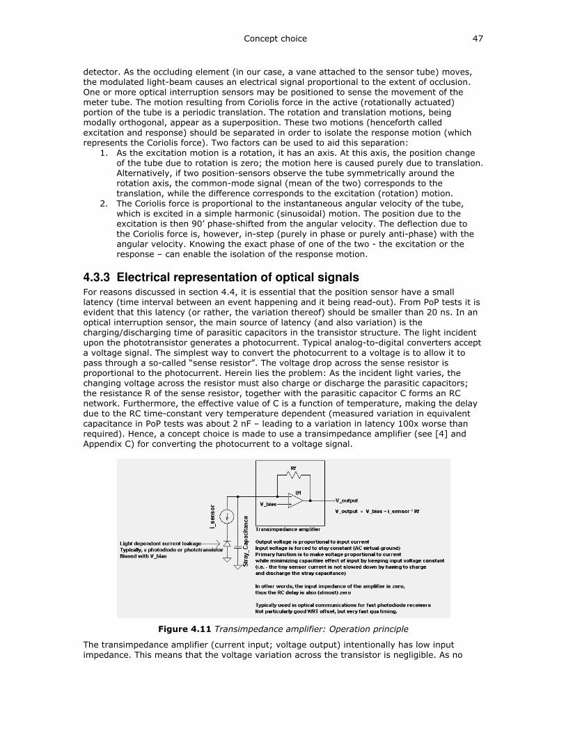
Concept choice 47
detector. As the occluding element (in our case, a vane attached to the sensor tube) moves,
the modulated light-beam causes an electrical signal proportional to the extent of occlusion.
One or more optical interruption sensors may be positioned to sense the movement of the
meter tube. The motion resulting from Coriolis force in the active (rotationally actuated)
portion of the tube is a periodic translation. The rotation and translation motions, being
modally orthogonal, appear as a superposition. These two motions (henceforth called
excitation and response) should be separated in order to isolate the response motion (which
represents the Coriolis force). Two factors can be used to aid this separation:
1. As the excitation motion is a rotation, it has an axis. At this axis, the position change
of the tube due to rotation is zero; the motion here is caused purely due to translation.
Alternatively, if two position-sensors observe the tube symmetrically around the
rotation axis, the common-mode signal (mean of the two) corresponds to the
translation, while the difference corresponds to the excitation (rotation) motion.
2. The Coriolis force is proportional to the instantaneous angular velocity of the tube,
which is excited in a simple harmonic (sinusoidal) motion. The position due to the
excitation is then 90’ phase-shifted from the angular velocity. The deflection due to
the Coriolis force is, however, in-step (purely in phase or purely anti-phase) with the
angular velocity. Knowing the exact phase of one of the two - the excitation or the
response – can enable the isolation of the response motion.
4.3.3 Electrical representation of optical signals For reasons discussed in section 4.4, it is essential that the position sensor have a small
latency (time interval between an event happening and it being read-out). From PoP tests it is
evident that this latency (or rather, the variation thereof) should be smaller than 20 ns. In an
optical interruption sensor, the main source of latency (and also variation) is the
charging/discharging time of parasitic capacitors in the transistor structure. The light incident
upon the phototransistor generates a photocurrent. Typical analog-to-digital converters accept
a voltage signal. The simplest way to convert the photocurrent to a voltage is to allow it to
pass through a so-called “sense resistor”. The voltage drop across the sense resistor is
proportional to the photocurrent. Herein lies the problem: As the incident light varies, the
changing voltage across the resistor must also charge or discharge the parasitic capacitors;
the resistance R of the sense resistor, together with the parasitic capacitor C forms an RC
network. Furthermore, the effective value of C is a function of temperature, making the delay
due to the RC time-constant very temperature dependent (measured variation in equivalent
capacitance in PoP tests was about 2 nF – leading to a variation in latency 100x worse than
required). Hence, a concept choice is made to use a transimpedance amplifier (see [4] and
Appendix C) for converting the photocurrent to a voltage signal.
Figure 4.11 Transimpedance amplifier: Operation principle
The transimpedance amplifier (current input; voltage output) intentionally has low input
impedance. This means that the voltage variation across the transistor is negligible. As no
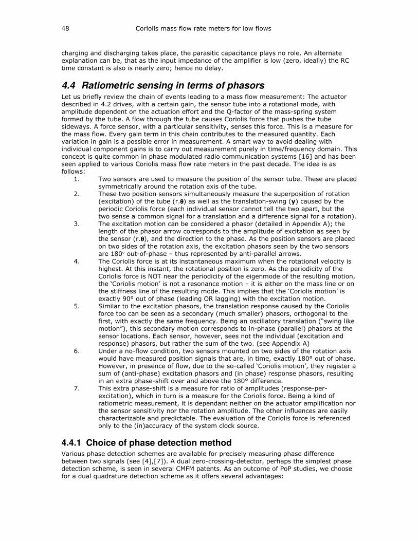
48 Coriolis mass flow rate meters for low flows
charging and discharging takes place, the parasitic capacitance plays no role. An alternate
explanation can be, that as the input impedance of the amplifier is low (zero, ideally) the RC
time constant is also is nearly zero; hence no delay.
4.4 Ratiometric sensing in terms of phasors Let us briefly review the chain of events leading to a mass flow measurement: The actuator
described in 4.2 drives, with a certain gain, the sensor tube into a rotational mode, with
amplitude dependent on the actuation effort and the Q-factor of the mass-spring system
formed by the tube. A flow through the tube causes Coriolis force that pushes the tube
sideways. A force sensor, with a particular sensitivity, senses this force. This is a measure for
the mass flow. Every gain term in this chain contributes to the measured quantity. Each
variation in gain is a possible error in measurement. A smart way to avoid dealing with
individual component gains is to carry out measurement purely in time/frequency domain. This
concept is quite common in phase modulated radio communication systems [16] and has been
seen applied to various Coriolis mass flow rate meters in the past decade. The idea is as
follows:
1. Two sensors are used to measure the position of the sensor tube. These are placed
symmetrically around the rotation axis of the tube.
2. These two position sensors simultaneously measure the superposition of rotation (excitation) of the tube (r.θθθθ) as well as the translation-swing (y) caused by the
periodic Coriolis force (each individual sensor cannot tell the two apart, but the
two sense a common signal for a translation and a difference signal for a rotation).
3. The excitation motion can be considered a phasor (detailed in Appendix A); the
length of the phasor arrow corresponds to the amplitude of excitation as seen by the sensor (r.θθθθ), and the direction to the phase. As the position sensors are placed
on two sides of the rotation axis, the excitation phasors seen by the two sensors are 180° out-of-phase – thus represented by anti-parallel arrows.
4. The Coriolis force is at its instantaneous maximum when the rotational velocity is
highest. At this instant, the rotational position is zero. As the periodicity of the
Coriolis force is NOT near the periodicity of the eigenmode of the resulting motion,
the ‘Coriolis motion’ is not a resonance motion – it is either on the mass line or on
the stiffness line of the resulting mode. This implies that the ‘Coriolis motion’ is
exactly 90° out of phase (leading OR lagging) with the excitation motion.
5. Similar to the excitation phasors, the translation response caused by the Coriolis
force too can be seen as a secondary (much smaller) phasors, orthogonal to the
first, with exactly the same frequency. Being an oscillatory translation (“swing like
motion”), this secondary motion corresponds to in-phase (parallel) phasors at the
sensor locations. Each sensor, however, sees not the individual (excitation and
response) phasors, but rather the sum of the two. (see Appendix A)
6. Under a no-flow condition, two sensors mounted on two sides of the rotation axis
would have measured position signals that are, in time, exactly 180° out of phase.
However, in presence of flow, due to the so-called ‘Coriolis motion’, they register a
sum of (anti-phase) excitation phasors and (in phase) response phasors, resulting
in an extra phase-shift over and above the 180° difference.
7. This extra phase-shift is a measure for ratio of amplitudes (response-per-
excitation), which in turn is a measure for the Coriolis force. Being a kind of
ratiometric measurement, it is dependant neither on the actuator amplification nor
the sensor sensitivity nor the rotation amplitude. The other influences are easily
characterizable and predictable. The evaluation of the Coriolis force is referenced
only to the (in)accuracy of the system clock source.
4.4.1 Choice of phase detection method Various phase detection schemes are available for precisely measuring phase difference
between two signals (see [4],[7]). A dual zero-crossing-detector, perhaps the simplest phase
detection scheme, is seen in several CMFM patents. As an outcome of PoP studies, we choose
for a dual quadrature detection scheme as it offers several advantages:
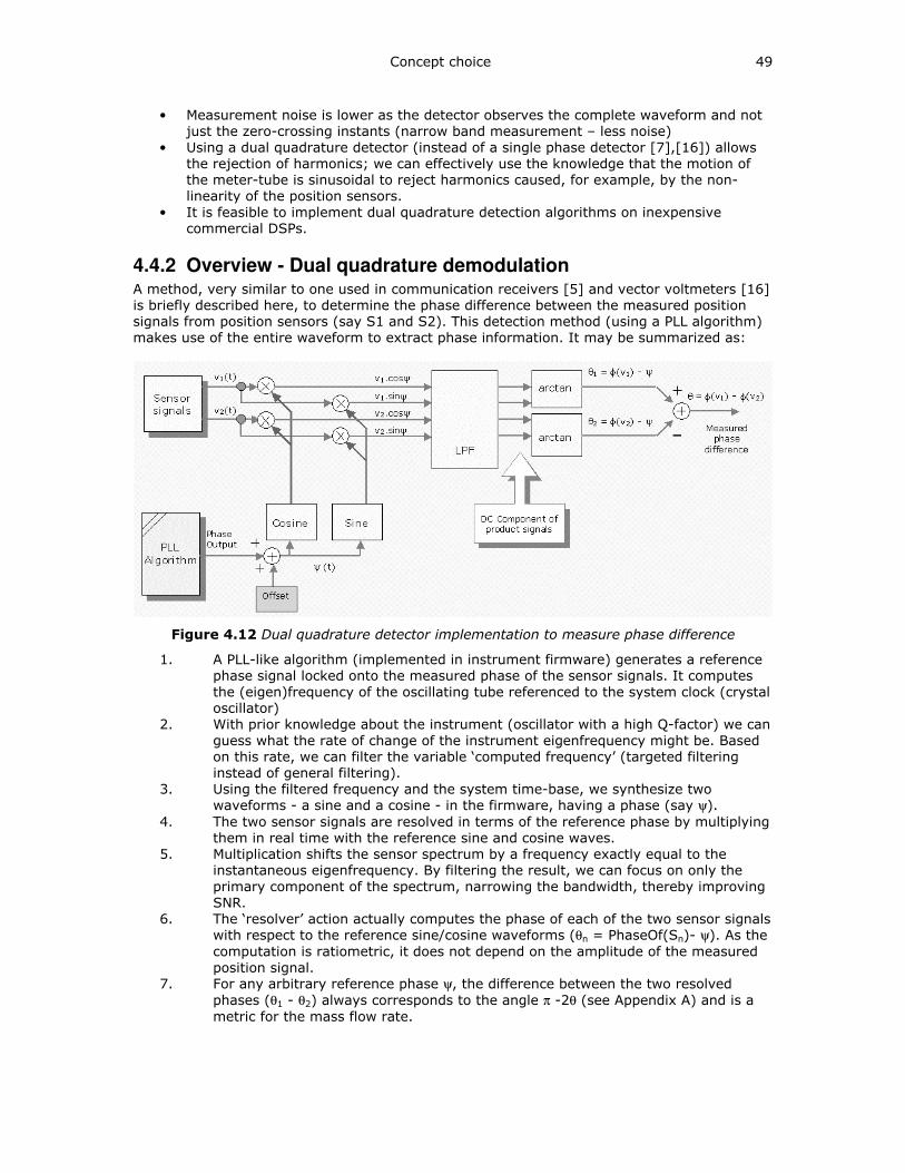
Concept choice 49
• Measurement noise is lower as the detector observes the complete waveform and not
just the zero-crossing instants (narrow band measurement – less noise)
• Using a dual quadrature detector (instead of a single phase detector [7],[16]) allows
the rejection of harmonics; we can effectively use the knowledge that the motion of
the meter-tube is sinusoidal to reject harmonics caused, for example, by the non-
linearity of the position sensors.
• It is feasible to implement dual quadrature detection algorithms on inexpensive
commercial DSPs.
4.4.2 Overview - Dual quadrature demodulation A method, very similar to one used in communication receivers [5] and vector voltmeters [16]
is briefly described here, to determine the phase difference between the measured position
signals from position sensors (say S1 and S2). This detection method (using a PLL algorithm)
makes use of the entire waveform to extract phase information. It may be summarized as:
Figure 4.12 Dual quadrature detector implementation to measure phase difference
1. A PLL-like algorithm (implemented in instrument firmware) generates a reference
phase signal locked onto the measured phase of the sensor signals. It computes
the (eigen)frequency of the oscillating tube referenced to the system clock (crystal
oscillator)
2. With prior knowledge about the instrument (oscillator with a high Q-factor) we can
guess what the rate of change of the instrument eigenfrequency might be. Based
on this rate, we can filter the variable ‘computed frequency’ (targeted filtering
instead of general filtering).
3. Using the filtered frequency and the system time-base, we synthesize two
waveforms - a sine and a cosine - in the firmware, having a phase (say ψ).
4. The two sensor signals are resolved in terms of the reference phase by multiplying
them in real time with the reference sine and cosine waves.
5. Multiplication shifts the sensor spectrum by a frequency exactly equal to the
instantaneous eigenfrequency. By filtering the result, we can focus on only the
primary component of the spectrum, narrowing the bandwidth, thereby improving
SNR.
6. The ‘resolver’ action actually computes the phase of each of the two sensor signals
with respect to the reference sine/cosine waveforms (θn = PhaseOf(Sn)- ψ). As the
computation is ratiometric, it does not depend on the amplitude of the measured
position signal. 7. For any arbitrary reference phase ψ, the difference between the two resolved
phases (θ1 - θ2) always corresponds to the angle π -2θ (see Appendix A) and is a
metric for the mass flow rate.
50 Coriolis mass flow rate meters for low flows
Noise vs. speed tradeoff Any measurement system has an associated measurement noise. The noise has a spectrum;
by decreasing measurement bandwidth, it is usually possible to decrease noise power. The use
of a dual quadrature detector offers algorithmic flexibility to trade-off speed for noise.
Adjusting the filter parameters of the low-pass filter module (after multiplication with the sine
and cosine reference signals) is a convenient way to achieve this.
4.5 Digital representation of electrical signals (and vice versa) Having made a concept choice to process signals digitally, it is important to choose analog-to-
digital conversion means that do not degrade measurement. Let us first consider the
digitization of the tube-position (sensor) signals. From PoP tests, it has been demonstrated [9]
that a 12-bit representation of each position is sufficient to implement basic functionality. In
the interest of reducing quantization noise, it is advantageous to use an A/D converter with a
higher resolution. It is important to remember that a high accuracy (of magnitude) is not
essential, as the measurement is phase-based. However, the (position) measurement must be
deterministic (accurate) in time. Any phase mismatch in the measurement instant of the two
position signals will be misinterpreted as a phase shift (caused by a non-existent Coriolis
force). Various analog-to-digital converters are commercially available. These include flash
converters, successive approximation converters, slope integrating converters, sigma-delta
converters etc. (see [4]). One particular type, the “audio CODEC” sigma-delta converter, is
particularly suited for this application:
• 20+ bits of resolution
• 48k samples-per-second typical conversion rate
• Multiple “parallel sampling” converter channels – This means that the position sensors
are sampled simultaneously – there is no significant time-interval between the
sampling of one sensor and the second sensor; compensation is not required. (This is
a big advantage over multiplexed ADCs)
• Interface is tailored for DSP applications; transferring high precision data at high
sample-rates to a DSP is efficiently carried out with minimal software overhead
Commercial CODEC ICs have an integrated high-resolution digital-to-analog converter, which
can be used for driving the actuator to oscillate the tube; a separate DAC is not required.
In order to achieve a high resolution, audio CODEC converters have a built-in digital filter.
Using this filter and a technique called oversampling [4] (sampling the analog signal at a rate
many times higher than the final conversion rate) together with noise shaping, the 20+ bits of
resolution is achieved. However, this filtering leads to a (deterministic) latency of a few
milliseconds. This needs to be accounted for in the system design. Due to the cyclic nature of
the tube movement, and the absence of fast control loops requiring low latencies, this
limitation of an audio CODEC (sigma delta ADC) is not a hindrance for our system.
4.6 Summary In this chapter, the background and concepts regarding several aspects of Coriolis meters
have been discussed. In particular, the discussions concern
• the shape of the tube
• the nature of oscillations
• various actuation concepts, and a particular near-ideal torque actuation concept
• sensing of tube position
• the processing of measurements
In case of multiple concepts, where appropriate, one of the possibilities has been chosen with
qualitative arguments.
5 Detailed design In order to design a mass flow rate measuring instrument as satisfying conditions laid down in
chapter 3, we have considered several concepts in chapter 4, weighed them according to
merit, and arrived at some concept choices; this entails the use of expert knowledge and
experience. Several PoP tests have been carried out at the same time to create insight into the
specific problem at hand. Modeling and simulations complement these two activities in order
to investigate “what if” scenarios and to generate order-of-magnitudes (numbers) for the
chosen concepts; they consider (a simplified version of) the underlying physics. Based upon
this physics, a detailed analysis can yield analytical expressions that characterize these
nuances of the instrument in addition to its macro behavior.
This chapter deals with the detailed design of the instrument; in this sense it is more precise
than the previous chapter – numbers and expressions are provided along with the analysis.
5.1 The meter tube - Shape and dimensions • Instrument has base dimensions of (H)100 mm x (B)60 mm x (D)30 mm; from PoP
tests it has been seen that a rectangular closed-frame form of the tube is suitable. It is
reasonable to assume that the entire meter tube will have a length that is about 6
times the base of the rectangle, which in turn is about 70% of the chassis base (4
sides of the rectangle + 2 middle sections – inlet and outlet)
• It is known that the meter tube should be as light as possible, but at the same time
carry, depending on the type, a certain mass flow rate of water, with the resulting
pressure drop not exceeding 1e5 Pa (1 bar)
• The tube should withstand 1e7 Pa (100 bar) pressure without bursting
5.1.1 Diameter of meter tube Fluid flow through a tube (see [13] pp A4/26 to A4/30) can be approximated as one of two
types – laminar or turbulent. The Reynolds’ number of a fluid flow is given by:
For a circular tube:
η
ρ IDvRn mean ⋅⋅
= …(Reynolds) (5.1)
Where
Rn Reynolds number [-]
ρ Density of fluid [kg/m3]
meanv Mean velocity of fluid through tube [m/s]
ID Diameter of tube [m]
η Dynamic viscosity [Pa.s], in other words, [kg /(m.s)]
Generally, for a flow having Reynolds’ number lower than 2300, the flow is laminar, while
Reynolds’ number higher than 2300 suggests that the flow is turbulent.
Depending on the flow type, for a hydraulically ‘smooth’ tube, a friction coefficient may be
estimated for the fluid:
Rn
flam
64= (5.2)
52 Coriolis mass flow rate meters for low flows
4
3164.0
Rnftur = …(Blasius, Moody diagram) (5.3)
Where
lamf Friction coefficient with laminar flow [-] (Laminar: Rn <~2300)
turf Friction coefficient with turbulent flow [-] (Turbulent: Rn >~2300)
Further, depending on the length of the tube in question, the pressure drop across the tube
may be estimated:
2
2
1meanxxx v
ID
LfP ⋅⋅⋅⋅=∆ ρ …(Darcy-Weisbach) (5.4)
Where
P∆ Pressure drop across tube [Pa] or [N/m2] or [kg/(m.s2)]
xxxf lamf or turf , the friction coefficient [-], to be used appropriately
L Length of tube [m]
ID Inner diameter of tube [m]
It is possible to use these equations, together with the 2300<Rn condition, to estimate the
relation between mass-flow-rate and pressure drop for a given tube diameter. For example,
for laminar flows, we have:
L
PIDv
⋅⋅
∆⋅⋅=Φ
η
π
128
4
…(Hagen-Poiseuille) (5.5)
Where
vΦ Volume flow-rate [m3/s]
Further, it is possible to relate the mass-flow rate mΦ and the volume flow rate as:
ρ⋅Φ=Φ vm (5.6)
Using 1e-3 [Pa.s] as the dynamic viscosity of water and 1e3 [kg/m3] as the density, a pair of
curves (Mass flow rate against pressure drop, laminar and turbulent) can be plotted. The
Reynolds number may be used to appropriately choose one of the two curves for a given flow.
5.1.2 Wall thickness of meter tube
Stress in thin walled cylindrical pressure vessel:
Consider a length dx of the pressure vessel
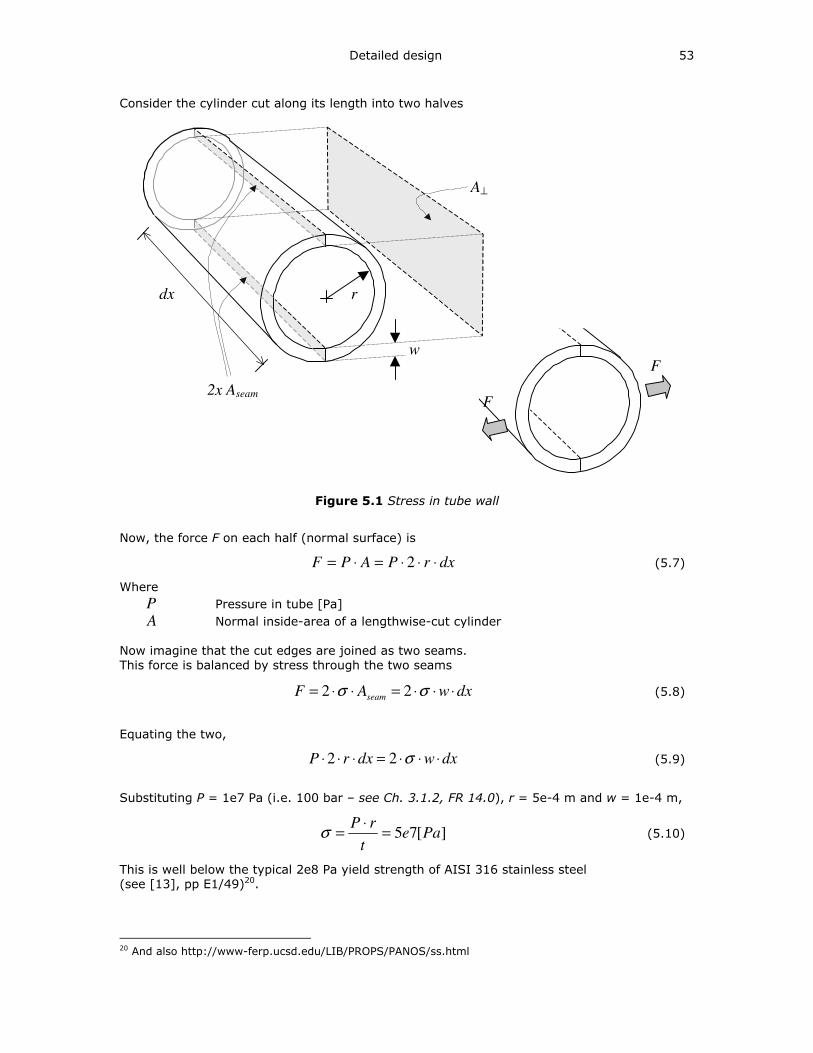
Detailed design 53
Consider the cylinder cut along its length into two halves
dx r
F
F
2x Aseam
A⊥
w
Figure 5.1 Stress in tube wall
Now, the force F on each half (normal surface) is
dxrPAPF ⋅⋅⋅=⋅= 2 (5.7)
Where
P Pressure in tube [Pa]
A Normal inside-area of a lengthwise-cut cylinder
Now imagine that the cut edges are joined as two seams.
This force is balanced by stress through the two seams
dxwAF seam ⋅⋅⋅=⋅⋅= σσ 22 (5.8)
Equating the two,
dxwdxrP ⋅⋅⋅=⋅⋅⋅ σ22 (5.9)
Substituting P = 1e7 Pa (i.e. 100 bar – see Ch. 3.1.2, FR 14.0), r = 5e-4 m and w = 1e-4 m,
][75 Paet
rP=
⋅=σ (5.10)
This is well below the typical 2e8 Pa yield strength of AISI 316 stainless steel
(see [13], pp E1/49)20.
20 And also http://www-ferp.ucsd.edu/LIB/PROPS/PANOS/ss.html
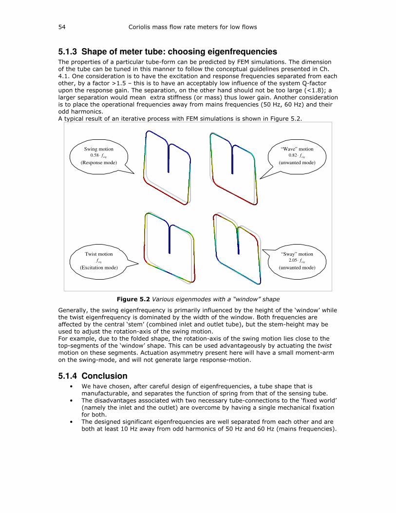
54 Coriolis mass flow rate meters for low flows
5.1.3 Shape of meter tube: choosing eigenfrequencies The properties of a particular tube-form can be predicted by FEM simulations. The dimension
of the tube can be tuned in this manner to follow the conceptual guidelines presented in Ch.
4.1. One consideration is to have the excitation and response frequencies separated from each
other, by a factor >1.5 – this is to have an acceptably low influence of the system Q-factor
upon the response gain. The separation, on the other hand should not be too large (<1.8); a
larger separation would mean extra stiffness (or mass) thus lower gain. Another consideration
is to place the operational frequencies away from mains frequencies (50 Hz, 60 Hz) and their
odd harmonics.
A typical result of an iterative process with FEM simulations is shown in Figure 5.2.
Swing motion
eigf⋅58.0
(Response mode)
Twist motion
eigf
(Excitation mode)
“Wave” motion
eigf⋅82.0
(unwanted mode)
“Sway” motion
eigf⋅05.2
(unwanted mode)
Figure 5.2 Various eigenmodes with a “window” shape
Generally, the swing eigenfrequency is primarily influenced by the height of the ‘window’ while
the twist eigenfrequency is dominated by the width of the window. Both frequencies are
affected by the central ‘stem’ (combined inlet and outlet tube), but the stem-height may be
used to adjust the rotation-axis of the swing motion.
For example, due to the folded shape, the rotation-axis of the swing motion lies close to the
top-segments of the ‘window’ shape. This can be used advantageously by actuating the twist motion on these segments. Actuation asymmetry present here will have a small moment-arm
on the swing-mode, and will not generate large response-motion.
5.1.4 Conclusion • We have chosen, after careful design of eigenfrequencies, a tube shape that is
manufacturable, and separates the function of spring from that of the sensing tube.
• The disadvantages associated with two necessary tube-connections to the ‘fixed world’
(namely the inlet and the outlet) are overcome by having a single mechanical fixation
for both.
• The designed significant eigenfrequencies are well separated from each other and are
both at least 10 Hz away from odd harmonics of 50 Hz and 60 Hz (mains frequencies).
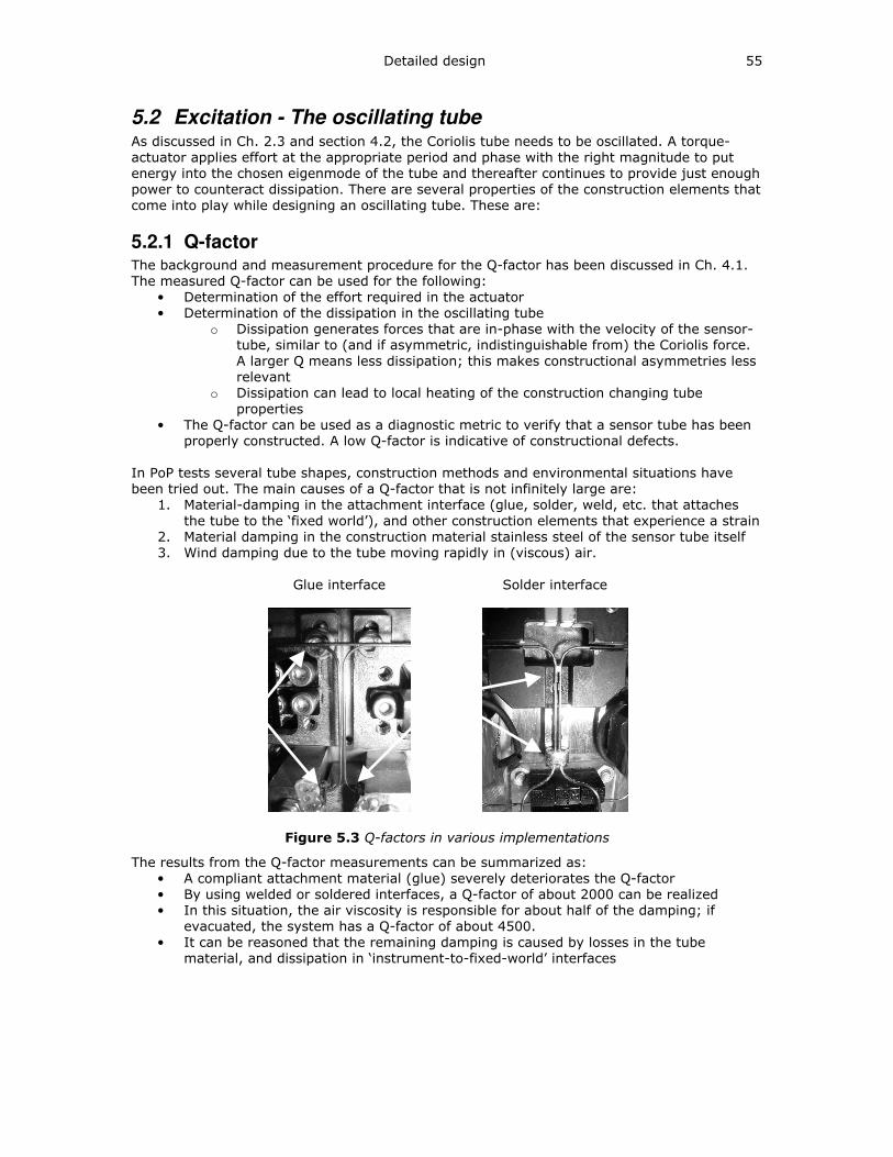
Detailed design 55
5.2 Excitation - The oscillating tube As discussed in Ch. 2.3 and section 4.2, the Coriolis tube needs to be oscillated. A torque-
actuator applies effort at the appropriate period and phase with the right magnitude to put
energy into the chosen eigenmode of the tube and thereafter continues to provide just enough
power to counteract dissipation. There are several properties of the construction elements that
come into play while designing an oscillating tube. These are:
5.2.1 Q-factor The background and measurement procedure for the Q-factor has been discussed in Ch. 4.1.
The measured Q-factor can be used for the following:
• Determination of the effort required in the actuator
• Determination of the dissipation in the oscillating tube
o Dissipation generates forces that are in-phase with the velocity of the sensor-
tube, similar to (and if asymmetric, indistinguishable from) the Coriolis force.
A larger Q means less dissipation; this makes constructional asymmetries less
relevant
o Dissipation can lead to local heating of the construction changing tube
properties
• The Q-factor can be used as a diagnostic metric to verify that a sensor tube has been
properly constructed. A low Q-factor is indicative of constructional defects.
In PoP tests several tube shapes, construction methods and environmental situations have
been tried out. The main causes of a Q-factor that is not infinitely large are:
1. Material-damping in the attachment interface (glue, solder, weld, etc. that attaches
the tube to the ‘fixed world’), and other construction elements that experience a strain
2. Material damping in the construction material stainless steel of the sensor tube itself
3. Wind damping due to the tube moving rapidly in (viscous) air.
Glue interface Solder interface
Figure 5.3 Q-factors in various implementations
The results from the Q-factor measurements can be summarized as:
• A compliant attachment material (glue) severely deteriorates the Q-factor
• By using welded or soldered interfaces, a Q-factor of about 2000 can be realized
• In this situation, the air viscosity is responsible for about half of the damping; if
evacuated, the system has a Q-factor of about 4500.
• It can be reasoned that the remaining damping is caused by losses in the tube
material, and dissipation in ‘instrument-to-fixed-world’ interfaces

56 Coriolis mass flow rate meters for low flows
5.2.2 Actuation of the Coriolis tube
Innovation: Pure torque generator:
The essential portion of the “Lorentz actuator” concept
chosen for driving the Coriolis tube into oscillations is
shown here (see Appendix B.1 for details), and works as
follows: A current i is introduced in the fluid carrying tube.
This current traverses the tube, passing through gaps in a
stator magnet yoke. A magnetic field is present in its gap,
having a flux density B perpendicular to the tube (and also
the current). A force is created in the current carrying
conductor, proportional to the cross product of the current,
the flux density, and the length of tube l exposed to the
magnetic flux.
iBlF ×⋅=
The construction shown here has the following properties:
1) There are two identical, antiparallel air-gaps.
2) The current flowing through the left gap is exactly
equal to that through the right gap.
3) Neglecting construction tolerances, this creates a
pure couple (effort) upon the tube.
4) This couple twists the central “torsion spring” (the
inlet and outlet tube pair), depending on the
instantaneous direction of the current
Motor constant of the actuator:
Consider half of the actuator; Moment arm r [m] Distance between the torsion axis and the centroid of
force acting on half the tube
Flux density in air-gap,
upon the tube B
[T] NdFeB magnets with a Br=1.3T are used to bias the air-
gap; approx. value from simulations
Current through tube i i [A] AC RMS
Effective length l [m] The pole-length over which the Lorentz force is generated
Lorentz Force: iBlF ×⋅= (5.11)
Torque: rF ⋅=Τ 2 (5.12)
Motor constant: 55.72 −=⋅⋅=Τ
= erBli
km [N⋅m/A] (5.13)
Torsion stiffness of the
tube construction
7.1e-2 [N.m/rad] Depends on material properties and dimensions of the
construction
Required deflection 2.8e-2 [rad] The amplitude of angular deflection desired
Required static torque 2.0e-3 [N.m] The static torque needed to deflect the tube
Typical Q-factor 2000 [-] Measured – a property of the tube and its surroundings
Required torque
amplitude
1e-6 [N.m] Q times smaller than the static torque
Required actuation
current
13.2e-3 [A] The current mki Τ= is needed (when the tube is
stably oscillating) to sustain oscillations at the said
amplitude (i.e. to counteract dissipation)
The “required actuation current” value is for the situation when the sensor tube is stably
oscillating; at the time of startup, more current is introduced into the tube to rapidly reach the
desired oscillation amplitude.
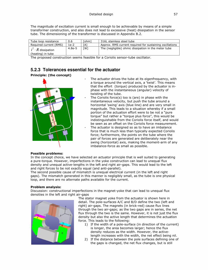
Detailed design 57
The magnitude of excitation current is small enough to be achievable by means of a simple
transformer construction, and also does not lead to excessive (heat) dissipation in the sensor
tube. The dimensioning of the transformer is discussed in Appendix B.2.
Tube loop resistance 0.6 [ohm] 316L stainless steel tube
Required current (RMS) 1e-2 [A] Approx. RMS current required for sustaining oscillations
Ri ⋅2dissipation
(heating) in tube
4.8e-5 [W] The (negligible) ohmic dissipation in the meter tube
The proposed construction seems feasible for a Coriolis sensor-tube oscillator.
5.2.3 Tolerances essential for the actuator Principle: (the concept)
- The actuator drives the tube at its eigenfrequency, with
a torque around the vertical axis, a ‘twist’. This means
that the effort (torque) produced by the actuator is in-
phase with the instantaneous (angular) velocity of
twisting of the tube.
- The Coriolis force(s) too is (are) in phase with the
instantaneous velocity, but push the tube around a
horizontal ‘swing’ axis (blue line) and are very small in
magnitude. This leads to a situation whereby if a small
portion of the actuation effort were to be not a “pure
torque” but rather a “torque plus force”, this would be
indistinguishable from the Coriolis force itself, and would
be seen as an offset on the Coriolis force measurement.
- The actuator is designed so as to have an imbalance
force that is much less than typically expected Coriolis
force; furthermore, the points on the tube where the
pair of forces are generated are deliberately near the
swing (horizontal) axis, making the moment-arm of any
imbalance-force as small as possible.
Possible problems:
In the concept choice, we have selected an actuator principle that is well suited to generating
a pure-torque. However, imperfections in the yoke construction can lead to unequal flux
density and unequal active-lengths in the left and right air-gaps. This would lead to the left
and right forces to be not exactly equal (and anti-parallel).
The second possible cause of mismatch is unequal electrical current (in the left and right
gaps). The mismatch generated in this manner is negligibly small, as the tube is one physical
loop, and there are no alternate paths available for the current.
Problem analysis: Discussion: constructional imperfections in the magnet-yoke that can lead to unequal flux
densities in the left and right air-gaps
The stator magnet yoke from the actuator is shown here in
detail. The pole-surfaces A/C and B/D define the two (left and
right) air-gaps. The magnets (in brick-red) cause flux lines
through the two air-gaps; as the two gaps are in series, the net
flux through the two is the same. However, it is not just the flux
density but also the active length that determines the actuation
force. This leads to the following:
1) If the width of a pole-surface (in direction of the current)
is longer, the area becomes larger; hence the flux
density reduces as the width. However, the active-
length increases with the width, the net effect being nil.
2) If the distance between the pole surfaces defining one of
the gaps is changed, the net flux changes, but is still
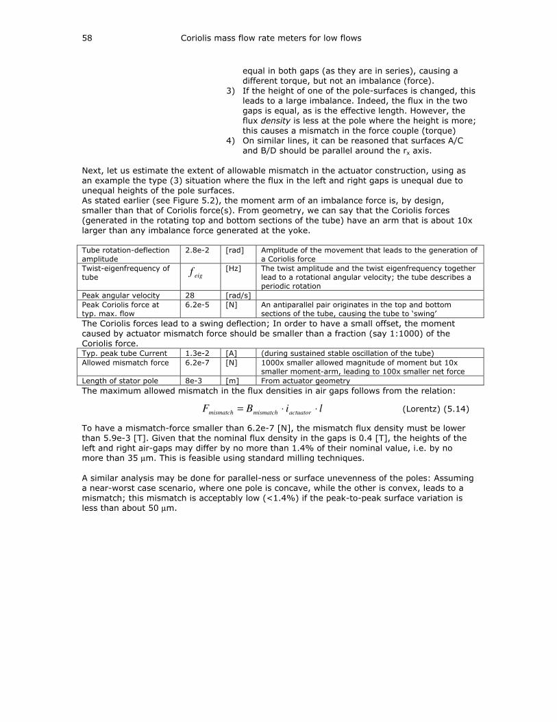
58 Coriolis mass flow rate meters for low flows
equal in both gaps (as they are in series), causing a
different torque, but not an imbalance (force).
3) If the height of one of the pole-surfaces is changed, this
leads to a large imbalance. Indeed, the flux in the two
gaps is equal, as is the effective length. However, the
flux density is less at the pole where the height is more;
this causes a mismatch in the force couple (torque)
4) On similar lines, it can be reasoned that surfaces A/C
and B/D should be parallel around the rx axis.
Next, let us estimate the extent of allowable mismatch in the actuator construction, using as
an example the type (3) situation where the flux in the left and right gaps is unequal due to
unequal heights of the pole surfaces.
As stated earlier (see Figure 5.2), the moment arm of an imbalance force is, by design,
smaller than that of Coriolis force(s). From geometry, we can say that the Coriolis forces
(generated in the rotating top and bottom sections of the tube) have an arm that is about 10x
larger than any imbalance force generated at the yoke.
Tube rotation-deflection
amplitude
2.8e-2 [rad] Amplitude of the movement that leads to the generation of
a Coriolis force
Twist-eigenfrequency of
tube eigf [Hz] The twist amplitude and the twist eigenfrequency together
lead to a rotational angular velocity; the tube describes a
periodic rotation
Peak angular velocity 28 [rad/s]
Peak Coriolis force at
typ. max. flow
6.2e-5 [N] An antiparallel pair originates in the top and bottom
sections of the tube, causing the tube to ‘swing’
The Coriolis forces lead to a swing deflection; In order to have a small offset, the moment
caused by actuator mismatch force should be smaller than a fraction (say 1:1000) of the
Coriolis force. Typ. peak tube Current 1.3e-2 [A] (during sustained stable oscillation of the tube)
Allowed mismatch force 6.2e-7 [N] 1000x smaller allowed magnitude of moment but 10x
smaller moment-arm, leading to 100x smaller net force
Length of stator pole 8e-3 [m] From actuator geometry
The maximum allowed mismatch in the flux densities in air gaps follows from the relation:
liBF actuatormismatchmismatch ⋅⋅= (Lorentz) (5.14)
To have a mismatch-force smaller than 6.2e-7 [N], the mismatch flux density must be lower
than 5.9e-3 [T]. Given that the nominal flux density in the gaps is 0.4 [T], the heights of the
left and right air-gaps may differ by no more than 1.4% of their nominal value, i.e. by no more than 35 µm. This is feasible using standard milling techniques.
A similar analysis may be done for parallel-ness or surface unevenness of the poles: Assuming
a near-worst case scenario, where one pole is concave, while the other is convex, leads to a
mismatch; this mismatch is acceptably low (<1.4%) if the peak-to-peak surface variation is less than about 50 µm.
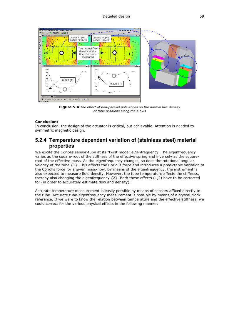
Detailed design 59
Convex ‘C’ pole
surface (+30µm)
-0.329 [T]
0.325 [T]
Concave ‘D’ pole
surface (-30µm)
The normal flux
density at this
line (z-axis) is measured
y
Z
Figure 5.4 The effect of non-parallel pole-shoes on the normal flux density at tube positions along the z-axis
Conclusion: In conclusion, the design of the actuator is critical, but achievable. Attention is needed to
symmetric magnetic design.
5.2.4 Temperature dependent variation of (stainless steel) material properties
We excite the Coriolis sensor-tube at its “twist mode” eigenfrequency. The eigenfrequency
varies as the square-root of the stiffness of the effective spring and inversely as the square-
root of the effective mass. As the eigenfrequency changes, so does the rotational angular
velocity of the tube 1. This affects the Coriolis force and introduces a predictable variation of
the Coriolis force for a given mass-flow. By means of the eigenfrequency, the instrument is
also expected to measure fluid density. However, the tube temperature affects the stiffness,
thereby also changing the eigenfrequency 2. Both these effects (1,2) have to be corrected
for (in order to accurately estimate flow and density).
Accurate temperature measurement is easily possible by means of sensors affixed directly to
the tube. Accurate tube-eigenfrequency measurement is possible by means of a crystal clock
reference. If we were to know the relation between temperature and the effective stiffness, we
could correct for the various physical effects in the following manner:
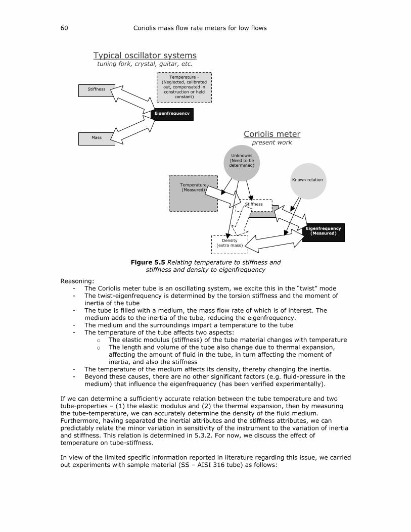
60 Coriolis mass flow rate meters for low flows
Eigenfrequency (Measured)
Density (extra mass)
Stiffness
Temperature (Measured)
Eigenfrequency
Mass
Stiffness
Temperature -
(Neglected, calibrated
out, compensated in construction or held
constant)
Unknowns
(Need to be determined)
Typical oscillator systems tuning fork, crystal, guitar, etc.
Coriolis meter present work
Known relation
Figure 5.5 Relating temperature to stiffness and stiffness and density to eigenfrequency
Reasoning:
- The Coriolis meter tube is an oscillating system, we excite this in the “twist” mode
- The twist-eigenfrequency is determined by the torsion stiffness and the moment of
inertia of the tube
- The tube is filled with a medium, the mass flow rate of which is of interest. The
medium adds to the inertia of the tube, reducing the eigenfrequency.
- The medium and the surroundings impart a temperature to the tube
- The temperature of the tube affects two aspects:
o The elastic modulus (stiffness) of the tube material changes with temperature
o The length and volume of the tube also change due to thermal expansion,
affecting the amount of fluid in the tube, in turn affecting the moment of
inertia, and also the stiffness
- The temperature of the medium affects its density, thereby changing the inertia.
- Beyond these causes, there are no other significant factors (e.g. fluid-pressure in the
medium) that influence the eigenfrequency (has been verified experimentally).
If we can determine a sufficiently accurate relation between the tube temperature and two
tube-properties – (1) the elastic modulus and (2) the thermal expansion, then by measuring
the tube-temperature, we can accurately determine the density of the fluid medium.
Furthermore, having separated the inertial attributes and the stiffness attributes, we can
predictably relate the minor variation in sensitivity of the instrument to the variation of inertia
and stiffness. This relation is determined in 5.3.2. For now, we discuss the effect of
temperature on tube-stiffness.
In view of the limited specific information reported in literature regarding this issue, we carried
out experiments with sample material (SS – AISI 316 tube) as follows:
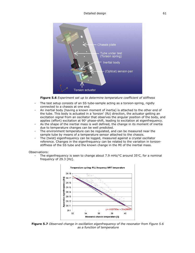
Detailed design 61
Figure 5.6 Experiment set up to determine temperature coefficient of stiffness
- The test setup consists of an SS tube-sample acting as a torsion-spring, rigidly
connected to a chassis at one end.
- An inertial body (having a known moment of inertia) is attached to the other end of
the tube. This body is actuated in a 'torsion' (Rz) direction, the actuator getting an
excitation signal from an oscillator that observes the angular position of the body, and applies (effort) excitation at 90° phase-shift, leading to excitation at eigenfrequency.
- As the shape of the inertial mass is well defined, the change in its moment of inertia
due to temperature changes can be well predicted.
- The environment temperature can be regulated, and can be measured near the
sample tube by means of a temperature sensor attached to the chassis.
- The (twist) eigenfrequency can be logged, measured against a crystal oscillator
reference. Changes in the eigenfrequency can be related to the variation in torsion-
stiffness of the SS tube and the known change in the MI of the inertial mass.
Observations:
- The eigenfrequency is seen to change about 7.9 mHz/°C around 35°C, for a nominal
frequency of 29.3 [Hz].
Figure 5.7 Observed change in oscillation eigenfrequency of the resonator from Figure 5.6 as a function of temperature
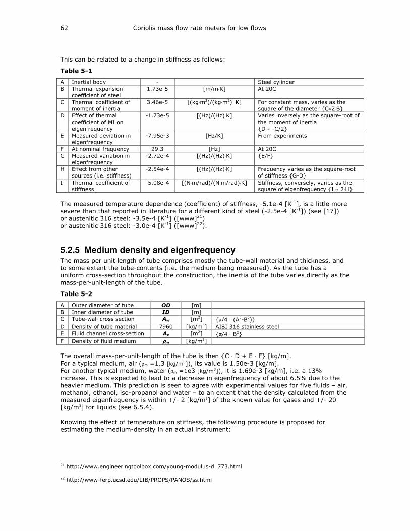
62 Coriolis mass flow rate meters for low flows
This can be related to a change in stiffness as follows:
Table 5-1
A Inertial body - Steel cylinder
B Thermal expansion
coefficient of steel
1.73e-5 [m/m⋅K] At 20C
C Thermal coefficient of
moment of inertia
3.46e-5 [(kg⋅m2)/(kg⋅m2) ⋅K] For constant mass, varies as the
square of the diameter C≈2⋅B
D Effect of thermal
coefficient of MI on
eigenfrequency
-1.73e-5 [(Hz)/(Hz)⋅K] Varies inversely as the square-root of
the moment of inertia
D ≈ -C/2
E Measured deviation in
eigenfrequency
-7.95e-3 [Hz/K] From experiments
F At nominal frequency 29.3 [Hz] At 20C
G Measured variation in
eigenfrequency
-2.72e-4 [(Hz)/(Hz)⋅K] E/F
H Effect from other
sources (i.e. stiffness)
-2.54e-4 [(Hz)/(Hz)⋅K] Frequency varies as the square-root
of stiffness G-D
I Thermal coefficient of
stiffness
-5.08e-4 [(N⋅m/rad)/(N⋅m/rad)⋅K] Stiffness, conversely, varies as the
square of eigenfrequency I ≈ 2⋅H
The measured temperature dependence (coefficient) of stiffness, -5.1e-4 [K-1], is a little more
severe than that reported in literature for a different kind of steel (-2.5e-4 [K-1]) (see [17])
or austenitic 316 steel: -3.5e-4 [K-1] ([www]21)
or austenitic 316 steel: -3.0e-4 [K-1] ([www]22).
5.2.5 Medium density and eigenfrequency The mass per unit length of tube comprises mostly the tube-wall material and thickness, and
to some extent the tube-contents (i.e. the medium being measured). As the tube has a
uniform cross-section throughout the construction, the inertia of the tube varies directly as the
mass-per-unit-length of the tube.
Table 5-2
A Outer diameter of tube OD [m]
B Inner diameter of tube ID [m]
C Tube-wall cross section Aw [m2] π/4 ⋅ (A2-B2)
D Density of tube material 7960 [kg/m3] AISI 316 stainless steel
E Fluid channel cross-section Ac [m2] π/4 ⋅ B2
F Density of fluid medium ρρρρm [kg/m3]
The overall mass-per-unit-length of the tube is then C ⋅ D + E ⋅ F [kg/m].
For a typical medium, air (ρm =1.3 [kg/m3]), its value is 1.50e-3 [kg/m].
For another typical medium, water (ρm =1e3 [kg/m3]), it is 1.69e-3 [kg/m], i.e. a 13%
increase. This is expected to lead to a decrease in eigenfrequency of about 6.5% due to the
heavier medium. This prediction is seen to agree with experimental values for five fluids – air,
methanol, ethanol, iso-propanol and water – to an extent that the density calculated from the
measured eigenfrequency is within +/- 2 [kg/m3] of the known value for gases and +/- 20
[kg/m3] for liquids (see 6.5.4).
Knowing the effect of temperature on stiffness, the following procedure is proposed for
estimating the medium-density in an actual instrument:
21 http://www.engineeringtoolbox.com/young-modulus-d_773.html
22 http://www-ferp.ucsd.edu/LIB/PROPS/PANOS/ss.html
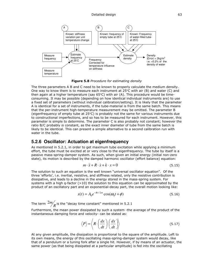
Detailed design 63
Measure frequency
Measure temperature
Estimate frequency at 25’C
Known: frequency of empty tube at 25’C
Known: stiffness variation per unit temperature change
Known: Frequency of water-filled tube at 25’C
Estimate density
Density |Error| < 2kg/m3
i.e. <0.2% of the density of water
A B C
Frequency Corrected for temperature influence on stiffness
Figure 5.8 Procedure for estimating density
The three parameters A B and C need to be known to properly calculate the medium density. One way to know them is to measure each instrument at 25°C with air (B) and water (C) and
then again at a higher temperature (say 65°C) with air (A). This procedure would be time-
consuming. It may be possible (depending on how identical individual instruments are) to use
a fixed set of parameters (without individual calibration/setting). It is likely that the parameter
A is identical for a set of instruments, if the tube-material is from the same batch. This means
that the per-instrument high-temperature measurement may be omitted. The parameter B (eigenfrequency of empty tube at 25°C) is probably not the same for various instruments due
to constructional imperfections, and so has to be measured for each instrument. However, this
parameter is simple to determine. The parameter C is also probably not constant; however the
ratio B/C probably is constant, as the exact inner diameter of tube from the same batch is
likely to be identical. This can present a simple alternative to a second calibration run with
water in the tube.
5.2.6 Oscillator: Actuation at eigenfrequency As mentioned in 5.2.1, in order to get maximum tube excitation while applying a minimum
effort, the tube must be excited at or very close to the eigenfrequency. The tube by itself is a
passive mass-spring-damper system. As such, when given an initial energy (initial non-zero
state), its motion is described by the damped harmonic oscillator (effort balance) equation:
0=⋅+⋅+⋅ xkxRxm &&& (5.15)
The solution to such an equation is the well known “universal oscillator equation”. Of the
three ‘efforts’, i.e. inertial, resistive, and stiffness related, only the resistive contribution is
dissipative, and leads to a decline in the energy stored in the mass-spring system. For
systems with a high q-factor (>10) the solution to this equation can be approximated by the
product of an oscillatory part and an exponential-decay part, the overall motion looking like:
)cos()( 0
2/
0 φω += −teAtx
mRt (5.16)
The term R
m2 is the “decay time constant” mentioned in 5.2.1
Furthermore, the mean power dissipated by such a system -the average of the product of the
instantaneous damping force and velocity- can be stated as:
⋅
⋅=
dt
dx
dt
dxRP (5.17)
At any given amplitude, the dissipation is proportional to the square of the amplitude. Left to
its own means, the energy of this oscillating mass-spring-damper system would decay, like
that of a pendulum or a tuning fork after a single hit. However, if by means of an actuator, the
same power (as that being dissipated at a particular amplitude) is fed into the oscillating
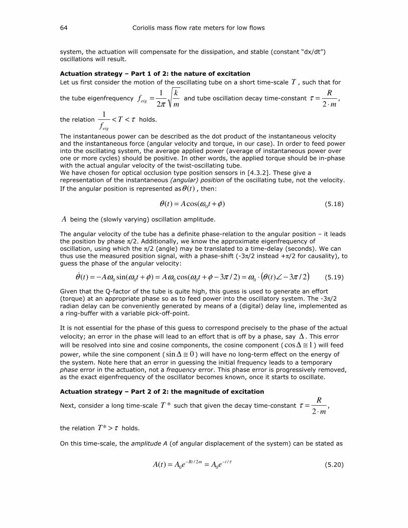
64 Coriolis mass flow rate meters for low flows
system, the actuation will compensate for the dissipation, and stable (constant “dx/dt”)
oscillations will result.
Actuation strategy – Part 1 of 2: the nature of excitation
Let us first consider the motion of the oscillating tube on a short time-scale T , such that for
the tube eigenfrequency m
kfeig
π2
1= and tube oscillation decay time-constant
m
R
⋅=
2τ ,
the relation τ<< Tfeig
1 holds.
The instantaneous power can be described as the dot product of the instantaneous velocity
and the instantaneous force (angular velocity and torque, in our case). In order to feed power
into the oscillating system, the average applied power (average of instantaneous power over
one or more cycles) should be positive. In other words, the applied torque should be in-phase
with the actual angular velocity of the twist-oscillating tube.
We have chosen for optical occlusion type position sensors in [4.3.2]. These give a
representation of the instantaneous (angular) position of the oscillating tube, not the velocity.
If the angular position is represented as )(tθ , then:
)cos()( 0 φωθ += tAt (5.18)
A being the (slowly varying) oscillation amplitude.
The angular velocity of the tube has a definite phase-relation to the angular position – it leads
the position by phase π/2. Additionally, we know the approximate eigenfrequency of
oscillation, using which the π/2 (angle) may be translated to a time-delay (seconds). We can
thus use the measured position signal, with a phase-shift (-3π/2 instead +π/2 for causality), to
guess the phase of the angular velocity:
( )2/3)()2/3cos()sin()( 00000 πθωπφωωφωωθ −∠⋅=−+=+−= ttAtAt& (5.19)
Given that the Q-factor of the tube is quite high, this guess is used to generate an effort (torque) at an appropriate phase so as to feed power into the oscillatory system. The -3π/2
radian delay can be conveniently generated by means of a (digital) delay line, implemented as
a ring-buffer with a variable pick-off-point.
It is not essential for the phase of this guess to correspond precisely to the phase of the actual
velocity; an error in the phase will lead to an effort that is off by a phase, say ∆ . This error
will be resolved into sine and cosine components, the cosine component ( 1cos ≅∆ ) will feed
power, while the sine component ( 0sin ≅∆ ) will have no long-term effect on the energy of
the system. Note here that an error in guessing the initial frequency leads to a temporary
phase error in the actuation, not a frequency error. This phase error is progressively removed,
as the exact eigenfrequency of the oscillator becomes known, once it starts to oscillate.
Actuation strategy – Part 2 of 2: the magnitude of excitation
Next, consider a long time-scale *T such that given the decay time-constant m
R
⋅=
2τ ,
the relation τ>*T holds.
On this time-scale, the amplitude A (of angular displacement of the system) can be stated as
τ/
0
2/
0)( tmRteAeAtA
−− == (5.20)
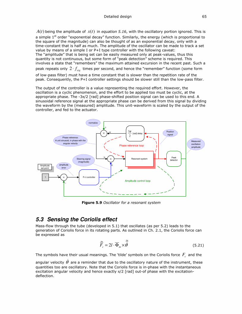
Detailed design 65
)(tA being the amplitude of )(tx in equation 5.16, with the oscillatory portion ignored. This is
a simple 1st order “exponential decay” function. Similarly, the energy (which is proportional to
the square of the magnitude) can also be thought of as an exponential decay, only with a
time-constant that is half as much. The amplitude of the oscillator can be made to track a set
value by means of a simple I or P+I type controller with the following caveat:
The “amplitude” that is being set can be easily measured only at peak-values, thus this
quantity is not continuous, but some form of “peak detection” scheme is required. This
involves a state that “remembers” the maximum attained excursion in the recent past. Such a
peak repeats only eigf⋅2 times per second, and hence the “remember” function (some form
of low-pass filter) must have a time constant that is slower than the repetition rate of the
peak. Consequently, the P+I controller settings should be slower still than the low-pass filter.
The output of the controller is a value representing the required effort. However, the
oscillation is a cyclic phenomenon, and the effort to be applied too must be cyclic, at the appropriate phase. The -3π/2 [rad] phase-shifted position signal can be used to this end. A
sinusoidal reference signal at the appropriate phase can be derived from this signal by dividing
the waveform by the (measured) amplitude. This unit-waveform is scaled by the output of the
controller, and fed to the actuator.
Phase reference loop
Resonant system
+1
Amplitudeset-point
Measured
oscillation
amplitude
P+I controller+
×Peak
detector
[rad] delay
2
3π×
−
÷
×
×
×
Position
signal
normalize
Phase reference:
A unit sinusoid, in phase with the
angular velocity
Amplitude control loop
amplitude
error
Steering signal
(magnitude)
Figure 5.9 Oscillator for a resonant system
5.3 Sensing the Coriolis effect Mass-flow through the tube (developed in 5.1) that oscillates (as per 5.2) leads to the
generation of Coriolis force in its rotating parts. As outlined in Ch. 2.1, the Coriolis force can
be expressed as
θ~
2~
&×Φ⋅= mc lF (5.21)
The symbols have their usual meanings. The ‘tilde’ symbols on the Coriolis force cF and the
angular velocity θ& are a reminder that due to the oscillatory nature of the instrument, these
quantities too are oscillatory. Note that the Coriolis force is in-phase with the instantaneous excitation angular velocity and hence exactly π/2 [rad] out-of phase with the excitation-
deflection.
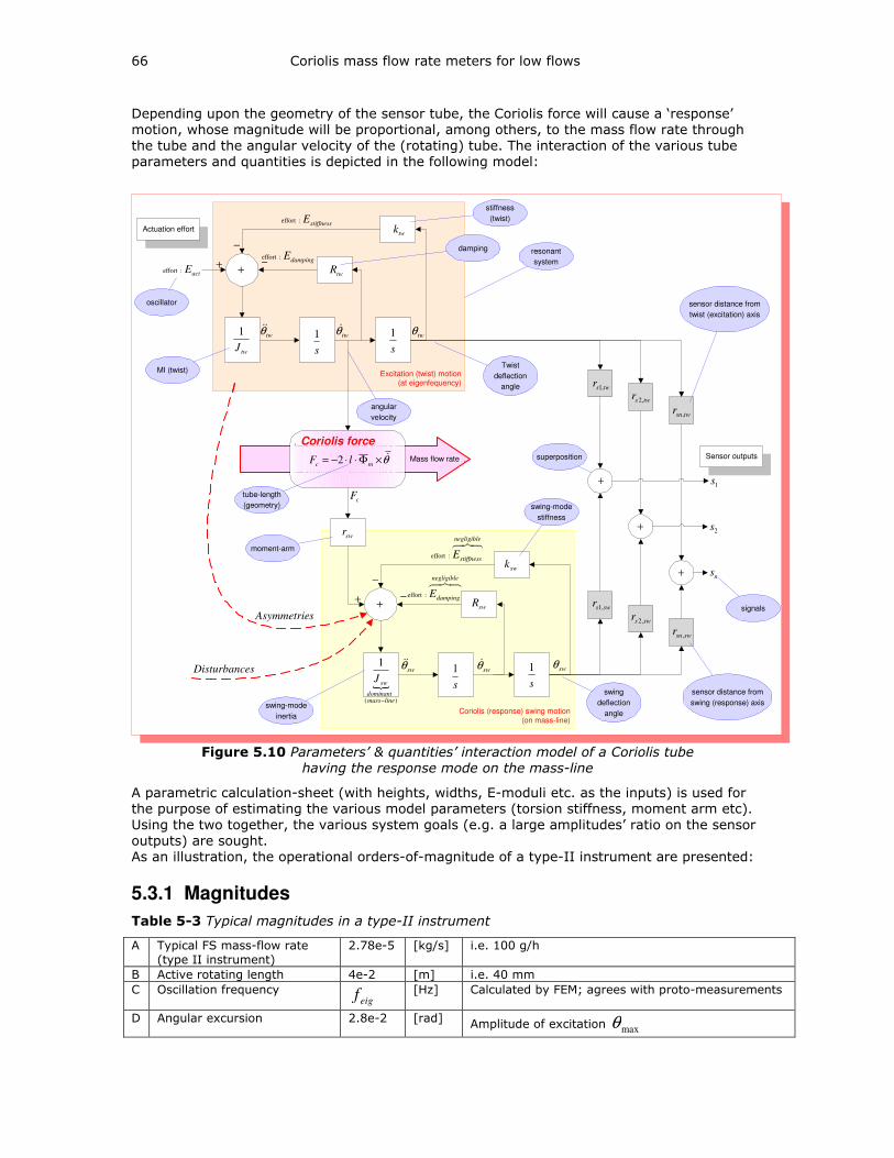
66 Coriolis mass flow rate meters for low flows
Depending upon the geometry of the sensor tube, the Coriolis force will cause a ‘response’
motion, whose magnitude will be proportional, among others, to the mass flow rate through
the tube and the angular velocity of the (rotating) tube. The interaction of the various tube
parameters and quantities is depicted in the following model:
Mass flow rate .
Coriolis (response) swing motion
(on mass-line)
Excitation (twist) motion(at eigenfequency)
actE:effort +
s
1
s
1twθ&& twθ&
twR
twk
twθ
stiffnessE:effort
dampingE:effort
−
−+
twJ
1
. Coriolis force
θ&×Φ⋅⋅−= mc lF 2
cF
+
s
1
s
1swθ&& swθ&
swR
swk
swθ
876negligible
stiffnessE:effort
876negligible
dampingE:effort
−
−+
)(
1
linemassnantdomi
swJ
−
swsr ,1
twsr ,1
+
swsr ,2
twsr ,2
+
swsnr ,
twsnr ,
+
1s
2s
ns
Actuation effort
Sensor outputs
oscillator
MI (twist)
stiffness
(twist)
tube-length
(geometry)
angular
velocity
Twist
deflection
angle
resonant
system
damping
sensor distance from
twist (excitation) axis
sensor distance from
swing (response) axis
signals
swing-mode
inertia
swing-mode
stiffness
swing
deflection
angle
sAsymmetrie
esDisturbanc
superposition
swr
moment-arm
Figure 5.10 Parameters’ & quantities’ interaction model of a Coriolis tube having the response mode on the mass-line
A parametric calculation-sheet (with heights, widths, E-moduli etc. as the inputs) is used for
the purpose of estimating the various model parameters (torsion stiffness, moment arm etc).
Using the two together, the various system goals (e.g. a large amplitudes’ ratio on the sensor
outputs) are sought.
As an illustration, the operational orders-of-magnitude of a type-II instrument are presented:
5.3.1 Magnitudes
Table 5-3 Typical magnitudes in a type-II instrument
A Typical FS mass-flow rate
(type II instrument)
2.78e-5 [kg/s] i.e. 100 g/h
B Active rotating length 4e-2 [m] i.e. 40 mm
C Oscillation frequency eigf
[Hz] Calculated by FEM; agrees with proto-measurements
D Angular excursion 2.8e-2 [rad] Amplitude of excitation maxθ
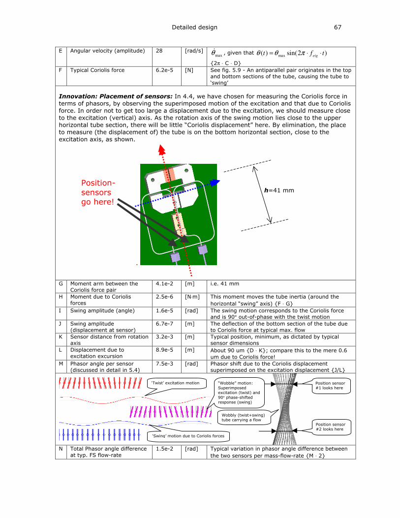
Detailed design 67
E Angular velocity (amplitude) 28 [rad/s] maxθ& , given that )2sin()( max tft eig ⋅⋅= πθθ
2π ⋅ C ⋅ D
F Typical Coriolis force 6.2e-5 [N] See fig. 5.9 - An antiparallel pair originates in the top
and bottom sections of the tube, causing the tube to
‘swing’
Innovation: Placement of sensors: In 4.4, we have chosen for measuring the Coriolis force in
terms of phasors, by observing the superimposed motion of the excitation and that due to Coriolis
force. In order not to get too large a displacement due to the excitation, we should measure close
to the excitation (vertical) axis. As the rotation axis of the swing motion lies close to the upper
horizontal tube section, there will be little “Coriolis displacement” here. By elimination, the place
to measure (the displacement of) the tube is on the bottom horizontal section, close to the
excitation axis, as shown.
.
G Moment arm between the
Coriolis force pair
4.1e-2 [m] i.e. 41 mm
H Moment due to Coriolis
forces
2.5e-6 [N⋅m] This moment moves the tube inertia (around the
horizontal “swing” axis) F ⋅ G
I Swing amplitude (angle) 1.6e-5 [rad] The swing motion corresponds to the Coriolis force
and is 90° out-of-phase with the twist motion
J Swing amplitude
(displacement at sensor)
6.7e-7 [m] The deflection of the bottom section of the tube due
to Coriolis force at typical max. flow
K Sensor distance from rotation
axis
3.2e-3 [m] Typical position, minimum, as dictated by typical
sensor dimensions
L Displacement due to
excitation excursion
8.9e-5 [m] About 90 um D ⋅ K; compare this to the mere 0.6
um due to Coriolis force!
M Phasor angle per sensor
(discussed in detail in 5.4)
7.5e-3 [rad] Phasor shift due to the Coriolis displacement
superimposed on the excitation displacement J/L
N Total Phasor angle difference
at typ. FS flow-rate
1.5e-2 [rad] Typical variation in phasor angle difference between
the two sensors per mass-flow-rate M ⋅ 2
h=41 mm Position-
sensors go here!
‘Swing’ motion due to Coriolis forces
‘Twist’ excitation motion
Position sensor #2 looks here
Position sensor #1 looks here
“Wobble” motion:
Superimposed excitation (twist) and
90° phase-shifted response (swing)
Wobbly (twist+swing) tube carrying a flow
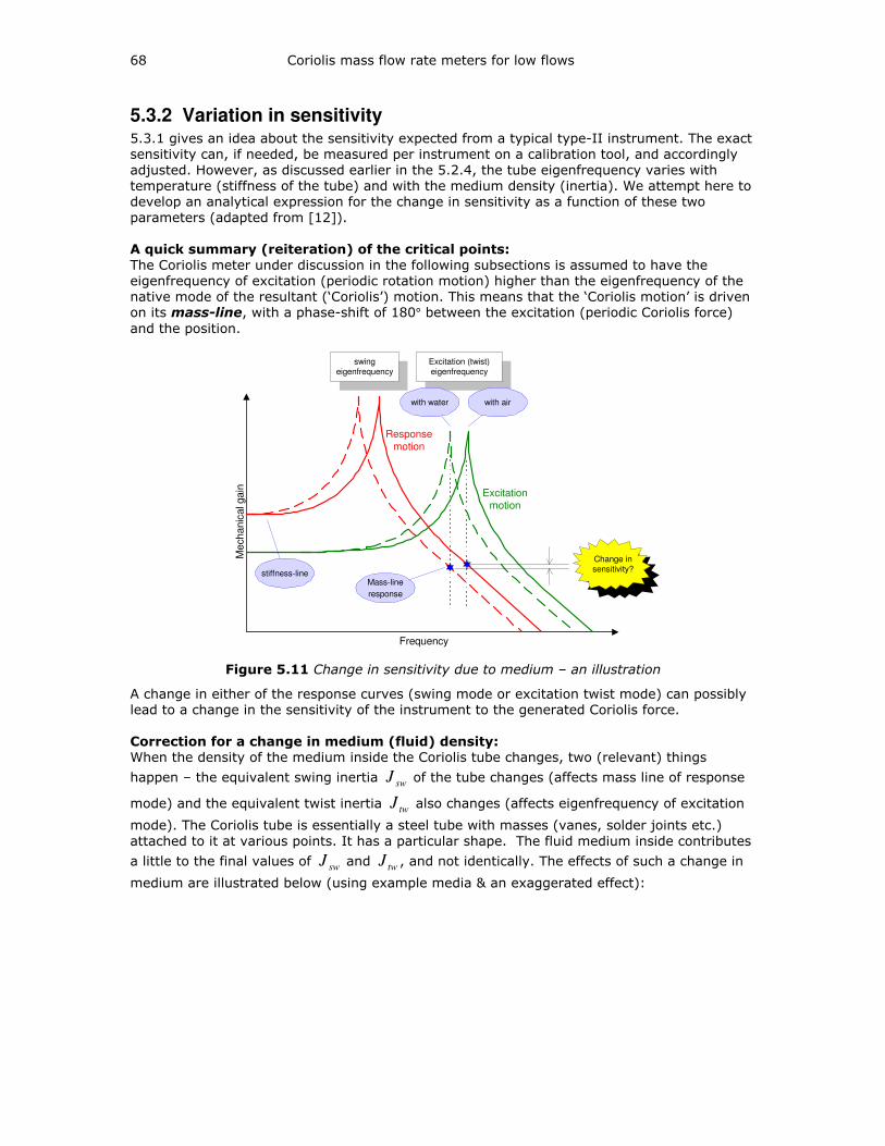
68 Coriolis mass flow rate meters for low flows
5.3.2 Variation in sensitivity 5.3.1 gives an idea about the sensitivity expected from a typical type-II instrument. The exact
sensitivity can, if needed, be measured per instrument on a calibration tool, and accordingly
adjusted. However, as discussed earlier in the 5.2.4, the tube eigenfrequency varies with
temperature (stiffness of the tube) and with the medium density (inertia). We attempt here to
develop an analytical expression for the change in sensitivity as a function of these two
parameters (adapted from [12]).
A quick summary (reiteration) of the critical points:
The Coriolis meter under discussion in the following subsections is assumed to have the
eigenfrequency of excitation (periodic rotation motion) higher than the eigenfrequency of the
native mode of the resultant (‘Coriolis’) motion. This means that the ‘Coriolis motion’ is driven on its mass-line, with a phase-shift of 180° between the excitation (periodic Coriolis force)
and the position.
Excitationmotion
Response
motion
Excitation (twist)eigenfrequency
Mechanic
al gain
Frequency
with water with air
Mass-line
response
stiffness-line
swingeigenfrequency
Change insensitivity?
Figure 5.11 Change in sensitivity due to medium – an illustration
A change in either of the response curves (swing mode or excitation twist mode) can possibly
lead to a change in the sensitivity of the instrument to the generated Coriolis force.
Correction for a change in medium (fluid) density: When the density of the medium inside the Coriolis tube changes, two (relevant) things
happen – the equivalent swing inertia swJ of the tube changes (affects mass line of response
mode) and the equivalent twist inertia twJ also changes (affects eigenfrequency of excitation
mode). The Coriolis tube is essentially a steel tube with masses (vanes, solder joints etc.)
attached to it at various points. It has a particular shape. The fluid medium inside contributes
a little to the final values of swJ and twJ , and not identically. The effects of such a change in
medium are illustrated below (using example media & an exaggerated effect):
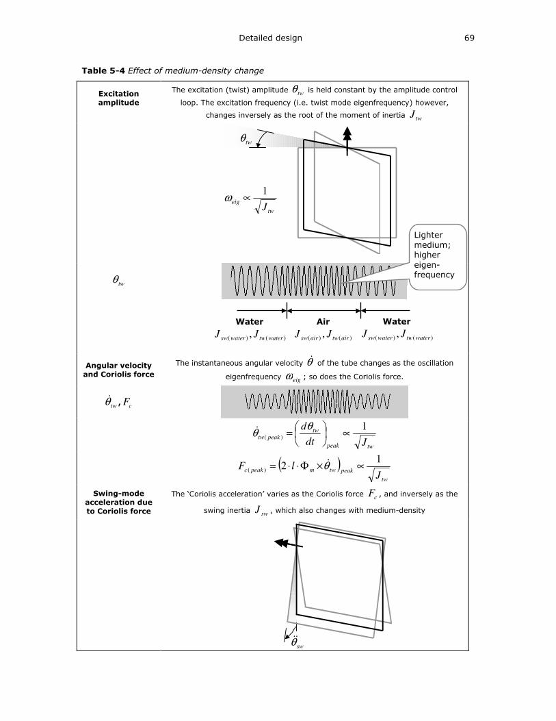
Detailed design 69
Table 5-4 Effect of medium-density change
Excitation
amplitude
The excitation (twist) amplitude twθ is held constant by the amplitude control
loop. The excitation frequency (i.e. twist mode eigenfrequency) however,
changes inversely as the root of the moment of inertia twJ
twθ
tw
eigJ
1∝ω
twθ
Angular velocity
and Coriolis force
The instantaneous angular velocity θ& of the tube changes as the oscillation
eigenfrequency eigω ; so does the Coriolis force.
twθ& , cF
twpeak
twpeaktw
Jdt
d 1)( ∝
=
θθ&
( )tw
peaktwmpeakcJ
lF1
2)( ∝×Φ⋅⋅= θ&
Swing-mode
acceleration due
to Coriolis force
The ‘Coriolis acceleration’ varies as the Coriolis force cF , and inversely as the
swing inertia swJ , which also changes with medium-density
swθ&&
Lighter
medium;
higher
eigen-frequency
Water
)()( , watertwwatersw JJ
Air
)()( , airtwairsw JJ
Water
)()( , watertwwatersw JJ
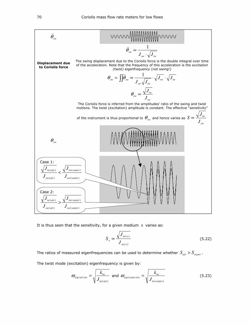
70 Coriolis mass flow rate meters for low flows
swθ&&
twsw
swJJ ⋅
∝1
θ&&
Displacement due
to Coriolis force
The swing displacement due to the Coriolis force is the double integral over time
of the acceleration. Note that the frequency of this acceleration is the excitation (twist) eigenfrequency (not swing!)
twtw
twsw
swsw JJJJ
⋅⋅∝= ∫∫1
θθ &&
sw
tw
swJ
J∝θ
The Coriolis force is inferred from the amplitudes’ ratio of the swing and twist
motions. The twist (excitation) amplitude is constant. The effective “sensitivity”
of the instrument is thus proportional to swθ and hence varies as
sw
tw
J
JS ∝
swθ
It is thus seen that the sensitivity, for a given medium x varies as:
)(
)(
xsw
xtw
xJ
JS ∝ (5.22)
The ratios of measured eigenfrequencies can be used to determine whether waterair SS > .
The twist mode (excitation) eigenfrequency is given by:
)(
)(
airtw
twtwaireig
J
k=ω and
)(
)(
watertw
twtwwatereig
J
k=ω (5.23)
Case 1:
)(
)(
)(
)(
watersw
watertw
airsw
airtw
J
J
J
J<
Case 2:
)(
)(
)(
)(
watersw
watertw
airsw
airtw
J
J
J
J>

Detailed design 71
Of these, if we assume that the torsion stiffness twk remains constant (though unknown) for a
given temperature, and if we accurately measure the twist eigenfrequencies of various modes,
we have:
twwatereig
twaireig
airtw
watertw
J
J
)(
)(
)(
)(
ω
ω= (5.24)
Similarly, it may be shown that the eigenfrequency of the response ‘swing’ mode, for a given
temperature (i.e. constant stiffness) has the relation:
)(
)(
)(
)(
airsw
watersw
swwatereig
swaireig
J
J=
ω
ω (5.25)
in other words,
2
)(
)(
)(
)(
=
swwatereig
swaireig
airsw
watersw
J
J
ω
ω (5.26)
From equations 5.22, 5.24 and 5.26, we may determine the ratio of the instrument
sensitivities for air and water:
)(
)(
)(
)(:
watersw
airsw
watertw
airtw
water
air
J
J
J
J
S
S= =
2
)(
)(
)(
)(:
swaireig
swwatereig
twaireig
twwatereig
ω
ω
ω
ω (5.27)
For any given medium, the swing and twist eigenfrequencies vary as a function of the density.
This function can be determined from two measurements with reference media (say air and
water) at the time of calibration. During operation, the medium density can be calculated
based upon the twist (excitation) eigenfrequency and the tube temperature (both of which can
be directly measured), as discussed in 5.2.4 and 5.2.5. Now, using the measured relation, the
swing eigenfrequency can be determined from the calculated density. The two
eigenfrequencies (twist and swing) can be used to predict the change in sensitivity of the
instrument as a consequence of a change in medium density as per Eq. 5.27.
In Ch. 6.5, we show that data measured from a prototype setup agree with the expected
sensitivity variations.
Correction for change in sensitivity due to temperature variations:
By the similar arguments as in Table 5-4, the expected change in sensitivity due to the
temperature variation (change in stiffness) may be calculated. However, there is only one
variable (torsion stiffness) that affects the sensitivity, as the Coriolis response lies on the
mass line of the response (swing) mode (and thus a change in swing-stiffness has no effect).
Let us consider an example where:
1. The temperature increases, thus the excitation mode (torsion) stiffness decreases.
2. The eigenfrequency decreases as the inverse square root of stiffness, as does the
Coriolis force, for the same actual mass flow (and medium). 3. Although the Coriolis force decreases, the period for each cycle (1/2πωeig) increases. As
a combined effect, the displacement (which is the double integral of acceleration
caused by the Coriolis force) increases as the period.
)(
)(
1
Teig
TSω
∝ (5.28)
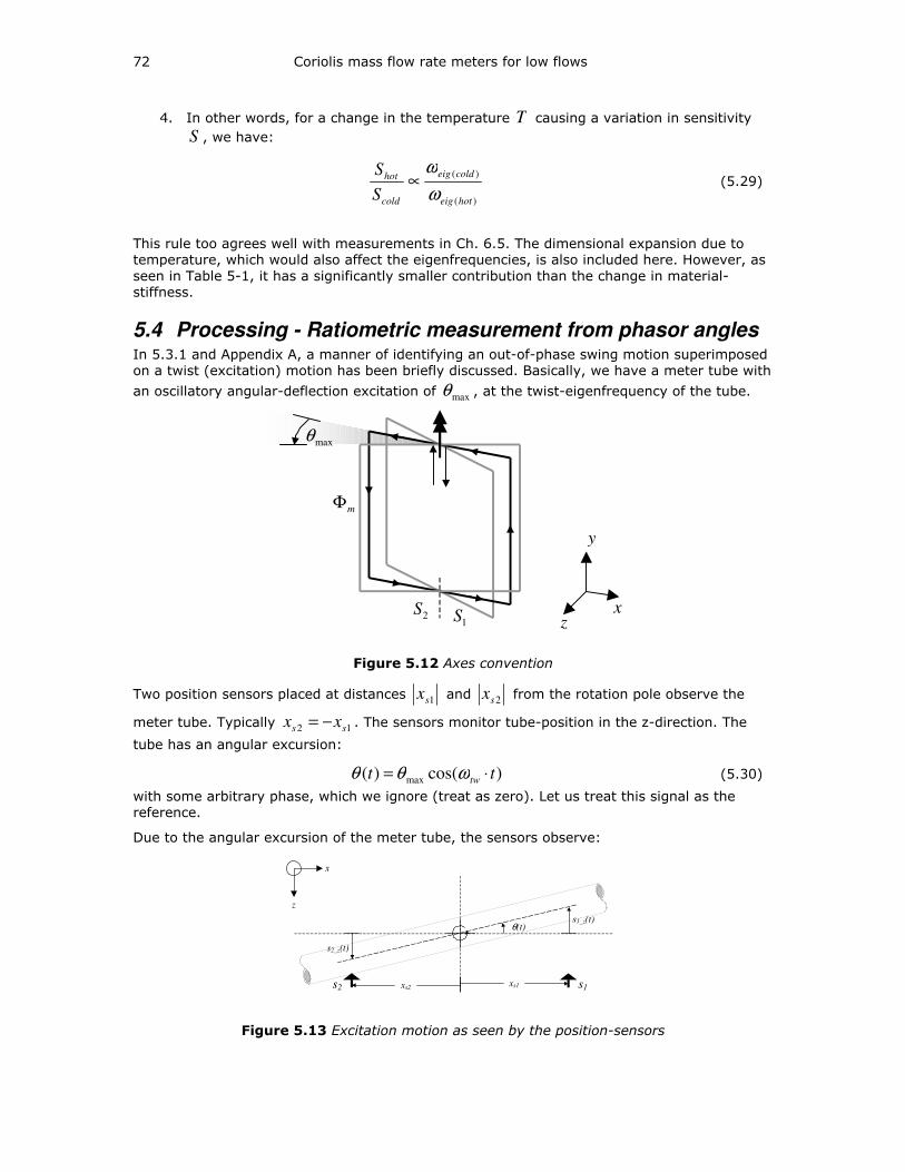
72 Coriolis mass flow rate meters for low flows
4. In other words, for a change in the temperature T causing a variation in sensitivity
S , we have:
)(
)(
hoteig
coldeig
cold
hot
S
S
ω
ω∝ (5.29)
This rule too agrees well with measurements in Ch. 6.5. The dimensional expansion due to
temperature, which would also affect the eigenfrequencies, is also included here. However, as
seen in Table 5-1, it has a significantly smaller contribution than the change in material-
stiffness.
5.4 Processing - Ratiometric measurement from phasor angles In 5.3.1 and Appendix A, a manner of identifying an out-of-phase swing motion superimposed
on a twist (excitation) motion has been briefly discussed. Basically, we have a meter tube with
an oscillatory angular-deflection excitation of maxθ , at the twist-eigenfrequency of the tube.
maxθ
x z
y
2S
1S
mΦ
Figure 5.12 Axes convention
Two position sensors placed at distances 1sx and 2sx from the rotation pole observe the
meter tube. Typically 12 ss xx −= . The sensors monitor tube-position in the z-direction. The
tube has an angular excursion:
)cos()( max tt tw ⋅= ωθθ (5.30)
with some arbitrary phase, which we ignore (treat as zero). Let us treat this signal as the
reference.
Due to the angular excursion of the meter tube, the sensors observe:
xs1
s1_z(t)
xs2
s2_z(t)
θ(t)
s2 s1
x
z
Figure 5.13 Excitation motion as seen by the position-sensors
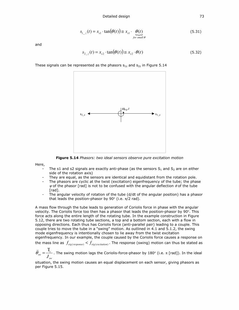
Detailed design 73
( )
θ
θθsmallfor
ssz txtxts )()(tan)( 11_1 ⋅≅⋅= (5.31)
and
( ) )()(tan)( 22_2 txtxts ssz θθ ⋅≅⋅= (5.32)
These signals can be represented as the phasors s1z and s2z in Figure 5.14
s1_z s2_z
ωeig.t
Figure 5.14 Phasors: two ideal sensors observe pure excitation motion
Here,
- The s1 and s2 signals are exactly anti-phase (as the sensors S1 and S2 are on either
side of the rotation axis)
- They are equal, as the sensors are identical and equidistant from the rotation pole.
- The phasors are cyclic at the twist (excitation) eigenfrequency of the tube; the phase
ψ of the phasor [rad] is not to be confused with the angular deflection θ of the tube
[rad].
- The angular velocity of rotation of the tube (d/dt of the angular position) has a phasor that leads the position-phasor by 90° (i.e. π/2 rad).
A mass flow through the tube leads to generation of Coriolis force in phase with the angular velocity. The Coriolis force too then has a phasor that leads the position-phasor by 90°. This
force acts along the entire length of the rotating tube. In the example construction in Figure
5.12, there are two rotating tube sections, a top and a bottom section, each with a flow in
opposing directions. Each thus has Coriolis force (anti-parallel pair) leading to a couple. This
couple tries to move the tube in a “swing” motion. As outlined in 4.1 and 5.1.2, the swing
mode eigenfrequency is intentionally chosen to lie away from the twist excitation
eigenfrequency. In our example, the couple caused by the Coriolis force causes a response on
the mass line as )()( excitationeigresponseeig ff < . The response (swing) motion can thus be stated as
sw
csw
J
Τ=θ&& . The swing motion lags the Coriolis-force-phasor by 180° (i.e. π [rad]). In the ideal
situation, the swing motion causes an equal displacement on each sensor, giving phasors as
per Figure 5.15.
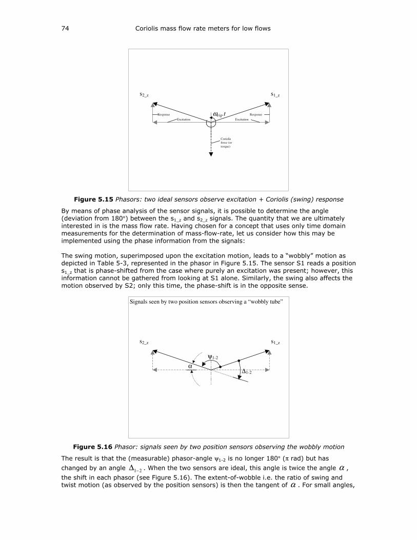
74 Coriolis mass flow rate meters for low flows
s1_z s2_z
ωeig.t Excitation Excitation
Response Response
Coriolis
force (or
torque)
Figure 5.15 Phasors: two ideal sensors observe excitation + Coriolis (swing) response
By means of phase analysis of the sensor signals, it is possible to determine the angle
(deviation from 180°) between the s1_z and s2_z signals. The quantity that we are ultimately
interested in is the mass flow rate. Having chosen for a concept that uses only time domain
measurements for the determination of mass-flow-rate, let us consider how this may be
implemented using the phase information from the signals:
The swing motion, superimposed upon the excitation motion, leads to a “wobbly” motion as
depicted in Table 5-3, represented in the phasor in Figure 5.15. The sensor S1 reads a position
s1_z that is phase-shifted from the case where purely an excitation was present; however, this
information cannot be gathered from looking at S1 alone. Similarly, the swing also affects the
motion observed by S2; only this time, the phase-shift is in the opposite sense.
s1_z s2_z
Signals seen by two position sensors observing a “wobbly tube”
α ∆1-2
ψ1-2
Figure 5.16 Phasor: signals seen by two position sensors observing the wobbly motion
The result is that the (measurable) phasor-angle ψ1-2 is no longer 180° (π rad) but has
changed by an angle 21−∆ . When the two sensors are ideal, this angle is twice the angle α ,
the shift in each phasor (see Figure 5.16). The extent-of-wobble i.e. the ratio of swing and twist motion (as observed by the position sensors) is then the tangent of α . For small angles,
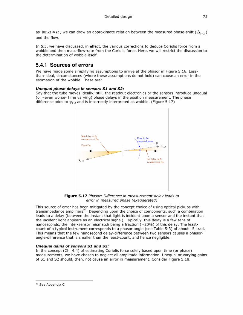
Detailed design 75
as αα ≈tan , we can draw an approximate relation between the measured phase-shift ( 21−∆ )
and the flow.
In 5.3, we have discussed, in effect, the various corrections to deduce Coriolis force from a
wobble and then mass-flow-rate from the Coriolis force. Here, we will restrict the discussion to
the determination of wobble itself.
5.4.1 Sources of errors We have made some simplifying assumptions to arrive at the phasor in Figure 5.16. Less-
than-ideal, circumstances (where these assumptions do not hold) can cause an error in the
estimation of the wobble. These are:
Unequal phase delays in sensors S1 and S2:
Say that the tube moves ideally; still, the readout electronics or the sensors introduce unequal
(or –even worse- time varying) phase delays in the position measurement. The phase difference adds to ψ1-2 and is incorrectly interpreted as wobble. (Figure 5.17)
s1_z
s2_z
Error in the
measured phase
Net delay on S1
measurement DS1
Net delay on S2
measurement DS2
DS2 ≠ DS1
Figure 5.17 Phasor: Difference in measurement-delay leads to error in measured phase (exaggerated)
This source of error has been mitigated by the concept choice of using optical pickups with
transimpedance amplifiers23. Depending upon the choice of components, such a combination
leads to a delay (between the instant that light is incident upon a sensor and the instant that
the incident light appears as an electrical signal). Typically, this delay is a few tens of
nanoseconds, the inter-sensor mismatch being a fraction (~20%) of this delay. The least-count of a typical instrument corresponds to a phasor angle (see Table 5-3) of about 15 µrad.
This means that the few nanosecond delay-difference between two sensors causes a phasor-
angle-difference that is smaller than the least-count, and hence negligible.
Unequal gains of sensors S1 and S2:
In the concept (Ch. 4.4) of estimating Coriolis force solely based upon time (or phase)
measurements, we have chosen to neglect all amplitude information. Unequal or varying gains
of S1 and S2 should, then, not cause an error in measurement. Consider Figure 5.18.
23 See Appendix C
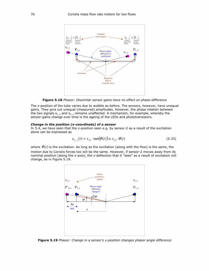
76 Coriolis mass flow rate meters for low flows
s1_z
s2_z
Phasor-angle-
difference is
unaffected
P2_z P1_z
Actuation
Response
Due to
Coriolis force
PositionActual
z
signalMeasured
z Ps _2_2 >
PositionActual
z
signalMeasured
z Ps _1_1 <
Unequal
sensor-gains
Figure 5.18 Phasor: Dissimilar sensor gains have no effect on phase-difference
The z-position of the tube varies due to wobble as before. The sensors, however, have unequal
gains. They give out unequal (measured) amplitudes. However, the phase relation between
the two signals s1_z and s2_z remains unaffected. A mechanism, for example, whereby the
sensor-gains change over time is the ageing of the LEDs and phototransistors.
Change in the position (x-coordinate) of a sensor
In 5.4, we have seen that the z-position seen e.g. by sensor-2 as a result of the excitation
alone can be expressed as
( ) )()(tan)( 22_2 txtxts ssz θθ ⋅≅⋅= (5.33)
where )(tθ is the excitation. As long as the excitation (along with the flow) is the same, the
motion due to Coriolis forces too will be the same. However, if sensor-2 moves away from its
nominal position (along the x-axis), the z-deflection that it “sees” as a result of excitation will
change, as in Figure 5.19.
s1_z s2_z
P2_z P1_z
Sensor
position is
shifted
P’2_z Phasor-angle-
difference
changes!!
Shift
ψ∆
x∆
ψ
x
Figure 5.19 Phasor: Change in a sensor’s x-position changes phasor angle difference
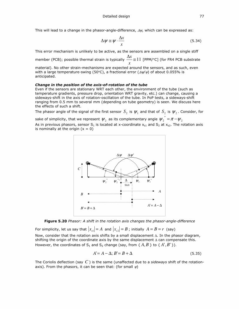
Detailed design 77
This will lead to a change in the phasor-angle-difference, ∆ψ, which can be expressed as:
x
x∆⋅≅∆ ψψ (5.34)
This error mechanism is unlikely to be active, as the sensors are assembled on a single stiff
member (PCB); possible thermal strain is typically 11≅∆
x
x [PPM/°C] (for FR4 PCB substrate
material). No other strain-mechanisms are expected around the sensors, and as such, even
with a large temperature-swing (50°C), a fractional error (∆ψ/ψ) of about 0.055% is
anticipated.
Change in the position of the axis-of-rotation of the tube
Even if the sensors are stationary WRT each other, the environment of the tube (such as
temperature gradients, pressure drop, orientation WRT gravity, etc.) can change, causing a
sideways-shift in the axis of rotation-oscillation of the tube. In PoP tests, a sideways-shift
ranging from 0.5 mm to several mm (depending on tube geometry) is seen. We discuss here
the effects of such a shift.
The phasor angle of the signal of the first sensor 2S is 1ψ and that of 2S is 2ψ . Consider, for
sake of simplicity, that we represent 2ψ as its complementary angle 2
*
2 ψπψ −=
As in previous phasors, sensor S1 is located at x-coordinate xs1 and S2 at xs2. The rotation axis
is nominally at the origin (x = 0)
Shift
ψ∆
C
1ψ∆
'ψ∆
'1ψ*
2ψ '*
2ψ
∆−= AA'∆+= BB'
BA
Figure 5.20 Phasor: A shift in the rotation axis changes the phasor-angle-difference
For simplicity, let us say that Axs =1 and Bxs =2 ; initially rBA == (say)
Now, consider that the rotation axis shifts by a small displacement ∆. In the phasor diagram,
shifting the origin of the coordinate axis by the same displacement ∆ can compensate this.
However, the coordinates of S1 and S2 change (say, from BA, to ',' BA ).
∆+=∆−= BBAA ';' (5.35)
The Coriolis deflection (say C ) is the same (unaffected due to a sideways shift of the rotation-
axis). From the phasors, it can be seen that: (for small ψ)
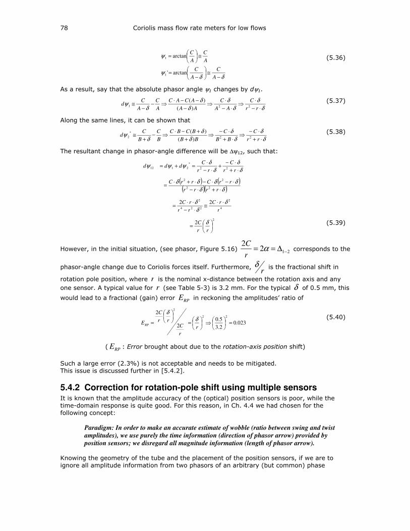
78 Coriolis mass flow rate meters for low flows
δδψ
ψ
−≅
−=
≅
=
A
C
A
C
A
C
A
C
arctan'
arctan
1
1 (5.36)
As a result, say that the absolute phasor angle ψ1 changes by dψ1.
δ
δ
δ
δ
δ
δ
δψ
⋅−
⋅⇒
⋅−
⋅⇒
−
−−⋅⇒−
−≅
rr
C
AA
C
AA
ACAC
A
C
A
Cd
221)(
)( (5.37)
Along the same lines, it can be shown that
δ
δ
δ
δ
δ
δ
δψ
⋅+
⋅−⇒
⋅+
⋅−⇒
+
+−⋅⇒−
+≅
rr
C
BB
C
BB
BCBC
B
C
B
Cd
22
*
2)(
)( (5.38)
The resultant change in phasor-angle difference will be ∆ψ12, such that:
δ
δ
δ
δψψψ
⋅+
⋅−+
⋅−
⋅=+=
rr
C
rr
Cddd
22
*
2112
( ) ( )( )( )δδ
δδδδ
⋅+⋅−
⋅−⋅−⋅+⋅=
rrrr
rrCrrC22
22
4
2
224
2 22
r
rC
rr
rC δ
δ
δ ⋅⋅≅
⋅−
⋅⋅=
2
2
=
rr
C δ (5.39)
However, in the initial situation, (see phasor, Figure 5.16) 2122
−∆== αr
C corresponds to the
phasor-angle change due to Coriolis forces itself. Furthermore, r
δ is the fractional shift in
rotation pole position, where r is the nominal x-distance between the rotation axis and any
one sensor. A typical value for r (see Table 5-3) is 3.2 mm. For the typical δ of 0.5 mm, this
would lead to a fractional (gain) error RPE in reckoning the amplitudes’ ratio of
023.0
2.3
5.0
2
222
2
=
⇒
=
=r
r
Crr
C
ERP
δδ
(5.40)
( RPE : Error brought about due to the rotation-axis position shift)
Such a large error (2.3%) is not acceptable and needs to be mitigated. This issue is discussed further in [5.4.2].
5.4.2 Correction for rotation-pole shift using multiple sensors It is known that the amplitude accuracy of the (optical) position sensors is poor, while the
time-domain response is quite good. For this reason, in Ch. 4.4 we had chosen for the
following concept:
Paradigm: In order to make an accurate estimate of wobble (ratio between swing and twist
amplitudes), we use purely the time information (direction of phasor arrow) provided by
position sensors; we disregard all magnitude information (length of phasor arrow).
Knowing the geometry of the tube and the placement of the position sensors, if we are to
ignore all amplitude information from two phasors of an arbitrary (but common) phase
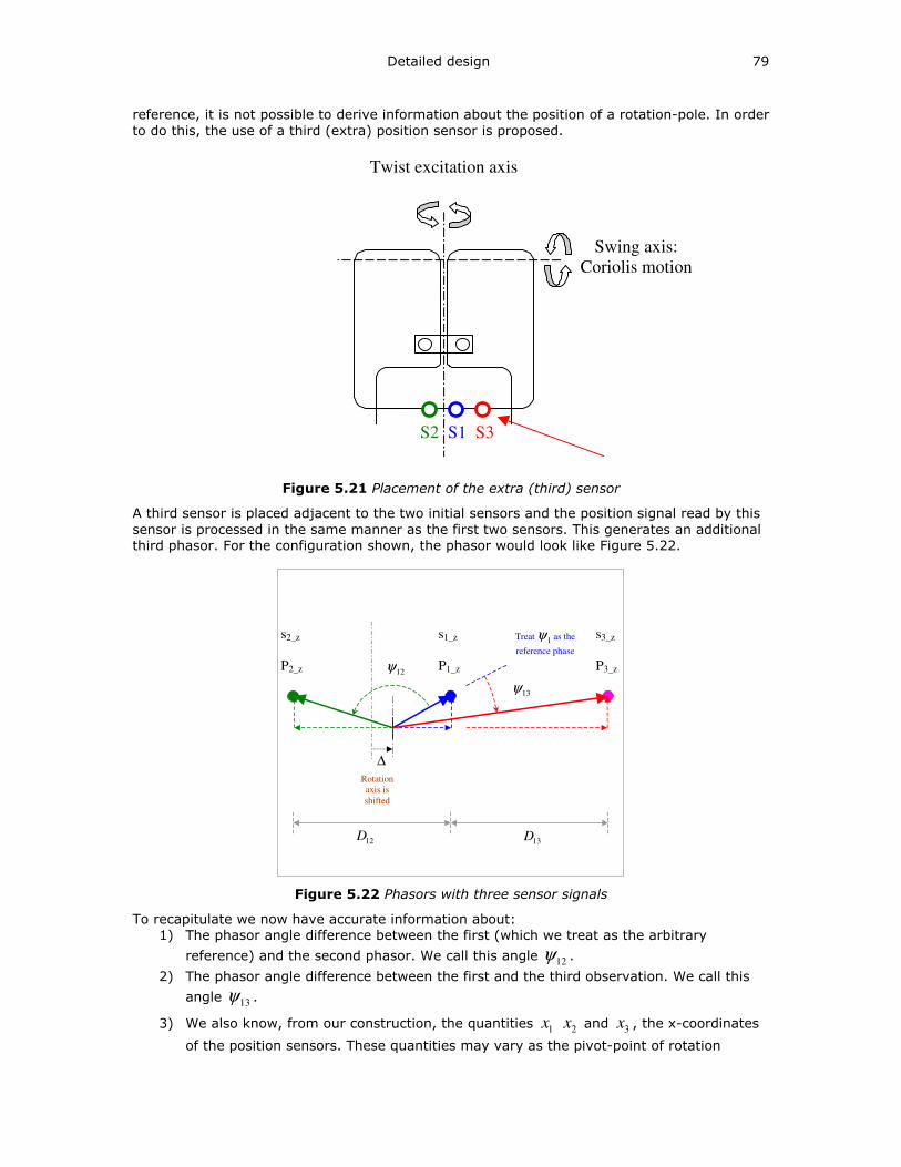
Detailed design 79
reference, it is not possible to derive information about the position of a rotation-pole. In order
to do this, the use of a third (extra) position sensor is proposed.
Twist excitation axis
Swing axis:
Coriolis motion
S2 S1 S3
Figure 5.21 Placement of the extra (third) sensor
A third sensor is placed adjacent to the two initial sensors and the position signal read by this
sensor is processed in the same manner as the first two sensors. This generates an additional
third phasor. For the configuration shown, the phasor would look like Figure 5.22.
s1_z s2_z
P2_z P1_z
Rotation
axis is
shifted
Treat 1ψ as the
reference phase
12ψ
∆
s3_z
P3_z
13ψ
12D 13D
Figure 5.22 Phasors with three sensor signals
To recapitulate we now have accurate information about:
1) The phasor angle difference between the first (which we treat as the arbitrary
reference) and the second phasor. We call this angle 12ψ .
2) The phasor angle difference between the first and the third observation. We call this
angle 13ψ .
3) We also know, from our construction, the quantities 1x 2x and 3x , the x-coordinates
of the position sensors. These quantities may vary as the pivot-point of rotation
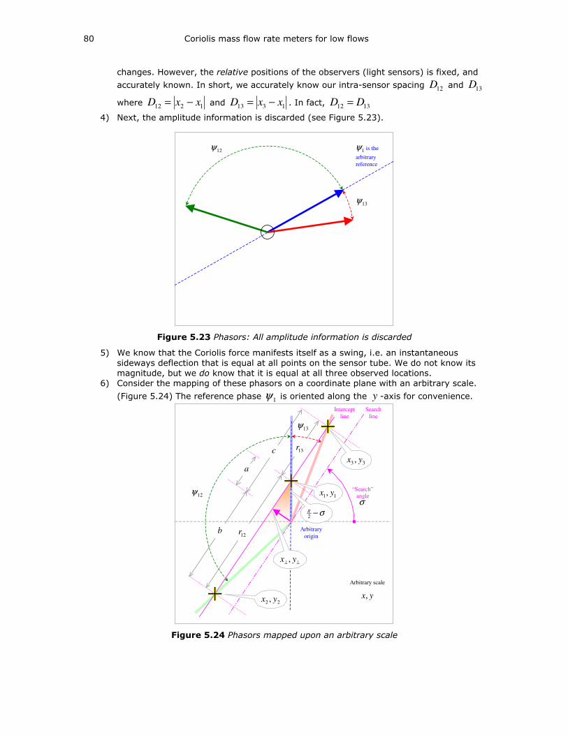
80 Coriolis mass flow rate meters for low flows
changes. However, the relative positions of the observers (light sensors) is fixed, and
accurately known. In short, we accurately know our intra-sensor spacing 12D and 13D
where 1212 xxD −= and 1313 xxD −= . In fact, 1312 DD =
4) Next, the amplitude information is discarded (see Figure 5.23).
1ψ is the
arbitrary
reference
12ψ
13ψ
Figure 5.23 Phasors: All amplitude information is discarded
5) We know that the Coriolis force manifests itself as a swing, i.e. an instantaneous
sideways deflection that is equal at all points on the sensor tube. We do not know its
magnitude, but we do know that it is equal at all three observed locations.
6) Consider the mapping of these phasors on a coordinate plane with an arbitrary scale.
(Figure 5.24) The reference phase 1ψ is oriented along the y -axis for convenience.
12ψ
13ψ
Arbitrary
origin
“Search”
angle
σ
12r
13r
11, yx
22 , yx
33 , yx
Arbitrary scale
yx,
b
c
a
σπ −2
⊥⊥ yx ,
Search
line
Intercept
line
Figure 5.24 Phasors mapped upon an arbitrary scale
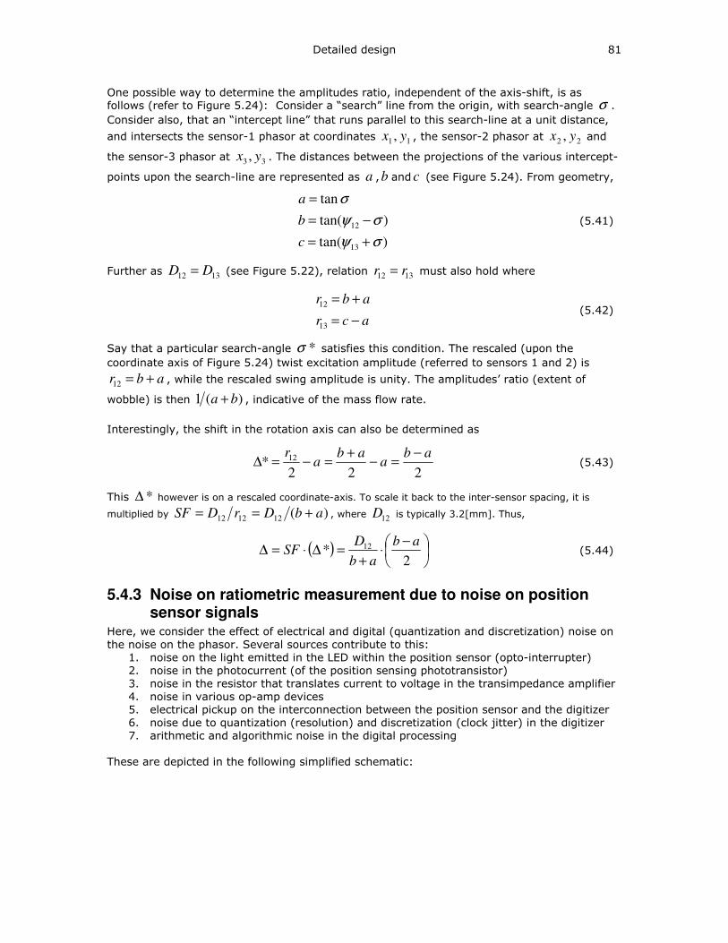
Detailed design 81
One possible way to determine the amplitudes ratio, independent of the axis-shift, is as follows (refer to Figure 5.24): Consider a “search” line from the origin, with search-angle σ .
Consider also, that an “intercept line” that runs parallel to this search-line at a unit distance,
and intersects the sensor-1 phasor at coordinates 11 , yx , the sensor-2 phasor at 22 , yx and
the sensor-3 phasor at 33 , yx . The distances between the projections of the various intercept-
points upon the search-line are represented as a ,b and c (see Figure 5.24). From geometry,
)tan(
)tan(
tan
13
12
σψ
σψ
σ
+=
−=
=
c
b
a
(5.41)
Further as 1312 DD = (see Figure 5.22), relation 1312 rr = must also hold where
acr
abr
−=
+=
13
12 (5.42)
Say that a particular search-angle *σ satisfies this condition. The rescaled (upon the
coordinate axis of Figure 5.24) twist excitation amplitude (referred to sensors 1 and 2) is
abr +=12 , while the rescaled swing amplitude is unity. The amplitudes’ ratio (extent of
wobble) is then )(1 ba + , indicative of the mass flow rate.
Interestingly, the shift in the rotation axis can also be determined as
222
* 12 aba
aba
r −=−
+=−=∆ (5.43)
This *∆ however is on a rescaled coordinate-axis. To scale it back to the inter-sensor spacing, it is
multiplied by )(121212 abDrDSF +== , where 12D is typically 3.2[mm]. Thus,
( )
−⋅
+=∆⋅=∆
2* 12 ab
ab
DSF (5.44)
5.4.3 Noise on ratiometric measurement due to noise on position sensor signals
Here, we consider the effect of electrical and digital (quantization and discretization) noise on
the noise on the phasor. Several sources contribute to this:
1. noise on the light emitted in the LED within the position sensor (opto-interrupter)
2. noise in the photocurrent (of the position sensing phototransistor)
3. noise in the resistor that translates current to voltage in the transimpedance amplifier
4. noise in various op-amp devices
5. electrical pickup on the interconnection between the position sensor and the digitizer
6. noise due to quantization (resolution) and discretization (clock jitter) in the digitizer
7. arithmetic and algorithmic noise in the digital processing
These are depicted in the following simplified schematic:
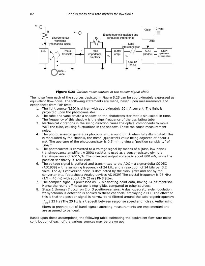
82 Coriolis mass flow rate meters for low flows
LED Photo-transistor
Trans-impedance amplifier
Buffer ampl.
iq
il
vo
vl
vb
ADC (Codec)
DSP: quadrature
demodulation
vcc Rl
Rs
Ground noise
Clock Crystal
Jitter
Tube + vane
Long interconnection
Environmental vibrations
(mechanical noise)
Electromagnetic radiated and conducted interference
Figure 5.25 Various noise sources in the sensor signal-chain
The noise from each of the sources depicted in Figure 5.25 can be approximately expressed as
equivalent flow-noise. The following statements are made, based upon measurements and
experiences from PoP tests:
1. The light source (LED) is driven with approximately 20 mA current. The light is
projected upon the phototransistor.
2. The tube and vane create a shadow on the phototransistor that is sinusoidal in time.
The frequency of this shadow is the eigenfrequency of the oscillating tube.
3. Mechanical vibrations in the swing direction cause the optical components to move
WRT the tube, causing fluctuations in the shadow. These too cause measurement
noise.
4. The phototransistor generates photocurrent, around 8 mA when fully illuminated. This
is modulated by the shadow, the mean (quiescent) value being adjusted at about 4
mA. The aperture of the phototransistor is 0.5 mm, giving a “position sensitivity” of
16A/m
5. The photocurrent is converted to a voltage signal by means of a (fast, low-noise) transimpedance amplifier. A 200Ω resistor is used as a sense-resistor, giving a
transimpedance of 200 V/A. The quiescent output voltage is about 800 mV, while the
position sensitivity is 3200 V/m.
6. The voltage signal is buffered and transmitted to the ADC – a sigma-delta CODEC
(AD1939) with a sampling frequency of 24 kHz and a resolution of 24 bits per 3.2
volts. The A/D conversion noise is dominated by the clock-jitter and not by the
converter bits. [datasheet: Analog devices AD1939] The crystal frequency is 25 MHz
(1/f = 40 ns) with about 5% (2 ns) RMS jitter.
7. The sampled signal is processed as 32-bit floating-point data, having 24-bit mantissa.
Hence the round-off noise too is negligible, compared to other sources.
8. Steps 1 through 7 occur on 2 or 3 position-sensors. A dual-quadrature-demodulation
w/ synchronous detection is applied to these channels, employing a PLL. The effect of
this is that the position signal is narrow-band filtered around the tube-eigenfrequency:
eigf ± 25 Hz (The 25 Hz is a tradeoff between response speed and noise). Antialiasing
filters to prevent out-of-band signals affecting measurements are implemented and
are assumed to be ideal.
Based upon these assumptions, the following table estimating the equivalent flow-rate noise
contribution of each of the various sources may be drawn up:
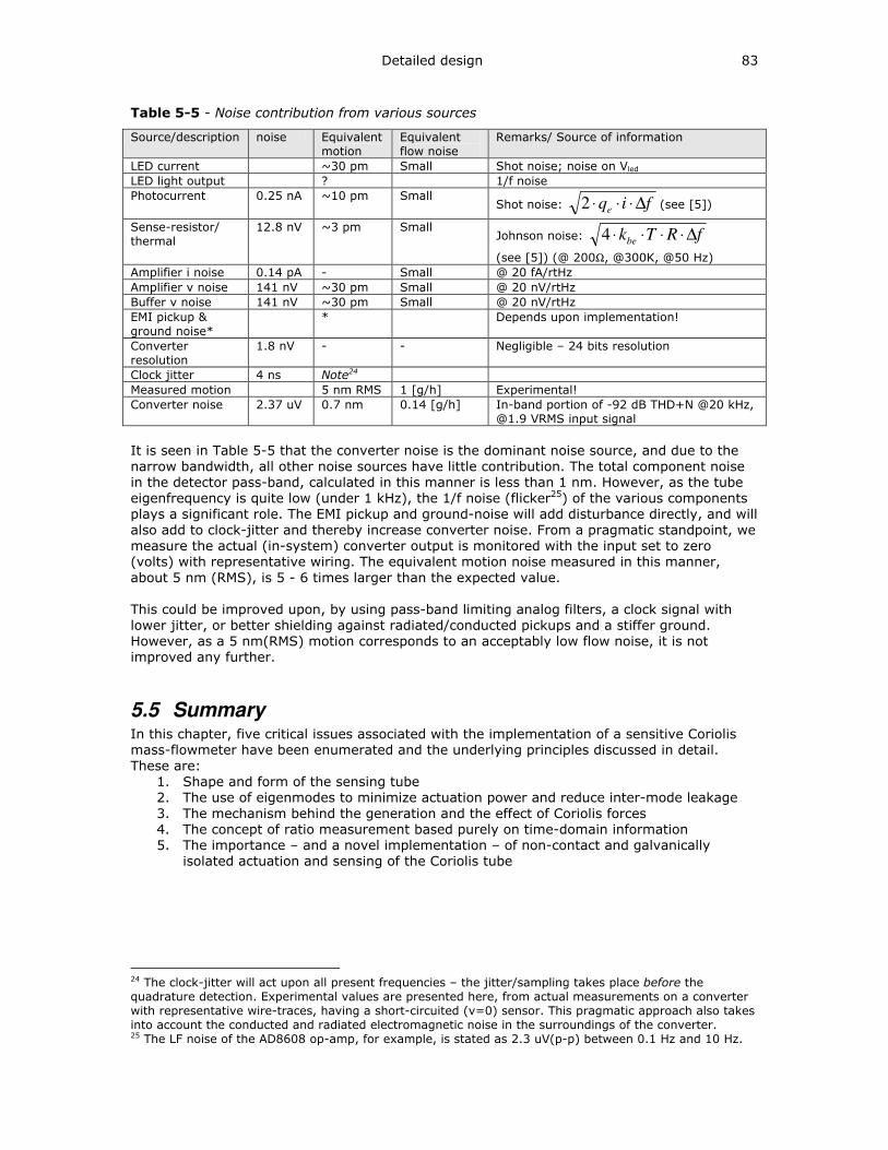
Detailed design 83
Table 5-5 - Noise contribution from various sources
Source/description noise Equivalent
motion
Equivalent
flow noise
Remarks/ Source of information
LED current ~30 pm Small Shot noise; noise on Vled
LED light output ? 1/f noise
Photocurrent 0.25 nA ~10 pm Small Shot noise: fiqe ∆⋅⋅⋅2 (see [5])
Sense-resistor/
thermal
12.8 nV ~3 pm Small Johnson noise: fRTkbe ∆⋅⋅⋅⋅4
(see [5]) (@ 200Ω, @300K, @50 Hz)
Amplifier i noise 0.14 pA - Small @ 20 fA/rtHz
Amplifier v noise 141 nV ~30 pm Small @ 20 nV/rtHz
Buffer v noise 141 nV ~30 pm Small @ 20 nV/rtHz
EMI pickup &
ground noise*
* Depends upon implementation!
Converter
resolution
1.8 nV - - Negligible – 24 bits resolution
Clock jitter 4 ns Note24
Measured motion 5 nm RMS 1 [g/h] Experimental!
Converter noise 2.37 uV 0.7 nm 0.14 [g/h] In-band portion of -92 dB THD+N @20 kHz,
@1.9 VRMS input signal
It is seen in Table 5-5 that the converter noise is the dominant noise source, and due to the
narrow bandwidth, all other noise sources have little contribution. The total component noise
in the detector pass-band, calculated in this manner is less than 1 nm. However, as the tube
eigenfrequency is quite low (under 1 kHz), the 1/f noise (flicker25) of the various components
plays a significant role. The EMI pickup and ground-noise will add disturbance directly, and will
also add to clock-jitter and thereby increase converter noise. From a pragmatic standpoint, we
measure the actual (in-system) converter output is monitored with the input set to zero
(volts) with representative wiring. The equivalent motion noise measured in this manner,
about 5 nm (RMS), is 5 - 6 times larger than the expected value.
This could be improved upon, by using pass-band limiting analog filters, a clock signal with
lower jitter, or better shielding against radiated/conducted pickups and a stiffer ground.
However, as a 5 nm(RMS) motion corresponds to an acceptably low flow noise, it is not
improved any further.
5.5 Summary In this chapter, five critical issues associated with the implementation of a sensitive Coriolis
mass-flowmeter have been enumerated and the underlying principles discussed in detail.
These are:
1. Shape and form of the sensing tube
2. The use of eigenmodes to minimize actuation power and reduce inter-mode leakage
3. The mechanism behind the generation and the effect of Coriolis forces
4. The concept of ratio measurement based purely on time-domain information
5. The importance – and a novel implementation – of non-contact and galvanically
isolated actuation and sensing of the Coriolis tube
24 The clock-jitter will act upon all present frequencies – the jitter/sampling takes place before the
quadrature detection. Experimental values are presented here, from actual measurements on a converter
with representative wire-traces, having a short-circuited (v=0) sensor. This pragmatic approach also takes
into account the conducted and radiated electromagnetic noise in the surroundings of the converter. 25 The LF noise of the AD8608 op-amp, for example, is stated as 2.3 uV(p-p) between 0.1 Hz and 10 Hz.

6 Evaluation and measurement results
Several concepts for the design and construction of a Coriolis mass flow rate meter have been
chosen in Chapter 4 and worked out in detail in Chapter 5. In this chapter, we evaluate the
function of various sub-systems and present measurement results for the instrument as a
whole. The measurement results are compared with the targets set in the specifications (listed
in Chapter 3).
A typical design cycle consists of stating the requirements (Ch 3), making concept choices
based on the requirements (Ch 4), working out the concepts, breaking them down into sub-
systems where possible, (Ch 5), constructing prototypes based upon the concepts, and
evaluating these with thorough measurements under varying circumstances (this chapter).
This process is done iteratively, with feedback from various intermediate evaluations and
measurements driving the concept choice and the detailed design. Evaluation results
presented in this chapter may appear to be a conclusion to the selected concepts and
constructed prototypes, but they are, from a chronological point-of-view concurrent with the
rest of the phases.
Measurement results, on the other hand, presented at the end of this chapter, document
the final performance (end-result) of the designed instrument and can typically be presented
to specify performance in the ‘product flyer’ of the instrument, intended for the end user.
6.1 Evaluation: The tube shape and dimensions
6.1.1 Pressure drop across tube Prototypes built with several tube diameters are tested with a set of fluids to verify the
estimated pressure drops for the various instrument-types.
The measured mass-flow-rate at 1
bar pressure-drop [g/h] at 20’C
Type I Type II Type III
With air 14 90 900
With water 120 1300 13000
Furthermore, it is seen that
- The length of the tube is significant in determining the pressure-drop. Bent corners in
the tube (bending radius >> tube-diameter) do not add substantially to the drop.
- For some fluids, the transition from laminar flow to turbulent flow occurs at a certain
flow-rate that lies within the operational range of the instrument. Artifacts (See Ch.
6.5, e.g. Figure 6.10) may occur upon the meter response during such a transition.
(Example –type II instrument with air at 80 g/h or type III instrument with water at
1e4 g/h)
Conclusion:
- For the required flow ranges [see Ch 3.1.1] for the types I, II and III meters, (i.e.
2e2, 2e3 and 2e4 g/h water and 1e1, 1e2 and 1e3 g/h air), the pressure-drop across
the meter-tube is somewhat higher than 1 bar (1e5 Pa). The higher (than calculated)
values are perhaps a result of non-smooth inner walls.
6.1.2 Eigenfrequencies of the meter tube For a given tube shape, the dimensions are to be chosen such that:
- The excitation and response eigenfrequencies are separated at least by a factor 1.5
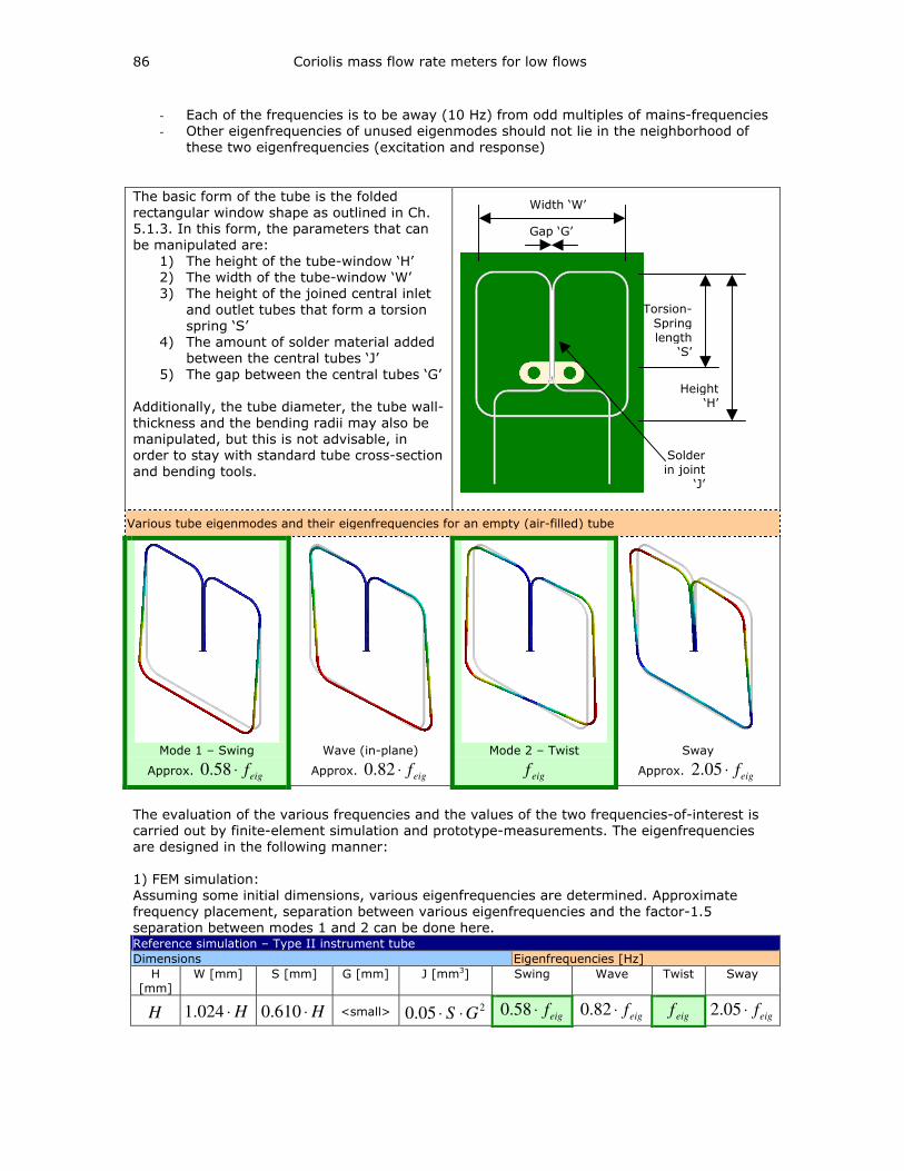
86 Coriolis mass flow rate meters for low flows
- Each of the frequencies is to be away (10 Hz) from odd multiples of mains-frequencies
- Other eigenfrequencies of unused eigenmodes should not lie in the neighborhood of
these two eigenfrequencies (excitation and response)
The basic form of the tube is the folded
rectangular window shape as outlined in Ch.
5.1.3. In this form, the parameters that can
be manipulated are:
1) The height of the tube-window ‘H’
2) The width of the tube-window ‘W’
3) The height of the joined central inlet
and outlet tubes that form a torsion
spring ‘S’
4) The amount of solder material added
between the central tubes ‘J’
5) The gap between the central tubes ‘G’
Additionally, the tube diameter, the tube wall-
thickness and the bending radii may also be
manipulated, but this is not advisable, in
order to stay with standard tube cross-section
and bending tools.
Various tube eigenmodes and their eigenfrequencies for an empty (air-filled) tube
Mode 1 – Swing
Approx. eigf⋅58.0
Wave (in-plane)
Approx. eigf⋅82.0
Mode 2 – Twist
eigf
Sway
Approx. eigf⋅05.2
The evaluation of the various frequencies and the values of the two frequencies-of-interest is
carried out by finite-element simulation and prototype-measurements. The eigenfrequencies
are designed in the following manner:
1) FEM simulation:
Assuming some initial dimensions, various eigenfrequencies are determined. Approximate
frequency placement, separation between various eigenfrequencies and the factor-1.5
separation between modes 1 and 2 can be done here. Reference simulation – Type II instrument tube
Dimensions Eigenfrequencies [Hz]
H
[mm]
W [mm] S [mm] G [mm] J [mm3] Swing Wave Twist Sway
H H⋅024.1 H⋅610.0 <small> 205.0 GS ⋅⋅ eigf⋅58.0 eigf⋅82.0 eigf eigf⋅05.2
Width ‘W’
Height ‘H’
Torsion-
Spring
length ‘S’
Solder
in joint ‘J’
Gap ‘G’
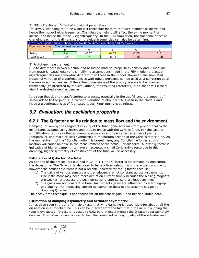
Evaluation and measurement results 87
2) FEM - Fractional 26effect of individual parameters:
Intuitively, changing the tube width will contribute more to the twist moment-of-inertia and
hence the mode-2 eigenfrequency. Changing the height will affect the swing moment of
inertia, and hence the mode-1 eigenfrequency. In the FEM simulation, the fractional effect of
changing each of the dimensions on the eigenfrequencies can also be determined. Fractional eigenfrequency change per fractional dimension-change (dimensionless)
The dimensions varied: Eigenfrequencies
H W S G J
Swing -1.4 -0.70 -0.02 -0.03 0.01
Twist (excit.) -0.65 -1.18 -0.33 -0.30 0.08
3) Prototype measurement:
Due to differences between actual and assumed material properties (density and E-modulus
from material datasheets) and simplifying assumptions made in the FEM model, the actual
eigenfrequencies are somewhat different than those in the model. However, the simulated
fractional variation of eigenfrequencies with tube dimensions can be used as a correction upon
the measured frequencies. If the actual dimensions of the prototype were to be changed
fractionally (as predicted by the simulations) the resulting (corrected) tube-shape will closely
yield the desired eigenfrequencies.
It is seen that due to manufacturing tolerances, especially in the gap ‘G’ and the amount of
solder added to the joint ‘J’, a piece-to-variation of about 0.5% is seen in the Mode 1 and
Mode 2 eigenfrequencies of fabricated tubes. Finer tuning is pointless.
6.2 Evaluation: the oscillation properties
6.2.1 The Q factor and its relation to mass flow and the environment Damping, driven by the (angular) velocity of the tube, generates an effort proportional to the
instantaneous (angular) velocity, and thus in-phase with the Coriolis force. For the sake of
simplification, let us say that all damping occurs as a lumped effect at a pair of points
(antiparallel and more-or–less symmetric) in the bottom section of the Coriolis meter tube. As
the moment-arm of the “Coriolis motion” is largest here, any Coriolis-like forces at this
location will cause an error in the measurement of the actual Coriolis force. A lower Q-factor is
indicative of higher damping; to have an acceptably small Coriolis-like force due to this
damping, higher symmetry of construction of the tube will be necessary.
Estimation of Q-factor of a tube: As per one of the procedures outlined in Ch. 4.1.1, the Q-factor is determined by measuring
the decay time. The Q-factor is also seen to have a fixed relation with the actuation current;
however the actuation current is not a reliable indicator for the Q-factor because:
1) The gains of various sensors and transducers are not constant across instruments.
One instrument may need more actuation current simply because the biasing magnets
are weaker, or because the position-sensing opto-sensors are less sensitive.
2) The gains are not constant in time. Instruments gains are influenced by warming-up
and ageing. (An increasing current consumption does not necessarily suggest a
dropping Q-factor.)
The decay-time technique is not dependent on the sensor gain – and hence suitable here.
Estimation of damping asymmetry and actuator asymmetry:
It has been seen in proof-of-principle tests that wind damping is responsible for about half the
dissipation in a Coriolis tube. This can be inferred from the fact that if the air surrounding the
tube is evacuated, (pressure reduced to 0.03 bara in experiments) the Q-factor approximately
doubles. This behavior can be used to test the combined net asymmetry of the actuator and
26 Fractional as in l
l
f
f ∆∆

88 Coriolis mass flow rate meters for low flows
(wind) damping. In vacuum, the actuation-current-consumption (for the same amplitude of
oscillation) drops to half its initial value. It may be argued that in this new situation,
1) The wind damping (and hence any tube asymmetry effect of it) is zero
2) The actuation effort is about half its normal magnitude– any offset due to asymmetric
actuation is thus also halved.
These two aspects are evaluated for a set of instruments by evacuating the air around the
oscillating tubes. The combined effect of actuator asymmetry and asymmetric wind-damping
causes an offset-change of less than 0.1 (g/h).
6.2.2 Actuation - power requirement and relation to the Q-factor We do not expect the power requirements for multiple instruments with the same Q-factor to
be identical – this difference is due to different component-gains; it is not essential to calibrate
these component gains for proper operation of the instrument, as the measurement is based
on ratios. This means that the actual tube oscillation amplitude in each instrument in a set of
instruments can be slightly different. This means that each instrument will consume a slightly
different power for actuation purposes. Furthermore, a Q-factor change will cause an inversely
proportional change in the required actuation power.
A way to temporarily increase the Q-factor of a tube is to evacuate it. Similarly, a way to
temporarily decrease the Q-factor of a tube is to set the instrument on (dissipative) damping
suspension.
The estimated power requirement:
In Ch. 5.2.2, we have estimated the current required to drive the Coriolis tube in steady-state
oscillations as about 13.2 mA. Apart from he i2R losses in the tube, the back-EMF generated in
the tube is:
][3.23122830.810.422 mVeeerlBerlB
b =−⋅⋅−⋅−⋅⇒⋅⋅⋅⋅= 32143421321&
&θ
θ (6.1)
thus,
][2932.1333.2 WPeeieP peakbpeak µ=⇒−⋅−⇒⋅= (6.2)
(A) - The excitation
This can also be calculated in a different way (as a check):
The instantaneous power P dissipated in a damped body with damping d and instantaneous
angular velocity θ& is:
θθθ &&& ⋅⋅=⋅Τ= )(dP (6.3)
Where the damping torque Τ is the damping d times the instantaneous angular velocity θ& .
From 4.1.1, we have:
eig
k
dkm
dQ
ω⋅=⋅=
11 (6.4)
For the type-II instrument for example, for excitation (twist) motion,
]/[21.7 radmNek ⋅−= , and 2000≈Q (measured).
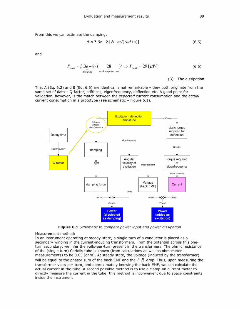
Evaluation and measurement results 89
From this we can estimate the damping:
)]//([83.3 sradmNed ⋅−≈ (6.5)
and
][29)28(83.3 2WPeP peak
rateangularpeakdamping
peak µ≈⇒⋅−≈ 43421 (6.6)
(B) - The dissipation
That A (Eq. 6.2) and B (Eq. 6.6) are identical is not remarkable – they both originate from the
same set of data – Q-factor, stiffness, eigenfrequency, deflection etc. A good point for
validation, however, is the match between the expected current consumption and the actual current consumption in a prototype (see schematic – Figure 6.1).
Decay time
Q-factor
eigenfrequency
Excitation: deflection
amplitude
Angularvelocity of
excitation
static torque
required for
deflection
damping
damping force
torque requiredat
eigenfrequency
eigenfrequency
Stiffness,Q-factor,
eigenfrequency
stiffness
Q-factor
Voltage(back EMF)
Current
Power(dissipated
as damping)
Power(added as
excitation)
(effort)
(flow)
(Power)
Motor constant
Motor constant
(effort) (flow)
(Power)
Figure 6.1 Schematic to compare power input and power dissipation
Measurement method:
In an instrument operating at steady-state, a single turn of a conductor is placed as a
secondary winding in the current-inducing transformers. From the potential across this one-
turn secondary, we infer the volts-per-turn present in the transformers. The ohmic resistance
of the (single turn) Coriolis tube is known (from calculations as well as ohm-meter
measurements) to be 0.63 [ohm]. At steady state, the voltage (induced by the transformer)
will be equal to the phasor sum of the back-EMF and the Ri ⋅ drop. Thus, upon measuring the
transformer volts-per-turn, and approximately knowing the back-EMF, we can calculate the
actual current in the tube. A second possible method is to use a clamp-on current meter to
directly measure the current in the tube; this method is inconvenient due to space constraints
inside the instrument
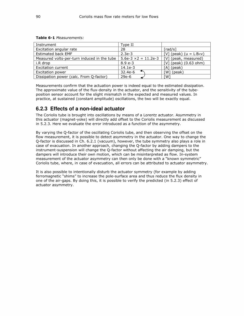
90 Coriolis mass flow rate meters for low flows
Table 6-1 Measurements:
Instrument Type II
Excitation angular rate 28 [rad/s]
Estimated back EMF 2.3e-3 [V] (peak) (u = L⋅B×v)
Measured volts-per-turn induced in the tube 5.6e-3 ×2 = 11.2e-3 [V] (peak, measured)
i.R drop 8.9 e-3 [V] (peak) (0.63 ohm)
Excitation current 14.1e-3 [A] (peak)
Excitation power 32.4e-6 [W] (peak)
Dissipation power (calc. From Q-factor) 29e-6 [W]
Measurements confirm that the actuation power is indeed equal to the estimated dissipation.
The approximate value of the flux-density in the actuator, and the sensitivity of the tube-
position sensor account for the slight mismatch in the expected and measured values. In
practice, at sustained (constant amplitude) oscillations, the two will be exactly equal.
6.2.3 Effects of a non-ideal actuator The Coriolis tube is brought into oscillations by means of a Lorentz actuator. Asymmetry in
this actuator (magnet-yoke) will directly add offset to the Coriolis measurement as discussed
in 5.2.3. Here we evaluate the error introduced as a function of the asymmetry.
By varying the Q-factor of the oscillating Coriolis tube, and then observing the offset on the
flow measurement, it is possible to detect asymmetry in the actuator. One way to change the
Q-factor is discussed in Ch. 6.2.1 (vacuum), however, the tube symmetry also plays a role in
case of evacuation. In another approach, changing the Q-factor by adding dampers to the
instrument-suspension will change the Q-factor without affecting the air damping, but the
dampers will introduce their own motion, which can be misinterpreted as flow. In-system
measurement of the actuator asymmetry can then only be done with a “known symmetric”
Coriolis tube, where, in case of evacuation, all errors can be attributed to actuator asymmetry.
It is also possible to intentionally disturb the actuator symmetry (for example by adding
ferromagnetic “shims” to increase the pole-surface area and thus reduce the flux density in
one of the air-gaps. By doing this, it is possible to verify the predicted (in 5.2.3) effect of
actuator asymmetry.
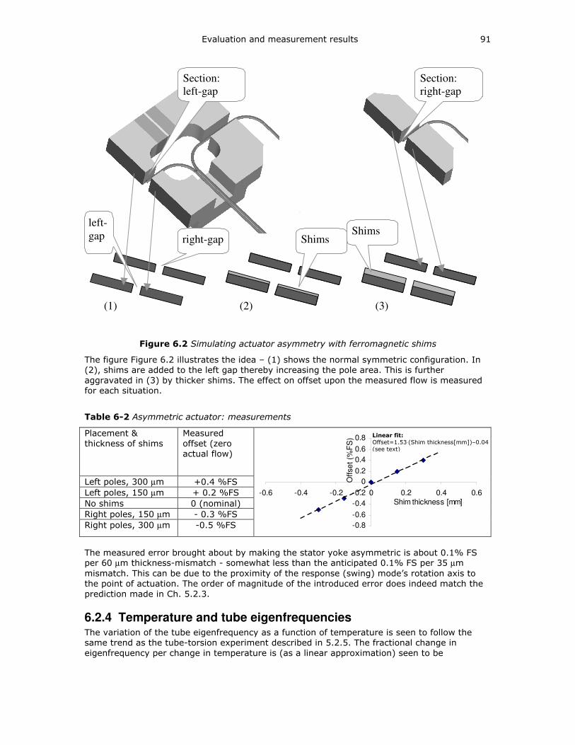
Evaluation and measurement results 91
Shims Shims
Section:
right-gap
Section:
left-gap
(1) (2) (3)
right-gap
left-
gap
Figure 6.2 Simulating actuator asymmetry with ferromagnetic shims
The figure Figure 6.2 illustrates the idea – (1) shows the normal symmetric configuration. In
(2), shims are added to the left gap thereby increasing the pole area. This is further
aggravated in (3) by thicker shims. The effect on offset upon the measured flow is measured
for each situation.
Table 6-2 Asymmetric actuator: measurements
Placement &
thickness of shims
Measured
offset (zero
actual flow)
Left poles, 300 µm +0.4 %FS
Left poles, 150 µm + 0.2 %FS
No shims 0 (nominal)
Right poles, 150 µm - 0.3 %FS
Right poles, 300 µm -0.5 %FS
y = 1.5333x - 0.04
-0.8
-0.6
-0.4
-0.2
0
0.2
0.4
0.6
0.8
-0.6 -0.4 -0.2 0 0.2 0.4 0.6Shim thickness [mm]
Offse
t (%
FS
)
The measured error brought about by making the stator yoke asymmetric is about 0.1% FS per 60 µm thickness-mismatch - somewhat less than the anticipated 0.1% FS per 35 µm
mismatch. This can be due to the proximity of the response (swing) mode’s rotation axis to
the point of actuation. The order of magnitude of the introduced error does indeed match the
prediction made in Ch. 5.2.3.
6.2.4 Temperature and tube eigenfrequencies The variation of the tube eigenfrequency as a function of temperature is seen to follow the
same trend as the tube-torsion experiment described in 5.2.5. The fractional change in
eigenfrequency per change in temperature is (as a linear approximation) seen to be
Linear fit:
Offset=1.53⋅(Shim thickness[mm])–0.04
(see text)
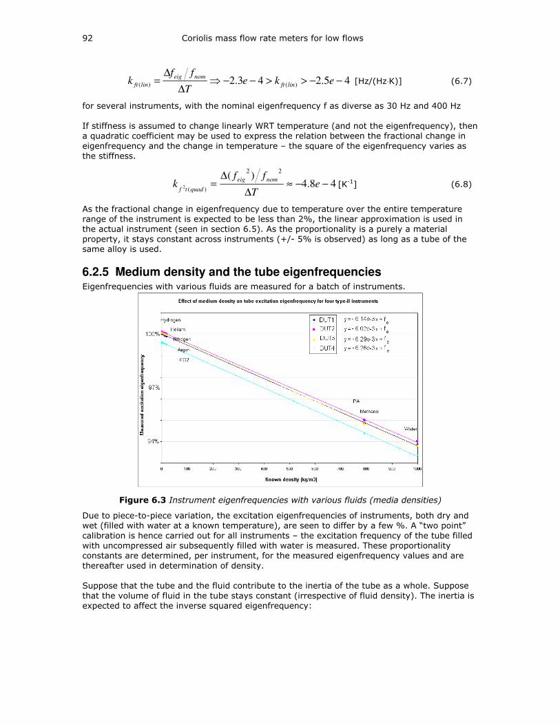
92 Coriolis mass flow rate meters for low flows
45.243.2 )()( −−>>−−⇒∆
∆= eke
T
ffk linft
nomeig
linft [Hz/(Hz⋅K)] (6.7)
for several instruments, with the nominal eigenfrequency f as diverse as 30 Hz and 400 Hz
If stiffness is assumed to change linearly WRT temperature (and not the eigenfrequency), then
a quadratic coefficient may be used to express the relation between the fractional change in
eigenfrequency and the change in temperature – the square of the eigenfrequency varies as
the stiffness.
48.4)(
22
)(2 −−≈∆
∆= e
T
ffk
nomeig
quadtf[K-1] (6.8)
As the fractional change in eigenfrequency due to temperature over the entire temperature
range of the instrument is expected to be less than 2%, the linear approximation is used in
the actual instrument (seen in section 6.5). As the proportionality is a purely a material
property, it stays constant across instruments (+/- 5% is observed) as long as a tube of the
same alloy is used.
6.2.5 Medium density and the tube eigenfrequencies Eigenfrequencies with various fluids are measured for a batch of instruments.
Figure 6.3 Instrument eigenfrequencies with various fluids (media densities)
Due to piece-to-piece variation, the excitation eigenfrequencies of instruments, both dry and
wet (filled with water at a known temperature), are seen to differ by a few %. A “two point”
calibration is hence carried out for all instruments – the excitation frequency of the tube filled
with uncompressed air subsequently filled with water is measured. These proportionality
constants are determined, per instrument, for the measured eigenfrequency values and are
thereafter used in determination of density.
Suppose that the tube and the fluid contribute to the inertia of the tube as a whole. Suppose
that the volume of fluid in the tube stays constant (irrespective of fluid density). The inertia is
expected to affect the inverse squared eigenfrequency:
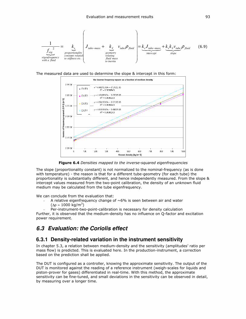
Evaluation and measurement results 93
fluid
slope
tubeJs
terceptin
masstubesfluidtube
inertiatomassfluid
relatinggeometry
Jmasstube
etcstiffnesstorelatedntconsta
alityproportion
s
fluidawithencyeigenfrequ
eig
vkkJkvkJkf
ρρ4342143421
+=
+= −−
.
2
1 (6.9)
The measured data are used to determine the slope & intercept in this form:
Figure 6.4 Densities mapped to the inverse-squared eigenfrequencies
The slope (proportionality constant) is not normalized to the nominal-frequency (as is done
with temperature) - the reason is that for a different tube-geometry (for each tube) the
proportionality is substantially different, and hence independently measured. From the slope &
intercept values measured from the two-point calibration, the density of an unknown fluid
medium may be calculated from the tube eigenfrequency.
We can conclude from the evaluation that:
- A relative eigenfrequency change of ~6% is seen between air and water (∆ρ ≈ 1000 kg/m3)
- Per-instrument-two-point-calibration is necessary for density calculation
Further, it is observed that the medium-density has no influence on Q-factor and excitation
power requirement.
6.3 Evaluation: the Coriolis effect
6.3.1 Density-related variation in the instrument sensitivity In chapter 5.3, a relation between medium-density and the sensitivity (amplitudes’ ratio per
mass flow) is predicted. This is evaluated here. In the production-instrument, a correction
based on the prediction shall be applied.
The DUT is configured as a controller, knowing the approximate sensitivity. The output of the
DUT is monitored against the reading of a reference instrument (weigh-scales for liquids and
piston-prover for gases) differentiated in real-time. With this method, the approximate
sensitivity can be fine-tuned, and small deviations in the sensitivity can be observed in detail,
by measuring over a longer time.
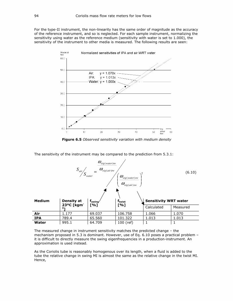
94 Coriolis mass flow rate meters for low flows
For the type-II instrument, the non-linearity has the same order of magnitude as the accuracy
of the reference instrument, and so is neglected. For each sample instrument, normalizing the
sensitivity using water as the reference medium (sensitivity with water is set to 1.000), the
sensitivity of the instrument to other media is measured. The following results are seen:
Figure 6.5 Observed sensitivity variation with medium density
The sensitivity of the instrument may be compared to the prediction from 5.3.1:
2
)(
)(
)(
)(
=
swaireig
swwatereig
twaireig
twwatereig
water
air
SS
ω
ω
ω
ω
(6.10)
Sensitivity WRT water Medium Density at 23ºC [kgm-
3]
fswing [%]
ftwist [%]
Calculated Measured
Air 1.177 69.037 106.758 1.066 1.070
IPA 789.4 65.560 101.322 1.013 1.013
Water 995.1 64.709 100 (ref) 1 1
The measured change in instrument sensitivity matches the predicted change – the
mechanism proposed in 5.3 is dominant. However, use of Eq. 6.10 poses a practical problem –
it is difficult to directly measure the swing eigenfrequencies in a production-instrument. An
approximation is used instead.
As the Coriolis tube is reasonably homogenous over its length, when a fluid is added to the
tube the relative change in swing MI is almost the same as the relative change in the twist MI.
Hence,
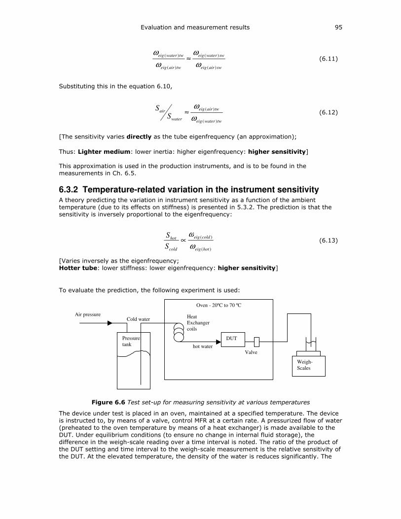
Evaluation and measurement results 95
swaireig
swwatereig
twaireig
twwatereig
)(
)(
)(
)(
ω
ω
ω
ω≈ (6.11)
Substituting this in the equation 6.10,
twwatereig
twaireig
water
air
SS
)(
)(
ω
ω≈ (6.12)
[The sensitivity varies directly as the tube eigenfrequency (an approximation);
Thus: Lighter medium: lower inertia: higher eigenfrequency: higher sensitivity]
This approximation is used in the production instruments, and is to be found in the
measurements in Ch. 6.5.
6.3.2 Temperature-related variation in the instrument sensitivity A theory predicting the variation in instrument sensitivity as a function of the ambient
temperature (due to its effects on stiffness) is presented in 5.3.2. The prediction is that the
sensitivity is inversely proportional to the eigenfrequency:
)(
)(
hoteig
coldeig
cold
hot
S
S
ω
ω∝ (6.13)
[Varies inversely as the eigenfrequency;
Hotter tube: lower stiffness: lower eigenfrequency: higher sensitivity]
To evaluate the prediction, the following experiment is used:
Oven - 20ºC to 70 ºC
Pressure
tank
DUT
Valve
Weigh-
Scales
Heat
Exchanger
coils
Air pressure Cold water
hot water
Figure 6.6 Test set-up for measuring sensitivity at various temperatures
The device under test is placed in an oven, maintained at a specified temperature. The device
is instructed to, by means of a valve, control MFR at a certain rate. A pressurized flow of water
(preheated to the oven temperature by means of a heat exchanger) is made available to the
DUT. Under equilibrium conditions (to ensure no change in internal fluid storage), the
difference in the weigh-scale reading over a time interval is noted. The ratio of the product of
the DUT setting and time interval to the weigh-scale measurement is the relative sensitivity of
the DUT. At the elevated temperature, the density of the water is reduces significantly. The
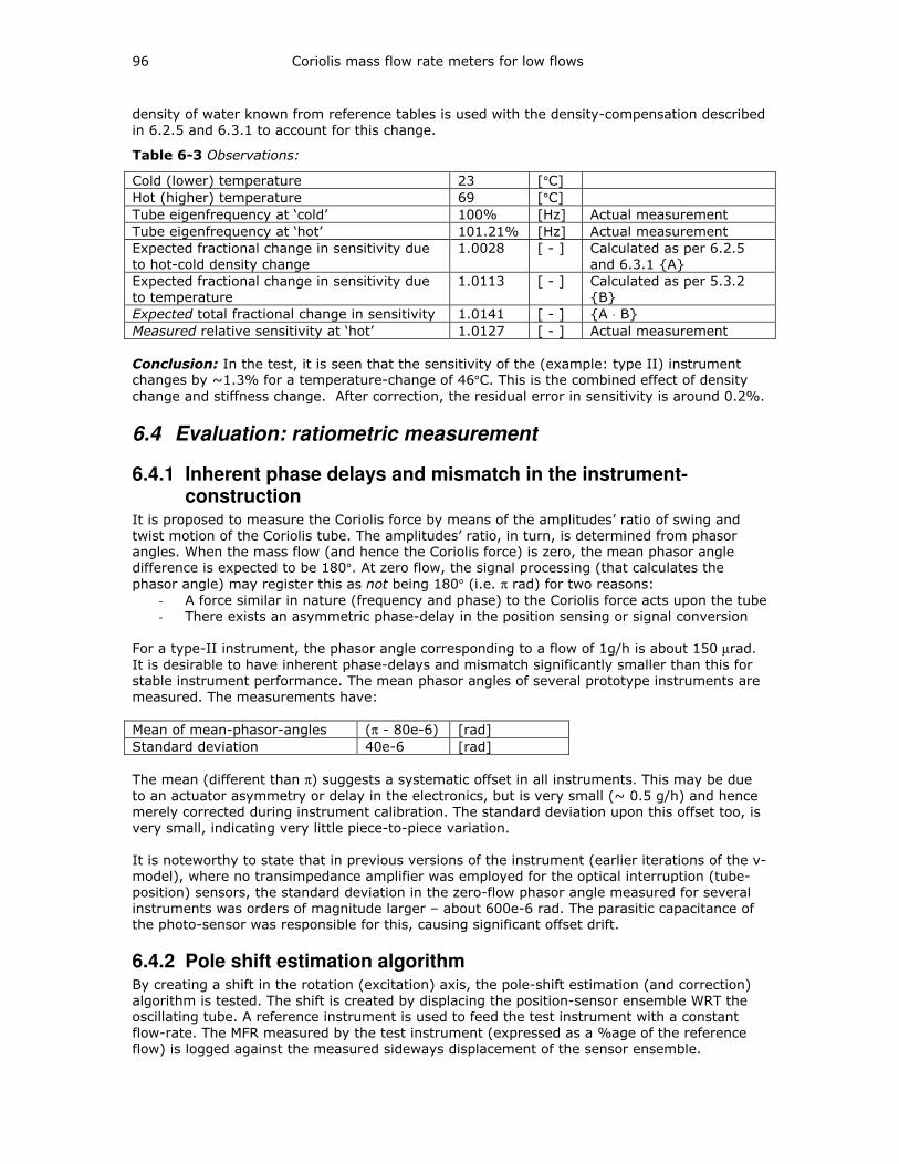
96 Coriolis mass flow rate meters for low flows
density of water known from reference tables is used with the density-compensation described
in 6.2.5 and 6.3.1 to account for this change.
Table 6-3 Observations:
Cold (lower) temperature 23 [°C]
Hot (higher) temperature 69 [°C]
Tube eigenfrequency at ‘cold’ 100% [Hz] Actual measurement
Tube eigenfrequency at ‘hot’ 101.21% [Hz] Actual measurement
Expected fractional change in sensitivity due
to hot-cold density change
1.0028 [ - ] Calculated as per 6.2.5
and 6.3.1 A
Expected fractional change in sensitivity due
to temperature
1.0113 [ - ] Calculated as per 5.3.2
B
Expected total fractional change in sensitivity 1.0141 [ - ] A ⋅ B
Measured relative sensitivity at ‘hot’ 1.0127 [ - ] Actual measurement
Conclusion: In the test, it is seen that the sensitivity of the (example: type II) instrument changes by ~1.3% for a temperature-change of 46°C. This is the combined effect of density
change and stiffness change. After correction, the residual error in sensitivity is around 0.2%.
6.4 Evaluation: ratiometric measurement
6.4.1 Inherent phase delays and mismatch in the instrument-construction
It is proposed to measure the Coriolis force by means of the amplitudes’ ratio of swing and
twist motion of the Coriolis tube. The amplitudes’ ratio, in turn, is determined from phasor
angles. When the mass flow (and hence the Coriolis force) is zero, the mean phasor angle difference is expected to be 180°. At zero flow, the signal processing (that calculates the
phasor angle) may register this as not being 180° (i.e. π rad) for two reasons:
- A force similar in nature (frequency and phase) to the Coriolis force acts upon the tube
- There exists an asymmetric phase-delay in the position sensing or signal conversion
For a type-II instrument, the phasor angle corresponding to a flow of 1g/h is about 150 µrad.
It is desirable to have inherent phase-delays and mismatch significantly smaller than this for
stable instrument performance. The mean phasor angles of several prototype instruments are
measured. The measurements have:
Mean of mean-phasor-angles (π - 80e-6) [rad]
Standard deviation 40e-6 [rad]
The mean (different than π) suggests a systematic offset in all instruments. This may be due
to an actuator asymmetry or delay in the electronics, but is very small (~ 0.5 g/h) and hence
merely corrected during instrument calibration. The standard deviation upon this offset too, is
very small, indicating very little piece-to-piece variation.
It is noteworthy to state that in previous versions of the instrument (earlier iterations of the v-
model), where no transimpedance amplifier was employed for the optical interruption (tube-
position) sensors, the standard deviation in the zero-flow phasor angle measured for several
instruments was orders of magnitude larger – about 600e-6 rad. The parasitic capacitance of
the photo-sensor was responsible for this, causing significant offset drift.
6.4.2 Pole shift estimation algorithm By creating a shift in the rotation (excitation) axis, the pole-shift estimation (and correction)
algorithm is tested. The shift is created by displacing the position-sensor ensemble WRT the
oscillating tube. A reference instrument is used to feed the test instrument with a constant
flow-rate. The MFR measured by the test instrument (expressed as a %age of the reference
flow) is logged against the measured sideways displacement of the sensor ensemble.
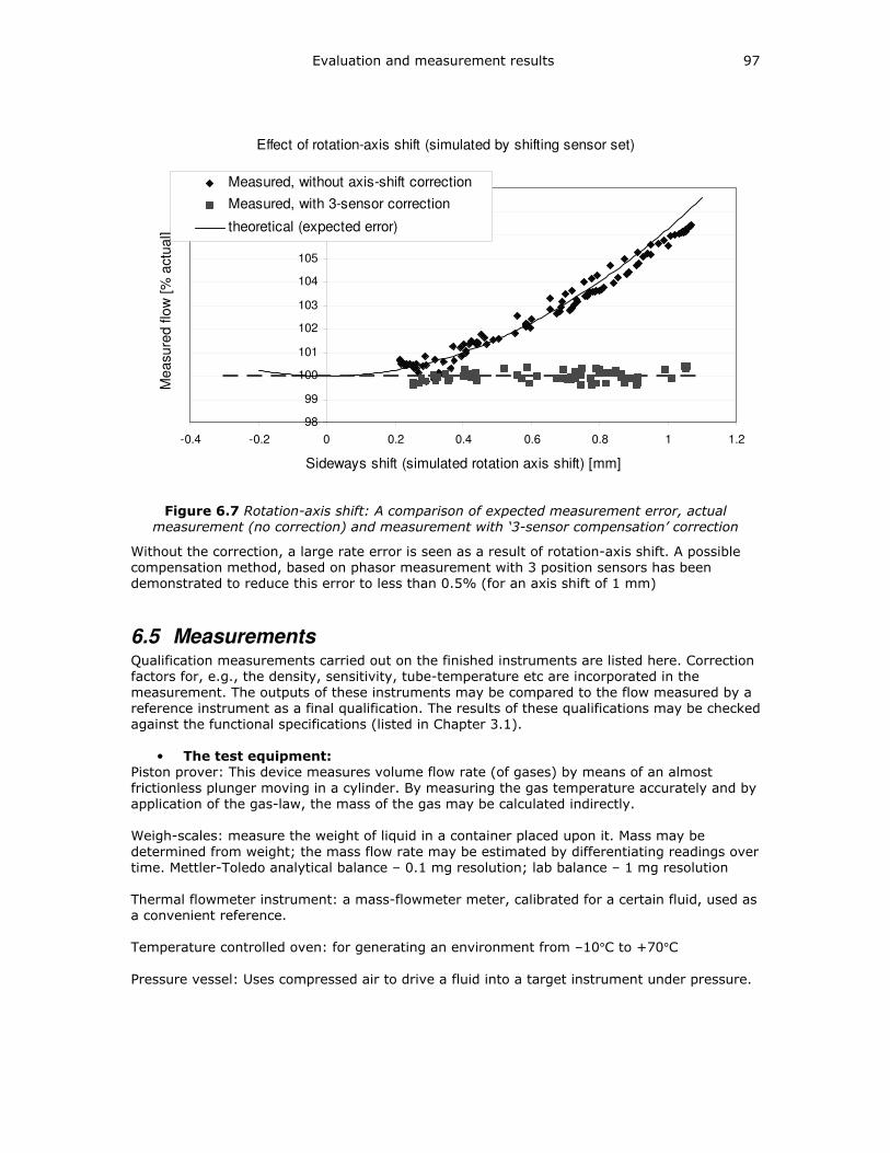
Evaluation and measurement results 97
Effect of rotation-axis shift (simulated by shifting sensor set)
98
99
100
101
102
103
104
105
106
107
108
-0.4 -0.2 0 0.2 0.4 0.6 0.8 1 1.2
Sideways shift (simulated rotation axis shift) [mm]
Measure
d flo
w [%
actu
al]
Measured, without axis-shift correction
Measured, with 3-sensor correction
theoretical (expected error)
Figure 6.7 Rotation-axis shift: A comparison of expected measurement error, actual measurement (no correction) and measurement with ‘3-sensor compensation’ correction
Without the correction, a large rate error is seen as a result of rotation-axis shift. A possible
compensation method, based on phasor measurement with 3 position sensors has been
demonstrated to reduce this error to less than 0.5% (for an axis shift of 1 mm)
6.5 Measurements Qualification measurements carried out on the finished instruments are listed here. Correction
factors for, e.g., the density, sensitivity, tube-temperature etc are incorporated in the
measurement. The outputs of these instruments may be compared to the flow measured by a
reference instrument as a final qualification. The results of these qualifications may be checked
against the functional specifications (listed in Chapter 3.1).
• The test equipment: Piston prover: This device measures volume flow rate (of gases) by means of an almost
frictionless plunger moving in a cylinder. By measuring the gas temperature accurately and by
application of the gas-law, the mass of the gas may be calculated indirectly.
Weigh-scales: measure the weight of liquid in a container placed upon it. Mass may be
determined from weight; the mass flow rate may be estimated by differentiating readings over
time. Mettler-Toledo analytical balance – 0.1 mg resolution; lab balance – 1 mg resolution
Thermal flowmeter instrument: a mass-flowmeter meter, calibrated for a certain fluid, used as
a convenient reference.
Temperature controlled oven: for generating an environment from –10°C to +70°C
Pressure vessel: Uses compressed air to drive a fluid into a target instrument under pressure.
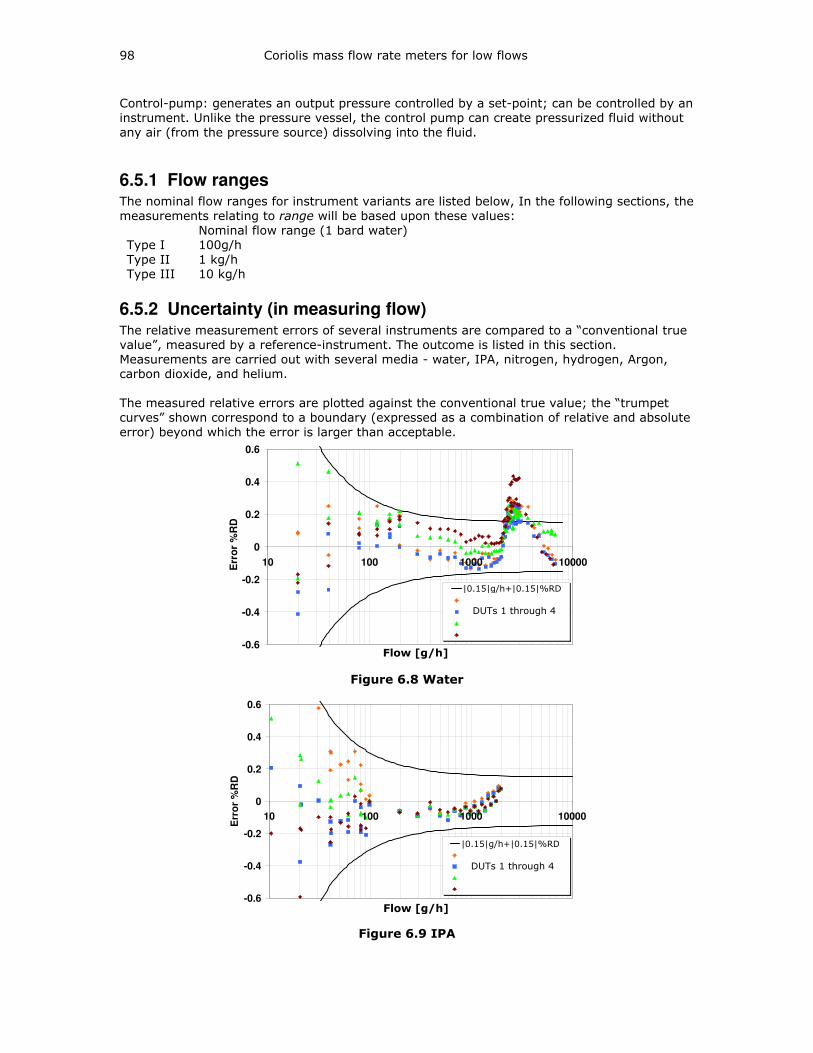
98 Coriolis mass flow rate meters for low flows
Control-pump: generates an output pressure controlled by a set-point; can be controlled by an
instrument. Unlike the pressure vessel, the control pump can create pressurized fluid without
any air (from the pressure source) dissolving into the fluid.
6.5.1 Flow ranges The nominal flow ranges for instrument variants are listed below, In the following sections, the
measurements relating to range will be based upon these values:
Type I
Type II
Type III
Nominal flow range (1 bard water)
100g/h
1 kg/h
10 kg/h
6.5.2 Uncertainty (in measuring flow) The relative measurement errors of several instruments are compared to a “conventional true
value”, measured by a reference-instrument. The outcome is listed in this section.
Measurements are carried out with several media - water, IPA, nitrogen, hydrogen, Argon,
carbon dioxide, and helium.
The measured relative errors are plotted against the conventional true value; the “trumpet
curves” shown correspond to a boundary (expressed as a combination of relative and absolute
error) beyond which the error is larger than acceptable.
-0.6
-0.4
-0.2
0
0.2
0.4
0.6
10 100 1000 10000
Flow [g/u]
Err
or
%R
D
|0.15|g/u +|0.15|%RDRB10.35RB10.32RB10.14RB10.13
Figure 6.8 Water
-0.6
-0.4
-0.2
0
0.2
0.4
0.6
10 100 1000 10000
Flow [g/u]
Err
or
%R
D
|0.15| g/u + |0.15|%RDRB10.35RB10.32RB10.14RB10.13
Figure 6.9 IPA
|0.15|g/h+|0.15|%RD
DUTs 1 through 4
|0.15|g/h+|0.15|%RD
DUTs 1 through 4
Flow [g/h]
Flow [g/h]
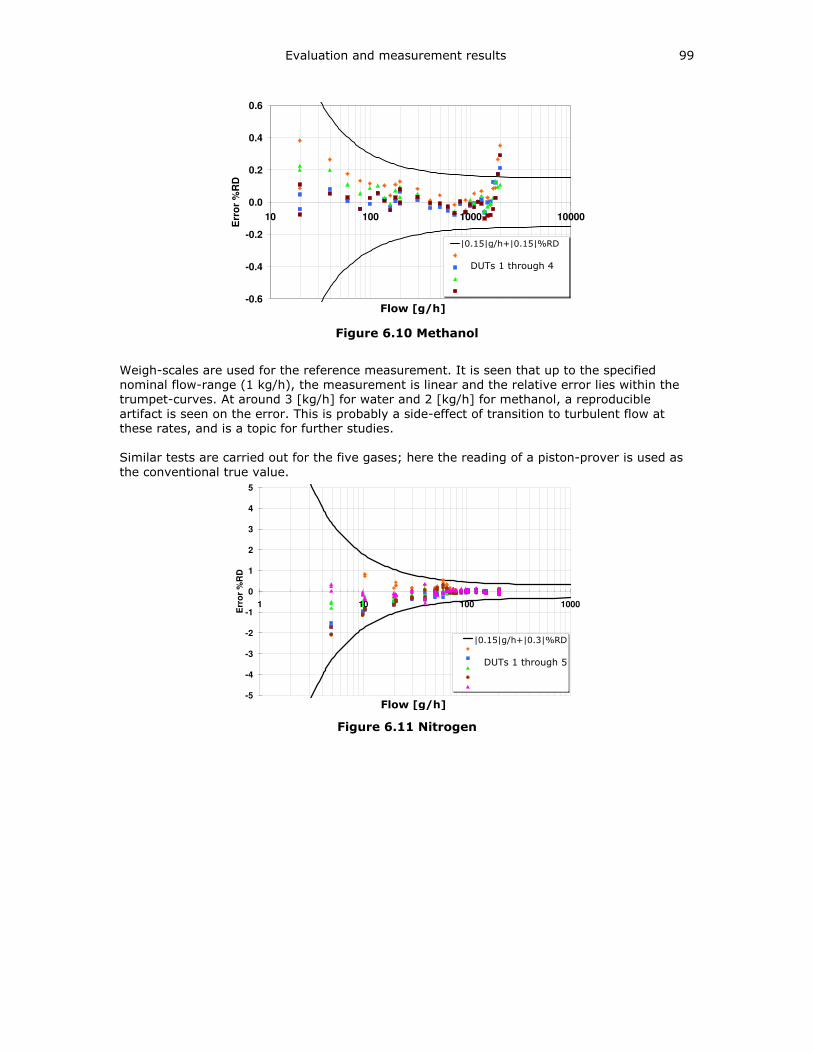
Evaluation and measurement results 99
-0.6
-0.4
-0.2
0.0
0.2
0.4
0.6
10 100 1000 10000
Flow [g/u]
Err
or
%R
D|0.15| g/u + |0.15|%RDRB10.35RB10.32RB10.14RB10.13
Figure 6.10 Methanol
Weigh-scales are used for the reference measurement. It is seen that up to the specified
nominal flow-range (1 kg/h), the measurement is linear and the relative error lies within the
trumpet-curves. At around 3 [kg/h] for water and 2 [kg/h] for methanol, a reproducible
artifact is seen on the error. This is probably a side-effect of transition to turbulent flow at
these rates, and is a topic for further studies.
Similar tests are carried out for the five gases; here the reading of a piston-prover is used as
the conventional true value.
-5
-4
-3
-2
-1
0
1
2
3
4
5
1 10 100 1000
Flow [g/h]
Err
or
%R
D
|0.15|g/h + |0.3|% RDRB10.35RB10.32RB10.14RB10.13RB10.17
Figure 6.11 Nitrogen
|0.15|g/h+|0.15|%RD
DUTs 1 through 4
|0.15|g/h+|0.3|%RD
DUTs 1 through 5
Flow [g/h]
Flow [g/h]
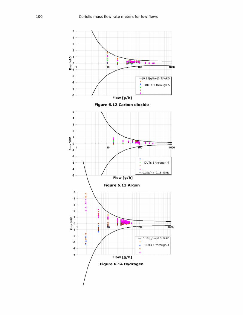
100 Coriolis mass flow rate meters for low flows
-5
-4
-3
-2
-1
0
1
2
3
4
5
1 10 100 1000
Flow [g/h]
Err
or
%R
D
|0.15|g/h + |0.3|% RDRB10.35RB10.32RB10.14RB10.13RB10.17
Figure 6.12 Carbon dioxide
-5
-4
-3
-2
-1
0
1
2
3
4
5
1 10 100 1000
Flow [g/h]
Err
or
%R
D
RB10.32
RB10.14
RB10.13
RB10.17
|0.3|g/h + |0.15|% RD
Figure 6.13 Argon
-5
-4
-3
-2
-1
0
1
2
3
4
5
1 10 100 1000
Flow [g/h]
Err
or
%R
D
|0.15|g/h + |0.3|% RD
RB10.35
RB10.32
RB10.13
RB10.17
Figure 6.14 Hydrogen
|0.15|g/h+|0.3|%RD
DUTs 1 through 5
DUTs 1 through 4
|0.3|g/h+|0.15|%RD
|0.15|g/h+|0.3|%RD
DUTs 1 through 4
Flow [g/h]
Flow [g/h]
Flow [g/h]
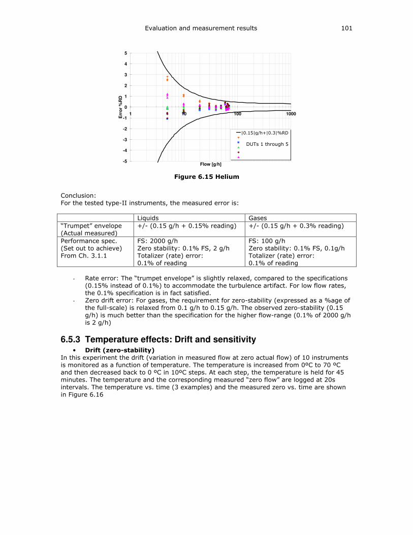
Evaluation and measurement results 101
-5
-4
-3
-2
-1
0
1
2
3
4
5
1 10 100 1000
Flow [g/h]
Err
or
%R
D
|0.15|g/h + |0.3|% RDRB10.35RB10.32RB10.14RB10.13RB10.17
Figure 6.15 Helium
Conclusion:
For the tested type-II instruments, the measured error is:
Liquids Gases
“Trumpet” envelope
(Actual measured)
+/- (0.15 g/h + 0.15% reading) +/- (0.15 g/h + 0.3% reading)
Performance spec.
(Set out to achieve)
From Ch. 3.1.1
FS: 2000 g/h
Zero stability: 0.1% FS, 2 g/h
Totalizer (rate) error:
0.1% of reading
FS: 100 g/h
Zero stability: 0.1% FS, 0.1g/h
Totalizer (rate) error:
0.1% of reading
- Rate error: The “trumpet envelope” is slightly relaxed, compared to the specifications
(0.15% instead of 0.1%) to accommodate the turbulence artifact. For low flow rates,
the 0.1% specification is in fact satisfied.
- Zero drift error: For gases, the requirement for zero-stability (expressed as a %age of
the full-scale) is relaxed from 0.1 g/h to 0.15 g/h. The observed zero-stability (0.15
g/h) is much better than the specification for the higher flow-range (0.1% of 2000 g/h
is 2 g/h)
6.5.3 Temperature effects: Drift and sensitivity • Drift (zero-stability)
In this experiment the drift (variation in measured flow at zero actual flow) of 10 instruments
is monitored as a function of temperature. The temperature is increased from 0ºC to 70 ºC
and then decreased back to 0 ºC in 10ºC steps. At each step, the temperature is held for 45
minutes. The temperature and the corresponding measured “zero flow” are logged at 20s
intervals. The temperature vs. time (3 examples) and the measured zero vs. time are shown
in Figure 6.16
|0.15|g/h+|0.3|%RD
DUTs 1 through 5
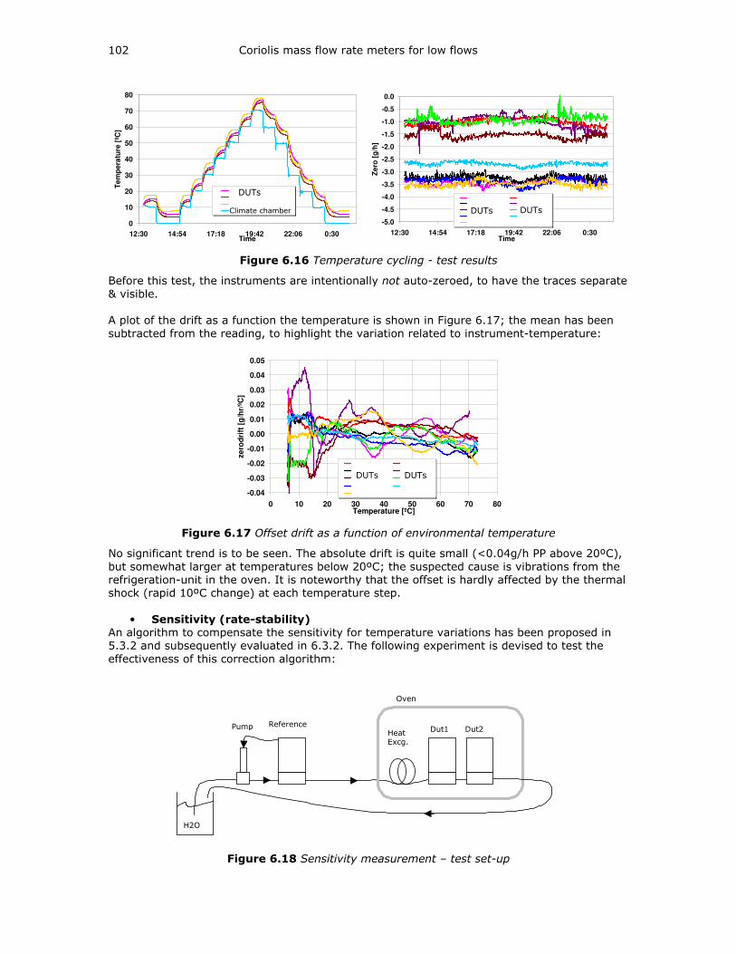
102 Coriolis mass flow rate meters for low flows
0
10
20
30
40
50
60
70
80
12:30 14:54 17:18 19:42 22:06 0:30Time
Te
mp
era
ture
[ºC
]
RB10.21RB10.35RB10.17Climate chamber
-5.0
-4.5
-4.0
-3.5
-3.0
-2.5
-2.0
-1.5
-1.0
-0.5
0.0
12:30 14:54 17:18 19:42 22:06 0:30Time
Zero
[g
/h]
RB10.21 RB10.26RB10.27 RB10.29RB10.35 RB10.32RB10.14 RB10.13RB10.17
Figure 6.16 Temperature cycling - test results
Before this test, the instruments are intentionally not auto-zeroed, to have the traces separate
& visible.
A plot of the drift as a function the temperature is shown in Figure 6.17; the mean has been
subtracted from the reading, to highlight the variation related to instrument-temperature:
-0.04
-0.03
-0.02
-0.01
0.00
0.01
0.02
0.03
0.04
0.05
0 10 20 30 40 50 60 70 80Temperature [ºC]
zero
dri
ft [
g/h
r/ºC
]
RB10.21 RB10.26RB10.27 RB10.29RB10.35 RB10.32RB10.14 RB10.13RB10.17
Figure 6.17 Offset drift as a function of environmental temperature
No significant trend is to be seen. The absolute drift is quite small (<0.04g/h PP above 20ºC),
but somewhat larger at temperatures below 20ºC; the suspected cause is vibrations from the
refrigeration-unit in the oven. It is noteworthy that the offset is hardly affected by the thermal
shock (rapid 10ºC change) at each temperature step.
• Sensitivity (rate-stability) An algorithm to compensate the sensitivity for temperature variations has been proposed in
5.3.2 and subsequently evaluated in 6.3.2. The following experiment is devised to test the
effectiveness of this correction algorithm:
Oven
Reference Dut1 Dut2 Pump
H2O
Heat Excg.
Figure 6.18 Sensitivity measurement – test set-up
DUTs Climate chamber
DUTs
DUTs
DUTs
DUTs
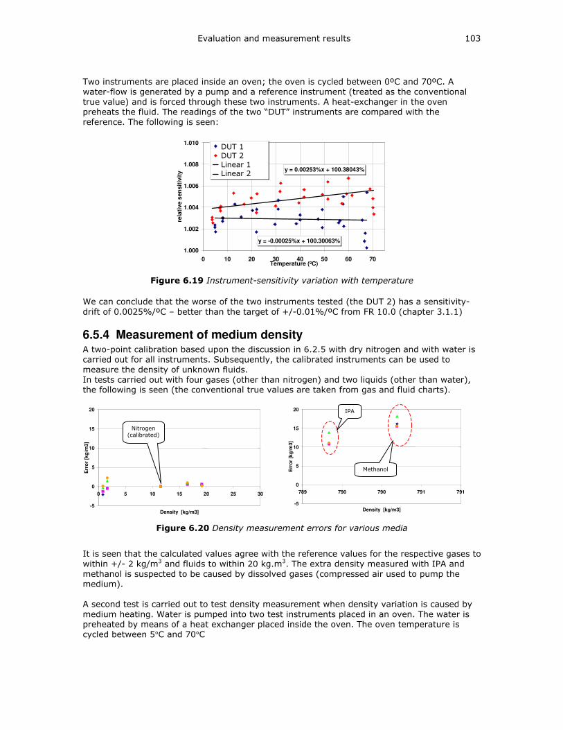
Evaluation and measurement results 103
Two instruments are placed inside an oven; the oven is cycled between 0ºC and 70ºC. A
water-flow is generated by a pump and a reference instrument (treated as the conventional
true value) and is forced through these two instruments. A heat-exchanger in the oven
preheats the fluid. The readings of the two “DUT” instruments are compared with the
reference. The following is seen:
y = 0.00253%x + 100.38043%
y = -0.00025%x + 100.30063%
1.000
1.002
1.004
1.006
1.008
1.010
0 10 20 30 40 50 60 70Temperature (ºC)
rela
tiv
e s
en
sit
ivit
y
RB10.33
RB10.34
Linear (RB10.34)
Linear (RB10.33)
Figure 6.19 Instrument-sensitivity variation with temperature
We can conclude that the worse of the two instruments tested (the DUT 2) has a sensitivity-
drift of 0.0025%/ºC – better than the target of +/-0.01%/ºC from FR 10.0 (chapter 3.1.1)
6.5.4 Measurement of medium density A two-point calibration based upon the discussion in 6.2.5 with dry nitrogen and with water is
carried out for all instruments. Subsequently, the calibrated instruments can be used to
measure the density of unknown fluids.
In tests carried out with four gases (other than nitrogen) and two liquids (other than water),
the following is seen (the conventional true values are taken from gas and fluid charts).
-5
0
5
10
15
20
0 5 10 15 20 25 30
Density [kg/m3]
Err
or
[kg
/m3]
RB10.35
RB10.32
RB10.14
RB10.13
-5
0
5
10
15
20
789 790 790 791 791
Density [kg/m3]
Err
or
[kg
/m3] RB10.35
RB10.32
RB10.14
RB10.13
Figure 6.20 Density measurement errors for various media
It is seen that the calculated values agree with the reference values for the respective gases to
within +/- 2 kg/m3 and fluids to within 20 kg.m3. The extra density measured with IPA and
methanol is suspected to be caused by dissolved gases (compressed air used to pump the
medium).
A second test is carried out to test density measurement when density variation is caused by
medium heating. Water is pumped into two test instruments placed in an oven. The water is
preheated by means of a heat exchanger placed inside the oven. The oven temperature is
cycled between 5°C and 70°C
IPA
Methanol
Nitrogen (calibrated)
DUT 1
DUT 2
Linear 1 Linear 2
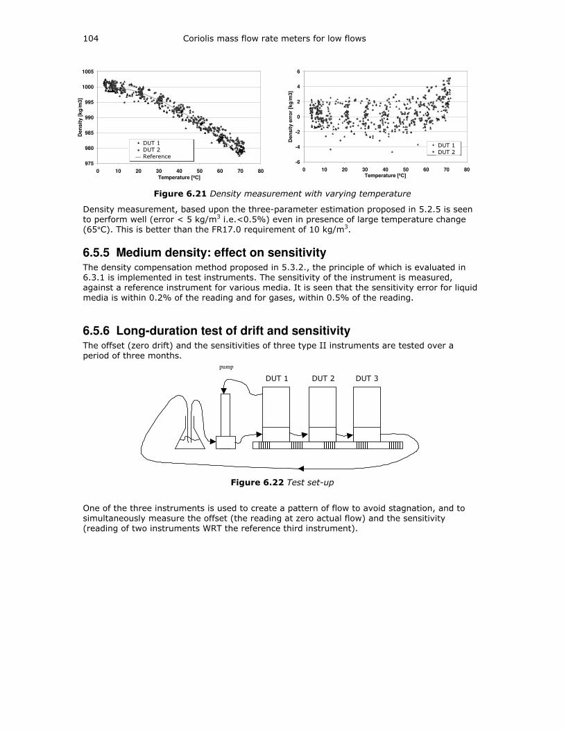
104 Coriolis mass flow rate meters for low flows
975
980
985
990
995
1000
1005
0 10 20 30 40 50 60 70 80
Temperature [ºC]
Den
sit
y [
kg
/m3
]
RB10.34
RB10.33
Reference density
-6
-4
-2
0
2
4
6
0 10 20 30 40 50 60 70 80Temperature [ºC]
De
nsit
y e
rro
r [k
g/m
3]
RV10.34
RB10.33
Figure 6.21 Density measurement with varying temperature
Density measurement, based upon the three-parameter estimation proposed in 5.2.5 is seen
to perform well (error < 5 kg/m3 i.e.<0.5%) even in presence of large temperature change
(65°C). This is better than the FR17.0 requirement of 10 kg/m3.
6.5.5 Medium density: effect on sensitivity The density compensation method proposed in 5.3.2., the principle of which is evaluated in
6.3.1 is implemented in test instruments. The sensitivity of the instrument is measured,
against a reference instrument for various media. It is seen that the sensitivity error for liquid
media is within 0.2% of the reading and for gases, within 0.5% of the reading.
6.5.6 Long-duration test of drift and sensitivity The offset (zero drift) and the sensitivities of three type II instruments are tested over a
period of three months.
M6205123A M6205694A M6205888A
pump
Figure 6.22 Test set-up
One of the three instruments is used to create a pattern of flow to avoid stagnation, and to
simultaneously measure the offset (the reading at zero actual flow) and the sensitivity
(reading of two instruments WRT the reference third instrument).
DUT 1 DUT 2
Reference
DUT 1
DUT 2
DUT 1 DUT 2 DUT 3
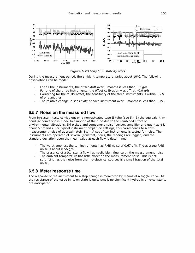
Evaluation and measurement results 105
-1.4
-1.2
-1.0
-0.8
-0.6
-0.4
-0.2
0.0
0.2
0.4
27-10 11-11 26-11 11-12 26-12 10-1 25-1
date 2007
zero
[g
/h]
M6205123A
M6205694A
M6206888A
Long term stability of
instrument sensitivity
Long term
offset stability
Reference
Figure 6.23 Long term stability plots
During the measurement period, the ambient temperature varies about 10°C. The following
observations can be made:
- For all the instruments, the offset-drift over 3 months is less than 0.2 g/h
- For one of the three instruments, the offset calibration was off, at –0.9 g/h
- Correcting for the faulty offset, the sensitivity of the three instruments is within 0.2%
of one another
- The relative change in sensitivity of each instrument over 3 months is less than 0.1%
6.5.7 Noise on the measured flow From in-system tests carried out on a non-actuated type II tube (see 5.4.3) the equivalent in-
band random Coriolis-mode-like motion of the tube due to the combined effect of
environmental vibrations, EM pickup and component noise (sensor, amplifier and quantizer) is
about 5 nm RMS. For typical instrument amplitude settings, this corresponds to a flow-
measurement noise of approximately 1g/h. A set of ten instruments is tested for noise. The
instruments are operated at several (constant) flows, the readings are logged, and the
standard deviation upon the mean value at each flow is determined
- The worst amongst the ten instruments has RMS noise of 0.67 g/h. The average RMS
noise is about 0.56 g/h.
- The presence of a (constant) flow has negligible influence on the measurement noise
- The ambient temperature has little effect on the measurement noise. This is not
surprising, as the noise from thermo-electrical sources is a small fraction of the total
noise.
6.5.8 Meter response time The response of the instrument to a step change is monitored by means of a toggle-valve. As
the resistance of the valve in its on state is quite small, no significant hydraulic time-constants
are anticipated.
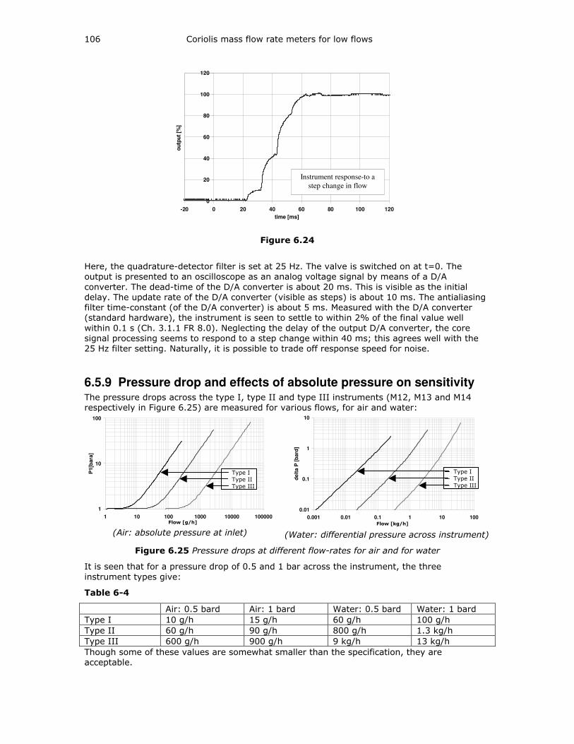
106 Coriolis mass flow rate meters for low flows
0
20
40
60
80
100
120
-20 0 20 40 60 80 100 120
time [ms]
ou
tpu
t [%
]RB8.10 Analog output
Instrument response-to a
step change in flow
Figure 6.24
Here, the quadrature-detector filter is set at 25 Hz. The valve is switched on at t=0. The
output is presented to an oscilloscope as an analog voltage signal by means of a D/A
converter. The dead-time of the D/A converter is about 20 ms. This is visible as the initial
delay. The update rate of the D/A converter (visible as steps) is about 10 ms. The antialiasing
filter time-constant (of the D/A converter) is about 5 ms. Measured with the D/A converter
(standard hardware), the instrument is seen to settle to within 2% of the final value well
within 0.1 s (Ch. 3.1.1 FR 8.0). Neglecting the delay of the output D/A converter, the core
signal processing seems to respond to a step change within 40 ms; this agrees well with the
25 Hz filter setting. Naturally, it is possible to trade off response speed for noise.
6.5.9 Pressure drop and effects of absolute pressure on sensitivity The pressure drops across the type I, type II and type III instruments (M12, M13 and M14
respectively in Figure 6.25) are measured for various flows, for air and water:
1
10
100
1 10 100 1000 10000 100000flow [g/h]
P1
[bara
]
M12
M13
M14
(Air: absolute pressure at inlet)
0.01
0.1
1
10
0.001 0.01 0.1 1 10 100
flow [gk/h]
de
lta
P [
ba
rd]
M12
M13
M14
(Water: differential pressure across instrument)
Figure 6.25 Pressure drops at different flow-rates for air and for water
It is seen that for a pressure drop of 0.5 and 1 bar across the instrument, the three
instrument types give:
Table 6-4
Air: 0.5 bard Air: 1 bard Water: 0.5 bard Water: 1 bard
Type I 10 g/h 15 g/h 60 g/h 100 g/h
Type II 60 g/h 90 g/h 800 g/h 1.3 kg/h
Type III 600 g/h 900 g/h 9 kg/h 13 kg/h
Though some of these values are somewhat smaller than the specification, they are
acceptable.
Flow [kg/h] Flow [g/h]
Type I Type II
Type III
Type I
Type II Type III
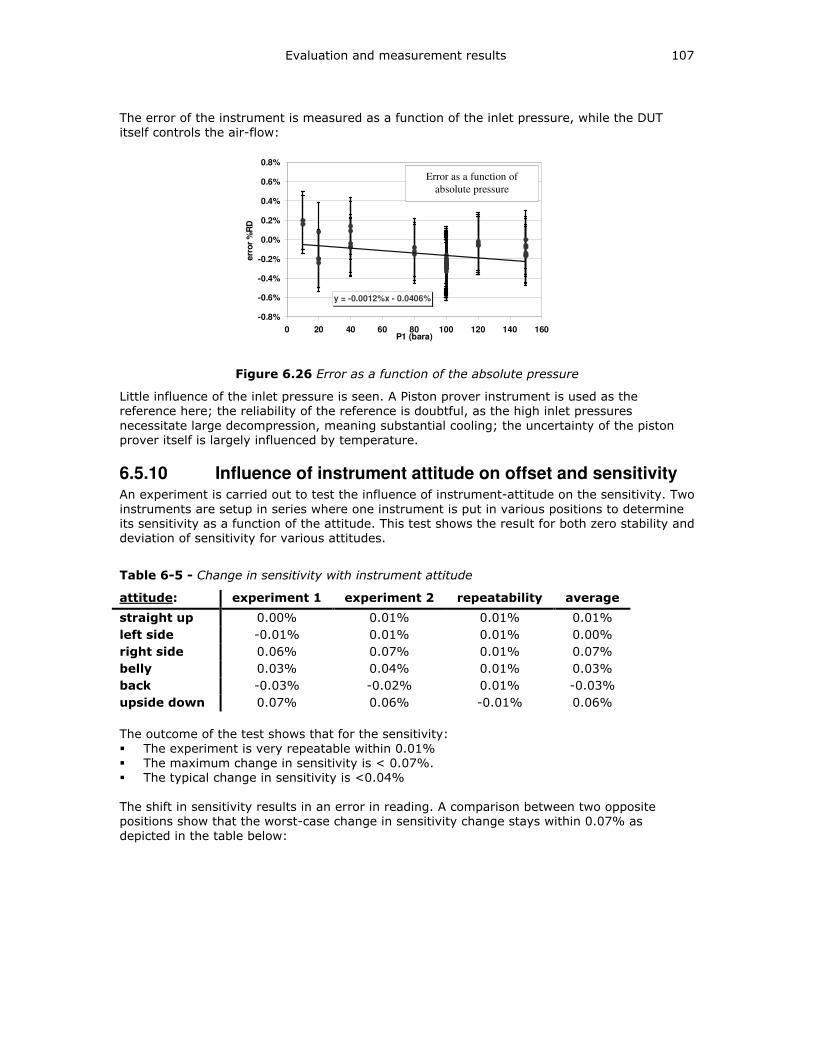
Evaluation and measurement results 107
The error of the instrument is measured as a function of the inlet pressure, while the DUT
itself controls the air-flow:
y = -0.0012%x - 0.0406%
-0.8%
-0.6%
-0.4%
-0.2%
0.0%
0.2%
0.4%
0.6%
0.8%
0 20 40 60 80 100 120 140 160P1 (bara)
err
or
%R
D
Accuracy RB10.72
Linear (Accuracy RB10.72)
Error as a function of
absolute pressure
Figure 6.26 Error as a function of the absolute pressure
Little influence of the inlet pressure is seen. A Piston prover instrument is used as the
reference here; the reliability of the reference is doubtful, as the high inlet pressures
necessitate large decompression, meaning substantial cooling; the uncertainty of the piston
prover itself is largely influenced by temperature.
6.5.10 Influence of instrument attitude on offset and sensitivity An experiment is carried out to test the influence of instrument-attitude on the sensitivity. Two
instruments are setup in series where one instrument is put in various positions to determine
its sensitivity as a function of the attitude. This test shows the result for both zero stability and
deviation of sensitivity for various attitudes.
Table 6-5 - Change in sensitivity with instrument attitude
attitude: experiment 1 experiment 2 repeatability average
straight up 0.00% 0.01% 0.01% 0.01%
left side -0.01% 0.01% 0.01% 0.00%
right side 0.06% 0.07% 0.01% 0.07%
belly 0.03% 0.04% 0.01% 0.03%
back -0.03% -0.02% 0.01% -0.03%
upside down 0.07% 0.06% -0.01% 0.06%
The outcome of the test shows that for the sensitivity:
The experiment is very repeatable within 0.01%
The maximum change in sensitivity is < 0.07%.
The typical change in sensitivity is <0.04%
The shift in sensitivity results in an error in reading. A comparison between two opposite
positions show that the worst-case change in sensitivity change stays within 0.07% as
depicted in the table below:
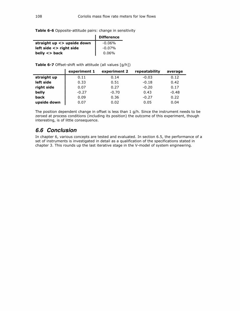
108 Coriolis mass flow rate meters for low flows
Table 6-6 Opposite-attitude pairs: change in sensitivity
Difference
straight up <> upside down -0.06%
left side <> right side -0.07%
belly <> back 0.06%
Table 6-7 Offset-shift with attitude (all values [g/h])
experiment 1 experiment 2 repeatability average
straight up 0.11 0.14 -0.03 0.12
left side 0.33 0.51 -0.18 0.42
right side 0.07 0.27 -0.20 0.17
belly -0.27 -0.70 0.43 -0.48
back 0.09 0.36 -0.27 0.22
upside down 0.07 0.02 0.05 0.04
The position dependent change in offset is less than 1 g/h. Since the instrument needs to be
zeroed at process conditions (including its position) the outcome of this experiment, though
interesting, is of little consequence.
6.6 Conclusion In chapter 6, various concepts are tested and evaluated. In section 6.5, the performance of a
set of instruments is investigated in detail as a qualification of the specifications stated in
chapter 3. This rounds up the last iterative stage in the V-model of system engineering.
7 Conclusions and recommendations
7.1 The output of the project This thesis is aimed at the design of a Coriolis mass-flow meter intended for low flow-rates. A
broad range of topics is treated from the Mechatronics perspective – ranging from tube-shapes
and eigenmodes to sensor and actuator design to data processing and presentation. Based
upon a set of concept and design choices – evaluated & selected from a number of existing
and novel ideas – three scale variants (having the same basis design components) are worked
out in detail. One of these three, the type II instrument, is illustratively discussed in detail in
this thesis. Based upon the concepts and design elements resulting from the present research,
a commercial instrument has been launched. Several patents have been assigned, and several
others are pending.
7.2 Conclusions at the system-level - An instrument capable of measuring low mass-flow-rates (100 g/h full-scale) has been
demonstrated. This is the cumulative result of choices made at the subsystem and
component levels and suitable system integration thereof.
- A zero (offset)-drift better than 0.1 g/h and a relative error against conventional reference
instruments better than 0.2% has been demonstrated.
- A measurement scheme for Coriolis force based on ratiometric measurement purely in the
time-domain has been demonstrated - at no point is any amplitude information used as a
measure for the mass flow. This eliminates the need for component-level calibration. As
the Coriolis force is miniscule compared to the actuation and oscillation forces, the high
precision (1:1e5) afforded by cheap time-references helps isolate the tiny Coriolis forces
(magnitudes).
- The construction of the demonstrated instrument is possible using conventional fine-
mechanical techniques (as opposed to micro-machining etc.) and COTS sensors and
processing electronics, with low production-costs to target the mass-market.
7.3 Conclusions at the subsystem level - In a Coriolis meter using an unconstrained oscillating tube, the ratio of the amplitude of
the Coriolis response motion -the “swing”- to the amplitude of excitation motion -the
rotation or “twist”- is an indication of the Coriolis force. It is an insufficient approximation
to relate the Coriolis force to the phasor-angle or time shift between position signals.
- The sensitivity of the Coriolis mass flow meter discussed in this thesis varies as a function
of the medium-density. This variation is the result of choices such as excitation at
eigenfrequency and Coriolis response on the mass line. Despite the variation, these
choices are made as they afford several advantages. The variation is well explainable and
a correction based on physical principles (rather than trial-and-error methods) is
demonstrated.
- The sensitivity of the Coriolis mass flow meter also varies as a function of the temperature
(primarily that of the tube material). Correction for this variation, based upon the
underlying physics, has been demonstrated.
- In order to increase instrument sensitivity to Coriolis motion, it is advantageous to have as
small a common-mode signal as possible. For this reason, it is advantageous to place the
tube-motion sensors close to the rotation axis. A shift in the rotation axis affects the ratio-
sensitivity. To correct for such a shift, using only time-domain (phasor) measurements,
three (or more) position sensors are essential.
7.4 Conclusions at the component-level - By using a tube with a high Q-factor (>1000) excited at its eigenfrequency, the excitation
effort is minimized, also minimizing the effect of actuator asymmetry on the Coriolis-mode
motion.
110 Coriolis mass flow rate meters for low flows
- A meter tube-shape whose geometry changes little due to temperature is realized by
means of a bent tube where the inlet and outlet are collocated.
- A shape for the resonant tube, whereby the ‘spring’ function is unified (single torsion
spring entity) and isolated from the ‘rotating tube’ function affords predictable and
constant performance (sensitivity and offset-stability).
- It is advantageous to choose a shape for the resonant tube where the excitation
eigenfrequency and Coriolis (response) eigenfrequency are in a ratio R such that
1.5<R<1.8. The lower limit (1.5) ensures that the response motion (gain) is not
significantly affected by a change in the Q-factor of the oscillating tube. The upper limit
(1.8) ensures that the response motion is not too far away (in our case, on the mass line);
this would mean a smaller gain.
- Tuning the ratio of the excitation and response modes is easily possible by tuning the
aspect-ratio of the rectangular tube-shape.
- A novel contactless actuation principle based on induction and Lorentz forces is
demonstrated for actuation of the tube. The contactless nature makes near-ideal actuation
(without attachment asymmetries) possible.
- A torque actuator construction is demonstrated, which due to the translation property of
torque, makes for a near-ideal actuator.
- The position of the actuator, very close to the rotation-axis of the response motion,
introduces an additional attenuation preventing the actuation of the Coriolis motion.
- Contactless sensing is carried out by means of optical interruption sensors. Time delays
inherent to these devices, caused by parasitic capacitance, are eliminated by the use of
transimpedance amplifier techniques.
- The sensor signals are interpreted by quadrature lock-in phase detection technique – this
technique inherently ignores harmonics, and hence non-linearity of the sensor signals is
inconsequential.
- Due to the quadrature lock-in phase detection technique, measurement happens in a
narrow frequency band around the excitation frequency. Being away from DC, this
inherently gets rid of flicker (1/f), and being a narrow-band measurement, it also affords
low measurement noise.
- A simple technique for creating sustained stable oscillations in the Coriolis tube is
demonstrated.
7.5 Recommendations Research into the following issues can further improve the instrument performance:
- Investigating laminar>turbulent transition
It is seen for some media that the transition from laminar flow to turbulent flow occurs
within the typical flow range. It is observed (see Ch. 6.5) that during this transition the
instrument shows a slightly higher sensitivity and the Q-factor of the tube too becomes
substantially lower. A possible explanation is that the flow resistance is modulated by the
tube oscillation leading to pulsating (at tube eigenfrequency) flow. This phenomenon
merits investigation.
- Optimization algorithm for the tube shape
Due to the multitude of parameters that may be varied, finding the ideal tube shape is a
challenge. By means of an automated “goal seeking” algorithm, it may be possible to
come up with a better tube shape than those presented in this work. Naturally a new
challenge will be to define all possible criteria, cost functions, and boundaries for such an
algorithm.
- Internal and external vibrations
All Coriolis flowmeters inherently have a moving flow-tube. Vibrations generated due to
the motion of this tube and external vibrations can potentially interfere with the
measurement of the generated Coriolis force. An investigation into options to reduce the
effect of external vibrations would add significantly to the present work.
- Reducing instrument noise
With the present device (type-II), at maximum bandwidth, the lower limit on measuring
flow is set by the noise at about 1 g/h. For applications with short interval times, it is
necessary to reduce the noise by improving signal and data path, especially the
instrument-ground-and-shield and converter clock jitter.
Conclusions and recommendations 111
- Detailed magnetic modeling
A Lorentz actuation is chosen for of the Coriolis tube in the present work. Detailed analysis
of the magnetic quantities and interaction with the other instrument components (leakage
fluxes etc.) would be useful for application of this concept to a range of instruments.

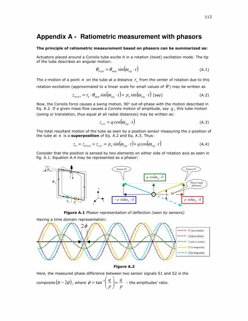
113
Appendix A - Ratiometric measurement with phasors
The principle of ratiometric measurement based on phasors can be summarized as:
Actuators placed around a Coriolis tube excite it in a rotation (twist) oscillation mode. The tip
of the tube describes an angular motion:
( )teigtwist ⋅= ωθθ sinmax (A.1)
The z-motion of a point n on the tube at a distance nr from the center of rotation due to this
rotation excitation (approximated to a linear scale for small values of θ ) may be written as
( ) ( )tptrz eigneigntwn ⋅=⋅⋅= ωωθ sinsinmax)( [say] (A.2)
Now, the Coriolis force causes a swing motion, 90° out-of-phase with the motion described in
Eq. A.2. If a given mass flow causes a Coriolis motion of amplitude, say q , this tube motion
(swing or translation, thus equal at all radial distances) may be written as:
( )tqz eigcor ⋅= ωcos (A.3)
The total resultant motion of the tube as seen by a position sensor measuring the z-position of the tube at n is a superposition of Eq. A.2 and Eq. A.3. Thus:
( ) ( )tqtpzzz eigeigncortwnn ⋅+⋅=+= ωω cossin)( (A.4)
Consider that the position is sensed by two elements on either side of rotation axis as seen in
fig. A.1. Equation A.4 may be represented as a phasor:
maxθ
x z
y
2S
1S
mΦ
( )tp eig ⋅⋅ ωsin
( )tq eig ⋅⋅ ωcos
( )tp eig ⋅⋅− ωsin
φ2
Sensor S1 Sensor S2
Phasor angle
difference
Figure A.1 Phasor representation of deflection (seen by sensors)
Having a time domain representation:
Figure A.2
Here, the measured phase difference between two sensor signals S1 and S2 is the
composite ( )φπ 2− , where p
q
p
q≈
= −1tanφ - the amplitudes’ ratio.


115
Appendix B - Lorentz actuation
B.1 Dimensioning of the stator yoke of the Lorentz actuator A static field yoke provides a pair of air-gaps with anti-parallel fields. A current-carrying
conductor passing through these two gaps will experience a force couple (a pair of equal and
opposite Lorentz forces). This principle is used to actuate the Coriolis tube in the type-II
apparatus in a torsion-mode excitation.
To make a compact construction, rare earth (NdFeB) magnets are used for the yoke (high
residual flux density). The two air-gaps in the yoke must be identical in gap-width and field
strength (antiparallel) in order to have a pure torque. Hence, the magnetic circuit of the yoke
is constructed in such a way that the two air-gaps are ‘connected’ in series, instead of using
two separate constructions. Being in series, the flux passing through each gap is equal.
Further, soft iron is used as the material for the yoke, as it has a saturation flux rating that is
suitable for use with NdFeB magnets, and is easily available and machineable.
Geometry
NdFeB magnets are typically available in 1.1 to 1.2 Tesla (residual flux density) rating. Flux
density (B [Tesla]) is a metric of the strength of a magnetic field. Two other metrics describe
the magnet: the surface area and the thickness. The surface area decides the total flux
available from the magnet (flux density × area = total flux). The flux “coming out” of the
magnet may be spread or concentrated using appropriate construction of a ‘pole shoe’ of a
ferromagnetic material (in this case – soft iron).
The residual flux density mentioned above (1.2 Tesla) is available from a magnet only if a high
permeability (analogous to low resistance) path is made available between the two poles of
the magnet. The total flux (Φ [Weber]) is equal at all cross sections of such a magnetic path
(irrespective of area). Now, for example, if the cross section of the high permeability ‘short
circuit’ path is constant over the entire length, the flux density (Tesla) is equal in the whole
path. In practice, if there is an air-gap in the magnetic path, it has the effect of reducing the
flux and hence also the flux density along the entire path in a ratio expressed by
gapmagnet
magnet
resgappathll
lBBB
+∗== (B.1)
Where Bres is the residual flux density (1.2 Tesla, in this case), and lmagnet is the thickness of
the magnet along the direction of polarization.
Thus, in case of a magnetic circuit with an air-gap, a thicker magnet causes higher flux and
hence higher flux density along the entire path (which can be best seen in the air-gap).
Further, ‘spreading’ the air gap to double the area has the same effect as halving the gap-
length (analogous to resistance). Thus a gap with double area causes more flux, (though lower
flux density within the gap). Consider the following example:
l,A l,A
l,2A l,A
][6.02.1 Teslall
lB =
+∗= ][8.0
2
2.1 Teslall
lB =
+∗=
][6.0 TeslaA
ABBgap =∗= ][4.0
2Tesla
A
ABBgap =∗=
B
Bgap
B
Bgap
Consider
lmagnet = l gap= l
Figure B.1 Illustration: Flux density in magnetic yoke with air-gap
116 Coriolis mass flow rate meters for low flows
Also, if several equal-area air gaps are present in series, their effective ‘resistance’ (length)
adds, but there is no ‘spreading’ effect (obviously, since flux in each gap is equal). Further,
since the air-gap areas are the same, the flux densities will also be equal.
Magnetic flux (ΦΦΦΦ): Generally, if an NdFeB magnet of pole surface area Amagnet and thickness lmagnet is placed in a
magnetic path as shown in Figure B.1, then the total flux in the path is approximately27 given
by the expression:
+
∗=Φ
gap
magnetgapmagnet
magnet
magnetTesla
path
A
All
lA
][2.1 (B.2)
Where lgap is the equivalent total gap length and Agap is the air-gap pole surface area
Creating a flux (density) in an air-gap: To create a magnetic air-gap, we need to first create a ‘path’ using a ferromagnetic material
around a magnet. If a magnetic path has a ‘break’ (e.g. - as shown in figure 2), where the
equivalent gap-length is much smaller than the thickness of the magnet itself, most of the flux
coming ‘out’ of the magnet will choose to travel through the gap. Some flux will leak through
the surrounding regions, either directly from the magnet or from parts of the magnetic path.
The main idea is to design a path such that most of the flux passes through the ‘break’ in the
magnetic path, i.e. the air-gap. Adding magnetic ‘insulators’ (diamagnetic materials) to block
leakage fields is usually impractical.
Flux density (B): In the example above, if the path cross-section area at some point (including in the air-gap) is
Acs, then the flux density (B) perpendicular to that cross-section is:
CS
pathCS A
BΦ
= (B.3)
For NdFeB magnets, as stated earlier, the residual flux density is about 1.2 Tesla. Although, in
theory, it is possible to have a path that acts as a ‘concentrator’ and creates a higher flux
density in an air-gap (say 5 Tesla), it is impractical. Why? The ‘saturation flux density’ Bsat of
a typical path material – say soft iron – is about 1.5 Tesla. In fact, the material shows soft
saturation above about 1 Tesla. This in turn means that if the flux density in any part of a
magnetic path constructed with soft iron is larger than 1 Tesla, the path will show larger
‘resistance’ than expected and there will be some flux leakage. A practical rule is to design for 1.0 Tesla flux density. (For some applications, if a lower flux density is desired, this is okay;
1.0 Tesla is only an upper limit)
Force (Electromagnetic actuation) If a conductor carrying a current I is placed in an air-gap with a magnetic field having flux
density Bgap, and if a length L of the conductor is exposed to the magnetic field (typically, the
breadth of the pole shoe), then a force Factuation is exerted on the conductor, which may be
expressed as:
ILBFactuation ∗×= )(rrr
(B.4)
Limiting design factors are:
- If the conductor (actuated element) has a certain stroke, the pole shoe must be as
broad (bstroke), typically 50% more, to provide uniform actuation force over the entire
stroke.
27 Saturation effects in core, leakage, etc. are not accounted for.

Lorentz actuation 117
- For the conductor (Actuated element) to move freely, the gap length lgap must be at
least as much as the thickness of the conductor, plus motion tolerances plus assembly
tolerances. This restriction, when used with the 1.0 Tesla rule, gives an estimate of the
required thickness of the magnet lmagnet (Typically 2 to 3 times as much as the gap)
and the surface area of the magnet (typically 1.0 to 1.5 times the pole shoe area)
- As stated previously, a practical value for flux density is 1.0 Tesla. If a force Factuation
is desired in a conductor carrying a current Iactuation, then the parameter to vary is the
actuation length Lactuation (not to be confused with the gap length lgap). Now, the air-
gap pole area is established as
strokeactuationgap bLA ⋅= (B.5)
- It is also possible to increase actuation force by increasing the current, Iactuation. There
are, however, two limitations to this
o A larger current often implies use of a thicker conductor. This may require a
wider air-gap length, which will in turn reduce flux. (Not a relevant issue in the
Coriolis actuator.)
o The current carrying conductor generates a field of its own. This is actually
what causes the actuation. Its interaction with the gap field must be
considered. (Not a relevant issue in the Coriolis actuator.)
- The actuation force on the conductor creates an equal and opposite reaction force,
that acts upon the magnetic path (yoke). The yoke should hence, by design, be
securely anchored.
Pure torque In the Window-tube, in interest of exciting the rotational mode alone, a pure torque needs to
be exerted. In principle, if we have the same current flowing through a tube (conductor), and
if the tube is placed in a pair of equal (antiparallel) magnetic air-gaps, this should be achieved.
To obtain identical air-gaps, the following points need to be considered:
1) The gaps should be mechanically identical. This means that the gap length, the
actuation length and the stroke length must be congruent in each gap. The following
errors may be expected:
a. If the gap length is not identical, no major difference in the flux density in the
gap will be seen. This is due to the fact that, by design, the two gaps form a
series magnetic circuit (see figure 1), and thus the flux through them is equal.
A minor difference will, however, be seen, as a wider gap will have slightly
different leakage pattern.
b. If the pole areas are unequal: (two cases)
i. If the stroke breadth bstroke is different for each pole, it will
substantially affect the flux densities [Tesla], as the same flux ΦΦΦΦ will
create different flux densities Bgap 1 and Bgap 2.
ii. If the actuation length Lactuation is different, say smaller in gap 2, it will
increase Bgap 2 (same flux, smaller area) but as the active length is
smaller, the two effects will cancel out, and the force will stay roughly
constant
2) The pole faces should be aligned sideways. If they are not, the construction is no
longer mirror-symmetric, and unequal leakages in each gap may result in an
(unexpected) unequal B-field in the air-gaps
3) The stroke breadth should be designed appropriately. We assume that the B field is
equal and uniform over the entire air-gap surface, and is perpendicular to it. In reality,
there are fringe effects (curved field lines near the edges). If, during assembly, the
tube is not exactly centered within the air-gap, then in too narrow a gap, an
unequal pair of forces will be exerted (not desirable).
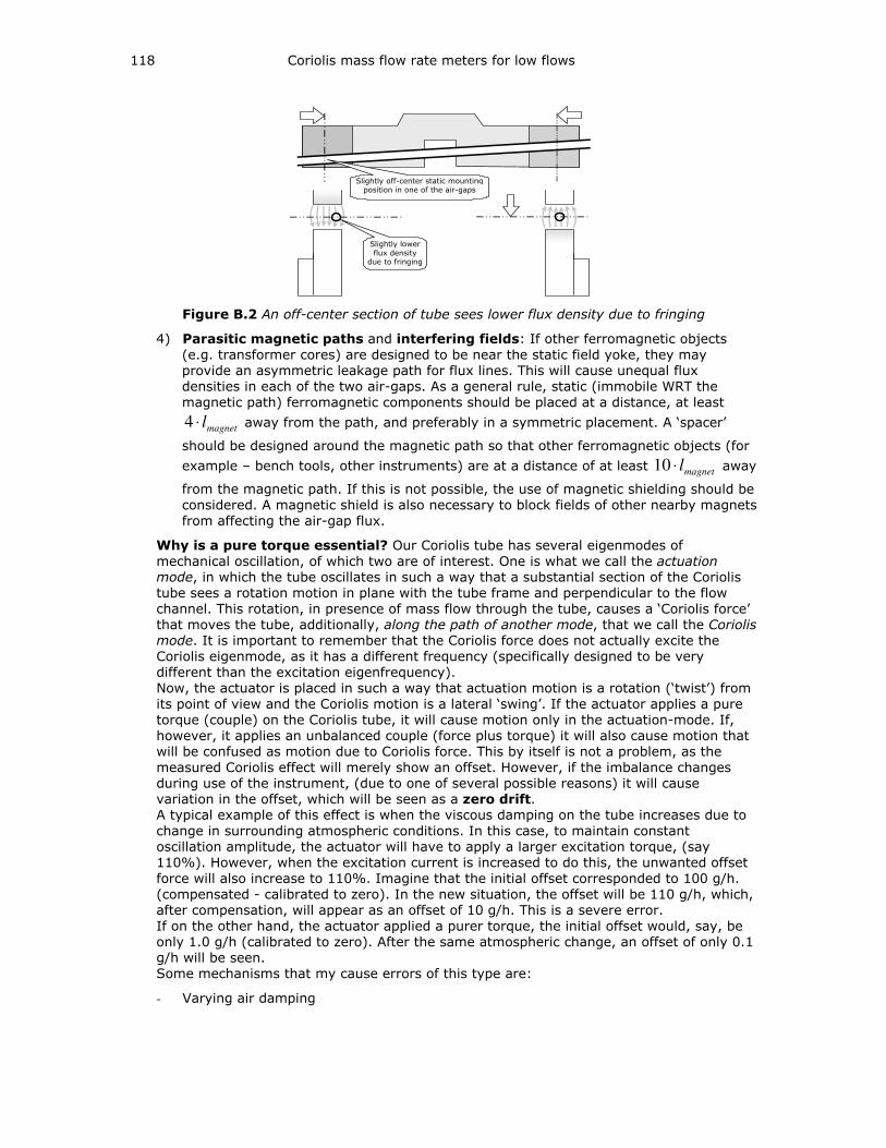
118 Coriolis mass flow rate meters for low flows
Slightly lower flux density
due to fringing
Slightly off-center static mounting position in one of the air-gaps
Figure B.2 An off-center section of tube sees lower flux density due to fringing
4) Parasitic magnetic paths and interfering fields: If other ferromagnetic objects
(e.g. transformer cores) are designed to be near the static field yoke, they may
provide an asymmetric leakage path for flux lines. This will cause unequal flux
densities in each of the two air-gaps. As a general rule, static (immobile WRT the
magnetic path) ferromagnetic components should be placed at a distance, at least
magnetl⋅4 away from the path, and preferably in a symmetric placement. A ‘spacer’
should be designed around the magnetic path so that other ferromagnetic objects (for
example – bench tools, other instruments) are at a distance of at least magnetl⋅10 away
from the magnetic path. If this is not possible, the use of magnetic shielding should be
considered. A magnetic shield is also necessary to block fields of other nearby magnets
from affecting the air-gap flux.
Why is a pure torque essential? Our Coriolis tube has several eigenmodes of
mechanical oscillation, of which two are of interest. One is what we call the actuation mode, in which the tube oscillates in such a way that a substantial section of the Coriolis
tube sees a rotation motion in plane with the tube frame and perpendicular to the flow
channel. This rotation, in presence of mass flow through the tube, causes a ‘Coriolis force’
that moves the tube, additionally, along the path of another mode, that we call the Coriolis mode. It is important to remember that the Coriolis force does not actually excite the
Coriolis eigenmode, as it has a different frequency (specifically designed to be very
different than the excitation eigenfrequency).
Now, the actuator is placed in such a way that actuation motion is a rotation (‘twist’) from
its point of view and the Coriolis motion is a lateral ‘swing’. If the actuator applies a pure
torque (couple) on the Coriolis tube, it will cause motion only in the actuation-mode. If,
however, it applies an unbalanced couple (force plus torque) it will also cause motion that
will be confused as motion due to Coriolis force. This by itself is not a problem, as the
measured Coriolis effect will merely show an offset. However, if the imbalance changes
during use of the instrument, (due to one of several possible reasons) it will cause
variation in the offset, which will be seen as a zero drift. A typical example of this effect is when the viscous damping on the tube increases due to
change in surrounding atmospheric conditions. In this case, to maintain constant
oscillation amplitude, the actuator will have to apply a larger excitation torque, (say
110%). However, when the excitation current is increased to do this, the unwanted offset
force will also increase to 110%. Imagine that the initial offset corresponded to 100 g/h.
(compensated - calibrated to zero). In the new situation, the offset will be 110 g/h, which,
after compensation, will appear as an offset of 10 g/h. This is a severe error.
If on the other hand, the actuator applied a purer torque, the initial offset would, say, be
only 1.0 g/h (calibrated to zero). After the same atmospheric change, an offset of only 0.1
g/h will be seen.
Some mechanisms that my cause errors of this type are:
- Varying air damping
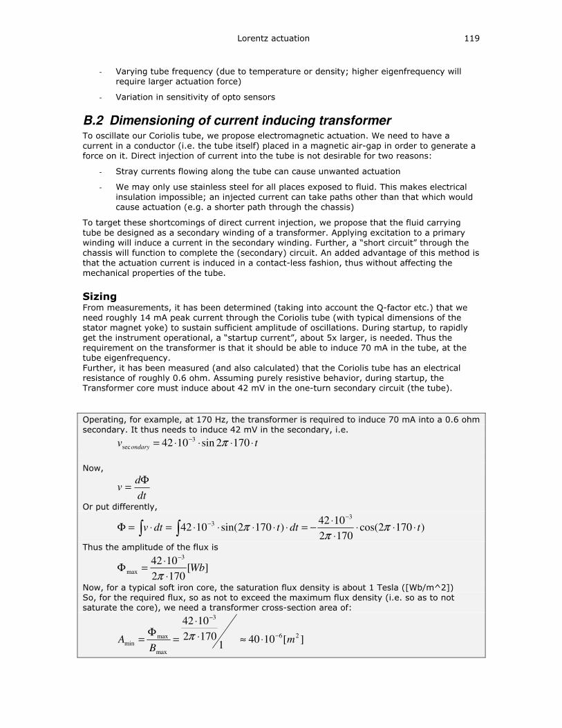
Lorentz actuation 119
- Varying tube frequency (due to temperature or density; higher eigenfrequency will
require larger actuation force)
- Variation in sensitivity of opto sensors
B.2 Dimensioning of current inducing transformer To oscillate our Coriolis tube, we propose electromagnetic actuation. We need to have a
current in a conductor (i.e. the tube itself) placed in a magnetic air-gap in order to generate a
force on it. Direct injection of current into the tube is not desirable for two reasons:
- Stray currents flowing along the tube can cause unwanted actuation
- We may only use stainless steel for all places exposed to fluid. This makes electrical
insulation impossible; an injected current can take paths other than that which would
cause actuation (e.g. a shorter path through the chassis)
To target these shortcomings of direct current injection, we propose that the fluid carrying
tube be designed as a secondary winding of a transformer. Applying excitation to a primary
winding will induce a current in the secondary winding. Further, a “short circuit” through the
chassis will function to complete the (secondary) circuit. An added advantage of this method is
that the actuation current is induced in a contact-less fashion, thus without affecting the
mechanical properties of the tube.
Sizing From measurements, it has been determined (taking into account the Q-factor etc.) that we
need roughly 14 mA peak current through the Coriolis tube (with typical dimensions of the
stator magnet yoke) to sustain sufficient amplitude of oscillations. During startup, to rapidly
get the instrument operational, a “startup current”, about 5x larger, is needed. Thus the
requirement on the transformer is that it should be able to induce 70 mA in the tube, at the
tube eigenfrequency.
Further, it has been measured (and also calculated) that the Coriolis tube has an electrical
resistance of roughly 0.6 ohm. Assuming purely resistive behavior, during startup, the
Transformer core must induce about 42 mV in the one-turn secondary circuit (the tube).
Operating, for example, at 170 Hz, the transformer is required to induce 70 mA into a 0.6 ohm
secondary. It thus needs to induce 42 mV in the secondary, i.e.
tv ondary ⋅⋅⋅⋅= − 1702sin1042 3
sec π
Now,
dt
dv
Φ=
Or put differently,
)1702cos(1702
1042)1702sin(1042
33
tdttdtv ⋅⋅⋅⋅
⋅−=⋅⋅⋅⋅⋅=⋅=Φ
−−
∫ ∫ ππ
π
Thus the amplitude of the flux is
][1702
1042 3
max Wb⋅
⋅=Φ
−
π
Now, for a typical soft iron core, the saturation flux density is about 1 Tesla ([Wb/m^2])
So, for the required flux, so as not to exceed the maximum flux density (i.e. so as to not
saturate the core), we need a transformer cross-section area of:
][10401
1702
1042
26
3
max
maxmin m
BA
−
−
⋅≈⋅
⋅
=Φ
= π
120 Coriolis mass flow rate meters for low flows
Number of primary turns We need to induce a certain flux (40e-6 [Wb] peak) at a certain frequency (170 [Hz]) in the
transformer core. To do this we need a voltage waveform with certain amplitude. A pragmatic
consideration is to choose this amplitude on basis of the available power supply. Using a full-
bridge amplifier, it is possible to get a peak output voltage equal to the supply voltage. A 10V
DC supply is a convenient choice; thus a peak voltage of 10V is available to induce flux.
The peak voltage, the induced flux and the number of turns are, once again, related as
dt
dNv
Φ= (B.6)
But the induced flux is sinusoidal in time, such that:
)1702sin(1040)2sin(. 6
max ttfeig ⋅⋅⋅⋅=Φ=Φ − ππ
Thus
)1702cos(17021040 6t
dt
d⋅⋅⋅⋅⋅⋅=
Φ − ππ
For a primary coil having N turns, this gives the peak amplitude of the voltage waveform as
NNv ⋅=⋅⋅⋅⋅= − 04.017021040 6
max π
But, Vmax must be less than 10V. Thus, the inequality
1004.0 ≤⋅ N
i.e.
250≤N must hold.
This is a good starting point for constructing the primary windings.
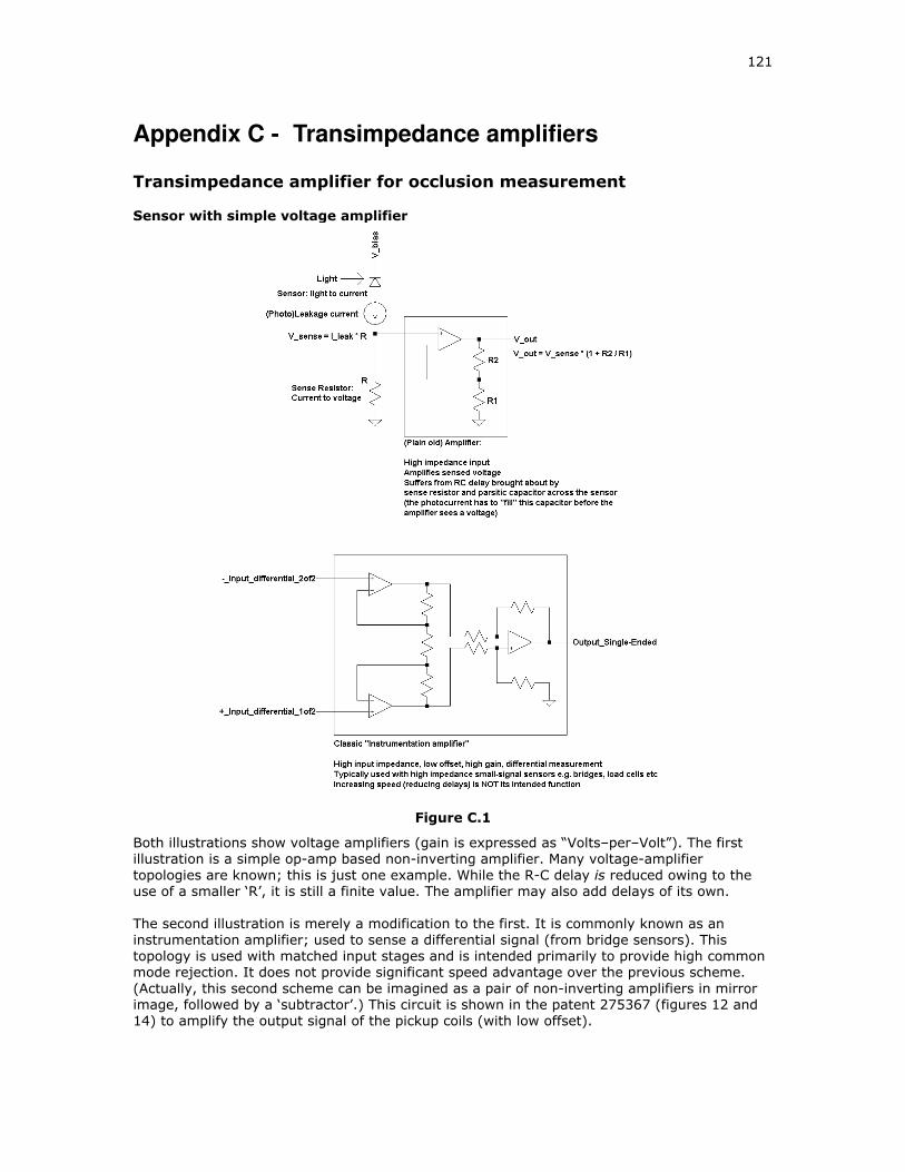
121
Appendix C - Transimpedance amplifiers Transimpedance amplifier for occlusion measurement
Sensor with simple voltage amplifier
Figure C.1
Both illustrations show voltage amplifiers (gain is expressed as “Volts–per–Volt”). The first
illustration is a simple op-amp based non-inverting amplifier. Many voltage-amplifier
topologies are known; this is just one example. While the R-C delay is reduced owing to the
use of a smaller ‘R’, it is still a finite value. The amplifier may also add delays of its own.
The second illustration is merely a modification to the first. It is commonly known as an
instrumentation amplifier; used to sense a differential signal (from bridge sensors). This
topology is used with matched input stages and is intended primarily to provide high common
mode rejection. It does not provide significant speed advantage over the previous scheme.
(Actually, this second scheme can be imagined as a pair of non-inverting amplifiers in mirror
image, followed by a ‘subtractor’.) This circuit is shown in the patent 275367 (figures 12 and
14) to amplify the output signal of the pickup coils (with low offset).
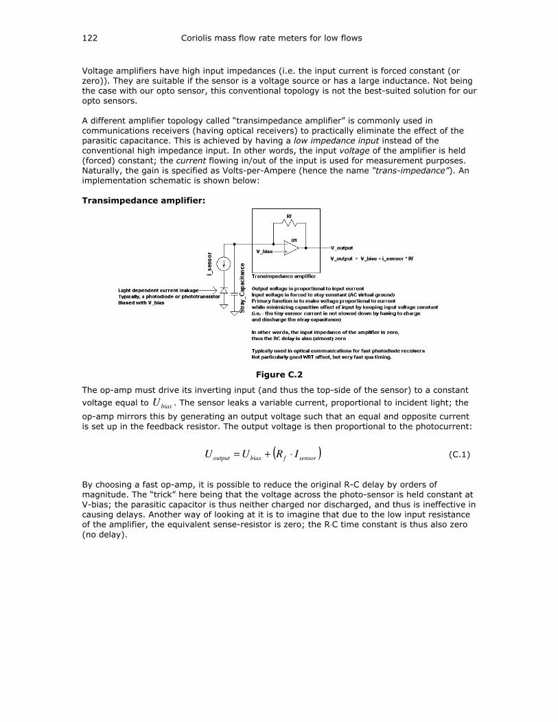
122 Coriolis mass flow rate meters for low flows
Voltage amplifiers have high input impedances (i.e. the input current is forced constant (or
zero)). They are suitable if the sensor is a voltage source or has a large inductance. Not being
the case with our opto sensor, this conventional topology is not the best-suited solution for our
opto sensors.
A different amplifier topology called “transimpedance amplifier” is commonly used in
communications receivers (having optical receivers) to practically eliminate the effect of the
parasitic capacitance. This is achieved by having a low impedance input instead of the
conventional high impedance input. In other words, the input voltage of the amplifier is held
(forced) constant; the current flowing in/out of the input is used for measurement purposes.
Naturally, the gain is specified as Volts-per-Ampere (hence the name “trans-impedance”). An
implementation schematic is shown below:
Transimpedance amplifier:
Figure C.2
The op-amp must drive its inverting input (and thus the top-side of the sensor) to a constant
voltage equal to biasU . The sensor leaks a variable current, proportional to incident light; the
op-amp mirrors this by generating an output voltage such that an equal and opposite current
is set up in the feedback resistor. The output voltage is then proportional to the photocurrent:
( )sensorfbiasoutput IRUU ⋅+= (C.1)
By choosing a fast op-amp, it is possible to reduce the original R-C delay by orders of
magnitude. The “trick” here being that the voltage across the photo-sensor is held constant at
V-bias; the parasitic capacitor is thus neither charged nor discharged, and thus is ineffective in
causing delays. Another way of looking at it is to imagine that due to the low input resistance of the amplifier, the equivalent sense-resistor is zero; the R⋅C time constant is thus also zero
(no delay).

123
Appendix D - Commercial Coriolis flowmeters
Coriolis mass-flow meters - state of the art
Listing of commercial instruments:
Manufacturer Lowest
range
Name
ABB unknown Coriolis-
Master
Emerson/
Brooks
150 g/h Quantim
Danfoss no more
Endress &
Hauser
450 kg/h Promass
FMC Smith
meter
unknown
Foxboro 1.8 kg/h CFS10
Krohne 300 g/h Optimass
Emerson/
MicroMotion
430 g/h LF2M
Oval 240 g/h CN00A
Schlumberger no more
Yokogawa 100 kg/h Rotamass
GE sensing new
Rheonik 240 g/h RHM015
Honeywell unknown
Siemens unknown

124
125
References
[1] Richard P. Feynman, Robert B. Leighton, Matthew Sands, The Feynman Lectures on Physics, The Definitive and Extended Edition, 2nd edition, Addison-Wesley (2005), ISBN
0-8053-9045-6
[2] Stephen Hawking, A brief history of time, Bantam (1988)
[3] M.P. Koster, Constructieprincipes, PPI Uitgeverij (2005), ISBN 90-78249-01-3
[4] P.P.L. Regtien, F. van der Heijden, M.J. Korsten, W. Olthuis, Measurement Science for Engineers, Kogan Page Science (2004), ISBN 1 9039 9658 9
[5] Simon Haykin, An Introduction to Analog and Digital Communication, Wiley (1989),
ISBN 0-471-85978-8
[6] W. Wrigley, W.M. Hollister, W.G. Denhard, Gyroscopic Theory, Design, and Instrumentation, The M.I.T. Press (1969), SBN 262 23037 2
[7] M.L. Meade, Lock-in amplifiers: principles and applications, IEE / Peter Peregrinus Ltd.
(1983)
[8] Dennis Schipper (PhD Thesis), Mobile Autonomous Robot Twente, Twente University
Press (2001), ISBN 9036516862
[9] Aditya Mehendale (Masters’ thesis), Validation, Characterization and Performance Enhancements for a Low Capacity Coriolis Mass Flow Meter, University of Twente (2003)
[10] Marcel Katerberg (Masters’ thesis), Coriolis Mass Flow Sensor and Controller, University
of Twente (2004)
[11] MIL-STD-961E (1 August 2003). Paragraph 5.9.1
[12] Aditya Mehendale, P.P.L. Regtien, System design of low capacity Coriolis mass-flow meters, Conference proceedings, I3S 2005 – Juelich (2005)
[13] Poly-technisch zakboek (Nederlands), 49th print, Elsevier (2002), ISBN 90-6228-358-6
[14] Piezoelectric Ceramics Speciality Ferrites, Data handbook MA03, Philips components
(1997)
[15] C.M. Lievers (Masters’ thesis), Coriolis Mass-Flow Meters, University of Twente (2000)
[16] Peter H. Sydenham, Richard Thorn, Handbook of measuring system design, volume 3,
Wiley (2005), ISBN 0-470-02143-8
[17] Lisa Bates, Timothy Beach and Maya Arnott, Determination of the temperature dependence of Young’s modulus for stainless steel using a tuning fork, Vol. 18 #1, The
journal of undergraduate research in physics (1999)
Literature
[18] A. Belhadj, R. Cheesewright, C. Clark, The simulation of Coriolis meter response to pulsating flow using a general purpose F.E. code, Journal of fluids and structures, Vol.
14, No. 5 (2000), pp 613-634
[19] Furio Cascetta, Effect of fluid pressure on Coriolis mass flowmeter's performance, ISA
transactions 35 (1996) pp 365-370
126
[20] R. Cheesewright, C. Clark, D. Bisset, Understanding the experimental response of Coriolis massflow meters to flow pulsations, Flow measurement and instrumentation 10
(1999) pp 207-215
[21] R. Cheesewright, C. Clark, D. Bisset, The identification of external factors which influence the calibration of Coriolis massflow meters, Flow measurement and
instrumentation 11 (2000) pp 1-10
[22] Thierry Corman, Peter Enoksson, Kjell Noren, Goran stemme, A low-pressure encapsulated resonant fluid density sensor with feedback control electronics, Meas. Sci.
Technol. 11 (2000) pp 205-211
[23] Thierry Corman, Peter Enoksson, Kjell Noren, Goran stemme, Novel burst technology for closed loop detection and excitation of resonant silicon sensors, KTH, Sweden
[24] Peter Enoksson, Goran Stemme, Erik Stemme, A silicon resonant sensor structure for Coriolis mass-flow measurements, Journal of microelectromechanical systems, Vol. 6,
No. 2 (1997)
[25] John Hemp, Lynn Hendry, The weight vector theory of Coriolis mass flowmeters - Part 2. Boundary source of secondary vibration, Flow Meas. Instrum., Vol. 6, No. 4 (1995) pp
259-264
[26] Manus Henry, On-line compensation in a digital Coriolis mass flow meter, Flow
measurement and instrumentation 12 (2001) pp 147-161
[27] Henry, Clarke, Archer, Bowles, Leahy, Liu, Vignos, Zhou, A self validating Coriolis mass-flow meter: an overview, Control engineering practice 8 (2000) pp 487-506
[28] K. Kolahi, Th. Gast, H. Rock, Coriolis mass flow measurement of gas under normal conditions, Flow measurement and instrumentation, Vol. 5(4) (1994) pp 275-283
[29] Tony Pankratz, Gary Pawlas, Improved mass flowrate measurement of gases using Coriolis mass flowmeters, SENSOR (1995), pp 103-108
[30] Ralf Storm, Kourosh Kolahi, Helmut Rock, Model based correction of Coriolis mass flowmeters, IEEE transactions on instrumentation and measurement, Vol. 51, No. 4
(2002)
[31] G. Sultan, J. Hemp, Modeling of the Coriolis mass flowmeter, Journal of Sound and
Vibration, 132(3) (1989) pp 473-489
[32] Timo Veijola, Thierry Corman, Peter Enoksson, Goran Stemme, Dynamic simulation model for a vibrating fluid density sensor, Sensors and actuators 76 (1999) pp 213-224
[33] Yafan Zang, Srinivas Tadigadapa, Nader Najafi, A micromachined Coriolis-force based mass flowmeter for direct mass flow and fluid density measurement, Transducers (2001)
pp 1460-1463
Patents
[34] Bergamini Giorgio, Campanale Nicola, Cocozza Onofrio, (US4895030) Process for the measurement of weight flow-rates and related devices, Nuovo Pignone (1990)
[35] Bose Tamal, Derby Howard Vincent, Levien Andrew Keith, Pankratz Anthony William,
(US5734112) Method and apparatus for measuring pressure in a Coriolis mass flowmeter, Flowtec (1998)
[36] Cage Donald R, (US4768385) Parallel path Coriolis mass flow meter, Micro-motion
(1988)
127
[37] Carpenter Brent L, (US4777833) Ferromagnetic drive and velocity sensors for a Coriolis mass flow rate meter, Micro-motion (1988)
[38] Corwon Michael E, Oliver Randy L, (US5044208) Double-pigtail-shaped Coriolis-type mass flow rate meter, Neptune Meas. (1991)
[39] Corwon Michael E, Oliver Randy L, (US4852410) Omega-shaped, Coriolis-type mass flow rate meter, Schlumberger (1989)
[40] Cox Bruce M, Ho Morris D, (US4192184) Mass flowmeter, Halliburton, (1980)
[41] Cox Bruce M, Ho Morris D, (US4311054) Mass flowmeter with sensor gain control, Halliburton (1982)
[42] Cunningham Timothy J, (US6199022) Drive circuit modal filter for a vibrating tube flowmeter, Micro-motion (2001)
[43] Cunningham Timothy J, Shelley Stuart J, (US6092429) Driver for oscillating a vibrating conduit, Micro-motion (2000)
[44] Derby Howard V, Bose Tamal, Rajan Seeraman, (US5555190) Method and apparatus for adaptive line enhancement in Coriolis mass flow meter measurement, Micro-motion
(1996)
[45] Gomi Shingo, Kitami Hirokazu, Endo Takashi, Matsuoka Kenichi, Ichinose Kimihiro,
Futagawa Osamu, Kobayashi Seiji, Kobayashi Kazuhide, (US5796012) Error correcting Coriolis flowmeter, Oval (1998)
[46] Hussain Yousif A, Machacek Milos J, (US5048350) Electromagnetic driver and sensor, Foxboro (1991)
[47] Kalotay Paul Z, (US5400653) Coriolis effect meter using optical fiber sensors, Micro-
motion (1995)
[48] Kalotay Paul Z, (US5469748) Noise reduction filter system for a Coriolis flowmeter, Micro-motion (1995)
[49] Laursen Mogens Bech, Hansen Henning Max, Birker Bertel, (US6138517) Mass flowmeter with bidirectionally wound oscillation detector, Danfoss (2000)
[50] Mansfield William M, (US6226195) Circuitry for supplying a controlled signal to a drive system, Micro-motion (2001)
[51] Mattar Wade M, Thompson Duane T, Decarlo Joseph P, Hussain Yousif, Chitty Gordon W,
(US4891991) Coriolis-type mass flowmeter, Foxboro (1990)
[52] Ollila Curtis John, Normen David Frederick, Lister Ernest Dale, (US5996225) Method for manufacturing a dual loop Coriolis effect mass flowmeter, Micro-motion (1999)
[53] Ollila Curtis John, Normen David Frederick, Lister Ernest Dale, (US6044715) Dual loop Coriolis effect mass flowmeter, Micro-motion (2000)
[54] Shelley Stuart J, Cunningham Timothy J, (US6230104) Combined pickoff and oscillatory driver for use in Coriolis flowmeters and method of operating the same, Micro-motion
(2001)
[55] Stadler Dietmar, (US6073495) Measuring and operating circuit of a Coriolis-type mass flow meter, Flowtec (2000)
[56] Thompson Duane T, (US4911020) Coriolis-type mass flowmeter circuitry, Foxboro
(1990)
[57] Thompson Duane T, (US5050439) Coriolis-type mass flowmeter circuitry, Foxboro
(1991)
[58] Yokoi Toyoaki, Owada Hiroshi, (US5578764) Coriolis type mass flowmeter utilizing phase shifters for phase shifting of the output signals, Yokogawa (1996)
128
[59] Yoshimura Hiroyuki, Kudo Takahiro, (US5869770) Coriolis type mass flowmeter having isolation form external vibration, Fuji Electric (1999)
[60] Yoshimura Hiroyuki, Kudo Takahiro, Kishiro Masami, (US5831178) Vibration type measuring instrument, Fuji Electric (1998)
[61] Yoshimura Hiroyuki, Morita Akira, (US5844408) Phase difference measuring apparatus for measuring phase difference between input signals, Fuji Electric (1998)
[62] Young Alan M, Blake E Ronald, (US4914956) Method and circuit for processing sensory input signals of the type obtained from Coriolis mass flow rate sensors and the like, Exac
(1990)
129
Acknowledgements
First and foremost, I thank "Aai" (mum) for being just that.
I began my journey in The Netherlands as a master’s student in 2001, and now, seven years
later, this proefschrift is ready, marking a major milestone. This journey was possible and
enjoyable thanks to many people.
Rini, you have been my mentor for most of this journey, and for this I am deeply indebted.
Your wisdom, knowledge and enormous patience, together with attention to detail without
losing sight of "the big picture" has been phenomenal. Additionally, you have sacrificed much
of your personal time - evenings and weekends - for the numerous reviews of this
dissertation. Thank you!
The chance to carry out this PhD research - a major part of my journey - was made possible in
the group of Prof. Regtien. Paul, I have learnt much about the art of measurement from you.
Thank you for all the freedom you gave me in the last four years.
Most of the work I did in the past years has been on the premises of Demcon - initially in
Hengelo and then Oldenzaal. The "Demcon family" - a group of talented and able technology-
enthusiasts - made every day worth looking forward to. Several people at Demcon have
collaborated in realizing the working Coriolis mass-flowmeter. Dennis, a big thank you! for
giving me the opportunity to be a part of the Demcon family, and for giving me the much
needed pep-talks to persevere to finish this dissertation. Peter, your know-how and
multidisciplinary expertise will never cease to amaze me. A special thanks to my office-mates
at Demcon: Jeroen H, Gino, Mark, Matthijs (get well soon!), Angela, Renee, Hernes and
Wouter, and also to the people in the Coriolis project - Mark, Wouter, Tom, Reinier, Bas,
Pieter, Martijn, Remco, Henry, Jeffrey, Ruud, Lucas, Ed K, Ed S, Joke, Rudy, Renee, Chris,
Hernes, Angela and Jos, and the behind-the-scene heroes Joke, Arno, Carla, Petra, Mirjam,
Mathijn and Elly. Lars – it has been a pleasure working with you on the microCoriolis project.
Thanks also to Jan L and Angela for feedback & corrections with the dissertation and Marvin
for the late evening discussions.
Marcel, your feedback on the instrument performance (much of chapter 6) has been
invaluable. It has been great working and sparring with you - discussing things from Indian
food to the formation of bubbles in ethanol ;). Thanks for all this and for the numerous
reviews of this dissertation. Thanks also to the team-that-may-not-be-named - especially
Ronald, Jan, Rob and Joost.
At the UT, thanks are due to people at the group where I was an AIO - Carla, Liesbeth, Joan,
Alfred, and also Brenda, Ellen and Ila for their organizational help - from TAS forms to
residence permits - and my fellow AIOs, especially Valer, Jianbo, Marcel G, Edwin & Gijs. After
the term of my PhD contract, I have been accepted as a researcher at the chair of mechanical
automation and mechatronics. Thanks to Prof. Jonker for this opportunity and to Dannis and
Martina for the organizational help.
My home in The Netherlands in these years has been Calslaan 7-3 "Maar-dan-niet". A big
thanks to the folks (and ex-folks) at home - Alex, Andrea, Ben, Bouke, Douwe, Edwin, Gert,
Jelmer, Mareike, Marjolein, Niels, Peter, Piet, Rama, Richard, Sjoerd, Steve, Vio, and of
course, Mies, for making the journey a pleasure!
Unorthodox as it seems, I find it unfair not to do so - so here goes: A big thanks to team
Blizzard, for making Starcraft/Broodwars - in my opinion the greatest game ever, and to Pepsi
- my favorite source of caffeine and sugar into the late nights.
Aditya Mehendale
Enschede, 2008

130
131
About the author
Aditya Mehendale was born on the 2nd of June 1976 in Pune, India. After finishing higher
secondary education, he went on to graduate with distinction (Bachelor's degree in electronics
engineering) from the University of Pune in 1998. Having done technical projects since age 12,
he joined in partnership in the company "IDG product development", with friend and fellow
alumnus Archis Bhave.
In 2001, he moved to the Netherlands to follow the master's program in Mechatronics at the
Universiteit Twente in Enschede. In 2003, after completing the master's program with honors,
he worked for a year as a researcher and subsequently began work towards a Ph.D., both
under Prof. Paul Regtien, and in close collaboration with Demcon, initially in Hengelo, and then
Oldenzaal.
Since June 2008, he works as a researcher in "Mechanical Automation and Mechatronics"
group of Prof. Ben Jonker, at Demcon, in the field of MEMS based (micro) Coriolis devices.