Embed Size (px)
Citation preview
.A t hesis subniitted to the
Depnrt men t of Corn pli ting and Information Science
in conformit- with the requirements for
the degree of '\laster of Science
Qiieen's h i v e r s i ty
Kingston. Ontario. Canada
January 2002
Copyright @ Andrew Bemat, 2002

National Library Bibliothèque nationale du Canada
Acquisitions and Acquisitions et Bibliqraphic Services seivices bibliographiques
395 WoUington Street 385, nie Wellington Oitawa ON K1A ON4 OaawaON K 1 A N Canada canada
The author has granted a non- exclusive licence aliowing the National Library of Canada to reproduce, loan, distribute or seii copies of this thesis in microform, paper or electronic formats.
The author retains ownership of the copyright in this thesis. Neither the thesis nor substantial extracts fkom it may be printed or otheiwise reproduced without the author's permission.
L'auteur a accordé une licence non exclusive permettant à la Bibliothèque nationale du Canada de reproduire, prêter, distribuer ou vendre des copies de cette thèse sous la forme de microfiche/fh, de reproduction sur papier ou sur format électronique.
L'auteur conserve la propriété du droit d'auteur qui protège cette thèse. Ni la thèse ni des extraits substantiels de celle-ci ne doivent être imprimés ou autrement reproduits sans son autorisation.
Abstract
Frnctal i rnag~ îumprcssion is an area where wr erpect very high rates of compression
as opposed to .JPEG miiprrssion ivhich prochces high quality images at cornparably
lm- rates of coniprcssionl in ii reiisonable amount of time. The siiccess. in terms
of compression ratio and image qiiality. of 3 fractd encoder Iies in the choice of a
partition scheme.
\te will revicw a forma1 model for a Partition Iteratcd Function System (PIFS) en-
coclrr/clecoclrr togctlier wi t b t hc nccessary mat heniat i d background. .\ description
of a fractal tool follows. This tool implernents the PIFS model and several partition
srhemes. It u s tvritten in C++ by Andrew Bernat (author of this thesis). Reason-
able theoretical boiinds on error and image quality for different partition schemes are
difficult to obtain: empirical studies are the only alternative. The fractal tool serves
t his purpose. 1 t can help to determine ivhich kinds of partition schemes yield higher
compression rates and larger signal-to-noise ratios (SSR) for particular images. We
discuss t his in the paper.
' W e will make precise the meaning of hi& and low.


Acknowledgement s
1 have had many cr~joyalle and sad moments while in Kingston. I'd iike to thank
d l rny fricnds for heing around throughoiit those tinies and alloiving me to be with
tiirm. Thanks .-\nibrlr. .\ncirew. Chris. Jeff. .Jcn. J~rcrny. Marta. Nitch.
I'd also likc to t haiik rny friends nway from Kingston whom 1 talked with over the
phone for niany hotirs about ttiesis work and lifr. Thnnk you Elena. Tuny. Also, niy
stipen-isor who ,pave me the opportunity t o work on anything that was cool.
SIy family has a l w q s supported me and they rarely have the opportunity to
rweive my gratitude. but the! know it is there. Thank o u klorn. Dad, Nami. Kati.
anci Bob.

Contents
1 Background Information 1
1 Introduction 3
1.1 Thesis Overview . . . . . . . . . . . . . . . . . . . . . . . . . . . . . . 3
. . . . . . . . . . . . . . . . . . . . . . . . . . . . . . . . . 1.2 3lotivntian 4
. . . . . . . . . . . . . . . . . . . . . . . . . . . . . . . . . . 1.3 Problem 5
. . . . . . . . . . . . . . . . . . . . . . . . . . . . . . . . . . . . 1.1 Thesis 5
1.5 Contributions . . . . . . . . . . . . . . . . . . . . . . . . . . . . . . . 6
2 Review 7 .i. . . . . . . . . . . . . . . . . . . . . . . . . 2.1 hlathernatical Background I
2.2 Application To Image Compression . . . . . . . . . . . . . . . . . . . 11
2.2.1 Justification . . . . . . . . . . . . . . . . . . . . . . . . . . . . II
2.3 Self-Similaritu Of Real- Worid Images . . . . . . . . . . . . . . . . . . 12
2.4 Partitioned Iterated Function Sqstems . . . . . . . . . . . . . . . . . 13
2.4.1 Informa1 Intuitive Treatment . . . . . . . . . . . . . . . . . . . 13
2.4 . 2 Forma1 Treatment . . . . . . . . . . . . . . . . . . . . . . . . . 15
2.4.3 Partitioning Techniques For 2D Images . . . . . . . . . . . . . 26
2 .4 .4 Domain-Range Vector Matching Techniques . . . . . . . . . . 27
vi CONTENTS
4 Evaluating Partition Schemes . . . . . . . . . . . . . . . . . . 28
II F'ractal Tool And Partition Schemes
3 Fractal Tool 33
3.1 The Cornpress Progrnm . . . . . . . . . . . . . . . . . . . . . . . . . 33
R.2 The Decornpress Program . . . . . . . . . . . . . . . . . . . . . . . . 36
3.3 Gericral D~ta i l s For Block Basecl Partition Srhemes . . . . . . . . . . 36
3.3.1 Oiitpiit Of h p p i n g s . . . . . . . . . . . . . . . . . . . . . . . 37
3.3.2 Finding Range Blocks . . . . . . . . . . . . . . . . . . . . . . 42
3.3.3 Block ClCusification . . . . . . . . . . . . . . . . . . . . . . . . 45
. . . . . 3.3.4 Quantizntion . . . . . . . . . . . . . . . . . . . . . .- 50
3.4 PartitionSchrrries . . . . . . . . . . . . . . . . . . . . . . . . . . . . . 52
4 Sample Test Data 55
5 Cornparison of Partition Schemes 57
5.0.1 Scheme 1 . . . . . . . . . . . . . . . . . . . . . . . . . . . . . 60
5.0.2 Scheme 2 . . . . . . . . . . . . . . . . . . . . . . . . . . . . . 64
5.0.3 Scheme 3 . . . . . . . . . . . . . . . . . . . . . . . . . . . . . 68
5.0.4 Scheme 4 . . . . . . . . . . . . . . . . . . . . . . . . . . . . . 70
LI- 5.0.5 Scheme 5 . . . . . . . . . . . . . . . . . . . . . . . . . . . . . i a
5.0.6 Compared to JPEG . . . . . . . . . . . . . . . . . . . . . . . . 77
CONTENTS vii
III Discussion
6 Interesting Questions 81
6.1 Son-Uniform Quantizer . . . . . . . . . . . . . . . . . . . . . . . . . . $1
. . . . . . . . . . . . . . . . . . . . . . . 6.2 Re-corripressing The Oiitpiit 82
6.3 Adnptiw Error . . . . . . . . . . . . . . . . . . . . . . . . . . . . . . 82
. . . . . . . . . . . . . . . . . . . . . . . . 6.1 Target Conipression Ratio 83
. . . . . . . . . . . . . . . . . . . 6.5 Fos t-Processing For Deconipression 93
. . . . . . . . . . . . . . . . . . . . . . . . . 6.6 Lossless Encoding Phase 83
. . . . . . . . . . . . . . . . 6.7 Silnibcr Of Iterations For Deronipression 81
7 Future Work 85
. 4 . 1 Frnctal Aiitlio Compression . . . . . . . . . . . . . . . . . . . . . . . . 85
7.2 Fractal TooI . . . . . . . . . . . . . . . . . . . . . . . . . . . . . . . . 85
8 Summary And Conclusions 87
Bibliography 89
A List of Symbols and Abbreviations 93
B Calculat ions For Comput ing Range-Domain Mapping 95
B.O.l blapping for ri . . . . . . . . . . . . . . . . . . . . . . . . . . 96
B.0.2 Mapping for rl . . . . . . . . . . . . . . . . . . . . . . . . . . 96
B.0.3 Mappings for other range blocks . . . . . . . . . . . . . . . . . 98
C Range Block Results 99

viii CONTENTS
D Compression Ratios
E SNR
Vita
List of Tables
4.1 Location of Test Data . . . . . . . . . . . . . . . . . . . . . . . . . . 56
. . . . . . 5.1 Niimber Of Distinct Alappings for Images Cnder Scheme 1 78
Rnnge Blocks For Schenie 1 . . . . . . . . . . . . . . . . . . . . . . . 100
Range Biocks For Scheme 1 . . . . . . . . . . . . . . . . . . . . . . . 101
Range Blocks For Scheme 1 . . . . . . . . . . . . . . . . . . . . . . . 102
Range Blocks For Scheme 2 . . . . . . . . . . . . . . . . . . . . . . . 103
Range Blocks For Scheme 2 . . . . . . . . . . . . . . . . . . . . . . . 104
Range Blocks For Scherne 3 . . . . . . . . . . . . . . . . . . . . . . . 105
Range Blocks For Scheme 4 . . . . . . . . . . . . . . . . . . . . . . . 106
Range Blocks For Scheme 4 . . . . . . . . . . . . . . . . . . . . . . . 107
Range BIocks For Scheme 4 . . . . . . . . . . . . . . . . . . . . . . . 108

x LIST OF TABLES
List of Figures
3.1 Bit L q o i i t Of -4 Range-Domnin 4Iappiiig . . . . . . . . . . . . . . . 37
. . . . . . . . . . . . . . . . 3.2 Divicle image into perfect square regions 43
3.3 Breakclown the perfect square regions into sizeable blocks . . . . . . . 45
3.1 Examine each block and t~ to Bnd a mapping for it . . . . . . . . . . -16
3.5 Algorithm to compute the class of block .A . . . . . . . . . . . . . . . 49
3.6 SIightly modified algorithm to compute the class of block .-2 . . . . . 49
3.1 Quantization code . . . . . . . . . . . . . . . . . . . . . . . . . . . . . 50
3.8 Dequantization code . . . . . . . . . . . . . . . . . . . . . . . . . . . 51
5.1 Spatial Transformations Of Domain Blocks . . . . . . . . . . . . . . . 66

Part 1
Background Informat ion

Chapter 1
Introduction
1.1 Thesis Overview
This t liesis iliscusses several variations on the quadtree partition sclieme[3]. These
paritioii s t h r n i t ~ s are rrtipiricalIy r~strd on various test images arid their resiilts are
reportrd in Cli i ipt~r 5 .
This thesis describes a forma1 mode1 of a partitioned iterated function -tem.
This mode1 is explained in the context of image compression. The necessary sim-
plifications to build a fractal cornpression/decompression systeni in software are also
discussed.
We discuss how to execute the fractal tool. There are many options for each
partition schenie that result in different behaviour. The details can be found in
Chapter 3.
Information about the test suite can be found in Chapter 4.
Experimental data can be found in the appendices.
4 Introduction
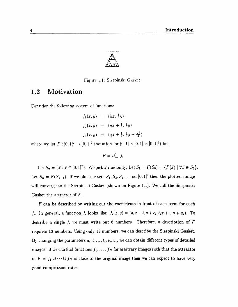
Figiirtl 1 . 1 : Sirrpinski Gasket
1.2 Motivation
Considcr t hc following systcrn of fiinctions:
t I j ( r . ) = ( 7.r. - :y) - 1 ( ) = (:.r + :. - A!)) -
\vhcw n-r let F : [O. 11' - [O. 11' (notat ion for [O. l] x [O. 11 is [O. 112) be:
Let Sn = {I : .? E [O. 11'). \fi. pirk P randomly. Let SI = F ( & ) = { F(f) 1 V.? E Sol.
Let Sn = F(S,_J . If me plot tlir sets SI. S?. S3.. . . on [O. lj2 then the plotted image
will converge to the Sierpinski Gasket (sliorvn on Figure 1 . 1 ) . We cal1 the Sierpinski
Gcasket t he attractor of F.
F can be described by writing out the coefficients in front of each term for each
f,. In general. a function /, looks like: /,(x. y) = ( a i l + b i y + t , ~ + U i g + ui ) . TO
describe a single /, ive must m i t e out 6 numbers. Therefore. a description of F
requires 19 numbers. Csing only 18 numbers. we can describe the Sierpinski Gasket.
By changing the parameters a,. b,. c,, t,. o,. u,: we can obtain different types of detailed
irnases. If we can find functions f,.. . . . jiy for arbitrary images such that the attractor
of F = JI u . . - u f,v is close to the original image then we can expect to have very
good compression rates.
1.3 Problem 5
1.3 Problem
T h systmi of fiinctioris wtiicli wr mil F = u:,/, is an ~ s a n i p l e of an iternted
fiiriçtioii systrni [2]. Iri a prrfwt ivorld. for any image we coiild find a system F
ivli~st. ;it t rnctur wotild t )cb 'close' to t tie original image. C'nfortunately, real-world
iriiiipt~s ;in3 not i-or~qdiwly sdf-siniilar (like the Sierpinski Gasket); so a more clever
solution is neecld. Chaptcr 2 will describe an iterated niodcl which is more practical
for r n t ~ i r d I ~ I ~ P S .
1.4 Thesis
Thr stuclu of fractnl sets is usually an area associated nith pure mathematics. How-
<.ver. in 1993 Arnaud .lacqiiin piiblished a paper that bridged the knowledge of fractal
sets to image compression by automatic computer analysis. The revolutionary corn-
ponent of his publication was about breaking the image down into a partition and
npplying an iternteci function system to a portion of the image. Since the publication
many partition schcmes have been created; however, few have been impiemented and
nnalyzed from an cmpirical viewpoint. We present several partition schemes based
on the qiiadtree partition that operate on several test images taken h m standard
image compression benchmark libraries. We make conclusions about these partition
schemes as they relate to particular images or error thresholds.

6 Introduction
1.5 Contributions
Ttit. (~iiiidtree partition s ch~n i e is well known: hoaever. the ides of using a local
iioiglil)oiirli00(1 ;iroiintl a range Mock whm scarching for a matching dornain block is
I . This tlitlsis rontribiitrs ro tiir arra of fractal image compression by exarnining
t tltl r f f w t s ~f 1~ca1 and rariclorxi neiglibourhood searches and ~Iassificatiori schemes.
\\il iilso riiake a n a t t rn ipt tu proride a fraitieaork for future partition schemes which
mn br tcsted on an image test suite.

Chapter 2
Review
2.1 Mat hemat ical Background
\\é introduce some niaterial which we will neeci to justify the use of iterated function
systmis for image compression. Most of the iollowing defini tions and t heorems can
IR lotirid in an- iinalysis test book.
Definition 1 .4 rnetric space is a space .Y together with a function d : S x X + R
suçh that the following conditions hold:
1. d ( r . y) 1 0 Qx. y E S
The function d is called the metrie, and the metric space ts denoted (X, d ) .
7

8 Review
Definition 2 .4 ntnp f : ,Y + S is contractive ouer the m e t r i space (.Y. d ) if:
( f . ( ) S . ) Kr. 9 E .Y
ichttrp O < s < 1 rs n d l d tlrr contmctivi ty i$ f.
Definition 3 -4 sequence { I ~ } F = ~ in .Y ts said to convetge to some x E .Y where
(S. d ) is u rnet7-i~ spuee if Vc > 0 3 .V > O such that:
Definition 4 A s e q t r i r i w {.K. }:=, t r r S i s (1 Cauchy seqaenre if Yc > O 3 .V > O
surh thtzt:
( ) < V n . m > . V
Definition 5 .4 complete metric space (Sr l ) is a metric spoce uhere every
Cm~h!y sequence conctcrges tu some r E S.
Definition 6 a E .Y is a f i e d point of the function f : .Y + S zf f(a) = a.
Theorem 1 Contmction Mapping Theorem: If f : .Y + .Y zs a contractive
rnnp ulhere ( S . (1) is a rumplete metric space then f has exactly one f i e d point a E il
and Vx E S the sepuence gzuen by:
converges to a .
NOTE: f "(z) denotes f composed uiith itself i tirnes.
2.1 Rlathematical Background 9
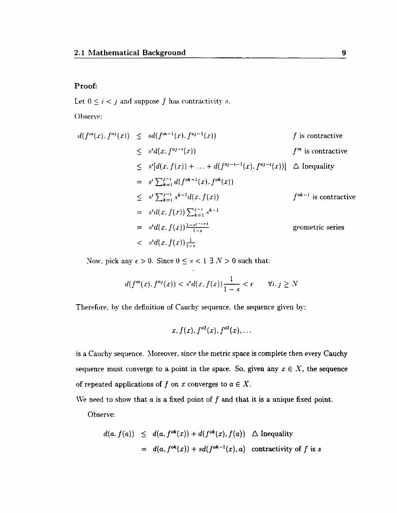
Proof:
Let O 5 i < j and suppose f hifi contrnc:tivity S.
O l m r v ~ :
d ( f m ( r ) . faJ(r ) ) 5 s d ( f " - l ( x ) . f u j - l ( r ) ) f is contractive
< - . s ld(r . /"-'(1)) f m is contractive
5 s l [ ( f ( ) + . . . + d ( / O ( ) . f O J ( ) ) ] A Iriequality
= ~ ' C ; ; ~ l ( f ~ ~ - ~ ( x ) . ~ ~ ~ ( x ) ) -
I - 1 Qk-I 5 -7' &l d ( - ~ I ( 1 ) ) f0'-' is contrnctivc
= s l d ( r . f ( r ) ) ~ ~ ~ ' 1 s" ' l - s J - k + l
= .yzd(x. j(x)) -
< s l d ( = . f ( x ) ) &
Now. pick an? c > O. Since O 5 s < 1 3 .V > O such that:
Thercforc. by the definition of Cauchy seqiience, the sequence given by:
is a Cauchy sequence. Iloreover, since the metric space is complete then every Cauchy
seqiience must converge to a point in the space. So, given any x E .Y, the sequence
of repeated applications of f on x converges to a E X.
We need to show that a is a fixed point of f and that it is a unique fixed point.
Observe:
d(a . f ( a ) ) 5 d(at f o k ( x ) ) + d( f (z), f ( a ) ) A Inequality
= d(a. fok((r) + s d ( f o k - - ' ( x ) , a ) contractivity of f is s
10 Review
If we k t k + .x then me know that Jok(x) + a . This implies t h a t the riglit hand side
of ttie ;tl~ovc rc1ii:ition ciln bc broiiglit down to O (a more rigoroiis argument c m l x
miide by coritriidiction). Therefore d(n . f ( c i ) ) <_ O. Cl~arly. this implies tha t n = ! ( a ) .
Hm(-P. (i is i i fisrcl poirit of f .
Sow. ive rriiist show that tr is thp imiqtw fisecl point of f . S I I ~ P O S P 3 two fixed
points of f. Narnely: n anil b siicti thiit f ( ( 1 ) = (1 and f ( b ) = b. Therefore:
d(o. b ) = d( f ( a ) . f ( b ) ) 5 d(«. b)
If s = O thrn cl(( i . h ) 5 O which iniplics ci = 6 . If s f O ttien d(n. I ) = O hivniise s < 1:
tlierefore. wc have t l iat (L = 6.
So. V r E S ttie scqiirrire of itrriitecl appliratiuris o f f on x converges to the unique
fixecl point of f . A s rrqtiired. O
This theorpin (2 . 171 is really n corollary of the Contraction 5Iapping Theoreni.
Theorem 2 Collage Theorem: I j (S. d ) r s (1 cornplete metric spoce and / : .Y + S
is a rontr<it:titw mrip with fixed point r i E S theri Yx E .Y
1 d ( x . a) < -d(r. f (z))
l - s
where s is the contractivity of f .
From the proof of the previous theorem we can see that:
1 4x7 i O k b ) ) 5 -4G f (X I ) l - s
2.2 Application To Image Compression 11
The rcçirlt follows. 0
The relevance to image corripression nia- not bc clear with the way tlie trvo tiieo-
rciris 11;n-e becri stat cd. Coiisicirr i i r i alterriate s t i i t~nimt of tlir Contraction Mapping
Ttieortm: Let .Y be the space of ining~s (which Iiiipperis to be complete). If we have
a contractire map f that operates frorii A' to X then t h e r ~ is a spccial image (called
the attractor of f ) such tliat if ive start rvith an- randoni image in X and apply f
iterativrly then tlie secluence will converge to the nttractor of j . This theotem ex-
plains why the motivational rs;irriple worked: the attrnctor of F (in the example) is
t t i ~ Sicrpinski Gaskct .
\\i. rridly want t o solw the followiiig probleni (cdled thr inverse problem(2l):
Civcn ;i target i m a g ~ S. fiiid a contractive niapping f siich that the at-
tractor of f is close to S.
If LW <.an firitl / for a given S t h n by ttlic Contraction Llapping Tlieorrni Ive can use
/ to approximate S by repeated applications of f to a random image.
2.2 Application To Image Compression
2.2.1 Justification
An image is a grid of different coloured pixels; eacli (z, y) position has a colour
associatecl with it. We can think of an image as a function of the position of a pixel
to its colour value. Pixel positions and colour values are discrete, so an image is a
function of the form f : ZC x Z+ + Z+ LI {O}. The domain of f is finite. There are
12 Review
sewrnl w1ys to measiire the distance tictw-vn 2 images. Example:
Tlic proof thii t d, is a metric cari br foiirid in ariy analysis test. Notice that d,
is a nirtric on the space o f iniagcs ivhidi is a finite space.
Kt. \vil1 ilse the following rrietric for tlettmiining the distance betweeri two images:
The fiirictiori i f is ;i nirtric o n tlic spacr of iiriiiges. Tlic proof can be found in ariy
;mil!-sis test.
Lemma 1 cf ( / . g ) is il mrtnr nherrl f. g W P jlrnrtion rrpr~srntcitions of images.
\Vc will h o t e the set of imng~s bu J I . LVe have shown that ( M d ) is a metric
spict.. Is (JI. d ) cornplete? Obsrrvo that if ivti fix the niauinluni size of images and the
niinihrr of ïolours allowcd thrri -11 is finite. In a finite spnce. rvcry Caiicliy sequcnce
converges: lience .\I is conipiete. TIiiw estra assumptions that WC have made are not
too restrictive. Real-aorld images are not arbitrarily large; moreover, the number of
allowd colours is also finite for cornputer applications. If we construct a contractive
map f : .\! + .\f then we know that f will have a unique attractor by the Contraction
XInpping Theorem. Sow. WC construct f such that its attractor is close to a target
image.
2.3 Self-Similarity Of Real-World Images
Vnlike the Sierpinski Gasket. real-world images are not cornpletely self-similar. Recall
that the Sierpinski Gasket, denoted S, is the Lxed point of a rnapping F = u:=, fi
2.4 Partitioned Iterated 'Function Systems 13
(sep ctiapter 1 for detnils). More forriially: F ( S ) = jl (S ) U f2(S) U h(S) = S. Each
fiirirtim f, takrs S ;u: its input m t l rnanipulates S in some w q so that the union of
the ft's is S. It is wry ciifficult to create such a mapping F for real-world images.
Corisirlibr titking a picturc of j-ourself. trnnsforming several copies of yoiir pictiire and
pnsting the traiisfornicd copies b x k together t o get a picture of ourself.
Instwii . ive create ftinctions jt whicli arc restricted to part of the entire image.
This rvorks becituse real-worltl images are partially self-similar; that is. some parts of
ari iniagc. iiri. siniilar to otlier parts of an image.
This is the idea of Partitioned Iterated Function Systems (PIFS) [6]. .A clear
rsp1;iniition follows.
2.4 Partitioned Iterated Function Systems
2.4.1 Informal Intuitive Treatment
Our goal is to find a contractive riiap II' whose fixed point is close to the image we
ivish to compress ( p ) . The mapping W* will be constructed by taking the union of
several fiinctions. w, which exploit partial self-similarity of p.
\Ce construct IV as follows:
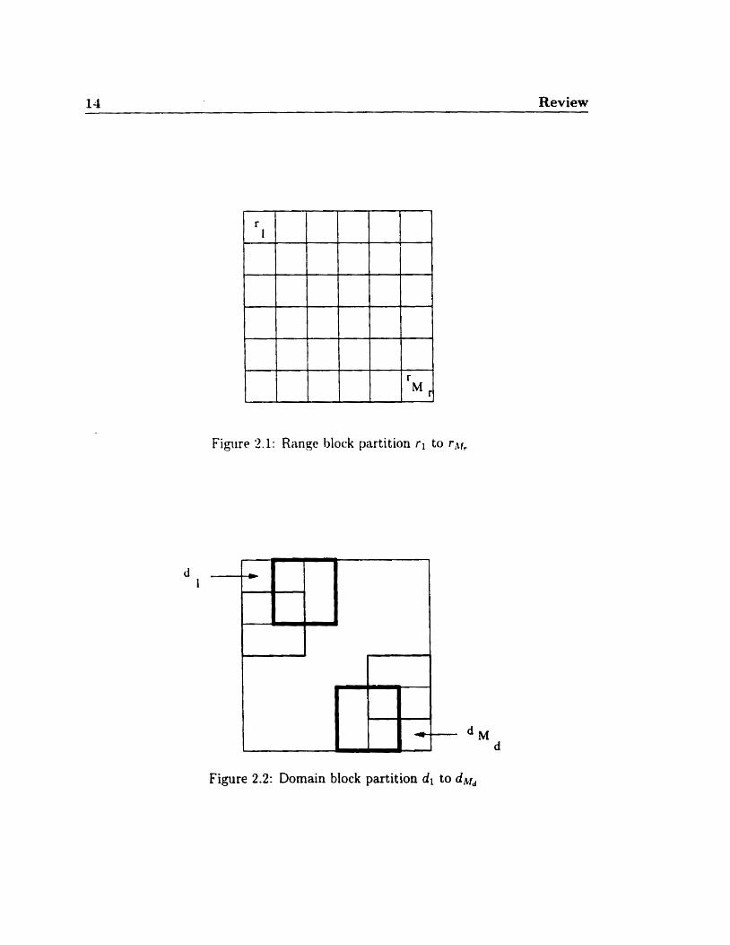
Divide I L into disjoint blocks r,. . . . , r,tfr, cdled range blocks, so that they cover
p. Call the set of range blocks R. hlr is the number of range blocks. i.e.
.\Ir =J R 1. See Figure 2.1.
Divide p into domain blocks d l , . . . . d M , . Dornain bloch are larger than range
blocks. but they are not necessarily disjoint. Call the set of domain blocks D.
Md is the nurnber of domain blocks.
14 Review
Figure 2.1: Range block partition rl to rd , ,
Figure 2.2: Domain block partition di to dbId
2.4 Partitioned Iterated Function Systems 15
0 For each r , E 'R. find a contractive mapping w, and a domain block dm, E 2)
siich t hat
Theorem 3 11. = u:.~ io, u contractiue where each ioi is contractiue.
Lrt v he the fixed point of II'. Sincc there ~ x i s t s a fiinction tu, that maps a p
prosimately ont0 each r,. where r, is n part of p. then W ( p ) = p =+ d(p , lY(p))
is sniall. Tlierefore. by the Collage Tlieorerri we kiiow tbat d(v. p) is small. Since
t h ~ tixnf point of Il' is dose to the original image thm ive know thnt CV is a good
rrprcsentation of the originai image. II' is a good description of p. Writing out CI;
( t m h I C ~ ) in fewer bits thnn the original image is the goal.
2.4.2 Formal Treatment
\Ve present a general matbernatical formulation of PIFS [3. 61. CVe will use 1 dimen-
sional signals; however, the technique generaiizes to higher dimensions.
Encoding
Given a vector (or block) p E P. we want to find W such that the h e d point of I.V
is close to p. The mapping IV must satîsfy:
IV must be contractive
16 Review
Lrt W t ) t b the set of rriappings I I * wiiich satisfy the abow two conditioiis. Fi~rtherrnore~
tvp rrqtiire that the fixeci point of I I ' . f,. has the property that:
Essmtially. the relation nt~ove is a forma1 description of the inverse problem.
Finding the optimal mapping I I * is difficiiit. We are ailling to sacrifice optimality for
Encoding Example
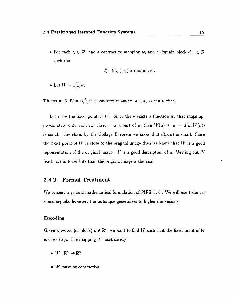
We aallow IV to be a system of .\Ir functions in, wliere ul, : RD + RB. D is the size of
a domain vector and B is the size of a range vector. Both range and domain vectors
are selected from the original signal. We want r, z w i ( d m ) for each i = l..Mr. .An
example is given below.
Let p = (8. 10.23,25,. . . . 1 3 . l 5 , l i . 19,. . .) E P.
Let rl = (8.10) and ds = (13,lL 17,19). See Figure 2.3
Suppose that al1 range blocks are of size 2 and domain blocks are of size 4.
2.4 Partitioned Iterated Function Systems 17
O a,, 6, are scalar parameters.
Thr fiinction d tnkes a clornain block and arerages out adjacent clernents in the block'.
This is how wr get w, to niap orito range blocks. i.r. By spntiiilly contracting the
doniain block by a factor of one t d .
Notice that @ ( d 6 ) = (14.LS). By inspection. we c m see that (S. 10) = $(14,18) + 1 ( 1. 1). So, r l = utI (&) = i ~ ( d ~ ) + l (1 .1) . In this example, ive were able to niap
n domain block esactly onto a range block. So. the wror is O. This is not true in
SirnplSying Assumptions For PIFS
Observe that given v E Rn then u = Ilr(v) = uZ, wi(&J where d, is a domain
rector in u that best matches the range vector, ri. in if. The output vector u is made
of .\Ir range blocks. Since I V : Rn + Rn then n = MrB.
We make the following assurnptions to make analysis of PIFS easier:
0 n is a power of 2 where n is the size of the vector.
B is a power of 2 where B is the size of a range vector.
The notation d(&, ) ( j ) rneans apply d to the domain block ci,,,, and take the j th ccoordinate of the resulting vector.
18 Review
D = 2 B wliere D is thr sizc of a rloniiiiri wctor.
Dh = B wlirrtl Dh is t h tiorizoritiil stiift distance ht~twen conscciitive domain
I)l»cks. Let c E P. Ttiv j t h iwordinntc of the clornain block of a is given
t y
Tlierefore. the niimbcr of dornnin blocks. dld7 is giwn by:
, b, are paranieters of ru,.
- I is â wctor of s ix B of 1's.
- d(dml) is defineci to I)e sonip spatial contraction from a domain vector to a
range vector. \\é define the j th . for j = 1.B. coordinate of a transformed
domain block (by O ) to be:
6 just takes the average of adjacent domain coordinates to produce a vector
that is the same size as a range vector. as in the previous example.
The proofs of the following 2 lrrnrnas are presented for completeness. The mapping
b t.akes a block of size D x D and outputs a block of size f x O.
Lernma 2 o ïs contractive.
2.4 Partitioned Iterated Function Systems * 19
Proof:
L N rl,,,, ; m l d,,' h~ E D (ie. they ;ire two tloniain rectors of size D).
~ ~ ~ = i ( f ) ? [< lm, (2k) + d,, (Yt - 1) - (&(2k) + dm2(2k - 1)12
Cliwly. 4 is coiitrnrtiw with contractivity of !.
Lernma 3 L d r be a range vector (E 72) O/ size B. Let w(r) = ar + b ( l ) B where
( 1) 1.. a range urct or. O / l 's and ci. 6 are scolnrs such that O 5 a < 1. Then w is
iwntractiue.
Let d l ) and ri2' be two range vectors.
Observe:
= &Li [a(dl))(i) + b ( 1 ) ~ - ( a ( r ( 2 ) ) ( 2 ) + b ( l ) B ) ] 2 definition of w
= JC,B=~ d[(r ( l ) ) ( i ) - ( r ( ? ) ) ( i ) ] *
Since O 5 a < 1 then clearly w is contractive with contractivity a.
20 Review
C \ é need u: t o be contractive so that II' = ~ : , , w i is contractive which means
t h svqtitariw of rt.pr;it.ed it~rations of IIw will converge. Q is contractive to gire the
iniagc detail. \\'ittiout it being contractive. each image in the sequence would appear
griiiriy 131.
Encoding a vector IL by PIFS is done as follorvs:
I . Partition Ir into range blocks. The jt" coordinate of the ich range block is givcn
t )y:
2 . Partition Ir into doniniri blocks. Recall that the j th coordinate of the m:h domain
t~lock is gi~pti by:
(LI, (1) = 14(m - W h + j )
rn, = l..Md and j = l..D.
3. For i = l..ill, do: find ai,bi,mi such that d( r i , wi(dm,)) = d(ri, ai#(&,) + b i ï B )
is minimized. Store the parameters: a, ,biomi.
Finding n,.b,.mt (as in step 3) may not be obrious. The most straightforward
method is to erhaustively search the domain vectors (m, = l..bk) for each range
vector. r , where i = 1 ... II,. For each range-domain vector pair, finding the values for
a, and bi to minimize d(a,o(dmt) + bi , r,) is a least squares problem with our chosen
met ric.
2.4 Partitioned Iterated F'unction Systems 21
Least Squares Solution For A Domain-Range Mapping
For a range vector Z = ( r l . . . . . r s ) and a spatially transformecl (by $) cloniain vector
d= (dl . . . . . d B ) . ae wniit to find a and b to mininiize:
which is the same as mininiizing:
This is a le.?st squares problem 131. We can find optimal a and b by taking the partial
d ~ r i v n t i w s and setting theni to O as follows:
We gct that:
When nfe are done. we espect tha t W ( p ) - * d(CCr(p), p ) is small. Therefore,
by the Collage Theorern. d ( p . A,) is also small where f, is the fixed point of I V . This
means t h a t p is close to f, so 11.' is a good representation of p.
Encoding and Decoding Example
An example tvill help illustrate the theory. Consider the vector:
22 Review
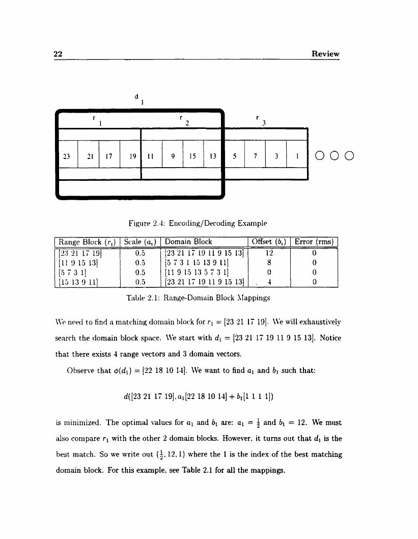
Figure 2.4: Eiicoding/ Drcoding Esam plr
Tihle 2.1 : Range-Dorniiin Block Nappings
KP rirr<l to find a matrhing tloniain block for rl = [23 21 17 191. \Ve will exhaiistively
search the clornain block space. We start with di = [23 21 17 19 11 9 15 131. Notice
that there exists 1 range vectors and 3 domain vectors.
Observe that o(dl) = [22 18 10 1-11. We Vewant to find al and bl such that:
Range Block (r,)
is niinimized. The optimal values for al and bi are: al = f and bl = 12. We must
also compare rl with the other 2 domain blocks. However. it tums out that dl is the
best match. So s e write out (i. 12.1) where the 1 is the index of the best matching
domain block. For this example, see Table 2.1 for al1 the mappings.
Scale (a,) 1 Dornain Block 0.5 j [ z 3 a i ; i 9 1 1 9 1 5 1 3 1
Offset (b , ) 1 Error (rms) 12 O
2.4 Partitioned Iterated Function Systems 23
Decoding
\\é can pick any mctor in ng" alid apply II' to it iterativeiy iintil the clifference
betwecn siiccessive iterations is negligible. The resiilt will be a vcctor close to the
origiiiitl vector that ae cnrodecl (p). I I w can be desrribcd as a seqtirnce of a,. I I , . and
m, values. For i = 1. we know that domnin vector dm, rnaps onto range vector r l .
We also know the pnrnmrters a l and b l . So. we know eeractly how IIv operates over
e x h clorriain block: the iiriion of al1 the transformcd doniain blocks produces a vector
in Rn.
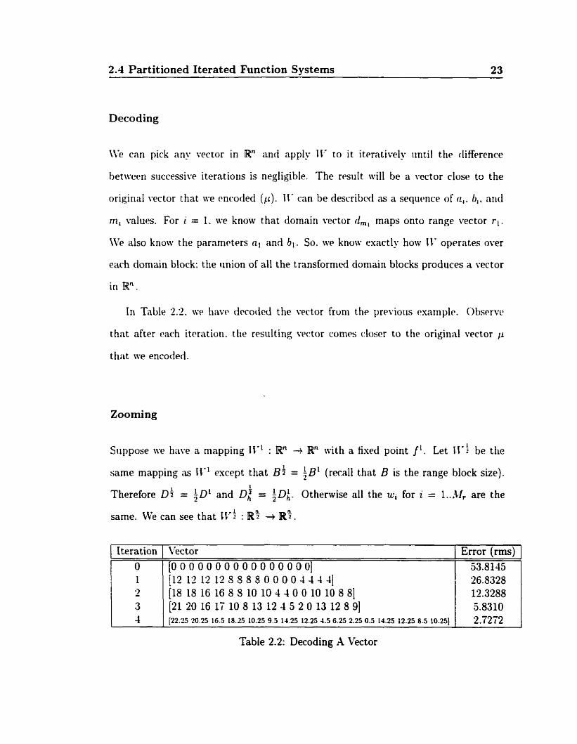
In Table 2.2. w~ h w r drcoclcd the vertor froni the prrvioiis rsnrnplr. O h s ~ r w
that after cach itrration. the resulting vector cornes closer to the original vector p
that we encoded.
Zooming
Siippose iw hiive ri rniipping II" : Rn i Rn rvith a fised point 1'. Let 11'1 be the
same mapping as II*' except that B+ = kB1 (recall that B is the range block size). -
same. CVe can see that I V : IP? -t I P ~ .
Table 2.2: Decoding A Vector
Iteration O 1 3 - 3 4
lrector
[ O O O O O O O O O O O O O O O O ] 112 12 12 1 2 8 8 8 S O O 0 0 4 4 4 4 ] (18 18 16 16 8 8 10 10 4 4 O O 10 10 8 81 (21 20 16 17 10 8 13 12 4 5 2 O 13 12 8 91 [22.2520.2516.5t8.2510.259.514.2512.254.56.252.250.514.2512.258.510.25)
Error (rms) 53.8145 26.8328 12.3288 5.8310 2.7272
24 Review
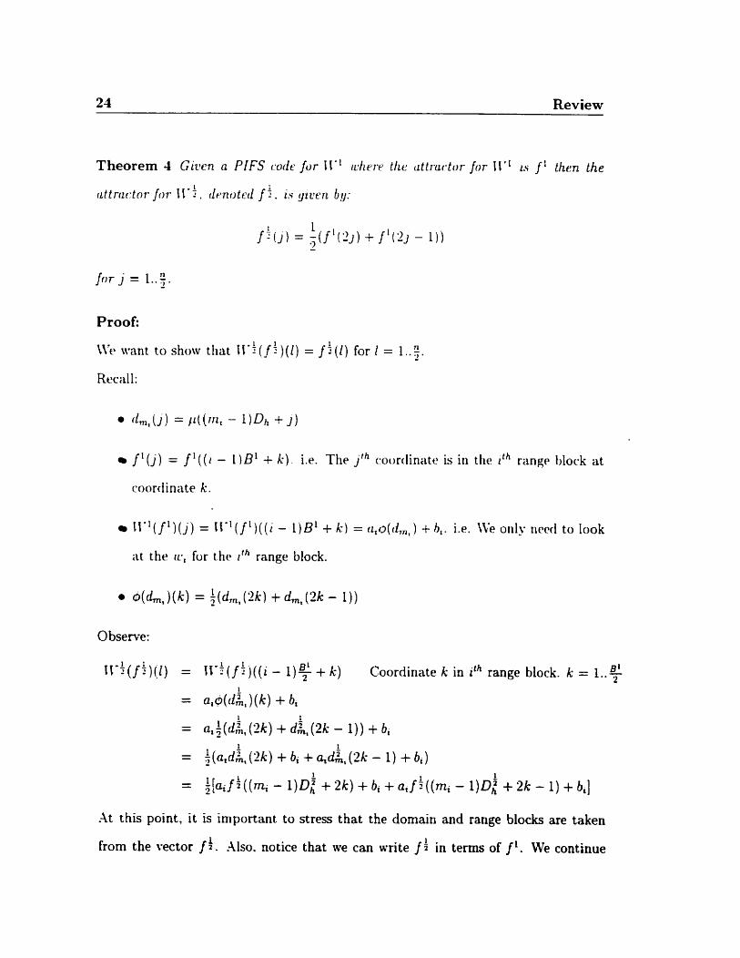
Theorem 1 Given a PIFS code /or I I " rchrr-e the <ittrwtor /or I I v 1 r s f ' theri the
iittrrictor fit- Il-f . d r n o t d f f . is yicrn by:
Proof: 1 1
\\il m n t to show tliat I I * j ( j : ) ( l ) = f f ( 1 ) for i = 1 . . $ - Recitll:
f 1 ( j ) = j' ( ( 1 - 1 1 B1 + k). i.e. The j t h mortlinatc. is in the i t h range tdocgk at
coorriinate A-.
W1( f ' ) ( j ) = W1( f ')((i - 1)B1 + k ) = (~,o(ii,,~) + h,. i-e. Ne only necd to look
at the ir, for the i t h range block.
Observe:
( ) ) = 1 ( f i - 1 ) + ) Coordinate k in ith range block. k = l..$
= a , p ( d k , ) (k) + 6, 1 t
= a, (d& ( 2 k ) + d$* ( 2 k - 1)) + 6, = ?(a ,db ( 2 k ) + b, + 4&, (5k - 1) + b,)
= $[%fi((, - 1 ) ~ i + 2 k ) + b, +a,f i ( (mi - 1 ) ~ : + 2 k - 1) + b,]
At this point, it is important to stress that the domain and range blocks are taken
frorn the vector fi. ..\lso. notice that we can f i in terms of f l . We continue
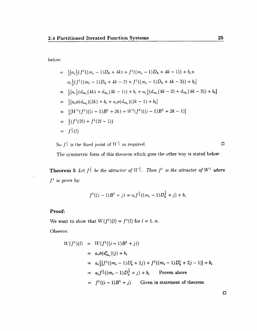
2.4 Partitioned Iterated Function Systerns 25
Su j ! is t h Asrd poin t of II*! ;is r t y i i i r t d . O
Thc syinmetric forni of this theormi which goes the other kay is stated below:
Theorem 5 Lrt f f be the attrnctor of l l w j . Then f ' is the attructor of W1 where
Proof:
We want to show that ilv( f ' ) (Z ) = f ' ( 1 ) for 1 = l..n.
W(f t ) ( l ) = W( f l ( ( i - 1)B1 + j)) = aid(dL,)(j) + bi = ai:[f1((mt - l)D$ + Z j ) + fL((mi - 1)Dh + 2 j - 1)) + b;
= ai f !((mi - i)f$ + j ) + bi Proven above
= f ((i - 1 ) + j ) Given in statement of theorem
26 Review
\\'lii~t do t licstl theoreiris rrie:tn'.' Tliey tcll ils how ive can zoom in and out of the
fisecl poii~t of I I - . I f wc tliink in tcriris uf irrxiges thcn the concliision of the second
tlitwrtm is qtiiro nice. It tells 11s how to zoom irito an image. This iipproach generatcs
artifiriiil <irt ; t i i iit mcli zooni Ievrl. Esperiirients revcal that zoorning in with fractal
ri)inprrww(l iiiiiigrs looks good wlirn zooniing irp to i~boiit 8 tirnes. Aft~rwards. the
art ificiid ( i ~ t ni1 is inenninglcss. Conversely. an iniage corii pressed wit h .J PEC requires
pisrl tlriplicat ion when zoorning in. This l e i h tu blockiness in the zoomed image.
2.4.3 Partit ioning Techniques For 2D Images
So fiir. wr-r 1i;ivr-r dividrd I r into unifc)rnily-sized range blocb. Suppose that for a
particiilnr rnngc block. the bcst dorniiin-rarige niatching yields a large error (the
rlistanw is big). If \i.c niake tliat pnrticirlar range block smaller then it is more
likely that a p will find a matching doniain block such that the distance is smaller.
ffuwrvrr. i f 1i.r iisc snialler range blocks then we will need more w, transformations.
This rrrlric~s the compression ratio. but improves the image quality.
.Jko. the size of oiir domain pool. .DD. affects the runtime and image quality. A
large dornain pool means that more domain blocks need to be searched for each range
block. Howewr. this improves the likelihood of finding a good match. Matching
techniques are mentioned briefly in section 2.4.4.
The choice of partition scheme has a significant impact on the level of compression.
Several partition schemes have been proposed: some give more weight to image quality
than others. \\è are not so concerned about image quality as we are worried about
compression rates.
2.4 Partitioned Iterated Function Systems 27
Quadtree Partition Scheme
Tliis piirtirioning schcrnc [1. 3. 9. 151 is clesigned to improve the image quality of
rtir coriipressed imagr by wrying the size of range blocks until a desirable error is
c i . .A qii;icitree partition is a representation of an image using a 4-child tree
structure. The root of the trce represents the initial image. The root node has 4
rliililrr~i. Each child node represents one quadrant of the parent node. The algorithni
is iriitinlized with the tree Iiaving a minimum depth along each path so that the size
of r;ic*ti qii;i(ir;int iri r fie Irai-rs is t lit1 initial range block size. For a given quadrant
r i t o c ) . i f thr I~rsr niatcliing domain block is not good eriough (distance is
large) tlirn dividc the q i i n h n t iiito 4 çhildren and t v again. This process cannot
coritiriiic inclefinit~ly: otherwise. n-e would be encoding each pixel separately which
woiild cause an explosion of bits. Therefore. we enforce a maximum depth on the
t ree. 'i'liis translates into a rnininium sized range block.
Tliis type of partitioriing scherne does complicate the encoding process because ive
ncrd to spccify the size of the range blocks in the output for the decoder. LIoreover,
the spatial transformations of domain blocks also reqiiires careful attention.
2.4.4 Domain-Range Vector Matching Techniques
For ench range block. we must examine al1 the domain blocks to find a good match;
this is a slow process. If ae wish to have reasonable image quality then we need a
large domain pool. tVe want good image quality and fast searching.
Classifying dornain and range blocks is an effective method of improving the
matching process. Each domain and range block belongs to 1 of N classes. We
knuw how earh w, affects the class of a block so we only need to search a particular
28 Review
class of rii~main blocks. There are several dever techniques for clnssifying blocks [Ki).
Orw cl:~~sification scheme involvrs:
1. Briuking ~ ; i c h block irito -1 sub-blucks.
'1. C'onipii ting the average piscl valrie of each sub-block.
Tlir ordrring of the intensity of average pixel values for a siib-block determines the
r-lxss of the block. In this case. t h e are 4! = 2-4 different classes.
Anor lier cliissificat ion sçhenie irivolms annlyzing propertics of blocks to deterniine
if r l i ~ I do& is smoot h o r if it h a ari cdge in it or it could have some other properties[6].
2 A.5 Evaluating Partition Schernes
-4s rntlnt ioned earlier. the partitioning scheme affects the image quality and the corn-
pression ratio. Therefore. stiidyirig the properties of a particular partition scheme
i l 1 t i f 1 Cnfort iinatrly. it is difficult to make strong mat hematical arguments
for a partition scheme. A good partitionirig scheme wiil adapt to different t-es of
images. However. we tvould like to know if one partitioning scheme produces higher
quality images. or higher compression rates, than another scheme. and on what kind
of images does one method 'out-do' another. We have chosen to empirically examine
various partitioning schemes by running thern on various test images and analyzing
the resiil ts.
To try out a partitioning scherne, we need a fractal tool which will accept a
partitioning scheme and an image as input to encode the image. This tool would
allow ils to compare partitioning schemes on specific images. It would also tell us if
particular method works %etter' on certain kinds of images; the word 'better' can

2.4 Part itioned Iterated Function Systems 29
niean sereral different things. It could niean higlicr compression ratio. lowcst average
pixel crror. or highest signal-to-noise ratio.

Review

Part II
Fractal Tool And Partition
Schemes

Chapter 3
Fractal Tool
. I Itwninghil thcorrtical resiilts about a partition schcme arc difficult to obtain; instead.
ire try to rcason eriipirically. The fractal tool serves tbis purpose. I t provides a
franiework for csernining partition schernes. Image partitioning techniques can be
pl i iggd into the framework and tested on sample data.
The fractal tool contains a compression and decompression program. Each par-
t i t ioning nicthod hm different program options which control the behaviour of the
pürtitioning algorithm. Cornpressing an image is a very slow process. For a small
image (128 x 1 2 ) , the runtime of the compressor is under 5 minutes. However, for a
vcry large image the compressor can take several hours.
3.1 The Cornpress Program
Run the cornpress program as follows:
compress C-e error-threshold) [-d dom-level] [-SI
I [-1 nbhd-size] [-r rnd-pts] 3 inf ilename . bmp outf ilename. f rac
34 F'ractal Tool
Typing: ~cornprcss gives a b r i ~ f tlescription of each option and its default value. .A
more (Ir tidecl explnnnt ion follorvs:
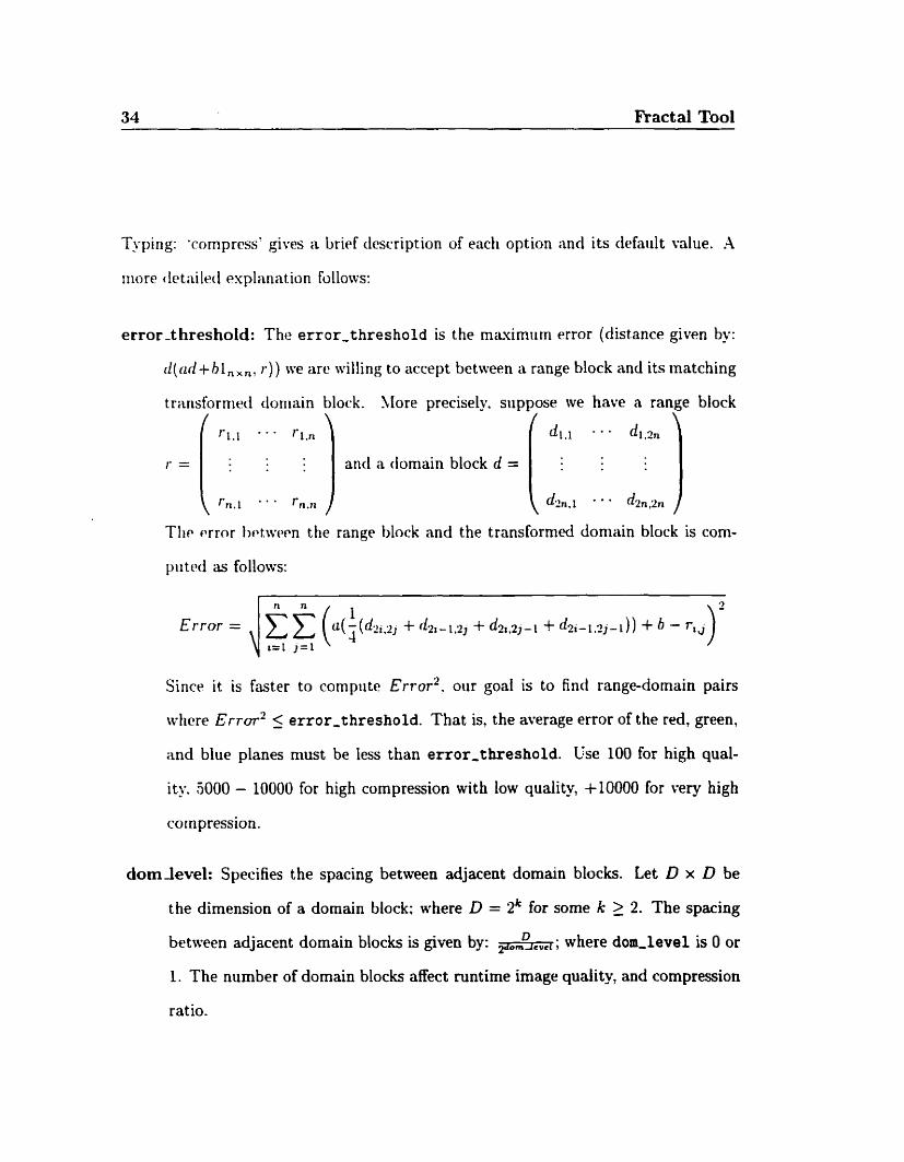
error-threshold: The error-threshold is the rnauimiirn error (distance given bu:
<l(<~d+hl,,,, 1 . ) ) ive are willing to accept between a range block and its inatching
transfornied ciorriain blork. >[ore precisely. suppose we have a range block
and a domain block d =
4 n . l . . d2n.2n
The prror 11t~t~rvet.n the range block and the transformeci domain block is com-
piitivl as follows:
Since it i s faster to cornputc Error2. oiir goal is to find range-domain pairs
tvticre Error2 5 error-threshold. That is, the average error of the red, green.
and blue planes must be less than error-threshold. Use 100 for high qual-
ity. 5000 - 10000 for high compression with low quality, +lOOOO for very high
corn pression.
domlevel: Specifies the spacing between adjacent domain blocks. Let D x D be
the dimension of a domain block; where D = 2* for some k 2 2. The spacing
between adjacent domain blocks is given by: hl; where dom-leva1 is O or
1. The number of domain blocks affect runtime image qudity, and compression
ratio.

3.1 The Cornpress Program 35
s: Turns on statistic reporting. The following statistics are reported for each range
block size:
0 Niimber of range blocks without a niatching doiriain block. Constant
colotired range blocks cio not need a matching dornain block.
Number of range blocks with a rnatching dornain hlock.
Average niapping error squared for red. green, blue planes and the variance.
0 Masimiirn and minimum error squared for red. green. blue.
Average distance betwen range and domain blocks.
. - \ v ~ r a g ~ ciifference for qiiantizrd and non-qiiantized error sqiiared calcula-
tion.
a Yiimber of domain blocks searched for ench range block size.
Orientation of matched domain blocks.
.A count of the different qiiantized levels for contrast and brightness.
nbhdsize: Applicable to particular partition schemes. For each range block, we
only search those domain blocks which are in a local neighbourhood of the
range block. If nbhd-size is N then we search an area of 32iV x 32N pixels
around the range block. This takes advantange of local self-similarity in an
image: if it exists.
rnd-pts: For particular partition schemes. For each range block, we search the local
neighbourhood and we also search rnd-pts random neighbourhoods of the same
size as the local neighbourhood.
36 Fracta1 Tool -. - - -
3.2 The Decompress Program
Run tlic derompress prograrn as follows:
decompress [-i num-iterations] infilename.frac
Typirig: .(i~cornpress' gires a brief description of each option and its default value. A
riiorr drr ailcd ~splariat ion follows:
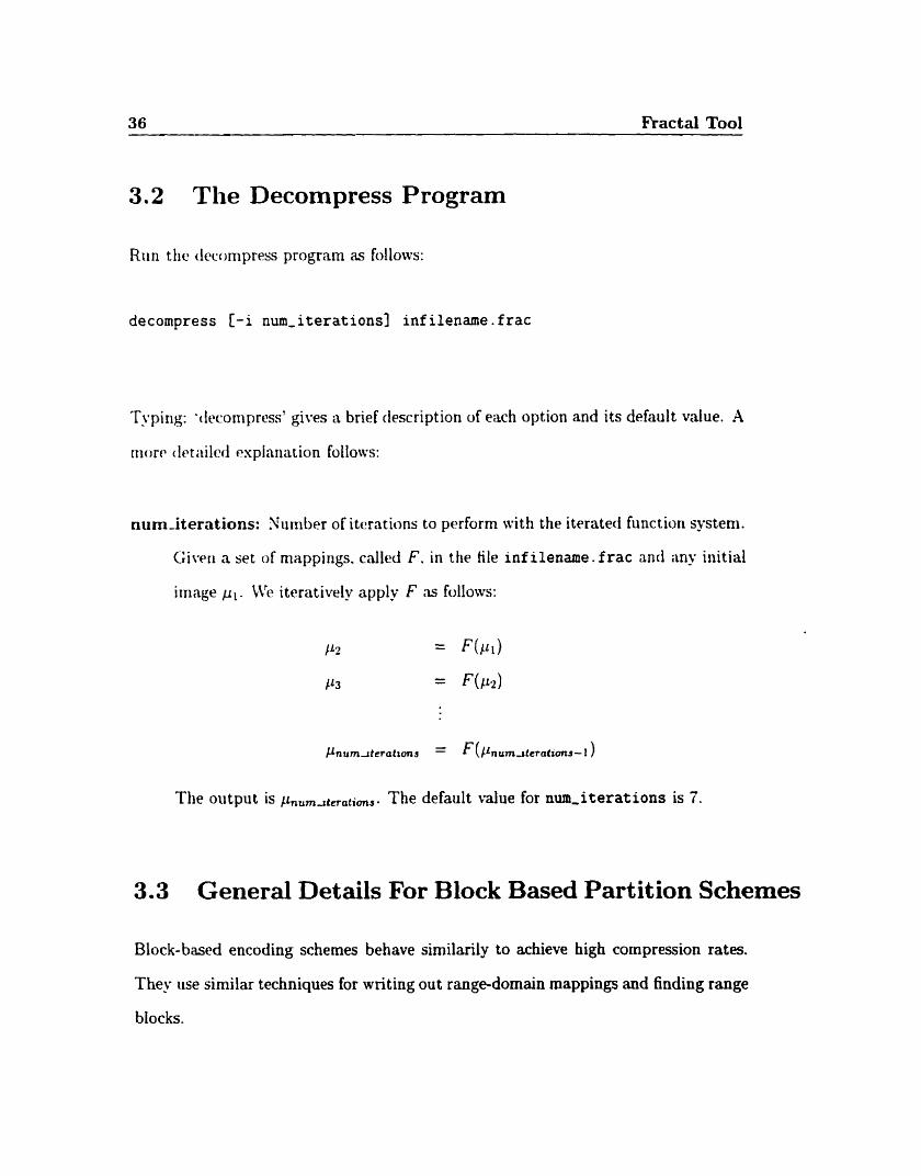
num-iterations: Xuniber of iterations to perform with the iterated function system.
Given a set of rnappings. called F . in the fi le infilename. frac and iinu initial
image pi. We iteratively apply F as fdlows:
The oiitput is pnumilmarimr. The default value for mm-îterations is 7.
3.3 General Details For Block Based Partition Schemes
Block-based encoding schemes behave similarily to achieve high compression rates.
They use similar techniques for writing out range-domain mappings and finding range
blocks.

3.3 General Details For Block Based Partition Schemes 37
3.3.1 Output Of Mappings
A range-clornain mapping is writtcn to the fractal (compressed) file as shown in Figure
red green blue red b lue contrast contrast contrasi brighinrss Kikness brightness orientation dornain id 1 I u u ü ü u u u 4 bits 4 bits 4 bits 6 bits 6 bits 6 bits 3 bits
Figure 3 . 1 : Bit Layout Of -4 Range-Domain blapping
Orimtatiori is only iised for tliose schemes that allow dornain blocks to bc rotated
and r d l w r ~ d . There are 4 possible rotations and 2 retlections for a domain block: 8
possible orientations in total. The domain id is a number that uniquely identifies a
clornairi block. The niimber of bits for the domain id depends on the size of the image.
Diiririg the decompressioii pliwe. the dornain id is used to recoristriict the position of
the domain block. Let:
0 D be the side length of a doniain block.
imgrow be the number of rows in the image.
imgcol be the number of columns in the image.
domrout 5 irngrow - D be the starting row of the domain block; indexed from
O.
d m c o i 5 irngcol - D be the starting colurnn of the domain block; indexed from
O.

rlmnspace = .,,,z,,,, be the spacing hetween adjacent domain blocks tvhert.
dornJecel = 0.1.
The obvious twy to conipiite the domain id is as follo~vs:
wiiere .VDB is the niirriber of domnin blocks in a row. If domain blocks are spaced
1 pixel apart then :VDB = irngcol - D + 1 . However. domain blocks are spaced
tlornspticr pixels apart. Herice the number of doniain blocks t h fit on a row is
rmqrnl- D iirrrnspocc + 1 . Thereforc. we have that:
Observe that timnrou: mod domspace = O and domcol rnod domspace = O because
dornain tilocks are (lonrspnce pixels apart. Thercfore:
(dom r ow ( irngcol - D moddomspace = O (*)
domspace
Recnll that domspace = , , ~ e v e i and that D is a power of 2. Therefore domspace
is also a power of 2. Le. domspace = 2' for some integer k. Therefore (*) implies that
the 1st k bits of domrou, 'zzit ( ( + 1 + domcol are always 0. It is not necessary 1 ) to write out those bits. So Ive compute the domain id as shown by Equation 3.1 [12].
domspace
The maximum domain id is giveo by Equation 3.2.
(imgrow - D) ( tmgcd- D domspac~ + (imgcol- D)
maxdomid = dumspace (3-2)
3.3 General Details For Block Based Partition Schemes 39
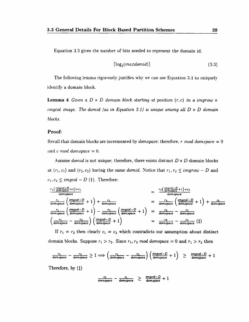
Equation 3.3 gives the number of bits needed to represent the domain id.
The following lernnia rigorousiy j (1st i lies why wr cari use Eqtiation 3.1 to iiniqiiel~
ideiitify a domain block.
Lemma 4 Giuen a D x D domain blocbk starting ut position ( r , c) in a imgrow x
irngcol image. The domid (as in Equation 3.1) is unique umong al1 D x LI domain
biocks.
Kecail that domain blocks are incrernented by domspace: therefore. r mod domspace = O
ancl c mod dornspnce = 0.
.Assume domid is not unique; therefore, there exists distinct D x D domain blocks
at ( r , , c l ) and ( r 2 , c2) having the same domid. Notice tha t r l , r . ~ 5 imgrow - D and
c l . c2 5 imgcol - D (t). Therelore:
- - imgcol- D + l) + dm?pace
=2 - C l domspace durnspace
(dom?pacr - r f L p a c e ) (~"p: + l ) - - domspace - dornspace ($)
If rl = r2 then clearly cl = cz which contradicts our assumption about distinct
domain blocks. Suppose rl > r2. Since rl, rz mod domspace = O and r , > r2 then
Therefore, by ($)
40 Fkactal Tool
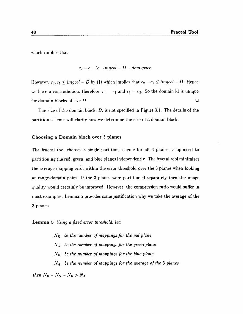
wliich irript ies t hat
(-2 - cl > irrtgcol - D + domspace
Howcwr. c2. CL <_ irngcol - D by (t) nhich implies that c? - cl 5 imgrol - D. Hence
w b;iw ir contradiction; t herefore. rl = r2 and cl = c2. So the domain id is unique
for doniain blocks of sizc D. 0
T h size of the domain block. D. is not specified in Figure 3.1. The details of the
piirtitiori sdierne will clarify how ivtl determine the size of a tlomain hlock.
Choosing a Domain block over 3 planes
The fractal tool chooses a single partition scheme for al1 3 planes as opposed to
part itiorii ng t lie red. green. and blue planes independently. The frac ta1 tool minimizes
the awragc niapping err& within the error threshold over the 3 planes when looking
iit rangedomain pairs. If the 3 planes were partitioned separately then the image
qiiality woiild certainly be iniproved. However, the compression ratio would sufier in
most esamples. Lemrna 5 provides some justification why we take the average of the
3 planes.
Lemma 5 Using a fized error threshold. let:
.YR be the number of mappings for the tzd plane
.k be the number of mappings jor the green plane
YB be the number of mappings for the blue plane
Vd4 be the number of mappings for the average of the 3 planes
3.3 General Details For Bkock Based Partition Schemes 41
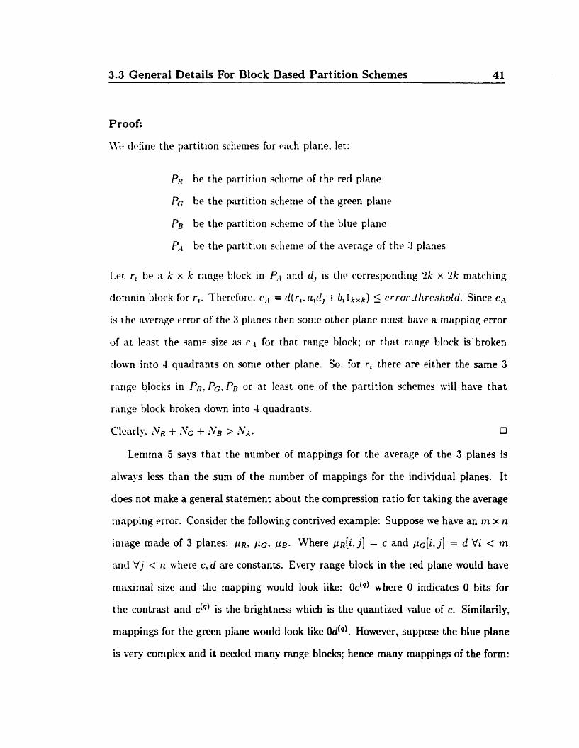
Proof:
\\'r M i n e the partition sclienies for rach plaiie. let:
PR bfi the partition scticrne of the red plane
Pr: be the partition schenie of the green pliiiie
PB be tlic partition schemc of ttie blue plane
P.., be the partition srlimir of the average of the 3 planes
Let r , t ~ e a k x k range block in P.., ancl d, is t h r corrcspoiiciing 21; x 2k matching
rloninin t~lock for r,. Therefore. e.., = d(r, . a,(!, + b, lk, k ) < errer-thr~shold. Since e.4
is t lie average errer of the 3 ylaries then some other plane nitist have a niapping error
of a t l e s t the sanie size i i s e+.l for ttiat range bIock; or ttiut range Llock is'broken
down into 4 quadrants on some other plane. So. for r , there are eithcr the same 3
ïilrigc t>locks iii PR, PG, PB or at l ~ a s t one of the partition schemes ail1 have that
riinge block broken down into 4 quadrants.
Clearly XR + .VG + XB > X.+ 0
Lemma 5 says that the niimber of mappings for the average of the 3 planes is
always less than the sum of the nurnber of rnappings for the individual planes. I t
does not make a general statement about the compression ratio for taking the average
mapping error. Consider the following contrived example: Suppose we have an m x n
image made of 3 planes: , 1 , p . Where pR[ i , j] = c and pc[i, jl = d Vi < m
a n d V j < n where co d are constants. Every range block in the red plane would have
maximal size and the rnapping would look like: O&) where O indicates O bits for
tlie con t ra t and c(q) is the brightness which is the quantized value of c. Sirnilarily,
mappings for the green plane would look like O&). However, suppose the blue plane
is very complex and it aeeded many range blocks; hence many mappings of the form:
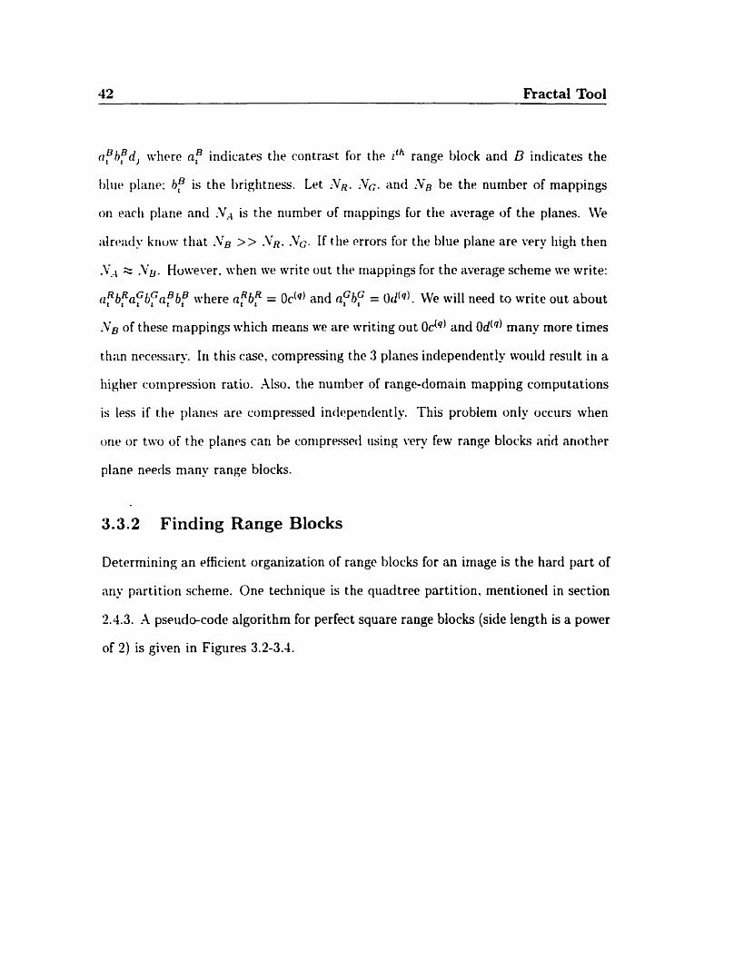
42 Fractal Tool
r f h f r i , where n l indicat~s the contrast for the l t h range block and B intiicates the
hliie plarir: h l is the hrightriess. Let N R . Xc. and :VB be the number of mappings
on eacti plarir and 'i, is tlie n imber of mappings for the average of the planes. We
; i l n d y kriuw t h .YB >> .YR. &. If ttie mors for the Mue plane are ver- Iiigh then
.Vg of these mappings which means we are writing out 0c(q) and 0d(4) many more times
t han necessaru. Ir1 t his case, comprrssiiig t hc 3 plancs inclependent ly would resiilt in a
Iiiglier conipr~ssioii ratio. Also. tlie nuriil>er of range-domain mapping computations
is less if the plitries are coiiipressed indepentlently. This probleni only occiirs wben
one or two of the plancs cari b~ coniprmscd iisiiig vcry few range blorks iirid nnoth~r
plane n~ecls rnany range blocks.
3.3.2 Finding Range Blocks
Deterrnining an efficient organization of range blocks for an image is the hard part of
any partition scheme. One technique is the qiiacitree partition. mentioned in section
2.4.3. A pseudecode algorithm for perfect square range blocks (side length is a power
of 2) is given in Figures 3.2-3.4.
3.3 General Details For Block Based Partition Schemes 43
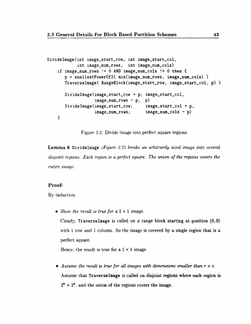
DivideImage(int image-start-rou, int image-start-col, int image-num-rous, int image-num-cols)
if image-num-rous ! = O AND image-num-cols != O then ( p = smallestPowerQf2( min(image-num-rovs, image-num-cols) )
TraverseImage ( RangeBlock(image-start-rou, image-start-col , p) )
image-start-col,
P) image-start-col + p, image-nu-cols - p)
Figurr 3.2: Divide image into perfmt square regions
Lemma 6 Div ide Image (Figure 3.2) breuks mi arbilrarily sized image into several
disjoint rtyiorts. Each region is a perfect square. The union of the regions covers the
mtire image.
Proof:
By induction.
Show the result is true for a 1 x 1 image.
Clearly. TraverseImage is called on a range block starting at position (0,O)
with 1 row and 1 column. So the image is covered by a single region that is a
perfect square.
Hence. the result is true for a 1 x 1 image.
Assume the result is true for al! images with dimensions smaller than r x c.
..\ssurne that TraverseImage is called on disjoint regions where each region is
2k x 2'. and the union of the regions cowrs the image.

44 Fkactal Tool
O Proz.~~ the rcsirlt ~ . s tnrr fin- mi r x c mage.
()hsrrvr that p = ~ i l l > ~ ? i m l n ( r + c ' ) ! < - ~ n l n ( r , C )
So. we c;ill TraverseIrnage startirig at (0.0) with p rows and p columns: hence
n . ~ Ii;iw rovrrt4 a prrfert sqiiare region of the image.
\fé nrr I ~ f t witti 2 srrialler disjoint images:
- The imagc starting at (p. O) with r - p rows and p columns.
- The i n i a g ~ stsring at (O. p) with r rows and c - p columns.
By t h p induction hypotlit%sia. ive c m cover the 2 smoller images ni th disjoint
square r~gions. Htm-e tlir entire imagc can bc covered by disjoint square regions.
K t \ stio~wd the result truc for 1 x 1 image. and when we assume the result
triie for i i l l images a i t h dimension smaller t han r x c then we showed the result
t rue for any r x c image. So. by the Principle Of Y at hematical Induction, the
rrsiilt is trtie for al1 images.
O
Clcarly. since the range block passed into Traverse Image (Figure 3.3) is a perfect
sqiiare t hen ench recursive cal1 of TraverseImage also passes in a range block with
prrfrr t sqiiare diniensions. TraverseImage cornpletely covers its region by perfect
squares. Sloreowr. each covering square will be the same size.
Observe that ExamineRangeBlock (Figure 3.4) outputs a O bit when it breaks
down a range block. This is how the decornpressor keeps track of the size of range
blocks and the corresponding domain blodrç (always twice the size of the range block).
The FindBestMatchingDomainBlock function searches through dl possible domain
3.3 General Details For Block Based Partition Schemes 45
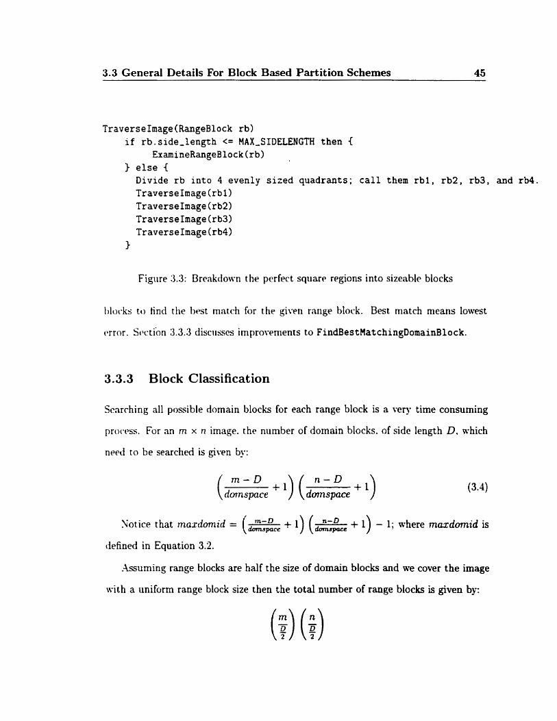
TraverseImage(RangeB1ock rb) if rb.side,length <= MAX-SIDELENCTH then <
ExamineRangeBlock(rb) ) else (
Divide rb into 4 evenly sized quadrants; cal1 them rbl, rb2, rb3, and rb4. TraverseImage (rbf ) TraverseImage(rb2) TraverseImage (rb3) Traverse Image (rb4)
Figure 3.3: Breakclown the pcrfect square regions into sizeable blocks
th- l is to fincl the hrst match for the given range block. Best match means lowest
tbrror. Swtbn 3.3.3 disciisscs irnprovenients to FindBest Mat chingDomain0lock.
3.3.3 Block Classification
Srnrrhing al1 possible domain blocks for each range block is a very time consuming
prowss. For an m x n image. the nurnber of domain blocks. of side length D. nhich
n e d to be searched is giwn by:
( m - D + l ) ( n - D +L) dmnspace domspace
Notice that r n a x d m i d = (e + 1) (e + 1) - 1; where mazdomid is
defined in Equation 3.2.
;\ssuming range blocks are half the size of domain bloclis and we cover the image
with a uniform range block size then the total number of range blocks is given by:
46 Fractal Tool
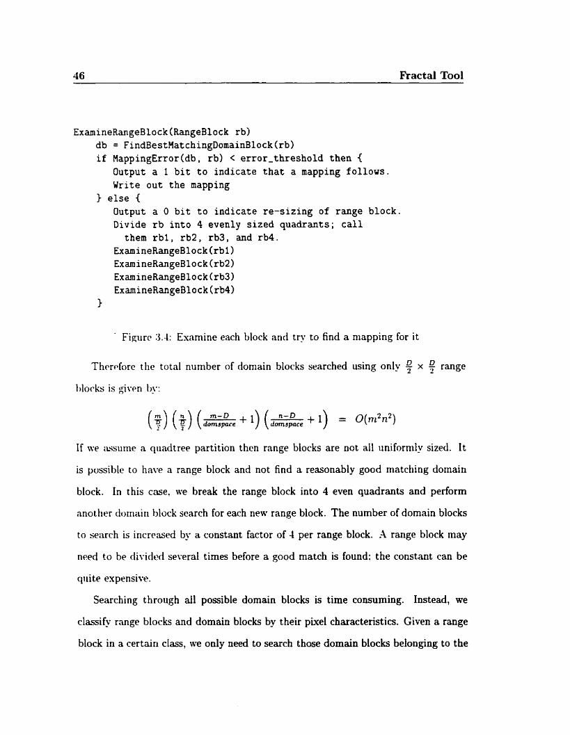
ExamineRangeBlock(RangeB1ock rb) db = FindBestMatchingDornainBlock(rb) if MappingError(db, rb) c error-threshold then (
Output a 1 b i t t o indicate tha t a mapping follovs. Write out the mapping
) else ( Output a O b i t to indicate re-sizing of range block. Divide rb into 4 evenly sized quadrants; cal1
them rbl, rb2, rb3, and rb4. ExamineRangeBlock(rb1) ExamineRangeBlock(rb2) ExamineRangeBlock(rb3) ExamineRangeBlock (rb4)
1
Figure 3.4: Examine each block and try to find a mapping for it
Thrrrfnrc the total number of domain blocks searched using only 5 x 4 range
If we xssiinw a qiiatltree partition thcn range blocks are not al1 uniformly sized. It
is possible to hnw a range block and not find a reasonably good matching domain
block. In this case, we break the range block into 4 even quadrants and perform
nnother domairi hlock search for each nen range block. The number of domain blocks
to search is incrrnsed by a constant factor of 4 per range block. A range block may
need to be divided several times before a good match is found: the constant can be
qiiite expensive.
Searching through al1 possible domain blocks is time consuming. Instead, we
classify r~mge blocks and domain blocks by their pixel characteristics. Given a range
block in a certain class, we only need to search those domain blocks belonging to the
3.3 General Details For Block Based Partition Schemes 47
snme class. Rather tliiin having one long list of domain blocks we have ari array of
lists of doniain blorks mhere each list contains domain blocks belonging to a particular
rlnss. We ctepend on a random distribution of block classes for an efficient search. It is
siniiliir to the way a hash table depends on a good hash function to evenly distribute
k c ~ s . Our hlock classifier is analgous to a hash function.
I.hfortunatcly. sonie blocks can be mis-classified which means the optimal match-
ing ilornain block for a particular range block may be in another class. It is up to the
dassifi~r on Iiow to Iiandle this problem. One solution is to alloa blocks to belong to
rriiiltipk cnli~sscs. or rhoosr a better classifier.
Soriie classification rnethocls are mentionert in section 2.4.4. The fracta1 tool clas-
sifirs blocks ncrording to the ordering of the sum of pixel values of each quadrant
[ 151. More prrcisely:
Givcn a block B. whose quadrant p ~ ~ e l sums are indexed by B[O], . . . , B[3] .
We define the following function:
( O otherwise
The class of a block B is given by:
class(B) = 6[f~(O.l) + f~(0,2) + /~(0,3)]+ ?[fl3(1,2) + f ~ ! l * 3)]+
f~ (273)
Lemma 7 Given two blocks -4 and B.
class(.-l) = class(B) o (.q[z] > A[j] o B[z] > B[j]Vi, j )
Proof:
If .-i[i] > A[j] e B[i] > B[ j ] V i , j then

48 Fracta1 Tool
j,.\(i. j ) = 1 .4[2] > A[;] * B[i] > B [ j ] * f ~ ( 1 . j ) = 1.
fq4( i . j ) = û - A [ i ] 3 .i[j] * B[i ] 3 B[jl * j&. j) = 0.
Ttierefore. it is clear tliat clnss(.-l) = class(B).
Iwratise every number from O to 23 can only be written in exactly one way 6((0.1,3,3))+
? ({O. 1 . 2 ) ) + I({O. 1))-
()k)servc:
Sincc 3) = fB(2. 3) then .-@] > A[3] B[2] > B[3]
If /.-l(l. 2) = O and f s ( l , 2 ) = 1 then it must be that jO4(1.3) = 1 and fB( l ,3) = 0.
Therefore. .4[1] # .4[2] but B [ 1 ] > B[2] and A[l] > A[3] but B[1] < B[3].
Hmce A [ 2 ] > .4[3] * f&3) = 1 and B[2] < 8[3] * f B ( 2 , 3 ) = O. This is a
contradiction. Hence it cannot be that fA(l? 2) = O and f B ( l . 2 ) = 1 .
Sirnilarily. fa&. 2) = 1 and f B ( l , 2) = O is not possible. They are both O or both 1 .
This means that A[1] > A[2] B[1] > B[2] and A[ l ] > 431 B[1] > B[3].
The same is true for A [ O ] > .1[1] o B[O] > B [ l ] and so on.
Therefore, A[i] > Ab] B[i] > B(j] Vi, j O
3.3 General Details For Block Based Partition Schemes 49
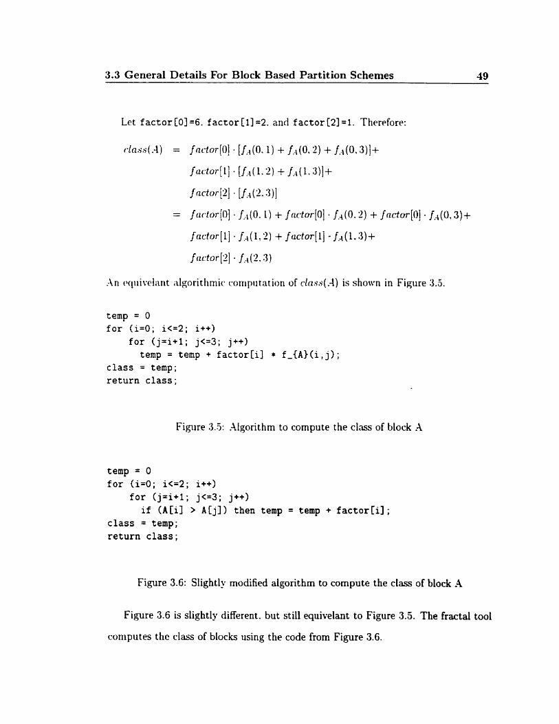
Let f a c t o r COI =6. f a c t o r (il =2. and f a c t o r [2] =l. Therefore:
r~ln.s.s(.-l) = fnctor[O] -[I..l(.i(O.i) +/ . . \ (0 .2)+ f.-,(0.3)]+
factor[l] . [f,-\(l . 2 ) -+ f..\(i. 3)1+
f tzctor [2] . [Je4 ('2.3)]
= fntfor[O] - f . . l ( O . l ) + fnctor[o]- f.4(0.-)+ffzctor[0]. fa4(o.3)+
factor [il . ja4 ( i ? 2) + /uctw[l] /f( ( 1.3) + f rrctor[Z] . f,@. 3)
A n qu ive lan t ;ilgoritlirniç cornpiitntion of c~lass(.-L) is sfiown in Figiire 3.5.
temp = O f o r (i=O; i<=2; i++)
f o r ( j = i + l ; j<=3; j++) temp = temp + f a c t o r Ci] * f -{A) (i , j) ;
c l a s s = temp; return c lass ;
Figiire 3.5: Algorithm to cornpute the class of block .A
temp = O for ( i = O ; i<=2; i++)
for ( j= i+ l ; j<=3; j++) i f ( A r i ] > A [ j ] ) then temp = temp + factorCi];
c lass = temp; return class;
Figure 3.6: Slightly rnodified algorithm to compute the class of block .4
Figure 3.6 is slightly different. but still equivelant to Figure 3.5. The fractal tool
cornputes the class of blocks using the code from Figure 3.6.
50 Fracta1 Tool
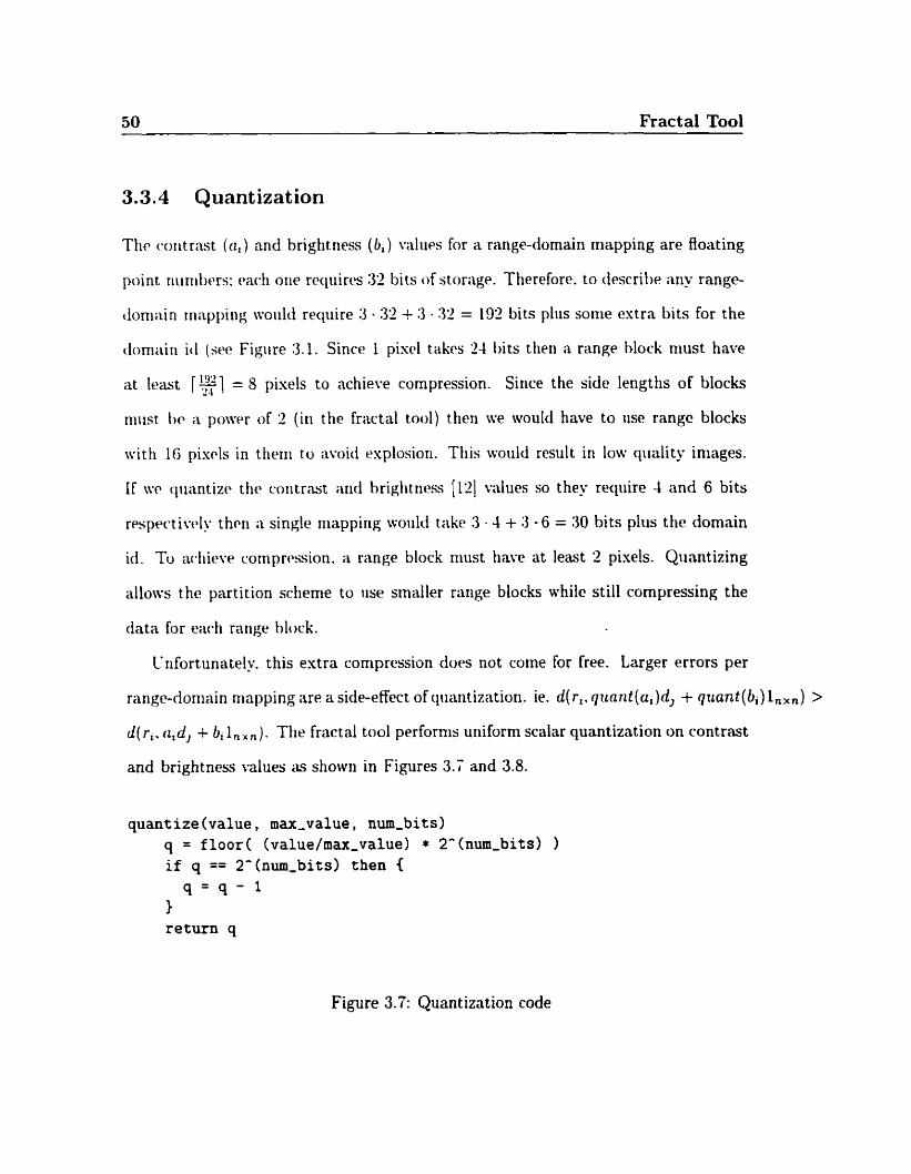
3.3.4 Quantizat ion
Tlit. ~.oritrnst ( ( 1 , ) and brightness ( 6 , ) vi i lu~s for a range-domain mapping are floating
point riunilwrs: rach one rcqiiircs 3'2 bits of storilge. Therefore. to dwxibe any range-
doniain rrinppiiig woiild reqiiire 3 - 32 + 3 . 32 = 192 bits plus some cstra bits for the
cloniaiii id (see Figure 3.1. Sincr 1 pixel takcs 24 bits tlien a range block niust have
at least [F] = 8 pixels to nchieve compression. Sirice the side lengths of blocks
niiist t,r ;\ powr of 2 ( i t i the fractnl tool) then we would have to use range blocks
witli 16 pixrls in ttierii to avoid explosiori. Ttiis woiild resiilt in low qiiality images.
IF wr qiiantizc* th<. roritriut and hriglitnrss [12] v;ilues so they reqiiire 4 and 6 bits
r ~ s p w t i d y t hrn a single niappirig woiiltl tiike 3 - 4 + 3 6 = 30 bits plus the domain
id. Tu tir-hirve comprt~ssion. ü range block riiust have at l e s t 2 pixels. Qiiantizing
allows the partition scheme to use smaller range blocks whilc still cornpressing the
data for eaîh range block.
Cnfortunately. this estra çonipression does not corne for free. Larger errors per
range-doniain mapping are a side-effect of quantization. ie. d( r , , quant (44 + quant ( D i ) l,,,) >
d ( r i . ci,d, + bi ln,,). The fractal tool performs uriiform scalar quantization on contrast
and brightness values as shown in Figures 3.7 and 3.8.
9'4-1 3 return q
Figure 3.7: Quant ization code
3.3 General Details For Block Based Partition Schemes 51
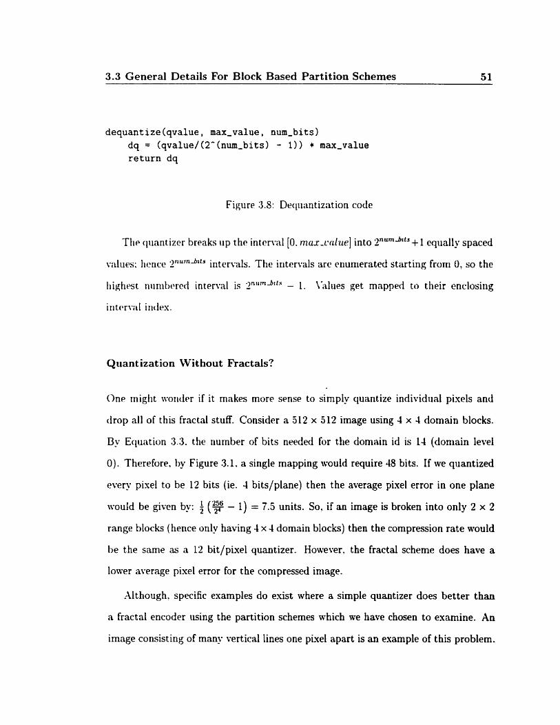
dequantize(qvalue, max-value, num-bits) dq = (qvalue/(2~(num-bits) - 1)) * max-value return dq
Figure 3.5: Deqiiantization code
Tiie qiiantizcr breaks iip the intemal [O. mur-rcrluil] into 2nUm"t' + 1 equally spaced
values; lience 2"U'nmts intervals. The intervals are cnunierated starting froni 0' so the
tiighcst riiirrlbcrcd interval is z " ~ " ~ ' ~ " - 1. \;dues get mnpped to tlieir enclosing
ir~trrvd i~icles.
Quant ka t ion Wit hout F'ractals?
One rriight woiid~r if i t makes more sense to simply cluantize individtinl pixels and
&op al1 of this fractal stuff. Consider a 512 x 512 image using 4 x 4 domain blocks.
By Equation 3.3. the number of bits needed for the domain id is 14 (doniain levei
O ) . Therefore. by Figure 3.1. a single mapping would require 48 bits. If we quantized
every pixel to be 12 bits (ie. 4 bitslplane) then the average pixel error in one plane
L 256 would be given by: 5 (T - 1) = 7.5 units. So, if an image is broken into only 2 x 2
range blocks (hence only having 4 x 4 domain blocks) then the compression rate would
be the same as a 12 bit/pïuel quantizer. However. the fractal scheme does have a
lower average pixel enor for the compressed image.
Although? specific examples do exist where a simple quantizer does better than
a fractal encoder rising the partition schemes which we have chosen to examine. An
image consisting of ma- vertical lines one pixel apart is an example of this problem.

52 Fracta1 Tool
3.4 Partition Schemes
Tlic fractal tool is p;ick;tged witii four quad t ree-li ke partition scliemes:
schemel llost simple techiiiqii~. Range t~locks haw power of 2 side Itjngtiis. aiid
riorriairi blocks tiaw side lerigtli rxactly trvire the size of their rnatching range
thck . Other notable featurcs are:
a Dornain blocks have only one orient. t' ron.
a For a givt!n rarigc block. the entirta imagta is sr;irchcd for domain blocks.
Blocks are classified nccorcling to the ortlcr of the sum of their pixels in
e:irli quadrant. Thertl are 2-4 hloc*k classes (set. Section 3.3.3).
scherne2: Slight ly more üdcinred t han the previous niet hod. Allows for different
transformations on a ciutriairi block. .
Domain blocks have 8 possible orientations. Reflections and rotations are
al lowd .
For a Aven range block. the entire image is searched for domain blocks.
Blocks are classified according to the order of the sum of their pixels in
each quadrant. There are 24 block classes (see Section 3.3.3).
scheme3: L'seful for examining local similarïty in an image. Xlso allows us to ex-
amine the effect of the classifier.
Domain blocks have 8 possible orientations. Reflections and rotations are
allowed.
For a @en range block. CVe search neighbourhoods for domain blocks.

3.4 Partition Schemes 53
Tliere is only 1 block chss.
scheme4: Examines loral siniilarity witli the use of the classifier.
Dornain blocks have S possibk orientations. Reflections and rotations are
al 1owec.i.
0 For ;i given range block. \Ve scarch neigtiboiirhootis for dornain blocks.
e Blocks are classified nccording to the ortler of the siim of their pixels in
cilch quaclrnnt. Tliere are 24 Mock classes.
sclieme5: Examiries loi~il siniilarity like schemc -4. hi i t ;illows bloclis to bclong to
more than one r-las.
Doiriain b1oi:ks have 8 possible orientations. Reflections and rotations are allo~vcd.
For a given range block. We senrch neighbourhoods for dornnin blocks.
Blocks which are close to another block class can belong to both classes.

54 Fractal Tool
Chapter 4
Sample Test Data
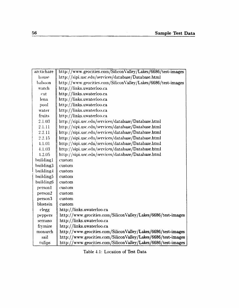
The sarnpie images whirh the esperiments are based on corne from various standard
image rcpositori~s fotind ori the InternetL and from ciistom-made images. Al1 test
images are 24 bits per pixel bitmaps. Xone of the test suites cover a broad range of
sample data: in pnrticuiar. there are fea cornputer generated images in the standard
test data. Xlso. thert. is no emphasis on symmetry and local similarity in the test
data. Howevcr. the stanclnrd tests do highlight typical real-wvorld data. ie. images
one might take with a cariiera. Using sample images. we will identify whicb partition
scheme is best suited for a pa,rticular type of image.
The location of the test images is given in the table below:
'Repositories can be found at:
a Waterloo Fractal Image Compression Project. (http://links.uwaterIoo.ca)
a JPEG Test Images. (htt p://~w.geocities.com/SiliconVdley/Lakes/~/test-images)
University Of Southern California Signal and Image Processing Institute. (ht tp: / / s ip i .usc .ec iu / sert - ices /databVe.html)
56 Sarn~le Test Data
arc t ichare tiorisr
t iii1)Oori Q X t d l
('itt
Icna pool w a k r fruits 2.1.0:3 2.1.1 1 2.2.11 " '1 1.5 -.-.
4.1.01 -1.1 .O3 4 2.05
hi i i chg 1 briilding;3 biiilding-l building5 building6 p m ~ n 1 pers0112 person3 blostein degg
PePPers Serrano frymire monarch
sail tulips
ht tp://aww .geocities.com/Silicon\.'alley/lakes/6686/ test-images lit t ~~://sipi.tisc.eclii/s~rvices/datsb~w/Database. html tit tp:/ /waw .geocit ies.coin/Siliconl*alley/Lakes/6686/test-images lit tp://liriks.uwaterloo.m ht tp://links.uwaterloo.ca http://Iinks.iii~atcrlon.ca k t p://links.uwaterloo.ca lit t p://links.uivatcrloo.ca Iit tp://links.ti~vaterloo.ca lit t p://sipi.usc.~clii/si~rvices/database/Database.litiril lit t p://sipi.iisc.~clii/scrvices/<iatab,uc/Database. htnil lit tp://sipi.usc.rclii/st~r~ices/rlatnb.?se/Database.html lit t p://sipi.usc.t~dii/s~rvices/clatnbnse/Dati~bi~e.html ht t p:/ /sipi.usc.ed~/scn.ices/database/Database.hti~il ht t~~://sipi.iisr.eciii/srwic~s/database/Database. html http:/ /sipi.iisc.cdti/sen.ires/<latabase/Dat~e.htnii ctistorn custorn custoni custom ciistom custom custorn custoni custom ht tp://links.ii~vaterloo.ca ht tp: / / ~ v ~ w . g e o c i t i e s . c o m / S i l i c o n v a l l e ~ http://links.uwaterloo.ca http://links.uwaterloo.ca ht t p://a-nnv.geocit ie~.com/SiliconVal1ey/Lakes/6686/test-images ht tp://nwtv.geocit ies.com/SiliconValley/Lakes/6686/ test-images ht tp://wiiw .geocities.com/Siliconvalley/Lakes/6686/test-images
Table 4.1: Location of Test Data
Chapter 5
Cornparison of Partition Schemes
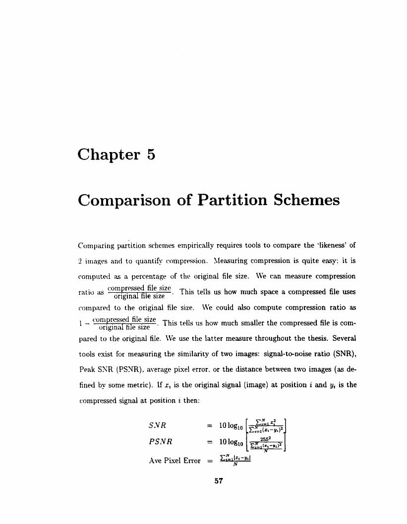
Comparing partition schernes empirically requires tools to compare the *likenessY of
2 iningrs and to quantif? compr~ssion. Measuring compression is quite emv; it is
conip~itecl as a percentage of the original file size. b'e can measure compression
ratio as "omprrssed 'le This tells us how rnuch space a compressed file uses original file size
cornpar~d to the original file size. We could also compute compression ratio as
1 - This tells us how rnuch srnaller the cornpressed file is corn- original file size
pared to the original file. \Ve use the latter measure throughout the thesis. Several
tools esist for measuring the similarity of two images: signal-to-noise ratio (SNR),
Peak SSR (PSYR), average pixel error. or the distance between tao images (as de-
fined by some metric). If r, is the original signal (image) at position i and yi is the
compressed signal at position i then:
58 Cornparison of Partition Schemes
Tlie wrrage pisel m o r nieaslires only the noise in the compressed signal. SXR
rntwslirrs t hc r~ l i l t i w niagnit ut de of the sigrid compared to the iinc~rtainty in t hat
signal (rioisr) on a per pisel basis. The PSKR rneasures the noise relative to the peak
signal ! 161.
h f o r t iinntely. one mensiire t iiat considers both compression ratio and image simi-
lari ty does iiot esist . Honever. the tno rneasures are related: we can trivially cornpress
;in irniigt. niaking it al1 I~lack (y, = O) . but the SYR would be very lowl. For fractal
i.oiiil)riwit ,ri. t 1 1 ~ type of imagc cmmbine(1 wit li n particrilar partition schrrrie and the
;il1o\v;iIilt~ Ior;il ( m o t (irt~rniines the rate o f rumprrssion and the comprcssed images
l i k m r s ri) l l i ~ original image. Lifortunately. cletermining a çliiss of iniagrs which
I>r~liavr siniilarily iinder a particiilar partition scheme is elusive.
.\Il tiw sc-iicines liehawd similarily whcn it cornes to compression ratio. The
difff3rmc.c br t w e n the best compression ratio and rvorst compression ratio r a s less
than 5% for al1 images: for most images it \vas less than 2%. The compression ratio
wrsiis the rrror thresliold curve has some interesting patterns ahich depend on the
image.
For ver' high quality compressed images (local error threshold is O to 1000), al1
partition schernes must break the image into many small range blocks2. This implies
that d l partition scliemes will use the same number of mappings: therefore. they will
have similar compression ratios. Furthermore, at this level of detail, domain level O
(full-width domain spacing) has a better compression ratio than domain level 1 (haK
rvidth domnin spacing) despite the fact that domain level 1 h a a larger domain pool.
This is because the local error threshold is so low that even at domain level 1 large
'The S9R wouId be 1 'Cornpressing any image using a local error threshold of 100 wilI remit in a partition consisting
almost entirely of 2 x 2 range blocks.
Cornparison of Partition Schemes 59
range blocks cannot be rnatched so the partition sclieme must divitle the image into
niinirnally sized range blocks3. However. writing out the id for a doniain block using
rloni;iin lei-el 1 rcquires at rnost 2 extra bits wer (loniain lerel O (this ran be seen by
relerring to Eqiiation 3.1 and observing that domspace is equal to D or 2). Since
t hc nuinber of mappings for domiiiii level O and levd 1 is the samr (sep .\ppendix
C) then it is clear that doniain level 1 will require more space. However, we are also
concernrd with iniagc quality. At t his error thresiiold. there is an abiindance of smail
range blocks at cfoniain lewl 0; thereforc, the sim of the domain pool is large which
implies the likelihood of a good match% high. Hence. the compressed image quality
at doniain Ievel O is close to tlie image quality nt domain level 1 (see Appendix E):
~Itbspite the fart thii t domain lrvel 1 dors have 4 timrs ns niany (lotnain blocks as
dumain level O.
For liigh quality compressed images (local error threshold is 1000 to 7000) the
clifference betwcen doniairi level O and domain level 1 is more significant. We can
see that the niimber of range blocks used by dornain level O is gea ter than tlie
niimber used by domain level 1 (see Appendix C). Therefore domain level 1 uses
fewer mappings; this directly affects the compression ratio. However, domain level 1
requires more bits per mapping for the domain id. These 2 properties of the different
domain levels seem to cancel each other out; leaving ils with domain level 1 and
domain level O having approximately the same compression ratio (see Appendix D).
The SNR varies depending on the scheme and the image being compressed (discussed
later).
Low quality images (local error threshold greater than 7000) cornpress equally well
3For this application, minimally sized range blocks is 2 x 2. IWe define a good domain-range match to be a rnatdùng whose error is below the local error
t hreshold.
60 Cornparison of Partition Schemes
for domain level O as they do for domain level 1. The rcason is the same as before.
Doniain level 1 uses feaer range blocks thnn domain level O. Oiie might wondcr if it
is worth the extra work (coniparing 4 times as rnany blocks) to use domain level 1 as
opposed to domain level O. If the SNR for domain level 1 is higher than dotnain level
O then the extra aork c m be justified.
This news is a little disappointing. In terms of compression, domain level O is a
bctter choicc than dornain level 1. The SKR value depends on the partition scheme.
LVe tlisciiss t his for each partition schcme separately.
5.0.1 Scheme 1
Compression Ratio
Domain level. 1 and domain level O are almost eqiiivelant in terms of compression
ratio. as discussed earlier. However. we should observe that some images compress
noticeably better than others using this scheme. The images with the worst com-
pression a t the highest error threshold were: serrano, frymire, clegg, and building3.
Three of those images (serrano. frymire. clegg) are cornputer generated (not wry
natural scenes). Further tests reveal that images with text and many straight lines
do not compress well: or if they do then the quality is terrible5. This is because
straight lines do not align nicely across range block boundaries and perfect lines do
not agree with our mode1 of self similarity. In particular, scaling a domain block by
half does not produce crisp lines. Other images did compress well. At the highest
error threshold, compression ratios of 95%6 and higher are common. At the lowest
'The SNR is low compared to other images. 695% means that the compressed file size oceupies 5% of the original size. ie. 1 - '-!r;':$f
Cornparison of Partition Schemes 61
rrror rhrcshold. compression ratios of 80% are typical. Images which compress very
wrll soriietimcs have dimensions which are a power of 16 (an implementation detail).
Thcy ;ilso have properties of symmet ry embedded in themselves. Furthemore, they
do iiot have many quick transitions betaeen colours (edges); instead, there are smooth
t r;irisit ions.
Irnagrs whirh have dimensions that are a power of 16 can be divided up in large
tilocks aithout having 2 x 2 blocks left over. This is partly why the irnplementations
which WC prrserit compress those images well. Images with symmetrical shapes (like
Imiltliiigs) or reflective properties (rnirrors. water) seem to have high self-sirnilarity
propcrties. .-\lthough. riot every synimetrical image compresses well. Those images
ttiat agrcr witli Our definition of siniilarityï compress well. For example, an image
with wenly spaced vertical lines is symmetrical but it does not cornpress well with
our rhoicr of transformations. An image with many sharp colour transitions will not
necessiiry compress poorly; however. if many of those transitions occur on an odd
pixel boundery then that transition will lie inside of a domain blocka. The problem
is that when ae shrink the domain block by half, we take the average of adjacent
pixels. This causes sharp transitions to become bluny. Moreover, it often incurs a
large error aloiig sharp edges which means that part of the image must be broken
down into srnaIl range blocks. On the contrary, very smooth areasg compress well.
By looking at Appendix Dy we see that this partition scheme does not have a
'based on the definition of our choice of contractive map. "ecause domain bloclcs have dimensions that are a power of 2 and images must have even
dimensions El
%mooth means uniform colour acros the block. ie. z, for any j, where zj denotes the j t h pixel in the block.
62 Cornparison of Partit ion Schemes
ver? high compression ratel0 when the local error threshold is lowLL. However, if we
i t l low i;i high loriil error threshold tlien we can achieve a rate of conipression that is
desirable. At tliis level, ive are only concerned that we can out-perform .JPEG1' and
t liat the image cari still be recognized. With this partition scheme, the highest error
thr~stiold still produces a recognizable image.
SNR
The SSR is n o t so simple when we compare it to domain level 1 and domain level
11 ~ t i tiic sarne partition scheme. For many images. the SNR is nearly equivelant
whct t i t~ ive iisc? domain level 1 or 0 (see Appendir E). However. there are some
itiiiigvs whtw tlie two ore not the sarne. For instance. if we look at arctichare. we can
o t ~ s ~ n - e a significant difference between the SNR for domain level 1 and O at higher
error thresholdst3. At low error thresholds, the size of range blocks is small whether
w~ use domain lewl O or 1. so we are likely to find good matches. Hence. there
is l i t t le differcnce between SNR of dornain Ievel O and 1. As we increase the error
threshold. the size of the range blucks and the corresponding domain blocks is large.
This means that the supply of domain blocks is less abundant; so anything we can do
to increase the might create better15 range-domain matches. The distance
between the SNR curve for domain levei O and domain level 1 increases as the error
threshold increases for some images (buildingô, house). It is difficult to determine
' o ~ ~ % is soniething we expect fiom JPEG; when we think of fracta1 compression we should expect 90% compression
' Belon- 7000 12Higher compression ratio and SNR l 3 It is interesting to note that the dope of the curve is almost O as we inuease the error threshold
beyond 7000 for this image, but the dope of the compression ratio curve is sirnilar to other images. 14Such as use domain level 1 LS Better in this case means Iower local m o r threshold for the range-domain rnapping
Cornparison of Partition Schemes 63
which images will have a higher SNR with domain level 1 as opposed to domain level
O
There were a few surprising results regarding SXR. For instance. there were a few
images wliere the SNR for domain level O was higher than domain level 1 (frymire).
These anomalies are rare. The most surprising resiilt is that some images (2.2.15,
22-11) had an increasing SXR (curve had positive slope) as the error threshold in-
rreased! This is also rare and difficult to explain. Both images are satellite images
and at a first glance appear random. They are not very structured images.
Some images do yield higher SNR using this partition sclieme than other images.
For instmce. images involving people and faces have the highest SNR (41.03, blostein,
personl. person2, person3, 4.2.05. cat). The fine details of the face may not be
arctirate. but most of the rest of the image is faithful to the original. The relationship
between SNR and compression ratio is not obvious. images with very low SNR do
not necessarily compress well or poorly in al1 cases. For instance, some images which
did compress well (pool) had relatively low SNR compared to most other images.
However, there were quite a few images which did not compress well and they had
the lowest SNR ( fiymire. serrano, baboon) .
The majority of images behave equally well with domain level 1 as they do with
domain level0. For this partition scheme, justihring the extra work needed for domain
level 1 is futile. Only on rare occasions d o s it seem useful (only in terms of SNR) to
use domain level 1. Unfortunately, it is difficult measure this beforehand.
64 Cornparison of Partition Schemes
5.0.2 Scheme 2
For a particular range block. scherne 2 considers more possible matchings than scheme
1. This is because schenie 2 allorvs a domain block to be rotated and reflected; each
domain block has 8 possible orientations.
Compression Ratio
Scheme 2 is sirnilar to scherne I in thnt domain level 1 and O are almost equi~pelant
in terms of compression ratio (sec Appendix D). We can sce that domain level 1
reqiiires f e w r range blocks than domain level O (as before - see Appendix C), but a
rnappine, with domain levrl 1 requirrs more bits.
SNR
Schcnic 2 behaves quite differently in terms of SNR cornpared to scheme 1. At
particular local error thresholds. the SNR for some images witli scheme 1 is slightly
higher than scheme 2. Since scheme 2 finds more matches for larger range blocks than
sclieme 1 then in some instances the local error for that rrgion of the image to be
better in scheme 1 than scheme 2 because scheme 1 would have broken the range block
down into smaller quadrants. An example will help to illustrate this point. Suppose
there exists a range block, r, in scheme 2 whose rnatching dornain block must be
rotated. In scheme 1, no such matching exists for r; therefore, r is broken down into
4 equally sized sub-blocks: r!'), ri1), ri1), and ri1). It is also possible that sorne of riL)
will be further broken down into rl(f), r!:), r,(?),rif) . Since scheme 1 requires a refined
partition then it is reasonable to expect that it may have a higher SNR than scheme
2: particularly a t higher local error thresholds (see Append~u E).
Cornparison of Partition Schemes 65
At lower error thresholds. the SXR for scherne 2 does at least as well as scheme
1 for almost ail images. This is because both schemes must use a fine grid for the
partition schemc: and since scheme 2 hi= more dornain blocks to choose frorn then it
is more likely to find a better match.
Some images siich as personl. pool. fruits, arctichare. building3 have an improved
SNR using scheme 2 as opposed to scheme 1. It is interesting to note that these
images use many domain blocks that are rotated 180" and reflected horizontally (see
Figure 5.02 as an esaniple, O-NONE. 1-ROT90. 2-ROT180, 3-ROT270. 4-REFHOR.
5-REFJER. 6-ROT90REF-VER. TROTSOREFAOR): the siim of the iiumber of
rotated and reflccted blocks used is greater than the number of non-rotated and non-
reflected blocks used. It would seern as though some images have a higher degrce of
t ransformed self-sirnilarity t han ot hen. This affects the qciality of image produced
!>y scheme 2.
Comparison To Scheme 1
The compression ratios for scheme 2 and scheme 1 are almost identical for al1 images;
this is clear by looking at Appendk D. Neither scheme differed from the other by
more than 5% compression. However, scheme 2 seemed to irnprove the compression
ratio of domain level O compared to scheme 1. We can compare the figures for the
compression ratio and see that the distance between the domain level 1 and O curves
for scheme 1 is larger than the same distance for scheme 2. The domain pool for
a range block in scheme 2 is 8 times larger than in scheme 1. Representing these
rotations and reflections requires 3 bits per mapping. At error thresholds > 1000,
scheme 2 compresses marginaily better than scheme 1 for most images. For lower
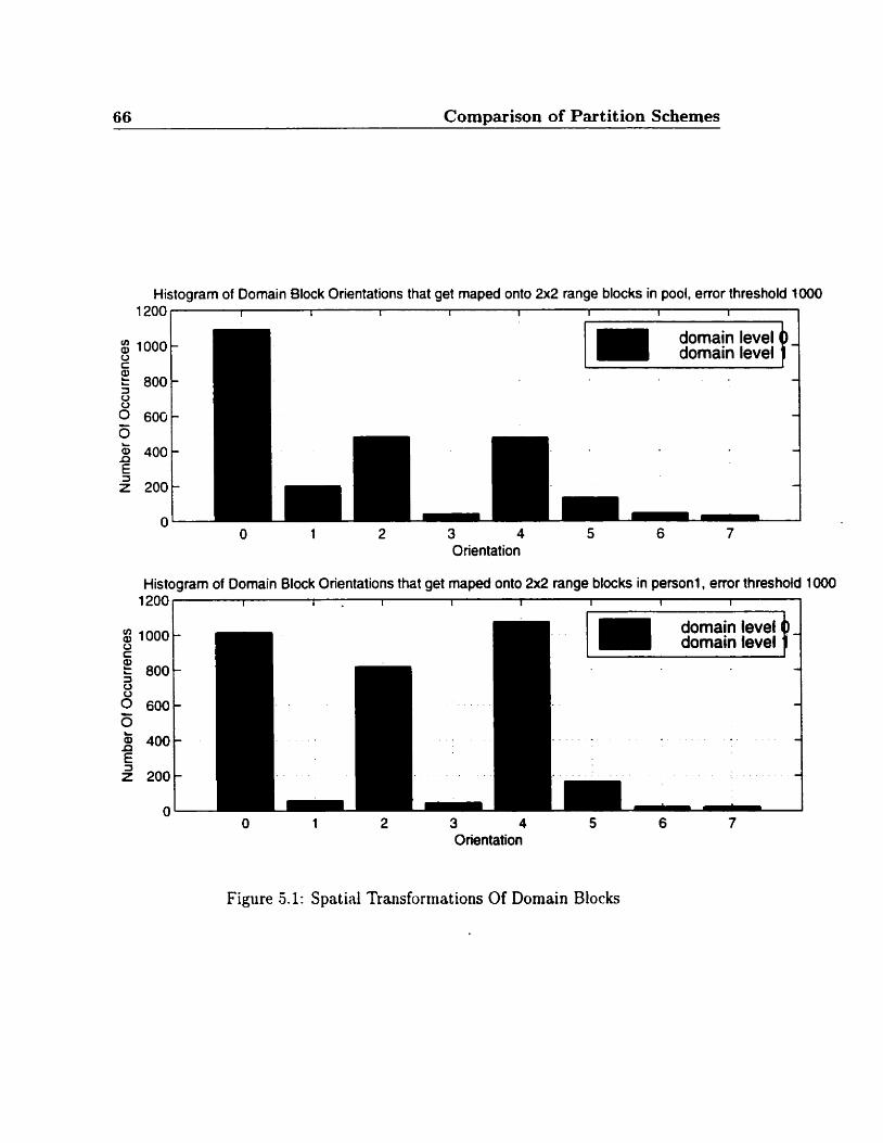
66 Cornparison of Partition Schemes
Histogram of Domain Block Orientations that get maped onto 2x2 range blocks in pool, error threshold 1000 1 200 I 1 1 I I I I 1
- O 1 2 3 4 5 6 7
Orientation
Histogram of Domain Bock Orientations that get rnaped ont0 2x2 range blocks in personl, emr threshold 1000 1200 1 I 1 I l 1 I I I
u
O 1 2 3 4 5 6 7 Orientation
Figure 5.1: Spatial Transformations Of Domain Blocks
Cornparison of Partit ion Schemes 67
error t hresholds. the type of image determines the differeiice in compression ratio
b~tweeii the two scliemrs. Images like: 2.1 .O3. sail. 22-11. buildingl, biiilding3,
frymire. serrano. baboon did not conipress as ive11 nt lower error thresholds with
scheme 2 than scheme 1. However. images like pool. watch. 2.2.15, personl, ra ter ,
4.1 .O3. person3 compressecl slightly better with schenie 3 at lowr error thresholds.
1s it wortti examining rotated and reflected domain I~locks'! Not from a compression
ratio point of view. I t is clifficuit to justify that much work for 1 percent improvernent.
The SNR for scherne 2 cornparecl to scherne 1 depends on the image and the
rrror threshold used. For instance, i l we look at the SNR for biiildingl. we can see
that scherne 2 has a higher SNR at error threshold 1000. and a lower SNR at error
t hresliold 22000. We expect tliis to be true at larger m o r thresliolds for niost images.
Scheme 2 is able to find a match for larger range blocks which means the local error is
quite high for a large region of the image. Scheme 1 is more likely not to find a match
so it must break down the range block; hence the local error for that same region of
the image may bc snialler. This means that scherne 2 is more likely to produce an
image that is faithful to our local error threshold requirements. Unfortunately, we do
not get a significant improvernent on the compression ratio in these instances.
Domain Block Rotations And Reflections
It is interesting to observe that the most frequently transformed domain blocks are:
not rotated or reflected. rotated 180°, and reflected horizontally. It seems as though
rnost natural images have a strong self-transfomability with respect to these three
operations on blocks. Scheme 2 attempts to take advantage of these characteristics
To improve compression, it would be interesting to only tly to use the two, or four
68 Cornparison of Partition Schemes
most comnion spatial t h & transformations. This woiild conserve t ao (one) bits in
tlie description of earli ritapping resiilting in iiripromd compression ratios.
5.0.3 Scheme 3
Schmie 3 does not ilse tlie blork classifier. Without the classifier, searching for a
niatrtiing domain blork is r e r y slow. For an m x n image, searching for a matching
clom;iin block For a single range hlock is O(rnn). More detailed analysis is found in
srvtioti 3.3.3. -4s a rcsiilt. sclicriir 3 does not s ~ a r c h the entire domain space for a
niatrhing doniain blovk. Ins t~ad it only searches a local nrighbourhood around the
range blork. Neverttiolts. wit hoiit the block classifier. this scherne is still painfully
slow? Scheme 3 optmtes on the suspicion that images have a high degree of 10-
r:il similarit': therefore. it is not worthahile to searcfi the entire image space for a
nintching domain block.
Compression Ratio
Li ke previous schemes: the clifference in compression ratio between domain level 1
and O is small. In fact- the sliape of the compression curve is identical to scheme 2
for most images. This is remarkably interesting because it indicates that images do
have a natural local similanty1'.
I6Images compressed using scherne 3 take at Ieast twice as long to cornpress compared to any O t her scherne.
"Csing Our very limited mode1 of similarïty baseci on our contractive maps.
Cornparison of Partition Schemes 69
SNR
Since schcme 3 does not use a classifier, the difference between domain level 1 and O
is not as signifirant as schenits 2. Therc are many dornain blocks to choose from for a
given range bl«isk. wwi at domein level O. The SNR behaves much like scheme 2 in
ternis of values af SSR and patterns for different images at different domain levels.
Comparison To Scheme 2
The rlassification scliernc is vital For rpasonable speed performance. However, it is
cwentinl t h t t lie hlock dassifier corrcctly classifies blocks. Suppose we are given a
range I~ lork r thrii 3 an optinial matdiing dornain hlock ralled d . h prrfect classi-
fication woiilci have range blocks r and d in the sarne block class. Ensuring optimal
matches is a Iinrd probiem [[13]]. The classifier used for the Fractal Tool is described
in Section 4.3.3. The compression ratio resulting from scheme 3 is quite similar to
schcme 2. Most images (such as buildingl, ttilips, fruits, etc . . . ) have the sarne
compression ratio with scheme 3 as they do with scheme 2; see Appendix D. There-
fore. the suspicion is that these images are locally self-similar because we were able to
find a reasonably good matching dornain block in a neighbourhood of a range block.
However. it would be interesting to see how well an image would be compressed if we
searched the entirc dornain space instead of a local neighbourhood. Unfortunately,
the amount of time this would take for a 128 x 128 image would be prohibitive. Some
images (building4 clegg, watch) did cornpress worse using scheme 3 compared to
scheme 2. However. the difference was not significant. It is likely that those images
did not posses as high a degree of local similarity as some other images; instead they
have global similarity. Pictures of buildings which are very symmetnc seemed to fa11
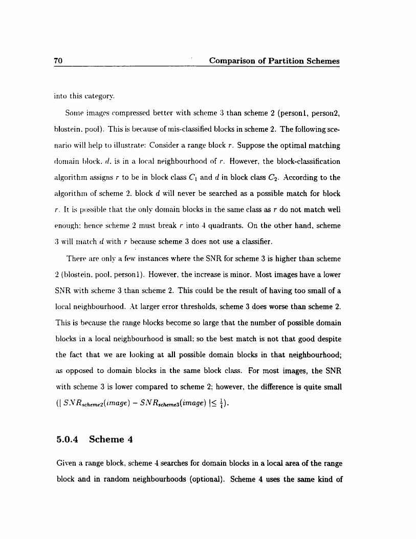
70 Cornparison of Partition Schemes
iiito this catcgory.
Soiiir irnagcs rornpressd bet ter wi t h scheme 3 t han scheme 2 (personl, person2,
hlost~in. pool). This is because of mis-classifieci blocks in scheme 2. The following sce-
nario ivill help to illiistratr: Consider a range block r . Suppose the optimal matching
doniain Idoçk. 11. is in a local neighboiirhood of r. However, the block-classification
algorithm assigiis r to be in block class Ci and d in block ciass C2. According to the
algorithiri of scheme 2 . block d ail1 never be searched as a possible match for block
r . It is ~~ossiblr t tint ttie oniy dornain blocks in the sanie class as r do not match well
P ~ O I I ~ ~ : hmce sclienie 2 rniist break r into -1 quadrants. On the ot her hand. scheme
:3 will match d with r bccausc scherne 3 does not use a classifier.
Theri. ;ire only a IPW instances where the SNR for scheme 3 is higher than scheme
2 (blostein. pool. personl). However, the increase is minor. Most images have a lower
SNR with scheme 3 than scheme 2. This could be the result of having too small of a
local neighbourhood. At liirger error thresholds, scheme 3 does worse than scheme 2.
This is because the range blocks hecome so large that the number of possible domain
blorks in a local neighboiirhood is small: so the best match is not that good despite
the fact that we are looking at al1 possible domain blocks in that neighbourhood;
as opposed to domain blocks in the same block class. For most images, the SNR
with scheme 3 is lower compared to scheme 2; however, the difference is quite small
( 1 S-VRxhtme2(image) - S~VR~&m3 (image) (5 i)
5.0.4 Scheme 4
Given a range block. scherne 4 searches for domain blocks in a local area of the range
block and in random neighbourhoods (optionai). Scheme 4 uses the same kind of
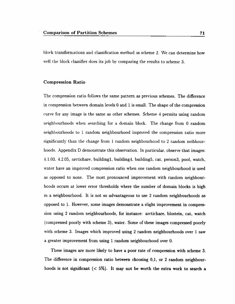
Cornparison of Partition Schemes 71
block transformations and classification method as schenie 2. We can determine how
wrll the block classifier does its job by comparing the results to schenic 3.
Compression Ratio
The compression ratio follows the same pattern as previous schemes. The difference
in compression between domain Ievels O and 1 is small. The shape of the compression
curve for any image is the same as other schemes. Schenie 4 permits using random
n~ighhourhoods when s~arching for a domain block. The change from O random
rieighbourlioods to 1 randoni neighbourhood iniproved the compression ratio more
significantly thnn the change from 1 random neighbourhoocl to 2 randorn neibtiour-
iioods. Appendix D demonstrate this observation. In particular. observe that images:
4.1.03. 4.2.05, arctichare. buildingl, building-l. building5. cat. person3, pool, watch.
water have an improved compression ratio when one random neighbourhood is used
ks opposed to none. The rnost pronounced improvement with raridom neighbour-
hoods occun at lower error thresholds where the number of domain biocks is high
in a neighbourhood. It is not so advantageous to use 7 random neighbourhoods as
opposed to 1. However, some images demonstrate a slight improvement in cornpres-
sion iising 2 random neighbourhoods, for instance: arctichare. blostein, cat, watch
(compressed poorly with scheme 3), water. Some of these images compressed poorly
with scheme 3. Images which improved using 2 random neighbourhoods over 1 saw
a greater irnprovement from using 1 random neighbourhood over O.
These images are more likely to have a poor rate of compression with scheme 3.
The difference in compression ratio between choosing 0,1, or 2 random neighbour-
hoods is not significant (< 5%). It may not be worth the extra work to search a
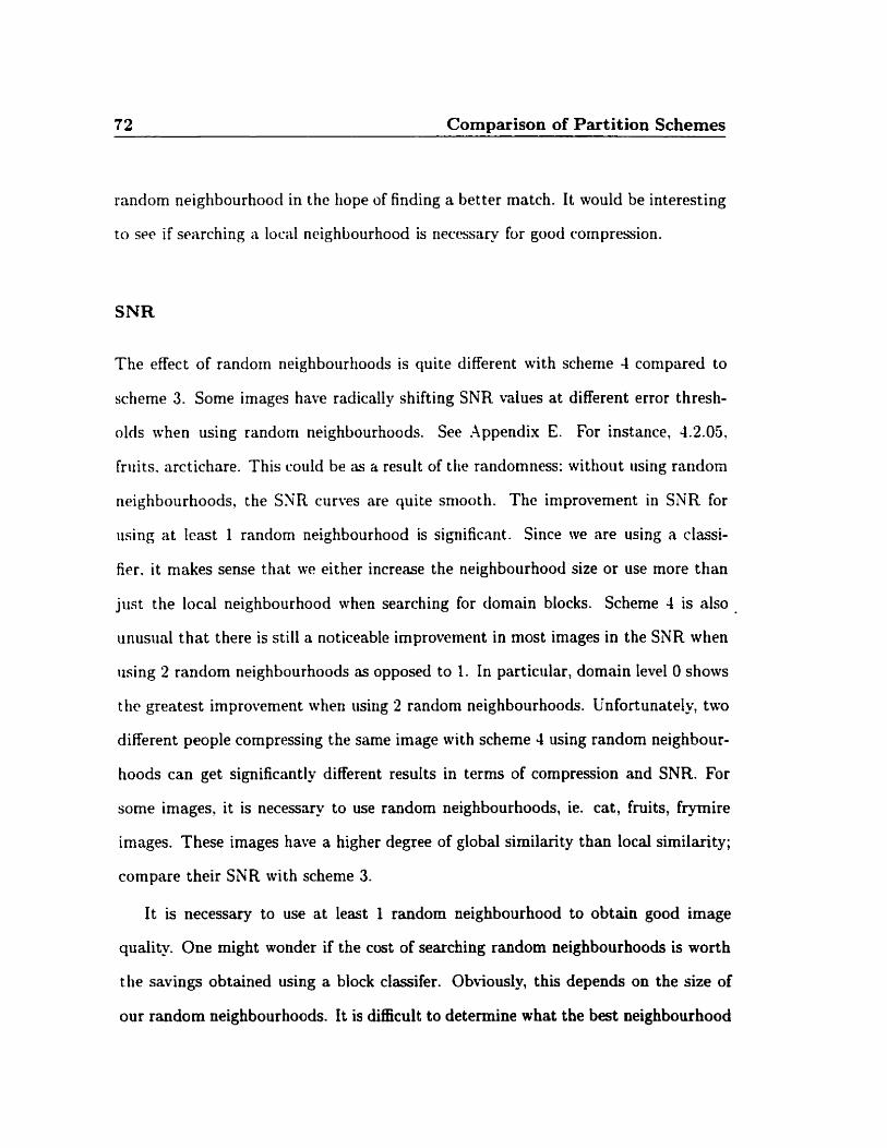
Cornparison of Partition Schemes
random neighbourhood in the Iiope of finding a better match. It would be interesting
to sec i f searching a loçitl neighbourhood is necessary for good compression.
SNR
The effect of randorn neighbourhoods is quite clifferent with scheme 4 compared to
scheme 3. Sorne images have radically shifting SNR values at different error thresh-
olds mhen using random neighbourhoods. See Appendix E. For instance, 1.2.05,
fruits. arctichare. This could be as ri result of the randomness: withoiit iising randon
neighbourhoods, the SNR ciirves are quite sniooth. The improvement in SNR for
iising a t least 1 random neighbourhood is sipificant. Since we are using a classi-
fier. it makes sense that we either increase the neighbourhood size or use more than
just the local neighbourhood when searching for domain blocks. Scheme 4 is also
unusiial that there is still a noticeable improvement in most images in the SNR when
iising 2 random neighbourhoods as opposed to 1. In particular, domain level O shows
t tic greatest improvement when usirig 2 random neighbourhoods. Unfortunately, two
different people cornpressing the sarne image with scheme 4 using random neighbour-
hoods can get significantly different results in terms of compression and SNR. For
some images. it is necessary to use random neighbourhoods, ie. cat, fruits, frymire
images. These images have a higher degree of global similanty than local similarity;
compare their SNR with scheme 3.
It is necessary to use at least 1 random neighbourhood to obtain good image
quality. One might wonder if the cwt of searching random neighbourhoods is worth
the savings obtained using a block classifer. Obviously, this depends on the size of
our random neighbourhoods. It is difficult to determine what the best neighbourhood
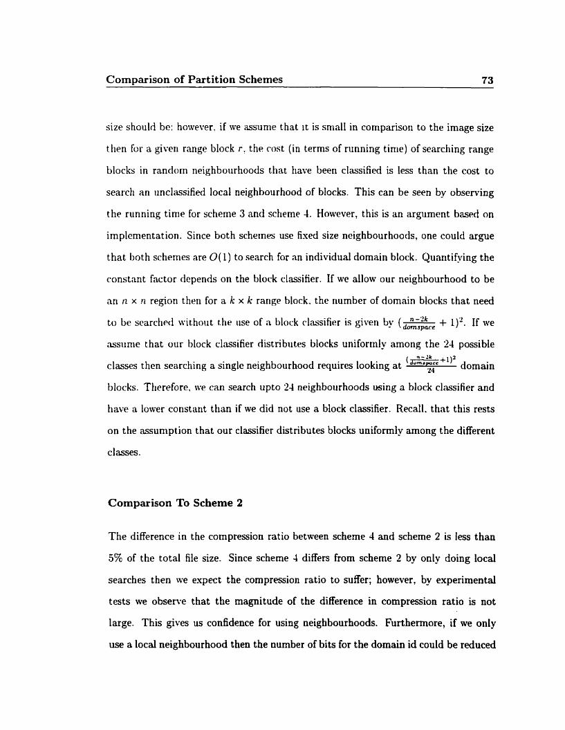
Cornparison of Partition Schemes 73
size shoiilrl be; however. if ive assunie that it is srna11 in cornparison to the image size
tlien for a given range block r. the cost (in terms of running tinie) of searcliing range
blocks in randoin neighboiirhoods ttiat have been classified is less than the cost to
search an unclassifiecl local neighbourhood of blocks. This can be seen by observing
the running tinie for scheme 3 and scheme 4. Houwer, this is an argument based on
implcmentation. Since both scheines use fixed size neighbourhoods, one could argue
that both schemes are O(1) to search for an inclividual domain block. Quantifying the
constant factor depends on the block classifier. If we allow our neighbourhood to be
nri n x n region theii for a k x k range block. the riumber of domain blocks that need
t« be srarched withoiit t h e use of a block classifier is given by (- + l)?. If ive
assiinie that our block classifier distributes blocks uniformly among the 24 possible n- Ik + 1l2
classes t hen searching a single neighbourhood requires looking a t ( J"" '~ ' dornain
blocks. Therefore. tve can search upto 24 neighboiirhoods using a block clessifier and
have a tower constant than if we did not use a block classifier. Recall. that this rests
on the rtssumpt ion t hat our classifier distributes blocks uniformly among the different
cl asses.
Comparison To Scheme 2
The difference in the compression ratio between scheme 4 and scheme 2 is less than
5% of the total file size. Since scheme 4 differs from scheme 2 by only doing local
searches then we expect the compression ratio to suffer; however, by experimental
tests we observe that the magnitude of the difference in compression ratio is not
large. This gives us confidence for using neighbourhoods. Furthemore, if we only
use a local neighbourhood then the number of bits for the domain id could be reduced
74 Cornparison of Partition Schemes
significaritly this wvould increase the compression ratio for scheme 4.
\Vitil regards to SNR. sclienie 4 behaves similarily to scheme 2. This is exciting
n w s : instead of seardiing the entire domain space. we only need to s~arch locally
witti a few randorn neighbourhoods. Using at least one random neighbourhood seems
to be ncccssary Slany images such as: 2.1.1 1. arctichare, 22.15 have an improved
SNR using scheme 4. However. these images have a lower compression rate usirig
scherne 4. So, the problem is that a large range block is not usually rnatched with
scheme 4 as opposed to scherne 2. Therefore. the range block is broken down into
snialler picces whrre ;t lower error mapping c m be found: hence we espect better
q~ialiry. \lé (-an s w this by looking at .lppcndis C: wc see that the nuniber of 2 x 3
range blocks is higher for scheme 4 than s r h m e 2 for most images.
Comparison To Scheme 3
Scheme 4 behwes similarily in terms of compression ratio to scheme 3. This instills
confidence in oiir choice of block classifier: it seems to produce results similar to a
local scheme without a classifier. hloreover, the amount of time it takes to cornpress
an image with scheme 3 is much higher compared to scheme 4.
In terms of SNR, scheme 4 seems to break down range blocks into smaller pieces
whicli means Ive expect a slightly worse compression ratio, but a higher SNR. For
some images, such as: 4.2.05, arctichare. blostein, and buildingl, the SNR for scheme
4 is lower than scheme 3. T h i s could be as a result of the classifier. In these images,
scheme 4 uses more range blocks; which implies smaller range blocks, but still has a
lower SNR. However, most images have nearly the same SNR using both scheme 4 (2
random neighbourhoods) and scheme 3.
Cornparison of Par t i t ion Schemes 75
Sclicme 4 seems to do rernarkably aell considering its limited domain block pool in
cornparison to other schemes which have a much larger domain pools. BIocks which
arc mis-classified are close to belonging to more than 1 block class where the meaning
of close depends on the choice of block classifier. With the classifier that Ive chose,
close means that given the siim of pixel values of 4 quadrants of a block: ql , q2, q3, q4
nt l e s t 2 of those sums are within 5 of each other. ie. 1 qi -q, I<_ 5 for i # j . Allowing
these blocks to belong to multiple classes might solve the probleni of mis-classifying
blocks.
5.0.5 Scheme 5
Scheme 5 behaves like scheme 4; hoivever. blocks can be put into nt most 2 classes in
srheme 5. A block is put in 2 classes if it is 'close' to another block class. This method
nttempts to correct any mistaken block classifications made by the block classifier by
slightly irirreasing the domain pool search size.
Compression Ratio
The compression ratio curve follows the same pattern as al1 the other schemes. Do-
niain levels O and 1 behave like previous schemes; ie. the curves a re close to each
other. Using random neighbourhoods only slightly improves the compression ratio on
a few images (ie. arctichare, buildingl, cat). The effect of random neighbourhoods is
not as pronounced as it was with scheme 4 possibly because the domain pool is larger.
We can see this by looking at the difference in compression ratio for scheme 5 with O
random neighbourhoods and 2 random neighbourhoods as opposed to the same dif-
ference with scheme 4. The classifier in scheme 5 seems to misclassify fewer blodrs.
76 Cornparison of Partition Schemes
Hoivewr. images w hich comprcssed poorly \vit ti sclicme 3 also cornpress poorly wit h
schcrne 5 (local neighbourhood search only).
SNR
Rancioni neighbourhoods improve SSR. We sas this with schenie 4 as well. The
rnodifird classifier has some effect on the SNR of t he final image; sec cornparison to
srht!mc 4. It is iriteresting to note t h the SNR For sorne images changes abniptly
ncrording t« the local thresholcl when random neighbourtioocis are heing iised (see
hiiilding-l. liiiilding5. cat. friiits). Without using random neighboiirhoocls. thesc im-
;igrs I in~c r e p large drops in the SNR at certain error thrcsholds. So. it woiilrl seem
thnt tlic self-sirnilarity of an image also deperids on the error threshold.
Cornparison To Scheme 4
Therc are man- blocks which are close to several block classes. One might wonder if
it is useful to allow a block to be in multiple block classes. If block 6 is in class cb,
but is close to being in class c, then adding block b into class c. is useful if there is no
block in c. that is close to cb. When we are dealing with low error thresholds, there is
an abundant supply of range blocks in each block class. It is very likely that if block
b is dose to class c, then there is a block a in c, that is close to class cb. It is not
so useful in these cases to add block b into class ca or vice versa. However, at larger
error thresholds where the pool of domain blocks is smaller there is an advantage to
increasing the domain pool by allowing blocks to belong to multiple block classes.
Comparison of Partition Schemes 77
5.0.6 Cornpared to JPEG
1s fractal imagr coriiprrssiori coriipnrnble to .JPEG? For Iiigh quiility representation.
the ;insiver is no. .JPEG coiripresses reasoiiably w l l (70-90%) with a high SNR. For
low c p l i t y reprcsentation. tiic c-ompressiun rate for JPEG is about the same as the
liactally conipressed files: ho\vcver. tliis is an unfair comparison. JPEG allows a loss-
1t.s encoding phase after its lossy compression. The fractal image cornpressor does
riot do this at the moment. To ohtain niasimal compression ratio for fractally corn-
prcssed images. it is riecessaru to i i s ~ a lossless encoclcr that rinderstands the format of
rriappings. Uany of the niappings froni ciornairi blocks to range blocks are the same.
Therrfore. a (.lever lossless m c o r l ~ r c m represent cornnion niappings with fewer bits.
\\é cari see froni Table 5.0.6 that the number of distinct mappings is frequently much
less than the total number of mappings used. refer to Table 5.0.6. This indicates an
rsce1ler.t opportunity for a dictionary style lossless coinpression algorithm. If many
mappings are common among images t hen a well known initial dictionary might be
admntageoiis. This coiild have a significant impact on compression.
By iising a standard JPEG compression tool, we managed to cornpress JPEG im-
ages smaller than the corresponding fractal image (wit hout a lossless encoder phase).
The SNR of the JPEG compressed image was higher than the fractal compressed
image. This is only slightly disapoint ing nem. Wit h an intelligent lossless encod-
ing phase a t the end of the fractal compression phase, ive expect compression ratios
higher than 95% which is what we currently have. At such high levels of compression,
we don't expect JPEG to perform well.
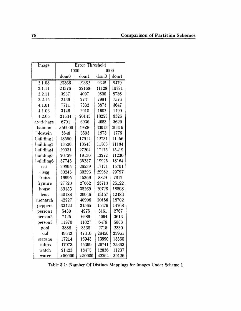
78 Cornparison of Partition Schemes
I ni agr
2.1 .O;3 '2.1.11 2.211 2.2.15 4.1.01 -1.1.03 4.2.05
iirc, t ichre h b 0 0 n l)lostt4n
t~uilcli~igl hiiilding3 hui1dir~g-l tmiltling5 hiildirig6
cat degg friii ts
frymire hoilse lena
nionarch PePPers person 1 person2 person3
pool sail
serrano tiilips watch ira t er
Error T hreshold
dom 1 5419 10781 $736 0-0
rai6 3647 1190 9326 3620 30316 1 ri6 11456 1 1 15-4 15419 11236 15164 15701 29197 7813
25122 1880s 12483 18702 14768 2767
Table .5.l: Number Of Distinct Mappings for Images Under Scheme 1

Part III
Discussion

Chapter 6
Interest ing Questions
6.1 Non-Uniform Quantizer
The range of quantized values for contrast and brightness are not uniformly dis-
tributed. In particular, for most images the brightneçs values are densely packed in
the center of the quantized range using any scheme. Therefore, using a non-uniform
scalar quantizer for the contrast and brightness values would improve the SNR, and
possibly improw compression. Obviously, the quantizer should have finer gradations
in the center of the quantized range than at the eàges. One rnight wonder how the
quality and compression ratio of the compressed image might improve. Early in-
vestigation seerns to indicate that the qualit? of the compressed image will not be
significantly higher using a non-uniform quantizer.
82 Interestine; Questions
6.2 Re-compressing The Output
Giwri an iniage. 11. ive cornpress the image to obtain pc. We then deconipress the
image to obtaiii /id. We hope that p d and p arc close to each otlier: hence the SNR
is higli. Consider what happens if ive conipress the image pd into p4. The image
,ud is already in block form (because we do not have a smoothing process) so we
ivoiild cspect a tiigher SNR and a better conipression ratio compared to p~ and 14.
The average pixcl crror I~etween p d and p woiild nlso be higher conipared to p~ and
\\é espect this lmause is /id an iniage that is the result of being rnodelleci by
fractals. Cornpressing is similar to re-constructing the mode1 that ic have already
biiilt. Simple trsts siipport tliis conclusion. If WC repeat this proccss. ac ivill get
c w n hettcr compression and higher SNR. Hoivever. the SNR is only in romparison
to the prerioiisly used image: not the original.
6.3 Adaptive Error
Certain parts of the image are not so important to represent as accurately as other
parts of the image. Determining which regions of the image are important is a difficult
problem. If ive solve this problem then adaptively modibng the error threshold to
be lower at the important regions would improve the image quaiity. The compression
ratio would not suffer because less important regions would have a high error threshold
and would have a high compression ratio.
\\é could try a very simplistic heunstic. For instance, the middle of the image
cotild have a lower local error threshold then the edges. The justification being that
the focus of the image is in the center and the rest of the image is not so important.
6.3 Target Compression Ratio 83
Obvioiisly. numerous coiinter-esaniples esist where this simple heuristic woiild fail.
6.4 Target Compression Ratio
Obtaining a target compression ratio. cl,,,,, . is an interesting project. Initially, we
ran stiirt with n large grid of range blocks. This is the minimum coinpression ratio
that ive c m achieve. cal1 it cm,,. If cm,, < c,.,,, then we can procwd to break up the
range hlock wit h the worst matching domnin block' . This gives us a new compression
ratio. cm,. We continue to break itp the the range block with the worst matching
doniaiil I~lock and iipdate cc,, ;ippropriately iintil c,, > s,,,,t[3].
6.5 Post-Processing For Decompression
Csing higher local error thresholds leads to noticeable blocks in the decompressed
image. Thcse blocks can be elirninated by adding n post-processing phase to the
dccornpression process to smooth the transition between adjacent blocks. Since the
decompression phase is reasonabl y fast and since the fractal file contains information
about the blocks then smoothing the transition between blocks should not be a costly
process. Smoothing only needs to occur at the edge of blocks; not inside them.
6.6 Lossless Encoding Phase
.A lossless encoding phase after the fractal compression would improve the compression
ratio. Unfortunately. the extra compression obtained by adding a lossless phase using
lWorst matching domain block means the mapping error is larger than the mapping error for any other rangedomain block pair
84 Interesting Questions
ciirrent tools is stnall. Current tools look at patterns of bits. In this case. it would
be ;idvantagcoiis to look at patterns of mnppings for lossless compression.
6.7 Number Of Iterations For Decompression
Several papcrs [[SI] have addresseci the issue of fast convergence for decompression.
Alost images need 7 iterations before the SNR becomes stable2. However, some images
nerd more iterations. Obviously. the easiest way to decornpress an image is to take
the ciiffwmcr hetwecn successive itcrations and when that difference is small enough
thv process ciin stop.
?Stable means that more iterations do not significantly irnprove the SNR
Chapter 7
Future Work
7.1 F'ractal Audio Compression
Aiidio, music in particular, has mmy repetitive patterns. Focusing on the self-
similarity aspect of music could be fruitful for fractnl audio compression. Using
tecliniqiirs that have been mentioned earlier. it might be possible to compress music
fractally by looking for self-similar patterns.
7.2 Fracta1 Tool
AIany improvements to the fractal tool can be made. The current colour model is
RGB. It may be advantageous to use HSB (hue, value. chroma) or some other colour
model. Furthermore, rnany components of the fractal tool can be manually optimized
to improve speed performance. Also? the ability to plug in new partition schemes is
not easy; the software engineering aspects of this problem can be explored hirther.
The decompression phase could also be improved by having a block smoother

86 Future Work
which woiild smooth oiit tlie pixel differences betwen adjacent blocks. This wotild
rliniinate t lie blockiness of deconipressed images.
Chapter 8
Summary And Conclusions
The rvholc idea of taking one block and mapping it onto another block for the purpose
of image compression secms liidicroiis; -et i t wor ks. The implementation provideà
with this thesis demonstrates that thcre are sereral methods to make this style of
image compression work.
Domain lerel 1 uses n lnrger domnin pool thnn domain level O. However. there
is no significant advantage over using domain lerel 1 because the compression ratio
is about the sanie as domain level O. Also, the SNR is nearly the same. It is dso
interesting to note that the rnost common spatial transformations are: none, rotate
180". and reflect horizontnlly out of the 8 possibilities. We may be able to improve
the compression ratio for many images by taking advantage of tbis fact. The speed
would definitely be improved if we only consider 3 possible spatial transformations.
One method for finding domain blocks is local neighbourhood searching combined
with random neighbourhoods. This style of domain block organization seems to be
effective. The compression ratio is aearly unchanged and the SNR is oniy a little lower
for some images. The block classification technique is more effective at lower error

88 Summary And Conclusions
tliresliolcls conipared to tiigher error thresholds; which is the result of an increased size
in the tloniain pool. At higher error thresholds. we observe that the SNR is increased
~vtitw ive allow t~locks tvhicli are close to more than one block class to belong to
riitiltiple t~lock rliissrs. However. since the clifference in SNR is not significant then
n.tb may roncluclt? t liat the classification scheme which ive have chosen is reasonable.
In conipirisori to .JPEG. c w have not clcnioristratetl that fractal image comrpession
is superior. However. the providecl implementation does not have a lossless encoding
ptiase like .JPEC;. \t'cl <lenionstr;ited that since the number of distinct mappings is
siti;iilcr tiian t lie total riuiriber of niappings used t hen it wvould be possible to achie~e
goo(l lossless coniprcwion rates with an intelligent encoder. .-ln intelligent encoder
riiiist iincierst;iri(l ttic? riotion of rnappings. If w .?dd this feature then it is quite
possible to aciiieve Iiighcr compression rates than .JPEG together with higher SNR
values.
Bibliography
[l] Al i . kfaariif and Clarkson. T.G. Suruey of Block Based Fractal Image Com-
prrssion and its ..lpplicotions Proceedings of the 2nd Conference of Information
Technology anci its .-\pplications. ITA'93
[2] Barnsley. SI. Frnctals Evenjwhere. Aradernic Press, 1993.
[3] Fisher. 1'. Fractal Image Compression: Theory and Application. Sprînger-Verlag,
1995.
[-II Forte. B. aiid Yrscay. E.R.. Theonj of generalzzed fractal t m n s f o m . Proceedings
of the NATO ;\SI Concerence. Fractal Image Encoding and Xnalysis, Trondheim,
July 1995. Berlin Heidelberg, 1998. Springer-Verlag.
[SI G haravi-Alkhansari, hl. and Huang, T.S. A fiactal-bmed Image Block-coding
.4 lgorithm University Of Illinois
[6] Jacquin. A. Fractal Image Coding: A Reviev Proceedings of the IEEE. Volume
$1, Xumber 10. October 1993
[ï'] Johnson. D.S. A Theoretician's Guide to the Ezperimental Analysis of Algorithm
ht tp://mnv.research.att .corn/ dsj/papers.html
89
90 BIBLIOGFMPHY
[SI Kominrk. J. Conuergence of Jrnctnl encoded images Proceedings DCC'95 Data
Compression Conference. .J. A. Storer. hl . Cohn (eds.), IEEE Computer Society
Press. h r c h 1993.
[9] Kominek. .J . ;Idvances in Fractal Compression for fbhllimedi~ Applications. Uni-
versity O f Waterloo. http://links.uwi.itrrloo.ca. April 1996.
[ I O ] Lii. Y. Fmctal Irringing. Academic Press. 1997.
[ 1 11 Ilarscltm -1. E. and Hoffmnn R I . J . Elementaq Classical Analysis. 2nd edition.
K . H . Frccwinri and Company, 1993.
[ l?] Ndson. Mark and Gailly. Jean-Loup. The Data Compression Book. 2nd edition.
UkT Books, 1996.
[13] Reusens. E. Padztzoning complexity issue for iterated funclions systerns based
image coding Proc. of VI1 EUSIPCO, Edinburgli, September 1994
[ I 41 Saiipe. D . Fractal Image Compression via Neorest Neighbor Search Proceedings
of the NATO .AS1 Conference. Fractal Image Encoding and Analysis, Trondheim,
.Jiily 1995.
[IS] Saupe. D. and Hamzaoui, R. and Hartenstein, H. Fractal Image Compression:
.4 n Introduct ory 0 u e n n . e ~ Revised version of Chapter 2 from Fractal Models for
Image Synt hesis, Encoding and -4naIysis.
[16] Sayood, Khalid. Introduction To Data Compmssion. 2nd edition. Morgan Kauf-
mann Publishers, 2000.

BIBLIOGRAPHY 91
[li] \,*rscay, E.R. A Hztchhiker 's Guide to 'Frartal-Based ' Function Approrirnation
and b n a g e Compression. University Of Waterloo. http://links.uwaterloo.ca. Au-
gust 1995.

92 BIBLIOGRAPHY
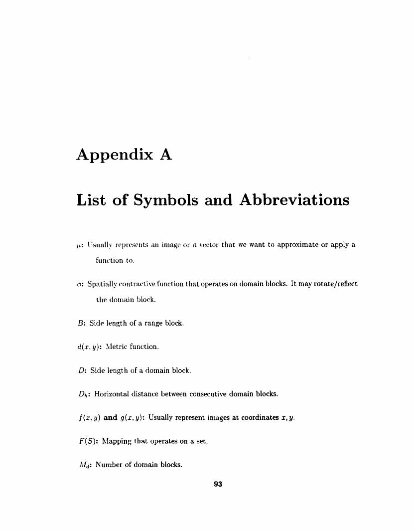
Appendix A
List of Symbols and Abbreviations
Ir : Ckially rrprrsrrits iiti image or ;i vector that ive wnnt to approximate or apply a
furict ion t o.
O: Spntially contractive hnct ion that oprrates on domain blocks. It may rotatelreflect
the cfomain block.
5: Sidp length of a range block.
d(x. y): lletric function.
D: Side length of a domain block.
Dh: Horizontal distance between consecutive domain blocks.
/(x. y) and g(x. y): Usually represent images at coordinates x, y.
F(S) : Mapping that operates on a set.
A&: Number of domain blocks.

94 List of Symbols and Abbreviations
.\Ir: Siimber of range blucks.
1 , : .-\ niapping from a clornain block to a block tliat is the sanie size as a range block.
I17(p): The union of al1 the to , rnappings. I I* operates on an image.
PSNR: Peak Signal r o Soise Ratio. Defined in Chapter 5.
SNR: Signal to Noise Ratio. Dcfined in Chapter 5 .
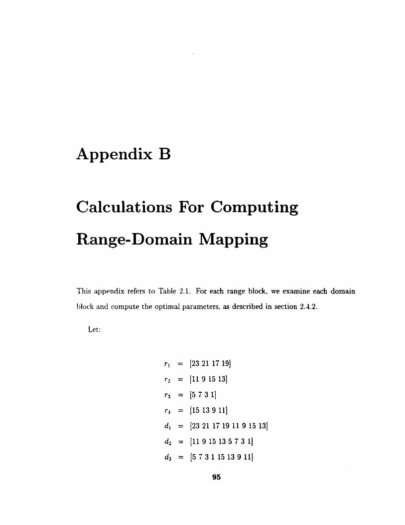
Appendix B
Calculat ions For Comput ing
Range-Domain Mapping
This appendis refers to Table 3.1. For each range block, we examine each domain
h l d and cornpute the optimal paramcters. as descnbed in section 2.1.2.
Let:
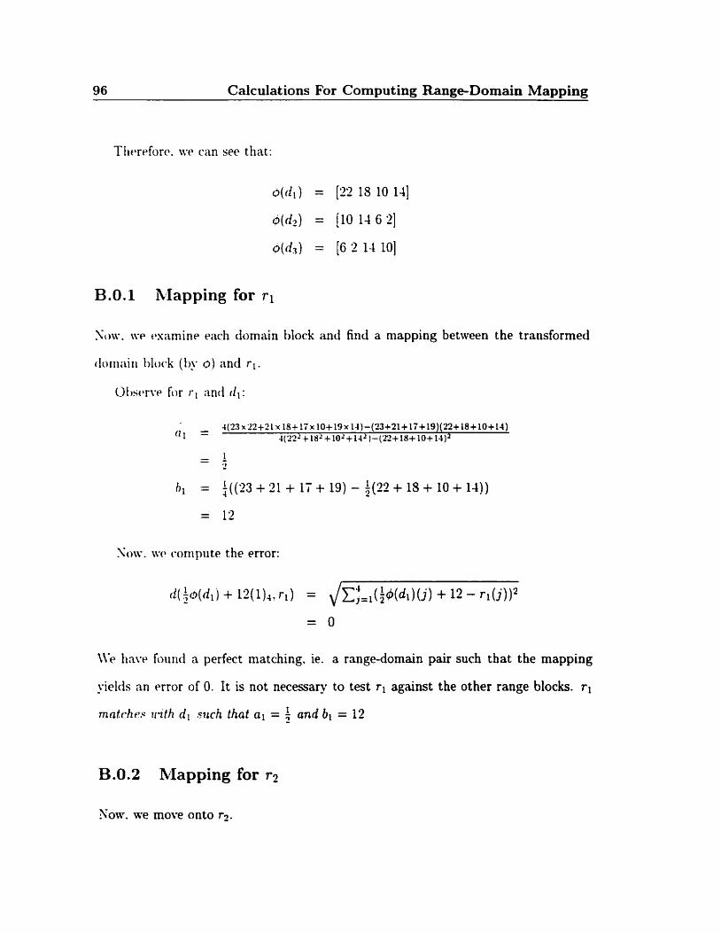
96 Calculations For Computing Range-Domain Mapping
Ke linw foiind n perfect matching. ie. a range-domain pair such that the mapping
yields an mror of O. I t is not necessary to test rl against the other range blocks. rl
matchez trith d l such that al = ! and b1 = 12
B.0.2 Mapping for r2
Xow. we move onto TI>.

Calculations For Computing Range-Domain Mapping 97
Observe for r2 and dl :
- 2 - -- 5
K e rcquire that the contrast (a2) be in [O. 1). Therefore, we must force a2 = O . Hence
t hc calculation for becomes:
= f(11+9+15+13)
= 12
Xow. ae compute the error:
Observe for rz and 4:
Thcrefore. the brightness woudld be:
Hence, the error would be the same as it was before:
Observe for rp and d3:
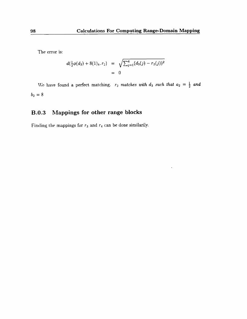
98 Calculations For Computing Range-Domain Mapping
The error is:
\\Q have found a perfect rnatching. r2 rnutches with d3 such that a? = h and b2 = 8
B.0.3 Mappings for other range blocks
Finding tlir mappings for r3 and r~ can be done similaril.
Appendix C
Range Block Results
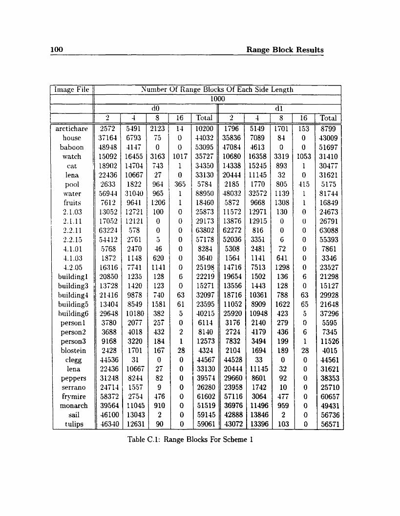
100 Range Block Results
Iiriage File
arc t ichare hause
baboon \vat ch
cat lena pool \vater fruits '1.1 .O3 2.1.11 2.2.11 -7 - - W . -7 15
41.01 4.1 .O3 4.2 .O5
building1 building3 building4 building5 biiilding6 person 1 person2 person3 blostein
~ 1 % lena
PePPers Serrano -mire
monarch sail
t ulips
Nuniber Of Range Bloch Of Each Side Length 1000
Total 8499 4.3009 51697 31410 30477 31621 5115 5 17-14 16849 '24613 26791 63088 55393 1861 3346 23527 2 1298 15127 29928 21648 37296 5895 7345 11526 4015 44561 31621 38353 25710 60657 49431 56736 56571
Table C.1: Range Bloch For Scheme 1
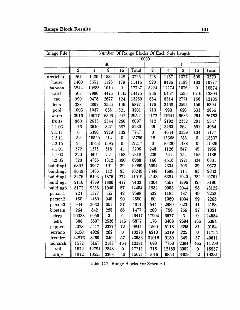
Range Biock Results 101
Image File
arct ickiare hoiise
baboon watch
cat lena pool
water fruits 2.1.03 2.1Sl 2 2 . 1 1 '2.3.15 4.1.01 4.1 .O3 4.2.05
building1 building3 building4 building5 building6 person l person2 person3 Dlostein
c h % iena
PePPem serrano frymire
monarch saiI
tulips
Surnber Of Range Blocks Of Each Side L e n d l
Total 3126 11416 17737 14475 13269 6877 3201 29541 6097 5230 7747 15766 13'217 2206 1318 6988 10999 10149 Il919 9132 1-1454 2598 2650 4614 1-177
26447 6877 9844 13278 43533 12381 17211 15621
Total 3270 10777 155'14 12804 12105 6394 2856 36'163 5347 4954 7177 15637 11926 1966 1186 633 1 9673 9343 10761 8190 13122 2253 2263 4188 1321
24584 6394 9154 11754 40611 11199 15957 14331
Table C.2: Range Blocks For Scheme 1
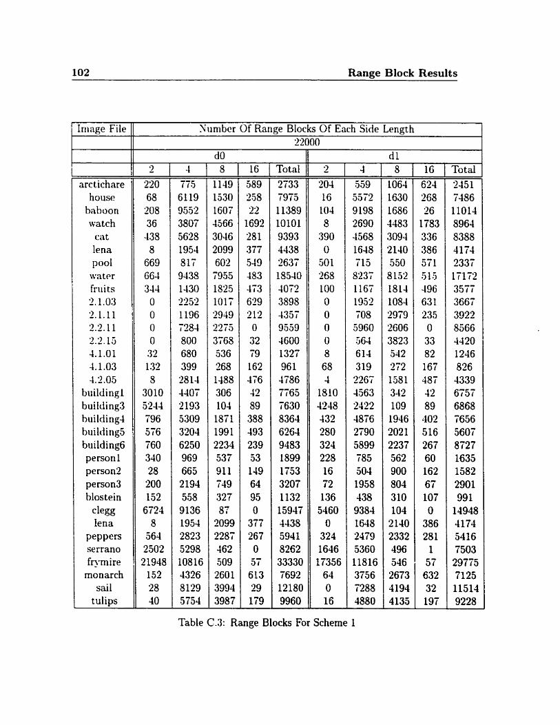
102 Range Block Results
Irriage File
arctichare house
baboori watch
ciit lena pool
water friii ts 2 . l .On 2.1.11 2.2.11 2.2.15 4.1.01 4.1 .O3 4.1.05
building1 building3 building4 building5 building6 personl person3 person3 blostein
clegg lena
PePPers Serrano frymire
monarch sail
tulips
Yumbcr Of Range Blocks Of Each Side Length 22000
Total 2733 19'75 Il389 10101 9393 4438 '2637 18540 4072 3895 4351 9559 4600 1327 961 4786 TG65 7630 8364 6264 9483 1899 1753 3207 1132 15947 4438 5941 8262 33330 7692 12180 9960
Tot al 2451 7486 11014 8964 5358 4174 2331 m i 2 3577 3667 3922 8566 4420 1246 826 4339 6157 6868 7656 5607 8727 1635 1582 2901 991
14948 4174 5416 7503 29775 7125 11514 9228
Table (2.3: Range Blocks For Scheme 1
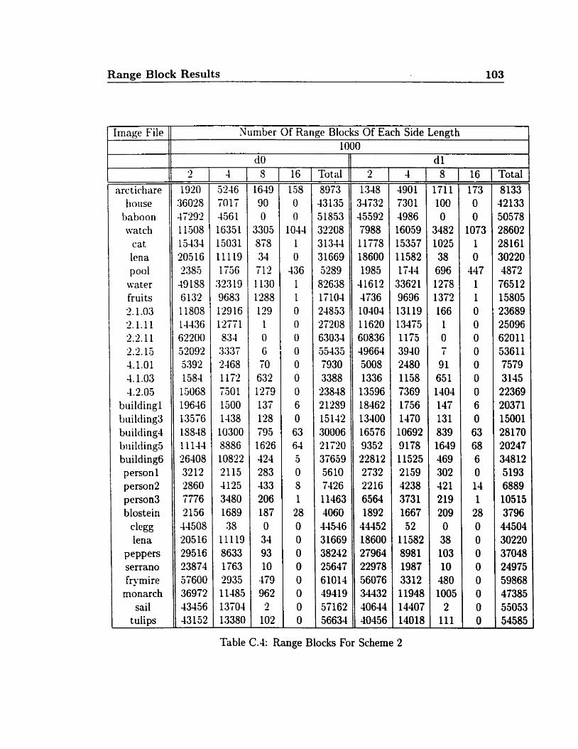
Range Block Results 103
arct ichare ho use
baboon vatch
cat lena pool
~ v ; ~ t er fruits 2.1 .O3 2.1.11 22.11 .> -.-. 9 15 -4.1.01 4.1 .O3 4.2.05
building1 biiilcIing3 building4 biiilding5 building6 person 1 person2 person3 blostein
ch% lena
Pe PPers serrano kymire
monarch sai 1
t ulips
Total 8973 43135 51853 32208 3 1344 31669 5289 81635 11104 24853 27208 63034 e55-435 7930 3388 23848 21289 15142 30006 2 1720 37659 5610 7426 11463 4060 -44546 31669 38242 25647 61014 49419 57162 56634
Image File
Total 8133 42133 50578 28602 28161 30220 4872 76512 15805 23689 25096 6201 1 5361 1 7579 3145 22369 20371 15001 28170 20247 34812 5193 6889 10515 3796 44504 30220 37048 24975 59868 47385 55053 54585
Number Of Range Blocks Of Each Side Length 1000
Table CA: Range Blocks For Scherne 2
- 7-
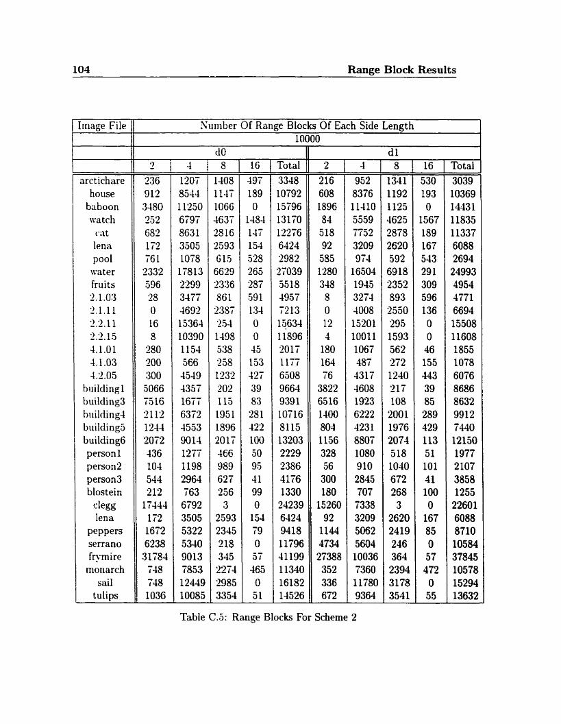
104 Range Block Results
arcticfiare hoiise
baboon \vatch
t-zit
lena pool water fruits 2.1 .O3 2.1.1 1 2.2-1 1 2.2.1.5 -4.1.01 4.1 .O3 4.1.05
building1 building3 biiilcling-l building5 building6 person 1 person2 person3 blostein
clegg lena
PePPers Serrano frymire
monarch sail
tulips
Tot al 3348 10792 15796 13170 1276 6324 2982 '31039 5518 4957 1213 15634 L 1896 '2017 1177 6508 9664 9391 10716 81 15 13203 2229 2386 4116 1330
24239 6424 9418 11796 41199 11340 16182 14526
Total 3039 10369 14131 11835 Il337 6088 2694
24993 4954 4771 6694 15508 11608 1855 1078 6076 8686 8632 9912 7440 12150 1977 2107 3858 1255
22601 6088 8710 10584 37845 10578 15294 13632
Table C.5: Range Blocks For Scheme 2
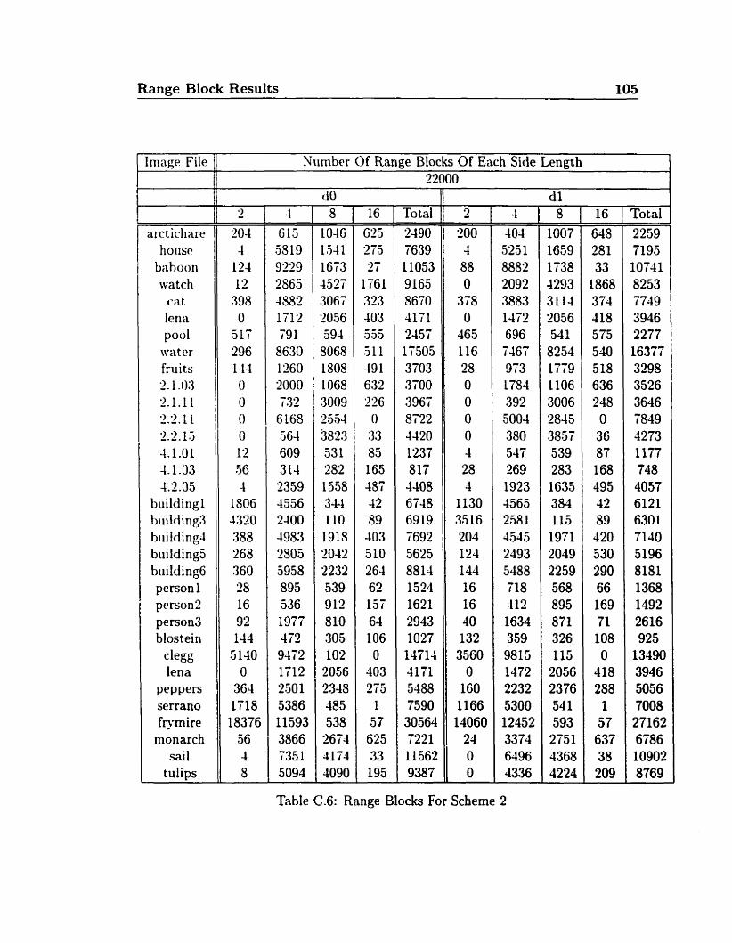
Range Block Results 105
Image File
arct ichare 11oi1sc
b;thoon watch
vat lena pool
ivatcr friii ts 2.1 * 0 : 3 2-1.1 1 2.2.1 l 2.1.1'1 -4.1.01 4.1 .O3 42.05
building1 building3 building4 building5 building6 personl person2 person3 blostein
clegg lena
PePPers serrano frymire
monarch sail
tulips
'iiirnber Of Range Blocks Of Each Side L e n ~ t h
Total 2490 7639 11053 9165 8670 4171 2454 11505 3703 3100 3961 8123 4420 1237 517 4408 6748 6919 7692 5625 8814 1524 1621 2943 1027 14714 4171 5488 7590 30564 4221 11562 9387
Total 2259 7195 10741 8253 7749 3946 2277 16377 3298 3526 3646 7839 4273 1177 748 4057 6121 6301 7140 5196 8151 1368 1492 2616 925
13490 3946 5056 7008 27162 6786 10902 8769
Table C.6: Range Blocks For Scheme 2
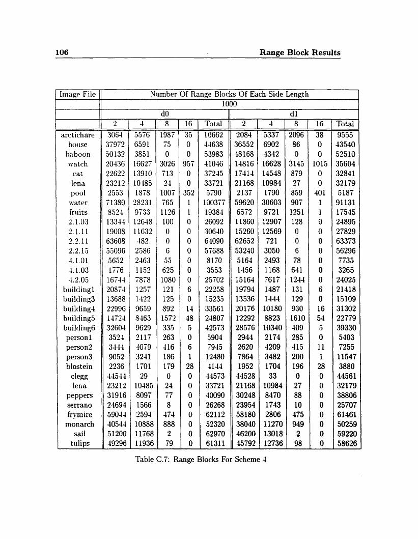
106 Range Block Results
Image File 1) Yuniber Of Range Blocks Of Each Side Length
iirct ichare hoilse
baboon m t c h
cat
lena pool
water fruits 2.1 .O3 2.1.1 1 2.2.11 2.2.15 4.1.01 4.1 .O3 -1.2.05
building1 l>uilcling3 building4 biiilding5 building6 person 1 peson2 person3 blostein
Lena PePPers Serrano fryrnire
monarch sai 1
tulips
Total 1 O662 44638 53983 41046 37245 33721 5790
100377 19384 26092 i30640 64090 57688 8170 3553
25702 22258 15235 33561 24807 42573 5904 7945 12480 4144
44573 33721 40090 26268 62112 52320 62970 61311
Total 9555 43540 52510 35604 32841 32179 5187 91131 17545 24895 27829 63373 56296 7735 3265
24025 21418 15109 31302 23779 39330 5403 7255 1154'7 3880 44561 32179 38806 25707 61461 50259 59220 58626
Table C.7: Range Blocks For Scheme 4
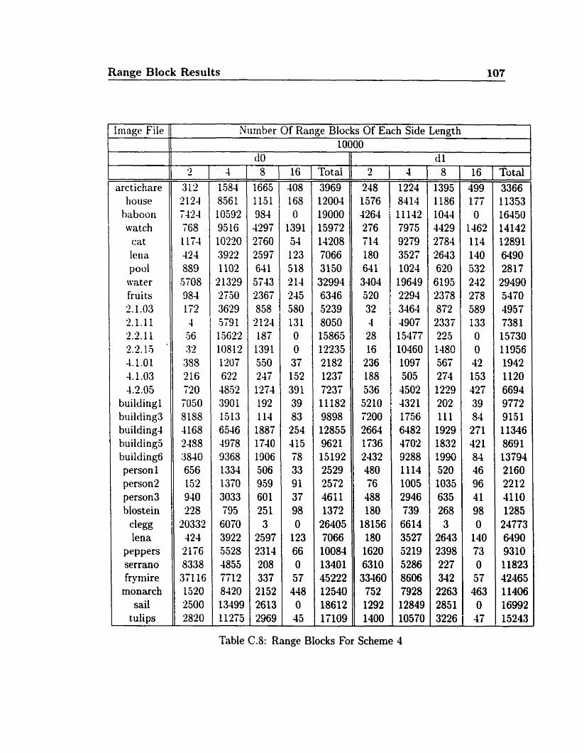
Range BIock Results 107
arc t ichare lioiise
haboon watch
cat letia pool
\rater fruits 2.1 .O3 2.1.11 2.2.11 '2.2.15 4.1.01 -1.1 .O3 1.2.05
building1 building3 biiilding-l building5 building6 person 1 person2 person3 blostein
clegg lena
PePPers Serrano frymire
monarch sail
tulips
Niimber Of Range Blocks Of Each Side Lendh
Total 3969 12004 19000 15972 14208 7066 3150 32994 6346 5239 8050 15865 12235 2182 1237 7237 11 182 9898 12855 9621 15192 2529 25'72 461 1 1372
26405 7066 10083 13401 45222 12540 18612 17109
Total 3366 11353 16450 14142 12891 6490 2817 29490 5470 4957 738 1 15130 11956 1942 1120 6694 9772 9151 11346 8691 13794 2160 2212 41 10 1285
24773 6490 9310 11823 42465 11406 16992 15243
Table C.8: Range Blocks For Scheme 4
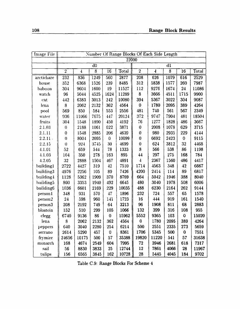
108 Range Block Results
image File
arct icliarc ~iousc
baboon [vat ch
(:a t Iena pool
wiit,cbr
fruits 1.1 .O3 '2.1.11 22.1 L $1 '1 15 W . - .
-1.1.01 -1.1 .O3 -1 -2.05
h i l d ingl building3 biiilding-l building5 building6 person 1 person2 person3 blostcin
clegg lena
PPPcrs serrano frymire
monarch sail
tulips
Stiniber Of Range Blocks Of Each Side Length
Tot al 2877 8485 11527 11259 10080 4564 2556 201'24 4192 3841 4639 10099 4699 1333 595 4891 7510 7426 8769 6645 10035 1896 1723 3213 1066 15962 4564 6214 8361 35388 7995 12744 10728
Total 2529 7987 1 IO86 9900 9087 4264 2349 18504 3661 3715 4244 9115 4468 1198 784
4417 6667 6817 8040 6006 9144 1578 1540 2883 955
15020 4264 5659 7551 31638 7317 11967 9702
Table C.9: Range Blocks For Scheme 4
Appendix D
Compression Ratios
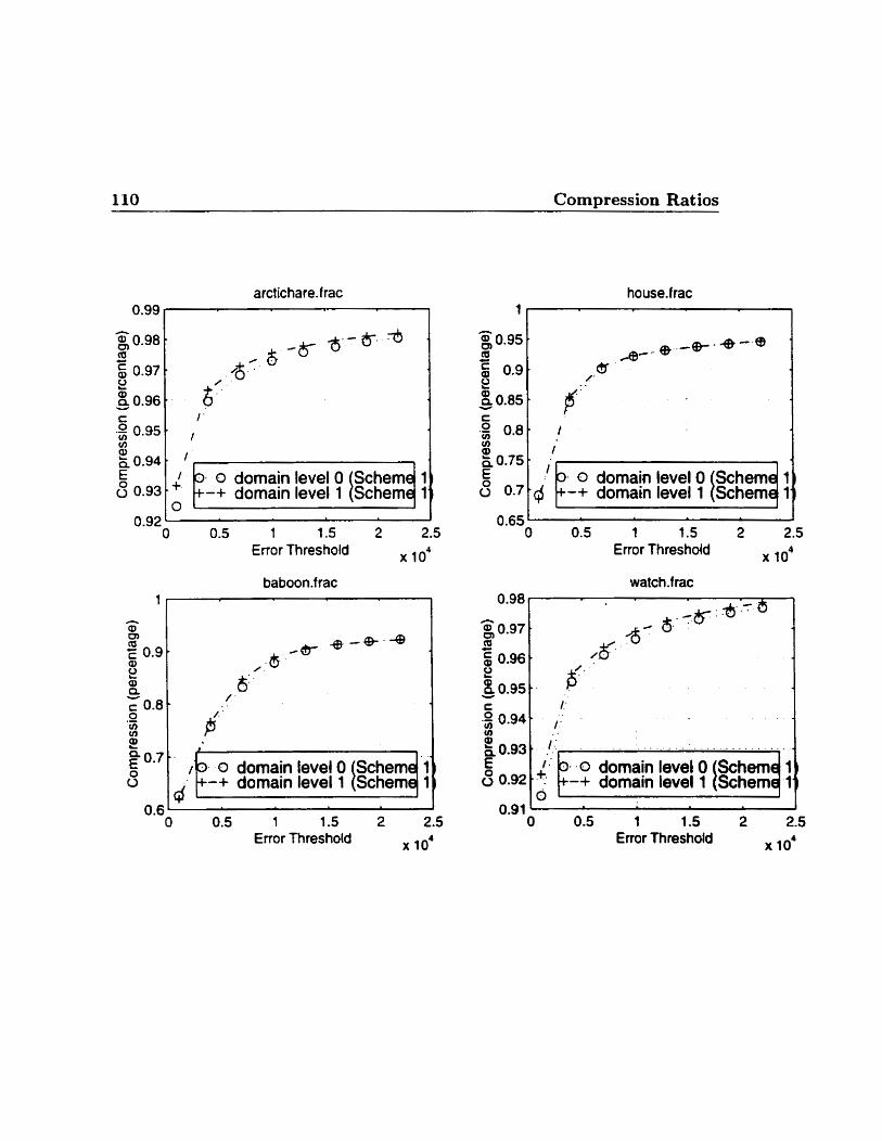
110 Compression Ratios
Error Threshold x 10'
1'3 0 dornain level O Scheme '
d , +-+ domain level1 Scheme ' 1 1 1.5
Enor Threshold
a
3- 0 domain level O +-+ domain level 1
Enor Threshold 10'
aï . . . . . . . k0.g31 € .!jj- 1 + . - .O domain level O Schern 1
8 0.92 ' -+ domain level 1 Schem 1 O
0.91 ' I
O 0.5 1 1.5 2 2.5 Error Threshold x IO'
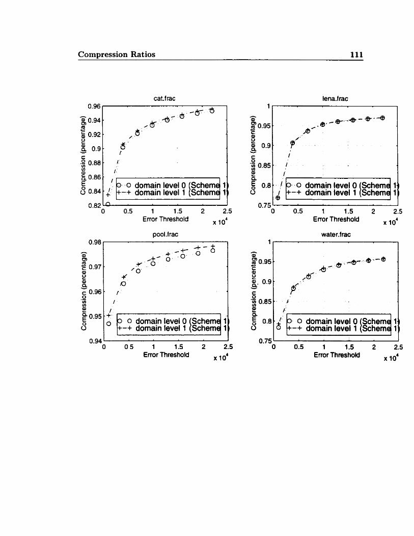
Compression Ratios 111
cat.f rac
0.82 1 O 0.5 1 1 .S 2 2.5
Error Threshold x IO*
V) Qi & 0.86 E 6 0.84
pool .frac 0.98 i 1
1.'
. ,
1ena.f rac
al Q w
c 0.96 O .- V) cn
O 0.5 1 1.5 2 2.5 Enor Threshold x IO'
1 .
KI . r
/
. 0 domain level O Schem 1 0 -+ domain level1 r i s c h m 1
o. . O domain level0 Scheme
O 0.94 -
O O 5 1 1 .S 2 2.5 Enor Threshold x IO'
V.. Y
O 0.5 1 1.5 2 2.5 Enor ThreshoM x 10'
:' +-+ domain level 1 l Schemq 1
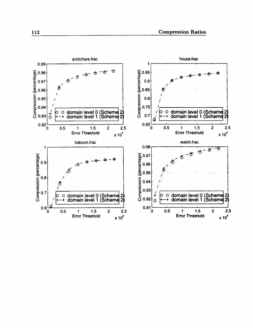
112 Compression Ratios
arctichare.f rac 0.99 11
0.92 O 0.5 1 1.5 2 2.5
Error Thres hold x 104
baboon .f rac
'1
Enor Threshold x 10'
0.65 ' l O 0.5 1 1.5 2 2.5
Enor Threshold x 10'
, E + O O domain level O Scheme
domain level 1 I Schemq
Enor Threshold x 10'
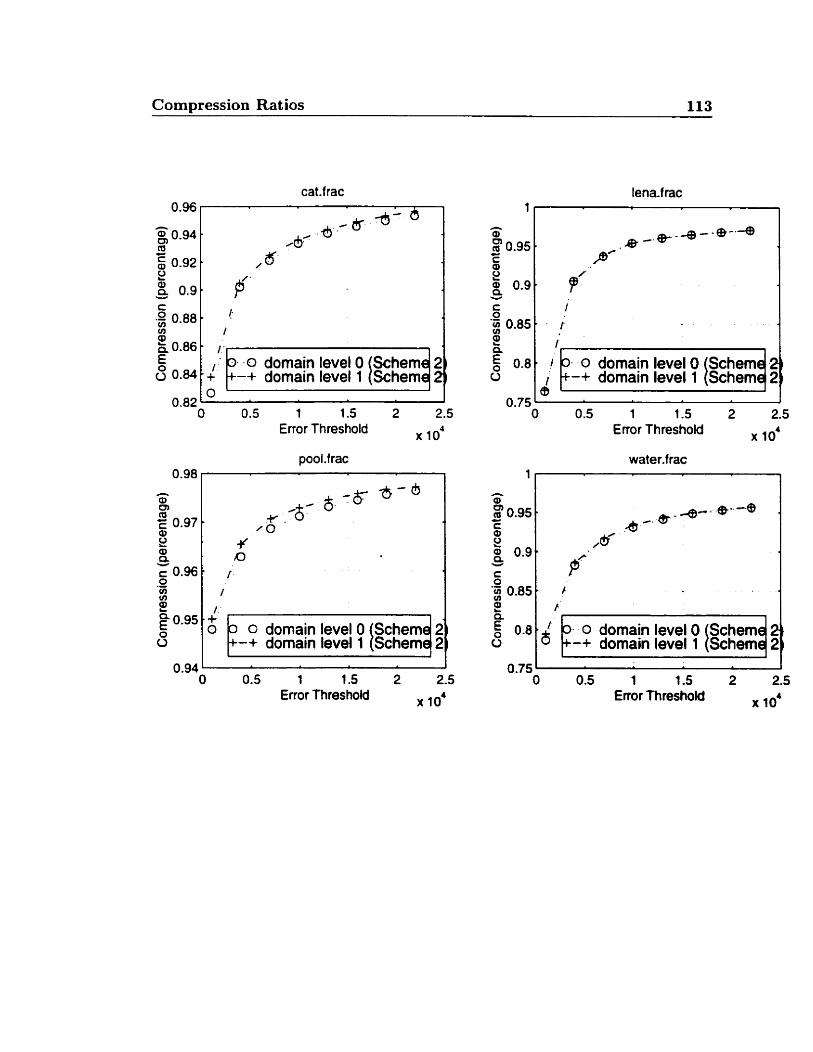
Compression Ratios 113
0)
0 . 8 5 o domain level0 Schem 2 o 0.84 + -+ domain level 1 Schem 2
n
Error Threshold x 10'
pool .f rac 0.98 1
0.94 ' 1 O 0.5 1 1.5 2 2.5
Error Threshold x 10'
2 al O V 6 0.96 -- CO Y,
2 E 0.95
0
1ena.f rac
I l
1 _ 0.8 ,! 0. -0 domain level O Schem t - O i +-+ domain level 1 I Schern
# A3
' f
/
/ .
Error Threshold x 10'
. + O . .O dornain level0
-+ domain level 1 O o domain level0 +-+ domain level1
0.5 1 1.5 2 2.5 Emr Threshokî x 10'
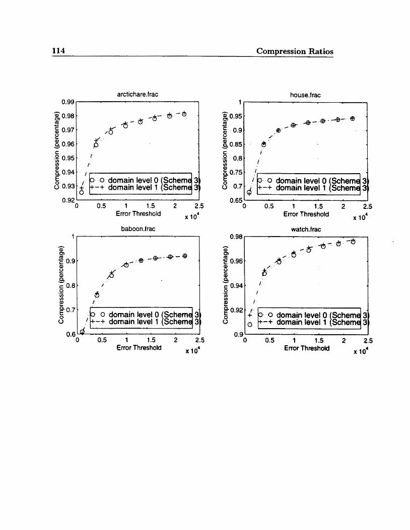
114 Compression Ratios
1 0.5 1 1.5 2 2.5 Error Threshold x 104
O 0.5 1 1.5 2 2.5 Enor Thres hold x 10'
Enor Threshold 10'
watch.frac
O 0.5 1 1 .S 2 2.5 Enor Threshoiâ 10'
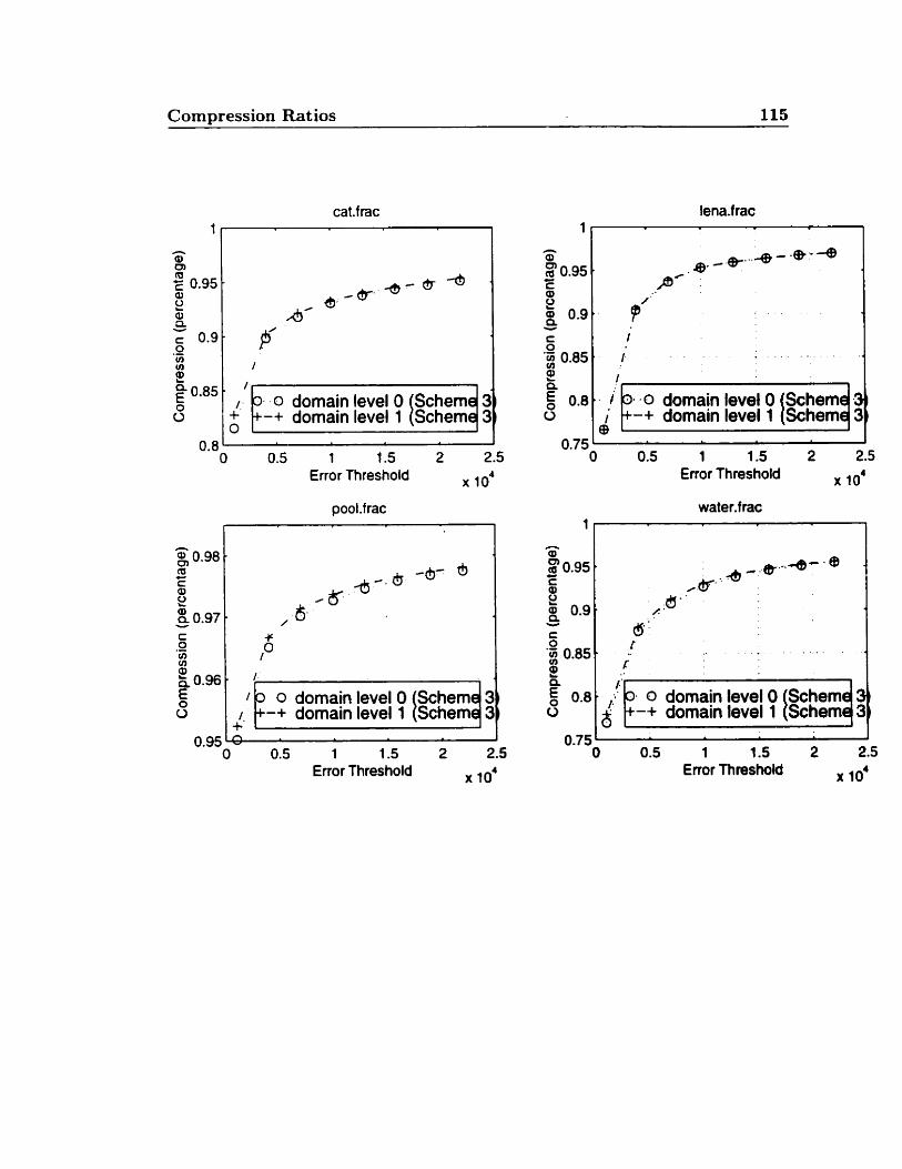
Com~ression Ratios 115
O.'' 1 1;' 3. 0 domain leval 0 Çcheme :
+ +-+ domain level 1 Scheme I 6 ln t 0.8 1
O 0.5 1 1.5 2 2.5 Error Threshold x 104
0.95 O 0.5 1 1.5 2 2.5
Enor Threshold x 10'
i o. .O domain level O ' +-+ domain level 1
,$. ,
Error Threshold x 10'
water.f iac
I l
+-+ domain level 1
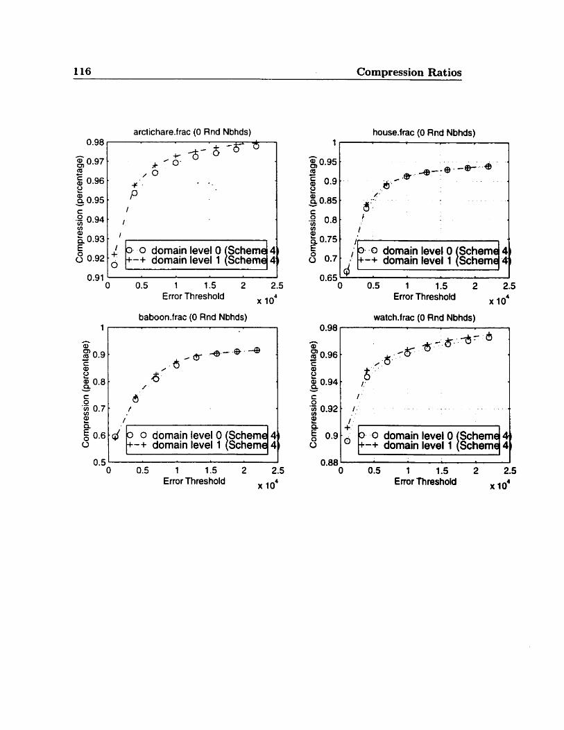
116 Compression Ratios
arctichare.frac (O Rnd Nbhds)
0.91 O 0.5 1 1.5 2 2.5
Error Threshold 1o4
baboon.frac (O Rnd Nbhds)
0.5 ' 1 O 0.5 1 1.5 2 2.5
Error Thres hold x 10'
1
h
al
% 0.9 c. c a 2 0.8.
O Y
C O . - 2 0.7 2 a 5 0.6 O
house.frac (O Rnd Nbhds) 1 ) 1
Error Threshold x IO'
. 4.- e. -@
6 AY 6'
d t
1. .
watch.frac (O Rnd Nbhds)
3 O domain level O Scherne 4 +-+ dornain level 1 l Schemq
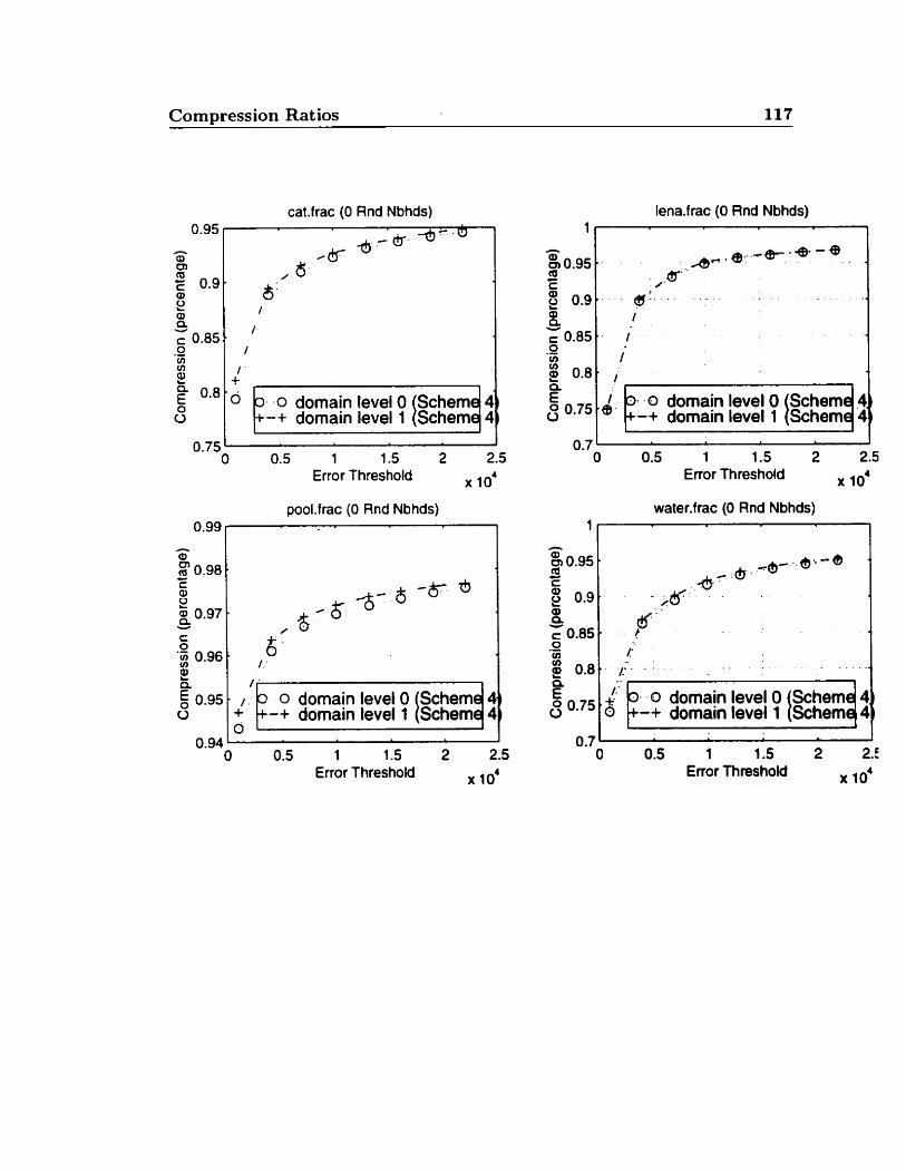
Compression Ratios 117
cat.frac (O Rnd Nbhds)
O O. 5 1 1.5 2 2.5 Error Threshold x 104
pool.frac (O Rnd Nbhds) 0.99
6 0.95 / 4,- O domain level0 Schern O -+ domain level 1 1 Schem i
0.94 1
O 0.5 1 1 .S 2 2.5 Error Threshold x 10'
lena-frac (O Rnd Nbhds)
1 - . .O domain level O " ' k-+ dornain level 1
Enor Threshold x 10'
water.frac (O Rnd Nbhds)
0
. . . .
.O domain level O -+ domain level 1
Enor Threshold x 10'
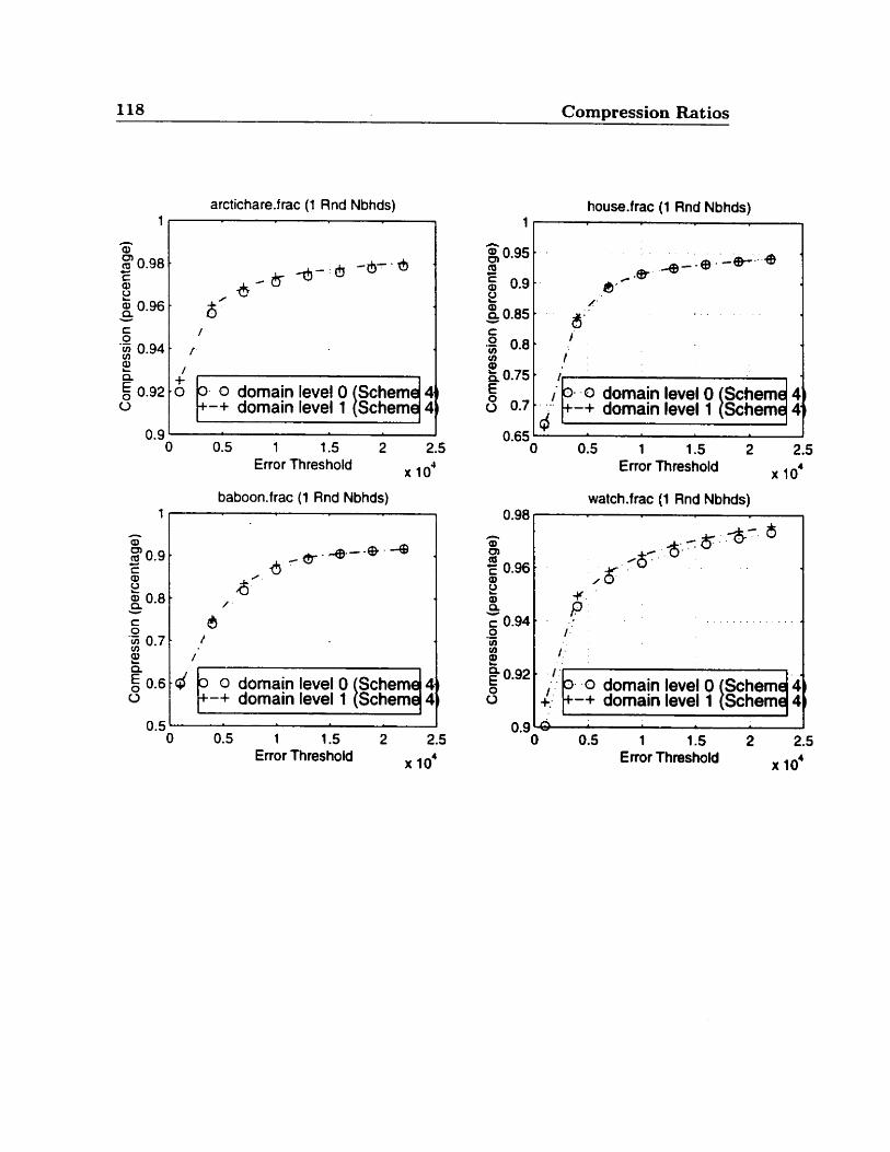
118 Compression Ratios
arctichate-frac (1 Rnd Nbhds)
/ + - o o. O domain level 0
+-+ domain level 1
0.9 L O 0.5 1 t .5 2 2.5
Error Threshold 104
baboomfrac (1 Rnd Nbhds) 1
A
0.5 1 O 0.5 1 1 .S 2 2.5
Enor Threshold x 10'
house.frac (1 Rnd Nbhds)
'1
; 0- . o domain level O Scheme 4 . . . ..
d A +-+ domain level 1 1 Scheme 4
Error Threshold IO'
watch.frac (1 Rnd Nbhds)
- .O domain level O -+ domain level 1
0.9 O 0.5 1 1 .S 2 2.5
Error Threshold x 10'
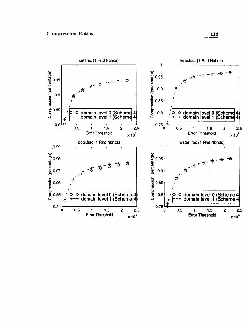
Compression Ratios 119
catfrac (1 Rnd Nbhds)
/ 0- O domain level0 +-+ domain level 1 +
O 0.5 1 1.5 2 2.5 Error Threshold x 1 0 4
pooLfrac (1 Rnd Nbhds)
h
0.94 ' 1 O 0.5 1 1.5 2 2.5
Enor Threshold x 10'
lena.frac (1 Rnd Nbhds)
I : 0- .O domain level O .' +-+ domain level 1
1 0.75 *
O 0.5 1 1 .S 2 2.5 Enor Threshold x 10'
water.frac (1 Rnd Nbhds) 1 ) 1
O domain level O Scheme O ,:-. +-+ domain level 1 I Schemq
Enor Threshold x IO'
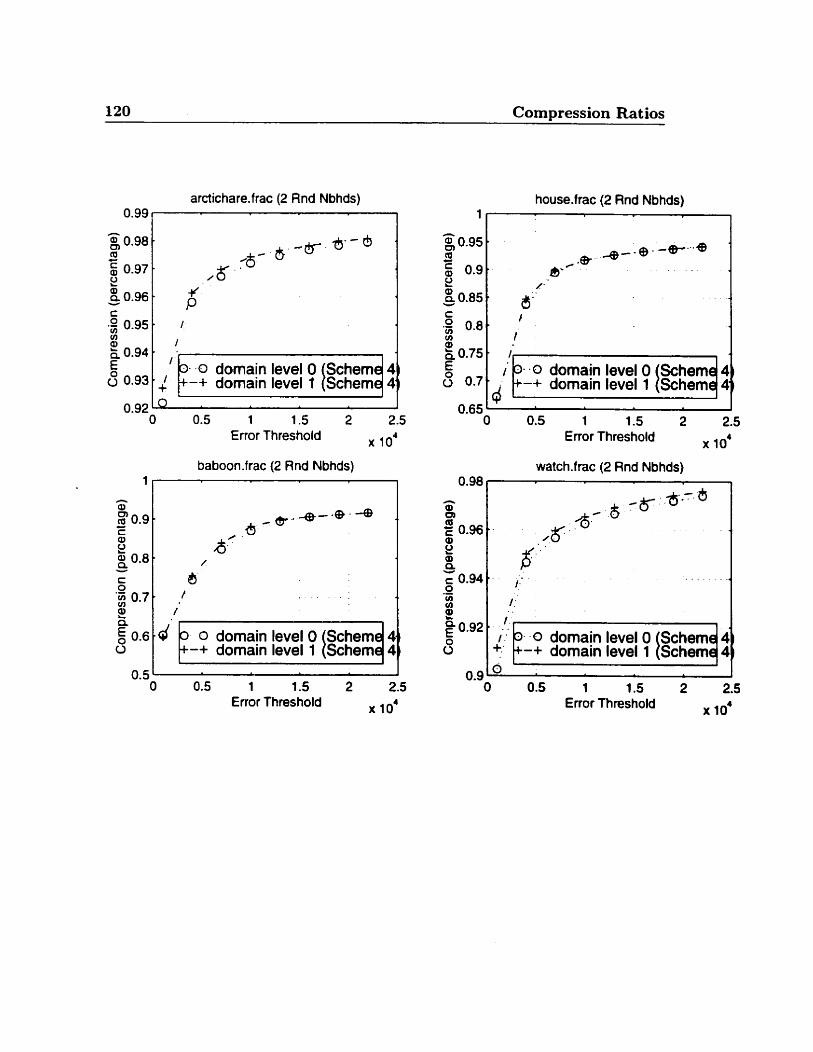
120 Compression Ratios
arctichare. frac (2 Rnd Nbhds)
N
. 0 dornain level O -+ domain level 1
Error Threshold x lod baboonfrac (2 Rnd Nbhds)
0 domain level O -+ domain level 1
Error Threshold x 10'
house.frac (2 Rnd Nbhds)
'1
O 0.5 1 1 .S 2 2.5 Enor Threshold x 10'
watch.frac (2 Rnd Nbhds)
i 0 .921 ' / * 1 : 3. .O domain level0
6 +: +-+ domain level 1 1 0 . 9 ~ ~ ' .
I
O 0.5 1 1.5 2 2.5 Enor Threshold x 10'
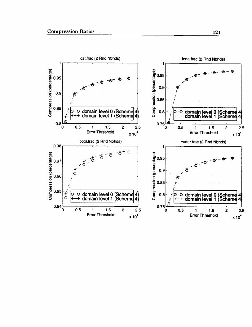
Compression Ratios 121
cat-frac (2 Rnd Nbhds)
/ 0. O domain level O Scheme 4
+! +-+ domain level1 Scheme 4 n
I Error Threshold x 10'
pool-frac (2 Rnd Nbhds)
O domain level0 -+ domain level 1
0.94 O 0.5 1 1.5 2 2.5
Enor Threshold x 10'
lena.frac (2 Rnd Nbhds)
1;: 0 ; &man level O [Scheme 1 +-+ domain level 1 Schemq 4
0.75 O 0.5 1 1.5 2 2.5
Error Threshold x 10'
watecfrac (2 Rnd Nbhds)
I l
b /.'o. 0 domain level O Scheme 4 +-+ domain level1 l Scheme 4
O 0.5 1 1.5 2 2.5 Enor Threshold x 10'
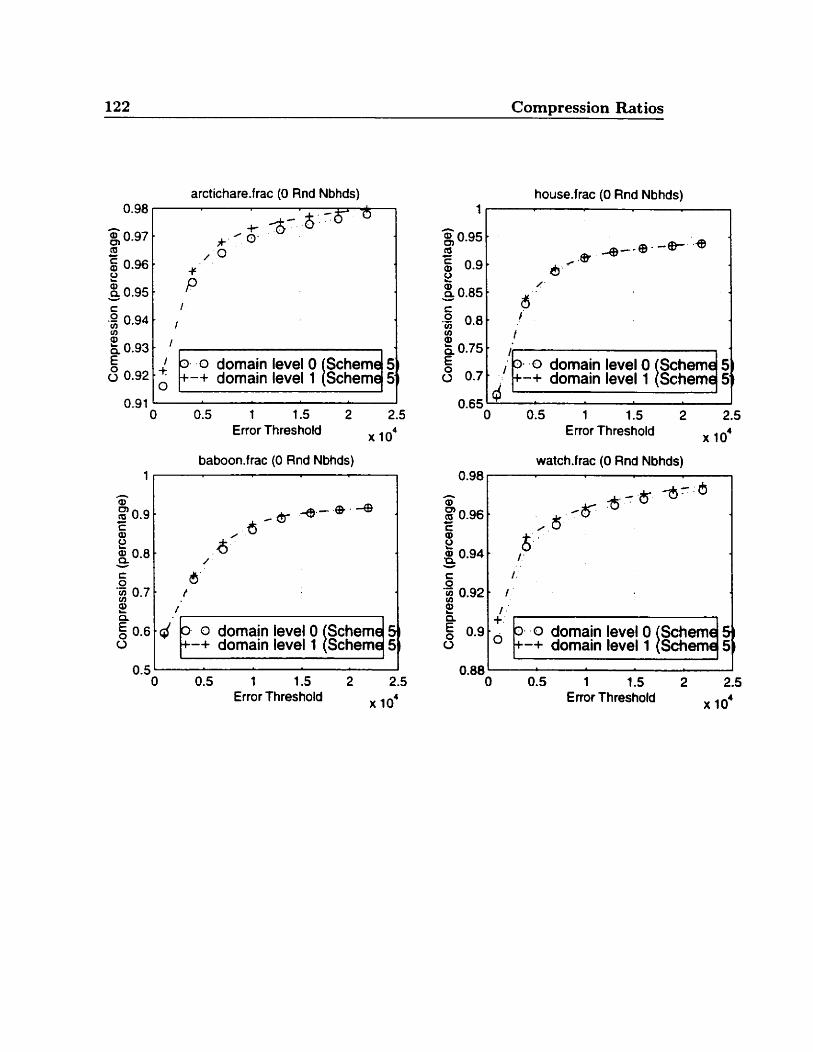
122 Compression Ratios
arctichare-frac (O Rnd Nbhds)
0.91 I
O 0.5 1 1.5 2 2.5 Error Threshold x 104
baboon.frac (O Rnd Nbhds)
O domain level O O -+ domain level 1
O 0.5 1 1 .S 2 2.5 Error Threshold x 10'
house.frac (O Rnd Nbhds)
0.65 ' 1 O 0.5 1 1.5 2 2.5
Enor Threshold x 10'
watch-frac (O Rnd Nbhds) 0.98 1
. .O domain level O O -+ domain level1
0.88 ' 1 O 0.5 1 1.5 2 2.5
Enor Threshold x 104
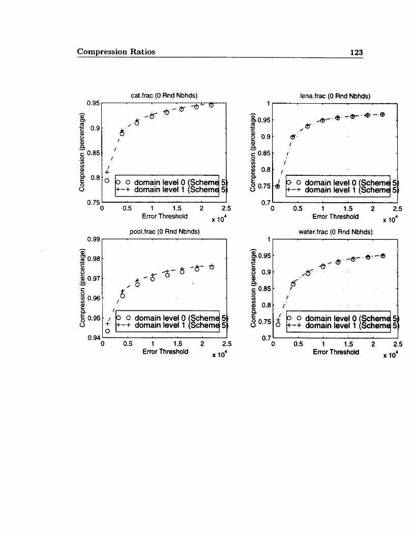
Compression Ratios 123
cat-frac (O Rnd Nbhds)
cn 1 2 +. 0.8 . .
O 3 0 domain Ievel O 0 +-+ domain level 1
Error Threshold to4
pool.frac (O Rnd Nbhcîs)
' /: O domain leuel 0 $chemq ! + -+ domain level 1 Schern f O
.
O 0.5 1 1.5 2 2.5 Enor Threshold x 10'
lena-frac (O Rnd Nbhds) 1 1 I
- 0 dornain level O -+ dornain level 1
0.7 ' l O 0.5 1 1.5 2 2.5
Error Threshold x 104
water-frac (O Rnd Nbhds)
I l
, f. b- 0 d o r n a i n T I ç c h e m s / t 0 -+ domain level1 Schern f
--- O 0.5 1 1.5 2 2.5
Error Threshold 10'
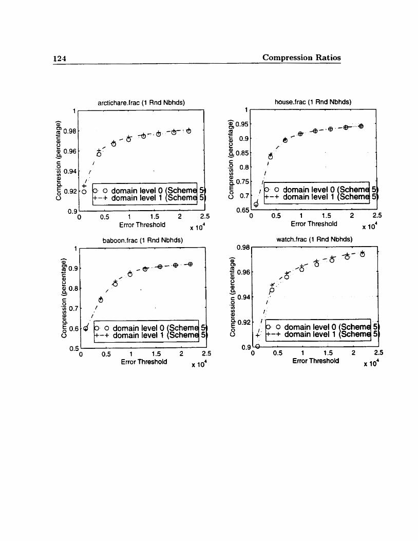
124 Compression Ratios
arcticharehac (1 Rnd Nbhds)
'1
O dornain level O O -+ domain level 1
Error Threshold x lod
baboon.frac (1 Rnd Nbhds) 1 1
:0.6/d (t - O domain level0 O -+ domain tevel 1
U.J
O 0.5 1 1.5 2 2.5 Error Threshold x IO'
house.frac (1 Rnd Nbhds)
I l
Error Thres hold 10'
watch.frac (1 Rnd Nbhds)
O 0.5 1 1.5 2 2.5 Enor Threshold x 10'
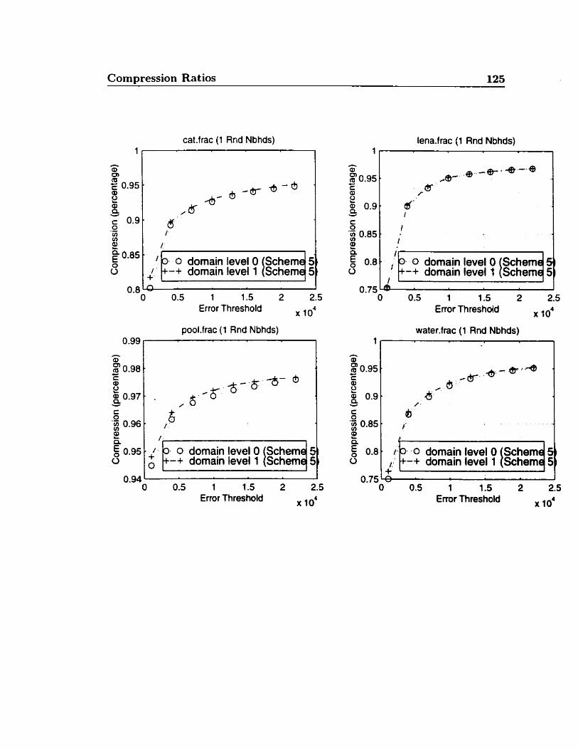
Conipression Ratios 125
cat.frac (1 Rnd Nbhds)
Error Threshold 104
pool.frac (1 Rnd Nbhds)
r
0 domain level0 b-+ domain level 1
lena.frac (1 Rnd Nbhds)
I l
r I
0. .O domain level O Schemer ! +-+ domain level 1 Scheme !
I I Enor Threshoid x lo4
water.frac (1 Rnd Nbhds)
. .O domain level 0 Schem f -+ domain level 1 r Schem el :
Error Threshold x 10' Enor Threshold x IO'
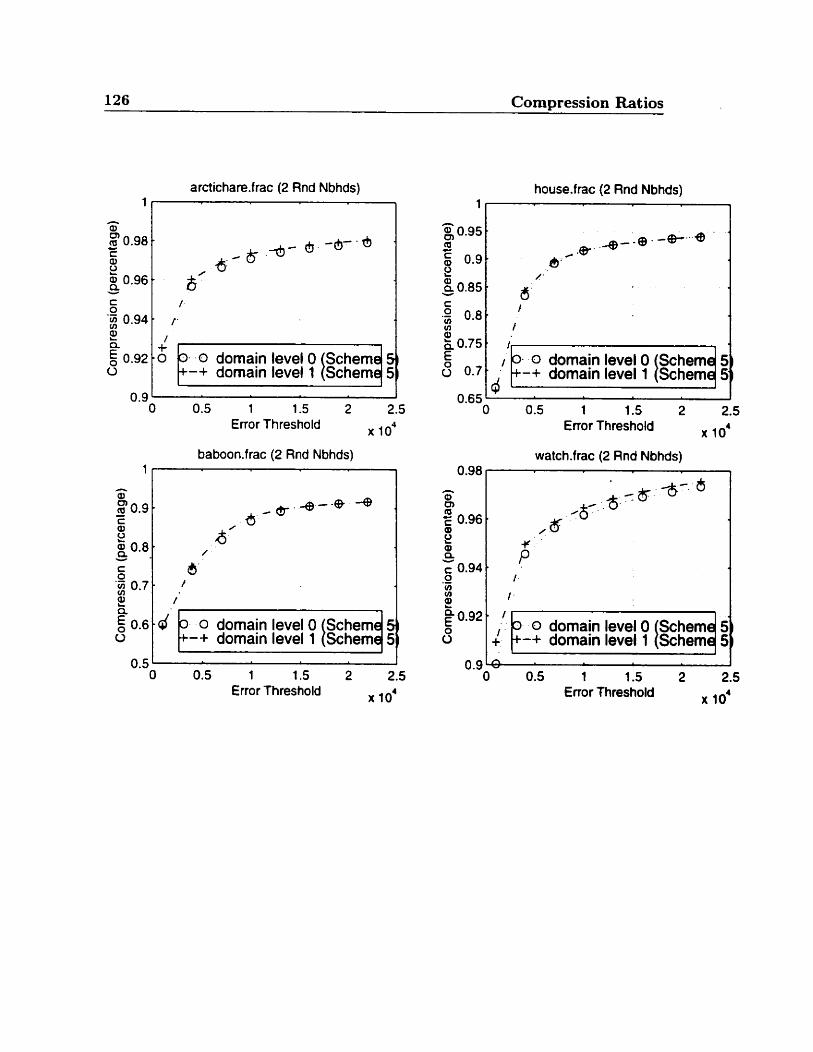
126 Compression Ratios
arctichare.frac (2 Rnd Nbhds)
0.9 ' O 0.5 1 1.5 2 2.5
Error Threshold x 104
baboomfrac (2 Rnd Nbhds)
0 domain level O -+ domain level 1
0.5 [ l O 0.5 1 1.5 2 2.5
Enor Threshold x 10'
house.frac (2 Rnd Nbhds)
I l
. ,O domain level O Schem 5 0 7 5 i d 0.7 1 -+ dornain level1 Schem 5
0.65 O 0.5 1 t.5 2 2.5
Enor Threshold 10'
watch.frac (2 Rnd Nbhds) 0.98 rrl
Enot Threshold 10'
0 domain level O Scheme 5 O 1:> i-+ dornain level 1 1 Schernq 5 1

Compression Ratios 127
cat-frac (2 Flnd Nbhds)
'1 0 domain level0 1 -+ domain level f 4-
1 1.5 Error Threshold
pool.frac (2 Rnd Nbhds)
0.94 1 O 0.5 1 1.5 2 2.5
Error Thres hold x IO'
lena.fr;tc (2 Rnd Nbhds)
I l
. .o domain level O O -+ domain level 1
I I ' I
Enor Threshold IO'
water.frac (2 Rnd Nbhds)
$ 0 damain level O [schernj ! . -+ domain level 1 Schem !
+ O 0.5 1 1.5 2 2.5
Enor Threshold x IO'

128 Compression Ratios
Appendix E
SNR
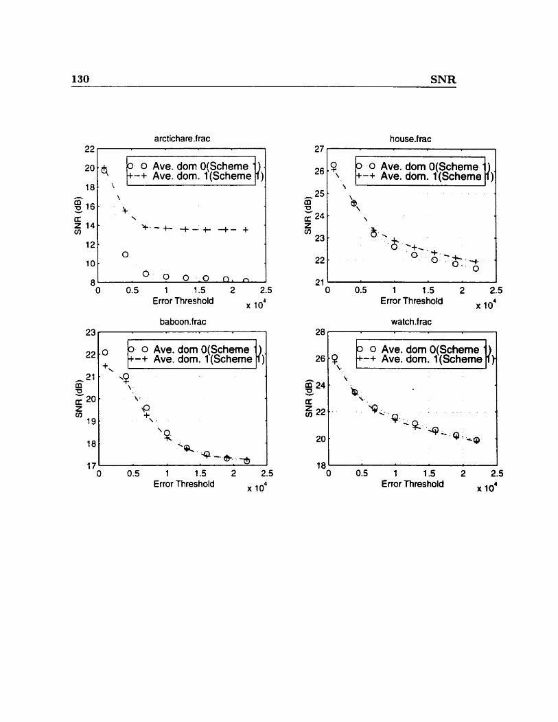
130 SNR
O 0.5 1 1.5 2 2.5 Error Threshold 10'
3- 0 Ave. dom O(Scheme ' +-+ Ave. dom. 1 (Scheme
+\ .
. .
O 0.5 1 1.5 2 2.5 Error Threshold x 104
house-f rac
O 0.5 1 1.5 2 2.5 Error Threshold IO'
watch.f rac
0 Ave. dom O(Scheme 261P 1-+ A v e . c i o r n . ~ ( S c h Z ~ )
Enor Threshold x 10'
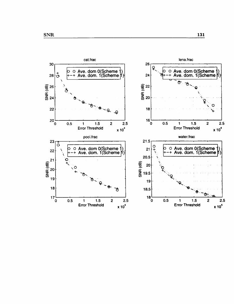
SNR 131
cat.f rac
- - 0 Ave. dom O(Scheme d -+ Ave. dom. 1(Scheme
Error Threshold x lo4
1 . /:o~ve. dom O(Scheme 1) 1. -+ Ave. dom. 1 (Scheme 1
O 0.5 1 1.5 2 2.5 Enor Threshold x 10'
lena-frac
'y O Ave. dom O(Scherne .) %+-+ Ave. dom. 1 (Scheme
0.5 1 1.5 2 2.5 Error Threshold x IO*
u + b 0 Ave. dom O(Scheme ' y. +-+ Ave. dom. 1 (Scheme
. . . . . . ';. . '
0.5 1 1.5 2 2.5 Error Thresbold x lo4
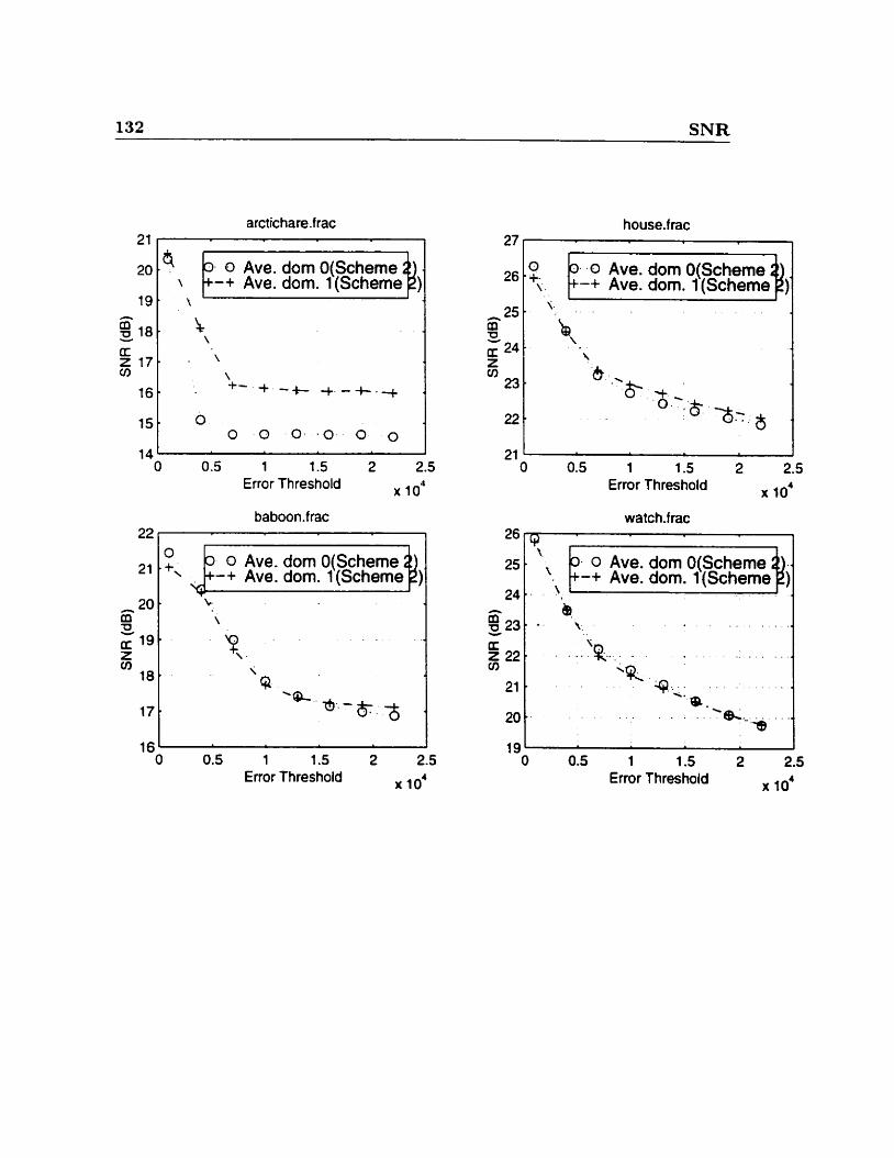
132 SNR
20 .Y 3. 0 Ave. dom O(Scherne \ +-+ Ave. dom. 1(Scheme
19. , i
Error Threshold x 104
O +
3 0 Ave. dom O(Scherne +-+ Ave. dom. 1 (Scheme
1 1.5 Error Threshold
. .O Ave. dom O(Scheme -+ Ave. dom. 1 (Scheme
21 1 O 0.5 1 1.5 2 2.5
Error Threshoid x IO'
0- 0 Ave. dom O(Scheme . +-+ Ave. dom. 1(Scheme
I O 0.5 1 1.5 2 2.5
Error Threshold 10'
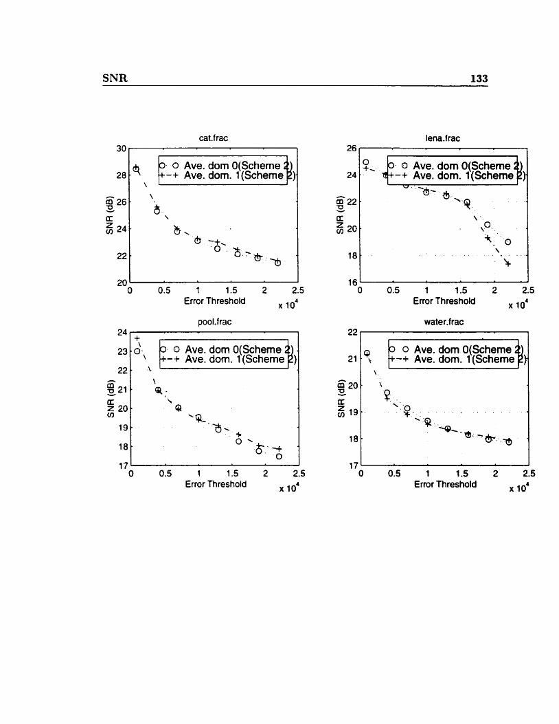
SNR 133
cat.f rac
0 Ave. dom O(Scherne -+ Ave. dom. 1 (Scheme ]
\
Error Threshold x 104
O 0.5 1 1 .S 2 2.5 Error Threshold x 104
lena-frac
0 Ave. dom O(Scheme -+ Ave. dom. 1 (Scheme
Error Threshold x 10'
water.f rac
I 1
0 Ave. dom O(Scheme t -+ Ave. dom. 1 (Scheme P
O 0.5 1 1.5 2 2.5 Error Threshold x 10'
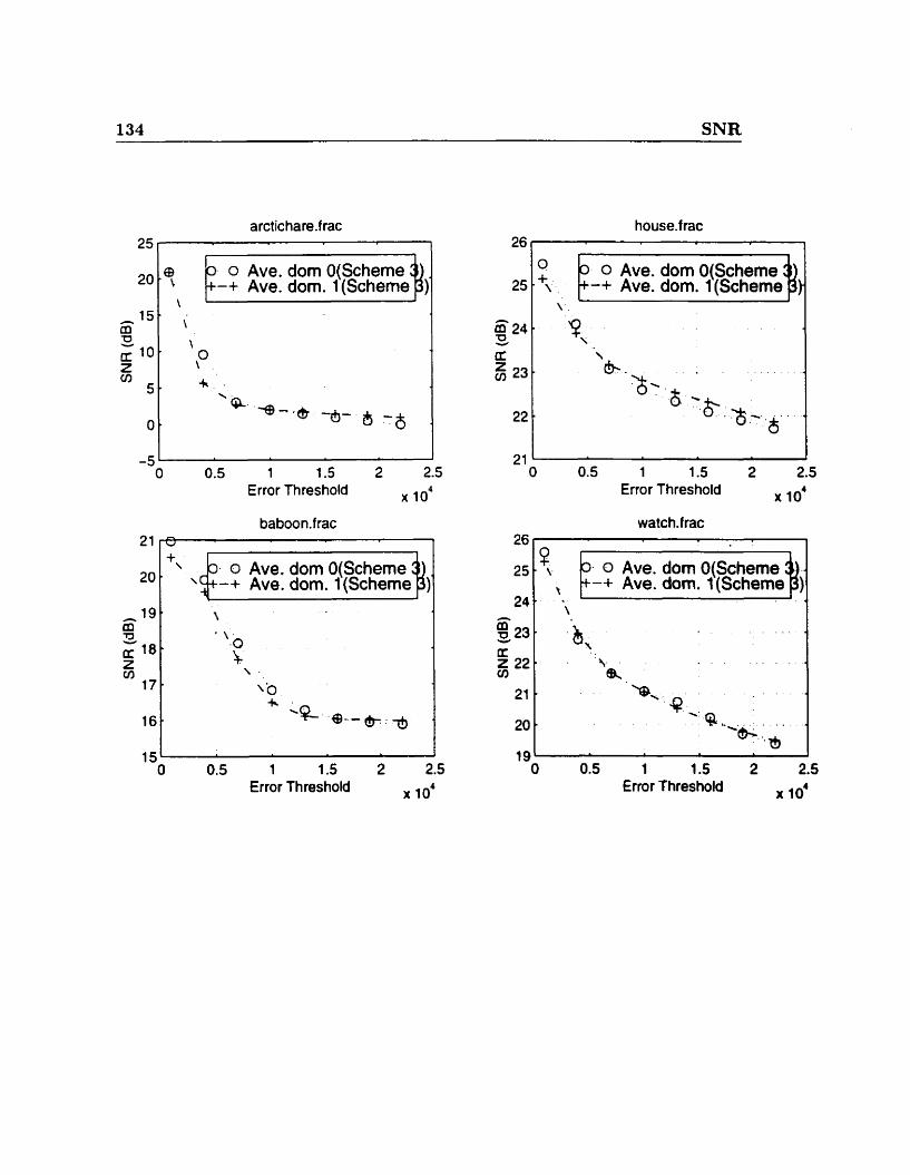
134 SNR
V
O 0.5 1 1.5 2 2.5 Error Threshold 104
0 Ave. dom O(Scheme -+ Ave. dom. 1 (Scheme
house-frac
. 0 Ave. dom O(Scheme Y., -+ Ave. dom. 1 (Scheme
O 0.5 1 1.5 2 2.5 Error Threshold x IO'
25t+tt O Ave. dom O(Scheme -+ Ave. dom. 1 (Scheme
O 0.5 1 1.5 2 2.5 Error Threshold x 10'
- -
O 0.5 1 1.5 2 2.5 Error Threshold x IO'
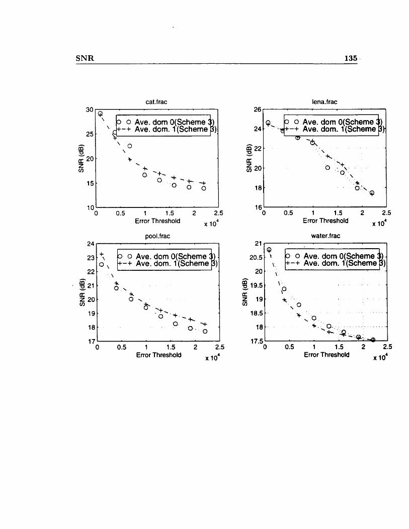
SNR 135 .
cat.f rac
0 Ave. dom O(Scheme -+ Ave. dom. 1 (Scheme
Error Threshold x 104
pool-f rac
0 Ave. dom O(Scherne -+ Ave. dom. 1(Scheme
O 0.5 1 1.5 2 2.5 Enor Threshold x 10'
& o Ave. dom O(Scheme 9k - -+ Ava. dom. 1 (Scherne
Error Threshold x 10'
o Ave. dom O(Scheme \ -+ Ave. dom. 1 (Scheme b )
O 0.5 1 1.5 2 2.5 Error Threshold x IO'
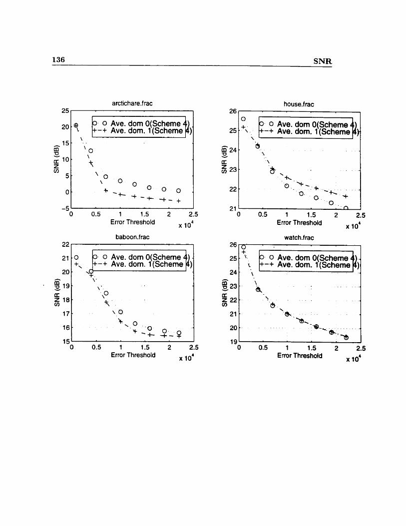
136 SNR
arctichare-f rac
o Ave. dom O(Scheme -+ Ave. dom. 1 (Scheme
0.5 1 1.5 2 2.5 Error Threshold 10'
0 Ave. dom O(Scheme
15' 0:5 I
O 1 1.5 2 2.5 Error Threshold x 10'
0 Ave. dom O(Scheme Ave. dom. 1 (Schem
O 0.5 1 1.5 2 2.5 Error Threshold x 10'
0 0 Ave. dom O(Scheme +-+ Ave. dom. 1(Scheme
O 0.5 1 1.5 2 2.5 Ermr Threshold x IO'
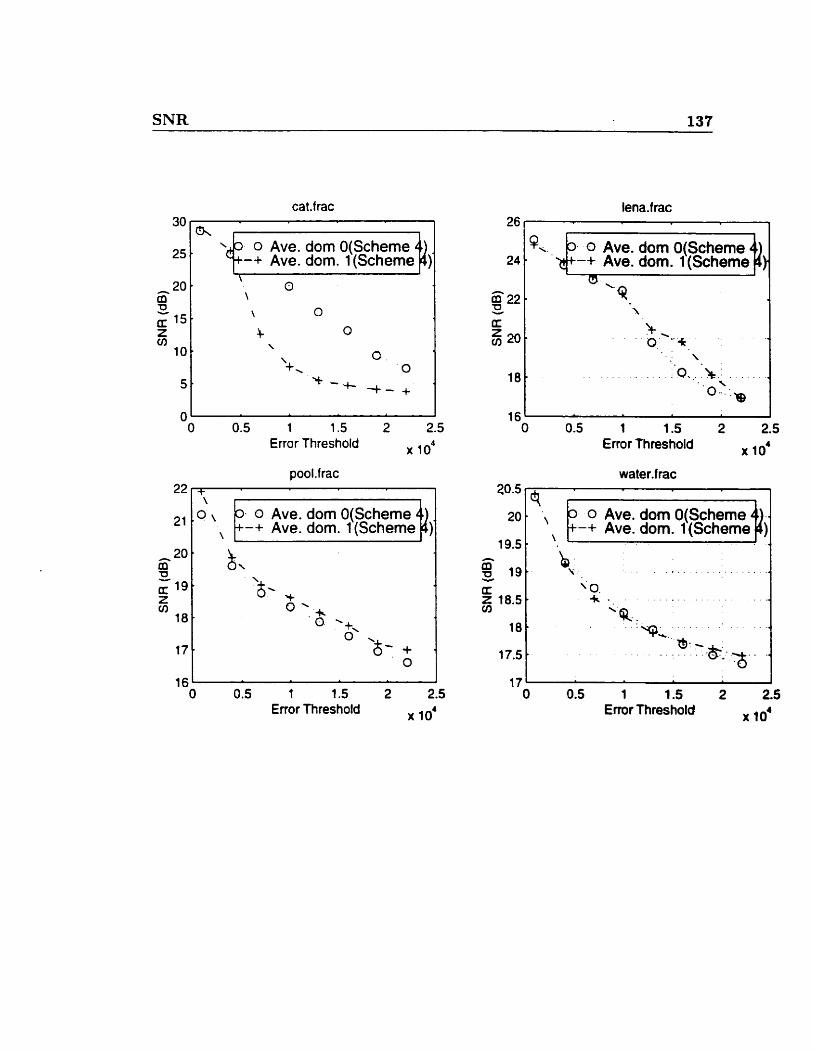
SNR 137
cat.f rac
o Ave. dom O(Scheme -+ Ave. dom. 1 (Scheme t 1
O 0.5 1 1.5 2 2.5 Error Threshold x 104
- O Ave. dom O(Scheme -+ Ave. dom. 1(Scheme 41 ) 1
16l 1 O 0.5 1 1 .S 2 2.5
Enor Threshold x 10'
0 Ave. dom -+ Ave. dom.
1 1.5 Error Threshold
water.f rac
O Ave. dom O(Scheme -+ Ave. dom. 1(Scheme
O 0.5 1 1.5 2 2.5 Enor Threshold x 10'
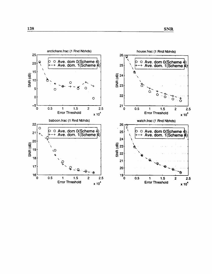
138 SNR
arctichare.frac (1 Rnd Nbhds) 9e:
0 Ave. dom O(Scheme
Error Threshold x 104
baboon.frac (1 Rnd Nbhds)
0 Ave. dom O(Scheme -+ Ave. dom. 1
O 0.5 1 1.5 2 2.5 Error Threshold 104
house.ffac (1 Rnd Nbhds) b ,
1 3 O Ave. dom O(Scheme
'. +-+ Ave. dom. 1 (Scheme \
h
Error Threshold
watch.frac (1 Rnd Nbhds) G -f- I
lgL O 0.5 1 1.5 2 2.5 Error Threshold x 10'
1 ' 3 O Ave. dom O(Scheme +-+ Ave. dom. 1 (Scheme
1
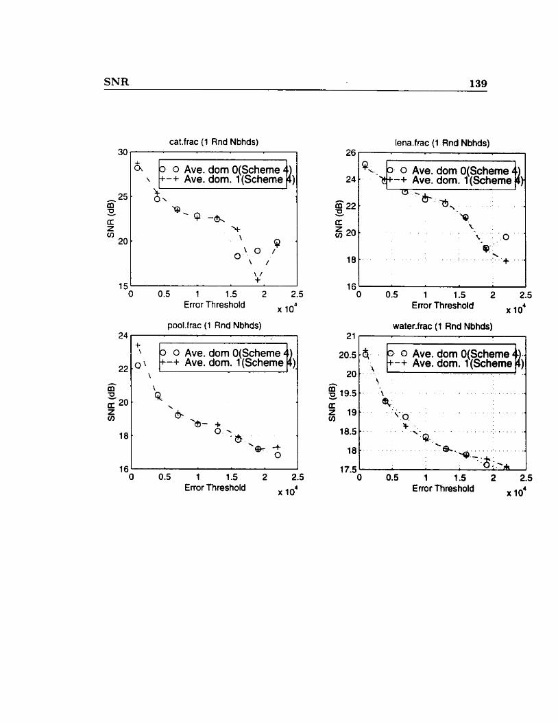
SNR 139
cat.frac (1 Rnd Nbhds)
Error Threshold x 10'
pool.frac (1 Rnd Nbhds)
16 O 0.5 1 1.5 2 2.5
Error Threshold x 104
lena.frac (1 Rnd Nbhds)
0 Ave. dom O(Scheme -+ Ave. dom. l(Scheme
O 0.5 t 1.5 2 2.5 Error Threshold 1o4
water.frac (7 Rnd Nbhds)
20.5 1 bit . 1. 0 Ave. dom, O(Scheme 1 -+ Ave. dom. 1 (Scheme
20 . . . : 4
Enor Threshoid x lo4
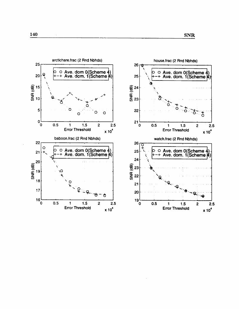
140 SNR
arctict-iare.frac (2 Rnd Nbhds)
O Ave. dom O(Scheme -+ Ave. dom. 1 (Scheme
O 0.5 1 1.5 2 2.5 Enor Threshold x 104
baboon.frac (2 Rnd Nbhds) 22 1
0 Ave. dom O(Scheme -+ Ave. dom. 1(Scheme
16 1 O 0.5 t 1.5 2 2.5
Enor Threshold 10'
house-frac (2 Rnd Nbhds)
-, 3 O Ave. dom O(Scheme . .. , +-+ Ave. dom. l(Scheme
Error Threshold x lo4
watch.frac (2 Rnd Nbhds)
r- 1. 0 Ave. dom O(Scheme
-+ Ave. dom. l(Scheme
j9' 015 I
O 1 1.5 2 2.5 Emr Threshold x 10'
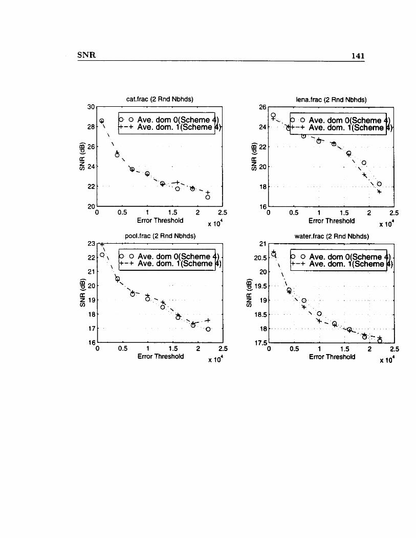
SNR 141
cat.frac (2 Rnd Nbhds)
0 Ave. dom O(Scheme -+ Ave. dom. 1 (Scheme
O 0.5 1 1.5 2 2.5 Error Threshold x 104
pool.frac (2 Rnd Nbhds) 231 +
O 0.5 1 1.5 2 2.5 Error Threshold x 104
\
lena.frac (2 Rnd Nbhds) 26
Q',
,
1 K . 4 O AVB. dom O(Scheme 24 -+ Ave. dom. 1 (Scheme
3- O Ave. dom O(Scheme +-+ Ave. dom. 1 (Scheme
Enor Threshold x 104
water-frac (2 Rnd Nbhds)
0.5 1 1.5 Emr Threshold

142 SNR
arctichare.frac (O Rnd Nbhds)
0 Ave. dom O(Scheme -+ Ave. dom. 1(Scheme
O 0.5 1 1.5 2 2.5 Error Thres hold x 104
baboon-frac (O Rnd Nbhds) 22 - t 1
0 Ave. dom O(Scheme -+ Ave. dom. 1 (Scheme
t O 0.5 1 1.5 2 2.5
Error Threshold x 10'
house.frac (O Rnd Nbhds)
, 3. . O Ave. dom O(Scheme Ave. dom. 1 (Scheme
O 0.5 1 1.5 2 2.5 Error Threshold x 10'
watch.frac (O Rnd Nbhds)
IgL 0:s I
O 1 1.5 2 2.5 Error Threshoîd x 10'
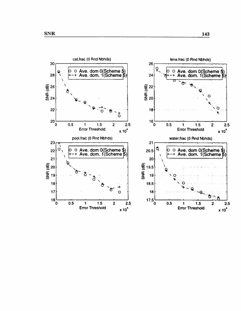
SNR 143
cat.frac (O Rnd Nbhds)
1 Q /: 0 Ave. dom O(Scherne 28 , -+ Ave. dom. 1 (Scheme
20 1 O 0.5 f 1.5 2 2.5
Error Threshold 10'
pooLfrac (O Rnd Nbhds) 231 +
\ 1 1
O Ave. dom O(Scheme +-+ Ave. dom. 1 (Scheme
21
vu - --
O 0.5 1 1.5 2 2.5 Enor Threshold x 10'
lena-frac (O Rnd Nbhds) 26 1 1
0 Ave. dom O(Scheme 24 -+ Ave. dom. l(Scheme
J -
O 1 1.5 2 2.5 Error Threshold lo4
water-frac (O Rnd Nbhds) 21 1 1
ZO.S /q,,, 0 Ave. dom O(Scheme $ 1 -+ Ave. dom. 1 (Scheme )
20
-
O 0.5 1 1 .S 2 2.5 Error Threshold x 104
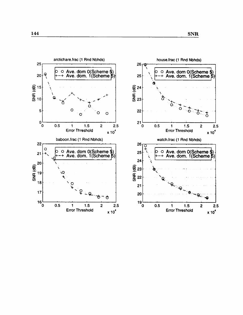
144 SNR
arctichare.frac (1 Rnd Nbhds) 25 i
0 Ave. dom O(Scheme
O ' l O 0.5 1 1.5 2 2.5
Error Threshold 10'
baboon-frac (1 Rnd Nbhds)
0 Ave. dom O(Scheme +-+ Ave. dom. 1(Scheme ) 1
16' I O 0.5 1 1.5 2 2.5
Error Threshold fo4
house.frac (1 Rnd Nbhds)
21 1 O 0.5 1 1.5 2 2.5
Error Threshold x IO'
,
watchhac (1 Rnd Nbhds)
24
3 O Ave. dom O(Scheme
19l I O 0.5 1 1.5 2 2.5
Error Threshold x 104
25 1 ; +-+ Ave. dom. 1 (Schernepd
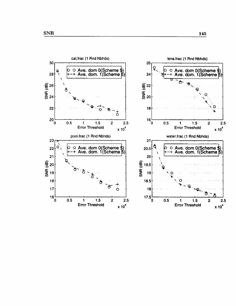
SNR 145
cat-frac (1 Rnd Nbhds)
l 1
- 0 Ave. dom O(Scheme -+ Ave. dom. 1 (Scheme
Error Threshold x 104
pool.frac (1 Rnd Nbhds)
O 0.5 1 1.5 2 2.5 Error Threshold IO'
lena.frac (1 Rnd Nbhds)
q-. - - . ?. O Ave. dom O(Scherne $ x+-+ Ave. dom. l(Scheme
Errer Threshold x 10'
water.frac (1 Rnd Nbhds)
4 => 0 Ave. dom O(Scheme \ +-+ Ave.dom. 1(Scherne
\
' P .
O 0.5 1 1.5 2 2.5 Enor Threshold x 10'
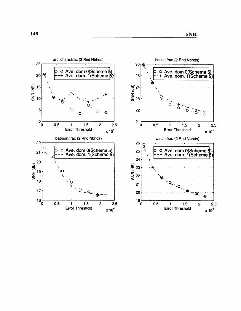
146 SNR
arctichare.frac (2 Rnd Nbhds) 25 5
I i: 0 Ave. dom O(Scheme 20 \ -+ Ave. dom. 1(Scheme
O 0.5 1 1.5 2 2.5 Error Threshold x 104
bzboon.frac (2 Rnd Nbhds) 33
- O Ave. dom O(Scheme f +-+ Ave. dom. l(Scheme ) 1
16' 0:s I
O 1 1.5 2 2.5 Error Threshold x 10'
house.frac (2 Rnd Nbhds)
0 Ave. dom O(Scherne -+ Ave. dom. 1 (Scheme
Enor Threshold x 104
watch.frac (2 Rnd Nbhds)
O Ave. dom O(Scherne -+ Ave. dom. 1 (Scheme
O 0.5 1 1.5 2 2.5 Emr Threshold x 10'
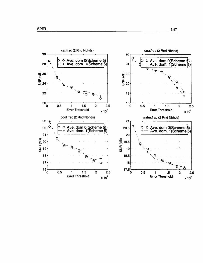
SNR 147
cat-frac (2 Rnd Nbhds) 30 1 I
0 Ave. dom O(Scheme -+ Ave. dom. 1 (Scheme
20 1 I O 0.5 1 1.5 2 2.5
Error Threshold x 104
pool.frac (2 Rnd Nbhds)
0 Ave. dom O(Scheme
21
I V
O 0.5 1 1.5 2 2.5 Error Threshold x 104
lena-frac (2 Rnd Nbhds)
1'- 9 0 Ave. dom O(Scheme 24 -+ Ave. dom. l(Scheme
t6I 1 O 0.5 1 1.5 2 2.5
Error Threshold x 10'
water.frac (2 Rnd Nbhds) 21 1 i
O Ave. dom O(Scheme -+ Ave. dom. 1 (Scheme
O 0.5 1 1.5 2 2.5 Error T hteshold x 10'