Embed Size (px)
Citation preview
Corporate cash shortfalls and financing decisions
Rongbing Huang and Jay R. Ritter∗
November 23, 2018
Abstract
Given their actual revenue and spending, most net equity issuers and an overwhelming majority
of net debt issuers would face immediate cash depletion without external financing. To fund
immediate cash needs, firms that anticipate large future cash needs are more likely to issue
equity instead of debt than other firms. On average, net debt issuers immediately spend almost
all of the proceeds, while net equity issuers, even those that would deplete cash immediately
without external financing, save most of the proceeds. Anticipated near-future cash needs,
uncertainties, and fixed costs of financing help explain the cross-sectional variation in the
savings rate.
Key Words: Cash Holdings, External Financing, Security Issuance, SEO, Private Placement in Public Equity (PIPE), Bond Offering, Bank Loan, Financing Decision, Capital Structure, Precautionary Saving, Market Timing, Corporate Lifecycle, Financial Flexibility, Static Tradeoff JEL: G32 G14
∗ Huang is from the Coles College of Business, Kennesaw State University, Kennesaw, GA 30144. Huang can be reached at [email protected]. Ritter is from the Warrington College of Business Administration, University of Florida, Gainesville, FL 32611. Ritter can be reached at [email protected]. We thank an anonymous referee, Harry DeAngelo, David Denis (editor), Ning Gao (our FMA discussant), Xiao Huang, David McLean, Zhaoguo Zhan, and the participants at the University of Arkansas, the Law, Accounting, and Business Workshop of the University of California, Berkeley, Harbin Institute of Technology, Hong Kong University of Science & Technology, Koc University, the University of Oregon, Penn State, the University of Sussex, Tsinghua PBC, Zhongnan University of Economics and Law, the 2015 FMA Annual Meeting, and the 2016 University of Ottawa’s Telfer Accounting and Finance Conference for useful comments.
1
Corporate cash shortfalls and financing decisions
1. Introduction
In this paper, we address three questions. First, given their actual revenue and spending,
do U.S. firms that raise net debt or net equity capital do so mainly when they would otherwise
run out of cash immediately or in the near-future? 1 The answer is yes, with firms that issue net
debt being more likely to run out of cash immediately than firms that issue net equity. Given
their actual revenue and spending, 75.0% of net debt issuers and 53.9% of net equity issuers
would have run out of cash by the end of the year without external financing.2 By the end of the
following year, 83.2% of net debt issuers and 72.5% of net equity issuers would have run out of
cash. These findings suggest that a near-term cash need rather than pure cash stockpiling or
leverage rebalancing is the primary motive for net debt or equity issuance.
Second, how is the nature of cash needs related to net financing? Cash needs can be the
result of low profitability or high spending. Unprofitable firms could continue to be unprofitable
and have large cash needs in the near future. We find that, among firms that would otherwise
face immediate cash depletion, given their actual revenue and spending, the likelihood of net
equity issuance is 18.3% for profitable firms and increases substantially to 48.2% for
unprofitable firms, while the likelihood of net debt issuance decreases from 70.1% to 53.2%.
Third, do firms save much of the net debt or net equity proceeds in the fiscal year in
which the net issue occurs? Our regression analysis shows that an extra dollar in the debt or
equity proceeds is associated with, respectively, an increase of 18.9 cents or 62.9 cents in cash
1 In this paper, cash needs in fiscal year t are viewed as immediate cash needs. Fiscal years t+1 and t+2 are viewed as near-future and medium-future, respectively, and both t and t+1 are viewed as near-term. 2 We examine net debt issuance and net equity issue decisions rather than gross debt issue and gross equity issue decisions. Unless explicitly stated as otherwise, “equity issue” and “net equity issue” are used interchangeably, as are “debt issue” and “net debt issue”. We focus on “significant” net issues, defined as greater than 5% of assets and 3% of the market value of equity.
2
savings. When firms that would not otherwise immediately be running out of cash issue debt or
equity, almost all of the proceeds are saved as cash instead of being used to rebalance leverage.
Even those equity issuers that would otherwise immediately run out of cash save most of the
proceeds when they do issue. We find that anticipated future cash needs, uncertainties, and fixed
costs of financing help explain the difference in the cash savings rate between debt and equity
issuers, and more generally, the cross-sectional variation in the issue size and the savings rate.
In this paper, we define net debt or net equity issues by U.S. firms from 1972-2013 using
information from cash flow statements. A firm is defined as using a net debt or net equity issue if
net debt or net equity proceeds in a year are at least 5% of the book value of assets and 3% of the
market value of equity at the beginning of the year. In our definition, equity issuers include firms
receiving cash from seasoned equity offerings (SEOs, also known as follow-ons), private
placements in public equity (PIPEs), large employee stock option exercises, and preferred stock
issues.3 Our sample includes 13,152 net equity issues. Debt issuers in our sample include firms
receiving cash from straight and convertible bond offerings and bank financings. Our sample
includes 26,324 net debt issues.
Our cash need measures use hypothetical cash balances. Our ex post measure, Cash ex post,
denotes what the cash balance at the end of t would have been if actual revenue and spending
occurred and there was no net external financing. It is equal to Casht-1 + NCFt, where Casht-1
denotes the amount of cash at the end of year t-1 and NCFt denotes the net cash flow in t, which
is the difference between the internal cash flow and net spending. Net spending equals the sum
of investment, change in net working capital, and dividends. Using Cash ex post, 75.0% of the net
debt issuers and 53.9% of the net equity issuers in our sample, respectively, would have run out
3 Since we require a one-year stock return prior to the current fiscal year, initial public offerings (IPOs) and SEOs shortly after the IPO are not included in our sample. Because cash flow statements are used, stock-financed acquisitions are not counted as equity issues.
3
of cash by the end of the year, consistent with DeAngelo, DeAngelo, and Stulz (2010),
henceforth DDS, and Denis and McKeon (2012). DDS find that 62.6% of firms conducting 4,291
SEOs from 1973-2001 would have run out of cash by the end of the following year if they did
not raise capital. Denis and McKeon document that, for the subsets of their sample of 2,314 firm
years with large leverage increases from 1971-1999, the likelihood of immediate cash depletion
ranges between 70.8% and 93.4%. The evidence that most firms wait until they are running out
of cash to raise external capital is broadly consistent with the pecking order model ((Myers
(1984)) and dynamic tradeoff models with issuing costs.
We further find that, given net equity issuers’ actual revenue and spending, if they were
not going to run out of money immediately, it might happen the following year: their likelihood
of cash depletion increases from 53.9% by the end of t to 72.5% by the end of t+1, and 74.2% of
them would have a subnormal cash ratio at the end of t. These results suggest that equity is also
often issued to optimize cash holdings for near-future spending or precautionary savings needs.
In contrast, debt issuers’ likelihood of cash depletion increases from 75.0% by the end of t to
83.2% by t+1, suggesting that net debt issuance is more motivated by immediate cash needs and
less motivated by near-future needs than net equity issuance. This finding is not surprising, given
that most debt issuers have revolving lines of credit, which can be drawn on continuously.
Spending and financing decisions are undoubtedly jointly determined. To alleviate this
concern, we use an ex ante measure of cash needs, Cash ex ante. It is equal to Casht-1 + NCFt-1,
using lagged NCF as projected NCF. Using Cash ex ante, the likelihoods of cash depletion by the
end of the year are 42.3% and 44.4% for the debt and the equity issuers, respectively, and their
likelihoods of having a subnormal cash ratio by the end of the year are 68.0% and 67.5%,
respectively. These results confirm the importance of near-term cash needs in motivating
4
external financing. However, the likelihoods of cash depletion or having a subnormal cash ratio
are lower when using Cash ex ante rather than Cash ex post, especially for debt issuers. This finding
is partly because the net cash flow from t-1 to t has low persistence, especially for debt issuers.
McLean and Palazzo (2018) also use an ex ante measure of cash needs, but they focus on gross
instead of net debt issues and find that refinancing is the primary motive for gross debt issues.
Rather than looking at the likelihood of cash depletion for net issuers, we also estimate a
multinomial logit regression to see how cash depletion is related to the likelihood of external
financing after controlling for other determinants of external financing that have been
documented in the literature. We find that, among the independent variables, an immediate cash
squeeze based on Cash ex post has the strongest association with net debt or equity issues, and an
immediate cash squeeze based on Cash ex ante is an important predictor.
Cash ex ante is still subject to an endogeneity concern if the current financings and the
lagged spending are jointly determined. To alleviate this additional concern, our third measure,
Cash fitted, is based on the fitted value from a regression of NCF on the lagged median NCF of
similar firms and other information. Our major results using Cash fitted are similar to those using
Cash ex ante. Although Cash ex ante and Cash fitted are presumably less endogenous than Cash ex post,
they are not necessarily better measures of cash needs, as they do not incorporate other important
information that is available to firm decision makers. A firm’s net spending can vary
substantially across time. Cash ex post could better reflect exogenous investment opportunity
changes in year t than the other two measures.
Cash shortfalls can be the result of large net spending, a low internal cash flow (ICF), or
a low initial cash balance. DDS and Denis and McKeon (2012) do not examine how the nature of
cash depletion is related to the choice between debt and equity issues. Our univariate analysis
5
shows that, when Cash ex post≤0, the likelihood of net equity issuance increases substantially from
18.3% for firms with a non-negative ICF to 48.2% for firms with a negative ICF, and the
likelihood of net debt issuance decreases from 70.1% to 53.2%. These results suggest that
immediate cash needs associated with a loss are more likely to be funded by equity instead of
debt than are immediate cash needs associated with higher spending. Using Cash ex ante and
lagged ICF yields qualitatively similar results. Our multivariate results confirm the univariate
results. Additional multivariate analysis shows that, conditional on immediate cash depletion and
external financing, unprofitable, small, and growth firms prefer equity issuance.
We also find that debt issuance is more strongly related to investment spending than to
profitability. Both the current and lagged internal cash flow have a similarly strong negative
relation with equity issuance, consistent with the findings of Denis and McKeon (2018). They
document that within our sample period Compustat-listed firms with losses have become more
common. They posit that much of the increase in losses is because of a change from investing in
tangible assets, which get capitalized and depreciated, to investing in intangible assets, which
often get expensed. They also document that, in recent decades, firms with a loss in year t have
continued to lose money for a median of four years in a row, and many of these money-losing
firms repeatedly raise equity capital.
When firms do raise external capital, they can choose to raise more than what they
immediately spend. Our regression analysis of the cash change on cash sources shows that each
incremental dollar of net debt proceeds is associated with an increase of 18.9 cents in cash, and
each extra dollar of net equity proceeds is associated with an increase of 62.9 cents in cash. The
finding that equity issues are related to large cash savings has been interpreted as consistent with
market timing (Kim and Weisbach (2008)). McLean (2011) also finds a high cash savings rate by
6
equity issuers, especially those with high R&D expenses, those in industries with high cash flow
volatility, and those that do not pay dividends, suggesting a precautionary savings motive.
Why don’t all firms raise external capital on an as-needed basis (i.e., issue when facing
immediate cash needs and immediately spend almost all of the proceeds)? One reason that some
firms could raise more than what they immediately spend is to avoid incurring the fixed costs of
raising capital again in the near future. Equity issuance can have higher fixed costs than debt
issuance. As discussed earlier, equity issuers typically have larger near-future (year t+1) cash
needs than debt issuers. Therefore, anticipated near-future cash needs, together with fixed costs
of financing, help explain our finding that the savings rate of equity issuers is higher than that of
debt issuers. Firms can raise debt or equity capital publicly or privately. As public issues
probably have higher fixed costs than private placements, are they related to a higher savings rate?
While McLean (2011) finds that precautionary needs help explain the cross-section of the
savings rate of net equity proceeds, what explains the cross-section of the savings rate of net debt
proceeds? We provide cross-sectional analysis of the association between net issues and cash
changes to address these important questions.
Our additional findings on the cash savings rate are generally consistent with theories
based on precautionary savings and fixed costs of financing. For both the net debt issue sample
and the net equity issue sample, Tobin’s Q, the default spread, R&D intensity, and industry cash
flow volatility are positively related to the savings rate, and dividend payers have a lower savings
rate than non-payers. After controlling for precautionary needs, SEO firms are related to a larger
net equity issue and a higher savings rate than PIPE firms, and firms that offer bonds publicly are
related to a larger net debt issue and a higher savings rate than bank financing firms.
2. Data, variables, summary statistics, and univariate sorts
7
2.1. Data and variables
We use Compustat to obtain financial information and CRSP to obtain stock prices for
each U.S. firm. We require the statement of cash flow information for fiscal years t and t-1.
Since the cash flow information is only available from 1971, our final sample starts from 1972.
Since we also examine stock returns in the three years after each financing decision, our sample
period ends at 2013. We also drop firm-year observations for which frequently used variables in
our paper have a missing value, the net sales is not positive (thus excluding many biotech firms),
the book value of assets or the market value of equity at the end of fiscal year t-1 is less than $10
million (expressed in terms of purchasing power at the end of 2010), the book value of assets at
the end of t-2 is missing, the cash flow identity is violated in t and t-1, or there is a major merger
in t.4 To avoid the effect of regulations on financing decisions, we remove financial and utility
firms from our analysis. Our final sample for most of our analysis includes 124,058 firm-year
observations from 1972-2013.
2.2. Summary statistics and univariate sorts
Panel A of Table 1 reports the sample distribution by financing. Net issue years are
defined as years in which either the net debt or net equity proceeds on the cash flow statement is
at least 5% of book assets and 3% of market equity at the beginning of the year. Using this
definition, a net debt issue and a net equity issue occur in 21.2% and 10.6% of the firm-years,
respectively.5 In comparison, DDS document that the probability of an SEO in a given year is
3.4%.6
4 A violation of the cash flow identity in year t is identified as where the absolution value of the difference between the use and the source of funds in year t is greater than 0.5% of Assetst-1. A major merger is identified by the Compustat footnote for net sales being AB, FD, FE, or FF. Our data requirements result in the dropping of firms that solved their cash shortfall problems by being acquired during year t. 5 Our net equity issue probabilities are lower than those reported in Fama and French (2005), who do not impose a minimum requirement for the issue size, and who include share issues that do not generate cash, such as those to

8
Panel B of Table 1 reports the sample distribution by cash depletion and financing or not.
Firms would run out of cash on the basis of Cash ex post in 23.8% of the years and on the basis of
Cash ex ante in 27.9% of the years. Cash ex post is defined as Casht-1 + NCFt. Due to the sources =
uses of funds identity, Cash ex post also equals Casht –∆Dt –∆Et, where ∆Dt is the net debt issue in t,
and ∆Et is the net equity issue in t. Cash ex ante is defined as Casht-1 + NCFt-1, using the realized
NCFt-1 as the projected NCFt. For years with no net issuance of debt or equity, the likelihood of
cash depletion is 6.3% on the basis of Cash ex post and 22.3% on the basis of Cash ex ante. In these
no-issuance years, most of the firms with Cash ex post ≤0 actually did some external financing, but
not enough to meet our 5% threshold.7 For net issuance years, the likelihood of cash depletion is
66.1% on the basis of Cash ex post and 41.7% on the basis of Cash ex ante. These results suggest that
net issuers have larger immediate cash needs than non-issuers, as expected.
Panel C of Table 1 reports the probability of issuance, conditional on either running out
of cash or not. 81.2% of the firms with Cash ex post ≤0 have a significant net issuance, but only
13.0% of firms with Cash ex post >0 do so. When Cash ex ante is used, the probabilities are 43.6%
and 23.6%, respectively.
Panel D of Table 1 shows that for pure debt issuers, the likelihood of cash depletion is
much lower when using Cash ex ante rather than Cash ex post. In contrast, for pure equity issuers, the
stock-financed acquisitions and contributions to employee stock ownership. McKeon (2015) reports that a 3% of market equity screen removes from the equity issue category almost all firm-years with only stock option exercises. 6 We investigated 50 randomly selected net equity issuers using the Thomson Reuters’ SDC database, Sagient Research’s Placement Tracker database, and annual reports on the S.E.C.’s EDGAR web site. We found that PIPEs were almost as frequent as SEOs, and that SDC missed some SEOs. PIPEs are more common among smaller firms, so our sample of net equity issuers is tilted towards smaller firms relative to DDS’ sample of SEOs. Gustafson and Iliev (2017) document that PIPEs have become less common following a 2008 S.E.C. regulatory change allowing small reporting companies (those with a public float of less than $75 million) to conduct shelf registrations. Billett, Floros, and Garfinkel (2018) document that “At-The-Market” (ATM) equity offerings, where non-underwritten shares are issued to secondary market investors via a placement agent strictly as a broker, have gained popularity in recent years. We do not distinguish between ATMs and other types of equity issues. 7 Internet Appendix Figure IA-1 reports the likelihoods of cash depletion for the subgroups of firms sorted by net
equity issue size and net debt issue size, respectively, as a percent of beginning-of-year assets.
9
likelihood is not very sensitive to whether Cash ex post or Cash ex ante is used. These differences are
partly because the net cash flow from t-1 to t has low persistence, especially for debt issuers.
Panel E of Table 1 shows that, among firms that do significant external financing in the
presence of a cash squeeze, 82.4% of firms issue net debt and 29.6% issue net equity, with 12.0%
of these firms raising both.
Panel F of Table 1 reports the sample distribution by financing and an indicator of
internal cash flow (ICF), a cash flow component. The likelihoods of debt issuance for negative
and non-negative ICF firms are 21.0% and 21.2%, respectively. Thus, profitability, by itself, is
unrelated to net debt issuance. However, the corresponding likelihoods for equity issuers are 26.5%
and 7.8%, respectively, suggesting that unprofitable firms are much more likely to issue equity
than profitable firms.
Panel G of Table 1 reports the sample distribution by financing, a profitability indicator
(whether ICF is negative), and an indicator for cash depletion. When Cash ex post ≤0, 53.2% of
unprofitable firms and 70.1% of profitable firms issue debt, and 48.2% of unprofitable firms and
18.3% of profitable firms issue equity. When Cash ex ante ≤0, 26.4% of unprofitable firms and
33.4% of profitable firms issue debt, and 38.0% of unprofitable firms and 24.0% of profitable
firms issue equity. These results suggest that the nature of immediate cash needs is important for
the funding choice. When Cash ex post >0, unprofitable firms are more likely to issue equity than
profitable firms, although there is almost no difference in the likelihood of debt issuance between
profitable and unprofitable firms. When Cash ex ante >0, unprofitable firms are more likely to
issue equity and less likely to issue debt than profitable firms.
Panel A of Table 2 reports the means and medians of cash and excess cash at the end of
each year from t-1 to t+1, all expressed as a percent of assets. The excess cash ratio is the
10
difference between the firm’s cash ratio and the median cash ratio of firms in the same industry,
tercile of Tobin’s Q, and tercile of total assets at the end of the same year. On average, pure
equity issuers have much higher cash ratios in the year before, the year of, and the year after the
issuance than the other firms, consistent with the precautionary saving theory. A high cash ratio
can be optimal for small growth firms. For example, a money-losing company will find it easier
to attract and retain employees if it has cash on the balance sheet. The average excess cash ratios
of pure equity issuers at t and t+1 are higher than those of the other firms.
In Panel B of Table 2, we present the likelihoods of cash depletion under a variety of
assumptions. In row (1), the probabilities of an ex post cash squeeze (Cash ex post = Casht –∆Dt –
∆Et≤0) by the end of t are 75.0% for debt issuers and 53.9% for equity issuers, suggesting that
most net equity issuers and an overwhelming majority of net debt issuers in our sample would
face immediate cash depletion without external financing, undercutting the importance of pure
cash stockpiling and leverage rebalancing motives.8
In rows (2) and (3), we use two alternative assumptions for the projected NCFt to
alleviate the concern that spending and financing are jointly determined. Using Cash ex ante (=
Casht-1 + NCFt-1) in row (2), the likelihoods of immediate cash depletion if they didn’t issue are
much lower at 42.3% and 44.4%, respectively, for the firms that actually did issue debt or equity.
These results confirm the importance of immediate cash needs in motivating external financing.
However, the likelihoods are much lower when using Cash ex ante in row (2) than when using
Cash ex post in row (1), especially for debt issuers. The difference is partly because the net cash
flow from t-1 to t has low persistence, especially for debt issuers. Therefore, although Cash ex ante
8 Pure leverage rebalancing, where debt is issued to retire equity and equity is issued to retire debt, has no effect on the cash balance. With pure cash stockpiling, the issuer saves all of the proceeds in cash and would not run out of cash even without external financing.
11
may be less endogenous than Cash ex post, it does not reflect the large changes in net spending that
frequently occur.
The lagged spending and the current year financing can also be jointly determined. To
alleviate this additional concern, we estimate a regression, reported in Appendix II, using a list of
variables to predict NCFt÷Assetst-1. Using this alternative, the likelihoods of cash depletion by t
for debt and equity issuers in row (3) are 36.1% and 36.3%, respectively. The likelihoods of cash
depletion are much lower using these two counterfactuals than using the actual NCF.
McLean (2011) assumes zero equity proceeds instead of zero net equity proceeds in
computing the likelihood of cash depletion. In row (4), the likelihood of cash depletion using
Casht – Gross Equity Proceedst is 59.0% for equity issuers in our sample. McLean’s equity issue
sample includes all firm years with positive gross equity proceeds on the cash flow statements,
including small amounts from employee stock option exercise. Our untabulated results show that
the likelihood of cash depletion by the end of a year for firms with positive (rather than 5%)
gross equity proceeds in our sample is 14.4%, which is close to the 17% that McLean reports and
the 15.6% that McKeon (2015) reports.
A large literature suggests that firms should hold an optimal amount of cash. Even if a
firm does not face immediate cash depletion, it could raise capital to avoid a subnormal cash
ratio. DDS document that 81.1% of SEO firms would have had a subnormal cash ratio without
the SEO proceeds. Following DDS, we compute the likelihoods of having a cash ratio at the end
of a year below the median cash ratio of firms in the same industry, tercile of Tobin’s Q, and
tercile of assets at the end of the same year.9 Using NCFt, in row (5) the likelihoods of having a
9 A fine industry classification could result in a group of a few firms in the same year, industry, Tobin’s Q tercile, and asset tercile as the firm, in which cases the median cash ratio can be very close to the firm’s cash ratio, biasing the excess cash ratio to zero. To minimize such effects, we use Fama-French’s 17 industry classification instead of a finer classification and assign a missing value to the median cash ratio if there are less than 10 firms in the group.
12
subnormal cash ratio at the end of t are 87.7% and 74.2% for debt and equity issuers,
respectively. Using NCFt-1, in row (6) the likelihoods are 68% and 67.5%, respectively. These
results confirm the importance of immediate cash needs for debt or equity issues.
We also compute the likelihood of cash depletion by the end of t+1 if a firm does not
issue equity or debt in both t and t+1. The likelihoods of near-term cash depletion in row (7) are
83.2% and 72.5% for debt and equity issuers, respectively. The rows (1) and (7) results together
suggest that, in addition to funding immediate spending, equity is also often issued for near-
future spending. In contrast, net debt is issued overwhelmingly for immediate needs.
Using the lagged NCF, in row (8) the likelihoods of cash depletion by t+1 become 51.2%
and 58.2% for debt and equity issuers, respectively. The likelihoods of near-term cash depletion
in row (9) when using the fitted-value NCF ratio are similar to those in row (8).
DDS examine the likelihood of cash depletion by the end of t+1 for firms with an SEO in
t, assuming zero SEO proceeds in t and holding other cash uses and sources at their actual values.
To make our results more comparable to theirs, in row (10) we compute the likelihood of Casht+1
–∆Et ≤0. For our sample of equity issuers, the likelihood of cash depletion by the end of t+1 is
59.4%, which is close to their 62.6%.
Panel A of Table 3 reports the summary statistics for the cash flow components, all
scaled by beginning-of-year assets, for different financing groups.10 On average, debt issuers and
non-issuers have similar profitability, while equity issuers are much less profitable with 37.1% of
them losing money. Both debt and equity issuers have a larger average investment ratio than
non-issuers. The overall mean cash dividend ratio is low because we are equally weighting firms,
and most small firms do not pay dividends. The mean ratio of change in non-cash net working
10
Internet Appendix Table IA-1 reports the means and medians of the cash flow components for the subgroups of firms sorted by net equity issue size and net debt issue size, respectively, as a percent of beginning-of-year assets.
13
capital for each financing group is much lower than the mean investment ratio, although the
pattern across the groups is similar. The mean ratio of cash change is 14.0% for equity issuers,
compared to 2.3% for debt issuers.
Panel B of Table 3 reports the summary statistics for the net spending and the cash
change as a percent of the net equity proceeds for equity issuers and as a percent of the net debt
proceeds for debt issuers. On average, net equity issuers increase cash by 31.0% of the proceeds
even though 37.1% of them have a negative internal cash flow that reduces cash, and net debt
issuers increase cash by only 6.9% of the proceeds. As a fraction of the proceeds, the net
spending is on average larger than cash increases, especially for net debt issues.
Panel C of Table 3 reports the serial correlations in the internal cash flow, net spending,
and net cash flow (NCF) from t-1 to t+2. The internal cash flow is highly persistent, while the net
spending has low persistence. Net equity issuers have more persistent internal cash flows and
losses from t-1 to t+2 than net debt issuers. Equity issuers also have more persistent net spending
from t-1 to t than debt issuers. The serial correlations between NCFt-1 and NCFt are 0.27 for net
debt issuers and 0.42 for net equity issuers, respectively. These results help explain our earlier
finding that the likelihoods of immediate cash depletion are lower when using Cash ex ante instead
of Cash ex post, with the pattern being stronger for debt issuers than for equity issuers.
Panel D of Table 3 reports the mean cash and cash flow components sorted by financing
and cash depletion. Internet Appendix Table IA-2 reports qualitatively similar patterns for the
medians. As expected, issuers that would otherwise deplete cash in year t have a lower average
beginning cash ratio than other issuers. On average, firms that issue equity when not facing
immediate cash depletion, measured by either Cash ex post or Cash ex ante, have a high average
beginning cash ratio of either 31.5% or 30.1% and they further increase cash holdings in t.
14
Future cash needs help explain the cash increases. These firms have very negative average NCFs
in t+1 and t+2, suggesting that they have large future cash needs. Furthermore, as shown in Table
2, many of these equity issuers would otherwise run out of cash in t+1. But future cash needs do
not explain why firms with Cash ex post >0 are associated with a larger average cash increase than
those with Cash ex post ≤0. On average, firms with Cash ex post >0 have less negative NCFs in t+1
and t+2, and thus smaller future cash needs, than those with Cash ex post ≤0. Whether they would
be running out of cash or not, on average, equity issuers are persistently much less profitable
than debt issuers from t-1 to t+2. When Cash ex post ≤0, debt or equity issuers have a more
negative average NCF in t than in t+1 and t+2, and equity issuers have much more negative
NCFs than debt issuers from t-1 to t+2. Firms that issue debt or equity when Cash ex post ≤0 have
much more negative average NCFs in t than those that issue when Cash ex post >0.
Table 4 presents the means and medians for the control variables that are used in our
regressions. For the full sample in Panel A, among the four subsets of firms, pure equity issuers
have the highest Tobin’s Q. Pure equity issuers and dual issuers have the highest average prior-
year stock returns and the lowest average 3-year buy-and-hold stock returns from year t+1 to t+3,
consistent with market timing (Huang and Ritter (2018)). On average, pure equity and dual
issuers are smaller, younger, more R&D intensive, in industries with higher cash flow volatility,
and less likely to be a dividend payer than other categories of firms.
Panel B of Table 4 reports the mean and medians for the controls conditional on either
running out of cash or not, using either Cash ex post or Cash ex ante. Firms that are running out of
cash and firms that are not appear to be different in prior-year stock return, 3-year buy-and-hold
stock return from t+1 to t+3, leverage, R&D intensity, industry cash flow volatility, and paying a
15
dividend or not. However, the other characteristics appear to be fairly similar between firms that
are running out of cash and firms that are not.
Table 5 uses univariate sorts to evaluate the relations of our cash need measures and
control variables with the propensities to raise capital. For each subgroup sorted by a variable,
we report the proportion of firm-years that fall into one of the three issuance categories.
Firms with more cash are less likely to issue debt but more likely to issue equity. The
Cash ex post ratio is very strongly related to debt issue probabilities, and is strongly related to
equity issue probabilities. The likelihoods of debt issuance for firms in this variable’s first and
fourth quartiles are 62.9% and 4.1%, respectively. The corresponding likelihoods of equity
issuance are 23.2% and 7.3%, respectively. The Cash ex ante ratio has a weaker relation with net
financings than the Cash ex post ratio, but the relation is still strong.
The net cash flows (NCFs) in different years are all scaled by Assetst-1. The NCF ratio in
year t has a much stronger relation with debt issuance in year t than the NCF ratios in other years.
For firms in the variable’s lowest and highest quartiles in year t, the likelihoods of debt issuance
are 55.0% and 3.1%, respectively, with the firms in the lowest quartile almost 18 times more
likely to issue debt. For firms in the first and fourth quartiles of the NCF ratio in year t, the
probabilities of equity issuance are 27.3% and 4.7%, respectively, a difference of 22.6%. For
firms in the lowest and highest quartiles of NCF ratios in t-1, t+1, and t+2, the probabilities of
equity issuance differ by 16.6%, 17.3%, and 13.8%, respectively. These findings suggest that
debt is issued almost exclusively for immediate cash needs, while equity issuers have large cash
needs not only in the issuance year, but also before and after the issuance year. These findings
also help explain why the likelihood of immediate cash depletion is so much higher when using
16
Cash ex post than when using Cash ex ante for debt issuers, while the likelihood is not very sensitive
to whether Cash ex post or Cash ex ante is used for equity issuers.
Less profitable firms, measured by either the ratios of internal cash flow or operating
income before depreciation, are more likely to issue equity. Firms in the highest quartile of the
investment ratio are more likely to issue debt or equity than other firms. For firms in the lowest
and highest quartiles of the investment ratio in t, the likelihoods of debt issuance are 8.5% and
47.1%, respectively, suggesting that immediate investment spending is the primary motive for
debt issuance. Firms in the highest quartile of the cash change ratio are associated with a much
higher likelihood of equity issuance than those in the other quartiles, but the same pattern does
not exist for the likelihood of debt issuance, even though both debt issuers and equity issuers
have experienced strong growth in non-cash assets.
Table 5 also shows that Tobin’s Q is strongly related to equity issuance. For firms in the
first and fourth quartiles of Tobin’s Q, the likelihoods of equity issuance in a given year are 4.3%
and 19.5%, respectively, a pattern qualitatively similar to that reported in Table 3 of DDS. In
contrast, Tobin’s Q is not strongly related to the likelihood of debt issuance. Firms in the highest
quartile of the stock return in year t-1 are more likely to issue debt or equity than other firms.
Unlike most of the sorts, the relation between lagged equity returns and equity issuance is non-
monotonic, with small, unprofitable firms with negative prior returns frequently resorting to
PIPEs. For a firm in the lowest quartile of the stock return from t+1 to t+3, the likelihood of
equity issuance is 18.8%, suggesting that a significant proportion of firms with poor future stock
performance are able to successfully time the market.
Inspection of Table 5 shows that the term spread and the default spread are not important
in predicting debt or equity issuance, although we will show in Table 6’s multinomial logit
17
regressions that a higher default spread does encourage equity issuance. Larger and older firms
are less likely to issue equity, consistent with the corporate lifecycle theory.11 Firms in the lowest
leverage quartile are the least likely to issue debt, consistent with the findings of Strebulaev and
Yang (2013). Consistent with the precautionary saving theory, R&D intensity, industry cash flow
volatility, and dividend paying status are positively related to net equity issuance.
3. Regression results
3.1. Cash depletion and financing decisions
Our summary statistics and univariate sorts suggest that it is important to estimate the
marginal effects of our immediate and future cash need measures and other variables on
financing decisions. Table 6 reports the multinomial logit results for the decision to raise external
capital in year t and the choice between debt and equity. The base category consists of firm years
with no external financing. Because the multinomial logit model is nonlinear, we report the
economic effects rather than the coefficients. As some of the independent variables are perhaps
endogenous, their economic effects should not be interpreted as causal effects.
In Table 6, the three dummy variables for immediate, near-future, and medium-future
cash depletion are defined using the actual net cash flows (NCFs) in t, t+1, and t+2. Immediate
Depletion equals one if the firm would run out of cash by the end of year t, and equals zero
otherwise. Near Depletion equals one if the firm would deplete cash by t+1 but not by t. Medium
Depletion equals one if the firm would deplete cash by t+2 but not by t+1. Immediate cash
depletion has an extremely strong relation with debt issuance. Firms that would face immediate
11 We use the number of years that a firm has been listed on CRSP as a measure for the firm’s age. CRSP first included NASDAQ stocks in December 1972. As DDS point out, the number of years on CRSP is not a reliable measure for firm age for these firms. Our major results are essentially the same if we add five years to the age of these firms or simply exclude these firms from our sample.
18
cash depletion are 63.5% more likely to issue debt in the same year than firms that would not
(70.2% vs. 6.7%).12 Near-future cash depletion also has a strong relation with debt issuance.
Firms that would deplete cash in t+1 but not by t are 11.3% more likely to issue debt than firms
that would not (31.3% vs. 20.0%). Immediate and near-future cash depletion is strongly related
to equity issuance. Firms that would run out of cash in t are 18.6% more likely to issue equity in
the same year than firms that would not (24.8% vs. 6.2%). Firms that would run out of cash in
t+1 are 11.1% more likely to issue equity than firms that will not (20.3% vs. 9.2%). Medium-
future cash depletion is less strongly related to debt or equity issuance than near-term cash
depletion.
A two standard deviation increase in Tobin’s Q decreases the likelihood of debt issuance
by 2.5% and increases the likelihood of equity issuance by 1.9%.13 A two standard deviation
increase in the stock return from t+1 to t+3 increases the likelihood of debt issuance by 0.4% and
decreases the likelihood of equity issuance by 2.8%, consistent with the market timing literature.
Firms are less likely to issue debt and more likely to issue equity when the default spread is high,
consistent with debt market timing or a precautionary demand.
A two standard deviation increase in firm size increases the likelihood of debt issuance
by 3.2% and decreases the likelihood of equity issuance by 6.1%. Older firms are less likely to
issue equity, consistent with DDS’ corporate lifecycle explanation. The economic effect of
lagged leverage on equity issuance is 3.2%, consistent with the static tradeoff theory.
Inconsistent with the tradeoff theory, however, the effect of lagged leverage on debt issuance is
12 The standard deviation of Immediate Depletion for the sample is 0.42. A two standard deviation increase in this variable increases the likelihood of debt issuance by 31.9% and the likelihood of equity issuance by 12.4%. 13 As discussed earlier, we require net issue size to be at least 5% of assets and 3% of market equity when defining a net debt or net equity issue. The economic effects of Tobin’s Q here are quite different from those in the literature (e.g., Huang and Ritter (2009)) that only require net issue size to be at least 5% of assets. For better comparison, we report the results that only require net issue size to be at least 5% of assets in Table IA-3 in the Internet Appendix.
19
negligible. This finding, together with our earlier finding of the primary importance of
immediate cash depletion for debt issuance, is consistent with the findings in Denis and McKeon
(2012), who conclude that most large debt issues are motivated by investment spending rather
than a desire to rebalance capital structure. R&D intensity and industry cash flow volatility are
positively related to equity issuance, and dividend payers are less likely to issue equity than non-
payers, consistent with a precautionary saving motive. The economic effects of the control
variables are much smaller than those of immediate cash depletion.
Reverse-causality could also explain the importance of our ex post measures (Baker,
Stein, and Wurgler (2003)). That is, companies that raise external capital have a lower net cash
flow (NCF) because they spend more and are less aggressive at controlling costs, compared to if
they had not raised external capital. More generally, firms determine spending and financing
jointly, and the joint determination can explain the importance of our ex post NCF measures. To
alleviate such concerns, we use two alternative measures of projected NCFs. In regression (1) of
Table 7, we replace the actual NCFs with the lagged NCF to define three dummy variables of
cash depletion, denoted by the subscript “ex ante”. Reassuringly, the ex ante measures of
immediate and near-future cash depletion are the primary predictors for debt issuance and
important predictors for equity issuance.14 The economic effects of Immediate Depletion ex ante on
debt and equity issuance are 13.3% and 7.5%, respectively, and the economic effects of Near
Depletion ex ante are 7.0% and 6.6%, respectively.
The lagged spending and the current financing could be jointly determined. To alleviate
this additional concern, we use the fitted value from a regression to define the projected NCF in
14 Internet Appendix Tables IA-4 uses Compustat quarterly data to examine the relation between cash depletion and external financing, with immediate being defined as the current quarter instead of the current year. The results using the quarterly data are qualitatively similar to the results using the annual data. Cash needs in the current quarter have a stronger relation with net debt or equity issuance than cash needs over the next four quarters. The relation between net debt issuance and the current quarter cash needs based on actual revenue and spending is especially strong.
20
regression (2) of Table 7, as we did in Panel B of Table 2. Immediate cash depletion using the
alternative NCF measure is still the most important predictor of debt issuance and an important
predictor of equity issuance. As we discussed earlier, it is not necessarily better to measure
exogenous cash needs using the lagged NCF and the fitted value of NCF rather than the actual
NCFs. Firms probably have additional information to determine their spending.
The economic effects of our control variables in Table 7 are sometimes quite different
from those in Table 6. For example, the economic effect of the year t-1 stock return on debt
issuance is 1.0% in Table 6, and 5.4% in regression (1) of Table 7. Such changes are partly
because the correlations between the actual NCFs and the controls are different from the
correlations between the projected NCFs and the controls.
3.2. The nature of cash needs and financing decisions
Cash depletion can be the result of a low initial cash balance, low internal cash flow
(ICF), or large spending. Panel A of Table 8 distinguishes between loss-related and non-loss-
related cash depletion in year t. In regression (1) when firms face immediate cash depletion
based on the actual net cash flow, the likelihood of equity issuance increases substantially from
16.8% for firms with a non-negative ICF to 26.7% for firms with a negative ICF, while the
likelihood of debt issuance decreases from 64.2% to 52.2%. In regression (2) when firms face
immediate cash depletion based on the lagged net cash flow, the likelihood of equity issuance
increases from 6.2% for firms with a non-negative lagged ICF to 13.6% for firms with a negative
lagged ICF, while the likelihood of debt issuance decreases from 13.9% to 10.9%. Consistent
with our finding of the positive relation between profitability and debt issuance, Denis and
McKeon (2012) find that covering reductions in operating profitability is the primary use of
funds in only 4% of the 2,314 debt issues in their sample.
21
Panel B of Table 8 examines the relations between cash flow components and net
issuance. Even after controlling for the cash flow components, the dummy variables for cash
depletion are still strongly related to net debt or equity issuance in both regressions (3) and (4).
In regression (3), among the current cash flow components, investment has the strongest relation
with debt issuance, and the cash flow components in t+1 and t+2 have negligible economic
effects on debt issuance, consistent with DeAngelo, DeAngelo, and Whited (2011). The current
investment also has a stronger relation with equity issuance than the other current cash flow
components. Among the lagged cash flow components in regression (4), the lagged investment
has the strongest relation with debt issuance, but the lagged ICF has the strongest relation with
equity issuance. The current investment has a much stronger relation with net issuance than the
lagged investment, partly because investment can vary substantially from t-1 to t. The current
and lagged ICF have a similarly strong relation with equity issuance, consistent with Denis and
McKeon (2018). Overall, the results suggest that large spending in year t is much more important
than low profitability in motivating debt issues, and equity issues are more likely to motivated by
low profitability than debt issues.15
In Table 9, we estimate a multinomial logit regression for the financing choice,
conditional on financing and immediate cash depletion. Small, low profitability, and high
Tobin’s Q firms probably have large future cash needs, and are thus expected to issue equity
instead of debt to fund immediate cash needs and preserve the capacity for funding future cash
needs. The results are consistent with these expectations. The lagged internal cash flow, Tobin’s
Q, the logarithm of net sales, and the stock return in t-1 are the most important explanatory
15 In Panel B of Table 8, the cash depletion dummy variables are correlated with the cash flow components. Internet Appendix Table IA-5 reports the multinomial logit results by excluding the cash depletion dummy variables from the independent variables. Excluding these dummy variables strengthens the relations between the cash flow components and net issuances, as expected.
22
variables and have the expected signs. Equity issues are associated with a lower stock return
from t+1 to t+3 than debt issues, providing some support for the market timing theory.
3.3. Financing and cash changes
When firms do raise external capital, they could raise more than what they immediately
spend for various reasons. Kim and Weisbach (2008) find that each additional dollar raised in the
SEO is on average associated with a cash balance increase of 53.4 cents in the fiscal year of the
SEO. McLean (2011, Table 6) finds that each extra dollar of equity raised is related to a cash
increase of 56.4 cents. Our number in Panel B of Table 10 is a little higher, at 62.9 cents saved
for each additional dollar of equity raised.
Panel A of Table 10 reports regression results using the cash change in year t, scaled by
Assetst-1, as the dependent variable, with firm characteristics and market conditions being the
independent variables. The regressions are estimated for the full sample, equity issue sample, and
debt issue sample, respectively. Our results in Panel A are generally consistent with the literature
on optimal cash holdings (Opler, Pinkowitz, Stulz, and Williamson (1999)). In regressions (1)
and (3), a higher lagged cash ratio is associated with a smaller cash increase. In all three
regressions, the coefficients on the lagged Tobin’s Q, R&D, stock return in t-1, the default
spread, and industry cash flow volatility are positive and statistically significant, and the
coefficients on the dividend payer dummy variable and firm age are negative and statistically
significant. In regressions (1) and (2), the coefficient on lagged leverage is negative and
statistically significant, perhaps because equity issuers with a high debt ratio can use the
proceeds to retire debt instead of increasing cash. However, the positive coefficients on lagged
net sales in regressions (1) and (2) and on lagged assets in regression (3) are unexpected.
23
Following Kim and Weisbach (2008) and McLean (2011), in Panel B of Table 10, we
relate the internal cash flow and external financing to the cash change. Regression (4) for our full
sample suggests that an extra dollar in net equity proceeds is associated with a cash increase of
54.1 cents. Regression (5) for the net equity issue sample suggests that firms save 62.9 cents of
each dollar of net proceeds.16 The two numbers differ because the full sample includes firm-
years in which an equity issue of less than 5% of assets or 3% of equity occurred. The intercept
of regression (5) is -8.8%, suggesting that the cash balance of the equity issuers would go down
by 8.8% of assets if there was zero debt or equity issue and the internal cash flow was zero.
According to regressions (6) for the debt issue sample, there is an increase of 18.9 cents
in cash for an extra dollar in net debt proceeds. This finding, together with our earlier findings on
cash depletion, suggests once again that net debt proceeds are primarily used for immediate
spending rather than cash stockpiling. Perhaps because they are more profitable, net debt issuers
save a smaller faction of the internal cash flow in cash than net equity issuers. McLean and
Palazzo (2018) also find a low savings rate of debt proceeds, although they focus on gross debt
issues rather than net debt issues and find that refinancing is the primary motive for gross debt
issues.
Near-future cash needs, uncertainties, and fixed costs of financing help explain why the
savings rate of equity issuers is so much higher than that of debt issuers. As we discussed earlier,
equity issuers often have greater future cash needs and face more uncertainties than debt issuers.
16 How is the regression slope coefficient of 0.629 related to the mean of ∆Casht÷∆Et of 0.31 in Panel B of Table 3? The regression equation is ∆Casht÷At-1 =a +b(∆Et÷At-1) +c(∆Dt÷At-1) +d(ICFt÷At-1) +et, where At-1 denotes Assetst-1. So ∆Casht÷∆Et =b+ [a +c(∆Dt÷At-1) +d(ICFt÷At-1) +et] ÷(∆Et÷At-1) =b +a(At-1÷∆Et) +c(∆Dt÷∆Et) +d(ICFt÷∆Et) +et(At-1÷∆Et). For our sample of equity issuers, the mean of At-1÷∆Et = 6.283, the mean of ∆Dt ÷∆Et =0.259, the mean of ICFt÷∆Et =0.329, and the mean of et ÷(∆Et÷At-1) =0.107. So the mean of ∆Casht÷∆Et =0.629 –0.088×6.283 +0.068×0.259 +0.316 ×0.329 +0.107 =0.305.
24
Fixed costs can be higher for equity issuance than for debt issuance, as equity is more
information-sensitive than debt.
Panel C of Table 10 reports the results for subsamples of net equity and net debt issuers
sorted by immediate cash depletion based on Cash ex post. Even equity issuers that would
otherwise deplete cash by the end of the year save most of the equity proceeds when they do
issue, perhaps to prepare for future cash needs. In contrast, firms that issue debt when running
out of cash spend almost all of the proceeds. For firms that issue when running out of cash, the
savings rate is 50.7 cents of each dollar of net equity proceeds for equity issuers and 10.9 cents
of each dollar of net debt proceeds for debt issuers. Net debt or equity issuers that would not
deplete cash immediately even without external financing save almost all of the proceeds in cash
instead of using the proceeds to rebalance leverage. According to Table 2, 46.1% of the firms
that issue net equity would not otherwise deplete cash immediately. For these equity issuers, the
savings rate is 80.2 cents of each dollar. For the 25.0% of firms that issue net debt and would not
otherwise deplete cash immediately, the savings rate is 83.9 cents of each dollar. The high
savings rate is partly attributable to large future cash needs. As shown in Table 2, if they did not
raise external capital, 18.6% of all net equity issuers and 8.2% of all net debt issuers would not
deplete cash in t, but would deplete cash in t+1.
Panel D of Table 10 shows the results for the subsamples based on Cash ex ante. For the
equity issue subsamples, the results using Cash ex ante are similar to those using Cash ex post. For
the subsample of firms that issue debt when not running out of cash, the savings rate is 23.6 cents
of each dollar when using Cash ex ante, compared to 83.9 cents of each dollar when using Cash ex
post. This difference is partly because spending can vary substantially across time and Cash ex ante
does not reflect spending changes from t-1 to t.
25
Kim and Weisbach (2008) interpret the high savings rate of SEO proceeds as evidence of
market timing. We caution that timing is not responsible for all of the cash increase. As Fama
and French (2005) and DDS note, many equity issuers are small and unprofitable and experience
substantial growth, and thus need to increase cash balances and prepare for future cash needs.
Using R&D, industry cash flow volatility, and a dividend paying dummy variable as proxies for
precautionary savings, McLean (2011) suggests a precautionary savings explanation for the high
savings rate of equity proceeds. Denis and McKeon (2018) point out that the precautionary
demand for cash has traditionally been framed in terms of uncertainty about future cash flows,
but the increasing fraction of firms that are incurring persistent losses suggests that (page 4)
“when the first moment of the cash flow distribution is negative, it is likely that the demand for
cash stems more from the expected level of cash flow than from its volatility.” We do not
explicitly separate the expected level and volatility of future cash flows. Proxies such as R&D
intensity and Tobin’s Q could capture both.
More cross-sectional analysis of the association between net issues and cash changes is
needed. Firms can raise debt or equity capital publicly or privately. Public offerings can have
higher fixed costs than private placements. Are public offerings associated with a higher savings
rate than private placements? What explains the substantial cross-sectional variation in the
savings rate of net debt proceeds? Tables 11 and 12 address these important questions.
The dependent variable in Table 11 is the cash change scaled by beginning-of-year
assets.17 The independent variables include the interactions between the net issue size and other
variables. Firms with larger anticipated future cash needs and more uncertainties are expected to
raise more capital and save more of the proceeds. Our findings are generally consistent with
these expectations. For both the net equity issue sample in regression (1) and the net debt issue
17 In Internet Appendix Table IA-6, we also examine the determination of the net issue size.
26
sample in regression (2), Tobin’s Q, the default spread, R&D intensity, and industry cash flow
volatility are positively related to the savings rate, and dividend payers have a lower savings rate
than non-payers. For equity issuers, leverage is negative related to the cash savings rate, perhaps
because high leverage firms can use the proceeds to retire existing debt instead of increasing
cash. For debt issuers, leverage is also negatively related to the cash savings rate, somewhat
unexpectedly. The lagged cash ratio is negatively associated with the savings rate for net debt
issuers, although it is not true for net equity issuers.18
Firms have an incentive to raise more capital than what they immediately spend to avoid
the fixed costs of raising capital again in the near future. Our Table 12 contributes to the
literature by examining how fixed costs of financing are related to the net issue size and the cash
savings rate. Firms can raise equity capital through SEOs or PIPEs or, in the last several years of
our sample period, At-The-Market (ATM) offerings, or raise debt capital through public bond
offerings or bank financings. Public issues could have higher fixed costs than private
placements.19 Bank financings often include revolving credit lines, and the costs of drawing
down the credit lines can be small. Bank-borrower relationships can also help lower the fixed
costs. Therefore, we posit that SEOs are associated with a larger net equity issue size and a
higher savings rate than PIPEs, and public bond offerings are associated with a larger net debt
issue size and a higher savings rate than bank financings. The results in Table 12 are generally
consistent with these expectations. In this table, we do not apply our screens of 5% of assets and
3% of the market value of equity.
18 In Internet Appendix Table IA-7, we also control for firm characteristics and market conditions, in addition to the interactions between these variables and cash sources. We continue to find that proxies for future cash needs and uncertainties are positively related to the savings rate. 19 Similar to PIPEs, ATM offerings may have lower fixed costs than SEOs. Billett, Floros, and Garfinkel (2008) document that announced ATM issuance programs by non-regulated and non-financial firms grew from 8 programs in 2008 to 163 programs in 2016.
27
In Panel A of Table 12, we report the summary statistics of cash flow components for
firms with different types of financing. On average, a year in which an SEO occurs is associated
with a larger net equity issue and a higher savings rate than a year with a PIPE. Firms with an
SEO and a PIPE in a year are associated with an average net equity issue size of 44.4% and 38.9%
of assets, respectively. Even though 30.4% of the SEO firms and 68.4% of the PIPE firms have a
negative internal cash flow that reduces cash, they have an average cash increase of 22.3% and
9.7% of assets, respectively. On average, PIPE firms are much less profitable and invest much
less than SEO firms, so it is important to control for firm characteristics when comparing their
cash savings. The average net debt issue size as a percentage of assets is low for both public
bond issuers and bank financing firms, partly because debt refinancing activity does not change
the net debt issue size (McLean and Palazzo (2018)). For both public bond issuers and bank
financing firms, the average cash increase is only slightly above zero, perhaps for different
reasons. The literature documents that firms that offer bonds publicly have stable profits and
high credit quality, so they possibly have little precautionary need to save much of the proceeds.
The fixed costs of bank financing are likely low, allowing firms to borrow from banks on an as-
needed basis and reducing the need for cash increases.
Panels B-E of Table 12 report the regression results. SEO firms and PIPE firms can have
very different characteristics, and firms that offer public bonds and firms that borrow from banks
can also be very different. We examine whether our major results are robust to whether
additional controls are included or not.
Panel B of Table 12 suggests that SEO firms are associated with a larger net equity issue
than PIPE firms. In regression (3), firms on average raise 22.8% more, as a percent of assets, in a
year with an SEO than in a year with a PIPE (e.g., 52.8% with an SEO versus 30.0% with a
28
PIPE), after controlling for other determinants of net issue size. In all three regressions, Tobin’s
Q is the most important explanatory variable. Since both the dependent variable and Tobin’s Q
have assets at t-1 in the denominator, the positive coefficients on Tobin’s Q are partly
mechanical. Firms with larger total assets raise less capital as a percent of assets. Firms with a
higher lagged cash ratio, especially SEO firms, raise more. For the sample of SEOs, other
important explanatory variables include the stock return in t-1, R&D intensity, and leverage. For
the sample of PIPEs, other important explanatory variables include R&D intensity, leverage, and
net sales.
According to Panel C of Table 12, SEO firms are associated with a larger cash increase
for each incremental dollar of net equity proceeds than PIPE firms. Regression (7) suggests that
SEO firms are related to a savings rate that is 8.1% higher than PIPE firms (e.g., 68.1% versus
60.0%), after controlling for other determinants of cash changes, consistent with fixed costs of
financing. Tobin’s Q, the default spread, R&D intensity, and industry cash flow volatility are
positively related to the savings rate, while the term spread and dividend paying status are
negatively related to the savings rate. The coefficient on leverage is negative, perhaps because
high leverage firms can use the newly issued equity to retire debt instead of increasing cash.
Panel D of Table 12 shows that public bond offerings are related to a slightly larger net
debt issue size than bank financings. After controlling for other variables in regression (10),
firms on average raise 2.8% less, as a percent of assets, in a bank financing year than in a public
bond offering year (e.g., 5.0% versus 7.8%). For the sample of public bond offerings in
regression (8), leverage, R&D intensity, total assets, Tobin’s Q, and the stock return in t-1 are
important explanatory variables and their coefficients have the expected signs. The lagged cash
ratio is also important, although the sign of its coefficient is positive, somewhat unexpectedly. In
29
regressions (9) and (10), net sales, Tobin’s Q, leverage, R&D intensity, and firm age are the most
important explanatory variables and their coefficients have the expected signs.
In Panel E of Table 12, bank financings are associated with a lower cash savings rate than
public bond offerings. Regression (14) suggests that bank financing firms are associated with a
savings rate that is 15.9% lower than firms that issue bonds publicly (e.g., -5.9% versus 10.0%),
after controlling for other variables, consistent with fixed costs of financing. The coefficients on
other variables are generally consistent with the importance of precautionary savings and market
conditions. Tobin’s Q, the interest rate spreads, leverage, and R&D intensity are positively
related to the cash savings rate of the net debt proceeds, and the lagged cash ratio and dividend
paying status are negatively related to the savings rate.
Consistent with the results in Table 10, the results in Panel C and Panel E of Table 12
suggest that the savings rates of net equity proceeds for SEO firms and PIPE firms are much
higher than those of net debt proceeds for public bond issuers and bank financing firms,
respectively. These findings are likely because SEO firms and PIPE firms are associated with
greater precautionary needs and higher fixed costs of financing than public bond issuers and
bank financing firms.
4. Conclusions
Welch (2004, p. 107) states that “corporate issuing motives themselves remain largely a
mystery.” Our paper makes important contributions to the understanding of external financing
motives. First, we add to the research by DeAngelo, DeAngelo, and Stulz (2010) on equity
financing and Denis and McKeon (2012) on debt financing. We find that near-term cash needs
based on actual revenue and spending rather than pure cash stockpiling or leverage rebalancing
can explain most net debt or equity issues, consistent with their findings. Furthermore, we find
30
that a significant fraction of net equity issuers would not otherwise face immediate cash
depletion, but chooses to issue equity to increase their cash holdings. In contrast, an
overwhelming majority of net debt issuers would otherwise face immediate cash depletion, given
their actual revenue and spending. This difference is partly because net equity issuers are less
profitable and have larger near-future cash needs than net debt issuers. Because actual spending
is likely to be higher if a company successfully raises capital, we also examine projected
spending. Projected cash needs in the near-term are less strongly related to net debt or net equity
issuance than those based on actual revenue and spending, but the relation is still strong.
Second, we contribute to the literature on financing choices by relating the nature of cash
needs to net financings. To fund an immediate cash need, firms anticipating large future cash
needs or more uncertainty (e.g., unprofitable firms) are more likely to issue equity and less likely
to issue debt than other firms, consistent with theories based on precautionary savings and
leverage adjustments. Among firms that are running out of cash immediately, given their actual
revenue and spending, the likelihood of net equity issuance is 18.3% for profitable firms and
increases substantially to 48.2% for unprofitable firms, while the likelihood of net debt issuance
decreases from 70.1% to 53.2%.
Third, we contribute to the literature on the relation between external financing and cash
holdings. Few existing studies explain the variations in the savings rate of net debt or equity
proceeds. In particular, the literature has provided little empirical evidence on whether fixed
costs of financing help explain the variations. We find that, on average, net debt issuers
immediately spend almost all of the net debt proceeds, but net equity issuers, even those that
would immediately run out of cash without external financing, save most of the proceeds.
Furthermore, proxies for future cash needs and uncertainties are positively related to the savings
31
rate for both the subsample of net equity issuers and the subsample of net debt issuers. After
controlling for precautionary needs, SEOs are associated with a larger net equity issuance size
and a higher cash savings rate than PIPEs, and public bond offerings are associated with a larger
net debt issue and a higher savings rate than bank financings. These results are consistent with
theories based on precautionary savings and fixed costs of financing.
32
References
Baker, M., Stein, J., and Wurgler, J., 2003. When does the stock market matter? Stock prices and
the investment of equity-dependent firms. Quarterly Journal of Economics 118, 969–1005.
Bates, T., Kahle, K., and Stulz, R., 2009. Why do U.S. firms hold so much more cash than they
used to? Journal of Finance 64, 1985-2021.
DeAngelo, H., DeAngelo, L., and Stulz, R. M., 2010. Seasoned equity offerings, market timing,
and the corporate lifecycle. Journal of Financial Economics 95, 275–295.
DeAngelo, H., DeAngelo, L., Whited, T. M., 2011. Capital structure dynamics and transitory
debt. Journal of Financial Economics 99, 235–261.
Billett, M. T., Floros, I. V. and Garfinkel, J. A., 2018, At-The-Market (ATM) Offerings, Journal
of Financial and Quantitative Analysis, forthcoming.
Denis, D. J., and McKeon, S. B., 2012. Debt financing and financial flexibility: evidence from
proactive leverage increases, Review of Financial Studies 25: 1897-1929.
Denis, D. J., and McKeon, S. B., 2018. Persistent operating losses and corporate financial
policies. Unpublished SSRN working paper.
Fama, E. F., and French, K. R., 2005. Financing decisions: Who issues stock? Journal of
Financial Economics 76, 549–582.
Frank, M. Z., and Goyal, V. K., 2003. Testing the pecking order theory of capital structure.
Journal of Financial Economics 67, 217–248.
Gustafson, M., and Iliev, P., 2017. The effects of removing barriers to equity issuance. Journal
of Financial Economics 124, 580-598.
Huang, R., and Ritter, J. R., 2009. Testing theories of capital structure and estimating the speed
of adjustment. Journal of Financial and Quantitative Analysis 44, 237–271.
Huang, R., and Ritter, J. R., 2018. The puzzle of frequent and large issues of debt and equity.
Unpublished SSRN working paper.
Kim, W., and Weisbach, M. S., 2008. Motivations for public equity offers: an international
perspective. Review of Financial Studies 87, 281-307.
33
McKeon, S. B., 2015. Employee option exercise and equity issuance motives. Unpublished
SSRN working paper.
McLean, R. D., 2011. Share issuance and cash savings. Journal of Financial Economics 99, 693-
715.
McLean, R. D., and Palazzo, B., 2018. The motives for long-term debt issues. Unpublished
SSRN working paper.
Myers, S. C., 1984. The capital structure puzzle. Journal of Finance 39, 575–592.
Opler, T., Pinkowitz, L., Stulz, R., and Williamson, R., 1999. The determinants and implications
of corporate cash holdings. Journal of Financial Economics 52, 3-46.
Strebulaev, I., and Yang, B., 2013. The mystery of zero-leverage firms. Journal of Financial
Economics 109, 1-23.
Welch, I., 2004. Capital structure and stock returns. Journal of Political Economy 112, 106–131.
34
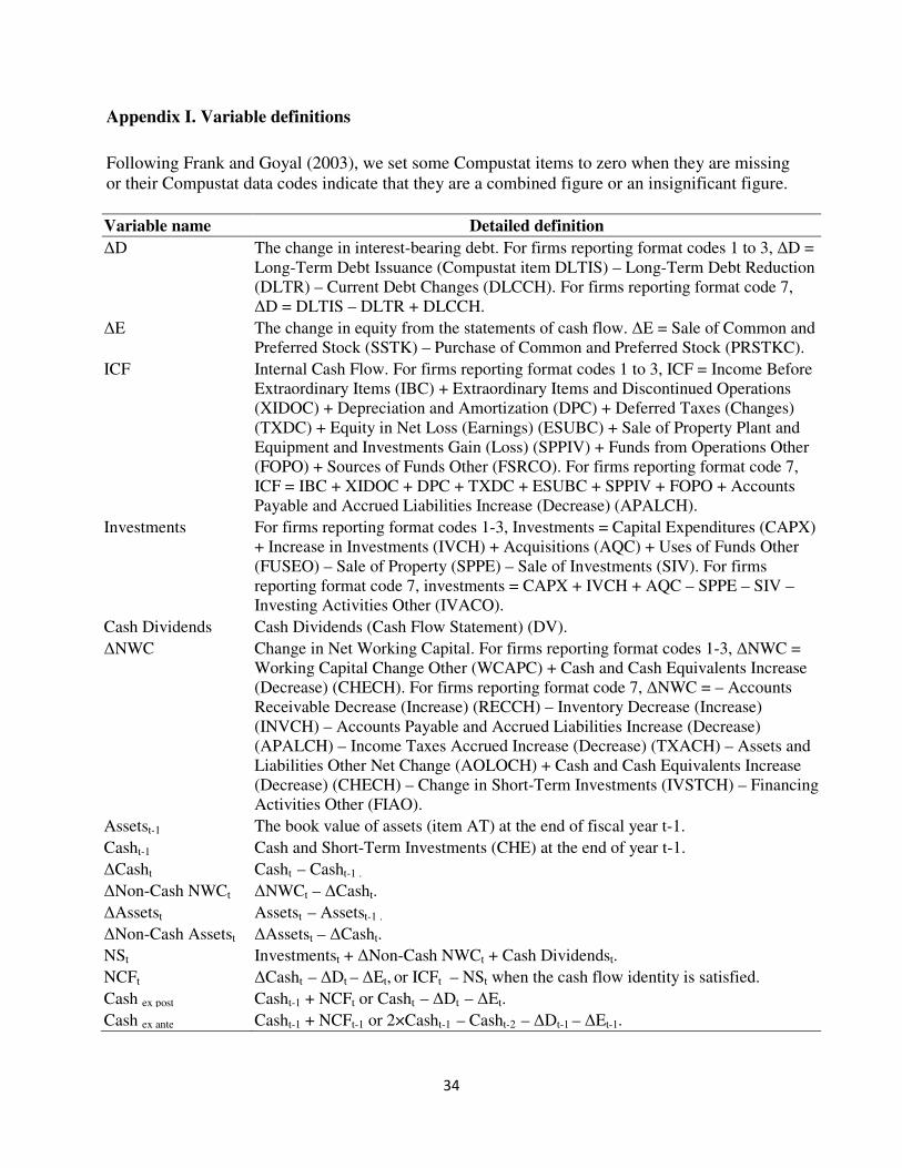
Appendix I. Variable definitions
Following Frank and Goyal (2003), we set some Compustat items to zero when they are missing or their Compustat data codes indicate that they are a combined figure or an insignificant figure.
Variable name Detailed definition
∆D The change in interest-bearing debt. For firms reporting format codes 1 to 3, ∆D = Long-Term Debt Issuance (Compustat item DLTIS) – Long-Term Debt Reduction (DLTR) – Current Debt Changes (DLCCH). For firms reporting format code 7, ∆D = DLTIS – DLTR + DLCCH.
∆E The change in equity from the statements of cash flow. ∆E = Sale of Common and Preferred Stock (SSTK) – Purchase of Common and Preferred Stock (PRSTKC).
ICF Internal Cash Flow. For firms reporting format codes 1 to 3, ICF = Income Before Extraordinary Items (IBC) + Extraordinary Items and Discontinued Operations (XIDOC) + Depreciation and Amortization (DPC) + Deferred Taxes (Changes) (TXDC) + Equity in Net Loss (Earnings) (ESUBC) + Sale of Property Plant and Equipment and Investments Gain (Loss) (SPPIV) + Funds from Operations Other (FOPO) + Sources of Funds Other (FSRCO). For firms reporting format code 7, ICF = IBC + XIDOC + DPC + TXDC + ESUBC + SPPIV + FOPO + Accounts Payable and Accrued Liabilities Increase (Decrease) (APALCH).
Investments For firms reporting format codes 1-3, Investments = Capital Expenditures (CAPX) + Increase in Investments (IVCH) + Acquisitions (AQC) + Uses of Funds Other (FUSEO) – Sale of Property (SPPE) – Sale of Investments (SIV). For firms reporting format code 7, investments = CAPX + IVCH + AQC – SPPE – SIV – Investing Activities Other (IVACO).
Cash Dividends Cash Dividends (Cash Flow Statement) (DV).
∆NWC Change in Net Working Capital. For firms reporting format codes 1-3, ∆NWC = Working Capital Change Other (WCAPC) + Cash and Cash Equivalents Increase (Decrease) (CHECH). For firms reporting format code 7, ∆NWC = – Accounts Receivable Decrease (Increase) (RECCH) – Inventory Decrease (Increase) (INVCH) – Accounts Payable and Accrued Liabilities Increase (Decrease) (APALCH) – Income Taxes Accrued Increase (Decrease) (TXACH) – Assets and Liabilities Other Net Change (AOLOCH) + Cash and Cash Equivalents Increase (Decrease) (CHECH) – Change in Short-Term Investments (IVSTCH) – Financing Activities Other (FIAO).
Assetst-1 The book value of assets (item AT) at the end of fiscal year t-1.
Casht-1 Cash and Short-Term Investments (CHE) at the end of year t-1.
∆Casht Casht – Casht-1 .
∆Non-Cash NWCt ∆NWCt – ∆Casht.
∆Assetst Assetst – Assetst-1 .
∆Non-Cash Assetst ∆Assetst – ∆Casht.
NSt Investmentst + ∆Non-Cash NWCt + Cash Dividendst.
NCFt ∆Casht – ∆Dt – ∆Et, or ICFt – NSt when the cash flow identity is satisfied.
Cash ex post Casht-1 + NCFt or Casht – ∆Dt – ∆Et.
Cash ex ante Casht-1 + NCFt-1 or 2×Casht-1 – Casht-2 – ∆Dt-1 – ∆Et-1.
35
Appendix I Continued:
Variable name Detailed definition
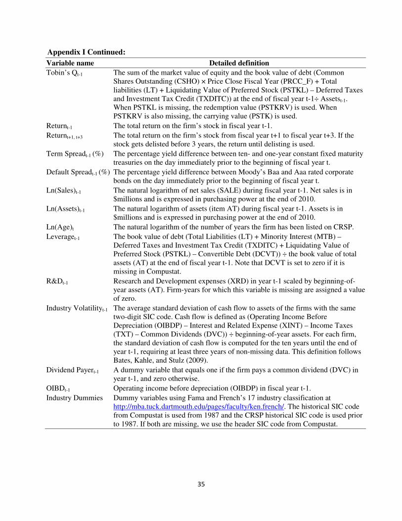
Tobin’s Qt-1 The sum of the market value of equity and the book value of debt (Common Shares Outstanding (CSHO) × Price Close Fiscal Year (PRCC_F) + Total liabilities (LT) + Liquidating Value of Preferred Stock (PSTKL) – Deferred Taxes and Investment Tax Credit (TXDITC)) at the end of fiscal year t-1÷ Assetst-1. When PSTKL is missing, the redemption value (PSTKRV) is used. When PSTKRV is also missing, the carrying value (PSTK) is used.
Returnt-1 The total return on the firm’s stock in fiscal year t-1.
Returnt+1, t+3 The total return on the firm’s stock from fiscal year t+1 to fiscal year t+3. If the stock gets delisted before 3 years, the return until delisting is used.
Term Spreadt-1 (%) The percentage yield difference between ten- and one-year constant fixed maturity treasuries on the day immediately prior to the beginning of fiscal year t.
Default Spreadt-1 (%) The percentage yield difference between Moody’s Baa and Aaa rated corporate bonds on the day immediately prior to the beginning of fiscal year t.
Ln(Sales)t-1 The natural logarithm of net sales (SALE) during fiscal year t-1. Net sales is in $millions and is expressed in purchasing power at the end of 2010.
Ln(Assets)t-1 The natural logarithm of assets (item AT) during fiscal year t-1. Assets is in $millions and is expressed in purchasing power at the end of 2010.
Ln(Age)t The natural logarithm of the number of years the firm has been listed on CRSP.
Leveraget-1 The book value of debt (Total Liabilities (LT) + Minority Interest (MTB) – Deferred Taxes and Investment Tax Credit (TXDITC) + Liquidating Value of Preferred Stock (PSTKL) – Convertible Debt (DCVT)) ÷ the book value of total assets (AT) at the end of fiscal year t-1. Note that DCVT is set to zero if it is missing in Compustat.
R&Dt-1 Research and Development expenses (XRD) in year t-1 scaled by beginning-of-year assets (AT). Firm-years for which this variable is missing are assigned a value of zero.
Industry Volatilityt-1 The average standard deviation of cash flow to assets of the firms with the same two-digit SIC code. Cash flow is defined as (Operating Income Before Depreciation (OIBDP) – Interest and Related Expense (XINT) – Income Taxes (TXT) – Common Dividends (DVC)) ÷ beginning-of-year assets. For each firm, the standard deviation of cash flow is computed for the ten years until the end of year t-1, requiring at least three years of non-missing data. This definition follows Bates, Kahle, and Stulz (2009).
Dividend Payert-1 A dummy variable that equals one if the firm pays a common dividend (DVC) in year t-1, and zero otherwise.
OIBDt-1 Operating income before depreciation (OIBDP) in fiscal year t-1.
Industry Dummies Dummy variables using Fama and French’s 17 industry classification at http://mba.tuck.dartmouth.edu/pages/faculty/ken.french/. The historical SIC code from Compustat is used from 1987 and the CRSP historical SIC code is used prior to 1987. If both are missing, we use the header SIC code from Compustat.
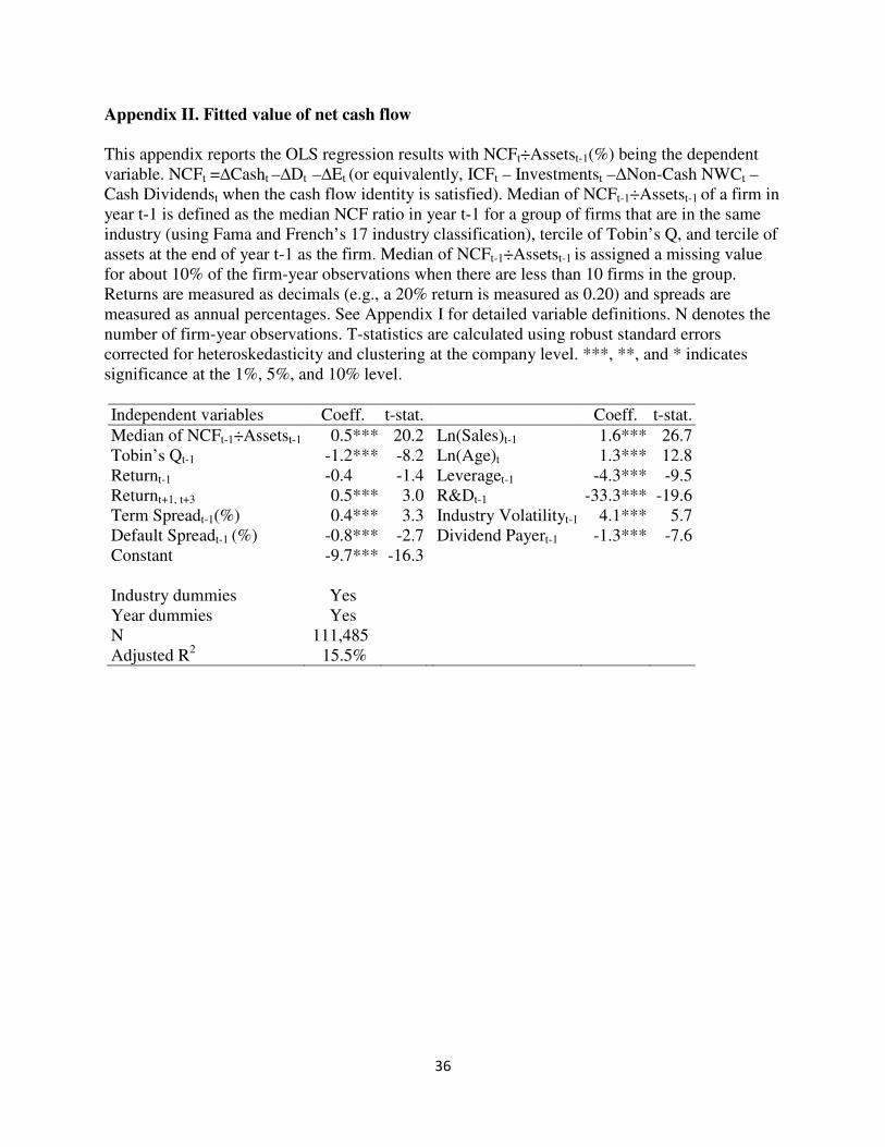
36
Appendix II. Fitted value of net cash flow
This appendix reports the OLS regression results with NCFt÷Assetst-1(%) being the dependent variable. NCFt =∆Casht –∆Dt –∆Et (or equivalently, ICFt – Investmentst –∆Non-Cash NWCt –Cash Dividendst when the cash flow identity is satisfied). Median of NCFt-1÷Assetst-1 of a firm in year t-1 is defined as the median NCF ratio in year t-1 for a group of firms that are in the same industry (using Fama and French’s 17 industry classification), tercile of Tobin’s Q, and tercile of assets at the end of year t-1 as the firm. Median of NCFt-1÷Assetst-1 is assigned a missing value for about 10% of the firm-year observations when there are less than 10 firms in the group. Returns are measured as decimals (e.g., a 20% return is measured as 0.20) and spreads are measured as annual percentages. See Appendix I for detailed variable definitions. N denotes the number of firm-year observations. T-statistics are calculated using robust standard errors corrected for heteroskedasticity and clustering at the company level. ***, **, and * indicates significance at the 1%, 5%, and 10% level.
Independent variables Coeff. t-stat. Coeff. t-stat.
Median of NCFt-1÷Assetst-1 0.5*** 20.2 Ln(Sales)t-1 1.6*** 26.7 Tobin’s Qt-1 -1.2*** -8.2 Ln(Age)t 1.3*** 12.8 Returnt-1 -0.4 -1.4 Leveraget-1 -4.3*** -9.5 Returnt+1, t+3 0.5*** 3.0 R&Dt-1 -33.3*** -19.6 Term Spreadt-1(%) 0.4*** 3.3 Industry Volatilityt-1 4.1*** 5.7 Default Spreadt-1 (%) -0.8*** -2.7 Dividend Payert-1 -1.3*** -7.6 Constant -9.7*** -16.3 Industry dummies Yes Year dummies Yes N 111,485 Adjusted R2 15.5%
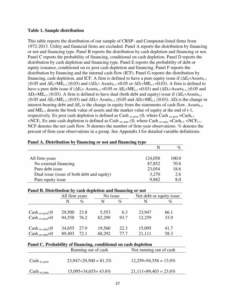
37
Table 1. Sample distribution
This table reports the distribution of our sample of CRSP- and Compustat-listed firms from 1972-2013. Utility and financial firms are excluded. Panel A reports the distribution by financing or not and financing type. Panel B reports the distribution by cash depletion and financing or not. Panel C reports the probability of financing, conditional on cash depletion. Panel D reports the distribution by cash depletion and financing type. Panel E reports the probability of debt or equity issuance, conditional on ex post cash depletion and financing. Panel F reports the distribution by financing and the internal cash flow (ICF). Panel G reports the distribution by financing, cash depletion, and ICF. A firm is defined to have a pure equity issue if (∆Et÷Assetst-1
≥0.05 and ∆Et÷MEt-1 ≥0.03) and (∆Dt÷ Assetst-1 <0.05 or ∆Dt÷MEt-1 <0.03). A firm is defined to have a pure debt issue if (∆Et÷ Assetst-1 <0.05 or ∆Et÷MEt-1 <0.03) and (∆Dt÷Assetst-1 ≥0.05 and ∆Dt÷MEt-1 ≥0.03). A firm is defined to have dual (both debt and equity) issue if (∆Et÷Assetst-1
≥0.05 and ∆Et÷MEt-1 ≥0.03) and ∆Dt÷ Assetst-1 ≥0.05 and ∆Dt÷MEt-1 ≥0.03). ∆Dt is the change in interest-bearing debt and ∆Et is the change in equity from the statements of cash flow. Assetst-1 and MEt-1 denote the book value of assets and the market value of equity at the end of t-1, respectively. Ex post cash depletion is defined as Cash ex post ≤0, where Cash ex post =Casht-1 +NCFt. Ex ante cash depletion is defined as Cash ex ante ≤0, where Cash ex ante =Casht-1 +NCFt-1. NCF denotes the net cash flow. N denotes the number of firm-year observations. % denotes the percent of firm-year observations in a group. See Appendix I for detailed variable definitions. Panel A. Distribution by financing or not and financing type
N %
All firm-years 124,058 100.0 No external financing 87,852 70.8 Pure debt issue 23,054 18.6 Dual issue (issue of both debt and equity) 3,270 2.6 Pure equity issue 9,882 8.0
Panel B. Distribution by cash depletion and financing or not
All firm years No issue Net debt or equity issue
N % N % N %
Cash ex post≤0 29,500 23.8 5,553 6.3 23,947 66.1 Cash ex post>0 94,558 76.2 82,299 93.7 12,259 33.9 Cash ex ante≤0 34,655 27.9 19,560 22.3 15,095 41.7 Cash ex ante>0 89,403 72.1 68,292 77.7 21,111 58.3
Panel C. Probability of financing, conditional on cash depletion
Running out of cash Not running out of cash
Cash ex post 23,947÷29,500 = 81.2% 12,259÷94,558 = 13.0% Cash ex ante 15,095÷34,655= 43.6% 21,111÷89,403 = 23.6%
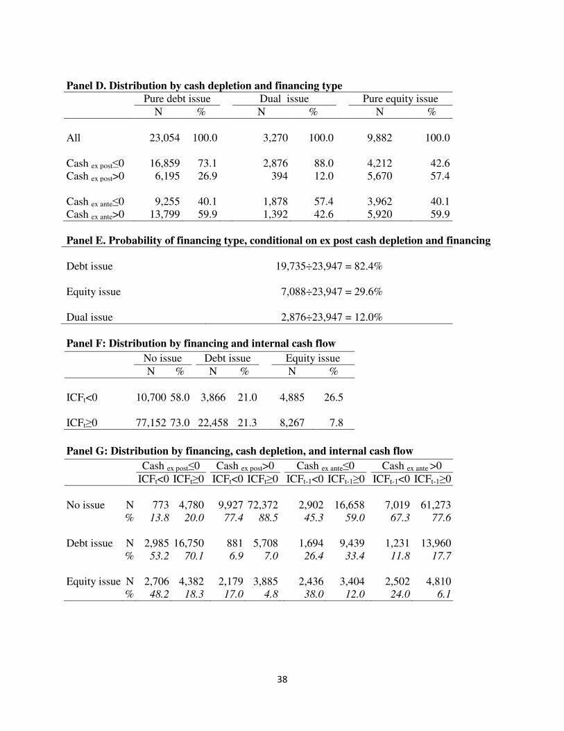
38
Panel D. Distribution by cash depletion and financing type
Pure debt issue Dual issue Pure equity issue
N % N % N %
All 23,054 100.0 3,270 100.0 9,882 100.0 Cash ex post≤0 16,859 73.1 2,876 88.0 4,212 42.6 Cash ex post>0 6,195 26.9 394 12.0 5,670 57.4 Cash ex ante≤0 9,255 40.1 1,878 57.4 3,962 40.1 Cash ex ante>0 13,799 59.9 1,392 42.6 5,920 59.9
Panel E. Probability of financing type, conditional on ex post cash depletion and financing
Debt issue 19,735÷23,947 = 82.4% Equity issue 7,088÷23,947 = 29.6% Dual issue 2,876÷23,947 = 12.0%
Panel F: Distribution by financing and internal cash flow
No issue Debt issue Equity issue
N % N % N %
ICFt<0 10,700 58.0 3,866 21.0 4,885 26.5 ICFt≥0 77,152 73.0 22,458 21.3 8,267 7.8
Panel G: Distribution by financing, cash depletion, and internal cash flow
Cash ex post≤0 Cash ex post>0 Cash ex ante≤0 Cash ex ante >0
ICFt<0 ICFt≥0 ICFt<0 ICFt≥0 ICFt-1<0 ICFt-1≥0 ICFt-1<0 ICFt-1≥0
No issue N 773 4,780 9,927 72,372 2,902 16,658 7,019 61,273 % 13.8 20.0 77.4 88.5 45.3 59.0 67.3 77.6
Debt issue N 2,985 16,750 881 5,708 1,694 9,439 1,231 13,960 % 53.2 70.1 6.9 7.0 26.4 33.4 11.8 17.7
Equity issue N 2,706 4,382 2,179 3,885 2,436 3,404 2,502 4,810 % 48.2 18.3 17.0 4.8 38.0 12.0 24.0 6.1
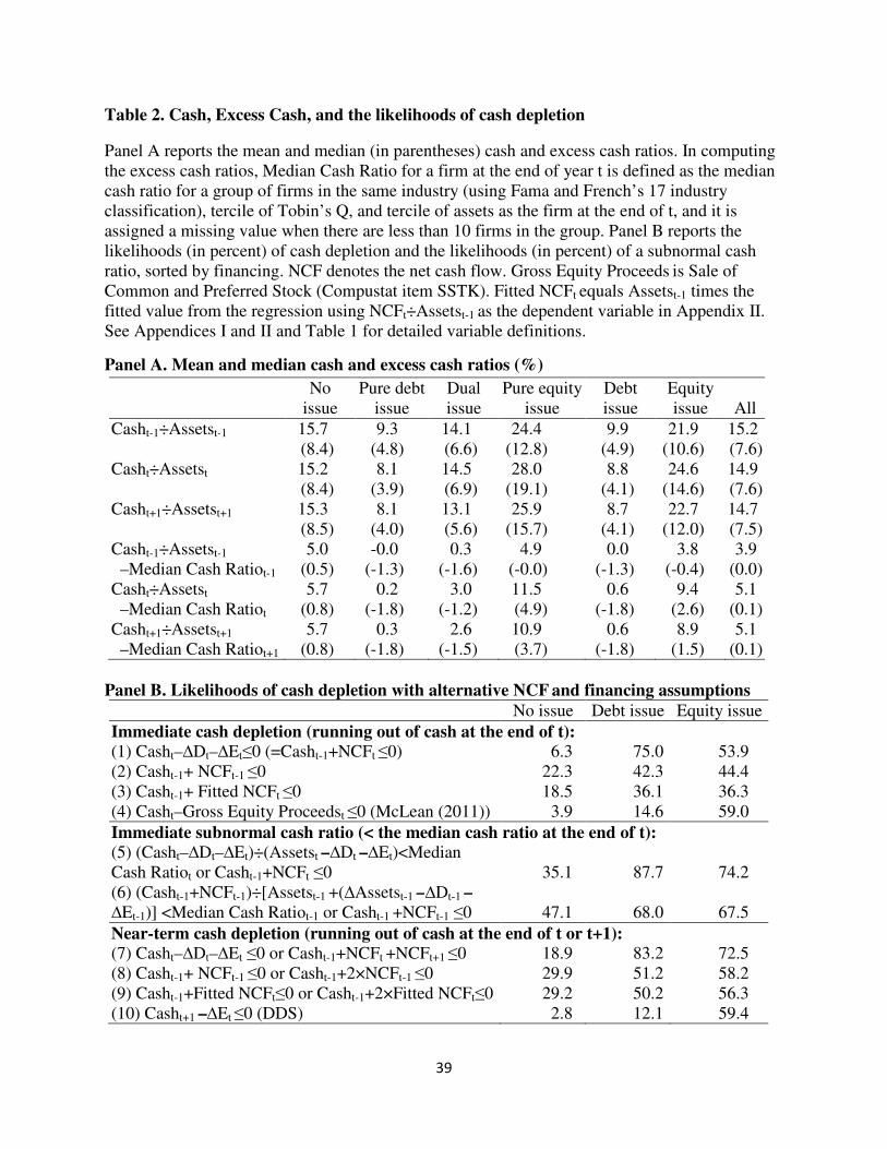
39
Table 2. Cash, Excess Cash, and the likelihoods of cash depletion
Panel A reports the mean and median (in parentheses) cash and excess cash ratios. In computing the excess cash ratios, Median Cash Ratio for a firm at the end of year t is defined as the median cash ratio for a group of firms in the same industry (using Fama and French’s 17 industry classification), tercile of Tobin’s Q, and tercile of assets as the firm at the end of t, and it is assigned a missing value when there are less than 10 firms in the group. Panel B reports the likelihoods (in percent) of cash depletion and the likelihoods (in percent) of a subnormal cash ratio, sorted by financing. NCF denotes the net cash flow. Gross Equity Proceeds is Sale of Common and Preferred Stock (Compustat item SSTK). Fitted NCFt equals Assetst-1 times the fitted value from the regression using NCFt÷Assetst-1 as the dependent variable in Appendix II. See Appendices I and II and Table 1 for detailed variable definitions.
Panel A. Mean and median cash and excess cash ratios (%)
No
issue Pure debt
issue Dual issue
Pure equity issue
Debt issue
Equity issue All
Casht-1÷Assetst-1 15.7 9.3 14.1 24.4 9.9 21.9 15.2
(8.4) (4.8) (6.6) (12.8) (4.9) (10.6) (7.6) Casht÷Assetst 15.2 8.1 14.5 28.0 8.8 24.6 14.9
(8.4) (3.9) (6.9) (19.1) (4.1) (14.6) (7.6) Casht+1÷Assetst+1 15.3 8.1 13.1 25.9 8.7 22.7 14.7
(8.5) (4.0) (5.6) (15.7) (4.1) (12.0) (7.5) Casht-1÷Assetst-1 5.0 -0.0 0.3 4.9 0.0 3.8 3.9 –Median Cash Ratiot-1 (0.5) (-1.3) (-1.6) (-0.0) (-1.3) (-0.4) (0.0) Casht÷Assetst 5.7 0.2 3.0 11.5 0.6 9.4 5.1 –Median Cash Ratiot (0.8) (-1.8) (-1.2) (4.9) (-1.8) (2.6) (0.1) Casht+1÷Assetst+1 5.7 0.3 2.6 10.9 0.6 8.9 5.1 –Median Cash Ratiot+1 (0.8) (-1.8) (-1.5) (3.7) (-1.8) (1.5) (0.1)
Panel B. Likelihoods of cash depletion with alternative NCF and financing assumptions
No issue Debt issue Equity issue
Immediate cash depletion (running out of cash at the end of t): (1) Casht–∆Dt–∆Et≤0 (=Casht-1+NCFt ≤0) 6.3 75.0 53.9 (2) Casht-1+ NCFt-1 ≤0 22.3 42.3 44.4 (3) Casht-1+ Fitted NCFt ≤0 18.5 36.1 36.3 (4) Casht–Gross Equity Proceedst ≤0 (McLean (2011)) 3.9 14.6 59.0
Immediate subnormal cash ratio (< the median cash ratio at the end of t): (5) (Casht–∆Dt–∆Et)÷(Assetst –∆Dt –∆Et)<Median Cash Ratiot or Casht-1+NCFt ≤0 35.1 87.7 74.2 (6) (Casht-1+NCFt-1)÷[Assetst-1 +(∆Assetst-1 –∆Dt-1 –
∆Et-1)] <Median Cash Ratiot-1 or Casht-1 +NCFt-1 ≤0 47.1 68.0 67.5
Near-term cash depletion (running out of cash at the end of t or t+1): (7) Casht–∆Dt–∆Et ≤0 or Casht-1+NCFt +NCFt+1 ≤0 18.9 83.2 72.5 (8) Casht-1+ NCFt-1 ≤0 or Casht-1+2×NCFt-1 ≤0 29.9 51.2 58.2 (9) Casht-1+Fitted NCFt≤0 or Casht-1+2×Fitted NCFt≤0 29.2 50.2 56.3 (10) Casht+1 –∆Et ≤0 (DDS) 2.8 12.1 59.4
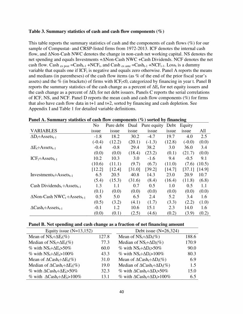
40
Table 3. Summary statistics of cash and cash flow components (%)
This table reports the summary statistics of cash and the components of cash flows (%) for our sample of Compustat- and CRSP-listed firms from 1972-2013. ICF denotes the internal cash flow, and ∆Non-Cash NWC denotes the change in non-cash net working capital. NS denotes the net spending and equals Investments +∆Non-Cash NWC +Cash Dividends. NCF denotes the net cash flow. Cash ex post =Casht-1 +NCFt, and Cash ex ante =Casht-1 +NCFt-1. Losst is a dummy variable that equals one if ICFt is negative and equals zero otherwise. Panel A reports the means and medians (in parentheses) of the cash flow items (as % of the end of the prior fiscal year’s assets) and the % (in brackets) of firms with ICFt<0, categorized by financing in year t. Panel B reports the summary statistics of the cash change as a percent of ∆Et for net equity issuers and the cash change as a percent of ∆Dt for net debt issuers. Panels C reports the serial correlations of ICF, NS, and NCF. Panel D reports the mean cash and cash flow components (%) for firms that also have cash flow data in t+1 and t+2, sorted by financing and cash depletion. See Appendix I and Table 1 for detailed variable definitions.
Panel A. Summary statistics of cash flow components (%) sorted by financing
VARIABLES
No issue
Pure debt issue
Dual issue
Pure equity issue
Debt issue
Equity issue All
∆Dt÷Assetst-1 -1.8 18.2 30.2 -4.7 19.7 4.0 2.5 (-0.4) (12.2) (20.1) (-1.3) (12.8) (-0.0) (0.0) ∆Et÷Assetst-1 -0.4 -0.8 29.4 38.2 3.0 36.0 3.4 (0.0) (0.0) (18.4) (23.2) (0.1) (21.7) (0.0) ICFt÷Assetst-1 10.2 10.3 3.0 -1.6 9.4 -0.5 9.1 (10.6) (11.1) (9.7) (6.7) (11.0) (7.6) (10.5) [12.2] [12.4] [31.0] [39.2] [14.7] [37.1] [14.9] Investmentst÷Assetst-1 6.5 20.5 40.8 14.3 23.0 20.9 10.7 (5.4) (15.3) (31.6) (8.4) (16.4) (11.8) (6.8) Cash Dividendst ÷Assetst-1 1.3 1.1 0.7 0.5 1.0 0.5 1.1 (0.1) (0.0) (0.0) (0.0) (0.0) (0.0) (0.0) ∆Non-Cash NWCt ÷Assetst-1 0.5 5.0 6.5 2.4 5.2 3.4 1.6 (0.5) (3.2) (4.1) (1.7) (3.3) (2.2) (1.0) ∆Casht÷Assetst-1 -0.1 1.2 10.6 15.1 2.3 14.0 1.6
(0.0) (0.1) (2.5) (4.6) (0.2) (3.9) (0.2)
Panel B. Net spending and cash change as a fraction of net financing amount
Equity issue (N=13,152) Debt issue (N=26,324)
Mean of NSt÷∆Et(%) 127.8 Mean of NSt÷∆Dt(%) 188.6
Median of NSt÷∆Et(%) 77.3 Median of NSt÷∆Dt(%) 170.9
% with NSt÷∆Et>50% 60.0 % with NSt÷∆Dt>50% 90.0
% with NSt÷∆Et>100% 43.3 % with NSt÷∆Dt>100% 80.3
Mean of ∆Casht÷∆Et(%) 31.0 Mean of ∆Casht÷∆Dt(%) 6.9
Median of ∆Casht÷∆Et(%) 19.0 Median of ∆Casht÷∆Dt(%) 1.5
% with ∆Casht÷∆Et>50% 32.3 % with ∆Casht÷∆Dt>50% 15.0
% with ∆Casht÷∆Et>100% 13.1 % with ∆Casht÷∆Dt>100% 6.5
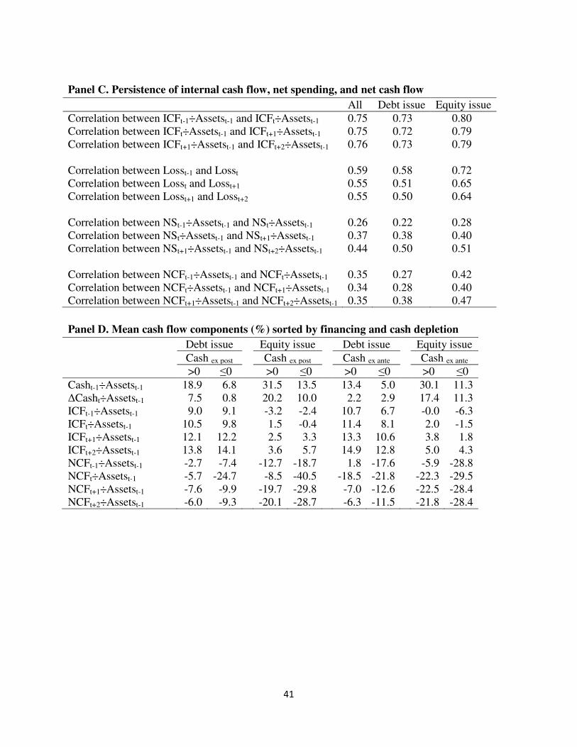
41
Panel C. Persistence of internal cash flow, net spending, and net cash flow
All Debt issue Equity issue
Correlation between ICFt-1÷Assetst-1 and ICFt÷Assetst-1 0.75 0.73 0.80 Correlation between ICFt÷Assetst-1 and ICFt+1÷Assetst-1 0.75 0.72 0.79 Correlation between ICFt+1÷Assetst-1 and ICFt+2÷Assetst-1 0.76 0.73 0.79 Correlation between Losst-1 and Losst 0.59 0.58 0.72 Correlation between Losst and Losst+1 0.55 0.51 0.65 Correlation between Losst+1 and Losst+2 0.55 0.50 0.64 Correlation between NSt-1÷Assetst-1 and NSt÷Assetst-1 0.26 0.22 0.28 Correlation between NSt÷Assetst-1 and NSt+1÷Assetst-1 0.37 0.38 0.40 Correlation between NSt+1÷Assetst-1 and NSt+2÷Assetst-1 0.44 0.50 0.51 Correlation between NCFt-1÷Assetst-1 and NCFt÷Assetst-1 0.35 0.27 0.42 Correlation between NCFt÷Assetst-1 and NCFt+1÷Assetst-1 0.34 0.28 0.40 Correlation between NCFt+1÷Assetst-1 and NCFt+2÷Assetst-1 0.35 0.38 0.47
Panel D. Mean cash flow components (%) sorted by financing and cash depletion
Debt issue Equity issue Debt issue Equity issue
Cash ex post Cash ex post Cash ex ante Cash ex ante
>0 ≤0 >0 ≤0 >0 ≤0 >0 ≤0
Casht-1÷Assetst-1 18.9 6.8 31.5 13.5 13.4 5.0 30.1 11.3 ∆Casht÷Assetst-1 7.5 0.8 20.2 10.0 2.2 2.9 17.4 11.3 ICFt-1÷Assetst-1 9.0 9.1 -3.2 -2.4 10.7 6.7 -0.0 -6.3 ICFt÷Assetst-1 10.5 9.8 1.5 -0.4 11.4 8.1 2.0 -1.5 ICFt+1÷Assetst-1 12.1 12.2 2.5 3.3 13.3 10.6 3.8 1.8 ICFt+2÷Assetst-1 13.8 14.1 3.6 5.7 14.9 12.8 5.0 4.3 NCFt-1÷Assetst-1 -2.7 -7.4 -12.7 -18.7 1.8 -17.6 -5.9 -28.8 NCFt÷Assetst-1 -5.7 -24.7 -8.5 -40.5 -18.5 -21.8 -22.3 -29.5 NCFt+1÷Assetst-1 -7.6 -9.9 -19.7 -29.8 -7.0 -12.6 -22.5 -28.4 NCFt+2÷Assetst-1 -6.0 -9.3 -20.1 -28.7 -6.3 -11.5 -21.8 -28.4
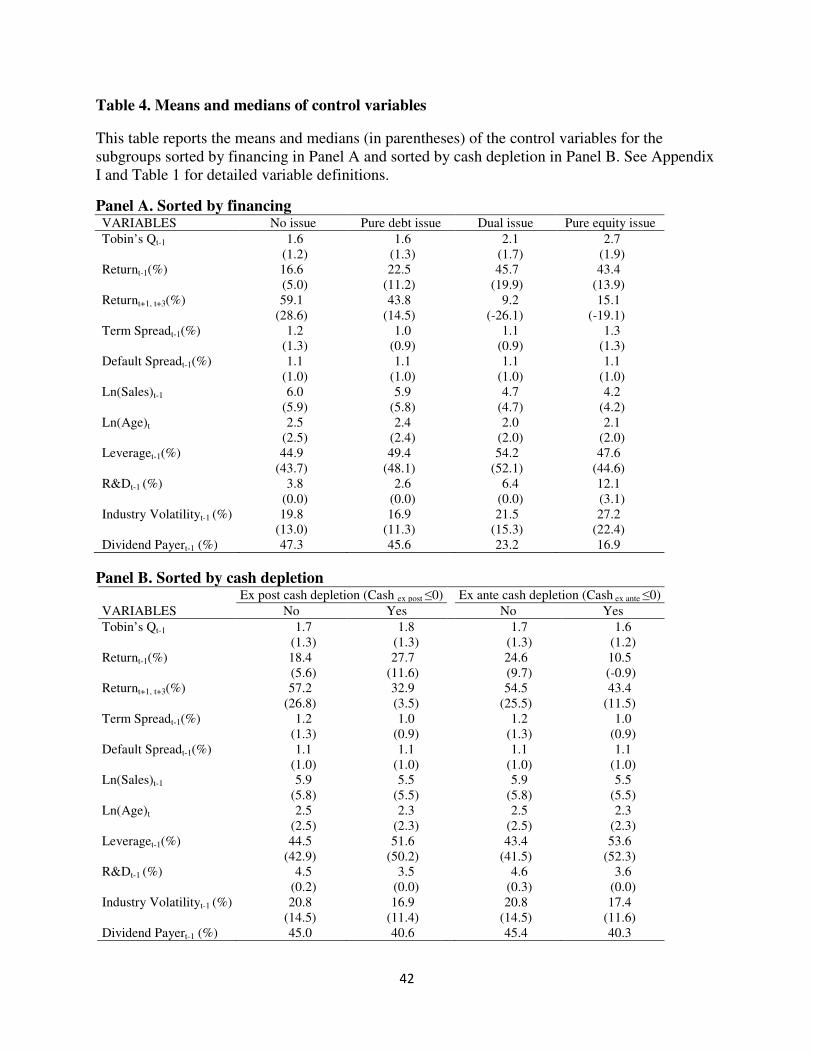
42
Table 4. Means and medians of control variables
This table reports the means and medians (in parentheses) of the control variables for the subgroups sorted by financing in Panel A and sorted by cash depletion in Panel B. See Appendix I and Table 1 for detailed variable definitions.
Panel A. Sorted by financing VARIABLES No issue Pure debt issue Dual issue Pure equity issue
Tobin’s Qt-1 1.6 1.6 2.1 2.7 (1.2) (1.3) (1.7) (1.9) Returnt-1(%) 16.6 22.5 45.7 43.4 (5.0) (11.2) (19.9) (13.9) Returnt+1, t+3(%) 59.1 43.8 9.2 15.1 (28.6) (14.5) (-26.1) (-19.1) Term Spreadt-1(%) 1.2 1.0 1.1 1.3 (1.3) (0.9) (0.9) (1.3) Default Spreadt-1(%) 1.1 1.1 1.1 1.1 (1.0) (1.0) (1.0) (1.0) Ln(Sales)t-1 6.0 5.9 4.7 4.2 (5.9) (5.8) (4.7) (4.2) Ln(Age)t 2.5 2.4 2.0 2.1 (2.5) (2.4) (2.0) (2.0) Leveraget-1(%) 44.9 49.4 54.2 47.6 (43.7) (48.1) (52.1) (44.6) R&Dt-1 (%) 3.8 2.6 6.4 12.1 (0.0) (0.0) (0.0) (3.1) Industry Volatilityt-1 (%) 19.8 16.9 21.5 27.2 (13.0) (11.3) (15.3) (22.4) Dividend Payert-1 (%) 47.3 45.6 23.2 16.9
Panel B. Sorted by cash depletion Ex post cash depletion (Cash ex post ≤0) Ex ante cash depletion (Cash ex ante ≤0)
VARIABLES No Yes No Yes
Tobin’s Qt-1 1.7 1.8 1.7 1.6 (1.3) (1.3) (1.3) (1.2) Returnt-1(%) 18.4 27.7 24.6 10.5 (5.6) (11.6) (9.7) (-0.9) Returnt+1, t+3(%) 57.2 32.9 54.5 43.4 (26.8) (3.5) (25.5) (11.5) Term Spreadt-1(%) 1.2 1.0 1.2 1.0 (1.3) (0.9) (1.3) (0.9) Default Spreadt-1(%) 1.1 1.1 1.1 1.1 (1.0) (1.0) (1.0) (1.0) Ln(Sales)t-1 5.9 5.5 5.9 5.5 (5.8) (5.5) (5.8) (5.5) Ln(Age)t 2.5 2.3 2.5 2.3 (2.5) (2.3) (2.5) (2.3) Leveraget-1(%) 44.5 51.6 43.4 53.6 (42.9) (50.2) (41.5) (52.3) R&Dt-1 (%) 4.5 3.5 4.6 3.6 (0.2) (0.0) (0.3) (0.0) Industry Volatilityt-1 (%) 20.8 16.9 20.8 17.4 (14.5) (11.4) (14.5) (11.6) Dividend Payert-1 (%) 45.0 40.6 45.4 40.3
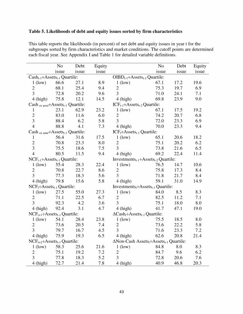
43
Table 5. Likelihoods of debt and equity issues sorted by firm characteristics
This table reports the likelihoods (in percent) of net debt and equity issues in year t for the subgroups sorted by firm characteristics and market conditions. The cutoff points are determined each fiscal year. See Appendix I and Table 1 for detailed variable definitions.
No issue
Debt issue
Equity issue
No issue
Debt issue
Equity issue
Casht-1÷Assetst-1 Quartile: OIBDt-1÷Assetst-2 Quartile: 1 (low) 66.6 27.1 8.9 1 (low) 67.1 17.2 19.6
2 68.1 25.4 9.4 2 75.3 19.7 6.9
3 72.8 20.2 9.6 3 71.0 24.1 7.1
4 (high) 75.8 12.1 14.5 4 (high) 69.8 23.9 9.0
Cash ex post÷Assetst-1 Quartile: ICFt-1÷Assetst-2 Quartile: 1 23.1 62.9 23.2 1 (low) 67.1 17.5 19.2
2 83.0 11.6 6.0 2 74.2 20.7 6.8
3 88.4 6.2 5.8 3 72.0 23.3 6.9
4 88.8 4.1 7.3 4 (high) 70.0 23.3 9.4
Cash ex ante÷Assetst-1 Quartile: ICFt÷Assetst-1 Quartile: 1 56.4 31.6 17.5 1 (low) 65.1 20.6 18.2
2 70.8 23.3 8.0 2 75.1 20.2 6.2
3 75.5 18.6 7.5 3 73.8 21.6 6.5
4 80.5 11.5 9.4 4 (high) 69.2 22.4 11.4
NCFt-1÷Assetst-1 Quartile: Investmentst-1÷Assetst-2 Quartile: 1 (low) 55.4 28.3 22.4 1 (low) 76.5 14.7 10.6
2 70.8 22.7 8.6 2 75.8 17.3 8.4
3 77.3 18.3 5.6 3 71.8 21.7 8.4
4 (high) 79.8 15.6 5.8 4 (high) 59.1 31.0 14.9
NCFt÷Assetst-1 Quartile: Investmentst÷Assetst-1 Quartile: 1 (low) 27.5 55.0 27.3 1 (low) 84.0 8.5 8.3
2 71.1 22.5 6.7 2 82.5 11.2 7.1
3 92.3 4.2 3.6 3 75.1 18.0 8.0
4 (high) 92.4 3.1 4.7 4 (high) 41.7 47.1 19.0
NCFt+1÷Assetst-1 Quartile: ∆Casht÷Assetst-1 Quartile: 1 (low) 54.1 28.4 23.8 1 (low) 75.5 18.5 8.0
2 73.6 20.5 7.4 2 73.6 22.2 5.8
3 79.7 16.7 4.5 3 71.6 23.3 7.2
4 (high) 75.9 19.3 6.5 4 (high) 62.6 20.8 21.4
NCFt+2÷Assetst-1 Quartile: ∆Non-Cash Assetst÷Assetst-1 Quartile: 1 (low) 58.3 25.6 21.6 1 (low) 84.8 8.0 8.3
2 75.1 19.2 7.2 2 84.7 9.6 6.2
3 77.8 18.3 5.2 3 72.8 20.6 7.6
4 (high) 72.7 21.4 7.8 4 (high) 40.9 46.8 20.3
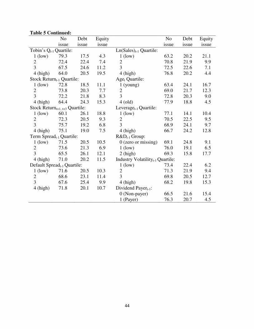
44
Table 5 Continued:
No issue
Debt issue
Equity issue
No issue
Debt issue
Equity issue
Tobin’s Qt-1 Quartile: Ln(Sales)t-1 Quartile: 1 (low) 79.3 17.5 4.3 1 (low) 63.2 20.2 21.1
2 72.4 22.4 7.4 2 70.8 21.9 9.9
3 67.5 24.6 11.2 3 72.5 22.6 7.1
4 (high) 64.0 20.5 19.5 4 (high) 76.8 20.2 4.4
Stock Returnt-1 Quartile: Aget Quartile: 1 (low) 72.8 18.5 11.1 1 (young) 63.4 24.1 16.7
2 73.8 20.3 7.7 2 69.0 21.7 12.3
3 72.2 21.8 8.3 3 72.8 20.3 9.0
4 (high) 64.4 24.3 15.3 4 (old) 77.9 18.8 4.5
Stock Returnt+1, t+3 Quartile: Leveraget-1 Quartile: 1 (low) 60.1 26.1 18.8 1 (low) 77.1 14.1 10.4
2 72.3 20.5 9.3 2 70.5 22.5 9.5
3 75.7 19.2 6.8 3 68.9 24.1 9.7
4 (high) 75.1 19.0 7.5 4 (high) 66.7 24.2 12.8
Term Spreadt-1 Quartile: R&Dt-1 Group: 1 (low) 71.5 20.5 10.5 0 (zero or missing) 69.1 24.8 9.1
2 73.6 21.3 6.9 1 (low) 76.0 19.1 6.5
3 65.5 26.1 12.1 2 (high) 69.3 15.8 17.7
4 (high) 71.0 20.2 11.5 Industry Volatilityt-1 Quartile: Default Spreadt-1 Quartile: 1 (low) 73.4 22.4 6.2
1 (low) 71.6 20.5 10.3 2 71.3 21.9 9.4
2 68.6 23.1 11.4 3 69.8 20.5 12.7
3 67.6 25.4 9.9 4 (high) 68.2 19.8 15.3
4 (high) 71.8 20.1 10.7 Dividend Payert-1: 0 (Non-payer) 66.5 21.6 15.4
1 (Payer) 76.3 20.7 4.5
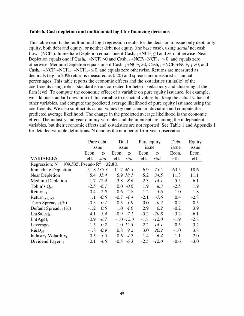
45
Table 6. Cash depletion and multinomial logit for financing decisions
This table reports the multinomial logit regression results for the decision to issue only debt, only equity, both debt and equity, or neither debt nor equity (the base case), using actual net cash flows (NCFs). Immediate Depletion equals one if Casht-1 +NCFt ≤0 and zero otherwise. Near Depletion equals one if Casht-1 +NCFt >0 and Casht-1 +NCFt +NCFt+1 ≤ 0, and equals zero otherwise. Medium Depletion equals one if Casht-1 +NCFt >0, Casht-1 +NCFt +NCFt+1 >0, and Casht-1 +NCFt +NCFt+1 +NCFt+2 ≤ 0, and equals zero otherwise. Returns are measured as decimals (e.g., a 20% return is measured as 0.20) and spreads are measured as annual percentages. This table reports the economic effects and the z-statistics (in italic) of the coefficients using robust standard errors corrected for heteroskedasticity and clustering at the firm level. To compute the economic effect of a variable on pure equity issuance, for example, we add one standard deviation of this variable to its actual values but keep the actual values of other variables, and compute the predicted average likelihood of pure equity issuance using the coefficients. We also subtract its actual values by one standard deviation and compute the predicted average likelihood. The change in the predicted average likelihood is the economic effect. The industry and year dummy variables and the intercept are among the independent variables, but their economic effects and z-statistics are not reported. See Table 1 and Appendix I for detailed variable definitions. N denotes the number of firm-year observations.
Pure debt issue
Dual issue
Pure equity issue
Debt issue
Equity issue
VARIABLES Econ. eff.
z-
stat. Econ. eff.
z-
stat. Econ. eff.
z-
stat. Econ. eff.
Econ. eff.
Regression: N = 109,535, Pseudo R2 = 32.8% Immediate Depletion 51.8 135.3 11.7 46.3 6.9 75.5 63.5 18.6 Near Depletion 5.4 35.4 5.9 18.1 5.2 34.5 11.3 11.1 Medium Depletion 1.7 12.4 3.8 8.6 2.3 14.1 5.5 6.1 Tobin’s Qt-1 -2.5 -6.1 0.0 -0.6 1.9 8.3 -2.5 1.9 Returnt-1 0.4 2.9 0.6 2.8 1.2 5.6 1.0 1.8 Returnt+1, t+3 1.1 -0.6 -0.7 -4.4 -2.1 -7.6 0.4 -2.8 Term Spreadt-1 (%) -0.3 0.1 0.5 1.9 0.0 0.2 0.2 0.5 Default Spreadt-1 (%) -1.2 0.6 1.0 4.0 2.9 6.2 -0.2 3.9 Ln(Sales)t-1 4.1 5.4 -0.9 -7.1 -5.2 -20.8 3.2 -6.1 Ln(Age)t -0.9 -8.7 -1.0 -12.0 -1.8 -12.0 -1.9 -2.8 Leveraget-1 -1.5 -0.7 1.0 12.3 2.2 14.1 -0.5 3.2 R&Dt-1 -1.8 -0.9 0.8 9.2 3.0 20.2 -1.0 3.8 Industry Volatilityt-1 0.5 3.5 0.6 4.7 1.4 6.4 1.1 2.0 Dividend Payert-1 -0.1 -4.6 -0.5 -6.3 -2.5 -12.0 -0.6 -3.0
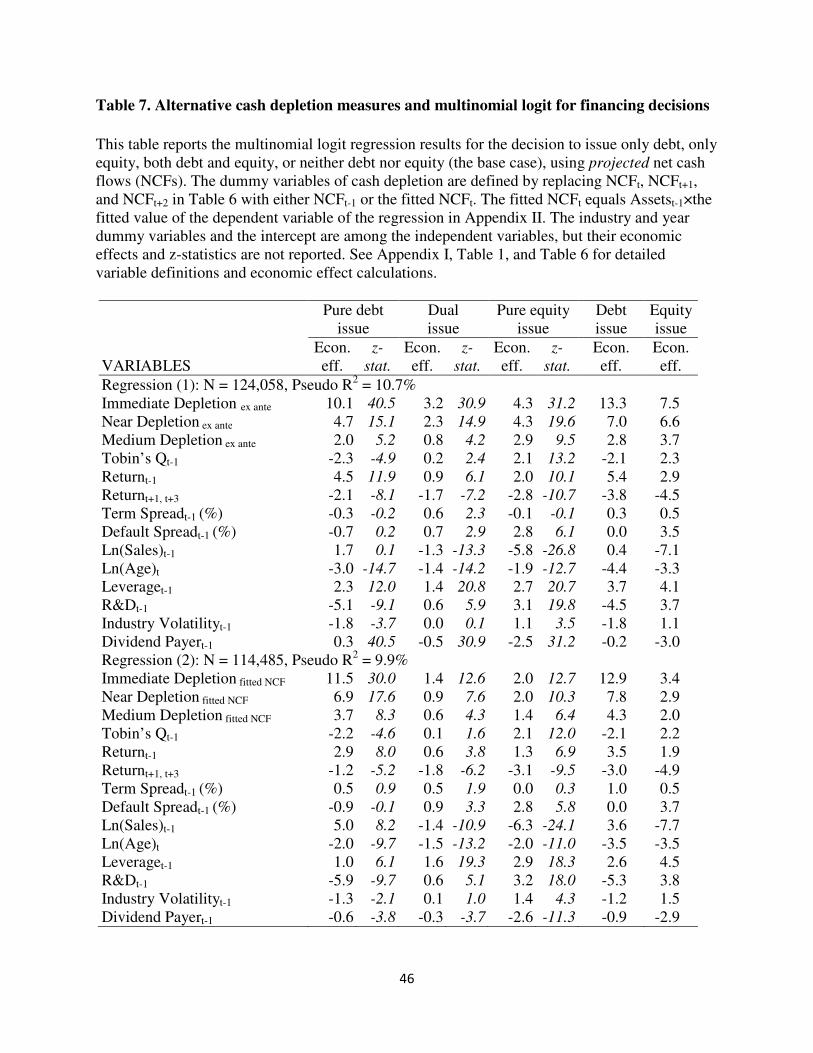
46
Table 7. Alternative cash depletion measures and multinomial logit for financing decisions
This table reports the multinomial logit regression results for the decision to issue only debt, only equity, both debt and equity, or neither debt nor equity (the base case), using projected net cash flows (NCFs). The dummy variables of cash depletion are defined by replacing NCFt, NCFt+1, and NCFt+2 in Table 6 with either NCFt-1 or the fitted NCFt. The fitted NCFt equals Assetst-1×the fitted value of the dependent variable of the regression in Appendix II. The industry and year dummy variables and the intercept are among the independent variables, but their economic effects and z-statistics are not reported. See Appendix I, Table 1, and Table 6 for detailed variable definitions and economic effect calculations.
Pure debt issue
Dual issue
Pure equity issue
Debt issue
Equity issue
VARIABLES Econ. eff.
z-
stat. Econ. eff.
z-
stat. Econ. eff.
z-
stat. Econ. eff.
Econ. eff.
Regression (1): N = 124,058, Pseudo R2 = 10.7% Immediate Depletion ex ante 10.1 40.5 3.2 30.9 4.3 31.2 13.3 7.5 Near Depletion ex ante 4.7 15.1 2.3 14.9 4.3 19.6 7.0 6.6 Medium Depletion ex ante 2.0 5.2 0.8 4.2 2.9 9.5 2.8 3.7 Tobin’s Qt-1 -2.3 -4.9 0.2 2.4 2.1 13.2 -2.1 2.3 Returnt-1 4.5 11.9 0.9 6.1 2.0 10.1 5.4 2.9 Returnt+1, t+3 -2.1 -8.1 -1.7 -7.2 -2.8 -10.7 -3.8 -4.5 Term Spreadt-1 (%) -0.3 -0.2 0.6 2.3 -0.1 -0.1 0.3 0.5 Default Spreadt-1 (%) -0.7 0.2 0.7 2.9 2.8 6.1 0.0 3.5 Ln(Sales)t-1 1.7 0.1 -1.3 -13.3 -5.8 -26.8 0.4 -7.1 Ln(Age)t -3.0 -14.7 -1.4 -14.2 -1.9 -12.7 -4.4 -3.3 Leveraget-1 2.3 12.0 1.4 20.8 2.7 20.7 3.7 4.1 R&Dt-1 -5.1 -9.1 0.6 5.9 3.1 19.8 -4.5 3.7 Industry Volatilityt-1 -1.8 -3.7 0.0 0.1 1.1 3.5 -1.8 1.1 Dividend Payert-1 0.3 40.5 -0.5 30.9 -2.5 31.2 -0.2 -3.0 Regression (2): N = 114,485, Pseudo R2 = 9.9% Immediate Depletion fitted NCF 11.5 30.0 1.4 12.6 2.0 12.7 12.9 3.4 Near Depletion fitted NCF 6.9 17.6 0.9 7.6 2.0 10.3 7.8 2.9 Medium Depletion fitted NCF 3.7 8.3 0.6 4.3 1.4 6.4 4.3 2.0 Tobin’s Qt-1 -2.2 -4.6 0.1 1.6 2.1 12.0 -2.1 2.2 Returnt-1 2.9 8.0 0.6 3.8 1.3 6.9 3.5 1.9 Returnt+1, t+3 -1.2 -5.2 -1.8 -6.2 -3.1 -9.5 -3.0 -4.9 Term Spreadt-1 (%) 0.5 0.9 0.5 1.9 0.0 0.3 1.0 0.5 Default Spreadt-1 (%) -0.9 -0.1 0.9 3.3 2.8 5.8 0.0 3.7 Ln(Sales)t-1 5.0 8.2 -1.4 -10.9 -6.3 -24.1 3.6 -7.7 Ln(Age)t -2.0 -9.7 -1.5 -13.2 -2.0 -11.0 -3.5 -3.5 Leveraget-1 1.0 6.1 1.6 19.3 2.9 18.3 2.6 4.5 R&Dt-1 -5.9 -9.7 0.6 5.1 3.2 18.0 -5.3 3.8 Industry Volatilityt-1 -1.3 -2.1 0.1 1.0 1.4 4.3 -1.2 1.5 Dividend Payert-1 -0.6 -3.8 -0.3 -3.7 -2.6 -11.3 -0.9 -2.9
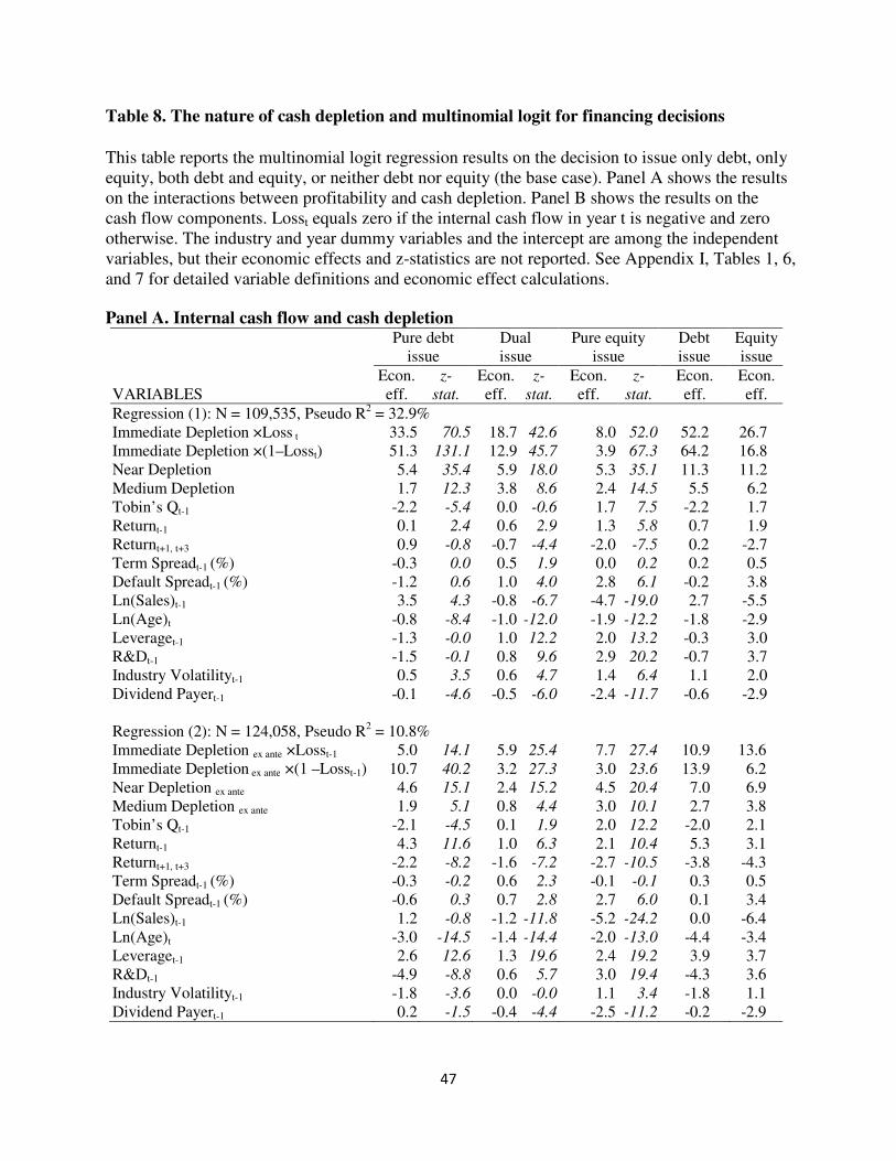
47
Table 8. The nature of cash depletion and multinomial logit for financing decisions
This table reports the multinomial logit regression results on the decision to issue only debt, only equity, both debt and equity, or neither debt nor equity (the base case). Panel A shows the results on the interactions between profitability and cash depletion. Panel B shows the results on the cash flow components. Losst equals zero if the internal cash flow in year t is negative and zero otherwise. The industry and year dummy variables and the intercept are among the independent variables, but their economic effects and z-statistics are not reported. See Appendix I, Tables 1, 6, and 7 for detailed variable definitions and economic effect calculations. Panel A. Internal cash flow and cash depletion
Pure debt issue
Dual issue
Pure equity issue
Debt issue
Equity issue
VARIABLES Econ. eff.
z-
stat. Econ. eff.
z-
stat. Econ. eff.
z-
stat. Econ. eff.
Econ. eff.
Regression (1): N = 109,535, Pseudo R2 = 32.9% Immediate Depletion ×Loss t 33.5 70.5 18.7 42.6 8.0 52.0 52.2 26.7 Immediate Depletion ×(1–Losst) 51.3 131.1 12.9 45.7 3.9 67.3 64.2 16.8 Near Depletion 5.4 35.4 5.9 18.0 5.3 35.1 11.3 11.2 Medium Depletion 1.7 12.3 3.8 8.6 2.4 14.5 5.5 6.2 Tobin’s Qt-1 -2.2 -5.4 0.0 -0.6 1.7 7.5 -2.2 1.7 Returnt-1 0.1 2.4 0.6 2.9 1.3 5.8 0.7 1.9 Returnt+1, t+3 0.9 -0.8 -0.7 -4.4 -2.0 -7.5 0.2 -2.7 Term Spreadt-1 (%) -0.3 0.0 0.5 1.9 0.0 0.2 0.2 0.5 Default Spreadt-1 (%) -1.2 0.6 1.0 4.0 2.8 6.1 -0.2 3.8 Ln(Sales)t-1 3.5 4.3 -0.8 -6.7 -4.7 -19.0 2.7 -5.5 Ln(Age)t -0.8 -8.4 -1.0 -12.0 -1.9 -12.2 -1.8 -2.9 Leveraget-1 -1.3 -0.0 1.0 12.2 2.0 13.2 -0.3 3.0 R&Dt-1 -1.5 -0.1 0.8 9.6 2.9 20.2 -0.7 3.7 Industry Volatilityt-1 0.5 3.5 0.6 4.7 1.4 6.4 1.1 2.0 Dividend Payert-1 -0.1 -4.6 -0.5 -6.0 -2.4 -11.7 -0.6 -2.9 Regression (2): N = 124,058, Pseudo R2 = 10.8% Immediate Depletion ex ante ×Losst-1 5.0 14.1 5.9 25.4 7.7 27.4 10.9 13.6 Immediate Depletion ex ante ×(1 –Losst-1) 10.7 40.2 3.2 27.3 3.0 23.6 13.9 6.2 Near Depletion ex ante 4.6 15.1 2.4 15.2 4.5 20.4 7.0 6.9 Medium Depletion ex ante 1.9 5.1 0.8 4.4 3.0 10.1 2.7 3.8 Tobin’s Qt-1 -2.1 -4.5 0.1 1.9 2.0 12.2 -2.0 2.1 Returnt-1 4.3 11.6 1.0 6.3 2.1 10.4 5.3 3.1 Returnt+1, t+3 -2.2 -8.2 -1.6 -7.2 -2.7 -10.5 -3.8 -4.3 Term Spreadt-1 (%) -0.3 -0.2 0.6 2.3 -0.1 -0.1 0.3 0.5 Default Spreadt-1 (%) -0.6 0.3 0.7 2.8 2.7 6.0 0.1 3.4 Ln(Sales)t-1 1.2 -0.8 -1.2 -11.8 -5.2 -24.2 0.0 -6.4 Ln(Age)t -3.0 -14.5 -1.4 -14.4 -2.0 -13.0 -4.4 -3.4 Leveraget-1 2.6 12.6 1.3 19.6 2.4 19.2 3.9 3.7 R&Dt-1 -4.9 -8.8 0.6 5.7 3.0 19.4 -4.3 3.6 Industry Volatilityt-1 -1.8 -3.6 0.0 -0.0 1.1 3.4 -1.8 1.1 Dividend Payert-1 0.2 -1.5 -0.4 -4.4 -2.5 -11.2 -0.2 -2.9
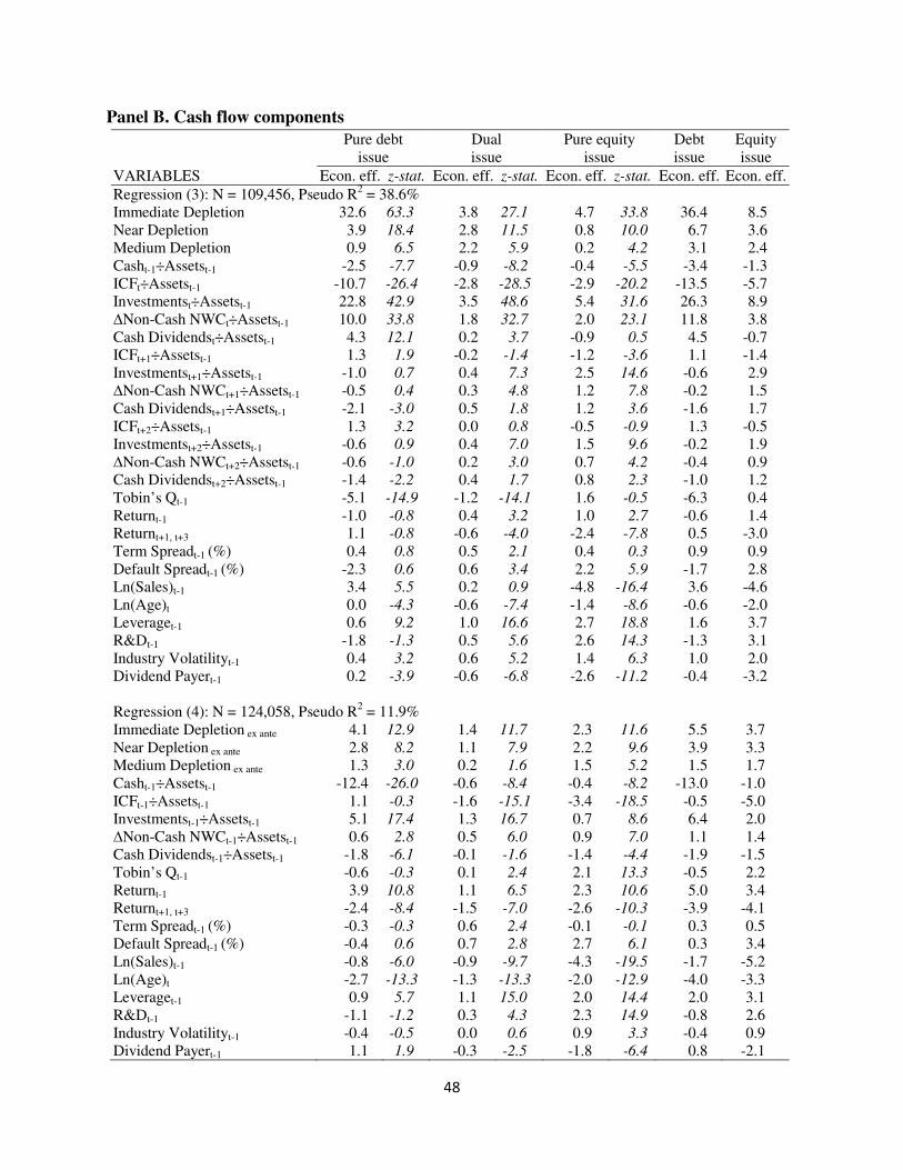
48
Panel B. Cash flow components
Pure debt issue
Dual issue
Pure equity issue
Debt issue
Equity issue
VARIABLES Econ. eff. z-stat. Econ. eff. z-stat. Econ. eff. z-stat. Econ. eff. Econ. eff.
Regression (3): N = 109,456, Pseudo R2 = 38.6%
Immediate Depletion 32.6 63.3 3.8 27.1 4.7 33.8 36.4 8.5 Near Depletion 3.9 18.4 2.8 11.5 0.8 10.0 6.7 3.6 Medium Depletion 0.9 6.5 2.2 5.9 0.2 4.2 3.1 2.4 Casht-1÷Assetst-1 -2.5 -7.7 -0.9 -8.2 -0.4 -5.5 -3.4 -1.3 ICFt÷Assetst-1 -10.7 -26.4 -2.8 -28.5 -2.9 -20.2 -13.5 -5.7 Investmentst÷Assetst-1 22.8 42.9 3.5 48.6 5.4 31.6 26.3 8.9 ∆Non-Cash NWCt÷Assetst-1 10.0 33.8 1.8 32.7 2.0 23.1 11.8 3.8 Cash Dividendst÷Assetst-1 4.3 12.1 0.2 3.7 -0.9 0.5 4.5 -0.7 ICFt+1÷Assetst-1 1.3 1.9 -0.2 -1.4 -1.2 -3.6 1.1 -1.4 Investmentst+1÷Assetst-1 -1.0 0.7 0.4 7.3 2.5 14.6 -0.6 2.9 ∆Non-Cash NWCt+1÷Assetst-1 -0.5 0.4 0.3 4.8 1.2 7.8 -0.2 1.5 Cash Dividendst+1÷Assetst-1 -2.1 -3.0 0.5 1.8 1.2 3.6 -1.6 1.7 ICFt+2÷Assetst-1 1.3 3.2 0.0 0.8 -0.5 -0.9 1.3 -0.5 Investmentst+2÷Assetst-1 -0.6 0.9 0.4 7.0 1.5 9.6 -0.2 1.9 ∆Non-Cash NWCt+2÷Assetst-1 -0.6 -1.0 0.2 3.0 0.7 4.2 -0.4 0.9 Cash Dividendst+2÷Assetst-1 -1.4 -2.2 0.4 1.7 0.8 2.3 -1.0 1.2 Tobin’s Qt-1 -5.1 -14.9 -1.2 -14.1 1.6 -0.5 -6.3 0.4 Returnt-1 -1.0 -0.8 0.4 3.2 1.0 2.7 -0.6 1.4 Returnt+1, t+3 1.1 -0.8 -0.6 -4.0 -2.4 -7.8 0.5 -3.0 Term Spreadt-1 (%) 0.4 0.8 0.5 2.1 0.4 0.3 0.9 0.9 Default Spreadt-1 (%) -2.3 0.6 0.6 3.4 2.2 5.9 -1.7 2.8 Ln(Sales)t-1 3.4 5.5 0.2 0.9 -4.8 -16.4 3.6 -4.6 Ln(Age)t 0.0 -4.3 -0.6 -7.4 -1.4 -8.6 -0.6 -2.0 Leveraget-1 0.6 9.2 1.0 16.6 2.7 18.8 1.6 3.7 R&Dt-1 -1.8 -1.3 0.5 5.6 2.6 14.3 -1.3 3.1 Industry Volatilityt-1 0.4 3.2 0.6 5.2 1.4 6.3 1.0 2.0 Dividend Payert-1 0.2 -3.9 -0.6 -6.8 -2.6 -11.2 -0.4 -3.2
Regression (4): N = 124,058, Pseudo R
2 = 11.9%
Immediate Depletion ex ante 4.1 12.9 1.4 11.7 2.3 11.6 5.5 3.7 Near Depletion ex ante 2.8 8.2 1.1 7.9 2.2 9.6 3.9 3.3 Medium Depletion ex ante 1.3 3.0 0.2 1.6 1.5 5.2 1.5 1.7 Casht-1÷Assetst-1 -12.4 -26.0 -0.6 -8.4 -0.4 -8.2 -13.0 -1.0 ICFt-1÷Assetst-1 1.1 -0.3 -1.6 -15.1 -3.4 -18.5 -0.5 -5.0 Investmentst-1÷Assetst-1 5.1 17.4 1.3 16.7 0.7 8.6 6.4 2.0 ∆Non-Cash NWCt-1÷Assetst-1 0.6 2.8 0.5 6.0 0.9 7.0 1.1 1.4 Cash Dividendst-1÷Assetst-1 -1.8 -6.1 -0.1 -1.6 -1.4 -4.4 -1.9 -1.5 Tobin’s Qt-1 -0.6 -0.3 0.1 2.4 2.1 13.3 -0.5 2.2 Returnt-1 3.9 10.8 1.1 6.5 2.3 10.6 5.0 3.4 Returnt+1, t+3 -2.4 -8.4 -1.5 -7.0 -2.6 -10.3 -3.9 -4.1 Term Spreadt-1 (%) -0.3 -0.3 0.6 2.4 -0.1 -0.1 0.3 0.5 Default Spreadt-1 (%) -0.4 0.6 0.7 2.8 2.7 6.1 0.3 3.4 Ln(Sales)t-1 -0.8 -6.0 -0.9 -9.7 -4.3 -19.5 -1.7 -5.2 Ln(Age)t -2.7 -13.3 -1.3 -13.3 -2.0 -12.9 -4.0 -3.3 Leveraget-1 0.9 5.7 1.1 15.0 2.0 14.4 2.0 3.1 R&Dt-1 -1.1 -1.2 0.3 4.3 2.3 14.9 -0.8 2.6 Industry Volatilityt-1 -0.4 -0.5 0.0 0.6 0.9 3.3 -0.4 0.9 Dividend Payert-1 1.1 1.9 -0.3 -2.5 -1.8 -6.4 0.8 -2.1
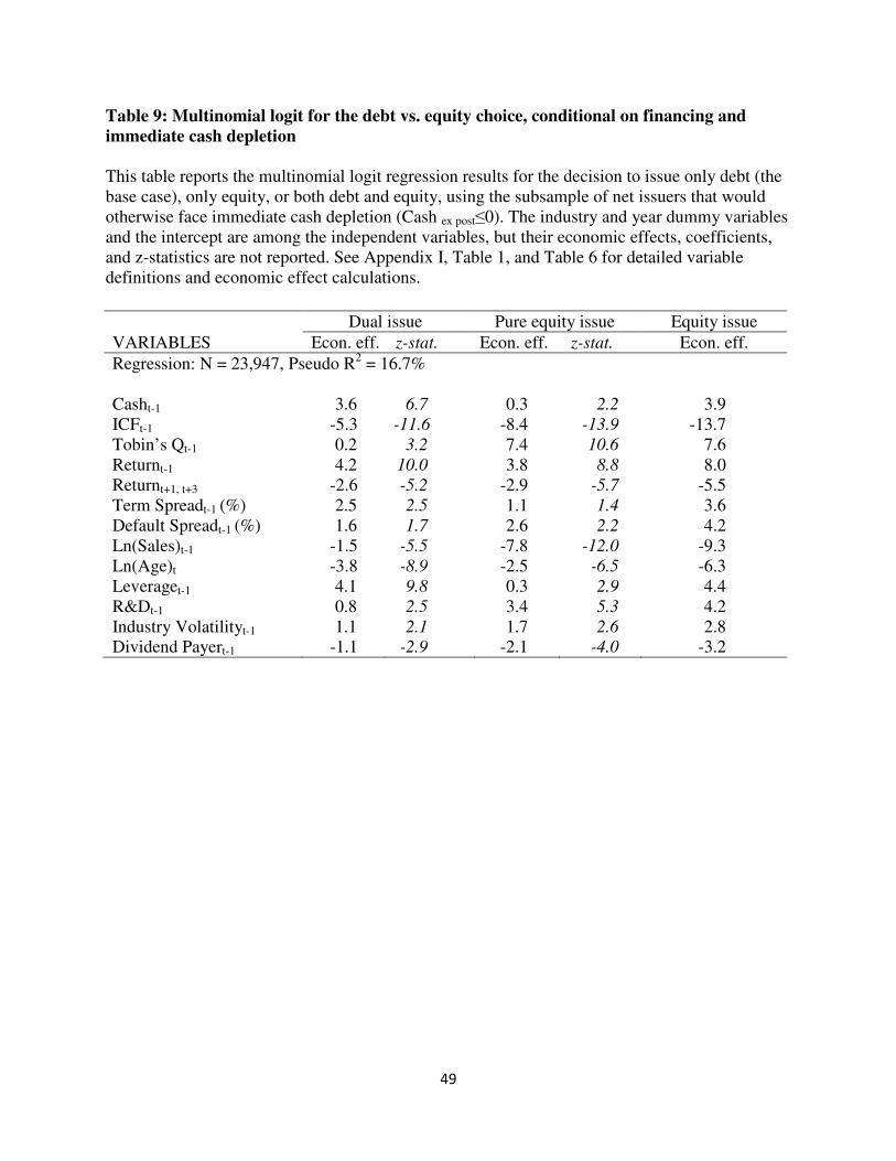
49
Table 9: Multinomial logit for the debt vs. equity choice, conditional on financing and
immediate cash depletion
This table reports the multinomial logit regression results for the decision to issue only debt (the base case), only equity, or both debt and equity, using the subsample of net issuers that would otherwise face immediate cash depletion (Cash ex post≤0). The industry and year dummy variables and the intercept are among the independent variables, but their economic effects, coefficients, and z-statistics are not reported. See Appendix I, Table 1, and Table 6 for detailed variable definitions and economic effect calculations.
Dual issue Pure equity issue Equity issue
VARIABLES Econ. eff. z-stat. Econ. eff. z-stat. Econ. eff.
Regression: N = 23,947, Pseudo R2 = 16.7%
Casht-1 3.6 6.7 0.3 2.2 3.9 ICFt-1 -5.3 -11.6 -8.4 -13.9 -13.7 Tobin’s Qt-1 0.2 3.2 7.4 10.6 7.6 Returnt-1 4.2 10.0 3.8 8.8 8.0 Returnt+1, t+3 -2.6 -5.2 -2.9 -5.7 -5.5 Term Spreadt-1 (%) 2.5 2.5 1.1 1.4 3.6 Default Spreadt-1 (%) 1.6 1.7 2.6 2.2 4.2 Ln(Sales)t-1 -1.5 -5.5 -7.8 -12.0 -9.3 Ln(Age)t -3.8 -8.9 -2.5 -6.5 -6.3 Leveraget-1 4.1 9.8 0.3 2.9 4.4 R&Dt-1 0.8 2.5 3.4 5.3 4.2 Industry Volatilityt-1 1.1 2.1 1.7 2.6 2.8 Dividend Payert-1 -1.1 -2.9 -2.1 -4.0 -3.2
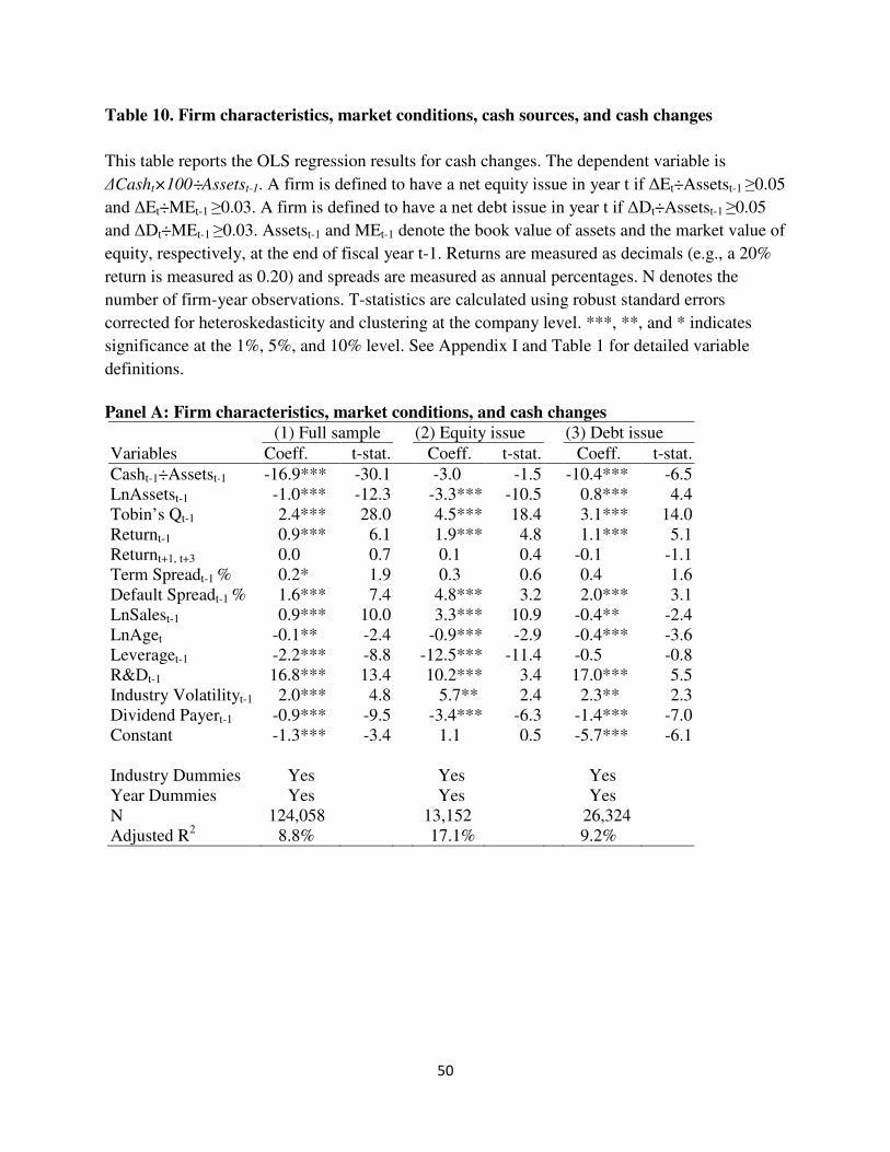
50
Table 10. Firm characteristics, market conditions, cash sources, and cash changes
This table reports the OLS regression results for cash changes. The dependent variable is
∆Casht×100÷Assetst-1. A firm is defined to have a net equity issue in year t if ∆Et÷Assetst-1 ≥0.05
and ∆Et÷MEt-1 ≥0.03. A firm is defined to have a net debt issue in year t if ∆Dt÷Assetst-1 ≥0.05
and ∆Dt÷MEt-1 ≥0.03. Assetst-1 and MEt-1 denote the book value of assets and the market value of
equity, respectively, at the end of fiscal year t-1. Returns are measured as decimals (e.g., a 20%
return is measured as 0.20) and spreads are measured as annual percentages. N denotes the
number of firm-year observations. T-statistics are calculated using robust standard errors
corrected for heteroskedasticity and clustering at the company level. ***, **, and * indicates
significance at the 1%, 5%, and 10% level. See Appendix I and Table 1 for detailed variable
definitions.
Panel A: Firm characteristics, market conditions, and cash changes
(1) Full sample (2) Equity issue (3) Debt issue
Variables Coeff. t-stat. Coeff. t-stat. Coeff. t-stat.
Casht-1÷Assetst-1 -16.9*** -30.1 -3.0 -1.5 -10.4*** -6.5 LnAssetst-1 -1.0*** -12.3 -3.3*** -10.5 0.8*** 4.4 Tobin’s Qt-1 2.4*** 28.0 4.5*** 18.4 3.1*** 14.0 Returnt-1 0.9*** 6.1 1.9*** 4.8 1.1*** 5.1 Returnt+1, t+3 0.0 0.7 0.1 0.4 -0.1 -1.1 Term Spreadt-1 % 0.2* 1.9 0.3 0.6 0.4 1.6 Default Spreadt-1 % 1.6*** 7.4 4.8*** 3.2 2.0*** 3.1 LnSalest-1 0.9*** 10.0 3.3*** 10.9 -0.4** -2.4 LnAget -0.1** -2.4 -0.9*** -2.9 -0.4*** -3.6 Leveraget-1 -2.2*** -8.8 -12.5*** -11.4 -0.5 -0.8 R&Dt-1 16.8*** 13.4 10.2*** 3.4 17.0*** 5.5 Industry Volatilityt-1 2.0*** 4.8 5.7** 2.4 2.3** 2.3 Dividend Payert-1 -0.9*** -9.5 -3.4*** -6.3 -1.4*** -7.0 Constant -1.3*** -3.4 1.1 0.5 -5.7*** -6.1 Industry Dummies Yes Yes Yes Year Dummies Yes Yes Yes N 124,058 13,152 26,324 Adjusted R2 8.8% 17.1% 9.2%
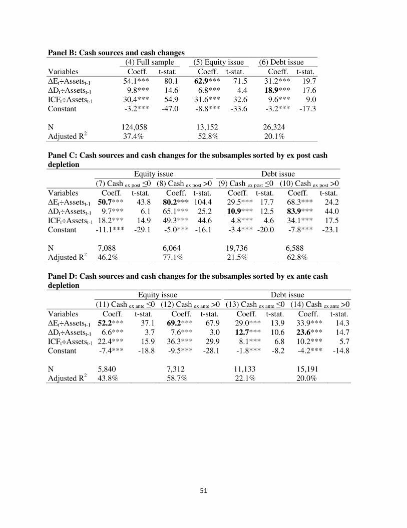
51
Panel B: Cash sources and cash changes
(4) Full sample (5) Equity issue (6) Debt issue
Variables Coeff. t-stat. Coeff. t-stat. Coeff. t-stat.
∆Et÷Assetst-1 54.1*** 80.1 62.9*** 71.5 31.2*** 19.7 ∆Dt÷Assetst-1 9.8*** 14.6 6.8*** 4.4 18.9*** 17.6 ICFt÷Assetst-1 30.4*** 54.9 31.6*** 32.6 9.6*** 9.0 Constant -3.2*** -47.0 -8.8*** -33.6 -3.2*** -17.3 N 124,058 13,152 26,324 Adjusted R2 37.4% 52.8% 20.1%
Panel C: Cash sources and cash changes for the subsamples sorted by ex post cash
depletion
Equity issue Debt issue
(7) Cash ex post ≤0 (8) Cash ex post >0 (9) Cash ex post ≤0 (10) Cash ex post >0
Variables Coeff. t-stat. Coeff. t-stat. Coeff. t-stat. Coeff. t-stat. ∆Et÷Assetst-1 50.7*** 43.8 80.2*** 104.4 29.5*** 17.7 68.3*** 24.2 ∆Dt÷Assetst-1 9.7*** 6.1 65.1*** 25.2 10.9*** 12.5 83.9*** 44.0 ICFt÷Assetst-1 18.2*** 14.9 49.3*** 44.6 4.8*** 4.6 34.1*** 17.5 Constant -11.1*** -29.1 -5.0*** -16.1 -3.4*** -20.0 -7.8*** -23.1 N 7,088 6,064 19,736 6,588 Adjusted R2 46.2% 77.1% 21.5% 62.8%
Panel D: Cash sources and cash changes for the subsamples sorted by ex ante cash
depletion
Equity issue Debt issue
(11) Cash ex ante ≤0 (12) Cash ex ante >0 (13) Cash ex ante ≤0 (14) Cash ex ante >0
Variables Coeff. t-stat. Coeff. t-stat. Coeff. t-stat. Coeff. t-stat. ∆Et÷Assetst-1 52.2*** 37.1 69.2*** 67.9 29.0*** 13.9 33.9*** 14.3 ∆Dt÷Assetst-1 6.6*** 3.7 7.6*** 3.0 12.7*** 10.6 23.6*** 14.7 ICFt÷Assetst-1 22.4*** 15.9 36.3*** 29.9 8.1*** 6.8 10.2*** 5.7 Constant -7.4*** -18.8 -9.5*** -28.1 -1.8*** -8.2 -4.2*** -14.8 N 5,840 7,312 11,133 15,191 Adjusted R2 43.8% 58.7% 22.1% 20.0%
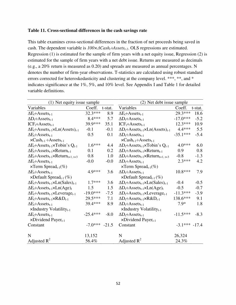
52
Table 11. Cross-sectional differences in the cash savings rate
This table examines cross-sectional differences in the fraction of net proceeds being saved in
cash. The dependent variable is 100×∆Casht÷Assetst-1. OLS regressions are estimated.
Regression (1) is estimated for the sample of firm years with a net equity issue, Regression (2) is
estimated for the sample of firm years with a net debt issue. Returns are measured as decimals
(e.g., a 20% return is measured as 0.20) and spreads are measured as annual percentages. N
denotes the number of firm-year observations. T-statistics are calculated using robust standard
errors corrected for heteroskedasticity and clustering at the company level. ***, **, and *
indicates significance at the 1%, 5%, and 10% level. See Appendix I and Table 1 for detailed
variable definitions.
(1) Net equity issue sample (2) Net debt issue sample
Variables Coeff. t-stat. Variables Coeff. t-stat.
∆Et÷Assetst-1 32.3*** 8.9 ∆Et÷Assetst-1 29.3*** 18.6 ∆Dt÷Assetst-1 8.4*** 5.7 ∆Dt÷Assetst-1 -17.0*** -5.2 ICFt÷Assetst-1 39.9*** 35.1 ICFt÷Assetst-1 12.3*** 10.9 ∆Et÷Assetst-1×Ln(Assets)t-1 -0.1 -0.1 ∆Dt÷Assetst-1×Ln(Assets)t-1 4.4*** 5.5 ∆Et÷Assetst-1
×Casht-1 ÷Assetst-1
0.5 0.1 ∆Dt÷Assetst-1
×Casht-1÷Assetst-1 -35.1*** -5.4
∆Et÷Assetst-1×Tobin’s Qt-1 1.6*** 4.4 ∆Dt÷Assetst-1×Tobin’s Qt-1 4.0*** 6.0 ∆Et÷Assetst-1×Returnt-1 0.1 0.2 ∆Dt÷Assetst-1×Returnt-1 0.9 0.8 ∆Et÷Assetst-1×Returnt+1, t+3 0.8 1.0 ∆Dt÷Assetst-1×Returnt+1, t+3 -0.8 -1.3 ∆Et÷Assetst-1
×Term Spreadt-1(%)
-0.0 -0.0 ∆Dt÷Assetst-1
×Term Spreadt-1(%) 2.3*** 4.2
∆Et÷Assetst-1
×Default Spreadt-1 (%)
4.9*** 3.6 ∆Dt÷Assetst-1
×Default Spreadt-1 (%) 10.8*** 7.9
∆Et÷Assetst-1×Ln(Sales)t-1 1.7*** 3.6 ∆Dt÷Assetst-1×Ln(Sales)t-1 -0.4 -0.5 ∆Et÷Assetst-1×Ln(Age)t 1.5 1.5 ∆Dt÷Assetst-1×Ln(Age)t -0.5 -0.7 ∆Et÷Assetst-1×Leveraget-1 -19.0*** -7.5 ∆Dt÷Assetst-1×Leveraget-1 -11.3*** -3.9 ∆Et÷Assetst-1×R&Dt-1 29.5*** 7.1 ∆Dt÷Assetst-1×R&Dt-1 138.6*** 9.1 ∆Et÷Assetst-1
×Industry Volatilityt-1 39.4*** 8.9 ∆Dt÷Assetst-1
×Industry Volatilityt-1 7.9* 1.8
∆Et÷Assetst-1
×Dividend Payert-1 -25.4*** -8.0 ∆Dt÷Assetst-1
×Dividend Payert-1 -11.5*** -8.3
Constant -7.0*** -21.5 Constant -3.1*** -17.4 N 13,152 N 26,324 Adjusted R2 56.4% Adjusted R2 24.3%
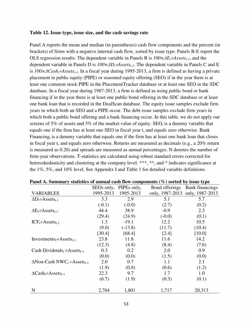
53
Table 12. Issue type, issue size, and the cash savings rate
Panel A reports the mean and median (in parentheses) cash flow components and the percent (in
brackets) of firms with a negative internal cash flow, sorted by issue type. Panels B-E report the
OLS regression results. The dependent variable in Panels B is 100×∆Et÷Assetst-1, and the
dependent variable in Panels D is 100×∆Dt÷Assetst-1. The dependent variable in Panels C and E
is 100×∆Casht÷Assetst-1. In a fiscal year during 1995-2013, a firm is defined as having a private
placement in public equity (PIPE) or seasoned equity offering (SEO) if in the year there is at
least one common stock PIPE in the PlacementTracker database or at least one SEO in the SDC
database. In a fiscal year during 1987-2013, a firm is defined as using public bond or bank
financing if in the year there is at least one public bond offering in the SDC database or at least
one bank loan that is recorded in the DealScan database. The equity issue samples exclude firm
years in which both an SEO and a PIPE occur. The debt issue samples exclude firm years in
which both a public bond offering and a bank financing occur. In this table, we do not apply our
screens of 5% of assets and 3% of the market value of equity. SEOt is a dummy variable that
equals one if the firm has at least one SEO in fiscal year t, and equals zero otherwise. Bank
Financingt is a dummy variable that equals one if the firm has at least one bank loan that closes
in fiscal year t, and equals zero otherwise. Returns are measured as decimals (e.g., a 20% return
is measured as 0.20) and spreads are measured as annual percentages. N denotes the number of
firm-year observations. T-statistics are calculated using robust standard errors corrected for
heteroskedasticity and clustering at the company level. ***, **, and * indicates significance at
the 1%, 5%, and 10% level. See Appendix I and Table 1 for detailed variable definitions.
Panel A. Summary statistics of annual cash flow components (%) sorted by issue type
VARIABLES
SEOs only, 1995-2013
PIPEs only, 1995-2013
Bond offerings only, 1987-2013
Bank financings only, 1987-2013
∆Dt÷Assetst-1 3.3 2.9 5.1 5.7 (-0.1) (-0.0) (2.7) (0.2) ∆Et÷Assetst-1 44.4 38.9 -0.9 2.3 (29.4) (24.9) (-0.0) (0.1) ICFt÷Assetst-1 1.3 -19.1 12.2 10.5 (9.0) (-13.8) (11.7) (10.4) [30.4] [68.4] [2.4] [10.0] Investmentst÷Assetst-1 23.8 11.8 11.6 14.2 (12.3) (4.8) (8.4) (7.6) Cash Dividendst ÷Assetst-1 0.3 0.2 2.0 0.9 (0.0) (0.0) (1.5) (0.0) ∆Non-Cash NWCt ÷Assetst-1 2.0 0.7 1.1 2.1 (1.9) (0.8) (0.6) (1.2) ∆Casht÷Assetst-1 22.3 9.7 1.7 1.0
(6.7) (1.9) (0.3) (0.1) N 2,764 1,801 1,717 20,313
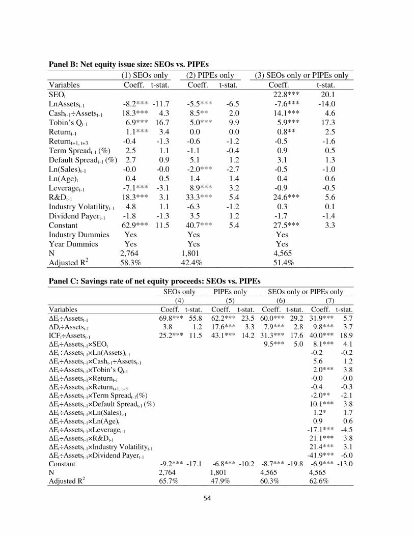
54
Panel B: Net equity issue size: SEOs vs. PIPEs
(1) SEOs only (2) PIPEs only (3) SEOs only or PIPEs only
Variables Coeff. t-stat. Coeff. t-stat. Coeff. t-stat.
SEOt 22.8*** 20.1 LnAssetst-1 -8.2*** -11.7 -5.5*** -6.5 -7.6*** -14.0 Casht-1÷Assetst-1 18.3*** 4.3 8.5** 2.0 14.1*** 4.6 Tobin’s Qt-1 6.9*** 16.7 5.0*** 9.9 5.9*** 17.3 Returnt-1 1.1*** 3.4 0.0 0.0 0.8** 2.5 Returnt+1, t+3 -0.4 -1.3 -0.6 -1.2 -0.5 -1.6 Term Spreadt-1 (%) 2.5 1.1 -1.1 -0.4 0.9 0.5 Default Spreadt-1 (%) 2.7 0.9 5.1 1.2 3.1 1.3 Ln(Sales)t-1 -0.0 -0.0 -2.0*** -2.7 -0.5 -1.0 Ln(Age)t 0.4 0.5 1.4 1.4 0.4 0.6 Leveraget-1 -7.1*** -3.1 8.9*** 3.2 -0.9 -0.5 R&Dt-1 18.3*** 3.1 33.3*** 5.4 24.6*** 5.6 Industry Volatilityt-1 4.8 1.1 -6.3 -1.2 0.3 0.1 Dividend Payert-1 -1.8 -1.3 3.5 1.2 -1.7 -1.4 Constant 62.9*** 11.5 40.7*** 5.4 27.5*** 3.3 Industry Dummies Yes Yes Yes Year Dummies Yes Yes Yes N 2,764 1,801 4,565 Adjusted R2 58.3% 42.4% 51.4%
Panel C: Savings rate of net equity proceeds: SEOs vs. PIPEs
SEOs only PIPEs only SEOs only or PIPEs only
(4) (5) (6) (7)
Variables Coeff. t-stat. Coeff. t-stat. Coeff. t-stat. Coeff. t-stat.
∆Et÷Assetst-1 69.8*** 55.8 62.2*** 23.5 60.0*** 29.2 31.9*** 5.7 ∆Dt÷Assetst-1 3.8 1.2 17.6*** 3.3 7.9*** 2.8 9.8*** 3.7 ICFt÷Assetst-1 25.2*** 11.5 43.1*** 14.2 31.3*** 17.6 40.0*** 18.9 ∆Et÷Assetst-1×SEOt 9.5*** 5.0 8.1*** 4.1 ∆Et÷Assetst-1×Ln(Assets)t-1 -0.2 -0.2 ∆Et÷Assetst-1×Casht-1÷Assetst-1 5.6 1.2 ∆Et÷Assetst-1×Tobin’s Qt-1 2.0*** 3.8 ∆Et÷Assetst-1×Returnt-1 -0.0 -0.0 ∆Et÷Assetst-1×Returnt+1, t+3 -0.4 -0.3 ∆Et÷Assetst-1×Term Spreadt-1(%) -2.0** -2.1 ∆Et÷Assetst-1×Default Spreadt-1 (%) 10.1*** 3.8 ∆Et÷Assetst-1×Ln(Sales)t-1 1.2* 1.7 ∆Et÷Assetst-1×Ln(Age)t 0.9 0.6 ∆Et÷Assetst-1×Leveraget-1 -17.1*** -4.5 ∆Et÷Assetst-1×R&Dt-1 21.1*** 3.8 ∆Et÷Assetst-1×Industry Volatilityt-1 21.4*** 3.1 ∆Et÷Assetst-1×Dividend Payert-1 -41.9*** -6.0 Constant -9.2*** -17.1 -6.8*** -10.2 -8.7*** -19.8 -6.9*** -13.0 N 2,764 1,801 4,565 4,565 Adjusted R2 65.7% 47.9% 60.3% 62.6%
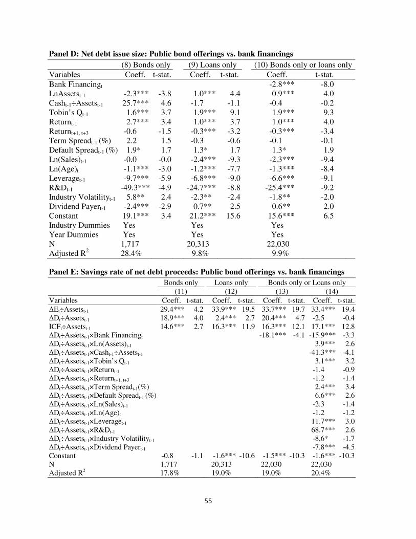
55
Panel D: Net debt issue size: Public bond offerings vs. bank financings
(8) Bonds only (9) Loans only (10) Bonds only or loans only
Variables Coeff. t-stat. Coeff. t-stat. Coeff. t-stat.
Bank Financingt -2.8*** -8.0 LnAssetst-1 -2.3*** -3.8 1.0*** 4.4 0.9*** 4.0 Casht-1÷Assetst-1 25.7*** 4.6 -1.7 -1.1 -0.4 -0.2 Tobin’s Qt-1 1.6*** 3.7 1.9*** 9.1 1.9*** 9.3 Returnt-1 2.7*** 3.4 1.0*** 3.7 1.0*** 4.0 Returnt+1, t+3 -0.6 -1.5 -0.3*** -3.2 -0.3*** -3.4 Term Spreadt-1 (%) 2.2 1.5 -0.3 -0.6 -0.1 -0.1 Default Spreadt-1 (%) 1.9* 1.7 1.3* 1.7 1.3* 1.9 Ln(Sales)t-1 -0.0 -0.0 -2.4*** -9.3 -2.3*** -9.4 Ln(Age)t -1.1*** -3.0 -1.2*** -7.7 -1.3*** -8.4 Leveraget-1 -9.7*** -5.9 -6.8*** -9.0 -6.6*** -9.1 R&Dt-1 -49.3*** -4.9 -24.7*** -8.8 -25.4*** -9.2 Industry Volatilityt-1 5.8** 2.4 -2.3** -2.4 -1.8** -2.0 Dividend Payert-1 -2.4*** -2.9 0.7** 2.5 0.6** 2.0 Constant 19.1*** 3.4 21.2*** 15.6 15.6*** 6.5 Industry Dummies Yes Yes Yes Year Dummies Yes Yes Yes N 1,717 20,313 22,030 Adjusted R2 28.4% 9.8% 9.9%
Panel E: Savings rate of net debt proceeds: Public bond offerings vs. bank financings
Bonds only Loans only Bonds only or Loans only
(11) (12) (13) (14)
Variables Coeff. t-stat. Coeff. t-stat. Coeff. t-stat. Coeff. t-stat.
∆Et÷Assetst-1 29.4*** 4.2 33.9*** 19.5 33.7*** 19.7 33.4*** 19.4 ∆Dt÷Assetst-1 18.9*** 4.0 2.4*** 2.7 20.4*** 4.7 -2.5 -0.4 ICFt÷Assetst-1 14.6*** 2.7 16.3*** 11.9 16.3*** 12.1 17.1*** 12.8 ∆Dt÷Assetst-1×Bank Financingt -18.1*** -4.1 -15.9*** -3.3 ∆Dt÷Assetst-1×Ln(Assets)t-1 3.9*** 2.6 ∆Dt÷Assetst-1×Casht-1÷Assetst-1 -41.3*** -4.1 ∆Dt÷Assetst-1×Tobin’s Qt-1 3.1*** 3.2 ∆Dt÷Assetst-1×Returnt-1 -1.4 -0.9 ∆Dt÷Assetst-1×Returnt+1, t+3 -1.2 -1.4 ∆Dt÷Assetst-1×Term Spreadt-1(%) 2.4*** 3.4 ∆Dt÷Assetst-1×Default Spreadt-1 (%) 6.6*** 2.6 ∆Dt÷Assetst-1×Ln(Sales)t-1 -2.3 -1.4 ∆Dt÷Assetst-1×Ln(Age)t -1.2 -1.2 ∆Dt÷Assetst-1×Leveraget-1 11.7*** 3.0 ∆Dt÷Assetst-1×R&Dt-1 68.7*** 2.6 ∆Dt÷Assetst-1×Industry Volatilityt-1 -8.6* -1.7 ∆Dt÷Assetst-1×Dividend Payert-1 -7.8*** -4.5 Constant -0.8 -1.1 -1.6*** -10.6 -1.5*** -10.3 -1.6*** -10.3 N 1,717 20,313 22,030 22,030 Adjusted R2 17.8% 19.0% 19.0% 20.4%