Embed Size (px)
Citation preview
8/6/2019 Corporate Finance Lecture
http://slidepdf.com/reader/full/corporate-finance-lecture 1/125
8/6/2019 Corporate Finance Lecture
http://slidepdf.com/reader/full/corporate-finance-lecture 2/125
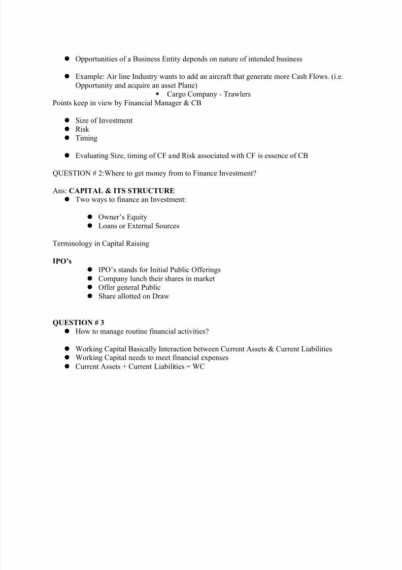
Opportunities of a Business Entity depends on nature of intended business
Example: Air line Industry wants to add an aircraft that generate more Cash Flows. (i.e.Opportunity and acquire an asset Plane)
Cargo Company - TrawlersPoints keep in view by Financial Manager & CB
Size of Investment Risk Timing
Evaluating Size, timing of CF and Risk associated with CF is essence of CB
QUESTION # 2:Where to get money from to Finance Investment?
Ans: CAP
IT
AL & IT
S ST
RUCT
URE Two ways to finance an Investment:
Owner¶s Equity Loans or External Sources
Terminology in Capital Raising
IPO¶s IPO¶s stands for Initial Public Offerings Company lunch their shares in market Offer general Public Share allotted on Draw
QUESTION # 3 How to manage routine financial activities?
Working Capital Basically Interaction between Current Assets & Current Liabilities Working Capital needs to meet financial expenses Current Assets + Current Liabilities = WC
8/6/2019 Corporate Finance Lecture
http://slidepdf.com/reader/full/corporate-finance-lecture 3/125
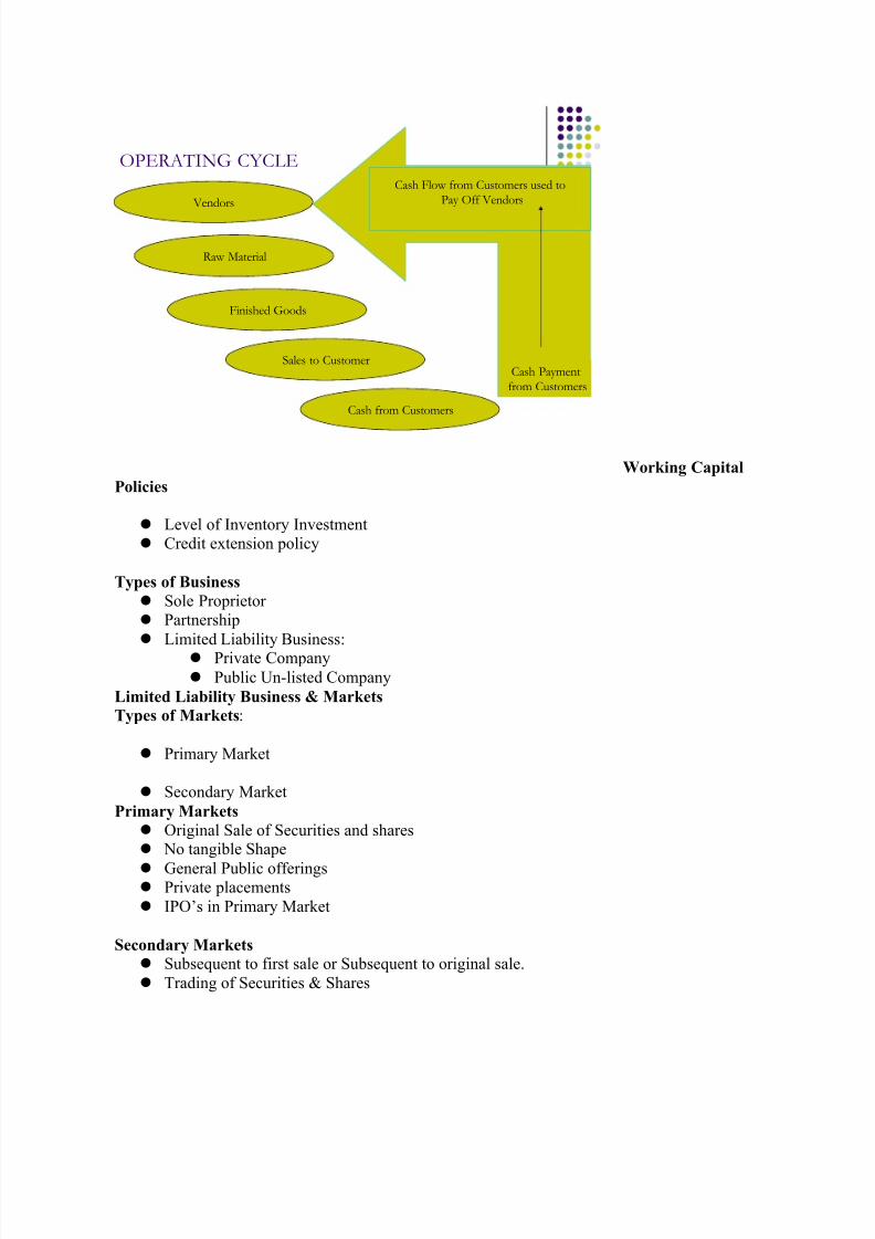
Vendors
Finished Goods
Raw Material
Cash from Customers
Sales to Customer
OPERATING CYCLE
Cash Flow from Customers used to
Pay Off Vendors
Cash Payment
from Customers
Working CapitalPolicies
Level of Inventory Investment Credit extension policy
Types of Business Sole Proprietor Partnership Limited Liability Business:
Private Company Public Un-listed Company
Limited Liability Business & MarketsTypes of Markets:
Primary Market
Secondary MarketPrimary Markets
Original Sale of Securities and shares
No tangible Shape General Public offerings Private placements IPO¶s in Primary Market
Secondary Markets Subsequent to first sale or Subsequent to original sale. Trading of Securities & Shares
8/6/2019 Corporate Finance Lecture
http://slidepdf.com/reader/full/corporate-finance-lecture 4/125
Tangible Markets Example stock Exchange
FINANCIAL STATEMENTS &COR PORATE FINANCE
THREE BASIC STATEMENTS
BALANCE SHEET INCOME STATEMENT CASH FLOW STATEMENT
BALANCE SHEET
Is a Statement of resources controlled by the business entity and obligations on a specificdate.
Contents of Balance Sheet
Assets = Fixed (tangible & intangible)& current assets
Liabilities = Long Term Liability + Current Or Short Term Liability Equity = shareholders¶ contribution + earnings
Fixed Assets: Earning assets Fixed Assets e.g. Plant, Machinery, Vehicles etc
Current Assets: Inventory, Prepayments, Cash & Bank Balance, Short Term Investment etc
Balance Sheet Format
Format of B/S in Pakistan is Governed by International Financial Reporting Standard or International Accounting Standard
B/S construction is Non-liquid or Illiquid Asset is at top
Two Conventions for B/S Construction
1st as in Pakistan IAS or IFRS 2nd Convention GAAP (General Accepted Accounting Principle) applicable in United
States GAAP ± In B/S top item is highly liquid asset i.e. cash or near money
Current Liabilities ingredients
Creditor, Accrued Liabilities, Short Term Finances Current Assets combine Current liabilities equal Working Capital
Liquidity
Conversion into cash without losing its value. Timing Loss of value

8/6/2019 Corporate Finance Lecture
http://slidepdf.com/reader/full/corporate-finance-lecture 5/125
Example: Bonds
Equity & Long Term Liabilities Equity
Paid up Capital
Reserves Profit & Loss Long Term Liabilities
Loans OR Financial Leverage
8/6/2019 Corporate Finance Lecture
http://slidepdf.com/reader/full/corporate-finance-lecture 6/125
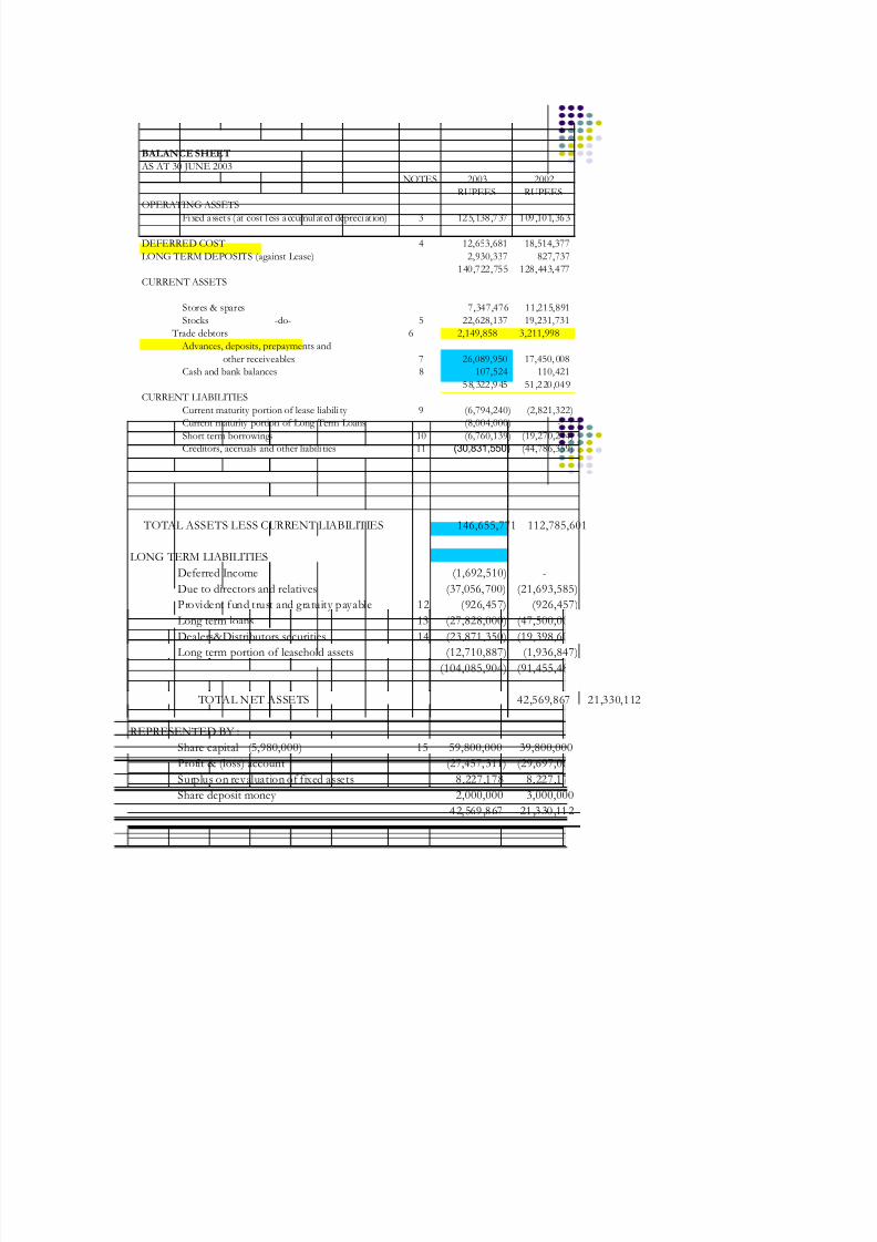
BALANCE SHEET
AS AT 30 JUNE 2003
NOTES 2003 2002
RUPEES RUPEES
OPERATING ASSETS
Fixed asset s ( at cost l ess accumulated depreci at ion) 3 125,138 ,737 109 ,101,363
DEFERRED COST 4 12,653,681 18,514,377
LONG TERM DEPOSITS (against Lease) 2,930,337 827,737
140,722,755 128,443,477
CURRENT ASSETS
Stores & spares 7,347,476 11,215,891
Stocks -do- 5 22,628,137 19,231,731
Trade debtors 6 2,149,858 3,211,998
Advances, deposits, prepayments and
other receiveables 7 26,089,950 17,450, 008
Cash and bank balances 8 107,524 110,421
58,322 ,945 51 ,220 ,049
CURRENT LIABILITIES
Current maturity portion of lease liabili ty 9 (6,794,240) (2,821,322)
Current maturity portion of Long Term Loans (8,004,000) - Short term borrowings 10 (6,760,139) (19,270,244)
Creditors, accruals and other liabili ties 11 (30,831,550) (44,786,359)
TOTAL ASSETS LESS CURRENT LIABILITIES 146,655,771 112,785,601
LONG TERM LIABILITIES
Deferred Income (1,692,510) -
Due to directors and relatives (37,056,700) (21,693,585)
Provident fund trust and gratuity payable 12 (926,457) (926,457)
Long term loans 13 (27,828,000) (47,500,000)
Dealers&Distributors securities 14 (23,871,350) (19,398,600) Long term portion of leasehold assets (12,710,887) (1,936,847)
(104,085,904) (91,455,489)
TOTAL NET ASSETS 42,569,867 21,330,112
REPRESENTED BY :
Share capital (5,980,000) 15 59,800,000 39,800,000
Profit & (loss) account (27,457,311) (29,697,066)
Surplus on revaluation of fixed assets 8,227,178 8,227,178
Share deposit money 2,000,000 3,000,000
42,569 ,867 21 ,330 ,112
8/6/2019 Corporate Finance Lecture
http://slidepdf.com/reader/full/corporate-finance-lecture 7/125
Corporate finance lecture No. 02
FINANCIAL STATEMENT &COR PORATE FINANCE
Management to Corporate Finance
Market Value Book Value
Market Value Negotiation or Dealing at Arm Length Contrary to Market Value financial statements are prepared on Book Value Book Value is not reflective of worth of assets.
Book Value
Cost minus Accumulated DepreciationIncome Statement
Work out Profit Three Terminologies interchangeably used
Sales Turnovers Revenues
In Profit Statement line item vary Organization to Organization , Industry toIndustry, there is no Rule of Thumb
Revenue ± Expenses = Profit Cash Flow Statement Generation of cash from different activities and its application Three Broad segment Operating Cash Flows Investing Cash Flows Financing cash flows
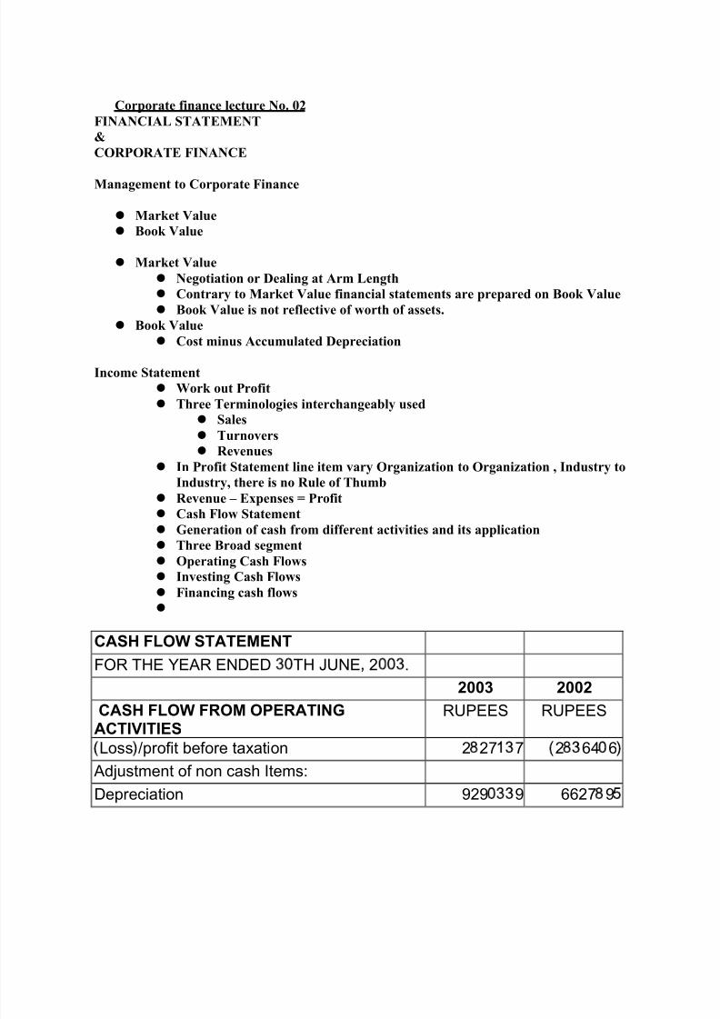
CASH FLOW STATEMENT
FOR THE YEAR ENDED TH JUNE 2 .
2003 2002 CASH FLOW FROM OPERATINGACTIVITIES
RUPEES RUPEES
Loss /profit before taxation 2 27 7 2 64 6
Adjustment of non cash Items:
Depreciation 929 9 6627 9
8/6/2019 Corporate Finance Lecture
http://slidepdf.com/reader/full/corporate-finance-lecture 8/125
8/6/2019 Corporate Finance Lecture
http://slidepdf.com/reader/full/corporate-finance-lecture 9/125
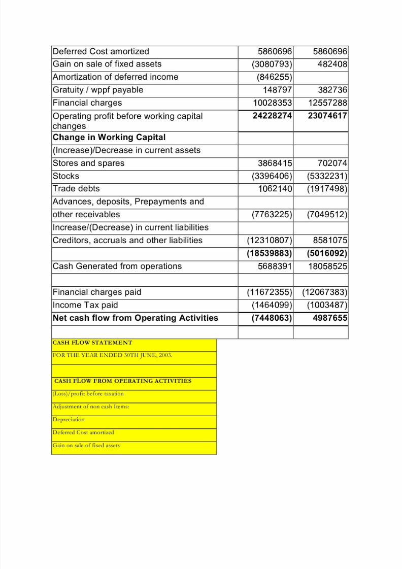
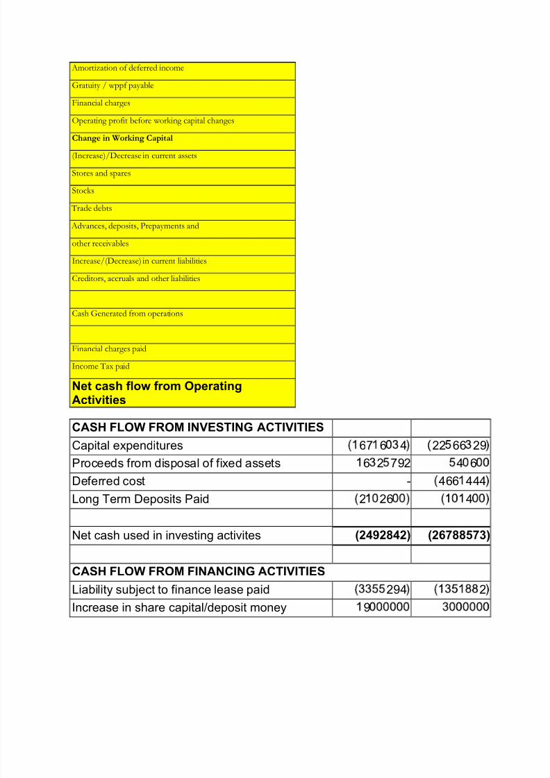
Amortization of deferred income
Gratuity / wppf payable
Financial charges
Operating prof it before work ing capital changes
Change in Working Capital
(Increase)/Decrease in current assets
Stores and spares
Stocks
Trade debts
Advances, deposits, Prepayments and
other recei vables
Increase/(Decrease) in current liabilitiesCreditors, accruals and other liabilities
Cash Generated from operations
Financial charges paid
Income Tax paid
Net cash flow from Operating
Activities
CASH FLOW FROM INVESTING ACTIVITIES
Capital expenditures 67 6 4 22 66 29
Proceeds from disposal of fixed assets 6 2 792 4 6
Deferred cost - 466 444
Long Term Deposits Paid 2 26 4
Net cash used in investing activites (2492842) (26788573)
CASH FLOW FROM FINANCING ACTIVITIES
Liability subject to finance lease paid 294 2
Increase in share capital/deposit money 9
8/6/2019 Corporate Finance Lecture
http://slidepdf.com/reader/full/corporate-finance-lecture 10/125
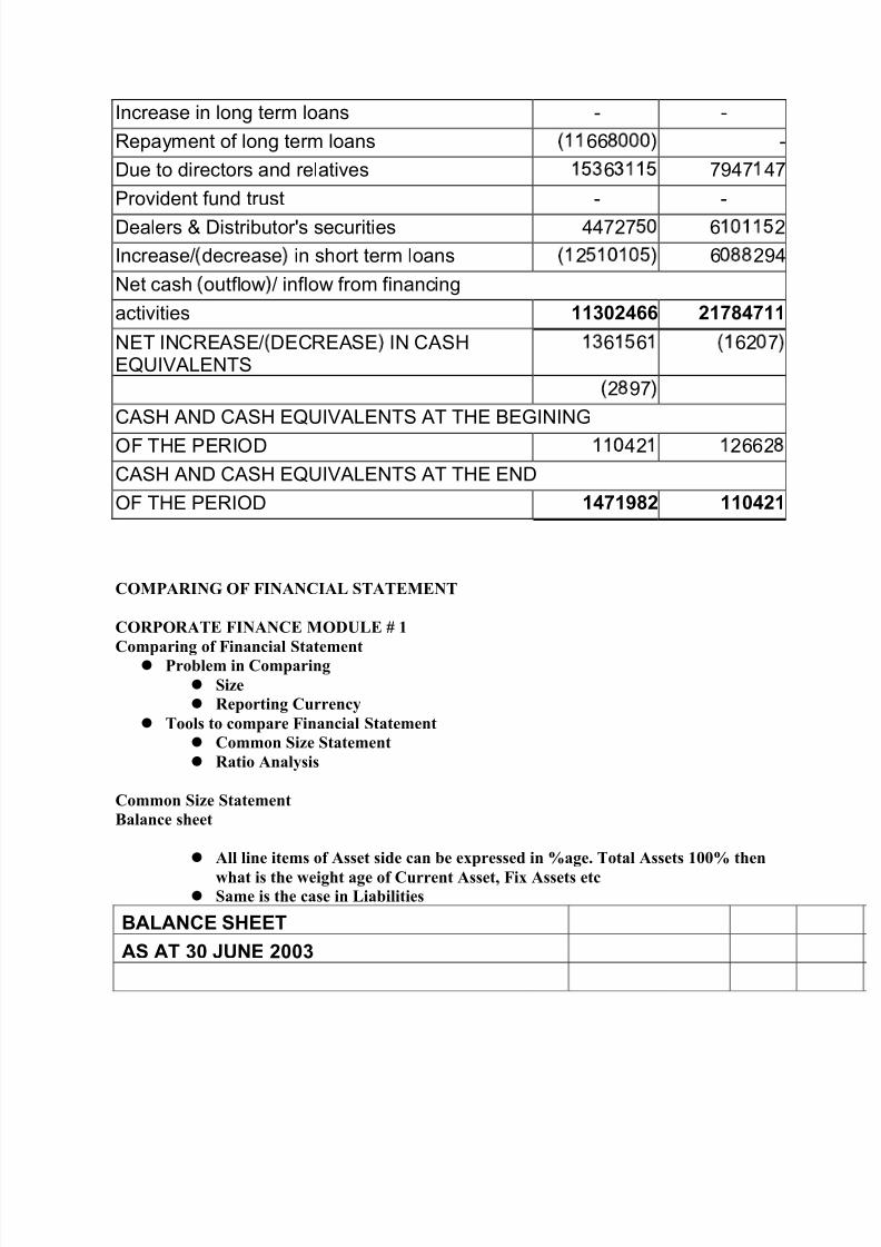
Increase in long term loans - -
Repayment of long term loans 66 -
Due to directors and relatives 6 7947 47
Provident fund trust - -
Dealers & Distributor's securities 44727 6 2
Increase/ decrease in short term loans 2 6 294
Net cash outflow / inflow from financing
activities 11302466 21784711
NET INCREASE/ DECREASE IN CASHEQUIVALENTS
6 6 62 7
2 97
CASH AND CASH EQUIVALENTS AT THE BEGININGOF THE PERIOD 42 2662
CASH AND CASH EQUIVALENTS AT THE END
OF THE PERIOD 1471982 110421
COMPARING OF FINANCIAL STATEMENT
COR PORATE FINANCE MODULE # 1Comparing of Financial Statement
Problem in Comparing Size Reporting Currency
Tools to compare Financial Statement Common Size Statement Ratio Analysis
Common Size StatementBalance sheet
All line items of Asset side can be expressed in %age. Total Assets 100% thenwhat is the weight age of Current Asset, Fix Assets etc
Same is the case in Liabilities
BALANCE SHEET
AS AT 30 JUNE 2003
8/6/2019 Corporate Finance Lecture
http://slidepdf.com/reader/full/corporate-finance-lecture 11/125
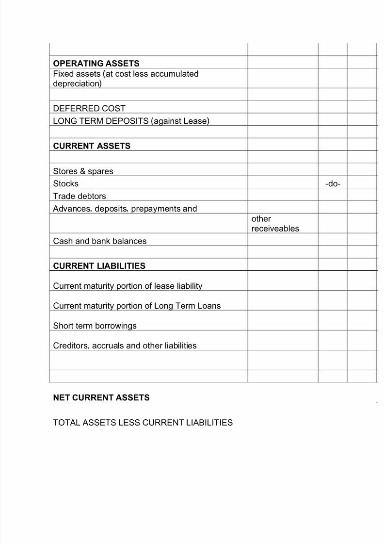
OPERATING ASSETS
Fixed assets at cost less accumulateddepreciation
DEFERRED COST
LONG TERM DEPOSITS against Lease
CURRENT ASSETS
Stores & spares
Stocks -do-Trade debtors
Advances deposits prepayments and
other receiveables
Cash and bank balances
CURRENT LIABILITIES
Current maturity portion of lease liability
Current maturity portion of Long Term Loans
Short term borrowings
Creditors accruals and other liabilities
NET CURRENT ASSETS
TOTAL ASSETS LESS CURRENT LIABILITIES
8/6/2019 Corporate Finance Lecture
http://slidepdf.com/reader/full/corporate-finance-lecture 12/125
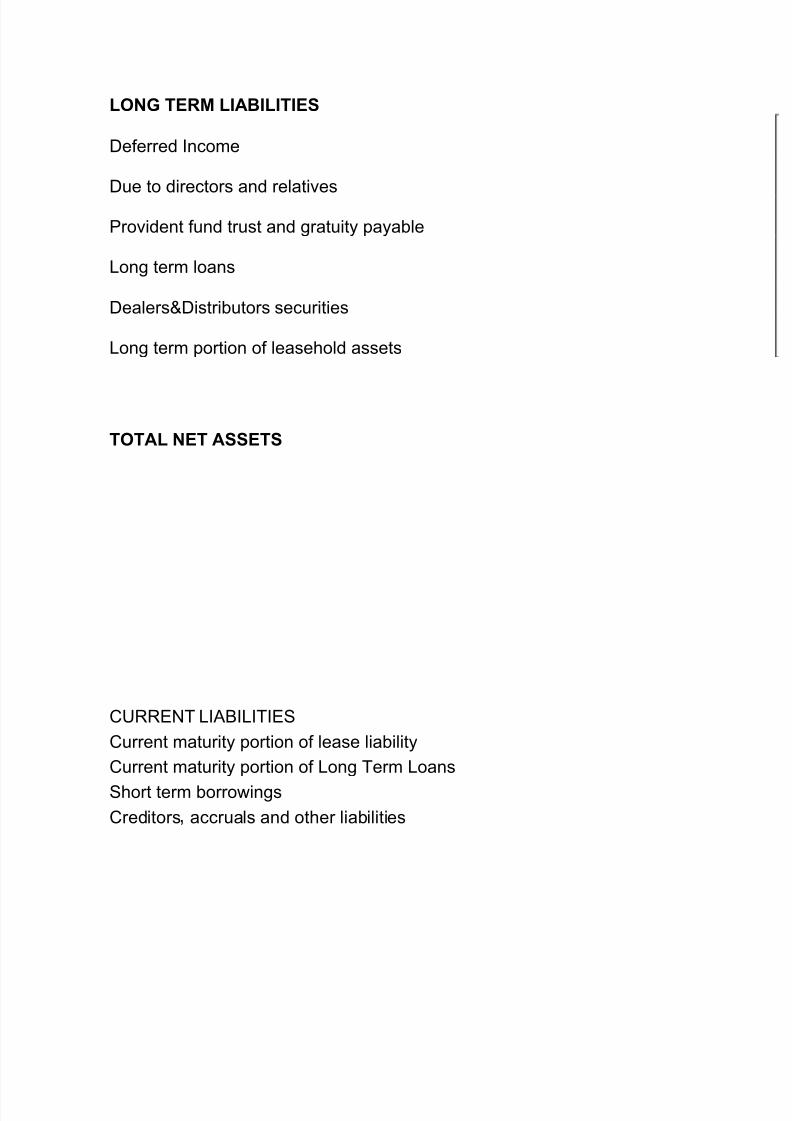
LONG TERM LIABILITIES
Deferred Income
Due to directors and relatives
Provident fund trust and gratuity payable
Long term loans
Dealers&Distributors securities
Long term portion of leasehold assets
TOTAL NET ASSETS
CURRENT LIABILITIES
Current maturity portion of lease liability
Current maturity portion of Long Term LoansShort term borrowings
Creditors accruals and other liabilities
8/6/2019 Corporate Finance Lecture
http://slidepdf.com/reader/full/corporate-finance-lecture 13/125
NET CURRENT ASSETS
TOTAL ASSETS LESS CURRENT LIABILITIES
LONG TERM LIABILITIES
Deferred Income
Due to directors and relatives
Provident fund trust and gratuity payable
Long term loans
Dealers&Distributors securities
Long term portion of leasehold assets
TOTAL NET ASSETS
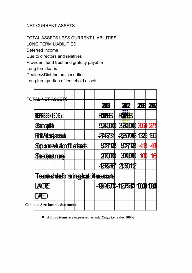
2003 2002 2003 2002
REPRESENTED BY : RUPEES RUPEES
Sharecapital 9 9 422
Profit &loss account -2747 -2969766 79 6Surplusonrevaluationof fiedassets 2277 2277 4 4
Sharedeposit money 2 6
426967 2 2
Theanneednotesformanintegral part of theseaccounts
LAORE -9947 - 27 6 100.00100.0DATED
Common Size Income Statement
All line items are expressed as sale %age i.e. Sales 100%
8/6/2019 Corporate Finance Lecture
http://slidepdf.com/reader/full/corporate-finance-lecture 14/125
2003 2002 2003 2002
RS. RS. RS. RS.
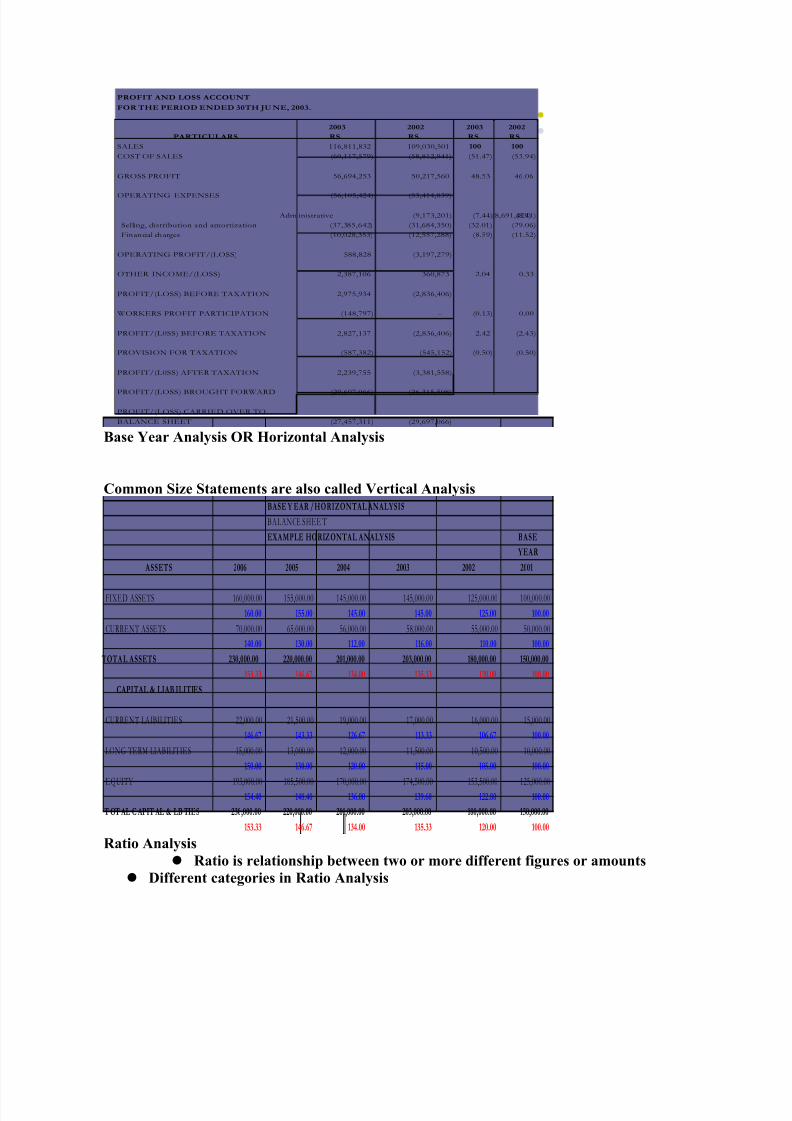
116,811,832 109,030,501 100 100
(60,117,579) (58,812,941) (51.47) (53.94)
56,694,253 50,217,560 48.53 46.06
(56,105,424) (53,414,839)
Adm inistrative (8,691,429)(9,173,201) (7.44) (8.41)
Selling, distribution and amortization (37,385,642) (31,684,350) (32.01) (29.06)
Financial charges (10,028,353) (12,557,288) (8.59) (11.52)
588,828 (3,197,279)
2,387,106 360,873 2.04 0.33
2,975,934 (2,836,406)
(148,797) - (0.13) 0.00
2,827,137 (2,836,406) 2.42 (2.43)
(587,382) (545,152) (0.50) (0.50)
2,239,755 (3,381,558)
(29,697,066) (26,315,508)
(27,457,311) (29,697,066)
PROFIT AND LOSS ACCOUNT
FOR THE PERIOD ENDED 30TH JU NE, 2003.
SALES
COST OF SALES
PARTICULARS
GROSS PROFIT
OPERATING EXPENSES
OPERATING PROFIT/(LOSS)
OTHER INCOME/(LOSS)
PROFIT/(LOSS) BEFORE TAXATION
PROFIT/(LOSS) BROUGHT FORWARD
PROFIT/(LOSS) CARRIED OVER TO
BALANCE SHEET
WORKERS PROFIT PARTICIPATION
PROFIT/(L0SS) BEFORE TAXATION
PROVISION FOR TAXATION
PROFIT/(L0SS) AFTER TAXATION
Base Year Analysis OR Horizontal Analysis
Common Size Statements are also called Vertical AnalysisBASE Y EAR /HORIZONTAL ANALYSIS
BALANCE SHEE T
EXAMPLE HORIZONTAL ANALYSIS BASE
YEAR
ASSETS 2006 2005 2004 2003 2002 2001
FIXED ASSETS 160,000.00 155,000.00 145,000.00 145,000.00 125,000.00 100,000.00
160.00 155.00 145.00 145.00 125.00 100.00
CURRENT ASSETS 70,000.00 65,000.00 56,000.00 58,000.00 55,000.00 50,000.00
140.00 130.00 112.00 116.00 110.00 100.00
TOTAL ASSETS 230,000.00 220,000.00 201,000.00 203,000.00 180,000.00 150,000.00
153.33 146.67 134.00 135.33 120.00 100.00
CAPITAL & LIAB ILITIES
CURRENT LAIBILITIES 22,000.00 21,500.00 19,000.00 17,000.00 16,000.00 15,000.00
146.67 143.33 126.67 113.33 106.67 100.00
LONG TERM LIABILITIES 15,000.00 13,000.00 12,000.00 11,500.00 10,500.00 10,000.00
150.00 130.00 120.00 115.00 105.00 100.00
EQUITY 193,000.00 185,500.00 170,000.00 174,500.00 153,500.00 125,000.00
154.40 148.40 136.00 139.60 122.80 100.00
T OT AL C APIT AL & LB TIES 230,000.00 220,000.00 201,000.00 203,000.00 180,000.00 150,000.00
153.33 146.67 134.00 135.33 120.00 100.00
Ratio Analysis Ratio is relationship between two or more different figures or amounts
Different categories in Ratio Analysis
8/6/2019 Corporate Finance Lecture
http://slidepdf.com/reader/full/corporate-finance-lecture 15/125
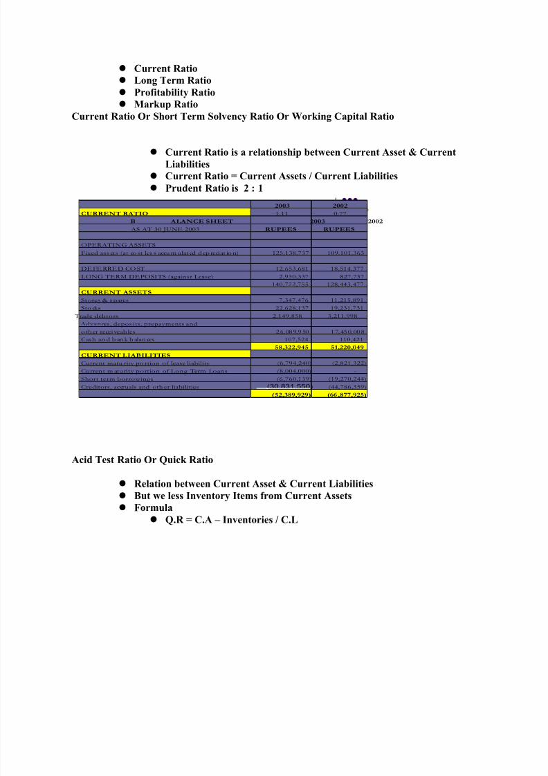
Current Ratio Long Term Ratio Profitability Ratio Markup Ratio
Current Ratio Or Short Term Solvency Ratio Or Working Capital Ratio
Current Ratio is a relationship between Current Asset & CurrentLiabilities
Current Ratio = Current Assets / Current Liabilities Prudent Ratio is 2 : 1
2003 2002
CURRENT RATIO 1.11 0.77
B ALANCE SHEET 2003 2002
AS AT 30 JUNE 2003 RUPEES RUPEES
OPERATING ASSETS
Fixed ass ets (at co st les s accu m ulat ed d ep reciat io n) 125,138,737 109,101,363
DEFERRED COST 12,653,681 18,514,377
LONG TERM DEPOSITS (against Lease) 2,930,337 827,737
140,722,755 128,443,477
CURRENT ASSETS
Stores & s pares 7,347,476 11,215,891
Sto cks 22,628,137 19,231,731
Trade debtors 2,149,858 3,211,998
Advances, depos its, prepayments and
other receiveab les 26,089,950 17,450,008
Cash an d b an k b alan ces 107,524 110,421
58,322,945 51,220,049
CURRENT LIA BILITIES
Current matu rity po rtion of lease liability (6,794,240) (2,821,322)
Current m aturity portion of Long Term Loans (8,004,000) -
Short term borrowings (6,760,139) (19,270,244)
Creditors, accruals and oth er liabilities (30,831,550) (44,786,359)
(52,389,929) (66 ,877,925)
Acid Test Ratio Or Quick Ratio
Relation between Current Asset & Current Liabilities But we less Inventory Items from Current Assets Formula
Q.R = C.A ± Inventories / C.L
8/6/2019 Corporate Finance Lecture
http://slidepdf.com/reader/full/corporate-finance-lecture 16/125
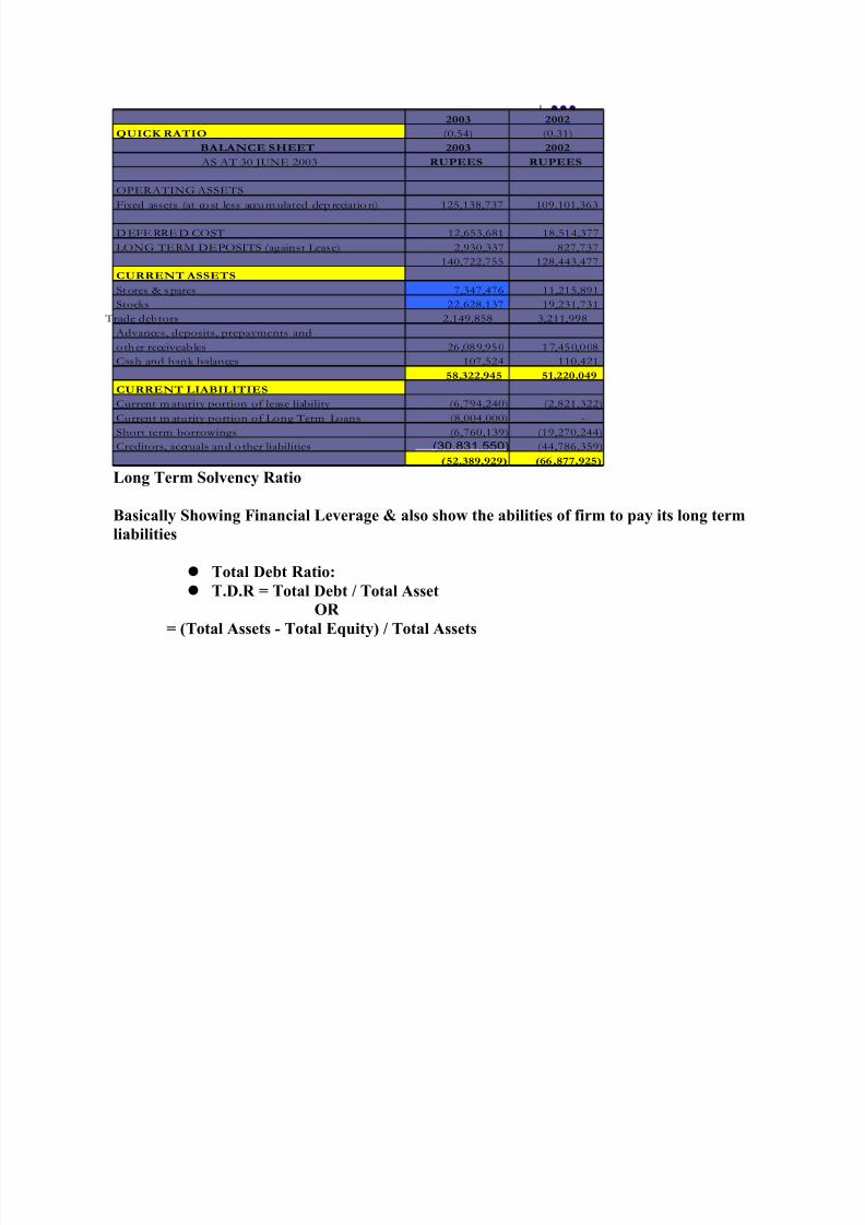
2003 2002
QUICK RATIO (0.54) (0.31)
BALANCE SHEET 2003 2002
AS AT 30 JUNE 2003 RUPEES RUPEES
OPERATING ASSETS
Fixed assets (at co st less accu m ulated dep reciatio n) 125,138,737 109,101,363
D EFE RRE D COST 12,653,681 18,514,377
LONG TERM DEPOSITS (against Lease) 2,930,337 827,737
140,722,755 128,443,477
CURRENT ASSETS
Stores & spares 7,347,476 11,215,891
Stocks 22,628,137 19,231,731
Trade debtors 2,149,858 3,211,998
Advances, deposits, prepayments and
other receiveables 26,089,950 17,450,008
Cash and bank balances 107,524 110,421
58,322,945 51,220,049
CURRENT LIABILITIES
Current m aturity portion of lease liability (6,794,240) (2,821,322)
Current m aturity portion of Long Term Loans (8,004,000) - Short term borrowings (6,760,139) (19,270,244)
Creditors, accruals and o ther liabilities (30,831,550) (44,786,359)
(52,389,929) (66 ,877,925)
Long Term Solvency Ratio
Basically Showing Financial Leverage & also show the abilities of firm to pay its long termliabilities
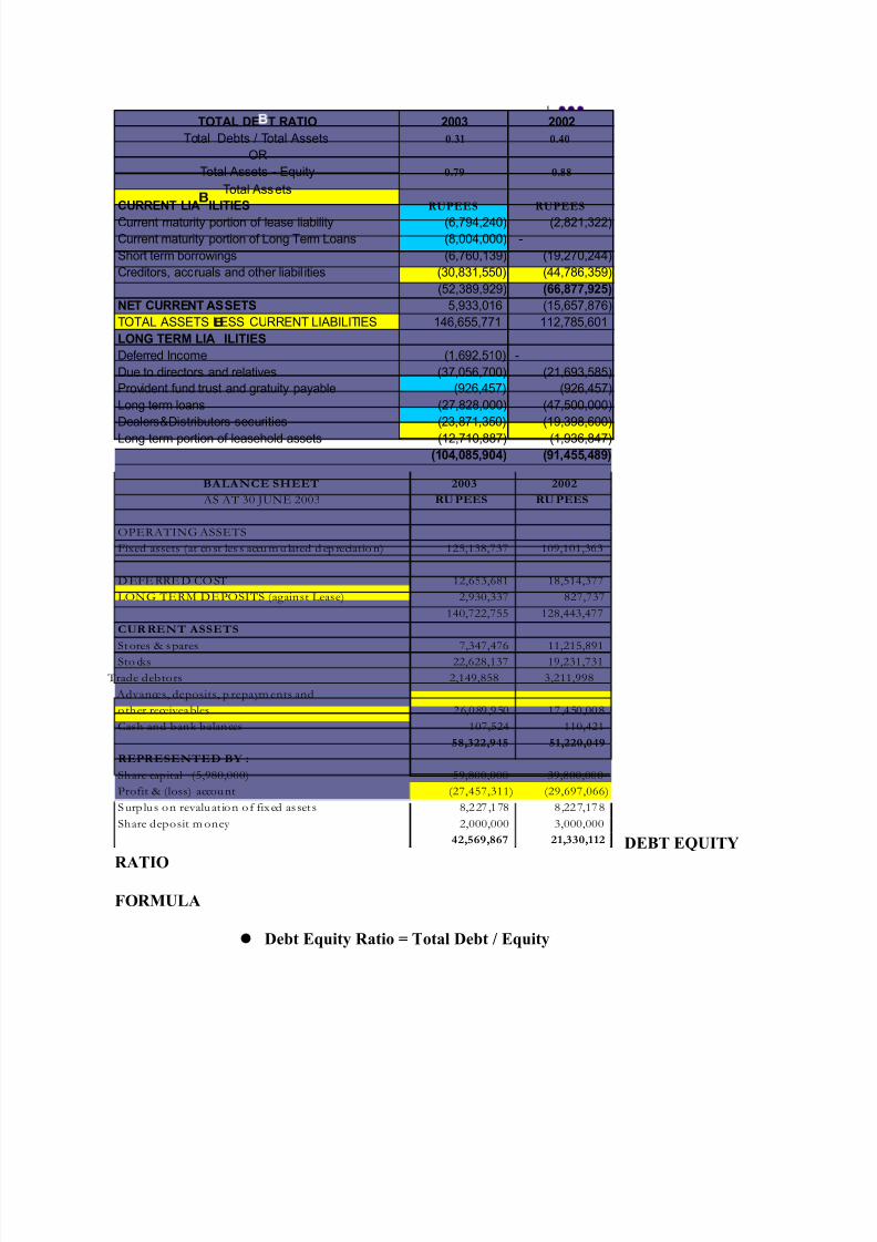
Total Debt Ratio: T.D.R = Total Debt / Total Asset
OR
= (Total Assets - Total Equity) / Total Assets
8/6/2019 Corporate Finance Lecture
http://slidepdf.com/reader/full/corporate-finance-lecture 17/125
TOTAL DE ¢ T RATIO 2003 2002
Total Debts / Total Assets 0.31 0.40
OR
Total Assets - Equity 0.79 0.88
Total Assets
CURRENT LIA
£
ILITIESRUPEES RUPEES
Current maturity portion of lease liability (6,794,240) (2,821,322)
Current maturity portion of Long Term Loans (8,004,000) -
Short term borrowings (6,760,139) (19,270,244)
Creditors, accruals and other liabil ities (30,831,550) (44,786,359)
(52,389,929) (66,877,925)
NET CURRENT ASSETS 5,933,016 (15,657,876)
TOTAL ASSETS LESS CURRENT LIABILITIES 146,655,771 112,785,601
LONG TERM LIA ¤ ILITIES
Deferred Income (1,692,510) -
Due to directors and relatives (37,056,700) (21,693,585)
Provident fund trust and gratuity payable (926,457) (926,457)
Long term loans (27,828,000) (47,500,000)
Dealers&Distributors securities (23,871,350) (19,398,600) Long term portion of leasehold assets (12,710,887) (1,936,847)
(104,085,904) (91,455,489)
BALANCE SHEET 2003 2002
AS AT 30 JUNE 2003 RUPEES RUPEES
OPERATING ASSETS
Fixed assets (at co st les s accu m u lated d ep reciatio n) 125,138,737 109,101,363
D EFE RRE D CO ST 12,653,681 18,514,377
LONG TERM DEPOSITS (against Lease) 2,930,337 827,737
140,722,755 128,443,477
CURR ENT ASSETS
Stores & s pares 7,347,476 11,215,891
Sto cks 22,628,137 19,231,731
Trade debtors 2,149,858 3,211,998
Advances, deposits, p repaym ents and
other receiveables 26,089 ,950 17 ,450 ,008
Cash and bank balances 107,524 110,421
58,322,945 51,220,049
R EPR ESENTED BY :
Share capital (5,980,000) 59,800,000 39,800,000
Profit & (loss) account (27,457,311) (29,697,066)
Surplus on revaluat ion of fixed as set s 8,227 ,178 8 ,227,178
Share deposit m oney 2,000,000 3,000,000
42,569,867 21,330,112
DEBT EQUITYRATIO
FORMULA
Debt Equity Ratio = Total Debt / Equity
8/6/2019 Corporate Finance Lecture
http://slidepdf.com/reader/full/corporate-finance-lecture 18/125
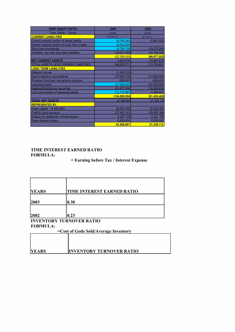
DEBT EQUITY RATIO 2003 2002
Total Debts / Equity (1.46) (3.35)
CURRENT LIABILITIES RUPEES RUPEES
Current maturity portion of lease liability (6,794,240) (2,821,322)
Current maturity portion of Long Term Loans (8,004,000) -
Short term borrowings (6,760,139) (19,270,244)
Creditors, accruals and other liabilities (30,831,550) (44,786,359)
(52,389,929) (66,877,925) NET CURRENT ASSETS 5,933,016 (15,657,876)
TOTAL ASSETS LESS CURRENT LIABILITIES 146,655,771 112,785,601
LONG TERM LIABILITIES
Deferred Income (1,692,510) -
Due to directors and relatives (37,056,700) (21,693,585)
Provident fund trust and gratuity payable (926,457) (926,457)
Long term loans (27,828,000) (47,500,000)
Dealers&Distributors securities (23,871,350) (19,398,600)
Long term portion of leasehold assets (12,710,887) (1,936,847)
(104,085,904) (91,455,489)
TOTAL NET ASSETS 42,569,867 21,330,112
REPRESENTED BY :
Share capital (5,980,000) 59,800,000 39,800,000
Profit & (loss) account (27,457,311) (29,697,066)Surplus on revaluat ion of fixed asset s 8,227,178 8,227,178
Share deposit money 2,000,000 3,000,000
42,569,867 21,330,112
TIME INTEREST EARNED RATIO FORMULA:
= Earning before Tax / Interest Expense
YEARS TIME INTEREST EARNED RATIO
2003 0.30
2002 0.23INVENTORY TURNOVER RATIO
FORMULA: =Cost of Gods Sold/Average Inventory
YEARS INVENTORY TURNOVER RATIO
8/6/2019 Corporate Finance Lecture
http://slidepdf.com/reader/full/corporate-finance-lecture 19/125
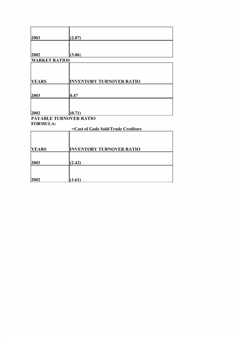
2003 (2.87)
2002 (3.06)MARKET RATIOS
YEARS INVENTORY TURNOVER RATIO
2003 0.47
2002 (0.71)PAYABLE TURNOVER RATIO FORMULA:
=Cost of Gods Sold/Trade Creditors
YEARS INVENTORY TURNOVER RATIO
2003 (2.42)
2002 (1.61)
8/6/2019 Corporate Finance Lecture
http://slidepdf.com/reader/full/corporate-finance-lecture 20/125
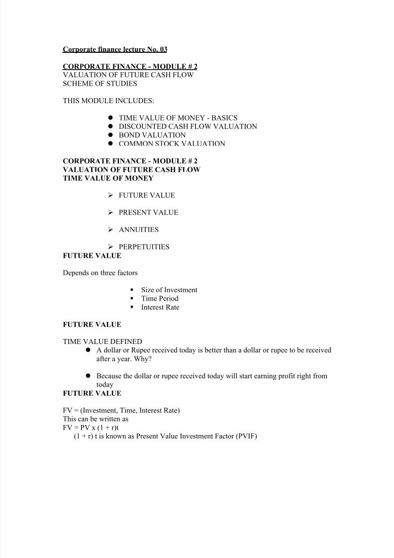
Corporate finance lecture No. 03
COR PORATE FINANCE - MODULE # 2VALUATION OF FUTURE CASH FLOWSCHEME OF STUDIES
THIS MODULE INCLUDES:
TIME VALUE OF MONEY - BASICS DISCOUNTED CASH FLOW VALUATION BOND VALUATION COMMON STOCK VALUATION
COR PORATE FINANCE - MODULE # 2VALUATION OF FUTURE CASH FLOW TIME VALUE OF MONEY
FUTURE VALUE
PRESENT VALUE
ANNUITIES
PERPETUITIESFUTURE VALUE
Depends on three factors
Size of Investment Time Period Interest Rate
FUTURE VALUE
TIME VALUE DEFINED A dollar or Rupee received today is better than a dollar or rupee to be received
after a year. Why?
Because the dollar or rupee received today will start earning profit right fromtoday
FUTURE VALUE
FV = (Investment, Time, Interest Rate)This can be written asFV = PV x (1 + r)t
(1 + r) t is known as Present Value Investment Factor (PVIF)
8/6/2019 Corporate Finance Lecture
http://slidepdf.com/reader/full/corporate-finance-lecture 21/125
r = Rate of Interestt = Time periodExampleYou invest Rs. 1000 today and will get Rs. 1100 at the end of one year, if interest rate is 10% p.a.
= 1000 X (1 + 0.10)= 1100At the end of second year your investment is worth:
1100 x (1 + 0.10) = 1210
Alternatively: 1000 x (1 + 0.10)2 = 1210COMPOUND INTEREST
After One year: 1000 X (1.10) = 1100
After two years: 1100 X (1.10) = 1210
At the end of 2nd year total Investment 1210 that means we earned 210 in terms of Interest.
210 = 100+100+1010 is basically Compound InterestCOMPOUND INTEREST
This 1210 has four parts: 1000 original investment 100 interest ± 1 year 100 interest ± 2 year 10 interest on Year 1 interest
Earning interest on interest is know as compoundingInterest over period is reinvested to earn moreinterest.LONG PERIOD EXAMPLE : (Future Value)
An investment opportunity pays 12% pa and a business entity intends to invest 500,000.What will be the worth of this investment in 7 years time? How much interest will thecompany earn in this period? What portion of total interest represents compound interest?
Solution
Worth after 7 years:
FV = PV x (1 + r)t
8/6/2019 Corporate Finance Lecture
http://slidepdf.com/reader/full/corporate-finance-lecture 22/125
FV =500000 x (1.12)7 =1105350
(1.12)7 = 2.21072nd Question: How much Interest will the Company earn in this period?
Total interest earned:1105350 ± 500000 = 605350Compound Interest:500000 x 12% x 7 = 420000=605350 ± 420000 = 185350
2nd Question: How much Interest will the Company earn in this period?
Total interest earned:1105350 ± 500000 = 605350Compound Interest:
500000 x 12% x 7 = 420000=605350 ± 420000 = 185350
PRESENT VALUE
You know that you will get 10000 at the end of 3rdyear from now. The interest rate is 10%. What is thePV of 10000 now?
FV = PV x (1+r)310000= PV x (1.10)3PV = 10000/ (1.10)3= 7513.14
We can find PV the other way too:PV = FV / (1 + r)t
1 / (1.10)3 = known as PVDFPV = FV X PVDFPV = 10000 X 0.7513*
= 7513
* From table A-3Comparison between two options
Option 1= Pay 4000 today and 6000 after 2 years to buy a computer
Option 2= Pay all today a get a credit of 500. (Net price today is 9500)
Interest rate is 10% at present. Which option is better?Option 1:
8/6/2019 Corporate Finance Lecture
http://slidepdf.com/reader/full/corporate-finance-lecture 23/125
Finding PV:PV = 4000 + (6000 / (1.10)2PV = 4000 + 4958.68 = 8958.68
It means that 4958.68 invested today @ 10% will yield 6000 at the end of year 2,
enabling you to pay off your liability.Option 2:
PV = 9500Option 1 is better because it cost 8958.68 as compared to 9500 of option 2.
So far we come across four factors of Time Value of Money: PV FV Interest factor or discount factor Time period
Given three we can find the fourth.Finding interest rate
An opportunity requires 1000 investment today that will double at the end of 8th year.What is the implicit interest rate?
PV = FV / (1 +r)81000 = 2000 / (1 +r)8(1 +r)8 = 2000/1000(1 +r)8 = 2
r =9%
Three Ways to Solve: Mathematical Equation Financial Calculator Time Value of Money Tables
Look FV table 8 year row select and move towards right unless under the interest Rate%age you read 2 or nearest to 2.
Implicit Interest Rate = 9%PER PETUITYDefined: Stream of equal cash payments equally spaced that continues for ever.If you wish to help a welfare trust by providing 100,000/- per annum forever and the interestrate is 10%, how much amount must be set-aside today?Formula:
PV of Perpetuity = C/r = 100000/0.10= 1,000,000/-
And if you wish to start payments after 3rd year, then what is the PV of this delayedPerpetuity?
PV of Perpetuity = 1,000,000 / (1.10)3
8/6/2019 Corporate Finance Lecture
http://slidepdf.com/reader/full/corporate-finance-lecture 24/125
= 751315ANNUITIES
Series of equal amount and equally spaced payments for limited period of time but not unlimited.
Valuation of Annuities: Using FV/PV tables Using formula
Example:You want to buy an asset for your business that willcost you 4000 per year for next three years.Assume interest rate of 10%. Find out the PV of thisannuity?Using table4000 x 1/(1.10)
4000 x 1/(1.10)24000 x 1/(1.10)3 = 9947.41Using Formula:
PV= Annuity x 1/0.1 ± 1/ 0.10(1.10)3
= 4000 x 2.4869 = 9947.60
8/6/2019 Corporate Finance Lecture
http://slidepdf.com/reader/full/corporate-finance-lecture 25/125
Corporate finance lecture No. 04
CASH FLOW VALUATIONS
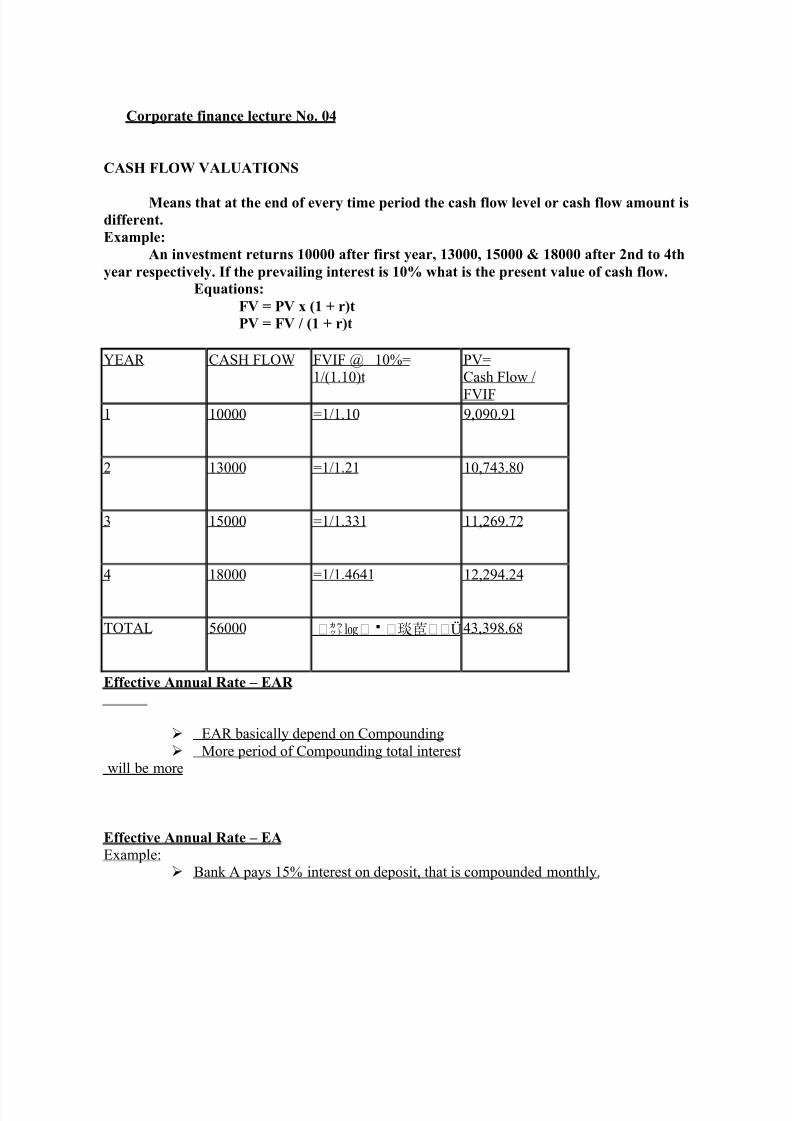
Means that at the end of every time period the cash flow level or cash flow amount isdifferent.Example:
An investment returns 10000 after first year, 13000, 15000 & 18000 after 2nd to 4thyear respectively. If the prevailing interest is 10% what is the present value of cash flow.
Equations:FV = PV x (1 + r)tPV = FV / (1 + r)t
YEAR CASH FLOW FVIF @ 10%=
1/(1.10)t
PV=
Cash Flow /FVIF
1 10000 =1/1.10 9,090.91
2 13000 =1/1.21 10,743.80
3 15000 =1/1.331 11,269.72
4 18000 =1/1.4641 12,294.24
TOTAL 56000 Ü43,398.68
Effective Annual Rate ± EAR
EAR basically depend on Compounding More period of Compounding total interest
will be more
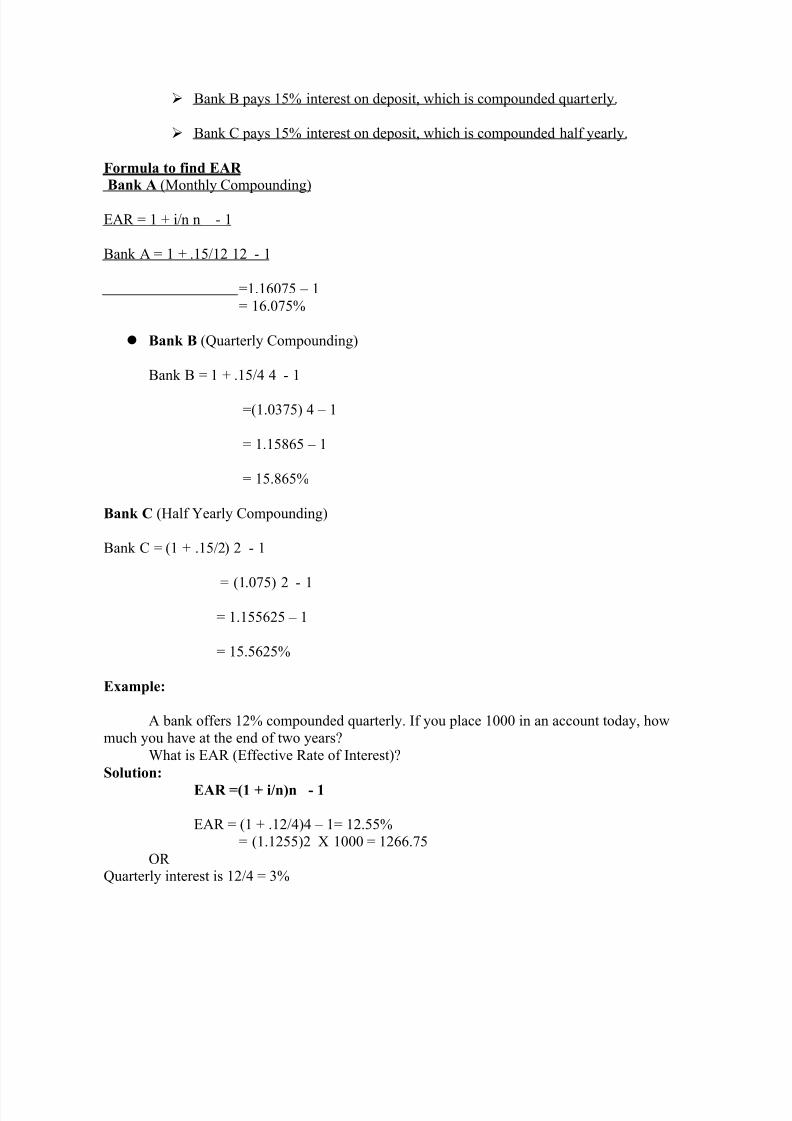
Effective Annual Rate ± EAExample:
Bank A pays 15% interest on deposit, that is compounded monthly.
8/6/2019 Corporate Finance Lecture
http://slidepdf.com/reader/full/corporate-finance-lecture 26/125
Bank B pays 15% interest on deposit, which is compounded quarterly.
Bank C pays 15% interest on deposit, which is compounded half yearly.
Formula to find EAR
Bank A (Monthly Compounding)
EAR = 1 + i/n n - 1
Bank A = 1 + .15/12 12 - 1
=1.16075 ± 1= 16.075%
Bank B (Quarterly Compounding)
Bank B = 1 + .15/4 4 - 1=(1.0375) 4 ± 1
= 1.15865 ± 1
= 15.865%
Bank C (Half Yearly Compounding)
Bank C = (1 + .15/2) 2 - 1
= (1.075) 2 - 1
= 1.155625 ± 1
= 15.5625%
Example:
A bank offers 12% compounded quarterly. If you place 1000 in an account today, howmuch you have at the end of two years?
What is EAR (Effective Rate of Interest)?Solution:
EAR =(1 + i/n)n - 1
EAR = (1 + .12/4)4 ± 1= 12.55%= (1.1255)2 X 1000 = 1266.75
OR Quarterly interest is 12/4 = 3%
8/6/2019 Corporate Finance Lecture
http://slidepdf.com/reader/full/corporate-finance-lecture 27/125
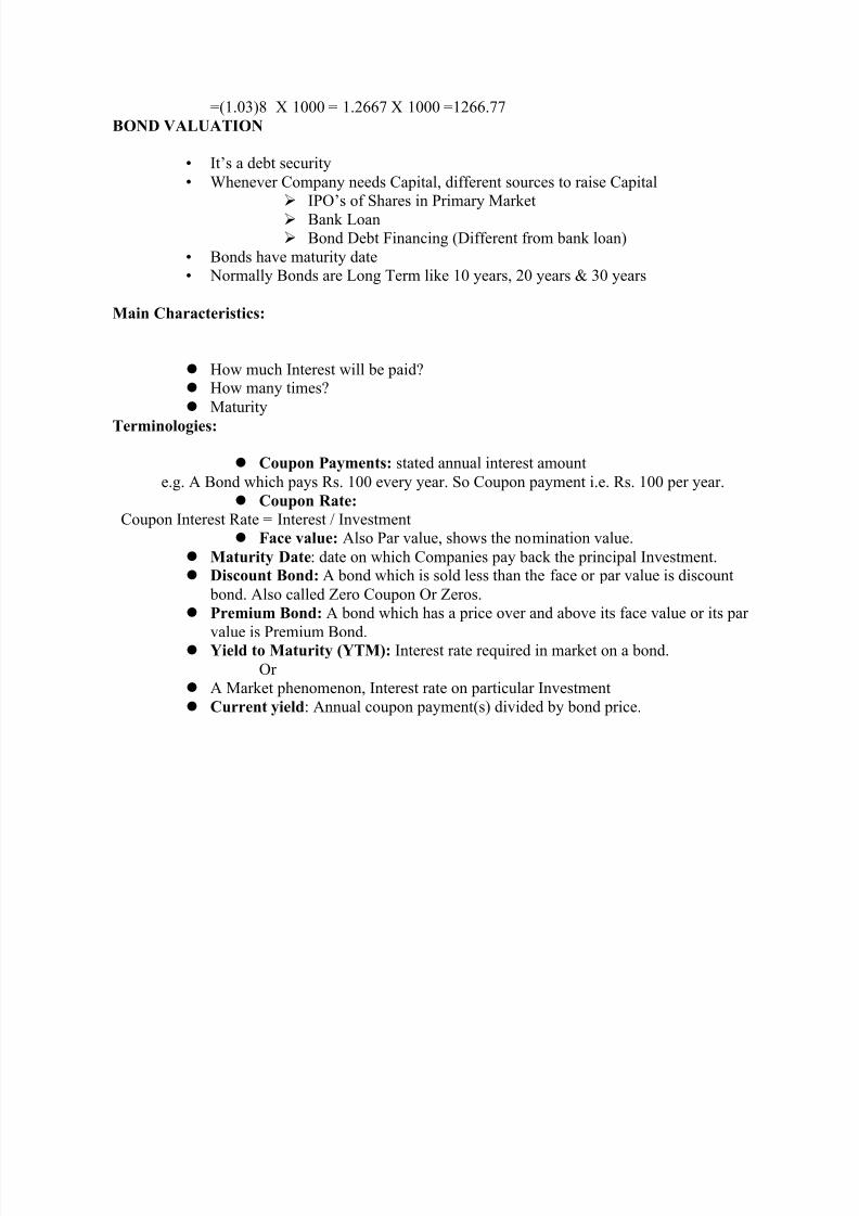
=(1.03)8 X 1000 = 1.2667 X 1000 =1266.77BOND VALUATION
� It¶s a debt security� Whenever Company needs Capital, different sources to raise Capital
IPO¶s of Shares in Primary Market Bank Loan
Bond Debt Financing (Different from bank loan)� Bonds have maturity date� Normally Bonds are Long Term like 10 years, 20 years & 30 years
Main Characteristics:
How much Interest will be paid? How many times?
MaturityTerminologies:
Coupon Payments: stated annual interest amounte.g. A Bond which pays Rs. 100 every year. So Coupon payment i.e. Rs. 100 per year.
Coupon Rate:Coupon Interest Rate = Interest / Investment
Face value: Also Par value, shows the nomination value. Maturity Date: date on which Companies pay back the principal Investment. Discount Bond: A bond which is sold less than the face or par value is discount
bond. Also called Zero Coupon Or Zeros. Premium Bond: A bond which has a price over and above its face value or its par
value is Premium Bond. Yield to Maturity (YTM): Interest rate required in market on a bond.
Or A Market phenomenon, Interest rate on particular Investment Current yield: Annual coupon payment(s) divided by bond price.
8/6/2019 Corporate Finance Lecture
http://slidepdf.com/reader/full/corporate-finance-lecture 28/125
Corporate finance lecture No. 05
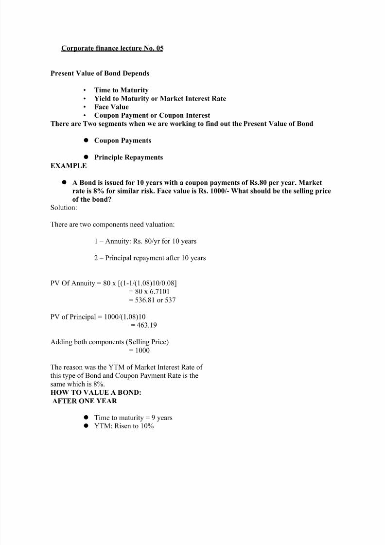
Present Value of Bond Depends
� T
ime to Maturity� Yield to Maturity or Market Interest Rate� Face Value� Coupon Payment or Coupon Interest
There are Two segments when we are working to find out the Present Value of Bond
Coupon Payments
Principle RepaymentsEXAMPLE
A Bond is issued for 10 years with a coupon payments of Rs.80 per year. Marketrate is 8% for similar risk. Face value is Rs. 1000/- What should be the selling price
of the bond?Solution:
There are two components need valuation:
1 ± Annuity: Rs. 80/yr for 10 years
2 ± Principal repayment after 10 years
PV Of Annuity = 80 x [(1-1/(1.08)10/0.08]= 80 x 6.7101= 536.81 or 537
PV of Principal = 1000/(1.08)10= 463.19
Adding both components (Selling Price)= 1000
The reason was the YTM of Market Interest Rate of this type of Bond and Coupon Payment Rate is thesame which is 8%.HOW TO VALUE A BOND:AFTER ONE YEAR
Time to maturity = 9 years YTM: Risen to 10%
8/6/2019 Corporate Finance Lecture
http://slidepdf.com/reader/full/corporate-finance-lecture 29/125
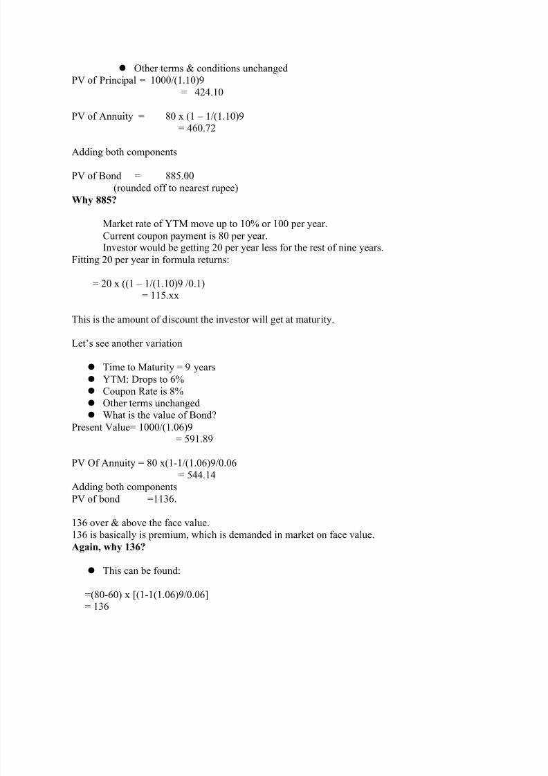
Other terms & conditions unchangedPV of Principal = 1000/(1.10)9
= 424.10
PV of Annuity = 80 x (1 ± 1/(1.10)9
= 460.72
Adding both components
PV of Bond = 885.00 (rounded off to nearest rupee)
Why 885?
Market rate of YTM move up to 10% or 100 per year.Current coupon payment is 80 per year.Investor would be getting 20 per year less for the rest of nine years.
Fitting 20 per year in formula returns:= 20 x ((1 ± 1/(1.10)9 /0.1)
= 115.xx
This is the amount of discount the investor will get at maturity.
Let¶s see another variation
Time to Maturity = 9 years YTM: Drops to 6% Coupon Rate is 8% Other terms unchanged What is the value of Bond?
Present Value= 1000/(1.06)9= 591.89
PV Of Annuity = 80 x(1-1/(1.06)9/0.06= 544.14
Adding both componentsPV of bond =1136.
136 over & above the face value.136 is basically is premium, which is demanded in market on face value.Again, why 136?
This can be found:
=(80-60) x [(1-1(1.06)9/0.06]= 136
8/6/2019 Corporate Finance Lecture
http://slidepdf.com/reader/full/corporate-finance-lecture 30/125
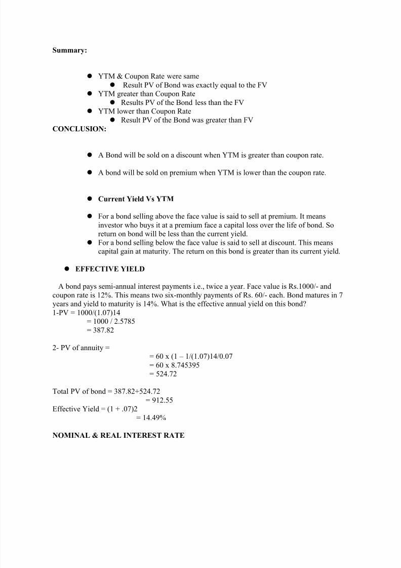
Summary:
YTM & Coupon Rate were same Result PV of Bond was exactly equal to the FV
YTM greater than Coupon Rate Results PV of the Bond less than the FV
YTM lower than Coupon Rate Result PV of the Bond was greater than FV
CONCLUSION:
A Bond will be sold on a discount when YTM is greater than coupon rate.
A bond will be sold on premium when YTM is lower than the coupon rate.
Current Yield Vs YTM
For a bond selling above the face value is said to sell at premium. It meansinvestor who buys it at a premium face a capital loss over the life of bond. Soreturn on bond will be less than the current yield.
For a bond selling below the face value is said to sell at discount. This meanscapital gain at maturity. The return on this bond is greater than its current yield.
EFFECTIVE YIELD
A bond pays semi-annual interest payments i.e., twice a year. Face value is Rs.1000/- andcoupon rate is 12%. This means two six-monthly payments of Rs. 60/- each. Bond matures in 7years and yield to maturity is 14%. What is the effective annual yield on this bond?1-PV = 1000/(1.07)14
= 1000 / 2.5785= 387.82
2- PV of annuity == 60 x (1 ± 1/(1.07)14/0.07= 60 x 8.745395= 524.72
Total PV of bond = 387.82+524.72= 912.55
Effective Yield = (1 + .07)2= 14.49%
NOMINAL & REAL INTEREST RATE
8/6/2019 Corporate Finance Lecture
http://slidepdf.com/reader/full/corporate-finance-lecture 31/125
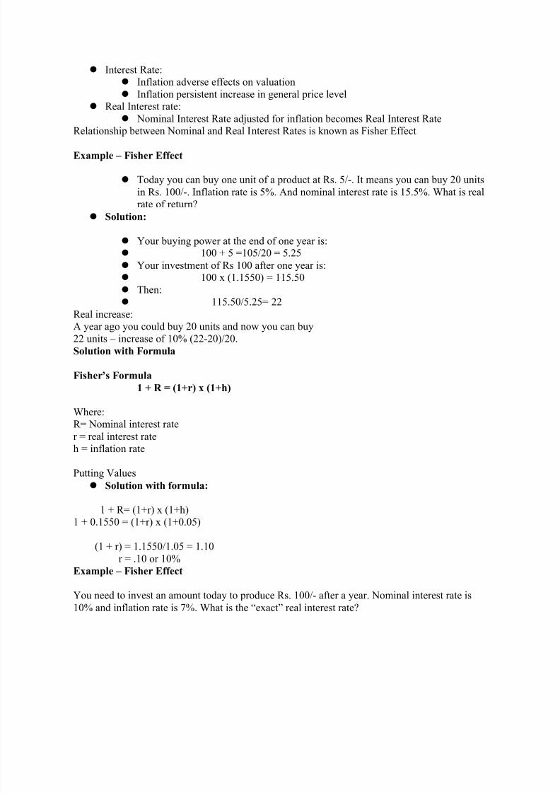
Interest Rate: Inflation adverse effects on valuation Inflation persistent increase in general price level
Real Interest rate: Nominal Interest Rate adjusted for inflation becomes Real Interest Rate
Relationship between Nominal and Real Interest Rates is known as Fisher Effect
Example ± Fisher Effect
Today you can buy one unit of a product at Rs. 5/-. It means you can buy 20 unitsin Rs. 100/-. Inflation rate is 5%. And nominal interest rate is 15.5%. What is realrate of return?
Solution:
Your buying power at the end of one year is: 100 + 5 =105/20 = 5.25
Your investment of Rs 100 after one year is: 100 x (1.1550) = 115.50 Then: 115.50/5.25= 22
Real increase:A year ago you could buy 20 units and now you can buy22 units ± increase of 10% (22-20)/20.Solution with Formula
Fisher¶s Formula 1 + R = (1+r) x (1+h)
Where:R= Nominal interest rater = real interest rateh = inflation rate
Putting Values Solution with formula:
1 + R= (1+r) x (1+h)1 + 0.1550 = (1+r) x (1+0.05)
(1 + r) = 1.1550/1.05 = 1.10r = .10 or 10%
Example ± Fisher Effect
You need to invest an amount today to produce Rs. 100/- after a year. Nominal interest rate is10% and inflation rate is 7%. What is the ³exact´ real interest rate?
8/6/2019 Corporate Finance Lecture
http://slidepdf.com/reader/full/corporate-finance-lecture 32/125
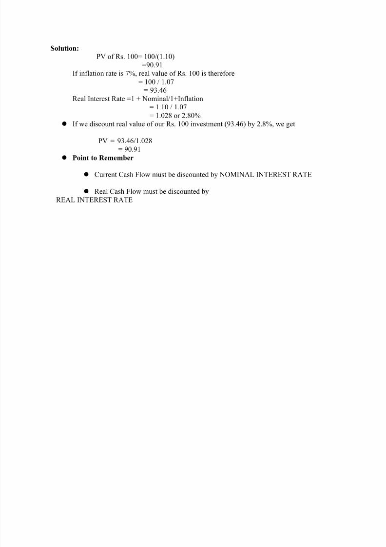
Solution:PV of Rs. 100= 100/(1.10)
=90.91If inflation rate is 7%, real value of Rs. 100 is therefore
= 100 / 1.07
= 93.46Real Interest Rate =1 + Nominal/1+Inflation= 1.10 / 1.07= 1.028 or 2.80%
If we discount real value of our Rs. 100 investment (93.46) by 2.8%, we get
PV = 93.46/1.028= 90.91
Point to Remember
Current Cash Flow must be discounted by NOMINAL INTEREST RATE
Real Cash Flow must be discounted byREAL INTEREST RATE
8/6/2019 Corporate Finance Lecture
http://slidepdf.com/reader/full/corporate-finance-lecture 33/125
Corporate finance lecture No. 06
TERM STRUCTURE OF INTEREST RATES
Interest Rates in Short & Long terms are different.
Relationship between LT & ST Rates is known as Term Structure of Interest.
Term Structure tells us Nominal Interest Rate on default free securities.
When:LT > ST
Term Structure will be upward sloping
8/6/2019 Corporate Finance Lecture
http://slidepdf.com/reader/full/corporate-finance-lecture 34/125
When:ST > LT Term Structure will be downward sloping
FACTORS OF TERM STRUCTURE
Real Interest Rate
Inflation Rate
Interest Rate Risk
REAL INTEREST RATEReal Interest Rate is basic component of Term Structure.When Real Interest Rate is high, all Interest Rates are high.Real Interest Rate remains constant regardless of maturity.
Real Interest Rates do not influence the shape of Term Structure of Interest.INFLATION RATEInflation Rate reduces the Time Value or Value of Money.If Interest Rate is high, Nominal Interest will increase.Due to Inflation, Investors demand compensation of the lost value. This is known asInflation Premium.Inflation Rate strongly influences the Term Structure of Interest.INTEREST RATE RISK
The fluctuation in Interest Rate also influences the Term Structure significantly.
Any slight fluctuation in Interest Rate can have a huge change in PV value due tocompounding effect.
Investors demand extra Risk Premium for change in Interest Rate. This is known as InterestRate Risk.
Yield Curve ± Coupon Based Bonds Three Factors Influence Yield Curve StructureDefault Risk Premium:
Coupon Base Bond is a promise with a risk that company may fail to pay interest.Taxability Premium:
Dividend bears TaxReturns are reduced by TaxesInvestor need this Premium
Liquidity Premium:If bond is more liquid, expected rate of return is low. For less liquid bonds,compensation is required as Liquidity Premium
TERM STRUCTURE YIELD CURVEMain Points:
8/6/2019 Corporate Finance Lecture
http://slidepdf.com/reader/full/corporate-finance-lecture 35/125
Interest Rate Risk Inflation PremiumReal Interest RateDefault Risk PremiumTaxability Premium
Liquidity PremiumCOMMON STOCK VALUATION
Features:
No promised Cash Flow for Dividend No redemption or No Date of MaturityProblems in Determining Rate of Return
Expected Returns:
Total Return = Dividends + Capital Gains
= D1 + (P1 ± P0) / P0
Where:D1 = Dividend after 1 Year P1 = Price of Stock after Year 1P0 = Price of Stock Period 0 or Current Price
Expected Returns:
Total Return = Dividends + Capital Gains
= D1 + (P1 ± P0) / P0
Where:D1 = Dividend after 1 Year P1 = Price of Stock after Year 1P0 = Price of Stock Period 0 or Current Price
For Example:P0 = Rs. 20/-Dividend1 = Rs. 2 per shareP1 = Rs. 23/-
Then expected return is:= 2 + (23 ± 20) / 20=5 / 20= 25%
Putting it the other way:We are trying to calculate the price today if the expected rate of return is 25%:
Price Today = D1 + P1 / 1 + r
8/6/2019 Corporate Finance Lecture
http://slidepdf.com/reader/full/corporate-finance-lecture 36/125
= 2 + 23 / 1.25= 25 / 1.25= 20
Putting it the other way:
We are trying to calculate the price today if the expected rate of return is 25%:
Price Today = D1 + P1 / 1 + r
= 2 + 23 / 1.25= 25 / 1.25= 20
If:Today Price > Rs. 20
Then the expected return should have been lower than
other shares of equivalent risk. If demand will lower, peopledispose off this share. It forces the price to settle on Rs. 20.
If:Today Price < Rs. 20
Then the expected return should have been higher thanother shares of same risk. Everyone will rush to buy it, thusforcing price to settle on Rs. 20.CONCLUSION
At each point in time of all shares of samerisk are priced to offer the same expectedrate of return.DIVIDEND DISCOUNT MODEL
It is not an easy job to predict or forecast Future Stock Price.
Dividend Discount Model states that today¶s Price is equal to the Present Value of all futureDividendsAfter One year:
P0 = Div + P1 / (1 + r)After 2 years the value of stock is:
=Div1/(1+r) + Div2+P2/(1+r)2After 3 years the value of stock is:=Div1/(1+r) + Div2/(1+r)2 + Div3 + P3/(1+r)3
When the time horizon is infinitely far, then we donot consider the final price as it has no Present
8/6/2019 Corporate Finance Lecture
http://slidepdf.com/reader/full/corporate-finance-lecture 37/125
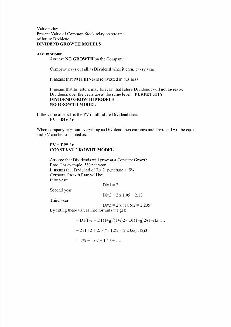
Value today.Present Value of Common Stock relay on streamsof future Dividend.DIVIDEND GR OWTH MODELS
Assumptions:Assume NO GR OWTH by the Company.
Company pays out all as Dividend what it earns every year.
It means that NOTHING is reinvested in business.
It means that Investors may forecast that future Dividends will not increase.Dividends over the years are at the same level ± PER PETUITY DIVIDEND GR OWTH MODELSNO GR OWTHMODEL
If the value of stock is the PV of all future Dividend then:PV = DIV / r
When company pays out everything as Dividend then earnings and Dividend will be equaland PV can be calculated as:
PV = EPS / rCONSTANT GR OWHT MODEL
Assume that Dividends will grow at a Constant GrowthRate. For example, 5% per year.It means that Dividend of Rs. 2 per share at 5%Constant Growth Rate will be:First year:
Div1 = 2Second year:
Div2 = 2 x 1.05 = 2.10Third year:
Div3 = 2 x (1.05)2 = 2.205By fitting these values into formula we get:
= D1/1+r + D1(1+g)/(1+r)2+ D1(1+g)2/(1+r)3 «.
= 2 /1.12 + 2.10/(1.12)2 + 2.205/(1.12)3
=1.79 + 1.67 + 1.57 + «.
8/6/2019 Corporate Finance Lecture
http://slidepdf.com/reader/full/corporate-finance-lecture 38/125
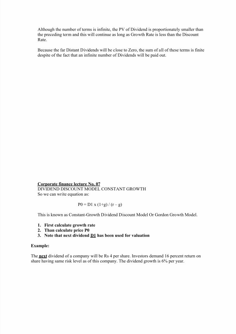
Although the number of terms is infinite, the PV of Dividend is proportionately smaller thanthe preceding term and this will continue as long as Growth Rate is less than the DiscountRate.
Because the far Distant Dividends will be close to Zero, the sum of all of these terms is finite
despite of the fact that an infinite number of Dividends will be paid out.
Corporate finance lecture No. 07 DIVIDEND DISCOUNT MODEL CONSTANT GROWTHSo we can write equation as:
P0 = D1 x (1+g) / (r ± g)
This is known as Constant-Growth Dividend Discount Model Or Gordon Growth Model.
1. First calculate growth rate2. Than calculate price P03. Note that next dividend D1 has been used for valuation
Example:
The next dividend of a company will be Rs 4 per share. Investors demand 16 percent return onshare having same risk level as of this company. The dividend growth is 6% per year.
8/6/2019 Corporate Finance Lecture
http://slidepdf.com/reader/full/corporate-finance-lecture 39/125
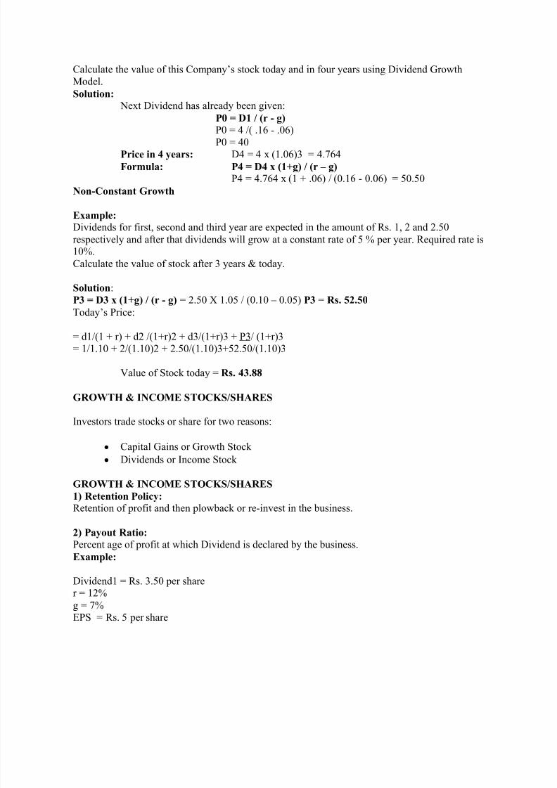
Calculate the value of this Company¶s stock today and in four years using Dividend GrowthModel.Solution:
Next Dividend has already been given:P0 = D1 / (r - g)
P0 = 4 /( .16 - .06)P0 = 40Price in 4 years: D4 = 4 x (1.06)3 = 4.764 Formula: P4 = D4 x (1+g) / (r ± g)
P4 = 4.764 x (1 + .06) / (0.16 - 0.06) = 50.50Non-Constant Growth
Example:Dividends for first, second and third year are expected in the amount of Rs. 1, 2 and 2.50respectively and after that dividends will grow at a constant rate of 5 % per year. Required rate is10%.
Calculate the value of stock after 3 years & today.Solution:P3 = D3 x (1+g) / (r - g) = 2.50 X 1.05 / (0.10 ± 0.05) P3 = Rs. 52.50Today¶s Price:
= d1/(1 + r) + d2 /(1+r)2 + d3/(1+r)3 + P3/ (1+r)3= 1/1.10 + 2/(1.10)2 + 2.50/(1.10)3+52.50/(1.10)3
Value of Stock today = Rs. 43.88
GR OWTH & INCOME STOCKS/SHARES
Investors trade stocks or share for two reasons:
y Capital Gains or Growth Stock y Dividends or Income Stock
GR OWTH & INCOME STOCKS/SHARES 1) Retention Policy:Retention of profit and then plowback or re-invest in the business.
2)P
ayout Ratio:Percent age of profit at which Dividend is declared by the business.Example:
Dividend1 = Rs. 3.50 per share r = 12%g = 7%EPS = Rs. 5 per share
8/6/2019 Corporate Finance Lecture
http://slidepdf.com/reader/full/corporate-finance-lecture 40/125
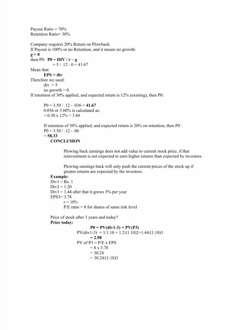
Payout Ratio = 70%Retention Ratio= 30%
Company requires 20% Return on Plowback.If Payout is 100% or no Retention, and it means no growth:
g = 0 then P0: P0 = DIV / r ± g= 5 / .12 - 0 = 41.67
Mean that:EPS = div
Therefore we used:div = 5no growth = 0
If retention of 30% applied, and expected return is 12% (existing), then P0:
P0 = 3.50 / .12 - .036 = 41.67
0.036 or 3.60% is calculated as:= 0.30 x 12% = 3.60
If retention of 30% applied, and expected return is 20% on retention, then P0 :P0 = 3.50 / .12 - .06= 58.33
CONCLUSION
Plowing back earnings does not add value to current stock price, if thatreinvestment is not expected to earn higher returns than expected by investors.
Plowing earnings back will only push the current prices of the stock up if greater returns are expected by the investors.
Example:Div1 = Rs. 1Div2 = 1.20Div3 = 1.44 after that it grows 5% per year EPS3= 3.78
r = 10%P/E ratio = 8 for shares of same risk level
Price of stock after 3 years and today?Price today:
P0 = PV(div1-3) + PV(P3)PV(div1-3) = 1/1.10 + 1.2/(1.10)2+1.44/(1.10)3
= 2.98PV of P3 = P/E x EPS
= 8 x 3.78= 30.24= 30.24/(1.10)3
8/6/2019 Corporate Finance Lecture
http://slidepdf.com/reader/full/corporate-finance-lecture 41/125
= 22.72Putting value of PV(div1-3) & PV of P3 in the main formula:
= 2.98 + 22.72P0 = 25.70
We can calculate P3 with Dividend Model:P
3 = div4 / (r ± g)
Div4 = div3 x (1+g)= 1.44 x 1.05 = 1.512
Putting value of Div4 in formula:P3 = 1.512 / (0.12 - .05)= 30.24
OTHER TOOLS OF STOCK EVALUATION
TECHNICAL ANALYSIS:
T
echnical analysis studies supply and demand in a market in a attempt todetermine what direction or trend will continue in future
Study of Market Sentiments
TECHNICAL ANALYSIS
Evaluating security by analyzing the statistics generated by market activity suchas Past Prices and Volume
Charts and other tools are used to identify patterns that suggest future activityTRENDS
A trend shows the general direction in which a security or market is headed
Types:Up-TrendsDown TrendsHorizontal Trends
TRENDS LENGTH Short TermMedium TermLong Term
Support & Resistance
Support is the lower ceiling price of a stock Resistance is the upper ceiling of stock
8/6/2019 Corporate Finance Lecture
http://slidepdf.com/reader/full/corporate-finance-lecture 42/125
CHAR T
A series of prices over a time period presented graphicallyTime scale: intraday, daily, weekly, monthly & yearlyPrice scale: change in price presented as absolute terms. Change shown in % is known
as Logarithmic ScaleCHAR T PATTERN
A distinct formation of point on chart that create trading signals or a sign of future movementHead & Shoulder: reversal pattern when formed, and signals that the security islikely to move against the previous trendCups & handle: continuation of bullish patternCONCLUSION
Technical Analysis method of evaluating stocks by analyzing statistics generatedby market activity.Technical traders take a short term approach to analyzing chart.Product of Technical Analysis is a trend.
Corporate finance lecture No. 08
COMMON STOCK VALUATIONFUNDAMENTAL ANALYSIS:
Analyst is trying to reach near the intrinsic value of company¶s share by reading andanalyzing the financial, non-financial information and industry comparison.Three step process:Economic indicators: GDP, Interest Rates, Inflation, Exchange RateIndustry Comparison and CompetitionIndividual Company Analysis
FinancialsCEO ReportAudited AccountsAuditors Report
CAPITAL BUDGETINGDefinition:It is a process in which we can evaluate the investment opportunities in order toacquire some capital asset. Types:
New ProjectExpansion Project
8/6/2019 Corporate Finance Lecture
http://slidepdf.com/reader/full/corporate-finance-lecture 43/125
Modernization / ReplacementOther / social responsibility ± Pollution control etc
Research & DevelopmentExploration
Capital Budgeting ProcessCB decisions are irreversible in nature
SWOT Analysis :S ± StrengthW ± WeaknessO ± OpportunitiesT ± Threats
CB targeted towards potential opportunitiesInvestment Opportunitie(s) is/are identifiedDifferent alternatives are considered
Every alternative is evaluatedThe best option (s) is/are undertakenPROJECT EVALUATION
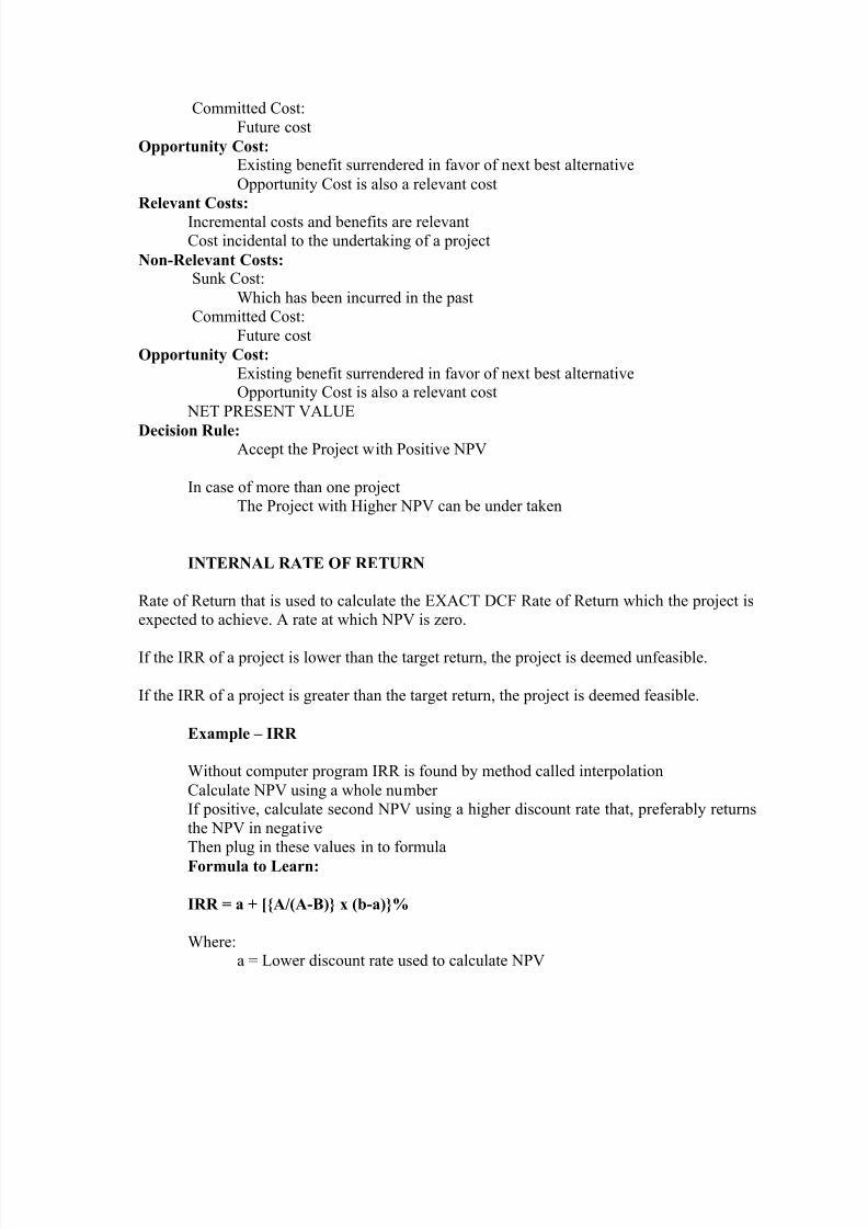
Relevant Costs:Incremental costs and benefits are relevantCost incidental to the undertaking of a project
Non-Relevant Costs:Sunk Cost:
Which has been incurred in the pastCommitted Cost:
Future costOpportunity Cost:
Existing benefit surrendered in favor of next best alternativeOpportunity Cost is also a relevant cost
Profit Vs Cash Flow NET PRESENT VALUE NPV = Discounted Benefits ± Initial Investment
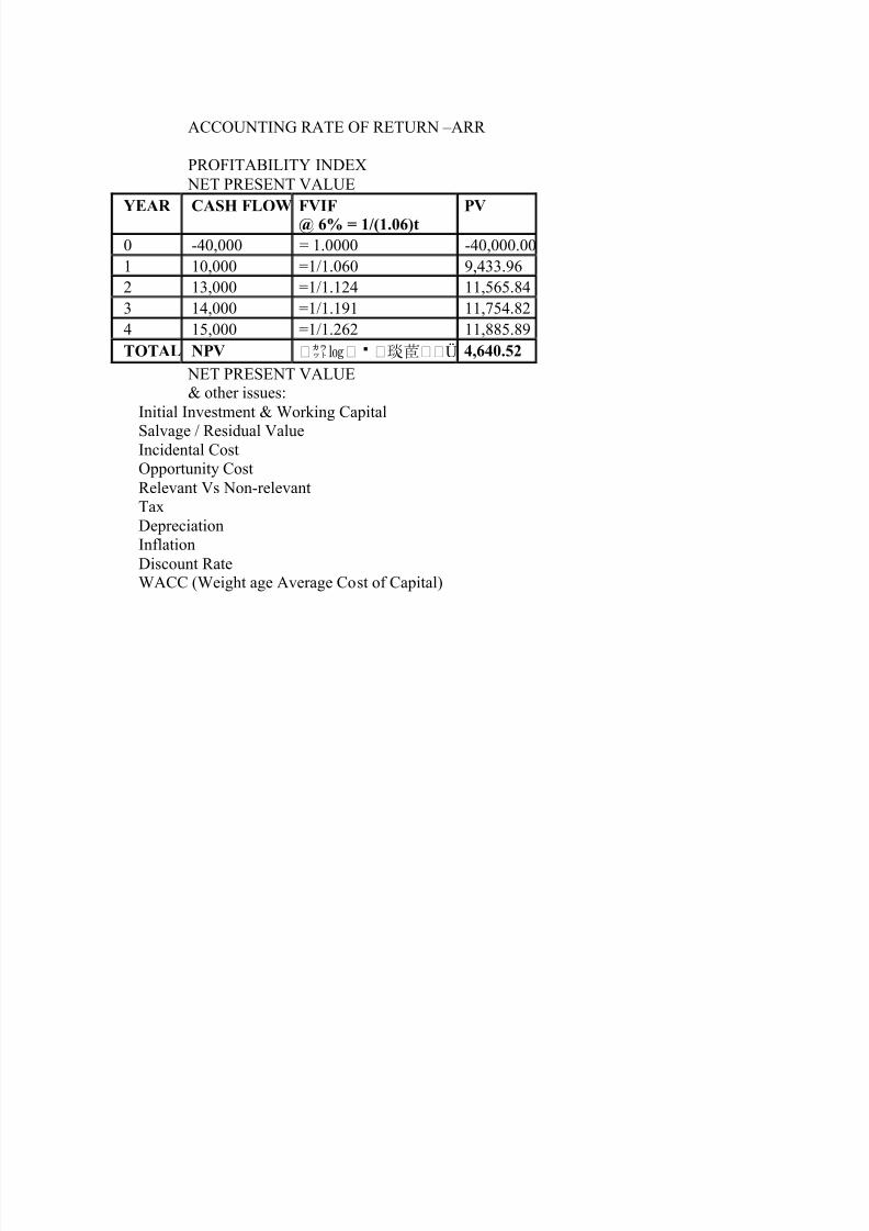
Example:An investment in an asset of Rs. 40,000 today returns 10000 after first year,13000, 14000 & 15000 after 2nd to 4th year respectively.If the prevailing interest is 6% what is the net present value of cash flow?
EVALUATING TECHNIQUES NET PRESENT VALUE / DCF
INTERNAL RATE OF RETURN ± IRR
PAYBACK PERIOD
DISCOUNTED PAYBACK PERIOD
8/6/2019 Corporate Finance Lecture
http://slidepdf.com/reader/full/corporate-finance-lecture 44/125
ACCOUNTING RATE OF RETURN ±ARR
PROFITABILITY INDEX NET PRESENT VALUE
YEAR CASH FLOW FVIF @ 6% = 1/(1.06)t PV
0 -40,000 = 1.0000 -40,000.001 10,000 =1/1.060 9,433.962 13,000 =1/1.124 11,565.843 14,000 =1/1.191 11,754.824 15,000 =1/1.262 11,885.89TOTAL NPV Ü 4,640.52
NET PRESENT VALUE & other issues:
Initial Investment & Working CapitalSalvage / Residual ValueIncidental CostOpportunity CostRelevant Vs Non-relevantTaxDepreciationInflationDiscount RateWACC (Weight age Average Cost of Capital)
8/6/2019 Corporate Finance Lecture
http://slidepdf.com/reader/full/corporate-finance-lecture 45/125
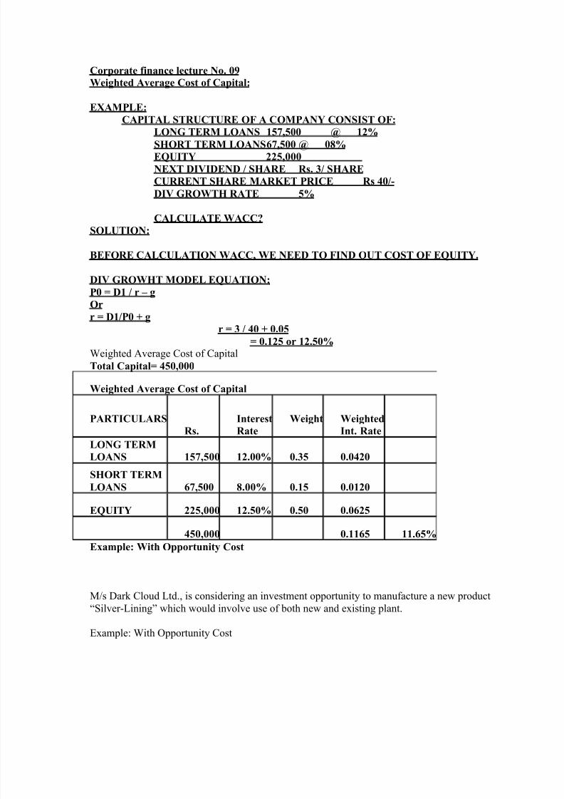
Corporate finance lecture No. 09Weighted Average Cost of Capital:
EXAMPLE:CAPITAL STRUCTURE OF A COMPANY CONSIST OF:
LO
NGT
ERM LO
ANS 157,500 @ 12%SHOR T TERM LOANS 67,500 @ 08%EQUITY 225,000NEXT DIVIDEND / SHARE Rs. 3/ SHARECURRENT SHARE MARKET PRICE Rs 40/-DIV GR OWTH RATE 5%
CALCULATE WACC?SOLUTION:
BEFORE CALCULATION WACC, WE NEED TO FIND OUT COST OF EQUITY.
DIV GR OWHT MODEL EQUATION:P0 = D1 / r ± gOrr = D1/P0 + g
r = 3 / 40 + 0.05= 0.125 or 12.50%
Weighted Average Cost of CapitalTotal Capital= 450,000
Weighted Average Cost of Capital
PAR TICULARS Rs.
Interest Rate
Weight Weighted Int. Rate
LONG TERMLOANS 157,500 12.00% 0.35 0.0420
SHOR T TERMLOANS 67,500 8.00% 0.15 0.0120
EQUITY 225,000 12.50% 0.50 0.0625
450,000 0.1165 11.65%
Example: With Opportunity Cost
M/s Dark Cloud Ltd., is considering an investment opportunity to manufacture a new product³Silver-Lining´ which would involve use of both new and existing plant.
Example: With Opportunity Cost
8/6/2019 Corporate Finance Lecture
http://slidepdf.com/reader/full/corporate-finance-lecture 46/125
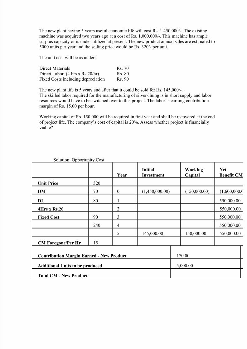
The new plant having 5 years useful economic life will cost Rs. 1,450,000/-. The existingmachine was acquired two years ago at a cost of Rs. 1,000,000/-. This machine has amplesurplus capacity or is under-utilized at present. The new product annual sales are estimated to5000 units per year and the selling price would be Rs. 320/- per unit.
The unit cost will be as under:
Direct Materials Rs. 70Direct Labor (4 hrs x Rs.20/hr) Rs. 80Fixed Costs including depreciation Rs. 90
The new plant life is 5 years and after that it could be sold for Rs. 145,000/-.The skilled labor required for the manufacturing of silver-lining is in short supply and labor resources would have to be switched over to this project. The labor is earning contributionmargin of Rs. 15.00 per hour.
Working capital of Rs. 150,000 will be required in first year and shall be recovered at the endof project life. The company¶s cost of capital is 20%. Assess whether project is financiallyviable?
Solution: Opportunity Cost
Year InitialInvestment
WorkingCapital
NetBene
Unit Price 320
DM 70 0 (1,450,000.00) (150,000.00) (1,60
DL 80 1 550,0
4Hrs x Rs.20 2 550,
Fixed Cost 90 3 550,0
240 4 550,0
5 145,000.00 150,000.00 550,0
CM Foregone/Per Hr 15
Contribution Margin Earned - New Product 170.00
Additional Units to be produced 5,000.00
Total CM - New Product
8/6/2019 Corporate Finance Lecture
http://slidepdf.com/reader/full/corporate-finance-lecture 47/125
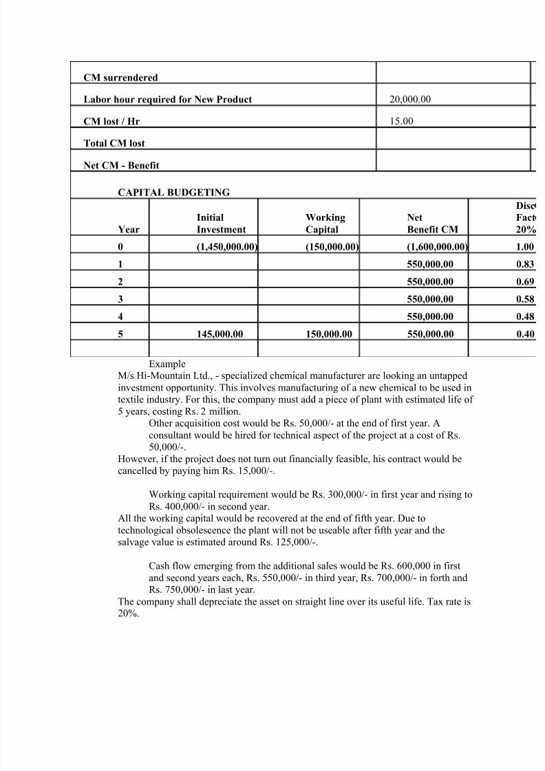
CM surrendered
Labor hour required for New Product 20,000.00
CM lost / Hr 15.00
Total CM lost
Net CM - Benefit
CAPITAL BUDGETING
Year Initial Investment
Working Capital
NetBenefit CM
0 (1,450,000.00) (150,000.00) (1,600,000.00)
1 550,000.00 2 550,000.00
3 550,000.00
4 550,000.00
5 145,000.00 150,000.00 550,000.00
ExampleM/s Hi-Mountain Ltd., - specialized chemical manufacturer are looking an untappedinvestment opportunity. This involves manufacturing of a new chemical to be used intextile industry. For this, the company must add a piece of plant with estimated life of 5 years, costing Rs. 2 million.
Other acquisition cost would be Rs. 50,000/- at the end of first year. Aconsultant would be hired for technical aspect of the project at a cost of Rs.50,000/-.
However, if the project does not turn out financially feasible, his contract would becancelled by paying him Rs. 15,000/-.
Working capital requirement would be Rs. 300,000/- in first year and rising toRs. 400,000/- in second year.
All the working capital would be recovered at the end of fifth year. Due totechnological obsolescence the plant will not be useable after fifth year and thesalvage value is estimated around Rs. 125,000/-.
Cash flow emerging from the additional sales would be Rs. 600,000 in firstand second years each, Rs. 550,000/- in third year, Rs. 700,000/- in forth andRs. 750,000/- in last year.
The company shall depreciate the asset on straight line over its useful life. Tax rate is20%.
8/6/2019 Corporate Finance Lecture
http://slidepdf.com/reader/full/corporate-finance-lecture 48/125
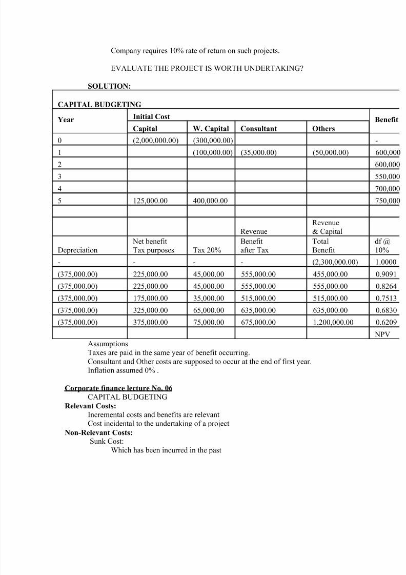
Company requires 10% rate of return on such projects.
EVALUATE THE PROJECT IS WORTH UNDERTAKING?
SOLUTION:
CAPITAL BUDGETING
Year Initial Cost
Capital W. Capital Consultant Others
0 (2,000,000.00) (300,000.00)
1 (100,000.00) (35,000.00) (50,000.00)
2
3
4
5 125,000.00 400,000.00
RevenueRevenue& Capital
Depreciation Net benefitTax purposes Tax 20%
Benefitafter Tax
TotalBenefit
- - - - (2,300,000.00)
(375,000.00) 225,000.00 45,000.00 555,000.00 455,000.00
(375,000.00) 225,000.00 45,000.00 555,000.00 555,000.00
(375,000.00) 175,000.00 35,000.00 515,000.00 515,000.00
(375,000.00) 325,000.00 65,000.00 635,000.00 635,000.00
(375,000.00) 375,000.00 75,000.00 675,000.00 1,200,000.00
AssumptionsTaxes are paid in the same year of benefit occurring.Consultant and Other costs are supposed to occur at the end of first year.Inflation assumed 0% .
Corporate finance lecture No. 06CAPITAL BUDGETING
Relevant Costs:Incremental costs and benefits are relevantCost incidental to the undertaking of a project
Non-Relevant Costs:Sunk Cost:
Which has been incurred in the past
8/6/2019 Corporate Finance Lecture
http://slidepdf.com/reader/full/corporate-finance-lecture 49/125
Committed Cost:Future cost
Opportunity Cost:Existing benefit surrendered in favor of next best alternativeOpportunity Cost is also a relevant cost
Relevant Costs:Incremental costs and benefits are relevantCost incidental to the undertaking of a project
Non-Relevant Costs:Sunk Cost:
Which has been incurred in the pastCommitted Cost:
Future costOpportunity Cost:
Existing benefit surrendered in favor of next best alternativeOpportunity Cost is also a relevant cost
NET PRESENT VALUEDecision Rule:Accept the Project with Positive NPV
In case of more than one projectThe Project with Higher NPV can be under taken
INTERNAL RATE OF RETURN
Rate of Return that is used to calculate the EXACT DCF Rate of Return which the project isexpected to achieve. A rate at which NPV is zero.
If the IRR of a project is lower than the target return, the project is deemed unfeasible.
If the IRR of a project is greater than the target return, the project is deemed feasible.
Example ± IRR
Without computer program IRR is found by method called interpolationCalculate NPV using a whole number If positive, calculate second NPV using a higher discount rate that, preferably returnsthe NPV in negativeThen plug in these values in to formulaFormula to Learn:
IRR = a + [{A/(A-B)} x (b-a)}%
Where:a = Lower discount rate used to calculate NPV
8/6/2019 Corporate Finance Lecture
http://slidepdf.com/reader/full/corporate-finance-lecture 50/125
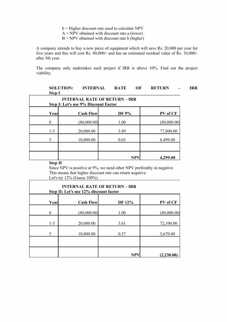
b = Higher discount rate used to calculate NPVA = NPV obtained with discount rate a (lower)B = NPV obtained with discount rate b (higher)
A company intends to buy a new piece of equipment which will save Rs. 20,000 per year for
five years and this will cost Rs. 80,000/- and has an estimated residual value of Rs. 10,000/-after 5th year.
The company only undertakes such project if IRR is above 10%. Find out the projectviability.
SOLUTION: INTERNAL RATE OF RETURN ± IRR Step I
INTERNAL RATE OF RETURN ± IRR Step I: Let's use 9% Discount Factor
Year Cash Flow DF 9% PV of CF
0 (80,000.00) 1.00 (80,000.00)
1-5 20,000.00 3.89 77,800.00
5 10,000.00 0.65 6,499.00
NPV 4,299.00
Step II Since NPV is positive at 9%, we need other NPV preferably in negative.This means that higher discount rate can return negative.Let's try 12% (Guess 100%)
INTERNAL RATE OF RETURN ± IRR Step II: Let's use 12% discount factor
Year Cash Flow DF 12% PV of CF
0 (80,000.00) 1.00 (80,000.00)
1-5 20,000.00 3.61 72,100.00
5 10,000.00 0.57 5,670.00
NPV (2,230.00)
8/6/2019 Corporate Finance Lecture
http://slidepdf.com/reader/full/corporate-finance-lecture 51/125
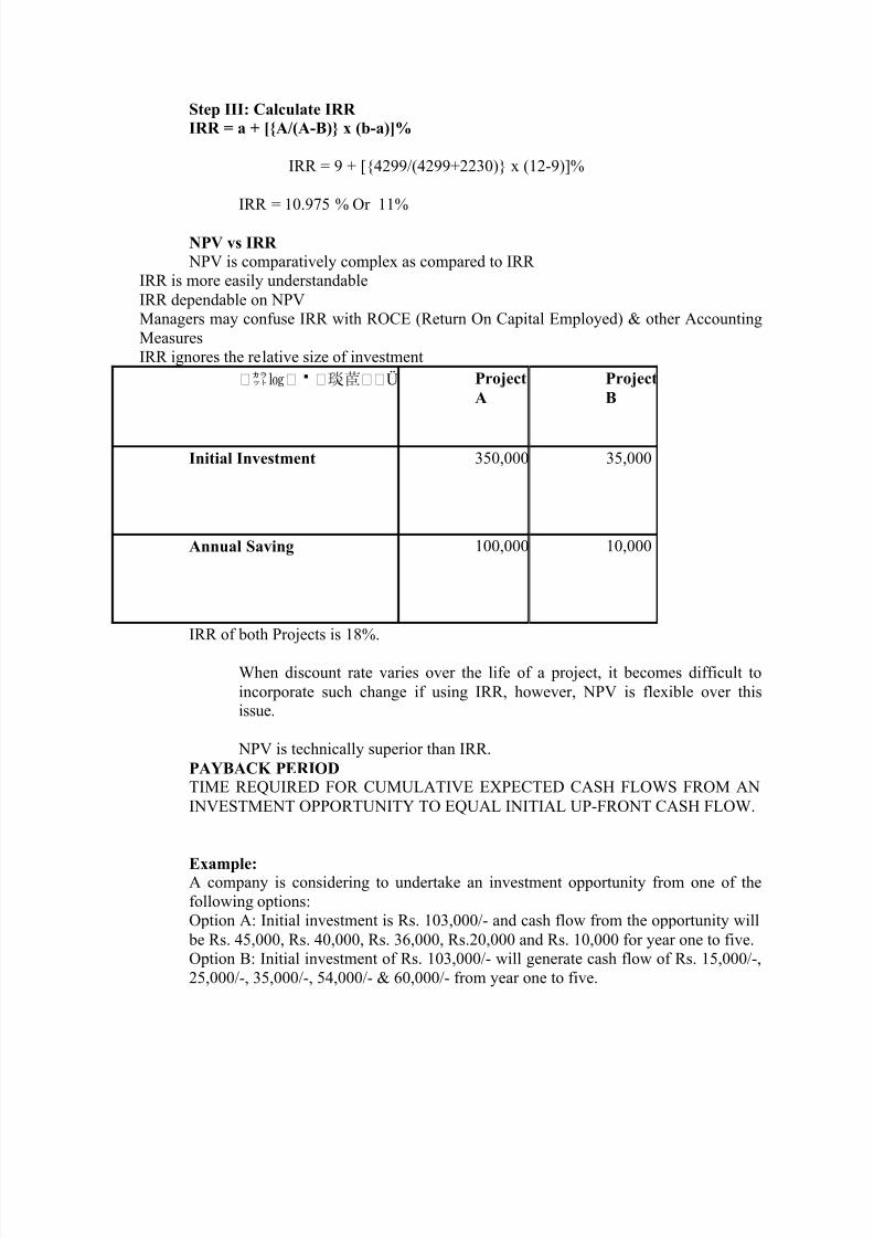
Step III: Calculate IRR IRR = a + [{A/(A-B)} x (b-a)]%
IRR = 9 + [{4299/(4299+2230)} x (12-9)]%
IRR = 10.975 % Or 11%
NPV vs IRR NPV is comparatively complex as compared to IRR
IRR is more easily understandableIRR dependable on NPVManagers may confuse IRR with ROCE (Return On Capital Employed) & other AccountingMeasuresIRR ignores the relative size of investment
Ü ProjectA
ProjectB
Initial Investment 350,000 35,000
Annual Saving 100,000 10,000
IRR of both Projects is 18%.
When discount rate varies over the life of a project, it becomes difficult toincorporate such change if using IRR, however, NPV is flexible over thisissue.
NPV is technically superior than IRR.PAYBACK PERIOD TIME REQUIRED FOR CUMULATIVE EXPECTED CASH FLOWS FROM ANINVESTMENT OPPORTUNITY TO EQUAL INITIAL UP-FRONT CASH FLOW.
Example:A company is considering to undertake an investment opportunity from one of thefollowing options:Option A: Initial investment is Rs. 103,000/- and cash flow from the opportunity will be Rs. 45,000, Rs. 40,000, Rs. 36,000, Rs.20,000 and Rs. 10,000 for year one to five.Option B: Initial investment of Rs. 103,000/- will generate cash flow of Rs. 15,000/-,25,000/-, 35,000/-, 54,000/- & 60,000/- from year one to five.
8/6/2019 Corporate Finance Lecture
http://slidepdf.com/reader/full/corporate-finance-lecture 52/125
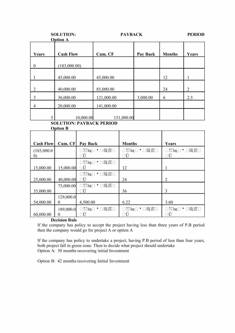
SOLUTION: PAYBACK PERIODOption A
Years Cash Flow Cum. CF Pay Back Months Years
0 (103,000.00)
1 45,000.00 45,000.00 12 1
2 40,000.00 85,000.00 24 2
3 36,000.00 121,000.00 3,000.00 6 2.5
4 20,000.00 141,000.00
5 10,000.00 151,000.00SOLUTION: PAYBACK PERIODOption B
Cash Flow Cum. CF Pay Back Months Years
(103,000.00)
Ü
Ü
Ü
15,000.00 15,000.00Ü 12 1
25,000.00 40,000.00Ü 24 2
35,000.0075,000.00
Ü 36 3
54,000.00129,000.00 4,500.00 6.22 3.60
60,000.00189,000.00
Ü
Ü
Ü
Decision Rule
If the company has policy to accept the project having less than three years of P.B periodthen the company would go for project A or option A
If the company has policy to undertake a project, having P.B period of less than four years, both project fall in green zone. Then to decide what project should undertakeOption A: 30 months recovering initial Investment
Option B: 42 months recovering Initial Investment
8/6/2019 Corporate Finance Lecture
http://slidepdf.com/reader/full/corporate-finance-lecture 53/125
Option A is preferable
Payback Very simple and easy to understandIgnores time value of money
Ignores size of Investment (Project)Ignores cash flows after payback.Can be used as rough or crude measure of appraisalCan be used for project filtration in case of more than one project.
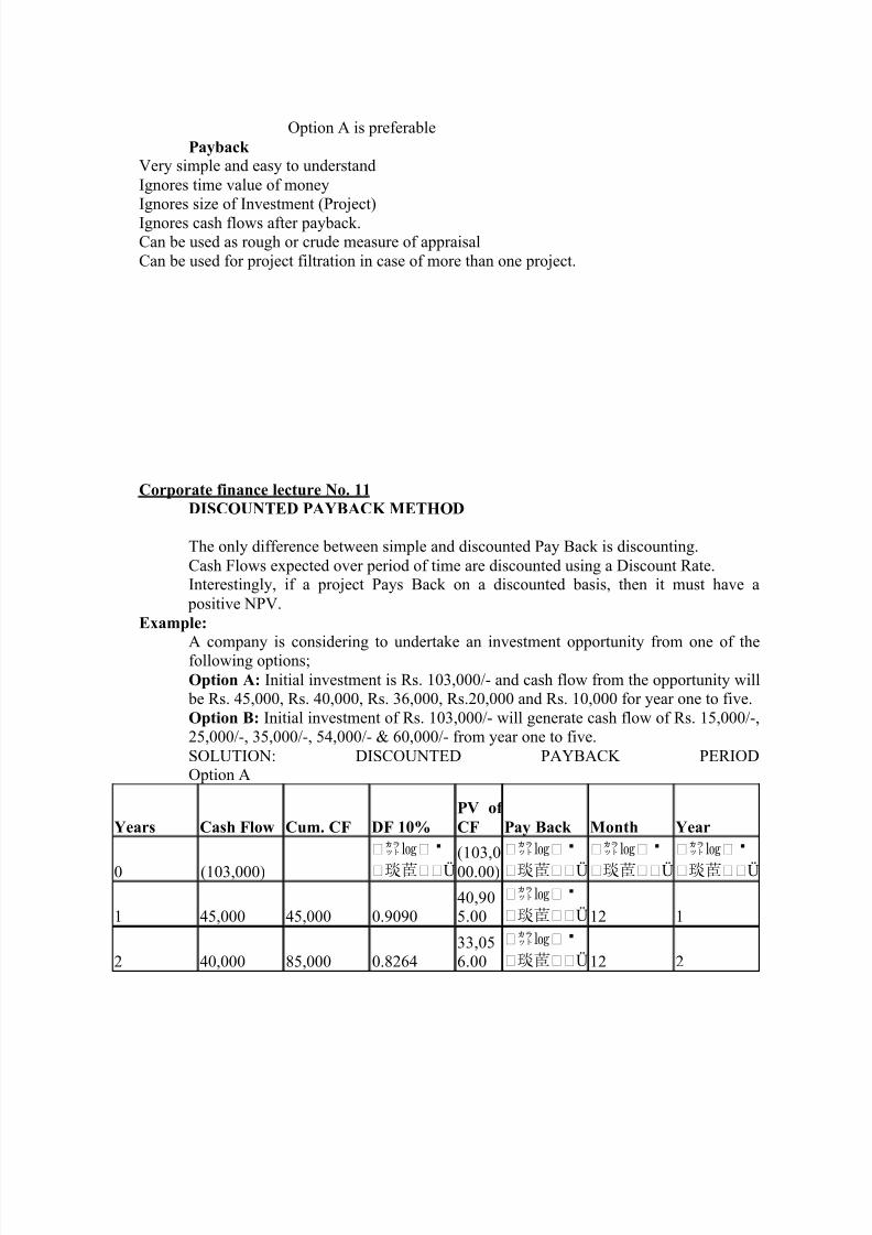
Corporate finance lecture No. 11DISCOUNTED PAYBACK METHOD
The only difference between simple and discounted Pay Back is discounting.Cash Flows expected over period of time are discounted using a Discount Rate.Interestingly, if a project Pays Back on a discounted basis, then it must have a positive NPV.
Example:A company is considering to undertake an investment opportunity from one of thefollowing options;Option A: Initial investment is Rs. 103,000/- and cash flow from the opportunity will be Rs. 45,000, Rs. 40,000, Rs. 36,000, Rs.20,000 and Rs. 10,000 for year one to five.Option B: Initial investment of Rs. 103,000/- will generate cash flow of Rs. 15,000/-,25,000/-, 35,000/-, 54,000/- & 60,000/- from year one to five.SOLUTION: DISCOUNTED PAYBACK PERIODOption A
Years Cash Flow Cum. CF DF 10% PV of CF Pay Back Month Year
0 (103,000)Ü
(103,000.00)
Ü
Ü
Ü
1 45,000 45,000 0.909040,905.00
Ü12 1
2 40,000 85,000 0.826433,056.00
Ü12 2
8/6/2019 Corporate Finance Lecture
http://slidepdf.com/reader/full/corporate-finance-lecture 54/125
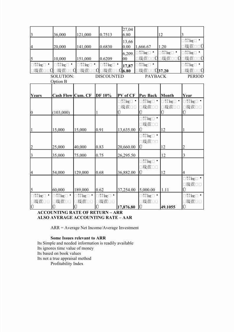
3 36,000 121,000 0.751327,046.80 12 3
4 20,000 141,000 0.683013,660.00 1,666.67 1.20
Ü
5 10,000 151,000 0.62096,209.00
Ü
Ü
Ü
Ü
Ü
Ü
Ü
17,876.80
Ü37.20
Ü
SOLUTION: DISCOUNTED PAYBACK PERIODOption B
Years Cash Flow Cum. CF DF 10% PV of CF Pay Back Month Year
0 (103,000) 1
Ü
Ü
Ü
Ü
1 15,000 15,000 0.91 13,635.00
Ü 12 1
2 25,000 40,000 0.83 20,660.00
Ü 12 2
3 35,000 75,000 0.75 26,295.50 12 3
4 54,000 129,000 0.68 36,882.00
Ü 12 4
5 60,000 189,000 0.62 37,254.00 5,000.00 1.11
Ü
Ü
Ü
Ü
Ü 17,876.80
Ü 49.1055
Ü
ACCOUNTING RATE OF RETURN ± ARR ALSO AVERAGE ACCOUNTING RATE ± AAR
ARR = Average Net Income/Average Investment
Some Issues relevant to ARR Its Simple and needed information is readily availableIts ignores time value of moneyIts based on book valuesIts not a true appraisal method
Profitability Index
8/6/2019 Corporate Finance Lecture
http://slidepdf.com/reader/full/corporate-finance-lecture 55/125
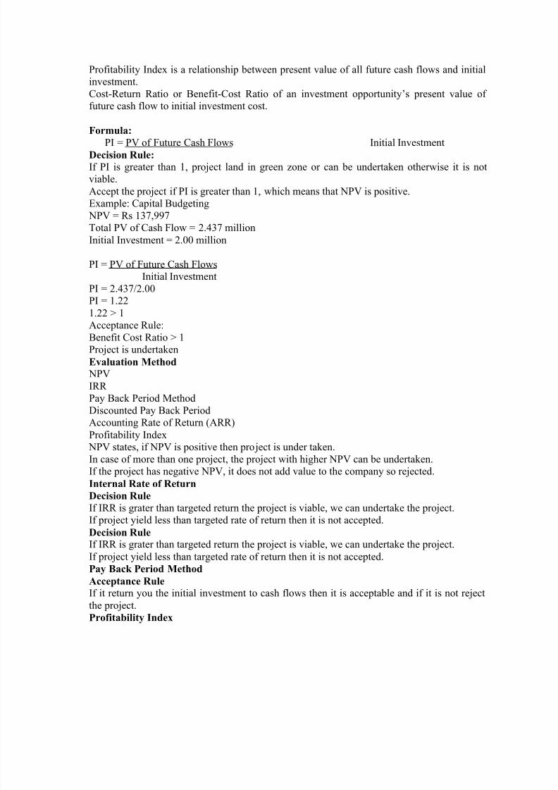
Profitability Index is a relationship between present value of all future cash flows and initialinvestment.Cost-Return Ratio or Benefit-Cost Ratio of an investment opportunity¶s present value of future cash flow to initial investment cost.
F
ormula:PI = PV of Future Cash Flows Initial InvestmentDecision Rule:If PI is greater than 1, project land in green zone or can be undertaken otherwise it is notviable.Accept the project if PI is greater than 1, which means that NPV is positive.Example: Capital Budgeting NPV = Rs 137,997Total PV of Cash Flow = 2.437 millionInitial Investment = 2.00 million
PI = PV of Future Cash FlowsInitial InvestmentPI = 2.437/2.00PI = 1.221.22 > 1Acceptance Rule:Benefit Cost Ratio > 1Project is undertakenEvaluation Method NPVIRR Pay Back Period MethodDiscounted Pay Back PeriodAccounting Rate of Return (ARR)Profitability Index NPV states, if NPV is positive then project is under taken.In case of more than one project, the project with higher NPV can be undertaken.If the project has negative NPV, it does not add value to the company so rejected.Internal Rate of Return Decision RuleIf IRR is grater than targeted return the project is viable, we can undertake the project.If project yield less than targeted rate of return then it is not accepted.Decision RuleIf IRR is grater than targeted return the project is viable, we can undertake the project.If project yield less than targeted rate of return then it is not accepted.Pay Back Period Method Acceptance RuleIf it return you the initial investment to cash flows then it is acceptable and if it is not rejectthe project.Profitability Index
8/6/2019 Corporate Finance Lecture
http://slidepdf.com/reader/full/corporate-finance-lecture 56/125
Relationship between Cash Flows and initial Investment.PI = PV of Future Cash Flows
Initial InvestmentBenefit cost ratio greater than 1 project land in green zone or can be undertaken otherwise itis not viable.
Advance EvaluationAdvance tool of Project Evaluation
Sensitivity AnalysisBreak Even AnalysisDegree of Operating Leverage
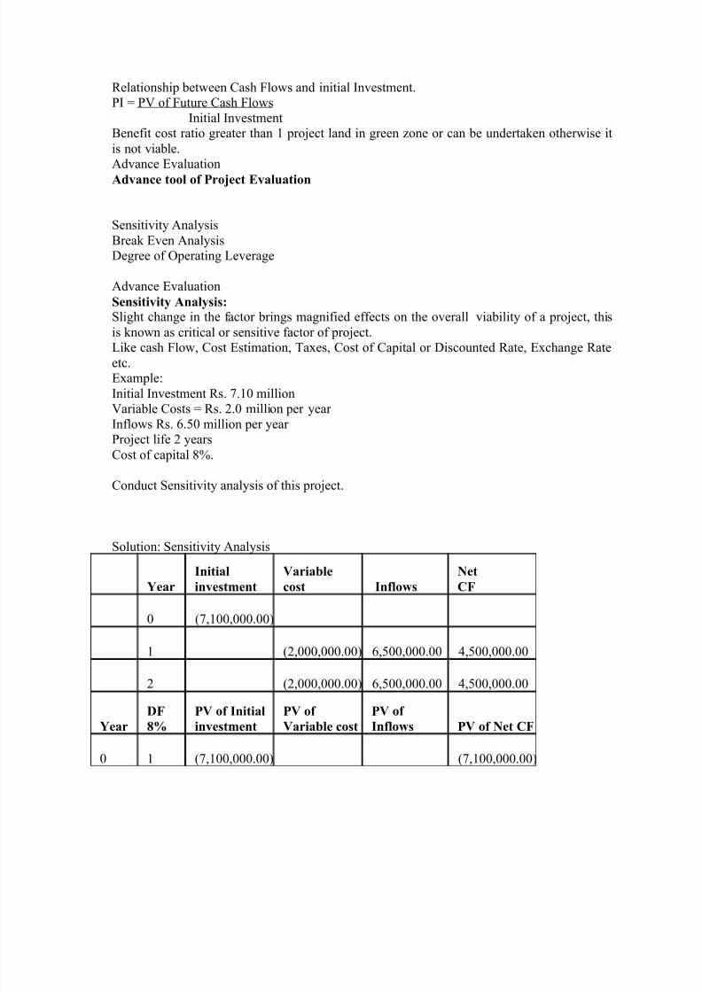
Advance EvaluationSensitivity Analysis:Slight change in the factor brings magnified effects on the overall viability of a project, this
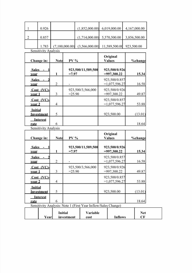
is known as critical or sensitive factor of project.Like cash Flow, Cost Estimation, Taxes, Cost of Capital or Discounted Rate, Exchange Rateetc.Example:Initial Investment Rs. 7.10 millionVariable Costs = Rs. 2.0 million per year Inflows Rs. 6.50 million per year Project life 2 yearsCost of capital 8%.
Conduct Sensitivity analysis of this project.
Solution: Sensitivity Analysis
Year Initialinvestment
Variablecost Inflows
NetCF
0 (7,100,000.00)
1 (2,000,000.00) 6,500,000.00 4,500,000.00
2 (2,000,000.00) 6,500,000.00 4,500,000.00
Year DF 8%
PV of Initialinvestment
PV of Variable cost
PV of Inflows PV of Net CF
0 1 (7,100,000.00) (7,100,000.00)
8/6/2019 Corporate Finance Lecture
http://slidepdf.com/reader/full/corporate-finance-lecture 57/125
1 0.926 (1,852,000.00) 6,019,000.00 4,167,000.00
2 0.857 (1,714,000.00) 5,570,500.00 3,856,500.00
1.783 (7,100,000.00) (3,566,000.00) 11,589,500.00 923,500.00Sensitivity Analysis
Change in: Note PV % OriginalValues %change
Sales - 1year 1
923,500/11,589,500=7.97
923,500/0.926=997,300.22 15.34
Sales - 2year 2 -
923,500/0.857=1,077,596.27 16.58
Cost (VC)-
year 1 3
923,500/3,566,000
=25.90
923,500/0.926
=997,300.22 49.87
Cost (VC)-year 2 4
923,500/0.857=1,077,596.27 53.88
InitialInvestment 5 923,500.00 (13.01)
Interestrate 6 18.64Sensitivity Analysis
Change in: Note P
V %
Original
Values %change
Sales - 1year 1
923,500/11,589,500=7.97
923,500/0.926=997,300.22 15.34
Sales - 2year 2 -
923,500/0.857=1,077,596.27 16.58
Cost (VC)-year 1 3
923,500/3,566,000=25.90
923,500/0.926=997,300.22 49.87
Cost (VC)-year 2 4
923,500/0.857=1,077,596.27 53.88
InitialInvestment 5 923,500.00 (13.01)
Interestrate 6 18.64Sensitivity Analysis: Note 1 (First Year Inflow/Sales Change)
Year Initialinvestment
Variablecost Inflows
NetCF
8/6/2019 Corporate Finance Lecture
http://slidepdf.com/reader/full/corporate-finance-lecture 58/125
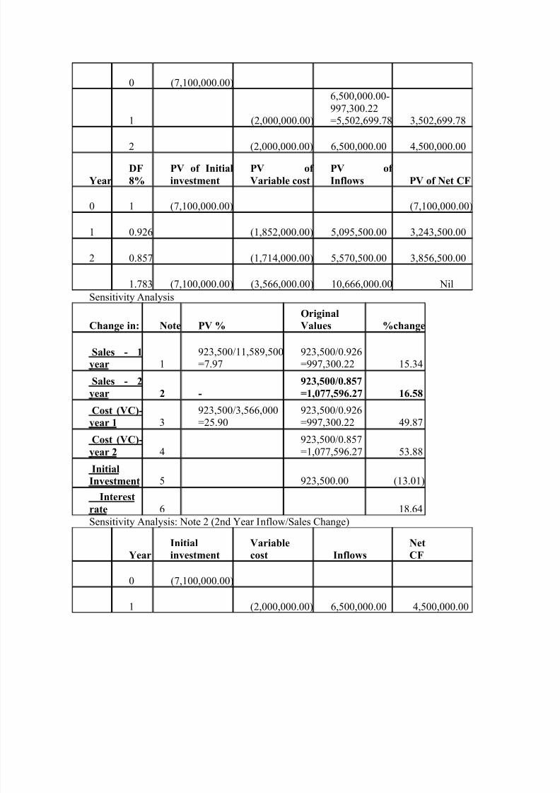
0 (7,100,000.00)
1 (2,000,000.00)
6,500,000.00-997,300.22=5,502,699.78 3,502,699.78
2 (2,000,000.00) 6,500,000.00 4,500,000.00
Year DF 8%
PV of Initialinvestment
PV of Variable cost
PV of Inflows PV of Net CF
0 1 (7,100,000.00) (7,100,000.00)
1 0.926 (1,852,000.00) 5,095,500.00 3,243,500.00
2 0.857 (1,714,000.00) 5,570,500.00 3,856,500.00
1.783 (7,100,000.00) (3,566,000.00) 10,666,000.00 NilSensitivity Analysis
Change in: Note PV % OriginalValues %change
Sales - 1year 1
923,500/11,589,500=7.97
923,500/0.926=997,300.22 15.34
Sales - 2year 2 -
923,500/0.857=1,077,596.27 16.58
Cost (VC)-year 1 3
923,500/3,566,000=25.90
923,500/0.926=997,300.22 49.87
Cost (VC)-year 2 4
923,500/0.857=1,077,596.27 53.88
InitialInvestment 5 923,500.00 (13.01)
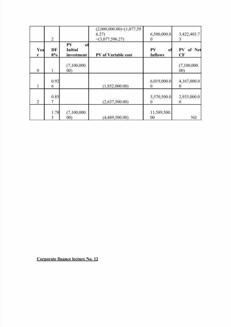
Interestrate 6 18.64Sensitivity Analysis: Note 2 (2nd Year Inflow/Sales Change)
Year Initialinvestment
Variablecost Inflows
NetCF
0 (7,100,000.00)
1 (2,000,000.00) 6,500,000.00 4,500,000.00
8/6/2019 Corporate Finance Lecture
http://slidepdf.com/reader/full/corporate-finance-lecture 59/125
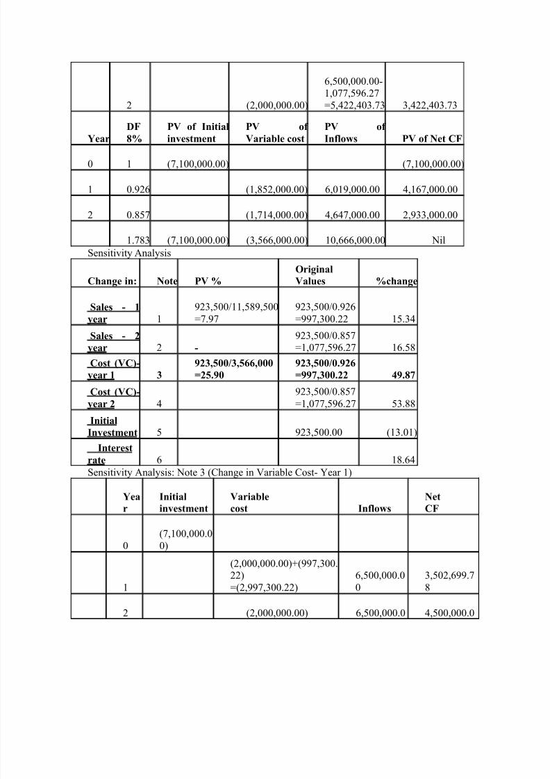
2 (2,000,000.00)
6,500,000.00-1,077,596.27=5,422,403.73 3,422,403.73
Year DF 8%
PV of Initialinvestment
PV of Variable cost
PV of Inflows PV of Net CF
0 1 (7,100,000.00) (7,100,000.00)
1 0.926 (1,852,000.00) 6,019,000.00 4,167,000.00
2 0.857 (1,714,000.00) 4,647,000.00 2,933,000.00
1.783 (7,100,000.00) (3,566,000.00) 10,666,000.00 NilSensitivity Analysis
Change in: Note PV % OriginalValues %change
Sales - 1year 1
923,500/11,589,500=7.97
923,500/0.926=997,300.22 15.34
Sales - 2year 2 -
923,500/0.857=1,077,596.27 16.58
Cost (VC)-year 1 3
923,500/3,566,000=25.90
923,500/0.926=997,300.22 49.87
Cost (VC)-year 2 4
923,500/0.857=1,077,596.27 53.88
InitialInvestment 5 923,500.00 (13.01)
Interestrate 6 18.64Sensitivity Analysis: Note 3 (Change in Variable Cost- Year 1)
Year
Initialinvestment
Variablecost Inflows
NetCF
0(7,100,000.00)
1
(2,000,000.00)+(997,300.22)=(2,997,300.22)
6,500,000.00
3,502,699.78
2 (2,000,000.00) 6,500,000.0 4,500,000.0
8/6/2019 Corporate Finance Lecture
http://slidepdf.com/reader/full/corporate-finance-lecture 60/125
0 0
Year
DF 8%
PV of Initialinvestment PV of Variable cost
PV of Inflows
PV of NetCF
0 1(7,100,000.00)
(7,100,000.00)
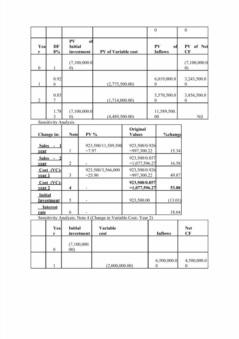
10.926 (2,775,500.00)
6,019,000.00
3,243,500.00
20.857 (1,714,000.00)
5,570,500.00
3,856,500.00
1.78
3
(7,100,000.0
0) (4,489,500.00)
11,589,500.
00 NilSensitivity Analysis
Change in: Note PV % OriginalValues %change
Sales - 1year 1
923,500/11,589,500=7.97
923,500/0.926=997,300.22 15.34
Sales - 2year 2 -
923,500/0.857=1,077,596.27 16.58
Cost (VC)-year 1 3
923,500/3,566,000=25.90
923,500/0.926=997,300.22 49.87
Cost (VC)-year 2 4 -
923,500/0.857=1,077,596.27 53.88
InitialInvestment 5 - 923,500.00 (13.01)
Interestrate 6 - 18.64Sensitivity Analysis: Note 4 (Change in Variable Cost- Year 2)
Year
Initialinvestment
Variablecost Inflows
NetCF
0(7,100,000.00)
1 (2,000,000.00)6,500,000.00
4,500,000.00
8/6/2019 Corporate Finance Lecture
http://slidepdf.com/reader/full/corporate-finance-lecture 61/125
2
(2,000,000.00)+(1,077,596.27)=(3,077,596.27)
6,500,000.00
3,422,403.73
Yea
r
DF
8%
PV of Initial
investment PV of Variable cost
PV of
Inflows
PV of Net
CF
0 1(7,100,000.00)
(7,100,000.00)
10.926 (1,852,000.00)
6,019,000.00
4,167,000.00
20.857 (2,637,500.00)
5,570,500.00
2,933,000.00
1.783
(7,100,000.00) (4,489,500.00)
11,589,500.00 Nil
Corporate finance lecture No. 12
8/6/2019 Corporate Finance Lecture
http://slidepdf.com/reader/full/corporate-finance-lecture 62/125
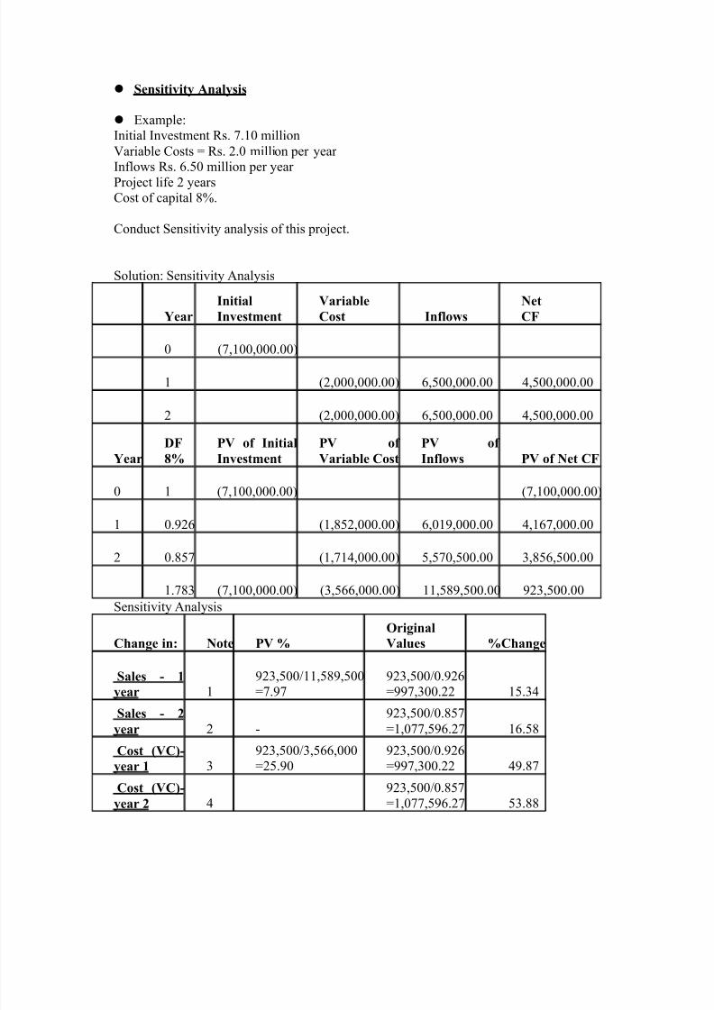
Sensitivity Analysis
Example:Initial Investment Rs. 7.10 millionVariable Costs = Rs. 2.0 million per year
Inflows Rs. 6.50 million per year Project life 2 yearsCost of capital 8%.
Conduct Sensitivity analysis of this project.
Solution: Sensitivity Analysis
Year InitialInvestment
VariableCost Inflows
NetCF
0 (7,100,000.00)
1 (2,000,000.00) 6,500,000.00 4,500,000.00
2 (2,000,000.00) 6,500,000.00 4,500,000.00
Year DF 8%
PV of InitialInvestment
PV of Variable Cost
PV of Inflows PV of Net CF
0 1 (7,100,000.00) (7,100,000.00)
1 0.926 (1,852,000.00) 6,019,000.00 4,167,000.00
2 0.857 (1,714,000.00) 5,570,500.00 3,856,500.00
1.783 (7,100,000.00) (3,566,000.00) 11,589,500.00 923,500.00Sensitivity Analysis
Change in: Note PV % OriginalValues %Change
Sales - 1
year 1
923,500/11,589,500
=7.97
923,500/0.926
=997,300.22 15.34Sales - 2year 2 -
923,500/0.857=1,077,596.27 16.58
Cost (VC)-year 1 3
923,500/3,566,000=25.90
923,500/0.926=997,300.22 49.87
Cost (VC)-year 2 4
923,500/0.857=1,077,596.27 53.88
8/6/2019 Corporate Finance Lecture
http://slidepdf.com/reader/full/corporate-finance-lecture 63/125
InitialInvestment 5 923,500.00 (13.01)
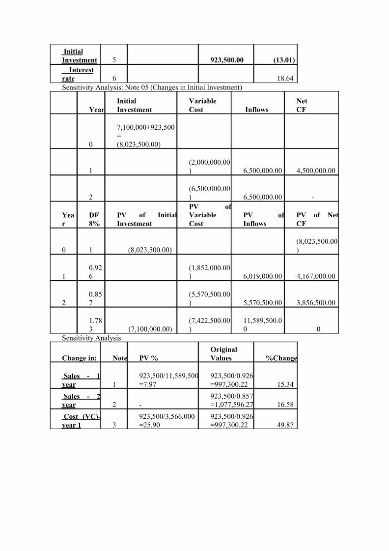
Interestrate 6 18.64Sensitivity Analysis: Note 05 (Changes in Initial Investment)
Year InitialInvestment
VariableCost Inflows
NetCF
0
7,100,000+923,500=(8,023,500.00)
1(2,000,000.00) 6,500,000.00 4,500,000.00
2(6,500,000.00) 6,500,000.00 -
Year
DF 8%
PV of InitialInvestment
PV of VariableCost
PV of Inflows
PV of NetCF
0 1 (8,023,500.00)(8,023,500.00)
10.926
(1,852,000.00) 6,019,000.00 4,167,000.00
20.857
(5,570,500.00) 5,570,500.00 3,856,500.00
1.783 (7,100,000.00)
(7,422,500.00)
11,589,500.00 0
Sensitivity Analysis
Change in: Note PV % OriginalValues %Change
Sales - 1year 1
923,500/11,589,500=7.97
923,500/0.926=997,300.22 15.34
Sales - 2year 2 -
923,500/0.857=1,077,596.27 16.58
Cost (VC)-year 1 3
923,500/3,566,000=25.90
923,500/0.926=997,300.22 49.87
8/6/2019 Corporate Finance Lecture
http://slidepdf.com/reader/full/corporate-finance-lecture 64/125
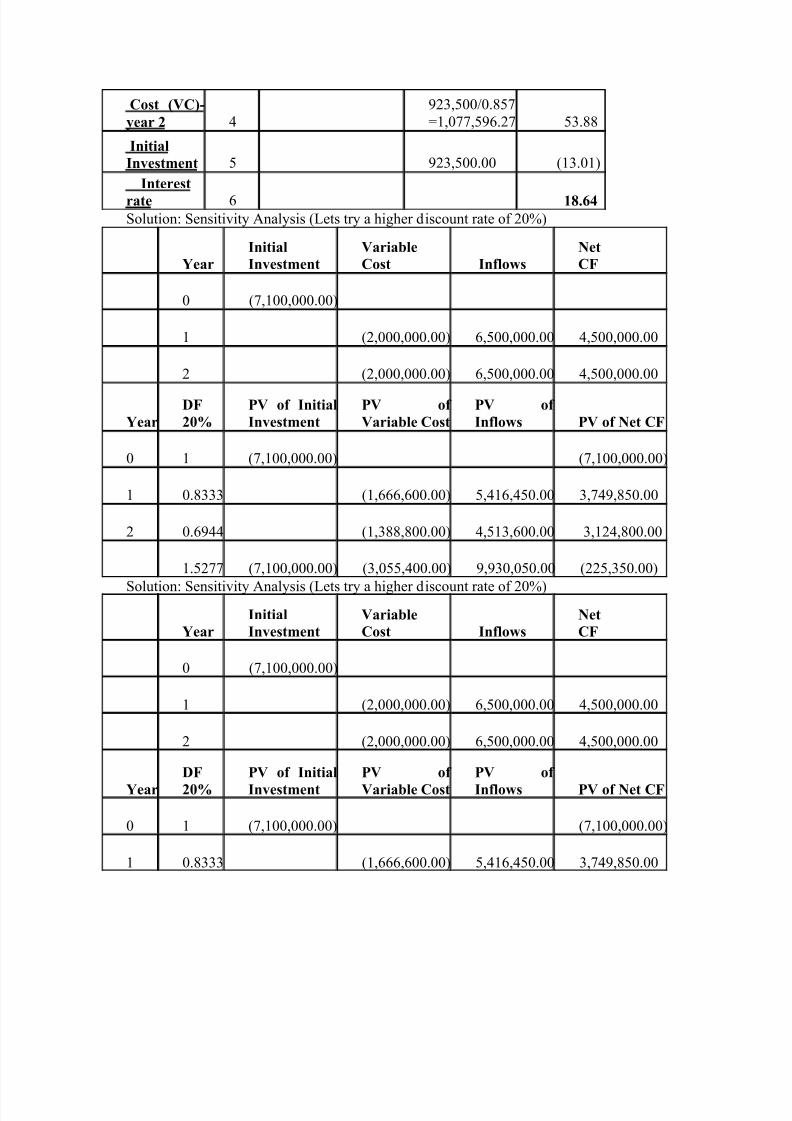
Cost (VC)-year 2 4
923,500/0.857=1,077,596.27 53.88
InitialInvestment 5 923,500.00 (13.01)
Interestrate 6 18.64Solution: Sensitivity Analysis (Lets try a higher discount rate of 20%)
Year InitialInvestment
VariableCost Inflows
NetCF
0 (7,100,000.00)
1 (2,000,000.00) 6,500,000.00 4,500,000.00
2 (2,000,000.00) 6,500,000.00 4,500,000.00
Year DF 20%
PV of InitialInvestment
PV of Variable Cost
PV of Inflows PV of Net CF
0 1 (7,100,000.00) (7,100,000.00)
1 0.8333 (1,666,600.00) 5,416,450.00 3,749,850.00
2 0.6944 (1,388,800.00) 4,513,600.00 3,124,800.00
1.5277 (7,100,000.00) (3,055,400.00) 9,930,050.00 (225,350.00)Solution: Sensitivity Analysis (Lets try a higher discount rate of 20%)
Year InitialInvestment
VariableCost Inflows
NetCF
0 (7,100,000.00)
1 (2,000,000.00) 6,500,000.00 4,500,000.00
2 (2,000,000.00) 6,500,000.00 4,500,000.00
Year DF 20%
PV of InitialInvestment
PV of Variable Cost
PV of Inflows PV of Net CF
0 1 (7,100,000.00) (7,100,000.00)
1 0.8333 (1,666,600.00) 5,416,450.00 3,749,850.00
8/6/2019 Corporate Finance Lecture
http://slidepdf.com/reader/full/corporate-finance-lecture 65/125
2 0.6944 (1,388,800.00) 4,513,600.00 3,124,800.00
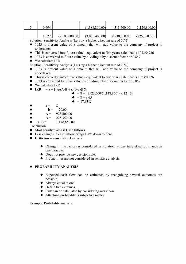
1.5277 (7,100,000.00) (3,055,400.00) 9,930,050.00 (225,350.00)Solution: Sensitivity Analysis (Lets try a higher discount rate of 20%)
1023 is present value of a amount that will add value to the company if project isundertaken This is converted into future value - equivalent to first years' sale, that is 1023/0.926 1023 is converted to future value by dividing it by discount factor or 0.857 We calculate IRR Solution: Sensitivity Analysis (Lets try a higher discount rate of 20%) 1023 is present value of a amount that will add value to the company if project is
undertaken This is converted into future value - equivalent to first years' sale, that is 1023/0.926 1023 is converted to future value by dividing it by discount factor or 0.857 We calculate IRR
IRR = a + [{A/(A-B)} x (b-a)}]% = 8 + [ {923,500/(1,148,850)} x 12} % = 8 + 9.65 = 17.65%
a = 8 b = 20.00 A = 923,500.00 B = 225,350.00 A+B = 1,148,850.00Conclusion Most sensitive area is Cash Inflows.
Less changes in cash inflow brings NPV down to Zero. Criticism ± Sensitivity Analysis
Change in the factors is considered in isolation, at one time effect of change inone variable.
Does not provide any decision rule. Probabilities are not considered in sensitive analysis.
PR OBABILITY ANALYSIS
Expected cash flow can be estimated by recognizing several outcomes are
possible Always equal to one Define two extremes Risk can be calculated by considering worst case Attaching probability is subjective matter
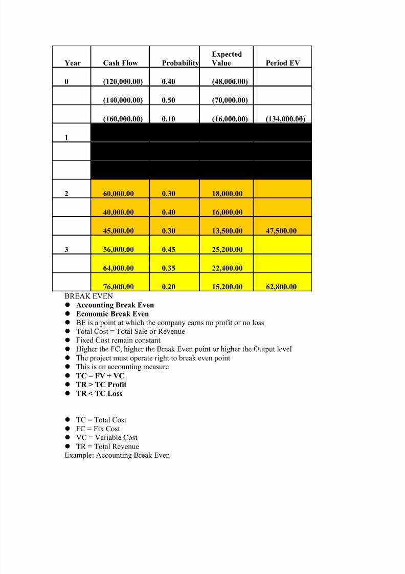
Example: Probability analysis
8/6/2019 Corporate Finance Lecture
http://slidepdf.com/reader/full/corporate-finance-lecture 66/125
Year Cash Flow Probability ExpectedValue Period EV
0 (120,000.00) 0.40 (48,000.00)
(140,000.00) 0.50 (70,000.00)
(160,000.00) 0.10 (16,000.00) (134,000.00)
1 50,000.00 0.35 17,500.00
60,000.00 0.40 24,000.00
70,000.00 0.25 17,500.00 59,000.00
2 60,000.00 0.30 18,000.00
40,000.00 0.40 16,000.00
45,000.00 0.30 13,500.00 47,500.00
3 56,000.00 0.45 25,200.00
64,000.00 0.35 22,400.00
76,000.00 0.20 15,200.00 62,800.00
BREAK EVEN Accounting Break Even Economic Break Even BE is a point at which the company earns no profit or no loss Total Cost = Total Sale or Revenue Fixed Cost remain constant Higher the FC, higher the Break Even point or higher the Output level The project must operate right to break even point This is an accounting measure TC = FV + VC TR > TC Profit
TR < TC Loss
TC = Total Cost FC = Fix Cost VC = Variable Cost TR = Total RevenueExample: Accounting Break Even
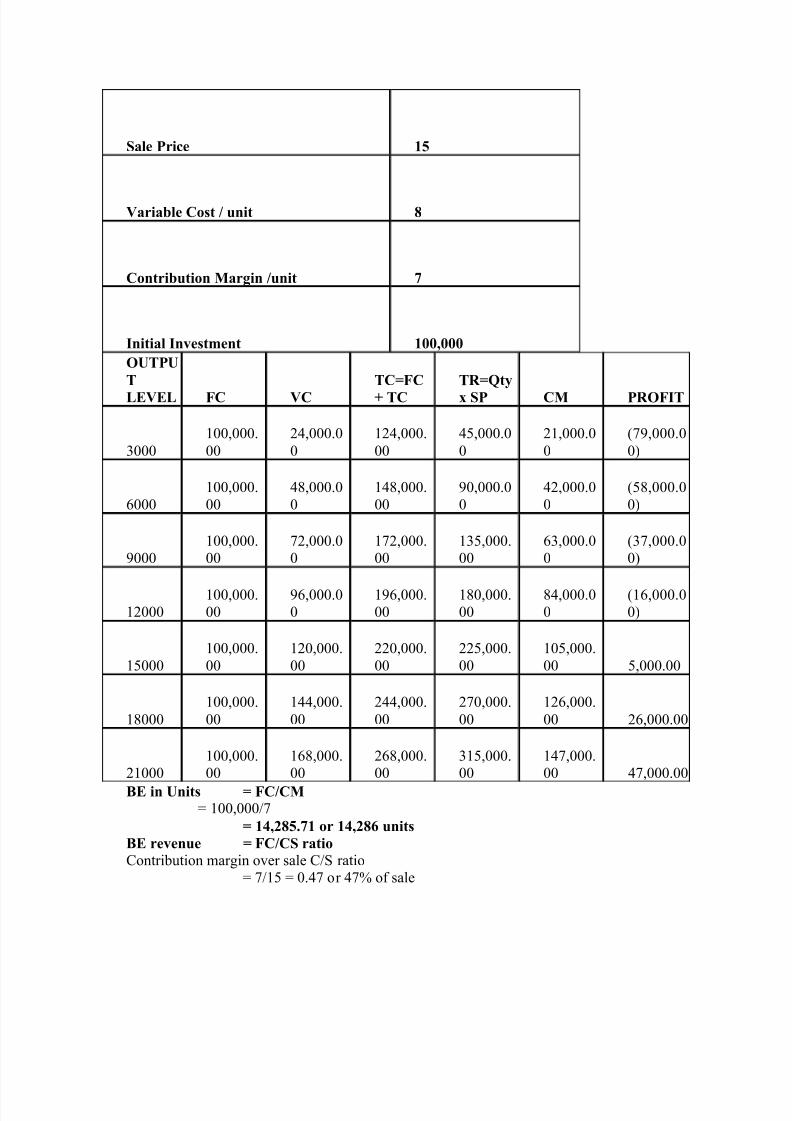
8/6/2019 Corporate Finance Lecture
http://slidepdf.com/reader/full/corporate-finance-lecture 67/125
Sale Price 15
Variable Cost / unit 8
Contribution Margin /unit 7
Initial Investment 100,000 OUTPU
T LEVEL FC VC TC=FC+ TC
TR=Qtyx SP CM PR OFIT
3000100,000.00
24,000.00
124,000.00
45,000.00
21,000.00
(79,000.00)
6000100,000.00
48,000.00
148,000.00
90,000.00
42,000.00
(58,000.00)
9000100,000.00
72,000.00
172,000.00
135,000.00
63,000.00
(37,000.00)
12000100,000.00
96,000.00
196,000.00
180,000.00
84,000.00
(16,000.00)
15000100,000.00
120,000.00
220,000.00
225,000.00
105,000.00 5,000.00
18000100,000.00
144,000.00
244,000.00
270,000.00
126,000.00 26,000.00
21000100,000.00
168,000.00
268,000.00
315,000.00
147,000.00 47,000.00
BE in Units = FC/CM= 100,000/7
= 14,285.71 or 14,286 units BE revenue = FC/CS ratioContribution margin over sale C/S ratio
= 7/15 = 0.47 or 47% of sale
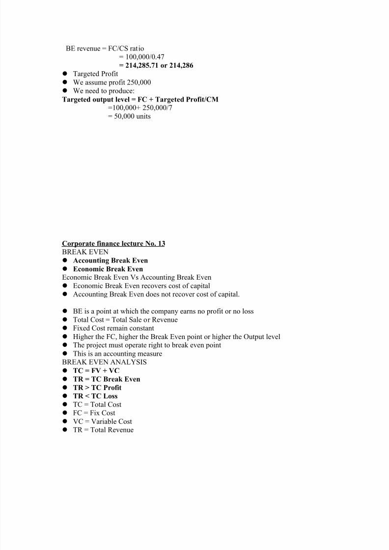
8/6/2019 Corporate Finance Lecture
http://slidepdf.com/reader/full/corporate-finance-lecture 68/125
BE revenue = FC/CS ratio= 100,000/0.47= 214,285.71 or 214,286
Targeted Profit We assume profit 250,000
We need to produce:Targeted output level = FC + Targeted Profit/CM=100,000+ 250,000/7= 50,000 units
Corporate finance lecture No. 13BREAK EVEN Accounting Break Even Economic Break EvenEconomic Break Even Vs Accounting Break Even Economic Break Even recovers cost of capital Accounting Break Even does not recover cost of capital.
BE is a point at which the company earns no profit or no loss Total Cost = Total Sale or Revenue Fixed Cost remain constant Higher the FC, higher the Break Even point or higher the Output level The project must operate right to break even point This is an accounting measureBREAK EVEN ANALYSIS TC = FV + VC TR = TC Break Even TR > TC Profit TR < TC Loss TC = Total Cost FC = Fix Cost VC = Variable Cost TR = Total Revenue
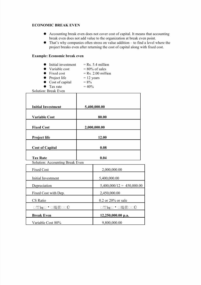
8/6/2019 Corporate Finance Lecture
http://slidepdf.com/reader/full/corporate-finance-lecture 69/125
ECONOMIC BREAK EVEN
Accounting break even does not cover cost of capital. It means that accounting break even does not add value to the organization at break even point.
That¶s why companies often stress on value addition ± to find a level where the
project breaks even after returning the cost of capital along with fixed cost.
Example: Economic break even
Initial investment = Rs. 5.4 million Variable cost = 80% of sales Fixed cost = Rs. 2.00 million Project life = 12 years Cost of capital = 8% Tax rate = 40%
Solution: Break Even
Initial Investment 5,400,000.00
Variable Cost 80.00
Fixed Cost 2,000,000.00
Project life 12.00
Cost of Capital 0.08
Tax Rate 0.04Solution: Accounting Break Even
Fixed Cost 2,000,000.00
Initial Investment 5,400,000.00
Depreciation 5,400,000/12 = 450,000.00
Fixed Cost with Dep. 2,450,000.00CS Ratio 0.2 or 20% or sale
Ü Ü
Break Even 12,250,000.00 p.a.
Variable Cost 80% 9,800,000.00
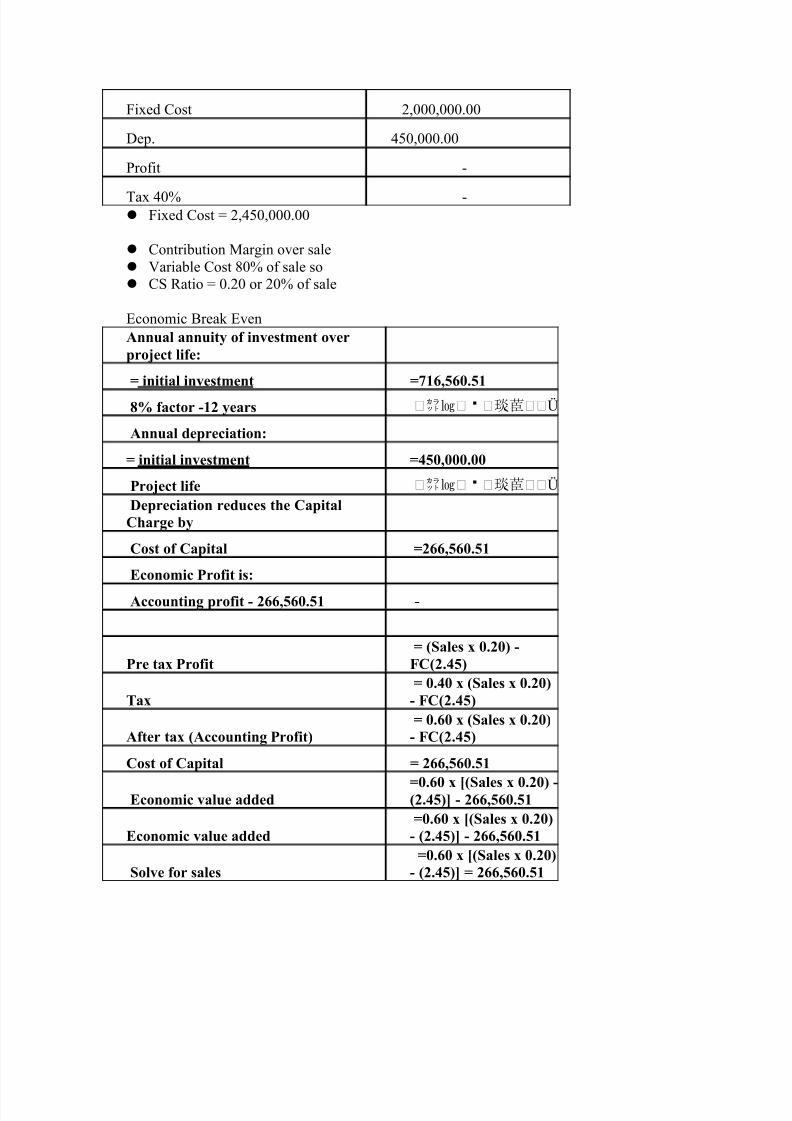
8/6/2019 Corporate Finance Lecture
http://slidepdf.com/reader/full/corporate-finance-lecture 70/125
Fixed Cost 2,000,000.00
Dep. 450,000.00
Profit -
Tax 40% - Fixed Cost = 2,450,000.00
Contribution Margin over sale Variable Cost 80% of sale so CS Ratio = 0.20 or 20% of sale
Economic Break EvenAnnual annuity of investment overproject life:
= initial investment =716,560.518% factor -12 years Ü
Annual depreciation:
= initial investment =450,000.00
Project life Ü
Depreciation reduces the CapitalCharge by
Cost of Capital =266,560.51
Economic Profit is:Accounting profit - 266,560.51 -
Pre tax Profit= (Sales x 0.20) -FC(2.45)
Tax= 0.40 x (Sales x 0.20)
- FC(2.45)
After tax (Accounting Profit)= 0.60 x (Sales x 0.20)
- FC(2.45)
Cost of Capital = 266,560.51
Economic value added=0.60 x [(Sales x 0.20) -(2.45)] - 266,560.51
Economic value added=0.60 x [(Sales x 0.20)
- (2.45)] - 266,560.51
Solve for sales=0.60 x [(Sales x 0.20)
- (2.45)] = 266,560.51
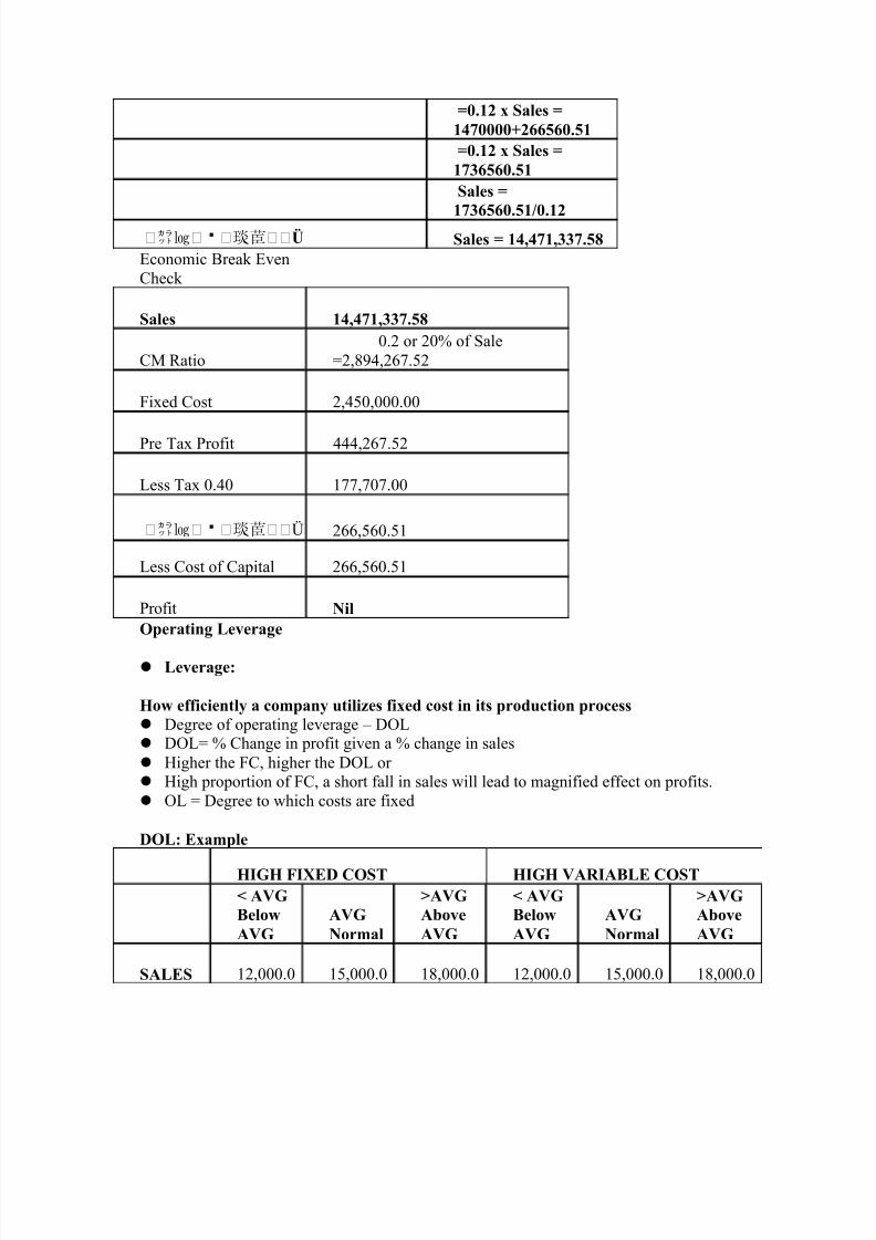
8/6/2019 Corporate Finance Lecture
http://slidepdf.com/reader/full/corporate-finance-lecture 71/125
=0.12 x Sales =
1470000+266560.51=0.12 x Sales =
1736560.51Sales =
1736560.51/0.12Ü Sales = 14,471,337.58
Economic Break EvenCheck
Sales 14,471,337.58
CM Ratio0.2 or 20% of Sale
=2,894,267.52
Fixed Cost 2,450,000.00
Pre Tax Profit 444,267.52
Less Tax 0.40 177,707.00
Ü 266,560.51
Less Cost of Capital 266,560.51
Profit Nil O
perating Leverage
Leverage:
How efficiently a company utilizes fixed cost in its production process Degree of operating leverage ± DOL DOL= % Change in profit given a % change in sales Higher the FC, higher the DOL or High proportion of FC, a short fall in sales will lead to magnified effect on profits. OL = Degree to which costs are fixed
DO
L: Example HIGH FIXED COST HIGH VARIABLE COST < AVGBelowAVG
AVGNormal
>AVGAboveAVG
< AVGBelowAVG
AVGNormal
>AVGAboveAVG
SALES 12,000.0 15,000.0
18,000.0
12,000.0
15,000.0
18,000.0
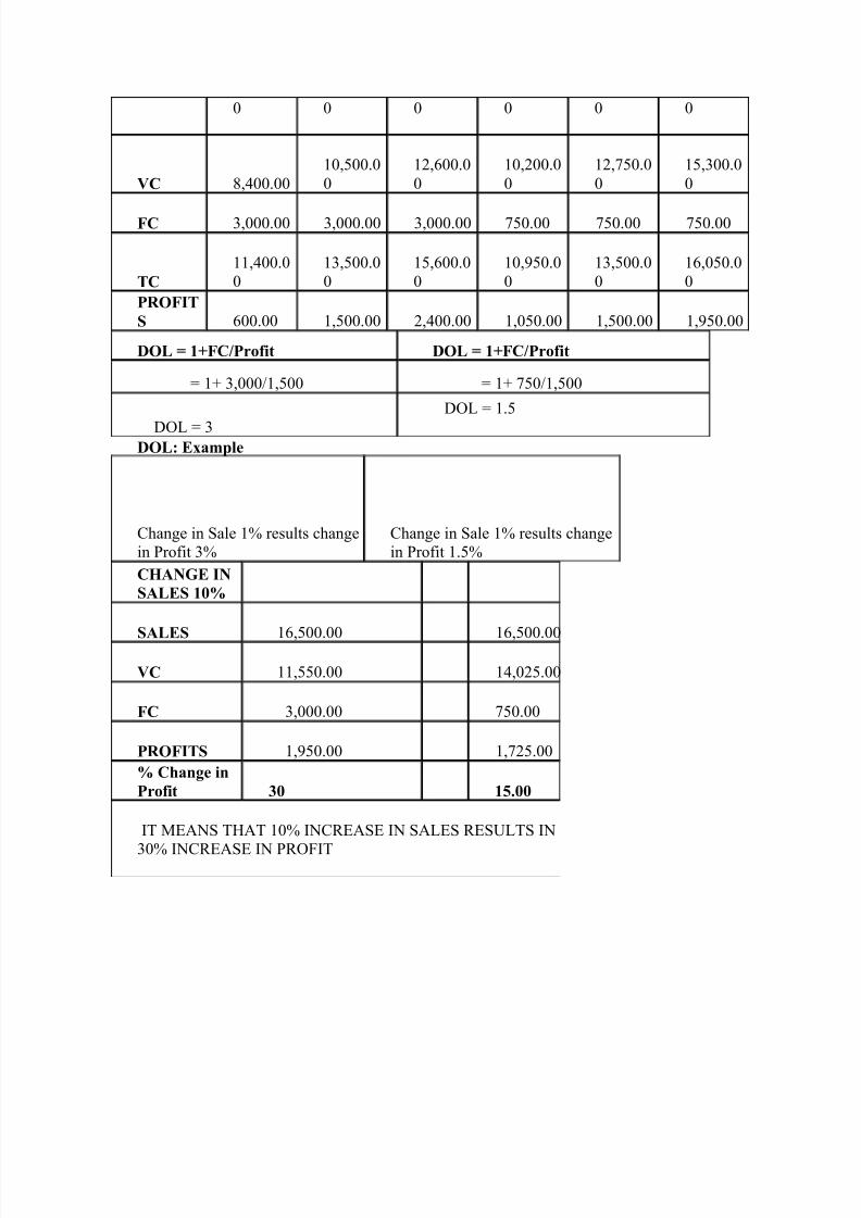
8/6/2019 Corporate Finance Lecture
http://slidepdf.com/reader/full/corporate-finance-lecture 72/125
0 0 0 0 0 0
VC 8,400.0010,500.00
12,600.00
10,200.00
12,750.00
15,300.00
FC 3,000.00 3,000.00 3,000.00 750.00 750.00 750.00
TC 11,400.00
13,500.00
15,600.00
10,950.00
13,500.00
16,050.00
PR OFITS 600.00 1,500.00 2,400.00 1,050.00 1,500.00 1,950.00
DOL = 1+FC/Profit DOL = 1+FC/Profit
= 1+ 3,000/1,500 = 1+ 750/1,500
DOL = 3 DOL = 1.5
DOL: Example
Change in Sale 1% results changein Profit 3%
Change in Sale 1% results changein Profit 1.5%
CHANGE INSALES 10%
SALES 16,500.00 16,500.00
VC 11,550.00 14,025.00
FC 3,000.00 750.00
PR OFITS 1,950.00 1,725.00% Change inProfit 30 15.00
IT MEANS THAT 10% INCREASE IN SALES RESULTS IN30% INCREASE IN PROFIT
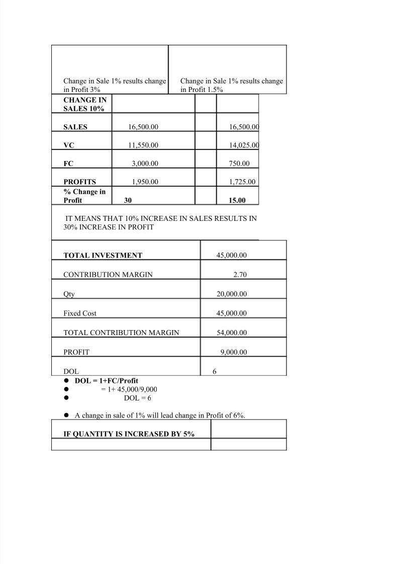
8/6/2019 Corporate Finance Lecture
http://slidepdf.com/reader/full/corporate-finance-lecture 73/125
Change in Sale 1% results changein Profit 3%
Change in Sale 1% results changein Profit 1.5%
CHANGE INSALES 10%
SALES 16,500.00 16,500.00
VC 11,550.00 14,025.00
FC 3,000.00 750.00
PR OFITS 1,950.00 1,725.00
% Change inProfit 30 15.00
IT MEANS THAT 10% INCREASE IN SALES RESULTS IN30% INCREASE IN PROFIT
TOTAL INVESTMENT 45,000.00
CONTRIBUTION MARGIN 2.70
Qty 20,000.00
Fixed Cost 45,000.00
TOTAL CONTRIBUTION MARGIN 54,000.00
PROFIT 9,000.00
DOL 6 DOL = 1+FC/Profit = 1+ 45,000/9,000 DOL = 6
A change in sale of 1% will lead change in Profit of 6%.
IF QUANTITY IS INCREASED BY 5%
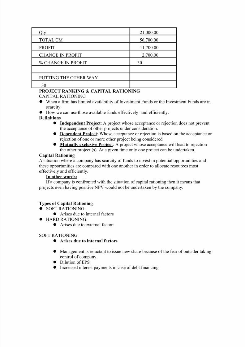
8/6/2019 Corporate Finance Lecture
http://slidepdf.com/reader/full/corporate-finance-lecture 74/125
Qty 21,000.00
TOTAL CM 56,700.00
PROFIT 11,700.00
CHANGE IN PROFIT 2,700.00
% CHANGE IN PROFIT 30
PUTTING THE OTHER WAY
30PR OJECT RANKING & CAPITAL RATIONINGCAPITAL RATIONING When a firm has limited availability of Investment Funds or the Investment Funds are in
scarcity. How we can use those available funds effectively and efficiently.
Definitions Independent Project: A project whose acceptance or rejection does not prevent
the acceptance of other projects under consideration. Dependent Project: Whose acceptance or rejection is based on the acceptance or
rejection of one or more other project being considered. Mutually exclusive Project: A project whose acceptance will lead to rejection
the other project (s). At a given time only one project can be undertaken.Capital Rationing A situation where a company has scarcity of funds to invest in potential opportunities andthese opportunities are compared with one another in order to allocate resources mosteffectively and efficiently.
In other words:If a company is confronted with the situation of capital rationing then it means that projects even having positive NPV would not be undertaken by the company.
Types of Capital Rationing SOFT RATIONING:
Arises due to internal factors HARD RATIONING:
Arises due to external factors
SOFT RATIONING Arises due to internal factors
Management is reluctant to issue new share because of the fear of outsider takingcontrol of company.
Dilution of EPS Increased interest payments in case of debt financing
8/6/2019 Corporate Finance Lecture
http://slidepdf.com/reader/full/corporate-finance-lecture 75/125
Company¶s will to maintain limited investment level that can be financed thruretained earnings.
HARD RATIONING Arises due to external factors
- If share prices are depressed or market is bearish, raising capital is very difficult.- Restriction on lending by Banks.- High interest rate- High cost associated with issuance of share / debt instrument.
Corporate finance lecture No. 14CAPITAL RATIONING
A situation where a company has scarcity of funds to invest in potential opportunitiesand these opportunities are compared with one another in order to allocate resources mosteffectively and efficiently.
Types of Capital Rationing SOFT RATIONING:
Arises due to internal factors HARD RATIONING:
Arises due to external factors
SOFT RATIONING Arises due to internal factors
Management is reluctant to issue new share because of the fear of outsider takingcontrol of company.
Dilution of EPS Increased interest payments in case of debt financing Company¶s will to maintain limited investment level that can be financed thru
retained earnings.
HARD RATIONING Arises due to external factors
- If share prices are depressed or market is bearish, raising capital is very difficult.- Restriction on lending by Banks.
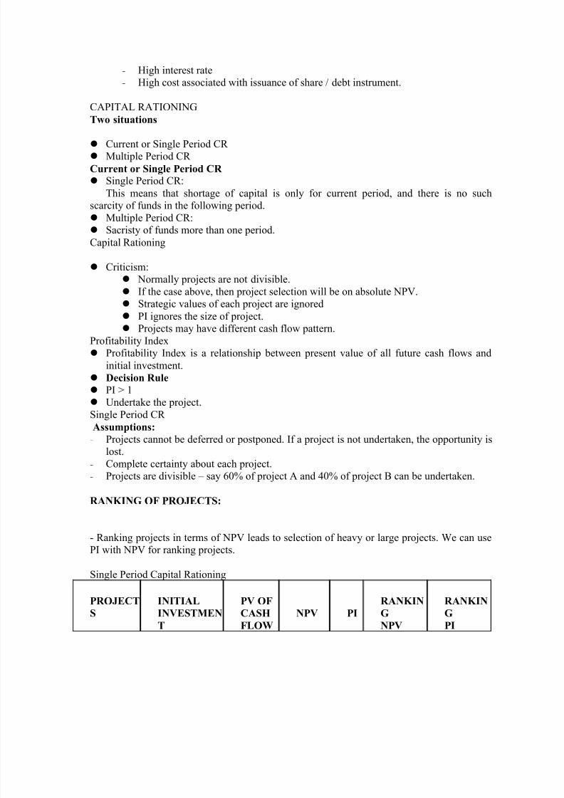
8/6/2019 Corporate Finance Lecture
http://slidepdf.com/reader/full/corporate-finance-lecture 76/125
- High interest rate- High cost associated with issuance of share / debt instrument.
CAPITAL RATIONINGTwo situations
Current or Single Period CR Multiple Period CR Current or Single Period CR Single Period CR:
This means that shortage of capital is only for current period, and there is no suchscarcity of funds in the following period. Multiple Period CR: Sacristy of funds more than one period.Capital Rationing
Criticism: Normally projects are not divisible.
If the case above, then project selection will be on absolute NPV. Strategic values of each project are ignored PI ignores the size of project. Projects may have different cash flow pattern.
Profitability Index Profitability Index is a relationship between present value of all future cash flows and
initial investment. Decision Rule PI > 1 Undertake the project.Single Period CR Assumptions:
- Projects cannot be deferred or postponed. If a project is not undertaken, the opportunity islost.
- Complete certainty about each project.- Projects are divisible ± say 60% of project A and 40% of project B can be undertaken.
RANKING OF PR OJECTS:
- Ranking projects in terms of NPV leads to selection of heavy or large projects. We can usePI with NPV for ranking projects.
Single Period Capital Rationing
PR OJECTS
INITIAL INVESTMENT
PV OF CASH FLOW
NPV PI RANKING NPV
RANKING PI
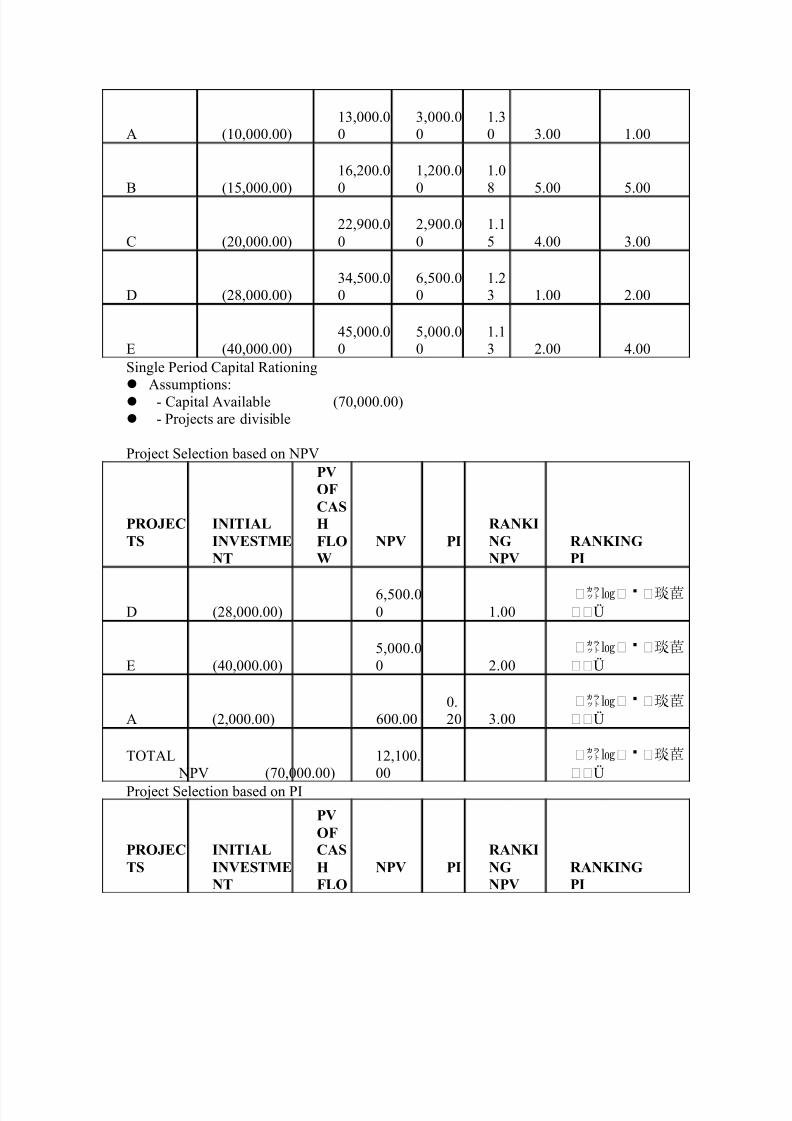
8/6/2019 Corporate Finance Lecture
http://slidepdf.com/reader/full/corporate-finance-lecture 77/125
A (10,000.00)13,000.00
3,000.00
1.30 3.00 1.00
B (15,000.00)
16,200.0
0
1,200.0
0
1.0
8 5.00 5.00
C (20,000.00)22,900.00
2,900.00
1.15 4.00 3.00
D (28,000.00)34,500.00
6,500.00
1.23 1.00 2.00
E (40,000.00)45,000.00
5,000.00
1.13 2.00 4.00
Single Period Capital Rationing
Assumptions: - Capital Available (70,000.00) - Projects are divisible
Project Selection based on NPV
PR OJECTS
INITIAL INVESTMENT
PVOF CASH FLOW
NPV PI RANKING NPV
RANKING PI
D (28,000.00)6,500.00 1.00
Ü
E (40,000.00)5,000.00 2.00
Ü
A (2,000.00) 600.000.20 3.00
Ü
TOTAL NPV (70,000.00)
12,100.00
Ü
Project Selection based on PI
PR OJECTS
INITIAL INVESTMENT
PVOF CASH FLO
NPV PI RANKING NPV
RANKING PI
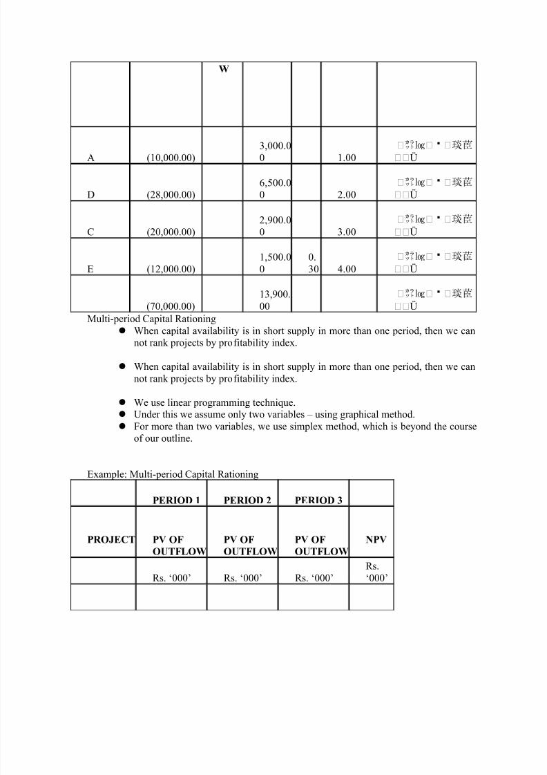
8/6/2019 Corporate Finance Lecture
http://slidepdf.com/reader/full/corporate-finance-lecture 78/125
W
A (10,000.00)3,000.00 1.00
Ü
D (28,000.00)6,500.00 2.00
Ü
C (20,000.00)2,900.00 3.00
Ü
E (12,000.00)1,500.00
0.30 4.00
Ü
(70,000.00)13,900.00
Ü
Multi-period Capital Rationing When capital availability is in short supply in more than one period, then we can
not rank projects by profitability index.
When capital availability is in short supply in more than one period, then we cannot rank projects by profitability index.
We use linear programming technique. Under this we assume only two variables ± using graphical method. For more than two variables, we use simplex method, which is beyond the course
of our outline.
Example: Multi-period Capital Rationing
PERIOD 1 PERIOD 2 PERIOD 3
PR OJECT PV OF OUTFLOW
PV OF OUTFLOW
PV OF OUTFLOW
NPV
Rs. µ000¶ Rs. µ000¶ Rs. µ000¶Rs.µ000¶

8/6/2019 Corporate Finance Lecture
http://slidepdf.com/reader/full/corporate-finance-lecture 79/125
X 30 10 10 50
Y 20 6 4 10
Capital Investment -Availability
PERIOD 1 36
PERIOD 2 10
PERIOD 3 8
Projects are divisibleSolution: Multi-period Capital Rationing Let x = Portion of project X Let y = Portion of project Y Establishing Constraints
PERIOD 1 =30x+Y20<=36 PERIOD 2 =10x + 6y<=10 PERIOD 3 =10x + 4y<= 8
Where: x & y <= 1 Means that portion of project is less than one or equal to one
x & y >= 0 Portion of project must be greater than equal to 0
Objective Function:
Maximize 50x + 10y
x y
1.20 1.80
1.00 1.67
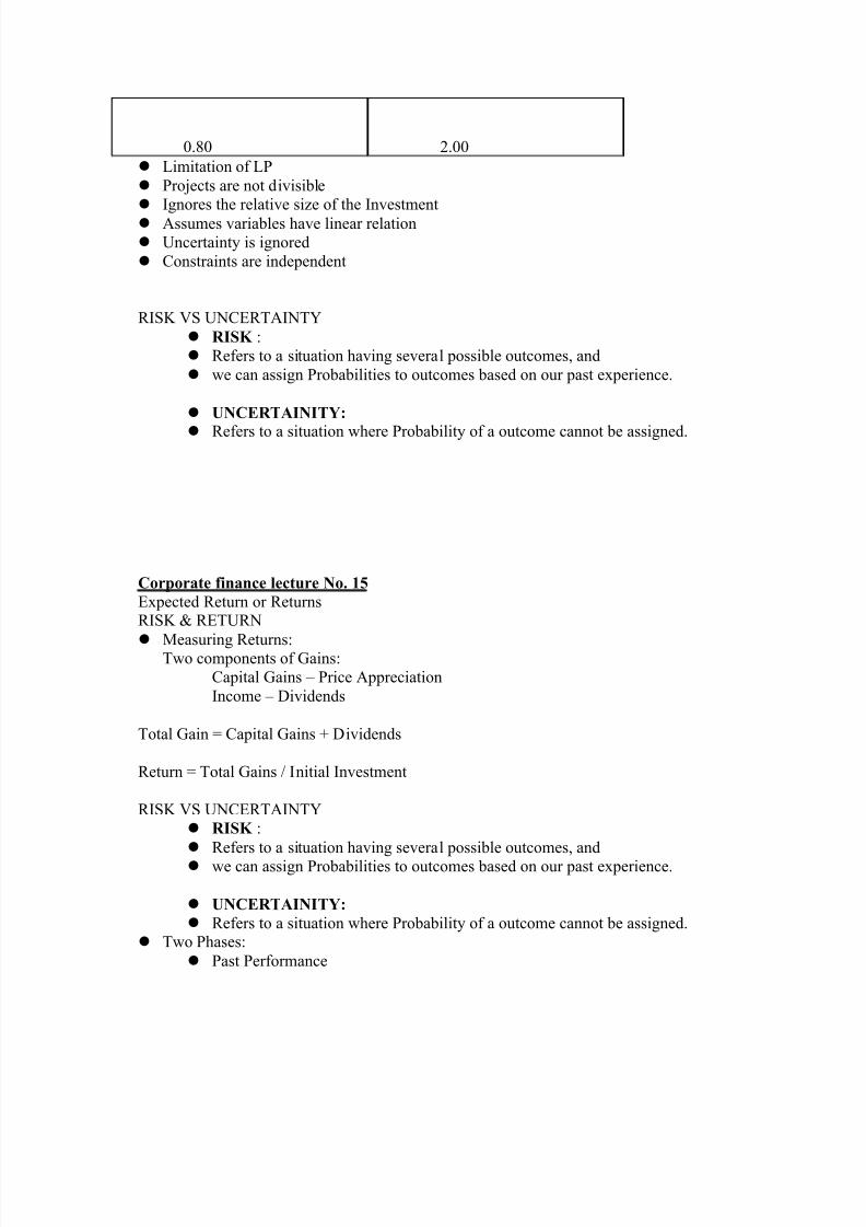
8/6/2019 Corporate Finance Lecture
http://slidepdf.com/reader/full/corporate-finance-lecture 80/125
0.80 2.00 Limitation of LP Projects are not divisible
Ignores the relative size of the Investment Assumes variables have linear relation Uncertainty is ignored Constraints are independent
RISK VS UNCERTAINTY RISK : Refers to a situation having several possible outcomes, and we can assign Probabilities to outcomes based on our past experience.
UNCER
T
AINIT
Y: Refers to a situation where Probability of a outcome cannot be assigned.
Corporate finance lecture No. 15Expected Return or Returns
RISK & RETURN Measuring Returns:Two components of Gains:
Capital Gains ± Price AppreciationIncome ± Dividends
Total Gain = Capital Gains + Dividends
Return = Total Gains / Initial Investment
RISK VS UNCERTAINTY RISK : Refers to a situation having several possible outcomes, and we can assign Probabilities to outcomes based on our past experience.
UNCER TAINITY: Refers to a situation where Probability of a outcome cannot be assigned.
Two Phases: Past Performance
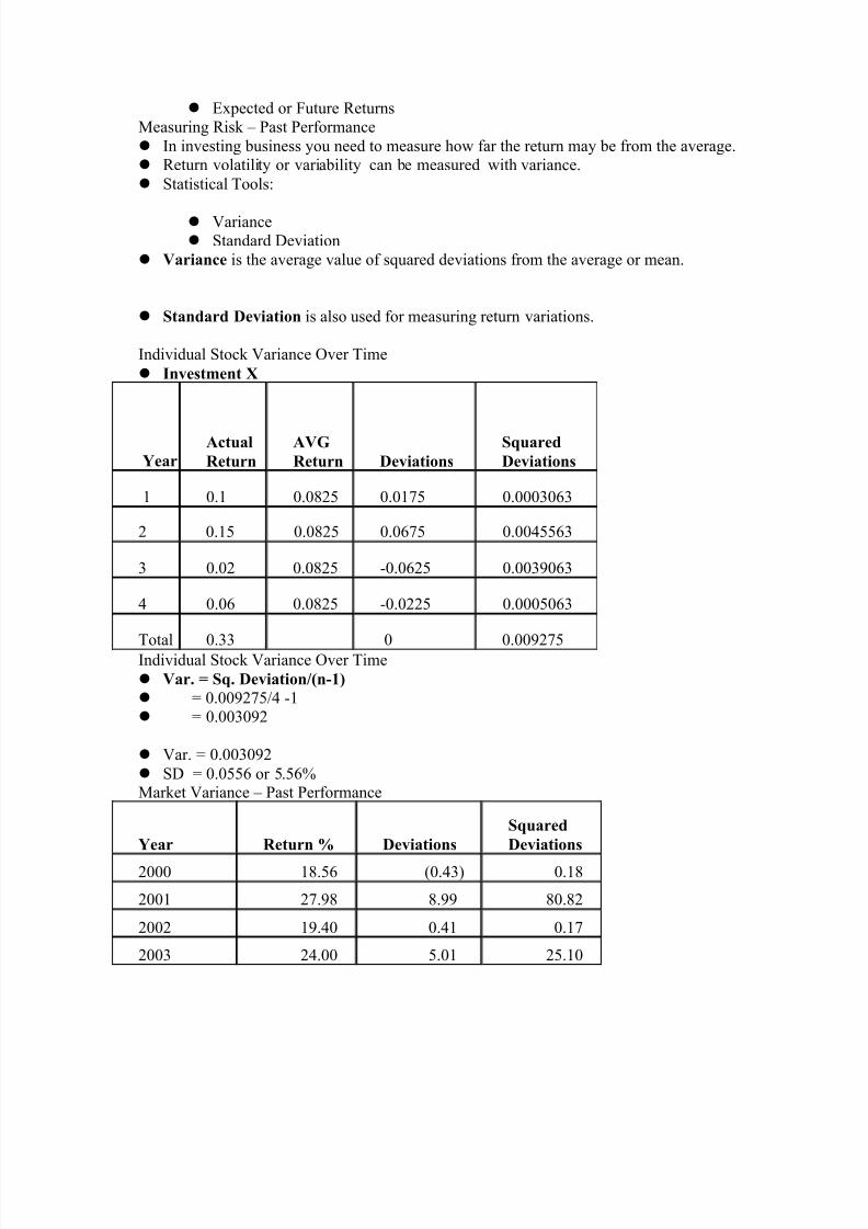
8/6/2019 Corporate Finance Lecture
http://slidepdf.com/reader/full/corporate-finance-lecture 81/125
Expected or Future ReturnsMeasuring Risk ± Past Performance In investing business you need to measure how far the return may be from the average. Return volatility or variability can be measured with variance. Statistical Tools:
Variance Standard Deviation
Variance is the average value of squared deviations from the average or mean.
Standard Deviation is also used for measuring return variations.
Individual Stock Variance Over Time Investment X
Year Actual Return
AVG Return Deviations
Squared Deviations
1 0.1 0.0825 0.0175 0.0003063
2 0.15 0.0825 0.0675 0.0045563
3 0.02 0.0825 -0.0625 0.0039063
4 0.06 0.0825 -0.0225 0.0005063
Total 0.33 0 0.009275Individual Stock Variance Over Time Var. = Sq. Deviation/(n-1) = 0.009275/4 -1 = 0.003092
Var. = 0.003092 SD = 0.0556 or 5.56%Market Variance ± Past Performance
Year Return % Deviations
Squared
Deviations
2000 18.56 (0.43) 0.18
2001 27.98 8.99 80.82
2002 19.40 0.41 0.17
2003 24.00 5.01 25.10
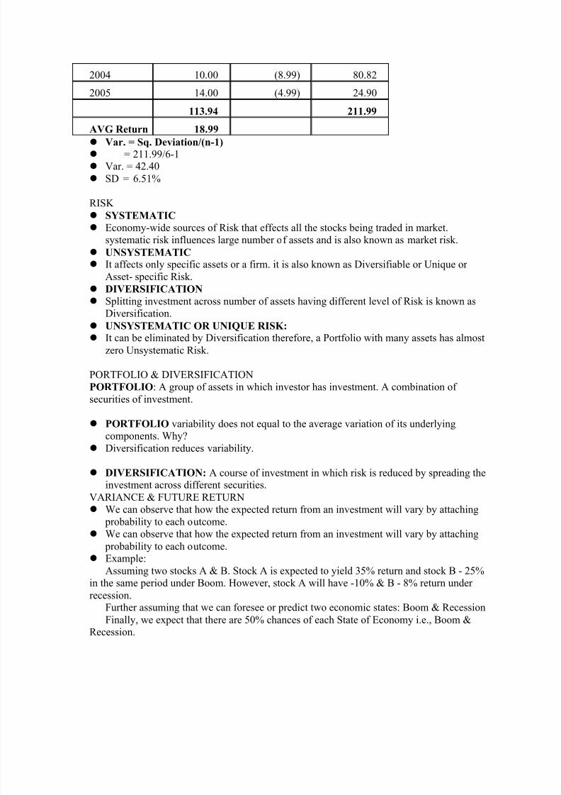
8/6/2019 Corporate Finance Lecture
http://slidepdf.com/reader/full/corporate-finance-lecture 82/125
2004 10.00 (8.99) 80.82
2005 14.00 (4.99) 24.90
113.94 211.99
AVG Return 18.99 Var. = Sq. Deviation/(n-1) = 211.99/6-1 Var. = 42.40 SD = 6.51%
RISK SYSTEMATIC Economy-wide sources of Risk that effects all the stocks being traded in market.
systematic risk influences large number of assets and is also known as market risk. UNSYSTEMATIC It affects only specific assets or a firm. it is also known as Diversifiable or Unique or
Asset- specific Risk. DIVERSIFICATION Splitting investment across number of assets having different level of Risk is known as
Diversification. UNSYSTEMATIC OR UNIQUE RISK: It can be eliminated by Diversification therefore, a Portfolio with many assets has almost
zero Unsystematic Risk.
PORTFOLIO & DIVERSIFICATIONPOR TFOLIO: A group of assets in which investor has investment. A combination of securities of investment.
POR TFOLIO variability does not equal to the average variation of its underlyingcomponents. Why?
Diversification reduces variability.
DIVERSIFICATION: A course of investment in which risk is reduced by spreading theinvestment across different securities.
VARIANCE & FUTURE RETURN We can observe that how the expected return from an investment will vary by attaching
probability to each outcome. We can observe that how the expected return from an investment will vary by attaching
probability to each outcome. Example:
Assuming two stocks A & B. Stock A is expected to yield 35% return and stock B - 25%in the same period under Boom. However, stock A will have -10% & B - 8% return under recession.
Further assuming that we can foresee or predict two economic states: Boom & RecessionFinally, we expect that there are 50% chances of each State of Economy i.e., Boom &
Recession.
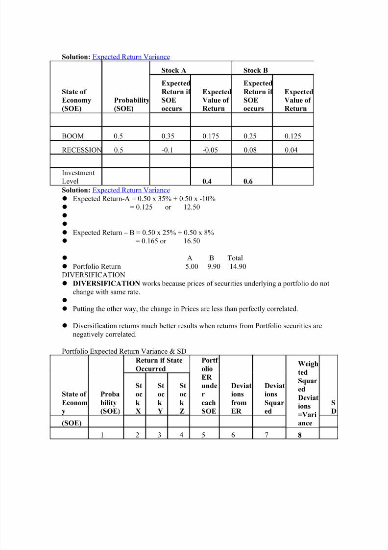
8/6/2019 Corporate Finance Lecture
http://slidepdf.com/reader/full/corporate-finance-lecture 83/125
Solution: Expected Return Variance
State of Economy (SOE)
Probability(SOE)
Stock A Stock B
Expected
Return if SOEoccurs
Expected Value of Return
Expected
Return if SOEoccurs
Expected Value of Return
BOOM 0.5 0.35 0.175 0.25 0.125
RECESSION 0.5 -0.1 -0.05 0.08 0.04
InvestmentLevel 0.4 0.6
Solution: Expected Return Variance Expected Return-A = 0.50 x 35% + 0.50 x -10% = 0.125 or 12.50 Expected Return ± B = 0.50 x 25% + 0.50 x 8% = 0.165 or 16.50
A B Total Portfolio Return 5.00 9.90 14.90DIVERSIFICATION
DIVERSIFICATION works because prices of securities underlying a portfolio do notchange with same rate.
Putting the other way, the change in Prices are less than perfectly correlated.
Diversification returns much better results when returns from Portfolio securities arenegatively correlated.
Portfolio Expected Return Variance & SD
State of Economy
Probability (SOE)
Return if StateOccurred
Portf olio
ER undereachSOE
Deviations fromER
Deviations Squared
Weigh
ted SquaredDeviations =Variance
SD
Stock X
Stock Y
Stock Z
(SOE)
1 2 3 4 5 6 7 8
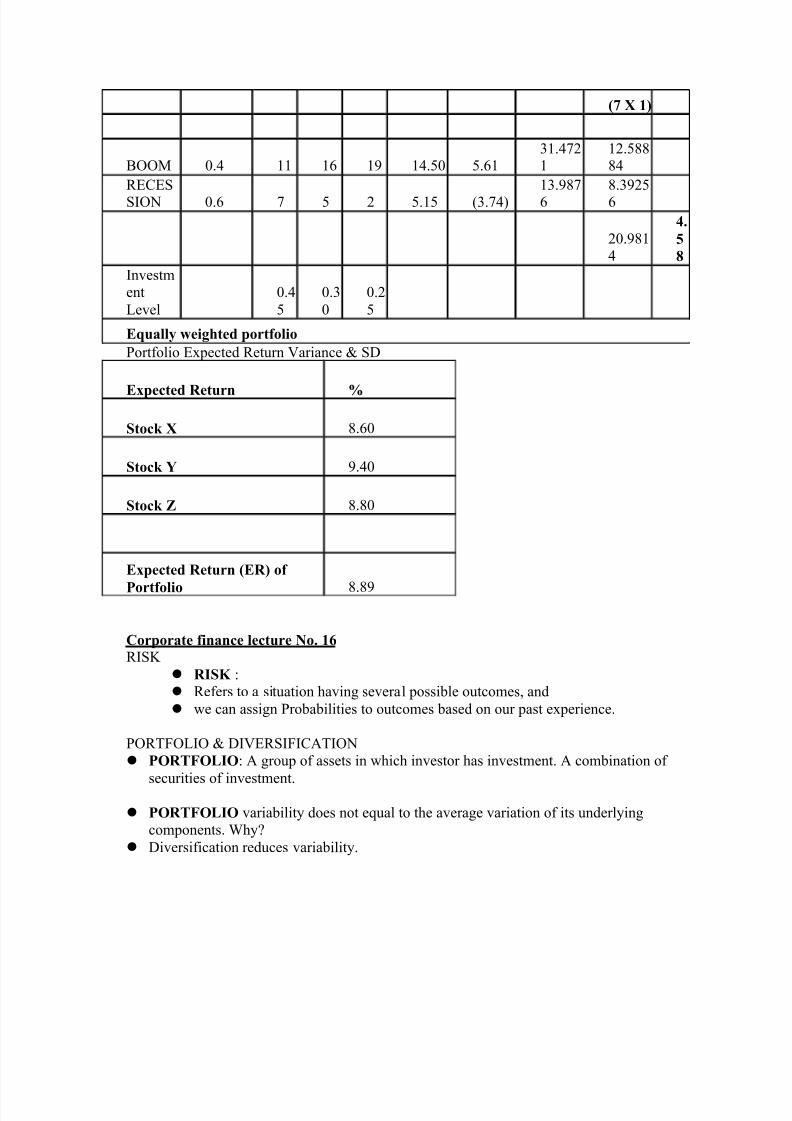
8/6/2019 Corporate Finance Lecture
http://slidepdf.com/reader/full/corporate-finance-lecture 84/125
(7 X 1)
BOOM 0.4 11 16 19 14.50 5.6131.4721
12.58884
RECESSION 0.6 7 5 2 5.15 (3.74) 13.9876 8.39256
20.9814
4.58
InvestmentLevel
0.45
0.30
0.25
Equally weighted portfolio Portfolio Expected Return Variance & SD
Expected Return %
Stock X 8.60
Stock Y 9.40
Stock Z 8.80
Expected Return (ER) of Portfolio 8.89
Corporate finance lecture No. 16RISK
RISK : Refers to a situation having several possible outcomes, and we can assign Probabilities to outcomes based on our past experience.
PORTFOLIO & DIVERSIFICATION
POR TFOLIO: A group of assets in which investor has investment. A combination of securities of investment.
POR TFOLIO variability does not equal to the average variation of its underlyingcomponents. Why?
Diversification reduces variability.
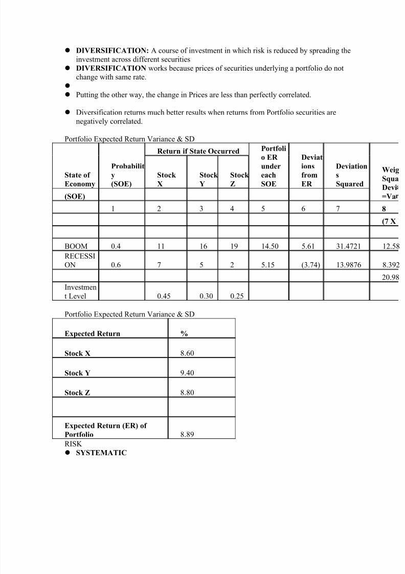
8/6/2019 Corporate Finance Lecture
http://slidepdf.com/reader/full/corporate-finance-lecture 85/125
DIVERSIFICATION: A course of investment in which risk is reduced by spreading theinvestment across different securities
DIVERSIFICATION works because prices of securities underlying a portfolio do notchange with same rate.
Putting the other way, the change in Prices are less than perfectly correlated.
Diversification returns much better results when returns from Portfolio securities arenegatively correlated.
Portfolio Expected Return Variance & SD
State of Economy
Probability (SOE)
Return if State Occurred Portfolio ER undereachSOE
Deviations fromER
Deviations Squared
Stock X
Stock Y
Stock Z
(SOE) 1 2 3 4 5 6 7
BOOM 0.4 11 16 19 14.50 5.61 31.4721 RECESSION 0.6 7 5 2 5.15 (3.74) 13.9876
Investmen
t Level 0.45 0.30 0.25
Portfolio Expected Return Variance & SD
Expected Return %
Stock X 8.60
Stock Y 9.40
Stock Z 8.80
Expected Return (ER) of Portfolio 8.89RISK SYSTEMATIC
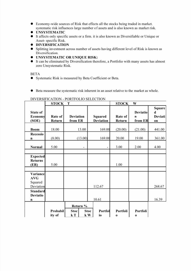
8/6/2019 Corporate Finance Lecture
http://slidepdf.com/reader/full/corporate-finance-lecture 86/125
Economy-wide sources of Risk that effects all the stocks being traded in market.systematic risk influences large number of assets and is also known as market risk.
UNSYSTEMATIC It affects only specific assets or a firm. it is also known as Diversifiable or Unique or
Asset- specific Risk.
DIVERSIF
ICAT
IO
N Splitting investment across number of assets having different level of Risk is known asDiversification.
UNSYSTEMATIC OR UNIQUE RISK: It can be eliminated by Diversification therefore, a Portfolio with many assets has almost
zero Unsystematic Risk.
BETA Systematic Risk is measured by Beta Coefficient or Beta.
Beta measure the systematic risk inherent in an asset relative to the market as whole.
DIVERSIFICATION - PORTFOLIO SELECTION
State of Economy(SOE)
STOCK T STOCK W
Rate of Return
Deviationfrom ER
SquaredDeviation
Rate of Return
Deviationfrom ER
SquaredDeviation
Boom 18.00 13.00 169.00 (20.00) (21.00) 441.00Recessio
n (8.00) (13.00) 169.00 20.00 19.00 361.00
Normal 5.00 - - 3.00 2.00 4.00
ExpectedReturns(ER) 5.00 1.00
VarianceAVG SquaredDeviation 112.67 268.67StandardDeviation 10.61 16.39
Probability of
Return %
Portfolio
Portfolio
Portfolio
Stock T
Stock W
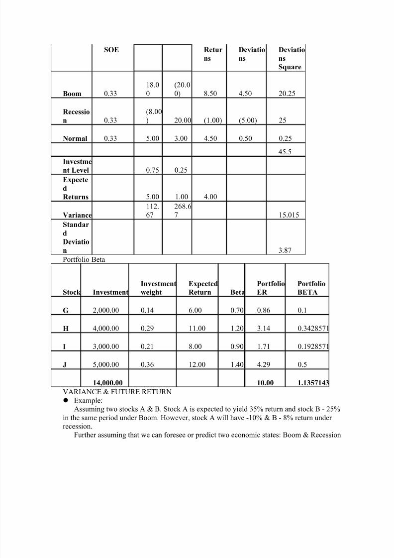
8/6/2019 Corporate Finance Lecture
http://slidepdf.com/reader/full/corporate-finance-lecture 87/125
SOE Returns
Deviations
DeviationsSquare
Boom 0.33
18.0
0
(20.0
0) 8.50 4.50 20.25
Recession 0.33
(8.00) 20.00 (1.00) (5.00) 25
Normal 0.33 5.00 3.00 4.50 0.50 0.25
45.5Investment Level 0.75 0.25Expecte
dReturns 5.00 1.00 4.00
Variance 112.67
268.67 15.015
StandardDeviation 3.87Portfolio Beta
Stock Investment Investment weight ExpectedReturn Beta Portfolio ER Portfolio BETA
G 2,000.00 0.14 6.00 0.70 0.86 0.1
H 4,000.00 0.29 11.00 1.20 3.14 0.3428571
I 3,000.00 0.21 8.00 0.90 1.71 0.1928571
J 5,000.00 0.36 12.00 1.40 4.29 0.5
14,000.00 10.00 1.1357143 VARIANCE & FUTURE RETURN Example:
Assuming two stocks A & B. Stock A is expected to yield 35% return and stock B - 25%in the same period under Boom. However, stock A will have -10% & B - 8% return under recession.
Further assuming that we can foresee or predict two economic states: Boom & Recession
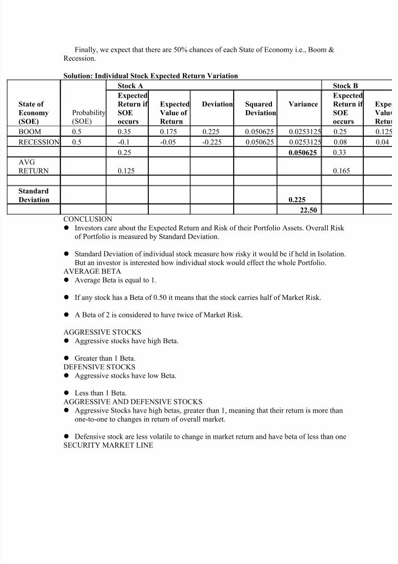
8/6/2019 Corporate Finance Lecture
http://slidepdf.com/reader/full/corporate-finance-lecture 88/125
Finally, we expect that there are 50% chances of each State of Economy i.e., Boom &Recession.
Solution: Individual Stock Expected Return Variation
State of EconomySOE)
Probability(SOE)
Stock A Stock B
ExpectedReturn if SOEoccurs
Expected Value of Return
Deviation Squared Deviation
Variance ExpectedReturn if SOEoccurs
BOOM 0.5 0.35 0.175 0.225 0.050625 0.0253125 0.25
RECESSION 0.5 -0.1 -0.05 -0.225 0.050625 0.0253125 0.08
0.25 0.050625 0.33AVGRETURN 0.125 0.165
StandardDeviation 0.225
22.50CONCLUSION Investors care about the Expected Return and Risk of their Portfolio Assets. Overall Risk
of Portfolio is measured by Standard Deviation.
Standard Deviation of individual stock measure how risky it would be if held in Isolation.But an investor is interested how individual stock would effect the whole Portfolio.
AVERAGE BETA Average Beta is equal to 1.
If any stock has a Beta of 0.50 it means that the stock carries half of Market Risk.
A Beta of 2 is considered to have twice of Market Risk.
AGGRESSIVE STOCKS Aggressive stocks have high Beta.
Greater than 1 Beta.DEFENSIVE STOCKS Aggressive stocks have low Beta.
Less than 1 Beta.AGGRESSIVE AND DEFENSIVE STOCKS Aggressive Stocks have high betas, greater than 1, meaning that their return is more than
one-to-one to changes in return of overall market.
Defensive stock are less volatile to change in market return and have beta of less than oneSECURITY MARKET LINE
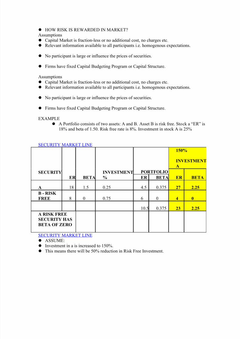
8/6/2019 Corporate Finance Lecture
http://slidepdf.com/reader/full/corporate-finance-lecture 89/125
HOW RISK IS REWARDED IN MARKET?Assumptions Capital Market is fraction-less or no additional cost, no charges etc. Relevant information available to all participants i.e. homogenous expectations.
No participant is large or influence the prices of securities.
Firms have fixed Capital Budgeting Program or Capital Structure.
Assumptions Capital Market is fraction-less or no additional cost, no charges etc. Relevant information available to all participants i.e. homogenous expectations.
No participant is large or influence the prices of securities.
Firms have fixed Capital Budgeting Program or Capital Structure.
EXAMPLE A Portfolio consists of two assets: A and B. Asset B is risk free. Stock a ³ER´ is
18% and beta of 1.50. Risk free rate is 8%. Investment in stock A is 25%
SECURITY MARKET LINE
SECURITY ER BETA INVESTMENT % PO
R TFO
LIO
150%
INVESTMENT A
ER BETA ER BETA
A 18 1.5 0.25 4.5 0.375 27 2.25 B - RISK FREE 8 0 0.75 6 0 4 0
10.5 0.375 23 2.25 A RISK FREESECURITY HASBETA OF ZER O
SECURITY MARKET LINE ASSUME: Investment in a is increased to 150%. This means there will be 50% reduction in Risk Free Investment.
8/6/2019 Corporate Finance Lecture
http://slidepdf.com/reader/full/corporate-finance-lecture 90/125
What happened when we invested 150% in Risky Investment A. Our Portfolio's ER Rate increased to 23% from 10.50%. Portfolio's Beta jumped to 2.25 from 0.375.
Now we can see the various investment combinations of.
Stock 'A' and Risk Free 'Bµ.
Corporate finance lecture No. 17SECURITY MARKET LINE HOW RISK IS REWARDED IN MARKET:EXAMPLE
A Portfolio consists of two assets: A and B. Asset B is risk free. Stock a ³ER´ is18% and beta of 1.50. Risk free rate is 8%. Investment in stock A is 25%
CHANGE IN INVESTMENT OF A SECURITY IN PORTFOLIOPart A
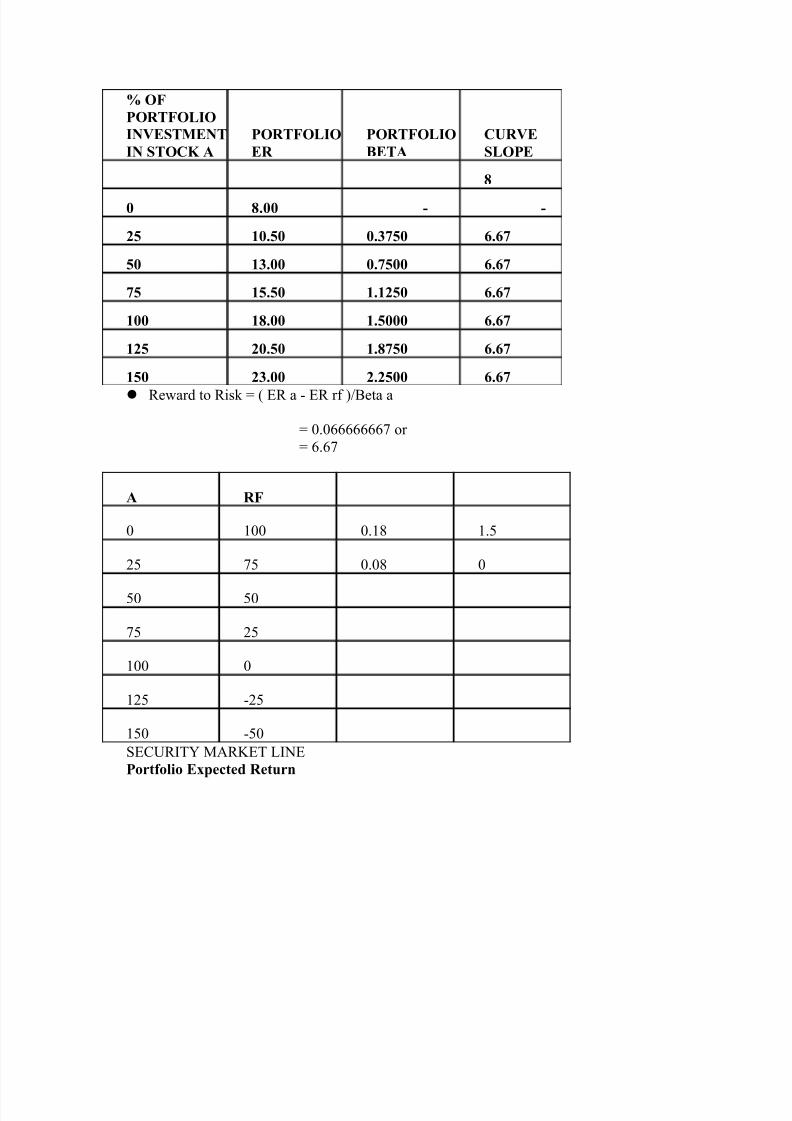
8/6/2019 Corporate Finance Lecture
http://slidepdf.com/reader/full/corporate-finance-lecture 91/125
% OF POR TFOLIO INVESTMENT IN STOCK A
POR TFOLIO ER
POR TFOLIO BETA
CURVESLOPE
8
0 8.00 - -
25 10.50 0.3750 6.67
50 13.00 0.7500 6.67
75 15.50 1.1250 6.67
100 18.00 1.5000 6.67
125 20.50 1.8750 6.67
150 23.00 2.2500 6.67 Reward to Risk = ( ER a - ER rf )/Beta a
= 0.066666667 or = 6.67
A R F
0 100 0.18 1.5
25 75 0.08 0
50 50
75 25
100 0
125 -25
150 -50SECURITY MARKET LINEPortfolio Expected Return
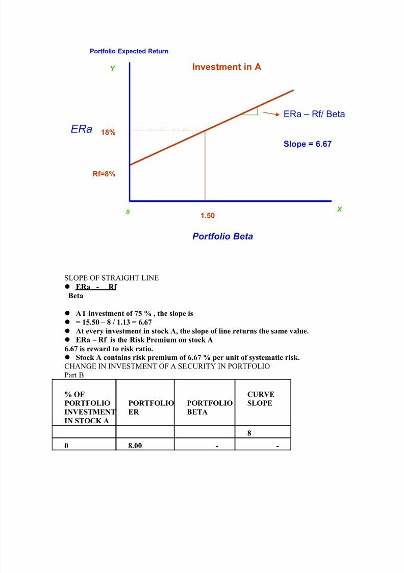
8/6/2019 Corporate Finance Lecture
http://slidepdf.com/reader/full/corporate-finance-lecture 92/125
SLOPE OF STRAIGHT LINE ERa - Rf
Beta
AT investment of 75 % , the slope is = 15.50 ± 8 / 1.13 = 6.67 At every investment in stock A, the slope of line returns the same value. ERa ± Rf is the Risk Premium on stock A6.67 is reward to risk ratio. Stock A contains risk premium of 6.67 % per unit of systematic risk.CHANGE IN INVESTMENT OF A SECURITY IN PORTFOLIOPart B
% OF POR TFOLIO INVESTMENT IN STOCK A
POR TFOLIO ER
POR TFOLIO BETA
CURVESLOPE
8
0 8.00 - -
ERa
Portfolio Beta
X
Y
Portfolio Expected Return
Rf=8%
0
18%
1.50
Investment in A
ERa ± Rf/ Beta
Slope = 6.67
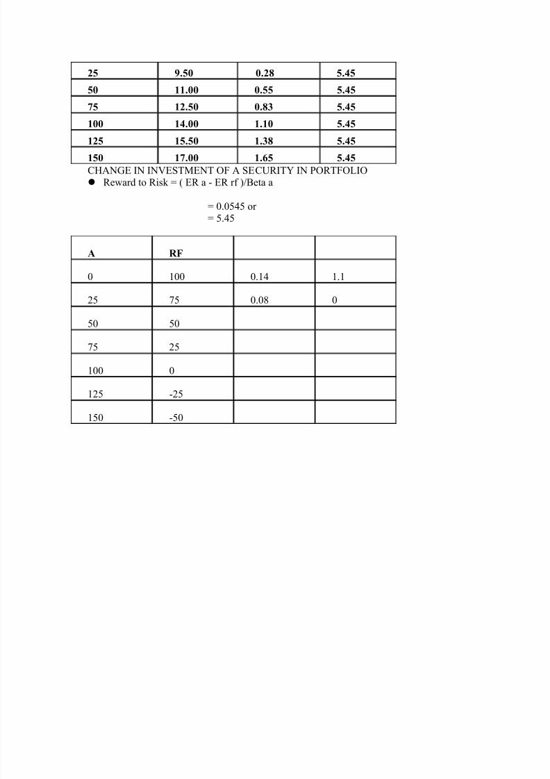
8/6/2019 Corporate Finance Lecture
http://slidepdf.com/reader/full/corporate-finance-lecture 93/125
25 9.50 0.28 5.45
50 11.00 0.55 5.45
75 12.50 0.83 5.45
100 14.00 1.10 5.45
125 15.50 1.38 5.45
150 17.00 1.65 5.45CHANGE IN INVESTMENT OF A SECURITY IN PORTFOLIO Reward to Risk = ( ER a - ER rf )/Beta a
= 0.0545 or = 5.45
A R F
0 100 0.14 1.1
25 75 0.08 0
50 50
75 25
100 0
125 -25150 -50
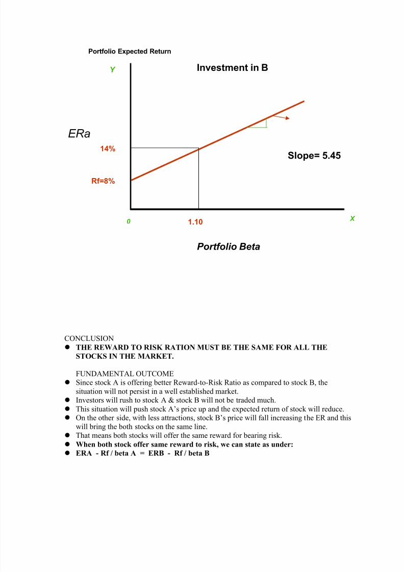
8/6/2019 Corporate Finance Lecture
http://slidepdf.com/reader/full/corporate-finance-lecture 94/125
CONCLUSION THE REWARD TO RISK RATION MUST BE THE SAME FOR ALL THE
STOCKS IN THE MARKET.
FUNDAMENTAL OUTCOME Since stock A is offering better Reward-to-Risk Ratio as compared to stock B, the
situation will not persist in a well established market. Investors will rush to stock A & stock B will not be traded much. This situation will push stock A¶s price up and the expected return of stock will reduce. On the other side, with less attractions, stock B¶s price will fall increasing the ER and this
will bring the both stocks on the same line. That means both stocks will offer the same reward for bearing risk. When both stock offer same reward to risk, we can state as under: ERA - Rf / beta A = ERB - Rf / beta B
ERa
Portfolio Beta
X
Y
Portfolio Expected Return
Rf=8%
0
14%
1.10
Investment in B
Slope= 5.45
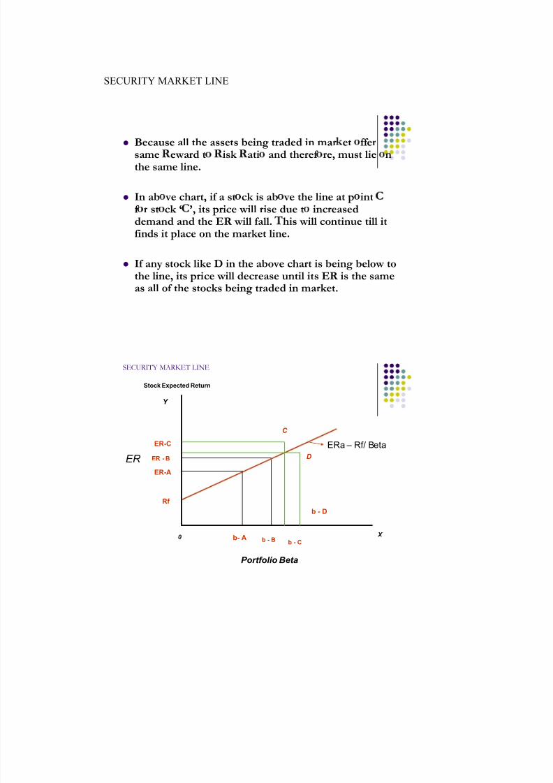
8/6/2019 Corporate Finance Lecture
http://slidepdf.com/reader/full/corporate-finance-lecture 95/125
SECURITY MARKET LINE
Because all the assets being traded in mar¥
et¦ ff er
same § eward t ¦ § isk § ati ¦ and theref ¦ re, must lie ¦ nthe same line.
In ab¦ v e chart, if a st
¦ ck is ab
¦ v e the line at p
¦ int
̈
f ¦ r st
¦ ck ¶
̈ ·, its price w ill rise due t
¦ increased
demand and the ER w ill f all. ©
his w ill continue till itfinds it place on the market line.
If any stock like D in the abo v e chart is being below to the line, its price w ill decrease until its ER is the same as all of the stocks being traded in market.
SECURITY MARKET LINE
ER
Portfolio Beta
X
Y
Stock Expected Return
Rf
0
ER-A
b- A
ERa ± Rf/ Beta
b - B
ER - B
b - C
ER-C
b - D
C
D
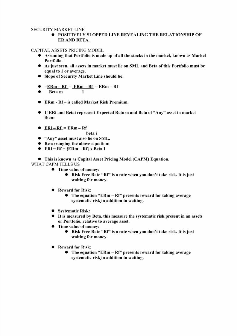
8/6/2019 Corporate Finance Lecture
http://slidepdf.com/reader/full/corporate-finance-lecture 96/125
SECURITY MARKET LINE POSITIVELY SLOPPED LINE REVEALING THE RELATIONSHIP OF
ER AND BETA.
CAPITAL ASSETS PRICING MODEL
Assuming thatP
ortfolio is made up of all the stocks in the market, known as MarketPortfolio. As just seen, all assets in market must lie on SML and Beta of this Portfolio must be
equal to 1 or average. Slope of Security Market Line should be:
=ERm ± Rf = ERm ± Rf = ERm ± Rf Beta m 1
ERm - Rf ± is called Market Risk Premium.
If ERi and Betai represent Expected Return and Beta of ³Any´ asset in marketthen:
ERi ± Rf = ERm ± Rf beta i
³Any´ asset must also lie on SML. Re-arranging the above equation: ERi = Rf + {ERm ± Rf} x Beta I
This is known as Capital Asset Pricing Model (CAPM) Equation.WHAT CAPM TELLS US
Time value of money: Risk Free Rate ³Rf´ is a rate when you don¶t take risk. It is just
waiting for money.
Reward for Risk: The equation ³ERm ± Rf´ presents reward for taking average
systematic risk in addition to waiting.
Systematic Risk: It is measured by Beta. this measure the systematic risk present in an assets
or Portfolio, relative to average asset. Time value of money:
Risk Free Rate ³Rf´ is a rate when you don¶t take risk. It is justwaiting for money.
Reward for Risk: The equation ³ERm ± Rf´ presents reward for taking average
systematic risk in addition to waiting.
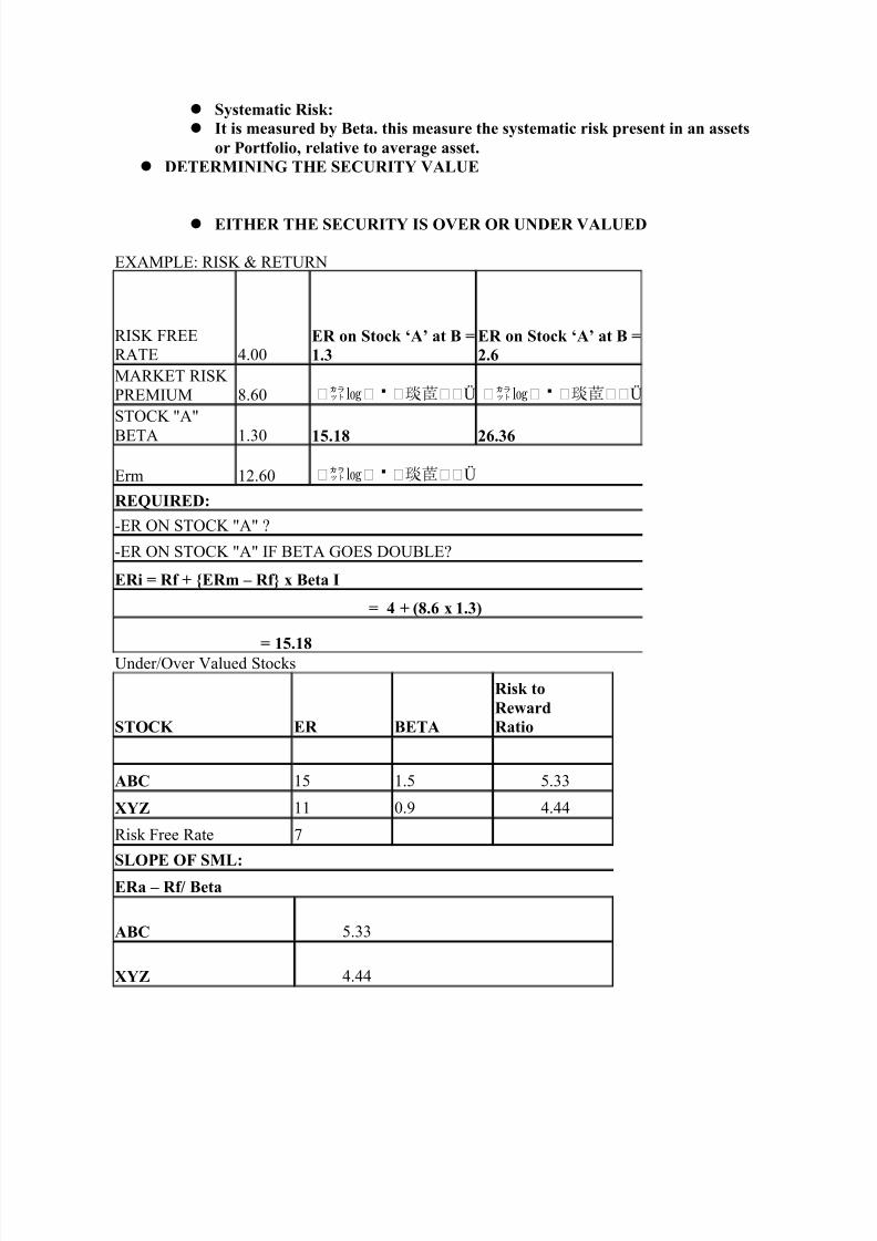
8/6/2019 Corporate Finance Lecture
http://slidepdf.com/reader/full/corporate-finance-lecture 97/125
Systematic Risk: It is measured by Beta. this measure the systematic risk present in an assets
or Portfolio, relative to average asset. DETERMINING THE SECURITY VALUE
EITHER THE SECURITY IS OVER OR UNDER VALUED
EXAMPLE: RISK & RETURN
RISK FREERATE 4.00
ER on Stock µA¶ at B =1.3
ER on Stock µA¶ at B =2.6
MARKET RISK PREMIUM 8.60 Ü Ü
STOCK "A"BETA 1.30 15.18 26.36
Erm 12.60 Ü
REQUIRED:
-ER ON STOCK "A" ?
-ER ON STOCK "A" IF BETA GOES DOUBLE?
ERi = Rf + {ERm ± Rf} x Beta I
= 4 + (8.6 x 1.3)
= 15.18 Under/Over Valued Stocks
STOCK ER BETA
Risk to Reward Ratio
ABC 15 1.5 5.33
XYZ 11 0.9 4.44
Risk Free Rate 7
SLOPE OF SML:
ERa ± Rf/ Beta
ABC 5.33
XYZ 4.44
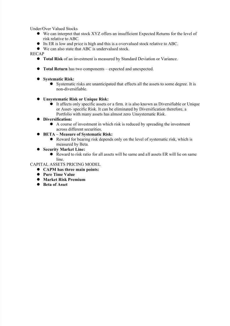
8/6/2019 Corporate Finance Lecture
http://slidepdf.com/reader/full/corporate-finance-lecture 98/125
Under/Over Valued Stocks We can interpret that stock XYZ offers an insufficient Expected Returns for the level of
risk relative to ABC. Its ER is low and price is high and this is a overvalued stock relative to ABC. We can also state that ABC is undervalued stock.
RECAP Total Risk of an investment is measured by Standard Deviation or Variance.
Total Return has two components ± expected and unexpected.
Systematic Risk: Systematic risks are unanticipated that effects all the assets to some degree. It is
non-diversifiable.
Unsystematic Risk or Unique Risk: It affects only specific assets or a firm. it is also known as Diversifiable or Unique
or Asset- specific Risk. It can be eliminated by Diversification therefore, aPortfolio with many assets has almost zero Unsystematic Risk. Diversification:
A course of investment in which risk is reduced by spreading the investmentacross different securities.
BETA ± Measure of Systematic Risk: Reward for bearing risk depends only on the level of systematic risk, which is
measured by Beta. Security Market Line:
Reward to risk ratio for all assets will be same and all assets ER will lie on sameline.
CAPITAL ASSETS PRICING MODEL CAPM has three main points: Pure Time Value Market Risk Premium Beta of Asset
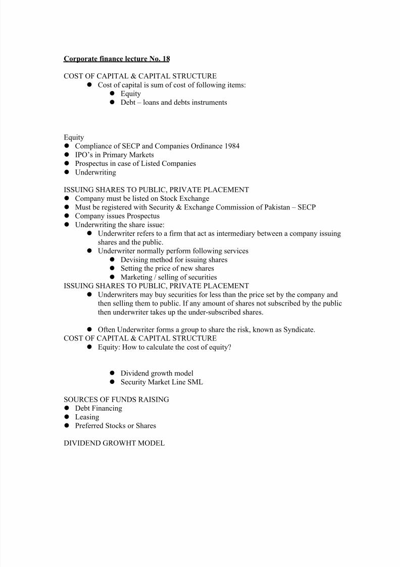
8/6/2019 Corporate Finance Lecture
http://slidepdf.com/reader/full/corporate-finance-lecture 99/125
Corporate finance lecture No. 18
COST OF CAPITAL & CAPITAL STRUCTURE Cost of capital is sum of cost of following items:
Equity Debt ± loans and debts instruments
Equity Compliance of SECP and Companies Ordinance 1984 IPO¶s in Primary Markets Prospectus in case of Listed Companies Underwriting
ISSUING SHARES TO PUBLIC, PRIVATE PLACEMENT Company must be listed on Stock Exchange Must be registered with Security & Exchange Commission of Pakistan ± SECP Company issues Prospectus Underwriting the share issue:
Underwriter refers to a firm that act as intermediary between a company issuingshares and the public.
Underwriter normally perform following services Devising method for issuing shares Setting the price of new shares Marketing / selling of securities
ISSUING SHARES TO PUBLIC, PRIVATE PLACEMENT Underwriters may buy securities for less than the price set by the company and
then selling them to public. If any amount of shares not subscribed by the publicthen underwriter takes up the under-subscribed shares.
Often Underwriter forms a group to share the risk, known as Syndicate.COST OF CAPITAL & CAPITAL STRUCTURE
Equity: How to calculate the cost of equity?
Dividend growth model Security Market Line SML
SOURCES OF FUNDS RAISING Debt Financing Leasing Preferred Stocks or Shares
DIVIDEND GROWHT MODEL
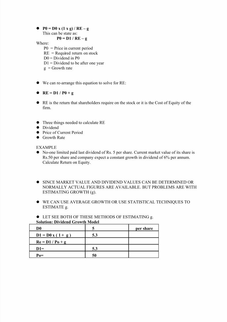
8/6/2019 Corporate Finance Lecture
http://slidepdf.com/reader/full/corporate-finance-lecture 100/125
P0 = D0 x (1 x g) / RE ± gThis can be state as:
P0 = D1 / RE ± gWhere:
P0 = Price in current period
RE = Required return on stock D0 = Dividend in P0D1 = Dividend to be after one year g = Growth rate
We can re-arrange this equation to solve for RE:
RE = D1 / P0 + g
RE is the return that shareholders require on the stock or it is the Cost of Equity of the
firm.
Three things needed to calculate RE Dividend Price of Current Period Growth Rate
EXAMPLE No-one limited paid last dividend of Rs. 5 per share. Current market value of its share is
Rs.50 per share and company expect a constant growth in dividend of 6% per annum.Calculate Return on Equity.
SINCE MARKET VALUE AND DIVIDEND VALUES CAN BE DETERMINED OR NORMALLY ACTUAL FIGURES ARE AVAILABLE. BUT PROBLEMS ARE WITHESTIMATING GROWTH (g).
WE CAN USE AVERAGE GROWTH OR USE STATISTICAL TECHNIQUES TOESTIMATE g.
LET SEE BOTH OF THESE METHODS OF ESTIMATING g.Solution: Dividend Growth Model
D0 5 per share
D1 = D0 x ( 1 + g ) 5.3
Re = D1 / Po + g
D1= 5.3
Po= 50
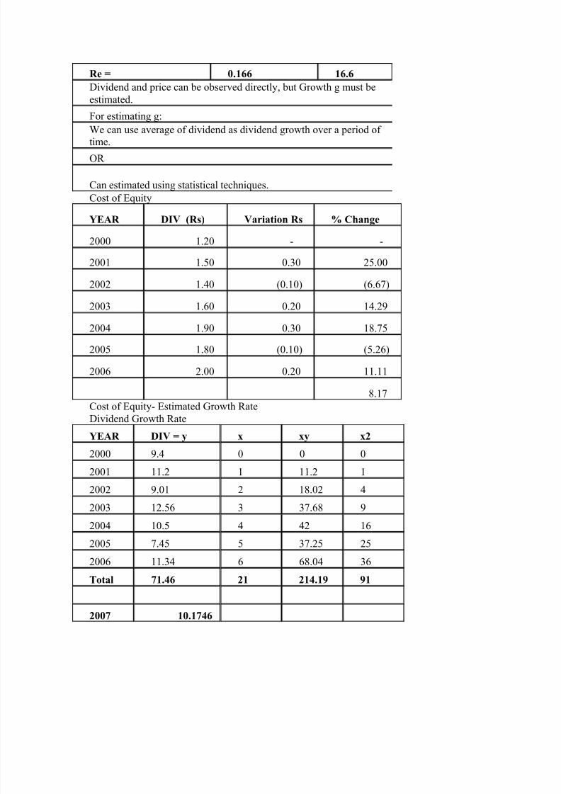
8/6/2019 Corporate Finance Lecture
http://slidepdf.com/reader/full/corporate-finance-lecture 101/125
Re = 0.166 16.6 Dividend and price can be observed directly, but Growth g must beestimated.
For estimating g:We can use average of dividend as dividend growth over a period of time.
OR
Can estimated using statistical techniques.Cost of Equity
YEAR DIV (Rs) Variation Rs % Change
2000 1.20 - -
2001 1.50 0.30 25.00
2002 1.40 (0.10) (6.67)
2003 1.60 0.20 14.29
2004 1.90 0.30 18.75
2005 1.80 (0.10) (5.26)
2006 2.00 0.20 11.11
8.17
Cost of Equity- Estimated Growth Rate Dividend Growth Rate
YEAR DIV = y x xy x2
2000 9.4 0 0 0
2001 11.2 1 11.2 1
2002 9.01 2 18.02 4
2003 12.56 3 37.68 9
2004 10.5 4 42 16
2005 7.45 5 37.25 25
2006 11.34 6 68.04 36
Total 71.46 21 214.19 91
2007 10.1746
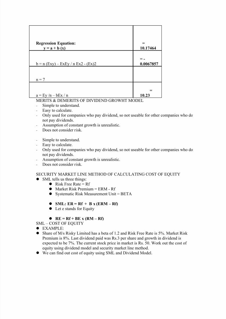
8/6/2019 Corporate Finance Lecture
http://slidepdf.com/reader/full/corporate-finance-lecture 102/125
Regression Equation:y = a + b (x)
=10.17464
b = n (Exy) ± ExEy / n Ex2 - (Ex)2= -0.0067857
n = 7
a = Ey /n ± bEx / n=
10.23MERITS & DEMERITS OF DIVIDEND GROWHT MODEL- Simple to understand.- Easy to calculate.- Only used for companies who pay dividend, so not useable for other companies who do
not pay dividends.- Assumption of constant growth is unrealistic.- Does not consider risk.
- Simple to understand.- Easy to calculate.- Only used for companies who pay dividend, so not useable for other companies who do
not pay dividends.- Assumption of constant growth is unrealistic.- Does not consider risk.
SECURITY MARKET LINE METHOD OF CALCULATING COST OF EQUITY SML tells us three things:
Risk Free Rate = Rf Market Risk Premium = ERM - Rf Systematic Risk Measurement Unit = BETA
SML: ER = Rf + B x (ERM ± Rf) Let e stands for Equity
RE = Rf + BE x (RM ± Rf)SML ± COST OF EQUITY EXAMPLE: Share of M/s Risky Limited has a beta of 1.2 and Risk Free Rate is 5%. Market Risk
Premium is 8%. Last dividend paid was Rs.3 per share and growth in dividend isexpected to be 7%. The current stock price in market is Rs. 50. Work out the cost of equity using dividend model and security market line method.
We can find out cost of equity using SML and Dividend Model.
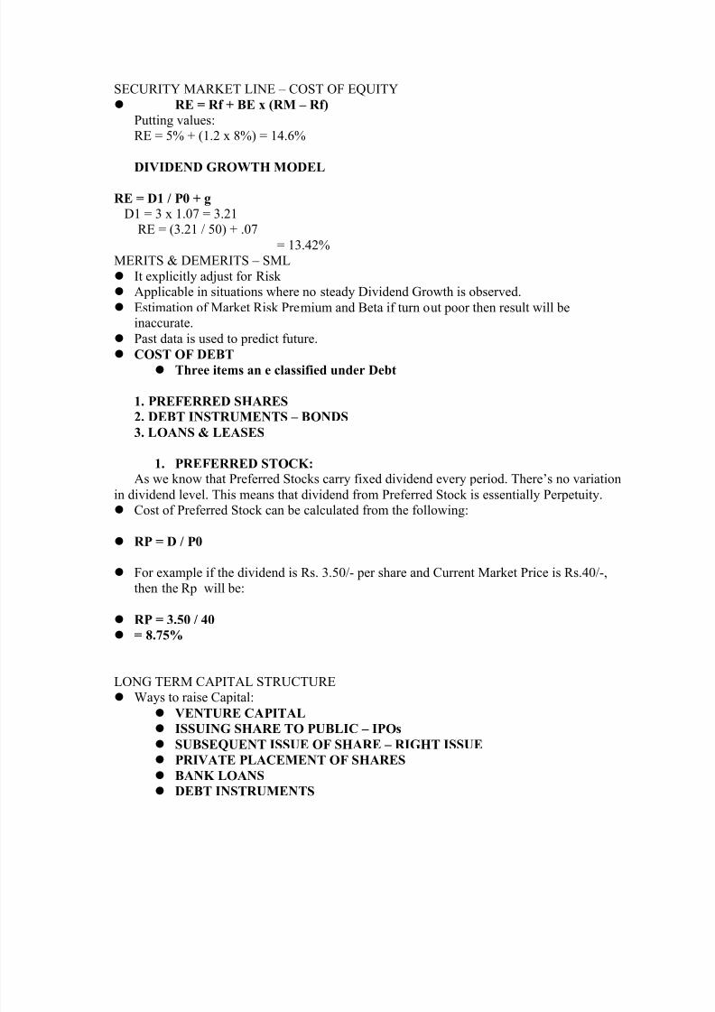
8/6/2019 Corporate Finance Lecture
http://slidepdf.com/reader/full/corporate-finance-lecture 103/125
SECURITY MARKET LINE ± COST OF EQUITY RE = Rf + BE x (RM ± Rf)
Putting values:RE = 5% + (1.2 x 8%) = 14.6%
DIVIDEND GR O
WTH
MO
DEL
RE = D1 / P0 + gD1 = 3 x 1.07 = 3.21
RE = (3.21 / 50) + .07= 13.42%
MERITS & DEMERITS ± SML It explicitly adjust for Risk Applicable in situations where no steady Dividend Growth is observed. Estimation of Market Risk Premium and Beta if turn out poor then result will be
inaccurate.
Past data is used to predict future. COST OF DEBT Three items an e classified under Debt
1. PREFERRED SHARES2. DEBT INSTRUMENTS ± BONDS3. LOANS & LEASES
1. PREFERRED STOCK:As we know that Preferred Stocks carry fixed dividend every period. There¶s no variation
in dividend level. This means that dividend from Preferred Stock is essentially Perpetuity. Cost of Preferred Stock can be calculated from the following:
R P = D / P0
For example if the dividend is Rs. 3.50/- per share and Current Market Price is Rs.40/-,then the Rp will be:
R P = 3.50 / 40 = 8.75%
LONG TERM CAPITAL STRUCTURE Ways to raise Capital:
VENTURE CAPITAL ISSUING SHARE TO PUBLIC ± IPOs SUBSEQUENT ISSUE OF SHARE ± RIGHT ISSUE PRIVATE PLACEMENT OF SHARES BANK LOANS DEBT INSTRUMENTS

8/6/2019 Corporate Finance Lecture
http://slidepdf.com/reader/full/corporate-finance-lecture 104/125
LEASESISSUING SHARES TO PUBLIC, PRIVATE PLACEMENT
Underwriters may buy securities for less than the price set by the company andthen selling them to public. If any amount of shares not subscribed by the publicthen underwriter takes up the under-subscribed shares.
Often Underwriter forms a group to share the risk, known as Syndicate.
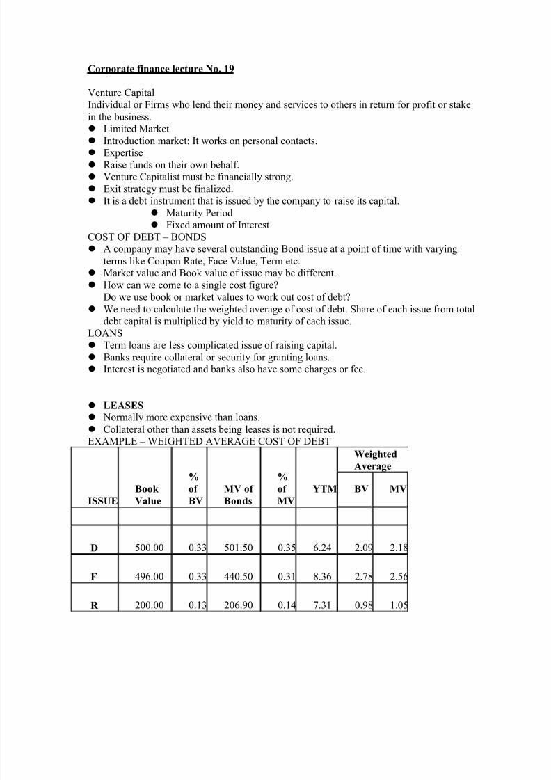
8/6/2019 Corporate Finance Lecture
http://slidepdf.com/reader/full/corporate-finance-lecture 105/125
Corporate finance lecture No. 19
Venture CapitalIndividual or Firms who lend their money and services to others in return for profit or stakein the business.
Limited Market Introduction market: It works on personal contacts. Expertise Raise funds on their own behalf. Venture Capitalist must be financially strong. Exit strategy must be finalized. It is a debt instrument that is issued by the company to raise its capital.
Maturity Period Fixed amount of Interest
COST OF DEBT ± BONDS A company may have several outstanding Bond issue at a point of time with varying
terms like Coupon Rate, Face Value, Term etc. Market value and Book value of issue may be different. How can we come to a single cost figure?
Do we use book or market values to work out cost of debt? We need to calculate the weighted average of cost of debt. Share of each issue from total
debt capital is multiplied by yield to maturity of each issue.LOANS Term loans are less complicated issue of raising capital. Banks require collateral or security for granting loans. Interest is negotiated and banks also have some charges or fee.
LEASES Normally more expensive than loans. Collateral other than assets being leases is not required.EXAMPLE ± WEIGHTED AVERAGE COST OF DEBT
ISSUE Book Value
%of BV
MV of Bonds
%of MV
YTM
WeightedAverage
BV MV
D 500.00 0.33 501.50 0.35 6.24 2.09 2.18
F 496.00 0.33 440.50 0.31 8.36 2.78 2.56
R 200.00 0.13 206.90 0.14 7.31 0.98 1.05
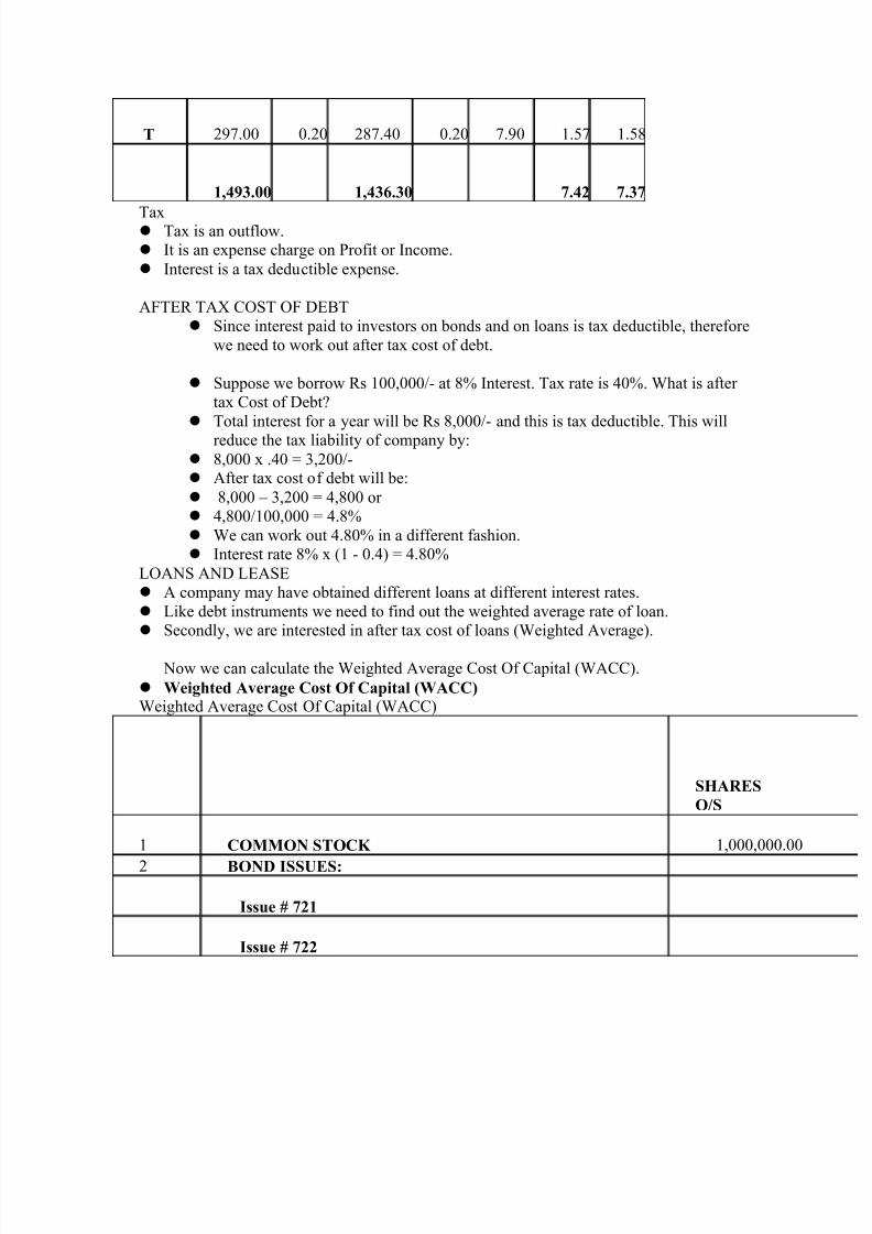
8/6/2019 Corporate Finance Lecture
http://slidepdf.com/reader/full/corporate-finance-lecture 106/125
T 297.00 0.20 287.40 0.20 7.90 1.57 1.58
1,493.00 1,436.30 7.42 7.37
Tax Tax is an outflow. It is an expense charge on Profit or Income. Interest is a tax deductible expense.
AFTER TAX COST OF DEBT Since interest paid to investors on bonds and on loans is tax deductible, therefore
we need to work out after tax cost of debt.
Suppose we borrow Rs 100,000/- at 8% Interest. Tax rate is 40%. What is after tax Cost of Debt?
Total interest for a year will be Rs 8,000/- and this is tax deductible. This willreduce the tax liability of company by:
8,000 x .40 = 3,200/- After tax cost of debt will be: 8,000 ± 3,200 = 4,800 or 4,800/100,000 = 4.8% We can work out 4.80% in a different fashion. Interest rate 8% x (1 - 0.4) = 4.80%
LOANS AND LEASE A company may have obtained different loans at different interest rates. Like debt instruments we need to find out the weighted average rate of loan.
Secondly, we are interested in after tax cost of loans (Weighted Average).
Now we can calculate the Weighted Average Cost Of Capital (WACC). Weighted Average Cost Of Capital (WACC)Weighted Average Cost Of Capital (WACC)
SHARES O/S
1 COMMON STOCK 1,000,000.002 BOND ISSUES:
Issue # 721
Issue # 722
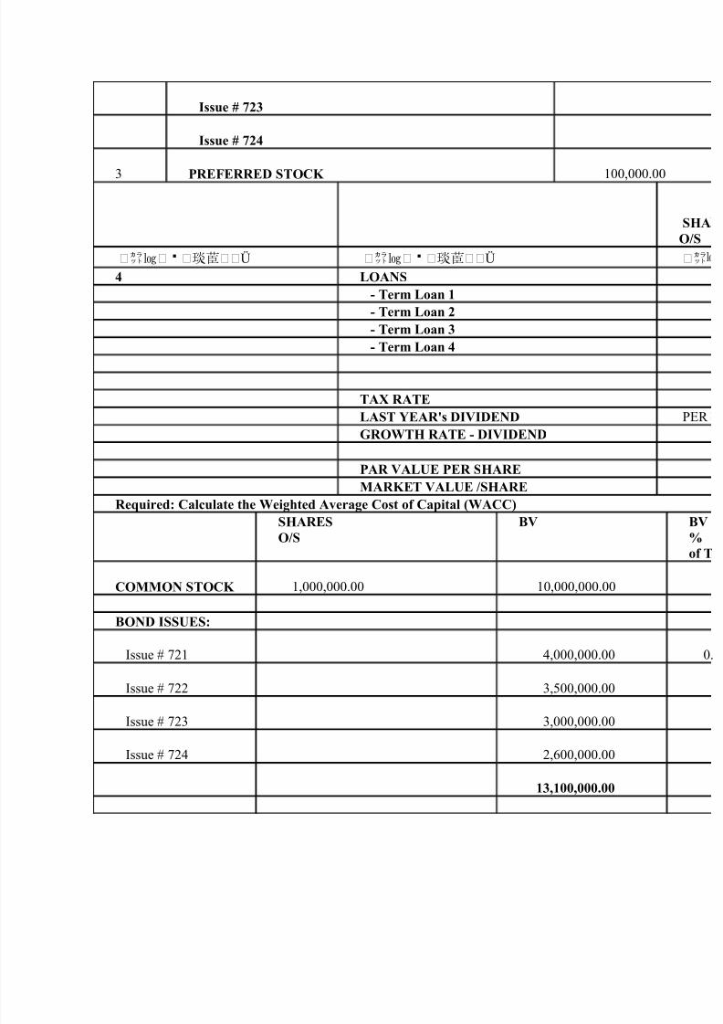
8/6/2019 Corporate Finance Lecture
http://slidepdf.com/reader/full/corporate-finance-lecture 107/125
Issue # 723
Issue # 724
3 PREFERRED STOCK 100,000.00
Ü Ü
4 LOANS - Term Loan 1 - Term Loan 2 - Term Loan 3
- Term Loan 4
TAX RATE LAST YEAR's DIVIDEND GR OWTH RATE - DIVIDEND
PAR VALUE PER SHARE MARKET VALUE /SHARE
Required: Calculate the Weighted Average Cost of Capital (WACC)
SHARES O/S BV
COMMON STOCK 1,000,000.00 10,000,000.00
BOND ISSUES:
Issue # 721 4,000,000.00
Issue # 722 3,500,000.00
Issue # 723 3,000,000.00
Issue # 724 2,600,000.00
13,100,000.00
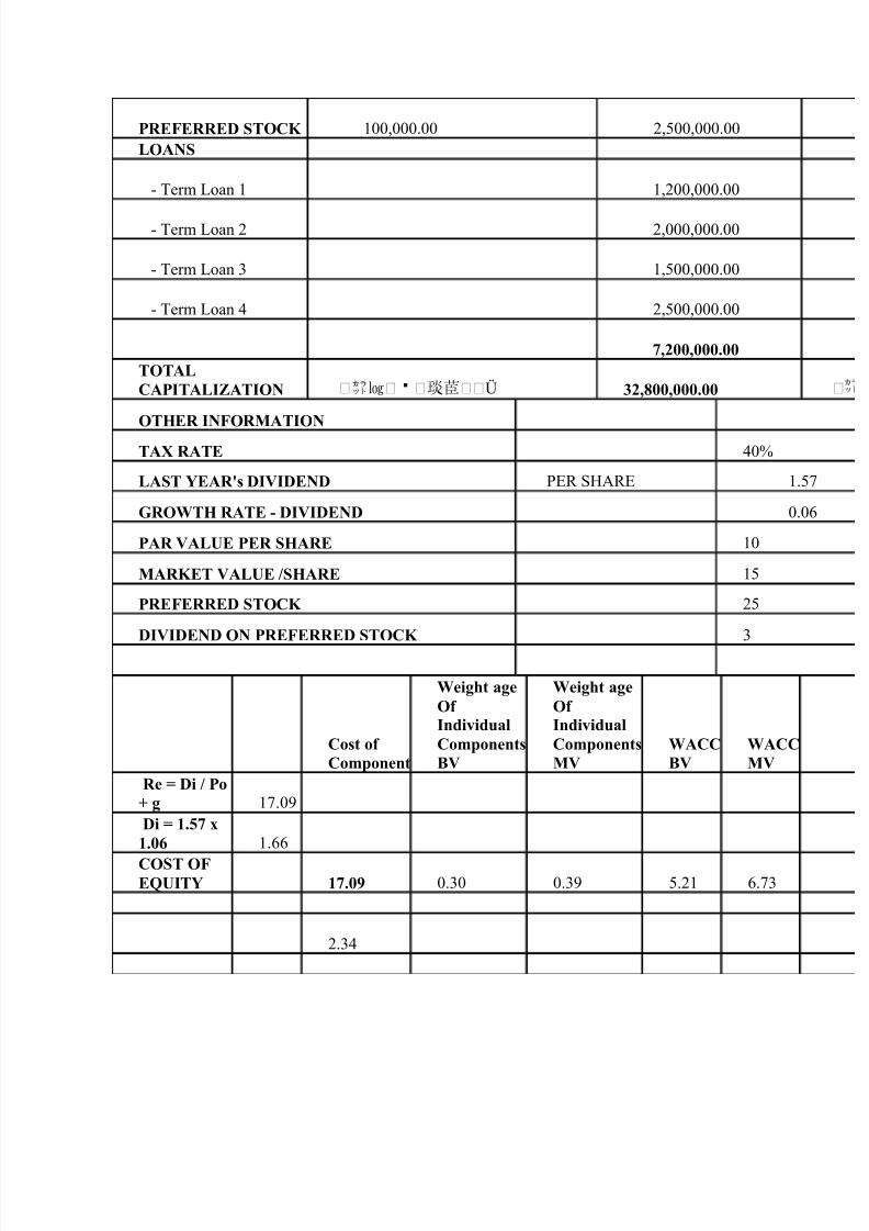
8/6/2019 Corporate Finance Lecture
http://slidepdf.com/reader/full/corporate-finance-lecture 108/125
PREFERRED STOCK 100,000.00 2,500,000.00LOANS
- Term Loan 1 1,200,000.00
- Term Loan 2 2,000,000.00
- Term Loan 3 1,500,000.00
- Term Loan 4 2,500,000.00
7,200,000.00TOTALCAPITALIZATION Ü 32,800,000.00
OTHER INFORMATION
TAX RATE 40%
LAST YEAR's DIVIDEND PER SHARE 1.5
GR OWTH RATE - DIVIDEND 0.0
PAR VALUE PER SHARE 10
MARKET VALUE /SHARE 15
PREFERRED STOCK 25
DIVIDEND ON PREFERRED STOCK 3
Cost of Component
Weight ageOf IndividualComponentsBV
Weight ageOf Individual ComponentsMV
WACCBV
WACCMV
Re = Di / Po+ g 17.09Di = 1.57 x
1.06 1.66COST OF EQUITY 17.09 0.30 0.39 5.21 6.73
2.34
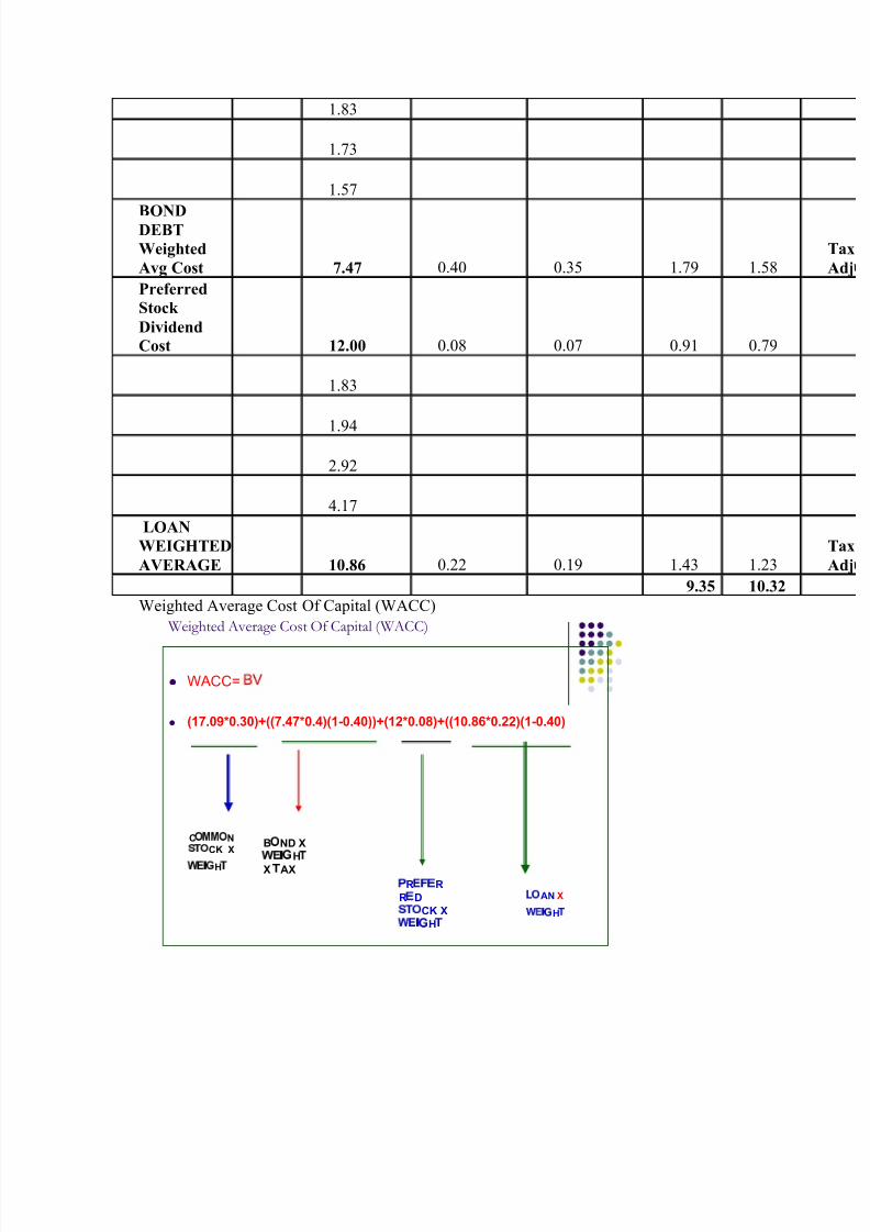
8/6/2019 Corporate Finance Lecture
http://slidepdf.com/reader/full/corporate-finance-lecture 109/125
1.83
1.73
1.57
BONDDEBT WeightedAvg Cost 7.47 0.40 0.35 1.79 1.58PreferredStock DividendCost 12.00 0.08 0.07 0.91 0.79
1.83
1.94
2.92
4.17LOAN
WEIGHTEDAVERAGE 10.86 0.22 0.19 1.43 1.23 9.35 10.32Weighted Average Cost Of Capital (WACC)
W eighted Average Cost Of Capital ( W ACC)
WACC=
(17.09*0.30)+((7.47*0.4)(1-0.40))+(12*0.08)+((10.86*0.22)(1-0.40)
C
N
CK X
H
B
ND X
!
"
H#
X#
AX
$ R % R
R
D&
#
CK X
!
"
H#
' AN X
H
8/6/2019 Corporate Finance Lecture
http://slidepdf.com/reader/full/corporate-finance-lecture 110/125
USING WACC IN CAPITAL BUDGETING EXAMPLE: A company intends to undertake a project that will yield after tax saving of Rs. 4 million
at the end of year one. However, after that these savings are estimated to grow at 6 percent.
The debt equity ratio of 0.5 or 2/3 (debt 2/3 and equity 1/3). Cost of equity is 25% andcost of debt is 11%.
This project has the same level of risk as the existing company business. Advise companyon the financial viability of project. Assume tax rate of 40 percent.
WACC = 2/3 x 25 + 1/3 x 11(1- 40) = 18.86
PV = BENEFIT / WACC - g PV = 4,000,000 /0 .1886 ± 0.06 = 31,104,199/-
Corporate finance lecture No. 20
Weighted Average Cost of Capital (WACC) WACC of a company reflects the level of risk and WACC is only appropriate discount
rate if the intended investment is replica of company¶s existing activities ± having samelevel of risk.
Using WACC as discount rate when the intended project has different risk level as of company then it will lead to incorrect rejections and/or incorrect acceptance.
For example, a company having two strategic units and one unit having lower risk thanthe other, using WACC to allocate resource will end up putting lower funds to high risk and larger funds to low risk division.
PURE PLAY When a unit or division of a firm has different risk level than the firm, we can look for
other companies (like of division in question) to know the beta, debt/equity capitalstructure so we could develop a discount rate for the division in question.
Pure Play refers to estimating the required return on investment that is unique to aspecific project, based on the projects similar to line of business.
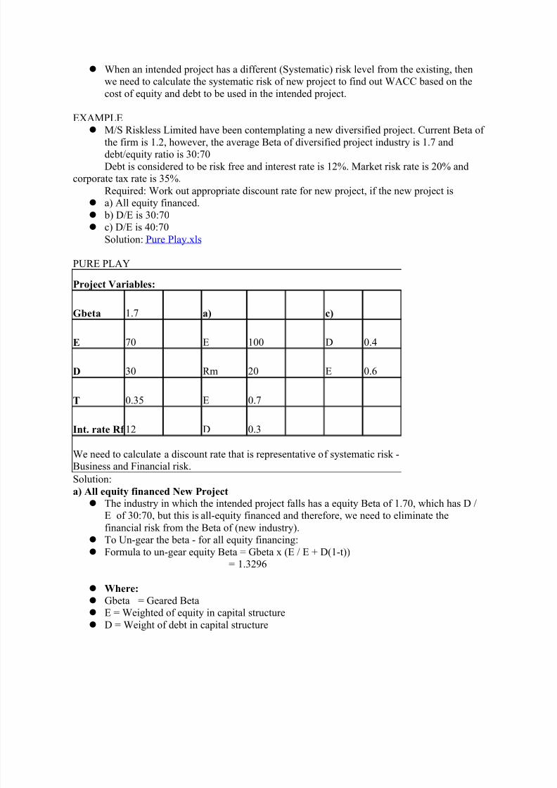
8/6/2019 Corporate Finance Lecture
http://slidepdf.com/reader/full/corporate-finance-lecture 111/125
When an intended project has a different (Systematic) risk level from the existing, thenwe need to calculate the systematic risk of new project to find out WACC based on thecost of equity and debt to be used in the intended project.
EXAMPLE
M/S Riskless Limited have been contemplating a new diversified project. Current Beta of the firm is 1.2, however, the average Beta of diversified project industry is 1.7 anddebt/equity ratio is 30:70Debt is considered to be risk free and interest rate is 12%. Market risk rate is 20% and
corporate tax rate is 35%.Required: Work out appropriate discount rate for new project, if the new project is
a) All equity financed. b) D/E is 30:70 c) D/E is 40:70
Solution: Pure Play.xls
PURE PLAYProject Variables:
Gbeta 1.7 a) c)
E 70 E 100 D 0.4
D 30 Rm 20 E 0.6
T 0.35 E 0.7
Int. rate Rf 12 D 0.3
We need to calculate a discount rate that is representative of systematic risk -Business and Financial risk.Solution:a) All equity financed New Project
The industry in which the intended project falls has a equity Beta of 1.70, which has D /E of 30:70, but this is all-equity financed and therefore, we need to eliminate thefinancial risk from the Beta of (new industry).
To Un-gear the beta - for all equity financing: Formula to un-gear equity Beta = Gbeta x (E / E + D(1-t))
= 1.3296
Where: Gbeta = Geared Beta E = Weighted of equity in capital structure D = Weight of debt in capital structure
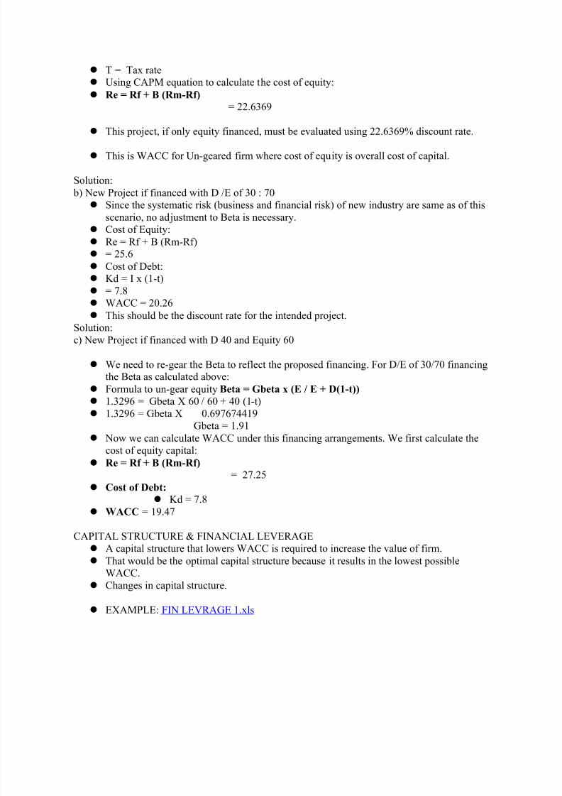
8/6/2019 Corporate Finance Lecture
http://slidepdf.com/reader/full/corporate-finance-lecture 112/125
T = Tax rate Using CAPM equation to calculate the cost of equity: Re = Rf + B (Rm-Rf)
= 22.6369
This project, if only equity financed, must be evaluated using 22.6369% discount rate.
This is WACC for Un-geared firm where cost of equity is overall cost of capital.
Solution: b) New Project if financed with D /E of 30 : 70
Since the systematic risk (business and financial risk) of new industry are same as of thisscenario, no adjustment to Beta is necessary.
Cost of Equity: Re = Rf + B (Rm-Rf) = 25.6
Cost of Debt: Kd = I x (1-t) = 7.8 WACC = 20.26 This should be the discount rate for the intended project.
Solution:c) New Project if financed with D 40 and Equity 60
We need to re-gear the Beta to reflect the proposed financing. For D/E of 30/70 financingthe Beta as calculated above:
Formula to un-gear equity Beta = Gbeta x (E / E + D(1-t)) 1.3296 = Gbeta X 60 / 60 + 40 (1-t) 1.3296 = Gbeta X 0.697674419
Gbeta = 1.91 Now we can calculate WACC under this financing arrangements. We first calculate the
cost of equity capital: Re = Rf + B (Rm-Rf)
= 27.25 Cost of Debt:
Kd = 7.8 WACC = 19.47
CAPITAL STRUCTURE & FINANCIAL LEVERAGE A capital structure that lowers WACC is required to increase the value of firm. That would be the optimal capital structure because it results in the lowest possible
WACC. Changes in capital structure.
EXAMPLE: FIN LEVRAGE 1.xls
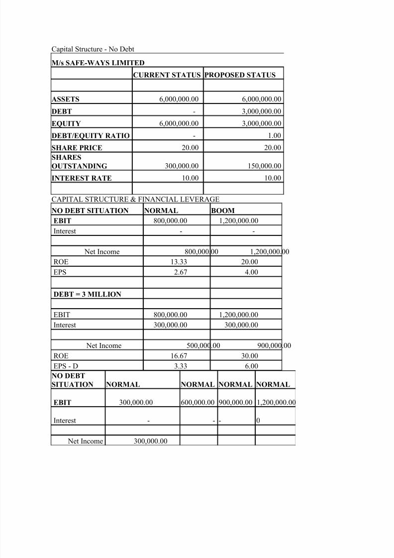
8/6/2019 Corporate Finance Lecture
http://slidepdf.com/reader/full/corporate-finance-lecture 113/125
Capital Structure - No Debt
M/s SAFE-WAYS LIMITED
CURRENT STATUS PR OPOSED STATUS
ASSETS 6,000,000.00 6,000,000.00
DEBT - 3,000,000.00
EQUITY 6,000,000.00 3,000,000.00
DEBT/EQUITY RATIO - 1.00
SHARE PRICE 20.00 20.00SHARESOUTSTANDING 300,000.00 150,000.00
INTEREST RATE 10.00 10.00
CAPITAL STRUCTURE & FINANCIAL LEVERAGE
NO DEBT SITUATION NORMAL BOOM
EBIT 800,000.00 1,200,000.00
Interest - -
Net Income 800,000.00 1,200,000.00
ROE 13.33 20.00
EPS 2.67 4.00
DEBT = 3 MILLION
EBIT 800,000.00 1,200,000.00
Interest 300,000.00 300,000.00
Net Income 500,000.00 900,000.00
ROE 16.67 30.00
EPS - D 3.33 6.00NO DEBT SITUATION NORMAL NORMAL NORMAL NORMAL
EBIT 300,000.00 600,000.00 900,000.00 1,200,000.00
Interest - - - 0
Net Income 300,000.00
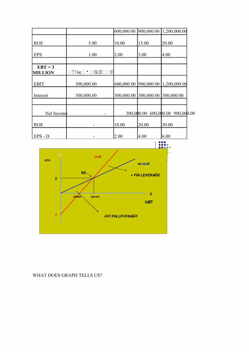
8/6/2019 Corporate Finance Lecture
http://slidepdf.com/reader/full/corporate-finance-lecture 114/125
600,000.00 900,000.00 1,200,000.00
ROE 5.00 10.00 15.00 20.00
EPS 1.00 2.00 3.00 4.00
DEBT = 3MILLION Ü
EBIT 300,000.00 600,000.00 900,000.00 1,200,000.00
Interest 300,000.00 300,000.00 300,000.00 300,000.00
Net Income - 300,000.00 600,000.00 900,000.00
ROE - 10.00 20.00 30.00
EPS - D - 2.00 4.00 6.00
EPS
EB (
)
600,000
2
N0
DEB1
DEB1
-2
300000
+ FIN LEVERA2
E
-IVE FIN LEVERA2
E
X
3
BE
WHAT DOES GRAPH TELLS US?
8/6/2019 Corporate Finance Lecture
http://slidepdf.com/reader/full/corporate-finance-lecture 115/125
Break even EBIT is 600,000, at this level EPS under both no-debt and debt situations is2. This is denoted as point BE in the above graph.
Area on the left or below BE representing negative impact on loan. Area right or above of BE point, represent positive impact of Financial leverage or
employment of loan.
CONCLUSION Financial leverage effect depends on the EBIT. Higher the EBIT, leverage is beneficial. Under normal scenario leverage increases the returns to shareholders ± measured by EPS
and ROE. Also shareholders are exposed to more risk under debt-equity structure.
corporate finance lecture No. 21
CAPITAL STRUCTURE & COST OF EQUITYMODIGLIANI AND MILLER MODEL
CAPITAL STRUCTURE & COST OF EQUITYMODIGLIANI AND MILLER MODEL Value of firm: Whatever the capital structure the operating income and value of its assets
will remain same or unchanged.
Proposition 1 of MM Model, says value of a firm is independent of its capital structure.CAPITAL STRUCTURE
OPTION1 OPTION 2Equity 40% 60%Loan ± debt 60% 40%Total capital 100% 100%
A firm may employ any of the above options of capital structure, the value of firm is notaffected as long as the capital is fixed (does not exceed 100%). This is because the operatingincome will remain constant and nothing positive (additional income) will increase the equityand share price.
WACC does not depend on debt equity ratio. Because it is the function of relative costsof debt & equity, and any change in debt and equity mix will change the cost of eachcomponent accordingly, making no movement in overall WACC.
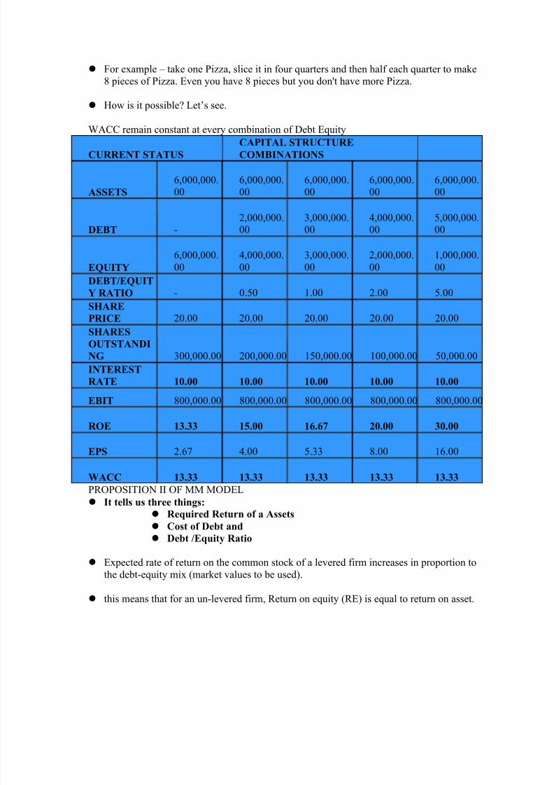
8/6/2019 Corporate Finance Lecture
http://slidepdf.com/reader/full/corporate-finance-lecture 116/125
For example ± take one Pizza, slice it in four quarters and then half each quarter to make8 pieces of Pizza. Even you have 8 pieces but you don't have more Pizza.
How is it possible? Let¶s see.
WACC remain constant at every combination of Debt Equity
CURRENT STATUS CAPITAL STRUCTURECOMBINATIONS
ASSETS 6,000,000.00
6,000,000.00
6,000,000.00
6,000,000.00
6,000,000.00
DEBT -2,000,000.00
3,000,000.00
4,000,000.00
5,000,000.00
EQUITY
6,000,000.
00
4,000,000.
00
3,000,000.
00
2,000,000.
00
1,000,000.
00DEBT/EQUITY RATIO - 0.50 1.00 2.00 5.00SHAREPRICE 20.00 20.00 20.00 20.00 20.00SHARESOUTSTANDING 300,000.00 200,000.00 150,000.00 100,000.00 50,000.00INTEREST RATE 10.00 10.00 10.00 10.00 10.00
EBIT 800,000.00 800,000.00 800,000.00 800,000.00 800,000.00
R OE 13.33 15.00 16.67 20.00 30.00
EPS 2.67 4.00 5.33 8.00 16.00
WACC 13.33 13.33 13.33 13.33 13.33PROPOSITION II OF MM MODEL It tells us three things:
Required Return of a Assets Cost of Debt and
Debt /Equity Ratio
Expected rate of return on the common stock of a levered firm increases in proportion tothe debt-equity mix (market values to be used).
this means that for an un-levered firm, Return on equity (RE) is equal to return on asset.
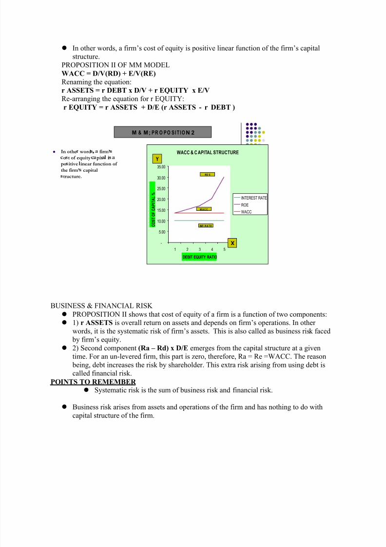
8/6/2019 Corporate Finance Lecture
http://slidepdf.com/reader/full/corporate-finance-lecture 117/125
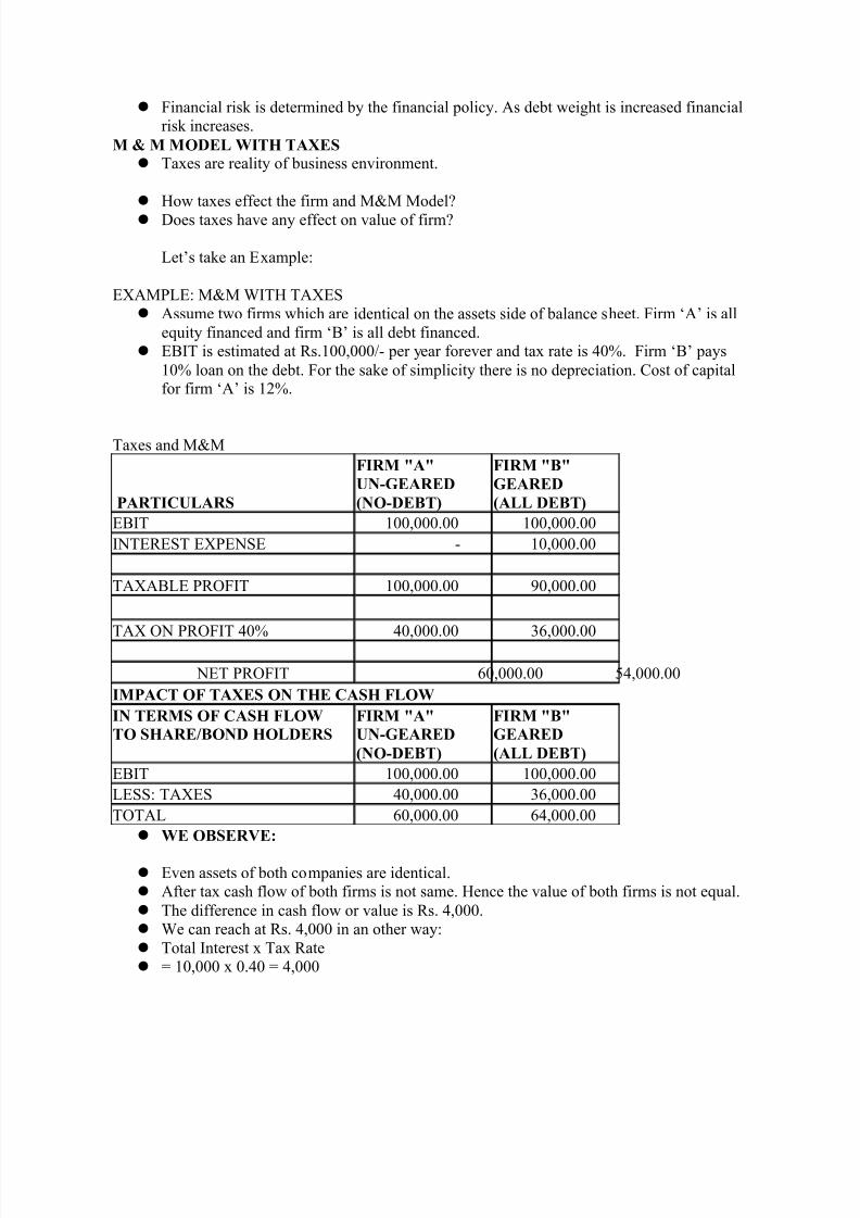
8/6/2019 Corporate Finance Lecture
http://slidepdf.com/reader/full/corporate-finance-lecture 118/125
Financial risk is determined by the financial policy. As debt weight is increased financialrisk increases.
M & M MODEL WITH TAXES Taxes are reality of business environment.
How taxes effect the firm and M&M Model? Does taxes have any effect on value of firm?
Let¶s take an Example:
EXAMPLE: M&M WITH TAXES Assume two firms which are identical on the assets side of balance sheet. Firm µA¶ is all
equity financed and firm µB¶ is all debt financed. EBIT is estimated at Rs.100,000/- per year forever and tax rate is 40%. Firm µB¶ pays
10% loan on the debt. For the sake of simplicity there is no depreciation. Cost of capitalfor firm µA¶ is 12%.
Taxes and M&M
PAR TICULARS
FIRM "A"UN-GEARED(NO-DEBT)
FIRM "B"GEARED(ALL DEBT)
EBIT 100,000.00 100,000.00INTEREST EXPENSE - 10,000.00
TAXABLE PROFIT 100,000.00 90,000.00
TAX ON PROFIT 40% 40,000.00 36,000.00
NET PROFIT 60,000.00 54,000.00IMPACT OF TAXES ON THE CASH FLOW IN TERMS OF CASH FLOW TO SHARE/BOND HOLDERS
FIRM "A" UN-GEARED (NO-DEBT)
FIRM "B" GEARED (ALL DEBT)
EBIT 100,000.00 100,000.00LESS: TAXES 40,000.00 36,000.00TOTAL 60,000.00 64,000.00
WE OBSERVE:
Even assets of both companies are identical. After tax cash flow of both firms is not same. Hence the value of both firms is not equal. The difference in cash flow or value is Rs. 4,000. We can reach at Rs. 4,000 in an other way: Total Interest x Tax Rate = 10,000 x 0.40 = 4,000
8/6/2019 Corporate Finance Lecture
http://slidepdf.com/reader/full/corporate-finance-lecture 119/125
Since interest is tax deductible, it generates saving called ³Interest Tax Shield´. Since debt is for ever, the value of firm µB¶ levered firm, will always be greater than firm
µA¶ by the present value of interest tax shield.
Present value of interest tax shield can be calculated as:
PV = Rs. 4000 / 0.1 = Rs. 40,000
M&M Model proposition 1 says: VL = VU + T X x D
Value of un-geared firm µA¶ can be worked out as under:
Vu = EBIT x (1-t) / Ru EBIT and taxable income of this firm is same.
Vu = 100,000 x (1 - 0.4)/ 0.12 = 500,000
We now find out the value of geared firm: VL = VE + Tx x D
= 500,000 + (100000 x 0.40) = 540,000 It means that for every Re. 1, the value of firm will increase by (Re.1 x tx) or 0.40.
Taxes do effect capital structure, therefore, we incorporate tax effect in proposition 1 of the Model:
V of Levered Firm = V of Un-levered Firm + Tax on Debt We also need to incorporate tax in Proposition II of M&M Model:
WACC = E/V(RE) + D/V (RD) x (1 ± t)Where t is the tax rate.
To find out Cost of Equity:
RE = RU + (RU ± RD) X D/E X (1 ± t)
Continuing our example to Proposition II Value of geared or levered firm was Rs. 540,000 because the debt is Rs.100,000 then the
equity must be 440,000.
Return on equity of levered or geared firm is then:
RE = RU + (RU ± RD) X D/E X (1 ± t)
8/6/2019 Corporate Finance Lecture
http://slidepdf.com/reader/full/corporate-finance-lecture 120/125
= .12 + (.12 - .10) x (100000/440000) x 0.4= 12.27%
WACC is:
= (4400/5400) x 12.27 + (1000/5400) x 0.1 x (1 ± 0.40) = 11.11%
AIDING UNDERSTANDING OF M&M MODEL Example M & M Model
EBIT = 80,000 Tax = 40% Debt = 50,000 Rate of Return (un-levered) firm = 20% Interest rate = 10%
Required: a) What is value of firm¶s equity? b) What is the cost of equity capital? c) What is WACC?
M&M MODELa) VALUE OF UN-LEVEREDFIRM VuWITH NO DEBT =EBIT x ( 1 - t) / Ru Vu = 240,000.00From MM proposition I, Value of
firm with Debt = VL VL = Vu + D x t 260,000.00Because this is the value of Leveredfirmthen, the equity value is:
E = VL - D
210,000.00b) Based on MM proposition 2,with tax cost of equity is:
RE = Ru + (Ru - Rd) x(D/E) x (1 - t)
0.21 21.438437.5
c) WACC
WACC = E/V(RE) + D/V(RD) x (1 ± t) 0.18 18.46
This shows that the WACC of a levered firm is lesser than that of un-levered.
8/6/2019 Corporate Finance Lecture
http://slidepdf.com/reader/full/corporate-finance-lecture 121/125
The WACC of un-levered firm was 20% and of levered firm is 18.46%.
This means that debt financing carries financial advantage.
corporate finance lecture No. 22
PROBLEMS ASSOCIATED WITH HIGH GEARING M&M Model says that debt financing increases the value of firm due to tax
shield.
However, there are certain aspects of high gearing that discourage borrowing.
BANKRUPTCY COSTS
Direct bankruptcy costs Indirect bankruptcy costs
FINANCIAL RELEVANCY COSTS These aspect are:
BANKRUPTCY COSTS: As debt increases chances of default of repayment of principal and interest
increases.
Direct Bankruptcy Costs: In case of liquidation disposal of assets will fetch less than going concern value of
assets. And there are other. Costs like liquidation and redundancy costs. The loss in value is normally borne
by the debt holders .
INDIRECT BANKRUPTCY COSTS When a firm goes into liquidation or approaches near bankruptcy because under sever
financial distress. Employees leaving Vendors refusing to supply goods on credit. Customers even leaving fearing firm will not be able to honor its warranty and
after sales services commitments. Value of firm down as sale decline. TAX POSITION:
8/6/2019 Corporate Finance Lecture
http://slidepdf.com/reader/full/corporate-finance-lecture 122/125
Firm must ensure that it will pay tax in future because the value increase isincidental with paying of taxes. High gearing reduces the taxable income againstwhich to off set interest expense.
DEPRECIATION:
Depreciation is also tax deductible and also affects the EBIT.OPTIMAL CAPITAL STRUCTURE
Debt has a magic in it. It increases the risk and reward to the firm and investors. Static theory of capital structure says that a firm should borrow to the extent where the
tax shield benefit is at least equal to the bankruptcy and financial distress costs incidentalto high gearing.
We can see the optimal combination of debt and value of the firm in graphical form. DIVIDEND POLICYOP TIMAL STRUCTURE
STATIC THEORY OF CAPITAL STRUCTURE
TOTAL DEBT
OPTIMAL DEBT LEVEL
VALUE OF FIRM
VL= VU + T x D
D
MAX
FIRM
VALUE
VL
PV OF TAX SHEILD
ACTUAL FIRM VALUE
Bankruptcy & FD
Value of No-Debt FirmVU
DIVIDEND POLICY
DVIDENDS HIGH & LOW PAYOUT DIVIDEND STRATEGIES
Two Components of Incomes:
Capital Gains ± Price AppreciationIncome ± Dividends
TYPES OF DIVIDENDS Cash dividends Stock dividends
8/6/2019 Corporate Finance Lecture
http://slidepdf.com/reader/full/corporate-finance-lecture 123/125
CASH & STOCK DIVIDENDS
Declaration date: The date on which dividend is announced. Ex-dividend date: to ensure dividend goes to right persons, this is two business
days before the record date. Record Date: On which the share register of the firm is updated for shareholdersrecord.
Date of Payment: On which the dividend cheques are sent to shareholders.
Ex-Dividend: For example, the Board of Directors declares dividend and recorddate is set to Monday 18 September 2006, then the ex-date will be Thursday 14September 2006. If someone buys the share in question on 13th Sept 2006, he/shewill be entitled to receive the dividend just declared. Someone buying the shareon 14th will not be.
WHY DIVIDEND POLICY IS IMPORTANT?
a) Affects shareholders attitude. b) Dividend policy has implications on capital budgeting program.c) It reduces cash flow position.d) It effects Debt Equity Ratio.
DIVIDEND POLICIES STABLE DIVIDEND PER SHARE:
per share fixed amount of dividend paid every year. Look favorably by investors and implies low risk firm. Investors can easily forecast and predict their earnings. Aid in financial planning.
CONSTANT DIVIDEND PAYOUT(DIV PER SHARE/EPS)
A fixed %age is paid out as dividend. Under this policy the dividend amount will vary because the net income is not constant.
HYBRID DIVIDEND POLICY This contains feature of both the above mentioned policies. Dividend consists of stable base amount and %age of increment in FAT income years. This is more flexible policy but increases uncertainty of future cash flow or return to
investors. The extra slice of %age is only paid when there is high jump in income. So it is not
regularly paid.FLUCTUATING DIVIDENDS
When the firm is having investment opportunities on its plate or unstable capitalexpenditure, then Dividends are of residual amount i.e. amount left after meeting capitalexpenditure.
FACTORS INFLUENCING DIVIDEND POLICY GROWTH OF FIRM
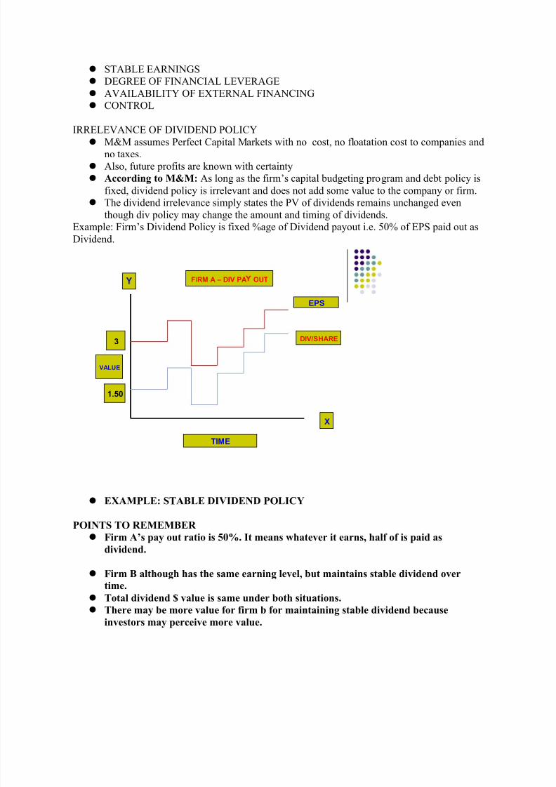
8/6/2019 Corporate Finance Lecture
http://slidepdf.com/reader/full/corporate-finance-lecture 124/125
STABLE EARNINGS DEGREE OF FINANCIAL LEVERAGE AVAILABILITY OF EXTERNAL FINANCING CONTROL
IRRELEVANCE OF DIVIDEND POLICY M&M assumes Perfect Capital Markets with no cost, no floatation cost to companies andno taxes.
Also, future profits are known with certainty According to M&M: As long as the firm¶s capital budgeting program and debt policy is
fixed, dividend policy is irrelevant and does not add some value to the company or firm. The dividend irrelevance simply states the PV of dividends remains unchanged even
though div policy may change the amount and timing of dividends.Example: Firm¶s Dividend Policy is fixed %age of Dividend payout i.e. 50% of EPS paid out asDividend.
EPS
DIV/SHARE
TIME
VALUE
X
@ FIRM A ± DIV PAA
OUT
1.50
3
EXAMPLE: STABLE DIVIDEND POLICY
POINTS TO REMEMBER
Firm A¶s pay out ratio is 50%. It means whatever it earns, half of is paid asdividend.
Firm B although has the same earning level, but maintains stable dividend overtime.
Total dividend $ value is same under both situations. There may be more value for firm b for maintaining stable dividend because
investors may perceive more value.
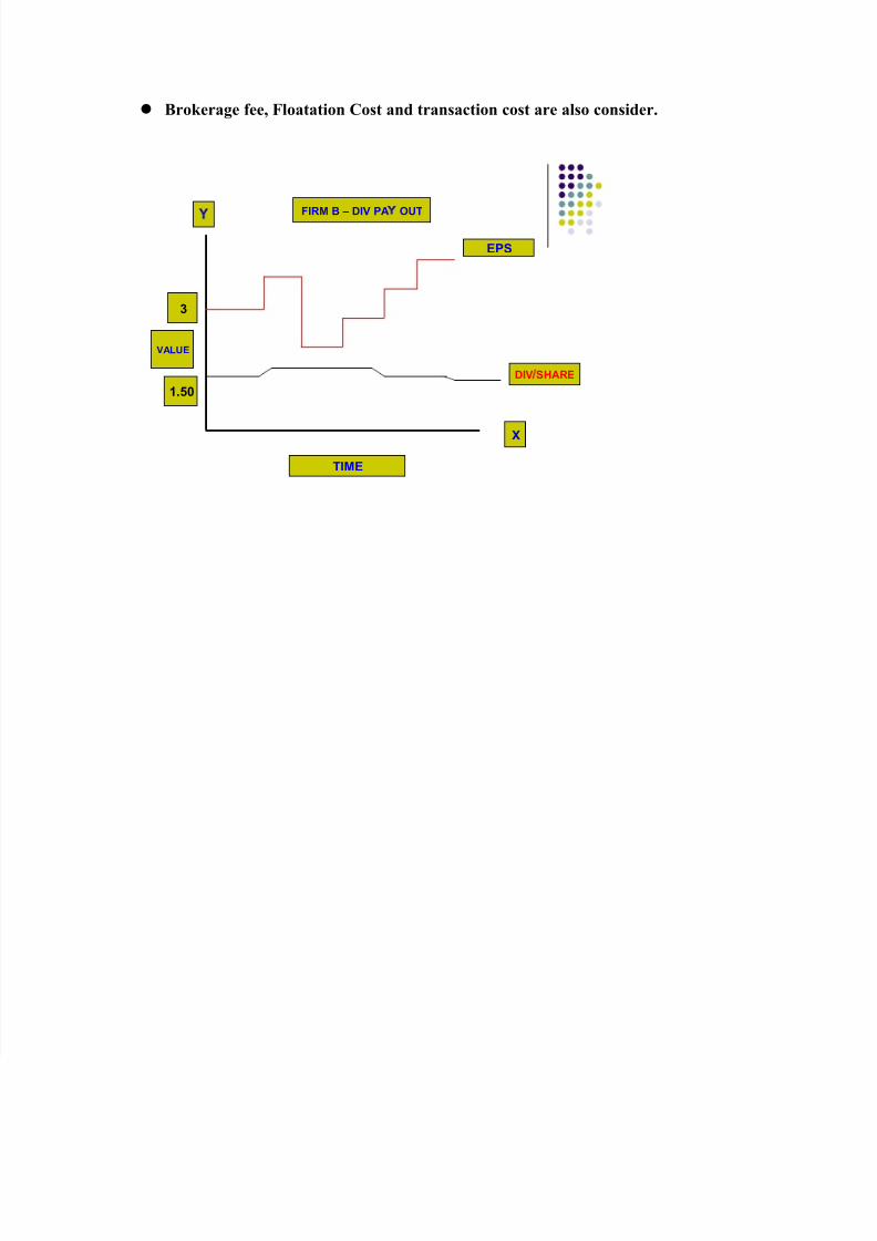
8/6/2019 Corporate Finance Lecture
http://slidepdf.com/reader/full/corporate-finance-lecture 125/125
Brokerage fee, Floatation Cost and transaction cost are also consider.
EPS
DIVB
SHARE
TIME
VALUE
X
C
FIRM B ± DIV PAD
OUT
1.50
3