Forthcoming, Quarterly Journal of Finance, 2018

Corporate Financial and Investment Policies

in the Presence of a Blockholder on the Board

Anup Agrawal and Tareque Nasser*

Current draft: May 2018

Comments welcome

* Agrawal: University of Alabama, Culverhouse College of Business, Tuscaloosa, AL 35487-0224, aagrawal@cba.ua.edu, (205) 348-8970. Nasser: 2097 BB, 1301 Lovers Lane, College of Business Administration, Kansas State University, Manhattan, KS 66506. Email: tnasser@ksu.edu, (785) 532-4375. We thank Jean Helwege and Fernando Zapatero (the editors), several anonymous referees, Lucian Bebchuk, Gennaro Bernile, Tim Burch, Jay Cai, Alex Edmans, Jeff Gordon, Vidhan Goyal, Nandini Gupta, Anzhela Knyazeva, Diana Knyazeva, Praveen Kumar, Junsoo Lee, Jim Ligon, John McConnell, Daniel Metzger, Kevin Murphy, Roberto Mura, DJ Nanda, Lalitha Naveen, Tom Noe, Harris Schlesinger, Shane Underwood, Tracie Woidtke, Rusty Yerkes, and seminar and conference participants at ALEA-Columbia, AFE-Philadelphia, CELS-Yale, CRSP Forum, Corporate Governance Conference at Erasmus University, FIRS-Minneapolis, University of Alabama and University of Miami for helpful comments and suggestions. Agrawal acknowledges financial support from the William A. Powell, Jr. Chair in Finance and Banking.

Corporate Financial and Investment Policies

in the Presence of a Blockholder on the Board

Abstract

We examine the relation between the presence of an independent director who is a blockholder (IDB) and

corporate policies, risk-taking and market valuation. After accounting for endogeneity, firms with an IDB

have significantly (1) lower levels of cash holdings, payout and R&D expenditures, (2) higher levels of

capital expenditures, and (3) lower risk. The market appears to value IDB presence and the associated

decrease in dividend yield. About 75% of the IDBs in our sample are individual investors, who drive most

of our results. Our findings suggest that IDB presence plays a valuable role in shaping some corporate

policies and allocating corporate resources.

JEL classification: G32, G34, G35

Keywords: Agency Problems, Corporate Governance, Boards of Directors, Blockholders, Corporate

Policies, Cash Holdings, Dividends, Investment, Financial Leverage, Firm Risk, Firm Valuation

2

Corporate Financial and Investment Policies

in the Presence of a Blockholder on the Board

1. Introduction

Separation of ownership and control creates agency problems between managers and

shareholders (see, e.g., Berle and Means (1932) and Jensen and Meckling (1976)). These problems can

affect a firm’s financial and investment policies (see, e.g., Easterbrook (1984), Jensen (1986), and La

Porta et al. (2000)). Several control mechanisms, both internal and external to the firm, work to reduce

these agency problems (see, e.g., Shleifer and Vishny (1986, 1997), Agrawal and Knoeber (1996), and

Becht, Bolton and Röell (2007)). In this paper, we examine (1) the relation between a potent governance

mechanism, namely the presence of an independent director who is a blockholder (IDB), and several key

corporate policies and (2) the market valuation of the changes in these policies associated with IDB

presence.

The crux of agency problems is weak monitoring and inefficient contracting with managers. In

firms with dispersed shareholdings, free-rider problems impede monitoring by shareholders. As

representatives of shareholders, boards of directors are charged with hiring, compensating, monitoring

and disciplining CEOs. But boards’ ability to monitor CEOs hinges on having strong, motivated and

independent directors. Morck (2008) argues that a powerful CEO can usually subdue nominally

independent directors, who often owe their board seats to the CEO. An IDB can serve as a powerful

control mechanism in a firm because she has both a strong incentive and the ability to monitor managers.

The incentive comes from his substantial shareholdings in the firm, while the ability comes from several

sources. A board seat gives an IDB a regular forum for monitoring managers. Large shareholdings give an

IDB direct voting power, the ability to form coalitions with other large shareholders, and greater influence

on the board relative to other outside directors, who typically have negligible stockholdings. Thus, an

3

IDB can play a more potent governance role than an independent blockholder without a board seat or an

independent director without a large shareholding.

But an IDB’s interests can diverge from those of other shareholders for at least two reasons. First,

an IDB can use her power and position to extract private benefits from the firm. Second, an IDB may be

more risk-averse than other shareholders. An IDB holds a substantial ownership stake in the firm and, as

the evidence in Faccio, Marchica and Mura (2011) suggests, likely holds an under-diversified portfolio.

So an IDB may prefer the firm to take less risk than other shareholders, who typically hold well-

diversified portfolios. Thus, whether an IDB acts to reduce agency problems or exacerbate them is an

empirical issue. Prior empirical evidence suggests that on net, IDB presence reduces managerial agency

problems (see, e.g., Bertrand and Mullainathan (2001), and Agrawal and Nasser (2018)).

An IDB can influence a firm’s investment and financial policies in two ways.1 First, these major

decisions are often subject to board approval, giving an IDB a direct say on them. Second, some financial

policies, such as debt and dividends, themselves serve as control mechanisms that reduce managerial

discretion by committing (or quasi-committing, in the case of dividends) the firm to pay out cash. Here,

an IDB’s presence acts as an alternate control mechanism that can substitute or complement the discipline

imposed by debt and dividends.

Alternatively, an IDB can mitigate agency problems by better contracting with the CEO, as prior

evidence (see, e.g., Bertrand and Mullainathan (2001), Cyert, Kang and Kumar (2002) and Agrawal and

Nasser (2018)) suggests, and leave the decisions on financial and investment policies to the CEO. The

IDB, in this case, avoids being a ‘back seat driver’, instead of second-guessing management on specific

corporate policies. Under this ‘hands-off’ approach, there would be no relation between IDB presence and

these corporate policies, but the presence of an IDB would still be valuable.

1 Anecdotal evidence suggests that IDBs do influence these policies. For instance, Kirk Kerkorian forced Chrysler to pay out about $8 billion in dividends and share repurchases in 1996 (see Henderson and Stern (1996)). Similarly, Carl Icahn pressured Time Warner to carry out a $20 billion stock repurchase program in 2006 (see Siklos and Sorkin (2006)).

4

In this paper, we examine three issues. First, we investigate the relation between IDB presence

and four key corporate financial and investment policy choices: the levels of cash holdings, payout,

investment, and financial leverage. We rely on prior evidence that IDB presence reduces agency problems

and try to characterize the nature of the dominant agency problem that arises when choosing different

corporate policies. Specifically, we attempt to distinguish among competing agency explanations of each

corporate policy choice based on their implications regarding an IDB’s effect on the policy, as discussed

in section 2 below. Our approach follows Bertrand and Mullainathan (2003), who try to distinguish

between two competing agency hypotheses about the nature of the agency problem that plagues corporate

investment decisions, and assume that closer monitoring of managers reduces agency problems.

Second, while prior evidence suggests that firm value is higher in IDB presence because of lower

agency problems (see Agrawal and Nasser (2018)), it does not identify the particular channels via which

this value-increase occurs. We provide direct evidence on this issue by building on the recent literature

that examines how the market evaluates changes in corporate cash holdings associated with various firm

and governance attributes. This literature uses a methodology developed by Faulkender and Wang (2006),

who examine how the marginal value of a firm’s cash holdings is related to its other financial policies.

Dittmar and Mahrt-Smith (2007) use this methodology to examine the relation between the quality of a

firm’s governance (as measured by shareholder rights and institutional ownership) and the valuation of its

cash holdings. Masulis, Wang and Xie (2009) extend this approach to dual-class firms and examine

changes in corporate cash holdings and capital expenditures associated with the divergence between

insiders’ voting rights and cash flow rights, and how the market values these changes. We contribute to

this literature by examining how the market values changes in each of the four corporate policy choices

associated with IDB presence.

Finally, we investigate the relation between IDB presence and risk-taking by a firm. A

blockholder is likely to underinvest in monitoring when the benefits of his monitoring are divided pro rata

among all stockholders, while he alone bears the costs. A firm becomes more valuable when this free-

rider problem can be reduced. Huddart (1993) argues that blockholder monitoring works best when stock

5

returns are not too risky, implying that blockholders would want to reduce risk. But different types of

blockholders may care about different types of risk. For instance, institutional shareholders may not be

too concerned about idiosyncratic risk because they hold well-diversified portfolios, but would be

concerned about systematic risk. IDBs’ portfolios, on the other hand, are likely under-diversified (see

Faccio, Marchica and Mura (2011)), so they would care about both systematic and unsystematic risk. This

implies that stocks of firms with IDBs should have lower levels of systematic, unsystematic and total risk.

An important issue in our analysis is the potential endogeneity of IDB presence in a firm. We

attempt to mitigate this concern using three different approaches. Our first approach exploits exogenous

variation in IDB presence using instrumental variables (IVs). We develop an instrument for IDB based on

the idea that wealthy individuals tend to invest in public companies located nearby, either due to better

monitoring ability or lower asymmetric information (see, e.g., Becker, Cronqvist and Fahlenbrach

(2011)).2 Given individual wealth constraints and preferences for the type of firm they want to invest in, a

wealthy individual investor is more likely to build up a substantial ownership stake in a local firm when

there is a large selection of small and mid-sized firms to choose from. Getting a board seat is also

somewhat easier in such firms compared to large firms. Moreover, a wealthy individual is more likely to

be prominent in an area that has fewer other wealthy investors, making it somewhat easier for him to

obtain a board seat in the firm. This is essentially a ‘big fish in a small pond’ effect. The instrument we

develop, which we call the ease of IDB formation (EIF), is a product of three binary variables that

together capture the ease of block formation and obtaining a board seat in a firm. EIF = (Fewer wealthy

individuals * More Compustat firms * More small firms). Fewer wealthy individuals=1, if the number of

million dollar homes in the area is less than the sample median for the year. More Compustat firms=1, if

the number of Compustat firms in the area is greater than the sample median for the year. More small

firms=1, if at least two-thirds of the Compustat firms in the area have market values below the top

quartile of the sample during the year. All three binary variables are based on an area that includes all

2 The tendency of individuals to invest locally is well-established in the literature on local bias in investing (see, e.g., Lerner (1995), Coval and Moskowitz (1999), and Bailey, Kumar and Ng (2008)).

6

counties within a 30-mile radius of the headquarters of a given firm. While EIF can explain IDB presence

in a firm, and empirically it does so significantly, it is plausibly exogenous to our main dependent

variables (corporate policies such as the levels of cash holdings, payout, debt, investment, and risk-

taking).3

Our second approach attempts to correct for the endogeneity caused by selection bias. Because

our main explanatory variable of interest, IDB, is binary, we use the Heckman two-stage treatment effect

models. Identification of these models is achieved through exclusion restrictions, a less demanding way of

identification than the IV approach. Third, we use firm fixed-effects regressions to mitigate endogeneity

concerns stemming from possible omitted variables. When we use firm fixed-effects regressions, instead

of OLS, the results are qualitatively similar. As with most studies in corporate finance, endogeneity is

hard to completely rule out. Despite any residual concerns about this issue, our results are quite

interesting.

We analyze these issues using a panel containing about 9,050 firm-years of data on S&P 1500

firms over 1998 to 2006. After controlling for other variables and accounting for the potential

endogeneity of IDB presence, we find that firms with IDBs have significantly (1) lower levels of cash

holdings and payout (dividend yields, repurchases, and total payout), (2) lower levels of R&D

expenditures, (3) higher levels of capital spending, particularly in high growth firms, and (4) lower

systematic, unsystematic and total risk. Finally, overall firm valuation is higher in firms with IDBs and

the market appears to value a decrease in dividend yield associated with IDB presence. About 75% of the

IDBs in our sample are individual investors, who drive most of our results.

These results have three implications. First, IDBs appear to take a hands-off approach for firms’

financial leverage, but take an active role in reducing cash holdings and risky R&D spending, while

increasing less risky capital expenditures. Second, lower payout in firms with IDBs and their higher

3 We also use the predicted value of IDB presence using a probit model as an instrument. Using this non-linear fitted value as an instrument (i.e., generated-IV) provides a ‘back-door’ identification (see, e.g., Angrist and Pischke (2009)). Since results from the 2SLS and generated-IV approaches are qualitatively similar, we only report the 2SLS results.

7

market valuation suggest that IDB presence acts as a substitute to dividends as a control mechanism.

Third, the prior literature has mixed findings on managerial preferences about the level of corporate

investment. The findings of Bertrand and Mullainathan (2003) and Aggarwal and Samwick (2006)

suggest that managers prefer a ‘quiet life’, while Gompers, Ishii and Metrick’s (2003) results point to

managers’ proclivity toward ‘empire building’. Our finding of higher levels of capital spending in IDB

presence suggests that the dominant agency problem with corporate investments is managers’ tendency

toward a ‘quiet life’. Overall, our results suggest that IDBs play a valuable role in valuable role in shaping

some corporate policies and allocating corporate resources.

In an excellent review article on blockholders, Holderness (2003) discusses that the endogeneity

of blockholder presence makes it difficult to assess their impact on corporate policies. He concludes,

“Surprisingly few major corporate decisions have been shown to be different in the presence of a

blockholder”. Our paper contributes to the literature on large shareholders’ impact on firms by (1) directly

analyzing a potential channel, namely the board of directors, via which they may effect corporate policies,

(2) accounting for the endogeneity of the presence of such independent blockholders with board seats via

several econometric methodologies, and (3) examining how the market values the changes in corporate

policies associated with IDB presence. We find that several corporate policies are significantly different

in IDB presence.

In related work, Cronqvist and Fahlenbrach (2009) argue that heterogeneity in blockholder effects

on corporate policies masks blockholder effects in prior studies. They find significant blockholder fixed

effects in corporate financial and investment policies and firm performance, which are larger when

blockholders hold larger blocks, have board seats or have management involvement. Becker, Cronqvist

and Fahlenbrach (2011) examine the effect of the presence of an individual, non-managerial blockholder

on several corporate policies and firm performance. Using an instrument to separate selection and

treatment effects of blockholder presence, they find that blockholder presence reduces a firm’s

8

investment, cash holdings and top executive pay, and increases payout and firm performance.4 They

conjecture that blockholders influence corporate policies via the board, but do not examine whether

blockholders indeed have board seats and whether they exercise their influence via those seats. We extend

Becker, Cronqvist and Fahlenbrach’s work by providing a direct examination of these issues. Our

findings about IDBs’ effects are similar to their findings about blockholders’ effects on cash holdings and

firm performance, but differ on investment and payout. In addition, we examine the market valuation of

the changes in corporate policies associated with IDB presence. Finally, we examine how firms’ risk-

taking changes in IDB presence, as issue not examined by Becker, et al.

The rest of the paper proceeds as follows. Section 2 discusses predictions of competing agency

models about an IDB’s effect on each corporate policy choice. Section 3 discusses the sample, data and

methodology. Section 4 presents the results on levels of cash holdings, dividends, investments, and

leverage. Section 5 presents the results on the valuation of corporate financial and investment policies

associated with IDB presence. Section 6 presents the results on firm risk. Section 7 concludes.

2. IDB presence and corporate policies

In this section, we attempt to characterize the nature of the dominant agency problem that plagues

each corporate policy choice. In doing this, we assume that managers who are monitored closely are less

likely to put their own interests ahead of shareholders. We rely on prior empirical evidence that the

presence of an independent director who owns a large block serves as an effective monitoring mechanism

and reduces managerial agency problems (see, e.g., Bertrand and Mullainathan (2001) and Agrawal and

Nasser (2018)). We then attempt to distinguish among predictions of competing agency models regarding

an IDB’s effect on each corporate policy choice. This approach follows Bertrand and Mullainathan

(2003). Table 1 summarizes these predictions.

4 Slovin and Sushka (1993) use a complementary approach to analyzing causality from blocks to corporate policies. They find (in Table VII) a large positive stock price reaction to the announcement of sale of a deceased insider’s block to an outsider, suggesting that the market views outside block formation favorably.

9

The first policy we examine is the level of corporate cash holdings. Cash creates two types of

agency problems. Jensen (1986) argues that excessive cash holdings allow managers to extract private

benefits from the firm (see Dittmar and Mahrt-Smith (2007) and Bates, Kahle, and Stulz (2009) for

supportive evidence). This is the agency problem of free cash flow. If IDBs reduce this agency problem,

their presence should decrease the level of cash holdings, after controlling for other factors. This is the

free cash flow hypothesis. On the contrary, Harford, Mansi and Maxwell (2008) argue that managers of

firms with weaker governance hold less cash to avoid a change in control. Large cash holdings can make

a firm more susceptible to takeover because a potential acquirer can use a highly leveraged bid to take

over the firm and use the target’s cash holdings to reduce debt after takeover. If IDBs reduce firms’

aversion to holding cash, the level of cash holdings ought to be higher in IDB presence. We refer to this

as the corporate control hypothesis.

The second policy we investigate is the level of corporate investment. Jensen (1986) argues that

managers have a taste for empire-building because they like the prestige, power and higher compensation

that comes with managing a larger firm. So overinvestment is a manifestation of agency problems. IDB

presence should reduce overinvestment, and consequently reduce investment levels. This is the empire-

building hypothesis. Alternatively, Bertrand and Mullainathan (2003) argue that mangers’ preference for a

‘quiet life’ can lead firms to underinvest. Here, IDB monitoring can force managers to increase

investment level. We refer to this as the quiet life hypothesis.

The next two corporate policies we analyze are the levels of debt and payout to shareholders.

Unlike the earlier two policies, debt and dividends can themselves act as control mechanisms that reduce

managerial discretion by bonding (or quasi-bonding, in case of dividends) the firm to pay out cash. Since

the presence of an IDB can also act as a control mechanism, the effect of IDB presence on these two

policies depends on whether IDB presence acts as a substitute or a complement to debt and dividends.

Easterbrook (1984) argues that higher payout reduces agency problems by increasing a firm’s

reliance on external capital and the resulting scrutiny from capital markets. Similarly, Jensen (1986)

argues that even when firms have large free cash flows, managers don’t like to pay it out because of the

10

discretion that cash provides them. Thus, low payout creates an agency problem by avoiding scrutiny

from capital markets and by increasing managerial discretion. To reduce the agency problem, an IDB may

force the firm to increase payout. Here, IDB monitoring complements payout as a control mechanism.

This argument implies that IDB presence should increase payout levels. We refer to this as the

complementary mechanism hypothesis. Alternatively, IDB monitoring can substitute payout as a control

mechanism, implying lower payout levels in IDB presence. We call this the substitute mechanism

hypothesis.

Similarly, Jensen (1986) argues that weak governance allows managers to choose less than the

optimal debt level to avoid market disciplining. IDBs can pressure managers to increase debt levels,

implying higher debt in IDB presence. Here, IDB presence complements debt as a control mechanism.

This is the complementary mechanism hypothesis. Alternatively, IDB monitoring can substitute for

monitoring by debtholders, implying lower debt levels in IDB presence. This is the substitute mechanism

hypothesis.

Next, as we find in section 3.1 below, most IDBs are individual investors.5 Individual wealth

constraints and the evidence in Facchio, Marchica and Mura (2011) imply that IDBs hold under-

diversified portfolios. Consequently, IDBs likely prefer lower risk-taking by the firm compared to well-

diversified investors. Accordingly, they appear to lower CEOs’ risk-incentives (see Agrawal and Nasser

(2018)). Therefore, we expect firms with IDBs to invest less in R&D, which are particularly high-risk,

lottery-like projects (see, e.g., Adhikari and Agrawal (2016)), and to take less risk overall. We also expect

IDBs to be averse to both systematic and idiosyncratic risk, which implies that stocks of firms with IDBs

should have lower levels of both risk components.

Finally, as discussed in the introduction, an IDB can mitigate agency problems by better

contracting with the CEO and leave decisions on specific corporate policies to the CEO. Under this

hands-off approach, there would be no relationship between IDB presence and any of the above corporate

5 This is perhaps not surprising, given the variety of constraints that prevent institutional investors from holding board seats (see, e.g., Roe (1994)).

11

policies, but the presence of an IDB would still be valuable. We call this the efficient contracting

hypothesis.

3. Sample, data and methodology

Our sample comes from firm-years that are common in three databases—RiskMetrics Directors

(RM Directors), Center for Research in Securities Prices (CRSP) and Compustat—over fiscal years 1998-

2006 and meet our data requirements. Our main sample of IDBs comes from RM Directors database,

which compiles its data from corporate proxy statements.6 We obtain data on several control variables

from RiskMetrics Governance (RM Governance), Thomson Reuters Institutional Ownership Data (TFN

Institutional) and ExecuComp databases. Finally, we hand-collect data on the identities of all the IDBs in

our sample. For each IDB, we started by reading their director profile in the proxy statement, accessed

using Livedgar. We then identified the nature of their ownership and investment vehicles from Wikipedia,

Who’s Who publications, business descriptions of investment vehicles on their Websites, news stories in

Factiva, and a variety of other Internet sources. Firms in our sample belong to the S&P 1500, which

consists of the S&P 500, S&P Mid-cap 400 and S&P Small-cap 600. This is the universe of firms covered

by RM Directors, RM Governance and Execucomp databases. We exclude financial and utility firms.

3.1 Main explanatory variable and sample construction

We define a blockholder as an individual who owns at least $15 million of a firm’s equity in 2000

dollars.7 This value is roughly equal to 1% of the median market capitalization ($1.6 billion) of our

sample firm-years.8 We define independent directors as directors classified as independent or designated

6 We confirm the validity of our data on IDB presence in a random sample of firm-years from corporate proxy statements (accessed via Livedgar), news stories (from Factiva), Wikipedia, and other Internet sources. 7 All variables that are that represent dollar value are expressed in constant 2000 dollars, using the CPI-All Urban Consumer series from the US Department of Labor. 8 In our main analysis, we use a dollar, rather than a percentage, threshold definition of a blockholder because a blockholder’s incentives are stronger when she invests significant personal wealth in the firm; that does not necessarily require her to own a significant proportion of the firm’s market capitalization. Nonetheless, we have replicated all of our results on corporate policies and risk-taking using a 1% ownership threshold to define a blockholder. These results are generally quite similar to those reported below.

12

in RM Directors.9 So an IDB is an independent director who is (or represents) a blockholder. The main

variable of interest for our analysis is IDB, which is a binary variable that equals one if there is at least

one IDB in a given firm-year, and equals zero otherwise.

Table 2 explains the construction of our sample. RM Directors obtains its data from proxy

statements for shareholder meeting dates starting in 1996. Some of the key variables needed to compute a

director’s shareholding are missing in the database for 1996. Also, some variables required for our

analysis were not available after 2006 at the time of data collection. Hence, our analysis makes use of data

for 1997-2006.

During 1997-2006, there are 16,967 distinct firm-calendar years in RM Directors.10 We find all

15,967 firm-calendar years on CRSP. Since we use a fiscal year as the unit of time, we match each annual

shareholder meeting date for a firm with the fiscal year in which the meeting is held. We obtain the fiscal

year ending month for each firm from Compustat. We next match these 15,967 firm-fiscal years

(henceforth, firm-years) with Compustat, and find 15,477 matches. After matching the annual meeting

dates to the appropriate fiscal year, 83 firm-years fall under the 2007 fiscal year. Due to data limitations,

we drop these observations. That leaves us with 15,394 RM Directors-CRSP-Compustat matched firm-

years. Out of these, we find 13,929 firm-years with non-missing CEO data in Execucomp. Our main

analysis omits observations for the 1997 fiscal year because information on board committees starts in

RM Directors database in 1998. In addition, we exclude 1,223 firm-year observations on dual-class firms

because such firms tend to be family-controlled (see DeAngelo and DeAngelo (1985)). After excluding

financial and utility firms from our sample and excluding the observations with missing information to

9 RM Directors defines as independent a director who is neither a current company employee nor is ‘affiliated’. An affiliated director is a director who is a former employee of the company or of a majority-owned subsidiary; a provider of professional services — such as legal, consulting or financial — to the company or an executive of the service provider; a customer or supplier of the company; a designee (i.e., a designated director) under a documented agreement between the company and a group, such as a significant shareholder; a director who controls more than 50% of the company’s voting power; a family member of an employee; an interlocking director or an employee of an organization or institution that receives charitable gifts from the company. 10 A single firm-calendar year often includes data from multiple proxy statements. Since directors are usually elected at the annual general meeting of shareholders, typically held three months after the end of a fiscal year, we use the list of directors from the proxy statement for this meeting.

13

construct the instrumental variable, our final sample for the main analysis consists of 9,050 firm-years

over 1998-2006.

Appendix Table A.1 provides an overview of our sample. Panel C shows that of the 9,050 firm-

years in our sample, 1,221 or 13.5% of the firm-years have an IDB. Panel A reports the distribution of the

number of fiscal years a firm is present in our sample. Over the 1998-2006 period, our sample contains

1,610 unique firms. Of these, 543 firms are present in all nine years during 1998-2006 and 1,214 firms are

present in at least three years. Panel B shows the distribution of the proportion of a given firm’s fiscal

years that have an IDB. For example, 1,189 firms have no IDB during all the fiscal years that they are

present in our sample. Panel C presents the number of firm-years in each fiscal year for IDB, non-IDB,

and all firms in the sample. The sample size ranges from 940 in 2006 to 1,064 in 2001. The percentage of

firms with IDBs ranges from 12.22 in 1998 to 15.25 in 2000. Panel D shows the sample distribution by

IDB-identity. About 74% of the IDBs in our sample are individual investors, who either own the stock

directly (62%) or indirectly via a beneficial trust or investment vehicle (12%). The remaining IDBs

represent hedge funds (3%), private equity funds (7%), venture capital firms (2%), corporations (6%), and

fiduciary trusts (8%). Most of our results are driven by individual investor IDBs, which is not surprising

given their preponderance in the sample. It is difficult to make inferences about the effects of the

remaining types of IDBs given their small presence in our sample.

Row 1 in Appendix Table A.2 reports the distribution of dollar stock ownership of the largest

IDB in the 1,221 firm-years in our sample with at least one IDB. The mean (median) stock ownership is

$215.20 million ($39.05 million) in constant 2000 dollars, representing about 13.20% (2.40%) of the

median market capitalization ($1,630 million) in our total sample of firm-years.

3.2. Instrumental variables and empirical methodology

Our main variable of interest, IDB, is likely endogenous. Individuals decide which firms to invest

in and whether to try to obtain a board seat. This endogeneity can affect our analysis through either

omitted variables or selection bias. In addition to including a large set of explanatory variables in our

14

regressions to reduce the possibility of omitted variables, we employ two main approaches to mitigate

concerns about the endogeneity of IDB presence in a firm: two-stage least squares (2SLS) and treatment

effect models. We discuss these models in the next two subsections. Moreover, we also use fixed-effects

regressions and a generated IV approach, with qualitatively similar results (un-tabulated).

3.2.1. 2SLS models

We estimate two-stage least squares (2SLS) models to account for potential endogeneity caused

by unobservable omitted variables. Because the potential endogenous variable is binary, we use the linear

probability model (LPM) in the first stage. As discussed in the introduction, we develop an instrument for

IDB presence based partly on the findings of the literature on ‘home bias at home’ (see, e.g., Coval and

Moskowitz (1999)) that individuals tend to invest more in stocks of local firms. Given individual wealth

constraints, block formation by an individual investor is more likely if there are a large number of small

to mid-size firms to choose from in an area. Consistent with a ‘big fish in a small pond’ effect, an

individual blockholder is more likely to obtain a board seat in the firm if she is prominent in the area near

the firm headquarters. Our instrument for IDB presence is the IV ease of IDB formation (EIF). EIF equals

one if the area covering all counties within a 30-mile radius centered at the firm headquarters has the

following characteristics: 1) the number of million dollar homes in the area is less than the sample median

for the year, 2) the number of firms in the area is greater than the sample median for the year, and 3) at

least two-thirds of the firms in the area have market values below the top quartile of the sample during the

year; it equals zero otherwise. While we expect EIF to explain IDB presence in a firm, and empirically it

does so significantly, there is no reason why it should explain our main dependent variables (i.e., levels of

cash holdings, dividends, investment, leverage, firm risk and excess return), except via its effects on IDB

presence in a firm.

We obtain data on residential property values for each county from the National Historical

Geographic Information System (NHGIS). We find zip codes of firm headquarters from Compustat, and

cross-check them with EDGAR filings to account for any changes of headquarters locations. We use the

SAS map area identification variables, particularly Federal Information Processing Standards (FIPS)

15

codes for identifying each county’s primary postal zip codes. We then use the SAS Zipcitydistance

Function to measure the distance between a firm’s headquarters location and the neighboring counties’

primary postal zip codes.

While the 2SLS estimator is potentially biased, it is consistent; and having a large sample makes

the 2SLS results more reliable. We test for exogeneity using the Durbin-Wu-Hausman test, which

examines the statistical difference between OLS and 2SLS coefficient estimates of the suspect

endogenous variable. Staiger and Stock (1997) suggest that the F-statistic of the IVs used in the first-stage

regression should be reasonably high (more than 10), which holds in our case. Given Bertrand and

Schoar’s (2003) finding of systematic differences in corporate decision-making across individual CEOs,

we compute robust standard errors clustered at the CEO-firm level.

Some of our main dependent variables in section 4 below take on a limited range of values. Given

that our main explanatory variable, IDB, is potentially endogenous, we use the methods suggested by

Rivers and Vuong (1988) and Smith and Blundell (1986) to test for potential endogeneity in regressions

of binary (e.g., dividend dummy) and censored (e.g., dividends, R&D expenditures or financial leverage)

dependent variables, respectively. Both of these methods use a two-stage procedure. In the first stage, the

residual is computed from the OLS regression of the potentially endogenous variable (i.e., IDB) on the

instrument and all the control variables of the main equation. In the second stage, the main probit (Rivers-

Vuong) or Tobit (Smith-Blundell) regression is estimated using the first-stage residual as an additional

regressor. If the t-test of the first-stage residual is insignificant, we conclude that IDB is not endogenous.

One advantage of these two methods is that if the first-stage residual is insignificant, the test of

exogeneity is valid without any distributional assumption on the error term in the first-stage regression

(see Wooldridge (2002, p. 474 and 531)). If these methods fail to reject endogeneity, we use IV-probit or

IV-Tobit methodology as an imperfect solution.11

11 These methods assume that the endogenous variable is continuous.

16

When the dependent variable is censored, we use the IV-Tobit maximum likelihood estimator

(MLE). In this framework, the main set of equations has a typical Tobit structure (i.e., the structural

equation and the selection equation). In addition, we regress the endogenous variable on all exogenous

variables from the structural equation and the IVs. We also conduct a Wald test for the exogeneity of the

instrumented variable. When the dependent variable is binary, we use the MLE of the probit model with

an endogenous explanatory variable, namely IV-probit (see Wooldridge (2002, p. 476)).

3.2.2. Treatment effect models

We next account for endogeneity stemming from a selection bias in IDB presence in a firm by

using treatment effect models. Heckman’s (1979) two-stage treatment effect model is appropriate for

estimating the average treatment effect and correcting for sample selection bias. In this model, the inverse

Mill’s ratio (Lambda), computed from the first-stage probit regression, is added as a covariate in the

second-stage regression to account for any selection bias.

We follow Agrawal and Nasser (AN, 2018) to develop the first-stage selection equation.

However, they define IDB presence based on a 1% ownership threshold definition of a blockholder

(IDB%). Hence, we report the descriptive statistics and regressions of determinants of IDB presence in a

firm based on our dollar threshold definition of a blockholder in Table 3 (IDB$ or IDB). Panel A presents

univariate tests of the determinants of IDB presence for firm-years with and without IDBs. Both mean

and median differences between IDB and non-IDB firms are significantly different for all except two

variables.12

Panel B of Table 3 presents regression results of IDB presence on its potential determinants.

Models 1, 2 and 3 implement OLS, Logit and Probit regressions, respectively, and include as covariates

the set of variables shown in Panel A. The results are similar to AN, except for a few interesting

12 These two variables are the fraction of independent directors on the board and the CEO’s presence on the nominating committee. In the regression framework, only the former variable is statistically significant. For the latter variable, a measure of CEO power, there are two opposing forces at work, which appear to offset each other. Firms with strong (and perhaps entrenched) CEOs stand to benefit more from IDB presence, increasing an investor’s incentive to acquire a large block and seek a board seat. But since independent blockholders (IBs) have strong incentives and the ability to monitor the CEO, powerful CEOs are likely to resist their appointment to the board.

17

differences. First, firms with IDB$ are larger in size, while firms with IDB% (in AN) are smaller. Second,

IDB$ firms have significantly higher Tobin’s q but are unrelated to past performance measured by

operating performance to sales (OPS); IDB% firms, on the other hand, are unrelated to Tobin’s q but have

significantly lower OPS. Finally, corporate policy variables such as cash holdings, dividend yields and

R&D expenditures are unrelated to IDB$ presence but are significantly negatively related to IDB%

presence. All these differences appear to be natural concomitants of the dollar threshold definition of a

blockholder.

Model 4 is the same as Model 3, except that we exclude cash holdings, dividend yield, R&D

expenditures and OPS as covariates. Using either Model 3 or 4 as the selection model of the treatment

effect models shows no qualitative differences in results. Hence, for reporting purpose we use Model 3 as

the selection equation for all treatment effect models.

3.3. Dependent variables

We construct all of the financial and investment policy variables of a firm using Compustat data.

To measure the level of cash, we define cash holdings as cash plus marketable securities divided by total

assets. We use four different variables to measure firms’ payout policies: dividend yield, dividend

dummy, repurchases and total payout. Dividend yield is defined as common dividends divided by market

capitalization; dividend dummy is a binary variable that equals one if a firm pays dividends in a given

fiscal year, and equals zero otherwise. We define repurchases as the total expenditure on the purchase of

common and preferred stock divided by equity market capitalization. Total payout is sum of dividend

yield and repurchases. We measure the level of a firm’s investment as capital expenditures or R&D

expenditures, both scaled by total assets. We also examine total investment, measured as the sum of

capital expenditures and R&D expenditures. Finally, we measure a firm’s debt level as leverage, which

equals total debt as a percentage of total assets.

We use three measures of equity risk: total risk, systematic risk and unsystematic risk. Using

CRSP data, we measure total risk as the variance of daily stock returns over a fiscal year. We then

decompose total risk using a market model. Variance of the predicted portion of the market model is

18

defined as the systematic risk and variance of the residual of the market model is defined as unsystematic

risk. Since all of these risk measures have skewed distributions, we use their natural logarithm in the

regressions. For valuation regressions, we use excess return as the dependent variable. We define excess

return as a firm’s buy and hold stock return over a fiscal-year minus the return on the corresponding Fama

and French (1993) 5×5 size and market-to-book value portfolio.13

Appendix Table A.2 provides descriptive statistics of these variables. The median cash holding is

7.10% of total assets. About 50% of our sample firm-years pay no dividends and the median dividend

yield for the firms that pay dividend is about 1.14% (not tabulated). Similarly, in un-tabulated data, 42%

(25%) of the sample firm-years have no repurchases (payouts). The median capital expenditures, R&D

expenditure and total debt are about 4.17%, 0.43% and 21.43% of total assets, respectively. In our

sample, about 12% of the firm-years have no debt and 46% of the firm-years incur no R&D expenditures

(un-tabulated).

3.4 Independent variables

In addition to IDB, our main explanatory variable of interest, the independent variables in our

analysis consist of financial ratios and characteristics of boards, CEOs, and firms. We also include year

dummies and Fama and French 12 industry dummies.14 We winsorize the top and bottom one-half percent

of the observations of all financial variables, ownership and compensation variables, firm size variables,

sales growth, Tobin’s q, stock returns and volatility. Appendix Table A.2 provides definitions and

descriptive statistics of these variables.

The typical firm in the sample is fairly large, with median market capitalization and total assets of

about $1.63 billion and $1.45 billion, respectively, in 2000 dollars. The median firm age (using earliest of

13 We obtain Fama and French 5×5 size and book-to-market portfolio returns from Professor Kenneth French’s website: http://mba.tuck.dartmouth.edu/pages/faculty/ken.french/data_library.html. We also obtain Fama and French industry classifications from this website. 14 Finer classifications, such as Fama and French (1997) 48 industries, result in partitions with many industries having only one or two firms in our sample. Since many of the board characteristic variables (e.g., IDB, board size) are highly persistent over time, using industry dummies based on finer industry classifications would be tantamount to including firm-specific dummies.

19

CRSP and Compustat listing dates) is 20 years. The median board size is 9 and the median fraction of

independent directors is 0.67. The median total ownership of a firm’s top five executives is 0.70% and the

median institutional ownership is 70%. The ratio of incentive pay to total pay for the top five managers

has a median value of 42%.

4. IDB presence and corporate policies

This section examines the relations between IDB presence in a firm and levels of cash holdings

(section 4.1), dividends and payout (section 4.2), investment (section 4.3), and financial leverage (section

4.4). Panel A of Table 4 shows univariate comparisons of mean and median values between IDB and non-

IDB firms. The mean (median) levels of cash holdings of IDB and non-IDB firms are 12.88% (5.92%)

and 14.89% (7.35%), respectively. Univariate tests show that firms with IDB presence hold significantly

lower levels of cash than firms without an IDB. A significantly higher proportion of IDB firms pay

dividends than non-IDB firms, about 55% as opposed to 49%; this is reflected in the higher median

dividend yields in IDB firms. But the mean difference in dividends yields between IDB and non-IDB

firms is statistically insignificant. Although the mean ratio of repurchases to market capitalization is

significantly lower in IDB firms than in non-IDB firms, total payout is barely significantly different. As

indicated by univariate tests, firms with IDB presence are associated with lower R&D expenditures but

higher capital expenditures. Finally, both the mean and median levels of financial leverage are

significantly higher in IDB firms than in non-IDB firms. So the univariate evidence shows that IDB

presence is related to several financial and investment policies of firms. But this evidence is preliminary,

because it does not control for other determinants of financial and investment policy choices and does not

account for the potential endogeneity of IDB presence, issues we deal with next.

4.1 IDB presence and the level of cash holdings

In this section, we examine the relation between IDB presence and the level of a firm’s cash

holdings using several regression-based methodologies. The results of these regressions are presented in

20

Table 5. We follow prior studies (see, e.g., Opler et al. (1999), Harford, Mansi and Maxwell (2008), and

Bates, Kahle and Stulz (2009)) to identify the control variables for cash holdings.

Cash holdings measure the liquid resources available to a firm, and provide a cushion against

bankruptcy risk. We control for a firm’s liquidity and bankruptcy risk via net working capital net of cash,

cash flow, leverage, and a loss indicator variable (i.e., whether the firm has suffered a negative net income

in a given fiscal year). Firms with stronger growth opportunities and limited access to capital markets

carry higher cash holdings. We control for growth opportunities via the average sales growth rate over the

prior five years, Tobin’s q and R&D expenditures. We control for a firm’s ability to access capital

markets via firm size (log of market capitalization). In addition, we include a bond rating dummy, a

variable that equals one if a firm has S&P long-term bond ratings, and zero otherwise. Bates, Kahle, and

Stulz (2009) argue that a firm has more cash immediately after raising capital; reduces cash as it pays

back debt or repurchases stock. Hence, we control for firms’ net equity issuance and net debt issuance.

Firms with greater precautionary needs require higher levels of cash holdings. We control for a firm’s

business condition via cash flow volatility, measured as the standard deviation of cash flows over the

prior ten years. Firms with higher levels of capital expenditures and acquisition activity tend to have

lower levels of cash holdings; we also control for these.

In addition to IDB presence in a firm, we control for other internal and external governance

mechanisms such as board structure (board size and fraction of independent directors on the board),

institutional ownership, managers’ option-based pay (i.e., the percentage of total pay for the top five

managers that is option-based), and G-index (Gompers, Ishii and Metrick’s (2003) shareholder rights

index). Following Harford el al. (2008), we include the lagged value of cash holdings as an independent

variable. The regressions also include year dummies and Fama and French 12 industry dummies.

Model 1 is the OLS regression of cash holdings, and we find that IDB presence is unrelated to a

firm’s cash holdings. Most of the control variables in the OLS regression take their expected signs in

model 1. Firms with lower cash holdings are larger, tend to have higher leverage and net working capital,

pay dividends, have a bond rating, and make more investments via capital expenditures and acquisitions.

21

On the other hand, firms with higher cash holdings have greater growth opportunities (Tobin’s q and

R&D expenditures), cash flow volatility, net debt issuance, and net equity issuance. Consistent with the

prior literature (e.g., Harford, Mansi and Maxwell (2008)), lower G-index and higher institutional

ownership, as measures of better governance, are associated with higher cash holdings.

In model 2, we instrument for IDB presence using EIF in the 2SLS framework. The F-statistic for

the IV in the first-stage regression is 19.24, far above the cut-off value of 10 recommended by Staiger and

Stock (1997), mitigating the concern about weak IV. However, the test for exogeniety indicates that IDB

presence is not endogenous in this regression.

We also estimate Heckman’s two-stage treatment effect model to account for possible selection

bias. Model 3 shows that the inverse Mills ratio is significantly positive, consistent with endogenous

selection of IDB presence. In this model, IDB presence reduces the level of cash holdings by 22.56%.

Hence, after accounting for potential selection bias of IDB presence, the result is consistent with the idea

that IDB presence mitigates agency problems by reducing excess cash holdings.

4.2 IDB presence and the levels of dividends and payout

We next examine the relation between IDB presence and four measures of firms’ payout

(dividend yield, dividend dummy, repurchases and total payout) in regression frameworks, after

controlling for other determinants of payout policies. Young growth firms are less prone to pay out cash

(see, e.g., Grullon and Michaely (2002), Fama and French (2002) and Grullon et al. (2011)). Hence, we

control for firm age, size, sales growth, and future growth options via Tobin’s q and R&D expenditures.

Among firms that pay out cash, riskier firms use repurchases whereas safer firms use dividends (e.g.,

Jagannathan, Stephens and Weisbach (2000), Guay and Harford (2000), and Grullon and Michaely

(2002)); we use a firm’s cash flow volatility to control for this effect. Following the prior literature, we

also control for stock return volatility as an additional measure of risk (see, e.g., Grullon and Michaely

(2014) and Grullon et al. (2011)). John, Knyazeva and Knyazeva (2015) find that dividends are preferred

over repurchases when agency problems are severe. Hence, in addition to IDB presence, we control for

22

firms’ governance via the G-index, institutional ownership, board size, the fraction of independent

directors, insider ownership, and proportion of the top management’s pay that is option based. We also

control for firms’ financial leverage and profitability. Finally, the regressions include year dummies and

Fama and French 12 industry dummies.

Panel A of Table 6 reports the results of regressions of dividend yield and dividend dummy.

Since about 50% of the firm-years in our sample have no dividends, we use the Tobit model to regress

dividend yield and the probit model to regress the dividend dummy on IDB and other covariates. We find

the coefficient estimate of IDB to be significantly negative in the Tobit regression but insignificant in the

probit regression. While IDB presence is unrelated to a firm’s decision on whether to pay dividends, it is

negatively related to dividend yield. The latter finding is consistent with La Porta et al.’s (2000)

‘substitute model’ of dividends. The idea that the monitoring effect of IDB presence substitutes for higher

dividends is bolstered by the fact that G-index has significant positive coefficients in both the probit and

Tobit models, which suggests that firms with lower shareholder rights use dividends as a substitute

governance mechanism.

The magnitude of the decrease in dividend yield in IDB presence is non-trivial. A coefficient of -

0.160 represents an 18% reduction compared to the unconditional mean dividend yield of 0.898%. This

result, however, does not account for the potential endogeneity of IDB presence in the context of dividend

yield. So we estimate Smith-Blundell regressions, where the potentially endogenous IDB variable is

instrumented by EIF. However, based on the p-value of the residual term, we conclude that IDB presence

is not endogenous in the dividend yield regression. Similarly, the p-value of the residual term in the

Rivers-Vuong model indicates that IDB presence is not endogenous in the regression of the dividend

dummy.

We next examine the relation between IDB presence and the levels of repurchases and total

payout. Similar to dividend yield, both of these variables contain a disproportionate mass at zero. Hence,

we use Tobit regressions. Panel B of Table 6 reports these results. We find that IDB presence reduces

both repurchases and total payout significantly. When we account for the potential endogeneity of IDB

23

presence using Smith-Blundell regressions, we find that IDB presence is not endogenous in both

repurchases (model 2) and total payout (model 4) regressions.

Overall, the results in Table 6 suggest that in addition to IDB presence being a ‘substitute’ for

higher dividends as a governance mechanism, it is also negatively related to the level of repurchases. The

results on the remaining covariates are mostly consistent with the prior literature. Larger, older, low

growth and low risk firms are more likely to pay dividends and to have larger payouts. Firms with lower

cash flow volatility, lower shareholder rights, lower option-based pay and larger board size have higher

dividend yields but lower repurchases. Firms with a higher fraction of independent directors and lower

institutional ownership have larger payouts. All of these results are statistically significant.

4.3 IDB presence and the levels of investment expenditures

In this section, we examine the relation between IDB presence and a firm’s investment policies

using several regression-based methodologies. Specifically, we examine capital expenditures and R&D

expenditures. The regressions control for other determinants of investment expenditures. First, a firm

incurs capital and R&D expenditures to exploit its future growth opportunities but is constrained by its

funding limitations (see, e.g., Fazzari, Hubbard and Petersen (1988) and Hubbard (1998)). Hence, we

need to control for a firm’s growth prospects and financial or liquidity constraints. We use lagged Tobin’s

q to control for a firm’s growth opportunities; we control for firm size, cash flow, cash holdings and

leverage to account for funding availability. Second, following the prior literature, we control for firm

profitability via lagged ROA and stock returns (see, e.g., Coles, Daniel and Naveen (2006)). We control

for other internal and external governance mechanisms via board structure (board size and the fraction of

independent directors), institutional ownership, proportion of the top management pay that is option-

based, and G-index. Finally, we include year dummies and Fama and French 12 industry dummies.

Panel A of Table 7 report regressions of capital expenditures on IDB presence and control

variables. In OLS regressions, we find that capital expenditures are unrelated to IDB presence. To account

for potential endogeneity, we instrument IDB presence with EIF in a 2SLS regression. The F-statistic for

24

significance of the IV in the first-stage regression is much larger than the minimum recommended cut-off

value of 10, a result that implies that the IVs are not weak. But the test of exogeneity indicates that IDB

presence is not endogenous in this regression, implying that OLS should be preferred in this case.

We next use Heckman’s treatment effect model to account for the possible selection bias

introduced by IDB presence in a firm. Identification in this model is achieved via exclusion restrictions.

The estimated coefficient of the inverse Mills ratio is highly significant. This result indicates that self-

selection is important here. A negative coefficient of the inverse Mills ratio suggests that the

characteristics that cause an IDB to be present in a firm-year are negatively related to capital

expenditures. We find that the coefficient of IDB in model 3 is significantly positive. This finding

suggests that IDBs self-select into firms where there is relative underinvestment and that their presence

increases capital expenditure. However, an important and strategic component of firms’ investment is

R&D expenditures. We next examine whether IDB presence is related to R&D expenditure.

Panel B of Table 7 reports regression results of R&D expenditures on IDB and other covariates.

Because a substantial proportion of firm incur zero R&D expenditures, we use the Tobit regression in

model 1. We find that IDB presence is unrelated to R&D expenditures. To account for the potential

endogeneity of IDB presence in a firm, we instrument for IDB presence with EIF in a Smith-Blundell

framework. The p-value of the residual term in model 2 indicates that IDB presence is endogenous in the

context of R&D expenditures. We therefore estimate an IV-Tobit regression in model 3, and find that

after accounting for endogeneity IDB presence has a significant negative impact on the level of a firm’s

R&D spending. As discussed earlier, the IV-Tobit methodology is an imperfect solution here because this

method assumes that the endogenous variable is continuous. So we refrain from interpreting the

magnitude of this coefficient.

The results on other covariates in the regressions in Panels A and B are also interesting. While

firm size measured as sales is negatively related to both capital and R&D expenditure, the proportion of

option-based pay for top executives is positively related to them. Firms with lower debt levels, higher

Tobin’s q, lower return on assets and lower insider ownership have higher levels of R&D expenditures.

25

Higher cash flows and higher stock returns are associated with higher levels of capital expenditures but

with lower levels of R&D expenditures. More shareholder rights, measured inversely with the G-index,

are associated with higher levels of capital and R&D expenditures; and a higher fraction of independent

directors is associated with higher R&D expenditures.

To further tease out whether IDB presence mitigates either ‘quiet life’ or ‘empire building’ or

both types of agency problems for capital and R&D expenditures, we perform additional regression

analyses in Panel C of Table 7, where we replace the IDB dummy with two interaction variables: IDB ×

High Tobin’s qt-1 and IDB × Low Tobin’s qt-1. Here, High (Low) Tobin’s q equals 1, when Tobin’s q is

above (below) the sample median; it equals zero otherwise. This specification allows us to examine

whether the effect of IDB presence is different in high growth and low growth firms. Model 1 shows OLS

estimates of capital expenditure regressions. We only perform the OLS regression here, because in Panel

A we find that IDB presence is not endogenous in the 2SLS framework. The other explanatory variables

are the same as in model 1 of Panel A. IDB presence has a significant effect on capital expenditure only

in firms with above median Tobin’s q. IDB presence increases capital expenditure by about 10.5%

compared to the median capital expenditure of 4.67% in High Q firms.

We next estimate a Tobit regression of R&D expenditure in model (2), where the explanatory

variables are the same as in model (1). We do not estimate an IV-Tobit model because (1) the endogenous

IDB term now appears in two variables and we have only one IV, and (2) in the Tobit model in Panel B,

the IDB variable suffers from an attenuation bias (i.e., it is biased toward zero), implying that the bias is

against finding a significant result. If we find a significant result in model (2) despite this bias, that would

imply that the true significance level is higher. We find that while the coefficient of IDB is negative for

both High q and Low q firms, it is statistically significant only for Low q firms, for which its absolute

magnitude is much larger. Based on the estimated coefficient of IDB for Low q firms, the effect of IDB

presence on R&D expenditure for a firm at the median level of Tobin’s q is about -1.33 (= -0.787*1.687)

26

percentage points or about 40% of the sample mean R&D of 3.36%. Thus, IDB presence reduces R&D

spending substantially in firms with lower growth opportunities.

4.4 IDB presence and the level of financial leverage

In Table 8, we examine the relation between IDB presence and a firm’s financial leverage in

regression frameworks. The regressions control for following variables. First, Stulz (1990) argues that

debt level is determined as a trade-off between the need for financial flexibility and the need to prevent

the waste of free cash flow. Hence, we include cash holdings, firm size, physical-to-total assets (PPE),

and R&D expenditures as covariates (see, e.g., Parsons and Titman (2008) for a discussion of the

relevance of these variables to financial leverage). Second, firms with more volatile cash flows, which are

exposed to a higher probability of bankruptcy for any given level of debt, should choose less debt. We use

cash flow volatility as a measure of firm risk. Third, Faulkender and Petersen (2006) find that firms with

access to public bond markets tend to have higher debt levels. We use the presence of S&P bond ratings

for a firm as a proxy for the firm’s access to public bond markets. Fourth, in trade-off models of financial

leverage, firms choose their leverage by balancing the tax advantage and the bankruptcy cost of debt (see,

e.g., Titman and Wessels (1988), and MacKie-Mason (1990)).15 Ceteris paribus, firms with higher risk of

bankruptcy tend to choose lower levels of debt, while firms with higher tax benefits choose higher levels

of debt. We measure a firm’s bankruptcy risk using the Altman (1968) Z-score, as modified by MacKie-

Mason (1990). We also control for a firm’s internal and external governance via board structure (board

size and the fraction of independent directors), institutional ownership, managers’ option-based pay, and

G-index. Finally, we include year and Fama and French 12 industry dummies.

We use the Tobit model to regress financial leverage on IDB and other covariates because about

12% of the firm-years in our sample have no debt. We find that IDB presence is unrelated to the level of

financial leverage. The coefficients of the other explanatory variables are mostly consistent with prior

15 Graham, Lemmon and Schallheim (1998) find a positive relationship between a firm’s simulated the marginal tax rate before financing (MTRB) and its debt levels. When MTRB is included as an explanatory variable (we thank Professor John Graham for providing us with this data), we find that it is unrelated to debt levels. Importantly, the inclusion of MTRB leaves our main results essentially unchanged. Since the inclusion of this variable causes a loss of one-third of our observations, we do not report them as our baseline results in the table.

27

studies and are generally statistically significant. To account for the potential endogeneity of IDB

presence, we next estimate the Smith-Blundell regressions using EIF as an instrument. However, the p-

value of the residual term indicates that IDB presence is not endogenous in this context. Overall, our

findings suggest that IDBs take a ‘hands off’ approach when it comes to financial leverage.

5. IDB presence and the valuation of firm policy choices

In this section, we examine the market valuation of various policy choices of a firm in the

presence of an IDB. To do this, we build on the framework developed by Faulkender and Wang (2006).

Masulis, Wang and Xie (2009) use this methodology to examine how the excess control rights of dual

class firms are related to the market valuation of firms’ cash holdings or capital expenditures in separate

regressions. We modify their model to examine the relation between IDB presence and the market

valuation of five different policy choices in the same regression. Specifically, our main regression

equation is specified as follows:

, , ∙ , ∑ ∙ , ∙∆ , ,

, ∑ ∙

∆ , ,

,

∙,

industry and year fixed‐effects , (1)

The dependent variable is stock i’s excess return over the fiscal year, defined as its return over

fiscal year t minus the return on its benchmark portfolio, , , during fiscal year t. Following prior studies,

we use the Fama and French (1993) size and book-to-market portfolio (5×5) return as the benchmark

portfolio. We follow Faulkender and Wang’s (2006) procedure to calculate , .

In equation (1), in addition to the IDB dummy variable, there are three sets of variables whose

coefficients are represented by , , and . There are five variables associated with the coefficient

vector ; each of them represents the change in the variable from year t -1 to t and is scaled by lagged

market capitalization. The variables are: 1) cash holdings, 2) dividends, 3) capital expenditures, 4) R&D

expenditures, and 5) total debt. The variable set associated with the vector are the same five change

variables associated with , but interacted with the IDB dummy variable. The vector (associated with

28

the coefficient vector ) represents the control variables: change in equity, change in interest expense,

change in earnings, change in net asset, lagged cash holdings, and total debt, all scaled by lagged market

capitalization. The regressions also control for year and Fama and French 12 industry dummies.

The main coefficients of interest are and . Since, the dependent variable measures excess

return and all of the non-binary variables are scaled by lagged market capitalization, the coefficients

and measure the dollar change in shareholder wealth for a one-dollar change in the policy

variables for firms with and without IDB presence, respectively.

Panel A of Table 4 shows that the mean (median) excess returns are 9.92% (1.40%) and 2.83% (-

3.10%) for firms with and without an IDB, respectively; these differences are highly statistically

significant. Hence, univariate tests suggest that the market values IDB presence significantly. Panel B of

Table 4 reports mean and median values of the covariates in equation (1) for IDB and non-IDB firm-years

and tests for differences between them. Mean changes in dividends, capital expenditure and R&D

expenditures are all significantly higher in IDB firms than in non-IDB firms; but mean changes in cash

holdings and debt are not statistically different. We next present regression-based evidence on how the

market values IDB presence and the changes in policy choices in presence of an IDB.

Table 9 presents regression results based on several variants of equation (1). We begin with

model 1, which is equation (1) except that it does not have the interaction terms. Using OLS estimation,

we find that excess returns are 5% higher in IDB presence. The coefficient of IDB is statistically

significant. The adjusted-R2 of the regression is 0.106. The coefficient estimates of the other covariates

are consistent with prior studies. Excess returns are related positively to changes in cash holdings,

dividends, capital expenditures, equity, earnings, and net assets; they are related negatively to changes in

interest expenses. These results hold up in all the regression models.

To account for the potential endogeneity of IDB presence, we estimate 2SLS regressions using

EIF as the instrument for IDB. Model 2 is same as model 1, except that it is estimated in 2SLS

framework. In this regression, the F-statistic for the significance of the IV in the first-stage regressions is

29

quite large at 21.28, suggesting that the IV is not weak. But the test of exogeneity is insignificant,

suggesting that IDB presence is not endogenous here. This implies that the OLS estimate is preferable to

2SLS, because the former estimate is unbiased and more efficient.

Next, we employ Heckman’s treatment effect model to account for possible selection bias. The

identification of the model is mainly derived from exclusion criteria. Using the two-stage treatment effect

model (model 3 in Table 9), we find that the estimated coefficient of inverse Mill’s ratio is insignificant

with a p-value of 0.714. This suggests that there is no selection bias. Models 2 and 3 suggest that IDB

presence is neither endogenous nor suffers from selection bias vis-à-vis excess returns.

Model 4 is the same as equation (1) in OLS framework. Since we have sufficiently eliminated the

possibility of endogeneity or selection bias of IDB presence in the context of excess returns, we can rely

on OLS estimates. In Model 4, we find that excess return is 4.85% higher in IDB presence with a p-value

of 0.003. Among all the interaction variables, only the interaction of dividend changes with the IDB

dummy is statistically significant with a p-value of 0.03 and has a coefficient of -3.84. The coefficient of

the change in dividends is 3.60 and is significant at the 1% level. Together, these coefficients suggest that

a one dollar decrease in dividends in the presence of IDB increases shareholder wealth by 24 cents.

Together with our finding in section 3.2 of lower dividends in IDB presence, this finding supports the

idea that shareholder wealth increases via dividend policy in IDB presence.

In Model 5, we keep the interaction of dividend changes and IDB dummy and drop other

interaction terms. The coefficients in this model suggest that a one dollar decrease in dividends in IDB

presence increases shareholder wealth by 23 cents, a result similar to that in model 4. In unreported

regressions, we also examined each interactions variable in the absence of other interactions, with results

similar to model 4.

6. IDB presence and firm risk

In this section we examine firm risk in the presence of an IDB. We use three measures of risk:

total risk, systematic risk and unsystematic risk. We measure total risk as the variance of daily stock

30

returns over the fiscal year and require at least two-third of the daily return observations be present. We

then decompose total risk into systematic risk and unsystematic risk by using the market model and with

the CRSP equal-weighted market portfolio as the proxy for the market portfolio. Unsystematic risk is

measured as the variance of the residuals from the market model. Systematic risk equals total risk minus

unsystematic risk. All risk measures are annualized and transformed using natural log.

Panel A of Table 4 presents means and medians for non-IDB and IDB firms and the

corresponding univariate tests. IDB firms have significantly lower mean and median values of all three

measures of risk than non-IDB firms. The Pearson product-moment correlations between the IDB dummy

variable and total risk, systematic risk, and unsystematic risk are -0.06, -0.03, and -0.06, respectively, and

all are highly significant. While univariate tests and correlations are consistent with the hypothesis that

IDB presence reduces firm risk, they do not control for other determinants of risk and do not account for

the potential endogeneity of IDB presence, a task we turn to next.

Panels A, B and C of Table 10 show coefficient estimates from regressions of total risk,

systematic risk and unsystematic risk, respectively. Our main explanatory variable is IDB presence. We

control for the other determinants of risk found to be important by prior studies (see, e.g., Anderson and

Reeb (2003), Coles, Daniel and Naveen (2006), and Low (2009)). We use the natural log of total assets to

control for firm size, lagged Tobin’s q as a proxy for investment opportunities and lagged return on assets

to control for profitability. Firm risk can be affected by the levels of financial leverage, capital

expenditures and R&D expenditures; hence we include them as controls. Characteristics of managers’

option-based compensation, in particular, the sensitivity of CEO wealth to stock volatility (vega) affects

firm risk (Guay (1999)). Coles, Daniel and Naveen (2006) argue that the sensitivity of CEO wealth to

stock price (delta) should also be used alongside vega in explaining firm risk. We use both delta and vega

as controls. We measure delta as the dollar change in CEO wealth for a one percent change in stock price

and scaled by the CEO’s total compensation.16 We measure vega as the dollar change in a CEO’s option

16 The literature on executive compensation measures delta either as the dollar change in CEO wealth for a dollar change in firm value as in Jensen and Murphy (1990) or the dollar change in CEO wealth for a percentage change in

31

holdings for a one percent change in stock return volatility. In calculating both delta and vega, we follow

the Core and Guay (2002) methodology. Firm risk is also affected by firm focus as measured by both the

number of business segments and the Herfindahl index (for sales across segments); we control for these

variables. Since a more entrenched management may take less risk, we control for governance

characteristics, in addition to IDB, via G-index. We also include year and Fama and French 12 industry

dummies.

First, we examine the results from OLS regressions. In Panel A, total risk is significantly

negatively related to IDB presence. In firms with IDB, total risk is 5.35% [= e-0.055 – 1] lower than the

total risk in non-IDB firms, after controlling for its other determinants. Panel B shows that IDB presence

is unrelated to systematic risk. In Panel C, unsystematic risk is 4.97% [= e-0.051 – 1] lower in IDB firms

than in non-IDB firms. Consistent with prior studies, all these risk-measures are significantly negatively

related to firm size and the return on assets, and positively related to Tobin’s q, R&D expenditures,

Herfindahl index of segment sales, and vega. Leverage is negatively related to systematic risk and

positively related to unsystematic risk. As expected, higher G-index is negatively related to all these types

of risk. These relations continue to hold under other regression methodologies below.

Second, we employ an instrumental variables approach to account for the potential endogeneity

of IDB presence using 2SLS regressions with EIF as the IV. In 2SLS regressions, IDB presence is

unrelated to all three measures of firm risk. Although the results of the F-test for the IV in the first-stage

suggest that the IV is not weak, the tests for endogeneity do not find IDB to be endogenous in all these

2SLS regressions, suggesting that OLS is unbiased. Given that OLS is more efficient, OLS results are

preferable to 2SLS.

Finally, we account for the possible selection bias in IDB presence using treatment effect models.

We estimate Heckman’s two-stage treatment effect models, where the first-stage probit regression is

stock price as in Core and Guay (1999). But neither measure compares the size of this wealth change to the level of CEO wealth, which is what ultimately matters to the CEO (see, e.g., Agrawal and Mandelker (1987) and Edmans, Gabaix and Landier (2009)). Since CEO wealth is unobservable, we use the CEO’s total compensation as a proxy that is likely to be correlated with his wealth.

32

model 3 in Panel B of Table 3. The inverse Mills ratio in the regression of each of the three risk measures

is positive and significant at the 1% level, consistent with endogenous selection of IDB presence. Positive

coefficient estimates of the inverse Mill’s ratio imply that the factors that induce IDBs to self-select into

particular firm years are related to higher risk. The treatment effects of IDB imply that IDB presence

significantly reduces total risk, systematic risk and unsystematic risk by about 43% [= e-0.558 – 1], 69% [=

e-1.180 – 1] and 36% [= e-0.448 – 1], respectively. The estimates of risk reduction due to IDB presence from

treatment effects models are substantially larger than the estimates from OLS regressions. Overall, the

evidence presented here suggests that IDB presence reduces risk.

7. Conclusion

The presence of an independent director who is a blockholder (IDB) can serve as a powerful

control mechanism because an IDB has both a strong incentive and the ability to monitor managers. But

an IDB can use his position and power to extract private benefits from the firm and may be more risk-

averse than well-diversified shareholders. One way to examine the agency implications of IDB presence

is to empirically examine whether and how IDB presence influences firms’ financial and investment

policies and risk-taking.

Although a large literature examines the relations between various governance mechanisms and

agency problems manifested in corporate financial and investment policies, no prior study has examined

the role of a large independent blockholder on the board in this context. We attempt to fill this gap in the

literature by examining the relation between IDB presence and four key financial and investment policy

choices of firms: the levels of cash holdings, payout, investment, and financial leverage. Next, using

Faulkender and Wang’s (2006) methodology, we examine whether agency problems are lower in IDB

presence by examining the market valuation of the changes in each policy associated with IDB presence.

Finally, we examine how risk-taking by a firm changes in IDB presence.

We analyze these issues using a panel containing about 9,050 firm-years of data. After controlling

for other variables and accounting for the possible endogeneity of IDB presence in several ways, we find

33

that firms with IDBs have significantly lower levels of cash holdings, payout (dividend yields,

repurchases, and total payout) and R&D expenditures, but higher levels of capital expenditures. IDB

presence, however, is unrelated to the levels of a firm’s financial leverage. Firms with IDBs have lower

systematic, unsystematic, and total risk. Finally, the market appears to value a decrease in dividend yield

in the presence of an IDB, and overall firm valuation is higher in IDB presence. About 75% of the IDBs

in our sample are individual investors, who drive most of our results. Why the market values changes in

dividend policy, but not on cash holdings and investment levels, associated with IDB presence is an

interesting question that we leave for future research.

Our results suggest that IDBs largely take a ‘hands-off’ approach for firms’ financial leverage,

but take an active role in reducing cash holdings and R&D expenditures, and increasing capital

expenditure. Lower dividends in firms with IDB suggest that IDB presence is a substitute control

mechanism to dividends, as evidenced by the higher market valuation of this IDB-induced dividend

decrease. Our finding that levels of capital spending are higher in IDB presence suggests that IDBs reduce

managers’ preference for a ‘quiet life’, identified as the dominant agency problem by Bertrand and

Mullainathan (2003) and Aggarwal and Samwick (2006). Overall, our findings suggest that IDBs play a

valuable role in reallocating corporate resources and shaping corporate policies.

34

Reference

Adhikari, Binay K. and Anup Agrawal, 2016, Religion, gambling attitudes and corporate innovation, Journal of Corporate Finance 37, 229–248.

Aggarwal, Rajesh K. and Andrew A. Samwick, 2006, Empire-builders and shirkers: Investment, firm performance, and managerial incentives, Journal of Corporate Finance 12, 489-515.

Agrawal, Anup, and Charles R. Knoeber, 1996, Firm performance and mechanisms to control agency problems between managers and shareholders, Journal of Financial and Quantitative Analysis 31, 377-397.

Agrawal, Anup, and Gershon N. Mandelker, 1987, Managerial incentives and corporate investment and financing decisions, Journal of Finance 42, 823-837.

Agrawal, Anup, and Tareque Nasser, 2018, Blockholders on boards and CEO compensation, turnover and firm valuation, Working Paper, https://papers.ssrn.com/sol3/papers.cfm?abstract_id=1443431.

Altman, Edward I., 1968, Financial ratios, discriminant analysis, and the prediction of corporate bankruptcy, Journal of Finance 23, 589-609.

Anderson, Ronald C., and David M. Reeb, 2003, Founding-family ownership, corporate diversification, and firm leverage, Journal of Law and Economics, 46, 653-684.

Angrist, Joshua D. and Jörn-Steffen Pischke, 2009, Mostly Harmless Econometrics: An Empiricist’s Companion, Princeton University Press, Princeton, NJ.

Bailey, Warren, Alok Kumar, and David T. Ng, 2008, Foreign Investments of U.S. Individual Investors: Causes and Consequences, Management Science 54, 443-459.

Bates, Thomas W., Kathleen M. Kahle, and René M. Stulz, 2009, Why do U.S. firms hold so much more cash than they used to? Journal of Finance, 64, 1985-2021.

Becht, Marco, Patrick Bolton, and Alisa Röell, 2007, Corporate law and governance, in A. Mitchell Polinsky and Steven Shavell, eds.: Handbook of Law and Economics, Volume 2. (Elsevier B.V., Amsterdam).

Becker, Bo, Henrik Cronqvist, and Rüdiger Fahlenbrach, 2011, Estimating the effects of large shareholders using a geographic instrument, Journal of Financial and Quantitative Analysis 46, 907-942.

Berle, Adolph A., and Means, Gardiner C., 1932, The Modern Corporation and Private Property, (MacMillan, New York).

Bertrand, Marianne and Sendhil Mullainathan, 2001, Are CEOs rewarded for luck? The ones without principals are, Quarterly Journal of Economics 116, 901-932.

Bertrand, Marianne, and Sendhil Mullainathan, 2003, Enjoying the quiet life? Corporate governance and managerial preferences, Journal of Political Economy 111, 1043-1075.

Bertrand, Marianne, and Antoinette Schoar, 2003, Managing with style: The effects of managers on firm policies, Quarterly Journal of Economics 118, 1169-1208.

Bound, John, David A. Jaeger, and Regina M. Baker, 1995, Problems with instrumental variables estimation when the correlation between the instruments and the endogenous explanatory variable is weak, Journal of the American Statistical Association 90, 443-450.

Coles, Jeffery L, Naveen D. Daniel, and Lalitha Naveen, 2006, Managerial incentives and risk-taking, Journal of Financial Economics, 79, 431-468.

35

Core, John, Guay, Wayne, 1999, The use of equity grants to manage optimal equity incentive levels, Journal of Accounting and Economics 28,151-184.

Core, John, Guay, Wayne, 2002, Estimating the value of employee stock option portfolios and their sensitivities to price and volatility, Journal of Accounting Research 40, 613-630.

Cronqvist, Henrik, and Rüdiger Fahlenbrach, 2009, Large shareholders and corporate policies, Review of Financial Studies 22, 3941-3976.

Coval, Joshua D., and Tobias J. Moskowitz, 1999, Home bias at home: Local equity preference in domestic portfolios, Journal of Finance 54, 2045-2073.

Cyert, Richard M., Sok-Hyon Kang and Praveen Kumar, 2002, Corporate governance, takeovers, and top-management compensation: Theory and evidence, Management Science 48, 453-469.

DeAngelo, Harry and Linda DeAngelo, 1985, Managerial ownership of voting rights: A study of public corporations with dual classes of common stock, Journal of Financial Economics 14, 33-69.

Dittmar, Amy, and Jan Mahrt-Smith, 2007, Corporate governance and the value of cash holdings, Journal of Financial Economics 83, 599-634.

Easterbrook, Frank H., 1984, Two agency-cost explanation of dividends, American Economic Review 74, 650-659.

Edmans, Alex, Xavier Gabaix, and Augustine Landier, 2009, A multiplicative model of optimal CEO incentives in market equilibrium, Review of Financial Studies, 22, 4881-4917.

Faccio, Mara, Maria-Teresa Marchica, and Roberto Mura, 2011, Large shareholder diversification and corporate risk-taking, Review of Financial Studies 24, 3601-3641.

Fama, Eugene F., and Kenneth R. French, 1993, Common risk factors in the returns on stocks and bonds, Journal of Financial Economics, 33, 3-56.

Fama, Eugene F., and Kenneth R. French, 1997, Industry costs of equity, Journal of Financial Economics 43, 153-193.

Fama, Eugene F., and Kenneth R. French, 2002, Testing tradeoff and pecking order predictions about dividends and debt, Review of Financial Studies 15, 1-33.

Faulkender, Michael, and Mitchell A. Petersen, 2006, Does the source of capital affect capital structure? Review of Financial Studies, 19, 45-79.

Faulkender, Michael, and Rong Wang, 2006, Corporate financial policy and the value of cash, Journal of Finance 61, 1957-1990.

Fazzari, Steven M., R. Glenn Hubbard, and Bruce C. Petersen, 1988, Financing constraints and corporate investment, Brookings Papers on Economic Activity, 1988, 141-195.

Gompers, Paul A., Joy Ishii, and Andrew Metrick, 2003, Corporate governance and equity prices, Quarterly Journal of Economics 118, 107-55.

Graham, John R., Michael L. Lemmon, and James S. Schallheim, 1998, Debt, leases, taxes and the endogeneity of corporate tax status, Journal of Finance, 53, 131-162.

Grullon, Gustavo, and Roni Michaely, 2002, Dividends, share repurchases, and the substitution hypothesis, Journal of Finance 57, 1649-1684.

Grullon, Gustavo, and Roni Michaely, 2014, The impact of product market competition on firms’ payout policy, Working paper, Rice University.

36

Grullon, Gustavo, Bradley Paye, Shane Underwood, and James P. Weston, 2011, Has the propensity to pay out declined? Journal of Financial and Quantitative Analysis 46, 1-24.

Guay, Wayne R., 1999, The sensitivity of CEO wealth to equity risk: an analysis of the magnitude and determinants, Journal of Financial Economics 53, 43-71.

Guay, Wayne, and Jarrad Harford, 2000, The cash-flow permanence and information content of dividend increases versus repurchases, Journal of Financial Economics 57, 385-415.

Harford, Jarrad, Sattar A. Mansi, and William F. Maxwell, 2008, Corporate governance and firm cash holdings in the US, Journal of Financial Economics 87, 535-555.

Heckman, James J., 1979, Sample selection bias as a specification error, Econometrica 47, 153-161.

Henderson, Angelo B. and Gabriella Stern, 1996, Chrysler corp., Kerkorian reach a five-year truce agreement—accord gives investor board representation, bars takeover moves, Wall Street Journal, February 9, A3.

Holderness, Clifford G., 2003, A survey of blockholders and corporate control, Federal Reserve Bank of New York Economic Policy Review 9, 51-64.

Hubbard, R. Glenn, 1998, Capital-market imperfections and investment, Journal of Economic Literature, 36, 193-225.

Huddart, Steven, 1993, The effect of a large shareholder on corporate value, Management Science, 39, 1407, 1421.

Jagannathan, Murali, Clifford P. Stephens, and Michael S. Weisbach, 2000, Financial flexibility and the choice between dividends and stock repurchases, Journal of Financial Economics 57, 355-384.

Jensen, Michael C., and William H. Meckling, 1976, Theory of the firm: Managerial behavior, agency costs and ownership structure, Journal of Financial Economics 3, 305-360.

Jensen, Michael, 1986, Agency costs of free cash flow, corporate finance, and takeovers, American Economic Review 76, 323-329.

Jensen, Michael C., and Kevin J. Murphy, 1990, Performance pay and top-management incentives, The Journal of Political Economy, 98, 225-264.

John, Kose, Anzhela Knyazeva, and Diana Knyazeva, 2015, Governance and payout precommitment, Journal of Corporate Finance 33, 101-117.

La Porta, Rafael, Florencio Lopez-De Silanes, Andrei Shleifer, and Robert W. Vishny, 2000, Agency problems and dividend policy around the world, Journal of Finance 55, 1-33.

Lerner, Joshua, 1995, Venture capitalists and the oversight of private firms, Journal of Finance 50, 301-318.

Low, Angie, 2009, Managerial risk-taking behavior and equity-based compensation, Journal of Financial Economics, 92, 470-490.

Mackie-Mason, Jeffery K., 1990, Do taxes affect corporate financing decisions? Journal of Finance 45, 1471-1493.

Masulis, Ronald W., Cong Wang, and Fei Xie, 2009, Agency problems at dual-class companies, Journal of Finance, 54, 1697-1727.

Morck, Randall, 2008, Behavioral finance in corporate governance: economics and ethics of the devil’s advocate, Journal of Management and Governance 12, 179-200.

37

Opler, Tim, Lee Pinkowitz, René Stulz, Rohan Williamson, 1999. The determinants and implications of corporate cash holdings, Journal of Financial Economics 52, 3-46.

Parsons, Christopher, and Sheridan Titman, 2008, Empirical capital structure: A review, Foundations and Trends in Finance 3, 1-93.

Rivers, Douglas, and Quang H. Vuong, 1988, Limited information estimators and exogeneity tests for simultaneous probit models, Journal of Econometrics 39, 347-366.

Roe, Mark J., 1994, Strong Managers, Weak Owners: The Political Roots of American Corporate Finance, Princeton University Press.

Shleifer, Andrei, and Robert W. Vishny, 1986, Large shareholders and corporate control, Journal of Political Economy 94, 461-488.

Shleifer, Andrei, and Robert W. Vishny, 1997, A survey of corporate governance, Journal of Finance 52, 737-783.

Siklos, Richard, and Andrew R. Sorkin, 2006, Time Warner and Icahn reach settlement, New York Times, February 18, C1.

Slovin, Myron B. and Marie E. Sushka, 1993, Ownership concentration, corporate control activity, and firm value: Evidence from the death of inside blockholders, Journal of Finance 48, 1293-1321.

Smith, Richard J., Richard W. Blundell, 1986, An exogeneity test for a simultaneous equation tobit model with an application to labor supply, Econometrica 54, 679-685.

Staiger, Douglas, and James H. Stock, 1997, Instrumental variables regression with weak instruments, Econometrica 65, 557-586.

Stulz, René M., 1990, Managerial discretion and optimal financing policies, Journal of Financial Economics 26, 3-27.

Titman, Sheridan, and Roberto Wessels, 1988, The determinants of capital structure choice, Journal of Finance, 43, 1-19.

Wooldridge, Jeffery M., 2002, Econometric Analysis of Cross Section and Panel Data, MIT Press, Cambridge, MA.

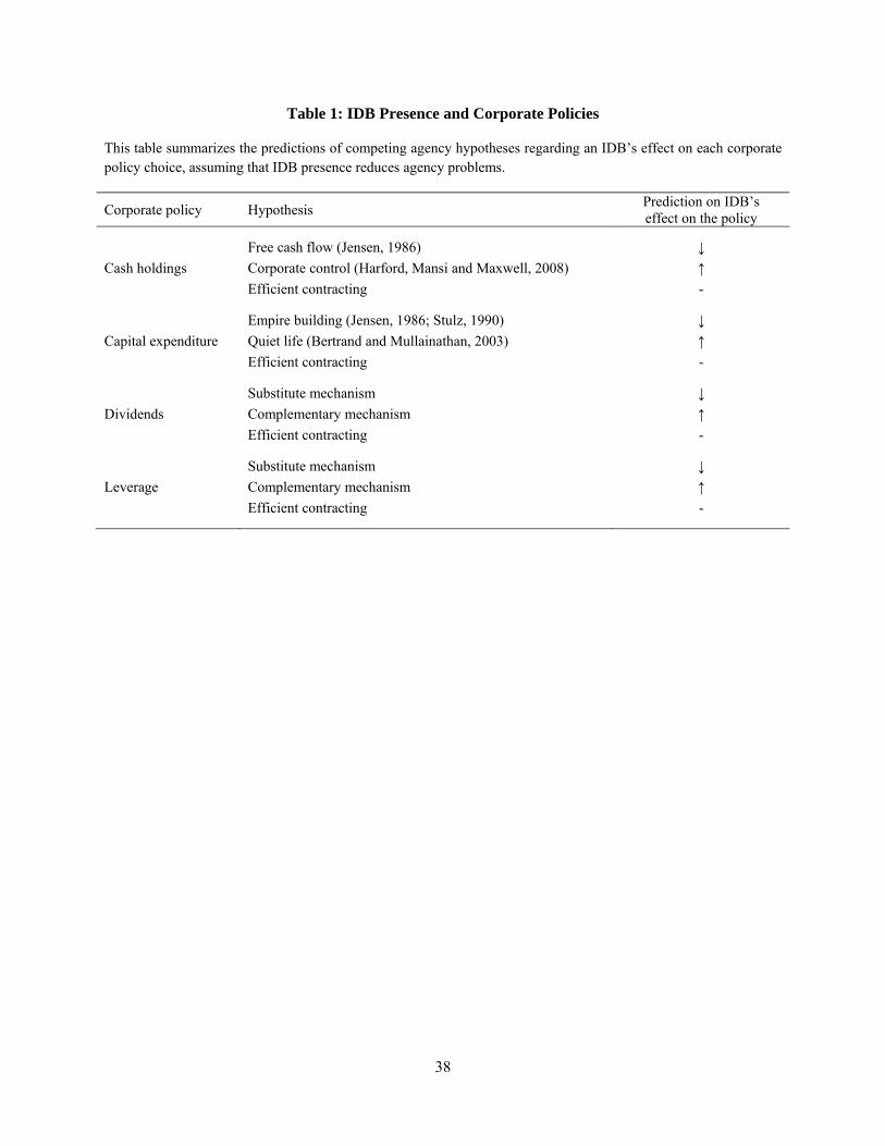
38

Table 1: IDB Presence and Corporate Policies

This table summarizes the predictions of competing agency hypotheses regarding an IDB’s effect on each corporate policy choice, assuming that IDB presence reduces agency problems.

Corporate policy Hypothesis Prediction on IDB’s effect on the policy

Cash holdings

Free cash flow (Jensen, 1986) ↓

Corporate control (Harford, Mansi and Maxwell, 2008) ↑

Efficient contracting -

Capital expenditure

Empire building (Jensen, 1986; Stulz, 1990) ↓

Quiet life (Bertrand and Mullainathan, 2003) ↑

Efficient contracting -

Dividends

Substitute mechanism ↓

Complementary mechanism ↑

Efficient contracting -

Leverage

Substitute mechanism ↓

Complementary mechanism ↑

Efficient contracting -

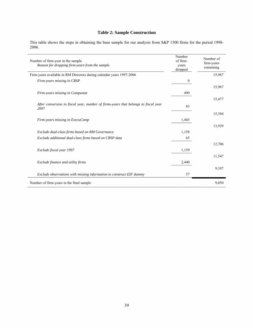
39

Table 2: Sample Construction

This table shows the steps in obtaining the base sample for our analysis from S&P 1500 firms for the period 1998-2006.

Number of firm-year in the sample Reason for dropping firm-years from the sample

Number of firm-

years dropped

Number of firm-years remaining

Firm-years available in RM Directors during calendar years 1997-2006 15,967

Firm-years missing in CRSP 0

15,967

Firm-years missing in Compustat 490

15,477 After conversion to fiscal year, number of firms-years that belongs to fiscal year 2007

83

15,394

Firm-years missing in ExecuComp 1,465

13,929

Exclude dual-class firms based on RM Governance 1,158

Exclude additional dual-class firms based on CRSP data 65

12,706

Exclude fiscal year 1997 1,159

11,547

Exclude finance and utility firms 2,440

9,107

Exclude observations with missing information to construct EIF dummy 57

Number of firm-years in the final sample

9,050

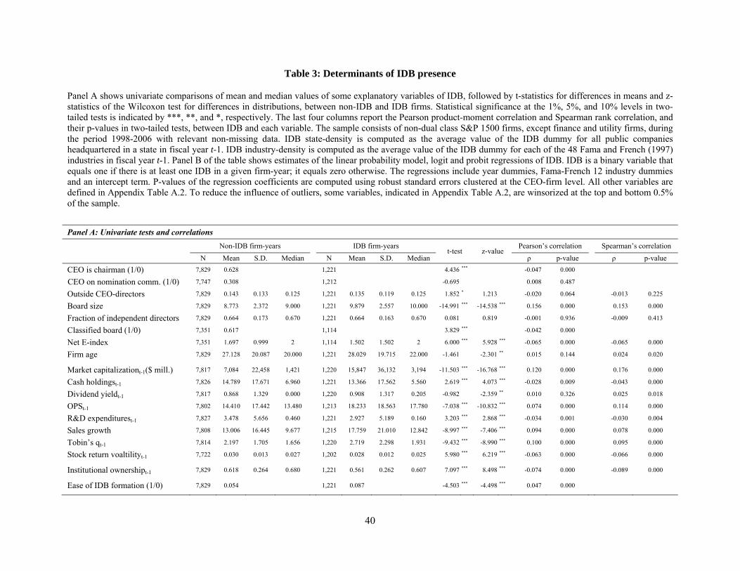
40

Table 3: Determinants of IDB presence

Panel A shows univariate comparisons of mean and median values of some explanatory variables of IDB, followed by t-statistics for differences in means and z-statistics of the Wilcoxon test for differences in distributions, between non-IDB and IDB firms. Statistical significance at the 1%, 5%, and 10% levels in two-tailed tests is indicated by ***, **, and *, respectively. The last four columns report the Pearson product-moment correlation and Spearman rank correlation, and their p-values in two-tailed tests, between IDB and each variable. The sample consists of non-dual class S&P 1500 firms, except finance and utility firms, during the period 1998-2006 with relevant non-missing data. IDB state-density is computed as the average value of the IDB dummy for all public companies headquartered in a state in fiscal year t-1. IDB industry-density is computed as the average value of the IDB dummy for each of the 48 Fama and French (1997) industries in fiscal year t-1. Panel B of the table shows estimates of the linear probability model, logit and probit regressions of IDB. IDB is a binary variable that equals one if there is at least one IDB in a given firm-year; it equals zero otherwise. The regressions include year dummies, Fama-French 12 industry dummies and an intercept term. P-values of the regression coefficients are computed using robust standard errors clustered at the CEO-firm level. All other variables are defined in Appendix Table A.2. To reduce the influence of outliers, some variables, indicated in Appendix Table A.2, are winsorized at the top and bottom 0.5% of the sample.

Panel A: Univariate tests and correlations

Non-IDB firm-years IDB firm-years

t-test z-value Pearson’s correlation Spearman’s correlation

N Mean S.D. Median N Mean S.D. Median ρ p-value ρ p-value

CEO is chairman (1/0) 7,829 0.628 1,221 4.436 *** -0.047 0.000

CEO on nomination comm. (1/0) 7,747 0.308 1,212 -0.695 0.008 0.487

Outside CEO-directors 7,829 0.143 0.133 0.125 1,221 0.135 0.119 0.125 1.852 * 1.213 -0.020 0.064 -0.013 0.225

Board size 7,829 8.773 2.372 9.000 1,221 9.879 2.557 10.000 -14.991 *** -14.538 *** 0.156 0.000 0.153 0.000

Fraction of independent directors 7,829 0.664 0.173 0.670 1,221 0.664 0.163 0.670 0.081 0.819 -0.001 0.936 -0.009 0.413

Classified board (1/0) 7,351 0.617 1,114 3.829 *** -0.042 0.000

Net E-index 7,351 1.697 0.999 2 1,114 1.502 1.502 2 6.000 *** 5.928 *** -0.065 0.000 -0.065 0.000

Firm age 7,829 27.128 20.087 20.000 1,221 28.029 19.715 22.000 -1.461 -2.301 ** 0.015 0.144 0.024 0.020

Market capitalizationt-1($ mill.) 7,817 7,084 22,458 1,421 1,220 15,847 36,132 3,194 -11.503 *** -16.768 *** 0.120 0.000 0.176 0.000

Cash holdingst-1 7,826 14.789 17.671 6.960 1,221 13.366 17.562 5.560 2.619 *** 4.073 *** -0.028 0.009 -0.043 0.000

Dividend yieldt-1 7,817 0.868 1.329 0.000 1,220 0.908 1.317 0.205 -0.982 -2.359 ** 0.010 0.326 0.025 0.018

OPSt-1 7,802 14.410 17.442 13.480 1,213 18.233 18.563 17.780 -7.038 *** -10.832 *** 0.074 0.000 0.114 0.000

R&D expenditurest-1 7,827 3.478 5.656 0.460 1,221 2.927 5.189 0.160 3.203 *** 2.868 *** -0.034 0.001 -0.030 0.004

Sales growth 7,808 13.006 16.445 9.677 1,215 17.759 21.010 12.842 -8.997 *** -7.406 *** 0.094 0.000 0.078 0.000

Tobin’s qt-1 7,814 2.197 1.705 1.656 1,220 2.719 2.298 1.931 -9.432 *** -8.990 *** 0.100 0.000 0.095 0.000

Stock return voaltilityt-1 7,722 0.030 0.013 0.027 1,202 0.028 0.012 0.025 5.980 *** 6.219 *** -0.063 0.000 -0.066 0.000

Institutional ownershipt-1 7,829 0.618 0.264 0.680 1,221 0.561 0.262 0.607 7.097 *** 8.498 *** -0.074 0.000 -0.089 0.000

Ease of IDB formation (1/0) 7,829 0.054 1,221 0.087 -4.503 *** -4.498 *** 0.047 0.000

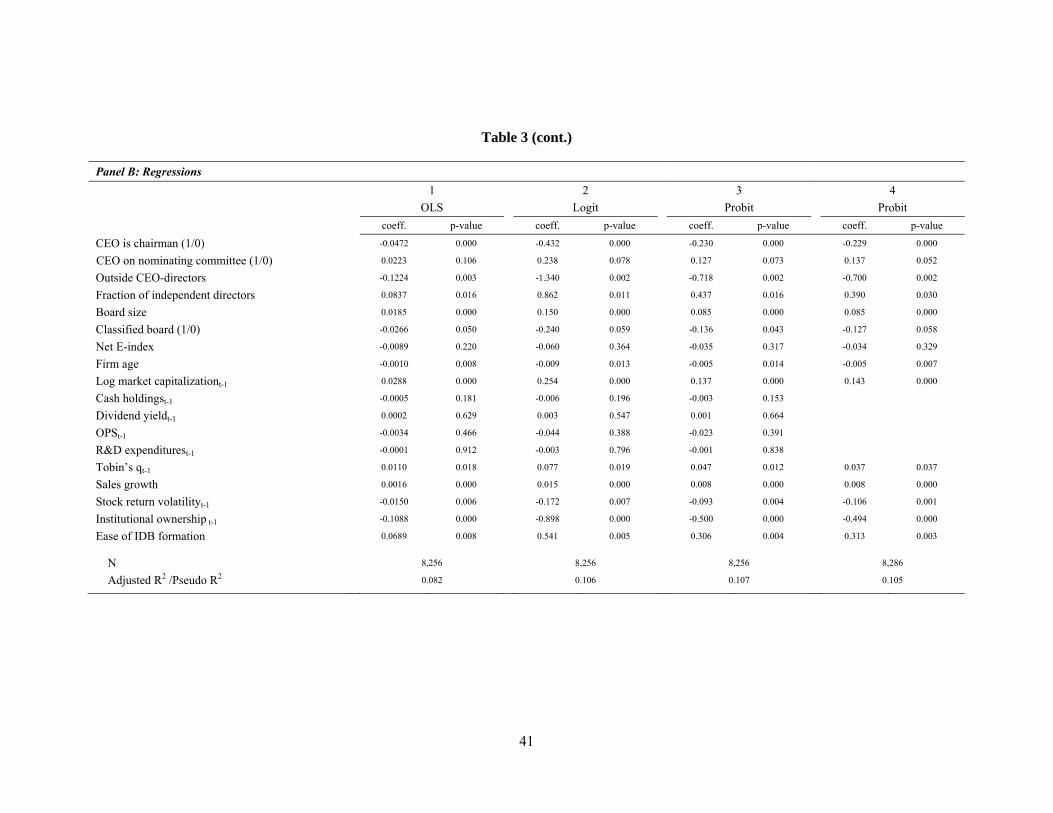
41

Table 3 (cont.)

Panel B: Regressions

1 2 3 4

OLS Logit Probit Probit

coeff. p-value coeff. p-value coeff. p-value coeff. p-value

CEO is chairman (1/0) -0.0472 0.000 -0.432 0.000 -0.230 0.000 -0.229 0.000

CEO on nominating committee (1/0) 0.0223 0.106 0.238 0.078 0.127 0.073 0.137 0.052

Outside CEO-directors -0.1224 0.003 -1.340 0.002 -0.718 0.002 -0.700 0.002

Fraction of independent directors 0.0837 0.016 0.862 0.011 0.437 0.016 0.390 0.030

Board size 0.0185 0.000 0.150 0.000 0.085 0.000 0.085 0.000

Classified board (1/0) -0.0266 0.050 -0.240 0.059 -0.136 0.043 -0.127 0.058

Net E-index -0.0089 0.220 -0.060 0.364 -0.035 0.317 -0.034 0.329

Firm age -0.0010 0.008 -0.009 0.013 -0.005 0.014 -0.005 0.007

Log market capitalizationt-1 0.0288 0.000 0.254 0.000 0.137 0.000 0.143 0.000

Cash holdingst-1 -0.0005 0.181 -0.006 0.196 -0.003 0.153

Dividend yieldt-1 0.0002 0.629 0.003 0.547 0.001 0.664

OPSt-1 -0.0034 0.466 -0.044 0.388 -0.023 0.391

R&D expenditurest-1 -0.0001 0.912 -0.003 0.796 -0.001 0.838

Tobin’s qt-1 0.0110 0.018 0.077 0.019 0.047 0.012 0.037 0.037

Sales growth 0.0016 0.000 0.015 0.000 0.008 0.000 0.008 0.000

Stock return volatilityt-1 -0.0150 0.006 -0.172 0.007 -0.093 0.004 -0.106 0.001

Institutional ownership t-1 -0.1088 0.000 -0.898 0.000 -0.500 0.000 -0.494 0.000

Ease of IDB formation 0.0689 0.008 0.541 0.005 0.306 0.004 0.313 0.003

N 8,256 8,256 8,256 8,286

Adjusted R2 /Pseudo R2 0.082 0.106 0.107 0.105

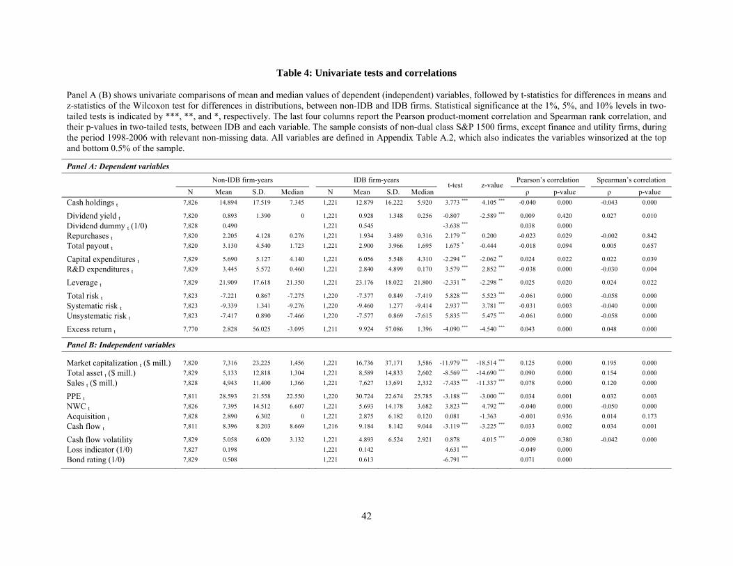
42

Table 4: Univariate tests and correlations

Panel A (B) shows univariate comparisons of mean and median values of dependent (independent) variables, followed by t-statistics for differences in means and z-statistics of the Wilcoxon test for differences in distributions, between non-IDB and IDB firms. Statistical significance at the 1%, 5%, and 10% levels in two-tailed tests is indicated by ***, **, and *, respectively. The last four columns report the Pearson product-moment correlation and Spearman rank correlation, and their p-values in two-tailed tests, between IDB and each variable. The sample consists of non-dual class S&P 1500 firms, except finance and utility firms, during the period 1998-2006 with relevant non-missing data. All variables are defined in Appendix Table A.2, which also indicates the variables winsorized at the top and bottom 0.5% of the sample.

Panel A: Dependent variables

Non-IDB firm-years IDB firm-years

t-test z-value Pearson’s correlation Spearman’s correlation

N Mean S.D. Median N Mean S.D. Median ρ p-value ρ p-value

Cash holdings t 7,826 14.894 17.519 7.345 1,221 12.879 16.222 5.920 3.773 *** 4.105 *** -0.040 0.000 -0.043 0.000

Dividend yield t 7,820 0.893 1.390 0 1,221 0.928 1.348 0.256 -0.807 -2.589 *** 0.009 0.420 0.027 0.010

Dividend dummy t (1/0) 7,828 0.490 1,221 0.545 -3.638 *** 0.038 0.000

Repurchases t 7,820 2.205 4.128 0.276 1,221 1.934 3.489 0.316 2.179 ** 0.200 -0.023 0.029 -0.002 0.842

Total payout t 7,820 3.130 4.540 1.723 1,221 2.900 3.966 1.695 1.675 * -0.444 -0.018 0.094 0.005 0.657

Capital expenditures t 7,829 5.690 5.127 4.140 1,221 6.056 5.548 4.310 -2.294 ** -2.062 ** 0.024 0.022 0.022 0.039

R&D expenditures t 7,829 3.445 5.572 0.460 1,221 2.840 4.899 0.170 3.579 *** 2.852 *** -0.038 0.000 -0.030 0.004

Leverage t 7,829 21.909 17.618 21.350 1,221 23.176 18.022 21.800 -2.331 ** -2.298 ** 0.025 0.020 0.024 0.022

Total risk t 7,823 -7.221 0.867 -7.275 1,220 -7.377 0.849 -7.419 5.828 *** 5.523 *** -0.061 0.000 -0.058 0.000

Systematic risk t 7,823 -9.339 1.341 -9.276 1,220 -9.460 1.277 -9.414 2.937 *** 3.781 *** -0.031 0.003 -0.040 0.000

Unsystematic risk t 7,823 -7.417 0.890 -7.466 1,220 -7.577 0.869 -7.615 5.835 *** 5.475 *** -0.061 0.000 -0.058 0.000

Excess return t 7,770 2.828 56.025 -3.095 1,211 9.924 57.086 1.396 -4.090 *** -4.540 *** 0.043 0.000 0.048 0.000

Panel B: Independent variables

Market capitalization t ($ mill.) 7,820 7,316 23,225 1,456 1,221 16,736 37,171 3,586 -11.979 *** -18.514 *** 0.125 0.000 0.195 0.000

Total asset t ($ mill.) 7,829 5,133 12,818 1,304 1,221 8,589 14,833 2,602 -8.569 *** -14.690 *** 0.090 0.000 0.154 0.000

Sales t ($ mill.) 7,828 4,943 11,400 1,366 1,221 7,627 13,691 2,332 -7.435 *** -11.337 *** 0.078 0.000 0.120 0.000

PPE t 7,811 28.593 21.558 22.550 1,220 30.724 22.674 25.785 -3.188 *** -3.000 *** 0.034 0.001 0.032 0.003

NWC t 7,826 7.395 14.512 6.607 1,221 5.693 14.178 3.682 3.823 *** 4.792 *** -0.040 0.000 -0.050 0.000

Acquisition t 7,828 2.890 6.302 0 1,221 2.875 6.182 0.120 0.081 -1.363 -0.001 0.936 0.014 0.173

Cash flow t 7,811 8.396 8.203 8.669 1,216 9.184 8.142 9.044 -3.119 *** -3.225 *** 0.033 0.002 0.034 0.001

Cash flow volatility 7,829 5.058 6.020 3.132 1,221 4.893 6.524 2.921 0.878 4.015 *** -0.009 0.380 -0.042 0.000

Loss indicator (1/0) 7,827 0.198 1,221 0.142 4.631 *** -0.049 0.000

Bond rating (1/0) 7,829 0.508 1,221 0.613 -6.791 *** 0.071 0.000

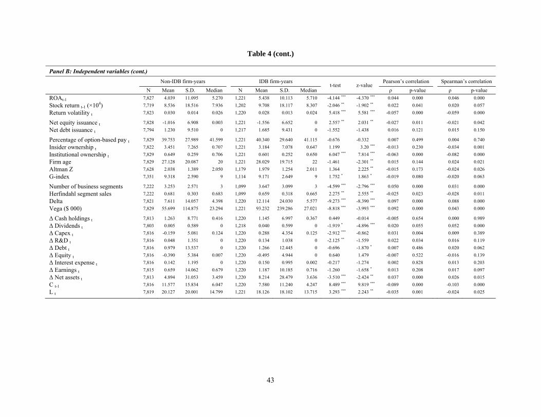
43

Table 4 (cont.)

Panel B: Independent variables (cont.)

Non-IDB firm-years IDB firm-years

t-test z-value Pearson’s correlation Spearman’s correlation

N Mean S.D. Median N Mean S.D. Median ρ p-value ρ p-value

ROAt-1 7,827 4.039 11.095 5.270 1,221 5.438 10.113 5.710 -4.144 *** -4.370 *** 0.044 0.000 0.046 0.000

Stock return t-1 (×104) 7,719 8.536 18.516 7.936 1,202 9.708 18.117 8.307 -2.046 ** -1.902 ** 0.022 0.041 0.020 0.057

Return volatility t 7,823 0.030 0.014 0.026 1,220 0.028 0.013 0.024 5.418 *** 5.581 *** -0.057 0.000 -0.059 0.000

Net equity issuance t 7,828 -1.016 6.908 0.003 1,221 -1.556 6.652 0 2.557 ** 2.031 ** -0.027 0.011 -0.021 0.042

Net debt issuance t 7,794 1.230 9.510 0 1,217 1.685 9.431 0 -1.552 -1.438 0.016 0.121 0.015 0.150

Percentage of option-based pay t 7,829 39.753 27.989 41.599 1,221 40.340 29.640 41.115 -0.676 -0.332 0.007 0.499 0.004 0.740

Insider ownership t 7,822 3.451 7.265 0.707 1,221 3.184 7.078 0.647 1.199 3.20 *** -0.013 0.230 -0.034 0.001

Institutional ownership t 7,829 0.649 0.259 0.706 1,221 0.601 0.252 0.650 6.047 *** 7.814 *** -0.063 0.000 -0.082 0.000

Firm age 7,829 27.128 20.087 20 1,221 28.029 19.715 22 -1.461 -2.301 ** 0.015 0.144 0.024 0.021

Altman Z 7,628 2.038 1.389 2.050 1,179 1.979 1.254 2.011 1.364 2.225 ** -0.015 0.173 -0.024 0.026

G-index 7,351 9.318 2.590 9 1,114 9.171 2.649 9 1.752 * 1.863 * -0.019 0.080 -0.020 0.063

Number of business segments 7,222 3.253 2.571 3 1,099 3.647 3.099 3 -4.599 *** -2.796 *** 0.050 0.000 0.031 0.000

Herfindahl segment sales 7,222 0.681 0.303 0.683 1,099 0.659 0.318 0.665 2.275 ** 2.555 ** -0.025 0.023 -0.028 0.011

Delta 7,821 7.611 14.057 4.398 1,220 12.114 24.030 5.577 -9.273 *** -8.390 *** 0.097 0.000 0.088 0.000

Vega ($ 000) 7,829 55.699 114.875 23.294 1,221 93.232 239.286 27.021 -8.818 *** -3.993 *** 0.092 0.000 0.043 0.000

Δ Cash holdings t 7,813 1.263 8.771 0.416 1,220 1.145 6.997 0.367 0.449 -0.014 -0.005 0.654 0.000 0.989

Δ Dividends t 7,803 0.005 0.589 0 1,218 0.040 0.599 0 -1.919 * -4.896 *** 0.020 0.055 0.052 0.000

Δ Capex t 7,816 -0.159 5.081 0.124 1,220 0.288 4.354 0.125 -2.912 *** -0.862 0.031 0.004 0.009 0.389

Δ R&D t 7,816 0.048 1.351 0 1,220 0.134 1.038 0 -2.125 ** -1.559 0.022 0.034 0.016 0.119

Δ Debt t 7,816 0.979 13.537 0 1,220 1.266 12.445 0 -0.696 -1.870 * 0.007 0.486 0.020 0.062

Δ Equity t 7,816 -0.390 5.384 0.007 1,220 -0.495 4.944 0 0.640 1.479 -0.007 0.522 -0.016 0.139

Δ Interest expense t 7,816 0.142 1.195 0 1,220 0.150 0.995 0.002 -0.217 -1.274 0.002 0.828 0.013 0.203

Δ Earnings t 7,815 0.659 14.062 0.679 1,220 1.187 10.185 0.716 -1.260 -1.658 * 0.013 0.208 0.017 0.097

Δ Net assets t 7,813 4.894 31.053 3.459 1,220 8.214 28.479 3.636 -3.510 *** -2.424 ** 0.037 0.000 0.026 0.015

C t-1 7,816 11.577 15.834 6.047 1,220 7.580 11.240 4.247 8.489 *** 9.819 *** -0.089 0.000 -0.103 0.000

L t 7,819 20.127 20.001 14.799 1,221 18.126 18.102 13.715 3.293 *** 2.243 ** -0.035 0.001 -0.024 0.025

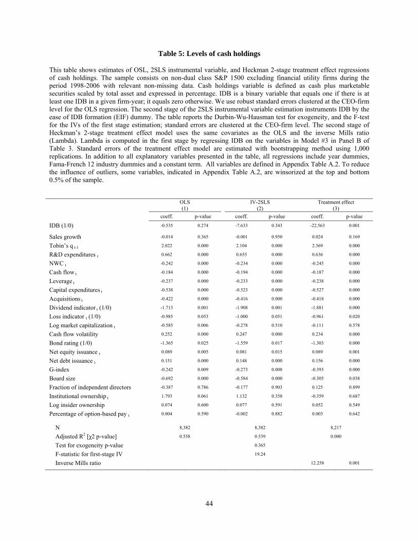
44

Table 5: Levels of cash holdings

This table shows estimates of OSL, 2SLS instrumental variable, and Heckman 2-stage treatment effect regressions of cash holdings. The sample consists on non-dual class S&P 1500 excluding financial utility firms during the period 1998-2006 with relevant non-missing data. Cash holdings variable is defined as cash plus marketable securities scaled by total asset and expressed in percentage. IDB is a binary variable that equals one if there is at least one IDB in a given firm-year; it equals zero otherwise. We use robust standard errors clustered at the CEO-firm level for the OLS regression. The second stage of the 2SLS instrumental variable estimation instruments IDB by the ease of IDB formation (EIF) dummy. The table reports the Durbin-Wu-Hausman test for exogeneity, and the F-test for the IVs of the first stage estimation; standard errors are clustered at the CEO-firm level. The second stage of Heckman’s 2-stage treatment effect model uses the same covariates as the OLS and the inverse Mills ratio (Lambda). Lambda is computed in the first stage by regressing IDB on the variables in Model #3 in Panel B of Table 3. Standard errors of the treatment effect model are estimated with bootstrapping method using 1,000 replications. In addition to all explanatory variables presented in the table, all regressions include year dummies, Fama-French 12 industry dummies and a constant term. All variables are defined in Appendix Table A.2. To reduce the influence of outliers, some variables, indicated in Appendix Table A.2, are winsorized at the top and bottom 0.5% of the sample.

OLS (1)

IV-2SLS (2)

Treatment effect

(3)

coeff. p-value coeff. p-value coeff. p-value

IDB (1/0) -0.535 0.274 -7.633 0.343 -22.563 0.001

Sales growth -0.014 0.365 -0.001 0.950 0.024 0.169

Tobin’s q t-1 2.022 0.000 2.104 0.000 2.369 0.000

R&D expenditures t 0.662 0.000 0.655 0.000 0.636 0.000

NWC t -0.242 0.000 -0.234 0.000 -0.245 0.000

Cash flow t -0.184 0.000 -0.194 0.000 -0.187 0.000

Leverage t -0.237 0.000 -0.233 0.000 -0.238 0.000

Capital expenditures t -0.538 0.000 -0.523 0.000 -0.527 0.000

Acquisitions t -0.422 0.000 -0.416 0.000 -0.418 0.000

Dividend indicator t (1/0) -1.713 0.001 -1.908 0.001 -1.881 0.000

Loss indicator t (1/0) -0.985 0.053 -1.000 0.051 -0.961 0.020

Log market capitalization t -0.585 0.006 -0.278 0.510 -0.111 0.578

Cash flow volatility 0.252 0.000 0.247 0.000 0.234 0.000

Bond rating (1/0) -1.365 0.025 -1.559 0.017 -1.303 0.000

Net equity issuance t 0.089 0.005 0.081 0.015 0.089 0.001

Net debt issuance t 0.151 0.000 0.148 0.000 0.156 0.000

G-index -0.242 0.009 -0.273 0.008 -0.393 0.000

Board size -0.692 0.000 -0.584 0.000 -0.305 0.038

Fraction of independent directors -0.387 0.786 -0.177 0.903 0.125 0.899

Institutional ownership t 1.793 0.061 1.132 0.358 -0.359 0.687

Log insider ownership 0.074 0.600 0.077 0.591 0.052 0.549

Percentage of option-based pay t 0.004 0.590 -0.002 0.882 0.003 0.642

N 8,382 8,382 8,217

Adjusted R2 [χ2 p-value] 0.558 0.539 0.000

Test for exogeneity p-value 0.365

F-statistic for first-stage IV 19.24

Inverse Mills ratio 12.258 0.001

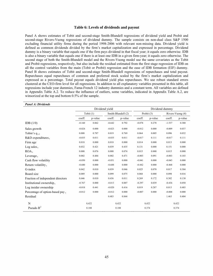
45

Table 6: Levels of dividends and payout

Panel A shows estimates of Tobit and second-stage Smith-Blundell regressions of dividend yield and Probit and second-stage Rivers-Vuong regressions of dividend dummy. The sample consists on non-dual class S&P 1500 excluding financial utility firms during the period 1998-2006 with relevant non-missing data. Dividend yield is defined as common dividends divided by the firm’s market capitalization and expressed in percentage. Dividend dummy is a binary variable that equals one if the firm pays dividend in that fiscal year; it equals zero otherwise. IDB is also a binary variable that equals one if there is at least one IDB in a given firm-year; it equals zero otherwise. The second stage of both the Smith-Blundell model and the Rivers-Vuong model use the same covariates as the Tobit and Probit regressions, respectively, but also include the residual estimated from the first stage regression of IDB on all the control variables from the main (Tobit or Probit) regression and the ease of IDB formation (EIF) dummy. Panel B shows estimates of Tobit and second-stage Smith-Blundell regressions of repurchases and total payout. Repurchases equal repurchases of common and preferred stock scaled by the firm’s market capitalization and expressed as a percentage. Total payout equals dividend yield plus repurchases. We use robust standard errors clustered at the CEO-firm level for all regressions. In addition to all explanatory variables presented in this table, all regressions include year dummies, Fama-French 12 industry dummies and a constant term. All variables are defined in Appendix Table A.2. To reduce the influence of outliers, some variables, indicated in Appendix Table A.2, are winsorized at the top and bottom 0.5% of the sample. Panel A: Dividends

Dividend yield Dividend dummy

Tobit (1) Smith-Blundell (2) Probit (3) Rivers-Vuong (4)

coeff. p-value coeff. p-value coeff. p-value coeff. p-value

IDB (1/0) -0.160 0.062 -0.642 0.792 -0.078 0.278 -1.537 0.380

Sales growth -0.024 0.000 -0.023 0.000 -0.012 0.000 -0.009 0.037

Tobin’s q t-1 0.008 0.787 0.019 0.769 0.064 0.005 0.096 0.032

R&D expenditures t -0.035 0.011 -0.035 0.011 -0.017 0.111 -0.017 0.111

Firm age 0.018 0.000 0.018 0.000 0.014 0.000 0.013 0.000

Log sales t 0.032 0.421 0.039 0.435 0.131 0.000 0.151 0.000

ROA t 0.008 0.076 0.008 0.074 0.015 0.000 0.015 0.000

Leverage t 0.002 0.484 0.002 0.471 -0.003 0.091 -0.003 0.103

Cash flow volatility -0.050 0.000 -0.051 0.000 -0.041 0.000 -0.043 0.000

Return volatility t -0.680 0.000 -0.688 0.000 -0.442 0.000 -0.468 0.000

G-index 0.042 0.010 0.039 0.046 0.025 0.070 0.017 0.304

Board size 0.089 0.000 0.099 0.075 0.068 0.000 0.098 0.016

Fraction of independent directors 0.646 0.010 0.656 0.011 0.269 0.172 0.302 0.130

Institutional ownership t -0.767 0.000 -0.813 0.007 -0.297 0.039 -0.436 0.050

Log insider ownership -0.018 0.441 -0.020 0.416 0.019 0.287 0.013 0.485

Percentage of option-based pay t -0.012 0.000 -0.012 0.000 -0.007 0.000 -0.008 0.000

Residual 0.483 0.844 1.463 0.404

N 8,422 8,422 8,422 8,422

Pseudo R2 0.188 0.188 0.374 0.374

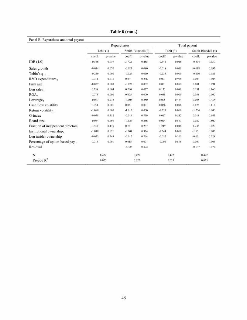
46

Table 6 (cont.)

Panel B: Repurchase and total payout

Repurchases Total payout

Tobit (1) Smith-Blundell (2) Tobit (3) Smith-Blundell (4)

coeff. p-value coeff. p-value coeff. p-value coeff. p-value

IDB (1/0) -0.546 0.019 3.772 0.455 -0.441 0.016 -0.304 0.939

Sales growth -0.014 0.070 -0.023 0.080 -0.018 0.011 -0.018 0.095

Tobin’s q t-1 -0.230 0.000 -0.324 0.010 -0.233 0.000 -0.236 0.021

R&D expenditures t 0.031 0.235 0.031 0.236 0.003 0.908 0.003 0.908

Firm age -0.027 0.000 -0.023 0.002 0.001 0.889 0.001 0.894

Log sales t 0.258 0.004 0.200 0.077 0.133 0.081 0.131 0.166

ROA t 0.075 0.000 0.075 0.000 0.058 0.000 0.058 0.000

Leverage t -0.007 0.272 -0.008 0.250 0.005 0.434 0.005 0.438

Cash flow volatility 0.054 0.001 0.061 0.001 0.026 0.096 0.026 0.112

Return volatility t -1.088 0.000 -1.013 0.000 -1.237 0.000 -1.234 0.000

G-index -0.038 0.312 -0.014 0.759 0.017 0.582 0.018 0.643

Board size -0.034 0.459 -0.123 0.266 0.024 0.533 0.022 0.809

Fraction of independent directors 0.840 0.175 0.741 0.237 1.249 0.018 1.246 0.020

Institutional ownership t -1.018 0.021 -0.604 0.374 -1.544 0.000 -1.531 0.005

Log insider ownership -0.033 0.548 -0.017 0.764 -0.052 0.305 -0.051 0.328

Percentage of option-based pay t 0.013 0.001 0.015 0.001 -0.001 0.876 0.000 0.906

Residual -4.328 0.392 -0.137 0.972

N 8,422 8,422 8,422 8,422

Pseudo R2 0.025 0.025 0.035 0.035

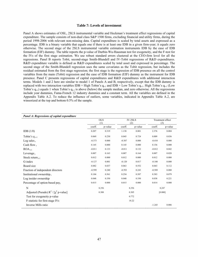
47

Table 7: Levels of investment

Panel A shows estimates of OSL, 2SLS instrumental variable and Heckman’s treatment effect regressions of capital expenditure. The sample consists of non-dual class S&P 1500 firms, excluding financial and utility firms, during the period 1998-2006 with relevant non-missing data. Capital expenditure is scaled by total assets and expressed as a percentage. IDB is a binary variable that equals one if there is at least one IDB in a given firm-year; it equals zero otherwise. The second stage of the 2SLS instrumental variable estimation instruments IDB by the ease of IDB formation (EIF) dummy. The table reports the p-value of Durbin-Wu-Hausman test for exogeneity, and the F-test for the IVs of the first stage estimation. We use robust standard errors clustered at the CEO-firm level for all the regressions. Panel B reports Tobit, second-stage Smith-Blundell and IV-Tobit regressions of R&D expenditures. R&D expenditure variable is defined as R&D expenditures scaled by total asset and expressed in percentage. The second stage of the Smith-Blundell regression uses the same covariates as the Tobit regression, but includes the residual estimated from the first stage regression; the first stage is the regression of IDB presence on all the control variables from the main (Tobit) regression and the ease of IDB formation (EIF) dummy as the instrument for IDB presence. Panel C presents regressions of capital expenditures and R&D expenditures with additional interaction terms. Models 1 and 2 here are similar to model 1 of Panels A and B, respectively, except that the IDB dummy is replaced with two interaction variables IDB × High Tobin’s qt-1 and IDB × Low Tobin’s qt-1. High Tobin’s qt-1 (Low Tobin’s qt-1) equals 1 when Tobin’s qt-1 is above (below) the sample median, and zero otherwise. All the regressions include year dummies, Fama-French 12 industry dummies and a constant term. All the variables are defined in the Appendix Table A.2. To reduce the influence of outliers, some variables, indicated in Appendix Table A.2, are winsorized at the top and bottom 0.5% of the sample.

Panel A: Regressions of capital expenditure

OLS (1)

IV-2SLS (2)

Treatment effect

(3)

coeff. p-value coeff. p-value coeff. p-value

IDB (1/0) 0.207 0.319 1.138 0.801 2.376 0.004

Tobin’s q t-1 0.069 0.230 0.045 0.724 0.009 0.836

Log sales t -0.373 0.000 -0.387 0.000 -0.410 0.000

Cash flow t 0.145 0.000 0.145 0.000 0.156 0.000

ROA t-1 -0.011 0.133 -0.011 0.132 -0.012 0.042

Leverage t 0.007 0.163 0.007 0.164 0.007 0.020

Stock return t-1 0.012 0.000 0.012 0.000 0.012 0.000

G-index -0.127 0.001 -0.120 0.017 -0.108 0.000

Board size 0.082 0.037 0.063 0.552 0.043 0.112

Fraction of independent directors -0.599 0.240 -0.593 0.243 -0.589 0.080

Institutional ownership t 0.184 0.561 0.254 0.587 0.383 0.079

Log insider ownership 0.048 0.350 0.048 0.350 0.038 0.221

Percentage of option-based payt 0.015 0.000 0.015 0.000 0.014 0.000

N 8,356 8,356 8,247

Adjusted (Pseudo) R2 / [χ2 p-value] 0.308 0.305 [0.000]

Test for exogeneity p-value 0.772

F-statistic for first-stage IVs 18.22

Inverse Mills ratio -1.243 0.006

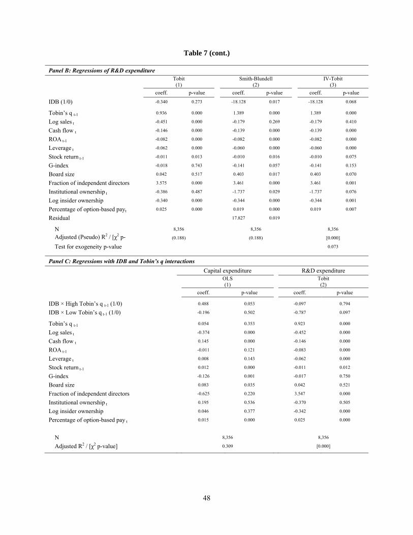
48

Table 7 (cont.)

Panel B: Regressions of R&D expenditure

Tobit (1)

Smith-Blundell (2)

IV-Tobit (3)

coeff. p-value coeff. p-value coeff. p-value

IDB (1/0) -0.340 0.273 -18.128 0.017 -18.128 0.068

Tobin’s q t-1 0.936 0.000 1.389 0.000 1.389 0.000

Log sales t -0.451 0.000 -0.179 0.269 -0.179 0.410

Cash flow t -0.146 0.000 -0.139 0.000 -0.139 0.000

ROA t-1 -0.082 0.000 -0.082 0.000 -0.082 0.000

Leverage t -0.062 0.000 -0.060 0.000 -0.060 0.000

Stock return t-1 -0.011 0.013 -0.010 0.016 -0.010 0.075

G-index -0.018 0.743 -0.141 0.057 -0.141 0.153

Board size 0.042 0.517 0.403 0.017 0.403 0.070

Fraction of independent directors 3.575 0.000 3.461 0.000 3.461 0.001

Institutional ownership t -0.386 0.487 -1.737 0.029 -1.737 0.076

Log insider ownership -0.340 0.000 -0.344 0.000 -0.344 0.001

Percentage of option-based payt 0.025 0.000 0.019 0.000 0.019 0.007

Residual 17.827 0.019

N 8,356 8,356 8,356

Adjusted (Pseudo) R2 / [χ2 p-l ]

(0.188) (0.188) [0.000]

Test for exogeneity p-value 0.073

Panel C: Regressions with IDB and Tobin’s q interactions

Capital expenditure R&D expenditure

OLS (1)

Tobit (2)

coeff. p-value coeff. p-value

IDB × High Tobin’s q t-1 (1/0) 0.488 0.053 -0.097 0.794

IDB × Low Tobin’s q t-1 (1/0) -0.196 0.502 -0.787 0.097

Tobin’s q t-1 0.054 0.353 0.923 0.000

Log sales t -0.374 0.000 -0.452 0.000

Cash flow t 0.145 0.000 -0.146 0.000

ROA t-1 -0.011 0.121 -0.083 0.000

Leverage t 0.008 0.143 -0.062 0.000

Stock return t-1 0.012 0.000 -0.011 0.012

G-index -0.126 0.001 -0.017 0.750

Board size 0.083 0.035 0.042 0.521

Fraction of independent directors -0.625 0.220 3.547 0.000

Institutional ownership t 0.195 0.536 -0.370 0.505

Log insider ownership 0.046 0.377 -0.342 0.000

Percentage of option-based pay t 0.015 0.000 0.025 0.000

N 8,356 8,356

Adjusted R2 / [χ2 p-value] 0.309 [0.000]

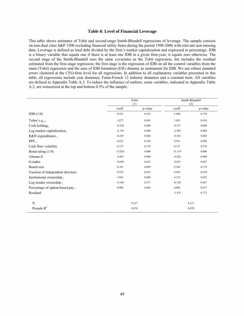
49

Table 8: Level of Financial Leverage

This table shows estimates of Tobit and second-stage Smith-Blundell regressions of leverage. The sample consists on non-dual class S&P 1500 excluding financial utility firms during the period 1998-2006 with relevant non-missing data. Leverage is defined as total debt divided by the firm’s market capitalization and expressed in percentage. IDB is a binary variable that equals one if there is at least one IDB in a given firm-year; it equals zero otherwise. The second stage of the Smith-Blundell uses the same covariates as the Tobit regression, but includes the residual estimated from the first-stage regression; the first stage is the regression of IDB on all the control variables from the main (Tobit) regression and the ease of IDB formation (EIF) dummy as instrument for IDB. We use robust standard errors clustered at the CEO-firm level for all regressions. In addition to all explanatory variables presented in this table, all regressions include year dummies, Fama-French 12 industry dummies and a constant term. All variables are defined in Appendix Table A.2. To reduce the influence of outliers, some variables, indicated in Appendix Table A.2, are winsorized at the top and bottom 0.5% of the sample.

Tobit (1)

Smith-Blundell (2)

coeff. p-value coeff. p-value

IDB (1/0) 0.523 0.543 3.990 0.739

Tobin’s q t-1 1.077 0.001 1.023 0.010

Cash holding t -0.330 0.000 -0.327 0.000

Log market capitalization t -2.750 0.000 -2.892 0.000

R&D expenditures t -0.287 0.002 -0.283 0.002

PPE t 0.032 0.102 0.032 0.098

Cash flow volatility 0.137 0.278 0.137 0.278

Bond rating (1/0) 15.020 0.000 15.119 0.000

Altman-Z -4.867 0.000 -4.826 0.000

G-index -0.058 0.652 -0.031 0.847

Board size 0.391 0.009 0.345 0.119

Fraction of independent directors 0.955 0.625 0.942 0.629

Institutional ownership t 3.862 0.008 4.152 0.022

Log insider ownership t -0.109 0.517 -0.120 0.487

Percentage of option-based pay t 0.000 0.964 0.002 0.877

Residual -3.479 0.772

N 8,217 8,217

Pseudo R2 0.078 0.078

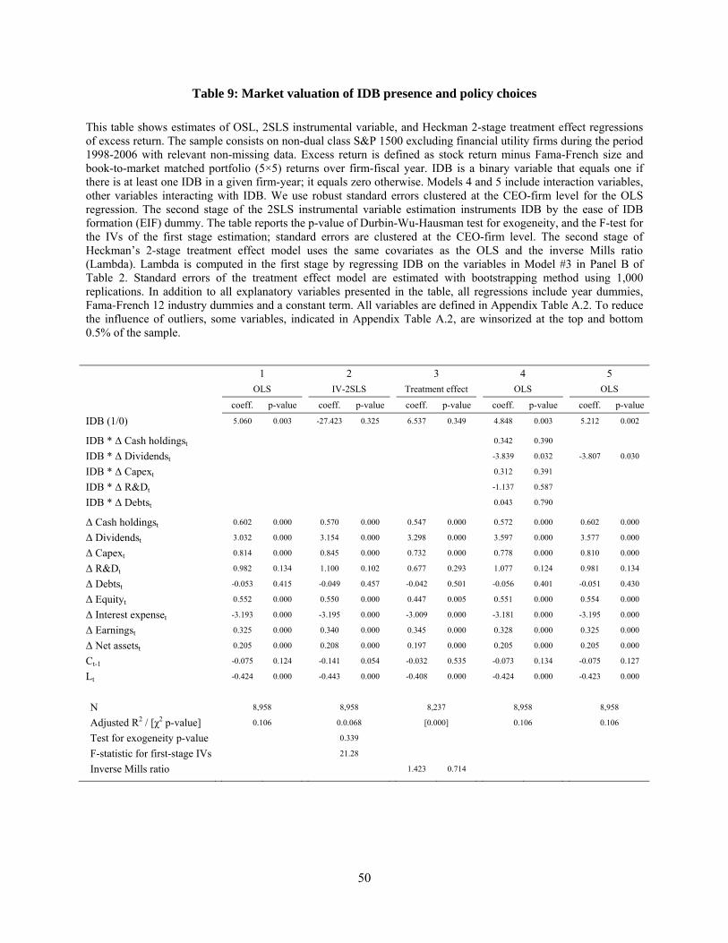
50

Table 9: Market valuation of IDB presence and policy choices

This table shows estimates of OSL, 2SLS instrumental variable, and Heckman 2-stage treatment effect regressions of excess return. The sample consists on non-dual class S&P 1500 excluding financial utility firms during the period 1998-2006 with relevant non-missing data. Excess return is defined as stock return minus Fama-French size and book-to-market matched portfolio (5×5) returns over firm-fiscal year. IDB is a binary variable that equals one if there is at least one IDB in a given firm-year; it equals zero otherwise. Models 4 and 5 include interaction variables, other variables interacting with IDB. We use robust standard errors clustered at the CEO-firm level for the OLS regression. The second stage of the 2SLS instrumental variable estimation instruments IDB by the ease of IDB formation (EIF) dummy. The table reports the p-value of Durbin-Wu-Hausman test for exogeneity, and the F-test for the IVs of the first stage estimation; standard errors are clustered at the CEO-firm level. The second stage of Heckman’s 2-stage treatment effect model uses the same covariates as the OLS and the inverse Mills ratio (Lambda). Lambda is computed in the first stage by regressing IDB on the variables in Model #3 in Panel B of Table 2. Standard errors of the treatment effect model are estimated with bootstrapping method using 1,000 replications. In addition to all explanatory variables presented in the table, all regressions include year dummies, Fama-French 12 industry dummies and a constant term. All variables are defined in Appendix Table A.2. To reduce the influence of outliers, some variables, indicated in Appendix Table A.2, are winsorized at the top and bottom 0.5% of the sample.

1 2 3 4 5

OLS IV-2SLS Treatment effect OLS OLS

coeff. p-value coeff. p-value coeff. p-value coeff. p-value coeff. p-value

IDB (1/0) 5.060 0.003 -27.423 0.325 6.537 0.349 4.848 0.003 5.212 0.002

IDB * Δ Cash holdingst 0.342 0.390

IDB * Δ Dividendst -3.839 0.032 -3.807 0.030

IDB * Δ Capext 0.312 0.391

IDB * Δ R&Dt -1.137 0.587

IDB * Δ Debtst 0.043 0.790

Δ Cash holdingst 0.602 0.000 0.570 0.000 0.547 0.000 0.572 0.000 0.602 0.000

Δ Dividendst 3.032 0.000 3.154 0.000 3.298 0.000 3.597 0.000 3.577 0.000

Δ Capext 0.814 0.000 0.845 0.000 0.732 0.000 0.778 0.000 0.810 0.000

Δ R&Dt 0.982 0.134 1.100 0.102 0.677 0.293 1.077 0.124 0.981 0.134

Δ Debtst -0.053 0.415 -0.049 0.457 -0.042 0.501 -0.056 0.401 -0.051 0.430

Δ Equityt 0.552 0.000 0.550 0.000 0.447 0.005 0.551 0.000 0.554 0.000

Δ Interest expenset -3.193 0.000 -3.195 0.000 -3.009 0.000 -3.181 0.000 -3.195 0.000

Δ Earningst 0.325 0.000 0.340 0.000 0.345 0.000 0.328 0.000 0.325 0.000

Δ Net assetst 0.205 0.000 0.208 0.000 0.197 0.000 0.205 0.000 0.205 0.000

Ct-1 -0.075 0.124 -0.141 0.054 -0.032 0.535 -0.073 0.134 -0.075 0.127

Lt -0.424 0.000 -0.443 0.000 -0.408 0.000 -0.424 0.000 -0.423 0.000

N 8,958 8,958 8,237 8,958 8,958

Adjusted R2 / [χ2 p-value] 0.106 0.0.068 [0.000] 0.106 0.106

Test for exogeneity p-value 0.339

F-statistic for first-stage IVs 21.28

Inverse Mills ratio 1.423 0.714

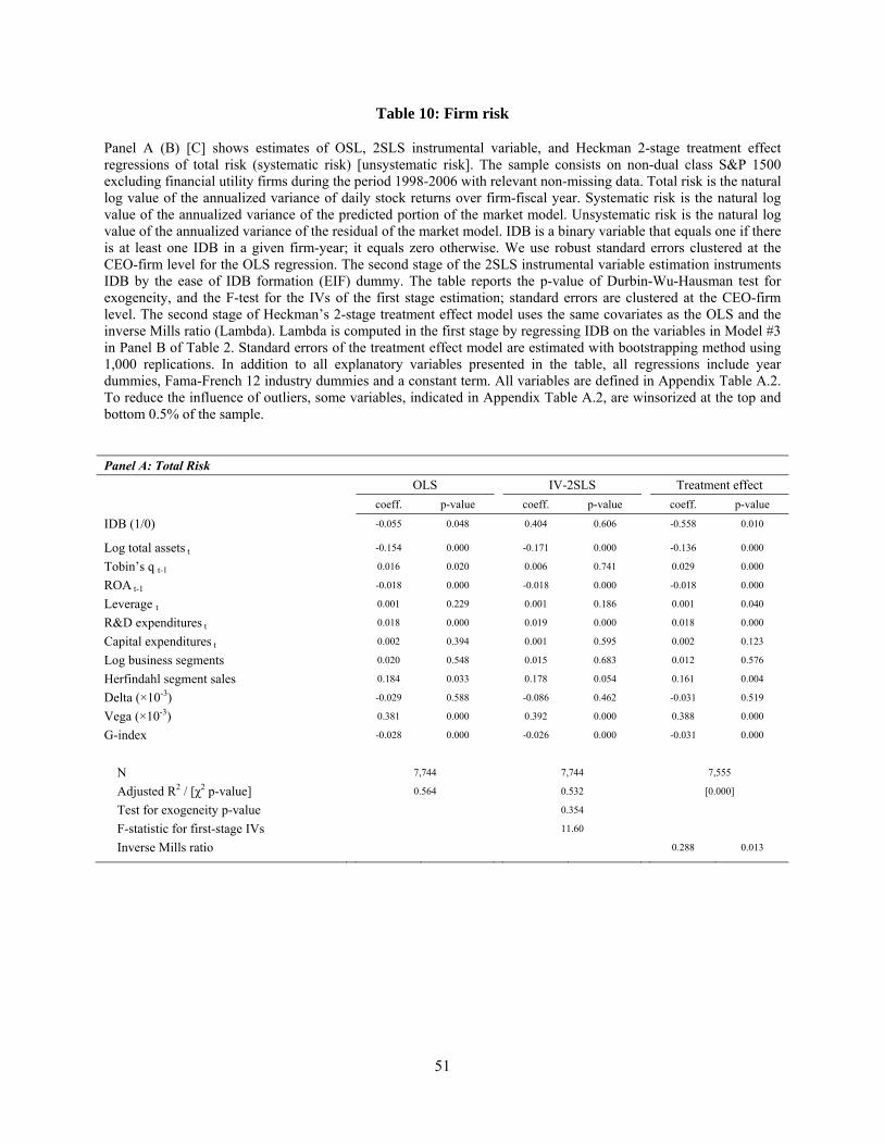
51

Table 10: Firm risk

Panel A (B) [C] shows estimates of OSL, 2SLS instrumental variable, and Heckman 2-stage treatment effect regressions of total risk (systematic risk) [unsystematic risk]. The sample consists on non-dual class S&P 1500 excluding financial utility firms during the period 1998-2006 with relevant non-missing data. Total risk is the natural log value of the annualized variance of daily stock returns over firm-fiscal year. Systematic risk is the natural log value of the annualized variance of the predicted portion of the market model. Unsystematic risk is the natural log value of the annualized variance of the residual of the market model. IDB is a binary variable that equals one if there is at least one IDB in a given firm-year; it equals zero otherwise. We use robust standard errors clustered at the CEO-firm level for the OLS regression. The second stage of the 2SLS instrumental variable estimation instruments IDB by the ease of IDB formation (EIF) dummy. The table reports the p-value of Durbin-Wu-Hausman test for exogeneity, and the F-test for the IVs of the first stage estimation; standard errors are clustered at the CEO-firm level. The second stage of Heckman’s 2-stage treatment effect model uses the same covariates as the OLS and the inverse Mills ratio (Lambda). Lambda is computed in the first stage by regressing IDB on the variables in Model #3 in Panel B of Table 2. Standard errors of the treatment effect model are estimated with bootstrapping method using 1,000 replications. In addition to all explanatory variables presented in the table, all regressions include year dummies, Fama-French 12 industry dummies and a constant term. All variables are defined in Appendix Table A.2. To reduce the influence of outliers, some variables, indicated in Appendix Table A.2, are winsorized at the top and bottom 0.5% of the sample.

Panel A: Total Risk

OLS IV-2SLS Treatment effect

coeff. p-value coeff. p-value coeff. p-value

IDB (1/0) -0.055 0.048 0.404 0.606 -0.558 0.010

Log total assets t -0.154 0.000 -0.171 0.000 -0.136 0.000

Tobin’s q t-1 0.016 0.020 0.006 0.741 0.029 0.000

ROA t-1 -0.018 0.000 -0.018 0.000 -0.018 0.000

Leverage t 0.001 0.229 0.001 0.186 0.001 0.040

R&D expenditures t 0.018 0.000 0.019 0.000 0.018 0.000

Capital expenditures t 0.002 0.394 0.001 0.595 0.002 0.123

Log business segments 0.020 0.548 0.015 0.683 0.012 0.576

Herfindahl segment sales 0.184 0.033 0.178 0.054 0.161 0.004

Delta (×10-3) -0.029 0.588 -0.086 0.462 -0.031 0.519

Vega (×10-3) 0.381 0.000 0.392 0.000 0.388 0.000

G-index -0.028 0.000 -0.026 0.000 -0.031 0.000

N 7,744 7,744 7,555

Adjusted R2 / [χ2 p-value] 0.564 0.532 [0.000]

Test for exogeneity p-value 0.354

F-statistic for first-stage IVs 11.60

Inverse Mills ratio 0.288 0.013

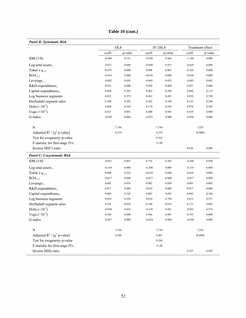
52

Table 10 (cont.)

Panel B: Systematic Risk OLS IV-2SLS Treatment effect

coeff. p-value coeff. p-value coeff. p-value

IDB (1/0) -0.068 0.151 -0.928 0.444 -1.180 0.000

Log total assets t -0.071 0.000 -0.040 0.415 -0.029 0.090

Tobin’s q t-1 0.079 0.000 0.098 0.001 0.108 0.000

ROA t-1 -0.016 0.000 -0.016 0.000 -0.016 0.000

Leverage t -0.002 0.056 -0.003 0.053 -0.003 0.002

R&D expenditures t 0.031 0.000 0.030 0.000 0.031 0.000

Capital expenditures t 0.004 0.265 0.005 0.208 0.004 0.113

Log business segments 0.032 0.579 0.041 0.493 0.010 0.790

Herfindahl segment sales 0.190 0.202 0.202 0.190 0.123 0.249

Delta (×10-3) 0.068 0.539 0.174 0.349 0.078 0.345

Vega (×10-3) 0.421 0.001 0.400 0.003 0.419 0.000

G-index -0.030 0.000 -0.033 0.000 -0.036 0.000

N 7,744 7,744 7,555

Adjusted R2 / [χ2 p-value] 0.319 0.270 [0.000]

Test for exogeneity p-value 0.363

F-statistic for first-stage IVs 11.60

Inverse Mill’s ratio 0.636 0.000

Panel C: Unsystematic Risk

IDB (1/0) -0.051 0.067 0.774 0.365 -0.448 0.020

Log total assets t -0.169 0.000 -0.200 0.000 -0.155 0.000

Tobin’s q t-1 0.008 0.224 -0.010 0.600 0.018 0.008

ROA t-1 -0.017 0.000 -0.017 0.000 -0.017 0.000

Leverage t 0.001 0.076 0.002 0.059 0.001 0.003

R&D expenditures t 0.017 0.000 0.019 0.000 0.017 0.000

Capital expenditures t 0.002 0.342 0.001 0.692 0.002 0.104

Log business segments 0.019 0.556 0.010 0.794 0.013 0.551

Herfindahl segment sales 0.191 0.028 0.180 0.076 0.173 0.003

Delta (×10-3) -0.038 0.455 -0.139 0.281 -0.041 0.372

Vega (×10-3) 0.345 0.000 0.366 0.001 0.355 0.000

G-index -0.027 0.000 -0.024 0.000 -0.030 0.000

N 7,744 7,744 7,555

Adjusted R2 / [χ2 p-value] 0.580 0.481 [0.000]

Test for exogeneity p-value 0.284

F-statistic for first-stage IVs 11.60

Inverse Mills ratio 0.227 0.029

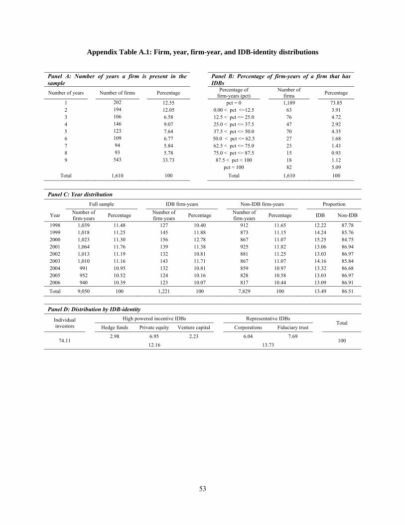
53

Appendix Table A.1: Firm, year, firm-year, and IDB-identity distributions

Panel A: Number of years a firm is present in the sample

Panel B: Percentage of firm-years of a firm that has IDBs

Number of years Number of firms Percentage Percentage of

firm-years (pct)

Number of firms

Percentage

1 202 12.55 pct = 0 1,189 73.85 2 194 12.05 0.00 < pct <=12.5 63 3.91 3 106 6.58 12.5 < pct <= 25.0 76 4.72 4 146 9.07 25.0 < pct <= 37.5 47 2.92 5 123 7.64 37.5 < pct <= 50.0 70 4.35 6 109 6.77 50.0 < pct <= 62.5 27 1.68 7 94 5.84 62.5 < pct <= 75.0 23 1.43 8 93 5.78 75.0 < pct <= 87.5 15 0.93 9 543 33.73 87.5 < pct < 100 18 1.12 pct = 100 82 5.09

Total 1,610 100 Total 1,610 100

Panel C: Year distribution

Full sample IDB firm-years Non-IDB firm-years Proportion

Year Number of firm-years

Percentage Number of

firm-years Percentage

Number of firm-years

Percentage IDB Non-IDB

1998 1,039 11.48 127 10.40 912 11.65 12.22 87.78 1999 1,018 11.25 145 11.88 873 11.15 14.24 85.76 2000 1,023 11.30 156 12.78 867 11.07 15.25 84.75 2001 1,064 11.76 139 11.38 925 11.82 13.06 86.94 2002 1,013 11.19 132 10.81 881 11.25 13.03 86.97 2003 1,010 11.16 143 11.71 867 11.07 14.16 85.84 2004 991 10.95 132 10.81 859 10.97 13.32 86.68 2005 952 10.52 124 10.16 828 10.58 13.03 86.97 2006 940 10.39 123 10.07 817 10.44 13.09 86.91

Total 9,050 100 1,221 100 7,829 100 13.49 86.51

Panel D: Distribution by IDB-identity

Individual investors

High powered incentive IDBs Representative IDBs Total

Hedge funds Private equity Venture capital Corporations Fiduciary trust

74.11 2.98 6.95 2.23 6.04 7.69

100 12.16 13.73

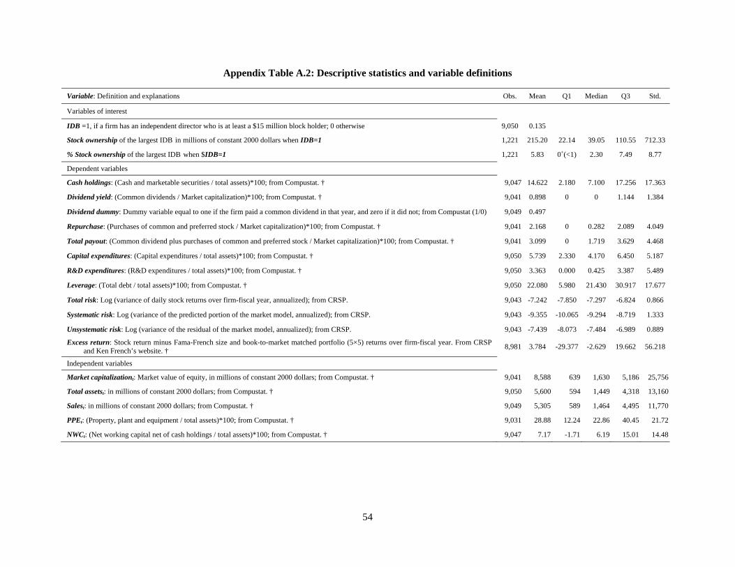
54

Appendix Table A.2: Descriptive statistics and variable definitions

Variable: Definition and explanations Obs. Mean Q1 Median Q3 Std.

Variables of interest

IDB =1, if a firm has an independent director who is at least a $15 million block holder; 0 otherwise 9,050 0.135

Stock ownership of the largest IDB in millions of constant 2000 dollars when IDB=1 1,221 215.20 22.14 39.05 110.55 712.33

% Stock ownership of the largest IDB when $IDB=1 1,221 5.83 0+(<1) 2.30 7.49 8.77

Dependent variables

Cash holdings: (Cash and marketable securities / total assets)*100; from Compustat. † 9,047 14.622 2.180 7.100 17.256 17.363

Dividend yield: (Common dividends / Market capitalization)*100; from Compustat. † 9,041 0.898 0 0 1.144 1.384

Dividend dummy: Dummy variable equal to one if the firm paid a common dividend in that year, and zero if it did not; from Compustat (1/0) 9,049 0.497

Repurchase: (Purchases of common and preferred stock / Market capitalization)*100; from Compustat. † 9,041 2.168 0 0.282 2.089 4.049

Total payout: (Common dividend plus purchases of common and preferred stock / Market capitalization)*100; from Compustat. † 9,041 3.099 0 1.719 3.629 4.468

Capital expenditures: (Capital expenditures / total assets)*100; from Compustat. † 9,050 5.739 2.330 4.170 6.450 5.187

R&D expenditures: (R&D expenditures / total assets)*100; from Compustat. † 9,050 3.363 0.000 0.425 3.387 5.489

Leverage: (Total debt / total assets)*100; from Compustat. † 9,050 22.080 5.980 21.430 30.917 17.677

Total risk: Log (variance of daily stock returns over firm-fiscal year, annualized); from CRSP. 9,043 -7.242 -7.850 -7.297 -6.824 0.866

Systematic risk: Log (variance of the predicted portion of the market model, annualized); from CRSP. 9,043 -9.355 -10.065 -9.294 -8.719 1.333

Unsystematic risk: Log (variance of the residual of the market model, annualized); from CRSP. 9,043 -7.439 -8.073 -7.484 -6.989 0.889

Excess return: Stock return minus Fama-French size and book-to-market matched portfolio (5×5) returns over firm-fiscal year. From CRSP and Ken French’s website. † 8,981 3.784 -29.377 -2.629 19.662 56.218

Independent variables

Market capitalizationt: Market value of equity, in millions of constant 2000 dollars; from Compustat. † 9,041 8,588 639 1,630 5,186 25,756

Total assetst: in millions of constant 2000 dollars; from Compustat. † 9,050 5,600 594 1,449 4,318 13,160

Salest: in millions of constant 2000 dollars; from Compustat. † 9,049 5,305 589 1,464 4,495 11,770

PPEt: (Property, plant and equipment / total assets)*100; from Compustat. † 9,031 28.88 12.24 22.86 40.45 21.72

NWCt: (Net working capital net of cash holdings / total assets)*100; from Compustat. † 9,047 7.17 -1.71 6.19 15.01 14.48

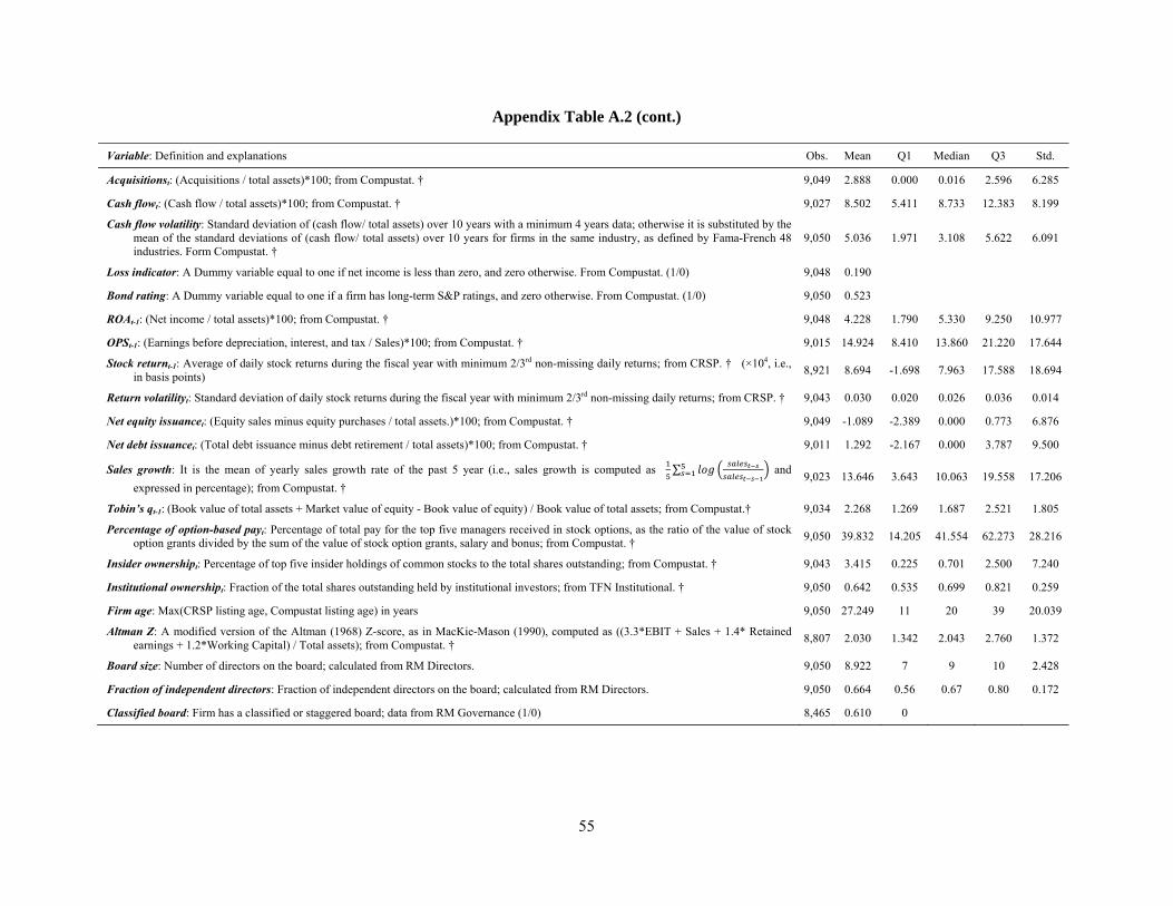
55

Appendix Table A.2 (cont.)

Variable: Definition and explanations Obs. Mean Q1 Median Q3 Std.

Acquisitionst: (Acquisitions / total assets)*100; from Compustat. † 9,049 2.888 0.000 0.016 2.596 6.285

Cash flowt: (Cash flow / total assets)*100; from Compustat. † 9,027 8.502 5.411 8.733 12.383 8.199

Cash flow volatility: Standard deviation of (cash flow/ total assets) over 10 years with a minimum 4 years data; otherwise it is substituted by the mean of the standard deviations of (cash flow/ total assets) over 10 years for firms in the same industry, as defined by Fama-French 48 industries. Form Compustat. †

9,050 5.036 1.971 3.108 5.622 6.091

Loss indicator: A Dummy variable equal to one if net income is less than zero, and zero otherwise. From Compustat. (1/0) 9,048 0.190

Bond rating: A Dummy variable equal to one if a firm has long-term S&P ratings, and zero otherwise. From Compustat. (1/0) 9,050 0.523

ROAt-1: (Net income / total assets)*100; from Compustat. † 9,048 4.228 1.790 5.330 9.250 10.977

OPSt-1: (Earnings before depreciation, interest, and tax / Sales)*100; from Compustat. † 9,015 14.924 8.410 13.860 21.220 17.644

Stock returnt-1: Average of daily stock returns during the fiscal year with minimum 2/3rd non-missing daily returns; from CRSP. † (×104, i.e., in basis points)

8,921 8.694 -1.698 7.963 17.588 18.694

Return volatilityt: Standard deviation of daily stock returns during the fiscal year with minimum 2/3rd non-missing daily returns; from CRSP. † 9,043 0.030 0.020 0.026 0.036 0.014

Net equity issuancet: (Equity sales minus equity purchases / total assets.)*100; from Compustat. † 9,049 -1.089 -2.389 0.000 0.773 6.876

Net debt issuancet: (Total debt issuance minus debt retirement / total assets)*100; from Compustat. † 9,011 1.292 -2.167 0.000 3.787 9.500

Sales growth: It is the mean of yearly sales growth rate of the past 5 year (i.e., sales growth is computed as ∑ and

expressed in percentage); from Compustat. † 9,023 13.646 3.643 10.063 19.558 17.206

Tobin’s qt-1: (Book value of total assets + Market value of equity - Book value of equity) / Book value of total assets; from Compustat.† 9,034 2.268 1.269 1.687 2.521 1.805

Percentage of option-based payt: Percentage of total pay for the top five managers received in stock options, as the ratio of the value of stock option grants divided by the sum of the value of stock option grants, salary and bonus; from Compustat. †

9,050 39.832 14.205 41.554 62.273 28.216

Insider ownershipt: Percentage of top five insider holdings of common stocks to the total shares outstanding; from Compustat. † 9,043 3.415 0.225 0.701 2.500 7.240

Institutional ownershipt: Fraction of the total shares outstanding held by institutional investors; from TFN Institutional. † 9,050 0.642 0.535 0.699 0.821 0.259

Firm age: Max(CRSP listing age, Compustat listing age) in years 9,050 27.249 11 20 39 20.039

Altman Z: A modified version of the Altman (1968) Z-score, as in MacKie-Mason (1990), computed as ((3.3*EBIT + Sales + 1.4* Retained earnings + 1.2*Working Capital) / Total assets); from Compustat. †

8,807 2.030 1.342 2.043 2.760 1.372

Board size: Number of directors on the board; calculated from RM Directors. 9,050 8.922 7 9 10 2.428

Fraction of independent directors: Fraction of independent directors on the board; calculated from RM Directors. 9,050 0.664 0.56 0.67 0.80 0.172

Classified board: Firm has a classified or staggered board; data from RM Governance (1/0) 8,465 0.610 0

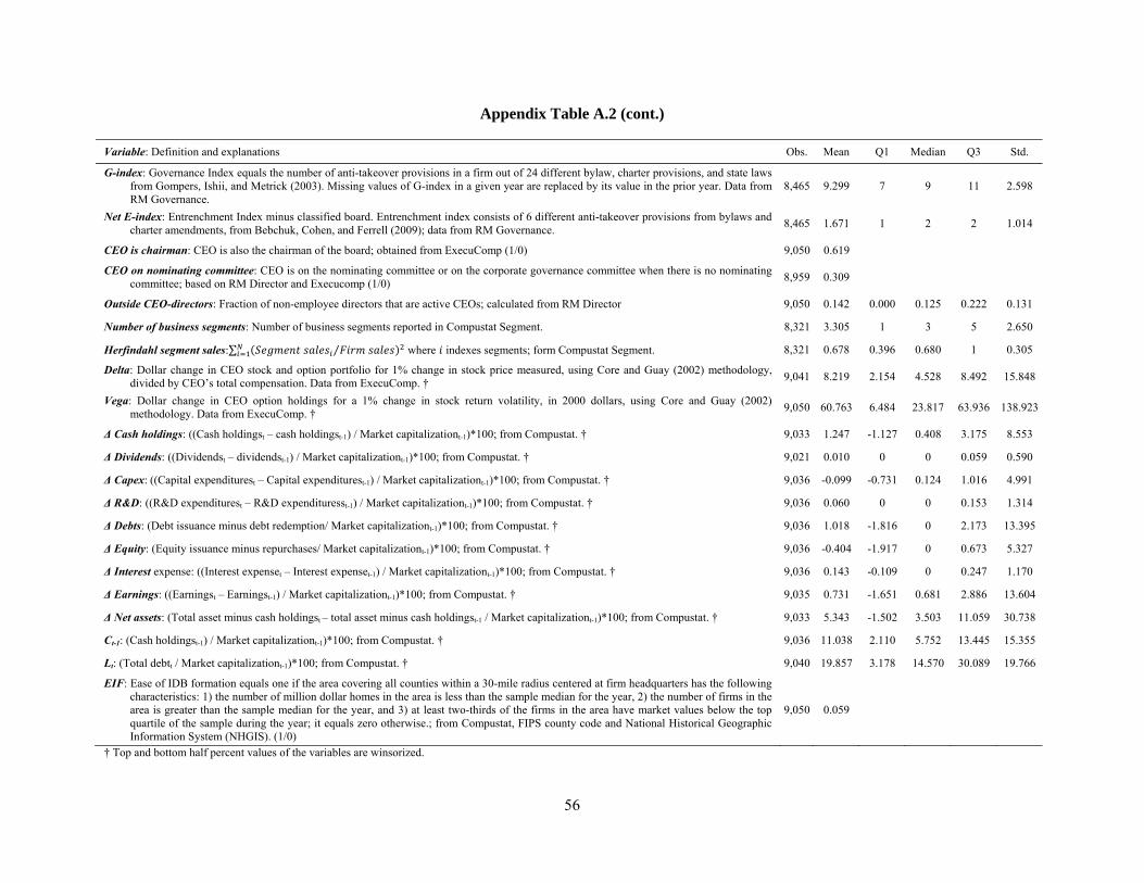
56

Appendix Table A.2 (cont.)

Variable: Definition and explanations Obs. Mean Q1 Median Q3 Std.

G-index: Governance Index equals the number of anti-takeover provisions in a firm out of 24 different bylaw, charter provisions, and state laws from Gompers, Ishii, and Metrick (2003). Missing values of G-index in a given year are replaced by its value in the prior year. Data from RM Governance.

8,465 9.299 7 9 11 2.598

Net E-index: Entrenchment Index minus classified board. Entrenchment index consists of 6 different anti-takeover provisions from bylaws and charter amendments, from Bebchuk, Cohen, and Ferrell (2009); data from RM Governance.

8,465 1.671 1 2 2 1.014

CEO is chairman: CEO is also the chairman of the board; obtained from ExecuComp (1/0) 9,050 0.619

CEO on nominating committee: CEO is on the nominating committee or on the corporate governance committee when there is no nominating committee; based on RM Director and Execucomp (1/0)

8,959 0.309

Outside CEO-directors: Fraction of non-employee directors that are active CEOs; calculated from RM Director 9,050 0.142 0.000 0.125 0.222 0.131

Number of business segments: Number of business segments reported in Compustat Segment. 8,321 3.305 1 3 5 2.650

Herfindahl segment sales:∑ ⁄ where indexes segments; form Compustat Segment. 8,321 0.678 0.396 0.680 1 0.305

Delta: Dollar change in CEO stock and option portfolio for 1% change in stock price measured, using Core and Guay (2002) methodology, divided by CEO’s total compensation. Data from ExecuComp. †

9,041 8.219 2.154 4.528 8.492 15.848

Vega: Dollar change in CEO option holdings for a 1% change in stock return volatility, in 2000 dollars, using Core and Guay (2002) methodology. Data from ExecuComp. †

9,050 60.763 6.484 23.817 63.936 138.923

Δ Cash holdings: ((Cash holdingst – cash holdingst-1) / Market capitalizationt-1)*100; from Compustat. † 9,033 1.247 -1.127 0.408 3.175 8.553

Δ Dividends: ((Dividendst – dividendst-1) / Market capitalizationt-1)*100; from Compustat. † 9,021 0.010 0 0 0.059 0.590

Δ Capex: ((Capital expenditurest – Capital expenditurest-1) / Market capitalizationt-1)*100; from Compustat. † 9,036 -0.099 -0.731 0.124 1.016 4.991

Δ R&D: ((R&D expenditurest – R&D expendituresst-1) / Market capitalizationt-1)*100; from Compustat. † 9,036 0.060 0 0 0.153 1.314

Δ Debts: (Debt issuance minus debt redemption/ Market capitalizationt-1)*100; from Compustat. † 9,036 1.018 -1.816 0 2.173 13.395

Δ Equity: (Equity issuance minus repurchases/ Market capitalizationt-1)*100; from Compustat. † 9,036 -0.404 -1.917 0 0.673 5.327

Δ Interest expense: ((Interest expenset – Interest expenset-1) / Market capitalizationt-1)*100; from Compustat. † 9,036 0.143 -0.109 0 0.247 1.170

Δ Earnings: ((Earningst – Earningst-1) / Market capitalizationt-1)*100; from Compustat. † 9,035 0.731 -1.651 0.681 2.886 13.604

Δ Net assets: (Total asset minus cash holdingst – total asset minus cash holdingst-1 / Market capitalizationt-1)*100; from Compustat. † 9,033 5.343 -1.502 3.503 11.059 30.738

Ct-1: (Cash holdingst-1) / Market capitalizationt-1)*100; from Compustat. † 9,036 11.038 2.110 5.752 13.445 15.355

Lt: (Total debtt / Market capitalizationt-1)*100; from Compustat. † 9,040 19.857 3.178 14.570 30.089 19.766

EIF: Ease of IDB formation equals one if the area covering all counties within a 30-mile radius centered at firm headquarters has the following characteristics: 1) the number of million dollar homes in the area is less than the sample median for the year, 2) the number of firms in the area is greater than the sample median for the year, and 3) at least two-thirds of the firms in the area have market values below the top quartile of the sample during the year; it equals zero otherwise.; from Compustat, FIPS county code and National Historical Geographic Information System (NHGIS). (1/0)

9,050 0.059

† Top and bottom half percent values of the variables are winsorized.