CORPORATION INCOME TAX ESTIMATING: USING …leg.mt.gov/.../fiscal/other-interim-reports/RTIC-Corp-Tax.pdfCORPORATION INCOME TAX ... and the magnified volatility of the corresponding

CORPORATION INCOME TAX ESTIMATING:

USING CONFIDENCE INTERVALS

TO MINIMIZE FORECASTING ERROR

A Report Prepared for the

Revenue & Transportation Interim Committee

By

Sam Schaefer

July 17, 2014

Legislative Fiscal Division 2 of 15 July 17, 2014

INTRODUCTION A common dilemma associated with forecasting state revenues is placing some measure of certainty on future estimates. This is especially true when dealing with revenue sources that are consistently volatile and follow no clear pattern from one year to another. Corporation income tax revenues in Montana have been extremely difficult to predict in recent years. The research detailed in this report seeks to minimize the error associated with corporation tax forecasts compared to actual collections as well as provide a measure of confidence associated with the magnitude of this error. The report is divided into five sections:

Section 1: Background

Section 2: Current research

Section 3: Confidence intervals

Section 4: Potential modeling alternatives

Section 5: Summary

Executive Summary Although data were not available to create a reliable prediction interval for future forecasts, methods to create confidence intervals for the mean error were employed and resulting intervals were obtained. Using these methods, various models were created and their resulting confidence intervals examined. This allowed for easy comparison between different models’ predictive performance and measures of certainty. Therefore, for models that predicted revenue with similar accuracy using different variables, those variables were chosen that provided the narrowest error bands. Due to the uncertainty associated with forecast variables’ distributions, it is extremely difficult to place a reliable level of certainty on a future point estimate. However, the methods discussed in this report allow for minimizing volatility associated with future revenues using the distributions of past collections’ errors alongside their prospective economic variables’ forecasts.

SECTION 1: BACKGROUND

Forecast Methodology Montana corporation tax liability is forecast using a variety of IHS economic variables as predictors. These variables are used to forecast calendar year tax liability by sector. Major sectors include manufacturing, financial services, retail trade, and mining. Once estimates have been produced individually for all relevant sectors, they are combined to form a total estimate of calendar year liability. The calendar year estimate is converted to a fiscal year estimate, with adjustments made to account for refunds, audits, penalties, and credit reimbursements.

Reasons for Volatility The volatility of this source can be attributed to many factors: sensitivity of corporation income to business cycles, industry composition in the state, reliance on a limited number of large taxpayers, and federal and state tax policy. For example, Montana law allows corporations to carry back current year losses for three years, and carry forward losses for up to seven years. The carry back provision may result in magnifying a downturn to the extent that corporations file amended prior year tax returns that include current year losses, and are thereby owed a refund of taxes paid in those previous years. Figure 1 on the following page shows the volatility of total corporation tax since FY 1995.


Figure 1

Sources of Forecasting Error The overall volatility of corporation income and the magnified volatility of the corresponding tax liability make accurate forecasting a challenge. Forecasting error is produced through three main channels: timing of data, in the inherent error of IHS forecast economic variables, and in the model itself as past collections are not predicted perfectly by selected IHS variables. Combined with the uncertainty involved in predicting audit and refund amounts, these sources of error can lead to revenues that may significantly deviate from forecast values and prior year collections. While corporations’ tax behavior—highlighted in the previous section—introduces forecasting error that is difficult to predict, this report explores methods to minimize the errors associated with the IHS forecasts of underlying economic variables. In addition, this report seeks to provide a means to compare standard errors associated with different models’ forecasts. While corporation income tax will likely continue to be a volatile source, the methods utilized in this paper should direct modeling choices that will minimize the error introduced by IHS forecast error.

SECTION 2: CURRENT RESEARCH

Forecast Intervals As noted above, there is an error term associated with the econometric variables used in the modeling process. This can make it extremely difficult to produce a reliable interval associated with an estimate for future corporation tax revenue. In statistics, theoretical prediction intervals have been developed and used extensively in linear regression modeling. Unlike confidence intervals, prediction intervals provide some interval and level of certainty where a future observation may lie. In contrast, confidence intervals pertain to some parameter such as a population mean. In order for the traditional prediction intervals associated with linear regression techniques to be applicable however, the distribution of the explanatory variables must be known or it must be a fixed point. This is not the case here, as the IHS econometric estimates may vary considerably from what is actually observed. In addition to the explanatory variables associated with the IHS estimates not being fixed, the distribution of them is also unknown. If the distribution were known, prediction intervals could be created with much more certainty pertaining to the individual corporate sectors, and eventually combined to form an interval for the corresponding final revenue estimate. Instead of studying each


econometric variable and attempting to discover its distribution, it may be easier to model the error term associated with each sector’s model. For the rest of this paper, the error term will be defined as:

( )

The error term is recorded as a proportion of the observed value to account for inflation as past years’ errors will likely be smaller on a nominal basis. Once this error term has been determined for each sector, an aggregate error term can be applied to the model’s final estimate.

Assumptions Two assumptions were made in order to perform this analysis: first, the various sector-by-sector mean errors are independent of one another; and second, the IHS estimating processes have remained relatively the same for the years when the error terms were examined. This allows the sector-specific errors to be modeled under the assumption that they came from the same distribution.

Derivation of Error Terms The error term was studied on a sector-by-sector basis. Ideally, each sector could be predicted perfectly by a single variable whose future value is known with certainty. Unfortunately this is not the case, but the modeling process used attempted to come as close to this ideal scenario as possible. Therefore, each sector was modeled using a variable that was not only an accurate predictor but also yielded the smallest discrepancy when comparing the IHS estimates to the observed values. Prior to examining correlations between various sectors’ revenues and economic variables, archived IHS estimates were studied to gain insight into the accuracy of IHS forecasts. Using this information, variables were chosen to model the various sectors based on a combination of their predictive power and the accuracy of their forecasts. To illustrate the entire process, the steps employed to model the manufacturing sector will be described in detail. Figure 2 shows manufacturing corporation tax liability from CY 1995 to CY 2011.

Figure 2

Of the economic variables provided by IHS, West Texas Intermediate (WTI) oil prices had a correlation of 0.94 with this sector’s revenue. A correlation coefficient of 1 implies a perfect linear

Equation 1


relationship between two variables. The standardized values of manufacturing corporation tax liability and WTI are shown in Figure 3.

Figure 3

To begin studying the error associated with this sector, a simple linear regression model was fit using years 1995 through 2002. This allows years 2004 through 2011 to be used as training data to test the model’s efficiency as opposed to testing the model with data used to create the model. Next, the IHS forecast WTI prices were obtained from archived files—specifically, the archived November forecasts, which have typically been used to produce the November RTIC estimate—to retrospectively predict 2004, 2005, and 2006 liabilities. The model’s predictions for years 2004, 2005, and 2006 were then compared to actual collections and recorded. This process was repeated through 2011, while simultaneously updating the original model with one more year of actual collections each year moving forward. For example, archived November 2003 estimates were used to predict years 2004, 2005, and 2006. Moving forward, the 2004 actual manufacturing tax revenue and WTI price were then used in the modeling process to create a model to predict years 2005, 2006, and 2007. Table 1 shows the error term—defined in Equation 1—by year of estimate for calendar years 2004 through 2011. Figure 4 shows the model estimates and actual tax collections, with the difference between actual and estimated values corresponding to the error term in Table 1.

Table 1

CY First Year Second Year Third Year

2004 50% 50% N/A

2005 45% 67% 70%

2006 29% 57% 73%

2007 33% 48% 70%

2008 -5% 13% 49%

2009 1% -44% -40%

2010 -6% 3% -17%

2011 4% 11% 3%

Error Term by Year of Estimate


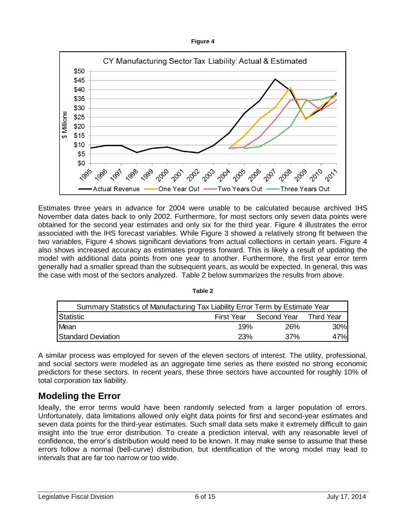
Figure 4

Estimates three years in advance for 2004 were unable to be calculated because archived IHS November data dates back to only 2002. Furthermore, for most sectors only seven data points were obtained for the second year estimates and only six for the third year. Figure 4 illustrates the error associated with the IHS forecast variables. While Figure 3 showed a relatively strong fit between the two variables, Figure 4 shows significant deviations from actual collections in certain years. Figure 4 also shows increased accuracy as estimates progress forward. This is likely a result of updating the model with additional data points from one year to another. Furthermore, the first year error term generally had a smaller spread than the subsequent years, as would be expected. In general, this was the case with most of the sectors analyzed. Table 2 below summarizes the results from above.

Table 2

A similar process was employed for seven of the eleven sectors of interest. The utility, professional, and social sectors were modeled as an aggregate time series as there existed no strong economic predictors for these sectors. In recent years, these three sectors have accounted for roughly 10% of total corporation tax liability.

Modeling the Error Ideally, the error terms would have been randomly selected from a larger population of errors. Unfortunately, data limitations allowed only eight data points for first and second-year estimates and seven data points for the third-year estimates. Such small data sets make it extremely difficult to gain insight into the true error distribution. To create a prediction interval, with any reasonable level of confidence, the error’s distribution would need to be known. It may make sense to assume that these errors follow a normal (bell-curve) distribution, but identification of the wrong model may lead to intervals that are far too narrow or too wide.

Statistic First Year Second Year Third Year

Mean 19% 26% 30%

Standard Deviation 23% 37% 47%

Summary Statistics of Manufacturing Tax Liability Error Term by Estimate Year


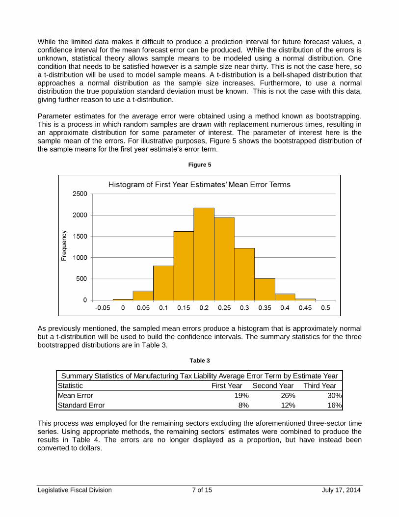
While the limited data makes it difficult to produce a prediction interval for future forecast values, a confidence interval for the mean forecast error can be produced. While the distribution of the errors is unknown, statistical theory allows sample means to be modeled using a normal distribution. One condition that needs to be satisfied however is a sample size near thirty. This is not the case here, so a t-distribution will be used to model sample means. A t-distribution is a bell-shaped distribution that approaches a normal distribution as the sample size increases. Furthermore, to use a normal distribution the true population standard deviation must be known. This is not the case with this data, giving further reason to use a t-distribution. Parameter estimates for the average error were obtained using a method known as bootstrapping. This is a process in which random samples are drawn with replacement numerous times, resulting in an approximate distribution for some parameter of interest. The parameter of interest here is the sample mean of the errors. For illustrative purposes, Figure 5 shows the bootstrapped distribution of the sample means for the first year estimate’s error term.

Figure 5

As previously mentioned, the sampled mean errors produce a histogram that is approximately normal but a t-distribution will be used to build the confidence intervals. The summary statistics for the three bootstrapped distributions are in Table 3.

Table 3

This process was employed for the remaining sectors excluding the aforementioned three-sector time series. Using appropriate methods, the remaining sectors’ estimates were combined to produce the results in Table 4. The errors are no longer displayed as a proportion, but have instead been converted to dollars.


Mean Error 19% 26% 30%

Standard Error 8% 12% 16%

Summary Statistics of Manufacturing Tax Liability Average Error Term by Estimate Year


Table 4

As expected, the standard error increases as the estimates are made farther into the future. While the mean error decreases with time, this does not imply that the forecasts are becoming more accurate. Instead, first year error terms are almost entirely positive while the second and third year error terms have both positive and negative deviations, thereby bringing the mean error closer to 0. This is depicted by the larger standard errors associated with the second and third year estimates. When the errors are examined on an absolute scale, they increase as the estimates progress into the future.

SECTION 3: CONFIDENCE INTERVALS For calendar years 2015, 2016 and 2017, the sector-based model produces corporation tax liability estimates of $135.0, $139.2 and $145.3 million respectively. Note that these estimates have not yet been converted to fiscal year amounts. Using characteristics of the t-distribution allows confidence intervals for the average error term to be produced for these estimates. The corresponding calculations for the 95% confidence intervals are shown below:

Table 5

The constants 2.365, 2.450, and 2.571 are critical values from the t-distribution, and are determined by the chosen confidence level and corresponding sample sizes. Because most sectors had only seven and six data points for the second and third year estimates respectively, the value of the constants increased. Table 6 shows the upper and lower bounds of the calendar estimates by adding the mean error and corresponding intervals calculated in Table 5. It also gives the 95% confidence interval range as a percent of the estimate.

Table 6


Mean Error $15.1 $13.3 $10.2

Standard Error 6.7 9.3 12.2

Manufacturing Tax Liability Average Error Term by Estimate Year ($ Millions)

Mean Error t-Statistic Standard Error Interval

First Year Error Bound = $15.1 ± 2.365 × $6.7 = [-$0.8,$30.9]

Second Year Error Bound = $13.3 ± 2.450 × $9.3 = [-$9.6,$36.1]

Third Year Error Bound = $10.2 ± 2.571 × $12.2 = [-$21.2,$41.6]

CY Corporation Income Tax Liability

95% Confidence Intervals for the Aggregate Average Error Term of the Sector-Based Estimate

($ Millions)

Estimate Year Estimate Lower Bound Upper Bound % Range

2015 $135.0 $134.2 $165.9 24%

2016 $139.2 $129.6 $175.3 33%

2017 $145.3 $124.1 $186.9 43%

CY Corporation Income Tax Liability

95% Confidence Intervals for the Sector-Based Estimate

($ Millions)


Figure 6 below shows the current model forecast and corresponding confidence intervals applied to the forecast.

Figure 6

Figure 6 illustrates that the range of the estimate increases as forecasts are made farther into the future, and shows that, on average, the estimate produced by the sector-specific model tends to fall on the conservative side of the upper and lower bounds. The calendar year estimates for the error bounds were converted to fiscal year estimates by converting the lower and upper calendar year estimate bounds to fiscal year estimates. The fiscal year spread between the lower and upper estimates decreases from the calendar year spread shown in Table 6 primarily due to the six-month shift closer to present time that occurs in the conversion. The results are shown in Table 7 and Figure 7.

Table 7


2015 $149.7 $149.0 $177.7 19%

2016 $147.9 $147.2 $176.2 20%

2017 $151.7 $142.9 $184.8 28%

FY Corporation Income Tax Liability

Using 95% Confidence Intervals for the Sector-Based Estimate

($ Millions)


Figure 7

SECTION 4: ANALYSIS ASSUMING PARTIAL DEPENDENCE As stated earlier, the assumption was made that the sector-by-sector errors are independent of one another. This assumption is predominantly used in the combination of the various sectors’ error terms. If the sectors are instead dependent, it is possible that the confidence intervals may widen, as some sectors’ errors may have a tendency to increase as similar sectors’ errors increase. This would add another level of variability to the combined error term. If some error terms are in fact not independent, the most likely corresponding sectors are those that use some variant of oil prices as a predictor. The mining, manufacturing, agriculture, and construction sectors’ revenue are all predicted by oil prices. These four sectors make up nearly half of the total corporate tax revenue. If IHS forecasts for oil prices are too high, it is likely that all of these sectors’ error terms may also be large. This tendency for variables to vary with one another is known as covariance. The analysis from above was performed again, this time accounting for the possibility of partial dependence and a covariance term that is not simply random fluctuations. Table 8 below shows the new results for the 95% confidence interval for the sector-based estimate’s error term.

Table 8

The resulting range increased 10% and 9% respectively for 2015 and 2016 and 12% for 2017. Figure 8 below shows the original 95% confidence interval with additional upper and lower bounds added if the assumption of independence does not hold. These are illustrated by the dashed lines in Figure 8.


2015 $149.7 $142.0 $184.7 29%

2016 $147.9 $140.0 $183.3 29%

2017 $151.7 $133.9 $193.9 40%


95% Confidence Intervals for the Sector-Based Estimate Assuming Partial Dependence

($ Millions)


Figure 8

SECTION 5: POTENTIAL MODELING ALTERNATIVES Single variable modeling would be much simpler and less time-intensive. However, few IHS variables by themselves predict final corporation tax revenue well. Several models using single variables were examined and compared to the sector-based model.

Single Variable Model Using WTI Using the method outlined in Section 3, the 95% confidence intervals are calculated for a single-variable model based in WTI price. For fiscal years 2015, 2016 and 2017, this model produces corporation tax liability estimates of $151.8, $148.8 and $157.9 million respectively. Table 9 shows the upper and lower bounds of the fiscal estimates by adding the calculated mean error and corresponding intervals. It also gives the 95% confidence interval range as a percent of the estimate.

Table 9

Figure 9 shows the forecast produced by the single-variable model based on WTI, as well as the corresponding confidence intervals applied to the forecast. Similarly to the sector-based model, the range of the estimate increases as forecasts are made farther into the future. Note that the spread between the upper and lower bounds based on this model is higher that the range of the sector-based model.


2015 $151.8 $76.6 $177.8 67%

2016 $148.8 $73.3 $176.2 69%

2017 $157.9 $75.0 $189.6 73%


95% Confidence Intervals for the Single Variable (WTI) Estimate

($ Millions)


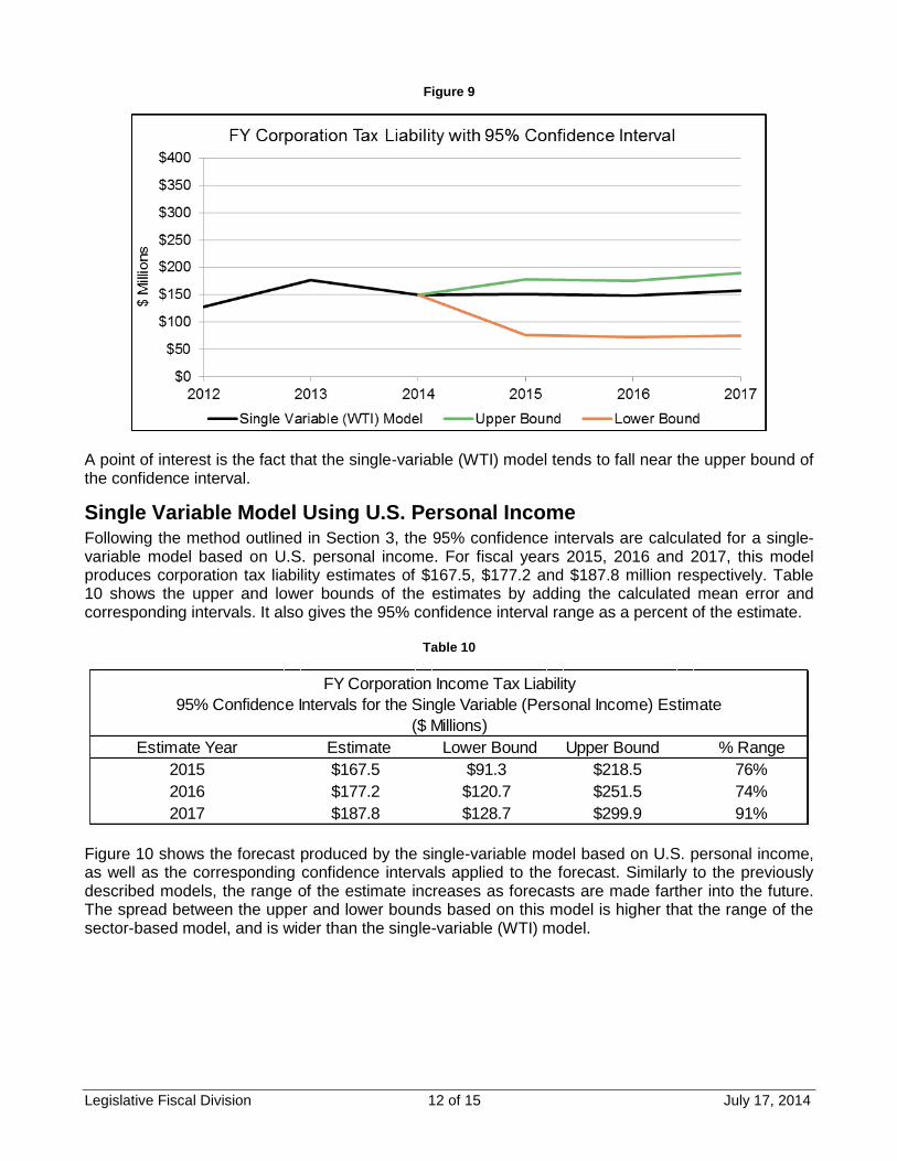
Figure 9

A point of interest is the fact that the single-variable (WTI) model tends to fall near the upper bound of the confidence interval.

Single Variable Model Using U.S. Personal Income Following the method outlined in Section 3, the 95% confidence intervals are calculated for a single-variable model based on U.S. personal income. For fiscal years 2015, 2016 and 2017, this model produces corporation tax liability estimates of $167.5, $177.2 and $187.8 million respectively. Table 10 shows the upper and lower bounds of the estimates by adding the calculated mean error and corresponding intervals. It also gives the 95% confidence interval range as a percent of the estimate.

Table 10

Figure 10 shows the forecast produced by the single-variable model based on U.S. personal income, as well as the corresponding confidence intervals applied to the forecast. Similarly to the previously described models, the range of the estimate increases as forecasts are made farther into the future. The spread between the upper and lower bounds based on this model is higher that the range of the sector-based model, and is wider than the single-variable (WTI) model.


2015 $167.5 $91.3 $218.5 76%

2016 $177.2 $120.7 $251.5 74%

2017 $187.8 $128.7 $299.9 91%


95% Confidence Intervals for the Single Variable (Personal Income) Estimate

($ Millions)


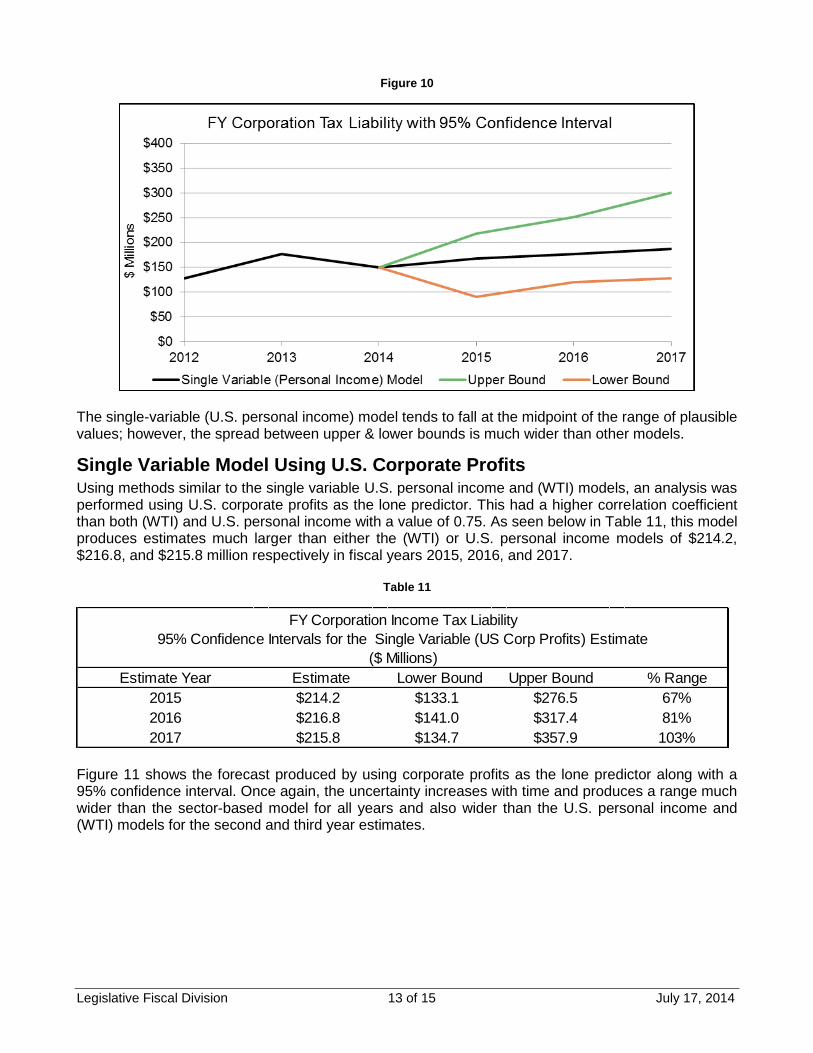
Figure 10

The single-variable (U.S. personal income) model tends to fall at the midpoint of the range of plausible values; however, the spread between upper & lower bounds is much wider than other models.

Single Variable Model Using U.S. Corporate Profits Using methods similar to the single variable U.S. personal income and (WTI) models, an analysis was performed using U.S. corporate profits as the lone predictor. This had a higher correlation coefficient than both (WTI) and U.S. personal income with a value of 0.75. As seen below in Table 11, this model produces estimates much larger than either the (WTI) or U.S. personal income models of $214.2, $216.8, and $215.8 million respectively in fiscal years 2015, 2016, and 2017.

Table 11

Figure 11 shows the forecast produced by using corporate profits as the lone predictor along with a 95% confidence interval. Once again, the uncertainty increases with time and produces a range much wider than the sector-based model for all years and also wider than the U.S. personal income and (WTI) models for the second and third year estimates.


2015 $214.2 $133.1 $276.5 67%

2016 $216.8 $141.0 $317.4 81%

2017 $215.8 $134.7 $357.9 103%


95% Confidence Intervals for the Single Variable (US Corp Profits) Estimate

($ Millions)


Figure 11

As seen above in Figure 11, this model tends to produce estimates that fall in the middle of the upper and lower bounds.

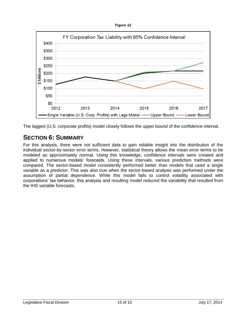
Model Using Lagged U.S. Corporate Profits Following the method outlined in Section 3, the 95% confidence intervals are calculated for a model using the three prior years’ U.S. corporate profits as predictors. For fiscal years 2015, 2016 and 2017, this model produces corporation tax liability estimates of $203.3, $216.6 and $217.5 million respectively. Table 12 shows the upper and lower bounds of the calendar estimates by adding the calculated mean error and corresponding intervals. It also gives the 95% confidence interval range as a percent of the estimate.

Table 12

Figure 12 shows the forecast produced by the single-variable model based on lagged U.S. corporate profits , as well as the corresponding confidence intervals applied to the forecast. The range of the estimate on average increases as forecasts are made farther into the future. The spread between the upper and lower bounds based on this model is higher that the range of the sector-based model, but are narrower than the single-variable (U.S. personal income) model.


2015 $203.3 $97.9 $209.5 55%

2016 $216.6 $148.7 $216.3 31%

2017 $217.5 $98.0 $271.8 80%


95% Confidence Intervals for the Single Variable (US Corp Profits) with Lags Estimate

($ Millions)


Figure 12

The lagged (U.S. corporate profits) model closely follows the upper bound of the confidence interval.

SECTION 6: SUMMARY For this analysis, there were not sufficient data to gain reliable insight into the distribution of the individual sector-by-sector error terms. However, statistical theory allows the mean error terms to be modeled as approximately normal. Using this knowledge, confidence intervals were created and applied to numerous models’ forecasts. Using these intervals, various prediction methods were compared. The sector-based model consistently performed better than models that used a single variable as a predictor. This was also true when the sector-based analysis was performed under the assumption of partial dependence. While this model fails to control volatility associated with corporations’ tax behavior, this analysis and resulting model reduced the variability that resulted from the IHS variable forecasts.

Documents

CORPORATION INCOME TAX ESTIMATING: USING …leg.mt.gov/.../fiscal/other-interim-reports/RTIC-Corp-Tax.pdfCORPORATION INCOME TAX ... and the magnified volatility of the corresponding