Research in Astron. Astrophys. 201x Vol. X No. XX, 000–000http://www.raa-journal.org http://www.iop.org/journals/raa

Research inAstronomy andAstrophysics

Correction and simulation of the intensity compensation algorithmin curvature wavefront sensing ∗

Zhi-Xu Wu1,2,3, Hua Bai1,2 and Xiang-Qun Cui1,2

1 National Astronomical Observatories/Nanjing Institute of Astronomical Optical & Technology,Nanjing, China; zxwu@niaot.ac.cn

2 Key Laboratory of Astronomical Optics & Technology, Nanjing Institute of Astronomical Optics &Technology, Chinese Academy of Sciences, Nanjing 210042, China

3 University of Chinese Academy of Sciences College, Beijing, 100049

Received 2014 June 24; accepted 2014 September 4

Abstract The wave-front measuring range and recovery precision of the curvature sensorcan be improved by Intensity compensation Algorithm. However, in the fast f-numberfocus system, especially in a telescope with large field of view, the accuracy of this algo-rithm can not meet the requirements. The theoretical analysis of the correction of Intensitycompensation algorithm in the fast f-number focus system is firstly introduced and after-wards the mathematical formulas of this algorithm are deduced. The correction result isthen verified through simulation. The method of such simulation is that: First, the curva-ture signal of the fast f-number focus system is simulated by Monte Carlo ray tracing;then the wave-front result is recovered by the inner loop of the FFT wave-front recoveryalgorithm and the outer loop of Intensity compensation Algorithm. Upon the comparisonof the Intensity compensation Algorithm of the ideal system and the corrected Intensitycompensation Algorithm, we reveal that the curvature sensor recovery precision can begreatly improved by the corrected Intensity compensation Algorithm.

Key words: active optics; curvature sensor; wave-front recovery; intensity compensation

1 INTRODUCTION

In the imaging process of telescopes, many factors will lead to the decline of image quality, such as op-tical design, optical fabrication error, gravity deformation, thermal deformation. The concept of ActiveOptics has changed the way of designing telescopes (Su & Cui 1999). People can take the initiative tocorrect the gravity deformation, temperature deformation, support error, and even the mirror machiningerror, and active optics make the image quality become better (Su & Cui 2004). In Active Optics, realtime sensing of wave-front error is very critical. There are two main kinds of Active Optical wave-frontsensors: Hartmann wave-front sensor and the wave-front curvature sensor. Hartmann wave-front sensorhad been used in many large telescopes, such as Chinese LAMOST (Cui et al. 2004, Zhang 2008), andits measuring precision is extremely high (Stepp 1994). But in the telescope with large field of view, thefield of view used for sensing is limited by Hartmann wave-front sensor, almost equal to zero. Wave-front curvature sensor is based on the measurement of the wave-front curvature. Compared with the

∗ Supported by the National Natural Science Foundation of China.

2 Z.-X. Wu et al.

Hartmann sensor, it has the advantages of simplicity, high throughput, and avoidance of calibration dif-ficulties, etc (Roddier & Roddier 1993). LSST (Manuel et al. 2010) and VISTA (Patterson & Sutherland2003) is proposed to use this method to measure the wave-front.

There are two common methods to recover wave-front by curvature sensors: FFT Algorithm andG-S Algorithm. Both algorithms require that the equivalent defocus distance is small and the wave-front aberration is not very large. Thus, Roddier proposed Intensity compensation Algorithm basedon the ideal system in 1993. By compensating the wave-front error of the defocus images, the wave-front measure range and recover precision of the curvature sensor can be improved greatly. Rodddierused his algorithm to real telescopes like ESO NTT and got very good results (Roddier & Roddier1993), but those testings were applied on the relative slow Cassegrain focus and the pupil grid distortionerrors can be ignored. In the fast f-number focus telescopes, the reference point is much different tothat of the ideal system, and the pupil grid distortion errors will lead to lower recovery precision, thusthis algorithm can not be used in those systems directly. In addition, in the situation of off-axis, theangle between the CCD and defocus surface can also cause the coordinate distortion. In this paper, wetheoretically deduce the corrected Intensity compensation formula in a fast f-number focus telescopes,and simulate the situation of on-axis and off-axis with a flat-field telescope. The results show that thecorrected Intensity compensation algorithm is more reasonable for wave-front recovery in the fast f-number focus telescopes.

2 FFT WAVE FRONT RECOVERY ALGORITHM AND INTENSITY COMPENSATIONALGORITHM

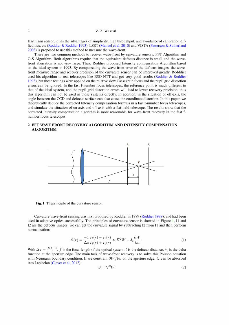
Fig. 1 Theprinciple of the curvature sensor.

Curvature wave-front sensing was first proposed by Roddier in 1989 (Roddier 1989), and had beenused in adaptive optics successfully. The principles of curvature sensor is showed in Figure 1, I1 andI2 are the defocus images, we can get the curvature signal by subtracting I2 from I1 and then performnormalization:

S(r) =−1∆z

I2(r) − I1(r)I2(r) + I1(r)

≈ ∇2W − δc∂W

∂n. (1)

With ∆z = f(f−l)l , f is the focal length of the optical system, l is the defocus distance, δc is the delta

function at the aperture edge. The main task of wave-front recovery is to solve this Poisson equationwith Neumann boundary condition. If we constrain ∂W/∂n on the aperture edge, δc can be absorbedinto Laplacian (Claver et al. 2012):

S = ∇2W. (2)

Correction and Simulation of the Intensity Compensation Algorithm 3

Make the Fourier transform at both side of formula (2) and

FTµ,υ{∇2W (x, y)} = −4π2(µ2 + υ2

)FTµ,υ{W (x, y)}. (3)

Thus:

W = IFTx,y

{FTµ,υ(S)

−4π2 (µ2 + υ2)

}. (4)

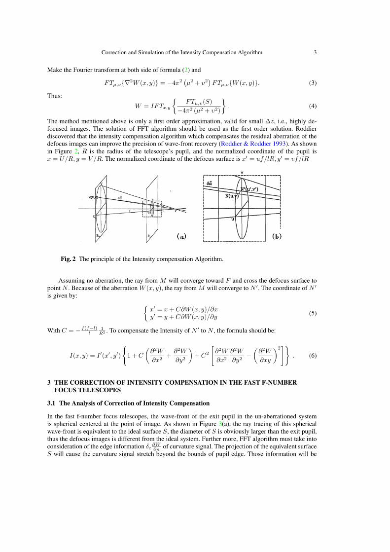
The method mentioned above is only a first order approximation, valid for small ∆z, i.e., highly de-focused images. The solution of FFT algorithm should be used as the first order solution. Roddierdiscovered that the intensity compensation algorithm which compensates the residual aberration of thedefocus images can improve the precision of wave-front recovery (Roddier & Roddier 1993). As shownin Figure 2, R is the radius of the telescope’s pupil, and the normalized coordinate of the pupil isx = U/R, y = V /R. The normalized coordinate of the defocus surface is x′ = uf/lR, y′ = vf/lR

Fig. 2 The principle of the Intensity compensation Algorithm.

Assuming no aberration, the ray from M will converge toward F and cross the defocus surface topoint N . Because of the aberration W (x, y), the ray from M will converge to N ′. The coordinate of N ′

is given by: {x′ = x + C∂W (x, y)/∂xy′ = y + C∂W (x, y)/∂y

(5)

With C = − f(f−l)l

1R2 . To compensate the Intensity of N ′ to N , the formula should be:

I(x, y) = I ′(x′, y′)

{1 + C

(∂2W

∂x2+

∂2W

∂y2

)+ C2

[∂2W

∂x2

∂2W

∂y2−

(∂2W

∂xy

)2]}

. (6)

3 THE CORRECTION OF INTENSITY COMPENSATION IN THE FAST F-NUMBERFOCUS TELESCOPES

3.1 The Analysis of Correction of Intensity Compensation

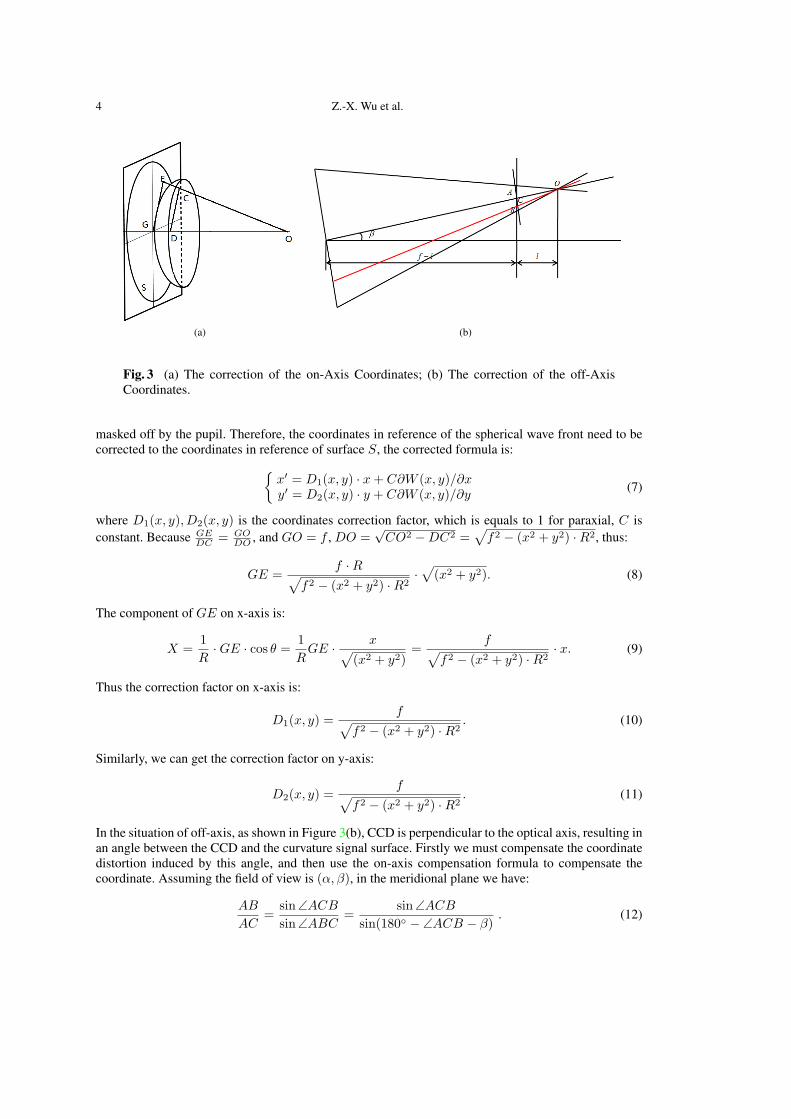
In the fast f-number focus telescopes, the wave-front of the exit pupil in the un-aberrationed systemis spherical centered at the point of image. As shown in Figure 3(a), the ray tracing of this sphericalwave-front is equivalent to the ideal surface S, the diameter of S is obviously larger than the exit pupil,thus the defocus images is different from the ideal system. Further more, FFT algorithm must take intoconsideration of the edge information δc

∂W∂n of curvature signal. The projection of the equivalent surface

S will cause the curvature signal stretch beyond the bounds of pupil edge. Those information will be

4 Z.-X. Wu et al.

(a) (b)

Fig. 3 (a) The correction of the on-Axis Coordinates; (b) The correction of the off-AxisCoordinates.

masked off by the pupil. Therefore, the coordinates in reference of the spherical wave front need to becorrected to the coordinates in reference of surface S, the corrected formula is:{

x′ = D1(x, y) · x + C∂W (x, y)/∂xy′ = D2(x, y) · y + C∂W (x, y)/∂y

(7)

where D1(x, y), D2(x, y) is the coordinates correction factor, which is equals to 1 for paraxial, C isconstant. Because GE

DC = GODO , and GO = f , DO =

√CO2 − DC2 =

√f2 − (x2 + y2) · R2, thus:

GE =f · R√

f2 − (x2 + y2) · R2·√

(x2 + y2). (8)

The component of GE on x-axis is:

X =1R

· GE · cos θ =1R

GE · x√(x2 + y2)

=f√

f2 − (x2 + y2) · R2· x. (9)

Thus the correction factor on x-axis is:

D1(x, y) =f√

f2 − (x2 + y2) · R2. (10)

Similarly, we can get the correction factor on y-axis:

D2(x, y) =f√

f2 − (x2 + y2) · R2. (11)

In the situation of off-axis, as shown in Figure 3(b), CCD is perpendicular to the optical axis, resulting inan angle between the CCD and the curvature signal surface. Firstly we must compensate the coordinatedistortion induced by this angle, and then use the on-axis compensation formula to compensate thecoordinate. Assuming the field of view is (α, β), in the meridional plane we have:

AB

AC=

sin ∠ACB

sin ∠ABC=

sin∠ACB

sin(180◦ − ∠ACB − β). (12)

Correction and Simulation of the Intensity Compensation Algorithm 5

since tan∠AOC = y·Rf/ cos β , then:

AC =AB

cos β − sinβ · cos β y·Rf

. (13)

Similarly, we can get the coordinate compensate formula in the sagittal plane:

AC =AB

cos α − sinα · cos α y·Rf

. (14)

(a) (b)

(c) (d)

Fig. 4 (a) the on-axis coordinates correction factor; (b) the vertical samples of correctionfactor; (c) the off-Axis coordinates correction factor; (d) the vertical samples of correctionfactor.

3.2 Compare the Coordinates Before and After Correction

The compensation of the distortion of the coordinate on axis is a procedure of non-linear scaling, asshow in Figure 4(a) and Figure 4(b), the correction factor is the smallest in the center of the aperture,and the scale of the ration is 1. In the situation of off axis, we can see from Figure 4(c) and Figure 4(d)that aside from the non-linear scaling of the coordinate, there is also a tilt factor on the coordinate.

4 RESULTS OF THE SIMULATION

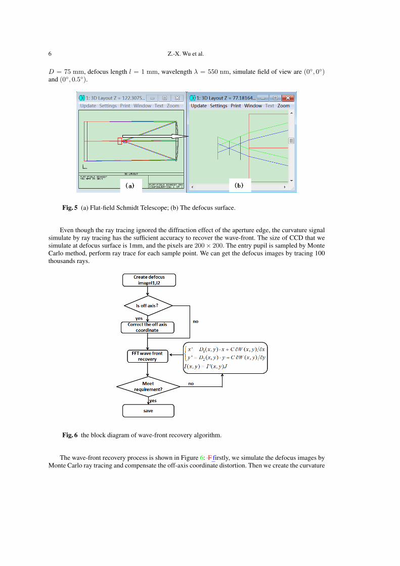
In order to testify the Intensity compensate algorithm, we used a flat-field Schmidt telescope (as showin Fig. 5) to simulate the curvature signal. The system parameters are: f = 100 mm, aperture diameter

6 Z.-X. Wu et al.

D = 75 mm, defocus length l = 1 mm, wavelength λ = 550 nm, simulate field of view are (0◦, 0◦)and (0◦, 0.5◦).

Fig. 5 (a) Flat-field Schmidt Telescope; (b) The defocus surface.

Even though the ray tracing ignored the diffraction effect of the aperture edge, the curvature signalsimulate by ray tracing has the sufficient accuracy to recover the wave-front. The size of CCD that wesimulate at defocus surface is 1mm, and the pixels are 200 × 200. The entry pupil is sampled by MonteCarlo method, perform ray trace for each sample point. We can get the defocus images by tracing 100thousands rays.

Fig. 6 the block diagram of wave-front recovery algorithm.

The wave-front recovery process is shown in Figure 6: F firstly, we simulate the defocus images byMonte Carlo ray tracing and compensate the off-axis coordinate distortion. Then we create the curvature

Correction and Simulation of the Intensity Compensation Algorithm 7

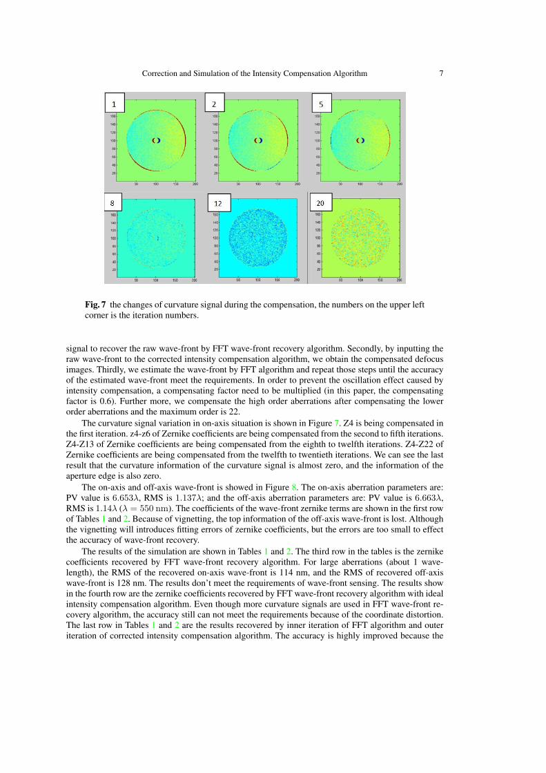
Fig. 7 the changes of curvature signal during the compensation, the numbers on the upper leftcorner is the iteration numbers.

signal to recover the raw wave-front by FFT wave-front recovery algorithm. Secondly, by inputting theraw wave-front to the corrected intensity compensation algorithm, we obtain the compensated defocusimages. Thirdly, we estimate the wave-front by FFT algorithm and repeat those steps until the accuracyof the estimated wave-front meet the requirements. In order to prevent the oscillation effect caused byintensity compensation, a compensating factor need to be multiplied (in this paper, the compensatingfactor is 0.6). Further more, we compensate the high order aberrations after compensating the lowerorder aberrations and the maximum order is 22.

The curvature signal variation in on-axis situation is shown in Figure 7. Z4 is being compensated inthe first iteration. z4-z6 of Zernike coefficients are being compensated from the second to fifth iterations.Z4-Z13 of Zernike coefficients are being compensated from the eighth to twelfth iterations. Z4-Z22 ofZernike coefficients are being compensated from the twelfth to twentieth iterations. We can see the lastresult that the curvature information of the curvature signal is almost zero, and the information of theaperture edge is also zero.

The on-axis and off-axis wave-front is showed in Figure 8. The on-axis aberration parameters are:PV value is 6.653λ, RMS is 1.137λ; and the off-axis aberration parameters are: PV value is 6.663λ,RMS is 1.14λ (λ = 550 nm). The coefficients of the wave-front zernike terms are shown in the first rowof Tables 1 and 2. Because of vignetting, the top information of the off-axis wave-front is lost. Althoughthe vignetting will introduces fitting errors of zernike coefficients, but the errors are too small to effectthe accuracy of wave-front recovery.

The results of the simulation are shown in Tables 1 and 2. The third row in the tables is the zernikecoefficients recovered by FFT wave-front recovery algorithm. For large aberrations (about 1 wave-length), the RMS of the recovered on-axis wave-front is 114 nm, and the RMS of recovered off-axiswave-front is 128 nm. The results don’t meet the requirements of wave-front sensing. The results showin the fourth row are the zernike coefficients recovered by FFT wave-front recovery algorithm with idealintensity compensation algorithm. Even though more curvature signals are used in FFT wave-front re-covery algorithm, the accuracy still can not meet the requirements because of the coordinate distortion.The last row in Tables 1 and 2 are the results recovered by inner iteration of FFT algorithm and outeriteration of corrected intensity compensation algorithm. The accuracy is highly improved because the

8 Z.-X. Wu et al.

Fig. 8 (a) the on-axis wave-front s; (b) the off-axis wave-front.

distortion of coordinate is removed by the coordinate correction. The RMS on-axis decline from 52.9 nmto 12.4 nm, and the RMS off-axis decline from 82.5 nm to 13.7 nm. We reveal by the simulation resultsthat the corrected intensity compensation algorithm is more reasonable for the wave-front recovery ofthe fast f-number focus system.

Table 1 the result of on-axis wave-front recovery

Zernike Terms Z4 Z5 Z6 Z7 Z8 Z9 Z10 Z11 Z12Zernike Coefficients (λ) −0.720 −0.602 0 0 0.502 0 −0.401 −0.017 0 RMS (nm)

FFT −0.591 −0.651 −0.013 0.025 0.528 0.023 −0.243 0.006 −0.011 114Paraxial −0.797 −0.628 −0.025 0 0.495 0.009 −0.413 −0.022 −0.005 52.9on-Axis −0.725 −0.609 0.018 0.013 0.500 0.008 −0.403 −0.018 0 12.4

Table 2 the result of off-axis wave-front recovery

Zernike Terms Z4 Z5 Z6 Z7 Z8 Z9 Z10 Z11 Z12Zernike Coefficients (λ) −0.729 −0.602 0.004 0.013 0.502 0 −0.401 −0.017 0 RMS (nm)

FFT −0.533 −0.662 0.032 0.018 0.512 0.018 −0.427 0.001 −0.002 128Paraxial −0.654 −0.633 −0.030 0.032 0.390 0 −0.430 −0.028 0.014 82.5off-Axis −0.727 −0.614 0.023 0.017 0.488 0.008 −0.399 −0.016 0 13.7

5 CONCLUSIONS

In this paper, We analyze the corrected intensity compensation algorithm of the fast f-number focussystem, and apply this algorithm to recovery the wavefront of a flat-field Schmidt telescope. By compar-ing simulation results of ideal intensity compensation algorithm and corrected intensity compensationalgorithm, we confirm that the corrected intensity compensation algorithm is more reasonable for thefast f-number focus system.

Acknowledgements This work was supported by the National Natural Science Foundation of China(11103048).

Correction and Simulation of the Intensity Compensation Algorithm 9

References

Claver, C. F., Chandrasekharan, S., Liang, M., et al. 2012, in Society of Photo-Optical InstrumentationEngineers (SPIE) Conference Series, Vol. 8444, 14 2

Cui, X., Su, D., Li, G., et al. 2004, in Society of Photo-Optical Instrumentation Engineers (SPIE)Conference Series, Vol. 5489 , Ground-based Telescopes, ed. J. M. Oschmann, Jr., 974 1

Manuel, A. M., Phillion, D. W., Olivier, S. S., Baker, K. L., & Cannon, B. 2010, Optics Express, 18,1528 2

Patterson, B. A., & Sutherland, W. J. 2003, in Society of Photo-Optical Instrumentation Engineers(SPIE) Conference Series, Vol. 4842 , Specialized Optical Developments in Astronomy, ed.E. Atad-Ettedgui & S. D’Odorico, 231 2

Roddier, C., & Roddier, F. 1993, Journal of the Optical Society of America A, 10, 2277 2, 3Roddier, N. 1989, Curvature sensing for Adaptive Optics: A computer simulation, Master’s thesis, The

University of Arizona 2Stepp, L. M., ed. 1994, Society of Photo-Optical Instrumentation Engineers (SPIE) Conference Series,

Vol. 2199, Advanced Technology Optical Telescopes V 1Su, D., & Cui, X. 1999, Progress in Astronomy, 17, 1 1Su, D.-Q., & Cui, X.-Q. 2004, ChJAA (Chin. J. Astron. Astrophys.), 4, 1 1Zhang, Y. 2008, in Society of Photo-Optical Instrumentation Engineers (SPIE) Conference Series, Vol.

7012, 70123H-11 1