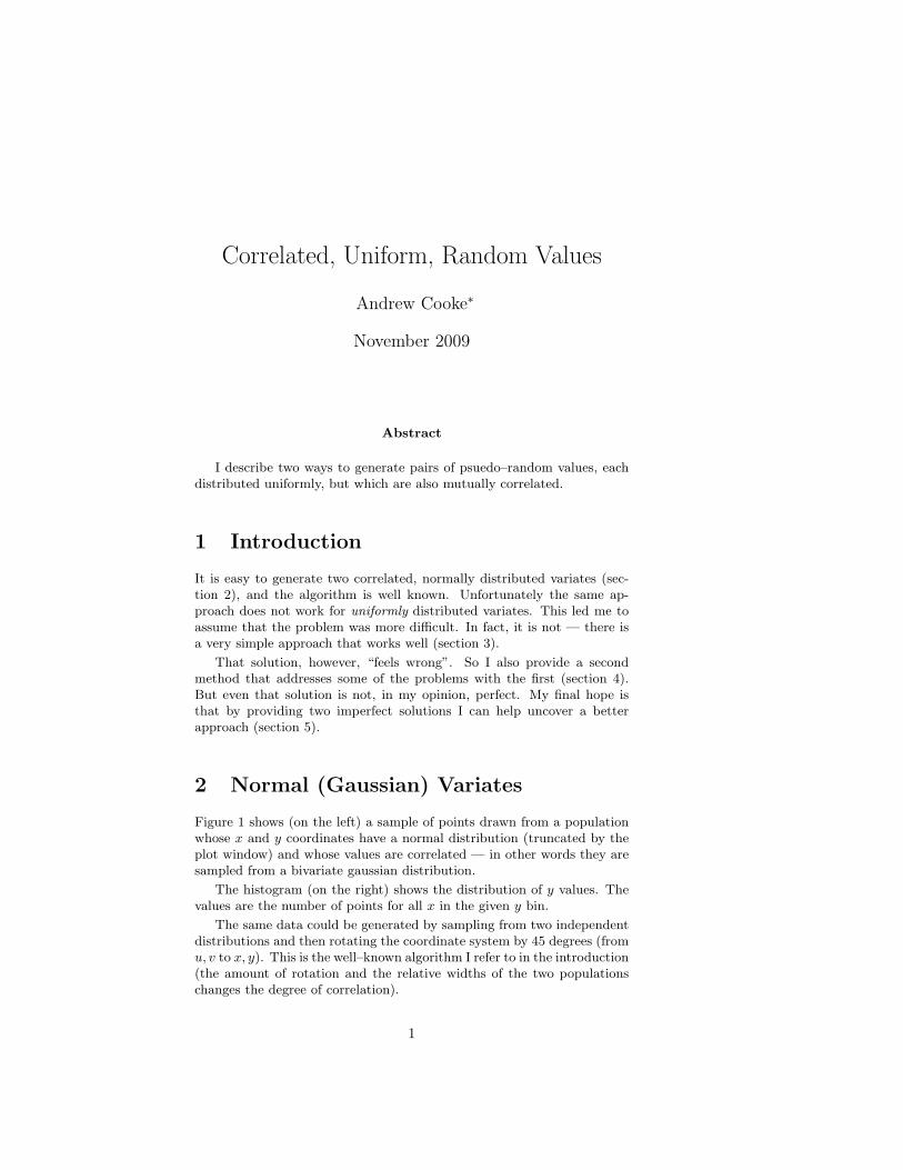
Correlated, Uniform, Random Values

Andrew Cooke∗

November 2009

Abstract

I describe two ways to generate pairs of psuedo–random values, eachdistributed uniformly, but which are also mutually correlated.

1 Introduction

It is easy to generate two correlated, normally distributed variates (sec-tion 2), and the algorithm is well known. Unfortunately the same ap-proach does not work for uniformly distributed variates. This led me toassume that the problem was more difficult. In fact, it is not — there isa very simple approach that works well (section 3).

That solution, however, “feels wrong”. So I also provide a secondmethod that addresses some of the problems with the first (section 4).But even that solution is not, in my opinion, perfect. My final hope isthat by providing two imperfect solutions I can help uncover a betterapproach (section 5).

2 Normal (Gaussian) Variates

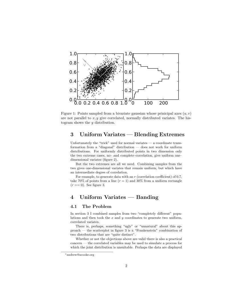
Figure 1 shows (on the left) a sample of points drawn from a populationwhose x and y coordinates have a normal distribution (truncated by theplot window) and whose values are correlated — in other words they aresampled from a bivariate gaussian distribution.

The histogram (on the right) shows the distribution of y values. Thevalues are the number of points for all x in the given y bin.

The same data could be generated by sampling from two independentdistributions and then rotating the coordinate system by 45 degrees (fromu, v to x, y). This is the well–known algorithm I refer to in the introduction(the amount of rotation and the relative widths of the two populationschanges the degree of correlation).

1

0.0 0.2 0.4 0.6 0.8 1.00.0

0.2

0.4

0.6

0.8

1.0

uv

0 100 2000.0

0.2

0.4

0.6

0.8

1.0

Figure 1: Points sampled from a bivariate gaussian whose prinicipal axes (u, v)are not parallel to x, y give correlated, normally distributed variates. The his-togram shows the y distribution.

3 Uniform Variates — Blending Extremes

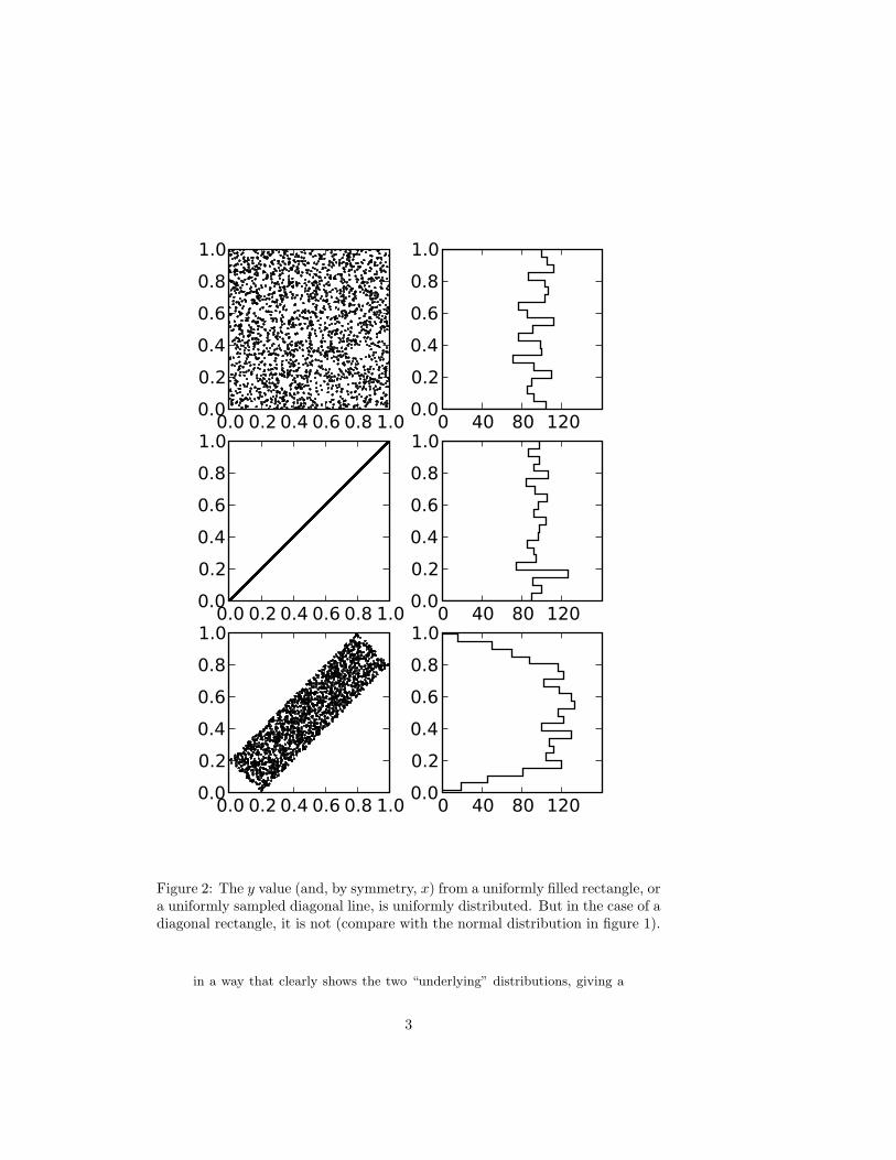
Unfortunately the “trick” used for normal variates — a coordinate trans-formation from a “diagonal” distribution — does not work for uniformdistributions. For uniformly distributed points in two dimension onlythe two extreme cases, no– and complete–correlation, give uniform one–dimensional variates (figure 2).

But the two extremes are all we need. Combining samples from thetwo gives one-dimensional variates that remain uniform, but which havean intermediate degree of correlation.

For example, to generate data with an r (correlation coefficient) of 0.7,take 70% of points from a line (r = 1) and 30% from a uniform rectangle(r == 0). See figure 3.

4 Uniform Variates — Banding

4.1 The Problem

In section 3 I combined samples from two “completely different” popu-lations and then took the x and y coordinates to generate two uniform,correlated variates.

There is, perhaps, something “ugly” or “unnatural” about this ap-proach — the scatterplot in figure 3 is a “Frankenstein” combination oftwo distributions that are “quite distinct”.

Whether or not the objections above are valid there is also a practicalconcern — the correlated variables may be used to simulate a process forwhich the joint distribution is unsuitable. Perhaps the data are displayed

∗andrew@acooke.org

2

0.0 0.2 0.4 0.6 0.8 1.00.0

0.2

0.4

0.6

0.8

1.0

0 40 80 1200.0

0.2

0.4

0.6

0.8

1.0

0.0 0.2 0.4 0.6 0.8 1.00.0

0.2

0.4

0.6

0.8

1.0

0 40 80 1200.0

0.2

0.4

0.6

0.8

1.0

0.0 0.2 0.4 0.6 0.8 1.00.0

0.2

0.4

0.6

0.8

1.0

0 40 80 1200.0

0.2

0.4

0.6

0.8

1.0

Figure 2: The y value (and, by symmetry, x) from a uniformly filled rectangle, ora uniformly sampled diagonal line, is uniformly distributed. But in the case of adiagonal rectangle, it is not (compare with the normal distribution in figure 1).

in a way that clearly shows the two “underlying” distributions, giving a

3

0.0 0.2 0.4 0.6 0.8 1.00

20406080

100120140

0.0 0.2 0.4 0.6 0.8 1.00.0

0.2

0.4

0.6

0.8

1.0

0.0 0.2 0.4 0.6 0.8 1.00.0

0.2

0.4

0.6

0.8

1.0

0 40 80 1200.0

0.2

0.4

0.6

0.8

1.0

Figure 3: 2000 points sampled from two different populations (bottom left).Each sample is taken from a completely correlated population with a probabilityof 0.7 and from a completely uncorrelated population with a probability of 0.3.The result, projected onto the x (top left) and y (bottom right) axes, are twovariates with r = 0.7. The top right plot shows the cumulative distribution forthe two variates.

misleading “feature”.

If the second problem is relevant then there must be additional con-straints, in addition to “uniform and correlated”. Without knowing whatthese constraints are I cannot address them here in detail, but I can stillillustrate how they might be managed by a second algorithm.

4

4.2 A Second Approach

A more “natural” approach to generating “uniform, correlated” variatesmight be based on the banded distribution shown in figure 2. That doesnot work as it stands, but perhaps it can be modified in some way?

Figure 4: Axes and points used in the calculation below.

The problem with the rectangle approach was too few points from the“end regions”. If the rectangle is extended as shown in figure 4 the resultis closer, but even that is insufficient.

Rather than continuing to guess I will parameterize the density dis-tribution and then solve for that, given the constraint that the x and y

coordinates must be uniformly distributed. To obtain both variates fromthe same calculation (which reduces the work involved considerably) thedistribution must be a function of u only. Furthermore, I will focus onlyon the bottom left corner (u < s) and assume that for u > s the desity(ρ) is a constant, ρ0 (the top right corner can be inferred from symmetrylater).

Given the above, for some x, where x < t, the constraint is:

∫ t+x

y=0

ρ(y) dy = 2tρ0

And for y > t − x, ρ(y) = ρ0, so:

∫ t−x

y=0

ρ(y) dy + 2xρ0 = 2tρ0

Transforming variables:

∫ t/√

2

u=x/√

2

ρ(u)√

2 du + 2xρ0 = 2tρ0

If the solution is a polynomial, ρ(u) =∑n

i=0aiu

i, then:

[

n∑

i=0

aiui+1

i + 1

]t/√

2

u=x/√

2

=√

2ρ0(t − x)

and comparing coefficients of xi it is clear that ai = 0 when i > 0, leaving:

5

a0

t − x√

2=

√

2ρ0(t − x)

a0 = 2

which is so simple that you can see it “geometricaally” by consideringsimilar triangles in figure 5.

4.3 Summary

The x and y coordinates of points sampled at random from the densitydistribution shown in figure 5 are uniformly distributed and correlated(the degree of correlation depends on the value of t; see the next section).

Figure 5: A density distribution for generating uniform, correlated, randomvariates. The darker area has twice the density of the lighter area.

This can be achieved by selecting points at random within the ex-tended rectangle indicated by the dotted lines (using a uniform density)and then “folding” those that lie outside the unit square into the moredarkly shaded areas.

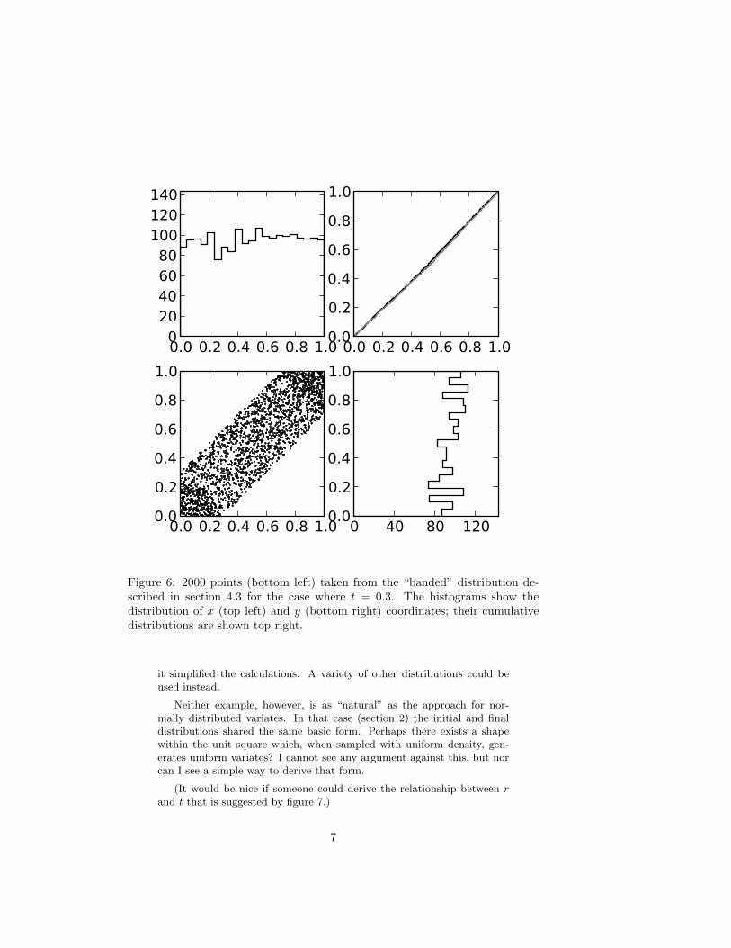
Example data for 2000 points when t = 0.3 are shown in figure 6.

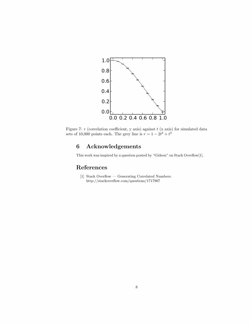
4.4 Correlation Coefficient

Figure 7 plots r against t for simulated data using 10,000 samples permeasurement. The grey line is the curve r = 1−2t2+t3. This is not derived

from the measurements in a rigorous manner, but appears to adequatelymodel the relationship.

5 Discussion

In sections 3 and 4 I have shown two different methods to generate twosamples of uniformly distributed values that are correlated.

The second approach also illustrated a more general approach to theproblem: normalisation of a suitably symmetric distribution function.There is nothing “special” about the banded form used there, except that

6

0.0 0.2 0.4 0.6 0.8 1.00

20406080

100120140

0.0 0.2 0.4 0.6 0.8 1.00.0

0.2

0.4

0.6

0.8

1.0

0.0 0.2 0.4 0.6 0.8 1.00.0

0.2

0.4

0.6

0.8

1.0

0 40 80 1200.0

0.2

0.4

0.6

0.8

1.0

Figure 6: 2000 points (bottom left) taken from the “banded” distribution de-scribed in section 4.3 for the case where t = 0.3. The histograms show thedistribution of x (top left) and y (bottom right) coordinates; their cumulativedistributions are shown top right.

it simplified the calculations. A variety of other distributions could beused instead.

Neither example, however, is as “natural” as the approach for nor-mally distributed variates. In that case (section 2) the initial and finaldistributions shared the same basic form. Perhaps there exists a shapewithin the unit square which, when sampled with uniform density, gen-erates uniform variates? I cannot see any argument against this, but norcan I see a simple way to derive that form.

(It would be nice if someone could derive the relationship between r

and t that is suggested by figure 7.)

7

0.0 0.2 0.4 0.6 0.8 1.00.0

0.2

0.4

0.6

0.8

1.0

Figure 7: r (correlation coefficient, y axis) against t (x axis) for simulated datasets of 10,000 points each. The grey line is r = 1− 2t2 + t3

6 Acknowledgements

This work was inspired by a question posted by “Gideon” on Stack Overflow[1].

References

[1] Stack Overflow — Generating Correlated Numbers.http://stackoverflow.com/questions/1717907

8