Embed Size (px)
Citation preview

Correlation and Regression
Spearman's rank correlation
• An alternative to correlation that does not make so many assumptions
• Still measures the strength and direction of association between two variables
• Uses the ranks instead of the raw data

Example: Spearman's rsVERSIONS:1. Boy climbs up rope, climbs down again2. Boy climbs up rope, seems to vanish, re-appears at top, climbs down again3. Boy climbs up rope, seems to vanish at top4. Boy climbs up rope, vanishes at top, reappears somewhere the audience was not looking5. Boy climbs up rope, vanishes at top, reappears in a place which has been in full view

Hypotheses
H0: The difficulty of the described trick is not correlated with the time elapsed since it was observed.
HA: The difficulty of the described trick is correlated with the time elapsed since it was observed.

East-Indian Rope Trick
0
1
2
3
4
5
6
0 10 20 30 40 50 60
Years Elapsed
Impressiveness Score

East-Indian Rope Trick
2 15 15 14 2
17 217 231 320 422 425 428 429 434 443 444 446 434 428 539 550 550 5
Years elapsed
ImpressivenessScore
13.53.52
5.55.513789
10.512
14.5171819
14.510.516
20.520.5
2225557
12.512.512.512.512.512.512.512.512.512.519.519.519.519.5
Rank Years
Rank Impressiveness
€
rS =
X i − X ( )∑ Yi −Y ( )
X i − X ( )2∑ Yi −Y ( )
2∑
€
rS = 0.784

East-Indian Rope Trick
€
rS = 0.784
TABLE H
n = 21, = 0.05Critical value: 0.435
P < 0.05, reject Ho

Spearman’s Rank Correlation - large n
• For large n (> 100), you can use the normal correlation coefficient test for the ranks
€
t =rs
SE rs
€
SE rs=
1− rs2
n − 2
Under Ho, t has a t-distribution with n-2 d.f.
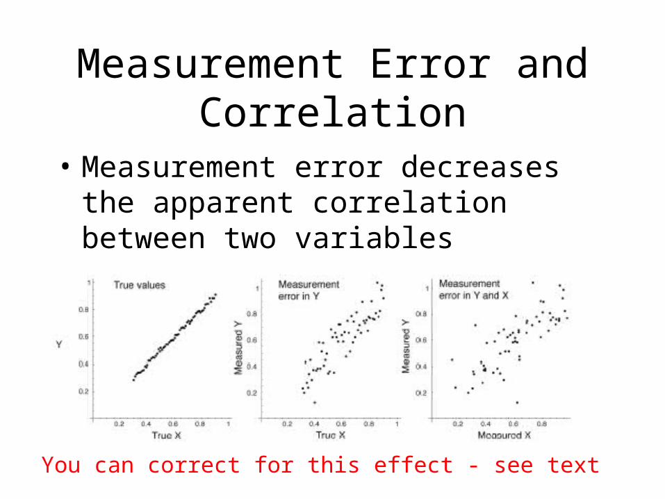
Measurement Error and Correlation
• Measurement error decreases the apparent correlation between two variables
You can correct for this effect - see text

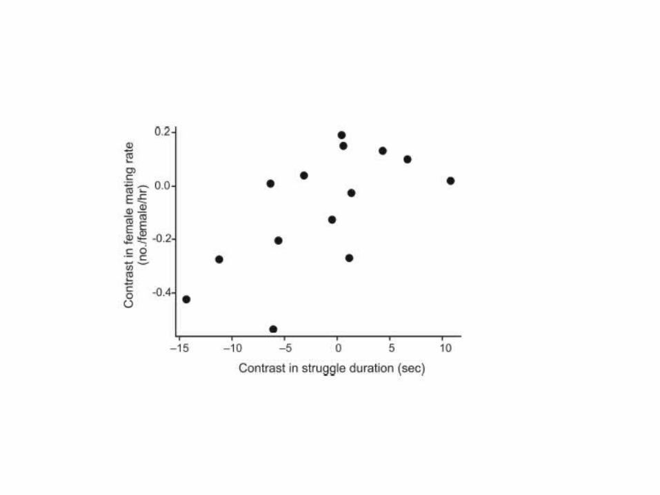
Species are not independent data points

Independent contrasts

Independent contrasts

Quick Reference Guide - Correlation Coefficient
• What is it for? Measuring the strength of a linear association between two numerical variables
• What does it assume? Bivariate normality and random sampling
• Parameter: • Estimate: r• Formulae:
€
r =
X i − X ( )∑ Yi − Y ( )
X i − X ( )2
∑ Yi − Y ( )2
∑
€
SEr =1− r 2
n − 2

Quick Reference Guide - t-test for zero linear correlation
• What is it for? To test the null hypothesis that the population parameter, , is zero
• What does it assume? Bivariate normality and random sampling
• Test statistic: t• Null distribution: t with n-2 degrees of
freedom• Formulae:
€
t =r
SEr

Sample
Test statistic
Null hypothesis=0
Null distributiont with n-2 d.f.
compare
How unusual is this test statistic?
P < 0.05 P > 0.05
Reject Ho Fail to reject Ho
T-test for correlation
€
t =r
SEr

Quick Reference Guide - Spearman’s Rank Correlation
• What is it for? To test zero correlation between the ranks of two variables
• What does it assume? Linear relationship between ranks and random sampling
• Test statistic: rs
• Null distribution: See table; if n>100, use t-distribution• Formulae: Same as linear correlation but based on
ranks

Sample
Test statisticrs
Null hypothesis=0
compare
How unusual is this test statistic?
P < 0.05 P > 0.05
Reject Ho Fail to reject Ho
Spearman’s rank correlation
Null distributionSpearman’s rank
Table H

Quick Reference Guide - Independent Contrasts
• What is it for? To test for correlation between two variables when data points come from related species
• What does it assume? Linear relationship between variables, correct phylogeny, difference between pairs of species in both X and Y has a normal distribution with zero mean and variance proportional to the time since divergence

Regression
• The method to predict the value of one numerical variable from that of another
• Predict the value of Y from the value of X
• Example: predict the size of a dinosaur from the length of one tooth

Linear Regression
• Draw a straight line through a scatter plot
• Use the line to predict Y from X

Linear Regression Formula
Y = + X
= intercept– The predicted value of Y when X is zero
= slope– the rate of change in Y per unit of change
in XParameters

Interpretations of &
positive negative = 0
higher
lower
X X X X
Y

Linear Regression Formula
Y = a + bX
• a = estimated intercept– The predicted value of Y when X is zero
• b = estimated slope– the rate of change in Y per unit of change
in X
^

How to draw the line?
X
Y
residuals
Y1
Y1^
Y2
Y2
^
Y3
Y3^
Y4
Y4^
(Y1-Y1)^

Least-squares Regression
• Draw the line that minimizes the sum of the squared residuals from the line
• Residual is (Yi-Yi)
• Minimize the sum: SSresiduals=Σ(Yi-Yi)2
^
^

Formulae for Least-Squares Regression
• The slope and intercept that minimize the sum of squared residuals are:
sum of products
sum of squares for X
€
b =
X i − X ( ) Yi − Y ( )i =1
n
∑
X i − X ( )2
i =1
n
∑
€
a = Y − bX

Example: How old is that lion?
X = proportion black
Y = age in years

Example: How old is that lion?

Example: How old is that lion?
X = proportion black
Y = age in years
X = 0.322Y = 4.309
Σ(X-X)2=1.222Σ(Y-Y)2=222.087Σ(X-X)(Y-Y)=13.012

€
b =
X i − X ( ) Yi −Y ( )i=1
n
∑
X i − X ( )2
i=1
n
∑=
13.012
1.222=10.647
€
a = Y − bX = 4.309 −10.647* 0.322
a = 0.879
€
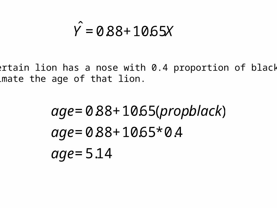
ˆ Y = 0.88 +10.65X

€
ˆ Y = 0.88 +10.65X
A certain lion has a nose with 0.4 proportion of black.Estimate the age of that lion.
€
age = 0.88 +10.65( prop.black)
age = 0.88 +10.65*0.4
age = 5.14

Standard error of the slope
€
SEb =MSresidual
X i − X ( )2∑
€
MSresidual =(Yi −Y )2 − b (X i − X )(Yi −Y )∑∑
n − 2
Sum of squares
Sum of products

€
MSresidual =(Yi −Y )2 − b (X i − X )(Yi −Y )∑∑
n − 2
MSresidual =222.087 −10.647(13.012)
32 − 2MSresidual = 2.785
€
SEb =MSresidual
X i − X ( )2∑
=2.785
1.222
SEb =1.510
Lion Example, continued…

Confidence interval for the slope
€
b − tα (2),df SEb < β < b + tα (2),df SEb

Lion Example, continued…
€
b − tα (2),df SEb < β < b + tα (2),df SEb
€
10.647 − 2.042(1.510) < β <10.64 + 2.042(1.510)
€
7.56 < β <13.73

Predicting Y from X
• What is our confidence for predicting Y from X?
• Two types of predictions:
• What is the mean Y for each value of X?– Confidence bands
• What is a particular individual Y at each value of X?– Prediction intervals

Predicting Y from X
• Confidence bands: measure the precision of the predicted mean Y for each value of X
• Prediction intervals: measure the precision of predicted single Y values for each value of X

Predicting Y from X
Confidence bands Prediction interval

Predicting Y from X
Confidence bands Prediction interval
How confident can we be about theregression line?
How confident can we be about thepredicted values?

Testing Hypotheses about a Slope
• t-test for regression slope
• Ho: There is no linear relationship between X and Y ( = 0)
• Ha: There is a linear relationship between X and Y ( ≠ 0)

Testing Hypotheses about a Slope
• Test statistic: t
• Null distribution: t with n-2 d.f.€
t =b
SEb

€
t =b
SEb
=10.65
1.51= 7.05
df = n-2 = 32-2 = 30
Critical value: 2.04
7.05 > 2.04 so we reject the null hypothesis
Conclude that 0
Lion Example, continued…
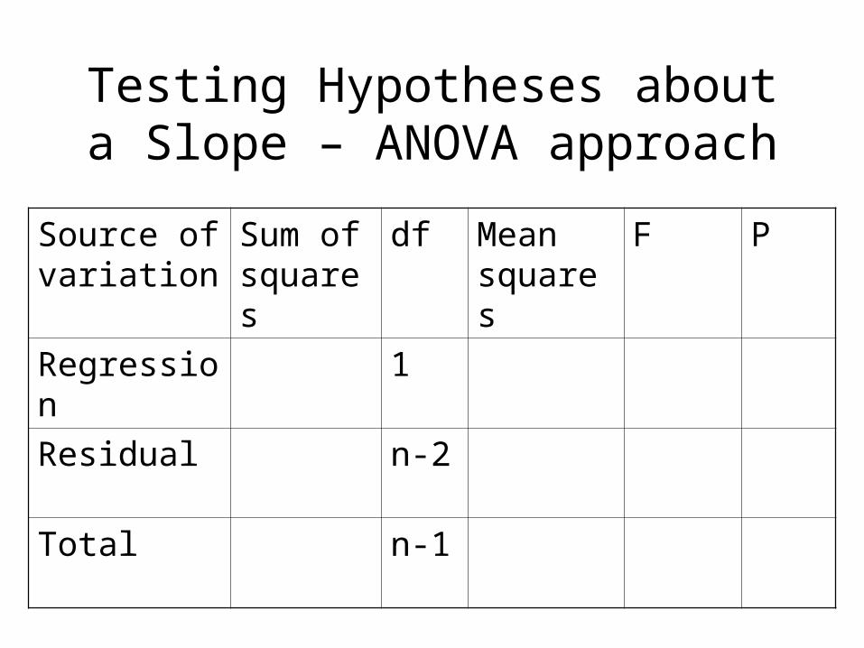
Source of variation
Sum of squares
df Mean squares
F P
Regression 1
Residual n-2
Total n-1
Testing Hypotheses about a Slope – ANOVA approach

Source of variation
Sum of squares
df Mean squares
F P
Regression 138.54 1 138.54 49.7 <0.001
Residual 83.55 30 2.785
Total 222.09 31
Lion Example, continued…
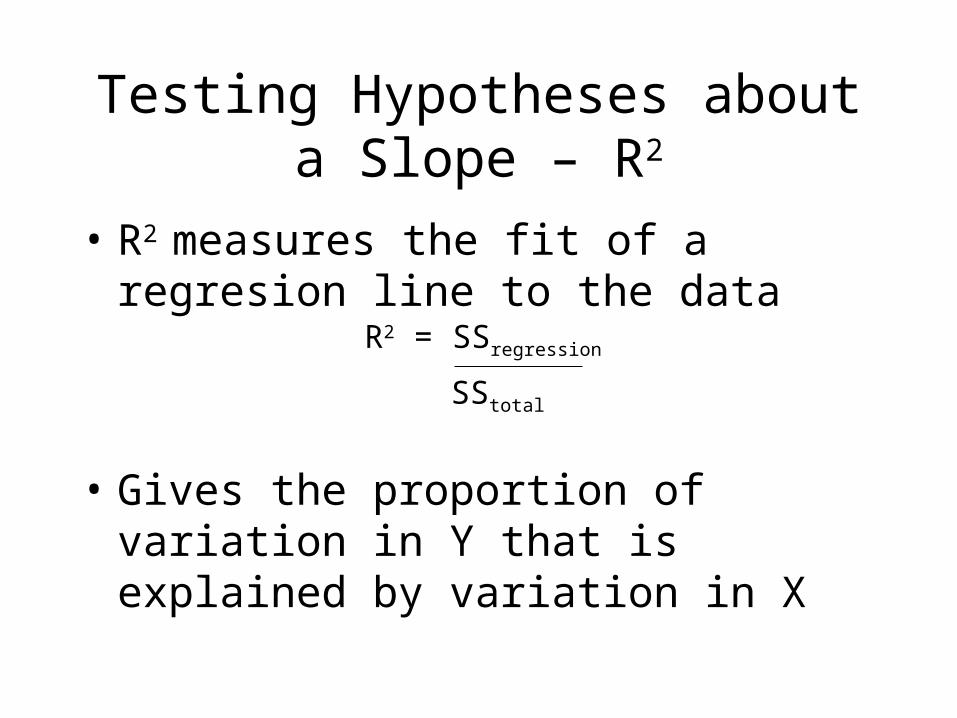
Testing Hypotheses about a Slope – R2
• R2 measures the fit of a regresion line to the data
• Gives the proportion of variation in Y that is explained by variation in X
R2 = SSregression
SStotal

Lion Example, Continued
€
R2 =SSregression
SStotal
=138.54
222.09
R2 = 0.63
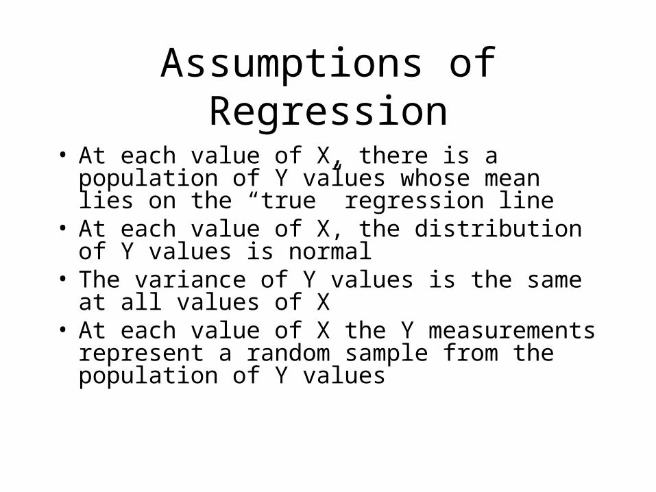
Assumptions of Regression
• At each value of X, there is a population of Y values whose mean lies on the “true” regression line
• At each value of X, the distribution of Y values is normal
• The variance of Y values is the same at all values of X
• At each value of X the Y measurements represent a random sample from the population of Y values

Detecting Linearity
• Make a scatter plot
• Does it look like a curved line would fit the data better than a straight one?

Non-linear relationship: Number of fish species vs. Size of desert pool
Number of species By Area of pool
Number of species
0
1
2
3
4
5
6
-20000 20000 40000 60000 80000 100000Area of pool

Taking the log of area:Number of species By Log10 area
Number of species
0
1
2
3
4
5
6
.5 1.0 1.5 2.0 2.5 3.0 3.5 4.0 4.5 5.0Log10 area

Detecting non-normality and unequal variance
• These are best detected with a residual plot
• Plot the residuals (Yi-Yi) against X
• Look for:– symmetric cloud of points– Little noticeable curvature– Equal variance above and below the line
^

Residual plots help assess assumptions
Original: Residual plot

Transformed dataLogs: Residual plot

What if the relationship is not a straight line?
• Transformations
• Non-linear regression

Transformations
• Some (but not all) nonlinear relationships can be made linear with a suitable transformation
• Most common – log transform Y, X, or both