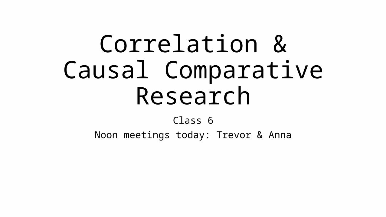
Correlation & Causal Comparative Research

Class 6Noon meetings today: Trevor & Anna

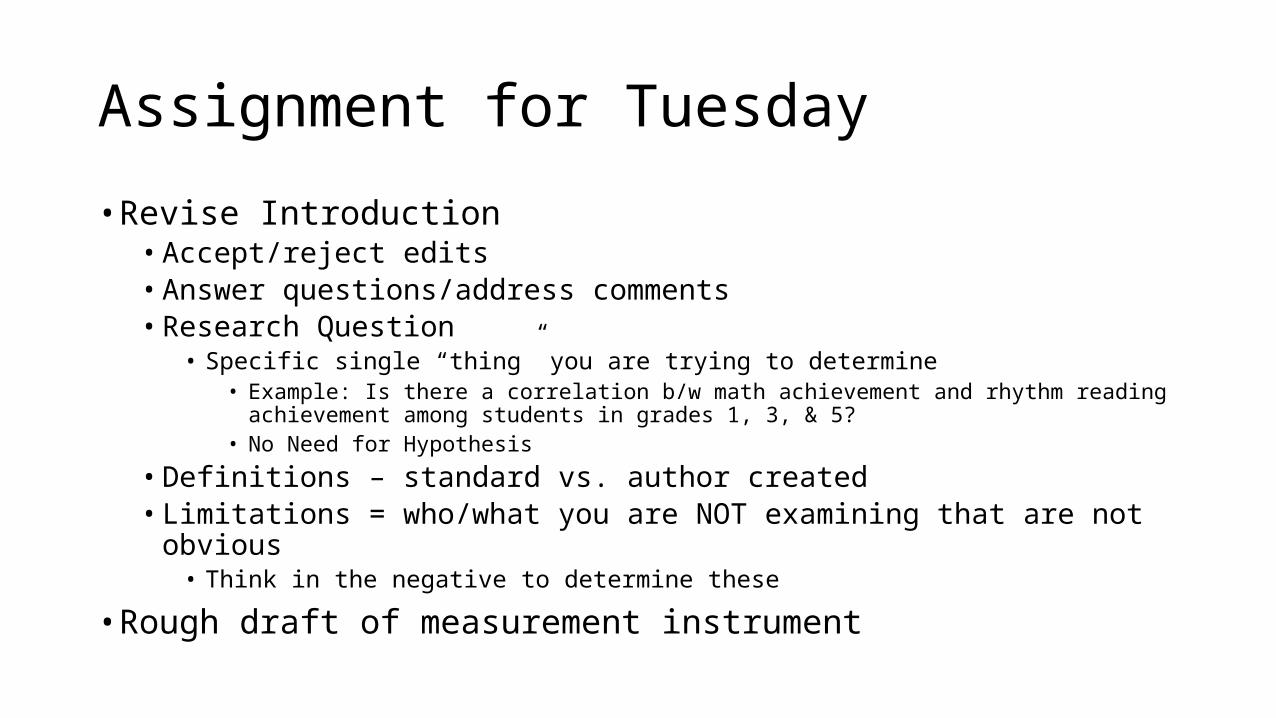
Assignment for Tuesday

• Revise Introduction• Accept/reject edits• Answer questions/address comments• Research Question

• Specific single “thing” you are trying to determine• Example: Is there a correlation b/w math achievement and rhythm reading achievement

among students in grades 1, 3, & 5?• No Need for Hypothesis

• Definitions – standard vs. author created• Limitations = who/what you are NOT examining that are not obvious

• Think in the negative to determine these

• Rough draft of measurement instrument

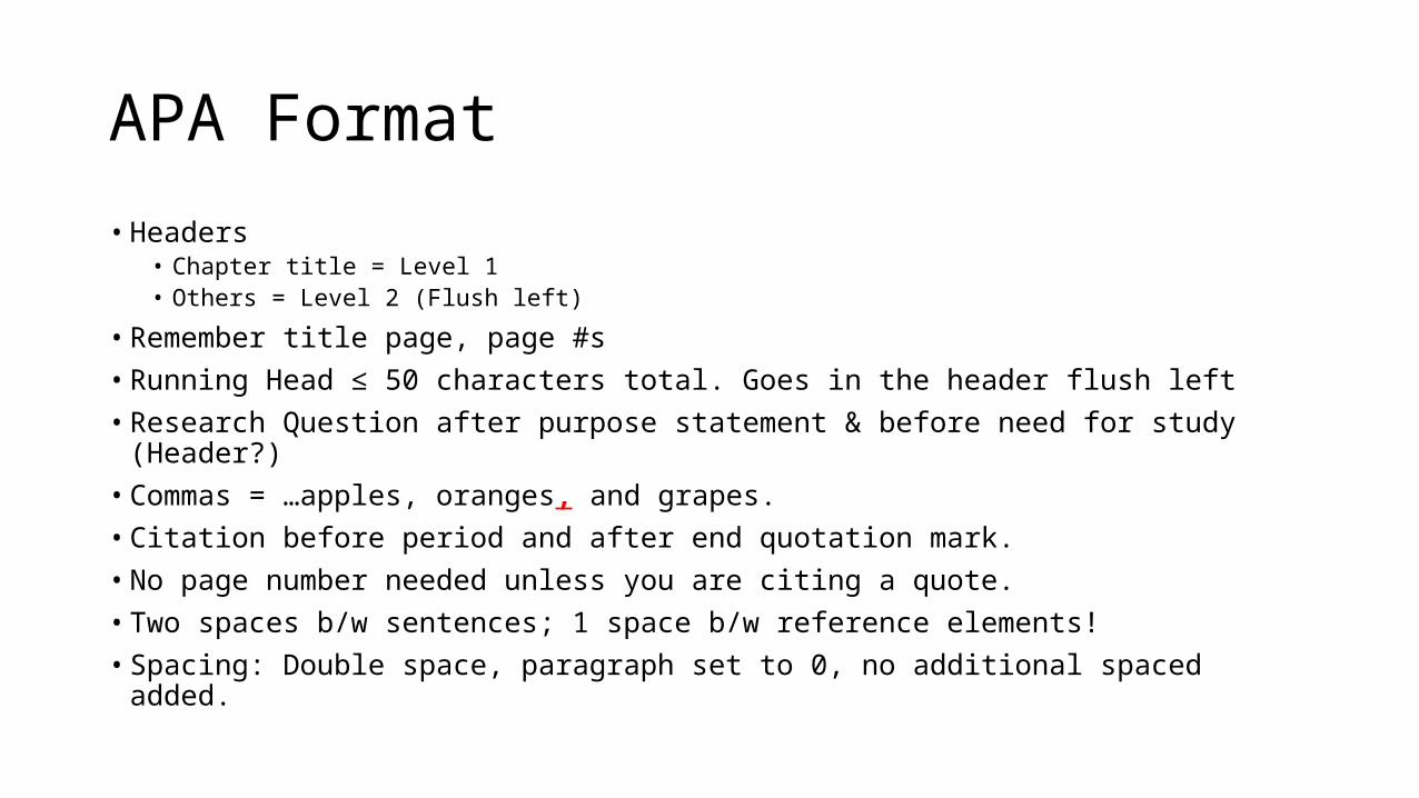
APA Format

• Headers• Chapter title = Level 1• Others = Level 2 (Flush left)

• Remember title page, page #s• Running Head ≤ 50 characters total. Goes in the header flush left• Research Question after purpose statement & before need for study (Header?)• Commas = …apples, oranges, and grapes.• Citation before period and after end quotation mark.• No page number needed unless you are citing a quote.• Two spaces b/w sentences; 1 space b/w reference elements!• Spacing: Double space, paragraph set to 0, no additional spaced added.

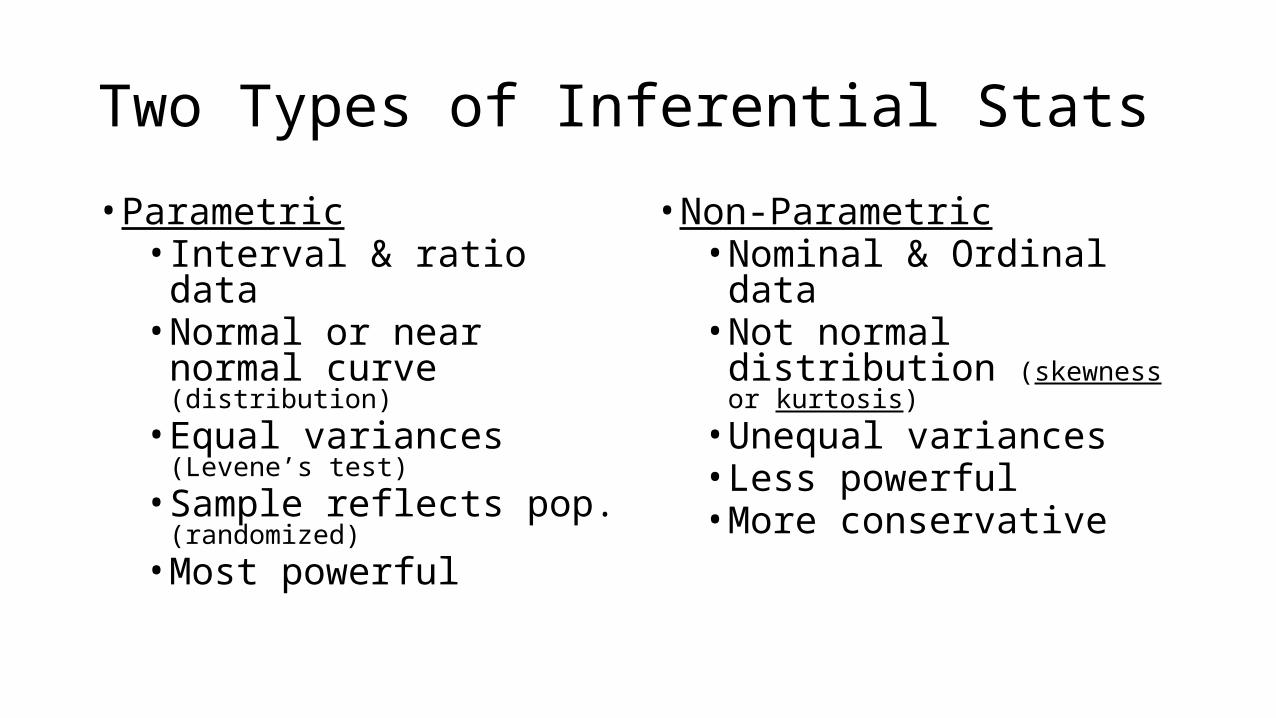
Two Types of Inferential Stats

• Parametric• Interval & ratio data• Normal or near normal curve

(distribution)• Equal variances (Levene’s test)• Sample reflects pop.

(randomized)• Most powerful

• Non-Parametric• Nominal & Ordinal data• Not normal distribution

(skewness or kurtosis)• Unequal variances • Less powerful• More conservative

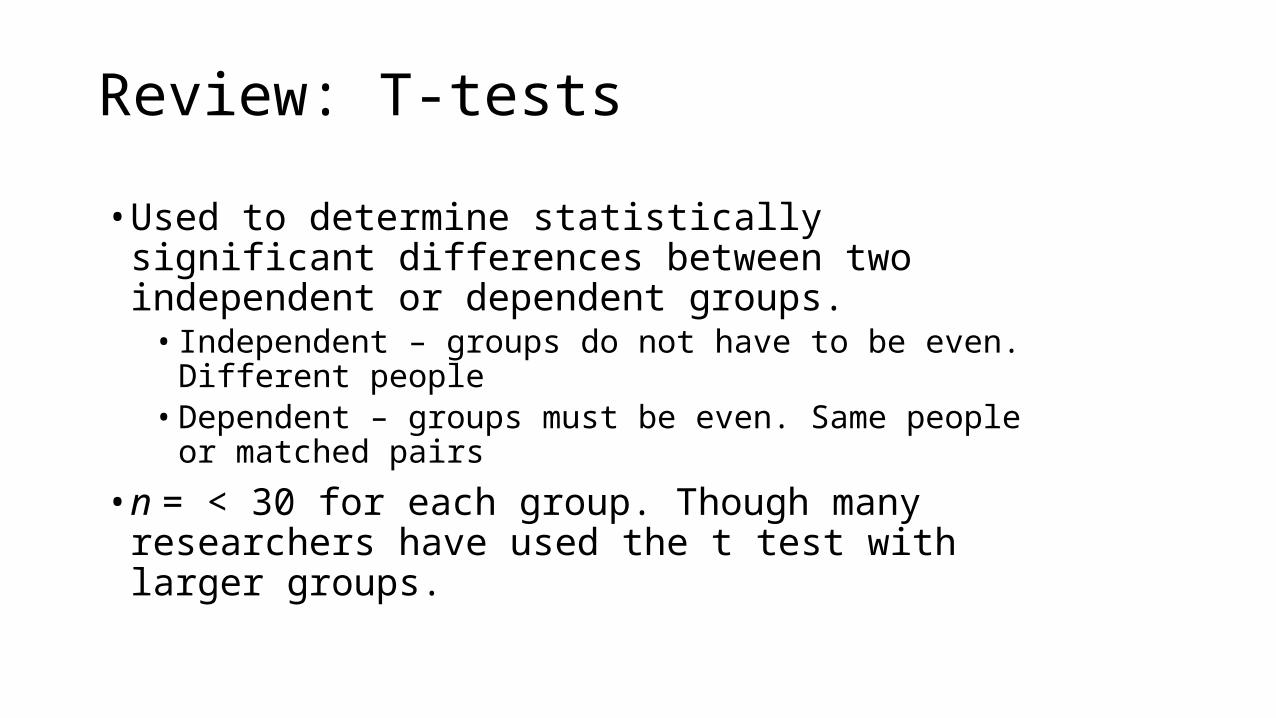
Review: T-tests

• Used to determine statistically significant differences between two independent or dependent groups.

• Independent – groups do not have to be even. Different people• Dependent – groups must be even. Same people or matched pairs

• n = < 30 for each group. Though many researchers have used the t test with larger groups.

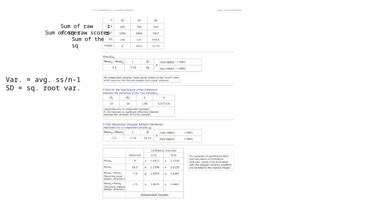
Sum of the sq

Sum of raw scoresSum of sq raw scores

Var. = avg. ss/n-1SD = sq. root var.

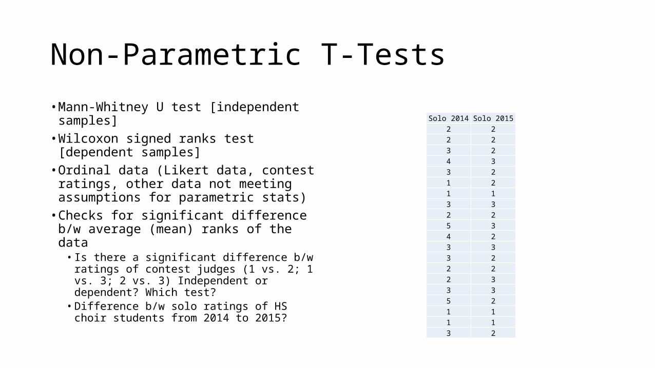
Non-Parametric T-Tests

• Mann-Whitney U test [independent samples]

• Wilcoxon signed ranks test [dependent samples]

• Ordinal data (Likert data, contest ratings, other data not meeting assumptions for parametric stats)

• Checks for significant difference b/w average (mean) ranks of the data

• Is there a significant difference b/w ratings of contest judges (1 vs. 2; 1 vs. 3; 2 vs. 3) Independent or dependent? Which test?

• Difference b/w solo ratings of HS choir students from 2014 to 2015?

Solo 2014 Solo 20152 22 23 24 33 21 21 13 32 25 34 23 33 22 22 33 35 21 11 13 2

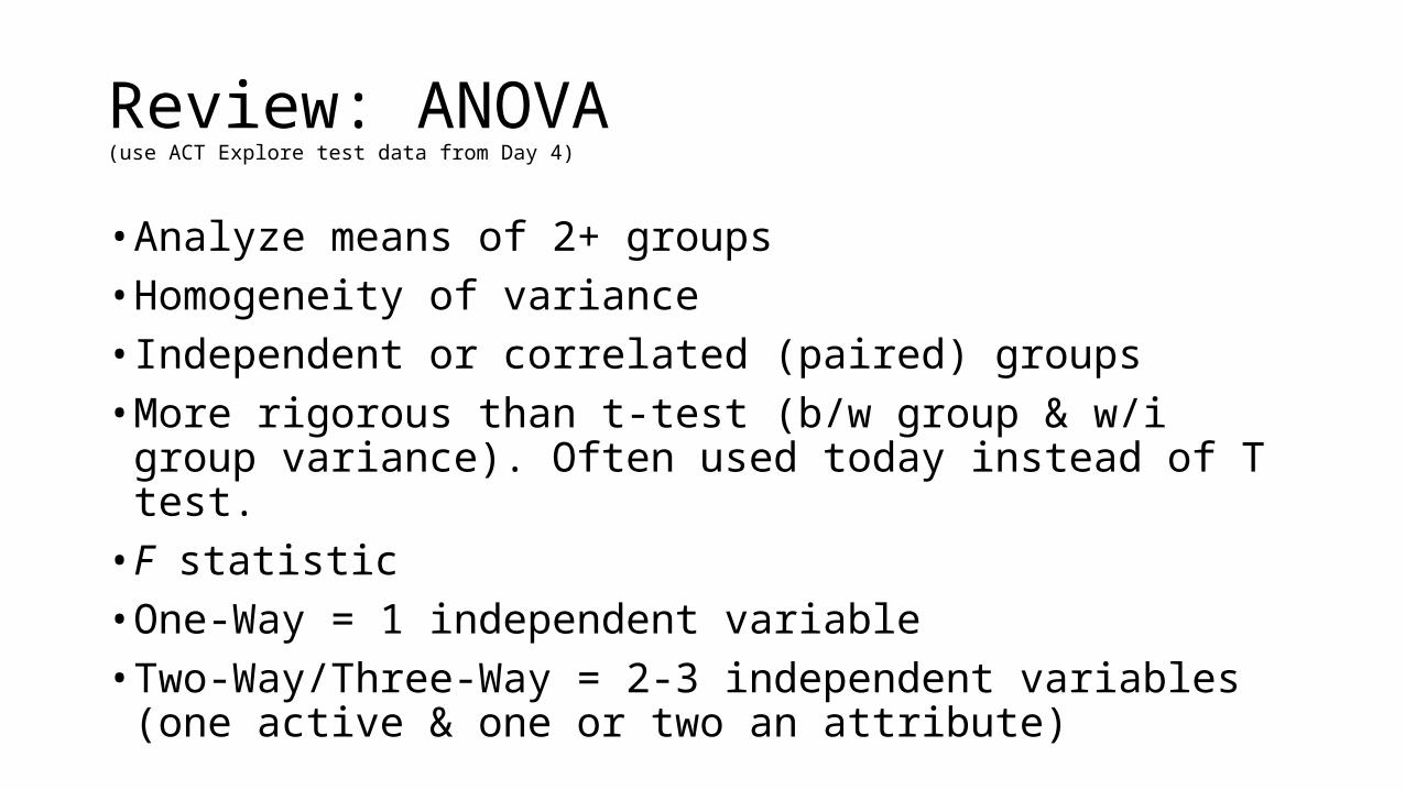
Review: ANOVA(use ACT Explore test data from Day 4)

• Analyze means of 2+ groups• Homogeneity of variance• Independent or correlated (paired) groups• More rigorous than t-test (b/w group & w/i group variance). Often

used today instead of T test.• F statistic• One-Way = 1 independent variable• Two-Way/Three-Way = 2-3 independent variables (one active & one

or two an attribute)

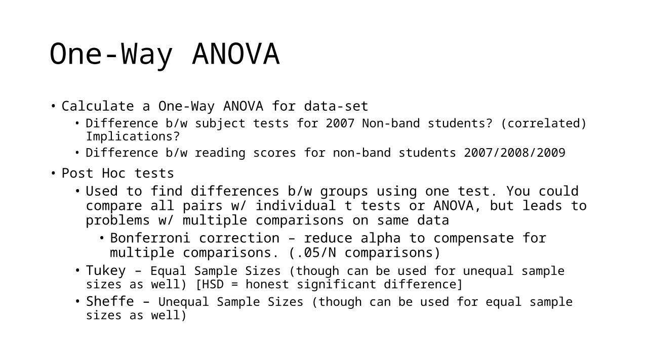
One-Way ANOVA

• Calculate a One-Way ANOVA for data-set• Difference b/w subject tests for 2007 Non-band students? (correlated) Implications?• Difference b/w reading scores for non-band students 2007/2008/2009

• Post Hoc tests• Used to find differences b/w groups using one test. You could compare all pairs w/ individual

t tests or ANOVA, but leads to problems w/ multiple comparisons on same data• Bonferroni correction – reduce alpha to compensate for multiple comparisons. (.05/N

comparisons)• Tukey – Equal Sample Sizes (though can be used for unequal sample sizes as well) [HSD = honest

significant difference]• Sheffe – Unequal Sample Sizes (though can be used for equal sample sizes as well)

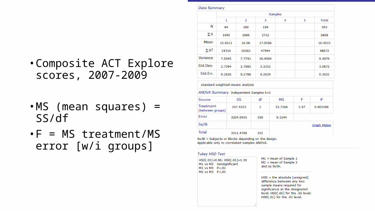
• Composite ACT Explore scores, 2007-2009

• MS (mean squares) = SS/df• F = MS treatment/MS error [w/i

groups]

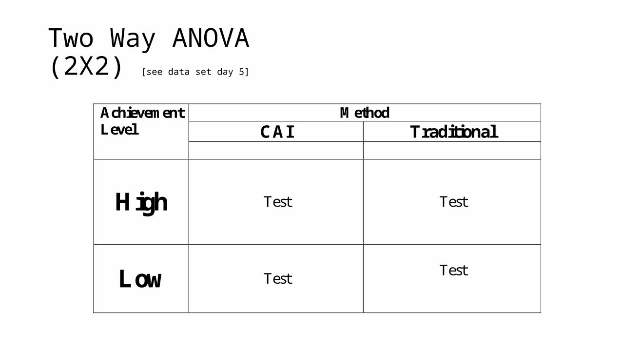
Two Way ANOVA(2X2) [see data set day 5]

Achievement Level

Method CAI Traditional

High

Test

Test

Low

Test

Test

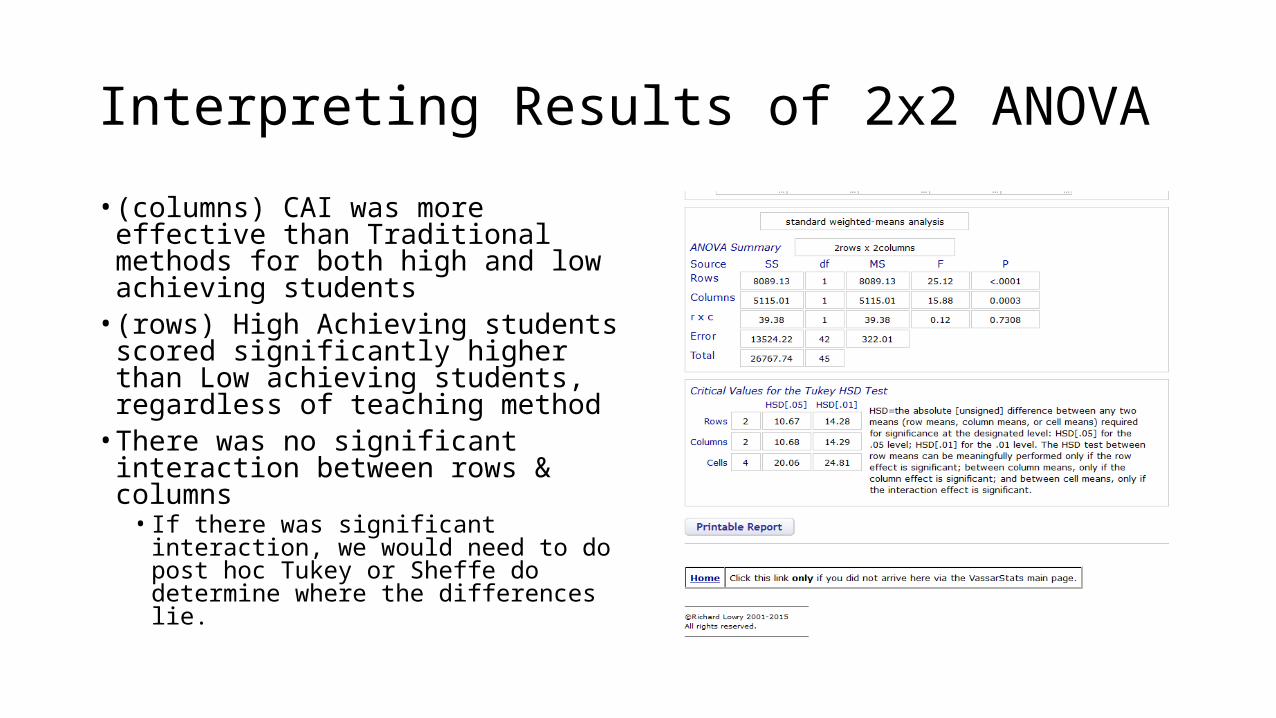
Interpreting Results of 2x2 ANOVA

• (columns) CAI was more effective than Traditional methods for both high and low achieving students

• (rows) High Achieving students scored significantly higher than Low achieving students, regardless of teaching method

• There was no significant interaction between rows & columns

• If there was significant interaction, we would need to do post hoc Tukey or Sheffe do determine where the differences lie.

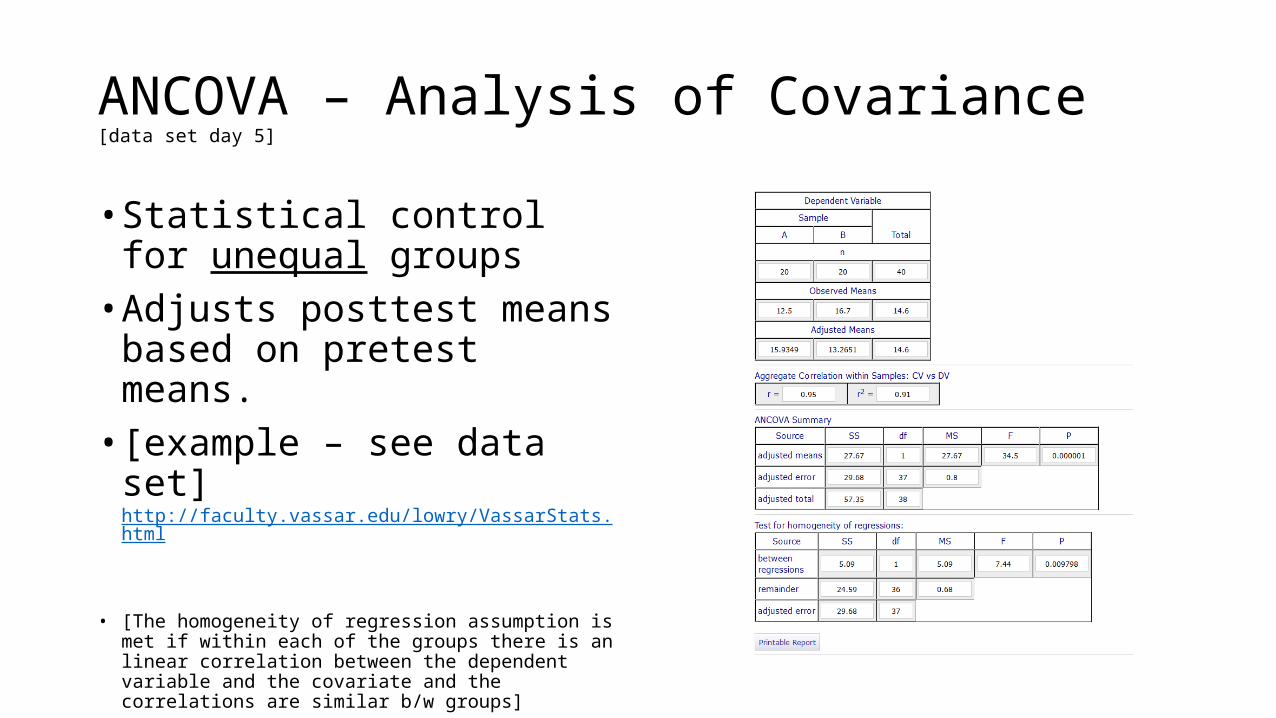
ANCOVA – Analysis of Covariance[data set day 5]

• Statistical control for unequal groups

• Adjusts posttest means based on pretest means.

• [example – see data set] http://faculty.vassar.edu/lowry/VassarStats.html

• [The homogeneity of regression assumption is met if within each of the groups there is an linear correlation between the dependent variable and the covariate and the correlations are similar b/w groups]

Correlational Research

Correlational Research Basics

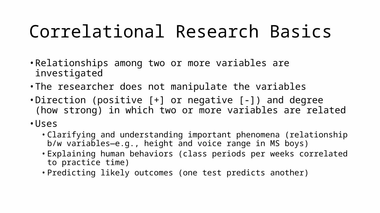
• Relationships among two or more variables are investigated• The researcher does not manipulate the variables• Direction (positive [+] or negative [-]) and degree (how strong) in

which two or more variables are related• Uses

• Clarifying and understanding important phenomena (relationship b/w variables—e.g., height and voice range in MS boys)

• Explaining human behaviors (class periods per weeks correlated to practice time)

• Predicting likely outcomes (one test predicts another)

Correlation Research Basics

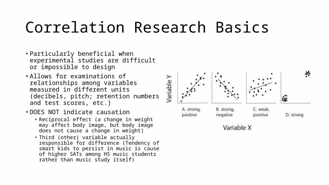
• Particularly beneficial when experimental studies are difficult or impossible to design

• Allows for examinations of relationships among variables measured in different units (decibels, pitch; retention numbers and test scores, etc.)

• DOES NOT indicate causation• Reciprocal effect (a change in weight may

affect body image, but body image does not cause a change in weight)

• Third (other) variable actually responsible for difference (Tendency of smart kids to persist in music is cause of higher SATs among HS music students rather than music study itself)

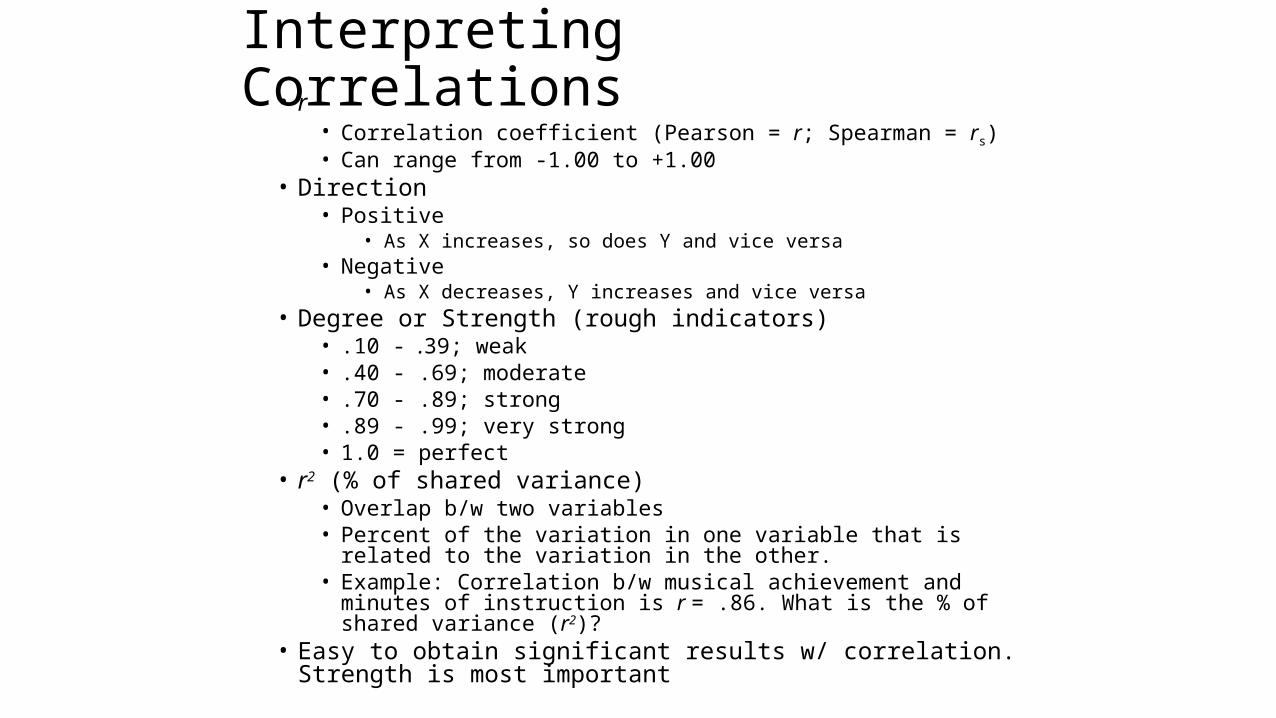
Interpreting Correlations• r

• Correlation coefficient (Pearson = r; Spearman = rs)• Can range from -1.00 to +1.00

• Direction• Positive

• As X increases, so does Y and vice versa• Negative

• As X decreases, Y increases and vice versa• Degree or Strength (rough indicators)

• .10 - .39; weak• .40 - .69; moderate• .70 - .89; strong• .89 - .99; very strong• 1.0 = perfect

• r2 (% of shared variance)• Overlap b/w two variables• Percent of the variation in one variable that is related to the variation in

the other.• Example: Correlation b/w musical achievement and minutes of

instruction is r = .86. What is the % of shared variance (r2)?• Easy to obtain significant results w/ correlation. Strength is most

important

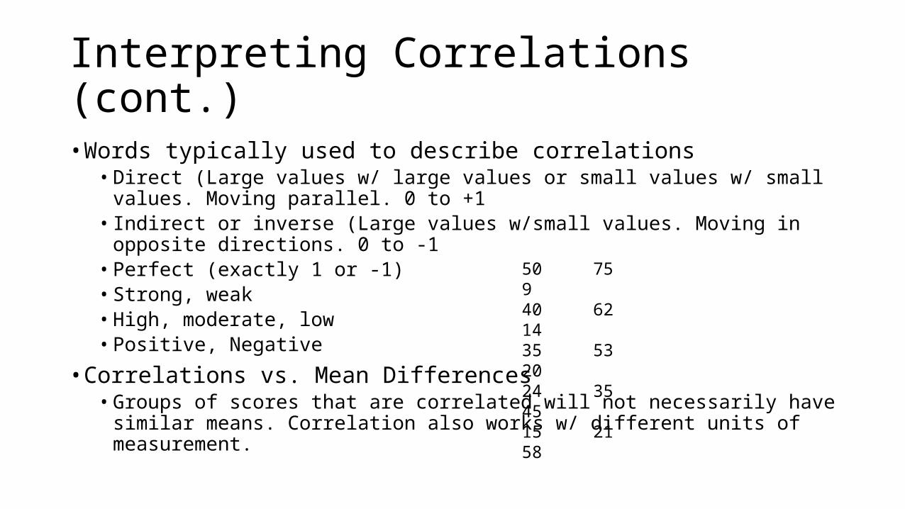
Interpreting Correlations (cont.)

• Words typically used to describe correlations• Direct (Large values w/ large values or small values w/ small values. Moving

parallel. 0 to +1• Indirect or inverse (Large values w/small values. Moving in opposite directions. 0 to

-1• Perfect (exactly 1 or -1)• Strong, weak• High, moderate, low• Positive, Negative

• Correlations vs. Mean Differences• Groups of scores that are correlated will not necessarily have similar means.

Correlation also works w/ different units of measurement.

50 75 9 40 62 1435 53 2024 35 4515 21 58

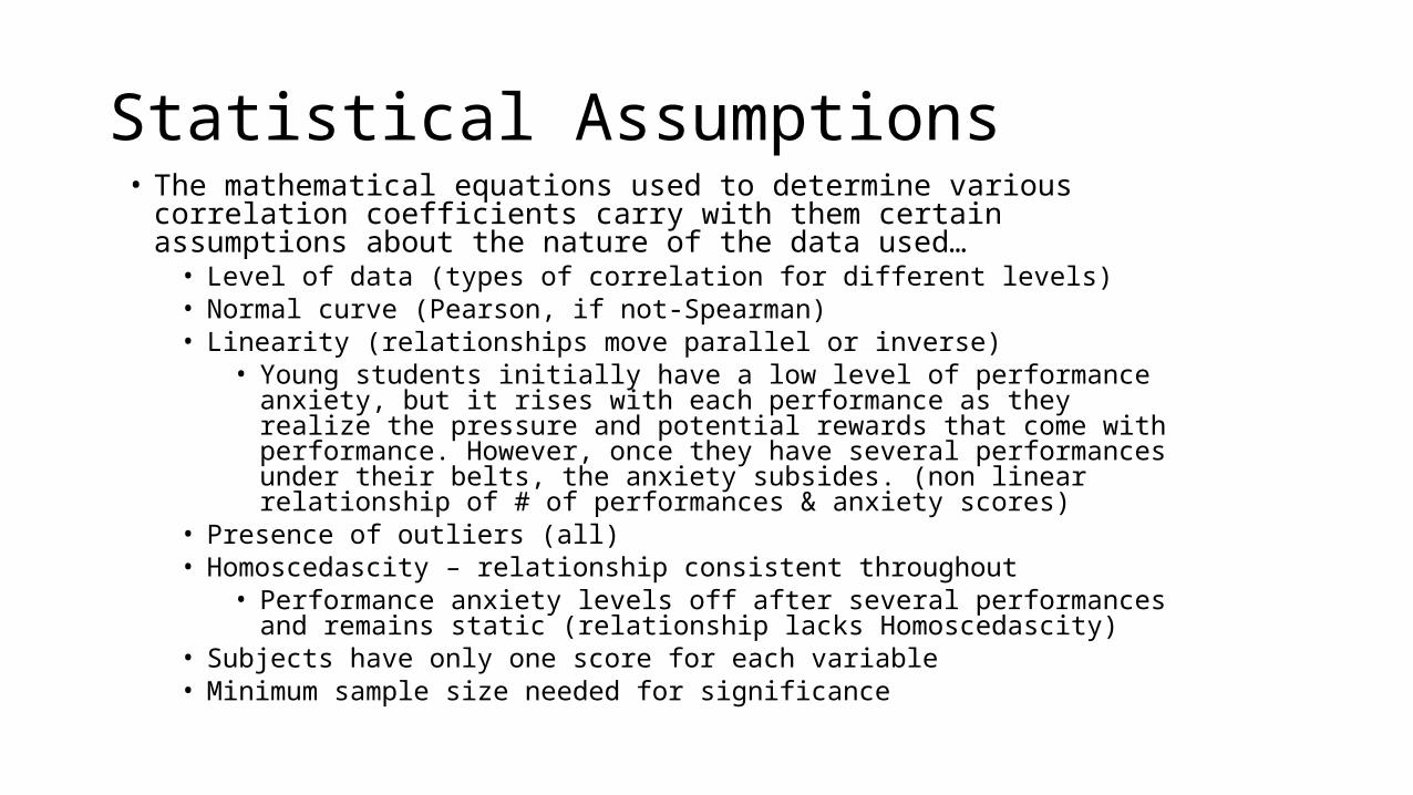
Statistical Assumptions• The mathematical equations used to determine various correlation coefficients carry

with them certain assumptions about the nature of the data used…• Level of data (types of correlation for different levels)• Normal curve (Pearson, if not-Spearman)• Linearity (relationships move parallel or inverse)

• Young students initially have a low level of performance anxiety, but it rises with each performance as they realize the pressure and potential rewards that come with performance. However, once they have several performances under their belts, the anxiety subsides. (non linear relationship of # of performances & anxiety scores)

• Presence of outliers (all)• Homoscedascity – relationship consistent throughout

• Performance anxiety levels off after several performances and remains static (relationship lacks Homoscedascity)

• Subjects have only one score for each variable• Minimum sample size needed for significance

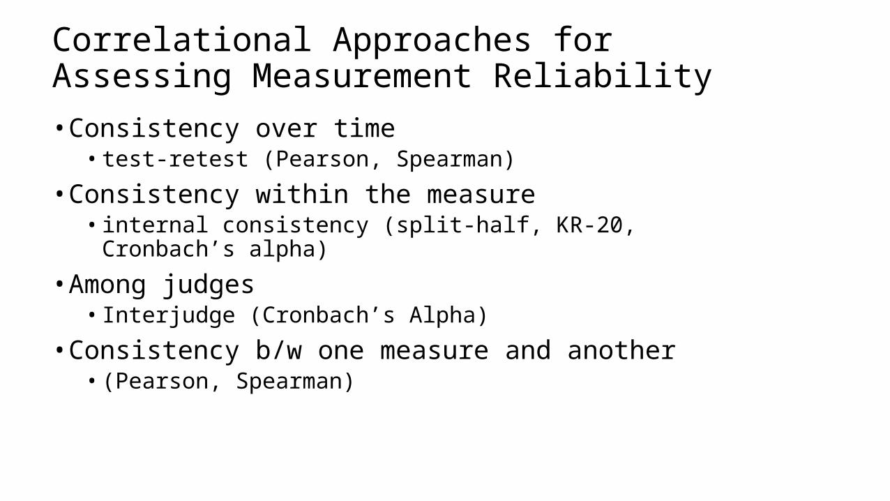
Correlational Approaches for Assessing Measurement Reliability

• Consistency over time• test-retest (Pearson, Spearman)

• Consistency within the measure• internal consistency (split-half, KR-20, Cronbach’s alpha)

• Among judges• Interjudge (Cronbach’s Alpha)

• Consistency b/w one measure and another• (Pearson, Spearman)

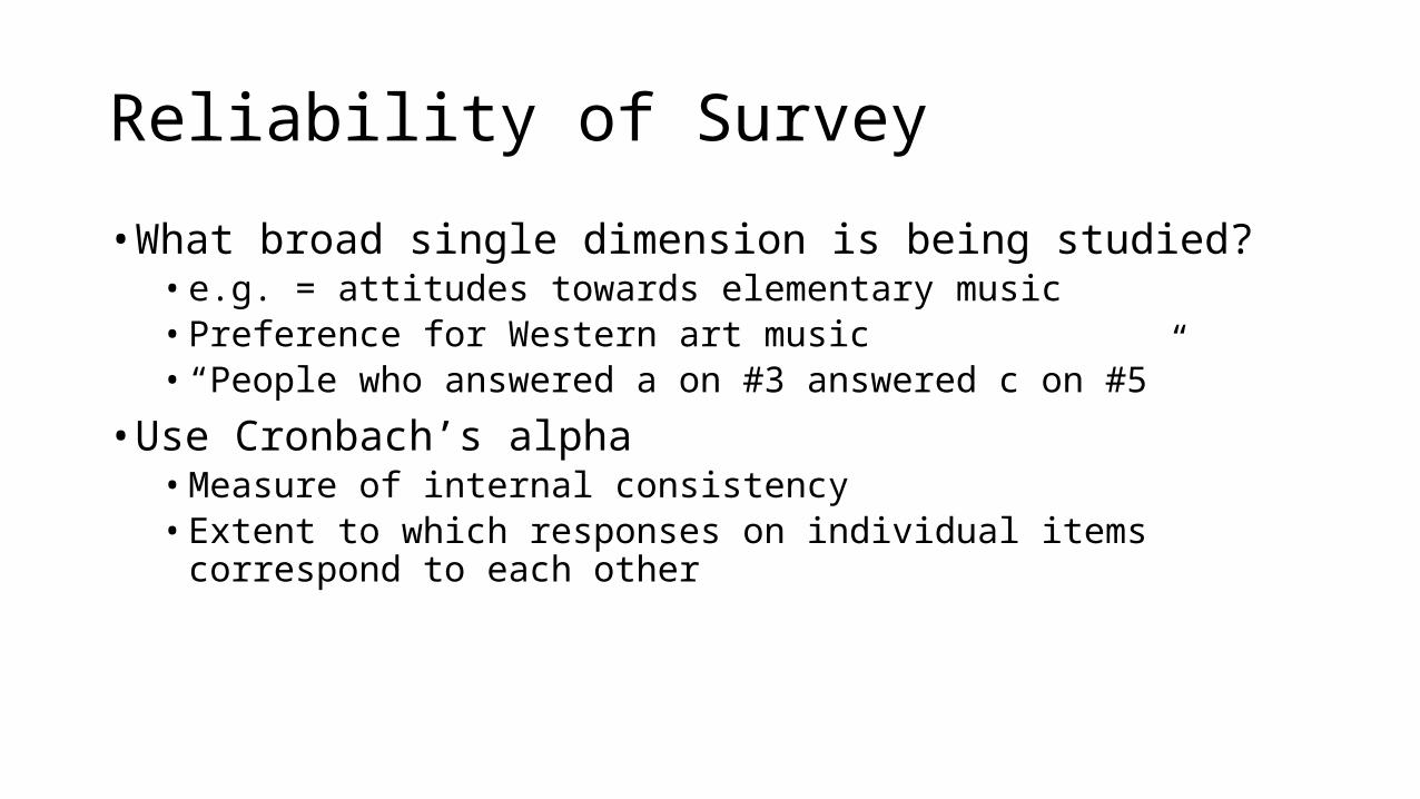
Reliability of Survey

• What broad single dimension is being studied?• e.g. = attitudes towards elementary music• Preference for Western art music• “People who answered a on #3 answered c on #5”

• Use Cronbach’s alpha• Measure of internal consistency• Extent to which responses on individual items correspond to each other

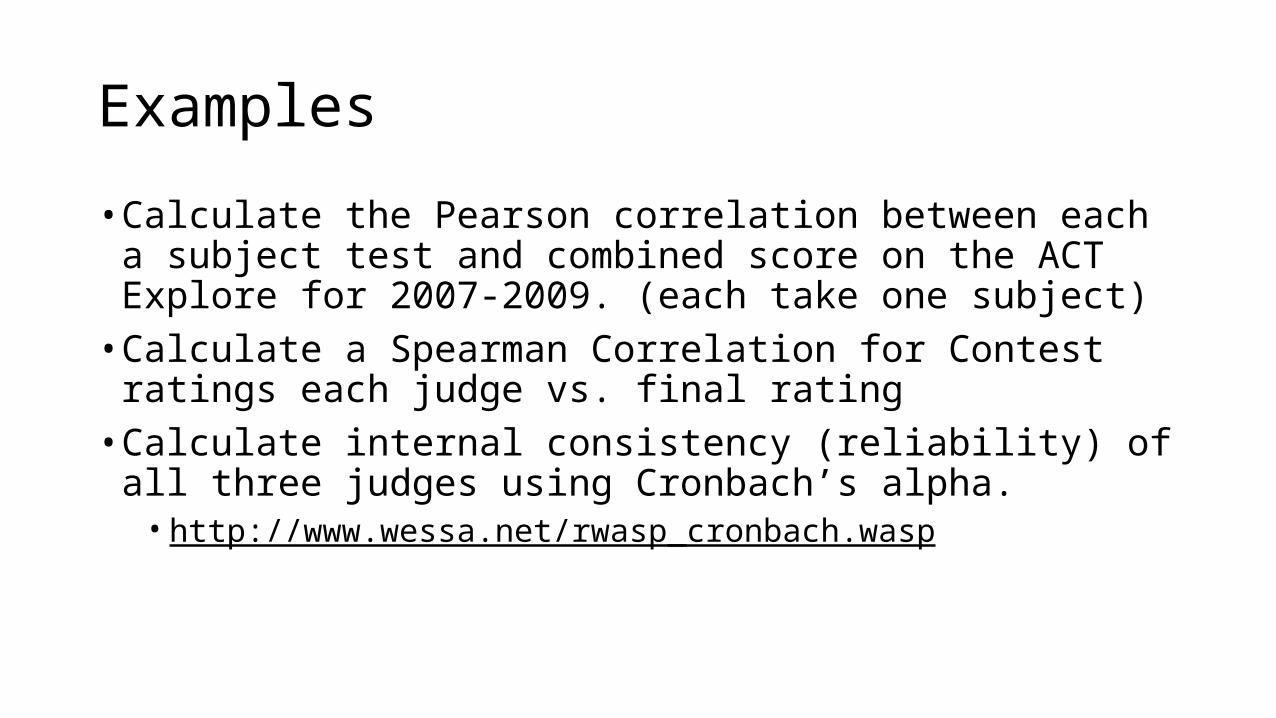
Examples

• Calculate the Pearson correlation between each a subject test and combined score on the ACT Explore for 2007-2009. (each take one subject)

• Calculate a Spearman Correlation for Contest ratings each judge vs. final rating

• Calculate internal consistency (reliability) of all three judges using Cronbach’s alpha.

• http://www.wessa.net/rwasp_cronbach.wasp

Other Stats

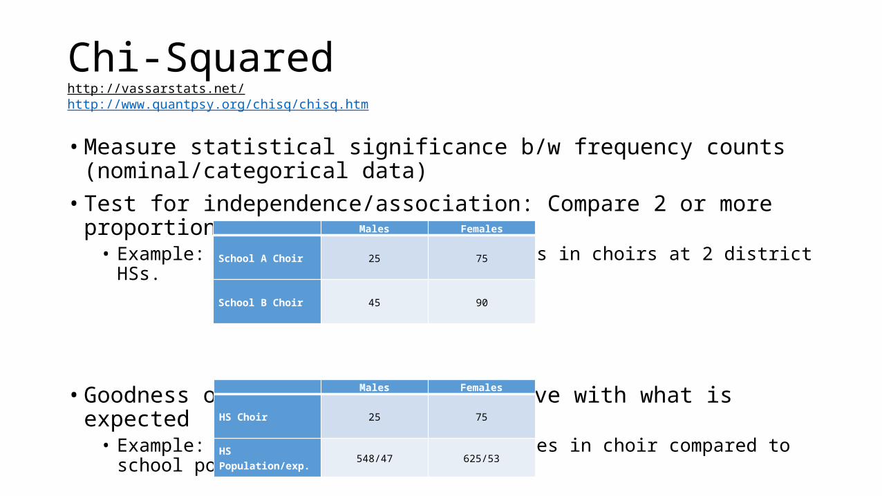
Chi-Squaredhttp://vassarstats.net/ http://www.quantpsy.org/chisq/chisq.htm

• Measure statistical significance b/w frequency counts (nominal/categorical data)• Test for independence/association: Compare 2 or more proportions

• Example: Proportion of females to males in choirs at 2 district HSs.

• Goodness of Fit: compare w/ you have with what is expected• Example: Proportions of females to males in choir compared to school population

  Males Females

School A Choir

25

75

School B Choir

45

90

  Males Females

HS Choir

25

75

HS Population/exp. 548/47 625/53

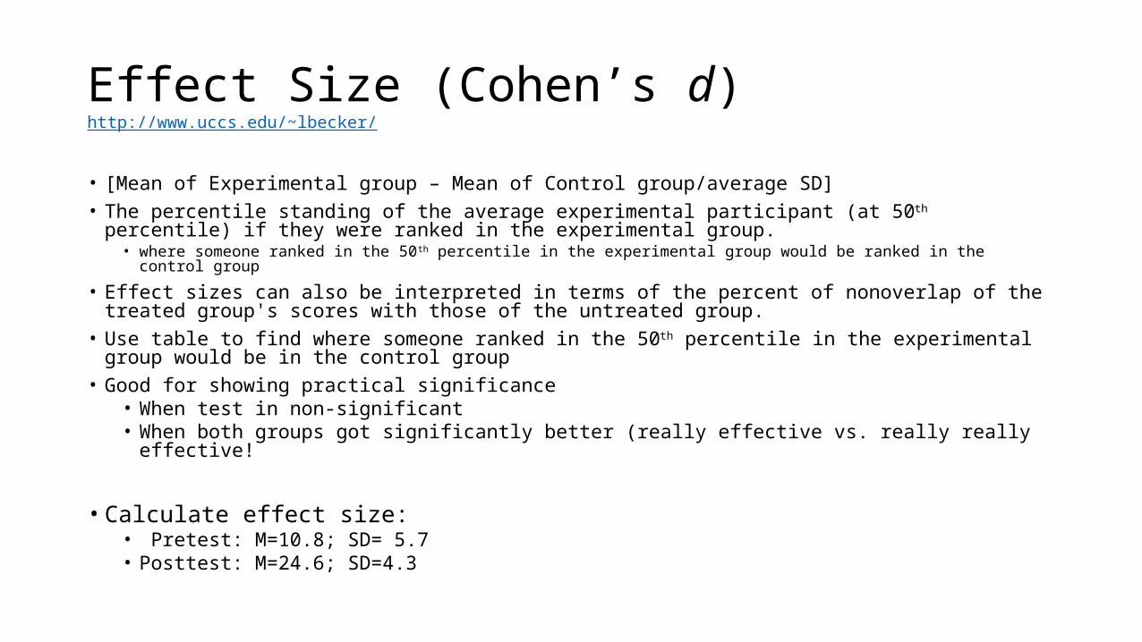
Effect Size (Cohen’s d)http://www.uccs.edu/~lbecker/

• [Mean of Experimental group – Mean of Control group/average SD]• The percentile standing of the average experimental participant (at 50th percentile) if they were ranked

in the experimental group.• where someone ranked in the 50th percentile in the experimental group would be ranked in the control group

• Effect sizes can also be interpreted in terms of the percent of nonoverlap of the treated group's scores with those of the untreated group.

• Use table to find where someone ranked in the 50th percentile in the experimental group would be in the control group

• Good for showing practical significance• When test in non-significant• When both groups got significantly better (really effective vs. really really effective!

• Calculate effect size:• Pretest: M=10.8; SD= 5.7• Posttest: M=24.6; SD=4.3

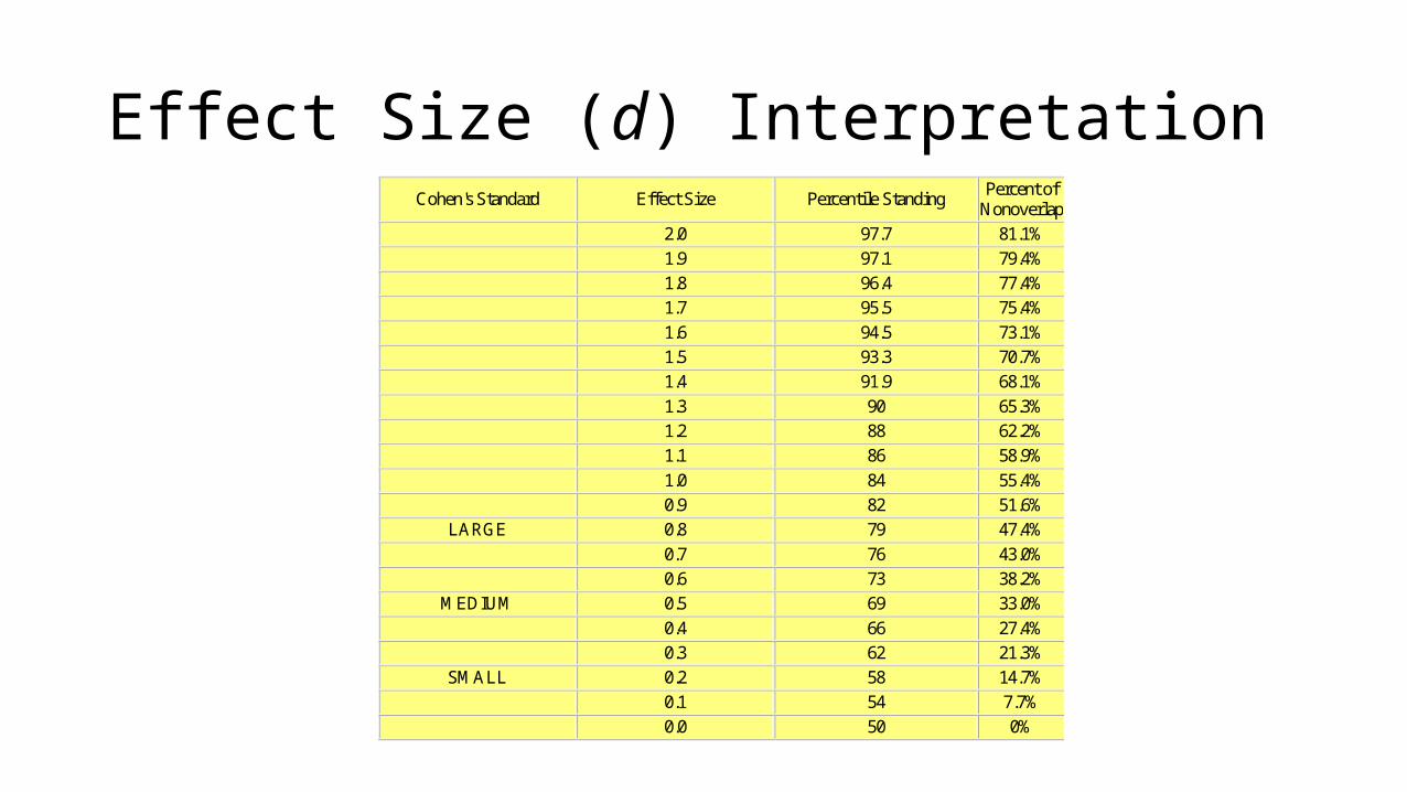
Effect Size (d) InterpretationCohen's Standard Effect Size Percentile Standing

Percent of Nonoverlap

2.0 97.7 81.1%

1.9 97.1 79.4%

1.8 96.4 77.4%

1.7 95.5 75.4%

1.6 94.5 73.1%

1.5 93.3 70.7%

1.4 91.9 68.1%

1.3 90 65.3%

1.2 88 62.2%

1.1 86 58.9%

1.0 84 55.4%

0.9 82 51.6%

LARGE 0.8 79 47.4%

0.7 76 43.0%

0.6 73 38.2%

MEDIUM 0.5 69 33.0%

0.4 66 27.4%

0.3 62 21.3%

SMALL 0.2 58 14.7%

0.1 54 7.7%

0.0 50 0%